computer algebra in scientific computing
TRANSCRIPT

Computer Algebra in Scientific Computing
Andreas Weber
www.mdpi.com/journal/mathematics
Edited by
Printed Edition of the Special Issue Published in Mathematics

Computer Algebra in Scientific Computing

Computer Algebra in Scientific Computing
Special Issue Editor
Andreas Weber
MDPI • Basel • Beijing •Wuhan • Barcelona • Belgrade
Special Issue Editor
Andreas Weber
Bonn University
Germany
Editorial Office
MDPI
St. Alban-Anlage 66
4052 Basel, Switzerland
This is a reprint of articles from the Special Issue published online in the open access journal
Mathematics (ISSN 2227-7390) from 2018 to 2019 (available at: https://www.mdpi.com/journal/
mathematics/special issues/Computer Algebra)
For citation purposes, cite each article independently as indicated on the article page online and as
indicated below:
LastName, A.A.; LastName, B.B.; LastName, C.C. Article Title. Journal Name Year, Article Number,
Page Range.
ISBN 978-3-03921-730-4 (Pbk)
ISBN 978-3-03921-731-1 (PDF)
c© 2019 by the authors. Articles in this book are Open Access and distributed under the Creative
Commons Attribution (CC BY) license, which allows users to download, copy and build upon
published articles, as long as the author and publisher are properly credited, which ensures maximum
dissemination and a wider impact of our publications.
The book as a whole is distributed by MDPI under the terms and conditions of the Creative Commons
license CC BY-NC-ND.

Contents
About the Special Issue Editor . . . . . . . . . . . . . . . . . . . . . . . . . . . . . . . . . . . . . . vii
Preface to ”Computer Algebra in Scientific Computing” . . . . . . . . . . . . . . . . . . . . . . . ix
Mohammadali Asadi, Alexander Brandt, Robert H. C. Moir and Marc Moreno Maza Algorithms and Data Structures for Sparse Polynomial ArithmeticReprinted from: Mathematics 2019, 7, 441, doi:10.3390/math7050441 . . . . . . . . . . . . . . . . . 1
Xiaojie Dou and Jin-San Cheng
A Heuristic Method for Certifying Isolated Zeros of Polynomial SystemsReprinted from: Mathematics 2018, 6, 166, doi:10.3390/math6090166 . . . . . . . . . . . . . . . . . 30
Mario Albert and Werner M. Seiler
Resolving Decompositions for Polynomial ModulesReprinted from: Mathematics 2018, 6, 161, doi:10.3390/math6090161 . . . . . . . . . . . . . . . . . 48
Valery Antonov, Wilker Fernandes, Valery G. Romanovski and Natalie L. Shcheglova First Integrals of the May–Leonard Asymmetric SystemReprinted from: Mathematics 2019, 7, 292, doi:10.3390/math7030292 . . . . . . . . . . . . . . . . . 65
Erhan Guler and Omer KisiDini-Type Helicoidal Hypersurfaces with Timelike Axis in Minkowski 4-Space E4
1
Reprinted from: Mathematics 2019, 7, 205, doi:10.3390/math7020205 . . . . . . . . . . . . . . . . . 80
Erhan Guler, Omer Kisi and Christos Konaxis
Implicit Equations of the Henneberg-Type Minimal Surface in the Four-Dimensional EuclideanSpaceReprinted from: Mathematics 2018, 6, 279, doi:10.3390/math6120279 . . . . . . . . . . . . . . . . . 88
Farnoosh Hajati, Ali Iranmanesh and Abolfazl Tehranian
A Characterization of Projective Special Unitary Group PSU(3,3) and Projective Special LinearGroup PSL(3,3) by NSEReprinted from: Mathematics 2018, 6, 120, doi:10.3390/math6070120 . . . . . . . . . . . . . . . . . 98
Maurice R. Kibler
Quantum Information: A Brief Overview and Some Mathematical AspectsReprinted from: Mathematics 2018, 6, 273, doi:10.3390/math6120273 . . . . . . . . . . . . . . . . . 108
v

About the Special Issue Editor
Andreas Weber (Prof. Dr.) studied mathematics and computer science at the Universities of
Tubingen, Germany, and Boulder, Colorado, U.S.A. He was awarded his MS in Mathematics
(Dipl.-Math) in 1990 and his Ph.D. (Dr. rer. nat.) in computer science from the University of Tubingen
in 1993. From 1995 to 1997, he was awarded a scholarship from Deutsche Forschungsgemeinschaft to
conduct research as a postdoctoral fellow at the Computer Science Department, Cornell University.
From 1997 to 1999 he was a member of the Symbolic Computation Group at the University of
Tubingen, Germany. From 1999 to 2001, he was a member of the research group Animation and
Image Communication at the Fraunhofer Institut for Computer Graphics. He has been Professor of
computer science at the University of Bonn, Germany, since his appointment in April 2001. He has
served as Chair of the Department of Computer Science from 2014 to 2016. During his academic
career, he has written more than 100 papers for journals and refereed conference proceedings and
has been the first supervisor of 9 completed Ph.D. theses and over 70 master’s and bachelor’s theses.
He has served as a reviewer for more than 60 different journals and conferences. In 2013, he has been
awarded the Teaching Award of the University of Bonn.
vii

Preface to ”Computer Algebra in Scientific Computing”Although scientific computing is very often associated with numeric computations, the use of
computer algebra methods in scientific computing has obtained considerable attention in the last two decades. Computer algebra methods are especially suitable for parametric analysis of the key properties of systems arising in scientific computing. The expression-based computational answers generally provided by these methods are very appealing as they directly relate properties to parameters and speed up testing and tuning of mathematical models through all their possible behaviors. The articles contained in this book cover a broad range of topics in the context of computer algebra in scientific computing. At the core of many computer algebra methods are algorithms for multivariate polynomials, and the first article on “Algorithms and Data Structures for Sparse Polynomial Arithmetic” is at the essence of this core, giving a comprehensive presentation of algorithms, data structures, and implementation techniques for high-performance sparse multivariate polynomial arithmetic over the integers and rational numbers as implemented in the freely available Basic Polynomial Algebra Subprograms (BPAS) library. “A Heuristic Method for Certifying Isolated Zeros of Polynomial Systems” deals with the fundamental problem of certifying the isolated zeros of polynomial systems. Computing Grobner bases and other kind of bases is another core of computer algebra. In “Resolving Decompositions for Polynomial Modules”, the authors deal with a fundamental task in “computational commutative algebra and algebraic geometry”, namely, the determination of free resolutions for polynomial modules. They introduce the novel concept of resolving decomposition of a polynomial module as a combinatorial structure that allows for the effective construction of free resolutions and provide a unifying framework for recent results involving different types of bases. The analysis of certain invariants of a dynamical system—which are at the heart of many problems in scientific computing—is another major area for computer algebra research. In the article “First Integrals of the May–Leonard Asymmetric System”, an important system arising in the life sciences is investigated, which is given by a quadratic system of the Lotka–Volterra type depending on six parameters. The authors look for subfamilies admitting invariant algebraic surfaces of degree two, and then for some such subfamilies, they construct first integrals of the Darboux type, identifying the systems with one first integral or with two independent first integrals. A problem based in physics, namely “Minkowski 4-space”, is treated in the article “Dini-Type Helicoidal Hypersurfaces with Timelike Axis in Minkowski 4-Space”. The authors consider Ulisse Dini-type helicoidal hypersurfaces with timelike axis in Minkowski 4-space, and by calculating the Gaussian and mean curvatures of the hypersurfaces, they demonstrate some special symmetries for the curvatures when they are flat and minimal. In the article “Implicit Equations of the Henneberg-Type Minimal Surface in the Four-Dimensional Euclidean Space” the authors find implicit algebraic equations of the Henneberg-type minimal surface of values (4,2). The exciting field of quantum computing has also lead to several problems in computer algebra. In “Quantum Information: A Brief Overview and Some Mathematical Aspects”, not only is a review of the main ideas behind quantum computing and quantum information presented, but the focus is also on some mathematical problems related to the so-called mutually unbiased bases used in quantum computing and quantum information processing. In this direction, the construction of mutually unbiased bases is presented via two distinct approaches: one based on the group SU(2) and the other on Galois fields and Galois rings.
Andreas Weber Special Issue Editor
ix

x
mathematics
Article
Algorithms and Data Structures for SparsePolynomial Arithmetic
Mohammadali Asadi, Alexander Brandt *, Robert H. C. Moir and Marc Moreno Maza
Department of Computer Science, University of Western Ontario, London, ON N6A 5B7, Canada;[email protected] (M.A.); [email protected] (R.H.C.M.); [email protected] (M.M.M.)* Correspondence: [email protected]
Received: 1 February 2019; Accepted: 12 May 2019; Published: 17 May 2019
Abstract: We provide a comprehensive presentation of algorithms, data structures, and implementationtechniques for high-performance sparse multivariate polynomial arithmetic over the integers andrational numbers as implemented in the freely available Basic Polynomial Algebra Subprograms(BPAS) library. We report on an algorithm for sparse pseudo-division, based on the algorithmsfor division with remainder, multiplication, and addition, which are also examined herein.The pseudo-division and division with remainder operations are extended to multi-divisorpseudo-division and normal form algorithms, respectively, where the divisor set is assumed to forma triangular set. Our operations make use of two data structures for sparse distributed polynomialsand sparse recursively viewed polynomials, with a keen focus on locality and memory usage foroptimized performance on modern memory hierarchies. Experimentation shows that these newimplementations compare favorably against competing implementations, performing between afactor of 3 better (for multiplication over the integers) to more than 4 orders of magnitude better(for pseudo-division with respect to a triangular set).
Keywords: sparse polynomials; polynomial arithmetic; normal form; pseudo-division;pseudo-remainder; sparse data structures
1. Introduction
Technological advances in computer hardware have allowed scientists to greatly expand thesize and complexity of problems tackled by scientific computing. Only in the last decade havesparse polynomial arithmetic operations (Polynomial arithmetic operations here refers to addition,subtraction, multiplication, division with remainder, and pseudo-division) and data structures comeunder focus again in support of large problems which cannot be efficiently represented densely.Sparse polynomial representations was an active research topic many decades ago out of necessity;computing resources, particularly memory, were very limited. Computer algebra systems of thetime (which handled multivariate polynomials) all made use of sparse representations, includingALTRAN [1], MACSYMA [2], and REDUCE [3]. More recent work can be categorized into two streams,the first dealing primarily with algebraic complexity [4,5] and the second focusing on implementationtechniques [6,7]. Recent research on implementation techniques has been motivated by the efficientuse of memory. Due to reasons such as the processor–memory gap ([8] Section 2.1) and the memorywall [9], program performance has become limited by the speed of memory. We consider these issuesforemost in our algorithms, data structures, and implementations. An early version of this workappeared as [10].
Sparse polynomials, for example, arise in the world of polynomial system solving—a criticalproblem in nearly every scientific discipline. Polynomial systems generally come from real-lifeapplications, consisting of multivariate polynomials with rational number coefficients. Core routines
Mathematics 2019, 7, 441; doi:10.3390/math7050441 www.mdpi.com/journal/mathematics1
Mathematics 2019, 7, 441
for determining solutions to polynomial systems (e.g., Gröbner bases, homotopy methods, or triangulardecompositions) have driven a large body of work in computer algebra. Algorithms, data structures,and implementation techniques for polynomial and matrix data types have seen particular attention.We are motivated in our work on sparse polynomials by obtaining efficient implementations oftriangular decomposition algorithms based on the theory of regular chains [11].
Our aim for the work presented in this paper is to provide highly optimized sparse multivariatepolynomial arithmetic operations as a foundation for implementing high-level algorithms requiringsuch operations, including triangular decomposition. The implementations presented herein arefreely available in the BPAS library [12] at www.bpaslib.org. The BPAS library is highly focusedon performance, concerning itself not only with execution time but also memory usage and cachecomplexity [13]. The library is mainly written in the C language, for high-performance, with asimplified C++ interface for end-user usability and object-oriented programming. The BPAS libraryalso makes use of parallelization (e.g., via the CILK extension [14]) for added performance on multi-corearchitectures, such as in dense polynomial arithmetic [15,16] and arithmetic for big prime fields basedon Fast Fourier Transform (FFT) [17]. Despite these previous achievements, the work presented hereis in active development and not yet been parallelized.
Indeed, parallelizing sparse arithmetic is an interesting problem and is much more difficult thanparallelizing dense arithmetic. Many recent works have attempted to parallelize sparse polynomialarithmetic. Sub-linear parallel speed-up is obtained for the relatively more simple schemes of Monaganand Pearce [18,19] or Biscani [20], while Gastineau and Laskar [7,21] have obtained near-linear parallelspeed-up but have a much more intricate parallelization scheme. Other works are quite limited:the implementation of Popescu and Garcia [22] is limited to floating point coefficients while the workof Ewart et al. [23] is limited to only 4 variables. We hope to tackle parallelization of sparse arithmeticin the future, however, we strongly believe that one should obtain an optimized serial implementationbefore attempting a parallel one.
Contributions and Paper Organization
Contained herein is a comprehensive treatment of the algorithms and data structures we haveestablished for high-performance sparse multivariate polynomial arithmetic in the BPAS library.We present in Section 2 the well-known sparse addition and multiplication algorithms from [24] toprovide the necessary background for discussing division with remainder (Section 3), an extensionof the exact division also presented in [24]. In Section 4 we have extended division with remainderinto a new algorithm for sparse pseudo-division. Our presentation of both division with remainderand pseudo-division has two levels: one which is abstract and independent of the supporting datastructures (Algorithms 3 and 5); and one taking advantage of heap data structures (Algorithms 4and 6). Section 5 extends division with remainder and pseudo-division to algorithms for computingnormal forms and pseudo-division with respect to a triangular set; the former was first seen in [25]and here we extend it to the case of pseudo-division. All new algorithms are proved formally.
In support of all these arithmetic operations we have created a so-called alternating arrayrepresentation for distributed sparse polynomials which focuses greatly on data locality andmemory usage. When a recursive view of a polynomial (i.e., a representation as a univariatepolynomial with multivariate polynomial coefficients) is needed, we have devised a succinctrecursive representation which maintains the optimized distributed representation for the polynomialcoefficients and whose conversion to and from the distributed sparse representation is highly efficient.Both representations are explained in detail in Section 6. The efficiency of our algorithms andimplementations are highlighted beginning in Section 7, with implementation-specific optimizations,and then Section 8, which gathers our experimental results. We obtain speed-ups between a factor of3 (for multiplication over the integers) and a factor of 18,141 (for pseudo-division with respect to atriangular set).
2
Mathematics 2019, 7, 441
2. Background
2.1. Notation and Nomenclature
Throughout this paper we use the notation R to denote a ring (commutative with identity),D to denote an integral domain, and K to denote a field. Our treatment of sparse polynomialarithmetic requires both a distributed and recursive view of polynomials, depending on whichoperation is considered. For a distributed polynomial a ∈ R[x1, . . . , xv], a ring R, and variableordering x1 < x2 < · · · < xv, we use the notation
a =na
∑i=1
Ai =na
∑i=1
aiXαi ,
where na is the number of (non-zero) terms, 0 �= ai ∈ R, and αi is an exponent vector for the variablesX = (x1, . . . , xv). A term of a is represented by Ai = aiXαi . We use a lexicographical term orderand assume that the terms are ordered decreasingly, thus lc(a) = a1 is the leading coefficient of a andlt(a) = a1Xα1 = A1 is the leading term of a. If a is not constant the greatest variable appearing in a(denoted mvar(a)) is the main variable of a. The maximum sum of the elements of αi is the total degree(denoted tdeg(a)). The maximum exponent of the variable xi is the degree with respect to xi (denoteddeg(a, xi)). Given a term Ai of a, coef(Ai) = ai is the coefficient, expn(Ai) = αi is the exponent vector,and deg(Ai, xj) is the component of αi corresponding to xj. We also note the use of a simplified syntaxfor comparing monomials based on the term ordering; we denote Xαi > Xαj as αi > αj.
To obtain a recursive view of a non-constant polynomial a ∈ R[x1, . . . , xv], we view a asa univariate polynomial in R[xj], with xj called the main variable (denoted mvar(a)) and whereR = R[x1, . . . , xj−1, xj+1, . . . , xv]. Usually, xj is chosen to be xv and we have a ∈ R[x1, . . . , xv−1][xv].Given a term Ai of a ∈ R[xj], coef(Ai) ∈ R[x1, . . . , xj−1, xj+1, . . . , xv] is the coefficient and expn(Ai) =
deg(Ai, xj) = deg(Ai) is the degree. Given a ∈ R[xj], an exponent e picks out the term Ai of a such thatdeg(Ai) = e, so we define in this case coef(a, xj, e) := coef(Ai). Viewed specifically in the recursiveway R[xj], the leading coefficient of a is an element of R called the initial of a (denoted init(a)) whilethe degree of a in the main variable xj is called the main degree (denoted mdeg(a)), or simply degreewhere the univariate view is understood by context.
2.2. Addition and Multiplication
Adding (or subtracting) two polynomials involves three operations: joining the terms of thetwo summands; combining terms with identical exponents (possibly with cancellation); and sortingof the terms in the sum. A naïve approach computes the sum a + b term-by-term, adding a termof the addend (b) to the augend (a), and sorting the result at each step, in a manner similar toinsertion sort. (This sorting of the result is a crucial step in any sparse operation. Certain optimizationsand tricks can be used in the algorithms when it is known that the operands are in some sorted order,say in a canonical form. For example, obtaining the leading term and degree is much simpler, and,as is shown throughout this paper, arithmetic operations can exploit this sorting.) This method isinefficient and does not take advantage of the fact that both a and b are already ordered. We followthe observation of Johnson [24] that this can be accomplished efficiently in terms of operations andspace by performing a single step of merge sort on the two summands, taking full advantage ofinitial sorting of the two summands. One slight difference from a typical merge sort step is that liketerms (terms with identical exponent vectors) are combined as they are encountered. This schemeresults in the sum (or difference) being automatically sorted and all like terms being combined.The algorithm is very straightforward for anyone familiar with merge sort. The details of the algorithmare presented in ([24], p. 65). However, for completeness we present the algorithm here using ournotation (Algorithm 1).
3
Mathematics 2019, 7, 441
Algorithm 1 ADDPOLYNOMIALS (a,b)
a, b ∈ R[x1, . . . , xv ], a = ∑nai=1 ai Xαi , b = ∑
nbj=1 bj X
βj ;return c = a + b = ∑nc
k=1 ck Xγk ∈ R[x1, . . . , xv ]
1: (i, j, k) := 12: while i ≤ na and j ≤ nb do3: if αi < β j then4: ck := bj ; γk := β j
5: j := j + 16: else if αi > β j then7: ck := ai ; γk := αi8: i := i + 19: else
10: ck := ai + bj ; γk := αi
11: i := i + 1; j := j + 112: if ck = 0 then13: continue #Do not increment k14: k := k + 115: end16: while i ≤ na do17: ck := ai ; γk := αi18: i := i + 1; k := k + 119: while j ≤ nb do20: ck := bj ; γk := β j
21: j := j + 1; k := k + 1
22: return c = ∑k−1�=1 c�Xγ�
Multiplication of two polynomials follows the same general idea of addition: Make use of thefact that the multiplier and multiplicand are already sorted. Under our sparse representation ofpolynomials multiplication requires production of the product terms, combining terms with equalexponents, and then sorting the product terms. A naïve method computes the product a · b (where ahas na terms and b has nb terms) by distributing each term of the multiplier (a) over the multiplicand(b) and combining like terms:
c = a · b = (a1Xα1 · b) + (a2Xα2 · b) + · · · .
This is inefficient because all nanb terms are generated, whether or not like terms are latercombined, and then all nanb terms must be sorted, and like terms combined. Again, followingJohnson [24], we can improve algorithmic efficiency by generating terms in sorted order.
We can make good use of the sparse data structure for
a =na
∑i=1
aiXαi , and b =nb
∑j=1
bjXβ j ,
based on the observation that for given αi and β j, it is always the case that Xαi+1+β j and Xαi+β j+1 areless than Xαi+β j in the term order. Since we always have Xαi+β j > Xαi+β j+1 , it is possible to generateproduct terms in order by merging na “streams” of terms computed by multiplying a single term of adistributed over b,
a · b =
⎧⎪⎪⎪⎪⎪⎨⎪⎪⎪⎪⎪⎩
(a1 · b1) Xα1+β1 + (a1 · b2) Xα1+β2 + (a1 · b3) Xα1+β3 + . . .
(a2 · b1) Xα2+β1 + (a2 · b2) Xα2+β2 + (a2 · b3) Xα2+β3 + . . ....
(ana · b1) Xαna+β1 + (ana · b2) Xαna+β2 + (ana · b3) Xαna+β3 + . . .
and then choosing the maximum term from the “heads” of the streams. We can consider this as anna-way merge where at each step, we select the maximum term from among the heads of the streams,making it the next product term, removing it from the stream in the process. The new head of thestream where a term is removed will then be the term to its right.
4
Mathematics 2019, 7, 441
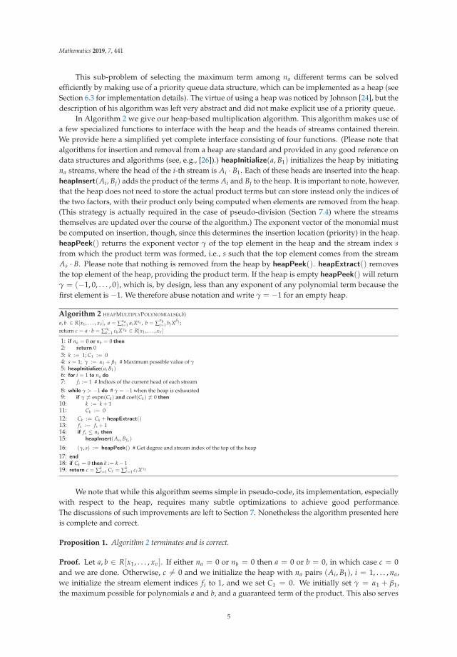
This sub-problem of selecting the maximum term among na different terms can be solvedefficiently by making use of a priority queue data structure, which can be implemented as a heap (seeSection 6.3 for implementation details). The virtue of using a heap was noticed by Johnson [24], but thedescription of his algorithm was left very abstract and did not make explicit use of a priority queue.
In Algorithm 2 we give our heap-based multiplication algorithm. This algorithm makes use ofa few specialized functions to interface with the heap and the heads of streams contained therein.We provide here a simplified yet complete interface consisting of four functions. (Please note thatalgorithms for insertion and removal from a heap are standard and provided in any good reference ondata structures and algorithms (see, e.g., [26]).) heapInitialize(a, B1) initializes the heap by initiatingna streams, where the head of the i-th stream is Ai · B1. Each of these heads are inserted into the heap.heapInsert(Ai, Bj) adds the product of the terms Ai and Bj to the heap. It is important to note, however,that the heap does not need to store the actual product terms but can store instead only the indices ofthe two factors, with their product only being computed when elements are removed from the heap.(This strategy is actually required in the case of pseudo-division (Section 7.4) where the streamsthemselves are updated over the course of the algorithm.) The exponent vector of the monomial mustbe computed on insertion, though, since this determines the insertion location (priority) in the heap.heapPeek() returns the exponent vector γ of the top element in the heap and the stream index sfrom which the product term was formed, i.e., s such that the top element comes from the streamAs · B. Please note that nothing is removed from the heap by heapPeek(). heapExtract() removesthe top element of the heap, providing the product term. If the heap is empty heapPeek() will returnγ = (−1, 0, . . . , 0), which is, by design, less than any exponent of any polynomial term because thefirst element is −1. We therefore abuse notation and write γ = −1 for an empty heap.
Algorithm 2 HEAPMULTIPLYPOLYNOMIALS(a,b)
a, b ∈ R[x1, . . . , xv ], a = ∑nai=1 ai Xαi , b = ∑
nbj=1 bj X
βj ;return c = a · b = ∑nc
k=1 ck Xγk ∈ R[x1, . . . , xv ]
1: if na = 0 or nb = 0 then2: return 03: k := 1; C1 := 04: s = 1; γ := α1 + β1 # Maximum possible value of γ5: heapInitialize(a, B1)6: for i = 1 to na do7: fi := 1 # Indices of the current head of each stream
8: while γ > −1 do # γ = −1 when the heap is exhausted9: if γ �= expn(Ck) and coef(Ck) �= 0 then
10: k := k + 111: Ck := 012: Ck := Ck + heapExtract()13: fs := fs + 114: if fs ≤ nb then15: heapInsert(As , Bfs )
16: (γ, s) := heapPeek() # Get degree and stream index of the top of the heap
17: end18: if Ck = 0 then k := k− 119: return c = ∑k
�=1 C� = ∑k�=1 c�Xγ�
We note that while this algorithm seems simple in pseudo-code, its implementation, especiallywith respect to the heap, requires many subtle optimizations to achieve good performance.The discussions of such improvements are left to Section 7. Nonetheless the algorithm presented hereis complete and correct.
Proposition 1. Algorithm 2 terminates and is correct.
Proof. Let a, b ∈ R[x1, . . . , xv]. If either na = 0 or nb = 0 then a = 0 or b = 0, in which case c = 0and we are done. Otherwise, c �= 0 and we initialize the heap with na pairs (Ai, B1), i = 1, . . . , na,we initialize the stream element indices fi to 1, and we set C1 = 0. We initially set γ = α1 + β1,the maximum possible for polynomials a and b, and a guaranteed term of the product. This also serves
5
Mathematics 2019, 7, 441
to enter the loop for the first time. Since C1 was initially set to 0, Ck = 0, so the first condition on line 9is met, but not the second, so we move to line 12. Lines 12 through 15 extract the top of the heap, add itto Ck (giving C1 = A1B1), and insert the next element of the first stream into the heap. This value ofC1 is correct. Since we add the top element of each stream to the heap, the remaining elements to beadded to the heap are all less than at least one element in the heap. The next heapPeek() sets γ to oneof α2 + β1 or α1 + β2 (or −1 if na = nb = 1), and sets s accordingly. Subsequent passes through theloop must do one of the following: (1) if Ck �= 0 and there exists another term with exponent expn(Ck),add it to Ck; (2) if Ck = 0, add to Ck the next greatest element (since for sparse polynomials we storeonly non-zero terms); or (3) when Ck �= 0 and the next term has lower degree (γk > γ), increase k andthen begin building the next Ck term. Cases (1) and (2) are both handled by line 12, since the conditionon line 9 fails in both cases, respectively because γ = expn(Ck) or because Ck = 0. Case (3) is handledby lines 9–12, since γ �= expn(Ck) and Ck �= 0 by assumption. Hence, the behavior is correct. The loopterminates because there are only nb elements in each stream, and lines 14–15 only add an element tothe heap if there is a new element to add, while every iteration of the loop always removes an elementfrom the heap at line 12.
3. Division with Remainder
3.1. Naïve Division with Remainder
We now consider the problem of multivariate division with remainder, where the inputpolynomials are a, b ∈ D[x1, . . . , xv], with b �= 0 being the divisor and a the dividend. While thisoperation is well-defined for a, b ∈ D[x1, . . . , xv] for an arbitrary integral domain D, provided that lc(b)is a divisor of the content of both a and b, we rather assume, for simplicity, that the polynomials a andb are over a field. We can therefore specify this operation as having the inputs a, b ∈ K[x1, . . . , xv],and outputs q, r ∈ K[x1, . . . , xv], where q and r satisfy (We note due to its relevance for the algorithmspresented in Section 5 that {b} is a Gröbner basis of the ideal it generates and the stated condition hereon the remainder r is equivalent to the condition that r is reduced with respect to the Gröbner basis{b} (see [27] for further discussion of Gröbner bases and ideals)):
a = qb + r, where r = 0 or lt(b) does not divide any term in r.
In an effort to achieve performance, we continue to be motivated by the idea of producing termsof the result (quotient and remainder) in sorted order. However, this is much trickier in the case ofdivision in comparison to multiplication. We must compute terms of both the quotient and remainderin order, while simultaneously producing terms of the product qb in order. We must also producethese product terms while q is being generated term-by-term throughout the algorithm. This is not sosimple, especially in implementation.
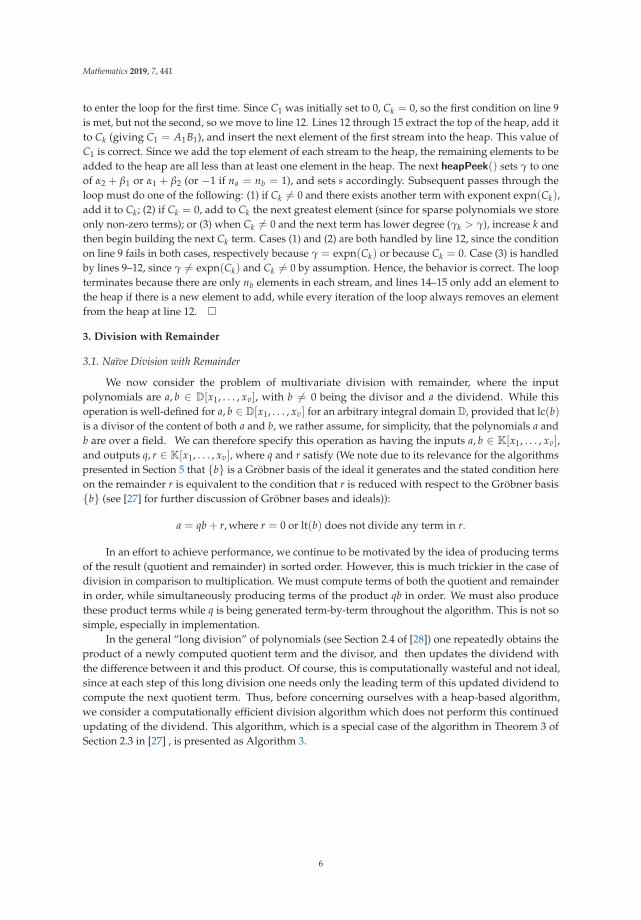
In the general “long division” of polynomials (see Section 2.4 of [28]) one repeatedly obtains theproduct of a newly computed quotient term and the divisor, and then updates the dividend withthe difference between it and this product. Of course, this is computationally wasteful and not ideal,since at each step of this long division one needs only the leading term of this updated dividend tocompute the next quotient term. Thus, before concerning ourselves with a heap-based algorithm,we consider a computationally efficient division algorithm which does not perform this continuedupdating of the dividend. This algorithm, which is a special case of the algorithm in Theorem 3 ofSection 2.3 in [27] , is presented as Algorithm 3.
6
Mathematics 2019, 7, 441
Algorithm 3 DIVIDEPOLYNOMIALS(a,b)a, b ∈ K[x1, . . . , xv ], b �= 0; return q, r ∈ K[x1, . . . , xv ] such that a = qb + r where r = 0 or lt(b) does not divide any term in r (r is reduced withrespect to the Gröbner basis {b}).
1: q := 0; r := 02: while (r := lt(a− qb− r)) �= 0 do3: if lt(b) | r then4: q := q + r/lt(b)5: else6: r := r + r7: end8: return (q, r)
In this algorithm, the quotient and remainder, q and r, are computed term-by-term by computingr = lt(a− qb− r) at each step. This works for division by deciding whether r should belong to theremainder or the quotient at each step. If lt(b) | r then we perform this division and obtain a newquotient term. Otherwise, we obtain a new remainder term. In either case, this r was the leading termof the expression a− qb− r and now either belongs to q or r. Therefore, in the next step, the old rwhich was added to either q or r will now cancel itself out, resulting in a new leading term of theexpression a− qb− r. This new leading term is non-increasing (in the sense of its monomial) relativeto the preceding r and thus terms of the quotient and remainder are produced in order.
Proposition 2. Algorithm 3 terminates and is correct. ([27], pp. 61–63)
3.2. Heap-Based Division with Remainder
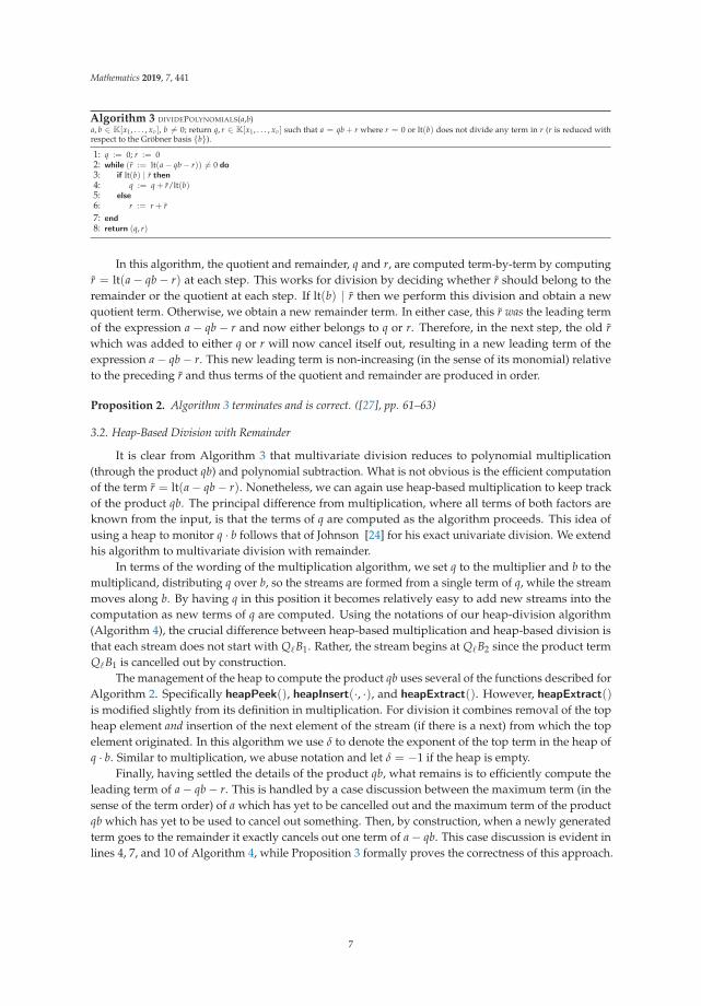
It is clear from Algorithm 3 that multivariate division reduces to polynomial multiplication(through the product qb) and polynomial subtraction. What is not obvious is the efficient computationof the term r = lt(a− qb− r). Nonetheless, we can again use heap-based multiplication to keep trackof the product qb. The principal difference from multiplication, where all terms of both factors areknown from the input, is that the terms of q are computed as the algorithm proceeds. This idea ofusing a heap to monitor q · b follows that of Johnson [24] for his exact univariate division. We extendhis algorithm to multivariate division with remainder.
In terms of the wording of the multiplication algorithm, we set q to the multiplier and b to themultiplicand, distributing q over b, so the streams are formed from a single term of q, while the streammoves along b. By having q in this position it becomes relatively easy to add new streams into thecomputation as new terms of q are computed. Using the notations of our heap-division algorithm(Algorithm 4), the crucial difference between heap-based multiplication and heap-based division isthat each stream does not start with Q�B1. Rather, the stream begins at Q�B2 since the product termQ�B1 is cancelled out by construction.
The management of the heap to compute the product qb uses several of the functions described forAlgorithm 2. Specifically heapPeek(), heapInsert(·, ·), and heapExtract(). However, heapExtract()is modified slightly from its definition in multiplication. For division it combines removal of the topheap element and insertion of the next element of the stream (if there is a next) from which the topelement originated. In this algorithm we use δ to denote the exponent of the top term in the heap ofq · b. Similar to multiplication, we abuse notation and let δ = −1 if the heap is empty.
Finally, having settled the details of the product qb, what remains is to efficiently compute theleading term of a− qb− r. This is handled by a case discussion between the maximum term (in thesense of the term order) of a which has yet to be cancelled out and the maximum term of the productqb which has yet to be used to cancel out something. Then, by construction, when a newly generatedterm goes to the remainder it exactly cancels out one term of a− qb. This case discussion is evident inlines 4, 7, and 10 of Algorithm 4, while Proposition 3 formally proves the correctness of this approach.
7

Mathematics 2019, 7, 441
Algorithm 4 HEAPDIVIDEPOLYNOMIALS(a,b)
a, b ∈ K[x1, . . . , xv ], a = ∑nai=1 ai Xαi = ∑na
i=1 Ai , b �= 0 = ∑nbj=1 bj X
βj = ∑nbj=1 Bj ; return q, r ∈ K[x1, . . . , xv ] such that a = qb + r where r = 0 or B1
does not divide any term in r (r is reduced with respect to the Gröbner basis {b}).
1: (q, r, l) := 02: k := 13: while (δ := heapPeek()) > −1 or k ≤ na do4: if δ < αk then5: r := Ak6: k := k + 17: else if δ = αk then8: r := Ak − heapExtract()9: k := k + 1
10: else11: r := −heapExtract()
12: if B1 | r then13: � := �+ 114: Q� := r/B115: q := q + Q�
16: heapInsert(Q� , B2)17: else18: r := r + r19: end20: return (q, r)
Proposition 3. Algorithm 4 terminates and is correct.
Proof. Let K be a field and a, b ∈ K[x1, . . . , xv] with tdeg(b) > 0. If b ∈ K then this degenerate case issimply a scalar multiplication by b−1
1 and proceeds as in Proposition 2. Then r = 0 and we are done.Otherwise, tdeg(b) > 0 and we begin by initializing q, r = 0, k = 1 (index into a), � = 0 (index into q),and δ = −1 (heap empty condition) since the heap is initially empty. The key change from Algorithm 3to obtain Algorithm 4 is to use terms of qb obtained from the heap to compute r = lt(a − qb − r).There are then three cases to track: (1) r is an uncancelled term of a; (2) r is a term from (a− r)− (qb),i.e., the degree of the greatest uncancelled term of a is the same as the degree of the leading term ofqb; and (3) r is a term of −qb with the property that the rest of the terms of a− r are smaller in theterm order. Let akXαk = Ak be the greatest uncancelled term of a. The three cases then correspond toconditions on the ordering of δ and αk. The term r is an uncancelled term of a (Case 1) either if theheap is empty (meaning either that no terms of q have yet been computed or all terms of qb have beenremoved), or if δ > −1 but δ < αk. In either of these two situations δ < αk holds and r is chosen tobe Ak. The term r is a term from the difference (a− r)− (qb) (Case 2) if both Ak and the top term in theheap have the same exponent vector (δ = αk). Lastly, r is a term of−qb (Case 3) whenever δ > αk holds.Algorithm 4 uses the above observation to compute r by adding conditional statements to comparethe components of δ and αk. Terms are only removed from the heap when δ ≥ αk holds, and thus we“consume” a term of qb. Simultaneously, when a term is removed from the heap, the next term fromthe given stream, if it exists, is added to the heap (by the definition of heapExtract()). The updatingof q and r with the new leading term r is almost the same as Algorithm 3, with the exception thatwhen we update the quotient, we also initialize a new stream with Q� in the multiplication of q · b.This stream is initialized with a head of Q�B2 because Q�B1, by construction, cancels a unique term ofthe expression a− qb− r. In all three cases, either the quotient is updated, or the remainder is updated.It follows from the case discussion of δ and αk that the leading term of a− qb− r is non-increasing foreach loop iteration and the algorithm therefore terminates by Proposition 2. Correctness is implied bythe condition that r = 0 at the end of the algorithm together with the fact that all terms of r satisfy thecondition lt(b) � Rk.
8

Mathematics 2019, 7, 441
4. Pseudo-Division
4.1. Naïve Pseudo-Division
The pseudo-division algorithm is essentially a univariate operation. Accordingly, we denotepolynomials and terms in this section as being elements of D[x1, . . . , xv−1][xv] = D[x] for an arbitraryintegral domain D. It is important to note that while the algorithms and discussion in this sectionare specified for univariate polynomials they are, in general, multivariate polynomials, and thus thecoefficients of these univariate polynomials are in general themselves multivariate polynomials.
Pseudo-division is essentially a fraction-free division: instead of dividing a by h = lc(b) (oncefor each term of the quotient q), a is multiplied by h to ensure that the polynomial division canoccur without being concerned with divisibility limitations of the ground ring. The outputs of apseudo-division operation are the pseudo-quotient q and pseudo-remainder r satisfying
h�a = qb + r, deg(r) < deg(b), (1)
where � satisfies the inequality 0 ≤ � ≤ deg(a) − deg(b) + 1. When � < deg(a) − deg(b) + 1 thepseudo-division operation is called lazy or sparse.
Under this definition, the simple multivariate division algorithm (Algorithm 3) can be readilymodified for pseudo-division by accounting for the required factors of h. This enters in two places:(i) each time a term of a is used, we must multiply the current term Ak of a by h�, where � is the numberof quotient terms computed so far, and (ii) each time a quotient term is computed we must multiply allthe previous quotient terms by h to ensure that h�a = qb + r will be satisfied. Algorithm 5 presentsthis basic pseudo-division algorithm modified from the simple multivariate division algorithm.
Algorithm 5 PSEUDODIVIDEPOLYNOMIALS(a,b)a, b ∈ D[x], b �= 0, h = lc(b); return q, r ∈ D[x] and � ∈ N such that h�a = qb + r, with deg(r) < deg(b).
1: (q, r, �) := 02: h := lc(b); β = deg(b)3: while (r := lt(h�a− qb− r)) �= 0 do4: if xβ | r then5: q := hq + r/xβ
6: � := �+ 17: else8: r := r + r9: end
10: return (q, r, �)
It is important to note that because pseudo-division is univariate, all of the quotient terms arecomputed before any remainder terms are computed. This is because we can always carry out apseudo-division step, and produce a new quotient term, provided that deg(b) ≤ deg(lt(h�a− qb− r)),where r = 0. When deg(b) > deg(lt(h�a− qb− r)) then the quotient is done being computed andwe have r = h�a− qb, satisfying the conditions (1) of a pseudo-remainder. The following propositionproves the correctness of our pseudo-division algorithm.
Proposition 4. Algorithm 5 terminates and is correct.
Proof. Let D be an integral domain and let a, b ∈ D[x] with β = deg(b) > 0. If deg(b) = 0, b = hand the divisibility test on line 4 always passes, all generated terms go to the quotient, and we get aremainder of 0 throughout the algorithm. Essentially this is a meaningless operation. q becomes hna−1aand the formula (1) holds with r = 0 and the convention that deg(0) = −∞. We proceed assumingdeg(b) > 0. We initialize q, r, � = 0. It is enough to show that for each loop iteration, the degreeof r strictly decreases. Since the degree of r is finite, r is zero after finitely many iterations. We usesuperscripts to denote the values of the variables of Algorithm 5 on the i-th iteration. We have twopossibilities for each i, depending on whether or not xβ | r(i) holds: (1) Q� = r(i)/xβ, Q� being a new
9

Mathematics 2019, 7, 441
quotient term; or (2) Rk = r(i), Rk being a new remainder term. In Case 1 we update only the quotientterm so r(i+1) = r(i); in Case 2 we update only the remainder term so q(i+1) = q(i).
Suppose, then, that r(i) has just been used to compute a term of q or r, and we now look tocompute r(i+1). Depending on whether or not xβ | r(i) we have:Case 1: xβ | lt(h�a− q(i)b− r(i)) and Q� = r(i)/xβ. Here, because we are still computing quotientterms, r(i+1) = r(i) = 0. Thus,
r(i+1) = lt(h�+1a− q(i+1)b− r(i+1)) = lt(h�+1a− ([hq(i) + Q�]b))
= lt(h�+1a− (hq(i)b + Q�b))
= lt(h�+1a− [hq(i)b + (hr(i) − hr(i)) + Q�b])
= lt(h�+1a− [hq(i)b + hr(i) + Q�(b− hxβ)])
= lt(h[h�a− q(i)b− r(i)]−Q�(b− B1))
= lt((h[h�a− q(i)b− r(i) − r(i)])−Q�(b− B1)
)< lt(r(i)) = r(i).
In the second last line, where r(i) = 0 appears, notice that since r(i) = lt(h�a− q(i)b− r(i)) andh ∈ D, we can ignore h for the purposes of choosing a term with highest degree and we have thereforethat lt(h�a− q(i)b− r(i) − r(i)) < lt(r(i)). Also, the expression Q�(b− B1) has leading term Q�B2 whichis strictly less than r(i) = Q�xβ, by the ordering of the terms of b. Hence r(i+1) is strictly less than r(i).Case 2: xβ � lt(h�a− q(i)b− r(i)) and Rk = r(i)
r(i+1) = lt(h�a− q(i+1)b− r(i+1)) = lt(h�a− q(i)b− (r(i) + Rk))
= lt((h�a− q(i)b− r(i))− r(i))
< lt(r(i)) = r(i).
Similar to Case 1, r(i) = lt(h�a− q(i)b− r(i)), thus the difference between (h�a− q(i)b− r(i)) andr(i) must have a leading term strictly less than r(i). The loop therefore terminates. The correctnessis implied by the condition that r = 0 at the end of the loop. The condition deg(r) < deg(b) ismet because the terms are only added to the remainder when xβ � r holds, i.e., when it is alwaysthe case that deg(h�a− qb) < deg(b). � ≤ deg(a)− deg(b) + 1 holds because � is only incrementedwhen a new quotient term is produced (i.e., xβ | r) and the maximum number of quotient terms isdeg(a)− deg(b) + 1.
4.2. Heap-Based Pseudo-Division
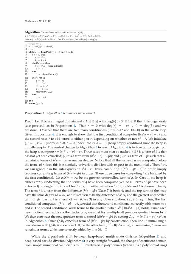
Optimization of Algorithm 5 using a heap proceeds in much the same way as for division. The onlyadditional concern to handle to reach Algorithm 6 is how to account for factors of h in the computationof lt(h�a− qb− r). Handling this requires adding the same number of factors of h to Ak that havebeen added to the quotient up to a given iteration, that is, h�. The number � is incremented when theprevious quotient terms are multiplied by h prior to adding a new quotient term. Other than this,the changes to Algorithm 5 to reach Algorithm 6 follow exactly the analogous changes to Algorithm 3to reach Algorithm 4. These observations therefore yield the following algorithm and proposition.
10
Mathematics 2019, 7, 441
Algorithm 6 HEAPPSEUDODIVIDEPOLYNOMIALS(a,b)
a, b ∈ D[x], a = ∑nai=1 ai xαi = ∑na
i=1 Ai , 0 �= b = ∑nbj=1 bj x
βj = ∑nbj=1 Bj , h = lc(b);
return q, r ∈ D[x] and � ∈ N such that h�a = qb + r, with deg(r) < deg(b).
1: (q, r, l) := 02: h := lc(b); β := deg(b)3: k := 14: while (δ := heapPeek()) > −1 or k ≤ na do5: if δ < αk then6: r := h�Ak7: k := k + 18: else if δ = αk then9: r := h�Ak − heapExtract()
10: k := k + 111: else12: r := −heapExtract()
13: if xβ | r then14: q := hq15: � := �+ 116: Q� := r/xβ
17: q := q + Q�
18: heapInsert(Q� , B2)19: else20: r := r + r21: end22: return (q, r, �)
Proposition 5. Algorithm 6 terminates and is correct.
Proof. Let D be an integral domain and a, b ∈ D[x] with deg(b) > 0. If b ∈ D then this degeneratecase proceeds as in Proposition 4. Then r = 0 with deg(r) = −∞ < 0 = deg(b) and weare done. Observe that there are two main conditionals (lines 5–12 and 13–20) in the while loop.Given Proposition 4, it is enough to show that the first conditional computes lt(h�a − qb − r) andthe second uses r to add terms to either q or r, depending on whether or not xβ | r. We initializeq, r = 0, k = 1 (index into a), � = 0 (index into q), δ = −1 (heap empty condition) since the heap isinitially empty. The central change to Algorithm 5 to reach Algorithm 6 is to take terms of qb fromthe heap to compute r = lt(h�a− qb− r). Three cases must then be tracked: (1) r is a term of h�a thathas not yet been cancelled; (2) r is a term from (h�a− r)− (qb); and (3) r is a term of −qb such that allremaining terms of h�a− r have smaller degree. Notice that all the terms of q are computed beforethe terms of r since this is essentially univariate division with respect to the monomials. Therefore,we can ignore r in the sub-expression h�a − r. Thus, computing lt(h�a − qb − r) in order simplyrequires computing terms of (h�a− qb) in order. These three cases for computing r are handled bythe first conditional. Let akXαk = Ak be the greatest uncancelled term of a. In Case 1, the heap iseither empty (indicating that no terms of q have been computed yet or all terms of qb have beenextracted) or deg(qb) = δ > −1 but δ < αk. In either situation δ < αk holds and r is chosen to be Ak.The term r is a term from the difference (h�a− qb) (Case 2) if both Ak and the top term of the heaphave the same degree (δ = αk) and r is chosen to be the difference of h�Ak and the greatest uncancelledterm of qb. Lastly, r is a term of −qb (Case 3) in any other situation, i.e., δ > αk. Thus, the firstconditional computes lt(h�a− qb− r), provided that the second conditional correctly adds terms to qand r. The second conditional adds terms to the quotient when xβ | lt(h�a− qb) holds. Since eachnew quotient term adds another factor of h, we must first multiply all previous quotient terms by h.We then construct the new quotient term to cancel lt(h�a− qb) by setting Q�+1 = lt(h�a− qb)/xβ, asin Algorithm 5. Since Q�B1 cancels a term of (h�a− qb) by construction, then line 18 initializing anew stream with Q�B2 is also correct. If, on the other hand, xβ � lt(h�a− qb), all remaining r terms areremainder terms, which are correctly added by line 20.
While the algorithmic shift between heap-based multivariate division (Algorithm 4) andheap-based pseudo-division (Algorithm 6) is very straight forward, the change of coefficient domainfrom simple numerical coefficients to full multivariate polynomials (when D is a polynomial ring)
11
Mathematics 2019, 7, 441
leads to many implementation challenges. This affects lines 6, 9 and 14 of Algorithm 6 in particularbecause they can involve multiplication of multivariate polynomials. These issues are discussed inSection 7.4.
5. Multi-Divisor Division and Pseudo-Division
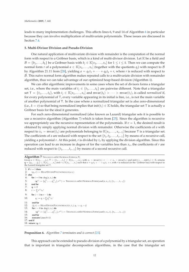
One natural application of multivariate division with remainder is the computation of the normalform with respect to a Gröbner basis, which is a kind of multi-divisor division. Let K be a field andB = {b1, . . . , bk} be a Gröbner basis with bj ∈ K[x1, . . . , xv] for 1 ≤ i ≤ k. Then we can compute thenormal form r of a polynomial a ∈ K[x1, . . . , xv] (together with the quotients qj) with respect to Bby Algorithm 21.11 from [28], yielding a = q1t1 + · · ·+ qktk + r, where r is reduced with respect toB. This naïve normal form algorithm makes repeated calls to a multivariate division with remainderalgorithm, thus we can take advantage of our optimized heap-based division (Algorithm 4).
We can offer algorithmic improvements in some cases where the set of divisors forms a triangularset, i.e., where the main variables of tj ∈ {t1, . . . , tk} are pairwise different. Note that a triangularset T = {t1, . . . , tk}, with tj ∈ K[x1, . . . , xv] and mvar(tk) > · · · > mvar(t1), is called normalized if,for every polynomial of T, every variable appearing in its initial is free, i.e., is not the main variableof another polynomial of T. In the case where a normalized triangular set is also zero-dimensional(i.e., k = v) so that being normalized implies that init(ti) ∈ K holds, the triangular set T is actually aGröbner basis for the ideal it generates.
For such zero-dimensional normalized (also known as Lazard) triangular sets it is possible touse a recursive algorithm (Algorithm 7) which is taken from [25]. Since the algorithm is recursivewe appropriately use the recursive representation of the polynomials. If v = 1, the desired result isobtained by simply applying normal division with remainder. Otherwise the coefficients of a withrespect to xv = mvar(tv) are polynomials belonging to K[x1, . . . , xv−1] because T is a triangular set.The coefficients of a are reduced with respect to the set {t1, t2, . . . , tv−1} by means of a recursive call,yielding a polynomial r. At this point, r is divided by tv by applying the division algorithm. Since thisoperation can lead to an increase in degree of for the variables less than xv, the coefficients of r arereduced with respect to {t1, . . . , tv−1} by means of a second recursive call.
Algorithm 7 TRIANGULARSETNORMALFORM (a,T)Given a ∈ K[x1, . . . , xv ], T = {t1, . . . , tv} ⊂ K[x1, . . . , xv ], with x1 = mvar(t1) < · · · < xv = mvar(tv) and init(t1), . . . , init(tv) ∈ K, returnsq = {q1, . . . , qv} ⊂ K[x1, . . . , xv ] and r ∈ K[x1, . . . , xv ] such that a = q1t1 + · · ·+ qvtv + r, with r is reduced (in the Gröbner bas) with respect tothe Lazard triangular set T.
1: if v = 1 then2: (q1, r) := HEAPDIVIDEPOLYNOMIALS(a, t1)3: else4: for i = 0 to deg(a, xv) do
5: (q(i) := {q(i)1 , . . . , q(i)v−1}, r(i)) := TRIANGULARSETNORMALFORM(coef(a, xv , i), {t1, . . . , tv−1})6: end for7: q := 08: r := ∑
ir(i)xv
i
9: for j = 1 to v− 1 do
10: qj := qj + ∑i
q(i)j xvi
11: end for12: (q, r) := HEAPDIVIDEPOLYNOMIALS(r, tv); qv := qv + q13: for i = 0 to deg(r, xv) do
14: (q(i) := {q(i)1 , . . . , q(i)v−1}, r(i)) := TRIANGULARSETNORMALFORM(coef(r, xv , i), {t1, . . . , tv−1})15: end for16: execute Lines 8–1117: end if18: return (q, r)
Proposition 6. Algorithm 7 terminates and is correct [25].
This approach can be extended to pseudo-division of a polynomial by a triangular set, an operationthat is important in triangular decomposition algorithms, in the case that the triangular set
12

Mathematics 2019, 7, 441
is normalized. The pseudo-remainder r and pseudo-quotients qj of a polynomial a ∈ K[x1, . . . , xv]
pseudo-divided by a triangular set T = {t1, . . . , tk}must satisfy
ha = q1t1 + · · ·+ qktk + r, deg(r, mvar(tj)) < deg(tj, mvar(tj)) for 1 ≤ j ≤ k, (2)
where h is a product of powers of the initials (leading coefficients in the univariate sense) of thepolynomials of T. If this condition is satisfied then r is said to be reduced with respect to T, again usingthe convention that deg(r) = −∞ if r = 0.
The pseudo-remainder r can be computed naïvely in k iterations where each iterationperforms a single pseudo-division step with respect to each main variable in decreasing ordermvar(tk), mvar(tk−1), . . . , mvar(t1). The remainder is initially set to a and is updated duringeach iteration. This naïve algorithm is inefficient for two reasons. First, since each pseudo-divisionstep can increase the degree of lower variables in the order, if a is not already reduced with respectto T, the intermediate pseudo-remainders can experience significant coefficient swell. Second, it isinefficient in terms of data locality because each pseudo-division step requires performing operationson data distributed throughout the polynomial.
A less naïve approach is a recursive algorithm that replaces each of the k pseudo-division steps inthe naïve algorithm with a recursive call, amounting to k iterations where multiple pseudo-divisionoperations are performed at each step. This algorithm deals with the first inefficiency issue of coefficientswell, but still runs into the issue with data locality. To perform this operation more efficientlywe conceive a recursive algorithm (Algorithm 8) based on the recursive normal form algorithm(Algorithm 7). Using a recursive call for each coefficient of the input polynomial a ensures that wework only on data stored locally, handling the second inefficiency of the naïve algorithm.
Algorithm 8 TRIANGULARSETPSEUDODIVIDE (a,T)Given a, t1, . . . , tk ∈ K[x1, . . . , xv ], T = {t1, . . . , tk}, with mvar(t1) < · · · < mvar(tk) and init(tj) /∈ {mvar(ti) | ti ∈ T} for 1 ≤ j ≤ k, returnsq = {q1, . . . , qk} ⊂ K[x1, . . . , xv ] and r, h ∈ K[x1, . . . , xv ] such that ha = q1t1 + · · ·+ qktk + r, where r is reduced with respect to T.
1: if k = 1 then2: (q1, r, e) := HEAPPSEUDODIVIDEPOLYNOMIALS(a, t1); h = init(t1)e
3: else4: xm := mvar(tk)5: for i = 0 to deg(a, xm) do
6: (q(i) := {q(i)1 , . . . , q(i)k−1}, r(i) , h(i)) := TRIANGULARSETPSEUDODIVIDE(coef(a, xm , i), {t1, . . . , tk−1})7: end for8: q = 09: h1 := lcm(h(i)), 0 ≤ i ≤ deg(a, xm)
10: r := ∑i(h1/h(i)) r(i)xi
m
11: for j = 1 to k− 1 do
12: qj := qj + ∑i(h1/h(i)) q(i)j xi
m
13: end for14: if mvar(r) = xm then15: (q, r, e) := HEAPPSEUDODIVIDEPOLYNOMIALS(r, tk)
16: h = init(tk)e
17: for j = 1 to k− 1 do18: qj := qj h19: end for20: qk := q21: for i = 0 to deg(r, xm) do
22: (q(i) := {q(i)1 , . . . , q(i)k−1}, r(i) , h(i)) := TRIANGULARSETPSEUDODIVIDE(coef(r, xm , i), {t1, . . . , tk−1})23: end for24: h2 := lcm(h(i)), 0 ≤ i ≤ deg(r, xm)25: for j = 1 to k do26: qj := qjh2
27: end for28: execute Lines 9–13 with h2 replacing h1
29: h := h1 hh230: else31: h := h1; qk = 032: end if33: end if34: return (q, r, h)
13

Mathematics 2019, 7, 441
Proposition 7. Algorithm 8 terminates and is correct.
Proof. The central difference between this algorithm and Algorithm 7 is the change from division topseudo-division. By Proposition 5 the computed pseudo-remainders are reduced with respect to theirdivisor. The fact that the loops of recursive calls are all for a triangular set with one fewer variablesensures that the total number of recursive calls is finite, and the algorithm terminates. If k = 1, thenProposition 5 proves correctness of this algorithm, so assume that k > 1.
We must first show that lines 4–13 correctly reduce a with respect to the polynomials
{t1, . . . , tk−1}. Let ci = coef(a, xm, i), so a = ∑deg(a,xm)i=0 cixi
m. Assuming the correctness of the
algorithm, the result of these recursive calls are q(i)j , r(i) and h(i) such that h(i)ci = ∑k−1j=1 q(i)j tj + r(i),
where deg(r(i), mvar(tj)) < deg(tj, mvar(tj)) and h(i) = ∏k−1j=1 init(tj)
ej for some non-negative integers
ej. It follows that ci =(
∑k−1j=1 q(i)j tj + r(i)
)/h(i). We seek a minimal h1 such that h1a = ∑i h1cixi
m =
∑i(h1/h(i))(
∑k−1j=1 q(i)j tj + r(i)
)xi
m is denominator-free, which is easily seen to be lcm(h(i)). This then
satisfies the required relation of the form (2), with h1 in place of h, by taking qj = ∑i(h1/h(i))q(i)j tjxim
and r = ∑i(h1/h(i))r(i)j xim. This follows from the conditions deg(r(i), mvar(tj)) < deg(tj, mvar(tj))
since h1 contains none of the main variables of {t1, . . . , tk−1} because T is normalized.If at this point mvar(r) �= xm, then no further reduction needs to be done and the algorithm
finishes with the correct result by returning (q1, . . . , qk−1, 0, r, h1). This is handled by the else clauseon lines 30 and 31 of the conditional on lines 14–32. If, on the other hand, mvar(r) = xm, we mustreduce r with respect to tk. Proposition 5 proves that after executing line 15, deg(r, mvar(tk)) <
deg(tk, mvar(tk)), and together with lines 16–20 implies that with the updated pseudo-quotients
hh1a =k
∑j=1
qjtj + r. (3)
Since the pseudo-division step at line 15 may increase the degrees of the variables of r lessthan xm in the variable ordering, we must issue a second set of recursive calls to ensure that (2) issatisfied. Again, given the correctness of the algorithm, it follows that the result of the recursive calls
on lines 21–23 taking as input r = ∑deg(r,xm)i=0 cixi
m, with ci = coef(r, xm, i), are q(i)j , r(i) and h(i) such that
h(i)ci = ∑k−1j=1 q(i)j tj + r(i), where deg(r(i), mvar(tj)) < deg(tj, mvar(tj)). Combining these results as
before and taking h2 = lcm(h(i)) it follows that
h2r =k−1
∑j=1
qjtj + r (4)
satisfies a reduction condition of the form (2) with q = ∑i(h2/h(i))q(i)j tjxim and r = ∑i(h2/h(i))r(i)j xi
m,
again because T is normalized. Multiplying (3) by h2 and using Equation (4) yields h2hh1a =
∑kj=1 h2qjtj + h2r = ∑k
j=1 h2qjtj +∑k−1j=1 qjtj + r = ∑k−1
j=1 (h2qj + qj)tj + h2qktk + r, which gives the correctconditions for updating the pseudo-quotients on lines 25–27, with the qj and r computed at line 28.Now r is reduced with respect to xm because r is and with respect to mvar(t1), . . . , mvar(tk−1) becauseof the above argument, so that the correct overall multiplier is h = h2hh1, set on line 29. The algorithmis therefore correct.
6. Data Structures
Polynomial arithmetic is fundamental to so many algorithms that it should naturally be optimizedas much as possible. Although algorithm choice is important for this, so too is making use ofappropriate data structures. When programming for modern computer architectures we must be
14

Mathematics 2019, 7, 441
concerned with the processor–memory gap: the exponentially increasing difference between processorspeeds and memory-access time. We combat this gap with judicial memory usage and management.In particular, the principle of locality and cache complexity describe how to obtain performance bymaximizing memory accesses that make best use of modern memory hierarchies (i.e., data locality).Basically, this means that the same memory address should be accessed frequently or, at the veryleast, accesses should be adjacent to those most recently accessed. Our implementation adheres to thisprinciple through the use of memory-efficient data structures with optimal data locality. We see later(in Section 7) that our algorithms have implementation-specific optimizations to exploit this localityand minimize cache complexity.
This section begins by reviewing our memory-efficient data structures for both sparse distributed(Section 6.1) polynomials and sparse recursive polynomials (Section 6.2). The latter is interesting asthe data structure is still flat and distributed but allows for the polynomial to be viewed recursively.Then, we discuss the implementation of our heap data structure (Section 6.3) which is specialized andoptimized for use in polynomial multiplication.
6.1. A Sparse Distributed Polynomial Data Structure
The most simple and common scheme for sparsely representing a polynomial is a linked list,or some similar variation of data blocks linked together by pointers [6,29,30]. This representation allowsfor very easy manipulation of terms using simple pointer manipulation. However, the indirectioncreated by pointers can lead to poor locality while the pointers themselves must occupy memory,resulting in memory wasted to encode the structure rather than the data itself. More efficient sparsedata structures have been explored by Gastineau and Laskar [29], where burst tries store monomialsin the TRIP computer algebra system, and Monagan and Peace [30], where the so-called POLY datastructure for MAPLE closely stores monomials in a dense array. In both cases, the multi-precisioncoefficients corresponding to those monomials are stored in a secondary structure and accessed byeither indices stored alongside the monomials (in the case of TRIP) or pointers (in the case of MAPLE).
Our distributed polynomial representation stores both coefficients and monomials side-by-sidein the same array. This representation, aptly named an alternating array, improves upon data locality;the coefficient and monomial which together make a single polynomial term are optimally localwith respect to each other. This decision is motivated by the fact that in arithmetic, coefficientsare accessed alongside their associated monomials (say to perform a multiplication or combinelike terms). In practice, this array structure is augmented by a simple C-struct holding three items: thenumber of terms; the number of variables; and a pointer to the actual array. This seemingly simplestructure abstracts away some complexities in both the coefficients and monomials. We begin withthe coefficients.
Due to the nature of arbitrary-precision coefficients, in our case either integers or rationalnumbers (We actually have two nearly identical yet distinct alternating array implementations.One implementation holds integer coefficients while the other holds rational number coefficients),we cannot say they are fully stored in the array. We make use of the GNU Multiple Precision Arithmetic(GMP) Library [31] for our coefficients. The implementation of arbitrary-precision numbers in thislibrary is broken into two distinct parts, which we will call the head and the tree. The head containsmetadata about the tree, as well as a pointer to the tree, while the tree itself is what holds thenumerical data. By the design of the GMP library users only ever interact with the head. Thus,our alternating array representation holds the heads of the GMP numbers directly in the arrayrather than pointers or indices to some other structure, which in turn would hold the heads ofthe GMP numbers. Figure 1 depicts an arbitrary polynomial of n terms stored in an alternating array,highlighting the GMP tree structure.
15

Mathematics 2019, 7, 441
a1 α1 a2 α2 · · · an αn
Term 1 Term 2 Term n
t1 t2 tn
Figure 1. An alternating array representation of n terms showing GMP trees as t1, t2, . . . , tn, GMPheads as a1, a2, . . . , an, and monomials as α1, α2, . . . , αn. One head and tree together make a singlearbitrary-precision number.
The alternating array diagram in Figure 1 may be misleading at first glance, since it appearsthat pointers are still being used; however, these pointers are completely internal to GMP and areunavoidable. Hence, where other structures use indices ([29], Figure 2) or pointers ([6], Figure 3)to a separate array of GMP coefficients, that coefficient array also further contains these pointersto GMP trees. Our implementation thus removes one level of indirection compared to these otherschemes. We do note, however, that the data structure described in [6,30] includes an additional featurewhich automatically makes use of machine-precision integers stored directly in the data structure,rather than GMP integers, if coefficients are small enough.
Next, we discuss the implementation of monomials. Under a fixed variable ordering itbecomes unnecessary to store the variables themselves with the monomial, and so we only storethe exponent vector. This greatly reduces the required memory for a monomial. However, even morememory is saved via exponent packing. Using bit-masks and bit-shifts, multiple partial degrees, eachtaking a small non-negative value, can easily be stored in a single machine word (usually 64 bits).This fact should be obvious by looking at the binary representation of a non-negative integer on acomputer. Integers are stored in some fixed size, typically 32 or 64 bits, and, when positive or unsigned,have many leading 0 bits. For example, 5 as a 32-bit integer is 0b00000000000000000000000000000101.By using a predetermined number of bits for each partial degree in an exponent vector, it becomeseasy to partition the 64 bits to hold many integers. Our alternating array thus holds a single machineword directly in the array for packing each exponent vector.
Exponent packing has been in use at least since the 60s in ALTRAN [1], but also in more recentworks such as [4,32]. Our implementation differs from others in that exponents are packed unevenly,i.e., each exponent is given a different number of bits in which to be encoded. This is motivatedby two factors. First, 64 bits is rarely evenly divided among the number of variables, meaningsome bits could be wasted. Second, throughout the process of operations such as pseudo-divisionor triangular decomposition the degrees of lower-ordered variables often increase more drasticallythan higher-ordered variables, and so we give more bits to the lower-ordered variables. This canallow for large computations to progress further without failing or having to revert to an unpackedexponent vector. One final highlight on exponent packing (first emphasized in [32]) is that monomialcomparisons and monomial multiplications respectively reduce to a single machine-integer comparisonand a single machine-integer addition. This result drastically reduces the time to complete monomialcomparisons, and thus sort monomials, a huge part of sparse polynomial arithmetic.
6.2. A Sparse Polynomial Data Structure for Viewing Polynomials Recursively
We take this section to describe our recursive polynomial data structure. That is not to say thatthe data structure itself is recursive, rather the polynomial is viewed recursively, as a univariatepolynomial with multivariate polynomial coefficients. In general, polynomials are stored using thedistributed representation; however, some operations, such as pseudo-division, require a specificallyunivariate view of the polynomial. Thus, we have created an in-place, very fast conversion betweenthe distributed and recursive representations, amounting to minimal overhead in both memory usage
16

Mathematics 2019, 7, 441
and time. As a result, we can use the same distributed representation everywhere, only converting asrequired. This recursive representation is shown in Figure 2.
3 x1x22x3
3 6 x1x22x2
3 4 x1x2x23 7 x1
3 x1x22 6 x1x2
2 4 x1x2 7 x1
3 1 2 2 0 1
�Distributed
Recursive
Figure 2. A distributed polynomial representation and its corresponding recursive polynomialrepresentation, showing the additional secondary array. The secondary array alternates between:(1) degree of the main variable, (2) size of the coefficient polynomial, and (3) a pointer to the coefficientpolynomial, which is simply an offset into the original distributed polynomial.
To view a polynomial recursively we begin by (conceptually) partitioning its terms into blocksbased on the degree of the main (highest-ordered) variable. Since our polynomials are stored usinga lexicographical term order, the terms of the polynomial are already sorted based on the degree ofthe main variable. Moreover, terms within the same block are already stored in lexicographical orderwith respect to the remaining variables. Therefore, each block will act as a multivariate polynomialcoefficient of the univariate polynomial in the main variable. The partitioning is done in-place, withoutany memory movement, simply by maintaining an offset into the alternating array which signifies thebeginning of a particular coefficient, in the recursive sense.
We create a secondary auxiliary array which holds these offsets, the number of terms in eachpolynomial coefficient, and the degree of the main variable. Simultaneously, the degree of the mainvariable in the original alternating array is set to 0. The degree of the main variable then does notpollute the polynomial coefficient arithmetic. This secondary array results in minimal overhead,particularly because its size is proportional to only the number of unique values of the degree of themain variable. Figure 2 highlights this secondary array as part of the recursive structure.
6.3. Heaps Optimized for Polynomial Multiplication
The largest effort required of our sparse multiplication algorithm (and thus also that of ourdivision and pseudo-division algorithms) is to sort the terms of the product. Our algorithm makesuse of a heap to do this sorting (much like heap sort), and thus arithmetic performance is largelydependent in the performance of the heap. Briefly, a heap is a data structure for efficiently obtainingthe maximum (or minimum) from a continually updating collection of elements. This is achieved byusing a binary tree, which stores key-value pairs, with a special heap property—children are always lessthan their parents in the tree. A more complete discussion of heaps can be found in ([26], Section 2.4).
The optimizations used in our heap implementation focus on two aspects, minimizing the workingmemory of the heap and minimizing the number of comparisons. The need for the latter should beobvious, while the need for the former is more subtle. Due to the encoding of a heap as a binary tree,parent nodes and child nodes are not adjacent to each other in memory; the heap must essentiallyperform random memory accesses across all its elements. In the sense of locality and cache usage, thisis not ideal, yet unavoidable. Therefore, we look to minimize the size of the heap in hopes that it willentirely fit in cache and allow for quick access to all its elements.
The first optimization is due to [33] which reduces the number of comparisons required to removethe maximum element of the heap by a factor of two. The usual implementation of a heap removesthe root node, swapping a leaf node into the hole, and then filtering it downward to re-establish theheap property. This requires two comparisons per level to determine which path to travel down.Instead, one can continuously promote the larger of the hole’s two children until the hole is a leaf node.This requires only one comparison per level.
17
Mathematics 2019, 7, 441
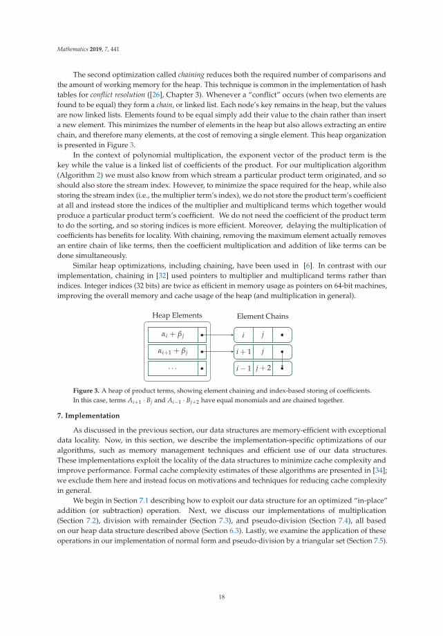
The second optimization called chaining reduces both the required number of comparisons andthe amount of working memory for the heap. This technique is common in the implementation of hashtables for conflict resolution ([26], Chapter 3). Whenever a “conflict” occurs (when two elements arefound to be equal) they form a chain, or linked list. Each node’s key remains in the heap, but the valuesare now linked lists. Elements found to be equal simply add their value to the chain rather than inserta new element. This minimizes the number of elements in the heap but also allows extracting an entirechain, and therefore many elements, at the cost of removing a single element. This heap organizationis presented in Figure 3.
In the context of polynomial multiplication, the exponent vector of the product term is thekey while the value is a linked list of coefficients of the product. For our multiplication algorithm(Algorithm 2) we must also know from which stream a particular product term originated, and soshould also store the stream index. However, to minimize the space required for the heap, while alsostoring the stream index (i.e., the multiplier term’s index), we do not store the product term’s coefficientat all and instead store the indices of the multiplier and multiplicand terms which together wouldproduce a particular product term’s coefficient. We do not need the coefficient of the product termto do the sorting, and so storing indices is more efficient. Moreover, delaying the multiplication ofcoefficients has benefits for locality. With chaining, removing the maximum element actually removesan entire chain of like terms, then the coefficient multiplication and addition of like terms can bedone simultaneously.
Similar heap optimizations, including chaining, have been used in [6]. In contrast with ourimplementation, chaining in [32] used pointers to multiplier and multiplicand terms rather thanindices. Integer indices (32 bits) are twice as efficient in memory usage as pointers on 64-bit machines,improving the overall memory and cache usage of the heap (and multiplication in general).
αi + β j
αi+1 + β j
. . .
i j
i + 1 j
i− 1 j + 2
Heap Elements Element Chains
Figure 3. A heap of product terms, showing element chaining and index-based storing of coefficients.In this case, terms Ai+1 · Bj and Ai−1 · Bj+2 have equal monomials and are chained together.
7. Implementation
As discussed in the previous section, our data structures are memory-efficient with exceptionaldata locality. Now, in this section, we describe the implementation-specific optimizations of ouralgorithms, such as memory management techniques and efficient use of our data structures.These implementations exploit the locality of the data structures to minimize cache complexity andimprove performance. Formal cache complexity estimates of these algorithms are presented in [34];we exclude them here and instead focus on motivations and techniques for reducing cache complexityin general.
We begin in Section 7.1 describing how to exploit our data structure for an optimized “in-place”addition (or subtraction) operation. Next, we discuss our implementations of multiplication(Section 7.2), division with remainder (Section 7.3), and pseudo-division (Section 7.4), all basedon our heap data structure described above (Section 6.3). Lastly, we examine the application of theseoperations in our implementation of normal form and pseudo-division by a triangular set (Section 7.5).
18

Mathematics 2019, 7, 441
7.1. In-Place Addition and Subtraction
An “in-place” algorithm suggests that the result is stored back into the same data structure as oneof operands (or the only operand). This strategy is often motivated by either limited available memoryresources or working with data that is too large to consider making a complete copy for the result.For our purposes, we are concerned with neither of these since our polynomial representations userelatively small amounts of memory. Hence, in-place operations are only of interest if they canimprove running time. Generally speaking, in-place algorithms require more operations and moremovement of data than out-of-place alternatives, making them most useful when the data set beingsorted is so large that a copy cannot be afforded. For example, in-place merge sort has been a topicof discussion for decades, however, these implementations run 25–200% slower than an out-of-placeimplementation [35–37].
Due to the similarities between merge sort and polynomial addition (subtraction) it would seemunlikely that an in-place scheme would lead to performance benefits. However, our in-place additionbecomes increasingly faster than out-of-place addition as coefficient sizes increase. This in-placeaddition scheme is not technically in-place, but it does exploit the structure of GMP numbers(as shown in Figure 1) for in-place coefficient arithmetic. In-place addition builds the resultingpolynomial out-of-place but reuses the GMP trees of one of the operand polynomials. Rather thanallocating a new GMP number—and thus a new GMP tree—in the resulting polynomial, we simplycopy the head of one GMP number (and the pointer to its existing tree) into the new polynomial’salternating array, performing the coefficient arithmetic in-place. This saves on memory allocationand memory copying, and benefits from the improved performance of GMP when using in-placearithmetic ([31], Section 3.11).
These surprising results are highlighted in Figure 4 where out-of-place addition and its in-placecounterpart are compared for various polynomial sizes with varying coefficient sizes. In-place additionhas a speed-up factor of up to 3 for the coefficient sizes tested, with continued improvements ascoefficient sizes grow larger. In-place arithmetic is put to use in pseudo-division to reduce thecost of polynomial coefficient arithmetic and improve the performance of pseudo-division itself.See Section 7.4 for this discussion.
103 104 105 106 10710−4
10−3
10−2
10−1
100
101
Number of Terms (n)
Run
ning
Tim
e(s
)
Q[x1, x2, x3] AdditionIn-place vs Out-of-place
Out, 256Out, 64Out, 8
In, 256In, 64In, 8
Figure 4. Comparing in-place and out-of-place polynomial addition. Random rational numberpolynomials in 3 variables are added together for various numbers of terms and for variouscoefficient sizes. The number of bits needed to encode the coefficients of the operands are shown in thelegend. Notice this is a log-log plot.
19
Mathematics 2019, 7, 441
7.2. Multiplication
The algorithm for polynomial multiplication (Algorithm 2) translates to code quite directly.However, we note some important implementation details to obtain better performance. Apart fromthe optimizations within the heap itself there are some implementation details concerning how theheap is used within multiplication to improve performance.
The first optimization makes use of the fact that multiplication is a commutative operation.Since the number of elements in the heap is equal to the number of streams, which is in turn equalto the number of terms in the multiplier (the factor a in a · b), then we choose the multiplier to be thesmaller operand, minimizing the size of the heap. The second optimization deals with the initializationof the heap. Due to the fact that for two terms Ai and Bj, Ai · Bj is always greater than Ai+1 · Bj in theterm order, then at the beginning of the multiplication algorithm it is only necessary to insert the termAi+1 · B1 after the term Ai · B1 has been removed from the heap.
A final optimization for multiplication deals with memory management. In particular,we know that for operands with na and nb terms each, the maximum size of the product is na · nb.Therefore, we can pre-allocate this maximal size of the product (and similarly pre-allocate a maximalsize na for the heap) before we begin computation. This eliminates any need for reallocation or memorymovement, which can cause slowdowns. However, in the case where na · nb is a very large number, say,exceeding 100 million, then we begin by only allocating 100 million terms for the product, doublingthe allocation as needed in order amortize the cost of reallocation. Of course, any memory allocated inexcess is freed at the end of the algorithm.
7.3. Division with Remainder
Polynomial division is essentially a direct application of polynomial multiplication. Again, we useheaps, with all the optimizations previously discussed, to produce the terms of the quotient-divisorproduct efficiently and in order. However, one important difference between division andmultiplication is that the one of the operands of the quotient-divisor product, the quotient,is simultaneously being produced and consumed throughout the algorithm. Thus, we cannotpre-allocate space for the product or heap since the size of the quotient is unknown. Instead, we againfollow a doubling of allocation strategy for the quotient and remainder to amortize the cost ofreallocation. Moreover, we reallocate the space for the heap whenever we reallocate q since weknow that the heap’s maximum size will be equal to the number of terms in q. The added benefit ofthis is that the heap is guaranteed to have enough space to store all elements and does not need tocheck for overflow on each insert.
7.4. Pseudo-Division
As seen in Section 4.1 the algorithms for division (Algorithms 3 and 4) can easily beadapted to pseudo-division (Algorithms 5 and 6) by multiplying the dividend and quotientby the divisor’s initial. However, the implementation between these two algorithms isvery different. In essence, pseudo-division is a univariate operation, viewing the input multivariatepolynomials recursively. That is, the dividend and divisor are seen as univariate polynomialsover some arbitrary (polynomial) integral domain. Therefore, coefficients can be, and indeed are,entire polynomials themselves. Coefficient arithmetic becomes non-trivial. Moreover, the normaldistributed polynomial representation would be inefficient to traverse and manipulate in this recursiveway. Therefore, we use the recursive polynomial representation described in Section 6.1 with minimaloverhead for conversion.
One of the largest performance concerns in this recursive view is the non-trivialcoefficient arithmetic. As coefficients are now full polynomials there is more overhead in manipulatingthem and performing arithmetic. One important implementation detail is to perform the addition(and subtraction) of like terms in-place. Such combinations occur when computing the leading
20

Mathematics 2019, 7, 441
term of h�a− qb and when combining like terms in the quotient-divisor product. In-place addition,as described in Section 7.1, performs exceedingly better than out-of-place addition as the size ofnumerical coefficients grows, which occurs drastically during pseudo-division.
Similarly, the update of the quotient by multiplying by the initial of the divisor requiresa multiplication of full polynomials. If we wish to save on memory movement we shouldperform this multiplication in-place as well. However, in our recursive representation (Figure 2),coefficient polynomials are tightly packed in a continuous array. To modify them in-place wouldrequire shifting all the following coefficients down the array to make room for the strictly large productpolynomial. To avoid this unnecessary memory movement we modify the recursive data structureexclusively for the quotient polynomial; we break the continuous array of coefficients into many arrays,one for each coefficient. This allows them to grow without displacing the following coefficients. At theend of the algorithm, once the quotient has finished being produced, we collect and compact all ofthese disjoint polynomials into a single, packed array. In contrast, the remainder is never updated onceits terms are produced, nor does it need to be viewed recursively, thus it is stored directly in the normaldistributed representation, avoiding the unnecessary conversion out of the recursive representation.
7.5. Multi-Divisor (Pseudo-)Division
The performance of our normal form and multi-divisor pseudo-division algorithms primarilyrelies on the performance of the basic operations of division and pseudo-division, respectively.Hence, our normal form and multi-divisor pseudo-division algorithms gain significant performancebenefits from the optimization of these lower-level operations. We only note two particularimplementation details for these multi-divisor algorithms.
Firstly, the algorithms for normal form (Algorithm 7) and triangular set pseudo-division(Algorithm 8) use distributed and recursive polynomial representations, respectively, to manipulateoperand polynomials appropriately for their operations. Secondly, we use in-place techniques,following the scheme of in-place addition (Section 7.1) to reduce the effects of GMP arithmetic andmemory movement. Due to the recursive nature of these algorithms we can use a pre-allocation ofmemory as a destination to store both the final remainder and the remainder in each recursive call,continually reusing GMP coefficients.
8. Experimentation and Discussion
As we have seen in the previous two sections, our implementation has focused well on localityand memory usage in interest of obtaining performance. Indeed, as a result of the processor–memorygap this is highly important on modern architectures. The experimentation and benchmarks providedin this section substantiate our efforts where we will compare similar heap-based arithmetic algorithmsprovided in MAPLE [38].
Let us begin with a discussion on the quantification of sparsity with respect to polynomials.For univariate polynomials, sparsity can easily be defined as the maximum degree difference betweenany two successive non-zero terms. However, in the multivariate case, and in particular usinglex ordering, there are infinitely many polynomial terms between x1 and x2, in the form of xi
1.For multivariate polynomial, sparsity is less easily defined. Inspired by Kronecker substitution ([28],Section 8.4) we propose the following sparsity measure for multivariate polynomials adapted fromthe univariate case. Let f ∈ R[x1, . . . , xv] be non-zero and define r = max(deg( f , xi), 1 ≤ i ≤ v) + 1.Then, every exponent vector e := (e1, . . . , ev) of a term of f can be viewed as an integer in a radix-rrepresentation, e1 + e2r + · · ·+ evrv−1. Viewing any two successive polynomial terms in f , say Fi andFi+1, as integers in this radix-r representation, say ci and ci+1, we call the sparsity of f the smallestinteger which is larger than the maximum value of ci − ci+1, for 1 ≤ i < n f .
Our experimentation uses randomly generated sparse polynomials whose generation isparameterized by several variables: the number of variables v, the number of terms n, the number ofbits used to encode any coefficient (denoted coefficient bound), and a sparsity value s used to compute
21
Mathematics 2019, 7, 441
the radix r = v√
s · n� for use in generating exponent vectors as just defined. Our arithmetic algorithms,and code for generating random test instances, are openly available in the BPAS library [12].
We compare our arithmetic implementations against MAPLE for both integer polynomials andrational number polynomials. Thanks to the work by Monagan and Pearce [6,18,19,32] in recentyears MAPLE has become the leader in integer polynomial arithmetic. Benchmarks there clearlyshow that their implementation outperforms many others including that of TRIP [39], MAGMA [40],SINGULAR [41], and PARI/GP [42]. Moreover, other common libraries like FLINT [43] andNTL [44] provide only univariate polynomials, so to compare our multivariate implementationagainst theirs would be unfair. Hence, we compare against MAPLE with its leading high-performanceimplementation. In particular, MAPLE 2017 with kernelopts(numcpus = 1) (which forces MAPLE torun serially.) Of course, the parallel arithmetic of MAPLE described in [18,19], which has been shownto achieve up to 17x parallel speed-up, could out-perform our serial implementation in some cases,such as multiplication and division over Z. However, to be fair, we compare serial against serial.
Our benchmarks were collected on a machine running Ubuntu 14.04 using an Intel Xeon X560processor (Intel, Santa Clara, CA, USA) at 2.67 GHz with 32 KB L1 data cache, 256 KB L2 cache,and 12288 KB L3 cache, with 12× 4 GB of DDR3 RAM at 1333 MHz. In all the following timings wepresent the median time among 3 trials using 3 different sets of randomly generated input polynomials.
8.1. Multiplication and Division with Remainder
We compare multiplication and division with remainder against MAPLE for both polynomialsover the rational numbers and the integers. For multiplication we call expand in MAPLE and fordivision with remainder we call Groebner:-NormalForm. Normal form is a more general algorithmfor many divisors but reduces to division with remainder in the case of a single divisor. This operationappears to be the only documented algorithm for computing division with remainder in MAPLE.The optimized integer polynomial exact division of [6] appears in MAPLE as the divide operation.It would be unfair to use our division with remainder algorithm to compute exact divisions to compareagainst [6] directly (although, some examples of such are shown in Section 8.4). However, internally,Groebner:-NormalForm clears contents to work, at least temporarily, with integer polynomials forcalls to divide and expand for division and multiplication operations, respectively, each of which isindeed optimized (Contents are cleared from (rational number) polynomials, to result in an integerpolynomial, either via the basis computation or directly in the call to the underlying normal formfunction Groebner:-Buchberger:-nfprocs).
We begin by comparing our multiplication and division with remainder algorithms forpolynomials over the rationals. MAPLE does not have an optimized data structure for polynomialswith rational number coefficients [30], so this benchmark is meant to highlight the necessity ofmemory-efficient data structures for algorithmic performance. The plot in Figure 5a shows theperformance of multiplication over Q for polynomials in 5 variables of varying sparsity and numberof terms. The parameters specified determine how both the multiplier and multiplicand whererandomly generated. The plot in Figure 5b shows the performance of division with remainder over Qfor polynomials in 5 variables of varying sparsity and number of terms. For this division, we constructtwo polynomials f and g using the parameters specified and then perform the division ( f · g + f )/g.The disparity in running times between BPAS and MAPLE is very apparent, with multiple ordersof magnitude separating the two. We see speed-ups of 333 for multiplication and 731 for divisionwith remainder.
The same set of experiments were performed again for integer polynomials. Figure 6a,b showsmultiplication and division with remainder, respectively, for polynomials over Z. In this case, MAPLE
features a more optimized data structure for polynomials over Z and performs relatively much better.However, BPAS still outperforms MAPLE with a speed-up factor of up to 3 for multiplication and 67for division with remainder. The speed-up factors continue to grow as sparsity increases. This growthcan be attributed to the fact that as sparsity increases, the number of like terms produced during
22
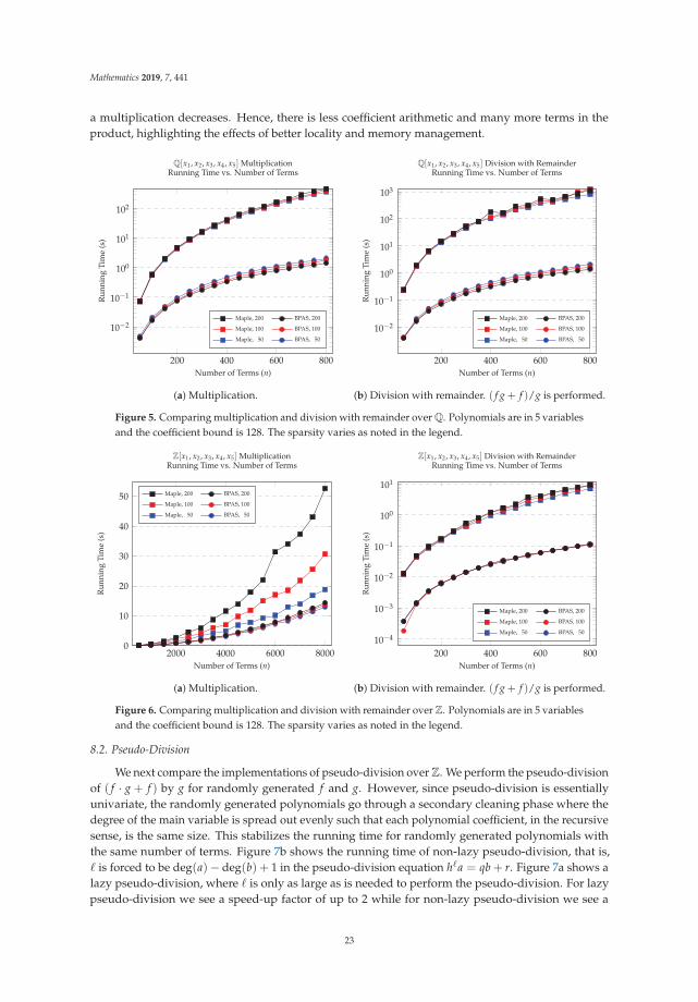
Mathematics 2019, 7, 441
a multiplication decreases. Hence, there is less coefficient arithmetic and many more terms in theproduct, highlighting the effects of better locality and memory management.
200 400 600 800
10−2
10−1
100
101
102
Number of Terms (n)
Run
ning
Tim
e(s
)
Q[x1, x2, x3, x4, x5] MultiplicationRunning Time vs. Number of Terms
Maple, 200 BPAS, 200
Maple, 100 BPAS, 100
Maple, 50 BPAS, 50
(a) Multiplication.
200 400 600 800
10−2
10−1
100
101
102
103
Number of Terms (n)R
unni
ngTi
me
(s)
Q[x1, x2, x3, x4, x5] Division with RemainderRunning Time vs. Number of Terms
Maple, 200 BPAS, 200
Maple, 100 BPAS, 100
Maple, 50 BPAS, 50
(b) Division with remainder. ( f g + f )/g is performed.
Figure 5. Comparing multiplication and division with remainder over Q. Polynomials are in 5 variablesand the coefficient bound is 128. The sparsity varies as noted in the legend.
2000 4000 6000 80000
10
20
30
40
50
Number of Terms (n)
Run
ning
Tim
e(s
)
Z[x1, x2, x3, x4, x5] MultiplicationRunning Time vs. Number of Terms
Maple, 200 BPAS, 200
Maple, 100 BPAS, 100
Maple, 50 BPAS, 50
(a) Multiplication.
200 400 600 80010−4
10−3
10−2
10−1
100
101
Number of Terms (n)
Run
ning
Tim
e(s
)
Z[x1, x2, x3, x4, x5] Division with RemainderRunning Time vs. Number of Terms
Maple, 200 BPAS, 200
Maple, 100 BPAS, 100
Maple, 50 BPAS, 50
(b) Division with remainder. ( f g + f )/g is performed.
Figure 6. Comparing multiplication and division with remainder over Z. Polynomials are in 5 variablesand the coefficient bound is 128. The sparsity varies as noted in the legend.
8.2. Pseudo-Division
We next compare the implementations of pseudo-division over Z. We perform the pseudo-divisionof ( f · g + f ) by g for randomly generated f and g. However, since pseudo-division is essentiallyunivariate, the randomly generated polynomials go through a secondary cleaning phase where thedegree of the main variable is spread out evenly such that each polynomial coefficient, in the recursivesense, is the same size. This stabilizes the running time for randomly generated polynomials withthe same number of terms. Figure 7b shows the running time of non-lazy pseudo-division, that is,� is forced to be deg(a)− deg(b) + 1 in the pseudo-division equation h�a = qb + r. Figure 7a shows alazy pseudo-division, where � is only as large as is needed to perform the pseudo-division. For lazypseudo-division we see a speed-up factor of up to 2 while for non-lazy pseudo-division we see a
23
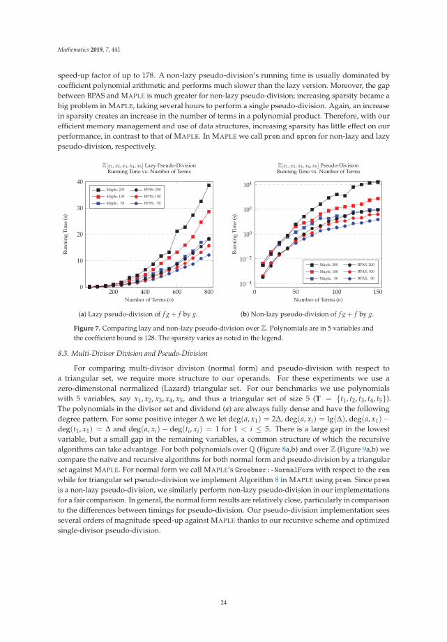
Mathematics 2019, 7, 441
speed-up factor of up to 178. A non-lazy pseudo-division’s running time is usually dominated bycoefficient polynomial arithmetic and performs much slower than the lazy version. Moreover, the gapbetween BPAS and MAPLE is much greater for non-lazy pseudo-division; increasing sparsity became abig problem in MAPLE, taking several hours to perform a single pseudo-division. Again, an increasein sparsity creates an increase in the number of terms in a polynomial product. Therefore, with ourefficient memory management and use of data structures, increasing sparsity has little effect on ourperformance, in contrast to that of MAPLE. In MAPLE we call prem and sprem for non-lazy and lazypseudo-division, respectively.
200 400 600 8000
10
20
30
40
Number of Terms (n)
Run
ning
Tim
e(s
)
Z[x1, x2, x3, x4, x5] Lazy Pseudo-DivisionRunning Time vs. Number of Terms
Maple, 200 BPAS, 200
Maple, 100 BPAS, 100
Maple, 50 BPAS, 50
(a) Lazy pseudo-division of f g + f by g.
0 50 100 15010−4
10−2
100
102
104
Number of Terms (n)
Run
ning
Tim
e(s
)
Z[x1, x2, x3, x4, x5] Pseudo-DivisionRunning Time vs. Number of Terms
Maple, 200 BPAS, 200
Maple, 100 BPAS, 100
Maple, 50 BPAS, 50
(b) Non-lazy pseudo-division of f g + f by g.
Figure 7. Comparing lazy and non-lazy pseudo-division over Z. Polynomials are in 5 variables andthe coefficient bound is 128. The sparsity varies as noted in the legend.
8.3. Multi-Divisor Division and Pseudo-Division
For comparing multi-divisor division (normal form) and pseudo-division with respect toa triangular set, we require more structure to our operands. For these experiments we use azero-dimensional normalized (Lazard) triangular set. For our benchmarks we use polynomialswith 5 variables, say x1, x2, x3, x4, x5, and thus a triangular set of size 5 (T = {t1, t2, t3, t4, t5}).The polynomials in the divisor set and dividend (a) are always fully dense and have the followingdegree pattern. For some positive integer Δ we let deg(a, x1) = 2Δ, deg(a, xi) = lg(Δ), deg(a, x1)−deg(t1, x1) = Δ and deg(a, xi) − deg(ti, xi) = 1 for 1 < i ≤ 5. There is a large gap in the lowestvariable, but a small gap in the remaining variables, a common structure of which the recursivealgorithms can take advantage. For both polynomials over Q (Figure 8a,b) and over Z (Figure 9a,b) wecompare the naïve and recursive algorithms for both normal form and pseudo-division by a triangularset against MAPLE. For normal form we call MAPLE’s Groebner:-NormalForm with respect to the remwhile for triangular set pseudo-division we implement Algorithm 8 in MAPLE using prem. Since premis a non-lazy pseudo-division, we similarly perform non-lazy pseudo-division in our implementationsfor a fair comparison. In general, the normal form results are relatively close, particularly in comparisonto the differences between timings for pseudo-division. Our pseudo-division implementation seesseveral orders of magnitude speed-up against MAPLE thanks to our recursive scheme and optimizedsingle-divisor pseudo-division.
24

Mathematics 2019, 7, 441
2 4 6 8 10 12
100
101
102
Δ
Run
ning
Tim
e(s
)
Q[x1, x2, x3, x4, x5] Multi-Divisor Normal FormRunning Time vs. Δ
MAPLE
BPAS Naïve
BPAS Recursive
(a) Normal form.
2 4 6 8 10
100
101
102
103
Δ
Run
ning
Tim
e(s
)
Q[x1, x2, x3, x4, x5] Multi-Divisor Pseudo-DivisionRunning Time vs. Δ
MAPLE
BPAS Naïve
BPAS Recursive
(b) Triangular set pseudo-division.
Figure 8. Comparing normal form and triangular set pseudo-division over Q. For each, the naïvealgorithm, the recursive algorithm, and the algorithm within MAPLE are compared. Polynomials are in5 variables and the coefficient bound is 128.
0 20 40 60 80 1000
2
4
6
8
10
12
Δ
Run
ning
Tim
e(s
)
Z[x1, x2, x3, x4, x5] Multi-Divisor Normal FormRunning Time vs. Δ
MAPLE
BPAS Naïve
BPAS Recursive
(a) Normal form.
2 4 6 8 10
10−2
10−1
100
101
102
103
Δ
Run
ning
Tim
e(s
)
Z[x1, x2, x3, x4, x5] Multi-Divisor Pseudo-DivisionRunning Time vs. Δ
MAPLE
BPAS Naïve
BPAS Recursive
(b) Triangular set pseudo-division.
Figure 9. Comparing normal form and triangular set pseudo-division over Z. For each, the naïvealgorithm, the recursive algorithm, and the algorithm within MAPLE are compared. Polynomials are in5 variables and the coefficient bound is 128.
8.4. Structured Problems
To further test our implementations on structured examples, rather than random, we look attwo problems proposed by Monagan and Pearce in [6,45] and a classic third problem. First is thesparse 10 variable problem. In this problem f1 = (∑9
i=1 (xixi+1 + xi) + x10x1 + x10 + 1)d and g1 =
(∑10i=1(
x2i + xi)+ 1)d. The multiplication h1 = f1 · g1 and the division q1 = h1/ f1 are performed.
Second is the very sparse 5 variable problem. In this problem f2 = (1 + x1 + x22 + x3
3 + x54 + x7
5)d and
g2 = (1 + x71 + x5
2 + x33 + x2
4 + x5)d. The multiplication h2 = f2 · g2 and the division q2 = h2/ f2
are performed. Lastly, a classic problem in polynomial factorization and division, f3 = xd − 1 andg3 = x− 1, performing f3/g3. Let us call this the dense quotient problem. The sparsity of the dividendis at a maximum, but the quotient produced is completely dense.
25

Mathematics 2019, 7, 441
In these problems the coefficients are strictly machine-word sized, i.e., less than 64-bits.We concede that MAPLE uses more advanced techniques for coefficient arithmetic, using machine-wordintegers and arithmetic, if possible. This contrasts with our implementation which uses onlyarbitrary-precision integers. It is expected then for MAPLE to out-perform BPAS on these exampleswith machine-integer coefficients. However, this is only the case for the first two problems. To focusexclusively on the polynomial algorithms and not the integer arithmetic, we repeat the first twoproblems with arbitrary-precision coefficients, each term in f1, g1, f2, g2 is given a random positiveinteger coefficient using a coefficient bound. Table 1 shows the execution time and memory used (for allinputs and outputs) for these problems for various values of d. Multiplication again shows speed-upof a factor between 1.2 and 21.6, becoming increasingly better with increasing sparsity and numberof terms. Division here is exact and, in comparison to division with remainder, MAPLE performsmuch better, likely thanks to their so-called divisor heap [32]. Only as sparsity increases does BPASout-perform MAPLE. In all multi-precision cases, however, memory usage in BPAS is significantlybetter, being less than half that of MAPLE.
Table 1. Comparing multiplication and division on the three structured problems.
Operation d Coef. BoundBPAS MAPLE
Time (s) Memory (MiB) Time (s) Memory (MiB)
Multiplication 4 1 4.28 172.11 1.78 79.31h1 = f1 · g1 4 64 8.22 353.27 9.58 810.23
5 64 155.51 2481.37 221.71 5569.25
Division 4 64 7.84 353.29 6.465 816.03q1 = h1/ f1 5 64 154.08 2509.42 124.37 5583.50
Multiplication 12 1 3.61 702.14 2.835 439.21h2 = f2 · g2 12 32 7.62 1878.96 52.80 4026.29
15 32 51.61 8605.52 1114.23 18,941.05
Division 12 32 8.09 1919.28 10.35 4033.57q2 = h2/ f2 15 32 57.09 8627.16 58.906 18,660.94
Division 1,000,000 1 0.18 38.59 1.505 164.54q3 = f3/g3 10,000,000 1 1.87 522.65 23.63 1102.21
9. Conclusions and Future Work
In this paper, we have described algorithms and data structures for the high-performancesparse polynomial arithmetic as implemented in the freely available BPAS library. We haveconsidered polynomials both over the integers and the rationals, where others have ignored therationals; arithmetic over the rationals is important for areas such as Gröbner bases and polynomialsystem solving. The operations of multiplication, and division, have been extended from [24] to alsoinclude division with remainder and a new algorithm for sparse pseudo-division. We employ thesefundamental algorithms for use in the mid-level algorithms of normal form and pseudo-divisionwith respect to a triangular set. Our experimentation against MAPLE highlights how the propertreatment of locality and data structures can result huge improvements in memory usage andrunning time. We achieve orders of magnitude speed-up (for arithmetic over the rationals and non-lazypseudo-division over the integers) or up to a factor of 67 (for other operations over the integers).
In the future we hope to apply these techniques for locality and arithmetic optimization to obtainefficient computations with regular chains and triangular decompositions. Following the design goalsof the BPAS library we plan to apply parallelization to both the arithmetic operations presented in thispaper and to upcoming work on triangular decompositions.
26
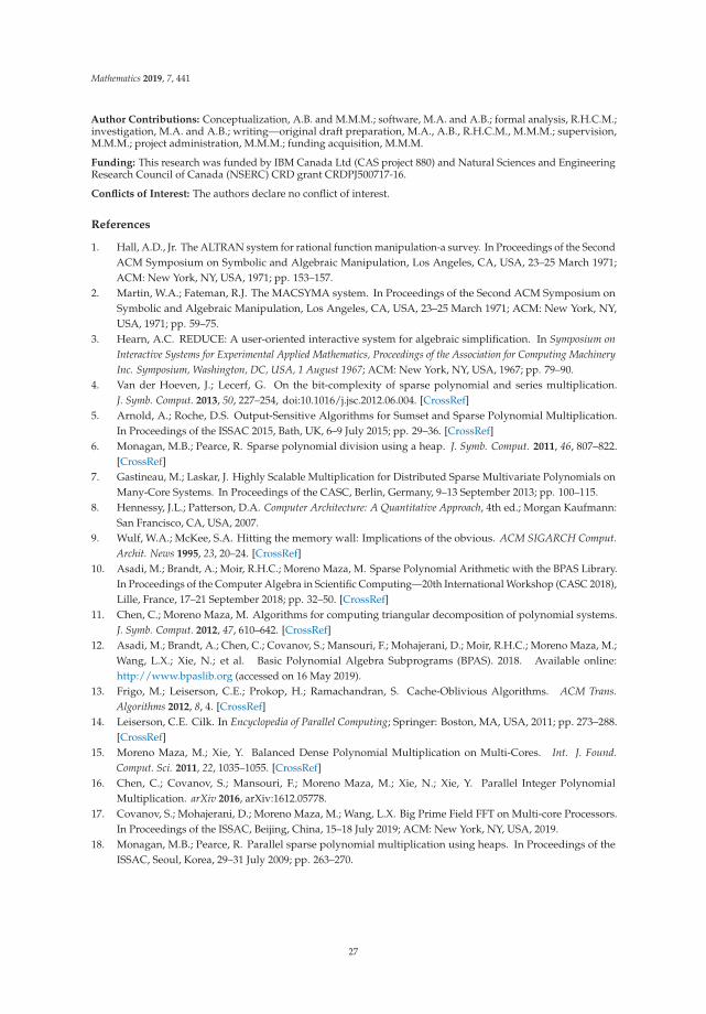
Mathematics 2019, 7, 441
Author Contributions: Conceptualization, A.B. and M.M.M.; software, M.A. and A.B.; formal analysis, R.H.C.M.;investigation, M.A. and A.B.; writing—original draft preparation, M.A., A.B., R.H.C.M., M.M.M.; supervision,M.M.M.; project administration, M.M.M.; funding acquisition, M.M.M.
Funding: This research was funded by IBM Canada Ltd (CAS project 880) and Natural Sciences and EngineeringResearch Council of Canada (NSERC) CRD grant CRDPJ500717-16.
Conflicts of Interest: The authors declare no conflict of interest.
References
1. Hall, A.D., Jr. The ALTRAN system for rational function manipulation-a survey. In Proceedings of the SecondACM Symposium on Symbolic and Algebraic Manipulation, Los Angeles, CA, USA, 23–25 March 1971;ACM: New York, NY, USA, 1971; pp. 153–157.
2. Martin, W.A.; Fateman, R.J. The MACSYMA system. In Proceedings of the Second ACM Symposium onSymbolic and Algebraic Manipulation, Los Angeles, CA, USA, 23–25 March 1971; ACM: New York, NY,USA, 1971; pp. 59–75.
3. Hearn, A.C. REDUCE: A user-oriented interactive system for algebraic simplification. In Symposium onInteractive Systems for Experimental Applied Mathematics, Proceedings of the Association for Computing MachineryInc. Symposium, Washington, DC, USA, 1 August 1967; ACM: New York, NY, USA, 1967; pp. 79–90.
4. Van der Hoeven, J.; Lecerf, G. On the bit-complexity of sparse polynomial and series multiplication.J. Symb. Comput. 2013, 50, 227–254, doi:10.1016/j.jsc.2012.06.004. [CrossRef]
5. Arnold, A.; Roche, D.S. Output-Sensitive Algorithms for Sumset and Sparse Polynomial Multiplication.In Proceedings of the ISSAC 2015, Bath, UK, 6–9 July 2015; pp. 29–36. [CrossRef]
6. Monagan, M.B.; Pearce, R. Sparse polynomial division using a heap. J. Symb. Comput. 2011, 46, 807–822.[CrossRef]
7. Gastineau, M.; Laskar, J. Highly Scalable Multiplication for Distributed Sparse Multivariate Polynomials onMany-Core Systems. In Proceedings of the CASC, Berlin, Germany, 9–13 September 2013; pp. 100–115.
8. Hennessy, J.L.; Patterson, D.A. Computer Architecture: A Quantitative Approach, 4th ed.; Morgan Kaufmann:San Francisco, CA, USA, 2007.
9. Wulf, W.A.; McKee, S.A. Hitting the memory wall: Implications of the obvious. ACM SIGARCH Comput.Archit. News 1995, 23, 20–24. [CrossRef]
10. Asadi, M.; Brandt, A.; Moir, R.H.C.; Moreno Maza, M. Sparse Polynomial Arithmetic with the BPAS Library.In Proceedings of the Computer Algebra in Scientific Computing—20th International Workshop (CASC 2018),Lille, France, 17–21 September 2018; pp. 32–50. [CrossRef]
11. Chen, C.; Moreno Maza, M. Algorithms for computing triangular decomposition of polynomial systems.J. Symb. Comput. 2012, 47, 610–642. [CrossRef]
12. Asadi, M.; Brandt, A.; Chen, C.; Covanov, S.; Mansouri, F.; Mohajerani, D.; Moir, R.H.C.; Moreno Maza, M.;Wang, L.X.; Xie, N.; et al. Basic Polynomial Algebra Subprograms (BPAS). 2018. Available online:http://www.bpaslib.org (accessed on 16 May 2019).
13. Frigo, M.; Leiserson, C.E.; Prokop, H.; Ramachandran, S. Cache-Oblivious Algorithms. ACM Trans.Algorithms 2012, 8, 4. [CrossRef]
14. Leiserson, C.E. Cilk. In Encyclopedia of Parallel Computing; Springer: Boston, MA, USA, 2011; pp. 273–288.[CrossRef]
15. Moreno Maza, M.; Xie, Y. Balanced Dense Polynomial Multiplication on Multi-Cores. Int. J. Found.Comput. Sci. 2011, 22, 1035–1055. [CrossRef]
16. Chen, C.; Covanov, S.; Mansouri, F.; Moreno Maza, M.; Xie, N.; Xie, Y. Parallel Integer PolynomialMultiplication. arXiv 2016, arXiv:1612.05778.
17. Covanov, S.; Mohajerani, D.; Moreno Maza, M.; Wang, L.X. Big Prime Field FFT on Multi-core Processors.In Proceedings of the ISSAC, Beijing, China, 15–18 July 2019; ACM: New York, NY, USA, 2019.
18. Monagan, M.B.; Pearce, R. Parallel sparse polynomial multiplication using heaps. In Proceedings of theISSAC, Seoul, Korea, 29–31 July 2009; pp. 263–270.
27
Mathematics 2019, 7, 441
19. Monagan, M.; Pearce, R. Parallel sparse polynomial division using heaps. In Proceedings of the PASCO,Grenoble, France, 21–23 July 2010; ACM: New York, NY, USA, 2010; pp. 105–111.
20. Biscani, F. Parallel sparse polynomial multiplication on modern hardware architectures. In Proceedings of the37th International Symposium on Symbolic and Algebraic Computation, Grenoble, France, 22–25 July 2012;ACM: New York, NY, USA, 2012; pp. 83–90.
21. Gastineau, M.; Laskar, J. Parallel sparse multivariate polynomial division. In Proceedings of the PASCO2015, Bath, UK, 10–12 July 2015; pp. 25–33. [CrossRef]
22. Popescu, D.A.; Garcia, R.T. Multivariate polynomial multiplication on gpu. Procedia Comput. Sci. 2016,80, 154–165. [CrossRef]
23. Ewart, T.; Hehn, A.; Troyer, M. VLI–A Library for High Precision Integer and Polynomial Arithmetic.In Proceedings of the International Supercomputing Conference, Leipzig, Germany, 16–20 June 2013;Springer: Berlin/Heidelberg, Germany, 2013; pp. 267–278.
24. Johnson, S.C. Sparse polynomial arithmetic. ACM SIGSAM Bull. 1974, 8, 63–71. [CrossRef]25. Li, X.; Moreno Maza, M.; Schost, É. Fast arithmetic for triangular sets: From theory to practice.
J. Symb. Comput. 2009, 44, 891–907. [CrossRef]26. Sedgewick, R.; Wayne, K. Algorithms, 4th ed.; Addison-Wesley: Boston, MA, USA, 2011.27. Cox, D.A.; Little, J.; O’shea, D. Ideals, Varieties, and Algorithms, 2 ed.; Springer: New York, NY, USA, 1997.28. Von zur Gathen, J.; Gerhard, J. Modern Computer Algebra, 2 ed.; Cambridge University Press: New York, NY,
USA, 2003.29. Gastineau, M.; Laskar, J. Development of TRIP: Fast Sparse Multivariate Polynomial Multiplication Using
Burst Tries. In Proceedings of the Computational Science—ICCS 2006, 6th International Conference, Reading,UK, 28–31 May 2006; Part II, pp. 446–453. [CrossRef]
30. Monagan, M.; Pearce, R. The design of Maple’s sum-of-products and POLY data structures for representingmathematical objects. ACM Commun. Comput. Algebra 2015, 48, 166–186. [CrossRef]
31. Granlund, T.; others. GNU MP 6.0 Multiple Precision Arithmetic Library; Samurai Media Limited:Surrey, UK, 2015.
32. Monagan, M.; Pearce, R. Polynomial division using dynamic arrays, heaps, and packed exponentvectors. In Proceedings of the CASC 2007, Bonn, Germany, 16–20 September 2007; Springer:Berlin/Heidelberg, Germany, 2007; pp. 295–315.
33. Gonnet, G.H.; Munro, J.I. Heaps on heaps. SIAM J. Comput. 1986, 15, 964–971. [CrossRef]34. Brandt, A. High Performance Sparse Multivariate Polynomials: Fundamental Data Structures and
Algorithms. Master’s Thesis, The University of Western Ontario, London, ON, Canada, 2018.35. Huang, B.C.; Langston, M.A. Practical in-place merging. Commun. ACM 1988, 31, 348–352. [CrossRef]36. Katajainen, J.; Pasanen, T.; Teuhola, J. Practical in-place mergesort. Nord. J. Comput. 1996, 3, 27–40.37. Dalkilic, M.E.; Acar, E.; Tokatli, G. A simple shuffle-based stable in-place merge algorithm.
Procedia Comput. Sci. 2011, 3, 1049–1054. [CrossRef]38. Waterloo Maple Inc. MAPLE 2017—The Essential Tool for Mathematics; Waterloo Maple Inc.: Waterloo, ON,
Canada, 2017.39. Gastineau, M.; Laskar, J. TRIP: A Computer Algebra System Dedicated to Celestial Mechanics and
Perturbation Series. ACM Commun. Comput. Algebra 2011, 44, 194–197. [CrossRef]40. Bosma, W.; Cannon, J.; Playoust, C. The Magma algebra system. I. The user language. J. Symb. Comput. 1997,
24, 235–265. [CrossRef]41. Decker, W.; Greuel, G.M.; Pfister, G.; Schönemann, H. SINGULAR 4-1-1—A Computer Algebra System
for Polynomial Computations. 2018 Available online: http://www.singular.uni-kl.de (accessed on15 March 2019).
42. The PARI Group, Univ. Bordeaux. PARI/GP Version 2.3.3. 2008. Available online: http://pari.math.u-bordeaux.fr/ (accessed on 15 March 2019).
43. Hart, W.; Johansson, F.; Pancratz, S. FLINT: Fast Library for Number Theory. V. 2.4.3. Available online:http://flintlib.org (accessed on 15 March 2019).
28

Mathematics 2019, 7, 441
44. Shoup, V. NTL: A Library for Doing Number Theory. Available online: www.shoup.net/ntl/ (accessed on15 March 2019).
45. Monagan, M.B.; Pearce, R. Sparse polynomial multiplication and division in Maple 14. ACM Commun.Comput. Algebra 2010, 44, 205–209. [CrossRef]
c© 2019 by the authors. Licensee MDPI, Basel, Switzerland. This article is an open accessarticle distributed under the terms and conditions of the Creative Commons Attribution(CC BY) license (http://creativecommons.org/licenses/by/4.0/).
29
mathematics
Article
A Heuristic Method for Certifying Isolated Zerosof Polynomial Systems
Xiaojie Dou 1 and Jin-San Cheng 2,*
1 College of Science, Civil Aviation University of China, Tianjin 300300, China; [email protected] KLMM, Academy of Mathematics and Systems Science, Chinese Academy of Sciences,
Beijing 100190, China* Correspondence: [email protected]
Received: 12 July 2018; Accepted: 3 September; Published: 11 September 2018
Abstract: In this paper, by transforming the given over-determined system into a squaresystem, we prove a necessary and sufficient condition to certify the simple real zeros of theover-determined system by certifying the simple real zeros of the square system. After certifyinga simple real zero of the related square system with the interval methods, we assert that thecertified zero is a local minimum of sum of squares of the input polynomials. If the value ofsum of squares of the input polynomials at the certified zero is equal to zero, it is a zero of theinput system. As an application, we also consider the heuristic verification of isolated zeros ofpolynomial systems and their multiplicity structures.
Keywords: over-determined polynomial system; isolated zeros; minimum point; sum ofsquares; interval methods
1. Introduction
Finding zeros of polynomial systems is a fundamental problem in scientific computing.Newton’s method is widely used to solve this problem. For a fixed approximate solution ofa system, we can use the α-theory [1–3], the interval methods or the optimization methods [4–9]to completely determine whether it is related to a zero of the system. However, the α-theory orthe interval methods focuses mainly on a simple zero of a square system, that is, a system with nequations and n unknowns.
Some special certifications of a rational solution of rational polynomials with certified sumof squares decompositions are considered [10–16].
What about singular zeros of a well-constrained polynomial system? Usually, an over-determined system which contains the same zero as a simple one is constructed by introducingnew equations. The basic idea is the deflation techniques [17–24]. In some studies [25–30],new variables are also included. Moreover, some authors verify that a perturbed system possessesan isolated singular solution within a narrow and computed error bound. The multiplicitystructures of singular zeros of a polynomial system are also studied [18,21,29]. Although it isin a theoretical sense and global sense, the method in [17] provides a sufficient condition thata zero is exactly a zero of a zero-dimensional polynomial system with rational coefficients.
For the deflation methods mentioned above, on the one hand, to be a zero of the perturbedsystems does not mean being a zero of the input system considering the difference between thetwo systems; on the other hand, although the over-determined systems without introducing
Mathematics 2018, 6, 166; doi:10.3390/math6090166 www.mdpi.com/journal/mathematics
30
Mathematics 2018, 6, 166
new variables have the same zeros as the input systems, the verification methods, such as theα-theory or the interval methods, could not be used directly on the over-determined systemsin general.
In [31], the authors extended the α-theory from well-constrained systems to over-determinedsystems. A main result about Newton’s method given in their paper is their Theorem 4 [31],which says that under the condition of 2α1(g, ζ) < 1, where g = (g1, . . . , gm) ∈(C[x1, . . . , xn])m(m ≥ n), J(g)(x)† is the Moore–Penrose inverse of the Jacobian matrix J(g)(x)of g and
α1(g, x) = β1(g, x)γ1(g, x),
β1(g, x) = ‖J(g)(x)†‖‖g(x)‖,
γ1(g, x) = supk≥2
(‖J(g)(x)†‖ Jk(g)(x)
k!
) 1k−1
,
ζ is an attractive fixed point for Newton’s method and, simultaneously, a strict local
minimum for ‖g‖2 =m∑
j=1‖gj‖2. However, as they stated, whether the attracting fixed points for
Newton’s method are always local minima of ‖g‖2, or the zeros of the input system, is unknown.In this paper, we consider the problem of certifying the simple real zeros of
an over-determined polynomial system. Given Σ = { f1, . . . , fm} ∈ (R[x1, . . . , xn])m(m ≥ n),
we construct a new square system Σ′ = { ∂ f∂x1
, . . . , ∂ f∂xn} with f =
m∑
i=1f 2i . After transforming the
input over-determined system into a square one, we can use both the α-theory and the intervalmethods to certify its simple zeros. In this paper, we only consider using the interval methods tocertify the simple real zeros of the over-determined system. We prove that the simple real zerosof the input system are local minima of sum of squares of the input polynomials. We also givethe condition that the local minimum is a simple zero of the input system.
Let R be the field of real numbers. Denote R[x] = R[x1, . . . , xn] as the polynomial ring.Let F = { f1, . . . , fm} ⊂ R[x] be a polynomial system. Let p = (p1, . . . , pn) ∈ Rn.
The following theorem is the main result of this paper.
Theorem 1. Let Σ = { f1, . . . , fm} ⊂ R[x] (m ≥ n) and f =m∑
i=1f 2i . Then, we have:
1. If p ∈ Rn is an isolated simple real zero of Σ, p is a local minimum of f .2. p is a simple real zero of Σ if and only if (p, 0) is a simple real zero of the square system
Σr = {J1( f ), . . ., Jn( f ), f − r}, where Ji( f ) = ∂ f∂xi
and r is a new variable.
In the above theorem, we get a necessary and sufficient condition to certify the simple realzeros of the input system Σ by certifying the simple real zeros of the square system Σr. Therefore,to certify that p is a simple real zero of Σ, the key point is verifying that f (p) = 0.
However, it is difficult to decide numerically if a point is a zero of a polynomial.Thus, we cannot use the necessary and sufficient condition to certify the simple real zerosof Σ by certifying the simple real zeros of Σr.
As an alternative, we refine and certify the simple real zeros of Σ by refining and certifying anew square system Σ′ = {J1( f ), . . ., Jn( f )}with the interval methods and get a verified inclusionX, which contains a unique simple real zero x of Σ′. In fact, x is a local minimum of f , which alsois a necessary condition for the certification. On the one hand, if f (x) = 0, by Theorem 1, (x, 0) is
31

Mathematics 2018, 6, 166
a simple real zero of Σr, and then x is a simple real zero of Σ. Thus, we certified the input systemΣ. On the other hand, if f (x) �= 0, we can only assert that Σr has a unique zero in the verifiedinclusion X× [0, f (x)], which means we certified the system Σr.
A big difference between this paper and our pervious work [32] is that we do not merelyconsider certifying simple zeros of over-determined polynomial systems, but also consider thecertification of the general isolated zeros. Specifically, as an application of our method, we givea heuristic method for certifying not only the isolated singular zeros of polynomial systems,but also the multiplicity structures of the isolated singular zeros of polynomial systems.
This paper is an extended version of the CASC’17 conference paper [32].The paper is organized as follows. We introduce some notations and preliminaries in the
next section. In Section 3, we give a method to show how to transform an over-determinedsystem into a square one. The interval verification method on the obtained square systemis considered in Section 4. We give two applications of our method in Section 5 and drawconclusions in Section 6.
2. Preliminaries
Let C be the field of complex numbers. Denote C[x] = C[x1, . . . , xn] as the polynomialring. Let F = { f1, . . . , fm} ⊂ C[x] be a polynomial system. Let p = (p1, . . . , pn) ∈ Cn. F(p) = 0
denote that p is a zero of F(x) = 0.Let A be a matrix. Denote AT as the transpose of A and rank(A) as the rank of A.
Let Mat(ai,j) denote the matrix whose i-th row j-th column element is ai,j.Let Σ = { f1, . . . , fm} ⊂ C[x] be a polynomial system. Denote J(Σ) as the Jacobian matrix of
Σ. That is,
J(Σ) =
⎛⎜⎜⎝∂ f1∂x1
. . . ∂ f1∂xn
.... . .
...∂ fm∂x1
. . . ∂ fm∂xn
⎞⎟⎟⎠ .
For a polynomial f ∈ C[x], let J( f ) denote ( ∂ f∂x1
, ∂ f∂x2
, . . . , ∂ f∂xn
), Ji( f ) = ∂ f∂xi
and
Ji,j( f ) = Jj(Ji( f )) = ∂2 f∂xj∂xi
. Denote Σr = {J1( f ), . . ., Jn( f ), f − r} with f =m∑
j=1f 2j .
We denote the value of a function matrix A ∈ C[x]n×n at a point p ∈ Cn as A(p). Let J(F)(p)
denote the value of a function matrix J(F) at a point p, similarly for J( f )(p).
Definition 1. An isolated solution of F(x) = 0 is a point p ∈ Cn which satisfies:
∃ ε > 0 : {y ∈ Cn : ‖y− p‖ < ε} ∩ F−1(0) = {p}.
Definition 2. We call an isolated solution p ∈ Cn of F(x) = 0 a singular solution if and only if
rank(J(F)(p)) < n.
Otherwise, we call p a simple solution.
Definition 3. A stationary point of a polynomial function f (x) ∈ C[x] is a point p ∈ Cn,which satisfies:
∂ f∂xi
(p) = 0, ∀ i = 1, . . . , n.
32
Mathematics 2018, 6, 166
We can find the following lemma in many undergraduate textbooks about linear algebra(see Example 7 on page 224 in [33] for example).
Lemma 1. Let A ∈ Rm×n be a real matrix with m ≥ n and B = AT A. Then, the ranks of A and B arethe same, especially for the case that A is of full rank.
In the following, we consider the real zeros of the systems with real coefficients. It isreasonable since, for a system (m equations and n unknowns) with complex coefficients,we can rewrite the system into a new one with 2 m equations and 2 n unknowns by splittingthe unknowns xi = xi,1 + i xi,2 and equations f j(x1, . . . , xn) = gj,1(x1,1, x1,2, . . . , xn,1, xn,2) +
i gj,2(x1,1, x1,2, . . . , xn,1, xn,2), where i2 = −1, f j ∈ C[x], gj,1, gj,2 ∈ R[x], j = 1, . . . , m, and find thecomplex zeros of the original system by finding out the real zeros of the new system.
3. Transforming Over-determined Polynomial Systems into Square Ones
In this section, we show how to transform an over-determined polynomial system into asquare one with their zeros having a one-to-one correspondence, especially for the simple zeros.
By Definition 3, we have the following lemma:
Lemma 2. Given a polynomial system Σ = { f1, . . . , fm} ⊂ R[x] (m ≥ n). Let f =m∑
i=1f 2i and
Σ′ = {J1( f ), J2( f ), . . . , Jn( f )}. If p ∈ Rn is an isolated real zero of Σ′, then p is a stationary point of f .
Lemma 3. Let Σ = { f1, . . . , fm} ⊂ R[x] (m ≥ n), Σ′ = {J1( f ), J2( f ), . . . , Jn( f )} with f =m∑
i=1f 2i .
If p ∈ Rn is an isolated real zero of Σ, then we have:
1. p is an isolated real zero of Σ′.2. rank(J(Σ)(p)) = rank(J(Σ′)(p)).
Proof. It is clear that p is an isolated real zero of Σ′ providing that p is an isolated real zero of Σ,
since Ji( f ) = 2m∑
k=1fk Ji( fk).
To prove the second part of this lemma, we rewrite Ji( f ) as follows.
Ji( f ) = 2 〈 f1, . . . , fm〉 〈Ji( f1), . . . , Ji( fm)〉T , (1)
where 〈 · 〉T is the transpose of a vector or a matrix 〈 · 〉. Then,
Ji,j( f ) = Jj(Ji( f )) = Jj(2m
∑k=1
fk Ji( fk)) = 2m
∑k=1
(Jj( fk)Ji( fk) + fk Ji,j( fk))
= 2 〈Jj( f1), . . . , Jj( fm)〉 〈Ji( f1), . . . , Ji( fm)〉T + 2m
∑k=1
fk Ji,j( fk).(2)
Then, the Jacobian matrix of Σ′ is
J(Σ′) =
⎛⎜⎝ J1,1( f ) . . . J1,n( f )...
. . ....
Jn,1( f ) . . . Jn,n( f )
⎞⎟⎠ = Mat(Ji,j( f )).
33

Mathematics 2018, 6, 166
We rewrite
Mat(Ji,j( f )) = 2 AT A + 2 Mat(m
∑k=1
fk Ji,j( fk)), (3)
where
A =
⎛⎜⎝ J1( f1) . . . Jn( f1)...
. . ....
J1( fm) . . . Jn( fm)
⎞⎟⎠is an m× n matrix which is exactly the Jacobian matrix of Σ, that is, J(Σ) = A. Then, we have
J(Σ′)(p) = 2A(p)T A(p). (4)
By Lemma 1, the second part of the lemma is true. This ends the proof.
Remark 1. In our construction of f and Σ′, the degrees of the polynomials almost be doubled comparedto the original one. However, to evaluate the Jacobian matrix of Σ′, we evaluate the Jacobian matrix of theoriginal system with m2n numerical products. One can find it from Equation (4) in the above proof. In fact,to get J(Σ′)(p), we only need to compute A(p), which does not increase our actual computing degree.
As a byproduct, thanks to the doubled degree of the polynomials, our final certified accuracy is alsoimproved in Lemma 4.
The following is the proof of Theorem 1:
Proof. In fact, by fixing the real zero p as an isolated simple zero in Lemma 3, we have p is anisolated simple real zero of Σ′ = {J1( f ), . . . , Jn( f )}. Since p is an isolated simple zero of Σ, A(p)
is a column full rank matrix. Therefore, it is easy to verify that J(Σ′)(p) = 2 A(p)T A(p) is apositive definite matrix. Thus, p is a local minimum of f and the first part of the theorem is true.Now, we consider the second part.
First, it is easy to verify that p is the real zero of Σ if and only if (p, 0) is the real zero of Σr.Notice that Σr = {Σ′, f − r}. Thus, with the same method as proving Lemma 3, we can computeeasily that
J(Σr)(p, 0) =
(J(Σ′)(p) 0
0 −1
)=
(2 J(Σ)(p)TJ(Σ)(p) 0
0 −1
),
which implies that
rank(J(Σ)(p)) = rank(J(Σ′)(p)) = rank(J(Σr)(p, 0))− 1, (5)
which means that J(Σr)(p, 0) is of full rank if and only if J(Σ)(p) is of full rank. Thus, p is anisolated simple zero of Σ if and only if (p, 0) is an isolated simple zero of Σr. The second part istrue. We have finished the proof.
From Theorem 1, we know that the simple real zeros of Σ and Σr are in one-to-onecorrespondence with the constraint that the value of the sum of squares of the polynomialsin Σ at the simple real zeros is identically zero. Thus, we can transform an over-determinedpolynomial system into a square system Σr.
We show a simple example to illustrate the theorem below.
34
Mathematics 2018, 6, 166
Example 1. The simple zero p = (0, 0) of the over-determined system Σ = { f1, f2, f3} corresponds to asimple zero of a square system Σr = {J1( f ), J2( f ), f − r}, where f = f 2
1 + f 22 + f 2
3 with
f1 = x2 − 2 y, f2 = y2 − x, f3 = x2 − 2 x + y2 − 2 y.
We can verify simply that (p, 0) is a simple zero of Σr.
Although the simple real zeros of Σ and Σr have a one-to-one correspondence, it cannot beused directly to do certification of the simple zeros of Σ since we cannot certify r = 0 numerically.However, we can certify the zeros of Σ′ = {J1( f ), J2( f ), . . . , Jn( f )} as an alternative, which is anecessary condition for the certification.
We discuss it in next section.
4. Certifying Simple Zeros of Over-determined Systems
In this section, we consider certifying the over-determined system with the interval methods.We prove the same local minimum result as [31].
The classical interval verification methods are based on the following theorem:
Theorem 2 ([5,6,8,30]). Let f = ( f1, . . . , fn) ∈ (R[x])n be a polynomial system, x ∈ Rn, real intervalvector X ∈ IRn with 0 ∈ X and real matrix R ∈ Rn×n be given. Let an interval matrix M ∈ IRn×n begiven whose i-th row Mi satisfies
{∇ fi(ζ) : ζ ∈ x + X} ⊆ Mi.
Denote by I the n× n identity matrix and assume
−Rf(x) + (I − RM)X ⊆ int(X),
where int(X) denotes the interior of X. Then, there is a unique x ∈ x + X with f(x) = 0. Moreover,every matrix M ∈ M is nonsingular. In particular, the Jacobian J(f)(x) is nonsingular.
About interval matrices, there is an important property in the following theorem.
Theorem 3 ([34]). A symmetric interval matrix AI is positive definite if and only if it is regular andcontains at least one positive definite matrix.
Given an over-determined polynomial system Σ = { f1, . . . , fm} ⊂ R[x] with an isolatedsimple real zero, we can compute a related square system
Σ′ = { ∂ f∂x1
,∂ f∂x2
, . . . ,∂ f∂xn
} with f =m
∑j=1
f 2j .
Based on Lemma 3, a simple zero of Σ is a simple zero of Σ′. Thus, we can compute theapproximate simple zero of Σ by computing the approximate simple zero of Σ′. Using Newton’smethod, we can refine these approximate simple zeros with quadratic convergence to a relativehigher accuracy. Then, we can certify them with the interval method mentioned before andget a verified inclusion X, which possesses a unique certified simple zero of the system Σ′ byTheorem 2, denoting as x ∈ X.
35
Mathematics 2018, 6, 166
However, even though we get a certified zero x of the system Σ′, considering Lemma 2,we cannot say x is a zero of the input system Σ. Because the certified zero x is just a stationarypoint of f . Considering Theorem 1 and the difference between Σ′ and Σr, we have thefollowing theorem.
Theorem 4. Let Σ, Σ′, Σr, f , x and the interval X be given as above. Then, we have:
1. x is a local minimum of f .2. There exists a verified inclusion X× [0, f (x)] that possesses a unique simple zero of the system Σr.
Especially, if f (x) = 0, the verified inclusion X possesses a unique simple zero of the input system Σ.
Proof. First, it is easy to see that computing the value of the matrix J(Σ′) at the interval X
will give a symmetric interval matrix, denoting as J(Σ′)(X). By Theorem 2, we know that, forevery matrix M ∈ J(Σ′)(X), M is nonsingular. Therefore, the interval matrix J(Σ′)(X) is regular.Especially, the matrix J(Σ′)(x), which is the Hessian matrix of f , is full rank and, therefore,is positive definite. Thus, x is a local minimum of f . By Theorem 3, we know that J(Σ′)(X) ispositive definite. Thus, for every point q ∈ X, J(Σ′)(q) is a positive definite matrix. ConsideringTheorem 2, it is trivial that, for the verified inclusion X× [0, f (x)], there exists a unique simplezero of the system Σr. If f (x) = 0, by Theorem 1, the verified inclusion X of the system Σ′ is averified inclusion of the original system Σ.
Remark 2. 1. In the above proof, we know that, for every point q ∈ X, J(Σ′)(q) is a positivedefinite matrix.
2. By Theorem 2, we know that there is a unique x ∈ X with Σ′(x) = 0. However, we could notknow what the exact x is. According to the usual practice, in actual computation, we take the midpoint p
of the inclusion X as x and verify whether f (p) = 0. Considering the uniqueness of x in X, therefore, iff (p) = 0, we are sure that the verified inclusion X possesses a unique simple zero of the input system Σ.If f (p) �= 0, we can only claim that there is a local minimum of f in the inclusion X and X× [0, f (p)] isa verified inclusion for the system Σr.
Considering the expression of Σ and f and for the midpoint p of X, we have a trivialresult below.
Lemma 4. Denote ε =m
maxj=1
| f j(p)|. Under the conditions of Theorem 4, we have | f (p)| ≤ mε2.
Based on the above idea, we give an algorithm below. In the verification steps,we apply algorithm verifynlss in INTLAB [30], which is based on Theorem 2, to computea verified inclusion X for the related square system Σ′. For simplicity, denote the intervalX = [x1, x1], · · · , [xm, xm] and the midpoint of X as p = [(x1 + x1)/2, . . . , (xm + xm)/2].
The correctness and the termination of the algorithm is obvious by the above analysis.We give two examples to illustrate our algorithm.
Example 2. Continue Example 1. Given an approximate zero p = (0.0003528, 0.0008131),using Newton’s method, we get a higher accuracy approximate zero
p′ = 10−11 · (−0.104224090958505,−0.005858368844383).
36
Mathematics 2018, 6, 166
Compute f = f 21 + f 2
2 + f 23 and Σ′ = {J1( f ), J2( f )}. After applying algorithm verifynlss on Σ′,
we have a verified inclusion:
X =
([−0.11330049261083, 0.11330049261083][−0.08866995073891, 0.08866995073891]
)· 10−321.
Based on Theorem 2, we know that there exists a unique x ∈ X, such that Σ′(x) = 0.Let Σr = {J1( f ), J2( f ), f − r}. By Theorem 1, we can certify the simple zero of Σ by certifying
the simple zero of Σr theoretically. Considering the difference between Σ′ and Σr, we check first whetherthe value of f at some point in the interval X is zero. According to the usual practice, we consider themidpoint p of X, which equals (0, 0) and, further, f (p) is zero. Therefore, we are sure that there exists aunique x = (x, y) ∈ X, s.t. Σr((x, 0)) = 0 and, then, there exists a unique simple zero (x, y) ∈ X of theinput system Σ, which means we certified the input system Σ.
Example 3. Let Σ = { f1 = x21 + 3 x1x2 + 3 x1x3 − 3 x2
3 + 2 x2 + 2 x3, f2 = −3 x1x2 + x1x3 − 2 x22 +
x23 + 3 x1 + x2, f3 = 2 x2x3 + 3 x1− 3 x3 + 2, f4 = −6 x2
2x3 + 2 x2x23 + 6 x2
2 + 15 x2x3− 6 x23− 9 x2−
7 x3 + 6} be an over-determined system. Consider an approximate zero
p = (−1.29655, 0.47055,−0.91761).
Using Newton’s method, we get a higher accuracy zero
p′ = (−1.296687216045438, 0.470344502045004,−0.917812633399457).
Computef = f 2
1 + f 22 + f 2
3 + f 24 and Σ′ = {J1( f ), J2( f ), J3( f )}.
After applying algorithm verifynlss on Σ′, we have a verified inclusion:
X =
⎛⎜⎝ [−1.29668721603974, −1.29668721603967][ 0.47034450205107, 0.47034450205114][−0.91781263339256, −0.91781263339247]
⎞⎟⎠ .
Similarly, based on Theorem 2, we know that there exists a unique x ∈ X, such that Σ′(x) = 0.Proceeding as in the above example, we consider the midpoint p of X and compute f (p) = 3.94 ·
10−31 �= 0. Thus, by Theorem 4, we get a verified inclusion X× [0, f (p)], which contains a unique simplezero of the system Σr. It means that X may contain a zero of Σ. Even if X does not contain a zero of Σ,it contains a local minimum of f , which has a minimum value no larger than f (p).
5. Two Applications
As an application, we consider certifying isolated singular zeros of over-determined systemsheuristically. Generally, dealing with the multiple zeros of polynomial systems directly is difficult.The classical method to deal with the isolated singular zeros of polynomial systems is thedeflation technique, which constructs a new system owning the same singular zero as an isolatedsimple one. Although the deflation method can be used to refine or verify the isolated zero ofthe original system, it is a pity that the multiplicity information of the isolated zero is missed.In this section, as an application of the method of converting an over-determined system into a
37

Mathematics 2018, 6, 166
square system in previous section, we give a heuristic method for certifying isolated singularzeros of polynomial systems and their multiplicity structures.
5.1. Certifying Isolated Singular Zeros of Polynomial Systems
Recently, Cheng et al. [35] proposed a new deflation method to reduce the multiplicityof an isolated singular zero of a polynomial system to get a final system, which owns theisolated singular zero of the input system as a simple one. Different from the previous deflationmethods, they considered the deflation of isolated singular zeros of polynomial systems fromthe perspective of linear combination.
In this section, we first give a brief introduction of their deflation method and, then,show how our method is applied to certify the isolated singular zeros of the input systemin a heuristic way.
Definition 4. Let f ∈ C[x], p ∈ Cn and a tolerance θ > 0, s.t. | f (p)| < θ. We say f is θ-singular atp if ∣∣∣∣∣∂ f (p)
∂xj
∣∣∣∣∣ < θ, ∀1 ≤ j ≤ n.
Otherwise, we say f is θ-regular at p.
Let F = { f1, . . . , fn} ⊂ C[x] be a polynomial system. p ∈ Cn is an approximate isolated zeroof F = 0. Consider a tolerance θ. First, we can compute the polynomials of all fi(i = 1, . . . , n),which is θ-regular at the approximate zero p. That is, we compute a polynomial set
G = {dγx ( f )|dγ
x ( f ) is θ-regular at p, f ∈ F}.
Then, put G and F together and compute a subsystem H = {h1, . . . , hs} ⊂ G ∪ F, whoseJacobian matrix at p has a maximal rank s. If s = n, we get the final system F′ = H. Otherwise,we choose a new polynomial h ∈ G∪ F \H and compute
g = h +s
∑i=1
αihi, gj =∂h∂xj
, j = 1, . . . , n,
where αj, j = 1, . . . , n are new introduced variables. Next, we check if
rank(J(H, g1, . . . , gn)(p)) = n + s. (6)
If Equation (6) holds, we get the final system F′ = H ∪ {g1, . . . , gn}. Otherwise,let H := H∪ {g1, . . . , gn} ⊂ C[x, α] and repeat again until Equation (6) holds.
Now, we give an example to illustrate the above idea.
Example 4. Consider a polynomial system F = { f1 = − 94 + 3
2 x1 + 2 x2 + 3 x3 + 4 x4 − 14 x2
1, f2 =
x1− 2 x2− 2 x3− 4 x4 + 2 x1x2 + 3 x1x3 + 4 x1x4, f3 = 8− 4 x1− 8 x4 + 2 x24 + 4 x1x4− x1x2
4, f4 =
−3 + 3 x1 + 2 x2 + 4 x3 + 4 x4}. Consider an approximate singular zero
p = ( p1, p2, p3, p4) = (1.00004659,−1.99995813,−0.99991547, 2.00005261)
of F = 0 and the tolerance ε = 0.005.
38
Mathematics 2018, 6, 166
First, we have the Taylor expansion of f3 at p:
f3 = 3× 10⁻⁹ − 3× 10⁻⁹(x1 − p1) + 0.00010522(x4 − p4) + 0.99995341(x4 − p4)2
−0.00010522(x1 − p1)(x4 − p4)− (x1 − p1)(x4 − p4)2.
Consider the tolerance θ = 0.05. Since
| f3(p)| < θ,∣∣∣∣∂ f3
∂xi(p)
∣∣∣∣ < θ(i = 1, 2, 3, 4),
∣∣∣∣∣∂2 f3
∂x24(p)
∣∣∣∣∣ > θ,
we get a polynomial∂ f3
∂x4= −8 + 4 x1 + 4 x4 − 2 x1x4,
which is θ-regular at p. Similarly, by the Taylor expansion of f1, f2, f4 at p, we have that f1, f2, f4 are allθ-regular at p.
Thus, we haveG = { f1, f2,−8 + 4 x1 + 4 x4 − 2 x1x4, f4}.
Computer = rank(J(G)(p), ε) = 3.
We can choose
H = {h1 = f1, h2 = f2, h3 = −8 + 4 x1 + 4 x4 − 2 x1x4}
from G∪ F. To h = f4 ∈ G∪ F \H, let
g = h + α1h1 + α2h2 + α3h3.
By solving a Least Square problem:
LeastSquares((J(H, h)(p))T [α1, α2, α3,−1]T = 0),
we get an approximate value:
(α1, α2, α3) = (−1.000006509,−0.9997557989, 0.000106178711).
Then, compute⎧⎪⎪⎪⎪⎪⎪⎪⎪⎪⎪⎪⎨⎪⎪⎪⎪⎪⎪⎪⎪⎪⎪⎪⎩
g1 =∂g∂x1
= 3 +32
α1 + α2 + 4α3 − 12
α1x1 + 2α2x2 + 3α2x3 + 4α2x4 − 2α3x4,
g2 =∂g∂x2
= 2 + 2α1 − 2α2 + 2α2x1,
g3 =∂g∂x3
= 4 + 3α1 − 2α2 + 3α2x1,
g4 =∂g∂x4
= 4 + 4α1 − 4α2 + 4α3 + 4α2x1 − 2α3x1,
and we get a polynomial setH′ = {h1, h2, h3, g1, g2, g3, g4},
39
Mathematics 2018, 6, 166
which satisfiesrank(J(H′)(p, α1, α2, α3), ε) = 7.
Thus, we get the final system F′(x, α) = H′.
In the above example, given a polynomial system F with an isolated singular zero p,by computing the derivatives of the input polynomials directly or the linear combinations of therelated polynomials, we compute a new system F′, which has a simple zero. However, generally,the final system F′ does not contain all fi(i = 1, . . . , n). Thus, to ensure that the simple zero orparts of the simple zero of the square system F′ really correspond to the isolated singular zeroof the original system, we put F and F′ together and consider certifying the over-determinedsystem F∪ F′ in the following.
Example 5. Continue with Example 4. we put F and F′ together and get the over-determined systemΣ = F∪ F′. According to our method in Section 4, let
f =4
∑j=1
f 2j + h2
3 +4
∑j=1
g2j .
Then, we compute
Σ′ = { ∂ f∂x1
, . . . ,∂ f∂x4
,∂ f∂α1
, . . . ,∂ f∂α3} and Σr = {Σ′, f − r}.
After applying algorithm verifynlss on Σ′ at (p, α1, α2, α3), we have a verified inclusion:
X =
⎡⎢⎢⎢⎢⎢⎢⎢⎢⎢⎣
[ 0.99999999999979, 1.00000000000019][−2.00000000000060,−1.99999999999945][−1.00000000000040,−0.99999999999956][ 1.99999999999998, 2.00000000000002][−1.00000000000026,−0.99999999999976][−1.00000000000022,−0.99999999999975][−0.00000000000012, 0.00000000000010]
⎤⎥⎥⎥⎥⎥⎥⎥⎥⎥⎦By Theorem 2, we affirm that there is a unique isolated simple zero x ∈ X, s.t. Σ′(x) = 0.Next, as in Examples 2 and 3, we consider the midpoint (p, α) of X and compute
f (p, α) = 4.0133× 10⁻²⁸. Thus, by Theorem 4, we get a verified inclusion X× [0, f (p, α)], whichcontains a unique simple zero of the system Σr. It means that X may contain a zero of Σ. Even if X doesnot contain a zero of Σ, it contains a local minimum of f , which has a minimum value no larger thanf (p, α).
In the above example, we get the verified inclusion X× [0, f (p, α)] of the system Σr. Noticingthat f (p, α) �= 0, according to Theorem 4, we are not sure if the verified inclusion X containsa unique simple zero of the system Σ. While, considering the value of f (p, α) is very small,under certain numerical tolerance condition(for example 10−25), we can deem that the verifiedinclusion X contains a simple zero of the system Σ. That is, we certified the over-determinedsystem Σ and further certified the original system F.
40
Mathematics 2018, 6, 166
5.2. Certifying the Multiplicity Structures of Isolated Singular Zeros of Polynomial Systems
In recent years, Mourrain et al. [21,36] proposed a new deflation method, which can be usedto refine the accuracy of an isolated singular zero and the parameters introduced simultaneouslyand, moreover, the parameters can describe the multiplicity structure at the zero. They alsoproved that the number of equations and variables in this deflation method depend polynomiallyon the number of variables and equations of the input system and the multiplicity of the singularzero. However, although they also showed that the isolated simple zeros of the extendedpolynomial system correspond to zeros of the input system, the extended system is usually anover-determined system. Therefore, the problem of knowing the multiplicity structure of theisolated singular zero exactly becomes the problem of solving or certifying the isolated simplezero of the over-determined system.
In this section, we first give a brief introduction of their deflation method and, then, showhow our method is applied to certify the multiplicity structure of the isolated singular zero ofthe input system heuristically.
Let F = { f1, . . . , fm} ⊂ C[x]. Let p = (p1, . . . , pn) ∈ Cn be an isolated multiple zero of F.Let I = 〈 f1, . . . , fm〉, mp be the maximal ideal at p and Q be the primary component of I at p sothat
√Q = mp.
Consider the ring of power series C[[∂p]] := C[[∂1,p, . . . , ∂n,p]] and we use the notation forβ = (β1, . . . , βn) ∈ Nn:
∂βp( f ) := ∂
β11,p · · · ∂βn
n,p =∂|β| f
∂xβ11 · · · ∂xβn
n(p), for f ∈ C[x].
The deflation method based on the orthogonal primal-dual pairs of bases for the spaceC[x]/Q and its dual D ⊂ C[∂], which is illustrated in the following lemma.
Lemma 5. Let F, p, Q, D be as in the above and δ be the multiplicity of F at p. Then, there exists aprimal-dual basis pair of the local ring C[x]/Q with the following properties:
1. (a) The primal basis of the local ring C[x]/Q has the form
B := {(x− p)α0 , (x− p)α1 , . . . , (x− p)αδ−1}.
We can assume that α0 = 0 and that the monomials in B are connected to 1. Define the set ofexponents in B
E := {α0, . . . , αδ−1}.
2. The unique dual basis Λ = {Λ0, Λ1, . . . , Λδ−1} ⊂ D orthogonal to B has the form:
Λ0 = ∂α0p = 1p,
Λ1 =1
α1!∂α1
p + ∑|β|<|α1|
β/∈E
να1,β1β!
∂βp,
...
Λδ−1 =1
αδ−1!∂
αδ−1p + ∑
|β|<|αδ−1|β/∈E
ναδ−1,β1β!
∂βp,
41

Mathematics 2018, 6, 166
The above lemma says that, once given a primal basis B of the local ring C[x]/Q, thereexists a unique dual basis Λ, which can be used to determine the multiplicity structure of p
in F and further the multiplicity δ of p, orthogonal to B. Based on the known primal basis B,Mourrain et.al constructed the following parametric multiplication matrices, which can be usedto determine the coefficients of the dual basis Λ.
Definition 5. Let B as defined in Lemma 5 and denote the exponents in B by E := {α0, . . . , αδ−1} asabove. Let
E+ :=n⋃
i=1
(E + ei)
with E + ei = {(γ1, . . . , γi + 1, . . . , γn) : γ ∈ E} and we denote ∂(E) = E+ \ E. We define an arrayμ of length nδ(δ− 1)/2 consisting of 0s, 1s and the variables μαi ,β as follows: for all αi, αk ∈ E andj ∈ {1, . . . , n} the corresponding entry is
μαi ,αl+ej =
⎧⎪⎪⎨⎪⎪⎩1, i f αi = αk + ej
0, i f αk + ej ∈ E, αi �= αk + ej
μαi ,αl+ej , i f αk + ej /∈ E.
The parametric multiplication matrices corresponding to E are defined for i = 1, . . . , n by
Mti(μ) :=
0 μα1,ei μα2,ei · · · μαδ−1,ei
0 0 μα2,α1+ei · · · μαδ−1,α1+ei...
......
0 0 0 · · · μαδ−1,αδ−2+ei
0 0 0 · · · 0
.
Definition 6. (Parametric normal form). Let K ⊂ C be a field. We define
Nz,μ : K[x] −→ K[z, μ]δ
f �−→ Nz,μ( f ) := f (z + M(μ))[1] = ∑γ∈Nn
1γ!
∂γz ( f )M(μ)γ[1].
where [1] = [1, 0, . . . , 0] is the coefficient vector of 1 in the basis B.
Based on the above lemma and definitions, the multiplicity structure are characterized bypolynomial equations in the following theorem.
Theorem 5 ([36]). Let K ⊂ C be any field, F ⊂ K[x], and let p ∈ Cn be an isolated zero of F.Let Q be the primary ideal at p and assume that B is a basis for K[x]/Q satisfying the conditions ofLemma 5. Let E ⊂ Nn be as in Lemma 5 and Mi(μ) for i = 1, . . . , n be the parametric multiplicationmatrices corresponding to E as in Definition 5 and Nz,μ be the parametric form as in Definition 6. Then,(z, μ) = (p, ν) is an isolated zero with multiplicity one of the polynomial system in K[z, μ]:{Nz,μ( fk) = 0, f or k = 1, . . . , m,
Mi(μ) · Mj(μ)− Mj(μ) · Mi(μ) = 0, f or i, j = 1, . . . , n.(7)
42
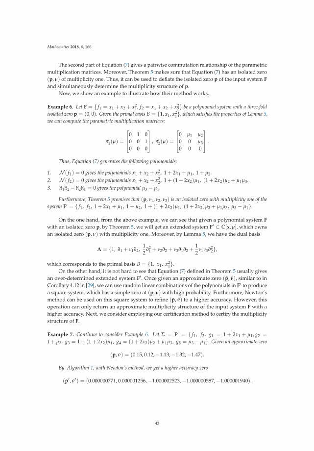
Mathematics 2018, 6, 166
The second part of Equation (7) gives a pairwise commutation relationship of the parametricmultiplication matrices. Moreover, Theorem 5 makes sure that Equation (7) has an isolated zero(p, ν) of multiplicity one. Thus, it can be used to deflate the isolated zero p of the input system F
and simultaneously determine the multiplicity structure of p.Now, we show an example to illustrate how their method works.
Example 6. Let F = { f1 = x1 + x2 + x21, f2 = x1 + x2 + x2
2} be a polynomial system with a three-foldisolated zero p = (0, 0). Given the primal basis B = {1, x1, x2
1}, which satisfies the properties of Lemma 5,we can compute the parametric multiplication matrices:
Mt1(μ) =
⎡⎢⎣0 1 00 0 10 0 0
⎤⎥⎦ , Mt2(μ) =
⎡⎢⎣0 μ1 μ2
0 0 μ3
0 0 0
⎤⎥⎦ .
Thus, Equation (7) generates the following polynomials:
1. N ( f1) = 0 gives the polynomials x1 + x2 + x21, 1 + 2x1 + μ1, 1 + μ2.
2. N ( f2) = 0 gives the polynomials x1 + x2 + x22, 1 + (1 + 2x2)μ1, (1 + 2x2)μ2 + μ1μ3.
3. M1M2 − M2M1 = 0 gives the polynomial μ3 − μ1.
Furthermore, Theorem 5 promises that (p, ν1, ν2, ν3) is an isolated zero with multiplicity one of thesystem F′ = { f1, f2, 1 + 2x1 + μ1, 1 + μ2, 1 + (1 + 2x2)μ1, (1 + 2x2)μ2 + μ1μ3, μ3 − μ1}.
On the one hand, from the above example, we can see that given a polynomial system F
with an isolated zero p, by Theorem 5, we will get an extended system F′ ⊂ C[x, μ], which ownsan isolated zero (p, ν) with multiplicity one. Moreover, by Lemma 5, we have the dual basis
Λ = {1, ∂1 + ν1∂2,12
∂21 + ν2∂2 + ν3∂1∂2 +
12
ν1ν3∂22},
which corresponds to the primal basis B = {1, x1, x21}.
On the other hand, it is not hard to see that Equation (7) defined in Theorem 5 usually givesan over-determined extended system F′. Once given an approximate zero (p, ν), similar to inCorollary 4.12 in [29], we can use random linear combinations of the polynomials in F′ to producea square system, which has a simple zero at (p, ν) with high probability. Furthermore, Newton’smethod can be used on this square system to refine (p, ν) to a higher accuracy. However, thisoperation can only return an approximate multiplicity structure of the input system F with ahigher accuracy. Next, we consider employing our certification method to certify the multiplicitystructure of F.
Example 7. Continue to consider Example 6. Let Σ = F′ = { f1, f2, g1 = 1 + 2x1 + μ1, g2 =
1 + μ2, g3 = 1 + (1 + 2x2)μ1, g4 = (1 + 2x2)μ2 + μ1μ3, g5 = μ3 − μ1}. Given an approximate zero
(p, ν) = (0.15, 0.12,−1.13,−1.32,−1.47).
By Algorithm 1, with Newton’s method, we get a higher accuracy zero
(p′, ν′) = (0.000000771, 0.000001256,−1.000002523,−1.000000587,−1.000001940).
43
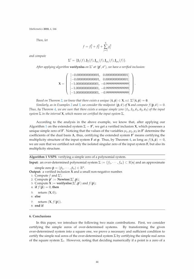
Mathematics 2018, 6, 166
Then, let
f = f 21 + f 2
2 +5
∑j=1
g2j
and computeΣ′ = {J1( f ), J2( f ), Jμ1
( f ), Jμ2( f ), Jμ3
( f )}.
After applying algorithm verifynlss on Σ′ at (p′, ν′), we have a verified inclusion:
X =
⎛⎜⎜⎜⎜⎜⎝[−0.00000000000001, 0.00000000000001][−0.00000000000001, 0.00000000000001][−1.00000000000001, −0.99999999999999][−1.00000000000001, −0.99999999999999][−1.00000000000001, −0.99999999999999]
⎞⎟⎟⎟⎟⎟⎠ .
Based on Theorem 2, we know that there exists a unique (x, μ) ∈ X, s.t. Σ′(x, μ) = 0.Similarly, as in Examples 2 and 3, we consider the midpoint (p, ν) of X and compute f (p, ν) = 0.
Thus, by Theorem 4, we are sure that there exists a unique simple zero (x1, x2, ν1, ν2, ν3) of the inputsystem Σ in the interval X, which means we certified the input system Σ.
According to the analysis in the above example, we know that, after applying ourAlgorithm 1 on the extended system Σ = F′, we get a verified inclusion X, which possesses aunique simple zero of F′. Noticing that the values of the variables μ1, μ2, μ3 in F′ determine thecoefficients of the dual basis Λ, thus, certifying the extended system F′ means certifying themultiplicity structure of the input system F at p. Thus, by Theorem 4, as long as f (x, μ) = 0,we are sure that we certified not only the isolated singular zero of the input system F, but also itsmultiplicity structure.
Algorithm 1 VSPS: verifying a simple zero of a polynomial system.
Input: an over-determined polynomial system Σ := { f1, · · · , fm} ⊂ R[x] and an approximate
simple zero p = ( p1, · · · , pn) ∈ Rn.Output: a verified inclusion X and a small non-negative number.
1: Compute f and Σ′;2: Compute p′ := Newton(Σ′, p);3: Compute X := verifynlss(Σ′, p′) and f (p);4: if f (p) = 0, then
5: return (X, 0);6: else
7: return (X, f (p)).8: end if
6. Conclusions
In this paper, we introduce the following two main contributions. First, we considercertifying the simple zeros of over-determined systems. By transforming the givenover-determined system into a square one, we prove a necessary and sufficient condition tocertify the simple real zeros of the over-determined system Σ by certifying the simple real zerosof the square system Σr. However, noting that deciding numerically if a point is a zero of a
44
Mathematics 2018, 6, 166
polynomial is difficult, we refine and certify the simple real zeros of Σ by refining and certifyinga new square system Σ′ with the interval methods and get a verified inclusion X, which containsa unique simple real zero x of Σ′. In fact, x is a local minimum of f , which is also a necessarycondition for the certification. By the necessary and sufficient condition in Theorem 1, we knowthat, as long as f (x) = 0, we can say that x is a simple real zero of Σ and we certified the inputsystem Σ.
Second, based on our work [35] and the work of Mourrain et al. [21,36], as an applicationof our method, we give a heuristic method for certifying not only the isolated singular zerosof polynomial systems, but also the multiplicity structures of the isolated singular zeros ofpolynomial systems.
In the future, for the certified zero x, trying to give a sufficient condition for the certificationis the direction of our effort.
Author Contributions: J.C. contributed for supervision, project administration, funding and conceived ofthe presented idea. X.D. developed the theory, performed the computations and wrote the initial draft ofthe paper. J.C. verified the analytical methods. Both authors read and approved the final version of thepaper.
Funding: The work was partially supported by NSFC Grants 11471327.
Acknowledgments: The authors would like to thank the anonymous referees very much for their usefulsuggestions that improved this paper.
Conflicts of Interest: The authors declare no conflict of interest.
References
1. Blum, L.; Cucker, F.; Shub, M.; Smale, S. Complexity and Real Computation; Springer: New York, NY,USA, 1998.
2. Hauenstein, J.D.; Sottile, F. Algorithm 921: AlphaCertified: Certifying Solutions to Polynomial Systems.ACM Trans. Math. Softw. 2012, 38, 28. [CrossRef]
3. Smale, S. Newton’s Method Estimates from Data at One Point. In The Disciplines: New Directions inPure, Applied and Computational Mathematics; Ewing, R., Gross, K., Martin, C., Eds.; Springer: New York,NY, USA, 1986.
4. Kanzawa, Y.; Kashiwagi, M.; Oishi, S. An algorithm for finding all solutions of parameter-dependentnonlinear equations with guaranteed accuracy. Electr. Commun. JPn. 1999, 82, 33–39. [CrossRef]
5. Krawczyk, R. Newton-Algorithmen zur Bestimmung von Nullstellen mit Fehlherschranken.Computing 1969, 4, 247–293. [CrossRef]
6. Moore, R.E. A test for existence of solutions to nonlinear systems. SIAM J. Numer. Anal. 1977, 14,611–615. [CrossRef]
7. Nakaya, Y.; Oishi, S.; Kashiwagi, M.; Kanzawa, Y. Numerical verification of nonexistence of solutionsfor separable nonlinear equations and its application to all solutions algorithm. Electr. Commun. Jpn.2003, 86, 45–53. [CrossRef]
8. Rump, S.M. Solving algebraic problems with high accuracy. Proceedings of the Symposium on A NewApproach to Scientific Computation; Academic Press Professional, Inc.: San Diego, CA, USA, 1983;pp. 51–120.
9. Yamamura, K.; Kawata, H.; Tokue, A. Interval solution of nonlinear equations using linearprogramming. BIT Numer. Math. 1998, 38, 186–199. [CrossRef]
10. Allamigeon, X.; Gaubert, S.; Magron, V.; Werner, B. Formal proofs for nonlinear optimization.J. Form. Reason. 2015, 8, 1–24.
11. Kaltofen, E.; Li, B.; Yang, Z.; Zhi, L. Exact certification of global optimality of approximatefactorizations via rationalizing sums-of-squares with floating point scalars. In Proceedings of the
45
Mathematics 2018, 6, 166
Twenty-first International Symposium on Symbolic and Algebraic Computation, ISSAC 08, Hagenberg,Austria, 20–23 July 2008; ACM: New York, NY, USA; pp. 155–164.
12. Kaltofen, E.L.; Li, B.; Yang, Z.; Zhi, L. Exact certification in global polynomial optimization viasums-of-squares of rational functions with rational coefficients. J. Symb. Computat. 2012, 47, 1–15.[CrossRef]
13. Monniaux, D.; Corbineau, P. On the generation of positivstellensatz witnesses in degenerate cases.In Interactive Theorem Proving; LNCS 6898; van Eekelen, M., Geuvers, H., Schmaltz, J., Wiedijk, F., Eds.;Springer: Berlin/Heidelberg, Germany, 2011; pp. 249–264.
14. Peyrl, H.; Parrilo, P.A. A Macaulay2 package for computing sum of squares decompositions ofpolynomials with rational coefficients. In Proceedings of the SNC 2007, Waterloo, AB, Canada, 2007;pp. 207–208.
15. Peyrl, H.; Parrilo, P.A. Computing sum of squares decompositions with rational coefficients.Theor. Comput. Sci. 2008, 409, 269–281. [CrossRef]
16. Safey, M.; Din, E.; Zhi, L. Computing rational points in convex semialgebraic sets and sum of squaresdecompositions. SIAM J. Optim. 2010, 20, 2876–2889.
17. Akogul, T.A.; Hauenstein, J.D.; Szanto, A. Certifying solutions to overdetermined and singularpolynomial systems over Q. J. Symb. Comput. 2018, 84, 147–171.
18. Dayton, B.; Zeng, Z. Computing the multiplicity structure in solving polynomial systems.In Proceedings of the 2005 International Symposium on Symbolic and Algebraic Computation, Beijing,China, 24–27 July 2005; Kauers, M., Ed.; ACM: New York, NY, USA, 2005; pp. 116–123.
19. Giusti, M.; Lecerf, G.; Salvy, B.; Yakoubsohn, J.-C. On location and approximation of clusters of zeros:case of embedding dimension one. Found. Comput. Math. 2007, 7, 1–58. [CrossRef]
20. Hauenstein, J.D.; Wampler, C.W. Isosingular sets and deflation. Found. Computat. Math. 2013, 13,371–403. [CrossRef]
21. Hauenstein, J.D.; Mourrain, B.; Szant, A. Certifying isolated singular points and their multiplicitystructure. In Proceedings of the Twenty-first International Symposium on Symbolic and AlgebraicComputation, ISSAC’ 15, Bath, UK, 6–9 July 2015; pp. 213–220.
22. Ojika, T. A numerical method for branch points of a system of nonlinear algebraic equations.Appl. Numer. Math. 1988, 4, 419–430. [CrossRef]
23. Ojika, T.; Watanabe, S.; Mitsui, T. Deflation algorithm for the multiple roots of a system of nonlinearequations. J. Math. Anal. Appl. 1983, 96, 463–479. [CrossRef]
24. Zeng, Z. Computing multiple roots of inexact polynomials. Math. Comput. 2005, 74, 869–903.[CrossRef]
25. Dayton, B.; Li, T.; Zeng, Z. Multiple zeros of nonlinear systems. Math. Comput. 2011, 80, 2143–2168.[CrossRef]
26. Kanzawa, Y.; Oishi, S. Approximate singular solutions of nonlinear equations and a numerical methodof proving their existence. Theory and application of numerical calculation in science and technology,II (Japanese) (Kyoto, 1996). Surikaisekikenkyusho Kokyuroku 1997, 990, 216–223.
27. Leykin, A.; Verschelde, J.; Zhao, A. Newton’s method with deflation for isolated singularities ofpolynomial systems. Theor. Comput. Sci. 2006, 359, 111–122. [CrossRef]
28. Li, N.; Zhi, L. Verified Error Bounds for Isolated Singular Solutions of Polynomial Systems. SIAM J.Numer. Anal. 2014, 52, 1623–1640. [CrossRef]
29. Mantzaflaris, A.; Mourrain, B. Deflation and certified isolation of singular zeros of polynomial systems.In Proceedings of the ISSAC 2011, San Jose, CA, USA, 17 January 2011; pp. 249–256.
30. Rump, S.M.; Graillat, S. Verified error bounds for multiple roots of systems of nonlinear equations.Numer. Algorithms 2010, 54, 359–377. [CrossRef]
31. Dedieu, J.P.; Shub, M. Newton’s method for overdetermined systems of equations. Math. Comput.1999, 69, 1099–1115. [CrossRef]
46
Mathematics 2018, 6, 166
32. Cheng, J.S.; Dou, X. Certifying simple zeros of over-determined polynomial systems. In ComputerAlgebra in Scientific Computing; CASC’17 Lecture Notes in Computer Science; Gerdt, V., Koepf, W.,Seiler W., Vorozhtsov E., Eds.; Springer: Cham, Switzerland, 2017; pp. 55–76.
33. Li, S. Linear Algebra; Higher Education Press: Beijing, China, 2006; ISBN 978-7-04-019870-6.34. Rohn, J. Positive definiteness and stability of interval matrices. SIAM J. Matrix Anal. Appl. 1994, 15,
175–184. [CrossRef]35. Cheng, J.S.; Dou, X.; Wen, J. A new deflation method for verifying the isolated singular zeros of
polynomial systems. preprint 2018.36. Hauenstein, J.D.; Mourrain, B.; Szanto, A. On deflation and multiplicity structure. J. Symb. Comput.
2017, 83, 228–253. [CrossRef]
c© 2018 by the authors. Licensee MDPI, Basel, Switzerland. This article is an openaccess article distributed under the terms and conditions of the Creative CommonsAttribution (CC BY) license (http://creativecommons.org/licenses/by/4.0/).
47

mathematics
Article
Resolving Decompositions for Polynomial Modules
Mario Albert † and Werner M. Seiler *,†
Institut für Mathematik, Universität Kassel, 34132 Kassel, Germany; [email protected]* Correspondence: [email protected]† These authors contributed equally to this work.
Received: 12 July 2018; Accepted: 4 September 2018; Published: 7 September 2018
Abstract: We introduce the novel concept of a resolving decomposition of a polynomial module as acombinatorial structure that allows for the effective construction of free resolutions. It provides aunifying framework for recent results of the authors for different types of bases.
Keywords: polynomial modules; free resolutions; combinatorial decompositions
MSC: 13D02; 13P10; 68W30
1. Introduction
The determination of free resolutions for polynomial modules is a fundamental task incomputational commutative algebra and algebraic geometry. Free resolutions are needed for derivedfunctors like Ext and Tor and many important homological invariants like the projective dimension orthe Castelnuovo-Mumford regularity are defined via the minimal resolution. Furthermore, already theBetti numbers, which measure the size of the minimal free resolution, give valuable information aboutthe geometry and topology of varieties.
Unfortunately, resolutions are computationally rather expensive. A rough estimate says that aresolution of length � requires to compute � Gröbner bases. In many situations, partial informationlike the Betti numbers already suffice. However, all classical algorithms for the computation ofBetti numbers require to always determine a full resolution. Indeed, one can observe in computeralgebra systems like SINGULAR that computing the Betti numbers needs as much computation time ascomputing a full resolution.
In the recent work [1], we developed a novel approach to this question consisting of a combinationof the theory of involutive bases—in the form of Pommaret bases—(see [2] for a general survey oninvolutive bases) and of algebraic discrete Morse theory (see [3,4]). We also implemented it in theCOCOALIB [5]. To the best of our knowledge, this approach is the only one that is able to compute(even individual) Betti numbers without first determining a full resolution. For most ideals, it istherefore much faster than classical methods (see the detailed benchmarks given in [1,6]). Furthermore,the new approach can be easily parallelised and scales much better with the problem size.
Because of these advantages, a generalisation of our approach to other situations is of great interest.Furthermore, it should be noted that Pommaret bases exist only in generic coordinates. As a first step,we extended it therefore to Janet bases [6], as these can be computed more efficiently and always exist.While the proofs follow the same lines, the use of a different involutive division entailed the adaptionof many technical points. Furthermore, we are currently considering the use of alternative ideal basesnot necessarily coming from an involutive division, but inducing combinatorial decompositions of theideal with essentially the same properties. The development of a syzygy theory for such bases againproceeds along the same ideas, but various proofs have to be modified in minor ways.
In a different line of work, we recently introduced the concept of a module marked on aquasi-stable submodule which is very useful for the explicit determination of equations for Hilbert
Mathematics 2018, 6, 161; doi:10.3390/math6090161 www.mdpi.com/journal/mathematics48
Mathematics 2018, 6, 161
and Quot schemes [7,8]. The marking induces a combinatorial decomposition based on Pommaretmultiplicative variables, but this time the key issue is that the head terms are not chosen with respectto a term order. Nevertheless, we showed that the most important results on resolutions presented [1]still remain essentially true. Again the proofs follow the same basic ideas, but require smaller technicalmodifications at some places.
This article represents a revised and expanded version of [9] which was presented at the conferenceComputer Algebra in Scientific Computing. Its main objective is to unify all our above-mentioned worksin a general axiomatic framework. It centers about the novel concept of a resolving decompositionof an ideal. It refines the classical Stanley decompositions by certain additional axioms implying theexistence of standard representations and normal forms. We then discuss how a free resolution andBetti numbers can be determined from a resolving decomposition.
The goal of this unification is not the development of any new algorithms. In particular,no algorithm for the construction of resolving decomposition will be presented. Instead, our resultsshould be considered as a “meta-machinery” which augments any concept of a basis that induces aresolving decomposition with an effective syzygy theory. As already mentioned above, we appliedthis “meta-machinery” already for the special case of Janet or Pommaret bases (including a concreteimplementation in the COCOALIB) [1,6]. The case of marked bases is considered in great detail in [7,8](the latter reference also describes a concrete implementation in COCOALIB for the case of ideals).
The article is structured as follows. The next section provides the definition of a resolvingdecomposition and shows explicitly that all the cases mentioned above are contained in it. The thirdsection discusses the construction of a syzygy resolution out of a resolving decomposition and some ofits properties. In the fourth section, an explicit formula for the differential of this resolution is derivedby relating our construction with the work of Sköldberg [10]. Finally, some conclusions are given.
2. Resolving Decompositions
Throughout this article, we will use the following notations. Let � be a field and P = �[x]
the polynomial ring in the variable x = (x0, . . . , xn). We write � for the set of terms xμ ∈ P .Let Pm
d =⊕m
i=1 P(−di)e(0)i be a finitely generated free P-module with grading d = (d1, . . . , dm)
and free generators e(0)1 , . . . , e
(0)m . A module U ⊆ Pm
d is called monomial module, if it is of the form
⊕mk=1 J(k)e(0)k with each J(k) a monomial ideal in P . A module term (with index i) is a term of the form
xμe(0)i . If J ⊆ P is a monomial ideal, we denote by N (J) ⊆ � the set of terms in � not belonging to J.
In the case of monomial module U, we analogously write N (U) =⋃m
k=1N (J(k))e(0)k . The support ofan element f ∈ Pm
d is the set supp(f) of all module terms appearing in f with a non-zero coefficient,
thus f = ∑xαe(0)iα∈supp(f)
cαxαe(0)iα . If B is a set of homogeneous elements of degree s in Pm
d , we write
〈B〉� for the �-vector space generated by B in (Pmd )s. For a module U ⊆ Pm
d , we denote by pd (U) theprojective dimension and by reg (U) the (Castelnuovo-Mumford) regularity of U.
Let B = {h1, . . . , hs} be a finite set of homogeneous elements in Pmd . We need the following data
to define a resolving decomposition of the submodule U defined by B. For every generator hi ∈ B, wechoose a term xμi e
(0)ki∈ supp hi denoted by hm (hi) and call it the head module term of hi. Furthermore,
we define the head module terms of B by hm (B) := Bigl{hm (h) | h ∈ BBigr} and the head module of Uby hm (U) = 〈hmB〉. Obviously, the monomial module hm (U) depends on the choice of both thegenerating set B and the head module terms hm (B). Furthermore, we assign to every head moduleterm hm(h) with h ∈ B a set of multiplicative variables XB(h) ⊆ x and denote by XB the set of all thesesets. Finally, we choose a term order ≺B on P s with s the number of generators in B.
Definition 1. The above introduced quadruple (B, hm (B), XB ,≺B) defines a resolving decomposition of asubmodule U ⊆ Pm
d , if the following five properties hold:
(i) U = 〈B〉.
49
Mathematics 2018, 6, 161
(ii) Let h ∈ B be an arbitrary generator. Each module term xμe(0)k ∈ supp(h) \ {hm(h)} must satisfy
xμe(0)k /∈ hm(U).
(iii) The assigned multiplicative variables induce direct sum decompositions of both the head module
hm(U) = Bigoplush∈B�[XB(h)] · hm(h) (1)
and the module itselfU = Bigoplush∈B�[XB(h)] · h . (2)
(iv) We have a direct sum decomposition (Pmd )r = Ur ⊕ 〈N (hm(U))r〉� for all degrees r ≥ 0.
(v) Let {e(1)1 , . . . , e
(1)s } denote the canonical basis of the free module P s. Given an arbitrary term xδ ∈ �
and an arbitrary generator hα ∈ B, we find for every term xεe(0)i ∈ supp(xδhα) ∩ hm(U) a unique
hBeta ∈ hm(B) such that xεe(0)i = xδ′ hm(hβ) with xδ′ ∈ �[XB(hBeta)] by (iii). Then the inequality
xδe(1)α �B xδ′eBeta(1) holds with respect to the term order ≺B .
In the sequel, we will always assume that (B, hm (B), XB ,≺B) is a resolving decomposition ofthe finitely generated module U = 〈B〉 ⊆ Pm
d . In addition to the multiplicative variables, we definefor h ∈ B the non-multiplicative variables as XB(h) = {x0, . . . , xn} \ XB(h).
Remark 1. Resolving decompositions refine the classical concept of Stanley decompositions [11]. Indeed,the equalities (1) and (2) simply represents Stanley decompositions of the head module of U and of U itself,respectively. This observation makes it straightforward to compute the Hilbert functions of hm(U) and of U,respectively. Since the two Stanley decompositions possess an identical structure, the arising Hilbert functionstrivially coincides. This fact represents a built-in term order free version of the well-known Macaulay theoremfor Gröbner bases—see e.g., [12]).
Condition (iii) implies the existence of a unique standard representation
f =s
∑α=1
Pαhα
with Pα ∈ �[XB(hα)] for every f ∈ U. Note that these representations are indeed unique due to the factthat each coefficient may only depend on the multiplicative variables. Condition (iv) implies the existence ofunique normal forms modulo U for all homogeneous elements f ∈ Pm
d . Due to it, we find a unique coefficientPα ∈ �[XB(hα)] for each generator hα ∈ B such that f′ = f−∑s
α=1 Pαhα ∈ 〈N (hm(U))〉�. It also followstrivially from (1) that for every generator in the basis B a different head module term is chosen.
For the goals of this article, the mere existence of normal forms suffices. Nevertheless, we remarkthat Condition (v) entails that these normal forms can be effectively determined. The head terms andmultiplicative variables inherent to a resolving decomposition allows for the definition of a naturalreduction relation. If there exists a term xεe
(0)i ∈ supp (f) ∩ hm (U) for some module element f ∈ Pm
d ,
then we find a unique head module term h ∈ hm(B) such that xεe(0)i = xδ hm(h) with xδ ∈ �[XB(h)]
and consequently a reduction fB−→ f− cxδh is possible for a suitably chosen scalar c ∈ �.
Lemma 1. For any resolving decomposition (B, hm (B), XB ,≺B) the transitive closure B−→∗ of the reduction
relation B−→ is Noetherian and confluent.
Proof. It is sufficient to prove that for every term xγe(0)k in hm(U), there is a unique g ∈ Pm
d such
that xγe(0)k
B−→∗ g and g ∈ 〈N (hm(U))〉. Since xγe(0)k ∈ hm(U), there exists a unique xδhα ∈ U such
that xδ hm(hα) = xγe(0)k and xδ ∈ XB(hα). Hence, xγe
(0)k
B−→ xγe(0)k − cxδhα for a suitably chosen
coefficient c ∈ �. Denoting again the canonical basis of P s by {e(1)1 , . . . , e
(1)s }, we associate the term
50
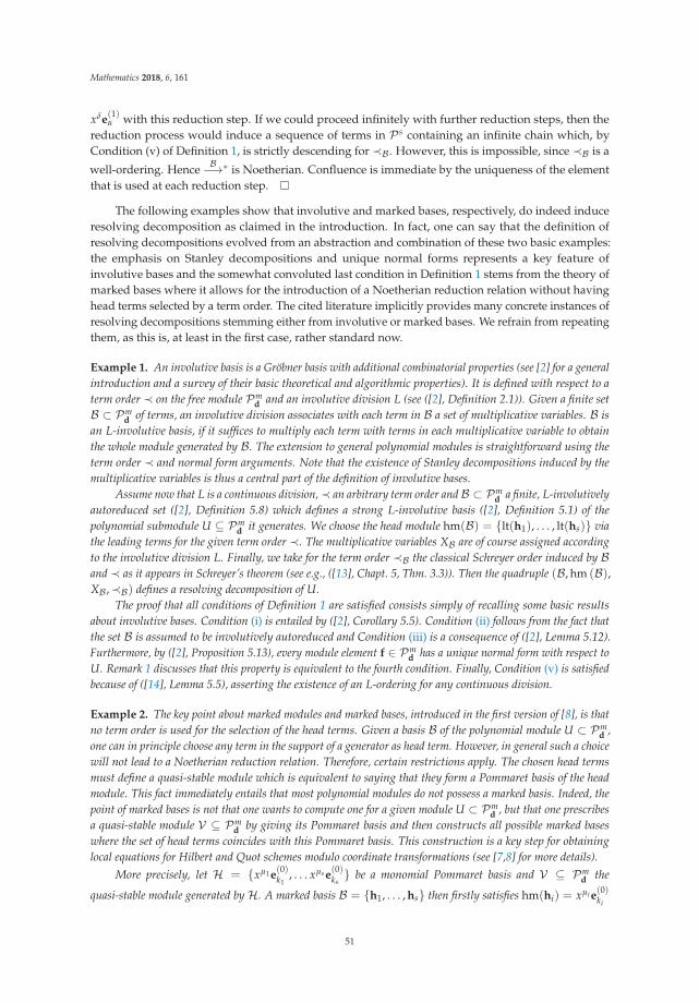
Mathematics 2018, 6, 161
xδe(1)α with this reduction step. If we could proceed infinitely with further reduction steps, then the
reduction process would induce a sequence of terms in P s containing an infinite chain which, byCondition (v) of Definition 1, is strictly descending for ≺B . However, this is impossible, since ≺B is a
well-ordering. Hence B−→∗ is Noetherian. Confluence is immediate by the uniqueness of the elementthat is used at each reduction step.
The following examples show that involutive and marked bases, respectively, do indeed induceresolving decomposition as claimed in the introduction. In fact, one can say that the definition ofresolving decompositions evolved from an abstraction and combination of these two basic examples:the emphasis on Stanley decompositions and unique normal forms represents a key feature ofinvolutive bases and the somewhat convoluted last condition in Definition 1 stems from the theory ofmarked bases where it allows for the introduction of a Noetherian reduction relation without havinghead terms selected by a term order. The cited literature implicitly provides many concrete instances ofresolving decompositions stemming either from involutive or marked bases. We refrain from repeatingthem, as this is, at least in the first case, rather standard now.
Example 1. An involutive basis is a Gröbner basis with additional combinatorial properties (see [2] for a generalintroduction and a survey of their basic theoretical and algorithmic properties). It is defined with respect to aterm order ≺ on the free module Pm
d and an involutive division L (see ([2], Definition 2.1)). Given a finite setB ⊂ Pm
d of terms, an involutive division associates with each term in B a set of multiplicative variables. B isan L-involutive basis, if it suffices to multiply each term with terms in each multiplicative variable to obtainthe whole module generated by B. The extension to general polynomial modules is straightforward using theterm order ≺ and normal form arguments. Note that the existence of Stanley decompositions induced by themultiplicative variables is thus a central part of the definition of involutive bases.
Assume now that L is a continuous division,≺ an arbitrary term order and B ⊂ Pmd a finite, L-involutively
autoreduced set ([2], Definition 5.8) which defines a strong L-involutive basis ([2], Definition 5.1) of thepolynomial submodule U ⊆ Pm
d it generates. We choose the head module hm(B) = {lt(h1), . . . , lt(hs)} viathe leading terms for the given term order ≺. The multiplicative variables XB are of course assigned accordingto the involutive division L. Finally, we take for the term order ≺B the classical Schreyer order induced by Band ≺ as it appears in Schreyer’s theorem (see e.g., ([13], Chapt. 5, Thm. 3.3)). Then the quadruple (B, hm (B),XB ,≺B) defines a resolving decomposition of U.
The proof that all conditions of Definition 1 are satisfied consists simply of recalling some basic resultsabout involutive bases. Condition (i) is entailed by ([2], Corollary 5.5). Condition (ii) follows from the fact thatthe set B is assumed to be involutively autoreduced and Condition (iii) is a consequence of ([2], Lemma 5.12).Furthermore, by ([2], Proposition 5.13), every module element f ∈ Pm
d has a unique normal form with respect toU. Remark 1 discusses that this property is equivalent to the fourth condition. Finally, Condition (v) is satisfiedbecause of ([14], Lemma 5.5), asserting the existence of an L-ordering for any continuous division.
Example 2. The key point about marked modules and marked bases, introduced in the first version of [8], is thatno term order is used for the selection of the head terms. Given a basis B of the polynomial module U ⊂ Pm
d ,one can in principle choose any term in the support of a generator as head term. However, in general such a choicewill not lead to a Noetherian reduction relation. Therefore, certain restrictions apply. The chosen head termsmust define a quasi-stable module which is equivalent to saying that they form a Pommaret basis of the headmodule. This fact immediately entails that most polynomial modules do not possess a marked basis. Indeed, thepoint of marked bases is not that one wants to compute one for a given module U ⊂ Pm
d , but that one prescribesa quasi-stable module V ⊆ Pm
d by giving its Pommaret basis and then constructs all possible marked baseswhere the set of head terms coincides with this Pommaret basis. This construction is a key step for obtaininglocal equations for Hilbert and Quot schemes modulo coordinate transformations (see [7,8] for more details).
More precisely, let H = {xμ1e(0)k1
, . . . xμs e(0)ks} be a monomial Pommaret basis and V ⊆ Pm
d the
quasi-stable module generated byH. A marked basis B = {h1, . . . , hs} then firstly satisfies hm(hi) = xμi e(0)ki
51
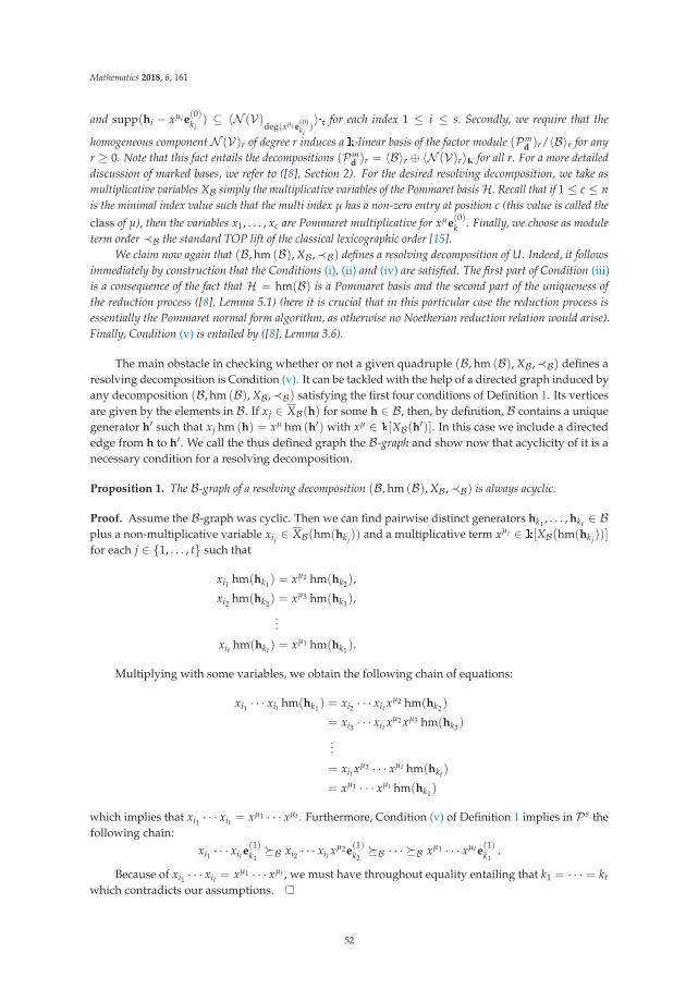
Mathematics 2018, 6, 161
and supp(hi − xμi e(0)ki
) ⊆ 〈N (V)deg(xμi e
(0)ki
)〉� for each index 1 ≤ i ≤ s. Secondly, we require that the
homogeneous component N (V)r of degree r induces a �-linear basis of the factor module (Pmd )r/〈B〉r for any
r ≥ 0. Note that this fact entails the decompositions (Pmd )r = 〈B〉r ⊕ 〈N (V)r〉� for all r. For a more detailed
discussion of marked bases, we refer to ([8], Section 2). For the desired resolving decomposition, we take asmultiplicative variables XB simply the multiplicative variables of the Pommaret basisH. Recall that if 1 ≤ c ≤ nis the minimal index value such that the multi index μ has a non-zero entry at position c (this value is called theclass of μ), then the variables x1, . . . , xc are Pommaret multiplicative for xμe
(0)k . Finally, we choose as module
term order ≺B the standard TOP lift of the classical lexicographic order [15].We claim now again that (B, hm (B), XB ,≺B) defines a resolving decomposition of U. Indeed, it follows
immediately by construction that the Conditions (i), (ii) and (iv) are satisfied. The first part of Condition (iii)is a consequence of the fact that H = hm(B) is a Pommaret basis and the second part of the uniqueness ofthe reduction process ([8], Lemma 5.1) (here it is crucial that in this particular case the reduction process isessentially the Pommaret normal form algorithm, as otherwise no Noetherian reduction relation would arise).Finally, Condition (v) is entailed by ([8], Lemma 3.6).
The main obstacle in checking whether or not a given quadruple (B, hm (B), XB ,≺B) defines aresolving decomposition is Condition (v). It can be tackled with the help of a directed graph induced byany decomposition (B, hm (B), XB ,≺B) satisfying the first four conditions of Definition 1. Its verticesare given by the elements in B. If xj ∈ XB(h) for some h ∈ B, then, by definition, B contains a uniquegenerator h′ such that xj hm (h) = xμ hm (h′) with xμ ∈ �[XB(h′)]. In this case we include a directededge from h to h′. We call the thus defined graph the B-graph and show now that acyclicity of it is anecessary condition for a resolving decomposition.
Proposition 1. The B-graph of a resolving decomposition (B, hm (B), XB ,≺B) is always acyclic.
Proof. Assume the B-graph was cyclic. Then we can find pairwise distinct generators hk1 , . . . , hkt ∈ Bplus a non-multiplicative variable xij ∈ XB(hm(hkj
)) and a multiplicative term xμj ∈ �[XB(hm(hkj))]
for each j ∈ {1, . . . , t} such that
xi1 hm(hk1) = xμ2 hm(hk2),
xi2 hm(hk2) = xμ3 hm(hk3),...
xit hm(hkt) = xμ1 hm(hk1).
Multiplying with some variables, we obtain the following chain of equations:
xi1 · · · xit hm(hk1) = xi2 · · · xit xμ2 hm(hk2)
= xi3 · · · xit xμ2 xμ3 hm(hk3)
...
= xit xμ2 · · · xμt hm(hkt)
= xμ1 · · · xμt hm(hk1)
which implies that xi1 · · · xit = xμ1 · · · xμt . Furthermore, Condition (v) of Definition 1 implies in P s thefollowing chain:
xi1 · · · xit e(1)k1�B xi2 · · · xit x
μ2e(1)k2�B · · · �B xμ1 · · · xμt e
(1)k1
.
Because of xi1 · · · xit = xμ1 · · · xμt , we must have throughout equality entailing that k1 = · · · = kt
which contradicts our assumptions.
52

Mathematics 2018, 6, 161
The following two results provide a converse of this proposition for the special case of a monomialgenerating set B by showing that whenever the B-graph of such a set is acyclic, then there exists aterm order satisfying Condition (v).
Lemma 2. Let B be a generating set consisting only of module terms. Assume that for the chosen multiplicativevariables XB , the B-graph is acyclic. Then it is not possible to find a chain of equalities of the form
xν1hk1 = xμ2hk2 , (3a)
xν2hk2 = xμ3hk3 , (3b)...
xνt hkt = xμ1hk1 (3c)
with multiplicative terms xμi ∈ �[XB(hki)] and arbitrary terms xνi ∈ �. Furthermore, whenever an equality
xν hm(hi) = xμ hm(hj) holds with a multiplicative term xμ ∈ �[XB(hj)], then the B-graph contains adirected path from hi to hj.
Proof. We show that any chain of the form (3) induces a cycle in the B-graph and thus violatesthe assumed acyclicity. Without loss of generality, we may assume that gcd(xνi , xμi+1) = 1 andxνi /∈ �[XB(hki
)]. This implies the existence of a non-multiplicative variable xi0 ∈ XB(hk1) dividing xν1 .Set xρ0 = xν1 /xi0 and let the normal form of xi0hk1 be xτ1 hl1 . Then xρ0 xτ1 hl1 = xμ2 hk2 . By assumption,there exists a non-multiplicative variable xi1 ∈ XB(hl1) dividing xρ0 xτ1 . Now set xρ1 = xρ0 xτ1 /xi1 andrepeat the procedure.
Due to the fact that the B-graph is acyclic and that there are only finitely many terms xρ, xτ
and generators hl such that xρxτhl = xμ2 hk2 , we find after finitely many steps xlt and hlt such thatxlt ∈ XB(hlt) divides xρt−1 xτt and such that the normal form of xlt hlt is xμ2 hk2 . Now we do the samefor hk2 , hk3 , . . . at the end we reach again hk1 . Hence, we have constructed a cycle in the B-graph.
The final assertion follows immediately from the construction above.
Lemma 3. Let B = {h1, . . . , hs} be a generating set consisting only of module terms. Assume that for thechosen multiplicative variables XB Conditions (i) to (iv) of Definition 1 are satisfied. Furthermore, let theB-graph be acyclic and the elements of B be numbered in such a way that for any path from hi to hj in the
B-graph we always have i < j. If ≺B is an arbitrary term order on P s such that xαe(0)i �B xBetae
(0)j whenever
i < j, then (B, hm (B), XB ,≺B) is a resolving decomposition.
Proof. We first remark that a numbering of the set B as assumed in the Lemma always exists for anacyclic graph. Now we only have to check Condition (v) of Definition 1. Take a generator hi ∈ Band an arbitrary term xδ ∈ �. Then xδhi = xαhj for a suitable multiplicative term xα ∈ �[XB(hj)].By Lemma 2, there exists a path from hi to hj in the B-graph and hence i < j. However, this implies
xδe(0)i �B xαe
(0)j proving the missing condition in the definition of a resolving decomposition.
The last lemma provides us with a simple check whether a monomial generating set together withthe chosen assignment of multiplicative variables can be used for defining a resolving decomposition:we only have to check whether the induced B-graph is acyclic. If this is the case, then we can choose anyterm order satisfying the property of Lemma 3 to complete the definition of a resolving decomposition.The existence of such a term order is obvious, as every POT lift fulfils this property [16].
53

Mathematics 2018, 6, 161
Example 3. Set P = �[x0, x1, x2, x3] with the standard grading and m = 1. Let U be the ideal generated byx0x1, x2
1, x2x3, x33 in P . A Stanley decomposition of U is then given by the set
B = {h1 = x0x1, h2 = x0x1x2, h3 = x20x1, h4 = x2
1, h5 = x21x3,
h6 = x0x1x3, h7 = x21x2
3, h8 = x0x1x23, h9 = x3
3, h10 = x2x3}
with multiplicative variables
XB(h1) = ∅, XB(h2) = {x0, x2}XB(h3) = {x0, x2}, XB(h4) = {x0, x1, x2}XB(h5) = {x1}, XB(h6) = {x0, x1}XB(h7) = {x1}, XB(h8) = {x0, x1}XB(h9) = {x0, x1, x3}, XB(h10) = {x0, x1, x2, x3} .
The corresponding B-graph is
h2 ��
��
h10
h1
��
��
����
h4 �� h5
��
��
��
h7
��
��
��
h9
h3
��
�� h6 ��
h8.
��
��
and obviously acyclic. Hence we can choose an arbitrary term order ≺B as described in Lemma 3 to complete thedefinition of a resolving decomposition (B, hm (B), XB ,≺B).
Example 4. It should be emphasised that not even in the monomial case does every Stanley decomposition inducea resolving decomposition, i.e., we cannot always find a corresponding term order ≺B . A simple counterexamplecan already be given based on the homogeneous maximal ideal U in P for n = 4 and the standard grading.In ([17], Page 31), it is shown that a Stanley decomposition of U is defined by the set
B = {h1 = x0, h2 = x1, h3 = x2, h4 = x3, h5 = x4, h6 = x0x1x3, h7 = x0x2x3,
h8 = x0x2x4, h9 = x1x2x4, h10 = x1x3x4, h11 = x0x1x2x3x4}
with multiplicative variables
XB(h1) = {x0, x1, x2}, XB(h2) = {x1, x2, x3}XB(h3) = {x2, x3, x4}, XB(h4) = {x0, x3, x4}XB(h5) = {x0, x1, x4}, XB(h6) = {x0, x1, x2, x3}XB(h7) = {x0, x2, x3, x4}, XB(h8) = {x0, x1, x2, x4}XB(h9) = {x1, x2, x3, x4}, XB(h10) = {x0, x1, x3, x4}
XB(h11) = {x0, x1, x2, x3, x4} .
The B-graph corresponding to this basis is
54
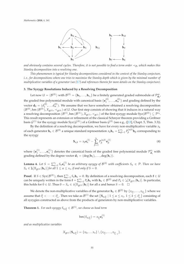
Mathematics 2018, 6, 161
h4
�� ��
h6 �� h10
��h1
��
��
h2
��
�� h3��
h11 h9
��h5
��
��
h7
��
h8��
and obviously contains several cycles. Therefore, it is not possible to find a term order ≺B , which makes thisStanley decomposition into a resolving one.
This phenomenon is typical for Stanley decompositions considered in the context of the Stanley conjecture,i. e., for decompositions where one tries to maximise the Stanley depth which is given by the minimal number ofmultiplicative variables of a generator (see [17] and references therein for more details on the Stanley conjecture).
3. The Syzygy Resolutions Induced by a Resolving Decomposition
Let now U = 〈B(0)〉 with B(0) = {h1, . . . , hs1} be a finitely generated graded submodule of Pmd0
,
the graded free polynomial module with canonical basis {e(0)1 , . . . , e
(0)m } and grading defined by the
vector d0 = (d(0)1 , . . . d(0)m ). We assume that we have somehow obtained a resolving decomposition(B(0), hm (B(0)), XB(0) ,≺B(0) ) of U. Our first step consists of showing that it induces in a natural waya resolving decomposition (B(1), hm (B(1)), XB(1) ,≺B(1) ) of the first syzygy module Syz(B(0)) ⊆ P s1 .This result represents an extension or refinement of the classical Schreyer theorem providing a Gröbnerbasis G(1) for the syzygy module Syz(G(0)) of a Gröbner basis G(0) (see e.g., ([13], Chapt. 5, Thm. 3.3)).
By the definition of a resolving decomposition, we have for every non-multiplicative variable xk
of each generator hα ∈ B(0) a unique standard representation xkhα = ∑s1β=1 P(α;k)
β hβ corresponding tothe syzygy
Sα;k = xke(1)α −
s1
∑β=1
P(α;k)β e
(1)β (4)
where {e(1)1 , . . . , e
(1)s1 } denotes the canonical basis of the graded free polynomial module P s1
d1with
grading defined by the degree vector d1 = (deg(h1), . . . , deg(hs)).
Lemma 4. Let S = ∑s1α=1 Sαe
(1)α be an arbitrary syzygy of B(0) with coefficients Sα ∈ P . Then we have
Sα ∈ �[XB(0) (hα)] for all 1 ≤ α ≤ s1, if and only if S = 0.
Proof. If S ∈ Syz(B(0)), then ∑s1α=1 Sαhα = 0. By definition of a resolving decomposition, each f ∈ U
can be uniquely written in the form f = ∑s1α=1 Pαhα with hα ∈ B(0) and Pα ∈ �[XB(0) (hα)]. In particular,
this holds for 0 ∈ U. Thus 0 = Sα ∈ �[XB(0) (hl)] for all α and hence S = 0.
We denote the non-multiplicative variables of the generator hα ∈ B(0) by {xiα1, . . . , xiαrα
} where we
assume that iα1 < · · · < iα
rα. Then we take as B(1) the set
{Sα;iαk
| 1 ≤ α ≤ s1, 1 ≤ k ≤ iαrα
}consisting of
all syzygies constructed as above from the products of generators by non-multiplicative variables.
Theorem 1. For each syzygy Sα;iαk∈ B(1), we choose as head term
hm(Sα;iαk) = xiαk
e(1)α
and as multiplicative variables
XB(1) (Sα;iαk) = {x0, . . . xn} \ {xiα1
, . . . , xiαk−1} .
55
Mathematics 2018, 6, 161
Furthermore, we take for ≺B(1) the Schreyer order associated to B(0) and ≺B(0) . Then the quadruple (B(1),hm (B(1)), XB(1) ,≺B(1) ) defines a resolving decomposition of the syzygy module Syz(B(0)).
Proof. We first show that (B(1), hm (B(1)), XB(1) ,≺B(1) ) is a resolving decomposition of 〈B(1)〉. In asecond step, we prove that furthermore 〈B(1)〉 = Syz(B(0)).
The first condition of Definition 1 is trivially satisfied. By construction, it is obvious that
hm(〈B(1)〉) = Bigopluss1α=1〈XB(0) (hα)〉e(1)α . (5)
It follows from (4) that any non head term xμe(1)l ∈ supp(Sα;k − xke
(1)α ) must satisfy xμ ∈
�[XB(0) (hl)] and hence we find xμe(1)l /∈ hm(〈B(1)〉) implying Condition (ii). Furthermore, it is
obvious that
〈XB(0) (hα)〉e(1)α =rα⊕
k=1
�[XB(1) (Sα,iαk)]xiαk
e(1)α .
If we combine this equation with (5), then the first part of Condition (iii) follows immediately.The second part of this condition is a bit harder to prove. We take an arbitrary module element
f ∈ 〈B(1)〉 and construct its standard representation using hm(〈B(1)〉). Assume first that the support off contains no multiple of a head term, i. e., supp(f) ∩ hm(〈B(1)〉) = ∅. Then all terms xεe
(1)α ∈ supp(f)
in the support must satisfy xε ∈ XB(0) (hα). Therefore, we get that f = 0 due to Lemma 4.
We may thus assume that supp(f) ∩ hm(〈B(1)〉) �= ∅ and we take the biggest term xμe(1)α in this
set with respect to the order ≺B(0) . By the already proven first part of Condition (iii), there must bea syzygy Sα;i such that xi | xμ and xμ/xi ∈ �[XB(1) (Sα;i)]. We reduce f by this syzygy and obtain thenew module element
f′ = f− cxμ
xiSα;i
for a suitable constant c ∈ � such that the term xμe(1)α is no longer in support of f′. Every term
xλe(1)β ∈ supp (f′) that is newly introduced by the subtraction of c xμ
xiSα;i and that also lies in hm(〈B(1)〉)
must be strictly less than the removed term xμe(1)α by Condition (v) of Definition 1 and by Equation (4)
defining the syzygy Sα;i.We repeat this reduction procedure until we eventually obtain a module element f′′ such that
supp(f′′) ∩ hm (〈B(1)〉) = ∅. This will happen after a finite number of steps, since the reduced termsforms a decreasing sequence with respect to the well-order ≺B(0) . By the same argument as above,this implies that we must have f′′ = 0, which concludes the proof of this condition.
The above procedure provides us with an algorithm to compute arbitrary normal forms andhence Condition (iv) follows immediately. For the last condition in Definition 1, we observe that thehead term xie
(1)α is the leading term of the syzygy Sα;i for the module term order ≺B(0) . Thus the used
Schreyer order indeed satisfies Condition (v).
As is the case for the classical Schreyer theorem, this construction can now be iterated to obtainresolving decompositions of the second and higher syzygy modules. This iteration thus leadsto a (generally non-minimal) free resolution of the submodule U where the constructed syzygiesdefine the columns of the matrices of the differentials. Note that for actually writing down allthese syzygies, we must compute many standard representations of products of generators bynon-multiplicative variables. This fact does not change compared to the classical situation (where oneconsiders S-polynomials instead of products by variables). However, since a resolving decompositioncontains much more information than a Gröbner basis, it is now possible to make at least precisestatements about the shape of the resolution. More precisely, it turns out that, without any furthercomputations, it is now possible to predict solely on the basis of the resolving decomposition (B(0),hm (B(0)), XB(0) ,≺B(0) ) the head terms of all higher syzygies and thus in particular their numbers
56

Mathematics 2018, 6, 161
corresponding to the ranks of the free modules appearing in the resolution. Furthermore, the length ofthe resolution can also be easily read off from (B(0), hm (B(0)), XB(0) ,≺B(0) ).
Theorem 2. Let (B(0), hm (B(0)), XB(0) ,≺B(0) ) define a resolving decomposition of the graded submodule
U ⊂ Pmd0
. Denote by β(k)0,j the number of generators h ∈ B(0) which are of degree j and have k multiplicative
variables. Furthermore, we write d = min {k | ∃j : β(k)0,j > 0} for the minimal number of multiplicative
variables of a generator. Then the submodule U possesses a graded free resolution of length n− d + 1 of the form
0 →⊕jP(−j)rn+1−d,j → · · · →⊕
jP(−j)r1,j →⊕
jP(−j)r0,j → U → 0 (6)
where the graded ranks of the appearing free modules are given by
ri,j =n+1−i
∑k=1
(n + 1− k
i
)β(k)0,j−i .
Proof. Iterating Theorem 1, we can construct a resolving decomposition (B(i), hm (B(i)), XB(i) ,≺B(i) )
of the ith syzygy module Syzi(U) for any i. Given an index 1 ≤ l ≤ m and a non-multiplicativevariable xk ∈ XB(0) (hα(l)), we find |XB(1) (Sl;k)| < |XB(0) (hα(l))|.
If di denotes the minimal number of multiplicative variables assigned to a head module termin hm (B(i)), then it is easy to see that the minimal number of multiplicative variables assigned to ahead term in hm (B(1)) is d + 1. This fact immediately entails the claimed length of the resolution (6).Furthermore, it follows from our construction of the basic syzygies via products of generators bynon-multiplicative variables that deg(Sk;i) = deg(hk) + 1.
The assertion about the graded ranks of the modules is obtained by a combinatorial calculation.We denote by β
(k)i,j the number of generators in B(i) of degree j with k multiplicative variables. It follows
from our construction, that we have
β(k)i,j =
k−1
∑t=1
β(t)i−1,j−1 ,
as each generator in B(i−1) of degree j− 1 with less than k multiplicative variables contributes onegenerator in B(i) with k multiplicative variables. We will now show by induction how β
(k)i,j can be
expressed in terms of β(k)0,j , namely that
β(k)i,j =
k−i
∑t=1
(k− t− 1
i− 1
)β(t)0,j−i.
The base case i = 1 is trivial. For the inductive step, we first note that obviously β(�)i,j = 0 if
� < i + 1. Using this observation and the inductive hypothesis, we get
β(k)i+1,j =
k−1
∑�=i+2
β(�)i,j−1 =
k−1
∑�=i+2
�−i
∑t=1
(�− t− 1
i− 1
)β(t)0,j−i =
k−i−1
∑t=1
[k−1
∑�=i+t
(�− t− 1
i− 1
)]βt
0,j−i .
A shift of the index in the inner sum by t + 1 proves our claim via the following identity obtainedby summing over one column in the Pascal triangle:
k−t−2
∑m=i−1
(m
i− 1
)=
(k− t− 2
i
).
57

Mathematics 2018, 6, 161
For the ranks of the free modules, we compute
ri,j =n+1
∑k=1
β(k)i,j =
n+1
∑k=1
k−i
∑t=1
(k− t− 1
i− 1
)β(t)0,j−i =
n+1−i
∑k=1
(n + 1− k
i
)β(k)0,j−i
where we used again the above identity for binomial coefficients for obtaining the last equality.
We now take a closer look at this iterative construction of the resolving decompositions (B(j),hm (B(j)), XB(j) ,≺B(j) ) for the syzygy modules Syzj(U). To define an element of B(j), we consider for
each generator hα ∈ B(0) all ordered integer sequences k = (k1, . . . , kj) with 0 ≤ k1 < · · · < kj ≤ nof length |k| = j such that xki
∈ XB(0) (hα) for all 1 ≤ i ≤ j. We denote for any 1 ≤ i ≤ j by kithe sequence obtained by eliminating ki from k. Then the generator Sα;k arises recursively fromthe standard representation of xkj
Sα;kj according to the resolving decomposition (B(j−1), hm (B(j−1)),XB(j−1) ,≺B(j−1) ):
xkjSα;kj =
s1
∑β=1
∑l
P(α;k)β;l Sβ;l. (7)
The second sum is over all ordered integer sequences l of length j− 1 such that for each entry�i the variable x�i
is non-multiplicative for the generator hBeta ∈ B(0). Denoting the free generators
of the free module which contains the jth syzygy module by e(j)α,l , such that α ∈ {1, . . . , s1} and l is an
ordered subset of XB(0) (hα) of length j− 1 we get the following representation for Sα,k:
Sα;k = xkje(j)α;kj−
s1
∑β=1
∑l
P(α;k)β;l e
(j)β;l.
An important consequence of our construction is that it allows us to bound certain homologicalinvariants of the submodule U in terms of data easily read off from the resolving decomposition (B(0),hm (B(0)), XB(0) ,≺B(0) ). Note, however, that in contrast to the situation in [14] where the resolutioninduced by a Pommaret basis was considered, we obtain indeed only bounds, whereas a Pommaretbasis gives directly the exact values of the invariants.
Corollary 1. In the situation of Theorem 2, define
d = min{
k | ∃j : β(k)0,j > 0}
, q = deg (B(0)) = maxBigl{deg (h) | h ∈ B(0)Bigr} .
Then we obtain the following bounds for the projective dimension, the Castelnuovo-Mumford regularity and thedepth, respectively, of the submodule U:
pd(U) ≤ n + 1− d , reg(U) ≤ q , depth(U) ≥ d .
Proof. The first estimate follows immediately from the resolution (6) induced by the resolvingdecomposition (B(0), hm (B(0)), XB(0) ,≺B(0) ) of U. The last estimate is a simple consequence of the firstone and the graded form of the Auslander-Buchsbaum formula ([18], Ex. 19.8). By construction, themodule Syzi(B(0)) is generated by syzygies of degree less than or equal to q + i. Hence U is q-regularwhich implies by definition the second estimate.
Remark 2. If one takes a closer look at the construction of the resolving decomposition (B(1), hm (B(1)), XB(1) ,≺B(1) ) of Syz(B(0)) provided in Theorem 1, then one notices that B(1) is always a Janet basis of Syz(B(0))
for the order ≺B(0) . This follows simply from the fact that the way in which we choose in Theorem 1 themultiplicative variables for (B(1), hm (B(1)), XB(1) ,≺B(1) ) is inspired by the definition of the Janet division.Thus, if the resolving decomposition (B(0), hm (B(0)), XB(0) ,≺B(0) ) stems from a Pommaret or a Janet basis,
58
Mathematics 2018, 6, 161
then all the resolving decompositions (B(i), hm (B(i)), XB(i) ,≺B(i) ) are actually also induced by Pommaret orJanet bases for a Schreyer order.
Gerdt [19] introduced a new involutive division called alex, since it is based on the anti degree lexicographicorder (a local term order for which terms of higher degree are always smaller than those of lower degree). It iseasy to see that a Janet basis which only consists of variables defines also an involutive basis for the alex division.Hence, the same assertions are true for resolving decompositions induced by alex bases.
Such observations already demonstrate some advantages of the introduction of such a general framework,like resolving decomposition. In our previous works on the free resolutions induced by an involutive basis,we always needed the assumption that the used involutive division L is of Schreyer type to ensure that ourconstruction yields at each step again an L-involutive basis for the syzygy module for a suitable Schreyer order.The construction in Theorem 1 always yields a Janet basis for Syz(B(0)), as in a resolving decomposition we canchoose the head terms and the multiplicative variables as we like. This allows us to extend the results of [14]to involutive bases for arbitrary involutive divisions (not necessarily of Schreyer type), provided the L-graphof the L-involutive basis is acyclic (which is guaranteed for continuous division). Note that, in contrast to theold approach, the here presented construction will not necessarily lead to an L-involutive basis for each syzygymodule, but for most applications this fact is irrelevant.
4. Explicitly Determining the Differentials
As in the previous section, let Pmd0
be a graded free module with free generators e(0)1 , . . . e
(0)m and
a grading defined by the vector d0 = (d(0)1 , . . . d(0)m ). We will always work with a finitely generatedgraded submodule U ⊂ Pm
d0with a resolving decomposition (B(0), hm (B(0)), XB(0) ,≺B(0) ) where
B(0) = {h1, . . . , hs1}.While Theorem 2 provides us with the shape of the induced resolution 6, we cannot obtain explicit
expressions for the differentials in the resolution. As discussed above, we only now the head termof each higher syzygy. Our goal in this section is to derive such explicit fomulae. We first describethe complex underlying the resolution (6) in a different manner. For this purpose, we introduce twofree P-modules,W =
⊕s1α=1 Pwα and V =
⊕ni=0 Pvi, the ranks of which are determined by the size
of the resolving decomposition (B(0), hm (B(0)), XB(0) ,≺B(0) ) and by the number of variables in thepolynomial ring P , respectively. Then we set Ci =W ⊗P ΛiV where Λ• denotes the exterior product.A P-linear basis of Ci is provided by the elements wα ⊗ vk where vk = vk1 ∧ · · · ∧ vki
for an orderedsequence k = (k1, . . . , ki) with 0 ≤ k1 < · · · < ki ≤ n. Then the free subcomplex S• ⊂ C• generatedby all elements wα ⊗ vk with k ⊆ XB(0) (hα) corresponds to (6), if we identify e
(i+1)α;k ↔ wα ⊗ vk.
Let ki+1 ∈ XB0(hα) \ k, then the differential comes from (7),
dS (wα ⊗ vk,ki+1) = xki+1
wα ⊗ vk −∑β,l
P(α;k,ki+1)β;l wβ ⊗ vl ,
and thus requires the explicit determination of all the higher syzygies (7).We will now present a method to directly compute the differential without computing higher
syzygies. It extends a construction of Sköldberg [10] using algebraic discrete Morse theory [3,4] andgeneralises our results in [1,6] for the resolution induced by a Pommaret or a Janet basis.
Definition 2. The graded submodule U possesses head linear syzygies, if it has a finite presentation
0 −→ ker η −→ W =s⊕
α=1
Pwαη−→ U −→ 0 (8)
such that ker η can be generated by a finite set H = {h1, . . . , ht} where one can choose for each generatorhα ∈ H a head module term hm(hα) of the form xiwα.
59

Mathematics 2018, 6, 161
Sköldberg’s construction begins with the following two-sided Koszul complex (F , dF ) defining afree resolution of U. Let V be a �-linear space with basis {v0, . . . , vn} and introduce the free P-moduleFj = P ⊗� ΛjV ⊗� U. Any �-linear basis {ma | a ∈ A} of U induces a P-linear basis of Fj consistingof all elements of the form 1⊗ vk ⊗ma with ordered sequences k of length j. The differential dF of thetwo-sided Koszul complex F is now defined as
dF (1⊗ vk ⊗ma) =j
∑i=1
(−1)i+1(xki⊗ vki ⊗ma − 1⊗ vki ⊗ xki
ma). (9)
Note that the second term on the right hand side is not yet expressed in the chosen �-linear basisof U and that this resolution is generally of infinite size, as the index set A is almost always infinite.For notational simplicity, we will drop in the sequel the tensor sign ⊗ and leading factors 1 whenwriting elements of F•.
Sköldberg uses a specialisation of head linear terms. He requires that for a given term order≺ the leading module of ker η in the presentation (8) must be generated by terms of the form xiwα.In this case, he says that U has initially linear syzygies. Our definition is term order free. Furthermore,Sköldberg considered exclusively the case that the presentation (8) is minimal. However, this representsa severe restriction, as the existence of such presentations cannot be guaranteed. As his constructionneeds this restriction only to ensure that the final resolution is minimal, we have dropped it.
For a module U with head linear syzygies via a presentation (8), we now construct a finiteresolution (G, dG) via a Morse matching. We call the variables
crit (wα) = {xj | xjwα ∈ hm (H)} ,
where H is chosen as in Definition 2, critical for the generator wα; the remaining non-critical onesare contained in the set ncrit (wα). Then a �-linear basis of U is given by all elements xμhα withhα = η(wα) and xμ ∈ �[ncrit (wα)]. Following [4], we define Gj ⊆ Fj as the free submodule generatedby those vertices vkhα where the ordered sequences k are of length j and such that every entry ki iscritical for wα. In particularW ∼= G0 with an isomorphism induced by wα �→ v∅hα.
The description of the differential dG is based on reduction paths in the associated Morse graph(for a detailed treatment of these notions, see [1,3,4]) and expresses the differential as a triple sum. If weassume that, after expanding the right hand side of (9) in the chosen �-linear basis of U, the differentialof the complex F• can be expressed as
dF (vkhα) = ∑m,μ,γ
Qk,αm,μ,γvm(xμhγ) ,
then dG is defined bydG(vkhα) = ∑
l,β∑
m,μ,γ∑p
ρp(Qk,α
m,μ,γvm(xμhγ))
(10)
where the first sum ranges over all ordered sequences l which consists entirely of critical indices forwβ. Moreover, the second sum may be restricted to all values such that a polynomial multiple ofvm(xμhγ) effectively appears in dF (vkhα) and the third sum ranges over all reduction paths p goingfrom vm(xμhγ) to vlhβ. Finally ρp is the reduction associated with the reduction path p satisfying
ρp(vm(xμhγ)
)= qpvlhβ
for some polynomial qp ∈ P .
Remark 3. The explicit formula (10) with its complicated summation ranges obviously looks rather cumbersomeand does not appear to be very useful for practical purposes. However, this first impression is misleading.In fact, (10) can be well exploited both theoretically and computationally. As shown by the COCOALIB
60
Mathematics 2018, 6, 161
implementations described in [1,6], it is for a computer rather straightforward to evaluate (10) for any concretesubmodule U. Moreover, the most valuable feature of (10) is that it provides an explicit expression for each entryin the differential which is independent of all other entries of the differential. This observation will be the key forthe efficient determination of Betti numbers (even individual ones).
In the sequel, we will show that for a finitely generated graded module U with resolvingdecomposition (B(0), hm (B(0)), XB(0) ,≺B(0) ) the resolution constructed by Sköldberg’s method isisomorphic to the resolution which is induced by the resolving decomposition, if we choose the headlinear syzygies properly. Firstly, we obtain the following trivial assertion.
Lemma 5. If the graded submodule U ⊆ P s1d0
possesses a resolving decomposition (B(0), hm (B(0)), XB(0) ,≺B(0) ), then it has head linear syzygies. More precisely, we can set crit(wα) = XB(0) (hα), i. e., the criticalvariables of the vector wα are simply the non-multiplicative variables of the generator hα = η(wα).
We will subsequently apply some lemmata from [1]. In this reference, they are formulated onlyfor the special case that the resolution is induced by a Pommaret basis. Nevertheless, if not explicitlystated otherwise, we can still use them in our more general setting, as their proofs remain correctalso for arbitrary resolving decompositions. This is due to the fact that the proofs only require theexistence of unique standard representations and a separation of the variables into multiplicativeand non-multiplicative ones. In some proofs, the notion of the class of a generator in B(0) appears.As already mentioned above, it is used to assign multiplicative variables for the Pommaret division.When working with an arbitrary resolving decomposition, one must simply substitute it by themaximal index of a multiplicative variable of the considered generator.
We could see above that the explicit description of the differential dG is based on reduction pathsin the associated Morse graph. We now take a closer look at them and their properties. Any reductionpath can be decomposed into so-called elementary ones which are always of length two. One candistinguish three different types of elementary reductions paths ([1], Section 4). Those of type 0 areirrelevant ([1], Lemma 4.5); the other ones have the form
vk(xμhα) −→ vk∪i(xμ
xihα) −→ vl(xνhβ) .
Here k∪ i denotes the ordered sequence arising when i is inserted into the sequence k; likewisek \ i stands for the sequence obtained by removing an index i ∈ k. Now we distinguish two furthertypes of elementary reduction paths depending on the form of the associated reduction.
Type 1: This is the case where l = (k ∪ i)\j, xν = xμ
xiand β = α. Note that it is allowed that i = j.
We define ε(i; k) = (−1)|{j∈k|j>i}|. Then the corresponding reduction is
ρ(vkxμhα) = ε(i; k∪ i)ε(j; k∪ i)xjv(k∪i)\j( xμ
xihα
).
Type 2: In this case l = (k∪ i) \ j and the term xνhβ appears in the involutive standard representation
of the productxμxj
xihα with the coefficient λj,i,α,μ,ν,β ∈ �. By the construction of the Morse
matching, we now always find i �= j. The corresponding reduction is
ρ(vkxμhα) = −ε(i; k∪ i)ε(j; k∪ i)λj,i,α,μ,ν,βv(k∪i)\j(xνhβ) .
This case distinction comes from the differential (9). Summands appearing in it possess one ofthe following two possible forms: xki
vki ma or vki (xkima). Each of these summands corresponds to a
directed edge in the Morse graph ΓAF• . Consider now an elementary reduction path
61

Mathematics 2018, 6, 161
vk(xμhα) −→ vk∪i( xμ
xihα
) −→ vl(xνhβ) .
If the second edge starts at a summand of the first resp. second form, then the elementaryreduction path is of type 1 resp. type 2.
For the proof of the existence of an isomorphism relating the resolution induced by a resolvingdecomposition to the resolution constructed via the above outlined method of Sköldberg, we recall awell-known result about the uniqueness of free resolutions.
Theorem 3. ([20], Theorem 1.6) Let U be a finitely generated graded P-module. If F is the graded minimalfree resolution of U and G an arbitrary graded free resolution of U, then G is isomorphic to the direct sum of Fand a trivial complex.
Theorem 4. Let U ⊂ Pmd be a graded submodule. The graded free resolution F induced by a resolving
decomposition (B(0), hm (B(0)), XB(0) ,≺B(0) ) of U and the graded free resolution G obtained by the method ofSköldberg in the case that the head linear syzygies have been chosen in such a way that crit(hα) = XB(0) (hα)
for every generator hα ∈ B(0) are isomorphic.
Proof. It is not difficult to see that bases for the free modules in the resolution G constructed bySköldberg’s method consists of those generators vkhα with xk ∈ XB(0) (hα) for all indices k containedin k. In the discussion following the proof of Theorem 2, we showed that bases for the modules in theresolution F coming from the resolving decomposition are induced by the syzygies Sα,k and are thusof the same cardinality. Hence, the two resolutions considered possess the same shape, meaning thatthe homogeneous components of the contained free modules satisfy dim� (Fi)j = dim� (Gi)j. Themade assertion is now a trivial consequence of Theorem 3.
This proof already indicates that the two considered resolutions actually possess very similardifferentials. To deepen the comparison of the resolutions a bit more, we now recall a few furthersimple observations made in [1]. It turns out that in the resolution G we may always choose as headmodule terms for the higher syzygies exactly the same terms that appear as head module terms inthe resolving decompositions (B(i), hm (B(i)), XB(i) ,≺B(i) ). In the case that we start with a resolvingdecomposition induced by an involutive bases and then obtain involutive bases for all syzygy modules(recall Remark 2), this entails that Sköldberg’s method also actually constructs involutive bases.
Lemma 6. ([1], Lemma 4.3) Given an index i such that xi ∈ crit (hα), let xihα = ∑s1β=1 P(α;i)
β hβ be the
standard representation. Then we have dG(vihα) = xiv∅hα −∑s1β=1 P(α;i)
β v∅hβ.
Our next statement may be interpreted in the following way. Assume that we choose in the Morsegraph a vertex vi(xμhα) having certain properties and then follow all possible reduction paths startingat it. Then we will never reach a point where it becomes necessary to calculate a standard representation.Assume furthermore that the chosen vertex possesses no critical (i.e., non-multiplicative) variables.Then no such variables will arise while we follow a reduction path. If we want to generalise thisstatement to higher homological degrees, then we must only replace the index conditions xi ∈ ncrit (hα)
and xj ∈ ncrit (hβ) by the conditions xk ∈ ncrit (hα) and x� ∈ ncrit (hβ) for all indices k and � containedin the ordered sequences k and l, respectively.
Lemma 7. ([1], Lemma 4.4) Assume that {xi} ∪ supp(xμ) ⊆ ncrit (hα). Then for any reduction pathp = vi(xμhα) → · · · → vj(xνhβ) we have xj ∈ ncrit (hβ). In particular, in this situation there is noreduction path p = vi(xμhα)→ · · · → vkhβ with xk ∈ crit (hβ).
62
Mathematics 2018, 6, 161
Our final corollary now asserts that we can indeed choose in the resolution G head module termsin such a way that there is a one-to-one correspondence to the head module terms in the resolution F .It is a direct consequence of Lemma 7 and provides us with an alternative explicit proof of Theorem 4.
Corollary 2. Let k = (k1, . . . , kj) with xki∈ crit hα for all i, then
xklvk\kl
hα ∈ supp(dG(vkhα)).
5. Conclusions
In this article, we introduced a framework that provides many different types of bases of gradedpolynomial submodules with an effective syzygy theory. The key is less the properties of the basesthemselves and more the combinatorial decompositions induced by them via the choice of head termsand multiplicative variables. Effectivity is guaranteed through the required term order.
Given any basis that induces a resolving decomposition in the sense of Definition 1, we obtainwith Theorem 1 a generalised version of the classical Schreyer theorem and iteration leads to a freeresolution. One should, however, note the following crucial difference. The classical Schreyer theoremyields only “in principle” a resolution; without actually performing the computations required forevery iteration step, no information about the final resolution can be obtained. By contrast, Theorem 2describes already the full shape of the final resolution based only on the resolving decomposition ofthe given submodule. Thus we could give (usually quite sharp) bounds for important homologicalinvariants in Corollary 1. In fact, the numbers ri,j given in Theorem 2 can also be interpreted as upperbounds for the Betti numbers.
In [1], we showed that with the help of Pommaret bases Sköldberg’s method for the constructionof an explicit resolution can be made fully effective and then yields essentially the same resolution, asthe one induced by the Pommaret basis. In Section 4, we extended these results to arbitrary resolvingdecompositions and thus provided an approach for the explicit computation of free resolutions basedon such a decomposition.
In [1,6], we presented a method to effectively compute graded Betti numbers via the inducedfree resolutions of Janet and Pommaret bases and the method of Sköldberg. It is well-known that oneneeds only the constant part of an arbitrary free resolution to determine the Betti numbers via linearalgebra over the field �. We showed that the method of Sköldberg allows us to compute directly onlythis constant part instead of the whole resolution which drastically improves the complexity of sucha computation. With this approach, it is even possible to determine a single Betti number withoutcomputing the complete constant part of the free resolution. The reason for this is that Sköldberg’sformula allows us to compute any entry of a differential in the free resolution independently of the restof the free resolution. Furthermore, the theorem about the induced free resolution gives us a formulato compute the ranks of any homogeneous component appearing in the resolution. These methods arealso applicable for an arbitrary resolving decomposition due to the fact that we proved Theorem 2 andthe form of the differential (10).
Author Contributions: Both authors contributed equally to conceptualisation and writing of this article.
Funding: The research of the first author was funded by Otto Braun-Stiftung and the research of the secondauthor partially by the European grant H2020-FETOPEN-2016-2017-CSA SC2 (712689).
Conflicts of Interest: The authors declare no conflict of interest.
63
Mathematics 2018, 6, 161
References
1. Albert, M.; Fetzer, M.; Sáenz-de Cabezón, E.; Seiler, W. On the free resolution induced by a Pommaret basis.J. Symb. Comp. 2015, 68, 4–26. [CrossRef]
2. Seiler, W. A Combinatorial Approach to Involution and δ-Regularity I: Involutive Bases in PolynomialAlgebras of Solvable Type. Appl. Algebr. Eng. Commun. Comput. 2009, 20, 207–259. [CrossRef]
3. Jöllenbeck, M.; Welker, V. Minimal Resolutions via Algebraic Discrete Morse Theory; Memoirs AmericanMathematical Society (AMS): Providence, RI, USA, 2009; Volume 197.
4. Sköldberg, E. Morse Theory from an Algebraic Viewpoint. Trans. Am. Math. Soc. 2006, 358, 115–129.[CrossRef]
5. Abbott, J.; Bigatti, M. COCOALIB: A C++ Library for Doing Computations in Commutative Algebra.Available online: http://cocoa.dima.unige.it/cocoalib (accessed on 9 August 2018).
6. Albert, M.; Fetzer, M.; Seiler, W.M. Janet Bases and Resolutions in CoCoALib. In Computer Algebra in ScientificComputing, Proceedings of the 17th International Workshop on Computer Algebra in Scientific Computing (CASC2015), Aachen, Germany, 14–18 September 2015; Gerdt, V.P., Koepf, W., Seiler, W.M., Vorozhtsov, E.V., Eds.;Springer International Publishing: Cham, Switzerland, 2015; pp. 15–29.
7. Albert, M. Computing Quot Schemes. Ph.D. Thesis, Institut für Mathematik, Universität Kassel, Kassel,Germany, 2017.
8. Albert, M.; Bertone, C.; Roggero, M.; Seiler, W.M. Computing Quot Schemes via Marked Bases overQuasi-Stable Modules. arXiv 2018, arXiv:1511.03547v2 .
9. Albert, M.; Seiler, W. Resolving Decompositions for Polynomial Modules. In Computer Algebra in ScientificComputing, Proceedings of the 18th International Workshop on Computer Algebra in Scientific Computing—CASC2016, Bucharest, Romania, 19–23 September 2016; Lecture Notes in Computer Science; Gerdt, V., Koepf, W.,Seiler, W., Vorozhtsov, E., Eds.; Springer: Cham, Switzerland, 2016; Volume 9890, pp. 13–27.
10. Sköldberg, E. Resolutions of Modules with Initially Linear Syzygies. arXiv 2011, arXiv:1106.1913.11. Stanley, R. Hilbert Functions of Graded Algebras. Adv. Math. 1978, 28, 57–83. [CrossRef]12. Cox, D.; Little, J.; O’Shea, D. Ideals, Varieties, and Algorithms; Undergraduate Texts in Mathematics; Springer:
New York, NY, USA, 1992.13. Cox, D.; Little, J.; O’Shea, D. Using Algebraic Geometry; Graduate Texts in Mathematics 185; Springer:
New York, NY, USA, 1998.14. Seiler, W. A Combinatorial Approach to Involution and δ-Regularity II: Structure Analysis of Polynomial
Modules with Pommaret Bases. Appl. Algebr. Eng. Commun. Comput. 2009, 20, 261–338. [CrossRef]15. Given a term order ≺ on P , its term over position (TOP) lifts to a module term order ≺TOP on Pm
d is defined
as follows: let xμe(0)k , xνe
(0)l ∈ Pm
d , then xμe(0)k �TOP xνe
(0)l if xμ � xν or if xμ = xν and k < l.
16. Given a term order ≺ on P , its position over term (POT) lift to a module term order ≺POT on Pmd is defined
as follows: let xμe(0)k , xνe
(0)l ∈ Pm
d , then xμe(0)k �POT xνe
(0)l if k < l or if k = l and xμ � xν.
17. Herzog, J. A Survey on Stanley Depth. In Monomial Ideals, Computations and Applications; Bigatti, A.,Gimenez, P., Sáenz-de Cabezón, E., Eds.; Lecture Notes in Mathemmatics; Springer: Berlin/Heidelberg,Germany, 2013; Volume 2083, pp. 3–45.
18. Eisenbud, D. Commutative Algebra with a View Toward Algebraic Geometry; Graduate Texts in Mathematics 150;Springer: New York, NY, USA, 1995.
19. Gerdt, V.P.; Blinkov, Y.A. Involutive Division Generated by an Antigraded Monomial Ordering. In ComputerAlgebra in Scientific Computing, Proceedings of the 13th International Workshop on Computer Algebra inScientific Computing (CASC 2011), Kassel, Germany, 5–9 September 2011; Gerdt, V.P., Koepf, W., Mayr, E.W.,Vorozhtsov, E. V., Eds.; Springer: Berlin/Heidelberg, Germany, 2011; pp. 158–174.
20. Eisenbud, D. The Geometry of Syzygies: A Second Course in Algebraic Geometry and Commutative Algebra(Graduate Texts in Mathematics); Springer: Berlin/Heidelberg, Germany, 2005.
c© 2018 by the authors. Licensee MDPI, Basel, Switzerland. This article is an open accessarticle distributed under the terms and conditions of the Creative Commons Attribution(CC BY) license (http://creativecommons.org/licenses/by/4.0/).
64
mathematics
Article
First Integrals of the May–LeonardAsymmetric System
Valery Antonov 1, Wilker Fernandes 2, Valery G. Romanovski 3,4,5,* and Natalie L. Shcheglova 6
1 Department of Mathematics, Peter the Great St. Petersburg Polytechnic University, Polytechnicheskaya, 29,195251 St. Petersburg, Russia; [email protected]
2 Departamento de Matemática e Estatística, Universidade Federal de São João del Rei, São João del Rei,Minas Gerais 36307-352, Brazil; [email protected]
3 Faculty of Electrical Engineering and Computer Science, University of Maribor, Koroška cesta 46,SI-2000 Maribor, Slovenia
4 Center for Applied Mathematics and Theoretical Physics, Mladinska 3, SI-2000 Maribor, Slovenia5 Faculty of Natural Science and Mathematics, University of Maribor, Koroška cesta 160,
SI-2000 Maribor, Slovenia6 Faculty of Mechanics and Mathematics, Belarusian State University, Nezavisimosti avenue 4,
220030 Minsk, Belarus; [email protected]* Correspondence: [email protected]
Received: 8 January 2019 ; Accepted: 15 March 2019; Published: 21 March 2019
Abstract: For the May–Leonard asymmetric system, which is a quadratic system of the Lotka–Volterratype depending on six parameters, we first look for subfamilies admitting invariant algebraic surfacesof degree two. Then for some such subfamilies we construct first integrals of the Darboux type,identifying the systems with one first integral or with two independent first integrals.
Keywords: integrability; invariant surfaces; Lotka–Volterra system; computational algebra
1. Introduction
An important class of mathematical models describing different phenomena in biology,ecology and chemistry are the so-called Lotka–Volterra systems, which are written in the form
xi = xi(n
∑j=1
aijxj + bi) (i = 1, . . . , n). (1)
They were introduced independently by Lotka and Volterra in the 1920s to model the interactionamong species, see [1,2], and continue being intensively investigated. For the class of systems inEquation (1), most studies are devoted to the case n = 3. One of simplest models of such a typedescribing a competition of three species was introduced by May and Leonard in [3]. It is a modeldepending on two parameters and is written as the differential system
x =x(1− x− αy− βz),
y =y(1− βx− y− αz),
z =z(1− αx− βy− z),
(2)
where x, y, z ≥ 0, 0 < α < 1 < β, andα + β > 2. (3)
Mathematics 2019, 7, 292; doi:10.3390/math7030292 www.mdpi.com/journal/mathematics65
Mathematics 2019, 7, 292
It was shown in [3] that system (2) has four singular points inR3+ = {(x, y, z) ∈ R3, x, y, z ≥ 0}—three of them are on the boundary of R3
+ in
E1 = (1, 0, 0), E2 = (0, 1, 0), E3 = (0, 0, 1)
and the fourth one in the interior point
C = ((1 + α + β)−1, (1 + α + β)−1, (1 + α + β)−1).
There is a separatix cycle F formed by orbits connecting E1, E2 and E3 on the boundary of R3+ and
every orbit in R3+, except of the equilibrium point C, has F as ω-limit. It was shown in [3] that in the
degenerate case α + β = 2, the cycle F becomes a triangle on the invariant plane
x + y + z = 1,
all orbits inside the triangle are closed and every orbit in the interior of R3+ has one of these closed
orbits as an ω-limit. Latter on, the dynamics of Equation (2) was studied in more details in [4–6] andsome other works.
A generalization of model (2) is the model described by the differential system
x =x(1− x− α1y− β1z) = X(x, y, z),
y =y(1− β2x− y− α2z) = Y(x, y, z),
z =z(1− α3x− β3y− z) = Z(x, y, z),
(4)
where x, y, z ≥ 0 and αi, βi > 0 (1 ≤ i ≤ 3), which is called the asymmetric May–Leonard model.The dynamics of Equation (4) were studied in [6–9]. In particular, Chi, Hsu and Wu [8] studied (4)under the assumption
0 < αi < 1 < βi (1 ≤ i ≤ 3) (5)
and showed that under this assumption the system has a unique interior equilibrium P, which islocally asymptotically stable if
A1 A2 A3 > B1B2B3,
where Ai = 1− αi, Bi = βi − 1, (1 ≤ i ≤ 3), and if
A1 A2 A3 < B1B2B3,
then P is a saddle point with a one-dimensional stable manifold. They also have shown that ifA1 A2 A3 �= B1B2B3, then the system does not have periodic solutions, and if
A1 A2 A3 = B1B2B3, (6)
then there is a family of periodic solutions. It was shown in [7] that even if assumption (5) is dropped,the system (4) still can have a family of periodic solutions. Moreover, it was shown there, that theperiodic solutions of the system do not arise as a result of Hopf bifurcations, but their existence is dueto the Lyapunov theorem on holomorphic integrals.
First integrals of the May–Leonard system (2) were studied by Leach and Miritzis [10] (see also [11]),who obtained the following first integrals:
(i) H1 = xyz(x+y+z)3 if α + β = 2 and α �= 1,
(ii) H2 = y(x−z)x(y−z) if α = β �= 1,
(iii) H3 = x/z and H4 = y/z, which are two independent first integrals, if α = β = 1.
66
Mathematics 2019, 7, 292
It was shown in [4] that system (2) is completely integrable, that is, it admits two independentfirst integrals, if either α + β = 2 or β = α.
In this paper we study integrability of the asymmetric May–Leonard model (4). Using algorithmsfrom elimination theory, we first find systems of the form in Equation (4) admitting invariant planesand invariant surfaces defined by the quadratic polynomials. Then we look for first integrals of theDarboux type constructed using these invariant surfaces and find subfamilies of (4) admitting one ortwo independent first integrals. As we show, the set of systems with first integrals is much larger forsystem (4) than for the classical May–Leonard system (2).
2. Preliminaries
In this section we recall some general results from elimination theory and the Darboux theory ofintegrability, which we shall use in our study.
Consider the system of differential equations
x =P(x, y, z),
y =Q(x, y, z),
z =R(x, y, z),
(7)
where P, Q and R are polynomials of degree at most m, and let X be the corresponding vector field,
X = P∂
∂x+ Q
∂
∂y+ R
∂
∂z.
A C1 functionH : U → R
with U ⊂ R3, non-constant in any open subset of U is a first integral of the differential system(7) if and only if XH ≡ 0 in U. Let H1 : U1 → R and H2 : U2 → R be two first integrals of thesystem (7). It is said that H1 and H2 are functionally independent in U1 ∩U2 if their gradients areindependent in all the points of U1 ∩U2 except perhaps in a zero Lebesgue measure set. Equivalently,Hi = Hi(x, y, z), i = 1, 2, are functionally independent if their Jacobian has maximal rank,
rank∂(H1, H2)
∂(x, y, z)= 2, (8)
in all the points of U1 ∩U2 except perhaps on a zero Lebesgue measure set. System (7) is completelyintegrable in R3 if it has two independent first integrals in R3.
A Darboux polynomial of system (7) is a polynomial f (x, y, z) such that
X f =∂ f∂x
P +∂ f∂y
Q +∂ f∂z
R = K f , (9)
where K(x, y, z) is a polynomial of degree at most m− 1. The polynomial K(x, y, z) is called the cofactorof f . It easy to see that if f is a Darboux polynomial of Equation (7), then the equation f = 0 defines analgebraic surface which is invariant under the flow of system (7). For this reason, f often is referred asan invariant algebraic surface of Equation (7).
A simple computation shows that if there are Darboux polynomials f1, f2, ..., fk with the cofactorsK1, K2, ..., Kk satisfying
k
∑i=1
λiKi = 0, (10)
67
Mathematics 2019, 7, 292
where λ1, . . . , λk are some non-zero real numbers, then
H = f λ11 · · · f λk
k , (11)
is a first integral of (7). An integral of the form in Equation (11) is called a Darboux integral of system (7).The ideas of the method go back to the works of Darboux [12,13]. Further developments of the
approach were presented in the works of Prelle and Singer [14] and Schlomiuk [15,16]. In [14], theauthors did not use the term “Darboux polynomials”, but they proposed an algorithm to find firstintegrals using them. This algorithm was put in relation with the Darboux method in the work ofSchlomiuk [15,16]. See also [17,18] for more details on the method.
To find Darboux polynomials (algebraic invariant surfaces) of system (4) we will use the followingresult from computational commutative algebra. Let I be an ideal in the polynomial ring k[x1, . . . , xn],where k is a field, and � be a fixed number from the set {0, 1, . . . , n− 1}. The �-th elimination ideal of Iis the ideal
I� = I ∩ k[x�+1, . . . , xn].
According to the Elimination Theorem (see, for example, [19,20]) in order to compute (for any0 � � � n− 1) the �-th elimination ideal I� of an ideal I in k[x1, . . . , xn], one can choose the lexicographicterm order with
x1 > x2 > · · · > xn
on the ring k[x1, . . . , xn] and compute a Gröbner basis G for the ideal I with respect to this order. Then,by the Elimination theorem, the set
G� := G ∩ k[x�+1, . . . , xn]
is a Gröbner basis for the �-th elimination ideal I�. Geometrically, the elimination means projecting thevariety V(I) of the ideal I to the affine space kn−� corresponding to the variables x�+1, . . . , xn.
3. Darboux Polynomials of System (4)
In this section, using the Elimination Theorem, we look for Darboux polynomials of degree twofor system (4). A general form of a polynomial of degree two is
f (x, y, z) = h000 + h100x + h010y + h001z + h200x2 + h110xy
+ h101xz + h020y2 + h011yz + h002z2.(12)
A cofactor of any Darboux polynomials of system (7) is a polynomial of degree one which wewrite in the form
K(x, y, z) = c0 + c1x + c2y + c3z. (13)
Polynomial (12) will be a Darboux polynomial of system (4) with cofactor (13) if
X f = K f , (14)
where nowX f :=
∂ f∂x
X +∂ f∂y
Y +∂ f∂z
Z,
with X, Y and Z defined in (4).Comparing the coefficients of the monomials on both sides of (14) we obtain the
polynomial systemg1 = g2 = ... = g19 = g20 = 0,
68
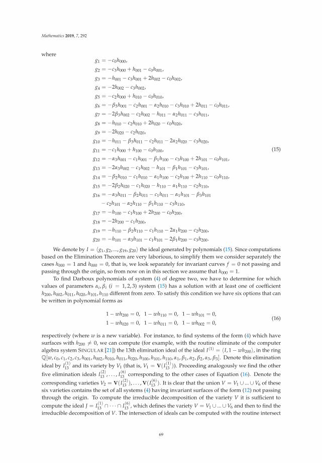
Mathematics 2019, 7, 292
whereg1 = −c0h000,
g2 = −c3h000 + h001 − c0h001,
g3 = −h001 − c3h001 + 2h002 − c0h002,
g4 = −2h002 − c3h002,
g5 = −c2h000 + h010 − c0h010,
g6 = −β3h001 − c2h001 − α2h010 − c3h010 + 2h011 − c0h011,
g7 = −2β3h002 − c2h002 − h011 − α2h011 − c3h011,
g8 = −h010 − c2h010 + 2h020 − c0h020,
g9 = −2h020 − c2h020,
g10 = −h011 − β3h011 − c2h011 − 2α2h020 − c3h020,
g11 = −c1h000 + h100 − c0h100,
g12 = −α3h001 − c1h001 − β1h100 − c3h100 + 2h101 − c0h101,
g13 = −2α3h002 − c1h002 − h101 − β1h101 − c3h101,
g14 = −β2h010 − c1h010 − α1h100 − c2h100 + 2h110 − c0h110,
g15 = −2β2h020 − c1h020 − h110 − α1h110 − c2h110,
g16 = −α3h011 − β2h011 − c1h011 − α1h101 − β3h101
− c2h101 − α2h110 − β1h110 − c3h110,
g17 = −h100 − c1h100 + 2h200 − c0h200,
g18 = −2h200 − c1h200,
g19 = −h110 − β2h110 − c1h110 − 2α1h200 − c2h200,
g20 = −h101 − α3h101 − c1h101 − 2β1h200 − c3h200.
(15)
We denote by I = 〈g1, g2, ..., g19, g20〉 the ideal generated by polynomials (15). Since computationsbased on the Elimination Theorem are very laborious, to simplify them we consider separately thecases h000 = 1 and h000 = 0, that is, we look separately for invariant curves f = 0 not passing andpassing through the origin, so from now on in this section we assume that h000 = 1.
To find Darboux polynomials of system (4) of degree two, we have to determine for whichvalues of parameters αi, βi (i = 1, 2, 3) system (15) has a solution with at least one of coefficienth200, h002, h011, h020, h101, h110 different from zero. To satisfy this condition we have six options that canbe written in polynomial forms as
1− wh200 = 0, 1− wh110 = 0, 1− wh101 = 0,
1− wh020 = 0, 1− wh011 = 0, 1− wh002 = 0,(16)
respectively (where w is a new variable). For instance, to find systems of the form (4) which havesurfaces with h200 �= 0, we can compute (for example, with the routine eliminate of the computeralgebra system SINGULAR [21]) the 13th elimination ideal of the ideal I(1) = 〈I, 1− wh200〉, in the ringQ[w, c0, c1, c2, c3, h001, h002, h010, h011, h020, h100, h101, h110, α1, β1, α2, β2, α3, β3]. Denote this eliminationideal by I(1)13 and its variety by V1 (that is, V1 = V(I(1)13 )). Proceeding analogously we find the other
five elimination ideals I(2)13 , . . . , I(6)13 corresponding to the other cases of Equation (16). Denote the
corresponding varieties V2 = V(I(2)13 ), . . . , V(I(6)13 ). It is clear that the union V = V1 ∪ ...∪V6 of thesesix varieties contains the set of all systems (4) having invariant surfaces of the form (12) not passingthrough the origin. To compute the irreducible decomposition of the variety V it is sufficient tocompute the ideal J = I(1)13 ∩ · · · ∩ I(6)13 , which defines the variety V = V1 ∪ ...∪V6 and then to find theirreducible decomposition of V. The intersection of ideals can be computed with the routine intersect
69
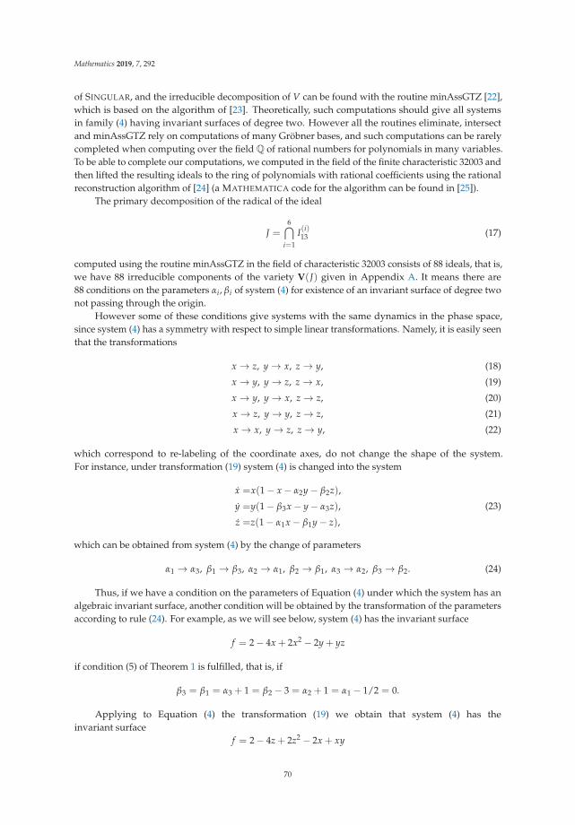
Mathematics 2019, 7, 292
of SINGULAR, and the irreducible decomposition of V can be found with the routine minAssGTZ [22],which is based on the algorithm of [23]. Theoretically, such computations should give all systemsin family (4) having invariant surfaces of degree two. However all the routines eliminate, intersectand minAssGTZ rely on computations of many Gröbner bases, and such computations can be rarelycompleted when computing over the field Q of rational numbers for polynomials in many variables.To be able to complete our computations, we computed in the field of the finite characteristic 32003 andthen lifted the resulting ideals to the ring of polynomials with rational coefficients using the rationalreconstruction algorithm of [24] (a MATHEMATICA code for the algorithm can be found in [25]).
The primary decomposition of the radical of the ideal
J =6⋂
i=1
I(i)13 (17)
computed using the routine minAssGTZ in the field of characteristic 32003 consists of 88 ideals, that is,we have 88 irreducible components of the variety V(J) given in Appendix A. It means there are88 conditions on the parameters αi, βi of system (4) for existence of an invariant surface of degree twonot passing through the origin.
However some of these conditions give systems with the same dynamics in the phase space,since system (4) has a symmetry with respect to simple linear transformations. Namely, it is easily seenthat the transformations
x → z, y → x, z → y, (18)
x → y, y → z, z → x, (19)
x → y, y → x, z → z, (20)
x → z, y → y, z → z, (21)
x → x, y → z, z → y, (22)
which correspond to re-labeling of the coordinate axes, do not change the shape of the system.For instance, under transformation (19) system (4) is changed into the system
x =x(1− x− α2y− β2z),
y =y(1− β3x− y− α3z),
z =z(1− α1x− β1y− z),
(23)
which can be obtained from system (4) by the change of parameters
α1 → α3, β1 → β3, α2 → α1, β2 → β1, α3 → α2, β3 → β2. (24)
Thus, if we have a condition on the parameters of Equation (4) under which the system has analgebraic invariant surface, another condition will be obtained by the transformation of the parametersaccording to rule (24). For example, as we will see below, system (4) has the invariant surface
f = 2− 4x + 2x2 − 2y + yz
if condition (5) of Theorem 1 is fulfilled, that is, if
β3 = β1 = α3 + 1 = β2 − 3 = α2 + 1 = α1 − 1/2 = 0.
Applying to Equation (4) the transformation (19) we obtain that system (4) has theinvariant surface
f = 2− 4z + 2z2 − 2x + xy
70
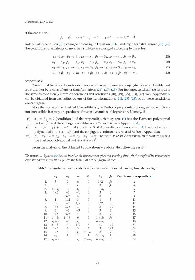
Mathematics 2019, 7, 292
if the conditionβ2 = β3 = α2 + 1 = β1 − 3 = α1 + 1 = α3 − 1/2 = 0
holds, that is, condition (3) is changed according to Equation (24). Similarly, after substitutions (20)–(22)the conditions for existence of invariant surfaces are changed according to the rules
α1 → α2, β1 → β2, α2 → α3, β2 → β3, α3 → α1, β3 → β1, (25)
α1 → β2, β1 → α2, α2 → β1, β2 → α1, α3 → β3, β3 → α3, (26)
α1 → β3, β1 → α3, α2 → β2, β2 → α2, α3 → β1, β3 → α1, (27)
α1 → β1, β1 → α1, α2 → β3, β2 → α3, α3 → β2, β3 → α2, (28)
respectively.We say, that two conditions for existence of invariant planes are conjugate if one can be obtained
from another by means of one of transformations (24), (25)–(28). For instance, condition (3) (which isthe same as condition (7) from Appendix A) and conditions (10), (19), (25), (33), (47) from Appendix Acan be obtained from each other by one of the transformations (24), (25)–(28), so all these conditionsare conjugate.
Note that some of the obtained 88 conditions give Darboux polynomials of degree two which arenot irreducible, but they are products of two polynomials of degree one. Namely, if
(i) α1 = β1 = 0 (condition 1 of the Appendix), then system (4) has the Darboux polynomial(−1 + x)2 (and the conjugate conditions are 22 and 36 from Appendix A);
(ii) α2 = β1 = β2 + α1 − 2 = 0 (condition 5 of Appendix A), then system (4) has the Darbouxpolynomial (−1 + x + z)2 (and the conjugate conditions are 44 and 78 from Appendix);
(iii) β1 + α3 − 2 = β2 + α1 − 2 = β3 + α2 − 2 = 0 (condition 88 of Appendix), then system (4) hasthe Darboux polynomial (−1 + x + y + z)2.
From the analysis of the obtained 88 conditions we obtain the following result.
Theorem 1. System (4) has an irreducible invariant surface not passing through the origin if its parametershave the values given in the following Table 1 or are conjugate to them.
Table 1. Parameter values for systems with invariant surfaces not passing through the origin.
α1 α2 α3 β1 β2 β3 Condition in Appendix A
1. 3 0 α3 0 1/2 β3 22. 3 0 α3 0 3 β3 43. 1 + α3 −1 α3 0 1− α3 0 64. 1/2 −1 −1 0 3 0 75. −1 3/2 3 0 3 0 86. 1 1/2 3 0 1 3 117. 3 −1 1/2 0 1/2 3 128. 1/2 3/2 3 0 3 1/2 149. 3 −1 −3 0 3 3 1510. 1/2 3/2 2 0 3 1/2 1611. 1− β3 2− β3 0 0 1 + β3 β3 1712. α3 − 2 −1 α3 0 4− α3 3 1813. 2− β2 3 1/2 3 β2 1/2 5314. 1/2 3 3 3 3 1/2 5415. 1/2 3 α3 2− α3 3 1/2 5516. α1 3 3 3 2− α1 3 6517. α3 − 2 3 α3 2− α3 4− α3 3 67
71

Mathematics 2019, 7, 292
Remark 1. For instance, the first row of the table means that the parameters α3 and β3 can be chosen arbitrary,the other parameters satisfy the condition
α1 = 3, α2 = β1 = 0, β2 =12
,
and this is condition 2 from Appendix A.
Proof of Theorem 1. For each case of the theorem we give below the irreducible Darboux polynomialf of degree two which defines the invariant quadratic invariant surface f = 0 not passing through theorigin and the corresponding cofactor:
1. f = 1− x− 2y + y2; K = −x− 2y;2. f = 1− 2x + x2 − 2y− 2xy + y2; K = −2(x + y);3. f = 2− 2x− 2y + yz; K = −x− y;4. f = 2− 4x + 2x2 − 2y + yz; K = −2x− y;5. f = 2− 4x + 2x2 + 2xy− 2z + xz; K = −2x− z;6. f = 2− 4x + 2x2 − 4y + 4xy + 2y2 − 2z + xz; K = −2x− 2y− z;7. f = 1− x− 2y + y2 + yz; K = −x− 2y;8. f = 2− 4x + 2x2 − 2y− 2z + xz; K = −2x− y− z;9. f = 1− 2x + x2 − 2y− 2xy + y2 + yz; K = −2(x + y);
10. f = 1− 2x + x2 − y− z + xz; K = −2x− y− z;11. f = 1− x− y− z + xz; K = −x− y− z;12. f = 1− 2x + x2 − 2y + 2xy + y2 + yz; K = −2(x + y);13. f = 1− x− y− 2z + z2; K = −x− y− 2z;14. f = 1− 2x + x2 − y− 2z− 2xz + z2; K = −2x− y− 2z;15. f = 1− 2x + x2 − y− 2z + 2xz + z2; K = −2x− y− 2z;16. f = 1− 2x + x2 − 2y + 2xy + y2 − 2z− 2xz− 2yz + z2; K = −2(x + y + z);17. f = 1− 2x + x2 − 2y + 2xy + y2 − 2z + 2xz− 2yz + z2; K = −2(x + y + z).
4. First Integrals of System (4)
In this section we look for Darboux first integrals of the system (4), which can be constructedusing the invariant surfaces obtained in the previous section.
Theorem 2. (a) If one of conditions 1–3, 11, 12, 17 of Theorem 1 holds, then the corresponding system (4)admits at least one Darboux first integral. (b) If one of conditions 4–10, 13–16 of Theorem 1 holds, then thecorresponding system (4) is completely integrable, that is, it admits two independents Darboux first integrals.
Proof. First note that system (4) always has the following three invariant surfaces of degree one,with the respective cofactors,
f1 = x; K1 = 1− x− α1y− β1z;
f2 = y; K2 = 1− β2x− y− α2z;
f3 = z; K3 = 1− α3x− β3y− z.
(29)
However, in most cases it is impossible to construct Darboux first integrals using just theseinvariant planes and the surfaces given by Theorem 1. To find the integrals we additionally lookfor invariant surfaces of the form (12) with h000 = 0 using the procedure described at the beginningof Section 3. For each considered case we have to solve system (15) with h000 = 0 and parametersαi, βi (i = 1, 2, 3) given by Theorem 1. Since some parameters are fixed the corresponding systems (15)are easily solved with MATHEMATICA (no need for computations with SINGULAR now).
Case (a). To prove statement (a) of the theorem, we present the Darboux first integrals for eachcase mentioned in the statement.
72
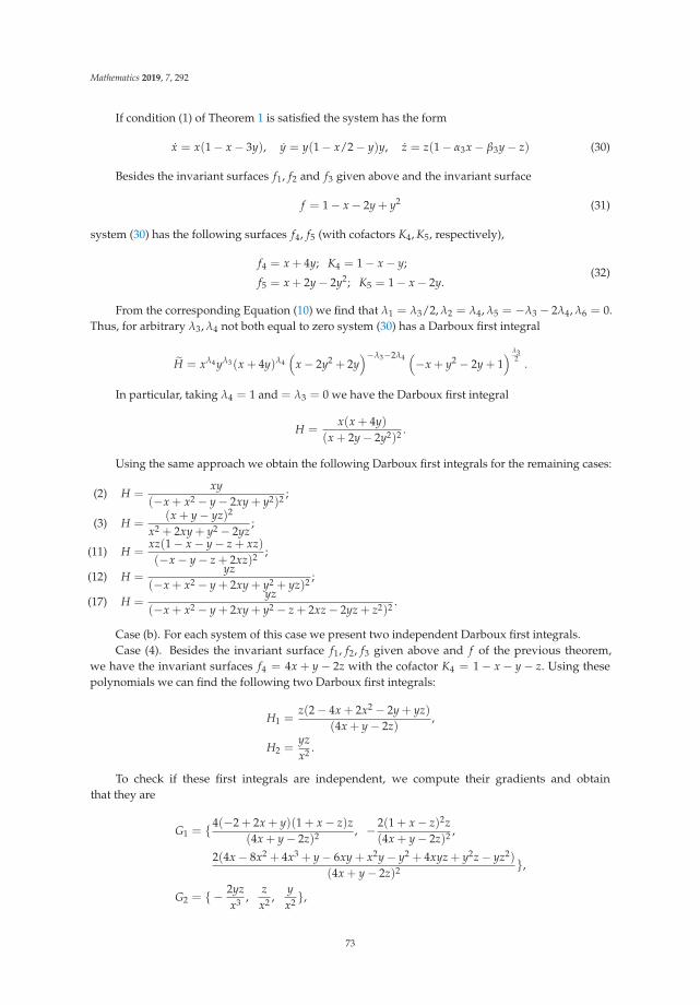
Mathematics 2019, 7, 292
If condition (1) of Theorem 1 is satisfied the system has the form
x = x(1− x− 3y), y = y(1− x/2− y)y, z = z(1− α3x− β3y− z) (30)
Besides the invariant surfaces f1, f2 and f3 given above and the invariant surface
f = 1− x− 2y + y2 (31)
system (30) has the following surfaces f4, f5 (with cofactors K4, K5, respectively),
f4 = x + 4y; K4 = 1− x− y;
f5 = x + 2y− 2y2; K5 = 1− x− 2y.(32)
From the corresponding Equation (10) we find that λ1 = λ3/2, λ2 = λ4, λ5 = −λ3 − 2λ4, λ6 = 0.Thus, for arbitrary λ3, λ4 not both equal to zero system (30) has a Darboux first integral
H = xλ4 yλ3(x + 4y)λ4(
x− 2y2 + 2y)−λ3−2λ4
(−x + y2 − 2y + 1
) λ32 .
In particular, taking λ4 = 1 and = λ3 = 0 we have the Darboux first integral
H =x(x + 4y)
(x + 2y− 2y2)2 .
Using the same approach we obtain the following Darboux first integrals for the remaining cases:
(2) H =xy
(−x + x2 − y− 2xy + y2)2 ;
(3) H =(x + y− yz)2
x2 + 2xy + y2 − 2yz;
(11) H =xz(1− x− y− z + xz)(−x− y− z + 2xz)2 ;
(12) H =yz
(−x + x2 − y + 2xy + y2 + yz)2 ;
(17) H =yz
(−x + x2 − y + 2xy + y2 − z + 2xz− 2yz + z2)2 .
Case (b). For each system of this case we present two independent Darboux first integrals.Case (4). Besides the invariant surface f1, f2, f3 given above and f of the previous theorem,
we have the invariant surfaces f4 = 4x + y− 2z with the cofactor K4 = 1− x − y− z. Using thesepolynomials we can find the following two Darboux first integrals:
H1 =z(2− 4x + 2x2 − 2y + yz)
(4x + y− 2z),
H2 =yzx2 .
To check if these first integrals are independent, we compute their gradients and obtainthat they are
G1 = {4(−2 + 2x + y)(1 + x− z)z(4x + y− 2z)2 , − 2(1 + x− z)2z
(4x + y− 2z)2 ,
2(4x− 8x2 + 4x3 + y− 6xy + x2y− y2 + 4xyz + y2z− yz2)
(4x + y− 2z)2 },
G2 = { − 2yzx3 ,
zx2 ,
yx2 },
73
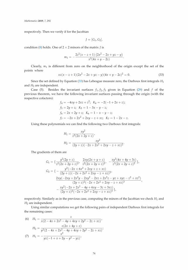
Mathematics 2019, 7, 292
respectively. Then we verify if for the Jacobian
J = [G1, G2].
condition (8) holds. One of 2× 2 minors of the matrix J is
m1 = −2z2(x− z + 1)(2x2 − 2x + yz− y
)x3(4x + y− 2z)
.
Clearly, m1 is different from zero on the neighborhood of the origin except the set of thepoints where
xz(x− z + 1)(2x2 − 2x + yz− y)(4x + y− 2z)2 = 0. (33)
Since the set defined by Equation (33) has Lebesgue measure zero, the Darboux first integrals H1
and H2 are independent.Case (5). Besides the invariant surfaces f1, f2, f3 given in Equation (29) and f of the
previous theorem, we have the following invariant surfaces passing through the origin (with therespective cofactors):
f4 = −4xy + 2xz + z2; K4 = −2(−1 + 2x + z);
f5 = 2y + z; K5 = 1− 3x− y− z;
f6 = 2x + 2y + z; K6 = 1− x− y− z;
f7 = −2x + 2x2 + 2xy− z + xz; K7 = 1− 2x− z.
Using these polynomials we can find the following two Darboux first integrals:
H1 =xy2
z2(2x + 2y + z),
H2 =xy2
(2y + z)(−2x + 2x2 + 2xy− z + xz)2 .
The gradients of them are
G1 = { y2(2y + z)z2(2x + 2y + z)2 ,
2xy(2x + y + z)z2(2x + 2y + z)2 , − xy2(4x + 4y + 3z)
z3(2x + 2y + z)2 },
G2 = { − y2(−2x + 6x2 + 2xy + z + xz)(2y + z)(−2x + 2x2 + 2xy− z + xz)3 ,
2xy(−2xy + 2x2y− 2xy2 − 2xz + 2x2z− yz + xyz− z2 + xz2)
(2y + z)2(−2x + 2x2 + 2xy− z + xz)3 ,
− xy2(−2x + 2x2 − 4y + 6xy− 3z + 3xz)(2y + z)2(−2x + 2x2 + 2xy− z + xz)3 },
respectively. Similarly as in the previous case, computing the minors of the Jacobian we check H1 andH2 are independent.
Using similar computations we get the following pairs of independent Darboux first integrals forthe remaining cases:
(6) H1 =z
x(2− 4x + 2x2 − 4y + 4xy + 2y2 − 2z + xz),
H2 =z(2x + 4y + z)
y2(2− 4x + 2x2 − 4y + 4xy + 2y2 − 2z + xz);
(7) H1 = − x2
yz(−1 + x + 2y− y2 − yz),
74

Mathematics 2019, 7, 292
H2 = − (x− 2z)2
z(y + z)(−1 + x + 2y− y2 − yz);
(8) H1 =xz(2− 4x + 2x2 − 2y− 2z + xz)
(y + z)2 ,
H2 =(2x + z)(y + z)2
xy2 ;
(9) H1 =yz(1− 2x + x2 − 2y− 2xy + y2 + yz)
x2 ,
H2 =y2z(4x− z)
x2(x2 − 2xy + y2 + yz);
(10) H1 = − x(y− z + xz + z2)
z(−2x + 2x2 − y− z + 2xz),
H2 =y2(x + z)
z(2x− 2x2 + y + z− 2xz)(y− z + xz + z2);
(13) H1 =(−x− y− 2z + 2z2)2
z2(1− x− y− 2z + z2),
H2 =xz2α1−2(x + y + 4z)2−2α1
y;
(14) H1 =(−2x + 2x2 − y− 2z− 4xz + 2z2)2
(x− z)2(1− 2x + x2 − y− 2z− 2xz + z2),
H2 =x(y + 4z)2(−2x + 2x2 − y− 2z− 4xz + 2z2)2
z(x− z)4(1− 2x + x2 − y− 2z− 2xz + z2)2 ;
(15) H1 =y(4x + y + 4z)
(2x− 2x2 + y + 2z− 4xz− 2z2)2 ,
H2 =x(4x + y + 4z)1−α3(−2x + 2x2 − y− 2z + 4xz + 2z2)1+α3
z(x + z)2(1− 2x + x2 − y− 2z + 2xz + z2);
(16) H1 =(x + y)z
(−x + x2 − y + 2xy + y2 − z− 2xz− 2yz + z2)2 ,
H2 =1y4 x4z2−2α1(1− 2x + x2 − 2y + 2xy + y2 − 2z− 2xz− 2yz + z2)1−α1
(−x + x2 − y + 2xy + y2 − z− 2xz− 2yz + z2)2α1−2.
Remark 2. Note that first two equations of (30) are independent of z, they are,
x = x(1− x− 3y), y = y(1− x/2− y)y. (34)
Therefore we cannot construct another independent first integral H2(x, y, z) of Equation (30) using only theplanes x = 0, y = 0, z = 0 and the surfaces defined by Equations (31) and (32). Indeed, since the equations of allsurfaces of this case, except of z = 0, are independent on z, if such integral would exist, it would be independent of z,but then two-dimensional system (34) would have two independent first integrals, which is impossible.
In case (2), similarly as in case (1), the system is separable into a two-dimensional system and a single firstorder equation, and we can construct only one Darboux first integral using the found invariant surfaces.
5. Conclusions
To summarize, we have found some Darboux first integrals of the May–Leonard system (4) whichare constructed using Darboux polynomials of degree one and two. We do not know if we foundall independent first integrals of system (4) which can be constructed from Darboux polynomialsof degree one and two. To verify if the list is complete, we have to find Darboux polynomials ofEquation (4), which define invariant algebraic surfaces passing through the origin, that is, polynomials(12) with h000 = 0. A naïve expectation is that this case should be simpler, than the case h000 = 1,
75
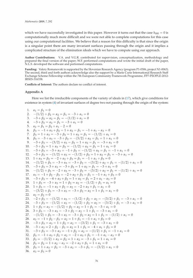
Mathematics 2019, 7, 292
which we have successfully investigated in this paper. However it turns out that the case h000 = 0 iscomputationally much more difficult and we were not able to complete computations for this caseusing our computational facilities. We believe that a reason for this difficulty is that since the originis a singular point there are many invariant surfaces passing through the origin and it implies acomplicated structure of the elimination ideals which we have to compute using our approach.
Author Contributions: V.A. and V.G.R. contributed for supervision, conceptualization, methodology andprepared the final version of the paper; W.F. performed computations and wrote the initial draft of the paper,N.L.S. developed the software and performed computations.
Funding: Valery Romanovski is supported by the Slovenian Research Agency (program P1-0306, project N1-0063).The second, third and forth authors acknowledge also the support by a Marie Curie International Research StaffExchange Scheme Fellowship within the 7th European Community Framework Programme, FP7-PEOPLE-2012-IRSES-316338.
Conflicts of Interest: The authors declare no conflict of interest.
Appendix A
Here we list the irreducible components of the variety of ideals in (17), which give conditions forexistence in system (4) of invariant surfaces of degree two not passing through the origin of the system:
1. α1 = β1 = 02. −(1/2) + β2 = α2 = β1 = −3 + α1 = 03. −3 + β2 = α2 = β1 = −(1/2) + α1 = 04. −3 + β2 = α2 = β1 = −3 + α1 = 05. α2 = β1 = β2 + α1 − 2 = 06. β3 = −1 + α3 + β2 = 1 + α2 = β1 = −1 + α1 − α3 = 07. β3 = 1 + α3 = −3 + β2 = 1 + α2 = β1 = −(1/2) + α1 = 08. β3 = −3 + α3 = −3 + β2 = −(3/2) + α2 = β1 = 1 + α1 = 09. −3 + β3 = −(3/2) + α3 = β2 = 1 + α2 = β1 = −3 + α1 = 0
10. −3 + β3 = 1 + α3 = β2 = −(1/2) + α2 = β1 = 1 + α1 = 011. −3 + β3 = −3 + α3 = −1 + β2 = −(1/2) + α2 = β1 = −1 + α1 = 012. −3 + β3 = −(1/2) + α3 = −(1/2) + β2 = 1 + α2 = β1 = −3 + α1 = 013. 1 + α3 = β2 = −2 + α2 + β3 = β1 = −1 + α1 + β3 = 014. −(1/2) + β3 = −3 + α3 = −3 + β2 = −(3/2) + α2 = β1 = −(1/2) + α1 = 015. −3 + β3 = 3 + α3 = −3 + β2 = 1 + α2 = β1 = −3 + α1 = 016. −(1/2) + β3 = −2 + α3 = −3 + β2 = −(3/2) + α2 = β1 = −(1/2) + α1 = 017. α3 = −1 + β2 − β3 = −2 + α2 + β3 = β1 = −1 + α1 + β3 = 018. −3 + β3 = −4 + α3 + β2 = 1 + α2 = β1 = 2 + α1 − α3 = 019. 1 + β3 = −3 + α3 = 1 + β2 = α2 = −(1/2) + β1 = α1 = 020. 1 + β3 = −1 + α3 + β2 = α2 = −2 + α3 + β1 = α1 = 021. −(3/2) + β3 = −3 + α3 = −3 + β2 = α2 = 1 + β1 = α1 = 022. α2 = β2 = 023. −2 + β3 = −(1/2) + α3 = −(1/2) + β2 = α2 = −(3/2) + β1 = −3 + α1 = 024. −3 + β3 = −(1/2) + α3 = −(1/2) + β2 = α2 = −(3/2) + β1 = −3 + α1 = 025. 1 + β3 = α3 = −(1/2) + β2 = α2 = 1 + β1 = −3 + α1 = 026. 3 + β3 = −3 + α3 = −3 + β2 = α2 = 1 + β1 = −3 + α1 = 027. −(1/2) + β3 = −3 + α3 = −3 + β2 = α2 = 1 + β1 = −(1/2) + α1 = 028. α3 = −1 + β2 − β3 = α2 = 1 + β1 = −1 + α1 + β3 = 029. −3 + β3 = α3 = 1 + β2 = α2 = −(3/2) + β1 = −3 + α1 = 030. −3 + α3 = 2 + β2 − β3 = α2 = 1 + β1 = −4 + α1 + β3 = 031. −3 + β3 = −3 + α3 = −1 + β2 = α2 = −(1/2) + β1 = −1 + α1 = 032. β3 = −1 + α3 + β2 = α2 = −2 + α3 + β1 = −1 + α1 − α3 = 033. β3 = −(1/2) + α3 = β2 = 1 + α2 = −3 + β1 = 1 + α1 = 034. β3 = β2 = 1 + α2 − α3 = −2 + α3 + β1 = 1 + α1 = 035. β3 = 1 + α3 = β2 = −3 + α2 = −3 + β1 = −(3/2) + α1 = 036. α3 = β3 = 0
76
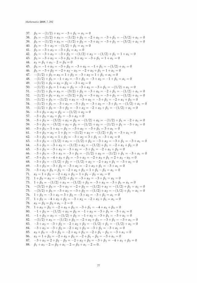
Mathematics 2019, 7, 292
37. β3 = −(1/2) + α3 = −3 + β1 = α1 = 038. β3 = −(1/2) + α3 = −(1/2) + β2 = −2 + α2 = −3 + β1 = −(3/2) + α1 = 039. β3 = −(1/2) + α3 = −(1/2) + β2 = −3 + α2 = −3 + β1 = −(3/2) + α1 = 040. β3 = −3 + α3 = −(1/2) + β1 = α1 = 041. β3 = −3 + α3 = −3 + β1 = α1 = 042. β3 = −3 + α3 = −3 + β2 = −(1/2) + α2 = −(1/2) + β1 = 1 + α1 = 043. β3 = −3 + α3 = −3 + β2 = 3 + α2 = −3 + β1 = 1 + α1 = 044. α1 = β1 + α3 − 2 = β3 = 045. β3 = −1 + α3 = −3 + β2 = −3 + α2 = −1 + β1 = −(1/2) + α1 = 046. β3 = −3 + β2 = −2 + α2 − α3 = −2 + α3 + β1 = 1 + α1 = 047. −(1/2) + β3 = α3 = 1 + β2 = −3 + α2 = 1 + β1 = α1 = 048. −(1/2) + β3 = −1 + α3 = −3 + β2 = −3 + α2 = −1 + β1 = α1 = 049. −(1/2) + β3 = α3 = β2 = −3 + α2 = 050. −(1/2) + β3 = 1 + α3 = β2 = −3 + α2 = −3 + β1 = −(1/2) + α1 = 051. −(1/2) + β3 = α3 = −(3/2) + β2 = −3 + α2 = −2 + β1 = −(1/2) + α1 = 052. −(1/2) + β3 = α3 = −(3/2) + β2 = −3 + α2 = −3 + β1 = −(1/2) + α1 = 053. −(1/2) + β3 = −(1/2) + α3 = −3 + α2 = −3 + β1 = −2 + α1 + β2 = 054. −(1/2) + β3 = −3 + α3 = −3 + β2 = −3 + α2 = −3 + β1 = −(1/2) + α1 = 055. −(1/2) + β3 = −3 + β2 = −3 + α2 = −2 + α3 + β1 = −(1/2) + α1 = 056. −3 + β3 = α3 = β2 = −(1/2) + α2 = 057. −3 + β3 = α3 = β2 = −3 + α2 = 058. −3 + β3 = −(3/2) + α3 = β2 = −(1/2) + α2 = −(1/2) + β1 = −2 + α1 = 059. −3 + β3 = −(3/2) + α3 = β2 = −(1/2) + α2 = −(1/2) + β1 = −3 + α1 = 060. −3 + β3 = 1 + α3 = β2 = −3 + α2 = −3 + β1 = 3 + α1 = 061. −3 + β3 = α3 = 1 + β2 = −(1/2) + α2 = −(1/2) + β1 = −3 + α1 = 062. −3 + β3 = α3 = 1 + β2 = −3 + α2 = 3 + β1 = −3 + α1 = 063. −3 + β3 = −(1/2) + α3 = −(1/2) + β2 = −3 + α2 = −3 + β1 = −3 + α1 = 064. −3 + β3 = −3 + α3 = −(1/2) + α2 = −(1/2) + β1 = −2 + α1 + β2 = 065. −3 + β3 = −3 + α3 = −3 + α2 = −3 + β1 = −2 + α1 + β2 = 066. −3 + β3 = −3 + α3 = −3 + β2 = −(1/2) + α2 = −(1/2) + β1 = −3 + α1 = 067. −3 + β3 = −4 + α3 + β2 = −3 + α2 = −2 + α3 + β1 = 2 + α1 − α3 = 068. −3 + β3 = −(1/2) + β2 = −(1/2) + α2 = −2 + α3 + β1 = −3 + α1 = 069. −3 + β3 = −3 + β2 = −3 + α2 = −2 + α3 + β1 = −3 + α1 = 070. −3 + α3 + β3 = β2 = −2 + α2 + β3 = 1 + β1 − β3 = α1 = 071. α3 = 1 + β2 = −2 + α2 + β3 = 1 + β1 − β3 = α1 = 072. 1 + β3 = α3 = −(3/2) + β2 = −3 + α2 = −3 + β1 = α1 = 073. 1 + β3 = −(1/2) + α3 = −(1/2) + β2 = −3 + α2 = −3 + β1 = α1 = 074. −(3/2) + β3 = −3 + α3 = −2 + β2 = −(1/2) + α2 = −(1/2) + β1 = α1 = 075. −(3/2) + β3 = −3 + α3 = −3 + β2 = −(1/2) + α2 = −(1/2) + β1 = α1 = 076. 1 + β3 = −3 + α3 = 3 + β2 = −3 + α2 = −3 + β1 = α1 = 077. 1 + β3 = −4 + α3 + β2 = −3 + α2 = −2 + α3 + β1 = α1 = 078. α3 = β2 = β3 + α1 − 2 = 079. 1 + α3 = β2 = −2 + α2 + β3 = −3 + β1 = −4 + α1 + β3 = 080. −1 + β3 = −(1/2) + α3 = β2 = −1 + α2 = −3 + β1 = −3 + α1 = 081. −1 + β3 = α3 = −(1/2) + β2 = −1 + α2 = −3 + β1 = −3 + α1 = 082. −(1/2) + α3 = −(1/2) + β2 = −2 + α2 + β3 = −3 + β1 = −3 + α1 = 083. −3 + α3 = −3 + β2 = −2 + α2 + β3 = −(1/2) + β1 = −(1/2) + α1 = 084. −3 + α3 = −3 + β2 = −2 + α2 + β3 = −3 + β1 = −3 + α1 = 085. α3 + β3 = −3 + β2 = −2 + α2 + β3 = −2 + β1 − β3 = −3 + α1 = 086. α3 = 1 + β2 = −2 + α2 + β3 = −2 + β1 − β3 = −3 + α1 = 087. −3 + α3 = 2 + β2 − β3 = −2 + α2 + β3 = −3 + β1 = −4 + α1 + β3 = 088. β1 + α3 − 2 = β2 + α1 − 2 = β3 + α1 − 2 = 0.
77
Mathematics 2019, 7, 292
References
1. Lotka, A.J. Analytical note on certain rhythmic relations in organic systems. Proc. Natl. Acad. Sci. USA1920, 6, 410–415. [CrossRef] [PubMed]
2. Volterra, V. Lecons sur la Théorie Mathématique de la Lutte pour la Vie; Gauthier-Villars: Paris, France, 1931.3. May, R.M.; Leonard, W.J. Nonlinear aspects of competition between three species. SIAM J. Appl. Math.
1975, 29, 243–253. [CrossRef]4. Blé, G.; Castellanos, V.; Llibre, J.; Quilantán, I. Integrability and global dynamics of the May–Leonard model.
Nonlinear Anal. Real World Appl. 2013, 14, 280–293. [CrossRef]5. Schuster, P.; Sigmund, K.; Wolf, R. On ω-limit for competition between three species. SIAM J. Appl. Math.
1979, 37, 49–54. [CrossRef]6. Zeeman, M.L. Hopf bifurcations in competitive three dimensional Lotka–Volterra systems. Dyn. Stab. Syst.
1993, 8, 189–216. [CrossRef]7. Antonov, V.; Dolicanin, D.; Romanovski, V.G.; Tóth, J. Invariant planes and periodic oscillations in the
May–Leonard asymmetric model. MATCH Commun. Math. Comput. Chem. 2016, 76, 455–474.8. Chi, C.-W.; Hsu, S.-B.; Wu, L.-I. On the asymmetric May–Leonard model of three competing species. SIAM J.
Appl. Math. 1998, 58, 211–226. [CrossRef]9. Van der Hoff, Q.; Greeff, J.C.; Fay, T.H. Defining a stability boundary for three species competition models.
Ecol. Model. 2009, 220, 2640–2645. [CrossRef]10. Leach, G.L.; Miritzis, J. Analytic behaviour of competition among three species. J. Nonlinear Math. Phys.
2006, 13, 535–548. [CrossRef]11. Llibre, J.; Valls, C. Polynomial, rational and analytic first integrals for a family of 3-dimensional
Lotka–Volterra systems. Z. Angew. Math. Phys. 2011, 62, 761–777. [CrossRef]12. Darboux, G. Mémoire sur les équations différentielles algébriques du premier ordre et du premier degré
(Mélanges). Bull. Sci. Math. 1878, 2, 60–96, 123–144, 151–200.13. Darboux, G. De l’emploi des solutions particulières algébriques dans l’intégration des systèmes d’équations
différentielles algébriques. C. R. Math. Acad. Sci. Paris 1878, 86, 1012–1014.14. Prelle, M.J.; Singer, M.F. Elementary first integrals of differential equations. Trans. Am. Math. Soc.
1983, 279, 613–636. [CrossRef]15. Schlomiuk, D. Algebraic and geometric aspects of the theory of polynomial vector fields. In Bifurcations and
Periodic Orbits of Vector Fields; Schlomiuk, D., Ed.; NATO ASI Series, Series C: Mathematical and PhysicalSciences; Kluwer Academic Publishers: New York, NY, USA, 1993; Volume 408, pp. 429–467.
16. Schlomiuk, D. Elementary first integrals and algebraic invariant curves of differential equations. Expos. Math.1993, 11, 433–454.
17. Llibre, J. On the integrability of the differential systems in dimension two and of the polynomial differentialsystems in arbitrary dimension. J. Appl. Anal. Comput. 2011, 1, 33–52.
18. Llibre, J.; Zhang, X. On the Darboux integrability of polynomial differential systems. Qual. Theory Dyn. Syst.2012, 11, 129–144. [CrossRef]
19. Romanovski, V.G.; Shafer, D.S. The Center and Cyclicity Problems: A Computational Algebra Approach; Birkhäuser:Boston, MA, USA, 2009.
20. Cox, D.; Little, J.; O’Shea, D. Ideals, Varieties, and Algorithms: An Introduction to Computational AlgebraicGeometry and Commutative Algebra; Springer: New York, NY, USA, 1997.
21. Decker, W.; Greuel, G.-M.; Pfister, G.; Shönemann, H. SINGULAR 3-1-6—A Computer Algebra Systemfor Polynomial Computations. 2012. Available online: http://www.singular.uni-kl.de (accessed on15 May 2017).
22. Decker, W.; Pfister, G.; Schönemann, H.; Laplagne, S. A SINGULAR 3.0 Library for Computing the PrimaryDecomposition and Radical of Ideals. 2005. Available online: http://www.singular.uni-kl.de (accessed on15 May 2017).
23. Gianni, P.; Trager, B.; Zacharias, G. Gröbner bases and primary decomposition of polynomials.J. Symb. Comput. 1998, 6, 146–167. [CrossRef]
78

Mathematics 2019, 7, 292
24. Wang, P.S.; Guy, M.J.T.; Davenport, J.H. P-adic reconstruction of rational numbers. SIGSAM Bull. 1982, 16, 2–3.[CrossRef]
25. Giné, J.; Christopher, C.; Prešern, M.; Romanovski, V.G.; Shcheglova, N.L. The resonant center problemfor a 2:−3 resonant cubic Lotka–Volterra system. In Proceedings of the 14th International Workshop onComputer Algebra in Scientific Computing CASC 2012, Maribor, Slovenia, 3–6 September 2012; LectureNotes in Computer Science; Springer: Berlin/Heidelberg, Germany, 2012; Volume 7442, pp. 129–142.
c© 2019 by the authors. Licensee MDPI, Basel, Switzerland. This article is an open accessarticle distributed under the terms and conditions of the Creative Commons Attribution(CC BY) license (http://creativecommons.org/licenses/by/4.0/).
79
mathematics
Article
Dini-Type Helicoidal Hypersurfaces with TimelikeAxis in Minkowski 4-Space E4
1
Erhan Güler * and Ömer Kisi
Department of Mathematics, Faculty of Sciences, Bartın University, 74100 Bartın, Turkey; [email protected]* Correspondence: [email protected]; Tel.: +90-378-5011000-1521
Received: 31 January 2019; Accepted: 13 February 2019; Published: 22 February 2019
Abstract: We consider Ulisse Dini-type helicoidal hypersurfaces with timelike axis in Minkowski4-space E4
1. Calculating the Gaussian and the mean curvatures of the hypersurfaces, we demonstratesome special symmetries for the curvatures when they are flat and minimal.
Keywords: Minkowski 4-space; Dini-type helicoidal hypersurface; Gauss map; timelike axis
1. Introduction
The concept of finite-type immersion of submanifolds of a Euclidean space has been known inclassifying and characterizing Riemannian submanifolds [1]. Chen proposed the problem of classifyingthese kinds surfaces in the three-dimensional Euclidean space E3. A Euclidean submanifold is calledChen finite-type if its coordinate functions are a finite sum of eigenfunctions of its Laplacian Δ [1].Hence, the idea of finite-type can be enlarged to any smooth functions on a submanifold of Euclideanor pseudo-Euclidean spaces.
Takahashi [2] obtained spheres and the minimal surfaces are the unique surfaces in E3 satisfyingthe condition Δr = λr, where r is the position vector, λ ∈ R. Ferrandez, Garay and Lucas [3] showedthe surfaces of E3 providing ΔH = AH. Here H is the mean curvature and A ∈ Mat(3, 3) are eitherof a right circular cylinder, or of an open piece of sphere, or minimal. Choi and Kim [4] worked theminimal helicoid with pointwise 1-type Gauss map of the first type.
Dillen, Pas, and Verstraelen [5] studied the unique surfaces in E3 providing Δr = Ar + B,A ∈ Mat(3, 3), B ∈ Mat(3, 1) are the spheres, the circular cylinder, the minimal surfaces. Senoussi andBekkar [6] obtained helicoidal surfaces in E3 by using the fundamental forms I, I I and I I I.
In classical surface geometry, it is well known a pair of the right helicoid and the catenoid isthe unique ruled and rotational surface, which is minimal. When we look at ruled (i.e., helicoid)and rotational surfaces, we meet Bour’s theorem in [7]. By using a result of Bour [7], Do Carmo andDajczer [8] worked isometric helicoidal surfaces.
Lawson [9] defined the generalized Laplace-Beltrami operator. Magid, Scharlach andVrancken [10] studied the affine umbilical surfaces in 4-space. Vlachos [11] introduced hypersurfaceswith harmonic mean curvature in E4. Scharlach [12] gave the affine geometry of surfaces andhypersurfaces in 4-space. Cheng and Wan [13] studied complete hypersurfaces of 4-space with CMC.Arslan, Deszcz and Yaprak [14] obtained Weyl pseudosymmetric hypersurfaces. Arvanitoyeorgos,Kaimakamais and Magid [15] wrote that if the mean curvature vector field of M3
1 satisfies the equationΔH = αH (α a constant), then M3
1 has constant mean curvature in Minkowski 4-space E41. This equation
is a natural generalization of the biharmonic submanifold equation ΔH = 0.General rotational surfaces in the four-dimensional Euclidean space were originated by
Moore [16,17]. Ganchev and Milousheva [18] considered the analogue of these surfaces in E41.
Verstraelen, Valrave, and Yaprak [19] studied the minimal translation surfaces in En for arbitrarydimension n. Kim and Turgay [20] studied surfaces with L1-pointwise 1-type Gauss map in E4. Moruz
Mathematics 2019, 7, 205; doi:10.3390/math7020205 www.mdpi.com/journal/mathematics80
Mathematics 2019, 7, 205
and Munteanu [21] considered hypersurfaces defined as the sum of a curve and a surface whose meancurvature vanishes in E4.
Yoon [22] considered rotational surfaces which has a finite-type Gauss map in E4. Dursun [23]introduced hypersurfaces of pointwise 1-type Gauss map in Minkowski space. Dursun and Turgay [24]studied minimal, pseudo-umbilical rotational surfaces in E4. Arslan, Bulca and Milousheva [25]focused pointwise 1-type Gauss map of meridian surfaces in E4. Aksoyak and Yaylı [26] workedboost-invariant surfaces with pointwise 1-type Gauss map in E4
1. Also they [27] considered generalizedrotational surfaces of pointwise 1-type Gauss map in E4
2. Güler, Magid and Yaylı [28] defined helicoidalhypersurface with the Laplace-Beltrami operator in E4. Furthermore, Güler, Hacısalihoglu and Kim [29]worked rotational hypersurface with the III Laplace-Beltrami operator and the Gauss map in E4.
There are few works in the literature about Italian Mathematician Ulisse Dini’s helicoidalsurface [30] in E3. Moreover, Güler and Kisi [31] introduced helicoidal hypersurfaces of Dini-type withspacelike axis in E4
1.In this paper, we study the Ulisse Dini-type helicoidal hypersurface with timelike axis in
Minkowski 4-space E41. We give some basic notions of Minkowskian geometry, and define helicoidal
hypersurface in Section 2. Moreover, we obtain the Dini-type helicoidal hypersurface timelike axis,and calculate its curvatures in the Section 3. We obtain some special symmetries in the last section.
2. Preliminaries
In this section, we will describe the notation that will be used in the paper, after we give somebasic facts and basic definitions.
Let Em1 be the Minkowski m-space with the Euclidean metric denoted by
g = 〈 , 〉 =m−1
∑i=1
dx2i − dx2
m,
where (x1, x2, . . . , xm) is a coordinate system in Em1 .
Consider an n-dimensional Minkowskian submanifold of the space Em1 . We denote Levi-Civita
connections of Em1 and M by ∇ and ∇, respectively. We will use letters X, Y, Z, W (resp., ξ, η) to
show vector fields tangent (resp., normal) to M. The Gauss and the Weingarten formulas are definedby as follows:
∇XY = ∇XY + h(X, Y),
∇Xξ = −Aξ(X) + DXξ,
where h, D, and A are the second fundamental form, the normal connection and the shape operator ofM, respectively.
The shape operator Aξ is a symmetric endomorphism of the tangent space Tp M at p ∈ M for eachξ ∈ T⊥p M. The second fundamental form and the shape operator are connected by
〈h(X, Y), ξ〉 = ⟨Aξ X, Y⟩
.
The Gauss and Codazzi equations are denoted, respectively, as follows:
〈R(X, Y, )Z, W〉 = 〈h(Y, Z), h(X, W)〉 − 〈h(X, Z), h(Y, W)〉, (1)
(∇Xh)(Y, Z) = (∇Yh)(X, Z). (2)
Here, R, RD are the curvature tensors related with connections ∇ and D, respectively, and ∇h isdefined by
(∇Xh)(Y, Z) = DXh(Y, Z)− h(∇XY, Z)− h(Y,∇XZ).
81

Mathematics 2019, 7, 205
2.1. Hypersurfaces of Minkowski Space
Assume that M be an oriented hypersurface in Minkowski space En1 , S its shape operator and
x its position vector. We think about a local orthonormal frame field {e1, e2, . . . , en} occurring of theprincipal directions of M matching to the principal curvatures ki for i = 1, 2, . . . n. Let {θ1, θ2, . . . , θ} bedual basis of this frame field. Then the first structural equation of Cartan is
dθi =n
∑i=1
θj ∧ωij, i = 1, 2, . . . , n.
Here, ωij demonstrates the connection forms matching to the chosen frame field. We show theLevi-Civita connection of M and En
1 by ∇ and ∇, respectively. Then, from the Codazzi Equation (2)we have
ei(kj) = ωij(ej)(ki − kj),
ωij(el)(ki − kj) = ωil(ej)(ki − kl)
for distinct i, j, l = 1, 2, . . . , n.We take sj = σj(k1, k2, . . . , kn), where σj is the j-th elementary symmetric function given by
σj(a1, a2, . . . , an) = ∑1≤i1<i2<...,ij≤n
ai1 ai2 . . . aij .
We also use the following notation
rji = σj(k1, k2, . . . , ki−1, ki+1, ki+2, . . . , kn).
By definition, we have r0i = 1 and sn+1 = sn+2 = · · · = 0.
On the other hand, we will call the function sk as the k-th mean curvature of M. We would like tonote that functions H = 1
n s1 and K = sn are called the mean and the Gauss-Kronecker curvatures ofM, respectively. Particularly, M is called j-minimal if sj ≡ 0 on M.
2.2. Helicoidal Hypersurfaces with Timelike Axis in Minkowskian Spaces
In this subsection, we will obtain the helicoidal hypersurfaces with timelike axis in Minkowski4-space E4
1. In the rest of this paper, we will identify a vector (a,b,c,d) with its transpose.Before we proceed, we would like to note that the definition of rotational hypersurfaces in
Riemannian space forms were defined in [32]. A rotational hypersurface M ⊂ En1 generated by a curve
C about an axis r does not meet C is generated by using the orbit of C under those orthogonaltransformations of En
1 which leave r pointwise fixed (See [32] remark 2.3).A curve C rotates about the axis r, and at the same time replaces parallel lines orthogonal to the
axis r, so that the speed of replacement is proportional to the speed of rotation. Finally, the resultinghypersurface is called the helicoidal hypersurface with axis r.
Consider the particular case n = 4 and let C be the curve parametrized by
γ(u) = ( f (u) , 0, 0, ϕ(u)) ,
where f and ϕ are differentiable functions. If r is the timelike vector (0, 0, 0, 1), then an orthogonaltransformation of E4
1 that leaves r pointwise fixed has the form Z(v, w) as follows:
82

Mathematics 2019, 7, 205
Z(v, w) =
⎛⎜⎜⎜⎝cos v cos w − sin v − cos v sin w 0cos w sin v cos v − sin v sin w 0
sin w 0 cos w 00 0 0 1
⎞⎟⎟⎟⎠ ,
and the following relations hold:
ZTεZ = ZεZT = ε, ZrT= rT , det Z = 1, ε = diag (1, 1, 1,−1) ,
v, w ∈ R. Therefore, the parametrization of the rotational hypersurface obtained by a curve C aroundan axis r is
H(u, v, w) = Z(v, w)γ(u)T + (av + bw) rT ,
where u ∈ I, v, w ∈ [0, 2π] and pitches a, b ∈ R\{0}.Clearly, an helicoidal hypersurface with timelike axis written as
H(u, v, w) =
⎛⎜⎜⎜⎝f (u) cos v cos wf (u) sin v cos w
f (u) sin wϕ(u) + av + bw
⎞⎟⎟⎟⎠ . (3)
When w = 0, we have an helicoidal surface with timelike axis in E41.
Now we give some basic elements of the Minkowski 4-space E41. Let M = M(u, v, w) be an
isometric immersion of a hypersurface M3 in E41. Using vectors−→x = (x1, x2, x3, x4),
−→y = (y1, y2, y3, y4)
and −→z = (z1, z2, z3, z4), the Minkowskian inner product and vector product are defined by as follows,respectively, −→x · −→y = x1y1 + x2y2 + x3y3 − x4y4,
−→x ×−→y ×−→z = (x2y3z4 − x2y4z3 − x3y2z4 + x3y4z2 + x4y2z3 − x4y3z2,− x1y3z4 + x1y4z3 + x3y1z4 − x3z1y4 − y1x4z3 + x4y3z1,
x1y2z4 − x1y4z2 − x2y1z4 + x2z1y4 + y1x4z2 − x4y2z1,x1y2z3 − x1y3z2 − x2y1z3 + x2y3z1 + x3y1z2 − x3y2z1).
For a hypersurface M in E41, the first fundamental form matrix is I =
(gij
)3×3
, and
det I = det(
gij
), and also the second fundamental form matrix is II =
(hij
)3×3
, and
det II = det(
hij
), where 1 ≤ i, j ≤ 3, g11 = Mu ·Mu, g12 = Mu ·Mv, ..., g33 = Mw ·Mw, and
h11 = Muu ·G, h12 = Muv · G, ..., h33 = Mww · G, and some partial differentials we represent areMu = ∂M
∂u , Muw = ∂2M∂u∂w ,
G =Mu ×Mv ×Mw
‖Mu ×Mv ×Mw‖
is the Gauss map.(
gij
)−1 (hij
)gives the matrix of shape operator (i.e., Weingarten map)
S = 1det I
(sij
)3×3
. Therefore, we get the Gaussian and the mean curvature formulas, respectively, as
follows:K = det(S) =
det II
det I, (4)
andH =
13
tr (S) . (5)
83
Mathematics 2019, 7, 205
3. Dini-Type Helicoidal Hypersurface with a Timelike Axis
Taking f (u) = sin u in (3), we define Dini-type helicoidal hypersurface with a timelike axis in E41,
as follows:
D(u, v, w) =
⎛⎜⎜⎜⎝sin u cos v cos wsin u sin v cos w
sin u sin wϕ(u) + av + bw
⎞⎟⎟⎟⎠ , (6)
where u ∈ R\{0} and 0 ≤ v, w ≤ 2π.Computing the first differentials of (6) depend on u, v, w, we obtain the first quantities as follows:
I =
⎛⎜⎝ cos2 u− ϕ′2 −aϕ′ −bϕ′
−aϕ′ sin2 u cos2 w− a2 −ab−bϕ′ −ab sin2 u− b2
⎞⎟⎠ ,
and havedet I = − sin2 u
{ϕ′2 sin2 u cos2 w +
[(b2 − sin2 u
)cos2 w + a2
]cos2 u}
,
where ϕ = ϕ(u), ϕ′ = dϕdu .
By using the second differentials depend on u, v, w, we have the second quantities as follows:
II =
⎛⎜⎜⎜⎜⎝− sin2 u cos w(ϕ′′ cos u+ϕ′ sin u)√
‖det I‖a sin u cos2 u cos w√
‖det I‖b sin u cos2 u cos w√
‖det I‖a sin u cos2 u cos w√
‖det I‖sin2 u cos2 w(b cos u sin w−ϕ′ sin u cos w)√
‖det I‖ − a sin2 u cos u sin w√‖det I‖
b sin u cos2 u cos w√‖det I‖ − a sin2 u cos u sin w√
‖det I‖ − ϕ′ sin3 u cos w√‖det I‖
⎞⎟⎟⎟⎟⎠ ,
and we get
det II =
⎛⎜⎜⎜⎜⎜⎝−ϕ′2 ϕ′′ sin8 u cos u cos5 w + bϕ′ϕ′′ sin7 u cos2 u sin w cos4 w
+a2 ϕ′′ sin6 u cos3 u sin2 w cos w− ϕ′3 sin9 u cos5 w+bϕ′2 sin8 u cos u cos4 w sin w
+(a2 (cos2 u cos2 w + sin2 u sin2 w
)− b2 cos4 u)
ϕ′ sin5 u cos2 u cos w−b(2a2 + b2 cos2 w
)sin4 u cos5 u sin w cos2 w
⎞⎟⎟⎟⎟⎟⎠(det I)3/2 .
The Gauss map of a helicoidal hypersurface with a timelike axis is
eD =1√
det I
⎛⎜⎜⎜⎝(ϕ′ sin u cos v cos2 w− a cos u sin v− b cos u cos v sin w cos w) sin u(ϕ′ sin u sin v cos2 w + a cos u cos v− b cos u sin v sin w cos w) sin u
(ϕ′ sin u sin w + b cos u cos w) sin u cos wsin2 u cos u cos w
⎞⎟⎟⎟⎠ .
Finally, we have the Gaussian curvature of a helicoidal hypersurface with a timelike axisas follows:
K =α1 ϕ′2 ϕ′′ + α2 ϕ′ϕ′′ + α3 ϕ′′ + α4 ϕ′3 + α5 ϕ′2 + α6 ϕ′ + α7
(det I)5/2 ,
whereα1 = − sin8 u cos u cos5 w,α2 = b sin7 u cos2 u sin w cos4 w,α3 = a2 sin8 u cos3 u sin2 w cos w,α4 = − sin9 u cos5 w,α5 = b sin8 u cos u sin w cos4 w,
84
Mathematics 2019, 7, 205
α6 =(a2 (cos2 u cos2 w + sin2 u sin2 w
)− b2 cos4 u)
sin5 u cos2 u cos w, :α7 = −b(2a2 + b2 cos2 w) sin4 u cos5 u sin w cos2 w.
Then we calculate the mean curvature of a helicoidal hypersurface with a timelike axis as follows:
H =β1 ϕ′′ + β2 ϕ′3 + β3 ϕ′2 + β4 ϕ′ + β5
3(det I)3/2 ,
whereβ1 = − ((b2 − sin2 u
)cos2 w + a2) sin4 u cos u cos w,
β2 = −2 sin5 u cos3 w,β3 = −b sin4 u cos u sin w cos2 w,β4 = −
(((b2 + cos2 u
)2 − 1)
cos2 w + a2 (2 cos2 u + 1))
sin3 u cos w,
β5 = b((b2 − sin2 u
)cos2 w + 2a2) sin2 u cos3 u sin w.
Therefore, we get the following theorems about flatness and minimality of the hypersurface.
Theorem 1. Let D : M3 −→ E41 be an isometric immersion given by (6). Then M3 is flat if and only if
α1 ϕ′2 ϕ′′ + α2 ϕ′ϕ′′ + α3 ϕ′′ + α4 ϕ′3 + α5 ϕ′2 + α6 ϕ′ + α7 = 0. (7)
Theorem 2. Let D : M3 −→ E41 be an isometric immersion given by (6). Then M3 is minimal if and only if
β1 ϕ′′ + β2 ϕ′3 + β3 ϕ′2 + β4 ϕ′ + β5 = 0. (8)
Solving these two equations is an attractive problem.In the next two propositions, we will use the function
ϕ(u) = cos u + log(
tanu2
)(9)
as in Dini helicoidal surface used by Ulisse Dini in Euclidean 3-space, and its following derivatives
ϕ′(u) =tan2 u
2 − 2 sin u tan u2 + 1
2 tan u2
(10)
and
ϕ′′(u) =tan4 u
2 − 4 cos u tan2 u2 − 1
4 tan2 u2
. (11)
Proposition 1. Let D is Dini-type flat hypersurface with a timelike axis (i.e. K = 0) in Minkowski 4-space.Using the function (9) and its derivatives (10), (11) and substituting them into the (7) in Theorem 1, we obtain
8
∑i=0
Ai tani(u
2
)= 0,
whereA8 = α1,A7 = −4α1 sin u + 2α2 + 2α4,A6 =(2 + 4 sin2 u− 4 cos u
)α1 − 4α2 sin u + 4α3 − 12α4 sin u + 4α5u,
A5 = (16 cos u− 4) α1 sin u + (−8 cos u + 2) α2 +(24 sin2 u + 6
)α4 − 16α5 sin u + 8α6,
A4 =(−16 sin2 u− 8
)α1 cos u + 16α2 cos u sin u− 16α3 cos u
+(−16 sin2 u− 24
)α4 sin u +
(16 sin2 u + 8
)α5 − 16α6 sin u + 16α7
A3 = (16 cos u + 4) α1 sin u + (−8 cos u− 2) α2 +(24 sin2 u + 6
)α4 − 16α5 sin u + 8α6,
85

Mathematics 2019, 7, 205
A2 =(−2− 4 sin2 u− 4 cos u
)α1 + 4α2 sin u− 4α3 − 12α4 sin u + 4α5,
A1 = 4α1 sin u− 2α2 + 2α4,A0 = −α1.
Proposition 2. Let D is Dini-type minimal helicoidal hypersurface with a timelike axis (i.e., H = 0) inMinkowski 4-space. Using the function (9) and its derivatives (10), (11) and substituting them into the (8) inTheorem 2, we get
6
∑i=0
Bi tani(u
2
)= 0,
whereB6 = β2,B5 = 2β1 − 6β2 sin u + 2β3,B4 =(3 + 12 sin2 u
)β2 − 8β3 sin u + 4β4,
B3 = −8β1 cos u− (12 sin u + 8 sin3 u)
β2 +(4 + 8 sin2 u
)β3 − 8β4 sin u + 8β5,
B2 =(3 + 12 sin2 u
)β2 − 8β3 sin u + 4β4,
B1 = −2β1 − 6β2 sin u + 2β3,B0 = β2.
Corollary 1. From the Proposition 1, and the Proposition 2, we obtain following special symmetries of D, respectively,
A8 ∼ A0, A7 ∼ A1, A6 ∼ A2, A5 ∼ A3,
andB6 = B0, B5 ∼ B1, B4 = B2,
where “∼” means the αi (i = 1, 2, ..., 7) and β j (j = 1, 2, ..., 5) term coefficients which ignored signs, respectively,are equal.
Author Contributions: E.G. considered the idea for Dini type helicoidal hypersurface with timelike axis in thefour dimensional Minkowski space. Then E.G. and Ö.K. checked and polished the draft.
Funding: This research received no external funding.
Conflicts of Interest: The authors declare that there is no conflict of interests regarding the publication ofthis paper.
References
1. Chen, B.Y. Total Mean Curvature and Submanifolds of Finite Type; World Scientific: Singapore, 1984.2. Takahashi, T. Minimal immersions of Riemannian manifolds. J. Math. Soc. Japan 1966, 18, 380–385. [CrossRef]3. Ferrandez, A.; Garay, O.J.; Lucas, P. On a certain class of conformally at Euclidean hypersurfaces. In Global
Analysis and Global Differential Geometry; Springer: Berlin, Germany, 1990; pp. 48–54.4. Choi, M.; Kim, Y.H. Characterization of the helicoid as ruled surfaces with pointwise 1-type Gauss map.
Bull. Korean Math. Soc. 2001, 38, 753–761.5. Dillen, F.; Pas, J.; Verstraelen, L. On surfaces of finite type in Euclidean 3-space. Kodai Math. J. 1990, 13, 10–21.
[CrossRef]6. Senoussi, B.; Bekkar, M. Helicoidal surfaces with ΔJr = Ar in 3-dimensional Euclidean space. Stud. Univ.
Babes-Bolyai Math. 2015, 60, 437–448.7. Bour, E. Theorie de la deformation des surfaces. J. Ecole Imp. Polytech. 1862, 22, 1–148.8. Do Carmo, M.; Dajczer, M. Helicoidal surfaces with constant mean curvature. Tohoku Math. J. 1982, 34, 351–367.
[CrossRef]9. Lawson, H.B. Lectures on Minimal Submanifolds, 2nd ed.; Mathematics Lecture Series 9; Publish or Perish, Inc.:
Wilmington, DE, USA, 1980.
86
Mathematics 2019, 7, 205
10. Magid, M.; Scharlach, C.; Vrancken, L. Affine umbilical surfaces in R4. Manuscr. Math. 1995, 88, 275–289.[CrossRef]
11. Vlachos, T. Hypersurfaces in E4 with harmonic mean curvature vector field. Math. Nachr. 1995, 172, 145–169.12. Scharlach, C. Affine geometry of surfaces and hypersurfaces in R4. In Symposium on the Differential Geometry
of Submanifolds; Dillen, F., Simon, U., Vrancken, L., Eds.; University Valenciennes: Valenciennes, France, 2007;Volume 124, pp. 251–256.
13. Cheng, Q.M.; Wan, Q.R. Complete hypersurfaces of R4 with constant mean curvature. Monatsh. Math. 1994,118, 171–204. [CrossRef]
14. Arslan, K.; Deszcz, R.; Yaprak, S. On Weyl pseudosymmetric hypersurfaces. Colloq. Math. 1997, 72, 353–361.[CrossRef]
15. Arvanitoyeorgos, A.; Kaimakamis, G.; Magid, M. Lorentz hypersurfaces in E41 satisfying ΔH = αH. Ill. J. Math.
2009, 53, 581–590.16. Moore, C. Surfaces of rotation in a space of four dimensions. Ann. Math. 1919, 21, 81–93. [CrossRef]17. Moore, C. Rotation surfaces of constant curvature in space of four dimensions. Bull. Am. Math. Soc. 1920, 26,
454–460. [CrossRef]18. Ganchev, G.; Milousheva, V. General rotational surfaces in the 4-dimensional Minkowski space. Turk. J. Math.
2014, 38, 883–895. [CrossRef]19. Verstraelen, L.; Valrave, J.; Yaprak, S. The minimal translation surfaces in Euclidean space. Soochow J. Math.
1994, 20, 77–82.20. Kim, Y.H.; Turgay, N.C. Surfaces in E4 with L1-pointwise 1-type Gauss map. Bull. Korean Math. Soc. 2013, 50,
935–949. [CrossRef]21. Moruz, M.; Munteanu, M.I. Minimal translation hypersurfaces in E4. J. Math. Anal. Appl. 2016, 439, 798–812.
[CrossRef]22. Yoon, D.W. Rotation Surfaces with finite type Gauss map in E4. Indian J. Pure Appl. Math. 2001, 32, 1803–1808.23. Dursun, U. Hypersurfaces with pointwise 1-type Gauss map in Lorentz-Minkowski space. Proc. Est. Acad. Sci.
2009, 58, 146–161. [CrossRef]24. Dursun, U.; Turgay, N.C. Minimal and pseudo-umbilical rotational surfaces in Euclidean space E4. Mediterr.
J. Math. 2013, 10, 497–506. [CrossRef]25. Arslan, K.; Bulca, B.; Milousheva, V. Meridian surfaces in E4 with pointwise 1-type Gauss map. Bull. Korean
Math. Soc. 2014, 51, 911–922. [CrossRef]26. Aksoyak, F.; Yaylı, Y. Boost invariant surfaces with pointwise 1-type Gauss map in Minkowski 4-Space E4
1.Bull. Korean Math. Soc. 2014, 51, 1863–1874. [CrossRef]
27. Aksoyak, F.; Yaylı, Y. General rotational surfaces with pointwise 1-type Gauss map in pseudo-Euclideanspace E4
2. Indian J. Pure Appl. Math. 2015, 46, 107–118. [CrossRef]28. Güler, E.; Magid, M.; Yaylı, Y. Laplace Beltrami operator of a helicoidal hypersurface in four space. J. Geom.
Symmetry Phys. 2016, 41, 77–95. [CrossRef]29. Güler, E.; Hacısalihoglu, H.H.; Kim, Y.H. The Gauss map and the third Laplace-Beltrami operator of the
rotational hypersurface in 4-space. Symmetry 2018, 10, 398. [CrossRef]30. Dini, U. Sopra le funzioni di una variabile complessa. Annali di Matematica Pura ed Applicata 1871, 4, 159–174.
[CrossRef]31. Güler, E.; Kisi, Ö. Helicoidal Hypersurfaces of Dini-Type in the Four Dimensional Minkowski Space.
In Proceedings of the International Conference on Analysis and Its Applications (ICAA-2018), Kırsehir,Türkiye, 11–14 September 2018; pp. 13–18.
32. Do Carmo, M.; Dajczer, M. Rotation Hypersurfaces in Spaces of Constant Curvature. Trans. Am. Math. Soc.1983, 277, 685–709. [CrossRef]
c© 2019 by the authors. Licensee MDPI, Basel, Switzerland. This article is an open accessarticle distributed under the terms and conditions of the Creative Commons Attribution(CC BY) license (http://creativecommons.org/licenses/by/4.0/).
87
mathematics
Article
Implicit Equations of the Henneberg-Type MinimalSurface in the Four-Dimensional Euclidean Space
Erhan Güler 1,*, Ömer Kisi 1 and Christos Konaxis 2
1 Department of Mathematics, Faculty of Sciences, Bartın University, 74100 Bartın, Turkey; [email protected] Department of Informatics and Telecommunications, National and Kapodistrian University of Athens,
15784 Athens, Greece; [email protected]* Correspondence: [email protected]; Tel.: +90-378-5011000-1521
Received: 18 October 2018; Accepted: 22 November 2018; Published: 25 November 2018
Abstract: Considering the Weierstrass data as (ψ, f , g) = (2, 1 − z−m, zn), we introduce atwo-parameter family of Henneberg-type minimal surface that we call Hm,n for positive integers(m, n) by using the Weierstrass representation in the four-dimensional Euclidean space E4. We defineHm,n in (r, θ) coordinates for positive integers (m, n) with m �= 1, n �= −1,−m + n �= −1, and also in(u, v) coordinates, and then we obtain implicit algebraic equations of the Henneberg-type minimalsurface of values (4, 2).
Keywords: Henneberg-type minimal surface; Weierstrass representation; four-dimensional space;implicit equation; degree
1. Introduction
The theory of surfaces has an important role in mathematics, physics, biology, architecture, see e.g.,the classical books [1,2] and papers [3–9].
A minimal surface in the three-dimensional Euclidean space E3, also in higher dimensions, is aregular surface for which the mean curvature vanishes identically. See [10–27] for details. On the otherhand, a Henneberg surface [4–6], also obtained by the Weierstrass representation [8,9] is well-knownclassical minimal surface in E3.
In the four-dimensional Euclidean space E4, a general definition of rotation surfaces was given byMoore in [28] as follows
X(u, t) =
⎛⎜⎜⎜⎝x1(u) cos(at)− x2(u) sin(at)x1(u) cos(at) + x2(u) sin(at)x3(u) cos(bt)− x4(u) sin(bt)x3(u) cos(bt) + x4(u) sin(bt)
⎞⎟⎟⎟⎠ .
A more restricted case can be found in [29]:
W(u, t) = (x1(u), x2(u), r(u) cos(t), r(u) sin(t)).
It is a bit too general since the curve is not located in any subspace before rotation.Güler and Kisi [30] studied the Weierstrass representation, the degree and the classes of surfaces
in E4, see [31–38] for some previous work.In this paper, we study a two-parameter family of Henneberg-type minimal surfaces using the
Weierstrass representation in E4. We give the Weierstrass equations for a minimal surface in E4,and obtain two normals of the surface in Section 2.
In Section 3, we introduce complex form of the Henneberg-type minimal surface in 4-dimension,considering 3-dimension case. Then we define Henneberg-type minimal surface in the polar
Mathematics 2018, 6, 279; doi:10.3390/math6120279 www.mdpi.com/journal/mathematics88
Mathematics 2018, 6, 279
coordinates using real part for values (m, n) called Hm,n, where m and n are positive integers withm �= 1, n �= −1, −m + n �= −1. We also focus on Henneberg-type minimal surface H4,2 using theWeierstrass representation in E4, and give explicit parametrizations for minimal Henneberg-typesurface of values (4, 2).
Finally, we describe how we obtained the implicit algebraic equation of the Henneberg-typesurface H4,2, by using elimination techniques based on Groebner Basis in the software package Maplein Section 4.
2. Weierstrass Equations for a Minimal Surface in E4
We identify −→x and−→xt without further comment. Let E4 =
({−→x = (x1, x2, x3, x4)t|xi ∈ R}, 〈·, ·〉)
be the 4-dimensional Euclidean space with metric 〈x, y〉 = x1y1 + x2y2 + x3y3 + x4y4.Hoffman and Osserman [12] gave the Weierstrass equations for a minimal surface in E4:
Φ(z) =ψ
2[1 + f g, i(1− f g), f − g,−i( f + g)] . (1)
Here, ψ is analytic and the order of the zeros of ψ must be greater than the order of the poles off , g at each point.
Xx − iXy = Φ(z)
= [(1 + f1g1 − f2g2)x− ( f2g1 + f1g2)y,
( f2g1 + f1g2) x− y + f1g1y− f2g2y,
( f1 − g1) x + (− f2 + g2)y, ( f2 + g2) x + ( f1 + g1)y]
−i[−y− f1(g2x + g1y) + f2(−g1x + g2y),
(−1 + f1g1 − f2g2)x− ( f2g1 + f1g2)y,
+(− f2 + g2)x + (− f1 + g1)y,
( f1 + g1) x− ( f2 + g2)y],
where ψ = 2z and f = f1 + i f2, g = g1 + ig2. We set
w1 = [−( f2g1x + f1g2x− y + f1g1y− f2g2y),
(1 + f1g1 − f2g2)x− ( f2g1 + f1g2)y,
−(( f2 + g2) x + ( f1 + g1)y),
( f1 − g1) x + (− f2 + g2)y]
which is perpendicular to Xx, and
w2 = [−((−1 + f1g1 − f2g2)x− ( f2g1 + f1g2)y),
−y− f1(g2x + g1y) + f2(−g1x + g2y),
−( f1x + g1x− ( f2 + g2)y),
− f2x + g2x + (− f1 + g1)y]
which is perpendicular to Xy.So far, we see that:
b = 〈Xx, w2〉= −(−1 + f 2
1 + f 22 )(1 + g2
1 + g22)(x2 + y2)
= −〈Xy, w1〉,
while
89
Mathematics 2018, 6, 279
a = 〈Xx, Xx〉= 〈Xy, Xy〉=(
1 + f 21 + f 2
2
)(1 + g2
1 + g22)(x2 + y2)
= 〈wj, wj〉.
Next, we use Gram-Schmidt to find an orthonormal basis for the normal space. Let e1 = Xx/√
aand e2 = Xy/
√a.
Then we get
n1 =
√a
a2 − b2
(w1 +
ba
Xy
)(2)
and
n2 =
√a
a2 − b2
(w2 − b
aXx
), (3)
where
a2 − b2 = 4(
f 21 + f 2
2
) (x2 + y2
)2 (g2
1 + g22 + 1)2
,√a
a2 − b2 =
√1 + f 2
1 + f 22
4(
f 21 + f 2
2)(x2 + y2)
(g2
1 + g22 + 1) ,
ba
= −−1 + f 21 + f 2
21 + f 2
1 + f 22
,
w1 =
⎛⎜⎜⎜⎝− ( f1g2 + f2g1) x− (−1 + f1g1 − f2g2) y
(1 + f1g1 − f2g2)x− ( f2g1 + f1g2)y− ( f2 + g2) x− ( f1 + g1)y( f1 − g1) x + (− f2 + g2)y
⎞⎟⎟⎟⎠ ,
w2 =
⎛⎜⎜⎜⎝−((−1 + f1g1 − f2g2)x− ( f2g1 + f1g2)y)−y− f1(g2x + g1y) + f2(−g1x + g2y)
−( f1x + g1x− ( f2 + g2)y)− f2x + g2x + (− f1 + g1)y
⎞⎟⎟⎟⎠ ,
Xx =
⎛⎜⎜⎜⎝(1 + f1g1 − f2g2)x− ( f2g1 + f1g2)yf2g1x + f1g2x− y + f1g1y− f2g2y
f1x− g1x + (− f2 + g2)yf2x + g2x + ( f1 + g1)y
⎞⎟⎟⎟⎠ ,
Xy =
⎛⎜⎜⎜⎝− ( f1g2 + f2g1) x + (−1− f1g1 + f2g2) y(−1 + f1g1 − f2g2)x− ( f2g1 + f1g2)y
(− f2 + g2) x + (− f1 + g1)y( f1 + g1) x− ( f2 + g2)y
⎞⎟⎟⎟⎠ .
With x = r cos(θ), y = r sin(θ), f1 = 1 − r−m cos(mθ), f2 = −r−m sin(mθ), g1 = rn cos(nθ),g2 = rn sin(nθ) we have the following two normals:
n1(r, θ) = A
⎛⎜⎜⎜⎝B sin (θ)− r2mrn sin ((n + 1) θ) + rmrn sin ((m + n + 1) θ)
B cos (θ) + r2mrn cos ((n + 1) θ)− rmrn cos ((m + n + 1) θ)
−r2m sin (θ) + rm sin ((m + 1) θ)− Brn sin ((n + 1) θ)
r2m cos (θ)− rm cos ((m + 1) θ)− Brn cos ((n + 1) θ)
⎞⎟⎟⎟⎠ , (4)
90
Mathematics 2018, 6, 279
and
n2(r, θ) = A
⎛⎜⎜⎜⎝B cos (θ)− r2mrn cos ((n + 1) θ) + rmrn cos ((m + n + 1) θ)
−B sin (θ)− r2mrn sin ((n + 1) θ) + rmrn sin ((m + n + 1) θ)
−r2m cos (θ) + rm cos ((m + 1) θ)− Brn cos ((n + 1) θ)
−r2m sin (θ) + rm sin ((m + 1) θ) + Brn sin ((n + 1) θ)
⎞⎟⎟⎟⎠ , (5)
where A =[B(r2n + 1) (
2r2m − 2rm cos (mθ) + 1)]−1/2 , B = r2m − 2rm cos (mθ) + 1.
When we check inner products of n1 and n2 with themselves, we get
〈n1, n1〉 = 〈n2, n2〉= A2
(r2n + 1) (
r2m + r4m − 2r3m cos (mθ) + B2)
= 1.
3. Henneberg Family of Surfaces Hm,n
In 3-space, the Weierstrass data of the Henneberg surface is known as ( f , g) = (1− 1/z4, z).In 4-space, we consider general case of it and choose ψ = 2, f = 1− 1/zm and g = zn in (1). This gives
Φ(z) =(1 + zn − zn−m, i(1− zn + zn−m), 1− z−m − zn,−i(1− z−m + zn)
). (6)
We integrate (6) to get complex form of the family of Henneberg-type minimal surface:
∫Φ(z)dz =
⎛⎜⎜⎜⎜⎜⎜⎜⎜⎜⎜⎜⎜⎝
z +zn+1
n + 1− z−m+n+1
−m + n + 1
i(
z− zn+1
n + 1+
z−m+n+1
−m + n + 1
)z− z−m+1
−m + 1− zn+1
n + 1
−i(
z− z−m+1
−m+1 +zn+1
n + 1
)
⎞⎟⎟⎟⎟⎟⎟⎟⎟⎟⎟⎟⎟⎠(7)
with m �= 1, n �= −1,−m + n �= −1. Therefore, we get following definition:
Definition 1. Taking the real part of the (7), with z = reiθ , we obtain family of Henneberg-type minimalsurface Hm,n as follows
Hm,n(r, θ) =
⎛⎜⎜⎜⎜⎜⎜⎜⎜⎜⎜⎜⎜⎝
r cos(θ) +rn+1 cos((n + 1)θ)
n + 1− r−m+n+1 cos((−m + n + 1)θ)
−m + n + 1
−r sin(θ) +rn+1 sin((n + 1)θ)
n + 1− r−m+n+1 sin((−m + n + 1)θ)
−m + n + 1
r cos(θ)− r−m+1 cos((−m + 1)θ)−m + 1
− rn+1 cos((n + 1)θ)n + 1
r sin(θ)− r−m+1 sin((−m + 1)θ)−m + 1
+rn+1 sin((n + 1)θ)
n + 1
⎞⎟⎟⎟⎟⎟⎟⎟⎟⎟⎟⎟⎟⎠, (8)
where m �= 1, n �= −1,−m + n �= −1.
Algebraic Henneberg-Type Minimal Surface H4,2
Next, we choose (ψ, f , g) = (2, 1− 1/z4, z2) in (1). This means (m, n) = (4, 2). Hence, we can defineHenneberg-type surface H4,2 in (r, θ) and (u, v) coordinates in the four-dimensional Euclidean space.
91
Mathematics 2018, 6, 279
Definition 2. In (r, θ) coordinates, taking m = 4, n = 2 in (8), we have Henneberg-type minimal surfaceas follows:
H4,2(r, θ) =
⎛⎜⎜⎜⎜⎜⎜⎜⎜⎜⎜⎜⎜⎝
r3 cos(3θ)
3+ r cos(θ) +
cos(θ)r
r3 sin(3θ)
3− r sin(θ)− sin(θ)
r
− r3 cos(3θ)
3+ r cos(θ) +
cos(3θ)
3r3
r3 sin(3θ)
3+ r sin(θ)− sin(3θ)
3r3
⎞⎟⎟⎟⎟⎟⎟⎟⎟⎟⎟⎟⎟⎠=
⎛⎜⎜⎜⎝x(r, θ)
y(r, θ)
z(r, θ)
w(r, θ)
⎞⎟⎟⎟⎠ . (9)
With the help of following equalities
r3 cos(3θ)
3=
13
r3 cos3 θ − r3 cos θ sin2 θ,
r3 sin(3θ)
3= −1
3r3 sin3 θ + r3 cos2 θ sin θ,
cos(3θ)
3r3 =1
3r3 cos3 θ − 1r3 cos θ sin2 θ,
sin(3θ)
3r3 = − 13r3 sin3 θ +
1r3 cos2 θ sin θ,
and substitutingcos(θ)
r=
uu2 + v2 ,
sin(θ)r
=v
u2 + v2 ,
into (9), we have following definition:
Definition 3. Henneberg-type minimal surface in (u, v) coordinates is defined by as follows:
H4,2(u, v) =
⎛⎜⎜⎜⎜⎜⎜⎜⎜⎜⎜⎜⎜⎝
13
u3 − uv2 + u +u
u2 + v2
−13
v3 + u2v− v− vu2 + v2
−13
u3 + uv2 + u +13
u3
(u2 + v2)3 −
uv2
(u2 + v2)3
−13
v3 + u2v + v +13
v3
(u2 + v2)3 −
u2v
(u2 + v2)3
⎞⎟⎟⎟⎟⎟⎟⎟⎟⎟⎟⎟⎟⎠=
⎛⎜⎜⎜⎝x(u, v)y(u, v)z(u, v)w(u, v)
⎞⎟⎟⎟⎠ , (10)
where u := r cos θ, v := r sin θ.
Next, we see algebraic surface and its degree:
Definition 4. With R4 = {(x, y, z, w) | x, y, z, w ∈ R}, the set of roots of a polynomial f (x, y, z, w) = 0gives an algebraic surface. An algebraic surface is said to be of degree n, when n = deg( f ).
On the other hand, we meet following lemma about an algebraic minimal surface and an algebraiccurve, obtained by Henneberg:
92
Mathematics 2018, 6, 279
Lemma 1. (Henneberg [5,7]) A plane intersects an algebraic minimal surface in an algebraic curve.
See also [16] for details.Considering the above definition and lemma in 4-space, we obtain the following corollaries for
the algebraic curves within the Henneberg-type minimal surface H4,2(u, v) in (10):
Corollary 1. The implicit equation of the curve
H4,2(u, 0) = γ4,2(u) =
⎛⎜⎜⎜⎜⎜⎝13
u3 + u +1u
0
−13
u3 + u +1
3u3
0
⎞⎟⎟⎟⎟⎟⎠on the xz-plane, obtained by eliminating u and v, is as follows (see Figure 1a)
γ4,2(x, z) = −729x6 + 6561x5z− 19683x4z2 + 19683x3z3 + 1458x5 − 10935x4z
+26244x3z2 − 19683x2z3 + 9720x4 − 32076x3z + 65610x2z2 + 6561xz3
−59049z4 − 14040x3 + 36936x2z− 49572xz2 − 729z3 − 38772x2
+72576xz− 116154z2 + 29016x− 27000z + 83240.
Its degree is deg(γ4,2(x, z)) = 6. Hence, the xz-plane intersects the algebraic minimal surface H4,2(u, v)in an algebraic curve γ4,2(u).
Corollary 2. The implicit equation of the curve
H4,2(0, v) = γ4,2(v) =
⎛⎜⎜⎜⎜⎜⎝0
−13
v3 − v− 1v
0
−13
v3 + v +1
3v3
⎞⎟⎟⎟⎟⎟⎠on the yw-plane, obtained by eliminating u and v, is as follows (see Figure 1b)
γ4,2(y, w) = 729w3y3 − 2187w2y4 + 2187wy5 − 729y6 + 2187w4
−8748w3y + 12636w2y2 − 3402wy3 + 14823y4
+13365w2 + 25623wy− 41175y2 + 39601,
and we see that its degree is deg(γ4,2(y, w)) = 6. Therefore, the yw-plane intersects the algebraic minimalsurface H4,2(u, v) in an algebraic curve γ4,2(v).
93
Mathematics 2018, 6, 279
(a) (b)
Figure 1. Henneberg algebraic curves. (a): γ4,2(x, z) = 0; (b): γ4,2(y, w) = 0.
Next, we will focus on the implicit equation of the algebraic surface H4,2(x, y, z, w) and on thedegree of the Henneberg-type surface H4,2(u, v).
By eliminating u and v of H4,2(u, v) using Groebner Basis in the Maple software package(see Section 4), we obtain the irreducible implicit equations of H4,2 (x, y, z, w) = 0 in the cartesiancoordinates x, y, z, w. The degrees of the 125 implicit equations vary from 12 to 15. Next, we show onlythe leading term of one of the degree 15 implicit equations:
H4,2(x, y, z, w) = −200357529114010966392986849696173135384400160212306238814
6921798341947018263352974811247016293579407850833661779885
3866925524317171303746574348380455005752233355972467214402
70054850560 xy2zw11 + 729 other lower degree terms.
Since deg (H4,2) = 15, we have that H4,2(x, y, z, w) = 0 is an implicit algebraic Henneberg-typeminimal surface in 4-space.
4. Maple Codes and Figures for Algebraic Henneberg Surface in E4
To compute the implicit equation of the Henneberg surface in E4 we have tried a series ofstandard techniques in elimination theory: projective (Macaulay) and sparse multivariate resultantsimplemented in the Maple package multires (The package can be found at http://www-sop.inria.fr/galaad/software/multires/multires), Maple’s native implicitization command Implicitize,and implicitization based on Maples’ native implementation of Groebner Basis. For the latter weimplemented in Maple the method in [39] (Chapter 3, p. 128).
All the above methods failed to give the implicit equations in reasonable time. In particular, for theresultant methods, the bottleneck was the computation of the determinant of the huge resultant matrix.
The final and successful method we have tried was to compute the equations defining theelimination ideal using the Groebner Basis package FGb [40]. The package can be found at:https://www-polsys.lip6.fr/~jcf/FGb/index.html.
The time required to output the 125 polynomials defining the elimination ideal was under 20 s.See Figures 2 and 3 for the projections in R3 of the surface defined by one of these polynomials.
94

Mathematics 2018, 6, 279
(a) (b)
Figure 2. Projection in R3 of a Henneberg algebraic surface. (a): H4,2(x, y, z) = 0; (b): H4,2(x, y, w) = 0.
(a) (b)
Figure 3. Projection in R3 of a Henneberg algebraic surface. (a): H4,2(x, z, w) = 0; (b): H4,2(y, z, w) = 0.
Author Contributions: E.G. gave the idea for Henneberg type minimal surface in 4-space. Then E.G., Ö.K. andC.K. checked and polished the draft.
Funding: This research received no external funding.
Conflicts of Interest: The author declares that there is no conflict of interests regarding the publication ofthis paper.
References
1. Darboux, G. Lecons sur la Theorie Generate des Surfaces III; Gauthier-Villars: Paris, France, 1894.2. Eisenhart, L.P. A Treatise on the Differential Geometry of Curves and Surfaces; Dover Publications:
New York, NY, USA, 1909.3. Bour, E. Théorie de la déformation des surfaces. J. l’Êcole Polytech. 1862, 22, 1–148.4. Henneberg, L. Über Salche Minimalfläche, Welche Eine Vorgeschriebene Ebene Curve sur Geodätishen Line
Haben. Ph.D. Thesis, Eidgenössisches Polythechikum, Zürich, Switzerland, 1875.5. Henneberg, L. Über diejenige minimalfläche, welche die Neilsche Parabel zur ebenen geodätischen Linie hat.
Wolf Z. 1876, XXI, 17–21.6. Henneberg, L. Über die Evoluten der ebenen algebraischen Curven. Wolf Z. 1876, 21, 71–72.
95

Mathematics 2018, 6, 279
7. Henneberg, L. Bestimmung der niedrigsten classenzahl der algebraischen minimalflachen. Ann. Mat.Pura Appl. 1878, 9, 54–57. [CrossRef]
8. Weierstrass, K. Untersuchungen über die flächen, deren mittlere Krümmung überall gleich null ist.Preuss Akad. Wiss. 1866, III, 219–220.
9. Weierstrass, K. Mathematische Werke; Mayer & Muller: Berlin, Germany, 1903; Volume 3.10. Takahashi, T. Minimal immersions of Riemannian manifolds. J. Math. Soc. Jpn. 1966, 18, 380–385. [CrossRef]11. Osserman, R. A Survey of Minimal Surfaces; Van Nostrand Reinhold Co.: New York, NY, USA, 1969.12. Hoffman, D.A.; Osserman, R. The Geometry of the Generalized Gauss Map; American Mathematical Society:
Providence, RI, USA, 1980.13. Lawson, H.B. Lectures on Minimal Submanifolds, 2nd ed.; Mathematics Lecture Series 9; Publish or Perish, Inc.:
Wilmington, NC, USA, 1980; Volume I.14. Do Carmo, M.; Dajczer, M. Helicoidal surfaces with constant mean curvature. Tohoku Math. J. 1982,
34, 351–367. [CrossRef]15. De Oliveira, M.E.G.G. Some new examples of nonorientable minimal surfaces. Proc. Am. Math. Soc. 1986,
98, 629–636. [CrossRef]16. Nitsche, J.C.C. Lectures on Minimal Surfaces. Vol. 1. Introduction, Fundamentals, Geometry and Basic Boundary
Value Problems; Cambridge University Press: Cambridge, UK, 1989.17. Small, A.J. Minimal surfaces in R3 and algebraic curves. Differ. Geom. Appl. 1992, 2, 369–384. [CrossRef]18. Small, A.J. Linear structures on the collections of minimal surfaces in R3 and R4. Ann. Glob. Anal. Geom.
1994, 12, 97–101. [CrossRef]19. Ikawa, T. Bour’s theorem and Gauss map. Yokohama Math. J. 2000, 48, 173–180.20. Ikawa, T. Bour’s theorem in Minkowski geometry. Tokyo J. Math. 2001, 24, 377–394. [CrossRef]21. Gray, A.; Abbena, E.; Salamon, S. Modern Differential Geometry of Curves and Surfaces with Mathematica R©, 3rd ed.;
Studies in Advanced Mathematics; Chapman & Hall/CRC: Boca Raton, FL, USA, 2006.22. Güler, E.; Turgut Vanlı, A. Bour’s theorem in Minkowski 3-space. J. Math. Kyoto Univ. 2006, 46, 47–63.
[CrossRef]23. Güler, E.; Yaylı, Y.; Hacısalihoglu, H.H. Bour’s theorem on the Gauss map in 3-Euclidean space. Hacet. J.
Math. Stat. 2010, 39, 515–525.24. Güler, E.; Yaylı, Y. Generalized Bour theorem. Kuwait J. Sci. 2015, 42, 79–90.25. Ji, F.; Kim, Y.H. Mean curvatures and Gauss maps of a pair of isometric helicoidal and rotation surfaces in
Minkowski 3-space. J. Math. Anal. Appl. 2010, 368, 623–635. [CrossRef]26. Ji, F.; Kim, Y.H. Isometries between minimal helicoidal surfaces and rotation surfaces in Minkowski space.
Appl. Math. Comput. 2013, 220, 1–11. [CrossRef]27. Dierkes, U.; Hildebrandt, S.; Sauvigny, F. Minimal Surfaces, 2nd ed.; Springer: Berlin/Heidelberg, Germany, 2010.28. Moore, C. Surfaces of rotation in a space of four dimensions. Ann. Math. 1919, 21, 81–93. [CrossRef]29. Ganchev, G.; Milousheva, V. An invariant theory of surfaces in the four-dimensional Euclidean or Minkowski
space. Pliska Stud. Math. Bulg. 2012, 21, 177–200.30. Güler, E.; Kisi, Ö. Weierstrass representation, degree and classes of the surfaces in the four dimensional
Euclidean space. Celal Bayar Univ. J. Sci. 2017, 13, 155–163. [CrossRef]31. Arslan, K.; Kılıç Bayram, B.; Bulca, B.; Öztürk, G. Generalized Rotation Surfaces in E4. Results Math. 2012,
61 315–327. [CrossRef]32. Xu, G.; Rabczuk, T.; Güler, E.; Wu X.; Hui, K.; Wang, G. Quasi-harmonic Bezier approximation of minimal
surfaces for finding forms of structural membranes. Comput. Struct. 2015, 161, 55–63. [CrossRef]33. Arslan, K.; Bayram, B.; Bulca, B.; Öztürk, G. On translation surfaces in 4-dimensional Euclidean space.
Acta Comment. Univ. Tartu. Math. 2016, 20, 123–133. [CrossRef]34. Güler, E.; Magid, M.; Yaylı, Y. Laplace Beltrami operator of a helicoidal hypersurface in four space. J. Geom.
Symmetry Phys. 2016, 41, 77–95. [CrossRef]35. Arslan, K.; Bulca, B.; Kosova, D. On generalized rotational surfaces in Euclidean spaces. J. Korean Math. Soc.
2017, 54, 999–1013. [CrossRef]36. The Hieu, D.; Ngoc Thang, N. Bour’s theorem in 4-dimensional Euclidean space. Bull. Korean Math. Soc.
2017, 54, 2081–2089.37. Güler, E.; Hacısalihoglu, H.H.; Kim, Y.H. The Gauss map and the third Laplace-Beltrami operator of the
rotational hypersurface in 4-Space. Symmetry 2018, 10, 398. [CrossRef]
96

Mathematics 2018, 6, 279
38. Güler, E. Isometric deformation of (m, n)-type helicoidal surface in the three dimensional Euclidean space.Mathematics 2018, 6, 226. [CrossRef]
39. Cox, D.; Little, J.; O’Shea, D. Ideals, Varieties, and Algorithms. An Introduction to Computational Algebraic Geometryand Commutative Algebra, 3rd ed.; Undergraduate Texts in Mathematics; Springer: New York, NY, USA, 2007.
40. Faugère, J.C. FGb: A library for computing Gröbner bases. In Proceedings of the Third InternationalCongress Conference on Mathematical Software (ICMS’10), Kobe, Japan, 13–17 September 2010; Springer:Berlin/Heidelberg, Germany, 2010; pp. 84–87.
c© 2018 by the authors. Licensee MDPI, Basel, Switzerland. This article is an open accessarticle distributed under the terms and conditions of the Creative Commons Attribution(CC BY) license (http://creativecommons.org/licenses/by/4.0/).
97
mathematics
Article
A Characterization of Projective Special UnitaryGroup PSU(3,3) and Projective Special Linear GroupPSL(3,3) by NSE
Farnoosh Hajati 1, Ali Iranmanesh 2,* and Abolfazl Tehranian 1
1 Department of Mathematics, Science and Research Branch, Islamic Azad University, Tehran 14515-775, Iran;F−[email protected] (F.H.); [email protected] (A.T.)
2 Department of Mathematics, Tarbiat Modares University, Tehran 14115-137, Iran* Correspondence: [email protected]
Received: 17 May 2018; Accepted: 29 June 2018; Published: 10 July 2018
Abstract: Let G be a finite group and ω(G) be the set of element orders of G. Let k ∈ ω(G) and mk bethe number of elements of order k in G. Let nse(G) = {mk|k ∈ ω(G)}. In this paper, we prove that ifG is a finite group such that nse(G) = nse(H), where H = PSU(3, 3) or PSL(3, 3), then G ∼= H.
Keywords: element order; number of elements of the same order; projective special linear group;projective special unitary group; simple Kn-group
1. Introduction
We devote this section to relevant definitions, basic facts about nse, and a brief historyof this problem. Throughout this paper, G is a finite group. We express by π(G) the setof prime divisors of |G|, and by ω(G), we introduce the set of order of elements from G.Set mk = mk(G) = |{g ∈ G|the order o f g is k}| and nse(G)={mk|k ∈ ω(G)}. In fact, mk is the numberof elements of order k in G and nse(G) is the set of sizes of elements with the same order in G.
One of the important problems in group theory is characterization of a group by a givenproperty, that is, to prove there exist only one group with a given property (up to isomorphism).A finite nonabelian simple group H is called characterizable by nse if every finite group G withnse(G) = nse(H) implies that G ∼= H.
After the monumental attempt to classify the finite simple groups, a huge amount of informationabout these groups has been collected. It has been noticed that some of the known simple groups arecharacterizable by some of their properties. Until now, different characterization are considered forsome simple groups.
The twentieth century mathematician J.G. Thompson posed very interesting problem [1] .Thompson Problem. Let T(G)={(k, mk)|k ∈ ω(G), mk ∈ nse(G)} where mk is the number of
elements with order k. Suppose that T(G) = T(H). If G is a finite solvable group, is it true that H isalso necessary solvable?
Characterization of a group G by nse(G) and |G|, for short, deals with the number of elementsof order k in the group G and |G|, where one must answer the question “is a finite group G, can becharacterized by the set nse(G) and |G|?” While mathematicians might undoubtedly give manyanswers to such a question, the answer in Shao et al. [2,3] would probably rank near the top of mostresponses. They proved that if G is a simple ki (i = 3, 4) group, then G is characterizable by nse(G)
and |G|. Several groups were characterized by nse and order. For example, in [4,5], it is proved that theSuzuki group, and sporadic groups are characterizable by nse and order. We remark here that not allgroups can be characterized by their group orders and the set nse. For example, let H1 = C4 × C4 andH2 = C2 ×Q8, where C2 and C4 are cyclic groups of order 2 and 4, respectively, and Q8 is a quaternion
Mathematics 2018, 6, 120; doi:10.3390/math6070120 www.mdpi.com/journal/mathematics98
Mathematics 2018, 6, 120
group of order 8. It is easy to see that nse(H1) = nse(H2) = {1, 3, 12} and |H1| = |H2| = 16 butH1 �∼= H2.
We know that the set of sizes of conjugacy classes has an essential role in determining thestructure of a finite group. Hence, one might ask whether the set of sizes of elements with thesame order has an essential role in determining the structure of a finite group. It is claimed thatsome simple groups could be characterized by exactly the set nse, without considering the order ofgroup. In [6–12], it is proved that the alternating groups An, where n ∈ {7, 8}, the symmetric groupsSn where n ∈ {3, 4, 5, 6, 7}, M12, L2(27), L2(q) where q ∈ {16, 17, 19, 23}, L2(q) where q ∈ {7, 8, 11, 13},L2(q) where q ∈ {17, 27, 29}, are uniquely determined by nse(G). Besides, in [13–16], it is proved thatU3(4), L3(4), U3(5), and L3(5) are uniquely determined by nse(G). Recently, in [17–19], it is provedthat the simple groups G2(4), L2(3n), where |π(L2(3n))| = 4, and L2(2m), where |π(L2(2m))| = 4,are uniquely determined by nse(G). Therefore, it is natural to ask what happens with other kinds ofsimple groups.
The purpose of this paper is to continue this work by considering the following theorems:
Theorem 1. Let G be a group such that nse(G) = nse(PSU(3, 3)). Then G is isomorphic to PSU(3, 3).
Theorem 2. Let G be a group such that nse(G) = nse(PSL(3, 3)). Then G is isomorphic to PSL(3, 3).
2. Notation and Preliminaries
Before we get started, let us fix some notations that will be used throughout the paper. For a naturalnumber n, by π(n), we mean the set of all prime divisors of n, so it is obvious that if G is a finite group,then π(G) = π(|G|). A Sylow r-subgroup of G is denoted by Pr and by nr(G), we mean the number ofSylow r- subgroup of G. Also the largest element order of Pr is signified by exp(Pr). In addition, G iscalled a simple Kn group if G is a simple group with |π(G)| = n. Moreover, we denote by φ, the Eulerfunction. In the following, we bring some useful lemmas which be used in the proof of main results.
Remark 1. If G is a simple K1- group, then G is a cyclic of prime order.
Remark 2. If |G| = paqb, with p and q distinct primes, and a, b non-negative integers, then by Burnside’spq-theorem, G is solvable. In particular, there is no simple K2-groups [20].
Lemma 1. Let G be a group containing more than two elements. If the maximal number s of elements of thesame order in G is finite, then G is finite and |G| ≤ s(s2 − 1) [21].
Lemma 2. Let G be a group. If 1 �= n ∈ nse(G) and 2 �| n, then the following statements hold [12]:
(1) 2||G|;(2) m2 = n;(3) for any 2 < t ∈ ω(G), mt �= n.
Lemma 3. Let G be a finite group and m be a positive integer dividing |G|. If Lm(G) = {g ∈ G|gm = 1},then m||Lm(G)| [22].
Lemma 4. Let G be a group and P be a cyclic Sylow p-group of G of order pα. If there is a prime r such thatpαr ∈ ω(G), then mpαr = mr(CG(P))mpα . In particular, φ(r)mpα |mpαr, where φ(r) is the Euler function ofr [23].
Lemma 5. Let G be a finite group and p ∈ π(G) be odd. Suppose that P is a Sylow p-subgroup of G andn = psm, where (p, m) = 1. If P is not cyclic group and s > 1, then the number of elements of order n isalways a multiple of ps [24].
99
Mathematics 2018, 6, 120
Lemma 6. Let G be a finite group, P ∈ Sylp(G), where p ∈ π(G). Let G have a normal series 1� K � L � G.If P ≤ L and p �| |K|, then the following hold [3]:
(1) NGK( PK
K ) = NG(P)KK ;
(2) |G : NG(P)| = |L : NL(P)|, that is, np(G) = np(L);(3) | L
K : N LK( PK
K )|t = |G : NG(P)| = |L : NL(P)|, that is, np(LK )t = np(G) = np(L) for some positive
integer t, and |NK(P)|t = |K|.
Lemma 7. Let G be a finite solvable group and |G| = mn, where m = pα11 · · · pαr
r , (m, n) = 1. Let π =
{p1, · · · , pr} and let hm be the number of π-Hall subgroups of G. Then hm = qβ11 · · · qβs
s satisfies the followingconditions for all i ∈ {1, 2, · · · , s} [25]:
(1) qβii = 1 (modpj) for some pj;
(2) The order of some chief factor of G is divisible by qβii .
Lemma 8. Let the finite group G act on the finite set X. If the action is semi regular, then |G| | |X| [26].
Let us mention the structure of simple K3-groups, which will be needed in Section 3.
Lemma 9. If G is a simple K3-group, then G is isomorphic to one of the following groups [27]: A5, A6, L2(7),L2(8), L2(17), L3(3), U3(3), U4(2).
3. Main Results
Suppose G is a group such that nse(G) = nse(H), where H = PSU(3, 3), or PSL(3, 3).By Lemma 1, we can assume that G is finite. Let mn be the number of elements of order n. We noticethat mn = kφ(n), where k is the number of cyclic subgroups of order n in G. In addition, we noticethat if n > 2, then φ(n) is even. If n ∈ ω(G), then by Lemma 3 and the above discussion, we have{
φ(n)|mn
n|∑d|n md(1)
In the proof of Theorem 1 and Theorem 2, we often apply formula (1) and the above comments.
Proof of Theorem 1. Let G be a group with
nse(G) = nse(PSU(3, 3)) = {1, 63, 504, 728, 1008, 1512, 1728},
where PSU(3, 3) is the projective special unitary group of degree 3 over field of order 3. The proof willbe divided into a sequence of lemmas.
Lemma 10. π(G) ⊆ {2, 3, 7}.
Proof. First, since 63 ∈ nse(G), by Lemma 2, 2 ∈ π(G) and m2 = 63. Let 2 �= p ∈ π(G), by formula (1),p|(1 + mp) and (p − 1)|mp, which implies that p ∈ {3, 5, 7, 13, 19, 1009}. Now, we prove that13 /∈ π(G). Conversely, suppose that 13 ∈ π(G). Then formula (1), implies m13 = 1728. On theother hand, by formula (1), we conclude that if 2.13 ∈ ω(G), then m2.13 ∈ {504, 1008, 1512, 1728}and 2.13|1 + m2 + m13 + m2.13(= 2296, 2800, 3304, 3520). Hence, (2.13|2296), (2.13|2800), (2.13|3304),or (2.13|3520), which is a contradiction, and hence 2.13 /∈ ω(G). Since 2.13 /∈ ω(G), the groupP13 acts fixed point freely on the set of elements of order 2, and so, by Lemma 8, |P13||m2, which isa contradiction. Hence 13 /∈ π(G). Similarly, we can prove that the prime numbers 19 and 1009 donot belong to π(G). Now, we prove 5 /∈ π(G). Conversely, suppose that 5 ∈ π(G). Then formula (1),implies m5 = 504. From the formula (1), we conclude that if 3.5 ∈ ω(G), then m15 = 1512. On the other
100
Mathematics 2018, 6, 120
hand, if 3.5 ∈ ω(G), then by Lemma 4, m3.5 = m5.φ(3).t for some integer t. Hence 1512 = (504)(2)t,which is a contradiction and hence 3.5 /∈ ω(G). Since 3.5 /∈ ω(G), the group P5 acts fixed point freelyon the set of elements of order 3, and so |P5||m3, which is a contradiction. From what has already beenproved, we conclude that π(G) ⊆ {2, 3, 7}.
Remark 3. If 3 , 7 ∈ π(G), then, by formula (1), m3 = 728 and m7 = 1728. If 7a ∈ ω(G),since m72 /∈ nse(G), then a = 1. By Lemma 3, |P7||(1 + m7) and so |P7||7. Suppose 7 ∈ π(G). Then since|P7| = 7, n7 = m7
φ(7) = 32.25||G|. Therefore, if 7 ∈ π(G), then 3, 2 ∈ π(G). Hence, we only have to considertwo proper sets {2}, {2, 3}, and finally the whole set {2, 3, 7}.
Now, we will show that π(G) is not equal {2} and {2, 3}. For this purpose at first, we need obtainsome information about elements of ω(G).
If 2a ∈ ω(G), then φ(2a) = 2a−1|m2a and so 0 ≤ a ≤ 7.By Lemma 3, |P2||(1 + m2 + m22 + · · ·+ m27) and so |P2||210.If 3a ∈ ω(G), then 1 ≤ a ≤ 4.
Lemma 11. π(G) �= {2} and π(G) �= {2, 3}.
Proof. We claim that π(G) �= {2}. Assume the contrary, that is, let π(G) = {2}. Since 28 /∈ ω(G), we haveω(G) ⊆ {1, 2, 22, 23, 24, 25, 26, 27}. Hence |G| = 2m = 5544+ 504k1 + 728k2 + 1008k3 + 1512k4 + 1728k5,where k1, k2, k3, k4, k5 and m are non-negative integers and 0 ≤ k1 + k2 + k3 + k4 + k5 ≤ 1.Since 5544 ≤ |G| = 2m ≤ 5544+ (k1 + k2 + k3 + k4 + k5)1728, we have 5544 ≤ |G| = 2m ≤ 5544+ 1728.Now, it is easy to check that the equation has no solution, which is a contradiction. Hence π(G) �= {2}.Our next claim is that π(G) �= {2, 3}. Suppose, contrary to our claim, that π(G) = {2, 3}.Since 35 /∈ ω(G), exp(P3) = 3, 32, 33, 34.
• Let exp(P3) = 3. Then by Lemma 3, |P3||(1 + m3) and so |P3||36. We will consider six cases for |P3|.
Case 1. If |P3| = 3, then since n3 = m3φ(3) = 22.7.13||G|, 13 ∈ π(G), which is a contradiction.
Case 2. If |P3| = 32, then since exp(P3) = 3 and 27.3 /∈ ω(G), we have ω(G) ⊆{1, 2, 22, 23, 24, 25, 26, 27} ∪ {3, 3.2, 3.22, 3.23, 3.24, 3.25, 3.26}, and |ω(G)| ≤ 15. Therefore,5544 + 504k1 + 728k2 + 1008k3 + 1512k4 + 1728k5 = |G| = 2a.9, where k1, k2, k3, k4, k5,and a are non-negative integers and 0 ≤ k1 + k2 + k3 + k4 + k5 ≤ 8. Since 5544 ≤ 2a.9 ≤5544 + 8.1728, we have a = 10 or a = 11.If a = 11, then since |P2||210, we have a contradiction.If a = 10, then 3672 = 504k1 + 728k2 + 1008k3 + 1512k4 + 1728k5 where 0 ≤ k1 + k2 + k3 +
k4 + k5 ≤ 8. By a computer calculation it is easily seen that the equation has no solution.Case 3. If |P3| = 33, then 5544 + 504k1 + 728k2 + 1008k3 + 1512k4 + 1728k5 = |G| = 2a.27,
where k1, k2, k3, k4, k5, and a are non-negative integers and 0 ≤ k1 + k2 + k3 + k4 + k5 ≤ 8.Since 5544 ≤ 2a.27 ≤ 5544 + 8.1728, we have a = 8 or a = 9 .If a = 8, then 1368 = 504k1 + 728k2 + 1008k3 + 1512k4 + 1728k5 where0 ≤ k1 + k2 + k3 + k4 + k5 ≤ 8. By a computer calculation, it is easily seen that the equationhas no solution.If a = 9, then 8280 = 504k1 + 728k2 + 1008k3 + 1512k4 + 1728k5 where0 ≤ k1 + k2 + k3 + k4 + k5 ≤ 8. In this case, the equation has nine solutions. For example,(k1, k2, k3, k4, k5) = (1, 0, 3, 2, 1) is one of the solutions. We show this is impossible.Since k2 = 0 and m3 = 728, it follows that m2i �= 728 for 1 ≤ i ≤ 7. On the otherhand, since 28 /∈ ω(G), exp(P2) = 2, 22, 23, 24, 25, 26, 27. Hence, if exp(P2) = 2i where1 ≤ i ≤ 7, then |P2||(1 + m2 + m22 + · · ·+ m2i ) by Lemma 3. Since m2i �= 728, for 1 ≤ i ≤ 7by a computer calculation, we have |P2||27, which is a contradiction. The same conclusioncan be drawn for other solutions.
101
Mathematics 2018, 6, 120
Case 4. If |P3| = 34, then 5544 + 504k1 + 728k2 + 1008k3 + 1512k4 + 1728k5 = |G| = 2a.81,where k1, k2, k3, k4, k5, and a are non-negative integers and 0 ≤ k1 + k2 + k3 + k4 + k5 ≤ 8.Since 5544 ≤ 2a.81 ≤ 5544 + 8.1728, we have a = 7. If a = 7, then 4824 = 504k1 + 728k2 +
1008k3 + 1512k4 + 1728k5 where 0 ≤ k1 + k2 + k3 + k4 + k5 ≤ 8. One sees immediately that theequation has no solution.
Case 5. If |P3| = 35, then 5544 + 504k1 + 728k2 + 1008k3 + 1512k4 + 1728k5 = |G| = 2a.243where k1, k2, k3, k4, k5, and a are non-negative integers and 0 ≤ k1 + k2 + k3 + k4 + k5 ≤ 8.Since 5544 ≤ 2a.243 ≤ 5544 + 8.1728, we have a = 5 or a = 6.If a = 5, then 2232 = 504k1 + 728k2 + 1008k3 + 1512k4 + 1728k5. By a computer calculation(1, 0, 0, 0, 1) is the only solution of this equation. Then |ω(G)| = 9, it is clear thatexp(P2) = 24 or exp(P2) = 25. Also since k2 = 0 and m3 = 728, m2i �= 728 for 1 ≤ i ≤ 7.If exp(P2) = 25, then since |G| = 25.35, the number of Sylow 2-subgroups of G is1, 3, 9, 27, 81, 243 and so the number of elements of order 2 is 1, 3, 9, 27, 81, 243 but none ofwhich belong to nse(G).If exp(P2) = 24, then ω(G) = {1, 2, 22, 23, 24} ∪ {3, 3.2, 3.22, 3.23}. Since 3.24 /∈ ω(G),it follows that the group P3 acts fixed point freely on the set of elements of order 24.Hence, |P3||m24 , which is a contradiction (m24 ∈ {504, 1008, 1512, 1728}).If a = 6, then 10, 008 = 504k1 + 728k2 + 1008k3 + 1512k4 + 1728k5. By a computercalculation, (0, 0, 2, 3, 2), and (1, 0, 0, 4, 2) are solutions of this equation. Since |ω(G)| = 14,we have ω(G) = {1, 2, 22, 23, 24, 25, 26} ∪ {3, 3.2, 3.22, 3.23, 3.24, 3.25, 3.26}. We know|G| = 26.35. It follows that, the number of Sylow 2-subgroups of G is 1, 3, 9, 27, 81, 243 andso the number of elements of order 2 is 1, 3, 9, 27, 81, 243 but none of which belong to nse(G).
Case 6. Similarly, we can rule out |P3| = 36.
• Let exp(P3) = 32. Then by Lemma 3, |P3||(1 + m3 + m32) and so |P3||33 (for example whenm9 = 1512 ). We will consider two cases for |P3|.
Case 1. If |P3| = 32, then n3 = m9φ(9) , since m9 ∈ {504, 1008, 1512, 1728}, n3 = 22.3.7 or n3 = 22.7.32
or n3 = 23.3.7, and so 7 ∈ π(G), which is a contradiction, and if n3 = 25.32, since a cyclicgroup of order 9 has two elements of order 3, m3 ≤ 25.32.2 = 576, which is a contradiction.
Case 2. If |P3| = 33, then since 27.3 /∈ ω(G) and 27.32 /∈ ω(G), |ω(G)| ≤ 22.Therefore, 5544 + 504k1 + 728k2 + 1008k3 + 1512k4 + 1728k5 = |G| = 2a.27, wherek1, k2, k3, k4, k5, and a are non-negative integers and 0 ≤ k1 + k2 + k3 + k4 + k5 ≤ 15.Since 5544 ≤ 2a.27 ≤ 5544 + 15.1728, we have a = 8, a = 9, or a = 10.If a = 8, then 1368 = 504k1 + 728k2 + 1008k3 + 1512k4 + 1728k5 where0 ≤ k1 + k2 + k3 + k4 + k5 ≤ 15. By a computer calculation, it is easily seen that theequation has no solution.If a = 9, then 8280 = 504k1 + 728k2 + 1008k3 + 1512k4 + 1728k5 where0 ≤ k1 + k2 + k3 + k4 + k5 ≤ 15. By a computer calculation, the equation has 22 solutions.For example, (k1, k2, k3, k4, k5) = (1, 0, 0, 4, 1). We show this solution is impossible.Since k2 = 0 and m3 = 728, it follows that m2i �= 728, for 1 ≤ i ≤ 7. On the other hand,if 2a ∈ ω(G), then 0 ≤ a ≤ 7. By Lemma 3, we have |P2||(1 + m2 + m22 + · · · + m27)
, since m2i �= 728 for 1 ≤ i ≤ 7, by a computer calculation we have |P2||27, which isa contradiction. Arguing as above, for other solutions, we have a contradiction.Similarly, a = 10 can be ruled out as the above method.
• Let exp(P3) = 33. Then by Lemma 3, |P3||(1 + m3 + m32 + m33) and so |P3||34 (for example when(m9 = 1512 and m27 = 1728)). We will consider two cases for |P3|.
102
Mathematics 2018, 6, 120
Case 1. If |P3| = 33, then n3 = m27φ(27) , since m27 ∈ {504, 1008, 1512, 1728}, n3 = 23.7 or n3 = 22.7 or
n3 = 22.3.7, and so 7 ∈ π(G), which is a contradiction, and if n3 = 25.3, since a cyclic groupof order 27 has two elements of order 3, m3 ≤ 25.3.2 = 192, which is a contradiction.
Case 2. If |P3| = 34, and P3 is not cyclic subgroup, then by Lemma 5, 27|m27. Since (27 �| 504) and(27 �| 1008), it is understood that m27 ∈ {1512, 1728}. Since 27.3 /∈ ω(G), 27.32 /∈ ω(G),and 27.33 /∈ ω(G), |ω(G)| ≤ 29. Therefore 5544 + 504k1 + 728k2 + 1008k3 + 1512k4 +
1728k5 = |G| = 2a.81, where k1, k2, k3, k4, k5, and a are non-negative integers and0 ≤ k1 + k2 + k3 + k4 + k5 ≤ 22. Since 5544 ≤ 2a.81 ≤ 5544 + 22.1728, we have a = 7 ,a = 8, or a = 9.If a = 7, then 4824 = 504k1 + 728k2 + 1008k3 + 1512k4 + 1728k5 where0 ≤ k1 + k2 + k3 + k4 + k5 ≤ 22. By a computer calculation, it is easily seen that theequation has no solution.If a = 8, then 15192 = 504k1 + 728k2 + 1008k3 + 1512k4 + 1728k5 where 0 ≤ k1 +
k2 + k3 + k4 + k5 ≤ 22. By a computer calculation, the equation has 22 solutions.For example, (k1, k2, k3, k4, k5) = (0, 0, 2, 3, 5). We show this solution is impossible.Since k2 = 0 and m3 = 728, it follows that m2i �= 728, for 1 ≤ i ≤ 7. On theother hand, by Lemma 3, we have |P2||(1 + m2 + m22 + · · · + m27), since m2i �= 728for 1 ≤ i ≤ 7, by a computer calculation we have |P2||27, which is a contradiction.Assume (k1, k2, k3, k4, k5) = (0, 9, 0, 0, 5) is a solution. Since |P2||(1 + m2 + m22 + · · ·+ m27)
by Lemma 3. Indeed, |P2||(1 + 63 + 504t1 + 728t2 + 1008t3 + 1512t4 + 1728t5) wheret1, t2, t3, t4, t5, are non-negative integers and 0 ≤ t1 + t2 + t3 + t4 + t5 ≤ 6. Since k1 = 0,k2 = 9, and k3 = 0, 0 ≤ t1 ≤ 1, 0 ≤ t2 ≤ 10, and 0 ≤ t3 ≤ 1. Since k4 = 0 and m27 = 1512or 1728, t4 = 0. Also k5 = 5, and thus 0 ≤ t5 ≤ 6. By an easy calculation, this is impossible.Arguing as above, for other solutions, we have a contradiction.If a = 9, then 35928 = 504k1 + 728k2 + 1008k3 + 1512k4 + 1728k5 where 0 ≤ k1 + k2 + k3 +
k4 + k5 ≤ 22. By a computer calculation, it is easily seen that the equation has no solution.
• Let exp(P3) = 34. Then by Lemma 3, |P3||(1 + m3 + m32 + m33 + m34) and so |P3||34 (for examplewhen (m9 = 504, m27 = 1008, and m81 = 1728)).
If |P3| = 34, then n3 = m81φ(81) , since m81 ∈ {1512, 1728}, n3 = 3.7 or n3 = 25. If n3 = 3.7,
then 7 ∈ π(G) which is a contradiction. If n3 = 25, since a cyclic group of order 81 has twoelements of order 3, then m3 ≤ 25.2, which is a contradiction.
Remark 4. According to Lemmas 10 and 11, Remark 3 we have π(G) = {2, 3, 7}.
Lemma 12. G ∼= PSU(3, 3).
Proof. First, we show that |G| = |PSU(3, 3|. From the above arguments, we have |P7| = 7.Since 3.7 /∈ ω(G), the group P3 acts fixed point freely on the set of elements of order 7, and so|P3||m7. Hence |P3||33. Likewise, 2.7 /∈ ω(G), and so |P2||26. Hence, we have |G| = 2m.3n.7.Since 5544 = 23.32.7.11 ≤ 2m.3n.7, we conclude that |G| = 26.33.7 or |G| = 25.33.7. The proof iscompleted by showing that there is no group such that |G| = 26.33.7 and nse(G) = nse(PSU(3, 3)).First, we claim that G is a non-solvable group. Suppose that G is solvable, since n7 = m7
φ(7) = 25.32,
by Lemma 7, 25 ≡ 1 (mod7), which is a contradiction. Therefore, G is a non-solvable group and72 �| |G|. Hence, G has a normal series 1 � N � H � G, such that N is a maximal solvable normalsubgroup of G and H
N is a non-solvable minimal normal subgroup of GN . Indeed, H
N is a non-abeliansimple K3-group, and so by Lemma 9, H
N is isomorphic to L2(7) or L2(8). Suppose that HN∼= L2(7).
We know n7(L2(7)) = 8. From Lemma 6, we have n7(HN )t = n7(G), and so, n7(G) = 8t for some
integer t. On the other hand, since n7(G)|26.33 and n7(G) = 1 + 7k, we have n7(G) = 1, n7(G) = 8,
103
Mathematics 2018, 6, 120
n7(G) = 36, n7(G) = 64, or n7(G) = 288. If n7(G) = 36, then since 36 = 8t has no integersolution, we have a contradiction. Similarly, if H
N∼= L2(8), we have a contradiction. As a result,
|G| = 25.33.7 = |PSU(3, 3)|. Hence |G| = |PSU(3, 3)|, and by assumption, nse(G) = nse(PSU(3, 3)) ,so by [2], G ∼= PSU(3, 3) and the proof is completed.
The remainder of this section will be devoted to the proof of Theorem 2.
Proof of Theorem 2. Let G be a group with
nse(G) = nse(PSL(3, 3)) = {1, 117, 702, 728, 936, 1404, 1728},
where PSL(3, 3) is the projective special linear group of degree 3 over field of order 3. The proof willbe divided into a sequence of lemmas.
Lemma 13. π(G) ⊆ {2, 3, 13}.
Proof. First, since 117 ∈ nse(G), by Lemma 2, 2 ∈ π(G) and m2 = 117. Applying formula (1), weobtain π(G) ⊆ {3, 5, 7, 13, 19, 937}. Now, we prove that 7 /∈ π(G). Conversely, suppose that 7 ∈ π(G).Then formula (1), implies m7 = 1728. From the formula (1), we conclude that if 2.7 ∈ ω(G), thenm14 = 702. On the other hand, if 2.7 ∈ ω(G), then by Lemma 4, m2.7 = m7.φ(2).t for some integert. Hence 702 = 1728t, which is a contradiction and hence 2.7 /∈ ω(G). Since 2.7 /∈ ω(G), the groupP7 acts fixed point freely on the set of elements of order 2 of G. Hence, by Lemma 8, |P7||m2, whichis a contradiction. In the same manner, we can see that 5 /∈ π(G). Now, we prove 19 /∈ π(G).Conversely, suppose that 19 ∈ π(G). Then formula (1), implies m19 ∈ {702, 1728}. On the other hand,by formula (1), we conclude that if 2.19 ∈ ω(G), then m2.19 ∈ {702, 936, 1404, 1728} . Now, if m19 = 702,then 2.19|1 + m2 + m19 + m2.19(= 1522, 1756, 2224, 2548), which is a contradiction, and if m19 = 1728,2.19|1 + m2 + m19 + m2.19(= 2548, 2782, 3250, 3574) which is a contradiction. Hence 2.19 /∈ ω(G).Since 2.19 /∈ ω(G), the group P19 acts fixed point freely on the set of elements of order 2 of G, and so|P19||m2., which is a contradiction. Similarly, we can prove that 937 /∈ π(G). From what has alreadybeen proved, we conclude that π(G) ⊆ {2, 3, 13}.
Remark 5. If 3, 13 ∈ π(G), then m3 = 728 and m13 = 1728. If (13)a ∈ ω(G), since m(13)2 /∈ nse(G),
then a = 1. By Lemma 3, |P13||1 + m13 and so |P13||13. Suppose 13 ∈ π(G). Then since |P13| = 13,n13 = m13
φ(13) = 32.24||G|.Therefore, if 13 ∈ π(G), then 3, 2 ∈ π(G). Hence, we only have to consider twoproper sets {2}, {2, 3}, and finally the whole set {2, 3, 13}.
Now, we will show that π(G) is not equal {2} and {2, 3}. For this purpose at first, we need obtainsome information about elements of ω(G).
If 2a ∈ ω(G), then, by formula (1), we have 0 ≤ a ≤ 4.By Lemma 3, |P2||(1 + m2 + m22 + · · ·+ m24) and so |P2||24.If 3a ∈ ω(G), then 1 ≤ a ≤ 4.
Lemma 14. π(G) �= {2} and π(G) �= {2, 3}.
Proof. We claim that π(G) �= {2}. Assume the contrary, that is, let π(G) = {2}. Then |ω(G)| ≤ 5.Since, nse(G) has seven elements and |ω(G)| ≤ 5, we have a contradiction. Hence π(G) �= {2}.Our next claim is that π(G) �= {2, 3}. Suppose, contrary to our claim, that π(G) = {2, 3}.Since 35 /∈ ω(G), exp(P3) = 3, 32, 33, 34.
• Let exp(P3) = 3. Then by Lemma 3, |P3||(1+ m3) and so |P3||36. We will consider six cases for |P3|.
Case 1. If |P3| = 3, then since n3 = m3φ(3) = 2.7.13||G|, 7 ∈ π(G), which is a contradiction.
104
Mathematics 2018, 6, 120
Case 2. If |P3| = 32, then since exp(P3) = 3 and 3.25 /∈ ω(G), |ω(G)| ≤ 10. Therefore 5616+ 702k1 +
728k2 + 936k3 + 1404k4 + 1728k5 = |G| = 2a.9 where k1, k2, k3, k4, k5, and a are non-negativeintegers and 0 ≤ k1 + k2 + k3 + k4 + k5 ≤ 3. Since 5616 ≤ 2a.9 ≤ 5616 + 3.1728, we havea = 10.If a = 10, then since |P2||24, we have a contradiction. Similarly, we can rule out other cases.
• Let exp(P3) = 32. Then by Lemma 3, |P3||(1+m3 +m32) and |P3||33 (for example when m9 = 702).We will consider two cases for |P3|.Case1. If |P3| = 32, then n3 = m9
φ(9) ||G|, since m9 ∈ {702, 936, 1404, 1728}, n3 = 32.13, n3 = 22.13.3,
or n3 = 2.32.13, and so 13 ∈ π(G), which is a contradiction, and if n3 = 25.32, since a cyclic groupof order 9 has two elements of order 3, m3 ≤ 25.32.2 = 576, which is a contradiction.Case 2. If |P3| = 33, then since exp(P3) = 32, 3.25 /∈ ω(G), and 32.25 /∈ ω(G), |ω(G)| ≤ 15.Therefore 5616 + 702k1 + 728k2 + 936k3 + 1404k4 + 1728k5 = |G| = 2a.27 where k1, k2, k3, k4, k5,and a are non-negative integers and 0 ≤ k1 + k2 + k3 + k4 + k5 ≤ 8. Since 5616 ≤ 2a.27 ≤5616 + 8.1728, we have a = 8 or a = 9, which is a contradiction.
• Let exp(P3) = 33. Then by Lemma 3, |P3||(1 + m3 + m32 + m33) and |P3||35 ( for example whenm9 = 702 and m27 = 1728). We will consider tree cases for |P3|.Case 1. If |P3| = 33, then n3 = m27
φ(27) , since m27 ∈ {702, 1404, 1728}, n3 = 3.13, or n3 = 2.3.13,
and so 13 ∈ π(G), which is a contradiction, and if n3 = 25.3, since a cyclic group of order 27 hastwo elements of order 3, m3 ≤ 25.3.2 = 192, which is a contradiction.Case 2. If |P3| = 34, then since exp(P3) = 33, 3.25 /∈ ω(G), 32.25 /∈ ω(G), and 33.25 /∈ ω(G),|ω(G)| ≤ 20. Therefore 5616 + 702k1 + 728k2 + 936k3 + 1404k4 + 1728k5 = |G| = 2a.81where k1, k2, k3, k4, k5, and a are non-negative integers and 0 ≤ k1 + k2 + k3 + k4 + k5 ≤ 13.Since 5616 ≤ 2a.81 ≤ 5616 + 13.1728, we have a = 7 or a = 8, which is a contradiction. In thesame way, we can rule out the case |P3| = 35
• Let exp(P3) = 34. Then by Lemma 3, |P3||(1 + m3 + m32 + m33 + m34) and |P3||35 ( for examplewhen m9 = 1404, m27 = m81 = 1728).We will consider two cases for |P3|.Case 1. If |P3| = 34, then n3 = m81
φ(81) , since m81 ∈ {702, 1404, 1728}, n3 = 13 or n3 = 13.2 and so
13 ∈ π(G), which is a contradiction. If n3 = 25, since a cyclic group of order 81 has two elementsof order 3, then m3 ≤ 25.2 which is a contradiction.Case 2. If |P3| = 35, since exp(P3) = 34, 3.25 /∈ ω(G), 32.25 /∈ ω(G), 33.25 /∈ ω(G), and 34.25 /∈ω(G), |ω(G)| ≤ 25. Therefore, 5616 + 702k1 + 728k2 + 936k3 + 1404k4 + 1728k5 = |G| = 2a.243where k1, k2, k3, k4, k5, and a are non-negative integers and 0 ≤ k1 + k2 + k3 + k4 + k5 ≤ 18.Since 5616 ≤ 2a.243 ≤ 5616 + 18.1728, we have a = 5 or a = 6 or a = 7, which is a contradiction.
Remark 6. According to Lemmas 13 and 14, and Remark 5, we have π(G) = {2, 3, 13}.
Lemma 15. G ∼= PSL(3, 3).
Proof. We show that |G| = |PSL(3, 3|. From the above arguments, we have |P13| = 13.Since 2.13 /∈ ω(G), it follows that, the group P2 acts fixed point freely on the set of elements oforder 13, and so |P2||m13. Hence, |P2||26. Likewise, 3.13 /∈ ω(G), and so |P3||33. and so |P2||m13.Hence, |P2||26. Likewise, 3.13 /∈ ω(G), and so |P3||33. Hence we have |G| = 2m.3n.13.
Since 5616 = 24.33.13 ≤ 2m.3n.13, we conclude that |G| = 26.33.13, |G| = 26.32.13, |G| = 25.33.13,or |G| = 24.33.13. The proof is completed by showing that there is no group such that |G| = 26.33.13,|G| = 26.32.13, or |G| = 25.33.13, and nse(G) = nse(PSL(3, 3)). First, we show that there is no groupsuch that |G| = 26.33.13 and nse(G) = nse(PSL(3, 3)). We claim that G is a non-solvable group.Suppose that G is a solvable group, since n13 = m13
φ(13) = 24.32, by Lemma 7, 24 ≡ 1 (mod13), which is
a contradiction. Therefore G is a non-solvable group and (13)2 �| |G|. Hence, G has a normal series
105
Mathematics 2018, 6, 120
1 � N � H � G, such that N is a maximal solvable normal subgroup of G and HN is a non-solvable
minimal normal subgroup of GN . Indeed, H
N is a non-abelian simple K3-group, and so by Lemma 9HN is isomorphic to one of the simple K3 groups. In fact, H
N∼= L3(3). We know n13(L3(3)) = 144.
From Lemma 6, we have n13(HN )t = n13(G), and so n13(G) = 144t for some integer t. On the other
hand, since n13(G)|26.33 and n13(G) = 1 + 13k, we have n13(G) = 1, n13(G) = 27, or n13(G) = 144.If n13(G) = 27, then since 27 = 144t has no integer solution, we have a contradiction. Similarly, we canrule out the case |G| = 25.33.13 and nse(G) = nse(PSL(3, 3)). Finally, we have to show that there isno group such that |G| = 26.32.13 and nse(G) = nse(PSL(3, 3)). By Lemma 7, it is easy to check thatG is a non-solvable group, and (13)2 �| |G|. Hence, G has a normal series 1 � N � H � G, such thatN is a maximal solvable normal subgroup of G and H
N is a non-solvable minimal normal subgroupof G
N . Indeed, HN is a non-abelian simple K3-group, and so by Lemma 9 H
N is isomorphic to L3(3).Therefore |H| = |N|24.33.13, which is a contradiction. As a result, |G| = 24.33.13 = |PSL(3, 3)|.Hence |G| = |PSL(3, 3)| and by assumption, nse(G) = nse(PSL(3, 3)) , so by [2], G ∼= PSL(3, 3) andthe proof is completed.
4. Conclusions
In this paper, we showed that the groups PSU(3, 3) and PSL(3, 3) are characterized by nse.Further investigations are needed to answer “is a group G isomorphic to PSU(3, q) (q > 8 is a primepower) if and only if nse(G) = nse(PSU(3, q))?” and “is a group G isomorphic to PSL(3, q) (q > 8is a prime power) if and only if nse(G) = nse(PSL(3, q))?”. In future work, these questions will beconsidered.
Author Contributions: All authors contributed equally on writing this paper. All authors have read and haveapproved the final manuscript.
Funding: This research received no external funding.
Acknowledgments: The authors would like to express their deep gratitude to the referees for their helpfulcomments and valuable suggestion for improvment of this paper. Part of this research work was done while thesecond author was spending his sabbatical leave at the Department of Mathematics of University of California,Berkeley. This author expresses his thanks for the hospitality and facilities provided by Department of Mathematicsof UCB.
Conflicts of Interest: The authors declare no conflict of interest.
References
1. Shi, W.. A new characterization of sporadic simple groups. In Group Theory, Proceedings of the 1987 SingaporeConference on Group Theory, Singapore, 8–9 June 1987; Walter de Gruyter: Berlin, Germany, 1989; pp. 531–540.
2. Shoa, C.; Shi, W.; Jiang, Q. A characterization of simple K3-groups. Adv. Math. 2009, 38, 327–330.3. Shoa, C.; Shi,W.; Jiang,Q. Characterization of simple K4-groups. Front. Math. China 2008, 3, 355–370.
[CrossRef]4. Iranmanesh, A.; Parvizi Mosaed, H.; Tehranian, A. Characterization of Suzuki group by nse and order of
group. Bull. Korean Math. Soc. 2016, 53, 651–656. [CrossRef]5. Khalili Asboei, A.; Salehi Amiri, S.S.; Iranmanesh, A.; Tehranian, A. A characterization of sporadic simple
groups by nse and order. J. Algebra Appl. 2013, 12. [CrossRef]6. Khalili Asboei, A.; Salehi Amiri, S.S.; Iranmanesh, A.; Tehranian, A. A new characterization of A7, A8. An.
St. Univ. Ovidius Constanta 2013, 21, 43–50. [CrossRef]7. Khalili Asboei, A.; Salehi Amiri, S.S.; Iranmanesh, A. A new characterization of Symmetric groups for some
n. Hacet. J. Math. Stat. 2013, 43, 715–723.8. Khalili Asboei, A.; Salehi Amiri, S.S.; Iranmanesh, A. A new note on characterization of a Mathieu group of
degree 12. Southeast Asian Bull. Math. 2014, 38, 383–388.9. Khalili Asboei, A. A new characterization of PSL(2, 27). Bol. Soc. Paran. Mat. 2014, 32, 43–50. [CrossRef]10. Khalili Asboei, A.; Salehi Amiri, S.S.; Iranmanesh, A. A new characterization of PSL(2,q) for some q.
Ukr. Math. J. 2016, 67, 1297–1305. [CrossRef]
106
Mathematics 2018, 6, 120
11. Khatami, M.; Khosravi, B.; Akhlaghi, Z. A new characterization for some linear groups. Monatsh. Math. 2011,163, 39–50. [CrossRef]
12. Shoa, C.; Jiang, Q. Characterization of groups L2(q) by nse where q ∈ {17, 27, 29}. Chin. Ann. Math.2016, 37B, 103–110. [CrossRef]
13. Chen, D. A characterization of PSU(3,4) by nse. Int. J. Algebra Stat. 2013, 2, 51–56. [CrossRef]14. Liu, S. A characterization of L3(4). Sci. Asia 2013, 39, 436–439. [CrossRef]15. Liu, S. A characterization of projective special unitary group U3(5) by nse. Arab J. Math. Sci. 2014, 20, 133–140.
[CrossRef]16. Liu, S. A characterization of projective special linear group L3(5) by nse. Ital. J. Pure Appl. Math. 2014, 32, 203–212.17. Jahandideh Khangheshlaghi, M.; Darafsheh, M.R. Nse characterization of the Chevalley group G2(4).
Arabian J. Math. 2018, 7, 21–26. [CrossRef]18. Parvizi Mosaed, H.; Iranmanesh, A.; Tehranian, A. Nse characterization of simple group L2(3n). Publ. Instit.
Math. Nouv. Ser. 2016, 99, 193–201. [CrossRef]19. Parvizi Mosaed, H.; Iranmanesh, A.; Foroudi Ghasemabadi, M.; Tehranian, A. A new characterization of
simple group L2(2m). Hacet. J. Math. Stat. 2016, 44, 875–886.20. Kurzweil, H.; Stellmacher, B. The Theory of Finite Groups an Introduction; Springer: New York, NY, USA, 2004 .21. Shen, R.; Shoa, C.; Q. Jiang, Q.; Shi., W.; Mazurov, V. A new characterization of A5. Monatsh. Math.
2010, 160, 337–341. [CrossRef]22. Frobenius, G. Verallgemeinerung der Sylowschen Satze. Berl. Ber. 1895, 2, 981–993.23. Shoa, C.; Jiang, Q. A new characterization of some linear groups by nse. J. Algebra Its Appl. 2014, 13.
[CrossRef]24. Miller, G.A. Addition to a theorem due to Frobenius. Bull. Am. Math. Soc. 1904, 11, 6–7. [CrossRef]25. Hall, M. The Theory of Groups; Macmillan: New York, NY, USA, 1959.26. Passman, D. Permutation Groups; W. A. Benjamin: New York, NY, USA, 1968.
27. Herzog, M. On finite simple groups of order divisible by three primes only. J. Algebra 1968, 10, 383–388.[CrossRef]
c© 2018 by the authors. Licensee MDPI, Basel, Switzerland. This article is an open accessarticle distributed under the terms and conditions of the Creative Commons Attribution(CC BY) license (http://creativecommons.org/licenses/by/4.0/).
107

mathematics
Article
Quantum Information: A Brief Overview and SomeMathematical Aspects
Maurice R. Kibler 1,2,3
1 CNRS/IN2P3, Institut de Physique Nucléaire, 69622 Villeurbanne, France; [email protected] Faculté des Sciences et Technologies, Université Claude Bernard Lyon 1, 69622 Villeurbanne, France3 Université de Lyon, 69361 Lyon, France
Received: 23 October 2018; Accepted: 20 November 2018; Published: 22 November 2018
Abstract: The aim of the present paper is twofold. First, to give the main ideas behind quantumcomputing and quantum information, a field based on quantum-mechanical phenomena. Therefore,a short review is devoted to (i) quantum bits or qubits (and more generally qudits), the analogues ofthe usual bits 0 and 1 of the classical information theory, and to (ii) two characteristics of quantummechanics, namely, linearity, which manifests itself through the superposition of qubits and the actionof unitary operators on qubits, and entanglement of certain multi-qubit states, a resource that is specificto quantum mechanics. A, second, focus is on some mathematical problems related to the so-calledmutually unbiased bases used in quantum computing and quantum information processing. In thisdirection, the construction of mutually unbiased bases is presented via two distinct approaches:one based on the group SU(2) and the other on Galois fields and Galois rings.
Keywords: linearity; superposition; entanglement; mutually unbiased bases; SU(2); Galois fields;Galois rings
1. Introduction
In the present days, there is a growing interest for the field of quantum information and quantumcomputing. Such a field emerged at the beginning of the 1980s when Feynman and other scientists askedthe question: is it possible to simulate the behaviour of a quantum system by using a classical computer?Then, the question evolved towards how to use quantum systems to do computations. This led to theidea of a quantum computer based on quantum physics with the hope to solve problems that would beintractable or difficult to solve with a classical computer. A fact in favour of a quantum computer is thelaw by Moore according to which the size of electronic and spintronic devices for a classical computershould approach 10 nm in 2020, the scale where quantum effects become important. The field ofquantum information and quantum computing is at the crossroads of experimental and theoreticalquantum physical sciences (physics and chemistry), discrete mathematics and informatics with theaim of building a quantum computer. We note in passing that physics, mathematics, informatics andengineering have already greatly benefited from the enormous amount of works achieved along theline of quantum information and quantum computing.
The unit of classical information is the bit (possible values 0 and 1). In a quantum computer,classical bits (0 and 1) are replaced by quantum bits or qubits (that interpolate in some sense between 0and 1). The most general qubit is a normalized vector |ψ〉 in the two-dimensional Hilbert space C2
|ψ〉 = a|0〉+ b|1〉, |a|2 + |b|2 = 1, a ∈ C, b ∈ C (1)
where |0〉 and |1〉 are the elements of an orthonormal basis in C2. The result of a measurement of |ψ〉 isnot deterministic since it gives |0〉 or |1〉with the probability |a|2 or |b|2, respectively. The considerationof N qubits leads to work in the 2N-dimensional Hilbert space C2N
. Note that the notion of qubit,
Mathematics 2018, 6, 273; doi:10.3390/math6120273 www.mdpi.com/journal/mathematics108

Mathematics 2018, 6, 273
corresponding to C2, is a particular case of the one of qudit, corresponding to Cd (d not necessarilyin the form 2N). A system of N qudits is associated with the Hilbert space CdN
. In this connection,the techniques developed for finite-dimensional Hilbert spaces are of paramount importance inquantum computation and quantum computing.
From a formal point of view, a quantum computer is a system producing qubits, the state of whichcan be controlled and manipulated via unitary transformations. These transformations correspondto the product of elementary unitary operators called quantum gates (the analogues of the logic gatesof a classical computer) acting on one, two or more qubits. Measurement of the qubits out-comingfrom a quantum circuit of quantum gates yields the result of a (quantum) computation. In other words,a realization of quantum information processing can be performed by preparing a quantum system ina quantum state, then submitting this state to unitary transformations and, finally, reading the outcomefrom a measurement.
The two basic characteristics of quantum mechanics used in a quantum computer are linearity(principle of superposition of quantum states) and entanglement. The superposition principle givesresources: the quantum computer can be in several states at the same time. This leads to a massivequantum parallelism with a speed up of computations (for N qubits, 2N computations can be achievedin parallel through the use of quantum algorithms). Entanglement, i.e., the fact that certain quantumsystems made of two or more sub-systems behave as an indissociable entity, is at the root of quantumcomputing and quantum teleportation. In quantum mechanics, each measurement on a quantum systemperturbs the system and the superposition principle makes impossible to duplicate a quantum state(no-cloning theorem). The two latter points and the use of the so-called mutually unbiased bases (MUBs),to be defined in Section 3, are the basic ingredients of quantum cryptography (illustrated by the BB84protocol, the first protocol of quantum cryptography).
The aim of this paper is to present to a community of computer engineers and mathematiciansthe basic grounds of quantum information and quantum computing as well as some mathematicalaspects and related open problems.
This paper is organized as follows. Section 2 deals with the general framework of quantuminformation and quantum computing (i.e., information and computing based on quantum physics):some of the concepts and ideas evoked above are further described. In Section 3, we address somemathematical aspects of quantum information; in particular, we review some of the methods forconstructing mutually unbiased bases (more precisely, methods based on the group SU(2) and onGalois rings and Galois fields). Sections 2 and 3 are mainly based on References [1,2], respectively.References [3–77] constitute an incomplete list (in chronological order) of original works of relevancefor an in-depth study of Sections 2 and 3. Finally, the reader will find in Reference [78] some calculationswith the help of the Python language illustrating the derivation of mutually unbiased bases accordingto the methods described in Section 3.
2. The General Framework of Quantum Information and Quantum Computing
2.1. Quantum Mechanics in a Few Words
Classical physics does not apply in the microscopic world. It is not appropriate for describing,explaining and predicting physical and chemical phenomena at the atomic and sub-atomic level.The convenient theory for quantum systems (i.e., molecules, atoms, nuclei and elementary particles) isquantum mechanics, an extension of the old quantum theory mainly due to Planck, Einstein, Bohr andSommerfeld (the word quantum comes from the fact that the energy exchanges between light andmatter occur in a quantized form). Quantum mechanics, which is often used in conjunction withsome other theories like relativity and quantum field theory, can be presented in two equivalent ways:wave mechanics initiated by de Broglie and Schrödinger and matrix mechanics pioneered by Heisenberg,Born and Jordan. It is not our purpose to list in detail the postulates of quantum mechanics. We shall
109
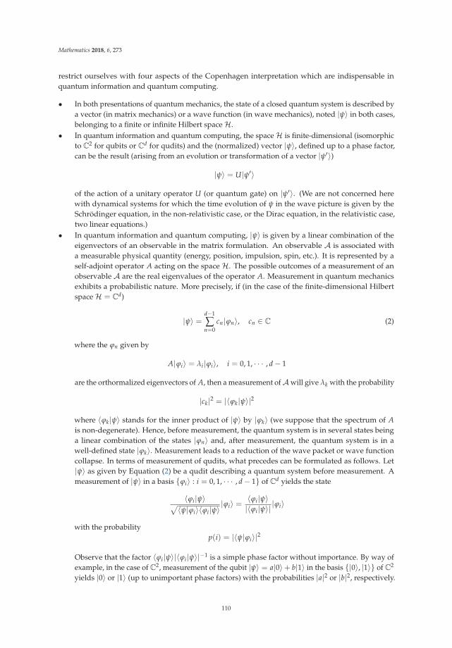
Mathematics 2018, 6, 273
restrict ourselves with four aspects of the Copenhagen interpretation which are indispensable inquantum information and quantum computing.
• In both presentations of quantum mechanics, the state of a closed quantum system is described bya vector (in matrix mechanics) or a wave function (in wave mechanics), noted |ψ〉 in both cases,belonging to a finite or infinite Hilbert spaceH.
• In quantum information and quantum computing, the spaceH is finite-dimensional (isomorphicto C2 for qubits or Cd for qudits) and the (normalized) vector |ψ〉, defined up to a phase factor,can be the result (arising from an evolution or transformation of a vector |ψ′〉)
|ψ〉 = U|ψ′〉
of the action of a unitary operator U (or quantum gate) on |ψ′〉. (We are not concerned herewith dynamical systems for which the time evolution of ψ in the wave picture is given by theSchrödinger equation, in the non-relativistic case, or the Dirac equation, in the relativistic case,two linear equations.)
• In quantum information and quantum computing, |ψ〉 is given by a linear combination of theeigenvectors of an observable in the matrix formulation. An observable A is associated witha measurable physical quantity (energy, position, impulsion, spin, etc.). It is represented by aself-adjoint operator A acting on the space H. The possible outcomes of a measurement of anobservable A are the real eigenvalues of the operator A. Measurement in quantum mechanicsexhibits a probabilistic nature. More precisely, if (in the case of the finite-dimensional HilbertspaceH = Cd)
|ψ〉 =d−1
∑n=0
cn|ϕn〉, cn ∈ C (2)
where the ϕn given by
A|ϕi〉 = λi|ϕi〉, i = 0, 1, · · · , d− 1
are the orthormalized eigenvectors of A, then a measurement ofAwill give λk with the probability
|ck|2 = |〈ϕk|ψ〉|2
where 〈ϕk|ψ〉 stands for the inner product of |ψ〉 by |ϕk〉 (we suppose that the spectrum of Ais non-degenerate). Hence, before measurement, the quantum system is in several states beinga linear combination of the states |ϕn〉 and, after measurement, the quantum system is in awell-defined state |ϕk〉. Measurement leads to a reduction of the wave packet or wave functioncollapse. In terms of measurement of qudits, what precedes can be formulated as follows. Let|ψ〉 as given by Equation (2) be a qudit describing a quantum system before measurement. Ameasurement of |ψ〉 in a basis {ϕi〉 : i = 0, 1, · · · , d− 1} of Cd yields the state
〈ϕi|ψ〉√〈ψ|ϕi〉〈ϕi|ψ〉|ϕi〉 = 〈ϕi|ψ〉
|〈ϕi|ψ〉| |ϕi〉
with the probabilityp(i) = |〈ψ|ϕi〉|2
Observe that the factor 〈ϕi|ψ〉|〈ϕi|ψ〉|−1 is a simple phase factor without importance. By way ofexample, in the case of C2, measurement of the qubit |ψ〉 = a|0〉+ b|1〉 in the basis {|0〉, |1〉} of C2
yields |0〉 or |1〉 (up to unimportant phase factors) with the probabilities |a|2 or |b|2, respectively.
110
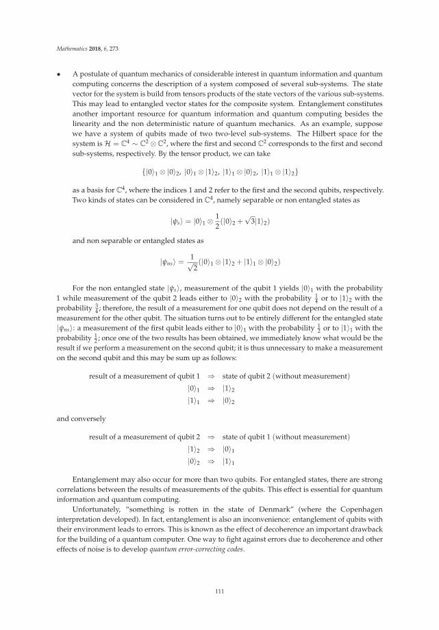
Mathematics 2018, 6, 273
• A postulate of quantum mechanics of considerable interest in quantum information and quantumcomputing concerns the description of a system composed of several sub-systems. The statevector for the system is build from tensors products of the state vectors of the various sub-systems.This may lead to entangled vector states for the composite system. Entanglement constitutesanother important resource for quantum information and quantum computing besides thelinearity and the non deterministic nature of quantum mechanics. As an example, supposewe have a system of qubits made of two two-level sub-systems. The Hilbert space for thesystem isH = C4 ∼ C2 ⊗C2, where the first and second C2 corresponds to the first and secondsub-systems, respectively. By the tensor product, we can take
{|0〉1 ⊗ |0〉2, |0〉1 ⊗ |1〉2, |1〉1 ⊗ |0〉2, |1〉1 ⊗ |1〉2}
as a basis for C4, where the indices 1 and 2 refer to the first and the second qubits, respectively.Two kinds of states can be considered in C4, namely separable or non entangled states as
|ψs〉 = |0〉1 ⊗ 12(|0〉2 +
√3|1〉2)
and non separable or entangled states as
|ψns〉 = 1√2(|0〉1 ⊗ |1〉2 + |1〉1 ⊗ |0〉2)
For the non entangled state |ψs〉, measurement of the qubit 1 yields |0〉1 with the probability1 while measurement of the qubit 2 leads either to |0〉2 with the probability 1
4 or to |1〉2 with theprobability 3
4 ; therefore, the result of a measurement for one qubit does not depend on the result of ameasurement for the other qubit. The situation turns out to be entirely different for the entangled state|ψns〉: a measurement of the first qubit leads either to |0〉1 with the probability 1
2 or to |1〉1 with theprobability 1
2 ; once one of the two results has been obtained, we immediately know what would be theresult if we perform a measurement on the second qubit; it is thus unnecessary to make a measurementon the second qubit and this may be sum up as follows:
result of a measurement of qubit 1 ⇒ state of qubit 2 (without measurement)
|0〉1 ⇒ |1〉2|1〉1 ⇒ |0〉2
and conversely
result of a measurement of qubit 2 ⇒ state of qubit 1 (without measurement)
|1〉2 ⇒ |0〉1|0〉2 ⇒ |1〉1
Entanglement may also occur for more than two qubits. For entangled states, there are strongcorrelations between the results of measurements of the qubits. This effect is essential for quantuminformation and quantum computing.
Unfortunately, “something is rotten in the state of Denmark” (where the Copenhageninterpretation developed). In fact, entanglement is also an inconvenience: entanglement of qubits withtheir environment leads to errors. This is known as the effect of decoherence an important drawbackfor the building of a quantum computer. One way to fight against errors due to decoherence and othereffects of noise is to develop quantum error-correcting codes.
111

Mathematics 2018, 6, 273
2.2. Qubits and Qudits
2.2.1. Qubits
LetB2 = {|0〉, |1〉}
be an orthonormal basis called the computational basis of the Hilbert space C2. Any normalized(to unity) vector |ψ〉, see Equation (1), in C2 is called a quantum bit or qubit. From the quantummechanical point of view, a qubit describes a state of a two-level quantum system. In the absence ofmeasurement (and decoherence), the state |ψ〉 is a superposition of |0〉 and |1〉. A measurement ofthe state |ψ〉 yields either |0〉 (with the probability |a|2) or |1〉 (with the probability |b|2). Therefore,the superposition of the states |0〉 and |1〉 is lost after the measurement. In matrix form, we take
|0〉 =(
10
), |1〉 =
(01
), |ψ〉 =
(ab
)
From a group-theoretical point of view, |0〉 and |1〉 can be considered as the basis vectors for thefundamental irreducible representation
(12
)of SU(2), in the chain SU(2) ⊃ U(1), with
|0〉 = |12
,12〉, |1〉 = |1
2,−1
2〉 (3)
in the notations of quantum angular momentum theory.The state |ψ〉 can be associated with a point (x, y, z, t) of the sphere S3 in R4 according to
C2 → S3 : a|0〉+ b|1〉 �→ (x, y, z, t)
with a = x + iy and b = z + it. In fact, the point (x, y, z, t) can be visualized as a point (1, θ, ϕ) of thesphere S2 in R3, referred to as the Bloch sphere, since ψ can be re-written as
|ψ〉 = cosθ
2|0〉+ eiϕ sin
θ
2|1〉, 0 ≤ θ ≤ π, 0 ≤ ϕ < 2π (4)
up to a global multiplicative phase factor. The application
S3 → S2 : (x, y, z, t) �→ (1, θ, ϕ)
corresponds to the first Hopf fibration S3 S1−→ S2 of compact fibre S1. Any qubit as given by Equation (4)can be represented by a point on the Bloch sphere. Table 1 gives the correspondence between someremarkable qubits |ψ〉 and points on the Bloch sphere. Any unitary transformation acting on a qubit|ψ〉 corresponds to a rotation around an axis passing through the centre of the Bloch sphere.
Table 1. Correspondence between qubits |ψ〉 = cos θ2 |0〉 + eiϕ sin θ
2 |1〉 and points (ξ = sin θ cos ϕ,η = sin θ sin ϕ, ζ = cos θ) of the Bloch sphere S2 in R3.
|ψ〉 |0〉 |1〉 1√2(|0〉+ |1〉) 1√
2(|0〉 − |1〉) 1√
2(|0〉+ i|1〉) 1√
2(|0〉 − i|1〉)
(ξ, η, ζ) (0, 0, 1) (0, 0,−1) (1, 0, 0) (−1, 0, 0) (0, 1, 0) (0,−1, 0)
Note that the sets
B0 =
{ |0〉+ |1〉√2
,|0〉 − |1〉√
2
}, B1 =
{ |0〉+ i|1〉√2
,|0〉 − i|1〉√
2
}, B2 = {|0〉, |1〉} (5)
112
Mathematics 2018, 6, 273
appearing in Table 1 are three orthonormal bases of the space C2. In addition, the vectors in B0, B1 andB2 are eigenvectors of the Pauli matrices σ1, σ2 and σ3 (defined in Equation (9) below), respectively.The bases B0, B1 and B2 constitute the simplest example of the so-called MUBs to be studied inSection 3.
2.2.2. Qudits
The generalisation from the two-dimensional Hilbert space C2 to the d-dimensional Hilbert spaceCd (d > 2) is immediate. Given an orthonormal basis (called the computational basis)
Bd = {|n〉 : n = 0, 1, · · · , d− 1} (6)
of Cd, any normalized vector
|ψ〉 =d−1
∑n=0
cn|n〉,d−1
∑n=0
|cn|2 = 1, ci ∈ C, i = 0, 1, · · · , d− 1
is called a qudit. From the point of view of quantum mechanics, the states |n〉 can be realized asgeneralized angular momentum states with
|n〉 = |j, m〉, n = j−m, d = 2j + 1 (7)
where for fixed j, the index m takes the values −j,−j + 1, · · · , j. This yields the correspondence
|0〉 = |j, j〉, |1〉 = |j, j− 1〉, · · · , |d− 1〉 = |j,−j〉
between qudits and angular momentum states. (Let us recall that the angular momentum state |j, m〉 is acommon eigenstate of the square J2 of a generalized angular momentum and of the z-component Jz ofthe angular momentum.) Therefore, |ψ〉 can be re-written
|ψ〉 =j
∑m=−j
dj−m|j, m〉
in the angular momentum basis {|j, m〉 : m = −j,−j + 1, · · · , j}. For instance, a qutrit |ψ〉 canbe written
|ψ〉 = c0|0〉+ c1|1〉+ c2|2〉in the ternary basis {|0〉, |1〉, |2〉} or
|ψ〉 = d2|1,−1〉+ d1|1, 0〉+ d0|1, 1〉
in the balanced basis {|1,−1〉, |1, 0〉, |1, 1〉} associated with the angular momentum j = 1.
113
Mathematics 2018, 6, 273
2.2.3. Qudits with d = 2N
In the case where d = 2N , the corresponding qudits can be obtained from tensor products.For example, for d = 4 a basis of C4 ∼ C2 ⊗C2 is
|0〉 ⊗ |0〉 =(
10
)⊗(
10
)=
⎛⎜⎜⎜⎝1000
⎞⎟⎟⎟⎠ , |0〉 ⊗ |1〉 =(
10
)⊗(
01
)=
⎛⎜⎜⎜⎝0100
⎞⎟⎟⎟⎠
|1〉 ⊗ |0〉 =(
01
)⊗(
10
)=
⎛⎜⎜⎜⎝0010
⎞⎟⎟⎟⎠ , |1〉 ⊗ |1〉 =(
01
)⊗(
01
)=
⎛⎜⎜⎜⎝0001
⎞⎟⎟⎟⎠Then, the most general quartit |ψ〉 is made of the superposition of tensor products of two qubits.
In detail, we have
|ψ〉 = a|0〉 ⊗ |0〉+ b|0〉 ⊗ |1〉+ c|1〉 ⊗ |0〉+ d|1〉 ⊗ |1〉
where a, b, c, d ∈ C (usually, in |i〉 ⊗ |j〉 the state |i〉 refers to the first qubit and |j〉 to the second).It is interesting to remark that the vectors |ψ〉 for d = 2, 22 and 23 are associated with the Hopf
fibrations S3 S1−→ S2 (connected to complex numbers), S7 S3−→ S4 (connected to quaternions) and
S15 S7−→ S8 (connected to octonions). Entanglement for d = 22 and 23 can be discussed in terms offibrations on spheres [21]. In the same vein, we may ask the question of the interest for entanglementof Cayley-Dickson algebras for d = 2N with N > 3 and of fibrations on hyperboloids [13].
2.3. Physical Realizations of Qubits
According to R. Landauer, information is physical so that qubits are realised by quantum systems,more specifically by two-level quantum systems, the qubits |0〉 and |1〉 corresponding to two different(energy) levels. We shall not be concerned here with the physical realization of qubits (and qudits). It isenough to say that any two-level quantum system may be considered as a qubit. Therefore, qubits canbe carried out by nuclear spins, ultra-cold trapped ions, neutral atoms and Bose-Einstein condensates,two different polarizations of a photon, and Josephson tunnel nanojunctions. For instance, in nuclearmagnetic resonance, the nuclear spins of an atom in an organic molecule can be aligned (giving thestate |0〉) or anti-aligned (giving the state |1〉) with an applied constant magnetic field; in generalizedangular momentum terminology, we have the quantum states given by Equation (3) and correspondingto the spin j = 1
2 . Similarly, for an ion cooled and trapped by electric fields in a cavity, qubits can beimplemented as electronic states (ground state for |0〉, excited state for |1〉). Vibrational states can alsobe used for realizing qubits (zero-phonon state for |0〉, one-phonon state for |1〉).
2.4. Entanglement
2.4.1. Generalities
Entanglement occurs only in quantum physics. It has no analogue in classical physics. The notionof entanglement goes back to the famous paper by Einstein, Poldosky and Rosen. In quantum physics,two (or more than two) particles are said to be entangled if the quantum state of each particle dependsof the quantum state(s) of the other(s) or cannot be described independently of the quantum state(s)of the other(s). In other words, there exist correlations between the physical properties of a systemof entangled particles. More generally, two entangled sub-systems S1 and S2 are not independent sothat the global system {S1, S2} must be considered as a whole even after separation by an arbitrarydistance. Then, a measurement made on one sub-system gives an information on the other (without
114
Mathematics 2018, 6, 273
measurement on the other sub-system). On the contrary, for a non entangled system consisting oftwo sub-systems, a measurement on one sub-system does not give in general an information on theother sub-system.
As an example, let us consider a system consisting of two particles, system having a total spinequal to 0. If the spin of one particle is measured to be 1
2 on a certain axis, then we know (without anymeasurement) that the spin on the other particle on the same axis is − 1
2 because
0 =12− 1
2
The two particles are not independent, even after separation. They still behave like an indivisiblesystem of spin 0.
Entanglement contradicts the principle of locality. There is non locality in the sense that whathappens in some place depends of what happens in another place. Indeed, quantum mechanics is anon local, non deterministic and linear physical theory.
2.4.2. Entanglement of Qubits
In quantum information, the notion of entanglement occurs for multi-qubit systems. Let usconsider a two-qubit system. There are two possibilities.
• The system is non entangled (or separable); it is then described by a state |ψs〉 ∈ C2⊗C2 such that
|ψs〉 = (a|0〉+ b|1〉)⊗ (c|0〉+ d|1〉)
which can be re-written as
|ψs〉 = ac|0〉 ⊗ |0〉+ ad|0〉 ⊗ |1〉+ bc|1〉 ⊗ |0〉+ bd|1〉 ⊗ |1〉
where a|0〉+ b|1〉 and c|0〉+ d|1〉 refer to the first and second qubit, respectively.• The system is entangled (or non separable); it is then described by a state |ψns〉 ∈ C4 such that
|ψs〉 = A|0〉 ⊗ |0〉+ B|0〉 ⊗ |1〉+ C|1〉 ⊗ |0〉+ D|1〉 ⊗ |1〉
cannot be written as the tensor product of two qubits in C2.
It is clear that a necessary and sufficient condition for an arbitrary two-qubit state
|ψ〉 = α|0〉 ⊗ |0〉+ β|0〉 ⊗ |1〉+ γ|1〉 ⊗ |0〉+ δ|1〉 ⊗ |1〉
of C4 to be non entangled isαδ− βγ = 0
Therefore, if αδ− βγ �= 0, then the state is entangled. The degree of entanglement of an arbitrarynormalized two-qubit state |ψ〉 is characterized by the concurrence defined by
C = |αδ− βγ|, 0 ≤ C ≤ 12
(8)
Non entangled states correspond to C = 0, maximally entangled states to C = 12 . (A maximally
entangled state is such that the density operator for each qubit is half the identity operator;it corresponds to a maximum value of the entropy.) Equation (8) can be straightforwardly generalizedto the case
|ψ〉 =d−1
∑i=0
d−1
∑j=0
aij|i〉 ⊗ |j〉
115
Mathematics 2018, 6, 273
of two qudits for which the concurrence C is defined as
C = det(aij), 0 ≤ C ≤ 1√dd
in agreement with Equation (8) for d = 2.
Example 1. Let us consider the four states (⊕ stands for the addition modulo 2)
|βxy〉 = 1√2[|0〉 ⊗ |y〉+ (−1)x|1〉 ⊗ |y⊕ 1〉], x, y = 0, 1
called Bell states (in reference to the work on the so-called Bell inequalities) or EPR pairs (in reference to thepaper by Einstein, Poldosky and Rosen). As a particular case
|β01〉 = 1√2(|0〉1 ⊗ |1〉2 + |1〉1 ⊗ |0〉2)
where the first qubit (qubit 1) and the second one (qubit 2) are clearly emphasized in order to avoid confusion.The result of a measurement of the qubit 1 gives
• either |0〉1 (with the probability 12 ) so that the qubit 2 is a priori (without measurement) in the state |1〉2
• or |1〉1 (with the probability 12 ) so that the qubit 2 is a priori (without measurement) in the state |0〉2
but no measurement can lead to both qubits 1 and 2 in the same state (|0〉 or |1〉). The result of a measurement ofthe qubit 1 provides information on the qubit 2 and reciprocally. It is then unnecessary to make a measurementof one qubit once the result of the measurement of the other is known. Similar conclusions can be obtainedfor the three other Bell states β00, β10 and β11. The four Bell states are maximally entangled (they correspondto C = 1
2 ).In passing note that
|βxy〉 = (−1)xy[(σ1)y(σ3)
x]⊗ σ0|β00〉where σ0, σ1 and σ3 are three of the four Pauli matrices
σ0 =
(1 00 1
), σ1 =
(0 11 0
), σ3 =
(1 00 −1
), σ2 = iσ1σ3 =
(0 −ii 0
)(9)
Thus, any Bell state |βxy〉 can be obtained from |β00〉.
Example 2. Let us consider the separable state
|ψ〉 = (a|0〉+ b|1〉)⊗ 1√5(|0〉+ 2|1〉) = 1√
5(a|0〉 ⊗ |0〉+ 2a|0〉 ⊗ |1〉+ b|1〉 ⊗ |0〉+ 2b|1〉 ⊗ |1〉)
tensor product of two normalized qubits. A measurement of the first qubit gives either |0〉 with the probability|a|2 = | a√
5|2 + | 2a√
5|2 or |1〉 with the probability |b|2 = | b√
5|2 + | 2b√
5|2 while a measurement of the second
qubit gives either |0〉 with the probability 15 = | a√
5|2 + | b√
5|2 or |1〉 with the probability 4
5 = | 2a√5|2 + | 2b√
5|2.
Therefore, a measurement on one qubit does not provide information on the other qubit (the state |ψ〉 correspondsto C = 0).
It is important to realize that entanglement of qubits (as in Example 1) and more generally ofqudits has no analogue for classical bits. To be clear, the bits in 00 or 01 or 10 or 11 are not correlated.This is not the case for the quantum bits in any of the Bell states βxy.
116

Mathematics 2018, 6, 273
2.5. Quantum Gates
2.5.1. One-Qubit Gates
In a classical computer, bits are handled with the help of logic gates (there exist seven basiclogic gates: AND, OR, XOR, NOT, NAND, NOR, and XNOR). A quantum computer processes qubitsarranged in registers. It is equipped with quantum gates which perform unitary transformationson qubits. Quantum gates can be represented by unitary matrices. Table 2 gives some examples ofquantum gates [G] for one-qubit systems together with their matrix representations G. The actions ofthe one-qubit gates of Table 2 on the qubit |x〉 (with x = 0 or 1) are given by
|x〉 → [I]→ |x〉, |x〉 → [NOT]→ |x⊕ 1〉|x〉 → [Sθ ]→ eixθ |x〉, |x〉 → [H]→ 1√
2(|0〉+ (−1)x|1〉) ≡ 1√
2(|x⊕ 1〉+ (−1)x|x〉)
(as an example, the quantum circuit |x〉 → [Sθ ] → eixθ |x〉 is described by the action Sθ |x〉 = eixθ |x〉).Therefore, by linearity
a|0〉+ b|1〉 → [NOT]→ b|0〉+ a|1〉a|0〉+ b|1〉 → [Sθ ]→ a|0〉+ eiθb|1〉
a|0〉+ b|1〉 → [H]→ 1√2(a + b)|0〉+ 1√
2(a− b)|1〉
a|0〉+ b|1〉 → [H]→ [H]→ a|0〉+ b|1〉
(the last circuit reflects that H2 = I). Note that the most general qubit can be obtained from thesequence [H]→ [S2θ ]→ [H]→ [S π
2 +ϕ] of one-qubit gates since
|0〉 → [H]→ [S2θ ]→ [H]→ [S π2 +ϕ]→ cos θ|0〉+ eiϕ sin θ|1〉
orS π
2 +ϕHS2θ H|0〉 = cos θ|0〉+ eiϕ sin θ|1〉up to the phase factor eiθ .
Table 2. Four basic quantum gates for one-qubit systems; the gates [I] and [NOT] also denoted [X] areassociated with the Pauli matrices σ0 or I and σ1 or σx, respectively; the two other Pauli matrices σ2 orσy and σ3 or σz define two further one-qubit gates denoted as [Y] and [Z], respectively.
Gate [G] Identity Gate [I] Not Gate [NOT] Phase Gate [Sθ] Hadamard Gate [H]
matrix form G I =(
1 00 1
)NOT =
(0 11 0
)Sθ =
(1 00 eiθ
)H = 1√
2
(1 11 −1
)
2.5.2. Multi-Qubit Gates
Quantum gates for two-qubit systems are important. For example, let us mention thecontrolled-NOT gate [CNOT] defined via
|x〉 ⊗ |y〉 → [CNOT]→ |x〉 ⊗ |y⊕ x〉
or in operator formCNOT |x〉 ⊗ |y〉 = |x〉 ⊗ |y⊕ x〉
117
Mathematics 2018, 6, 273
where the first input qubit |x〉 and the second input qubit |y〉 are called control qubit and target qubit,respectively. Here, the corresponding quantum circuit has two inputs (|x〉 and |y〉) and two outputs(|x〉 and |y⊕ x〉). In matrix form, we have the permutation matrix
CNOT =
⎛⎜⎜⎜⎝1 0 0 00 1 0 00 0 0 10 0 1 0
⎞⎟⎟⎟⎠Clearly, (CNOT)
2 = I. Note that
CNOT |x〉 ⊗ |0〉 = |x〉 ⊗ |x〉 (10)
where x = 0 or 1; however, this result does not mean that an arbitrary state |ψ〉 = a|0〉+ b|1〉 can becloned by using the gate [CNOT] since we generally have (see Section 2.6)
CNOT |ψ〉 ⊗ |0〉 �= |ψ〉 ⊗ |ψ〉
to be compared with Equation (10). Note also that
|x〉 ⊗ |y〉 → [H⊗ I]→ [CNOT]→ |βxy〉
or|βxy〉 = CNOT(H ⊗ I)|x〉 ⊗ |y〉
that shows the interest of the gate [CNOT] for producing Bell states (i.e., entangled states) from nonentangled states. (By [H⊗ I], we mean that the quantum gates [H] and [I] act on |x〉 and |y〉, respectively.Hence, H ⊗ I stands for the direct product of the matrices H and I.)
More generally, the quantum gate [Uf] is defined through
|x〉 ⊗ |y〉 → [Uf]→ |x〉 ⊗ |y⊕ f (x)〉
or in an equivalent wayUf |x〉 ⊗ |y〉 = |x〉 ⊗ |y⊕ f (x)〉
where f stands for the function f : {0, 1} → {0, 1}. Clearly, (Uf )2 = I.
Another important two-qubit gate is the controlled phase gate [CPθ ] such that
|x〉 ⊗ |y〉 → [CPθ ]→ |x〉 ⊗ eixyθ |y〉
orCPθ |x〉 ⊗ |y〉 = |x〉 ⊗ eixyθ |y〉
with
CPθ =
⎛⎜⎜⎜⎝1 0 0 00 1 0 00 0 1 00 0 0 eiθ
⎞⎟⎟⎟⎠Note that
[CNOT] = [I⊗H]→ [CP π2]→ [CP π
2]→ [I⊗H]
so that the gate [CNOT] can be obtained from the gates [I ⊗ H] and [CP π2
].There exist other two-qubit gates. Moreover, use is also made of n-qubit gates (n > 2).
The advantage of the quantum gates over the classical logic gates is that all the quantum gates
118
Mathematics 2018, 6, 273
are reversible or invertible due to the unitary property of the matrices representing quantum gates;this is not always the case for classical logic gates.
The preceding examples are sufficient for illustrating how works the algorithm set up by Deutschand Jozsa [1].
2.5.3. Quantum Computing Algorithms
The Deutsch-Jozsa algorithm addresses the following problem: to find with only one measurementif the function
f : {0, 1}⊗n → {0, 1}is constant or balanced ( f is balanced means either f (0) = 0 and f (1) = 1 or f (0) = 1 and f (1) = 0;f is constant means f (0) = f (1) = 0 or 1). The classical algorithm requires 2n−1 + 1 evaluations of fwhereas only one measurement is necessary in order to get the answer. For n = 1, the proof based onthe quantum circuit [H⊗H]→ [Uf]→ [H⊗ I] of two-qubit gates is as follows. It is easy to show that
|0〉 ⊗ |1〉 → [H⊗H]→ [Uf]→ [H⊗ I]→ |x〉 ⊗ |y〉
alternatively|x〉 ⊗ |y〉 = (H ⊗ I)Uf (H ⊗ H)|0〉 ⊗ |1〉
where
|x〉 ⊗ |y〉 = ±|0〉 ⊗ 1√2(|0〉 − |1〉) if f is constant
|x〉 ⊗ |y〉 = ±|1〉 ⊗ 1√2(|0〉 − |1〉) if f is balanced
Then, the result of a single measurement of the first output qubit can be⎧⎪⎪⎨⎪⎪⎩|0〉 ⇒ f is constant
or
|1〉 ⇒ f is balanced
Therefore, a single measurement (instead of two in the classical case) is sufficient for getting theanswer. The Deutsch-Jozsa algorithm is of little interest. However, it shows the superiority of thequantum approach on the classical one (namely, only one measurement instead of 2n−1 + 1 evaluationsin the general case where f : {0, 1}⊗n → {0, 1}).
Let us briefly mention two other historical algorithms, viz, the Shor algorithm and the Groveralgorithm [1]. The Shor algorithm concerns the search of the period of a periodic function and isused for the factorization of a composite integer into prime factors. It constitutes an alternative to theclassical RSA code. The Grover algorithm makes it possible to find an item in an unstructured databasis consisting of n entries; the quantum speed up for this algorithm is n → √
n (O(n) researches forthe classical case and O(
√n) for the quantum case). The two preceding algorithms are based on the
massive quantum parallelism. They formally show the superiority of a (still hypothetical) quantumcomputer on a classical one. The present evolution is towards quantum cryptography.
2.6. No-Cloning Theorem
We may ask the question: does there exist a unitary operator (or quantum gate) U such that
U|ψ〉 ⊗ |0〉 = |ψ〉 ⊗ |ψ〉 (11)
119

Mathematics 2018, 6, 273
where |ψ〉 = a|0〉+ b|1〉 is an arbitrary qubit. As a consequence of the linearity of quantum mechanics,the answer is no: it is not possible to clone an arbitrary qubit |ψ〉 [8]. This result can be proved in thefollowing way. Suppose that there exists U such that Equation (11) is true. Then, by linearity
U|ψ〉 ⊗ |0〉 = U(a|0〉+ b|1〉)⊗ |0〉= U(a|0〉 ⊗ |0〉+ b|1〉 ⊗ |0〉)
(12)= aU|0〉 ⊗ |0〉+ bU|1〉 ⊗ |0〉= a|0〉 ⊗ |0〉+ b|1〉 ⊗ |1〉
On another side, we have
U|ψ〉 ⊗ |0〉 = |ψ〉 ⊗ |ψ〉= (a|0〉+ b|1〉)⊗ (a|0〉+ b|1〉) (13)
= a2|0〉 ⊗ |0〉+ ab(|0〉 ⊗ |1〉+ |1〉 ⊗ |0〉) + b2|1〉 ⊗ |1〉
Compatibility between Equations (12) and (13) yields
a2 = a (⇒ a = 0, 1), b2 = b (⇒ b = 0, 1), ab = 0 (⇒ a = 0 or b = 0)
The sole solutions are (a = 1, b = 0) and (a = 0, b = 1) in agreement with Equation (10). There areno solution in the general case. This proves the no-cloning theorem (a theorem that does not have ananalogue in classical information).
Another way to understand this result is to realize that in order to clone an arbitrary state|ψ〉 = a|0〉 + b|1〉 one must measure it so that one gets |0〉 or |1〉, two states that differ from |ψ〉in general.
2.7. Quantum Teleportation
It is not possible to clone an arbitrary quantum state. However, it is feasible to teleporte it,i.e., to transfer it from one place to another without an effective transportation. In other words,without a material transportation of a qubit, it is possible to transmit at distance the informationcontained in the qubit. We shall not deal here with some physical device making teleportation possible.We shall rather limit ourselves to the corresponding quantum algorithm [15].
Suppose someone, Alice, wants to send a qubit |ψ〉 = a|0〉+ b|1〉 (for which she does not know aand b) to somebody, Bob, by a quantum circuit and the possibility of using a classical communicationchannel. The only requirement for Bob and Alice is to dispose of and EPR pair |β00〉, the first qubit ofwhich belongs to Alice and the second one to Bob. Thus, the entry |ϕ0〉 of the quantum circuit is
|ϕ0〉 = |ψ〉 ⊗ |β00〉= (a|0〉1 + b|1〉1)⊗ 1√
2(|0〉2 ⊗ |0〉3 + |1〉2 ⊗ |1〉3)
=1√2
[a|0〉1 ⊗ (|0〉2 ⊗ |0〉3 + |1〉2 ⊗ |1〉3) + b|1〉1 ⊗ (|0〉2 ⊗ |0〉3 + |1〉2 ⊗ |1〉3)
]=
1√2
[a(|0〉1 ⊗ |0〉2 ⊗ |0〉3 + |0〉1 ⊗ |1〉2 ⊗ |1〉3) + b(|1〉1 ⊗ |0〉2 ⊗ |0〉3 + |1〉1 ⊗ |1〉2 ⊗ |1〉3)
]
120
Mathematics 2018, 6, 273
where qubits 1 and 2 refer to the Alice qubit and qubit 3 to the Bob qubit. Then, Alice sends her qubitsto a controlled-NOT gate producing the state
|ϕ1〉 =1√2
[a(|0〉1 ⊗ |0〉2 ⊗ |0〉3 + |0〉1 ⊗ |1〉2 ⊗ |1〉3) + b(|1〉1 ⊗ |1〉2 ⊗ |0〉3 + |1〉1 ⊗ |0〉2 ⊗ |1〉3)
]=
1√2
[a|0〉1 ⊗ (|0〉2 ⊗ |0〉3 + |1〉2 ⊗ |1〉3) + b|1〉1 ⊗ (|1〉2 ⊗ |0〉3 + |0〉2 ⊗ |1〉3)
]Next, qubit 1 goes to an Hadamard gate giving
|ϕ2〉 = 12[a(|0〉1 + |1〉1)⊗ (|0〉2 ⊗ |0〉3 + |1〉2 ⊗ |1〉3) + b(|0〉1 − |1〉1)⊗ (|1〉2 ⊗ |0〉3 + |0〉2 ⊗ |1〉3)
]which can be re-arranged as
|ϕ2〉 =12[(|0〉1 ⊗ |0〉2)⊗ (a|0〉3 + b|1〉3) + (|0〉1 ⊗ |1〉2)⊗ (a|1〉3 + b|0〉3)
+ (|1〉1 ⊗ |0〉2)⊗ (a|0〉3 − b|1〉3) + (|1〉1 ⊗ |1〉2)⊗ (a|1〉3 − b|0〉3)]
Measurement of qubits 1 and 2 by Alice can give
|0〉1 ⊗ |0〉2 with the probability 14 , |0〉1 ⊗ |1〉2 with the probability 1
4
|1〉1 ⊗ |0〉2 with the probability 14 , |1〉1 ⊗ |1〉2 with the probability 1
4
Suppose Alice gets |0〉1 ⊗ |0〉2. Then, she communicates this result to Bob by a classical channel(telephone or mail). Thus, Bob knows that |ψ〉 is a|0〉3 + b|1〉3. Should Alice have got |0〉1 ⊗ |1〉2 or|1〉1 ⊗ |0〉2 or |1〉1 ⊗ |1〉2, then Bob would obtain a|0〉3 + b|1〉3 after the use of the gates [X] or [Z] or[T] with T = ZX on the states a|1〉3 + b|0〉3 or a|0〉3 − b|1〉3 or a|1〉3 − b|0〉3, respectively. In all cases,the qubit |ψ〉 = a|0〉+ b|1〉 has been teleported. This proof shows that entanglement (via the EPR pair)plays a crucial role in teleportation.
3. Some Mathematical Aspects: Mutually Unbiased Bases
3.1. Introducing MUBs
3.1.1. Generalities about MUBs
Unitary operator bases in the Hilbert space Cd are of pivotal importance for quantum informationand quantum computing as well as for quantum mechanics in general. The interest for unitary operatorbases started with the seminal work by Schwinger [5]. In this connection, MUBs play a key role inquantum information and quantum computing. Two distinct orthonormal bases of Cd are said to beunbiased if and only if the modulus of the inner product of any vector of one basis with any vector ofthe other one is equal to 1√
d(see the detailed definition in Section 3.1.2).
MUBs proved to be useful in classical information theory (network communicationprotocols) [17,47]. They play an important role in quantum mechanics as for the discrete Wignerfunction [11,29,34,42,43,55,62], for the solution of the Mean King problem [20,26,33,34,43], for theunderstanding of the Feynman path integral formalism [57,63] and potentially for studies of theWeyl-Heisenberg group in connection with quantum optics. MUBs are of central importance inquantum information theory as for instance in quantum state tomography (deciphering an unknownquantum state) [38,56,77], quantum cryptography (secure quantum key exchange) [9,25] and quantumteleportation [15]. Along this line, measurements corresponding to MUBs are appropriate for anoptimal determination of the density matrix of a quantum system and the use of MUBs ensure themaximum of security for quantum communication (especially in the BB84 quantum cryptography
121
Mathematics 2018, 6, 273
protocol). Let us also mention that MUBs are connected with the notion of maximal entanglement ofquantum states a result of great importance for quantum computing.
Here, it is not our purpose to give some details about all the applications listed above.The interested reader may consult the quoted original references for a full description of eachapplication. It is enough to say that a central common point to all the applications is given byEquation (15) that reflects the uniform probability nature of the results of measurements using MUBs.This is especially obvious in the BB84 protocol where the probability of detection of Eve (a spy) on aquantum communication channel between Alice and Bob is maximum when Alice and Bob use MUBs.
There exist numerous ways of constructing sets of MUBs (e.g., see [58,64,65]). Most of themare based on discrete Fourier transform over Galois fields and Galois rings [2,14,17,28–30,36,41,72],discrete Wigner distribution [11,29,34,42,55], generalized Pauli spin matrices [22,23,27,30], mutuallyorthogonal Latin squares [33,35], graph theory [74], finite and projective geometries [49,61], convexpolytopes [40], complex projective 2-designs [19,39,67], quantum angular momentum theory [44],group theoretical methods [24,45,50,53], discrete phase states [68] and Hadamard matrices [73]. In thissection, from quantum theory of angular momentum theory (or, in mathematical terms, from the Liealgebra A1 of the group SU(2) or SU(2,C) or SL(2,C)) we shall derive a formula for a complete set ofMUBs in dimension p with p prime. Moreover, we shall construct complete sets of MUBs in dimensionpm with p prime and m positive integer from the additive characters of the Galois field GF(pm) for podd and of the Galois ring GR(22, m) for p = 2.
3.1.2. Definition of MUBs
Definition 1. Let Ba and Bb two distinct orthonormal bases
Ba = {|aα〉 : α = 0, 1, · · · , d− 1}, Bb = {|bβ〉 : β = 0, 1, · · · , d− 1}
of the Hilbert space Cd. The bases Ba and Bb (a �= b) are said to be unbiased if and only if
∀α ∈ Zd, ∀β ∈ Zd : |〈aα|bβ〉| = 1√d
(14)
where 〈 | 〉 denotes the inner product of Cd [5,6,10,11]. In other words, the inner product 〈aα|bβ〉 has a modulusindependent of α and β. The relation
|〈aα|bβ〉| = δa,bδα,β +1√d(1− δa,b)
makes it possible to describe both the cases Ba = Bb and Ba �= Bb.
As a typical example, the bases B0, B1 and B2 of C2, see Equation (5), constitute a set of threeMUBS whose basis vectors are specific qubits.
3.1.3. Well-Known Results about MUBs
The main results concerning MUBs are [6,14,19,35,37]:
1. MUBs are stable under unitary or anti-unitary transformations. More precisely, if two unbiasedbases undergo the same unitary or anti-unitary transformation, they remain mutually unbiased.
2. The number N(d) of MUBs in Cd cannot exceed d + 1. Thus
N(d) ≤ d + 1
3. The maximum number d + 1 of MUBs is attained when d is a power pm (m ≥ 1) of a primenumber p. Thus
N(pm) = pm + 1
122

Mathematics 2018, 6, 273
4. When d is a composite number, N(d) is not known but it can be shown that
3 ≤ N(d) ≤ d + 1
As a more accurate result, for d = ∏i pmii with pi prime and mi positive integer, we have
min(pmii ) + 1 ≤ N(d) ≤ d + 1
By way of illustration, let us mention the following cases.
• In the particular composite case d = 6 = 2× 3, we have
3 ≤ N(6) ≤ 7
and it was conjectured that N(6) = 3. Indeed, in spite of an enormous amount of computationalworks, no more than three MUBs were found for d = 6.
• For d = 15 = 3× 5 and d = 21 = 3× 7, there are at least four MUBs.• For d = 676 = 22 × 132, we have
22 + 1 = 5 ≤ N(676) ≤ 677
but it is known how to construct at least six MUBs.
A set of d + 1 MUBs in Cd is referred to as a complete set. Such sets exist for d = pm (p prime,m positive integer) and this result opens the way to establish a link between MUBs and Galois fieldsand/or Galois rings.
For d composite (different from a power of a prime), the question to know if there exist completesets in dimension d, i.e., to know if N(d) can be equal to d+ 1, is still an open problem (in 2018). Indeed,for d different from a power of a prime, it was conjectured (SPR conjecture [32]) that the problemof the existence of a set of d + 1 MUBs in Cd is equivalent to the problem of whether there exist aprojective plane of order d. As another conjecture for d composite (different from a power of a prime),the problem of the existence of a set of d + 1 MUBs in Cd is equivalent to the one of the existence of adecomposition of the Lie algebra of SU(d) into d + 1 Cartan subalgebras of dimension d− 1.
3.1.4. Interests of MUBs
MUBs are or relevance in advanced quantum mechanics. From a very general point of view,MUBs are closely connected to the principle of complementarity introduced by Bohr in the early days ofquantum mechanics. This principle, quite familiar in terms of observables like position and momentum,tells that for two non-commuting observables, if we have a complete knowledge of one observable,then we have a total uncertainty of the other. Equation (14) indicates that the development in the basisBa of any vector of the basis Bb is such that each vector of Ba appears in the development with theprobability 1
d . This is especially interesting when translated in terms of measurements, the bases Ba
and Bb corresponding to the (non-degenerate) eigenvectors of two non-commuting observables.A significance of MUBs in terms of quantum measurements can be seen as follows. Let A and B
be two non-degenerate (i.e., with multiplicity-free eigenvalues) self-adjoint (or hermitian) operatorsassociated with two observables A and B of a quantum system with the Hilbert space Cd of dimensiond. Suppose that the eigenvectors of A and B yield two unbiased bases Ba and Bb, respectively. When thequantum system is prepared in an eigenvector |bβ〉 of the observable B, no information can be obtainedfrom a measurement of the observable A. This result follows from the development in the basis Ba ofany vector of the basis Bb
|bβ〉 =d−1
∑α=0|aα〉〈aα|bβ〉
123
Mathematics 2018, 6, 273
which shows that the d probabilities
|〈aα|bβ〉|2 =1d
, α, β = 0, 1, · · · , d− 1 (15)
of obtaining any state vector |aα〉 in a measurement of A are equal.Indeed, the two operators A and B do not commute. The two corresponding observables A
and B are said to be complementary (Bohr’s principle of complementarity introduced in the earlydays of quantum mechanics): a precise knowledge of one of them implies a total uncertainty ofthe other (or, all possible results of measurements of the other one are equally probable). This canbe made more explicit through the generalized Heisenberg uncertainty principle. Let A and B betwo hermitian operators associated with two observables and |ψ〉 a vector of Cd. The generalizedHeisenberg uncertainty principle can be expressed as
ΔAΔB ≥ 12|〈ψ|[A, B]−|ψ〉|
where [A, B]− = AB− BA and ΔO stands for the standard deviation
ΔO =√〈ψ|O2|ψ〉 − 〈ψ|O|ψ〉2
of the operator O = A or B. (The most familiar example is for d infinite. The position A = x andthe momentum B = px, along the x direction, of a particle are complementary observables. Theysatisfy the commutation relations [x, px]− = ih, where h is the Planck constant. Hence, ΔxΔpx ≥ 1
2 hso that more precise is Δx more imprecise is Δpx and vice versa.) Therefore, if A and B correspond toobservables generating MUBs, then a precise knowledge of A yields a complete indeterminacy of Band vice versa.
Note that
d + 1 =d2 − 1d− 1
is the number of different measurements to fully determine a quantum state for a quantum systemin dimension d. (This follows from the fact that a d× d density matrix, that is to say an Hermitianmatrix with a trace equal to 1, contains d2 − 1 real parameters and each measurement gives d− 1 realparameters.) Note also that d2 − 1 and d− 1 are the number of generators and the rank of the specialunitary group SU(d) in d dimensions, respectively, and that for d = p (prime number) their ratio p + 1is the number of disjoint sets of p− 1 commuting generators of SU(p).
The rest of the paper is structured in the following way. In Section 3.2, we give a completesolution, based on a nonstandard approach to the Lie algebra of the group SU(2) (equivalently, to thequantum theory of angular momentum), for the construction of MUBs in the case where d = pis a prime number. Further developments are discussed in Section 3.3 in relation with Weyl pairs.Sections 3.4 and 3.5 are concerned with the construction of MUBs from Galois fields (for d = pm,a power of an odd prime number) and Galois rings (for d = 2m, a power of the even prime number),respectively. (See Refs. [31,46,48] for the formalism of Galois quantum systems.)
3.2. Group-Theoretical Construction of MUBs
3.2.1. Standard Basis for SU(2)
Equation (7) shows that the vectors |n〉 (with n = 0, 1, · · · , d− 1) of the computational basis (6)can be viewed as the basis vectors |j, m〉 (with m = j, j− 1, · · · ,−j) for the irreducible representation(j) of SU(2) in the chain SU(2) ⊃ U(1). In the language of group theory (and quantum angularmomentum theory), the vector |j, m〉 is a common eigenvector of the Casimir operator J2 (the square of
124
Mathematics 2018, 6, 273
an angular momentum) and of a Cartan generator Jz (the z component of the angular momentum) ofthe Lie algebra A1 of the group SU(2). More precisely, we have the eigenvalue equations
J2|j, m〉 = j(j + 1)|j, m〉, Jz|j, m〉 = m|j, m〉
with the orthonormality relations
〈j, m|j, m′〉 = δm,m′ , m, m′ = j, j− 1, · · · ,−j
In other words, the computational basis Bd can be visualized as the basis
B2j+1 = {|j, m〉 : m = j, j− 1, · · · ,−j}
known as the standard basis for the irreducible representation (j) of SU(2) or the angular momentumbasis corresponding to the angular momentum quantum number j, referred to as spin angularmomentum for j = 1
2 .
3.2.2. Nonstandard Bases for SU(2)
As far as the representation theory of SU(2) is concerned, we can replace the complete set {J2, Jz}by another complete set of two commuting operators. For instance, we may consider the set {J2, va},where the unitary operator va is defined by
va|j, m〉 =
⎧⎪⎪⎨⎪⎪⎩|j,−j〉 if m = j
ω(j−m)a|j, m + 1〉 if m = j− 1, j− 2, · · · ,−j
where
ω = ei 2π2j+1
is a primitive (2j + 1)-th root of unity and a is a fixed parameter in the ring Z2j+1. The operator va
takes its origin in a polar decomposition of the two generators E± = J± of the group SU(2). For fixeda, the common eigenvectors of J2 and va provide an alternative basis to that given by the commoneigenstates of J2 and Jz. This can be made precise by the following result.
Proposition 1. For fixed j and a (with 2j ∈ N∗ and a ∈ Z2j+1), the 2j + 1 common eigenvectors of J2 and va
can be taken in the form
|jα; a〉 = 1√2j + 1
j
∑m=−j
ω12 (j+m)(j−m+1)a+(j+m)α|j, m〉
with α = 0, 1, · · · , 2j. The corresponding eigenvalues of va are given by
va|jα; a〉 = ω ja−α|jα; a〉
Then, the spectrum of va is non-degenerate.
The inner product
〈jα; a|jβ; a〉 = δα,β, α, β = 0, 1, · · · , 2j
125
Mathematics 2018, 6, 273
shows that for fixed j and a
Ba = {|jα; a〉 : α = 0, 1, · · · , 2j}
is an orthonormal set which provides a nonstandard basis for the irreducible representation (j) ofSU(2). For fixed j, there exists 2j + 1 orthonormal bases Ba since a can take 2j + 1 distinct values(a = 0, 1, · · · , 2j).
3.2.3. Bases in Quantum Information
We now go back to quantum information. By introducing
|aα〉 = |jα; a〉
together with the change of notations (7), the eigenvectors of va can be written as
|aα〉 = 1√d
∑n∈Zd
ω12 (n+1)(d−n−1)a−(n+1)α|n〉
where ω = ei 2πd . The vector |aα〉 satisfies the eigenvalue equation
va|aα〉 = ω12 (d−1)a−α|aα〉
For fixed d and a, each eigenvector |aα〉 is a linear combination of the qudits |0〉, |1〉, · · · , |d− 1〉and the basis
Ba = {|aα〉 : α = 0, 1, · · · , d− 1}
is an alternative to the computational basis Bd. For fixed d, we therefore have d + 1 remarkable basesof the d-dimensional space Cd, namely, Bd and Ba for a = 0, 1, · · · , d− 1.
The operator va can be represented by a d-dimensional unitary matrix Va. The matrix Va, built onthe basis Bd with the ordering 0, 1, · · · , d− 1 for the lines and columns, reads
Va =
⎛⎜⎜⎜⎜⎜⎜⎝0 ωa 0 · · · 00 0 ω2a · · · 0...
...... · · · ...
0 0 0 · · · ω(d−1)a
1 0 0 · · · 0
⎞⎟⎟⎟⎟⎟⎟⎠The eigenvectors of Va are
φ(aα) =1√d
∑n∈Zd
ω12 (n+1)(d−n−1)a−(n+1)αφn
with α = 0, 1, · · · , d− 1, where φn with n = 0, 1, · · · , d− 1 are the column vectors
φ0 =
⎛⎜⎜⎜⎜⎝10...0
⎞⎟⎟⎟⎟⎠ , φ1 =
⎛⎜⎜⎜⎜⎝01...0
⎞⎟⎟⎟⎟⎠ , · · · , φd−1 =
⎛⎜⎜⎜⎜⎝00...1
⎞⎟⎟⎟⎟⎠
126
Mathematics 2018, 6, 273
representing the qudits |0〉, |1〉, · · · , |d − 1〉, respectively. The vectors φ(aα) satisfy theeigenvalue equation
Vaφ(aα) = ω12 (d−1)a−αφ(aα)
with the orthonormality relationφ(aα)†φ(aβ) = δα,β
for α, β = 0, 1, · · · , d− 1.The matrix Va can be diagonalized by means of the d-dimensional matrix Ha of elements
(Ha)nα =1√d
ω12 (n+1)(d−n−1)a−(n+1)α
with the lines and columns of Ha arranged from left to right and from top to bottom in the ordern, α = 0, 1, · · · , d− 1. Indeed, by introducing the d× d permutation matrix
P =
⎛⎜⎜⎜⎜⎜⎜⎜⎜⎝
1 0 0 · · · 0 00 0 0 · · · 0 10 0 0 · · · 1 0...
...... · · · ...
...0 0 1 · · · 0 00 1 0 · · · 0 0
⎞⎟⎟⎟⎟⎟⎟⎟⎟⎠we can check that
(HaP)†Va(HaP) = ω12 (d−1)a
⎛⎜⎜⎜⎜⎝ω0 0 · · · 00 ω1 · · · 0...
... · · · ...0 0 · · · ωd−1
⎞⎟⎟⎟⎟⎠from which we recover the eigenvalues of Va. Note that the complex matrix Ha is a unitary matrixfor which each entry has a modulus equal to 1√
d. Thus, Ha is a generalized Hadamard matrix.
This establishes a connection between MUBs and Hadamard matrices [35,51,52,60,64,66,73].
3.2.4. MUBs for d = p (p Prime)
Going back to the case where d is arbitrary, we now examine an important property for the couple(Ba, Bd) and its generalization to couples (Ba, Bb) with b �= a (a, b = 0, 1, · · · , d− 1). For fixed d and a,we verify that
|〈n|aα〉| = 1√d
, n, α = 0, 1, · · · , d− 1
which shows that Ba and Bd are two unbiased bases of the Hilbert space Cd.Other examples of unbiased bases can be obtained for d = 2 and 3. We easily check that the bases
B0 and B1 for d = 2 are unbiased. Similarly, the bases B0, B1 and B2 for d = 3 are mutually unbiased.Therefore, by taking into account the computational basis Bd, we end up with d + 1 = 3 MUBs ford = 2 and d + 1 = 4 MUBs for d = 3. This is in agreement with the general result according to which,in dimension d, the maximum number d + 1 of MUBs is attained when d is a prime number or a powerof a prime number. The results for d = 2 and 3 can be generalized through the following proposition.
127
Mathematics 2018, 6, 273
Proposition 2. For d = p, p a prime number, the bases B0, B1, · · · , Bp form a complete set of p + 1MUBs. The p2 vectors |aα〉, with a, α = 0, 1, · · · , p − 1, of the bases B0, B1, · · · , Bp−1 are given by asingle formula, namely
|aα〉 = 1√p ∑
n∈Fp
ω12 (n+1)(p−n−1)a−(n+1)α|n〉, ω = ei 2π
p (16)
that gives the p basis vectors for each basis Ba. In matrix form, |aα〉 and |n〉 are replaced by φ(aα) andφn, respectively.
Proof. First, the computational basis Bp is clearly unbiased to any of the p bases B0, B1, · · · , Bp−1.Second, let us consider
〈aα|bβ〉 = 1p
p−1
∑k=0
ei πp {(a−b)k2+[(b−a)p+2(β−α)]k}
for b �= a. The inner product 〈aα|bβ〉 can be rewritten by making use of the generalized quadraticGauss sum [18]
S(u, v, w) =|w|−1
∑k=0
ei πw (uk2+vk)
where u, v and w are integers such that u and w are co-prime, uw is non-vanishing and uw + v is even.This leads to
〈aα|bβ〉 = 1p
S(u, v, w), u = a− b, v = −(a− b)p− 2(α− β), w = p
It can be shown that |S(u, v, w)| = √p. Consequently
|〈aα|bβ〉| = 1√p
for b �= a and α, β = 0, 1, · · · , p− 1. This completes the proof.
In many of the papers dealing with the construction of MUBs for d = p a prime number or d = pm
a power of a prime number, the explicit derivation of the bases requires the diagonalization of a set ofmatrices. Equation (16) arises from the diagonalization of a single matrix. It allows to derive in onestep the p(p + 1) vectors (or qupits, i.e., qudits with d = p) of a complete set of p + 1 MUBs in Cp via asingle formula easily encodable on a classical computer.
Note that, for d arbitrary, the inner product 〈aα|bβ〉 can be rewritten as
〈aα|bβ〉 =(
Ha† Hb
)αβ
in terms of the generalized Hadamard matrices Ha and Hb. In the case where d = p is a prime number,we find that ∣∣∣∣(Ha
† Hb
)αβ
∣∣∣∣ = |〈aα|bβ〉| = 1√p
Therefore, the product Ha† Hb is another generalized Hadamard matrix [64].
Finally note that the passage, given by Equation (16), from the computational basis Bp = {|n〉 :n = 0, 1, · · · , p− 1} to the the basis B0 = {|0α〉 : α = 0, 1, · · · , p− 1} corresponds to a discrete Fouriertransform. Similarly, the passage from the basis Bp to the the basis Ba = {|aα〉 : α = 0, 1, · · · , p− 1}with a = 1, 2, · · · , p− 1 corresponds to a quadratic discrete Fourier transform.
128
Mathematics 2018, 6, 273
Example 3. d = 2. In this case, relevant for a spin j = 12 or for a qubit, we have ω = eiπ and a, α ∈ F2.
The matrices of the operators va are
V0 =
(0 11 0
)= σ1, V1 =
(0 −11 0
)= −iσ2
The d + 1 = 3 MUBs B0, B1 and B2 are the following:
B0 : |00〉 = |0〉+ |1〉√2
=1√2
(11
), |01〉 = −|0〉 − |1〉√
2= − 1√
2
(1−1
)
B1 : |10〉 = i|0〉 − i|1〉√
2=
i√2
(1−i
), |11〉 = −i
|0〉+ i|1〉√2
= − i√2
(1i
)
B2 : |0〉 =(
10
), |1〉 =
(01
)
to be compared with Equation (5).
Example 4. d = 3. This case corresponds to an angular momentum j = 1 or to a qutrit. Here, we haveω = ei 2π
3 and a, α ∈ F3. The matrices of the operators va are
V0 =
⎛⎜⎝0 1 00 0 11 0 0
⎞⎟⎠ , V1 =
⎛⎜⎝0 ω 00 0 ω2
1 0 0
⎞⎟⎠ , V2 =
⎛⎜⎝0 ω2 00 0 ω
1 0 0
⎞⎟⎠The d + 1 = 4 MUBs B0, B1, B2 and B3 are the following:
B0 : |00〉 = |0〉+ |1〉+ |2〉√3
, |01〉 = ω2|0〉+ ω|1〉+ |2〉√3
, |02〉 = ω|0〉+ ω2|1〉+ |2〉√3
B1 : |10〉 = ω|0〉+ ω|1〉+ |2〉√3
, |11〉 = |0〉+ ω2|1〉+ |2〉√3
, |12〉 = ω2|0〉+ |1〉+ |2〉√3
B2 : |20〉 = ω2|0〉+ ω2|1〉+ |2〉√3
, |21〉 = ω|0〉+ |1〉+ |2〉√3
, |22〉 = |0〉+ ω|1〉+ |2〉√3
B3 : |0〉, |1〉, |2〉
This can be transcribed in terms of column vectors as follows:
B0 : |00〉 = 1√3
⎛⎜⎝111
⎞⎟⎠ , |01〉 = 1√3
⎛⎜⎝ω2
ω
1
⎞⎟⎠ , |02〉 = 1√3
⎛⎜⎝ ω
ω2
1
⎞⎟⎠B1 : |10〉 = 1√
3
⎛⎜⎝ω
ω
1
⎞⎟⎠ , |11〉 = 1√3
⎛⎜⎝ 1ω2
1
⎞⎟⎠ , |12〉 = 1√3
⎛⎜⎝ω2
11
⎞⎟⎠B2 : |20〉 = 1√
3
⎛⎜⎝ω2
ω2
1
⎞⎟⎠ , |21〉 = 1√3
⎛⎜⎝ω
11
⎞⎟⎠ , |22〉 = 1√3
⎛⎜⎝ 1ω
1
⎞⎟⎠B3 : |0〉 =
⎛⎜⎝100
⎞⎟⎠ , |1〉 =
⎛⎜⎝010
⎞⎟⎠ , |2〉 =
⎛⎜⎝001
⎞⎟⎠
129

Mathematics 2018, 6, 273
To close this section, note that it is not necessary to treat separately the cases p odd and p even:Equation (16) for |aα〉 is valid both for p even prime (p = 2) and for p odd prime. In the case where pis odd, there exists a useful alternative formula to Equation (16) as shown in the next section.
3.2.5. MUBs for d = p (p Odd Prime)
In the special case where d = p is an odd prime number, the formula
|aα〉′ = 1√p ∑
n∈Fp
ω(an+α)n|n〉, ω = ei 2πp (17)
provides an alternative to Equation (16). Indeed, it can be shown that
Ba′ = {|aα〉′ : α = 0, 1, · · · , p− 1}
where a can take any of the values 0, 1, · · · , p− 1 constitutes an orthonormal basis of Cd and that the pbases Ba
′ (a = 0, 1, · · · , p− 1) form, with the computational basis Bp, a complete set of p + 1 MUBs.The proof, based on the properties of Gauss sums, is analogous to that given in Section 3.2.4.
It is to be emphasized that for p even prime (p = 2) the bases B0′, B1
′ and B2 do not form acomplete set of MUBs while the proposition given in Section 3.2.4 is valid for p odd prime and equallywell for p even prime. The interest of Equation (17) is that it can be easily extended in the case whereFp is replaced by the Galois field GF(pm) with m > 1.
3.2.6. MUBs for d Power of a Prime
We may ask what becomes the proposition in Section 3.2.4 when the prime number p is replacedby an arbitrary (not prime) number d. In this case, Equation (16), with p replaced by d, does notprovide a complete set of d + 1 MUBs. However, it is easy to verify that the bases B0, B1 and Bd arethree MUBs in Cd, in agreement with the well-known result according to which the number of MUBsin Cd, with d arbitrary, is greater than or equal to 3.
Equation (16) for Cp can be used for deriving a complete set of pm + 1 MUBs in Cpm(p prime and
m ≥ 2) by tensor products of order m of vectors in Cp. The general case is very much involved. Hence,we shall limit ourselves to the case d = 22.
The case d = 4 corresponds to the spin angular momentum j = 32 . The four bases Ba for
a = 0, 1, 2, 3 consisting of the vectors |aα〉 calculated for d = 4 from Section 3.2.3 and the computationalbasis B4 do not constitute a complete set of d + 1 = 5 MUBs. Nevertheless, it is possible to findd + 1 = 5 MUBs because d = 22 is the power of a prime number. Indeed, another way to deal with thesearch for MUBs in C4 is to consider two systems of qubits associated with the spin angular momentaj1 = 1
2 ⇔ d1 = p = 2 and j2 = 12 ⇔ d2 = p = 2. Then, bases of C4 can be constructed from tensor
products |aα〉 ⊗ |bβ〉 which are eigenvectors of the operator va ⊗ vb, where va corresponds to the firstsystem of qubits and vb to the second one. Obviously, the set
Bab = {|aα〉 ⊗ |bβ〉 : α, β = 0, 1}
is an orthonormal basis of C4. Four of the five MUBs for d = 22 = 4 can be constructed from thevarious bases Bab. It is evident that B00 and B11 are two unbiased bases since the modulus of the innerproduct of |1α′〉 ⊗ |1β′〉 by |0α〉 ⊗ |0β〉 is
|〈0α|1α′〉〈0β|1β′〉| = 1√4=
1√d
A similar result holds for the two bases B01 and B10. However, the four bases B00, B11, B01 andB10 are not mutually unbiased. A possible way to overcome this no-go result is to keep the bases B00
130
Mathematics 2018, 6, 273
and B11 intact and to re-organize the vectors inside the bases B01 and B10 in order to obtain four MUBs.We are thus left with the four bases
W00 ≡ B00, W11 ≡ B11, W01, W10
which together with the computational basis B4 give five MUBs. In detail, we have
W00 = {|0α〉 ⊗ |0β〉 : α, β = 0, 1}W11 = {|1α〉 ⊗ |1β〉 : α, β = 0, 1}W01 = {λ|0α〉 ⊗ |1β〉+ μ|0α⊕ 1〉 ⊗ |1β⊕ 1〉 : α, β = 0, 1}W10 = {λ|1α〉 ⊗ |0β〉+ μ|1α⊕ 1〉 ⊗ |0β⊕ 1〉 : α, β = 0, 1}
where the addition ⊕ should be understood modulo 4; furthermore
λ =1− i
2, μ =
1 + i2
and the vectors of type |aα〉 are given by Equation (16). As a résumé, only two formulas are necessaryfor obtaining the d2 = 16 vectors |ab; αβ〉 for the bases Wab, namely
W00, W11 : |aa; αβ〉 = |aα〉 ⊗ |aβ〉W01, W10 : |aa⊕ 1; αβ〉 = λ|aα〉 ⊗ |a⊕ 1β〉+ μ|aα⊕ 1〉 ⊗ |a⊕ 1β⊕ 1〉
for all a, α, β in F2. A simple development of W00, W11, W01 and W10 gives the following expressions.
The W00 basis:
|00; 00〉 =12(|0〉 ⊗ |0〉+ |0〉 ⊗ |1〉+ |1〉 ⊗ |0〉+ |1〉 ⊗ |1〉)
|00; 01〉 =12(|0〉 ⊗ |0〉 − |0〉 ⊗ |1〉+ |1〉 ⊗ |0〉 − |1〉 ⊗ |1〉)
|00; 10〉 =12(|0〉 ⊗ |0〉+ |0〉 ⊗ |1〉 − |1〉 ⊗ |0〉 − |1〉 ⊗ |1〉)
|00; 11〉 =12(|0〉 ⊗ |0〉 − |0〉 ⊗ |1〉 − |1〉 ⊗ |0〉+ |1〉 ⊗ |1〉)
or in column vectors
12
⎛⎜⎜⎜⎝1111
⎞⎟⎟⎟⎠ ,12
⎛⎜⎜⎜⎝1−11−1
⎞⎟⎟⎟⎠ ,12
⎛⎜⎜⎜⎝11−1−1
⎞⎟⎟⎟⎠ ,12
⎛⎜⎜⎜⎝1−1−11
⎞⎟⎟⎟⎠The W11 basis:
|11; 00〉 =12(|0〉 ⊗ |0〉+ i|0〉 ⊗ |1〉+ i|1〉 ⊗ |0〉 − |1〉 ⊗ |1〉)
|11; 01〉 =12(|0〉 ⊗ |0〉 − i|0〉 ⊗ |1〉+ i|1〉 ⊗ |0〉+ |1〉 ⊗ |1〉)
|11; 10〉 =12(|0〉 ⊗ |0〉+ i|0〉 ⊗ |1〉 − i|1〉 ⊗ |0〉+ |1〉 ⊗ |1〉)
|11; 11〉 =12(|0〉 ⊗ |0〉 − i|0〉 ⊗ |1〉 − i|1〉 ⊗ |0〉 − |1〉 ⊗ |1〉)
131
Mathematics 2018, 6, 273
or in column vectors
12
⎛⎜⎜⎜⎝1ii−1
⎞⎟⎟⎟⎠ ,12
⎛⎜⎜⎜⎝1−ii1
⎞⎟⎟⎟⎠ ,12
⎛⎜⎜⎜⎝1i−i1
⎞⎟⎟⎟⎠ ,12
⎛⎜⎜⎜⎝1−i−i−1
⎞⎟⎟⎟⎠The W01 basis:
|01; 00〉 =12(|0〉 ⊗ |0〉+ |0〉 ⊗ |1〉 − i|1〉 ⊗ |0〉+ i|1〉 ⊗ |1〉)
|01; 11〉 =12(|0〉 ⊗ |0〉 − |0〉 ⊗ |1〉+ i|1〉 ⊗ |0〉+ i|1〉 ⊗ |1〉)
|01; 01〉 =12(|0〉 ⊗ |0〉 − |0〉 ⊗ |1〉 − i|1〉 ⊗ |0〉 − i|1〉 ⊗ |1〉)
|01; 10〉 =12(|0〉 ⊗ |0〉+ |0〉 ⊗ |1〉+ i|1〉 ⊗ |0〉 − i|1〉 ⊗ |1〉)
or in column vectors
12
⎛⎜⎜⎜⎝11−ii
⎞⎟⎟⎟⎠ ,12
⎛⎜⎜⎜⎝1−1
ii
⎞⎟⎟⎟⎠ ,12
⎛⎜⎜⎜⎝1−1−i−i
⎞⎟⎟⎟⎠ ,12
⎛⎜⎜⎜⎝11i−i
⎞⎟⎟⎟⎠The W10 basis:
|10; 00〉 =12(|0〉 ⊗ |0〉 − i|0〉 ⊗ |1〉+ |1〉 ⊗ |0〉+ i|1〉 ⊗ |1〉)
|10; 11〉 =12(|0〉 ⊗ |0〉+ i|0〉 ⊗ |1〉 − |1〉 ⊗ |0〉+ i|1〉 ⊗ |1〉)
|10; 01〉 =12(|0〉 ⊗ |0〉+ i|0〉 ⊗ |1〉+ |1〉 ⊗ |0〉 − i|1〉 ⊗ |1〉)
|10; 10〉 =12(|0〉 ⊗ |0〉 − i|0〉 ⊗ |1〉 − |1〉 ⊗ |0〉 − i|1〉 ⊗ |1〉)
or in column vectors
12
⎛⎜⎜⎜⎝1−i1i
⎞⎟⎟⎟⎠ ,12
⎛⎜⎜⎜⎝1i−1
i
⎞⎟⎟⎟⎠ ,12
⎛⎜⎜⎜⎝1i1−i
⎞⎟⎟⎟⎠ ,12
⎛⎜⎜⎜⎝1−i−1−i
⎞⎟⎟⎟⎠The computational basis:
|0〉 ⊗ |0〉, |0〉 ⊗ |1〉, |1〉 ⊗ |0〉, |1〉 ⊗ |1〉
or in column vectors ⎛⎜⎜⎜⎝1000
⎞⎟⎟⎟⎠ ,
⎛⎜⎜⎜⎝0100
⎞⎟⎟⎟⎠ ,
⎛⎜⎜⎜⎝0010
⎞⎟⎟⎟⎠ ,
⎛⎜⎜⎜⎝0001
⎞⎟⎟⎟⎠It is to be noted that the vectors of the bases W00 and W11 are not entangled (i.e., each vector is the
tensor product of two vectors) while the vectors of the bases W01 and W10 are entangled (i.e., each vector
132
Mathematics 2018, 6, 273
is not the tensor product of two vectors). In fact, all the state vectors for W01 and W10 are maximallyentangled (the entanglement entropy is maximum for W01 and W10 and vanishes for W00 and W11).
Generalization of the formulas given above for two systems of qubits can be obtained in morecomplicated situations (two systems of qupits, three systems of qubits, etc.). The generalization of thebases W00 and W11 is immediate. The generalization of W01 and W10 can be achieved by taking linearcombinations of vectors such that each linear combination is made of vectors corresponding to thesame eigenvalue of the relevant tensor product of operators of type va.
3.3. Weyl Pairs
3.3.1. Shift and Phase Operators
Let us go back to the case d arbitrary. The matrix Va can be decomposed as
Va = XZa, a = 0, 1, · · · , d− 1
where
X =
⎛⎜⎜⎜⎜⎜⎜⎝0 1 0 · · · 00 0 1 · · · 0...
...... · · · ...
0 0 0 · · · 11 0 0 · · · 0
⎞⎟⎟⎟⎟⎟⎟⎠ , Z =
⎛⎜⎜⎜⎜⎜⎜⎝1 0 0 · · · 00 ω 0 · · · 00 0 ω2 · · · 0...
...... · · · ...
0 0 0 · · · ωd−1
⎞⎟⎟⎟⎟⎟⎟⎠ , ω = ei 2πd
The matrices X and Z satisfy
Zφn = ωnφn, n = 0, 1, · · · , d− 1, Xφn = φn−1 mod d =
⎧⎪⎪⎨⎪⎪⎩φd−1, n = 0
φn−1, n = 1, 2, · · · , d− 1
The linear operators corresponding to the matrices X and Z are known in quantum informationas flip or shift and clock or phase operators, respectively. The unitary matrices X and Z ω-commute inthe sense that
XZ−ωZX = Od
In addition, they satisfy
Xd = Zd = Id
where Id and Od are the d-dimensional unity and zero matrices, respectively. The last two equationsshow that X and Z constitute a so-called Weyl pair [3].
Note that the Weyl pair (X, Z) can be deduced from the master matrix Va via
X = V0, Z = V0†V1
which shows a further interest of the matrix Va. Indeed, the matrix Va condensates all that can be donewith the matrices X and Z. This has been seen in Section 3.2.4 with the derivation of a single formulafor the determination from Va of a complete set of p + 1 MUBs when d = p is prime whereas manyother determinations of such a complete set needs repeated use of the matrices X and Z.
133
Mathematics 2018, 6, 273
A connection between X and Z can be deduced from the expression of (HaP)†Va(HaP) given inSection 3.2.3. By taking a = 0, we obtain
(H0P)†X(H0P) = Z ⇔ X = (H0P)Z(H0P)†
where H0 is the matrix of a discrete Fourier transform that allows to pass from the vectorsφn (n = 0, 1, · · · , d− 1) to the vector φ(0, α) according to
φ(0, α) = ∑n∈Zd
(H0)nα φn = (−1)α 1√d
∑n∈Zd
e−i 2πd nαφn
cf. the expression of φ(a, α) in Section 3.2.3.
3.3.2. Generalized Pauli Matrices
For d arbitrary, let us define the matrices
Uab = XaZb, a, b ∈ Zd
The matrices Uab belong to the unitary group U(d). The d2 matrices Uab are called generalizedPauli matrices in dimension d. They satisfy the trace relation
tr(
Uab†Ua′b′)= d δa,a′ δb,b′
Thus, the set {Uab : a, b ∈ Zd} of unitary matrices is an orthogonal set with respect to theHilbert-Schmidt inner product. Consequently, the d2 pairwise orthogonal matrices Uab can be used asa basis of Cd×d.
Example 5. The case d = 2 ⇔ j = 12 (⇒ ω = eiπ and a, b = 0, 1) corresponds to the two-dimensional
ordinary Pauli matrices of quantum mechanics. The matrices XaZb are
I2 = X0Z0 =
(1 00 1
), X = X1Z0 =
(0 11 0
), Z = X0Z1 =
(1 00 −1
), Y = X1Z1 =
(0 −11 0
)
so that the matrices X and Z generate the ordinary Pauli matrices. Indeed, we have
I2 = σ0, X = V0 = σ1, Y = XZ = V1 = −iσ2, Z = σ3
in terms of the usual (Hermitian and unitary) Pauli matrices.
Example 6. The case d = 3 ⇔ j = 1 (⇒ ω = ei 2π3 and a, b = 0, 1, 2) yields nine three-dimensional matrices.
More precisely, the matrices X and Z generate I3 = X0Z0 and
X = V0, X2, Z, Z2, XZ = V1, X2Z2, XZ2 = V2, X2Z
134
Mathematics 2018, 6, 273
In the detail, the matrices XaZb are
X0Z0 =
⎛⎜⎝1 0 00 1 00 0 1
⎞⎟⎠ , X0Z1 =
⎛⎜⎝1 0 00 ω 00 0 ω2
⎞⎟⎠ , X0Z2 =
⎛⎜⎝1 0 00 ω2 00 0 ω
⎞⎟⎠X1Z0 =
⎛⎜⎝0 1 00 0 11 0 0
⎞⎟⎠ , X1Z1 =
⎛⎜⎝0 ω 00 0 ω2
1 0 0
⎞⎟⎠ , X1Z2 =
⎛⎜⎝0 ω2 00 0 ω
1 0 0
⎞⎟⎠X2Z0 =
⎛⎜⎝0 0 11 0 00 1 0
⎞⎟⎠ , X2Z1 =
⎛⎜⎝0 0 ω2
1 0 00 ω 0
⎞⎟⎠ , X2Z2 =
⎛⎜⎝0 0 ω
1 0 00 ω2 0
⎞⎟⎠They constitute a natural extension in dimension d = 3 of the usual Pauli matrices.
3.3.3. Weyl Pair and Groups
For arbitrary d, the Weyl pair (X = V0, Z = V†0 V1) is a basic ingredient for generating the Pauli
group Pd in d dimensions and the Lie algebra of the linear group GL(d,C) in d dimensions, groups ofcentral interest in group theory, quantum mechanics and quantum information.
The Pauli group. For arbitrary d, let us define the matrices
Vabc = ωaUbc = ωaXbZc, a, b, c ∈ Zd, ω = ei 2πd
The matrices Vabc are unitary and satisfy
tr(
Vabc†Va′b′c′)= ωa′−a d δb,b′ δc,c′
In addition, we have the following result.
Proposition 3. The set {Vabc : a, b, c ∈ Zd} is a finite group of order d3, denoted Pd, for the internal law(matrix multiplication)
VabcVa′b′c′ = Va′′b′′c′′ , a′′ = a + a′ − cb′, b′′ = b + b′, c′′ = c + c′
It is a non-commutative (for d ≥ 2) nilpotent group with nilpotency class equal to 3.
The group Pd is called the Pauli group in dimension d. It is of considerable importance in quantuminformation, especially for quantum computation and for quantum error-correcting codes. The groupPd is a sub-group of the unitary group U(d). The normalizer of Pd in U(d) is called Clifford group(denoted as Cd) in d dimensions. More precisely, Cd is the set {U ∈ U(d) : UPdU† = Pd} endowedwith matrix multiplication. The Pauli group Pd as well as any other invariant sub-group of Cd areuseful for quantum error-correcting codes in the case of N-qubit systems corresponding to d = 2N .
Moreover, the Pauli group is connected to the Heisenberg-Weyl group. In fact, the group Pdcorresponds to a discretization of the Heisenberg-Weyl group HW(R). From an abstract point of view,the group HW(R) is the set S = {(x, y, z) : x, y, z ∈ R} equipped with the internal law S× S → Sdefined via
(x, y, z)(x′, y′, z′) = (x + x′ − zy′, y + y′, z + z′)
135
Mathematics 2018, 6, 273
This group is a non-commutative Lie group of order 3. It is non-compact and nilpotent with anilpotency class equal to 3. The passage from HW(R) to Pd amounts to replace the infinite field R bythe finite ring Zd so that HW(R) gives HW(Zd) ≡ Pd.
The three generators of HW(R) are
H =1i
∂
∂x, Q =
1i
∂
∂y, P =
1i
(∂
∂z− y
∂
∂x
)They satisfy the commutation relations
[Q, P]− = iH, [P, H]− = 0, [H, Q]− = 0
Therefore, the Lie algebra hw(R) of HW(R) is a three-dimensional nilpotent Lie algebra withnilpotency class equal to 3. The commutation relations of Q, P and H are reminiscent of the Heisenbergcommutation relations. As a matter of fact, the Heisenberg commutation relations correspond toan infinite-dimensional irreducible representation by Hermitian matrices of hw(R). The Lie algebrahw(R) also admits finite-dimensional irreducible representations at the price to abandon the Hermitiancharacter of the representation matrices.
The linear group. The Weyl pair consisting of the generalized Pauli matrices X and Z in ddimensions can be used for constructing a basis of the Lie algebra of U(d). More precisely, we have thetwo following propositions.
Proposition 4. For arbitrary d, the set {XaZb : a, b ∈ Zd} forms a basis for the Lie algebra gl(d,C) of thelinear group GL(d,C) or for the Lie algebra u(d) of the unitary group U(d). The Lie brackets of gl(d,C) insuch a basis are
[XaZb, XeZ f ]− = ∑i∈Zd
∑j∈Zd
(ab, e f ; ij)XiZj
with the structure constants
(ab, e f ; ij) = δi,a+eδj,b+ f
(ω−be −ω−a f
)where a, b, e, f , i, j ∈ Zd.
Note that the commutator [Uab, Ue f ]− = UabUe f − Ue f Uab and the anti-commutator[Uab, Ue f ]+ = UabUe f + Ue f Uab of Uab and Ue f are given by
[Uab, Ue f ]± =(
ω−be ±ω−a f)
Uij, i = a + e, j = b + f
Consequently, [Uab, Ue f ]− = 0 if and only if a f − be = 0 (mod d) and [Uab, Ue f ]+ = 0 if and onlyif a f − be = 1
2 d (mod d). Therefore, all anti-commutators [Uab, Ue f ]+ are different from 0 if d is anodd integer.
Proposition 5. For d = p, with p a prime number, the simple Lie algebra sl(p,C) of the special linear groupSL(p,C) or its compact real form su(d) of the special unitary group SU(d) can be decomposed into a sum ofp + 1 Abelian subalgebras of dimension p− 1
sl(p,C) = V0 ⊕ V1 ⊕ · · · ⊕ Vp
where each of the p + 1 subalgebras V0,V1, · · · ,Vp is a Cartan subalgebra generated by a set of p − 1commuting matrices.
136
Mathematics 2018, 6, 273
A similar result holds for d = pm, a power of a prime number [7,12,16,53,64].The decomposition of sl(p,C), called orthogonal decomposition of sl(p,C), is trivial for p = 2.
In fact, for p = 2 we have the following decomposition
su(2) = σ1 ⊕ σ2 ⊕ σ3
in terms of vector space sum.
3.3.4. MUBs and the Special Linear Group
According to the orthogonal decomposition proposition, in the case where d = p is a primenumber (even or odd), the set {XaZb : a, b ∈ Zp} \ {X0Z0} of cardinality p2 − 1 can be partitionedinto p + 1 subsets containing each p− 1 commuting matrices.
As an example, let us consider the case d = 5. For this case, we are left with the six following setsof four commuting matrices
V0 = {01, 02, 03, 04}, V1 = {10, 20, 30, 40}, V2 = {11, 22, 33, 44}V3 = {12, 24, 31, 43}, V4 = {13, 21, 34, 42}, V5 = {14, 23, 32, 41}
where ab is used as an abbreviation of XaZb.More generally, for d = p with p prime, the p + 1 sets of p− 1 commuting matrices are easily seen
to be
V0 = {X0Za : a = 1, 2, · · · , p− 1}V1 = {XaZ0 : a = 1, 2, · · · , p− 1}V2 = {XaZa : a = 1, 2, · · · , p− 1}V3 = {XaZ2a : a = 1, 2, · · · , p− 1}
...
Vp−1 = {XaZ(p−2)a : a = 1, 2, · · · , p− 1}Vp = {XaZ(p−1)a : a = 1, 2, · · · , p− 1}
Each of the p + 1 sets V0,V1, · · · ,Vp can be put in a one-to-one correspondence with one basisof the complete set of p + 1 MUBs. In fact, V0 is associated with the computational basis whileV1,V2, · · · ,Vp are associated with the p remaining MUBs in view of
Va ∈ Va+1 = {XbZab : b = 1, 2, · · · , p− 1}, a = 0, 1, · · · , p− 1
More precisely, we have
Z ∈ V0, X ∈ V1, XZ ∈ V2, · · · , XZp−1 ∈ Vp
The eigenvectors of the p + 1 unitary operators
Z, X, XZ, · · · , XZp−1
generate p + 1 MUBs (one basis is associated with each of the p + 1 operators).
3.4. Galois Field Approach to MUBs
The existence of a complete set of pm + 1 MUBS in Cpm(p prime and m positive integer) is an
indication of a possible utility of Galois fields and Galois rings for the construction of MUBs in Cpm
(p prime, m ≥ 2). Indeed, the passage from the case d = p to the case d = pm (p prime, m ≥ 2) can be
137

Mathematics 2018, 6, 273
achieved by considering the Galois field GF(pm) for p odd prime and the Galois ring GR(22, m) forp = 2 [2,28]. In this section, we shall deal with the construction of a complete set of pm + 1 MUBs inCpm
, corresponding to the case of m qupits, via the use of the Galois field GF(pm) for p odd prime andm greater than 1.
3.4.1. The Computational Basis
We first have to define the computational basis Bpm in the framework of GF(pm), p odd primeand m ≥ 2. The vectors of the basis Bpm of the Hilbert space Cpm
can be labeled by the elements x ofthe Galois field GF(pm). This can be done in two ways according to as the elements x are taken in themonomial form (x = 0, α� with � = 1, 2, · · · , pm − 1) or in the polynomial form (x = [x0x1 · · · xm−1]
with x0, x1, · · · , xm−1 ∈ Fp). In both cases, we have
Bpm = {|0〉 or φ0, |1〉 or φ1, · · · , |pm − 1〉 or φpm−1}
in terms of vectors or column vectors. More precisely, this can be achieved as follows.
• In the monomial form, we define the vectors of Bpm via the correspondences
x = 0 �→ |0〉 or φ0, x = α� �→ |�〉 or φ� with � = 1, 2, · · · , pm − 1
where α is a primitive element of GF(pm).• In the polynomial form, we can range the vectors of Bpm in the order 0, 1, · · · , pm − 1 by adopting
the lexicographical order for the elements [x0x1 · · · xm−1].
These notations are reminiscent of those employed for the computational basis
Bp = {|0〉 or φ0, |1〉 or φ1, · · · , |p− 1〉 or φp−1}
corresponding to the limit case m = 1.
3.4.2. Shift and Phase Operators for GF(pm)
The notion of Weyl pair can be extended to any Galois field GF(pm) with p (even or odd) primeand m ≥ 2. Let x and y be two elements of GF(pm) and φy be the basis column vector of Bpm associatedwith y. For fixed x, we define the matrices Xx (shift operators) and Zx (phase operators) via the actions
Xxφy = φy−x, Zxφy = χ(xy)φy = ei 2πp Tr(xy)
φy
where y is arbitrary. One easily verifies the properties
Xx+y = XxXy = XyXx, Zx+y = ZxZy = ZyZx
andXxZy − χ(xy)ZyXx = Opm , χ(xy) = ei 2π
p Tr(xy)
In the limit case m = 1 (i.e., for the base field Fp) the matrices
X = X1, Z = Z1
corresponding to x = y = 1 satisfy
XZ− ei 2πp ZX = Op
to be compared with the relations satisfied by the Weyl pair (X, Z) defined in Section 3.3.1.
138
Mathematics 2018, 6, 273
3.4.3. Bases in the Frame of GF(pm)
We might use the Weyl pair (Xx, Zy) defined in the framework of GF(pm), see Section 3.4.2,for determining a complete set of pm + 1 MUBs in Cpm
in a way similar to that used for m = 1 with thehelp of the matrix Va for a in Fp. However, it is quicker to start from Equation (17) giving MUBs in Cp
in order to generate a formula for Cpmgiving back Equation (17) in Cp in the limit case m = 1. In this
direction, a possible way to pass from the basis vector
1√p ∑
x∈Fp
ei 2πp (ax+α)x|x〉
of Cp to a basis vector of Cpmis to replace
ei 2πp (ax+α)x, a, α, x ∈ Fp
by
χ(ax2 + αx) = ei 2πp Tr(ax2+αx), a, α, x ∈ GF(pm)
where χ is the canonical additive character of GF(pm). This yields the two following propositions.
Proposition 6. For p odd prime and m ≥ 2, the set
Ba = {|aα〉 : α ∈ GF(pm)}
where|aα〉 = 1√
pm ∑x∈GF(pm)
ei 2πp Tr(ax2+αx)|x〉, a ∈ GF(pm)
constitutes an orthonormal basis of Cpm.
Proof. See the proof of the next proposition.
Note that for m = 1Tr(ax2 + αx) = ax2 + αx
so that the vector |aα〉 coincides with the vector |aα〉′ derived in Section 3.2.5. This explains why wechose to extend Equation (17) valid for Cp to the case Cpm
. Indeed, the same kind of extension appliedto Equation (16) is not possible since Tr[ 1
2 n(p− n)a + nα] does not make sense.
3.4.4. MUBs in the Frame of GF(pm)
Proposition 7. For p odd prime and m ≥ 2, the pm bases Ba, a ranging in GF(pm), constitute with thecomputational basis Bpm a complete set of pm + 1 MUBs in Cpm
.
Proof. Let |aα〉 and |bβ〉 two vectors belonging to the bases Ba and Bb, respectively. We have
〈aα|bβ〉 = 1pm ∑
x∈GF(pm)
ei 2πp Tr[(b−a)x2+(β−α)x], a, b, α, β ∈ GF(pm)
By using [2,4,18]∣∣∣∣∣∣ ∑x∈GF(pm)
ei 2πp Tr(ux2+vx)
∣∣∣∣∣∣ = √pm, u ∈ GF(pm)∗, v ∈ GF(pm)
139
Mathematics 2018, 6, 273
(valid for p odd prime), we obtain
|〈aα|bβ〉| =
⎧⎪⎪⎨⎪⎪⎩δα,β if b = a
1√pm if b �= a
or in compact form
|〈aα|bβ〉| = δa,bδα,β +1√pm (1− δa,b)
which shows that Ba is an orthonormal basis and that the couple (Ba, Bb) with b �= a is a couple ofunbiased bases. Of course, each basis Ba is unbiased to the computational basis Bpm . We thus end upwith a total of pm + 1 MUBs as desired.
The previous result applies in the limit case m = 1 for which we recover the p + 1 MUBs in Cp.
3.5. Galois Ring Approach to MUBs
In dimension d = 2m, m ≥ 2, the use of the Galois field GF(2m) for constructing a complete setof 2m + 1 MUBs in C2m
according to the method employed in Section 3.4 for d = pm, p odd prime,would lead to a no-win situation because gcd(2, 2m) �= 1 (while gcd(2, pm) = 1 for p odd prime).For d = 2m, which corresponds to the case of m qubits, we can use the Galois ring GR(22, m), denotedR4m too, for constructing MUBs in C2m
.
3.5.1. Bases in the Frame of GR(22, m)
We start with the residue class ring
GR(22, m) = Z22 [ξ]/〈Pm(ξ)〉
where Pm(x) is a monic basic irreducible polynomial of degree m (i.e., its restriction Pm(x) = Pm(x)modulo 2 is irreducible over Z2). The 2m vectors of the computational basis B2m are labeled by the 2m
elements of the Teichmüller set Tm associated with the ring Z22 [ξ]/〈Pm(ξ)〉. Thus
B2m = {|x〉 : x ∈ Tm}
(the set Tm and the ring GR(22, m) contain 2m and 4m elements, respectively).
Proposition 8. For a and α in Tm, let
|aα〉 = 1√2m ∑
x∈Tm
χ[(a + 2α)x]|x〉 = 1√2m ∑
x∈Tm
ei 2π4 Tr(ax+2αx)|x〉 = 1√
2m ∑x∈Tm
iTr(ax+2αx)|x〉
where χ is an additive character vector of GR(22, m) and the trace takes its values in Z4. For fixed a in Tm,the set
Ba = {|aα〉 : α ∈ Tm}constitutes an orthonormal basis of C2m
.
Proof. See the proof of the next proposition. �Note that for m = 1
Tr(ax + 2αx) = ax + 2αx
140
Mathematics 2018, 6, 273
so that|aα〉 = 1√
2∑
x∈F2
iax+2αx|x〉 (18)
to be compared with the vector
|aα〉 = 1√2
∑x∈F2
ei 2π2 [ 1
2 ax(2−x)+αx]|1− x〉 = 1√2
∑x∈F2
iax(2−x)+2αx|1− x〉 (19)
given by Equation (16). In view of the fact that
iax+2αx = iax(2−x)+2αx
for x = 0 and x = 1, the two vectors |aα〉 in Equations (18) and (19) are the same up to an interchangeof the vectors |0〉 and |1〉.
3.5.2. MUBs in the Frame of GR(22, m)
Proposition 9. The 2m bases Ba, with m ≥ 2 and a ranging in the Teichüller set Tm associated with the Galoisring GR(22, m), constitute with the computational basis B2m a complete set of 2m + 1 MUBs in C2m
.
Proof. Let |aα〉 and |bβ〉 two vectors belonging to the bases Ba and Bb, respectively. We have
〈aα|bβ〉 = 12m ∑
x∈Tm
ei π2 Tr[(b−a+2β−2α)x]
By using [2,4,18]
∣∣∣∣∣ ∑x∈Tm
ei π2 Tr(ux)
∣∣∣∣∣ =⎧⎪⎪⎪⎪⎪⎪⎪⎨⎪⎪⎪⎪⎪⎪⎪⎩
0 if u ∈ 2Tm, u �= 0
2m if u = 0
√2m otherwise
we obtain
|〈aα|bβ〉| =
⎧⎪⎪⎨⎪⎪⎩δα,β if b = a
1√2m if b �= a
or in compact form
|〈aα|bβ〉| = δa,bδα,β +1√2m
(1− δa,b)
which shows that Ba is an orthonormal basis and that the couple (Ba, Bb) with b �= a is a couple ofunbiased bases. Of course, each basis Ba is unbiased to the computational basis B2m . We thus end upwith a total of 2m + 1 MUBs and we are done.
The previous result applies in the limit case m = 1 for which we can recover the 2 + 1 MUBsin C2.
141
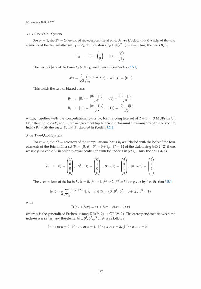
Mathematics 2018, 6, 273
3.5.3. One-Qubit System
For m = 1, the 2m = 2 vectors of the computational basis B2 are labeled with the help of the twoelements of the Teichmüller set T1 = Z2 of the Galois ring GR(22, 1) = Z22 . Thus, the basis B2 is
B2 : |0〉 =(
10
), |1〉 =
(01
)
The vectors |aα〉 of the basis Ba (a ∈ T1) are given by (see Section 3.5.1)
|aα〉 = 1√2
1
∑x=0
i(a+2α)x|x〉, α ∈ T1 = {0, 1}
This yields the two unbiased bases
B0 : |00〉 = |0〉+ |1〉√2
, |01〉 = |0〉 − |1〉√2
B1 : |10〉 = |0〉+ i|1〉√2
, |11〉 = |0〉 − i|1〉√2
which, together with the computational basis B2, form a complete set of 2 + 1 = 3 MUBs in C2.Note that the bases B0 and B1 are in agreement (up to phase factors and a rearrangement of the vectorsinside B1) with the bases B0 and B1 derived in Section 3.2.4.
3.5.4. Two-Qubit System
For m = 2, the 2m = 4 vectors of the computational basis B4 are labeled with the help of the fourelements of the Teichmüller set T2 = {0, β1, β2 = 3 + 3β, β3 = 1} of the Galois ring GR(22, 2) (here,we use β instead of α in order to avoid confusion with the index α in |aα〉). Thus, the basis B4 is
B4 : |0〉 =
⎛⎜⎜⎜⎝1000
⎞⎟⎟⎟⎠ , |β1 or 1〉 =
⎛⎜⎜⎜⎝0100
⎞⎟⎟⎟⎠ , |β2 or 2〉 =
⎛⎜⎜⎜⎝0010
⎞⎟⎟⎟⎠ , |β3 or 3〉 =
⎛⎜⎜⎜⎝0001
⎞⎟⎟⎟⎠The vectors |aα〉 of the basis Ba (a = 0, β1 or 1, β2 or 2, β3 or 3) are given by (see Section 3.5.1)
|aα〉 = 12 ∑
x∈T2
iTr(ax+2αx)|x〉, α ∈ T2 = {0, β1, β2 = 3 + 3β, β3 = 1}
withTr(ax + 2αx) = ax + 2αx + φ(ax + 2αx)
where φ is the generalized Frobenius map GR(22, 2)→ GR(22, 2). The correspondence between theindexes a, α in |aα〉 and the elements 0, β1, β2, β3 of T2 is as follows
0 ↔ a or α = 0, β1 ↔ a or α = 1, β2 ↔ a or α = 2, β3 ↔ a or α = 3
142
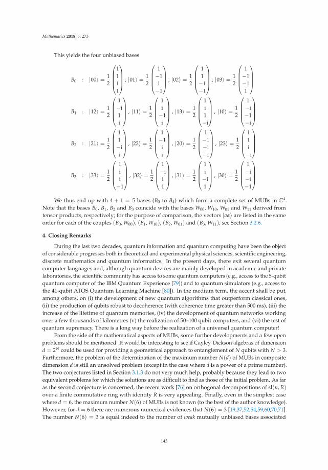
Mathematics 2018, 6, 273
This yields the four unbiased bases
B0 : |00〉 = 12
⎛⎜⎜⎜⎝1111
⎞⎟⎟⎟⎠ , |01〉 = 12
⎛⎜⎜⎜⎝1−11−1
⎞⎟⎟⎟⎠ , |02〉 = 12
⎛⎜⎜⎜⎝11−1−1
⎞⎟⎟⎟⎠ , |03〉 = 12
⎛⎜⎜⎜⎝1−1−11
⎞⎟⎟⎟⎠
B1 : |12〉 = 12
⎛⎜⎜⎜⎝1−i1i
⎞⎟⎟⎟⎠ , |11〉 = 12
⎛⎜⎜⎜⎝1i−1
i
⎞⎟⎟⎟⎠ , |13〉 = 12
⎛⎜⎜⎜⎝1i1−i
⎞⎟⎟⎟⎠ , |10〉 = 12
⎛⎜⎜⎜⎝1−i−1−i
⎞⎟⎟⎟⎠
B2 : |21〉 = 12
⎛⎜⎜⎜⎝11−ii
⎞⎟⎟⎟⎠ , |22〉 = 12
⎛⎜⎜⎜⎝1−1
ii
⎞⎟⎟⎟⎠ , |20〉 = 12
⎛⎜⎜⎜⎝1−1−i−i
⎞⎟⎟⎟⎠ , |23〉 = 12
⎛⎜⎜⎜⎝11i−i
⎞⎟⎟⎟⎠
B3 : |33〉 = 12
⎛⎜⎜⎜⎝1ii−1
⎞⎟⎟⎟⎠ , |32〉 = 12
⎛⎜⎜⎜⎝1−ii1
⎞⎟⎟⎟⎠ , |31〉 = 12
⎛⎜⎜⎜⎝1i−i1
⎞⎟⎟⎟⎠ , |30〉 = 12
⎛⎜⎜⎜⎝1−i−i−1
⎞⎟⎟⎟⎠We thus end up with 4 + 1 = 5 bases (B0 to B4) which form a complete set of MUBs in C4.
Note that the bases B0, B1, B2 and B3 coincide with the bases W00, W10, W01 and W11 derived fromtensor products, respectively; for the purpose of comparison, the vectors |aα〉 are listed in the sameorder for each of the couples (B0, W00), (B1, W10), (B2, W01) and (B3, W11), see Section 3.2.6.
4. Closing Remarks
During the last two decades, quantum information and quantum computing have been the objectof considerable progresses both in theoretical and experimental physical sciences, scientific engineering,discrete mathematics and quantum informatics. In the present days, there exit several quantumcomputer languages and, although quantum devices are mainly developed in academic and privatelaboratories, the scientific community has access to some quantum computers (e.g., access to the 5-qubitquantum computer of the IBM Quantum Experience [79]) and to quantum simulators (e.g., access tothe 41-qubit ATOS Quantum Learning Machine [80]). In the medium term, the accent shall be put,among others, on (i) the development of new quantum algorithms that outperform classical ones,(ii) the production of qubits robust to decoherence (with coherence time greater than 500 ms), (iii) theincrease of the lifetime of quantum memories, (iv) the development of quantum networks workingover a few thousands of kilometres (v) the realization of 50–100 qubit computers, and (vi) the test ofquantum supremacy. There is a long way before the realization of a universal quantum computer!
From the side of the mathematical aspects of MUBs, some further developments and a few openproblems should be mentioned. It would be interesting to see if Cayley-Dickson algebras of dimensiond = 2N could be used for providing a geometrical approach to entanglement of N qubits with N > 3.Furthermore, the problem of the determination of the maximum number N(d) of MUBs in compositedimension d is still an unsolved problem (except in the case where d is a power of a prime number).The two conjectures listed in Section 3.1.3 do not very much help, probably because they lead to twoequivalent problems for which the solutions are as difficult to find as those of the initial problem. As faras the second conjecture is concerned, the recent work [76] on orthogonal decompositions of sl(n, R)over a finite commutative ring with identity R is very appealing. Finally, even in the simplest casewhere d = 6, the maximum number N(6) of MUBs is not known (to the best of the author knowledge).However, for d = 6 there are numerous numerical evidences that N(6) = 3 [19,37,52,54,59,60,70,71].The number N(6) = 3 is equal indeed to the number of weak mutually unbiased bases associated
143
Mathematics 2018, 6, 273
with the smallest prime divisor of 6 (the recently introduced notion of weak MUBs in dimension dcorresponds to the Definition (14) where
√d is replaced by
√f where f is a prime divisor of d [69,75]).
Author Contributions: The author confirms to be the sole contributor of this paper.
Acknowledgments: This paper was presented at the 20th International Workshop on Computer Algebra inScientific Computing (CASC 2018). The author wishes to thank Vladimir P. Gerdt (Dubna) for his kind invitationto give an invited talk at CASC 2018 and Andreas Weber (Bonn) for his encouragement to put the text of the talkin a form convenient for a community of computer engineers and mathematicians. He is also indebted to WolframKoepf (Kassel) and François Boulier (Lille) for their logistic help during the preparation of this paper. Finally,the author thanks the Referees for their remarks and suggestions.
Conflicts of Interest: The author declares no conflict of interest.
References
1. Nielsen, M.A.; Chuang, I.L. Quantum Computation and Quantum Information; Cambridge University Press:Cambridge, UK, 2003.
2. Kibler, M.R. Galois Fields and Galois Rings Made Easy; ISTE Press–Elsevier: London/Oxford, UK, 2017.3. Weyl, H. The Theory of Groups and Quantum Mechanics; Dover Publications: New York, NY, USA, 1931.4. Weil, A. On some exponential sums. Proc. Natl. Acad. Sci. USA 1948, 34, 204–207. [CrossRef] [PubMed]5. Schwinger, J. Unitary operator bases. Proc. Natl. Acad. Sci. USA 1960, 46, 570–579. [CrossRef] [PubMed]6. Ivanovic, I.D. Geometrical description of quantal state determination. J. Phys. A Math. Gen. 1981, 14,
3241–3245. [CrossRef]7. Kostrikin, A.I.; Kostrikin, I.A.; Ufnarovskiı, V.A. Orthogonal decompositions of simple Lie algebras (type An).
Trudy Mat. Inst. Steklov 1981, 158, 105–120. (In Russian)8. Wootters, W.K.; Zurek, W.H. A single quantum cannot be cloned. Nature 1982, 299, 802. [CrossRef]9. Bennett, C.H.; Brassard, G. Quantum cryptography: Public key distribution and coin tossing. In Proceedings
of the IEEE International Conference on Computers, Systems, and Signal Processing, Bangalore, India,10–12 December 1984; pp. 175–179.
10. Wootters, W.K. Quantum mechanics without probability amplitudes. Found. Phys. 1986, 16, 391–405.[CrossRef]
11. Wootters, W.K. A Wigner function formulation of finite-state quantum mechanics. Ann. Phys. (N. Y.) 1987,176, 1–21. [CrossRef]
12. Patera, J.; Zassenhaus, H. The Pauli matrices in n dimensions and finest gradings of simple Lie algebras oftype An−1. J. Math. Phys. 1988, 29, 665–673. [CrossRef]
13. Lambert, D.; Kibler, M. An algebraic and geometric approach to non-bijective quadratic transformations.J. Phys. A Math. Gen. 1988, 21, 307–343. [CrossRef]
14. Wootters, W.K.; Fields, B.D. Optimal state-determination by mutually unbiased measurements. Ann. Phys.(N. Y.) 1989, 191, 363–381. [CrossRef]
15. Bennett, C.H.; Brassard, G.; Crépeau, C.; Jozsa, R.; Peres, A.; Wootters, W.K. Teleporting an unknownquantum state via dual classical and Einstein-Podolsky-Rosen channels. Phys. Rev. Lett. 1993, 70, 1895.[CrossRef] [PubMed]
16. Kostrikin, A.I.; Tiep, P.H. Orthogonal Decompositions and Integral Lattices; Walter de Gruyter: Berlin,Germany, 1994.
17. Calderbank, A.R.; Cameron, P.J.; Kantor, W.M.; Seidel, J.J. Z4–Kerdock codes, orthogonal spreads,and extremal Euclidean line-sets. Proc. Lond. Math. Soc. 1997, 75, 436–480. [CrossRef]
18. Berndt, B.C.; Evans, R.J.; Williams, K.S. Gauss and Jacobi Sums; Wiley: New York, NY, USA, 1998.19. Zauner, G. Quantendesigns: Grundzüge einer Nichtcommutativen Designtheorie. Bachelor’s Thesis,
University of Wien, Wien, Austria, 1999.20. Englert, B.-G.; Aharonov, Y. The mean king’s problem: Prime degrees of freedom. Phys. Lett. A 2001, 284, 1–5.
[CrossRef]21. Mosseri, R.; Dandoloff, R. Geometry of entangled states, Bloch spheres and Hopf fibrations. J. Phys. A
Math. Gen. 2001, 34, 10243–10252. [CrossRef]22. Bandyopadhyay, S.; Boykin, P.O.; Roychowdhury, V.; Vatan, F. A new proof for the existence of mutually
unbiased bases. Algorithmica 2002, 34, 512–528.
144
Mathematics 2018, 6, 273
23. Lawrence, J.; Brukner, C.; Zeilinger, A. Mutually unbiased binary observable sets on N qubits. Phys. Rev. A2002, 65, 032320. [CrossRef]
24. Chaturvedi, S. Aspects of mutually unbiased bases in odd prime power dimensions. Phys. Rev. A 2002,65, 044301. [CrossRef]
25. Cerf, N.J.; Bourennane, M.; Karlsson, A.; Gisin, N. Security of quantum key distribution using d-levelsystems. Phys. Rev. Lett. 2002, 88, 127902. [CrossRef] [PubMed]
26. Aravind, P.K. Solution to the King’s problem in prime power dimensions. Z. Naturforsch. 2003, 58, 85–92.[CrossRef]
27. Lawrence, J. Mutually unbiased bases and trinary operator sets for N qutrits. Phys. Rev. A 2004, 70, 012302.[CrossRef]
28. Klappenecker, A.; Rötteler, M. Constructions of mutually unbiased bases. Lect. Notes Comput. Sci. 2004, 2948,137–144.
29. Gibbons, K.S.; Hoffman, M.J.; Wootters, W.K. Discrete phase space based on finite fields. Phys. Rev. A 2004,70, 062101. [CrossRef]
30. Pittenger, A.O.; Rubin, M.H. Mutually unbiased bases, generalized spin matrices and separability.Linear Algebr. Appl. 2004, 390, 255–278. [CrossRef]
31. Vourdas, A. Quantum systems with finite Hilbert space. Rep. Prog. Phys. 2004, 67, 267–320. [CrossRef]32. Saniga, M.; Planat, M.; Rosu, H. Mutually unbiased bases and finite projective planes. J. Opt. B Quantum
Semiclass. Opt. 2004, 6, L19–L20. [CrossRef]33. Hayashi, A.; Horibe, M.; Hashimoto, T. Mean king’s problem with mutually unbiased bases and orthogonal
Latin squares. Phys. Rev. A 2005, 71, 052331. [CrossRef]34. Paz, J.P.; Roncaglia, A.J.; Saraceno, M. Qubits in phase space: Wigner-function approach to quantum-error
correction and the mean-king problem. Phys. Rev. A 2005, 72, 012309. [CrossRef]35. Wocjan, P.; Beth, T. New construction of mutually unbiased bases in square dimensions.
Quantum Inf. Comput. 2005, 5, 93–101.36. Archer, C. There is no generalization of known formulas for mutually unbiased bases. J. Math. Phys. 2005,
46, 022106. [CrossRef]37. Grassl, M. On SIC-POVMs and MUBs in dimension 6. In Proceedings of the ERATO Conference on Quantum
Information Science (EQIS’04), Tokyo, Japan, 1–5 September 2004; pp. 60–61.38. Grassl, M. Tomography of quantum states in small dimensions. Electron. Notes Discret. Math. 2005, 20,
151–164. [CrossRef]39. Klappenecker, A.; Rötteler, M. Mutually unbiased bases are complex projective 2-designs. In Proceedings of
the 2005 IEEE International Symposium on Information Theory, Adelaide, Australia, 4–9 September 2005;pp. 1740–1744.
40. Bengtsson, I.; Ericsson, A.A. Mutually unbiased bases and the complementary polytope. Open Syst. Inf. Dyn.2005, 12, 107–120. [CrossRef]
41. Durt, T. About mutually unbiased bases in even and odd prime power dimensions. J. Phys. A Math. Gen.2005, 38, 5267–5283. [CrossRef]
42. Pittenger, A.O.; Rubin, M.H. Wigner functions and separability for finite systems. J. Phys. A Math. Gen. 2005,38, 6005–6036. [CrossRef]
43. Durt, T. About the Mean King’s problem and discrete Wigner distributions. Int. J. Mod. Phys. B 2006, 20,1742–1760. [CrossRef]
44. Kibler, M.R. Angular momentum and mutually unbiased bases. Int. J. Mod. Phys. B 2006, 20, 1792–1801.[CrossRef]
45. Kibler, M.R.; Planat, M. A SU(2) recipe for mutually unbiased bases. Int. J. Mod. Phys. B 2006, 20, 1802–1807.[CrossRef]
46. Vourdas, A. Galois quantum systems, irreducible polynomials and Riemann surfaces. J. Math. Phys. 2006,47, 092104. [CrossRef]
47. Heath, R.W.; Strohmer, T.; Paulraj, A.J. On quasi-orthogonal signatures for CDMA systems. IEEE Trans.Inf. Theory 2006, 52, 1217–1226. [CrossRef]
48. Vourdas, A. Quantum systems in finite Hilbert space: Galois fields in quantum mechanics. J. Phys. AMath. Theor. 2007, 40, R285–R331. [CrossRef]
145
Mathematics 2018, 6, 273
49. Klimov, A.B.; Romero, J.L.; Björk, G.; Sánchez-Soto, L.L. Geometrical approach to mutually unbiased bases.J. Phys. A Math. Theor. 2007, 40, 3987–3998. [CrossRef]
50. Šulc, P.; Tolar, J. Group theoretical construction of mutually unbiased bases in Hilbert spaces of primedimensions. J. Phys. A Math. Theor. 2007, 40, 15099. [CrossRef]
51. Aschbacher, M.; Childs, A.M.; Wocjan, P. The limitations of nice mutually unbiased bases. J. Algebr. Comb.2007, 25, 111–123. [CrossRef]
52. Bengtsson, I.; Bruzda, W.; Ericsson, A.A.; Larsson, J.-A.A.; Tadej, W.; Zyczkowski, K. Mutually unbiasedbases and Hadamard matrices of order six. J. Math. Phys. 2007, 48, 052106. [CrossRef]
53. Boykin, P.O.; Sitharam, M.; Tiep, P.H.; Wocjan, P. Mutually unbiased bases and orthogonal decompositionsof Lie algebras. Quantum Inf. Comput. 2007, 7, 371–382.
54. Butterley, P.; Hall, W. Numerical evidence for the maximum number of mutually unbiased bases in dimensionsix. Phys. Lett. A 2007, 369, 5–8. [CrossRef]
55. Björk, G.; Romero, J.L.; Klimov, A.B.; Sánchez-Soto, L.L. Mutually unbiased bases and discrete Wignerfunctions. J. Opt. Soc. Am. B 2007, 24, 371–378. [CrossRef]
56. Klimov, A.B.; Muñoz, C.; Fernández, A.; Saavedra, C. Optimal quantum-state reconstruction for cold trappedions. Phys. Rev. A 2008, 77, 060303(R). [CrossRef]
57. Svetlichny, G. Feynman’s integral is about mutually unbiased bases. arXiv 2008, arXiv:0708.3079v3.58. Kibler, M.R. Variations on a theme of Heisenberg, Pauli and Weyl. J. Phys. A Math. Theor. 2008, 41, 375302.
[CrossRef]59. Brierley, S.; Weigert, S. Maximal sets of mutually unbiased quantum states in dimension six. Phys. Rev. A
2008, 78, 042312. [CrossRef]60. Brierley, S.; Weigert, S. Constructing mutually unbiased bases in dimension six. Phys. Rev. A 2009, 79, 052316.
[CrossRef]61. Appleby, D.M. SIC-POVMS and MUBS: Geometrical relationships in prime dimension. In Proceedings
of the AIP Conference, Foundations of Probability and Physics-5, San Diego, CA, USA, 26–31 May 2009;Volume 1101, pp. 223–232.
62. Albouy, O. The isotropic lines of Z2d. J. Phys. A Math. Theor. 2009, 42, 072001. [CrossRef]
63. Tolar, J.; Chadzitaskos, G. Feynman’s path integral and mutually unbiased bases. J. Phys. A Math. Theor.2009, 42, 245306. [CrossRef]
64. Kibler, M.R. An angular momentum approach to quadratic Fourier transform, Hadamard matrices,Gauss sums, mutually unbiased bases, the unitary group and the Pauli group. J. Phys. A Math. Theor.2009, 42, 353001. [CrossRef]
65. Durt, T.; Englert, B.-G.; Bengtsson, I.; Zyczkowski, K. On mutually unbiased bases. Int. J. Quantum Inf. 2010,8, 535–640. [CrossRef]
66. Dita, P. Hadamard matrices from mutually unbiased bases. J. Math. Phys. 2010, 51, 072202. [CrossRef]67. Zauner, G. Quantum designs: Foundations of a noncommutative design theory. Int. J. Quantum Inf. 2011, 9,
445–507. [CrossRef]68. Daoud, M.; Kibler, M.R. Phase operators, phase states and vector phase states for SU3 and SU2,1.
J. Math. Phys. 2011, 52, 082101. [CrossRef]69. Shalaby, M.; Vourdas, A. Weak mutually unbiased bases. J. Phys. A Math. Theor. 2012, 45, 052001. [CrossRef]70. McNulty, D.; Weigert, S. The limited role of mutually unbiased product bases in dimension six. J. Phys. A
Math. Theor. 2012, 45, 102001. [CrossRef]71. McNulty, D.; Weigert, S. All mutually unbiased product bases in dimension six. J. Phys. A Math. Theor. 2012,
45, 135307. [CrossRef]72. Ghiu, I. Generation of all sets of mutually unbiased bases for three-qubit systems. Phys. Scr. 2013, 153, 014027.
[CrossRef]73. Goyeneche, D. Mutually unbiased triplets from non-affine families of complex Hadamard matrices in
dimension 6. J. Phys. A Math. Theor. 2013, 46, 105301. [CrossRef]74. Spengler, C.; Kraus, B. Graph-state formalism for mutually unbiased bases. Phys. Rev. A 2013, 88, 052323.
[CrossRef]75. Olupitan, T.; Lei, C.; Vourdas, A. An analytic function approach to weak mutually unbiased bases. Ann. Phys.
(N. Y.) 2016, 371, 1–19. [CrossRef]
146
Mathematics 2018, 6, 273
76. Sriwongsa, S.; Zou, Y.M. Orthogonal abelian Cartan subalgebra decomposition of sln over a finitecommutative ring. Linear Multilinear Algebra 2018. [CrossRef]
77. Rao, H.S.S.; Sirsi, S.; Bharath, K. Mutually disjoint, maximally commuting set of physical observables foroptimum state determination. arXiv 2018, arXiv:1809.06762.
78. Trifa, Y. Utilisation et construction de bases mutuellement non biaisées en théorie de l’information quantique.In Rapport de Stage, IPN Lyon—ENS Lyon; IPN: Lyon, France; ENS: Lyon, France, 2018.
79. IBM Quantum Experience. Available online: https://quantumexperience.ng.bluemix.net/qx/experience(accessed on 21 November 2018).
80. ATOS Quantum Learning Machine. Available online: https://atos.net/en/insights-and-innovation/quantum-computing/atos-quantum (accessed on 21 November 2018).
c© 2018 by the author. Licensee MDPI, Basel, Switzerland. This article is an open accessarticle distributed under the terms and conditions of the Creative Commons Attribution(CC BY) license (http://creativecommons.org/licenses/by/4.0/).
147


MDPISt. Alban-Anlage 66
4052 BaselSwitzerland
Tel. +41 61 683 77 34Fax +41 61 302 89 18
www.mdpi.com
Mathematics Editorial OfficeE-mail: [email protected]
www.mdpi.com/journal/mathematics


MDPI St. Alban-Anlage 66 4052 Basel Switzerland
Tel: +41 61 683 77 34 Fax: +41 61 302 89 18
www.mdpi.com ISBN 978-3-03921-731-1