Computer Algebra - with a View Toward Reliable NumericComputation

Michael Sagraloff

December 22, 2017

Contents

1 Basic Arithmetic 221.1 The School Method for Integer Multiplication . . . . . . . . . . . . . . . . . . . 221.2 The Toom-Cook Algorithm . . . . . . . . . . . . . . . . . . . . . . . . . . . . . 551.3 Approximate Computation . . . . . . . . . . . . . . . . . . . . . . . . . . . . . . 1010

1.3.1 Fixed Point Arithmetic . . . . . . . . . . . . . . . . . . . . . . . . . . . 10101.3.2 Interval Arithmetic . . . . . . . . . . . . . . . . . . . . . . . . . . . . . . 12121.3.3 Floating point arithmetic (Under construction) . . . . . . . . . . . . . . 1515

1.4 Division . . . . . . . . . . . . . . . . . . . . . . . . . . . . . . . . . . . . . . . . 1818

2 The Fast Fourier Transform and Fast Polynomial Arithmetic 22222.1 Schönhage-Strassen Multiplication . . . . . . . . . . . . . . . . . . . . . . . . . 2222

2.1.1 The Algorithm in a Nutshell . . . . . . . . . . . . . . . . . . . . . . . . . 22222.1.2 Fast Fourier Transform . . . . . . . . . . . . . . . . . . . . . . . . . . . . 24242.1.3 Fast Multiplication in Z and Z[x]. . . . . . . . . . . . . . . . . . . . . . 29292.1.4 Fast Multiplication over arbitrary Rings? . . . . . . . . . . . . . . . . . 3333

2.2 Fast Polynomial Division and Applications . . . . . . . . . . . . . . . . . . . . . 35352.3 Fast Polynomial Arithmetic in C[x] . . . . . . . . . . . . . . . . . . . . . . . . . 4141

3 The Extended Euclidean Algorithm and (Sub-) Resultants 45453.1 Gauss’ Lemma . . . . . . . . . . . . . . . . . . . . . . . . . . . . . . . . . . . . 45453.2 The Extended Euclidean Algorithm . . . . . . . . . . . . . . . . . . . . . . . . . 50503.3 The Half-GCD Algorithm (under construction) . . . . . . . . . . . . . . . . . . 55553.4 The Resultant . . . . . . . . . . . . . . . . . . . . . . . . . . . . . . . . . . . . . 56563.5 Subresultants . . . . . . . . . . . . . . . . . . . . . . . . . . . . . . . . . . . . . 6464

1

Chapter 1

Basic Arithmetic

In this section, we present an efficient algorithm due to Toom and Cook for multiplying twointegers, which already considerably improves upon the method that most people have learnedin school. We further investigate in methods for carrying out approximate computations onfixed-point and floating-point numbers, and we derive bounds on the occurring error whenusing approximate instead of exact arithmetic. In addition, we introduce the concepts ofinterval arithmetic and box-functions and show that these concepts yield a powerful andvery practical approach for carrying out approximate arithmetic. This is due to the fact thatadaptive bounds on the error can directly be computed "on the fly", and that these bounds areoften much better than any a priori bounds obtained by a worst-case error analysis. Finally,we give an efficient method to compute an arbitrary good approximation of the quotient oftwo integers or, more generally, two arbitrary complex values.

1.1 The School Method for Integer Multiplication

We represent integers a ∈ Z as digit strings with respect to a fixed base B ∈ N≥2. That is,

a = (−1)s ·n−1∑i=0

ai ·Bi, with s ∈ 0, 1 and ai ∈ 0, . . . , B − 1 for all i = 0, . . . , n− 1.

We call the ai’s the digits and s the sign digit of a with respect to B. For convenience, wealso write (if B is fixed)

a = (−1)s an−1an−2 . . . a0

if the base B is fixed.

Example: Important bases are B = 2, 10, 16, and 2k for some k ∈ N. The integer 29 writesas

29 = 1 · 20 + 0 · 21 + 1 · 22 + 1 · 23 + 1 · 24 = 11101.

The length (or bitsize for B = 2) of an integer a with respect to B is defined as the number ofdigits needed to represent a. For convenience, we use the term n-digit number to denote aninteger of length n. Notice that any n-digit number can always be considered as an N -digitnumber for arbitrary N ≥ n. This is advantageous in the analysis of many algorithms as itallows us to assume that the length of the input is a power of 2 (or some other value k).

2

Algorithm 1: School Method for AdditionInput : Two non-negative n-digit integers a = an−1 . . . a0 and b = bn−1 . . . b0.Output: An (n+ 1)-digit integer c = cn . . . c0 with c = a+ b.

1 γ0 := 02 for i = 0, . . . , n− 1 do3 Recursively define4 γi+1 ·B + ci = ai + bi + γi with ci, γi ∈ 0, . . . , B − 15 cn := γn6 return cn . . . c0

We mainly consider two different ways of measuring the efficiency of an algorithm. Thefirst one is to count the number of additions and multiplications between integers that analgorithm needs to return a result. This is referred to as the arithmetic complexity of an algo-rithm. Notice that the arithmetic complexity might be unrelated to the actual running timeof an algorithm as the involved integers can be arbitrarily large. Hence, a more meaningfuland precise way of measuring the efficiency of an algorithm is to count instead the numberof primitive operations (or bit operations if the base B equals 2) that are carried out by thealgorithm, often referred to as the bit complexity of an algorithm. Notice that the result of aprimitive operations is always a one- or two-digit number.

Example: A prominent example is Gaussian elimination for solving a linear system in nunknowns. It is easy to see that the method uses O(n3) arithmetic operations, hence thearithmetic complexity of Gaussian elimination is polynomial in the input size. However, astraight forward analysis does NOT guarantee that the intermediate results as computed bythe algorithm (which are rationals if the input matrix has integer entries) have size that ispolynomial in the size of the input, thus it is not obvious that Gaussian elimination actuallyconstitutes a polynomial time algorithm for solving linear systems. A more refined argumenthowever shows that by recursively removing common factors of the intermediate results, it canbe guaranteed that all intermediate results have polynomial size. We will go into more detailin one of the exercises. Later, we will also consider a different approach based on modularcomputation that does not come with any of these drawbacks.

We now review and analyze the school method for adding and multiplying two non-negativen-digit integers a = an−1 . . . a0 and b = bn−1 . . . b0. We first start with addition; see Algo-rithm 11. The γi’s are called carries. Using induction, it is easy to see that γi ∈ 0, 1 for alli. Further notice that γi+1 is non-zero if and only if the sum of the two digits ai and bi andthe previous carry γi is larger than the base B. We also remark that, for subtraction (i.e. thecomputation of a − b), we can assume that a ≥ b. The recursion for ci and γ is then almostidentical. More specifically, we have

−γi+1 ·B + ci = ai − bi − γi with ci, γi ∈ 0, . . . , B − 1.

The proof of the following theorem is straight-forward.

Theorem 1.1.1. The school method for adding (or subtracting) two n−digit numbers requiresat most 2n primitive operations. The addition of an m-digit number and an n-digit numberuses at most m+ n+ 2 primitive operations.

3

Algorithm 2: School Method for MultiplicationInput : Two non-negative n-digit integers a = an−1 . . . a0 and b = bn−1 . . . b0.Output: A 2n-digit integer c = c2n−1 . . . c0 with c = a · b.

1 P0 := 02 for j = 0, . . . , n− 1 do3 for i = 0, . . . , n− 1 do4 Define5 ai · bj = cij ·B + dij with cij , dij ∈ 0, . . . , B − 16 cj := cn−1,j . . . c0,j07 dj := dn−1,j . . . , d0,j

8 pj = pn,j . . . p0,j := cj + dj

// * Notice that pj = a · bj, and thus a · b =∑n−1

j=0 pj ·Bj *//9 Pj+1 := Pj + pj ·B

10 return Pn

In the next step, we consider the school method for multiplying integers; see Algorithm 22.Let us count the number of primitive operations that Algorithm 22 needs:

• The computation of each product ai · bj requires one primitive operations, thus n2 manyprimitive operations in total.

• Computing each of the integers pj amounts for adding two (n+1)-digit numbers. Hence,in total, we need 2n(n+ 1) primitive operations.

• For computing Pn we need n additions each involving 2n-digit numbers. Thus, we need2n2 many primitive operations for this step.

We now obtain the following result. For the second claim on the complexity of computingthe product of an m-digit number and an n-digit number, a completely analogous argumentapplies.

Theorem 1.1.2. Using the school method, we need at most 5n2 + 2n = O(n2) primitiveoperations to multiply two n-digit numbers. Multiplication of an n-digit number and an m-digit number needs O(mn) primitive operations.

Exercise 1.1.3. Let f = a0 + · · · + ad · xd ∈ Z[x] be a polynomial of degree d with integercoefficients of length at most L, and let m ∈ Z be an `-digit number. Show that

(a) f(m) is a O(d`+ L)-digit number.

(b) Computing f(m) using Horner’s method

f(m) = a0 +m · (a1 +m · (a2 + · · ·m · (ad−1 +m · ad))

and the school method for multiplication uses O(d · (d`2 + ` · L))) primitive operations.

We will later see that it is even possible to compute f(m) in only O(d · (`+ L)) primitiveoperations, where O(.) means that poly-logarithmic factors are suppressed, that is, O(T ) =O(T · (log T )c) for some constant c. For the special case, where f has only a few non-zerocoefficients, f(m) can be evaluated in a faster manner via repeated squaring :

4

Exercise 1.1.4 (Sparse Polynomial Evaluation). Let f =∑k

j=1 aij · xij ∈ R[x] be a so-calledsparse polynomial (also k-nomial) of degree n with k non-zero coefficients and m ∈ R be anarbitrary real value. Show that f(m) can be computed using O(k · log n) arithmetic operations.

Hint: Show the claim for a single monomial xn first. For this, use repeated squaring

xn =

dlogne∏i=0

x[ni·i],

to compute xn, where n =∑dlogne

i=0 ni · 2i, with ni ∈ 0, 1, is the binary representation of nand x[j] is recursively defined as

x[0] := 1, x[1] := x, and x[i] :=(x[i−1]

)2for i ≥ 2.

Exercise 1.1.5. Let A = (ai,j)i,j=1,...,n ∈ Zn×n be an n×n-matrix with integer entries ai,j oflength at most L.

(a) Derive an upper bound on the number of primitive operations that are needed to computethe inverse A−1 of A.

(b) Show that the entries of A−1 are rational numbers with numerators and denominatorsof length O(n(L+ log n)).

(c∗) Suppose that Gaussian elimination with pivoting is used to compute the determinant ofA. Further suppose that, after each iteration, we reduce all intermediate entries a′i,j =pq ∈ Q, that is, we ensure that gcd(p, q) = 1. Show that p and q can be represented usingO(n2(L+ log n)) digits and conclude that Gaussian elimination constitutes a polynomialtime algorithm for computing determinants.

Hints: For (a), consider Gaussian elimination to compute A−1 and derive a bound on thenumerators and denominators of the rational entries of the matrices produced after eachiteration. For (b), use Cramer’s Rule to write the entries of A−1 as fractions of determinantsof suitable n× n-matrices and use the definition of the determinant to bound the size of thenumerator and denominator. For (c), show that, in each iteration, the pivot element can bewritten as the quotient of the determinants of two sub-matrices of A.

1.2 The Toom-Cook Algorithm

We now investigate in algorithms for multiplying integers that are considerably faster thanthe school method. We start with a simple algorithm due to Karatsuba [AY62AY62] (from 1960).Its running time O(nlog2 3) already constitutes a considerable improvement upon the runningtime O(n2) of the school method. Then, we show how to generalize the approach to achievea running time O(n1+ε) for arbitrary ε > 0.

Let a = an−1 . . . a0 and b = bn−1 . . . b0 be integers of length n. We first write

a = an−1 . . . a0 = a′ ·Bdn/2e + a′′, and

b = bn−1 . . . b0 = b′ ·Bdn/2e + b′′,

5

Algorithm 3: Karatsuba Multiplication (1960)Input : Two non-negative n-digit integers a = an−1 . . . a0 and b = bn−1 . . . b0.Output: A 2n-digit integer c = c2n−1 . . . c0 with c = a · b.

1 if n ≤ 4 then2 Compute c = a · b using Algorithm 22

3 else4 Define

a = an−1 . . . a0 = a′ ·Bdn/2e + a′′, and

b = bn−1 . . . b0 = b′ ·Bdn/2e + b′′,

with integers a′, a′′, b′, b′′ of length n/2.5 A := a′ + a′′

6 B := b′ + b′′

7 Compute P1 := a′ · b′, P2 := A ·B, and P3 := a′′ · b′′ by recursively callingAlgorithm 33.

8 P := P1 ·B2dn/2e + (P2 − P1 − P3) ·Bdn/2e + P3

9 return P

with integers a′, a′′, b′, b′′ of length dn/2e. Then, it holds that

a · b = (a′ ·Bdn/2e + a′′) · (b′ ·Bdn/2e + b′′)

= a′b′ ·B2dn/2e + (a′b′′ + a′′ · b′) ·Bdn/2e + a′′b′′

= a′b′︸︷︷︸=:P1

·B2dn/2e + [(a′ + a′′)(b′ + b′′)︸ ︷︷ ︸=:P2

−(a′b′ + a′′b′′)] ·Bdn/2e + a′′b′′︸︷︷︸=:P3

(1.1)

What have we gained in the last step? They crucial point is that, when passing from thesecond line to the last line, we reduced the problem to three (instead of four!) multiplica-tions and six (instead of three) additions. Notice that there are actually five multiplications,however, each of the products P1 and P2 appears twice, and thus only 3 different productsneed to be computed. So the total number of additions and multiplication has increased,however, additions are much cheaper than multiplications. We can now recursively use theabove approach for multiplication until all remaining multiplications are numbers with fouror less digits; see Algorithm 33

Theorem 1.2.1. Using Karatsuba multiplication, we need O(nlog 3) = O(n1.58...) primitiveoperations to multiply two n-digit numbers.

Proof. Let T (n) denote the maximal number of operations needed to multiply two n-digitnumbers using the Karatsuba algorithm. If n ≤ 4, Theorem 1.1.21.1.2 yields that T (n) ≤ 5n2 +2n ≤ 88. For n ≥ 5, it holds that

T (n) ≤ 3 · T (dn/2e+ 1) + 6 · (4n).

as we need to compute 3 products involving dn/2e- or (dn/2e+1)-digit numbers and 6 additionsinvolving 2n-digit numbers. Now, a general version of the Master Theorem (e.g. see [MS08MS08,Sec. 2.6]) yields a total running time of size O(nlog2 3).

6

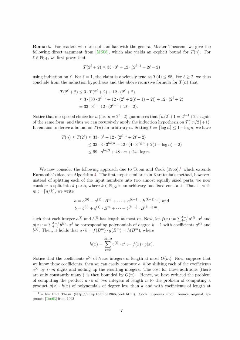
Remark. For readers who are not familiar with the general Master Theorem, we give thefollowing direct argument from [MS08MS08], which also yields an explicit bound for T (n). For` ∈ N≥1, we first prove that

T (2` + 2) ≤ 33 · 3` + 12 · (2`+1 + 2`− 2)

using induction on `. For ` = 1, the claim is obviously true as T (4) ≤ 88. For ` ≥ 2, we thusconclude from the induction hypothesis and the above recursive formula for T (n) that

T (2` + 2) ≤ 3 · T (2` + 2) + 12 · (2` + 2)

≤ 3 · [33 · 3`−1 + 12 · (2` + 2(`− 1)− 2)] + 12 · (2` + 2)

= 33 · 3` + 12 · (2`+1 + 2`− 2).

Notice that our special choice for n (i.e. n = 2`+2) guarantees that dn/2e+1 = 2`−1+2 is againof the same form, and thus we can recursively apply the induction hypothesis on T (dn/2e+1).It remains to derive a bound on T (n) for arbitrary n. Setting ` := dlog ne ≤ 1+log n, we have

T (n) ≤ T (2`) ≤ 33 · 3` + 12 · (2`+1 + 2`− 2)

≤ 33 · 3 · 3logn + 12 · (4 · 3logn + 2(1 + log n)− 2)

≤ 99 · nlog 3 + 48 · ·n+ 24 · log n.

We now consider the following approach due to Toom and Cook (1966),11 which extendsKaratsuba’s idea; see Algorithm 44. The first step is similar as in Karatsuba’s method, however,instead of splitting each of the input numbers into two almost equally sized parts, we nowconsider a split into k parts, where k ∈ N≥2 is an arbitrary but fixed constant. That is, withm := dn/ke, we write

a = a(0) + a(1) ·Bm + · · ·+ a(k−1) ·B(k−1)·m, and

b = b(0) + b(1) ·Bm + · · ·+ b(k−1) ·B(k−1)·m,

such that each integer a(i) and b(i) has length at most m. Now, let f(x) :=∑k−1

i=0 a(i) · xi and

g(x) :=∑k−1

i=0 b(i) · xi be corresponding polynomials of degree k − 1 with coefficients a(i) and

b(i). Then, it holds that a · b = f(Bm) · g(Bm) = h(Bm), where

h(x) =

2k−2∑i=0

c(i) · xi := f(x) · g(x).

Notice that the coefficients c(i) of h are integers of length at most O(m). Now, suppose thatwe know these coefficients, then we can easily compute a · b by shifting each of the coefficientsc(i) by i ·m digits and adding up the resulting integers. The cost for these additions (thereare only constantly many!) is then bounded by O(n). Hence, we have reduced the problemof computing the product a · b of two integers of length n to the problem of computing aproduct g(x) · h(x) of polynomials of degree less than k and with coefficients of length at

1In his Phd Thesis (http://cr.yp.to/bib/1966/cook.html), Cook improves upon Toom’s original ap-proach [Too63Too63] from 1963

7

Algorithm 4: Toom-Cook-k AlgorithmInput : Two non-negative integers a and b of length at most n.Output: The product c = a · b.

1 Write

a = a(0) + a(1) ·Bm + · · ·+ a(k−1) ·B(k−1)·m, and

b = b(0) + b(1) ·Bm + · · ·+ b(k−1) ·B(k−1)·m,

with m := dn/ke and integers a(i), b(i) of length at most m.2 f(x) := a(0) + a(1) · x+ · · ·+ a(k−1) · xk−1

3 g(x) := b(0) + b(1) · x+ · · ·+ b(k−1) · xk−1

4 for j = 0, . . . , 2k − 2 do5 Define xj = j

// * We can also choose other values for xj unless the xj’s are pairwise distinct andof constant length *//

6 Compute fj := f(xj) and gj := g(xj)7 Compute hj := fj · gj by calling the Algorithm 44 recursively.

8 Compute the inverse V −1 of the Vandermonde Matrix

V := Vand(x0, . . . , x2k−2) :=

1 x0 · · · x2k−2

0

1 x1 · · · x2k−21

......

......

1 x2k−2 · · · x2k−22k−2

Compute

c(0)

c(1)...

c(2k−2)

= V −1 ·

h0

h1

...h2k−2

C0 = c(0)

9 for j = 1, . . . , 2k − 2 do10 Cj = Cj +Bmj · c(j)

11 return C2k−2 = c = a · b

most dn/ke. For the latter problem, we consider an evaluation/interpolation approach, thatis, we first evaluate f and g at 2k − 1 many different points x0, . . . , x2k−2 ∈ Z of constantlength. Typically, we consider xj := j for j = 0, . . . , 2k−2 but also other choices are possible.Then, the resulting integer values fj = f(xj) and gj := g(xj) are of length O(m) according toExercise 1.1.31.1.3. For computing the k products hj := fj · gj = f(xj) · g(xj) = h(xj), we call themultiplication algorithm recursively. In the third step, we interpolate h(x) from its values hj

8

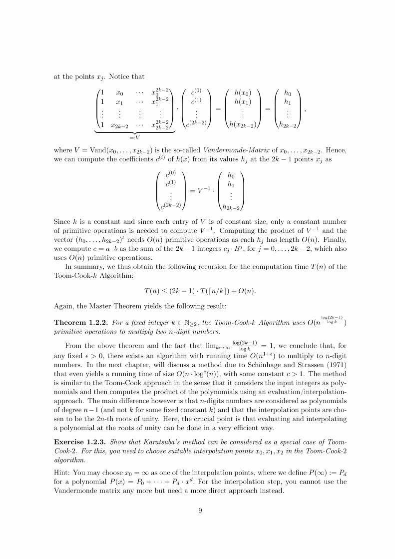
at the points xj . Notice that1 x0 · · · x2k−2

0

1 x1 · · · x2k−21

......

......

1 x2k−2 · · · x2k−22k−2

︸ ︷︷ ︸

=:V

·

c(0)

c(1)

...

c(2k−2)

=

h(x0)h(x1)...

h(x2k−2)

=

h0

h1

...h2k−2

,

where V = Vand(x0, . . . , x2k−2) is the so-called Vandermonde-Matrix of x0, . . . , x2k−2. Hence,we can compute the coefficients c(i) of h(x) from its values hj at the 2k − 1 points xj as

c(0)

c(1)

...

c(2k−2)

= V −1 ·

h0

h1

...h2k−2

Since k is a constant and since each entry of V is of constant size, only a constant numberof primitive operations is needed to compute V −1. Computing the product of V −1 and thevector (h0, . . . , h2k−2)t needs O(n) primitive operations as each hj has length O(n). Finally,we compute c = a · b as the sum of the 2k− 1 integers cj ·Bj , for j = 0, . . . , 2k− 2, which alsouses O(n) primitive operations.

In summary, we thus obtain the following recursion for the computation time T (n) of theToom-Cook-k Algorithm:

T (n) ≤ (2k − 1) · T (dn/ke) +O(n).

Again, the Master Theorem yields the following result:

Theorem 1.2.2. For a fixed integer k ∈ N≥2, the Toom-Cook-k Algorithm uses O(nlog(2k−1)

log k )primitive operations to multiply two n-digit numbers.

From the above theorem and the fact that limk 7→∞log(2k−1)

log k = 1, we conclude that, forany fixed ε > 0, there exists an algorithm with running time O(n1+ε) to multiply to n-digitnumbers. In the next chapter, will discuss a method due to Schönhage and Strassen (1971)that even yields a running time of size O(n · logc(n)), with some constant c > 1. The methodis similar to the Toom-Cook approach in the sense that it considers the input integers as poly-nomials and then computes the product of the polynomials using an evaluation/interpolation-approach. The main difference however is that n-digits numbers are considered as polynomialsof degree n−1 (and not k for some fixed constant k) and that the interpolation points are cho-sen to be the 2n-th roots of unity. Here, the crucial point is that evaluating and interpolatinga polynomial at the roots of unity can be done in a very efficient way.

Exercise 1.2.3. Show that Karatsuba’s method can be considered as a special case of Toom-Cook-2. For this, you need to choose suitable interpolation points x0, x1, x2 in the Toom-Cook-2algorithm.

Hint: You may choose x0 =∞ as one of the interpolation points, where we define P (∞) := Pdfor a polynomial P (x) = P0 + · · · + Pd · xd. For the interpolation step, you cannot use theVandermonde matrix any more but need a more direct approach instead.

9

Exercise 1.2.4. For two integers a = a(0) +a(1) ·Bdne+a(3) ·B2dne and b = b(0) + b(1) ·Bdne+b(3) ·B2dne of length n, use the Toom-Cook-3 approach to derive a relation between the valuesa(i) and b(i) that is similar to the relation in (1.11.1) as considered in Karatsuba’s method.

1.3 Approximate Computation

1.3.1 Fixed Point Arithmetic

A common approach when dealing with non-integer values a (e.g. 1/3,√

2, or π) is to approx-imate them by rational numbers a = m · B−ρ, with B the working base, m ∈ Z and ρ ∈ N,such that |a − a| ≤ B−ρ+1. That is, a constitutes the best approximation of a among allfixed-point number with base B and precision ρ:

FB,ρ := a = (−1)s ·B−ρ ·n−1∑i=0

aiBi with n ∈ N, s ∈ 0, 1, and ai ∈ 0, . . . , B − 1

If B and ρ are clear from the context, we also write F = FB,ρ. For convenience, we also write

a = (−1)s an−1 . . . aρ+1aρ, aρ−1 . . . a0

for an arbitrary element a = (−1)s ·B−ρ ·∑n−1

i=0 aiBi ∈ FB,ρ. The length of a (with respect to

B) is defined as the number n of digits that is needed to represent a. It is common to considerthe base B = 2 and to work with so called dyadic numbers (also called dyadic rationals).These are exactly the fixed point numbers with respect to base 2 and arbitrary but finiteprecision:

D :=∞⋃ρ=0

F2,ρ = p · 2−ρ : p ∈ Z and ρ ∈ N.

In what follows, we always assume that the base B and the precision ρ is fixed. For anarbitrary real value x, we define

flu(x) := mina ∈ F : x ≤ a

andfld(x) := maxa ∈ F : x ≥ a.

the two rounding functions to the nearest fixed-point number that is larger/smaller than orequal to a. fl(.) defines the rounding to nearest, that is, fl(x) = flu(x) if |flu(x) − x| <|fld(x)− x| and fl(x) = fld(x) if |fld(x)− x| < |flu(x)− x|. In case of ties (i.e. |fld(x)− x| =| flu(x)−x|), we round to even, that is, fl(x) = flu(x) if the last digit of flu(x) is even, otherwisefl(x) = fld(x). For each arithmetic operations ∈ +,−, ·, we now consider a correspondingapproximate variant , where we use fl(.) to round the exact result to a nearby number in F:

Definition 1.3.1. For x, y ∈ R and ∈ +,−, ·, we define

xy := fl(fl(x) fl(y)).

In particular, we have xy := fl(x y) for x, y ∈ F.

10

Notice that the above definition yields a canonical way of approximately evaluating a poly-nomial f(x) = a0 + · · · ad · xd ∈ R[x] at an arbitrary real value x. More precisely, we considersome evaluation method (e.g. Horner Evaluation) and replace each of the occurring arithmeticoperations by the corresponding fixed point variant . We denote the so-obtained result byfF(x). We remark at this point that the result may crucially depend on the chosen evaluationmethod. That is, we might get completely different values when using Horner Evaluationinstead of the "classical" way of evaluating the polynomial, that is, by first computing allpowers xi of x, then multiplying each power with the corresponding coefficient ai, and finallysumming up the obtained values. In other terms, it does not necessarily hold that

a0 + x · (a1 + · · · (ad−1 + x · ad) . . .) = a0 + a1 · x + · · · + ad · x · x · · ·x · x

Exercise 1.3.2. Give an example where Horner Evaluation and classical evaluation give dif-ferent results for fF(x).

The above approach for approximately evaluating a univariate polynomial at a point thenfurther extends to polynomials F (x) ∈ R[x] = R[x1, . . . , xn] in several variables. Since eachcomplex number z can be written as z = x+ i · y with x, y ∈ R, and since each addition andmultiplication in C amounts for a constant number of additions and multiplications in R, wemay further extend the approach to polynomials with complex coefficients. In this case, theset of complex fixed point numbers is given as

FC := F + i · F,

and the set of complex dyadic numbers is given as

DC := D + i · D.

In the next step, we investigate the error when performing a series of additions and multipli-cations using fixed point arithmetic. Assume that we are given approximations x, y ∈ FC oftwo complex numbers x, y ∈ C with |x− x| < εx and |x− x| < εy. Then, it holds that

|(x + y)− (x+ y)| ≤√

2 ·B−(ρ+1) + |(x+ y)− (x+ y)| < B−ρ + εx + εy, (1.2)

and the same error bound holds true for subtraction. For multiplication, we have

|x · y − x · y| ≤√

2 ·B−(ρ+1) + |(x · y)− x · y| < B−ρ + εx · |y|+ εy · |x|+ εx · εy. (1.3)

From the above error bounds, we can now derive a bound on the error |f(x0) − fF(x0)|that we obtain when using Horner evaluation and fixed point arithmetic to compute the valueof a polynomial f at a complex point x0.

Theorem 1.3.3. For any x0 ∈ C and any polynomial f ∈ C[x] of degree d with coefficientsof absolute value less than 2L, with L ∈ Z≥0, it holds that

|f(x0)− fF(x0)| < 4(d+ 1)2 · 2L ·B−ρ ·max(1, |x0|)d.

if Horner Evaluation and fixed point arithmetic with a precision ρ ≥ log d is used for theevaluation of f at x0.

11

Proof. We argue by induction on the degree d of f = a0 + · · ·+ ad · xd. Obviously, the errorbound is true for d = 0 as

|a0 − fl(a0)| ≤√

2 ·B−(ρ+1),

When using Horner evaluation to evaluate a polynomial f of degree d ≥ 1 at x0, we firstevaluate f := a1 + a2 · x+ · · ·+ ad · xd−1 at x0, then multiply the result by x0 and eventuallyadd a0. Using fixed point arithmetic with precision ρ, our induction hypotheses yields that

|fF(x0)− f(x0)| < ε := 4d2 · 2L ·B−ρ ·max(1, |x0|)d−1

Since |f(x0)| ≤ d · 2L ·max(1, |x0|)d−1 and |x0 − fl(x0)| ≤√

2 · B−(ρ+1) < B−ρ, we concludefrom (1.31.3) that

|x0 · f(x0)− fl(x0) · fF(x0))| <√

2 ·B−(ρ+1) + ε · |x0|+B−ρ · |f(x0)|+B−ρ · ε

< B−ρ + ε ·max(1, |x0|) +B−ρ · |f(x0)|+ ε ·max(1, |x0|)d

< B−ρ · [1 + 5d · 2L ·max(1, |x0|)d−1 + 4d2 · 2L ·max(1, |x0|)d].≤ B−ρ ·max(1, |x0|)d · 2L · (1 + 5d+ 4d2)

Adding the constant a0 increases the error by less than 2 ·B−ρ due to (1.21.2). Hence, the totalerror is bounded by

B−ρ · 2L · (3 + 5d+ 4d2) ·max(1, |x0|)d ≤ 4(d+ 1)2 · 2L ·B−ρ ·max(1, |x0|)d.

Hence, the claim follows.

1.3.2 Interval Arithmetic

Instead of computing an approximation of the value f(x0) that a function f : R 7→ R (or moregeneral, f : C 7→ C) takes at a specific point x0 ∈ R (or x0 ∈ C), it is often useful to computean approximation of the image f([a, b]) (or f([a, b] + i · [c, d])) of an interval [a, b] (rectangle[a, b] + i · [c, d]) under the mapping f .

Definition 1.3.4 (Interval Extensions and Box Functions). Let f : R 7→ R be an arbitraryfunction. An interval extension f : H 7→ H of f is a function from the halfplane H :=[a, b] : a, b ∈ R with a ≤ b of intervals X = [a, b] to itself such that f(x) ∈ f(X) for allx ∈ X. For continuous f , f is a continuous interval extension (or box-function) if

∞⋂i=1

f(Xi) = f(x0)

for any sequence X1 ⊃ X2 ⊃ · · · such that⋂∞i=1Xi contains only a single point x0.

In simpler terms, an interval extension f of f is a function that maps an interval [a, b]to an interval [A,B] such that f(x) ∈ [A,B] for any x ∈ [a, b]. Notice that this is not a veryrestricting condition as we can simply choose f as the function that maps any interval to(−∞,+∞). However, for a box function, it must also hold that [A,B] shrinks to one point(f(x0)) if [a, b] shrinks to one point (x0).

We further remark that Definition 1.3.41.3.4 further generalizes to complex valued functionsf : C 7→ C. Then, an interval extension f : HC 7→ HC computes for each rectangle

12

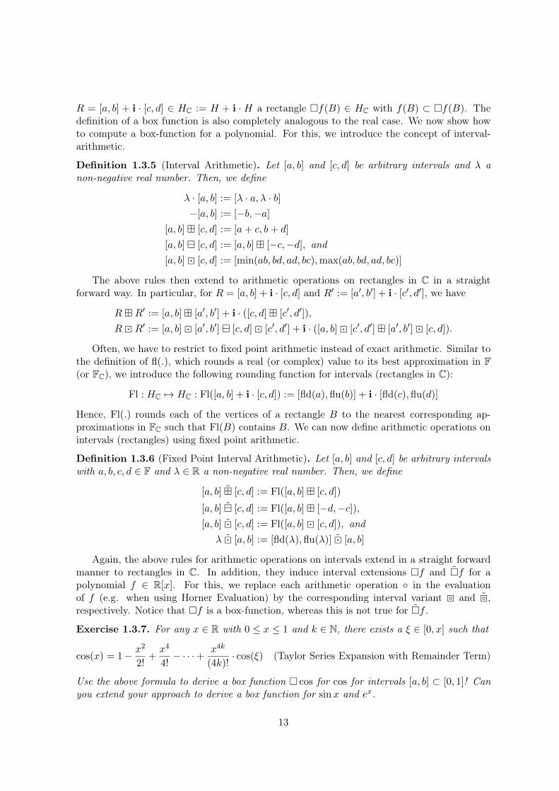
R = [a, b] + i · [c, d] ∈ HC := H + i · H a rectangle f(B) ∈ HC with f(B) ⊂ f(B). Thedefinition of a box function is also completely analogous to the real case. We now show howto compute a box-function for a polynomial. For this, we introduce the concept of interval-arithmetic.

Definition 1.3.5 (Interval Arithmetic). Let [a, b] and [c, d] be arbitrary intervals and λ anon-negative real number. Then, we define

λ · [a, b] := [λ · a, λ · b]−[a, b] := [−b,−a]

[a, b] [c, d] := [a+ c, b+ d]

[a, b] [c, d] := [a, b] [−c,−d], and[a, b] [c, d] := [min(ab, bd, ad, bc),max(ab, bd, ad, bc)]

The above rules then extend to arithmetic operations on rectangles in C in a straightforward way. In particular, for R = [a, b] + i · [c, d] and R′ := [a′, b′] + i · [c′, d′], we have

RR′ := [a, b] [a′, b′] + i · ([c, d] [c′, d′]),

RR′ := [a, b] [a′, b′] [c, d] [c′, d′] + i · ([a, b] [c′, d′] [a′, b′] [c, d]).

Often, we have to restrict to fixed point arithmetic instead of exact arithmetic. Similar tothe definition of fl(.), which rounds a real (or complex) value to its best approximation in F(or FC), we introduce the following rounding function for intervals (rectangles in C):

Fl : HC 7→ HC : Fl([a, b] + i · [c, d]) := [fld(a),flu(b)] + i · [fld(c),flu(d)]

Hence, Fl(.) rounds each of the vertices of a rectangle B to the nearest corresponding ap-proximations in FC such that Fl(B) contains B. We can now define arithmetic operations onintervals (rectangles) using fixed point arithmetic.

Definition 1.3.6 (Fixed Point Interval Arithmetic). Let [a, b] and [c, d] be arbitrary intervalswith a, b, c, d ∈ F and λ ∈ R a non-negative real number. Then, we define

[a, b] [c, d] := Fl([a, b] [c, d])

[a, b] [c, d] := Fl([a, b] [−d,−c]),[a, b] [c, d] := Fl([a, b] [c, d]), and

λ [a, b] := [fld(λ),flu(λ)] [a, b]

Again, the above rules for arithmetic operations on intervals extend in a straight forwardmanner to rectangles in C. In addition, they induce interval extensions f and f for apolynomial f ∈ R[x]. For this, we replace each arithmetic operation in the evaluationof f (e.g. when using Horner Evaluation) by the corresponding interval variant and ,respectively. Notice that f is a box-function, whereas this is not true for f .

Exercise 1.3.7. For any x ∈ R with 0 ≤ x ≤ 1 and k ∈ N, there exists a ξ ∈ [0, x] such that

cos(x) = 1− x2

2!+x4

4!− · · ·+ x4k

(4k)!· cos(ξ) (Taylor Series Expansion with Remainder Term)

Use the above formula to derive a box function cos for cos for intervals [a, b] ⊂ [0, 1]! Canyou extend your approach to derive a box function for sinx and ex.

13

Exercise 1.3.8. Let f(x) = a0 + a1x + · · · + adxd ∈ Z[x] be an arbitrary polynomial with

integer coefficients. Our goal is to count all real roots of f, provided that f has only simpleroots.

(a) Show that all real roots of f have absolute value bounded by M := 1 + max0≤i<d | aian |.22

(b) Use box functions for f and its derivative f ′ to derive a method that allows you to decidewhether a certain interval I contains no root or exactly one root. Your method mayfail (with the output “I don’t know”); however, it should succeed for sufficiently smallintervals I.

(c) Formulate an algorithm to determine the number of real roots of f .

(Hint: By Rolle’s theorem, any interval I which contains more than one root of f also containsa root of its derivative f ′.)

We now investigate a bound on the size of the intervals (rectangles) that are obtained whenperforming a series of additions and multiplication according to the above rules. Notice thatthere are similarities to our considerations in the previous section, where we derived boundson the error that occurs when adding or multiplying numbers using fixed point arithmetic.Namely, you might think of two rectangles R := [a, b] + i · [c, d] and R′ := [a′, b′] + i · [c′, d′] asapproximations of its centers mR := a+b

2 + i · c+d2 and mR′ := a′+b′

2 + i · c′+d′2 up to an error ofsize at most ε :=

√2 ·w(R) and ε′ :=

√2 ·w(R′), respectively, where w(R) = max(b−a, d− c)

and w(R′) = max(b′−a′, d′− c′) are defined as the width of R and R′. Then, the output of anarithmetic operation between R and R′ can again be considered as an approximation of thecorresponding arithmetic operation between mR and mR′ . Hence, similarly to the bounds in(1.21.2) and (1.31.3), we obtain for any two rectangles R and R′ with vertices in F + i · F that

w(RR′) ≤ w(R R′) ≤ w(R) + w(R′) + 2 ·B−ρ (1.4)

and

w(RR′) ≤ w(R) · w(R′) + |mR| · w(R′) + |mR′ | · w(R) + 2 ·B−ρ. (1.5)

Exercise 1.3.9. Prove correctness of the inequalities in (1.41.4) and (1.51.5).

Exercise 1.3.10. Let f ∈ C[x] be a polynomial of degree d with coefficients of absolute valueless than 2L, with L ∈ Z≥0, let ρ ∈ N be a precision with ρ > log d, and let F the correspondingset of fixed point numbers with precision ρ. Let R = [a, b] + i · [c, d] be a rectangle of widthw(R) < 1

d with vertices in F + i · F, and suppose that we compute f (and f) using HornerEvaluation and fixed point interval arithmetic with a precision ρ. Then, it holds

w(f(R)) ≤ w(f(R)) < 8 · (d+ 1)2 · 2L ·max(1, |mR|)d · w(R). (1.6)

Hint: Consider a similar argument as in the proof of Theorem 1.3.31.3.3.

Notice that the bound (1.61.6) on w(f(R)) and w(f(R)) tends to zero if we consider arectangle (square) R of width c · B−ρ, for some constant c, and the precision ρ tends to ∞.Hence, in order to compute an approximation of f(x0) for some complex value x0, we may

2The bound M is also called Cauchy’s Root Bound in the literature.

14

first approximate x0 by some fixed point number x0 = x0,< + i · x0,= ∈ FB,ρ + i · FB,ρ suchthat |x0 − x0| ≤ B−ρ and consider a rectangle

R := [x0,< −B−ρ, x0,< +B−ρ] + i · [x0,= −B−ρ, x0,= +B−ρ]

of width 2B−ρ whose vertices are obtained by adding and subtracting B−ρ from the real andcomplex part of x0. Then, R contains x0 and we can use use interval arithmetic to compute therectangle f(R), which contains f(x0). Its center m constitutes an approximation of f(x0)with |m−f(x0)| < w(f(R)). Hence, for computing an approximationm with |m−f(x0)| < ε,we can iteratively compute f(R) with increasing precision ρ = 1, 2, 4, 8, . . . until w(f(R)) <ε, and then return the center of f(R). Exercise 1.3.101.3.10 guarantees that we must succeed assoon as the precision ρ fulfills the inequality

ρ > ρε := logB[16(d+ 1)2 · 2L ·max(1, |x0|)d · ε−1] = O(log d+ d log max(1, |x0|) +L+ | log ε|),

where we used that

max(1, |mR|)d ≤ max(1, |x0|+B−ρ) ≤ max(1, |x0|)d · (1 + 1/d2)d ≤ 2 max(1, |x0|)d

for any ρ > 2 log d. Since we double ρ in each step, this shows that we succeed for a precisionρ < 2ρε. We fix this result, which will turn out to be useful at several places in the followingconsiderations.

Theorem 1.3.11. Let f ∈ C[x] be a polynomial of degree d with coefficients of absolute valueless than 2L, with L ∈ Z≥0, and let x0 be an arbitrary complex value. For any non-negativeinteger `, we can compute an approximation y0 of y0 = f(x0) with |y0 − y0| < 2−` using fixedpoint interval arithmetic with a precision ρ bounded by

O(log d+ d log max(1, |x0|) + L+ `).

Notice that the above bound on ρ that is needed in the worst-case is also a (worst-case)bound on the input precision as, in each iteration, we need approximations of the coefficientsof f as well as of x0 to an error less than B−ρ. We further remark that, as an alternativeto the above approach, one could also use fixed point arithmetic directly to compute anapproximation of f(x0), and to estimate the occurring error using Theorem 1.3.31.3.3. This yieldsa comparable bound on the needed precision in the worst case. However, the main drawbackof this approach is that one has to work with an a priori computed worst-case error bound,which means that the needed precision is always of size Ω(log d+d log max(1, |x0|)+L+`). Incontrast, when using interval arithmetic with increasing precision, we might already succeedwith a much smaller precision.

Exercise 1.3.12. Suppose that a polynomial f ∈ R[x] as well as a real value x0 is given bymeans of an oracle that returns arbitrary good dyadic approximations of the coefficients of fand x0. Under the assumption that f(x0) 6= 0, formulate an algorithm that computes an ` ∈ Zsuch that 2−` < |f(x0)| < 2`+2. How does its running time depend on |f(x0)|?

1.3.3 Floating point arithmetic (Under construction)

When actually implementing algorithms, the standard approach for the approximate computa-tion with real (complex) numbers is NOT fixed point arithmetic but floating point arithmetic.

15

However, a corresponding error analysis is more delicate, and thus, for the seek of simplicity,we decided to use fixed point arithmetic as our main tool for approximate computation. Nev-ertheless, we give a self-contained introduction for the interested reader. It originally appearedin the appendix of [MOS11MOS11].

Hardware floating point arithmetic is standardized in the IEEE floating point standard33.A floating point number is specified by a sign s, a mantissa m, and an exponent e. The signis +1 or −1. The mantissa consists of ρ bits m1, . . . , mρ, and e is an integer in the range[emin , emax ]. The range of possible exponents contains zero and emin ≤ −ρ− 2. The numberrepresented by the triple (s,m, e) is as follows:

• If emin < e ≤ emax , the number is s · (1 +∑

1≤i≤ρmi2−i) ·2e. This is called a normalized

number.

• If e = emin , then the number is s ·∑

1≤i≤ρmi2−i2emin+1. This is called a subnormal

number. Observe that the exponent is emin + 1. This is to guarantee that the distancebetween the largest subnormal number (1 − 2−ρ)2emin+1 and the smallest normalizednumber 1 · 2emin+1 is small.

• In addition, there are the special numbers −∞ and +∞ and a symbol NaN which standsfor not-a-number. It is used as an error indicator, e.g., for the result of a division byzero.

Let F = F(ρ, emin , emax ) be the set of real numbers (including +∞ and −∞) that can berepresented as above.44 A real number in F is called representable, a number in R \ F is callednon-representable. The largest positive representable number (except for ∞) is maxF = (2 −2−ρ) · 2emax , the smallest positive representable number is minF = 2−ρ · 2emin+1 = 2−ρ+emin+1,and the smallest positive normalized representable number is mnormF = 1 ·2emin+1 = 2emin+1.

F is a discrete subset of R. For any real x, let fl(x) be a floating point number closest55

to x. By convention, if x > maxF, fl(x) = ∞, and if x < −maxF, fl(x) = −∞. As forfixed point arithmetic, arithmetic on floating point numbers is only approximate. Again, wedistinguish between a mathematical operation ∈ −,+, · and the corresponding floatingpoint implementation . We further use 1/2 for the square-root operation and√ for its floatingpoint implementation. The floating point implementations of the operations +, −, ·, and 1/2

yield the best possible result. This is an axiom of floating point arithmetic. That is, if x, y ∈ Fand ∈ +,−, ·, then

xy = fl(x y)

and √x = fl(x1/2).

We need bounds on the error in the floating point evaluation of simple arithmetic expres-sions. Any real constant or variable is an arithmetic expression, and if A and B are arithmetic

3IEEE standard 754-1985 for binary floating-point arithmetic, 1987.4Double precision floating point numbers are represented in 64 bits. One bit is used for the sign, 52

bits for the mantissa (ρ = 52) and 11 bits for the exponent. These 11 bits are interpreted as an integerf ∈ [0...211 − 1] = [0...2047]. The exponent e equals f − 1023; f = 2047 is used for the special values, andhence emin = −1023 and emax = 1023. The rules for f = 2047 are: If all mi are zero and f = 2047, then thenumber is +∞ or −∞ depending on s. If f = 2047 and some mi is nonzero, the triple represents NaN ( = nota number).

5The IEEE-standard also specifies how to break ties. This is of no concern here.

16

E condition E mE indE cE degE

a constant in R \ F fl(a) max(mnormF , | fl(a)|) 1 max(1, | fl(a)|) 0

a constant in F a max(mnormF , |a|) 0 max(1, |a|) 0

x var. ranging over R fl(x) max(mnormF , | fl(x)|) 1 1 1

x var. ranging over F x max(mnormF , |x|) 0 1 1

A+B A⊕ B mA ⊕mB 1 + max(indA, indB) cA + cB max(degA, degB)

A−B A B mA ⊕mB 1 + max(indA, indB) cA + cB max(degA, degB)

A ·B A B max(mnormF ,mA mB) 1 + indA + indB cAcB degA+ degB

A1/2 A < umA 0 2(t+1)/2√mA 2 + indA not defined

A1/2 A ≥ umA√A max(

√A,mA

√A) 2 + indA not defined

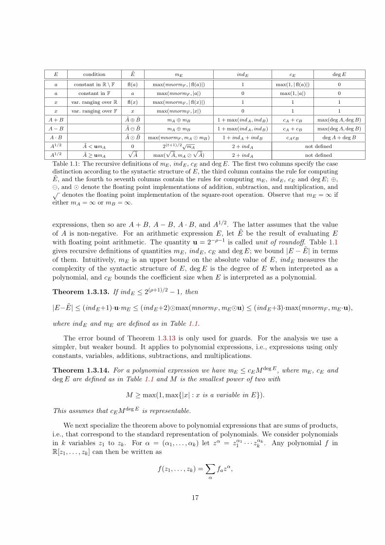
Table 1.1: The recursive definitions of mE , indE , cE and degE. The first two columns specify the casedistinction according to the syntactic structure of E, the third column contains the rule for computingE, and the fourth to seventh columns contain the rules for computing mE , indE , cE and degE; ⊕,, and denote the floating point implementations of addition, subtraction, and multiplication, and√ denotes the floating point implementation of the square-root operation. Observe that mE = ∞ ifeither mA =∞ or mB =∞.

expressions, then so are A + B, A − B, A · B, and A1/2. The latter assumes that the valueof A is non-negative. For an arithmetic expression E, let E be the result of evaluating Ewith floating point arithmetic. The quantity u = 2−ρ−1 is called unit of roundoff. Table 1.11.1gives recursive definitions of quantities mE , indE , cE and degE; we bound |E − E| in termsof them. Intuitively, mE is an upper bound on the absolute value of E, indE measures thecomplexity of the syntactic structure of E, degE is the degree of E when interpreted as apolynomial, and cE bounds the coefficient size when E is interpreted as a polynomial.

Theorem 1.3.13. If indE ≤ 2(ρ+1)/2 − 1, then

|E−E| ≤ (indE+1)·u·mE ≤ (indE+2)max(mnormF ,mEu) ≤ (indE+3)·max(mnormF ,mE ·u),

where indE and mE are defined as in Table 1.11.1.

The error bound of Theorem 1.3.131.3.13 is only used for guards. For the analysis we use asimpler, but weaker bound. It applies to polynomial expressions, i.e., expressions using onlyconstants, variables, additions, subtractions, and multiplications.

Theorem 1.3.14. For a polynomial expression we have mE ≤ cEMdegE, where mE, cE and

degE are defined as in Table 1.11.1 and M is the smallest power of two with

M ≥ max(1,max|x| : x is a variable in E).

This assumes that cEMdegE is representable.

We next specialize the theorem above to polynomial expressions that are sums of products,i.e., that correspond to the standard representation of polynomials. We consider polynomialsin k variables z1 to zk. For α = (α1, . . . , αk) let zα = zα1

1 · · · zαkk . Any polynomial f in

R[z1, . . . , zk] can then be written as

f(z1, . . . , zk) =∑α

fazα,

17

where fα is the coefficient of the monomial term zα. For simplicity assume that the coefficientsare representable as floating point numbers. For a monomial term, Z = fαz

α, we have cZ =max(1, |fα|), degZ = deg(zα) =

∑i αi, and indZ = 2 degZ. For the entire polynomial, we

have cf =∑

α max(1, |fα|) and deg f equal to the total degree of f . The index depends on theorder in which we add the monomial terms. If we sum serially, as in ((((t1+t2)+t3)+t4)+t5)),the index is the number of monomial terms minus one plus the largest index of any monomialterm. If we sum in the form of a binary tree as in ((t1 + t2) + ((t3 + t4) + t5)), the index is thelogarithm of the number of monomial terms rounded upwards plus the largest index of anymonomial term.

Theorem 1.3.15. Let f(z1, . . . , zk) =∑

α faxα be a polynomial of total degree N . Let cf =∑

α max(1, |fα|) and let mf = |α : fα 6= 0| be the number of monomial terms in f . LetM ≥ 1 be a power of two and let z1 to zk be real values with |zi| ≤M for all i. Then

|f(z1, . . . , zk)− f(fl(z1), . . . ,fl(zk))| ≤ cf (mf + 2N)MN2−ρ−1,

where f is the floating point version of f , i.e., all operations in f are replaced by their floatingpoint counterpart.

Proof. We use Theorems 1.3.131.3.13 and 1.3.141.3.14. The index is largest if the monomial terms aresummed serially. It is then equal to mf + 2N − 1. Also mE ≤ cfMN .

The above theorem also generalizes to complex values xi and polynomials defined overthe complex numbers. The obtained error bound is comparable, that is, it only differs by amultiplicative constant from the above bound.

1.4 Division

-b

1/b

xi xi+1

Figure 1.1: The graph of the functionf(x) = 1

x − b. The value xi+1 resultsfrom applying one step of the Newton-Raphson method to xi.

In the previous sections, we have shown how to effi-ciently carry out additions and multiplications on inte-gers. We also considered corresponding operations onfixed-point numbers and intervals and estimated the er-ror that occurs when using approximate instead of exactarithmetic. So far, any such treatment for the divisionof integers or fixed-/floating-point numbers a and b ismissing. We will first show how to compute an arbitrarygood dyadic approximation q ∈ D of a rational numberq := a

b ∈ Q using only additions and multiplications ofintegers. We start with the special case, where a = 1and b is a positive integer of length less than n. Thecrucial idea underlying the approach is to consider q asthe unique solution of the equation f(x) := 1

x − b = 0and to use the Newton-Raphson method to derive anapproximation of q. That is, with x0 := 2−dlog be ∈ D, we define

xi+1 := xi −f(xi)

f ′(xi)= xi −

1xi− b− 1x2i

= 2 · xi − b · x2i = xi · (2− b · xi) ∈ D for i ∈ N≥1. (1.7)

18

Algorithm 5: DivisionInput : Two non-negative n-digit integers a and b and a non-negative integer L.Output: A dyadic number q ∈ D of length O(n+ L) such that |q − a/b| < 2−L.

1 L′ := dlog ae+ L+ 12 N := dlogL′e3 x0 := 2−dlog be · (2− b · 2−dlog be)4 for i = 1, . . . , N − 1 do5 Recursively define6

xi+1 := fl(xi · (2− b · xi)),

where fl(.) is defined as "rounding to the nearest element" in F2,ρi andρi := 2i+1 + 2n.

7 Compute q := fl(a · xN−1), where fl(.) is defined as rounding to the nearest in F2,L.8 return q

The first part of the following exercise shows that the sequence xi converges quadratically toq. Roughly speaking, this means that the number of correct digits doubles in each iteration.We then conclude that, after dlogLe iterations, we have computed a dyadic approximationq of q = 1/b with |q − q| < 2−L. However, there is a small problem with this approach,namely, the lengths of the dyadic numbers xi double in each iteration, and since x0 has lengthdlogBe ≤ n, we end up with dyadic numbers of length O(nL) after dlogLe iterations. In Part(c) of the exercise, we show that we can improve upon this approach by rounding the resultobtained in the i-th iteration to the ρi-th digit after the binary point, with ρi := 2i+1 + 2n.As a result, we can reduce the length of the occurring numbers from O(nL) to O(n+ L).

Exercise 1.4.1. Let (xi)i be defined as above and L be an arbitrary positive number. Showthat, for all i, it holds that

(a)∣∣xi+1 − 1

b

∣∣ ≤ b · ∣∣xi − 1b

∣∣2 and

(b)∣∣xi − 1

b

∣∣ < 1b · 2

−2i . In particular, it holds that∣∣xi − 1

b

∣∣ < 2−L for all i ≥ logL.

(c) Suppose now that we start with y0 := x1 = 2−dlog be · (2− b · 2−dlog be) and define

yi+1 := fl(yi · (2− b · yi)) for i ∈ N≥1,

where we consider rounding to the nearest fixed-point number of precision ρi := 2i+1 + 2n.Then, it holds

∣∣yi − 1b

∣∣ < 1b+1 · 2

−2i for all i.

Hint: For (c), use that the error 2−ρi−1 that is induced by the rounding in the (i + 1)-st

iteration is smaller than 2−2i+1

(b+1)2 . Then, use induction on i to prove the claim.

From the above consideration, we conclude that we can compute a dyadic number q with|q − 1/b| < 2−L using O(logL) additions and multiplications of integers of length O(L + n).Now, computing a corresponding approximation q of q := a

b , with integers a and b of lengthless than n, is straightforward; see Algorithm 55. Namely, we first compute a dyadic q′ of lengthO(L+ n) such that |q′ − 1/b| < 2−L−dae−1 and then determine the product a · q′. The result

19

is eventually rounded to the L-th digit after the binary point. The so-obtained q = fl(a · q′)has length O(n+ L) and it holds that |q − q| < 2−L. We fix this result:

Theorem 1.4.2. Let a and b be integers of length n. For any non-negative L, Algorithm 55computes a dyadic approximation q ∈ D of length O(n+L) such that |q − q| < 2−L. For this,it uses O(log(n+ L)) additions and multiplications of O(n+ L)-digit integers.

We can now go one step further and derive a bound on the cost for computing an approx-imation of the quotient of two arbitrary complex numbers a = a0 + i · a1 and b = b0 + i · b1.Here, we assume that, for any L′ ∈ N, we can ask for dyadic approximations a, b ∈ D suchthat |a− a|, |b− b| < 2−L

′ . Notice that

a

b=a0 + i · a1

b0 + i · b1=

(a0 + i · a1) · (b0 + i · b1)

(b0 + i · b1) · (b0 − i · b1)=

(a0b0 − a1b1) + i · (a1b0 + a0b1)

|b|2,

thus we can restrict to quotients of real numbers a, b ∈ R 6=0. Suppose that dyadic approxima-tions a, b ∈ R6=0 with |a− a|, |b− b| < 2−L

′< |b|/2 are given. Then, we have

∣∣∣∣ ab − a

b

∣∣∣∣ =

∣∣∣∣∣ba− abbb

∣∣∣∣∣ =

∣∣∣b(a− a)− a(b− b)∣∣∣∣∣∣b2 + b(b− b)

∣∣∣ < 2−L′+1 · |a|+ |b|

|b|2≤ 2−L

′+2 · max(|a|, |b|)min(1, |b|)2

.

For L′ > L+ dlog max(1, |a|)e+ 3d| log b|e+ 3, this implies that∣∣∣ ab− a

b

∣∣∣ < 2−L−1. Hence, we

may first consider L′-digit approximations a, b ∈ D of a and b, and then compute an (L+ 1)-digit approximation q ∈ D of their quotient q = a

busing the method from above. Then, it

holds that |q − a/b| < 2−L. We fix this result:

Theorem 1.4.3. Let a, b ∈ C be arbitrary complex numbers and L ∈ N. Then, there exists apositive integer L′ of size

L′ := O(L+ dlog max(1, |a|)e+ d| log |b||e)

such that we can compute a fixed point number q ∈ F + i · F of length L′ with |q − q| < 2−L

using O(logL′) additions and multiplications of O(L′)-digit integers. The values a and b needto be approximated to an error of size 2−L

′ .

Exercise 1.4.4. For arbitrary x ∈ R with 0 ≤ x ≤ 1, it holds that

arctan(x) = x− x3

3+x5

5− x7

7+ · · · (1.8)

Now, for given L ∈ N, use the above formula and the fact (due to Euler) that

π = 20 · arctan(1/7) + 8 · arctan(3/79)

to derive an efficient algorithm (i.e. with a running time polynomial in L) for computing afixed point approximation π (wrt. base 2) of π to an error less than 2−L.

Hint: Estimate the error when considering only the first k summands in (1.81.8). Then, proceedwith a suitably truncated series.

20

Exercise 1.4.5. For arbitrary x ∈ R with 0 ≤ x ≤ 1, we have

cos(x) = 1− x2

2!+x4

4!− · · ·

For fixed n ∈ N≥8 and arbitrary L ∈ N, formulate an efficient method to compute an L-digitapproximation ω of ω := cos(2π/n).

Hint: Proceed similar as in Exercise 1.4.41.4.4 and use a sufficiently good approximation π of π.For the evaluation of the truncated series at x = π, use Theorem 1.3.31.3.3.

21

Chapter 2

The Fast Fourier Transform and FastPolynomial Arithmetic

2.1 Schönhage-Strassen Multiplication

In the previous chapter, we have seen that the cost M(n) for computing the product of twointegers of length n is bounded by O(n1+ε), where ε is a an arbitrary but fixed positive realvalue. For sufficiently large k, this bound is achieved by the Toom-Cook-k algorithm. Inthis section, we present a method [SS71SS71] due to Schönhage and Strassen whose running timeis bounded by11 O(n log n ·M(log n)) = O(n log2+ε n). Before we go into detail, we give anoverview of the main steps.

2.1.1 The Algorithm in a Nutshell

In the first step, we split a and b into n blocks a(i) and b(i), that is, we write

a = a(0) + a(1) ·B + · · ·+ a(n−1) ·Bn−1, and

b = b(0) + b(1) ·B + · · ·+ b(n−1) ·Bn−1

with one-digit numbers ai, b(i) ∈ 0, . . . , B − 1. Notice the difference to the Toom-Cookalgorithm, where we split a and b into only constantly many (i.e. k) blocks of size dn/ke.Similar to the Toom-Cook method, we now consider corresponding polynomials

f(x) := a(0) + a(1) · x+ · · ·+ a(n−1) · xn−1, and

g(x) := b(0) + b(1) · x+ · · ·+ b(n−1) · xn−1 (2.1)

of degree n− 1 (instead of k as in the Toom-Cook method) with coefficients a(i) and b(i), andreduce the computation of a ·b to the problem of computing the product h =

∑2n−2i=0 c(i) ·xi :=

f ·g of the polynomials f and g, followed by the evaluation of h at x = B. For the computationof h, we again use an evaluation/interpolation approach, that is, we first evaluate f and gat 2n points x0, . . . , x2n−1, compute each of the products f(xi) · g(xi) = h(xi), and then

1We remark that there exists a slightly more involved variant of the Schönhage-Strassen method that needsonly O(n logn log logn) primitive operations. For the seek of simplicity, we decided to only present the variantwith slightly worse running time but hint to the faster approach when discussing the corresponding steps inmore detail.

22

reconstruct h from its values at the points xi. The crucial part of the algorithm is the specialchoice of the points xi, that is, instead of considering arbitrary distinct values for the pointsxi, we now choose xi = ωi for i = 0, . . . , 2n−1, where ω ∈ C is a primitive 2n-th root of unity.

Im

Re

Figure 2.1: The dots on the unit cir-cle are the 8-th roots of unity. Thered dots are primitive.

That is, ω is a solution of the equation x2n − 1 = 0, andit holds that ωi 6= 1 for any integer i with 1 ≤ i < 2n. Forconvenience, we choose ω := e

πin = cos(π/n) + i · sin(π/n),

even though other choices are possible. We will see that, forn a power of two, there exists a very efficient method, calledFast Fourier Transform (FFT for short) due to Cooley andTukey (1965), that needs only O(n log n) additions andmultiplications of complex numbers in order compute theso-called Discrete Fourier Transform (DFT for short)

DFTω(f) := (f(1), f(ω), . . . , f(ω2n−1)).

The efficiency of the method is based on the fact that thereare only 2n different values for xji for any i, j if xi = ω,whereas, for a general choice of xi, there are 2n2 differentvalues for xji . We will further show that the fast convo-lution method can also be used to interpolate h from thevalues h(xi) in a comparably efficient manner.

One problem of the approach is that, since ω is not a rational number in general, thecomputations involving ω can only be carried out with approximate arithmetic. However,we will show that the total (absolute) error that occurs during the computation is less than1/2 if we use fixed point arithmetic with a precision ρ > ρ0 in each step, where ρ0 is somecomputable number of size O(log n). In addition, we will show that all occurring numbers inthe intermediate results have length bounded by O(log n), and thus we may conclude that,using O(n log n) arithmetic operations on fixed-point numbers of length O(log n), we cancompute approximations c(i) of the coefficients c(i) of h with |c(i) − c(i)| < 1/2. Since eachcoefficient c(i) is an integer, we can thus derive the exact value c(i) from its approximation c(i).We give the following example to illustrate the last step: Suppose that our approach yieldsthe approximation

h = 2.34 · x10 − 0.14 · x9 + 0.98 · x8 + · · ·+ 0.67 · x+ 1.11 (2.2)

for the product h = f · g of two integer polynomials f and g. In addition, according to thechoice of our precision ρ, we can guarantee that the absolute error is less than 1/2. Now, sincethe coefficients of h are integers and since they differ from the corresponding approximationsby less than 1/2, we conclude that h = 2 · x10 + x8 + · · ·+ x+ 1.

It remains to show how to recover the product c = a ·b from the polynomial h. For this, weevaluate h at x = B, which amounts for shifting each coefficient c(i) by i digits and summingup the so obtained numbers. Here, it is crucial that each c(i) has length O(log n), and thus eachsummation uses onlyO(log n) primitive operations. We conclude that the total cost is boundedby O(n log n ·M(log n))) = O(n(log n)2+ε) primitive operations, where ε is an arbitrary fixedpositive number. Instead of using the Toom-Cook algorithm for the occurring multiplicationsin the Schönhage-Strassen method, we could instead call the Schönhage-Strassen methodrecursively. This yields the running time

O(n log nM(n)) = O(n(log n)(log logn)M(log log n)) = O(n(log n)2(log log n)2M(log log log n))

23

and so on. As already mentioned above, it is possible to slightly improve upon this approach.This is achieved by splitting the initial numbers not into ≈ n/ log n blocks of size ≈ log n.Then, recursively calling the algorithm even yields the complexity bound O(nM(log n))). Wenow give details in the following two sections.

2.1.2 Fast Fourier Transform

Even though we are mainly interested in solving problems defined over the real or complexnumbers, it will turn out to be useful to work over an arbitrary ring R (or a field K). In whatfollows, we always assume that R is a commutative ring with 1 = 1R.

We start with the following definition:

Definition 2.1.1 (Convolution). Let f = a0 + · · ·+aN−1 ·xN−1 and g = b0 + · · ·+bN−1 ·xN−1

be two polynomials of degree less than N in R[x]. We define

f ?N g :=N−1∑k=0

ck · xk :=N−1∑k=0

∑i,j:i+j=k mod N

ai · bj

· xkas the convolution of f and g.

Example. Let f = 1 + x+ x2 ∈ Z[x] and g := 2− x, then f · g = 2 + x+ x2 − x3, and

f ?3 g = (2− 1) + 1 · x+ 1 · x2 = 1− x+ x2.

Notice that, in general, f ?N g = f · g mod (xN − 1). In particular, if we consider two poly-nomials f and g of degree less than n as polynomials of degree less than 2n − 1 (by settingan = · · · = a2n−1 = bn = · · · = b2n−1 = 0), then it holds that f ?2n g = f · g.

In our overview of the Schönhage-Strassen multiplication for n-digit numbers, we men-tioned that the method considers an evaluation/interpolation approach using the 2n-th com-plex roots of unity. Again, we generalize this approach to arbitrary rings.

Definition 2.1.2 (Root of Unity and Discrete Fourier Transform (DFT)). Let ω ∈ R, andN ∈ N. We call ω an N -th root of unity if ωN = 1. We further call ω primitive if ωN/i − 1 isnot a zero-divisor22 in R for any divisor i of N . For fixed ω, the Discrete Fourier Transformof a polynomial f ∈ R[x] is defined as

DFTω(f) := (f(1), f(ω), . . . , f(ωN−1)).

For a vector a = (a0, . . . , aN−1)t ∈ RN , we define DFTω(a) := DFTω(∑N−1

i=0 aixi).

We remark that there does not always exist a primitive N -th root of unity in a ring R.For instance, this is the case for R = Z or R = R. The following exercise (taken from [GG03GG03,Sec. 8]) gives a necessary and sufficient condition on the existence of a primitive root of unityin the finite field Fp = Z/pZ.

2An element a ∈ R is a zero divisor if there exists an r ∈ R with a · r = 0 = 0R or r · a = 0. A zero-divisordoes not have to be zero. For instance, a = 3 ∈ R = Z/6Z is a zero divisor in R as 2 · 3 = 0.

24

Exercise 2.1.3. Denote by Fp = Z/pZ the finite field with p elements for some prime p, andlet N ∈ 1, . . . , p− 1. Show that Fp contains a primitive N -th root of unity if and only if Ndivides p− 1, and conclude that the multiplicative group F×p of Fp is cyclic.

Hints:

1. Use (without proof) Fermat’s little theorem: For arbitrary a ∈ Z arbitrary, it holds

ap ≡ a mod p.

In particular, if a ∈ 1, . . . , p− 1, then

ap−1 ≡ 1 mod p.

2. Let q ∈ N be a divisor of p − 1 and q = qe11 · · · qerr its prime factorization. For a ∈ F×p ,we denote by ord(a) := mini ∈ N>0 : ai = 1 the order of a in F×p .Prove the following facts:

• ord(a) = q if and only if aq = 1 and aq/qi 6= 1 for i = 1, . . . , r.

• For each i, F×p contains an element ai with qeii | ord(ai). Conclude that there is anelement bi with ord(bi) = qeii .

• If a, b ∈ F×p are elements of coprime orders, then ord(ab) = ord(a) ord(b).

• F×p contains an element of order q.

Lemma 2.1.4. For N ∈ N, suppose that there exists a primitive N -root of unity ω in R. Forany two polynomials f, g ∈ R[x] of degree less than N , it holds that

DFTω(f ?N g) = DFTω(f) ·DFTω(g) = (f(1) · g(1), f(ω) · g(ω), . . . , f(ωN−1) · g(ωN−1)).

Proof. There exists a polynomial q ∈ R[x] with f ?N g = f · g + q · (xN − 1). Thus, we have

(f ?N g)(ωi) = f(ωi) · g(ωi) + q(ωi) · ((ωi)N − 1) = f(ωi) · g(ωi) + q(ωi) · ((ωN )i − 1) =

= f(ωi) · g(ωi) + q(ωi) · (1i − 1) = f(ωi) · g(ωi).

In our overview of the Schönhage-Strassen method, one step is to compute the DiscreteFourier Transforms DFTω(f) and DFTω(g) of two polynomials of degree at most n−1, whereω is an N -th root of unity in C, with N := 2n. Now from the above lemma and the fact thatf ?N g = f · g = h, we conclude that

DFTω(h) = DFTω(f · g) = DFTω(f ?N g) = DFTω(f) ·DFTω(g). (2.3)

Notice that the mapping DFTω : RN 7→ RN is given by the Vandermonde matrix

Vω := Vand(1, ω, . . . , ωN−1) =

1 1 · · · 11 ω · · · ωN−1

......

......

1 ωN−1 · · · ωN(N−1)

.

25

That is, the coefficient vector a := (a0, . . . , aN−1)t of a polynomial f =∑N−1

i=0 ai · xi ∈ R[x]is mapped to the vector v := (f(1), f(ω), . . . , f(ωN−1))t = Vω · a. Vice versa, if v is known,then the coefficients ai of f can be reconstructed as a = V −1

ω · v. It turns out that a multipleof V −1

ω can be easily computed.

Theorem 2.1.5. Let ω be a primitive N -th root in R. Then, ωN−1 = ω−1 is also a primitiveN -th root of unity and Vω · Vω−1 = N · IdN , with IdN the N ×N -identity matrix.

Proof. We split the proof into four parts:

(1) ωn−1 = ω−1 is a primitive N -th root of unity: Since

(ωN−1)N = (ωN )N−1 = 1N−1 = 1,

it follows that ωN−1 is an root of unity. Now suppose that there exists a divisor t of N and ab ∈ R with ((ωN−1)N/t − 1). Then, multiplication with ωN/t implies that

0 = ωN/t · ((ωN−1)N/t − 1) = [(ω · ωN−1)N/t − ωN/t) · b = (1− ωN/t) · b,

and thus ωN/t − 1 is a zero-divisor in R, which contradicts our assumption.

(2) ω` − 1 is not a zero divisor for all ` ∈ N with 1 ≤ ` < N : Let g := gcd(`,N) be thegreatest common divisor of ` and N. Then, there exist integers33 s and t with s · `+ t ·N = g.Since g < n, there exists a prime divisor p of N that divides N/g, and thus g divides N/p.Hence, we obtain

ωN/p − 1 = (ωg)Npg − 1 = (ωg − 1) ·

Npg−1∑

i=0

ωi·g︸ ︷︷ ︸=:r

.

Now, suppose that there exists a b ∈ R with b·(ωg−1) = 0, then we also have b·(ωN/p−1) = 0,and thus b = 0 as ω is not a zero divisor. This shows that ωg − 1 is not a zero divisor as well.Notice that ω` − 1 divides ωs` − 1 = (ω` − 1) ·

∑s−1i=0 ω

i`, and since

ωs` − 1 = ωs` · (ωN )t − 1 = ωs`+tN − 1 = ωg − 1

we conclude that ω` − 1 also divides ωg − 1. It follows that ω` − 1 is not a zero divisor asb · (ω` − 1) = 0 implies that b · (ωg − 1) = 0, and thus b = 0.

(3) It holds that∑

0≤j<N ω`j = 0 for any ` ∈ N with 1 ≤ ` < N : It holds that

(ω` − 1) ·∑N−1

j=0ω`j = ω`N − 1 = 0,

and thus∑N−1

j=0 ω`j = 0 as ω` − 1 is not a zero divisor.

(4) Vω · Vω−1 = N · IdN : The (i, k)-th entry cij of Vω · Vω−1 is given as

cij =

N−1∑j=0

ωijω−jk =

N−1∑j=0

ω(i−k)j =

N if i = k

0 if i 6= k,

where we used (3) for the case i 6= k.

26

Algorithm 6: Fast Fourier TransformInput : A polynomial f = a0 + · · ·+ aN−1 · xN−1 ∈ R[x], with N = 2k and k ∈ N0,

and a primitive N -th root of unity ω ∈ R.Output: DFTω(f).

1 if N=1 then2 return a0

3 Compute ωi := ωi for i = 0, . . . , N − 1

4 f ev :=∑N/2−1

i=0 a2i · xi and fodd :=∑N/2−1

i=0 a2i+1 · xi5 Call Algorithm 66 recursively to compute

(dev0 , . . . , d

evN/2−1) := DFTω2(f ev)

and(dodd

0 , . . . , doddN/2−1) := DFTω2(fodd).

for i = 1, . . . , N − 1 do6 Let j = i mod N/2. Compute

di := devj + ωi · dodd

j .

7 return (d0, . . . , dN−1)

Exercise 2.1.6. Let F = Z/29Z.

1. Find a primitive 4-th root of unity ω ∈ F and compute its inverse ω−1 ∈ F.

2. Check that the product of the two matrices DFTω and DFTω−1 equals 4 · Id4.

Theorem 2.1.52.1.5 shows that polynomial interpolation is essentially the same as polynomialevaluation when considering the N -th roots of unity as interpolation points. In particular,applying DFTω−1 to both sides of (2.32.3), we obtain for the coefficient vector c := (c0, . . . , cN−1)t

of h =∑N−1

i=0 cixi that

N · c = DFTω−1(DFTω(h)) = DFTω−1(DFTω(f) ·DFTω(g)). (2.4)

Hence, for the evaluation/interpolation step in the Schönhage-Strassen algorithm, we need tocarry out three computations of a DFT plus one pointwise multiplication of two DFTs. Wenext describe an efficient method [CT65CT65] due to Cooley und Tukey (from 1965) for computingthe discrete Fourier Transform DFTω(f) for some polynomial f of degree less than N − 1and ω a primitive N -th root of unity.44 In what follows, we assume that R supports the FFT,that is, it contains an N -th root of unity for any N = 2k, with k ∈ N. In the followingconsiderations, we further assume that N is such a power of two. We can now write a

3This follows from the extended Euclidean Algorithm, which we will treat in detail in the next chapter.4In fact, it was Gauss who invented the algorithm already 160 years earlier. Cooley and Tukey rediscovered

and popularized the method. The algorithm has a series of applications in engineering, applied mathematics,and the natural sciences. The original paper from 1965 has more than 13400 citations!

27

DFTω(a0, . . . , a7)

DFTω2(a0, a2, a4, a6)

DFTω4(a0, a4)

a0 a4

·ω?DFTω4(a2, a6)

a2 a6

·ω?

·ω?DFTω2(a1, a3, a5, a7)

DFTω4(a1, a5)

a1 a5

·ω?DFTω4(a3, a7)

a3 a4

·ω?

·ω?

·ω?

Figure 2.2: Starting with the coefficients ai = DFTω8(ai) of f , we iteratively compute four DFT’s oflength 2, two DFT’s of length 4, and eventually DFTω(f), which has length 8. In Step `, the i-thentry of a Discrete Fourier Transform of size N/2` is computed as the the sum of the j-th entry of theleft child and the j-th entry of the right child multiplied by ωi (illustrated by the edge labelling "·ω?"in the above picture), where j = i mod N/2`+1.

polynomial f(x) = a0 + · · ·+ aN−1 · xN−1 ∈ R[x] as

f(x) =

N/2−1∑i=0

a2i · x2i +

N/2−1∑i=0

a2i+1 · x2i+1 = f ev(x2) + x · fodd(x2),

with f ev :=∑N/2−1

i=0 a2i · xi and fodd :=∑N/2−1

i=0 a2i+1 · xi. Plugging x = ωi into the aboveequation then yields that

f(ωi) = f ev(ω2i) + ωi · fodd(ω2i). (2.5)

Notice that ω2 is a primitive N/2-root, hence the computation of DFTω(f) = (d0, . . . , dN−1)can be reduced to the computation of the two Discrete Fourier Transforms DFTω2(f ev) =(dev

0 , . . . , devN/2−1) and DFTω2(fodd) = (dodd

0 , . . . , doddN/2−1) followed by the computation of di :=

devj + ωi · dodd

j for all i = 0, . . . , N and j = i mod N/2; see Algorithm 66.In terms of complexity, this means that we can compute a Discrete Fourier Transform

of size N by computing two Discrete Fourier Transforms of size N/2 plus 3N additionaladditions and multiplications (by powers of ω). If we use T (N) to denote the number ofarithmetic operations in R that are needed in the worst case to compute the Discrete FourierTransform DFTω(f) for a polynomial f of degree less than N and a primitive N -th root ofunity ω, the above consideration implies that

T (N) ≤ 2 · T (N/2) + 3 ·N.

Hence, we obtain the following result:

Theorem 2.1.7. Let f ∈ R[x] be a polynomial of degree less than N and ω be a primitiveN -th root of unity ω in R, then Algorithm 66 computes DFTω(f) using O(N logN) arithmeticoperations in R.

For an illustration of the FFT Algorithm when applied to a polynomial f = a0 + · · ·+ a7 ·x7 ∈ R[x] of degree 7 and ω a primitive 8-th root of unity, see Figure 2.22.2.

28

Algorithm 7: Fast ConvolutionInput : A commutative ring R, two polynomials f, g ∈ R[x] of degree less than

N = 2k, with k ∈ N0, and a primitive N -th root of unity ω ∈ R.Output: f ?N g.

1 Compute:2 ω−1 = ωN−1.3 Df := DFTω(f) and Dg := DFTω(g)4 Dh := Df ·Dg

5 E :=DFTω−1 (Dh)

N6 return E

From (2.42.4) and the FFT algorithm, we can can now directly derive an efficient algorithmfor computing the convolution f ?N g of two polynomials f, g ∈ R[x] of degree less than N .Namely, we first compute DFTω(f) and DFTω(g) and their pointwise product P . Then, wecompute DFTω−1(P ) and divide each of its entries by N ; see Algorithm 77. Notice that allbut the last operation use O(n log n) arithmetic operations in R. According to Section 1.41.4,the division by N is relatively cheap in the special case where R = C, however, it might bean entirely non-trivial task for a different ring.

Theorem 2.1.8. Let f, g ∈ R[x] be polynomials of degree less than N = 2k with k ∈ N.Suppose that a primitive N -th root of unity ω in R is given. Then, Algorithm 77 computesf ?N g using O(N logN) arithmetic operations in R plus N divisions by N .

For two polynomial f, g ∈ R[x] of degree n or less, it holds that f · g = f ?N g, withN := 2dlogne+1. Hence, if a primitive N -th root of unity is given, then Algorithm 77 computesthe product of f and g using O(n log n) arithmetic operations in R plus N divisions by N .

Corollary 2.1.9. Let f, g ∈ R[x] be polynomials of degree less than n, and N := 2dlogne+1.If a primitive N -th root of unity ω in R is given, then Algorithm 66 computes f · g usingO(N logN) = O(n log n) arithmetic operations in R plus N divisions by N .

2.1.3 Fast Multiplication in Z and Z[x].

We are now coming back to our original problem of computing the product of two integerpolynomials f, g ∈ Z[x] of degree less than n. We further assume that the coefficients of fand g have absolute value less than 2L. Since Z does not contain a primitive N -th root ofunity for any integer N > 2, we cannot directly apply the above approach (with R = Z)to compute the product f · g. However, since f, g can also be considered as polynomialswith complex coefficients and since C supports the FFT, Corollary 2.1.92.1.9 implies that we cancompute the product using O(n log n) arithmetic operations in C plus N divisions by N , whereN := 2dlogne+1. As already mentioned in our overview of the Schönhage-Strassen method, weneed to address the problem that these operations can only be carried out with approximatearithmetic. Now, suppose that we use fixed point arithmetic with base 2 and a fixed precisionρ in each step of Algorithm 77. Then, we aim to answer the question how large ρ needs to bechosen such that the final error is smaller than 1/2, which would allow us to derive the exactcoefficients of f · g from the computed approximations; see (2.22.2) for the example we gave at

29

the beginning of the chapter. Before running Algorithm 77, we first compute an approximationω ∈ F = F2,ρ of the N -th root of unity ω = cos(2π/N) + i · sin(2π/N) such that |ω−ω| < 2−ρ.According to Exercise 1.4.41.4.4 and Exercise 1.4.51.4.5, the cost for this computation is bounded byO(ρc) for some constant c. From Theorem 1.3.31.3.3, we further conclude that

|P (ω)− PF(ω)| < 4N2 · 2−ρ ·max(1, |ω|)N−1 = 4N2 · 2−ρ

for P (x) := xi and an arbitrary i ∈ 0, . . . , N − 1. Hence, recursively taking powers of theapproximation ω1 := ω and using fixed point arithmetic in each step yields approximations ωiof ωi := ωi with |ωi − ωi| < 4N2 · 2−ρ.

In the Fast Fourier Transform, the entries of DFTω(f) = (c0, . . . , cN−1) are recursivelycomputed from the coefficients of f = a0 + · · · + aN−1 · xN−1. That is, at the highest levelof the recursion, we start with a suitable permutation of the coefficients ai and recursivelycompute corresponding DFT’s of size 2, 4, 8, . . . until we obtain DFTω(f). More specifically,at level ` of the recursion, the i-th entry di of each DFT of size N/2`−1 is computed as

di = devj + ωi · dodd

j

where devj and dodd

j are the j-th entries of previously computed DFT’s of size N/2` andj = i mod N/2`. Now suppose that we use a precision ρ > 2(logN + 1) and that we havealready computed approximations dev

j and doddj of the entries dev

j and doddj , respectively, with

|devj − dev

j |, |doddj − dodd

j | < ε. Then di := devj + wi · dodd

j constitutes an approximation of diwith

|di − di| < 2−ρ+1 + ε+ ε · |ωi|+ 4N2 · 2−ρ · |doddj |+ 4N2 · 2−ρ · ε

= ε · (2 + 4N2 · 2−ρ) + 2−ρ · (2 + 4N2 · doddj )

< 3ε+ 4N2 · 2−ρ · (1 + |doddj |), (2.6)

where we used our bounds (1.21.2) and (1.31.3) for the error that occurs when using fixed pointarithmetic. Further notice that dodd

j is an entry of DFTωN/2

` (f), where f is an integer poly-nomial of degree less than N/2`, whose coefficients form a subset of the set of coefficients off . Hence, we have dodd

j < N2`· 2L < N

2 · 2L, and thus (2.62.6) yields

|di − di| < 8 ·max(ε, 4N3 · 2L · 2−ρ)

Since there are logN steps in the recursion, we conclude that the computed approximationsof the entries of DFTω(f) differ from the exact values by at most 8logN times the maximumof the input error55 for the coefficients ai and the value 4N3 · 2L · 2−ρ. Hence, the total erroris bounded by 4N6 · 2L · 2−ρ. The same bound then also applies to the error that we obtainwhen computing DFTω(g) with fixed point arithmetic.

We may now assume that we have computed approximations Df = (f0, . . . , fN−1) andDg = (g0, . . . , gN−1) of

Df = (f0, . . . , fN−1) := DFTω(f)

andDg = (g0, . . . , gN−1) := DFTω(g)

5Here, the coefficients are given exactly, and thus the input error is zero. However, our analysis also appliesto the case where only approximations ai of the coefficients ai are given. Then the total error is bounded by8logN ·max(4N3 · 2L · 2−ρ,maxi |ai − ai|).

30

to an absolute error bounded by 4N6 · 2L · 2−ρ. Pointwise multiplication of Df and Dg

(again using fixed point arithmetic with precision ρ) then yields an approximation Dh =(h0, . . . , hN−1) := Df · Dg of Dh = DFTω(h) = (h0, . . . , hN−1), and according to (1.31.3), theabsolute error |hi − hi| is bounded by

2−ρ + 4N6 · 2L · 2−ρ ·N · 2L · (|fi|+ |gi|) + (4N6 · 2L · 2−ρ)2 < 32N12 · 22L · 2−ρ

as |fi|, |gi| ≤ N · 2L for all i = 0, . . . , N − 1.It remains to estimate the error when computing 1

N ·DFTω−1(Dh) with fixed point arith-metic. In completely analogous manner as above, one shows that the output error of thecomputation of DFTω−1(Dh) is bounded by 8logN · maxi |hi − hi| < 32N15 · 22L · 2−ρ. Thefinal division by N amounts for a shift by logN bits as N is a power of two, which shows thatthe total error is at most 32N14 · 22L · 2−ρ. Hence, in order to guarantee an output error ofless than 1/2, it suffices to consider a precision

ρ > ρ0 := log(64N14 · 22L) = 6 + 14 logN + 2L = O(log n+ L).

Each of the intermediate results is an approximation of an entry of some DFTωN/2

` (f), where` ∈ 0, . . . , logN and f is a polynomial of degree at most N with integer coefficients thatform a subset of the set of coefficients of f , g, or f · g. Hence, each of these coefficients hasabsolute value less than N ·2L. It follows that each intermediate result is a fixed point numberof length 2O(logN+L+ρ). Since we succeed for ρ = 2ρ0, it follows that the computation of f · guses O(n log n) arithmetic operations of fixed numbers of length O(log n+ L). The followingresult then follows directly.

Theorem 2.1.10. Let f, g ∈ Z[x] be polynomials of degree less than n and with one-digitinteger coefficients. Then, the product f ·g can be computed using O(n log n·M(log n)) primitiveoperations.

From the above theorem, we can now derive the following result on the cost for multiplyingtwo integers of length less than n:

Theorem 2.1.11. Given two integers a and b of length less than n, the product a · b canbe computed using O(n log n ·M(log n)) = O(n(log n)2+ε) primitive operations, where ε is anarbitrary but fixed constant. Furthermore, we can compute a dyadic approximation q with|q − a/b| < 2−L using O((n+ L) · (log(n+ L))3+ε) primitive operations.

Proof. The polynomials f = a(0)+· · ·+a(n−1)·xn−1 and f = b(0)+· · ·+b(n−1)·xn−1 in (2.12.1) haveone digit coefficients, hence we can compute the product h = f · g using O(n log n ·M(log n))primitive operations according to Theorem 2.1.102.1.10. The computation of a·b = h(B) is boundedby O(n log n) primitive operations as this step requires O(n) additions, each involving aninteger of length O(n) and an integer of length O(log n). The bound on the cost for theapproximate division then follows directly from Theorem 1.4.21.4.2.

You might wonder why we have not given a more general bound in Theorem 2.1.102.1.10 thatapplies to polynomials with integer coefficients of arbitrary length. Namely, if the length of thecoefficients is bounded by L, then our above considerations show that the cost for multiplyingf and g is bounded by O(n log n ·M(log n + L)) primitive operations if a sufficiently goodapproximation ω of ω with |ω − ω| = 2−Ω(L+logn) is already computed. But this is actually

31

critical as we have only shown that the cost for this step is bounded by O((log n + L)c).Hence, in order to derive a bound on the total running time that is near-linear in L, weneed a different approach.66 Here, we consider an approach known as Kronecker substitution.The crucial idea is that if an upper bound on the length of the coefficients of a polynomialF (x) = c0 + c1 · x+ · · · cn · xn is known, then one can recover the coefficients from the valueof F at a single point. Namely, suppose that each ci has length less than L (with respect tosome base B), then evaluating F at x = BL yields

F (BL) = c0 +BL · c1 +B2L · c2 + ·+BnL · cn.

Since each ci has length less than L and since multiplication by BiL yields a shift of ci by iLdigits, the coefficients can directly be read off the value F (BL) as there is no overlap. As anexample, consider the polynomial F (x) = 12 + 34 · x+ 45 · x2 + 67 · x3 + 8x4, where we havef(1000) = 8067045034012. Kronecker substitution now allows us to reduce the problem ofcomputing the product h = f · g of two polynomials f, g ∈ Z[x] with coefficients of length lessthan L to the problem of multiplying two integers of length O(n(L + log n)). This works asfollows: Each coefficient of h has length less than L′ := d2L+ log ne. Hence, we can directlyderive the coefficients of h from the value h(BL′) = f(BL′) · g(BL′). Evaluating f (or g)at x = BL′ amounts for shifting the corresponding coefficients ai (or bi) by iL′ digits andsumming up the so obtained numbers. This step uses O(n(L + log n)) primitive operations.The values f(BL′) and g(BL′) are integers of length O(n(L+log n)), and thus we can computetheir product using O(nL) primitive operations, where the O - notation indicates that we areomitting poly-logarithmic factors in the input. That is, O(N) = O(N · logcN) for someconstant c. We fix this result:

Theorem 2.1.12. Let f, g ∈ Z[x] be polynomials of degree less than n and with integercoefficients of length less than L. Then, the product f · g can be computed using O(nL)primitive operations.

We also state the following complexity bound for the evaluation of a polynomial f ∈ Z[x]at a rational point.

Theorem 2.1.13. Let f ∈ Z[x] be a polynomial of degree n with coefficients of length less than2L, and let x0 = p/q be a rational point with integers p, q of length less than `. Then, usingHorner Evaluation, we can compute the value f(x0) using O(n2(`+ L)) primitive operations.

Proof. We define f0 := an, and

fi+1 = x · fi + an−i−1 ∈ Z[x] for i = 0, . . . , n− 1.

Notice that, when using Horner Evaluation, we recursively compute the values vi := fi(x0).Since fi is a polynomial of degree i, we conclude that vi = pi

qiis a rational number with

denominator qi = qi and numerator pi of length less than log n+ L+ i · `. Hence, computingfi+1(x0) from fi amount for a constant number of arithmetic operations of integers of lengthO(log n+L+ i · `) = O(L+n · `). Each such operations uses O(L+n · `) primitive operations,thus the claimed bound follows.

6In fact, one can show that a such an approximation of ω can be computed in a number of primitiveoperations that is near linear in n and L. However, this requires to introduce some additional tools that wewill treat only in one of the following chapters.

32

In the following exercise, we present a different evaluation method that yields a complexitybound that is near-optimal.

Exercise 2.1.14 (Estrin Evaluation). You already know Horner’s method for polynomial eval-uation. An alternative method is due to Estrin: In order to evaluate a polynomial f(x) =a0 + · · ·+ an · xn, let m := 2dlogne−1 and write f as

f(x) = (anxm + an−1x

m−1 + · · · am︸ ︷︷ ︸=:fH(x)

) · xm + am−1xm−1 + am−2x

m−2 + · · ·+ a0︸ ︷︷ ︸=:fL(x)

,

where fH and fL are polynomials of degree at most m. Recursively evaluate fH and fL andreconstruct f(x) = fH(x) · xm + fL(x).

Show that Estrin’s method uses only O(n(L+ `)) primitive operations to compute f(x0) iff has integer coefficients of length L and x0 = p/q ∈ Q is a rational point with integers p, qof length less than `.

Exercise 2.1.15 (Computing Euler’s Number e). Show that(11

11

0 1

)·(

12

12

0 1

)· · ·(

1n

1n

0 1

)=

(1n!

∑ni=1

1i!

0 1

).

Derive an algorithm with running time O(L) for computing a rational approximation e ofEuler’s number e with |e− e| < 2−L!

Remark. Instead of using fixed-point arithmetic in each step of the Fast Convolution al-gorithm, we could have used fixed-point interval arithmetic. A corresponding analysis thenyields comparable bounds on the needed precision. However, we might again profit fromthe fact that each interval approximation of some value carries a canonical adaptive boundon the approximation error (i.e. the width of the computed interval), whereas we have towork with a worst-case error bound if fixed point arithmetic is used. For instance, for theSchönhage-Strassen method, this means that we can iteratively increase the precision until thefinal interval approximations of the coefficients of h have width less than 1/2 or, alternatively,until they contain only one integer.

2.1.4 Fast Multiplication over arbitrary Rings?

We have already shown that if R supports the FFT and if division by 2 can be carried out inan efficient manner in R, then computing the product of two polynomials f, g ∈ R[x] of degreeless than n uses only O(n log n) arithmetic operations in R. Can we also give a comparablebound for arbitrary commutative rings that do not support the FFT? The answer is yes,however, we will not give the details here, but only a rough idea of the approach. There arecertain cases that need to be distinguished and the actual approach is slightly more involvedthan what we describe below. The interested reader should have a look into Section 8.3 ofthe textbook [GG03GG03] "Modern Computer Algebra" from von zur Gathen und Gerhard, whichcontains a comprehensive description of the algorithm and its analysis.

The crucial idea underlying the approach is to adjoin a so-called virtual root of unity. Forthis, suppose that 2 is a unit in R and that N = 2k is a power of two. Then, we defineDN := R[x]/〈xN + 1〉, an extension of the ring R. Since x2N = (xN )2 = 1 mod (xN + 1), weconclude that ω := x mod (xN + 1) is a 2N -th root of unity in DN . Suppose that, for some

33

divisor ` of 2N and some b ∈ D, we have b · (ω2N/` − 1) · b = 0. Since N is a power of two,the same holds for `, and thus we may write ω2N/` − 1 as ωN/`′ − 1 with `′ = `/2. Hence, weobtain

b · (ωN − 1) = b · (ωN/`′−1) ·`′−1∑i=0

ωin/`′

= 0.

Since ωN − 1 = −2 is a unit in R, it is also a unit in DN , and thus we must have b = 0. Thisshows that ω is a primitive 2N -th root of unity. Now, how does this help to multiply twopolynomials f, g ∈ R[x] of degree less than n? Remember that, when multiplying two integersof length n using either the Toom-Cook approach or the Schönhage-Strassen method, we firstpartitioned each integer into k blocks of size n/k and derived corresponding polynomials ofdegree k whose coefficients are integers of length n/k. We now proceed in a similar way witha suitably chosen k. More specifically, we first partition the coefficients of f =

∑n−1i=0 aix

i andg =

∑n−1i=0 bix

i into blocks of size√N , where N := 2dlog 2ne. That is, we write

f(x) =

√N−1∑j=0

fj(x) · x√N ·j and g(x) =

√N−1∑j=0

gj(x) · x√N ·j ,

with polynomials fj and gj of degree less than√N . Then, we consider polynomials F and G

in R[x][y] of degree less than√N (in the variable y) with coefficients in R[x] of degree less

than√N :

F (x) :=

√N−1∑j=0

fj(x) · yj and G(x) :=

√N−1∑j=0

gj(x) · yj

such that f(x) = F (x, x√N ) and g(x) = G(x, x

√N ). We now consider the coefficients of F

and G as elements in the ring D2√N . Computationally, nothing happens at this step, however,

in order to distinguish the polynomials F and G, which are contained in R[x][y], from theircorresponding images in D2

√N [y], we use F ∗ and G∗ to denote these images. Notice that since

the coefficients of the product H := F ·G ∈ R[x][y] are polynomials of degree less than 2√D,

they coincide with the corresponding coefficients of the productH∗ := F ∗·G∗ ∈ D2√N [y]. This

shows that we can reduce the computation of H (and thus also that of h = f ·g) to that of H∗.What we have gained with this approach is that since D2

√N supports the DFT, we can use the

fast convolution algorithm to compute H∗. For the latter computation, we need three FFTcomputations of size 2

√N over the ring D2

√N plus 2

√N essential multiplications in D2

√N .

Notice that the remaining multiplications in the FFT’s are easy as each such multiplicationjust amounts for a multiplication by xi modulo x2

√N + 1. Each essential multiplication

amounts for computing the product of two polynomials in R[x] of degree less than 2√N . For

these multiplications, we then call the algorithm recursively. A careful analysis then yieldsthe claimed complexity bound as given in Theorem 2.1.162.1.16.

You may notice that√N may not always be an integer, in particular, when calling the

algorithm recursively for an N that is different from the initial one. In this case, one has toconsider a corresponding rounding to the next power of two. We further remark that there isa variant of the approach that also works for rings, where 3 is a unit. One can further combinethe latter two methods to an algorithm to compute the product of f, g ∈ R[x], where R is anarbitrary commutative ring with 1. Details can be found in [GG03GG03, Sec. 8.3].

34

Theorem 2.1.16. Let R be a commutative ring with 1 and f, g ∈ R[x] polynomials of degreeless than n. The product of f and g can be computed using O(n log n log log n) arithmeticoperations in R.

The following Exercise gives an idea of the approach sketched above. Therein, we describea simplified variant of one of the two algorithms for integer multiplication that Schönhage andStrassen published in their original paper from 1971.

Exercise 2.1.17. Let n = 22k with k ∈ N.

(a) Show that ω := 8 is a primitive√n-th root of unity in R := Z/(23

√n+1).

(b) Let a = an−1an−2 . . . a0 and b = bn−1bn−2 . . . b0 be two integers of length n. Considerthe integer polynomials

f(x) :=∑√

n−1

i=0(a(i+1)

√n−1 . . . ai

√n+1ai

√n) · xi

g(x) :=∑√

n−1

i=0(b(i+1)

√n−1 . . . bi

√n+1bi

√n) · xi,

and their images f∗ := f mod (23√n + 1) and g∗ := f mod (23

√n + 1) in R[x]. Show

that the coefficients of h∗ = f∗ ?2√n g∗ ∈ R[x] equal the coefficients of f · g ∈ Z[x], and

conclude that h can be computed with O(n log n) arithmetic operations in R.

(c) Notice that, for computing h∗, we need only 2√n essential multiplications in R, whereas

the remaining multiplications are multiplications by powers of ω. Which complexitybound can you derive for the computation of a · b when using the approach recursivelyfor the essential multiplications?

Hint: You should first prove that each of these essential multiplications can be reducedto a constant number of additions and multiplications of integers of length

√n.

2.2 Fast Polynomial Division and Applications

We start with the following definition of a Euclidean domain.

Definition 2.2.1. A Euclidean domain is an integral domain77 R together with a functiond : R 7→ N ∪ −∞ if for all a, b ∈ R, with b 6= 0, there exist q, r ∈ R with a = q · b + r andd(r) < d(b). We call q and r the quotient and remainder of a and b, respectively, and writeq = quo(a, b) and r = rem(a, b).

Exercise 2.2.2. For R = Z and R = F [x], with F an arbitrary field, give a function d : R 7→N∪−∞ such that R together with d is a Euclidean domain. Does there exist such a functiond such that R = Z[x] is a Euclidean domain?

In what follows, we now assume that R is an integral domain and that R[x] together withthe degree function d := deg is a Euclidean domain. Hence, for two polynomials f =

∑ni=0 aix

i

and g =∑m

i=0 bixi in R[x], with n ≥ m, there exist polynomials q, r ∈ R[x] with

f(x) = q(x) · g(x) + r(x) and deg(r) < m. (2.7)

7An integral domain is a commutative ring with 1 that contains no zero-divisor.

35

Notice that the polynomials q and r in the above representation are uniquely defined if bm isa unit in R. Namely, f = q · g + r = q∗ · g + r∗(x) implies that r − r∗ = g · (q∗ − q), andthus r = r∗ and q∗ = q as otherwise deg(g · (q∗ − q)) > deg(r − r∗). Hence, we can assumethat g is monic, that is, bm = 1. We now give an efficient method for computing q and r. Iff = q · g + r, then

f(1/x) = q(1/x) · g(1/x) + r(1/x)

and thus

xn · f(1/x)︸ ︷︷ ︸=:f(x)

= xn−m · q(1/x)︸ ︷︷ ︸=:q(x)

·xm · g(1/x)︸ ︷︷ ︸=:g(x)

+xn−m+1 · (xm−1 · r(1/x)).

Notice that f , g, and q are obtained by just reversing the coefficients of f, g, and q, respectively.In addition, since r has degree less than m, xm−1 · r(1/x) is a polynomial. Hence, we obtain

f(x) = q(x) · g(x) mod xn−m+1,

which shows that, in order to compute q(x) (and thus q(x)), we can alternatively computethe product of f(x) and an inverse of g(x) modulo xn−m+1. This does not sound much easier,however, there is a simple way of recursively computing an inverse hi ∈ R[x]/〈x2i〉 of g(x)mod x2i such that hi · g = 1 mod x2i . Notice that g has constant coefficient g0 = 1 as g ismonic, and thus h0 := 1 fulfills the equation h0 · g0 mod x. Now, for i ≥ 0, we recursivelydefine:

hi+1 := 2hi − g · h2i mod x2i+1

. (2.8)

You might remember that we have already used a similar recursion in (1.71.7) to compute anapproximation of 1/b for some integer b based on Newton iteration. The following computationnow shoes that hi has indeed the desired property. Using induction, we may assume thathi · g = 1 mod x2i , and thus hi · g = 1 + si · x2i for some si ∈ R[x]. From (2.82.8), we furtherconclude that there exists a polynomial s ∈ R[x] with hi+1 := 2hi − g · h2

i + s · x2i+1 . Hencewe obtain

hi+1 · g = [hi · (2− g · hi) + s · x2i+1] · g

= hi · g · (2− g · hi) mod x2i+1

= (1 + si · x2i) · (2− si · x2i) mod x2i+1

= 1− s2 · x2i+1mod x2i+1

= 1 mod x2i+1

It follows that, for i0 := dlog(n−m+ 1)e, we have

hi0 · g = 1 mod xn−m+1.

Since q has degree at most n−m, we can now immediately compute q from hi0 as

q = f · hi0 mod xn−m+1.

36

Algorithm 8: Fast Polynomial DivisionInput : A Euclidean ring R[x], a polynomial f ∈ R[x] of degree n, and a monic

polynomial g ∈ R[x] of degree m, with m ≤ n.Output: Polynomials q, r ∈ R[x] with f = q · g + r and deg r < deg g.

1 f := xn · f(1/x) and g := xm · g(1/x).2 h0 := 13 i0 := dlog(n−m+ 1)e4 for i = 1, . . . , i0 do5 Recursively define

hi+1 := 2hi − g · h2i mod x2i+1

6 q := f · hi0 mod xn−m+1

7 q := xn−m · q(1/x)8 r := f − q · g9 return q, r

This further yields the polynomial q(x) = xn−m · q(1/x), and eventually the remainder

r(x) = f(x)− q(x) · g(x).

We now estimate the computational cost of the above approach. The computation of hiamounts for two multiplications and one addition of polynomials in R[x] of degree 22i+1 .Hence, we conclude that the cost for computing all polynomials hi for i = 0, . . . , i0 is boundedby

4 · [MP (0) +MP (2) +MP (4) + · · ·+MP (n)] < 8 ·MP (n),

where MP (N) denotes the cost for adding or multiplying two polynomials in R[x] of degree atmost N . According to Theorem 2.1.162.1.16, we haveMP (n) = O(n log n log log n). The cost for thelast two steps is comparable as there are two multiplications and one addition of polynomialsof degree n or less. We fix this result:

Theorem 2.2.3. Let f ∈ R[x] be a polynomial of degree n, and g a monic polynomial ofdegree m, with m ≤ n. Then, we can compute polynomials q, r ∈ R[x] with

f(x) = q(x) · g(x) + r(x) and deg(r) < m

in a number of arithmetic operations in R bounded by 8 ·MP (n) = O(n log n log logn).

Exercise 2.2.4. Let

f = 30x7 + 31x6 + 32x5 + 33x4 + 34x3 + 35x2 + 36x+ 37

andg = 17x3 + 18x2 + 19x+ 20

be two polynomials in Z/101[x].

(i) Compute f−1 mod x4.

37

g3,1 = (x− x1) · · · (x− x8)

g2,1 = (x− x1) · · · (x− x4)

g1,1 = (x− x1) · (x− x2)

g0,1 = x− x1 g0,2 = x− x2

g1,2 = (x− x3) · (x− x4)

g0,3 = x− x3 g0,4 = x− x4

g2,2 = (x− x5) · · · (x− x8)

g1,3 = (x− x5) · (x− x6)

g0,5 = x− x5 g0,6 = x− x6

g1,4 = (x− x7) · (x− x8)

g0,7 = x− x7 g0,8 = x− x8

Figure 2.3: Illustration for the computation of all polynomials gi,j for n = 8.

(ii) Compute q and r in Z/101[x] with f = q · g + r and deg r < 3 = deg g.

Exercise 2.2.5. Let p be an arbitrary prime and a an integer that is not divisible by p.

• Derive an algorithm to compute an integer b ∈ 1, . . . , p` − 1 with a · b ≡ 1 mod p`,where ` 6= 0 is an arbitrary given integer.

Hint: Use Newton iteration.

• Compute 97−1 mod 4096.

Exercise 2.2.6. Let f, g ∈ Q[x] be polynomials of degrees m and n, respectively, and m ≥ n.If the length of the numerators and denominators of the coefficients of f and g are less thanL, then the coefficients of q and r, with

f = q · g + r and deg r < deg g,

have bitsize O(nL).

There are a series of applications of the fast division algorithm. We start with an algo-rithm [MB72MB72] due to Moenck and Borodin (from 1972) that allows us to evaluate a polynomialf ∈ R[x] of degree n at n points x1, . . . , xn ∈ R in only O(MP (n) · log n) = O(n) primitiveoperations. This can be considered as a generalization of the FFT algorithm. For the seek ofa simplified presentation, we again assume that n = 2k is a power of two. Starting with linearforms g0,j(x) := x− xj , we recursively compute

gi,j(x) := gi−1,2j−1(x)·gi−1,2j = (x−x(j−1)·2i+1) · · · (x−xj·2i) for i = 1, . . . , k and j = 1, . . . ,n

2i.

Notice that each gi,j is a product of 2i linear forms, and that gk,1(x) =∏ni=1(x− xi); see also

Figure 2.32.3 for an illustration in the case n = 8.In the second step, we start with rk,1 := f , and recursively compute

rk−i,j : = f(x) mod gk−i,j for i = 1, . . . , k and j = 1, . . . ,n

2k−i

= rk−i+1,dj/2e mod gk−i,j ,

38

Algorithm 9: Fast Multipoint EvaluationInput : A Euclidean ring R[x], a polynomial f ∈ R[x] of degree n = 2k, with k ∈ N,

and x1, . . . , xn ∈ ROutput: (f(x1), . . . , f(xn))

1 g0,j(x) := x− xj for j = 1, . . . , n2 for i = 1, . . . , k do3 Recursively define

gi,j(x) := gi−1,2j−1(x) · gi−1,2j for j = 1, . . . , 2k−i.

4 rk,1 := f5 for i = 1, . . . , k do6 Recursively define

rk−i,j := rk−i+1,dj/2e mod gk−i,j for j = 1, . . . , 2i.

7 return (r0,1, . . . , r0,n)

where the latter equality follows from the fact that gk−i,j divides gk−i+1,dj/2e and

f(x) = qk−i+1,dj/2e(x) · gk−i+1,dj/2e + rk−i+1,dj/2e

=

[qk−i+1,dj/2e(x) ·

gk−i+1,dj/2e

gk−i,j

]· gk−i,j + rk−i+1,dj/2e

for some qk−i+1,j ∈ R[x]. Since each ri,j is the remainder of a polynomial division by somegi,j′ , it follows that ri,j has degree less than 2i. Further notice that

r0,j = f(x) mod g0,j(x) = f(x) mod (x− xj) = f(xj),

thus we have computed all values f(x1), . . . , f(xn); see Algorithm 99 for pseudocode.It remains to bound the cost for running Algorithm 99. The computation of each gi,j

amounts for multiplying two polynomials in R[x] of degree 2i−1. For the computation of eachri,j , we need to carry out one division with remainder between a polynomial of degree lessthan 2i+1 and a polynomial of degree 2i. Hence, from Theorem 2.1.162.1.16 and 2.2.32.2.3, we concludethat the total cost is bounded by

k∑i=1

2k−i · 8MP (2i)) =

k∑i=1

8MP (n) = 8 log n ·MP (n).

We fix this result:

Theorem 2.2.7. Let f ∈ R[x] be a polynomial of degree n, and x1, . . . , xn ∈ R. Then,Algorithm 99 computes all values f(xi), for i = 1, . . . , n, using at most 6 log n · MP (n) =O(n log2 n log logn) arithmetic operations in R.

In the next step, we focus on the inverse problem, that is, given n distinct elementsx1, . . . , xn ∈ R, with n = 2k, and corresponding values v1, . . . , vn ∈ R, determine a polynomial

39

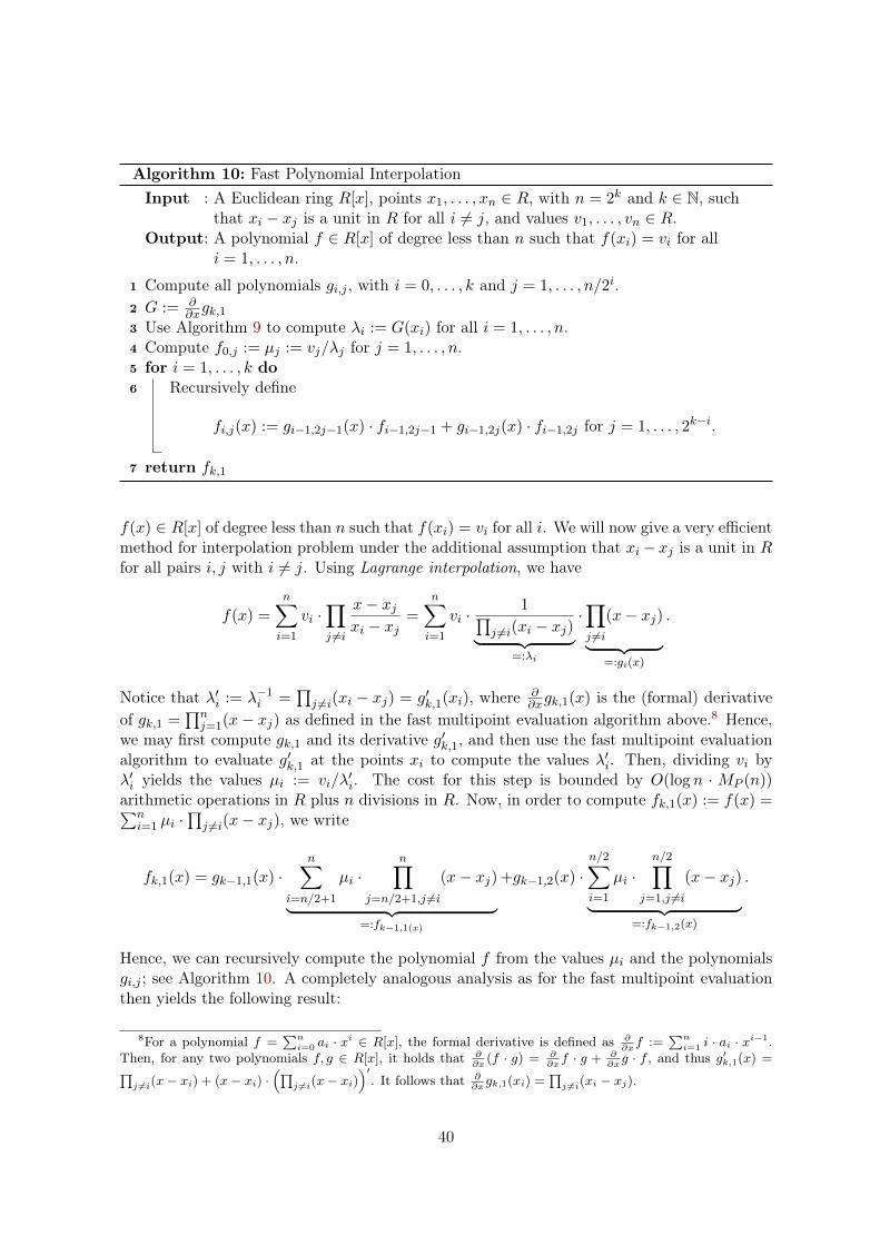
Algorithm 10: Fast Polynomial InterpolationInput : A Euclidean ring R[x], points x1, . . . , xn ∈ R, with n = 2k and k ∈ N, such

that xi − xj is a unit in R for all i 6= j, and values v1, . . . , vn ∈ R.Output: A polynomial f ∈ R[x] of degree less than n such that f(xi) = vi for all

i = 1, . . . , n.

1 Compute all polynomials gi,j , with i = 0, . . . , k and j = 1, . . . , n/2i.2 G := ∂

∂xgk,13 Use Algorithm 99 to compute λi := G(xi) for all i = 1, . . . , n.4 Compute f0,j := µj := vj/λj for j = 1, . . . , n.5 for i = 1, . . . , k do6 Recursively define

fi,j(x) := gi−1,2j−1(x) · fi−1,2j−1 + gi−1,2j(x) · fi−1,2j for j = 1, . . . , 2k−i.

7 return fk,1

f(x) ∈ R[x] of degree less than n such that f(xi) = vi for all i. We will now give a very efficientmethod for interpolation problem under the additional assumption that xi− xj is a unit in Rfor all pairs i, j with i 6= j. Using Lagrange interpolation, we have

f(x) =n∑i=1

vi ·∏j 6=i

x− xjxi − xj

=n∑i=1

vi ·1∏

j 6=i(xi − xj)︸ ︷︷ ︸=:λi

·∏j 6=i

(x− xj)︸ ︷︷ ︸=:gi(x)

.

Notice that λ′i := λ−1i =

∏j 6=i(xi − xj) = g′k,1(xi), where ∂

∂xgk,1(x) is the (formal) derivativeof gk,1 =

∏nj=1(x− xj) as defined in the fast multipoint evaluation algorithm above.88 Hence,

we may first compute gk,1 and its derivative g′k,1, and then use the fast multipoint evaluationalgorithm to evaluate g′k,1 at the points xi to compute the values λ′i. Then, dividing vi byλ′i yields the values µi := vi/λ

′i. The cost for this step is bounded by O(log n · MP (n))

arithmetic operations in R plus n divisions in R. Now, in order to compute fk,1(x) := f(x) =∑ni=1 µi ·

∏j 6=i(x− xj), we write

fk,1(x) = gk−1,1(x) ·n∑

i=n/2+1

µi ·n∏

j=n/2+1,j 6=i

(x− xj)︸ ︷︷ ︸=:fk−1,1(x)

+gk−1,2(x) ·n/2∑i=1

µi ·n/2∏

j=1,j 6=i(x− xj)︸ ︷︷ ︸

=:fk−1,2(x)

.

Hence, we can recursively compute the polynomial f from the values µi and the polynomialsgi,j ; see Algorithm 1010. A completely analogous analysis as for the fast multipoint evaluationthen yields the following result:

8For a polynomial f =∑ni=0 ai · x

i ∈ R[x], the formal derivative is defined as ∂∂xf :=

∑ni=1 i · ai · x

i−1.Then, for any two polynomials f, g ∈ R[x], it holds that ∂

∂x(f · g) = ∂

∂xf · g + ∂

∂xg · f , and thus g′k,1(x) =∏

j 6=i(x− xi) + (x− xi) ·(∏

j 6=i(x− xi))′. It follows that ∂

∂xgk,1(xi) =

∏j 6=i(xi − xj).

40

Theorem 2.2.8. Let x1, . . . , xn ∈ R be arbitrary points in R such that xi − xj is a unitfor all i 6= j, and let v1, . . . , vn ∈ R be arbitrary points in R. Then, computing the uniquepolynomial f ∈ R[x] of degree less than n with f(xi) = vi for all i uses O(log n ·MP (n)) =O(n log2 n log log n) additions and multiplication plus n divisions in R.

We give a final application of the fast division algorithm, that is, the computation of aTaylor shift x 7→ m + x for a polynomial f =

∑ni=0 ai · xi ∈ R[x] of degree n. Given the

coefficients of f and a point m ∈ R, we aim to compute the coefficients of f(x) := f(m+x) =∑ni=0 ai · xi. The idea is to reduce the problem to a fast multipoint evaluation followed by

an interpolation. Suppose that there exist points x1, . . . , xn such that xi − xj is a unit in Rfor all i 6= j. Then, we evaluate f at the points xi := m + xi, and eventually interpolate ffrom its values f(xi) = f(xi) at the points xi. Notice that, if R supports the FFT, we mayalso choose xi = ωi, with ω a 2n-th root of unity. Then, the interpolation step amounts fora single FFT computation. The following result immediately follows from Theorem 2.2.72.2.7 andTheorem 2.2.82.2.8.

Theorem 2.2.9. Suppose that R contains elements x1, . . . , xn such that xi − xj is a unitin R for all i 6= j (or R supports the FFT). Then, for an arbitrary polynomial f ∈ R[x]and a point m ∈ R, we can compute the coefficients of f(m + x) using O(log n ·MP (n)) =O(n log2 n log log n) additions and multiplication plus n divisions in R.

2.3 Fast Polynomial Arithmetic in C[x]

We finally investigate in fast numerical variants of the algorithms presented in the previoustwo sections. Here, we assume that the coefficients of the input polynomial f ∈ C[x] (or anyother input points in C) are only given up to a certain precision, that is, for arbitrary ρ ∈ N,we may ask for a dyadic approximation in F = F2,ρ of each coefficient (or of each point) to anerror less than 2−ρ. For short, we call a corresponding approximation f of f an (absolute) ρ-bitapproximation of f . We start with a method for the approximate computation of a productof two polynomials.

Theorem 2.3.1. Let f, g ∈ C[x] be polynomials of degree less than n and with coefficients ofabsolute value less than 2L. Then, an ` - bit approximation h =

∑2n−2i=0 hi · xi of the product

h =∑2n−2

i=0 hi · xi := f · g (i.e. |hi − hi| < 2−` for all i) can be computed using O(n(L + `))primitive operations. For this, we need ρ-bit approximations of f and g for some ρ of sizeO(log n+ `+ L).

Proof. We reduce the multiplication of f and g to that of integer polynomials. For a non-negative integer ρ, consider ρ-bit approximations f =

∑n−1i=0 ai · xi and g =

∑n−1i=0 bi · xi of f

and g. Then, h =∑2n−2

i=0 ci ·xi := f · g constitutes an approximation of h =∑2n−2

i=0 cixi := f ·g

with|hi − hi| < n · [2L+1 · 2−ρ + 2−2ρ] < 2L+2+dlogne−ρ,

which follows from the fact that |aibj − aibj | < (|ai| + |bj |) · 2−ρ + 2−2ρ for all i, j. Hence,in order to guarantee that h approximate h to an error less than 2−`, it suffices to chooseρ := L+ 2 + dlog ne+ `. In order to compute the product f · g, we first compute the product(2ρ · f) · (2ρ · g) of integer polynomials and then shift the coefficients of the result by 2ρbits. The latter product can be computed in O(n(` + L)) primitive operations according toTheorem 2.1.122.1.12.

41

For a corresponding numerical variant of the fast polynomial division, we have to workharder. We start with following lemma:

Lemma 2.3.2. Let f ∈ C[x] be a polynomial of degree n, g ∈ C[x] a monic polynomial ofdegree m, with m ≤ n, and q, r ∈ C[x] with f = q · g + r and deg r < m. Then, it holds that

log max(‖q‖∞, ‖r‖∞) = O(L+ n+ (n−m) · Γ),

where L and Γ are non-negative integers with max(‖f‖∞, ‖g‖∞) < 2L and |z| < 2Γ for anycomplex root z of g.

Proof. Let f(x) = a0 + · · ·+ an · xn and g(x) = b0 + · · ·+ bm · xm, then we have

f(x)

xn−m · g(x)=q(x) · g(x) + r(x)

xn−m · g(x)=

q(x)

xn−m+

r(x)

xn−m · g(x)

= qn−m +qn−m−1

x+ · · ·+ q0

xn−m+ · · · (2.9)

where q(x) = q0 + · · · + qn−m · xn−m. Here, we use the fact that r(x)/g(x) is a holomor-phic function in the domain D := x ∈ C : |x| > 2Γ. Using a corresponding result fromComplex Analysis, we thus conclude that it can be written as a Laurent series

∑∞i=−∞ ci · xi,

which converges for all x ∈ D. We further remark that ci = 0 for all i ≥ 0 as, otherwise,limx7→∞

|x·r(x)||g(x)| =∞, which contradicts the fact that deg r < m. Now, from (2.92.9), we conclude

thatf

xn−m · g(x)· xi−1 = qn−m · xi−1 + · · ·+ qn−m−i

x+ · · · ,

and thus the Residue Theorem yields that

1

2πi

∮|x|=2Γ+1

f(x)

xn−m−i+1 · g(x)dx = qn−m−i for all i = 0, . . . , n−m

or1

2πi

∮|x|=2Γ+1

f(x)

xj+1 · g(x)dx = qj for all j = 0, . . . , n−m.

For |x| = 2Γ+1, we have |f(x)| ≤ (n + 1) · 2L · 2n(Γ+1) and |g(x)| ≥ 2mΓ. Hence, it followsthat the absolute value of the integrand is upper bounded by B = (n+ 1) · 2L+n+(n−m)Γ. Weconclude that each coefficient qj of q is bounded by B · 2Γ+1 = 2O(L+n+(n−m)Γ). The claimregarding the size of the coefficients of r then immediately follows from the bound on ‖q‖∞and the fact that r = f − q · g.

Using the above lemma, we can now derive a bound on the polynomials hi ∈ C[x] ascomputed in Algorithm 88. Namely, let hi be a polynomial of degree less than 2i− 1 such thathi · g = 1 mod x2i , with g(x) = xm · g(1/x) and g ∈ C[x] a monic polynomial of degree m.Then, there exists a polynomial si ∈ C[x] of degree less than m such that

g(x) · hi = 1 + x2i · si(x)⇒ xm · g(1/x)︸ ︷︷ ︸=g(x)

·x2i · hi(1/x)︸ ︷︷ ︸=:hi

= xm+2i + xm · si(1/x)︸ ︷︷ ︸si

.

Hence, the polynomials hi := x2i ·hi(1/x) and si := xm ·si(1/x) are the quotient and remainderobtained dividing xm+2i by g(x). Lemma 2.3.22.3.2 then yields that

log ‖hi‖∞ = log ‖hi‖∞ = O(log ‖g‖∞ + n+ nΓ),

42

with Γ ≥ 0 a bound on log |zi| for every complex root of g. In the (i+ 1) - st iteration step inAlgorithm 88, we compute hi+1 = 2hi− g ·h2

i mod x2i+1 . Hence, if we use ρ-bit approximationsof hi and g instead of the exact polynomials hi and g, then Theorem 2.3.12.3.1 shows that weobtain an approximation of hi+1 to an error less than 2−ρ+O(log ‖g‖∞+n+nΓ). In other wordsthe precision loss in each iteration is bounded by O(log ‖g‖∞ + n + nΓ). Since there are atmost dlog ne many iterations, the total precision loss is bounded by O(log ‖g‖∞ + n + nΓ).Hence, we can use fixed point arithmetic with precision ρ = ` + O(log ‖g‖∞ + n + nΓ) toguarantee an output error of less than 2−`.

Theorem 2.3.3. Let f and g be polynomials as in Lemma 2.3.22.3.2. Then, computing `-bitapproximations q and r of q and r uses O(n(`+ L+ n+ nΓ)) primitive operations. For this,we need ρ-bit approximations of the polynomials f and g for some ρ of size `+ O(L+n+nΓ).

We briefly summarize out findings from Theorems 2.3.12.3.1 and 2.3.32.3.3: A multiplication of twopolynomials f, g ∈ C[x] using fixed point arithmetic with precision ρ yields a loss in precisionbounded by O(log n + log max(‖f‖∞, ‖g‖∞)), whereas the precision loss of a correspondingdivision with remainder is bounded by O(n+ log max(‖f‖∞, ‖g‖∞ + nΓ). Now, what can weconclude about the precision loss in the fast multipoint evaluation algorithm? The polynomialsgi,j are products of linear forms x − xs, hence log ‖gi,j‖∞ is bounded by O(nΓ∗) with Γ∗ :=max(1, log maxi=1,...,n |xi|). Since the depth of the recursion is log n, we conclude that theprecision loss is bounded by O(nΓ∗ · log n). Now, for the divisions in the algorithm, noticethat we start with rk,1 = f . In each step of the recursion, we divide a previously computedremainder ri,j by some gi′,j′ . Further notice that ri,j = f mod gi,j , and thus log ‖ri,j‖∞ =O(L + nΓ∗) according to Lemma 2.3.22.3.2. It follows that the precision loss in each of theconsidered divisions is bounded by O(L + nΓ∗). Now, since the depth of the recursion isbounded by O(log n), we conclude that the total loss in precision is bounded by O((L+nΓ∗)).Thus, in order to guarantee an output error of size less than 2−`, it suffices to use fixed pointarithmetic with a precision of size `+ O(L+ nΓ∗).

Theorem 2.3.4. Let f ∈ C[x] be a polynomial of degree n with coefficients of absolute valuebounded by 2L, with L ∈ N≥1, and let x1, . . . , xn ∈ C be arbitrary points of absolute valueless than 2Γ∗, with Γ∗ ≥ 1. For an arbitrary non-negative number `, we can compute `-bitapproximations vi of all values vi := f(xi) using O(n · (`+L+ Γ∗)) primitive operations. Forthis, we need ρ-bit approximations of f and the points xi for some ρ of size `+ O(L+ nΓ∗).

Corollary 2.3.5. Let f ∈ C[x] be a polynomial of degree n with coefficients of absolute valuebounded by 2L, with L ∈ N≥1, and m ∈ C be an arbitrary point of absolute value less than 2Γ∗ ,with Γ∗ ≥ 1. For an arbitrary non-negative number `, we can compute an `-bit approximationsof F (x) = F (m + x) using O(n · (` + L + Γ∗)) primitive operations. For this, we need ρ-bitapproximations of f and m for some ρ of size `+ O(L+ nΓ∗).

Proof. The proof is left as an exercise.

Exercise 2.3.6. Let f ∈ Z[x] be an integer polynomial of degree less than n with coefficientsof absolute value less than 2L. Furthermore, let x1, . . . , xn be n be distinct rational points in[0, 1] of bitsize ` (i.e., xi = pi/qi ∈ [0, 1] with integers pi and qi of absolute value less than 2`).

We say that the point xi is large for f among X := x1, . . . , xn if

4 · |f(xi)| ≥ max1≤j≤n

|f(xj)| =: λ.

43

• Determine the cost of finding a large point in a naive way, that is, by evaluating f at allpoints xj exactly.

• Show how to find a large point in O(n(L+ log max(1, λ−1))) bit operations.

Hint: Use approximate multipoint evaluation with increasing precision.

Exercise 2.3.7 (Sparse Approximate Polynomial Evaluation). Let f =∑k

j=1 aij · xij ∈ C[x]

be a k-nomial of degree n with k non-zero coefficients of absolute value bounded by 2L, withL ∈ N≥1, and let x0 ∈ C be an arbitrary point of absolute value less than 2Γ∗, with Γ∗ ≥ 1. Foran arbitrary non-negative number `, we can compute an `-bit approximations of v := f(x0)using O(k · (`+L+ Γ∗)) primitive operations. For this, we need ρ-bit approximations of f andx0 for some ρ of size `+ O(L+ nΓ∗).

Hint: Use Exercise 1.1.41.1.4

44

Chapter 3

The Extended Euclidean Algorithmand (Sub-) Resultants

3.1 Gauss’ Lemma

In what follows, we assume that R is a commutative ring with 1.

Definition 3.1.1 (Integral Domain). R is called an integral domain if it does not contain azero-divisor, that is, if there exists no a, b ∈ R \ 0 with a · b = 0. We further use R∗ todenote the set of invertible elements in R.

Examples. we give several examples for commutative rings that are (not) integral domains:

1. Z is an integral domain and Z∗ = −1, 1.

2. Z/q is an integral domain if and only if q is a prime.

3. If R is an integral domain, then R[x1, . . . , xn] is an integral domain.

Definition 3.1.2. Let R be an integral domain and a, b ∈ R.

1. a is a divisor of b iff there exists a c ∈ R with a · c = b. We write a|b.

2. a, b are associated iff there exists a u ∈ R∗ with a = u · b. We write a ∼ b.

3. q ∈ R \R∗ is irreducible if q = a · b, with a, b,∈ R, implies that a ∈ R∗ or b ∈ R∗.

4. p ∈ R \R∗ is prime if p|a · b, with a, b ∈ R, implies that p|a or p|b.

It holds that

Theorem 3.1.3. In an integral domain R, it holds that

p ∈ R is prime ⇒ p is irreducible.

Proof. Suppose that p is prime and that p = a · b with a, b ∈ R. Hence, p divides a or b.W.l.o.g. we may assume that p divides a, hence there exists a c ∈ R with p = p · c · b, orequivalently p · (1− b · c) = 0. Since R is an integral domain, we must have 1− b · c = 0, andthus b ∈ R∗ with b−1 = c.

45

Definition 3.1.4 (Ideal). A subset I ⊂ R in a ring R is called an ideal if, for all a, b ∈ I andall r ∈ R, we have

a+ b ∈ I and r · a ∈ I.

If there exist elements a1, . . . , an ∈ R such that each a ∈ I can be written as

a = r1 · a1 + · · ·+ rn · an, with ri ∈ R,

then we say that I is generated by a1, . . . , an. For short, we write I = 〈a1, . . . , an〉. If I isgenerated by only one element, we say that I is a principal ideal. R is called a principal idealring (or just principal) if each ideal in R is a principal ideal.

Examples.

1. Each polynomial f(x) ∈ Z[x] that has a root at x = 0 of multiplicity k is contained inI := 〈xk〉.

2. Each polynomial f(x, y) ∈ Z[x, y] with f(1, 2) = 0 is contained in I := 〈x− 1, y − 2〉.

3. Z is principal but Z[x] is not principal.

4. Q[x] is principal.

Exercise 3.1.5. Show that every Euclidean domain is principal.

Definition 3.1.6 (Factorial Ring). An integral domain R is called a factorial ring if, for alla ∈ R \R∗, there exists a factorization

a = p1 · · · pr

of a into primes p1, . . . , pr.

We remark that the above factorization of a into primes is unique.

Theorem 3.1.7. In a factorial ring R, the factorization a = p1 · · · pr of an element a ∈ R\R∗into primes pi is unique up to ordering and a unit in R.

Proof. Suppose that a = p1 · · · pr = q1 · · · qs with primes pi, qj . Since p1 is prime, there mustbe a qj with p|qj . W.l.o.g. we assume that q1 = w1 ·p1 for some w ∈ R. Since q1 is irreducible,we further conclude that w ∈ R∗. Hence, we get p2 · · · pr = w ·q2 · · · qs. Notice that p2 does notdivide w as otherwise, p2 would be also invertible. Hence, the claim follows by induction.

Definition 3.1.8 (Noetherian Ring). A ring R is Noether if each ideal of R is finitely gen-erated.

Examples. We give examples of rings that are (not) Noether:

1. Z,Q,R,C are Noether.

2. Q[x] is Noether. This follows from the extended Euclidean algorithm, which shows that〈f, g〉 = 〈gcd(f, g)〉 for any two polynomials f, g ∈ Q[x]. We give an independent proofof a more general result in the following theorem.

46

3. Q[x1, x2, . . .] is not Noether.

4. The ring Int(Z) := f ∈ Q[x] : f(x) ∈ Z for all x ∈ Z of so-called integer-valuedpolynomials is not Noether. One can show (the proof is non-trivial) that I := 〈x, x(x−1)/2, x(x− 1)(x− 2)/3, . . . , 〉 is not finitely generated.

The crucial fact is that a Noetherian ring R is that it passes this property to its corre-sponding polynomial ring R[x].

Theorem 3.1.9 (Hilbert’s Basis Theorem). If R is Noether, then R[x] is Noether as well. Inparticular, R[x1, . . . , xn] is Noether for R = Z,Q,R,C.

Proof. For a polynomial f(x) = a0 + · · · an · xn ∈ R[x], we use LT(f) = an · xn to denote theleading term of f , and LC(f) = an to denote the leading coefficient of f . We call f monic ifLC(f) = 1. Now, suppose that R[x] is not Noether, then there exists an ideal I ⊂ R[x] thatis not finitely generated. Let f1 ∈ I with deg f1 be an element in I of minimal degree, f2 bean element in I2 \ 〈f1〉 of minimal degree, etc. Then, it follows that

deg(f1) ≤ deg(f2) ≤ · · · ≤ deg(fk) ≤ · · · ,

and thus we obtain an ascending chain of ideals in R

〈LC(f1)〉︸ ︷︷ ︸=:J1

⊂ 〈LC(f1),LC(f2)〉︸ ︷︷ ︸=:J2

⊂ · · ·

We first show that the above chain is strictly ascending, that is, Jk 6= Jk+1 for all k. Namely,if Jk = Jk+1, then there exist bj ∈ R with LC(fk+1) =

∑kj=1 bj · LC(fj), and thus it follows

that

g :=

k∑j=1

bj · xdeg(fk+1)−deg(fk) · fj

is contained in 〈f1, . . . , fk〉 and that it has the same leading coefficient as fk+1. Since fk+1 /∈〈f1, . . . , fk〉, we also have g− fk+1 /∈ 〈f1, . . . , fk〉. In addition, g− fk+1 has lower degree thanfk+1, which contradicts our choice of fk+1.

Now, let J :=⋃∞k=1 Jk be the union of all Jk. J is an ideal in R, hence finitely generated

by elements a1, . . . , ar. Since each ai is contained in some Jki , J must be contained in theunion of all Jki , with i = 1, . . . , r. However, the fact that the sequence of the ideals Jk isstrictly increasing.

Theorem 3.1.10. Let R be Noether, then each a ∈ R \R∗ can be written as

a = q1 · · · qr

with irreducible q1, . . . , qr ∈ R.

Proof. If a is irreducible, then there is nothing to prove. Otherwise, there exist a1, b1 /∈ R∗with a = a1 · b1. If a1 and b1 are both irreducible, we are done. Otherwise, we may assumethat a1 = a2 · b2 with a2, b2 ∈ R∗. Continuing with this approach, we obtain a sequence ofprincipal ideals

〈a〉 ⊂ 〈a1〉 ⊂ 〈a2〉 ⊂ · · ·

Since R is Noether, the ideal generated by all elements ai is finitely generated, and thus theabove sequence must become stationary.

47

We have already seen that Z is factorial. Our goal is to prove that Z[x1, . . . , xn] is factorialas well. Since Z[x1, . . . , xn] is Noether, Theorem 3.1.103.1.10 guarantees that each element f ∈Z[x1, . . . , xn] can be written as a product of irreducible factors. It remains to answer thequestion whether this factors are also prime and whether they are unique (up to ordering).

Theorem 3.1.11. In a factorial ring R, we have

q ∈ R irreducible ⇔ q prime.

Proof. Theorem 3.1.33.1.3 already shows that q prime implies that q is irreducible. For the counterdirection, write q as product q = p1 · · · pr with primes pi. Since q is irreducible, we must haver = 1 and q = p1.

Exercise 3.1.12. In a principal ideal domain R, it holds that

q ∈ R irreducible ⇔ q prime.

Definition 3.1.13 (Primitive Polynomials). Let R be factorial, and f =∑n

i=0 ai · xi ∈ R[x].Then, f is called pimitive if there exists no a ∈ R \ R∗ that divides each coefficient of f .We call cont(f) ∈ R a content11 of f if cont(f) divides each coefficient of f and f/ cont(f) isprimitive.

Example. The polynomial f(x) = 7x2 + 3x+ 6 ∈ Z[x] is primitive, however, g(x) = 12x2 +3x+ 6 ∈ Z[x] is not primitive.

Lemma 3.1.14 (Gauss’Lemma). Let R be a factorial ring and

F :=ab

: a, b ∈ R and b 6= 0

its quotient field22. Then, it holds:

1. The product of two primitive polynomials f, g ∈ R[x] is again primitive.

2. A polynomial f ∈ R[x] is irreducible (over R) if and only if it is irreducible over F .

Proof. For simplicity, we assume that R = Z and F = Q. The argument for the general caseis completely analogous.

For (1), suppose that there exists a prime p that divides each coefficients of f · g. Then,let i and j minimal such that p does not divide ai and p does not divide bj . The coefficientci+j of xi+j in the product f · g is given as

ci+j = ai · bj + ai−1 · bj+1 + · · ·+ ai+1 · bj−1 + · · ·

Since p divides each term in the above sum except ai · bj , we conclude that p does not divideci+j , which contradicts our assumption that f · g is not primitive.

For (2), it obviously suffices to show that a polynomial is irreducible over Z is also irre-ducible over Q. Hence, suppose that f = g · h with polynomials g, h ∈ Q[x] \Q. We can nowchoose integers a, b ∈ Z such that a · g and b · h are both primitive polynomials in Z[x]. Then,part (1) implies that the product (ab) · f = (ag) · (bh) is primitive as well. Thus, we obtaina · b = ±1, which shows that g, h ∈ Z[x].

1Notice that the content is unique up to a factor in R∗.2Addition and multiplication in F is defined as for rational numbers, that is, a

b+ a′

b′ := ab′+a′bbb′ and

ab· a

′

b′ = aa′

bb′ . Two elements aband a′

b′ are equal if and only if ab′ = a′b.

48

We can now prove that R[x] is factorial if R is factorial:

Theorem 3.1.15. If R is factorial, then R[x] is factorial as well.

Proof. Let F be the quotient ring of R. For simplicity, we again assume that R = Z andF = Q. Since Q[x] is a principal domain, Q[x] is also factorial. Namely, each f can be writtenas q1 · · · qs with irreducible qi ∈ Q[x] according to Theorem 3.1.103.1.10, and the qi’s are also primeaccording to Exercise 3.1.123.1.12. Now, let f ∈ Z[x] be a polynomial. We aim to show that thereexists a factorization of f into prime factors qi ∈ Z[x]. We may assume that f is primitive as,otherwise, there exists a common divisor r ∈ Z of all coefficients such that f/r is primitive,and since Z is factorial, r can be written as a product of primes. Now, since Q[x] is factorial,there exists a factorization

f(x) = q1 · · · qsof f into prime factors qi ∈ Q[x]. We can now choose r1, . . . , rs ∈ Z such that ri · qi ∈ Z[x] isprimitive. This implies that

(r1 · · · rs) · f = (r1q1) · · · (rsqs)

is primitive as well, and thus r1 · · · rs = ±1. Hence, we have ri = ±1 for all i. Since each qi isirreducible in Q[x], it is also irreducible in Z[x]. It remains to show that the above factorizationof f into irreducible polynomials is unique. For this, suppose that we have f(x) = q1 · · · qs′with irreducible polynomials qi ∈ Z[x]. Since the factorization into irreducible polynomialsin Q[x] is (unique up to ordering and a unit in Q), we have s = s′ and we may assume thataibi· qi = qi with integers ai, bi ∈ Z \ 0. Since qi is irreducible in Z[x], it must be primitive

as well. Since qi is also primitive, we thus conclude from aiqi = biqi that ai = bi. This showsthat the factorization is unique. We conclude that qi is prime as, in every integral domainthat yields a unique factorization into irreducibles, an element is prime if and only if it isirreducible.

From the above theorem, we conclude that Z[x1, . . . , xn] is a factorial ring. The same holdstrue for F [x1, . . . , xn], where F is an arbitrary field.

Definition 3.1.16 (GCD and LCM). Let R be an integral domain and a, b, c ∈ R. Then, cis a greatest common divisor of a and b (c = gcd(a, b) for short) if

• c divides a and b, and

• for all d ∈ R, it holds that if d divides a and b, then d divides c.

We further define c = lcm(a, b) a least common multiple of a and b if

• a and b divide c, and

• for all d ∈ R, it holds that if a and b divide d, then c divides d.

Notice that we do not use the article "the" in definitions of a greatest common divisorand a least common multiple. The reason is that, in general, gcd(a, b) and lcm(a, b) are notuniquely defined. For instance, 2 as well as −2 are greatest common divisors of the two integers4 and 14. Also, for a = x2 − 1 ∈ Q[x] and b = x2 + 2x − 1, both of the two polynomials(x + 1) · (x2 − 1) = x3 + x2 − x − 1 and 1

2 · (x3 + x2 − x − 1) are least common multiples of

a and b. Hence, it makes sense to normalize the polynomials, which allows us to speak about"the" greatest common divisor and the least common multiple.

49

Definition 3.1.17 (Normal Form). Let R be an integral domain, then we call a functionnormal : R 7→ R a normal form if normal(a) ∼ a for all a ∈ R and the following twoproperties are fulfilled:

• normal(0) = 0,

• a ∼ b⇒ normal(a) = normal(b), and

• normal(a · b) = normal(a) · normal(b).

We call the unique e ∈ R∗ with e · normal(a) = a the leading coefficient of a (LC(a) = e forshort). For a = 0, we define LC(0) = 1.

In the special case, where R = F [x] with F a field, it is easy to see that normal(f) :=LC(f)−1 · f is a normal form.

3.2 The Extended Euclidean Algorithm

In this section, we study the extended Euclidean algorithm (EEA for short) to compute thegcd of two polynomials f, g ∈ F [x], where F a field. We further show that the algorithm hasa polynomial bit complexity when applied to compute the gcd of two polynomials f, g withinteger coefficients. The proof of the latter fact is non-trivial at all (even though it seems likethis) and requires a deeper understanding of the method.

Before we formulate the algorithm in its general form, we first review the Euclidean algo-rithm for computing the gcd of two integers a, b ∈ Z. For this, we consider a simple example:In order to compute the c := gcd(a, b) of a := 130 and b := 56, we first divide r0 := a = 130by r1 := b = 56:

130 = 2 · 56 + 18 or 18 = 1 · 130− 2 · 56.

This yields the remainder r2 = 18. Since c divides r0 and r1, it must also divide r2. Vice versa,each divisor of r1 and r2 divides r0, and thus it follows that c = gcd(r0, r1) = gcd(r1, r2). Thisshows that we recursively continue with r1 and r2 (instead of r0 and r1) in this way in orderto compute c. Dividing r1 by r2 yields a remainder r3 := 2:

56 = 3 · 18 + 2 or 2 = 56− 3 · 18 = 56− 3 · (130− 2 · 56) = (−3) · 130 + 7 · 56.

Finally, we divide r2 by r3, which yields the remainder r4 = 0:

18 = 9 · 2 + 0 or 0 = 18− 9 · 2 = (130− 2 · 56)− 9 · ((−3) · 130 + 7 · 56) = 28 · 130− 65 · 56.

We conclude that gcd(130, 56) = 2. Further notice that, in each step of the recursion, weexpressed the remainder ri as a linear combination of a and b. In particular, this holds forr3 := gcd(130, 56):

2 = (−3) · 130 + 7 · 56.

Exercise 3.2.1. Show that, for two integers a, b ∈ Z of length at most L, the Euclideanalgorithm uses O(L) iterations. Further show that this bound is optimal, and derive a boundon the bit complexity of the Euclidean algorithm!

Hint: Show first that ri−1 > 2 · ri+1, where ri is the remainder obtained in the i-th iterationof the algorithm.

50

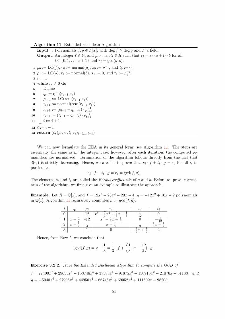
Algorithm 11: Extended Euclidean AlgorithmInput : Polynomials f, g ∈ F [x], with deg f ≥ deg g and F a field.Output: An integer ` ∈ N, and ρi, ri, si, ti ∈ R such that ri = si · a+ ti · b for all

i ∈ 0, 1, . . . , `+ 1 and r` = gcd(a, b).

1 ρ0 := LC(f), r0 := normal(a), s0 := ρ−10 , and t0 := 0.

2 ρ1 := LC(g), r1 := normal(b), s1 := 0, and t1 := ρ−11 .

3 i := 14 while ri 6= 0 do5 Define6 qi := quo(ri−1, ri)7 ρi+1 := LC(rem(ri−1, ri))8 ri+1 := normal(rem(ri−1, ri))

9 si+1 := (si−1 − qi · si) · ρ−1i+1

10 ti+1 := (ti−1 − qi · ti) · ρ−1i+1

11 i := i+ 1

12 ` := i− 113 return (`, (ρi, si, ti, ri)i=0,...,`+1)

We can now formulate the EEA in its general form; see Algorithm 1111. The steps areessentially the same as in the integer case, however, after each iteration, the computed re-mainders are normalized. Termination of the algorithm follows directly from the fact thatd(ri) is strictly decreasing. Hence, we are left to prove that si · f + ti · g = ri for all i, inparticular,

s` · f + t` · g = r` = gcd(f, g).

The elements s` and t` are called the Bézout coefficients of a and b. Before we prove correct-ness of the algorithm, we first give an example to illustrate the approach.

Example. Let R = Q[x], and f = 12x3 − 28x2 + 20x− 4, g = −12x2 + 10x− 2 polynomialsin Q[x]. Algorithm 1111 recursively computes h := gcd(f, g):

i qi ρi ri si ti0 12 x3 − 7

3x2 + 5

3x−13

112 0

1 x− 32 -12 x2 − 5

6x+ 16 0 − 1

12

2 x− 12

14 x− 1

313

13x−

12

3 1 0 −13x+ 1

6 2

Hence, from Row 2, we conclude that

gcd(f, g) = x− 1

3=

1

3· f +

(1

3· x− 1

2

)· g.

Exercise 3.2.2. Trace the Extended Euclidean Algorithm to compute the GCD of

f = 77400x7 + 29655x6 − 153746x5 + 37585x4 + 91875x3 − 130916x2 − 21076x+ 51183 and

g = −5040x6 + 27906x5 + 44950x4 − 66745x3 + 69052x2 + 111509x− 98208,

51

considered as polynomials in Q[x] with rational coefficients. What do you observe?

Exercise 3.2.3 (Sturm Sequences). A Sturm Sequence S is a sequence of polynomials f0, . . . , f` ∈R[x] such that the following conditions are fulfilled:

• deg f0 > deg f1 > · · · > deg f` = 0,

• f0 has no multiple roots,

• If f0(ξ) = 0, then sign(f1(ξ)) = sign(f ′0(ξ)), and

• if fi(ξ) = 0 for i ∈ 1, . . . , `− 1, then sign(fi−1(ξ)) = − sign(fi+1(ξ))

For an arbitrary ξ ∈ R, we define

var(S, ξ) = #i : ∃j > i with fi+1(ξ) = · · · = fj−1(ξ) = 0 and fi(ξ) · fj(ξ) < 0

as the number of sign changes (ignoring zeroes) in the sequence f0(ξ), . . . , f`(ξ).

(a)∗ Show that, for arbitrary a, b ∈ R with a < b, it holds that

#roots of f0 in (a, b] = var(S, a)− var(S, b).

(b) Let f ∈ R[x] be a polynomial, and let r0, . . . , r`+1 ∈ R[x] and ρ0, . . . , ρ`+1 ∈ R be ascomputed by the EEA with input f and g = f ′. We recursively define σ0 := sign(ρ0),σ1 := sign(ρ1), and σi := − sign(σi−1 · ρi+1) for i > 1. Show that the sequence S :=ri := σi · rii=0,...,`, is a Sturm sequence if f has no multiple roots.33

(c) Derive an algorithm to compute all real roots of a polynomial f ∈ Z[x] within a giveninterval [a, b]!

Hint: For (a), use the fact that the number var(S, ξ) can only change at a root ξ of one ofthe polynomials fi. Further show that each root of f0 is not a root of any other polynomial fi.Finally, show that each such root of f0 yields a change of var(S, ξ), whereas each root of fi,with i 6= 0, does not yield a change.

Lemma 3.2.4. Let f and g be polynomials in F [x] and let ρi, si, ti as computed in the EEAwith input f, g, then

(a) gcd(f, g) = gcd(ri, ri+1) = r`

(b) si · f + ti · g = ri for all i = 0, . . . , `+ 1. In particular, s` · f + t` · g = r` = gcd(a, b).

(c) gcd(si, ti) = 1 for all i = 0, . . . , `

(d) deg si =∑

2≤j<i deg qj = deg g − deg ri−1 for all i with 2 ≤ i ≤ `+ 1

(e) deg ti =∑

1≤j<i deg qj = deg f − deg ri−1 for all i with 1 ≤ i ≤ `+ 1.3One can even show that, also for polynomials f with multiple roots, the sequence S has the property that

var(S, a)− var(S, b) equals the number of distinct roots of f in (a, b].

52

Proof. From the definition of the ρi, ri, and qi, we obtain for i = 1, . . . , `:

ρi · ri+1 = ri−1 − qi · riρi+1 · si+1 = si−1 − qi · siρi+1 · ti+1 = ti−1 − qi · ti.

Hence, with Qi :=

(0 1

ρ−1i+1 −qi · ρ−1

i+1

), we have

Qi ·(ri−1

ri

)=

(ri

(ri−1 − qi · ri) · ρ−1i+1

)=

(riri+1

)

for i = 1, . . . , `. Hence, with Q0 :=

(s0 t0s1 t1

)and Ri := Qi · · ·Q1Q0, we conclude that

Ri ·(fg

)= Qi · · ·Q1 ·

(fg

)= Qi · · ·Q1 ·

(ρ−1

0 0

0 ρ−11

)·(fg

)= Qi · · ·Q1 ·

(r0

r1

)=

(riri+1

).

Furthermore, we have

Qi ·(si−1 ti−1

si ti

)=

(si tisi+1 ti+1

), and thus Ri =

(si tisi+1 ti+1

).

We are now ready to prove (a)-(e):We have (

r`0

)=

(r`r`+1

)= Q` · · ·Q0 ·

(fg

)= Q` · · ·Qi+1 ·

(riri+1

),

from which we conlude that r` can be written as a linear combination of ri and ri+1. It follows

that gcd(ri, ri+1) divides r` for all i. In addition, since Qi is invertible and Q−1i =

(qi ρi+1

1 0

),

we have (riri+1

)= Q−1

i+1 · · ·Q−1` ·

(r`0

),

and thus r` divides ri as well as ri+1. Hence, (a) follows.Part (b) follows directly from the fact that

Qi · · ·Q0 =

(si tisi+1 ti+1

)and Qi · · ·Q0 ·

(ab

)=

(riri+1

).

For (c), we use that

si ·ti+1 +si+1 ·ti = det

(si tisi+1 ti+1

)= detQi · · · detQ1 ·det

(s0 t0s1 t1

)= (−1)i ·(ρ0 · · · ρi+1)−1,

which implies that gcd(si, ti) = 1.For (d), we first show by induction that deg si−1 < deg si for all i with 2 ≤ i ≤ `+ 1. For

i = 2, we have

s2 = ρ−12 · (s0 − q1 · s1) = (ρ−1

0 − q1 · 0) · ρ−12 = ρ−1

2 · ρ−10 ,

53

and thus deg s1 = −∞ < 0 = deg s2. Now, suppose that for i with 2 ≤ i ≤ i0, the claim isalready proven. Then, we have

deg si0−1 < deg si0 < deg ri0−1 − deg ri0 + deg si0 = deg qi0 + deg si0 = deg qi0si0 ,

where we used that qi0 = quo(ri0−1, ri0), and thus deg ri0−1 − deg ri0 = deg qi0 . From theabove inequality, we conclude that

deg si0+1 = deg(si0−1 − qi0 · si0) = deg(qi0 · si0) = deg qi0 + deg si0 > deg si0 ,

anddeg si0+1 = deg qi0 + deg si0 =

∑2≤j<i0

deg qj + deg qi0 =∑

1≤j≤ideg qj .

The proof for (e) is completely analogous to that of (d).

The algorithm is called extended Euclidean Algorithm as it does not only return the gcdof a and b, but also its Bézout representation s` · f + t` · g = gcd(f, g). Obviously, thealgorithm uses at most m := deg g many iterations, and each iteration uses O(n) arithmeticoperations in F , where n = deg f . Hence, the total arithmetic complexity is bounded byO(nm). We will study a variant of the algorithm (called Half-GCD) that uses only O(n)arithmetic operations. However, this does not directly imply that the bit complexity of thealgorithm is also polynomial when applied to polynomials f, g ∈ Q[x] with rational coefficients.Namely, it is non-trivial to prove that the bitsizes of the intermediate results do not growexponentially in n. For this, a deeper understanding of the algorithm is necessary. Before wegive details, we give some applications of the EEA.

Definition 3.2.5 (and Lemma). Let R be a factorial ring and f = a0 + · · · + anxn ∈ R[x].

We call f square-free if there exists no polynomial g ∈ R[x] \R such that g2 divides f . Thereexists a unique factorization

f = cont(f) ·k∏i=1

gii (3.1)

of f into square-free and primitive polynomials gi ∈ R[x] that are pairwise coprime. We calla factorization as above the square-free factorization of f . The polynomial f∗ :=

∏ki=1 gi =

f/ gcd(f, f ′) is called the square-free part of f .

Proof. Since R is factorial, R[x] is factorial as well. Hence, there exists a unique factorization

f = cont(f) ·k′∏j=1

fdjj

of f into irreducible, primitive, and distinct polynomials fj . Then, cont(f) ·∏ki=1 g

ii, with

gi :=∏j:dj=i

fj , is the unique square-free factorization of f . In addition, we have

f ′ = cont(f) ·k′∑j=1

dj · ffj· f ′j ,

54

Algorithm 12: Yun’s Square-Free Factorization AlgorithmInput : f ∈ R[x] primitive, with R a factorial ring.Output: A square-free factorization as in (3.13.1).

1 u := gcd(f, f ′), v1 := fu , w1 := f ′

u , i = 12 while vi 6= 1 do3 Recursively define4 gi := gcd(vi, wi − v′i)5 vi+1 := vi

gi

6 wi+1 :=wi−v′igi

7 i = i+ 1

8 m := i− 19 return g1 . . . gm

and thus fdj−1j divides f ′ for all j. Suppose that fdii divides f for some i. Then, since fdii

divides dj ·ffj

for all j 6= i, it must also divide di·ffi

, which is impossible. Hence, it follows that

f ′ = h ·k′∏j=1

fdj−1j ,

with some polynomial h ∈ R[x] that is not divisible by any fj . It thus follows that gcd(f, f ′) =

cont(f) ·∏k′

j=1 fdj−1j and f∗ = f/ gcd(f, f ′).

Exercise 3.2.6 (Yun’s Square-Free Factorization Algorithm). Show that Yun’s algorithm com-putes a square-free factorization of a polynomial f ∈ R[x]!

Exercise 3.2.7. Let f ∈ F [x] be a polynomial, with F a field, and let ` be defined as in theExtended Euclidean Algorithm when applied to f and f ′; that is,

s` · f + t` · f ′ = gcd(f, f ′).

Show that the polynomial t`+1 as computed in the next iteration of the algorithm equals thesquare-free part f∗ of f .

3.3 The Half-GCD Algorithm (under construction)

The main goal of this section is to prove the following theorem:

Theorem 3.3.1. Let f and g be polynomials in F [x] of degree m and n, respectively, wherem ≥ n. Using O(m) arithmetic operations in F , we can compute

• the greatest common divisor r` := gcd(f, g) of f and g,

• the polynomials s` and t` as computed in the EEA such that s` · f + t` + g = r`, and

• the polynomials si, ti, and ri for an arbitrary index i ∈ 0, . . . , `+ 1.

55

3.4 The Resultant

In what follows, we always assume that R is a factorial ring. Given two polynomials f =a0 + · · ·+ am · xm and g = b0 + · · ·+ bn · xn in R[x], we can always write

u · f + v · g = 0,

with u := ggcd(f,g) and v := − f

gcd(f,g) . If the greatest common divisor of f and g is non-trivial(i.e. gcd(f, g) ∈ R[x]\R), then we have deg u < n and deg v < m. Vice versa, if 0 = u′ ·f+v ·gfor polynomials u′, v′ ∈ R[x] of degrees less than n and m, respectively, then f and g mustshare a non-trivial common factor. This gives a necessary and sufficient condition for gcd(f, g)to be non-trivial:

Lemma 3.4.1. Let f, g ∈ R[x] be two polynomials of degrees m and n, respectively. Then, fand g share a non-trivial divisor if and only if there exists polynomials u, v ∈ R[x] with

u · f + v · g = 0 and deg u < n, deg v < m. (3.2)

The above lemma now allows us to reformulate the problem of deciding whether gcd(f, g) isnon-trivial in terms of linear algebra. Namely, considering polynomials u = u0+· · ·+un−1·xn−1

and v = v0+· · ·+vm−1·xm−1 of degrees less than n andm, respectively, and with indeterminatecoefficients. Then, the condition (3.23.2) is equivalent to

(un−1 · · · u0 vm−1 · · · v0

)·

am · · · a0

am · · · a0

. . .. . .

am · · · a0

bn · · · b0bn · · · b0

. . .. . .

bn · · · b0

︸ ︷︷ ︸

=:Syl(f,g)

= 0

Here, Syl(f, g) is an (m+n)× (m+n)-matrix, which is called the Sylvester Matrix of f and g.Notice that the above equality can only be fulfilled if the rows of Syl(f, g) are linear dependent,hence we must have det Syl(f, g) = 0. Vice versa, if the determinant of the Sylvester Matrixvanishes, then there exists a coefficient vector (un−1, . . . , u0, vm−1, . . . , v0) such that the aboveequality holds. We call Res(f, g) := det Syl(f, g) the Resultant of f and g. Notice that thedefinition of Syl as well as Res crucially depends on the degrees of f and g.

Theorem 3.4.2. Let f, g ∈ R[x] be polynomials of degrees m and n, respectively. It holds:

(a) gcd(f, g) ∈ R[x] \R⇔ Res(f, g) = 0

(b) There exist polynomials u, v ∈ R[x] of degrees less than n and m, respectively, such that

Res(f, g) = u · f + v · g.

(c) Res(f, c) = cm for an arbitrary constant c ∈ R

56

(d) Res(f, g) = (−1)mn · Res(g, f)

(e) For R a field, m ≥ n, and r(x) := rem(f, g), we have

Res(f, g) = (−1)mn · LC(g)m−deg r · Res(g, r).

Proof. Part (a) follows from our considerations above. For (b), we distinguish the two casesRes(f, g) = 0 and Res(f, g) 6= 0. In the first case, the claim follows directly from Lemma 3.4.13.4.1.For Res(f, g) 6= 0, consider the matrix

Syl∗(f, g) :=

am · · · a0 xn−1 · fam · · · a0 xn−2 · f

. . .. . .

...am · · · x0 · f

bn · · · b0 xm−1 · gbn · · · b0 xm−2 · g

. . .. . .

...bn · · · x0 · g

obtained by replacing the last column of Syl(f, g) by (xn−1 · f, . . . , x0 · f, xm−1 · g, . . . , x0 · g)t.Using linearity of the determinant, we obtain

det Syl∗(f, g) = Res(f, g) +m+n−1∑j=1

det(Sj) · xj ,

with

Sj :=

am · · · a0 aj−(n−1)

am · · · a0 aj−(n−2)

. . .. . .

...am · · · aj

bn · · · b0 bj−(m−1)

bn · · · b0 bj−(m−2)

. . .. . .

...bn · · · bj

,

where we define ai = bi = 0 for i < 0. Now, notice that the (m + n − j)-th column of Dj

coincides with the last column ofDj , and thus we have Res(f, g) = det Syl∗(f, g). Hence, usingLaplace expansion for the computation of det Syl∗(f, g) yields that Res(f, g) = det Syl∗(f, g) =u · f + v · g with polynomials u and v of degrees less than n and m, respectively.

Parts (c) and (d) follow immediately from the definition of Res and the fact that thedeterminant switches sign if two rows are switched. It remains to prove (e): For this, let

57

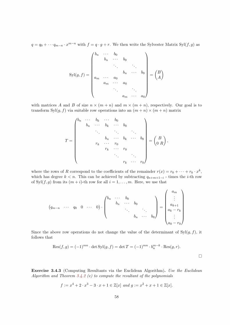
q = q0 + · · · qm−n · xm−n with f = q · g + r. We then write the Sylvester Matrix Syl(f, g) as

Syl(g, f) =

bn · · · b0bn · · · b0

. . .. . .

bn · · · b0am · · · a0

am · · · a0

. . .. . .

am · · · a0

=

(BA

)

with matrices A and B of size n × (m + n) and m × (m + n), respectively. Our goal is totransform Syl(g, f) via suitable row operations into an (m+ n)× (m+ n) matrix

T =

bn · · · bk · · · b0bn · · · bk · · · b0

. . .. . .

. . .

bn · · · bk · · · b0rk · · · r0

rk · · · r0

. . .. . .

rk · · · r0

=

(B

0 R

),

where the rows of R correspond to the coefficients of the remainder r(x) = r0 + · · ·+ rk · xk,which has degree k < n. This can be achieved by subtracting qn+m+1−i - times the i-th rowof Syl(f, g) from its (m+ i)-th row for all i = 1, . . . ,m. Here, we use that

(qm−n · · · q0 0 · · · 0

)·

bn · · · b0

bn · · · b0. . .

. . .

bn · · · b0

=

am...

ak+1

ak − rk...

a0 − r0

Since the above row operations do not change the value of the determinant of Syl(g, f), itfollows that

Res(f, g) = (−1)mn · det Syl(g, f) = detT = (−1)mn · bm−kn · Res(g, r).

Exercise 3.4.3 (Computing Resultants via the Euclidean Algorithm). Use the EuclideanAlgorithm and Theorem 3.4.23.4.2 (e) to compute the resultant of the polynomials

f := x4 + 2 · x3 − 3 · x+ 1 ∈ Z[x] and g := x2 + x+ 1 ∈ Z[x].

58

Exercise 3.4.4 (Specialization Property of Resultants). An important property of the resul-tant is that it is compatible with respect to specialization. More specifically, let φ : R 7→ R′

be a ring homomorphism44 between factorial rings R and R′, and φ : R[x] 7→ R′[x] itscanonical extension to the corresponding polynomial rings (i.e. φ(a0 + · · · + am · xm) =φ(a0) + · · · + φ(am) · xm). Suppose that deg φ(f) = deg f and deg φ(g) = deg g for poly-nomials f, g ∈ R[x], then it holds that

φ(Res(f, g)) = Res(φ(f), φ(g)).

Give an example of two polynomials f, g ∈ Z[x] and a prime p such that Res(f, g) 6= Res(f , g),where we define f , g ∈ Z/p[x] as the canonical images of f and g in Z/p[x].

Exercise 3.4.5. Let f := y2 +2 ·x2 +x ·y−4 ·x−2 ·y+2 and g := 3 ·x2 +y2−4 ·x be two poly-nomials in Z[x]. Show that f = g = 0 has exactly one real solution and determine this solution.

Hint: Consider f and g as polynomials in R[y], with R = Z[x]. Then, use Exercise 3.4.43.4.4 withthe ring homomorphism φ : R 7→ R that maps an h ∈ Z[x] to its value h(x0) at some fixedpoint x0 ∈ R. You should also use the fact that f(x0, y) and g(x0, y) have a common (complex)root if and only if their greatest common divisor is non-trivial.

Exercise 3.4.6 (The Field of Algebraic Numbers). We aim to show that the set of algebraicnumbers

Q := α ∈ C : there exists an f ∈ Q[x] such that f(α) = 0 ⊂ C

over Q is a field.

(a) Let α, β ∈ C and f and g be polynomials in Q[x] such that f(α) = 0 and g(β) = 0. Showhow to construct polynomials h ∈ Q[x] that satisfy

• h(−α) = 0, or

• h(α+ β) = 0, or

• h(α · β) = 0, or

• h(1/α) = 0, or

• h( k√α) = 0 for some k ∈ N≥2, respectively.

Hint: Use resultants to show that the coordinates of any solution of a bivariate sys-tem F (x, y) = G(x, y) = 0, with F,G ∈ Z[x, y], is a root of a polynomial with in-teger coefficients. Then, derive a corresponding bivariate system in α and γ, whereγ = α+ β, α · β, 1/α, etc.

(b) Determine a polynomial f ∈ Z[x] with f(√

3− 3√

3 + 1) = 0.4A mapping φ : R 7→ R′ is a ring homomorphism if φ(1R) = 1R′ , and φ(a + b) = φ(a) + φ(b) and

φ(a · b) = φ(a) · φ(b) for all a, b ∈ R.

59

Theorem 3.4.7. Let f, g ∈ R[x] be polynomials of degrees m and n, respectively, and α anarbitrary element in R. Then, it holds that

Res((x− α) · f, g) = g(α) · Res(f, g).

For polynomials f, g ∈ C[x] with complex roots α1, . . . , αm and β1, . . . , βn, respectively, it holdsthat:

Res(f, g) = LC(f)n ·m∏i=1

g(αi) = (−1)mn ·LC(g)m ·n∏i=1

f(βi) = LC(f) ·LC(g) ·m∏i=1

n∏j=1

(αi−βj).

Proof. Write f = a0 + · · ·+ am · xm and g = b0 + · · ·+ bn · xn. Now, we define

f∗ := (x− α) · f = −α · a0 +m∑i=1

(αi−1 − αai) · xi + am · xm+1,

and consider the Sylvester Matrix of f∗ and g:

Syl(f∗, g) =

am am−1 − αam · · · −αa0

am am−1 − αam · · · −αa0

. . .. . .

am am−1 − αam · · · −αa0

bn bn−1 · · · b0bn bn−1 · · · b0

. . .. . .

bn bn−1 · · · b0

.

Our goal is to transform the above matrix into a matrix of the form

Syl(f∗, g) =

0

Syl(f, g) 00

∗ ∗ ∗ g(α)

. (3.3)

For this, we start with Syl(f∗, g) and add the first column multiplied by α to the secondcolumn. Then, the second column multiplied by α is added to the third column, and so on.This yields the matrix

S :=

am am−1 · · · a0am am−1 · · · a0

. . .. . .

am am−1 · · · a0 0bn bn−1 + αbn bn−2 + αbn−1 + α2bn−2 · · ·

bn bn−1 + αbn · · · · · ·. . .

bn bn−1 + αbn · · · · · · b0 + · · ·+ bnαn

.

In a second step, we subtract α-times the (n + 2)-nd row of the above matrix from the(n + 1)-st row. Then, we subtract the (n + 3)-rd row multiplied by α from the (n + 2)-nd,

60

and so on. Following this approach, we obtain a matrix as in (3.33.3), whose determinant equalsg(α) · Syl(f, g). This proves the first part.

For the second part, notice that f(x) = LC(f)·∏mi=1(x−αi) and g(x) = LC(g)·

∏ni=1(x−βi).

Now, recursive application of the first part and Theorem 3.4.23.4.2 (c) yields that

Res(f, g) = LC(f)n · Res(m∏i=1

(x− αi), g) = LC(f)n ·m∏i=1

g(αi).

Since Res(f, g) = (−1)mn · Res(g, f), we further conclude that

Res(f, g) = (−1)mn · LC(g)m ·m∏i=1

f(βi) = (−1)mn · LC(g)m · LCn ·m∏i=1

n∏j=1

(βi − αj).

As a consequence of the above result, we are now ready to prove some useful bounds onthe absolute values of the roots of a polynomial f ∈ Z[x] as well as on the distances betweendistinct roots.

Theorem 3.4.8 (and Definition). Let f = a0 + · · · + anxn ∈ C[x] be a polynomial of degree

n with coefficients of absolute value less than 2L, and let α1, . . . , αn be the complex roots of f .Then, it holds

(a) The Mahler Measure

Mea(f) := LC(f) ·n∏i=1

max(1, |αi|)

is upper bounded by the 2-norm ‖f‖2 :=√a2

0 + · · ·+ a2n ≤√n+ 1 · 2L of f .

(b) if f has integer coefficients of length less than L and if the roots αi are pairwise distinct,then the separation

sep(αi, f) := minj 6=i|αi − αj |

of each root αi is lower bounded by 2−O(n(logn+L)). We call sep(f) := mini sep(αi, f) theseparation of f .

Proof. For (a), we first show that

‖(x− z) · f‖2 = ‖(zx− 1) · f‖2

for arbitrary z = a+i·b ∈ C and its cojugate z = a−i·b. Namely, with f(x) = a0+· · ·+an ·xnand a−1 = an+1 = 0, we have (x− z) · f =

∑n+1i=0 (ai−1 − z · ai) · xi, and thus

‖(x− z) · f‖2 =n+1∑i=0

(ai−1 − zai) · (ai−1 − zai)

=

n+1∑i=0

[(|ai−1|2 + |z|2|ai|2)− (zaiai−1 + zai−1ai)

]= (1 + |z|2) ·

n∑i=0

|ai|2 −n∑i=0

(zaiai−1 + zaiai−1)

61

In completely analogous manner, we can expand ‖(zx−1) ·f‖2, which yields exactly the sameexpression. Hence, we conclude that

‖f‖2 = ‖an ·n∏i=1

(x− αi)‖2

= ‖an ·∏

i:|αi|≥1

(x− αi) ·∏

i:|αi|<1

(x− αi)‖2

= ‖an ·∏

i:|αi|≥1

(xαi − 1) ·∏

i:|αi|<1

(x− αi)‖2

Since the leading coefficient of f∗ := an ·∏i:|αi|≥1(xαi−1) ·

∏i:|αi|<1(x−αi) equals the Mahler

measure of f , it follows that Mea(f) ≤ ‖f∗‖2 = ‖f‖2.We now prove (b): We first show that

2−4n(logn+L) <∏i∈I|f ′(αi)| < 24n(logn+L)

for any subset I of 1, . . . , n. For the right inequality, we use that |f ′(αi)| < n2 · 2L ·max(1, αi)

n−1, and thus∏i∈I|f ′(αi)| < n2n · 2nL ·Mea(f)n−1 < (n+ 1)

n−12 · n2n · 22nL < 23n(logn+L).

Since f and f ′ do not share a common factor (f has only simple roots), Res(f, f ′) is non-zero.Since Res(f, f ′) is the determinant of an integer matrix, we further conclude that Res(f, f ′)is a non-zero integer, which implies that

1 ≤ |Res(f, f ′)| = |LC(f)|n−1 ·n∏i=1

|f ′(αi)| < 24n(logn+L),

and thus∏i∈I|f ′(αi)| =

∏ni=1 |f ′(αi)|∏i/∈I |f ′(αi)|

>|Res(f, f ′)| · LC(f)−(n−1)∏

i/∈I |f ′(αi)|>

2−(n−1)L

23n(logn+L)> 2−4n(logn+L).

In order to estimate the separation of a specific root αi, consider a root αji 6= αi that minimizesthe distance between αi and any other root such that sep(αi, f) = |αji − αi|. Then, since|f ′(αi)| = |an| ·

∏j 6=i |αi − αj |, we obtain

|f ′(αi)| = sep(αi, f) · |an| ·∏j 6=i,ij

|αj − αi|

< sep(αi, f) ·Mea(f(x+ αi))

< sep(αi, f) ·√n+ 1 · 22n+L ·max(1, |αi|)n,

where the latter two inequalities follow from the fact that f(x + αi) has the roots αj − αi,with j = 1, . . . , n, and that the coefficients of f(x + αi) are of absolute value less than(n+ 1) · 2L · 2n ·max(1, |αi|)n < 22n+L ·max(1, |αi|)n. We thus obtain

sep(αi, f) >|f ′(αi)|

22n+L ·√n+ 1 ·max(1, |αi|)n

>2−4n(logn+L)

23n+L · 2n(L+1)> 2−8n(logn+L).

62

For the product∏i∈I sep(αi, f) over an arbitrary subset I of 1, . . . , n, we obtain:

∏i∈I

sep(αi, f) >∏i∈I

|f ′(αi)|22n+L ·

√n+ 1 ·max(1, |αi|)n

>2−4n(logn+L)

2n(3n+L) ·Mea(f)n> 2−8n(n+L)

Exercise 3.4.9. For two polynomials f, g ∈ C[x] and a disk ∆ in complex space, Rouché’sTheorem states that if

|f(z)| > |f(z)− g(z)| for all z ∈ ∂∆,

with ∂∆ the boundary of ∆, then f and g have the same number of roots in ∆. Use Rouché’sTheorem to show that, for n ≥ 8, the so-called Mignotte polynomial

f(x) = xn − (2L · x− 1)2

has two distinct real roots x1 and x2 with |x1 − x2| < 2−nL2

+1.

Hint: Use the fact that g := −(2L · x − 1)2 has a root of multiplicity 2 at m = 2−L. Then,consider a disc ∆ centered at m and of suitable radius, and compare the values of |f | and|f − g| at the boundary of ∆.

Without proof, we state the following theorem that extends the results from Theorem 3.4.83.4.8to the general case, where f is allowed to have multiple roots. It further provides amortizedbounds on the (weighted) product of all separations. Notice that the bound in (a) alsoconstitutes an improvement upon the bound

∑ni=1 | log sep(αi, f)| = O(n(n+L)) that we have

already derived in the proof of Theorem 3.4.83.4.8. For proofs of Theorem 3.4.103.4.10, consider [MSW15MSW15,Thm. 5] and [KS15KS15, Thm. 9].

Theorem 3.4.10. Let f ∈ Z[x] be a polynomial of degree n with integer coefficients of lengthless than L, and let α1, . . . , αm be the distinct complex roots of f with corresponding multi-plicities µi := µ(αi, f). Then, for an arbitrary subset I of 1, . . . ,m, it holds that

(a)∑

i∈I | log sep(αi, f)| = O(n(log n+ L)),

(b)∑

i∈I µi · | log sep(αi, f)| = O(n(n+ L)), and

(c)∑

i∈I | log ∂µif∂xµi (αi)| = O(n(log n+ L)).

Another application of Theorem 3.4.83.4.8 (a) is a bound on the length of the coefficientsof a divisor g ∈ Z[x1, . . . , xn] of a multivariate polynomial f ∈ Z[x1, . . . , xn] with integercoefficients.

Theorem 3.4.11. Let f ∈ Z[x1, . . . , xn] be an integer polynomial of total degree d with integercoefficients of length less than 2L. Then, each divisor g ∈ Z[x1, . . . , xn] of f has coefficientsof length O(d log d+ L).

Proof. We prove the claim via induction over n. For a univariate f ∈ Z[x1], we remark thatMea(g) ≤ Mea(f) ≤ ‖f‖2 ≤ (d + 1) · 2L, and thus the absolute value of each coefficient of gis bounded by 2d Mea(g) ≤ (d+ 1) · 2d+L.

63

For the general case, we write

f(x1, . . . , xn) =∑

λ=(λ1,...,λn−1)

aλ(xn) · xλ11 · · ·x

λn−1

n−1 , with aλ ∈ Z[xn]

andg(x1, . . . , xn) =

∑λ=(λ1,...,λn−1)

bλ(xn) · xλ11 · · ·x

λn−1

n−1 , with bλ ∈ Z[xn].

For a fixed xn ∈ 0, . . . , d, the polynomial g(x1, . . . , xn−1, xn) ∈ Z[x1, . . . , xn−1] is a divisor off(x1, . . . , xn−1, xn) ∈ Z[x1, . . . , xk−1]. In addition, since |xn|d ≤ dd = 2d log d and since aλ(xn)has degree d or less, it follows that f(x1, . . . , xn−1, xn) has coefficients of length O(d log d+L).Hence, from the induction hypothesis, we conclude that the polynomial g(x1, . . . , xn−1, xn)has coefficients of length O(L + d log d). It thus follows that bλ(xn) ∈ Z has length boundedby O(L + d log d)) for all xn ∈ 0, . . . , d Since bλ(xn) is a polynomial of degree at most d,we further conclude that bλ(xn) is uniquely determined by its values at xn = 0, . . . , n. Hence,Lagrange interpolation yields

bλ(x) =d∑i=0

bλ(i) · x · (x− 1) · · · (x− i+ 1)(x− i− 1) · · · (x− d)

i · (i− 1) · · · 1 · (−1) · · · (i− d)

Expanding the numerator of the fraction yields an integer polynomial with coefficients oflength O(d log d). The denominator is a non-zero integer, and thus each coefficient of bλ(xn)has length O(L+d log d) because bλ(i) has length O(L+d log d) and there are d+1 summands.This proves the claim.

3.5 Subresultants

We have seen in the previous section that the problem of deciding whether two polynomialsf, g ∈ R[x] share a common non-trivial factor can be reduced to the computation of thedeterminant of a matrix whose entries are the coefficients of the given polynomials. We nowextend this approach to determine the actual degree k0 = deg h of the greatest commondivisor h := gcd(f, g) of f and g. We will further show how to obtain h as the determinant ofa Sylvester-like matrix. For this, we start with a generalization of Lemma 3.4.13.4.1:

Lemma 3.5.1. Let f, g ∈ R[x] be two polynomials of degrees m and n, respectively, and letk0 = deg h be the degree of h := gcd(f, g). Then, k0 is the minimal integer k such that

∀u, v ∈ R[x] with deg u < n− k and 0 ≤ deg v < m− k it hold that deg(u · f + v · g) ≥ k.(3.4)

Proof. Let k∗ be the minimal k such that (3.43.4) holds. We first show that k0 ≤ k∗: Defineu := g/h and t = −f/h, then deg u = n− k0 < n− (k0 − 1), deg v = m− k0 < m− (k0 − 1),and deg(uf + vg) = −∞. Hence, it follows that k0 − 1 < k∗.

It remains to show that k0 ≥ k∗: Consider polynomials u, v ∈ R[x] with deg u < n − k0

and 0 ≤ deg v < m−k0. Since u ·f+v ·g is a multiple of h, we either have deg(u ·f+v ·g) ≥ k0

or u · f + v · g = 0. Since f/h and g/h are coprime, u · f = −v · g implies that g/h divides uand that f/h divides v. However, since deg f/h = m − k0 and deg g/h = n − k0, this is notpossible because of the degree bounds on u and v. This shows that deg(u · f + v · g) ≥ k0, andthus k0 ≥ k∗.

64

In order to reformulate the above lemma in terms of linear algebra, we consider the con-trapositive of (3.43.4): If k0 is the degree of h = gcd(f, g), then, for all k < k0, there existpolynomials u = u0 + · · · + un−k−1 · xn−k−1 and v = v0 + · · · + vn−k−1 · xn−k−1 6= 0 suchthat deg(u · f + v · g) < k. This is equivalent to the existence of a non-trivial solution of thefollowing linear system, where we use a0, . . . , am and b0, . . . , bn to denote the coefficients ofthe polynomials f and g, respectively:

(un−k−1 · · · u0 vm−k−1 · · · v0

)·

am · · · a0

am · · · a0

. . .. . .

am · · · akbn · · · b0

bn · · · b0. . .

. . .

bn · · · bk

︸ ︷︷ ︸

=:Sylk(f,g)

= 0 (3.5)

Here, Sylk(f, g) is an (m+ n− 2k)× (m+ n− 2k)-matrix, which is called the k-th SylvesterSubmatrix of f and g. It can be obtained from the corresponding Sylvester matrix by removingthe last 2k columns and the rows numbered from n − k + 1 until n and from n + m − k + 1until n+m. Now, similar to the definition of the resultant, we introduce the following moregeneral definition:

Lemma 3.5.2 (and Definition of Subresultants). The k-th (polynomial) subresultant of fand g is defined as Sresk(x) := det Syl∗k ∈ R[x], with

Syl∗k :=

am · · · a0 xn−k−1 · fam · · · a0 xn−2 · f

. . .. . .

...am · · · ak+1 x0 · f

bn · · · b0 xm−k−1 · gbn · · · b0 xm−2 · g

. . .. . .

...bn · · · bk+1 x0 · g

.

Sresk = ck,0 + · · ·+ ck,k · xk is a polynomial of degree at most k and ck,k = det Sylk(f, g). Wecall sresk := det Sylk(f, g) the k-th leading subresultant coefficient of f and g. It further holdsthat

Sresk(f, g) = uk · f + vk · g,

with polynomials uk, vk ∈ R[x] of degree less than n− k and m− k, respectively.

Proof. The proof is similar to the one of Theorem 3.4.23.4.2 (b). Namely, using linearity of thedeterminant, we obtain

det Syl∗k(f, g) =

m+n−k−1∑j=0

det(Sk,j) · xj ,

65

with

Sk,j :=

am · · · a0 aj−(n−k−1)

am · · · a0 aj−(n−k−2)

. . .. . .

...am · · · ak+1 aj

bn · · · b0 bj−(m−k−1)

bn · · · b0 bj−(m−k−2)

. . .. . .

...bn · · · bk+1 bj

,

where we define ai = bi = 0 for i < 0, ai = 0 for i > m, and bj = 0 for j > n. Now, noticethat, for j > k, the (m + n − k − j)-th column of Sk,j coincides with the last column ofSk,j , and thus we have detSk,j(f, g) = 0 for all j > k. Furthermore, since Sk,k = Sylk(f, g),the coefficient of xk of Sresk equals det Sylk(f, g). The last claim follows directly from usingLaplace expansion for the computation of det Syl∗k(f, g).

Notice that Sres0(f, g) equals the determinant of Syl0(f, g), and that Syl0(f, g) is just theSylvester matrix of f and g. Hence, we have Sres0(f, g) = sres0(f, g) = Res(f, g). In the abovetheorem, we have shown that there exists polynomials uk, vk ∈ R[x] of respective degrees lessthan n−k and m−k such that Sresk(f, g) = uk ·f+vk ·g. According to the following exercise,the cofactors uk and vk can be written as determinants of Sylvester-like matrices.

Exercise 3.5.3. Show that

uk :=

∣∣∣∣∣∣∣∣∣∣∣∣∣∣∣∣∣∣

am · · · a0 xn−k−1

am · · · a0 xn−2

. . .. . .

...am · · · ak+1 x0

bn · · · b0 0bn · · · b0 0

. . .. . .

...bn · · · bk+1 0

∣∣∣∣∣∣∣∣∣∣∣∣∣∣∣∣∣∣, vk :=

∣∣∣∣∣∣∣∣∣∣∣∣∣∣∣∣∣∣

am · · · a0 0am · · · a0 0

. . .. . .

...am · · · ak+1 0

bn · · · b0 xm−k−1

bn · · · b0 xm−2

. . .. . .

...bn · · · bk+1 x0

∣∣∣∣∣∣∣∣∣∣∣∣∣∣∣∣∣∣are polynomials of respective degrees less than n− k and m− k such that

uk · f + vk · g = Sresk(f, g).

Combining Lemma 3.5.13.5.1 and 3.5.23.5.2 now yields the following result, which allows us to readoff the degree of the gcd of f and g directly from the subresultants of f and g.

Corollary 3.5.4. For f, g ∈ R[x], it holds that

k0 := deg gcd(f, g) = mink ∈ N : Sresk(f, g) 6≡ 0 = mink ∈ N : sresk(f, g) 6= 0.

For R a field, we further have Sresk0(f, g) ∼ gcd(f, g).

Proof. Since uk · f + vk · g = Sresk(f, g) = 0, it follows that h := gcd(f, g) divides Sresk(f, g).Hence, since deg Sresk(f, g) ≤ k for all k, it follows that Sres ≡ 0 for all k < k0. For k = k0,Lemma 3.5.13.5.1 guarantees that there does not exist a solution of (3.53.5), and thus sresk0(f, g) 6= 0.If R is a field, then we must have Sresk0(f, g) ∼ h as h divides Sresk0(f, g) and has the samedegree as Sresk0(f, g).

66

In the next step, we aim to show that the polynomials si, ti, ri as computed in the ExtendedEuclidean Algorithm are associated to polynomials uki , vki , and Sreski . For this, we make useof the following result:

Lemma 3.5.5. Let F be a field and r, s, t, f, g ∈ F [x] be polynomials such that

r = s · f + t · g, t 6= 0, and deg r + deg t < deg f = m

Let r0, . . . , r`+1 be the remainders as computed by the EEA with input f and g, and let j ∈0, . . . , `+1 be the unique value with deg rj ≤ deg r < deg rj−1. Then, there exists a λ ∈ F [x]such that

r = λ · rj , , s = λ · sj , and t = λ · tj .

Proof. We first argue by contradiction that sj · t = s · tj : Suppose that sj · t 6= s · tj , then the

matrix(sj tjs t

)is invertible. Hence, using Cramer’s Rule, we obtain

(sj tjs t

)·(fg

)=

(rjr

)⇒ f =

∣∣∣∣rj tjr t

∣∣∣∣∣∣∣∣sj tjs t

∣∣∣∣ .However, this is not possible as

deg(rj · t− r · tj) ≤ max(deg rj + deg t,deg r + deg tj)

= max(deg rj + deg t,deg r +m− deg rj−1)

< max(m,deg rj−1 +m− deg rj−1)

= deg f.

Here, we used Lemma 3.2.43.2.4 (e) to show that deg tj = m− deg rj−1. In Lemma 3.2.43.2.4, we havefurther shown that sj and tj are coprime, and thus sj divides s and tj divides t. It followsthat there exist polynomials λ, λ′ ∈ F [x] with s = λ · sj and t = λ′ · tj , and since sj · t = s · tj ,we further conclude that λ = λ′. Finally, we have

r = s · f + t · g = λ · (sj · f + tj · g) = λ · rj .

We are now ready to prove one of the main results in this section, namely that eachremainder as computed by the EEA coincide with the corresponding subresultant polynomialof the same degree up to a factor in F .

Theorem 3.5.6. Let ni := deg ri be the degree of the remainder ri as computed by the EEAwith input f, g ∈ F [x]. Then, we have ri ∼ Sresni(f, g). Furthermore, sresk(f, g) vanishes ifand only if k does not appear in the degree sequence n0, n1, . . . , n`.

Proof. We have already shown that there exist polynomials uk and vk of respective degree lessthan n− k and m− k such that

uk · f + vk · g = Sresk(f, g).

67

Now, let i, with 2 ≤ j ≤ `+1, be the unique index such that ni ≤ k∗ := deg Sresk(f, g) < ni−1.Then, s := uk and t := vk fulfill the conditions in Lemma 3.5.53.5.5, and thus there exists a λ ∈ F [x]such that uk = λ · si, vk = λ · ti, and λ · ri = λ · Sresk(f, g). It further holds that

m− ni−1 < deg tj ≤ deg vk < m− k ⇒ ni−1 > k,

and thus ni ≤ k∗ ≤ k < ni−1. Hence, k cannot appear in the degree sequence if k∗ 6= k. Viceversa, if k does not appear in the degree sequence, then the equality

si · f + ti · g = ri

implies that sresk(f, g) = 0 as deg si = n − ri−1 < n − k, deg ti = m − ri−1 < m − k, anddeg ri = ni < k. We thus conclude that k appears in the degree sequence if and only ifsresk(f, g) 6= 0.

It remains to show that Sresni ∼ ri. In this case, there exist a λ ∈ F [x] with uni = λ · si,vni = λ · ti, and λ · ri = λ ·Sresni(f, g). Since both polynomials ri and Sresni(f, g) have degreeni, we must have λ ∈ F , hence the claim follows.

We can now bound the bitsize of the coefficients of the polynomials ri, si, and ti for inputpolynomials f, g ∈ Z[x].

Theorem 3.5.7. Let f and g be polynomials of respective degrees m and n, with m ≥ n, andinteger coefficients of length less than L. Then, the polynomials ri, si, and ti computed bythe EEA with input f and g, have rational coefficients with numerators and denominators oflength O(m(logm+ L)).

Proof. Let uk and vk be the polynomials in Z[x] of respective degrees less than n − k andm − k such that uk · f + vk · g = Sresk(f, g). Each coefficient of each of the polynomials uk,vk, and Sresk(f, g) can be computed as the determinant of a square matrix M = (mi,j)i,j ofsize N ≤ (m+ n)× (m+ n) with integer entries of length at most L. The determinant of Mis given as

detM =∑σ∈SN

sign(σ) ·m1,σ(1) · · ·mN,σ(N),

where we sum over all permutations σ of the the integers 1, . . . , N . Hence, detM is an integerof absolute value less than N ! · 2NL, which shows that the polynomials uk, vk, and Sresk(f, g)have coefficients of length bounded by O(m(logm + L)). According to Theorem 3.5.63.5.6, thereexists a rational λ with ri = λ ·Sresni(f, g), si = λ ·uni and ti = λ ·vni , with ni = deg ri. Sinceri is monic, we thus conclude that λ := LC(Sresni(f, g))−1 = sresni(f, g)−1, which proves ourclaim.

Notice that we can now use Exercise 2.2.62.2.6 to bound the bitsize of the coefficients of thequotients qi and of the leading coefficient of the remainders rem(ri−1, ri) as computed in Step 66of the EEA. Namely, since

ri−1 = qi · ri + ρi · ri+1

it follows from the above bound on the bitsize of the coefficients of the rk’s that the coefficientsof qi as well as the leading coefficient ρi of the remainder rem(ri−1, ri) have bitsize boundedby O(m2L). In fact, we can derive a bound that is by a factor n better:

68

Exercise 3.5.8. Let ri be the remainders as computed in the EEA, and let

ri−1 = qi · ri + ρi+1 · ri+1.

Show that there exist integers µi of length O(m(τ + logm)) such that µi · ρi and µi · qi areintegers (integer polynomials) of length (with coefficients of length) O(m(τ + logm))!

Proceed as follows:

1. Use that a comparable result has already been shown for si, ti, and ri!

2. Recall that

Ri =

(si tisi+1 ti+1

)= R0 ·

i∏j=1

Qj , where

R0 =

(s0 t0s1 t1

)and Qj =

(0 1

ρ−1j+1 −qjρ−1

j+1

)

and, in particular,∣∣∣∣ si tisi+1 ti+1

∣∣∣∣ = (−1)i−1(ρ0 · · · ρi)−1. Use these identities to derive a

bound on the length of the numerator and denominator of ρi.

3. Show that f = q · g with f, g ∈ Z[x] polynomials of degree less than N and with integercoefficients of length less than L, and q ∈ Q[x] implies that there exists a λ ∈ Z with|λ| < 2L such that λ · q is a polynomial with integer coefficients of length O(n+ L).

Notice that the bounds on the bitsizes of the polynomials ri, si, and ti as derived aboveimply that the EEA runs in polynomial time. Namely, since the intermediate results havebitsize bounded by O(L(m+ logm)), it follows that the cost for the division of ri−1 by ri inthe i-th iteration is bounded by O(m2L). Hence, the total cost is bounded by O(m3L). Inthe following section, we will see that is possible to reduce the cost to O(m2L) using a moreefficient variant of the EEA.

Exercise 3.5.9. Let f, g ∈ Z[x] be integer polynomials of degree bounded by n and coefficientsof absolute value less than 2τ , let p be prime such that p - LC(f) and p - LC(g), and defined := deg gcd(f, g) to be the degree of the GCD of f and g.

1. Show that

gcd(f, g) ≡ gcd(f , g) mod p if and only if p - sresd(f, g),

where f and g are the modular images of f and g in Z/pZ[x].

2. Develop a modular algorithm to compute under guarantee the degree d of gcd(f, g) ∈ Z[x]and determine its bit complexity in terms of n and τ .

Exercise 3.5.10. (a) Let

f = x3 + 4x2 − 2ax− a2 and

g = x2 − 2a2.

Choose a such that deg gcd(f, g) = 1.

69

(b) Determine the gcd of

f = x2 +( 1

10

√5− 3

10

)x+

( 3

50

√5− 7

50

)and

g = 4x2 +(− 1

10

√5 +

3

10

)x+

( 1

25

√5− 4

25

).

70

Bibliography

[AY62] Karatsuba A. and Ofman Y. “Multiplication of Many-Digital Numbers by Auto-matic Computers”. In: Doklady Akademii Nauk SSSR 14 (1962), pp. 293–294 (cit.on p. 55).

[CT65] James W. Cooley and John W. Tukey. “An Algorithm for the Machine Calculationof Complex Fourier Series”. In:Mathematics of Computation 19.90 (1965), pp. 297–301. issn: 00255718, 10886842 (cit. on p. 2727).

[GG03] J. von zur Gathen and J. Gerhard. Modern Computer Algebra. Cambridge Univer-sity Press, 2003. isbn: 9780521826464 (cit. on pp. 2424, 3333, 3434).

[KS15] Alexander Kobel and Michael Sagraloff. “On the complexity of computing withplanar algebraic curves”. In: J. Complexity 31.2 (2015), pp. 206–236 (cit. on p. 6363).

[MB72] Robert T. Moenck and Allan Borodin. “Fast modular transforms via division”. In:13th. 1972, pp. 90–96 (cit. on p. 3838).

[MOS11] Kurt Mehlhorn, Ralf Osbild, and Michael Sagraloff. “A general approach to theanalysis of controlled perturbation algorithms”. In: Comput. Geom. 44.9 (2011),pp. 507–528 (cit. on p. 1616).

[MS08] K. Mehlhorn and P. Sanders. Algorithms and Data Structures: The Basic Toolbox.SpringerLink: Springer e-Books. Springer, 2008. isbn: 9783540779773 (cit. on pp. 66,77).

[MSW15] Kurt Mehlhorn, Michael Sagraloff, and Pengming Wang. “From approximate fac-torization to root isolation with application to cylindrical algebraic decomposition”.In: J. Symb. Comput. 66 (2015), pp. 34–69 (cit. on p. 6363).

[SS71] A. Schönhage and V. Strassen. “Schnelle Multiplikation großer Zahlen”. In: Com-puting 7.3 (1971), pp. 281–292. issn: 1436-5057 (cit. on p. 2222).

[Too63] Andrei Toom. “The Complexity of a Scheme of Functional Elements Realizing theMultiplication of Integers”. In: Soviet Mathematics-Doklady 7 (1963), pp. 714–716(cit. on p. 77).

71