computer appendix: survival analysis on the computer978-0-387-29150-5/1.pdfcomputer appendix:...
TRANSCRIPT

ComputerAppendix:SurvivalAnalysison theComputerIn this appendix, we provide examples of computer programsfor carrying out the survival analyses described in this text.This appendix does not give an exhaustive survey of all com-puter packages currently available, but rather is intended todescribe the similarities and differences among three of themost widely used packages. The software packages that wedescribe are Stata (version 7.0), SAS (version 8.2), and SPSS(version 11.5). A complete description of these packages is be-yond the scope of this appendix. Readers are referred to thebuilt-in Help functions for each program for further informa-tion.
463

464 Computer Appendix: Survival Analysis on the Computer
Datasets
Most of the computer syntax and output presented in this ap-pendix are obtained from running step-by-step survival anal-yses on the “addicts” dataset. The other dataset that is utilizedin this appendix is the “bladder cancer” dataset for analysesof recurrent events. The addicts and bladder cancer data aredescribed below and can be downloaded from our Web siteat http://www.sph.emory.edu/∼dkleinb/surv2.htm. On thisWeb site we also provide many of the other datasets that havebeen used in the examples and exercises throughout this text.The data on our Web site are provided in several forms: (1) asStata datasets (with a .dta extension), (2) as SAS version 8.2datasets (with a .sas7bdat extension), (3) as SPSS datasets(with a .sav extension), and (4) as text datasets (with a .datextension).
Addicts Dataset (addicts.dat)
In a 1991 Australian study by Caplehorn et al., two methadonetreatment clinics for heroin addicts were compared to assesspatient time remaining under methadone treatment. A pa-tient’s survival time was determined as the time, in days, untilthe person dropped out of the clinic or was censored. The twoclinics differed according to their live-in policies for patients.The variables are defined as follows.
ID—Patient ID.SURVT—The time (in days) until the patient dropped out of the
clinic or was censored.STATUS—Indicates whether the patient dropped out of the clinic
(coded 1) or was censored (coded 0).CLINIC—Indicates which methadone treatment clinic the pa-
tient attended (coded 1 or 2).PRISON—Indicates whether the patient had a prison record
(coded 1) or not (coded 0).DOSE—A continuous variable for the patient’s maximum
methadone dose (mg/day).
Bladder Cancer Dataset (bladder.dat)
The bladder cancer dataset contains recurrent event outcomeinformation for 86 cancer patients followed for the recurrenceof bladder cancer tumor after transurethral surgical excision(Byar and Green, 1980). The exposure of interest is the effectof the drug treatment of thiotepa. Control variables are theinitial number and initial size of tumors. The data layout issuitable for a counting processes approach. The variables aredefined as follows.

Stata Computer Appendix: Survival Analysis on the Computer 465
ID—Patient ID (may have multiple observations for the samesubject).
EVENT—Indicates whether the patient had a tumor (coded 1) ornot (coded 0).
INTERVAL—A counting number representing the order of thetime interval for a given subject (coded 1 for the subject’s firsttime interval, 2 for a subject’s second time interval, etc.).
START—The starting time (in months) for each interval.STOP—The time of event (in months) or censorship for each
interval.TX—Treatment status (coded 1 for treatment with thiotepa and
0 for the placebo).NUM—The initial number of tumor(s).SIZE—The initial size (in centimeters) of the tumor.
Software
What follows is a detailed explanation of the code and outputnecessary to perform the type of survival analyses described inthis text. The rest of this appendix is divided into three broadsections, one for each of the following software packages,
A. Stata,B. SAS, andC. SPSS.
Each of these sections is self-contained, allowing the readerto focus on the particular statistical package of his or herinterest.
A. StataAnalyses using Stata are obtained by typing the appropriatestatistical commands in the Stata Command window or in theStata Do-file Editor window. The key commands used to per-form the survival analyses are listed below. These commandsare case sensitive and lowercase letters should be used.
stset—Declares data in memory to be survival data. Used todefine the “time-to-event” variable, the “status” variable, andother relevant survival variables. Other Stata commands be-ginning with st utilize these defined variables.
sts list—Produces Kaplan–Meier (KM) or Cox adjusted survivalestimates in the output window. The default is KM survivalestimates.
sts graph—Produces plots of Kaplan–Meier (KM) survival es-timates. This command can also be used to produce Cox ad-justed survival plots.
466 Computer Appendix: Survival Analysis on the Computer Stata
sts generate—Creates a variable in the working dataset that con-tains Kaplan–Meier or Cox adjusted survival estimates.
sts test—Used to perform statistical tests for the equality of sur-vival functions across strata.
stphplot—Produces plots of log–log survival against the log oftime for the assessment of the proportional hazards (PH) as-sumption. The user can request KM log–log survival plots orCox adjusted log–log survival plots.
stcoxkm—produces KM survival plots and Cox adjusted survivalplots on the same graph.
stcox—Used to run a Cox proportional hazard model, a stratifiedCox model, or an extended Cox model (i.e., containing time-varying covariates).
stphtest—Performs statistical tests on the PH assumption basedon Schoenfeld residuals. Use of this command requires that aCox model be previously run with the command stcox and theschoenfeld( )option.
streg—Used to run parametric survival models.
Four windows will appear when Stata is opened. These win-dows are labeled Stata Command, Stata Results, Review, andVariables. The user can click on File → Open to select a work-ing dataset for analysis. Once a dataset is selected, the namesof its variables appear in the Variables window. Commandsare entered in the Stata Command window. The output gen-erated by commands appears in the Results window after thereturn key is pressed. The Review window preserves a his-tory of all the commands executed during the Stata session.The commands in the Review window can be saved, copied, oredited as the user desires. Commands can also be run from theReview window by double-clicking on the command. Com-mands can also be saved in a file by clicking on the log buttonon the Stata tool bar.
Alternatively, commands can be typed or pasted into the Do-file Editor. The Do-file Editor window is activated by clickingon Window → Do-file Editor or by simply clicking on theDo-file Editor button on the Stata tool bar. Commands areexecuted from the Do-file Editor by clicking on Tools → Do.The advantage of running commands from the Do-file Editoris that commands need not be entered and executed one at atime as they do from the Stata Command window. The Do-file Editor serves a similar function to that of the programeditor in SAS. In fact, by typing #delim in the Do-file Editorwindow, the semicolon becomes the delimiter for completingStata statements (as in SAS) rather than the default carriagereturn.

Stata Computer Appendix: Survival Analysis on the Computer 467
The survival analyses demonstrated in Stata are as follows.
1. Estimating survival functions (unadjusted) and compar-ing them across strata;
2. Assessing the PH assumption using graphical approaches;3. Running a Cox PH model;4. Running a stratified Cox model;5. Assessing the PH assumption with a statistical test;6. Obtaining Cox adjusted survival curves;7. Running an extended Cox model;8. Running parametric models;9. Running frailty models; and
10. Modeling recurrent events.
The first step is to activate the addicts dataset by clicking onFile → Open and selecting the Stata dataset, addicts.dta.Once this is accomplished, you will see the command use“addicts.dta”, clear in the review window and results win-dow. This indicates that the addicts dataset is activated inStata’s memory.
To perform survival analyses, you must indicate which vari-able is the “time-to-event” variable and which variable is the“status” variable. Rather than program this in every survivalanalysis command, Stata provides a way to program it oncewith the stset command. All survival commands beginningwith st utilize the survival variables defined by stset as longas the dataset remains in active memory. The code to definethe survival variables for the addicts data is as follows.
stset survt, failure(status ==1) id(id)
Following the word stset comes the name of the “time-to-event” variable. Options for Stata commands follow a comma.The first option used is to define the variable and value that in-dicates an event (or failure) rather than a censorship. Withoutthis option, Stata assumes all observations had an event (i.e.,no censorships). Notice two equal signs are used to expressequality. A single equal sign is used to designate assignment.The next option defines the id variable as the variable, ID. Thisis unnecessary with the addicts dataset because each observa-tion represents a different patient (cluster). However, if therewere multiple observations and multiple events for a singlesubject (cluster), Stata can provide robust variance estimatesappropriate for clustered data.

468 Computer Appendix: Survival Analysis on the Computer Stata
The stset command will add four new variables to the dataset.Stata interprets these variables as follows:
t—the “time-to-event” variable;d—the “status variable” (coded 1 for an event, 0 for a censor-
ship);t0—the beginning “time variable”. All observations start at time
0 by default; andst—indicates which variables are used in the analysis. All obser-
vations are used (coded 1) by default.
To see the first 10 observations printed in the output window,enter the command:
list in 1/10
The command stdes provides descriptive information (outputbelow) of survival time.
stdes
failure -d: status == 1analysis time -t: survt
id: id
----------per subject----------| |Category total mean min median max- - - - - - - - - - - - - - - - - - - - - - - - - - - - - - - - - - - - - - - - - - - - - - - - - - - - - - - - - - - - - - - - - - - - - - - - - - - - - -no. of subjects 238no. of records 238 1 1 1 1
(first) entry time 0 0 0 0(final) exit time 402.5714 2 367.5 1076
subjects with gap 0time on gap if gap 0 . . . .time at risk 95812 402.5714 2 367.5 1076
failures 150 .6302521 0 1 1- - - - - - - - - - - - - - - - - - - - - - - - - - - - - - - - - - - - - - - - - - - - - - - - - - - - - - - - - - - - - - - - - - - - - - - - - - - - - -
The commands strate and stir can be used to obtain incidentrate comparisons for different categories of specified vari-ables. The strate command lists the incident rates by CLINICand the stir command gives rate ratios and rate differences.Type the following commands one at a time (output omitted).
strate clinicstir clinic
Stata Computer Appendix: Survival Analysis on the Computer 469
For the survival analyses that follow, it is assumed that thecommand stset has been run for the addicts dataset, asdemonstrated on the previous page.
1. ESTIMATING SURVIVAL FUNCTIONS(UNADJUSTED) AND COMPARINGTHEM ACROSS STRATA
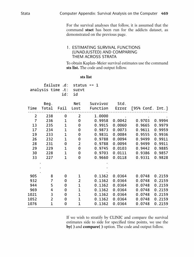
To obtain Kaplan–Meier survival estimates use the commandsts list. The code and output follow.
sts list
failure -d: status == 1analysis time -t: survt
id: id
Beg. Net Survivor Std.Time Total Fail Lost Function Error [95% Conf. Int.]- - - - - - - - - - - - - - - - - - - - - - - - - - - - - - - - - - - - - - - - - - - - - - - - - - - - - - - - - - - - - - - - - - - - - - - - - - - - - - - - -2 238 0 2 1.0000 . . .7 236 1 0 0.9958 0.0042 0.9703 0.999413 235 1 0 0.9915 0.0060 0.9665 0.997917 234 1 0 0.9873 0.0073 0.9611 0.995919 233 1 0 0.9831 0.0084 0.9555 0.993626 232 1 0 0.9788 0.0094 0.9499 0.991128 231 0 2 0.9788 0.0094 0.9499 0.991129 229 1 0 0.9745 0.0103 0.9442 0.988530 228 1 0 0.9703 0.0111 0.9386 0.985733 227 1 0 0.9660 0.0118 0.9331 0.9828. .. .. .
905 8 0 1 0.1362 0.0364 0.0748 0.2159932 7 0 2 0.1362 0.0364 0.0748 0.2159944 5 0 1 0.1362 0.0364 0.0748 0.2159969 4 0 1 0.1362 0.0364 0.0748 0.21591021 3 0 1 0.1362 0.0364 0.0748 0.21591052 2 0 1 0.1362 0.0364 0.0748 0.21591076 1 0 1 0.1362 0.0364 0.0748 0.2159
If we wish to stratify by CLINIC and compare the survivalestimates side to side for specified time points, we use theby( ) and compare( ) option. The code and output follow.

470 Computer Appendix: Survival Analysis on the Computer Stata
sts list, by(clinic) compare at (0 20 to 1080)
failure -d: status == 1analysis time -t: survt
id: id
Survivor Functionclinic 1 2- - - - - - - - - - - - - - - - - - - - - - - - - - - - - - - - - - - - - - - - - - - - - -time 0 1.0000 1.0000
20 0.9815 0.986540 0.9502 0.959560 0.9189 0.945980 0.9000 0.9320100 0.8746 0.9320120 0.8681 0.9179140 0.8422 0.9038160 0.8093 0.8753180 0.7690 0.8466200 0.7420 0.8323220 0.6942 0.8179
.
.
.840 0.0725 0.5745860 0.0543 0.5745880 0.0543 0.5171900 0.0181 0.5171920 . 0.5171940 . 0.5171960 . 0.5171980 . 0.51711000 . 0.51711020 . 0.51711040 . 0.51711060 . 0.51711080 . .
Notice that the survival rate for CLINIC = 2 is higher thanCLINIC = 1. Other survival times could have been requestedusing the compare( ) option.
To graph the Kaplan–Meier survival function (against time),use the code
sts graph
Stata Computer Appendix: Survival Analysis on the Computer 471
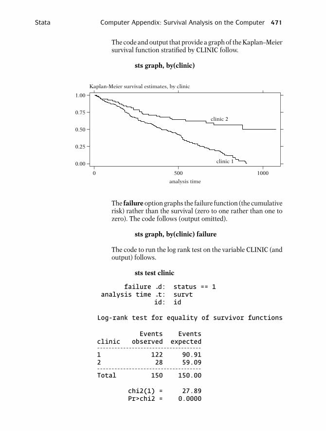
The code and output that provide a graph of the Kaplan–Meiersurvival function stratified by CLINIC follow.
sts graph, by(clinic)
clinic 2
clinic 1
0
0.00
0.25
0.50
0.75
1.00
500 1000
Kaplan-Meier survival estimates, by clinic
analysis time
The failure option graphs the failure function (the cumulativerisk) rather than the survival (zero to one rather than one tozero). The code follows (output omitted).
sts graph, by(clinic) failure
The code to run the log rank test on the variable CLINIC (andoutput) follows.
sts test clinic
failure -d: status == 1analysis time -t: survt
id: id
Log-rank test for equality of survivor functions
Events Eventsclinic observed expected- - - - - - - - - - - - - - - - - - - - - - - - - - - - - - - - - - - -1 122 90.912 28 59.09- - - - - - - - - - - - - - - - - - - - - - - - - - - - - - - - - - - -Total 150 150.00
chi2(1) = 27.89Pr>chi2 = 0.0000

472 Computer Appendix: Survival Analysis on the Computer Stata
The Wilcoxon, Tarone–Ware, Peto, and Flemington–Harrington tests can also be requested. These tests arevariations of the log rank test but weight each observationdifferently. The Wilcoxon test weights the jth failure time bynj (the number still at risk). The Tarone–Ware test weightsthe jth failure time by
√n j . The Peto test weights the jth
failure time by the survival estimate s(t j ) calculated overall groups combined. This survival estimate s(t j ) is similarbut not exactly equal to the Kaplan–Meier survival estimate.The Flemington–Harrington test uses the Kaplan–Meiersurvival estimate s(t) over all groups to calculate its weightsfor the jth failure time s(t j−1)p[1 − s(t j−1)]q , so it takes twoarguments (p and q). The code follows (output omitted).
sts test clinic, wilcoxonsts test clinic, twarests test clinic, petosts test clinic, fh(1,3)
Notice that the default test for the sts test command is the logrank test. The choice of which weighting of the test statistic touse (e.g., log rank or Wilcoxon) depends on which test is be-lieved to provide the greatest statistical power, which in turndepends on how it is believed the null hypothesis is violated.However, one should make an a priori decision on which sta-tistical test to use rather than fish for a desired p-value.
A stratified log rank test for CLINIC (stratified by PRISON)can be run with the strata option. With the stratified approach,the observed minus expected number of events is summedover all failure times for each group within each stratumand then summed over all strata. The code follows (outputomitted).
sts test clinic, strata(prison)
The sts generate command can be used to create a new vari-able in the working dataset containing the KM survival esti-mates. The following code defines a new variable called SKM(the variable name is the user’s choice) that contains KM sur-vival estimates stratified by CLINIC.
sts generate skm=s, by(clinic)
The ltable command produces life tables. Life tables are analternative approach to Kaplan–Meier that are particularlyuseful if you do not have individual level data. The code andoutput that follow provide life table survival estimates, strat-ified by CLINIC, at the time points (in days) specified by theinterval( ) option.

Stata Computer Appendix: Survival Analysis on the Computer 473
ltable survt status,by (clinic) interval(60 150 200 280 365 730 1095)
Beg. Std.Interval Total Deaths Lost Survival Error [95% Conf. Int.]
- - - - - - - - - - - - - - - - - - - - - - - - - - - - - - - - - - - - - - - - - - - - - - - - - - - - - - - - - - - - - - - - - - - - - - - - - - - - - - - - - - - - -clinic = 10 . 163 13 4 0.9193 0.0215 0.8650 0.952360 150 146 14 6 0.8293 0.0300 0.7609 0.8796150 200 126 13 3 0.7427 0.0352 0.6661 0.8043200 280 110 17 2 0.6268 0.0393 0.5446 0.6984280 365 91 10 6 0.5556 0.0408 0.4720 0.6313365 730 75 41 15 0.2181 0.0367 0.1509 0.2934730 1095 19 14 5 0.0330 0.0200 0.0080 0.0902clinic = 20 . 75 4 2 0.9459 0.0263 0.8624 0.979460 150 69 5 3 0.8759 0.0388 0.7749 0.9334150 200 61 3 0 0.8328 0.0441 0.7242 0.9015200 280 58 5 1 0.7604 0.0508 0.6429 0.8438280 365 52 3 2 0.7157 0.0540 0.5943 0.8065365 730 47 7 23 0.5745 0.0645 0.4385 0.6890730 1095 17 1 16 0.5107 0.0831 0.3395 0.6584
2. ASSESSING THE PH ASSUMPTION USINGGRAPHICAL APPROACHES
Several graphical approaches for the assessment of the PHassumption for the variable CLINIC are demonstrated:
1. Log–log Kaplan–Meier survival estimates (stratified byCLINIC) plotted against time (or against the log of time);
2. Log–log Cox adjusted survival estimates (stratified byCLINIC) plotted against time; and
3. Kaplan–Meier survival estimates and Cox adjusted survivalestimates plotted on the same graph.
All three approaches are somewhat subjective yet, it is hoped,informative. The first two approaches are based on whetherthe log–log survival curves are parallel for different levels ofCLINIC. The third approach is to determine if the COX ad-justed survival curve (not stratified) is close to the KM curve.In other words, are predicted values from the PH model (fromCOX) close to the “observed” values using KM?
The first two approaches use the stphplot command whereasthe third approach uses the stcoxkm command. The code andoutput for the log–log Kaplan–Meier survival plots follow.

474 Computer Appendix: Survival Analysis on the Computer Stata
stphplot, by(clinic) nonegative
−5.0845
1.38907
1.94591 6.98101
In(analysis time)
Ln
[-L
n(S
urv
ival
Pro
bab
ilit
ies)
]B
y C
ateg
orie
s of
Cod
ed 1
or
2
clinic = 1 clinic = 2
The left side of the graph seems jumpy for CLINIC = 1 but itonly represents a few events. It also looks as if there is someseparation between the plots at the later times (right side).The nonegative option in the code requests log(−log) curvesrather than the default −log(−log) curves. The choice is ar-bitrary. Without the option the curves would go downwardrather than upward (left to right).
Stata (as well as SAS) plots log(survival time) rather than sur-vival time on the horizontal axis by default. As far as check-ing the parallel assumption, it does not matter if log(survivaltime) or survival time is on the horizontal axis. However,if the log–log survival curves look like straight lines withlog(survival time) on the horizontal axis, then there is evi-dence that the “time-to-event” variable follows a Weibull dis-tribution. If the slope of the line equals one, then there isevidence that the survival time variable follows an exponen-tial distribution, a special case of the Weibull distribution. Forthese situations, a parametric survival model can be used.
It may be visually more informative to graph the log–log sur-vival curves against survival time (rather than log survivaltime). The nolntime option can be used to put survival timeon the horizontal axis. The code and output follow.

Stata Computer Appendix: Survival Analysis on the Computer 475
stphplot, by(clinic) nonegative nolntime
clinic = 1 clinic = 21.38907
−5.0845
7 1076
Ln
[-L
n(S
urv
ival
Pro
bab
ilit
ies)
]B
y C
ateg
orie
s of
Cod
ed 1
or
2
analysis time
The graph suggests that the curves begin to diverge over time.
The stphplot command can also be used to obtain log–logCox adjusted survival estimates. The code follows.
stphplot, strata(clinic) adjust(prison dose) nonegative nolntime
The log–log curves are adjusted for PRISON and DOSE usinga stratified COX model on the variable CLINIC. The meanvalues of PRISON and DOSE are used for the adjustment.The output follows.
clinic = 1 clinic = 21.65856
−5.23278
7 1076
Ln
[-L
n(S
urv
ival
Pro
bab
ilit
ies)
]
By
Cat
egor
ies
of C
oded
1 o
r 2
analysis time
The Cox adjusted curves look very similar to the KM curves.

476 Computer Appendix: Survival Analysis on the Computer Stata
The stcoxkm command is used to compare Kaplan–Meiersurvival estimates and Cox adjusted survival estimates plottedon the same graph. The code and output follow.
stcoxkm, by(clinic)
Observed: clinic = 1
Predicted: clinic = 1
Observed: clinic = 2
Predicted: clinic = 2
0.00
0.25
0.50
0.75
1.00
2 1076Ob
serv
ed v
s. P
red
icte
d S
urv
ival
Pro
bab
ilit
ies
By
Cat
egor
ies
of C
oded
1 o
r 2
analysis time
The KM and adjusted survival curves are very close togetherfor CLINIC = 1 and less so for CLINIC = 2. These graphicalapproaches suggest there is some violation with the PH as-sumption. The predicted values are Cox adjusted for CLINIC,and therefore assume the PH assumption. Notice that the pre-dicted survival curves are not parallel by CLINIC even thoughwe are adjusting for CLINIC. It is the log–log survival curves,rather than the survival curves, that are forced to be parallelby Cox adjustment.
The same graphical analyses can be performed with PRISONand DOSE. However, DOSE would have to be categorizedsince it is a continuous variable.
3. RUNNING A COX PH MODEL
For a Cox PH model, the key assumption is that the hazardis proportional across different patterns of covariates. Thefirst model that is demonstrated contains all three covariates:PRISON, DOSE, and CLINIC. In this model, we are assumingthe same baseline hazard for all possible patterns of these co-variates. In other words, we are accepting the PH assumptionfor each covariate (perhaps incorrectly). The code and outputfollow.

Stata Computer Appendix: Survival Analysis on the Computer 477
stcox prison clinic dose, nohr
failure -d: status == 1analysis time -t: survt
id: id
Iteration 0: log likelihood = -705.6619Iteration 1: log likelihood = -674.54907Iteration 2: log likelihood = -673.407Iteration 3: log likelihood = -673.40242Iteration 4: log likelihood = -673.40242Refining estimates:Iteration 0: log likelihood = -673.40242
Cox regression -- Breslow method for ties
No. of subjects = 238 Number of obs = 238No. of failures = 150Time at risk = 95812
LR chi2(3) = 64.52Log likelihood = -673.40242 Prob > chi2 = 0.0000
- - - - - - - - - - - - - - - - - - - - - - - - - - - - - - - - - - - - - - - - - - - - - - - - - - - - - - - - - - - - - - - - - - - - - - - - - - - - - - - - - - - - --t-d Coef. Std. Err. z p>|z| [95% Conf. Interval]
- - - - - - - - - - - - - - - - - - - - - - - - - - - - - - - - - - - - - - - - - - - - - - - - - - - - - - - - - - - - - - - - - - - - - - - - - - - - - - - - - - - - -prison .3265108 .1672211 1.95 0.051 -.0012366 .6542581clinic -1.00887 .2148709 -4.70 0.000 -1.430009 -.5877304dose -.0353962 .0063795 -5.55 0.000 -.0478997 -.0228926
- - - - - - - - - - - - - - - - - - - - - - - - - - - - - - - - - - - - - - - - - - - - - - - - - - - - - - - - - - - - - - - - - - - - - - - - - - - - - - - - - - - - -
The output indicates that it took five iterations for the loglikelihood to converge at −673.40242. The iteration historytypically appears at the top of Stata model output, however,the iteration history will subsequently be omitted. The final ta-ble lists the regression coefficients, their standard errors, anda Wald test statistic (z) for each covariate, with correspondingp-value and 95% confidence interval.
The nohr option in the stcox command requests the regres-sion coefficients rather than the default exponentiated coef-ficients (hazard ratios). If you want the exponentiated coeffi-cients, omit the nohr option. The code and output follow.

478 Computer Appendix: Survival Analysis on the Computer Stata
stcox prison clinic dose
Cox regression -- Breslow method for ties
No. of subjects = 238 Number of obs = 238No. of failures = 150Time at risk = 95812
LR chi2(3) = 64.52Log likelihood = -673.40242 Prob > chi2 = 0.0000
- - - - - - - - - - - - - - - - - - - - - - - - - - - - - - - - - - - - - - - - - - - - - - - - - - - - - - - - - - - - - - - - - - - - - - - - - - - - - - - - - - - - --t-d Haz. Ratio Std. Err. z p>|z| [95% Conf. Interval]
- - - - - - - - - - - - - - - - - - - - - - - - - - - - - - - - - - - - - - - - - - - - - - - - - - - - - - - - - - - - - - - - - - - - - - - - - - - - - - - - - - - - -prison 1.386123 .231789 1.95 0.051 .9987642 1.923715clinic .3646309 .0783486 -4.70 0.000 .2393068 .5555868dose .965223 .0061576 -5.55 0.000 .9532294 .9773675
This table contains the hazard ratios, its standard errors, andcorresponding confidence intervals. Notice that you do notneed to supply the “time-to event” variable or the status vari-able when using the stcox command. The stcox commanduses the information supplied from the stset command. ACox model can also be run using the cox command, whichdoes not rely on the stset command having previously beenrun. The code follows.
cox survt prison clinic dose, dead(status)
Notice that with the cox command, we have to list the variableSURVT. The dead() option is used to indicate that the variableSTATUS distinguishes events from censorship. The variableused with the dead() option needs to be coded nonzero forevents and zero for censorships. The output from the coxcommand follows.
Cox regression -- Breslow method for tiesEntry time 0 Number of obs = 238
LR chi2(3) = 64.52Prob > chi2 = 0.0000
Log likelihood = -673.40242 Pseudo R2 = 0.0457
- - - - - - - - - - - - - - - - - - - - - - - - - - - - - - - - - - - - - - - - - - - - - - - - - - - - - - - - - - - - - - - - - - - - - - - - - - - - - - - - - - - - -survtstatus Coef. Std. Err. z p>|z| [95% Conf. Interval]- - - - - - - - - - - - - - - - - - - - - - - - - - - - - - - - - - - - - - - - - - - - - - - - - - - - - - - - - - - - - - - - - - - - - - - - - - - - - - - - - - - - -prison .3265108 .1672211 1.95 0.051 -.0012366 .6542581clinic -1.00887 .2148709 -4.70 0.000 -1.430009 -.5877304dose -.0353962 .0063795 -5.55 0.000 -.0478997 -.0228926
- - - - - - - - - - - - - - - - - - - - - - - - - - - - - - - - - - - - - - - - - - - - - - - - - - - - - - - - - - - - - - - - - - - - - - - - - - - - - - - - - - - - -

Stata Computer Appendix: Survival Analysis on the Computer 479
The output is identical to that obtained from the stcox com-mand except that the regression coefficients are given by de-fault. The hr option for the cox command supplies the expo-nentiated coefficients.
Notice in the previous output that the default method of han-dling ties (i.e., when multiple events happen at the same time)is the Breslow method. If you wish to use more exact methodsyou can use the exactp option (for the exact partial likelihood)or the exactm option (for the exact marginal likelihood) in thestcox or cox command. The exact methods are computation-ally more intensive and typically have a slight impact on theparameter estimates. However, if there are a lot of events thatoccur at the same time then exact methods are preferred. Thecode and output follow.
stcox prison clinic dose,nohr exactm
Cox regression -- exact marginal likelihood
No. of subjects = 238 Number of obs = 238No. of failures = 150Time at risk = 95812
LR chi2(3) = 64.56Log likelihood = -666.3274 Prob > chi2 = 0.0000
- - - - - - - - - - - - - - - - - - - - - - - - - - - - - - - - - - - - - - - - - - - - - - - - - - - - - - - - - - - - - - - - - - - - - - - - - - - - - - - - - - - - --t-d Coef. Std. Err. z p>|z| [95% Conf. Interval]
- - - - - - - - - - - - - - - - - - - - - - - - - - - - - - - - - - - - - - - - - - - - - - - - - - - - - - - - - - - - - - - - - - - - - - - - - - - - - - - - - - - - -prison .326581 .1672306 1.95 0.051 -.0011849 .6543469clinic -1.009906 .2148906 -4.70 0.000 -1.431084 -.5887285dose -.0353694 .0063789 -5.54 0.000 -.0478718 -.0228669
Suppose you are interested in running a Cox model with twointeraction terms with PRISON. The generate command canbe used to define new variables. The variables CLIN PR andCLIN DO are product terms that are defined from CLINIC ×PRISON and CLINIC × DOSE. The code follows.
generate clin pr=clinic∗prisongenerate clin do=clinic∗dose
Type describe or list to see that the new variables are in theworking dataset.

480 Computer Appendix: Survival Analysis on the Computer Stata
The following code runs the Cox model with the two interac-tion terms.
stcox prison clinic dose clin pr clin do, nohr
Cox regression -- Breslow method for ties
No. of subjects = 238 Number of obs = 238No. of failures = 150Time at risk = 95812
LR chi2(5) = 68.12Log likelihood = -671.59969 Prob > chi2 = 0.0000
- - - - - - - - - - - - - - - - - - - - - - - - - - - - - - - - - - - - - - - - - - - - - - - - - - - - - - - - - - - - - - - - - - - - - - - - - - - - - - - - - - - - --t-d Coef. Std. Err. z P>|z| [95% Conf. Interval]
- - - - - - - - - - - - - - - - - - - - - - - - - - - - - - - - - - - - - - - - - - - - - - - - - - - - - - - - - - - - - - - - - - - - - - - - - - - - - - - - - - - - -prison 1.191998 .5413685 2.20 0.028 .1309348 2.253061clinic .1746985 .893116 0.20 0.845 -1.575777 1.925174dose -.0193175 .01935 -1.00 0.318 -.0572428 .0186079
clin-pr -.7379931 .4314868 -1.71 0.087 -1.583692 .1077055clin-do -.0138608 .0143275 -0.97 0.333 -.0419422 .0142206
The lrtest command can be used to perform likelihood ratiotests. For example, to perform a likelihood ratio test on thetwo interaction terms CLIN PR and CLIN DO in the preced-ing model, we can save the −2 log likelihood statistic of thefull model in the computer’s memory by typing the followingcommand.
lrtest, saving(0)
Now the reduced model (without the interaction terms) canbe run (output omitted) by typing:
stcox prison clinic dose
After the reduced model is run, the following command pro-vides the results of the likelihood ratio test comparing the fullmodel (with the interaction terms) to the reduced model.
lrtest

Stata Computer Appendix: Survival Analysis on the Computer 481
The resulting output follows.
Cox: likelihood-ratio test chi2(2) = 3.61Prob > chi2 = 0.1648
The p-value of 0.1648 is not significant at the alpha = 0.05level.
4. RUNNING A STRATIFIED COX MODEL
If the proportional hazard assumption is not met for the vari-able CLINIC, but is met for the variables PRISON and DOSE,then a stratified Cox analysis can be performed. The stcoxcommand can be used to run a stratified Cox model. Thefollowing code (with output) runs a Cox model stratified onCLINIC.
stcox prison dose, strata(clinic)
Stratified Cox regr. -- Breslow method for ties
No. of subjects = 238 Number of obs = 238No. of failures = 150Time at risk = 95812
LR chi2(2) = 33.94Log likelihood = -597.714 Prob > chi2 = 0.0000
- - - - - - - - - - - - - - - - - - - - - - - - - - - - - - - - - - - - - - - - - - - - - - - - - - - - - - - - - - - - - - - - - - - - - - - - - - - - - - - - - - - - --t-d Haz. Ratio Std. Err. z P>|z| [95% Conf. Interval]
- - - - - - - - - - - - - - - - - - - - - - - - - - - - - - - - - - - - - - - - - - - - - - - - - - - - - - - - - - - - - - - - - - - - - - - - - - - - - - - - - - - - -prison 1.475192 .2491827 2.30 0.021 1.059418 2.054138dose .9654655 .0062418 -5.44 0.000 .953309 .977777
- - - - - - - - - - - - - - - - - - - - - - - - - - - - - - - - - - - - - - - - - - - - - - - - - - - - - - - - - - - - - - - - - - - - - - - - - - - - - - - - - - - - -Stratified by clinic
The strata() option allows up to five stratified variables.
A stratified Cox model can be run including the two interac-tion terms. Recall that the generate command created thesevariables in the previous section. This model allows for theeffect of PRISON and DOSE to differ for different values ofCLINIC. The code and output follow.

482 Computer Appendix: Survival Analysis on the Computer Stata
stcox prison dose clin pr clin do, strata(clinic) nohr
Stratified Cox regr. -- Breslow method for ties
No. of subjects = 238 Number of obs = 238No. of failures = 150Time at risk = 95812
LR chi2(4) = 35.81Log likelihood = -596.77891 Prob > chi2 = 0.0000
- - - - - - - - - - - - - - - - - - - - - - - - - - - - - - - - - - - - - - - - - - - - - - - - - - - - - - - - - - - - - - - - - - - - - - - - - - - - - - - - - - - - --t-d Coef. Std. Err. z p>|z| [95% Conf. Interval]
- - - - - - - - - - - - - - - - - - - - - - - - - - - - - - - - - - - - - - - - - - - - - - - - - - - - - - - - - - - - - - - - - - - - - - - - - - - - - - - - - - - - -prison 1.087282 .5386163 2.02 0.044 .0316135 2.142951dose -.0348039 .0197969 -1.76 0.079 -.0736051 .0039973
clin-pr -.584771 .4281291 -1.37 0.172 -1.423889 .2543465clin-do -.0010622 .014569 -0.07 0.942 -.0296169 .0274925
Stratified by clinic
Suppose we wish to estimate the hazard ratio for PRISON =1 vs. PRISON = 0 for CLINIC = 2. This hazard ratio can beestimated by exponentiating the coefficient for prison plus2 times the coefficient for the clinic–prison interaction term.This expression is obtained by substituting the appropriatevalues into the hazard in both the numerator (for PRISON =1) and denominator (for PRISON = 0) (see below).
HR = h0(t) exp[1β1 + β2DOSE + (2)(1)β3 + β4CLIN DO]h0(t) exp[0β1 + β2DOSE + (2)(0)β3 + β4CLIN DO]
= exp(β1 + 2β3)
The lincom command can be used to exponentiate linearcombinations of parameters. Run this command directly af-ter running the model to estimate the HR for PRISON whereCLINIC = 2. The code and output follow.
lincom prison+2∗clin pr, hr
(1) prison + 2.0 clin-pr = 0.0- - - - - - - - - - - - - - - - - - - - - - - - - - - - - - - - - - - - - - - - - - - - - - - - - - - - - - - - - - - - - - - - - - - - - - - - - - - - - - - - - --t Haz. Ratio Std. Err. z p>|z| [95% Conf. Interval]
- - - - - - - - - - - - - - - - - - - - - - - - - - - - - - - - - - - - - - - - - - - - - - - - - - - - - - - - - - - - - - - - - - - - - - - - - - - - - - - - - -(1) .9210324 .3539571 -0.21 0.831 .4336648 1.956121- - - - - - - - - - - - - - - - - - - - - - - - - - - - - - - - - - - - - - - - - - - - - - - - - - - - - - - - - - - - - - - - - - - - - - - - - - - - - - - - - -

Stata Computer Appendix: Survival Analysis on the Computer 483
Models can also be run on a subset portion of the data usingthe if statement. The following code (with output) runs a Coxmodel on the data where CLINIC = 2.
stcox prison dose if clinic==2
Cox regression -- Breslow method for ties
No. of subjects = 75 Number of obs = 75No. of failures = 28Time at risk = 36254
LR chi2(2) = 9.70Log likelihood = -104.37135 Prob > chi2 = 0.0078
- - - - - - - - - - - - - - - - - - - - - - - - - - - - - - - - - - - - - - - - - - - - - - - - - - - - - - - - - - - - - - - - - - - - - - - - - - - - - - - - - - - - --t-d Haz. Ratio Std. Err. z p>|z| [95% Conf. Interval]
- - - - - - - - - - - - - - - - - - - - - - - - - - - - - - - - - - - - - - - - - - - - - - - - - - - - - - - - - - - - - - - - - - - - - - - - - - - - - - - - - - - - -prison .9210324 .3539571 -0.21 0.831 .4336648 1.956121dose .9637452 .0118962 -2.99 0.003 .9407088 .9873457
- - - - - - - - - - - - - - - - - - - - - - - - - - - - - - - - - - - - - - - - - - - - - - - - - - - - - - - - - - - - - - - - - - - - - - - - - - - - - - - - - - - - -
The hazard ratio estimates for PRISON = 1 vs. PRISON = 0(for CLINIC = 2) are exactly the same using the stratified Coxapproach with product terms and the subset data approach(0.9210324).
5. ASSESSING THE PH ASSUMPTION USINGA STATISTICAL TEST
The stphtest command can be used to perform a statisticaltest of the PH assumption. A statistical test gives objectivecriteria for assessing the PH assumption compared to usingthe graphical approach. This does not mean that this statisti-cal test is better than the graphical approach. It is just moreobjective. In fact, the graphical approach is generally moreinformative for descriptively characterizing the form of a PHviolation.
The command stphtest outputs a PH global test for all thecovariates simultaneously and can also be used to obtain atest for each covariate separately with the detail option. Torun these tests, you must obtain Schoenfeld residuals for theglobal test, and Schoenfeld scaled residuals for separate testswith each covariate. The idea behind the PH test is that ifthe PH assumption is satisfied, then the residuals should notbe correlated with survival time (or ranked survival time). Onthe other hand, if the residuals tend to be positive for subjectswho become events at a relatively early time and negativefor subjects who become events at a relatively late time (orvice versa), then there is evidence that the hazard ratio is notconstant over time (i.e., PH assumption is violated).

484 Computer Appendix: Survival Analysis on the Computer Stata
Before the stphtest can be implemented, the stcox com-mand needs to be run to obtain the Schoenfeld residuals(with the schoenfeld() option) and the scaled Schoenfeldresiduals (with the scaledsch() option). In the parenthesesare the names of newly defined variables; schoen∗ createsSCHOEN1, SCHOEN2, and SCHOEN3 whereas scaled∗ cre-ates SCALED1, SCALED2, and SCALED3. These variablescontain the residuals for PRISON, DOSE, and CLINIC, re-spectively (the order that the variables were entered in themodel). The user is free to type any variable name in the paren-theses. The Schoenfeld residuals are used for the global testand the scaled Schoenfeld residuals are used for the testingof the PH assumption for individual variables.
stcox prison dose clinic, schoenfeld(schoen∗) scaledsch(scaled∗)
Once the residuals are defined, the stphtest command can berun. The code and output follow.
stphtest, rank detail
Test of proportional hazards assumptionTime: Rank(t)- - - - - - - - - - - - - - - - - - - - - - - - - - - - - - - - - - - - - - - - - - - - - - - - - - - - - - - - -
rho chi2 df Prob>chi2- - - - - - - - - - - - - - - - - - - - - - - - - - - - - - - - - - - - - - - - - - - - - - - - - - - - - - - - -prison -0.04645 0.32 1 0.5689dose 0.08975 1.08 1 0.2996clinic -0.24927 10.44 1 0.0012- - - - - - - - - - - - - - - - - - - - - - - - - - - - - - - - - - - - - - - - - - - - - - - - - - - - - - - - -global test 12.36 3 0.0062- - - - - - - - - - - - - - - - - - - - - - - - - - - - - - - - - - - - - - - - - - - - - - - - - - - - - - - - -
The tests suggest that the PH assumption is violated forCLINIC with the p-value at 0.0012. The tests do not suggestviolation of the PH assumption for PRISON or DOSE.
The plot() option of the stphtest command can be used toproduce a plot of the scaled Schoenfeld residuals for CLINICagainst survival time ranking. If the PH assumption is met, thefitted curve should look horizontal because the scaled Schoen-feld residuals would be independent of survival time. The codeand graph follow.
stphtest,rank plot(clinic)

Stata Computer Appendix: Survival Analysis on the Computer 485
−5
0
5
scal
ed S
choe
nfe
ld-c
lin
ic
Test of PH Assumption
0 50 100 150
Rank(t)
The fitted curve slopes slightly downward (not horizontally).
6. OBTAINING COX ADJUSTED SURVIVAL CURVES
Adjusted survival curves can be obtained with the sts graphcommand. Adjusted survival curves depend on the patternof covariates. For example, the adjusted survival estimatesfor a subject with PRISON = 1, CLINIC = 1, and DOSE =40 are generally different than for a subject with PRISON =0, CLINIC = 2, and DOSE = 70. The sts graph commandproduces adjusted baseline survival curves. The followingcode produces an adjusted survival plot with PRISON = 0,CLINIC = 0, and DOSE = 0 (output omitted).
sts graph, adjustfor(prison dose clinic)
It is probably of more interest to create adjusted plots for rea-sonable patterns of covariates (CLINIC = 0 is not even a validvalue). Suppose we are interested in graphing the adjustedsurvival curve for PRISON = 0, CLINIC = 2, and DOSE =70. We can create new variables with the generate commandthat can be used with the sts graph command.
generate clinic2=clinic-2generate dose70=dose-70
These variables (PRISON, CLINIC2, and DOSE70) producethe desired pattern of covariate when each is set to zero. Thefollowing code produces the desired results.
sts graph, adjustfor(prison dose70 clinic2)

486 Computer Appendix: Survival Analysis on the Computer Stata
Survivor functionadjusted for prison dose70 clinic2
1.00
0.75
0.50
0.25
0.00
0 1000500
analysis time
Adjusted stratified Cox survival curves can be obtained withthe strata() option. The following code creates two survivalcurves stratified by clinic (CLINIC = 1, PRISON = 0, andDOSE = 70) and (CLINIC = 2, PRISON = 0, and DOSE =70).
sts graph, strata(clinic) adjustfor(prison dose70)
Survivor functions, by clinicadjusted for prison dose70
1.00
0.75
0.50
0.25
0.00
0 1000500
analysis time
clinic 2
clinic 1
The adjusted curves suggest there is a strong effect fromCLINIC on survival.

Stata Computer Appendix: Survival Analysis on the Computer 487
Suppose the interest is in comparing adjusted survival plotsof PRISON = 1 to PRISON = 0 stratified by CLINIC. In thissetting, the sts graph command cannot be used directly be-cause we cannot simultaneously define both levels of prison(PRISON = 1 and PRISON = 0) as the baseline level (recallsts graph plots only the baseline survival function). How-ever, survival estimates can be obtained using the sts gener-ate command twice; once where PRISON = 0 is defined asbaseline and once where PRISON = 1 is defined as baseline.The following code creates variables containing the desiredadjusted survival estimates.
generate prison1=prison-1sts generate scox0=s, strata(clinic) adjustfor(prison dose70)sts generate scox1=s, strata(clinic) adjustfor(prison1 dose70)
The variables SCOX1 and SCOX0 contain the survival esti-mates for PRISON = 1 and PRISON = 0, respectively, adjust-ing for dose and stratifying by clinic. The graph command isused to plot these estimates. If you are using a higher versionof Stata than Stata 7.0 (e.g., Stata 8.0), then you should re-place the graph command with the graph7 command. Thecode and output follow.
graph scox0 scox1 survt, twoway symbol([clinic] [clinic]) xlabel(365,730,1095)
1
.009935
365 730 1095
survival time in days
S(t+0), adjusted S(t+0), adjusted
We can also graph PRISON = 1 and PRISON = 0 with thedata subset where CLINIC = 1. The option twoway requestsa two-way scatterplot. The options symbol, xlabel, and titlerequest the symbols, axis labels, and title, respectively.

488 Computer Appendix: Survival Analysis on the Computer Stata
graph7 scox0 scox1 survt if clinic==1, twoway symbol(ox) xlabel(365,730,1095)t1(“symbols O for prison=0, × for prison=1”) title(“subsetted by clinic==1”)
1
.009935
365 730 1095
survival time in dayssubset by clinic==1
symbols O for prison=0, × for prison=1
7. RUNNING AN EXTENDED COX MODEL
If the PH assumption is not satisfied, a possible strategy is torun a stratified Cox model. Another strategy is to run a Coxmodel with time-varying covariates (an extended Cox model).The challenge of running an extended Cox model is to choosethe appropriate function of survival time to include in themodel.
Suppose we want to include a time-dependent covariateDOSE times the log of time. This product term could be appro-priate if the hazard ratio comparing any two levels of DOSEmonotonically increases (or decreases) over time. The tvc op-tion() of the stcox command can be used to declare DOSE atime-varying covariate that will be multiplied by a function oftime. The specification of that function of time is stated in thetexp option with the variable t representing time. The codeand output for a model containing the time-varying covariate,DOSE × ln( t), follow.

Stata Computer Appendix: Survival Analysis on the Computer 489
stcox prison clinic dose, tvc(dose) texp( ln( t)) nohr
Cox regression -- Breslow method for ties
No. of subjects = 238 Number of obs = 238No. of failures = 150Time at risk = 95812
LR chi2(4) = 66.29Log likelihood = -672.51694 Prob > chi2 = 0.0000- - - - - - - - - - - - - - - - - - - - - - - - - - - - - - - - - - - - - - - - - - - - - - - - - - - - - - - - - - - - - - - - - - - - - - - - - - - - - - - - - - - - -
-t-d Coef. Std. Err. z p>|z| [95% Conf. Interval]
- - - - - - - - - - - - - - - - - - - - - - - - - - - - - - - - - - - - - - - - - - - - - - - - - - - - - - - - - - - - - - - - - - - - - - - - - - - - - - - - - - - - -rh
prison .3404817 .1674672 2.03 0.042 .012252 .6687113clinic -1.018682 .215385 -4.73 0.000 -1.440829 -.5965352dose -.0824307 .0359866 -2.29 0.022 -.1529631 -.0118982
- - - - - - - - - - - - - - - - - - - - - - - - - - - - - - - - - - - - - - - - - - - - - - - - - - - - - - - - - - - - - - - - - - - - - - - - - - - - - - - - - - - - -t
dose .0085751 .0064554 1.33 0.184 -.0040772 .0212274- - - - - - - - - - - - - - - - - - - - - - - - - - - - - - - - - - - - - - - - - - - - - - - - - - - - - - - - - - - - - - - - - - - - - - - - - - - - - - - - - - - - -note: second equation contains variables that continuously vary
with respect to time; variables interact with currentvalues of ln(-t).
The parameter estimate for the time-dependent covariateDOSE × ln( t) is .0085751, however, it is not statistically sig-nificant with a Wald test p-value of 0.184.
A Heaviside function can also be used. The following coderuns a model with a time-dependent variable equal to CLINICif time is greater than or equal to 365 days and 0 other-wise.
stcox prison dose clinic, tvc(clinic) texp(-t >=365) nohr
Stata recognizes the expression ( t >= 365) as taking the value1 if survival time is ≥365 days and 0 otherwise. The outputfollows.

490 Computer Appendix: Survival Analysis on the Computer Stata
Cox regression -- Breslow method for ties
No. of subjects = 238 Number of obs = 238No. of failures = 150Time at risk = 95812
LR chi2(4) = 74.17Log likelihood = -668.57443 Prob > chi2 = 0.0000- - - - - - - - - - - - - - - - - - - - - - - - - - - - - - - - - - - - - - - - - - - - - - - - - - - - - - - - - - - - - - - - - - - - - - - - - - - - - - - - - - - - -
-t-d Coef. Std. Err. z p>|z| [95% Conf. Interval]
- - - - - - - - - - - - - - - - - - - - - - - - - - - - - - - - - - - - - - - - - - - - - - - - - - - - - - - - - - - - - - - - - - - - - - - - - - - - - - - - - - - - -rh
prison .377704 .1684024 2.24 0.025 .0476414 .7077666dose -.0355116 .0064354 -5.52 0.000 -.0481247 -.0228985
clinic -.4595628 .2552911 -1.80 0.072 -.959924 .0407985- - - - - - - - - - - - - - - - - - - - - - - - - - - - - - - - - - - - - - - - - - - - - - - - - - - - - - - - - - - - - - - - - - - - - - - - - - - - - - - - - - - - -t
clinic -1.368665 .4613948 -2.97 0.003 -2.272982 -.464348- - - - - - - - - - - - - - - - - - - - - - - - - - - - - - - - - - - - - - - - - - - - - - - - - - - - - - - - - - - - - - - - - - - - - - - - - - - - - - - - - - - - -note: second equation contains variables that continuously vary
with respect to time; variables interact with currentvalues of -t>=365.
Unfortunately, the texp option can only be used once in thestcox command. This makes it more difficult to run the equiv-alent model with two Heaviside functions. However, it can beaccomplished using the stsplit command, which adds extraobservations to the working dataset. The following code cre-ates a variable called V1 and adds new observations to thedataset.
stsplit v1, at(365)
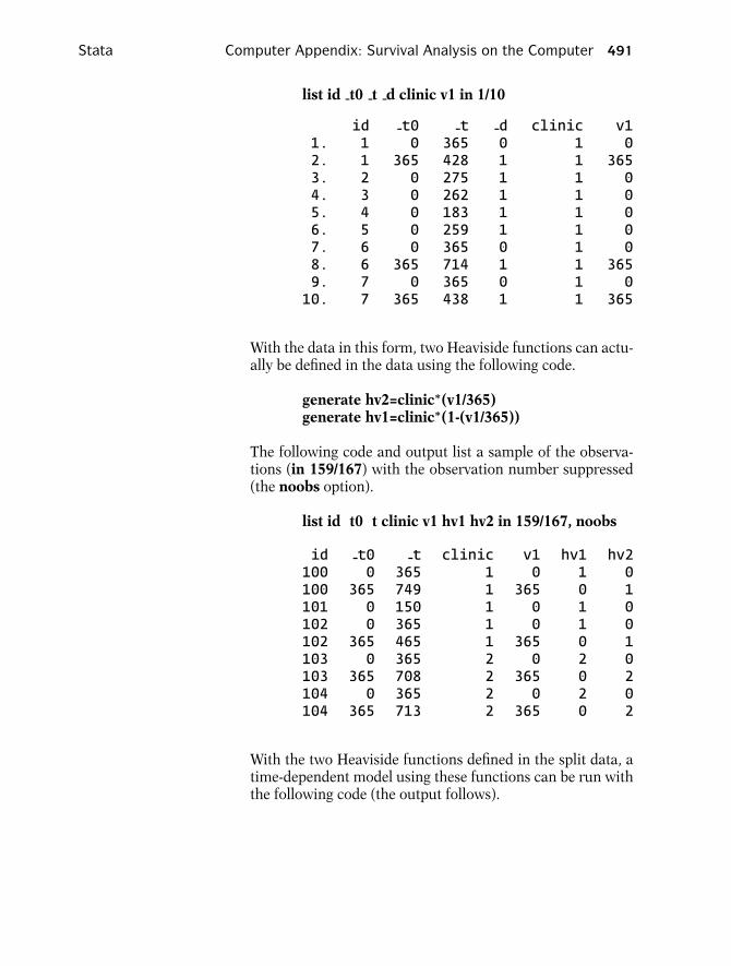
After the above stsplit command is executed, any subject fol-lowed more than 365 days is represented by two observationsrather than one. For example, the first subject (ID = 1) hadan event on the 428th day; the first observation for that sub-ject shows no event between 0 and 365 days whereas the sec-ond observation shows an event on the 428th day. The newlydefined variable v1 has the value 365 for observations withsurvival time exceeding or equal to 365 and 0 otherwise. Thefollowing code lists the first 10 observations for the requestedvariables (output follows).
Stata Computer Appendix: Survival Analysis on the Computer 491
list id t0 t d clinic v1 in 1/10
id -t0 -t -d clinic v11. 1 0 365 0 1 02. 1 365 428 1 1 3653. 2 0 275 1 1 04. 3 0 262 1 1 05. 4 0 183 1 1 06. 5 0 259 1 1 07. 6 0 365 0 1 08. 6 365 714 1 1 3659. 7 0 365 0 1 010. 7 365 438 1 1 365
With the data in this form, two Heaviside functions can actu-ally be defined in the data using the following code.
generate hv2=clinic∗(v1/365)generate hv1=clinic∗(1-(v1/365))
The following code and output list a sample of the observa-tions (in 159/167) with the observation number suppressed(the noobs option).
list id t0 t clinic v1 hv1 hv2 in 159/167, noobs
id -t0 -t clinic v1 hv1 hv2100 0 365 1 0 1 0100 365 749 1 365 0 1101 0 150 1 0 1 0102 0 365 1 0 1 0102 365 465 1 365 0 1103 0 365 2 0 2 0103 365 708 2 365 0 2104 0 365 2 0 2 0104 365 713 2 365 0 2
With the two Heaviside functions defined in the split data, atime-dependent model using these functions can be run withthe following code (the output follows).

492 Computer Appendix: Survival Analysis on the Computer Stata
stcox prison clinic dose hv1 hv2, nohr
No. of subjects = 238 Number of obs = 360No. of failures = 150Time at risk = 95812
LR chi2(4) = 74.17Log likelihood = -668.57443 Prob > chi2 = 0.0000- - - - - - - - - - - - - - - - - - - - - - - - - - - - - - - - - - - - - - - - - - - - - - - - - - - - - - - - - - - - - - - - - - - - - - - - - - - - - - - - - - - - -
-t-d Coef. Std. Err. z p>|z| [95% Conf. Interval]
- - - - - - - - - - - - - - - - - - - - - - - - - - - - - - - - - - - - - - - - - - - - - - - - - - - - - - - - - - - - - - - - - - - - - - - - - - - - - - - - - - - - -prison .377704 .1684024 2.24 0.025 .0476414 .7077666dose -.0355116 .0064354 -5.52 0.000 -.0481247 -.0228985hv1 -.4595628 .2552911 -1.80 0.072 -.959924 .0407985hv2 -1.828228 .385946 -4.74 0.000 -2.584668 -1.071788
The stsplit command is complicated but it offers a powerfulapproach for manipulating the data to accommodate time-varying analyses.
If you wish to return the data to their previous form, drop thevariables that were created from the split and then use thestjoin command:
drop v1 hv1 hv2stjoin
It is possible to split the data at every single failure time, butthis uses a large amount of memory. However, if there is onlyone time-varying covariate in the model, the simplest wayto run an extended Cox model is by using the tvc and texpoptions with the stcox command.
One should not confuse an individual’s survival time variable(the outcome variable) with the variable used to define thetime-dependent variable ( t in Stata). The individual’s survivaltime variable is a time-independent variable. The time of theindividual’s event (or censorship) does not change. A time-dependent variable, on the other hand, is defined so that itcan change its values over time.
8. RUNNING PARAMETRIC MODELS
The Cox PH model is the most widely used model in survivalanalysis. A key reason why it is so popular is that the dis-tribution of the survival time variable need not be specified.However, if it is believed that survival time follows a partic-ular distribution, then that information can be utilized in aparametric modeling of survival data.

Stata Computer Appendix: Survival Analysis on the Computer 493
Many parametric models are accelerated failure time (AFT)models. Whereas the key assumption of a PH model is thathazard ratios are constant over time, the key assumption foran AFT model is that survival time accelerates (or deceler-ates) by a constant factor when comparing different levels ofcovariates.
The most common distribution for parametric modeling ofsurvival data is the Weibull distribution. The Weibull distri-bution has the desirable property that if the AFT assump-tion holds, then the PH assumption also holds. The exponen-tial distribution is a special case of the Weibull distribution.The key property for the exponential distribution is that thehazard is constant over time (not just the hazard ratio). TheWeibull and exponential model can be run as a PH model(the default) or an AFT model.
A graphical method for checking the validity of a Weibull as-sumption is to examine Kaplan–Meier log–log survival curvesagainst log survival time. This is accomplished with the stsgraph command (see Section 2 of this appendix). If the plotsare straight lines, then there is evidence that the distributionof survival times follows a Weibull distribution. If the slope ofthe line equals one, then the evidence suggests that survivaltime follows an exponential distribution.
The streg command is used to run parametric models. Eventhough the log–log survival curves obtained using the addictsdataset are not straight lines, the data are used for illustration.First a parametric model using the exponential distributionis demonstrated. The code and output follow.
streg prison dose clinic, dist(exponential) nohr
Exponential regression -- log relative-hazard form
No. of subjects = 238 Number of obs = 238No. of failures = 150Time at risk = 95812
LR chi2(3) = 49.91Log likelihood = -270.47929 Prob > chi2 = 0.0000
- - - - - - - - - - - - - - - - - - - - - - - - - - - - - - - - - - - - - - - - - - - - - - - - - - - - - - - - - - - - - - - - - - - - - - - - - - - - - - - - - - - - --t Coef. Std. Err. z p>|z| [95% Conf. Interval]
- - - - - - - - - - - - - - - - - - - - - - - - - - - - - - - - - - - - - - - - - - - - - - - - - - - - - - - - - - - - - - - - - - - - - - - - - - - - - - - - - - - - -prison .2526491 .1648862 1.53 0.125 -.070522 .5758201dose -.0289167 .0061445 -4.71 0.000 -.0409596 -.0168738
clinic -.8805819 .210626 -4.18 0.000 -1.293401 -.4677625-cons -3.684341 .4307163 -8.55 0.000 -4.528529 -2.840152
- - - - - - - - - - - - - - - - - - - - - - - - - - - - - - - - - - - - - - - - - - - - - - - - - - - - - - - - - - - - - - - - - - - - - - - - - - - - - - - - - - - - -
494 Computer Appendix: Survival Analysis on the Computer Stata
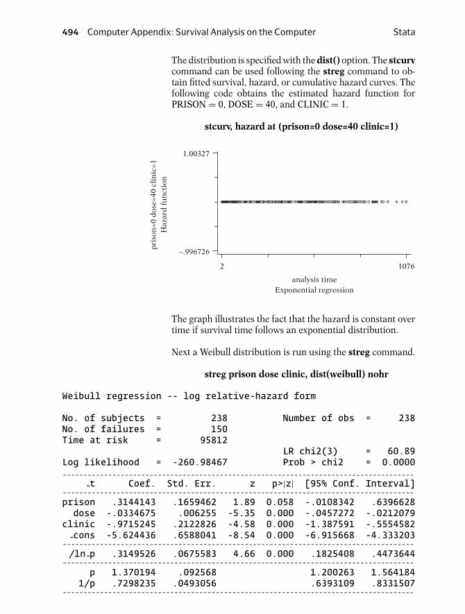
The distribution is specified with the dist() option. The stcurvcommand can be used following the streg command to ob-tain fitted survival, hazard, or cumulative hazard curves. Thefollowing code obtains the estimated hazard function forPRISON = 0, DOSE = 40, and CLINIC = 1.
stcurv, hazard at (prison=0 dose=40 clinic=1)
2 1076
analysis timeExponential regression
−.996726
1.00327p
riso
n=
0 d
ose=
40 c
lin
ic=
1H
azar
d f
un
ctio
n
The graph illustrates the fact that the hazard is constant overtime if survival time follows an exponential distribution.
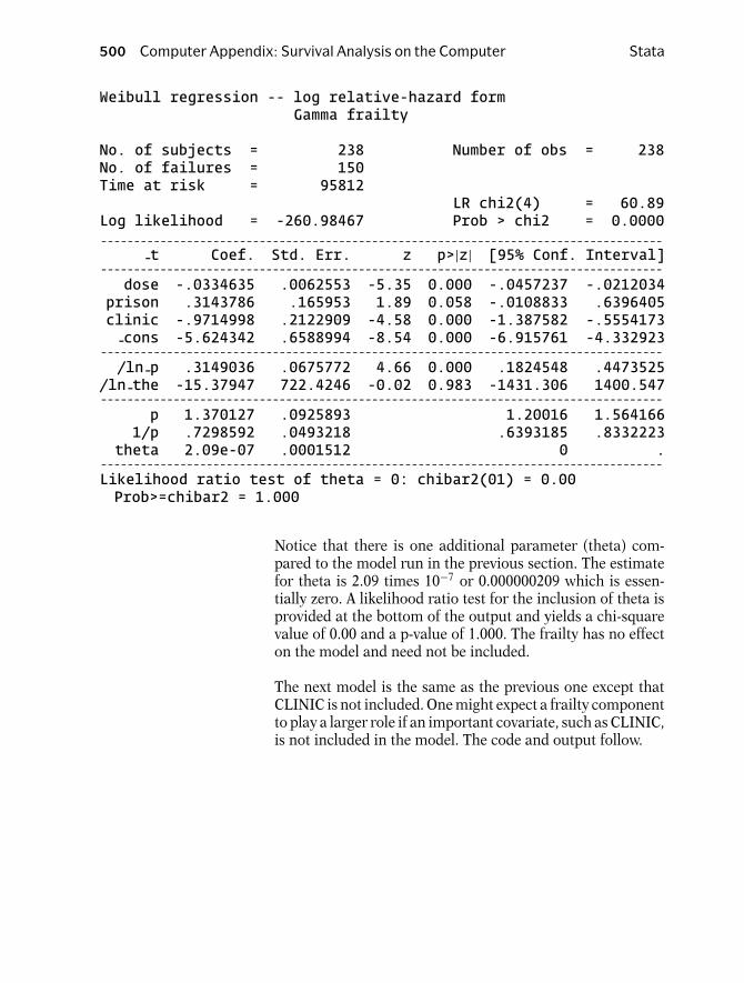
Next a Weibull distribution is run using the streg command.
streg prison dose clinic, dist(weibull) nohr
Weibull regression -- log relative-hazard form
No. of subjects = 238 Number of obs = 238No. of failures = 150Time at risk = 95812
LR chi2(3) = 60.89Log likelihood = -260.98467 Prob > chi2 = 0.0000- - - - - - - - - - - - - - - - - - - - - - - - - - - - - - - - - - - - - - - - - - - - - - - - - - - - - - - - - - - - - - - - - - - - - - - - - - - - - - - - - - - - -
-t Coef. Std. Err. z p>|z| [95% Conf. Interval]- - - - - - - - - - - - - - - - - - - - - - - - - - - - - - - - - - - - - - - - - - - - - - - - - - - - - - - - - - - - - - - - - - - - - - - - - - - - - - - - - - - - -prison .3144143 .1659462 1.89 0.058 -.0108342 .6396628dose -.0334675 .006255 -5.35 0.000 -.0457272 -.0212079
clinic -.9715245 .2122826 -4.58 0.000 -1.387591 -.5554582-cons -5.624436 .6588041 -8.54 0.000 -6.915668 -4.333203
- - - - - - - - - - - - - - - - - - - - - - - - - - - - - - - - - - - - - - - - - - - - - - - - - - - - - - - - - - - - - - - - - - - - - - - - - - - - - - - - - - - - -/ln-p .3149526 .0675583 4.66 0.000 .1825408 .4473644
- - - - - - - - - - - - - - - - - - - - - - - - - - - - - - - - - - - - - - - - - - - - - - - - - - - - - - - - - - - - - - - - - - - - - - - - - - - - - - - - - - - - -p 1.370194 .092568 1.200263 1.564184
1/p .7298235 .0493056 .6393109 .8331507- - - - - - - - - - - - - - - - - - - - - - - - - - - - - - - - - - - - - - - - - - - - - - - - - - - - - - - - - - - - - - - - - - - - - - - - - - - - - - - - - - - - -

Stata Computer Appendix: Survival Analysis on the Computer 495
Notice that the Weibull output has a parameter p that the ex-ponential distribution does not have. The hazard function fora Weibull distribution is λptp−1. If p = 1 then the Weibull dis-tribution is also an exponential distribution (h(t) =λ). Hazardratio parameters are given by default for the Weibull distri-bution. If you want the parameterization for an AFT model,then use the time option.
The code and output for a Weibull AFT model follow.
streg prison dose clinic,dist(weibull) time
Weibull regression -- accelerated failure-time form
No. of subjects = 238 Number of obs = 238No. of failures = 150Time at risk = 95812
LR chi2(3) = 60.89Log likelihood = -260.98467 Prob > chi2 = 0.0000
- - - - - - - - - - - - - - - - - - - - - - - - - - - - - - - - - - - - - - - - - - - - - - - - - - - - - - - - - - - - - - - - - - - - - - - - - - - - - - - - - - - - --t Coef. Std. Err. z p>|z| [95% Conf. Interval]
- - - - - - - - - - - - - - - - - - - - - - - - - - - - - - - - - - - - - - - - - - - - - - - - - - - - - - - - - - - - - - - - - - - - - - - - - - - - - - - - - - - - -prison -.2294669 .1207889 -1.90 0.057 -.4662088 .0072749dose .0244254 .0045898 5.32 0.000 .0154295 .0334213
clinic .7090414 .1572246 4.51 0.000 .4008867 1.017196-cons 4.104845 .3280583 12.51 0.000 3.461863 4.747828
- - - - - - - - - - - - - - - - - - - - - - - - - - - - - - - - - - - - - - - - - - - - - - - - - - - - - - - - - - - - - - - - - - - - - - - - - - - - - - - - - - - - -/ln-p .3149526 .0675583 4.66 0.000 .1825408 .4473644
- - - - - - - - - - - - - - - - - - - - - - - - - - - - - - - - - - - - - - - - - - - - - - - - - - - - - - - - - - - - - - - - - - - - - - - - - - - - - - - - - - - - -p 1.370194 .092568 1.200263 1.564184
1/p .7298235 .0493056 .6393109 .8331507
The relationship between the hazard ratio parameter βj andthe AFT parameter αj is βj = −αj p. For example, using thecoefficient estimates for PRISON in the Weibull PH and AFTmodels yields the relationship 0.3144 = (−0.2295)(1.37).
The stcurv can again be used following the streg commandto obtain fitted survival, hazard, or cumulative hazard curves.The following code obtains the estimated hazard function forPRISON = 0, DOSE = 40, and CLINIC = 1.
stcurv, hazard at (prison=0 dose=40 clinic=1)

496 Computer Appendix: Survival Analysis on the Computer Stata
.006504
.000634p
riso
n=
0 d
ose=
40 c
lin
ic=
1H
azar
d f
un
ctio
n2
1076
analysis timeWeibull regression
The plot of the hazard is monotonically increasing. With aWeibull distribution, the hazard is constrained such that itcannot increase and then decrease. This is not the case withthe log-logistic distribution as demonstrated in the next exam-ple. The log-logistic model is not a PH model, so the defaultmodel for the streg command is an AFT model. The code andoutput follow.
streg prison dose clinic, dist(loglogistic)
Log-logistic regression -- accelerated failure-time form
No. of subjects = 238 Number of obs = 238No. of failures = 150Time at risk = 95812
LR chi2(3) = 52.18Log likelihood = -270.42329 Prob > chi2 = 0.0000
- - - - - - - - - - - - - - - - - - - - - - - - - - - - - - - - - - - - - - - - - - - - - - - - - - - - - - - - - - - - - - - - - - - - - - - - - - - - - - - - - - - - --t Coef. Std. Err. z p>|z| [95% Conf. Interval]
- - - - - - - - - - - - - - - - - - - - - - - - - - - - - - - - - - - - - - - - - - - - - - - - - - - - - - - - - - - - - - - - - - - - - - - - - - - - - - - - - - - - -prison -.2912719 .1439646 -2.02 0.043 -.5734373 -.0091065dose .0316133 .0055192 5.73 0.000 .0207959 .0424307
clinic .5805977 .1715695 3.38 0.001 .2443276 .9168677-cons 3.563268 .3894467 9.15 0.000 2.799967 4.32657
- - - - - - - - - - - - - - - - - - - - - - - - - - - - - - - - - - - - - - - - - - - - - - - - - - - - - - - - - - - - - - - - - - - - - - - - - - - - - - - - - - - - -/ln-gam -.5331424 .0686297 -7.77 0.000 -.6676541 -.3986306- - - - - - - - - - - - - - - - - - - - - - - - - - - - - - - - - - - - - - - - - - - - - - - - - - - - - - - - - - - - - - - - - - - - - - - - - - - - - - - - - - - - -gamma .5867583 .040269 .5129104 .6712386
Note that Stata calls the shape parameter gamma for a log-logistic model. The code to produce the graph of the haz-ard function for PRISON = 0, DOSE = 40, and CLINIC = 1follows.
stcurv, hazard at (prison=0 dose=40 clinic=1)

Stata Computer Appendix: Survival Analysis on the Computer 497
2 1076
.000809
.007292
analysis timeLog-logistic regression
pri
son
=0
dos
e=20
cli
nic
=1
Haz
ard
fu
nct
ion
The hazard function (in contrast to the Weibull hazard func-tion) first increases and then decreases.
The corresponding survival curve for the log-logistic distribu-tion can also be obtained with the stcurve command.
stcurv, survival at (prison=0 dose=40 clinic=1)
2 1076
.064154
.999677
analysis timeLog-logistic regression
pri
son
=0
dos
e=40
cli
nic
=1
Su
rviv
al
If the AFT assumption holds for a log-logistic model, then theproportional odds assumption holds for the survival function(although the PH assumption would not hold). The propor-tional odds assumption can be evaluated by plotting the logodds of survival (using KM estimates) against the log of sur-vival time. If the plots are straight lines for each pattern ofcovariates, then the log-logistic distribution is reasonable. Ifthe straight lines are also parallel, then the proportional oddsand AFT assumptions also hold. The following code will plotthe estimated log odds of survival against the log of time byCLINIC (output omitted).

498 Computer Appendix: Survival Analysis on the Computer Stata
sts generate skm=s,by (clinic)generate logodds=ln(skm/(1-skm))generate logt=ln(survt)graph7 logodds logt,twoway symbol([clinic] [clinic])
Another context for thinking about the proportional odds as-sumption is that the odds ratio estimated by a logistic re-gression does not depend on the length of the follow-up. Forexample, if a follow-up study was extended from three to fiveyears then the underlying odds ratio comparing two patternsof covariates would not change. If the proportional odds as-sumption is not true, then the odds ratio is specific to thelength of follow-up.
Both the log-logistic and Weibull models contain an extrashape parameter that is typically assumed constant. This as-sumption is necessary for the PH or AFT assumption to holdfor these models. Stata provides a way of modeling the shapeparameter as a function of predictor variables by use of theancillary option in the streg command (see Chapter 7 un-der the heading, “Other Parametric Models”). The followingcode runs a log-logistic model in which the shape parametergamma is modeled as a function of CLINIC and λ is modeledas a function of PRISON and DOSE.
streg prison dose, dist(loglogistic) ancillary(clinic)
The output follows.
Log-logistic regression -- accelerated failure-time form
No. of subjects = 238 Number of obs = 238No. of failures = 150Time at risk = 95812
LR chi2(2) = 38.87Log likelihood = -272.65273 Prob > chi2 = 0.0000
- - - - - - - - - - - - - - - - - - - - - - - - - - - - - - - - - - - - - - - - - - - - - - - - - - - - - - - - - - - - - - - - - - - - - - - - - - - - - - - - - - - - - - - - - - - --t Coef. Std. Err. z p>|z| [95% Conf. Interval]
- - - - - - - - - - - - - - - - - - - - - - - - - - - - - - - - - - - - - - - - - - - - - - - - - - - - - - - - - - - - - - - - - - - - - - - - - - - - - - - - - - - - - - - - - - - -
-tprison -.3275695 .1405119 -2.33 0.020 -.6029677 -.0521713dose .0328517 .0054275 6.05 0.000 .022214 .0434893-cons 4.183173 .3311064 12.63 0.000 3.534216 4.83213
- - - - - - - - - - - - - - - - - - - - - - - - - - - - - - - - - - - - - - - - - - - - - - - - - - - - - - - - - - - - - - - - - - - - - - - - - - - - - - - - - - - - - - - - - - - -ln-gam
clinic .4558089 .1734819 2.63 0.009 .1157906 .7958273-cons -1.094496 .2212143 -4.95 0.000 -1.528068 -.6609238
- - - - - - - - - - - - - - - - - - - - - - - - - - - - - - - - - - - - - - - - - - - - - - - - - - - - - - - - - - - - - - - - - - - - - - - - - - - - - - - - - - - - - - - - - - - -

Stata Computer Appendix: Survival Analysis on the Computer 499
Notice there is a parameter estimate for CLINIC as well asan intercept ( cons) under the heading ln gam (the log ofgamma). With this model, the estimate for gamma depends onwhether CLINIC = 1 or CLINIC = 2. There is no easy interpre-tation for the predictor variables in this type of model, whichis why it is not commonly used. However, for any specifiedvalue of PRISON, DOSE, and CLINIC, the hazard and sur-vival functions can be estimated by substituting the parame-ter estimates into the expressions for the log-logistic hazardand survival functions.
Other distributions supported by streg are the generalizedgamma, the lognormal, and the Gompertz distributions.
9. RUNNING FRAILTY MODELS
Frailty models contain an extra random component designedto account for individual level differences in the hazard oth-erwise unaccounted for by the model. The frailty α is a multi-plicative effect on the hazard assumed to follow some distri-bution. The hazard function conditional on the frailty can beexpressed as h(t|α) = α[h(t)].
Stata offers two choices for the distribution of the frailty: thegamma and the inverse-Gaussian, both of mean 1 and vari-ance theta. The variance (theta) is a parameter estimated bythe model. If theta = 0, then there is no frailty.
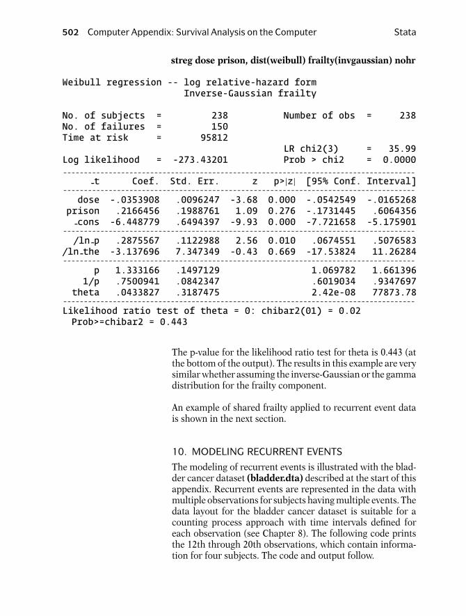
For the first example, a Weibull PH model is run withPRISON, DOSE, and CLINIC as predictors. A gamma dis-tribution is assumed for the frailty component. The codefollows.
streg dose prison clinic, dist(weibull) frailty(gamma) nohr
The frailty() option requests that a frailty model be run. Theoutput follows.
500 Computer Appendix: Survival Analysis on the Computer Stata
Weibull regression -- log relative-hazard formGamma frailty
No. of subjects = 238 Number of obs = 238No. of failures = 150Time at risk = 95812
LR chi2(4) = 60.89Log likelihood = -260.98467 Prob > chi2 = 0.0000- - - - - - - - - - - - - - - - - - - - - - - - - - - - - - - - - - - - - - - - - - - - - - - - - - - - - - - - - - - - - - - - - - - - - - - - - - - - - - - - - - - - -
-t Coef. Std. Err. z p>|z| [95% Conf. Interval]- - - - - - - - - - - - - - - - - - - - - - - - - - - - - - - - - - - - - - - - - - - - - - - - - - - - - - - - - - - - - - - - - - - - - - - - - - - - - - - - - - - - -dose -.0334635 .0062553 -5.35 0.000 -.0457237 -.0212034
prison .3143786 .165953 1.89 0.058 -.0108833 .6396405clinic -.9714998 .2122909 -4.58 0.000 -1.387582 -.5554173-cons -5.624342 .6588994 -8.54 0.000 -6.915761 -4.332923
- - - - - - - - - - - - - - - - - - - - - - - - - - - - - - - - - - - - - - - - - - - - - - - - - - - - - - - - - - - - - - - - - - - - - - - - - - - - - - - - - - - - -/ln-p .3149036 .0675772 4.66 0.000 .1824548 .4473525
/ln-the -15.37947 722.4246 -0.02 0.983 -1431.306 1400.547- - - - - - - - - - - - - - - - - - - - - - - - - - - - - - - - - - - - - - - - - - - - - - - - - - - - - - - - - - - - - - - - - - - - - - - - - - - - - - - - - - - - -
p 1.370127 .0925893 1.20016 1.5641661/p .7298592 .0493218 .6393185 .8332223
theta 2.09e-07 .0001512 0 .- - - - - - - - - - - - - - - - - - - - - - - - - - - - - - - - - - - - - - - - - - - - - - - - - - - - - - - - - - - - - - - - - - - - - - - - - - - - - - - - - - - - -Likelihood ratio test of theta = 0: chibar2(01) = 0.00Prob>=chibar2 = 1.000
Notice that there is one additional parameter (theta) com-pared to the model run in the previous section. The estimatefor theta is 2.09 times 10−7 or 0.000000209 which is essen-tially zero. A likelihood ratio test for the inclusion of theta isprovided at the bottom of the output and yields a chi-squarevalue of 0.00 and a p-value of 1.000. The frailty has no effecton the model and need not be included.
The next model is the same as the previous one except thatCLINIC is not included. One might expect a frailty componentto play a larger role if an important covariate, such as CLINIC,is not included in the model. The code and output follow.

Stata Computer Appendix: Survival Analysis on the Computer 501
streg dose prison, dist(weibull) frailty(gamma) nohr
Weibull regression -- log relative-hazard formGamma frailty
No. of subjects = 238 Number of obs = 238No. of failures = 150Time at risk = 95812
LR chi2(3) = 36.00Log likelihood = -273.42782 Prob > chi2 = 0.0000- - - - - - - - - - - - - - - - - - - - - - - - - - - - - - - - - - - - - - - - - - - - - - - - - - - - - - - - - - - - - - - - - - - - - - - - - - - - - - - - - - - - -
-t Coef. Std. Err. z p>|z| [95% Conf. Interval]- - - - - - - - - - - - - - - - - - - - - - - - - - - - - - - - - - - - - - - - - - - - - - - - - - - - - - - - - - - - - - - - - - - - - - - - - - - - - - - - - - - - -dose -.0358231 .010734 -3.34 0.001 -.0568614 -.0147849
prison .2234556 .2141028 1.04 0.297 -.1961783 .6430894-cons -6.457393 .6558594 -9.85 0.000 -7.742854 -5.171932
- - - - - - - - - - - - - - - - - - - - - - - - - - - - - - - - - - - - - - - - - - - - - - - - - - - - - - - - - - - - - - - - - - - - - - - - - - - - - - - - - - - - -/ln-p .2922832 .1217597 2.40 0.016 .0536385 .5309278
/ln-the -2.849726 5.880123 -0.48 0.628 -14.37456 8.675104- - - - - - - - - - - - - - - - - - - - - - - - - - - - - - - - - - - - - - - - - - - - - - - - - - - - - - - - - - - - - - - - - - - - - - - - - - - - - - - - - - - - -
p 1.339482 .163095 1.055103 1.7005091/p .7465571 .0909006 .5880591 .9477747
theta .0578602 .340225 5.72e-07 5855.31- - - - - - - - - - - - - - - - - - - - - - - - - - - - - - - - - - - - - - - - - - - - - - - - - - - - - - - - - - - - - - - - - - - - - - - - - - - - - - - - - - - - -Likelihood ratio test of theta = 0: chibar2(01) = 0.03Prob>=chibar2 = 0.432
The variance (theta) of the frailty is estimated at 0.0578602.Although this estimate is not exactly zero as in the previousexample, the p-value for the likelihood ratio test for theta isnonsignificant at 0.432. So the addition of frailty did not ac-count for CLINIC being omitted from the model.
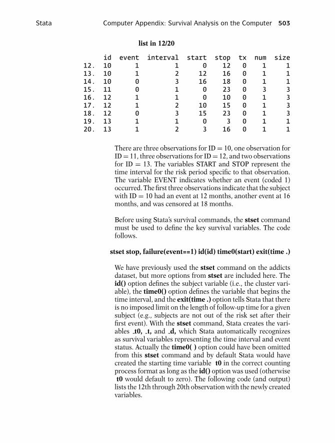
Next the same model is run except that the inverse-Gaussiandistribution is used for the frailty rather than the gamma dis-tribution. The code and output follow.
502 Computer Appendix: Survival Analysis on the Computer Stata
streg dose prison, dist(weibull) frailty(invgaussian) nohr
Weibull regression -- log relative-hazard formInverse-Gaussian frailty
No. of subjects = 238 Number of obs = 238No. of failures = 150Time at risk = 95812
LR chi2(3) = 35.99Log likelihood = -273.43201 Prob > chi2 = 0.0000- - - - - - - - - - - - - - - - - - - - - - - - - - - - - - - - - - - - - - - - - - - - - - - - - - - - - - - - - - - - - - - - - - - - - - - - - - - - - - - - - - - - -
-t Coef. Std. Err. z p>|z| [95% Conf. Interval]- - - - - - - - - - - - - - - - - - - - - - - - - - - - - - - - - - - - - - - - - - - - - - - - - - - - - - - - - - - - - - - - - - - - - - - - - - - - - - - - - - - - -dose -.0353908 .0096247 -3.68 0.000 -.0542549 -.0165268
prison .2166456 .1988761 1.09 0.276 -.1731445 .6064356-cons -6.448779 .6494397 -9.93 0.000 -7.721658 -5.175901
- - - - - - - - - - - - - - - - - - - - - - - - - - - - - - - - - - - - - - - - - - - - - - - - - - - - - - - - - - - - - - - - - - - - - - - - - - - - - - - - - - - - -/ln-p .2875567 .1122988 2.56 0.010 .0674551 .5076583
/ln-the -3.137696 7.347349 -0.43 0.669 -17.53824 11.26284- - - - - - - - - - - - - - - - - - - - - - - - - - - - - - - - - - - - - - - - - - - - - - - - - - - - - - - - - - - - - - - - - - - - - - - - - - - - - - - - - - - - -
p 1.333166 .1497129 1.069782 1.6613961/p .7500941 .0842347 .6019034 .9347697
theta .0433827 .3187475 2.42e-08 77873.78- - - - - - - - - - - - - - - - - - - - - - - - - - - - - - - - - - - - - - - - - - - - - - - - - - - - - - - - - - - - - - - - - - - - - - - - - - - - - - - - - - - - -Likelihood ratio test of theta = 0: chibar2(01) = 0.02Prob>=chibar2 = 0.443
The p-value for the likelihood ratio test for theta is 0.443 (atthe bottom of the output). The results in this example are verysimilar whether assuming the inverse-Gaussian or the gammadistribution for the frailty component.
An example of shared frailty applied to recurrent event datais shown in the next section.
10. MODELING RECURRENT EVENTS
The modeling of recurrent events is illustrated with the blad-der cancer dataset (bladder.dta) described at the start of thisappendix. Recurrent events are represented in the data withmultiple observations for subjects having multiple events. Thedata layout for the bladder cancer dataset is suitable for acounting process approach with time intervals defined foreach observation (see Chapter 8). The following code printsthe 12th through 20th observations, which contain informa-tion for four subjects. The code and output follow.
Stata Computer Appendix: Survival Analysis on the Computer 503
list in 12/20
id event interval start stop tx num size12. 10 1 1 0 12 0 1 113. 10 1 2 12 16 0 1 114. 10 0 3 16 18 0 1 115. 11 0 1 0 23 0 3 316. 12 1 1 0 10 0 1 317. 12 1 2 10 15 0 1 318. 12 0 3 15 23 0 1 319. 13 1 1 0 3 0 1 120. 13 1 2 3 16 0 1 1
There are three observations for ID = 10, one observation forID = 11, three observations for ID = 12, and two observationsfor ID = 13. The variables START and STOP represent thetime interval for the risk period specific to that observation.The variable EVENT indicates whether an event (coded 1)occurred. The first three observations indicate that the subjectwith ID = 10 had an event at 12 months, another event at 16months, and was censored at 18 months.
Before using Stata’s survival commands, the stset commandmust be used to define the key survival variables. The codefollows.
stset stop, failure(event==1) id(id) time0(start) exit(time .)
We have previously used the stset command on the addictsdataset, but more options from stset are included here. Theid() option defines the subject variable (i.e., the cluster vari-able), the time0() option defines the variable that begins thetime interval, and the exit(time .) option tells Stata that thereis no imposed limit on the length of follow-up time for a givensubject (e.g., subjects are not out of the risk set after theirfirst event). With the stset command, Stata creates the vari-ables t0, t, and d, which Stata automatically recognizesas survival variables representing the time interval and eventstatus. Actually the time0( ) option could have been omittedfrom this stset command and by default Stata would havecreated the starting time variable t0 in the correct countingprocess format as long as the id() option was used (otherwiset0 would default to zero). The following code (and output)
lists the 12th through 20th observation with the newly createdvariables.

504 Computer Appendix: Survival Analysis on the Computer Stata
list id t0 t d tx in 12/20
id -t0 -t -d tx12. 10 0 12 1 013. 10 12 16 1 014. 10 16 18 0 015. 11 0 23 0 016. 12 0 10 1 017. 12 10 15 1 018. 12 15 23 0 019. 13 0 3 1 020. 13 3 16 1 0
A Cox model with recurrent events using the counting processapproach can now be run with the stcox command. The pre-dictors are treatment status (TX), initial number of tumors(NUM), and the initial size of tumors (SIZE). The robust op-tion requests robust standard errors for the coefficient esti-mates. Omit the nohr option if you want the exponentiatedcoefficients. The code and output follow.
stcox tx num size, nohr robust
Cox regression –– Breslow method for ties
No. of subjects = 85 Number of obs = 190No. of failures = 112Time at risk = 2711
Wald chi2(3) = 11.25Log likelihood = -460.07958 Prob > chi2 = 0.0105
(standard errors adjusted for clustering on id)- - - - - - - - - - - - - - - - - - - - - - - - - - - - - - - - - - - - - - - - - - - - - - - - - - - - - - - - - - - - - - - - - - - - - - - - - - - - - - - - - --t Robust-d Coef. Std. Err. z p>|z| [95% Conf. Interval]
- - - - - - - - - - - - - - - - - - - - - - - - - - - - - - - - - - - - - - - - - - - - - - - - - - - - - - - - - - - - - - - - - - - - - - - - - - - - - - - - - -tx -.4070966 .2432658 -1.67 0.094 -.8838889 .0696956num .1606478 .0572305 2.81 0.005 .0484781 .2728174size -.0400877 .0726459 -0.55 0.581 -.182471 .1022957- - - - - - - - - - - - - - - - - - - - - - - - - - - - - - - - - - - - - - - - - - - - - - - - - - - - - - - - - - - - - - - - - - - - - - - - - - - - - - - - - -
The interpretation of these parameter estimates is discussedin Chapter 8.

Stata Computer Appendix: Survival Analysis on the Computer 505
A stratified Cox model can also be run using the data in thisformat with the variable INTERVAL as the stratified variable.The stratified variable indicates whether subjects were at riskfor their 1st, 2nd, 3rd, or 4th event. This approach is calledconditional 1 in Chapter 8 and is used if the investigatorwants to distinguish the order in which recurrent events oc-cur. The code and output follow.
stcox tx num size, nohr robust strata(interval)
stratified Cox regr. –– Breslow method for ties
No. of subjects = 85 Number of obs = 190No. of failures = 112Time at risk = 2711
Wald chi2(3) = 7.11Log likelihood = -319.85912 Prob > chi2 = 0.0685
(standard errors adjusted for clustering on id)- - - - - - - - - - - - - - - - - - - - - - - - - - - - - - - - - - - - - - - - - - - - - - - - - - - - - - - - - - - - - - - - - - - - - - - - - - - - - - - - - --t Robust-d Coef. Std. Err. z p>|z| [95% Conf. Interval]
- - - - - - - - - - - - - - - - - - - - - - - - - - - - - - - - - - - - - - - - - - - - - - - - - - - - - - - - - - - - - - - - - - - - - - - - - - - - - - - - - -tx -.3342955 .1982339 -1.69 0.092 -.7228268 .0542359num .1156526 .0502089 2.30 0.021 .017245 .2140603size -.0080508 .0604807 -0.13 0.894 -.1265908 .1104892- - - - - - - - - - - - - - - - - - - - - - - - - - - - - - - - - - - - - - - - - - - - - - - - - - - - - - - - - - - - - - - - - - - - - - - - - - - - - - - - - -
Stratified by interval
Interaction terms between the treatment variable (TX) andthe stratified variable could be created to examine whetherthe effect of treatment differed for the 1st, 2nd, 3rd, or 4thevent. (Note that in this dataset subjects have a maximum of4 events).
Another stratified approach (called conditional 2) is a slightvariation of the conditional 1 approach. The difference is inthe way the time intervals for the recurrent events are defined.There is no difference in the time intervals when subjects areat risk for their first event. However, with the conditional 2approach, the starting time at risk gets reset to zero for eachsubsequent event. The following code creates data suitablefor using the conditional 2 approach.
generate stop2 = t - t0stset stop2, failure(event==1) exit(time .)

506 Computer Appendix: Survival Analysis on the Computer Stata
The generate command defines a new variable called STOP2representing the length of the time interval for each observa-tion. The stset command is used with STOP2 as the outcomevariable ( t). By default Stata sets the variable t0 to zero.The following code (and output) lists the 12th through 20thobservations for selected variables.
list id t0 t d tx in 12/20
id -t0 -t -d tx12. 10 0 12 1 013. 10 0 4 1 014. 10 0 2 0 015. 11 0 23 0 016. 12 0 10 1 017. 12 0 5 1 018. 12 0 8 0 019. 13 0 3 1 020. 13 0 13 1 0
Notice that the id() option was not used with the stset com-mand for the conditional 2 approach. This means that Statadoes not know that multiple observations correspond to thesame subject. However the cluster() option can be used di-rectly in the stcox command to request that the analysis beclustered by ID (i.e., by subject). The following code runs astratified Cox model using the conditional 2 approach with thecluster() and robust options. The code and output follow.
stcox tx num size, nohr robust strata(interval) cluster(id)
Stratified Cox regr. –– Breslow method for ties
No. of subjects = 190 Number of obs = 190No. of failures = 112Time at risk = 2711
Wald chi2(3) = 11.99Log likelihood = -363.16022 Prob > chi2 = 0.0074
(standard errors adjusted for clustering on id)- - - - - - - - - - - - - - - - - - - - - - - - - - - - - - - - - - - - - - - - - - - - - - - - - - - - - - - - - - - - - - - - - - - - - - - - - - - - - - - - - --t Robust-d Coef. Std. Err. z p>|z| [95% Conf. Interval]
- - - - - - - - - - - - - - - - - - - - - - - - - - - - - - - - - - - - - - - - - - - - - - - - - - - - - - - - - - - - - - - - - - - - - - - - - - - - - - - - - -tx -.2695213 .2093108 -1.29 0.198 -.6797628 .1407203num .1535334 .0491803 3.12 0.002 .0571418 .2499249size .0068402 .0625862 0.11 0.913 -.1158265 .129507- - - - - - - - - - - - - - - - - - - - - - - - - - - - - - - - - - - - - - - - - - - - - - - - - - - - - - - - - - - - - - - - - - - - - - - - - - - - - - - - - -
Stratified by interval
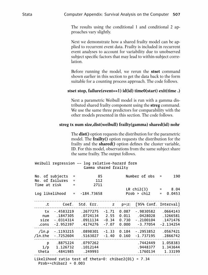
Stata Computer Appendix: Survival Analysis on the Computer 507
The results using the conditional 1 and conditional 2 ap-proaches vary slightly.
Next we demonstrate how a shared frailty model can be ap-plied to recurrent event data. Frailty is included in recurrentevent analyses to account for variability due to unobservedsubject specific factors that may lead to within-subject corre-lation.
Before running the model, we rerun the stset commandshown earlier in this section to get the data back to the formsuitable for a counting process approach. The code follows.
stset stop, failure(event==1) id(id) time0(start) exit(time .)
Next a parametric Weibull model is run with a gamma dis-tributed shared frailty component using the streg command.We use the same three predictors for comparability with theother models presented in this section. The code follows.
streg tx num size,dist(weibull) frailty(gamma) shared(id) nohr
The dist() option requests the distribution for the parametricmodel. The frailty() option requests the distribution for thefrailty and the shared() option defines the cluster variable,ID. For this model, observations from the same subject sharethe same frailty. The output follows.
Weibull regression –– log relative-hazard formGamma shared frailty
No. of subjects = 85 Number of obs = 190No. of failures = 112Time at risk = 2711
LR chi2(3) = 8.04Log likelihood = -184.73658 Prob > chi2 = 0.0453
- - - - - - - - - - - - - - - - - - - - - - - - - - - - - - - - - - - - - - - - - - - - - - - - - - - - - - - - - - - - - - - - - - - - - - - - - - - - - - - - - - - - --t Coef. Std. Err. z p>|z| [95% Conf. Interval]
- - - - - - - - - - - - - - - - - - - - - - - - - - - - - - - - - - - - - - - - - - - - - - - - - - - - - - - - - - - - - - - - - - - - - - - - - - - - - - - - - - - - -tx -.4583219 .2677275 -1.71 0.087 -.9830582 .0664143num .1847305 .0724134 2.55 0.011 .0428028 .3266581size -.0314314 .0911134 -0.34 0.730 -.2100104 .1471476-cons -2.952397 .4174276 -7.07 0.000 -3.77054 -2.134254
- - - - - - - - - - - - - - - - - - - - - - - - - - - - - - - - - - - - - - - - - - - - - - - - - - - - - - - - - - - - - - - - - - - - - - - - - - - - - - - - - - - - -/ln-p -.1193215 .0898301 -1.33 0.184 -.2953852 .0567421
/ln-the -.7252604 .5163027 -1.40 0.160 -1.737195 .2866742- - - - - - - - - - - - - - - - - - - - - - - - - - - - - - - - - - - - - - - - - - - - - - - - - - - - - - - - - - - - - - - - - - - - - - - - - - - - - - - - - - - - -
p .8875224 .0797262 .7442449 1.0583831/p 1.126732 .1012144 .9448377 1.343644
theta .4841985 .249993 .1760134 1.33199- - - - - - - - - - - - - - - - - - - - - - - - - - - - - - - - - - - - - - - - - - - - - - - - - - - - - - - - - - - - - - - - - - - - - - - - - - - - - - - - - - - - -Likelihood ratio test of theta=0: chibar2(01) = 7.34Prob>=chibar2 = 0.003

508 Computer Appendix: Survival Analysis on the Computer SAS
The model output is discussed in Chapter 8.
The counting process data layout with multiple observationsper subject need not only apply to recurrent event data butcan also be used for a more conventional survival analysis inwhich each subject is limited to one event. A subject with fourobservations may be censored for the first three observationsbefore getting the event in the time interval represented by thefourth observation. This data layout is particularly suitablefor representing time-varying exposures, which may changevalues over different intervals of time (see the stsplit com-mand in Section 7 of this appendix).
B. SASAnalyses are carried out in SAS by using the appropriate SASprocedure on a SAS dataset. The key SAS procedures for per-forming survival analyses are as follows.
PROC LIFETEST. This procedure is used to obtain Kaplan–Meier survival estimates and plots. It can also be used to outputlife table estimates and plots. It will generate output for thelog rank and Wilcoxon test statistics if stratifying by a covari-ate. A new SAS dataset containing survival estimates can berequested.
PROC PHREG. This procedure is used to run the Cox propor-tional hazards model, a stratified Cox model, and an extendedCox model with time-varying covariates. It can also be used tocreate a SAS dataset containing adjusted survival estimates.These adjusted survival estimates can then be plotted usingPROC GPLOT.
PROC LIFEREG. This procedure is used to run parametric ac-celerated failure time (AFT) models.
Analyses on the addicts dataset are used to illustrate these pro-cedures. The addicts dataset was obtained from a 1991 Aus-tralian study by Caplehorn et al., and contains informationon 238 heroin addicts. The study compared two methadonetreatment clinics to assess patient time remaining undermethadone treatment. The two clinics differed according tolive-in policies for patients. A patient’s survival time was de-termined as the time (in days) until the person dropped outof the clinic or was censored. The variables are defined at thestart of this appendix.

SAS Computer Appendix: Survival Analysis on the Computer 509
All of the SAS programming code is written in capital lettersfor readability. However, SAS is not case sensitive. If a pro-gram is written with lowercase letters, SAS reads them as up-percase. The number of spaces between words (if more thanone) has no effect on the program. Each SAS programmingstatement ends with a semicolon.
The addicts dataset is stored as a permanent SAS datasetcalled addicts.sas7bdat. A LIBNAME statement is neededto indicate the path to the location of the SAS dataset. In ourexamples, we assume the file is located on the A drive (i.e., ona disk). The LIBNAME statement includes a reference nameas well as the path. We call the reference name REF. The codeis as follows.
LIBNAME REF ‘A:\’;
The user is free to define his or her own reference name. Thepath to the location of the file is given between the quotationmarks. The general form of the code is
LIBNAME Your reference name ‘Your path to file location’;
PROC CONTENTS, PROC PRINT, PROC UNIVARIATE,PROC FREQ, and PROC MEANS can be used to list or de-scribe the data. SAS code can be run in one batch or high-lighted and submitted one procedure at a time. Code can besubmitted by clicking on the submit button on the toolbarin the editor window. The code for using these proceduresfollows (output omitted).
PROC CONTENTS DATA=REF.ADDICTS;RUN;PROC PRINT DATA=REF.ADDICTS;RUN;PROC UNIVARIATE DATA=REF.ADDICTS;VAR SURVT;RUN;PROC FREQ DATA=REF.ADDICTS;TABLES CLINIC PRISON;RUN;PROC MEANS DATA=REF.ADDICTS;VAR SURVT;CLAS CLINIC;RUN;
Notice that each SAS statement ends with a semicolon. If eachprocedure is submitted one at a time then each proceduremust end with a RUN statement. Otherwise one RUN state-ment at the end of the last procedure is sufficient. With theLIBNAME statement, SAS recognizes a two-level file name:the reference name and the file name without an extension.For our example, the SAS file name is REF.ADDICTS. Alter-natively, a temporary SAS dataset could be created and usedfor these procedures.

510 Computer Appendix: Survival Analysis on the Computer SAS
Text that you do not wish SAS to process should be written asa comment:
/∗ A comment begins with a forward slash followedby a star and ends with a star followed by aforward slash. ∗/
∗A comment can also be created by beginning with astar and ending with a semicolon;
The survival analyses demonstrated in SAS are:
1. Demonstrating PROC LIFETEST to obtain Kaplan–Meierand life table survival estimates (and plots);
2. Running a Cox PH model with PROC PHREG;3. Running a stratified Cox model;4. Assessing the PH assumption with a statistical test;5. Obtaining Cox adjusted survival curves;6. Running an extended Cox model (i.e., containing time-
varying covariates);7. Running parametric models with PROC LIFEREG; and8. Modeling recurrent events.
1. DEMONSTRATING PROC LIFETEST TO OBTAINKAPLAN–MEIER AND LIFE TABLE SURVIVALESTIMATES (AND PLOTS)
PROC LIFETEST produces Kaplan–Meier survival estimateswith the METHOD=KM option. The PLOTS=(S) option plotsthe estimated survival function. The TIME statement definesthe time-to-event variable (SURVT) and the value for censor-ship (STATUS = 0). The code follows (output omitted).
PROC LIFETEST DATA=REF.ADDICTS METHOD=KM PLOTS=(S);TIME SURVT∗STATUS(0);RUN;
Use a STRATA statement in PROC LIFETEST to compare sur-vival estimates for different groups (e.g., strata clinic). ThePLOTS=(S,LLS) option produces log–log curves as well as sur-vival curves. If the proportional hazard assumption is met thelog–log survival curves will be parallel. The STRATA statementalso provides the log rank test and Wilcoxon test statistics. Thecode follows.

SAS Computer Appendix: Survival Analysis on the Computer 511
PROC LIFETEST DATA=REF.ADDICTS METHOD=KM PLOTS=(S,LLS);TIME SURVT∗STATUS(0);STRATA CLINIC;RUN;
PROC LIFETEST yields the following edited output.
The LIFETEST Procedure (stratified)
Stratum 1: CLINIC = 1
Product-Limit Survival EstimatesSurvivalStandard Number Number
SURVT Survival Failure Error Failed Left
0.00 1.0000 0 0 0 1632.00∗ . . . 0 1627.00 0.9938 0.00617 0.00615 1 16117.00 0.9877 0.0123 0.00868 2 160. . . . . .. . . . . .836.00 0.0869 0.9131 0.0295 118 6837.00 0.0725 0.9275 0.0279 119 5
Stratum 2: CLINIC = 2
Product-Limit Survival EstimatesSurvivalStandard Number Number
SURVT Survival Failure Error Failed Left
0.00 1.0000 0 0 0 752.00∗ . . . 0 7413.00 0.9865 0.0135 0.0134 1 7326.00 0.9730 0.0270 0.0189 2 72. . . . . .. . . . . .
Test of Equality over Strata
Pr >Test Chi-Square DF Chi-Square
Log-Rank 27.8927 1 <.0001Wilcoxon 11.6268 1 0.0007-2Log(LR) 26.0236 1 <.0001

512 Computer Appendix: Survival Analysis on the Computer SAS
Both the log rank and Wilcoxon test yield highly significantchi-square test statistics. The Wilcoxon test is a variation ofthe log rank test weighting the observed minus expected scoreof the jth failure time by nj (the number still at risk at the jthfailure time).
The requested log–log plots from PROC LIFETEST follow.
2
0
−2
−4
−6
1 2 3 4 5 6 7
Log
Neg
ativ
e L
og S
DF
Log of survival time in daysCLINIC=1 CLINIC=2STRATA
SAS (as well as Stata) plots log(survival time) rather than sur-vival time on the horizontal axis by default for log–log curves.As far as checking the parallel assumption, it does not matterif log(survival time) or survival time is on the horizontal axis.However, if the log–log survival curves look like straight lineswith log(survival time) on the horizontal axis, then there isevidence that the “time-to-event” variable follows a Weibulldistribution. If the slope of the line equals one, then there isevidence that the survival time variable follows an exponen-tial distribution, a special case of the Weibull distribution. Forthese situations, a parametric survival model can be used.
You can gain more control over what and how variables areplotted, by creating a dataset that contains the survival esti-mates. Use the OUTSURV = option in the PROC LIFETESTstatement to create a SAS data containing the KM survivalestimates. The option OUTSURV = DOG creates a datasetcalled dog (make up your own name) containing the survivalestimates in a variable called SURVIVAL. The code follows.
PROC LIFETEST DATA=REF.ADDICTS METHOD=KM OUTSURV=DOG;TIME SURVT∗STATUS(0);STRATA CLINIC;RUN;

SAS Computer Appendix: Survival Analysis on the Computer 513
Data dog contains the survival estimates but not thelog(–(log)) of the survival estimates. Data cat is created inthe following code from data dog (using the statement SETDOG) and defines a new log–log variable called LLS.
DATA CAT;SET DOG;LLS=LOG(-LOG(SURVIVAL));RUN;
In SAS, the LOG function returns the natural log, not the logbase 10.
PROC PRINT prints the data in the output window.
PROC PRINT DATA=CAT; RUN;
The first 10 observations from PROC PRINT are listed below.
Obs CLINIC SURVT -CENSOR- SURVIVAL LLS
1 1 0 0 1.00000 .2 1 2 1 1.00000 .3 1 7 0 0.99383 -5.084504 1 17 0 0.98765 -4.388245 1 19 0 0.98148 -3.979656 1 28 1 0.98148 -3.979657 1 28 1 0.98148 -3.979658 1 29 0 0.97523 -3.685619 1 30 0 0.96898 -3.4573610 1 33 0 0.96273 -3.27056
The PLOT LLS∗SURVT=CLINIC statement plots the variableLLS (the log–log survival variables) on the vertical axis andSURVT on the horizontal axis, stratified by CLINIC. The SYM-BOL option can be used to choose plotting colors for eachlevel of clinic. The code and output for plotting the log–logcurves by CLINIC follow.
SYMBOL COLOR=BLUE;SYMBOL2 COLOR=RED;
PROC GPLOT DATA=CAT;PLOT LLS*SURVT=CLINIC;RUN;

514 Computer Appendix: Survival Analysis on the Computer SAS
−6
−5
−4
−3
−2
−1
2
0
1
0 100 200 300 600500400 700 800 900 11001000
survival time in daysCoded 1 or 2 1 2
ll s
The plot has survival time (in days) rather than the defaultlog(survival time). The log–log survival plots look parallel forCLINIC the first 365 days but then seem to diverge. This in-formation can be utilized when developing an approach tomodeling CLINIC with a time-dependent variable in an ex-tended Cox model.
You can also obtain survival estimates using life tables. Thismethod is useful if you do not have individual level survivalinformation but rather have group survival information forspecified time intervals. The user determines the time inter-vals using the INTERVALS=option. The code follows (outputomitted).
PROC LIFETEST DATA=REF.ADDICTSMETHOD=LT INTERVALS= 50 100 150200 TO 1000 BY 100 PLOTS=(S);TIME SURVT*STATUS(0);RUN;
2. RUNNING A COX PROPORTIONAL HAZARDMODEL WITH PROC PHREG
PROC PHREG is used to request a Cox proportional hazardsmodel. The code follows.
PROC PHREG DATA=REF.ADDICTS;MODEL SURVT*STATUS(0)= PRISON DOSE CLINIC;RUN;

SAS Computer Appendix: Survival Analysis on the Computer 515
The code SURVT*STATUS(0) in the MODEL statementspecifies the time-to-event variable (SURVT) and the valuefor censorship (STATUS = 0). Three predictors are includedin the model: PRISON, DOSE, and CLINIC. The PH assump-tion is assumed to follow for each of these predictors (perhapsincorrectly). The output produced by PROC PHREG follows.
The PHREG Procedure
Model Information
Data Set REF.ADDICTSDependent Variable SURVT survival time in daysCensoring Variable STATUS status (0=censored, 1=endpoint)Censoring Value(s) 0Ties Handling BRESLOW
Summary of the Number of Event and Censored ValuesPercent
Total Event Censored Censored
238 150 88 36.97
Model Fit Statistics
Without WithCriterion Covariates Covariates
-2 LOG L 1411.324 1346.805AIC 1411.324 1352.805SBC 1411.324 1361.837
Analysis of Maximum Likelihood Estimates
Parameter Standard HazardVariable DF Estimate Error Chi-Square Pr > ChiSq Ratio Variable Label
PRISON 1 0.32650 0.16722 3.8123 0.0509 1.386 0=none, 1=prisonrecord
DOSE 1 -0.03540 0.00638 30.7844 <.0001 0.965 methadone dose(mg/day)
CLINIC 1 -1.00876 0.21486 22.0419 <.0001 0.365 Coded 1 or 2
The table above lists the parameter estimates for the regres-sion coefficients, their standard errors, a Wald chi-square teststatistic for each predictor, and corresponding p-value. Thecolumn labeled HAZARD RATIO gives the estimated hazardratio per one-unit change in each predictor by exponentiatingthe estimated regression coefficients.

516 Computer Appendix: Survival Analysis on the Computer SAS
You can use the TIES=EXACT option in the model statementrather than run the default TIES=BRESLOW option that wasused in the previous model. The TIES=EXACT option is acomputationally intensive method to handle events that occurat the same time. If many events occur simultaneously in thedata then the TIES=EXACT option is preferred. Otherwise,the difference between this option and the default is slight.The option RL in the MODEL statement of PROC PHREGprovides 95% confidence intervals for the hazard ratio esti-mates.
PROC PHREG DATA=REF.ADDICTS;MODEL SURVT*STATUS(0)= PRISON DOSE CLINIC/TIES=EXACT RL;RUN;
The output is shown below.
The PHREG Procedure
Model Information
Data Set REF.ADDICTSDependent Variable SURVT survival time in daysCensoring Variable STATUS status (0=censored, 1=endpoint)Censoring Value(s) 0Ties Handling EXACT
Analysis of Maximum Likelihood Estimates
Parameter Standard Hazard 95% Hazard RatioVariable DF Estimate Error Chi-Square Pr > ChiSq Ratio Confidence Limits
PRISON 1 0.32657 0.16723 3.8135 0.0508 1.386 0.999 1.924DOSE 1 -0.03537 0.00638 30.7432 <.0001 0.965 0.953 0.977CLINIC 1 -1.00980 0.21488 22.0832 <.0001 0.364 0.239 0.555
The parameter estimates and their standard errors vary onlyslightly from the previous model without the TIES=EXACToption. Notice the type of ties handling approach is listed inthe table called MODEL INFORMATION in the output.
Suppose we wish to assess interaction between PRISON andCLINIC and between PRISON and DOSE. We can define twointeraction terms in a new temporary SAS dataset (called ad-dicts2) and then run a model containing those terms. Prod-uct terms for CLINIC times PRISON (called CLIN PR) andCLINIC time DOSE (called CLIN DO) are defined in the fol-lowing data step.

SAS Computer Appendix: Survival Analysis on the Computer 517
DATA ADDICTS2;SET REF.ADDICTS;CLIN-PR=CLINIC*PRISON;CLIN-DO=CLINIC*DOSE;RUN;
The interaction terms (called CLIN PR and CLIN DO) areadded to the model.
PROC PHREG DATA=ADDICTS2;MODEL SURVT*STATUS(0)=PRISON DOSE CLINIC CLIN-PR CLIN-DO;RUN;
The PROC PHREG output follows.
The PHREG Procedure
Model Information
Data Set WORK.ADDICTS2Dependent Variable SURVT survival time in daysCensoring Variable STATUS status (0=censored, 1=endpoint)Censoring Value(s) 0Ties Handling BRESLOW
Model Fit Statistics
Without WithCriterion Covariates Covariates
-2 LOG L 1411.324 1343.199AIC 1411.324 1353.199SBC 1411.324 1368.253
Analysis of Maximum Likelihood Estimates
Parameter Standard HazardVariable DF Estimate Error Chi-Square Pr > ChiSq Ratio
PRISON 1 1.19200 0.54137 4.8480 0.0277 3.294DOSE 1 -0.01932 0.01935 0.9967 0.3181 0.981CLINIC 1 0.17469 0.89312 0.0383 0.8449 1.191CLIN-PR 1 -0.73799 0.43149 2.9253 0.0872 0.478CLIN-DO 1 -0.01386 0.01433 0.9359 0.3333 0.986

518 Computer Appendix: Survival Analysis on the Computer SAS
The estimates of the hazard ratios (left column) may be de-ceptive when product terms are in the model. For example,by exponentiating the estimated coefficient for PRISON atexp(1.19200) = 3.284, we obtain the estimated hazard ratiofor PRISON = 1 vs. PRISON = 0 where DOSE = 0 andCLINIC = 0. This is a meaningless hazard ratio becauseCLINIC is coded 1 or 2 and DOSE is always greater than zero(all patients are on methadone).
The Wald chi-square p-values for the two product terms are0.0872 for CLIN PR and 0.3333 for CLIN DO. Alternatively,a likelihood ratio test can simultaneously test both productterms by subtracting the −2 log likelihood statistic for the fullmodel (with the two product terms) from the reduced model(without the product terms). The −2 log likelihood statisticcan be found on the output in the table called MODEL FITSTATISTICS and under the column called WITH COVARI-ATES. The −2 log likelihood statistic is 1343.199 for the fullmodel and 1346.805 for the reduced model. The test is a 2-degree of freedom test because 2 product terms are simulta-neously tested.
The PROBCHI function in SAS can be used to obtain p-valuesfor chi-square tests. The code follows.
DATA TEST;REDUCED = 1346.805;FULL = 1343.199;DF = 2;P-VALUE = 1 - PROBCHI(REDUCED-FULL,DF);RUN;
PROC PRINT DATA=TEST;RUN;
Note that you must write 1 minus the PROBCHI function toobtain the area under the right side of the chi-square prob-ability density function. The output from the PROC PRINTfollows.
Obs REDUCED FULL DF P-VALUE
1 1346.81 1343.20 2 0.16480
The p-value for the likelihood ratio test for both product termsis 0.16480.

SAS Computer Appendix: Survival Analysis on the Computer 519
3. RUNNING A STRATIFIED COX MODEL
Suppose we believe that the variable CLINIC violates the pro-portional hazards assumption but the variables PRISON andDOSE follow the PH assumption within each level of CLINIC.A stratified Cox model on the variable CLINIC can be run withPROC PHREG using the STRATA CLINIC statement.
PROC PHREG DATA=REF.ADDICTS;MODEL SURVT*STATUS(0)=PRISON DOSE;STRATA CLINIC;RUN;
The output of the parameter estimates follows.
The PHREG ProcedureAnalysis of Maximum Likelihood Estimates
Parameter Standard HazardVariable DF Estimate Error Chi-Square Pr > ChiSq Ratio
PRISON 1 0.38877 0.16892 5.2974 0.0214 1.475DOSE 1 -0.03514 0.00647 29.5471 <.0001 0.965
Notice there is no parameter estimate for CLINIC be-cause CLINIC is the stratified variable. The hazard ratio forPRISON = 1 vs. PRISON = 0 is estimated at 1.475. This haz-ard ratio is assumed not to depend on CLINIC because aninteraction term between PRISON and CLINIC was not in-cluded in the model.
Suppose we wish to assess interaction between PRISON andCLINIC as well as DOSE and CLINIC in a Cox model stratifiedby CLINIC. We can define interaction terms in a new SASdataset (called addicts2) and then run a model containingthese terms. Notice that when we stratify by CLINIC we donot put the variable CLINIC in the model statement. However,the interaction terms CLIN PR and CLIN DO are put in themodel statement and CLINIC is put in the strata statement.
DATA ADDICTS2;SET REF.ADDICTS;CLIN-PR=CLINIC*PRISON;CLIN-DO=CLINIC*DOSE;RUN;
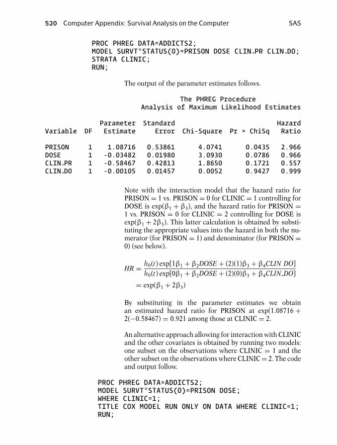
520 Computer Appendix: Survival Analysis on the Computer SAS
PROC PHREG DATA=ADDICTS2;MODEL SURVT*STATUS(0)=PRISON DOSE CLIN-PR CLIN-DO;STRATA CLINIC;RUN;
The output of the parameter estimates follows.
The PHREG ProcedureAnalysis of Maximum Likelihood Estimates
Parameter Standard HazardVariable DF Estimate Error Chi-Square Pr > ChiSq Ratio
PRISON 1 1.08716 0.53861 4.0741 0.0435 2.966DOSE 1 -0.03482 0.01980 3.0930 0.0786 0.966CLIN-PR 1 -0.58467 0.42813 1.8650 0.1721 0.557CLIN-DO 1 -0.00105 0.01457 0.0052 0.9427 0.999
Note with the interaction model that the hazard ratio forPRISON = 1 vs. PRISON = 0 for CLINIC = 1 controlling forDOSE is exp(β1 + β3), and the hazard ratio for PRISON =1 vs. PRISON = 0 for CLINIC = 2 controlling for DOSE isexp(β1 + 2β3). This latter calculation is obtained by substi-tuting the appropriate values into the hazard in both the nu-merator (for PRISON = 1) and denominator (for PRISON =0) (see below).
HR = h0(t) exp[1β1 + β2DOSE + (2)(1)β3 + β4CLIN DO]h0(t) exp[0β1 + β2DOSE + (2)(0)β3 + β4CLIN DO]
= exp(β1 + 2β3)
By substituting in the parameter estimates we obtainan estimated hazard ratio for PRISON at exp(1.08716 +2(−0.58467) = 0.921 among those at CLINIC = 2.
An alternative approach allowing for interaction with CLINICand the other covariates is obtained by running two models:one subset on the observations where CLINIC = 1 and theother subset on the observations where CLINIC = 2. The codeand output follow.
PROC PHREG DATA=ADDICTS2;MODEL SURVT*STATUS(0)=PRISON DOSE;WHERE CLINIC=1;TITLE COX MODEL RUN ONLY ON DATA WHERE CLINIC=1;RUN;

SAS Computer Appendix: Survival Analysis on the Computer 521
A WHERE statement in a SAS procedure limits the num-ber of observations for analyses. A TITLE statement canalso be added to the procedure. The output containingthe parameter estimates subset on the observations whereCLINIC = 1 follows.
COX MODEL RUN ONLY ON DATA WHERE CLINIC=1Analysis of Maximum Likelihood Estimates
Parameter Standard HazardVariable DF Estimate Error Chi-Square Pr > ChiSq Ratio
PRISON 1 0.50249 0.18869 7.0918 0.0077 1.653DOSE 1 -0.03586 0.00774 21.4761 <.0001 0.965
Similarly, the code and output follow containing the param-eter estimates subset on the observations where CLINIC = 2.
PROC PHREG DATA=ADDICTS2;MODEL SURVT*STATUS(0)=PRISON DOSE;WHERE CLINIC=2;TITLE COX MODEL RUN ONLY ON DATA WHERE CLINIC=2;RUN;
COX MODEL RUN ONLY ON DATA WHERE CLINIC=2Analysis of Maximum Likelihood Estimates
Parameter Standard HazardVariable DF Estimate Error Chi-Square Pr > ChiSq Ratio Variable Label
PRISON 1 -0.08226 0.38430 0.0458 0.8305 0.921 0=none, 1=prisonrecord
DOSE 1 -0.03693 0.01234 8.9500 0.0028 0.964 methadone dose(mg/day)
The estimated hazard ratio for PRISON = 1 vs. PRISON = 0is 0.921 among CLINIC = 2 controlling for DOSE. This resultis consistent with the stratified Cox model previously run inwhich all the product terms with CLINIC were included inthe model.

522 Computer Appendix: Survival Analysis on the Computer SAS
4. ASSESSING THE PH ASSUMPTION WITHA STATISTICAL TEST
The following SAS program makes use of the addicts datasetto demonstrate how a statistical test of the proportional haz-ard assumption is performed for a given covariate (Harrel andLee, 1986). This is accomplished by finding the correlation be-tween the Schoenfeld residuals for a particular covariate andthe ranking of individual failure times. If the proportionalhazard assumption is met then the correlation should be nearzero.
The p-value for testing this correlation can be obtained fromPROC CORR (or PROC REG). The Schoenfeld residuals fora given model can be saved in a SAS dataset using PROCPHREG. The ranking of events by failure time can be savedin a SAS dataset using PROC RANKED. The null hypothesisis that the PH assumption is not violated.
First run the full model. The output statement creates aSAS dataset, the OUT=option defines an output dataset, andthe RESSCH=statement is followed by user-defined variablenames so that the output dataset contains the Schoenfeldresiduals. The order of the names corresponds to the orderof the independent variables in the model statement. The ac-tual variable names are arbitrary. The name we chose for thedataset is RESID and the names we chose for the variablescontaining the Schoenfeld residuals for CLINIC, PRISON,and DOSE are RCLINIC, RPRISON, and RDOSE. The codefollows.
PROC PHREG DATA=REF.ADDICTS;MODEL SURVT*STATUS(0)=CLINIC PRISON DOSE;OUTPUT OUT=RESID RESSCH=RCLINIC RPRISON RDOSE;RUN;
PROC PRINT DATA=RESID;RUN;

SAS Computer Appendix: Survival Analysis on the Computer 523
The first 10 observations of the PROC PRINT are shown be-low. The three columns on the right are the variables contain-ing the Schoenfeld residuals.
Obs SURVT STATUS CLINIC PRISON DOSE RCLINIC RPRISON RDOSE
1 428 1 1 0 50 -0.18715 -0.40641 -8.21002 275 1 1 1 55 -0.15841 0.55485 -2.62773 262 1 1 0 55 -0.16453 -0.45197 -2.56354 183 1 1 0 30 -0.14577 -0.48727 -26.08235 259 1 1 1 65 -0.16306 0.54313 7.37016 714 1 1 0 55 -0.25853 -0.50074 -8.53477 438 1 1 1 65 -0.19292 0.58106 6.60728 796 0 1 1 60 . . .9 892 1 1 0 50 -0.34478 -0.22372 -15.908810 393 1 1 1 65 -0.17712 0.57376 6.6886
Next, create a SAS dataset that deletes censored observations(i.e., only contains observations that fail).
DATA EVENTS;SET RESID;IF STATUS=1;RUN;
Use PROC RANK to create a dataset containing a variablethat ranks the order of failure times. The user supplies thename of the output data set using the OUT= option. The vari-able to be ranked is SURVT (the survival time variable). TheRANKS statement precedes a user-defined variable name forthe rankings of failure times. The user-defined names are ar-bitrary. The name we chose for this variable is TIMERANK.The code follows.
PROC RANK DATA=EVENTS OUT=RANKED TIES=MEAN;VAR SURVT;RANKS TIMERANK;RUN;
PROC PRINT DATA=RANKED;RUN;
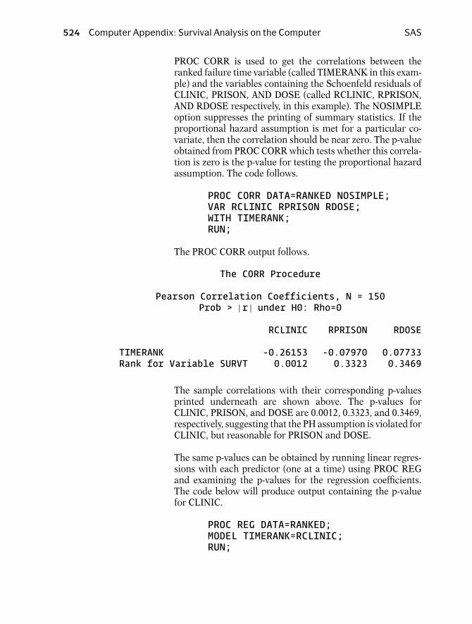
524 Computer Appendix: Survival Analysis on the Computer SAS
PROC CORR is used to get the correlations between theranked failure time variable (called TIMERANK in this exam-ple) and the variables containing the Schoenfeld residuals ofCLINIC, PRISON, AND DOSE (called RCLINIC, RPRISON,AND RDOSE respectively, in this example). The NOSIMPLEoption suppresses the printing of summary statistics. If theproportional hazard assumption is met for a particular co-variate, then the correlation should be near zero. The p-valueobtained from PROC CORR which tests whether this correla-tion is zero is the p-value for testing the proportional hazardassumption. The code follows.
PROC CORR DATA=RANKED NOSIMPLE;VAR RCLINIC RPRISON RDOSE;WITH TIMERANK;RUN;
The PROC CORR output follows.
The CORR Procedure
Pearson Correlation Coefficients, N = 150Prob > |r | under H0: Rho=0
RCLINIC RPRISON RDOSE
TIMERANK -0.26153 -0.07970 0.07733Rank for Variable SURVT 0.0012 0.3323 0.3469
The sample correlations with their corresponding p-valuesprinted underneath are shown above. The p-values forCLINIC, PRISON, and DOSE are 0.0012, 0.3323, and 0.3469,respectively, suggesting that the PH assumption is violated forCLINIC, but reasonable for PRISON and DOSE.
The same p-values can be obtained by running linear regres-sions with each predictor (one at a time) using PROC REGand examining the p-values for the regression coefficients.The code below will produce output containing the p-valuefor CLINIC.
PROC REG DATA=RANKED;MODEL TIMERANK=RCLINIC;RUN;

SAS Computer Appendix: Survival Analysis on the Computer 525
The output produced by PROC REG follows.
The REG Procedure
Parameter Estimates
Parameter StandardVariable Estimate Error t Value Pr > |t |
Intercept 75.49955 3.43535 21.98 <.0001RCLINIC -28.38848 8.61194 -3.30 0.0012
The p-value for CLINIC (0.0012) is shown in the column onthe right and matches the p-value that was obtained usingPROC CORR.
5. OBTAINING COX ADJUSTED SURVIVAL CURVES
We can use the BASELINE statement in PROC PHREG tocreate an output dataset containing Cox adjusted survival es-timates for a specified pattern of covariates. The particularpattern of covariates of interest must first be created in a SASdataset that is subsequently used as the input dataset for theCOVARIATES=option in the BASELINE statement of PROCPHREG. Each pattern of covariates yields a different sur-vival curve (assuming nonzero effects). Adjusted log(− log)survival plots can also be obtained for assessing the PH as-sumption. This is illustrated with three examples.
Ex1—Run a PH model using PRISON, DOSE, and CLINIC andobtain adjusted survival curves where PRISON = 0, DOSE =70, and CLINIC = 2.
Ex2—Run a stratified Cox model (by CLINIC). Obtain two ad-justed survival curves using the mean value of PRISON andDOSE for CLINIC = 1 and CLINIC = 2. Use the log–log curvesto assess the PH assumption for CLINIC adjusted for PRISONand DOSE.
Ex3—Run a stratified Cox model (by CLINIC) and obtain ad-justed survival curves for PRISON = 0, DOSE = 70, and forPRISON = 1, DOSE = 70. This yields four survival curves inall, two for CLINIC = 1 and two for CLINIC = 2.

526 Computer Appendix: Survival Analysis on the Computer SAS
Basically there are these steps:
1. Create the input dataset containing the pattern (values) ofcovariates used for the adjusted survival curves.
2. Run a Cox model with PROC PHREG using the BASELINEstatement to input the dataset from Step (1) and output adataset containing the adjusted survival estimates.
3. Plot the adjusted survival estimates from the output datasetcreated in Step (2).
For Ex1 we create an input dataset (called IN1) with one ob-servation where PRISON = 0, DOSE = 70, and CLINIC =2. We then run a model and create an output dataset (calledOUT1) containing a variable with the adjusted survival esti-mates (called S1). Finally, the adjusted survival curve is plot-ted using PROC GPLOT. The code follows.
DATA IN1;INPUT PRISON DOSE CLINIC;CARDS;0 70 2;
PROC PHREG DATA=REF.ADDICTS;MODEL SURVT*STATUS(0)=PRISON DOSE CLINIC;BASELINE COVARIATES=IN1 OUT=OUT1 SURVIVAL=S1/NOMEAN;RUN;
PROC GPLOT DATA=OUT1;PLOT S1*SURVT;TITLE Adjusted survival for prison=0, dose=70, clinic=2;RUN;
The BASELINE statement in PROC PHREG specifies the in-put dataset, the output dataset, and the name of the variablecontaining the adjusted survival estimates. The NOMEAN op-tion suppresses the survival estimates using the mean valuesof PRISON, DOSE, and CLINIC. The next example (Ex2) doesnot use the NOMEAN option.

SAS Computer Appendix: Survival Analysis on the Computer 527
The output for PROC GPLOT follows.
1000 200 300 400 500 600 700 800 900
survival time in days
1.0
0.9
0.8
0.7
0.6
0.5
0.4
S(t)
Adjusted survival for prison = 0, dose = 70, clinic = 2
For Ex2 we wish to create and output a dataset (called OUT2)that contains the adjusted survival estimates from a Coxmodel stratified by CLINIC using the mean values of PRISONand DOSE An input dataset need not be specified because bydefault the mean values of PRISON and DOSE will be used ifthe NOMEAN option is not used in the BASELINE statement.The code follows.
PROC PHREG DATA=REF.ADDICTS;MODEL SURVT*STATUS(0) = PRISON DOSE CLINIC;BASELINE OUT=OUT2 SURVIVAL=S2 LOGLOGS=LS2;RUN;
PROC GPLOT DATA=OUT2;PLOT S2*SURVT=CLINIC;TITLE adjusted survival stratified by clinic;RUN;
PROC GPLOT DATA=OUT2;PLOT LS2*SURVT=CLINIC;TITLE log–log curves stratified by clinic, adjusted forprison, dose;RUN;

528 Computer Appendix: Survival Analysis on the Computer SAS
The code PLOT LS2∗SURVT=CLINIC in the second PROCGPLOT will plot LS2 on the vertical axis, SURVT on the hori-zontal axis, stratified by CLINIC on the same graph. The vari-able LS2 was created in the BASELINE statement of PROCPHREG and contains the adjusted log–log survival estimates.The PROC GPLOT output for the log–log survival curves strat-ified by CLINIC adjusted for PRISON and DOSE follows.
−6
−5
−4
−3
−2
−1
2
0
1
0 100 200 300 600500
survival time in days
400 700 800 900
Coded 1 or 2 1 2
Log
of
Neg
ativ
e L
og o
f S
UR
VIV
AL
Log–log curves stratified by clinic, adjusted for prison, dose
The adjusted log–log plots look similar to the unadjusted log–log Kaplan–Meier plots shown earlier in that the plots lookreasonably parallel before 365 days but then diverge suggest-ing that the PH assumption is violated after 1 year.
For Ex3, a stratified Cox (by CLINIC) is run and adjustedcurves are obtained for PRISON = 1 and PRISON = 0 holdingDOSE = 70. An input dataset (called IN3) is created with twoobservations for both levels of PRISON with DOSE = 70. Anoutput dataset (called OUT3) is created with the BASELINEstatement that contains a variable (called S3) of survival es-timates for all four curves (two for each stratum of CLINIC).The code follows.

SAS Computer Appendix: Survival Analysis on the Computer 529
DATA IN3;INPUT PRISON DOSE;CARDS;1 700 70;
PROC PHREG DATA=REF.ADDICTS;MODEL SURVT*STATUS(0)= PRISON DOSE;STRATA CLINIC;BASELINE COVARIATES=IN3 OUT=OUT4 SURVIVAL=S3/NOMEAN;RUN;
PROC GPLOT DATA=OUT3;PLOT S3*SURVT=CLINIC;TITLE adjusted survival stratified by clinic for both levelsof prison;RUN;
The PROC GPLOT output follows.
0 100 200 300 400 500 600 700 800 900
survival time in daysCoded 1 or 2 1 2
0.0
0.1
0.2
0.3
0.4
0.5
0.6
0.7
0.8
1.0
0.9
Su
rviv
al f
un
ctio
n e
stim
ate
Adjusted survival stratified by clinic for both levels of prison
For the above graph, the PH assumption is not assumed forCLINIC because that is the stratified variable. However, thePH assumption is assumed for PRISON within each stratumof CLINIC (i.e., CLINIC = 1 and CLINIC = 2).

530 Computer Appendix: Survival Analysis on the Computer SAS
6. RUNNING AN EXTENDED COX MODEL
Models containing time-dependent variables are run usingPROC PHREG. Time-dependent variables are created withprogramming statements within the PROC PHREG proce-dure. Sometimes users incorrectly define time-dependentvariables in the data step. This leads to wrong estimates be-cause the time variable used in the data step (SURVT) is ac-tually time-independent and therefore different than the timevariable (also called SURVT) used to define time-dependentvariables in the PROC PHREG statement. See the discussionon the extended Cox likelihood in Chapter 6 for further clari-fication of this issue.
We have evaluated the PH assumption for the variable CLINICby plotting KM log–log curves and Cox adjusted log–log curvesstratified by CLINIC and checking whether the curves wereparallel. We could do similar analyses with the variablesPRISON and DOSE although with DOSE we would need tocategorize the continuous variable before comparing plots fordifferent strata of DOSE.
If it is expected that the hazard ratio for the effect of DOSEincreases (or decreases) monotonically with time we couldadd a continuous time-varying product term with DOSE andsome function of time. The model defined below contains atime-varying variable (LOGTDOSE) defined as the product ofDOSE and the natural log of time (SURVT). In some sense aviolation of the proportional hazard assumption for a partic-ular variable means that there is an interaction between thatvariable and time. Note that the variable LOGTDOSE is de-fined within the PHREG procedure and not in the data step.The code follows.
PROC PHREG DATA=REF.ADDICTS;MODEL SURVT*STATUS(0)=PRISON CLINIC DOSE LOGTDOSE;LOGTDOSE=DOSE*LOG(SURVT);RUN;

SAS Computer Appendix: Survival Analysis on the Computer 531
The output produced by PROC PHREG follows.
The PHREG ProcedureAnalysis of Maximum Likelihood Estimates
Parameter Standard HazardVariable DF Estimate Error Chi-Square Pr > ChiSq Ratio
PRISON 1 0.34047 0.16747 4.1333 0.0420 1.406CLINIC 1 -1.01857 0.21538 22.3655 <.0001 0.361DOSE 1 -0.08243 0.03599 5.2468 0.0220 0.921LOGTDOSE 1 0.00858 0.00646 1.7646 0.1841 1.009
The Wald test for the time-dependent variable LOGTDOSEyields a p-value of 0.1841. A nonsignificant p-value does notnecessarily mean that the PH assumption is reasonable forDOSE. Perhaps a different defined time-dependent variablewould have been significant (e.g., DOSE × (TIME − 100)).Also the sample size of the study is a key determinant of thepower to reject the null, which in this case means rejection ofthe PH assumption.
Next we consider time-dependent variables for CLINIC. Thenext two models use Heaviside functions that allow a differenthazard ratio for CLINIC before and after 365 days. The firstmodel uses two Heaviside functions in the model (HV1 andHV2) but not CLINIC. The second model uses one Heavisidefunction (HV) but also includes CLINIC in the model. Thesetwo models yield the same hazard ratio estimates for CLINICbut are coded differently. The code follows.
PROC PHREG DATA=REF.ADDICTS;MODEL SURVT*STATUS(0)=PRISON DOSE HV1 HV2;IF SURVT < 365 THEN HV1 = CLINIC; ELSE HV1 = 0;IF SURVT >= 365 THEN HV2 = CLINIC; ELSE HV2 = 0;RUN;
PROC PHREG DATA=REF.ADDICTS;MODEL SURVT*STATUS(0)=CLINIC PRISON DOSE HV;IF SURVT >= 365 THEN HV = CLINIC; ELSE HV = 0;RUN;
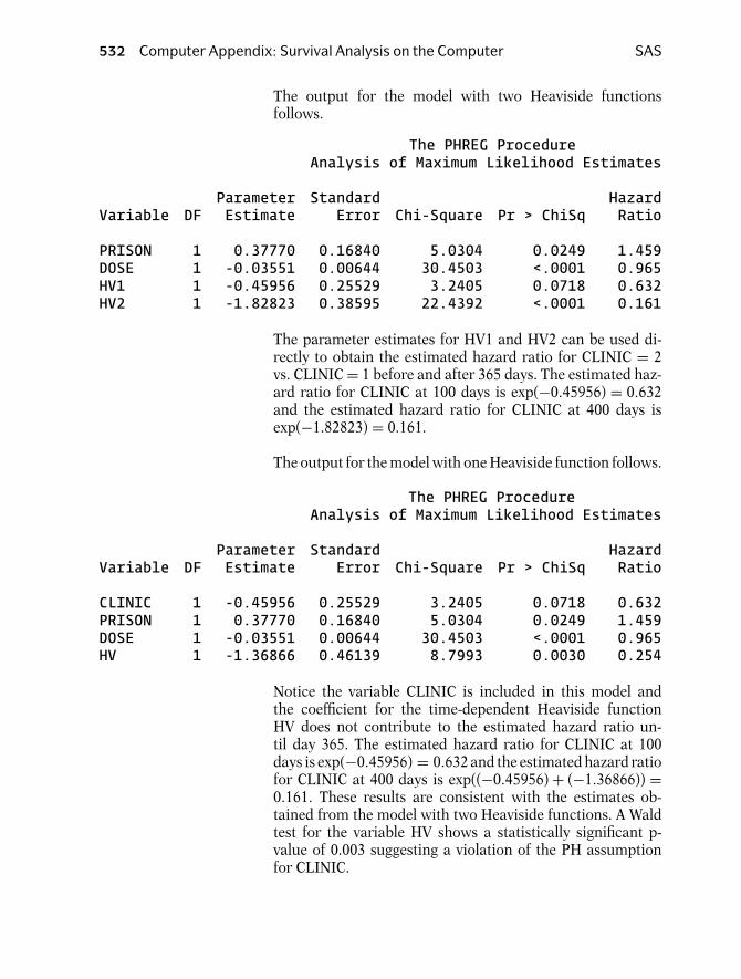
532 Computer Appendix: Survival Analysis on the Computer SAS
The output for the model with two Heaviside functionsfollows.
The PHREG ProcedureAnalysis of Maximum Likelihood Estimates
Parameter Standard HazardVariable DF Estimate Error Chi-Square Pr > ChiSq Ratio
PRISON 1 0.37770 0.16840 5.0304 0.0249 1.459DOSE 1 -0.03551 0.00644 30.4503 <.0001 0.965HV1 1 -0.45956 0.25529 3.2405 0.0718 0.632HV2 1 -1.82823 0.38595 22.4392 <.0001 0.161
The parameter estimates for HV1 and HV2 can be used di-rectly to obtain the estimated hazard ratio for CLINIC = 2vs. CLINIC = 1 before and after 365 days. The estimated haz-ard ratio for CLINIC at 100 days is exp(−0.45956) = 0.632and the estimated hazard ratio for CLINIC at 400 days isexp(−1.82823) = 0.161.
The output for the model with one Heaviside function follows.
The PHREG ProcedureAnalysis of Maximum Likelihood Estimates
Parameter Standard HazardVariable DF Estimate Error Chi-Square Pr > ChiSq Ratio
CLINIC 1 -0.45956 0.25529 3.2405 0.0718 0.632PRISON 1 0.37770 0.16840 5.0304 0.0249 1.459DOSE 1 -0.03551 0.00644 30.4503 <.0001 0.965HV 1 -1.36866 0.46139 8.7993 0.0030 0.254
Notice the variable CLINIC is included in this model andthe coefficient for the time-dependent Heaviside functionHV does not contribute to the estimated hazard ratio un-til day 365. The estimated hazard ratio for CLINIC at 100days is exp(−0.45956) = 0.632 and the estimated hazard ratiofor CLINIC at 400 days is exp((−0.45956) + (−1.36866)) =0.161. These results are consistent with the estimates ob-tained from the model with two Heaviside functions. A Waldtest for the variable HV shows a statistically significant p-value of 0.003 suggesting a violation of the PH assumptionfor CLINIC.

SAS Computer Appendix: Survival Analysis on the Computer 533
Suppose it is believed that the hazard ratio for CLINIC = 2 vs.CLINIC = 1 is constant over the first year but then monoton-ically increases (or decreases) after the first year. The follow-ing code defines a model allowing for a time-varying covariatecalled CLINTIME (defined in the code) which contributes tothe hazard ratio for CLINIC after 365 days. The code follows(output omitted).
PROC PHREG DATA=REF.ADDICTS;MODEL SURVT*STATUS(0)=CLINIC PRISON DOSE CLINTIME;IF SURVT < 365 THEN CLINTIME=0;ELSE IF SURVT >= 365 THEN CLINTIME = CLINIC*(SURVT-365);RUN;
7. RUNNING PARAMETRIC MODELSWITH PROC LIFEREG
PROC LIFEREG runs parametric accelerated failure time(AFT) models rather than proportional hazards (PH) mod-els. Whereas the key assumption of a PH model is that haz-ard ratios are constant over time, the key assumption for anAFT model is that survival time accelerates (or decelerates)by a constant factor when comparing different levels ofcovariates.
The most common distribution for parametric modeling ofsurvival data is the Weibull distribution. The hazard functionfor a Weibull distribution is λptp−1. If p = 1 then the Weibulldistribution is also an exponential distribution. The Weibulldistribution has a desirable property in that if the AFT as-sumption holds then the PH assumption also holds. The ex-ponential distribution is a special case of the Weibull distri-bution. The key property for the exponential distribution isthat the hazard is constant over time (h(t) = λ). In SAS, theWeibull and exponential model are run only as AFT models.
The Weibull distribution has the property that the log–logof the survival function is linear with the log of time. PROCLIFETEST can be used to plot Kaplan–Meier log–log curvesagainst the log of time. If the curves are approximatelystraight lines (and parallel) then the assumption is reason-able. Furthermore, if the straight lines have a slope of 1, thenthe exponential distribution is appropriate. The code belowproduces log–log curves stratified by CLINIC and PRISONthat can be used to check the validity of the Weibull assump-tion for those variables.

534 Computer Appendix: Survival Analysis on the Computer SAS
PROC LIFETEST DATA=REF.ADDICTS METHOD=KM PLOTS=(LLS);TIME SURVT*STATUS(0);STRATA CLINIC PRISON;RUN;
The log–log survival plots produced by PROC LIFETESTfollow.
2
0
−2
−4
−6
Log
Neg
ativ
e L
og S
DF
321 4 5 6 7
Log of survival time in days
CLINIC = 2 PRISON = 0CLINIC = 1 PRISON = 1CLINIC = 2 PRISON = 1
CLINIC = 1 PRISON = 0STRATA
The log–log curves do not look straight but for illustration weproceed as if the Weibull assumption were appropriate. Firstan exponential model is run with PROC LIFEREG. In thismodel the Weibull shape parameter (p) is forced to equal 1,which forces the hazard to be constant.
PROC LIFEREG DATA=REF.ADDICTS;MODEL SURVT*STATUS(0)=PRISON DOSE CLINIC/DIST=EXPONENTIAL;RUN;
The DIST=EXPONENTIAL option in the MODEL statementrequests the exponential distribution. The output of parame-ter estimates obtained from PROC LIFEREG follows.
Analysis of Parameter Estimates
Standard 95% Confidence Chi-Parameter DF Estimate Error Limits Square Pr > ChiSq
Intercept 1 3.6843 0.4307 2.8402 4.5285 73.17 <.0001PRISON 1 -0.2526 0.1649 -0.5758 0.0705 2.35 0.1255DOSE 1 0.0289 0.0061 0.0169 0.0410 22.15 <.0001CLINIC 1 0.8806 0.2106 0.4678 1.2934 17.48 <.0001Scale 0 1.0000 0.0000 1.0000 1.0000Weibull Shape 0 1.0000 0.0000 1.0000 1.0000

SAS Computer Appendix: Survival Analysis on the Computer 535
The exponential model assumes a constant hazard. This is in-dicated in the output by the value of the Weibull shape pa-rameter (1.0000). The output can be used to calculate theestimated hazard for any subject given a pattern of covari-ates. For example, a subject with PRISON = 0, DOSE = 50,and CLINIC = 2 has an estimated hazard of exp(−(3.6843 +50(0.0289) + 2(0.8806)) = .001. Note that SAS gives the pa-rameter estimates for the AFT form of the exponential model.Multiply the estimated coefficients by negative one to get esti-mates consistent with the PH parameterization of the model(see Chapter 7).
Next a Weibull AFT model is run with PROC LIFEREG.
PROC LIFEREG DATA=REF.ADDICTS;MODEL SURVT*STATUS(0)=PRISON DOSE CLINIC/DIST=WEIBULL;RUN;
The DIST=WEIBULL option in the MODEL statement re-quests the Weibull distribution. The output for the parameterestimates follows.
Analysis of Parameter Estimates
Standard 95% Confidence Chi-Parameter DF Estimate Error Limits Square Pr > ChiSq
Intercept 1 4.1048 0.3281 3.4619 4.7478 156.56 <.0001PRISON 1 -0.2295 0.1208 -0.4662 0.0073 3.61 0.0575DOSE 1 0.0244 0.0046 0.0154 0.0334 28.32 <.0001CLINIC 1 0.7090 0.1572 0.4009 1.0172 20.34 <.0001Scale 1 0.7298 0.0493 0.6393 0.8332Weibull Shape 1 1.3702 0.0926 1.2003 1.5642
The Weibull shape parameter is estimated at 1.3702. SAS callsthe reciprocal of the Weibull shape parameter, the Scale pa-rameter, estimated at 0.7298. The acceleration factor compar-ing CLINIC = 2 to CLINIC = 1 is estimated at exp(0.7090) =2.03. So the estimated median survival time (time off heroin)is double for patients enrolled in CLINIC = 2 compared toCLINIC = 1.
To obtain the hazard ratio parameters from the Weibull AFTmodel, multiply the Weibull shape parameter by the negativeof the AFT parameter (see Chapter 7). For example, the HRestimate for CLINIC = 2 vs. CLINIC = 1 controlling for theother covariates is exp(1.3702(−0.7090)) = 0.38.

536 Computer Appendix: Survival Analysis on the Computer SAS
Next a log-logistic AFT model is run with PROC LIFEREG.
PROC LIFEREG DATA=REF.ADDICTS;MODEL SURVT*STATUS(0)=PRISON DOSE CLINIC/DIST=LLOGISTIC;RUN;
The output of the log-logistic parameter estimates follows.
Analysis of Parameter Estimates
Standard 95% Confidence Chi-Parameter DF Estimate Error Limits Square Pr >ChiSq
Intercept 1 3.5633 0.3894 2.8000 4.3266 83.71 <.0001PRISON 1 -0.2913 0.1440 -0.5734 -0.0091 4.09 0.0431DOSE 1 0.0316 0.0055 0.0208 0.0424 32.81 <.0001CLINIC 1 0.5806 0.1716 0.2443 0.9169 11.45 0.0007Scale 1 0.5868 0.0403 0.5129 0.6712
From this output, the acceleration factor comparingCLINIC = 2 to CLINIC = 1 is estimated as exp(0.5806) =1.79. If the AFT assumption holds for a log-logistic model,then the proportional odds assumption holds for the survivalfunction (although the PH assumption will not hold). The pro-portional odds assumption can be evaluated by plotting thelog odds of survival (using KM estimates) against the log ofsurvival time. If the plots are straight lines for each pattern ofcovariates then the log-logistic distribution is reasonable. Ifthe straight lines are also parallel then the proportional oddsand AFT assumptions also hold.
A SAS dataset containing the KM survival estimates can becreated using PROC LIFETEST (see Section 1 of this ap-pendix). Once this variable is created, a dataset containingvariables for the estimated log odds of survival and the log ofsurvival time can also be created. PROC GPLOT can then beused to plot the log odds of survival against survival time.
Another context for thinking about the proportional odds as-sumption is that the odds ratio estimated by a logistic re-gression does not depend on the length of the follow-up. Forexample, if a follow-up study were extended from three to fiveyears then the underlying odds ratio comparing two patternsof covariates would not change. If the proportional odds as-sumption is not true, then the odds ratio is specific to thelength of follow-up.

SAS Computer Appendix: Survival Analysis on the Computer 537
An AFT model is a multiplicative model with respect to sur-vival time or equivalently an additive model with respect to thelog of time. In the previous example, the median survival timewas estimated as 1.79 times longer for CLINIC = 2 comparedto CLINIC = 1. In that example survival time was assumedto follow a log-logistic distribution or equivalently the log ofsurvival time was assumed to follow a logistic distribution.
SAS allows additive failure time models to be run (seeChapter 7 under the heading “Other Parametric Models”). TheNOLOG option in the MODEL statement of PROC LIFEREGsuppresses the default log link function which means thattime, rather than log(time), is modeled as a linear functionof the regression parameters. The following code requests anadditive failure time model in which time follows a logistic(not log-logistic) distribution.
PROC LIFEREG DATA=REF.ADDICTS;MODEL SURVT*STATUS(0)=PRISON DOSE CLINIC/DIST=LLOGISTIC NOLOG;RUN;
Even though the option DIST=LLOGISTIC appears to re-quest that survival time follow a log-logistic distribution, theNOLOG option actually means that survival time is assumedto follow a logistic distribution. (Note that the NOLOG op-tion in Stata means something completely different using thestreg command: that the iteration log file not be shown inthe output.) The output from the additive failure time modelfollows.
Analysis of Parameter Estimates
Standard 95% Confidence Chi-Parameter DF Estimate Error Limits Square Pr > ChiSq
Intercept 1 -358.482 114.0161 -581.949 -135.014 9.89 0.0017PRISON 1 -89.7816 42.9645 -173.990 -5.5727 4.37 0.0366DOSE 1 10.3893 1.6244 7.2055 13.5731 40.91 <.0001CLINIC 1 214.2525 53.1204 110.1385 318.3665 16.27 <.0001Scale 1 172.4039 11.3817 151.4792 196.2191

538 Computer Appendix: Survival Analysis on the Computer SAS
The parameter estimate for CLINIC is 214.2525. The inter-pretation for this estimate is that the median survival time(or time to any fixed value of S(t)) is estimated at 214 daysmore for CLINIC = 2 compared to CLINIC = 1. In otherwords, you add 214 days to the estimated median survivaltime for CLINIC = 1 to get the estimated median survivaltime for CLINIC = 2. This contrasts with the previous AFTmodel in which you multiply estimated median survival timefor CLINIC = 1 by 1.79 to get the estimated median survivaltime for CLINIC = 2. The additive model can be viewed as ashifting of survival time whereas the AFT model can be viewedas a scaling of survival time.
If survival time follows a logistic distribution and the ad-ditive failure time assumption holds, then the proportionalodds assumption also holds. The logistic assumption can beevaluated by plotting the log odds of survival (using KM es-timates) against time (rather than against the log of time asanalogously used for the evaluation of the log-logistic assump-tion). If the plots are straight lines for each pattern of covari-ates then the logistic distribution is reasonable. If the straightlines are also parallel then the proportional odds and additivefailure time assumptions hold.
Other distributions supported by PROC LIFEREG arethe generalized gamma (DIST=GAMMA) and lognormal(DIST=LNORMAL) distributions. If the NOLOG option isspecified with the DIST=LNORMAL option in the model state-ment, then survival time is assumed to follow a normal dis-tribution. SAS version 8.2 does not support frailty survivalmodels.
8. MODELING RECURRENT EVENTS
The modeling of recurrent events is illustrated with the blad-der cancer dataset (bladder.sas7bdat) described at the startof this appendix. Recurrent events are represented in thedata with multiple observations for subjects having multipleevents. The data layout for the bladder cancer dataset is suit-able for a counting process approach with time intervals de-fined for each observation (see Chapter 8). The following codeprints the 12th through 20th observation, which contains in-formation for four subjects. The code follows.
PROC PRINT DATA=REF.BLADDER (FIRSTOBS= 12 OBS=20);RUN;

SAS Computer Appendix: Survival Analysis on the Computer 539
The output follows.
OBS ID EVENT INTERVAL START STOP TX NUM SIZE12 10 1 1 0 12 0 1 113 10 1 2 12 16 0 1 114 10 0 3 16 18 0 1 115 11 0 1 0 23 0 3 316 12 1 1 0 10 0 1 317 12 1 2 10 15 0 1 318 12 0 3 15 23 0 1 319 13 1 1 0 3 0 1 120 13 1 2 3 16 0 1 1
There are three observations for ID = 10, one observation forID = 11, three observations for ID = 12, and two observationsfor ID = 13. The variables START and STOP represent thetime interval for the risk period specific to that observation.The variable EVENT indicates whether an event (coded 1)occurred. The first three observations indicate that the subjectwith ID = 10 had an event at 12 months, another event at16 months, and was censored at 18 months.
PROC PHREG can be used for survival data using a count-ing processes data layout. The following code runs a modelwith the predictors, treatment status (TX), initial number oftumors (NUM), and the initial size of tumors (SIZE) includedin the model.
PROC PHREG DATA=BLADDER COVS(AGGREGATE);MODEL (START,STOP)*EVENT(0)=TX NUM SIZE;ID ID;RUN;
The code (START,STOP)∗EVENT(0) in the MODEL state-ment indicates that the time intervals for each observationare defined by the variables START and STOP and thatEVENT = 0 denotes a censored observation. The ID state-ment defines ID as the variable representing subject. TheCOVS(AGGREGATE) option in the PROC PHREG statementrequests robust standard errors for the parameter estimates.The output generated by PROC PHREG follows.

540 Computer Appendix: Survival Analysis on the Computer SAS
The PHREG Procedure
Model Information
Data Set WORK.BLADDERDependent Variable STARTDependent Variable STOPCensoring Variable EVENTCensoring Value(s) 0Ties Handling BRESLOW
Analysis of Maximum Likelihood Estimates
Parameter Standard StdErr HazardVariable Estimate Error Ratio Chi-Square Pr > ChiSq Ratio
TX -0.40710 0.24183 1.209 2.8338 0.0923 0.666NUM 0.16065 0.05689 1.185 7.9735 0.0047 1.174SIZE -0.04009 0.07222 1.028 0.3081 0.5788 0.961
Coefficient estimates are provided with robust standard er-rors. The column under the heading StdErrRatio providesthe ratio of the robust to the nonrobust standard errors.For example, the standard error for the coefficient for TX(0.24183) is 1.209 greater than the standard error would beif we had not requested robust standard errors (i.e., omit theCOVS(AGGREGATE) option). The robust standard errors areestimated slightly differently compared to the correspondingmodel in Stata.
A stratified Cox model can also be run using the data in thisformat with the variable INTERVAL as the stratified variable.The stratified variable indicates whether the subject was atrisk for a 1st, 2nd, 3rd, or 4th event. This approach is calledconditional 1 in Chapter 8 and is used if the investigatorwants to distinguish the order in which recurrent events oc-cur. The code for a stratified Cox follows.
PROC PHREG DATA=BLADDER COVS(AGGREGATE);MODEL (START,STOP)*EVENT(0)=TX NUM SIZE;ID ID;STRATA INTERVAL;RUN;

SAS Computer Appendix: Survival Analysis on the Computer 541
The only additional code from the previous model is theSTRATA statement indicating that the variable INTERVAL isthe stratified variable. The output containing the parameterestimates follows.
Analysis of Maximum Likelihood Estimates
Parameter Standard StdErr HazardVariable Estimate Error Ratio Chi-Square Pr > ChiSq Ratio
TX -0.33430 0.19706 0.912 2.8777 0.0898 0.716NUM 0.11565 0.04991 0.930 5.3690 0.0205 1.123SIZE -0.00805 0.06012 0.827 0.0179 0.8935 0.992
Interaction terms between the treatment variable (TX) andthe stratified variable could be created to examine whetherthe effect of treatment differed for the 1st, 2nd, 3rd, or 4thevent.
Another stratified approach (called conditional 2) is a slightvariation of the conditional 1 approach. The difference is inthe way the time intervals for the recurrent events are defined.There is no difference in the time intervals when subjects areat risk for their first event. However, with the conditional 2approach, the starting time at risk gets reset to zero for eachsubsequent event. The following code creates data suitablefor using the conditional 2 approach.
DATA BLADDER2;SET REF.BLADDER;START2=0;STOP2=STOP-START;RUN;
The new dataset (BLADDER2) copies the data fromREF.BLADDER and creates two new variables for the timeinterval: START2, which is always set to zero and STOP2,which is the length of the time interval (i.e., STOP – START).The following code uses these newly created variables to runthe conditional 2 approach with PROC PHREG.
PROC PHREG DATA=BLADDER2 COVS(AGGREGATE);MODEL (START2,STOP2)*EVENT(0)=TX NUM SIZE;ID ID;STRATA INTERVAL;RUN;

542 Computer Appendix: Survival Analysis on the Computer SPSS
The output follows.
Parameter Standard StdErr HazardVariable Estimate Error Ratio Chi-Square Pr > ChiSq Ratio
TX -0.26952 0.20808 1.002 1.6778 0.1952 0.764NUM 0.15353 0.04889 0.938 9.8620 0.0017 1.166SIZE 0.00684 0.06222 0.889 0.0121 0.9125 1.007
The results using the conditional 1 and conditional 2 ap-proaches vary slightly.
The counting process data layout with multiple observationsper subject need not only apply to recurrent event data butcan also be used for more conventional survival analyses inwhich each subject is limited to one event. A subject with fourobservations may be censored for the first three observationsbefore getting the event in the time interval represented by thefourth observation. This data layout is particularly suitablefor representing time-varying exposures (i.e., exposures thatchange values over different intervals of time).
C. SPSSAnalyses are carried out in SPSS by using the appropriateSPSS procedure on an SPSS dataset. Most users select pro-cedures by pointing and clicking the mouse through a seriesof menus and dialog boxes. The code, or command syntax,generated by these steps can be viewed and edited.
Analyses on the addicts dataset are used to illustrate theseprocedures. The addicts dataset was obtained from a 1991Australian study by Caplehorn et al., and contains infor-mation on 238 heroin addicts. The study compared twomethadone treatment clinics to assess patient time remainingunder methadone treatment. The two clinics differed accord-ing to live-in policies for patients. A patient’s survival time wasdetermined as the time (in days) until the person dropped outof the clinic or was censored. The variables are defined at thestart of this appendix.

SPSS Computer Appendix: Survival Analysis on the Computer 543
After getting into SPSS, open the dataset addicts.sav. Thedata should appear on your screen. This is now your work-ing dataset. To obtain a basic descriptive analysis of theoutcome variable (SURVT) click on Analyze → DescriptiveStatistics → Descriptive from the drop-down menus to reachthe dialog box to specify the analytic variables. Select the sur-vival time variable (SURVT) from the list of variables andenter it into the Variable box. Click on OK to view the out-put. Alternatively you can click on Paste (rather than OK) toobtain the corresponding SPSS syntax. The syntax can thenbe submitted (by clicking the button under Run), edited, orsaved for another session. The syntax created is as follows(output omitted).
DESCRIPTIVESVARIABLES=survt/STATISTICS=MEAN STDDEV MIN MAX
There are some analyses that SPSS only performs by submit-ting syntax rather than using the point and click approach(e.g., running an extended Cox model with two time-varyingcovariates). Each time the point and click approach is pre-sented the corresponding syntax will also be presented.
To obtain more detailed descriptive statistics on survival timestratified by CLINIC, click on Analyze → Descriptive Statis-tics → Explore from the drop-down menus. Select SURVTfrom the list of variables and enter it into the Dependent Listand then select CLINIC and enter it into the Factor List. Clickon OK to see the output. The syntax created from clicking onPaste (rather than OK) is as follows (output omitted).
EXAMINEVARIABLES=survt BY clinic/PLOT BOXPLOT STEMLEAF/COMPARE GROUP/STATISTICS DESCRIPTIVES/CINTERVAL 95/MISSING LISTWISE/NOTOTAL
Survival analyses can be performed in SPSS by selecting An-alyze → Survival. There are then four choices for selection:Life Tables, Kaplan–Meier, Cox Regression, and Cox w/ Time-Dep Cov. The key SPSS procedures for survival analysis arethe KM and COXREG procedures.
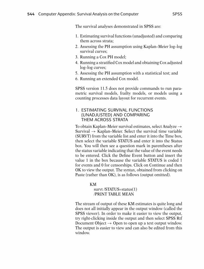
544 Computer Appendix: Survival Analysis on the Computer SPSS
The survival analyses demonstrated in SPSS are:
1. Estimating survival functions (unadjusted) and comparingthem across strata;
2. Assessing the PH assumption using Kaplan–Meier log–logsurvival curves;
3. Running a Cox PH model;4. Running a stratified Cox model and obtaining Cox adjusted
log–log curves;5. Assessing the PH assumption with a statistical test; and6. Running an extended Cox model.
SPSS version 11.5 does not provide commands to run para-metric survival models, frailty models, or models using acounting processes data layout for recurrent events.
1. ESTIMATING SURVIVAL FUNCTIONS(UNADJUSTED) AND COMPARINGTHEM ACROSS STRATA
To obtain Kaplan–Meier survival estimates, select Analyze →Survival → Kaplan–Meier. Select the survival time variable(SURVT) from the variable list and enter it into the Time box,then select the variable STATUS and enter it into the Statusbox. You will then see a question mark in parentheses afterthe status variable indicating that the value of the event needsto be entered. Click the Define Event button and insert thevalue 1 in the box because the variable STATUS is coded 1for events and 0 for censorships. Click on Continue and thenOK to view the output. The syntax, obtained from clicking onPaste (rather than OK), is as follows (output omitted).
KMsurvt /STATUS=status(1)/PRINT TABLE MEAN
The stream of output of these KM estimates is quite long anddoes not all initially appear in the output window (called theSPSS viewer). In order to make it easier to view the output,try right-clicking inside the output and then select SPSS RtfDocument Object → Open to open up a text output window.The output is easier to view and can also be edited from thiswindow.

SPSS Computer Appendix: Survival Analysis on the Computer 545
To obtain KM survival estimates and plots by CLINIC as wellas log rank (and other) test statistics, select Analyze → Sur-vival → Kaplan–Meier and then select SURVT as the time-to-event variable and STATUS as the status variable as de-scribed above. Enter CLINIC into the Factor box and clickthe Compare Factor button. You have a choice of three teststatistics for testing the equality of survival functions acrossCLINIC. Select all three (log rank, Breslow, and Tarone–Ware)for comparison and click Continue. Click the Options buttonto request plots. There are four choices (unfortunately log–log survival plots are not included). Select Survival to obtainKM plots by clinic. Click Continue and then OK to view theoutput. To edit (and better view) the output, right-click on theoutput and then select SPSS Rtf Document Object → Openin order to open up a text output window.
The syntax follows.
KMsurvt BY clinic /STATUS=status(1)/PRINT TABLE MEAN/PLOT SURVIVAL/TEST LOGRANK BRESLOW TARONE/COMPARE OVERALL POOLED
The output containing the KM estimates for the first fourevent-times from CLINIC = 1 and CLINIC = 2 as well forthe log rank, Breslow, and Tarone–Ware tests follows.
Survival Analysis for SURVT Survival time (days)
Factor CLINIC = 1.00
Time Status Cumulative Standard Cumulative NumberSurvival Error Events Remaining
2.00 censored 0 1627.00 endpoint .9938 .0062 1 16117.00 endpoint .9877 .0087 2 16019.00 endpoint .9815 .0106 3 15928.00 censored 3 15828.00 censored 3 15729.00 endpoint .9752 .0122 4 156
.
.

546 Computer Appendix: Survival Analysis on the Computer SPSS
Factor CLINIC = 2.00
Time Status Cumulative Standard Cumulative NumberSurvival Error Events Remaining
2.00 censored 0 7413.00 endpoint .9865 .0134 1 7326.00 endpoint .9730 .0189 2 7235.00 endpoint .9595 .0229 3 7141.00 endpoint .9459 .0263 4 70
.
.
Test Statistics for Equality of Survival Distributions for CLINIC
Statistic df Significance
Log Rank 27.89 1 .0000Breslow 11.63 1 .0007Tarone-Ware 17.60 1 .0000
Note that what SPSS calls the Breslow test statistic isequivalent to what Stata (and SAS) call the Wilcoxon teststatistic.
Life table estimates can be obtained by selecting Analyze →Survival → Life Tables. The time-to-event and status variablesare defined similarly to those described above for Kaplan–Meier estimates. However, with life tables, SPSS presents aDisplay Time Intervals box. This allows the user to define thetime intervals used for the life table analysis. For example, 0to 1000 by 100 would define 10 time intervals of equal length.Life table plots can similarly be requested as described abovefor the KM plots.
2. ASSESSING THE PH ASSUMPTION USINGKAPLAN–MEIER LOG–LOG SURVIVAL CURVES
SPSS does not provide unadjusted KM log–log curves by di-rectly using the point and click approach with the KM com-mand. SPSS does provide adjusted log–log curves from run-ning a stratified Cox model (described later in the stratifiedCox section). A log–log curve equivalent to the unadjusted KMlog–log curve can be obtained in SPSS by running a stratifiedCox without including any covariates in the model. In thissection, however, we illustrate how new variables can be de-fined in the working dataset and then used to plot unadjustedlog–log KM plots.

SPSS Computer Appendix: Survival Analysis on the Computer 547
First a variable is created containing the KM survival esti-mates. Then another new variable is created containing thelog–log of the survival estimates. Finally the log–log survivalestimates are plotted against survival time to see if the curvesfor CLINIC = 1 and CLINIC = 2 are parallel. Each step canbe done with the point-and-click approach or by typing in thecode directly.
A variable containing the survival estimates can be createdby selecting Analyze → Survival → Kaplan–Meier and thenselecting SURVT as the time-to-event variable, STATUS as thestatus variable, and CLINIC as the factor variable as describedabove. Then click the Save button. This opens a dialog boxcalled Kaplan–Meier Save New Variables. Check Survival andclick on Continue and then on Paste. The code that is createdis as follows.
KMsurvt BY clinic /STATUS=status(1)/PRINT TABLE MEAN/SAVE SURVIVAL
By submitting this code, a new variable containing the KMestimates called sur 1 is created. To create a new variablecalled lls containing the log(− log) of sur 1 submit the fol-lowing code.
COMPUTE lls = LN(-LN (sur-1)) .EXECUTE
The above code could also be generated by selecting Trans-form → Compute and defining the new variable in the dialogbox. To plot lls against survival time submit the code:
GRAPH/SCATTERPLOT(BIVAR)=survt WITH lls BY clinic/MISSING=LISTWISE
This final piece of code could also be run by selectingGraphs → Scatter and then clicking on Simple and then De-fine in the Scatterplot dialogue box. Select LLS for the Y-axis,SURVT for the X-axis, and CLINIC in the Set Marker By box.Clicking on paste creates the code or clicking OK submits theprogram. A plot of LLS against log(SURVT) could similarlybe created. Parallel curves support the PH assumption forCLINIC.
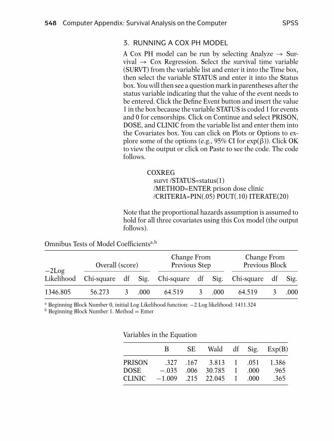
548 Computer Appendix: Survival Analysis on the Computer SPSS
3. RUNNING A COX PH MODEL
A Cox PH model can be run by selecting Analyze → Sur-vival → Cox Regression. Select the survival time variable(SURVT) from the variable list and enter it into the Time box,then select the variable STATUS and enter it into the Statusbox. You will then see a question mark in parentheses after thestatus variable indicating that the value of the event needs tobe entered. Click the Define Event button and insert the value1 in the box because the variable STATUS is coded 1 for eventsand 0 for censorships. Click on Continue and select PRISON,DOSE, and CLINIC from the variable list and enter them intothe Covariates box. You can click on Plots or Options to ex-plore some of the options (e.g., 95% CI for exp(β)). Click OKto view the output or click on Paste to see the code. The codefollows.
COXREGsurvt /STATUS=status(1)/METHOD=ENTER prison dose clinic/CRITERIA=PIN(.05) POUT(.10) ITERATE(20)
Note that the proportional hazards assumption is assumed tohold for all three covariates using this Cox model (the outputfollows).
Omnibus Tests of Model Coefficientsa,b
Change From Change FromOverall (score) Previous Step Previous Block−2Log
Likelihood Chi-square df Sig. Chi-square df Sig. Chi-square df Sig.
1346.805 56.273 3 .000 64.519 3 .000 64.519 3 .000
a Beginning Block Number 0, initial Log Likelihood function: −2 Log likelihood: 1411.324b Beginning Block Number 1. Method = Enter
Variables in the Equation
B SE Wald df Sig. Exp(B)
PRISON .327 .167 3.813 1 .051 1.386DOSE −.035 .006 30.785 1 .000 .965CLINIC −1.009 .215 22.045 1 .000 .365
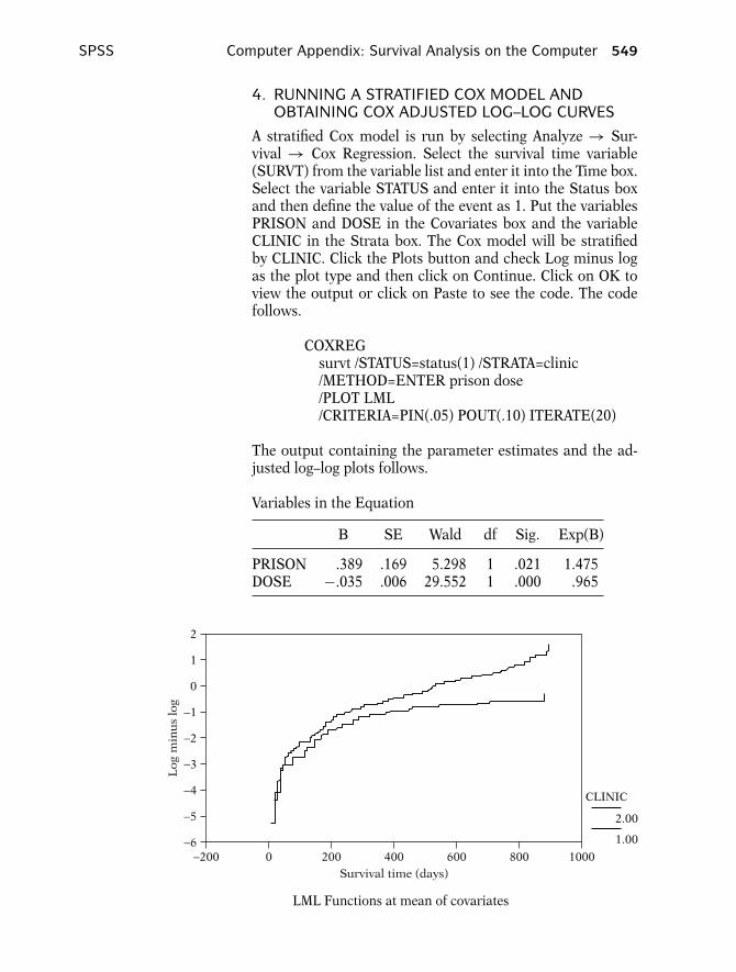
SPSS Computer Appendix: Survival Analysis on the Computer 549
4. RUNNING A STRATIFIED COX MODEL ANDOBTAINING COX ADJUSTED LOG–LOG CURVES
A stratified Cox model is run by selecting Analyze → Sur-vival → Cox Regression. Select the survival time variable(SURVT) from the variable list and enter it into the Time box.Select the variable STATUS and enter it into the Status boxand then define the value of the event as 1. Put the variablesPRISON and DOSE in the Covariates box and the variableCLINIC in the Strata box. The Cox model will be stratifiedby CLINIC. Click the Plots button and check Log minus logas the plot type and then click on Continue. Click on OK toview the output or click on Paste to see the code. The codefollows.
COXREGsurvt /STATUS=status(1) /STRATA=clinic/METHOD=ENTER prison dose/PLOT LML/CRITERIA=PIN(.05) POUT(.10) ITERATE(20)
The output containing the parameter estimates and the ad-justed log–log plots follows.
Variables in the Equation
B SE Wald df Sig. Exp(B)
PRISON .389 .169 5.298 1 .021 1.475DOSE −.035 .006 29.552 1 .000 .965
2
0
1
−1
−2
−6−200 0 200 400 600 800 1000
−5
−4
−3
Log
min
us
log
Survival time (days)
CLINIC
2.00
1.00
LML Functions at mean of covariates

550 Computer Appendix: Survival Analysis on the Computer SPSS
Notice that there are parameter estimates for PRISON andDOSE but not CLINIC because CLINIC is the stratified vari-able. The Cox adjusted log–log plots are fitted using the meanvalues of PRISON and DOSE and are used to evaluate the PHassumption for CLINIC.
Suppose rather than using the mean value of DOSE for the ad-justed log–log plots, you wish to obtain adjusted plots in whichDOSE = 70. Run the same code as before, up to clicking onthe Plots button and checking Log minus log as the plot type.Now click on DOSE(Mean) in the window called CovariateValues Plotted at. Type in the value 70 in the box underneathcalled Change Value and click on the button called Change.Now the variable in the window should be called DOSE(70)rather than DOSE(Mean). Click on Continue and then OK toview the output.
5. ASSESSING THE PH ASSUMPTION WITHA STATISTICAL TEST
SPSS does not easily accommodate a statistical test on theproportional hazards assumption using the Schoenfeld resid-uals. However, it can be programmed using several steps. Thesteps are as follows.
1. Run a Cox PH model to obtain the Schoenfeld residuals forall the covariates. These residuals are saved as new vari-ables in the working dataset.
2. Delete observations that were censored.3. Create a variable that contains the ranked order of survival
time. For example, the subject who had the fourth eventgets a value of 4 for this variable.
4. Run correlations on the survival rankings with the Schoen-feld residuals.
5. The p-value for testing whether the correlation is zero be-tween the ranked survival time and the covariate’s Schoen-feld residuals is the p-value for the statistical test that thePH assumption is violated. The null hypothesis is that thePH assumption is not violated.
First, run a Cox PH model with CLINIC, PRISON, and DOSE.Click on the Save button before submitting the model. A dia-log box appears that is called Cox Regression: Save New Vari-ables. Check Partial Residuals (under Diagnostics) and clickon Continue. This creates three new variables in the workingdataset called pr1 1, pr2 1, and pr3 1, which are the partialresiduals for CLINIC, PRISON, and DOSE, respectively. ClickOK to run the model (or Paste to generate the code).

SPSS Computer Appendix: Survival Analysis on the Computer 551
Next, delete all censored observations (i.e., only keep observa-tions in which STATUS = 1). To do this, select Data → SelectCases. Then check If condition is satisfied, and then click on If.Type status=1 in the dialog box and click on Continue. CheckDeleted in the box called Unselected Cases Are. Click OK andonly observations with events will be kept in the dataset.
Create the variable that contains the ranking of survival timesby selecting Transform → Ranked Cases. Select the survivaltime variable (SURVT) in the Variables box. Click on RankTypes, check Ranks, and click on Continue and then click onTies, check Mean, and click Continue. Click OK and a newvariable (called rsurvt) will be created containing the rankedsurvival time.
Finally, obtain correlations (and their p-values) between theranked survival and the Schoenfeld residuals. Select Ana-lyze → Correlate. → Bivariate. Move the ranked survival timevariable as well as the three partial residual variables into thevariable box. Check Pearson (for Pearson correlations) andTwo-tailed for a two-tail test of significance and click OK tosee the output. The code that is generated from these stepsfollows.
COXREGsurvt /STATUS=status(1)/METHOD=ENTER clinic prison dose/SAVE= PRESID/CRITERIA=PIN(.05) POUT(.10) ITERATE(20)
FILTER OFF.USE ALL.SELECT IF(status=1).EXECUTE
RANKVARIABLES=survt (A) /RANK /PRINT=YES/TIES=MEAN
CORRELATIONS/VARIABLES=rsurvt pr1-1 pr2-1 pr3-1/PRINT=TWOTAIL NOSIG/MISSING=PAIRWISE
552 Computer Appendix: Survival Analysis on the Computer SPSS
The output containing the correlations follows.
Correlations
Partial Partial PartialRANK of Residual Residual ResidualSURVT for CLINIC for PRISON for DOSE
RANK of Pearson Correlation 1 −.262∗∗ −.080 .077SURVT Sig. (2-tailed) — .001 .332 .347
N 150 150 150 150Partial Pearson Correlation −.262∗∗ 1 .010 .023
residual for Sig. (2-tailed) .001 — .904 .776CLINIC N 150 150 150 150
Partial Pearson Correlation −.080 .010 1 .171∗residual for Sig. (2-tailed) .332 .904 — .037PRISON N 150 150 150 150
Partial Pearson Correlation −.077 .023 .171∗ 1residual Sig. (2-tailed) .347 .776 .037 —for DO N 150 150 150 150
∗∗ Correlation is significant at the 0.01 level (2-tailed).∗ Correlation is significant at the 0.05 level (2-tailed).
The p-values for the correlations are the p-values for the PHtest. In the output, examine the row labeled RANK of SURVTSig(2-tailed). Notice that the null hypothesis is rejected forCLINIC (p = 0.001) but not for PRISON (p = 0.332 ) or DOSE(p = 0.347).
6. RUNNING AN EXTENDED COX MODEL
An extended Cox model with exactly one time-dependent co-variate can be run using the point and click approach. Sup-pose we want to include a time-dependent covariate DOSEtimes the log of survival time. This product term could beappropriate if the hazard ratio comparing any two levels ofDOSE monotonically increases (or decreases) over time. Se-lect Analyze → Survival → Cox w/ Time-Dep Cov. This opensa dialog box called Expression for T COV . The user defines atime-dependent variable (called T COV ) in this box. A vari-able T is included in the variable list. This is the variablethat represents time-varying survival (as opposed to SURVTwhich is an individual’s fixed time of event). We wish to de-fine T COV to be the log of T times DOSE. Enter the expres-sion LN(T )∗DOSE into the dialog box and click on the Modelbutton. Now run a Cox model that includes the covariates:PRISON, CLINIC, DOSE, and T COV . The code generated isas follows.
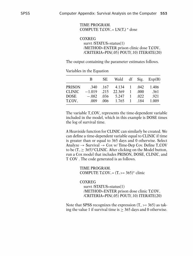
SPSS Computer Appendix: Survival Analysis on the Computer 553
TIME PROGRAM.COMPUTE T-COV-= LN(T-) ∗ dose
COXREGsurvt /STATUS=status(1)/METHOD=ENTER prison clinic dose T-COV-/CRITERIA=PIN(.05) POUT(.10) ITERATE(20)
The output containing the parameter estimates follows.
Variables in the Equation
B SE Wald df Sig. Exp(B)
PRISON .340 .167 4.134 1 .042 1.406CLINIC −1.019 .215 22.369 1 .000 .361DOSE −.082 .036 5.247 1 .022 .921T-COV- .009 .006 1.765 1 .184 1.009
The variable T COV represents the time-dependent variableincluded in the model, which in this example is DOSE timesthe log of survival time.
A Heaviside function for CLINIC can similarly be created. Wecan define a time-dependent variable equal to CLINIC if timeis greater than or equal to 365 days and 0 otherwise. SelectAnalyze → Survival → Cox w/ Time-Dep Cov. Define T COVto be (T ≥ 365)∗CLINIC. After clicking on the Model button,run a Cox model that includes PRISON, DOSE, CLINIC, andT COV . The code generated is as follows.
TIME PROGRAM.COMPUTE T-COV-= (T->= 365)∗ clinic
COXREGsurvt /STATUS=status(1)/METHOD=ENTER prison dose clinic T-COV-/CRITERIA=PIN(.05) POUT(.10) ITERATE(20)
Note that SPSS recognizes the expression (T >= 365) as tak-ing the value 1 if survival time is ≥ 365 days and 0 otherwise.

554 Computer Appendix: Survival Analysis on the Computer SPSS
The output follows.
Variables in the Equation
B SE Wald df Sig. Exp(B)
PRISON .378 .168 5.030 1 .025 1.459CLINIC −.460 .255 3.241 1 .072 .632DOSE −.036 .006 30.450 1 .000 .965T-COV- −1.369 .461 8.799 1 .003 .254
Notice the variable CLINIC is included in this model andthe time-dependent Heaviside function T COV does not con-tribute to the estimated hazard ratio until day 365. The esti-mated hazard ratio for CLINIC at 100 days is exp(−0.460) =0.632 and the estimated hazard ratio for CLINIC at 400 daysis exp((−0.460) + (−1.369)) = 0.161.
It may be of interest to define two Heaviside functions (withCLINIC) and not include CLINIC in the model. This is essen-tially the same model as the one described above with oneHeaviside function. However, the coding of two Heavisidefunctions makes it somewhat computationally more conve-nient for estimating the two hazard ratios for CLINIC (HRfor <365 days and HR for ≥365 days). Unfortunately, SPSSallows just one time-dependent variable (i.e., T COV ) usingthe point and click approach. However, by examining the codecreated for the single Heaviside function, there is only a slightadjustment needed to create code for two Heaviside functions.The following code creates two Heaviside functions (calledHV1 and HV2) and runs a model containing PRISON, DOSE,HV1, and HV2.
TIME PROGRAM.COMPUTE hv2= (T->= 365)∗ clinicCOMPUTE hv1= (T-< 365)∗ clinic
COXREGsurvt /STATUS=status(1)/METHOD=ENTER prison dose hv1 hv2/CRITERIA=PIN(.05) POUT(.10) ITERATE(20)

SPSS Computer Appendix: Survival Analysis on the Computer 555
The output follows.
Variables in the Equation
B SE Wald df Sig. Exp(B)
PRISON .378 .168 5.030 1 .025 1.459DOSE −.036 .006 30.450 1 .000 .965HV1 −.460 .255 3.241 1 .072 .632HV2 −1.828 .386 22.439 1 .000 .161
The parameter estimates for HV1 and HV2 can be used di-rectly to obtain the estimated hazard ratio for CLINIC = 2vs. CLINIC = 1 before and after 365 days. The estimatedhazard ratio for CLINIC at 100 days is exp(−0.460) = 0.632and the estimated hazard ratio for CLINIC at 400 days isexp(−1.828) = 0.161. These results are consistent with theestimates obtained from the previous model with one Heavi-side function.

TestAnswers
557

558 Test Answers
Chapter 1 True-False Questions
1. T2. T3. T4. F: Step function.5. F: Ranges between 0 and 1.6. T7. T8. T9. T
10. F: Median survival time is longer for group 1 than forgroup 2.
11. F: Six weeks or greater.12. F: The risk set at 7 weeks contains 15 persons.13. F: Hazard ratio.14. T15. T16. h(t) gives the instantaneous potential per unit time for the
event to occur given that the individual has survived up totime t; h(t) is greater than or equal to 0; h(t) has no upperbound.
17. Hazard functions
� give insight about conditional failure rates;� help to identify specific model forms (e.g., exponen-tial, Weibull);� are used to specify mathematical models for survivalanalysis.
18. Three goals of survival analysis are:
� to estimate and interpret survivor and/or hazardfunctions;� to compare survivor and/or hazard functions;� to assess the relationship of explanatory variables tosurvival time.
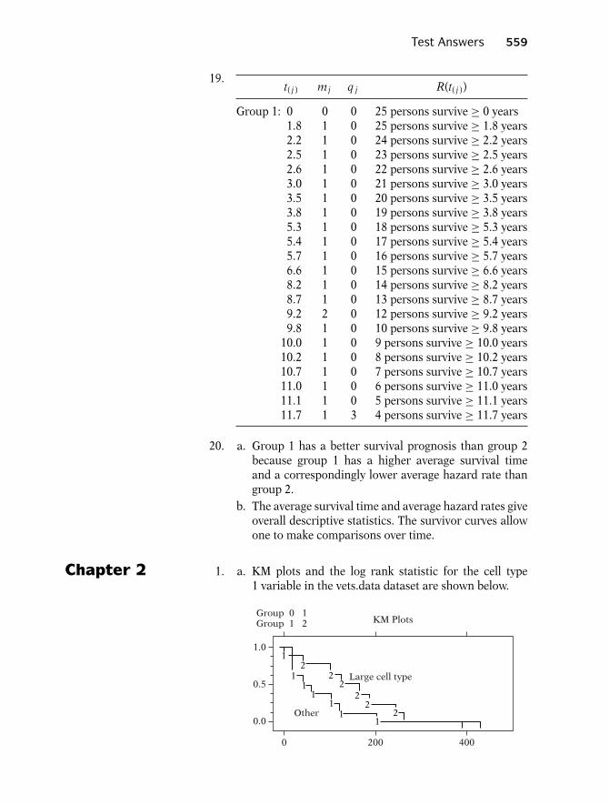
Test Answers 559
19.t( j ) mj q j R(t( j ))
Group 1: 0 0 0 25 persons survive ≥ 0 years1.8 1 0 25 persons survive ≥ 1.8 years2.2 1 0 24 persons survive ≥ 2.2 years2.5 1 0 23 persons survive ≥ 2.5 years2.6 1 0 22 persons survive ≥ 2.6 years3.0 1 0 21 persons survive ≥ 3.0 years3.5 1 0 20 persons survive ≥ 3.5 years3.8 1 0 19 persons survive ≥ 3.8 years5.3 1 0 18 persons survive ≥ 5.3 years5.4 1 0 17 persons survive ≥ 5.4 years5.7 1 0 16 persons survive ≥ 5.7 years6.6 1 0 15 persons survive ≥ 6.6 years8.2 1 0 14 persons survive ≥ 8.2 years8.7 1 0 13 persons survive ≥ 8.7 years9.2 2 0 12 persons survive ≥ 9.2 years9.8 1 0 10 persons survive ≥ 9.8 years
10.0 1 0 9 persons survive ≥ 10.0 years10.2 1 0 8 persons survive ≥ 10.2 years10.7 1 0 7 persons survive ≥ 10.7 years11.0 1 0 6 persons survive ≥ 11.0 years11.1 1 0 5 persons survive ≥ 11.1 years11.7 1 3 4 persons survive ≥ 11.7 years
20. a. Group 1 has a better survival prognosis than group 2because group 1 has a higher average survival timeand a correspondingly lower average hazard rate thangroup 2.
b. The average survival time and average hazard rates giveoverall descriptive statistics. The survivor curves allowone to make comparisons over time.
Chapter 2 1. a. KM plots and the log rank statistic for the cell type1 variable in the vets.data dataset are shown below.
0.0
0.5
1.0
0 200
Large cell type
KM Plots
400
Other
2
22
22
11
11
11
1
2
Group 0 1Group 1 2

560 Test Answers
Events EventsGroup observed expected
1 102 93.452 26 34.55
Total 128 128.00
Log rank = chi2(2) = 3.02p-value = Pr > chi2 = 0.0822
The KM curves indicate that persons with large cell typehave a consistently better prognosis than persons withother cell types, although the two curves are essentiallythe same very early on and after 250 days. The log ranktest is not significant at the .05 level, which gives some-what equivocal findings.
b. KM plots and the log rank statistic for the four cate-gories of cell type are shown below.
0
0.2
0.4
0.6
0.8
1
0 200 400 600
LargeSmallAdeno
Squamous
The KM curves suggest that persons with adeno or smallcell types have a poorer survival prognosis than personswith large or squamous cell types. Moreover, there doesnot appear to be a meaningful difference between adenoor small cell types. Also, persons with squamous celltype seem to have, on the whole, a better prognosis thanpersons with large cell type.Computer results from Stata giving log rank statisticsare now shown.
Events EventsGroup observed expected
1 26 34.552 26 15.693 45 30.104 31 47.65
Total 128 128.00
Log rank = chi2(2) = 25.40P-value = Pr > chi2 = 0.0000

Test Answers 561
The log-rank test yields highly significant p-values, in-dicating that there is some overall difference betweenall four curves; that is, the null hypothesis that the fourcurves have a common survival curve is rejected.
2. a. KM plots for the two clinics are shown below. Theseplots indicate that patients in clinic 2 have a consis-tently better prognosis for remaining under treatmentthan do patients in clinic 1. Moreover, it appears thatthe difference between the two clinics is small beforeone year of follow-up but diverges after one year offollow-up.
0
0.2
0.4
0.6
0.8
1
0 300 600 900
Clinic 1
Clinic 2
b. The log rank statistic (27.893) and Wilcoxon statistic(11.63) are both significant well below the .01 level, in-dicating that the survival curves for the two clinics aresignificantly different. The log rank statistic is never-theless much larger than the Wilcoxon statistic, whichmakes sense because the log rank statistic emphasizesthe later survival experience, where the two survivalcurves are far apart, whereas the Wilcoxon statistic em-phasizes earlier survival experience, where the two sur-vival curves are closer together.
c. If methadone dose is categorized into high (70+),medium (55–70) and low (<55), we obtain the KMcurves shown below.
0
0.2
0.4
0.6
0.8
1
0 300 500 900
High
Medium
Low

562 Test Answers
The KM curves indicate that persons with high doses havea consistently better survival prognosis (i.e., maintenance)than persons with medium or low doses. The latter twogroups are not very different from each other, although themedium dose group has a somewhat better prognosis upto the first 400 days of follow-up.The log rank test statistic is shown below for the abovecategorization scheme.
Events EventsGroup observed expected
0 45 30.931 74 54.092 31 64.99
Total 150 150.00
Log rank = chi2(2) = 33.02P-value = Pr>chi2 = 0.0000
The test statistic is highly significant, indicating that thesethree curves are not equivalent.
Chapter 3 1. a. h(t,X) = h0(t) exp[β1T 1 + β2T2 + β3PS + β4DC+ β5BF + β6(T1 × PS) + β7(T2 × PS)+ β8(T1 × DC) + β9(T2 × DC)+ β10(T1 × BF) + β11(T2 × BF)]
b. Intervention A: X∗ = (1, 0, PS, DC, BF, PS, 0, DC, 0,BF, 0)Intervention C: X = (−1, −1, PS, DC, BF, −PS, −PS,−DC, −DC, −BF, −BF)
HR = h(t,X∗)h(t,X)
= exp[2β1 + β2 + 2β6PS + β7PS
+ 2β8DC + β9DC + 2β10BF
+ β11BF]
c. H0 : β6 = β7 = β8 = β9 = β10 = β11 = 0 in the fullmodel.Likelihood ratio test statistic: −2 ln L R − (−2 ln L F ),which is approximately χ2
6 under H0, where R denotesthe reduced model (containing no product terms) un-der H0, and F denotes the full model (given in Part 1aabove)
d. The two models being compared are:Full model (F ): h(t,X) = h0(t)exp[β1T1 + β2T2+ β3PS + β4DC + β5BF]

Test Answers 563
Reduced model (R): h(t,X) = h0(t)exp[β3PS+ β4DC + β5BF]H0: β1 = β2 = 0 in the full modelLikelihood ratio test statistic: −2 ln L R − (−2 ln L F ),which is approximately χ2
2 under H0.e.
Intervention A :
S(t,X) = [S0(t)]exp[β1+(PS)β3+(DC)β4+(BF)β5]
Intervention B :
S(t,X) = [S0(t)]exp[β2+(PS)β3+(DC)β4+(BF)β5]
Intervention C :
S(t,X) = [S0(t)]exp[−β1−β2+(PS)β3+(DC)β4+(BF)β5]
2. a. h(t,X) = h0(t)exp[β1 CHR + β2 AGE + β3(CHR ×AGE)]
b. H0: β3 = 0LR statistic = 264.90 − 264.70 = 0.21; χ2 with 1 d.f.under H0; not significant.Wald statistic gives a chi-square value of .01, also notsignificant. Conclusions about interaction: the modelshould not contain an interaction term.
c. When AGE is controlled (using the gold standard model2), the hazard ratio for the effect of CHR is exp(.8051) =2.24, whereas when AGE is not controlled, the haz-ard ratio for the effect of CHR (using Model 1) isexp(.8595) = 2.36. Thus, the hazard ratios are not ap-preciably different, so AGE is not a confounder.Regarding precision, the 95% confidence interval forthe effect of CHR in the gold standard model (Model2) is given by exp[.8051 ± 1.96(.3252)] = (1.183, 4.231)whereas the corresponding 95% confidence intervalin the model without AGE (Model 1) is given byexp[.8595 ± 1.96(.3116)] = (1.282, 4.350). Both confi-dence intervals have about the same width, with thelatter interval being slightly wider. Thus, controlling forAGE has little effect on the final point and interval esti-mates of interest.
d. If the hazard functions cross for the two levels of theCHR variable, this would mean that none of the modelsprovided is appropriate, because each model assumesthat the proportional hazards assumption is met foreach predictor in the model. If hazard functions crossfor CHR, however, the proportional hazards assumptioncannot be satisfied for this variable.

564 Test Answers
e. For CHR = 1: S(t,X) = [S0(t)]exp[0.8051+0.0856(AGE)]
For CHR = 0: S(t,X) = [S0(t)]exp[0.0856(AGE)]
f. Using Model 1, which is the best model, there is evi-dence of a moderate effect of CHR on survival time,because the hazard ratio is about 2.4 with a 95% con-fidence interval between 1.3 and 4.4, and the Wald textfor significance of this variable is significant below the.01 level.
3. a. Full model (F = Model 1): h(t,X) = h0(t) exp[β1 Rx+ β2Sex + β3 log WBC + β4(Rx × Sex)+ β5(Rx × log WBC)]Reduced model (R = model 4):h(t,X) = h0(t) exp[β1 Rx + β2Sex + β3 log WBC]H0: β4 = β5 = 0LR statistic = 144.218 − 139.030 = 5.19; χ2 with 2 d.f.under H0; not significant at 0.05, though significant at0.10. The chunk test indicates some (though mild) evi-dence of interaction.
b. Using either a Wald test (p-value = .776) or a LR test,the product term Rx × log WBC is clearly not signifi-cant, and thus should be dropped from Model 1. Thus,Model 2 is preferred to Model 1.
c. Using Model 2, the hazard ratio for the effect ofRx is given by: HR = (h(t,X∗))/(h(t,X)) = exp[0.405+ 2.013 Sex]
d. Males (Sex = 0): HR = exp[0.405] = 1.499Females (Sex = 1) : HR = exp[0.405 + 2.013(1)] =11.223
e. Model 2 is preferred to Model 3 if one decides thatthe coefficients for the variables Rx and Rx × Sex aremeaningfully different for the two models. It appearsthat such corresponding coefficients (0.405 vs. 0.587and 2.013 vs. 1.906) are different. The estimated haz-ard ratios for Model 3 are 1.799 (males) and 12.098 (fe-males), which are different, but not very different fromthe estimates computed in Part 3d for Model 2. If it isdecided that there is a meaningful difference here, thenwe would conclude that log WBC is a confounder; oth-erwise log WBC is not a confounder. Note that the logWBC variable is significant in Model 2 (P = .000), butthis addresses precision and not confounding. When indoubt, as in this case, the safest thing to do (for validityreasons) is to control for log WBC.
f. Model 2 appears to be best, because there is signifi-cant interaction of Rx × Sex (P = .023) and becauselog WBC is a likely confounder (from Part e).

Test Answers 565
Chapter 4 1. The P (PH) values in the printout provide GOF statisticsfor each variable adjusted for the other variables in themodel. These P (PH) values indicate that the clinic variabledoes not satisfy the PH assumption (P << .01), whereasthe prison and dose variables satisfy the PH assumption(P > .10).
2. The log–log plots shown are parallel. However, the reasonwhy they are parallel is because the clinic variable has beenincluded in the model, and log–log curves for any variablein a PH model must always be parallel. If, instead, the clinicvariable had been stratified (i.e., not included in the model),then the log–log plots comparing the two clinics adjustedfor the prison and dose variables might not be parallel.
3. The log–log plots obtained when the clinic variable isstratified (i.e., using a stratified Cox PH model) are not par-allel. They intersect early on in follow-up and diverge fromeach other later in follow-up. These plots therefore indi-cate that the PH assumption is not satisfied for the clinicvariable.
4. Both graphs of log–log plots for the prison variable showcurves that intersect and then diverge from each other andthen intersect again. Thus, the plots on each graph appearto be quite nonparallel, indicating that the PH assumptionis not satisfied for the prison variable. Note, however, thaton each graph, the plots are quite close to each other, sothat one might conclude that, allowing for random varia-tion, the two plots are essentially coincident; with this latterpoint of view, one would conclude that the PH assumptionis satisfied for the prison variable.
5. The conclusion of nonparallel log–log plots in Question 4gives a different result about the PH assumption for theprison variable than determined from the GOF tests pro-vided in Question 1. That is, the log–log plots suggest thatthe prison variable does not satisfy the PH assumption,whereas the GOF test suggests that the prison variable sat-isfies the assumption. Note, however, if the point of viewis taken that the two plots are close enough to suggest co-incidence, the graphical conclusion would be the same asthe GOF conclusion. Although the final decision is some-what equivocal here, we prefer to conclude that the PHassumption is satisfied for the prison variable because thisis strongly indicated from the GOF test and questionablycounterindicated by the log–log curves.
566 Test Answers
6. Because maximum methadone dose is a continuous vari-able, we must categorize this variable into two or moregroups in order to graphically evaluate whether it satisfiesthe PH assumption. Assume that we have categorized thisvariable into two groups, say, low versus high. Then, ob-served survival plots can be obtained as KM curves for lowand high groups separately. To obtain expected plots, wecan fit a Cox model containing the dose variable and thensubstitute suitably chosen values for dose into the formulafor the estimated survival curve. Typically, the values sub-stituted would be either the mean or median (maximum)dose in each group.After obtaining observed and expected plots for low andhigh dose groups, we would conclude that the PH assump-tion is satisfied if corresponding observed and expectedplots are not widely discrepant from each other. If a notice-able discrepancy is found for at least one pair of observedversus expected plots, we conclude that the PH assumptionis not satisfied.
7. h(t,X) = h0(t)exp[β1 clinic + β2 prison + β3 dose+ δ1 (clinic × g (t)) + δ2 (prison × g (t))+ δ3 (dose × g (t))]
where g (t) is some function of time. The null hypothe-sis is given by H0: δ1 = δ2 = δ3 = 0. The test statistic isa likelihood ratio statistic of the form LR = −2 ln L R −(−2 ln L F ) where R denotes the reduced (PH) model ob-tained when all δs are 0, and F denotes the full modelgiven above. Under H0, the LR statistic is approximatelychi-square with 3 d.f.
8. Drawbacks of the extended Cox model approach:
� Not always clear how to specify g (t); differentchoices may give different conclusions;� Different modeling strategies to choose from, for ex-ample, might consider g (t) to be a polynomial in tand do a backward elimination to eliminate non-significant higher-order terms; alternatively, mightconsider g (t) to be linear in t without evaluatinghigher-order terms.Different strategies may yield different conclusions.

Test Answers 567
9. h(t,X) = h0(t)exp[β1 clinic + β2 prison + β3 dose+ δ1(clinic × g (t))] where g (t) is some function of time.The null hypothesis is given by H0: δ1 = 0, and the teststatistic is either a Wald statistic or a likelihood ratiostatistic. The LR statistic would be of the form LR = −2ln L R − (−2 ln L F ), where R denotes the reduced (PH)model obtained when δ1 = 0, and F denotes the full modelgiven above. Either statistic is approximately chi-squarewith 1 d.f. under the null hypothesis.
10. t > 365 days: HR = exp[β1 + δ1]t ≤ 365 days: HR = exp[β1]If δ1 is not equal to zero, then the model does not sat-isfy the PH assumption for the clinic variable. Thus, a testof H0: δ1 = 0 evaluates the PH assumption; a significantresult would indicate that the PH assumption is violated.Note that if δ1 is not equal to zero, then the model assumesthat the hazard ratio is not constant over time by givinga different hazard ratio value depending on whether t isgreater than 365 days or t is less than or equal to 365 days.
Chapter 5 1. By fitting a stratified Cox (SC) model that stratifies on clinic,we can compare adjusted survival curves for each clinic,adjusted for the prison and dose variables. This will allowus to visually describe the extent of clinic differences onsurvival over time. However, a drawback to stratifying onclinic is that it will not be possible to obtain an estimate ofthe hazard ratio for the effect of clinic, because clinic willnot be included in the model.
2. The adjusted survival surves indicate that clinic 2 has a bet-ter survival prognosis than clinic 1 consistently over time.Moreover, it seems that the difference between the effectsof clinic 2 and clinic 1 increases over time.
3. hg (t,X) = h0g (t)exp[β1 prison + β2 dose], g = 1, 2This is a no-interaction model because the regression coef-ficients for prison and dose are the same for each stratum.
4. Effect of prison, adjusted for clinic and dose: HR =1.475, 95% CI: (1.059, 2.054). It appears that having aprison record gives a 1.475 increased hazard for failurethan not having a prison record. The p-value is 0.021, whichis significant at the 0.05 level.
5. Version 1: hg (t,X) = h0g (t)exp[β1g prison + β2g dose],g = 1, 2Version 2: hg (t,X) = h0g (t)exp[β1 prison + β2 dose+ β3 (clinic × prison) + β4 (clinic × dose)], g = 1, 2

568 Test Answers
6. g = 1 (clinic 1) :h1(t,X) = h01(t)exp[(0.502)prison + (−0.036)dose]g = 2 (clinic 2) :h2(t,X) = h02(t)exp[(−0.083)prison + (−0.037)dose]
7. The adjusted survival curves stratified by clinic are virtu-ally identical for the no-interaction and interaction models.Consequently, both graphs (no-interaction versus interac-tion) indicate the same conclusion that clinic 2 has con-sistently larger survival (i.e., retention) probabilities thanclinic 1 as time increases.
8. H0: β3 = β4 = 0 in the version 2 model (i.e., the no-interaction assumption is satisfied). LR = −2 ln L R −(−2 ln L F ) where R denotes the reduced (no-interaction)model and F denotes the full (interaction) model. Underthe null hypothesis, LR is approximately a chi-square with2 degrees of freedom.Computed LR = 1195.428 − 1193.558 = 1.87; p-value =0.395; thus, the null hypothesis is not rejected and we con-clude that the no-interaction model is preferable to the in-teraction model.
Chapter 6 1. For the chemo data, the −log–log KM curves intersect ataround 600 days; thus the curves are not parallel, and thissuggests that the treatment variable does not satisfy the PHassumption.
2. The P (PH) value for the Tx variable is 0, indicating that thePH assumption is not satisfied for the treatment variablebased on this goodness-of-fit test.
3. h(t,X) = h0(t)exp[β1(T x)g1(t) + β2(T x)g2(t)
+ β3(T x)g3(t)]
where
g1(t) ={
1 if 0 ≤ t < 250 days0 if otherwise
g2(t) ={
1 if 250 ≤ t < 500 days0 if otherwise
g3(t) ={
1 if t ≥ 500 days0 if otherwise
4. Based on the printout the hazard ratio estimates andcorresponding p-values and 95% confidence intervals aregiven as follows for each time interval:

Test Answers 569
[95% Conf.Haz. Ratio p > |z| Interval]
0 ≤ t < 250 days: 0.221 0.001 0.089 0.545250 ≤ t < 500 days: 1.629 0.278 0.675 3.934t ≥ 500 days: 1.441 0.411 0.604 3.440
The results show a significant effect of treatment below250 days and a nonsignificant effect of treatment in eachof the two intervals after 250 days. Because the codingfor treatment was 1 = chemotherapy plus radiation versus2 = chemotherapy alone, the results indicate that the haz-ard for chemotherapy plus radiation is 1/0.221 = 4.52times the hazard for chemotherapy alone. The hazard ratioinverts to a value less than 1 (in favor of chemotherapy plusradiation after 250 days), but this result is nonsignificant.Note that for the significant effect of 1/0.221 = 4.52 be-low 250 days, the 95% confidence interval ranges between1/0.545 = 1.83 and 1/0.089 = 11.24 when inverted, whichis a very wide interval.
5. Model with two Heaviside functions:
h(t,X) = h0(t)exp[β1(Tx)g1(t) + β2(Tx)g2(t)]
where
g1(t) ={
1 if 0 ≤ t < 250 days0 if otherwise
g2(t) ={
1 if t ≥ 250 days0 if otherwise
Model with one Heaviside function:
h(t,X) = h0(t)exp[β1(Tx) + β2(Tx)g1(t)]
where g1(t) is defined above.6. The results for two time intervals give hazard ratios that
are on the opposite side of the null value (i.e., 1). Below 250days, the use of chemotherapy plus radiation is, as in theprevious analysis, 4.52 times the hazard when chemother-apy is used alone. This result is significant and the sameconfidence interval is obtained as before. Above 250 days,the use of chemotherapy alone has 1.532 times the hazardof chemotherapy plus radiation, but this result is nonsignif-icant.

570 Test Answers
Chapter 7 1. F: They are multiplicative models, although additive on thelog scale.
2. T3. T4. F: If the AFT assumption holds in a log-logistic model, the
proportional odds assumption holds.5. F: An acceleration factor greater than one suggests the ex-
posure is beneficial to survival.6. T7. T8. T9. F: ln(T) follows an extreme value minimum distribution.
10. F: The subject is right-censored.11.
γ = exp[α0 + α1(2) + α2PRISON + α3DOSE + α4PRISDOSE]exp[α0 + α1(1) + α2PRISON + α3DOSE + α4PRISDOSE]
= exp(α1)
γ = exp(0.698) = 2.01
95% CI = exp[0.698 ± 1.96(0.158)] = (1.47, 2.74)
The point estimate for the acceleration factor (2.01) sug-gests that the survival time (time off heroin) is double forthose enrolled in CLINIC = 2 compared to CLINIC = 1. The95% confidence interval does not include the null value of1.0 indicating a statistically significant preventive effect forCLINIC = 2 compared to CLINIC = 1.
12.HR = exp[β0 + β1(2) + β2PRISON + β3DOSE + β4PRISDOSE]
exp[β0 + β1(1) + β2PRISON + β3DOSE + β4PRISDOSE]
= exp(β1)
HR = exp(−0.957) = 0.38
95% CI = exp[−0.957 ± 1.96(0.213)] = (0.25, 0.58)
The point estimate of 0.38 suggests the hazard of goingback on heroin is reduced by a factor of 0.38 for thoseenrolled in CLINIC = 2 compared to CLINIC = 1. Or fromthe other perspective: the estimated hazard is elevated forthose in CLINIC = 1 by a factor of exp(+0.957) = 2.60.
13. β1 = −α1 p for CLINIC, so β1 = −(0.698)(1.370467) =−0.957, which matches the output for the PH form of themodel.
Test Answers 571
14. The product term PRISDOSE is included in the model asa potential confounder of the effect of CLINIC on survival.It is not an effect modifier because under this model thehazard ratio or acceleration factor for CLINIC does notdepend on the value of PRISDOSE. The PRISDOSE termwould cancel in the estimation of the hazard ratio or ac-celeration factor (see Questions 11 and 12). On the otherhand, a product term involving CLINIC would be a poten-tial effect modifier.
15. Using the AFT form of the model:
1
λ1/p= exp[α0 + α1CLINIC + α2PRISON + α3DOSE
+ α4PRISDOSE]Median survival time for CLINIC = 2, PRISON = 1, DOSE= 50, PRISDOSE = 100:
t = [− ln S(t)]1/p × 1
λ1/p= [− ln(0.5)]1/p
× exp[β0 + 2β1 + β2 + 50β3 + 100β4]
t (median) = 403.66 days (obtained by substituting param-eter estimates from output).
16. Using the same approach as the previous question:Median survival time for CLINIC = 1, PRISON = 1,DOSE = 50, PRISDOSE = 100:
t = [−ln(0.5)]1/p × exp[β0 + 1β1 + β2 + 50β3 + 100β4]
t (median) = 200.85 days.17. The ratio of the median survival times is 403.66/200.85 =
2.01. This is the estimated acceleration factor for CLINIC =2 vs. CLINIC = 1 calculated in Question 11. Note that if weused any survival probability (i.e., any quantile of survivaltime), not just S(t) = 0.5 (the median), we would have ob-tained the same ratio.
18. The addition of the frailty component did not change anyof the other parameter estimates nor did it change the loglikelihood of −260.74854.
19. If the variance of the frailty is zero (theta = 0), then thefrailty has no effect on the model. A variance of zero meansthe frailty (α) is constant at 1. Frailty is defined as a mul-tiplicative random effect on the hazard h(t|α) = αh(t). Ifα = 1 then h(t|α) = h(t), and there is no frailty.
572 Test Answers
Chapter 8 1. Cox PH Model for CP approach to Defibrillator Study:
h(t,X) = h0(t)exp[β tx + γ smoking]
where tx = 1 if treatment A, 0 if treatment B,smoking status = 1 if ever smoked, 0 if never smoked
2. Using the CP approach, there is no significant effect of treat-ment status adjusted for smoking. The estimated hazardratio for the effect of treatment is 1.09, the correspondingP-value is 0.42, and a 95% CI for the hazard ratio is (0.88,1.33).
3. No-interaction SC model for marginal approach:
hg(t,X) = h0g(t)exp[β tx + γ smoking], g = 1, 2, 3
Interaction SC model for marginal approach:
hg(t,X) = h0g(t)exp[βg tx + γg smoking], g = 1, 2, 3
4. LR = −2 ln LR − (−2 ln LF) is approximately χ2 with 4 dfunderH0: no-interaction SC model is appropriate, whereR denotes the reduced (no interaction SC) model andF denotes the full (interaction SC) model.
5. The use of a no-interaction model does not allow you toobtain stratum-specific HR estimates, even though you areassuming that strata are important.
6. The CP approach makes sense for these data because re-current defibrillator (shock) events on the same subject arethe same kind of event no matter when it occurred.
7. You might use the marginal approach if you determinedthat different recurrent events on the same subject weredifferent because they were of different order.
8. The number in the risk set (nj) remains unchanged throughday 68 because every subject who failed by this time wasstill at risk for a later event.
9. Subjects 3, 6, 10, 26, and 31 all fail for the third time at day98 and are not followed afterwards.
10. Subjects 9, 15, and 28 fail for the second time at 79 days,whereas subject #16 is censored at 79 days.
11. Subjects 4, 14, 15, 24, and 29 were censored between days111 and 112.
12. Subject #5 gets his first event at 45 days and his secondevent at 68 days, after which he drops out of the study. Thissubject is the first of the 36 subjects to drop out of the study,so the number in the risk set changes from 36 to 35 after68 days.

Test Answers 573
13. i. None of the above.ii. The product limit formula is not applicable to the CP
data; in particular, P(T > t | T ≥ t) does not equal “# fail-ing in time interval /# in the risk set at start of interval.”
14. Use the information provided in Table T.2 to complete thedata layouts for plotting the following survival curves.a. S1(t) = Pr(T1 > t) where T1 = time to first event from
study entry
t(j) nj mj qj S(t(j)) = S(t(j−1)) × Pr(T1 > t | T1 ≥ t)
0 36 0 0 1.0033 36 2 0 0.9434 34 3 0 0.8636 31 3 0 0.7837 28 2 0 0.7238 26 4 0 0.6139 22 5 0 0.4740 17 1 0 0.4441 16 1 0 0.4243 15 1 0 0.3944 14 1 0 0.3645 13 2 0 0.3146 11 2 0 0.2548 9 1 0 0.2249 8 1 0 0.1951 7 2 0 0.19 × 5/7 = 0.1457 5 2 0 0.14 × 3/5 = 0.0858 3 2 0 0.08 × 1/3 = 0.0361 1 1 0 0.03 × 0/1 = 0.00
b. Conditional S2c(t) = Pr(T2c > t) where T2c = time tosecond event from first event.
t(j) nj mj qj S(t(j)) = S(t(j−1)) × Pr(T1 > t | T1 ≥ t)
0 36 0 0 1.005 36 1 0 0.979 35 1 0 0.94
18 34 2 0 0.8920 32 1 0 0.8621 31 2 1 0.8123 28 1 0 0.7824 27 1 0 0.75
(Continued )

574 Test Answers
(Continued)
t(j) nj mj qj S(t(j)) = S(t(j−1)) × Pr(T1 > t | T1 ≥ t)
25 26 1 0 0.7226 25 2 0 0.6627 23 2 0 0.6028 21 1 0 0.5829 20 1 0 0.5530 19 1 0 0.5231 18 3 0 0.4332 15 1 0 0.4033 14 5 0 0.2635 9 1 0 0.2339 8 2 0 0.1740 6 2 0 0.17 × 4/6 = 0.1241 4 1 0 0.12 × 3/4 = 0.0942 3 1 0 0.09 × 2/3 = 0.0646 2 1 0 0.06 × 1/2 = 0.0347 1 1 0 0.03 × 0/1 = 0.00
c. Marginal S2m(t) = Pr(T2m > t) where T2m = time tosecond event from study entry.
t(j) nj mj qj S(t(j)) = S(t(j−1)) × Pr(T1 > t | T1 ≥ t)
0 36 0 0 1.0063 36 2 0 0.9464 34 3 0 0.8665 31 2 0 0.8166 29 3 0 0.7267 26 4 0 0.6168 22 2 0 0.5669 20 1 0 0.5370 19 1 0 0.5071 18 1 0 0.4772 17 2 0 0.4273 15 1 0 0.3974 14 1 0 0.3676 13 1 0 0.3377 12 1 0 0.3178 11 2 0 0.2579 9 3 1 0.25 × 6/9 = 0.1780 5 2 0 0.17 × 3/5 = 0.1081 3 2 0 0.10 × 1/3 = 0.0397 1 1 0 0.03 × 0/1 = 0.00

Test Answers 575
15. The survival curves corresponding to the above data lay-outs will differ because they are describing different sur-vival functions. In particular, the composition of the riskset differs in all three data layouts and the ordered survivaltimes being plotted are different as well.
Chapter 9 1. Cause-specific no-interaction model for local recurrence ofbladder cancer (event = 1):
h1(t,X) = h01(t)exp[β11tx + β21num + β31size]
2. Censored subjects have bladder metastasis (event = 2) orother metastasis (event = 3).
3. Cause-specific no-interaction model for bladder metastasis(event = 1):
h2(t,X) = h02(t)exp[β12tx + β22num + β32size]
where censored subjects have local recurrence of bladdercancer (event = 1) or other metastasis (event = 3).
4. A sensitivity analysis would consider worst-case violationsof the independence assumption. For example, subjectscensored from failing from events = 2 or 3 might be treatedin the analysis as either all being event-free (i.e., changeevent status to 0 and time to 53) or all experiencing theevent of interest (i.e., change event status to 1 and leavetime as is).
5. a. Verify the CIC1 calculation provided at failure timetj = 8 for persons in the treatment group (tx = 1):
h1(8) = 1/23 = 0.0435
S(4) = S(3)Pr(T > 4|T ≥ 4) = 0.9630(1 − 2/26)
= 0.9630(0.9231) = 0.8889
I1(8) = h1(8)S(4) = 0.0435(.8889) = 0.0387
CIC1(8) = CIC1(4) + 0.0387 = 0 + 0.0387 = 0.0387
b. Verify the CIC1 calculation provided at failure timetj = 25 for persons in the placebo group (tx = 0):
h1(25) = 1/6 = 0.1667
S(23) = S(21)Pr(T > 23|T ≥ 23) = 0.4150(1−1/8)
= 0.4150(0.875) = 0.3631
I1(25) = h1(25)S(23) = 0.1667(.3631) = 0.0605
CIC1(25) = CIC1(23) + 0.0605 = 0.2949 + 0.0605
= 0.3554
c. Interpret the CIC1 values obtained for both the treat-ment and placebo groups at tj = 30.For tx = 1, CIC1(tj = 30) = 0.3087 and for tx = 0,CIC1(tj = 30) = 0.3554.

576 Test Answers
Thus, for treated subjects (tx = 1), the cumulative risk(i.e., marginal probability) for local bladder cancer re-currence is about 30.1% at 30 months when allowing forthe presence of competing risks for bladder metastasisor other metastasis.For placebo subjects (tx = 1), the cumulative risk (i.e.,marginal probability) for local bladder cancer recur-rence is about 35.5% at 30 months when allowing forthe presence of competing risks for bladder metastasisor other metastasis.The placebo group therefore has a 5% increased risk offailure than the treatment group by 30 months of follow-up.
d. Calculating the CPC1 values for both treatment andplacebo groups at ti = 30:The formula relating CPC to CIC is given byCPCc = CICc/(1 − CICc′ ) where CICc = CIC for cause-specific risk event = 1 and CICc′ = CIC from risks forevents = 2 or 3 combinedFor tx = 1, CIC1(ti = 30) = 0.3087 and for tx = 0,
CIC1(tj = 30) = 0.3554.The calculation of CICc′ involves recoding the event vari-able to 1 for subjects with bladder metastasis or othermetastasis and 0 otherwise and then computing CICc′ .Calculation of CICc′ involves the following calculations.
tx = 1 (Treatment A)
tj nj d1j h 1(tj) S(tj−1) I1(tj) CIC1′ (tj)
0 27 0 0 — — —2 27 1 .0370 1 .0370 .03703 26 2 .0769 .9630 .0741 .11114 24 0 0 .8889 0 .11118 23 1 .0435 .8889 .0387 .14989 21 1 .0476 .8116 .0386 .1884
10 20 1 .0500 .7729 .0386 .227015 17 1 .0588 .7343 .0432 .270216 15 1 .0667 .6479 .0432 .313418 14 0 0 .6047 0 .313422 12 0 0 .6047 0 .313423 11 0 0 .5543 0 .313424 8 0 0 .5039 0 .313426 7 0 0 .4409 0 .313428 4 1 .2500 .3779 .0945 .407929 2 0 0 .2835 0 .407930 1 0 0 .2835 0 .4079

Test Answers 577
tx = 0 (Placebo)
tj nj d1j h 1(tj) S(tj−1) I1(tj) CIC1(tj)
0 26 0 0 — — —1 26 0 0 1 0 02 24 0 0 .9615 0 03 23 0 0 .9215 0 05 21 1 .0476 .8413 .0400 .04006 20 2 .1000 .8013 .0801 .12017 18 1 .0556 .7212 .0401 .1602
10 16 1 .0625 .6811 .0426 .202812 15 1 .0667 .6385 .0426 .245414 13 0 0 .6835 0 .245416 12 1 .0833 .5534 .0461 .291517 10 0 0 .4612 0 .291518 9 0 0 .4150 0 .291521 8 1 .1250 .4150 .0519 .343423 7 0 0 .3632 0 .343425 6 1 .1667 .3632 .0605 .403929 4 0 0 .2421 0 .403930 2 0 0 .2421 0 .4039
From these tables, we find that for tx = 1, CIC1′ (ti = 30) =0.4079 and for tx = 0, CIC1′ (tj = 30) = 0.4039.Thus, for tx = 1, CPC1(tj = 30) = CIC1/(1 − CIC1′ ) =0.3087/(1 − 0.4079) = 0.5213 and for tx = 0, CPC1(tj =30) = CIC1/(1 − CIC1′ ) = 0.3554/(1 − 0.4039) = 0.5962.
6. a. What is the effect of treatment on survival from hav-ing a local recurrence of bladder cancer and is it signi-ficant?
HR1(tx = 1 vs. tx = 0) = 0.535(= 1/1.87),
p-value = 0.250, N.S.
b. What is the effect of treatment on survival from de-veloping metastatic bladder cancer and is it signifi-cant?
HR2(tx = 1 vs. tx = 0) = 0.987,
p-value = .985, N.S.
c. What is the effect of treatment on survival from othermetastatic cancer and is it significant?
HR3(tx = 1 vs. tx = 0) = 0.684 (= 1/1.46),
p-value = .575, N.S.

578 Test Answers
7. a. State the hazard model formula for the LM model usedfor the above output.
hg∗(t,X)
g=1,2,3= h0g
∗(t)exp[β1tx + β2num + β3size
+ δ1(txd2) + δ2(numd2)
+ δ3(sized2) + δ4(txd3)
+ δ5(numd3) + δ6(sized3)]
where d2 = 1 if bladder metastasis and 0 otherwise,and
d3 = 1 if or other metastasis and 0 otherwise
b. Determine the hazard ratios for the effect of each of the3 cause-specific events based on the above output.
HR1(tx = 1 vs. tx = 0) = exp(−0.6258)
= 0.535(= 1/1.87)
HR2(tx = 1 vs. tx = 0) = exp(−0.6258 + .6132)
= 0.987
HR3(tx = 1 vs. tx = 0) = exp(−0.6258 + .2463)
= 0.684(= 1/1.46)c. Verify that the hazard ratios computed in Part b are
identical to the hazard ratios computed in Question 6.The HRs are identical.
8. a. State the hazard model formula for the LMalt modelused for the above output.
hg′(t,X)
g=1,2,3= h0g
′(t)exp[δ′11txd1 + δ′
12numd1 + δ′13sized1
+ δ′21txd2 + δ′
22numd2
+ δ′23sized2 + δ′
31txd3
+ δ′32numd3 + δ′
33sized3]
where d1 = 1 if local bladder cancer recurrence and 0otherwise
d2 = 1 if bladder metastasis and 0 otherwise,and
d3 = 1 if or other metastasis and 0 otherwise

Test Answers 579
b. Determine the hazard ratios for the effect of each ofthe three cause-specific events based on the aboveoutput.
HR1(tx = 1 vs. tx = 0) = exp(−0.6258)
= 0.535 (= 1/1.87)
HR2(tx = 1 vs. tx = 0) = exp(−0.0127) = 0.987
HR3(tx = 1 vs. tx = 0) = exp(−0.3796)
= 0.684(= 1/1.46)
c. Verify that the hazard ratios computed in Part b areidentical to the hazard ratios computed in Questions 6and 7.Corresponding hazard ratios are identical.
9. State the formula for a no-interaction SC LM model forthese data.
h∗g(t,X)
g=1,2,3
= h∗0g(t)exp[β1tx + β2num + β8size]
Assumes HR1(X) = HR2(X) = HR3(X) for any X variablee.g., Rx = 0 vs. Rx = 1:HR1(tx) = HR2(tx) = HR3(tx) = exp[β1]
10. Describe how you would test whether a no-interaction SCLM model would be more appropriate than an interactionSC LM model.Carry out the following likelihood ratio test:
H0: δgj = 0, g = 2, 3; j = 1, 2, 3
where δgj is coefficient of DgXj in the interaction SC LMmodel
Likelihood Ratio test: LR = −2 log LR − (−2 log LF)approx χ2
6 under H0
R = no-interaction SC (reduced) modelF = interaction SC (full) model

References
Andersen, P.K., Borgan, O., Gill, R.D., and Keiding, N. 1993. Sta-tistical Models Based on Counting Processes. New York: Springer-Verlag.
AREDS Research Group. 2003. Potential public health impactof age-related eye disease study results. Arch. Opthamol. 121:1621–1624.
Byar, D. 1980. The Veterans Administration study of chemopro-phylaxis for recurrent stage I bladder tumors: Comparisons ofplacebo, pyridoxine, and topical thiotepa. In Bladder Tumors andOther Topics in Urological Oncology. New York: Plenum, 363–370.
Byar, D. and Green, S. 1980. The choice of treatment for cancerpatients based on covariate information. Bulletin du Cancer 67:4, 477–490.
Byar, D. and Corle, D. 1977. Selecting optimal treatment in clin-ical trials using covariate information. J. Chronic. Dis. 30: 445–459.
581
582 References
Caplehorn, J. et al. 1991. Methadone dosage and retention ofpatients in maintenance treatment. Med. J. Aust. 154: 195–199.
Clayton, D. 1994. Some approaches to the analysis of recurrentevent data. Stat. Meth. Med. Res. 3: 244–262.
Cox, D.R. and Oakes, D. 1984. Analysis of Survival Data. London:Chapman & Hall.
Crowley, J. and Hu, M. 1977. Covariance analysis of heart trans-plant data. J. Amer. Stat. Assoc. 72: 27–36.
Dixon, W.J. 1990. BMDP, Statistical Software Manual, Berkeley,CA: University of California Press.
Fine, J. and Gray, R. 1999. A proportional hazards model forthe subpopulation of a competing risk, J. Amer. Stat. Assoc. 94:496–509.
Freireich, E.O. et al. 1963. The effect of 6-mercaptopmine on theduration of steroid induced remission in acute leukemia. Blood,21: 699–716.
Gebski, V. 1997. Analysis of Censored and Correlated Data (AC-CORD). Eastwood, NSW, Australia: Data Analysis and ResearchTechnologies.
Grambsch, P.M. and Therneau, T.M. 1994. Proportional hazardstests and diagnostics based on weighted residuals. Biometrika81: 515–526.
Gray, R.J. 1988. A class of k-sample tests for comparingthe cumulative incidence of a competing risk. Ann. Stat. 16:1141–1154.
Gutierrez, R.G. 2002. Parametric frailty and shared frailty sur-vival models. Stata J. 2: 22–44.
Harrel, F. and Lee, K. 1986. Proceedings of the Eleventh AnnualSAS User’s Group International. 823–828.
Harris, E. and Albert, A. 1991. Survivorship Analysis for ClinicalStudies. New York: Marcel Dekker.
Hosmer, D.W. and Lemeshow, S. 1989. Applied Survival Analysis.New York: Wiley.
References 583
Kalbfleisch, J.D. and Prentice, R.L. 1980. The Statistical Analysisof Failure Time Data, New York: Wiley.
Kay, R. 1986. Treatment effects in competing-risk analysis ofprostate cancer data. Biometrics 42: 203–211.
Kleinbaum, D.G. and Klein, M. 2002. Logistic Regression—ASelf Learning Text, Second Edition. New York: Springer-Verlag,Chapter 11.
Kleinbaum, D.G., Kupper, L.L., and Morgenstern, H. 1982. Epi-demiologic Research: Principles and Quantitative Methods. NewYork: Van Nostrand Reinhold.
Kleinbaum, D.G., Kupper, L.L., and Muller, K.A. 1987. AppliedRegression Analysis and Other Multivariable Methods, SecondEdition. Belmont, CA: Wadsworth.
Krall, J.M., Uthoff, V.A., and Harley, J.B. 1975. A step-up pro-cedure for selecting variables associated with survival data.Biometrics. 31: 49–57.
Lee, E.T. 1980. Statistical Methods for Survival Data Analysis.Belmont, CA: Wadsworth.
Lin, D.Y. and Wei, L.J. 1989. The robust inference for the Coxproportional hazards model. J. Amer. Stat. Assoc. 84: 1074–1078.
Lunn, M. 1998. Applying k-sample tests to conditional probabil-ities for competing risks in a clinical trial. Biometrics 54: 1662–1672.
Lunn, M. and McNeil, D. 1995. Applying Cox regression to com-peting risks. Biometrics 51: 524–532.
Makuch, R.W. and Parks, W.P. 1988. Statistical methods for theanalysis of HIV-1 core polypeptide antigen data in clinical stud-ies. AIDS Res. Hum. Retroviruses 4: 305–316.
Pepe, M.S. and Mori, M. 1993. Kaplan–Meier, marginal or condi-tional probability curves in summarizing competing risks failuretime data? Stat. Med. 12: 737–751.
Prentice, R.L. and Marek. 1979. A qualitative discrepancy be-tween censored data rank tests. Biometrics 34.

584 References
Prentice, R.L., Williams, B.J. and Peterson, A.V. 1981. On theregression analysis of multivariate failure time data. Biometrika68 (2): 373–79.
Schoenbach, V.J., Kaplan, B.H., Fredman, L., and Kleinbaum,D.G. 1986. Social ties and mortality in Evans County, Georgia.Amer. J. Epid., 123:4, 577–591.
Schoenfeld, D. 1982. Partial residuals for the proportional haz-ards model. Biometrika, 69: 51–55.
Stablein, D., Carter, W., and Novak, J. 1981. Analysis of sur-vival data with non-proportional hazard functions. Control. Clin.Trials 2: 149–159.
Tai, B.C., Machin, D., White, I., and Gebski, V. 2001. Competingrisks analysis of patients with osteosarcoma: a comparison offour different approaches. Stat. Med. 20(5): 661–684.
Wei, L.J., Lin, D.Y., and Weissfeld, L. 1989. Regression analysis ofmultivariate incomplete failure time data by modeling marginaldistributions. J. Amer. Stat. Assoc. 84: 408.
Zeger, S.L. and Liang, C.Y. 1986. Longitudinal data analysis fordiscrete and continuous outcomes. Biometrics 42: 121–130.
Index
Accelerated failure time(AFT), see AFTentries
Acceleration factor, 266–267exponential, 269–271with frailty, 303, 309log-logistic, 281Weibull, 276
Addicts dataset, 464data analysis, 230–234,
248with SAS programming,
508–538with SPSS programming,
542–555with STATA
programming,467–502
Additive failure time model,285
Adjusted survival curves,104
log-log plots, 159observed versus expected
plots, 150stratified Cox procedure,
180using Cox PH model,
103–107, 116, 118AFT (accelerated failure
time) assumption,266–268
AFT models, 265–266,282–284, 309,313–317
Age–Related Eye DiseaseStudy (AREDS),359–364
AIC (Akaike’s informationcriterion), 286
585

586 Index
Average hazard rate, 24in Cox PH model, 94–95, 134in extended Cox model, 219in stratified Cox model, 181
Baseline hazard function, 94, 134Biased results, 405Binary regression, 290Bladder cancer dataset, 464–465Bladder cancer patients
comparison of results for, 355–357counting process for first 26
subjects, 339hypothetical subjects, 336–337interaction model results for, 354no-interaction model results for, 354
Byar data, 399–400cause-specific competing risk analysis,
401–403Lunn-McNeil models, 422, 427
Cause-specific hazard function, 400Censored data, 5–8
interval-censored, 286, 289left-censored, 7, 286right-censored, 7, 286
Censoring, 5non-informative (independent),
403–407informative (dependent), 405–406
CIC (cumulative incidence curves), 393,412–420
Competing risks, 4, 392, 396examples of data, 396–398CIC, 412CPC (Conditional Probability Curves),
420independence assumption, 403Lunn-McNeil models, 421, 427separate models for different event
types, 400–403Complementary log-log binary model, 293Complementary log-log link function, 292Computer
augmented (Lunn-McNeil approach)data layout for, 422
counting process data layout for,337–338
general data layout for, 15–19marginal approach data layout for,
348–349Conditional failure rate, 11Conditional probability curves (CPC),
420–421Conditional survival function, 295Confounding effect, 26–27Counting process (CP) approach, 334–336
example, 336–337general data layout, 338–344results for example, 346–347
Cox adjusted survival curvesusing SAS, 525–529using SPSS, 549–550using Stata, 485–488
Cox likelihood, 111–115extended for time dependent variables,
239–242Cox PH cause-specific model, 400Cox proportional hazards (PH) model
adjusted survival curves using,103–107
computer example using, 86–94extension of, see Extended Cox modelformula for, 94–96maximum likelihood estimation of,
98–100popularity of, 96–98review of, 214–216using SAS, 514–518using SPSS, 548using Stata, 476–481
CP, see Counting process approachCPC (conditional probability curves),
420–421Cumulative incidence, viiiCumulative incidence curves (CIC), 393,
412–420
Data layout for computer, 15–19Datasets, 464–465Decreasing Weibull model, 13Discrete survival analysis, 293

Index 587
Empirical estimation, 344Estimated -ln(-ln) survivor curves, 136Estimated survivor curves, 25Evans County Study,
Cox proportional hazards (PH) modelapplication to, 124–126
Kaplan-Meier survival curves for,73–75
multivariable example using, 29–31ordered failure times for, 41–42survival data from, 119–122
Event, 4Event types, different, separate models for,
400–403Expected versus observed plots, 145–150Exponential regression, 12
accelerated failure-time form, 319log relative-hazard form, 319
Extended Cox likelihood, 239–242Extended Cox model, 110, 219
application to Stanford hearttransplant data, 235–239
application to treatment of heroinaddiction, 230–234
hazard ratio formula for, 221–223using SAS, 530–533using SPSS, 552–555using Stata, 488–492time-dependent variables,
219–221
Failure, 4Failure rate, conditional, 11Flemington-Harrington test, 65Frailty component, 295Frailty effect, 300Frailty models, 294–308
using Stata, 499–502
Gamma distribution, 296Gamma frailty, 301Gastric carcinoma data, 253–254General stratified Cox (SC) model,
180–181Generalized gamma model, 284GOF, see Goodness-of-fit entries
Gompertz model, 285Goodness-of-fit (GOF) testing approach,
151–153Goodness-of-fit (GOF) tests, 136
Hazard function, 8, 9–10cause–specific, 400probability density function and,
262–263Hazard ratio, 32
formula fpr Cox PH model, 100–103formula for extended Coxmodel, 221–223
Heaviside function, 227
Increasing Weibull model, 13Independence assumption, 403–411Information matrix, 346Informative censoring, in competing
risks survival analysis, 405Instantaneous potential, 49Interactions, 27Interval-censored data, 286, 289–294Inverse-Gaussian distribution, 296
Kaplan-Meier (KM) curves, 46example of, 51–55general features of, 56–57log-log survival curves, 141
Left-censored data, 7–8, 286Leukemia remission-time data, 17, 26
Cox proportional hazards (PH) modelapplication to, 86–94
increasing Weibull for, 13Kaplan-Meier survival curves for,
51–55, 75–77log-log KM curves for, 141–145
recurrent event data for, 335exponential survival, 263–265stratified Cox (SC) model application
to, 176–188Likelihood function, 111–115
for Cox PH model,for extended Cox model, 239–242for parametric models, 286–289

588 Index
Likelihood ratio (LR) statistic, 89LM, see Lunn-McNeil approachLog-log plots, 137–145Log–log survival curves, 137–145Log-logistic regression, 277–282
accelerated failure-time form, 320Log-rank test, 46
alternatives to, 63–68for several groups, 61–63for two groups, 57–61
Logit link function, 292Lognormal survival models, 13, 284Lunn-McNeil (LM) approach, 393,
421–427alternative, 427–434
Macular degeneration data set, 359–364results for, 361–362Marginal probability, 414
Maximum likelihood (ML) estimation ofCox PH model, 98–100
Multiplicative model, 285
No-interaction assumption in stratifiedCox model, 182–188
Noninformative censoring, 403–407
Observed versus expected plots, 145–150
Parametric approach using shared frailty,357–359
Parametric survival models,defined, 260examples
exponential model, 263–265, 268–277log-logistic model, 277–282Weibull model, 272–277
likelihood function, 286–289other models, 284–286SAS use, 533–538Stata use, 492–499
Pepe-Mori test, 421, 437Peto test, 63PH assumption
assessment using time-dependentcovariates, 153–157, 224–229
evaluating (Chapter 4), 132–171meaning of, 107–111assessment using goodness of fit test
with Schonfield residuals, 151–153assessment using Kaplan-Meier log-log
survival curves, 546–547assessment using observed versus
expected plots, 145–150assessment using SAS, 522–525assessment using SPSS, 550–552assessment using Stata, 473–476,
483–485PH model, Cox, see Cox proportional
hazards (PH) modelPO (proportional odds) assumption, 292Precision, 92Probability, 11Probability density function, 262–263PROC LIFEREG (SAS), 533–538PROC LIFETEST (SAS), 510–514PROC PHREG, 514–518Product limit formula, 46Proportional hazards, see PH entriesProportional odds (PO) assumption, 292
Recurrent event survival analysis(Chapter 8), 332–390
Counting process approach, 336–344definition of recurrent events, 4, 332examples of recurrent event data,
334–336other approaches for analysis 347–353parametric approach using shared
frailty, 357–359SAS modeling, 538–542Stata modeling, 502–508survival curves with, 364–367
Right-censored data, 7, 286Risk set, 22Robust estimation, 344–346Robust standard error, 347Robust variance, 345
SAS, 508–542assessing PH assumption, with
statistical tests, 522–525

Index 589
demonstrating PROC LIFETEST,510–514
modeling recurrent events, 538–542obtaining Cox adjusted survival
curves, 525–529running Cox proportional hazards (PH)
model, with PROC PHREG,514–518
running extended Cox model, 530–533running parametric models, with PROC
LIFEREG, 533–538running stratified Cox (SC) model,
519–521SC, see Stratified Cox modelSchonfield residuals, 151–152, 522–523Score residuals, 346Semi-parametric model, 96, 261Sensitivity analysis (with competing
risks), 408–411Shape parameter, 272Shared frailty, 306–308, 358
recurrent events analysis using,357–359
Shared frailty model, 306SPSS, 542–555
assessing PH assumptionwith statistical tests, 550–552using Kaplan-Meier log-log survival
curves, 546–547estimating survival functions, 544–546running Cox proportional hazards (PH)
model, 548running extended Cox model, 552–555running stratified Cox (SC) model,
549–550Stanford Heart Transplant Study
extended Cox model application to,235–239
transplants versus nontransplants,244–245
Stata, 60, 465–508assessing PH assumption
using graphical approaches, 473–476using statistical tests, 483–485
estimating survival functions, 469–473modeling recurrent events, 502–508
obtaining Cox adjusted survival curveswith, 485–488
running Cox proportional hazards (PH)model, 476–481
running extended Cox model,488–492
running frailty models, 499–502running parametric models, 492–499running stratified Cox (SC) model,
481–483Step functions, 9Strata variable, 347Stratification variables, several, 188–193Stratified Cox (SC) model, 176–180,
364–367for analyzing recurrent event data,
347–353conditional approaches, 347–351general, 180–181graphical view of, 193–194marginal approach, 347–351using SAS, 519–521using SPSS, 549–550using Stata, 481–483 Subdistribution
function, 419Survival curves
adjusted, 104using Cox PH model, 103–107
Cox adjusted, see Cox adjustedsurvival curves
with recurrent events, 364–367Survival functions
conditional, 295probability density function and,
262–263SAS estimation, 525–529SPSS estimation, 544–546Stata estimation , 469–473unconditional, 295
Survival time, 4Survival time variable, 14Survivor function, 8–9
Tarone-Ware test statistic, 64Time-dependent covariates, assessing PH
assumption using, 153–157

590 Index
Time-dependent variables, 134definition and examples of, 216–219extended Cox model for, 219–221
Time-independent variables, PHassumption and, 224–229
Unconditional survival function, 295Unshared frailty, 306
Veterans Administration Lung CancerData
Kaplan–Meier survival curves for, 62–63model with no frailty, 296
proportional hazards assumptionevaluation for, 161–164
with several stratification variables,188–193
stratified Cox (SC) model applicationto, 201–204
Wald statistic, 89Weibull model, 272–277Weibull regression
accelerated failure-time form, 322, 325log relative-hazard form, 323, 325
Wilcoxon test, 64