computer architecture support for database applications

Computer Architecture Support for Database Applications

byKimberly Kristine Keeton

B.S. (Carnegie Mellon University) 1991M.S. (University of California at Berkeley) 1994

A dissertation submitted in partial satisfaction of the requirements for the degree ofDoctor of Philosophy

inComputer Science

in theGRADUATE DIVISION

of theUNIVERSITY of CALIFORNIA at BERKELEY

Committee in charge:

Professor David A. Patterson, Chair

Professor Joseph M. Hellerstein

Professor Kenneth Y. Goldberg

Dr. James N. Gray

Fall 1999

The dissertation of Kimberly Kristine Keeton is approved:

University of California at Berkeley

Fall 1999

DateChair

Date

Date

Date


Copyright 1999by

Kimberly Kristine KeetonAll rights reserved

1

Abstract


by

Kimberly Kristine Keeton

Doctor of Philosophy in Computer Science

University of California at Berkeley

Professor David A. Patterson, Chair

Database workloads are an important class of applications, responsible for one-third of the symmetric multi-

processor (SMP) server market. Despite their importance, they are seldom used in computer architecture per-

formance evaluations, which favor technical applications, such as SPEC. Database applications are often

avoided because they are difficult to study in fully-scaled configurations, for reasons including large hard-

ware requirements and complicated software configuration and tuning issues.

This dissertation addresses several of the challenges posed by database workloads. First, we characterize the

architectural behavior of two standard database workloads, namely online transaction processing (OLTP) and

decision support (DSS), running on a commercial database on a commodity Intel-based SMP server with fully

scaled data sets. We show that the architectural characteristics of these two workloads differ in important

ways, including cycles per instruction (CPI) decomposition, cache miss rates, and branch behavior. OLTP has

a much higher CPI than DSS; the majority of this CPI is comprised by stall cycles attributable mainly to in-

struction and data cache misses. Stalls comprise the minority of most DSS query CPIs; the decomposition of

these stalls depends on the query. Branch prediction, superscalarness, and out-of-order execution all prove to

be somewhat less effective for OLTP than for DSS.

Second, we demonstrate that a simpler microbenchmark suite can approximate the more complex OLTP and

DSS workloads. This microbenchmark approach is based on posing queries to the database that generate the

same dominant I/O patterns as the full workloads. A random test, based on an index scan, approximates OLTP

behavior, and a sequential test, based on a sequential table scan, approximates DSS behavior.

2

Finally, to address the extraordinary growth in the storage capacity and computational requirements of DSS

workloads, we introduce a storage system design that uses "intelligent" disks (IDISKs). An IDISK is a hard

disk containing an embedded general-purpose processor, tens to hundreds of megabytes of memory, and gi-

gabit-per-second network links. We analyze the potential performance benefits of an IDISK architecture us-

ing analytic models of simple DSS operations, such as sequential scan and join, which are based on our

measurements of DSS behavior. We find that IDISK outperforms alternate cluster- and SMP-based servers

by up to an order of magnitude.

_________________________________________________

iii

Table of Contents

CHAPTER 1. Introduction ..................................................................................... 1

1.1. Database Workloads ................................................................................... 21.2. Challenges for Computer System Designers .............................................. 21.2.1. Difficulties of Studying Database Workload Performance...................... 31.2.2. Multi-user Commercial vs. Technical ...................................................... 71.2.3. Increasing DSS Data Requirements ......................................................... 81.3. This Thesis.................................................................................................. 91.3.1. Contributions............................................................................................ 91.3.2. Methodology: Experimental Platform.................................................... 111.3.3. Thesis Outline ........................................................................................ 12

CHAPTER 2. Experimental Methodology .......................................................... 14

2.1. Introduction .............................................................................................. 142.2. Measurement vs. Simulation .................................................................... 142.3. Experimental System Hardware Configurations ...................................... 162.3.1. Processor and Memory Configurations.................................................. 172.3.2. I/O Subsystem Configurations ............................................................... 182.4. Software Architecture............................................................................... 222.4.1. Transaction Processing (OLTP) Software.............................................. 222.4.2. Decision Support (DSS) Software.......................................................... 232.4.3. Microbenchmark Software..................................................................... 242.4.4. Discussion .............................................................................................. 242.5. Pentium Pro Processor Architecture......................................................... 242.5.1. Overview ................................................................................................ 242.5.2. Potential Sources of Pentium Pro Stalls ................................................. 262.6. Measurement Methodology...................................................................... 272.6.1. OLTP Measurement ............................................................................... 302.6.2. DSS Measurement.................................................................................. 302.6.3. Microbenchmark Measurement.............................................................. 312.6.4. Formulae for Architectural Characteristics ............................................ 312.6.5. Measurement Overheads ........................................................................ 322.7. Summary................................................................................................... 33

CHAPTER 3. Analysis of Online Transaction Processing Workloads............. 35

3.1. Introduction .............................................................................................. 353.2. OLTP Workload Description.................................................................... 363.3. Experimental Results: CPI....................................................................... 383.4. Experimental Results: Memory System Behavior.................................... 413.4.1. How do OLTP cache miss rates vary with L2 cache size? .................... 413.4.2. What effects do larger caches have on OLTP throughput and stall cycles?

43

iv

3.4.3. How successful are non-blocking L2 caches at reducing OLTP memory stalls?...................................................................................................... 43

3.5. Experimental Results: Processor Issues ................................................... 443.5.1. How useful is superscalar issue and retire for OLTP? ........................... 443.5.2. How effective is branch prediction for OLTP?...................................... 463.5.3. Is out-of-order execution successful at hiding stalls for OLTP?............ 473.6. Experimental Results: Multiprocessor Scaling Issues.............................. 503.6.1. How well does OLTP performance scale as the number of processors in-

creases?................................................................................................... 503.6.2. How do OLTP CPI components change as the number of processors is

scaled? .................................................................................................... 503.6.3. How prevalent are cache misses to dirty data in other processors’ caches for

OLTP? .................................................................................................... 513.6.4. Is the four-state (MESI) invalidation-based cache coherence protocol

worthwhile for OLTP? ........................................................................... 533.6.5. How does OLTP memory system performance scale with increasing cache

sizes and increasing processor count?.................................................... 553.7. Experimental Results: I/O Characterization ............................................. 563.8. Related Work............................................................................................ 573.8.1. Uniprocessor Studies.............................................................................. 583.8.1.1. Maynard, et al.: IBM RS/6000............................................................. 583.8.1.2. Cvetanovic and Bhandarkar: Alpha Workstation Characterization..... 603.8.1.3. Rosenblum, et al.: MIPS-based SGI Workstations.............................. 613.8.1.4. Perl and Sites: Alpha PCs .................................................................... 623.8.2. Symmetric Multiprocessor Studies ........................................................ 633.8.2.1. Thakkar and Sweiger: Sequent Symmetry........................................... 633.8.2.2. Cvetanovic and Donaldson: AlphaServer 4100 Characterization ....... 653.8.2.3. Barroso, et al.: Alpha Servers .............................................................. 653.8.3. CC-NUMA Multiprocessor Studies ....................................................... 663.8.3.1. Lovett and Clapp: Sequent STiNG ...................................................... 663.8.3.2. Ranganathan, et al.: Effects of ILP and Out-of-Order Execution........ 673.8.4. Multithreading Studies ........................................................................... 683.8.4.1. Eickemeyer, et al.: Coarse-grained Multithreading ............................. 683.8.4.2. Lo, et al.: Simultaneous Multithreading (SMT) .................................. 683.8.5. This Thesis in Context of Related Work................................................ 693.9. Proposal for an OLTP-centric Processor Design...................................... 693.10. Conclusions .............................................................................................. 71

CHAPTER 4. Analysis of Decision Support Workloads.................................... 74

4.1. Introduction .............................................................................................. 744.2. DSS Workload Description ...................................................................... 754.2.1. TPC-D Background................................................................................ 754.2.2. Our DSS Workload ................................................................................ 774.3. Experimental Results: CPI....................................................................... 794.4. Experimental Results: Memory System Behavior................................... 82

v

4.4.1. How do DSS cache miss rates vary with L2 cache size? ....................... 824.4.2. What impact do larger L2 caches have on DSS database performance and

stall cycles? ............................................................................................ 844.4.3. How prevalent are cache misses to dirty data in other processors’ caches in

DSS?....................................................................................................... 854.4.4. Is the four-state (MESI) invalidation-based cache coherence protocol

worthwhile for DSS?.............................................................................. 864.4.5. How does DSS memory system performance scale with increasing cache

sizes? ...................................................................................................... 884.5. Experimental Results: Processor Issues .................................................. 904.5.1. How useful is superscalar issue and retire for DSS?.............................. 904.5.2. How effective is branch prediction for DSS?......................................... 944.5.3. Is out-of-order execution successful at hiding stalls for DSS? .............. 954.6. Experimental Results: I/O Characterization ............................................. 984.7. Related Work............................................................................................ 994.7.1. Trancoso, et al.: Postgres95 on CC-NUMA Multiprocessor ............... 1004.7.2. Barroso, et al.: Alpha Servers............................................................... 1024.7.3. Ranganathan, et al.: Effects of ILP and Out-of-Order Execution ........ 1034.7.4. Discussion: Conventional Wisdom and This Thesis............................ 1034.8. Proposal for a DSS-centric Processor and System Design..................... 1054.9. Conclusions ............................................................................................ 106

CHAPTER 5. Towards a Simplified Workload................................................ 109

5.1. Introduction ............................................................................................ 1095.2. Approach: Microbenchmarks to Approximate TPC Workloads ............ 1095.2.1. Microbenchmark Design ...................................................................... 1105.2.2. Experimental Methodology.................................................................. 1135.3. Random I/O Approximations for OLTP................................................. 1135.3.1. Random Microbenchmark CPI Analysis.............................................. 1145.3.2. Random Microbenchmark Cache Behavior ......................................... 1155.3.3. Random Microbenchmark ILP and Branch Behavior.......................... 1165.3.4. Computation per Row for the Random Microbenchmark.................... 1185.3.5. Discussion ............................................................................................ 1185.4. Sequential I/O Approximations for DSS................................................ 1185.4.1. Sequential Microbenchmark CPI Analysis .......................................... 1195.4.2. Sequential Microbenchmark Cache Behavior...................................... 1205.4.3. Sequential Microbenchmark ILP Behavior.......................................... 1215.4.4. Computation per Row for the Sequential Microbenchmark ................ 1225.4.5. Discussion ............................................................................................ 1235.5. Comparison Between Commercial Databases........................................ 1235.5.1. Comparison of CPI Breakdowns.......................................................... 1235.5.2. Comparison of Cache Behavior ........................................................... 1265.5.3. Comparison of ILP and Branch Behavior ............................................ 1275.5.4. Comparison of Computation per Row and Predictive Performance .... 1285.5.5. Common Trends and Discussion.......................................................... 129

vi

5.6. Related Work .......................................................................................... 1305.6.1. Ailamaki, et al.: In-Memory Microbenchmarks to Compare Commercial

Databases.............................................................................................. 1305.6.2. Unlu: Database “Mini-Benchmarks” ................................................... 1325.7. Conclusions ............................................................................................ 132

CHAPTER 6. The Case for Intelligent Disks (IDISKs) ................................... 134

6.1. Introduction ............................................................................................ 1346.2. Strengths and Weakness of DSS Clusters .............................................. 1366.3. Technological Trends ............................................................................. 1406.4. The Intelligent Disk Architecture ........................................................... 1436.4.1. Hardware Architecture ......................................................................... 1436.4.2. Software Architecture .......................................................................... 1466.5. Performance and Scalability Evaluation................................................. 1486.5.1. Methodology ........................................................................................ 1496.5.2. Selection ............................................................................................... 1516.5.3. Hash Join .............................................................................................. 1536.5.4. Index Nested Loops Join ...................................................................... 1576.5.5. Discussion ............................................................................................ 1616.6. Historical Perspective and Related Work............................................... 1626.7. Conclusions ............................................................................................ 164

CHAPTER 7. Conclusions .................................................................................. 166

7.1. Summary of Results................................................................................ 1667.2. Future Work............................................................................................ 1707.2.1. OLTP and DSS Workload Characterization ........................................ 1707.2.2. Microbenchmark Future Work............................................................. 1717.2.3. IDISK Challenges and Research Areas................................................ 173

Bibliography ............................................................................................................. 175

CHAPTER 8. Appendix A: Pentium Pro Counter Formulae ......................... 183

8.1. Glossary of Pentium Pro Hardware Counter Events .............................. 1838.2. Pentium Pro Counter Formulae .............................................................. 187

CHAPTER 9. Appendix B: Comparison of Database and Operating System

Behavior for OLTP Workload................................................... 195

9.1. Cache Behavior....................................................................................... 1959.2. Impact of L2 Cache Size on CPI and OLTP Throughput....................... 1959.3. Effectiveness of Superscalar Issue and Retire ........................................ 1989.4. Effectiveness of MESI Cache Coherence Protocol ................................ 1989.5. NT Performance Monitor Characterization............................................ 201

vii

CHAPTER 10. Appendix C: Elaboration of DSS Results ................................. 202

10.1. Effectiveness of Out-of-Order Execution............................................... 20210.2. DSS I/O Characterization ....................................................................... 20710.3. Appendix: NT Performance Monitor Characterization .......................... 212

CHAPTER 11. Appendix D: Supporting Evidence for Intelligent Disks ......... 213

11.1. 1999 DSS System Configurations .......................................................... 21311.2. Appendix: Factors Affecting Analytic Models....................................... 21411.3. Appendix: Bottleneck Analysis for System Performance ...................... 215

viii

List of Figures

CHAPTER 1. ................................................................................................................. 1

Figure 1-1. Dataquest server market breakdown [94]. ......................................... 1Figure 1-2. TPC-C price performance over time [103]. ..................................... 11Figure 1-3. TPC-D (100 GB) price performance over time [104]...................... 12Figure 1-4. TPC-D (300 GB) price performance over time [104]...................... 13

CHAPTER 2. ............................................................................................................... 14

Figure 2-1. CPI as a function of query execution time for DSS query Q5......... 16Figure 2-2. OLTP I/O subsystem configuration. ................................................ 19Figure 2-3. DSS I/O subsystem configuration.................................................... 20Figure 2-4. Microbenchmark I/O subsystem configuration. .............................. 21Figure 2-5. Block diagram of Pentium Pro processor architecture. ................... 25

CHAPTER 3. ............................................................................................................... 35

Figure 3-1. Conceptual rendering of typical TPC-C configurations [58]........... 38Figure 3-2. Breakdown of cycles per micro-operation (µCPI) for base system. 40Figure 3-3. L2 cache miss behavior for the four-processor system as a function

of L2 cache size. .............................................................................. 42Figure 3-4. Overall CPI breakdown for the four-processor system as a function

of L2 cache size. .............................................................................. 43Figure 3-5. Decomposition of instruction and micro-operation decode and

retirement cycles for the four-processor, 1 MB L2 cache system. .. 45Figure 3-6. Instruction and micro-operation decode and retirement profiles,

broken down by instructions, for the base system. .......................... 46Figure 3-7. Non-overlapped and measured CPI as a function of L2 cache size. 49Figure 3-8. OLTP throughput scalability. .......................................................... 51Figure 3-9. OLTP file read and write rates......................................................... 57

CHAPTER 4. ............................................................................................................... 74

Figure 4-1. Q5 CPI as a function of query execution time................................. 79Figure 4-2. Breakdown of cycles per micro-operation (µCPI) for system with 1

MB L2 cache.................................................................................... 81Figure 4-3. CPI breakdown by L2 cache size..................................................... 84Figure 4-4. Macro-instruction decode profile decomposed by (a) cycles and (b)

instructions....................................................................................... 91Figure 4-5. Macro-instruction retirement profile decomposed by (a) cycles and

(b) instructions. ................................................................................ 92Figure 4-6. Micro-operation retirement profiles decomposed by (a) cycles and

(b) instructions. ................................................................................ 93

ix

Figure 4-7. Non-overlapped and measured CPI for DSS Q6 as a function of L2 cache size. ........................................................................................ 97

Figure 4-8. Q6 file read and write rates.............................................................. 99Figure 4-9. Q5 file read and write rates............................................................ 100Figure 4-10. Q5 file read and write sizes............................................................ 101

CHAPTER 5. ............................................................................................................. 109

Figure 5-1. Microbenchmark database schema. ............................................... 111Figure 5-2. Breakdown of cycles per micro-operation (µCPI) for the random

microbenchmark. ........................................................................... 115Figure 5-3. Random microbenchmark µop retirement profile, decomposed by

cycles. ............................................................................................ 117Figure 5-4. Random microbenchmark µop retirement profile, broken down by

µops................................................................................................ 117Figure 5-5. Breakdown of cycles per micro-operation (µCPI) for the sequential

microbenchmark. ........................................................................... 120Figure 5-6. Sequential microbenchmark µop retirement profile, decomposed by

cycles. ............................................................................................ 122Figure 5-7. Sequential microbenchmark µop retirement profile, broken down by

µops................................................................................................ 122Figure 5-8. Breakdown of cycles per micro-operation (µCPI) for the random and

sequential microbenchmarks for both database systems. .............. 125Figure 5-9. Comparison of microbenchmark µop retirement profiles,

decomposed by cycles. .................................................................. 127Figure 5-10. Comparison of microbenchmark µop retirement profiles, broken

down by µops................................................................................. 128

CHAPTER 6. ............................................................................................................. 134

Figure 6-1. Typical high-end decision support server computer architecture: NCR WorldMark 5200. ................................................................. 139

Figure 6-2. IDISK architecture. ........................................................................ 143Figure 6-3. Evolutionary IDISK architecture. .................................................. 146Figure 6-4. Query plan for selection query based on TPC-D Q1. .................... 151Figure 6-5. System performance for selection query. ...................................... 152Figure 6-6. Query plan for hash join query, which is loosely based on TPC-D

Q12................................................................................................. 154Figure 6-7. Hash join query times as a function of IDISK memory. ............... 156Figure 6-8. System performance for hash join query. ...................................... 157Figure 6-9. Memory requirements for one-pass hash join query. .................... 158Figure 6-10. Query plan for index nested loops join query, which is also loosely

based on TPC-D Q12. .................................................................... 159Figure 6-11. System performance for index nested loops join query................. 160

x

Figure 6-12. System performance for index nested loops join as a function of index size. ...................................................................................... 161

CHAPTER 7. ............................................................................................................. 166

CHAPTER 8. ............................................................................................................. 183

CHAPTER 9. ............................................................................................................. 195

CHAPTER 10. ........................................................................................................... 202

Figure 10-1. Non-overlapped and measured CPI for DSS Q1 as a function of L2 cache size. ...................................................................................... 203


Figure 10-3. Non-overlapped and measured CPI for DSS Q5.1 as a function of L2 cache size. ...................................................................................... 204





Figure 10-8. Non-overlapped and measured CPI for OLTP as a function of L2 cache size. ...................................................................................... 206

Figure 10-9. Q1 file read and write rates............................................................ 207Figure 10-10. Q4 file read and write rates............................................................ 208Figure 10-11. Q8 file read and write rates............................................................ 209Figure 10-12. Q11 file read and write rates.......................................................... 210Figure 10-13. Q11 file read sizes.......................................................................... 211

CHAPTER 11. ........................................................................................................... 213

xi

List of Tables

CHAPTER 1. ................................................................................................................. 1

Table 1-1. Summary of full-scale configurations for TPC price-performance leaders [103] [104]............................................................................. 4

Table 1-2. Comparison of multi-user commercial and technical workloads [64].. 7

CHAPTER 2. ............................................................................................................... 14

Table 2-1. Summary of system configurations. ................................................ 17Table 2-2. Additional architectural parameters varied in OLTP evaluation. .... 18Table 2-3. Parameters for Quantum Atlas II disk, which is used in the OLTP

and DSS I/O subsystems [82]. ......................................................... 19Table 2-4. Parameters for Seagate Barracuda disk, which is used in the

microbenchmark I/O subsystem [89]............................................... 21Table 2-5. Pentium Pro L1 and L2 cache characteristics. ................................. 26Table 2-6. Pentium Pro hardware counter characteristics for the four-processor

system in idle state. .......................................................................... 32Table 2-7. NT performance monitor characteristics for the idle four-processor

system. ............................................................................................. 33

CHAPTER 3. ............................................................................................................... 35

Table 3-1. Transaction types used in TPC-C workload. ................................... 36Table 3-2. Breakdown of cycles per micro-operation (µCPI) and cycles per

macro-instruction (CPI) components for four-processor, 1MB L2 cache system. ................................................................................... 39

Table 3-3. Effects of non-blocking for 256 KB L2 cache for the uniprocessor system. ............................................................................................. 44

Table 3-4. Branch behavior for the four-processor, 1 MB L2 cache system. ... 47Table 3-5. CPI Components as the number of processors is scaled.................. 52Table 3-6. Percentage of L2 cache misses to dirty data in another processor’s

cache as a function of L2 cache size and number of processors...... 53Table 3-7. State of L2 line on L2 hit. ................................................................ 54Table 3-8. Overall memory system utilization as a function of L2 cache size

and number of processors. ............................................................... 55Table 3-9. Application memory latency as a function of L2 cache size and

number of processors. (All values are in processor cycles.)............ 56Table 3-10. Summary of uniprocessor related work. .......................................... 59Table 3-11. Summary of (non-threaded) multiprocessor related work. .............. 64Table 3-12. Summary of contributions of this thesis. ......................................... 70

CHAPTER 4. ............................................................................................................... 74

xii

Table 4-1. Summary of query plans for DSS queries. ...................................... 78Table 4-2. Breakdown of time, measured cycles per micro-operation (µCPI)

and measured cycles per macro-instruction (CPI) for the four-processor system with the 1 MB L2 cache. ..................................... 80

Table 4-3. L2 cache local miss behavior as a function of L2 cache size. ......... 82Table 4-4. L1 cache and ITLB miss behavior for the four-processor system with

the 1 MB L2 cache........................................................................... 83Table 4-5. Impact of L2 cache size on CPI and database performance. ........... 85Table 4-6. Percentage of L2 cache misses to dirty data in another processor’s

cache as a function of L2 cache size................................................ 86Table 4-7. State of L2 line on L2 hit for the four-processor system with the 1

MB L2 cache.................................................................................... 87Table 4-8. Overall memory system utilization as a function of L2 cache size for

the four-processor SMP. .................................................................. 88Table 4-9. Application memory read latency as a function of L2 cache size for

the four-processor SMP. All values are in processor cycles............ 89Table 4-10. Branch behavior. .............................................................................. 95Table 4-11. Summary of most relevant multiprocessor related work. .............. 104

CHAPTER 5. ............................................................................................................. 109

Table 5-1. Breakdown of time, measured cycles per micro-operation (µCPI) and measured cycles per macro-instruction (CPI) for the random microbenchmark. ........................................................................... 114

Table 5-2. Random microbenchmark overall cache behavior......................... 116Table 5-3. Random microbenchmark branch behavior. .................................. 118Table 5-4. Random microbenchmark instruction and clock cycle count behavior.

118Table 5-5. Breakdown of time, measured cycles per micro-operation (µCPI)

and measured cycles per macro-instruction (CPI) for the sequential microbenchmark. ........................................................................... 119

Table 5-6. Sequential microbenchmark overall cache behavior. .................... 121Table 5-7. Sequential microbenchmark instruction and clock cycle count

behavior. ........................................................................................ 123Table 5-8. Breakdown of time, measured cycles per micro-operation (µCPI)

and measured cycles per macro-instruction (CPI) for both microbenchmarks for both database systems................................. 124

Table 5-9. Comparison of microbenchmark overall cache behavior. ............. 126Table 5-10. Comparison of microbenchmark branch behavior......................... 128Table 5-11. Comparison of microbenchmark instruction and cycle count

behavior. ........................................................................................ 129

CHAPTER 6. ............................................................................................................. 134

xiii

Table 6-1. 1999 Comparison of embedded and desktop processors. [21] [22] [23]................................................................................................. 139

Table 6-2. TPC-D 3 TB NCR WorldMark 5200 price breakdown (2/15/99). 140Table 6-3. Projected 2004 systems used in IDISK evaluation. ....................... 149Table 6-4. Estimated instruction counts per I/O operation for common DSS

database operations. ....................................................................... 150

CHAPTER 7. ............................................................................................................. 166

CHAPTER 8. ............................................................................................................. 183

Table 8-1. L1 cache-related events. ................................................................ 183Table 8-2. L2 cache-related events. ................................................................ 184Table 8-3. Memory bus-related events............................................................ 185Table 8-4. Events relating to instruction decoding and retirement. ................ 186Table 8-5. Branch-related events. ................................................................... 186Table 8-6. Events related to stalls and cycle counts........................................ 187Table 8-7. Formulae for simple CPI calculations. .......................................... 188Table 8-8. Formulae for non-overlapped CPI components............................. 189Table 8-9. Formulae for L1 cache characteristics. .......................................... 190Table 8-10. Formulae for L2 cache characteristics. .......................................... 190Table 8-11. Formulae for L2 MESI characteristics........................................... 191Table 8-12. Formulae for memory system characteristics. ............................... 192Table 8-13. Formulae for branch characteristics............................................... 192Table 8-14. Formulae for ILP characteristics.................................................... 193

CHAPTER 9. ............................................................................................................. 195

Table 9-1. Overall cache access and miss behavior as a function of L2 cache size. ................................................................................................ 196

Table 9-2. Database-only cache access and miss behavior as a function of L2 cache size. ...................................................................................... 196

Table 9-3. Operating system-only cache access and miss behavior as a function of L2 cache size. ............................................................................ 197

Table 9-4. Relative database throughput and CPI breakdown as function of L2 cache size. ...................................................................................... 197

Table 9-5. Instruction decode profile. ............................................................. 198Table 9-6. Macro-instruction retirement profile. ............................................ 199Table 9-7. Micro-operation retirement profile. ............................................... 199Table 9-8. State of L2 line on L2 hit for the database. (Table shows percentage

of L2 accesses.).............................................................................. 200Table 9-9. State of L2 line on L2 hit for the operating system. (Table shows

percentage of L2 accesses.) ........................................................... 200

xiv

Table 9-10. NT performance monitor characteristics for the OLTP workload. 201

CHAPTER 10. ........................................................................................................... 202

Table 10-1. NT performance monitor characteristics for the OLTP workload. 212

CHAPTER 11. ........................................................................................................... 213

Table 11-2. 1999 disk parameters used as basis for IDISK evaluation [90]. .... 213Table 11-1. 1999 TPC-D 300 GB SF performance-leading configurations used as

basis for IDISK evaluation [105] [46] [70]. .................................. 214Table 11-3. Bottleneck analysis for performance of the selection queries

presented in Figure 6-5 on page 152.............................................. 216Table 11-4. Bottleneck analysis for performance of the hash join query presented

in Figure 6-8 on page 157. ............................................................. 216Table 11-5. Bottleneck analysis for performance of the index nested loop query

presented in Figure 6-11 on page 160............................................ 217Table 11-6. Sensitivity analysis for performance of the index nested loop queries

presented in Section 6.5.4. on page 157. ....................................... 217

xv

Acknowledgments

It has been my privilege at Berkeley to work closely with two stellar systems researchers, Professor David

Patterson and Dr. Jim Gray. Dave has been an excellent advisor, and I am immensely grateful for the help he

has given me. His talents in looking at the big picture and asking high-level clarifying questions, combined

with the depth of his technical knowledge have provided me with incredible amounts of insightful feedback

on my research. He is truly a visionary of future computer architectures, and his enthusiasm about pursuing

new research directions has been infectious to those around him. Dave has been incredibly generous with his

time, attention, and resources. In addition to his advice on technical issues, he has provided counsel in many

other areas, including technical writing, giving effective presentations, running research projects, managing

time, and dealing with people. Easy-going, funny, and fun-loving, he communicates his joy in teaching and

advising students. Dave provides a strong role model of someone who can balance a successful career as a

professor and researcher with his devotion to family life. I have greatly enjoyed working with him.

In the last five years, I’ve also been very fortunate to work with Jim Gray from Microsoft’s Bay Area Re-

search Center. Jim has been an astute technical advisor and a supportive mentor. The breadth and depth of his

technical expertise have allowed him to provide critical and constructive feedback of my work, ranging from

performance analysis of communication protocols to database systems. He continually asks the hard ques-

tions, forcing me to delve deeper to explain technical mysteries and to understand what questions I’m asking.

Jim is a visionary of future software systems, ranging from databases to cluster computing; this vision and

his cutting edge knowledge of the computer systems industry make me think about research issues from a

different perspective. Jim has also provided excellent advice on dealing with the stresses of earning a PhD,

help in making contacts with researchers in the database field, and aid in interviewing for jobs. I thank him

for his support and confidence in my abilities.

I am also grateful to the other members of my dissertation committee, Professor Joe Hellerstein and Professor

Ken Goldberg. Joe possesses amazing enthusiasm for his research area of databases; I can only hope to con-

vey the same level of enthusiasm to students in the future. Since his arrival at Berkeley, we have learned a lot

xvi

from one another, finding a common language to bridge the gap between databases and computer architec-

ture. His insightful questions and feedback on my work constantly encourage me to think about issues from

an alternate perspective. His down-to-earth manner makes him easy to approach, and a wonderful sounding

board for new ideas. Ken is a master of interdisciplinary research, and my work has been greatly improved

from his encouragement to explain issues in a manner accessible to a broad audience.

I have been fortunate to work on a variety of topics as a graduate student. In my early years at Berkeley, I

benefited greatly from working with Professor Randy Katz. Randy was an excellent master’s advisor, offer-

ing me my first lessons in executing research and communicating research results. I learned a great deal from

his strong overall technical skills and expertise in storage systems, as well as his experiences at DARPA in

Washington, DC.

Much of my dissertation work has involved the analysis of real systems, and I have benefited considerably

from my interactions with industrial colleagues. John He, a performance analysis expert at Informix, has pro-

vided invaluable help in configuring the hardware and software systems measured in this thesis and assistance

in interpreting the experimental results. Roger Raphael of Informix also provided performance analysis ex-

pertise during the early phases of my experiments. Seckin Unlu from Intel has provided tremendous assis-

tance in interpreting the Pentium Pro hardware counters, and in calibrating our measurements. I also learned

a great deal about the inner workings and design of the TPC benchmarks from discussions with Walter Baker

and Jack Stephens, both now at Gradient Systems. Michael Koster from Sun Microsystems has provided very

useful feedback on my performance studies. More recently, Don Slutz of Microsoft has been incredibly help-

ful in teaching me how to configure local installations of SQLServer, Oracle, and Informix, and in providing

friendly words of encouragement. I am also grateful to Bob Ensor at Bell Laboratories for serving as my men-

tor throughout my Lucent Technologies GRPW fellowship.

Computer systems research is often a group effort, and my discussions with faculty members, staff engineers,

and my fellow graduate students have helped to shape my thoughts about research issues and the graduate

student experience. As a younger graduate student, I learned quite a bit from the RAID and Sprite group mem-

xvii

bers, including Mary Baker, Pete Chen, Ann Chervenak, John Hartman, Ed Lee, Ken Lutz, Ethan Miller, John

Ousterhout, Srini Seshan, and Ken Shirriff. My knowledge of networking and mobile computing was en-

hanced by discussions with Hari Balakrishnan, Domenico Ferrari, Armando Fox, Bruce Mah, Srini Seshan,

and Ron Widyono. My conversations with my NOW colleagues, especially Eric Anderson, Tom Anderson,

Remzi Arpaci-Dusseau, David Culler, Alan Mainwaring, Rich Martin, Drew Roselli, Nisha Talagala, and

Randy Wang, broadened my perspective to include a wider range of systems issues. I’ve learned more about

current topics in database research from Paul Aoki, Marcel Kornacker, and Adam Sah. Finally, my conver-

sations with members of the IRAM and ISTORE teams, especially staff engineer Jim Beck, Aaron Brown,

Christoforos Kozyrakis, John Kubiatowicz, David Oppenheimer, and Randi Thomas, have proven to be es-

pecially stimulating.

Berkeley EECS department staff members are some of the department’s greatest resources. Kathryn Crabtree,

the computer science graduate assistant, fiercely protects graduate students from the administrative bureau-

cracy. She personalizes the graduate student experience by getting to know us and always lends a sympathetic

ear to graduate student woes. Theresa Lessard-Smith, our grant administrator and retreat co-organizer, shields

the systems students from many financial matters. With Terry’s friendly manner, expertise in gardening, for-

eign travels and extracurricular pursuits in dance, there are always fun and interesting conversations to be

shared. Bob Miller, our retreat co-organizer and equipment coordinator, makes purchases seem seamless. I

will truly miss his sarcastic wit and not-so-subtle teasing. Melise Munroe and Vickie Bell, our administrative

and financial matters assistants, have been incredibly helpful in dealing with financial and scheduling matters.

Jon Forrest and Eric Fraser have been superb system administrators of our research machines, and are always

willing to help diagnose the problems that arise. These folks have saved the day on many occasions, and I am

very thankful for their invaluable help.

As a woman in the EECS department, I have greatly enjoyed my interactions with the members of WICSE

(Women in Computer Science and Electrical Engineering). We owe a debt of gratitude to Dr. Sheila Hum-

phreys for maintaining this supportive atmosphere for women graduate students. Throughout the years,

WICSE has provided many role models and peer mentors; in addition, a number of close friendships blos-

xviii

somed out of this “young girls’ club.” Sheila has taken a personal interest in our progression as graduate stu-

dents; I thank her for her support over the years. Ann Chervenak has regularly lent her wisdom of greater

experience, her kindness, and her support. Marti Hearst has been a role model for successfully navigating the

transition from industrial research back to academic life as a faculty member. Mor Harchol-Balter’s intensity

has fueled wonderfully thought-provoking conversations (and amazing shopping experiences). My lunches

and coffee breaks with Francesca Barrientos have provided a pick-me-up for both of us throughout our grad-

uate experience.

In addition to providing mutual support, my close friendships with Eric Anderson, Armando Fox, Bruce Mah,

Trevor Pering, and Ron Widyono have cultivated (and in some cases renewed) my interest in ballroom dance,

musical collaborations, investment, and Broadway musicals. The weekly gatherings of the “fest” crowd for

episodes of “The X-Files” and other television fare provided a much-needed break from the world of com-

puter science. I thank the fest crowd, especially John Bennett, Heather Bourne, Eric Freeman, and Havi Gla-

ser for these carefree times. My friendship with Sandy Felt has provided much happiness, supportiveness, and

many fun-filled experiences.

I’ve been fortunate to find several creative outlets during the last half of my graduate career. I’ve pursued my

theatrical interests as part of a group of amateur thespians known as the Haste Street Players. Through this

group, I was introduced to a whole generation of former Berkeley computer science graduate students, includ-

ing Chris Black, Eric Enderton, Mike Hohmeyer, Dan Jurafsky, Steve Lucco, and Mike Schiff, who have pro-

vided a fun social outlet as well as support during the tougher moments. HSP also has non-CS grads, including

Tristan Barrientos, Erin Dare, Madeleine Fitzgerald, Laurel Jamtgaard, Phil Lowery, Chris Walton, and Mike

Ward, who remind me that there is life outside Soda Hall. Several of these HSP members and their roommates

at the Hillegass house for wayward computer scientists also regularly welcomed me into their home for fun-

filled dinner parties and games of mah-jongg.

xix

I’ve pursued my singing interests through an East-Bay choir called the Pacific Mozart Ensemble. Although

the group is comprised of about forty voices, the genuine affection these people have for one another makes

the group feel like a large, happy, and supportive family.

My real family, including my parents Doris and Gary, brother Geoff, and grandmother Wanda, have been en-

thusiastic supporters of my graduate aspirations. Although they are geographically distant, I feel their encour-

agement, confidence, love, and support close by. I thank them from the bottom of my heart.

Finally, I am indebted to my partner Gene Hern for his love and support during the last four years. Although

he is busy with his own career as an emergency medicine resident, he still finds the time to take care of all

sorts of tasks when I’m too busy or stressed to finish (or even start) them myself. He has shown great com-

passion, understanding, and patience with my varying stress levels and occasionally bizarre work schedules.

I hope that I have been able to reciprocate in the face of his own work demands. His humor lightens my dark

moments, and his breadth of interests has opened many new worlds for me. I look forward to continuing the

journey we have begun together.

.

1

1 Introduction

Commercial applications are an important class of applications with a large installed base. According to

Dataquest, commercial server applications, such as database service, file service, media and email service,

print service, and custom applications, were the dominant applications run on shared-memory multiprocessor

server machines in 1995 and are projected to be the dominant server applications in 2000 [94]. As shown in

Figure 1-1, commercial applications comprised about 85% of the 1995 server market, and are projected to

continue this dominance as the server market grows 15 percent annually. Database workloads alone motivate

the sale of vast quantities of symmetric multiprocessor (SMP) machines, and hold the dominant fraction of

the massively parallel computing market [74]: databases motivated 32% of the server volume in 1995, and

will motivate 39% of the 2000 server volume.

1995 Server Market Volume

32%

32%

16%

9%

6%5%

2000 Server Market Volume

39%

25%

14%

7%

8%7%

Database

File server

Scientific &engineering

Print server

Media &email

Other

Figure 1-1. Dataquest server market breakdown [94].

2

1.1. Database Workloads

The database community widely recognizes two major types of commercial database workloads: online

transaction processing (OLTP) and decision support systems (DSS). OLTP systems, such as airline reserva-

tion systems, handle the operational aspects of day-to-day business transactions. DSS systems provide his-

torical support for forming business decisions. A monthly sales report is an example of a DSS-style

operation. Microsoft Research’s Dr. Philip Bernstein estimates that decision support systems (DSS) account

for about 35% of database servers, a percentage that is increasing over time [14].

The two database workloads have different characteristics. OLTP uses short, moderately complex queries

that read and/or modify a relatively small portion of the overall database. These access patterns translate into

small random disk accesses. These workloads typically have a high degree of multiprogramming, due to the

large number of concurrent users. In contrast, DSS queries are typically long-running, moderately to very

complex queries, that scan large portions of the database in a read-mostly fashion. This access pattern trans-

lates into large sequential disk accesses. Updates are propagated either through periodic batch runs or

through background “trickle” update streams. The multiprogramming level in DSS systems is typically

much lower than that of OLTP systems.

1.2. Challenges for Computer System Designers

These workloads present several challenges to the designers of the computer systems on which they run.

First, both OLTP and DSS workloads are difficult to study in fully-scaled configurations for several reasons,

including large hardware requirements and complicated software configuration issues; this difficulty leads

to a need for a simpler experimental methodology. Second, multi-user commercial workloads exhibit very

different characteristics than the technical workloads typically used in computer architecture performance

studies, implying that computer architects must use a wider variety of application benchmarks to evaluate

new designs. Third, the I/O capacity and computational requirements of DSS workloads are increasing faster

than the growth rates for disk capacity and processor speed, requiring a more scalable I/O system design for

these data-intensive services. This section describes these challenges in more detail.

3

1.2.1. Difficulties of Studying Database Workload Performance

The first challenge for computer system designers is that both OLTP and DSS database server systems are

hard to study, for a number of reasons. The only standardized benchmarks for OLTP and DSS workloads are

quite complex, with large hardware requirements for full-scale systems. In addition, database server systems

present a multitude of both hardware and software configuration parameters that must be reasonably well-

tuned. Researchers must also deal with several logistical issues, such as lack of access to source code and

performance publishing restrictions. We explore these difficulties in more detail in this section.

Complex standardized benchmarks. The Transaction Processing Performance Council (TPC) defines and

maintains several industry standard database benchmarks. TPC-C, described in Section 2.4.1. on page 22,

specifies an OLTP workload; TPC-D, described in Section 2.4.2. on page 23, is the DSS benchmark. The

implementation of the benchmark workload on the database requires the researcher to make many choices,

including whether data is accessed through the file system or through the raw disk device interface, the layout

of data on disk to avoid access hot spots, and the choice of index creation to improve the performance of the

workload. Running the benchmark workloads require tuning additional configuration parameters, such as

database size (e.g., TPC-C’s number of warehouses or TPC-D’s scale factor) and the number of simulated

OLTP clients.

In addition to the complexity of setting up and tuning the benchmarks, the TPC specifications also lead to

logistical complications. The benchmark’s performance metrics (for example, transactions per minute C, or

tpmC) can be reported only if the benchmark configuration has been audited by a TPC-certified auditor, to

ensure full benchmark compliance. This auditing process is quite costly. Finally, as with all benchmarks,

some performance experts question whether the benchmarks are representative of all client OLTP and DSS

application behavior.

Large hardware requirements for full scale. Studying full-scale database TPC performance requires large,

expensive hardware configurations. Table 1-1 presents the hardware configurations for the leading price-per-

formance systems for TPC-C and TPC-D. We observe that each of the four configurations requires tens or

hundreds of disk drives and gigabytes of main memory. Researchers hoping to measure the performance of

4

a real system must construct such a system, costing hundreds of thousands of dollars. If, instead, the

researcher wishes to simulate a full-scale system, he or she must simulate a large and complex I/O subsystem,

requiring considerable computational resources and time.

Numerous configuration parameters. Database servers pose both hardware and software configuration

challenges. The large hardware systems described above present numerous hardware configuration parame-

ters. For instance, the researcher must decide on the number and speed of disks, I/O controllers, the disk I/O

bus, and the processor I/O bus. In addition, he or she must configure various policies, such as the amount of

caching provided by the I/O controllers. The amount and configuration of the physical memory may impact

System Dell PowerEdge 6350

HP NetServer LXr8000

NCR World-Mark 4400

Hitachi AD450NX

Database Microsoft SQLServer 7.0 Enterprise Edition

Oracle 8i Enter-prise Edition 8.1.5.1

Teradata V2R3.0 IBM DB2 UDB 5.2.0

Operating

System

Microsoft Win-dows NT 4.0 Enter-prise Edition

Microsoft Win-dows NT 4.0 Enterprise Edition SP 3

UNIX SVR4 MP-RAS 03.02.00

Microsoft Win-dows NT 4.0 Enterprise Edition SP 4

Benchmark TPC-C TPC-D 300 GB TPC-D 100 GB TPC-D 30 GB

Price-perform. $18.28/tpmC $162 / QphD@300 $83 / QphD@100 $233 / QphD @30

Performance 23,460.57 tpmC 8124.3 QppD@300, 1324.7 QthD@300

17,115.2 QppD@100, 869.1 QthD@100

2,261.2 QppD@30, 325.9 QthD@30

Processors 4 x 500 MHz Pen-tium II Xeon w/ 2 MB L2 cache

4 x 450 MHz Pen-tium II Xeon w/ 2 MB L2 cache



Memory 4 GB 4 GB 2 GB 2 GB

Disk drives 182 x 9 GB,

8 x 18 GB

168 x 17.4 GB,

1 x 8.7 GB

63 x 9 GB 31 x 17.9 GB,

3 x 9 GB

Hardware price $259,975 $379,887 $154,099 $137,677

Report date 3/28/99 2/11/99 2/15/99 2/15/99

Table 1-1. Summary of full-scale configurations for TPC price-performance leaders [103] [104].

The Dell system has the best TPC price-performance, and the other systems lead in TPC-D price-performance at data sizes 300 GB, 100 GB, and 30 GB, respectively.

5

the memory bandwidth delivered by the system. For example, some systems provide the maximum memory

bandwidth only if the memory system is fully configured [8].

Database servers and operating systems are complicated software systems with numerous configurations

“knobs.” The documentation of commercially available database software indicates that these server prod-

ucts have 75 to 200 initialization parameters to control runtime management issues such as the buffer pool

size and management strategy, the degree of multithreading/processing, logging, disk read-ahead, and DSS-

specific memory management alternatives. The operating system also presents numerous configuration alter-

natives, such as the choice of asynchronous vs. synchronous I/O, buffer management for I/O operations,

parameters for striping files across multiple disks, time slice values and network transmission and buffering

parameters. Although default values are often provided for these configuration parameters, they do not nec-

essarily match the requirements of the intended workloads.

Lack of useful proprietary information. Researchers rarely have access to proprietary information, such

as database source code and multi-user traces. Access to this information is unlikely without a strict non-dis-

closure agreement with the database company. Even if such an agreement is drawn, it unclear whether access

to certain types of information, like database source code, would be beneficial. Database server programs are

comprised of approximately two to five millions of lines of code, which could prove unwieldy to a database

novice. Other types of proprietary performance information, such as traces, are useful to researchers. How-

ever, this information is often only available through close interaction with commercial database perfor-

mance analysts, for example, across inter- or intra-corporation organizational boundaries, or through

academic residency in an industrial environment.

Publishability issues for results. The commercial database community has instituted legal publishability

restrictions for performance-related information. Due to the community’s history of “benchmarketing,”

where each company designed its own benchmark to highlight its performance advantages over its compet-

itors, database companies want to avoid unfavorable performance results reported by competitors or third

parties. In addition, database performance on the TPC benchmarks, which is highly competitive, often forms

the cornerstone of corporate marketing campaigns. As a result, database companies want to prevent the

6

reporting of sub-optimal TPC performance for improperly configured systems. To prevent this behavior,

nearly all of the commercial databases (except IBM’s DB2 UDB) include a clause in their licensing agree-

ments to restrict the publication of performance information. The following is an example of such a clause:

“Benchmark Testing. You may not disclose the results of any benchmark test of either the Server Software

of Client Software to any third party without [XXX’s] prior written approval.” [67]

Discussion. Both academic and industrial researchers have been able to find at least partial workarounds to

address some of these difficulties. For instance, many academic researchers choose to work in concert with

a computer systems or database company to study database server performance. With this partnership, they

can leverage the large-scale hardware construction effort mounted by the company, take advantage of the

configuration tuning expertise of industrial performance gurus, and utilize the company’s measurement

infrastructure, including facilities for trace gathering.

Researchers may also choose to simulate and/or measure scaled-back hardware configurations. Some take

care to validate their scaled-back environments against well-tuned fully-scaled configurations, which

requires access to these configurations, often found only in industry. A handful of others ignore the perfor-

mance tuning issues, and try to adjust their experimental data to factor out inefficiencies like idle time. The

danger in this approach is that the behavior of the scaled-back configurations may not reflect that of the fully-

scaled configurations. This danger is discussed in more detail in Section 2.2. on page 14.

Researchers have also found workarounds for the TPC reporting rule and database performance publication

restrictions. Performance studies almost never measure fully compliant TPC benchmark performance.

Instead, they report “TPC-X-like performance”, or performance for a “workload based on TPC-X” for unau-

dited workloads that modify some of the benchmark details governing uncommon modes of operation. For

instance, researchers seldom measure the performance of TPC-C checkpoints or TPC-D update operations.

In addition, researchers have been able to circumvent the database vendor-imposed publication restrictions,

either through careful negotiation with the database vendor or by avoiding mention of the database company

(for example, system A, B, or C).

7

Although some computer architecture researchers have found methods for working around many of the dif-

ficulties, the barriers to studying database workloads still exist. Essentially, one must have close industrial

ties to study interesting configurations. Computer system designers would benefit from simpler benchmarks

with more modest hardware requirements, to decrease the start-up cost for studying database workload per-

formance. In addition, they would benefit from a prioritization of the hardware and software tuning parame-

ters required for reasonable performance.

1.2.2. Multi-user Commercial vs. Technical

As noted in the literature [64] and in this thesis, multi-user commercial server applications, such as OLTP,

have significantly different execution characteristics from technical applications. Table 1-2 describes these

differences. The large number of concurrent users in commercial applications leads to higher multiprogram-

ming levels and context switch rates. Commercial applications also exhibit high I/O rates with random access

patterns and non-looping branch behavior. Because of these characteristics, commercial applications have

been less able to effectively use the memory system of traditional workstation and server architectures.

Unfortunately, due to some of the other challenges discussed in this section, commercial applications are

often ignored in preference to technical benchmarks, such as SPEC, LINPACK or SPLASH, in computer

architecture performance studies. A survey of the two major computer architecture conferences (ISCA and

ASPLOS) over the last five years indicates that database workloads are used in less than 10% of all evalua-

Characteristic Multi-user Commercial Technical

Number of concurrent users 100s to 1000s 1

Process switching High process switch rates and multiprogramming levels

Single-user; occupy time slice

Percentage of OS Non-negligible (20 - 30%) Negligible (< 5%)

Branch behavior Fewer loops; non-looping branches

Tight loops

Data types String and integer Floating point and integer

I/O characteristics High I/O rates; random access to most of disk

Often little/none; if present, sequential accesses

Table 1-2. Comparison of multi-user commercial and technical workloads [64].

8

tions. The potential implication of these differences is profound: computers optimized for technical work-

loads may not provide good performance for multi-user commercial applications, and these applications may

not exploit advances in processors at the same rate as technical applications such as SPEC. This problem is

exacerbated because I/O and memory system performance improvement rates lag far behind processor per-

formance improvements. As a result, computer architects must consider a wide range of applications when

designing and evaluating processor, memory system, and I/O system architectures, especially those intended

to be used in symmetric multiprocessors (SMPs).

1.2.3. Increasing DSS Data Requirements

The third challenge for computer system designers is the design of a scalable, high-performance I/O sub-

system for DSS workloads. The size and computational requirements of DSS systems are growing at a rapid

rate due to numerous factors [75] [117]:

• More detailed information being saved, such as all of the items in a shopping cart at a retail store;

• Companies expanding the length of the history they examine (for example, three years versus six

months) to make better decisions;

• Companies being able to build larger disk systems, due to the declining price of disks;

• More people wanting access to the historical systems, increasing the number of queries to the DSS.

In addition, when mergers occur, the decision support system of one company must quickly grow to accom-

modate the historical record of the other; that is, mergers lead to fewer, larger decision support systems with

a larger number of users.

According to Dr. Greg Papadopoulos, chief technical officer at Sun Microsystems Computer Company, the

demand for decision support doubles every 6 to 12 months, making its growth faster than both the growth

rate of disk capacity (2X in 18 months) and the growth rate of processor performance (2X in 18 months) [75].

This suggests a demand for server designs that can scale processor performance and the number of disks far

beyond the evolutionary path of today’s server systems.

9

Results from the 1997 and 1998 Winter Very Large Database (VLDB) surveys illustrate these phenomenal

growth trends [117] [118]. The Sears, Roebuck, and Co. DSS database, the largest Unix-based DSS data-

base reported in 1998, grew more than 350% in that year from 1.3 TB to 4.6 TB. As part of this growth, Sears

added 550% more rows, for a total of 33 billion in 1998. Wal-Mart’s DSS database, the largest Unix-based

DSS database reported in 1997, nearly doubled in size from 2.4 TB to 4.4 TB in 1998. The number of rows

increased 150% from 20 billion to 50 billion. Unfortunately, it is not clear that server designs will scale

accordingly [117]: “Wal-Mart says that a major obstacle to its VLDB plans is that hardware vendors can

barely keep up with its growth!”

DSS requires systems with scalable I/O capacity and performance, as well as scalable processing, to handle

increasing computational demands. It is not clear that existing DSS server architectures, such as shared-noth-

ing clusters comprised of workstations, PCs, or SMPs, can meet these demands. The chief strengths of clus-

ters are their incremental scalability and the high performance afforded by developments in parallel shared-

nothing database algorithms. However, shared-nothing clusters have several weaknesses, including the

potential oversubscription of each node’s I/O bus due to the need for network communication, the challenge

of distributed system administration, and packaging inefficiencies. Thus, the final challenge is designing a

scalable, high-performance I/O system for these data-intensive services.

1.3. This Thesis

This thesis addresses many of the challenges introduced in Section 1.2, including the characterization of both

OLTP and DSS standard benchmark behavior, the need for a simpler methodology to study database work-

loads, and the need for a more scalable I/O system design for data-intensive services. In this section we

describe the contributions of this thesis, including the methodology employed and the experimental results.

1.3.1. Contributions

The contributions of this dissertation are as follows:

10

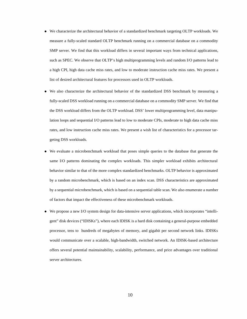
• We characterize the architectural behavior of a standardized benchmark targeting OLTP workloads. We

measure a fully-scaled standard OLTP benchmark running on a commercial database on a commodity

SMP server. We find that this workload differs in several important ways from technical applications,

such as SPEC. We observe that OLTP’s high multiprogramming levels and random I/O patterns lead to

a high CPI, high data cache miss rates, and low to moderate instruction cache miss rates. We present a

list of desired architectural features for processors used in OLTP workloads.

• We also characterize the architectural behavior of the standardized DSS benchmark by measuring a

fully-scaled DSS workload running on a commercial database on a commodity SMP server. We find that

the DSS workload differs from the OLTP workload. DSS’ lower multiprogramming level, data manipu-

lation loops and sequential I/O patterns lead to low to moderate CPIs, moderate to high data cache miss

rates, and low instruction cache miss rates. We present a wish list of characteristics for a processor tar-

geting DSS workloads.

• We evaluate a microbenchmark workload that poses simple queries to the database that generate the

same I/O patterns dominating the complex workloads. This simpler workload exhibits architectural

behavior similar to that of the more complex standardized benchmarks. OLTP behavior is approximated

by a random microbenchmark, which is based on an index scan. DSS characteristics are approximated

by a sequential microbenchmark, which is based on a sequential table scan. We also enumerate a number

of factors that impact the effectiveness of these microbenchmark workloads.

• We propose a new I/O system design for data-intensive server applications, which incorporates “intelli-

gent” disk devices (“IDISKs”), where each IDISK is a hard disk containing a general-purpose embedded

processor, tens to hundreds of megabytes of memory, and gigabit per second network links. IDISKs

would communicate over a scalable, high-bandwidth, switched network. An IDISK-based architecture

offers several potential maintainability, scalability, performance, and price advantages over traditional

server architectures.

11

• We present initial evidence demonstrating that IDISK-based architectures can outperform comparably

equipped SMPs and clusters for decision support operations. This analysis is based on measurements

quantifying the computation costs associated with random and sequential I/O patterns of these opera-

tions.

1.3.2. Methodology: Experimental Platform

The predominant methodology used in this dissertation employs measurements of workloads running on

commercial databases on a commodity SMP server. Our choice of SMP server is based on the observation

that cost-effective low-end servers are increasingly prominent for both OLTP and DSS workloads. Figure 1-

2 shows the recent trends for TPC-C server price performance, and Figure 1-3 and Figure 1-4 show analo-

gous data for the TPC-D benchmark.

We note two trends: 1) that price-performance is decreasing over time, implying that cost-effective low-end

servers are increasingly important and 2) that Intel-based servers (generally running Windows NT) are

Figure 1-2. TPC-C price performance over time [103].

TPC-C price performance is expressed in US dollars ($) per transactions per minute C(tpmC). This metric is explained in more detail in Section 2.4.1. on page 22.

1

10

100

1000

3/15/95 9/11/95 3/9/96 9/5/96 3/4/97 8/31/97 2/27/98 8/26/98 2/22/99

Time

TP

C-C

Pri

ce P

erfo

rman

ce (

$/tp

mC

)

MIPS

PowerPC

Digital Alpha 21x64

HP PA-RISC

Sun UltraSPARC

Intel

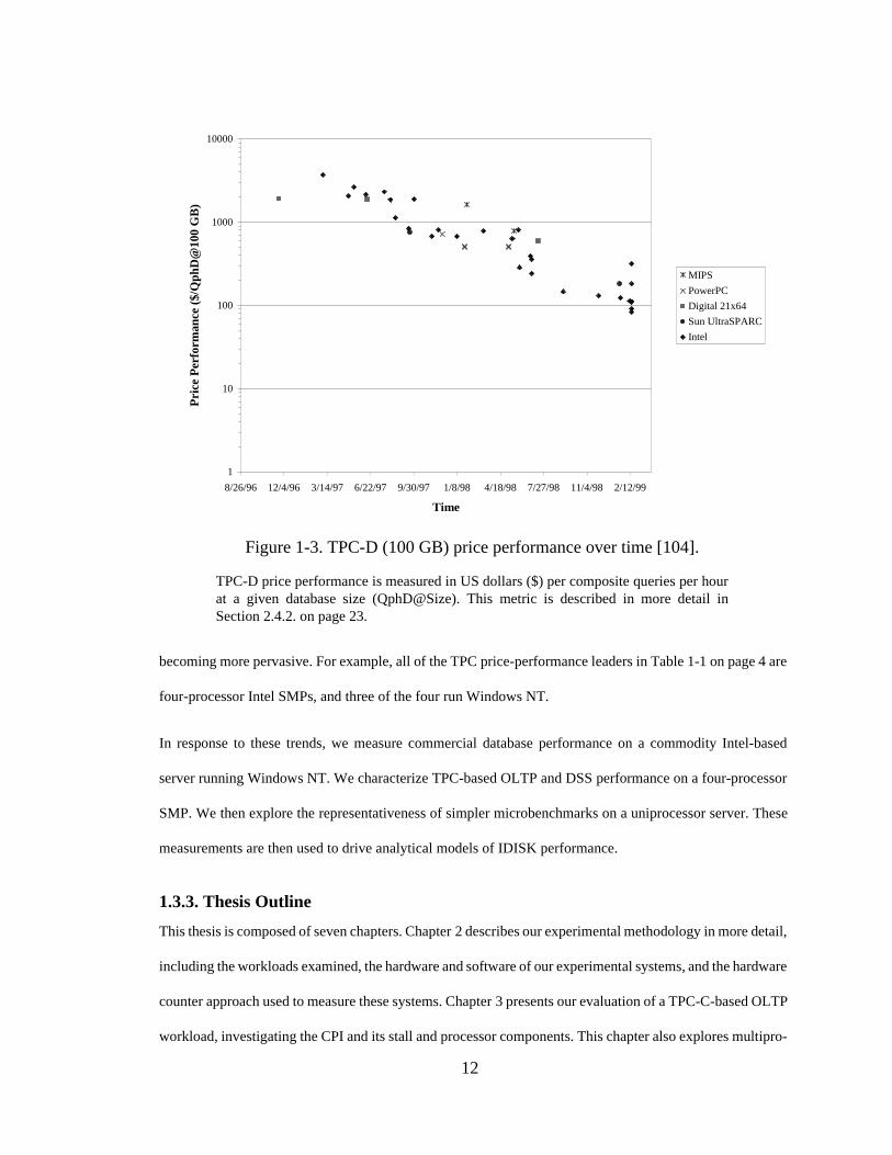
12

becoming more pervasive. For example, all of the TPC price-performance leaders in Table 1-1 on page 4 are

four-processor Intel SMPs, and three of the four run Windows NT.

In response to these trends, we measure commercial database performance on a commodity Intel-based

server running Windows NT. We characterize TPC-based OLTP and DSS performance on a four-processor

SMP. We then explore the representativeness of simpler microbenchmarks on a uniprocessor server. These

measurements are then used to drive analytical models of IDISK performance.

1.3.3. Thesis Outline

This thesis is composed of seven chapters. Chapter 2 describes our experimental methodology in more detail,

including the workloads examined, the hardware and software of our experimental systems, and the hardware

counter approach used to measure these systems. Chapter 3 presents our evaluation of a TPC-C-based OLTP

workload, investigating the CPI and its stall and processor components. This chapter also explores multipro-

Figure 1-3. TPC-D (100 GB) price performance over time [104].

TPC-D price performance is measured in US dollars ($) per composite queries per hourat a given database size (QphD@Size). This metric is described in more detail inSection 2.4.2. on page 23.

1

10

100

1000

10000

8/26/96 12/4/96 3/14/97 6/22/97 9/30/97 1/8/98 4/18/98 7/27/98 11/4/98 2/12/99

Time

Pri

ce P

erfo

rman

ce (

$/Q

phD

@10

0 G

B)

MIPS

PowerPC

Digital 21x64

Sun UltraSPARC

Intel

13

cessor scaling, and proposes a list of architectural characteristics desired in an OLTP-centric processor.

Chapter 4 performs a similar analysis for a TPC-D-based DSS workload. Chapter 5 proposes a simplified

workload with architectural characteristics similar to those of the more complex standardized benchmarks

examined in Chapter 3 and Chapter 4. Chapter 6 introduces the intelligent disk (IDISK) concept, outlining

the technological trends supporting this architecture, and presenting an initial evaluation of IDISK effective-

ness based on the measurements in Chapter 4. Our conclusions are presented in Chapter 7.

Figure 1-4. TPC-D (300 GB) price performance over time [104].

1

10

100

1000

10000

100000

8/23/96 12/1/96 3/11/97 6/19/97 9/27/97 1/5/98 4/15/98 7/24/98 11/1/98 2/9/99

Time

Pri

ce P

erfo

rman

ce (

$/Q

phD

@30

0 G

B)

MIPS

PowerPC

Digital 21x64

HP PA-RISC

Sun UltraSPARC

Intel

14

2 Experimental Methodology

2.1. Introduction

The insights drawn in this thesis are based on measurements of commercial software and hardware systems

running industry standard benchmarks. In this chapter, we compare different evaluation techniques, illustrat-

ing the benefits of direct measurement for I/O-intensive workloads. We also discuss the hardware and soft-

ware of our experimental systems and describe the hardware counter methodology used to measure these

systems.

2.2. Measurement vs. Simulation

As computer systems become increasingly complex, it becomes more and more important to fully evaluate

the systems we build with a variety of workloads before looking forward to the next architectural design.

Hardware measurement studies using processor and system performance counters can provide a wealth of

information on the performance of today’s machines. Direct measurement of real hardware allows the exam-

ination of fully scaled workloads at full speed, while varying a small set of parameters (e.g., number of pro-

cessors). Real hardware requires only validation of the instrumentation, not of the hardware model.

Unfortunately, measurement usually implies that many architectural parameters, such as the number of func-

tional units and reorder buffer entries, are fixed.

To investigate future architectural alternatives, researchers often employ simulation techniques. Here an arbi-

trary level of detail is possible, with the trade-off that increased detail is time-consuming and resource-inten-

sive. The difficulties with this approach are that validation of complex simulators is quite difficult, and

simulations can run up to 10,000 times slower than real-time, making it difficult to simulate large-scale fully

configured systems.

15

As an illustration of these limitations, we consider the following example. Simulation studies examining

decision support systems (DSS) performance are typically limited to analyzing a small portion of a represen-

tative query, due to the complexity of simulation. For instance, Ranganathan et al., report simulating approx-

imately 200 million instructions of one standard query (Q6 of the TPC-D DSS benchmark) for their

evaluation of an in-memory database on out-of-order processor multiprocessors [83]. These 200 million

instructions would take a fraction of a second on their 1 GHz simulated processor. This kernel analysis may

be limiting, as query behavior often varies over the course of the query. Even if an entire query is simulated,

execution variations may not be observed if the datasets have been scaled back to reduce the I/O require-

ments, as in [13], where a 500 MB in-memory database is employed. Another study scales back the data set

even further to 20 MB to facilitate simulation, necessitating a decrease in the size of the hardware caches

simulated [106].

Figure 2-1 illustrates the variation in CPI over query execution time for one standard query (Q5 of the TPC-

D DSS benchmark). The standard deviation of Q5’s CPI is 26% of the CPI mean across the query’s execution

time. This quantity is commonly referred to as the coefficient of variation. Q5’s coefficient of variation is

much larger than the coefficients of variation for the other DSS queries examined, which are less than 10%.

Clearly this query has several different execution phases, which exhibit drastically different behavior. The

first phase, from the start of the query to about 700 seconds on this machine, is well-behaved, much like the

other queries examined in this thesis. The second phase, which begins at about 700 seconds, coincides with

a period of disk write activity initiated to store intermediate results for one of the hash join operations

employed in the query. The intermediate result table is too big to fit into the memory buffer pool, and must

be spilled to disk, resulting in an increase in operating system time to perform I/O, and hence a higher CPI.

We can also observe a third phase, beginning at about 1120 seconds, which corresponds to the period where

the intermediate result table written to disk is read into memory to serve as one of the inputs of a subsequent

hash join operation.

Because of these variations in behavior across the duration of query execution, simulating a small kernel of

only a few seconds may lead to conclusions that don’t apply to all query phases. Researchers employing sim-

16

ulation techniques must be very careful to pick kernels that represent all phases of query execution. This care

will become even more important as query complexity increases in future versions of the TPC-D benchmark.

In addition, reduced datasets may not exhibit behavior that is representative of fully-scaled systems, where

large data requirements may generate I/O that impacts performance. Measurement of full-scaled workloads

on real systems offers an advantage here, in that we can see all phases of a query’s execution, and gauge the

effects of large data.

In this thesis, we show that there is some middle ground between direct measurement and simulation. We

measure a real machine running fully-scaled workloads, but vary hardware parameters, including second-

level cache size, the number of outstanding bus transactions, and the number of processors, to explore archi-

tectural trade-offs. The flexibility in configuration parameters afforded by our system allows us to overcome

some of the traditional limitations of measurement approaches.

2.3. Experimental System Hardware Configurations

This section begins the discussion of our experimental systems, focusing on the hardware configuration. We

present a description of the processor and memory organizations, followed by a discussion of the I/O sub-

system configurations.

Figure 2-1. CPI as a function of query execution time for DSS query Q5.

0

0.5

1

1.5

2

2.5

3

3.5

4

4.5

5 255 505 755 1005

Query Time (seconds)

Cyc

les

per

Mac

ro-i

nstr

ucti

on (

CP

I)

DSS Q5

17

2.3.1. Processor and Memory Configurations

Table 2-1 describes the Intel Pentium Pro-based systems measured in Chapter 3 through Chapter 5. For the

more complex OLTP and DSS workloads, we measure a four-processor SMP, as it is the building block for

small- to mid-range database servers. In these two chapters, L2 cache size was modified by physically swap-

ping processor/cache boards to switch between the three cache sizes. For microbenchmark evaluation, we

use a uniprocessor-based machine.

In Chapter 3, we also vary the number of processors and the number of outstanding memory bus transactions

to study their effects on OLTP performance. Table 2-2 shows the values of these parameters. The number of

processors was varied at boot time, so that the system was restricted to having only one, two, or four proces-

Characteristic OLTP (Chapter 3) DSS (Chapter 4)Microbenchmarks (Chapter 5)

Processor Pentium Pro Pentium Pro Pentium Pro

Processor speed 200 MHz 200 MHz 200 MHz

Number of processors 4 4 1

L1 data cache 8 KB 8 KB 8 KB

L1 instruction cache 8 KB 8 KB 8 KB

L2 cache (unified) 256 KB, 512 KB, 1 MB 256 KB, 512 KB, 1 MB 256 KB

System chipset 82450 KX/GX (Orion) 82450 KX/GX (Orion) 82440 FX

System bus speed 66 MHz 66 MHz 66 MHz

Memory size 4 GB (2 GB per process) 4 GB (3 GB per process) 256 MB (128 MB for DB)

Memory organization 4-way interleaved 4-way interleaved Non-interleaved

Memory read bandwidth 213 MB/s 213 MB/s 99 MB/s

Memory read latency (dependent loads)

190 ns (38 cycles) 190 ns (38 cycles) 315 ns (63 cycles)

Operating System NT 4.0 Enterprise Server, Service Pack 3

NT 4.0 Enterprise Server, Service Pack 3

NT 4.0 Server, Service Pack 4

Database Server Informix ODS Informix IDS Informix IDS, Microsoft SQLServer, Oracle

Table 2-1. Summary of system configurations.

Memory performance is measured by uniprocessor microbenchmarks similar to those inthe lmbench suite [65]. Read bandwidth is sequential read bandwidth. Read latency mea-sures dependent load latency, where the program fetches the next address based on thecontents of the current location; this test corresponds to the worst-case read latency. Notethat the same physical hardware was measured for both Chapter 3 and Chapter 4. The I/Osubsystems of these configurations are shown in Figure 2-2 through Figure 2-4.

18

sors active. Finally, the number of outstanding bus transactions was varied by changing a BIOS parameter to

limit the “I/O queue depth” of the controller [50]. Ideally, we would like to limit each processor to a single

outstanding bus transaction, to explore the effects of the non-blocking L2 cache. The BIOS only allows us,

however, to limit the overall system (in other words, all four processors) to a single outstanding bus transac-

tion. Thus, we perform this experiment with a uniprocessor configuration, comparing the default of up to four

outstanding bus transactions per processor with the alternative of a single outstanding bus transaction.

2.3.2. I/O Subsystem Configurations

Figure 2-2 through Figure 2-4 illustrate the I/O subsystem configurations for the database data used in each

of the three workload studies. The fully-scaled OLTP and DSS workloads require extensive I/O configura-

tions. These configurations were designed by experts at Informix to support the I/O patterns common to each

workload. OLTP does predominantly small (e.g., 2 KB to 8 KB) random read and write I/Os to access par-

ticular index and data pages. This pattern implies that the primary principle of OLTP I/O subsystem design

is to maximize the number of disk arms. As shown in Figure 2-2, the OLTP I/O configuration uses 90 data

disks spread over both channels of three SCSI controllers. The parameters for the Quantum disks used in this

I/O configuration are shown in Table 2-3.

The predominant I/O operation in DSS is large (e.g., 64 KB to 1 MB) sequential reads, which are used for

scanning entire tables. Smaller random reads and writes are also employed for more complex joining and

sorting operations if the data is too big to fit into memory; however, these operations are far less common.

Thus, the primary principle of DSS I/O subsystem design is to maximize disk bandwidth. The resulting con-

figuration, shown in Figure 2-3, employs fewer (56) disks, but spreads them across four SCSI controllers,

using only a single channel per controller. The choice of four SCSI controllers (versus three, as in Figure 2-

Parameter Values

Number of processors 1, 2, 4 processors

Outstanding bus transactions Uniprocessor: 1, up to 4 transactions

Table 2-2. Additional architectural parameters varied in OLTP evaluation.

The buffer memory available to the database was held constant at 512 MB per processor.

19

2) and a single channel per controller (versus both channels, as in Figure 2-2) is motivated by the goal of

increasing potential bandwidth, and limiting the possibility of the SCSI controller becoming a bottleneck.

Table 2-3 shows the parameters for the Quantum disk drives used in the DSS I/O configuration.

PCIController

Dual-Channel SCSI 3

ControllerCtrl 0

00

01

02

03

04

05

06

07

08

09

10

11

12

13

14

00

01

02

03

04

05

06

07

08

09

10

11

12

13

14

Dual-Channel SCSI 3

ControllerCtrl 1

00

01

02

03

04

05

06

07

08

09

10

11

12

13

14

00

01

02

03

04

05

06

07

08

09

10

11

12

13

14

Dual-Channel SCSI 3

ControllerCtrl 2

00

01

02

03

04

05

06

07

08

09

10

11

12

13

14

00

01

02

03

04

05

06

07

08

09

10

11

12

13

14

Channel 0

Channel 1

Channel 0

Channel 1

Channel 0

Channel 1

Figure 2-2. OLTP I/O subsystem configuration.

The I/O configuration for OLTP data contains 90 Quantum Atlas II 4.55 GB Ultra SCSI-3 disks spread across three Adaptec AHA-3940 Ultra-Wide dual-channel SCSI-3 con-trollers. Both channels of each controller are employed for this setup. The parameters ofthe Quantum Atlas II disk drive are shown in Table 2-3.

.

Characteristic Quantum XP34550

Formatted disk capacity 4.55 GB

Rotational speed 7200 RPM

Media transfer rate 15.13 MB/s

Average seek time (read) 8.0 ms

Track-to-track seek time 1.0 ms

Average rotational latency 4.17 ms

Table 2-3. Parameters for Quantum Atlas II disk, which is used in the OLTP and DSS I/O subsystems [82].

20

The microbenchmark design, shown in Figure 2-4, employs a modest six 4.0 GB disks on a single SCSI bus.

The goal in this design was to minimize the I/O hardware as much as possible. Although our dataset is only

1 GB, which would fit on even a single disk, we use multiple disks to decrease the overall idle time due to

I/O waits. Table 2-4 presents the parameters for the Seagate disk used in the microbenchmark I/O configu-

ration.

PCIController

Dual-Channel SCSI 3

ControllerCtrl 0

00

01

02

03

04

05

06

07

08

09

10

11

12

13

Dual-Channel SCSI 3

ControllerCtrl 1

00

01

02

03

04

05

06

07

08

09

10

11

12

13

Dual-Channel SCSI 3

ControllerCtrl 2

00

01

02

03

04

05

06

07

08

09

10

11

12

13

Channel 0

Channel 0

Channel 0

Figure 2-3. DSS I/O subsystem configuration.

The I/O configuration for the DSS data contains 56 Quantum Atlas II 4.55 GB UltraSCSI-3 disks spread across four Adaptec AHA-3940 Ultra-Wide dual-channel SCSI-3controllers. Only a single channel from each controller is employed in this setup. Thenumber of disks (56) is chosen to match the number of months covered by some of thetables in the TPC-D benchmark, an attribute commonly used to distribute the data acrossthe disks. Thus, each disk can hold a month’s worth of data. The parameters for theQuantum Atlas II drive are shown in Table 2-3.

Dual-Channel SCSI 3

ControllerCtrl 3

00

01

02

03

04

05

06

07

08

09

10

11

12

13 Channel 0

21

Note that all of the I/O subsystems utilize a hierarchy of controllers. The memory controller interfaces with

one or more internal I/O bus (PCI) controllers, which communicate with one or more external I/O bus (SCSI)

controllers, which then communicate with the disks. (High-end SMP servers in the late 1990s include mul-

tiple internal I/O busses to improve I/O performance.) Although this hierarchical I/O system design is typical

in the late 1990s, it possesses several scalability challenges. Foremost, the system cannot use 100% of the

busses’ bandwidth, due to the need to keep queue lengths manageably short and due to the bus protocol com-

mand overhead. In Chapter 6, we describe these limitations in more detail, and we propose an alternative I/O

subsystem design to overcome them.

PCIController

U/UW SCSI

Controller

00

01

02

03

04

05

Figure 2-4. Microbenchmark I/O subsystem configuration.

The I/O configuration for the microbenchmark data contains 6 Seagate Barracuda 4.2 GBUltra SCSI disks, numbered 00 through 05, on an Adaptec AHA-2940 Ultra/Ultra-WideSCSI controller.

.

Characteristic Seagate ST-15150W


Rotational speed 7200 RPM

Media transfer rate 5.93 MB/s - 8.99 MB/s




Table 2-4. Parameters for Seagate Barracuda disk, which is used in the microbenchmark I/O subsystem [89].

22

2.4. Software Architecture

We continue our experimental system discussion in this section by describing the software architectures and

workloads measured in Chapter 3 through Chapter 5. These subsequent chapters present more detailed

descriptions of these workloads.

2.4.1. Transaction Processing (OLTP) Software

For the transaction processing study in Chapter 3, we measured a variant of the Transaction Processing

Council’s TPC-C benchmark [35]. TPC-C is an OLTP benchmark that simulates an order-entry environment,

and includes the activities of entering and delivering orders, recording payments, checking the status of

orders, and monitoring the level of stock at the warehouses. TPC-C is currently the only active OLTP bench-

mark supported by the TPC. It uses a mix of five transactions, rather than a single debit-credit transaction,

like the now-defunct TPC-A and TPC-B benchmarks. TPC-C employs a more complex database structure

and utilizes nonuniform data access patterns to simulate data hot spots, resulting in higher levels of conten-

tion for data access and update. The performance metric for TPC-C is transaction throughput, in particular

the number of NewOrder transactions per minute (tpmC).

We used a modified version of TPC-C, where two client machines simulate thousands of remote terminal

emulators (RTEs), generating requests with no think time between requests. The resulting load presented to

the database server strongly resembles the full configuration with RTEs, and thus stresses the server in sim-

ilar ways [107].

We measured the performance of this OLTP workload running on a tuned prototype version of Informix

Online Dynamic Server [49], a shared-memory database. ODS is a parallel shared-memory database server.

It uses a single multi-threaded process; the NT threads exploit processor affinity to ensure that each NT

thread is run exclusively on its assigned CPU. User-level threads are then multiplexed on top of these NT

threads. Database server threads communicate through a shared memory buffer pool, which is 2 GB in our

system. Disk I/O is done to raw disk partitions, not through the file system.

23

2.4.2. Decision Support (DSS) Software

For the decision support study in Chapter 4, we measured a variant of the Transaction Processing Council’s

TPC-D benchmark [105]. TPC-D is a DSS benchmark that simulates the activity of a wholesale supplier in

doing complex business analysis. It includes the following classes of business analysis: pricing and promo-

tions, market share study, shipping management, supply and demand management, profit and revenue man-

agement and customer satisfaction study. The database size is specified by a scale factor (SF), where a SF

of 1 corresponds to 1 GB of raw data. Typical database sizes for audited runs are 100 GB to 3000 GB. In

this study, we use a 100 GB (e.g., SF 100) database.

We used version 1.3 of the TPC-D benchmark, which includes 17 read-only queries and two update queries.

We focus on a representative set of the read-only queries chosen based on the variety of operations per-

formed, query complexity and query duration. Several other studies have presented performance analyses of

TPC-D queries (e.g., Q1, Q4, Q5, Q6, Q8, Q13 for [13], Q6 for [83], and Q3, Q6, and Q12 for [106]). Since

the four-processor system described in [13] is comparable to our system, we attempt to match this query set

closely, for comparability of results. Our query set includes Q1, Q4, Q5, Q6, Q8, and Q11. We substitute Q11

for Q13 because Q13’s short duration (e.g., a few seconds) prevented us from measuring it effectively. Fur-

thermore, Q13 was decommissioned in the next version (version 2.0) of the TPC-D benchmark, which was

released in February 1999. We describe the new version of the benchmark in more detail in Chapter 4.

We measured the performance of this DSS workload running on a tuned prototype version of Informix

Dynamic Server (IDS) with the Advanced Decision Support (AD) and Extended Parallel Processing (XP)

Options [48]. IDS is a more recent parallel shared-memory database server with support for performing

numerous database operations, such as selects, sorts, joins and aggregations, in parallel. Like its predecessor,

IDS also multiplexes user-level threads over multiple affinitied NT threads. For the DSS queries examined

in Chapter 4, up to eight threads are used per processor. The shared memory buffer pool for this system is 3

GB. Again, disk I/O is done to raw disk partitions, not through the file system.

24

2.4.3. Microbenchmark Software

For the microbenchmark study in Chapter 5, we pose simple SQL queries of each database to generate

sequential and random I/O access patterns. For the sequential pattern, we pose a query requiring a sequential

scan of a database table. For the random pattern, we pose a query that performs a non-clustered index scan,

which requires fetching a random data page for each row examined. These queries are described in more

detail in Chapter 5.

For this study, we measured the Informix IDS 7.3 database server engine, an even more recent version of the

same code base used in the OLTP and DSS studies. An evaluation copy of this engine was downloaded from

the company’s web site in February 1999, and installed with the default parameters. To simplify setup, all

I/O was performed through the NTFS file system.

2.4.4. Discussion

The operating system used in all of these studies is Microsoft Windows NT 4.0, with different versions and

service packs (the NT analog of an operating system patch) used for each study. These variants are described

in more detail in Table 2-1 on page 17. We note that I/O is done only in the kernel for NT systems.

Since this work began, there have been new releases of these software products, with improved performance.

For this reason and due to the TPC reporting rules, we do not present absolute database performance results;

we instead focus on performance relative to the base systems described in Table 2-1. These relative perfor-

mance metrics will be clarified in the application performance sections of Chapter 3 and Chapter 4.

2.5. Pentium Pro Processor Architecture

This section concludes our discussion of the experimental systems used in this thesis by giving an overview

of the Pentium Pro processor and outlining where this out-of-order processor may experience performance-

limiting stalls.

2.5.1. Overview

Figure 2-5 shows the architecture of Intel’s Pentium Pro processor. The Pentium Pro implements dynamic

execution using an out-of-order, speculative execution engine, which employs register renaming, non-block-

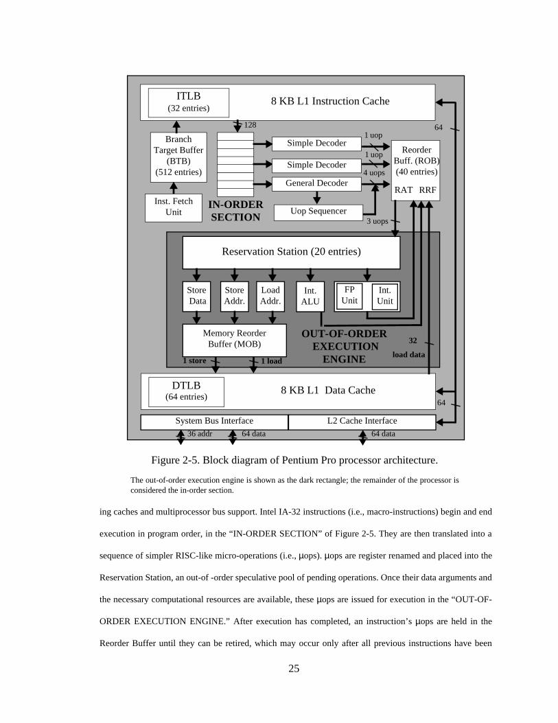
25

ing caches and multiprocessor bus support. Intel IA-32 instructions (i.e., macro-instructions) begin and end

execution in program order, in the “IN-ORDER SECTION” of Figure 2-5. They are then translated into a

sequence of simpler RISC-like micro-operations (i.e., µops). µops are register renamed and placed into the

Reservation Station, an out-of -order speculative pool of pending operations. Once their data arguments and

the necessary computational resources are available, these µops are issued for execution in the “OUT-OF-

ORDER EXECUTION ENGINE.” After execution has completed, an instruction’s µops are held in the

Reorder Buffer until they can be retired, which may occur only after all previous instructions have been

8 KB L1 Instruction Cache

IN-ORDER SECTION

DTLB (64 entries)

8 KB L1 Data Cache

Store Data

Load Addr.

Int. ALU

FP Unit

Reservation Station (20 entries)

Int. Unit

Memory Reorder Buffer (MOB)

OUT-OF-ORDER EXECUTION

ENGINE

System Bus Interface L2 Cache Interface

Branch Target Buffer

(BTB) (512 entries)

Reorder Buff. (ROB)(40 entries)

RAT RRF

Store Addr.

Figure 2-5. Block diagram of Pentium Pro processor architecture.

The out-of-order execution engine is shown as the dark rectangle; the remainder of the processor isconsidered the in-order section.

ITLB

(32 entries)

Simple Decoder

Simple Decoder

General Decoder

Uop Sequencer

1281 uop

1 uop

4 uops

3 uops

64

64

64 data64 data36 addr

1 store 1 loadload data

32

Inst. Fetch Unit

26

retired, and all of the constituent µops have completed. The Pentium Pro retires up to three µops per clock

cycle, yielding a theoretical minimum cycles per µop (µCPI) of 0.33.

Table 2-5 summarizes the characteristics of the Pentium Pro caches.

More detailed descriptions of the Pentium Pro’s architectural features can be found in [15] [25] [39] [50]

[76]. We will also present additional details in subsequent sections, when discussing our measurement

results.

2.5.2. Potential Sources of Pentium Pro Stalls

In practice, the 0.33 theoretical minimum µCPI is seldom achieved, due to stalls from cache misses, over-

subscription of certain resources, and under-utilization of other resources. For example, starting at the begin-

ning of the pipeline, misses to the L1 instruction cache or instruction translation look-aside buffer (ITLB)

can stall the beginning of the pipeline, impeding further progress. If these misses hit in the L2 cache, the pro-

cessor experiences an additional four-cycle latency. If they miss in the L2 cache, the processor will experi-

ence a delay of tens to one hundred cycles to access memory.

In addition, a branch misprediction can cause delays of 11 or more cycles. ([39] suggests that the typical

branch misprediction penalty is 15 cycles.) Two types of branch mispredictions can occur. First, a branch can

be found in the branch target buffer (BTB), but with an incorrect predicted target address. The second type

of misprediction occurs when the branch misses the BTB, and a static (backward taken, forward not taken)

prediction scheme is used; this static scheme is typically less accurate than the two-level adaptive scheme

employed [120].

Characteristic L1 Inst. L1 Data L2 (unified)

Size 8 KB 8 KB 256 KB, 512 KB, 1 MB

Associativity 4-way 2-way 4-way

Hit penalty 3 cycles 3 cycles 4 cycles (additional)

Non-blocking (e.g., hit-under-miss, miss-under-miss)? yes yes yes

Outstanding misses four four four

Write policy write-back

write-back

Table 2-5. Pentium Pro L1 and L2 cache characteristics.

27

The instruction mix of the workload may not match the mix of simple and general decoders, preventing the

machine from achieving its full instruction decode bandwidth. The first (general) decoder in the queue can

handle any x86 instruction; the others are restricted to simple (e.g., register-to-register) instructions that pro-

duce a single µop. Assuming that instruction bytes are available, a single µop will be decoded per cycle.

Because instructions must be decoded in program order, additional instructions will be decoded in the same

cycle only if they can be handled by the simple decoders. Thus, a long sequence of complex instructions or

instructions that operate on memory (e.g., requiring a load µop, an ALU µop, and possibly a store µop), can

cause the simple decoders to be under-utilized, leading to decreased performance.

Limited reorder buffer (ROB) resources may also limit the Pentium Pro’s performance. The ROB has forty

entries, and its internal and interface bandwidths are restricted. For example, decoder bandwidth into the

reorder buffer is limited to a total of six µops per cycle, statically distributed over the decoders as shown in

Figure 2-5. ROB result bandwidth is limited to three results per cycle, which may be insufficient if the main

(e.g., integer + FP) arithmetic unit produces multiple results in a cycle where the integer ALU and data cache

also produce results. Internally, register renaming and µop logging bandwidth is limited to three µops per

cycle. ROB store bandwidth for µop retirement is limited to three µops per cycle.

Finally, the out-of-order execution engine contains several sources of potential stalls. The number of reser-

vation station and memory reorder buffer (MOB) entries may prove to be insufficient. As in any processor,

the mix of available instructions may not match the mix of functional units, implying that fewer than five

µops will be dispatched per cycle. Finally, loads and stores may need to wait in the MOB for access to the

dual-ported L1 data cache, which can accept one load and one store per cycle as long as the accesses are from

different banks.

2.6. Measurement Methodology

We measured the experimental systems using both the NT performance monitor and the Pentium Pro hard-

ware counters. The performance monitor was used to measure a handful of system-level characteristics, such

as the breakdown of user, system, and idle time, system calls per second, context switches per second, inter-

rupts per second, and disk reads and writes per second and their sizes. To be minimally intrusive, we config-

28

ured the performance monitor to sample these counts once every ten seconds. As shown in Table 2-7 in

Section 2.6.5, the resulting perturbation is less than 0.5%.

To collect data on processor behavior, we use the Pentium Pro hardware counters. Each processor has two

counters that can measure the number of a variety of events, such as instructions and µops retired, branch

behavior, L1 and L2 cache misses, various bus transactions, and stalls, for user-level activity, system-level

activity or aggregate activity in both user+system modes [50]. The same event pair is simultaneously mea-

sured across all four processors.

We use a proprietary Intel tool called emon control the counters. The emon driver is responsible for zeroing

the counters, setting the appropriate event type, and reading the event count after a user-specified time inter-

val or after a program has completed execution. The syntax of the command is:

emon.exe {event string} -t time -l loop prog.exe

The event string is a list of events to be measured, two at a time, in each of the processors in the system.

Each measurement interval will be time seconds long, and there will be loop passes through the event

list, provided that the duration of prog.exe is sufficiently long. Event monitoring ceases when one of the

following conditions is met: the number of specified loops has been completed, or the specified program

ends. Generally, we use a program that can be run for a user-specified amount of time (for example, sleep),

and specify values such that the time to complete the loops equals the time of the program execution.

For example, to count the instructions retired for both user and system modes during five-second measure-

ment intervals over the course of thirty seconds, we would execute the following command:

emon.exe -C INST_RETIRED:user -C INST_RETIRED:sup -t 5 -l 6 sleep.exe 30

The result of this command would be six “data points”, where each data point includes the number of user

instructions retired and the number of supervisor instructions retired for each of the processors in the system

over the five-second measurement interval.

29

Multiple pairs of events can also be counted in a single emon invocation, by specifying a longer string of

events. For example, to measure both the cycle counts and instruction counts during five-second measure-

ment windows over the course of thirty seconds, we would execute the following command:

emon.exe -C INST_RETIRED:user -C INST_RETIRED:sup -C

CPU_CLK_UNHALTED:user -C CPU_CLK_UNHALTED:sup -t 5 -l 3 sleep.exe 30

Here, each loop would consist of instruction count measurement for the first five seconds and cycle count

measurement for the second five seconds, resulting in three ten-second loops during the thirty-second eval-

uation. The output would be three data points for instructions retired, and three data points for cycles exe-

cuted.

We find that emon measurement of the counters is also minimally intrusive, as shown in Table 2-6 in

Section 2.6.5.

Although there are many sources of potential stalls, as described in Section 2.5.2, it is often difficult to pin-

point the exact cause of a stall. The Pentium Pro provides event types to monitor two main aggregate stall

categories: resource stalls and instruction-related stalls. Instruction-related stalls count the number of cycles

that instruction fetch is stalled for any reason, including L1 instruction cache misses, ITLB misses, ITLB

faults, and other minor stalls [15] [50]. Resource stalls account for cycles in which the decoder gets ahead of

execution. For example, resource stalls encompass the conditions where register renaming buffer entries,

reorder buffer entries, memory buffer entries, or execution units are full. In addition, serializing instructions

(e.g., CPUID), interrupts, and privilege level changes may spend considerable cycles in execution, forcing

the decoder to wait and incrementing the resource stalls counter. Stalls due to data cache misses are not

explicitly included in resource stalls; however, if some other resource becomes oversubscribed due to a long

data cache miss, the resource stall counter will be incremented.

We use roughly 50 hardware event types for the data presented in this thesis. For each event and processor,

we compute a trimmed mean; that is, we remove the minimum and maximum observations, and then compute

the mean from the remaining observations [84]. After trimming, we have at least 30 (in some cases 40) obser-

30

vations for each event type. We then examine the data to determine the amount of noise due to the measure-

ment methodology.

The exact measurement methodology differs from workload to workload. The following sections describe

these differences in more detail.

2.6.1. OLTP Measurement

In evaluating the OLTP workload, we did at least five database runs for each hardware configuration. Each

run consists of a fifteen-minute warm-up period, which is sufficient to bring the database to steady state, and

a forty-minute measurement period. (Forty minutes is chosen to maximize the measurement time before a

checkpoint must be taken.) The forty-minute measurement period is broken into five-second fixed duration

intervals, during which an event is measured for both user and system level. We chose five-second measure-

ment intervals to minimize the variation in cycle count between intervals. This variation is sometimes as

much as 20 million cycles, which is a significant percentage of smaller intervals (e.g, 10% of the 200 million

cycles expected in a one-second measurement interval).

Typically, each database run results in six to eleven observations per event type. To obtain enough data points

to draw statistical conclusions, we perform at least five database runs for each hardware configuration. Some

runs measure all events, and others focus on a subset of important events. We cycle through the counters in

a different order for each run, to greater increase their coverage.

Since aggregate (e.g., user + system) activity is of most interest to architects, we present aggregate charac-

teristics in Chapter 3. This benchmark typically spends 20% to 25% of its execution time in system mode.

Differences in user and system behavior are noted in the appendix in Chapter 9. The standard deviation for

a given event for a given processor is less than 10% of the mean for that event/processor combination, for

nearly all of the event types.

2.6.2. DSS Measurement

Since DSS queries spend nearly all of their time at user-level (with user time typically accounting for more

than 95% of execution time), we decided to measure aggregate activity and not differentiate between user

31

and system modes. For each configuration, we run each query multiple times, measuring a single pair of

events during each run. Each run is again broken into 5-second fixed duration intervals, and the number of

events occurring during that 5-second window is recorded.

For each event and processor, we compute a trimmed mean of the observations during a query phase. For all

queries except Q5, a phase corresponds to the entire query run. For Q5, we separately analyzed the three

phases introduced in Section 2.2. For Q5 phase 2, we only considered the periods where writes are actively

performed, ignoring the intervening computation which largely resembles the first phase. The standard devi-

ation for a given event for a given processor was less than 10% of the mean for that event/processor combi-

nation, for nearly all of the event types for queries Q1, Q5 phase 1, Q6, and Q8. For Q4, Q5 phase3, and

Q11, the standard deviation was at most 20% of the mean for that event/processor combination for nearly all

event types. The variation for the second phase of Q5 was greater than 20%; we suspect that this high vari-

ability is due to the mismatch of 5-second measurement windows and the phenomena being measured. To

minimize the effects of this variation on our analysis, we sum the total number of events (of a given type)

that occur during the write phases, and then compute the average number of events in a 5-second window.

2.6.3. Microbenchmark Measurement

The systems used to measure microbenchmark characteristics have modest I/O subsystems, which result in

non-trivial idle time during experiments. On a uniprocessor, NT implements the idle loop using the HALT

instruction. The event counters are inactive during this idle loop, ensuring that we can reliably separate

system-mode counter observations for the operating system and the idle loop. Thus, we present aggregate

activity for this workload, factoring out the idle loop. For each configuration, we run each query multiple

times, measuring a single pair of events during each run. Each run is broken into two-second fixed duration

intervals, and the number of events occurring during that two-second window is recorded. We find that the

standard deviation for a given event was less than 10% of the mean for nearly all event types measured.

2.6.4. Formulae for Architectural Characteristics

The Pentium Pro event types and formulae used to compute the architectural characteristics presented in sub-

sequent chapters are shown in the appendix in Chapter 8. Unless otherwise stated, the computations listed in

32

the tables are performed on a per-processor basis. In our presentation of the collected data in subsequent

chapters, we will present the average values across all active processors in the system, since in most cases

the processors exhibit similar behavior. Any deviations from this norm will be noted.

2.6.5. Measurement Overheads

Although we have attempted to minimize the overhead of our NT performance monitor and hardware counter

measurements by choosing long (5 to 10 second) intervals, the measurement techniques do impose a small

overhead on the system being measured. We quantify these overheads in Table 2-6 and Table 2-7 by showing

the quantities measured for an idle system.

Table 2-6 presents hardware counter information for the idle four-processor system; all values are averaged

across the four processors. We observe that the system spends less than 1% of its execution time at user level.

The system experiences a relatively high CPI of 3.58 (µCPI of 0.64), incurred by the high percentage of time

Quantity Idle System

Percent user time 0.41%

Cycles per macro-instruction (CPI) 3.58

Cycles per micro-operation (µop) (µCPI) 0.64

Resource stalls per µop 0.00

Instruction-related stalls per µop 0.00

Computation µCPI 0.41

Instruction fetches per 1000 instructions retired 3572.22

Data references per 1000 instructions retired 454.09

L1 I-cache misses per 1000 instructions retired 0.55

L1 D-cache misses per 1000 instructions retired 0.49

ITLB misses per 1000 instructions retired 0.02

L2 I-related misses per 1000 instructions retired 0.01

L2 D-related misses per 1000 instructions retired 0.06

Average memory latency 83.92 cycles

Branches per 1000 instructions retired 364.76

Branch mispredictions per 1000 instructions retired 0.11

µops per instruction 5.62

Table 2-6. Pentium Pro hardware counter characteristics for the four-processor system inidle state.

33

spent in the operating system. This CPI is comprised predominantly of computation, with negligible

resource-related and instruction-related stalls. The number of cache misses at all levels is negligible - much

less than one miss per 1000 instructions retired for both instructions and data at the first level and second

level. Branches comprise roughly one-third of the idle workload, with a negligible misprediction rate.

Table 2-7 presents the characteristics collected by NT’s performance monitor for the idle system. Again, we

see that negligible time (less than 0.5%) is spent at user level and at system level. The system experiences a

moderate rate of thread context switches and system calls every second. The file read and write activity is

negligible for the idle system.

The data presented in Table 2-6 and Table 2-7 show that both the NT performance monitor and the hardware

counter monitoring mechanism impose little measurement overhead on the machine.

2.7. Summary

This chapter introduced the methodology employed in this thesis: the measurement of real systems running

full-scale versions of industry standard benchmarks. We described the hardware systems measured in subse-

Characteristic Idle System

Average user time (across four processors) 0.02%

Average system time (across four processors) 0.04%

Average idle time (across four processors) 99.94%

Average interrupts per second (across four processors) 69.06

Thread context switches per second 682.23

System calls per second 640.34

File reads per second 0.10

File writes per second 0.60

Average read size -

Average write size -

Table 2-7. NT performance monitor characteristics for the idle four-processor system.

The quantities listed as “average” above were measured separately for each of the fourprocessors; the number presented is the average across the four processors in the system.The number of system calls per second is generally 640, but periodically (roughly everythirty seconds) this rate increases to 1029 system calls per second. Likewise, the numberof file writes per second is generally quite low; once every minute, however, this rateincreases slightly to 6.1 writes per second.

34

quent chapters, including discussions of the I/O subsystems, the Pentium Pro processor architecture, and the

memory system. We also described the database and benchmark software measured for this thesis. Finally,

we presented our evaluation methodology, which is based on Pentium Pro hardware counter and NT perfor-

mance monitor measurements.

35

3 Analysis of Online Transaction Processing Workloads

3.1. Introduction

In this chapter we measure the architectural features of a four-processor Pentium Pro-based server running a

commercial database executing a TPC-C-like OLTP workload. Recall that OLTP does short, moderately

complex transactions that read and/or modify a relatively small portion of the overall database. These access

patterns translate into many small, random I/O operations, as index and data pages are accessed. These work-

loads typically have a large number of concurrent users, and as a result, a high degree of multiprogramming.

The database implements locking (to maintain isolation between users) and logging (to ensure that updates

are completed atomically, even in the face of system failure). The combination of these tasks implies a large

instruction working set and an even larger data footprint for the database server.

We find that overall (database + operating system) CPI is roughly five times higher than the theoretical min-

imum CPI for the architecture, and much higher than the CPI of SPECInt95. Resource and instruction-related

stalls comprise the majority of these cycles. We observe that out-of-order execution is somewhat effective at

hiding memory hierarchy latency and other stalls. We find that the Pentium Pro branch prediction algorithms

and hardware support do not work nearly as well for this database workload as they do for SPECInt95. We

observe that increasing the macro-instruction superscalar issue and retire width will likely be only marginally

helpful for this workload. However, the workload may benefit from an increased superscalar width at the

micro-operation level.

Not surprisingly, we find that caches are effective at reducing the processor traffic to memory. We observe

improvements in L2 cache miss rates for L2 cache sizes up to 1 MB, the largest available for this processor.

36

While larger caches are effective, this benefit is not without consequences. Coherence traffic, in the form of

cache misses to dirty data in other processors’ caches, increases as caches get bigger, and as the number of

processors increases. We find that the exclusive state of the four-state MESI cache coherence protocol is

under-utilized for multiprocessor configurations, and could likely be omitted in favor of a simpler three-state

protocol for this workload. Finally, multiprocessor scaling of this workload is good, but even modest memory

system utilization degrades application memory latency.

This chapter is organized as follows. Section 3.2 describes our OLTP workload, based on the TPC-C bench-

mark. We discuss the decomposition of CPI in Section 3.3, and then further explore its memory hierarchy

component in Section 3.4 and its processor component in Section 3.5. Multiprocessor scaling is explored in

Section 3.6, and OLTP I/O characteristics are described in Section 3.7. We analyze related work in

Section 3.8, and propose a design for an OLTP-centric processor in Section 3.9. Conclusions are presented

in Section 3.10.

3.2. OLTP Workload Description

We measured a variant of the Transaction Processing Council’s TPC-C benchmark [35] [58]. TPC-C is a

moderately complex OLTP benchmark that simulates an order-entry environment, and includes the activities

of entering and delivering orders, recording payments, checking the status of orders, and monitoring the level

of stock at the warehouses.

The benchmark uses a mix of five transactions, rather than a single debit-credit transaction, like the

now-defunct TPC-A and TPC-B benchmarks. Table 3-1 presents these five transactions and their typical fre-

quency in the workload. These transactions operate against a database of nine tables, performing updates,

Transaction Type Typical Frequency Description

NewOrder 45% Enter a new order from a customer

Payment 43% Update customer balance to reflect a payment

OrderStatus 4% Deliver orders (done as batch transaction)

Delivery 4% Retrieve status of customer’s most recent order

StockLevel 4% Monitor warehouse inventory

Table 3-1. Transaction types used in TPC-C workload.

37

insertions, deletions, and transaction aborts, and employing index accesses. TPC-C relies on a moderately

complex database structure and utilizes nonuniform data access patterns to simulate data hot spots, resulting

in higher levels of contention for data access and update. Transactions have response-time requirements:

90% of each type of transaction must have a response time of five seconds or less, except the StockLevel

transaction, which must complete in 20 seconds or less. The performance metrics for TPC-C are transaction

throughput, in particular the number of NewOrder transactions per minute (tpmC), and price performance,

specifically dollars per tpmC ($/tpmC). To be considered official, results must be audited by TPC-certified

auditors.

The database size and the number of users scale linearly with the throughput. The TPC-C specification places

several constraints on the relationship between transaction throughput and the database size; more specifi-

cally, the ratio of NewOrder transactions per minute to the number of warehouses must be between 9.0 and

12.7. This constraint is designed to ensure a certain amount of disk I/O, given the memory and disk subsystem

configurations. Configurations falling outside this range may exhibit different behavior, such as different

disk I/O rates and different user-OS breakdown, which may affect the code paths and architectural behaviors

measured [51] [52]. We ensure that our configurations fall within the prescribed range, by reducing the

number of warehouses if necessary when the system is scaled back via smaller L2 caches or fewer processors.

By keeping our configurations within the prescribed range, we keep the load offered to the system as consis-

tent as possible across different configurations.

Audited configurations use a three-tier client/server (C/S) configuration, as shown in Figure 3-1. This con-

figuration employs the database server, as well as a TPC-C application program, a transaction monitor, and

numerous remote terminal emulators (RTEs). The transaction monitor multiplexes many (hundreds to tens

of thousands) clients down to a few (tens or hundreds) of database connections. The resulting load presented

to the database by the transaction monitor looks like a few clients with zero think time between requests. Our

experimental setup simplifies this three-tier configuration; it includes the back-end of the transaction monitor

and all of the database server, as shown in Figure 3-1. Here the client machines simulate thousands of RTEs,

generating requests with zero think time. The load presented to the database server by the two-tier configu-

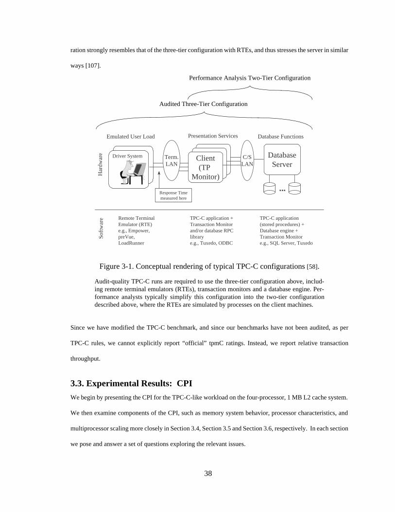
38

ration strongly resembles that of the three-tier configuration with RTEs, and thus stresses the server in similar

ways [107].

Since we have modified the TPC-C benchmark, and since our benchmarks have not been audited, as per

TPC-C rules, we cannot explicitly report “official” tpmC ratings. Instead, we report relative transaction

throughput.

3.3. Experimental Results: CPI

We begin by presenting the CPI for the TPC-C-like workload on the four-processor, 1 MB L2 cache system.

We then examine components of the CPI, such as memory system behavior, processor characteristics, and

multiprocessor scaling more closely in Section 3.4, Section 3.5 and Section 3.6, respectively. In each section

we pose and answer a set of questions exploring the relevant issues.

Audited Three-Tier Configuration

Performance Analysis Two-Tier Configuration

Figure 3-1. Conceptual rendering of typical TPC-C configurations [58].

Audit-quality TPC-C runs are required to use the three-tier configuration above, includ-ing remote terminal emulators (RTEs), transaction monitors and a database engine. Per-formance analysts typically simplify this configuration into the two-tier configurationdescribed above, where the RTEs are simulated by processes on the client machines.

Response Timemeasured here

DatabaseServer

......

Client(TP

Monitor)

C/SLAN

Term.LAN

Presentation Services Database FunctionsEmulated User Load

Har

dwar

e

Remote TerminalEmulator (RTE) e.g., Empower,preVue,LoadRunner

Soft

war

e TPC-C application +Transaction Monitor and/or database RPC librarye.g., Tuxedo, ODBC

TPC-C application (stored procedures) + Database engine +Transaction Monitore.g., SQL Server, Tuxedo

Driver System

39

The question motivating this section is: “how does OLTP database CPI compare with the theoretical µCPI

possible on the Pentium Pro?” Using the Pentium Pro events that count the number of cycles and the number

of instructions retired during the measurement period, we computed the cycles per micro-operation, µCPI,

and the cycles per macro-instruction, CPI, for the database, the operating system, and the overall system.

Table 3-2 and Figure 3-2 present this data. We begin by discussing the µCPI.

The overall measured µCPI is 1.55. Our system spends between 76% and 80% of its execution time in data-

base code, which has a measured µCPI of 1.37. The remaining time is spent in the operating system at a

measured µCPI of 2.87, over two times the database µCPI. The system is idle for less than 1% of the time.

We note that the percentage of time in the OS is not higher because the database re-implements some OS

services (for example, buffer management, user-level thread management). This structure leaves the OS with

only minimal tasks, such as disk I/O initiation and completion and network communication. These µCPI

values are 4X to 8.5X greater than the 0.33 theoretical minimum µCPI for the Pentium Pro. To understand

this discrepancy, we further decompose the µCPI into computation and stall cycles, as shown in Table 3-2

and Figure 3-2.

Computation µCPI is based on the µop retire profile presented in Section 3.5.1. We assume µops retired in

triple-retire cycles require 0.33 cycles in the steady state, double-retire cycle µops take 0.5 cycles, and sin-

µCPI/CPI ComponentµCPI: Overall µCPI: DB µCPI: OS

CPI: Overall

CPI: DB

CPI: OS

Resource stalls 0.35 0.25 1.15 0.66 0.45 2.56

Instruction-related stalls 0.66 0.62 1.00 1.24 1.13 2.24

Computation: µops 0.54 0.53 0.56 1.00 0.97 1.24

Computed µCPI/CPI 1.55 1.40 2.71 2.89 2.55 6.04

Measured µCPI/CPΙ 1.55 1.37 2.87 2.90 2.52 6.41

Table 3-2. Breakdown of cycles per micro-operation (µCPI) and cycles per macro-instruction (CPI) components for four-processor, 1MB L2 cache system.

The difference between µCPI and CPI is the ratio of µops to macro-instructions. This ratio is1.87 overall, 1.84 for the database alone, and 2.23 for the operating system alone. Comparingthe measured CPIs against those calculated from the computation, resource stall andinstruction-related stall components, we find that the computed values are within 6% ofthe measured values in all cases.

40

gle-retire µops need one cycle. This computation determines the number of cycles per µop. We note that this

model assumes a steady-state execution time of one cycle per µop. For example, if 53% of the database µops

are retired in triple-retire cycles, 22% in double-retire cycles, and 25% in single-retire cycles, the database

computation µCPI is 0.53*0.33 + 0.22*0.5 + 0.25*1 = 0.53 cycles per µop.

Comparing computation and stall µCPI, we note that stalls dominate. Stalls comprise 65% of the overall

µCPI, 63% of the database µCPI and 75% of the operating system µCPI. The bulk of these stalls are due to

cache misses, which will be described in more detail in Section 3.4. We note that the relative importance of

the CPI components is different for the database and operating system. For the database alone, instruc-

Figure 3-2. Breakdown of cycles per micro-operation (µCPI) for base system.

Recall from Section 2.6 on page 27. that the Pentium Pro provides event types to monitorresource stalls and instruction-related stalls. Instruction-related stalls count the number ofcycles instruction fetch is stalled for any reason, including L1 instruction cache misses,ITLB misses, ITLB faults, and other minor stalls [15] [50]. Resource stalls account forcycles in which the decoder gets ahead of execution. For example, resource stalls encom-pass the conditions where register renaming buffer entries, reorder buffer entries, memorybuffer entries, or execution units are full. In addition, serializing instructions (e.g.,CPUID), interrupts, and privilege level changes may spend considerable cycles in execu-tion, forcing the decoder to wait and incrementing the resource stalls counter. Stalls dueto data cache misses are not explicitly included in resource stalls; however, if some otherresource becomes oversubscribed due to a long data cache miss, the resource stall counterwill be incremented.

0

0.5

1

1.5

2

2.5

3

DB OS Overall

Mode

Cyc

les

per

µop

( µC

PI)

Resource StallsInstruction StallsComputation

Theoretical:0.33

41

tion-related stalls are the biggest CPI component, followed by computation and resource stalls. In contrast,

the order of importance for the OS alone is resource stalls, followed by instruction-related stalls and compu-

tation. We hypothesize that the importance of resource stalls is due to the prevalence of long-lasting opera-

tions in the OS that cause execution to lag behind the decoder (e.g., serializing instructions, interrupt

handling, and privilege level changes).

Table 3-2 also shows the breakdown of cycles per macro-instruction (CPI). The difference between these

values and the µCPI values is the ratio of µops per macro-instruction. The measured CPI for the overall

system is 2.90, which can be decomposed into the measured database component, 2.52, and the measured

operating system component, 6.41. In contrast, the majority of the SPEC 95 programs have a CPI between

0.5 and 1.5 on the Pentium Pro with a 256 KB L2 cache [15].

3.4. Experimental Results: Memory System Behavior

We begin our more in-depth analysis of the CPI components by examining memory system behavior. In the

following sections we present results for the overall system (database + operating system) only, without

detailed discussion of the differences between database and operating system behavior. Detailed perfor-

mance information for the overall system behavior, database-only behavior and the OS-only behavior, are

shown in the appendix in Chapter 9. In general, the characteristics of the database and OS are similar, with

the OS exhibiting somewhat worse behavior. For a discussion of the database-only behavior, we refer the

interested reader to [53].

3.4.1. How do OLTP cache miss rates vary with L2 cache size?

We examined how cache miss ratios change as cache size increases by physically changing the processor

boards to measure configurations with 256 KB, 512 KB and 1 MB L2 caches. Figure 3-3 summarizes the

overall system L2 cache miss behavior. As expected, the high-order effect of increasing cache size is a

decrease in L2 cache misses, and in the corresponding cache miss rates. Overall L2 miss rates decrease by

31% (from 16% to 9%) as L2 cache size increases from 256 KB to 512 KB, and by another 33% (from 9%

to 6%) as the size is further doubled to 1 MB. We see that instruction-related L2 cache misses are nearly

fully satisfied by the 1 MB cache. As shown in Figure 3-3, only one L2 cache miss occurs for every 1000

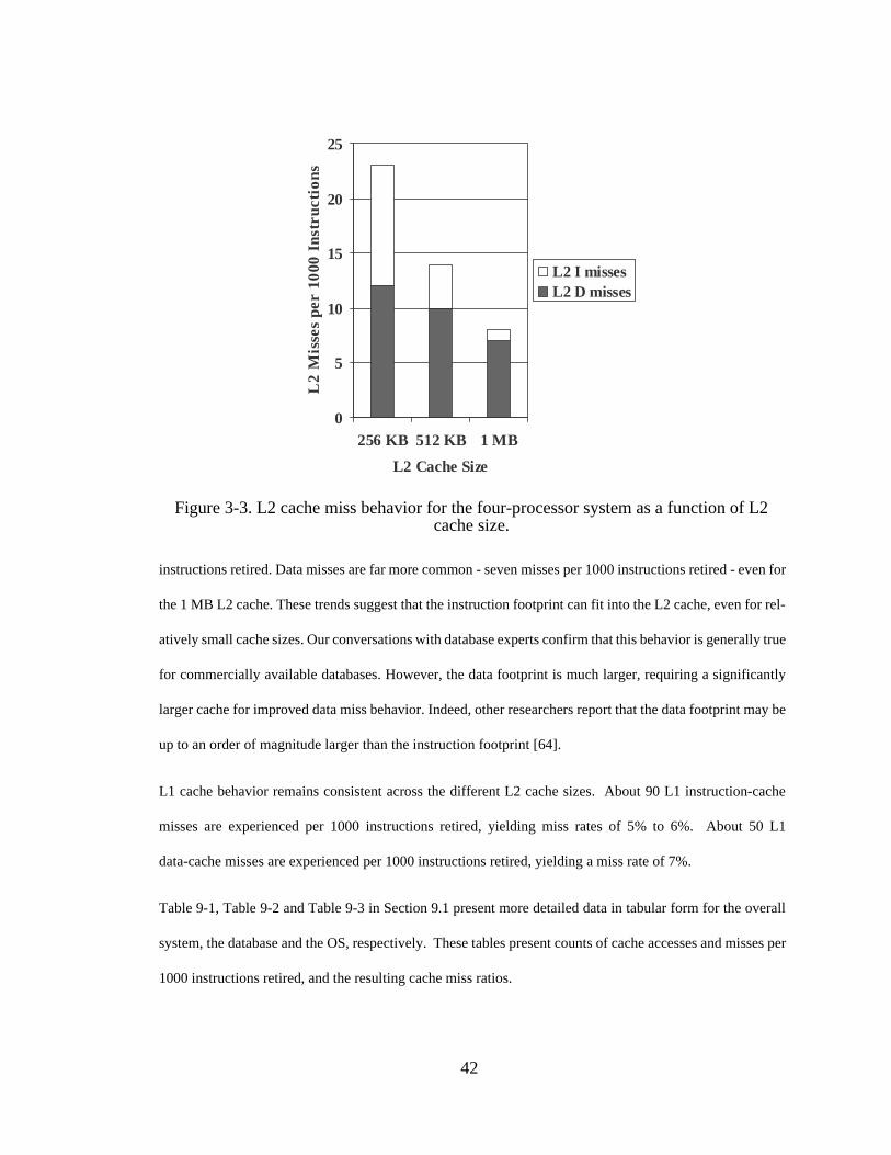
42

instructions retired. Data misses are far more common - seven misses per 1000 instructions retired - even for

the 1 MB L2 cache. These trends suggest that the instruction footprint can fit into the L2 cache, even for rel-

atively small cache sizes. Our conversations with database experts confirm that this behavior is generally true

for commercially available databases. However, the data footprint is much larger, requiring a significantly

larger cache for improved data miss behavior. Indeed, other researchers report that the data footprint may be

up to an order of magnitude larger than the instruction footprint [64].

L1 cache behavior remains consistent across the different L2 cache sizes. About 90 L1 instruction-cache

misses are experienced per 1000 instructions retired, yielding miss rates of 5% to 6%. About 50 L1

data-cache misses are experienced per 1000 instructions retired, yielding a miss rate of 7%.

Table 9-1, Table 9-2 and Table 9-3 in Section 9.1 present more detailed data in tabular form for the overall

system, the database and the OS, respectively. These tables present counts of cache accesses and misses per

1000 instructions retired, and the resulting cache miss ratios.

0

5

10

15

20

25

256 KB 512 KB 1 MB

L2 Cache Size

L2

Mis

ses

per

1000

Ins

truc

tion

s

L2 I missesL2 D misses

Figure 3-3. L2 cache miss behavior for the four-processor system as a function of L2 cache size.

43

3.4.2. What effects do larger caches have on OLTP throughput and stall cycles?

Figure 3-4 shows the overall system CPI breakdown for the three L2 cache sizes. Doubling the second-level

cache size from 256 KB to 512 KB results in a 15% improvement in CPI, and quadrupling the cache size to

1 MB results in a 25% improvement in CPI. This improvement is attributable to improvements in both

instruction-related and resource stalls. Improvements in database transaction throughput roughly mirror the

CPI improvements: transaction throughput increases 16% as L2 cache size is doubled to 512 KB, and 28%

as the L2 size is quadrupled to 1 MB. More detailed numerical data is presented in Table 9-4 in Section 9.2.

3.4.3. How successful are non-blocking L2 caches at reducing OLTP memory stalls?

To study the effectiveness of non-blocking second-level caches, we take advantage of a BIOS parameter that

allows us to limit the number of outstanding system bus requests [50]. Ideally, we would limit each of the

four processors to a single outstanding bus request, and compare behavior under this regime against the

behavior under normal bus operation (up to 4 requests outstanding per processor, and up to 8 requests across

all processors). However, our BIOS parameter permits only two options for the total number of outstanding

bus requests across all processors: up to 8, and one. Thus, we instead compare a uniprocessor under the

Figure 3-4. Overall CPI breakdown for the four-processor system as a function of L2 cache size.

0

0.5

1

1.5

2

2.5

3

3.5

4

4.5

256 KB 512 KB 1 MB

L2 Cache Size

Cyc

les

per

Mac

ro-i

nstr

ucti

on (

CP

I)


44

normal bus operation (up to 4 requests outstanding for the single processor) with a uniprocessor limited to a

single outstanding bus request.

We performed this experiment for both 1 MB and 256 KB caches, and in both cases found negligible differ-

ence between the configuration where the processor was allowed 4 outstanding requests, versus the config-

uration where the processor was limited to a single outstanding request. Table 3-3 presents results for several

key parameters for the 256 KB experiment.

The latencies to memory on an L2 cache miss are too long for the out-of-order engine to cover them com-

pletely. It should be possible, though, for two or more L2 misses to overlap with each other, thus reducing

memory-related stall time. This does not appear to be the case, however: improvements in stalls are negli-

gible. This behavior leads us to believe that multiple outstanding requests from a single processor aren’t

prevalent enough to greatly improve the stall component of CPI. However, in a multiprocessor environment,

we would expect cache misses from multiple processors to be overlappable.

3.5. Experimental Results: Processor Issues

In addition to memory hierarchy-related stall CPI components, a significant component of CPI (both compu-

tation and stall cycles) is due to processor features. In this section we examine some of these processor fea-

tures.

3.5.1. How useful is superscalar issue and retire for OLTP?

In the Pentium Pro, three parallel decoders translate x86 macro-instructions into µops. Each cycle, up to

three µops can be retired in the out-of-order engine, and up to three x86 instructions can be retired in the

Characteristic 1 bus req. up to 4 bus req.

Measured CPI 3.08 3.02

Computation CPI 1.00 1.01

Resource Stall CPI 0.52 0.49

Instruction Stall CPI 1.55 1.52

Average memory latency 60 cyc. 58 cyc.

Table 3-3. Effects of non-blocking for 256 KB L2 cache for the uniprocessor system.

45

in-order engine. Figure 3-5 and Figure 3-6 present the profiles for instruction and micro-operation decode

and retire behavior, broken down by cycles and instructions, respectively. Section 9.3 presents this data in

tabular form, including data for database-only and OS-only behavior. Figure 3-5 shows that the system expe-

riences a high percentage (e.g., 65% to 75%) of cycles where zero instructions (or µops) are decoded or

retired. In contrast, the SPEC integer programs with high L2 cache miss rates show far fewer cycles (i.e.,

35% to 51%) with no instructions decoded or retired [15].

Figure 3-6 presents the same profiles, organized by the percent of instructions (or µops) decoded/retired in

each type of cycle. At the macro-instruction level, only 32% of all instructions are decoded in triple-decode

cycles, and only 22% of all instructions are retired in triple-retire cycles. Since there is only a modest benefit

from macro-instruction triple-decode and -retire cycles, this workload may not benefit from increases in

macro-instruction superscalar width. The system more effectively exploits the superscalar width in the

out-of-order execution of µops: 53% of all µops are retired in triple-retire cycles. Thus, increasing super-

scalar width for the out-of-order engine may prove to be beneficial.

0%

20%

40%

60%

80%

100%

Inst.Decoded

Inst.Retired

UopsRetired

Per

cent

of

Cyc

les

3-inst2-inst1-inst0-inst

Figure 3-5. Decomposition of instruction and micro-operation decode and retirement cycles for the four-processor, 1 MB L2 cache system.

46

Finally, we note that 1.87 µops are retired for every macro-instruction for the transaction processing work-

load. In contrast, the average number of µops per macro-instruction is around 1.35 for the SPEC programs

[15]. This implies that the transaction processing workload utilizes more complex x86 instructions than the

SPEC programs do.

3.5.2. How effective is branch prediction for OLTP?

Table 3-4 shows branch behavior for the overall system, the database alone and the operating system alone.

The behavior of the overall system is nearly identical to the behavior of the database alone. Branches com-

prise about 21% of the overall instruction mix. The branch misprediction ratio is 15%, which is quite high

relative to the branch misprediction ratios of less than 10% for the SPECInt applications.

Branch Target Buffer (BTB) miss ratios are also quite high: 56% for both the overall system and the database

alone. The operating system exhibits much better BTB miss behavior, with a 33% miss rate. The overall ratio

is in contrast to the SPEC workloads, where all programs except one integer program exhibit a BTB miss

ratio of less than about 30%. Most SPEC BTB miss ratios are well below 15% [15].

0%

20%

40%

60%

80%

100%

Inst.Decoded

Inst.Retired

UopsRetired

Per

cent

of

Inst

ruct

ions

3-inst2-inst1-inst

Figure 3-6. Instruction and micro-operation decode and retirement profiles, broken down by instructions, for the base system.

47

One reason for this branch and BTB behavior is that the compilation process used for the database application

employed only traditional compiler optimization techniques, but did not employ more advanced optimization

techniques, such as profile-based optimization. This technique, which can move infrequently executed basic

blocks out of line and lay out more frequently interacting basic blocks contiguously, could improve branch

misprediction and BTB miss behavior, as well as L1 instruction cache miss behavior [87]. However, there

is a limit to the savings this technique can offer. Furthermore, processors must be able to efficiently execute

code even if it has not been aggressively optimized. At the least, these miss ratios suggest that this workload

requires a much larger BTB, and perhaps a different branch prediction method. Hilgendorf and Heim report

that BTB miss rates improve for BTBs up to ~16k entries for OLTP workloads [45].

Finally, we note that the speculative execution factor, or the number of macro-instructions decoded divided

by the macro-instructions retired, is 1.4 for the overall system. The speculative execution factor for nearly all

SPEC programs is between 1.0 and 1.3 [15].

3.5.3. Is out-of-order execution successful at hiding stalls for OLTP?

The Pentium Pro implements dynamic execution using an out-of-order, speculative execution engine, which

employs register renaming and non-blocking caches. How effective is dynamic execution for OLTP database

workloads?

Characteristic Overall DB OS

Branch frequency 21.5% 20.9% 27.3%

Branch misprediction ratio 14.6% 14.3% 16.6%

BTB miss ratio 55.7% 55.6% 32.9%

Speculative exec. factor 1.43 1.40 1.75

Table 3-4. Branch behavior for the four-processor, 1 MB L2 cache system.

The Pentium Pro processor implements a branch prediction scheme derived from thetwo-level adaptive scheme described by Yeh and Patt [120]. The branch target buffer(BTB), which contains 512 entries, maintains branch history information and the pre-dicted branch target address. A static prediction scheme (backwards taken, forward nottaken) is employed. Mispredicted branches incur a penalty of at least 11 cycles, with theaverage misprediction penalty being 15 cycles [39].

48

It is difficult to answer this question precisely, without the ability to turn off out-of-order execution. Instead,

our approach is to compare non-overlapped CPI vs. measured CPI, as described in [15]. If out-of-order exe-

cution is effective, the individual components of the non-overlapped CPI should be overlappable, and the

measured CPI should be less than the non-overlapped CPI.

To compute the non-overlapped CPI, we treat the machine as if it were in-order, and explicitly account for

computation and all potential stall cycles, such as instruction and data cache miss-related stalls, branch

misprediction penalties, resource-related stalls, and other minor stalls. Cache miss and branch misprediction

penalties are computed by multiplying the number of misses per instruction by the associated miss penalty.

The computation component is somewhat more challenging to compute accurately. As shown in

Section 3.5.1, this workload takes advantage of the superscalar retire capabilities of the Pentium Pro’s

out-of-order core. It is difficult to discern, however, how much of this instruction-level parallelism (ILP) is

due to the out-of-order nature of the processor and how much is due to the superscalar nature that an in-order

processor could exploit. As a result, we calculate the computation component for our non-overlapped CPI in

two ways, to provide an upper and lower bound on the amount of non-overlapped computation. The naive

estimate (“OPT”) treats all µops as single-issue, effectively attributing all of the ILP to out-of-order execu-

tion. The OPT computation component allocates one cycle for each µop retired per macro-instruction. We

calculate the pessimistic (“PES”) estimate, which allocates all of the ILP to superscalar-ness that could be

exploited by an in-order processor, from the µop retirement profile, as described in Section 3.3. We assume

a steady-state µCPI of 0.33 for triple-retire cycles, 0.5 for double-retire cycles, and 1 for single-retire cycles.

The computation CPI is then computed by multiplying the µCPI by the µops per macroinstruction. The OPT

and PES estimates provide upper and lower bounds, respectively, on the degree to which stall components

can be overlapped in an out-of-order processor. Neither model is completely accurate; the true value lies

somewhere in this range.

Figure 3-7 presents the non-overlapped and measured CPI for the three different L2 cache sizes. The stacked

bars for each configuration include the resource stalls, and decompose the stall components further to include

L1 I and D cache misses, L2 cache misses, branch misprediction stalls, ITLB misses and other minor stalls.

49

“OPT” presents the optimistic estimate, and “PES” presents the pessimistic estimate, as described above. The

black line in each column marks the measured CPI for that configuration. Note that the only difference

between the “OPT” and “PES” bars is the computation component.

For all cache sizes, the measured CPI is less than the non-overlapped total, implying that out-of-order exe-

cution is effectively hiding some of the potential stalls. Using the OPT computation model, out-of-order exe-

cution hides 41% of the non-overlapped CPI for the 256 KB L2 cache, 37% for 512 KB L2 and 34% for the

1 MB L2. Out-of-order execution is less effective according to the PES computation model: 32% of the

non-overlapped CPI can be hidden for the 256 KB L2 cache, 24% for the 512 KB L2 and 18% for the 1 MB

L2. Thus, out-of-order execution is effectively overlapping some of the CPI components to achieve a lower

actual CPI. In comparison, the measured CPI of SPECInt programs is 35% to 55% (averaging 46%) of the

OPT non-overlapped total for a 256 KB L2 [15].

Figure 3-7. Non-overlapped and measured CPI as a function of L2 cache size.

Latency from each of the components above is shown as a portion of the bar graph. L1miss penalties are presented in Table 2-5 on page 26, L2 miss penalties in Table 3-9,and branch misprediction penalties in the caption for Table 3-4. PES attributes ILP tosuperscalar-ness that can be exploited by an in-order processor, while OPT attributesILP to out-of-order execution. Note that, for a given cache size, the only difference betweenthe PES and OPT stacked bars is the computation component; all stall components are the same.

0

1

2

3

4

5

6

7

L2 Cache Size

Non

-ove

rlap

ped

CP

I ComputationL2 I MissesL2 D MissesResource StallsInst Len Decoder StallsITLB MissesL1 I MissesL1 D MissesBranch Mispredictions

Measured CPI

256 KB 512 KB 1 MB

PES OPT PES OPT PES OPT

50

3.6. Experimental Results: Multiprocessor Scaling Issues

In this section, we explore the scalability of the Pentium Pro architecture for running OLTP workloads as the

number of processors is varied from one to two to four. Specifically, we examine the increase in L2 coher-

ence misses, the MESI profile for L2 caches, and the memory system utilization as the number of processors

is increased.

3.6.1. How well does OLTP performance scale as the number of processors increases?

Figure 3-8 shows the scalability of relative database transaction throughput as a function of the number of

processors. We present a separate graph for each L2 cache size, with throughput relative to the uniprocessor

configuration for that cache size (e.g., performance for the 512 KB two- and four-processor configurations

is relative to the 512 KB uniprocessor.) For these experiments, the number of processors is restricted at boot

time, and the database buffer memory is held constant at 512 MB per processor. As stated in Section 3.2, the

ratio of TPC-C throughput to database size (i.e., number of warehouses) must fall within the range from 9 to

12.7. To maintain the correct ratio values, we scaled the size of the database for the two-processor and uni-

processor cases.

As demonstrated in the figure, transaction throughput scales reasonably well as the number of processors is

increased from one to four. However, linear speedup is not achieved due to several software and hardware

factors, collectively known as multiprocessor stretch [113]. Software factors include the increased conten-

tion for database and operating system data structures and the resulting growth in code path for inter-proces-

sor synchronization. Hardware factors include greater memory bus and memory system contention and

increases in cache coherency traffic. We explore several of the sources of multiprocessor stretch in the fol-

lowing sections.

3.6.2. How do OLTP CPI components change as the number of processors is scaled?

Table 3-5 shows the measured CPI and its constituent computation and stall components for each of the con-

figurations shown in Figure 3-8. We observe that for each cache size, measured CPI, resource stalls, and

instruction-related stalls increase as the number of processors is scaled from one to four. These increases are

51

largest for the 256 KB cache: a 28% increase in overall CPI, coupled with a 78% increase in resource stalls

and a 35% increase in instruction-related stalls. The magnitude of the increases slows with the larger cache

sizes, resulting in a 7% increase in CPI for the 1 MB cache.

We hypothesize that the behavioral differences between cache sizes are due to the differing impacts of L2

miss behavior. We explore three aspects of this behavior, namely the prevalence of cache coherence traffic,

memory system utilization, and application memory latency, in the following two sections.

3.6.3. How prevalent are cache misses to dirty data in other processors’ caches for OLTP?

Although increasing the L2 cache size has the potential to decrease the number of capacity and conflict

misses, it also has the potential to increase the number of communication (or coherence) cache misses

between processor caches. In particular, “dirty misses,” or misses to dirty data in other processors’ caches,

Figure 3-8. OLTP throughput scalability.

Throughput for each cache size is relative to the uniprocessor configurationfor that cache size. In each experiment, memory is held constant at 512 MBper processor. For the one- and two-processor configurations, the size of thedatabase is scaled to maintain the prescribed throughput to database sizeratio.

100

150

200

250

300

350

400

1 2 3 4

Number of Processors

Rel

ativ

e T

hrou

ghpu

t (p

erce

nt)

Linear1 MB L2512 KB L2256 KB L2

Cache 1 P 2 P 4 P

Linear 100% 200% 400%

256 KB 100% 194% 345%

512 KB 100% 194% 324%

1 MB 100% 184% 296%

52

have been shown to be a key factor in OLTP performance [12] [73] [83]. This difficulty arises in some archi-

tectures because many RISC processors have been optimized to give the local CPU priority to the L2 cache.

In addition, they are typically optimized for providing high bandwidth, rather than low latency, to the L2

cache for the CPU and incoming requests. These optimizations often have the side effect of increasing the

latency for dirty misses [34].

Unfortunately, the Pentium Pro counters provide no events for determining the latency of dirty misses. It is

still useful, however, to quantify the frequency of this operation, and determine how it is affected by L2 cache

size.

Table 3-6 presents the percentage of L2 cache misses to dirty data in other processors’ caches for one-, two-,

and four-processor servers and different L2 cache sizes. It appears that doubling the size of the cache nearly

doubles the percentage of L2 misses to dirty data. Likewise, doubling the number of processors roughly dou-

bles the percentage of L2 misses to dirty data. As the cache size increases, this percentage could be quite

large.

Characteristic 1 P 2 P 4 P

256 KB

Measured CPI 3.02 3.27 3.86

Resource stalls 0.49 0.60 0.87

Instruction-related stalls 1.52 1.68 2.05

Computation 1.01 1.00 0.98

512 KB





1 MB





Table 3-5. CPI Components as the number of processors is scaled.

53

3.6.4. Is the four-state (MESI) invalidation-based cache coherence protocol worthwhile for OLTP?

Cache lines may be in one of four states in the MESI protocol: modified (M), exclusive (E), shared (S), or

invalid (I). Some coherence protocols don’t distinguish between exclusive (exclusive clean) and modified

(exclusive dirty). In this section, we investigate whether all four states are used by this workload, and use this

analysis to confirm the effectiveness of the cache write policy.

The Pentium Pro counters allow us to monitor the MESI state of an L2 cache line on an access to the L2 cache

(e.g., instruction fetch, load or store.) Accesses to “invalid” lines correspond to cache misses, while accesses

to lines in other states correspond to hits to an L2 line found in that state, before any modifications due to that

access are made. Table 3-7 shows the percentages of L2 cache instruction fetches, loads and stores, broken

down by MESI state. (Table 9-8 and Table 9-9 present database- and operating system-specific MESI behav-

ior.)

Nearly all of the instruction fetches that hit in the L2 cache are to shared cache lines. This observation is

expected, since instructions aren’t modified, and as a result there is no need to keep them in the modified or

exclusive states. The exclusive state is heavily utilized for loads in the uniprocessor case, as might be

expected for a single processor, where nothing need be shared with other processors. In the dual- and

Table 3-6. Percentage of L2 cache misses to dirty data in another processor’s cache as a function of L2 cache size and number of processors.

The absolute number of dirty misses across all active processors for the five-second mea-surement window is given in millions by the number in parentheses. We hypothesize thatthe count for the uniprocessor case is non-zero because we did not specify the uniproces-sor status at operating system and database start-up times. As a result, both the operatingsystem and the database may be exercising their multiprocessor code paths, even thoughthey are executing on a single processor. Another possible explanation for the non-zerocounts is that the signal used to indicate a hit to dirty data is also raised, in conjunctionwith another signal, to indicate that the processor wishes to stall during the snoop buscycle.

L2 Cache Size 1 P 2 P 4 P

256 KB 0.4% (0.03M) 3.4% (0.49M) 5.7% (1.38M)

512 KB 0.7% (0.04M) 6.1% (0.62M) 11.8% (1.96M)

1 MB 1.1% (0.04M) 11.2% (0.80M) 22.0% (2.45M)

54

quad-processor configurations, hits resulting from loads are distributed across the different states, going pre-

dominantly to shared lines, followed by modified lines and finally exclusive lines. The high percentage of

load hits to modified lines indicates that the processor reads data in the same line as it has recently written.

In addition, over 90% of the database store hits are to modified lines, with few write accesses to shared or

exclusive lines. These measurements provide quantitative evidence of the temporal locality present in the

workload, and validate the usefulness of the writeback write policy employed by the Pentium Pro caches.

A primary advantage of the exclusive state is that it allows the processor to avoid the invalidation bus trans-

action on a store to a shared line: if the line is already in the exclusive state, it is the only copy currently

cached. However, we see that store hits to exclusive lines rarely occur. Thus, it isn’t clear whether the bene-

fits of the E state are worth the cost of implementing the fourth state for this workload. A three-state protocol

might be sufficient, and not result in significantly increased bus traffic.

Configuration and L2 Access Type M E S

(Miss)I

INST. FETCH

1 processor 0.0% 0.8% 97.8% 1.4%

2 processors 0.0% 0.0% 98.8% 1.2%

4 processors 0.0% 0.0% 98.8% 1.2%

LOAD

1 processor 25.4% 55.5% 1.1% 18.0%

2 processors 21.7% 17.6% 43.9% 16.9%

4 processors 24.7% 15.1% 46.0% 14.2%

STORE

1 processor 78.5% 1.5% 0.1% 19.9%

2 processors 78.0% 1.0% 4.4% 16.6%

4 processors 81.2% 0.6% 6.7% 10.5%

Table 3-7. State of L2 line on L2 hit.

Table shows percentage of L2 accesses. Note that the Stores category includes indications from the L1 D cache that a line has changed state from invalid to modified; thus the L2 is aware of the modified status of modified lines residing in the L1 data cache.

55

3.6.5. How does OLTP memory system performance scale with increasing cache sizes and increasing processor count?

Table 3-8 presents the memory system utilization across all of the processors in the system for different cache

sizes. By memory system utilization, we mean the time the bus is busy transferring data (or control informa-

tion), or the time when the bus is not busy but unavailable. This latter case may happen when some bus agent,

for example the memory controller, falls behind in its internal processing. The exact counters and formulae

used to compute memory system utilization are shown in Table 8-12 on page 197.

As expected, memory system utilization decreases with increasing cache size, and increases with more pro-

cessors. Utilization grows more slowly for the 1 MB cache size as the number of processors grows, reaching

a maximum of nearly 50% for four processors. However, even at these relatively low utilizations, bus activ-

ity has an impact on the memory latency perceived by the database and operating system.

Table 3-9 presents the application memory latency as a function of the L2 size and the number of processors.

These cycle counts are calculated from counter values that measure the number of cycles where data read

transactions are outstanding on the bus, and the total number of data read transactions. (The exact counters

and formulae are shown in Table 8-12 on page 197.) This technique for computing application memory

latency was calibrated with the dependent load latency reported in Table 2-1 on page 17: both techniques

yield a nominal dependent load latency of 38 processor cycles. We note that this measure does not account

for any overlap of memory accesses supported by the Pentium Pro’s non-blocking L2 cache.

We see that application reads take roughly 60 cycles for the uniprocessor case, but nearly 100 cycles for the

four-processor configuration for the 1 MB cache size. These latencies are considerably longer than the nom-

inal 38-cycle dependent load latency. Because memory system utilization and application memory latency

Table 3-8. Overall memory system utilization as a function of L2 cache size and number of processors.


256 KB 30.2% 53.9% 89.3%

512 KB 22.4% 41.9% 67.0%

1 MB 18.3% 30.7% 47.3%

56

continue to grow as processors are added, even for larger cache sizes, it is not clear to what degree this

memory system will scale to support additional processors.

3.7. Experimental Results: I/O Characterization

In this section, we explore the following question: “what is the frequency and size of I/O operations in the

OLTP workload?” We show that there are two predominant kinds of accesses, namely small random reads

and writes. For the version of Informix we examined, these small operations typically access 2 KB per I/O

operation [40]. Small reads are used for index and data page lookups, while small writes are used for updates

to index and data pages and for logging purposes. We measure I/O patterns during the steady-state

(non-checkpoint) transaction activity of the OLTP workload. We hypothesize that the average absolute read

and write rates, and the ratio between reads and writes may be different during the checkpoint phase of the

workload.

We examine this question using NT’s performance monitor, by measuring the number of file operations per

second, and the number of bytes read or written per second. Figure 3-9 displays the read and write rates for

the OLTP workload. Each data point in the figure shows the number of file operations per second, averaged

over a 15-second measurement interval. We observe that the average read rate is relatively constant at 1585

reads per second. The write rate experiences slightly more variation, possibly due to the bursty nature of log-

ging activity, averaging 1295 writes per second. Thus, the ratio of reads to writes for this workload is about

1.22X.

Table 3-9. Application memory latency as a function of L2 cache size and number of processors. (All values are in processor cycles.)


256 KB 58 cyc 72 cyc 118 cyc

512 KB 58 cyc 72 cyc 111 cyc

1 MB 58 cyc 74 cyc 97 cyc

57

3.8. Related Work

Several recent studies began the examination of the architectural impacts of transaction processing database

workloads. The activities of these studies range from OLTP workload characterization to evaluation of new

processor architectures and architectural features to new methodological advances in performing work-

load-driven evaluations. Several points of common wisdom have emerged from these studies. OLTP spends

a non-negligible percentage (15% to 30%) of time in the operating system, and typically performs more I/O

than other technical workloads. OLTP’s CPI is considerably higher than the CPI of the SPEC integer bench-

marks, and possesses a significant stall component. These stalls are generally due to high instruction- and

data-cache miss rates. Several simulation studies have indicated that larger caches, with higher associativity

and larger line sizes, can alleviate these high miss rates. This improvement comes at a cost, however:

increased cache sizes lead to non-negligible communication (coherence) misses in multiprocessors, espe-

0

200

400

600

800

1000

1200

1400

1600

1800

0:00:00 0:02:30 0:05:00 0:07:30 0:10:00 0:12:30 0:15:00 0:17:30 0:20:00 0:22:30

Time

File

Ope

rati

ons

per

Seco

nd

File Reads per Sec

File Writes per Sec

Figure 3-9. OLTP file read and write rates.

Each data point corresponds to the average number of file operations per second, aver-aged over a 15-second measurement interval.

58

cially as the number of processors grows large. Several studies have observed benefits from superscalar issue

and retire and out-of-order execution.

Initial studies reported that I/O bottlenecks limited the performance of their systems. These bottlenecks were

generally due to under-configured I/O systems. More recent studies with reasonably configured I/O sub-

systems report that the I/O-related stall time is negligible.

Several points remain unresolved. Conventional wisdom dictates that branch prediction is not as effective for

OLTP as for technical workloads, yet several studies using the Alpha 21164 report that OLTP branch predic-

tion is no worse than that of SPECint. Two studies indicate that little benefit is gained from making L2 caches

in out-of-order processors non-blocking, because multiple outstanding misses occur very infrequently.

Another study reports some benefits from non-blocking L2 caches, possibly due to the aggressiveness of the

processor and memory system simulated. Finally, rules of thumb have been proposed for scaling back OLTP

benchmarks to reduce the I/O requirements, but there has been no independent validation of these rules of

thumb for a different processor architecture or database server.

We have organized the related work into several categories: uniprocessor studies, symmetric multiprocessor

studies, CC-NUMA studies, and multithreading studies. The uniprocessor and (non-multithreaded) studies

are summarized in Table 3-10 and Table 3-11. The first part of these tables describes the configuration(s)

evaluated, including hardware, application software and workloads, and the evaluation technique. If no con-

figuration information is presented, it is because it was not sufficiently described in the paper. The second

part of the tables enumerates the conventional wisdom discussed above. The final sections of the tables

present other (non-contradictory) results and contradictory results demonstrated by each study. The follow-

ing sections describe the studies in more detail.

3.8.1. Uniprocessor Studies

3.8.1.1. Maynard, et al.: IBM RS/6000

Maynard, et al., used a proprietary software instrumentation tool to examine the performance of various tech-

nical and commercial workloads, including TPC-A and TPC-C, on the IBM RS/6000, which employs a Pow-

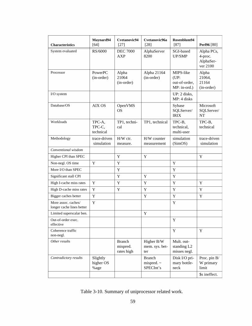
59

CharacteristicsMaynard94 [64]

Cvetanovic94 [27]

Cvetanovic96a [28]

Rosenblum94 [87] Perl96 [80]

System evaluated RS/6000 DEC 7000 AXP

AlphaServer 8200

SGI-based UP/SMP

Alpha PCs, 4-proc. AlphaSer-ver 2100

Processor PowerPC (in-order)

Alpha 21064 (in-order)


MIPS-like (UP: out-of-order,MP: in-ord.)

Alpha 21064, 21164 (in-order)

I/O system UP: 2 disks, MP: 4 disks

Database/OS AIX OS OpenVMS OS

Sybase SQLServer/IRIX

Microsoft SQLServer/NT

Workloads TPC-A, TPC-C, technical

TP1, techni-cal

TP1, technical TPC-B, technical, multi-user

TPC-B, technical

Methodology trace-driven simulation

H/W ctr. measure.

H/W counter measurement

simulation (SimOS)

trace-driven simulation

Conventional wisdom

Higher CPI than SPEC Y Y Y

Non-negl. OS time Y Y Y

More I/O than SPEC Y Y

Significant stall CPI Y Y Y

High I-cache miss rates Y Y Y Y Y

High D-cache miss rates Y Y Y Y Y

Bigger caches better Y Y Y Y

More assoc. caches/longer cache lines better

Y Y

Limited superscalar ben. Y

Out-of-order exec. effective

Y

Coherence traffic non-negl.

Y Y

Other results Branch mispred. rates high

Higher B/W mem. sys. bet-ter

Mult. out-standing L2 misses negl.

Contradictory results Slightly higher OS %age

Branch mispred. ~ SPECInt’s

Disk I/O pri-mary bottle-neck

Proc. pin B/W primary limit

$s ineffect.

Table 3-10. Summary of uniprocessor related work.

60

erPC processor [64]. In particular, they studied the execution-time breakdown between user and kernel mode,

branch misprediction, inter-branch distance, instruction execution frequency, and various cache miss rates.

With respect to operating system activity, they also studied process dispatch duration, which is the average

number of instructions a process executes before being context switched out. Their work also used simulation

to explore a variety of cache configurations, such as increased cache size, associativity, and block size.

This paper was the first to outline a broad categorization of the differences between OLTP workloads and

technical workloads. Their main findings were that common OLTP application factors, such as a large

number of user processes, high percentage of OS activity and non-looping branch behavior, create large

instruction footprints. These larger footprints cause higher L1 instruction cache miss rates, and would be

helped by increased cache size, up to 512 KB. Moreover, large instruction footprints are sensitive to dispatch-

ing behavior. Increasing associativity (e.g., beyond 2-way) and line size (e.g., up to 128 B) for large L1 and

L2 caches helps, but doesn’t help for small L1 caches. Finally, the large number of user processes leads to

very large aggregate data footprint for commercial workloads; they observed data footprints ten times larger

than the large instruction footprints. Because most of the data is process private, this data is not (and cannot

be) cache-effective. A slight benefit is seen for larger L1 data caches (e.g., up to 128 KB) with higher asso-

ciativity (e.g., up to 2-way) and larger line sizes (e.g., up to 32 or 64 bytes).

This study observed a higher percentage of operating system time than other more recent studies, including

ours, did. Their operating system percentage is roughly twice the percentage we observed. We hypothesize

that their database may not have been as well tuned as those used in the more recent studies.

3.8.1.2. Cvetanovic and Bhandarkar: Alpha Workstation Characterization

Cvetanovic and Bhandarkar studied the impact of several architectural characteristics on commercial and

technical workload performance for the Alpha 21064-based Alpha AXP [27] and Alpha 21164-based

AlphaServer 8200 [28]. In particular, they used built-in hardware counters to examine the breakdown of

user-kernel time and privileged architecture library (PAL) time, a decomposition of memory latency, L1 and

L2 cache miss rates, percentage of dual-issued instructions, and instruction set usage breakdown.

61

In [27], they find that commercial workloads, such as databases running TP1 and sorting benchmarks, have

higher OS activity (e.g., 20% - 25% vs. less than 5%) and make higher I/O subsystem demands than the SPEC

benchmarks. Commercial workloads also make higher demands on the cache/memory subsystem: 20% of

commercial application execution time is spent stalled waiting for memory, compared to less than 2% for

most SPEC workloads. Commercial applications also spend more time in PAL code, handling TLB misses,

interlocked queue operations, and mode changes. Finally, the pipeline stall time varies significantly between

the two workloads.

In [28], they demonstrate that the faster clock, larger on-chip cache, multiple instruction issue and low

latency memory system of the Alpha 21164 provide a nearly two-fold increase in TP1 transactions per second

over the Alpha 21064. In particular, the larger on-chip cache reduced the number of off-chip misses by a

factor of 1.7 times in TP workloads. They suggest that even larger caches would benefit TP1 more. The lower

latency and higher bandwidth memory subsystem helped commercial workloads, but not the SPEC bench-

marks. The doubling of FP and integer pipelines improves the multi-issuing time by 2 - 3X compared to the

21064. However, they find that for commercial workloads, the processor spends only 7% of the time

multi-issuing because of higher stall time. There is a slight reduction in the stall time. A larger on-chip

48-entry instruction TLB and separate 64-entry data TLB reduced the time spent handling TLB misses only

slightly.

3.8.1.3. Rosenblum, et al.: MIPS-based SGI Workstations

Rosenblum, et al., used the SimOS CPU simulator to study uniprocessor and multiprocessor performance of

Sybase SQL Server running a TPC-B-based OLTP database workload, as well as program development and

engineering workloads [87]. They analyzed I/O and memory system performance, and provided a detailed

decomposition of execution time (e.g., instruction execution time, instruction and memory stall time, and

synchronization time) for both user level and kernel level. They examined single instruction issue processors

with blocking caches, and multiple instruction issue processors with branch prediction and latency tolerating

features such as dynamic scheduling, non-blocking caches, and larger caches.

62

Their main finding was that disk I/O is the primary uniprocessor bottleneck, and its importance continues to

increase with new latency tolerant architectures. This finding differs from ours; we hypothesize that this dif-

ference is due to the small I/O configuration and the small number of server processes used in their simula-

tions. (Typically, a large number of server processes or threads is used when running OLTP workloads in

well-tuned configurations.)

The memory system was the second major bottleneck; the CPU is stalled for 50% of its (non-idle) execution

time waiting for memory. Larger caches and latency tolerance features such as non-blocking caches, improve

this bottleneck. Larger L1 instruction and data caches (e.g., up to 128 KB each), as well as increased L1 asso-

ciativity prove beneficial. Similarly, larger L2 caches (e.g., up to 4 MB) provide performance gains. They

demonstrate that dynamically scheduled processors are reasonably effective at hiding the shorter latencies of

L1 cache misses. However, they observed negligible reductions in stall time due to multiple outstanding L2

misses; this observation concurs with ours. Decoupling of the fetch and execute units in out-of-order proces-

sors is effective at hiding the latency of instruction cache misses; instruction cache miss latency may be over-

lapped with data cache miss latency. The study reports a modest 25% speedup from out-of-order, due

predominantly to the high percentage of I/O-induced idle time due to their underconfigured simulated disk

system.

They observe a non-negligible amount of coherence traffic for the multiprocessor simulations, due to the fre-

quent rescheduling of processes on different processors; this effect could be mitigated somewhat with the use

of processor affinity scheduling. Multiprocessor operating system services consume 30% to 70% more time

than the corresponding uniprocessor services, due to overhead and lock contention, coherence misses, and

extra instructions/misses for different data structures.

3.8.1.4. Perl and Sites: Alpha PCs

Perl and Sites used the PatchWrx tracing facility to gather traces of several technical workloads and a

TPC-B-based OLTP workload run by Microsoft SQL Server on a Windows NT-based Alpha 21064 PC [80].

They examined the processor pin bandwidth required for these workloads for two uniprocessor designs,

based on the 21064 the 21164. This examination is based on an estimation of the bandwidth required to

63

achieve a CPI of 1, and comparison of the estimated bandwidth to the actual bandwidth provided by the pro-

cessor. They also examined the prevalence of lock contention in a four-processor AlphaServer 2100.

Their primary finding is that processor pin bandwidth is the primary limitation to OLTP performance: they

estimate that the pins are overcommitted by factors of 2X to 4X for these processors. With this bottleneck,

other latency tolerance features, such as multiple instruction issue, code scheduling, improved external cache

latency or cache prefetching, prove ineffective. One possible explanation, pointed out in [13], is that the

authors ignored the latency-dependent nature of the OLTP workload. The dependent loads and branches

would likely limit performance before pin bandwidth became an issue.

Unlike the other papers in the literature, this study suggests that caching is ineffective for this workload: “The

trace looks somewhat similar to white noise - there is very little correlation between addresses. This applica-

tion falsifies the premise of a cache: that accessing a location is a good predictor that the same or a nearby

location will be accessed in the near future.” We hypothesize that this cache mis-behavior, as well as the high

pin bandwidths, may be due to the generation of synthetic addresses for 73% of the data locations accessed.

The other main finding in this paper is that lock contention and cache coherence overhead prevent the appli-

cation from scaling up beyond a small number of processors. A small number of locks contribute to the high

degree of contention, including convoy effects where processors line up spinning for a lock. Cache coherence

traffic is attributed to false sharing, which could be improved by putting frequently acquired locks in cache

lines separate from other variables.

3.8.2. Symmetric Multiprocessor Studies

3.8.2.1. Thakkar and Sweiger: Sequent Symmetry

Thakkar and Sweiger used a hardware monitoring tool to study the bus utilization, cache coherence miss

rates, and I/O rates for the TP1 benchmark running on a Sequent Symmetry cache-coherent symmetric mul-

tiprocessor (SMP) [100]. In addition, they explored the effects of larger caches, a faster clock rate, and pro-

cess migration. For memory-resident databases (e.g., “fully cached”), they found that performance is limited

by bus saturation caused by processes ping-ponging between processors. This effect was improved by pro-

64

CharacteristicsThakkar90 [100]

Cvetan96b [29]

Barroso98 [13]

Lovett96 [61]

Ranganath98 [83]

System evaluated 24-proc. Sequent Symmetry

4-proc. AlphaServer 4100 SMP


32-proc. Sequent CC- NUMA

4-proc. CC-NUMA server

Processor Alpha 21164 (in-order)



Pentium Pro

simulated (out-of- order)

I/O system 12 disks sim: in-mem. in-memory

Database/OS DYNIX OS Sybase Oracle/Unix Oracle/Unix

Workloads TP1 TPC-C,tech, multi-user

TPC-B, TPC-D

TPC-B, TPC-D Q6

TPC-B, TPC-D Q6

Methodology H/W counter meas.


H/W meas., trace-driven simulation

Model-based simula-tion


Conventional wisdom

Higher CPI than SPEC Y Y Y

Non-negl. OS time Y

More I/O than SPEC

Significant stall CPI Y Y Y

High I-cache miss rates Y Y Y

High D-cache miss rates Y Y Y

Bigger caches better Y Y Y

More assoc. caches/longer lines better

Y

Limited superscalar ben. Y Y


Y


Y Y Y

Other results OS and I/O lat. don’t dominate well-tuned DB behavior

Avg mem. latency incr. w/ more pro-cessors

Larger inst. windows provide more OOO benefit

Guide for scaling back

Inst stream buffer good

Contradictory results Bus satur. limits mem- res. perf.

Branch mispred. ~ SPECInt’s

Can exploit 2 outst. L2 $ misses

I/O limits perf.

Table 3-11. Summary of (non-threaded) multiprocessor related work.

65

cessor affinity and a reduction in the amount of intra-database communication. For the non-memory resident

(e.g., “scaled”) case, they reported that I/O was the limiting factor; these effects can be improved by connect-

ing more disk drives or increasing the size of main memory.

3.8.2.2. Cvetanovic and Donaldson: AlphaServer 4100 Characterization

Cvetanovic and Donaldson used the Alpha 21164 hardware counters to characterize the performance of the

four-processor AlphaServer 4100 family running a TPC-C-based OLTP workload on Sybase [29]. They also

examined several technical and multiuser workloads. Their study focused on the application CPI and its com-

putation and stall components, the effects of off-chip cache size, prevalence of cache misses, issue width

effectiveness, and instruction mix. Using the measured values as inputs, they describe a time allocation

model to estimate how time is allocated between various computation and stall components.

They report a CPI of about 3.7 for Sybase running TPC-C; this CPI is 2X to 4X higher than the SPECInt95

CPIs they measured on the same hardware. They found that roughly 80% of the time the processor was

stalled. Data-related (e.g., “frozen”) stalls, such as data cache misses and register and floating point conflicts,

comprised nearly 50%, and “dry” stalls, where there is no instruction to issue, comprised the remaining 30%.

They argue that the high stall time is caused by a high number of cache misses and the high associated miss

penalties when accessing the L3 (B) cache and memory. In contrast to our results, Cvetanovic and Donaldson

report that branch and branch misprediction frequencies for TPC-C on the Alpha 21164 are comparable to

those of SPECInt [29].

3.8.2.3. Barroso, et al.: Alpha Servers

Barroso, et al., use hardware counter measurements and SimOS simulation to evaluate the memory system

performance of a TPC-B-based OLTP workload running on Oracle on Alpha 21164-based SMPs [13].

Although their TPC-B database was small enough to fit into memory, they state that I/O operations still occur

for logging purposes. Furthermore, they state that the processor and memory behavior of their scaled-back

workload resembles that of a fully scaled TPC-C workload on the same hardware.

66

They find that operating system activity and I/O latencies don’t dominate behavior of well-tuned DB work-

loads on modern commercial engines. They report a CPI of 7.0 for the workload, which is roughly twice the

audited TPC-C CPI. More than 75% of the time is spent in memory hierarchy stalls. These stalls are split

nearly evenly between instruction and data-related cache misses. The time is split between hits to the 96 KB

second-level (S) cache and the 2 MB third-level (B) cache. Their simulation results indicate that both larger

(e.g., up to 8 MB L2) and more associative (e.g., up to two-way) B-caches, with longer cache lines (e.g., up

to 128 bytes), are beneficial to the workload. They report a high communication miss rate and the trend that

communication stalls increase linearly with the number of processors. Dirty misses are a large portion of

these communication misses: they comprise roughly 60% of all B-cache misses for a four-processor config-

uration with 8 MB 2-way set-associative B caches. Beyond an 8 MB B-cache, they observe that performance

is limited by true sharing misses.

This paper also gives guidelines for scaling back OLTP workloads, to reduce the I/O capacity and bandwidth

costs associated with fully-configured systems. When scaling back the datasets so that they fit into memory,

researchers must ensure that the relevant data structures are still orders of magnitude larger than the size of

the hardware caches in the system. The resulting reduction in disk capacity and bandwidth means that file

system files can be used for I/O, rather than raw devices. In this case, it is important to limit the size of the

file system buffer cache to avoid double buffering problems. Researchers must also use as many server pro-

cesses as would have been required to hide the I/O latencies in a non-scaled (i.e., out-of-memory) run. This

scaling is critical, because the number of processes per processor has a significant impact in the workload’s

cache behavior.

3.8.3. CC-NUMA Multiprocessor Studies

3.8.3.1. Lovett and Clapp: Sequent STiNG

In [61], Lovett and Clapp present the Sequent STiNG (later renamed NUMA-Q) CC-NUMA multiprocessor,

which is constructed from commodity quad Pentium Pro SMPs connected via a Scalable Coherent Interface

(SCI) ring. This design was intended to address the high latency present in large bus-based systems, by using

a two-level interconnect where most memory references could be satisfied with low latency by local memory.

67

The authors used TPC-B to evaluate the scalability of this new architecture, and to decompose the remote

latency experienced on an L2 cache miss. Their model-based simulation technique uses as its input perfor-

mance data from counters embedded in the cache and bus controllers and logic analyzer evaluation of the

system bus of existing machines.

They find that the average latency to satisfy a second-level cache miss increases with system size, as

quad-to-quad transfers are introduced, limiting the scalability of OLTP workload performance. Examining

remote memory latency for a 32-processor system, they find that protocol processing consumes the most

time, followed by the time spent arbitrating for and transferring data over the quad SMP bus. Both of these

categories is greater than the time spent sending and receiving SCI packets. They propose several alternatives

for improving the protocol processing overhead, including hardware support and an improved coherence pro-

tocol.

3.8.3.2. Ranganathan, et al.: Effects of ILP and Out-of-Order Execution

Ranganathan, et al., use trace-based simulation to explore the benefits of instruction-level parallelism (ILP)

out-of-order execution, non-blocking caches, instruction window size for a TPC-B-based OLTP workload

[83]. Traces were gathered for Oracle running on an AlphaServer 4100 platform, and then used as input to

an RSIM user-level simulation.

They report a CPI that is roughly 10 times the minimum possible CPI for their simulated system. L2 cache

misses, especially data communication misses, are a significant component of the stall cycles. They find that

the benefits of increasing issue width level off at two-way issue for in-order processors, and at four-way for

out-of-order processors. Out-of-order execution is beneficial because it presents the opportunity to overlap

instruction miss latency with previous instructions due to the decoupling of fetch and execute pipeline stages.

It also provides the opportunity to overlap data miss latency with other instructions. Larger instruction win-

dows provide more potential for overlap, leveling off at 64 entries. The benefits of out-of-order execution

and instruction issue width prove to be synergistic: they observe a 1.5X improvement for a wide-issue,

out-of-order multiprocessor over multiprocessor system with single-issue in-order processors. Their OLTP

workload can exploit up to 2 outstanding L2 cache misses; after this point the benefits diminish. Once these

68

proposed changes are made, they find that the main limiting factors for OLTP are instruction misses and

dirty data misses. These limitations can be eased with a small (e.g., four-entry) instruction stream buffer and

with software prefetch and flush hints, respectively. This study also experiments with speculative memory

consistency models, observing a 26% improvement in execution time over sequential consistency.

We hypothesize that their conclusions are more optimistic than ours because of the aggressive memory

system and processor features used in their simulations.

3.8.4. Multithreading Studies

3.8.4.1. Eickemeyer, et al.: Coarse-grained Multithreading

Eickemeyer, et al., simulate a coarse-grained multithreaded uniprocessor using traces from an AS/400 run-

ning the OS/400 native database and a TPC-C workload. They investigate cache miss rates, and use an ana-

lytic queueing model to examine workload response times.

Coarse-grained multithreading interleaves the instructions of different threads on some long-latency

event(s), in this case an L2 cache miss. They find that multithreading can decrease mean response time and

increase throughput for multithreaded uniprocessors over a single-threaded processor. Surprisingly, multi-

threading has a relatively small effect on cache miss rates; multithreading-induced increases in miss rates are

smaller in larger caches, higher associativity caches, and caches with smaller line size. The number of threads

required for optimal performance depends on the processor speed, cache miss rates, memory latency, and the

chip area required by the threads. They find that two to three threads provide the best performance for con-

temporary designs; this number will increase with future designs.

3.8.4.2. Lo, et al.: Simultaneous Multithreading (SMT)

Lo, et al., simulate a simultaneous multithreaded processor with multiple hardware contexts using traces

from an AlphaServer 4100 multiprocessor [60]. The workload examined is a TPC-B-based OLTP workload

running on Oracle on Digital Unix. They examine the memory system behavior of SMT for an eight-context,

eight-instruction issue width uniprocessor. The simulation methodology they use is the same as that used in

[83].

69

SMT refers to an architecture where the processor issues multiple instructions from multiple threads in each

cycle. They find that although DB workloads have large footprints, there is substantial reuse resulting in a

small, cacheable "critical" working set. They observe a high number of cache conflicts, especially in the

per-process private data, that often resulted from poorly-suited mapping policies in the OS. They find that by

using an appropriate mapping policy, they are able to reduce the number of conflict misses on an 8-context

SMT to the level of a superscalar processor. If the cache conflicts can be reduced to a superscalar level, SMT

can achieve performance gains (e.g., 1/3 the CPI) over a superscalar processor with similar resources.

3.8.5. This Thesis in Context of Related Work

This thesis contributes to the growing body of literature on OLTP performance analysis in several ways. As

shown in Table 3-12, we corroborate much of the conventional wisdom of this literature for a new combina-

tion of environments. We measured an actual system running a fully-scaled version of a TPC-C-like OLTP

workload. The system in our study, the four-processor Intel server running Microsoft Windows NT, is an

increasingly popular low-end server architecture. The Pentium Pro processor, which is one of the few com-

mercially available out-of-order processors, is at the core of several subsequent generations of Intel proces-

sors, such as the Pentium II, Pentium II Xeon, and Pentium III, used in more recent enterprise servers.

We also discovered other new results, as shown in Table 3-12, and explored new degrees of freedom for mea-

surement studies. Unlike several previous measurement studies, we were not limited to measuring a single

configuration. Instead, we examined multiple configurations by physically changing the hardware or by lim-

iting BIOS parameters at boot time.

3.9. Proposal for an OLTP-centric Processor Design

Using the results of our experiments and the results reported in the literature, we outline several rules of

thumb for designing OLTP-friendly architectures. As observed in this study and in [13], the I/O subsystem

hardware and the database software must be configured to minimize the amount of I/O-induced idle time.

This rule likely means a moderate number of disks, spread over several I/O controllers, and numerous server

processes and/or threads, to hide the latency of I/O operations. Following this rule of thumb will lead to a

70

system where the memory system and processor design, rather than the I/O subsystem, are the potential bot-

tlenecks.

To minimize the stall time due to instruction and data cache misses, we advise moderately sized first-level

caches (e.g., 128 KB each for L1 instruction and L1 data caches). These caches, especially the instruction

cache, should be two- to four-way set associative, and have moderately sized (e.g., 128 B) cache lines.

Because the first-level caches will not capture all of the instruction and data references, the time for an L1

Characteristics This Thesis

System evaluated 4-proc. Pentium Pro

Processor Pentium Pro (out-of-order)

I/O system 90 data disks

Database/OS Informix/NT

Workloads TPC-C

Methodology H/W counter measurement

Conventional wisdom

Higher CPI than SPEC Y

Non-negl. OS time Y

More I/O than SPEC Y

Significant stall CPI Y

High I-cache miss rates Y

High D-cache miss rates Y

Bigger caches better Y

More assoc. caches/longer lines better

Lim. superscalar ben. Y


Y


Y

Other results Branch/BTB mispred. worse

E state not used in MESI

Mult. outstanding L2 misses negligible

Mem. util. and latency increase w/ more proc.

OS-only char. worse than DB-only char.

Read:write I/O ratio: 1.2X

Contradictory results

Table 3-12. Summary of contributions of this thesis.

71

cache miss to hit in the L2 cache should be minimized. To absorb as many references as possible, the (uni-

fied) L2 cache should be relatively large (e.g., 4 MB to 8 MB). Because communication cache misses (espe-

cially dirty misses) have been shown to be prevalent in this workload, an effort should be made to minimize

the cache-to-cache latency. A three-state invalidation-based cache coherence protocol (e.g., MSI) would

likely suffice for this workload, rather than a protocol with four states.

The processor should employ speculative execution techniques, such as out-of-order execution, multiple

issue width, and non-blocking caches. Studies show that the benefits of increasing issue width diminish after

four instructions per cycle, so superscalar issue width should be at most four. The instruction window must

be large enough to allow overlap of L1 cache misses to the L2 cache. [83] suggests that a 64-entry instruction

window captures most of this benefit. The advantages of non-blocking L1 caches are great; therefore the pro-

cessor should permit up to four outstanding misses for different cache lines for both the L1 I- and L1

D-caches. Since the non-blocking property has proven less beneficial for the L2 cache, we propose limiting

the L2 to two outstanding misses. Branch prediction schemes should be re-examined with the OLTP work-

load in mind. It is clear that a larger (e.g., 8 K entry) branch target buffer would be useful for this workload.

The final recommendation is methodologically motivated. The inclusion of more detailed hardware monitors

would prove to be useful for performance analysts. Event types that provide detailed accounting of stall

sources allow performance analysts to pinpoint the exact architectural bottlenecks in a system. The counters

should also allow a logical combination of events (e.g., event A AND event B), to decipher all of the signal

combinations provided by the processor. Finally, the ability to measure the same quantity in multiple ways

provides a sanity check that event types provide an accurate count.

3.10. Conclusions

We used the Pentium Pro’s built-in hardware counters to monitor numerous architectural features of a

four-processor SMP running a properly configured commercial database executing a TPC-C-like transaction

processing workload. In addition, we varied several hardware and firmware parameters, including the

number of processors, L2 cache sizes and the number of outstanding bus transactions. We investigated the

72

effectiveness of out-of-order and speculative execution, superscalar design, branch prediction, multiproces-

sor scaling and several cache parameters.

We found that out-of-order execution is only somewhat effective for this database workload. The overall CPI

is 2.90, which can be decomposed into a 2.52-cycle database component, which applies for 80% of the exe-

cution time, and a 6.41-cycle operating system component, which applies for the remaining 20% of execution

time. Stall cycles comprise roughly 65% of the overall CPI. To improve this situation, computer architects

could provide more detailed performance counters that allow performance analysts to decompose resource

stalls and instruction-related stalls further.

This workload does not fully exploit the existing macro-instruction superscalar issue and retire width. Zero

macro-instructions are decoded and retired in more than 65% of the overall cycles. Only 22% of

macro-instructions are decoded in triple-decode cycles, and only 32% of macro-instructions are retired in tri-

ple-retire cycles. Thus, it is not clear that increasing the macro-instruction decode and retire width further

will be beneficial for this workload. However, at the micro-operation level, 53% of all µops are retired in

triple-retire cycles, implying that increased superscalar width for the out-of-order engine may be helpful.

The Pentium Pro’s branch prediction scheme is not nearly as effective for this OLTP workload as it is for

SPEC workloads. Furthermore, the branch target buffer’s 512 entries are insufficient for this workload.

Although some performance benefit may come from compilation and binary editing tools, there is room for

innovation in branch prediction algorithms and hardware structures to better support database workloads.

We found that caches are effective at reducing the processor traffic to memory: Only 0.4% of all instruction

and data accesses reach memory. We found that the nonblocking nature of the L2 cache does not aid in reduc-

ing memory stalls. We speculate that the workload does not have multiple outstanding cache misses fre-

quently enough to take advantage of this feature.

Examining the four-state MESI cache coherence policy, we saw that the exclusive state is not often utilized

for store operations. Hence, architects could employ a three-state (MSI) cache coherence protocol without

significant increase in bus traffic due to writebacks of potentially dirty data.

73

As expected, the amount of time when the memory system is unavailable decreases with larger caches, and

increases as more processors are added. However, even low to medium memory system utilization can

increase application memory latency, which affects the scalability of transaction throughput.

74

4 Analysis of Decision Support Workloads

4.1. Introduction

Although the online transaction processing (OLTP) workloads described in the previous chapter comprise

roughly 65% of the database market, many experts agree that decision support (DSS) workloads are the data-

base growth area [14]. Recall that DSS queries are typically long-running, moderately to very complex que-

ries, that scan large portions of the database in a read-mostly fashion. This access pattern translates into large,

sequential disk I/O read operations. The multiprogramming level in DSS systems is typically lower than that

of OLTP systems. This definition of DSS corresponds to the relational online analytic processing, or R-

OLAP, database systems implemented by companies such as Informix and Oracle.

In this chapter, we again use hardware counters to measure the performance of a four-processor Pentium Pro-

based server running an Informix database executing a DSS workload based on TPC-D. We find that a server

architecture optimized for DSS workloads would diverge from an OLTP-optimized design. We observe that

out-of-order execution provides potentially more benefit for DSS than for a TPC-C-like OLTP workload

[53]. The DSS CPIs of 1.4 to 1.8 are roughly half of the 2.90 OLTP CPI, due to considerably lower resource

and instruction-related stalls. DSS queries spend at most 5% of their execution time in the operating system,

in contrast with OLTP, which spends 22% of its time in the OS. DSS performance is less sensitive to L2

cache size than OLTP performance. This insensitivity arises from the fact that the instruction working set

fits comfortably within even small (e.g., 512 KB) L2 caches. Furthermore, the spatial locality of DSS stream-

ing data accesses result in relatively low data-related L2 miss rates. Existing branch prediction schemes are

more effective for this workload. Increasing the micro-operation retire width in the Pentium Pro’s out-of-

75

order RISC core may provide performance improvements, but DSS (like OLTP) would see little benefit from

increasing the superscalar issue and retire width at the macro-instruction level.

We find that dirty misses are less prevalent for DSS than OLTP. Because of the reduced memory system

contention due to DSS’s lower L2 cache miss rates, application memory latency is somewhat lower for this

workload than for OLTP. The exclusive state of the four-state MESI cache coherence protocol is under-uti-

lized for multiprocessor configurations for both the DSS and OLTP workloads, and could likely be omitted

in favor of a simpler three-state protocol.

Finally, we observe that several of the DSS queries have different computational phases which exhibit behav-

ioral variations at the architectural level. This observation provides a caveat for simulation studies which

focus on a very narrow window of execution: all phases of the queries must be examined before one can

draw meaningful conclusions about the DSS workload as a whole.

This chapter is organized as follows. Section 4.2 describes our TPC-D-based DSS workload. We discuss the

decomposition of CPI in Section 4.3, and then further explore its memory hierarchy component in Section

4.4 and its processor component in Section 4.5. We present related work in Section 4.7, and describe rules

of thumb for a DSS-centric system design in Section 4.8. Conclusions are stated in Section 4.9.

4.2. DSS Workload Description

4.2.1. TPC-D Background

We measured a variant of the Transaction Processing Council’s TPC-D benchmark version 1.3 [95] [105].

TPC-D is a DSS benchmark that simulates the activity of a wholesale supplier in doing complex business

analysis. It includes the following classes of business analysis: pricing and promotions, market share study,

shipping management, supply and demand management, profit and revenue management and customer sat-

isfaction study. The benchmark includes 17 read-only queries and 2 update queries, which manipulate a total

of eight relations. The read-only queries vary in complexity, from a simple table scan and aggregation (Query

1, Q1, and Q6) to an eight-relation join (Q2).

76

The database size is specified by a scale factor (SF), where a SF of 1 corresponds to 1 GB of raw data. Eight

scale factors have been defined: 1, 10, 30, 100, 300, 1000, 3000 and 10,000. Today, results are commonly

reported for SF 100 to SF 3000. In this study, we use a 100 GB (e.g., SF 100) database. Benchmark config-

urations may create indices for faster access to the data. Thus, the total storage requirements for the tables,

indices and temporary spaces may be much larger (e.g., 3X to 5X) than the size of the raw database. Results

within a scale factor are comparable; comparisons between different SFs are discouraged. To be considered

official, benchmark configurations must be audited by a TPC-certified auditor.

TPC-D defines three performance metrics for report: power (QppD@Size), throughput (QthD@Size), and

price/performance ($/QphD@Size). Both the power and throughput metrics represent the number of queries

performed per gigabyte hour. The power metric focuses on performance for a single stream of queries (i.e.,

with no concurrency). It computes a geometric mean of query times, as shown in Equation 4-1.

Equation 4-1.

where

The throughput metric concentrates on performance for multiple concurrent read-only query streams with a

single update stream. It employs an arithmetic mean, as shown in Equation 4-2.

Equation 4-2.

where

QppD@Size3600 SF•

QI i( )

i 1=

17

∏ UI j( )

j 1=

2

∏⋅19

----------------------------------------------------=

QI i( ) Timing interval for Query i≡

UI j( ) Timing interval for Update j≡

SF Scale Factor≡

QthD@SizeS 17•

TS3600------------

----------------- SF•=

S number of read-only query streams≡

77

The power and throughput metrics are combined to produce the composite queries per hour metric

(QphD@Size), as shown in Equation 4-3. Price performance is reported as the cost (in US dollars) per com-

posite queries per hour ($/QphD@Size).

Equation 4-3.

At the time of this writing (Spring 1999), commercial databases have evolved to use summary tables, or

materialized views, to maintain the appropriate aggregated values used to answer queries. Thus, a query that

might have taken several hours to complete using a sequential table scan might take only a few seconds with

a materialized view. Although views can be used effectively in this manner if queries are known a priori, ad

hoc queries cannot benefit from this technique. The TPC has recognized this divergence in workloads, and

defined two new benchmarks, TPC-R and TPC-H, to reflect the distinction. TPC-R models a business report-

ing environment where queries are known in advance. This benchmark permits auxiliary data structures with

pre-computed answers, such as materialized views. TPC-H models an environment with only ad hoc queries,

where materialized views are not permitted.

These new benchmarks use the same data set as TPC-D, but require higher multiprogramming levels with

more (22 instead of 17) queries with increased query complexity [102]. Some of the current queries will be

retired, as they are thought to be too simple. In addition, the performance metrics will be simplified, to a

single metric, the composite queries per hour metric ({QphR,QphH}@Size). As our focus is on ad hoc que-

ries without materialized views, TPC-H will supersede the TPC-D version used in this study.

4.2.2. Our DSS Workload

We focus on a representative set of the read-only queries from TPC-D version 1.3, chosen based on the vari-

ety of operations performed, query complexity and query duration. Several other studies have presented per-

formance analyses of TPC-D queries (e.g., Q1, Q4, Q5, Q6, Q8, Q13 for [13], Q6 for [60], [61], and [83],

and Q3, Q6, and Q12 for [106]). Since the four-processor system described in [13] is comparable to our sys-

TS elapsed time of test (seconds)≡

QphD@Size Qppd@Size QthD@Size•=

78

tem, we attempt to match this query set closely, for comparability of results. Table 4-1 summarizes the oper-

ations performed in each of our representative queries. We substitute Q11 for Q13 because Q13’s short

duration (e.g., a few seconds) prevented us from measuring it effectively. Furthermore, Q13 is scheduled to

be decommissioned in TPC-R and TPC-H. We note that all five of the queries chosen for our study are

included in the new TPC benchmarks. We examine a single query stream, rather than multiple simultaneous

streams, by observing each query individually.

Most of these queries exhibit consistent behavior during the course of their execution. However, recall from

Section 2.2. on page 14 that Q5 on this platform experiences three distinct phases of execution. Figure 4-1

illustrates these execution phases by showing the variation in CPI over query execution time. The first phase,

from the start of the query to about 700 seconds, is comprised of well-behaved, memory-resident computa-

tion, much like the other queries examined in this study. The second phase, which begins at about 700 sec-

onds and ends at about 1000 seconds, coincides with a period of disk write activity initiated to store

temporary tables for one of the hash join operations employed in the query. The hash table is too big to fit

into memory, and must be spilled to disk, resulting in an increase in operating system time to perform I/O,

and hence a higher CPI. We can also observe a third phase, beginning at about 1120 seconds, which corre-

QueryTables Used Selects Joins Sorts Groups Aggregates

Q1 1 1 SS - 1 1 8

Q4 2 2 SS 1 HJ 1 1 1

Q5 6 6 SS 5 HJ 1 1 1

Q6 1 1 SS - - - 1

Q8 7 8 SS 6 HJ, 1 NLJ 1 1 2

Q11 3 4 SS, 2 IS 2 HJ, 2 NLJ 1 2 3

Table 4-1. Summary of query plans for DSS queries.

Select operations scan a single table, and may be performed sequentially on the table itself(SS), or using an index (IS). A join takes two tables as its input and produces a singleresult table, merging rows that match a specified criteria. Database servers commonlyimplement three different join algorithms: nested-loops join (NLJ), which compares eachrow in the first table against each row in the second table (which is commonly an index);hash join (HJ), which builds a hash from the first table and probes the hash with the sec-ond table; and sort-merge join (SMJ), which sorts both tables and compares the resultingsorted lists. Databases also perform aggregate operations to compute sums, averages,minima and maxima.

79

sponds to the period where the hash partitions written to disk are read into memory to complete the probe

phase of the hash join operation.

In subsequent sections, we will present results for each of the query phases. For all queries except Q5, a phase

corresponds to the entire query run. For Q5, we separately analyzed the three phases described above. For

Q5 phase 2, we only considered the periods where writes are actively performed, ignoring the intervening

computation which largely resembles the first phase.

4.3. Experimental Results: CPI

We begin by presenting the CPI for the six DSS queries. We then examine components of the CPI, such as

memory system behavior and processor characteristics more closely in Section 4.4 and Section 4.5, respec-

tively. In each section we pose and answer a set of questions exploring the relevant issues. For comparison,

we also present data from the last chapter for the OLTP workload. The OLTP workload was measured on the

same hardware system with a slightly older database server.

The question motivating this section is: “how does DSS database CPI compare with the theoretical µCPI pos-

sible on the Pentium Pro?” We show that DSS µCPI is nearly three times the theoretical 0.33 µCPI possible

0

0.5

1

1.5

2

2.5

3

3.5

4

4.5

5 255 505 755 1005

Query Time (s)

Cyc

les

per

Mac

ro-i

nstr

ucti

on (

CP

I)

DSS Q5

Figure 4-1. Q5 CPI as a function of query execution time.

80

on the Pentium Pro, with nearly half of the µCPI is attributable to instruction-related and resource stalls. In

comparison, OLTP µCPI is nearly 5X the theoretical µCPI, where 65% is comprised of stall components.

Using the Pentium Pro events that count the number of cycles and the number of instructions (and µops)

retired during the measurement period, we computed the cycles per micro-operation, µCPI, and the cycles

per macro-instruction, CPI, for the six DSS queries. Table 4-2 presents these quantities and the breakdown

of time for the system with a 1 MB L2 cache.

Nearly all of the DSS queries spend at most 5% of their execution time at kernel-level, with negligible idle

time. The only exceptions are phases 2 and 3 of Q5, where I/O wait time results in a higher idle time compo-

nent. In contrast, the OLTP workload spends about 22% of its time in the operating system. We see that the

µCPI is 0.85 to 1.02 for all but one of the DSS query phases, which is roughly three times the processor’s

theoretical minimum µCPI of 0.33. The OLTP µCPI is even higher, at 1.55. We further decompose the µCPI

into computation and stall cycles, as shown in Figure 4-2.

Figure 4-2 presents the decomposed µCPI, computed from these three components. The computed µCPIs

are within 6% of the measured µCPIs reported in Table 4-2 for the OLTP workload and for all DSS queries

except Q5.3 and Q11, where the computed µCPI is within 24% and 10% of the measured µCPI, respectively.

We hypothesize that the computation µCPI component for these query phases is underestimated. Each of the

three aggregate operations in Q11 sums a product of two numbers, incurring more multiply operations than

Characteristic Q1 Q4 Q5.1 Q5.2 Q5.3 Q6 Q8 Q11 OLTP

% User Time 99.2% 96.3% 97.0% 79.6% 16.0% 95.2% 93.5% 98.5% 77.7%

% Kernel Time 0.8% 2.3% 2.6% 2.7% 5.5% 4.7% 3.2% 0.4% 21.7%

% Idle Time 0.0% 1.4% 0.4% 17.7% 78.5% 0.1% 3.3% 1.1% 0.6%

µCPI 0.85 0.92 0.96 1.52 0.74 0.88 0.89 1.02 1.55

CPI 1.36 1.59 1.66 2.54 2.98 1.55 1.60 1.79 2.90

µops/instruction 1.60 1.72 1.73 1.67 4.05 1.73 1.80 1.75 1.87

Table 4-2. Breakdown of time, measured cycles per micro-operation (µCPI) and measured cycles per macro-instruction (CPI) for the four-processor system with the 1 MB L2 cache.

In this and subsequent tables and figures, Q5.1, Q5.2 and Q5.3 correspond to the first, sec-ond, and third phases of Q5.

81

the other queries. Multiply operations will take longer than a single cycle, and this “extra” time is not

accounted for in our computation µCPI model. For Q5.3, we hypothesize that operating system instructions

to poll disk I/O status may take longer than a single cycle, making the computation µCPI model underpredict.

Comparing computation and stall µCPI, we note that stalls comprise nearly half of the µCPI for the DSS que-

ries, and 65% of the OLTP µCPI. For Q1, Q11 and the OLTP workloads, the bulk of these stalls are instruc-

tion-related stalls due to cache misses, which will be described in more detail in Section 4.4. Resource stalls

dominate for Q5.1, Q5.2, Q6 and Q8. Instruction-related stalls and resource stalls are equally important for

Q4 and Q5.3.

Figure 4-2. Breakdown of cycles per micro-operation (µCPI) for system with 1 MB L2 cache.

Recall that computation µCPI is based on the µop retire profile presented in Section 4.5.1:we assume µops retired in triple-retire cycles require 0.33 cycles in the steady state, dou-ble-retire cycle µops take 0.5 cycles, and single-retire µops need one cycle. (Note that thismodel implicitly assumes that µop execution takes one cycle.) This calculation deter-mines the number of cycles per µop. Also recall that instruction-related stalls count thenumber of cycles instruction fetch is stalled for any reason, including L1 instruction cachemisses, ITLB misses, ITLB faults, and other minor stalls [15] [50]. Resource stallsaccount for cycles in which the decoder gets ahead of execution.

0

0.2

0.4

0.6

0.8

1

1.2

1.4

1.6

1.8

Q1 Q4 Q5.1 Q5.2 Q5.3 Q6 Q8 Q11 OLTP

Workload

Cyc

les

per

µop

( µC

PI)


Theoretical:0.33

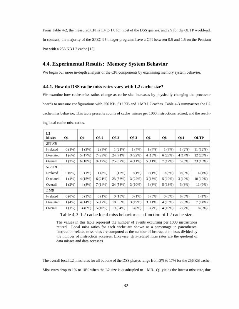
82

From Table 4-2, the measured CPI is 1.4 to 1.8 for most of the DSS queries, and 2.9 for the OLTP workload.

In contrast, the majority of the SPEC 95 integer programs have a CPI between 0.5 and 1.5 on the Pentium

Pro with a 256 KB L2 cache [15].

4.4. Experimental Results: Memory System Behavior

We begin our more in-depth analysis of the CPI components by examining memory system behavior.

4.4.1. How do DSS cache miss rates vary with L2 cache size?

We examine how cache miss ratios change as cache size increases by physically changing the processor

boards to measure configurations with 256 KB, 512 KB and 1 MB L2 caches. Table 4-3 summarizes the L2

cache miss behavior. This table presents counts of cache misses per 1000 instructions retired, and the result-

ing local cache miss ratios.

The overall local L2 miss rates for all but one of the DSS phases range from 3% to 17% for the 256 KB cache.

Miss rates drop to 1% to 10% when the L2 size is quadrupled to 1 MB. Q1 yields the lowest miss rate, due

L2 Misses Q1 Q4 Q5.1 Q5.2 Q5.3 Q6 Q8 Q11 OLTP

256 KB

I-related 0 (1%) 1 (3%) 2 (8%) 1 (21%) 1 (4%) 1 (4%) 1 (8%) 1 (2%) 11 (12%)

D-related 1 (6%) 5 (17%) 7 (23%) 24 (71%) 3 (22%) 4 (15%) 6 (23%) 4 (14%) 12 (26%)

Overall 1 (3%) 6 (10%) 9 (17%) 25 (67%) 4 (11%) 5 (11%) 7 (17%) 5 (5%) 23 (16%)

512 KB

I-related 0 (0%) 0 (1%) 1 (3%) 1 (15%) 0 (1%) 0 (1%) 0 (3%) 0 (0%) 4 (4%)

D-related 1 (4%) 4 (15%) 6 (21%) 23 (56%) 3 (22%) 3 (13%) 5 (19%) 3 (10%) 10 (19%)

Overall 1 (2%) 4 (8%) 7 (14%) 24 (53%) 3 (10%) 3 (8%) 5 (13%) 3 (3%) 11 (9%)

1 MB

I-related 0 (0%) 0 (1%) 0 (1%) 0 (10%) 0 (1%) 0 (0%) 0 (3%) 0 (0%) 1 (1%)

D-related 1 (4%) 4 (14%) 5 (17%) 18 (36%) 3 (19%) 3 (11%) 4 (16%) 2 (8%) 7 (14%)

Overall 1 (1%) 4 (6%) 5 (10%) 19 (34%) 3 (8%) 3 (7%) 4 (10%) 2 (2%) 8 (6%)

Table 4-3. L2 cache local miss behavior as a function of L2 cache size.

The values in this table represent the number of events occurring per 1000 instructionsretired. Local miss ratios for each cache are shown as a percentage in parentheses.Instruction-related miss rates are computed as the number of instruction misses divided bythe number of instruction accesses. Likewise, data-related miss rates are the quotient ofdata misses and data accesses.

83

to its computationally intensive eight aggregate calculations.The heavily pipelined natures of both Q5 and

Q8, where scans produce data consumed by hash join operations, cause high miss rates for Q5.1, Q5.2 and

Q8. OLTP L2 miss rates are high (16% for 256 KB), yet drop similarly to 6% for the 1 MB L2 size. We

note that although the miss percentages are comparable for DSS and OLTP, the absolute number of DSS L2

misses per 1000 instructions is about half the number of misses for the OLTP workload.

This data quantifies our conversations with database experts suggesting that the DSS instruction stream can

be effectively cached for all commercially available databases. The main instruction working set for the

DSS queries is fully cacheable in the 512 KB cache, while the OLTP instruction working set is nearly cache-

able in 1 MB. In contrast, L2 data misses still occur at 1 MB for both workloads, suggesting potential benefits

from larger L2 cache sizes.

Table 4-4 presents L1 cache and ITLB miss behavior for the system with the 1 MB L2 cache. All but one of

the DSS queries experience L1 instruction-cache misses of 4% or less. The only exception is Q11, which

has an 8% miss rate. We hypothesize that the higher instruction miss rate is due to the larger code working

set for this query, including both sequential and index scans, hash and nested-loop joins, group by, sorting

and aggregate operations. All queries except Q5.2 have an L1 data cache miss rate of 4% or less; Q5.2 exhib-

its an 8% data miss rate. These miss rates are somewhat lower than those for OLTP: 6% for the L1 I-cache

and 7% for the L1 D-cache. Again, the DSS workload has fewer absolute L1 cache misses than the OLTP

workload - less than half for the L1 I-cache misses, and less than 60% for the L1 D-cache misses. L1 cache

behavior remains consistent across the different L2 cache sizes.

Misses Q1 Q4 Q5.1 Q5.2 Q5.3 Q6 Q8 Q11 OLTP

L1 I 39 (4%) 35 (3%) 19 (1%) 5 (0%) 21 (1%) 18 (1%) 17 (1%) 75 (8%) 93 (6%)

L1 D 23 (4%) 30 (4%) 31 (4%) 48 (8%) 17 (3%) 28 (4%) 27 (4%) 29 (4%) 51 (7%)

ITLB 1 1 0 0 1 0 0 2 4

Table 4-4. L1 cache and ITLB miss behavior for the four-processor system with the 1 MB L2 cache.

The values in this table represent the number of events occurring per 1000 instructionsretired. Miss ratios for the L1 I- and D-caches are shown as a percentage in parentheses.

84

4.4.2. What impact do larger L2 caches have on DSS database performance and stall cycles?

Figure 4-3 shows the overall system CPI breakdown for the three L2 cache sizes. Table 4-5 summarizes the

CPI and database performance gains from larger L2 caches. Quadrupling the second-level cache size from

256 KB to 1 MB results in a relatively small (e.g., up to 9%) improvement in CPI for most of the DSS queries.

These improvements are due to roughly equal decreases in instruction-related and resource stalls. These

modest CPI improvements translate into modest (e.g., up to 10%) query execution time speedups. Q5.1, Q5.2

and Q8 see a larger (nearly 15%) CPI improvement as L2 size is quadrupled. We hypothesize that the

increased L2 cache size permits more effective data sharing between the producers and consumers in the

query pipelines for Q5 and Q8. These queries experience greater speedups of nearly 20% as the L2 cache size

is quadrupled.

In contrast, for OLTP, quadrupling the cache size to 1 MB results in a 25% improvement in CPI. The bulk

of this improvement is attributable to decreases in both instruction-related and resource stalls. Improvements

in database transaction throughput roughly mirror the CPI improvements: transaction throughput increases

28% as the L2 size is quadrupled to 1 MB.

0

0.5

1

1.5

2

2.5

3

3.5

4

4.5

L2 Cache Size by Workload

Cyc

les

per

Mac

ro-i

nst

ruct

ion

(CP

I)

Resource Stalls

Instruction Stalls

Computation

OLTPQ1 Q4 Q6 Q8 Q11Q5.1 Q5.2 Q5.3

256K512K

1M256K

512K1M

256K512K

1M256K

512K1M

256K512K

1M256K

512K1M

256K512K

1M256K

512K1M

256K512K

1M

Figure 4-3. CPI breakdown by L2 cache size.

The three bars for each workload show the CPI breakdown for 256 KB, 512 KB and 1MB, respectively.

85

This CPI and speedup behavior demonstrates that DSS performance is generally much less sensitive to L2

cache size than OLTP performance, for these small L2 caches. Coupled with the low overall L2 miss rates

reported for DSS in Table 4-3, it also suggests that the majority of the instruction-related stalls are due to L1

I-cache misses that hit in the unified L2 cache.

4.4.3. How prevalent are cache misses to dirty data in other processors’ caches in DSS?

Increasing the L2 cache size also has the potential to increase the number of coherence cache misses. In par-

ticular, “dirty misses,” or misses to dirty data in other processors’ caches, have been shown to be a key factor

in OLTP performance [13] [73]. Table 4-6 presents the percentage and absolute count of L2 cache misses to

dirty data in other processors’ caches for different L2 cache sizes. Dirty misses comprise 1% to 37% of all

1 MB L2 misses for the DSS queries. They form 22% of the 1 MB L2 misses for OLTP. While these per-

centages are comparable, the absolute counts of DSS dirty misses are less than the OLTP count, due to the

fact that there are fewer total L2 cache misses for DSS. The absolute counts are the smallest for query phases

where tables are sequentially scanned (Q1 and Q6) and where intermediate results are materialized to disk

(Q5.2). The number of dirty misses in queries that perform join operations (Q4, Q5.1, Q5.3, Q8, and Q11),

CPI DB Perf.

Workload 256 KB 512 KB 1 MB 256 KB 512 KB 1 MB

Q1 100% 99% 98% 100% 101% 101%

Q4 100% 95% 91% 100% 107% 110%

Q5.1 100% 91% 85% 100% 111% 120%

Q5.2 100% 100% 87%

Q5.3 100% 100% 97%

Q6 100% 98% 94% 100% 106% 107%

Q8 100% 92% 86% 100% 111% 117%

Q11 100% 95% 93% 100% 104% 107%

OLTP 100% 85% 75% 100% 116% 128%

Table 4-5. Impact of L2 cache size on CPI and database performance.

CPI and database performance are shown relative to the 256 KB cache. Database per-formance improvement is shown as scaleup of transaction throughput for OLTP, andspeedup of query execution time for the DSS queries.

86

however, is higher: these dirty miss counts are between 53% and 84% of the OLTP counts. In general, dirty

miss counts are highest for queries that perform the most join operations (Q5.1 and Q8).

Thus, dirty misses are far less prevalent in DSS scan-based queries than in OLTP. Dirty misses for join-inten-

sive DSS queries, however, are only slightly less prevalent than for OLTP.

4.4.4. Is the four-state (MESI) invalidation-based cache coherence protocol worthwhile for DSS?

Some coherence protocols don’t distinguish between exclusive (exclusive clean) and modified (exclusive

dirty) data when expressing the state of data in the L2 cache. In this section, we show that the exclusive state

is not utilized by the DSS workload.

Recall that the Pentium Pro counters allow us to monitor the MESI state of an L2 cache line on an access to

the L2 cache. Accesses to “invalid” lines correspond to cache misses, while accesses to lines in other states

correspond to hits to an L2 line found in that state, before any modifications due to that access are made.

Table 4-7 shows the percentages of L2 cache instruction fetches, loads and stores, broken down by MESI

state.

Table 4-6. Percentage of L2 cache misses to dirty data in another processor’s cache as a function of L2 cache size.

The absolute number of dirty misses across all active processors for the five-second measurementwindow is given in millions by the number in parentheses.

L2 Cache Size 256 KB 512 KB 1 MB

Q1 10.1% (0.50M) 15.8% (0.53M) 21.2% (0.53M)

Q4 5.9% (0.88M) 9.0% (1.07M) 13.0% (1.29M)

Q5.1 7.1% (1.31M) 11.1% (1.68M) 16.2% (2.05M)

Q5.2 0.5% (0.17M) 0.7% (0.23M) 1.4% (0.41M)

Q5.3 20.9% (1.09M) 27.1% (1.20M) 36.6% (1.40M)

Q6 5.0% (0.57M) 7.9% (0.69M) 9.0% (0.76M)

Q8 6.9% (1.15M) 13.7% (1.85M) 14.2% (1.50M)

Q11 12.6% (1.31M) 18.6% (1.33M) 25.7% (1.41M)

OLTP 5.7% (1.38M) 11.8% (1.96M) 22.0% (2.45M)

87

As expected, nearly all of the instruction fetches that hit in the L2 cache are to shared cache lines. Hits result-

ing from loads are distributed across the different states, going predominantly to shared lines, followed by

Workload M E S(Miss)I

Inst. Fetch

Q1 0.0% 0.0% 99.9% 0.1%

Q4 0.0% 0.0% 99.6% 0.4%

Q5.1 0.0% 0.0% 99.0% 1.0%

Q5.2 0.0% 0.0% 91.8% 9.1%

Q5.3 0.0% 0.0% 99.2% 0.8%

Q6 0.0% 0.0% 99.7% 0.3%

Q8 0.0% 0.0% 99.1% 0.9%

Q11 0.0% 0.0% 99.8% 0.2%

OLTP 0.0% 0.0% 98.8% 1.2%

Load

Q1 19.7% 13.4% 63.6% 4.3%

Q4 25.3% 13.4% 47.0% 14.3%

Q5.1 27.9% 15.3% 37.9% 18.9%

Q5.2 1.9% 16.9% 45.6% 35.6%

Q5.3 22.7% 4.1% 57.6% 15.6%

Q6 22.9% 16.9% 44.8% 15.4%

Q8 26.3% 17.1% 39.2% 17.4%

Q11 20.2% 12.1% 60.3% 7.4%

OLTP 24.7% 15.1% 46.0% 14.2%

Store

Q1 96.4% 0.2% 2.4% 1.0%

Q4 88.4% 1.6% 2.3% 7.6%

Q5.1 80.3% 4.1% 4.5% 11.2%

Q5.2 70.2% 1.6% 10.6% 17.6%

Q5.3 78.0% 0.0% 14.4% 7.6%

Q6 93.8% 0.3% 2.2% 3.7%

Q8 83.0% 3.2% 2.2% 11.6%

Q11 85.6% 1.0% 5.4% 8.3%

OLTP 81.2% 0.6% 6.7% 10.5%

Table 4-7. State of L2 line on L2 hit for the four-processor system with the 1 MB L2 cache.

Table shows percentage of L2 accesses. Note that the Stores category includes indicationsfrom the L1 D cache that a line has changed state from invalid to modified; thus the L2 isaware of the modified status of modified lines residing in the L1 data cache.

88

modified lines and finally exclusive lines. The high percentage of load hits to modified lines indicates that

the processor reads data in the same line as it has recently written. In addition, 84% to 97% of the database

store hits are to modified lines, with few write accesses to shared or exclusive lines. These measurements

provide quantitative evidence of the temporal locality present in the workload, and validate the usefulness of

the writeback write policy employed by the Pentium Pro caches. All of these observations apply to both DSS

and OLTP.

A primary advantage of the exclusive state is that it allows the processor to avoid the invalidation bus trans-

action on a store to a shared line: if the line is already in the exclusive state, it is the only copy currently

cached. However, we see that store hits to exclusive lines rarely occur. Thus, it isn’t clear whether the bene-

fits of the E state are worth the cost of implementing the fourth state for this workload. A three-state protocol

would be sufficient, and not result in significantly increased bus traffic.

4.4.5. How does DSS memory system performance scale with increasing cache sizes?

Table 4-8 presents the memory system utilization across all of the processors in the system for different cache

sizes. Recall that we define memory system utilization to include the time the bus is busy transferring data

(or control information), as well as the time when the bus is not busy but unavailable. The exact counters and

formulae used to compute the memory system utilization are presented in Table 8-12 on page 197.

The DSS queries exhibit a wide range of memory system utilizations, ranging from 12% to 82% for the 256

KB L2 cache size. All but one of these utilizations are less than 65%. We note that the scan-based queries

(Q1 and Q6) exhibit two of the three lowest utilizations. As discussed in the previous section, Q1 performs

numerous computationally intensive aggregate operations, which generate very few L2 misses, resulting in

the lowest memory system utilization. Q6 performs fewer aggregate operations, resulting in slightly more L2

Table 4-8. Overall memory system utilization as a function of L2 cache size for the four-processor SMP.

L2 Cache Q1 Q4 Q5.1 Q5.2 Q5.3 Q6 Q8 Q11 OLTP

256 KB 11.8% 65.1% 82.3% 53.9% 22.5% 30.9% 80.0% 41.7% 89.3%

512 KB 8.0% 53.3% 69.7% 55.7% 19.3% 27.4% 63.9% 29.3% 67.0%

1 MB 6.0% 45.5% 59.7% 42.2% 18.7% 25.6% 53.3% 21.2% 47.3%

89

misses and a slightly larger memory system utilization. Q5.3 also experiences a low memory utilization,

because it spends the majority of its time in the idle loop, generating few L2 cache misses.

Join-intensive queries, such as Q4, Q5.1, Q8, and Q11 experience higher memory system utilizations, due to

their higher L2 cache miss frequencies and higher percentage of dirty misses. Q5.2 experiences a high L2

miss rate, resulting in a moderately high memory system utilization. As expected, memory system utilization

decreases with increasing cache size, ranging from 6% to 60% for the 1 MB L2.

In contrast, the higher L2 cache miss rates experienced by the OLTP workload translate into a generally

higher memory system utilization (e.g., 89% for 256 KB). Utilization drops more drastically for this work-

load as L2 size is quadrupled to 1 MB, resulting in a 47% utilization comparable to the utilization experienced

by several of the DSS queries.

Even at these relatively low utilizations, however, bus activity has an impact on the memory latency per-

ceived by the database. Table 4-9 presents the application memory latency as a function of the L2 size. These

cycle counts are calculated from counter values that measure the number of cycles where data read transac-

tions are outstanding on the bus, and the total number of data read transactions. We note that this measure

does not account for any overlap of memory accesses supported by the Pentium Pro’s non-blocking L2 cache.

We see that DSS application reads take 57 to 95 cycles for the 1 MB cache size. OLTP reads are somewhat

slower, at 97 cycles for the 1 MB L2. These application memory latencies are much greater than the nominal

38-cycle latency reported for dependent loads by lmbench, as described in Table 2-1 on page 17. We use

these application memory latencies in Section 4.5.3 as the penalties for L2 misses.

Table 4-9. Application memory read latency as a function of L2 cache size for the four-processor SMP. All values are in processor cycles.

L2 Cache Q1 Q4 Q5.1 Q5.2 Q5.3 Q6 Q8 Q11 OLTP

256 KB 67 98 113 63 66 103 116 82 118

512 KB 61 87 104 75 73 94 112 73 111

1 MB 57 77 95 69 76 91 81 69 97

90

Several unexplained anomalies should be noted. First, the memory system utilization of Q6 is one of the

lowest reported, yet the corresponding application memory latency is among the highest. We hypothesize

that this is due to the high read I/O rate experienced by this query. Second, the application memory latency

for Q5.3 increases, rather than decreases, for increasing cache size. We believe that this effect is due to the

increase in cache coherence traffic that accompanies larger L2 sizes. Third, the memory latency for Q5.2

increases for the 512 KB cache, relative to the 256 KB cache, and then decreases for the 1 MB cache relative

to the 512 KB cache. This behavior is consistent with the count of dirty misses for these cache sizes for this

query phase.

Because memory system utilization and application memory latency continue to grow as processors are

added, even for larger cache sizes, it is not clear to what degree this memory system will scale to support

additional processors.

4.5. Experimental Results: Processor Issues

In addition to memory hierarchy-related stall CPI components, a significant component of CPI (both compu-

tation and stall cycles) is due to processor features. In this section we examine some of these processor fea-

tures, including superscalar issue and retire, branch prediction and out-of-order execution.

4.5.1. How useful is superscalar issue and retire for DSS?

In this section, we show that the DSS workload exploits the three-way retirement of µops in the out-of-order

engine, which suggests that an increased µop retirement width might provide performance benefits. This

workload does not exploit the superscalar decode and retire width for macro-instructions to nearly the same

degree, suggesting little benefit from increased macro-instruction superscalar width.

In the Pentium Pro, three parallel decoders translate x86 macro-instructions into µops. Each cycle, up to

three µops can be retired in the out-of-order engine, and up to three x86 instructions can be retired in the in-

order engine. Figure 4-4 through Figure 4-6 present the profiles for instruction and micro-operation decode

and retire behavior, broken down by cycles and instructions.

91

Figure 4-4a and Figure 4-5a illustrate that the DSS queries experience a high percentage (49% to 77%) of

cycles where zero instructions are decoded or retired. The percentages of zero-decode (69%) and zero-retire

(76%) cycles are also high for OLTP. In contrast, the SPEC integer programs show far fewer cycles (20% to

50%) with no instructions decoded [15]. Figure 4-6a shows that zero µops are retired in 43% to 65% of all

0%

20%

40%

60%

80%

100%

Q1 Q4 Q5.1 Q5.2 Q5.3 Q6 Q8 Q11 OLTP

Workload

Per

cent

of

Inst

ruct

ions

3-inst2-inst1-inst

Figure 4-4. Macro-instruction decode profile decomposed by (a) cycles and (b) instructions.

(a)

(b)

0%

20%

40%

60%

80%

100%

Q1 Q4 Q5.1 Q5.2 Q5.3 Q6 Q8 Q11 OLTP

Workload

Per

cent

of C

ycle

s3-inst2-inst1-inst0-inst

92

cycles for DSS, and in 66% of all cycles for OLTP. Zero µops are retired in 25% to 55% of all cycles for

SPEC integer programs [15].

Figure 4-4b, Figure 4-5b and Figure 4-6b present the same profiles, organized by the percent of instructions

(or µops) decoded/retired in each type of cycle. At the macro-instruction level, 40% to 45% of instructions

for nearly all DSS queries are decoded in triple-decode cycles, and 27% to 45% of all instructions are retired

0%

20%

40%

60%

80%

100%

Q1 Q4 Q5.1 Q5.2 Q5.3 Q6 Q8 Q11 OLTP

Workload

Per

cent

of

Inst

ruct

ions

3-inst2-inst1-inst

0%

20%

40%

60%

80%

100%

Q1 Q4 Q5.1 Q5.2 Q5.3 Q6 Q8 Q11 OLTP

Workload

Per

cent

of

Cyc

les

3-inst2-inst1-inst0-inst

(a)

(b)

Figure 4-5. Macro-instruction retirement profile decomposed by (a) cycles and (b) instructions.

93

in triple-retire cycles. The only exception of Q5.3, where only 14% of instructions are decoded in triple-

decode cycles. We hypothesize that the high ratio of µops to macro-instructions (just over 4) contributes to

this low percentage. Since most of Q5.3’s instructions must be decoded into a sequence of µops, this phase

cannot take advantage of the Pentium Pro’s simple decoders, which decode simple x86 instructions into a

(a)

(b)

Figure 4-6. Micro-operation retirement profiles decomposed by (a) cycles and (b) instructions.

0%

20%

40%

60%

80%

100%

Q1 Q4 Q5.1 Q5.2 Q5.3 Q6 Q8 Q11 OLTP

Workload

Per

cent

of

Mic

ro-o

pera

tion

s

3-uop2-uop1-uop

0%

20%

40%

60%

80%

100%

Q1 Q4 Q5.1 Q5.2 Q5.3 Q6 Q8 Q11 OLTP

Workload

Per

cent

of C

ycle

s3-uop2-uop1-uop0-uop

94

single µop. Because of the low percentage of simple instructions in the instruction mix, the processor cannot

fully exploit the 3-instruction superscalar instruction decode width.

For OLTP, 32% of all instructions are triple-decoded, and only 22% of instructions are triple-retired. In com-

parison, 33% to 54% of SPEC integer program instructions are decoded in triple-decode cycles [15]. Since

there is only a modest benefit from macro-instruction triple-decode and triple-retire cycles, DSS and OLTP

workloads may not benefit from increases in macro-instruction superscalar width.

The system more effectively exploits the µop retire width in the out-of-order engine: 60% to 74% of DSS

µops and 53% of OLTP µops are retired in triple-retire cycles. (For SPEC integer programs, 65% to 80%

µops are retired in triple-retire cycles [15].) Thus, increasing µop retire width for the out-of-order engine

may prove to be beneficial.

Finally, as shown in Table 4-2 on page 80, we note that the number of µops retired for every macro-instruc-

tion ranges from 1.60 to 1.82 for all but one of the DSS queries. Again, the exception is Q5.3, which retires

4.05 µops for every macro-instruction, as described above. For OLTP, 1.87 µops are retired for every macro-

instruction. In contrast, the average number of µops per macro-instruction is around 1.35 for the SPEC pro-

grams [15]. This implies that the database workloads utilize somewhat more complex x86 instructions than

the SPEC programs do.

4.5.2. How effective is branch prediction for DSS?

Table 4-10 shows branch behavior for the DSS queries and the OLTP workload. Branches comprise 13% to

15% of the overall instruction mix for nearly all of the DSS queries. Branch frequencies of 22% to 28% are

observed for Q5.2, Q5.3 and OLTP. All DSS branch misprediction rates are under 10%. These misprediction

rates are consistent with the looping nature of many DSS queries: the same set of data manipulation opera-

tions is applied to each record in a relatively tight loop. The 15% OLTP branch misprediction rate is much

higher, likely due to the non-looping branching constructs typically used in transaction processing code [64].

In OLTP, each query executes a relatively small amount of data manipulation code, which is interleaved with

code for client connection management, lock acquisition and management, logging, and other operations.

95

Both the branch frequencies and misprediction rates for DSS are consistent with SPECInt rates; the OLTP

misprediction rate is higher than that for most SPECInt programs [15].

Although the OLTP workload experienced a very high Branch Target Buffer (BTB) miss ratio (56%), the

BTB miss ratio is lower for the DSS queries, ranging from 13% to 40%. These ratios are somewhat higher

than those of the SPEC integer programs, where all programs except one exhibit a BTB miss ratio of less than

30%. Most SPECInt BTB miss ratios are well below 15% [15]. These miss ratios suggest that the DSS work-

load might benefit from a slightly larger BTB.

Finally, we note that the speculative execution factor, or the number of macro-instructions decoded per

macro-instruction retired, ranges from 1.10 to 1.34 for the DSS queries, which is consistent with the specu-

lative execution factor reported for nearly all SPEC programs [15]. OLTP decodes slightly more macro-

instructions per macro-instruction retired, possibly due to its higher branch misprediction ratio, resulting in

a speculative execution factor of 1.43.

4.5.3. Is out-of-order execution successful at hiding stalls for DSS?

The Pentium Pro implements dynamic execution using an out-of-order, speculative execution engine, which

employs register renaming and non-blocking caches. How effective is dynamic execution for decision sup-

port workloads?

Characteristic Q1 Q4 Q5.1 Q5.2 Q5.3 Q6 Q8 Q11 OLTP

Branch frequency 15.2% 14.0% 13.2% 22.6% 27.8% 15.4% 13.8% 15.4% 21.5%

Branch mispredict. ratio

9.5% 6.5% 6.0% 0.6% 2.3% 10.0% 6.4% 8.4% 14.6%

BTB miss ratio 31.5% 34.7% 33.0% 22.1% 13.4% 27.0% 31.1% 39.5% 55.7%

Speculative exec. factor

1.24 1.16 1.13 1.10 1.34 1.25 1.14 1.17 1.43

Table 4-10. Branch behavior.

The Pentium Pro processor implements a branch prediction scheme derived from thetwo-level adaptive scheme described by Yeh and Patt [120]. The branch target buffer(BTB), which contains 512 entries, maintains branch history information and the pre-dicted branch target address. A static prediction scheme (backwards taken, forward nottaken) is employed. Mispredicted branches incur a penalty of at least 11 cycles, with theaverage misprediction penalty being 15 cycles [39].

96

As in the previous chapter, we compare non-overlapped CPI vs. measured CPI to address this question. If

out-of-order execution is effective, the individual components of the non-overlapped CPI should be overlap-

pable, and the measured CPI should be less than the non-overlapped CPI.

To compute the non-overlapped CPI, we again treat the machine as if it were in-order, and explicitly account

for computation and all potential stall cycles, such as instruction and data cache miss-related stalls, branch

misprediction penalties, resource-related stalls, and other minor stalls. Cache miss and branch misprediction

penalties are computed by multiplying the number of misses per instruction by the associated miss penalty.

Recall that we calculate the computation component for our non-overlapped CPI in two ways, to provide an

upper and lower bound on the amount of non-overlapped computation. The naive estimate (called “OPT” in

the figures) treats all µops as single-issue, effectively attributing all of the instruction-level parallelism (ILP)

to out-of-order execution. The OPT computation component allocates one cycle for each µop retired per

macro-instruction. We calculate the pessimistic (“PES”) estimate, which allocates all of the ILP to supersca-

lar-ness that could be exploited by an in-order processor, from the µop retirement profile, as described in Sec-

tion 4.3.

Figure 4-7 presents the non-overlapped CPIs and the measured CPI for Q6, a representative DSS query, for

the three different L2 cache sizes. Breakdowns for the other DSS queries and the OLTP workload are

included in the appendix in Chapter 10. The stacked bars for each configuration include the resource stalls,

and decompose the stall components further to include L1 I and D cache misses, L2 cache misses, branch

misprediction stalls, ITLB misses and other minor stalls. “OPT” presents the optimistic estimate, and “PES”

presents the pessimistic estimate, as described above. The black line in each column marks the measured CPI

for that configuration. Note that the only difference between the “OPT” and “PES” bars is the computation

component.

For all cache sizes, workloads and computational models, the measured CPI is less than the non-overlapped

total. For the OPT computational model, Q6 measured CPI is roughly 50% of the non-overlapped CPI for

all L2 cache sizes. Q6 measured CPI is roughly 70% of the PES non-overlapped CPI for all L2 sizes. (In

comparison, OLTP measured CPI is 54% of the OPT non-overlapped CPI for the 256 KB L2, 57% for the

97

512 KB L2 and 58% for the 1 MB L2. For the PES computational model, OLTP measured CPI is 62% of

the total bar height for the 256 KB L2 cache, 67% for the 512 KB L2 and 70% for the 1 MB L2.) The mea-

sured CPI of SPECInt programs is 45% to 65% (averaging 54%) of the OPT non-overlapped total for the 256

KB L2 cache [15].

While the actual CPIs vary somewhat between the different DSS queries, the overall relationships between

the measured and OPT and PES non-overlapped CPIs are the same across the query set. Thus, out-of-order

execution is effectively overlapping the CPI components to achieve a lower actual CPI for both the DSS and

OLTP workloads. Based on the OPT non-overlapped CPI, it appears that out-of-order execution holds

slightly more potential for DSS workloads. However, based on the PES non-overlapped CPI, it appears that

out-of-order execution holds roughly the same potential for both OLTP and DSS. The OPT and PES compu-

Figure 4-7. Non-overlapped and measured CPI for DSS Q6 as a function of L2 cache size.

Latency from each of the components above is shown as a portion of the bar graph. L1miss penalties are presented in Table 2-5 on page 26, L2 miss penalties in Table 4-9, andbranch misprediction penalties in the caption for Table 4-10. PES attributes ILP to super-scalar-ness that can be exploited by an in-order processor, while OPT attributes ILP toout-of-order execution. Note that, for a given cache size, the only difference between thePES and OPT stacked bars is the computation component; all stall components are thesame.

0

1

2

3

4

L2 Cache Size

Non

-ove

rlap

ped

CP


Measured CPI

256 KB 512 KB 1 MB


98

tational models provide an upper and lower bound, respectively, for the degree of stall components that can

be overlapped in the out-of-order engine. Neither model is strictly accurate; the true value lies somewhere

in this range.

4.6. Experimental Results: I/O Characterization

In this section, we explore the following question: “what is the frequency and size of I/O operations in the

DSS workload?” We show that there are two predominant kinds of accesses, namely large sequential

accesses and small random accesses. Large sequential reads are used for table scan/select operations, and typ-

ically access 64 KB per I/O operation for this version of the Informix database. Smaller accesses - both reads

and writes - are used for several purposes, including indexed access and spilling temporary results to disk.

For this version of Informix, small reads and writes operate on a 4 KB to 8 KB granularity.

We examine this question using NT’s performance monitor, by measuring the number of file operations per

second, and the number of bytes read or written per second. In this section we will present data for Q6 and

Q5, which are the simplest and most complex queries, respectively; data for the other queries in our set is

included in the appendix in Chapter 10. Figure 4-8 shows the read and write rates for Q6, a well-behaved

DSS query that performs a sequential table scan with selection and aggregation operations. We note that the

read rate is nearly constant at about 745 reads per second for the entire duration of the query. Read sizes are

constant at 64 KB per read. Writes are negligible for this query.

Figure 4-9 illustrates the I/O access patterns for Q5, a complex query comprised of six sequential table scans

and five two-table hash-join operations. We note that the general patterns in this figure closely match the CPI

patterns illustrated in Figure 4-1 on page 79. The first phase of the query, which lasts from the beginning of

the query to the 12-minute mark, exhibits a moderately high read rate of 300 to 600 reads per second; no

writes occur during this period. This period includes several of the table scan and hash join algorithms that

have data working sets small enough to fit into memory. At about 12 minutes, a result set is generated for

one of the hash join operations that is too big to reside in memory, and hence must be spilled to disk. This

behavior marks the beginning of phase 2, where we observe four bursts of write activity, requiring 600 to 800

writes per second. Read activity during phase 2 is negligible. This temporary result set must later be used as

99

the input to a subsequent hash join operation, and is read from disk during phase 3, which starts at about the

19-minute mark. Here we observe a much higher rate of read operations - greater than 1400 reads per second

- with negligible write activity.

The sizes of these read and write operations vary, as shown in Figure 4-10. The phase 1 sequential scan oper-

ations employ large 64 KB read operations. The phase 2 temporary result write operations use a much smaller

8 KB granularity. Finally, the phase 3 reads must use the same granularity as the write operations performed

in phase 2, resulting in an 8 KB read granularity.

4.7. Related Work

Several recent studies began the examination of the architectural impacts of decision support database work-

loads for multiprocessors [13] [83] [106]. Although they used a very different approach to evaluate the DSS

workloads, in general these papers corroborate our findings. Inconsistent results can generally be explained,

0

100

200

300

400

500

600

700

800

0:00:00 0:00:30 0:00:59 0:01:30 0:02:00 0:02:30 0:03:00 0:03:30 0:03:59

Time

File

Ope

rati

ons

per

Seco

nd

File Reads per Sec

File Writes per Sec

Figure 4-8. Q6 file read and write rates.

Each point in the graph corresponds to the average number of file operations per second,averaged over a ten-second measurement period.

100

either by differences in hardware or software or both. In this section, we highlight the methodologies and

findings of these studies.

4.7.1. Trancoso, et al.: Postgres95 on CC-NUMA Multiprocessor

Trancoso, et al., simulate three TPC-D-based DSS queries (Q3, Q6, and Q12) running on Postgres95 on a

four-processor CC-NUMA multiprocessor [106]. They study the memory access patterns of this workload

for a memory-resident database.

They find that the memory use of queries differs largely, depending on whether the database uses index scans

or sequential table scans to access database data. Index queries suffer most of their shared-data misses on the

indices, and on lock-related metadata structures. Sequential queries, on the other hand, suffer most of their

shared-data misses on the table rows as they are scanned. Both index and sequential queries exhibit spatial



0

200

400

600

800

1000

1200

1400

1600

1800

0:00:00 0:02:30 0:05:01 0:07:30 0:10:00 0:12:30 0:15:01 0:17:30

Time

File

Ope

rati

ons

per

Seco

nd

File Reads/sec

File Writes/sec

101

locality, and can benefit from relatively large cache lines. However, there is little temporal locality within a

query. They find that the performance of sequential queries can be improved with data prefetching.

The detailed results of this paper are incomparable with our work, for two reasons. First, this study uses

Postgres95, an academic database with publicly available source code. This database engine does not auto-

matically parallelize queries, as most commercially available databases do. In addition, it has inefficient pro-

cess and I/O models. Second, this study greatly scales back the size of the memory resident database - to

about 20 MB - to make their simulations tractable. This modification prompts the authors to also reduce the

size of the memory hierarchy of the machine simulated. They model a machine with slightly over 20 MB of

main memory, 128 KB L2 caches, and 4 KB L1 caches. It is not clear that the data is sufficiently larger than

the hardware caches for the workload to exhibit representative behavior.

Figure 4-10. Q5 file read and write sizes.

0

10000

20000

30000

40000

50000

60000

70000

0:00:00 0:02:30 0:05:01 0:07:30 0:10:00 0:12:30 0:15:01 0:17:30 0:19:40

Time

Byt

es (

B)

Average Read Size

Average Write Size

102

4.7.2. Barroso, et al.: Alpha Servers

Barroso, et al., use hardware counter measurements and SimOS simulation to evaluate the memory system

performance of a nearly identical set of TPC-D-based DSS queries running Alpha 21164-based SMPs [13].

They measured the Oracle database, and configured it to employ parallel query execution for the DSS work-

load. Their 500 MB database was small enough to fit into main memory.

They find that the DSS workload is primarily sensitive to the size and latency of the on-chip caches, and

somewhat insensitive to off-chip cache size and to memory and dirty miss latencies. They report CPIs of 1.3

to 1.9, with a somewhat different composition of user, kernel and idle modes: slightly lower user time (e.g.,

82% to 94%), and higher kernel (2.5% to 5%) and idle (3.5% to 13%) time. Roughly half of the execution

time is spent stalling for instruction- and data-related memory accesses. This memory stall time is dominated

by L1 cache misses that hit in the L2 cache. Through simulation, they demonstrate that larger first-level

caches (up to 128 KB) are beneficial for queries Q5 and Q6. They also show that larger off-chip cache line

sizes (up to 256 bytes) capture more of the spatial locality in the DSS workload, resulting in lower miss rates.

The system measured in this study (e.g., a four-processor AlphaServer 4100 using a 21164 processor with 8

KB first-level on-chip I- and D-caches, 96 KB second-level on-chip S-cache and 2 MB board-level B-cache)

experiences higher cache miss rates than those we report in this chapter. Our L1 cache miss rates are roughly

half of those measured in this study; we hypothesize that the direct-mapped nature of the 21164’s first-level

caches contributes to the higher miss rate over the Pentium Pro’s 4-way set associative L1 I-cache and 2-way

set associative L1 D-cache. Our L2 cache miss rates are also lower than those reported for the AlphaServer;

again, we hypothesize that the 4-way associativity of the Pentium Pro’s L2 cache is more effective than the

direct-mapped 21164 B-cache. The increased density of Pentium Pro CISC code may also contribute to our

improved I-cache behavior. The Alpha 21164’s 64-bit addressing may also contribute to the disparity in D-

cache miss rates.

They report a low prevalence of dirty misses, with considerably lower percentages than described in our

results. Possible explanations for this discrepancy are the higher overall miss rate of the direct-mapped B-

103

cache, with more conflict misses yielding a smaller percentage for dirty misses, and their use of a different

database (Oracle).

4.7.3. Ranganathan, et al.: Effects of ILP and Out-of-Order Execution

Ranganathan, et al., use trace-based simulation to explore the benefits of instruction-level parallelism (ILP)

out-of-order execution, non-blocking caches, instruction window size for DSS Q6 [83]. Traces were gathered

for an in-memory database with Oracle running on an AlphaServer 4100 platform, and then used as input to

an RSIM user-level simulation of a four-processor CC-NUMA multiprocessor.

They find that going from single issue to 8-way issue achieves 32% reduction in execution time for Q6 in an

in-order processor and a 56% reduction in an out-of-order processor. The large magnitude of these increases

is due to the low memory stall time from the large L1 and L2 (8 MB) caches. They also report considerable

reduction in Q6 execution time due to out-of-order execution, ranging from 11% for 1-way issue to 43% for

4-way and 8-way issue. Out-of-order instruction windows of up to 32 instructions prove beneficial. They find

that the DSS workload can exploit up to 4 outstanding L2 cache misses. The main limitation for the DSS

workload in their simulations is the number of functional units (2 integer arithmetic, 2 floating point, and 2

address translation).

The authors report a much smaller cache miss stall component for Q6 (e.g., less than about 20% for simulated

out-of-order processors with up to 4-way superscalar issue). We hypothesize that this difference is due to

the much larger caches employed by their simulated processor. Their simulated 128 KB L1 I- and D-caches

achieve miss rates of less than 1%.

4.7.4. Discussion: Conventional Wisdom and This Thesis

As described above, the body of literature describing DSS workload characteristics is much smaller than the

OLTP literature. Even though the number of studies is small, some conventional wisdom has begun to

emerge. First, DSS queries tend to have lower CPIs than OLTP, and stalls play a less significant role: most

studies report at most half of the CPI is comprised by stalls. These stalls are due mainly to on-chip cache

misses that hit in the off-chip cache, rather than off-chip cache misses that must be satisfied by memory. In

fact, most DSS queries are relatively insensitive to the size of the L2 cache. Second, because DSS queries

104

CharacteristicsTrancoso97 [106] Barroso98 [13]

Ranganath98 [83] This Thesis

System evaluated 4-proc. CC-NUMA


4-proc. CC-NUMA server

4-proc. Pentium Pro

Processor simulated (in-order)


simulated (out-of- order)

Pentium Pro (out-of-order)

I/O system sim: in-mem. sim: in-mem. in-memory 56 data disks

Database/OS Postgres95 Oracle/Unix Oracle/Unix Informix/NT

Workloads TPC-D Q3, Q6, Q12

TPC-D Q1, Q4, Q5, Q6, Q8, Q13, TPC-B

TPC-D Q6, TPC-B

TPC-D Q1, Q4, Q5, Q6, Q8, Q11

Methodology trace-driven simulation

H/W meas., trace-driven simulation



Conventional wisdom

Lower CPI than OLTP Y Y Y

Lower OS time Y Y

Stalls up to 1/2 CPI Y Y Y Y

L1 misses comprise major-ity of stalls

Y Y Y

Performance more insensi-tive to L2 size

Y Y Y

Superscalar more beneficial than for OLTP

Y Y

Out-of-order exec. more effective than for OLTP

Y Y

Dirty misses negl. for scans Y Y Y

Other results Descr. data structs. resp. for $ misses

OS and I/O lat. don’t dominate DB behavior

Smaller inst. windows for OOO benefit

Query phases may vary drasti-cally

Larger L2 lines capture locality

Larger off-chip $ lines better

Can exploit 4 outst. L2 $ misses

Branch predict. more effective than for OLTP

Larger L1 caches better

Larger L1 caches better

Dirty misses non-negl. for joins

E state not used in MESI

Contradictory results Higher cache miss rates

Lower $ miss stalls

Lower %age of dirty misses

Table 4-11. Summary of most relevant multiprocessor related work.

105

tend to perform I/O on a coarser granularity, they typically spend less time in the operating system. The scan-

intensive nature of many DSS queries leads to fewer dirty cache misses than in OLTP. Finally, studies indi-

cate that the DSS workloads benefit more from wider superscalar decode and retire widths, and from out-of-

order execution than the OLTP workload does. We summarize the most relevant studies and whether they

agree with this conventional wisdom in Table 4-11.

This thesis contributes to the growing body of literature on DSS performance analysis in several ways. As

with the OLTP contributions described in Chapter 3, and as shown in Table 4-11, we corroborate much of

the conventional wisdom of this literature for a new combination of environments. We measured an actual

system running a fully-scaled version of TPC-D DSS queries. The system in our study, the four-processor

Intel server running Microsoft Windows NT, is increasingly popular, both as a low-end DSS server architec-

ture and as a building block for higher-end DSS workloads. The Pentium Pro processor, which is one of the

few commercially available out-of-order processors, is at the core of several subsequent generations of Intel

processors, such as the Pentium II, Pentium II Xeon, and Pentium III, used in more recent enterprise servers.

We also discovered other new results, as shown in Table 4-11. The most notable new result is that for fully-

scaled data sets, the behavior of more complex queries may vary greatly during execution. We also demon-

strate that dirty misses are more prevalent for join-intensive DSS queries than for scan-intensive DSS queries,

but still not quite as prevalent as for OLTP.

4.8. Proposal for a DSS-centric Processor and System Design

Using the results of our experiments and the results reported in the literature, we outline several rules of

thumb for designing DSS-friendly architectures. First, as observed in Chapter 2, the I/O subsystem hardware

and the database software must be configured to minimize the amount of I/O-induced idle time. This rule,

coupled with the mostly sequential I/O access patterns used in DSS, implies a moderate number of disks,

spread over several I/O controllers, in a configuration optimized for high-bandwidth transfers. The database

software must be configured to use multiple server processes and/or threads, to hide the latency of I/O oper-

ations.

106

A large component of DSS memory-related stall time comes from L1 instruction misses that hit in the L2

cache. To remedy this problem, we advise a moderately sized first-level instruction cache (e.g., 128 KB) with

two- to four-way associativity. A reasonably sized L2 cache (e.g., 4 MB to 8 MB), with somewhat larger lines

(e.g., 128 B to 256 B) will likely capture much of the spatial locality in DSS data access patterns. Large L2

caches should not pose a problem for cache coherence traffic, since dirty misses are not prevalent in this

workload. A three-state invalidation-based cache coherence protocol (e.g., MSI) would likely suffice for this

workload, rater than a protocol with four states.

The processor should employ speculative execution techniques, such as out-of-order execution, multiple

issue width, and non-blocking caches. Studies have shown that benefits can be reaped for issue widths of up

to four instructions per cycle. The instruction window must be large enough to allow overlap of shorter-dura-

tion stalls, such as L1 cache misses that hit in the L2 cache. [83] suggests that a 32-entry instruction window

is sufficient. Non-blocking first-level caches are invaluable to this workload. As a result, the processor should

permit at least four outstanding misses for different cache lines for both the L1 instruction and L1 data caches.

This workload exhibits good branch prediction behavior under traditional branch prediction schemes, so

there is little need for innovation in this area.

4.9. Conclusions

Commercial OLTP database applications have received increasing attention in computer architecture perfor-

mance studies in recent years. However, researchers are just beginning to study decision support, an emerg-

ing database workload. DSS’s different execution characteristics and its growth in popularity suggest that it

should be given the same attention as OLTP.

We used the Pentium Pro hardware counters to measure the performance of a four-processor SMP server for

several representative DSS queries from the TPC-D benchmark on an Informix database for a fully-scaled

100 GB dataset. We examined the efficiency of out-of-order execution, caching, superscalar issue and retire,

branch prediction and memory system scalability.

107

We find that out-of-order execution somewhat effectively overlaps the CPI components to achieve a lower

actual CPI for both the DSS and OLTP workloads. We compute upper and lower bounds for the degree of

overlap offered by out-of-order processing. Based on the upper bound, out-of-order execution appears to

hold slightly more potential for DSS workloads than OLTP. Although out-of-order execution provides ben-

efits, the DSS µCPI is still nearly three times the theoretical minimum µCPI possible on the Pentium Pro.

Nearly half of the µCPI is attributable to instruction-related and resource stalls.

We observe that DSS instruction streams can be effectively cached, even in relatively small L2 caches. The

main instruction working set for the DSS queries is fully cacheable in the 512 KB cache. While L2 data-

related miss rates are lower for DSS than for OLTP, L2 data misses still occur at 1 MB for both workloads,

suggesting that somewhat larger L2 caches could be beneficial. L2 cache misses do not appear to have a

large impact on the instruction-related stalls for DSS: these stalls are due rather to L1 I-cache misses that hit

in the unified L2 cache. This implies that a larger L1 I-cache would be quite beneficial for DSS.

Additionally, we find that dirty misses are less prevalent in the DSS queries than in OLTP. The E state of

the MESI protocol isn’t utilized by this workload, implying that a three-state cache coherence protocol could

be employed with little increase in memory bus traffic.

Memory system utilization varies across the DSS query set, ranging from as low as 10% to as high as 68%

for the 1 MB L2 cache. As expected, memory system utilization decreases with increasing cache size. How-

ever, even at these relatively low utilizations, bus activity has an impact on the memory latency perceived by

the database. We see that DSS application reads take 1.6X to 2.5X the nominal dependent load latency for

the 1 MB cache size. Because memory system utilization and application memory latency continue to grow

as processors are added, even for moderately sized L2 caches, it is not clear to what degree this memory

system will scale to support additional processors.

We show that the DSS workload exploits the three-way retirement of µops in the out-of-order engine, which

suggests that an increased µop retirement width might provide performance benefits. This workload does

not exploit the superscalar decode and retire width for macro-instructions to nearly the same degree, suggest-

ing little benefit from increased macro-instruction superscalar width. We find that the looping nature of the

108

DSS workload results in branch misprediction rates that are comparable to those of SPECInt applications,

and BTB miss ratios that are roughly comparable.

Finally, we demonstrated that one of the DSS queries examined exhibits variations in behavior across the

duration of query execution. Researchers (especially those employing simulation techniques) must be very

careful to pick kernels that represent all phases of query execution. In addition, reduced datasets may not

exhibit behavior that is representative of fully-scaled systems, where large data requirements may generate

I/O that impacts performance.

While today’s single-user model of decision support exhibits characteristics that differ from transaction pro-

cessing workloads, the future of DSS includes higher multiprogramming levels and more complex queries.

These emerging characteristics may blur the distinctions between these two database workloads in the future.

109

5 Towards a Simplified Workload

5.1. Introduction

Chapter 3 and Chapter 4 presented evaluations of fully-scaled, standard OLTP and DSS workloads on a com-

modity Intel-based SMP. As described in Chapter 1, however, few researchers have the resources to con-

struct such a hardware system, nor the expertise to tune workload- and database-specific parameters so that

the workloads run efficiently. In this chapter, we explore the hypothesis that a simpler workload composed

of microbenchmarks may, in fact, approximate the behavior of the more complex TPC workloads. The poten-

tial benefits from this microbenchmark workload include smaller hardware requirements, less extensive

workload parameter tuning, and simpler database parameter tuning. Section 5.2 discusses our initial proposal

for a microbenchmark workload, and reviews our experimental methodology. Section 5.3 and Section 5.4

present the characterization of our microbenchmarks, comparing their behavior with the behavior of the TPC

workloads. The microbenchmarks are then used to compare the behavior of two commercial databases in

Section 5.5. We outline related work in Section 5.6 and conclude in Section 5.7.

5.2. Approach: Microbenchmarks to Approximate TPC Workloads

Our high-level goal is to simplify the task of studying fully-scaled OLTP and DSS workloads, while design-

ing a simpler microbenchmark suite that possesses characteristics similar to those of the more complex work-

loads. Folklore proposes that the behavior of common OLTP and DSS database workloads can be

approximated by simple queries that generate the same general I/O patterns found in the more complex work-

loads. The primary question we want to answer, then, is whether this folklore is accurate. OLTP workloads

are dominated by small random I/O operations - both reads and writes. DSS, on the other hand, is dominated

110

by large sequential operations, which are mostly reads. Thus, microbenchmarks approximating these work-

loads must include small random I/O operations for OLTP, and large sequential I/O operations for DSS.

A study of database microbenchmark performance also affords the opportunity to investigate several other

secondary questions. First, we want to quantify the differences between architectural characteristics for dif-

ferent commercial databases. This information will indicate the generalizability of the OLTP and DSS rec-

ommendations from Chapter 3 and Chapter 4. Second, we would like to determine a lower bound on the

amount of computation required to process the simple database operations that commonly accompany

random and sequential I/O patterns. Finally, we wish to investigate the hypothesis that performance differ-

ences between databases for these I/O-centric microbenchmarks will predict performance differences

between those databases for TPC workloads.

5.2.1. Microbenchmark Design

Our general approach is to pose simple queries against a database table whose size is larger than the size of

main memory, ensuring that the queries will generate I/O requests. Sequential I/O patterns are performed by

requesting a sequential scan of the table (without using any indices). For the random I/Os, we create a non-

clustered index on the table; the term non-clustered means that the order of the index data is not the same as

the order of the table data as it is stored on disk. Thus, reading the index in order will result in a series of

random read operations to retrieve the data pages from disk. To ensure that output data processing (for exam-

ple, the communication of results between the server and client, and the formatting and presentation of the

data by the client program) does not dominate the I/O processing of the queries, we compute aggregate func-

tions, such as a count of the eligible rows, on the output data. Thus, only a single number is passed between

the server and client, and formatted and displayed by the client. The use of aggregates in the microbenchmark

is representative of the more complex workloads. DSS queries are designed to summarize data trends, and as

a result, most of the TPC-D queries compute one or more aggregates instead of returning large amounts of

data to the user. In addition, OLTP workloads are designed to retrieve or modify a small portion of the data-

base, resulting in a small amount of data returned to the client.

111

Figure 5-1 presents the database schema for our microbenchmark workload. The table ubench has 100 byte

records (rows), which are fashioned after the AS^3AP benchmark schema [35]. To ensure that the table is

too big to fit into the 256 MB main memory of our machines, we generate data for 10 million rows, for a total

of 1 GB of data. For the random experiment, we also create the non-clustered index ubench_ix.intRand

on the intRand column.

The most important column attributes for our experiments are the intOrd, intRand, and intConst

attributes; the remaining column attributes are added for future experiments, including manipulation of other

data types. The table is organized on disk according to the intOrd attribute, which is a unique ordinal inte-

ger attribute with values assigned sequentially from 0 to 9,999,999; it can be considered a row identifier. We

note that there is no primary key index on intOrd. intRand is a unique integer attribute whose values are

assigned pseudo-randomly, according to a permutation to ensure that index accesses require a new random

read for each row retrieved. We use the following permutation to assign each successive intRand value to

a new data page:

Figure 5-1. Microbenchmark database schema.

CREATE TABLE ubench {intOrd INTEGER (4)NOT NULL, /* unique; sequential */intRand INTEGER (4)NOT NULL, /* unique; random */ intConst INTEGER (4)NOT NULL, /* constant value = 0 */floatOrd REAL (4)NOT NULL, doubleRand DOUBLE (8)NOT NULL, decimOrd NUMERIC (18,2)NOT NULL, decimRand NUMERIC (18,2)NOT NULL, dateOrd DATETIME (8)NOT NULL, Char10Const CHAR (10)NOT NULL, Char20Const CHAR (20)NOT NULL, Vchar20Const VARCHAR (20)NOT NULL,

}

CREATE INDEX ubench_ix.intRand ON ubench (intRand) BTREE

intRandi intOrdi % rowsPerPage( ) n× umPages intOrdi / rowsPerPage( )+=

112

Here rowsPerPage corresponds to the number of rows that can fit in the page size dictated by the database.

numPages is the number of pages required to store the table. The operator ‘%’ corresponds to a modulus

operation, and the operator ‘/’ corresponds to integer division. Finally, the intConst attribute is a assigned

a constant value for all rows. We chose 0 as the constant value.

To generate sequential read accesses, we use the following query:

SELECT COUNT(*) FROM ubench WHERE intOrd < const;

In the absence of a primary index on the intOrd column, the database optimizer doesn’t know that the data

is sorted by the intOrd attribute. As a result, this query requires that the intOrd attribute for all of the

rows in the ubench table be examined; the database optimizer expresses this query as a sequential table

scan. We chose a const value of 1000. Other research indicates that varying this const value, which varies

the selectivity of the query, may impact the observed architectural behavior [2]. We leave this experiment as

future work.

The random read accesses are generated using the following query:

SELECT COUNT(*) FROM ubench WHERE intRand >= minimum AND intRand < maximum

AND intConst = 0;

Here the intRand attribute is examined to prompt the database to use the ubench_ix.intRand index.

We include the check on the value of intConst to ensure that the database retrieves the data page for the

row - thus generating a random read operation - rather than simply answering the query from the index alone.

On each successive run, we change the values of minimum and maximum to ensure that new data is

accessed, requiring new random I/O operations. The [minimum...maximum] range impacts the opti-

mizer’s choice of minimum-cost query plan: for small ranges, the optimizer chooses the index scan, which

will generate a small number of random I/O operations. For larger ranges, the optimizer determines that the

cost of many random I/Os will be too high, and instead chooses a sequential table scan. Thus, we must strike

a balance between minimizing the range for the optimizer to choose the desired plan, and maximizing the

range to increase the query execution (and measurement) time. For our experiments, we chose a [mini-

113

mum...maximum] range of 20,000. We note that for one of the databases, we could not find a range small

enough for the optimizer to pick the index scan for this query. As a result, we employed a vendor-specific

optimizer directives to force the optimizer to pick the desired query plan.

5.2.2. Experimental Methodology

As described in Chapter 2, our microbenchmark measurements are performed on a uniprocessor server with

256 MB of main memory. The I/O system includes a single system/monitoring disk and six data disks, which

are managed as a Windows NT file system (NTFS) stripe set. We create the microbenchmark database on

top of an NTFS file created on the stripe set; thus, the ubench table data is spread evenly across the six data

disks. We chose to use the file system to manage data layout to minimize the expertise required to set up the

I/O system using the database-specific raw device interfaces.

In each case, we attempted to use the default database settings as much as possible, changing only a minimal

number of run-time parameters, such as the amount of memory allocated to the database buffer pool and the

degree of I/O readahead. We allocated half of the physical memory (128 MB) to the database buffer pool.

Readahead was set to maximize the number of pages read at a single time for sequential I/O operations.

The sequential and random queries were created as stored procedures on the database, to ensure that the query

would be statically “compiled” (optimized) before being run, thus eliminating the run-time overhead of com-

piling the query. The stored procedures were invoked using the command-line client interface provided with

the database.

5.3. Random I/O Approximations for OLTP

In this section, we determine how closely the random database microbenchmark approximates the architec-

tural behavior of the OLTP workload measured in Chapter 3. We note that this OLTP workload contains both

read accesses and updates to the data, which generate logging activity. Thus, OLTP includes both read and

write traffic to the data. Can a simple index scan (read-only) operation approximate the behavior of the OLTP

workload?

114

5.3.1. Random Microbenchmark CPI Analysis

We begin our analysis by quantifying the breakdown of cycles and CPIs of the systems, shown in Table 5-1.

We observe that the breakdown of user, kernel, and idle time is roughly consistent between the random

microbenchmark and the OLTP workload on a uniprocessor with comparably sized cache (256 KB). The

only difference is that the microbenchmark spends about 5% more time in the kernel (and correspondingly

5% less time at user level). The slightly increased kernel role in the microbenchmark system is likely due to

its use of the file system, rather than the raw disk interface, for I/O. (Recall from Chapter 2 that the OLTP

system used the raw disk interface.)

We also see from Table 5-1 that the microbenchmark’s overall CPI and µops per instruction closely mirror

(within 10%) those of the full OLTP workload. Figure 5-2 shows a more detailed breakdown of the µCPI

components, including computation, instruction-related stalls and resource stalls. In both cases, stall cycles,

rather than computation cycles, dominate the µCPI. The computation components are very similar across the

workloads, but the stall components vary more widely. The microbenchmark configuration experiences

about half as many instruction-related stalls as the full OLTP workload. This effect is due to the better

instruction cache behavior exhibited by the microbenchmark. The cache behavior of these configurations is

described more fully in the next section. The microbenchmark has nearly 2X the resource stalls of the OLTP

CharacteristicRandom Microbenchmark OLTP (256 KB, 1 P)

% User Time 78.0% 82.8%

% Kernel Time 21.7% 17.2%

% Idle Time 0.3% 0.0%

Overall µCPI 1.38 1.58

Overall CPI 2.85 3.02

Overall µops/instruction 2.06 1.91

Table 5-1. Breakdown of time, measured cycles per micro-operation (µCPI) and measured cycles per macro-instruction (CPI) for the random microbenchmark.

The OLTP column refers to the TPC-C-like OLTP workload running on a uniprocessorwith the same L2 cache size (256 KB).

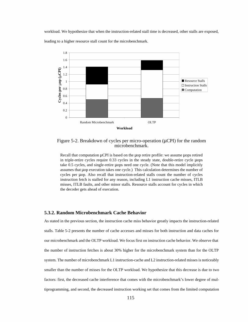
115

workload. We hypothesize that when the instruction-related stall time is decreased, other stalls are exposed,

leading to a higher resource stall count for the microbenchmark.

5.3.2. Random Microbenchmark Cache Behavior

As stated in the previous section, the instruction cache miss behavior greatly impacts the instruction-related

stalls. Table 5-2 presents the number of cache accesses and misses for both instruction and data caches for

our microbenchmark and the OLTP workload. We focus first on instruction cache behavior. We observe that

the number of instruction fetches is about 30% higher for the microbenchmark system than for the OLTP

system. The number of microbenchmark L1 instruction-cache and L2 instruction-related misses is noticeably

smaller than the number of misses for the OLTP workload. We hypothesize that this decrease is due to two

factors: first, the decreased cache interference that comes with the microbenchmark’s lower degree of mul-

tiprogramming, and second, the decreased instruction working set that comes from the limited computation

Figure 5-2. Breakdown of cycles per micro-operation (µCPI) for the random microbenchmark.

Recall that computation µCPI is based on the µop retire profile: we assume µops retiredin triple-retire cycles require 0.33 cycles in the steady state, double-retire cycle µopstake 0.5 cycles, and single-retire µops need one cycle. (Note that this model implicitlyassumes that µop execution takes one cycle.) This calculation determines the number ofcycles per µop. Also recall that instruction-related stalls count the number of cyclesinstruction fetch is stalled for any reason, including L1 instruction cache misses, ITLBmisses, ITLB faults, and other minor stalls. Resource stalls account for cycles in whichthe decoder gets ahead of execution.

0

0.2

0.4

0.6

0.8

1

1.2

1.4

1.6

1.8

Random Microbenchmark OLTP

Workload

Cyc

les

per

µop

( µC

PI)

Resource Stalls

Instruction Stalls

Computation

116

of the microbenchmark. As described earlier, this microbenchmark does not include update operations,

which generate logging activity, including the kernel operations for performing disk writes. These lower

instruction cache miss rates lead to the decreased instruction stalls that the microbenchmark experiences, rel-

ative to the OLTP system, as shown in Figure 5-2.

Focusing on the data cache behavior, we note that the microbenchmark’s L1 data-cache miss count is about

60% of the miss count for the OLTP workload. We again hypothesize that the lower degree of multiprogram-

ming and the decreased working set lead to better cache behavior for the microbenchmark. Microbenchmark

L2 data cache behavior is similar to the OLTP L2 data behavior.

5.3.3. Random Microbenchmark ILP and Branch Behavior

Figure 5-3 illustrates the micro-operation retirement profile for the workloads, decomposed by cycles. We

note that both workloads retire zero µops in roughly 65% of all cycles. Second-most common are single-

retire cycles, followed by triple-retire cycles and double-retire cycles. Figure 5-4 shows the same µop retire-

ment profile, broken down by how many µops are retired in each type of retirement cycle. We observe that

the majority of µops (54% to 62%) are retired in triple-retire cycles, followed by single-retire cycles and

finally double-retire cycles.


Instruction fetches 1907 1446

Data references 437 483

L1 I-cache misses 61 (3%) 99 (7%)

L1 D-cache misses 32 (4%) 51 (7%)

ITLB misses 1 4

L2 Inst.-related misses 3 (4%) 10 (11%)

L2 Data-related misses 10 (27%) 13 (26%)

Overall L2 misses 13 (13%) 23 (16%)

Table 5-2. Random microbenchmark overall cache behavior.

The values in this table represent the number of events occurring per 1000 instructionsretired. Miss ratios for each cache are shown as a percentage in parentheses.

117

We present the branch behavior of the workloads in Table 5-3. We see that both workloads have similar

branch frequencies of about 20%. The microbenchmark’s branch misprediction rate is about half the mispre-

diction rate experienced by the OLTP system. We hypothesize that this effect is due to the tighter instruction

loop used for the microbenchmark, which minimizes jumps to logging and kernel write routines; this tighter

loop leads to better branch prediction behavior.

Figure 5-3. Random microbenchmark µop retirement profile, decomposed by cycles.

0%

10%

20%

30%

40%

50%

60%

70%

80%

90%

100%


Workload

Per

cent

of

Cyc

les

3-uop

2-uop

1-uop

0-uop

Figure 5-4. Random microbenchmark µop retirement profile, broken down by µops.

0%

10%

20%

30%

40%

50%

60%

70%

80%

90%

100%


System

Per

cent

of

Mic

ro-o

pera

tion

s

3-uop

2-uop

1-uop

118

5.3.4. Computation per Row for the Random Microbenchmark

One of the secondary goals of this microbenchmark study is to determine a lower bound for the amount of

computation performed per row for simple operations. Table 5-4 shows the estimated instruction pathlength

and processor clock cycle count per row for the random microbenchmark. The system performs about 30k

instructions per row for the index scan. Multiplying by the CPI, we obtain the cycle counts per row for this

operation, which is about 90k cycles per row.

5.3.5. Discussion

The random microbenchmark is a promising approach for approximating more complex OLTP behavior with

a simple test. The characteristic that differs the most between the microbenchmark and the OLTP workload

is the instruction cache behavior. We propose that the microbenchmark instruction footprint could be made

more realistic by introducing update operations, and by increasing the microbenchmark multiprogramming

level. The first-level data cache behavior, which differs somewhat between the workloads, may also benefit

from these proposals.

5.4. Sequential I/O Approximations for DSS

This section examines how closely the architectural characteristics of the sequential microbenchmark resem-

ble those of the DSS workload measured in Chapter 4. We base our comparison on two of the scan-based


Branch frequency 18.7% 20.2%

Branch mispredict. ratio 8.6% 16.7%

Table 5-3. Random microbenchmark branch behavior.

CharacteristicRandom Microbenchmark

Overall instructions per row 31,835

Overall clock cycles per row 90,670

Table 5-4. Random microbenchmark instruction and clock cycle count behavior.

119

queries measured, Q1 and Q6, since they are the operations most comparable to the sequential microbench-

mark. We note, however, that these DSS queries compute complex aggregate functions (for example, sums

and averages of decimal data types), which require more computation per row than the sequential

microbenchmark. Q6 computes one such aggregate, while Q1 computes eight aggregates (predominantly of

decimal types, with a few integer aggregates). Can the simple microbenchmark approximate the behavior of

these more computationally-intensive queries?

5.4.1. Sequential Microbenchmark CPI Analysis

We first examine the breakdown of cycles and CPIs of the various workloads, shown in Table 5-5. We

observe that the microbenchmark system exhibits more kernel time than the DSS queries running on a four-

processor system with the same cache size (256 KB). Again, we hypothesize that this increase is due to the

use of the NT file system for data storage, rather than the raw disk interface used for the DSS workload. As

in the random benchmark, the sequential microbenchmark experiences negligible idle time.

The µop to instruction ratio of the microbenchmark system is within 10% of that for DSS Q6, and within

15% of that for DSS Q1. The microbenchmark system’s overall µCPI, however, differs from the DSS que-

ries’ µCPIs by 13% to 25%. (CPI differences range from 20% to 45%.) To understand this discrepancy, we

decompose the µCPI into its computation and stall components.

CharacteristicSequential Microbenchmark DSS Q1 (256 KB, 4 P) DSS Q6 (256 KB, 4 P)

% User Time 87.6% 98.8% 93.4%

% Kernel Time 12.3% 1.2% 3.5%

% Idle Time 0.1% 0.0% 3.1%

Overall µCPI 1.06 0.86 0.94

Overall CPI 2.00 1.39 1.65

Overall µops/instruction 1.88 1.62 1.75

Table 5-5. Breakdown of time, measured cycles per micro-operation (µCPI) and measured cycles per macro-instruction (CPI) for the sequential microbenchmark.

The DSS columns refer to the TPC-D-like DSS workload (queries Q1 and Q6) running ona four-processor system with the same L2 cache size (256 KB). Ideally, we would com-pare performance against a uniprocessor with the same L2 cache size, but we did not col-lect DSS data for the uniprocessor configuration.

120

Figure 5-5 shows this detailed breakdown of the µCPI components. For all workloads, stall cycles comprise

roughly half (45% to 55%) of the µCPI. The computation component is nearly identical for all workloads.The

microbenchmark’s instruction stall component is comparable to that of DSS Q1. Its resource stall component

is roughly 20% larger than that of Q6. We hypothesize that this difference is due to increased resource con-

tention resulting from additional data-related L2 misses. The cache behavior of these configurations is

described more fully in the next section.

5.4.2. Sequential Microbenchmark Cache Behavior

Table 5-6 presents the number of cache accesses and misses for both instruction and data caches for the

sequential microbenchmark and the DSS queries. We begin our discussion with instruction cache behavior.

We observe that the microbenchmark’s instruction cache miss behavior closely mirrors the behavior of Q1,

leading to the similar instruction-related stall components shown in Figure 5-5. The bulk of these stall cycles

come from L1 cache misses that hit in the L2 cache. We note that differences in L1 instruction cache miss

behavior also exist between the two DSS queries. We believe that Q1 experiences more L1 I-cache misses

due to the increased footprint required for the different aggregate computations it must perform.We hypoth-

esize that the tight loop of the microbenchmark leads to an instruction footprint that includes both database

Figure 5-5. Breakdown of cycles per micro-operation (µCPI) for the sequential microbenchmark.

0

0.2

0.4

0.6

0.8

1

1.2

SequentialMicrobenchmark

DSS Q1 DSS Q6

System

Cyc

les

per

µop

( µC

PI)

Resource Stalls

Instruction Stalls

Computation

121

code and file system read code. This combination leads to a microbenchmark footprint comparable to that of

DSS Q1.

The microbenchmark’s L1 D-cache behavior is comparable to that of Q1, but its L2 data-related misses are

up to 2X the L2 data misses of the DSS queries. We believe that this increased miss rate occurs because the

microbenchmark performs less computation per row than either of the DSS queries. This hypothesis is sup-

ported by the trend observed in the DSS queries: Q6, which performs a single aggregate operation, experi-

ences more L2 data misses than Q1, which performs more complex aggregates. We hypothesize that this

higher L2 data-related miss behavior may contribute to the increased resource stalls experienced by the

microbenchmark: conflicts for memory reorder buffer or register renaming entries may occur in the time the

processor must wait for the L2 miss to be satisfied by memory.

5.4.3. Sequential Microbenchmark ILP Behavior

Figure 5-6 illustrates the micro-operation retirement profile for the workloads, decomposed by cycles. The

zero-retirement prevalence reflects the percentage of stall cycles: all workloads retire zero µops in roughly

50% of all cycles. Triple-retire cycles are second-most common, followed by double-retire cycles and finally

single-retire cycles. We note that this relative ordering is somewhat different than the ordering observed for

the random/OLTP workload. Figure 5-7 shows the same µop retirement profile, broken down by how many

CharacteristicSequential Microbenchmark DSS Q1 (256 KB, 4 P) DSS Q6 (256 KB, 4 P)

Instruction fetches 1440 954 1428

Data references 549 668 537

L1 I-cache misses 42 (3%) 40 (4%) 18 (1%)

L1 D-cache misses 23 (3%) 23 (4%) 29 (4%)

ITLB misses 0 1 0

L2 Inst.-related misses 1 (3%) 0 (1%) 1 (4%)

L2 Data-related misses 7 (28%) 1 (6%) 4 (15%)

Overall L2 misses 8 (12%) 2 (3%) 5 (11%)

Table 5-6. Sequential microbenchmark overall cache behavior.


122

µops are retired in each type of retirement cycle. We observe that the majority of µops (about 65%) are retired

in triple-retire cycles; single-retire and double-retire cycles account nearly equally for the remaining µops.

5.4.4. Computation per Row for the Sequential Microbenchmark

Using the above information, we can determine a lower bound for the amount of computation performed per

row for a simple sequential access. Table 5-7 shows the estimated instruction pathlength and clock cycle

Figure 5-6. Sequential microbenchmark µop retirement profile, decomposed by cycles.

0%

10%

20%

30%

40%

50%

60%

70%

80%

90%

100%

Sequential Microbenchmark DSS Q1 DSS Q6

System

Per

cent

of

Cyc

les

3-uop

2-uop

1-uop

0-uop

Figure 5-7. Sequential microbenchmark µop retirement profile, broken down by µops.

0%

10%

20%

30%

40%

50%

60%

70%

80%

90%

100%

Sequential Microbenchmark DSS Q1 DSS Q6

System

Per

cent

of

Mic

ro-o

pera

tion

s

3-uop

2-uop

1-uop

123

count per row for the sequential microbenchmark. These systems perform about 1700 instructions per row

for the sequential scan, an order of magnitude fewer instructions than for the index scan. Multiplying by the

CPI, we obtain the cycle count per row for this operation (about 3400 cycles per row).

5.4.5. Discussion

Again, the initial results suggest that the sequential microbenchmark is a promising technique for simplifying

the evaluation of DSS workloads. We believe that the degree of computation per row is an important factor

in determining the architectural characteristics of the microbenchmark. Therefore, we propose adding more

computationally-intensive operations to more closely approximate the behavior of the DSS queries.

5.5. Comparison Between Commercial Databases

All of the experiments described so far in this dissertation have been performed on different revisions of a

single vendor’s database server. A natural question is how generalizable are the reported results to database

servers from different vendors? This section uses the microbenchmark workloads introduced above to com-

pare the behavior of our base database (reported above) with the behavior for a different commercially avail-

able database. We will call these two databases System A and System B, respectively. We also explore the

question of whether differences in microbenchmark performance can predict performance differences for the

complex OLTP and DSS workloads.

5.5.1. Comparison of CPI Breakdowns

Table 5-8 presents the breakdown of time and CPIs of Systems A and B for both the random and sequential

microbenchmarks. For the random microbenchmark, the two systems have very different time breakdowns,

with System B spending nearly half of its time idle. Kernel-level execution comprises two-thirds of B’s non-

idle time, and user-level execution the remaining third. The breakdown of execution time is more uniform

CharacteristicSequential Microbenchmark

Overall instructions per row 1715

Overall clock cycles per row 3420

Table 5-7. Sequential microbenchmark instruction and clock cycle count behavior.

124

for the sequential microbenchmark, with roughly 85% of the execution time spent at user level and about

10% spent in the kernel. System B’s sequential microbenchmark also experiences a higher percentage of idle

time. The variation in the idle time component suggests that System A does sufficient computation per I/O

operation for the six data disks in our configuration to keep the processor busy, while System B’s computa-

tion per I/O is low enough that a greater number of disks is needed to keep the processor busy.

For the random microbenchmark, the two systems’ overall µCPI values are within 10% of each other. System

B’s overall CPI and µops per instruction, however, are roughly 25% greater than the corresponding System

A values. We hypothesize that this is due to the large percentage of kernel time for this workload. The kernel

typically exhibits a higher CPI and uses more complex instructions, resulting in a higher µops per instruction

ratio, as shown by the analysis presented in Chapter 3. The database-only values shown in Table 5-8 support

this hypothesis; the System B database-only values come within 10% of the System A database-only values.

For the sequential microbenchmark, System B has consistently lower µCPI and CPI values. B’s µCPI values

(both overall and database-only) are about 65% of the corresponding values for System A. Similarly, B’s CPI

overall and database-only CPI values are about 55% of A’s CPI values. To better understand these differ-

ences, we decompose the µCPI into stall and computation components, as shown in Figure 5-8.

CharacteristicRandom System A

Random System B

Sequential System A

Sequential System B

% User Time 78.0% 18.4% 87.6% 83.0%

% Kernel Time 21.7% 36.2% 12.3% 8.9%

% Idle Time 0.3% 45.4% 0.1% 8.1%

Overall µCPI 1.38 1.48 1.06 0.68

Overall CPI 2.85 3.58 2.00 1.14

Overall µops/instruction 2.06 2.41 1.88 1.66

DB-only µCPI 1.52 1.41 1.04 0.64

DB-only CPI 2.96 2.82 1.92 1.06

DB-only µops/instruction 1.95 1.99 1.84 1.64

Table 5-8. Breakdown of time, measured cycles per micro-operation (µCPI) and measured cycles per macro-instruction (CPI) for both microbenchmarks for both database systems.

System A refers to the system measured in the previous sections, and System B refers to adifferent commercially available database server.

125

For the random microbenchmark, stall cycles dominate the µCPI, comprising 60% to 65% of the µCPI for

both System A and System B. The computation components are very similar between the two systems, but

the stall components vary more widely. System B experiences about 1.5X as many instruction-related stalls

as System A, and about one-third as many resource stalls. This stall behavior is due to the instruction and

data cache miss behavior, as described in Section 5.5.2.

For the sequential microbenchmark, stall cycles play less of a role for both systems: stalls comprise about

33% of System B’s µCPI and 55% of System A’s µCPI. As in the random microbenchmark case, the com-

putation component is nearly identical for both systems, but the stall components vary. System B’s resource

stall component is about one-third that of System A, and its instruction-related stall component is about one-

fourth of System A’s. As we will show in the following section, these differences are due to System B’s very

low cache miss rates.

Figure 5-8. Breakdown of cycles per micro-operation (µCPI) for the random and sequential microbenchmarks for both database systems.

We note that the sum of the computation and stall components for System B running therandom microbenchmark is about 10% less than the measured value reported inTable 5-8. We hypothesize that this under-prediction is due to our model for computa-tion cycles, which assigns a steady-state value of one cycle per µop. This model under-predicts for certain long-latency µops used in the kernel. System B’s randommicrobenchmark is affected because it spends the most time in the kernel.

0

0.2

0.4

0.6

0.8

1

1.2

1.4

1.6

Random System A Random System B Sequential SystemA

Sequential SystemB

System

Cyc

les

per

µop

( µC

PI)

Resource Stalls

Instruction Stalls

Computation

126

5.5.2. Comparison of Cache Behavior

As described in the previous section, many of the differences in stall behavior for the two systems are due to

differences in instruction and data cache behavior. Table 5-9 shows the cache behavior for both systems for

both microbenchmarks.

We examine the random microbenchmark behavior first. System B experiences about twice as many L1

instruction-cache misses as System A, implying that its instruction working set doesn’t fit as well into the 8

KB on-chip instruction cache. The instruction-related L2 miss behavior is nearly identical between the two

systems. Thus, B’s increased L1 I-cache miss count is responsible for System B’s higher instruction-related

stalls, as shown in the previous section. System B also exhibits more L1 data cache misses - about 1.6X as

many as System A. B’s data-related L2 miss counts, however, are about one-third that of System A. This

reduction in L2 data-related misses likely contributes (indirectly) to the smaller resource stall component

exhibited by the random microbenchmark running on System B.

Focusing on the sequential microbenchmark behavior, we observe that System B experiences considerably

fewer cache misses - both instruction and data, and at the first and second cache levels. These reduced cache

miss rates are responsible for the smaller instruction-related and resource stall components experienced by

the sequential microbenchmark on System B. Furthermore, because of the negligible L2 instruction miss fre-


Random System B

Sequential System A

Sequential System B

Instruction fetches 1907 1629 1440 1001

Data references 437 474 549 675

L1 I-cache misses 61 (3%) 124 (8%) 42 (3%) 9 (1%)

L1 D-cache misses 32 (4%) 52 (7%) 23 (3%) 4 (1%)

ITLB misses 1 4 0 0

L2 Inst.-related misses 3 (4%) 3 (3%) 1 (3%) 0 (3%)

L2 Data-related misses 10 (27%) 3 (6%) 7 (28%) 2 (37%)

Overall L2 misses 13 (13%) 6 (4%) 8 (12%) 2 (14%)

Table 5-9. Comparison of microbenchmark overall cache behavior.


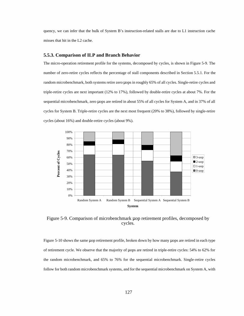
127

quency, we can infer that the bulk of System B’s instruction-related stalls are due to L1 instruction cache

misses that hit in the L2 cache.

5.5.3. Comparison of ILP and Branch Behavior

The micro-operation retirement profile for the systems, decomposed by cycles, is shown in Figure 5-9. The

number of zero-retire cycles reflects the percentage of stall components described in Section 5.5.1. For the

random microbenchmark, both systems retire zero µops in roughly 65% of all cycles. Single-retire cycles and

triple-retire cycles are next important (12% to 17%), followed by double-retire cycles at about 7%. For the

sequential microbenchmark, zero µops are retired in about 55% of all cycles for System A, and in 37% of all

cycles for System B. Triple-retire cycles are the next most frequent (20% to 38%), followed by single-retire

cycles (about 16%) and double-retire cycles (about 9%).

Figure 5-10 shows the same µop retirement profile, broken down by how many µops are retired in each type

of retirement cycle. We observe that the majority of µops are retired in triple-retire cycles: 54% to 62% for

the random microbenchmark, and 65% to 76% for the sequential microbenchmark. Single-retire cycles

follow for both random microbenchmark systems, and for the sequential microbenchmark on System A, with

Figure 5-9. Comparison of microbenchmark µop retirement profiles, decomposed by cycles.

0%

10%

20%

30%

40%

50%

60%

70%

80%

90%

100%

Random System A Random System B Sequential System A Sequential System B

System

Per

cent

of

Cyc

les

3-uop

2-uop

1-uop

0-uop

128

the double-retire cycles comprising the remaining percentage. For System B’s sequential benchmark, the

remaining 24% are split roughly evenly between double- and single-retire cycles.

We compare the branch behavior of the systems in Table 5-10. We see that both systems have similar branch

frequencies of about 20% for both workloads. For the random microbenchmark, System B’s branch mispre-

diction rate is about twice the misprediction rate experienced by System A. In contrast, System B’s sequential

microbenchmark branch misprediction rate is negligible.

5.5.4. Comparison of Computation per Row and Predictive Performance

Table 5-11 shows the estimated instruction pathlengths and clock cycle counts per row for the systems.

Examining the random microbenchmark, these systems perform 20k to 30k instructions per row for the index

scan. Multiplying by the CPI, we obtain the cycle counts per row for this operation, which range from 80k

to 90k cycles per row. We note that the ratio of cycle counts is 1.1X.

Figure 5-10. Comparison of microbenchmark µop retirement profiles, broken down by µops.

0%

10%

20%

30%

40%

50%

60%

70%

80%

90%

100%

Random System A Random System B Sequential System A Sequential System B

System

Per

cent

of

Mic

ro-o

pera

tion

s

3-uop

2-uop

1-uop


Random System B

Sequential System A

Sequential System B

Branch frequency 18.7% 19.6% 17.9% 18.9%

Branch mispredict. ratio 8.6% 18.5% 4.2% 0.7%

Table 5-10. Comparison of microbenchmark branch behavior.

129

The instruction counts per row for the sequential microbenchmark are nearly 20X smaller than for the

random test: 1000 to 2000 instructions per row. The cycle counts are also at least an order of magnitude

smaller, ranging from 1300 to 3400 cycles per row.

A secondary goal of this study is to investigate the hypothesis that differences between database microbench-

mark performance will predict TPC workload differences for those databases. To test this hypothesis, we

looked up TPC benchmark reports for System A and System B running on comparable Windows NT-based

four-processor Pentium Pro systems during the Fall of 1996 [103]. The reported results indicate that TPC-C

performance (measured in tpmC) of System B is 1.1X better than the performance of System A. While this

is a single comparison point, it supports the hypothesis that random microbenchmark performance differ-

ences predict TPC performance differences. Clearly, this hypothesis should be validated with additional sys-

tems.

Unfortunately, we did not find two published TPC-D benchmark results for System A and System B on hard-

ware and software configurations comparable to those used in our microbenchmark experiments. Thus, we

were unable to explore this hypothesis for the sequential microbenchmark.

5.5.5. Common Trends and Discussion

From our observations of a second commercial database, we see that databases from different vendors do,

indeed, exhibit different behavior. Furthermore, just because a system has comparatively better behavior (for

Characteristic System A System B Ratio (A/B)

Random Microbenchmark

Overall instructions per row 31,835 22,700 1.4X

Overall cycles per row 90,670 81,170 1.1X

TPC-C performance 1.1X

Sequential Microbenchmark

Overall instructions per row 1715 1150 1.5X

Overall cycles per row 3420 1305 2.6X

TPC-D performance N/A

Table 5-11. Comparison of microbenchmark instruction and cycle count behavior.

130

example, CPI or L1 cache behavior) for one workload doesn’t necessarily imply that its behavior is better for

other workloads.

While variation exists between these two systems for a given microbenchmark, both exhibit similar trends

between the random and sequential microbenchmarks. These microbenchmark trends reflect the trends for

the more complex workloads, as described in Chapter 3 and Chapter 4. Both systems spend more time at user

level and less time at kernel level for the sequential microbenchmark, due mainly to the lower overhead of

processing larger I/O operations in the sequential microbenchmark. Both systems exhibit a higher (µ)CPI for

the random test than for the sequential test, due to the higher percentage of stall cycles for the random test

(60% to 65% for random vs. 33% to 56% for sequential). The sequential microbenchmark on both systems

exhibits better instruction and data cache behavior at both cache levels than the random microbenchmark

does. In addition, the µop superscalar retirement width is more frequently exploited for the sequential work-

load, where 65% to 76% of µops are retired in triple-retire cycles, than for the random workload, where 54%

to 62% are retired in triple-retire cycles. The Pentium Pro’s branch prediction algorithms are more effective

for the sequential workload than for the random workload. Finally, the processor executes an order of mag-

nitude fewer instructions (cycles) per row for the sequential test than for the random test.

5.6. Related Work

Very few researchers have examined the use of database microbenchmarks as a means of simplifying the

hardware and software requirements of database performance evaluation. In this section, we describe two

recent studies that examine these and related issues.

5.6.1. Ailamaki, et al.: In-Memory Microbenchmarks to Compare Commercial Databases

Ailamaki, et al., use in-memory microbenchmarks similar to the ones described above to evaluate commer-

cial databases running on next-generation Intel hardware, a 400 MHz Pentium II Xeon uniprocessor, running

Windows NT 4.0 [2]. A primary goal is to determine how database designers can modify their code to exe-

cute more efficiently on modern architectures. A second goal is to compare the differences in behavior

131

between commercial databases. Their microbenchmarks examine sequential table scans, index scans, and

sequential join operations.

They find that half of the execution time is spent in stalls, which corroborates our findings. The majority of

the stalls are due to second-level data cache misses and first-level instruction cache misses. These findings

imply that database designers should focus on data placement for the L2 cache and instruction placement for

the L1 instruction cache. A minority of the stalls are due to other factors such as branch misprediction. They

find that the selectivity of a query can impact the contribution of branch mispredictions and L1 instruction

cache stalls. While there are differences in the magnitudes of stall components between different databases,

the relative importance of stall components is roughly consistent between the databases. They find that the

microbenchmark behavior is similar to an in-memory version of TPC-D on the same database. A scaled-back

version of TPC-C incurs more second-level cache and resource stalls than the microbenchmarks.

The biggest differences between this study and our study are that: 1) our microbenchmarks include I/O oper-

ations, which are a critical component of database workloads; 2) they use a different model of query execu-

tion time, as described below; and 3) they measure a larger collection of commercial databases and an

additional relational operator (join). This study employed a different model of query execution time, which

directly measures some stall characteristics (such as L1 instruction-cache miss stalls and resource stalls), and

models the stalls from other execution characteristics (such as L1 and L2 data-related stalls, L2 instruction-

related stalls and branch misprediction stalls). While some of these stall components are overlappable (for

example, L1 data cache misses), the model does not explicitly reflect this potential overlap. It is not clear

how closely the resulting CPI predicted by their model reflects the actual measured CPI, nor whether the

breakdown of stall cycles reflects the actual stall decomposition. In contrast, our study directly measures stall

components, and the summation of these stall components and the computation component is within 10%

(often within 5%) of the measured CPI.

Furthermore, they express stall components as a percentage of the query execution time, rather than present-

ing the CPI. This approach was chosen to obscure the differences in performance between the different data-

132

base systems, to provide more confidentiality. The choice also has the unfortunate effect of making it more

difficult to perform an apples-to-apples comparison between their results and our results.

5.6.2. Unlu: Database “Mini-Benchmarks”

Unlu describes Intel’s use of database “mini-benchmarks,” which evaluate selected standard algorithms from

a database in a stand-alone fashion, without requiring the full database [110]. The goals are to pick algorithms

representative of full-scale benchmarking systems, while preserving confidentiality by using implementa-

tions that are generalized across commercial systems. To date, they have focused on buffer search and

pseudo-code evaluation, which each comprise about 10% of the execution time in OLTP workloads. Buffer

search simulates a multi-threaded search for data buffers cached in memory, including hashing to locate the

buffer entry, and then locking and traversing the hash chain to locate the desired buffer. The pseudo-code

benchmark simulates the execution of a small virtual machine that executes simple hand-coded programs,

including simple operations that manipulate abstract data in buffers. They find that both mini-benchmarks

have representative data access patterns, but smaller code footprints than the fully-scaled OLTP workload.

The mini-benchmarks also have somewhat higher CPIs than the fully-scaled workload. They are constructing

a tool to combine these (and other) individual mini-benchmarks to obtain a more representative workload.

5.7. Conclusions

This chapter has taken an important first step in simplifying the technique for studying OLTP and DSS work-

loads. We proposed a very simple set of microbenchmarks based on the predominant I/O patterns of the

workloads. The random microbenchmark, based on an index scan, approximates the behavior of the OLTP

workload. The characteristics of the sequential microbenchmark, based on a sequential table scan, resemble

the characteristics of some common DSS queries. The initial results of our study show that this approach is

a promising method for reducing the complexity of database performance evaluation.

We enumerated a number of factors that impact the effectiveness of these workloads, including the multipro-

gramming level and presence of updates for the random microbenchmark, and the computational complexity

for the sequential microbenchmark. We investigated the differences in architectural characteristics between

two commercial databases running each microbenchmark, and found that they have very different instruction

133

and data footprints, which leads to different stall behavior. While behavioral differences exist between the

databases for a given workload, we found many commonalities when comparing a single database’s behavior

between the two microbenchmarks. Finally, we quantified a lower bound for the amount of computation per

I/O for these simple random and sequential scan and aggregate operations.

134

6 The Case for Intelligent Disks (IDISKs)

6.1. Introduction

As described in Chapter 1, the key challenge posed by decision support (DSS) workloads is the explosive

growth of their I/O capacity and computational requirements. Dr. Greg Papadopoulos, the Chief Technical

Officer (CTO) of Sun Microsystems, estimates that the demand for decision support doubles every 6 to 12

months [75], a rate supported by the large commercial systems summarized in the Winter Very Large Data-

base (VLDB) surveys [118] [117]. This evidence implies that DSS growth is faster than the growth rate of

disk capacity (which doubles every 18 months) and the growth rate of processor performance (which also

doubles every 18 months). This phenomenal growth trend requires a more scalable I/O system design for

these data-intensive services.

Shared-nothing clusters comprised of workstations, PCs or symmetric multiprocessors (SMPs) are com-

monly used as decision support server architectures. The chief strengths of clusters are their incremental scal-

ability and the high performance afforded by developments in parallel shared-nothing database algorithms.

Shared-nothing clusters have several weaknesses, however, including the I/O bus bottleneck of their nodes,

the challenge of distributed system administration, packaging inefficiencies, and the unsuitability of desktop

microprocessors for database applications.

This chapter presents a vision of an alternative approach to scalable decision support: replacing the standard

nodes in a cluster server with “intelligent” disks (“IDISKs”), where each IDISK is a hard disk containing an

embedded processor, tens to hundreds of megabytes of memory, and gigabit per second network links. Links

135

from each disk are connected via switches so that IDISKs can simultaneously communicate with each other

at full link bandwidth.

An IDISK-based architecture offers several potential scalability, manageability, performance, and price

advantages over traditional server architectures. The IDISK architecture allows the processing of the system

to scale with increasing storage demand. By using a switch-based interconnect between IDISKs, this archi-

tecture provides a truly scalable I/O subsystem, overcoming the I/O bus bottleneck of conventional bus-based

systems. By collocating processing with the disk, IDISK offers a system that can continuously monitor itself

and automatically adapt to failures and performance degradation. The aggregate computational capability of

the IDISK I/O system may be greater than the central computational capabilities of a comparable traditional

system, providing performance improvements for numerous algorithms. IDISK pushes computation closer

to the data, thus providing a potential reduction in data movement through the I/O subsystem. By off-loading

computation from expensive central desktop processors to inexpensive embedded disk processors and by

leveraging the cabinetry, cooling and power supplies already needed for the disks, IDISK systems may cost

much less than conventional systems.

This architecture is motivated by trends in several computer architecture fields. First, hard disks are being

designed with an increasing amount of general purpose processing and memory on-board. Second, embedded

processors possess increasing computational capability, and are available at a fraction of the cost and power

dissipation of desktop processors. Third, switch-based interconnects and advances in high-speed serial com-

munication mean that high bandwidth does not require physical proximity: processors 10 meters apart can

communicate as quickly as those communicating over a bus.

Intelligent disk processing for database workloads is not a new idea. Database machines, an active area of

research in the 1970s and early 1980s, typically included a central host processor plus intelligent disk pro-

cessing in the form of a processor per head, track or disk or a multiprocessor disk cache arrangement. These

systems fell out of favor in the late 1980s and 1990s because their modest performance did not justify the

high cost of special-purpose hardware. However, the increasing demands of DSS workloads, the commod-

136

itization of more intelligent disk subsystems, processor and communication technology trends, and advances

in database algorithms suggest that it is now time to re-examine intelligent disk processing.

This chapter explores the IDISK vision, rather than the performance of a real system. We focus on the scal-

ability and performance advantages offered by IDISK architectures. For a more complete discussion of

IDISK’s potential administrative advantages, we refer the reader to [19]. To set the stage for IDISK we first

review the strengths and weaknesses of today’s servers in Section 6.2. Section 6.3 presents the technological

trends that lead to the IDISK hardware and software architecture described in Section 6.4. In Section 6.5 we

present an initial evaluation of the performance and scalability advantages offered by the IDISK architecture.

Since IDISK is reminiscent of past database machines, Section 6.6 then reviews the successes and failures of

these machines and suggests which might apply to IDISK. Section 6.7 concludes.

6.2. Strengths and Weakness of DSS Clusters

Large-scale decision support systems typically employ shared-nothing clusters of workstations, PCs, or

SMPs. Although this hardware architecture possesses strengths that facilitate the development and execution

of database software, the architecture also presents several weaknesses. This section discusses these archi-

tectural strengths and weaknesses.

The main advantage of cluster organizations is their incremental scalability: machines can easily be added

or subtracted as needed by the application. Another advantage of clusters is the high performance afforded

by developments in parallel shared-nothing database algorithms. One such example is Berkeley’s NOWSort,

a shared-nothing sort implemented on a cluster of UltraSparc workstations, which held the Minute Sort

record for sorting 8.41 GB in a minute, and the Datamation Sort record for sorting one million 100 B records

in 2.41 seconds [7]. Berkeley’s Millennium Sort, the current holder of the Datamation Sort record (1.18 sec-

onds), runs on a cluster of Intel-based two-processor SMPs [20]. A final strength is that clusters today lever-

age the hardware development investment in the desktop, thus using processors, memory, and disks without

paying for separate development costs.

We observe four weaknesses in cluster architectures:

137

1. System administration challenges

2. The I/O bus bottleneck

3. Packaging and cost difficulties

4. High price of desktop microprocessors for database applications

We explore these weaknesses further below.

The first weakness of clusters is the high cost of cluster system administration. Managing the distributed

resources of a cluster typically involves performing diagnostic and maintenance operations for each individ-

ual node in the cluster. Unfortunately, few tools exist to automate these diagnostic and maintenance tasks at

the database level [36] and at the operating system level [81]. As a result, cluster system administration typ-

ically requires human supervision, which drives up the associated costs [6]. The annual personnel costs can

be three times the cost of the disks.

The second weakness of shared-nothing clusters is I/O busses. Clusters often utilize commodity desktop

machines such as PCs or workstations as building blocks, which employ standard processor I/O busses, such

as PCI or Sun’s S-bus. Unfortunately, the performance of these I/O bus standards is limited by the rate of

committee decision-making, rather than the rate of technological improvements. As a result, the increase in

bus bandwidth is typically much slower than the increase in bandwidth provided by high-performance disk

and network peripherals. For example, transfer rates of disks improve at 40% per year, suggesting about a

150 MB/sec transfer rate in 2004. It is not clear that I/O bus performance will keep up.

The limitations of current I/O busses become even more evident when we consider that both disk and network

peripherals must simultaneously use an I/O bus to transfer data. The I/O subsystem of some workstations is

quickly saturated by just a few high-performance disks and network communication for cluster-based data-

base applications [8].

The third cluster weakness is that cluster packaging is often inefficient and expensive. Because clusters rely

on more cost-effective commodity building blocks, they must deal with the tower or “pizza box” packaging

that houses the processor, memory, and I/O peripherals of these commodity machines. When assembling a

138

large number of such nodes, these packaging configurations occupy significant space and are not nearly as

efficient as rack-mountable systems. Commodity desktop processors also have high power requirements,

which increases the cost of cooling and power supplies.

A final weakness of clusters is the ineffectiveness of desktop processors for database workloads. The design

of a desktop microprocessor requires significant design effort and capital outlay, so a company needs the

volume sales of the desktop to justify the expense. Unfortunately, architectural innovations that aid floating

point and desktop integer programs, such as multiple instruction issues per cycle, branch prediction and out-

of-order execution, are generally less helpful for databases [13] [83]. For example, as shown in Chapter 4,

despite a theoretical peak of 3.0 instructions executed per clock cycle, the Pentium Pro executes on average

only 0.74 instructions per clock cycle for the scan and aggregate operations defined in TPC-D Q1.

The complexity of desktop processor innovations results in increased die size, power requirements, cost, and

price, yet yields little improvement in integer performance over much simpler embedded processor designs.

Table 6-1 shows the characteristics of desktop microprocessors versus several embedded microprocessors.

Larger die size, power, cost and price of desktop chips may be justified for SPECfp95, but using SPECint95

or Dhrystone we see a much smaller difference. Thus, we see cost/power/price differences of factors of 5 to

20 yielding integer performance differences of 1.5X to 2X.

Figure 6-1 shows the configuration of a high-end cluster-based decision support server used for the 3 TB

TPC-D benchmark [105]. The NCR WorldMark 5200 cluster is fully configured with 44 nodes, where each

node contains a four-processor Pentium II Xeon SMP, 2 GB of main memory and two disk arrays containing

20 disks each [69]. NCR adds value by repackaging these commodity parts more efficiently, and including

their proprietary interconnect, the BYNET switched network. This server contains a hierarchy of busses and

networks to connect disks to processors, which not only add cost to system, but also serve as potential bot-

tlenecks.

Table 6-2 shows the hardware prices for this WorldMark configuration. The repackaging and proprietary

interconnect provided by NCR prove to be quite costly. Note that the processors, main memory, boards and

139

ProcessorDigital SA-

110

NEC VR 5464 (MIPS

R5400)MIPS

R12000 Sun Ultra-IIHP PA-

8500

Intel Pentium II

Xeon

Class Embedded Embedded Desktop Desktop Desktop Desktop

Clock rate 233 MHz 250 MHz 300 MHz 400 MHz 440 MHz 450 MHz

Cache size (I /D)

16 K / 16 K 32 K / 32 K 32 K / 32 K / 4 M

16 K / 16 K / 4 M

512 K / 1 M 16 K / 16 K / 512 K

IC process 0.35 µm 3 M 0.25 µm 3 M 0.25 µm 4 M 0.29 µm 4 M 0.25 µm 4 M 0.25 µm 4 M

Die size 50 mm2 47 mm2 204 mm2 126 mm2 475 mm2 118 mm2

SPEC95 base (int/fp)

n/a 10/4.5 (est) 17/27 14.0/22.8 30/50 18.9/13.3

Dhrystone 268 MIPS 519 MIPS n/a n/a n/a 500 MIPS (est)

Power 0.36 W 4.4 W 20 W 20 W > 40 W 18 W

Est. mfr’s cost

$18 $25 $140 $70 $330 $55

Price $39 $95 n/a $4249 n/a $821

Report Date 3/29/99 3/8/99 1/25/99 1/25/99 1/25/99 1/25/99

Table 6-1. 1999 Comparison of embedded and desktop processors. [21] [22] [23]

Figure 6-1. Typical high-end decision support server computer architecture: NCR WorldMark 5200.

This cluster has 44 nodes, each with four processors and 2 GB memory and 43 disks.This system uses a total of 176 processors, 88 GB of memory, and 1892 disks for a 3TB TPC-D configuration [69].

…

BYNET switched network

…

… …

bus bridge

……

1

… …scsi

……

bus bridge

88

Bus

bridge

Proc

Mem

1

ProcProcProc Mem

Bus

bridge

Proc

44

ProcProcProc

scsi

scsi

scsi

scsi

scsi

Mem Mem

pci pci

140

enclosures cost over $9M. The disk I/O subsystem, including the disks, controllers, and disk enclosures, costs

just over $4M.

Given these characteristics of clusters, performance analysis experts suggest that configuring a system for

decision support databases typically involves:

1. Putting the maximum number of processors in a box to amortize the cost of the enclosures;

2. Putting the maximum amount of memory into the box to get maximum memory bandwidth and to avoid

going to disk for temporary I/O in memory-sensitive algorithms, thereby avoiding I/O bus bottlenecks;

3. Attaching as many disks as needed for high bandwidth transfers and to spread data over multiple disks

for quickly loading information into memory.

Decision support databases on architectures configured to follow this advice are normally CPU bound, and

the disks are typically not very busy [41]. Furthermore, only a small fraction of the disks’ capacity is utilized

(for example, 1 / 8 to 1 / 10).

We found this observation surprising: we thought that the data-intensive nature of decision support would

translate into an I/O-bound system, rather than a CPU-bound system. Given that a significant fraction of the

cost of such a configuration is the disk subsystem, we should be able to construct a system with sufficient

processing and communication bandwidth so that the performance limit is also the disks.

6.3. Technological Trends

We observe five trends that make IDISK viable:

1. Commodity disks include embedded processors and memory.

2. Embedded CPUs have much lower costs, with integer performance within 2X that of desktop CPUs.

CPUs, DRAM, enclosures, boards, power.

$9,562k

Disks, controllers $3,570k

Disk enclosures $678k

Cables $22k

Console $12k

Hardware total $13,844k

Table 6-2. TPC-D 3 TB NCR WorldMark 5200 price breakdown (2/15/99).

141

3. Disks are beginning to include high speed serial links.

4. High speed links and switches are economical.

5. Integrated devices combining embedded processors, memories, and serial lines are being developed that

match the requirements of disk manufacturers.

In this section, we explore these trends further. For a more detailed discussion of processor, memory, net-

work, and disk trends, see [79].

The first trend is increased disk-resident processing and memory. Moore’s Law says the number of transis-

tors per chip will double every 1.5 years and transistor speed is improving at about 1.3X per year. In light of

these advances, disk manufacturers are increasingly using embedded processors to execute tasks previously

performed in special-purpose hardware. Many drives include a digital signal processor (DSP) with good real-

time performance for servo control and a separate general-purpose processor for other tasks, such as error

correction calculation and SCSI command processing. Using software for these features gives disk manufac-

turers flexibility and reuse in disk development. Power budgets for such processors inside the disk assembly

are on the order of 2 watts [66]. The low power consumption of embedded processors allows the combined

disk and processor to remain well within the allotted power budget.

In addition to on-disk processing, disk manufacturers are including more and more memory on disk. For

instance, the Seagate Cheetah hard drive includes 1 MB of track buffer memory. Seagate also offers the

option of increasing the track buffer memory to 4 MB, for an additional fee [90]. By the year 2001, experts

at Seagate estimate that a high-end disk drive will have 100 MIPS to 200 MIPS in processing, plus up to 64

MB of memory provided by one or two high-density memory chips [4].

A second trend that supports IDISK is the cost-performance of embedded processors versus desktop proces-

sors. As mentioned above, given the highly competitive desktop environment, CPU designers are willing to

make trade-offs that raise the costs by factors of 5 to 10, while improving integer performance by less than

factors of 2. Embedded designs provide integer performance within 2X that of desktop designs, at a fraction

of the cost and power.

142

A third technology trend is that disk manufacturers are moving away from busses to fast serial lines, such as

Fibre Channel Arbitrated Loop (FC-AL) and Serial Storage Architecture (SSA). The inclusion of fast serial

line technology and serial cables in mainstream disks makes IDISK more plausible. Gigabit per second serial

lines imply that a few pins can supply substantial bandwidth. A state-of-the-art serial line today operates at

4 to 5 Gbit/sec [30] [119]. To put these bandwidths into perspective, today’s peak PCI bus bandwidth (64-

bit wide, 33 MHz) is 2.2 Gbit per second. Hence, Intel recently announced their plans to use a Gbit/sec serial

bus as a follow-on to 64-bit, 66 MHz PCI busses [18]. Thus, moving from busses to point-to-point connec-

tions can offer bandwidth increases as well as pin efficiency.

Serial lines provide a unique opportunity for IDISK that is not possible for conventional cluster building

blocks. The problem is that workstations, PCs, and SMPs are not designed to have anything on their propri-

etary memory interconnect but a fixed number of processors, memory modules, and bridges to standard I/O

busses. These devices must be few in number and carefully designed to match the speed demands, to maintain

the symmetry of uniform latency to memory or I/O devices. As long as these commodity building blocks are

constructed from many chips connected over short distances via proprietary interfaces, optional peripherals,

such as the network, will likely be connected via the I/O bus.

Switch designers are also taking advantage of the transistor density and speed growth trends of Moore’s Law

to build switches on a single chip. One example of a state-of-the-art nonblocking, fully connected switch

comes from AMCC [3]. This single-chip, 32 x 32 port switch has links that operate at 1.5 Gbit/sec. Since it

is a single chip, the price is about $400 [3]. Such switches can be cascaded together in various topologies to

provide the desired bandwidth and connectivity [24].

Fitting sufficient logic into the constrained space and power budgets of commodity disks has proven to be a

challenge for disk manufacturers. Fortunately, there are products and research projects looking at integrating

several components into a single chip--processor, DRAM, and even networks--thereby reducing some of

these latencies and vastly increasing the bandwidth [77] [92]. One example project is Berkeley’s IRAM, or

“intelligent RAM,” project [77]. Such integration reduces memory latency by factors of 5 to 10 and increases

memory bandwidth by factors of 25 to 50 [77]. This integration is also important to meet the power and size

143

restrictions of the disk assembly, since integration of several chips reduces size and also reduces power by

avoiding the driving of the pins to send signals off chip.

6.4. The Intelligent Disk Architecture

Given the background of the prior sections, we can now describe the hardware parameters and software

model for the IDISK architecture.

6.4.1. Hardware Architecture

Figure 2 shows the IDISK architecture. The standard nodes in a conventional shared-nothing cluster decision

support database server are replaced with IDISKs. Each IDISK has an embedded processor, memory, and

gigabit per second serial links. IDISKs communicate with each other using these serial lines, which are con-

nected via high-speed non-blocking crossbar switches.

We note that this embedded processor is in addition to the DSP (digital signal processing) processor used to

control the disk servo. Several disk experts have informed us that this DSP processor does not have sufficient

spare computing capacity to be leveraged in IDISK [4]. In addition, disk vendors are reluctant to expose a

programmatic interface to this processor, which performs the critical task of controlling the disk mechanics.

The goal of IDISK is to leverage the increasing integration of processing, memory, and high-speed commu-

nication on the actual disk. The associated physical restrictions impact the speed of the processor and the

size of memory. An IDISK processor will have about half the performance of a central desktop processor,

Figure 6-2. IDISK architecture.

…

crossbar

…… …

…

P+M

P+M P+M

P+M

…… …

…

P+M

P+M P+M

P+M

crossbar crossbar

144

and its memory might be limited to about 32 MB to 64 MB in the year 2000 time frame. Thus with hundreds

of disks there are gigabytes of memory, but the memory is distributed. Each node could have a small number

(for example, up to eight) of 2 gigabit/sec links. Depending on the bandwidth desired, such links can be con-

nected in topologies that range from point-to-point rings to fully interconnected switches, with many possible

compromises between these two extremes. Applications requiring low bandwidth could use some of these

serial lines for redundancy.

Since the disk must already have a power supply, enclosure, and cabling to the outside world, an IDISK

system could be made available at little extra cost over a conventional disk subsystem. Even including the

extra cost of the crossbar switches, it is possible to imagine the extra cost of an IDISK system to be on the

order of 10% to 25% of the cost of a traditional disk subsystem.

Although the IDISK architecture is similar in some ways to a traditional cluster, IDISK exhibits several key

differences. First, the memory capacity on a single IDISK is limited, due to the strict power and area budget

of the disk. IDISK memory capacity may be as much as 5X to 10X smaller than the capacity of a cluster

workstation, PC, or SMP. This constraint presents research challenges in designing memory-conscious algo-

rithms.

Second, IDISK’s ratios between computation power, memory capacity, disk bandwidth, and network band-

width are more fixed than those of the traditional cluster building block. IDISK’s one-to-one mapping

between disks and processors and memory capacity limits present fewer node configuration options than the

options provided by traditional cluster building blocks, which have a lower degree of system integration.

Although the IDISK architecture presents several research challenges, it also solves several of the shortcom-

ings of traditional cluster architectures. First, by integrating the processor with the disk, the issue of limited

I/O bus bandwidth is sidestepped, provided that the processor’s I/O interface can keep up with the bandwidth

requirements of a single disk and the high-speed network. By using a switch-based interconnect between

IDISKs, this architecture provides a truly scalable I/O subsystem.

145

Second, IDISK systems may cost less than conventional cluster systems, for several reasons. One cost reduc-

tion comes from off-loading computation from expensive desktop processors to less expensive embedded

disk processors. Since computation and communication are directly integrated into the disk, the bulky pack-

aging of conventional cluster building blocks can be eliminated. An IDISK system can then be built in

roughly the same floor space and with the same amount of cabinetry as a conventional disk subsystem. Addi-

tionally, an IDISK architecture will require only marginally greater power and cooling budgets than conven-

tional disk systems, which are far less than the power-hungry behavior of central processing in conventional

cluster systems.

Finally, by collocating processing on each disk, IDISK provides a potential opportunity for system adminis-

tration [19]. Each device has computational ability that may be used to monitor itself, the software running

on the device, and the hardware and software running on its neighbors. Through continuous monitoring, the

system can autonomously detect and predict failures and performance degradation. A device may even take

itself off-line for repair.

In addition to solving cluster challenges, IDISK also provides several new opportunities. First, through the

one-to-one coupling of processors and disks, the IDISK architecture allows the processing of the system to

scale with increasing storage demand. Since each IDISK also contains a high-speed network interface, the

communication bandwidth of the system grows, as well. Adding another IDISK to the system automatically

adds processing and communication bandwidth to help address the explosive growth in decision support data

capacity and associated processing and communication requirements.

Second, by locating processing closer to the disk, IDISK gives the opportunity for closer coupling between

application software and on-disk scheduling and physical resource management. For instance, by under-

standing the physical layout of data and the location of the disk head, an IDISK processor could reorder a

series of IDISK requests to minimize the number of costly random seek operations, thus improving disk per-

formance.

Perhaps the easiest way to think about the IDISK architecture, as shown in Figure 6-2, is as the next step in

the life cycle of clusters for data-intensive applications. Economic and packaging arguments suggest that

146

IDISK will eventually be the cluster building block for these applications. However, until a single IDISK

possesses enough computation and memory capacity to run arbitrary database applications, we envision a

more evolutionary design. Figure 6-3 illustrates this evolutionary IDISK architecture. Although IDISK

trades inexpensive IDISK processing for expensive central processing, the evolutionary design retains some

centralized processing to simplify the programming model, accept and optimize user queries, and assist in

executing queries too complex for IDISK alone. To reduce price, evolutionary IDISK servers may incorpo-

rate inexpensive lower-end PCs or SMPs for the centralized resources, with few CPUs and less memory. An

IDISK itself (or a small collection of such devices) may eventually even be used as the front-end computing

resources.

6.4.2. Software Architecture

The goal of IDISK is to move data-intensive processing closer to the data. We see four main software archi-

tecture options, where each option seems well-suited for a particular IDISK architecture:

1. Run a complete shared-nothing database server and operating system on each disk processor.

Given the commercial and research experience with cluster (shared-nothing) databases, this well-under-

stood model seems suited to the IDISK architecture shown in Figure 6-2. The disadvantage is that it

takes up a non-trivial amount of the precious DRAM inside each disk to contain copies of whole operat-

Figure 6-3. Evolutionary IDISK architecture.

…

…

Mem

XbarProcProcProcProcsEnet

…… …

…

P+M

P+M P+M

P+M

…… …

…

P+M

P+M P+M

P+M

crossbar crossbar

147

ing systems and database code. For the small IDISK memory capacities anticipated in the near-term

future, this could sacrifice performance. However, as computational and memory capacity per IDISK

grow, this approach seems the most desirable for the cluster-based IDISK architecture.

The software memory requirements for this model may be aided by the development of small footprint

embedded operating systems (for example, VxWorks [116] or QNX [44]) and small footprint databases

intended for palmtop computers (for example, Oracle 8i Lite [71] or Sybase ASA Ultralite [98]). These

palmtop databases generally achieve their small footprint by implementing reduced functionality (for

example, predominantly disconnected operation with minimal communication capabilities or read-only

access to resident data). Embedded operating systems generally have a microkernel architecture, where

additional functionality can be added as an external module. In its current form, this reduced software

functionality doesn’t match the requirements of a cluster database. However, as vendors have demon-

strated their ability and commitment for producing small footprint software, this path may be worth pur-

suing in the future.

2. Run only a library of functions specified by the disk manufacturer on the disk processor.

In this alternative, the database would be executed entirely on the centralized front end node of an evolu-

tionary IDISK design, as shown in Figure 6-3. A small library would contain the functions needed to

turn record accesses into physical disk addresses. This library might also perform low-level optimiza-

tions, such as scheduling of accesses to minimize costly seek operations. The chief advantage of this

approach is that it would entail minimal changes to database software. However, this alternative pro-

vides only a small evolutionary step beyond the interface that disks offer today; it is not clear that this

approach would take advantage of the available on-disk processing capabilities.

3. Run all of the database storage/data manager and a reduced operating system on each disk node.

Similarly to the previous alternative, the remaining database functionality would be executed on a cen-

tralized front end node, as shown in Figure 6-3. This approach would reduce the IDISK memory costs,

simplifying both the database code and hopefully the operating system to be run on the IDISK. An

advantage of this approach is that the interface between the storage/data manager and the rest of the

148

database is reasonably clearly defined: most databases are typically broken into two subsystems, the

storage/data manager and the higher-level relational algorithms. However, this tuple-based interface

may be too low-level to allow considerable functionality to be implemented on-disk.

4. Run a reduced operating system, the storage/data manager, and relational operators, such as scan, sort,

and join, on the disk processor.

As in the previous two alternatives, the remaining database functionality would be executed on the front

end. This approach would keep memory costs low, yet allow considerable data-intensive functionality

to be implemented on disk. The research challenge to this approach is to define a general-purpose inter-

face to allow primitive operations to be downloaded to and executed on the IDISK processor. From our

perspective, this option is the most desirable for the evolutionary IDISK architecture.

Initial reactions to our proposal have been mixed, with some industrial database experts suggesting that

IDISK can succeed only if it requires minimal changes to existing database software. This outlook inverts

the historic roles of hardware and software, implying that hardware is now flexible and easy to change, while

software is now brittle and hard to change.

We think it is unwise to accept such restrictions, for several reasons. First, researchers should explore a wider

space than what industry considers practical immediately if we are to have a foundation of ideas for future

systems. Second, the cost of software maintenance and innovations such as Java may lead companies to re-

engineer their software just to stay in business, thereby simplifying such changes. Finally, if it is true that

legacy software prevents database companies from innovating, then such inertia will create a market oppor-

tunity for new companies with an innovative idea and no software legacy.

6.5. Performance and Scalability Evaluation

In this section we supply initial quantitative evidence supporting the performance and scalability claims of

IDISK. We examine several relational database operators commonly used in DSS workloads, including

selection, hash join and index nested-loops join.

149

6.5.1. Methodology

To examine IDISK’s effectiveness, we compare an IDISK architecture of the year 2004 against what we

believe will be contemporary traditional DSS architectures. Table 6-3 enumerates the parameters of these

systems. These alternate systems are based on scaled-up versions of current systems that provide leading per-

formance for the TPC-D 300 GB SF benchmark. The parameters of the original systems are described in

more detail in the appendix in Chapter 11. The IDISK04 server is a cluster of disks, each with its own pro-

cessor, memory, and network interface. The “NCR04” server is a cluster of small-way SMPs, each with mul-

tiple disks. The “HP04” server is a single large-way SMP.

We assume that certain parameters remain constant across the three configurations. For example, we hold the

number of disks in each configuration constant at 672. All disks have the same capacity of 95.4 GB, and the

same maximum media transfer rate of 154.6 MB/s. For those systems that use an interconnect between pro-

Characteristic IDISK04 NCR04 HP04

Per node

Processors 1 * 2500 MHz 4 * 4500 MHz 32 * 4400 MHz

Memory capacity 32 MB - 512 MB 20 GB 320 GB

Disk capacity 1 * 95.4 GB 21 * 95.4 GB 672 * 95.4 GB

Max disk transfer rate 154.6 MB/s 154.6 MB/s 154.6 MB/s

Processor interconnect bandwidth (per-node)

600 MB/s 600 MB/s N/A

Intra-node I/O interconnect N/A 1 * 64-bit, 100 MHz PCI

8 * 64-bit, 100 MHz PCI

I/O interconnect bandwidth N/A 800 MB/s 6400 MB/s

Overall system

Nodes 672 32 1

Total processors 672 128 32

Memory capacity 21.5 GB - 344 GB 640 GB 320 GB

Total disks 672 672 672

Disk Capacity 64,110 GB 64,110 GB 64,110 GB

Table 6-3. Projected 2004 systems used in IDISK evaluation.

These systems are based on the performance-leading configurations for the 300 GB SFTPC-D benchmark [104]. The parameters of these original systems are included in inthe appendix in Chapter 11.

150

cessors (IDISK04 and NCR04), the per-node bandwidth is held constant at 600 MB/s. For the systems using

I/O busses (NCR04 and HP04), the I/O bus speed is fixed at 64 bits wide, 100 MHz.

Several of the component characteristics differ across the three configurations. We note that the speed of the

IDISK04 processor is roughly half of the speed of the processors used in the NCR04 and HP04 systems. The

aggregate memory size varies across the systems. We examine a range of IDISK memory sizes, from 32 MB

to 512 MB. Given current memory capacities (for example, 32 MB for a minimally configured PC), we

expect IDISKs in 2004 to possess 128 MB to 256 MB of memory.

Our evaluation is based on analytic models of DSS query behavior on the three target systems. To make these

models as realistic as possible, we base them on measurements of I/O traffic and CPI from the TPC-D queries

studied in Chapter 4. From these measurements, we estimate the number of instructions executed per I/O

request for certain database operations. Table 6-4 presents these instruction count estimates.

We compare the execution time for three types of operations, namely selection, hash join, and index nested

loops join. These operations are posed as queries based on queries from the TPC-D v. 1.3.1 specification

[105]. Just as we scaled the hardware systems above, we also scaled the data sizes: our experimental data sets

are taken from the 1000 GB scale factor TPC-D database schema. The following sections describe these que-

Database OperationRead vs. Write

Sequential vs. Random (I/O size)

Estimated Instructions per I/O

Used in Analysis for:

Scan + select + project + aggregate (simple)

read sequential (64 KB) 800,000 Selection

Scan + select + project + aggregate (complex)

read sequential (64 KB) 4,000,000 Selection

Scan + select + project + hash join (one-pass)

read sequential (64 KB) 1,200,000 Hash join

Write tmp table data write sequential (16 KB) 1,600,000 N/A

Index scan + nested loop join read random (4 KB) 280,000 Index nested loop join

Write intermediate result to disk in two-pass algorithm

write random (8 KB) 400,000 Hash join

Table 6-4. Estimated instruction counts per I/O operation for common DSS database operations.

151

ries and the performance of our hypothetical systems in more detail. The appendix in Chapter 11 provides

additional discussion on modeling factors that affect the relative performance of the systems.

6.5.2. Selection

The selection query, which is based on TPC-D Q1 and Q6, includes several operations: a sequential table

scan, the selection of rows that satisfy one or more query predicates, the projection of rows to obtain only the

columns of interest, and the aggregation of the selected (row, column) values. Figure 6-4 illustrates the query

plan for our selection query. In the IDISK04 and NCR04 environments, we assume that the lineitem rows are

evenly distributed across the nodes in the cluster.

At the time of this writing (Spring 1999), commercial databases have evolved to use summary tables, or

materialized views, to maintain the appropriate aggregated values used to answer this and similar queries.

Thus, in the existing NCR and HP systems that form the basis for our evaluation, Q1 using a materialized

view takes less than two seconds, whereas a sequential scan of the appropriate table would have taken hun-

dreds or thousands of seconds. Although views can be used effectively in this manner if queries are known

a priori, ad hoc queries cannot benefit from this technique. Thus, sequential scans are still interesting opera-

tions for ad hoc workloads, and worthy of our consideration, as we believe many real DSS systems routinely

run ad hoc queries.

SCAN lineitem

GROUP BY

SORT BY

5.94 billion rows * 145 bytes/row

4 rows * 69 bytes/row

Figure 6-4. Query plan for selection query based on TPC-D Q1.

152

The selection query performance of the IDISK04, NCR04, and HP04 systems is shown in Figure 6-5. This

figure shows the query time for both simple aggregation operations (requiring fewer instructions per I/O) and

complex aggregation operations (requiring more instructions per I/O), as quantified in Table 6-4. We observe

that IDISK04 achieves speedups of 3.8X over the NCR04 system, and 15.2X over the HP04 system for the

simple aggregation operations. For the complex aggregates, IDISK04 speedups are slightly lower: 2.9X over

NCR04 and 11.9X over HP04.

A quantitative analysis of the system bottlenecks for all of the query workloads is presented in the appendix

in Chapter 11. We summarize the findings for the selection queries here. For the simple selection operations,

all three systems are I/O-limited. IDISK04 is limited by disk transfer bandwidths, while the other two sys-

Figure 6-5. System performance for selection query.

Simple and complex refer to the complexity of the aggregation operations performed inthe query. As described in Table 6-4, simple aggregates require roughly 800,000 instruc-tions per I/O, while complex aggregates require nearly 4,000,000 instructions per I/O.The “10X” in “NCR04 10X” and “HP04 10X” refers to the 10X speedup imposed on thePCI busses for those configurations. The number above each bar graph refers to thespeedup that IDISK achieves relative to that configuration for the corresponding com-plexity.

0

100

200

300

400

500

600

IDISK04 NCR04 HP04 NCR04 10X HP04 10X

System

Que

ry T

ime

(sec

onds

)

Simple

Complex

3.8X

2.9X

15.2X

11.9X

2.9X

2.4X

9.6X

11.9X

153

tems are limited by PCI bus bandwidth. All three systems are computation-limited for the complex selection

operations, due to the high number of instructions executed per I/O operation.

Since the PCI bus proves to be a bottleneck for the simple selection operations, and since industry is inves-

tigating follow-on I/O interconnects with higher and more scalable I/O rates, we also examine the NCR04

and HP04 configurations if the speed of the I/O interconnect is increased tenfold. Figure 6-5 shows this per-

formance data as “NCR04 10X” and “HP04 10X.” Improving the I/O interconnect speed improves the per-

formance of these systems for the simple operations, which were previously limited by PCI performance:

IDISK04’s speedup is reduced to 2.4X over NCR04 10X and 9.6X over HP04 10X. As expected, the com-

putational bottleneck of the complex operations results in the same speedups, even when the I/O interconnect

speed is improved.

The selection with a sequential table scan represents the best case for shared nothing cluster environments,

such as IDISK04 and NCR04, in that the processing is embarrassingly parallel and that all I/O is sequential.

Selection is also the best case for memory constrained environments, because the streaming nature of selec-

tion data processing causes this query to be insensitive to configuration memory size. The next two queries

illustrate performance when these characteristics no longer hold.

6.5.3. Hash Join

The hash join query, which is loosely based on TPC-D’s Q12 (not included in Chapter 4), is presented in

Figure 6-6. The left input (often called the build input) is used to build a hash table based on the join predi-

cate. This hash table is then probed by the right input (often called the probe input). In this case, the build

input is a sequential scan of the order relation, and the probe input is a sequential scan of the lineitem relation.

This query does not exhibit the embarrassingly parallel characteristic of the selection query. In a shared-noth-

ing environment, the nodes typically need to communicate with one another to redistribute one or both of the

hash join inputs. One of the inputs may need to be redistributed if the two relations have been distributed

across the nodes according to different partitioning criteria. Both relations must be exchanged if neither par-

titioning criterion matches the join predicate (for example, if both relations are partitioned according to a

154

column attribute that is not the join predicate attribute). However, if both relations have been distributed

using the same partitioning criteria on the join attribute, then no communication is necessary.

The hash join query is much more sensitive to memory capacity than the selection query, due to the desire to

maintain the hash table in memory. If memory is sufficiently large, the hash table will be built entirely in

memory, and the probe input will be accessed in a streaming fashion, where the hash table is probed for each

row in the probe input. However, if memory is not large enough to hold the hash table, the system must

employ a multi-pass algorithm, where the inputs are split into several partitions that are processed individu-

ally. Of the several multi-pass hash join algorithms that exist, the most robust is called hybrid hash join [91].

During the first pass of this algorithm, both the build and probe inputs are partitioned. As the build input is

read from disk and hashed to the appropriate partition, all partitions except partition 0 are written as tempo-

rary output to disk, while an in-memory hash table is built for partition 0. Then the probe input is read from

disk and hashed to the appropriate partition. Again, all partitions except partition 0 are written as temporary

output to disk, while the partition 0 tuples are used to probe the in-memory hash table. In the second pass of

SCAN order

GROUP BY

SORT BY



Figure 6-6. Query plan for hash join query, which is loosely based on TPC-D Q12.

SCAN lineitem


HASH JOIN

“BUILD” input “PROBE” input

155

the algorithm, subsequent partitions are read from disk, and for each partition an in-memory hash table is

built and then probed.

Our model for the hash join query assumes the hybrid hash join algorithm described above. Again, we assume

that both input relations are evenly distributed across the nodes in the cluster configurations. We assume that

only one of the inputs (order, the build input) needs to be communicated in the cluster environments. We

assume a complete transposition of the data where each of the N nodes sends 1/N of its portion of the order

table to each of the other nodes.

For the data sizes described in Figure 6-6, both the NCR04 and HP04 systems have sufficient memory to use

one-pass (in other words, in-memory) join algorithms. However, depending on the memory capacity of each

IDISK, the IDISK04 system may employ a two-pass algorithm. Figure 6-7 examines the join query sensitiv-

ity to IDISK memory size. We observe that for memory sizes up to 128 MB, IDISK04 must use a two-pass

algorithm to join the data. In this case, the cost of the temporary I/O for both lineitem and order dominates

the cost of the algorithm, due to the expense of the random I/O operations employed to write the temporary

partitions. Once IDISK memory capacity reaches 256 MB, the IDISK04 system can use an in-memory algo-

rithm. In the one-pass case, the factor limiting performance is the speed of computation.

As described in Section 6.5.1, we expect IDISKs in the year 2004 to have between 128 MB and 256 MB of

memory. We focus on these two configurations in our comparison of IDISK04 system performance with

NCR04 and HP04 performance in Figure 6-8.

As shown in Figure 6-8, the one-pass IDISK04 algorithm takes roughly 25% of the time required for the two-

pass analog. If the IDISK04 system has sufficient memory to employ a one-pass join algorithm (in other

words, 256 MB or greater), its performance is better than the NCR04 and HP04 systems, by factors of 3.7X

and 11.2X, respectively. The potential parallelism of all disks simultaneously transferring data to their local

processors gives IDISK04 its performance edge. The performance of both the NCR04 and HP04 systems is

limited by the PCI bus performance, although the computation rate nearly matches the I/O interconnect rate.

To address the PCI limitation, we again increase the speed of the I/O interconnect tenfold, which improves

the performance of these systems slightly. As expected, computation now becomes the bottleneck, leading

156

to IDISK speedups of 3.5X over NCR04 10X and 10.6X over HP04 10X. Finally, as shown in Figure 6-8, if

IDISK04 must use a two-pass algorithm, its performance is about 25% of the one-pass performance.

As seen in Figure 6-7, the choice of a one-pass vs. a two-pass algorithm has a considerable impact on perfor-

mance. We explored the placement of this one-pass crossover point for a single IDISK04 cluster size (672

nodes) and a single dataset size (TPC-D 1000 GB scale factor). Figure 6-9 extends this analysis to find the

crossover points for other cluster sizes and other scale factors. This figure demonstrates the memory required

per IDISK node for our hash-join query to be completed in a single pass. The memory allocation assumptions

are described in the caption of the figure. The x-axis corresponds to the TPC-D scale factors, and each line

corresponds to a different IDISK cluster size. As alluded to in Figure 6-7, the crossover point for 672 nodes

and the 1000 GB is 198 MB. We observe that for small scale factors (under 100 GB), the memory require-

ments are dominated by the size of the communication buffers. In this region of the figure, the larger clusters

require the most memory for a given scale factor. For larger scale factors (above 300 GB), the memory

requirements are dominated by the size of the relation used to build the hash table. In this region of the figure,

Figure 6-7. Hash join query times as a function of IDISK memory.

0

10

20

30

40

50

60

70

80

32 64 128 256 512

IDISK Memory (MB)

Que

ry T

ime

(sec

onds

)

Temp I/O for L

Temp I/O for O

Network permute

Scan and hash L

Scan and hash O

one-passtwo-pass

157

the smaller clusters require the most memory per node for a given scale factor, to ensure enough aggregate

memory to hold the entire build relation.

6.5.4. Index Nested Loops Join

A common criticism of intelligent disk and database machine systems is that they apply a brute force solution

to problems that may be better solved by more clever algorithm design. As described in Section 6.6, one of

the reasons that database machines failed is that they did not anticipate the invention of indexing techniques,

which require less overall I/O than sequential scans, and in some cases, only negligible I/O.

In response to these criticisms, this section explores the performance of an index-based join algorithm. We

assume that the index is small enough to be entirely cached in the memory of the NCR04 and HP04 systems,

but large enough to require I/O for the IDISK04 system. As in the hash join case, it is possible that one or

Figure 6-8. System performance for hash join query.

The numbers above the bar graphs refer to the speedup of the IDISK04 system (with256 MB of memory per IDISK node) relative to the performance of that configuration.Again, the “10X” in “NCR04 10X” and “HP04 10X” refers to the 10X speedup imposedon the PCI busses for those configurations.

0

20

40

60

80

100

120

140

IDISK04-128

IDISK04-256

NCR04 HP04 NCR04 10X HP04 10X

System

Que

ry T

ime

(sec

onds

)

Temp I/O for L

Temp I/O for O

Network permute

Scan and hash L

Scan and hash O4.2X

3.7X

11.2X

3.5X

10.6X

158

both of the join inputs may need to be communicated in a shared nothing cluster environment. For simplicity,

we assume no communication for our case study.

Figure 6-10 illustrates the query plan for the index nested loop query. The query asks the same question as

the hash join query, but assumes that an index exists for the order table; this index includes all of the order

attributes necessary to answer the query. This query plan uses a nested loops join operator, which, as its name

suggests, effectively performs a nested loop of comparisons. For every row in the outer input (in this case

the lineitem scan), we look for matching rows in the inner input (in this case the order index scan). This algo-

rithm is especially useful when the outer input has relatively few rows for comparison (for example, when a

Figure 6-9. Memory requirements for one-pass hash join query.

These per-node memory requirements are calculated for the hash-join query describedin Figure 6-6. Memory is most constrained during the initial communication and hashtable build phase of the one-pass algorithm. During this phase, we assume that eachnode’s memory contains an image of a small-footprint operating system and a small-footprint database, send and receive buffers for the communication of the build relation(the order table), and space for the local hash table to be build for the order table. Weassume that the aggregate code footprint is 2 MB. We assume double-buffered send andreceive communication buffers (8 KB each), for a total of (4 buffers * 8 KB * number ofnodes) memory required for communication. The hash table is assumed to be the size ofthe build relation.

1

10

100

1000

10000

1 10 30 100 300 1000 3000 10000

TPC-D Scale Factor (GB)

Per

-Nod

e M

emor

y R

equi

red

for

One

-Pas

s H

ash

Join

(M

B)

200 nodes

400 nodes

600 nodes

672 nodes

800 nodes

1000 nodes

159

selection operation filters out most of its input). Nested loops join is also useful when the inner input can fit

entirely into memory, once it has been initially accessed. We note that both of these cases apply for the car-

dinalities shown in Figure 6-10.

Figure 6-11 illustrates the performance of the three systems for the index nested loops query shown above in

Figure 6-10. Although IDISK04 must read the contents of the index from disk (using random read opera-

tions), we observe that it still outperforms NCR04 and HP04 by factors of 3.3X and 13.3X, respectively.

Again, this performance is due to the inherent parallelism possible with 672 processor/disk nodes transferring

and processing data independently. NCR04 and HP04 performance is limited by the speed of the PCI bus

used to transfer the lineitem data. When this bottleneck is removed, performance improves, but only for the

portion of the algorithm performing I/O: IDISK speedups are reduced to 2.2X over NCR04 10X, and to 9.0X

over HP04 10X. The new bottleneck in these systems is the required computation.

To explore the effects of index-related random I/O operations further, we vary the size of the index, as shown

in Figure 6-12. We see that regardless of the amount of index data to be read from disk, the IDISK04 system

outperforms NCR04 and HP04. The margins change slightly, however, as the index size increases. For the

SCAN lineitem

GROUP BY

SORT BY



Figure 6-10. Query plan for index nested loops join query, which is also loosely based on TPC-D Q12.

INDEX SCAN order


NESTED LOOPS JOIN

3.12 million rows * 14 bytes/row

“INNER” input“OUTER” input

160

750 million-row index, IDISK04 achieves speedups of 3.4X over NCR04 and 13.6X over HP04; these speed-

ups drop to 2.5X and 10.1X, respectively, as the index size is increased to 6 billion rows. This drop is due to

the increased time for I/O operations in the IDISK04 system; the other systems experience only increased

computation, but no additional I/O as the index size is increased. When I/O is performed on the NCR04 and

HP04 systems (for the lineitem relation), PCI is the limiting factor for performance. Increasing PCI speed

tenfold again improves the performance of these systems, but only for the portion of the algorithm perform-

ing I/O. The new IDISK04 speedups over NCR04 10X and HP04 10X are 2.2X and 9.0X for the 750 million-

row index, and 2.0X and 8.0X for the 6 billion-row index.

It is unlikely, however, that some of these larger index sizes would actually be retained in the memory of the

NCR04 and HP04 systems. The 6 billion-row index would occupy about 16% of the NCR04 memory and

33% of the HP04 memory Thus, IDISK04 performance gains would likely be closer to the higher margins

described above.

Figure 6-11. System performance for index nested loops join query.

0

20

40

60

80

100

120

IDISK04 NCR04 HP04 NCR04 10X HP04 10X

System

Que

ry T

ime

(sec

onds

)

3.3X

13.3X

2.2X

9.0X

161

6.5.5. Discussion

The case studies above demonstrate that an IDISK-based system can achieve high performance for a variety

of different DSS operations, and that an IDISK system can scale to a large number of nodes. In nearly all of

the cases we examined, IDISK outperforms cluster and SMP systems that possess faster processors and

higher aggregate memory capacity by factors of up to 4X and 14X, respectively. This high performance is

due to the increased parallelism possible: all disks can transfer data simultaneously, without the potential bot-

tleneck of a bus-based I/O interconnect. In addition, embarrassingly parallel algorithms (or even embarrass-

ingly parallel portions of other algorithms) can exploit the one-to-one mapping of IDISK processors to disks,

leading to much higher aggregate computational potential than the other systems examined.

To compensate for its somewhat smaller memory capacity, an IDISK can trade off disk I/O bandwidth for

memory capacity, as seen in the index nested loop join and hash join examples. This technique was com-

Figure 6-12. System performance for index nested loops join as a function of index size.

0

20

40

60

80

100

120

140

160

180

200

0.75 1.50 3.00 6.00

Number of Index Rows (billions)

Que

ry T

ime

(sec

onds

)

IDISK04

NCR04

HP04

NCR04 10X

HP04 10X

162

pletely effective in the index nested loops join case, and reasonably effective in the two-pass hash join case,

where it resulted in no more than a 10% slowdown over the NCR04 system.

This analysis could be extended in several ways. First, it would be interesting to utilize pathlength estimates

from the atomic operations described in Chapter 5. These measurements provide more information by sepa-

rating the confounding influences of multiple algorithms, and by providing pathlength information relative

to input and output cardinalities, rather than I/O operation counts. Second, we could expand the scope of the

study to include a multi-user workload, instead of the single-user workload examined here. We could also

explore the behavior of additional TPCP-D queries. Third, the analytic models could be augmented by sim-

ulation or even prototype implementation.

6.6. Historical Perspective and Related Work

The concept of putting processing closer to the disk is not a new one. In the late 1970s and early 1980s the

field of hardware database machines was an active area of research [47] [32]. The disk processing in the

database machines fell into roughly four categories: processor per head (e.g., OSU’s DBC [10], SURE [56]),

processor per track (e.g., CASSM [97], RAP [72], RARES [59], and CAFS [9]), processor per disk (e.g.,

SURE [56]), and multi-processor cache (e.g., RAP.2 [88], DIRECT [31], INFOPLEX [62], RDBM [42], and

DBMAC [68]). In each architecture, a central processor(s) acted as the front end of the system. For the most

part, these machines were exceptionally good at pushing simple processing, such as scan operations, closer

to the disk, achieving great performance improvements.

Database machines experienced many pitfalls, however, which eventually led to their demise [17]. First and

foremost, most database machines used non-commodity hardware, such as associative disks, associative

CCD devices, and magnetic bubble memory. Unfortunately, the performance gains weren’t great enough to

justify the additional cost of the special-purpose hardware. Second, while scan performance was impressive,

performance gains were not as forthcoming for more complex operations, such as joins and sorts. Again,

such narrowly defined speedup often did not justify the extra cost. Third, the “brute” force solution provided

by database machines was surpassed by the performance given by smarter algorithms, such as new indexing

techniques. Fourth, communication performance between the processing elements was insufficient: band-

163

width was not high, and message overheads were quite large. Fifth, improvements in disk transfer rates

didn’t keep pace with processing element speed improvements, resulting in low utilization for disk proces-

sors. Finally, authors of legacy commercial database code didn’t rewrite their applications to take advantage

of the new hardware advances.

Although initially the IDISK concept seems similar to the database machines of old, there are, in fact, a

number of reasons why the same criticisms do not apply today. Most importantly, disk manufacturers are

including general-purpose embedded processing and increased memory on disk. If such processing can pro-

vide great performance gains for important applications like databases, it could lead to even greater process-

ing and memory in commodity disks. In addition, numerous algorithmic advances have been made over the

last 15 to 20 years, including shared-nothing sort and join algorithms and multi-pass algorithms that trade off

I/O bandwidth for memory capacity. IDISK can leverage these developments to provide high performance,

even for more complex operations.

From a technological standpoint, advances in serial line communication will provide high-bandwidth com-

munication between disk processors. With serial standardization efforts, such as Fibre Channel Arbitrated

Loop (FC-AL), these interfaces will be available on commodity disk drives.

Research in disk-resident processing has experienced a resurgence in the 1990s [16]. Two other academic

research projects, the “active” disk projects at Carnegie Mellon and UC Santa Barbara/Maryland, are exam-

ining the advantages of downloading application-specific code to more intelligent disks for database, data

mining and multimedia applications [1] [85]. CMU’s active disk project has focused on scan-based algo-

rithms for nearest neighbor searches, frequent sets, and image edge detection [85]. These algorithms require

relatively weak on-disk processing, low on-disk memory capacity and no communication between disks. The

Santa Barbara/Maryland active disk group has focused on similar applications, including database select,

external sort, datacube operations, and image processing [1]. Their architecture assumes more powerful on-

disk processing, higher on-disk memory capacity, and restricted disk-to-disk communication through a cen-

tral front end. In contrast, the IDISK proposal described in this chapter permits much higher bandwidth disk-

to-disk communication, permitting more general-purpose parallel computation.

164

Ongoing IDISK research is not limited to database applications. One example IDISK file system research

issue is reducing write latency by having writes occur anywhere within a cylinder, leaving the decision to the

IDISK processor and informing the file system later [112]. Earlier work in the DataMesh project by Wilkes,

et al., foreshadowed the IDISK architecture shown in Figure 6-2, and presented a file system to exploit the

DataMesh architecture [114] [115].

In addition to file service, we can also imagine IDISKs offering an advantage for many other application

areas:

• automatic reconfiguration: IDISKs could automatically balance the load between disks, and provide

support for “plug and play,” where a new IDISK is automatically recognized and incorporated into the

system.

• backup acceleration: IDISKs could compress data as it is written to tertiary storage across the high-

speed interconnect.

• multimedia service: IDISKs could perform image manipulations or on-the-fly video transcoding.

• web service: IDISKs could scale up quickly to match the sudden popularity potential of a single WWW

site.

• software-implemented RAID: IDISKs could execute distributed algorithms for parity, eliminating the

need for specialized RAID hardware support.

6.7. Conclusions

"The history of DBMS research is littered with innumerable proposals to construct hardware database

machines to provide high performance operations. In general these have been proposed by hardware types

with a clever solution in search of a problem on which it might work. [96]”

As this quote indicates, work on database machines has a checkered past, causing some to doubt this new

line of research. We view this skepticism as healthy, and in overcoming our own doubts we have become

increasingly convinced that intelligent disks can be efficient and cost-effective in the short term. Advances

in algorithms, communication and the possibility that on-disk processors will become commodities make

165

IDISK more viable than these earlier efforts. In fact, these technological trends for disks, processors, and

communication point to IDISK as the well-balanced cluster of the future: many cheap embedded processors

rather than a few expensive desktop processors, and a switch-based interconnect, instead of busses. We

believe that this configuration will also confer several packaging, power, and potential administration advan-

tages. If we are correct, then the emergence of IDISK represents a major opportunity to retool data-intensive

software systems for significantly increased manageability, scalability, performance, and cost-efficiency.

This chapter outlined the IDISK vision and described two hardware architectures and several software sce-

narios for IDISK. In addition, we enumerated several potential advantages of this system design, and out-

lined challenges that must be overcome for this design to be successful. Using analytic models based on TPC-

D pathlength characterizations, we evaluated the performance of our proposed IDISK server and compared

it against the performance of more traditional cluster and SMP-based configurations. We find that the

increased potential for parallelism, both in data transfer and computation, allows IDISK to provide superior

performance. IDISK is not without shortcomings, however; we demonstrate that the somewhat limited

memory capacity of IDISK nodes can be reasonably overcome by algorithms that trade off increased disk

I/O bandwidth for memory capacity.

166

7 Conclusions

This dissertation has addressed the hardware system requirements of an important, yet often overlooked class

of applications, namely online transaction processing (OLTP) and decision support (DSS) databases. Data-

base workloads present several challenges to computer systems designers. First, both OLTP and DSS data-

base workloads are difficult to study in fully-scaled configurations, for reasons including large hardware

requirements, complicated software configuration issues, lack of access to proprietary performance tuning

information, and restrictions on the publication of performance data. These difficulties lead to the need for a

simpler experimental methodology. Second, multi-user commercial workloads, such as OLTP, exhibit very

different characteristics than the technical workloads generally used in computer architecture performance

studies. As a result, computer systems designers must be careful to employ a wide range of application bench-

marks to evaluate new system designs. Third, DSS I/O capacity and computational requirements are increas-

ing faster than the growth rates for disk capacity and processor speed, creating the need for a more scalable

I/O system design for these data intensive services.

7.1. Summary of Results

This dissertation has addressed many of the challenges described above. First, we characterized the architec-

tural behavior of fully-scaled OLTP and DSS workloads running on a commercial database on a commodity

Pentium Pro-based SMP server in Chapter 3 and Chapter 4, respectively. These workloads exhibit different

behavior from one another, and from the technical workloads commonly used in computer architecture per-

formance studies. We find the major differences between these workloads to be the following:

167

• The OLTP and DSS workloads possess different user/system breakdowns: OLTP spends about 80% of

its time at user level and the remaining 20% in the kernel. The comparable DSS breakdown is about 95%

user level and 5% system level.

• Both OLTP and DSS workloads experienced a much higher µCPI than the theoretical minimum µCPI

for the Pentium Pro. The OLTP µCPI was roughly 5X the theoretical µCPI, while the DSS µCPI was

only about 3X the minimum µCPI.

• Decomposing the µCPI into its computation and stall components, we observed that stalls play a differ-

ent role for the two workloads. Stalls comprise 65% of the execution time for OLTP, while they occupy

only 40% to 55% of the execution time for the DSS queries we examined.

• The relative importance of stall components differs between OLTP and DSS. Instruction-related stalls

are twice as prevalent as resource-related stalls for OLTP. The importance of stall components in DSS

varies across the queries. For three of the six DSS queries examined, the reverse relationship is true:

resource stalls are twice as prevalent as instruction stalls. Two other queries experience 3X as many

instruction stalls as resource stalls. The final query experiences roughly equivalent stalls in both catego-

ries.

• Instruction-related stalls are determined by the instruction cache behavior of the workload. We observed

that the L1 instruction cache miss frequencies for the DSS queries are only 20% to 40% of the miss fre-

quency for OLTP. The DSS instruction working set appears to be cacheable in a 512 KB L2 cache,

while the OLTP instruction working set requires a 1 MB cache.

• Data-related cache miss behavior also differs between the workloads. The DSS workload’s L1 data

cache miss frequencies are about 60% of the OLTP L1 D-cache miss frequency. The same general 60%

relationship applies to L2 data-related misses.

• With respect to multiprocessor support, we found that the OLTP workload experiences considerable

communication misses between processors, especially “dirty” misses, or misses to data that is present in

the modified state in another processor’s cache. Scan-intensive DSS queries experience negligible dirty

168

misses, while join-intensive DSS queries experience non-negligible dirty misses. Both workloads expe-

rience little benefit from the four-state (MESI) invalidation-based cache coherency scheme; the exclu-

sive (E) state could be eliminated without significant performance penalty.

• Current two-level adaptive branch prediction schemes are sufficient for the DSS queries, but prove sub-

optimal for the OLTP workload. Both workloads, especially OLTP, could benefit from a larger branch

target buffer (BTB).

• Both OLTP and DSS benefit from the superscalar retirement width of the Pentium Pro’s out-of-order

core, which retires up to three µops per cycle. The superscalar width is somewhat more effective for

DSS than for OLTP: just over 50% of OLTP µops are retired during triple-retire cycles, while DSS

retires 60% to 75% of its µops in triple-retire cycles.

• Similarly, out-of-order execution proves to be somewhat more effective for DSS than for OLTP, as evi-

denced by the fact that measured CPI is only a fraction of the “non-overlapped” CPI, which is computed

as if all potential stall sources are independent. Part of this advantage for both workloads comes from the

effectiveness of non-blocking L1 data and instruction caches. Non-blocking L2 caches prove to be less

useful, since multiple outstanding memory requests from a single processor occur infrequently.

• Finally, the I/O patterns of these workloads differ considerably. The predominant pattern of OLTP is

small, random read and write operations. DSS, on the other hand, is dominated by large sequential read

operations. We note that the other I/O patterns are present (although less common) for both workloads,

for OLTP logging and DSS index access and temporary I/O.

Both Chapter 3 and Chapter 4 also include recommendations to designers of future systems reflecting these

findings.

Our OLTP and DSS performance studies benefited greatly from the hardware resources and software exper-

tise at Informix. We recognize that not everyone has access to these resources, though, necessitating the

design of a simpler experimental methodology. In Chapter 5 we evaluated a simpler workload that approxi-

mates the behavior of the more complex OLTP and DSS workloads. This “microbenchmark” approach is

based on posing queries to the database that generate the same dominant I/O patterns as the full workloads.

169

The random microbenchmark, based on an index scan, approximates OLTP behavior, and the sequential

microbenchmark, based on a sequential table scan, approximates DSS behavior. The initial results from our

study show that this approach is a promising method for reducing the complexity of database performance

evaluation. We enumerated a number of factors that impact the effectiveness of the microbenchmarks,

including the degree of multiprogramming and instruction footprint for OLTP and the computational com-

plexity for DSS.

Chapter 5 also reports our experiences in running the microbenchmark suite on multiple commercial data-

bases. We found that the two databases examined have very different instruction and data cache miss behav-

ior, which leads to different stall behavior and CPI. Although variations exist between databases for a single

microbenchmark, both systems experienced similar behavioral differences across the two microbenchmarks.

This chapter also quantified a lower bound of the computation required for the simple random and sequential

I/O patterns, and provided limited initial evidence that performance differences between systems running the

microbenchmarks predict performance differences between those systems for the more complex TPC work-

loads.

Finally, to address the explosive growth in the I/O capacity and computational requirements of DSS work-

loads, in Chapter 6 we introduced a storage system design that uses “intelligent” disks (“IDISKs”). An IDISK

is a hard disk containing an embedded processor, tens to hundreds of megabytes of memory, and gigabit per

second network links. IDISKs are connected via a scalable switch-based interconnect. An IDISK-based I/O

architecture offers several advantages in scalability, manageability, performance, and cost-effectiveness over

more traditional server I/O architecture designs.

We analyzed the potential performance benefits of an IDISK architecture using analytic models based on

instruction-count estimates for DSS operations derived from the data presented in Chapter 4. Our case studies

included a sequential scan, a hash join, and an index nested loops join. We compared IDISK performance

against scaled up versions of today’s cluster-based and SMP-based DSS servers.

We found that in nearly all cases, IDISK outperforms the cluster and SMP systems by factors of 2X to 14X,

even though those systems possess faster processors and higher aggregate memory capacity. This high per-

170

formance is attributable to the increased parallelism possible: all disks can transfer data simultaneously, with-

out the potential bottleneck of a bus-based I/O interconnect. Embarrassingly parallel operations, such as the

scan, and portions of the two join algorithms, can exploit the one-to-one mapping of IDISK processors to

disks, leading to much higher aggregate computational capacity than the other systems examined.

IDISK systems can compensate for their somewhat smaller memory capacity by using multi-pass algorithms

that trade off disk I/O bandwidth for memory capacity. This technique that proved completely effective for

the index-based nested loops join algorithm, and reasonably effective in the two-pass hash join case.

7.2. Future Work

While this dissertation has made numerous contributions towards the challenges presented by OLTP and

DSS workloads, it has, by no means, answered all questions. To aid others in pursuing these challenges, we

now describe several open research questions. By enabling researchers to simplify the methodologies

required for studying database workloads, we hope to entice more system designers to use these important

workloads to evaluate their designs.

7.2.1. OLTP and DSS Workload Characterization

We see many interesting avenues of future research worth pursuing. First, the hypotheses articulated in

Chapter 3 and Chapter 4 should be investigated. For example, do complex math operations (for example,

integer multiplication) lead to higher cycle counts per µop and underpredictive µCPI models? Does the

increased computation per row for DSS Q1 gives lower cache miss rates? Do more complex join operations

in DSS queries result in higher dirty miss counts? Chapter 4 also suggested that the instruction-related stalls

for DSS are caused primarily by L1 misses that hit in the L2, implying that larger L1 instruction caches would

improve DSS performance. An obvious next step, then, is to measure the DSS workload on a Pentium II

Xeon system, which has larger 16 KB L1 I- and L1 D-caches.

Given our upper and lower bounds for the effectiveness of out-of-order, it would be useful to further inves-

tigate the distinct advantages offered by superscalar width vs. out-of-order processing. Ranganathan, et al.,

have provided a strong foundation for this line of investigation for a TPC-B-based OLTP workload and a

171

single, well-behaved DSS query (Q6) [83]. We must evaluate a wider query set. An alternative approach to

simulation would be to measure the effectiveness of a wide superscalar in-order processor, such as the

UltraSPARC, for DSS workloads.

The different execution phases exhibited by Q5 (and other queries not included in this study) should be exam-

ined carefully. One way to study the less frequent phases is to understand what algorithm is being executed

during that phase, and then create a new (and longer duration) experiment using that algorithm alone. For

OLTP, the checkpoint phase should also be examined.

The increased complexity and higher multiprogramming levels of TPC-R and TPC-H will likely change the

characteristics of the industry-standard DSS benchmark. The increased multiprogramming levels may blur

the distinction between the characteristics of DSS and OLTP, as described by this thesis and the literature. It

will be important to quantify the characteristics of this new workload. In addition, other multi-tier workloads,

such as SAP, should be examined.

Another area for further investigation is the importance of system configuration in determining observed per-

formance. Many researchers scale back problem sizes or underconfigure the hardware in their systems when

measuring database workloads, violating the TPC guidelines. Again, initial investigations have been per-

formed in this area [11] [52] [55], but we need to understand how the impacts of these concessions on the

measured behavior. In addition, it would be interesting to compare fully untuned (“out-of-the-box”) perfor-

mance with highly tuned performance.

7.2.2. Microbenchmark Future Work

The initial results of our microbenchmark study in Chapter 5 only scratched the surface; many interesting

questions remain open:

• As discussed in Chapter 4, complex DSS workloads can have multiple phases of execution, which are

dominated by other relational database atomic operations. What are the characteristics of these other

atomic operations, such as sequential and random update operations, sorts, hash joins, nested loops

joins? Update operations, such as those commonly used in OLTP, will generate logging activity, which

172

increases both the database and kernel instruction working set. Join operators are binary operations,

which operate on two or more inputs, rather than the unary scan operations utilized by our sequential and

random microbenchmarks.

• What are the characteristics of more exotic online analytic processing (OLAP) operators, such as

datacube, which computes multi-dimensional aggregates that are indexed by values of multiple aggre-

gates?

• Given that typical OLTP workloads possess high multiprogramming levels, (how) does the behavior of

the random test change if we introduce more simultaneous client requests? Since the new version of

TPC-D includes more multiprogramming, (how) does the behavior of the sequential test change with

more simultaneous client requests? Will higher multiprogramming levels make the microbenchmarks

better predictors of TPC performance?

• Given that the amount of computation per row is typically much higher for DSS workloads, how do the

characteristics of the sequential test change if we include more complex aggregate operations, such as

those involving decimal type arithmetic? For example, what behavior would be exhibited if we include

the product of one or more decimal attributes?

• (How) would moving the fields to be accessed from the beginning to the middle of each record impact

the cache behavior of the microbenchmarks?

• How do other databases (and operating systems) behave for these microbenchmark queries? How much

variability in architectural behavior exists between commercial databases for a common workload that

permits an apples-to-apples comparison?

• What impact does the database page size have on the architectural characteristics of the workload? A

simple way to answer this question is to compare the behavior of different page sizes on a database with

support for variable page sizes. For example, Oracle 8 allows the database administrator to specify the

page size at the time of database creation.

173

• How does behavior change when the raw disk interface is used for I/O, rather than the NT file system?

This change may affect other aspects of operation, such as the degree of multithreading possible in the

database and the amount of disk readahead for sequential operations, which may in turn impact architec-

tural behavior.

• How closely would the behavior of an in-memory version of the microbenchmarks match that of the I/O-

centric version? This change would further simplify the configuration requirements of the microbench-

marks.

• Our microbenchmark configurations have undergone only minimal parameter tuning. How would the

behavior of a minimally tuned OLTP or DSS workload compare? (Our OLTP and DSS configurations

were tuned by experts at the database vendor.) Would tuning the database parameters have the same

effects for the microbenchmark system as for the system running the more complex workload?

• Most OLTP workloads are run on multiprocessors; they experience significant sharing traffic between

the processors’ L2 caches. How can the random benchmark (including updates) be extended to approxi-

mate these communication misses on a multiprocessor?

7.2.3. IDISK Challenges and Research Areas

Given that Chapter 6 presents a vision for a new storage architecture, not surprisingly it leaves many open

questions. Below are several questions to be explored:

• What is the software model for IDISK; i.e., in an evolutionary IDISK architecture, how should applica-

tion software be partitioned between the central processor(s) and the IDISK processors?

• What operating system services should be provided by the IDISK runtime system?

• We believe that technology trends dictate the inclusion of processing power on each disk, leading to a

one-to-one ratio between processors and disk arms. What benefits and/or challenges are presented when

this ratio changes, for example, when a processor is placed on a disk controller in charge of several

disks?

174

• How “intelligent” must IDISK nodes be to run important database software? Can algorithms for these

kernels trade-off more disk accesses for less memory capacity, to accommodate IDISK’s reduced mem-

ory capacity, and still have reasonable performance?

• Will algorithmic and index innovation reduce processing demands and disk accesses for decision sup-

port? Or will decision support, by its ad hoc nature, always ask new questions that are best answered

using substantial processing and disk accesses?

• How would plug-and-play be implemented in an IDISK system? How would RAID be implemented?

• How can IDISK processing and multiple serial lines be used to provide data redundancy and high avail-

ability in the presence of disk failures?

• How can the information made available by the tighter integration of disk and CPU be used to improve

manageability? How can performance be improved by this additional information?

• An IDISK processor can be used for many operations (e.g., device health monitoring, database function-

ality, disk arm scheduling). How should these and other competing demands be scheduled effectively?

• How well do IDISK architectures scale as decision support systems grow in size and requests in the

future?

• How well will the IDISK architecture work for more update-intensive workloads, such as OLTP? or

combined DSS/OLTP workloads, as presented by online e-commerce services?

• Will commercial database authors restructure their code to take advantage of potential IDISK benefits?

175

Bibliography

[1] A. Acharya, M. Uysal, and J. Saltz. “Active disks: programming model, algorithms and evalua-tion,” Proc. 8th Int. Conf. on Architectural Support for Programming Languages and OperatingSystems (ASPLOS-VIII), October 1998.

[2] A. G. Ailamaki, D. J. DeWitt, M. D. Hill, and D. A. Wood. “DBMSs on modern processors:Where does time go?” to appear in Proc. of the 25th International Conference on Very LargeDatabases (VLDB ‘99), September 1999.

[3] AMCC S2025 single-chip switch. http://www.amcc.com/Products/CPSwitch/S2025.htm.

[4] D. Anderson. “Consideration for smarter storage devices,” presentation given at National StorageIndustry Consortium’s (NSIC’s) Network-Attached Storage Devices (NASD) working groupmeeting, June 1998. Available from http://www.nsic.org/nasd/.

[5] D. Anderson, Seagate Corporation. Personal communication, October 1998.

[6] E. Anderson. “Results of the 1995 SANS Survey,” ;login, the Usenix Association newsletter, Vol.20, No. 5, October 1995.

[7] A. C. Arpaci-Dusseau, R. H. Arpaci-Dusseau, D. E. Culler, J. M. Hellerstein, and D. A. Patterson.“High-performance sorting on networks of workstations,” Proc. of the ACM-SIGMOD Conferenceon Management of Data (SIGMOD ‘97), pages 243 - 254, May 1997.

[8] R. H. Arpaci-Dusseau, A. C. Arpaci-Dusseau, D. E. Culler, J. M. Hellerstein, and D. A. Patterson.“The architectural costs of streaming I/O: a comparison of workstations, clusters, and SMPs,”Proc. 4th Symposium on High-Performance Computer Architecture (HPCA-4), pages 90 - 101,February 1998.

[9] E. Babb. “Implementing a relational database by means of specialized hardware,” ACM Transac-tions on Database Systems, Vol. 4, No. 1, March 1979.

[10] J. Banerjee, et al. “DBC - a database computer for very large data bases,” IEEE Trans. on Comput-ers, June 1979.

[11] L. Barroso. “Experience with database studies,” presented at the tutorial session “The impact ofhardware and software configuration on computer architecture performance evaluation,” at ASP-LOS-VIII, October 1998.

176

[12] L. Barroso and K. Gharachorloo. “System design considerations for a commercial applicationenvironment,” presented at the First Workshop on Computer Architecture Evaluation using Com-mercial Workloads (CAECW ‘98), in conjunction with HPCA-4, February 1998.

[13] L. Barroso, K. Gharachorloo and E. Bugnion. “Memory system characterization of commercialworkloads,” Proc. of the 25th Intl. Symposium on Computer Architecture (ISCA), June 1998.

[14] P. Bernstein. “Database technology: what’s coming next?” keynote speech at HPCA-4, February1998.

[15] D. Bhandarkar and J. Ding. “Performance characterization of the Pentium Pro processor,” Proc. ofHPCA-3, February 1997.

[16] D. Bitton and J. Gray. “The rebirth of database machine research,” invited talk at VLDB '98,August 1998.

[17] H. Boral and D. J. DeWitt. “Database machines: an idea whose time has passed? A critique of thefuture of database machines,” Proc. of the Third International Workshop on Database Machines,1983, pp. 166 - 187.

[18] R. Boyd-Merritt. “Gigabit bus carries Intel into communications territory,” EE Times, http://techweb.cmp.com/eet/news/98/998news/gigabit.html.

[19] A. Brown, D. Oppenheimer, K. Keeton, R. Thomas, J. Kubiatowicz, and D. Patterson. “ISTORE:introspective storage for data-intensive network services,” Proc. of the 7th Workshop on Hot Top-ics in Operating Systems (HotOS-VII), March 1999.

[20] P. Buonadonna, J. Coates, S. Low and D. E. Culler. “Millennium sort; a cluster-based applicationfor Windows NT using DCOM, River primitives and the Virtual Interface Architecture,” to appearin Proc. of the Third USENIX Windows NT Symposium, July 1999.

[21] “Chart watch: workstation processors,” Microprocessor Report, page 31, January 25, 1999.

[22] “Chart watch: embedded processors,” Microprocessor Report, page 27, March 8, 1999.

[23] “Chart watch: mobile processors,” Microprocessor Report, page 27, March 29, 1999.

[24] F. T. Chong, E. Brewer, F. T. Leighton, and T. F. Knight, Jr. “Building a better butterfly: the mul-tiplexed metabutterfly,” Proc. of the International Symposium on Parallel Architectures, Algo-rithms, and Networks, December 1994.

[25] R. P. Colwell and R. L. Steck. “A 0.6um BiCMOS processor with dynamic execution,” Interna-tional Solid State Circuits Conference (ISSCC) Digest of Technical Papers, pages 176-177, Febru-ary 1995.

[26] D. Culler and J. P. Singh. Parallel Computer Architecture: A Hardware/Software Approach, Mor-gan Kaufmann Publishers, Inc., 1998.

[27] Z. Cvetanovic and D. Bhandarkar. “Characterization of Alpha AXP performance using TP andSPEC workloads,” Proc. of the 21st ISCA, pages 60 - 70, April 1994.

[28] Z. Cvetanovic and D. Bhandarkar. “Performance characterization of the alpha 21164 microproces-sor using TP and SPEC workloads,” Proc. of HPCA-2, pages 270–280, February 1996.

177

[29] Z. Cvetanovic and D. D. Donaldson. “AlphaServer 4100 performance characterization,” DigitalTechnical Journal, 8(4):3-20, 1996.

[30] W. J. Dally and J. Poulton. “Equalized 4 Gb/s signalling,” Hot Interconnects IV SymposiumRecord, September 1996.

[31] D. J. DeWitt. “DIRECT - A multiprocessor organization for supporting relational database man-agement systems,” IEEE Transactions on Computers, pages 395-406, June 1979.

[32] D. J. DeWitt and P. B. Hawthorn. “A performance evaluation of database machine architectures,”Proc. of the 7th VLDB, pages 199 - 213, 1981.

[33] R. J. Eickemeyer, R. E. Johnson, S. R. Kunkel, M. S. Squillante, and S. Liu. “Evaluation of multi-threaded uniprocessors for commercial application environments,” Proc. of the 21st ISCA, pages203 - 212, June 1996.

[34] K. Gharachorloo, Compaq Western Research Laboratory. Personal communication, April 1998.

[35] J. Gray. The Benchmark Handbook for Database and Transaction Processing Systems. MorganKaufmann Publishers, Inc., 2nd edition, 1993. Updated version available online at http:///www.benchmarkresources.com/handbook/index.html.

[36] J. Gray. “Parallel Database Systems,” tutorial given at VLDB ‘94, September 1994. Availablefrom http://www.research.microsoft.com/barc/Gray/.

[37] J. Gray, Microsoft Bay Area Research Center. Personal communication, June 1998.

[38] E. Grochowski. “IBM leadership in disk storage technology,” available from http://www.storage.ibm.com/storage/technolo/grochows/grocho01.htm.

[39] L. Gwennap. “Intel's P6 uses decoupled superscalar design,” Microprocessor Report, 9(2):9-15,1995.

[40] J. He, Informix Software. Personal communication, April 1999.

[41] J. He and R. Raphael, Informix Software. Personal communication, January 1998.

[42] W. Hell. “RDBM - A relational data base machine: architecture and hardware design,” Proc. 6thWorkshop on Computer Architecture for Non-Numeric Processing, June 1981.

[43] J. L. Hennessy and D. A. Patterson. Computer Architecture: A Quantitative Approach, second edi-tion, Morgan Kaufman, San Mateo, CA, 1996.

[44] D. Hildebrand. “An architectural overview of QNX,” QNX Software Systems white paper, 1999,available from http://www.qnx.com/literature/whitepapers/archover-view.html.

[45] R. B. Hilgendorf and G. J. Heim. “Evaluating branch prediction methods for an S390 processorusing traces from commercial application workloads,” presented at CAECW ‘98, in conjunctionwith HPCA-4, February 1998.

[46] HP 9000 V2500 Enterprise Server home page, available from http://www.datacenterso-lutions.hp.com/vclass_servers_index.html.

178

[47] A. R. Hurson, L. L. Miller and S. H. Pakzad. Parallel Architectures for Database Systems, IEEEComputer Society Press, Washington, D. C., 1989.

[48] Informix Software. Informix Dynamic Server Administrator’s Guide, Vol. 1 and Vol. 2, InformixPress.

[49] Informix Software. Informix Online Dynamic Server Administrator’s Guide, Vol. 1 and Vol. 2,Informix Press.

[50] Intel Corporation. Pentium Pro family developer's manual, volume 3: Operating system writer'smanual. Intel Corporation, 1996, Order number 242692.

[51] Intel ISV Performance Labs. “Scaling,” white paper, March 1998.

[52] K. Keeton and D. A. Patterson. “The impact of hardware and software configuration on computerarchitecture performance evaluation,” presented at CAECW ‘98, in conjunction with HPCA-4,February 1998.

[53] K. Keeton, D. A. Patterson, Y. Q. He, R. C. Raphael, and W. E. Baker. “Performance Character-ization of the quad Pentium Pro SMP using OLTP workloads,” Proc. of the 25th ISCA, pages 15 -26, June 1998. An extended version of this paper is available as University of California Com-puter Science Division Technical Report UCB/CSD-98-1001.

[54] K. Keeton, D. A. Patterson and J. M. Hellerstein. "A case for intelligent disks (IDISKs)," SIG-MOD Record, Vol. 27, No. 3, September 1998.

[55] M. Koster. “System scaling effects on database workload behavior,” presented at the tutorial ses-sion “The impact of hardware and software configuration on computer architecture performanceevaluation,” at ASPLOS-VIII, October 1998.

[56] H. O. Leilich, G. Stiege, and H. C. Zeidler. “A search processor for data base management sys-tems,” Proc. of the 4th VLDB, 1978.

[57] C. H. C. Leung and K. S. Wong. “File processing efficiency on the content addressable file store,”Proc. of the 11th VLDB, pages 282 - 291, 1985.

[58] C. Levine. “TPC-C: the OLTP benchmark,” presented at “Standard benchmarks for database sys-tems” tutorial at ACM-SIGMOD ‘97. Slides available from http://www.tpc.org/.

[59] S. C. Lin, D. C. P. Smith, and J. M. Smith. “The design of a rotating associative memory for rela-tional database applications,” Transactions on Database Systems, 1(1):53-75, March 1976.

[60] J. L. Lo, L. A. Barroso, S. J. Eggers, K. Gharachorloo, H. M. Levy, and S. S. Parekh. “An analysisof database workload performance on simultaneous multithreaded processors,” Proc. of the 25thISCA, June 1998.

[61] T. Lovett and R. Clapp. “STiNG: A CC-NUMA computer system for the commercial market-place,” Proc. of the 23rd ISCA, pages 308-317, May 1996.

[62] S. E. Madnick. “The Infoplex database computer: concepts and directions,” Proc. IEEE ComputerConf., February 1979.

[63] R. Martin, UC Berkeley. Personal communication, April 1999.

179

[64] A. M. Grizzaffi Maynard, C. M. Donnelly, and B. R. Olszewski. “Contrasting characteristics andcache performance of technical and multi-user commercial workloads,” Proc. of ASPLOS-VI,pages 145–156, October 1994.

[65] L. McVoy and C. Staelin. “lmbench: Portable tools for performance analysis,” Proc. of theUSENIX 1996 Annual Technical Conference, January 1996.

[66] J. Menon, IBM Almaden Research Center. Personal communication, Feb. 22, 1998.

[67] Microsoft Corporation, SQL Server 6.5 Licensing Agreement, 1996.

[68] M. Missikoff. “An overview of the project DBMAC for a relational machine,” Proc. of the 6thWorkshop on Computer Architecture for Non-Numeric Processing, June 1981.

[69] NCR WorldMark/Teradata 3 TB TPC-D executive summary, available from http://www.tpc.org/.

[70] NCR WorldMark 5200 Server home page, available from http://www3.ncr.com/prod-uct/integrated/pages/5200.htm.

[71] Oracle Corporation, “Oracle 8i Lite product information,” available from http://www.ora-cle.com/mobile/olite/html/prodinfo.html.

[72] E. A. Ozkarahan, S. A Schuster, and K. C. Smith. “RAP - associative processor for database man-agement,” AFIPS Conference Proc., Vol. 44, pages 379 - 388, 1975.

[73] G. Papadopoulos. “How I learned to stop worrying and love shared memory?” Keynote speech atHPCA-3, Feb., 1997.

[74] G. Papadopoulos. “Mainstream parallelism: Taking sides on the smp/mpp/cluster debate,” seminarpresented at UC Berkeley Computer Science Division, November 1995.

[75] G. Papadopoulos. “Moore’s Law ain’t good enough,” keynote speech at Hot Chips X, August1998.

[76] D. Papworth. “Tuning the Pentium Pro microarchitecture,” IEEE Micro, pages 8-15, April 1996.

[77] D. Patterson, T. Anderson, N. Cardwell, R. Fromm, K. Keeton, C. Kozyrakis, R. Thomas, and K.Yelick. “A case for intelligent RAM,” IEEE Micro, vol.17, no.2, pages 34-44, March-April 1997.

[78] D. A. Patterson and J. L. Hennessy. Computer Organization and Design: The Hardware/SoftwareInterface, second edition, Morgan Kaufman Publishers, Inc., 1998.

[79] D. Patterson and K. Keeton. “Hardware technology trends and database opportunities,” keynoteaddress at ACM-SIGMOD ‘98, June 1998. Available at http://www.cs.berkeley.edu/~pattrsn/talks.html.

[80] S. E. Perl and R. L. Sites. “Studies of windows NT performance using dynamic execution traces,”Proc. of the Second USENIX Symposium on Operating Systems Design and Implementation(OSDI), pages 169-184, 1996.

[81] G. F. Pfister. In search of clusters: the coming battle in lowly parallel computing, Prentice HallPTR, Upper Saddle River, New Jersey, 1995.

180

[82] Quantum Atlas II (XP34550) disk drive datasheet, available from http://www.quan-tum.com/products/hdd/atlas_II/datasheet.html.

[83] P. Ranganathan, et al. “Performance of database workloads on shared-memory systems with out-of-order processors,” Proc. of ASPLOS-VIII, October 1998.

[84] J. A. Rice. Mathematical statistics and data analysis, Duxbury Press, 1995. 2nd edition.

[85] E. Riedel, G. Gibson, and C. Faloutsos. "Active Storage For Large-Scale Data Mining and Multi-media," Proc. of the 24th VLDB, August 1998.

[86] T. Romer, et al. “Instrumentation and optimization of Win32/Intel executables using Etch,” Proc.of the USENIX Windows NT Workshop, pages 1-7, August 1997.

[87] M. Rosenblum, E. Bugnion, S. A. Herrod, et al. “The impact of architectural trends on operatingsystem performance,” Proc. of the 15th ACM Symposium on Operating Systems Principles(SOSP), pages 285–298, December 1995.

[88] S. Schuster, et al. “RAP.2 - an associative processor for databases and its applications,” IEEETrans. on Computers, June 1979.

[89] Seagate Barracuda (ST15150W) disk drive datasheet, available from http://www.seagate.com:80/support/disc/specs/st15150w.shtml.

[90] Seagate Cheetah (ST39102FC) disk drive homepage, accessible from http://www.seagate.com:80/cda/disc/tech/detail/0,1248,25,00.shtml.

[91] L. D. Shapiro, “Join processing in database systems with large main memories,” ACM Transac-tions on Database Systems, Vol. 11, No. 3, pages 239-264, September 1986.

[92] T. Shimizu, et al. “A multimedia 32 b RISC microprocessor with 16 Mb DRAM,” ISSCC Digestof Technical Papers, pages 216-217, 448, Februrary 1996.

[93] The Sort Benchmark Homepage. http://www.research.microsoft.com/research/barc/SortBenchmark/default.html.

[94] P. Stenstrom, E. Hagersten, D. J. Lilja, M. Martonosi, and M. Venugopal. “Trends in shared mem-ory multiprocessing,” IEEE Computer, pages 44-50, December 1997.

[95] J. Stephens. “TPC-D: the industry standard decision support benchmark,” presented at “Standardbenchmarks for database systems” tutorial at ACM-SIGMOD ‘97. Slides available from http://www.tpc.org/.

[96] M. Stonebraker, editor. Readings in Database Systems, second edition, Morgan Kaufmann Pub-lishers, San Francisco, page 603, 1994.

[97] S. Y. W. Su and G. J. Lipovski. “CASSM: a cellular system for very large data bases,” Proc. of theVLDB Conference, pages 456-472, 1975.

[98] Sybase Software, “Ultralite deployment option for SQL Anywhere Studio,” available fromhttp://www.sybase.com/products/ultralite/.

[99] N. Talagala, UC Berkeley. Personal communication, April 1999.

181

[100] S. S. Thakkar and M. Sweiger. “Performance of an OLTP application on Symmetry multiprocessorsystem,” Proc. of the 17th ISCA, pages 228-238, June 1990.

[101] J. Torrellas, et al. “Characterizing the cache performance and synchronization behavior of a multi-processing operating system,” Proc. of ASPLOS-V, pages 162–174, October 1992.

[102] “TPC announces plan to release TPC-D, version 2.0,” http://www.tpc.org/.

[103] TPC-C audited benchmark executive summaries, available from http://www.tpc.org/.

[104] TPC-D v. 1.2 and v. 1.3 audited benchmark executive summaries, available from http://www.tpc.org/.

[105] Transaction Processing Performance Council. TPC Benchmark D (Decision Support) StandardSpecification, Revision 1.2.1, December 1996, http://www.tpc.org/.

[106] P. Trancoso, J.-L. Larriba-Pey, Z. Zhang and J. Torrellas. “The memory performance of DSS com-mercial workloads in shared-memory multiprocessors,” Proc. of HPCA-3, February 1997.

[107] T. Tsuei, A. Packer, and K. Ko. “Database buffer size investigation for OLTP workloads,” Proc. ofACM-SIGMOD ‘97, pages 112-122, May 1997.

[108] J. Turley. “NEC VR5400 makes media debut,” Microprocessor Report, March 9, 1998.

[109] S. Unlu, Intel Corporation. Personal communication, February 1998.

[110] S. Unlu. “Database mini-benchmarks,” presented at the tutorial session “The impact of hardwareand software configuration on computer architecture performance evaluation,” at ASPLOS-VIII,October 1998.

[111] B. Verghese, S. Devine, A. Gupta and M. Rosenblum. “Operating system support for improvingdata locality on CC-NUMA computer servers,” Proc. of ASPLOS-VII, pages 279-289, October1996.

[112] R. Wang. “Virtual log based file systems for a programmable disk,” Proc. of the Third OSDI,pages 29 - 43, February 1999.

[113] B. Waters. “Performance evaluation of OLTP workloads,” presented at the tutorial session “Theimpact of hardware and software configuration on computer architecture performance evaluation,”at ASPLOS-VIII, October 1998.

[114] J. Wilkes. “DataMesh - parallel storage systems for the 1990s,” Proc. of the 11th IEEE Mass Stor-age Symposium, October 1991.

[115] J. Wilkes. “DataMesh research project, phase 1,” Proc. USENIX File Systems Workshop, pages 63- 69, May 1992.

[116] Wind River Systems, “VxWorks 5.4 product overview,” available from http://www.wrs.com/products/html/vxwks54.html.

[117] R. Winter and K. Auerbach. “Giants walk the earth: the 1997 VLDB survey,” Database Pro-gramming and Design, volume 10, number 9, pages S2 - S9+, September 1997.

182

[118] R. Winter and K. Auerbach. “The big time: the 1998 VLDB survey,” Database Programmingand Design, volume 11, number 8, August 1998.

[119] C. K. Yang and M. A. Horowitz. “A 0.8 mm CMOS 2.5 Gb/s oversampled receiver for seriallinks,” 1996 IEEE ISSCC Digest of Technical Papers, February 1996.

[120] T. Yeh and Y. Patt. “Two-level adaptive training branch prediction,” Proc. IEEE Micro-24, pages51-61, November 1991.

183

8 Appendix A: Pentium Pro Counter Formulae

This appendix includes a glossary of Pentium Pro hardware counter events, and tables showing the formulae

used to transform the counter values into meaningful architectural characteristics.

8.1. Glossary of Pentium Pro Hardware Counter Events

The Pentium Pro hardware counter events are organized into several categories, including events related to

L1 cache behavior, L2 cache behavior, memory bus activity, instruction decoding and retirement, branch

behavior, and stalls and cycle counts.

Event Name Event Description

DATA_MEM_REFS All data memory references, both cacheable and non-cacheable.

DCU_LINES_IN Total lines allocated in the DCU; essentially the number of L1 data cache misses.

IFU_IFETCH Number of instruction fetches, both cacheable and non-cacheable.

ITLB_MISS Number of ITLB misses.

Table 8-1. L1 cache-related events.

The Pentium Pro’s L1 data cache is called the “data cache unit” (DCU), and the L1instruction cache is called the “instruction fetch unit” (IFU). The number of L1 instruc-tion cache misses can be measured as described in Table 8-2. The event to monitor thenumber of data TLB misses did not count reliably, so it was unavailable in our versionof the measurement tool.

184


L2_IFETCH Number of L2 instruction fetches; also considered the number of L1 instruc-tion cache misses. *

L2_LD Number of L2 data loads; essentially the number of data read requests to the L2 cache.

L2_ST Number of L2 data stores; essentially the number of data write requests to the L2 cache.

L2_LINES_IN Number of lines allocated in the L2; essentially the number of L2 cache misses.

:u8, :u4, :u2, :u1 When appended to L2_IFETCH, L2_LD, or L2_ST, the masks :u8, :u4, :u2, and :u1 correspond to the number of modified, exclusive, shared, and invalid accesses, respectively.

Table 8-2. L2 cache-related events.

* We note that L2_IFETCH includes instruction prefetch requests from the L1 instruc-tion cache, when prefetching is enabled. The number of L1 instruction cache misses dis-counting prefetching is given by IFU_IFETCH_MISS. Prefetching is disabled for thePentium Pro processor measured in this thesis, resulting in roughly similar counts forboth the L2_IFETCH and IFU_IFETCH_MISS events. In contrast, future versions ofthe processor (for example, the Pentium II Xeon) enable prefetching, resulting in differ-ent values for the two events.

185


BUS_DRDY_CLOCKS:u20 Number of processor clocks (designated by the mask :u20) during which any agent is driving DRDY, the data transfer signal.

BUS_REQ_OUTSTANDING Number of bus requests outstanding for full-line cacheable data reads; count is incremented by one for each cycle that a bus request is outstanding.

BUS_TRANS_BRD Number of burst read transactions.

BUS_TRANS_RFO Number of read for ownership transactions.

BUS_TRANS_WB Number of write back transactions.

BUS_TRANS_IFETCH Number of instruction fetch transactions.

BUS_TRANS_INVAL Number of invalidate transactions.

BUS_TRANS_MEM Number of memory transactions.

BUS_BNR_DRV Number of bus clock cycles during which this processor is driving “bus not ready” pin. This occurs when a bus agent has fallen behind in its internal processing and is not ready to participate in the next phase of bus transactions.

BUS_HIT_DRV Number of bus clock cycles during which this processor is driving the “hit” pin, indicating that its cache possesses the recently requested line in an unmodified state.

BUS_HITM_DRV Number of bus clock cycles during which this processor is driving the “hitm” pin, indicating that its cache possesses the recently requested line in a modified state.

Table 8-3. Memory bus-related events.

In the parlance of memory bus designers, a bus “transaction” is synonomous with a busrequest. The hardware transactions in this context are not to be confused with databasetransactions, which occur much higher up in the system, at the application softwarelayer.

186


INST_RETIRED Number of x86 instructions retired; in each cycle the count is incremented by the number of instructions retired in that cycle.

UOPS_RETIRED Number of µops retired; in each cycle the count is incremented by the num-ber of µops retired in that cycle.

INST_DECODED Number of x86 instructions decoded; in each cycle the count is incremented by the number of instructions decoded in that cycle.

:c3, :c2, :c1 When appended to INST_RETIRED, UOPS_RETIRED, or INST_DECODED, the masks :cX corresponds to the number of cycles where X or more events occur. For instance, INST_RETIRED:c2 corre-sponds to the number of cycles where two or more instructions are retired.

:i1 When appended to one of the above masks, inverts the condition specified by the mask. For instance, INST_RETIRED:c1:i1 corresponds to the number of cycles where fewer than one (in other words, zero) instructions are retired.

Table 8-4. Events relating to instruction decoding and retirement.

Recall that the Pentium Pro decodes macro-instructions (x86 instructions) into asequence of simpler RISC-like micro-operations (µops). We note that our version of themeasurement tool was unable to measure the event for the number of µops issued in agiven cycle.


BR_INST_RETIRED Number of branch instructions retired.

BR_MISS_PRED_RETIRED Number of mispredicted branches retired.

BR_INST_DECODED Number of branch instructions decoded.

BTB_MISSES Number of branches that miss the branch target buffer (BTB).

Table 8-5. Branch-related events.

187

8.2. Pentium Pro Counter Formulae

Each table has several columns: quantity, numerator, denominator, and multiplier. The quantity is the archi-

tectural quantity being computed (for example, cycles per instruction or L1 instruction cache miss rate).

These quantities are typically expressed as quotients of hardware counter values; hence the numerator

column contains the values in the numerator, and the denominator column those values used in the denomi-

nator. For example, for the CPI calculation, the numerator is CPU_CLK_UNHALTED, and the denominator

is INST_RETIRED. Some architectural quantities are multiplied by a constant value, which is shown in the


IFU_MEM_STALL Number of cycles that the instruction fetch pipe stage is stalled, including cache misses, ITLB misses, ITLB faults, and victim cache evictions.

ILD_STALL Number of cycles that the instruction length decoder is stalled.

RESOURCE_STALLS Number of cycles during which the decoder gets ahead of exe-cution. This component does not explicitly include data cache miss-related stalls, but will count cycles where other resources become over-subscribed due to a long-latency data miss.

CPU_CLK_UNHALTED Number of cycles during which the processor is not halted.

Table 8-6. Events related to stalls and cycle counts.

188

multiplier column. Examples of multipliers are cache or branch misprediction penalties or 100% for miss

rates.

Quantity Numerator Denominator Multiplier

CPI CPU_CLK_UNHALTED INST_RETIRED 1

µCPI CPU_CLK_UNHALTED UOPS_RETIRED 1

Simple µCPI Compo-nents:

Resource stalls / µop RESOURCE_STALLS UOPS_RETIRED 1

Inst stalls / µop IFU_MEM_STALL UOPS_RETIRED 1

Computation µCPI (% uops retired in triple uop cycles * 0.33 + % uops retired in double uop cycles * 0.5 + % uops retired in single uop cycles * 1)

- 1

Table 8-7. Formulae for simple CPI calculations.

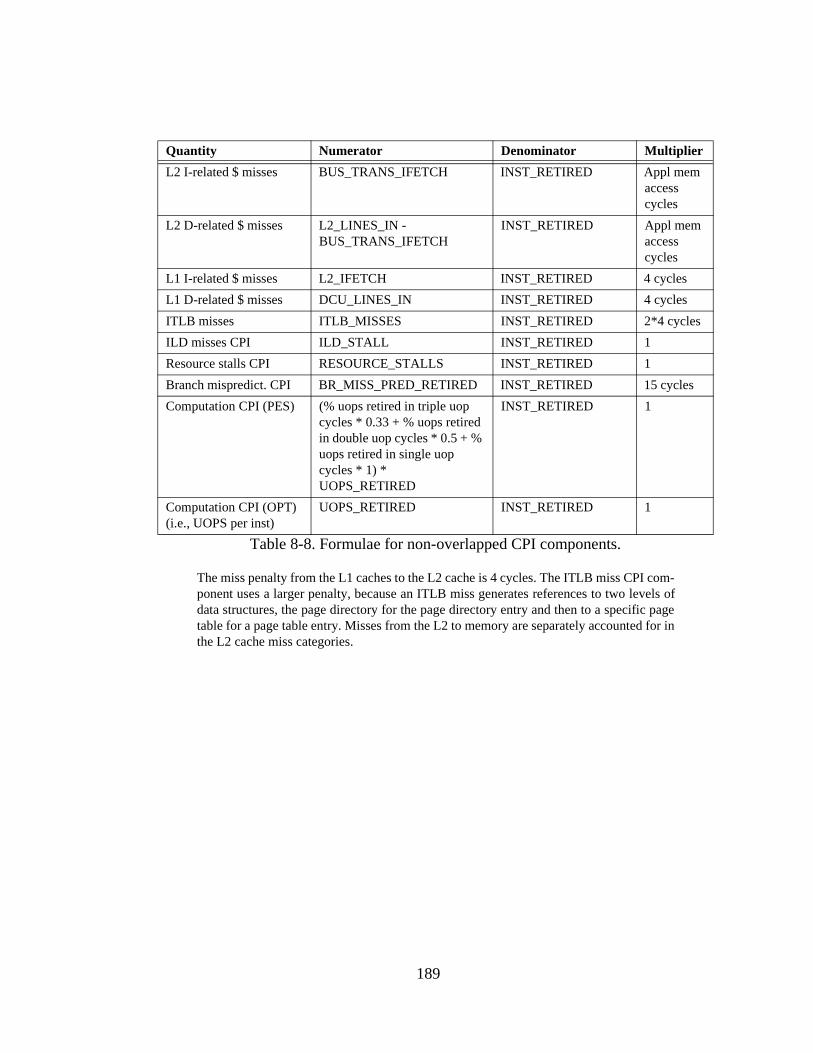
189


L2 I-related $ misses BUS_TRANS_IFETCH INST_RETIRED Appl mem access cycles

L2 D-related $ misses L2_LINES_IN - BUS_TRANS_IFETCH

INST_RETIRED Appl mem access cycles

L1 I-related $ misses L2_IFETCH INST_RETIRED 4 cycles

L1 D-related $ misses DCU_LINES_IN INST_RETIRED 4 cycles

ITLB misses ITLB_MISSES INST_RETIRED 2*4 cycles

ILD misses CPI ILD_STALL INST_RETIRED 1

Resource stalls CPI RESOURCE_STALLS INST_RETIRED 1

Branch mispredict. CPI BR_MISS_PRED_RETIRED INST_RETIRED 15 cycles

Computation CPI (PES) (% uops retired in triple uop cycles * 0.33 + % uops retired in double uop cycles * 0.5 + % uops retired in single uop cycles * 1) * UOPS_RETIRED

INST_RETIRED 1

Computation CPI (OPT) (i.e., UOPS per inst)

UOPS_RETIRED INST_RETIRED 1

Table 8-8. Formulae for non-overlapped CPI components.

The miss penalty from the L1 caches to the L2 cache is 4 cycles. The ITLB miss CPI com-ponent uses a larger penalty, because an ITLB miss generates references to two levels ofdata structures, the page directory for the page directory entry and then to a specific pagetable for a page table entry. Misses from the L2 to memory are separately accounted for inthe L2 cache miss categories.

190


L1 I-related miss rate L2_IFETCH IFU_IFETCH 100%

L1 D-related miss rate DCU_LINES_IN DATA_MEM_REFS 100%

Data refs per 1000 inst DATA_MEM_REFS INST_RETIRED 1000

Inst refs per inst per 1000 inst

IFU_IFETCH INST_RETIRED 1000

L1 I-related misses per 1000 inst

L2_IFETCH INST_RETIRED 1000

L1 D-related misses per 1000 inst

DCU_LINES_IN INST_RETIRED 1000

ITLB Misses per 1000 inst

ITLB_MISS INST_RETIRED 1000

Table 8-9. Formulae for L1 cache characteristics.


L2 I-related miss rate BUS_TRANS_IFETCH L2_IFETCH 100%

L2 I-related misses per 1000 inst

BUS_TRANS_IFETCH INST_RETIRED 1000

L2 D-related miss rate L2_LINES_IN - BUS_TRANS_IFETCH

L2_LD + L2_ST 100%

L2 D-related misses per 1000 inst

L2_LINES_IN - BUS_TRANS_IFETCH

INST_RETIRED 1000

% dirty L2 misses BUS_HITM_DRV (sum over 4 procs)

L2_LINES_IN (sum over 4 procs)

100%

Table 8-10. Formulae for L2 cache characteristics.

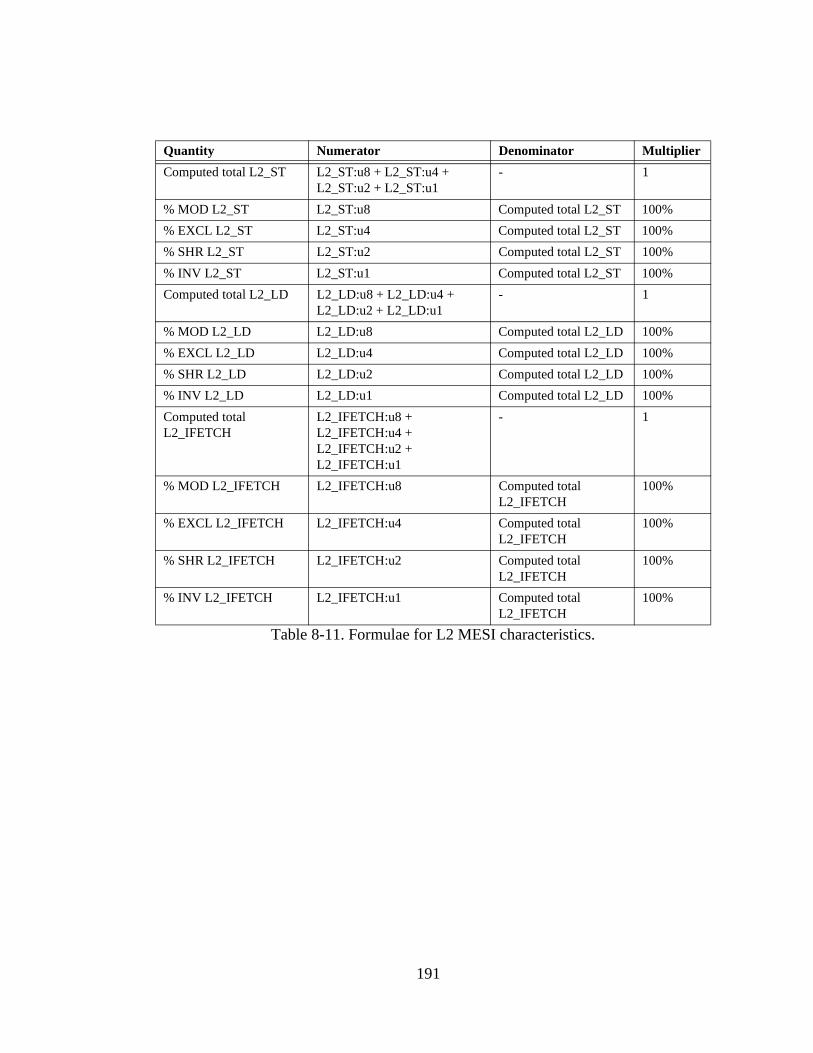
191


Computed total L2_ST L2_ST:u8 + L2_ST:u4 + L2_ST:u2 + L2_ST:u1

- 1

% MOD L2_ST L2_ST:u8 Computed total L2_ST 100%

% EXCL L2_ST L2_ST:u4 Computed total L2_ST 100%

% SHR L2_ST L2_ST:u2 Computed total L2_ST 100%

% INV L2_ST L2_ST:u1 Computed total L2_ST 100%

Computed total L2_LD L2_LD:u8 + L2_LD:u4 + L2_LD:u2 + L2_LD:u1

- 1

% MOD L2_LD L2_LD:u8 Computed total L2_LD 100%

% EXCL L2_LD L2_LD:u4 Computed total L2_LD 100%

% SHR L2_LD L2_LD:u2 Computed total L2_LD 100%

% INV L2_LD L2_LD:u1 Computed total L2_LD 100%

Computed total L2_IFETCH

L2_IFETCH:u8 + L2_IFETCH:u4 + L2_IFETCH:u2 + L2_IFETCH:u1

- 1

% MOD L2_IFETCH L2_IFETCH:u8 Computed total L2_IFETCH

100%

% EXCL L2_IFETCH L2_IFETCH:u4 Computed total L2_IFETCH

100%

% SHR L2_IFETCH L2_IFETCH:u2 Computed total L2_IFETCH

100%

% INV L2_IFETCH L2_IFETCH:u1 Computed total L2_IFETCH

100%

Table 8-11. Formulae for L2 MESI characteristics.

192


Memory system uti-lization

BUS_DRDY_CLOCKS:u20 CPU_CLK_UNHALTED (1/0.8) * k * 100%

Avg memory latency

BUS_REQ_OUTSTANDING BUS_TRANS_BRD - BUS_TRANS_IFETCH

1

Bus memory txns. BUS_TRANS_BRD + BUS_TRANS_RFO + BUS_TRANS_WB + BUS_TRANS_INVAL

- 1

Bus burst txns. BUS_TRANS_BRD + BUS_TRANS_RFO + BUS_TRANS_WB

- 1

Table 8-12. Formulae for memory system characteristics.

The formula for the memory system utilization requires further explanation. The datatransfer portion of each bus request (measured in processor clocks byBUS_DRDY_CLOCKS:u20) comprises only 4 of the 5 bus cycles required to handle therequest. We account for this bus turn-around time by dividing by 0.8. The constant mul-tiplicative factor k accounts for cycles where bus agents (for example, the memory con-troller) fall behind in their internal processing, preventing further bus activity fromproceeding. Empirical evidence suggests that this factor is about 2 for workloads withnon-trivial inter-processor L2 communication misses (for example, OLTP and join-intensive DSS queries like Q4, Q5.1, Q5.3, Q8, and Q11). For workloads that exhibitnegligible inter-processor communication misses (for example, scan-based DSS querieslike Q1, Q6, and Q5.2), the constant factor is closer to 1. The source of this memory uti-lization formula and these constant values is [109].


Branch mispred ratio BR_MISS_PRED_RETIRED BR_INST_RETIRED 100%

BTB miss ratio BTB_MISSES BR_INST_DECODED 100%

Branch frequency BR_INST_RETIRED INST_RETIRED 100%

Speculative execution INST_DECODED INST_RETIRED

Table 8-13. Formulae for branch characteristics.

193


#cycles w/ triple inst/uop decoded/retired (ex: UOPS_RETIRED)

UOPS_RETIRED:c3 - 1

#cycles w/ double inst/uop decoded/retired (ex: UOPS_RETIRED)

UOPS_RETIRED:c2 - UOPS_RETIRED:c3

- 1

#cycles w/ single inst/uop decoded/retired (ex: UOPS_RETIRED)

UOPS_RETIRED:c1 - UOPS_RETIRED:c2

- 1

# cycles w/ zero inst/uop decoded/retired (ex: UOPS_RETIRED)

UOPS_RETIRED:c1:i1 - 1

Computed total cycles # triple cycles + # double cycles + # single cycles + # zero cycles

- 1

% triple inst/uop decode/retire cycles (ex: UOPS_RETIRED)

# triple cycles Computed total cycles 100%

% double inst/uop decode/retire cycles (ex: UOPS_RETIRED)

#double cycles Computed total cycles 100%

% single inst/uop decode/retire cycles (ex: UOPS_RETIRED)

#single cycles Computed total cycles 100%

% zero inst/uop decode/retire cycles (ex: UOPS_RETIRED)

# zero cycles Computed total cycles 100%

Computed total inst/uops decoded/retired

3 * # triple cycles + 2 * # dou-ble cycles + 1 * # single cycles

- 1

% inst/uops retired in tri-ple inst/uop decode/retire cycles (ex: UOPS_RETIRED)

3 * # triple cycles Computed total inst/uops decoded/retired

100%

% inst/uops retired in double inst/uop decode/retire cycles (ex: UOPS_RETIRED)

2 * # double cycles Computed total inst/uops decoded/retired

100%

% inst/uops retired in sin-gle inst/uop decode/retire cycles (ex: UOPS_RETIRED)

1 * # single cycles Computed total inst/uops decoded/retired

100%

Table 8-14. Formulae for ILP characteristics.

194

Computation µCPI (% uops retired in triple uop cycles * 0.33 + % uops retired in double uop cycles * 0.5 + % uops retired in single uop cycles * 1)

- 1

Computation CPI (PES) Computation µCPI * UOPS_RETIRED

INST_RETIRED 1


Table 8-14. Formulae for ILP characteristics.

195

9 Appendix B: Comparison of Database and Operating System Behavior for OLTP Workload

This appendix provides a more detailed analysis of the database and operating system components of the

OLTP workload, highlighting the differences between these two components. The aggregate (database plus

operating system) OLTP behavior was described in Chapter 3. In particular, this appendix explores cache

behavior, the impact of L2 cache size on CPI and OLTP throughput, the effectiveness of superscalar issue

and retire, and the effectiveness of the MESI coherence protocol.

9.1. Cache Behavior

Table 9-1, Table 9-2 and Table 9-3 present the cache access and miss behavior as a function of L2 cache size

for the overall system, the database alone and the operating system alone, respectively. (The L2 miss data is

shown graphically in Figure 3-3 on page 42.) We note that DTLB misses are not included in these tables,

because they could not be measured reliably.

L1 and L2 cache miss rates for the database resemble those for the overall system. The operating system’s

L1 I-cache miss rates are somewhat lower than those of the overall system, and the L1 D-cache miss rates

are somewhat higher. L2 cache miss rates for the operating system alone are at least 1.6X that for the data-

base alone.

9.2. Impact of L2 Cache Size on CPI and OLTP Throughput

Table 9-4 shows the breakdown of CPI for the overall system, the database alone and the operating system

alone as a function of L2 cache size. (The overall system data is presented graphically in Figure 3-4 on page

43.)

196

As discussed in previous sections, the OS-only CPI is more than 2X that of the DB-only CPI. For both the

overall CPI and the database-only CPI, the relative importance of the components is instruction-related stalls,

followed by computation and finally resource stalls. The relative importance of operating system CPI com-

ponents is somewhat different. For the smaller L2 cache sizes, the instruction-related and resource stalls are

most important. For the 1 MB L2 cache, resource stalls are most important, followed by instruction-related

stalls and computation.

Characteristic 256 KB 512 KB 1 MB



L1 I-cache misses 92 (5%) 93 (5%) 93 (6%)

L1 D-cache misses 48 (7%) 51 (7%) 51 (7%)

ITLB misses 3 4 4



Overall L2 misses 23 (16%) 11 (9%) 8 (6%)

Table 9-1. Overall cache access and miss behavior as a function of L2 cache size.





L1 I-cache misses 88 (7%) 89 (6%) 89 (7%)

L1 D-cache misses 46 (6%) 48 (7%) 48 (7%)

ITLB misses 3 4 4



Overall L2 misses 20 (15%) 11 (9%) 7 (5%)

Table 9-2. Database-only cache access and miss behavior as a function of L2 cache size.


197




L1 I-cache misses 130 (4%) 122 (3%) 132 (4%)

L1 D-cache misses 70 (9%) 70 (10%) 84 (11%)

ITLB misses 2 6 6


L2 Data-related misses

27 (39%) 20 (28%) 17 (22%)

Overall L2 misses 53 (26%) 28 (14%) 19 (9%)

Table 9-3. Operating system-only cache access and miss behavior as a function of L2 cache size.



Relative transaction throughput

100% 116% 128%

Overall System




Computation: µops 0.98 0.98 1.00

Database-only





Operating system-only





Table 9-4. Relative database throughput and CPI breakdown as function of L2 cache size.

198

9.3. Effectiveness of Superscalar Issue and Retire

Table 9-5 and Table 9-6 present the macro-instruction decode and retirement profiles for the overall system,

the database alone, and the operating system alone. Table 9-7 presents the micro-operation retirement profile,

similarly decomposed. The overall system data from these tables was presented graphically in Figure 3-5

through Figure 3-6.

Similar behavior is exhibited by the database and the operating system, with a few exceptions. The OS alone

experiences a higher percentage of zero-instruction decode and retire cycles, and a higher percentage of

zero-µop retire cycles than the database alone. A higher percentage of the OS macro-instructions are

decoded and retired in single-decode and -retire cycles, implying that wider macro-instruction superscalar

issue and retire would be even less useful for operating system code than for database code. Both the database

and the operating system retire about half of all µops in triple-µop retire cycles. Thus, micro-operation super-

scalar retire width appears to be equally as useful for the operating system as it is for the database.

9.4. Effectiveness of MESI Cache Coherence Protocol

Table 9-8 and Table 9-9 decompose accesses to the L2 cache among the modified (M), exclusive (E), shared

(S) and invalid (I) states for the database alone and the operating system alone, respectively. The overall

system data is presented in Table 3-7 on page 54.

.

% cycles % inst.

Characteristic Overall Database OS Overall Database OS

0-instruction decode 68.7% 65.5% 80.8% n/a n/a n/a

1-instruction decode 17.9% 19.4% 12.1% 35.7% 34.7% 43.2%



Table 9-5. Instruction decode profile.

In the Pentium Pro, three parallel decoders translate IA-32 macro-instructions (e.g.,instructions) into triadic micro-operations (e.g., µops). Most instructions are converted toa single µop, some are converted into two to four µops, and complex instructions requiremicrocode, which is a longer sequence of µops. Up to five µops can be issued each clockcycle.

199

These tables illustrate several differences in behavior between user level and system level. Load operations

for the dual- and quad-processor configurations miss the L2 cache nearly 2X as often for the operating system

as for the database. Also, the OS experiences a higher percentage of store hits to shared lines for dual- and

quad-processor configurations: 20 to 30%, in comparison with less than 5% for the database alone. We

hypothesize that there is an increased incidence of read-modify-write operations on operating system data

shared between the processors: a load operation misses in the originating processor’s cache, causing the line

to be loaded from another cache in shared mode. A subsequent store operation then updates the shared line.

% cycles % inst.


0-instruction retire 76.2% 72.7% 88.2% n/a n/a n/a

1-instruction retire 15.2% 17.0% 8.6% 43.3% 41.9% 55.2%



Table 9-6. Macro-instruction retirement profile.

In the Pentium Pro, up to three x86 instructions can be retired in a single cycle.

% cycles % inst.


µops per macro-instruction 1.87 1.84 2.23

0-µop retire 66.0% 62.8% 78.6% n/a n/a n/a

1-µop retire 15.6% 16.7% 10.9% 24.6% 23.7% 28.3%

2-µop retire 7.0% 7.9% 3.9% 22.2% 22.5% 20.3%

3-µop retire 11.3% 12.6% 6.6% 53.2% 53.7% 51.3%

Table 9-7. Micro-operation retirement profile.

In the Pentium Pro, up to three µops can be retired in a single cycle.

200


(Miss)I

INST. FETCH

1 processor 0.0% 0.8% 98.0% 1.2%

2 processors 0.0% 0.0% 98.9% 1.1%

4 processors 0.0% 0.0% 98.9% 1.1%

LOAD

1 processor 23.7% 56.8% 1.2% 18.3%

2 processors 21.2% 17.7% 45.2% 16.0%

4 processors 25.7% 15.6% 46.4% 12.2%

STORE

1 processor 76.3% 1.6% 0.0% 22.1%

2 processors 79.9% 1.1% 1.9% 17.0%

4 processors 85.8% 0.6% 2.9% 10.5%

Table 9-8. State of L2 line on L2 hit for the database. (Table shows percentage of L2 accesses.)


(Miss)I

INST. FETCH

1 processor 0.0% 0.7% 96.8% 2.5%

2 processors 0.0% 0.0% 97.5% 2.5%

4 processors 0.0% 0.0% 98.0% 2.0%

LOAD

1 processor 37.1% 46.7% 0.4% 15.8%

2 processors 25.3% 17.0% 34.0% 23.6%

4 processors 18.5% 12.1% 42.7% 26.7%

STORE

1 processor 89.2% 0.9% 0.8% 9.1%

2 processors 67.4% 0.5% 17.7% 14.4%

4 processors 57.0% 0.3% 25.8% 16.8%

Table 9-9. State of L2 line on L2 hit for the operating system. (Table shows percentage of L2 accesses.)

201

9.5. NT Performance Monitor Characterization

Characteristics OLTP

Average user time 77.6%

Average system time 21.7%

Average idle time 0.7%

Average interrupts per second 828.9

Thread context switches per second 84.3

System calls per second 3516.1

File reads per second 1585.0

File writes per second 1292.5

Average read size [40] 2 KB

Average write size [40] 2 KB

Table 9-10. NT performance monitor characteristics for the OLTP workload.

The quantities listed as “average” above were measured separately for each of the fourprocessors; the number presented is the average across the four processors in the system.

202

10 Appendix C: Elaboration of DSS Results

10.1. Effectiveness of Out-of-Order Execution

Figure 10-1 through Figure 10-8 present the non-overlapped CPIs and the measured CPI for Q1, Q4, Q5.1,

Q5.2, Q5.3, Q8, Q11, and the OLTP workload. While the actual CPIs vary somewhat between the different

DSS queries, the overall relationships between the measured and OPT and PES non-overlapped CPIs are the

same as those described for Q6 in Section 4.5.3. on page 95. The only exception is Q5.3, shown in Figure 10-

5, where the pessimistic non-overlapped CPI is actually less than the measured CPI. This discrepancy is due

to the assumptions of the PES computation CPI model, which underpredict the computation for this query

phase. Recall that the PES computation model implicitly assumes that µop execution takes one cycle. For

Q5.3, we hypothesize that operating system instructions to poll disk I/O status may take longer than a single

cycle, making the computation model underpredict the computation CPI.

203


0

1

2

3

L2 Cache Size

Non

-ove

rlap

ped

CP


Measured CPI

256 KB 512 KB 1 MB



0

1

2

3

4

L2 Cache Size

Non

-ove

rlap

ped

CP


Measured CPI

256 KB 512 KB 1 MB


204

Figure 10-3. Non-overlapped and measured CPI for DSS Q5.1 as a function of L2 cache size.

0

1

2

3

4

L2 Cache Size

Non

-ove

rlap

ped

CP


Measured CPI

256 KB 512 KB 1 MB



0

1

2

3

4

5

6

L2 Cache Size

Non

-ove

rlap

ped

CP


Measured CPI

256 KB 512 KB 1 MB


205


0

1

2

3

4

5

L2 Cache Size

Non

-ove

rlap

ped

CP


Measured CPI

256 KB 512 KB 1 MB



0

1

2

3

4

L2 Cache Size

Non

-ove

rlap

ped

CP


Measured CPI

256 KB 512 KB 1 MB


206


0

1

2

3

4

L2 Cache Size

Non

-ove

rlap

ped

CP


Measured CPI

256 KB 512 KB 1 MB


Figure 10-8. Non-overlapped and measured CPI for OLTP as a function of L2 cache size.

0

1

2

3

4

5

6

7

L2 Cache Size

Non

-ove

rlap

ped

CP


Measured CPI

256 KB 512 KB 1 MB


207

10.2. DSS I/O Characterization

This appendix describes the I/O characteristics of the remainder of our DSS query set, including Q1, Q4, Q8,

and Q11. The read and write rates for Q1 are shown in Figure 10-9. Q1 performs a sequential table scan of

the largest table in the dataset, with selection and eight aggregation operations. This set of operations results

in a nearly constant rate of about 145 read operations per second for the duration of the query. Q1’s read rate

is considerably lower than the read rate for Q6, the other query in our set that performs a table scan with selec-

tion and aggregation. (Q6’s read rates are shown in Figure 4-8 on page 99.) This difference is due to the

increased computational complexity of Q1’s eight aggregate operations (versus Q6’s single aggregate). The

sequential reads for this query operate on a 64 KB granularity. Writes are negligible for this query.



0

20

40

60

80

100

120

140

160

180

0:00

:00

0:08

:10

0:16

:20

0:24

:30

0:32

:40

0:40

:50

0:49

:00

0:57

:10

1:05

:20

1:13

:30

1:21

:40

1:29

:50

1:38

:00

1:46

:10

1:54

:20

2:02

:30

2:10

:40

2:18

:50

2:27

:00

Time

File

Ope

rati

ons

per

Seco

nd

File Reads per Sec

File Writes per Sec

208

Figure 10-10 shows the read and write rates for Q4, which performs a nested query. The nested subquery

scans and filters two tables and performs a hash join; this processing is done during the first six and a half

minutes of the query, resulting in a read rate of about 350 reads per second. These sequential reads use a 64

KB granularity. The result of the nested subquery is materialized and written to disk as a temporary file at

about six minutes and 40 seconds, resulting in the write spike of about 360 writes per second. These writes

are performed in 16 KB sequential blocks. The last ten seconds or so of the query corresponds to the outer

query’s read of the temporary file in 64 KB increments.



0

50

100

150

200

250

300

350

400

450

0:00:00 0:00:50 0:01:40 0:02:30 0:03:20 0:04:09 0:05:00 0:05:49 0:06:40

Time

File

Ope

rati

ons

per

Seco

nd

File Reads per Sec

File Writes per Sec

209

Figure 10-11 illustrates the read rates for Q8, which performs eight sequential table scans, six hash joins, and

a nested loops join. The first forty seconds correspond to the first two table scans and the nested loops join,

and result in a rate of about 1000 reads per second. The next seventeen-minute period corresponds to addi-

tional table scans and several hash joins, resulting in a steady rate of about 470 reads per second. The drop

in read rate occurs due to an imbalance in the I/O processing: some of the disks aren’t used in this phase of

the query, leading to a lower I/O rate. The remainder of the query corresponds to additional table scans and

hash join operations. All reads are done sequentially in 64 KB blocks. As shown in the figure, writes are neg-

ligible for this query.



0

200

400

600

800

1000

1200

0:00:00 0:03:21 0:06:41 0:10:00 0:13:21 0:16:41 0:20:01 0:23:21

Time

File

Ope

rati

ons

per

Seco

nd

File Reads per Sec

File Writes per Sec

210

The read patterns and read sizes of our final query, Q11, are shown in Figure 10-12 and Figure 10-13, respec-

tively. Q11 performs a set of nested selection statements, where each statement performs two sequential table

scans, an index scan, a hash join, and a nested loops join. We consider both figures simultaneously. The first

data point in both figures shows the 64 KB sequential reads used for the nested subquery’s table scans. The

next eight (roughly) data points show the 4 KB random reads performed for the nested subquery’s index scan.

The following three (roughly) data points correspond to the 64 sequential KB reads used for the outer query’s

table scans. The remaining data points correspond to the final index scan, which uses 4 KB random reads.


Each point in the graph corresponds to the average number of file operations per second,averaged over a five-second measurement period. We note that this measurement intervaldoes not match exactly with the time scale of the file read activity measured and illustratedin this figure and in Figure 10-13..

0

200

400

600

800

1000

1200

1400

1600

1800

0:00:00 0:00:16 0:00:31 0:00:45 0:01:00 0:01:15 0:01:30

Time

File

Ope

rati

ons

per

Seco

nd

File Reads per Sec

File Writes per Sec

211

Figure 10-13. Q11 file read sizes.

0

10000

20000

30000

40000

50000

60000

70000

0:00:00 0:00:16 0:00:31 0:00:45 0:01:00 0:01:15 0:01:30

Time

Byt

es (

B)

Average Read Size

212

10.3. Appendix: NT Performance Monitor Characterization

Characteristic Q1 Q4 Q5.1 Q5.2 Q5.3 Q6 Q8 Q11

Average user time 99.2% 96.3% 97.0% 79.6% 16.0% 95.2% 93.5% 92.9%

Average system time 0.8% 2.3% 2.6% 2.7% 5.5% 4.7% 3.2% 3.2%

Average idle time 0.0% 1.4% 0.4% 17.7% 78.5% 0.1% 3.3% 3.9%

Average interrupts per second

103.7 152.0 161.6 232.3 436.4 253.4 185.9 246.2

Thread context switches per second

312.3 292.8 292.3 540.1 3314.9 293.6 350.8 349.9

System calls per sec-ond

384.8 636.6 700.0 1087.4 3369.6 991.8 826.8 1001.1

File reads per second 145.1 313.3 378.1 36.1 1470.7 745.9 475.1 712.0

File writes per sec-ond

0.6 0.7 0.6 624.3 0.9 0.6 0.6 1.2

Average read size 64 KB 64 KB 64 KB 64 KB 8 KB 64 KB 64 KB 8 KB

Average write size - - - 8 KB - - - -

Table 10-1. NT performance monitor characteristics for the OLTP workload.

The quantities listed as “average” above were measured separately for each of the fourprocessors; the number presented is the average across the four processors in the system.

213

11 Appendix D: Supporting Evidence for Intelligent Disks

11.1. 1999 DSS System Configurations

Table 11-1 shows the TPC-D 300 GB SF performance-leading configurations used as the basis for the extrap-

olated “NCR04” and “HP04” systems in Chapter 6. In the absence of detailed information about the disks for

these configurations, we assume the parameters of a Seagate disk of comparable capacity, as shown in

Table 11-2. To obtain the 2004 extrapolated systems, we increase processor speed, disk capacity, and

memory capacity by roughly 60% per year. Disk media transfer rate is increased by 40% per year, and aver-

age disk access time is decreased by 8% per year. These growth trends are well-documented in the disk-

industry literature [38]. We assume that PCI bandwidth increases by a factor of 3X, through the use of a faster

clock rate. Per-node network bandwidth is increased by a factor of 5X.

.

CharacteristicSeagate Cheetah 9LP ST39102 FC


Rotational speed 10,033 RPM

Media transfer rates (outer, inner tracks)

28.9 MB/s (max), 19.0 MB/s (min)




Table 11-2. 1999 disk parameters used as basis for IDISK evaluation [90].

214

11.2. Appendix: Factors Affecting Analytic Models

In this appendix, we describe some of the “implementation” choices that affect the behavior of our analytic

models.

First, assumptions about disk and I/O bus transfer rates affect the estimated time to perform I/O operations.

We assume that large sequential disk accesses are able to achieve roughly 75% of the disk media transfer

rate. This rate is consistent with observed behavior of current disks [99]. We assume that smaller random

accesses achieve 10% of the media transfer rate. For PCI bus-based I/O systems, we assume that the bus(es)

can be at most 80% utilized.

Second, numerous communication parameters impact the model. As described in Section 6.5.3. on page 153,

one factor is how many inputs need to be communicated for join operations. Our assumptions for this factor

were described in the discussion of these algorithms. Other parameters that impact the time to communicate

data are the overhead for sending and receiving messages, the size of the messages, and the achievable net-

work bandwidth. Our assumptions are as follows. We assume that the overhead for sending and receiving a

message is 100 instructions; this value is consistent with the implementation of today’s fast messaging layers

CharacteristicNCR WorldMark 5200 w/ Teradata

HP 9000 V2500 Enterprise Server w/ Oracle8i

Per node

Processors 4 * 450 MHz 32 * 440 MHz

Memory capacity 2 GB 32 GB

Disk capacity 40 * 9 GB 680 *9.1 GB

Processor interconnect bandwidth (per-node)

120 MB/s N/A

Intra-node I/O interconnect 1 * 64-bit, 33 MHz PCI (?) 8 * 64-bit, 33 MHz PCI

I/O interconnect bandwidth 264 MB/s 2112 MB/s

Overall system

Nodes 32 1

Total processors 128 32

Memory capacity 64 GB 32 GB

Disk Capacity 11,610 GB 6228 GB

Table 11-1. 1999 TPC-D 300 GB SF performance-leading configurations used as basis for IDISK evaluation [105] [46] [70].

215

such as Active Messages [63]. The size of messages is a tension between larger messages for achieving

higher bandwidth and smaller messages for lower buffer memory requirements. We assume 4 KB messages

for IDISKs with 32 MB to 64 MB of memory, 8 KB messages for IDISKs with 128 MB or more of memory,

and 64 KB messages for the NCR04 system. We assume that the maximum achievable network bandwidth

is 80% of the media transfer rate.

Third, the fill factor of data and index pages will affect how much data needs to be transferred from disk, as

well as the memory capacity required for holding the data. Fill factor refers to how “full” data and index

pages are. Database administrators will typically leave part of the pages empty if a workload anticipates pro-

cessing insertion operations. Because DSS workloads are read-mostly, and for simplicity, we assume that

pages are full (in other words, a 100% fill factor). In reality, this number is likely somewhat lower.

Fourth, the sparseness of a hash table can impact its memory requirements. To avoid collisions when building

the hash table, hash functions are often chosen to create sparse hash tables. We assume a very dense hash

table representation where the table is the same size as the data it holds. A sparser design would require more

memory capacity, leading IDISK to require a two-pass join algorithm for even larger memories than those

described in Section 6.5.3. on page 153.

11.3. Appendix: Bottleneck Analysis for System Performance

In this appendix, we quantify the bottlenecks of each of our hypothetical systems for the three different query

workloads.

Each of the tables in this appendix has a number of columns: PCI only, 10X PCI only, disks only, commu-

nication only, computation only, query time, and query time (10X PCI). The sections to the left of the vertical

double line (labeled “only”) refer to the time for that component alone to transfer or process data. For exam-

ple, the PCI only column refers to the time it takes for all of the necessary data to be transferred across the

PCI bus, and 10X PCI only refers to the PCI transfer time when the PCI rate is increased tenfold. These col-

umns include only a partial cost of completing the query. The sections to the right of the double line represent

the overall cost of executing the query, including transferring, communicating, and processing the data.

216

In each table row, we italicize the bottleneck component of the system. The rows for the NCR04 and HP04

systems generally have two italicized columns, one bottleneck for the system as specified, and one bottleneck

for the system with the 10X higher PCI busses.

.

ConfigurationPCI only

10X PCI only

Disks only

Commun-ication only

Computation only

Query Time

Query Time (10X PCI)

Simple scan

IDISK04 - - 10.5 s 0.0 s 8.5 s 10.5 s -

NCR04 40.1 s 4.0 s 10.5 s 0.0 s 24.8 s 40.1 s 24.8 s

HP04 160.4 s 16.0 s 10.5 s 0.0 s 101.5 s 160.4 s 101.5 s

Complex scan

IDISK04 - - 10.5 s 0.0 s 42.6 s 42.6 s -

NCR04 40.1 s 4.0 s 10.5 s 0.0 s 124.1 s 124.1 s 124.1 s

HP04 160.4 s 16.0 s 10.5 s 0.0 s 507.7 s 507.7 s 507.7 s

Table 11-3. Bottleneck analysis for performance of the selection queries presented in Figure 6-5 on page 152.

.


10X PCI only

Disks only

Commun-ication only

Computation only

Query Time


IDISK04 128 MB (two-pass)

- - 40.6 s 0.9 s 34.0 s 43.1 s -

IDISK04 256 MB (one pass)

- - 7.7 s 0.9 s 9.4 s 10.5 s -

NCR04 29.3 s 2.9 s 7.7 s 9.1 s 27.2 s 38.4 s 36.3 s

HP04 117.2 s 11.7 s 7.7 s - 111.3 s 117.2 s 111.3 s

Table 11-4. Bottleneck analysis for performance of the hash join query presented in Figure 6-8 on page 157.

217

.


10X PCI only

Disks only

Commun-ication only

Computation only Query Time


IDISK04 - - 7.8 s 0.0 s 6.3 s 7.9 s -

NCR04 23.6 s 2.4 s 6.2 s 0.0 s 17.4 s 26.4 s 17.4 s

HP04 94.3 s 9.4 s 6.2 s 0.0 s 71.2 s 105.8 s 71.2 s

Table 11-5. Bottleneck analysis for performance of the index nested loop query presented in Figure 6-11 on page 160.

.


10X PCI only

Disks only

Commun-ication only

Computation only

Query Time (Figure6-12)


0.75 million rows

IDISK04 - - 7.5 s 0.0 s 6.1 s 7.6 s -

NCR04 23.6 s 2.4 s 6.2 s 0.0 s 16.9 s 25.9 s 16.9 s

HP04 94.3 s 9.4 s 6.2 s 0.0 s 69.1 s 103.7 s 69.1 s

1.50 million rows

IDISK04 - - 8.8 s 0.0 s 7.1 s 9.0 s -

NCR04 23.6 s 2.4 s 6.2 s 0.0 s 19.2 s 28.2 s 19.2 s

HP04 94.3 s 9.4 s 6.2 s 0.0 s 78.6 s 113.2 s 78.6 s

3.00 million rows

IDISK04 - - 11.4 s 0.0 s 9.2 s 11.6 s -

NCR04 23.6 s 2.4 s 6.2 s 0.0 s 23.8 s 32.8 s 23.8 s

HP04 94.3 s 9.4 s 6.2 s 0.0 s 97.4 s 132.0 s 97.4 s

6.00 million rows

IDISK04 - - 16.7 s 0.0 s 13.3 s 16.8 s -

NCR04 23.6 s 2.4 s 6.2 s 0.0 s 33.0 s 42.0 s 33.0 s

HP04 94.3 s 9.4 s 6.2 s 0.0 s 135.2 s 169.8 s 135.2 s

Table 11-6. Sensitivity analysis for performance of the index nested loop queries presented in Section 6.5.4. on page 157.

computer architecture support for database applications

Documents