computer-assisted generation and curation of genome-scale
TRANSCRIPT

COMPUTER-ASSISTED GENERATION AND CURATION OF GENOME-SCALE METABOLIC MODELS WITH CASE STUDIES IN THE METHANOGEN GENUS METHANOSARCINA
BY
MATTHEW NICHOLAS BENEDICT
DISSERTATION
Submitted in partial fulfillment of the requirements for the degree of Doctor of Philosophy in Chemical Engineering
in the Graduate College of the University of Illinois at Urbana-Champaign, 2014
Urbana, Illinois
Doctoral Committee:
Associate Professor Nathan D. Price, Chair, Institute for Systems Biology Professor William W. Metcalf Professor Huimin Zhao Associate Professor Christopher V. Rao
ii
Abstract
Methanogenic archaea, organisms that make methane as a byproduct of their metabolism, play a critical
role in the global carbon cycle and have potential as a source of renewable biofuels. As a result, there
has been a great deal of interest in understanding how methanogenesis works. A wide array of tools has
been developed for studying methanogen metabolism, including genetic manipulation tools and
efficient culturing techniques. These tools are especially well developed in model methanogens such as
Methanococcus maripaludis, Methanosarcina acetivorans and Methanosarcina barkeri. Methanosarcina
species are particularly attractive model organisms for methanogenesis due to their wide substrate
utilization capabilities (compared to other methanogens): the diversity in metabolic capabilities for
these organisms enables manipulations of methanogenesis pathways that would be lethal in other
methanogens. Genetic manipulation tools have been valuable for identifying functions of individual
enzymes and pathways in these organisms, but more holistic methods are needed in order to
understand how these work together to accomplish observed phenotypes.
Genome-scale metabolic networks allow researchers to put information on individual parts of
metabolism together in a way that is useful for making novel insights. For my first Ph.D. project, I built
and carefully curated a genome-scale metabolic network for Methanosarcina acetivorans and used
constraint-based analysis tools to build a quantitative model based on that network. I then used the
model to make predictions about how M. acetivorans utilizes carbon monoxide and the impact of the
soluble heterodisulfide reductase HdrABC on its metabolic activity.
While highly-curated metabolic networks are useful for studying metabolic phenotypes, the process of
building them is not scalable. A genome-scale metabolic network for a single organism can take months
to years to curate using the established protocols. One key reason for the lack of scalability of this
process is a dearth of adequate tools to aid users in evaluating annotations and gene calls that form a
bedrock for the automated generation of draft networks. The main focus of my Ph.D. has been the
development of two software packages to improve the scalability of generating and curating genome-
scale metabolic networks. One of these software packages, likelihood-based gap filling, uses annotation
likelihood estimates for alternative gene annotations to identify pathways to fill gaps in metabolic
networks that are maximally consistent with available genomic data. The other package, ITEP
(Integrated Toolkit for Exploration of metabolic Pan-genomes), is a set of tools for curating and studying

iii
patterns in gains and losses of genes across groups of related organisms. In this dissertation, I describe
how these tools can be used to build and to assess the quality of different parts of metabolic networks.
As my final project, I have developed a new method of combining comparative genomics (using ITEP)
with metabolic modeling to expose errors in both genomes and metabolic networks. I applied this
method to 30 species in the genus Methanosarcina, 27 of which were newly sequenced, and
demonstrated specific examples of these errors and possible ways to address them. The approach I
developed makes certain classes of errors readily apparent that are not obvious when only examining
individual organisms.

iv
Acknowledgements
I would first and foremost like to thank all of the members of my family for their consistent support of
my decision to pursue a Ph.D. and continuing encouragement throughout the process. Thanks also to
my wonderful girlfriend Meng Sun (孙梦) for showing me the meaning of devotion, opening my eyes to
a whole new world, and always keeping a positive perspective even when my own has wavered. I
couldn’t have done this without you.
I am deeply indebted to a lot of friends here at UIUC for too many things to list. Special thanks for
Nicholas Chia for working closely with me and teaching me most of what I know about Linux and
bioinformatics and for being incredibly supportive. Special thanks also to Ahmet Badur for always
believing in me and for lots of good times. Thanks also to my prior roommates for many memories in the
old house on Illinois street: Shuyi Ma, Kristine Pangan-okimoto, Josh and Ritika Tice, and Samantha
Weiss. Thanks to Dawn Eriksen for convincing me to come here . Thanks to my Chinese and Taiwanese
friends for your support and putting up with (and even encouraging!) my 不好中文: Wan-ting Chen,
Mei-hsiu Lai, Qidi Sun, Chunjing Wang, Yuliang Wang, Su Xiao, Wanwan Yang, Yuanchang Zhou, Peiyun
Zhou, and others who have moved on to greener pastures or taller cities.
Thanks also go out to my friends back in Connecticut, especially Katie Bowers, without whose
encouragement I would certainly not have applied to graduate school, and Bryne Botticelli, who has
been a lifelong friend.
Thank you to Nathan Price, William Metcalf, Christopher Rao and Huimin Zhao for taking the time to
serve on my prelim and defense committee. Your time investment is greatly appreciated.
Thank you to Nathan Price for being a very patient and understanding advisor. Thanks to him, I have had
the opportunity to interact with a truly world-class body of scientists. In addition to Nathan, I am deeply
indebted to numerous collaborators for help with scoping, implementing and interpreting the results of
the projects in this dissertation. In no particular order, thanks to James Henriksen, Petra Kohler, Judy
Luke, William Metcalf, Sarah Reinhart, Rachel Whitaker, and Nick Youngblut for working with me on
methanogens and comparative genomics. Thanks to Scott Devoid and Chris Henry at Argonne National
Labs and to Mike Mundy and Nicholas Chia at the Mayo Clinic for working with me on the KBase-related

v
projects and for many interesting discussions on modeling. Thanks to Gary Olsen at UIUC and to Jim
Davis, Ross Overbeek, and Fangfang Xia at Argonne National Labs for inviting me to join in on numerous
interesting discussions on annotation improvement and software development. Thanks to John Cole and
Zan Luthey-Schulten for help with visualization efforts and scientific discussions.
Thanks to the entire Price lab for being such an awesome group of people. I am especially indebted to
Caroline Milne, James Eddy, Matt Gonnerman, Matt Richards, and Shuyi Ma for working with me on the
projects in this dissertation, putting up with my badgering over Gchat, and reading over and editing
manuscripts, proposals, posters and presentations. Additional special thanks go to Chunjing Wang and
Caroline Milne for extensive moral support.
I’m truly grateful to the staff of the Department of Chemical and Biomolecular Engineering and the
Institute for Genomic Biology at UIUC, who have consistently supported me despite having plenty of
opportunity not to in the last few years of my time here. I especially want to thank Christine Bowser, Kay
Moran , Cathy Paceley, and Debbie Piper for helping with countless administrative issues over the years.
Thanks also to Theresa Fitzgerald at ISB for her help with similar issues there.
Last and certainly not least, thank you to Carl Woese for highly enlightening discussions on the nature of
evolution and for being an awesome person. We all miss you.
vi
Table of contents
Chapter 1: Introduction .................................................................................................................. 1
Chapter 2: Genome-scale metabolic reconstruction and hypothesis testing in the methanogenic archaeon Methanosarcina acetivorans C2A ................................................................................... 9
Chapter 3: Likelihood-based gene annotations for gap filling and quality assessment in genome-scale metabolic models ................................................................................................................. 34
Chapter 4: ITEP: An integrated toolkit for exploration of microbial pan-genomes. .................... 58
Chapter 5: Curation of genome-scale metabolic networks using comparative genomics ........... 76
Chapter 6: Conclusions and future work ...................................................................................... 88
Bibliography .................................................................................................................................. 95
Appendix A: Supplemental methods for likelihood-based gap filling ........................................ 108
Appendix B: Tutorial for building models and running likelihood-based gap filling in the DOE KnowledgeBase using the web-based CLI ................................................................................... 110
Appendix C: Description of the KBASE Client API for likelihood-based gap filling workflows ... 127
1
Chapter 1: Introduction
Methanogenesis and methanogens
Methanogens are strictly anaerobic archaea that generate methane as their primary metabolic
byproduct. It has been estimated that 5x10¹⁴ g of methane is released into the atmosphere each year by
the action of methanogenesis [1], which represents about 4% of the total annual global carbon
circulation [2]. Methane is a potent greenhouse gas with 25 times the potency of carbon dioxide [3],
contributing about 20% of the annual radiative forces of anthropomorphically-sourced greenhouse
gasses in the atmosphere [4], and methanogenesis is the chief mechanism by which this methane is
emitted into the atmosphere [5]. Therefore, it is of great interest to understand methanogenesis and
the potential responses of methanogens to global warming. Methanogens play a critical role in the
global carbon cycle, metabolizing the waste products of other organisms such as acetogenic bacteria.
The metabolism of these waste products keeps their concentration low, allowing the metabolic
pathways of these other organisms to remain thermodynamically feasible [6].
Methanogens are a metabolically, physiologically, and phylogenetically diverse collection of organisms,
all of which fall into the domain Archaea. Methanogens have adapted to life in a wide range of
temperatures, salt concentrations, and levels of substrate availability [2] in which they coexist with
other organisms such as sulfate reducers [7, 8], nitrate reducers and iron reducing organisms [9].
Different groups of methanogens have adapted to utilize different substrates [10] and have vastly
different pathways for utilization of the same substrates [2]. These pathway differences have
implications for the survival strategies and ecological roles of these groups: some organisms grow more
slowly but require less substrate for survival, while others grow more quickly but have greater growth
requirements [2] .
There are at least three major phylogenetically coherent classes of methanogens: the group I
methanogens, the group II methanogens (Methanomicrobiales) and the group III methanogens
(Methanosarcinales) [11]. Each of these classes has divergent energy conservation pathways and
substrate utilization capabilities [11].
2
The group I methanogens include Methanococcus maripalidus and Methanocaldococcus jannaschii, two
key model methanogens from which genetic manipulation techniques have been developed and from
which many archaeal-specific pathways have been deduced [12]. Most group I methanogens grow by
reducing CO2 with molecular hydrogen, although some (such as M. maripalidus) can also grow using
formate as an electron donor instead of hydrogen [13]. The Methanosphaera are an exception: they are
only capable of growing by reducing methanol with H2 to make ATP and assimilating acetate as a source
of carbon for anabolic functions [14].
The group II methanogens (Methanomicrobiales) are relatively poorly studied but they include
Methanofollis ethanolicus [15], which grows by using ethanol as an electron donor, Methanogenium
organiphilum [16], which grows on 2-propanol and other secondary alcohols as electron donors, and
several other species that can grow on H2\CO2 or formate.
The group III methanogens (Methanosarcinales) contain the only organisms in the methanogens that are
capable of growth on acetate as a sole carbon and energy source and the only ones that use
cytochromes in their energy conservation pathways [2]. It has been argued that the use of cytochromes
has enabled the Methanosarcinales to occupy ecological niches separate from the group I and group II
methanogens, even when growing on the same substrates (e.g. H2/CO2 or methanol+H2) because the
energy conservation mechanisms are more efficient [2]. The Methanosarcinales contain the genus
Methanosarcina, whose members have the greatest substrate utilization diversity of any known
methanogens. The Methanosarcina genus has members that are capable of growth on acetate,
methanol, methylamines, methylsulfides, or H2. However, not all of the Methanosarcina are capable of
growth on hydrogen [17] and at least one has been experimentally proven to lack hydrogenase activity
[18].
Genetic manipulation techniques have been developed for several model methanogen species, including
Methanosarcina acetivorans [19-21], Methanosarcina barkeri [21, 22], and Methanococcus maripalidus
[23]. The ability to delete, insert, and manipulate the expression of targeted genes in these organisms
has enabled researchers to determine the function of many novel genes in methanogenesis and has
helped elucidate the interactions between them [21]. In addition, genetic manipulation has been and
will continue to be instrumental in engineering novel methanogen strains. In the first published example
of an effort to rationally engineer a novel methanogenic pathway, Lessner et al. developed novel
3
Methanosarcina strains that are able to grow on methyl acetate and methyl propionate, two substrates
which are not utilized by wild-type strains [24].
Genome-scale modeling
Genome-scale network modeling has emerged as a powerful tool for integration and interpretation of
diverse data sets such as genetic, proteomic, and transcriptomic data [25]. Genome-scale models have
been applied to understand disease mechanisms [26], discover novel drug targets [27-29], and guide the
design of robust strains that optimize production of industrially useful compounds such as ethanol and
butanol [30, 31]. Genome-scale network models are especially useful for strain design when combined
with genetic manipulation tools such as the ability to add and delete genes.
Genome-scale network models are dependent on the generation of interaction networks between
cellular components such as metabolites, proteins, and RNAs. Such networks can be generated using a
variety of approaches, including by statistical inference from high-throughput data (“top-down”), and by
collection of individually supported nodes and edges into a cohesive whole (“bottom-up”) [32]. Many
successful approaches have combined data of different types, using the well-supported metabolic
networks (which are reconstructed from the bottom up) as a scaffold on which to interpret other data
such as transcription data [27, 33, 34], proteomic data [35] or metabolomics data [36].
Constraint-based analysis techniques such as flux balance analysis (FBA) [37] are one way to make
quantitative predictions based on the physical and physiological constraints implied by reconstructed
metabolic networks and experimental data. FBA is an optimization technique that seeks to identify sets
of reaction rates (or “fluxes”) that maximize a presumed cellular objective, such as maximization of
growth rate. The objective is maximized subject to physical constraints - such as mass and energy
conservation - and constraints imposed by the cell upon itself such as regulatory constraints. Additional
constraints can be imposed on reaction rates based on biochemical knowledge such as measurements of
metabolite concentrations, transcript abundance, or protein abundance, which allows one to draw
conclusions about the implied effects of differences in these quantities on cellular metabolism.
There are many different choices for cellular objectives, and it has been found that the most accurate
objective function varies depending on the growth conditions [38]. In order to ensure sufficient
4
completeness of the network and to simulate conditions of maximum growth potential, it is common to
construct a “biomass equation” which is a sink of essential metabolites generated by the cell in pre-
defined proportions, and then maximize that subject to physical and biological constraints [39]. Other
common objectives include maximization of ATP yield or minimization of total flux through all reactions
in the cell [38].
The existence of such tools and of whole-genome sequences for model Methanosarcina species and the
usefulness of these organisms as models of methanogenesis has motivated the generation of genome-
scale metabolic models for these species. In Chapter 2 of this thesis, I describe the development,
curation and applications of a genome-scale metabolic network model for the methanogen
Methanosarcina acetivorans [40], a Methanosarcina species that lacks hydrogenases. A second model
was concurrently developed for M. barkeri [41], a hydrogenase-dependent Methanosarcina species.
Therefore, there are now highly-accurate genome-scale metabolic networks and models for both of the
major metabolic subtypes in the Methanosarcina genus.
Automated reconstruction of genome-scale metabolic networks
Genome-scale metabolic models have been constructed and manually curated for over 50 organisms
[42]. Manual curation is used to check and correct gene functional annotations, to ensure that the
resulting metabolic network reflects available biochemical knowledge as accurately as possible, and to
reconcile differences between simulations and experimental data (Figure 1.1) [43]. Extensive manual
curation is necessary to obtain accurate models, in part because of the prevalence of missing, inaccurate,
or ambiguous functional annotations for genes [43]. As a result, the model-building process is time- and
labor-intensive, often taking months or even years to complete [43]. Clearly, at the current pace, model
building cannot keep up with the recent surge in availability of whole genome sequences.
To accelerate the rate of discoveries possible using these models and to keep pace with the rapid
proliferation of available whole-genome sequences, it is necessary to improve the quality of the
automatically generated basis models used as a starting point for manual reconstruction and also to
improve metrics for the quality of reconstructed networks. Important advances towards the former goal
have included the development of curated databases of biochemical and genetic information [44] and
5
the design of algorithms to improve network structure and suggest resolutions for discrepancies
between predicted and experimental data [45]. Importantly, frameworks have been designed to
integrate biochemical data with network-building algorithms, automating the process of building a draft
metabolic network [46]. Towards the latter goal, methods have been developed to estimate the
likelihood that an annotation is correct given the level of sequence homology to other genes with similar
function, conservation of gene neighborhoods and consistency of regulatory patterns, among other lines
of evidence [47].
In Chapter 3 of this thesis, I describe an algorithm that ties together these two approaches, linking
likelihood estimates for gene function with the automated generation of network models from a high-
quality biochemical database. My method both provides solutions that maximize the consistency of gap
filling solutions with available genetic evidence and presents users with an interpretable metric of the
quality of evidence for inclusion of each gap filled reaction. The algorithm has been implemented as part
of the DOE KnowledgeBase framework, permitting ready access to users anywhere in the world.
High-throughput genomics and pan-genomes
Due to the advancement of nucleotide sequencing technology, the cost of whole-genome sequencing
has fallen substantially since the advent of the genomic era, to the point where it will soon be possible
to sequence a human genome for less than a thousand dollars [48]. Complete genome sequences are
now publicly available for thousands of bacteria and archaea, including at least 50 methanogens across
all three classes1. Complementing the increased accessibility of whole-genome sequencing, there has
been increased interest in the study of collections of closely-related organisms and the analysis of the
full complement of genes in a species, the sum of which is called a "pan-genome". A pan-genome
analysis typically includes an assessment of the portions of the species' genomes that are well-
conserved ("core") and those that are not conserved ("variable") [49]. Studying patterns in the
distribution of variable genes has led to insight on potential genetic underpinnings of observed
differences in the biology of different strains. For example, studying variable gene sets in Escherichia coli
[50], Salmonella enterica [51] and the genus Yersinia [52] has led to the discovery of pathovar-specific
pathogenicity islands and virulence factors. Similar studies in species Lactobacillus delbrueckii have
1 There were 50 complete genome sequences for methanogens in Genbank as of 01-03-2014
6
identified unique genetic features of the industrial strain L. delbrueckii subsp. bulgaricus that could be
responsible for its exceptional usefulness in yogurt production [53].
With an expansion of available pan-genomic datasets has come a corresponding increase in the
available software tools with which to analyze these datasets. Numerous web interfaces [47, 54-56] and
desktop software tools [57-59] have been developed for comparative genomics. Software tools have
also been developed to tackle the specific problems related to analysis of pan-genomes, such as the
identification and functional analysis of core and variable gene sets [60-63] phylogenetic analysis [59,
64], curation of genomes and gene calls [65], and comparison of different orthologous group prediction
methods [66]. Unfortunately, no tool was yet available to tie these aspects together these in a flexible
way. I designed a software suite, ITEP (Integrated Toolkit for Exploration of microbial Pan-genomes),
with these goals in mind. ITEP is described in Chapter 4 of this thesis.
To tie these efforts back to the methanogen work, I have used ITEP to identify differences in metabolic
genes between Methanosarcina acetivorans, M. barkeri (two strains which have genome-scale
metabolic models) and 28 other strains of Methanosarcina. By combining comparative genomics and
predictions from metabolic modeling, I was able to identify and in some cases fix errors in either the
models or in gene calls (missing genes). This work is described in Chapter 5.
Research objectives and dissertation overview
The overarching objectives of my thesis were: 1) to build an accurate genome-scale model of a model
methanogen, 2) to build tools for comparative genomics and automatic generation of high-quality
genome-scale metabolic models, and 3) to apply these tools to study the metabolic capabilities of
relatives of the reference methanogens and improve the quality of the metabolic network
reconstruction. The chapters in this thesis, addressing these objectives, are organized as follows:
Chapter 2 discusses the reconstruction and manual curation of the model methanogen Methanosarcina acetivorans C2A and the use of this model to make novel metabolic insights.
Chapter 3 discusses the design and implementation of an algorithm to estimate annotation likelihoods and use these estimates to optimally fill gaps in draft metabolic models.

7
Chapter 4 discusses the design and applications of a new software toolkit, ITEP (Integrated Toolkit for the Exploration of Pan-genomes), that makes it easy to perform pan-genomic analysis such as the study of gene gain and loss patterns, compare and contrast results of different clustering methods, and design pipelines for further analysis and curation of these results.
Chapter 5 discusses the use of ITEP's comparative genomics capabilities to find and suggest fixes for inconsistencies between gene gain and loss patterns and metabolic model predictions in the genus Methanosarcina.
Finally, Chapter 6 discusses how this work fits into the greater scheme of metabolic modeling and where I believe both this work and the field in general are heading.
8
Figures and tables
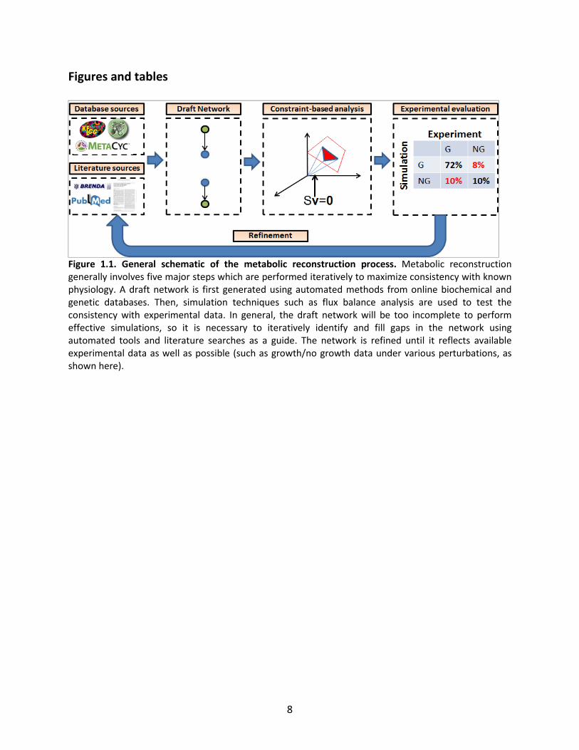
Figure 1.1. General schematic of the metabolic reconstruction process. Metabolic reconstruction generally involves five major steps which are performed iteratively to maximize consistency with known physiology. A draft network is first generated using automated methods from online biochemical and genetic databases. Then, simulation techniques such as flux balance analysis are used to test the consistency with experimental data. In general, the draft network will be too incomplete to perform effective simulations, so it is necessary to iteratively identify and fill gaps in the network using automated tools and literature searches as a guide. The network is refined until it reflects available experimental data as well as possible (such as growth/no growth data under various perturbations, as shown here).
9
Chapter 2: Genome-scale metabolic reconstruction and hypothesis testing in the methanogenic archaeon Methanosarcina acetivorans
C2A2
Abstract
Methanosarcina acetivorans strain C2A is a marine methanogenic archaeon notable for its substrate
utilization, genetic tractability, and novel energy conservation mechanisms. To help probe the
phenotypic implications of this organism’s unique metabolism, we have constructed and manually
curated a genome-scale metabolic model of M. acetivorans, iMB745, which accounts for 745 of the 4540
predicted protein coding genes (16%) in the M. acetivorans genome. The reconstruction effort has
identified key knowledge gaps and differences in peripheral and central metabolism between
methanogenic species. Using flux balance analysis, the model quantitatively predicts wild type
phenotypes and is 96% accurate in knockout lethality predictions compared to currently available
experimental data. The model was used to probe the mechanisms and energetics of byproduct
formation and growth on carbon monoxide, and the nature of the reaction catalyzed by the soluble
heterodisulfide reductase HdrABC in M. acetivorans. The genome-scale model provides quantitative and
qualitative hypotheses that can be used to help iteratively guide additional experiments to further the
state of knowledge about methanogenesis.
Introduction
Methanogenic archaea are unique in their ability to grow on low energy substrates such as acetic acid by
converting them into methane and other byproducts. Methanogens are a critical part of the global
carbon cycle, consuming byproducts of other natural bioprocesses that would otherwise be recalcitrant
in sulfate poor, anaerobic environments [67]. They also play an important role in global warming, since
methane is a greenhouse gas twenty times as potent as carbon dioxide [68] and methanogenesis is the
primary mechanism for methane emission into the atmosphere [5].
2 This chapter uses previously published material and is reprinted with the permission of the publisher. The
citation is as follows: Benedict MN, Gonnerman MC, Metcalf WW, Price ND: Genome-Scale Metabolic Reconstruction and Hypothesis Testing in the Methanogenic Archaeon Methanosarcina acetivorans C2A. J Bacteriol 2012, 194(4):855-865.
10
Methanosarcina is the only known genus of methanogens with members that can utilize all of the
known methanogenic pathways (acetoclastic, methylotrophic, hydrogenotrophic, and methyl reduction)
[69]. This metabolic diversity makes these species relatively permissive to metabolic and genetic
manipulations compared to other methanogens. To help capitalize on this, the genomes of three
Methanosarcina species have been sequenced [70-72]. In addition, genetic tools have been developed
for several of these species, including methods for directed mutagenesis and regulated expression of
specific genes [19, 24, 73, 74].
The constraint-based reconstruction and analysis (COBRA) strategy is a powerful paradigm for
consolidating large amounts of metabolic knowledge and synthesizing that knowledge into quantitative
phenotypic predictions [32, 75]. To perform constraint-based analysis on an individual organism, its
metabolic network is reconstructed from the bottom up, beginning with a sequenced and annotated
genome and ending with a network of reactions and reaction-gene associations that directly link
genotype and phenotype. Many metabolic reconstructions have been curated by hand and used to
make useful predictions such as identification of putative drug targets and the design of novel strains for
enhanced biofuel production [43, 75].
In recent years, there have been major advances towards automating much of the reconstruction
process [46]. Automation is needed to continue the exponential increase in the number of genome-scale
metabolic models [30, 75]. However, automated reconstructions for methanogens are still particularly
problematic for three major reasons: 1) automated predictions tend to be overly homogenized due to
their strong reliance on homology-based methods; 2) reaction and gene databases have a more limited
coverage of archaea than the other domains of life, and 3) the energy conservation mechanisms of
methanogens are highly specialized [10]. Hence, manual curation is necessary to obtain reliable
predictions from metabolic models of these organisms.
Amongst methanogens, M. acetivorans is notable for its substrate utilization. It can grow and produce
methane using methylated substrates, carbon monoxide or acetate, but it cannot grow with hydrogen
as its primary energy source [17]. Also, unlike most methanogens, M. acetivorans is genetically tractable.
Therefore, this organism offers opportunities to learn about novel energy conservation mechanisms.

11
An independent reconstruction for M. acetivorans strain C2A has recently been reported [76]. The
previously reported reconstruction was primarily curated using an automated curation pipeline
including the GapFind, GapFill, and GrowMatch algorithms [77, 78]. Herein we present iMB745, an
extensively curated manual reconstruction that differs significantly from the other published model. As
many literature sources as available were integrated to generate a highly accurate list of metabolic
reactions, making this reconstruction a valuable knowledge base for this organism. In addition, curation
has enabled us to make quantitative phenotypic predictions using constraint-based modeling. We
demonstrate the usefulness of this model to probe hypotheses for the workings of incompletely
understood parts of the M. acetivorans metabolic network. The analysis thus represents a successful
application of the hypothesis-driven modeling approach.
Methods
Model Reconstruction
An initial list of potential reaction-gene associations in Methanosarcina acetivorans str. C2A was
generated based on a union of data in the Kyoto Encyclopedia of Genes and Genomes (KEGG) [79],
MetaCyc [80], the Model SEED reconstruction [46], the Transport Protein Analysis Database
(TransportDB) [81], and UniProt [82]. Reactions from the existing Methanosarcina barkeri str. Fusaro
reconstruction [83] and the BiGG database [84] were added if there was sufficient evidence for their
inclusion, based on sequence homology and/or literature-based curation, or to fill gaps in the
annotation. Some gene suggestions from EFICAZ, which includes evidence from other bioinformatics
tools like PFAM, were also incorporated [85]. Gene associations were verified whenever possible using
bidirectional BLASTP against archaeal protein products with experimentally verified functions [86]. In
case of conflicts, metabolic functions suggested from literature were chosen over those suggested in the
databases, and inconsistent reactions were removed from the model (see supplemental material for a
comprehensive list).
Reaction and metabolite nomenclature consistent with the BiGG database was utilized whenever
possible to facilitate comparison to existing manually curated metabolic models [84]. Reactions and
metabolites without BiGG identifiers were assigned abbreviations in a similar manner to those present
in the database (see supplemental material for a complete list).

12
Logical gene protein reaction (GPR) relationships were constructed manually based on literature or
database evidence. For example, genes annotated or characterized to be separate subunits of a complex
were given an "AND" relationship. If there was no evidence of a protein complex catalyzing a reaction
with multiple genes, the genes were all assigned an OR relationship.
All intracellular and transport reactions were computationally mass and charge balanced at a pH of 7
based on charges and formulas computed with ACD/Labs software (Version 12; Advanced Chemistry
Development, Inc.). Charges and formulas are available in the supplemental material.
Construction of the Biomass Reaction
The biomass reaction is a sink on essential cell components that represents the consumption of
molecular building blocks (such as amino acids and nucleotides) required for cell division. The biomass
reaction for Methanosarcina acetivorans str. C2A was modified from the closest relative for which a
biomass reaction had previously been built, Methanosarcina barkeri str. Fusaro [83]. This biomass
objective function was first expanded by incorporating more detailed carbohydrate data from M. barkeri
[87] and adding methanofuran-B to the list of required cofactors [88] . Then, coefficients for lipids were
modified based on available data on the unique lipid composition of M. acetivorans [89]. Nucleotide and
amino acid coefficients specific to M. acetivorans were calculated based the published genome
sequence according to established procedures [43]. The coefficients of compounds in the soluble pool
were assumed to be the same as those in the M. barkeri biomass equation.
Flux Balance Analysis (FBA)
Exponential growth phenotypes were predicted using flux balance analysis (FBA), which has been
previously reviewed [37]. Briefly, all reactions in the model were represented in a stoichiometric matrix,
S, in which each column represented a reaction and each row a metabolite. Hence, the entry (i,j) of S
contained the stoichiometric coefficient of metabolite i in reaction j. If metabolite concentrations are
assumed to be constant (steady state), conservation of mass requires that:
Sv = 0

13
where v is the vector of reaction fluxes (reaction rates). Because there were more reactions than
metabolites in the model (as is typical), multiple possible flux distributions were possible that all
satisfied the mass balance.
Reaction fluxes were also constrained by setting minimum and maximum fluxes. In the current study,
the reversibility of each reaction was determined based on literature, database evidence, and
thermodynamic calculations. The flux through reversible reactions was unconstrained, while that of
irreversible reactions was set to have a vmin=0. Substrate uptake rates were set to experimentally
measured values for purposes of simulations (see supplemental material for values and references). The
reaction rate through the non-growth associated ATP maintenance reaction (ATPM) was set to 2.5
mmol/gDW/hr to account for upkeep energy costs. This value is somewhat lower than the experimental
value of 8.39 mmol/gDW/hr used in the current E. coli model, and larger than that in the published M.
barkeri model [83]. Growth-associated ATP maintenance was included in the biomass equation and was
set to 65 mmol/gDW, similar to the M. barkeri and E. coli FBA models [83, 90], to account for energy
costs for growth (such as production of macromolecules from biomass components. Both growth
associated maintenance (GAM) and non-growth associated maintenance (NGAM) costs were chosen to
best match experimentally measured growth and secretion rates. The NGAM is about 1.5 mmol/gDW/hr
more than that of the previously published M. barkeri model [83], primarily because ion pumping
inefficiencies for membrane-bound pumps such as Fpo were lumped into the NGAM rather than
explicitly stated in the reaction stoichiometry. Detailed calculations and references related to the
biomass equation are available in the supplemental material.
Under the assumption that the cell seeks to maximize its growth potential, the specific growth rate was
predicted by maximizing the flux through the biomass reaction subject to the aforementioned
constraints:
Max vbiomass
Subject to:
Sv = 0
vmin ≤ v ≤ vmax

14
Reaction fluxes were predicted in mmol/gDW/hr, and growth rates were predicted in hr-1. FBA problems
were solved using the COBRA toolbox in MATLAB [91] linked to the GLPK linear program solver.
Simulations were also repeated using the CPLEX package via the TOMLAB 7.0 interface, with identical
results. Defined high salt (HS) media without vitamin supplement was used for all simulations. The
complete media composition is listed in the supplemental material and was defined from Sowers et al.
[92].
Flux Variability Analysis
Flux balance analysis (FBA) does not necessarily yield a unique flux distribution, although it will yield a
unique optimal value for the objective function. Flux variability analysis (FVA) was thus used to calculate
the possible range of each flux under optimal growth conditions. Mathematically, the possible range of
flux through each reaction i was calculated by maximizing and minimizing its flux vi while constraining
the objective to be larger than a certain threshold [93]:
Min/Max vi
Subject to:
Sv = 0
vmin ≤ v ≤ vmax
vbiomass ≥ pct*vbiomass,MAX
All flux variability analyses in this paper were performed with pct = 100% (the biomass objective
function was fixed to its maximum value, within rounding error). Flux variability analysis was performed
using the fluxVariability function in the COBRA toolbox [91].
Knockout lethality studies
To perform knockout lethality studies, knocked out genes were assigned a value of 0 (FALSE) and other
genes were assigned a value of 1 (TRUE). The Boolean GPRs were evaluated for every reaction, and
reactions with a GPR evaluating to FALSE were removed from the model. After modifying the network
in this way, FBA was used to make a growth-no growth prediction (growth was defined as a predicted
vbiomass>10-5 hr-1) for all knockouts of metabolic genes. Lethality predictions were compared to published
15
gene knockout phenotype data (see supplemental material for references). For substrates with an
unknown uptake rate (such as monomethylamine), the uptake rate was assumed to be 15
mmol/gDW/hr, similar to the calculated rate for growth on methanol [94], for purposes of FBA
simulations.
Calculation of Theoretical ATP Yield and Thermodynamic Efficiency
To calculate theoretical (maximum possible) ATP yield under various conditions, a flux balance analysis
problem was solved, but the flux through the non-growth associated maintenance (ATPM) reaction was
maximized instead of flux through of the biomass equation. If necessary, the model was forced to carry
flux through a specific ATP generating pathways (such as acetogenesis) by adding constraints on other
ATP-generating pathways (such as methanogenesis). The theoretical ATP yield was calculated by dividing
the maximum flux through the ATP maintenance reaction by the CO uptake rate. Thermodynamic
efficiency was calculated as the ratio of the theoretical ATP yield predicted by the model and the ATP
yield if the entire Gibbs energy available from the production of methane and CO2 from a given
substrate (under standard conditions) was used to generate ATP [95].
Thermodynamics
Experimental standard Gibbs free energy change of reactions were unavailable for most of the reactions
in the network, but they were available and included for some methanogenesis reactions [2, 95] and
reactions involved in central metabolism [96] based on experimental Gibbs free energies of formation.
When available, the free energy changes were used to help make decisions about reaction reversibility
(in combination with direct experimental or modeling evidence).
To estimate the standard Gibbs free energy change of reactions for which no experimental data was
available, Mol files were generated to represent all compounds in the model, containing charged
structures at a pH of 7. The mol files contain the structures and location of charged moieties in each
compound in the model. Charges were computed and charged mol files were exported using ACD/Labs
software (Version 12; Advanced Chemistry Development, Inc.). The Gibbs energy of each compound was
estimated using a previously published group contribution method [97]. Standard Gibbs free energies of
formation and reaction are reported in the supplemental material under the following conditions:
16
temperature of 250C, pH of 7, an ionic strength of 0, water in the liquid phase, and all other compounds
in aqueous phase at a concentration of 1M.
Results
Model Reconstruction
The metabolic network of Methanosarcina acetivorans was curated and validated as described in the
methods. The final network accounts for the activity of 745 metabolic genes and contains 715
intracellular metabolites and 756 reactions (excluding exchange and biomass reactions). The network is
considerably larger than that in the manually curated model of M. barkeri [83] and is comparable in size
to that found in other genome-scale metabolic reconstructions [98]. In addition to reactions included in
the model, reactions that were specifically excluded from the model due to literature or modeling
evidence were also recorded. Complete lists of reactions included, GPR relationships, and excluded
reactions may be found in the supplemental material.
The metabolic network of M. acetivorans consists mostly of reactions required for synthesis of amino
acids, nucleotides, and cofactors (Figure 2.1 A). This was not surprising given the relatively small number
of growth factors required for the growth of this organism. The reconstructed network includes
pathways for synthesizing most of the cofactors required for methanogenesis in Methanosarcina species.
The exception is methanophenazine, which to the authors’ knowledge has no complete synthesis
pathway proposed in any organism. Synthesis pathways were also included for several other cofactors
such as NAD, biotin, flavins and folate.
There are still significant gaps in the knowledge of central metabolic pathways. For example, no
homologues to currently known IMP dehydrogenase genes could be found in the genome of M.
acetivorans, but the reaction catalyzed by this enzyme is predicted to be essential for nucleic acid
synthesis. In addition, several of the methanogenic cofactor synthesis pathways that are completely or
partially characterized in Methanocaldococcus jannaschii seem to have diverged in Methanosarcina.
Although this is perhaps not surprising given the great evolutionary distance between
Methanocaldococcus and Methanosarcina, the identification of these differences could provide

17
motivation for further investigation into the evolution of these species. A detailed discussion of these
differences and other identified gaps in metabolic pathways is provided in the supplemental text..
Comparison to Existing Genome-Scale Reconstructions of Methanosarcina Species
The iMB745 model is the third model of members of Methanosarcina to be published. The first was
iAF692, a manually curated model of M. barkeri str. Fusaro [83]. The iAF692 model was used to estimate
the ion-pumping stoichiometry of the Ech hydrogenase and the ATP requirements of nitrogenase in that
organism. The second was iVS941, a genome-scale model of M. acetivorans C2A based heavily on
automated approaches [76]. The iVS941 model was used to study the essentiality of methanogenesis
pathways during growth on CO, acetate, and methanol and to predict ways to reconcile simulated
knockout lethality predictions with available data.
Many of the differences between iMB745 and each of the previously published models are due to new
literature sources for novel metabolic paths unique to the archaea. For example, both of the previously
published models include the non-oxidative portion of the pentose phosphate pathway for synthesis of
five-carbon sugars. However, the genes encoding for reactions in that pathway are apparently absent in
many methanogens, including both M. acetivorans and M. barkeri. An alternative pathway for synthesis
of ribulose-5-phosphate was recently characterized in Methanocaldococcus jannaschii [99], which unlike
the pentose phosphate pathway generates formaldehyde as a byproduct. The genes involved in that
pathway had strong homology to genes in M. acetivorans. Therefore, the reactions in the pentose
phosphate pathway were excluded from the iMB745 model and the new pathway was added to the
model. Other gaps in the previously existing models were also filled based on recent literature; see
supplemental text for details.
The iMB745 model accounts for key differences in methanogenesis pathways between M. acetivorans
and M. barkeri (Figure 2.1 B-D). Critically, the Fpo and Vht hydrogenases are not functional in M.
acetivorans, as has been shown experimentally [18], even though sequence homology suggests that
both are present. Due to the strong sequence identity between the M. acetivorans and M. barkeri
homologues, the automated reconstruction approach from the previous M. acetivorans reconstruction
incorrectly included these reactions in the model. The automated model also did not include the
18
recently-characterized soluble heterodisulfide reductase (HdrABC), which plays an important role in
methanogenesis during growth on methylated substrates [100].
Other important differences also are found between existing models. For example, M. acetivorans
cannot grow on H2 and CO2 and grows on CO using a completely different pathway that involves
secretion of acetate, methylsulfides and formate [101, 102]. M. acetivorans is also able to grow on
dimethylsulfide, whereas M. barkeri can only perform methanogenesis from that substrate [103]. The
iMB745 network includes pathways and genes necessary to perform these functions which are not
found in either of the previously-existing reconstructions. The iMB745 network also includes novel
pathways for synthesis of methanofuran and cell wall polymers that were newly added to the biomass
equation (see methods), and accounts for experimentally determined differences in lipid composition
compared to M. barkeri [89]. Therefore, the description of essential biochemistry is more complete in
this model than in the previously published ones.
Estimation of Rnf and Mrp Ion-pumping Stoichiometry
The stoichiometry of ion pumps in the electron transport chain can have a significant effect on the
quantitative predictions of metabolic models [90]. In lieu of experimental data, it becomes necessary to
estimate the stoichiometry by simulation. In the M. acetivorans model, flux balance analysis was used to
estimate the stoichiometry of ion exchange due to the H+/Na+ exchanging complex Mrp and the Rnf
complex, two methanogenesis enzymes found in M. acetivorans but not M. barkeri [104]. The Rnf
complex is thought to catalyze the reduction of methanophenazine by ferredoxin, and generate either a
proton or sodium motive force [105]. The specific ion pumped by Rnf is unknown, but Mrp is strongly
up-regulated on acetate compared to methyltrophic substrates, suggesting an increased importance for
H+/Na+ exchange across the membrane on that substrate [104]. Since the ion pumping activity of Rnf is
essential for growth on acetate and Mrp and Rnf are co-regulated [104], it was assumed for modeling
purposes that Rnf pumps sodium ions.
The ATP yield of methanogenesis on substrates that utilize Rnf is strongly dependent on both the
number of sodium ions pumped by Rnf and the H+/Na+ exchange ratio of Mrp, neither of which has been
determined experimentally. H+/Na+ exchange proteins are known in other organisms that pump protons
and sodium ions in 2:1 [106], 3:2 [107], or 1:1 ratios [108]. To find which combination was most likely in
19
light of experimental growth data, a sensitivity study was performed, varying the number of sodium ions
pumped by Rnf as well as the H+/Na+ ratio of Mrp. The closest match between the predicted and
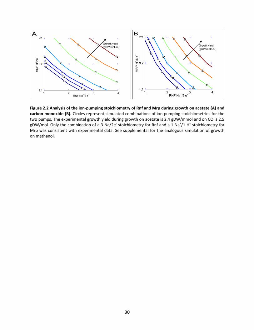
experimental growth yields occurred when Rnf was set to pump 3 Na+/2 e- and Mrp to 1 H+/Na+ (Figure
2.2). Changes in these ratios had minimal effect on predicted product secretion rates. Due to the close
match with experimental growth yields, these ratios were chosen for all further simulations.
The calculated ratios are consistent with thermodynamic data. The Rnf complex utilizes the same
electron acceptor (methanophenazine) as the F420 dehydrogenase (Fpo), but uses ferredoxin instead of
F420 as the electron donor. The reaction catalyzed by Fpo is coupled to the pumping of two protons
across the membrane [109]. Since ferredoxin has a lower redox potential than F420, it is reasonable to
expect that Rnf can pump more proton equivalents across the membrane than Fpo.
F420 Regeneration during Growth on Carbon Monoxide
Both M. acetivorans and M. barkeri grow on carbon monoxide by oxidizing it to CO2 and subsequently
reducing CO2 to methane [110]. In methanogens, the reduction of carbon dioxide to methane requires
oxidation of two equivalents of reduced coenzyme F420. Therefore, to achieve growth on carbon
monoxide, a mechanism for generating reduced coenzyme F420 must be present in the cell. In CO-grown
M. barkeri, reduced F420 is probably regenerated by generation of molecular hydrogen via the reverse
action of Ech hydrogenase, followed by H2-dependent reduction of F420 via the F420-reducing
hydrogenase, Frh [111, 112]. Ech hydrogenase is not present in the M. acetivorans genome, and
although an frh operon is present, it does not encode a functional enzyme [18]. Thus, the mechanism for
F420 regeneration in M. acetivorans during growth on CO remains unknown [110].
Our model suggests that F420 is regenerated by the combined action of F420 dehydrogenase (Fpo) and the
Rnf complex (Figure 2.3 A). In the proposed pathway, Rnf would reduce methanophenazine with
ferredoxin, and subsequently, reverse electron transport via Fpo would be used to generate reduced F420.
Reverse electron transport by Fpo has not been observed experimentally, but it is thermodynamically
feasible in an environment containing excesses of oxidized F420 and reduced methanophenazine. In
addition, this hypothesis is consistent with the high levels of Fpo protein and transcript measured during
growth on CO [113]. Finally, the estimated proton pumping stoichiometries for Rnf and Fpo (3 and 2
proton equivalents, respectively) suggest that M. acetivorans would conserve one proton for each unit
20
of F420 reduced. This is consistent with the level of conservation in M. barkeri, in which the Ech
hydrogenase pumps at least one proton out of the cell [114].
As an alternative hypothesis, we also tried to implement a F420-ferredoxin oxioreductase reaction for the
purposes of regenerating coenzyme F420 during growth on CO [100]:
FFRED: f420-2(aq) + 2 fdred(aq) + h(aq) f420-2h2(aq) + 2 fdox(aq)
Growth on CO was predicted to be possible if reaction FFRED was added to the model (data not shown).
However, the presence of FFRED was also predicted to make a Δrnf mutant viable on acetate, contrary
to experimental evidence (N.R. Baun, A.M. Guss, G. Kulkarni, and W. W. Metcalf, Unpublished Results),
and therefore the reaction was not included in the model. According to the model, a Δrnf mutant
growing on acetate could survive with a lower growth rate by reducing coenzyme F420 with FFRED and
then generating a proton gradient with Fpo and heterodisulfide reductase (Hdr).
It is possible that an enzyme catalyzing a reaction like FFRED really exists, but that the ATP yield of this
alternative path is insufficient to make the cell viable for growth on acetate. According to the model, the
theoretical maximum wild type ATP yield of methanogenesis from acetate (utilizing Rnf) is only about
0.75 ATP/acetate, corresponding to about a 65% thermodynamic efficiency (at pH 7) or 30% efficiency
(at pH 0) [95]. The efficiency is considerably higher than that of methanogenesis from carbon monoxide
(0.56 ATP/CO, 34%) or methanol (0.75 ATP/methanol, 27%), possibly because the cell is not viable with
less efficient ATP production from this substrate.
Model Consistency with Knockout Lethality Data
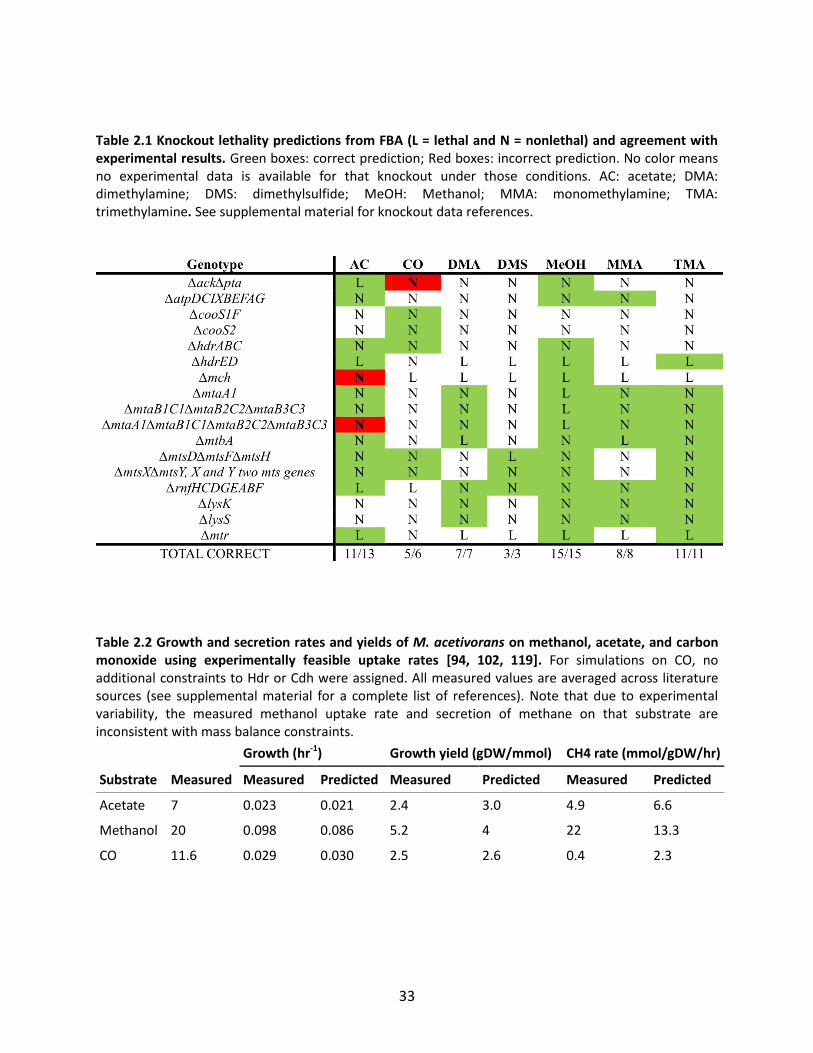
Comparison of knockout lethality predictions to available data indicates that the model correctly
predicts the growth/no growth phenotypes of 60/63 knockout mutants correctly (Table 1). All of the
incorrect predictions were cases in which genes were experimentally shown to be lethal but predicted
to be nonlethal. Two of the incorrect lethality predictions involved acetogenesis during growth on
carbon monoxide. The genes encoding Pta and Ack are essential for growth on CO [102]. However, flux
balance analysis incorrectly predicts that a ΔptaΔack mutant can grow by producing methane and
carbon dioxide as sole byproducts. Although inhibition of Mtr and (if the Mtr bypass indeed exists)
21
another reaction in methanogenesis would cause the ΔptaΔack mutation to be lethal, we cannot rule
out the possibility that other mechanisms such as regulatory constraints are responsible for the
essentiality of these genes. Physiological evidence exists both supporting [102] and refuting [101]
inhibition of methanogenesis reactions by carbon monoxide.
A ∆mch mutant was predicted to be viable on acetate (Table 2.1), but this knockout is known to be
lethal on that substrate [115]. The mch gene was hypothesized to be essential for growth on acetate
because it generates reduced F420, which M. acetivorans requires for use in anabolic reactions such as
the F420-dependent glutamate synthase [116]. However, when growing on CO, Mch cannot be used to
generate reduced F420, because it is required to carry flux in the direction of F420 oxidation. Therefore, to
achieve growth on CO, another enzyme (in the model, this is predicted to be Fpo) must be present that
is able to reduce F420. Flux balance analysis predicts that this other enzyme could also be used to reduce
F420 during growth on acetate, therefore making mch nonessential for growth on acetate. However, the
incorrect prediction depended on the ability of M. acetivorans to secrete methyl sulfides during growth
on acetate, which is unlikely given that the Mts methyltransferase required for methyl-sulfide synthesis
is down-regulated during growth on acetate [113, 117]. Hence, including the regulatory constraint
would fix the phenotype prediction.
Knockout data was useful for refining the model and finding gene annotations in the M. acetivorans
genome that are inconsistent with experimental data. For example, M. acetivorans uses Ack and Pta to
activate acetate to acetyl-CoA during acetoclastic methanogenesis, and cannot grow on acetate without
the encoding genes [102]. However, the M. acetivorans genome also encodes genes (MA3168 and
MA3602) with high sequence identity to the ADP-forming acetyl-CoA synthase of Methanocaldococcus
jannaschii that catalyzes an alternative pathway for activating acetate [118]. Including this reaction
would make Pta and Ack nonessential for growth on acetate. On this basis, the reactions in the
alternative pathway were excluded from the model.
Model Consistency with Growth Phenotype Data
The iMB745 model was used to predict growth phenotypes for wild type strains of Methanosarcina
acetivorans growing on acetate, methanol, and carbon monoxide, the three substrates for which growth
and substrate uptake data are available [94, 102, 119]. Predicted growth rates were highly dependent
22
on substrate uptake rates, which varied up to two-fold depending on the data set used to perform the
calculation (see supplemental material). It was possible to pick uptake rates within the experimentally
feasible ranges for each substrate that matched the observed growth rates and growth yields within 20%
(Table 2.2).
Both growth and secretion rates closely matched the experimental values during growth on acetate. On
methanol, the rate of methanogenesis was predicted to be much lower than experiment, but the ratios
of products are consistent with experimental data. When maximizing ATP yield during growth on
methanol, the predicted ratio of methane to CO2 produced was exactly 3:1, as would be expected to
balance redox potentials in the cell [100]. When optimizing for growth, the actual ratio of methane to
CO2 secreted was predicted in the model to be 3.8:1, because the carbon dioxide-fixing activity of
carbon monoxide dehydrogenase/acetyl CoA synthase reduced the net secretion of carbon dioxide. The
actual ratio in M. barkeri has been measured as 3.4:1 or 4.4:1 [120].
M. acetivorans produces acetate, formate, methane, and methylsulfides as byproducts when grown on
carbon monoxide (in addition to CO2) [101, 102]., but the mechanisms of formate and methylsulfide
formation are unclear. Therefore, to make predictions about the necessary conditions to produce these
byproducts, it was necessary to hypothesize mechanisms for how they are produced.
It is currently unknown how or why M. acetivorans generates formate during growth on CO, although it
is probably not coupled to methanogenesis [101]. It is possible that formate is produced as a byproduct
of carbon monoxide dehydrogenase during growth on CO to prevent toxic CO accumulation in the cell
[101, 121]. The CO dehydrogenase enzyme from Rhodospirillum rubrum has been shown to create
formate as a byproduct, and formate may formed by a similar mechanism in M. acetivorans [122],
although the physiological substrate for the reaction is still unknown [121]. In order to investigate
formate production, the following reaction was tentatively included in the model:
CODH3_SIDERXN: co(g) + h2o(l) → for(aq) + h(aq)
This reaction implies that formate production from CO does not yield ATP, which is likely to be true since
this reaction is endergonic (∆G0’=+24 kJ/mol, or +6 kJ/mol if CO is treated in aqueous phase) under
standard conditions [96].
23
The recently-characterized Mts enzymes are necessary for production of dimethylsulfide (DMS) in M.
acetivorans, although due to the very low ratio of dimethylsulfide production rate to the transcription
level of these enzymes, the in vivo function of these enzymes remains unclear [123]. The source of
methylsulfide needed as a substrate for Mts to make dimethylsulfide is unknown. However, due to the
similar structure of sulfide (HS-) and methylsulfide, one could reasonably hypothesize that methylsulfide
is formed by the same Mts enzyme that produces dimethylsulfide:
MSS: m5hbc(aq) + h2s(aq) + h(aq) → ch4s(aq) + 5hbc_red(aq)
Here, m5hbc is the methylated form of a cobalamide cofactor utilized in methyltransferases in
Methanosarcina [124] and 5hbc_red is the unmethylated form.
Despite inclusion of reactions to make the observed byproducts acetate, formate, and methylsulfides,
FBA predicted that only methane and CO2 would be produced as byproducts during growth on CO.
Consequently, the methane secretion rate was significantly higher than that observed in experiments
(Table 2). To investigate the reason for this incorrect prediction, the theoretical ATP yield was calculated
for production of each byproduct per mole of CO consumed, as described in the methods. The
theoretical ATP yield from methanogenesis was significantly higher than acetogenesis, methylsulfide
production, or formate generation (Figure 2.3 B). Because most biosynthesis reactions were
unconstrained in the direction necessary for biosynthesis, FBA predicted utilization of pathways with
greater ATP production efficiency, because if less substrate is needed to satisfy the ATP requirements of
the cell, then more is available to produce biomass. We subsequently examined possible conditions
under which these byproducts could be produced in an FBA model.
Formate Production and Regulation of CO Levels in M. acetivorans
M. acetivorans encodes at least two complete carbon monoxide dehydrogenase (CODH) operons, and
their relative expression during growth on CO may depend on the concentration of CO in the media
[121]. Since formate production may be a result of a side reaction of CODH [122], it is tempting to
speculate that the level of carbon monoxide in the cell is regulated by the balance of the levels of these
proteins, one of which produces formate as a byproduct and one which does not. FBA predicts that if
24
the proposed mechanism for formate production is correct, reducing the flux through the primary
reaction catalyzed by CODH leads to production of formate (Figure 2.3 C). This indicates that CO toxicity
could be controlled by balancing the rates of the side reaction and the primary reaction of CODH
enzymes.
CO Inhibition of the Methyltransferase Mtr and its Possible Role in Acetogenesis
The sodium-pumping methyltransferrase Mtr catalyzes the reversible transfer of methyl from methyl-
tetrahydrosarcinopterin to methyl-Coenzyme M via a cobalamide intermediate. This enzyme is strongly
down-regulated during growth on CO compared to other substrates [121]. It has been hypothesized that
methanogenesis is kinetically limited during growth on CO [102], possibly including Mtr, although this
hypothesis is controversial [101]. Flux balance analysis predicted that if Mtr was not inhibited, the cell
could still survive without methanogenesis or acetogenesis by producing methylsulfides. The theoretical
ATP yield of methylsulfide production, including ATP generation due to the sodium gradient created by
Mtr (0.33 ATP/CO), is sufficient to overcome the ATP maintenance requirement (0.22 ATP/CO; see
Figure 2.3 B). Since acetogenesis is actually essential for growth on carbon monoxide [102], and
methylsulfide production is actually very low, this prediction suggests that either Mtr activity is strongly
limited during growth on carbon monoxide, or that production of methylsulfides is kinetically limited.
Despite the down-regulation and possible inhibition of Mtr during growth on CO, significant
methanogenesis is still observed during growth on this substrate [101, 102]. The combination of these
observations has inspired the hypothesis that a Mtr bypass reaction exists that performs the same
reaction but does not generate a sodium gradient [110]:
MTR_BYPASS: mh4spt(aq) + 5hbc_red(aq) + h(aq) h4spt(aq) + m5hbc(aq)
This reaction, when coupled with methyl transfer to coenzyme M, would be strongly thermodynamically
favored in the direction of methyl-CoM formation (∆G0=-30 kJ/mol) [2]. The presence of the bypass
reaction could permit tolerance for a wider range of environmental CO concentrations by permitting the
cell to balance the increased ATP potential of Mtr with a possible greater kinetic capacity of the Mtr
bypass reaction [110].
25
To test the effects of the Mtr bypass reaction on metabolism, the bypass reaction was added to the
metabolic network, and the sodium-pumping Mtr was removed from the model. The modified model
was still predicted only to perform methanogenesis and not acetogenesis, because theoretical ATP yield
of methanogenesis was still higher than that of acetogenesis (0.44 ATP/CO and 0.38 ATP/CO,
respectively, see also Figure 2.3 B). In addition, flux variability analysis indicated that no alternative
optimal solutions led to acetate secretion. As a result, Mtr inhibition is probably not the sole reason for
acetogenesis during growth on CO.
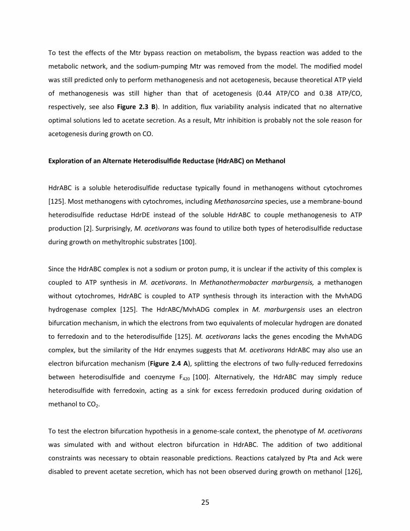
Exploration of an Alternate Heterodisulfide Reductase (HdrABC) on Methanol
HdrABC is a soluble heterodisulfide reductase typically found in methanogens without cytochromes
[125]. Most methanogens with cytochromes, including Methanosarcina species, use a membrane-bound
heterodisulfide reductase HdrDE instead of the soluble HdrABC to couple methanogenesis to ATP
production [2]. Surprisingly, M. acetivorans was found to utilize both types of heterodisulfide reductase
during growth on methyltrophic substrates [100].
Since the HdrABC complex is not a sodium or proton pump, it is unclear if the activity of this complex is
coupled to ATP synthesis in M. acetivorans. In Methanothermobacter marburgensis, a methanogen
without cytochromes, HdrABC is coupled to ATP synthesis through its interaction with the MvhADG
hydrogenase complex [125]. The HdrABC/MvhADG complex in M. marburgensis uses an electron
bifurcation mechanism, in which the electrons from two equivalents of molecular hydrogen are donated
to ferredoxin and to the heterodisulfide [125]. M. acetivorans lacks the genes encoding the MvhADG
complex, but the similarity of the Hdr enzymes suggests that M. acetivorans HdrABC may also use an
electron bifurcation mechanism (Figure 2.4 A), splitting the electrons of two fully-reduced ferredoxins
between heterodisulfide and coenzyme F420 [100]. Alternatively, the HdrABC may simply reduce
heterodisulfide with ferredoxin, acting as a sink for excess ferredoxin produced during oxidation of
methanol to CO2.
To test the electron bifurcation hypothesis in a genome-scale context, the phenotype of M. acetivorans
was simulated with and without electron bifurcation in HdrABC. The addition of two additional
constraints was necessary to obtain reasonable predictions. Reactions catalyzed by Pta and Ack were
disabled to prevent acetate secretion, which has not been observed during growth on methanol [126],
26
and the flux through pyruvate-acetyl CoA oxioreductase was set to be equal to the wild-type value to
prevent secretion of formate and other unobserved byproducts during growth on methanol [119]. In the
presence of Rnf, flux variability analysis did not predict utilization of HdrABC regardless of mechanism.
However, a Δrnf mutant was predicted to utilize HdrABC to oxidize ferredoxin using any optimal flux
distribution (Figure 2.4 B). The Δrnf mutant was predicted to grow 35% slower than the wild type
without bifurcation and 20% slower with bifurcation. A Δrnf mutant actually grew about 25% slower on
methanol than the wild type (William Metcalf, unpublished data), so within experimental error it is
difficult to tell which mechanism is correct. Further experiments could help elucidate the true
mechanism.
Discussion
We have built and manually curated a computable genome-scale model of metabolism in M. acetivorans,
only the third methanogen species to be reconstructed (after M. barkeri [83] and M. jannaschii [127])
and the second in the genus Methanosarcina. We have focused on three approaches to model-guided
discovery using the Methanosarcina acetivorans model: 1) identification of knowledge gaps and
“missing” reactions in metabolic pathways, 2) detailed study of metabolic differences between closely
related methanogenic species, and 3) use of constraint-based modeling to study alternative hypotheses
about the workings of the metabolic network and the implications of those hypotheses on predicted
phenotypes.
The reconstruction endeavor has helped pinpoint gaps in our knowledge of the metabolic networks,
both due to unknown differences between different archaeal species and differences between archaea
and other domains of life. Interestingly, even some pathways for synthesis of specialized methanogenic
cofactors, such as those for tetrahydrosarcinopterin and coenzyme M, seem to have diverged from
those observed in other methanogens such as Methanocaldococcus jannaschii. However, the synthesis
pathways for other methanogenic cofactors (such as coenzyme B synthesis) are conserved across these
genera. This observation raises interesting questions about the evolution of these ecologically important
organisms and the role of the environment in the selection of metabolic pathways.
Constraint-based modeling proved useful for integrating experimental data from different sources and
identifying tensions between data sets. Some of these tensions, such as the disparity between the ability

27
of M. acetivorans to grow on CO and the lethality of a mch knockout, may have been difficult to identify
without a genome-scale model and its accompanying predictions. These findings highlight the usefulness
of an integrative, genome-scale modeling approach for both validating model predictions and identifying
gaps in our knowledge of methanogen biology.
One of the strengths of genome-scale metabolic modeling is the ability to continually update the model
as additional experimental data becomes available [128]. Our investigations of alternative hypotheses
for the mechanism of F420 regeneration during growth on carbon monoxide, pathways for synthesis of
byproducts observed during growth on CO, and the precise reaction catalyzed by the soluble
heterodisulfide reductase HdrABC have yielded predictions that can be tested in the laboratory. As
additional data becomes available, improved models may be constructed and used to provide further
novel hypotheses in an iterative process that lies at the heart of systems biology.
Supplemental material
Supplemental material related to this chapter is located online at:
http://jb.asm.org/content/194/4/855/suppl/DC1

28
List of Abbreviations
Metabolites (as in model): 5hbc_red: 5-Hydroxybenzimidazolylcob(I)amide; ch4s: Methyl sulfide; co:
Carbon monoxide; co2: Carbon dioxide; com: Coenzyme m; cob: Coenzyme b; f420-2: Oxidized F420;
f420-2h2: Reduced F420; fdox: Reduced ferredoxin; fdred: Reduced ferredoxin; for: Formate; formmfr(b):
Formylmethanofuran(b); h: H+; h2o: Water; hsfd: Heterodisulfide; mh4spt: Methyl-
tetrahydrosarcinopterin; mphen: Oxidized methanophenazine; mphenh2: Reduced methanophenazine;
m5hbc: Co-Methyl-Co-5-hydroxybenzimidazolylcobamide; na1: Na+;
Genes and proteins: ack: Acetate kinase; cdh: CO dehydrogenase/acetyl CoA synthase; ech: Ech
hydrogenase; fpo: F420 dehydrogenase; frh: F420-reducing hydrogenase; hdr: Heterodisulfide reductase;
mch: Methenyl-H4SPt cyclohydrolase; mrp: Multiple resistance protein (Na+/H+ exchange pump); mtr:
Sodium-pumping h4spt-coenzyme M methyltransferase; mts: Dimethylsulfide-coenzyme M
methyltransferase; pta: Phosphotransacetylase; rnf: Putative ferredoxin-methanophenazine
oxioreductase
Modeling: COBRA: Constraint-based reconstruction and analysis; FBA: Flux balance analysis; FVA: Flux
variability analysis; GAM: Growth-associated maintenance cost; NGAM: Non-growth associated
maintenance cost.

29
Figures and Tables
Figure 2.1. Properties of the model of Methanosarcina acetivorans and comparison to other existing Methanosarcina models. (A): After curation, the metabolic model contained reactions related to synthesis of essential biomass components, cell wall components, and methanogenesis, among others. (B-D): Comparison of the electron transport chains in the three available Methanosarcina models. Red reactions are reversible in that model. Note that the curated M. acetivorans model includes the Rnf complex and the soluble heterodisulfide reductase (HdrABC) and excludes Frh and Vht, two hydrogenases known to be inactive in M. acetivorans but present and active in M. barkeri.
30
Figure 2.2 Analysis of the ion-pumping stoichiometry of Rnf and Mrp during growth on acetate (A) and carbon monoxide (B). Circles represent simulated combinations of ion pumping stoichiometries for the two pumps. The experimental growth yield during growth on acetate is 2.4 gDW/mmol and on CO is 2.5 gDW/mol. Only the combination of a 3 Na/2e- stoichiometry for Rnf and a 1 Na+/1 H+ stoichiometry for Mrp was consistent with experimental data. See supplemental for the analogous simulation of growth on methanol.

31
Figure 2.3 Analysis of growth of M. acetivorans on carbon monoxide. (A) Regeneration of coenzyme F420 during growth on carbon monoxide for both M. barkeri (left) and proposed pathway for M. acetivorans (right). (B) Theoretical ATP yields during growth on CO varied depending on the byproduct produced and whether sodium-pumping Mtr or its non-pumping bypass reaction (Mtr_b) is active. Red: formate generation; black: acetogenesis; blue: methanogenesis (with Mtr), green: methylsulfide production (with Mtr), gold: methylsulfide production (with Mtr_b), dark red: methanogenesis (with Mtr_b). At least 0.22 ATP/CO is required to overcome the non-growth associated maintenance requirement and an additional 65 mmol ATP/gDW is required for growth. (C) FBA predicts that limitation of CO dehydrogenase activity leads to formate production.

32
Figure 2.4 Studies on the soluble heterodisulfide reductase HdrABC during growth on methanol. (A) Hypothesized bifurcation mechanism of the soluble heterodisulfide reductase HdrABC during growth on methylotrophic substrates in M. acetivorans. The alternative hypothesis is that the reaction does not involve F420 (dashed lines). (B) Flux balance analysis predicts that, during growth on methyltrophic substrates (methanol shown), HdrABC is not used when Rnf is available, but a Δrnf mutant is predicted to carry flux through HdrABC. The growth rate for the Δrnf was predicted to be about 20% less with bifurcation and 35% less without.
33
Table 2.1 Knockout lethality predictions from FBA (L = lethal and N = nonlethal) and agreement with experimental results. Green boxes: correct prediction; Red boxes: incorrect prediction. No color means no experimental data is available for that knockout under those conditions. AC: acetate; DMA: dimethylamine; DMS: dimethylsulfide; MeOH: Methanol; MMA: monomethylamine; TMA: trimethylamine. See supplemental material for knockout data references.
Table 2.2 Growth and secretion rates and yields of M. acetivorans on methanol, acetate, and carbon monoxide using experimentally feasible uptake rates [94, 102, 119]. For simulations on CO, no additional constraints to Hdr or Cdh were assigned. All measured values are averaged across literature sources (see supplemental material for a complete list of references). Note that due to experimental variability, the measured methanol uptake rate and secretion of methane on that substrate are inconsistent with mass balance constraints.
Growth (hr-1) Growth yield (gDW/mmol) CH4 rate (mmol/gDW/hr)
Substrate Measured Measured Predicted Measured Predicted Measured Predicted
Acetate 7 0.023 0.021 2.4 3.0 4.9 6.6
Methanol 20 0.098 0.086 5.2 4 22 13.3
CO 11.6 0.029 0.030 2.5 2.6 0.4 2.3
34
Chapter 3: Likelihood-based gene annotations for gap filling and quality assessment in genome-scale metabolic models3
Abstract
Genome-scale metabolic models provide a powerful means to harness information from genomes to
predict cellular phenotypes and deepen biological insights. With exponentially increasing sequencing
capacity, there is an enormous need for automated reconstruction techniques that can provide more
accurate models in a short time frame. Current methods for automated metabolic network
reconstruction rely on gene and reaction annotations to build draft metabolic networks and algorithms
to fill gaps in these networks. However, automated reconstruction is hampered by database
inconsistencies, incorrect annotations, and gap filling largely without considering genomic information.
Here we develop a metric for applying genomic information to predict alternative functions for genes
and estimate their likelihoods from sequence homology. We show that computed likelihood values were
significantly higher for annotations found in manually curated metabolic networks than those that were
not. We then apply these alternative functional predictions to estimate reaction likelihoods, which are
used in a new gap filling approach called likelihood-based gap filling to predict more genomically
consistent solutions. To validate the likelihood-based gap filling approach, we applied it to models
where essential pathways were removed, finding that likelihood-based gap filling identified more
biologically relevant solutions than network-based gap filling approaches. We also demonstrate that
models gap filled using likelihood-based gap filling provide greater coverage and genomic consistency
with metabolic gene functions compared to network-based approaches. Interestingly, despite these
findings, we found that likelihoods did not significantly affect consistency of gap filled models with
Biolog and knockout lethality data. This indicates that the phenotype data alone cannot necessarily be
used to discriminate between alternative solutions for gap filling and therefore, that the use of other
information is necessary to obtain a more accurate network. All described workflows are implemented
as part of the DOE Systems Biology Knowledgebase (KBase) and are publicly available via API or
command-line web interface.
Author summary
3 This chapter has been submitted as a manuscript to PLOS Computational Biology. Thanks go to my co-authors:
Michael Mundy, Christopher Henry, Nicholas Chia and Nathan Price.
35
Genome-scale metabolic modeling is a powerful approach that allows one to computationally simulate a
variety of metabolic phenotypes. However, manually constructing accurate metabolic networks is
extremely time intensive and it is thus desirable to have automated computational methods for
providing high-quality metabolic networks. Incomplete knowledge of biological chemistries leads to
missing, ambiguous, or inaccurate gene annotations, and thus gives rise to incomplete metabolic
networks. Computational algorithms for filling these gaps in a metabolic model rely on network
topology based approaches that can result in solutions that are inconsistent with existing genomic data.
We developed an algorithm that directly incorporates genomic evidence into the decision-making
process for gap filling reactions. This algorithm both maximizes the consistency of gap filled reactions
with available genomic data and identifies candidate genes for gap filled reactions. The algorithm has
been integrated into KBase’s metabolic modeling service, an automated metabolic network
reconstruction framework that includes the ModelSEED automated metabolic reconstruction tools.
Introduction
Genome-scale metabolic models (GEMs) integrate available information about metabolism to provide a
basis for holistic modeling and prediction of metabolic phenotypes [129]. GEMs have been utilized
broadly [30, 40, 130, 131] across all three domains of life [132] to accelerate research in such areas as
network evolution [133-135], synthetic biology [31, 136], and the discovery of novel drug targets [137].
However, achieving a sufficiently accurate metabolic model to enable high utility currently requires a
very time-intensive manual reconstruction process, often taking many months or even years to
complete [43]. As the throughput of sequencing technologies continues to increase and as research on
microbial populations produces more and more genomes [138], there is a growing need for methods
that automate high-quality metabolic model reconstruction.
Since the advent of genome-scale metabolic modeling, protocols [43], databases [80, 84, 139],
algorithms [46, 77, 140] and toolboxes [46, 141, 142] have been developed to help systematize the
lengthy and iterative process of collecting, curating, and integrating large volumes of biochemical
knowledge. There have also been previous efforts to fully automate this process, including, notably, the
Department of Energy’s ModelSEED [46]. Despite these important advances, significant barriers to high-
quality automated metabolic reconstructions still persist. Even with human curation, ambiguous or
36
incorrect annotations are still pervasive [143]. Incomplete annotations leave gaps in the metabolic
networks that need to be filled in order to make simulation possible [43, 144]. Inaccurate annotations
also give rise to the need to identify and assess the merits of alternative annotations for genes, a
process that typically done manually as part of the model curation process [43]. An automated approach
to model building that accounts for alternative annotations would help expedite manual curation and
ensure that the draft models maximally account for alternatives that can be identified based on
available data.
Existing algorithms for filling gaps, or dead-end reactions, in metabolic networks broadly fall into
approaches based on network topology [77, 145], pre-defined pathways [146], or phenotype data [78,
147, 148]. Network topology-based algorithms such as GapFill identify dead-end reactions in a metabolic
network and identify the minimum number of modifications to the network that can be made to
activate those reactions [77]. Variations of GapFill have been developed that assign specific penalties
based on thermodynamics or database incompleteness [145]. Pathway-based algorithms, such as that
implemented in the PathwayTools [146], automatically complete pre-defined pathways that have
sufficient representation in the draft model. Finally, several algorithms use phenotype data to help
choose gap filling pathways, including OMNI, which maximizes model consistency with reaction rate
data [147], GrowMatch, which maximizes consistency with experimental growth/no growth results [78],
and MIRAGE, which maximizes the co-occurrence and co-expression of connected reactions [148].
Uniquely among these methods, MIRAGE also automatically identifies gene candidates for optimal gap
fill solutions.
While existing methods capably activate the necessary reactions to allow growth simulations, they often
do so by over fitting, resulting in the inclusion of spurious pathways. This is epitomized by a recent
article that showed that in some cases, pruning these spurious pathways can lead to significant
improvements in simulation accuracy [149]. Although genomic evidence may be incorporated after gap
filling through human curation of potential solutions [150], these solutions are unlikely to fully reflect all
the available knowledge of the genome. Methods that addresses both the resolution of dead-end
metabolites and the identification of gene-reaction pairings for the reactions added to the model during
the resolution of the gaps in the reaction network help researchers identify poorly-supported solutions
when building models, thus helping to reduce over-fitting.
37
The goal of our work is to improve the quality of automatically generated metabolic reconstructions and
models by explicitly incorporating alternative potential gene annotations and their estimated likelihoods
into the gap filling process. We have developed a likelihood-based gap filling workflow that (1) assigns
likelihood scores based on sequence homology to multiple annotations per gene and, from these,
likelihoods for reactions in a network and (2) identifies maximum-likelihood pathways for gap filling
using a mixed-integer linear programming (MILP) formulation. We have also developed a workflow to
iteratively identify pathways that activates gene-associated orphaned reactions in a network and
assesses the likelihood of these pathways. Critically, the likelihood-based approach makes the gap filling
solution genome-specific and provides users with putative gene-protein-reaction relationships and
confidence metrics for each result. We show that our likelihood-based approach improves the quantity
and quality of new gene annotations compared to the existing gap filling algorithm, while the resulting
models have comparable accuracy when simulating high-throughput growth phenotype data, when
compared with previous network-based gap filling algorithms. The workflow tools are fully integrated
within the Department of Energy’s System Biology Knowledgebase (KBase), and are publicly available via
both a web-based command line interface (available at http://kbase.us) and a web service API.
Results
Gap filling workflows using likelihood and network-based approaches
Confidence scores are useful for building models and assessing the quality of the annotations, reactions
and pathways therein [43]. We have developed a quantitative likelihood measurement for the evidence
that a gene carries a specific annotated function and a technique by which these likelihood estimates
can be converted into the likelihood of existence of a reaction in a cell's metabolic network (see
Methods). Importantly, we simultaneously compute the likelihoods of multiple annotations for a single
gene, which both broadens the space of testable annotation hypotheses in gap filling solutions and
helps mitigate possible errors in the most likely annotation.
The conversion from annotation to reaction likelihood scores is performed based on the reaction-role
links in the SEED reaction database [46]. We have implemented four gap filling workflows (Figure 3.1
and Appendix B) that use these reaction likelihoods (likelihood-based gap filling) or rely only on network
context (network-based gap filling), in conjunction with two distinct gap filling strategies.
38
In the first strategy, which is the most commonly used in the field, gap filling is used to activate one
particular reaction in a model such as the biomass reaction [77]. We call this approach targeted gap
filling because it seeks to activate a single target reaction in the network. A successful application of
targeted gap filling enables simulations to be performed on the resulting model using an increasingly
large suite of constraint-based analysis algorithms [32, 151].
In the second strategy, which we call iterative gap filling, gap filling is used to activate the maximum
number of orphaned reactions in a model in an iterative fashion, activating high-priority reactions first
(see Methods). One could imagine such an approach would sacrifice specificity for sensitivity (while
targeted gap filling would do the opposite). In the iterative gap filling workflow, a post-processing step is
also used to reduce the redundancy resulting from attempting to activate every gene-associated
reaction, to assess the value of each gap filled pathway in terms of how much of the original annotated
network is corrected by the pathway, and optionally, to apply a cutoff to the cost of pathways added to
the model (see Methods and Appendices B and C).
Likelihoods reflect a measure of confidence in predicted function
As part of the model curation process, it is necessary to evaluate the quality of each annotation and fix
those which are found to be problematic [43]. We have implemented a simple method to estimate
annotation likelihoods accounting for two sources of ambiguity: (1) sequence divergence between query
genes and the genes in the reference database, and (2) inconsistencies in annotation within the
reference database (see Methods). We characterized the utility of our reaction likelihoods by comparing
the gene-reaction links created using our automated likelihood-based approach to those present in
manually curated metabolic networks of Escherichia coli K12 [130] and Bacillus subtilis str. 168 [145].
We found that highly likely gene-reaction links were significantly enriched in the models compared to
less-likely gene-reaction links (Figure 3.2) indicating that a higher likelihood score reflects higher
confidence in the predicted function. We also identified large numbers of high-likelihood gene
annotations that are not in the comparison models, which reflect promising candidates for further
investigation and possible inclusion in the models.
39
Proof of principle for likelihood-based gap filling
Unlike the network-based gap filling approach, the likelihood-based approach is able to produce
different solutions for different organisms, even if the starting network is identical, based on the
organisms' genetic content. To demonstrate the utility of this approach in improving model quality, we
identified a set of 32 reactions from the iBsu1103 genome-scale metabolic model of B. subtilis [145] that
were predicted to be essential for growth and whose existence in the model was supported by literature
evidence[152]. This set of reactions represented a gold standard set of reactions that should be
incorporated into gap filling solutions if they were missing. We then removed all 32 gold standard
reactions from the iBsu1103 model and applied the targeted network-based gap filling and likelihood-
based gap filling algorithms to restore biomass production in the knockout model.
In order to evaluate the effects of parameterizing each algorithm, we modified the chosen penalties for
transporters and for thermodynamically unfavorable reversibility changes. The optimal penalty for
transporters was higher for network-based gap filling (55 or greater - equivalent to adding about 7
intracellular reactions on average) than for likelihood-based gap filling (25 or greater). Optimal penalties
for thermodynamically unfavorable reversibility changes were also higher for network-based than
likelihood-based gap fill (40 and 12, respectively). Despite the same number of tuning parameters
available for each method, likelihood-based gap filling successfully outperformed the network-based
method by replacing a maximum of 31 of the 32 gold-standard reactions. Network-based gap filling only
replaced only a maximum of 24 reactions, even with extremely high penalties for transporters and
unfavorable reversibility changes. Given that no transporters or reversibility changes were part of this
test, the parameters chosen to be optimal for network-based gap filling were unreasonably high.
Therefore we used the optimal penalties for likelihood-based gap filling for the remainder of the results
in this manuscript (Appendix A).
The failures in network-based gap filling were a result of picking shorter pathways to fill certain gaps for
which longer pathways are the correct choice. For example, the synthesis of isopentyl diphosphate
(IPDP), a primary precursor for lipid synthesis, can occur by one of two routes, the mevalonate pathway
and the non-mevalonate pathway [153]. B. subtilis uses the non-mevalonate pathway for IPDP synthesis
[154, 155]. The mevalonate pathway contains fewer reactions than the non-mevalonate pathway, and
thus the network-based gap filling approach incorrectly used the mevalonate pathway to restore IPDP
40
production (Figure 3.3). However, all of the knocked out reactions in the non-mevalonate pathway had
high estimated likelihoods. Hence, likelihood-based gap filling correctly chose this pathway to restore
production of IPDP.
Annotation of likelihood-based gap filling reactions
Mapping between genes and reactions allows for a useful connection to genetic manipulations, drug
targets, and experimental validation. One important step in curating gap filling solutions is identifying
genes in the genome that could be responsible for catalyzing the gap filled reactions and assessing the
quality of the genomic evidence behind these assignments[150]. We have compared the ability to do
identify these genes with likelihood-based and network-based gap filling by using the estimated Gene-
Protein-Reaction relationships (GPR) from our likelihood computations to assign genes to reactions that
are gap filled using each approach. We found that likelihood-based gap filling produced significantly
more links between genes and reactions and more gene-associated reactions than post-processing of
network-based gap filling results (i.e. seeking for gene homology after reactions were gap filled). This
was true for both the targeted gap filling and iterative gap filling approaches ( , Wilcoxon
signed-rank test; Figure 3.4). The result suggests that the likelihood-based approach typically yields
more and better-supported candidate annotations and associations that are not apparent when using
the common post-processing procedure.
In addition to improved quantity, the likelihood-based approach also improved the average quality of
annotation hypotheses generated from gap filling. In particular, the average likelihood of gene
associations added using likelihood-based gap filling was significantly greater than that using network-
based gap filling ( , Wilcoxon signed-rank test; Figure 3.5). The effect of using reaction
likelihoods on the number and likelihood of added genes was more pronounced for iterative gap filling,
indicating that likelihood-based gap filling was able to find more likely pathways to activate peripheral
model reactions in addition to the biomass reaction.
Consistency of automatically generated models with experimental phenotypes
One commonly-used method to verify the integrity of genome-scale metabolic models is to compare
their predictions with high-throughput phenotyping data, such as knockout lethality screens [43]. To test
41
the impact of each of our workflows on the accuracy of model phenotype predictions, we applied our
workflows to construct and fill gaps in genome-scale models for 22 organisms for which either Biolog or
gene knockout lethality data was available. We then compared the predictions of these models to the
phenotype data, without fitting to the data (Table 3.1). There were many differences in the pathways
identified using likelihood-based gap filling compared to network-based gap filling: between 5% and 30%
of the reactions in a likelihood-based gap filling solution were not found in the network-based solution,
despite using the same parameters for each (see Appendix A). However, the use of likelihoods did not
significantly affect the phenotype predictions. For Biolog data, iterative gap filling increased the
sensitivity by 11% compared to targeted gap fill, but decreased specificity (more false positives) by 13%-
15%. The overall accuracy (total correct/total experiments) decreased by about 5% for iterative
compared to targeted gap filling.
Since gap filling only adds a small number of genes to the model compared to the number in the draft
model (about a 7% increase for iterative gap filling), the sensitivity and specificity of knockout lethality
predictions were very similar for all four workflows. The sensitivity varied from 84-86% and specificity
from 64-67%. We also examined the lethality predictions specifically for genes added in gap filling
(Figure 3.6). The negative predictive value was essentially identical for all four workflows at 40%.
However, there was a notable improvement in the positive predictive value in the iterative gap filling
workflows (80%) compared to network-based workflows (40%). Taken together, these results indicate
that iterative gap filling mostly adds genes predicted to be nonlethal knockouts, and that most of these
predictions are correct.
Discussion
We have used genomic evidence-based likelihood metrics for annotations and reactions to increase the
consistency of gap filled pathways with available genomic data compared to the common procedure of
post-processing network-based solutions. This approach increases the quantity of hypothesized gene-
associated reactions compared to post-processing network-based gap filling solutions. However, despite
the significantly increased level of evidence for gap filling solutions resulting from likelihood-based gap
filling, there was not a significant difference in knockout lethality or growth (Biolog) predictions. This
result suggests that using phenotype data to filter gap-filling solutions may not result in a more accurate
metabolic network (that is, one that better reflects biological evidence for the specific components

42
included). Indeed, validation metrics such as consistency with knockout lethality predictions have a large
number of ways in which they could be fit to become consistent with phenotype data, which can lead to
decreases in observed accuracy when the model is tested on new data not available during its
construction [149]. Therefore, alternative methods such as quantification of quality of individual
reactions or pathways in the network are important metrics for validation.
An important feature of the likelihood-based gap filling algorithm is that it can differentiate between
genomes by assigning organism-specific likelihoods for each reaction in a network. As a direct result, the
gap filling solutions resulting from this algorithm are also organism-specific. This direct link back to
evidence in the genome directly enables the identification of pathways that are not parsimonious, but
that are most consistent with genomic data. We have shown that the likelihood-based approach
increases both the quality and the quantity of hypothesized gene associations from gap filling, especially
when using the iterative approach to maximize the number of activated reactions subject to evidence
constraints. Of course, when building a high-quality network model, gap filled pathways should be
evaluated by experts to evaluate the evidence cited in the algorithm, to search for existing experimental
evidence in favor of or refuting the suggested solutions, or to design new experiments to test the
existence of the hypothesized functions in the modeled organism [43, 141]. The reported confidence
metrics for annotations and for reactions will help curators target these curation efforts.
Our implementations of the likelihood-based, network-based, network-based iterative, and likelihood-
based iterative gap filling workflows are available in KBase via a web service API or web-based command
line interface. The integration of our implementation in KBase’s infrastructure captures the provenance
of modeling data and enables users to readily build new, functioning models (Appendices B and C). In
addition to gap filling, KBase includes implementations of many other modeling and reconstruction tools
such as tools for the automatic generation of compartmentalized community models [156] and
phenotype reconciliation tools.
The proposed integration of likelihoods into gap filling can also serve as a tool for hypothesis generation
in biology. An initial pool of potential annotations with associated likelihoods can be generated using
many different methods such as protein co-localization or co-occurrence [47, 157] or from high-
throughput '-omics' datasets such as metabolomics. This initial pool can be quite broad (many
alternative functions for each gene). The likelihood-based gap filling approach we have outlined is
43
sufficiently general to incorporate likelihoods based on any type of evidence. The gap filling algorithm
then selects from this broad pool of hypotheses for the new annotations that best explain a complex
combination of biological observations, providing insights into enzyme promiscuity, adaptation, and
evolution. Importantly, KBase is a unified platform across multiple databases and data types; the
integration of likelihood-based gap filling in this platform provides a roadmap for the integration of
these diverse data sets. As systems biology expands to incorporate a greater number of high-throughput
biological measures, the utility of a computational framework for leveraging this vast knowledge in toto
grows rapidly.
Methods
The likelihood-based gap filling method consists of three major steps: (1) the calculation of annotation
likelihoods for each individual gene, (2) the calculation of reaction likelihoods for the cell as a whole, and
(3) the use of reaction likelihoods to inform the gap filling process. Each of these steps is detailed below.
The iterative gap filling approach consists of two major steps: (1) iteratively integrating gap filling
solutions into a model, and (2) performing reaction sensitivity analysis to prune redundant or poorly
supported reactions. We have included as part of the Supporting Information detailed tutorials on the
use of the KBase web-based interface (Appendix B) or the web service API (Appendix C) to perform this
analysis.
Likelihood-based and iterative gap filling workflow description
The first step of the workflow (Figure 3.1) is importing an annotated genome into a workspace in the
KBase system. (KBase workspaces provide a way for users to store, share, and manage data objects that
they have uploaded or generated by running KBase analyses.) The genes in the genome are then used to
generate a draft model using the ModelSEED algorithm [46] and, for our likelihood-based approach, to
compute annotation and reaction likelihoods. Next, gap filling is done on the model (either with or
without likelihood weights, and with or without the iterative approach) to generate one or more
solutions, which are integrated into the model to create a gap filled model. The initial gap filling solution
allows growth on 'complete' media, which consists of all compounds for which the organism has
transport reactions in the draft reconstruction. For iterative gap filling, the user has the option of
performing a reaction sensitivity analysis to remove both poorly-supported gap filling solutions (those

44
with high cost) and those which have no effect on the model's solution space. Once the reaction
sensitivity analysis is complete, the model is gap filled again to achieve growth on a minimal medium,
which fills in more pathways and is necessary to permit simulations of Biolog data.
Generating a database of high-confidence gene annotations
In order to maximize the quality of computationally inferred functions of query genes, it was necessary
to build a database of high-confidence gene annotations to compare against. We compiled a list of the
protein sequences for all proteins whose function was either literature-supported or called as part of at
least one SEED subsystem [54]. The functional annotations in the SEED subsystems are manually curated
using multiple sources of information such as sequence similarity, phylogeny and gene context, and
therefore represent a high-confidence reference set.
To minimize the amount of redundancy in the list of target proteins, they were binned into organism
taxonomic units (OTUs) with roughly 97% 16S rRNA similarity [158]. The final target database included at
most one protein from each OTU for each functional role. When possible, the representative protein
was chosen from the representative organism of the OTU, which tends to be a better-understood
organism with higher-quality annotations such as Escherichia coli K-12. If the representative organism
for an OTU did not have a protein with that role in a subsystem or with a literature backing, a
representative protein was chosen at random from another member of the OTU.
Calculating annotation likelihoods
The computation of annotation likelihood scores was designed based on the principle that genes with
more similar sequences are more likely to share the same function, but recognizing that these
relationships are far from perfectly predictive [159]. The computation thus attempts to quantify the
uncertainty in relation to the available database of high-confidence annotations. Annotation likelihoods
were calculated by first running BLASTP [86, 160] with an E-value cutoff of against all of the genes
in the high-confidence gene annotation data set. A log-score for each (query, target) pair was computed
as:

45
is the E-value for the BLAST hit between genes i and j and is the log-score between them. The
parameter was used to prevent the log E-value from being undefined due to a reported E-
value of zero. After calculating log-scores for all (query, target) pairs, a likelihood score that each gene
, where GO is the set of genes in the organism, has a given functional annotation a was computed
as follows:
∑
∑
represents the set of genes with annotation a, is the maximum score of BLAST hits
from a gene in the query organism to a gene in the high-quality database, and is a
pseudocount used to dilute the likelihoods of annotations for annotations with weak homology to the
query. The pseudocount was chosen to set the likelihood of a gene having moderately high homology
(E=1E-40) to a single protein in the database to 50% and has proven to yield a reasonable spread of
likelihoods. According to this formulation, in order to have a high likelihood score for annotation a, the
query protein must have strongly significant sequence similarity to proteins with that annotation and
not possess similarly strong similarity to proteins with other annotations. Therefore, the metric takes
into account two different sources of annotation ambiguity: divergence of sequence and disparity of
annotations for similar proteins in the target database.
Calculating reaction likelihoods
Reaction likelihoods were computed from annotation likelihoods using the ModelSEED reaction
database [46], which links annotations to functions, protein complexes, and finally to reactions. In the
first step, gene annotation likelihoods were converted into gene-specific role likelihoods to account for
the possibility that an annotation implies multiple functional roles. The likelihood that each gene
had role r was computed as the sum of the likelihood of all annotations that implied that role, according
to the database mappings from annotations to , the set of all genes with role r:

46
∑
This definition ensures that if a protein could be multi or single-functional, the final reaction likelihoods
reflect both of those possibilities.
In the second step, the overall likelihood that at least one gene in had role r was computed as the
maximum likelihood of the role across all its genes.
The genes most likely to fulfill role r (within 80% of the maximum) were retained and linked with an OR
relationship to form a Boolean Gene-Function relationship.
In the third step, the ModelSEED reaction database was used to compute the likelihood of existence of
protein complexes from the likelihood of existence of functional roles within the cell. A protein complex
represents a set of functional roles that must all be present for a complex to exist. Hence, the likelihood
of the existence of a complex c in the cell was computed as the minimum likelihood of the roles
associated with it.
The individual functions in the complex were linked with an AND relationship to form a Boolean Gene-
Protein relationship.
In the fourth step, reaction likelihoods were computed from protein complex likelihoods using complex-
reaction links in the ModelSEED. Since multiple complexes can independently catalyze a reaction, the
likelihood of the existence of a reaction x in the cell was computed as the maximum likelihood of the
possible complexes that could catalyze it.
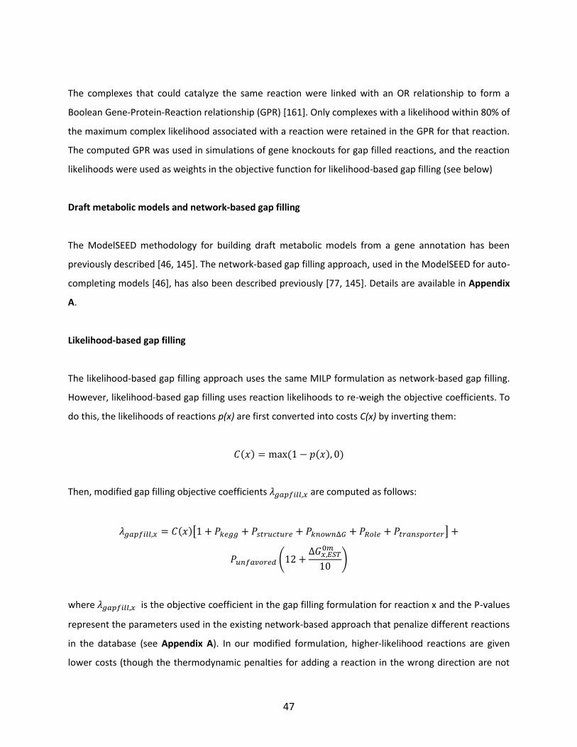
47
The complexes that could catalyze the same reaction were linked with an OR relationship to form a
Boolean Gene-Protein-Reaction relationship (GPR) [161]. Only complexes with a likelihood within 80% of
the maximum complex likelihood associated with a reaction were retained in the GPR for that reaction.
The computed GPR was used in simulations of gene knockouts for gap filled reactions, and the reaction
likelihoods were used as weights in the objective function for likelihood-based gap filling (see below)
Draft metabolic models and network-based gap filling
The ModelSEED methodology for building draft metabolic models from a gene annotation has been
previously described [46, 145]. The network-based gap filling approach, used in the ModelSEED for auto-
completing models [46], has also been described previously [77, 145]. Details are available in Appendix
A.
Likelihood-based gap filling
The likelihood-based gap filling approach uses the same MILP formulation as network-based gap filling.
However, likelihood-based gap filling uses reaction likelihoods to re-weigh the objective coefficients. To
do this, the likelihoods of reactions p(x) are first converted into costs C(x) by inverting them:
Then, modified gap filling objective coefficients are computed as follows:
[ ]
(
)
where is the objective coefficient in the gap filling formulation for reaction x and the P-values
represent the parameters used in the existing network-based approach that penalize different reactions
in the database (see Appendix A). In our modified formulation, higher-likelihood reactions are given
lower costs (though the thermodynamic penalties for adding a reaction in the wrong direction are not

48
changed) and are therefore favored in the optimization provided their benefit outweighs costs of other
reactions in a pathway. The numeric parameters (12 and 10) in the equation make changing the
reversibility of a reaction with low estimated Gibbs energy equivalent to adding (on average) one to two
intracellular reactions in a favorable direction, while changing a reaction with reaction with an estimated
Gibbs energy of 10 kCal/mol is equivalent to adding three average intracellular reactions in a favorable
direction.
Iterative gap filling
In targeted gap filling, a single reaction (e.g., biomass production) is targeted to enable a non-zero
reaction rate under a specified media condition. In iterative gap filling, all reactions in the model that are
associated with one or more genes are targeted to enable flux. Iterative gap filling is similar to the
previously gap find and gap fill algorithms [77], but operates on inactive reactions rather than dead-end
or orphaned metabolites. This is accomplished by performing targeted gap filling on one reaction at a
time until as many reactions as possible are functional. The results of iterative gap filling depend on the
order in which the targets are processed. In our studies, the order was selected based on the region of
metabolism in which the reaction occurs. Central carbon reactions were gap filled first to ensure that
core metabolism was functional. These were followed by reactions involved in biosynthesis of essential
metabolites (amino acids, nucleotides, and cofactors), finally culminating in reactions involved in
peripheral utilization and degradation pathways.
After ordering reactions according to this priority, flux variability analysis [93] was used to determine if
each reaction had a non-zero maximum flux. If the maximum flux was zero, gap filling (likelihood or non-
likelihood-based) was run to attempt to activate the reactions with pathways from the ModelSEED
reaction database. If a gap filling solution was found, it was integrated into the model before moving
onto the next reaction in the model. The final result was a set of pathways that activated a maximum
number of reactions in the model.
Reaction sensitivity analysis
Since iterative gap filling attempts to fill the maximum number of gaps in a model, solutions that fill
different gaps in the model are often redundant or very poorly supported. To solve this problem, we
49
have implemented a reaction sensitivity analysis that identifies for each gap filled reaction: a) whether
each gap filled reaction causes other reactions in the model to become inactive when it is removed and
b) whether the gap filled reaction is predicted to be essential for growth. Gap filled reactions which
were non-essential and which did not activate any other reactions in the network were removed. For
network-based iterative gap filling, reaction sensitivity was done on all reactions in the reverse order in
which they were added, so that lower-priority gap filling solutions would be tested for removal first. For
likelihood-based iterative gap filling, reaction sensitivity analysis was done in order from lowest to
highest likelihood so that gap filled reactions that were unsupported by genetic evidence would be
tested for removal first.
Phenotype simulations
The ModelSEED algorithm [46] was used to build a draft model for each of 22 organisms for which either
gene knockout lethality data (8 organisms), Biolog data (9 organisms), or both (5 organisms) was
available [90, 162-173]. All four gap filling workflows (targeted network-based, targeted likelihood-
based, iterative network-based, and iterative likelihood-based) were independently applied to the draft
model to build working models of each of these organisms (Figure 3.1). The gap filled models were
verified to predict positive biomass production on Carbon-D-Glucose media using flux balance analysis
[37] before performing further simulations.
To simulate gene knockout lethality phenotypes, the models growing on Carbon-D-Glucose media were
first further gap filled (if necessary) to achieve nonzero biomass production on the media in which
knockout experiments had been performed (this was only necessary for Mycobacterium tuberculosis).
Subsequently, the knockouts were simulated by evaluating the Boolean GPR rules for each reaction and
setting the maximum rate of each reaction whose GPR evaluated to FALSE to 0. Flux balance analysis
was then used to maximize the biomass equation. The knockout was considered lethal if the predicted
biomass production rate was less than .
To simulate biolog data, the models growing on Carbon-D-Glucose media were modified to possess
transporters for every compound in every media in the biolog array. After this modification, growth on
each medium was tested by setting exchange reactions for each compound not in the media to zero and
50
using flux balance analysis to predict the biomass production rate. The model was considered non-
growing if the predicted biomass production rate was less than .
Workflow implementation details
All gap filling for this manuscript was performed outside of KBase using CPLEX under an academic license
(IBM Corporation, version 12.5) [174]. Due to licensing restrictions, gap filling performed on KBase
servers is done using SCIP 3.0.2 [175]. Phenotype simulations and sensitivity analysis were performed
using GLPK version 4.43. The gap filling and likelihood computations are implemented in the KBase
framework with web service APIs and a web interface (http://iris.kbase.us). Detailed descriptions of all
steps in the workflow are available in Appendices B and C.
Acknowledgements
MNB and NDP gratefully acknowledge support from the Department of Energy awards #DE-FG02-
10ER64999 and ER65103 and the Camille Dreyfus Teacher-Scholar Award. MM and NC gratefully
acknowledge support from the Center for Individualized Medicine at the Mayo Clinic, the Minnesota
Biotechnology Partnership, and from the Mayo Clinic Research National Institutes of Health (NIH) Relief
Grant Program. CSH acknowledges support from the Office of Science, Office of Biological and
Environmental Research, of the US Department of Energy under contract number DE-ACO2-06CH11357,
as part of the DOE Systems Biology Knowledgebase.
Supplemental material
Supplemental text and figures for this chapter are provided as Appendices A, B, and C of the thesis.
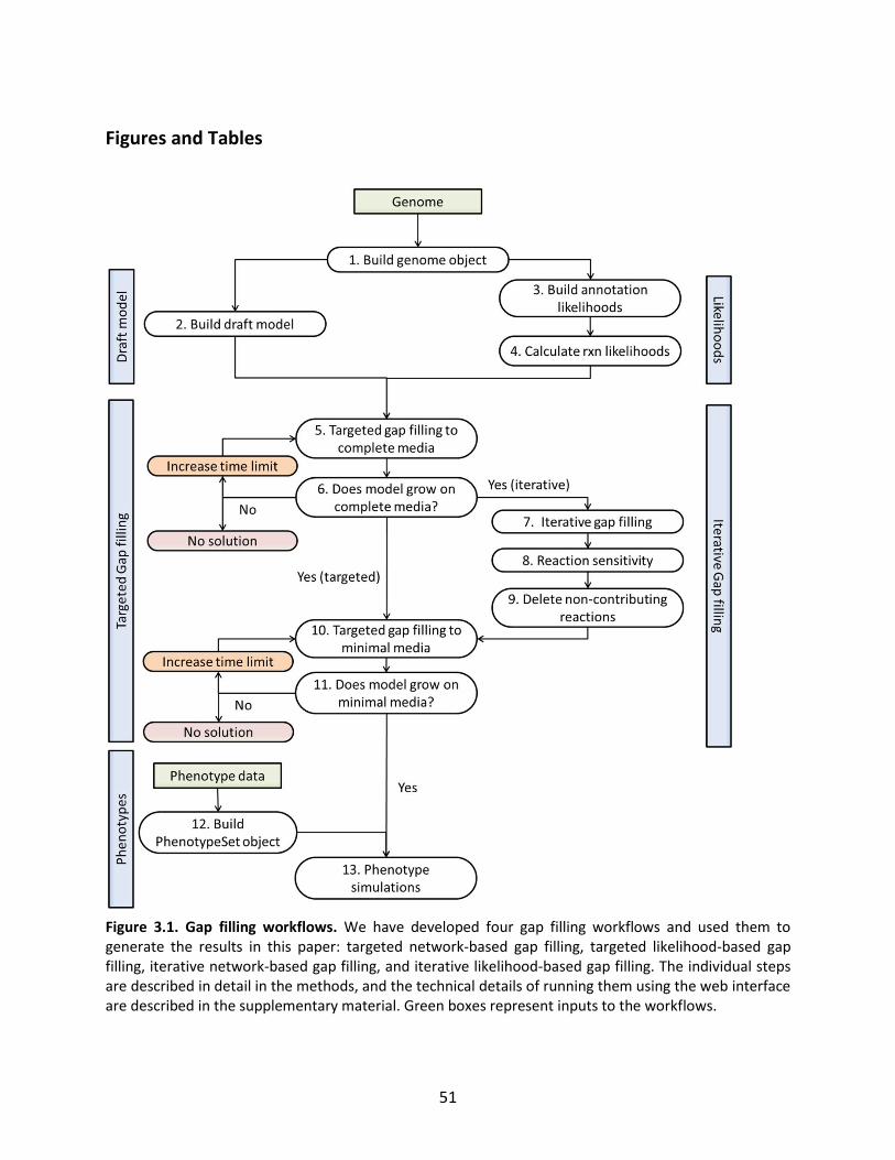
51
Figures and Tables
Figure 3.1. Gap filling workflows. We have developed four gap filling workflows and used them to generate the results in this paper: targeted network-based gap filling, targeted likelihood-based gap filling, iterative network-based gap filling, and iterative likelihood-based gap filling. The individual steps are described in detail in the methods, and the technical details of running them using the web interface are described in the supplementary material. Green boxes represent inputs to the workflows.
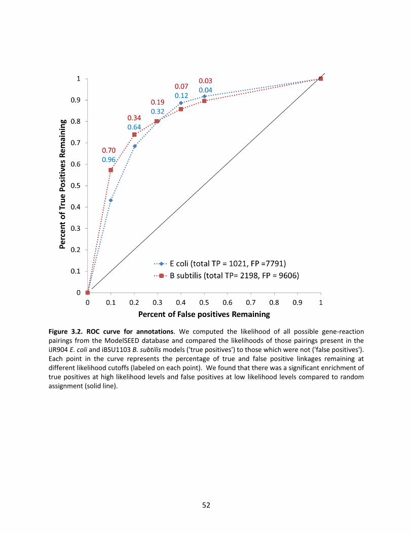
52
Figure 3.2. ROC curve for annotations. We computed the likelihood of all possible gene-reaction pairings from the ModelSEED database and compared the likelihoods of those pairings present in the iJR904 E. coli and iBSU1103 B. subtilis models ('true positives') to those which were not ('false positives'). Each point in the curve represents the percentage of true and false positive linkages remaining at different likelihood cutoffs (labeled on each point). We found that there was a significant enrichment of true positives at high likelihood levels and false positives at low likelihood levels compared to random assignment (solid line).

53
Figure 3.3. Proof of principle: Gap filling highly-likely reactions in B. subtilis. B. subtilis synthesizes lipids via the non-mevalonate pathway (blue) [155]. We removed this pathway from the B. subtilis genome-scale model and then tried to fill the gap using both the likelihood and network-based approaches. The network-based gap filling approach instead filled the gap with the mevalonate pathway (red), which is shorter but not supported by genetic evidence. The likelihood-based approach filled the gap with the correct pathway. Black indicates reactions that were not knocked out (there was no explicit link to literature evidence in the B. subtilis model). The numeric labels are the computed likelihoods of gap filling reactions.
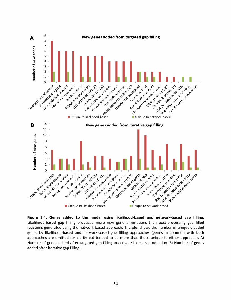
54
Figure 3.4. Genes added to the model using likelihood-based and network-based gap filling. Likelihood-based gap filling produced more new gene annotations than post-processing gap filled reactions generated using the network-based approach. The plot shows the number of uniquely-added genes by likelihood-based and network-based gap filling approaches (genes in common with both approaches are omitted for clarity but tended to be more than those unique to either approach). A) Number of genes added after targeted gap filling to activate biomass production. B) Number of genes added after iterative gap filling.
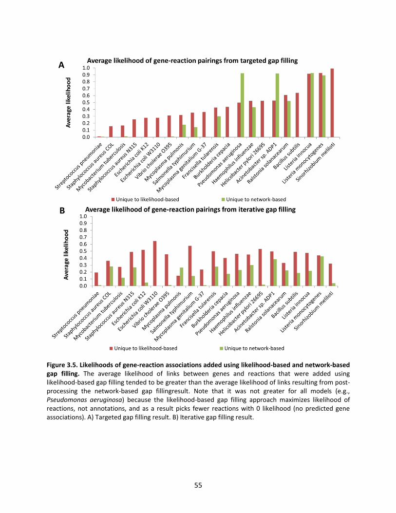
55
Figure 3.5. Likelihoods of gene-reaction associations added using likelihood-based and network-based gap filling. The average likelihood of links between genes and reactions that were added using likelihood-based gap filling tended to be greater than the average likelihood of links resulting from post-processing the network-based gap fillingresult. Note that it was not greater for all models (e.g., Pseudomonas aeruginosa) because the likelihood-based gap filling approach maximizes likelihood of reactions, not annotations, and as a result picks fewer reactions with 0 likelihood (no predicted gene associations). A) Targeted gap filling result. B) Iterative gap filling result.
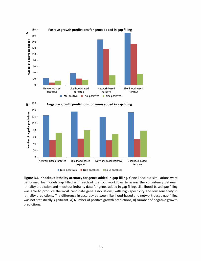
56
Figure 3.6. Knockout lethality accuracy for genes added in gap filling. Gene knockout simulations were performed for models gap filled with each of the four workflows to assess the consistency between lethality prediction and knockout lethality data for genes added in gap filling. Likelihood-based gap filling was able to produce the most candidate gene associations, with high specificity and low sensitivity in lethality predictions. The difference in accuracy between likelihood-based and network-based gap filling was not statistically significant. A) Number of positive growth predictions, B) Number of negative growth predictions.

57
Table 3.1. Average phenotype consistency across all test organisms for models gap filled using the four evaluated algorithms. Iterative gap filling greatly increased the sensitivity (more correct positive growth conditions) and reduced the specificity (more incorrect positive growth conditions) of Biolog simulations. The use of likelihoods did not have a significant effect on the specificity or sensitivity of Biolog simulations. The overall model accuracy for essentiality data was similar for all four algorithms because genes added due to likelihood-based gap filling represented only at most about 7% of the genes in the model. See Figure 3.6 for the results of knockout simulations using only genes added to gap filling solutions.
Biolog data Essentiality data
Sensitivity Specificity Sensitivity Specificity
Targeted network-based 56% 70% 86% 66%
Targeted likelihood-based 56% 70% 84% 67%
Iterative network-based 67% 57% 86% 64%
Iterative likelihood-based 67% 55% 85% 65%

58
Chapter 4: ITEP: An integrated toolkit for exploration of microbial pan-genomes.4
Abstract
Background
Comparative genomics is a powerful approach for studying variation in physiological traits as well as the
evolution and ecology of microorganisms. Recent technological advances have enabled sequencing large
numbers of related genomes in a single project, requiring computational tools for their integrated
analysis. In particular, accurate annotations and identification of gene presence and absence are critical
for understanding and modeling the cellular physiology of newly sequenced genomes. Although many
tools are available to compare the gene contents of related genomes, new tools are necessary to enable
close examination and curation of protein families from large numbers of closely related organisms, to
integrate curation with the analysis of gain and loss, and to generate metabolic networks linking the
annotations to observed phenotypes.
Results
We have developed ITEP, an Integrated Toolkit for Exploration of microbial Pan-genomes, to curate
protein families, compute similarities to externally-defined domains, analyze gene gain and loss, and
generate draft metabolic networks from one or more curated reference network reconstructions in
groups of related microbial species among which the combination of core and variable genes constitute
the their "pan-genomes". The ITEP toolkit consists of: (1) a series of modular command-line scripts for
identification, comparison, curation, and analysis of protein families and their distribution across many
genomes; (2) a set of Python libraries for programmatic access to the same data; and (3) pre-packaged
4 This chapter uses previously published, open-access material and is reprinted with the permission of the
publisher. The citation is as follows: Benedict MN, Henriksen JR, Metcalf WW, Whitaker RJ, Price ND: ITEP: An integrated toolkit for exploration of microbial pan-genomes. BMC Genomics 2014, 15:8.
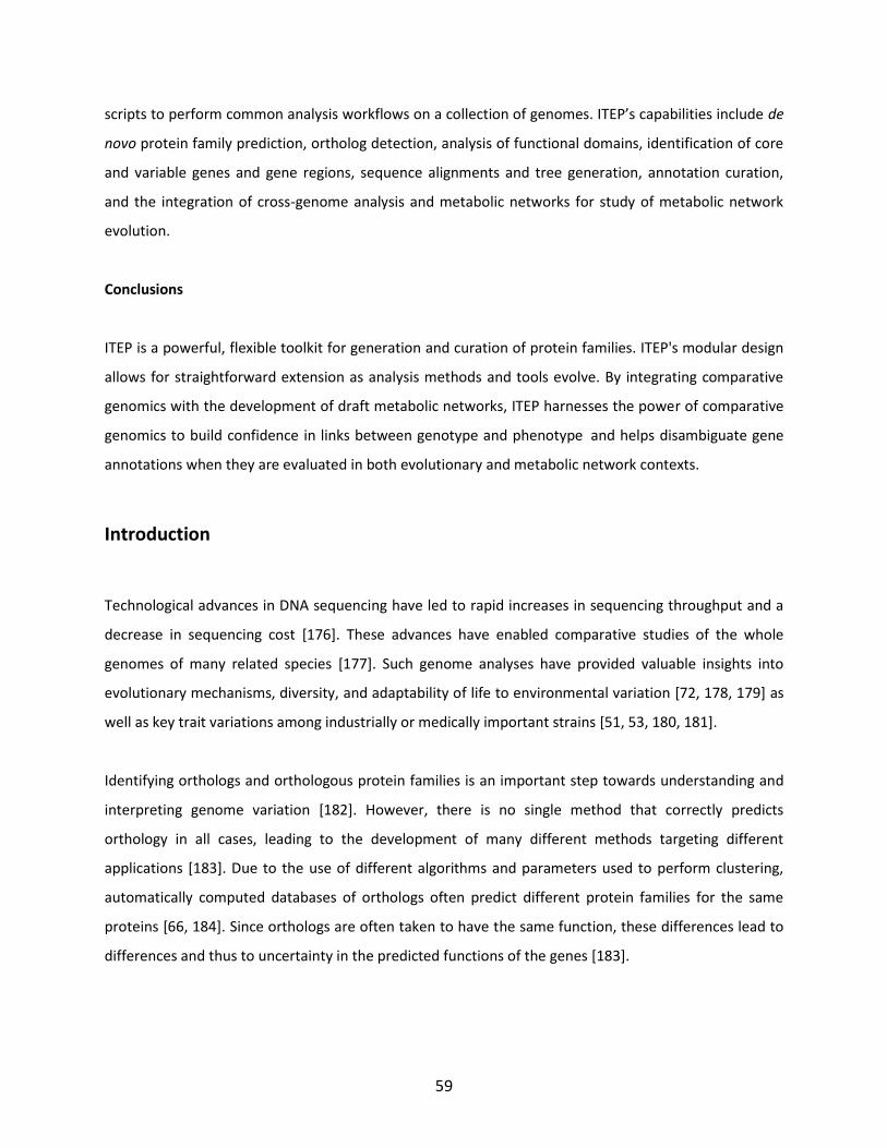
59
scripts to perform common analysis workflows on a collection of genomes. ITEP’s capabilities include de
novo protein family prediction, ortholog detection, analysis of functional domains, identification of core
and variable genes and gene regions, sequence alignments and tree generation, annotation curation,
and the integration of cross-genome analysis and metabolic networks for study of metabolic network
evolution.
Conclusions
ITEP is a powerful, flexible toolkit for generation and curation of protein families. ITEP's modular design
allows for straightforward extension as analysis methods and tools evolve. By integrating comparative
genomics with the development of draft metabolic networks, ITEP harnesses the power of comparative
genomics to build confidence in links between genotype and phenotype and helps disambiguate gene
annotations when they are evaluated in both evolutionary and metabolic network contexts.
Introduction
Technological advances in DNA sequencing have led to rapid increases in sequencing throughput and a
decrease in sequencing cost [176]. These advances have enabled comparative studies of the whole
genomes of many related species [177]. Such genome analyses have provided valuable insights into
evolutionary mechanisms, diversity, and adaptability of life to environmental variation [72, 178, 179] as
well as key trait variations among industrially or medically important strains [51, 53, 180, 181].
Identifying orthologs and orthologous protein families is an important step towards understanding and
interpreting genome variation [182]. However, there is no single method that correctly predicts
orthology in all cases, leading to the development of many different methods targeting different
applications [183]. Due to the use of different algorithms and parameters used to perform clustering,
automatically computed databases of orthologs often predict different protein families for the same
proteins [66, 184]. Since orthologs are often taken to have the same function, these differences lead to
differences and thus to uncertainty in the predicted functions of the genes [183].
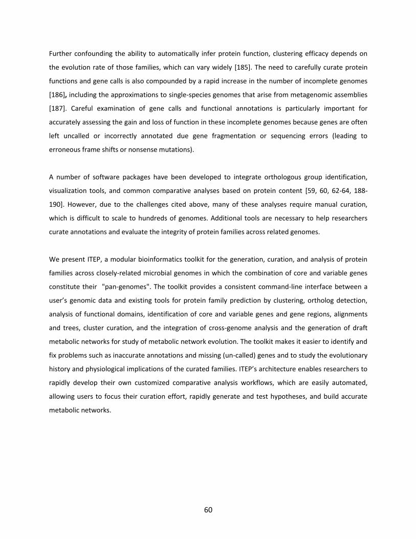
60
Further confounding the ability to automatically infer protein function, clustering efficacy depends on
the evolution rate of those families, which can vary widely [185]. The need to carefully curate protein
functions and gene calls is also compounded by a rapid increase in the number of incomplete genomes
[186], including the approximations to single-species genomes that arise from metagenomic assemblies
[187]. Careful examination of gene calls and functional annotations is particularly important for
accurately assessing the gain and loss of function in these incomplete genomes because genes are often
left uncalled or incorrectly annotated due gene fragmentation or sequencing errors (leading to
erroneous frame shifts or nonsense mutations).
A number of software packages have been developed to integrate orthologous group identification,
visualization tools, and common comparative analyses based on protein content [59, 60, 62-64, 188-
190]. However, due to the challenges cited above, many of these analyses require manual curation,
which is difficult to scale to hundreds of genomes. Additional tools are necessary to help researchers
curate annotations and evaluate the integrity of protein families across related genomes.
We present ITEP, a modular bioinformatics toolkit for the generation, curation, and analysis of protein
families across closely-related microbial genomes in which the combination of core and variable genes
constitute their "pan-genomes". The toolkit provides a consistent command-line interface between a
user’s genomic data and existing tools for protein family prediction by clustering, ortholog detection,
analysis of functional domains, identification of core and variable genes and gene regions, alignments
and trees, cluster curation, and the integration of cross-genome analysis and the generation of draft
metabolic networks for study of metabolic network evolution. The toolkit makes it easier to identify and
fix problems such as inaccurate annotations and missing (un-called) genes and to study the evolutionary
history and physiological implications of the curated families. ITEP’s architecture enables researchers to
rapidly develop their own customized comparative analysis workflows, which are easily automated,
allowing users to focus their curation effort, rapidly generate and test hypotheses, and build accurate
metabolic networks.
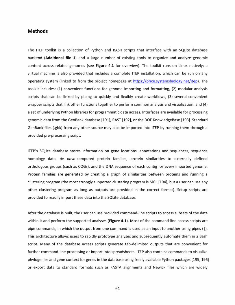
61
Methods
The ITEP toolkit is a collection of Python and BASH scripts that interface with an SQLite database
backend (Additional file 1) and a large number of existing tools to organize and analyze genomic
content across related genomes (see Figure 4.1 for overview). The toolkit runs on Linux natively; a
virtual machine is also provided that includes a complete ITEP installation, which can be run on any
operating system (linked to from the project homepage at https://price.systemsbiology.net/itep). The
toolkit includes: (1) convenient functions for genome importing and formatting, (2) modular analysis
scripts that can be linked by piping to quickly and flexibly create workflows, (3) several convenient
wrapper scripts that link other functions together to perform common analysis and visualization, and (4)
a set of underlying Python libraries for programmatic data access. Interfaces are available for processing
genomic data from the GenBank database [191], RAST [192], or the DOE KnowledgeBase [193]. Standard
GenBank files (.gbk) from any other source may also be imported into ITEP by running them through a
provided pre-processing script.
ITEP’s SQLite database stores information on gene locations, annotations and sequences, sequence
homology data, de novo-computed protein families, protein similarities to externally defined
orthologous groups (such as COGs), and the DNA sequence of each contig for every imported genome.
Protein families are generated by creating a graph of similarities between proteins and running a
clustering program (the most strongly supported clustering program is MCL [194], but a user can use any
other clustering program as long as outputs are provided in the correct format). Setup scripts are
provided to readily import these data into the SQLite database.
After the database is built, the user can use provided command-line scripts to access subsets of the data
within it and perform the supported analyses (Figure 4.1). Most of the command-line access scripts are
pipe commands, in which the output from one command is used as an input to another using pipes (|).
This architecture allows users to rapidly prototype analyses and subsequently automate them in a Bash
script. Many of the database access scripts generate tab-delimited outputs that are convenient for
further command-line processing or import into spreadsheets. ITEP also contains commands to visualize
phylogenies and gene context for genes in the database using freely available Python packages [195, 196]
or export data to standard formats such as FASTA alignments and Newick files which are widely
62
supported in other visualization and bioinformatics software. Many of the same analyses implemented
in the command-line scripts are also accessible programmatically via a set of Python libraries to aid
developers who wish to build their own tools upon ITEP’s data structures. Finally, pre-packaged
workflow scripts are provided for common analysis tasks such as the generation of concatenated core
gene trees. These can be used to quickly obtain a result or as a working starting point from which to
develop new analysis pipelines.
De novo clustering for computation of protein families
Running the BLASTP program [86] all vs. all provides a graph of similarities between pairs of proteins, in
which the genes are nodes and each significant pairing is an edge weighted by some similarity metric.
The ITEP toolkit's setup scripts directly support the generation of protein families de novo by clustering
these graphs using the Markov Cluster (MCL) algorithm [197]. The toolkit allows many different
definitions of the homology graph: it can be generated from arbitrary subsets of organisms in the
database with arbitrary cutoffs and inflation parameters (clustering sensitivity), and three scoring
metrics that emphasize different aspects of the protein pair homology (Additional file 2) [197-199].
A user can also import results from any other orthologous family prediction method, allowing flexibility
that is necessary due to differences in the strengths and weaknesses of individual algorithms. All
downstream analyses (e.g. phylogenetic analysis of gene gain and loss) can then be performed in the
same manner as if the clusters were generated using MCL. For example, a wrapper function is provided
to interface between the ITEP database and OrthoMCL, a program that applies a percent identity cutoff
between pairs of homologous proteins, identifies likely orthologs by using a modified bidirectional-best-
hits approach, and then runs MCL to cluster the smaller subset of nodes and edges into protein families
[200]. It thus performs MCL only on filtered subsets of the homologous pairs of organisms rather than
simply applying a simple cutoff for a homology score. The consistent storage of clustering results from
multiple different clustering methods in a single database enables users to easily compare the effects of
the choice of clustering algorithm and the choices of organisms to cluster on the predicted protein
families.

63
Protein family curation and visualization tools
Several biological and non-biological variables can cause automatically computed protein families to be
incorrect or incomplete, such as the presence of gene fusions or multiple-domain proteins, incomplete
or inaccurate gene calling, sequence and/or functional divergence, and the lack of rate homogeneity in
evolution rates. In light of these challenges and in order to increase confidence that conclusions about
the evolution of protein families are correct, we have implemented tools to generate and visualize
multiple alignments and trees for protein families, to study gene neighborhoods of genes in a family, to
search for possibly missing genes, and to assess the function of proteins in the light of their conserved
domain architecture.
Multiple alignments and phylogenetic trees are useful to analyze the phylogenetic history of particular
protein families and to sort out the potential presence of paralogs [201]. The ITEP toolkit contains
convenient interfaces for generating protein and nucleotide alignments [202, 203], curating alignments
[204], and generating maximum-likelihood phylogenies [205, 206]. ITEP’s tree visualization capabilities
provide an interface between a user’s genomic data and the ETE Python package for tree manipulation
and rendering [195]. The ITEP scripts include the option of appending gene neighborhood information to
a protein tree, which is useful for identifying the functions of novel genes [64, 207]. The user also has
the option to attach numeric data (as a heatmap) or arbitrary text tables to any tree (see Figures 4.2,
4.3).
To help identify missing genes, we have implemented an interface that links genomic data in ITEP to
tBLASTn, which is useful for finding genes that are fragmented, miscalled (e.g. with frameshifts or
nonsense mutations resulting from sequencing errors), or that are not yet annotated [65]. The ITEP
interface to tBLASTn identifies significant hits from a set of query genes to a particular genome (or set of
genomes) in the database, and then automatically identifies whether the hit was to a called gene and
whether the called gene was on the same strand as the hit. From this result, a researcher can examine
and (if appropriate) add missing proteins to protein families. The gene neighborhood and tree
generation and visualization scripts support the visualization of tBLASTn hits in their genetic context in
the same manner as called genes (see Figure 4.3). We have also provided a tool that attempts to identify
frame shifts, insertions, and nonsense mutation events from the tBLASTn results, which helps identify
64
specific mutations that could lead to loss of function or that could indicate errors in the genome
sequence.
Finally, to assist the curation of annotations, we have implemented automatic generation and storage of
RPSBLAST hits to the NCBI CDD database [208]. The interface allows a user to rapidly search for the IDs
of conserved domains that correspond to certain keywords (such as “purine synthesis”) and to identify
all proteins in a genome that have significant homology to a specific set of conserved domains. ITEP also
includes tools for identifying and visualizing all conserved domains that are found in a specific query
protein or set of proteins (Figure 4.4), providing insight into the functions of those proteins.
Analysis of core and variable gene content
Studying gene gain and loss and examining the core (conserved) and variable (non-conserved) genes in a
collection of organisms can provide insights into the plasticity of cellular functions and can be used to
identify genes that define a clade [209]. To assist such analyses, ITEP includes functions that identify
interesting subsets of genes based on presence and absence patterns, such as genes that are present in
all of a particular group of organisms (conserved genes), any members of a group (present genes), only
members of that group relative to those all of the organisms to generate the protein families (unique
genes), or none of the members of that group. The script can also optionally identify genes that are
conserved in any given fraction of a group of organisms, allowing for some flexibility due to missed gene
calls or divergent sequences. Finally, if an organism phylogeny is available (or built with other ITEP
scripts), a tool is also available to identify presence and absence patterns based on each phylogenetic
clade, allowing a researcher to, for example, identify all of the genes that are conserved in or unique to
each individual species or all genomes in a clade.
Integration with metabolic networks
A key reason to identify protein families is to use the results to propagate annotations and subsequently
identify the physiological capabilities of an organism based on those of its relatives. In the context of
genome-scale metabolic modeling, the predicted presence or absence of particular protein families may
be used as evidence for the presence or absence of reactions in a metabolic network. In a metabolic
network reconstruction, the relationship between a gene and the reactions catalyzed by the encoded
65
enzyme is typically encoded in a Boolean gene-protein-reaction relationship (GPR), in which complexes
and other sets of genes that must all be present for a reaction to occur are given an AND relationship,
while isozymes or sets of genes with unknown relationships are given an OR relationship [43]. To assess
whether a reaction is catalyzed or not within a cell, each associated gene is assigned a 1 (TRUE) if it is
present and a 0 (FALSE) if it is absent, and then the GPR is logically evaluated. If the GPR evaluates to
TRUE then the reaction is present and otherwise it is absent.
We have implemented a function in ITEP that directly evaluates Boolean gene-protein-reaction
relationships associated with existing metabolic reconstructions of strains in the database based on the
presence-absence calls of de novo clustering with arbitrary parameters. In this way, a researcher can
rapidly generate draft metabolic network reconstructions based on genomic comparisons with one or
more reference networks. Subsequently, these network reconstructions can be curated to generate
high-quality models of each related organism.
Results
Test data set
We chose to use the Group 1 Clostridia as a test case to illustrate capabilities of the ITEP toolkit. This
metabolically diverse phylogenetic clade includes industrially important organisms such as the
solventogenic organisms Clostridium acetobutylicum and C. beijerinckii, as well as several medically
important strains such as C. perfringes and C. botulinum [210]. C. botulinum and C. perfringes genomes
have both been heavily sampled, therefore providing the opportunity to study genetic differences at
both species and at the genus-scale. In addition, manually-curated metabolic models are available for C.
acetobutylicum ATCC 824 [211, 212] and C. beijerinckii NCIMB 8052 [31], affording an opportunity to use
ITEP to examine metabolic differences between these and the other Clostridium species in the clade.
The species belonging to the Group 1 Clostridia were determined based on the PATRIC database [213]
and the ARB Living Tree 16S rRNA tree [214]. All complete and draft genomes from this group were
downloaded from RefSeq in March 2013 (including plasmids) along with the genome of an outgroup
organism, Acetobacterium woodii. Overall, 26 complete and 26 incomplete Clostridia genomes were
66
downloaded and analyzed (see Additional file 2 for complete strain names and RefSeq accession
numbers).
The test dataset was chosen to be relatively small for purposes of illustration. ITEP currently supports
creation of databases containing up to about 200 genomes on a modern workstation with 1TB of hard
drive space, 16 GB of RAM, and 12 processors (using which all vs. all BLAST, MCL, and RPSBlast would
take about 6 days altogether). Disk space and time requirements grow as O(N2) where N is the number
of genomes.
In this example, MCL was used to perform clustering and predict protein families. The relative strengths
of this and other methods for predicting protein function have been reviewed at length [184, 215-217].
Importantly, if the user desires to use different algorithms for clustering, ITEP supports exporting
subsets of BLAST data in formats convenient for import into clustering tools, importing the clustering
results back into the SQLite database, and applying the same workflows as described here to interpret
and curate them.
Complete tutorials for performing the analyses described in this section and many others are available in
the package documentation (included as Additional file 5). A link to an up-to-date web version of this
documentation is linked to from the project website (https://price.systemsbiology.net/itep).
Analysis of gene gain and loss patterns across phylogeny
As a starting point for the analysis of the Group 1 Clostridia pan-genome, we used ITEP to compute the
number of conserved gene families (one member or more in every organism) in each clade in the Group
1 Clostridia and in A. woodii (Figure 4.2). The results indicate that a large number of genes are conserved
between closely related strains (such as C. sporogenes and C. botulinum A, B and F subtypes) but the
number of conserved genes drops off rapidly as more diverse strains are added. The identities of the
conserved genes can easily be extracted from ITEP and used to examine physiological differences
between the clades of organisms and at what point a particular function was lost. In the same manner,
ITEP can be used to identify gene families unique to each clade or those that are found in exactly one
copy in each member. Importantly, the curation tools in ITEP can be used to verify conclusions drawn
from analyzing these gain and loss patterns (see later sections for some examples).
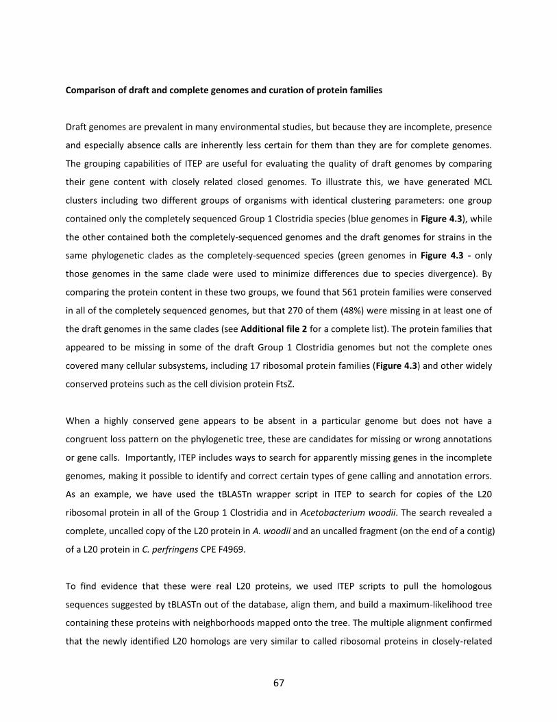
67
Comparison of draft and complete genomes and curation of protein families
Draft genomes are prevalent in many environmental studies, but because they are incomplete, presence
and especially absence calls are inherently less certain for them than they are for complete genomes.
The grouping capabilities of ITEP are useful for evaluating the quality of draft genomes by comparing
their gene content with closely related closed genomes. To illustrate this, we have generated MCL
clusters including two different groups of organisms with identical clustering parameters: one group
contained only the completely sequenced Group 1 Clostridia species (blue genomes in Figure 4.3), while
the other contained both the completely-sequenced genomes and the draft genomes for strains in the
same phylogenetic clades as the completely-sequenced species (green genomes in Figure 4.3 - only
those genomes in the same clade were used to minimize differences due to species divergence). By
comparing the protein content in these two groups, we found that 561 protein families were conserved
in all of the completely sequenced genomes, but that 270 of them (48%) were missing in at least one of
the draft genomes in the same clades (see Additional file 2 for a complete list). The protein families that
appeared to be missing in some of the draft Group 1 Clostridia genomes but not the complete ones
covered many cellular subsystems, including 17 ribosomal protein families (Figure 4.3) and other widely
conserved proteins such as the cell division protein FtsZ.
When a highly conserved gene appears to be absent in a particular genome but does not have a
congruent loss pattern on the phylogenetic tree, these are candidates for missing or wrong annotations
or gene calls. Importantly, ITEP includes ways to search for apparently missing genes in the incomplete
genomes, making it possible to identify and correct certain types of gene calling and annotation errors.
As an example, we have used the tBLASTn wrapper script in ITEP to search for copies of the L20
ribosomal protein in all of the Group 1 Clostridia and in Acetobacterium woodii. The search revealed a
complete, uncalled copy of the L20 protein in A. woodii and an uncalled fragment (on the end of a contig)
of a L20 protein in C. perfringens CPE F4969.
To find evidence that these were real L20 proteins, we used ITEP scripts to pull the homologous
sequences suggested by tBLASTn out of the database, align them, and build a maximum-likelihood tree
containing these proteins with neighborhoods mapped onto the tree. The multiple alignment confirmed
that the newly identified L20 homologs are very similar to called ribosomal proteins in closely-related
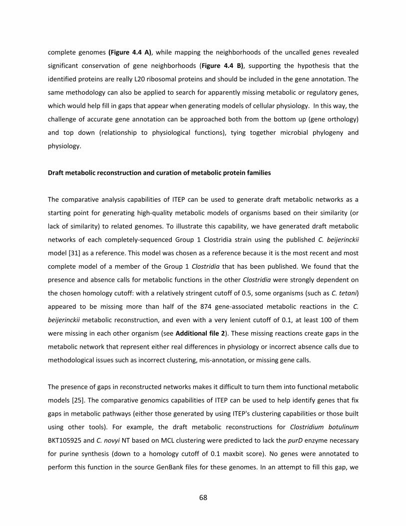
68
complete genomes (Figure 4.4 A), while mapping the neighborhoods of the uncalled genes revealed
significant conservation of gene neighborhoods (Figure 4.4 B), supporting the hypothesis that the
identified proteins are really L20 ribosomal proteins and should be included in the gene annotation. The
same methodology can also be applied to search for apparently missing metabolic or regulatory genes,
which would help fill in gaps that appear when generating models of cellular physiology. In this way, the
challenge of accurate gene annotation can be approached both from the bottom up (gene orthology)
and top down (relationship to physiological functions), tying together microbial phylogeny and
physiology.
Draft metabolic reconstruction and curation of metabolic protein families
The comparative analysis capabilities of ITEP can be used to generate draft metabolic networks as a
starting point for generating high-quality metabolic models of organisms based on their similarity (or
lack of similarity) to related genomes. To illustrate this capability, we have generated draft metabolic
networks of each completely-sequenced Group 1 Clostridia strain using the published C. beijerinckii
model [31] as a reference. This model was chosen as a reference because it is the most recent and most
complete model of a member of the Group 1 Clostridia that has been published. We found that the
presence and absence calls for metabolic functions in the other Clostridia were strongly dependent on
the chosen homology cutoff: with a relatively stringent cutoff of 0.5, some organisms (such as C. tetani)
appeared to be missing more than half of the 874 gene-associated metabolic reactions in the C.
beijerinckii metabolic reconstruction, and even with a very lenient cutoff of 0.1, at least 100 of them
were missing in each other organism (see Additional file 2). These missing reactions create gaps in the
metabolic network that represent either real differences in physiology or incorrect absence calls due to
methodological issues such as incorrect clustering, mis-annotation, or missing gene calls.
The presence of gaps in reconstructed networks makes it difficult to turn them into functional metabolic
models [25]. The comparative genomics capabilities of ITEP can be used to help identify genes that fix
gaps in metabolic pathways (either those generated by using ITEP's clustering capabilities or those built
using other tools). For example, the draft metabolic reconstructions for Clostridium botulinum
BKT105925 and C. novyi NT based on MCL clustering were predicted to lack the purD enzyme necessary
for purine synthesis (down to a homology cutoff of 0.1 maxbit score). No genes were annotated to
perform this function in the source GenBank files for these genomes. In an attempt to fill this gap, we
69
used ITEP to perform a tBLASTn search against these two organisms using the copy of purD from C.
beijerinckii (Cbei_1060) as a reference. Interestingly, we found a very strong homology between the C.
beijerinckii purD and the N-terminal end of much larger proteins in C. botulinum BKT105925 and C. novyi
NT (CbC4_1757 and NT01CX_2418, respectively). Searching these genes against the RPSBLAST results
that were stored in the ITEP database revealed that the large proteins from C. botulinum BKT105925 and
C. novyi NT are in fact fusions of purD and purL (Figure 4.5), in agreement with the assignments based
on MetaCyc [80], RAST [192], and the SEED [54]. Therefore, the gap in the metabolic network can be
fixed by assigning the same function to both of these genes, making simulations performed using other
tools [46, 91, 141] more accurate.
Conclusions
The ITEP toolkit integrates a large number of existing bioinformatics tools into a single cohesive, flexible
framework for comparative analysis of physiological variation in microbial pan-genomes. The modular
design of the toolkit makes it straightforward to add additional functionality to the toolkit, as illustrated
by our implementation of novel tools for generation of draft metabolic reconstructions from a curated
reference network. It also makes the analysis very flexible, empowering researchers to quickly develop
analysis workflows while also providing a wide array of tools for curation of annotations and gene calls.
The ability to rapidly curate protein families and propagate metabolic networks from reference
organisms to related strains will streamline the process of generating high-quality physiological and
evolutionary hypotheses and ultimately lead to an improvement in the inter-genome consistency of
metabolic models of microbes.
Supplemental Material
Supplemental material related to this chapter is located online at
http://www.biomedcentral.com/1471-2164/15/8/abstract

70
List of Abbreviations
AIR: Aminoimidazole ribotide; BLAST: Basic Local Alignment Search Tool; FGAM: 5'-
Phosphoribosylformylglycinamidine; FGAR: N-Formylglycinamide ribonucleotide; GAR: Glycinamide
ribonucleotide; GPR: Gene-Protein-Reaction relationship; ITEP: Integrated Toolkit for the Exploration of
Pan-genomes; MCL: Markov Cluster (clustering algorithm); PRPP: 5-Phosphoribosyl 1-pyrophosphate;
RAST: Rapid Annotation using Subsystem Technology, tBLASTn: Translated BLAST against nucleotides.
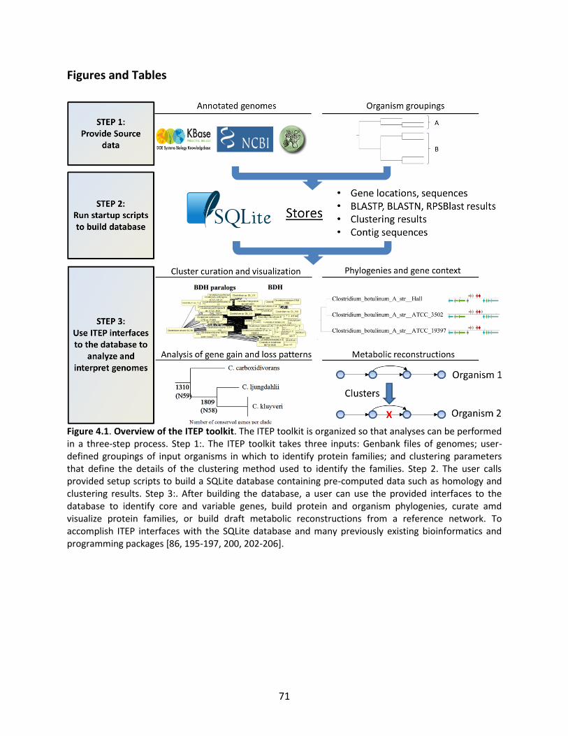
71
Figures and Tables
Figure 4.1. Overview of the ITEP toolkit. The ITEP toolkit is organized so that analyses can be performed in a three-step process. Step 1:. The ITEP toolkit takes three inputs: Genbank files of genomes; user-defined groupings of input organisms in which to identify protein families; and clustering parameters that define the details of the clustering method used to identify the families. Step 2. The user calls provided setup scripts to build a SQLite database containing pre-computed data such as homology and clustering results. Step 3:. After building the database, a user can use the provided interfaces to the database to identify core and variable genes, build protein and organism phylogenies, curate amd visualize protein families, or build draft metabolic reconstructions from a reference network. To accomplish ITEP interfaces with the SQLite database and many previously existing bioinformatics and programming packages [86, 195-197, 200, 202-206].
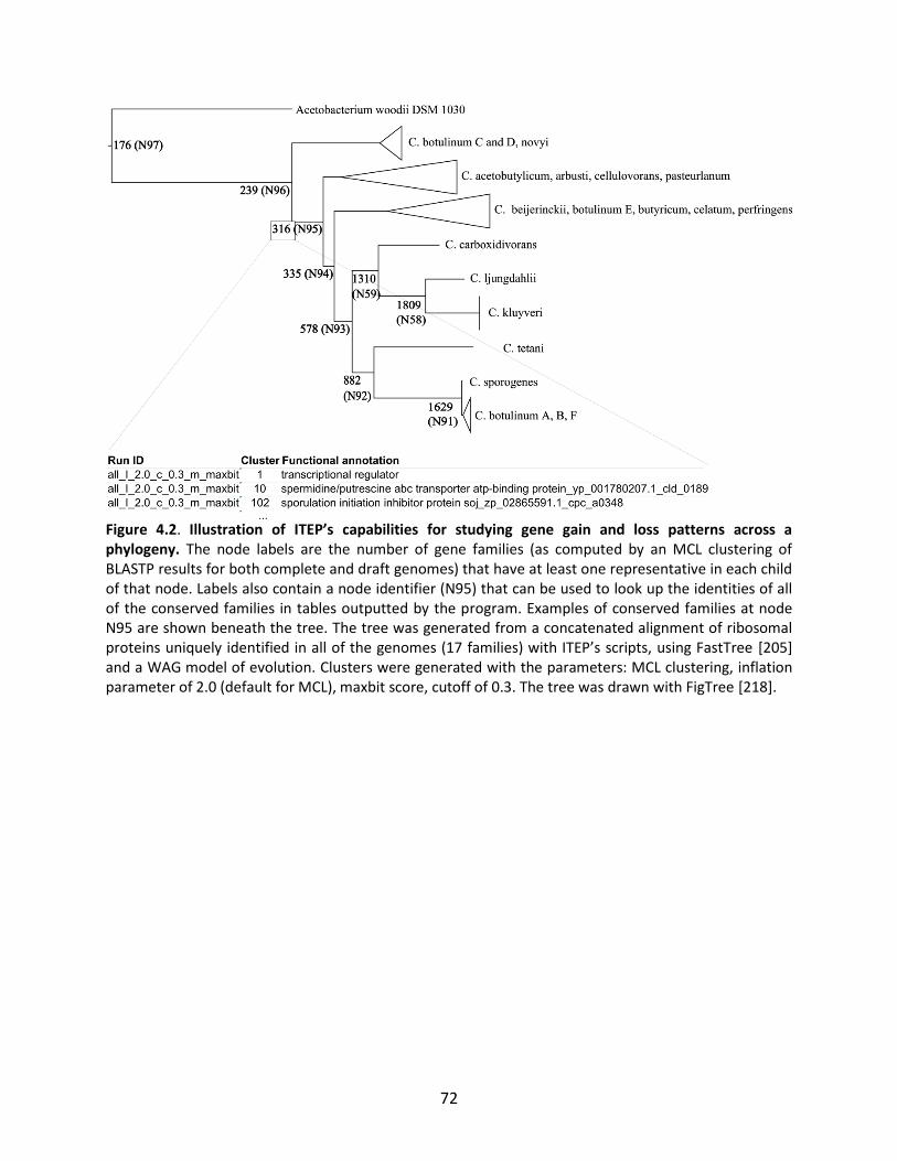
72
Figure 4.2. Illustration of ITEP’s capabilities for studying gene gain and loss patterns across a phylogeny. The node labels are the number of gene families (as computed by an MCL clustering of BLASTP results for both complete and draft genomes) that have at least one representative in each child of that node. Labels also contain a node identifier (N95) that can be used to look up the identities of all of the conserved families in tables outputted by the program. Examples of conserved families at node N95 are shown beneath the tree. The tree was generated from a concatenated alignment of ribosomal proteins uniquely identified in all of the genomes (17 families) with ITEP’s scripts, using FastTree [205] and a WAG model of evolution. Clusters were generated with the parameters: MCL clustering, inflation parameter of 2.0 (default for MCL), maxbit score, cutoff of 0.3. The tree was drawn with FigTree [218].
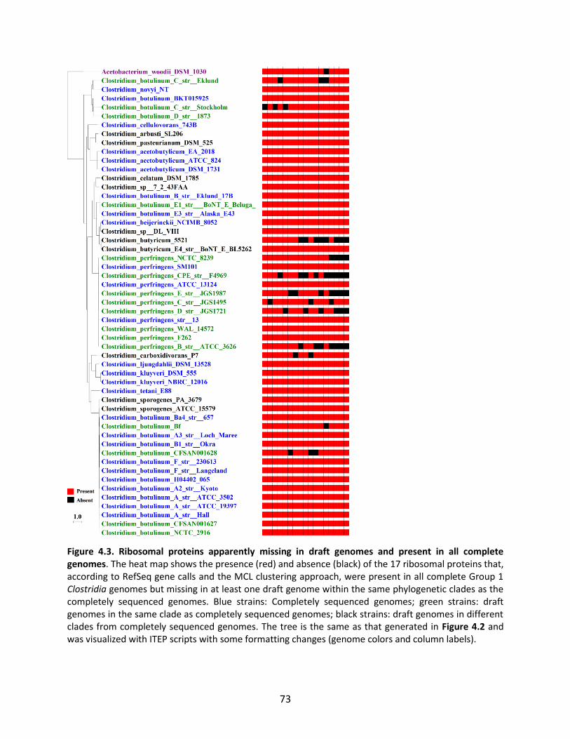
73
Figure 4.3. Ribosomal proteins apparently missing in draft genomes and present in all complete genomes. The heat map shows the presence (red) and absence (black) of the 17 ribosomal proteins that, according to RefSeq gene calls and the MCL clustering approach, were present in all complete Group 1 Clostridia genomes but missing in at least one draft genome within the same phylogenetic clades as the completely sequenced genomes. Blue strains: Completely sequenced genomes; green strains: draft genomes in the same clade as completely sequenced genomes; black strains: draft genomes in different clades from completely sequenced genomes. The tree is the same as that generated in Figure 4.2 and was visualized with ITEP scripts with some formatting changes (genome colors and column labels).
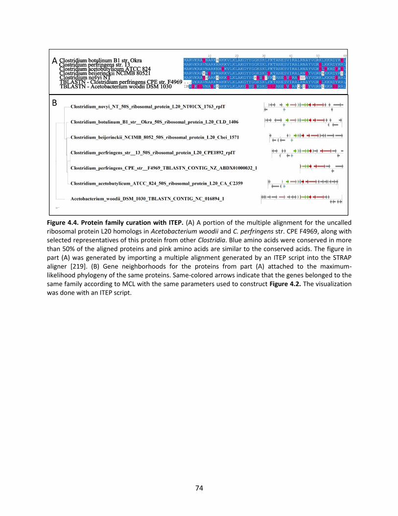
74
Figure 4.4. Protein family curation with ITEP. (A) A portion of the multiple alignment for the uncalled ribosomal protein L20 homologs in Acetobacterium woodii and C. perfringens str. CPE F4969, along with selected representatives of this protein from other Clostridia. Blue amino acids were conserved in more than 50% of the aligned proteins and pink amino acids are similar to the conserved acids. The figure in part (A) was generated by importing a multiple alignment generated by an ITEP script into the STRAP aligner [219]. (B) Gene neighborhoods for the proteins from part (A) attached to the maximum-likelihood phylogeny of the same proteins. Same-colored arrows indicate that the genes belonged to the same family according to MCL with the same parameters used to construct Figure 4.2. The visualization was done with an ITEP script.
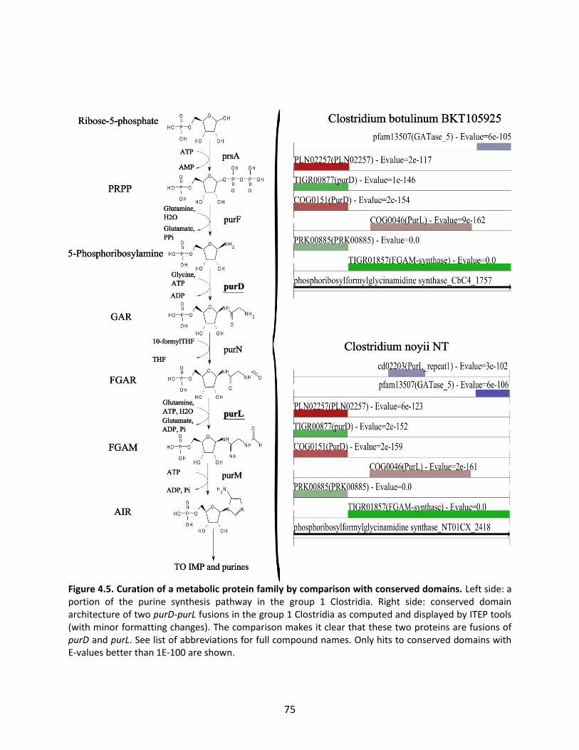
75
Figure 4.5. Curation of a metabolic protein family by comparison with conserved domains. Left side: a portion of the purine synthesis pathway in the group 1 Clostridia. Right side: conserved domain architecture of two purD-purL fusions in the group 1 Clostridia as computed and displayed by ITEP tools (with minor formatting changes). The comparison makes it clear that these two proteins are fusions of purD and purL. See list of abbreviations for full compound names. Only hits to conserved domains with E-values better than 1E-100 are shown.
76
Chapter 5: Curation of genome-scale metabolic networks using comparative genomics5
Abstract
Genome-scale metabolic modeling is a powerful way to turn genomic information into phenotype
predictions. The most common approach to building the networks on which these models are based is
to perform detailed reconstructions on a species-by-species basis. In this chapter, I argue that the
accuracy of metabolic networks can be greatly enhanced by harnessing genomic information across
multiple related species. Using the previously published ITEP tool and the genome-scale models for
Methanosarcina acetivorans and M. barkeri, I show that genes that are predicted to be essential for
growth are significantly more conserved than those that are not. However, many of these essential
genes are not conserved in other Methanosarcina strains and species. Upon closer examination, I
identify cases in which the gene calls or annotations in the other Methanosarcina genomes were clearly
incorrect. I also discuss specific fixes that were made to the models based on biochemical knowledge,
and remaining differences that may represent interesting physiological adaptations. The results of this
chapter can be applied to any lesser-characterized genus to increase the quality of genome-scale
metabolic networks.
Introduction
Genome-scale metabolic modeling is a powerful way to both consolidate large amounts of biological
information and to synthesize this information to make novel predictions on the effects of perturbations
on cellular function [42]. Metabolic modeling has applications ranging from biotechnology to medicine
[28, 30, 45] and the range of applications has been growing every year [128, 161]. One important
application of genome-scale metabolic models is the comparative analysis of metabolism for groups of
related organisms. Although many metabolic enzymes are conserved across large swaths of the tree of
life, there is a large amount of variability in metabolic pathways [220], which can be understood by
building and comparing metabolic networks for related organisms. For example, in a recent study,
genome-scale metabolic networks were built for 55 completely-sequenced strains of E. coli and used to
5 This chapter uses unpublished genomic data used with permission from William Metcalf's lab at the University of
Illinois at Urbana-Champaign. A manuscript describing the genomes is in preparation.

77
predict differences in substrate utilization and vitamin auxotrophies [221]. Auxotrophy predictions from
12 of the strains were experimentally tested, resulting in a 80% prediction accuracy [221].
In many comparative genomics applications, genome sequences being compared will vary in quality,
particularly if they were sequenced as part of different projects or by different groups. Differences in
quality can occur due to limited experimental resources, technical limitations such as short read length,
or software issues such as differences in assemblies obtained using different pipelines [222]. In addition,
problems with gene calling and annotation cause incorrect prediction of the functions present and
absent in a cell [143]. As part of the curation process for metabolic networks, it is necessary to
distinguish between these types of problems and real differences that lead to phenotypic insight. Given
that the process of curating a metabolic network can take months to years to complete [43], it is
imperative that tools and methods be developed to help make such distinctions.
In this chapter, I demonstrate how comparative genomics can identify problems both in genome
annotation and in genome-scale models, therefore leading to increased confidence in both. I have
utilized the ITEP tool [223] to compare the predicted metabolic capabilities of 30 strains of
Methanosarcina compared to two previously-published manually curated genome-scale metabolic
models of Methanosarcina species [40, 41]. I then identify discrepancies between expected and
observed patterns in gene gain and loss and use tools such as tBLASTn [224] to search for and identify
solutions to some of these discrepancies. The methods I have developed can be used for any clade for
which a sufficient number of related genomes and one or more metabolic network reconstructions are
available.
Methods
Genomic data
The genomes for Methanosarcina acetivorans str. C2A, M. barkeri str. Fusaro and M. mazei Gö1 have
been previously sequenced and published [70-72]. The latest versions of these genomes (as of January
2014) were downloaded from GenBank [191]. An additional 27 Methanosarcina genomes included in
this analysis have been sequenced by the Metcalf lab (Table 5.1; manuscript in preparation). Out of all
of the genomes sequenced in the Metcalf lab, 20 were closed, 2 had only one sequencing gap, and 5
78
were not closed. The RAST server [192] was used to call genes and perform functional annotations for
all Methanosarcina genomes sequenced by the Metcalf lab. The RAST gene calls were post-processed to
remove very short genes and to fix pyrrolysine-containing genes before performing any bioinformatic
analysis.
Metabolic network prediction using orthologous group prediction
The BLASTP algorithm was used to quantify the pairwise similarity between each pair of proteins
encoded in the Methanosarcina genomes [86, 160]. OrthoMCL, a method which identifies bidirectional
best hits and closely-related paralogs and then clusters them using a Markov chain-based clustering
algorithm, was used to predict orthologous protein families [200]. The ITEP toolkit (Chapter 4, [223])
and various scripts within were used to store, manage and interpret the clustering results.
Curated lists of metabolic genes in the Methanosarcina were taken from two previously-published
genome-scale metabolic models of organisms in this genus: the iMB745 model of M. acetivorans
(Chapter 2, [40]) and the iMG746 model of M. barkeri [41]. The other organisms possessing an ortholog
for each metabolic gene were identified based on the OrthoMCL result. Organisms lacking an ortholog
to a metabolic gene were presumed not to possess the encoded function (this result was checked as
described below for selected families).
Curation of orthology predictions
Orthology predictions for selected metabolic genes were verified by examining the phylogeny of the
broader protein families and correcting the predictions if needed. Phylogenetic trees for the protein
families to which these genes belong were computed using MAFFT to align the amino acid sequences
[202], Gblocks to trim the alignments (not allowing gaps) [204] and RAxML to compute a maximum-
likelihood tree from the concatenated alignment using the WAG model of protein evolution [206].
After curating orthology predictions, each putatively absent metabolic gene was verified to be absent
from the assembly using tBLASTn [224]. If significant, uncalled portions of these genes were identified
in the assembly, we attempted to identify whether there was a likely insertion, frameshift, inversion, or
mutation event that could cause loss of function by looking at the patterns of consecutive tBLASTn hits,

79
and also identified whether or not the gene in question fell on the end of a contig (such cases often
indicate assembly issues). If no reasonable cause could be assigned to the putative absence of the gene,
it was flagged as a likely gene-calling error.
Building a Methanosarcina species tree
A concatenated ribosomal protein tree was built and used to represent the organism phylogeny, as is
common in the field (e.g. [225]). To build this tree, ITEP tools were used to extract a list of all conserved
protein families and extracted from this a list of ribosomal protein families. Alignments for each
ribosomal protein were built using MAFFT [202] and concatenated. The ribosomal protein tree was built
using RaxML [206] with the WAG model of protein evolution. The tree was rooted with ribosomal
proteins from Methanococcoides burtonii.
Phenotype simulations
Phenotype simulations used to obtain lists of essential genes were performed using Flux Balance
Analysis [37] as implemented in the COBRA tookbox [91]. Knockout lethality predictions were computed
based on models as they were published without further modification. Methanol was used as a growth
substrate, since all the sequenced Methanosarcina strains are known to be able to grow on this
substrate. The minimal media composition was as described by Sowers et al. [92], excluding non-
essential growth factors.
Results
Consistency of nonessential and essential metabolic genes in M. acetivorans and M. barkeri models
I first examined the consistency of metabolic gene calls in the M. acetivorans and M. barkeri metabolic
models, as a basis for comparison with other Methanosarcina strains. Taken together, the previously-
published M. acetivorans and M. barkeri genome-scale metabolic networks contain a total of 1479
metabolic genes. OrthoMCL predicted that these fell into 804 distinct orthologous protein families. Of
these, 698 had at least one representative in each organism, 62 were only found in M. acetivorans, and
44 were only found in M. barkeri (Figure 5.1). The genes predicted to be unique to M. acetivorans

80
included those in the mrp and rnf operons, which are well known to be absent from M. barkeri [104].
Those predicted to be unique to M. barkeri included the ech operon, which serves a similar role in M.
barkeri and M. mazei to rnf in M. acetivorans [112, 114]. Other genes predicted to be unique to one of
the two organisms included several families of transporters and enzymes involved in divergent
carbohydrate metabolism.
Out of all of the metabolic genes from the two models, 385 were predicted to be essential for growth on
methanol: 211 in M. acetivorans and 174 in M. barkeri. Almost all of the essential genes (382 out of 385)
were predicted to be conserved in both M. acetivorans and M. barkeri (Figure 5.1), confirming the that
although differences could occur (e.g. due to bona fide differences in growth requirements), most
essential genes tend to be conserved across related organisms, at least in this genus.
Presence and absence patterns of essential genes in related Methanosarcina
After establishing that essential genes are well conserved between M. acetivorans and M. barkeri, I used
the same methodology to test this pattern in the other 28 sequenced Methanosarcina strains. The
presence and absence patterns for every essential metabolic gene cluster in the Methanosarcina strains
is mapped onto the organism phylogeny (concatenated ribosomal protein tree) in Figure 5.2. Most
essential metabolic genes (90%) were conserved across the Methanosarcina species. Each other group
was missing in at least one strain. Perhaps unsurprisingly, the most divergent organisms in the clade - M.
baltica, M. calensis, and Methanosarcina sp. MTP4 - were predicted to have the most essential genes
missing. The two most divergent of these organisms (M. baltica and M. calensis) did not have closed
genomes (Table 5.2), so it is possible that some of the metabolic genes were simply missing from the
assembly. However, the genes that appeared to only be missing in these genomes could not be detected
in tBLASTn searches, so if they are present, either too little of the gene was present in the assembly to
be detected or the genes diverged beyond the sensitivity of the tBLASTn algorithm.
Identification of specific model issues and potential fixes
Some of the losses of essential genes appear to be phylogenetically coherent. Phylogenetically coheremt
gene losses are arguably more likely to represent real, interesting differences in physiology. One of the
observed differences, in cysteine synthesis, has been established previously. All Methanosarcina possess
81
a tRNA-dependent pathway for cysteine synthesis, the SepRS pathway, wherein a cys-tRNA is created for
use in protein synthesis [226]. Some Methanosarcina, but not all of them, also possess a copy of the
tRNA-independent cysteine pathway that was horizontally transferred from the bacteria. Interestingly,
the models predicted that cysteine synthesis was essential for growth (the bacterial pathway is found in
both M. barkeri Fusaro and M. acetivorans). Cysteine synthase was predicted to be essential because
the model lacked a mechanism by which free cysteine could be generated from cys-tRNA (Figure 5.3).
Free cysteine is required for synthesis of several cofactors, including Coenzyme M [227], but to the
author's knowledge no mechanism has been described for generating it via the SepRS pathway. This
therefore could be an interesting avenue for further investigation.
The comparative genomics approach can also expose gene associations or biochemistry that are suspect
in a model. For example, one gene, Mbar_A1762 ( annotated as a formylmethanofuran dehydrogenase
subunit "Formylmethanofuran dehydrogenase [molybdenum] subunit C" ), was predicted to be essential
in the M. barkeri model. However, orthologs were only identified in one other Methanosarcina strain.
Upon closer examination, I found that this gene and the next (Mbar_A1763) are short fragments with
high homology to the real subunit C, Mbar_A1290, and therefore should not be considered essential for
this reaction to occur. Therefore, the network's accuracy would be improved by removing these two
genes from the gene-protein-reaction relationship for this reaction.
Identification of specific genome issues and potential fixes
Genes are often incorrectly predicted to be absent from an organism because of problems with gene
calling. Mistakes in gene calls often occur when a gene falls on the end of a contig or when one gene
overlaps with another gene by a small number of base pairs. Incorrect calls of gene overlaps are often
caused by an incorrect translation start site prediction for the downstream gene. Although long overlaps
between genes are uncommon except in viruses, there are documented cases of short overlaps in the
coding regions of neighboring genes in the Bacteria [228].
The tBLASTn wrapper tool in ITEP [224] can readily be used to search for genes in a genome
independently of gene calls, and therefore is useful for identifying potential gene calling errors. For
example, in the Methanosracina genomes, the gene Glucose-1-phosphate thymidylyltransferase, which
is essential for synthesis of carbohydrates, was predicted to be present in all the Methanosarcina strains
82
except M. mazei SarPi. However, upon running tBLASTn to verify the absence, I found that the genome
sequence for that organism possesses the code for an almost identical protein (97% similarity) with
extremely high consistency in genome context (Figure 5.4). The high consistency of gene context and
sequence suggests that the gene calling software made an error and this gene should be considered
present in M. mazei SarPi.
Discussion
As the price of sequencing continues to fall, datasets with dozens (or even hundreds) of related
genomes are becoming increasingly common [177]. New ways to take advantage of this genomic data to
make stronger biological insights are sorely needed. In this chapter, I have demonstrated how
comparative genomics allows a user to take advantage of evolutionary theories such as conservation of
gene context [229] and the relatively slow rate of gain and loss of metabolic enzymes [220] to both
propagate and check the accuracy of metabolic networks and models. I have demonstrated that this can
be done by identifying phyologenetically consistent gene losses, which often indicate interesting
physiological divergence between clades, and by using of gene context and nucleotide sequence
searches (tBLASTn) to check and fix incorrect gene calls highlighted by comparing to a reference network.
The approaches are useful for improving the accuracy of both annotations and networks across a set of
related organisms.
Importantly, the approaches I have developed sidestep many issues with comparing metabolic models,
and particularly the effects of nomenclature conflicts. This is important because although great care was
taken to make sure nomenclature in the Methanosarcina models is consistent, nomenclature conflicts
between different models are a very common problem. In order to get around this, the described
methods do not check whether the genes are attached to the same reactions, but rather check if a
metabolic gene in one model has closely related genes in the other. Using my approach, it would be
possible to compare models with different biochemical frameworks and conventions (e.g. one built
using the SEED [46] and one using KEGG [230]) as long as gene IDs can be converted to a common
standard.
One important finding from this study is that, consistent with the previous study of E. coli metabolic
networks, there is significant variation in metabolic capabilities, even among closely-related clades.

83
Although almost all genes that were predicted to be essential for growth were conserved between M.
acetivorans and M. barkeri, many of them were missing in other strains. As a result, if direct propagation
was to be used to build models of the other Methanosarcina strains, most of them would be unable to
predict growth on the same minimal media used to simulate M. acetivorans and M. barkeri. This
complicates the process of building models for a clade, particularly when genomes are incomplete, since
one of the steps for converting a reconstruction to a model is to fill gaps to enforce growth on a defined
media (Chapter 3). Data on specific growth requirements of each clade member may be necessary to
distinguish gene calling, annotation and assembly errors (fixed by gap filling) from real differences in
metabolic capabilities.
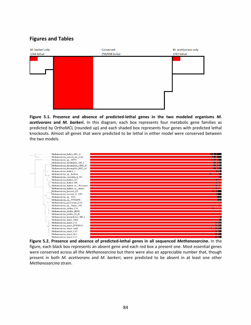
84
Figures and Tables
Figure 5.1. Presence and absence of predicted-lethal genes in the two modeled organisms M. acetivorans and M. barkeri. In this diagram, each box represents four metabolic gene families as predicted by OrthoMCL (rounded up) and each shaded box represents four genes with predicted lethal knockouts. Almost all genes that were predicted to be lethal in either model were conserved between the two models.
Figure 5.2. Presence and absence of predicted-lethal genes in all sequenced Methanosarcina. In the figure, each black box represents an absent gene and each red box a present one. Most essential genes were conserved across all the Methanosarcina but there were also an appreciable number that, though present in both M. acetivorans and M. barkeri, were predicted to be absent in at least one other Methanosarcina strain.
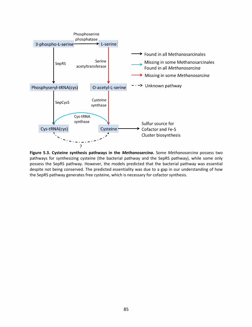
85
Figure 5.3. Cysteine synthesis pathways in the Methanosarcina. Some Methanosarcina possess two pathways for synthesizing cysteine (the bacterial pathway and the SepRS pathway), while some only possess the SepRS pathway. However, the models predicted that the bacterial pathway was essential despite not being conserved. The predicted essentiality was due to a gap in our understanding of how the SepRS pathway generates free cysteine, which is necessary for cofactor synthesis.
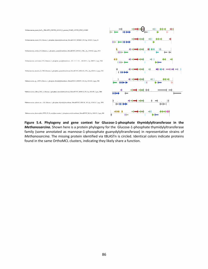
86
Figure 5.4. Phylogeny and gene context for Glucose-1-phosphate thymidylyltransferase in the Methanosarcina. Shown here is a protein phylogeny for the Glucose-1-phosphate thymidylyltransferase family (some annotated as mannose-1-phosophate guanydylyltransferase) in representative strains of Methanosarcina. The missing protein identified via tBLASTn is circled. Identical colors indicate proteins found in the same OrthoMCL clusters, indicating they likely share a function.
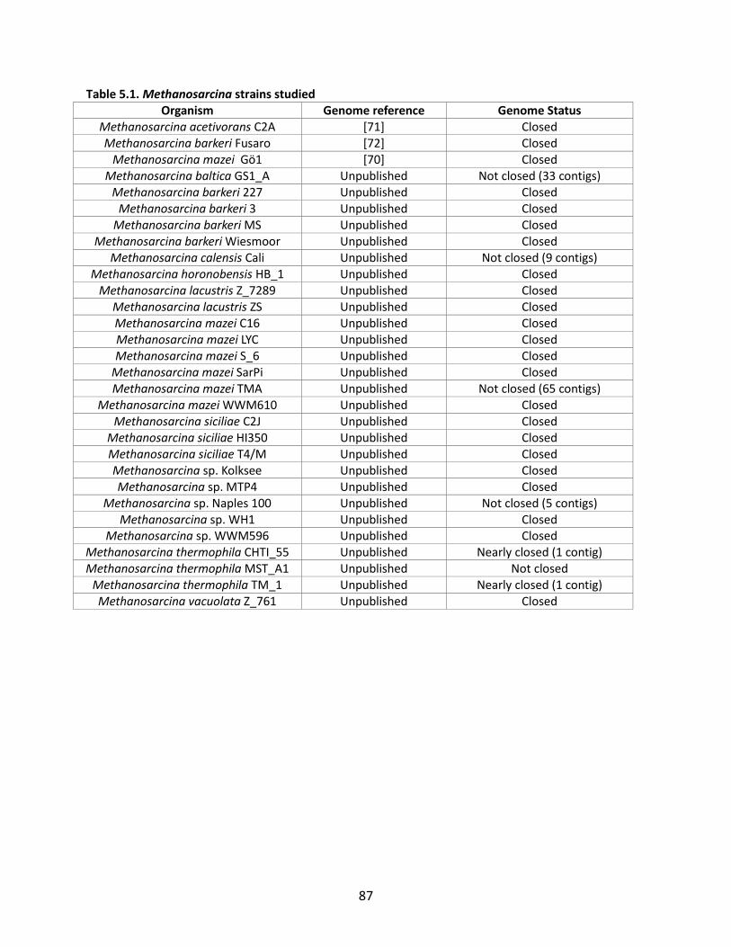
87
Table 5.1. Methanosarcina strains studied Organism Genome reference Genome Status
Methanosarcina acetivorans C2A [71] Closed Methanosarcina barkeri Fusaro [72] Closed
Methanosarcina mazei Gö1 [70] Closed Methanosarcina baltica GS1_A Unpublished Not closed (33 contigs)
Methanosarcina barkeri 227 Unpublished Closed Methanosarcina barkeri 3 Unpublished Closed
Methanosarcina barkeri MS Unpublished Closed Methanosarcina barkeri Wiesmoor Unpublished Closed
Methanosarcina calensis Cali Unpublished Not closed (9 contigs) Methanosarcina horonobensis HB_1 Unpublished Closed
Methanosarcina lacustris Z_7289 Unpublished Closed Methanosarcina lacustris ZS Unpublished Closed Methanosarcina mazei C16 Unpublished Closed Methanosarcina mazei LYC Unpublished Closed Methanosarcina mazei S_6 Unpublished Closed
Methanosarcina mazei SarPi Unpublished Closed Methanosarcina mazei TMA Unpublished Not closed (65 contigs)
Methanosarcina mazei WWM610 Unpublished Closed Methanosarcina siciliae C2J Unpublished Closed
Methanosarcina siciliae HI350 Unpublished Closed Methanosarcina siciliae T4/M Unpublished Closed Methanosarcina sp. Kolksee Unpublished Closed Methanosarcina sp. MTP4 Unpublished Closed
Methanosarcina sp. Naples 100 Unpublished Not closed (5 contigs) Methanosarcina sp. WH1 Unpublished Closed
Methanosarcina sp. WWM596 Unpublished Closed Methanosarcina thermophila CHTI_55 Unpublished Nearly closed (1 contig) Methanosarcina thermophila MST_A1 Unpublished Not closed
Methanosarcina thermophila TM_1 Unpublished Nearly closed (1 contig) Methanosarcina vacuolata Z_761 Unpublished Closed
88
Chapter 6: Conclusions and future work The work I have described in this thesis centers on the generation of high-quality genome-scale
metabolic networks. High-quality metabolic networks are essential for building accurate models of
metabolism, which have applications in medicine and in biotechnology. My experience in building
genome-scale metabolic networks began with generating one for a methanogen, Methanosarcina
acetivorans (Chapter 2), using a careful, manual curation approach. From this work, I identified
bottlenecks in the curation process, including database and algorithmic problems, that must be
addressed to make an accurate network. For the remainder of this thesis (Chapters 3-5), I focused on
approaches that I implemented and applied to address one of these bottlenecks: inaccuracies in
functional annotations for genes. The tools I have built will help those building metabolic models in the
future ensure the quality of their models and tie together more tightly the processes of correcting
annotations and building metabolic networks.
In this chapter, I discuss the genome-scale reconstruction process with a particular focus on the
bottlenecks in analysis and how my tools and other tools that have been developed in the field have
addressed them. I then discuss what I believe to be key future challenges in the genome-scale modeling
field.
Bottlenecks in the genome-scale metabolic reconstruction process
I began my Ph.D. work by manually building a genome-scale metabolic model of Methanosarcina
acetivorans (Chapter 2). During the course of this work, I carefully curated the metabolic network and
linked a maximum number of reactions to literature evidence [40]. Like many other manually curated
genome-scale models, it took a long time to build this model to sufficient accuracy that it could be used
to make reasonable predictions and gain biological insights. I experienced first-hand what the
bottlenecks are for building and curating metabolic networks - an experience which heavily influenced
the focus of the remainder of my Ph.D. In my opinion, the majority of the effort involved in building the
network was involved in identifying and fixing problems in one of the following four categories:
1. Inconsistencies between databases of biochemical information 2. Incomplete, incorrect, or ambiguous biochemistry 3. Incorrect or ambiguous gene annotations

89
4. Incorrect or missing links between gene annotations and biochemistry
This thesis has focused primarily on methods to identify and fix incorrect or ambiguous gene
annotations (problem 3), but much progress has been made in the field to address the others. The
following paragraphs describe how each of these problems affects genome-scale metabolic models and
progress that has been made in the field to mitigate them.
Inconsistencies between databases of biochemical information
There is no one standard source of data from which to build a genome-scale metabolic network.
Different curated networks are built based on an agglomeration of biochemical knowledge from an
array of sources, including KEGG [79], MetaCYC [80], existing genome-scale metabolic reconstructions of
other organisms [84], and biochemical literature. Although incorporation of biochemical knowledge
from different sources can increase the breadth of the metabolic network [31], it also makes it
necessary to perform extensive cross-comparison of the databases to prevent redundancy and reduce
effects of database-specific annotation errors.
One of the inconsistencies between biochemical information databases is the use of different
representations of identical chemical transformations. One source of this inconsistency is the relatively
poor set of links between identifiers for identical compounds and reactions. There has been a push for
the use of database-independent identifiers in metabolic models [43], but unfortunately, links from
databases of biochemistry to these identifiers are incomplete, and different databases refer to different
sets of universal identifiers, making it difficult to compare them. In addition, slightly different versions
of a compound could be used in an otherwise-identical reaction in two different databases. For example,
in the KEGG database [79], certain methanogenesis reactions use the cofactor "F420" (C00876) as an
electron carrier. On the other hand, the manually-curated metabolic networks of Methanosarcina
barkeri and M. acetivorans use a version of F420 ("f420-2") that is modified by covalent attachment of
two glutamates [41, 83]. This version of the cofactor is not found in KEGG but is technically the most
common form found in this organism [231]. The choice of which version to use in the model does not
affect the simulation results. Instead, it is a tradeoff between technical correctness of one model and
consistency across many. Manually-curated models tend to favor the former at the expense of the latter,
making comparisons between them notoriously difficult.
90
Incomplete, incorrect, or ambiguous biochemistry
Metabolic models have strict requirements for biochemical reactions that are not required for other
applications such as pathway visualization. All reactions in a metabolic model must be mass and charge
balanced (at the same pH) and should not contain ambiguous compounds. Ubiquitous compounds such
as water are often omitted from reactions cited in biochemical literature and therefore the reactions
taken from these sources must be carefully checked before adding to a metabolic network. The quality
of compiled biochemical databases varies: while some databases strive to use consistent mass and
charge balancing at a standard pH [80], some do not explicitly specify these standards or use different
methods of calculating charge that can yield different results for the same compounds. Similarly, levels
of evidence necessary for inclusion of a particular reaction in the database differ from source to source.
Fortunately, in the time since I began the M. acetivorans reconstruction, databases have been built that
are designed to synthesize biochemical information across different sources and present it in formats
suitable for modeling. In particular, the ModelSEED project [46] has made a great deal of progress on
this by providing a standard nomenclature for reactions and compounds that is linked to many other
biochemical databases, all of which are mass and charge balanced at a standard pH. The existence of
this database makes it much easier to focus curation efforts on organism-specific problems. Other
databases such as MetRxn [232] have also been developed to synthesize different sources of
biochemical information.
Incorrect or ambiguous gene annotations
The first step in building a genome-scale metabolic model is to use the predicted functions of each of
the genes in a genome to automatically build a draft metabolic network. However, the draft metabolic
network is always incorrect because of two separate but equally important problems: incorrect
functional annotations for genes, and insufficient links between annotations and metabolic activity. One
major focus of my thesis has been the development of tools to assist users in curating functional
annotations for genes and the resultant metabolic networks.
91
In one particular study of the quality of annotations in commonly-used databases (such as Refseq), up to
40% of annotations were found to be incorrect [143]. The prevalence of incorrect gene annotations
varied depending on the source database [143] and was shown to have become worse over time as the
available genomic data has expanded. Incorrect gene annotations cause problems in metabolic
modeling because they link to incorrect biochemistry and therefore result in false positives in the
network. Unfortunately, most gene annotations available online do not have quality metrics or evidence
attached to them, making it difficult to identify these problems except by essentially re-annotating the
genome as part of the model-building process. Methods to quantify gene annotation support have been
implemented [47], but they tend not to be linked to existing biochemical and annotation databases. In
addition, because annotations are different across different databases and the annotation processes
involved are somewhat opaque, it can be difficult to compare and evaluate them.
Incorrect or missing links between gene annotations and biochemistry
Functional annotations must be linked to the correct reactions in order to use them to reconstruct the
metabolic capabilities of an organism. Arguably the best way to create and maintain these links is to
create and maintain a controlled vocabulary for annotations, in which all genes with the same function
are given the same name. The SEED's focus on maintaining uniform, consistent functional roles across
the tree of life [54] is largely responsible for the success of the ModelSEED. In databases which do not
enforce such a controlled vocabulary , annotations for genes with identical function can vary wildly. For
example, as of January 2014 the KEGG annotation for E. coli K12 MG1655 phosphofructokinase is "6-
phosphofructokinase I (EC:2.7.1.11)" while the annotation for the E. coli O55:H7 CB9615 ortholog is "6-
phosphofructokinase isozyme 1". While it is obvious to a human observer that these two genes are
intended to have identical function, it is far from obvious to a computational algorithm trying to link
these annotations to the appropriate biochemistry.
Many genome databases attempt to get around the inconsistency in annotations across genomes by
clustering genes based on sequence data and assigning the same function to each member of a cluster
(e.g. [79, 200]). However, despite the usefulness of clustering for identifying similar groups of proteins,
different clustering methods will produce different groupings and are appropriate under different
circumstances. As a result, it is necessary to carefully examine the clusters, assumptions, and methods

92
behind them. With existing tools, such details are often not transparent or difficult to adjust for
individual datasets.
How my work addresses problems in metabolic reconstruction and modeling
In this thesis, I have described two distinct approaches for dealing with inaccuracies in gene functional
annotations during the metabolic reconstruction process. My approaches have focused on the rapid
identification of potential problems in annotations and their effects on metabolic networks. Importantly,
my tools can also often be used to pinpoint potential solutions to these problems, helping expert
modelers of the future ensure the quality of their models and tie together more tightly the processes of
correcting annotations and building metabolic networks.
In my first approach, I have designed and implemented an algorithm that uses estimates for the
uncertainty of functional annotations to find maximally-consistent ways to fill gaps in metabolic
networks (Chapter 3). Importantly, the method I have implemented directly ties together likelihood
computations with an existing annotation database (the SEED subsystems [54]) and biochemical
database (the ModelSEED [46]), making it possible for modeling experts to directly evaluate evidence for
inclusion of reactions against these databases. The quantification of reaction and annotation likelihoods
included as part of the algorithm helps define targets for further experimentation, while their use in the
gap filling algorithm ensures the identification of the most strongly-supported pathways. As part of that
work, I found that the use of likelihoods in gap filling did not have a significant effect on the models'
consistency with phenotype data. This finding suggests that the often-used approach of modifying the
network to reconciling model predictions with phenotype data [76, 78, 145] would not necessarily
improve the accuracy of the network's representation of cellular biochemistry.
My second approach to dealing with annotation inaccuracy has been the development of ITEP, a tool
that allows users to flexibly generate, compare, and assess the quality of gene clusters for their own
genomes (Chapter 4). I have demonstrated the use of ITEP tools to readily identify and suggest
solutions for inconsistencies between the curated metabolic networks of Methanosarcina acetivorans
and M. barkeri and networks implied by other strains in that genus (Chapter 5). The comparative
analysis approach implemented in ITEP has been fruitful in expediting the discovery of key metabolic
93
within the Methanosarcina and Clostridia and is general enough to apply to any closely-related microbial
clade.
Future directions for the project
Due to the increasing prevalence of multiple-genome sequencing projects, there is an increasing
opportunity to use comparative genomics to assess the consistency of predicted gene functions in
models across a species or a genus. One key direction in which this project will be taken is the
integration of the likelihood-based gapfill approach with the comparative genomics approaches I have
outlined in this thesis. By combining these approaches, high-quality metabolic network models can be
constructed not only for individual strains but also for all members of a clade [221]. Studying a clade as a
whole can lead to phenotypic insights that have medical or biotechnological applications, such as the
identification of potential differences in sensitivity to a particular drug in different strains of a pathogen.
In addition, by building models of clade members, it will be possible to find patterns in commonly lost
pathways and correlations with the environment in which they are found, leading to insight into the
nature of metabolic network evolution.
I show in Chapter 3 how the use of likelihoods to inform the model building process can lead to
improved metabolic networks, but the likelihood-based gapfill approach that I outlined uses only very
simplistic computations of likelihood based on sequence similarity. The likelihood approach itself is very
general, and as a result could be used to incorporate many other forms of evidence that are not
completely certain but that can push a network in a particular direction. For example, conservation of
gene context [47, 229] can often be used to predict gene functions that are difficult to identify by
sequence alone, but these predictions also come with their own level of uncertainty. Another possibility
is to use quantified likelihood of existence of particular compounds from metabolomics experiments to
influence the choice of pathways in a model. By combining multiple levels of evidence, pathways can be
built that maximize utilization of available data. As likelihood scores become more robust, it is likely that
they will be used not only for gap filling but during the entire network-building process.
The future of genomics and of modeling lies not in the analysis of individual organisms but in
communities. There is an increasing volume of metagenomic data arising from a wide range of
ecosystems such as the human gut [233], aquatic ecosystems [234], deep subsurface [235], and the air

94
of a typical urban environment [236]. Modeling will play a key role in turning these data into testable
hypothesis and phenotypic insight, but due to the volume of genomes and scarcity of experimental data
on many of the members of the ecosystem, the automated generation of high-quality draft networks
will become more and more important. Both the likelihood-based gap filling approach and comparative
genomics-based genome curation using ITEP have important roles to play in the process of building
community models. Likelihood-based gap filling helps build a draft networks that are as accurate as
possible given limitations in reference data, while the ITEP tools help solve problems common to
incomplete genome sequences that characterize metagenomic assemblies. While it is likely that ITEP
and likelihood-based reconstruction techniques will need to be adapted to unique challenges facing the
analysis of metagenomes, it is my hope that they will provide a solid foundation.

95
Bibliography 1. Tyler SC: The global methane budget. In: Microbial production and consumption of greenhouse
gases: methane, nitrogen oxides, and halomethanes. Edited by Rodgers JE, Whitman WB. Washington, D.C: American Society for Microbiology; 1991.
2. Thauer RK, Kaster AK, Seedorf H, Buckel W, Hedderich R: Methanogenic archaea: ecologically relevant differences in energy conservation. Nat Rev Microbiol 2008, 6(8):579-591.
3. Solomon S, Intergovernmental Panel on Climate Change., Intergovernmental Panel on Climate Change. Working Group I.: Climate change 2007 : the physical science basis : contribution of Working Group I to the Fourth Assessment Report of the Intergovernmental Panel on Climate Change. Cambridge ; New York: Cambridge University Press; 2007.
4. Dlugokencky EJ, Nisbet EG, Fisher R, Lowry D: Global atmospheric methane: budget, changes and dangers. Philos Trans A Math Phys Eng Sci 2011, 369(1943):2058-2072.
5. Anderson B, Bartlett K, Frolking S, Hayhoe K, Jenkins J, Salas W, Report ER: Methane and Nitrous Oxide Emissions from Natural Sources. In.: Environmental Protection Agency; 2010.
6. Garcia JL, Patel BK, Ollivier B: Taxonomic, phylogenetic, and ecological diversity of methanogenic Archaea. Anaerobe 2000, 6(4):205-226.
7. Oremland RS, Polcin S: Methanogenesis and sulfate reduction: competitive and noncompetitive substrates in estuarine sediments. Appl Environ Microbiol 1982, 44(6):1270-1276.
8. Raskin L, Rittmann BE, Stahl DA: Competition and coexistence of sulfate-reducing and methanogenic populations in anaerobic biofilms. Appl Environ Microbiol 1996, 62(10):3847-3857.
9. Achtnich C, Bak F, Conrad R: Competition for Electron-Donors among Nitrate Reducers, Ferric Iron Reducers, Sulfate Reducers, and Methanogens in Anoxic Paddy Soil. Biology and Fertility of Soils 1995, 19(1):65-72.
10. Deppenmeier U: The unique biochemistry of methanogenesis. Prog Nucleic Acid Res Mol Biol 2002, 71:223-283.
11. Anderson I, Ulrich LE, Lupa B, Susanti D, Porat I, Hooper SD, Lykidis A, Sieprawska-Lupa M, Dharmarajan L, Goltsman E et al: Genomic characterization of methanomicrobiales reveals three classes of methanogens. PLoS One 2009, 4(6):e5797.
12. Leigh JA, Albers SV, Atomi H, Allers T: Model organisms for genetics in the domain Archaea: methanogens, halophiles, Thermococcales and Sulfolobales. FEMS Microbiol Rev 2011, 35(4):577-608.
13. Jones WJ, Paynter MJB, Gupta R: Characterization of Methanococcus-Maripaludis Sp-Nov, a New Methanogen Isolated from Salt-Marsh Sediment. Archives of Microbiology 1983, 135(2):91-97.
14. Miller TL, Wolin MJ: Methanosphaera stadtmaniae gen. nov., sp. nov.: a species that forms methane by reducing methanol with hydrogen. Arch Microbiol 1985, 141(2):116-122.
15. Imachi H, Sakai S, Nagai H, Yamaguchi T, Takai K: Methanofollis ethanolicus sp. nov., an ethanol-utilizing methanogen isolated from a lotus field. Int J Syst Evol Microbiol 2009, 59(Pt 4):800-805.
16. Widdel F: Growth of methanogenic bacteria in pure culture with 2-propanol and other alcohols as hydrogen donors. Appl Environ Microbiol 1986, 51(5):1056-1062.
96
17. Sowers KR, Baron SF, Ferry JG: Methanosarcina acetivorans sp. nov., an Acetotrophic Methane-Producing Bacterium Isolated from Marine Sediments. Appl Environ Microbiol 1984, 47(5):971-978.
18. Guss AM, Kulkarni G, Metcalf WW: Differences in hydrogenase gene expression between Methanosarcina acetivorans and Methanosarcina barkeri. J Bacteriol 2009, 191(8):2826-2833.
19. Zhang JK, White AK, Kuettner HC, Boccazzi P, Metcalf WW: Directed mutagenesis and plasmid-based complementation in the methanogenic archaeon Methanosarcina acetivorans C2A demonstrated by genetic analysis of proline biosynthesis. J Bacteriol 2002, 184(5):1449-1454.
20. Zhang JK, Pritchett MA, Lampe DJ, Robertson HM, Metcalf WW: In vivo transposon mutagenesis of the methanogenic archaeon Methanosarcina acetivorans C2A using a modified version of the insect mariner-family transposable element Himar1. Proc Natl Acad Sci U S A 2000, 97(17):9665-9670.
21. Kohler PR, Metcalf WW: Genetic manipulation of Methanosarcina spp. Front Microbiol 2012, 3:259.
22. Boccazzi P, Zhang JK, Metcalf WW: Generation of dominant selectable markers for resistance to pseudomonic acid by cloning and mutagenesis of the ileS gene from the archaeon Methanosarcina barkeri fusaro. J Bacteriol 2000, 182(9):2611-2618.
23. Gardner WL, Whitman WB: Expression vectors for Methanococcus maripaludis: overexpression of acetohydroxyacid synthase and beta-galactosidase. Genetics 1999, 152(4):1439-1447.
24. Lessner DJ, Lhu L, Wahal CS, Ferry JG: An engineered methanogenic pathway derived from the domains bacteria and archaea. MBio 2010, 1(5).
25. Durot M, Bourguignon PY, Schachter V: Genome-scale models of bacterial metabolism: reconstruction and applications. FEMS Microbiol Rev 2009, 33(1):164-190.
26. Barabasi AL, Gulbahce N, Loscalzo J: Network medicine: a network-based approach to human disease. Nat Rev Genet 2011, 12(1):56-68.
27. Colijn C, Brandes A, Zucker J, Lun DS, Weiner B, Farhat MR, Cheng TY, Moody DB, Murray M, Galagan JE: Interpreting expression data with metabolic flux models: predicting Mycobacterium tuberculosis mycolic acid production. PLoS Comput Biol 2009, 5(8):e1000489.
28. Folger O, Jerby L, Frezza C, Gottlieb E, Ruppin E, Shlomi T: Predicting selective drug targets in cancer through metabolic networks. Mol Syst Biol 2011, 7:501.
29. Sigurdsson G, Fleming RM, Heinken A, Thiele I: A systems biology approach to drug targets in Pseudomonas aeruginosa biofilm. PLoS One 2012, 7(4):e34337.
30. Milne CB, Kim PJ, Eddy JA, Price ND: Accomplishments in genome-scale in silico modeling for industrial and medical biotechnology. Biotechnol J 2009, 4(12):1653-1670.
31. Milne CB, Eddy JA, Raju R, Ardekani S, Kim PJ, Senger RS, Jin YS, Blaschek HP, Price ND: Metabolic network reconstruction and genome-scale model of butanol-producing strain Clostridium beijerinckii NCIMB 8052. BMC Syst Biol 2011, 5:130.
32. Price ND, Reed JL, Palsson BO: Genome-scale models of microbial cells: evaluating the consequences of constraints. Nat Rev Microbiol 2004, 2(11):886-897.
33. Shlomi T, Cabili MN, Herrgard MJ, Palsson BO, Ruppin E: Network-based prediction of human tissue-specific metabolism. Nat Biotechnol 2008, 26(9):1003-1010.
34. Chandrasekaran S, Price ND: Probabilistic integrative modeling of genome-scale metabolic and regulatory networks in Escherichia coli and Mycobacterium tuberculosis. Proc Natl Acad Sci U S A 2010, 107(41):17845-17850.
35. Labhsetwar P, Cole JA, Roberts E, Price ND, Luthey-Schulten ZA: Heterogeneity in protein expression induces metabolic variability in a modeled Escherichia coli population. Proc Natl Acad Sci U S A 2013, 110(34):14006-14011.
97
36. Hoppe A, Hoffmann S, Holzhutter HG: Including metabolite concentrations into flux balance analysis: thermodynamic realizability as a constraint on flux distributions in metabolic networks. BMC Syst Biol 2007, 1:23.
37. Orth JD, Thiele I, Palsson BØ : What is flux balance analysis? Nat Biotechnol 2010, 28(3):245-248. 38. Schuetz R, Kuepfer L, Sauer U: Systematic evaluation of objective functions for predicting
intracellular fluxes in Escherichia coli. Mol Syst Biol 2007, 3:119. 39. Feist AM, Palsson BO: The biomass objective function. Curr Opin Microbiol 2010, 13(3):344-349. 40. Benedict MN, Gonnerman MC, Metcalf WW, Price ND: Genome-Scale Metabolic Reconstruction
and Hypothesis Testing in the Methanogenic Archaeon Methanosarcina acetivorans C2A. J Bacteriol 2012, 194(4):855-865.
41. Gonnerman MC, Benedict MN, Feist AM, Metcalf WW, Price ND: Genomically and biochemically accurate metabolic reconstruction of Methanosarcina barkeri Fusaro, iMG746. Biotechnol J 2013, 8(9):1070-1079.
42. Oberhardt MA, Palsson BO, Papin JA: Applications of genome-scale metabolic reconstructions. Mol Syst Biol 2009, 5:320.
43. Thiele I, Palsson BØ : A protocol for generating a high-quality genome-scale metabolic reconstruction. Nat Protoc 2010, 5(1):93-121.
44. Galperin MY, Fernandez-Suarez XM: The 2012 Nucleic Acids Research Database Issue and the online Molecular Biology Database Collection. Nucleic Acids Res 2012, 40(Database issue):D1-8.
45. Kim TY, Sohn SB, Kim YB, Kim WJ, Lee SY: Recent advances in reconstruction and applications of genome-scale metabolic models. Curr Opin Biotechnol 2012, 23(4):617-623.
46. Henry CS, DeJongh M, Best AA, Frybarger PM, Linsay B, Stevens RL: High-throughput generation, optimization and analysis of genome-scale metabolic models. Nat Biotechnol 2010, 28(9):977-982.
47. von Mering C, Huynen M, Jaeggi D, Schmidt S, Bork P, Snel B: STRING: a database of predicted functional associations between proteins. Nucleic Acids Res 2003, 31(1):258-261.
48. Hayden EC: Nanopore genome sequencer makes its debut. In: Nature News. 2012. 49. Medini D, Donati C, Tettelin H, Masignani V, Rappuoli R: The microbial pan-genome. Curr Opin
Genet Dev 2005, 15(6):589-594. 50. Rasko DA, Rosovitz MJ, Myers GS, Mongodin EF, Fricke WF, Gajer P, Crabtree J, Sebaihia M,
Thomson NR, Chaudhuri R et al: The pangenome structure of Escherichia coli: comparative genomic analysis of E. coli commensal and pathogenic isolates. J Bacteriol 2008, 190(20):6881-6893.
51. Jacobsen A, Hendriksen RS, Aaresturp FM, Ussery DW, Friis C: The Salmonella enterica pan-genome. Microb Ecol 2011, 62(3):487-504.
52. Chen PE, Cook C, Stewart AC, Nagarajan N, Sommer DD, Pop M, Thomason B, Thomason MP, Lentz S, Nolan N et al: Genomic characterization of the Yersinia genus. Genome Biol 2010, 11(1):R1.
53. Hao P, Zheng H, Yu Y, Ding G, Gu W, Chen S, Yu Z, Ren S, Oda M, Konno T et al: Complete sequencing and pan-genomic analysis of Lactobacillus delbrueckii subsp. bulgaricus reveal its genetic basis for industrial yogurt production. PLoS One 2011, 6(1):e15964.
54. Overbeek R, Begley T, Butler RM, Choudhuri JV, Chuang HY, Cohoon M, de Crecy-Lagard V, Diaz N, Disz T, Edwards R et al: The subsystems approach to genome annotation and its use in the project to annotate 1000 genomes. Nucleic Acids Res 2005, 33(17):5691-5702.
55. Dehal PS, Joachimiak MP, Price MN, Bates JT, Baumohl JK, Chivian D, Friedland GD, Huang KH, Keller K, Novichkov PS et al: MicrobesOnline: an integrated portal for comparative and functional genomics. Nucleic Acids Res 2010, 38(Database issue):D396-400.
98
56. Wang T, Liu J, Shen L, Tonti-Filippini J, Zhu Y, Jia H, Lister R, Whitaker JW, Ecker JR, Millar AH et al: STAR: an integrated solution to management and visualization of sequencing data. Bioinformatics 2013, 29(24):3204-3210.
57. Delcher AL, Salzberg SL, Phillippy AM: Using MUMmer to identify similar regions in large sequence sets. Curr Protoc Bioinformatics 2003, Chapter 10:Unit 10 13.
58. Darling AC, Mau B, Blattner FR, Perna NT: Mauve: multiple alignment of conserved genomic sequence with rearrangements. Genome Res 2004, 14(7):1394-1403.
59. Tamura K, Peterson D, Peterson N, Stecher G, Nei M, Kumar S: MEGA5: molecular evolutionary genetics analysis using maximum likelihood, evolutionary distance, and maximum parsimony methods. Mol Biol Evol 2011, 28(10):2731-2739.
60. Zhao Y, Wu J, Yang J, Sun S, Xiao J, Yu J: PGAP: pan-genomes analysis pipeline. Bioinformatics 2012, 28(3):416-418.
61. Fouts DE, Brinkac L, Beck E, Inman J, Sutton G: PanOCT: automated clustering of orthologs using conserved gene neighborhood for pan-genomic analysis of bacterial strains and closely related species. Nucleic Acids Res 2012, 40(22):e172.
62. Linard B, Thompson JD, Poch O, Lecompte O: OrthoInspector: comprehensive orthology analysis and visual exploration. BMC Bioinformatics 2011, 12:11.
63. Laing C, Buchanan C, Taboada EN, Zhang Y, Kropinski A, Villegas A, Thomas JE, Gannon VP: Pan-genome sequence analysis using Panseq: an online tool for the rapid analysis of core and accessory genomic regions. BMC Bioinformatics 2010, 11:461.
64. Seitzer P, Huynh TA, Facciotti MT: JContextExplorer: a tree-based approach to facilitate cross-species genomic context comparison. BMC Bioinformatics 2013, 14:18.
65. Pati A, Ivanova NN, Mikhailova N, Ovchinnikova G, Hooper SD, Lykidis A, Kyrpides NC: GenePRIMP: a gene prediction improvement pipeline for prokaryotic genomes. Nat Methods 2010, 7(6):455-457.
66. Filippova D, Gadani A, Kingsford C: Coral: an integrated suite of visualizations for comparing clusterings. BMC Bioinformatics 2012, 13:276.
67. Capone DG, Kiene RP: Comparison of Microbial Dynamics in Marine and Freshwater Sediments: Contrasts in Anaerobic Carbon Catabolism. Limnol Oceanogr 1988, 33:725-749.
68. Milich L: The role of methane in global warming: where might mitigation strategies be focused? Global Environmental Change 1999, 9:179-201.
69. Welander PV, Metcalf WW: Loss of the mtr operon in Methanosarcina blocks growth on methanol, but not methanogenesis, and reveals an unknown methanogenic pathway. Proc Natl Acad Sci U S A 2005, 102(30):10664-10669.
70. Deppenmeier U, Johann A, Hartsch T, Merkl R, Schmitz RA, Martinez-Arias R, Henne A, Wiezer A, Bäumer S, Jacobi C et al: The genome of Methanosarcina mazei: evidence for lateral gene transfer between bacteria and archaea. J Mol Microbiol Biotechnol 2002, 4(4):453-461.
71. Galagan JE, Nusbaum C, Roy A, Endrizzi MG, Macdonald P, FitzHugh W, Calvo S, Engels R, Smirnov S, Atnoor D et al: The genome of M. acetivorans reveals extensive metabolic and physiological diversity. Genome Res 2002, 12(4):532-542.
72. Maeder DL, Anderson I, Brettin TS, Bruce DC, Gilna P, Han CS, Lapidus A, Metcalf WW, Saunders E, Tapia R et al: The Methanosarcina barkeri genome: comparative analysis with Methanosarcina acetivorans and Methanosarcina mazei reveals extensive rearrangement within methanosarcinal genomes. J Bacteriol 2006, 188(22):7922-7931.
73. Apolinario EE, Jackson KM, Sowers KR: Development of a plasmid-mediated reporter system for in vivo monitoring of gene expression in the archaeon Methanosarcina acetivorans. Appl Environ Microbiol 2005, 71(8):4914-4918.
99
74. Xu H, Aurora R, Rose GD, White RH: Identifying two ancient enzymes in Archaea using predicted secondary structure alignment. Nat Struct Biol 1999, 6(8):750-754.
75. Oberhardt MA, Palsson BØ , Papin JA: Applications of genome-scale metabolic reconstructions. Mol Syst Biol 2009, 5:320.
76. Kumar VS, Ferry J, Maranas C: Metabolic reconstruction of the archaeon methanogen Methanosarcina Acetivorans. BMC Systems Biology 2011, 5(1):28.
77. Kumar VS, Dasika MS, Maranas CD: Optimization based automated curation of metabolic reconstructions. BMC Bioinformatics 2007, 8:212.
78. Kumar VS, Maranas CD: GrowMatch: an automated method for reconciling in silico/in vivo growth predictions. PLoS Comput Biol 2009, 5(3):e1000308.
79. Kanehisa M, Goto S, Furumichi M, Tanabe M, Hirakawa M: KEGG for representation and analysis of molecular networks involving diseases and drugs. Nucleic Acids Res 2010, 38(Database issue):D355-360.
80. Caspi R, Altman T, Dale JM, Dreher K, Fulcher CA, Gilham F, Kaipa P, Karthikeyan AS, Kothari A, Krummenacker M et al: The MetaCyc database of metabolic pathways and enzymes and the BioCyc collection of pathway/genome databases. Nucleic Acids Res 2010, 38(Database issue):D473-479.
81. Ren Q, Chen K, Paulsen IT: TransportDB: a comprehensive database resource for cytoplasmic membrane transport systems and outer membrane channels. Nucleic Acids Res 2007, 35(Database issue):D274-279.
82. The Uniprot C: The Universal Protein Resource (UniProt) in 2010. Nucleic Acids Res 2010, 38(Database issue):D142-148.
83. Feist AM, Scholten JCM, Palsson BØ , Brockman FJ, Ideker T: Modeling methanogenesis with a genome-scale metabolic reconstruction of Methanosarcina barkeri. Mol Syst Biol 2006, 2:2006.0004.
84. Schellenberger J, Park JO, Conrad TM, Palsson BO: BiGG: a Biochemical Genetic and Genomic knowledgebase of large scale metabolic reconstructions. BMC Bioinformatics 2010, 11:213.
85. Arakaki AK, Huang Y, Skolnick J: EFICAz2: enzyme function inference by a combined approach enhanced by machine learning. BMC Bioinformatics 2009, 10:107.
86. Camacho C, Coulouris G, Avagyan V, Ma N, Papadopoulos J, Bealer K, Madden TL: BLAST+: architecture and applications. BMC Bioinformatics 2009, 10:421.
87. Kandler O, Hippe H: Lack of peptidoglycan in the cell walls of Methanosarcina barkeri. Arch Microbiol 1977, 113(1-2):57-60.
88. Mahlmann A, Deppenmeier U, Gottschalk G: Methanofuran-B Is Required for Co2 Formation from Formaldehyde by Methanosarcina-Barkeri. Fems Microbiology Letters 1989, 61(1-2):115-120.
89. Sprott GD, Dicaire CJ, Choquet CG, Patel GB, Ekiel I: Hydroxydiether Lipid Structures in Methanosarcina spp. and Methanococcus voltae. Appl Environ Microbiol 1993, 59(3):912-914.
90. Feist AM, Henry CS, Reed JL, Krummenacker M, Joyce AR, Karp PD, Broadbelt LJ, Hatzimanikatis V, Palsson BØ : A genome-scale metabolic reconstruction for Escherichia coli K-12 MG1655 that accounts for 1260 ORFs and thermodynamic information. Mol Syst Biol 2007, 3:121.
91. Becker SA, Feist AM, Mo ML, Hannum G, Palsson BØ , Herrgard MJ: Quantitative prediction of cellular metabolism with constraint-based models: the COBRA Toolbox. Nat Protoc 2007, 2(3):727-738.
92. Sowers KR, Boone JE, Gunsalus RP: Disaggregation of Methanosarcina spp. and Growth as Single Cells at Elevated Osmolarity. Appl Environ Microbiol 1993, 59(11):3832-3839.
93. Mahadevan R, Schilling CH: The effects of alternate optimal solutions in constraint-based genome-scale metabolic models. Metab Eng 2003, 5(4):264-276.
100
94. Summer H: Improved approach for transferring and cultivating Methanosarcina acetivorans C2A (DSM 2834). Lett Appl Microbiol 2009, 48(6):786-789.
95. Thauer RK, Jungermann K, Decker K: Energy conservation in chemotrophic anaerobic bacteria. Bacteriol Rev 1977, 41(1):100-180.
96. Alberty RA: Thermodynamics of biochemical reactions. Cambridge, MA: Massachusetts Institute of Technology; 2003.
97. Jankowski MD, Henry CS, Broadbelt LJ, Hatzimanikatis V: Group contribution method for thermodynamic analysis of complex metabolic networks. Biophys J 2008, 95(3):1487-1499.
98. Feist AM, Herrgard MJ, Thiele I, Reed JL, Palsson BO: Reconstruction of biochemical networks in microorganisms. Nat Rev Microbiol 2009, 7(2):129-143.
99. Grochowski LL, Xu H, White RH: Ribose-5-phosphate biosynthesis in Methanocaldococcus jannaschii occurs in the absence of a pentose-phosphate pathway. J Bacteriol 2005, 187(21):7382-7389.
100. Buan NR, Metcalf WW: Methanogenesis by Methanosarcina acetivorans involves two structurally and functionally distinct classes of heterodisulfide reductase. Mol Microbiol 2010, 75(4):843-853.
101. Oelgeschläger E, Rother M: Influence of carbon monoxide on metabolite formation in Methanosarcina acetivorans. FEMS Microbiol Lett 2009, 292(2):254-260.
102. Rother M, Metcalf WW: Anaerobic growth of Methanosarcina acetivorans C2A on carbon monoxide: an unusual way of life for a methanogenic archaeon. Proc Natl Acad Sci U S A 2004, 101(48):16929-16934.
103. Tallant TC, Krzycki JA: Methylthiol:coenzyme M methyltransferase from Methanosarcina barkeri, an enzyme of methanogenesis from dimethylsulfide and methylmercaptopropionate. J Bacteriol 1997, 179(22):6902-6911.
104. Rohlin L, Gunsalus RP: Carbon-dependent control of electron transfer and central carbon pathway genes for methane biosynthesis in the Archaean, Methanosarcina acetivorans strain C2A. BMC Microbiol 2010, 10:62.
105. Li Q, Li L, Rejtar T, Lessner DJ, Karger BL, Ferry JG: Electron transport in the pathway of acetate conversion to methane in the marine archaeon Methanosarcina acetivorans. J Bacteriol 2006, 188(2):702-710.
106. Taglicht D, Padan E, Schuldiner S: Overproduction and purification of a functional Na+/H+ antiporter coded by nhaA (ant) from Escherichia coli. J Biol Chem 1991, 266(17):11289-11294.
107. Pinner E, Padan E, Schuldiner S: Kinetic properties of NhaB, a Na+/H+ antiporter from Escherichia coli. J Biol Chem 1994, 269(42):26274-26279.
108. Aronson PS: Kinetic properties of the plasma membrane Na+-H+ exchanger. Annu Rev Physiol 1985, 47:545-560.
109. Baumer S, Ide T, Jacobi C, Johann A, Gottschalk G, Deppenmeier U: The F420H2 dehydrogenase from Methanosarcina mazei is a Redox-driven proton pump closely related to NADH dehydrogenases. J Biol Chem 2000, 275(24):17968-17973.
110. Ferry JG: CO in methanogenesis. Ann Microbiol 2008, 190:257-269. 111. O'Brien JM, Wolkin RH, Moench TT, Morgan JB, Zeikus JG: Association of hydrogen metabolism
with unitrophic or mixotrophic growth of Methanosarcina barkeri on carbon monoxide. J Bacteriol 1984, 158(1):373-375.
112. Meuer J, Kuettner HC, Zhang JK, Hedderich R, Metcalf WW: Genetic analysis of the archaeon Methanosarcina barkeri Fusaro reveals a central role for Ech hydrogenase and ferredoxin in methanogenesis and carbon fixation. Proc Natl Acad Sci U S A 2002, 99(8):5632-5637.
101
113. Lessner DJ, Li L, Li Q, Rejtar T, Andreev VP, Reichlen M, Hill K, Moran JJ, Karger BL, Ferry JG: An unconventional pathway for reduction of CO2 to methane in CO-grown Methanosarcina acetivorans revealed by proteomics. Proc Natl Acad Sci U S A 2006, 103(47):17921-17926.
114. Welte C, Krätzer C, Deppenmeier U: Involvement of Ech hydrogenase in energy conservation of Methanosarcina mazei. FEBS J 2010, 277(16):3396-3403.
115. Guss AM, Mukhopadhyay B, Zhang JK, Metcalf WW: Genetic analysis of mch mutants in two Methanosarcina species demonstrates multiple roles for the methanopterin-dependent C-1 oxidation/reduction pathway and differences in H(2) metabolism between closely related species. Mol Microbiol 2005, 55(6):1671-1680.
116. Raemakers-Franken PC, Brand RJ, Kortstee AJ, Van der Drift C, Vogels GD: Ammonia assimilation and glutamate incorporation in coenzyme F420 derivatives of Methanosarcina barkeri. Antonie Van Leeuwenhoek 1991, 59(4):243-248.
117. Bose A, Kulkarni G, Metcalf WW: Regulation of putative methyl-sulphide methyltransferases in Methanosarcina acetivorans C2A. Mol Microbiol 2009, 74(1):227-238.
118. Musfeldt M, Schönheit P: Novel type of ADP-forming acetyl coenzyme A synthetase in hyperthermophilic archaea: heterologous expression and characterization of isoenzymes from the sulfate reducer Archaeoglobus fulgidus and the methanogen Methanococcus jannaschii. J Bacteriol 2002, 184(3):636-644.
119. Sowers KR, Nelson MJ, Ferry JG: Growth of acetotrophic, methane-producing bacteria in a pH auxostat. Curr Microbiol 1984, 11:227-229.
120. Blaut M, Muller V, Fiebig K, Gottschalk G: Sodium ions and an energized membrane required by Methanosarcina barkeri for the oxidation of methanol to the level of formaldehyde. J Bacteriol 1985, 164(1):95-101.
121. Rother M, Oelgeschläger E, Metcalf WM: Genetic and proteomic analyses of CO utilization by Methanosarcina acetivorans. Arch Microbiol 2007, 188(5):463-472.
122. Heo J, Skjeldal L, Staples CR, Ludden PW: Carbon monoxide dehydrogenase from Rhodospirillum rubrum produces formate. J Biol Inorg Chem 2002, 7(7-8):810-814.
123. Oelgeschlager E, Rother M: In vivo role of three fused corrinoid/methyl transfer proteins in Methanosarcina acetivorans. Mol Microbiol 2009, 72(5):1260-1272.
124. Ferguson T, Soares JA, Lienard T, Gottschalk G, Krzycki JA: RamA, a protein required for reductive activation of corrinoid-dependent methylamine methyltransferase reactions in methanogenic archaea. J Biol Chem 2009, 284(4):2285-2295.
125. Stojanowic A, Mander GJ, Duin EC, Hedderich R: Physiological role of the F420-non-reducing hydrogenase (Mvh) from Methanothermobacter marburgensis. Arch Microbiol 2003, 180(3):194-203.
126. Li Q, Li L, Rejtar T, Karger BL, Ferry JG: Proteome of Methanosarcina acetivorans Part II: comparison of protein levels in acetate- and methanol-grown cells. J Proteome Res 2005, 4(1):129-135.
127. Tsoka S, Simon D, Ouzounis CA: Automated metabolic reconstruction for Methanococcus jannaschii. Archaea 2004, 1(4):223-229.
128. Feist AM, Palsson BO: The growing scope of applications of genome-scale metabolic reconstructions using Escherichia coli. Nat Biotechnol 2008, 26(6):659-667.
129. Edwards J, Palsson B: The Escherichia coli MG1655 in silico metabolic genotype: its definition, characteristics, and capabilities. Proceedings of the National Academy of Sciences 2000, 97(10):5528-5533.
130. Reed JL, Vo TD, Schilling CH, Palsson BO, others: An expanded genome-scale model of Escherichia coli K-12 (iJR904 GSM/GPR). Genome Biol 2003, 4(9):R54.
102
131. Duarte NC, Herrgӓard MJ, Palsson BØ: Reconstruction and validation of Saccharomyces cerevisiae iND750, a fully compartmentalized genome-scale metabolic model. Genome research 2004, 14(7):1298-1309.
132. Woese CR, Fox GE: Phylogenetic structure of the prokaryotic domain: the primary kingdoms. Proceedings of the National Academy of Sciences 1977, 74(11):5088-5090.
133. Ibarra RU, Edwards JS, Palsson BO: Escherichia coli K-12 undergoes adaptive evolution to achieve in silico predicted optimal growth. Nature 2002, 420(6912):186-189.
134. Ma H, Zeng A-P: Reconstruction of metabolic networks from genome data and analysis of their global structure for various organisms. Bioinformatics 2003, 19(2):270-277.
135. Pál C, Papp B, Lercher MJ: Adaptive evolution of bacterial metabolic networks by horizontal gene transfer. Nature Genetics 2005, 37(12):1372-1375.
136. Lee JY, Jang Y-S, Lee J, Papoutsakis ET, Lee SY: Metabolic engineering of Clostridium acetobutylicum M5 for highly selective butanol production. Biotechnology journal 2009, 4(10):1432-1440.
137. Lee D-S, Burd H, Liu J, Almaas E, Wiest O, Barabási A-L, Oltvai ZN, Kapatral V: Comparative genome-scale metabolic reconstruction and flux balance analysis of multiple Staphylococcus aureus genomes identify novel antimicrobial drug targets. Journal of bacteriology 2009, 191(12):4015-4024.
138. Nelson KE, Weinstock GM, Highlander SK, Worley KC, Creasy HH, Wortman JR, Rusch DB, Mitreva M, Sodergren E, Chinwalla AT et al: A catalog of reference genomes from the human microbiome. Science (New York, NY) 2010, 328(5981):994-999.
139. Kanehisa M, Goto S, Sato Y, Furumichi M, Tanabe M: KEGG for integration and interpretation of large-scale molecular data sets. Nucleic acids research 2012, 40(D1):D109-D114.
140. DeJongh M, Formsma K, Boillot P, Gould J, Rycenga M, Best A: Toward the automated generation of genome-scale metabolic networks in the SEED. BMC Bioinformatics 2007, 8(1):139.
141. Agren R, Liu L, Shoaie S, Vongsangnak W, Nookaew I, Nielsen J: The RAVEN toolbox and its use for generating a genome-scale metabolic model for Penicillium chrysogenum. PLoS Comput Biol 2013, 9(3):e1002980.
142. Schellenberger J, Que R, Fleming RM, Thiele I, Orth JD, Feist AM, Zielinski DC, Bordbar A, Lewis NE, Rahmanian S et al: Quantitative prediction of cellular metabolism with constraint-based models: the COBRA Toolbox v2. 0. Nature Protocols 2011, 6(9):1290-1307.
143. Schnoes AM, Brown SD, Dodevski I, Babbitt PC: Annotation error in public databases: misannotation of molecular function in enzyme superfamilies. PLoS Comput Biol 2009, 5(12):e1000605.
144. Orth JD, Palsson BØ : Systematizing the generation of missing metabolic knowledge. Biotechnology and bioengineering 2010, 107(3):403-412.
145. Henry CS, Zinner JF, Cohoon MP, Stevens RL: iBsu1103: a new genome-scale metabolic model of Bacillus subtilis based on SEED annotations. Genome Biol 2009, 10(6):R69.
146. Karp PD, Paley S, Romero P: The pathway tools software. Bioinformatics 2002, 18(suppl 1):S225-S232.
147. Herrgӓard MJ, Fong SS, Palsson BØ : Identification of genome-scale metabolic network models using experimentally measured flux profiles. PLoS computational biology 2006, 2(7):e72.
148. Vitkin E, Shlomi T: MIRAGE: a functional genomics-based approach for metabolic network model reconstruction and its application to cyanobacteria networks. Genome biology 2012, 13(11):R111.
103
149. Heavner BD, Smallbone K, Price ND, Walker LP: Version 6 of the consensus yeast metabolic network refines biochemical coverage and improves model performance. Database: the journal of biological databases and curation 2013, 2013.
150. Blais EM, Chavali AK, Papin JA: Linking Genome-Scale Metabolic Modeling and Genome Annotation. In: Systems Metabolic Engineering. Springer; 2013: 61-83.
151. Lewis NE, Nagarajan H, Palsson BO: Constraining the metabolic genotype-phenotype relationship using a phylogeny of in silico methods. Nature Reviews Microbiology 2012, 10(4):291-305.
152. Oh YK, Palsson BØ , Schilling CH, R M: Genome-scale reconstruction of metabolic network in Bacillus subtilis based on high-throughput phenotyping and gene essentiality data. Journal of Biological Chemistry 2007, 282:28791-28799.
153. Kuzuyama T: Mevalonate and nonmevalonate pathways for the biosynthesis of isoprene units. Bioscience, biotechnology, and biochemistry 2002, 66(8):1619-1627.
154. Rohdich F, Kis K, Bacher A, Eisenreich W: The non-mevalonate pathway of isoprenoids: genes, enzymes and intermediates. Current opinion in chemical biology 2001, 5(5):535-540.
155. Eisenreich W, Bacher A, Arigoni D, Rohdich F: Biosynthesis of isoprenoids via the non-mevalonate pathway. Cellular and Molecular Life Sciences CMLS 2004, 61(12):1401-1426.
156. Taffs R, Aston J, Brileya K, Jay Z, Klatt C, McGlynn S, Mallette N, Montross S, Gerlach R, Inskeep W et al: In silico approaches to study mass and energy flows in microbial consortia: a syntrophic case study. BMC systems biology 2009, 3(1):114.
157. Plata G, Fuhrer T, Hsiao T-L, Sauer U, Vitkup D: Global probabilistic annotation of metabolic networks enables enzyme discovery. Nature Chemical Biology 2012, 8(10):848-854.
158. Davis JJ, Olsen GJ, Overbeek R, Vonstein V, Xia F: In search of genome annotation consistency: solid gene clusters and how to use them. 3 Biotech 2013:1-5.
159. Eisen JA: Phylogenomics: improving functional predictions for uncharacterized genes by evolutionary analysis. Genome research 1998, 8(3):163-167.
160. Altschul SF, Gish W, Miller W, Myers EW, Lipman DJ: Basic local alignment search tool. J Mol Biol 1990, 215(3):403-410.
161. Reed JL, Palsson BØ : Thirteen years of building constraint-based in silico models of Escherichia coli. Journal of Bacteriology 2003, 185(9):2692-2699.
162. Forsyth RA, Haselback RJ, Ohlsen KL, Yamamoto RT, Xu H, al. e: A genome-wide strategy for the identification of essential genes in Staphylococcus aureus. Molecular Microbiology 2002, 43(6):1387-1400.
163. Salama N, Shepherd B, Falkow S: Global transposon mutagenesis and essential gene analysis of Helicobacter pylori. Journal of Bacteriology 2004, 186(23):7926-7935.
164. Sassetti C, Boyd D, Rubin E: Genes required for mycobacterial growth defined by high density mutagenesis. Molecular Microbiology 2003, 48(1):77-84.
165. Akerley B, Rubin E, Novick V, Amaya K, Judson N, Mekalanos J: A genome-scale analysis for identification of genes required for growth or survival of Haemophilus influenzae. Proceedings of the National Academy of Sciences 2002, 99(2):966-977.
166. Durot M, Le Fèvre F, de Berardinis V, Kreimeyer A, Vallenet D, Combe C, Smidtas S, Salanoubat M, Weissenbach J, V S: Iterative reconstruction of a global metabolic model of Acinetobacter baylyi ADP1 using high-throughput growth phenotype and gene essentiality data. BMC Systems Biology 2008, 2(85).
167. Gallagher L, Ramage E, Jacobs M, Kaul R, Brittnacher M, Manoil C: A comprehensive transposon mutant library of Francisella novicida, a bioweapon surrogate. Proceedings of the National Academy of Sciences 2007, 104(3):1009-1014.
104
168. French C, Lao P, Loraine A, BT M, Yu H, K D: Large-scale transposon mutagenesis of Mycoplasma pulmonis. Molecular Microbiology 2008, 69(1):67-76.
169. Glass J, Assad-Garcia N, Alperovich N, Yooseph S, Lewis M, Maruf M, Hutchison Cr, Smith H, Venter J: Essential genes of a minimal bacterium. Proceedings of the National Academy of Sciences 2006, 103(2):425-430.
170. Kobayashi K, al. e: Essential Bacillus subtilis genes. Proceedings of the National Academy of Sciences 2003, 100(8):4678-4683.
171. Jacobs M, Alwood A, Thaipisuttikul I, Spencer D, Haugen E, Ernst S, Will O, Kaul R, Raymond C, Levy R et al: Comprehensive transposon mutant library of Pseudomonas aeruginosa. Proceedings of the National Academy of Sciences 2003, 100(24):14339-14344.
172. Thanassi JA, Hartman-Neumann SL, Dougherty TJ, Dougherty BA, Pucci MJ: Identification of 113 conserved essential genes using a high-througput gene disruption system in Streptococcus pneumoniae. Nucleic Acids Research 2002, 30(14):3152-3162.
173. Ji Y, Zhang B, Van SF, Horn PW, Woodnutt G, Burnham MKR, Rosenberg M: Identification of Critical Staphylococcal Genes Using Conditional Phenotypes Generated by Anitsense RNA. Science (New York, NY) 2001, 293(5538):2266-2269.
174. High-performance software for mathematical programming and optimization 175. Achterberg T: SCIP: solving constraint integer programs. Mathematical Programming
Computation 2009, 1(1):1-41. 176. Mardis ER: A decade's perspective on DNA sequencing technology. Nature 2011,
470(7333):198-203. 177. Mira A, Martin-Cuadrado AB, D'Auria G, Rodriguez-Valera F: The bacterial pan-genome:a new
paradigm in microbiology. Int Microbiol 2010, 13(2):45-57. 178. Reno ML, Held NL, Fields CJ, Burke PV, Whitaker RJ: Biogeography of the Sulfolobus islandicus
pan-genome. Proc Natl Acad Sci U S A 2009, 106(21):8605-8610. 179. Huynen MA, Bork P: Measuring genome evolution. Proc Natl Acad Sci U S A 1998, 95(11):5849-
5856. 180. Borneman AR, McCarthy JM, Chambers PJ, Bartowsky EJ: Comparative analysis of the
Oenococcus oeni pan genome reveals genetic diversity in industrially-relevant pathways. BMC Genomics 2012, 13:373.
181. Conlan S, Mijares LA, Becker J, Blakesley RW, Bouffard GG, Brooks S, Coleman H, Gupta J, Gurson N, Park M et al: Staphylococcus epidermidis pan-genome sequence analysis reveals diversity of skin commensal and hospital infection-associated isolates. Genome Biol 2012, 13(7):R64.
182. Koonin EV: Orthologs, paralogs, and evolutionary genomics. Annu Rev Genet 2005, 39:309-338. 183. Dessimoz C, Gabaldon T, Roos DS, Sonnhammer EL, Herrero J: Toward community standards in
the quest for orthologs. Bioinformatics 2012, 28(6):900-904. 184. Altenhoff AM, Dessimoz C: Phylogenetic and functional assessment of orthologs inference
projects and methods. PLoS Comput Biol 2009, 5(1):e1000262. 185. Luz H, Vingron M: Family specific rates of protein evolution. Bioinformatics 2006, 22(10):1166-
1171. 186. Chain PS, Grafham DV, Fulton RS, Fitzgerald MG, Hostetler J, Muzny D, Ali J, Birren B, Bruce DC,
Buhay C et al: Genomics. Genome project standards in a new era of sequencing. Science 2009, 326(5950):236-237.
187. Teeling H, Glockner FO: Current opportunities and challenges in microbial metagenome analysis--a bioinformatic perspective. Brief Bioinform 2012, 13(6):728-742.

105
188. Caporaso JG, Kuczynski J, Stombaugh J, Bittinger K, Bushman FD, Costello EK, Fierer N, Pena AG, Goodrich JK, Gordon JI et al: QIIME allows analysis of high-throughput community sequencing data. Nat Methods 2010, 7(5):335-336.
189. Novichkov PS, Ratnere I, Wolf YI, Koonin EV, Dubchak I: ATGC: a database of orthologous genes from closely related prokaryotic genomes and a research platform for microevolution of prokaryotes. Nucleic Acids Res 2009, 37(Database issue):D448-454.
190. Richter M, Lombardot T, Kostadinov I, Kottmann R, Duhaime MB, Peplies J, Glockner FO: JCoast - a biologist-centric software tool for data mining and comparison of prokaryotic (meta)genomes. BMC Bioinformatics 2008, 9:177.
191. Benson DA, Karsch-Mizrachi I, Clark K, Lipman DJ, Ostell J, Sayers EW: GenBank. Nucleic Acids Res 2012, 40(Database issue):D48-53.
192. Aziz RK, Bartels D, Best AA, DeJongh M, Disz T, Edwards RA, Formsma K, Gerdes S, Glass EM, Kubal M et al: The RAST Server: rapid annotations using subsystems technology. BMC Genomics 2008, 9:75.
193. DOE Systems Biology KnowledgeBase [http://kbase.science.energy.gov] 194. van Dongen S, Abreu-Goodger C: Using MCL to Extract Clusters from Networks. Bacterial
Molecular Networks: Methods and Protocols 2012, 804:281-295. 195. Huerta-Cepas J, Dopazo J, Gabaldon T: ETE: a python Environment for Tree Exploration. BMC
Bioinformatics 2010, 11:24. 196. Cock PJ, Antao T, Chang JT, Chapman BA, Cox CJ, Dalke A, Friedberg I, Hamelryck T, Kauff F,
Wilczynski B et al: Biopython: freely available Python tools for computational molecular biology and bioinformatics. Bioinformatics 2009, 25(11):1422-1423.
197. Enright AJ, Van Dongen S, Ouzounis CA: An efficient algorithm for large-scale detection of protein families. Nucleic Acids Res 2002, 30(7):1575-1584.
198. Van Dongen S: Graph Clustering by Flow Simulation. Amsterdam, Netherlands: University of Utrecht; 2000.
199. Chan CX, Mahbob M, Ragan MA: Clustering evolving proteins into homologous families. BMC Bioinformatics 2013, 14(1):120.
200. Li L, Stoeckert CJ, Jr., Roos DS: OrthoMCL: identification of ortholog groups for eukaryotic genomes. Genome Res 2003, 13(9):2178-2189.
201. Dufayard JF, Duret L, Penel S, Gouy M, Rechenmann F, Perriere G: Tree pattern matching in phylogenetic trees: automatic search for orthologs or paralogs in homologous gene sequence databases. Bioinformatics 2005, 21(11):2596-2603.
202. Katoh K, Standley DM: MAFFT Multiple Sequence Alignment Software Version 7: Improvements in Performance and Usability. Mol Biol Evol 2013, 30(4):772-780.
203. Suyama M, Torrents D, Bork P: PAL2NAL: robust conversion of protein sequence alignments into the corresponding codon alignments. Nucleic Acids Res 2006, 34(Web Server issue):W609-612.
204. Talavera G, Castresana J: Improvement of phylogenies after removing divergent and ambiguously aligned blocks from protein sequence alignments. Syst Biol 2007, 56(4):564-577.
205. Price MN, Dehal PS, Arkin AP: FastTree 2--approximately maximum-likelihood trees for large alignments. PLoS One 2010, 5(3):e9490.
206. Stamatakis A: RAxML-VI-HPC: maximum likelihood-based phylogenetic analyses with thousands of taxa and mixed models. Bioinformatics 2006, 22(21):2688-2690.
207. Overbeek R, Fonstein M, D'Souza M, Pusch GD, Maltsev N: The use of gene clusters to infer functional coupling. Proc Natl Acad Sci U S A 1999, 96(6):2896-2901.
106
208. Marchler-Bauer A, Zheng C, Chitsaz F, Derbyshire MK, Geer LY, Geer RC, Gonzales NR, Gwadz M, Hurwitz DI, Lanczycki CJ et al: CDD: conserved domains and protein three-dimensional structure. Nucleic Acids Res 2013, 41(Database issue):D348-352.
209. Ochman H, Lerat E, Daubin V: Examining bacterial species under the specter of gene transfer and exchange. Proc Natl Acad Sci U S A 2005, 102 Suppl 1:6595-6599.
210. Collins MD, Lawson PA, Willems A, Cordoba JJ, Fernandez-Garayzabal J, Garcia P, Cai J, Hippe H, Farrow JA: The phylogeny of the genus Clostridium: proposal of five new genera and eleven new species combinations. Int J Syst Bacteriol 1994, 44(4):812-826.
211. Lee J, Yun H, Feist AM, Palsson BO, Lee SY: Genome-scale reconstruction and in silico analysis of the Clostridium acetobutylicum ATCC 824 metabolic network. Appl Microbiol Biotechnol 2008, 80(5):849-862.
212. Senger RS, Papoutsakis ET: Genome-scale model for Clostridium acetobutylicum: Part I. Metabolic network resolution and analysis. Biotechnol Bioeng 2008, 101(5):1036-1052.
213. Gillespie JJ, Wattam AR, Cammer SA, Gabbard JL, Shukla MP, Dalay O, Driscoll T, Hix D, Mane SP, Mao C et al: PATRIC: the comprehensive bacterial bioinformatics resource with a focus on human pathogenic species. Infect Immun 2011, 79(11):4286-4298.
214. Yarza P, Ludwig W, Euzeby J, Amann R, Schleifer KH, Glockner FO, Rossello-Mora R: Update of the All-Species Living Tree Project based on 16S and 23S rRNA sequence analyses. Syst Appl Microbiol 2010, 33(6):291-299.
215. Kuzniar A, van Ham RC, Pongor S, Leunissen JA: The quest for orthologs: finding the corresponding gene across genomes. Trends Genet 2008, 24(11):539-551.
216. Kristensen DM, Wolf YI, Mushegian AR, Koonin EV: Computational methods for Gene Orthology inference. Brief Bioinform 2011, 12(5):379-391.
217. Frech C, Chen N: Genome-wide comparative gene family classification. PLoS One 2010, 5(10):e13409.
218. FigTree [http://tree.bio.ed.ac.uk/software/figtree/] 219. Gille C, Frommel C: STRAP: editor for STRuctural Alignments of Proteins. Bioinformatics 2001,
17(4):377-378. 220. Peregrin-Alvarez JM, Tsoka S, Ouzounis CA: The phylogenetic extent of metabolic enzymes and
pathways. Genome Res 2003, 13(3):422-427. 221. Monk JM, Charusanti P, Aziz RK, Lerman JA, Premyodhin N, Orth JD, Feist AM, Palsson BO:
Genome-scale metabolic reconstructions of multiple Escherichia coli strains highlight strain-specific adaptations to nutritional environments. Proc Natl Acad Sci U S A 2013, 110(50):20338-20343.
222. Birney E: Assemblies: the good, the bad, the ugly. Nat Methods 2011, 8(1):59-60. 223. Benedict MN, Henriksen JR, Metcalf WW, Whitaker RJ, Price ND: ITEP: An integrated toolkit for
exploration of microbial pan-genomes. BMC Genomics 2014, 15(1):8. 224. Gertz EM, Yu YK, Agarwala R, Schaffer AA, Altschul SF: Composition-based statistics and
translated nucleotide searches: improving the TBLASTN module of BLAST. BMC Biol 2006, 4:41. 225. Matte-Tailliez O, Brochier C, Forterre P, Philippe H: Archaeal phylogeny based on ribosomal
proteins. Mol Biol Evol 2002, 19(5):631-639. 226. Sauerwald A, Zhu W, Major TA, Roy H, Palioura S, Jahn D, Whitman WB, Yates JR, 3rd, Ibba M,
Soll D: RNA-dependent cysteine biosynthesis in archaea. Science 2005, 307(5717):1969-1972. 227. Graham DE, Taylor SM, Wolf RZ, Namboori SC: Convergent evolution of coenzyme M
biosynthesis in the Methanosarcinales: cysteate synthase evolved from an ancestral threonine synthase. Biochem J 2009, 424(3):467-478.
228. Scherbakov DV, Garber MB: Overlapping genes in bacterial and phage genomes. Molecular Biology 2000, 34(4):485-495.
107
229. Osterman A, Overbeek R: Missing genes in metabolic pathways: a comparative genomics approach. Curr Opin Chem Biol 2003, 7(2):238-251.
230. Ogata H, Goto S, Sato K, Fujibuchi W, Bono H, Kanehisa M: KEGG: Kyoto encyclopedia of genes and genomes. Nucleic acids research 1999, 27(1):29-34.
231. Peck MW: Changes in concentrations of coenzyme F420 analogs during batch growth of Methanosarcina barkeri and Methanosarcina mazei. Appl Environ Microbiol 1989, 55(4):940-945.
232. Kumar A, Suthers PF, Maranas CD: MetRxn: a knowledgebase of metabolites and reactions spanning metabolic models and databases. BMC Bioinformatics 2012, 13:6.
233. Le Chatelier E, Nielsen T, Qin J, Prifti E, Hildebrand F, Falony G, Almeida M, Arumugam M, Batto JM, Kennedy S et al: Richness of human gut microbiome correlates with metabolic markers. Nature 2013, 500(7464):541-546.
234. Debroas D, Humbert JF, Enault F, Bronner G, Faubladier M, Cornillot E: Metagenomic approach studying the taxonomic and functional diversity of the bacterial community in a mesotrophic lake (Lac du Bourget--France). Environ Microbiol 2009, 11(9):2412-2424.
235. Dong Y, Kumar CG, Chia N, Kim PJ, Miller PA, Price ND, Cann IK, Flynn TM, Sanford RA, Krapac IG et al: Halomonas sulfidaeris-dominated microbial community inhabits a 1.8 km-deep subsurface Cambrian Sandstone reservoir. Environ Microbiol 2013.
236. Tringe SG, Zhang T, Liu X, Yu Y, Lee WH, Yap J, Yao F, Suan ST, Ing SK, Haynes M et al: The airborne metagenome in an indoor urban environment. PLoS One 2008, 3(4):e1862.
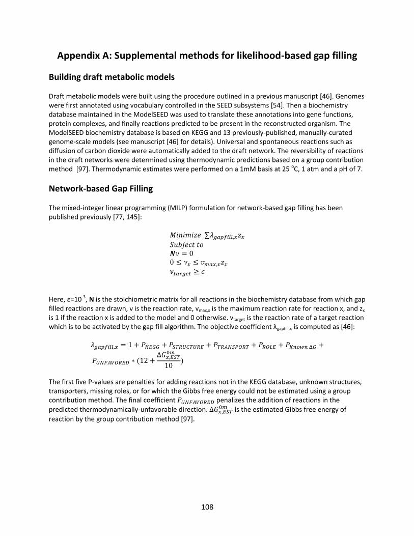
108
Appendix A: Supplemental methods for likelihood-based gap filling
Building draft metabolic models Draft metabolic models were built using the procedure outlined in a previous manuscript [46]. Genomes were first annotated using vocabulary controlled in the SEED subsystems [54]. Then a biochemistry database maintained in the ModelSEED was used to translate these annotations into gene functions, protein complexes, and finally reactions predicted to be present in the reconstructed organism. The ModelSEED biochemistry database is based on KEGG and 13 previously-published, manually-curated genome-scale models (see manuscript [46] for details). Universal and spontaneous reactions such as diffusion of carbon dioxide were automatically added to the draft network. The reversibility of reactions in the draft networks were determined using thermodynamic predictions based on a group contribution method [97]. Thermodynamic estimates were performed on a 1mM basis at 25 oC, 1 atm and a pH of 7.
Network-based Gap Filling The mixed-integer linear programming (MILP) formulation for network-based gap filling has been published previously [77, 145]:
∑
Here, ε=10-3, N is the stoichiometric matrix for all reactions in the biochemistry database from which gap filled reactions are drawn, ν is the reaction rate, vmax,x is the maximum reaction rate for reaction x, and zx is 1 if the reaction x is added to the model and 0 otherwise. vtarget is the reaction rate of a target reaction which is to be activated by the gap fill algorithm. The objective coefficient λgapfill,x is computed as [46]:
The first five P-values are penalties for adding reactions not in the KEGG database, unknown structures, transporters, missing roles, or for which the Gibbs free energy could not be estimated using a group contribution method. The final coefficient penalizes the addition of reactions in the
predicted thermodynamically-unfavorable direction. is the estimated Gibbs free energy of
reaction by the group contribution method [97].

109
The values of the penalties used in this manuscript were as follows (though they can be adjusted by the user).
PKEGG: 0 for reactions in KEGG and 1 for other reactions,
PSTRUCTURE: 0 for reactions with only metabolites with known structure and 1 otherwise
PTRANSPORT: 25, which works out to about 3-4 internal reaction changes on average.
PKnown delta G: 0 for reactions with estimated Gibbs energy and 1 otherwise
PUNFAVORED: 0 if the reaction is in the thermodynamically favorable direction (or if it is predicted to be reversible) and 1 otherwise. This makes changing a reaction with an estimated Gibbs energy of 10 kCal/mol equivalent to adding (on average) three intracellular reactions in a favorable direction.
The same values of the parameters were used for network-based and likelihood-based gap filling; thus the likelihood-based algorithm reduces to the network-based algorithm in the limit of 0 likelihood for every reaction.

110
Appendix B: Tutorial for building models and running likelihood-based gap filling in the DOE KnowledgeBase using the web-based CLI
Overview This tutorial describes how to build metabolic models using the four workflows that we have described in the manuscript. There are actually two ways to run this workflow:
Using the Client API, or
Using the Web-based command line interface
This tutorial focuses on the second one. The web-based command line interface is available at:
http://iris.kbase.us
Users log in (signing up is easy and free), create a workspace, and run the commands sequentially in the provided window. The API is described in a separate tutorial. This tutorial is divided into three parts: A quick command reference (commands are outlined with minimal explanation), a brief overview of the KBase infrastructure necessary to run the commands, and detailed information about each step we ran in the manuscript to come up with the reported results. Depending on the type of gap filling you wish to run there are a total of up to 13 steps. See Figure B.1 for detailed workflows for reproducing our results from the manuscript (or running your own) with network-based gap filling, iterative gap filling, likelihood-based gap filling, and likelihood-based iterative gap filling. Look up the appropriate section below for a detailed description of the commands for each step. Skip over anything in gray for a particular analysis.
Quick command reference The following is a list of all the commands (in order) that you can run in IRIS to perform a complete analysis from loading a genome from the SEED to performing a likelihood-based gap filling and analyzing phenotype data (in the same manner as was done in the manuscript). The numbers here correspond to the numbers in the workflows above. Anything denoted as $STUFF should be replaced with the actual name of the desired inputs and outputs. In order to run any of these commands you will need to first need a Globus Online account. If you dont have one, create one here: https://gologin.kbase.us/SignUp Go to IRIS (http://iris.kbase.us) and log in. You will then need a workspace in which to store your data. If you don't have one, create one using: $ ws-createws $WORKSPACE_NAME
111
Then switch to that workspace using: $ ws-workspace $WORKSPACE_NAME
1. Build a genome object (this example imports the genome from the PubSEED, other options are availbale) $ fba-loadgenome --seed $SEED_ID
This will create a Genome object called $SEED_ID in your workspace (this is hereafter referred to as $GENOME_OBJECT_NAME since other sources are possible) 2. Build draft model $ fba-buildfbamodel $GENOME_OBJECT_NAME --model $DRAFT_MODEL_NAME
This will create a Model object called $DRAFT_MODEL_NAME in your workspace. 3. Build annotation likelihoods $ pa-annotate $GENOME_OBJECT_NAME $PROBANNO_OBJECT_NAME
This will create a ProbAnno object called $PROBANNO_OBJECT_NAME in your workspace. This is a long-running job (takes about 4-5 hours on average). You can check the status of your job using $ pa-checkjob --job 52efbcb7e4b0ef8357332113 Job '52efbcb7e4b0ef8357332113' (pa-annotate for genome 171101.1.genome to
probanno 171101.1.probanno for user mmundy) has status 'running blast' and is
working on task 3 of 5. Check again later.
4. Calculate reaction likelihoods $ pa-calculate $PROBANNO_OBJECT_NAME $RXNPROBS_OBJECT_NAME
This will create a RxnProbs object called $RXNPROBS_OBJECT_NAME in your workspace. 5. Fill gaps on complete media. How you do this depends on the type of gap filling you want to do. This is a long-running job (takes from 1 hour to 1 day depending on the number of gaps in the original network).
Network-based gap fill:
$ fba-gapfill $DRAFT_MODEL_NAME --modelout $GAPFILLED_MODEL_NAME \
--transpen 25 --singletranspen 25 --biomasstranspen 25 --directionpen 12 \
--intsol
Likelihood-based gap fill:
$ fba-gapfill $DRAFT_MODEL_NAME --modelout $GAPFILLED_MODEL_NAME \
--transpen 25 --singletranspen 25 --biomasstranspen 25 --directionpen 12 \

112
--intsol --probrxn $RXNPROBS_OBJECT_NAME
6. Check growth on complete media $ fba-runfba $GAPFILLED_MODEL_NAME --fbaid $FBA_OBJECT_NAME.
Should give you non-zero objective value. The results are stored in an FBA object named $FBA_OBJECT_NAME for future reference. 7. If you are doing iterative gap filling, run the following after doing all the above for targeted gap filling (this is a long-running job, it takes 2-3 days on average to run):
Iterative gap fill:
$ fba-gapfill $GAPFILLED_MODEL_NAME --modelout $ITER_GAPFILLED_MODEL_NAME \
--transpen 25 --singletranspen 25 --biomasstranspen 25 --directionpen 12 \
--intsol --iterativegf
Likelihood-based iterative gap fill:
$ fba-gapfill $GAPFILLED_MODEL_NAME --modelout $ITER_GAPFILLED_MODEL_NAME \
--transpen 25 --singletranspen 25 --biomasstranspen 25 --directionpen 12 \
--intsol --iterativegf --probrxn $RXNPROBS_OBJECT_NAME
Note that this job can take up to a couple days for some problems. The final result will be a new Model object $ITER_GAPFILLED_MODEL_NAME in the workspace. 8. Reaction sensitivity analysis (iterative gap fill only) To run a reaction sensitivity analysis you need a GapFill solution ID. Run this: $ fba-getmodels --pretty $gapfilled_model_name $WORKSPACE_ID \
> $gapfilled_model_filename
Then search for "integrated_gapfillings" in the output file . "integrated_gapfillings" : [
[
"kb|g.166872.fbamdl1.gf.3",
"652/14/1",
"Complete",
"262/34/1",
0,
[]
]
],
You want the first element of the array ( kb|g.166872.fbamdl1.gf.3 in this example). Add "gfsol.0" to that string to get the GapFill solution ID (note - the 0 means you want to integrate solution number 0, i.e. the first solution):

113
kb|g.166872.fbamdl1.gf.3.gfsol.0
For iterative gap fill: $ fba-reactionsensitivity $ITER_GAPFILLED_MODEL_NAME \
--rxnsensid $RXN_SENSITIVITY_NAME \
--gapfill $GAPFILL_SOLUTION_ID --deleterxns
For likelihood-based iterative gap fill: $ fba-reactionsensitivity $ITER_GAPFILLED_MODEL_NAME \
--rxnsensid $RXN_SENSITIVITY_NAME \
--gapfill $GAPFILL_SOLUTION_ID --deleterxns --rxnprobs $RXNPROBS_OBJECT_NAME
The result will be a RxnSensitivity object $RXN_SENSITIVITY_NAME in your workspace. 9. Delete non-contributing reactions $ fba-delete_noncontributing_reactions $RXN_SENSITIVITY_NAME \
--newmodel $FILTERED_MODEL_NAME
It will make new Model object $FILTERED_MODEL_NAME in your workspace with flagged reactions deleted. 10. Gapfill to minimal media We used Carbon-D-Glucose but other minimal media will work as well. For network-based (targeted or iterative) gap fill, use the following to fill gaps to Carbon-D-Glucose (do not use iterative gapfill again on minimal media even if you did it on complete media): $ fba-gapfill $INPUT_MODEL_NAME --modelout $MINIMAL_GAPFILL_MODEL_NAME \
--transpen 25 --singletranspen 25 --biomasstranspen 25 --directionpen 12 \
--intsol --media Carbon-D-Glucose --mediaws KBaseMedia
For likelihood-based or likelihood-based iterative use the following: $ fba-gapfill $INPUT_MODEL_NAME --modelout $MINIMAL_GAPFILL_MODEL_NAME \
--transpen 25 --singletranspen 25 --biomasstranspen 25 --directionpen 12 \
--intsol --probrxn $RXNPROBS_OBJECT_NAME --media Carbon-D-Glucose \
--mediaws KbaseMedia
Depending on whether you have are doing targeted or iterative gap fill workflows, $INPUT_MODEL_NAME should be $GAPFILLED_MODEL_NAME or $FILTERED_MODEL_NAME, respectively.
11. Check for growth on minimal media
114
$ fba-runfba $MINIMAL_GAPFILL_MODEL_NAME --fbaid $MINIMAL_FBA_OBJECT_NAME \
--media Carbon-D-Glucose --mediaws KBaseMedia
Like before, you should get a non-zero objective. If it fails try rerunning gap filling with higher time limits. 12. Import phenotype data Note - we already loaded the phenotype data cited in the manuscript in the KBasePhenotypeDatasets directory so if you want to use that data you can skip this step. Compile your phenotype data into a tab-delimted table (see detailed description below). Then run: $ fba-importpheno $GENOME_ID $YOUR_PHENOTYPE_FILE \
--phenoid $PHENOTYPE_SET_ID
The function will create a PhenotypeSet object $PHENOTYPE_SET_ID in your workspace. 13. Do phenotype simulations For biolog data make sure you specify to add transporters for growth conditions. The input model $MODEL_NAME should be the model that has been gap filled to grow on minimal media. $ fba-simpheno $MINIMAL_GAPFILL_MODEL_NAME $PHENOTYPE_SET_ID \
--phenows KBasePhenotypeDatasets \
--phenosimid $OUTPUT_SIMULTATIONS --alltransporters
For knockout data just make sure the model grows on the media in which knockouts were done (if not, do a gap filling to that media - step 9-10, but replace Carbon-D-Glucose with your media ). Then run: $ fba-simpheno $MINIMAL_GAPFILL_MODEL_NAME $PHENOTYPE_SET_ID \
--phenows KBasePhenotypeDatasets \
--phenosimid $OUTPUT_SIMULATIONS
These commands will create a PhenotypeSimulationSet object called $OUTPUT_SIMULATIONS in your workspace, storing all the simulation results.
A very brief introduction to the KBase The DOE KnowledgeBase (KBase) is, to me, three things: a. A database with consistent identifiers, cross-linked to show connections between genomes, genes, functions, and (perhaps most importantly) biochemistry. We won’t talk about this much in the demo but it does make it much easier to import external data and have it generate the right links... b. A set of tools (particularly, modeling tools) that can be used to analyze that data, along with a set of consistent APIs that can be used to develop your own tools and a web front-end that can run them from anywhere

115
c. A provider of computational resources such as processing and storage In the KBase your data will be saved on KBase machines (which are backed up regularly) and processed on their servers. All of the below commands are run in a web environment hosted by the KBase team. A. Sign up for a KBase account. To use the KBase you will need to sign up for an account through Globus Online. Do so through their website: https://gologin.kbase.us/SignUp B. IRIS IRIS is a web-based command line tool, located here: http://iris.kbase.us I’ll show you some commands you can use to build models in IRIS - you just type them in and they run on some computer in KBase-land. No installation necessary. To begin using IRIS, you need to log in using your Globus Online account. After you log in, you can upload your data, run commands with it, and export the data back to your computer. If you log in on another computer, your data will still be there. A nice tutorial on the interface for IRIS is available here so I won't repeat the words from it. I recommend you read it to become familiar with how to upload and download files, run commands etc. http://kbase.science.energy.gov/developer-zone/tutorials/iris/introduction-to-the-kbase-iris-interface/ C. Workspaces and objects (KBase data storage) After you upload your data you will need to run a script to convert it into a KBase object. For example, there is a command to take a FASTA file and turn it into a genome object, to take a SBML file and turn it into a model object, etc. There are also interfaces to automatically download data from various databases (such as the SEED) and save them as KBase objects. All KBase objects are given a specific type and saved in a workspace (think of it like a folder) on the KBase computers. Most KBase commands take an object of one type and convert them into another object of the same type or an object of a different type (for example, there is a command to convert a genome object into a model object). In order to move forward you will need to create a workspace to store your files. Do that with the ws-createws command. Type the following into IRIS to create a workspace, replacing $WORKSPACE_NAME with the name of the workspace you want to create (which by default no one but you can read. You can always change permissions later):

116
$ ws-createws $WORKSPACE_NAME
Then change to that workspace using ws-workspace $ ws-workspace $WORKSPACE_NAME
You are now in your workspace $WORKSPACE_NAME. You can list the objects in that workspace at any time by typing ws-listobj $ ws-listobj
To list objects in a specific workspace (not the one you're currently in) use -w. For example use this command to list all the media in the KBaseMedia workspace. $ ws-listobj --workspace KBaseMedia
The functions used in this workflow can take both an ID and a workspace for any of the objects that they require as inputs. They usually will use your current workspace by default if you don't specify it; this is omitted in the example commands below, in which we assume you are currently in the workspace that you wish to save objects into. D. KBase services A service is basically a collection of related commands (often operating on just a few different types of objects). There are lots of services in the KBase for genome annotation, clustering and orthology analysis, analysis of transcription data, etc. I haven’t used most of them myself. To do likelihood-based gap filling, you will need to use commands in three of them: - The workspace service, which is used to save, move, and retrieve data from workspaces (think of them as personal folders on KBase machines that store objects with specific formats). You'll need to use this with practically every other service. - The modeling service, which has functions to import and annotate genomes, import existing models or generate new ones from an annotated genome, run gap filling, compare models, etc. It uses the ModelSEED as a back-end - The probabilistic annotation service, which calculates annotation and reaction likelihoods for use in gap filling. In IRIS you can see the list of services in the tab on the left (Figure B.2).
117
Detailed workflow tutorial The following is a detailed description of the relevant commands to run our workflow in IRIS. Anytime you see $STUFF , replace it with the actual name of your input and outputs. 1. Build genome object In order to work with your genome in the KBase you will need to import it into a workspace. Genomes, like everything else in workspaces, are saved as typed objects which have formats that all of the KBase functions understand and store all necessary information. Fortunately, doing this conversion is rather simple, especially for genomes in the SEED, the KBase central store, or RAST. Note that for model building to work properly you will need to be using the same annotation conventions as are used in the SEED\RAST\KBase central store so it is highly recommended that you take your genomes from one of those sources. For example, pull a genome from the SEED by its SEED ID using: $ fba-loadgenome --seed $SEED_ID
This will create a Genome object called $SEED_ID in your workspace (this is hereafter referred to as $GENOME_OBJECT_NAME since other sources are possible). Take a look at the other options for fba-loadgenome if your source is different. 2. Build draft model After you load your genome into a workspace, you can use the ModelSEED algorithm (Ref: see Henry et al. 2010) to build a draft model using: $ fba-buildfbamodel $GENOME_OBJECT_NAME --model $DRAFT_MODEL_NAME
This will create a Model object called $DRAFT_MODEL_NAME in your workspace based on the annotations in the genome object. The draft model is not yet gap filled so it will not grow due to missing or incorrect annotations. However, a biomass equation will automatically be created and after gap filling is done (see later steps) it should be able to grow provided the solving did not fail. 3. Build annotation likelihoods The pa-annotate command (in the Probabilistic Annotation service on IRIS) is responsible for computing the likelihoods of annotations for each gene in a genome as described in the manuscript. It takes a genome object as an input and produces a ProbAnno object: $ pa-annotate $GENOME_OBJECT_NAME $PROBANNO_OBJECT_NAME
Running this command will result in queueing a probanno job on the KBase servers. The command takes about 4 hours to run on average, and therefore the job is placed in a queue and runs when the queue is cleared. You can always check on your job using ws-checkjob:

118
$ pa-checkjob $JOB_ID
When the job is complete, a ProbAnno object called $PROBANNO_OBJECT_NAME will be created in your workspace. This object will contain multiple possible annotations for each gene, each attached to a likelihood. 4. Building reaction likelihoods The pa-calculate function takes a ProbAnno object as an input and calculates the likelihood of each reaction based on the procedure outlined in the manuscript. It is run as follows: $ pa-calculate $PROBANNO_OBJECT_NAME $RXNPROBS_OBJECT_NAME
The result is a RxnProbs object called $RXNPROBS_OBJECT_NAME, which is saved in your workspace (unlike pa-annotate, pa-calculate runs quickly). The RxnProbs object stores computed reaction likelihoods along with the predicted gene-protein-reaction (GPR) relationships for each reaction and some data on the complexes used to build them. You can use either a RxnProbs object or a ProbAnno object as an input to gap filling. These are the inputs to likelihood-based gap filling as described in the manuscript. However, we recommend using the RxnProbs object so that you can use it as input to other functions to help interpret gap filling results. 5. Running Gap filling to Complete Media Draft models build using fba-buildfbamodel will not be able to simulate growth in general, due to the existence of annotation gaps. It is necessary to fill gaps in the model to achieve growth. Gap filling is done using the fba-gapfill command, which has many options (some of which were not used in this manuscript). The total commands used were as follows, which are described in detail below
Network-based gap fill:
$ fba-gapfill $DRAFT_MODEL_NAME --modelout $GAPFILLED_MODEL_NAME \
--transpen 25 --singletranspen 25 --biomasstranspen 25 --directionpen 12 \
--intsol
Likelihood-based gap fill:
$ fba-gapfill $DRAFT_MODEL_NAME --modelout $GAPFILLED_MODEL_NAME \
--transpen 25 --singletranspen 25 --biomasstranspen 25 --directionpen 12 \
--intsol --probrxn $RXNPROBS_OBJECT_NAME
The following options to fba-gapfill were always used in simulations done in this manuscript: --transpen 25 --singletranspen 25 --biomasstranspen 25 --directionpen 12 \
--intsol
119
--transpen, --singletranspen, --biomasstranspen, and --directionpen are penalties for adding transporters for various things instead of intracellular reactions (I like to set these to be quite high but you can feel free to play with them) and the base penalty for changing reversibility if a reaction is not thermodynamically favorable in the reverse direction. --intsol means "integrate solution"; gap fill will NOT automatically integrate the solution into your model unless you select this option. If you want to look at the solution and decide whether you agree before adding the reactions to your model, you can do so by omitting this option. We do not talk in this tutorial about how to integrate solutions after-the-fact but you can look at the fba-integratesolution command for some details. When you run fba-gapfill, it will do some pre-processing and then will queue the job and give you an ID. Gapfill takes quite a while to run so go do something else for a day, come back and it should be done (if you are doing iterative gapfill, give it two or three days). You can always check the status of your job by using ws-checkjob. If the solver fails and gives you a nonsense solution (e.g. 3000 reactions), try increasing the time per solution and total time using --timepersol and --timelimit (the default time limit for solving is 3600 seconds per solution). Likelihood-based gapfilling To do likelihood-based gapfilling as described in the manuscript, you need to either provide a probabilistic annotation object or a probabilistic reaction object (which contains the reaction likelihoods calculated from the probabilistic annotation object), which are calculated as described in steps 3-4 of this tutorial. The ProbAnno object can be incorporated directly into gapfilling (without calculating reaction likelihoods) with the --probanno flag to fba-gapfill. However, we recommend using the pa-calculate function to compute them yourself and get a RxnProbs object so that you can take a look at the reaction likelihoods that are generated. The RxnProbs object can be used as input to gapfilling by providing the --probrxn flag to fba-gapfill. 6. Checking growth on complete media You can run FBA within the KBase tool (along with many other simple simulations such as FVA, doing simulation to try to figure out what biomass components can't be produced in a model, etc…) using the fba-runfba command. I recommend doing this to make sure the gapfilling was successful in producing a growing model. The fba-runfba command will create an FBA object which stores the FBA results including the fluxes of every reaction (and if you ask for it, FVA results, results of running knockouts, etc. - I won't cover all of that stuff but take a look at the help text for an idea of what it can do). I suggest saving the FBA object to a place where you know where to find it \ how it was run using the --fba flag: $ fba-runfba --fba $FBA_OBJECT_NAME $GAPFILLED_MODEL_NAME

120
The default is to run FBA on complete media so this is all you need to do to test if growth is possible. If the growth rate is 0, the gapfill failed. Depending on the reasons for failure you might be able to get a good solution by re-running gapfill with a higher time limit. Try increasing the time per solution and total time using --timepersol and --timelimit (the default time limit for solving is 3600 seconds per solution). 7. Iterative gapfilling Iterative gapfilling, as described in the manuscript, is the gapfilling of ALL of the dead-ends in a model, not just those that have to be filled to achieve growth. It is called iterative because it fills them one a time according to a pre-defined priority until they are all filled (or as many as can be filled given what is in the database). Here are some recommendations on how to use it for maximum effectiveness.
You only need to ask for one solution (do not use --numsol. It will be ignored anyway) You should only do iterative gapfilling on complete media (which is the default - don't use the -m/--
media or --mediaws flags). You should only do iterative gap fill after doing a normal gap filling (and integrating the solution and
checking to make sure the model achieves growth on complete media). This greatly reduces the computation time necessary because gap filling to biomass makes many other gap fills unnecessary.
Be aware that iterative gapfilling takes a long time because you're filling so many gaps. This is why we only use it when gapfilling to complete media and not when gapfilling to minimal media (step 10)
Use --intsol - since you're only getting one solution you might as well just integrate it automatically. In fact, for iterative gapfill this is set whether you set it or not, but set it anyway so you don't forget.
To do an iterative gapfilling use the --iterativegf flag in the fba-gapfill function. Likelihood-based iterative gap filling Likelihood-based iterative gap filling can be done by providing both --probrxn (or --probanno) and --iterativegf to the fba-gapfill function. Otherwise, use the same guidelines as for network-based iterative gap filling. The overall commands we used were as follows:
Iterative gap fill:
$ fba-gapfill $GAPFILLED_MODEL_NAME --modelout $ITER_GAPFILLED_MODEL_NAME \
--transpen 25 --singletranspen 25 --biomasstranspen 25 --directionpen 12 \
--intsol --iterativegf
Likelihood-based iterative gap fill:
$ fba-gapfill $GAPFILLED_MODEL_NAME --modelout $ITER_GAPFILLED_MODEL_NAME \

121
--transpen 25 --singletranspen 25 --biomasstranspen 25 --directionpen 12 \
--intsol --iterativegf --probrxn $RXNPROBS_OBJECT_NAME
8. Reaction sensitivity analysis Reaction sensitivity analysis as described in the manuscript is a way to prune unneeded gap filling solutions by testing the effects of removing each one on the activity of other reactions in the network and on the ability of the cell to predict nonzero biomass production rates. If deleting a gap filled reaction is nonlethal and does not inactivate any reactions in the model, it is flagged as unnecessary. Reaction sensitivity analysis is done using the fba-reactionsensitivity function in IRIS. This function can be run in two different ways (only one of which is covered above, because it's the one we used when doing our simulations):
1. The user can specify (in the order that he or she wants to test them) a list of reactions in the model for which the sensitivity should be tested. To do this use the --rxnstotest flag. For example, if rxn00001 and rxn00002 are in your model $MODEL_ID, you can test the effects of deleting them by running this command:
$ fba-reactionsensitivity $ITER_GAPFILLED_MODEL_NAME --rxnstotest "rxn00001;rxn00002"
You can also specify a direction (e.g. "+rxn00001") to test.
2. The user can specify a GapFill solution ID. If the user specifies this, then the following happens: 1. A list is generated of all of the reaction changes (with the direction) added by that specific
gap filling run. 2. For network-based gap fill (no RxnProbs object specified), the order of reactions to test is
the reverse of the order in which they were added by the algorithm, with the idea that later gapfills are to lower-priority parts of the network so we want to try to remove them first.
3. For likelihood-based gap fill, specify a RxnProbs object with --rxnprobs . A further stable sort will be done based on the reaction likelihoods and the lowest-likelihood reactions will be tested for removal first. Ties are broken by using the same ordering as for non-likelihood-based gap filling.
The process of getting a GapFill solution ID is as follows. Given a model that has an integrated iterative gapfill (using --intsol), run: $ fba-getmodels –pretty $gapfilled_model_name $WORKSPACE_ID \
> $gapfilled_model_filename
Then search for "integrated_gapfillings" in the output file . "integrated_gapfillings" : [
[
"kb|g.166872.fbamdl1.gf.3",
"652/14/1",
"Complete",
"262/34/1",
0,
[]
]
],

122
You want the first element of the array ( kb|g.166872.fbamdl1.gf.3 in this example). Add "gfsol.0" to that string to get the GapFill solution ID (note - the 0 means you want to integrate solution number 0, i.e. the first solution): kb|g.166872.fbamdl1.gf.3.gfsol.0
Optionally, the reaction sensitivity analysis will delete each reaction that is unnecessary before proceeding to the next one (in this case, the reactions will be flagged for deletion in the Reaction Sensitivity object and the sensitivity results of every reaction after it will depend on the fact that that reaction was deleted). To get this behavior specify --deleterxns on the command line. We used this flag in the manuscript workflow. Putting all of this together, the final commands we used as part of the manuscript workflow were: Network-based gap fill $ fba-reactionsensitivity $ITER_GAPFILLED_MODEL_NAME --rxnsensid $RXN_SENSITIVITY_NAME
--gapfill $GAPFILL_SOLUTION_ID --deleterxns
For likelihood-based gap fill: $ fba-reactionsensitivity $ITER_GAPFILLED_MODEL_NAME --rxnsensid $RXN_SENSITIVITY_NAME
--gapfill $GAPFILL_SOLUTION_ID --deleterxns --rxnprobs $RXNPROBS_OBJECT_NAME
9. Deleting non-contributing reactions After you run a reaction sensitivity analysis with --deleterxns, you can run fba-delete_noncontributing_reactions to actually delete the unnecessary reactions from the model. The RxnSensitivity object is automatically linked to a specific model so you will not need to specify the input model in this function. However, you can (and probably should) specify a different ID to use for the model with reactions deleted. Do so with the --newmodel flag. $ fba-delete_noncontributing_reactions $RXN_SENSITIVITY_NAME \
--newmodel $FILTERED_MODEL_NAME
10. Gap filling to minimal media We used the same commands as outlined in step 5 (gap filling to complete media) except for two things:
A. By default, the gap fill algorithm only tries to achieve growth on "complete" media. You can specify other media using -m - you will also probably have to specify a media workspace. We recommend (and have implemented in this workflow) running gap filling on complete media first before trying to achieve growth on any specific media. Doing so greatly simplifies the gap filling problem and also highlights those reactions that would be essential regardless of the chosen media condition (unless new transporters are added).
B. We recommend you do not perform iterative gap filling in this step (do not use the --iterativegf flag on minimal media).
123
You can define your own media conditions with which to perform gap filling by creating a Media object in your workspace using fba-addmedia. However, the KBase also has about 700 default media conditions saved in the workspace KBaseMedia. To fill gaps in the model and achieve growth on a specific media condition, fill gaps on complete media first (since that solution is a basis for all other media conditions) and then call fba-gapfill again and use these flags: -m $MEDIA_NAME --mediaws KBaseMedia
11. Checking growth on minimal media To run FBA to a specific media (with a Media object in a workspace) use the -m flag (and --mediaws if the media is not in your current workspace) to the fba-runfba command. The default media for KBase are found in the KBaseMedia workspace so use the following to run FBA on one of those media conditions (you can also create your own media and put it in your workspace, in which case use that workspace instead with the—mediaws argument): $ fba-runfba --fba $FBA_ID --media $MEDIA_NAME --mediaws KbaseMedia \
$MINIMAL_GAPFILLED_MODEL_NAME
If you imported your media condition using fba-addmedia you can specify that media (and your workspace name) instead. 12. Importing phenotype data Note that we have already done this for the phenotype data used in the manuscript and saved them in the KBasePhenotypeDatasets workspace. If you only want to use those, you can skip this step. However, you will need to do this to do simulations of your own phenotype data. The phenotype data is imported from a tab-delimited table with the following headers (the headers must be exactly the same as this, but can be in any order):
4. media - Name of the Media object containing the media for which the phenotype was measured 5. mediaws - Workspace in which the Media object above is located (often KBaseMedia, or your
own workspace) 6. growth - 1 for Grows, 0 for Does Not Grow 7. geneko - OPTIONAL. If specified, it is a semicolon-delimited list of gene knockouts. The gene IDs
must match the IDs from your original genome source (e.g. SEED IDs in form fig|#.#.peg.# where each # is some number).
8. addtlcpd - OPTIONAL. If specified, it is a semicolon-delimited list of compounds added to the specified Media condition before measuring the phenotype (use it for example to record the effects of making small changes to media and testing effects on growth).
Example: You did knockouts of "fig|83333.1.peg.1", "fig|83333.1.peg.2" and "fig|83333.1.peg.3" separately and tried to grow your organism on Carbon-D-Glucose. The ∆fig|83333.1.peg.1 strain grew but the ∆fig|83333.1.peg.2 and ∆fig|83333.1.peg.1 strains did not. The input file would then look like this: (note that the separator between each field is a tab, including in the header). media mediaws growth geneko
124
Carbon-D-Glucose KBaseMedia 1 fig|83333.1.peg.1 Carbon-D-Glucose KBaseMedia 0 fig|83333.1.peg.2 Carbon-D-Glucose KbaseMedia 0 fig|83333.1.peg.3 Example 2: You tried a triple knockout of these three genes and it did not grow. You can add a line like this to the above file to account for this: Carbon-D-Glucose KbaseMedia 0 fig|83333.1.peg.1;fig|83333.1.peg.2;fig|83333.1.peg.3 Note that it is possible to import other IDs such as locus tags into a genome file and then use them in the phenotype table. Doing so is outside the scope of this tutorial but see fba-importtranslation for details. Once you have set up this table, import it into IRIS using its file import capability and then run: $ fba-importpheno $GENOME_ID $PHENOTYPE_FILE --phenoid $PHENOTYPE_SET_ID
13. Phenotype simulations Run phenotype simulations using the fba-simpheno command. In order to run this you will need a phenotype set. Several phenotype sets for the organisms we discussed in the manuscript are available in the KBasePhenotypeDatasets workspace. Otherwise you will need to import your phenotype data as a PhenotypeSet object (step 12) first. We recommend that for knockout simulations you first try to run FBA on the media in which the knockouts were performed (step 11). If you get a 0 growth rate, you should run gap filling to that media so that you don't get all negative growth predictions. If you do this, don’t use iterative gap filling, but use either likelihood or network-based gap fill algorithms depending on what you have been using to get this far. Once you have a growing model just use fba-simpheno to simulate the phenotype. $ fba-simpheno $MODEL_NAME --phenows KBasePhenotypeDatasets $PHENOTYPE_SET_ID \
--phenosimid $OUTPUT_SIMULATIONS
--phenosimid should be specified if you want to give the resulting phenotype simulation set a specific name (recommended). You can then take a look at that object and identify the correct and incorrect growth predictions relative to the available phenotype data. For biolog simulations you should perform gap filling to achieve growth on a minimal media (such as Carbon-D-Glucose) before running simulations. You should also specify --alltransporters in the fba-simpheno command so that transporters are automatically added for all compounds in all tested growth conditions before simulation is done. This is necessary because transporters are the hardest to get right, and it is quite likely that the model will be missing transporters that, if present, would allow the cell to grow with the rest of what's in the network. The final command to use becomes: $ fba-simpheno $MODEL_NAME --phenows KBasePhenotypeDatasets $PHENOTYPE_SET_ID \
-- phenosimid $OUTPUT_SIMULATIONS --alltransporters

125
Figures and tables
Figure B.1. Gap filling workflows implemented in the KnowledgeBase. Gray boxes indicate steps to skip in a particular workflow.
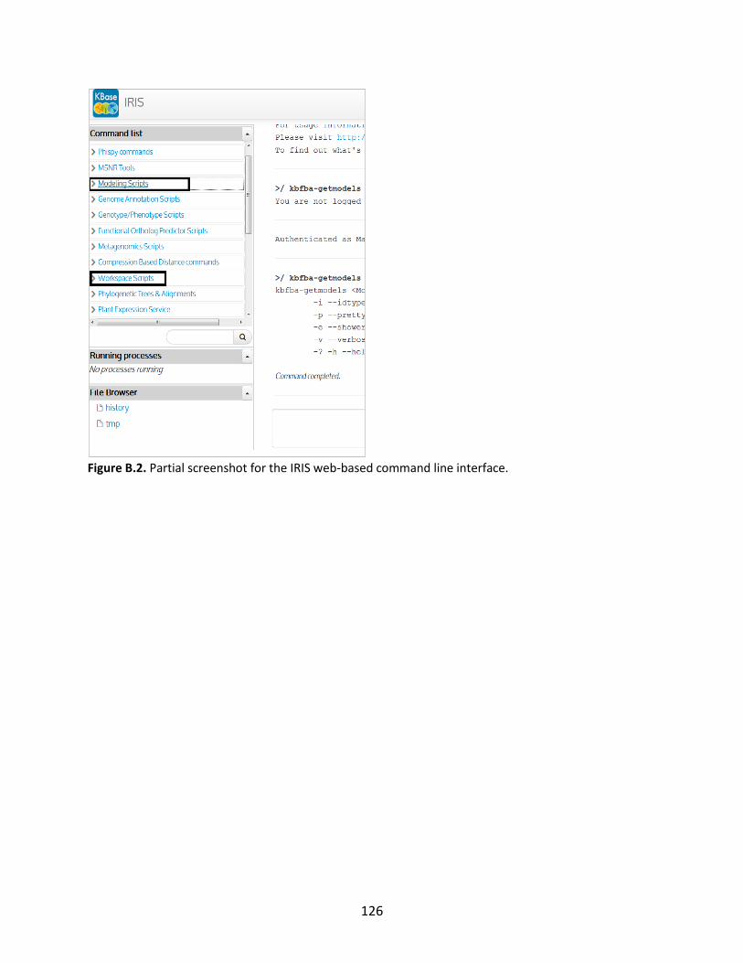
126
Figure B.2. Partial screenshot for the IRIS web-based command line interface.

127
Appendix C: Description of the KBASE Client API for likelihood-based gap filling workflows
This tutorial describes how to build metabolic models using the four workflows that we have described in the manuscript. There are actually two ways to run this workflow:
Using the Client API, or
Using the Web-based command line interface
This tutorial describes a script that uses the client API to perform the workflows. Please see the other tutorial file (Supplemental file 2) for a detailed description of the workflows themselves. Obtaining a Globus Online account You will need to create a Globus Online account and a workspace (see Supplemental file 2 for details) before running the workflow script. Do not use the same password as used in other websites in case the password is echoed and logged somewhere, though we try to use getpass() to avoid that. Obtaining the KBase client API First you will need to have the following packages installed:
3. Python, version 2.6 or 2.7 4. The following built-in packages are used by client libraries: urllib2, httplib, urlparse,
random, base64, ConfigParser, json 5. The following built-in packages are used by the workflow script: argparse, subprocess,
traceback, sys, time, operator 6. Python packages (get using apt-get or pip or whatever you have to install it):
7. httplib2 For example in Ubuntu do the following to get httplib2 $ sudo apt-get install python-httplib2 Second, download the "ClientWorkflow.zip" provided with this manuscript. Finally, add the extracted directory (the one that contains the "biokbase" directory) to your PYTHONPATH.

128
Running the workflow script The workflow script has the following syntax: usage: Workflow [-h] [--password PASSWORD] [--genome_source SOURCE] [-w WORKSPACE] [--force] [--network] [--prob] [--iterative] [--iterativeprob] [--num-solutions NUMSOLUTIONS] [--ws-url WSURL] [--fba-url FBAURL] [--pa-url PAURL] [--knockout KNOCKOUT] [--knockoutws KNOCKOUTWS] [--biologdata BIOLOG] [--biologdataws BIOLOGWS] [--positiveTransportersOnly] [--maxtime MAXTIME] genome username The required arguments are a genome ID (by default coming from the PubSEED, http://pubseed.theseed.org) and a username. The script asks for a password interactively if it is not provided on the command line. Alternative genome sources You can specify that you want your genome to come from the KBase central store instead of the PubSEED by specifying this using --genome_source . The four workflows You can specify which workflow to run using the following flags:
C. --network: Run the targeted network-based gap fill workflow (activate biomass only) D. --prob : Run the targeted likelihood-based gap fill workflow (activate biomass only) E. --iterative: Run the iterative network-based gap fill workflow F. --iterativeprob: Run the iterative likelihood-based gap fill workflow
You can also specify that you want to run the biolog or knockout lethality phenotype predictions after gap filling using:
--biologdata: For biolog data
--knockout: For knockout data For biolog data you have the option of fitting to it by adding transporters only for growth-positive substrates using --positiveTransportersOnly. By default, transporters are added for ALL media in the biolog data before running simulations. If a gap fill job fails due to lack of time you can increase the time limit using --maxtime. The argument is provided in units of seconds. Note: The servers are prone to random failures (504s etc). If you restart the workflow script with the same arguments as were used before the error, it will start back up where it left off. It is recommended to check the results of the last step first to see if an object is present and if results are in it - you might

129
need to delete the object (using ws-delete) before starting the workflow again. Also check to see if your job is still running - the workflow might have just failed while checking to see if your job was done. If this happens, wait for the job to finish and then restart the workflow using the same arguments. Specifying where your data is All data used in Workflow.py is extracted from and saved in workspaces. By default the Workflow.py looks for everything in the last workspace you were in when logged in. Alternatives to the default can be specified as follows:
C. -w: This specifies where all the results of Workflow.py itself will be saved. D. --knockoutws: This specifies where knockout data is located, if you are running that part of the
workflow. E. --biologdataws: This specifies where biolog data is located, if you are running that part of the
workflow. In order to run the Workflow, you must have write permissions in the main workspace (-w) and read permission in the knockout/biolog workspaces. I suggest using IRIS (see other tutorial) to create the workspace and manage permissions. Specifying what servers to use Every server is specified by a URL. If the URL ever changes you will need to specify the new URL using the URL arguments (or go in and change the default):
--ws-url : Workspace service URL --fba-url : FBA Modeling service URL --pa-url: Probabilistic Annotation service URL
Rerunning from scratch If you want to force the workflow to rebuild every object instead of checking to see if they exist and restarting the workflow from where it left off, use --force.