Model Answer

AS-2359

M.C.A. (Fifth Semester) Examination, 2013

Computer Graphics

(MCA-502)

Time Allowed: Three hours

Maximum Marks:60

Note: question no.1 is compulsory. Attempt any four questions from remaining.

Section-A

Q.1 (10X2=20 Marks)

1) Resolution is defined as

A. The number of pixels in the horizontal direction X the number pixels in the vertical direction.

B. The number of pixels in the vertical direction X the number pixels in the horizontal direction. C. The number of pixels in the vertical direction + the number pixels in the horizontal direction. D. The number of pixels in the vertical direction - the number pixels in the horizontal direction.

2) Aspect ratio is

A. The ratio of image’s width to its height B. The ratio of window to viewport height C. The ratio of image’s intensity levels D. The ratio of image’s height to its width

3) Refresh rate is

A. The rate at which the number of bit planes are accessed at a given time

B. The rate at which the picture is redrawn C. The frequency at which the aliasing takes place D. The frequency at which the contents of the frame buffer is sent to the display monitor

4) Frame buffer is

A. The memory area in which the image, being displayed, is stored B. The device which controls the refresh rate C. The device used for displaying the colors of an image D. The memory area in which the graphics package is stored

5) Pixel on the graphics display represents?

A. mathematical point B. a region which theoretically can contain an infinite number of points

C. voltage values D. picture

6) Display processor is also called a? A. graphics controller B. display coprocessor

C. both a and b D. out put device for graphics

7) Graphics software acts as a very powerful tool to create? A. Images

B. animated pictures C. both a and b D. system interface

8) The purpose of display processor is __from the graphics routine task?

A. to free the CPU B. To free the secondary memory C. to free the main memory D. Both a & c

9) random-scan monitors typically offer __color choices?

A. Only a few

B. wide range C. just 1 or 2 D. moderate range of

10) The basic principle of Bresenham`s line algorithm is__?

A. to select the optimum raster locations to represent a straight line B. to select either ∆x or ∆y, whichever is larger, is chosen as one raster unit C. we find on which side of the line the midpoint lies

D. both a and b

(4X10=40 Marks)

Q.2 Develop the Bresenham’s line drawing to draw lines of any scope. Compare this with the DDA Algorithm.

Ans. The Bresenham-Algorithm creates exactly the same result as the simple DDA, but suffices

using only integer arithmetic. Thus it is faster, easier to implement in firm- or hardware, and

further it can be easily adopted to fit other curves like circles, ellipses, spline curves and so

on.

For 0 < |m| < 1, from the known location of the pixel in the column xk the y-value of the pixel in

the next column xk+1 is not being exactly calculated, but rather there’s made a decision, whether yk

or yk+1 lies closer to the exact y-value.

From y = mx + b follows the exact y-value for the column right to xk

y = m.(xk + 1) + b

The distance to yk is dlower = y − yk = m(xk + 1) + b − yk

The distance to yk+1 is dupper = (yk + 1) − y = yk + 1 − m(xk + 1) − b

If the difference dlower − dupper = 2m.(xk + 1) − 2yk

+ 2b − 1

is negative, then the lower point (xk+1,yk) is chosen. Otherwise, if the

difference is positive, the upper point (xk+1,yk+1) is set.

Substituting m = ∆y/∆x ( ∆x = xend – x0, ∆y = yend – y0 ), and

multiplying this difference with ∆x results in a decision variable pk =

∆x.(dlower − dupper) = 2∆y.xk − 2∆x.yk

+ c , which has the same sign as dlower − dupper, but doesn’t need

any division.

Now, when the decision variable pk = 2∆y.xk − 2∆x.yk + c for xk is known, the decision variable for

xk+1 can easily be calculated:

pk+1 = 2∆y.xk+1 − 2∆x.yk+1 + c + pk – 2∆y.xk + 2∆x.yk – c = pk

+ 2∆∆∆∆y − 2∆− 2∆− 2∆− 2∆x.(yk+1 −−−− yk)

namely just by adding a number, which is constant for all points of the line. p0 = ∆y − ∆x

So far the Bresenham-Algorithm roughly looks like this:

1. store left line endpoint in (x0

,y0

)

2. plot pixel (x0,y

0)

3. calculate constants ∆x, ∆y, 2∆y, 2∆y − 2∆x, and obtain p0

= 2∆y − ∆x

4. At each xk

along the line, perform test:

5. if pk<0

6. then plot pixel (xk+1,y

k); p

k+1 = p

k+ 2∆y

7. else plot pixel (xk+1,y

k+1); p

k+1= p

k+ 2∆y − 2∆x

8. perform step 4 (∆x − 1) times.

Example:

k pk

(xk+1

,yk+1

(20,41)

0 -4 (21,41)

1 2 (22,42)

2 -12 (23,42)

3 -6 (24,42)

4 0 (25,43)

5 -14 (26,43)

6 -8 (27,43)

7 -2 (28,43)

8 4 (29,44)

9 -10 (30,44)

Difference Between DDA Line Drawing Algorithm and Bresenhams Line Drawing Algorithm.

Digital Differential Analyzer

Line Drawing Algorithm

Arithmetic DDA algorithm uses

Operations DDA algorithm uses

multiplication and

Speed DDA algorithm

Bresenhams algorithm in line drawing

because it uses real arithmetic (floating

point operations).

Accuracy &

Efficiency

DDA algorithm is not as accurate and

efficient as Bresenham algorithm.

Drawing DDA algorithm can draw circles and curves

but that are not as accurate as Bresenhams

Round Off DDA algorithm round off the coordinates to

integer that is

Expensive DDA algorithm uses an enormous number

of floating-point multiplications so it is

k+1)

Line Drawing Algorithm and Bresenhams Line Drawing Algorithm.

Digital Differential Analyzer

Line Drawing Algorithm

Bresenhams Line Drawing Algorithm

DDA algorithm uses floating points i.e. Real

Arithmetic.

Bresenhams algorithm uses

points i.e.

DDA algorithm uses

and division in its operations.

Bresenhams algorithm uses only

subtraction and

DDA algorithm is rather slowly than

Bresenhams algorithm in line drawing

because it uses real arithmetic (floating-

point operations).

Bresenhams algorithm is faster than DDA

algorithm in line drawing because it

performs only addition and subtraction in

its calculation a

arithmetic so it runs significantly

DDA algorithm is not as accurate and

efficient as Bresenham algorithm.

Bresenhams algorithm

much accurate than DDA algorithm.

algorithm can draw circles and curves

but that are not as accurate as Bresenhams

algorithm.

Bresenhams algorithm can draw circles and

curves with much more accuracy than

DDA algorithm round off the coordinates to

integer that is nearest to the line.

Bresenhams algorithm does not

off but takes the incremental value in its

DDA algorithm uses an enormous number

point multiplications so it is

expensive.

Bresenhams algorithm is less expensive tha

DDA algorithm as it uses only addition and

subtraction.

Line Drawing Algorithm and Bresenhams Line Drawing Algorithm.

Bresenhams Line Drawing Algorithm

Bresenhams algorithm uses fixed

i.e. Integer Arithmetic.

Bresenhams algorithm uses only

and addition in its operations.

Bresenhams algorithm is faster than DDA

algorithm in line drawing because it

performs only addition and subtraction in

its calculation and uses only integer

arithmetic so it runs significantly faster.

Bresenhams algorithm is more efficient and

much accurate than DDA algorithm.

Bresenhams algorithm can draw circles and

curves with much more accuracy than DDA

algorithm.

Bresenhams algorithm does not round

but takes the incremental value in its

operation.

Bresenhams algorithm is less expensive than

DDA algorithm as it uses only addition and

subtraction.

Or

Write short note on Color CRT Monitor. Explain Shadow Mask Method.

Ans. A CRT monitor displays color picture by using a combination of phosphor that emit

different-colored light. By combining the emitted light from the different phosphor, a range of colors can be generated. The two basic techniques for producing color displays with a CRT are the beam-penetration method and the shadow-mask method.

The beam-penetration method for displaying color pictures has been used with

random-scan monitors. Two layers of phosphor, usually red and green, are coated onto the

inside of the CRT screen, and the displayed color depends on how far the electron beam

penetrates into the phosphor layers. A beam of slow electrons excites only the outer red

layer. A beam of very fast electron penetrates through the red layer and excites the inner

green layer. At intermediate beam speeds, combinations of red and green light are emitted to

show two additional colors, orange and yellow. The speed of the electrons, and hence the

screen color at any point, is controlled by the beam-acceleration voltage. Beam penetration

has been an inexpensive way to produce color in random-scan monitor, but only four colors

are possible, and the quality of picture is not as good as with other methods.

Shadow-mask methods are commonly used in raster-scan system (including color TV)

because they produce a much wider range of colors than the beam penetration method. A

shadow-mask CRT has three phosphor color dots at each pixel position. One phosphor dot

emits a red light, another emits a green light, and the third emits a blue light. This type

ofCRT has three electron guns, one for each color dot, and a shadow-mask grid just behind

the phosphor-coated screen. Figure illustrates the delta-delta shadow-mask method,

commonly used in color CRT system. The three beams are deflected and focused as a group

onto the shadow mask, which contains a series of holes aligned with the phosphor-dot

patterns. When the three beams pass through a hole in the shadow mask, they activate a dot

triangle, which appears as a small color spot on the screen. The phosphor dots in the

triangles are arranged so that each electron beam can activate only its corresponding color

dot when it passes through the shadow mask. Another configuration for the three electron

guns is an in-line arrangement in which the three electron guns, and the corresponding red-

green-blue color dots on the screen, are aligned along one scan line instead of in a triangular

pattern. This in-line arrangement of electron guns is easier to keep in alignment and is

commonly used in high-resolution color CRTs.

We obtain color variations in a shadow-mask CRT by varying the intensity levels of the three

electron beams. By turning off the red and green guns, we get only the color coming from the

blue phosphor. Other combinations of beam intensities produce a small light spot for each

pixel position, since our eyes tend to merge the three colors into one composite. The color we

see depends on the amount of excitation of the red, green, and blue phosphors. A white (or

gray) area is the result of activating all three dots with equal intensity. Yellow is produced

with the green and red dots only, magenta is produced with the blue and red dots, any cyan

shows up when blue and green are activated equally. In some low-cost systems, the electron

beam can only be set to on or off, limiting displays to eight colors. More sophisticated

systems can set intermediate level for the electron beam, allowing several million different

colors to be generated.

Color graphics systems can be designed to be used with several types of CRT display

devices. Some inexpensive home-computer system and video games are designed for use

with a color TV set and an RF (radio-frequency) modulator. The purpose of the RF modulator

is to simulate the signal from a broad-cast TV station. This means that the color and intensity

information of the picture must be combined and superimposed on the broadcast-frequency

carrier signal that the TV needs to have as input. Then the circuitry in the TV takes this signal

from the RF modulator, extracts the picture information, and paints it on the screen. As we

might expect, this extra handling of the picture information by the RF modulator and TV

circuitry decreased the quality of displayed images.

Figure: Shadow Mask Color CRT

Q.3 Explain Flat-Panel Displays, with neat sketch?

Ans. Flat-Panel Displays

Although most graphics monitors are still constructed with CRTs, other technologies are emerging that may soon replace CRT monitors. The term Flat-panel display refers to a class of video devices that have reduced volume, weight, and power requirements compared to a CRT. A significant feature of flat-panel displays is that they are thinner than CRTs, and we can hang them on walls or wear them on our wrists. Since we can even write on some flat-panel displays, they will soon be available as pocket notepads. Current uses for flat-panel displays include small TV monitors, calculators, pocket video games, laptop computers, armrest viewing of movies on airlines, as advertisement boards in elevators, and as graphics displays in applications requiring rugged, portable monitors. We can separate flat-panel displays into two categories: emissive displays and non-emissive displays. The emissive displays (or emitters) are devices that convert electrical energy into light. Plasma panels, thin-film electroluminescent displays, and Light-emitting diodes are examples of emissive displays. Flat CRTs have also been devised, in which electron beams arts accelerated parallel to the screen, then deflected 90 degree to the screen. But flat CRTs have not proved to be as successful as other emissive devices. Non-emmissive displays (or non-emitters) use optical effects to convert sunlight or light from some other source into graphics patterns. The most important example of a non-emisswe flat-panel display is a liquid-crystal device. Plasma panels, also called gas-discharge displays, are constructed by filling the region between two glass plates with a mixture of gases that usually in dudes neon. A series of vertical conducting ribbons is placed on one glass panel, and a set of horizontal ribbons is built into the other glass panel (Fig. below). Firing voltages applied to a pair of horizontal and vertical conductors cause the gas at the intersection of the two conductors to break down into a glowing plasma of electrons and ions. Picture definition is stored in a refresh buffer, and the firing voltages are applied to refresh the pixel positions (at the intersections of the conductors) 60 times per second. Alternating –current methods are used to provide faster application of the firing voltages, and thus brighter displays. Separation between pixels is provided by the electric field of the conductors. Figure below shows a high definition plasma panel. One disadvantage of plasma panels has been that they were strictly monochromatic devices, but systems have been developed that are now capable of displaying color and grayscale.

Figure :Basic design of a plasma-panel display device.

Thin-film electroluminescent displays are similar in construction to a plasma panel. The diffemnce is that the region between the glass plates is filled with a phosphor, such as zinc sulfide doped with manganese, instead of a gas (see Fig. below). When a sufficiently high voltage is applied to a pair of crossing electrodes, the phosphor becomes a conductor in the area of the intersection of the two electrodes. Electrical energy is then absorbed by the manganese atoms, which then release the energy as a spot of light similar to the glowing plasma effect in a plasma panel. Electroluminescent displays require more power than plasma panels, and good color and gray scale displays are hard to achieve.

Figure :Basic design of a thin-film electroluminescent display device

A third type of emissive device is the light-emitting diode (LED). A matrix of diodes is arranged to form the pixel positions in the display, and picture definition is stored in a refresh buffer. As in scan-line refreshing of a CRT, information is read from the refresh buffer and converted to voltage levels that are applied to the diodes to produce the light patterns in the display. Liquid Crystal Display (LCD) are commonly used in small systems, such as calculators (see figure below) and portable, laptop computers. These nonemissive devices produce a picture by passing polarized light from the surroundings or from an internal light source through a liquid-Crystal material that can be aligned to either block or transmit the light. The term liquid crystal refers to the fact that these compounds have a crystalline arrangement of molecules, yet they flow like a liquid. Flat-panel displays commonly use nematic (threadlike) liquid-crystal compounds that tend to keep the long axes of the rod-shaped molecules aligned. A flat-panel display can then be constructed with a nematic liquid crystal, as demonstrated in Fig. 2-16. Two glass plates, each containing a light polarizer at right angles to the-other plate, sandwich the liquid-crystal material. Rows of horizontal transparent conductors are built into one glass plate, and columns of vertical conductors are put into the other plate. The intersection of two conductors defines a pixel position. Normally, the molecules are aligned as shown in the "on state". Polarized light passing through the material is twisted so that it will pass through the opposite polarizer. The light is then mfleded back to the viewer. To turn off the pixel, we apply a voltage to the two intersecting conductors to align the mole cules so that the light is not .twisted. This type of flat-panel device is referred to as a passive-matrix LCD. Picture definitions

are stored in a refresh buffer, and the screen is refreshed at the rate of 60 frames per second, as in the emissive devices. Back lighting is also commonly applied using solid-state electronic devices, so that the system is not completely dependent on outside light sources. Colors can be displayed by using different materials or dyes and by placing a triad of color pixels at each screen location. Another method for constructing LCDs is to place a transistor at each pixel location, using thin-film transistor technology. The transistors are used to control the voltage at pixel locations and to prevent charge from gradually leaking out of the liquid-crystal cells. These devices are called active-matrix displays.

Figure: The light-twisting, shutter effect used in the design of most liquid crystal display

devices.

Q.4 With suitable example and appropriate mathematical models, explain various

projections?

Ans.

Projections -In geometry several types of projections are known. However, in computer

graphics mainly only the parallel and the perspective projection are of interest.

Taxonomy of Projection

There are various types of projections according to the view that is desired. The following

Figure below shows taxonomy of the families of Perspective and Parallel Projections. This

categorization is based on whether the rays from the object converge at COP or not and

whether the rays intersect the projection plane perpendicularly or not. The former condition

separates the perspective projection from the parallel projection and the latter condition

separates the Orthographic projection from the Oblique projection.

Figure : Taxonomy of projection

The direction of rays is very important only in the case of Parallel projection. On the other

hand, for Perspective projection, the rays converging at the COP, they do not have a fixed

direction i.e., each ray intersects the projection plane with a different angle. For Perspective

projection the direction of viewing is important as this only determines the occurrence of a

vanishing point.

Parallel-Projection

A parallel-projection can be done either orthogonal to an image-plane, or oblique (e.g. when

casting shadows).

The parallel-projection with a right angle can be done very easily. Under the assumption, that

the direction of projection is the z-axis, simply omit the z-value of a point, i.e. set its z-value to

zero. The corresponding matrix is therefore also very simple, because the z-coordinate is just

replaced by zero.

An oblique parallel-projection, which is defined by the

angles α and φ, can be done as follows: the

distance L is the distance between two points, the

one is the projection with a right angle onto the z-

plane, which results in (x, y, (0)), and the other

one is the result of the oblique projection, which

results in (xp, yp, (0)). The distance L is then the

cathetus of the right-angled triangle with vertices (x, y, z),

(x, y, 0) and (xp, yp, 0), and at the same time L is the hypotenuse

of the also right-angled triangle in the image-plane with the catheti (xp–x) and (yp–y). This

yields on the one hand L = z/tan α, and on the other hand xp = x + L�cos φ and yp = y + L�sin φ.

If L is replaced in the other equations this results the given matrix.

Perspective Projection

With a perspective projection some laws of affine transformations are not valid anymore (e.g.

parallel lines may not be parallel anymore after the persp. proj. has been applied). Therefore,

since it’s not an affine transformation anymore, it

can’t be described by a 3x3 matrix anymore. Luckily,

again homogeneous coordinates can help in this

case. However, this is the sole case where the

homogeneous component h is not equal to 1.

Therefore, in a subsequent step a division by this

value is needed.

Let us first examine the case where the projected

image lies on the plane z=0. The image of a point

P(x, y, z) is the point, where the line through the point itself and the center of projection (0, 0,

zprp) crosses the plane z=0. When viewed from above, similar right-angled triangles can be

found with the catheti dp and xp on the one hand, and and dpz (because z is on the negative

side of the z-axis) and x on the other.

This yields xp : x = dp : (dp−z) or xp = x·dp/(dp−z)

and analogous yp : y = dp : (dp−z) or yp = y·dp/(dp−z)

and of course zp = 0.

If we are going to project onto another plane z = zvp ≠ 0 not much has to be changed: only dp is

replaced by the z-value of the center of projection zprp:

xp : x = dp : (zprp−z) or xp = x·dp / (zprp−z)

yp : y = dp : (zprp−z) or yp = y·dp / (zprp−z)

zp = zvp.

This can be written as a homogeneous matrix like the following:

In general the value of h of the

resulting vector will not be equal to

1. This is the reason why the

resulting vector has to be divided by

h (in other words, it is scaled by 1/h)

to get the correct resulting point:

xp = xh/h, yp = yh/h and zp results in zvp.

By representing projections in forms of a matrix, it is now possible to formulate the whole

transformation from model-coordinates to device-coordinates by just multiplying the single

matrices together to one matrix. If a perspective projection is involved, one must not forget

that the result has to be divided by the homogeneous component h.

Oblique projection

If the direction of projection d=(d1,d2,d3) of the rays is not perpendicular to the view plane(or

d does not have the same direction as the view plane normal N), then the parallel projection is

called an Oblique projection (see Figure).

Figure (a): Oblique projection Figure (b): Oblique projection

In oblique projection only the faces of the object parallel to the view plane are shown at their true size and shape, angles and lengths are preserved for these faces only. Faces not parallel to the view plane are discarded.

In Oblique projection the line perpendicular to the projection plane are foreshortened (shorter

in length of actual lines) by the direction of projection of rays. The direction of projection of

rays determines the amount of foreshortening. The change in length of the projected line (due

to the direction of projection of rays) is measured in terms of foreshortening factor, f.

Isometric Projection There are 3 common sub categories of Orthographic (axonometric) projections: 1) Isometric: The direction of projection makes equal angles with all the three principal axes. 2) Dimetric: The direction of projection makes equal angles with exactly two of the three principal axes. 3) Trimetric: The direction of projection makes unequal angles with all the three principal axes. Isometric projection is the most frequently used type of axonometric projection, which is a

method used to show an object in all three dimensions in a single view. Axonometric

projection is a form of orthographic projection in which the projectors are always

perpendicular to the plane of projection. However, the object itself, rather than the projectors,

are at an angle to the plane of projection.

Figure shows a cube projected by isometric projection. The cube is angled so that all of its

surfaces make the same angle with the plane of projection. As a result, the length of each of the

edges shown in the projection is somewhat shorter than the actual length of the edge on the

object itself. This reduction is called foreshortening. Since, all of the surfaces make the angle

with the plane of projection, the edges foreshorten in the same ratio. Therefore, one scale can

be used for the entire layout; hence, the term isometric which literally means the same scale.

Figure : isometric projection

Construction of an Isometric Projection

In isometric projection, the direction of projection d = (d1,d2,d3) makes an equal angles with all

the three principal axes. Let the direction of projection d = (d1,d2,d3) make equal angles (say α)

with the positive side of the x,y, and z axes(see Figure ).

Dimetric Projections

In this class of projections, viewplane normal n = (nx, n

y, n

z) is set so that it makes equal angles

with two of the axes. In this class, only lines drawn along the two equally foreshortened axes are scaled by the same factor. This condition can be satisfied only if the viewplane normal n in any of the two directions are equal, i.e. n

x = | n

y |, n

x = | n

z |, or n

y = | n

z |. Figure below shows

a dimetric projection of a cube. When the viewplane is parallel to a major axis, measurements of lines are maintained in the projection for lines, which are parallel to this axis.

Figure: Dimetric Projection

Q.5 Rotate a triangle A(0,0) , B(2,2) , C(4,2) about the origin and about P(-2,-2) by and

angle of ���.

Sol-

The given triangle ABC can be represented by a matrix, formed from the homogeneous

coordinates of the vertices.

�0 2 40 2 21 1 1 ��� = �� �45� −���45� 0���45� � �45� 00 0 1

��� =�����√22 −√22 0√22 √22 00 0 1��

���

So the coordinates of the rotated triangle ABC are

�������� =�����√22 − √22 0√22 √22 00 0 1��

���

. �0 2 40 2 21 1 1

�������� = �0 0 √20 2√2 3√21 1 1

Rotate about P(-2,-2)

The rotation matrix is given by "#$ . % = &'. "#$ . &('

"#$ . % = �1 0 −20 1 −20 0 1 . �����√22 − √22 0√22 √22 00 0 1��

��� . �1 0 20 1 20 0 1

"#$ . % =�����√22 − √22 −2√22 √22 2√2 − 20 0 1 ��

���

*�+�+�+, = "#$ . %. *���,

*�+�+�+, =�����√22 − √22 −2√22 √22 2√2 − 20 0 1 ��

��� . �0 2 40 2 21 1 1

*�+�+�+, = - −2 −2 √2 − 22√2 − 2 4√2 − 2 5√2 − 21 1 1 .

�+ = /−2, 2√2 − 21, �+/−2,4√2 − 21, �+* √2 − 2, 5√2 − 2,

Q.6 Explain Area Subdivision algorithm with suitable figure? List the advantages and

disadvantages of Area Subdivision algorithm.

Ans. Area-Subdivision

Area Subdivision like with the quadtree-representation of images, simple problems

are solved in low resolution and more complicated ones are simplified by subdividing the

area into 4 quarters. If applied recursively until to the image-resolution, a pixel-accurate

solution of the visibility-problem is achieved.

The area-subdivision method takes advantage of area coherence in a scene by locating

those view areas that represent part of a single surface. We apply this method by

successively dividing the total viewing area into smaller and smaller rectangles until each

small area is the projection of part of a single visible surface or no surface at all. We continue

this process until the subdivisions are easily analyzed as belonging to a single surface or until

they are reduced to the size of a single pixel.

To do so, a method is needed which quickly

discovers the location of the polygon’s

projection onto a (quadric) image-window.

There are four possibilities: (1) the polygon

covers the whole window, (2) the polygon lies

partly inside and partly outside the window, (3) the polygon is completely inside the

window or (4) the polygon lies completely outside the window.

There are three visibility-decisions:

1. all polygons lie outside the window → done

2. only one polygon has an intersection with the window

→ draw this polygon

3. one polygon covers the whole window and lies in front

of all other polygons in the windowed area → draw

this polygon

If all three tests fail, then the window is divided into 4

quarters, which then will be processed recursively. Note

that polygons, which had already been completely outside

the window, are also outside its child-windows. Likewise, if a polygon has covered the

whole window, all its child-windows will also be covered by this polygon. If the child-

window has reached the size of only one pixel, the polygon nearest polygon is chosen. As

can be seen in the example, this happens at those edges at which the visibility changes.

Advantages-

1. It follows the divided and conquer strategy therefore parallel computers can be used

to speed up the process.

2. Extra memory buffer is not required.

Disadvantages

1. Works in image-space .

2. Examine and divide if necessary.

3. Area Coherence is exploited.

Q.7 Explain Cohen Sutherland line clipping algorithm with suitable example.

Ans.

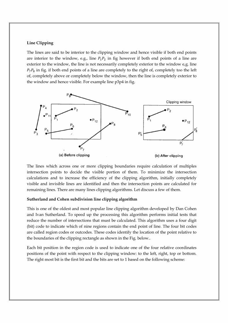
Line Clipping

The lines are said to be interior to the clipping window and hence visible if both end points

are interior to the window, e.g., line %2%3 in fig however if both end points of a line are

exterior to the window, the line is not necessarily completely exterior to the window e,g. line %4%5 in fig. if both end points of a line are completely to the right of, completely too the left

of, completely above or completely below the window, then the line is completely exterior to

the window and hence visible. For example line p3p4 in fig.

The lines which across one or more clipping boundaries require calculation of multiples

intersection points to decide the visible portion of them. To minimize the intersection

calculations and to increase the efficiency of the clipping algorithm, initially completely

visible and invisible lines are identified and then the intersection points are calculated for

remaining lines. There are many lines clipping algorithms. Let discuss a few of them.

Sutherland and Cohen subdivision line clipping algorithm

This is one of the oldest and most popular line clipping algorithm developed by Dan Cohen

and Ivan Sutherland. To speed up the processing this algorithm performs initial tests that

reduce the number of intersections that must be calculated. This algorithm uses a four digit

(bit) code to indicate which of nine regions contain the end point of line. The four bit codes

are called region codes or outcodes. These codes identify the location of the point relative to

the boundaries of the clipping rectangle as shown in the Fig. below..

Each bit position in the region code is used to indicate one of the four relative coordinates

positions of the point with respect to the clipping window: to the left, right, top or bottom.

The right most bit is the first bit and the bits are set to 1 based on the following scheme:

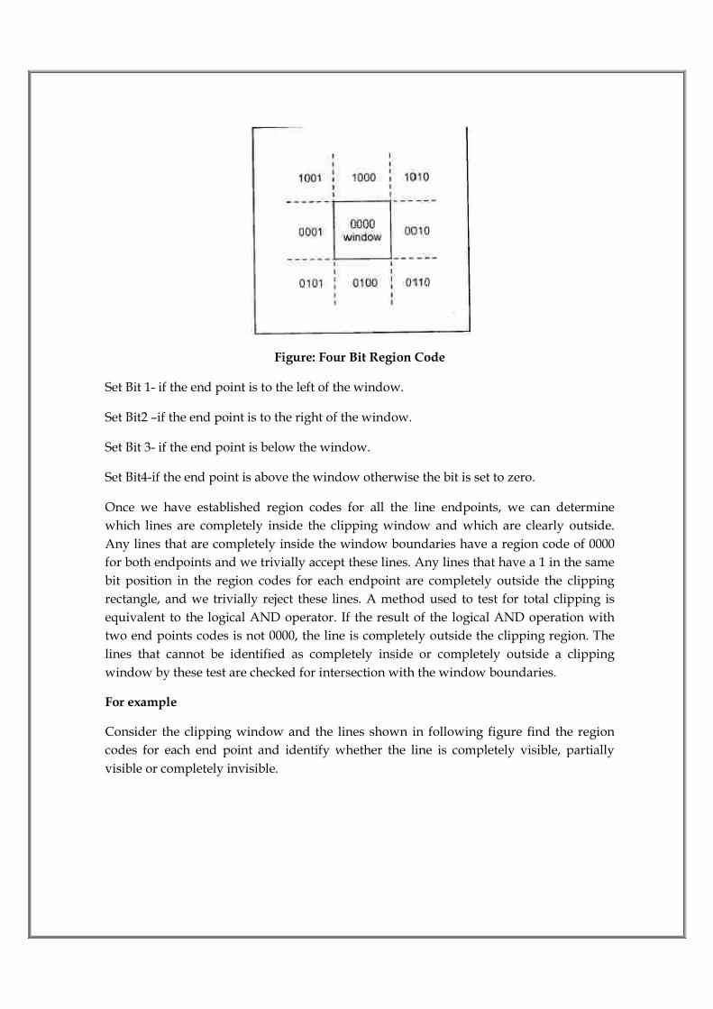
Figure: Four Bit Region Code

Set Bit 1- if the end point is to the left of the window.

Set Bit2 –if the end point is to the right of the window.

Set Bit 3- if the end point is below the window.

Set Bit4-if the end point is above the window otherwise the bit is set to zero.

Once we have established region codes for all the line endpoints, we can determine

which lines are completely inside the clipping window and which are clearly outside.

Any lines that are completely inside the window boundaries have a region code of 0000

for both endpoints and we trivially accept these lines. Any lines that have a 1 in the same

bit position in the region codes for each endpoint are completely outside the clipping

rectangle, and we trivially reject these lines. A method used to test for total clipping is

equivalent to the logical AND operator. If the result of the logical AND operation with

two end points codes is not 0000, the line is completely outside the clipping region. The

lines that cannot be identified as completely inside or completely outside a clipping

window by these test are checked for intersection with the window boundaries.

For example

Consider the clipping window and the lines shown in following figure find the region

codes for each end point and identify whether the line is completely visible, partially

visible or completely invisible.

Figure: Example clipping window

If we solve the above problem. The following figure shows the clipping window and

lines with region codes. These codes are tabulated and end point codes are logically

ANDed to identify the visibility of the line in table below.

Line EndPoints Codes

Logical ANDing Result

P1P2 0000 0000 0000 Completely Visible

P3P4 0001 0001 0001 Completely Invisible

P5P6 0001 0000 0000 partially Visible

P7P8 0100 0010 0000 partially

Visible

P9P10 1000 0010 0000 partially Visible

The Sutherland Cohen algorithm begins the clipping process for a partially visible line by

comparing an outside endpoint to a clipping boundary to determine how much of the

line can be discarded. Then the remaining part of the line is checked against the other

boundaries and the process is continued until either the line is totally discarded or a

section is found inside the window.

Figure : Clipping Process

As shown in the figure above line P1P2 is a partially visible and point P1 is outside the

window. starting with point P1, the intersection point P1’ is found and we get two line

segment P1-P1’ and P1’-P2. We know that, for P1-P1’ one end point i.e. P1 is outside the

window and thus the line segment P1-P1’ is discarded. The line is now reduced to the

section from P1’ to P2. Since P2 is outside the clip window, it is checked against the

boundaries and intersection point P2’ is found . again the line segment is divided into

two segments giving P1’-P2’ and P2’-P2. We know that, for P2’-P2 one end point i.e. P2 is

outside the window and thus the line segment P2’-P2 is discarded. The remaining line

segment P1’-P2’ is completely inside the clipping window and hence made visible.

The intersection points with a clipping boundary can be calculated using the slope-

intercept from of the line equation. The equation for line passing through points

P1(x1,y1) and P2(x2,y2) is

6 = 7*8 − 82, + 62 or 6 = 7*8 − 83, + 63

Where 7 = :;(:<=;(=< *�> ?@ A Bℎ@ >��@,

Therefore the intersections with the clipping boundaries of the window are given as:

>@AB ∶ EF, 6 = 7*EF − E2, + G2 ; 7 ≠ ∞

�JℎB ∶ EK , 6 = 7*EK − E2, + G2 ; 7 ≠ ∞

& ? ∶ GL , E = E2 + 17 *GL − G2, ; 7 ≠ 0

� BB 7 ∶ GM , E = E2 + 17 *GM − G2, ; 7 ≠ 0

Q.8 What is an illumination model? Develop an illumination model to consider ambient

light, specular reflection and diffused reflection?

Ans.

An illumination model (also lighting model or shading model) is used for determining the

color and brightness a viewer perceives and therefore which color a pixel should have,

according to the lighting conditions and surface-properties of the objects. Together with

the perspective projection, this is one of the most important contributions to the realistic

look of computer-generated images.

To keep things simple, all of the following examinations and formulas refer only to the

brightness of the lighting. To handle colors, all the calculations have to be done in

various wavelengths. The simplest case is to do them in red, green and blue.

• Light Sources and Surfaces

Light Source

To calculate the influence of light, light

sources are needed. Properties of those

can be: Form: Light-direction, point

light, directional point light, area light

source, …

Properties: brightness, color, distance, …

Object surfaces

Surfaces can reflect light

equally in every direction,

like paper or chalk. This is

called diffuse reflection.

Surfaces can also reflect

most of the light in a

particular direction, like metal, varnish or polish. This is called specular reflection.

Furthermore, surfaces can be transparent, which means that light goes through the surface

and leaves it on the other side, as with glass or water. Real surfaces usually have a

mixture of these properties. Note that light not only incidents from light sources, but also

from reflections from other surfaces.

A simple Lighting-Model

A physically exact simulation of light and it’s interaction with surfaces is very complex.

Therefore, in practice, simplified and empirical lighting-models are used, which are

based on the following.

Background light (ambient light)

Since every object reflects a part of the incoming light, it’s not completely dark

in areas where there is no direct light incident from a light source. This

everywhere existent light is called background light or ambient light. In simple

illumination-models a constant value Ia is included in the lighting calculations

for the ambient light.

Lambert’s law

This law states, that the flatter the light incidents on a surface, the darker

this surface appears. Through this effect we finally get the impression of a

spatial form. Let Il be the brightness of the involved light source and kd, 0 ≤

kd ≤ 1, the diffuse reflection coefficient which indicates, how much percent of

incoming light is reflected equally in all directions. Furthermore let θ be the

angle between the surface-normal and the direction to the light source,

which is the direction of light incident. Then the resulting intensity I at the surface-point

is:

Ι = Ι = Ι = Ι = κκκκδδδδ ⋅ ΙΙΙΙλλλλ ⋅ χοσ θ χοσ θ χοσ θ χοσ θ = κκκκδδδδ ⋅ ΙΙΙΙλλλλ ⋅ Ν Ν Ν Ν⋅ΛΛΛΛ

[Ν⋅L means scalar product]

If the ambient light is added, a nice

sphere is the result (upper sphere = only

diffuse light, lower sphere = diffuse +

ambient).

Specular Highlights

Almost all surfaces are slightly reflecting. If this is not modeled in an illumination model,

the objects appear dull. Because the exact computation of reflections is quite complicated

to calculate, a simple function, which has similar characteristics as the highlight, is used

as an approximation instead. The function used is cosn. With the free parameter n the

glossiness of the surface can be controlled. The bigger n, the smaller the highlight and

therefore the surface appears “harder” or “more polished” (left sphere). The smaller n is,

the duller the surface appears (right sphere). To add the highlights to the lighting-model,

the specular reflection coefficient ks is introduced. The highlight is then calculated according

to the Phong-illumination-model as follows:

Il,spec = ks ⋅ Il ⋅ cosnφ = ks ⋅ Il ⋅ (R⋅V)n.

The angle φ is the difference between the exact ray of reflection and the direction to the

eye.

A more physically correct model is the usage of the Fresnel

equations for reflectance, which describe that the reflectance

is also dependent on the angle of light-incidence. This means

that the coefficient ks is actually a function W(N) of light-

incidence. For most materials however, this value is almost

constant. This is the reason why usually this more complex

model is not applied, unless a material is used where this

behavior is noticeable. The image on the right shows the

dependence of the function W(N) on the angle between light-

incident and the surface-normal for three different materials.

When calculating the vector R it should be noted, that those vectors are in 3d-space, L, N

and R must lie in one plane and all of them have to have unit-length 1. R can be

calculated as R = (2N·L) N – L. Since the function for the highlights is just a rough

estimation, often a more simple formula is used, where R⋅V is replaced by N⋅H. The angle

between N and the bisector H between L and V is very similar to φ.

If we combine all those lighting-components, we get a

simple and complete lighting-model: I =ka ⋅ Ia + Σl=1-n (kd ⋅ Il ⋅ N⋅L + ks ⋅ Il ⋅ (N⋅Hl)n)

There are a lot more aspects which have to be considered to get closer to “real” images,

but this will not be described here: color-shift depending on the view-direction, influence

of the distance to the light source, anisotropic surfaces and light sources, transparency,

atmospheric effects, shadows, etc.

Diffuse Reflection- Diffuse reflection is characteristic of light reflected from a dull, non shiny surface. Objects illuminated solely by diffusely reflected light exhibit an equal light intensity from all viewing directions. That is in diffuse reflection light incident on the surface is reflected equally in all directions and is attenuated by an amount dependent upon the physical properties of the surface. Since light is reflected equally in all directions the perceived illumination of the surface is not dependent on the position of the observer. Diffuse reflection models the light reflecting properties of matt surfaces i.e. surfaces that are rough or grainy which tend to scatter the reflected light in all directions. This scattered light is called diffuse reflection.

References- 1. R. Steinmetz and K. Nahrstedt, Multimedia: Computing, Communications and Applications,

Prentice Hall P T R, 1995. 2. Computer Graphics (Principles and Practice) by Foley, van Dam, Feiner and Hughes, Addisen Wesley (Indian Edition) 3. Computer Graphics by D Hearn and P M Baker, Printice Hall of India (Indian Edition). 4.Mathematical Elements for Computer Graphics by D F Rogers.

5. www.google.com

6. Computer graphics –schum series. 7. Computer Graphics by Godse.