Computer Graphics Labs

Abel J. P. Gomes

LAB. 2

Department of Computer Science and Engineering University of Beira Interior

Portugal 2011

Copyright © 2009-2011 All rights reserved.

LAB. 2

GEOMETRIC TRANSFORMATIONS 1. Learning goals 2. Getting started 3. Euclidean transformations 4. Affine transformations 5. 3D transformations in OpenGL 6. Example 7. Programming exercises 8. Final remarks

Lab. 2

GEOMETRIC TRANSFORMATIONS In this lecture we are going to deal with geometric transformations in 2D as their generalization in 3D is straightforward. These geometric transformations are also called affine transformations.

1 . Learn ing Goals

At the end of this chapter you should be able to :

1. Explain what transformations are and why we use them in computer graphics.

2. List the three main transformations we use in computer graphics and describe what each one does.

3. Understand how to rotate a point around an arbitrary point.

4. Understand what homogenous coordinates are and why we use them in computer graphics.

5. Understand the importance of the order of operations in a matrix multiplication expression.

6. Understand what a CTM (Combined Transformation Matrix) is and understand what order the transformations must be in to achieve the desired CTM.

7. Be aware of the default facilities of OpenGL; for example, the default 2D domain is OpenGL is [-1,1]x[-1,1].

2 . Gett ing Star ted

Geometric transformations are used to fulfill two main requirements in computer graphics:

1. To model and construct scenes.

2. To nav igate our way around 2 and 3 dimensional space.

For example, when a street building has n identical windows, we proceed as follows:

1. To construct a single window by means of graphics primitives;

2. To replicate n times the window.

3. To put each window at a desirable location using translations and rotations.

This shows that transformations such as translations and rotations can be used as scene model ing operations.

These transformations can be also used to move a bot or an avatar in the virtual environment of a First-Person Shooter (FPS) game.

3 . Euc l idean Transformat ions

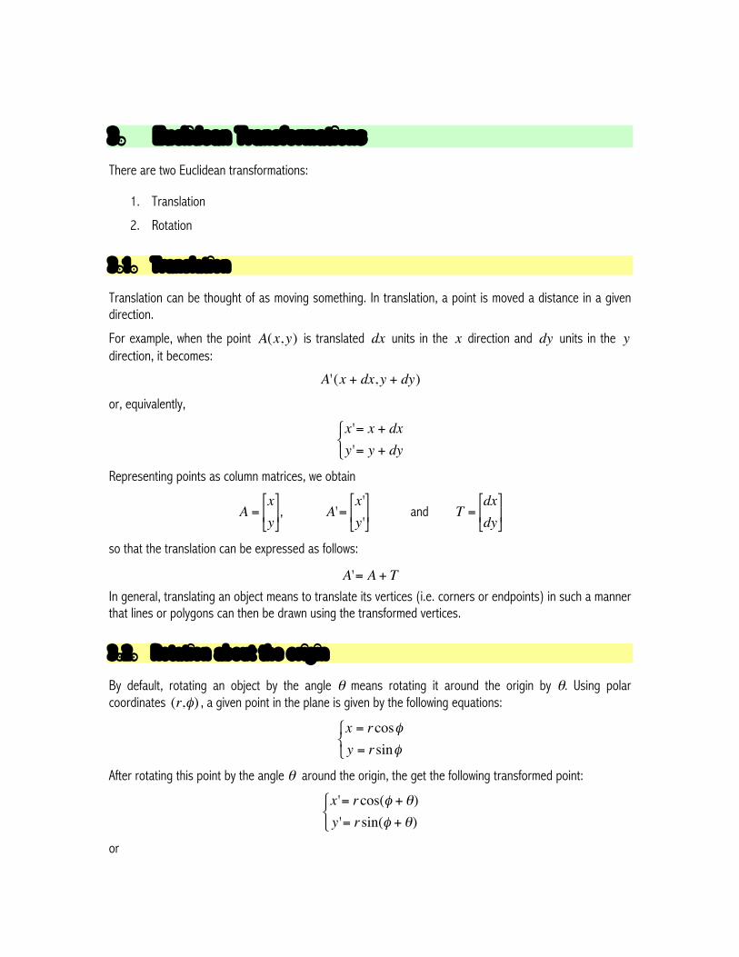
There are two Euclidean transformations:

1. Translation

2. Rotation

3.1. Trans lat ion

Translation can be thought of as moving something. In translation, a point is moved a distance in a given direction.

For example, when the point

€

A(x,y) is translated

€

dx units in the

€

x direction and

€

dy units in the

€

y direction, it becomes:

€

A'(x + dx,y + dy)

or, equivalently,

€

x '= x + dxy '= y + dy⎧ ⎨ ⎩

Representing points as column matrices, we obtain

€

A =xy⎡

⎣ ⎢ ⎤

⎦ ⎥ ,

€

A'=x'y'⎡

⎣ ⎢ ⎤

⎦ ⎥ and

€

T =dxdy⎡

⎣ ⎢

⎤

⎦ ⎥

so that the translation can be expressed as follows:

€

A'= A + T

In general, translating an object means to translate its vertices (i.e. corners or endpoints) in such a manner that lines or polygons can then be drawn using the transformed vertices.

3 .2. Rotat ion about the or ig in

By default, rotating an object by the angle θ means rotating it around the origin by θ. Using polar coordinates

€

(r,φ) , a given point in the plane is given by the following equations:

€

x = rcosφy = rsinφ

⎧ ⎨ ⎩

After rotating this point by the angle θ around the origin, the get the following transformed point:

€

x '= rcos(φ + θ)y '= rsin(φ + θ)

⎧ ⎨ ⎩

or

€

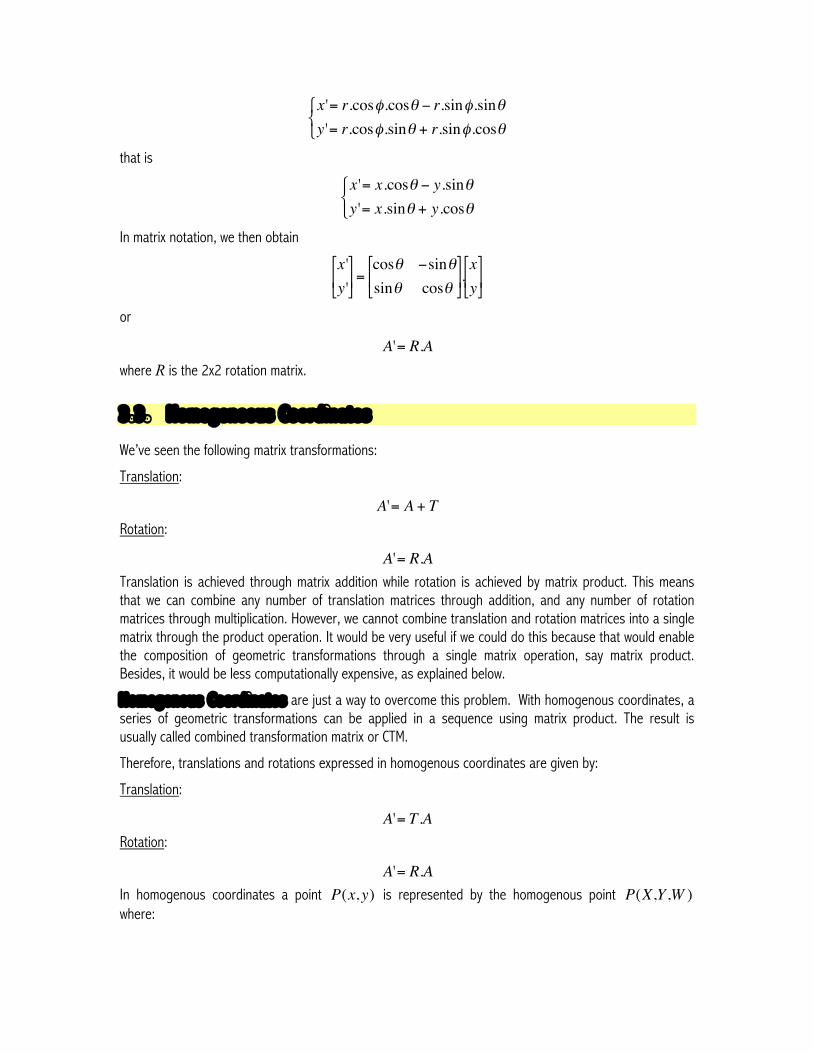
x '= r.cosφ.cosθ − r.sinφ.sinθy '= r.cosφ.sinθ + r.sinφ.cosθ⎧ ⎨ ⎩

that is

€

x '= x.cosθ − y.sinθy '= x.sinθ + y.cosθ⎧ ⎨ ⎩

In matrix notation, we then obtain

€

x 'y '⎡

⎣ ⎢ ⎤

⎦ ⎥ =

cosθ −sinθsinθ cosθ⎡

⎣ ⎢

⎤

⎦ ⎥ .xy⎡

⎣ ⎢ ⎤

⎦ ⎥

or

€

A'= R.A

where R is the 2x2 rotation matrix.

3 .3. Homogeneous Coord inates

We’ve seen the following matrix transformations:

Translation:

€

A'= A + T

Rotation:

€

A'= R.A

Translation is achieved through matrix addition while rotation is achieved by matrix product. This means that we can combine any number of translation matrices through addition, and any number of rotation matrices through multiplication. However, we cannot combine translation and rotation matrices into a single matrix through the product operation. It would be very useful if we could do this because that would enable the composition of geometric transformations through a single matrix operation, say matrix product. Besides, it would be less computationally expensive, as explained below.

Homogenous Coord inates are just a way to overcome this problem. With homogenous coordinates, a series of geometric transformations can be applied in a sequence using matrix product. The result is usually called combined transformation matrix or CTM.

Therefore, translations and rotations expressed in homogenous coordinates are given by:

Translation:

€

A'= T.A

Rotation:

€

A'= R.A

In homogenous coordinates a point

€

P(x,y) is represented by the homogenous point

€

P(X,Y,W ) where:

€

X =xW

and

€

Y =yW

,

where

€

W usually equals 1 in computer graphics for simplicity.

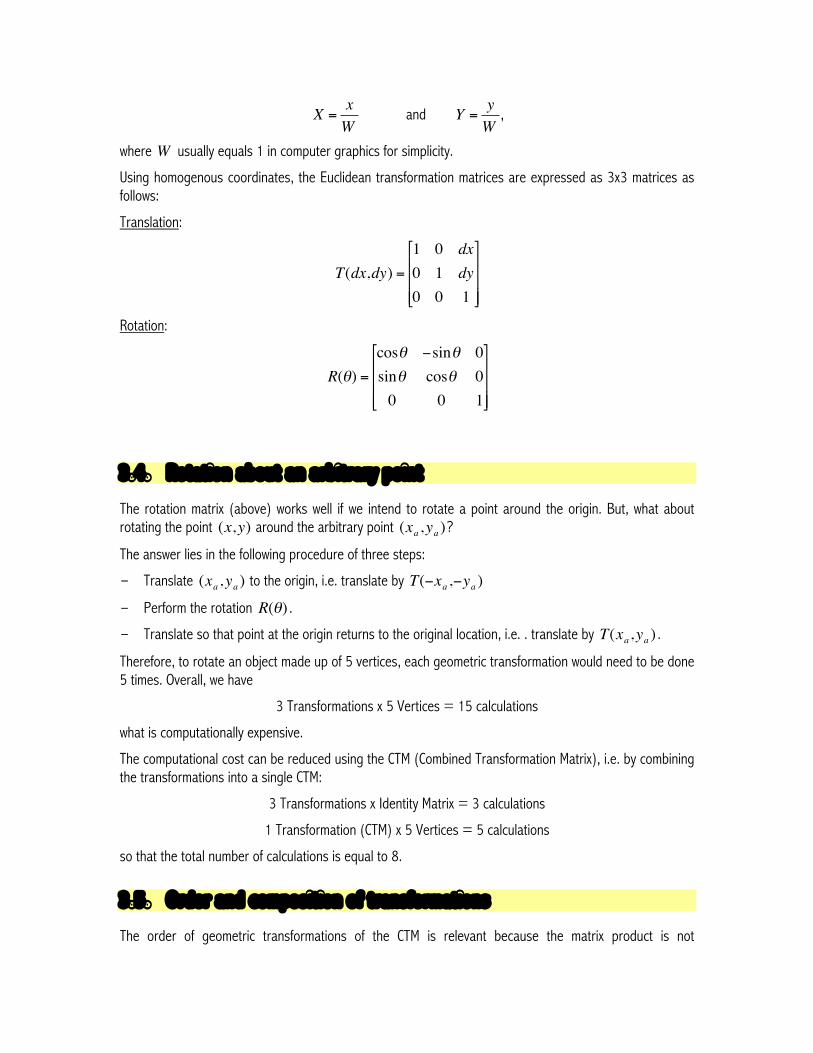
Using homogenous coordinates, the Euclidean transformation matrices are expressed as 3x3 matrices as follows:

Translation:

€

T(dx,dy) =

1 0 dx0 1 dy0 0 1

⎡

⎣

⎢ ⎢ ⎢

⎤

⎦

⎥ ⎥ ⎥

Rotation:

€

R(θ) =

cosθ −sinθ 0sinθ cosθ 00 0 1

⎡

⎣

⎢ ⎢ ⎢

⎤

⎦

⎥ ⎥ ⎥

3 .4. Rotat ion about an arb i t rary po int

The rotation matrix (above) works well if we intend to rotate a point around the origin. But, what about rotating the point

€

(x,y) around the arbitrary point

€

(xa ,ya )?

The answer lies in the following procedure of three steps:

- Translate

€

(xa ,ya ) to the origin, i.e. translate by

€

T(−xa ,−ya )

- Perform the rotation

€

R(θ) . - Translate so that point at the origin returns to the original location, i.e. . translate by

€

T(xa,ya ) .

Therefore, to rotate an object made up of 5 vertices, each geometric transformation would need to be done 5 times. Overall, we have

3 Transformations x 5 Vertices = 15 calculations

what is computationally expensive.

The computational cost can be reduced using the CTM (Combined Transformation Matrix), i.e. by combining the transformations into a single CTM:

3 Transformations x Identity Matrix = 3 calculations

1 Transformation (CTM) x 5 Vertices = 5 calculations

so that the total number of calculations is equal to 8.

3 .5. Order and composi t ion of t ransformat ions

The order of geometric transformations of the CTM is relevant because the matrix product is not

commutative. In fact,

Matrix product is associative:

When multiplying matrices, the order we carry out the multiplications is not relevant, that is

€

A .B .C = (A .B) .C = A . (B .C)

Matrix multiplication is not commutative:

When multiplying matrices together, we carry out the multiplications is relevant, that is

€

A .B ≠ B . A

The question is then how do we work out the order of our matrices when creating the CTM? Turning back to the steps to rotate the point around the point , let us rewrite the corresponding procedure:

- Translate

€

(xa ,ya ) to the origin, i.e. translate by

€

T(−xa ,−ya )

- Perform the rotation

€

R(θ) . - Translate so that point at the origin returns to the original location, i.e. . translate by

€

T(xa,ya ) .

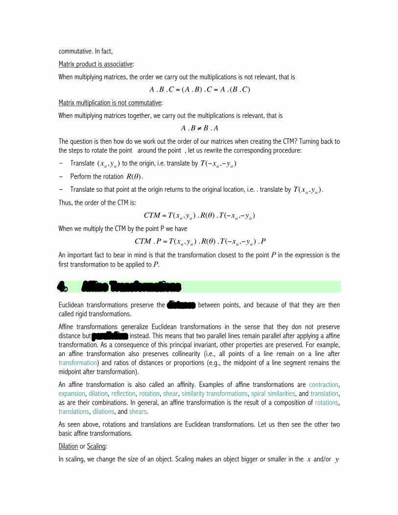
Thus, the order of the CTM is:

€

CTM = T(xa,ya ) .R(θ) .T(−xa,−ya )

When we multiply the CTM by the point P we have

€

CTM .P = T(xa,ya ) .R(θ) .T(−xa,−ya ) .P

An important fact to bear in mind is that the transformation closest to the point P in the expression is the first transformation to be applied to P.

4 . Af f ine Transformat ions

Euclidean transformations preserve the d istance between points, and because of that they are then called rigid transformations.

Affine transformations generalize Euclidean transformations in the sense that they don not preserve distance but para l le l ism instead. This means that two parallel lines remain parallel after applying a affine transformation. As a consequence of this principal invariant, other properties are preserved. For example, an affine transformation also preserves collinearity (i.e., all points of a line remain on a line after transformation) and ratios of distances or proportions (e.g., the midpoint of a line segment remains the midpoint after transformation).

An affine transformation is also called an affinity. Examples of affine transformations are contraction, expansion, dilation, reflection, rotation, shear, similarity transformations, spiral similarities, and translation, as are their combinations. In general, an affine transformation is the result of a composition of rotations, translations, dilations, and shears.

As seen above, rotations and translations are Euclidean transformations. Let us then see the other two basic affine transformations.

Dilation or Scaling:

In scaling, we change the size of an object. Scaling makes an object bigger or smaller in the

€

x and/or

€

y

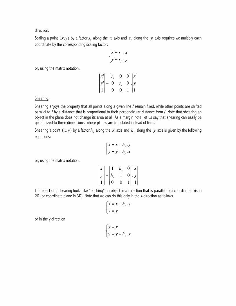
direction.

Scaling a point

€

(x,y) by a factor

€

sx along the

€

x axis and

€

sy along the

€

y axis requires we multiply each coordinate by the corresponding scaling factor:

€

x '= sx . xy '= sy . y⎧ ⎨ ⎩

or, using the matrix notation,

€

x 'y '1

⎡

⎣

⎢ ⎢ ⎢

⎤

⎦

⎥ ⎥ ⎥

=

sx 0 00 sy 00 0 1

⎡

⎣

⎢ ⎢ ⎢

⎤

⎦

⎥ ⎥ ⎥

.xy1

⎡

⎣

⎢ ⎢ ⎢

⎤

⎦

⎥ ⎥ ⎥

Shearing:

Shearing enjoys the property that all points along a given line l remain fixed, while other points are shifted parallel to l by a distance that is proportional to their perpendicular distance from l. Note that shearing an object in the plane does not change its area at all. As a margin note, let us say that shearing can easily be generalized to three dimensions, where planes are translated instead of lines.

Shearing a point

€

(x,y) by a factor

€

hx along the

€

x axis and

€

hy along the

€

y axis is given by the following equations:

€

x '= x + hx .yy '= y + hy .x⎧ ⎨ ⎩

or, using the matrix notation,

€

x 'y '1

⎡

⎣

⎢ ⎢ ⎢

⎤

⎦

⎥ ⎥ ⎥

=

1 hx 0hy 1 00 0 1

⎡

⎣

⎢ ⎢ ⎢

⎤

⎦

⎥ ⎥ ⎥

.xy1

⎡

⎣

⎢ ⎢ ⎢

⎤

⎦

⎥ ⎥ ⎥

The effect of a shearing looks like “pushing” an object in a direction that is parallel to a coordinate axis in 2D (or coordinate plane in 3D). Note that we can do this only in the x-direction as follows

€

x '= x + hx .yy'= y⎧ ⎨ ⎩

or in the y-direction

€

x'= xy '= y + hy .x⎧ ⎨ ⎩

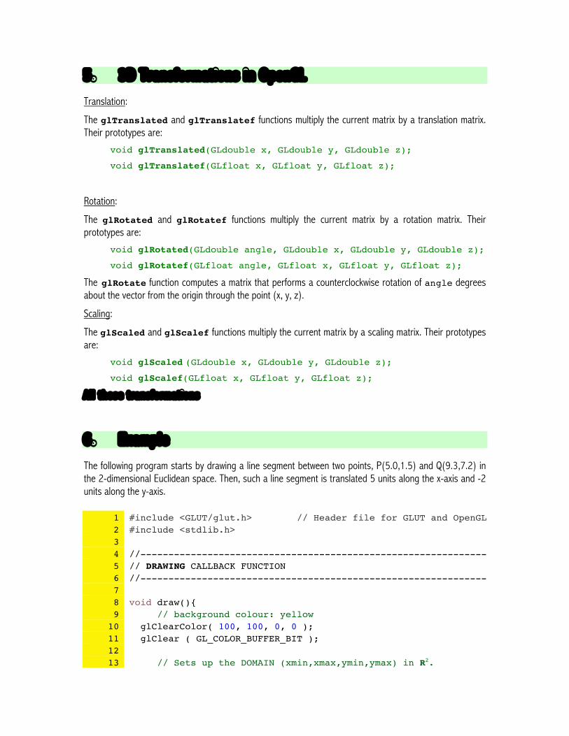
5. 3D Transformat ions in OpenGL

Translation:

The glTranslated and glTranslatef functions multiply the current matrix by a translation matrix. Their prototypes are:

void glTranslated(GLdouble x, GLdouble y, GLdouble z);

void glTranslatef(GLfloat x, GLfloat y, GLfloat z);

Rotation:

The glRotated and glRotatef functions multiply the current matrix by a rotation matrix. Their prototypes are:

void glRotated(GLdouble angle, GLdouble x, GLdouble y, GLdouble z);

void glRotatef(GLfloat angle, GLfloat x, GLfloat y, GLfloat z);

The glRotate function computes a matrix that performs a counterclockwise rotation of angle degrees about the vector from the origin through the point (x, y, z).

Scaling:

The glScaled and glScalef functions multiply the current matrix by a scaling matrix. Their prototypes are:

void glScaled (GLdouble x, GLdouble y, GLdouble z); void glScalef(GLfloat x, GLfloat y, GLfloat z);

Al l these transformat ions

6 . Example

The following program starts by drawing a line segment between two points, P(5.0,1.5) and Q(9.3,7.2) in the 2-dimensional Euclidean space. Then, such a line segment is translated 5 units along the x-axis and -2 units along the y-axis.

1 #include <GLUT/glut.h> // Header file for GLUT and OpenGL 2 #include <stdlib.h> 3 4 //-------------------------------------------------------------- 5 // DRAWING CALLBACK FUNCTION 6 //-------------------------------------------------------------- 7 8 void draw(){ 9 // background colour: yellow

10 glClearColor( 100, 100, 0, 0 ); 11 glClear ( GL_COLOR_BUFFER_BIT ); 12 13 // Sets up the DOMAIN (xmin,xmax,ymin,ymax) in R2.

14 // Let (xmin,xmax,ymin,ymax)=(0.0,20.0,0.0,20.0) 15 glMatrixMode(GL_PROJECTION); 16 glLoadIdentity(); 17 gluOrtho2D(0.0,20.0,0.0,20.0); 18 19 // Let us now define the line segment in red 20 // Endpoints: (5.0,1.5) and (9.3,7.2) 21 glMatrixMode(GL_MODELVIEW); 22 glLoadIdentity(); 23 glTranslatef(5,-2,0); 24 glColor3f( 1, 0, 0 ); 25 glBegin(GL_LINES); 26 glVertex2f(5.0,1.5); 27 glVertex2f(9.3,7.2); 28 glEnd(); 29 30 // display line segment 31 glutSwapBuffers(); 32 } 33 34 //-------------------------------------------------------------- 35 // KEYBOARD CALLBACK FUNCTION 36 //-------------------------------------------------------------- 37 38 void keyboard(unsigned char key,int x,int y) 39 { 40 // press ESC key to quit 41 if(key==27) exit(0); 42 } 43 44 //-------------------------------------------------------------- 45 // MAIN FUNCTION 46 //-------------------------------------------------------------- 47 48 int main(int argc, char ** argv) 49 { 50 glutInit(&argc, argv); 51 // Double Buffered RGB display 52 glutInitDisplayMode( GLUT_RGB | GLUT_DOUBLE); 53 // Set window size 54 glutInitWindowSize( 500,500 ); 55 glutCreateWindow("Line Segment"); 56 // Declare callback functions 57 glutDisplayFunc(draw); 58 glutKeyboardFunc(keyboard); 59 // Start the main loop of events 60 glutMainLoop(); 61 return 0; 62 }

Comments:

(1) The translation appears on line 23, just before the object. Why? (2) Assume that now we wish to rotate the line segment by 45 degrees. Where do you put the rotation

function? Before or after the translation function? Why?

7 . Programming Exerc ises

1. Re-write the house-building program implemented in the last class in a way that all building blocks (body, roof, windows and door) are constructed from the origin. Then, use translations to place these blocks at the desired locations. Each block is constructed in a separate function. In the particular case of the window, we need to call it twice because we are assuming that the house has two windows.

2. Add the toggle facilities to the previous program 1. in a manner that to add/remove the house body by pressing the ‘b’ key, roof by pressing the ‘r’ key, windows by pressing the ‘w’ key, and door by pressing the ‘d’ key.

3. Let us now replicate twice the house. The first copy of the original house must be reduced down to ¾ and placed side-by-side on the left of the original house. The second house copy must be scaled up to 5/4 and placed side-by-side on the right of the original house.

4. Write a program to draw a circle of a given radius r. 5. Let us now add the bright sun to the scene of the previous program, changing the position of the sun

by clicking on the ‘s’ key. The trajectory of the sun is a circle arc.

8 . Fina l Remarks

1. Transformations are mathematical functions that allow us to model and to navigate within 2D and 3D spaces.

2. In computer graphics, we use three main transformations: translation, scaling and rotation.

3. Homogenous coordinates allow us to treat translation, scaling and rotation in the same manner. Consequently, all affine transformations can be combined into a CTM that substantially reduces the calculations that need to be made.

4. Matrix multiplication is associative but not commutative.

5. A CTM combines a number of transformations into a single matrix.

6. The order of drawing objects in OpenGL is the same as the one of the sequence of the C program, i.e. top-bottom order. However, the order of applying geometric transformations to objects is the opposite, and follows the logic of a stack: last in, first out. The stack here is the GL_MODELVIEW.