http://www.bcanotes.gurukpo.com/suggestions to the under mentioned address. Author For more detail:- http://www.gurukpo.comSyllabus BCA Computer Graphics 1. Graphic Application and Hardware : Need of Graphics, Display and Input Devices. 2. Transformation : Matrix Representation and Homogeneous Coordinates : Basic Transformations-2-dimensions and 3-dimensions : Translations, Scaling and Rotations. 3. Output Primitives : Line Drawing Algorithms : DDA Bresenham Line Drawing, Circle Drawing Midpoint Algo, Ellipse Generating Midpoint Algo. 4. Clipping : Sutherland – Cohen Algo, Cyrus, Beck Algo. 5. Hidden Surface Removal : Back Face Detection, Depth Buffer, Depth Sorting, Scan Line and A Buffer Techniques. 6. Curves and Surface : Hermit Curves, Bezier Curves, B – Spline Curves, Properties and Continuity Concepts. 7. Image Processing : Capture and Storage of Digital Images, File Formats, Basic Digital Techniques like Convolutions the Holding and Histogram Manipulations, Image Enhancement, Geometric Manipulation and their Applications the Automatic Identification and Extraction of Objects of Interest. 8. Multimedia : Hardware, Software Application, Non Temporal Media : Text, Hypertext, Images, Cameras, Scanner, Frames Grabbers, Formats; Audio : Analog Video Operations, Compression, Digital Video MPEG, JPEG; Graphics Animation : Tweaking, Morphing Motion Specification, Simulating Acceleration. □ □ □For more detail:- http://www.gurukpo.comContent S.No. Name of Topic Page No. 1. Graphics Application and Hardware 7-19 1.1 Introduction to Computer Graphics 1.2 Application of Computer Graphics 1.3 Video Display Devices 1.4 Raster Scan Displays 1.5 Random Scan Displays 1.6 Color CRT Monitor 1.7 Shadow Mask Methods 2. Transformation 20-30 2.1 Transformation in 2-dimension & 3-dimension 2.2 Rotation in 2-dimansion & 3-dimension 2.3 Scaling in 2-dimansion & 3-dimension 2.4 Composite Transformation 2.5 Reflection

2.6 Shear 3. Output Primitives 31-49 3.1 Line Drawing Algorithms (a) DDA (b) Bresenham’s Algorithm 3.2 Circle Drawing Algorithm 3.3 Ellipse Drawing Algorithm 3.4 Boundary Fill Algorithm 3.5 Flood Fill Algorithm 4. Clipping Algorithm 50-58 4.1 Introduction to Clipping 4.2 Application of Clipping 4.3 Line Clipping Methods (a) Cohen Sutherland Method (b) Cyrus – Beck Algorithm For more detail:- http://www.gurukpo.comS.No. Name of Topic Page No. 5. Visible Surface Detection 59-70 5.1 Depth Buffer Method 5.2 Z – Buffer Method 5.3 Object Space Method 5.4 Image Space Method 5.5 Painter’s Algorithm 5.6 Back – Face Detection 5.7 A – Buffer Method 5.8 Scan Line Method 6. Curves and Surfaces 71-82 6.1 Bezier Curves and Surfaces 6.2 Properties of Bezier Curves 6.3 B - Spline Line and Surfaces 6.4 Properties of B – Spline Curves 6.5 Hermite Interpolation 6.6 Continuity Conditions 7. Image Processing 83-90 7.1 Introduction to Image Processing 7.2 Operations of Image Processing 7.3 Application of Image Processing 7.4 Image Enhancement Techniques 8. Multimedia 91-102 8.1 Introduction to Multimedia 8.2 Application of Multimedia 8.3 Tweaking 8.4 Morphing 8.5 Frame Grabbers 8.6 Scanners 8.7 Digital Cameras 8.8 JPEG Compression Technique

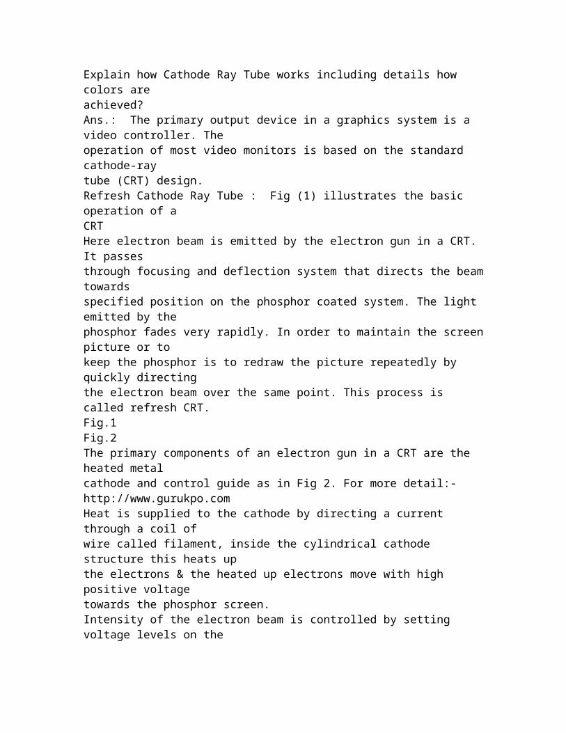
8.9 MPEG Compression Technique 8.10 Data Stream 8.11 Hypertext / Hypermedia □ □ □For more detail:- http://www.gurukpo.comChapter-1Graphics Application and Hardware Q.1 What is Computer Graphics? What is its application?Ans.: Computer has become a powerful tool for rapid and economical production of pictures. There is virtually no area in which graphical displays cannot is used to some advantage. To day computer graphics is used delusively in such areas as science, medicine, Engineering etc. Application of computer graphics : (1) Computer – Aided Design : Generally used in the design of building, automobiles, aircrafts, textiles and many other products. (2) Presentation Graphics : This is used to produce illustration for or to generate 35-cm slides or trans pare miss for use with projectors. (3) Computer Art : Computer graphics methods are widely used in both fine arts and Commercial Arts Applications. (4) Entertainment : Computer graphics methods are now commonly used in making motion pictures, music videos, television shows. (5) Education and Training : Computer generated models of physical, financial, and economic systems are after used as education aids. (6) Visualization : This is used in connation with data sets related to commerce, industry and other scientific areas. (7) Image Processing : It applies techniques to modify or inter put existing pictures such as photographs. (8) Graphical user Interface : It is common now for software packages to provide a graphical Interface. For more detail:- http://www.gurukpo.comQ.2 What are Video Display Devices? or Explain how Cathode Ray Tube works including details how colors are achieved? Ans.: The primary output device in a graphics system is a video controller. The operation of most video monitors is based on the standard cathode-ray tube (CRT) design.Refresh Cathode Ray Tube : Fig (1) illustrates the basic operation of a CRT Here electron beam is emitted by the electron gun in a CRT. It passes through focusing and deflection system that directs the beam towards specified position on the phosphor coated system. The light emitted by the phosphor fades very rapidly. In order to maintain the screen picture or to keep the phosphor is to redraw the picture repeatedly by quickly directing the electron beam over the same point. This process is called refresh CRT.Fig.1 Fig.2 The primary components of an electron gun in a CRT are the heated metal

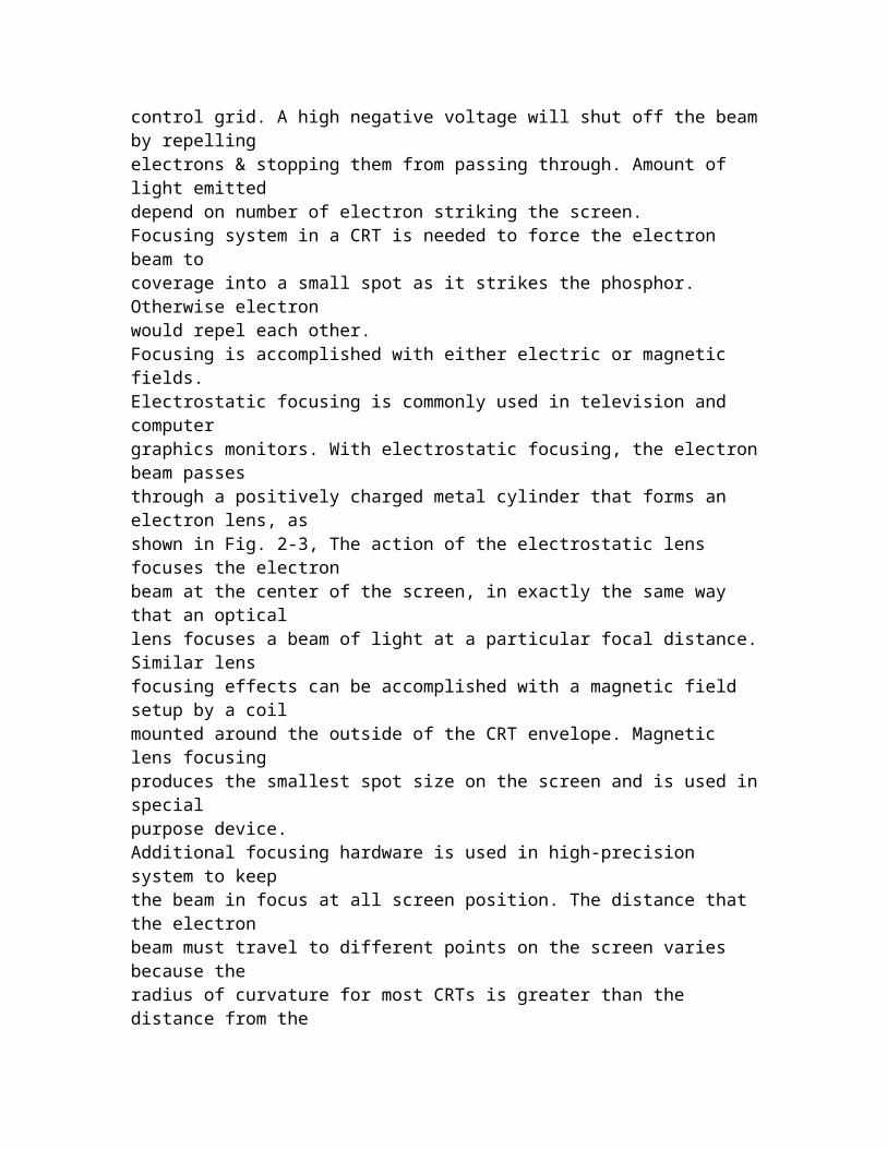
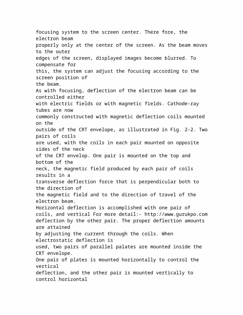
cathode and control guide as in Fig 2. For more detail:- http://www.gurukpo.comHeat is supplied to the cathode by directing a current through a coil of wire called filament, inside the cylindrical cathode structure this heats up the electrons & the heated up electrons move with high positive voltage towards the phosphor screen. Intensity of the electron beam is controlled by setting voltage levels on the control grid. A high negative voltage will shut off the beam by repelling electrons & stopping them from passing through. Amount of light emitted depend on number of electron striking the screen. Focusing system in a CRT is needed to force the electron beam to coverage into a small spot as it strikes the phosphor. Otherwise electron would repel each other. Focusing is accomplished with either electric or magnetic fields. Electrostatic focusing is commonly used in television and computer graphics monitors. With electrostatic focusing, the electron beam passes through a positively charged metal cylinder that forms an electron lens, as shown in Fig. 2-3, The action of the electrostatic lens focuses the electron beam at the center of the screen, in exactly the same way that an optical lens focuses a beam of light at a particular focal distance. Similar lens focusing effects can be accomplished with a magnetic field setup by a coil mounted around the outside of the CRT envelope. Magnetic lens focusing produces the smallest spot size on the screen and is used in special purpose device. Additional focusing hardware is used in high-precision system to keep the beam in focus at all screen position. The distance that the electron beam must travel to different points on the screen varies because the radius of curvature for most CRTs is greater than the distance from the focusing system to the screen center. There fore, the electron beam properly only at the center of the screen. As the beam moves to the outer edges of the screen, displayed images become blurred. To compensate for this, the system can adjust the focusing according to the screen position of the beam. As with focusing, deflection of the electron beam can be controlled either with electric fields or with magnetic fields. Cathode-ray tubes are now commonly constructed with magnetic deflection coils mounted on the outside of the CRT envelope, as illustrated in Fig. 2-2. Two pairs of coils are used, with the coils in each pair mounted on opposite sides of the neck of the CRT envelop. One pair is mounted on the top and bottom of the neck, the magnetic field produced by each pair of coils results in a transverse deflection force that is perpendicular both to the direction of the magnetic field and to the direction of travel of the electron beam. Horizontal deflection is accomplished with one pair of coils, and vertical For more detail:- http://www.gurukpo.comdeflection by the other pair. The proper deflection amounts are attained by adjusting the current through the coils. When electrostatic deflection is used, two pairs of parallel palates are mounted inside the CRT envelope.

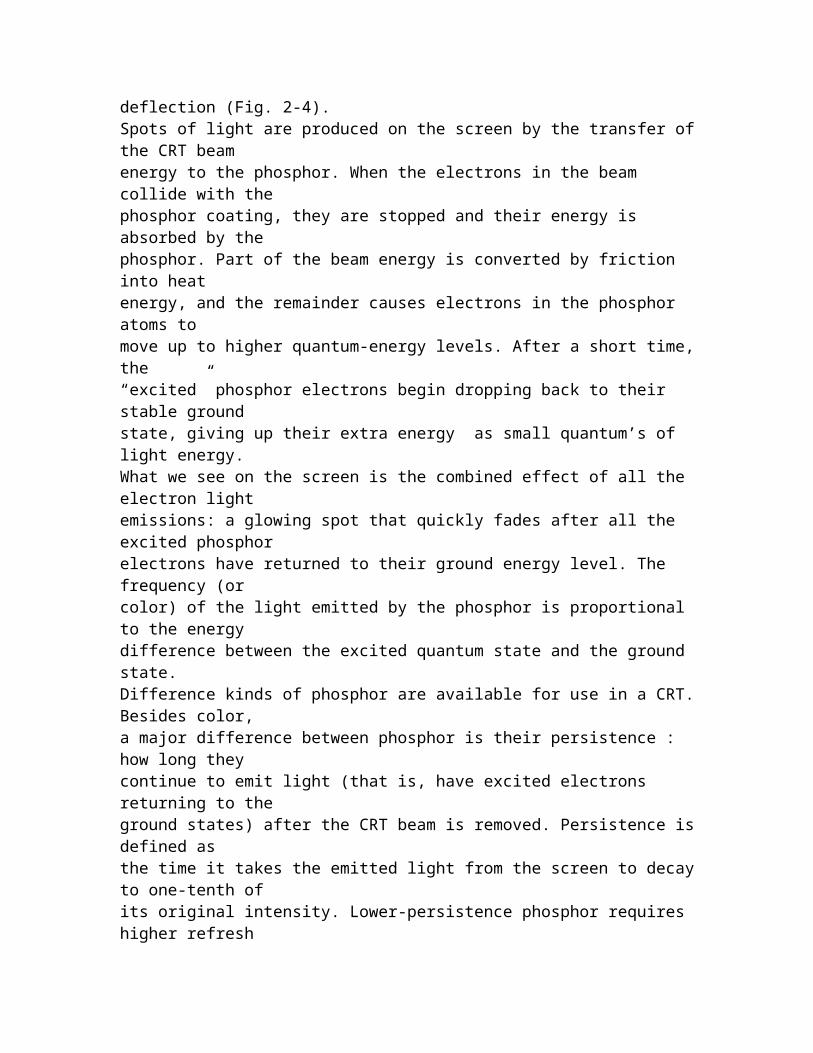
One pair of plates is mounted horizontally to control the vertical deflection, and the other pair is mounted vertically to control horizontal deflection (Fig. 2-4). Spots of light are produced on the screen by the transfer of the CRT beam energy to the phosphor. When the electrons in the beam collide with the phosphor coating, they are stopped and their energy is absorbed by the phosphor. Part of the beam energy is converted by friction into heat energy, and the remainder causes electrons in the phosphor atoms to move up to higher quantum-energy levels. After a short time, the “excited” phosphor electrons begin dropping back to their stable ground state, giving up their extra energy as small quantum’s of light energy. What we see on the screen is the combined effect of all the electron light emissions: a glowing spot that quickly fades after all the excited phosphor electrons have returned to their ground energy level. The frequency (or color) of the light emitted by the phosphor is proportional to the energy difference between the excited quantum state and the ground state. Difference kinds of phosphor are available for use in a CRT. Besides color, a major difference between phosphor is their persistence : how long they continue to emit light (that is, have excited electrons returning to the ground states) after the CRT beam is removed. Persistence is defined as the time it takes the emitted light from the screen to decay to one-tenth of its original intensity. Lower-persistence phosphor requires higher refresh rates to maintain a picture on the screen without flicker. A phosphor with low persistence is useful for displaying highly complex, static, graphics monitors are usually constructed with persistence in the range from 10 to 60 microseconds. Figure 2-5 shows the intensity distribution of a spot on the screen. The intensity is greatest at the center of the spot, and decreases with a For more detail:- http://www.gurukpo.comGaussian distribution out to the edge of the spot. This distribution corresponds to the cross-sectional electron density distribution of the CRT beam. The maximum number of points that can be displayed without overlap on a CRT is referred to as the resolution. A more precise definition of resolution is the number of points per centimeter that can be plotted horizontally and vertically, although it is often simply stated as the total number of points in each direction. Spot intensity has a Gaussian distribution (Fig. 2-5), so two adjacent spot will appear distinct as long as their separation is greater than the diameter at which each spot has intensity in Fig. 2-6. Spot size also depends on intensity. As more electrons are accelerated toward the phosphor per second, the CRT beam diameter and the illuminated spot increase. In addition, the increased excitation energy tends to spread to neighboring phosphor atoms not directly in the path of the beam, which further increases the spot diameter. Thus, resolution of a CRT is dependent on the type of phosphor, the intensity to be displayed, and the focusing and deflection

system. Typing resolution on high-quality system is 1280 by 1024, with higher resolution available on many systems. High resolution systems are often referred to as high-definition system. The physical size of a graphics monitor is given as the length of the screen diagonal, with sizes varying form about 12 inches to 27 inches or more. A CRT monitor can be attached to a variety of computer systems, so the number of screen points that can actually be plotted depends on the capabilities of the system to which it is attached. Another property of video monitors is aspect ratio. This number gives the ratio of vertical points to horizontal points necessary to produce equallength lines in both directions on the screen. (Sometimes aspect ratio is stated in terms of the ratio of horizontal to vertical points.) An aspect ratio of ¾ means that a vertical line plotted with three points has the same length as a horizontal line plotted with four points.

Q.3 Write short note on Raster–Scan Displays and Random Scan Displays. Ans.: Raster–Scan Displays : The most common type of graphics monitor employing a CRT is the raster-scan display, based on television technology. In a rater-scan system, the electron beam is swept across the screen, one row at a time from top to bottom. As the electron beam moves For more detail:- http://www.gurukpo.comacross each row, the beam intensity is turned on and off to create a pattern of illuminated spots. Picture definition is stored in a memory area called the refresh buffer or frame buffer. This memory area holds the set of intensity values for all the screen points. Stored intensity values are then retrieved from the refresh buffer and “Painted” on the screen one row (scan line) at a time (Fig. 2-7). Each screen point is referred to as a pixel or pel (shortened forms of picture element). The capability of a raster-scan system to store intensity information for each screen point makes it well suited for the realistic display of scenes containing subtle shading and color patterns. Home television sets and printers ate examples are examples of other system using raster-scan methods. Intensity range for pixel positions depends on the capability of the raster system. In a simple black-and –white system, each screen point is either on or off, so only one bit per pixel is needed to control the intensity of screen position. For a bi-level system, a bit value of 1 indicates that the electron beam is to be turned on at that position, and a value of 0 indicates that the beam intensity is to be off. Additional bits are needed when color and intensity variations can be displayed. Up to 24 bits per pixel are included in high-quality system, which can require several megabytes of storage for the frame buffer, depending on the resolution of the system. A system with 24 bits per pixel and a screen resolution of 1024 by 1024 requires 3 megabytes of storage for the frame buffer. On a black-andwhite system with one bit per pixel, the frame buffer is commonly called a

bitmap. For system with multiple bits per pixel, the frame buffer is often referred to as a pixmap.Refreshing on raster-scan displays is carried out at the rate of 60 to 80 frames per second, although some systems are designed for higher refresh rates. Sometimes, refresh rates are described in units of cycle per second, or Hertz (Hz), where a cycle corresponds to one frame. Using these units, we would describe a refresh rate of 60 frames per second as simply 60 Hz. At the end of each scan line, the electron beam returns to the left side of the screen to begin displaying the next scan line. The return to the left of the screen, after refreshing each scan line, is called the horizontal retraceof the electron beam. And at the end of each frame (displayed in 1/80th to 1/60th of a second), the electron beam returns (vertical retrace) to the top left corner of the screen to begin the next frame. For more detail:- http://www.gurukpo.comOn some raster-scan system (and in TV sets), each frame is displayed in two passes using an interlaced refresh procedure. In the first pass, the beam sweeps across every other scan line form top to bottom. Then after the vertical retrace, the beam sweeps out the remaining scan lines (Fig. 2-8). Interlacing of the scan lines in this way allows us to see the entire screen displayed in one-half the time it would have taken to sweep across all the lines at once from top to bottom. Interlacing is primarily used with slower refreshing rates. On an older, 30 frame-per-seconds, no interlaced display, for instance, some flicker is noticeable. But with interlacing, each of the two passes can be accomplished in 1/60th of a second, which brings the refresh rate nearer to 60 frames per second. This is an effective technique for avoiding flicker, providing that adjacent scan lines contain similar display information.

Random Scan Displays : When operated as a random-scan display unit, a CRT has the electron beam directed only to the parts of the screen where a picture is to be drawn. Random-scan monitor draw a picture one line at a time and for this reason are also referred to as vector displays (or strokewriting of calligraphic displays). The component lines of a picture can be drawn and refreshed by a random-scan system in any specified order For more detail:- http://www.gurukpo.com(Fig. 2-9). A pen plotter in a similar way and is an example of a randomscan, hard-copy device. Refresh rate on a random-scan system depends on the number of lines to be displayed. Picture definition is now stored as a set of line-drawing commands in an area of memory referred to as the refresh display file.

Sometimes the refresh display file is called the display list, display program, or simply the refresh buffer. To display a specified picture, the system cycles through the set of commands in the display file, drawing each component line in turn. After all line drawing commands have been processed, the system cycle back to the first line command in the list. Random-scan displays are designed to draw all the component lines of a picture 30 to 60 times each second. High-quality vector systems are capable of handling approximately 100,000 “short” lines at this refresh rate. When a small set of lines is to be displayed, each refresh cycle is delayed to avoid refresh rates greater than 60 frames per second. Otherwise, faster refreshing of the set of lines could burn out the phosphor. Random-scan systems are designed for line-drawing applications and can-not display realistic shaded scenes. Since picture definition is stored as a set of line-drawing instruction and not as a set of intensity values for all screen points, vector displays generally have higher resolution then raster system. Also, vector displays produce smooth line drawings because the CRT beam directly follows the line path. A raster system, in contrast, produces jagged lines that are plotted as discrete point sets. For more detail:- http://www.gurukpo.comQ.4 Write short note on Color CRT Monitor. Explain Shadow Mask Method. Ans.: A CRT monitor displays color picture by using a combination of phosphor that emit different-colored light. By combining the emitted light from the different phosphor, a range of colors can be generated. The two basic techniques for producing color displays with a CRT are the beampenetration method and the shadow-mask method. The beam-penetration method for displaying color pictures has been used with random-scan monitors. Two layers of phosphor, usually red and green, are coated onto the inside of the CRT screen, and the displayed color depends on how far the electron beam penetrates into the phosphor layers. A beam of slow electrons excites only the outer red layer. A beam of very fast electron penetrates through the red layer and excites the inner green layer. At intermediate beam speeds, combinations of red and green light are emitted to show two additional colors, orange and yellow. The speed of the electrons, and hence the screen color at any point, is controlled by the beam-acceleration voltage. Beam penetration has been an inexpensive way to produce color in random-scan monitor, but only four colors are possible, and the quality of picture is not as good as with other methods. For more detail:- http://www.gurukpo.comShadow-mask methods are commonly used in raster-scan system (including color TV) because they produce a much wider range of colors than the beam penetration method. A shadow-mask CRT has three phosphor color dots at each pixel position. One phosphor dot emits a red light, another emits a green light, and the third emits a blue light. This

type ofCRT has three electron guns, one for each color dot, and a shadowmask grid just behind the phosphor-coated screen. Figure 2-10 illustrates the delta-delta shadow-mask method, commonly used in color CRT system. The three beams are deflected and focused as a group onto the shadow mask, which contains a series of holes aligned with the phosphordot patterns. When the three beams pass through a hole in the shadow mask, they activate a dot triangle, which appears as a small color spot on the screen. The phosphor dots in the triangles are arranged so that each electron beam can activate only its corresponding color dot when it passes through the shadow mask. Another configuration for the three electron guns is an in-line arrangement in which the three electron guns, and the corresponding red-green-blue color dots on the screen, are aligned along one scan line instead of in a triangular pattern. This in-line arrangement of electron guns is easier to keep in alignment and is commonly used in high-resolution color CRTs. We obtain color variations in a shadow-mask CRT by varying the intensity levels of the three electron beams. By turning off the red and green guns, we get only the color coming from the blue phosphor. Other combinations of beam intensities produce a small light spot for each pixel position, since our eyes tend to merge the three colors into one composite. The color we see depends on the amount of excitation of the red, green, and blue phosphors. A white (or gray) area is the result of activating all three dots with equal intensity. Yellow is produced with the green and red dots only, magenta is produced with the blue and red dots, any cyan shows up when blue and green are activated equally. In some low-cost For more detail:- http://www.gurukpo.comsystems, the electron beam can only be set to on or off, limiting displays to eight colors. More sophisticated systems can set intermediate intensity level for the electron beam, allowing several million different colors to be generated. Color graphics systems can be designed to be used with several types of CRT display devices. Some inexpensive home-computer system and video games are designed for use with a color TV set and an RF (radiofrequency) modulator. The purpose of the RF modulator is to simulate the signal from a broad-cast TV station. This means that the color and intensity information of the picture must be combined and superimposed on the broadcast-frequency carrier signal that the TV needs to have as input. Then the circuitry in the TV takes this signal from the RF modulator, extracts the picture information, and paints it on the screen. As we might expect, this extra handling of the picture information by the RF modulator and TV circuitry decreased the quality of displayed images.

Q. 5 Differentiate between Raster Scan and Random Scan Display? Ans. : S.No. Raster Scan Random Scan

1. In this, the electron beam is swept across the screen, one row at a time from top to bottom. In this, the electron beam is directed only to the parts of the screen where a picture is to be drown. 2. The pattern is created by illuminated spots. Here a picture is drawn one line at a time. 3. Refreshing on Raster Scan display is carried out at the rate of 60 to 80 frames per second. Refresh cycle is displayed to aroid refresh rate greater than 60 frames per second for small set of lines. Refresh rate depends on number of lines to be displayed. 4. This display porous produces smooth line drawings as the CRT beam directly follows the line path. In this display it produces jagged lines that are potted as discrete point sets. 5. This provides higher resolution. This provides lower resolution. For more detail:- http://www.gurukpo.comChapter-2Transformation Q.1 What is Transformation? What are general Transformations Techniques? Ans.: Transformation are basically applied to an object to reposition and resize two dimensional objects. There are three transformation techniques. (1) Translation : A translation is applied to an object by repositioning it along a straight line path from one coordinate location to another. We translate a two-dimensional point by adding translation distances tx and ty to the original coordinate position (x, y) to more the point to a new position (x’, y’). x’ = x + tx y’ = y + ty _ _ _ (1)

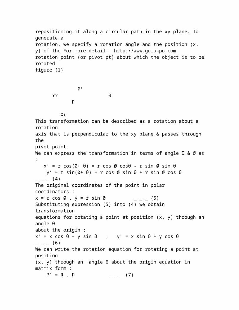
The translation distance pair (tx, ty) is called translation vector on shift vector : P 12xx⎡ ⎤=⎢ ⎥⎣ ⎦ , P’ 12x '=x'⎡ ⎤⎢ ⎥⎣ ⎦ , T xytt⎡ ⎤= ⎢ ⎥⎣ ⎦ _ _ _ (2)2 – dimensional translation matrix form : P’ = P + T _ _ _ (3) In this case, we would write in matrix as row : P = [x, y] , T = [tx , ty] Translation is a rigid body transformation that moves object without deformation. That is T1 every point on the object is translated by the same amount. A straight line segment is translated by applying the transformation equation (3) to each of the line end point & redrawing the line between the new end point positions. (2) Rotation : A two dimensional rotation is applied to an object by repositioning it along a circular path in the xy plane. To generate a rotation, we specify a rotation angle and the position (x, y) of the For more detail:- http://www.gurukpo.comrotation point (or pivot pt) about which the object is to be rotated

figure (1)

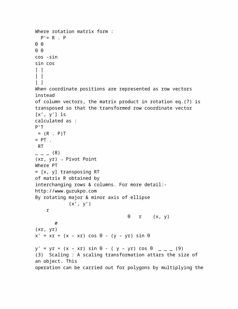
P’ Yr θ P XrThis transformation can be described as a rotation about a rotation axis that is perpendicular to the xy plane & passes through the pivot point. We can express the transformation in terms of angle θ & Ø as : x’ = r cos(Ø+ θ) = r cos Ø cosθ - r sin Ø sin θ y’ = r sin(Ø+ θ) = r cos Ø sin θ + r sin Ø cos θ _ _ _ (4) The original coordinates of the point in polar coordinators : x = r cos Ø , y = r sin Ø _ _ _ (5)Substituting expression (5) into (4) we obtain transformation equations for rotating a point at position (x, y) through an angle θabout the origin : x’ = x cos θ – y sin θ , y’ = x sin θ + y cos θ _ _ _ (6) We can write the rotation equation for rotating a point at position (x, y) through an angle θ about the origin equation in matrix form : P’ = R . P _ _ _ (7)Where rotation matrix form : P’= R . P θ θθ θcos -sinsin cos⎡ ⎤⎢ ⎥⎣ ⎦When coordinate positions are represented as row vectors instead of column vectors, the matrix product in rotation eq.(7) is transposed so that the transformed row coordinate vector [x’, y’] is calculated as : P’T = (R . P)T = PT . RT _ _ _ (8) (xr, yr) → Pivot Point Where PT= [x, y] transposing RT of matrix R obtained by interchanging rows & columns. For more detail:- http://www.gurukpo.com

By rotating major & minor axis of ellipse (x’, y’) r θ r (x, y) ø (xr, yr) x' = xr + (x – xr) cos θ - (y – yr) sin θ y' = yr + (x – xr) sin θ - ( y – yr) cos θ _ _ _ (9)(3) Scaling : A scaling transformation attars the size of an object. This operation can be carried out for polygons by multiplying the coordinate values (x, y) for each vertex by scaling factors Sx and Syto produce the transformed coordinates (x’, y’) x’ = x . Sx ‘ y’ = y . Sy _ _ _ (10) Scaling factors Sx scales objects in the x direction while Sy scales in the y direction. The transformation equation (10) can also be written in the matrix form : ''xy⎡ ⎤⎢ ⎥⎣ ⎦ = xys 00 s⎡ ⎤⎢ ⎥⎣ ⎦xy⎡ ⎤⎢ ⎥⎣ ⎦ _ _ _ (11) Or P’ = S . P _ _ _ (12) Where S is 2x2 scaling in eq.(11) any positive numeric values can be assigned to the scaling factors Sx and Sy values less than 1 reduce the size of object; values greater than 1 reduce the size of object & specifying a value of 1 for both Sx and Sy leaves the size of object unchanged. When Sxand Sy are assigned the same value, a uniform scaling is produced that maintains relative object proportions unequal values of Sx and Sy result in

a differential scaling that is often used in design application where picture are constructed form a few basic shapes that can be adjusted by scaling & positioning transformation.

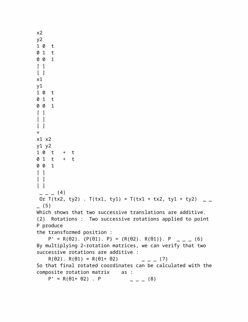
Q.2 What are composite Transformation? Give the 3-types of Composite Transformation. Ans.: Composite transformation Matrix can be obtained by calculating. The matrix product of the individual transformations forming products of For more detail:- http://www.gurukpo.comtransformation matrix is often referred to as concatenation or composition of matrices. (1) Translation : If two successive translation vectors (tx1, ty1) and (tx2, ty2) are applied to a coordinate position P, final transformed location P’ is calculated as : P’ = T (tx2, ty2) . {T (tx1, ty1) . P} = {T(tx2, ty2) .T(tx1, ty1)} . P _ _ _ (3) Where P and P’ are represented as homogenous – coordinate column vectors. We can verify this result by calculating the matrix product for the tow associative groupings. Composite Matrix for this sequence is : x2y21 0 t0 1 t0 0 1⎡ ⎤⎣ ⎦x1y11 0 t0 1 t0 0 1⎡ ⎤⎢ ⎥⎣ ⎦= x1 x2y1 y21 0 t + t0 1 t + t0 0 1⎡ ⎤⎢ ⎥

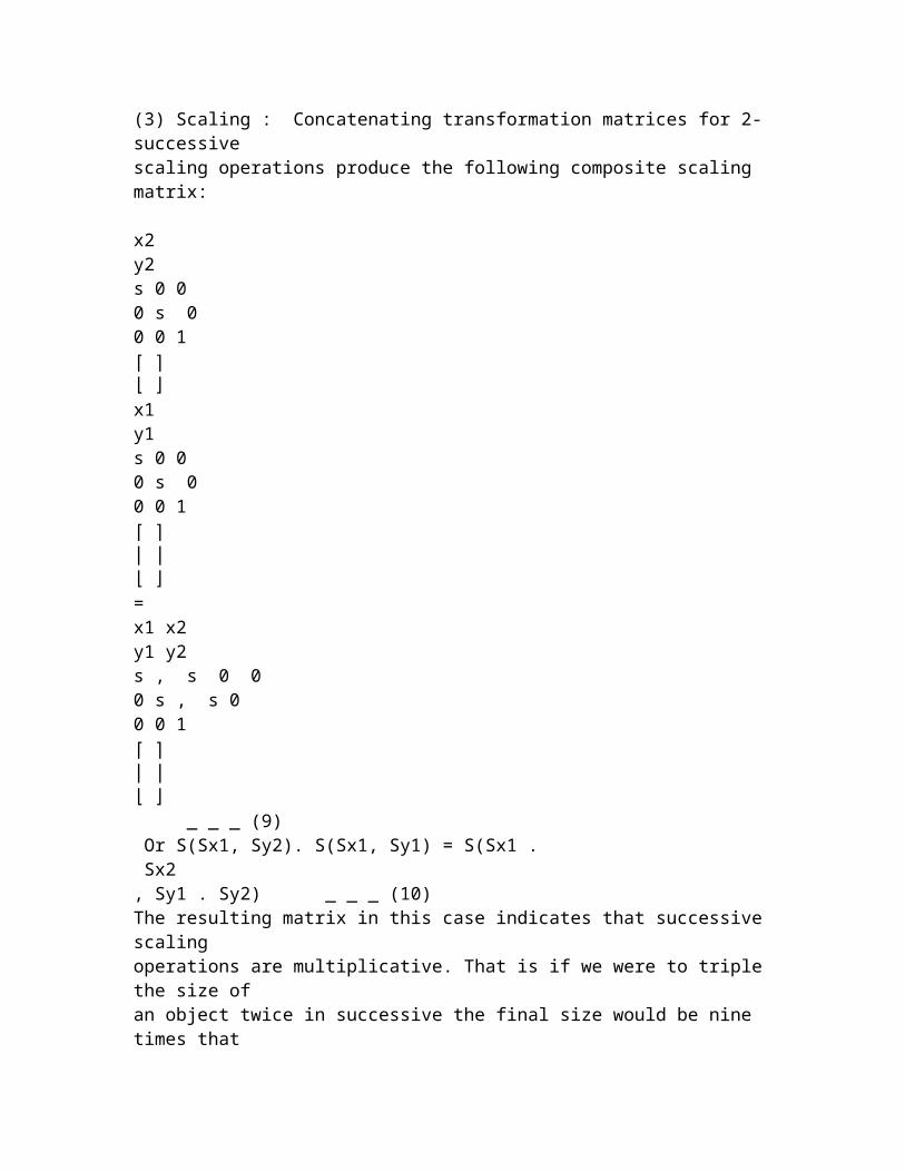
⎣ ⎦ _ _ _ (4) Or T(tx2, ty2) . T(tx1, ty1) = T(tx1 + tx2, ty1 + ty2) _ _ _ (5)Which shows that two successive translations are additive. (2) Rotations : Two successive rotations applied to point P produce the transformed position : P’ = R(θ2). {P(θ1). P} = {R(θ2). R(θ1)}. P _ _ _ (6) By multiplying 2–rotation matrices, we can verify that two successive rotations are additive : R(θ2). R(θ1) = R(θ1+ θ2) _ _ _ (7)So that final rotated coordinates can be calculated with the composite rotation matrix as : P’ = R(θ1+ θ2) . P _ _ _ (8)(3) Scaling : Concatenating transformation matrices for 2-successive scaling operations produce the following composite scaling matrix: x2y2s 0 00 s 00 0 1⎡ ⎤⎣ ⎦x1y1s 0 00 s 00 0 1⎡ ⎤⎢ ⎥⎣ ⎦= x1 x2y1 y2s , s 0 00 s , s 00 0 1⎡ ⎤⎢ ⎥⎣ ⎦ _ _ _ (9) Or S(Sx1, Sy2). S(Sx1, Sy1) = S(Sx1 . Sx2 , Sy1 . Sy2) _ _ _ (10)The resulting matrix in this case indicates that successive scaling operations are multiplicative. That is if we were to triple the size of

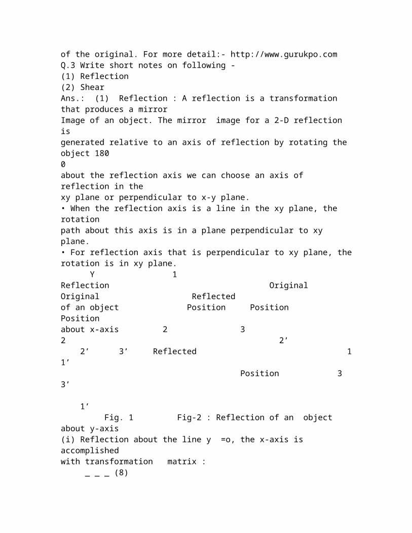
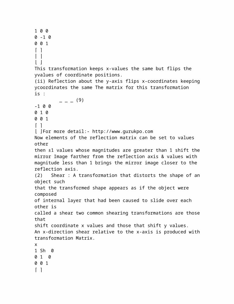
an object twice in successive the final size would be nine times that of the original. For more detail:- http://www.gurukpo.comQ.3 Write short notes on following - (1) Reflection (2) Shear Ans.: (1) Reflection : A reflection is a transformation that produces a mirror Image of an object. The mirror image for a 2-D reflection is generated relative to an axis of reflection by rotating the object 1800about the reflection axis we can choose an axis of reflection in the xy plane or perpendicular to x-y plane. • When the reflection axis is a line in the xy plane, the rotation path about this axis is in a plane perpendicular to xy plane. • For reflection axis that is perpendicular to xy plane, the rotation is in xy plane. Y 1Reflection Original Original Reflected of an object Position Position Position about x-axis 2 3 2 2’ 2’ 3’ Reflected 1 1’ Position 3 3’ 1’ Fig. 1 Fig-2 : Reflection of an object about y-axis (i) Reflection about the line y =o, the x-axis is accomplished with transformation matrix : _ _ _ (8)1 0 00 -1 00 0 1⎡ ⎤⎢ ⎥⎣ ⎦This transformation keeps x-values the same but flips the yvalues of coordinate positions. (ii) Reflection about the y-axis flips x-coordinates keeping ycoordinates the same The matrix for this transformation is : _ _ _ (9)-1 0 00 1 00 0 1⎡ ⎤⎣ ⎦For more detail:- http://www.gurukpo.comNow elements of the reflection matrix can be set to values other then ±1 values whose magnitudes are greater than 1 shift the mirror Image farther from the reflection axis & values with

magnitude less than 1 brings the mirror image closer to the reflection axis. (2) Shear : A transformation that distorts the shape of an object such that the transformed shape appears as if the object were composed of internal layer that had been caused to slide over each other is called a shear two common shearing transformations are those that shift coordinate x values and those that shift y values. An x-direction shear relative to the x-axis is produced with transformation Matrix. x1 Sh 00 1 00 0 1⎡ ⎤⎣ ⎦ _ _ _ (3)Which transforms coordinate position as : x' = x +Shx . y y’ = y _ _ _ (4) Any real number can be assigned to shear parameter Shx. We can rene5rate x-direction shears relative to other reference lines with. yry _ _ _ (5)x x r1 Sh - Sh .y0 1 00 0 1⎡ ⎤⎢ ⎥⎣ ⎦With coordinate position transformed as : x' = x + Shx (y -yry) , y’ = y _ _ _ (6)A y-direction shear relative to the line x = xry is generated with translation matrix : _ _ _ (7)y y1 0 0Sh 1 - Sh .x0 0 1⎡ ⎤⎢ ⎥⎣ ⎦Which generates transformed coordinate position

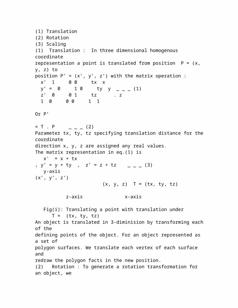
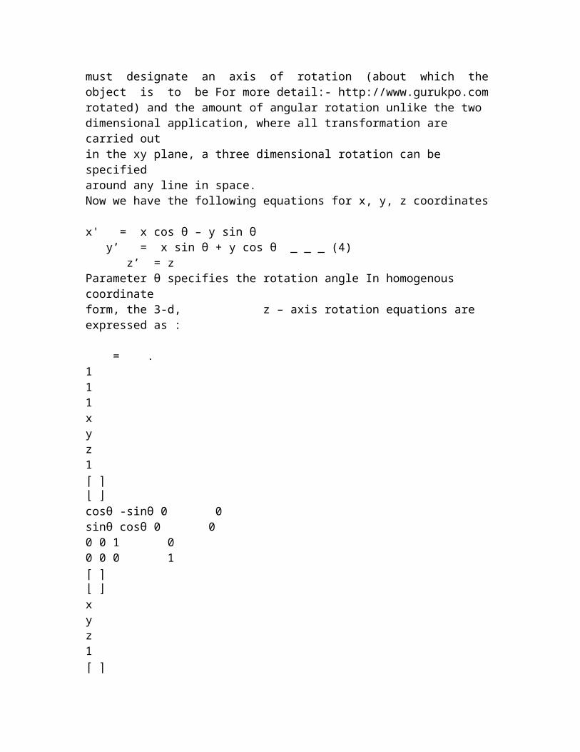
x' = x , y’ = Shy (x -xry) + y _ _ _ (8) For more detail:- http://www.gurukpo.comQ.4 Explain 3-different types of Transformations in 3- dimension? Ans.: The there different types of transformations are : (1) Translation (2) Rotation (3) Scaling (1) Translation : In three dimensional homogenous coordinate representation a point is translated from position P = (x, y, z) to position P’ = (x’, y’, z’) with the matrix operation : x’ 1 0 0 tx x y’ = 0 1 0 ty y _ _ _ (1) z’ 0 0 1 tz . z 1 0 0 0 1 1 Or P’ = T . P _ _ _ (2) Parameter tx, ty, tz specifying translation distance for the coordinate direction x, y, z are assigned any real values. The matrix representation in eq.(1) is x' = x + tx , y’ = y + ty , z’ = z + tz _ _ _ (3) y-axis (x’, y’, z’) (x, y, z) T = (tx, ty, tz) z-axis x-axis Fig(i): Translating a point with translation under T = (tx, ty, tz) An object is translated in 3-diminision by transforming each of the defining points of the object. For an object represented as a set of polygon surfaces. We translate each vertex of each surface and redraw the polygon facts in the new position. (2) Rotation : To generate a rotation transformation for an object, we must designate an axis of rotation (about which the object is to be For more detail:- http://www.gurukpo.comrotated) and the amount of angular rotation unlike the two dimensional application, where all transformation are carried out in the xy plane, a three dimensional rotation can be specified around any line in space. Now we have the following equations for x, y, z coordinates x' = x cos θ – y sin θ y’ = x sin θ + y cos θ _ _ _ (4) z’ = z

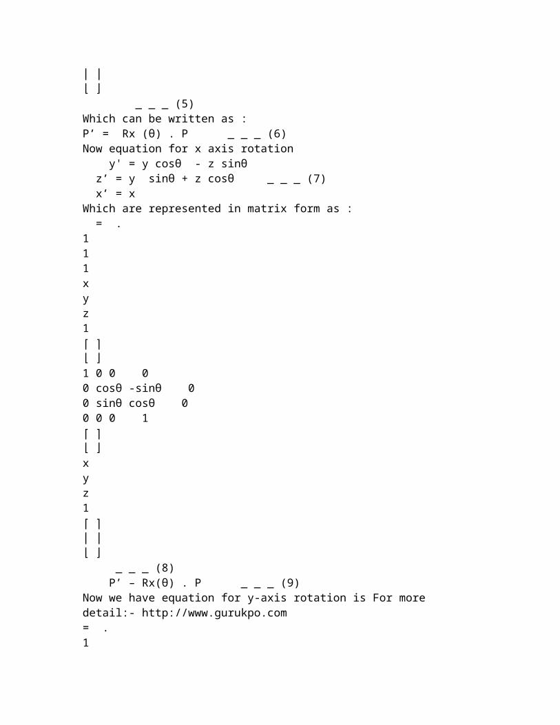
Parameter θ specifies the rotation angle In homogenous coordinate form, the 3-d, z – axis rotation equations are expressed as : = . 111xyz1⎡ ⎤⎣ ⎦cosθ -sinθ 0 0sinθ cosθ 0 00 0 1 00 0 0 1⎡ ⎤⎣ ⎦xyz1⎡ ⎤⎢ ⎥⎣ ⎦ _ _ _ (5) Which can be written as : P’ = Rx (θ) . P _ _ _ (6) Now equation for x axis rotation y' = y cosθ - z sinθ z’ = y sinθ + z cosθ _ _ _ (7) x’ = x Which are represented in matrix form as : = . 111xyz1⎡ ⎤⎣ ⎦1 0 0 00 cosθ -sinθ 0

0 sinθ cosθ 00 0 0 1⎡ ⎤⎣ ⎦xyz1⎡ ⎤⎢ ⎥⎣ ⎦ _ _ _ (8) P’ – Rx(θ) . P _ _ _ (9)Now we have equation for y-axis rotation is For more detail:- http://www.gurukpo.com= . 111xyz1⎡ ⎤⎣ ⎦cosθ 0 sinθ 00 1 0 0-sinθ 0 cosθ 00 0 0 1⎡ ⎤⎣ ⎦xyz1⎡ ⎤⎢ ⎥⎣ ⎦ _ _ _ (8) Equations are : z'= z cosθ – x sinθ x’ = z sinθ + x cosθ _ _ _ (11) y’ = y P’ = Ry (θ) . P _ _ _ (12) (3) Scaling : The matrix expression for the scaling transformation of a position P=(x,y,z) relative to the coordinate origin can be written

as : = . 111xyz1⎡ ⎤⎣ ⎦S 0 0 00 S 0 00 0 0 S0 0 0 1xyz⎡ ⎤⎣ ⎦xyz1⎡ ⎤⎢ ⎥⎣ ⎦ _ _ _ (13) P’ = S . P _ _ _ (14) Where scaling Parameters Sx, Sy, and Sz are assigned any positive values. x' = x . Sx , y’ = y. Sy , z’ = z . Sz _ _ _ (15) Scaling an object with transformation changes the size of the object and repositions the object relative to the coordinate origin. Also if the transformation is not all equal relative dimensions in the object are changed. We pressure the original shape of an object with uniform scaling (Sx = Sy = Sz). Scaling with respect to a selected fixed position (xf. yf. zf) can be represented with following transformation sequence (i) Translate the fixed point to the origin. (ii) Scale the object relative to the coordinate origin. (iii) Translate the fixed point to its original position. □ □ □For more detail:- http://www.gurukpo.comChapter-3Output Primitives

Q.1 Explain the Line Drawing Algorithms? Explain DDA and Bresenham’s Line Algorithm. Ans.: Slope intercept equation for a straight line is y = m x + b _ _ _ (1) with m representing the slope of the line and b as the y intercept. Where the two end point of a line segment are specified at positions (x1, y1) and (x2, y2) as shown is Fig.(1) we can determine values for the slope m and y intercept b with the following calculations. M = 2 12 1y - yx - x _ _ _ (2) y2 b = y1 – mx1 _ _ _ (3) y1Obtain value of y interval ∆y – m . ∆x _ _ _ (4) x1 x2Similarly we can obtain ∆ x interval Fig. (1) Line Path between endpoint ∆ x = y mΔ position (x1, y1) & (x2, y2) For lines with slope magnitude m <1, ∆x can be set Proportional to a small horizontal deflection voltage and the corresponding vertical deflection is then set proportional to ∆y. For lines with slope magnitude m >1, ∆y can be set proportional to a small deflection voltage with the corresponding horizontal deflection voltage set proportional to ∆x. For lines with m = 1 ∆x = ∆y. DDA Algorithm : The Digital Differential Analyzer (DDA) is a scan. Conversion line Algorithm based on calculating either ∆y or ∆x using equation (4) & (5). We sample the line at unit intervals in one coordinate and determine corresponding integer values nearest. The line paths for the other coordinate. For more detail:- http://www.gurukpo.comNow consider first a line with positive slope, as shown in Fig.(1). If the slope is less than one or equal to 1. We sample at unit x intervals (∆x = 1) compute each successive y values as : yk+1 = yk + m _ _ _ (6) Subscript k takes integer values starting form 1, for the first point & increase by 1 until the final end point is reached. For lines with positive slope greater than 1, we reverse the role of x and y.

That is we sample at unit y intervals (∆y = 1) and calculate each succeeding x value as : xk+1 = xk + 1 m _ _ _ (7) Equation (6) and (7) are based on assumption that lines are to be processed form left end point to the right end point. If this processing is reversed the sign is changed ∆x = - 1 & ∆y = - 1 yk+1 = yk – m _ _ _ (8) xk+1 = xk – 1 m _ _ _(9)Equations (6) to (9) are used to calculate pixel position along a line with negative slope. When the start endpoint is at the right we set ∆x = -1 and obtain y position from equation (7) similarly when Absolute value of Negative slope is greater than 1, we use ∆y = -1 & eq.(9) or we use ∆y = 1 & eq.(7).

Bresenham’s Line Algorithm : An accurate and efficient raster line generating Algorithm, developed by Bresenham, scan concerts line using only incremental integer calculations that can be adapted to display circles and other curves. The vertical axes show scan-line position, & the horizontal axes identify pixel columns as shown in Fig. (5) & (6) 13 Specified Line 12 Path 50 Specified Line 11 49 Path For more detail:- http://www.gurukpo.com10 48 10 11 12 13 50 51 52 53 53 Fig.5 Fig.6 To illustrate Bresenham’s approach we first consider the scan conversion process for lines with positive slope less than 1. Pixel position along a line path are then determined by sampling at unit x intervals starting form left and point (x0 , y0) of a given line, we step at each successive column (x position) & plot the pixel whose scan line y is closest to the line path. Now assuming we have to determine that the pixel at (xk , yk) is to be displayed, we next need to divide which pixel to plot in column xk+1. Our choices are the pixels at position (xk+1 , yk) and (xk+1

, yk+1). At sampling position xk+1, we label vertical pixel separations from the mathematical line path as d1 and d2. Fig.(8). The y coordinate on the mathematical line at pixel column position xk+1 is calculated as : y = m(xk + 1) +b _ _ _(10) Then d1 = y – yk = m (xk + 1) +b - ykand d2 = (yk + 1) –y = yk + 1 – m (xk + 1) – b The difference between these two separations is d1 - d2 = 2m (xk+1) - 2yk + 2b - 1 _ _ _ (11) A decision Parameter Pk for the Kth step in the line algorithm can be obtained by rearranging eq.(11) so that it involves only integer calculation. We accomplish this by substituting m = ∆y/∆x. where ∆y & ∆x are the vertical & horizontal separation of the endpoint positions & defining. Pk = ∆x (d1 – d2) = 2∆y. xk - 2∆x yk + c _ _ _ (12)The sign of Pk is same as the sign of d1 - d2. Since ∆x > 0 for our example Parameter C is constant & has the value 2∆y + ∆x (2b -1), which is independent of pixel position. If the pixel position at yk is closer to line path than the pixel at yk+1 (that is d1 < d2), then decision Parameter Pk is Negative. In that case we plot the lower pixel otherwise we plot the upper pixel. Coordinate changes along the line owner in unit steps in either the x or directions. Therefore we can obtain the values of successive decision For more detail:- http://www.gurukpo.comParameter using incremental integer calculations. At step k = 1, the decision Parameter is evaluated form eq.(12) as : Pk+1 = 2∆y . xk+1 - 2∆x . yk+1 + C yk+1 • d2 y • d1 yk • xk+1 Fig.8Subtracting eq.(12) from the preceding equation we have Pk+1 – Pk = 2∆y (xk+1 – xk) - 2∆x (yk+1 – yk) But xk+1 = xk + 1 So that, Pk+1 = Pk + 2∆y - 2∆x (yk+1 – yk) _ _ _ (13)Where the term yk+1 - yk is either 0 or 1, depending on sign of Parameter Pk. This recursive calculation of decision Parameter is performed each integer x position, starting at left coordinate endpoint of the line. The first parameter P0 is evaluated from equation (12) at starting pixel position (x0, y0) and with m evaluated as ∆y/∆x. P0 = 2∆y - ∆x _ _ _ (14) Bresenham’s Line Drawing Algorithm for m <1 : (1) Input the two line endpoints & store the left end point in (x0 , y0).

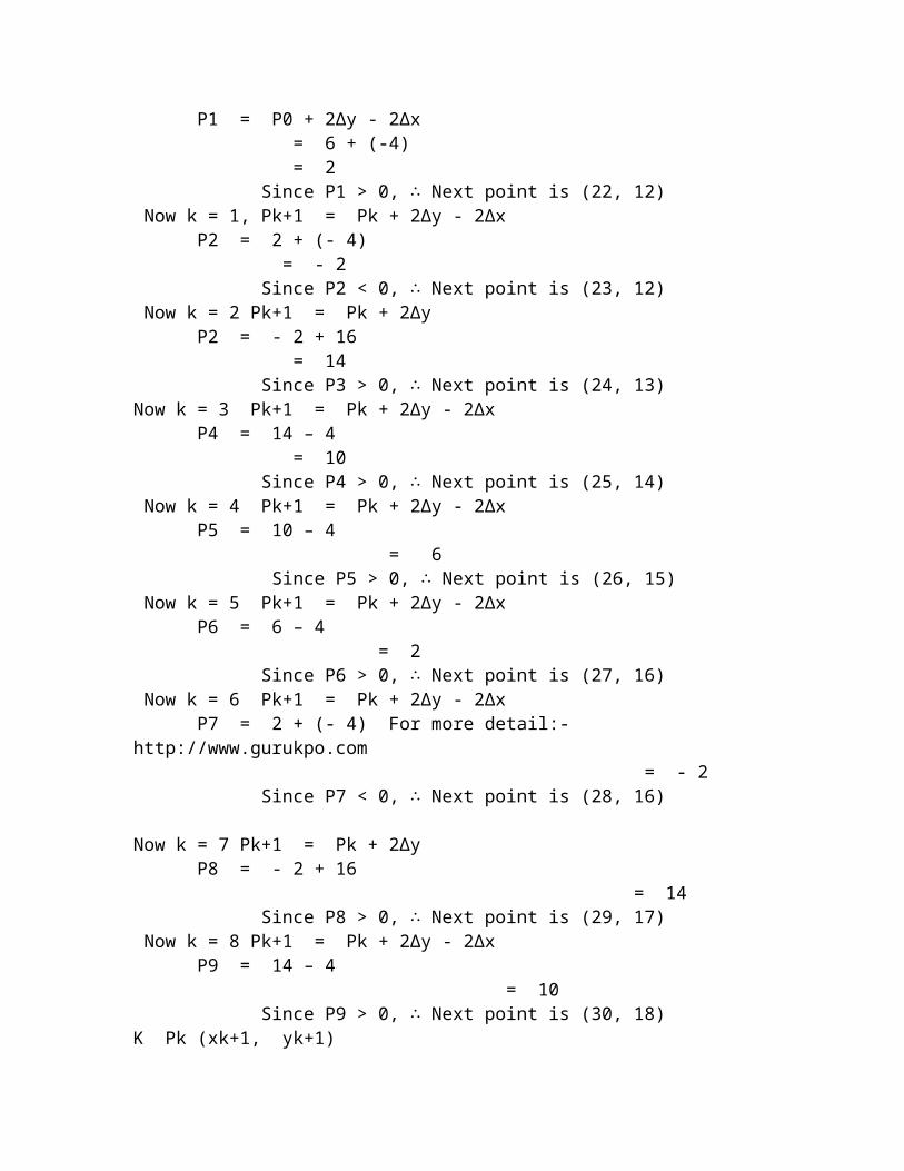
(2) Load (x0 , y0) into frame buffer that is plot the first point. (3) Calculate constants ∆x, ∆y, 2∆y and 2∆y - 2∆x and obtain the starting value for the decision parameter as : P0 = 2∆y - ∆x. (4) At each xk along the line starting at k = 0, perform the following test if Pk < 0 the next point to plot is (xk+1 , yk) and Pk+1 = Pk + 2∆y otherwise the next point to plot is (xk+1 , yk+1) and Pk+1 = Pk +2∆y - 2∆x. (5) Repeat step 4 ∆x times. For more detail:- http://www.gurukpo.comQ.2 Digitize the line with end points (20, 10) & (30, 18) using Bresenham’s Line Drawing Algorithm. Ans.: slope of line, m = 2 12 1y - yx - x=18 - 1030 - 20=810= 0.8∆x = 10 , ∆y = 8 Initial decision parameter has the value P0 = 2∆y - ∆x = 2x8 – 10 = 6 Since P0 > 0, so next point is (xk + 1, yk + 1) (21, 11) Now k = 0, Pk+1 = Pk + 2∆y - 2∆x P1 = P0 + 2∆y - 2∆x = 6 + (-4) = 2 Since P1 > 0, ∴ Next point is (22, 12) Now k = 1, Pk+1 = Pk + 2∆y - 2∆x P2 = 2 + (- 4) = - 2 Since P2 < 0, ∴ Next point is (23, 12) Now k = 2 Pk+1 = Pk + 2∆y P2 = - 2 + 16 = 14 Since P3 > 0, ∴ Next point is (24, 13) Now k = 3 Pk+1 = Pk + 2∆y - 2∆x P4 = 14 – 4 = 10 Since P4 > 0, ∴ Next point is (25, 14)

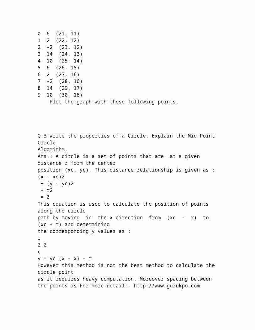
Now k = 4 Pk+1 = Pk + 2∆y - 2∆x P5 = 10 – 4 = 6 Since P5 > 0, ∴ Next point is (26, 15) Now k = 5 Pk+1 = Pk + 2∆y - 2∆x P6 = 6 – 4 = 2 Since P6 > 0, ∴ Next point is (27, 16) Now k = 6 Pk+1 = Pk + 2∆y - 2∆x P7 = 2 + (- 4) For more detail:- http://www.gurukpo.com = - 2 Since P7 < 0, ∴ Next point is (28, 16) Now k = 7 Pk+1 = Pk + 2∆y P8 = - 2 + 16 = 14 Since P8 > 0, ∴ Next point is (29, 17) Now k = 8 Pk+1 = Pk + 2∆y - 2∆x P9 = 14 – 4 = 10 Since P9 > 0, ∴ Next point is (30, 18) K Pk (xk+1, yk+1) 0 6 (21, 11) 1 2 (22, 12) 2 -2 (23, 12) 3 14 (24, 13) 4 10 (25, 14) 5 6 (26, 15) 6 2 (27, 16) 7 -2 (28, 16) 8 14 (29, 17) 9 10 (30, 18) Plot the graph with these following points.

Q.3 Write the properties of a Circle. Explain the Mid Point Circle Algorithm. Ans.: A circle is a set of points that are at a given distance r form the center position (xc, yc). This distance relationship is given as : (x – xc)2 + (y – yc)2 – r2 = 0 This equation is used to calculate the position of points along the circle

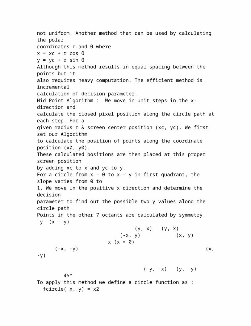
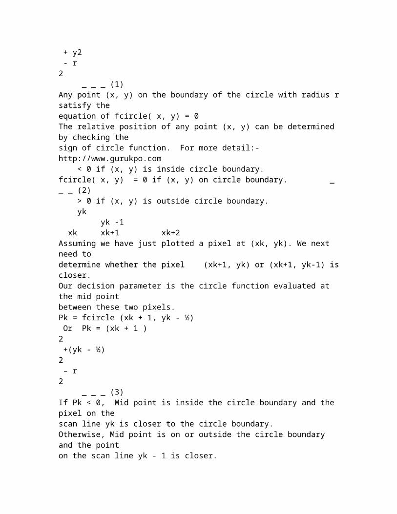
path by moving in the x direction from (xc - r) to (xc + r) and determining the corresponding y values as : ±2 2cy = yc (x - x) - rHowever this method is not the best method to calculate the circle point as it requires heavy computation. Moreover spacing between the points is For more detail:- http://www.gurukpo.comnot uniform. Another method that can be used by calculating the polar coordinates r and θ where x = xc + r cos θy = yc + r sin θAlthough this method results in equal spacing between the points but it also requires heavy computation. The efficient method is incremental calculation of decision parameter. Mid Point Algorithm : We move in unit steps in the x-direction and calculate the closed pixel position along the circle path at each step. For a given radius r & screen center position (xc, yc). We first set our Algorithm to calculate the position of points along the coordinate position (x0, y0). These calculated positions are then placed at this proper screen position by adding xc to x and yc to y. For a circle from x = 0 to x = y in first quadrant, the slope varies from 0 to 1. We move in the positive x direction and determine the decision parameter to find out the possible two y values along the circle path. Points in the other 7 octants are calculated by symmetry. y (x = y) (y, x) (y, x) (-x, y) (x, y) x (x = 0) (-x, -y) (x, -y) (-y, -x) (y, -y) 45º To apply this method we define a circle function as : fcircle( x, y) = x2 + y2 - r2 _ _ _ (1) Any point (x, y) on the boundary of the circle with radius r satisfy the equation of fcircle( x, y) = 0 The relative position of any point (x, y) can be determined by checking the sign of circle function. For more detail:- http://www.gurukpo.com < 0 if (x, y) is inside circle boundary. fcircle( x, y) = 0 if (x, y) on circle boundary. _ _ _ (2)

> 0 if (x, y) is outside circle boundary. yk yk -1 xk xk+1 xk+2Assuming we have just plotted a pixel at (xk, yk). We next need to determine whether the pixel (xk+1, yk) or (xk+1, yk-1) is closer.Our decision parameter is the circle function evaluated at the mid point between these two pixels. Pk = fcircle (xk + 1, yk - ½) Or Pk = (xk + 1 )2 +(yk - ½)2 – r2 _ _ _ (3)If Pk < 0, Mid point is inside the circle boundary and the pixel on the scan line yk is closer to the circle boundary. Otherwise, Mid point is on or outside the circle boundary and the point on the scan line yk - 1 is closer. Successive decision parameters are obtained by incremental calculations. Next decision parameter at next sampling position. xk+1 + 1 = xk + 2 Pk+1 = fcircle(xk+1 + 1, yk+1 - ½) Or Pk+1 = [(xk + 1) + 1]2 + (yk+1 - ½)2 – r2Or Pk+1 = Pk + 2(xk + 1) + (yk+12 – yk2) – (yk + 1 – yk) + 1 _ _ _ (4) Successive increment for Pk is 2xk+1 +1(If Pk < 0) otherwise (2xk+1 +1 - 2yk+1) where 2xk+1 = 2xk + 2 & 2yk+1 = 2yk – 2Initial decision parameter P0 is obtained as (0, r) = (x0, y0) P0 = fcircle(x, y) = fcircle (1, r - ½) = 1 + (r - ½)2 – r2For more detail:- http://www.gurukpo.comOr P0 = 5

4 - rIf r is a integer then P0 = 1 – r Algorithm : (1) Input radius r and circle center ( xc, yc) and obtain the first point on circumference of a circle centered on origin (x0, y0) = (0, r) (2) Calculate the initial value of the decision parameter as : P0 = 54 - r(3) At each xk position, starting at k = 0 if Pk < 0 the next point along the circle is (xk+1, yk) and Pk+1 = Pk + 2xk+1 + 1, otherwise the next point along the circle is (xk + 1, yk - 1) and Pk+1 = Pk + 2xk+1 + 1 – 2yk+1 where 2xk+1 = 2xk + 2 & 2yk+1 = 2yk – 2. (4) Determine symmetry points in other seven octants. (5) Move each calculated pixel position (x, y) onto the circular path centered on (xc, yc) & plot coordinate values x = x + xc & y = y + yc.(6) Repeat step (3) through (5) until x ≥ y. Q.4 Demonstrate the Mid Point Circle Algorithm with circle radius, r = 10. Ans.: P0 = 1 – r =1 - 10 = - 9 Now the initial point (x0, y0) = (0, 10) and initial calculating terms for calculating decision parameter are 2x0 = 0 , 2y0 = 20 Since Pk < 0, ∴Next point is (1, 10) P1 = - 9 +3 = - 6 Now P1 < 0, ∴Next point is (2, 10) P2 = - 6 + 5 = - 1 Now P2 < 0, ∴Next point is (3, 10) P3 = -1+ 7 = 6 Now P3 > 0, ∴Next point is (4, 9) P4 = 6 + 9 - 18 = - 3 Now P4 < 0, ∴Next point is (5, 9) P5 = - 3 + 11 = 8 Now P5 > 0, ∴Next point is (6, 8) P6 = 8 +13 - 16 = 5 Now P6 > 0, ∴Next point is (7, 7) For more detail:- http://www.gurukpo.comK (xk+1, yk+1) 2xk+1 2yk+10 (1, 10) 2 20 1 (2, 10) 4 20 2 (3, 10) 6 20 3 (4, 9) 8 18 4 (5, 9) 10 18 5 (6, 8) 12 16 6 (7, 7) 14 14 Plot the graph with these points. Q.5 Give the properties of Ellipse & explain the Algorithm. Ans.: An ellipse is defined as a set of points such that the sum of distances from two fixed points (foci) is same for all points given a point P = (x, y), distances are d1 & d2, equation is : d1 + d2 = constant _ _ _ (1) In terms of local coordinates F1 = (x1, y1) & F2 (x2, y2)

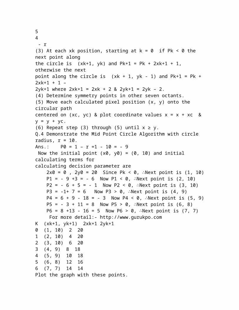
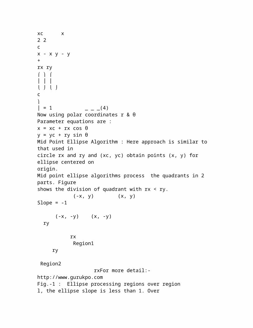
Equation is : 2 2 2 21 1 2 2(x - x ) +(y - y ) (x - x ) +(y - y ) 0 + = _ _ _ (2)This can also be written in the form : Ax2 + By2 + Cxy + Dx + Ey + F = 0 _ _ _ (3)(More A, B, C, D, E, & F are evaluated in terms of focal coordinates & major minor axis). • Major axis – which extends form 1 point to other through foci. • Minor axis – which spans the shouter dimension bisecting major axis at ellipse center. An interactive method for specifying an ellipse in an arbitrary orientation is to input two foci & a point on ellipse boundary & evaluate constant in equation (1) & so on. Equation can be simplified if ellipse is in “standard position” with major & minor axis oriented parallel to x and y axis. For more detail:- http://www.gurukpo.com y yc xc x 2 2cx - x y - y+rx ry⎛ ⎞ ⎛⎜ ⎟ ⎜⎝ ⎠ ⎝ ⎠c⎞⎟ = 1 _ _ _(4) Now using polar coordinates r & θ Parameter equations are : x = xc + rx cos θy = yc + ry sin θMid Point Ellipse Algorithm : Here approach is similar to that used in circle rx and ry and (xc, yc) obtain points (x, y) for ellipse centered on origin. Mid point ellipse algorithms process the quadrants in 2 parts. Figure shows the division of quadrant with rx < ry. (-x, y) (x, y)

Slope = -1 (-x, -y) (x, -y) ry rx Region1 ry Region2 rxFor more detail:- http://www.gurukpo.comFig.-1 : Ellipse processing regions over region l, the ellipse slope is less than 1. Over region 2, the magnitude of slope is greater than 1. Fig.-2 : Shows the symmetry of an ellipse Region 1 & 2 can be processed in different ways: Region 1 is processed starting at (0, ry) we step clockwise along the path in unit steps in x- direction & then unit steps in y- direction. Ellipse function can be written as : fellipse(x, y) = (0, ry) fellipse(x, y) = ry2 x2 + rx2y2 - rx2ry2 _ _ _ (5)Which has the following properties : < 0 (x, y) is inside boundary. fellipse = 0 (x, y) is on the boundary. > 0 (x, y) is outside the boundary. Thus the ellipse function fellipse(x, y) serves as a decision parameter in the mid point Algorithm. Starting at (0, ry) we step in x direction until we reach boundary between Region 1 & 2 slope is calculated at each step as : dydx =22

-2r x2r xyx - {from eq.(5)}At boundary dydx = -1 So, 2ry2 x = 2rx2y ∴ We move out of Region 1 when 2ry2 x ≥ 2rx2y _ _ _ (7)Figure (1) shows mid point between 2-candidate pixel at (xk+1), we have selected pixel at (xk, yk) we need to determine the next pixel. yk • yk-1 mid point xk xk+1 Fig.:1 P1k = fellipse( xk + 1, yk – ½) = ry2( xk + 1)2 + rx2 (yk - ½)2 – rx2ry2 _ _ _ (8) For more detail:- http://www.gurukpo.comNext symmetric point (xk+1 +1, yk+1 - ½) P1k +1 = ry2 [(xk + 1) + 1]2 + r2x [(yk +1 – ½)

2 (yk – ½)2] _ _ _ (9) Where yk + 1 is either yk or yk -1 depending on sign of P1k 2ry2 xk+1 + ry2 if Pk < 0 Increments = 2ry2 xk+1 – 2rx2 yk+1 + ry2 if Pk ≥ 0 With initial position (0, ry) the two terms evaluate to 2ry2x = 0 , 2rx2y = 2rx2ry Now when x & y are incremented the updated values are 2ry2 xk+1 = 2ry2 xk + 2ry2 , 2rx2 yk+1 = 2rx2 yk – 2rx2 And these values are compared at each step & we move out of Region 1 when condition (7) is satisfied initial decision parameter for region 1 is calculated as : P10 = fellipse(x0, y0) = (1, ry – ½) = ry2 + rx2

( ry - ½)2 – rx2 ry2 P10 = ry2 – rx2 ry + ¼ rx2 _ _ _ (10) Over Region 2, we step in (-)ve y-direction & mid point selected is between horizontal pixel positions P2k = fellipse(x, y) = (xk + ½, yk – 1) P2k = ry2(xk + ½)2 + rx2( yk – 1)2 – rx2ry2 _ _ _ (11) yk yk-1 • xk xk+1If P2k > 0 then we select pixel at xk +1 Initial decision parameter for region (2) is calculated by taking (x0, y0) as last point in Region (1) P2k + 1 = fellipse(xk+1 + ½, yk+1 –1) = ry2(xk+1 + ½)2 + rx2[(yk – 1) -1]2 – rx2ry

2 P2k + 1 = P2k – 2rx2(yk – 1) + rx2 + ry2[(xk +1 + ½)2 – (xk + ½)2] _ _ _ (12) At initial position (x0, y0) For more detail:- http://www.gurukpo.comP20 = fellipse(x0 +½, y0 – 1) = ry2( x0 + ½)2 + rx2(y0 – 1)2 – rx2ry2 _ _ _ (13) Mid Point Ellipse Algorithm : (1) Input rx, ry and ellipse centre (xc, yc) obtain the first point (x0, y0) = (0, ry) (2) Calculate the initial value of the decision parameter in region 1 as P10 = ry2 – rx2ry + ¼ rx2(3) At each xk position in region 1, starting at K = 0. If Pk < 0, then next point along ellipse is (xk+1, yk) and P1k+1 = P1k + 2ry2xk+1 + ry2 otherwise next point along the circle is (xk +1, yk –1) and P1k+1 = P1k+ 2ry2xk + 1 – 2rx2yk + 1 + ry2 with 2ry

2xk+1 = 2ry2xk + 2ry2, 2rx2yk+1 = 2rx2yk – 2rx2 and continue until 2ry2x ≥ 2rx2y. (4) Calculate the initial value of the decision parameter in region (2) using last point (x0, y0) calculated in region 1 as P20 = ry2 (x0 + ½)2 + rx2 (y0 – 1)2 – rx2ry2.(5) At each yk position in region (2), starting at k = 0 perform following test : If P2k > 0 next point is (xk, yk – 1) and P2k+1 = P2k – 2rx2yk + 1 + rx2otherwise next point is ( xk + 1, yk – 1) and P2k+1 = P2k + 2ry2xk + 1 – 2rx2yk+1 + rx2.(6) Determine the symmetry points in other three quadrants. (7) More each calculated pixel position (x, y). Center on (xc, yc), plot

coordinate values x = x + xc & y = y + yc.(8) Repeat the steps for region 1 until 2ry2x ≥ 2rx2y. Q.6 Illustrate the Mid Point Ellipse Algorithm by ellipse parameter rx = 8 ry= 6 Ans.: rx2 = 64, ry2 = 36 2rx2 = 128, 2ry2 = 72 P10 = 36 – (64 x 6) + 14 x 64 = 36 – 384 + 16 = – 332 P10 < 0 ∴ Next point is (1, 6) P11 = – 332 + 72 x 1 + 36 = – 332 + 108 = – 224 P11 < 0 ∴ Next point is (2, 6) P12 = – 224 + 72 x 2 + 36 = – 224 + 144 + 36 = – 44 P12 < 0 ∴ Next point is (3, 6) For more detail:- http://www.gurukpo.comP13 = – 44 + 72 x 3 + 36 = – 44 + 216 + 36 = 208 P13 > 0 ∴ Next point is (4, 5) P14 = 208 + 72 x 4 – 128 x 5 +36 = 208 + 288 – 640 + 36 = – 108 P14 < 0 ∴ Next point is (5, 5) P15 = – 108 + 72 x 5 + 36 = 288 P15 > 0 ∴ Next point is (6, 4) P16 = 288 + 72 x 6 – 128 x 4 + 36 = 244 P16 > 0 ∴ Next point is (7, 3) P17 = 244 + 72 x 7 – 128 x 3 + 36 = 1168 K12 P1k (xk+1, yk+1) 2ry2xk+1 2rx2yk+11 – 332 (1, 6) 72 768 1 – 224 (2, 6) 144 768 2 – 44 (3, 6) 216 768 3 208 (4, 5) 288 640 4 – 108 (5, 5) 360 640

5 288 (6, 4) 432 512 6 244 (7, 3) 504 384 Now we move to region 2 since 2rx2 > 2rx2y Now For region the initial point is (x0, y0 = (7, 3) the initial decision parameter is P20 = f(7 + ½, 3 – 1) = 36 (7 + ½)2 + 64 (2)2 – 64 x 36 = 2025 + 256 – 2304 =– 23 The remaining positions are then calculated as : K P1k (xk+1, yk+1) 2ry2xk+1 2rx2yk+10 – 23 (8, 2) 576 256 1 – 215 (8, 1) 576 128 2 – 279 (8, 0) - - For more detail:- http://www.gurukpo.comNow Plot these point on the graph.

Q.7 Why is DDA Algorithm not good & efficient Algorithm? Ans.: (1) DDA traces out the successive x & y values by simultaneously increasing x & y by small steps proportional to their first derivative. In our example the x increment is 1 but y increment is dydx= m. since the real values have limited Precision, the accumulation of round off error in “m” causes the accumulative error. Build up which drifts the pixel positions from the true line path in most lines. (2) Moreover the round off operations & floating point incrementation is still time consuming.

Q.8 What do you understand by Area Filling? Discuss any one Algorithm. Ans.: A standard out put primitive in general graphics package is a solid-color or patterned polygon area. There are two basic approaches to area filling on raster system :

(1) To fill an area is to determine the overlap intervals for scan lines that cross the area. (2) Another is t start from a given interior position & point outward from this point until we specify the boundary conditions. Now scan line approach is typically used in general graphics package to still polygons, circles, ellipses and simple curses. Fill methods starting from an interior point are useful with more complex boundaries and in interactive painting systems. Boundary Fill Algorithm : Another approach to area filling is to start at a point inside a region and paint the interior outward toward the boundary. If the boundary is specified in a single color, the fill Algorithm precedes outward pixel by pixel until the boundary color is encountered. This method is called Boundary Fill Algorithm. Boundary Fill Algorithm procedure accepts as input the coordinates of an interior point (x, y), a fill color and a boundary color. Starting with (x, y), neighbouring boundary points are also tested. This process continues till all the pixels up to the boundary color for the area is tested. For more detail:- http://www.gurukpo.comDiagram 1 Fill method applied to 4-connuted area. 2 Fill method applied to 8-connuted area. Recursive boundary fill Algorithm may not fill regions correctly if some interior pixels are already displayed in the fill color. This occurs because the Algorithm checks next point both for boundary color and for fill color. The pixel positions are stored in form of a stack in the Algorithm. Flood Fill Algorithm : Sometimes we want to fill in (or recolor) an area that is not defined within a single color boundary suppose we take an area which is bordered by several different color. We can paint such area by replacing a specified interior color instead of searching for a boundary color value. This approach is called flood fill Algorithm. We start from interior paint (x, y) and reassign all pixel values that are currently set to a given interior color with the desired fill color. If the area we want to paint has move than one interior color, we can first reassign pixel value so that all interior points have the same color. □ □ □For more detail:- http://www.gurukpo.com

Chapter-4Clipping Algorithm

Q.1 What is Clipping? How can a point be clipped? Ans. : Any procedure that identifies those portion of a picture that are either inside or outside of a specified region of space is referred to as a clipping Algorithm or clipping. This region against which an object is to be clipped is called a clip window. Application of Clipping : (1) Extracting parts of defined scene for veiwing. (2) Identifying visible surface in three dimentional views. (3) Antialising line segments or object boundaries. (4) Creating objects using solid-modeling procedures. (5) Displaying multi window environment. (6) Drawing and painting operations. Point Clipping : Assuring that clip window is a rectangle in standard Position, we save a point P = (x, y) for display if following inequalities are satisfied. xwmin ≤ x ≤ xwmax ywmin ≤ y ≤ ywmax Where the edges of clip window (xwmin, xwmax, ywmin, ywmax) can be either would coordinate window boundaries or view port boundaries. If any one of these inequalities is not satisfied the point is clipped. Application : Point clipping can be applied to scenes involving explosions or sea foam that are modeled with particles (points) distributed in some region of the scene.

Q. 2 What is Line Clipping? Explain Cohen Sutherland Method of Line Clipping. Ans. A line clipping procedure involves several parts First, we can test a givenline segment to determine whether it lies completely inside the clipping For more detail:- http://www.gurukpo.comwindow. If it does not, we try to determine whether it lies completely outside the window. Finally if we can not identify a line as completely inside or completely outside we must perform intersection calculation with one or move clipping boundaries. We process lines through insideoutside tests by checking the line end points. P9 P4 P10 P8

P5 P5 P3 P7 P2 P1 P6 • A line with both end paints inside all clipping boundaries such as line form P1 to P2 is saved. • A line with both end points outside any one of the clip boundaries (line P3, P4 in Fig.) is outside the window. • All other lines cross one or more clipping boundaries and may require calculation of multiple intersection point. For a line segment with end points (x1, y1) and (x2, y2) and one or both end points outside clipping rectangle, the parametric representation. x = x1 + u(x2 – x1) y = y1 + u(y2 – y1), 0 ≤ u ≤ 1 Could be used to determine values of parameter u for intersections with the clipping boundary coordinates. If the value of u for an intersection with a rectangle boundary edge is outside the range 0 to 1, the line does not enter the interior of the window at that boundary. If the value of u is within the range from 0 to 1, the line segment does indeed cross into the clipping area. Cohen - SutherlandLline Clipping : This is one of the oldest and most popular line clipping procedures. Generally, the method speeds up the processing of line segments by performing initial test that reduces the number of intersections that must be calculated. Every line end point in a picture is assigned a four digit binary code called, a region code, that identifies the location of the points relative to the boundaries of the For more detail:- http://www.gurukpo.comclipping rectangle. Regions are set up in reference to the boundaries as shown is Fig.: 1001 1000 1010 0001 0010 0101 0100 0110 0000 WINDOWEach bit position in the region code is used to indicate one the four relative coordinate positions of the point with respect to the clip window: to the left, right, top and bottom. By numbering the bit position in the region code as 1 through 4 right to left, the coordinate regions can be correlated with the bit positions as : bit 1 : left ; bit 2 : right ; bit 3 : below ; bit 4 : above A value of 1 in any bit position indicates that point is in that relative position otherwise the bit position is set to 0. • Now here bit values in the region are determined by comparing end point coordinate values (x, y) to the clip boundaries.

Bit 1 is set to 1 if x < xwminBit 2 is set to 1 it xwmax < x Now Bit 1 sign bit of x – xwmin Bit 2 sign bit of xwmax – x Bit 3 sign bit of y – ywmin Bit 4 sing bit of ywmax – y (1) Any lines that are completely inside the clip window have a region code 0000 for both end points few points to be kept in mind while checking. (2) Any lines that have 1 in same bit position for both end points are considered to be completely outside. (3) Now here we use AND operation with both region codes and if result is not 0000 then line is completely outside. For more detail:- http://www.gurukpo.comNow for lines that cannot be identified as completely inside or completely outside the window by this test are checked by intersection with window boundaries. For eg. P2 P2’ P3 P3’ P1 P4 P2’’ P1’We check P1 against left right we find it is below window. We find intersection point P1’ and then discard line section P1 to P1’ & Now we have P1 to P2. Now we take P2 we find it in left position outside window then we take an intersection point P2’’. But we find it outside window then we again calculate final intersection point P2’’. Now we discard line P2 to P2’’. We finally get a line P2’’ to P1’ inside window similarly check for line P3 to P4. For end points (x1, y1) (x2, y2) y–coordinate with vertical boundary can be calculated as y = y1 + m(x – x1) where x is set to xwmin to xwmax Q.3 Discuss the Cyrus Beck Algorithm for Clipping in a Polygon Window. Ans. Cyrus Beck Technique : Cyrus Beck Technique can be used to clip a 2–D line against a rectangle or 3–D line against an arbitrary convex polyhedron in 3-d space. Liang Barsky Later developed a more efficient parametric line clipping Algorithm. Now here we follow Cyrus Beck development to introduce parametric clipping now in parametric representation of line Algorithm has a parameter t representation of the line segment for the point at which that segment intersects the infinite line on which the clip edge lies, Because all clip edges are in general intersected by the line, four values of

t are calculated. Then a series of comparison are used to check which out For more detail:- http://www.gurukpo.comof four values of (t) correspond to actual intersection, only then are the (x, y) values of two or one actual intersection calculated. Advantage of this on Cohen Sutherland : (1) It saves time because it avoids the repetitive looping needed to clip to multiple clip rectangle edge. (2) Calculation in 3D space move complicated than 1-D E PEi Ni • [P(t) – PEi] < 0 Ni • [P(t) – PEi] > 0 P1 Fig.1 Ni • [P(t) – PEi] = 0 P0 Ni Cyrus Beck Algorithm is based on the following formulation the intersection between 2-lines as in Fig.1 & shows a single edge Ei of clip rectangle and that edge’s outward normal Ni (i.e. outward of clip rectangle). Either the edge or the line segment has to be extended in order to find intersection point. Now before this line is represented parametrically as : P(t) = P0 + (P1 – P0 )t Where t = 0 at P0 t = 1 at P1Now pick an arbitrary point PEi on edge Ei Now consider three vectors P(t) – PEi to three designated points on P0 to P1. Now we will determine the endpoints of the line on the inside or outside half plane of the edge. Now we can determine in which region the points lie by looking at the dot product Ni • [P(t) – PEi]. For more detail:- http://www.gurukpo.com Negative if point is inside half plane Ni • [P(t) – PEi] Zero if point is on the line containing the edge Positive if point lies outside half plane. Now solve for value of t at the intersection P0P1 with edge. Ni • [P(t) – PEi] = 0 Substitute for value P(t) Ni • [P0 + (P1 – P0) t – PEi] = 0 Now distribute the product Ni • [P0 – PEi] + Ni [P1 – P0] t = 0 Let D = (P1 – P0) be the from P0 to P1 and solve for t t = Ni • [P - PEi]0- Ni • D _ _ _ (1)This gives a valid value of t only if denominator of the expression is nonzero.

Note : Cyrus Beck use inward Normal Ni, but we prefer to use outward normal for consistency with plane normal in 3d which is outward. Our formulation differs only in testing of a sign. (1) For this condition of denominator to be non-zero. We check the following : Ni ≠ 0 (i. e Normal should not be Zero) D ≠ 0 (i.e P1 ≠ P0) Now hence Ni • D ≠ 0 (i.e. edge Ei and line between P0 to P1 are not parallel. If they were parallel then there cannot be any intersection point. Now eq.(1) can be used to find the intersection between the line & the edge. Now similarly determine normal & an arbitrary PEi say an end of edge for each clip edge and then find four arbitrary points for the “t”. (2) Next step after finding out the four values for “t” is to find out which value corresponds to internal intersection of line segment. (i) Now 1st only value of t outside interval [0, 1] can be discarded since it lies outside P0P1. For more detail:- http://www.gurukpo.com(ii) Next is to determine whether the intersection lies on the clip boundary. P1 (t = 1) PE P1 (t = 1) P1 (t = 1) PL Line 1 PL PL P0 PE Line 2 PL (t = 0) P0 (t = 0) Line 3 PE PE P0 (t = 0) Fig.2 Now simply sort the remaining values of t choose the intermediate value of t for intersection points as shown in Fig.(2) for case of line 1. Now the question arises how line 1 is different from line 2 & line 3. In line 2 no portion of the line lies on the clip boundary and so the intermediate value of t correspond to points not on the clip boundary. In line 3 we have to see which points are on the clip boundary. Now here intersections are classified as : PE Potential entering PL Potential leaving (i) Now if moving from P0 to P1 and the line causes to cross a particular edge t enter the edge inside half plane the intersection is PE. (ii) Now if it causes to leave the inside plane then it is denoted

as PL.Formally it can be checked by calculating angle between P0, P1 and Ni. Ni • D < 0 PE (angle is greater than 90o) Ni • D > 0 PL (angle is less than 90o) (3) Final steps are to select a pair (PE, PL) that defines the clipped line. Now we suggest that PE intersection with largest t value which we call tE and the PL intersection with smallest t value tL. Now the For more detail:- http://www.gurukpo.comintersection line segment is then defined by range ( tE, tL). But this was in case of an infinite line. But we want the range for P0 to P1line. Now we set this as : t = 0 is a upper bound for tEt = 1 is a upper bound for tL But if tE > tL Now this is case for line 2, no portion of P0P1 is in clip rectangle so whole line is discarded. Now tE and tL that corresponds to actual intersection is used to find value of x & y coordinates. Table 1 : For Calculation of Parametric Values. Clip edge i Normal Ni PEi P0 – PEi 0.( ).Ni P PEitNi D−=−Left : x = xmin (– 1, 0) (xmin, y) (x0 – xmin, y0 – y) 0 min0(( ))x xx x− −−right : x = xmax (1, 0) (xmax, y) (x0 – xmax, y0 – y) 0 max

1 0(( ))x xx x−− −bottom : y = ymin (0, – 1) (x, ymin) (x0 – x, y0 – ymin) 0 min1 0( )( )y yy y− −−top : y = ymax (0, 1) (x, ymax) (x0 – x, y0 – ymax) 0 max)1 0(( )y yy y−− −□ □ □

Chapter-5Visible Surface Detection

Q.1 Explain the Depth Buffer Method in detail or Z–Buffer Method. Ans.: This is commonly used image space approach to detecting visible surfaces is the depth buffer method, which compares surface depths at each pixel position on the projection plane. This procedure is referred to as the zbuffer method since object depth is usefully me as used from the view plane along z-axis of the viewing system. Each surface of a scene is processed separately, one point at a time across the surface. This method is mainly applied to scenes containing only polygon surfaces, because For more detail:- http://www.gurukpo.com

depth values can be computed very quickly and method is easy to implement. With object descriptions converted to projection coordinates, each (x, y, z) position on the polygon surface corresponds to the orthographic projection point (x, y) on the view plane. Therefore, for each pixel position(x, y) on the view plane, object depths can be compared by comparing z-values. This Fig.(1) shows three surfaces at varying distances along the orthographic projection line form position (x, y) in a view plane taken as xvyv plane. Surface S1 is closest at this position, so its surface intensity value at (x, y) is saved. As implied by name of this method, two buffer areas are required. A depth buffer is used to store depth values for each (x, y) position as surfaces are processed and the refresh buffer stores the intensity values for each position. yv (x, y) xv z Fig.(1) : At view plane position (x, y) surface s1 has the smallest depth form the view plane and so is visible at that position. Initially all values/positions in the depth buffer are set to 0 (minimum depth) and the refresh buffer is initialized to the back ground intensity. Each surface listed in polygon table is then processed, one scan line at a time, calculating the depth (z-values) at each (x, y) pixel position. The calculated depth is compared to the value previously stored in the depth Buffer at that position. If the calculated depth is greater than the value stored in the depth buffer, the depth value is stored and the surface intensity at that position is determined and placed in the same xy location in the refresh Buffer. For more detail:- http://www.gurukpo.comDepth Buffer Algorithm : (1) Initialize the depth buffer and refresh buffer so that for all buffer position (x, y). depth ( x, y) = 0 , refresh (x, y) = IBackgnd(2) For each position on each polygon surface, compare depth values to previously stored values in the depth buffer, to determine visibility. • Calculate the depth z for each (x, y) position on the polygon. • If z > depth (x, y) : then set depth (x, y) = z , refresh (x, y) = Isurf.(x, y) Where Ibackgnd. is the value for the background intensity Isurf.(x, y) is the projected intensity value for the surface at pixel (x, y). After all surfaces have been processed, the depth Buffer contains depth values for the visible surfaces and the refresh Buffer contains the corresponding intensity values for those surfaces.

Depth values for a surface position (x, y) are calculated form the plane equation for each surface : - Ax - By - DCZ = _ _ _ (1) y-axis y y-1 x-axis x x+1 Fig.(2) : From position (x, y) on a scan line, the next position across the line has coordinate (x+1, y) and the position immediately below on the next line has coordinate (x, y–1). The depth z’ of the next position (x+1, y) along the scan line is obtained from equation (1) as : For more detail:- http://www.gurukpo.com- A(x+1) - By - DZ'=C _ _ _ (2) AZ' = Z - C _ _ _ (3)The ratio – A/C is constant for each surface, so succeeding depth values across a scan line are obtained form preceding values with a single addition. Depth values for each successive position across the scan line are then calculated by equation (3). Now we first determine the y–coordinate extents of each polygon and process the surface from the topmost scan line to the bottom scan line as shown in Fig.(3). Top Scan Line Y – Scan Line Let Edge Intersection Bottom Scan Line Fig.(3) : scan lines intersecting a polygon surface. Starting at a top vertex we can recursively calculate x–positions down a left edge of the polygon as x’ =1m, where m is the slope of the edge. Depth values down the edge are then obtained as : 'AB

mZ ZC+= + _ _ _ (4) If we process down a vertical edge, the slope is infinite and the recursive calculation reduce to BZ'=Z + C _ _ _ (5) One way to reduce storage requirement is to process one section of the scene at a time, using smaller depth buffer. After each view section is processed, the buffer is reused for next section. For more detail:- http://www.gurukpo.comQ.2 How is Depth Buffer Method different form A Buffer Method? Ans.: S.No. Z – Buffer Method A – Buffer Method 1. In Z–Buffer method alphabet Z – represents depth. The A–Buffer method represents an antialised, area averaged, accumulation Buffer method. 2. It can find only one visible surface at each pixel position that is it deals only with opaque surfaces. In this each position in the buffer can reference a linked list of surfaces. 3. This can’t accumulate intensity values for more than one surface. More than one surface intensity can be taken into consideration at each pixel position.

Q.3 What is Object Space Method of Visible Surface Detection? Ans.: Visible surface detection algorithm is broadly classified according to whether they deal with object definitions directly or with their projected Images. These two approaches are called.

• object – space methods • Image – space methods. An object – space method compares objects and parts of objects to each other within the scheme definition to determine which surfaces, as a whole, we should label as visible. Object space methods can be used effectively to locate visible surfaces in some cases. Line display algorithm uses object space method to identify visible lines in wire frame displays.

Q. 4 Differentiate between Object Space Method and Image Space Method? Ans.: S.No. Z – Buffer Method A – Buffer Method 1. This method deals with object definition directly This method deals with their projected Images. For more detail:- http://www.gurukpo.com2. This method compares objects and parts of objects to each other within the scene definition. In this visibility is decided point by point at each pixel position on the projection plane. 3. This method can be used effectively to locate visible surfaces in some cases. Most visible surfaces use this Method.

Q.5 Explain Painter’s Algorithm for removing hidden surfaces? Ans.: Depth sorting methods for solving hidden surface problem is often refered to as Painter’s Algorithm. Now using both image space and object space operations, the depth sorting method performs following basic functions : (1) Surfaces are sorted in order of decreasing depth. (2) Surfaces are scan consented in order, starting with the surface of greatest depth. Sorting operations carried out in both image and object space, the scan

conversion of the polygon surface is performed in image space. For e.g. : In creating an oil painting, an artist first paints the background colors. Next the most distant objects are added, then the nearer objects and so forth. At the final step, the foreground objects are painted on the canvas over the Background and other objects that have been painted on the canvas. Each layer of paint covers up the previous layer using similar technique, we first of sort surfaces according to their distances form view plane. The intensity value for the farthest surface are then entered into the refresh Buffer. Taking each succeeding surface in turn (in decreasing depth) we paint the surface intensities onto the frame buffer over the intensities of the previously processed surfaces. Painting polygon surfaces onto the frame buffer according to depth is carried out in several steps. Viewing along Z – direction, surfaces are ordered on the first pass according to smallest Z value on each surface with the greatest depth is then compared to other surfaces S in the list to determine whether there are any overlaps in depth. if no depth overlaps occurs, S is scan converted. Fig.1 : Two surfaces with no depth overlap For more detail:- http://www.gurukpo.com YV ZMax. S ZMin. ZMax. S’ ZMin. XV ZVThis process is then repeated for the next surface in the list. As long as no overlaps occur, each surface is processed in depth order until all have been scan converted. If a depth overlap is detected at any point in the list we need to make some additional comparison tests. We make the test for each surface that overlaps with S. If any one of these test is true, no reordering is necessary for that surface. (1) The bounding rectangle in the xy plane for the two surfaces does not overlap. (2) Surface S is completely behind the overlapping surface relative to the viewing position. (3) The overlapping surface is completely in front of S relative to the viewing position. (4) The projection of the two surfaces onto the view plane do not overlap. We perform these tests in the order listed and processed to the next overlapping surface as soon as we find one of the test is true. If all the overlapping surfaces pass at least one of these tests none of them is behind S. No reordering necessary and S is scan converted.

(1) Test 1 is performed in two parts. We first check for overlap in x direction, then we check for overlap in y direction. If either of these directions shows no overlap the two planes can’t obscure one another. Fig.(2) shows depth overlap that is overlap in z – direction but no overlap in x – direction. For more detail:- http://www.gurukpo.com YV S S’ XV XMin. XMax. XMin. XMax. (2) Test 2 and 3 with an inside outside polygon test. That is, we substitute the coordinates for all vertices of S into the plane equation for the overlapping surface and check the sign of the result. If the plane equations are set u, so that the outside of the surface is towards the viewing position, then S is behind S’ if all the vertices of S are inside S’. similarly S’ is completely in front of S it all vertices of S are outside of S’ YV S S’ XVFig.(3) shows an overlapping surface S that is completely in front of S but s is not completely inside S’. (i. e test 2 is not true) YV S S’ XVFig.(4) shows overlapping surface S’ is completely in front (“outside”) of surface S but S is not completely behind S’. For more detail:- http://www.gurukpo.comNow if test 1 through 3 has all failed, we try test 4 by checking for intersection between the bounding edges of the two surfaces using line equation in xy plane. Fig.(5) Two surfaces with overlapping bounding rectangle in the xy plane. (a) (b) If all four tests fail with a particular overlapping surface S’, we interchange surfaces S and S’ in the sorted list. Q.6 Write short notes on - (i) Back Face Detection (ii) A – Buffer Method (iii) Scan Line Method Ans.: Back Face Detection : A fast and simple object space method for identifying the back faces of a polyhedron is based on “inside-outside” tests discussed. A point (x, y, z) is inside a polygon surface with plane

parameters A, B, C and D if Ax + By + Cz + D < 0 _ _ _ (1) When an inside point is along the line of sight to the surface, the polygon must be back face (we are inside that face and can’t see the front of it from our viewing position). We can simplify this test by considering the normal vector N to a polygon surface which has Cartesian components (A, B, C). In general if v is a vector in the viewing direction from the eye (a camera) Position shown in fig we then this polygon is a back if V. N > 0 _ _ _ (2) For more detail:- http://www.gurukpo.comIf object description have been converted to projection coordinates and our viewing direction is parallel to the viewing Zv axis then V = (0, 0, Vz) and V. N = VzC So that we only need to consider sign of C the Z component of Normal vector N. N (A, B, C) V Fig.(1) : Vector V in the viewing direction and a back face normal vector N of the Polyhedron. In right handed viewing system with viewing direction along negative Zvaxis Fig.(2). YV N (A, B, C) XV Fig.(2) V ZV The polygon surface is back face if C < 0, Also we can’t see any face whose normal has Z component C = 0. Since our viewing direction is grazing that polygon. Thus in general, we label any polygon as a back face if its normal vector has a Z – component value. C ≤ 0 By examining Parameter C for the different planes defining an object, we can immediately identify all the Back faces. For a single convex polyhedron such as pyramid in Fig.(2) this test identifies all the hidden surfaces on the object, since each surface is either completely visible or completely hidden. For other objects such as concave polyhedron more tests need to be performed to determine whether these are additional faces that are to tally or partly obscured by other Faces. For more detail:- http://www.gurukpo.comA – Buffer Method : An extension of the ideas in the depth Buffer method is A – Buffer method. The A – buffer method represents an antialised, area averaged, accumulation buffer method. The A – Buffer method expands the depth buffer so that each position in the buffer can reference a linked list of surfaces. Thus move than one intensity can be taken into consideration at each pixel position and object edges can be antialised.

Each position A in A – Buffer has two fields : (1) Depth Field : Stores a positive and negative real Number. (2) Intensity Field : Stores surface Intensity Information or a painter value. depth Intensity depth Intensity d > 0 I d < 0 Surf 1 Surf 1 field field field field • • • Fig.(1) organization of A – Buffer pixel position : (a) Shows single surface overlap of corresponding pixel area. (b) Shows multiple surface overlap. If the depth field is positive, the member stored at that position is the depth of a single surface overlapping the corresponding pixel area. The intensity field then stores RGB components of surface color at that point and the percentage of pixel coverage as shown in Fig.(1). Data for each surface in the linked list includes : 1) RGB Intensity Component 5) Surface Identifier 2) Opacity Parameter 6) Other Surface Rendering Parameter 3) Depth 7) Pointer to Next Surface 4) Percent of Area Coverage Scan – Line Method : The image space method for removing hidden surfaces is a extension of the scan line Algorithm for filling Polygon interior of filling first one surface we now deal with the multiple surfaces. As each scan line is processed, all Polygon surfaces intersecting that line are examined to determine which are visible. Across each scan line depth calculations are made for each overlapping surface to determine which is nearest to the view plane. When the visible surface has been determined, the intensity value for that position is entered into the refresh Buffer. Two tables are used for various surfaces : (i) Edge Table (ii) Polygon Table For more detail:- http://www.gurukpo.comEdge Table : contains coordinate end points for each line in the scene, the inverse slope of each line and pointers into the polygon table to identify the surface bounded by each line. Polygon Table : Contains coefficient of the plane equation for each surface, intensity information for the surfaces and possible pointers into the edge table. □ □ □Send your requisition atinfo@biyanicolleges.org

3 Transformations3.1 2D TransformationsGiven a point cloud, polygon, or sampled parametric curve, we can use transformations for severalpurposes:1. Change coordinate frames (world, window, viewport, device, etc).2. Compose objects of simple parts with local scale/position/orientation of one part definedwith regard to other parts. For example, for articulated objects.3. Use deformation to create new shapes.4. Useful for animation.There are three basic classes of transformations:1. Rigid body - Preserves distance and angles.• Examples: translation and rotation.2. Conformal - Preserves angles.• Examples: translation, rotation, and uniform scaling.3. Affine - Preserves parallelism. Lines remain lines.• Examples: translation, rotation, scaling, shear, and reflection.Examples of transformations:• Translation by vector ~t: p¯1 = ¯p0 + ~t.• Rotation counterclockwise by θ: p¯1 =µcos(θ) − sin(θ)sin(θ) cos(θ)§p¯0.Copyright c 2005 David Fleet and Aaron Hertzmann 10CSC418 / CSCD18 / CSC2504 Transformations• Uniform scaling by scalar a: p¯1 =µa 00 a

§p¯0.• Nonuniform scaling by a and b: p¯1 =µa 00 b§p¯0.• Shear by scalar h: p¯1 =µ1 h0 1§p¯0.• Reflection about the y-axis: p¯1 =µ−1 00 1§p¯0.3.2 Affine TransformationsAn affine transformation takes a point p¯ to q¯ according to q¯ = F(¯p) = Ap¯+ ~t, a linear transformation followed by a translation. You should understand the following proofs.Copyright c 2005 David Fleet and Aaron Hertzmann 11CSC418 / CSCD18 / CSC2504 Transformations• The inverse of an affine transformation is also affine, assuming it exists.Proof:Let q¯ = Ap¯+ ~t and assume A−1exists, i.e. det(A) = 0 6 .Then Ap¯ = ¯q − ~t, so p¯ = A−1q¯− A−1~t. This can be rewritten as p¯ = Bq¯+ ~d,where B = A−1and~d = −A−1~t.Note:The inverse of a 2D linear transformation isA−1=µa bc d

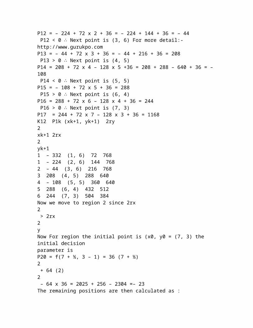
§−1=1ad − bcµd −b−c a§.• Lines and parallelism are preserved under affine transformations.Proof:To prove lines are preserved, we must show that q¯(λ) = F(¯l(λ)) is a line, whereF(¯p) = Ap¯+ ~t and¯l(λ) = ¯p0 + λ~d.q¯(λ) = A¯l(λ) + ~t= A(¯p0 + λ~d) + ~t= (Ap¯0 + ~t) + λA~dThis is a parametric form of a line through Ap¯0 + ~t with direction A~d.• Given a closed region, the area under an affine transformation Ap¯+ ~t is scaled by det(A).Note:– Rotations and translations have det(A) = 1.– Scaling A =µa 00 b§has det(A) = ab.– Singularities have det(A) = 0.Example:The matrix A =µ1 00 0§maps all points to the x-axis, so the area of any closedregion will become zero. We have det(A) = 0, which verifies that any closedregion’s area will be scaled by zero.

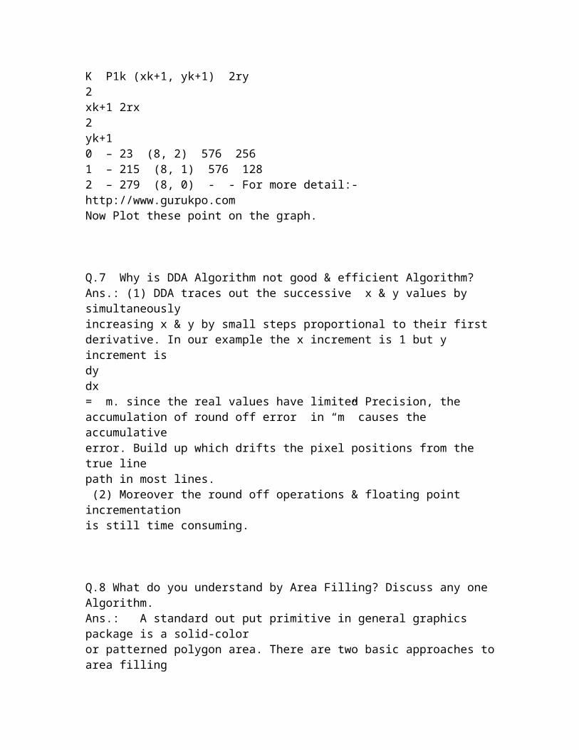
Copyright c 2005 David Fleet and Aaron Hertzmann 12CSC418 / CSCD18 / CSC2504 Transformations• A composition of affine transformations is still affine.Proof:Let F1(¯p) = A1p¯+ ~t1 and F2(¯p) = A2p¯+ ~t2.Then,F(¯p) = F2(F1(¯p))= A2(A1p¯+ ~t1) + ~t2= A2A1p¯+ (A2~t1 + ~t2).Letting A = A2A1 and ~t = A2~t1 + ~t2, we have F(¯p) = Ap¯ + ~t, and this is