computer programs in seismology - department of … · 2011-07-07 · computer programs in...
TRANSCRIPT
COMPUTER PROGRAMS IN SEISMOLOGY
SURFACE WAVES, RECEIVER FUNCTIONSAND CRUSTAL STRUCTURE
Robert B. Herrmann Charles. J. Ammon
Professor of Geophysics AssociateProfessorDepartment of Earth and Department of Geosciences
Atmospheric SciencesSaint Louis University PennState University
Version 3.302002
Copyright © 2002 by R. B. Herrmann and C. J. Ammon
Version 3.30 14 June 2007

-2-
Contents
Preface vi
Chapter 1: Crustal Structure?1. Introduction 1-12. A Simple Example 1-13. Caveats 1-10
Chapter 2: Review of Inv ersion Theory1. Introduction 2-12. Means, variances and standard deviations 2-13. Linear Regression 2-44. Linear Regression - Known, but Uniform Variance 2-125. Weighted Linear Regression 2-145.1 Weights 2-155.2 Stochastic Weights 2-166. Weighted Linear Regression - Combining Data 2-177. One Model - Two Different Data Sets 2-207.1 Development 2-207.2 Actual Data Processing 2-207.3 Reduction to a Single System 2-218. Matrix Formulation 2-229. General Linear Least Squares 2-249.1 Correlation Coefficient 2-2510. Non-Linear Least Squares by Linearization 2-2511. L-1 Norms 2-2512. Problems 2-2613. References 2-26
DRAFT iii 14 June 2007

Chapter 3: Surface Wav eAnalysis1. Introduction 3-12. The Surface Processing 3-13. Graphical Interfaces 3-134. Data Preparation 3-235. surf96 3-256. Example 3-307. Discussion 3-358. References 3-35
Chapter 4: Inversion of Receiver Functions1. Introduction 4-12. Joint Inversion Mathematics 4-23. Data Preparation 4-24. rftn96 4-65. Example 4-106. Discussion 4-16
Chapter 5: Joint Inversion Dispersion1. Introduction 5-12. Joint Inversion Mathematics 5-13. joint96 5-34. Example 5-95. Discussion 5-15
Appendix A: Installation1. Tailoring Shell Scripts A-12. Hard Copy A-2
DRAFT iv 14 June 2007

DRAFT v 14 June 2007

PREFACE
Version 3.30 vi 14 June 2007
CHAPTER 1CRUSTAL STRUCTURE?
1. Introduction
This volume discusses techniques for estimating shallow earth structure that use dif-ferent parts of the seismogram - the surface wav e and the time series associated withsome body-wav e arrivals. Techniques for deriving surface wav e dispersion from therecorded surface wav eand for defining the receiver function for initial P- or S-wav es willbe presented along with programs to invert these data sets for shalloEarth structure veloc-ity models.
Seismic data sets are never complete enough to uniquely define earth structurebecause of the effects of noise, limited frequency band or other reasons for lack of obser-vations. To impress this reality, perfect data sets will be inverted for earth structure andtheir differences in predicting independent observations will be compared.
2. A Simple Example
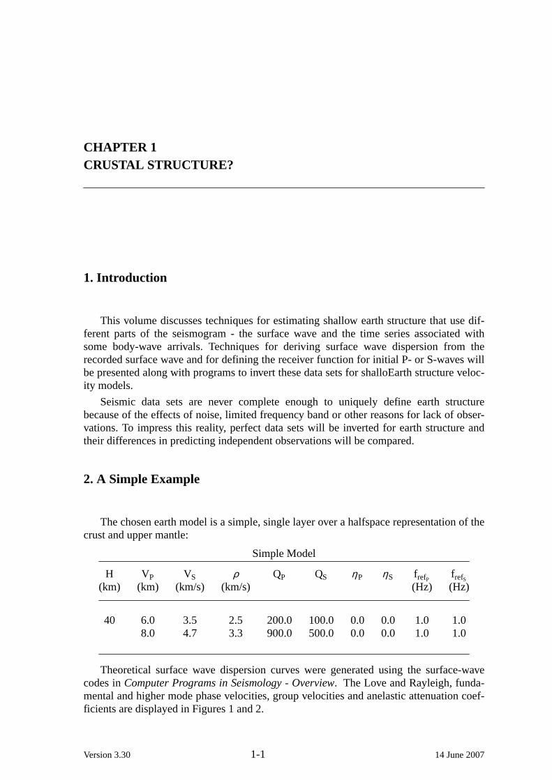
The chosen earth model is a simple, single layer over a halfspace representation of thecrust and upper mantle:
Simple Model
H VP VS ρ QP QS ηP ηS frefP frefS(km) (km) (km/s) (km/s) (Hz) (Hz)
40 6.0 3.5 2.5 200.0 100.0 0.0 0.0 1.0 1.08.0 4.7 3.3 900.0 500.0 0.0 0.0 1.0 1.0
Theoretical surface wav e dispersion curves were generated using the surface-wav ecodes inComputer Programs in Seismology - Overview. The Love and Rayleigh, funda-mental and higher mode phase velocities, group velocities and anelastic attenuation coef-ficients are displayed in Figures 1 and 2.
Version 3.30 1-1 14 June 2007

Computer Programs in Seismology - Crustal Structure Inv ersion
8 . 0 0
1 6 . 0 0
2 4 . 0 0
3 2 . 0 0
4 0 . 0 0
4 8 . 0 0
5 6 . 0 0
6 4 . 0 0
7 2 . 0 0
DE
PT
H (
KM
)
3 . 6 0 4 . 0 0 4 . 4 0 4 . 8 0VS (KM/S)
C u r r e n t
I n i t i a l101
PERIOD
3.0
03
.50
VE
LO
CIT
Y (
KM
/S)
4.0
04
.50
5.0
0
LOVE
101
PERIOD
2.5
03
.13
VE
LO
CIT
Y (
KM
/S)
3.7
54
.38
5.0
0
RAYLEIGH
Fig. 1. Earth model and dispersion points used for inversion test.
8 . 0 0
1 6 . 0 0
2 4 . 0 0
3 2 . 0 0
4 0 . 0 0
4 8 . 0 0
5 6 . 0 0
6 4 . 0 0
7 2 . 0 0
DE
PT
H (
KM
)
- 0 . 1 0QBINV * 1 0 - 1
0 . 1 0
C u r r e n t
I n i t i a l101
PERIOD
0.5
55
.41
GA
MM
A (
1/K
M)
*10
-4
10
.28
15
.14
20
.00
LOVE
101
PERIOD
0.3
55
.26
GA
MM
A (
1/K
M)
*10
-4
10
.18
15
.09
20
.00
RAYLEIGH
Fig. 2. Q−1S model and anelastic attenuation coefficietns,γ , for Love and Rayleigh,fundamental and 1st
higher modes.
The period range chosen for inversion, 5 - 60 seconds, represents the author’s (RBH)experience in determining dispersion for small earthquakes in eastern North America.The lower period limit is controlled by source excitation and anelastic attenuation and theupper period limit by the low signal noise. In reality one would almost never hav eallthese data points - perhaps the group velocity values for the fundamental mode, and a fewother data points.
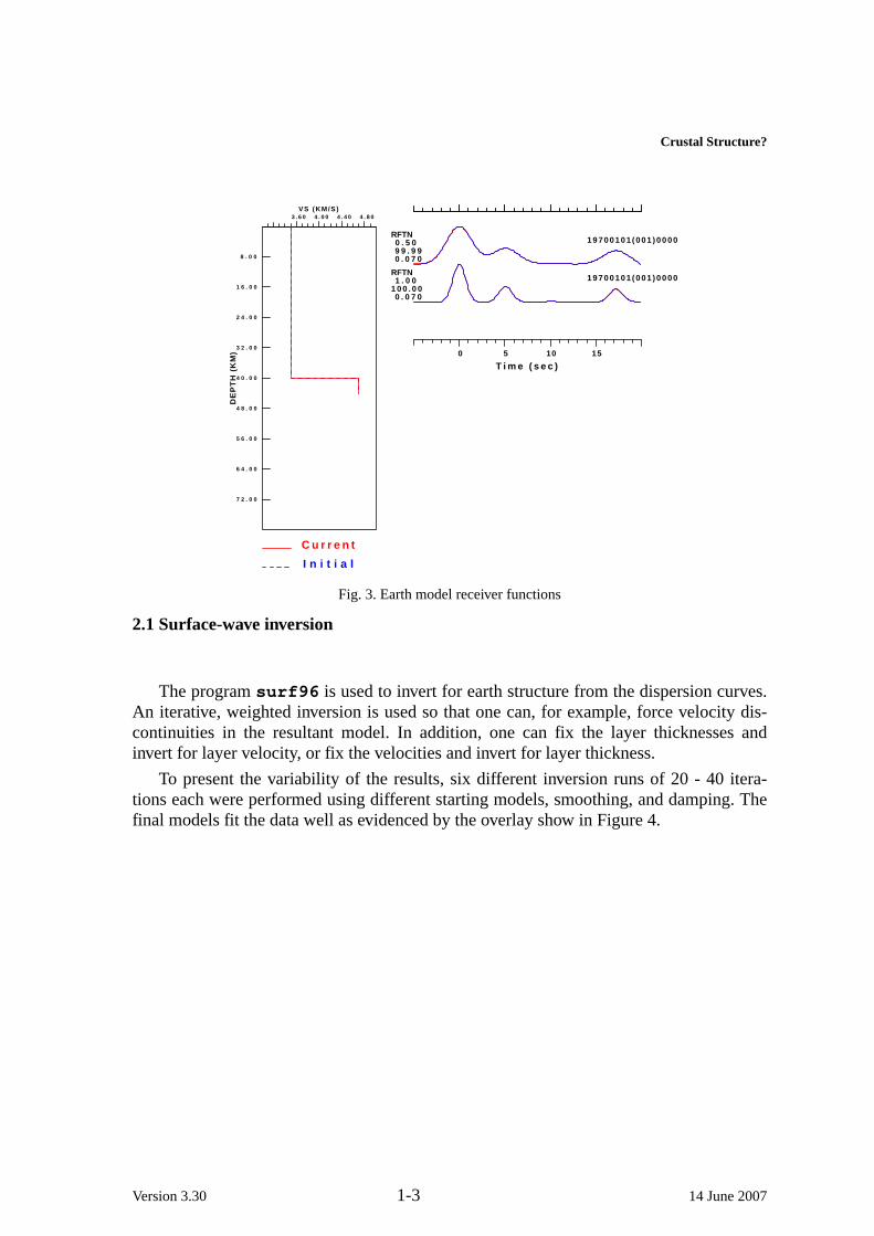
For the same model, P-wav e receiver functions were computed using the programhrftn96 for a teleseismic signal with ray parameterp = 0.07 sec/km and Gaussian filterparameters of 0.50 and 1.0. Figure 3 presents the earth model again together with thereceiver functions.
Version 3.30 1-2 14 June 2007
Crustal Structure?
8 . 0 0
1 6 . 0 0
2 4 . 0 0
3 2 . 0 0
4 0 . 0 0
4 8 . 0 0
5 6 . 0 0
6 4 . 0 0
7 2 . 0 0
DE
PT
H (
KM
)
3 . 6 0 4 . 0 0 4 . 4 0 4 . 8 0VS (KM/S)
C u r r e n t
I n i t i a l
0 5 10 15
T i m e ( s e c )
19700101 (001 )0000RFTN 0 . 5 0 9 9 . 9 9 0 . 0 7 0
19700101 (001 )0000RFTN 1 . 0 01 0 0 . 0 0 0 . 0 7 0
Fig. 3. Earth model receiver functions
2.1 Surface-wave inv ersion
The programsurf96 is used to invert for earth structure from the dispersion curves.An iterative, weighted inversion is used so that one can, for example, force velocity dis-continuities in the resultant model. In addition, one can fix the layer thicknesses andinvert for layer velocity, or fix the velocities and invert for layer thickness.
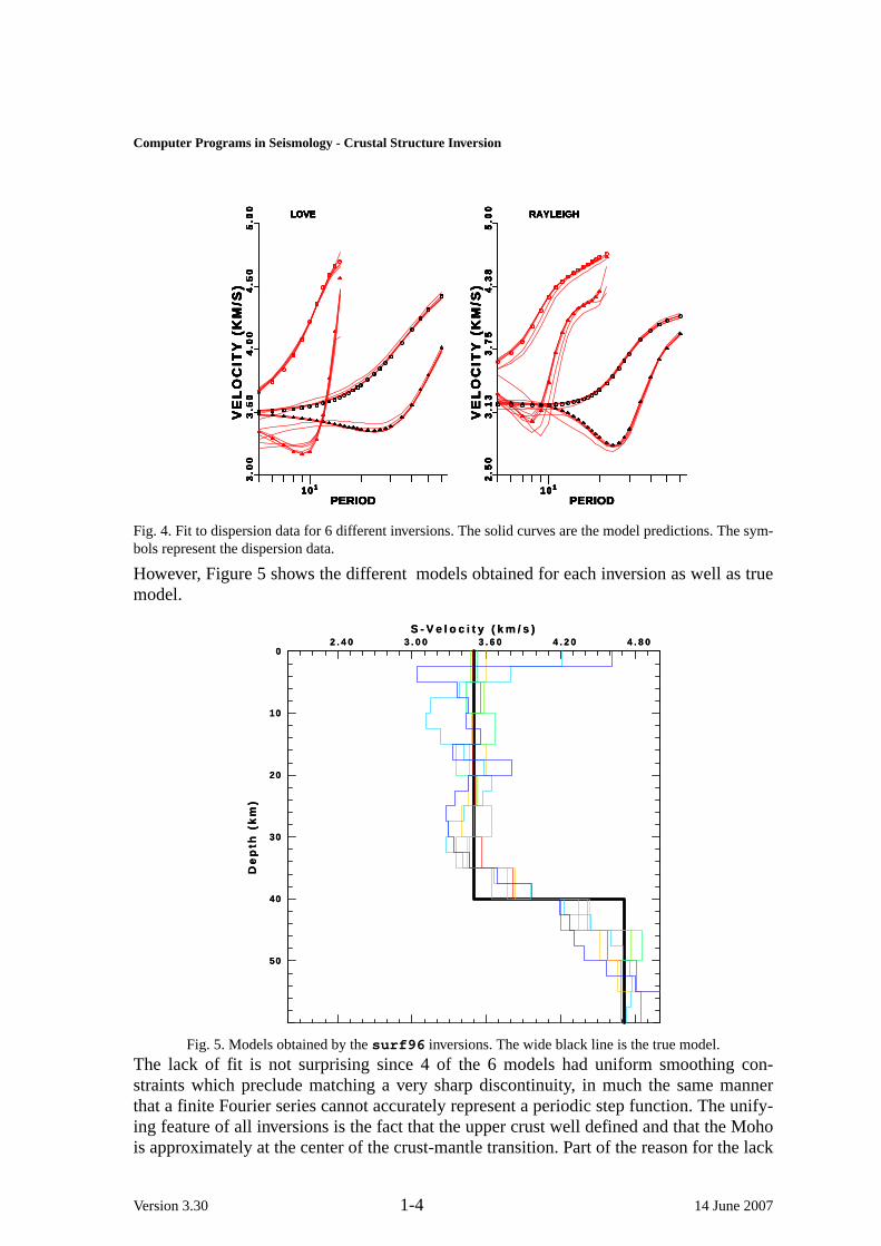
To present the variability of the results, six different inversion runs of 20 - 40 itera-tions each were performed using different starting models, smoothing, and damping. Thefinal models fit the data well as evidenced by the overlay show in Figure 4.
Version 3.30 1-3 14 June 2007
Computer Programs in Seismology - Crustal Structure Inv ersion
101
PERIOD
3.0
03
.50
VE
LO
CIT
Y (
KM
/S)
4.0
04
.50
5.0
0
LOVE
101
PERIOD2
.50
3.1
3V
EL
OC
ITY
(K
M/S
) 3
.75
4.3
85
.00
RAYLEIGH
101
PERIOD
3.0
03
.50
VE
LO
CIT
Y (
KM
/S)
4.0
04
.50
5.0
0
LOVE
101
PERIOD2
.50
3.1
3V
EL
OC
ITY
(K
M/S
) 3
.75
4.3
85
.00
RAYLEIGH
101
PERIOD
3.0
03
.50
VE
LO
CIT
Y (
KM
/S)
4.0
04
.50
5.0
0
LOVE
101
PERIOD2
.50
3.1
3V
EL
OC
ITY
(K
M/S
) 3
.75
4.3
85
.00
RAYLEIGH
101
PERIOD
3.0
03
.50
VE
LO
CIT
Y (
KM
/S)
4.0
04
.50
5.0
0
LOVE
101
PERIOD2
.50
3.1
3V
EL
OC
ITY
(K
M/S
) 3
.75
4.3
85
.00
RAYLEIGH
101
PERIOD
3.0
03
.50
VE
LO
CIT
Y (
KM
/S)
4.0
04
.50
5.0
0
LOVE
101
PERIOD2
.50
3.1
3V
EL
OC
ITY
(K
M/S
) 3
.75
4.3
85
.00
RAYLEIGH
101
PERIOD
3.0
03
.50
VE
LO
CIT
Y (
KM
/S)
4.0
04
.50
5.0
0
LOVE
101
PERIOD2
.50
3.1
3V
EL
OC
ITY
(K
M/S
) 3
.75
4.3
85
.00
RAYLEIGH
Fig. 4. Fit to dispersion data for 6 different inversions. The solid curves are the model predictions. The sym-bols represent the dispersion data.
However, Figure 5 shows the different modelsobtained for each inversion as well as truemodel.
2 . 4 0 3 . 0 0 3 . 6 0 4 . 2 0 4 . 8 0S - V e l o c i t y ( k m / s )
50
40
30
20
10
0
De
pth
(k
m)
2 . 4 0 3 . 0 0 3 . 6 0 4 . 2 0 4 . 8 0S - V e l o c i t y ( k m / s )
50
40
30
20
10
0
De
pth
(k
m)
Fig. 5. Models obtained by thesurf96 inversions. The wide black line is the true model.
The lack of fit is not surprising since 4 of the 6 models had uniform smoothing con-straints which preclude matching a very sharp discontinuity, in much the same mannerthat a finite Fourier series cannot accurately represent a periodic step function. The unify-ing feature of all inversions is the fact that the upper crust well defined and that the Mohois approximately at the center of the crust-mantle transition. Part of the reason for the lack
Version 3.30 1-4 14 June 2007

Crustal Structure?
of fit was that the upper mantle velocity was free to change. In the actual earth, we wouldexpect upper mantle velocities to be known or at least bounded so that they can be fixed.
The impact of these different earth models is seen if the models are used for some-thing other than predicting surface-wav e dispersion in the 5 - 60 second period range,such as predicting first arrival times for use in event location. The true model and the 6inverted models were used as input to the programtimmod96 to predict the P-wav efi rstarrival times from 0 - 800 km for a surface event. The results of these computations areshown in Figure 6. All but one model predicts the direct arrival well. However, the vari-ability in the lower crust leads to predicted travel time differences of several seconds.
100 300 500 700
X ( k m )
2
4
6
8
10
12
T -
X /
8.0
100 300 500 700
X ( k m )
2
4
6
8
10
12
T -
X /
8.0
Fig. 6. P-wav efi rst arrival times for the true model, solid black line, and inverted models.
2.2 P-wave receiver f unction inversion
The next exercise is to invert the P-wav e receiver function data using the programrftn96. The results of 5 inversions are presented. Figure 7 presents the data fits, Figure8 the models and Figure 9 the predicted travel times.
Version 3.30 1-5 14 June 2007

Computer Programs in Seismology - Crustal Structure Inv ersion
0 5 10 15
T i m e ( s e c )
19700101 (001 )0000RFTN 0 . 5 0 9 9 . 9 6 0 . 0 7 0
19700101 (001 )0000RFTN 1 . 0 0 9 9 . 5 2 0 . 0 7 0
0 5 10 15
T i m e ( s e c )
19700101 (001 )0000RFTN 0 . 5 0 9 9 . 6 2 0 . 0 7 0
19700101 (001 )0000RFTN 1 . 0 0 9 7 . 0 7 0 . 0 7 0
0 5 10 15
T i m e ( s e c )
19700101 (001 )0000RFTN 0 . 5 0 9 9 . 9 3 0 . 0 7 0
19700101 (001 )0000RFTN 1 . 0 0 9 9 . 2 8 0 . 0 7 0
0 5 10 15
T i m e ( s e c )
19700101 (001 )0000RFTN 0 . 5 0 9 9 . 9 4 0 . 0 7 0
19700101 (001 )0000RFTN 1 . 0 0 9 9 . 7 9 0 . 0 7 0
0 5 10 15
T i m e ( s e c )
19700101 (001 )0000RFTN 0 . 5 0 9 8 . 5 9 0 . 0 7 0
19700101 (001 )0000RFTN 1 . 0 0 9 8 . 5 9 0 . 0 7 0
Fig. 7. Fit to receiver function for 5 different inversions.
2 . 4 0 3 . 0 0 3 . 6 0 4 . 2 0 4 . 8 0S - V e l o c i t y ( k m / s )
50
40
30
20
10
0
De
pth
(k
m)
2 . 4 0 3 . 0 0 3 . 6 0 4 . 2 0 4 . 8 0S - V e l o c i t y ( k m / s )
50
40
30
20
10
0
De
pth
(k
m)
Fig. 8. Models obtained by therftn96 inversions. The wide black line is the true model.
Version 3.30 1-6 14 June 2007
Crustal Structure?
100 200 300 400
X ( k m )
2
4
6
8
10
12T
- X
/8
.0
100 200 300 400
X ( k m )
2
4
6
8
10
12T
- X
/8
.0
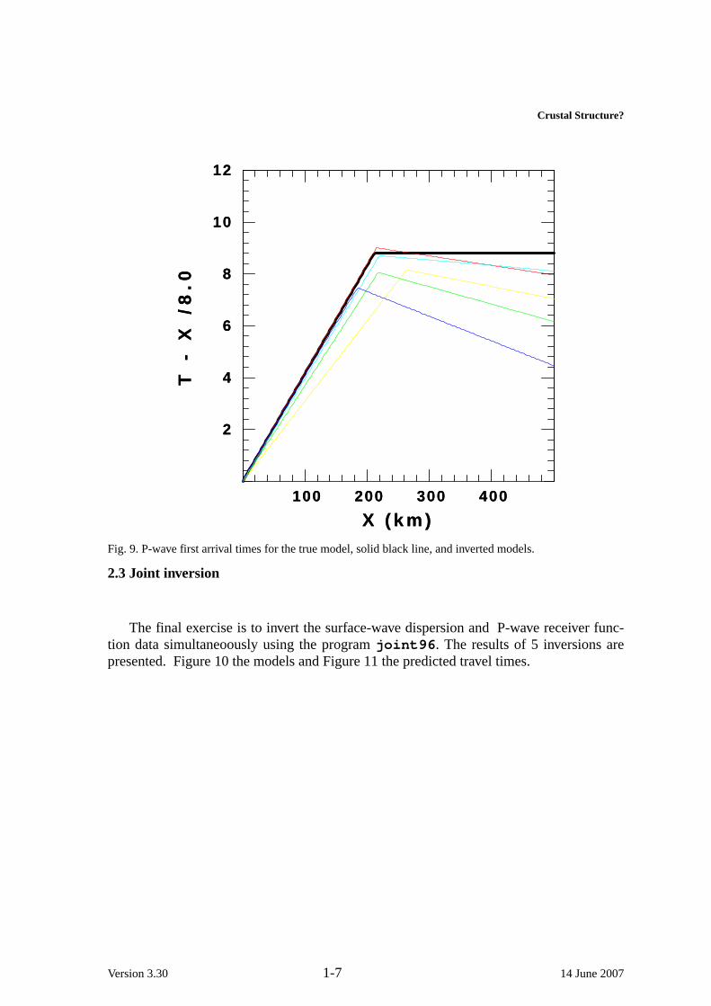
Fig. 9. P-wav efi rst arrival times for the true model, solid black line, and inverted models.
2.3 Joint inversion
The final exercise is to invert the surface-wav edispersion andP-wav ereceiver func-tion data simultaneoously using the programjoint96. The results of 5 inversions arepresented. Figure10 the models and Figure 11 the predicted travel times.
Version 3.30 1-7 14 June 2007

Computer Programs in Seismology - Crustal Structure Inv ersion
2 . 4 0 3 . 0 0 3 . 6 0 4 . 2 0 4 . 8 0S - V e l o c i t y ( k m / s )
50
40
30
20
10
0
De
pth
(k
m)
2 . 4 0 3 . 0 0 3 . 6 0 4 . 2 0 4 . 8 0S - V e l o c i t y ( k m / s )
50
40
30
20
10
0
De
pth
(k
m)
Fig. 10. Models obtained by thejoint96 inversions. The wide black line is the true model.
Version 3.30 1-8 14 June 2007
Crustal Structure?
100 200 300 400
X ( k m )
2
4
6
8
10
12T
- X
/8
.0
100 200 300 400
X ( k m )
2
4
6
8
10
12T
- X
/8
.0
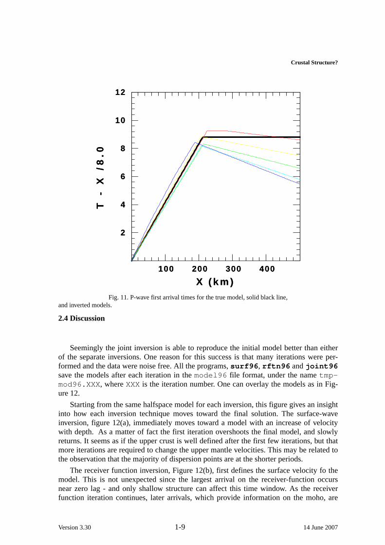
Fig. 11. P-wav efi rst arrival times for the true model, solid black line,and inverted models.
2.4 Discussion
Seemingly the joint inversion is able to reproduce the initial model better than eitherof the separate inversions. One reason for this success is that many iterations were per-formed and the data were noise free. All the programs,surf96, rftn96 andjoint96save the models after each iteration in themodel96 fi le format, under the nametmp-mod96.XXX, whereXXX is the iteration number. One can overlay the models as in Fig-ure 12.
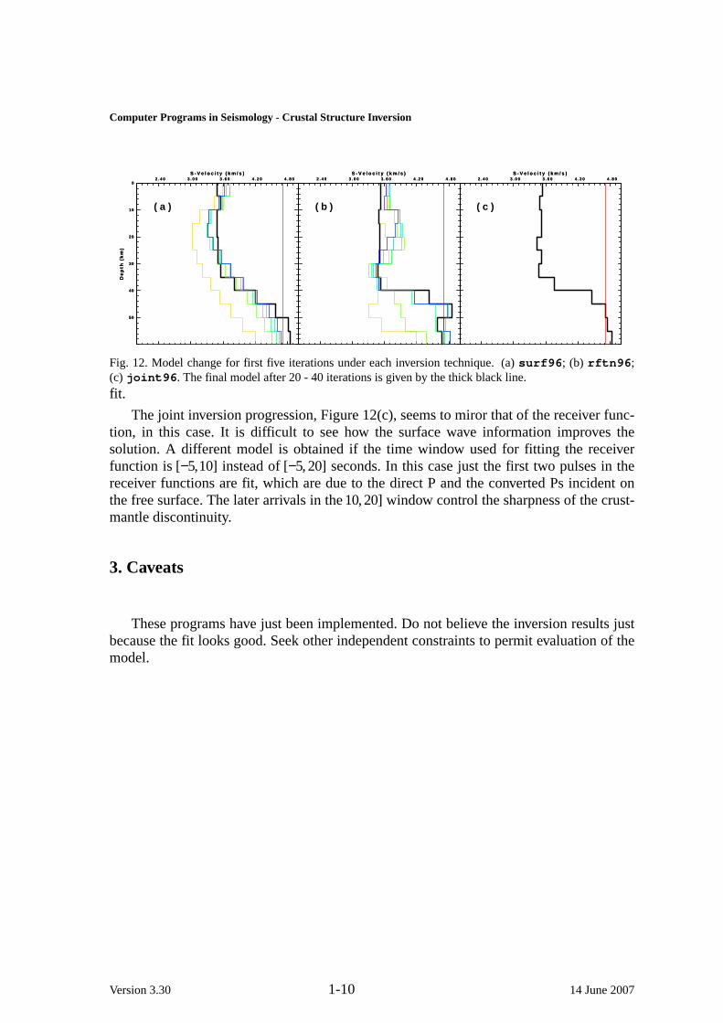
Starting from the same halfspace model for each inversion, this figure gives an insightinto how each inversion technique moves tow ard the final solution. The surface-wav einversion, figure 12(a), immediately moves tow ard a model with an increase of velocitywith depth. As a matter of fact the first iteration overshoots the final model, and slowlyreturns. It seems as if the upper crust is well defined after the first few iterations, but thatmore iterations are required to change the upper mantle velocities. This may be related tothe observation that the majority of dispersion points are at the shorter periods.
The receiver function inversion, Figure 12(b), first defines the surface velocity fo themodel. This is not unexpected since the largest arrival on the receiver-function occursnear zero lag - and only shallow structure can affect this time window. As the receiverfunction iteration continues, later arrivals, which provide information on the moho, are
Version 3.30 1-9 14 June 2007
Computer Programs in Seismology - Crustal Structure Inv ersion
2 . 4 0 3 . 0 0 3 . 6 0 4 . 2 0 4 . 8 0S - V e l o c i t y ( k m / s )
50
40
30
20
10
0
De
pth
(k
m)
2 . 4 0 3 . 0 0 3 . 6 0 4 . 2 0 4 . 8 0S - V e l o c i t y ( k m / s )
50
40
30
20
10
0
De
pth
(k
m)
2 . 4 0 3 . 0 0 3 . 6 0 4 . 2 0 4 . 8 0S - V e l o c i t y ( k m / s )
2 . 4 0 3 . 0 0 3 . 6 0 4 . 2 0 4 . 8 0S - V e l o c i t y ( k m / s )
2 . 4 0 3 . 0 0 3 . 6 0 4 . 2 0 4 . 8 0S - V e l o c i t y ( k m / s )
2 . 4 0 3 . 0 0 3 . 6 0 4 . 2 0 4 . 8 0S - V e l o c i t y ( k m / s )
( a ) ( b ) ( c )
Fig. 12. Model change for first fiv e iterations under each inversion technique.(a) surf96; (b) rftn96;(c) joint96. The final model after 20 - 40 iterations is given by the thick black line.
fi t.
The joint inversion progression, Figure 12(c), seems to miror that of the receiver func-tion, in this case. It is difficult to see how the surface wav e information improves thesolution. A different model is obtained if the time window used for fitting the receiverfunction is[−5, 10] instead of[−5, 20] seconds. In this case just the first two pulses in thereceiver functions are fit, which are due to the direct P and the converted Ps incident onthe free surface. The later arrivals in the10, 20] window control the sharpness of the crust-mantle discontinuity.
3. Caveats
These programs have just been implemented. Do not believe the inversion results justbecause the fit looks good. Seek other independent constraints to permit evaluation of themodel.
Version 3.30 1-10 14 June 2007

Crustal Structure?
CHAPTER 2REVIEW OF INVERSION THEORY
1. Introduction
Having discussed the separate inversion of receiver functions and surface-wav edis-persion for earth structure, we now present the joint inversion of these two data sets.Thissection will review basic concepts of regression analysis. Such a review is appropriatesince regression analysis defines the coefficients of a chosen model that best fit observa-tional data. These concepts will be illustrated using simple models. Hopefully, a goodunderstanding of simple regression problems will serve as a basis for understandinginversion theory.
2. Means, variances and standard deviations
Assume that we can observe some phenomena and make repeated measurements.Also assume that we expect to obtain the same observation, but that there is someunknown, random observational error that prevents this.
Version 3.30 2-1 14 June 2007

Computer Programs in Seismology - Crustal Structure Inv ersion
An example of this is to imagine aninclined ramp on a table.A metal sphericalball rolls down the incline. At the bottom ofthe incline the balltravels horizontally witha velocity V. From elementary physics, weknow the ball will impact the floor after atime
t = 2gH
1 /2
,
where H is the vertical distance from thefloor to the base of the ramp.At the sametime the ball will be a horizontal distance
X = V t
from the base of the ramp. As a matter offact, we would expect that the path of theball from the table to the floor would be aparabola if we do not have to worry aboutair resistance.
If the ball is repeatedly released at the top of the ramp, the pattern of impacts willgenerally be at a distance ofX f rom the base of the ramp, with some impacts at shorterand greater distances. The variation may be due to variations over which the experi-menter has no control: e.g., the ball is not perfectly spherical, the ramp may distort withchanges in room temperature, there may be different patterns of swirling air currents, orthe ball is not released in exactly the same way.
Let xi be thei′th measured distance. LetN be the number of times the experiment isrepeated. Let the expected value ofx, E(x), beµ, which we call the mean. Finally letε i bethe random error of the i′th observation. Thusthe i′th observation is
Version 3.30 2-2 14 June 2007

Review of Inversion Theory
xi = µ + ε i
At this point an important assumption is made about the random error process -- thisprocess has a zero mean, i.e., E(ε) = 0. Thiscan be written as
N→∞lim
1
N
N
i=1Σ ε i → 0
That there is no bias in the measurements, such as might arise from a bad measuringscale, is an article of faith. Furtherwe assume that the errors are truly random and notcorrelated. Althoughnot necessary here, the error is often assumed to arise from a nor-mal, or Gaussian, distribution with zero mean and varianceσ 2
ε i~N(0,σ 2).
For such a distribution, we expect about 68% if the observations to lie within the range(µ − σ , µ + σ ), and 95% within the range (µ − 2σ , µ + 2σ ).
Mathematically the normal distribution N(z,σ 2) is defined as
N(z,σ 2) =1
σ √ 2πe−z26/ 2σ 2
This is a probability distribution and theZ
−∞∫ N(z,σ 2)dz is called the cumulative probabil-
ity, which varies from0 at Z = −∞ to 1at Z= +∞.
Our task is to use all observations to estimate theµ and the varianceσ 2. We acknowl-edge that we cannot determine theµ, but only estimateanx since we have only a finitenumber of observations. Oneway to accomplish this is by trying to find ana that mini-mizes the sum of square residuals
S=N
i=1Σ (xi − a)2
This value is determined by requiring∂S
∂x= 0 Solving gives
a=1
N
N
i=1Σ xi
The standard deviation s,an estimate ofσ , is defined by
s2 =1
N −1
N
i=1Σ (xi − x)2 (A.2.1)
=1
N −1
N
i=1Σ x2
i − Nx2
(the N−1 is used instead ofN sincex has already been specified and onlyN −1 pieces ofindependent information are available to estimateσ 2. This also guarantees thatE(s2) = σ 2)
The symbol ~ means "is distributed as".
Version 3.30 2-3 14 June 2007

Computer Programs in Seismology - Crustal Structure Inv ersion
Because we have only a finite set of observations, thex estimate ofµ is not perfect.We estimate the standard error of the distribution ofx by the relation
s2x =
s2
N=
1N(N − 1)
N
i=1Σ (xi − x)2 (A.2.2)
At this stage, we can examine the residuals,xi − x, and test whether we can reject thehypothesis that the random error process is normal. We could also test the inappropriate-ness of other distributions.
The meaning of the estimated values is simple. If we perform the experiment once bycollecting Nsamples, we are able to estimate the trueµ, the error process varianceσ 2 andthe variance on the mean, s2.
x
If we perform the experiment again by collecting additional samples from the samenoise contaminated population, we would expect the new x to lie about the trueµ with adistribution controlled bys2
x. The s2 indicates the spread in future observations, and thes2x
indicates the spread in thex estimates ofµ.
Finally as the number of observations Nincreases, we expect thatx→ µ, s2 → σ 2, andsx → 0, in probability.
If the noise process is assumed to be Gaussian (normal) thenconfidence limits can beplaced on the measured quantities.Discuss confidence limits on the x etc to give meaningto the x bar sigmas perhaps give a tabular example and show a histogram
3. Linear Regression
Assume now that the observed data are generated by a true linear process, e.g.,
Y = A + Bx (A.3.1)
The observations are again affected by a zero mean random error:
yi = A + Bxi + ε i
Our objective is to use the data to estimate the true values Aand Bas well as some prop-erties of theε process.
The least squares problem is to find thea and bthat minimizes
S(a, b)=N
i=1Σ ε 2
i =N
i=1Σ
yi − a− bxi
2
, (A.3.2)
where thea and bare estimates ofA and B.
The condition that thea and bmake S a minimum requires∂S
∂a= 0 and
∂S
∂b= 0. These
conditions yield two linear equations, the normal equations, in the unknowns aand b:
N
Σ xi
Σ xi
Σ x2i
a
b
=
Σ yi
Σ xiyi
(A.3.3)
(for simplicity the summation indices are dropped). The solution of this linear equation
Version 3.30 2-4 14 June 2007

Review of Inversion Theory
is obtained by taking the inverse of the square matrix which leads to
ab
=1
N Σ x2i − (Σ xi)2
Σ x2i
− Σ xi
− Σ xi
N
Σ yi
Σ xiyi
(A.3.4)
We can easily show that thea and bvalues arising from the normal equations gives
S(a, b)= Σ y2i − aΣ yi − bΣ xiyi (A.3.5)
An alternative way of writing (A.3.4) explicitly is
b= Σ(x− − x) (yi − y)
Σ(xi − x)2
and
a= y − bx
The estimated variance of the error process is
s2 =1
N − 2S(a, b) (A.3.6)
The confidence limits ona and bare given through the use of the t-distribution:
∆a= t(N − 2, 1− α /2)s2 Σ x2
i
N Σ x2i − (Σ xi)2
1 /2
(A.3.7)
and
∆b= t(N − 2, 1− α /2)s2 N
N Σ x2i − (Σ xi)2
1 /2
(A.3.8)
where t(N − 2, 1− α /2) is the Student-t distribution forN − 2 degrees of freedom and the1 − α /2 confidence level [For 95% confidence,α = 0. 05 and t(∞, 0. 975 )=1. 96]. If theseconfidence bounds are interpreted in the same sense as for the simple example of section2, these are the confidence that the true value ofA l ies withina± ∆a, and similarly thevalue of B lies within b± ∆b. There is one slight complication, and that is that the errorestimates∆a and∆b may be interrelated.
The confidence limits that the predicted regression liney = a+ bx lies near the trueline y= A + Bx are
±t(N − 2, 1− α /2)s2
Σ x2
i − 2xΣ xi + Nx2
N Σ x2i − (Σ xi)2
1 /2
(A.3.9)
±t(N − 2, 1− α /2)s2
Σ(x − x)2
Σ(xi − x)2
1 /2
The confidence limits on the distribution of the data (or future data) about the regres-sion line y= a+ bx are
Version 3.30 2-5 14 June 2007

Computer Programs in Seismology - Crustal Structure Inv ersion
±t(N − 2, 1− α /2)s2
1+ Σ x2
i − 2xΣ xi + Nx2
N Σ x2i − (Σ xi)2
1 /2
(A.3.10)
The first equation gives two hyperbolas about the regression line whose asymptotesare y= (a+ ∆a)+ (b − ∆b)x and y= (a− ∆a)+ (b + ∆b)x. If the experiment were repeated,there is a(1 − α /2) ×100% chance that the resultant regression line will lie within theselimits. Thesecond equation indicates where future data may lie. The hyperbolic natureof the error bound is interesting since it indicates that the prediction error increases as onegets away from the centroid(x,y) of the data set; this is to be expected when extrapolatingbeyond the data set.
The interrelationship of error ina and bcan be examined by searching through possi-ble values ofA and B,comparing the sum of squared residuals to that of the least squaressolution(Draper and Smith, 1966, §2.6 and §10.3):
S(A, B) = S(a, b)1+
2
N − 2F(2, N− 2, 1− α )
(A.3.11)
Rearranging, one would contour the following function ofA and B, which is related tothe F-statistic:
S(A, B) − S(a, b)
S(a, b)
N − 2
2
= F(2, N− 2, 1− α ) (A.3.12)
Because our model was linear, the contours in the(A, B) space satisfying this relation willbe ellipses. In general the major axis of the elliptical contour may be inclined, indicatingsome interdependence between thea and bvalues. In this case, a change in the value ofbcauses a change in a.
Since Draper and Smith (1966) may be the only ones to define confidence ellipses inthis manner, an alternative expression is
[A − a, B− b]
N
Σ xi
Σ xi
Σ x2i
A − a
B − b
= 2s2F(2, N− 2, 1− α )
Example 1
Consider the following data set of 10 points:
Table A.3.1.xi yi xi yi
1 1 7 82 1 9 71 2 10 83 3 12 146 5 14 16
From this data set we form the sums
Version 3.30 2-6 14 June 2007

Review of Inversion Theory
N = 10 Σ yi = 65
Σ xi = 65 Σ y2i = 66 9
Σ x2i = 621 Σ xiyi = 63 5
For a 95% confidence level, t(8, 0. 975 )= 2. 306. (The Fischer, Student t-distribution hasthe property thatt(inf , α ) = Normaldistribution. Using these sums and thet-value, weobtain
a= − 0. 458 4±1. 988 4
b=1. 0705± 0. 2523
s2 = 2. 376 5
Figure 1 shows the regression line and the 95% confidence hyperbolas on the regres-sion line. The confidence hyperbolas mean that another data set from the same data popu-lation would lead to a regression line which has a95% chance of being within thesehyperbolas. (These statements are repetitious but the distinction between scatter in dataand model parameters is important).
Figure 2 shows the regression line and the 95% confidence limits on the data. If weselect additional samples from the population, then 95% of them should lie within thehyperbolas.
Version 3.30 2-7 14 June 2007

Computer Programs in Seismology - Crustal Structure Inv ersion
- 1 5 . 0 0 - 7 . 5 0 0 . 0 0 7 . 5 0X
1 5 . 0 0 2 2 . 5 0 3 0 . 0 0
-15
.00
-7.5
00
.00
7.5
0
Y1
5.0
02
2.5
03
0.0
0
Fig. 1. Regression line (black) and 95% confidence bounds (light gray) on the regression line.
Version 3.30 2-8 14 June 2007

Review of Inversion Theory
- 1 5 . 0 0 - 7 . 5 0 0 . 0 0 7 . 5 0X
1 5 . 0 0 2 2 . 5 0 3 0 . 0 0
-15
.00
-7.5
00
.00
7.5
0
Y1
5.0
02
2.5
03
0.0
0
Fig. 2. Regression line (black) and 95% confidence bounds (light gray) on the data set. The data are shownby the points.
Figure 3 plots the F-statistic at 50%, 75%, 90%, 95%, 97.5% and 99% levels. Thesmallest region, centered on the regression values (a, b)= (−0. 458, 1. 071 ), indicates thatthere is only a 50% chance that the true values of(a, b) are located within this region. Asthe confidence increases, the confidence region increases. We can always state with 100%confidence that the true value is somewhere within the(a, b) plane, if our originalassumption of a linear model is correct.
Example 2
Consider the same data set of 10 points, except that the origin is shifted to the(x,y) ofthe previous data set. Subtracting thex = 6. 5from all x andy = 6. 5from all y values gives:
Version 3.30 2-9 14 June 2007

Computer Programs in Seismology - Crustal Structure Inv ersion
- 3 . 0 0 - 2 . 0 0 - 1 . 0 0 0 . 0 0 1 . 0 0
0 . 4 0
0 . 8 0
1 . 2 0
1 . 6 0
2 . 0 0
a
b
Fig. 3. Plot of the F-statistic usingS(a, b).Contours are drawn atF(2, 8,p) = 0.757 for50%, 1.66 for 75%,3.11 for 90%, 4.46 for 95%, 6.06 for 97.5% and 6.85 for 99%.
Table A.3.2xi yi xi yi
-5.5 -5.5 0.5 1.5-4.5 -5.5 2.5 0.5-5.5 -4.5 3.5 1.5-3.5 -3.5 5.5 7.5-0.5 -1.5 7.5 9.5
From this data set we obtain the sums:
N = 10 Σ yi = 0
Σ xi = 0 Σ y2i = 246. 5
Σ x2i = 198. 5 Σ xiyi = 21 2.5
Since theΣ xi = 0, the matrices in (A.3.3) and (A.3.4) are diagonal.For a 95%
Version 3.30 2-10 14 June 2007
Review of Inversion Theory
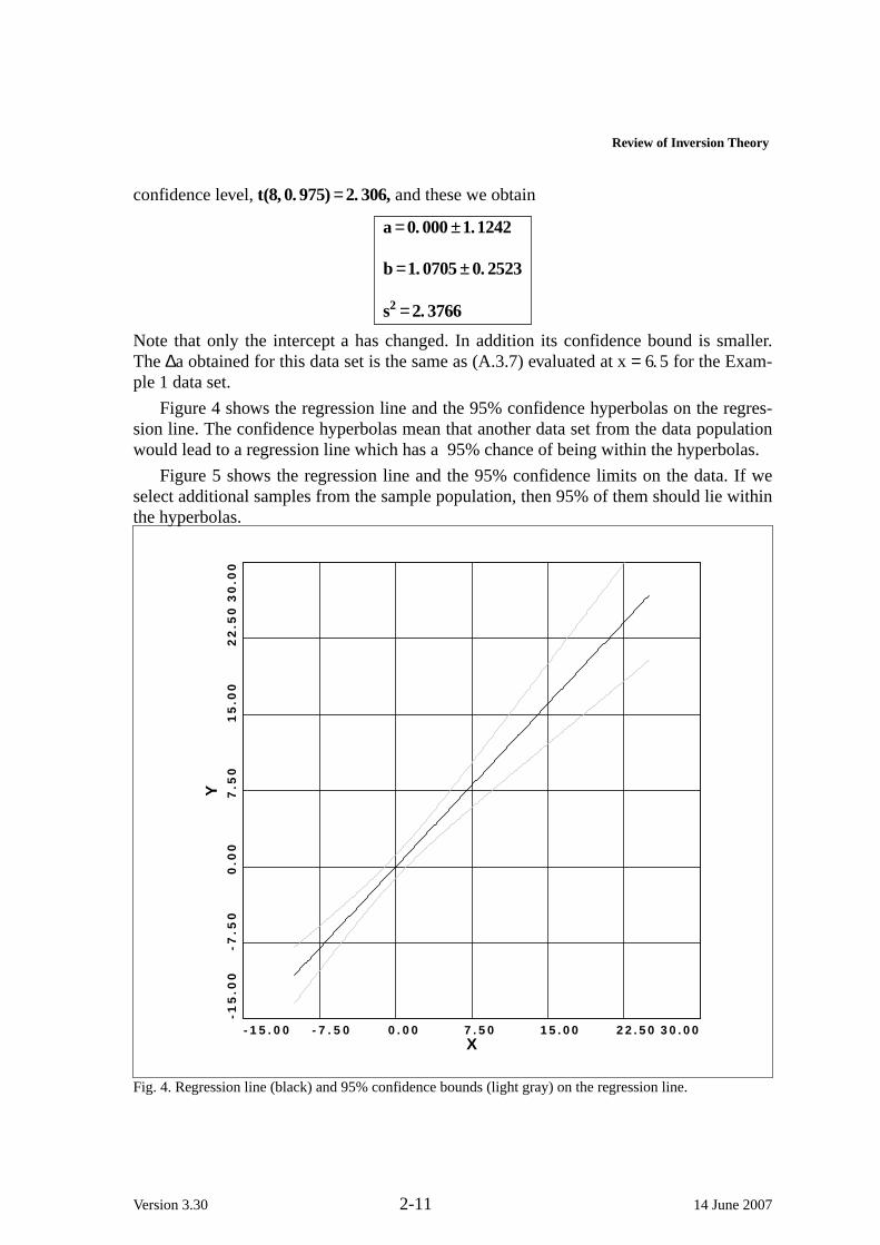
confidence level, t(8, 0. 975) = 2. 306, and these we obtain
a= 0. 000±1. 124 2
b =1. 070 5± 0. 252 3
s2 = 2. 3766
Note that only the intercepta has changed. In addition its confidence bound is smaller.The∆a obtained for this data set is the same as (A.3.7) evaluated atx = 6. 5for the Exam-ple 1 data set.
Figure 4 shows the regression line and the 95% confidence hyperbolas on the regres-sion line. The confidence hyperbolas mean that another data set from the data populationwould lead to a regression line which has a 95% chance of being within the hyperbolas.
Figure 5 shows the regression line and the 95% confidence limits on the data. If weselect additional samples from the sample population, then 95% of them should lie withinthe hyperbolas.
- 1 5 . 0 0 - 7 . 5 0 0 . 0 0 7 . 5 0X
1 5 . 0 0 2 2 . 5 0 3 0 . 0 0
-15
.00
-7.5
00
.00
7.5
0
Y1
5.0
02
2.5
03
0.0
0
Fig. 4. Regression line (black) and 95% confidence bounds (light gray) on the regression line.
Version 3.30 2-11 14 June 2007

Computer Programs in Seismology - Crustal Structure Inv ersion
- 1 5 . 0 0 - 7 . 5 0 0 . 0 0 7 . 5 0X
1 5 . 0 0 2 2 . 5 0 3 0 . 0 0
-15
.00
-7.5
00
.00
7.5
0
Y1
5.0
02
2.5
03
0.0
0
Fig. 5. Regression line (black) and 95% confidence bounds (light gray) on the data set. The data are shownby the points.
Figure 6 plots the F-statistic at 50%, 75%, 90%, 95%, 97.5% and 99% levels. Thesmallest region, centered on the regression values (a, b)= (0. 0,1. 071 ), indicates that thereis only a 50% chance that the true values of(a, b) are located within this region. We notenow that the confidence bounds are no longer inclined ellipses - the major and minor axesare aligned with thea and baxes. Thisis a direct consequence of the fact thatΣ xi = 0.This inclination of the ellipse indicates that there is no trade-off, or co-variance betweenthe a and b values for this data set. In the previous data set, increasing the slopebrequired a smallera to continue to have the line pass through the centroid of the data.
4. Linear Regression - Known, but Uniform Variance
The next way to perform the same regression analysis uses a priori knowledge of thevariance,σ 2, of the random error as a weight. For the straight line problem, we now mini-mize
Version 3.30 2-12 14 June 2007

Review of Inversion Theory
- 2 . 0 0 - 1 . 0 0 0 . 0 0 1 . 0 0 2 . 0 0
0 . 4 0
0 . 8 0
1 . 2 0
1 . 6 0
2 . 0 0
a
b
Fig. 6. Plot of the F-statistic usingS(a, b).Contours are drawn atF(2, 8,p) = 0.757 for50%, 1.66 for 75%,3.11 for 90%, 4.46 for 95%, 6.06 for 97.5% and 6.85 for 99%.
S(a, b)=N
i=1Σ
yi − a− bxi
σ
2
(A.4.1)
AsN→∞lim , we expect that the minimum value isS(a, b)= N because of the definition ofσ as
the limit of s as the number of observations increase. Applying the necessary conditions
for a minimum,∂S
∂a= 0 and
∂S
∂b= 0, yields the two linear equations
Σ 1
σ 2
Σ xi
σ 2
Σ xi
σ 2
Σ x2i
σ 2
a
b
=
Σ yi
σ 2
Σ xiyi
σ 2
(A.4.2)
The solution of the linear equation is simply
Version 3.30 2-13 14 June 2007

Computer Programs in Seismology - Crustal Structure Inv ersion
a
b
=1
Σ 1
σ 2 Σ xi
σ 2− (Σ xi
σ 2)2
Σ x2i
σ 2
− Σ xi
σ 2
− Σ xi
σ 2
Σ 1
σ 2
Σ yi
σ 2
Σ xiyi
σ 2
(A.4.3)
The confidence limits ona and bare given through the use of the z-distribution:
∆a= z(1− α /2)
Σ x2i
σ 2
Σ 1
σ 2 Σ xi
σ 2− (Σ xi
σ 2)2
1 /2
(A.4.4)
and
∆b= z(1− α /2)
Σ 1
σ 2
Σ 1
σ 2 Σ xi
σ 2− (Σ xi
σ 2)2
1 /2
. (A.4.5)
The expression for the confidence bounds ona and bis identical to that of Section 3 if wereplace s2 by σ 2. The confidence on the regression line is
±z(1− α /2)
Σ x2i
σ 2− 2x Σ xi
σ 2+ Σ 1
σ 2x2
Σ 1
σ 2 Σ xi
σ 2− (Σ xi
σ 2)2
1 /2
(A.4.6)
and the confidence limits on the distribution of the data (or future data) about theregression line y= a+ bx are
±z(1− α /2)
σ 2 +Σ x2
i
σ 2− 2x Σ xi
σ 2+ Σ 1
σ 2x2
Σ 1
σ 2 Σ xi
σ 2− (Σ xi
σ 2)2
1 /2
(A.4.7)
The reason that the normal, z-, distribution is used instead of the t-distribution is that thevariances are known.
5. Weighted Linear Regression
During the acquisition of data, more may be known qualitatively or quantitativelyabout an observation. This may occur if a data pair is repeated in the observations, or ifthe data variance is better known. We denote this by assigning each(xi, yi) data pair witha weight wi or a data varianceσ i . In its simplest form thewi may indicate that therewere repeated(xi, yi) values in the data set, and that we wish to use only one pair but indi-cate frequency of repeated values. In another form, thewi may reflect a subjective assess-
ment of data quality, perhaps varying between[0,1]. Finally if σ i is known, wi =1
σ 2i
. The
Version 3.30 2-14 14 June 2007
Review of Inversion Theory
object of this section is to show how presentations in Sections 4 and 5 are to be modifiedand also how they are related.
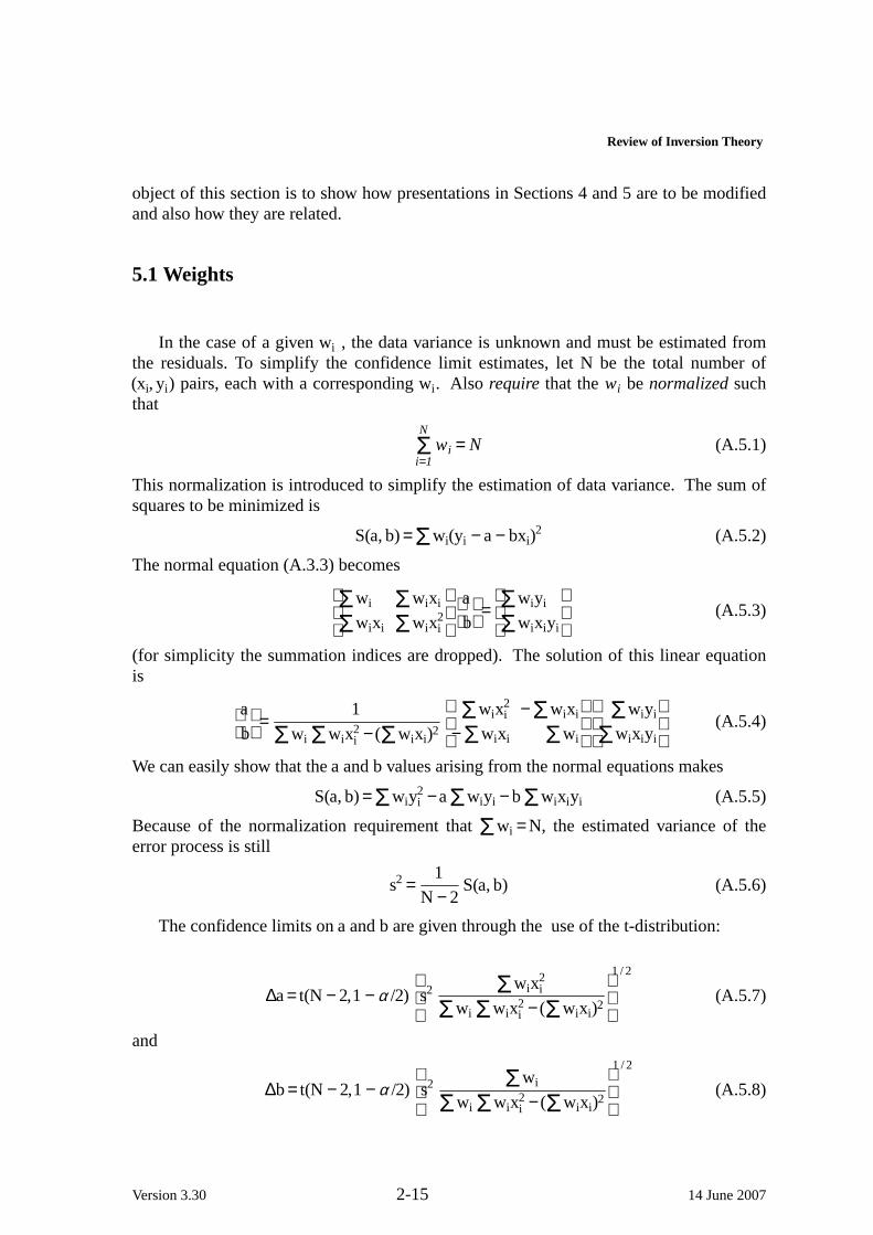
5.1 Weights
In the case of a given wi , the data variance is unknown and must be estimated fromthe residuals. To simplify the confidence limit estimates, letN be the total number of(xi, yi) pairs, each with a correspondingwi . Also require that thewi be normalized suchthat
N
i=1Σ wi = N (A.5.1)
This normalization is introduced to simplify the estimation of data variance. Thesum ofsquares to be minimized is
S(a, b)= Σwi(yi − a− bxi)2 (A.5.2)
The normal equation (A.3.3) becomes
Σwi
Σwixi
Σwixi
Σwix2i
a
b
=
Σwiyi
Σwixiyi
(A.5.3)
(for simplicity the summation indices are dropped). The solution of this linear equationis
a
b
=1
Σwi Σwix2i − (Σwixi)2
Σwix2i
− Σwixi
− Σwixi
Σwi
Σwiyi
Σwixiyi
(A.5.4)
We can easily show that thea and bvalues arising from the normal equations makes
S(a, b)= Σwiy2i − aΣwiyi − bΣwixiyi (A.5.5)
Because of the normalization requirement thatΣwi = N, the estimated variance of theerror process is still
s2 =1
N − 2S(a, b) (A.5.6)
The confidence limits ona and bare given through the use of the t-distribution:
∆a= t(N − 2, 1− α /2)s2 Σwix
2i
Σwi Σwix2i − (Σwixi)2
1 /2
(A.5.7)
and
∆b= t(N − 2, 1− α /2)s2 Σwi
Σwi Σwix2i − (Σwixi)2
1 /2
(A.5.8)
Version 3.30 2-15 14 June 2007

Computer Programs in Seismology - Crustal Structure Inv ersion
The confidence limits on the predicted regression liney = a + bx are
±t(N − 2, 1− α /2)s2
Σwix
2i − 2xΣwixi + Σwix
2i
Σwi Σwix2i − (Σwixi)2
1 /2
(A.5.9)
The confidence limits on the distribution of the data (or future data) about the regres-sion line y= a+ bx are
±t(N − 2, 1− α /2)s2
1+ Σwix
2i − 2xΣwixi + Σwix
2
Σwi Σwix2i − (Σwixi)2
1 /2
(A.5.10)
The confidence contours in the(a, b) plane are still given by (A.3.12). Notethat the t-distribution was used here since the variances are not known, only estimated.
5.2 Stochastic Weights
This section is very similar to that of §4, but with the distinction that the known vari-ances of each observation may be different. The effective weighting of the observations issimilar to that of §5.1. The task here is to minimize
S(a, b)=N
i=1Σ
yi − a− bxi
σ i
2
(A.5.11)
The equations of Section 4 continue to apply with the slight modification that allσ valuesare replaced byσ i . We again note that forN large, (A.5.11) should approachN and that
s2 =S(a, b)
N − 2→1 as N→ ∞
Thus (A.4.3) becomes
a
b
=1
Σ 1
σ 2i
Σ xi2
σ i2
− (Σ xi
σ 2i
)2
Σ x2i
σ 2i
− Σ xi
σ 2i
− Σ xi
σ 2i
Σ 1
σ 2i
Σ yi
σ 2i
Σ xiyi
σ 2i
(A.5.12)
and the confidence limits ona an b giv en in (A.4.4) and (A.4.5) become
∆a= z(1− α /2)
Σ x2i
σ 2i
Σ 1
σ 2i
Σ xi2
σ i2
− (Σ xi
σ 2i
)2
1 /2
(A.5.13)
and
Version 3.30 2-16 14 June 2007

Review of Inversion Theory
∆b= z(1− α /2)
Σ 1
σ 2i
Σ 1
σ 2i
Σ xi2
σ i2
− (Σ xi
σ 2i
)2
1 /2
. (A.5.14)
6. Weighted Linear Regression - Combining Data
One may collect sufficient data in an experiment to perform some preprocessingbefore regression. An example might be repeated surface-wav edispersion measurementsalong the same path for the same frequencies. One could use all data or one could use justthe mean observations at each frequency, the latter may be preferable since it reduces thework required in an inversion scheme since a smaller number of data points are pro-cessed. Thequestion arises of how to determine the correct error estimates.
To dev elop this topic, construct a data set consisting of 1000 observations at each of10 abscissa, xi . The observations are from the model
yij = 0. 0+1. 0xi + ε ij
for i = 1,. . .,10 and j = 1,. . .,1000. Theε ij is from a normal distribution of zero mean andvarianceσ 2
i (Presset al, 19XX). Table A.6.1 gives the tenxi, the target yi andσ assignedto the Gaussian error process. The computedy, sy and sy are derived from the data setfor eachxi. Even with 1000 observations at eachxi, we see that the observed mean is notexactly the target value, but that 9 of the 10y ’s are within onesy of the targety.
Table A.6.1 Statistics of Test Datai x y σ y sy sy
1 0 0 4.00 0.080 4.144 0.1312 1 1 4.00 0.965 4.071 0.1293 2 2 4.00 1.993 4.117 0.1304 3 3 2.00 2.985 1.985 0.0635 4 4 2.00 4.047 2.023 0.0646 5 5 2.00 5.035 1.928 0.0617 6 6 1.00 6.043 0.946 0.0308 7 7 1.00 7.032 0.996 0.0319 8 8 1.00 8.011 0.984 0.031
10 9 9 1.00 9.015 0.985 0.031
Given this data set of 10,000 observations or the 10 reduced observations from theabove table, we consider three minimization problems:
a) Usingthe entire data set, minimize:10
i=1Σ
1000
j=1Σ (yij − a− bxi)
2
Version 3.30 2-17 14 June 2007

Computer Programs in Seismology - Crustal Structure Inv ersion
b) Usingthe entire data set and the sy values for each i:
10
i=1Σ
1000
j=1Σ
yij − a− bxi
σyi
2
c) Usingthe reduced data set consisting of the 10 xi,yi, syi:
10
i=1Σ
yi − a− bxi
σyi
2
Case a) is solved using (A.3.4) - (A.3.8), Case b) is solved using §5.2 (A.5.12 -A.5.14) and Case c) is also solved using §5.2 except thatyi and σ i in (A.5.11) arereplaced byyi and syi
, respectively. To understand how this may relate to actual data sets,for which we do know not theσ ’s, we replace eachσ in these minimization problems bythe corresponding estimates also given in Table A.6.1. This is essential for Case c)because theσyi
must be zero since we do not assume an error in the fundamental data set.
Table A.6.2
10
i=1Σ
1000
j=1Σ (yij − a− bxi)
210
i=1Σ
1000
j=1Σ
yij − a− bxi
syi
2 10
i=1Σ
yi − a− bxi
syi
2
N = 10000 N= 10000 N= 10
Σ 1
s2yi
= 55 42. 32 Σ 1
sy2i
= 51 32. 48
Σ xi = 45 0 0 0 Σ xi
s2yi
= 36 590. 06 Σ xi
sy2i
= 34568. 24
Σ x2i = 28 5000 Σ x2
i
s2yi
= 26 4022.57 Σ x2i
sy2i
= 25 25 23. 32
Σ yi = 45 209. 243 Σ yi
s2yi
= 36 728. 95 Σ yi
sy2i
= 34696. 42
Σ y2i = 353317. 02 Σ y2
i
s2yi
= 27735 4.62 Σ y2i
sy2i
= 25 4195. 59
Σ xiyi = 28 5988.53 Σ xiyi
s2yi
= 26 491 5.86 Σ xiyi
sy2i
= 2533 56. 99
a = 0. 018 4± 0. 0478 a= 0. 032 0± 0. 0461 a= 0. 0351 ± 0. 0500b = 1. 0006 ± 0. 008 9 b = 0. 998 9± 0. 006 7 b = 0. 998 5± 0. 0071
Σ ε 2i = 11 542.16 Σ ε 2
i = 1. 678 4s2 = 6. 62488 2 s2 = 1. 15445 s2 = 0. 2098t(1000-2,0.975)=1.96 t(10000-2,0.975)=1.96 t(10-2,0.975)=2.31
For simplicity the ± error bounds are given assuming that the Student-t distribution ist( )=1, e.g., they are one-sigma bounds and not a given probability. The probability comes
Version 3.30 2-18 14 June 2007

Review of Inversion Theory
from the t-distribution.
A comparison of the results of this table indicates that alla, bestimates of are withinone sigma of the assumed trueA, B values of 0 and 1, respectively. We also note that the
Σ ε 2i values for Case b) is very close to the number of observations N!On the other hand,
theΣ ε 2i << N for Case c).
As mentioned in §5 we might consider thesi as weights, and then apply (A.5.4),(A.5.7) and (A.5.8). We must be careful though. If we use the definition wi =1 /syi
2, andthe formula
10
i=1Σ
1000
j=1Σ wi
yij − a− bxi
2
we obtain for the data of Case b)
a= 0. 032 0± 0. 049 4 b= 0. 998 9± 0. 0071
which is essentially the same as that in the center column of Table A.6.1 Use of the equa-tions of §5.1 requires that the error estimate be based on the lack of fit to the observa-tions, and our sample of 10,000 points seems sufficiently large for this to be stably esti-mated here.
However, if we apply this to the xi, yi, syiand minimize
10
i=1Σwi
yi − a− bxi
2
using wi =1 /σyi
2, we obtain
a= 0. 0351 ± 0. 0228 b= 0. 998 5± 0. 0033
The aand bvalues agree with those of the third column of Table (A.6.2), but the errorestimates∆a and ∆b are approximately two times smaller. The reason for that isrelatedto the fact that we have only 10 data points to fit, and the fit, which is used to estimate thes2, happens to be better than with the original 10,000 points.Thus thes2 is underesti-mated. From our discussion of the statistical weighting, we would expectΣ ε 2
i should be10, or equivalently that statistical weighting should give s2 =1 for large numbers of obser-vations. Thus the errors are underestimated by a factor ofsqrt(10.0/1.67). This suggeststhat if statistical weighting is used, that we base the error estimate on s2, but that wenever permit this value to be less than 1. 0.
By performing this exercise, we have learned the following:
• All three procedures yield that same results.
• If the observations at onexi are collapsed into a singleyi , then statistical weighting iscorrect if we use theσy. We cannot use the σy is this case!
• If statistical weighting is used, the relation ofΣ ε 2i to N can be used to determine if
the data set can be used to estimate the parameter errors from the actual residuals offi t.
this is the same as saying that we base error estimates on the lack of fit unless the fitis too good to be true. The initialσ value forces a minimum error on the solution.
Version 3.30 2-19 14 June 2007

Computer Programs in Seismology - Crustal Structure Inv ersion
7. One Model - Two Different Data Sets
Often two different physical quantities can be measured that are functions of the sameparameters. In seismology these may be body-wav etravel times and surface-wav edisper-sion or teleseismic receiver functions and surface-wav e dispersion. Or we may haveobservations of surface-wav edispersion and anelastic attenuation and which to derive theshear-wav evelocities.
7.1 Development
The problem is that we wish to determineA and Bsuch that the observations are
zi = Axi + Byi + N( 0,σz2i) (A.7.1)
ti = Aui + Bvi + N( 0,σ t2i)
The observations zi and ti have different units and different variances.
Let us assume further that we desire to use a parameterp such thatp= 0 implies theuse of only thez(x, y) data set andp=1 implies the use of only thet(u, v) data set.Achoice p= 0. 5will imply that we desire the data sets to have equal influence on the solu-tion.
Keeping in mind the desire that the problem reduce to the familiar solution of Section4 , we construct the functional S(a, b)to be minimized:
S(a, b)=
(1 − p)
N
N
i=1Σ
zi − axi − byi
σzi
2
+p
M
M
j=1Σ
t j − auj − bvj
σ tj
2
(A.7.2)
Note that this functional does reduce to the correct form forp = 0 or p = 1. Theuse ofthe statistical weighting, e.g., division by the respective σ ensures that the dimensionshave been accounted for. In addition, for large sets of observations, we expect thatS(a, b)=1 by construction.
7.2 Actual Data Processing
A problem with actual data is that the number of observations may not be large comparedto the model parameters. Thus we may not be able to obtain a good estimate of the datavariances from the model misfit. On the other hand we may be able to establish reason-able lower bounds on the expected error by carefully studying the data processing thatleads to the observations.
The following strategy may be acceptable.
Version 3.30 2-20 14 June 2007

Review of Inversion Theory
1. For each data set, zi and ti, define a minimum value of σz and σ t
2. Use these to form weights and solve the weighted least squares normalequations for a and b.
3. Compute S(a, b)/N. If this is less than 1, use 1 for the error esti-mates, other wise use this value for the error estimates. Continue tosearch for the minimum. The error estimate is a modification of(A.5.13)
∆a= t(N − 2, 1− α /2)S(a, b)
N
Σ x2i
σ 2i
Σ 1σ 2
iΣ xi
σ i2
− (Σ xi
σ 2i
)2
1 /2
4. Compute the misfit of the model to each data set, giving sz and st.This may be used in the future as better initial estimates of the errors
5. Since we often solve non-linear problems by iterative application ofleast squares, we repeat steps 2 - 4. For error analysis, adjust
This procedure combines the concepts ofa priori knowledge ofσ and dataestimatedσ from the s. Step 4 ensures that a small data set, for whichs ≈ 0, will not give artifi-cially small estimates of errors ina andb.
7.3 Reduction to a Single System
For large N and Min (A.7.2) and the correcta and bthe minimum value ofS(a, b)is 1.If we define
wzi
2 = (1 − p) /Nσzi
2
wt j
2 = p/Mσ t j
2
then (A.7.2) the minimization problem looks like that discussed in Section 5, e.g., mini-mize
S(a, b)= Σwi(pi − aqi − bri)2
and similar equations for (A.5.3 - A.5.9)
The formulation discussed in this section assumes that the parameterp is a priorispecified, and is not a free parameter. We assume thatp = 1/ 2 implies equal contributionof each data set to the final model. (A.7.2) was carefully constructed to reduce to simplerstatistical weighting for the end cases ofp = 0 or p = 1. If we solve for thea andb foreach fixed p, we can then plot theS(a( p), b(p)) as a function ofp as an exercise, but thisshould not be used in the selection ofp.
Version 3.30 2-21 14 June 2007

Computer Programs in Seismology - Crustal Structure Inv ersion
In terms of earth model determination, the formulation permits us to appreciate therange of earth models as a function of p. Comparing thep = 1/2 solution to thep = 0 andp = 1 solutions may give us an insight on how the two independent data sets interact witheach other to give a, perhaps, more realistic model that builds upon the strengths and sen-sitivity of each data set.
8. Matrix Formulation
The least squares problem can be stated on that solves the problem
|Ax − b| = MIN
where A is an mxn matrix,x is an nx1 matrix andb is an mx1 matrix representingmequations inn unknowns. The classic least-squares solution of this problem is given by
x = (ATA)−1ATb
which is adequate if(ATA)−1 exists.
It may be desirable to place a constraint on the problem to solve the related problem
|Ax − b| + |σ x| = MIN
which is the same as
(Ax − b)T(Ax − b) + σ 2xTx = MIN
This problem can be solved using the singular value deconposition ofA as A = UΛVT,AT = VΛUT, and the definitions UUT = I and VTV = I. These lead to the solution vector x,the variance-covariance matrixC and the resolution matrixR (Crosson, 1976):
x = V(Λ2 + σ 2I)−1ΛUTb
= Hb
C = HHT = V(Λ2 + σ 2I)−1Λ2(Λ2 + σ 2I)−1VT
R = V(Λ2 + σ 2I)−1Λ2VT (6.5)
This modified problem, known as the Levenberg-Marquardt generalized inverse, deter-mines the best solution to theAx = b problem subject to the constraint that the size ofx iskept small. For a well behaved A matrix, σ 2 = 0 giv es the classic least squares solution.Larger values ofσ 2 force the solution to be one of steepest descent if the algorithm isapplied iteratively.
The solution vector xnow depends upon the parameterσ . If we consider thex forσ = 0 to be the true value, and thex for a given σ to be an estimate of the true value, onecan replaceb by the definition Ax to yield
Version 3.30 2-22 14 June 2007

Review of Inversion Theory
xest = V(Λ2 + σ 2I)−1ΛUTAxtrue
The resolutionR is defined by the relationxest= Rxtrue. The resolution matrix is symmet-ric in this case and is equal to the identy matrix ifσ 2 = 0.
Consider now a slightly different problem. Introduce another variable yrelated to thesolution vector xby
Wx = y or x = W−1y
Let us now state that we wish a value ofx or equivalently y that minimizes
|Ax − b| + |σ Wx| = MIN
or
|AW−1y − b| + |σ y| = MIN
DefineA = AW −1 = UλVT . HereU, λ andV are matrices. Helvetica font rather than italicfont is used because these matrices will be different than those of the previous problemThe solution to this problem is just
x = W−1V(λ 2 + σ 2I )−1λUT b
with resolution and variance-covariance matrices
R(x) = W−1V(λ 2 + σ 2I )−1λ 2VTW
C = W−1V(λ 2 + σ 2I )−1λ 2(λ 2 + σ 2I )−1VT(W −1)T
Note now that the resolution matrix is not symmetric.Also note thatthe least squaresproblem solved herediffers significantly from the first example. Thelength of the vectorx is not minimized but rather the weighted vector Wx.
The matrix W can be the effect of several cumulative contraints, W= W1. . .Wn. If we
only use W= W1W2, and W2 is
W2 =
1
0
0
..
0
−1
1
0
..
0
0
−1
1
..
0
. .
. .
. .
. .
. .
0
0
0
..
1
with
Version 3.30 2-23 14 June 2007

Computer Programs in Seismology - Crustal Structure Inv ersion
W−12 =
1
0
0
..
0
1
1
0
..
0
1
1
1
..
0
. .
. .
. .
. .
0
1
1
1
..
1
the minimization constraint attempts to minimize the difference between adjacent valuesof xi . In an inv ersion for an earth model, where thex represents the change in velocityfrom an initial model, this form ofW2 forces a degree of smoothness on the changes invelocity.
If W2 = I, then there is no smoothness constraint in an interative non-linear inversion,just a restriction that the changes inx be small.
A useful functional form for W1 is that of a diagonal matrix
W1 = diag
σ −11 ,σ −1
2 , . . . ,σ −1n
The effet of this is to apply a relative weight to the constraints. For example, to force asharp discontinuity at a given boundary when using the smoothing constraint, make theσ −1
k small.
It is possible to create aW2 matrix that combines smoothness and lack of smoothnesswith a suitable W1 that fixes xin certain layers.
9. General Linear Least Squares
Sections 2 - 8 used the example of the simple linear model
Y = A + BX
which was both linear in terms of theA and B coefficients but also in terms of the inde-pendent variable X.This model was used to illustrate data sets. The only requirement forlinear least squares is that the predicted value be a linear function of the unknown modelcoefficients. Thusdata models such as
log Y= A + BX ,
Y = A + B sin X + C cos X,
or
Version 3.30 2-24 14 June 2007
Review of Inversion Theory
1
Y= A +
B
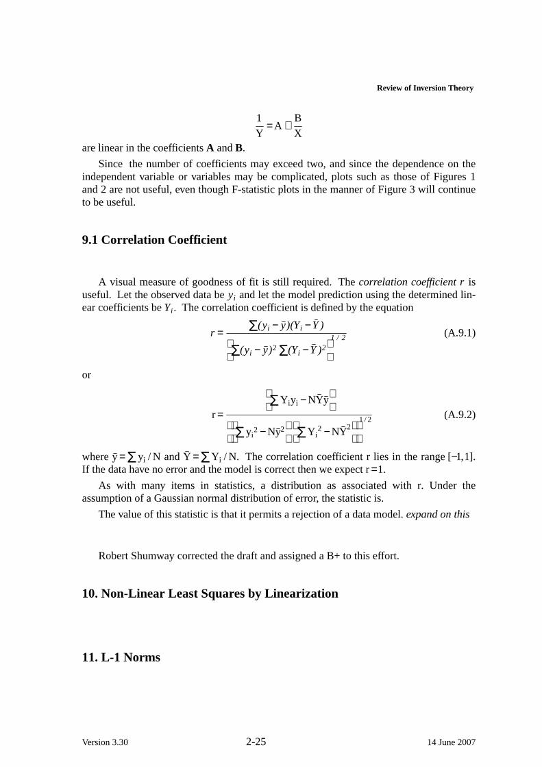
Xare linear in the coefficientsA andB.
Since thenumber of coefficients may exceed two, and since the dependence on theindependent variable or variables may be complicated, plots such as those of Figures 1and 2 are not useful, even though F-statistic plots in the manner of Figure 3 will continueto be useful.
9.1 Correlation Coefficient
A visual measure of goodness of fit is still required.The correlation coefficient r isuseful. Letthe observed data beyi and let the model prediction using the determined lin-ear coefficients beYi. The correlation coefficient is defined by the equation
r = Σ(yi − y)(Yi − Y )
Σ(yi − y)2 Σ(Yi − Y )2
1 / 2 (A.9.1)
or
r =
ΣYiyi − NYy
Σ yi
2 − Ny2
ΣYi
2 − NY2
1 /2 (A.9.2)
wherey = Σ yi / N and Y = ΣYi / N. The correlation coefficient r lies in the range[−1, 1].If the data have no error and the model is correct then we expect r=1.
As with many items in statistics, a distribution as associated withr. Under theassumption of a Gaussian normal distribution of error, the statistic is.
The value of this statistic is that it permits a rejection of a data model.expand on this
Robert Shumway corrected the draft and assigned a B+ to this effort.
10. Non-Linear Least Squares by Linearization
11. L-1 Norms
Version 3.30 2-25 14 June 2007

Computer Programs in Seismology - Crustal Structure Inv ersion
Acknowledgements
Robert Shumway corrected the draft and assigned a B+ TO THIS EFFORT.
12. Problems
1. Prove that (A.3.5) follows from (A.3.2) and (A.3.3). Hint: do not substitute thea and bvalues from (A.3.4). Rather use the algebraic property that(A + B)(A + B) = A(A + B) + B(A + B).
13. References
Crosson, R. S. (1976). Crustal structure modeling of earthquake data I. Simultaneousleast squares estimation of hypocenter ande velocity parameters, J. Geophys. Res.81,3036-3046.
Draper, N. R., and H. Smith (1966). Applied Regression Analysis, John Wiley & Sons,New York, 407 pp.
Press, .... Numerical Recipes in C
Version 3.30 2-26 14 June 2007
Review of Inversion Theory
CHAPTER 3SURFACE WAVE ANALY SIS
1. Introduction
The study of surface wav es holds a special place in seismology for several reasons.Because of their large amplitudes compared to body wav es for teleseisms, these are themost recognizable part of the seismogram, especially along paths between the earthquakeand seismograph station that cross deep oceans. These wav es are also significant becausethey arise from boundary conditions near the Earth’s surface - a low velocity wav e guidefor Love wav es and a stress free surface for Rayleigh wav es - hence their name ofsurfacewave.
Because of their ubiquitous presence in data, they are an obvious choice for the studyof primarily shear-wav evelocity structure near the surface.
We will discuss the data processing of observational data to provide phase velocity, c,and group velocity, U, velocity dispersion curves as well as anelastic attenuation coef-ficients,γ , which can be inverted for the elastic wav evelocities andQ−1. The organiza-tion of this chapter address basic surface wav etheory, methods for determination of phasevelocity and group velocity, and finally the inversion for earth structure.
2. The Surface Processing
2.1 Surface wave representation
The surface-wav ein a flat-layered earth is usually the largest low frequency signal atlarge distances because its geometrical spreading is less than that of the direct bodywaves. The Fourier transform of the surface-wav esignal fora single-mode observed at adistance rfrom the source is written as
1
√ ( r)S(ω) A(ω)e−i(kr+ψ )
whereω is the angular frequency, k is the horizontal wav enumber which is related to the
Version 3.30 3-1 14 June 2007

Computer Programs in Seismology - Crustal Structure Inv ersion
phase velocity c by the definition ω = kc. S(ω) is complex source spectrum, andA(ω) exp(−iψ ) represents the complex excitation of surface wav es for a point source. Theexcitation is a function of frequency, source depth and properties of the elastic medium.
The Fourier transform of the surface wav ewhich includes the higher modes is givenby
1
√ rS(ω)
mΣAm(ω)e−i(kmr+ψm)
where the index m is the mode number. The presence of high modes complicates theinterpretation of phase or group velocities, especially because the excitation of each modedepends upon frequency, which may may make mode identification difficult.
2.2 Phase Velocity Determination
McMechan and Yedlin (1981) described a technique to obtain phase velocity disper-sion from an array of seismic traces. They proposed first performing ap − τ stack fol-lowed by a transformation into thep − ω domain. Aseparate stacking procedure is notrequired to accomplish this if operations are performed in the frequency domain..Mokhtaret al (1988) describe how this can be done. Let the observed Fourier spectrum ofa seismic signal at distancern be
A(ω , rn )eiφ (ω )n (1)
One possiblep − ω stack ofN traces at different distances from the same source isdefined by the relation
F(p,ω) =N
n=1Σ C(ω, r1,rn)
−1A(ω, rn)eiφneiωprn. (2)
where
C(ω) = A(ω, r1, rn)eiφ1 √ rn
r1
Division byC(ω, r1, rn) is a simple artifice to remove the source spectrum from the obser-vations, and to correct for geometrical spreading. If the signal is only that of a singlemode, then the depth dependent excitation is also removed.
Since the observed spectrum is assumed to be the superposition ofM surface-wav emodes such that
A(ω, ri)ejφ i =
S(ω
√ ri
M
m=1Σ Am(ω, ri)e
j[ψ0m(ω)−ωp0m(ω)ri], (3)
Version 3.30 3-2 14 June 2007

Surface Wav eAnalysis
the operation in (2) does correct for geometrical spreading and the source excitation. Inthis notation theψ0m is the actual excitation phase of thek’th mode, andkm = ωp0m. Thisexpression separates the phase intodistance dependent and independent contributions.Interpretation of (2) is difficult unless the is only a single mode or the amplitude of onemode is so large at a given frequency that its contribution outweighs that of other modes.
If the signal consists of a single noise free surface-wav e mode, then the quantityF(p,ω ) will have a maximum when p= p0k. Searching for the maxima of
|F(p,ω)| (4)
yields the possibledispersion curves. Since there areN distances, the maximum value ofthe quantity|F(p,ω)| should be equal to N.
If this value is less thanN, then we can attribute this to an error in the ray parameterbetween the stations. If we assume that in the neighborhood of a maximum of the stack,∆p = p − p0k has a normal distribution with zero mean and a varianceσ 2, then theexpected value of any term in (1) is
E[e− j2π f∆pri] = e−2σ 2π 2f2r2i (5)
where we used the definitionω = 2π f.
Since each term in (4) is always positive, the expected value of the stack (1) of a sin-gle mode is just
|N
i=1Σe−2σ 2π 2f2(ri−r1)
2| (6)
Given the stack value (4), a Newton-Raphson technique is used to find the value ofσfrom (6) that corresponding to this value. The error in phase velocity is obtained using thedefinition p = 1/c and the relation
∆c = σ c2. (7)
This relation was tested by numerically modeling a stacking operation in which the rayparameter error had the assumed distribution.
In the more realistic case of multimode surface wav es, (4) will not yield a maximumindependent of the amplitude spectrum of the other modes. Thus the stack value will typ-ically be largest for one mode and smaller for others. The simplistic error analysis willyield larger, perhaps unwarranted, errors for the other modes. This is an inherent prob-lem with this technique, that can only be resolved if a phase matched filter technique isfi rst applied to each input spectra to isolate a single mode before the phase velocity stackis performed.
Version 3.30 3-3 14 June 2007

Computer Programs in Seismology - Crustal Structure Inv ersion
The programsacpom96 implements this technique. Figure 1 presents the processingflow for this program:
sacpom96
stdout pom96.dsp SACPOM96.PLT
fi le list
Fig. 1. Processing flow for sacpom96
Program control is through the command line:
sacpom96 [flags], where the command flags are-C [spcfil] (default stdin) : Input data file name-ci [ci] (default=2.0) : starting phase velocity-ce [ce] (default=5.0) : ending phase velocity-nray [nray] (default = 20) : number of ray parameters-fmin [fmin] (default=0.02) : minimum frequency for plot-fmax [fmax] (default=0.25) : maximum frequency for plot-vmin [vmin] (default 2.0) : minimum velocity for plot-vmax [vmax] (default 5.0) : maximum velocity for plot-xlin (default= false) : linear frequency axis-xlog (default= true) : logarithmic frequency axis-ylin (default = false): linear velocity axis-ylog (default = true ): logarithmic velocity axis-V (default = false): verbose output-O (default = false): c-f values from maxima on STDOUT-E (default = false): plot error bars-T (default = false): x-axis is period not f
Version 3.30 3-4 14 June 2007

Surface Wav eAnalysis
-R (default = true ): data are Rayleigh-L (default = false): data are Love-S (default = false): contour shading
The output is a tabulation of peak motions from the stack:
POM96 R C -1 45.511 4.0000 0.0026 6.0000 1
POM96 R C -1 7.9380 4.0000 0.3301 2.0351 2
POM96 R C -1 5.2648 4.0000 0.4403 1.2643 3
The output consists of 9 columns with the following meaning:
Col Description
1 SACPOM96 Name of the generating program2 R Wa ve type, eitherL for Love or R for Rayleigh.3 C Dispersion measurement. Always C for phase velocity4 0 Mode identification.0 for fundamental,1 for 1’st, etc. Note the program
do_pom is available to runsacpom96 and to interactively identify themodes. A value of-1 indicates that no mode identification has been made
5 1.6787 Period of observation in seconds. Thesurf96 dispersion formatrequired periods in seconds, and dispersion in km/s.
6 0.66658 Phase velocity inkm/s.7 0.16019E-02 Error estimate ofvelocity in km/s. From equation (7).8 1 Amplitude order of the stack. The1 indicates that for this phase velocity,
this periods had the largest stack amplitude. this may permit one to followthe modes.
9 48.940 The value of equation (4). The maximum value of this is the num-ber of traces.
One of the difficulties of the phase velocity stack is due to the discrete sampling infrequencies and the analyst’s expectation of a single phase velocity for each frequency inthe manner of the multiple filter analysis programsacmft96 for group velocity. Thisprogram actually starts with a given phase velocity and then searches for the 8 frequen-cies for which the stack is a maximum. The presentation will then show many phasevelocities for each frequency. To assist in organizing the results it may be useful to sortthe output by period. The command
sort -n +4 < pom96.dsp > pom.sort
will give
POM96 R C -1 23.011 2.0843 0.8231 1.0353 7
POM96 R C -1 23.011 3.4699 0.0010 6.0000 1
On the basis of the stack amplitude, last column, I would associate the velocity 3.4699km/s with the period of3.011 seconds and ignore the other value.
Version 3.30 3-5 14 June 2007

Computer Programs in Seismology - Crustal Structure Inv ersion
Example
The following example demonstrates the use of this program using a simple crustalearth model.
#!/bin/sh
#this depth and model gives a spectra hole at 15-20 secHS=10STK=0RAKE=0DIP=90AZ=45NMODE=10####### changing the RAKE to 45 removes some of the spectral hole# = 0 Strike slip if dip is 90# = 90 dip slip is dip is 45 -- good hole############ create file of distances for synthetics# DISTANCE DT NPTS T0 VRED#####cat > dfile << EOF1000.0 1.000 2048 -1.0 8.01050.0 1.000 2048 -1.0 8.01100.0 1.000 2048 -1.0 8.01150.0 1.000 2048 -1.0 8.01200.0 1.000 2048 -1.0 8.01250.0 1.000 2048 -1.0 8.0EOF
###### create the earth model#####cat > model.d << EOFMODELTEST MODELISOTROPICKGSFLAT EARTH1-DCONSTANT VELOCITYLINE08LINE09LINE10LINE11HR VP VS RHO QP QS ETAP ETAS FREFP FREFS40. 6.0 3.5 2.8 0.0 0.0 0.0 0.0 1.0 1.000. 8.0 4.7 3.3 0.0 0.0 0.0 0.0 1.0 1.0EOF
###### Calculate multimode dispersion and make synthetics#####
sprep96 -M model.d -NMOD NMODE − HSHS -HR 0 -d dfile -L -Rsdisp96sregn96slegn96sdpegn96 -R -C -PER -TXT -XLOG -YMIN 2.5 -YMAX 5sdpegn96 -L -C -PER -TXT -XLOG -YMIN 2.5 -YMAX 5spulse96 -d dfile -D -p -EQ -2 > file96
fmech96 -A AZ − ROT− DDIP -R RAKE − SSTK -M0 1.0E+20 < file96 > 3.96
Version 3.30 3-6 14 June 2007

Surface Wav eAnalysis
f96tosac -B 3.96cp B0101Z00.sac Z1.saccp B0201Z00.sac Z2.saccp B0301Z00.sac Z3.saccp B0401Z00.sac Z4.saccp B0501Z00.sac Z5.saccp B0601Z00.sac Z6.sac
These synthetics represent the recordings of a regional earthquake by a modern set ofbroadband seismic stations. The traces generated are presented in Figure 2.
Fig. 2. Record section plot of the synthetics
To runsacpom86 one performs the following operations
Version 3.30 3-7 14 June 2007

Computer Programs in Seismology - Crustal Structure Inv ersion
#####
# create a list of SAC file to be processed
#####
ls Z?.sac > cmdfil
sacpom96 -C cmdfil -PMIN 4.0 -PMAX 100.0 -nray 100 \
-A -VMIN 2.00 -VMAX 5.00 -R -S
#####
# the output in the file pom96.dsp. consists of
#
#POM96 L C 0 period phase_velocity err_phase_vel no_peak stack_amplitude
# or
#POM96 R C 0 period phase_velocity err_phase_vel no_peak stack_amplitude
#
# the CALPLOT graphics file POM96.PLT, a control file for do_pom
# named pom96.ctl, and a shell script POM96CMP
#####
rm cmd
the graphic output inPOM96.PLT can be merged with the predicted Rayleigh wav ephase velocity values inSREGNC.PLT to create theCALPLOT fi le by doing
POM96CMP
cat POM96.PLT SREGNC.PLT > BIG.PLT
if the data are for Rayleigh wav es. Of course an earth model must exist and theoreticaleigenfunction files must have been created. The purpose of doing this here is to indicatehow well the technique works in obtaining correct phase velocities.
Version 3.30 3-8 14 June 2007

Surface Wav eAnalysis
101 102
P e r i o d ( s e c )
3 . 0 0
4 . 0 0
Ph
as
e V
elo
cit
y (
km
/s)
Fig. 3. Phase velocity stack values overlain by model predicted phase velocity dispersion curves. Thecolors indicate the stack value, with red corresponding to the largest. The black symbols represent thechosen peaks from the stack after a two dimensional search over the phase velocity - period grid. Thelight black curves are the theoretical dispersion values. Note the difficulty in identifying the highermodes.
2.3 Multiple filter analysis
The purpose of this note is to develop an analytic expression for a Gaussian filtereddispersed surface wav e into order to assess the effects of signal spectrum shape on thedispersion. The impetus for this is the recommendation by Levshin (19XX) that theinstantaneous frequency should be used rather than the filter frequency when determininggroup velocity dispersion.Block et al. (1969) and Herrmann (1973) ignored the effect ofsurface wav eamplitude spectrum on the interpretation of the results.
Bhattacharya (1983) studied the bias effect in detail and recommended two applica-tions of multiple filter analysis to obtain bias free estimates of group velocity and spectralamplitude. This note follows the presentation by Bhattacharya (1983) except that a Gaus-sian signal amplitude spectrum will be assumed rather than a linear shape and attentionwill be given to the use of the instantaneous frequency in the interpretation. The objec-tive is to avoid specifying the source signal spectrum.
Version 3.30 3-9 14 June 2007
Computer Programs in Seismology - Crustal Structure Inv ersion
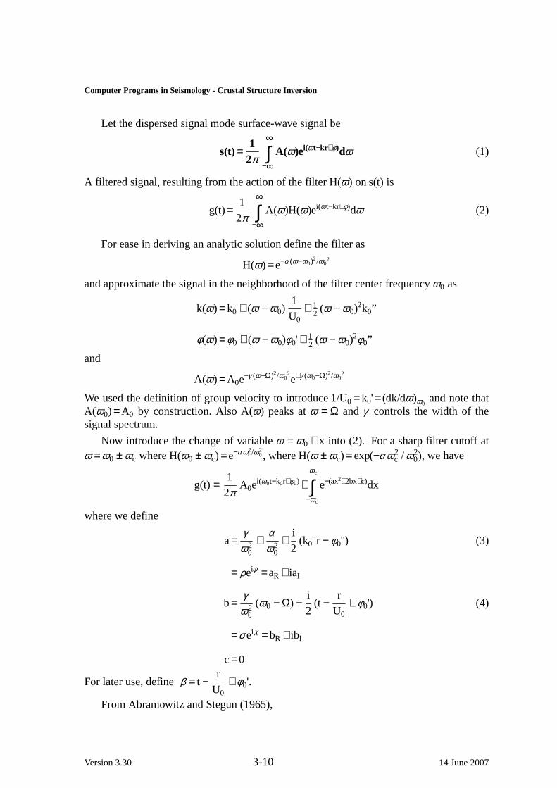
Let the dispersed signal mode surface-wav esignal be
s(t)=1
2π
∞
−∞∫ A(ω)ei(ω t−kr +φ)dω (1)
A filtered signal, resulting from the action of the filter H(ω) on s(t ) is
g(t) =1
2π
∞
−∞∫ A(ω)H(ω)ei(ω t−kr+φ)dω (2)
For ease in deriving an analytic solution define the filter as
H(ω) = e−α (ω−ω0)2/ω02
and approximate the signal in the neighborhood of the filter center frequencyω0 as
k(ω) = k0 + (ω − ω0)1
U0+ 1
2 (ω − ω0)2k0”
φ(ω) = φ0 + (ω − ω0)φ0' + 12 (ω − ω0)
2φ0”
and
A(ω) = A0e−γ (ω−Ω)2/ω0
2e+γ (ω0−Ω)2/ω0
2
We used the definition of group velocity to introduce1/U0 = k0' = (dk/dω)ω0and note that
A(ω0) = A0 by construction. AlsoA(ω) peaks atω = Ω andγ controls the width of thesignal spectrum.
Now introduce the change of variableω = ω0 + x into (2). For a sharp filter cutoff atω = ω0 ± ωc where H(ω0 ± ωc) = e−αω 2
c/ω 20, where H(ω ± ωc) = exp(−αω 2
c / ω 20), we have
g(t) =1
2πA0e
i(ω0t−k0r+φ0) ⋅ωc
−ωc
∫ e−(ax2+2bx+c)dx
where we define
a=γ
ω 20
+αω 2
0
+i
2(k0"r − φ0") (3)
= ρeiψ = aR + iaI
b=γ
ω 20
(ω0 − Ω) −i
2(t −
r
U0+ φ0') (4)
= σ ei χ = bR + ibI
c= 0
For later use, defineβ = t −r
U0+ φ0'.
From Abramowitz and Stegun (1965),
Version 3.30 3-10 14 June 2007

Surface Wav eAnalysis
I = ∫ eax2+2bx+c)dx= 12 √ π
ae(b2−ac) /aerf
√ax+b
√a
Sinceerf (−z)= − erf (z), we hav efor g(t)
g(t) =1
2πA0e
i(ω0t−k0r+φ0) (5)
⋅√ πρ
e−i 12ψ e
σ 2
ρei(2χ −ψ )
⋅
12 erf
√aωc +b
√a
+ 12 erf
√aωc −b
√a
or
g(t) =1
2πA0e
i(ω0t−k0r+φ0) (6)
⋅√ πρ
e−i 12ψ e
aR(b2R−b2
I )+2aIbRbI
a2R + a2
I ei−aI(b
2R−b2
I )+2aRbRbI
a2R + a2
I
⋅
12 erf
√aωc +b
√a
+ 12 erf
√aωc −b
√a
At this stage no approximation has been made. If we assume that the filter is narrow,then following Bhattacharya (1983), the two erf termsare replaced by the single real term
erf
√ ρ cos12 ψ
We can also write g(t) as
g(t) = Θ(t )eiθ(t )
where Θ(t )= |g(t )| and θ(t )= arg g(t). The extreme positions ofΘ are obtained fromdΘ/dt = 0, The instantaneous frequency is defined atω i = dθ /dt. Since timet only entersinto the expression forg(t) in theω0t term and inβ or equivalently thebI , we can showthat the extreme values inΘ(t ) occur when
−aRbI + aIbR = 0
and that the instantaneous frequency is
ω I = ω0 +2aRbR + aIbI
a2R + a2
I
− 1
2
= ω0 + δ ω0i
At the envelope maximum, we have
Version 3.30 3-11 14 June 2007

Computer Programs in Seismology - Crustal Structure Inv ersion
δ ω0i = −bI
aI= −
bR
aR(7)
For the special case of a flat signal spectrum,γ = 0, bR = 0, δ ω0i = 0 andbI = 0. Substi-tuting into the expression for the maximum, and the factorbI , we hav efrom (7)
t −r
U0+ φ0' ≡ − 2bI = −
2aIbR
aR(8)
=−2aIγ (ω0 − Ω)
γ + αFollowing Bhattacharya (1983), consider the use of two values of the filter parameterα ,so that
t1 −r
U0+ φ0' =
−2aIγ (ω0 − Ω)
γ + α1= 2aIδ ω1
and
t2 −r
U0+ φ0' =
−2aIγ (ω0 − Ω)
γ + α2= 2aIδ ω2
Subtracting,
t1 − t2 = − 2aIγ (ω0 − Ω)
1
γ + α1−
1
γ + α2
But from (7)
δ ω1 = −γ (ω0 − Ω)
γ + α1(9)
and
δ ω2 = −γ (ω0 − Ω)
γ + α2(10)
Thus
t1 − t2 = 2aI(δ ω1 − δ ω2) (11)
and
t2 −r
U0+ φ0' =
t1 − t2δ ω1 − δ ω2
δ ω2
or a better estimate of U0 is
U0 =r
t2 − δ ω2(t1 − t2)/(δ ω1 − δ ω2) + φ0′(12)
Note that we cannot resolve the time delay due to the derivative of the source phase,φ0'but hope that the estimate ofU0 by assuming thatφ0′ is closer to the true value than thesimple estimater/t2.
We hav ethus paralleled the Bhattacharya formula for improved group velocity.
At this stage we have aI from (7) which is an essential component for computing thecorrect spectral amplitude.
Version 3.30 3-12 14 June 2007

Surface Wav eAnalysis
aI = 12
t1 − t2
δ ω1 − δ ω2(13)
By the definition ofδ ω0i,
bI = − aIδ ω0i (14)
Taking the ratio of (7) to (8) solving forγ , if γ ≠ 0, gives
γ =
α2 − α1
δ ω1
δ ω2
δ ω1
δ ω2−1
Thus
aR =γ + α
ω 20
, (15)
bR = − aRδ ω0 (16)
and
Ω = ω0 − bRω 20/γ (17)
The analysis presented highlights several important aspects of multiple filter analysis.First, the effect of the source phase on phase and group delay cannot be eliminated usinga single seismogram. Second, the spectral amplitude shape can skew the group velocitymeasurements. Thisis seen in the dependence of the instantaneous frequency on theamplitude spectrum. Levshin (19XX) recommends associating the instantaneous fre-quency with the group arrival time, but this is not always effective. One could use thegroup times associated with two filter parametersα as developed here, but the difficultyof automatically associating the corresponding envelope peaks for different α ’s is nottrivial. The spectral amplitude estimate is good only when theα is larger as distanceincreases.
3. Graphical Interfaces
To assist in the task of selecting phase velocity or ground velocity dispersion pointsfrom the possibilities created by the programssacpom96 andsacmft96, respectively,two interactive display programs were created for the purpose of selecting the desiredSAC file, setting processing parameters, and then interactively selecting the dispersionpoints.
3.1 Test of multiple filter analysis
Version 3.30 3-13 14 June 2007

Computer Programs in Seismology - Crustal Structure Inv ersion
The discussion above shows that the choice ofα is crucial to a good estimate ofgroup velocity and spectral amplitude. To test the use of the programsacmft96, we gener-ate synthetics with the following shell script
#!/bin/sh
set -x
HS=40
#this depth and model gives a spectra hole at 33-40 sec
STK=0
RAKE=0
DIP=90
AZ=45
NMODE=10
######
# changing the RAKE to 45 removes some of the spectral hole
# = 0 Strike slip if dip is 90
# = 90 dip slip is dip is 45 -- good hole
######
cat > dfile << EOF
500.0 1.000 2048 -1.0 8.0
1000.0 1.000 2048 -1.0 8.0
2000.0 1.000 2048 -1.0 8.0
3000.0 1.000 2048 -1.0 8.0
4000.0 1.000 2048 -1.0 8.0
8000.0 1.000 2048 -1.0 8.0
EOF
cat > model.d << EOF
MODEL
TEST MODEL
ISOTROPIC
KGS
FLAT EARTH
1-D
CONSTANT VELOCITY
LINE08
LINE09
LINE10
LINE11
HR VP VS RHO QP QS ETAP ETAS FREFP FREFS
40. 6.0 3.5 2.8 0.0 0.0 0.0 0.0 1.0 1.0
00. 8.0 4.7 3.3 0.0 0.0 0.0 0.0 1.0 1.0
Version 3.30 3-14 14 June 2007

Surface Wav eAnalysis
EOF
#####
# Chapter 3
#####
sprep96 -M model.d -NMOD $NMODE -HS $HS \
-HR 0 -d dfile -L -R
sdisp96
sregn96
slegn96
sdpegn96 -R -U -PER -TXT -XLOG -YMIN 2.5 -YMAX 5
sdpegn96 -L -U -PER -TXT -XLOG -YMIN 2.5 -YMAX 5
plotxvig < SREGNU.PLT
plotxvig < SLEGNU.PLT
spulse96 -d dfile -D -p -EQ -2 > file96
fmech96 -A $AZ -ROT -D $DIP -R $RAKE \
-S $STK -M0 1.0E+20 < file96 > 3.96
f96tosac -B 3.96
cp B0101Z00.sac Z1.sac
cp B0201Z00.sac Z2.sac
cp B0301Z00.sac Z3.sac
cp B0401Z00.sac Z4.sac
cp B0501Z00.sac Z5.sac
cp B0601Z00.sac Z6.sac
rm -f B*.sac
for MODE in 0 1 2 3 4
do
spulse96 -d dfile -D -p -EQ -2 -M $MODE | \
fmech96 -A $AZ -ROT -D $DIP -R $RAKE \
-S $STK -M0 1.0E+20 > 3.96.$MODE
f96tosac -B 3.96.$MODE
cp B0101Z00.sac Z1.$MODE.sac
cp B0201Z00.sac Z2.$MODE.sac
cp B0301Z00.sac Z3.$MODE.sac
cp B0401Z00.sac Z4.$MODE.sac
cp B0501Z00.sac Z5.$MODE.sac
cp B0601Z00.sac Z6.$MODE.sac
done
rm -f B*sac
The following plots is obtained usingsacmft96 and the trace at a distance of 4000 km.
sacmft96 -f Z5.sac -PMIN 4.0 -PMAX 100.0 \
-a0 100.0 -A -VMIN 2.0 -VMAX 5.0 -U cm -R -S
Version 3.30 3-15 14 June 2007

Computer Programs in Seismology - Crustal Structure Inv ersion
This command says to use the SAC file Z5.sac, use the automatically generated del peri-ods between4.0 and100.0 seconds, the filter parameterα = 10 0. 0, contour with abso-lute amplitudes,-A, and the plot group velocities in the range of.0 and 5.0 km/s. Theinput traces units are incm, The trace is a Rayleigh wav e, -R. Provide a color shaded plot,-S. The output graphic is in the fileMFT96.PLT which is shown in Figure 4.
1 01 1 02
P e r i o d ( s e c )
3 . 0 0
4 . 0 0
Gr
ou
p V
elo
cit
y (
km
/s)
1 . 6 0 7 E - 0 81 01 1 02
P e r i o d ( s e c )
1 0- 9
1 0- 8
1 0- 7
1 0- 6
cm
-se
c
Fig. 4. Graphic output of sacmft96. Anα =100 is used.
Figure 5 overlays the model predicted group velocity dispersion and the modal spectralamplitudes
1 01 1 02
P e r i o d ( s e c )
3 . 0 0
4 . 0 0
Gr
ou
p V
elo
cit
y (
km
/s)
1 . 6 0 7 E - 0 81 01 1 02
P e r i o d ( s e c )
1 0- 9
1 0- 8
1 0- 7
1 0- 6
cm
-se
c
Fig. 5. Overlay of true group velocity dispersion and modal spectral amplitudes onthe sacmft96 output.
3.2 do_mft
The most time consuming part of multiple filter analysis is the need for manuallyselecting the correct dispersion from the program output. This is made easier by the useof the programdo_mft what permits selection of the SAC file to process, defining thetrace units and filter parameters, interactive identification of modes, choice of phasematch filtering, andsaving of processing results. The following figures present several of
Version 3.30 3-16 14 June 2007

Surface Wav eAnalysis
the menus. One can start the program with the simple command
do_mft *
whereby the program looks at all files in the current directory to determine whether theyare SAC files. The result is the initial screen
The second screen permits one to define the units and to review, but not change, the con-tents of the SAC header. The DIST is required.
Selecting theDo MFT button, leads to the next stage, whereby one can change the peri-ods for processing, the filter parameterα , the shading, and the wav etype (UNKNOWN,
Version 3.30 3-17 14 June 2007

Computer Programs in Seismology - Crustal Structure Inv ersion
LOVE or RAYLEIGH), and the plotting parameters.
If the Do MFT is again pressed, the programsacmft96 is run in the background to createthree files: the dispersion file, the graphic plot, and an index file to the graphic.do_mftdisplays this together with processing buttons.
One can zoom in on a portion of the dispersion plot:
Version 3.30 3-18 14 June 2007

Surface Wav eAnalysis
define the mode and then select the dispersion values a single point at a time,Pick or byfinding values near a connected line,Auto. If desired one move to the phase match filterstage,Match
which requires the specification of a single mode. After phase match filtering the initialfi le menu is updated so that one could perform the multiple filter analysis on the presum-ably single mode trace.
Version 3.30 3-19 14 June 2007
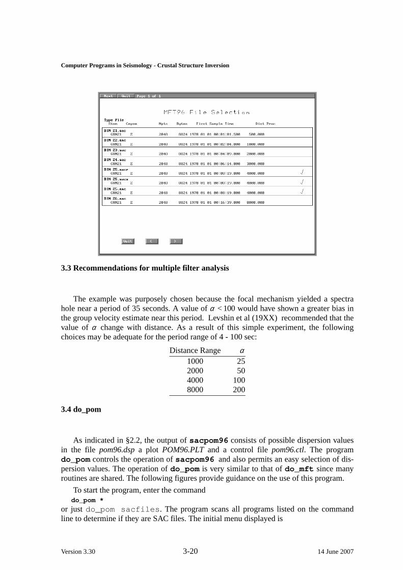
Computer Programs in Seismology - Crustal Structure Inv ersion
3.3 Recommendations for multiple filter analysis
The example was purposely chosen because the focal mechanism yielded a spectrahole near a period of 35 seconds. A value ofα < 100 would have shown a greater bias inthe group velocity estimate near this period.Levshin et al (19XX) recommended that thevalue of α change with distance. As a result of this simple experiment, the followingchoices may be adequate for the period range of 4 - 100 sec:
Distance Range α1000 252000 504000 1008000 200
3.4 do_pom
As indicated in §2.2, the output ofsacpom96 consists of possible dispersion valuesin the file pom96.dsp a plot POM96.PLT and a control file pom96.ctl. The programdo_pom controls the operation ofsacpom96 and also permits an easy selection of dis-persion values. The operation ofdo_pom is very similar to that ofdo_mft since manyroutines are shared. The following figures provide guidance on the use of this program.
To start the program, enter the commanddo_pom *
or just do_pom sacfiles. The program scans all programs listed on the commandline to determine if they are SAC files. The initial menu displayed is
Version 3.30 3-20 14 June 2007

Surface Wav eAnalysis
Initial display. If all SAC files are to be click on "SelectALL." If some are not desired,click "Reject" and then click on the appropriate box. An accepted file is indicated by ared ’X’ and a rejected by an ’X’. When the trace selection is complete, click on the "DoPOM" button at the top.
The second page permits one to define the command line parameters forsacpom96f1.When the "Do POM" button at the top is pressed, the programssacpom96 is run in the background with the command line indicated in the very topmargin.
Version 3.30 3-21 14 June 2007
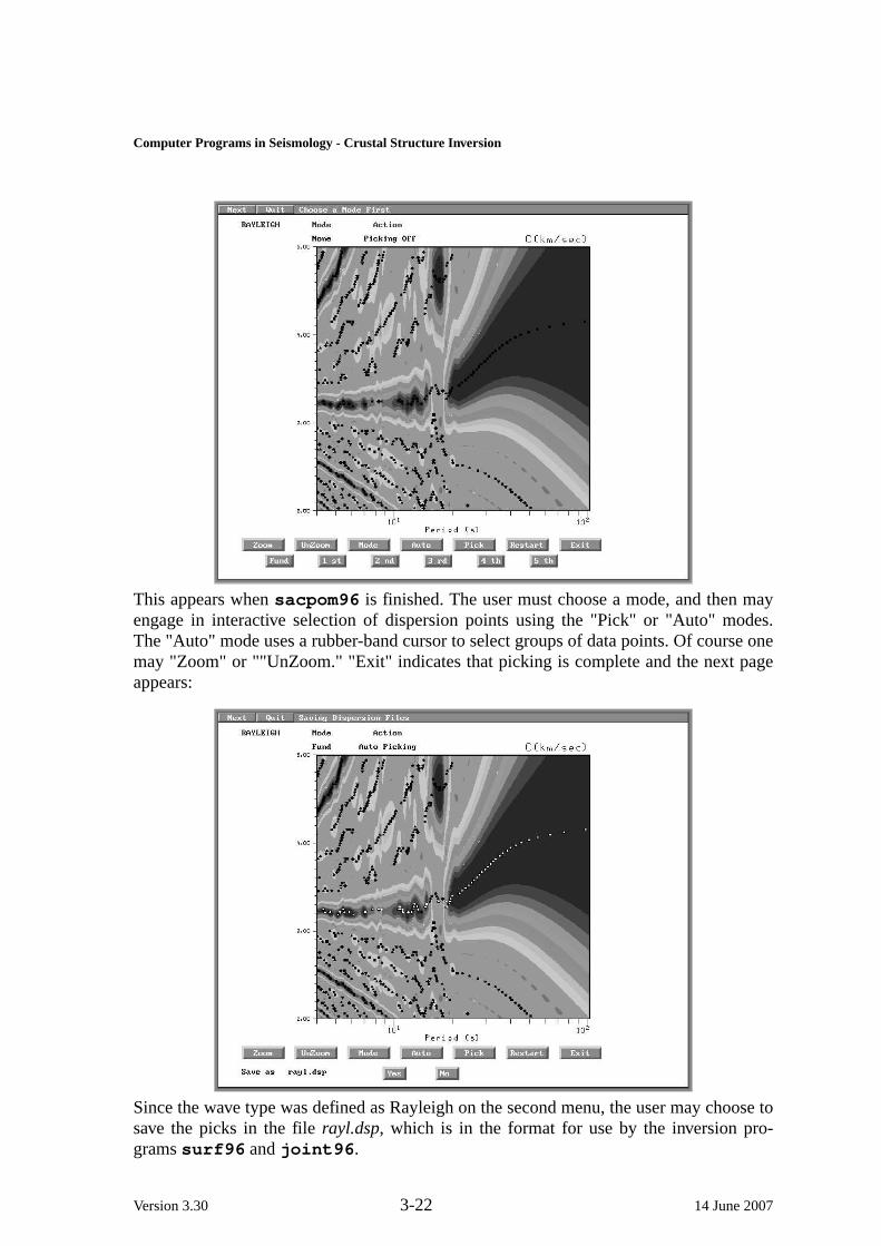
Computer Programs in Seismology - Crustal Structure Inv ersion
This appears whensacpom96 is finished. The user must choose a mode, and then mayengage in interactive selection of dispersion points using the "Pick" or "Auto" modes.The "Auto" mode uses a rubber-band cursor to select groups of data points. Of course onemay "Zoom" or ""UnZoom." "Exit" indicates that picking is complete and the next pageappears:
Since the wav etype was defined as Rayleigh on the second menu, the user may choose tosave the picks in the file rayl.dsp, which is in the format for use by the inversion pro-gramssurf96 andjoint96.
Version 3.30 3-22 14 June 2007
Surface Wav eAnalysis
4. Data Preparation
Data preparation consists of two parts: preparing the SAC trace file for analysis andperforming the analysis. Multiple filter analysis requires that the instrument response beremoved and that the recording be reduced to ground displacement, velocity or accelera-tion in some frequency range.
A typical response file representation is in terms of poles and zeros. If such a fileexists, pz_file, SAC can be used to remove the instrument response with the followingcommands:
read SAC_filertrtapertransfer from polezero subtype pz_file to none freqlimits 0.01 0.02 0.2 0.4new_SAC_file
This operation removes linear trends from the data, and then removes the complexresponse in the frequency domain as represented by the pole-zero description. The fre-qlimits, here 0.01 0.02 0.2 0.4 as an example, band pass the signal to prevent emphasizinglow frequency and high frequency noise. Oneshould note these band limits since the dis-persion points should only be believed in the frequency range between 0.02 and 0.20 Hz.
If the program SAC is not available, one can use the pole-zero with the programsacfilt to accomplish the same result.
One should be careful of the meaning of the pole-zero response file. If it is obtainedfrom AUTODRM software, then the pole-zero response in SAC format will present thedisplacement sensitivity in units of counts/micron. If the pole-zero response is desired inGSE format, then the units are counts/nanometer, I believe. Read the manual.
If one uses an FDSN SEED response file with the programevalresp from IRIS, twofi les will be created: one a table of the amplitude and the other a table fo the phaseresponse as a function of frequency. The evalresp program permits the user to select theoutput in units of counts/m, counts/m/sec or counts/m/s/sec. To remove the instrumentresponse using these tables, one can use the programsacevalr with the SAC file.
It is up to the user to know what the units actually are for the response. This is essen-tial for source studies. The programdo_mft permits the user to define the units of thetrace after response correction. One must just be very careful and consistent.
Instrument correction prior to phase velocity stacking is only required if the sensorshave different responses.
For the program to work, the SAC file must have the time of first sample, origin time,distance and azimuth fields filled. If one uses SAC and fills the event and station lati-tudes and longitudes, these latter two values will be computed automatically.
The final step before inverting for earth structure is to merge the output ofdo_pomand/or do_mft into a surf96 dispersion file. The rayl.dsp or love.dsp arealready in the correct format:
Version 3.30 3-23 14 June 2007

Computer Programs in Seismology - Crustal Structure Inv ersion
SURF96 R C T 0 25.28 3.54550 0.00190 5.9999SURF96 R C T 0 25.92 3.57580 0.00300 5.9998SURF96 R C T 0 26.95 3.60610 0.00160 5.9999SURF96 R C T 0 27.68 3.63640 0.00080 6.0000SURF96 R C T 0 28.44 3.66670 0.00330 5.9998SURF96 R C T 0 29.68 3.69700 0.00270 5.9999SURF96 R C T 0 30.57 3.72730 0.00150 6.0000SURF96 R C T 0 31.51 3.75760 0.00030 6.0000SURF96 R C T 0 32.51 3.78790 0.00130 6.0000SURF96 R C T 0 33.57 3.81820 0.00310 5.9999SURF96 R C T 0 35.31 3.84850 0.00200 6.0000SURF96 R C T 0 36.57 3.87880 0.00080 6.0000
However the output ofdo_mft is not in thesurf96 format. Thefollowing lists threelines from a file, BLONMBHT.dsp, created by answeringYES to the Save query indo_mft. The \ represents an extension because of the many columns in the output.
MFT96 L U 0 42 3.91380 0.22821 2819.1001 76.3 3.6300e-04 37.540001 \-118.879997 39.171902 -86.522202 0 1 41.119999 COMMENT: BLO BHT 2007 163 7 23
MFT96 L U 0 40 3.81550 0.20656 2819.1001 76.3 3.8180e-04 37.540001 \-118.879997 39.171902 -86.522202 0 1 39.340000 COMMENT: BLO BHT 2007 163 7 23
The columns of this output represent the following:1 MFT96 tag 9 source-to-receiver azimuth 18 COMMENT2 Rayleigh or Love 10 Spectral amplitude (cm-sec) 19 Station,component, date3 U for group velocity 11 Event latitude4 Mode (0 for fundamental) 12 Event longitude5 Period (sec) 13 Stationlatitude6 Group velocity (km/sec) 14 Stationlongitude7 Error in group velocity* 15 Flag to represent peak8 Distance km 16 Instantaneousperiod
The reason for this extensive output which is much more than required by thesurf96format, is that one may wish to use the spectra amplitudes to estimate source properties orattenuation, or one may wish to incorporate the measured dispersion into a tomographicstudy. The error is group velocity is not a true error, since the dispersion is based on onlyone observation. Sincethe Gaussian filter has a longer impulse response at longer peri-ods, a reading error could be associated with a misplaced maximum - the number com-puted here assumes that the travel time can be mis-measured by one filter period.
The table given above can be easily converted into thesurf96 format by usingawk,a standard utility on UNIX/LINUX systems, in a simple example:
cat GRN21Z.dsp | \awk ’ printf "SURF96 %s %s X %s %s %s %s\n", $2, $3, $4, $5, $6, $7’
which extracts
SURF96 R U X 0 85 3.98400 1.34900SURF96 R U X 0 80 3.96800 1.26000SURF96 R U X 0 75 3.95300 1.17200
from theGRN21Z.dsp fi le.
To combine different dispersion files, e.g., for Love and Rayleigh, one just concate-nates them together using the UNIXcat or the DOSCOPY command into one file, per-haps calleddisp.d.
Version 3.30 3-24 14 June 2007

Surface Wav eAnalysis
5. surf96
The programsurf96 is based on the programsurf initially written by David Rus-sell in 1985. The use of the new surf96 andmodel96 fi le formats was incorporatedinto the new version. In addition, the graphics interface was improved to enhance thevisualization of the inversion success in fitting the data.
5.1 Interactive control file setup
The following example shows the interactive dialog for the case that the dispersionfi le and initial earth model file do not exist. If either or both exist, then just enter the filename and the program proceeds. The user input is indicated by theitalic font.
surf96Enter h,dcl,dcr
h = fraction change in period to get group vel(0.005 is reasonable)
dcl, dcr are phase velocity increment in rootsearch for Love and Rayl respectively
0.005 0.005 0.005Enter 1 if variance based on residual or
0 if variance based on obs std err1Enter maximum number of Love gamma modes to process
0 means DO NO PROCESS LOVE gamma data2Enter maximum number of Love Phvel modes to process
0 means DO NO PROCESS LOVE phase vel data2Enter maximum number of Love Gpvel modes to process
0 means DO NO PROCESS LOVE group vel data2Enter maximum number of Rayl gamma modes to process
0 means DO NO PROCESS RAYL gamma data2Enter maximum number of Rayl Phvel modes to process
0 means DO NO PROCESS RAYL phase vel data2Enter maximum number of Rayl Gpvel modes to process
0 means DO NO PROCESS RAYL group vel data0Enter inversion technique
0 invert for Vs :Va,rho fixed1 : invert for Vs :Poisson fixed, rho from Vp
1Enter name of model file
modl.dInteractively setting up initial model file:modl.dIs model flat (0) or spherical (1)
Version 3.30 3-25 14 June 2007

Computer Programs in Seismology - Crustal Structure Inv ersion
0Enter descriptive title for this model
Test modelEnter d,a,b,rho,qa,qbd=0.0 or EOF indicates halfspace and end of input
40 6 3.5 2.5 100 1000 8 4.7 3.3 1000 1000Enter name of dispersion file
disp.dEnter ilvry,iporg,imode,per,val,dvalilvry=1(Love)
=2(Rayleigh)iporg=1 (phase velocity km/s)
=2 (group velocity km/s)=3 (gamma 1/km)
imode (mode number) e.g., 0=fundamental, 1=firstper=the period
val=dispersion value, velocity or gammadval=error in dispersion value
(Enter 1.0 if stderr from residuals)NOTE: Enter all zeros or negative to terminate input
1 1 0 10.0 3.5 0.011 2 0 15.0 3.6 0.012 2 0 20.0 3.0 0.010 0 0 0 0 0
If this is successful, then the initial program menu will be presented.Before presentingthis, the requested input in the initial setup must be described.
Enter h,dcl,dcr
Determination of surface wav edispersion requires a search in the frequency - phasevelocity space of the surface-wav e period equation. Is is know that all surface wav emodes are bounded at the low end by some fraction of the smallest shear-wav evelocity,or in the case of a surface fluid layer, the lowest compressional-wav evelocity. The upperbound of the dispersion for a fixed period, is the halfspace shear-wav evelocity. dcl anddcr are the search increments to find the roots of the period equation. If these numbersare too large, modes may be missed by jumping past them. If the numbers are too small,computations take too long. The value of0.005 km/sec are acceptable for crustal studies,but could be made smaller when studying dispersion in low velocity sediments.
The parameterh is used to compute group-velocity partial derivatives. For example,∂U/∂VS can be computed by using∂c/∂VS(f) and ∂c/∂VS(( 1 + h)f). The recom-mended value of0.005 seems adequate.
Enter 1 if variance based on residual or
0 if variance based on obs std err
This relates to the computation of confidence limits in the earth model and also theweighting of the individual data.Currently only the surface wav edata permits a tabula-tion of the confidence of any observation.
Enter maximum number of Love gamma modes to process
0 means DO NO PROCESS LOVE gamma data
Version 3.30 3-26 14 June 2007

Surface Wav eAnalysis
This sequence of 6 questions permits the user to invert subsets of the data containedwithin the dispersion file.
Enter inversion technique
0 invert for Vs :Va,rho fixed
1 : invert for Vs :Poisson fixed, rho from Vp
The first option,0 was introduced for the special case of investigating receiver func-tion in deep soil layers for which the P-velocity was known. The second case,1, itera-tively inverts for the S-wav evelocity and then updates the P-velocity using the Vp/Vsratio of the initial model; the new density is computed from the new Vp using the Nafe-Drake relation.
After this the names of the earth model file and dispersion file names are requested. Ifthe files do not exist, then they are interactively constructed. Once this is done interac-tively, the format of each is correctly prototyped and the user may use an editor to modifythe files faster than using this interactive dialog.
5.2 Main menu
SURF96 MENU0- Display menu 24- ASCII Q Resolving (file name,lam)1- Run Dispersion 27- ASCII Veloc Dispersion (file name)2- Run Velocity Inversion 28- ASCII Model File (file name, lam)3- Run Q(beta) Inversion 29- ASCII Vel Resolving(file name,lam)4- Run Simultaneous Veloc-Q Inversion 30- (0) Fix Vp,(1) Fix Vp/Vs5- Set Thick(0)/Velocity(1) Inversion 31- Change dd(i), enter i,dd(i)6- Update Model (need lam) 32- Enter Damping Factor (lam)7- Plot RFTN/Dispersion/Velocity Model 35- Inversion: (0) Non-Causal (default)8- Plot Gamma / Qb inverse Model (1) Decoupled Causal9- Plot Resolution Kernel (2) Coupled Causal10- List Singular Values 36- Smoothing: (0) Global reset none11- Gamma Data Partial Derivatives (1) Global reset diff12- Gamma Data Dispersion 37- Reset Number of Iterations13- List Q Model (need lam) 38- Temporary End14- Q(beta) Resolving Kernel (need lam) 39- Permanent End16- Velocity Data Partial Derivatives 40- Enter Sigv minimum17- Velocity Data Dispersion 41- Enter Sigg minimum18- List Velocity Model (need lam) 45- Show Velocity Weights19- Velocity Resolving Kernels(need lam)46- Show Qinv Weights22- ASCII Gamma Dispersion (file name) 47- Show Inversion Controls23- ASCII Q(beta) File (file name,lam) 48- Modify Individual Layer SmoothingEnter Command at READY Promptready
This menu appears once the control file sobs.d exists. If the dispersion and initialmodel do not exist, then error messages will appear.
This menu is hopefully self-explanatory. Entering one of these numbers at thereadyprompt causes an action. Actions45, 46 and47 present other menus.
If 45 is entered, and the no smoothing option was chosen, e.g.,36 with option 0,then the velocity weights shown are
Version 3.30 3-27 14 June 2007
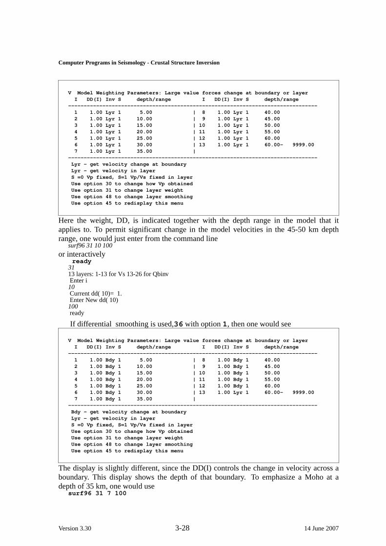
Computer Programs in Seismology - Crustal Structure Inv ersion
V Model Weighting Parameters: Large value forces change at boundary or layerI DD(I) Inv S depth/range I DD(I) Inv S depth/range
--------------------------------------------------------------------------------1 1.00 Lyr 1 5.00 | 8 1.00 Lyr 1 40.002 1.00 Lyr 1 10.00 | 9 1.00 Lyr 1 45.003 1.00 Lyr 1 15.00 | 10 1.00 Lyr 1 50.004 1.00 Lyr 1 20.00 | 11 1.00 Lyr 1 55.005 1.00 Lyr 1 25.00 | 12 1.00 Lyr 1 60.006 1.00 Lyr 1 30.00 | 13 1.00 Lyr 1 60.00- 9999.007 1.00 Lyr 1 35.00 |
--------------------------------------------------------------------------------Lyr - get velocity change at boundaryLyr - get velocity in layerS =0 Vp fixed, S=1 Vp/Vs fixed in layerUse option 30 to change how Vp obtainedUse option 31 to change layer weightUse option 48 to change layer smoothingUse option 45 to redisplay this menu
Here the weight, DD, is indicated together with the depth range in the model that itapplies to. To permit significant change in the model velocities in the 45-50 km depthrange, one would just enter from the command line
surf96 31 10 100
or interactivelyready
3113 layers: 1-13 for Vs 13-26 for QbinvEnter i10Current dd( 10)= 1.Enter New dd( 10)100ready
If dif ferential smoothingis used,36 with option1, then one would see
V Model Weighting Parameters: Large value forces change at boundary or layerI DD(I) Inv S depth/range I DD(I) Inv S depth/range
--------------------------------------------------------------------------------1 1.00 Bdy 1 5.00 | 8 1.00 Bdy 1 40.002 1.00 Bdy 1 10.00 | 9 1.00 Bdy 1 45.003 1.00 Bdy 1 15.00 | 10 1.00 Bdy 1 50.004 1.00 Bdy 1 20.00 | 11 1.00 Bdy 1 55.005 1.00 Bdy 1 25.00 | 12 1.00 Bdy 1 60.006 1.00 Bdy 1 30.00 | 13 1.00 Lyr 1 60.00- 9999.007 1.00 Bdy 1 35.00 |
--------------------------------------------------------------------------------Bdy - get velocity change at boundaryLyr - get velocity in layerS =0 Vp fixed, S=1 Vp/Vs fixed in layerUse option 30 to change how Vp obtainedUse option 31 to change layer weightUse option 48 to change layer smoothingUse option 45 to redisplay this menu
The display is slightly different, since the DD(I) controls the change in velocity across aboundary. This display shows the depth of that boundary. To emphasize a Moho at adepth of 35 km, one would use
surf96 31 7 100
Version 3.30 3-28 14 June 2007
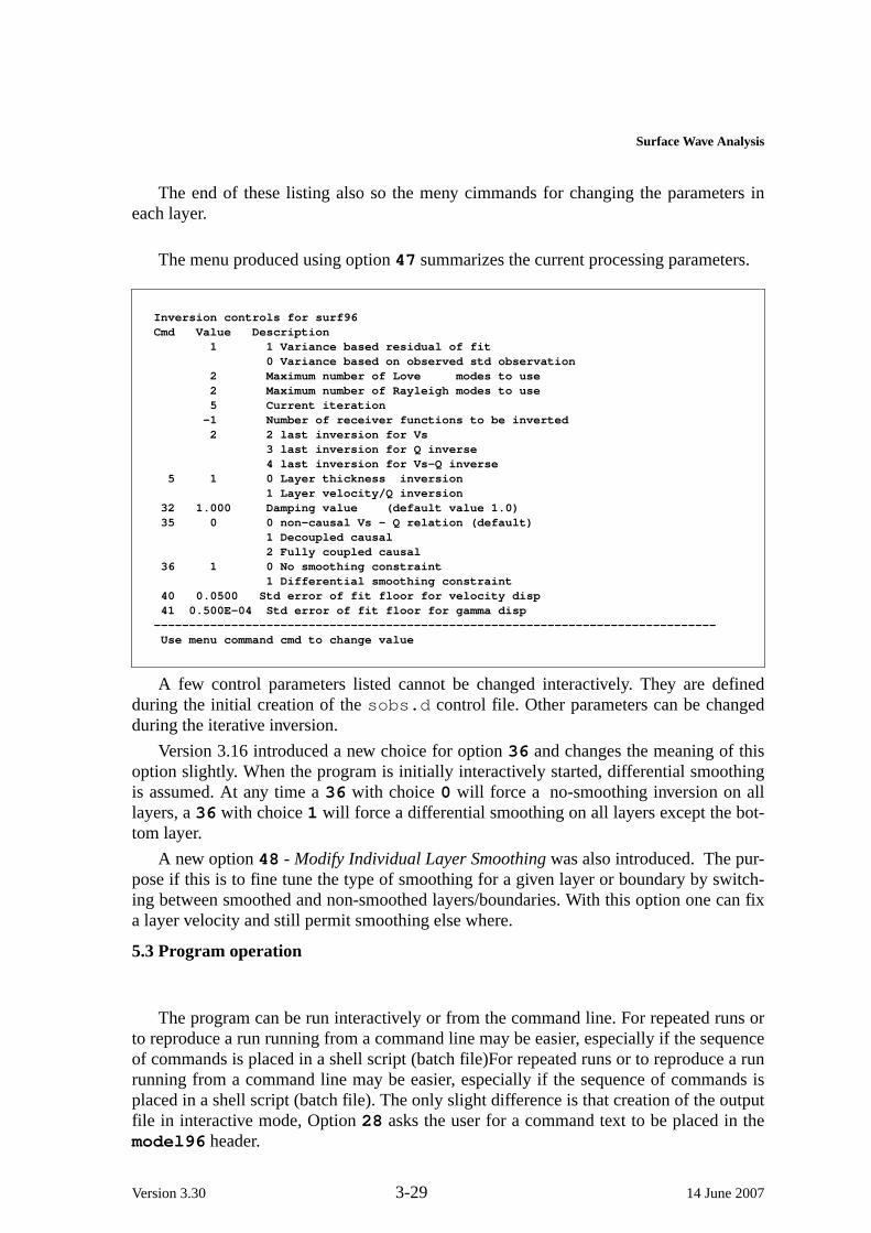
Surface Wav eAnalysis
The end of these listing also so the meny cimmands for changing the parameters ineach layer.
The menu produced using option47 summarizes the current processing parameters.
Inversion controls for surf96Cmd Value Description
1 1 Variance based residual of fit0 Variance based on observed std observation
2 Maximum number of Love modes to use2 Maximum number of Rayleigh modes to use5 Current iteration
-1 Number of receiver functions to be inverted2 2 last inversion for Vs
3 last inversion for Q inverse4 last inversion for Vs-Q inverse
5 1 0 Layer thickness inversion1 Layer velocity/Q inversion
32 1.000 Damping value (default value 1.0)35 0 0 non-causal Vs - Q relation (default)
1 Decoupled causal2 Fully coupled causal
36 1 0 No smoothing constraint1 Differential smoothing constraint
40 0.0500 Std error of fit floor for velocity disp41 0.500E-04 Std error of fit floor for gamma disp
--------------------------------------------------------------------------------Use menu command cmd to change value
A few control parameters listed cannot be changed interactively. They are definedduring the initial creation of thesobs.d control file. Other parameters can be changedduring the iterative inv ersion.
Version 3.16 introduced a new choice for option36 and changes the meaning of thisoption slightly. When the program is initially interactively started, differential smoothingis assumed. At any time a36 with choice0 will force a no-smoothing inversion on alllayers, a36 with choice1 will force a differential smoothing on all layers except the bot-tom layer.
A new option48 - Modify Individual Layer Smoothing was also introduced. The pur-pose if this is to fine tune the type of smoothing for a given layer or boundary by switch-ing between smoothed and non-smoothed layers/boundaries. With this option one can fixa layer velocity and still permit smoothing else where.
5.3 Program operation
The program can be run interactively or from the command line. For repeated runs orto reproduce a run running from a command line may be easier, especially if the sequenceof commands is placed in a shell script (batch file)For repeated runs or to reproduce a runrunning from a command line may be easier, especially if the sequence of commands isplaced in a shell script (batch file). The only slight difference is that creation of the outputfi le in interactive mode, Option28 asks the user for a command text to be placed in themodel96 header.
Version 3.30 3-29 14 June 2007

Computer Programs in Seismology - Crustal Structure Inv ersion
6. Example
This example uses the same dispersion information presented in Chapter 3 and thesame receiver functions presented in Chapter 4. These synthetic data sets were created forthe single layer over a halfspace model
MODELTEST MODELISOTROPICKGSFLAT EARTH1-DCONSTANT VELOCITYLINE08LINE09LINE10LINE11HR VP VS RHO QP QS ETAP ETAS FREFP FREFS40 6 3.5 2.5 200.0 100.0 0.0 0.0 1.0 1.00 8 4.7 3.3 900.0 500.0 0.0 0.0 1.0 1.0
To demonstrate operation of the program, the following shell script was run. It is assumedthat the control file jobs.d and the initial earth model, dispersion and receiver functionfi les exist in the current directory. The contents ofjobs.d are
0.00499999989 0.00499999989 0. 0.00499999989 0.1 2 2 2 2 2 2 0 1 0
modl.d../MKSURF/disp.drftn.lst
The initial model,modl.d consists of a halfspace -MODELTEST MODELISOTROPICKGSFLAT EARTH1-DCONSTANT VELOCITYLINE08LINE09LINE10LINE11HR VP VS RHO QP QS ETAP ETAS FREFP FREFS5 84.71 3.3 0.0 0.0 0.0 0.0 1.0 1.05 84.71 3.3 0.0 0.0 0.0 0.0 1.0 1.05 84.71 3.3 0.0 0.0 0.0 0.0 1.0 1.05 84.71 3.3 0.0 0.0 0.0 0.0 1.0 1.05 84.71 3.3 0.0 0.0 0.0 0.0 1.0 1.05 84.71 3.3 0.0 0.0 0.0 0.0 1.0 1.05 84.71 3.3 0.0 0.0 0.0 0.0 1.0 1.05 84.71 3.3 0.0 0.0 0.0 0.0 1.0 1.05 84.71 3.3 0.0 0.0 0.0 0.0 1.0 1.05 84.71 3.3 0.0 0.0 0.0 0.0 1.0 1.05 84.71 3.3 0.0 0.0 0.0 0.0 1.0 1.05 84.71 3.3 0.0 0.0 0.0 0.0 1.0 1.00 84.72 3.3 0.0 0.0 0.0 0.0 1.0 1.0
Version 3.30 3-30 14 June 2007

Surface Wav eAnalysis
#!/bin/sh
###### clean up#####surf96 39
###### define damping#####surf96 32 1.
###### Select differential smoothing#####surf96 36 1
###### set up repeated run for 5 iterations#####surf96 1 2 6 1 2 6 1 2 6 1 2 6 1 2 6 1 2
###### plot the model and show the data fit after 5 iterations#####srfphv96plotnps -EPS -K -F7 -W10 < SRFPHV96.PLT > figsrf1.eps
###### save current model#####surf96 28 modl.out
###### compare the individual models from the inversion# to the true model#####shwmod96 -K 1 -W 0.05 model.truemv SHWMOD96.PLT T.PLT
shwmod96 -K -1 tmpmod96.???mv SHWMOD96.PLT I.PLT
cat T.PLT I.PLT > IT.PLTplotnps -EPS -K -F7 -W10 < IT.PLT > figsrf2.eps
The command sequencesurf96 1 2 6 1 2 6 1 2 6 1 2 6 1 2 6 1 2
sets up fiv e complete iterations consisting of1 computing the partial derivatives, 2 per-forming the singular value decomposition, and6 updating the model. The output forthese iterations consists of the following:
Version 3.30 3-31 14 June 2007

Computer Programs in Seismology - Crustal Structure Inv ersion
Dispersion fit (vel) std err : 0.3089 (km/s)Dispersion fit (vel) mean residual : -1.0676 (km/s)Dispersion fit (vel) avg |residual|: 1.0676 (km/s)Percent of Signal Power Fit (Disp) : 89.05252% for 68 SW ObsRMS change in S-wave velocity model : 1.2439 km/secITERATION 1 done: UPDATING V----------------------------------------------------------------------------Dispersion fit (vel) std err : 0.2187 (km/s)Dispersion fit (vel) mean residual : 0.3442 (km/s)Dispersion fit (vel) avg |residual|: 0.3443 (km/s)Percent of Signal Power Fit (Disp) : 98.77078% for 160 SW ObsRMS change in S-wave velocity model : 0.3918 km/secITERATION 2 done: UPDATING V----------------------------------------------------------------------------Dispersion fit (vel) std err : 0.1029 (km/s)Dispersion fit (vel) mean residual : -0.0178 (km/s)Dispersion fit (vel) avg |residual|: 0.0776 (km/s)Percent of Signal Power Fit (Disp) : 99.91705% for 152 SW ObsRMS change in S-wave velocity model : 0.0656 km/secITERATION 3 done: UPDATING V----------------------------------------------------------------------------Dispersion fit (vel) std err : 0.0773 (km/s)Dispersion fit (vel) mean residual : 0.0140 (km/s)Dispersion fit (vel) avg |residual|: 0.0575 (km/s)Percent of Signal Power Fit (Disp) : 99.95382% for 156 SW ObsRMS change in S-wave velocity model : 0.0519 km/secITERATION 4 done: UPDATING V----------------------------------------------------------------------------Dispersion fit (vel) std err : 0.0590 (km/s)Dispersion fit (vel) mean residual : 0.0058 (km/s)Dispersion fit (vel) avg |residual|: 0.0426 (km/s)Percent of Signal Power Fit (Disp) : 99.97384% for 158 SW ObsRMS change in S-wave velocity model : 0.0307 km/secITERATION 5 done: UPDATING V----------------------------------------------------------------------------Dispersion fit (vel) std err : 0.0484 (km/s)Dispersion fit (vel) mean residual : 0.0037 (km/s)Dispersion fit (vel) avg |residual|: 0.0345 (km/s)Percent of Signal Power Fit (Disp) : 99.98243% for 158 SW Obs
This display shows the interation number, and parameters describing the degree of fitto the data. The best fit is defined as that for which the Dispersion fits are 0.0 and the Per-cent of signal power fit is 100%.
Option1 computes the predictions and partial derivatives for the current model.Thedispersion information is summarized by given the mean difference between observedand predicted dispersion, the standard error of fit and the L1 norm of the fit.
The changes in the model obtained for the current model can be seen by invoking
Version 3.30 3-32 14 June 2007
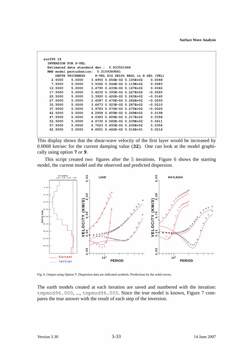
Surface Wav eAnalysis
surf96 18INVERSION FOR S-VELEstimated data standard dev.: 0.833521664RMS model perturbation: 0.0159389861
DEPTH THICKNESS S-VEL SIG DELVL RESL in H DEL (VEL)2.5000 5.0000 3.4950 0.654E-02 0.105E+02 0.00687.5000 5.0000 3.5062 0.544E-02 0.119E+02 0.008312.5000 5.0000 3.4790 0.433E-02 0.167E+02 0.006217.5000 5.0000 3.4235 0.393E-02 0.227E+02 -0.002522.5000 5.0000 3.3920 0.420E-02 0.263E+02 -0.016027.5000 5.0000 3.4587 0.470E-02 0.282E+02 -0.025532.5000 5.0000 3.6673 0.523E-02 0.287E+02 -0.021037.5000 5.0000 3.9783 0.575E-02 0.275E+02 -0.002542.5000 5.0000 4.2958 0.609E-02 0.249E+02 0.019847.5000 5.0000 4.5383 0.609E-02 0.217E+02 0.035852.5000 5.0000 4.6730 0.565E-02 0.239E+02 0.041157.5000 5.0000 4.7023 0.493E-02 0.200E+02 0.035662.5000 0.0000 4.6551 0.462E-02 0.516E+01 0.0214
This display shows that the shear-wav evelocity of the first layer would be increased by0.0068 km/sec for the current damping value (32). Onecan look at the model graphi-cally using option7 or 9.
This script created two figures after the 5 iterations.Figure 6 shows the startingmodel, the current model and the observed and predicted dispersion.
6 . 5 0
1 3 . 0 0
1 9 . 5 0
2 6 . 0 0
3 2 . 5 0
3 9 . 0 0
4 5 . 5 0
5 2 . 0 0
5 8 . 5 0
DE
PT
H (
KM
)
3 . 6 0 4 . 0 0 4 . 4 0 4 . 8 0VS (KM/S)
C u r r e n t
I n i t i a l101
PERIOD
3.0
03
.50
VE
LO
CIT
Y (
KM
/S)
4.0
04
.50
5.0
0
LOVE
101
PERIOD
2.5
03
.13
VE
LO
CIT
Y (
KM
/S)
3.7
54
.38
5.0
0
RAYLEIGH
Fig. 6. Output using Option7. Dispersion data are indicated symbols. Predictions by the solid curves.
The earth models created at each iteration are saved and numbered with the iteration:tmpmod96.000, ..., tmpmod96.005. Since the true model is known, Figure 7 com-pares the true answer with the result of each step of the inversion.
Version 3.30 3-33 14 June 2007
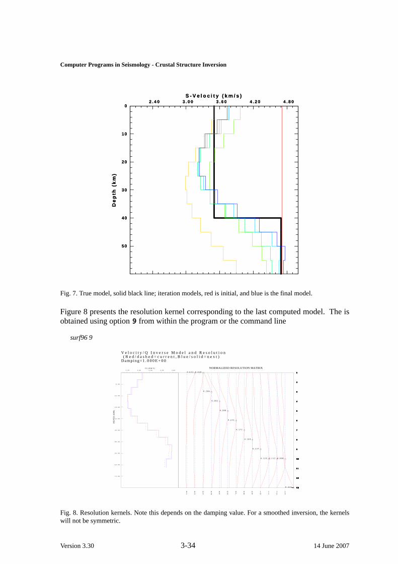
Computer Programs in Seismology - Crustal Structure Inv ersion
2 . 4 0 3 . 0 0 3 . 6 0 4 . 2 0 4 . 8 0S - V e l o c i t y ( k m / s )
50
40
30
20
10
0
De
pth
(k
m)
2 . 4 0 3 . 0 0 3 . 6 0 4 . 2 0 4 . 8 0S - V e l o c i t y ( k m / s )
50
40
30
20
10
0
De
pth
(k
m)
Fig. 7. True model, solid black line; iteration models, red is initial, and blue is the final model.
Figure 8 presents the resolution kernel corresponding to the last computed model.The isobtained using option9 from within the program or the command line
surf96 9
V e l o c i t y / Q I n v e r s e M o d e l a n d R e s o l u t i o n ( R e d / d a s h e d = c u r r e n t , B l u e / s o l i d = n e x t )Damp ing=1 . 0 0 0 E + 0 0
8 . 0 0
1 6 . 0 0
2 4 . 0 0
3 2 . 0 0
4 0 . 0 0
4 8 . 0 0
5 6 . 0 0
6 4 . 0 0
7 2 . 0 0
DE
PT
H (
KM
)
3 . 2 0 3 . 6 0 4 . 0 0 4 . 4 0 4 . 8 0V S ( K M / S ) NORMALIZED RESOLUTION MATRIX
01
02
03
04
05
06
07
08
09
10
11
12
13
1
2
3
4
5
6
7
8
9
1 0
1 1
1 2
1 3
0 . 6 3 3 1
2
3
4
5
6
7
8
9
1 0
1 1
1 2
1 3
0 . 4 2 8 1
2
3
4
5
6
7
8
9
1 0
1 1
1 2
1 3
0 . 2 8 6
1
2
3
4
5
6
7
8
9
1 0
1 1
1 2
1 3
0 . 2 8 2
1
2
3
4
5
6
7
8
9
1 0
1 1
1 2
1 3
0 . 2 8 8
1
2
3
4
5
6
7
8
9
1 0
1 1
1 2
1 3
0 . 2 3 1
1
2
3
4
5
6
7
8
9
1 0
1 1
1 2
1 3
0 . 1 7 1
1
2
3
4
5
6
7
8
9
1 0
1 1
1 2
1 3
0 . 1 4 4
1
2
3
4
5
6
7
8
9
1 0
1 1
1 2
1 3
0 . 1 3 7
1
2
3
4
5
6
7
8
9
1 0
1 1
1 2
1 3
0 . 1 2 5
1
2
3
4
5
6
7
8
9
1 0
1 1
1 2
1 3
0 . 1 1 2
1
2
3
4
5
6
7
8
9
1 0
1 1
1 2
1 3
0 . 0 9 8
1
2
3
4
5
6
7
8
9
1 0
1 1
1 2
1 30 . 4 4 3
Fig. 8. Resolution kernels. Note this depends on the damping value. For a smoothed inversion, the kernelswill not be symmetric.
Version 3.30 3-34 14 June 2007

Surface Wav eAnalysis
7. Discussion
The simplest way to run the program is just to try a sequence of commands of theform
surf96 1 2 18 6
8. References
Abramowitz, M. and. I. A. Stegun (1965).Handbook of Mathematical Functions, Doverpublications, Inc., New York.
Bhattacharya, S. N. (1983).Higher order accuracy in multiple filter technique,Bull.Seism. Soc. Am. 73,1395-1406.
Dziewonski, A., S. Bloch and M. Landisman (1969).A technique for analysis of tran-sient seismic signals,Bull. Seism. Soc. Am. 59,427-444.
Herrmann, R. B., (1973). Some aspects of band-pass filtering of surface wav es, Bull.Seism. Soc. Am. 63,663-671.
McMechan, G. A. and M. J. Yedlin (1981). Analysis of dispersive wav es by wav efieldtransformation,Geophysics 46,869-874.
Mokhtar, T. A., R. B. Herrmann and D. R. Russell (1988). Seismic velocity and Q modelfor the shallow structure of the Arabian shield from short-period Rayleigh wav es,Geophysics 53,1379-1387.
Version 3.30 3-35 14 June 2007

Computer Programs in Seismology - Crustal Structure Inv ersion
CHAPTER 4INVERSION OF RECEIVER FUNCTIONS
1. Introduction
A property of elastic wav epropagation in an isotropic medium is that P or SV wav esincident at a medium boundary are converted to P and SV wav es upon reflection or trans-mission. This property leads to complicated surface recordings for a layered medium.The receiver function is a time series constructed from the surface recordings in a mannerthat focuses on the layered structure itself.
Consider the surface 3-component recording of a distant earthquake, such as thetraces shown in Figure 1.
Fig. 1. SLM recordings of the destructive August 17, 1999 earthquake in Turkey. Atotal of 3600 seconds of ground motion is displayed. Note the small amplitude of theinitial P wav es.
The initial P-wav emotion, shown in Figure 2, demonstrates the complexity of themotion, which is the composite effects of the source, the 84° propagation path, and thelocal structure beneath St. Louis, Missouri. The vertical component has the largestamplitude, with the radial motions less than one-half the vertical. The transverse compo-nent motions are even smaller. For an ideal earth model, the transverse component wouldbe zero and the radial a fraction of the vertical, due to the teleseismic P-wav e’s near
Version 3.30 4-1 14 June 2007

Computer Programs in Seismology - Crustal Structure Inv ersion
vertical incidence at the surface.
Fig. 2. Plot of initial P-wav emotion at SLM.
We can ask an interesting question though, "What are the transfer functions thatwould convert the vertical component signal to the radial and horizontal component sig-nals?"
Fig. 3. Plot of Z→R and Z→T transfer functions.
2. Joint Inversion Mathematics
3. Data Preparation
Version 3.30 4-2 14 June 2007

Inversion of Receiver Functions
3.1. DataOrganization
The basic idea governing receiver-function data organization is to group the signalsinto "clusters" that sample the same structure. Most observations are also naturally clus-tered by the distance and azimuth of appropriate sources.
Wa ves approaching a seismometer from different directions may sample very differ-ent structures. An extreme example is shown to the right.
At most stations, the structure varies with azimuth and even in the simplest cases, theresponse can vary with distance from the station.
We usually group the observations by azimuth, then distance. We stack, or average,waveforms from the same azimuth and distance range, although at times, when the cover-age is very broad, studying the response as a more continuous function of azimuth or dis-tance is a nice way to study the structure.
3.2. Instrument Responses and Gains
For the Rftn analysis, you need three-component observations, preferably with a widebandwidth. If the instrument response of the components is matched, you do not have toremove the instrument effects before proceeding, but you must insure that the gains areequalized before proceeding to the receiver function deconvolution. To correct for differ-ences in instrument gain, use the scalar division command "div" in SAC. If the instru-ments are not matched, you should remove or replace them with a set of uniform instru-ment responses, which you can do with the "transfer" command in SAC.
For example, suppose I had three seismograms from SNZO: myevent.z myevent.nmyevent.e The instrument responses for the station are matched, with the exception of asmall variation in the gain. To remove the slight difference, I would execute the followingSAC commands:
r myevent.e myevent.n myevent.zdiv 6.465442 6.478608 6.307450w over
The gains are actually the values above x 10ˆ13, but the constant factor doesn’t matter,only the variable coefficient.
3.3. SAC Header Values
Once you have the instrument response worked out, you next need to supply the infor-mation necessary for SAC to rotate the horizontal seismograms into the theoreticallybased radial and tangential directions. Specifically, you set several header variables ineach of your wav eforms:
• The event latitude and longitude• The component azimuth
Version 3.30 4-3 14 June 2007

Computer Programs in Seismology - Crustal Structure Inv ersion
• The component incident angle
To set these values for each seismogram, you use the change header command:SAC Commands Commentsr my_seismogram read in the seismogramch evla _____ch evlo _____ change header valuesch evdp _____ (fill in the blanks)ch cmpaz _____ch cmpinc _____wh Overwrite the header
The "r" command reads the seismogram into memory. The "wh" command writes theheader, saving the appropriate information. Once this information is stored in the header,SAC will automatically compute the distance and back azimuth of the observation. Lati-tude is positive north of the equator, longitude is positive east of Greenwich, England.Enter the numbers in decimal degrees. The cmpaz is the component azimuth also in deci-mal degrees, north is 0°, east is 90 °, etc. After you have made these additions to the fileheader values, you can view the great-circle distance and back azimuth using the "lh"command
lh gcarc baz
3.4. Windowing the Data
The final data-preparation stage consists of windowing the P wav eform from the pre-sig-nal noise and the rest of the seismic signal. The amount of record that you use dependssomewhat on the seismogram. You want to isolate the P-wav eform from the remainingsignal. For the usual teleseismic distances (30° to 95°) you are usually safe by usingabout 60 seconds of signal "leader" and 60 seconds of signal following the onset of the Pwave. The precise duration can vary if needed, these are typical values. At times detailsin the estimated receiver function may be sensitive to substantial (10s of seconds) varia-tions in length, and you can get a feel for the variations by comparing several lengths ofsignal during the source equalization procedure.
To cut the desired part of the seismogram from SAC, you use the "cut" command. TheSAC time reference system is based on two different times. A reference time which isstored in the header "kzdate and kztime" and the begin time of the trace. For our pur-poses, the begin time is most important, since we will use that value to reference the cut.Suppose that the P-wav eonset occurs at about 80 seconds into the seismogram, then wewould want to window the signal between 20 and 140 seconds. We also should removethe mean and taper the ends of the signal to avoid signal processing artifacts later in theprocessing. The following SAC commands with perform the desired operations.
r myseismogram.e myseismogram.n myseismogram.zqdp offp1cuterr fillzcut 20 140rrmeanw over
Normally if a cut lies beyond the bounds of the data, SAC will report an error and the bad
Version 3.30 4-4 14 June 2007

Inversion of Receiver Functions
start cut and/or end cut will be replaced with the file begin and/or file end. Further auto-matic use of the trace output will be in error. Thecuterr fillz will avoid this error by plac-ing zeros at the beginning and/or end of the trace. This is satisfactory unless the file has aDC offset, in which case an undesirable discontinuity may be introduced. In this caseread the file first, remove the mean, then save the file.
Once the data are windowed, we are ready to calculate the the radial and tangentialreceiver functions. See the Source Equalization Page for a discussion of the procedure.
3.5 A SAC Macro For Pre-Processing Raw Observations
If you have many wav eforms to prepare, the above will get tiring. Here is a SAC macrothat I have used to handle cutting, detrending, tapering, and separating noisy observationsfrom the better signals. The data are stored in files named: *BHZ, *BHN, *BHE, wherethe * means "whatever". Make a directory with a copy of your observations (Data fileswill be overwritten if you execute this macro - work with a copy of the data!) and executethis macro.
The macro is interactive - you will be picking the approximate P onset from the verticalcomponent using the PPK command in SAC. When the cursor appears, place it at the P-onset time and enter "t" "0" (that’s a zero) to set the t0 header value. Enter "q" to go ontothe next part of the macro, where you decide whether to keep the data or move them intothe "Noisy" directory. You only need to identify the time the time within a few seconds,don’t agonize over precision.
If the data are all noisy, just enter "q" and then enter an "t" later to move the signal to the"Trash" directory.
The mean and a trend are removed from the observations and a cosine taper is applied onthe left and right fifth (about 25 seconds if you keep the time limits in the macro) of thesignal.
You must edit the "div" line to put in the correct instrument gains, or just delete that lineand correct the gains later.
The SAC Macro Comments
sc mkdir Trash Make directories.sc mkdir GoodOnesqdp offygrid ondo file wild *BHZ Key on thesetbb vert $file vertical...setbb east ’( CHANGE ’BHZ’ ’BHE’ %vert )’setbb north ’( CHANGE ’BHZ’ ’BHN’ %vert )’ Synchronize ther %vert %east %north file start times.synchw overr %vert Pick the P onset &rmean mark it in thertr header.ppksetbb t0 &1,t0 Cut the data 60 sr %vert %east %north before and 90 s
Version 3.30 4-5 14 June 2007

Computer Programs in Seismology - Crustal Structure Inv ersion
ch t0 %t0 after the P onset.w overcuterr fillzcut t0 -60 t0 +90r %vert %east %north Remove the mean, armean trend, and correctrtr the gain of eachtaper w 0.2 instrument.div 6.307450 6.465442 6.478608w overp1setbb resp (REPLY "Enter t to trash the file") Move the files intoif %resp eq "t" then the directorysc mv %vert Trash "GoodOnes" if theysc mv %east Trash look usable, orsc mv %north Trash into "Trash" if
else they look reallysc mv %vert GoodOnes bad.sc mv %east GoodOnessc mv %north GoodOnes
endif Turn cut off and docut off the next one.enddo
3.1 Data Selection
3.2 Data Preparation
3.3 Iterative Deconvolution
4. rftn96
Operation of the program requires the existence of therobs.d control file, a sur-face-wav edispersion file, and the list of the receiver functions to be inverted. If none ofthese exist, the program will permit the user to interactive create the files.
4.1. Data preparation
The receiver functions must be prepared as described in Chapter 4.It is essential thatthe Gaussian filter parameter, $ alpha $ be placed in USER0, the ray parameter in USER4and the receiver function delay be mirrored in the B value of the SAC header for eachreceiver function.
4.2. Interactive control file setup
The following example shows the interactive dialog for the case that neither the initialearth model file nor the list of receiver functions exist. The user input is indicated by the
Version 3.30 4-6 14 June 2007

Inversion of Receiver Functions
italic font.
rftn96Enter 1 if variance based on residual or
0 if variance based on obs std err0Enter inversion technique
0 invert for Vs :Va,rho fixed1 : invert for Vs :Poisson fixed, rho from Vp
1Enter name of model file
modl.dInteractively setting up initial model file:modl.dIs model flat (0) or spherical (1)
0Enter descriptive title for this model
Test modelEnter d,a,b,rho,qa,qbd=0.0 or EOF indicates halfspace and end of input
40 6 3.5 2.5 100 1000 8 4.7 3.3 1000 1000Enter name of receiver function file list
rftn.lstInteractively setting up receiver function file list:rftn.lstEnter receiver function SAC binary file name, EOF to end../MKRFTN/05.rfn../MKRFTN/10.rfnCTRL D (for UNIX/LINUX, CTRL Z for DOS)
If this is successful, then the initial program menu will be presented.Before presentingthis, the requested input in the initial setup must be described.
Enter 1 if variance based on residual or0 if variance based on obs std err
This relates to the computation of confidence limits in the earth model and also theweighting of the individual data.Currently only the surface wav edata permits a tabula-tion of the confidence of any observation.
Enter inversion technique0 invert for Vs :Va,rho fixed1 : invert for Vs :Poisson fixed, rho from Vp
The first option,0 was introduced for the special case of investigating receiver func-tion in deep soil layers for which the P-velocity was known. The second case,1, itera-tively inverts for the S-wav evelocity and then updates the P-velocity using the Vp/Vsratio of the initial model; the new density is computed from the new Vp using the Nafe-Drake relation.
After this the names of the earth model file, dispersion and receiver function list arerequested. If the files do not exist, then they are interactively constructed. Once this isdone interactively, the format of each is correctly prototyped and the user may use an edi-tor to modify the files faster than using this interactive dialog.
4.3. Main menu
Version 3.30 4-7 14 June 2007

Computer Programs in Seismology - Crustal Structure Inv ersion
RFTN96 MENU0- Display menu 35- Inversion: (0) Non-Causal (default)1- Run Dispersion (1) Decoupled Causal2- Run Velocity Inversion (2) Coupled Causal5- Set Thick(0)/Velocity(1) Inversion 36- Smoothing: (0) Global reset none6- Update Model (need lam) (1) Global reset diff7- Plot RFTN/Dispersion/Velocity Model 37- Reset Number of Iterations9- Plot Resolution Kernel 38- Temporary End10- List Singular Values 39- Permanent End18- List Velocity Model (need lam) 42- Enter Sigr minimum19- Velocity Resolving Kernels(need lam)43- Joint Weighting: 0=RFTN <--> 1=SRFW28- ASCII Model File (file name, lam) 44- 2x RFTN computation (0) no, (1) yes29- ASCII Vel Resolving(file name,lam) 45- Show Velocity Weights30- (0) Fix Vp,(1) Fix Vp/Vs 47- Show Inversion Controls31- Change dd(i), enter i,dd(i) 48- Modify Individual Layer Smoothing32- Enter Damping Factor (lam) 49- Show RFTN information and weight33- Enter Tmin for RFTN (default -5 s) 50- Change individual RFTN weight34- Enter Tmax for RFTN (default 20 s)Enter Command at READY Prompt
RFTN96 MENUready
This menu appears once the control file robs.d exists. If the dispersion, initial modeland file listing receiver functions do not exist, then error messages will appear.
This menu is hopefully self-explanatory. Entering one of these numbers at thereadyprompt causes an action. Actions45, 46 and47 present other menus.
If 45 is entered, and the no smoothing option was chosen, e.g.,36 with option 0,then the velocity weights shown are
V Model Weighting Parameters: Large value forces change at boundary or layerI DD(I) Inv S depth/range I DD(I) Inv S depth/range
--------------------------------------------------------------------------------1 1.00 Bdy 1 5.00 | 8 1.00 Bdy 1 40.002 1.00 Bdy 1 10.00 | 9 1.00 Bdy 1 45.003 1.00 Bdy 1 15.00 | 10 1.00 Bdy 1 50.004 1.00 Bdy 1 20.00 | 11 1.00 Bdy 1 55.005 1.00 Bdy 1 25.00 | 12 1.00 Bdy 1 60.006 1.00 Bdy 1 30.00 | 13 1.00 Bdy 1 60.00- 9999.007 1.00 Bdy 1 35.00 |
--------------------------------------------------------------------------------Bdy - get velocity change at boundaryLyr - get velocity in layerS =0 Vp fixed, S=1 Vp/Vs fixed in layerUse option 30 to change how Vp obtainedUse option 31 to change layer weightUse option 48 to change layer smoothingUse option 45 to redisplay this menu
Here the weight, DD, is indicated together with the depth range in the model that itapplies to. To permit significant change in the model velocities in the 45-50 km depthrange, one would just enter from the command line
rftn96 31 10 100
or interactivelyready
3113 layers: 1-13 for Vs 13-26 for QbinvEnter i10
Version 3.30 4-8 14 June 2007

Inversion of Receiver Functions
Current dd( 10)= 1.Enter New dd( 10)100ready
If dif ferential smoothingis used,36 with option1, then one would see
V Model Weighting Parameters: Large value forces change at boundary or layerI DD(I) Inv S depth/range I DD(I) Inv S depth/range
--------------------------------------------------------------------------------1 1.00 Bdy 1 5.00 | 8 1.00 Bdy 1 40.002 1.00 Bdy 1 10.00 | 9 1.00 Bdy 1 45.003 1.00 Bdy 1 15.00 | 10 1.00 Bdy 1 50.004 1.00 Bdy 1 20.00 | 11 1.00 Bdy 1 55.005 1.00 Bdy 1 25.00 | 12 1.00 Bdy 1 60.006 1.00 Bdy 1 30.00 | 13 1.00 Lyr 1 60.00- 9999.007 1.00 Bdy 1 35.00 |
--------------------------------------------------------------------------------Bdy - get velocity change at boundaryLyr - get velocity in layerS =0 Vp fixed, S=1 Vp/Vs fixed in layerUse option 30 to change how Vp obtainedUse option 31 to change layer weightUse option 48 to change layer smoothingUse option 45 to redisplay this menu
The display is slightly different, since the DD(I) controls the change in velocity across aboundary. This display shows the depth of that boundary. To emphasize a Moho at adepth of 35 km, one would use
rftn96 31 7 100
Version 3.16 introduced a new choice for option36 and changes the meaning of thisoption slightly. When the program is initially interactively started, differential smoothingis assumed. At any time a36 with choice0 will force a no-smoothing inversion on alllayers, a36 with choice1 will force a differential smoothing on all layers except the bot-tom layer.
A new option48 - Modify Individual Layer Smoothing was also introduced. The pur-pose if this is to fine tune the type of smoothing for a given layer or boundary by switch-ing between smoothed and non-smoothed layers/boundaries. With this option one can fixa layer velocity and still permit smoothing else where.
The menu produced using option47 summarizes the current processing parameters.
Version 3.30 4-9 14 June 2007

Computer Programs in Seismology - Crustal Structure Inv ersion
Inversion controls for rftnCmd Value Description
1 1 Variance based residual of fit0 Variance based on observed std observation
5 Current iteration4 Number of receiver functions to be inverted2 2 last inversion for Vs
3 last inversion for Q inverse4 last inversion for Vs-Q inverse
5 1 0 Layer thickness inversion1 Layer velocity/Q inversion
32 1.000 Damping value (default value 1.0)33 -5.000 Minimum window for RFTN (default -5.0 s)34 20.000 Maximum window for RFTN (default 20.0 s)35 0 0 non-causal Vs - Q relation (default)
1 Decoupled causal2 Fully coupled causal
36 1 0 No smoothing constraint1 Differential smoothing constraint
42 0.0500 Std error of fit floor for RFTN44 0 0 Match observed RFTN window
1 Use 2x times series to compute RFTN--------------------------------------------------------------------------------Use menu command cmd to change valueready
A few control parameters listed cannot be changed interactively. They are defined duringthe initial creation of therobs.d control file. Other parameters can be changed duringthe iterative inv ersion. The most interesting parameter is the "Joint inversion influenceparameter," option 43 which is used to change the relative importance of the receiverfunction and surface wav edispersion data sets for determining the "best model"
4.4. Program operation
The program can be run interactively or from the command line. For repeated runs orto reproduce a run running from a command line may be easier, especially if the sequenceof commands is placed in a shell script (batch file)For repeated runs or to reproduce a runrunning from a command line may be easier, especially if the sequence of commands isplaced in a shell script (batch file). The only slight difference is that creation of the outputfi le in interactive mode, Option28 asks the user for a command text to be placed in themodel96 header.
5. Example
This example computes P-wav ereceiver functions for a single layer over a halfspace.These synthetic data sets were created for the single layer over a halfspace model
Version 3.30 4-10 14 June 2007

Inversion of Receiver Functions
MODELTEST MODELISOTROPICKGSFLAT EARTH1-DCONSTANT VELOCITYLINE08LINE09LINE10LINE11HR VP VS RHO QP QS ETAP ETAS FREFP FREFS40 6 3.5 2.5 200.0 100.0 0.0 0.0 1.0 1.00 8 4.7 3.3 900.0 500.0 0.0 0.0 1.0 1.0
If this model is calledmodel.true, then the commands for create the receiver func-tions usinghrftn96 are
#!/bin/shP=0.10
for CALP in 05 10 25 50docase $CALP in
05) ALP=0.5 ;;10) ALP=1.0 ;;25) ALP=2.5 ;;50) ALP=5.0 ;;
esachrftn96 -P -ALP $ALP -DT 0.1 -D 10. -RAYP $P -M model.true -2mv hrftn96.sac $CALP.rfndone
To demonstrate operation of the program, the following shell script was run. It is assumedthat the control file robs.d and the initial earth model, dispersion and receiver functionfi les exist in the current directory. The contents ofrobs.d are
1 0 0 0 0 0 0 0 1 0modl.drftn.lst
Version 3.30 4-11 14 June 2007

Computer Programs in Seismology - Crustal Structure Inv ersion
#!/bin/sh###### clean up#####rftn96 39###### define damping#####rftn96 32 1.###### Select differential smoothing#####rftn96 36 1###### define TMIN and TMAX for receiver function fit#####rftn96 33 -5.0 34 20.0###### set up repeated run for 5 iterations#####rftn96 1 2 6 1 2 6 1 2 6 1 2 6 1 2 6 1 2###### show menus#####rftn96 0 > menu00.txtrftn96 45 > menu45.txtrftn96 47 > menu47.txt###### save last model#####rftn96 28 modl.out###### plot resolution kernel#####srfphr96mv SRFPHR96.PLT R.PLTplotnps -EPS -K < R.PLT > figrfnr.eps###### plot the model and show the data fit after 5 iterations#####rftnpv96plotnps -EPS -K -F7 -W10 < RFTNPV96.PLT > figrfn1.eps###### compare the individual models from the inversion# to the true model#####shwmod96 -K 1 -W 0.05 model.truemv SHWMOD96.PLT T.PLTshwmod96 -K -1 tmpmod96.???mv SHWMOD96.PLT I.PLTcat T.PLT I.PLT > IT.PLTplotnps -EPS -K -F7 -W10 < IT.PLT > figrfn2.eps
The command sequencerftn96 1 2 6 1 2 6 1 2 6 1 2 6 1 2 6 1 2
sets up fiv e complete iterations consisting of1 computing the partial derivatives, 2 per-forming the singular value decomposition, and6 updating the model. The output forthese iterations consists fo the following:
Version 3.30 4-12 14 June 2007

Inversion of Receiver Functions
Processing RFTN Partials for Layer Velocity - Window [ -5.00, 20.00]IncP Delay Dt Rayp Gauss Npts 2x Fit(%) Sta Weight FileT 10.00 0.10 0.100 0.50 512 F 36.8486 RFTN 2.00 ../MKRFTN/05.rfnT 10.00 0.10 0.100 1.00 512 F 34.8793 RFTN 1.00 ../MKRFTN/10.rfnT 10.00 0.10 0.100 2.50 512 F 36.4601 RFTN 0.40 ../MKRFTN/25.rfnT 10.00 0.10 0.100 5.00 512 F 38.1616 RFTN 0.20 ../MKRFTN/50.rfn
Receiver function fit std err : 0.010452Percent of Signal Power Fit (RFTN) : 36.32523% for 4 RFTNs 1004 pointsRMS change in S-wave velocity model : 0.7285 km/secITERATION 1 done: UPDATING V----------------------------------------------------------------------------Processing RFTN Partials for Layer Velocity - Window [ -5.00, 20.00]IncP Delay Dt Rayp Gauss Npts 2x Fit(%) Sta Weight FileT 10.00 0.10 0.100 0.50 512 F 92.4736 RFTN 2.00 ../MKRFTN/05.rfnT 10.00 0.10 0.100 1.00 512 F 89.3117 RFTN 1.00 ../MKRFTN/10.rfnT 10.00 0.10 0.100 2.50 512 F 84.5864 RFTN 0.40 ../MKRFTN/25.rfnT 10.00 0.10 0.100 5.00 512 F 82.5842 RFTN 0.20 ../MKRFTN/50.rfn
Receiver function fit std err : 0.002016Percent of Signal Power Fit (RFTN) : 90.29457% for 4 RFTNs 1004 pointsRMS change in S-wave velocity model : 0.2156 km/secITERATION 2 done: UPDATING V----------------------------------------------------------------------------Processing RFTN Partials for Layer Velocity - Window [ -5.00, 20.00]IncP Delay Dt Rayp Gauss Npts 2x Fit(%) Sta Weight FileT 10.00 0.10 0.100 0.50 512 F 97.6074 RFTN 2.00 ../MKRFTN/05.rfnT 10.00 0.10 0.100 1.00 512 F 96.5370 RFTN 1.00 ../MKRFTN/10.rfnT 10.00 0.10 0.100 2.50 512 F 92.0701 RFTN 0.40 ../MKRFTN/25.rfnT 10.00 0.10 0.100 5.00 512 F 86.1939 RFTN 0.20 ../MKRFTN/50.rfn
Receiver function fit std err : 0.001088Percent of Signal Power Fit (RFTN) : 96.18314% for 4 RFTNs 1004 pointsRMS change in S-wave velocity model : 0.0446 km/secITERATION 3 done: UPDATING V----------------------------------------------------------------------------Processing RFTN Partials for Layer Velocity - Window [ -5.00, 20.00]IncP Delay Dt Rayp Gauss Npts 2x Fit(%) Sta Weight FileT 10.00 0.10 0.100 0.50 512 F 97.8811 RFTN 2.00 ../MKRFTN/05.rfnT 10.00 0.10 0.100 1.00 512 F 97.4736 RFTN 1.00 ../MKRFTN/10.rfnT 10.00 0.10 0.100 2.50 512 F 93.5274 RFTN 0.40 ../MKRFTN/25.rfnT 10.00 0.10 0.100 5.00 512 F 86.5704 RFTN 0.20 ../MKRFTN/50.rfn
Receiver function fit std err : 0.000958Percent of Signal Power Fit (RFTN) : 96.77037% for 4 RFTNs 1004 pointsRMS change in S-wave velocity model : 0.0180 km/secITERATION 4 done: UPDATING V----------------------------------------------------------------------------Processing RFTN Partials for Layer Velocity - Window [ -5.00, 20.00]IncP Delay Dt Rayp Gauss Npts 2x Fit(%) Sta Weight FileT 10.00 0.10 0.100 0.50 512 F 98.0282 RFTN 2.00 ../MKRFTN/05.rfnT 10.00 0.10 0.100 1.00 512 F 97.7485 RFTN 1.00 ../MKRFTN/10.rfnT 10.00 0.10 0.100 2.50 512 F 93.9118 RFTN 0.40 ../MKRFTN/25.rfnT 10.00 0.10 0.100 5.00 512 F 86.3817 RFTN 0.20 ../MKRFTN/50.rfn
Receiver function fit std err : 0.000931Percent of Signal Power Fit (RFTN) : 96.96196% for 4 RFTNs 1004 pointsRMS change in S-wave velocity model : 0.0165 km/secITERATION 5 done: UPDATING V----------------------------------------------------------------------------Processing RFTN Partials for Layer Velocity - Window [ -5.00, 20.00]IncP Delay Dt Rayp Gauss Npts 2x Fit(%) Sta Weight FileT 10.00 0.10 0.100 0.50 512 F 98.2216 RFTN 2.00 ../MKRFTN/05.rfnT 10.00 0.10 0.100 1.00 512 F 97.9625 RFTN 1.00 ../MKRFTN/10.rfnT 10.00 0.10 0.100 2.50 512 F 94.0691 RFTN 0.40 ../MKRFTN/25.rfnT 10.00 0.10 0.100 5.00 512 F 86.1935 RFTN 0.20 ../MKRFTN/50.rfn
Receiver function fit std err : 0.000914Percent of Signal Power Fit (RFTN) : 97.13911% for 4 RFTNs 1004 points
Version 3.30 4-13 14 June 2007

Computer Programs in Seismology - Crustal Structure Inv ersion
Option1 computes the predictions and partial derivatives for the current model. Theinformation for the receiver functions presents the time window used for comparison withthe observed, whether the wav eis an incident P-wav e, the time delay, sample interval, rayparameter insec/km, the $ alpha $ parameter of the Gaussian filter, the number of datapoint in the observed receiver function, whether a $2x$ length series is computed to avoidFast Fourier Transform wrap around, the fit between the observed and predicted receiverfunctions, the station and file names.
The weight assigned to the particular file is that assigned using option31, divided bythe Gaussian filter parameter valueα . The division is required since largerα correspondto greater bandwidths which then affects the amplitude of the initial pulse in the receiverfunction. If this internal divisision byα were not done, a noisy recveivr function obsti-naed usingα = 5. 0 might dominate the inversion.,
The changes in the model obtained for the current model can be seen by invokingoptikon18.
rftn96 18INVERSION FOR S-VELEstimated data standard dev.: 0.0195770562RMS model perturbation: 0.0118706543
DEPTH THICKNESS S-VEL SIG DELVL RESL in H DEL (VEL)2.5000 5.0000 3.6548 0.881E-02 0.196E+02 -0.00997.5000 5.0000 3.6175 0.728E-02 0.222E+02 -0.012012.5000 5.0000 3.5894 0.624E-02 0.244E+02 -0.015717.5000 5.0000 3.6772 0.587E-02 0.229E+02 -0.018622.5000 5.0000 3.6809 0.591E-02 0.186E+02 -0.017627.5000 5.0000 3.6928 0.606E-02 0.164E+02 -0.019232.5000 5.0000 3.7408 0.633E-02 0.156E+02 -0.024937.5000 5.0000 3.8260 0.674E-02 0.155E+02 -0.025242.5000 5.0000 4.3141 0.717E-02 0.149E+02 0.010047.5000 5.0000 4.8778 0.764E-02 0.156E+02 0.008152.5000 5.0000 4.9445 0.745E-02 0.184E+02 -0.016757.5000 5.0000 4.8957 0.648E-02 0.226E+02 -0.018562.5000 0.0000 4.8677 0.535E-02 0.782E+01 -0.0103
This display shows that the shear-wav evelocity of the first layer would be increased by0.0014 km/sec for the current damping value (32). At present the estimated errors in thevelocity are imperfectly computed. One can look at the model graphically using option7or 9.
This script created threefigures after the 5 iterations. Figure 1 shows the starting model,the current model and the observed and predicted dispersion, while Figure 2 shows themodels and the observed and predicted receiver functions.
Version 3.30 4-14 14 June 2007

Inversion of Receiver Functions
6 . 5 0
1 3 . 0 0
1 9 . 5 0
2 6 . 0 0
3 2 . 5 0
3 9 . 0 0
4 5 . 5 0
5 2 . 0 0
5 8 . 5 0
DE
PT
H (
KM
)
3 . 5 0 4 . 0 0 4 . 5 0 5 . 0 0VS (KM/S)
C u r r e n t
I n i t i a l
0 5 10 15
T i m e ( s e c )
19700101 (001 )0000RFTN 0 . 5 0 9 8 . 5 8 0 . 1 0 0
19700101 (001 )0000RFTN 1 . 0 0 9 8 . 0 3 0 . 1 0 0
19700101 (001 )0000RFTN 2 . 5 0 9 3 . 4 6 0 . 1 0 0
19700101 (001 )0000RFTN 5 . 0 0 8 5 . 8 2 0 . 1 0 0
Fig. 1. Output using Option7. The observed and predicted RFTN’s are plotted in blue and red, respectively. The receiver functions arelabeled with the year/month/day (day of year) hour/minute at the upper right of each trace, and with the station name, Gaussian filterparameter, the percentage of fit, and the ray parameter (sec/km) at the left of each trace. A time scale is also provided.
The earth models created at each iteration are saved and numbered with the iteration:tmpmod96.000, ..., tmpmod96.005. Since the true model is known, Figure 3 com-pares the true answer with the result of each step of the inversion.
2 . 4 0 3 . 0 0 3 . 6 0 4 . 2 0 4 . 8 0S - V e l o c i t y ( k m / s )
50
40
30
20
10
0
De
pth
(k
m)
2 . 4 0 3 . 0 0 3 . 6 0 4 . 2 0 4 . 8 0S - V e l o c i t y ( k m / s )
50
40
30
20
10
0
De
pth
(k
m)
Version 3.30 4-15 14 June 2007

Computer Programs in Seismology - Crustal Structure Inv ersion
Fig. 2. True model, solid black line; iteration models, red is initial, and blue is the final model.
The commandrftn96 9 plots the resolution kernels after the sequencerftn96 1andrftn96 2 have been fun to compute the partial derivatives and perform the singularvalue decomposition.
V e l o c i t y / Q I n v e r s e M o d e l a n d R e s o l u t i o n ( R e d / d a s h e d = c u r r e n t , B l u e / s o l i d = n e x t )Damp ing=1 . 0 0 0 E + 0 0
8 . 0 0
1 6 . 0 0
2 4 . 0 0
3 2 . 0 0
4 0 . 0 0
4 8 . 0 0
5 6 . 0 0
6 4 . 0 0
7 2 . 0 0
DE
PT
H (
KM
)
3 . 6 0 3 . 9 0 4 . 2 0 4 . 5 0 4 . 8 0V S ( K M / S ) NORMALIZED RESOLUTION MATRIX
01
02
03
04
05
06
07
08
09
10
11
12
13
1
2
3
4
5
6
7
8
9
1 0
1 1
1 2
1 3
0 . 9 7 4 1
2
3
4
5
6
7
8
9
1 0
1 1
1 2
1 3
0 . 4 8 3
1
2
3
4
5
6
7
8
9
1 0
1 1
1 2
1 3
0 . 3 7 1
1
2
3
4
5
6
7
8
9
1 0
1 1
1 2
1 3
0 . 3 8 4
1
2
3
4
5
6
7
8
9
1 0
1 1
1 2
1 3
0 . 3 2 1
1
2
3
4
5
6
7
8
9
1 0
1 1
1 2
1 3
0 . 3 4 5
1
2
3
4
5
6
7
8
9
1 0
1 1
1 2
1 3
0 . 2 8 3
1
2
3
4
5
6
7
8
9
1 0
1 1
1 2
1 3
0 . 2 9 3
1
2
3
4
5
6
7
8
9
1 0
1 1
1 2
1 3
0 . 2 7 9
1
2
3
4
5
6
7
8
9
1 0
1 1
1 2
1 3
0 . 2 5 9
1
2
3
4
5
6
7
8
9
1 0
1 1
1 2
1 3
0 . 2 2 1
1
2
3
4
5
6
7
8
9
1 0
1 1
1 2
1 3
0 . 1 8 7
1
2
3
4
5
6
7
8
9
1 0
1 1
1 2
1 30 . 2 7 9
Fig. 3. Resolution kernels
6. Discussion
Version 3.30 4-16 14 June 2007

Inversion of Receiver Functions
CHAPTER 5JOINT INVERSION DISPERSION
1. Introduction
Having discussed the separate inversion of receiver functions and surface-wav edis-persion for earth structure, we now present the joint inversion of these two data sets.
2. Joint Inversion Mathematics
The joint inversion attempts to simultaneously invert two different set of observationsthat are sensitive to different aspects of earth structure. Defining the following parame-ters:
OriObserved receiver function at time ti
PriPredicted receiver function at time ti
σ riStandard error of observation at ti
Osjj’th Observed surface-wav edispersion
Psjj’th Predicted surface-wav edispersion point
σsjStandard error of j’th surface-wav eobservation
Nr Total number of receiver function pointsNs Total number of surface-wav edispersion pointsp Influence factor, 0 ≤ p ≤ 1.
We seek and earth model that minimizes the functional
S=(1 − p)
Nr
Nr
i=0Σ
Ori
− Pri
σ ri
2
+p
Ns
Ns
j=0Σ
Osj− Psj
σ r j
2
(1)
We see that the parameterp changes the influence of either data set on the minimizationprocedure. Ap = 0 forces a receiver function only solution, which ap = 1 forces a solu-tion based solely ont he surface wav edispersion. An advantage of the statistical weight-ing in the terms within the large parentheses is that dividing by the observed standarderror, corrects for the different physical units of the receiver function (sec−1) and the dis-persion (km/sec). Thepresence of the1/Nr and 1/Ns before the summation sign serves to
Version 3.30 5-1 14 June 2007

Computer Programs in Seismology - Crustal Structure Inv ersion
avoid onedata set dominating the other.
From the point of view of estimating model error, equation (1)is not in any of theforms introduced in Chapter 2 because for a large data set with the correct data vari-ances, the expected minimum value of S is
E(S)= 1
To force this to be in the form of the weighted inverse discussed in §2.4, we could attemptto minimize the quantity
S= (1 − p)Nr + pNs
(1 − p)
Nr
Nr
i=0Σ
Ori
− Pri
σ ri
2
+p
Ns
Ns
j=0Σ
Osj− Psj
σ r j
2
(2)
This functional form has leads to the correct error statistics for the end member casesp = 0 and p= 1. This is not done, however, because the mapping of lack of fit into theEarth model error is imperfect in this non-linear problem. Instead a number of goodnessof fit parameters are output, and it is up to the user to find a realistic model that fits theobservations well. This is because the best numerical solution to the problem may not bethe best geophysically plausible solution.
Because the forward problem is non-linear in terms of the model parameters, an itera-tive sequence of linearized inversions is computed. To do this the residual correspondingto the current model is modeled as a linear combination of changes to the current model.This means that the error statistics discussed in Chapter 2 apply to the changes in themodel parameters instead of the model parameters themselves. Once the solution hasconverged to a minimum, not necessary the global minimums, the confidence in thechanges may be attributed to the model itself.
A major problem is the estimation of theσ r’s and σs’s.If repeated observations aremade, and the observations averaged, theσ ’s must be the standard errors of the mean.This estimation is possible if surface wav eobservations are averages, or if receiver func-tions are stacked.
At present, the inversion program permits input of the surface-wav esigma’s in thesurf96 dispersion format, but does not permit receiver function error traces to be input.The program does attempt to estimate these standard error values.
To apply the weighting scheme, the program uses the standard error of model fit tothe receiver functions,sr , and in the case that the dispersion data has no correspondingσ s
estimate, thess in the following manner.
When the forward predictions are computed, the standard error of model predictionto the observations, sis computed. Initially this will be a large number since the observa-tions as poorly fit. As iteration progresses and the model fit becomes better, the computeds is compared to a user provided least bound. The default receiver function value is 0.05sec (Option 42) and the default surface wav evelocity error is 0.05 km/sec (Option 40).The value ofσ used is
max[s, user _bound]
The slight disadvantage of this is that initially one data set may be emphasized more if itscomputed sis nearer to the trueσ . As iteration progresses, the initial goal of controlled
Version 3.30 5-2 14 June 2007

Joint In version Dispersion
the influence of each data set is met.
Equation (1) is minimized by applying singular value decomposition to estimate thechanges in the model,∆m:
wr∂r
∂m1∆m1+. . .+wr
∂r
∂mN∆mN = wrres
. . .
ws∂s
∂m1∆m1+. . .+ws
∂r
∂mN∆mN = wsres
where the weights
wr = (1 − p)
Nrσ 2r
1/2
ws =
p
Nsσ 2s
1/2
are used for each receiver function and dispersion observation, respectively. The partial
derivatives of the receiver function,∂r
∂mand surface-wav edispersion
∂s
∂mare computed as
in rftn96 andsurf96.
3. joint96
The operation ofjoint96 is similar to that ofsurf96 andrftn96. Operation ofthe program requires the existence of thejobs.d control file, a surface-wav edispersionfi le, and the list of the receiver functions to be inverted. If none of these exist, the pro-gram will permit the user to interactive create the files.
3.1. Data preparation
The data preparation was discussed in detail in Chapter 3 for surface wav es and Chap-ter 4 for receiver functions.
The surface-wav edispersion data must be insurf96 format.
The receiver functions must be prepared as described in Chapter 4.It is essential thatthe Gaussian filter parameter, α be placed in USER0, the ray parameter in USER4 andthe receiver function delay be mirrored in the B value of the SAC header for each receiver
Version 3.30 5-3 14 June 2007

Computer Programs in Seismology - Crustal Structure Inv ersion
function.
3.2. Interactive control file setup
The following example shows the interactive dialog for the case that neither the dis-persion file, initial earth model file nor the list of receiver functions exist. The user inputis indicated by theitalic font.
joint96Enter h,dcl,dcr
h = fraction change in period to get group vel(0.005 is reasonable)
dcl, dcr are phase velocity increment in rootsearch for Love and Rayl respectively
0.005 0.005 0.005Enter 1 if variance based on residual or
0 if variance based on obs std err1Enter maximum number of Love gamma modes to process
0 means DO NO PROCESS LOVE gamma data0Enter maximum number of Love Phvel modes to process
0 means DO NO PROCESS LOVE phase vel data2Enter maximum number of Love Gpvel modes to process
0 means DO NO PROCESS LOVE group vel data2Enter maximum number of Rayl gamma modes to process
0 means DO NO PROCESS RAYL gamma data0Enter maximum number of Rayl Phvel modes to process
0 means DO NO PROCESS RAYL phase vel data2Enter maximum number of Rayl Gpvel modes to process
0 means DO NO PROCESS RAYL group vel data0Enter inversion technique
0 invert for Vs :Va,rho fixed1 : invert for Vs :Poisson fixed, rho from Vp
1Enter name of model file
modl.dInteractively setting up initial model file:modl.dIs model flat (0) or spherical (1)
0Enter descriptive title for this model
Test modelEnter d,a,b,rho,qa,qbd=0.0 or EOF indicates halfspace and end of input
40 6 3.5 2.5 100 1000 8 4.7 3.3 1000 1000Enter name of dispersion file
disp.dEnter ilvry,iporg,imode,per,val,dvalilvry=1(Love)
=2(Rayleigh)iporg=1 (phase velocity km/s)
=2 (group velocity km/s)=3 (gamma 1/km)
imode (mode number) e.g., 0=fundamental, 1=first
Version 3.30 5-4 14 June 2007

Joint In version Dispersion
per=the periodval=dispersion value, velocity or gammadval=error in dispersion value
(Enter 1.0 if stderr from residuals)NOTE: Enter all zeros or negative to terminate input
1 1 0 10.0 3.5 0.011 2 0 15.0 3.6 0.012 2 0 20.0 3.0 0.010 0 0 0 0 0Enter name of receiver function file list
rftn.lstInteractively setting up receiver function file list:rftn.lstEnter receiver function SAC binary file name, EOF to end../MKRFTN/05.rfn../MKRFTN/10.rfnCTRL D (for UNIX/LINUX, CTRL Z for DOS)
If this is successful, then the initial program menu will be presented.Before presentingthis, the requested input in the initial setup must be described.
Enter h,dcl,dcr
Determination of surface wav edispersion requires a search in the frequency - phasevelocity space of the surface-wav e period equation. Is is know that all surface wav emodes are bounded at the low end by some fraction of the smallest shear-wav evelocity,or in the case of a surface fluid layer, the lowest compressional-wav evelocity. The upperbound of the dispersion for a fixed period, is the halfspace shear-wav evelocity. dcl anddcr are the search increments to find the roots of the period equation. If these numbersare too large, modes may be missed by jumping past them. If the numbers are too small,computations take too long. The value of0.005 km/sec are acceptable for crustal studies,but could be made smaller when studying dispersion in low velocity sediments.
The parameterh is used to compute group-velocity partial derivatives. For example,∂U/∂VS can be computed by using∂c/∂VS(f) and ∂c/∂VS(( 1 + h)f). The recom-mended value of0.005 seems adequate.
Enter 1 if variance based on residual or0 if variance based on obs std err
This relates to the computation of confidence limits in the earth model and also theweighting of the individual data.Currently only the surface wav edata permits a tabula-tion of the confidence of any observation.
Enter maximum number of Love gamma modes to process0 means DO NO PROCESS LOVE gamma data
This sequence of 6 questions permits the user to invert subsets of the data containedwithin the dispersion file. Currently the anelastic attenuation coefficients are used in thejoint inversion to determine the Q structure.
Enter inversion technique0 invert for Vs :Va,rho fixed1 : invert for Vs :Poisson fixed, rho from Vp
The first option,0 was introduced for the special case of investigating receiver func-tion in deep soil layers for which the P-velocity was known. The second case,1, itera-tively inverts for the S-wav evelocity and then updates the P-velocity using the Vp/Vsratio of the initial model; the new density is computed from the new Vp using the Nafe-Drake relation.
Version 3.30 5-5 14 June 2007

Computer Programs in Seismology - Crustal Structure Inv ersion
After this the names of the earth model file, dispersion and receiver function list arerequested. If the files do not exist, then they are interactively constructed. Once this isdone interactively, the format of each is correctly prototyped and the user may use an edi-tor to modify the files faster than using this interactive dialog.
3.3. Main menu
JOINT96 MENU0- Display menu 30- (0) Fix Vp,(1) Fix Vp/Vs1- Run Dispersion 31- Change dd(i), enter i,dd(i)2- Run Velocity Inversion 32- Enter Damping Factor (lam)3- Run Q(beta) Inversion 33- Enter Tmin for RFTN (default -5 s)4- Run Simultaneous Veloc-Q Inversion 34- Enter Tmax for RFTN (default 20 s)5- Set Thick(0)/Velocity(1) Inversion 35- Inversion: (0) Non-Causal (default)6- Update Model (need lam) (1) Decoupled Causal7- Plot RFTN/Dispersion/Velocity Model (2) Coupled Causal8- Plot Gamma / Qb inverse Model 36- Smoothing: (0) Global reset none9- Plot Resolution Kernel (1) Global reset diff10- List Singular Values 37- Reset Number of Iterations11- Gamma Data Partial Derivatives 38- Temporary End12- Gamma Data Dispersion 39- Permanent End13- List Q Model (need lam) 40- Enter Sigv minimum14- Q(beta) Resolving Kernel (need lam) 41- Enter Sigg minimum16- Velocity Data Partial Derivatives 42- Enter Sigr minimum17- Velocity Data Dispersion 43- Joint Weighting: 0=RFTN <--> 1=SRFW18- List Velocity Model (need lam) 44- 2x RFTN computation (0) no, (1) yes19- Velocity Resolving Kernels(need lam)45- Show Velocity Weights22- ASCII Gamma Dispersion (file name) 46- Show Qinv Weights23- ASCII Q(beta) File (file name,lam) 47- Show Inversion Controls24- ASCII Q Resolving (file name,lam) 48- Modify Individual Layer Smoothing27- ASCII Veloc Dispersion (file name) 49- Show RFTN information and weight28- ASCII Model File (file name, lam) 50- Change individual RFTN weight29- ASCII Vel Resolving(file name,lam)Enter Command at READY Prompt
This menu appears once the control file jobs.d exists. If the dispersion, initial modeland file listing receiver functions do not exist, then error messages will appear.
This menu is hopefully self-explanatory. Entering one of these numbers at thereadyprompt causes an action. Actions45, 46 and47 present other menus.
If 45 is entered, and the no smoothing option was chosen, e.g.,36 with option 0,then the velocity weights shown are
Version 3.30 5-6 14 June 2007

Joint In version Dispersion
V Model Weighting Parameters: Large value forces change at boundary or layerI DD(I) Inv S depth/range I DD(I) Inv S depth/range
--------------------------------------------------------------------------------1 1.00 Lyr 1 0.00- 5.00 | 8 1.00 Lyr 1 35.00- 40.002 1.00 Lyr 1 5.00- 10.00 | 9 1.00 Lyr 1 40.00- 45.003 1.00 Lyr 1 10.00- 15.00 | 10 1.00 Lyr 1 45.00- 50.004 1.00 Lyr 1 15.00- 20.00 | 11 1.00 Lyr 1 50.00- 55.005 1.00 Lyr 1 20.00- 25.00 | 12 1.00 Lyr 1 55.00- 60.006 1.00 Lyr 1 25.00- 30.00 | 13 1.00 Lyr 1 60.00- 9999.007 1.00 Lyr 1 30.00- 35.00 |
--------------------------------------------------------------------------------Bdy - get velocity change at boundaryLyr - get velocity in layerS =0 Vp fixed, S=1 Vp/Vs fixed in layerUse option 30 to change how Vp obtainedUse option 31 to change layer weightUse option 48 to change layer smoothingUse option 45 to redisplay this menu
Here the weight, DD, is indicated together with the depth range in the model that itapplies to. To permit significant change in the model velocities in the 45-50 km depthrange, one would just enter from the command line
joint96 31 10 100
or interactivelyready
3113 layers: 1-13 for Vs 13-26 for QbinvEnter i10Current dd( 10)= 1.Enter New dd( 10)100ready
If dif ferential smoothingis used,36 with option1, then one would see
V Model Weighting Parameters: Large value forces change at boundary or layerI DD(I) Inv S depth/range I DD(I) Inv S depth/range
--------------------------------------------------------------------------------1 1.00 Bdy 1 5.00 | 8 1.00 Bdy 1 40.002 1.00 Bdy 1 10.00 | 9 1.00 Bdy 1 45.003 1.00 Bdy 1 15.00 | 10 1.00 Bdy 1 50.004 1.00 Bdy 1 20.00 | 11 1.00 Bdy 1 55.005 1.00 Bdy 1 25.00 | 12 1.00 Bdy 1 60.006 1.00 Bdy 1 30.00 | 13 1.00 Lyr 1 60.00- 9999.007 1.00 Bdy 1 35.00 |
--------------------------------------------------------------------------------Bdy - get velocity change at boundaryLyr - get velocity in layerS =0 Vp fixed, S=1 Vp/Vs fixed in layerUse option 30 to change how Vp obtainedUse option 31 to change layer weightUse option 48 to change layer smoothingUse option 45 to redisplay this menu
The display is slightly different, since the DD(I) controls the change in velocity across aboundary. This display shows the depth of that boundary. To emphasize a Moho at adepth of 35 km, one would use
joint96 31 7 100
Version 3.30 5-7 14 June 2007

Computer Programs in Seismology - Crustal Structure Inv ersion
The menu produced using option47 summarizes the current processing parameters.
Inversion controls for joint96Cmd Value Description
1 1 Variance based residual of fit0 Variance based on observed std observation
2 Maximum number of Love modes to use2 Maximum number of Rayleigh modes to use5 Current iteration4 Number of receiver functions to be inverted2 2 last inversion for Vs
3 last inversion for Q inverse4 last inversion for Vs-Q inverse
5 1 0 Layer thickness inversion1 Layer velocity/Q inversion
32 1.000 Damping value (default value 1.0)33 -5.000 Minimum window for RFTN (default -5.0 s)34 20.000 Maximum window for RFTN (default 20.0 s)35 0 0 non-causal Vs - Q relation (default)
1 Decoupled causal2 Fully coupled causal
36 1 0 No smoothing constraint1 Differential smoothing constraint
40 0.0500 Std error of fit floor for velocity disp42 0.0005 Std error of fit floor for RFTN43 0.500 Joint inversion influence parameter
RFTN = 0 <= p <= 1 Surface Wave44 0 0 Match observed RFTN window
1 Use 2x times series to compute RFTN--------------------------------------------------------------------------------Use menu command cmd to change value
A few control parameters listed cannot be changed interactively. They are defined duringthe initial creation of thejobs.d control file. Other parameters can be changed duringthe iterative inv ersion. The most interesting parameter is the "Joint inversion influenceparameter," option 43 which is used to change the relative importance of the receiverfunction and surface wav edispersion data sets for determining the "best model"
Version 3.16 introduced a new choice for option36 and changes the meaning of thisoption slightly. When the program is initially interactively started, differential smoothingis assumed. At any time a36 with choice0 will force a no-smoothing inversion on alllayers, a36 with choice1 will force a differential smoothing on all layers except the bot-tom layer.
A new option48 - Modify Individual Layer Smoothing was also introduced. The pur-pose if this is to fine tune the type of smoothing for a given layer or boundary by switch-ing between smoothed and non-smoothed layers/boundaries. With this option one can fixa layer velocity and still permit smoothing else where.
3.4. Program operation
The program can be run interactively or from the command line. For repeated runs orto reproduce a run running from a command line may be easier, especially if the sequenceof commands is placed in a shell script (batch file)For repeated runs or to reproduce a runrunning from a command line may be easier, especially if the sequence of commands is
Version 3.30 5-8 14 June 2007

Joint In version Dispersion
placed in a shell script (batch file). The only slight difference is that creation of the outputfi le in interactive mode, Option28 asks the user for a command text to be placed in themodel96 header.
4. Example
This example uses the same dispersion information presented in Chapter 3 and thesame receiver functions presented in Chapter 4. These synthetic data sets were created forthe single layer over a halfspace model
MODELTEST MODELISOTROPICKGSFLAT EARTH1-DCONSTANT VELOCITYLINE08LINE09LINE10LINE11HR VP VS RHO QP QS ETAP ETAS FREFP FREFS40 63.5 2.5 200.0 100.0 0.0 0.0 1.0 1.00 84.7 3.3 900.0 500.0 0.0 0.0 1.0 1.0
To demonstrate operation of the program, the following shell script was run. It is assumedthat the control file jobs.d and the initial earth model, dispersion and receiver functionfi les exist in the current directory. The contents ofjobs.d are
0.00499999989 0.00499999989 0. 0.00499999989 0.1 2 2 2 2 2 2 0 1 0
modl.d../MKSURF/disp.drftn.lst
The initial model,modl.d consists of a halfspace -MODELTEST MODELISOTROPICKGSFLAT EARTH1-DCONSTANT VELOCITYLINE08LINE09LINE10LINE11HR VP VS RHO QP QS ETAP ETAS FREFP FREFS5 84.71 3.3 0.0 0.0 0.0 0.0 1.0 1.05 84.71 3.3 0.0 0.0 0.0 0.0 1.0 1.05 84.71 3.3 0.0 0.0 0.0 0.0 1.0 1.05 84.71 3.3 0.0 0.0 0.0 0.0 1.0 1.05 84.71 3.3 0.0 0.0 0.0 0.0 1.0 1.05 84.71 3.3 0.0 0.0 0.0 0.0 1.0 1.05 84.71 3.3 0.0 0.0 0.0 0.0 1.0 1.05 84.71 3.3 0.0 0.0 0.0 0.0 1.0 1.0
Version 3.30 5-9 14 June 2007

Computer Programs in Seismology - Crustal Structure Inv ersion
5 84.71 3.3 0.0 0.0 0.0 0.0 1.0 1.05 84.71 3.3 0.0 0.0 0.0 0.0 1.0 1.05 84.71 3.3 0.0 0.0 0.0 0.0 1.0 1.05 84.71 3.3 0.0 0.0 0.0 0.0 1.0 1.00 84.72 3.3 0.0 0.0 0.0 0.0 1.0 1.0
#!/bin/sh
###### clean up#####joint96 39# define damping#####joint96 32 1.###### Select differential smoothing#####joint96 36 1###### set joint weighting between the two data sets#####joint96 43 0.5###### set up repeated run for 5 iterations#####joint96 1 2 6 1 2 6 1 2 6 1 2 6 1 2 6 1 2###### save last model#####joint96 28 modl.out###### plot the model and show the data fit after 5 iterations#####srfphv96plotnps -EPS -K -F7 -W10 < SRFPHV96.PLT > figjnt1.epsrftnpv96plotnps -EPS -K -F7 -W10 < RFTNPV96.PLT > figjnt2.eps###### compare the individual models from the inversion# to the true model#####shwmod96 -K 1 -W 0.05 model.truemv SHWMOD96.PLT T.PLT
shwmod96 -K -1 tmpmod96.???mv SHWMOD96.PLT I.PLT
cat T.PLT I.PLT > IT.PLTplotnps -EPS -K -F7 -W10 < IT.PLT > figjnt3.eps
The command sequencejoint96 1 2 6 1 2 6 1 2 6 1 2 6 1 2 6 1 2
sets up fiv e complete iterations consisting of1 computing the partial derivatives, 2 per-forming the singular value decomposition, and6 updating the model. The output forthese iterations consists fo the following:
Version 3.30 5-10 14 June 2007

Joint In version Dispersion
Processing RFTN Partials for Layer Velocity - Window [ -5.00, 20.00]IncP Delay Dt Rayp Gauss Npts 2x Fit(%) Sta Weight FileT 10.00 0.10 0.100 0.50 512 F 36.8486 RFTN 2.00 ../MKRFTN/05.rfnT 10.00 0.10 0.100 1.00 512 F 34.8793 RFTN 1.00 ../MKRFTN/10.rfnT 10.00 0.10 0.100 2.50 512 F 36.4601 RFTN 0.40 ../MKRFTN/25.rfnT 10.00 0.10 0.100 5.00 512 F 38.1616 RFTN 0.20 ../MKRFTN/50.rfn
Receiver function fit std err : 0.010452Dispersion fit (vel) std err : 0.3089 (km/s)Dispersion fit (vel) mean residual : -1.0676 (km/s)Dispersion fit (vel) avg |residual|: 1.0676 (km/s)Percent of Signal Power Fit (RFTN) : 36.32523% for 4 RFTNs 1004 pointsPercent of Signal Power Fit (Disp) : 89.05252% for 68 SW ObsRMS change in S-wave velocity model : 1.2049 km/secITERATION 1 done: UPDATING V----------------------------------------------------------------------------Processing RFTN Partials for Layer Velocity - Window [ -5.00, 20.00]IncP Delay Dt Rayp Gauss Npts 2x Fit(%) Sta Weight FileT 10.00 0.10 0.100 0.50 512 F 90.0604 RFTN 2.00 ../MKRFTN/05.rfnT 10.00 0.10 0.100 1.00 512 F 83.9401 RFTN 1.00 ../MKRFTN/10.rfnT 10.00 0.10 0.100 2.50 512 F 80.2502 RFTN 0.40 ../MKRFTN/25.rfnT 10.00 0.10 0.100 5.00 512 F 80.9305 RFTN 0.20 ../MKRFTN/50.rfn
Receiver function fit std err : 0.002381Dispersion fit (vel) std err : 0.2257 (km/s)Dispersion fit (vel) mean residual : 0.2867 (km/s)Dispersion fit (vel) avg |residual|: 0.2908 (km/s)Percent of Signal Power Fit (RFTN) : 86.89568% for 4 RFTNs 1004 pointsPercent of Signal Power Fit (Disp) : 99.01604% for 160 SW ObsRMS change in S-wave velocity model : 0.3340 km/secITERATION 2 done: UPDATING V----------------------------------------------------------------------------Processing RFTN Partials for Layer Velocity - Window [ -5.00, 20.00]IncP Delay Dt Rayp Gauss Npts 2x Fit(%) Sta Weight FileT 10.00 0.10 0.100 0.50 512 F 95.6311 RFTN 2.00 ../MKRFTN/05.rfnT 10.00 0.10 0.100 1.00 512 F 91.4207 RFTN 1.00 ../MKRFTN/10.rfnT 10.00 0.10 0.100 2.50 512 F 86.0853 RFTN 0.40 ../MKRFTN/25.rfnT 10.00 0.10 0.100 5.00 512 F 84.6284 RFTN 0.20 ../MKRFTN/50.rfn
Receiver function fit std err : 0.001621Dispersion fit (vel) std err : 0.0976 (km/s)Dispersion fit (vel) mean residual : 0.0135 (km/s)Dispersion fit (vel) avg |residual|: 0.0726 (km/s)Percent of Signal Power Fit (RFTN) : 92.93363% for 4 RFTNs 1004 pointsPercent of Signal Power Fit (Disp) : 99.92731% for 156 SW ObsRMS change in S-wave velocity model : 0.0880 km/secITERATION 3 done: UPDATING V----------------------------------------------------------------------------Processing RFTN Partials for Layer Velocity - Window [ -5.00, 20.00]IncP Delay Dt Rayp Gauss Npts 2x Fit(%) Sta Weight FileT 10.00 0.10 0.100 0.50 512 F 96.9917 RFTN 2.00 ../MKRFTN/05.rfnT 10.00 0.10 0.100 1.00 512 F 93.4524 RFTN 1.00 ../MKRFTN/10.rfnT 10.00 0.10 0.100 2.50 512 F 87.6105 RFTN 0.40 ../MKRFTN/25.rfnT 10.00 0.10 0.100 5.00 512 F 85.5576 RFTN 0.20 ../MKRFTN/50.rfn
Receiver function fit std err : 0.001413Dispersion fit (vel) std err : 0.0673 (km/s)Dispersion fit (vel) mean residual : 0.0086 (km/s)Dispersion fit (vel) avg |residual|: 0.0492 (km/s)Percent of Signal Power Fit (RFTN) : 94.47678% for 4 RFTNs 1004 pointsPercent of Signal Power Fit (Disp) : 99.96575% for 158 SW ObsRMS change in S-wave velocity model : 0.0436 km/secITERATION 4 done: UPDATING V----------------------------------------------------------------------------Processing RFTN Partials for Layer Velocity - Window [ -5.00, 20.00]IncP Delay Dt Rayp Gauss Npts 2x Fit(%) Sta Weight FileT 10.00 0.10 0.100 0.50 512 F 97.6121 RFTN 2.00 ../MKRFTN/05.rfnT 10.00 0.10 0.100 1.00 512 F 94.5526 RFTN 1.00 ../MKRFTN/10.rfn
Version 3.30 5-11 14 June 2007

Computer Programs in Seismology - Crustal Structure Inv ersion
T 10.00 0.10 0.100 2.50 512 F 88.5034 RFTN 0.40 ../MKRFTN/25.rfnT 10.00 0.10 0.100 5.00 512 F 86.1384 RFTN 0.20 ../MKRFTN/50.rfnReceiver function fit std err : 0.001296Dispersion fit (vel) std err : 0.0510 (km/s)Dispersion fit (vel) mean residual : 0.0017 (km/s)Dispersion fit (vel) avg |residual|: 0.0370 (km/s)Percent of Signal Power Fit (RFTN) : 95.25683% for 4 RFTNs 1004 pointsPercent of Signal Power Fit (Disp) : 99.98046% for 156 SW ObsRMS change in S-wave velocity model : 0.0269 km/secITERATION 5 done: UPDATING V----------------------------------------------------------------------------Processing RFTN Partials for Layer Velocity - Window [ -5.00, 20.00]IncP Delay Dt Rayp Gauss Npts 2x Fit(%) Sta Weight FileT 10.00 0.10 0.100 0.50 512 F 98.0505 RFTN 2.00 ../MKRFTN/05.rfnT 10.00 0.10 0.100 1.00 512 F 95.3041 RFTN 1.00 ../MKRFTN/10.rfnT 10.00 0.10 0.100 2.50 512 F 89.1835 RFTN 0.40 ../MKRFTN/25.rfnT 10.00 0.10 0.100 5.00 512 F 86.7527 RFTN 0.20 ../MKRFTN/50.rfn
Receiver function fit std err : 0.001202Dispersion fit (vel) std err : 0.0425 (km/s)Dispersion fit (vel) mean residual : 0.0052 (km/s)Dispersion fit (vel) avg |residual|: 0.0309 (km/s)Percent of Signal Power Fit (RFTN) : 95.81573% for 4 RFTNs 1004 pointsPercent of Signal Power Fit (Disp) : 99.98636% for 158 SW Obs
Option1 computes the predictions and partial derivatives for the current model. Theinformation for the receiver functions presents the time window used for comparison withthe observed, whether the wav ein an incident P-wav e, the time delay, sample interval, rayparameter insec/km, theα parameter of the Gaussian filter, the number of data point inthe observed receiver function, whether a2x length series is computed to avoid FastFourier Transform wrap around, the fit between the observed and predicted receiver func-tions, the station and file names.
The dispersion information is summarized by given the mean difference betweenobserved and predicted dispersion, the standard error of fit and the L1 norm of the fit.
The changes in the model obtained for the current model can be seen by invoking
joint96 18INVERSION FOR S-VELEstimated data standard dev.: 0.0204858948
DEPTH THICKNESS S-VEL SIG DELVL RESL in H DEL (VEL)RMS Velocity model perturbation : 0.02116279492.5000 5.0000 3.5128 0.241E-02 0.107E+02 0.00467.5000 5.0000 3.4995 0.200E-02 0.123E+02 0.007912.5000 5.0000 3.4593 0.160E-02 0.170E+02 0.007517.5000 5.0000 3.4339 0.145E-02 0.226E+02 0.000322.5000 5.0000 3.4199 0.154E-02 0.256E+02 -0.011827.5000 5.0000 3.4700 0.174E-02 0.272E+02 -0.019332.5000 5.0000 3.6238 0.193E-02 0.280E+02 -0.014437.5000 5.0000 3.9229 0.211E-02 0.270E+02 0.002942.5000 5.0000 4.2981 0.224E-02 0.246E+02 0.024247.5000 5.0000 4.5746 0.224E-02 0.215E+02 0.037452.5000 5.0000 4.7159 0.208E-02 0.238E+02 0.039857.5000 5.0000 4.7167 0.181E-02 0.201E+02 0.032662.5000 0.0000 4.6566 0.169E-02 0.535E+01 0.0181
This display shows that the shear-wav evelocity of the first layer would be increased by0.0046 km/sec for the current damping value (32). At present the estimated errors in thevelocity are imperfectly computed. One can look at the model graphically using option7
Version 3.30 5-12 14 June 2007

Joint In version Dispersion
or 9.
This script created threefigures after the 5 iterations. Figure 1 shows the starting model,the current model and the observed and predicted dispersion, while Figure 2 shows themodels and the observed and predicted receiver functions.
6 . 5 0
1 3 . 0 0
1 9 . 5 0
2 6 . 0 0
3 2 . 5 0
3 9 . 0 0
4 5 . 5 0
5 2 . 0 0
5 8 . 5 0
DE
PT
H (
KM
)
3 . 6 0 4 . 0 0 4 . 4 0 4 . 8 0VS (KM/S)
C u r r e n t
I n i t i a l101
PERIOD
3.0
03
.50
VE
LO
CIT
Y (
KM
/S)
4.0
04
.50
5.0
0LOVE
101
PERIOD
2.5
03
.13
VE
LO
CIT
Y (
KM
/S)
3.7
54
.38
5.0
0
RAYLEIGH
Fig. 1. Output using Option7. Dispersion data are indicated symbols. Predictions by the solid curves.
6 . 5 0
1 3 . 0 0
1 9 . 5 0
2 6 . 0 0
3 2 . 5 0
3 9 . 0 0
4 5 . 5 0
5 2 . 0 0
5 8 . 5 0
DE
PT
H (
KM
)
3 . 6 0 4 . 0 0 4 . 4 0 4 . 8 0VS (KM/S)
C u r r e n t
I n i t i a l
0 5 10 15
T i m e ( s e c )
19700101 (001 )0000RFTN 0 . 5 0 9 8 . 0 5 0 . 1 0 0
19700101 (001 )0000RFTN 1 . 0 0 9 5 . 3 0 0 . 1 0 0
19700101 (001 )0000RFTN 2 . 5 0 8 9 . 1 8 0 . 1 0 0
19700101 (001 )0000RFTN 5 . 0 0 8 6 . 7 5 0 . 1 0 0
Fig. 2. Output using Option7 (second page). The observed and predicted RFTN’s are plotted in blue and red, respectively. Thereceiver functions are labeled with the year/month/day (day of year) hour/minute at the upper right of each trace, and with the stationname, Gaussian filter parameter, the percentage of fit, and the ray parameter (sec/km) at the left of each trace. A time scale is also pro-vided.
Version 3.30 5-13 14 June 2007

Computer Programs in Seismology - Crustal Structure Inv ersion
The earth models created at each iteration are saved and numbered with the iteration:tmpmod96.000, ..., tmpmod96.005. Since the true model is known, Figure 3 com-pares the true answer with the result of each step of the inversion.
2 . 4 0 3 . 0 0 3 . 6 0 4 . 2 0 4 . 8 0S - V e l o c i t y ( k m / s )
50
40
30
20
10
0
De
pth
(k
m)
2 . 4 0 3 . 0 0 3 . 6 0 4 . 2 0 4 . 8 0S - V e l o c i t y ( k m / s )
50
40
30
20
10
0
De
pth
(k
m)
Fig. 3. True model, solid black line; iteration models, red is initial, and blue is the final model.
V e l o c i t y / Q I n v e r s e M o d e l a n d R e s o l u t i o n ( R e d / d a s h e d = c u r r e n t , B l u e / s o l i d = n e x t )Damp ing=1 . 0 0 0 E + 0 0
8 . 0 0
1 6 . 0 0
2 4 . 0 0
3 2 . 0 0
4 0 . 0 0
4 8 . 0 0
5 6 . 0 0
6 4 . 0 0
7 2 . 0 0
DE
PT
H (
KM
)
3 . 2 0 3 . 6 0 4 . 0 0 4 . 4 0 4 . 8 0V S ( K M / S ) NORMALIZED RESOLUTION MATRIX
01
02
03
04
05
06
07
08
09
10
11
12
13
1
2
3
4
5
6
7
8
9
1 0
1 1
1 2
1 3
0 . 3 3 8 1
2
3
4
5
6
7
8
9
1 0
1 1
1 2
1 3
0 . 3 2 4 1
2
3
4
5
6
7
8
9
1 0
1 1
1 2
1 3
0 . 2 1 8
1
2
3
4
5
6
7
8
9
1 0
1 1
1 2
1 3
0 . 1 8 8
1
2
3
4
5
6
7
8
9
1 0
1 1
1 2
1 3
0 . 1 8 9
1
2
3
4
5
6
7
8
9
1 0
1 1
1 2
1 3
0 . 1 8 7
1
2
3
4
5
6
7
8
9
1 0
1 1
1 2
1 3
0 . 1 7 4
1
2
3
4
5
6
7
8
9
1 0
1 1
1 2
1 3
0 . 1 5 8
1
2
3
4
5
6
7
8
9
1 0
1 1
1 2
1 3
0 . 1 4 0
1
2
3
4
5
6
7
8
9
1 0
1 1
1 2
1 3
0 . 1 1 8
1
2
3
4
5
6
7
8
9
1 0
1 1
1 2
1 3
0 . 1 0 0
1
2
3
4
5
6
7
8
9
1 0
1 1
1 2
1 3
0 . 0 8 1
1
2
3
4
5
6
7
8
9
1 0
1 1
1 2
1 30 . 3 7 0
Fig. 4. Resolution kernels obtained usingjoint96 9.
Version 3.30 5-14 14 June 2007

Joint In version Dispersion
5. Discussion
The example shows that the surface wav edispersion data are fit well by the modeldespite the fact that this is a smoothed version of the true single layer over a halfspacemodel. Smoothing is required for stable inversion of a many-layered model with thepenalty that sharp discontinuities are not permitted.
The same model fits the receiver function data fairly well for the smallest value of thefi lter parameter, α = 0. 5. The smooth model has difficulty fitting the converted phase att = 6 sec for higherα especially the later phases at t = 16 sec.
The receiver function can be fit better by continuing the iterations with a lower valueof damping (Option 32 ) which relaxes the smoothing condition. This many introducesome problems though, in that a receiver function forced discontinuity may be at thewrong depth and the surface wav edispersion may be slightly misfit.
As mentioned in the discussion ofsurf96, the fit to the surface-wav edata may bebiased toward one period range. Since the depth of penetration of a surface wav eis pro-portional to its period, a data set such as the one used here, will place more weight on theshallow part of the structure because or the greater proportion of data at the shorter peri-ods.
In practice neither the receiver function nor the surface-wav e dispersion is welldefined, and fits to small "bumps" in the receiver function may not be significant.
Version 3.30 5-15 14 June 2007

Computer Programs in Seismology - Crustal Structure Inv ersion
APPENDIX AINSTALLATION
1. Tailoring Shell Scripts
All required programs are compiled and installed as part of the normal installationprocedure. Somefine tuning is required for the following shell scripts which are locatedin PROGRAMS.325/bin:
rftnvp.batsrfgph.batsrfrph.batsrfvph.bat
Consider the scriptrftnvp.bat.#!/bin/shcase $TERM invt100|vt100n) clear
mgotekrftnpv96 -plot4014 < RFTNPV96.PLTrm RFTNPV96.PLTsleep 10mrttek ;;
4014|tek)clearrftnpv96plot4014 < RFTNPV96.PLTrm RFTNPV96.PLTsleep 10;;
xterm|ddterm|sun-cmd)rftnpv96plotxvig < RFTNPV96.PLTrm RFTNPV96.PLT;;
*) echo ’TERMINAL UNKNOWN USE TEKTRONIX’ ;;esac
Since the programssurf96, rftn96 and joint96 can be run interactively orfrom the command line from a wide variety of terminals, the program itself does notknow which graphics device to use for output. Instead it examines theTERM environmentparameter to guess the type of graphics device. For example, the terminal emulation pro-gramTeraterm supports various DEC VT-??? termminal emulations but also emulatesa Tektronics srotage terminal. If theTERM is set tovt100, then the program turns onthe Tektronix emulation,mgotek, runs the program to compute the graphics output,rftnpv96, and then converts the binary CALPLOT file, RFTNPV96.PLT to drive theTektronix graphics.
Version 3.30 A-1 14 June 2007

Computer Programs in Seismology - Crustal Structure Inv ersion
If theTERM parameter isxtterm or SUN’sdtterm or SUN’ssun-cmd, then X11graphics is used. The| symbol in the case choices is a logicalor.
2. Hard Copy
Since the shell scripts remove the CALPLOT file, how does one get a nice plot forooptions7, , 8 or 9? Just do the following from within any of the three programs:
38
rbh> rftnpv96rbh> plotnps < RFTNPV96.PLT > rftn.ps
Just temporarily leave the program without deleting any of the control files, 38. At theshell prompt type the name fo the approprite program. And then use the CALPLOT pro-grams to convert the output to the suitable format, e.g.,plotnps -EPS -K.
Version 3.30 A-2 14 June 2007

Installation
Version 3.30 A-3 14 June 2007