computer science 173 course notes - university of...
TRANSCRIPT
Computer Science 173Course Notes
Professor L. Pitt
scribe: Bardia Sadri
Note: These notes are likely to have typos and errors. Theerrors will be fixed and posted online as they are found.
January 4, 2010

2

Contents
1 Propositional Logic 9
1.1 Propositions . . . . . . . . . . . . . . . . . . . . . . . . . . . . . . 9
1.2 Compound Propositions . . . . . . . . . . . . . . . . . . . . . . . 10
1.3 Logical Equivalence . . . . . . . . . . . . . . . . . . . . . . . . . . 12
1.4 Famous Logical Equivalences . . . . . . . . . . . . . . . . . . . . 14
2 Predicate Logic 17
2.1 Predicates . . . . . . . . . . . . . . . . . . . . . . . . . . . . . . . 17
2.2 Quantifiers . . . . . . . . . . . . . . . . . . . . . . . . . . . . . . 18
2.3 Negation of a quantified predicate . . . . . . . . . . . . . . . . . 20
2.4 Free and bound variables . . . . . . . . . . . . . . . . . . . . . . 21
2.5 Meaning of multiply quantified predicates . . . . . . . . . . . . . 22
3 Proof Techniques 25
3.1 Rules of Inference . . . . . . . . . . . . . . . . . . . . . . . . . . . 25
3.2 Important Rules of Inference . . . . . . . . . . . . . . . . . . . . 26
3.3 Fallacies . . . . . . . . . . . . . . . . . . . . . . . . . . . . . . . . 29
3.3.1 Fallacy of a!rming the conclusion . . . . . . . . . . . . . 29
3.3.2 Fallacy of denying the hypothesis . . . . . . . . . . . . . . 30
3.3.3 Other mistakes . . . . . . . . . . . . . . . . . . . . . . . . 30
3
4 CONTENTS
3.4 Proof methods . . . . . . . . . . . . . . . . . . . . . . . . . . . . 30
3.4.1 Vacuous proof . . . . . . . . . . . . . . . . . . . . . . . . 30
3.4.2 Trivial Proof . . . . . . . . . . . . . . . . . . . . . . . . . 31
3.4.3 Direct Proof . . . . . . . . . . . . . . . . . . . . . . . . . 31
3.4.4 Indirect proof . . . . . . . . . . . . . . . . . . . . . . . . . 31
3.4.5 Proof by contradiction . . . . . . . . . . . . . . . . . . . . 31
3.4.6 Proof by cases . . . . . . . . . . . . . . . . . . . . . . . . 32
3.4.7 Constructive vs. non-constructive existence proofs . . . . 33
4 Set Theory 35
4.1 Proper Subset . . . . . . . . . . . . . . . . . . . . . . . . . . . . . 36
4.2 Ways to Define Sets . . . . . . . . . . . . . . . . . . . . . . . . . 37
4.2.1 Russell’s Paradox . . . . . . . . . . . . . . . . . . . . . . . 38
4.3 Cardinality of a Set . . . . . . . . . . . . . . . . . . . . . . . . . . 38
4.4 Power Set . . . . . . . . . . . . . . . . . . . . . . . . . . . . . . . 38
4.5 Cartesian Product . . . . . . . . . . . . . . . . . . . . . . . . . . 39
4.6 Set Operations . . . . . . . . . . . . . . . . . . . . . . . . . . . . 39
4.6.1 Union of Two Sets . . . . . . . . . . . . . . . . . . . . . . 39
4.6.2 Intersection of Two Sets . . . . . . . . . . . . . . . . . . . 40
4.6.3 Complement of a Set . . . . . . . . . . . . . . . . . . . . . 40
4.6.4 Set Di"erence of two Sets . . . . . . . . . . . . . . . . . . 41
4.6.5 Symmeteric Di"erence (Exclusive-Or) of two Sets . . . . . 41
4.7 Famous Set Identities . . . . . . . . . . . . . . . . . . . . . . . . 42
4.8 4 Ways to Prove Identities . . . . . . . . . . . . . . . . . . . . . . 43
4.9 Generalized Union and Intersection . . . . . . . . . . . . . . . . . 44
4.10 Representation of Sets as Bit Strings . . . . . . . . . . . . . . . . 44
4.11 Principle of Inclusion/Exclusion . . . . . . . . . . . . . . . . . . . 45

CONTENTS 5
4.12 General Inclusion/Exclusion . . . . . . . . . . . . . . . . . . . . . 45
4.13 Functions . . . . . . . . . . . . . . . . . . . . . . . . . . . . . . . 45
4.14 Bijections . . . . . . . . . . . . . . . . . . . . . . . . . . . . . . . 48
4.15 Cardinality of Infinite Sets . . . . . . . . . . . . . . . . . . . . . . 49
4.15.1 Rational Numbers are Countably Infinite . . . . . . . . . 50
4.15.2 Real Numbers are NOT Countably Infinite . . . . . . . . 51
4.15.3 Can All Functions Be Computed by Programs? . . . . . . 52
5 Boolean Functions 55
5.1 Propositions vs. Boolean Functions . . . . . . . . . . . . . . . . . 55
5.2 New Notation . . . . . . . . . . . . . . . . . . . . . . . . . . . . . 55
5.3 Boolean Functions of n variables . . . . . . . . . . . . . . . . . . 56
5.4 Standard Sum of Products . . . . . . . . . . . . . . . . . . . . . . 57
5.5 Standard Product of Sums . . . . . . . . . . . . . . . . . . . . . . 57
5.6 Karnaugh Maps . . . . . . . . . . . . . . . . . . . . . . . . . . . . 58
5.7 Design and Implementation of Digital Networks . . . . . . . . . . 60
5.7.1 One Bit Adder . . . . . . . . . . . . . . . . . . . . . . . . 61
5.7.2 Half Adder . . . . . . . . . . . . . . . . . . . . . . . . . . 62
6 Familiar Functions and Growth Rate 63
6.1 Familiar Functions . . . . . . . . . . . . . . . . . . . . . . . . . . 63
6.2 Sequences . . . . . . . . . . . . . . . . . . . . . . . . . . . . . . . 64
6.3 Summation . . . . . . . . . . . . . . . . . . . . . . . . . . . . . . 64
6.3.1 Famous Sums . . . . . . . . . . . . . . . . . . . . . . . . . 65
6.3.2 Geometric Series . . . . . . . . . . . . . . . . . . . . . . . 66
6.4 Growth of Functions . . . . . . . . . . . . . . . . . . . . . . . . . 67
6.4.1 Guidlines . . . . . . . . . . . . . . . . . . . . . . . . . . . 68
6.4.2 Other Big-Oh Type Estimates . . . . . . . . . . . . . . . 71

6 CONTENTS
7 Mathematical Induction 73
7.1 Why it works . . . . . . . . . . . . . . . . . . . . . . . . . . . . . 73
7.2 Well Ordering Property . . . . . . . . . . . . . . . . . . . . . . . 74
7.3 Strong Mathematical Induction . . . . . . . . . . . . . . . . . . . 79
7.4 Inductive (recursive) Definitions . . . . . . . . . . . . . . . . . . . 81
7.4.1 Sets can Be Defined Inductively . . . . . . . . . . . . . . . 81
7.4.2 Strings and Recursive Definitions . . . . . . . . . . . . . . 84
8 Running Time of Algorithms 87
8.1 Iterative Algorithms . . . . . . . . . . . . . . . . . . . . . . . . . 88
8.1.1 Complexity (Running Time) . . . . . . . . . . . . . . . . 89
8.1.2 Correctness of Iterative Algorithms . . . . . . . . . . . . . 89
8.2 Complexity . . . . . . . . . . . . . . . . . . . . . . . . . . . . . . 92
8.2.1 Average Case Complexity . . . . . . . . . . . . . . . . . . 93
8.2.2 Binary Search . . . . . . . . . . . . . . . . . . . . . . . . . 93
8.3 The Complexity of an Algorithm . . . . . . . . . . . . . . . . . . 94
8.3.1 Why Worst Case? . . . . . . . . . . . . . . . . . . . . . . 96
8.4 Recursive Algorithms . . . . . . . . . . . . . . . . . . . . . . . . . 96
8.4.1 Complexity of Recursive Algorithms . . . . . . . . . . . . 101
8.5 Typical Divide & Conquer Recurrences — Cheat Sheet . . . . . . 104
9 Relations 105
9.0.1 Properties of Relations on Sets . . . . . . . . . . . . . . . 106
9.0.2 Combining Relations . . . . . . . . . . . . . . . . . . . . . 107
9.1 Representing Relations . . . . . . . . . . . . . . . . . . . . . . . . 108
9.1.1 As Matrices . . . . . . . . . . . . . . . . . . . . . . . . . . 108
9.1.2 As Directed Graphs . . . . . . . . . . . . . . . . . . . . . 110
9.2 Closure . . . . . . . . . . . . . . . . . . . . . . . . . . . . . . . . 111

CONTENTS 7
9.2.1 Transitive Closure . . . . . . . . . . . . . . . . . . . . . . 112
10 Equivalence Relations and Partial Orders 115
10.1 Equivalence Relations . . . . . . . . . . . . . . . . . . . . . . . . 115
10.2 Equivalence Classes . . . . . . . . . . . . . . . . . . . . . . . . . . 116
10.3 Partial Orders . . . . . . . . . . . . . . . . . . . . . . . . . . . . . 119
10.3.1 Hasse Diagrams . . . . . . . . . . . . . . . . . . . . . . . . 121
10.3.2 Upper and Lower Bounds . . . . . . . . . . . . . . . . . . 123
10.3.3 From Partial Orders to Total Orders . . . . . . . . . . . . 125

8 CONTENTS
Chapter 1
Propositional Logic
1.1 Propositions
Definition 1 A proposition is a declarative statement that is either true (T)or false (F) (but not both).
EXAMPLE ! Propositions:
• “CS 173 is taught in 124 Burrill.”
• “ 3 + 2 = 5.”
• “ 3 + 2 = 32.”
• “Prof Pitt is the queen of England.”
• “The earth is flat.”
• “The earth is an oblate spheroid.”
• “There is no gravity.” The earth sucks.
EXAMPLE ! Non-propositions:
• “Eat your peas.”
• “Will you study hard?”
• “ 3 + 2.”
• “x+ y = z.”
9

10 CHAPTER 1. PROPOSITIONAL LOGIC
• “Your place or mine?”
Definition 2 negation of a proposition p is written p (or ¬p or ! p) and hasmeaning “It is not the case that p.”
EXAMPLE ! “It is not the case that CS 173 is taught in 1243 Burrill.” (CS173 is not taught in 124 Burrill).
EXAMPLE ! “It is not the case that 3 + 2 = 5.” (3 + 2 "= 5).
EXAMPLE ! “It is not the case that Prof Pitt is the queen of England.” (ProfPitt is not the queen of England).
Note.
• p is true exactly when p is false.
• p is false exactly when p is true.
Truth table:
p pT FF T
1.2 Compound Propositions
Let p and q be propositions. We form new propositions from p, q, and LogicalOperators: ¬,#,$,%,&,' as follows.
Conjunction (And)
English: “and”
p q p # qT T TT F FF T FF F F
EXAMPLE ! “John is tall and slim” is false if John is short, fat, or both.

1.2. COMPOUND PROPOSITIONS 11
Disjunction (Or)
English: “or” (inclusive)
p q p $ qT T TT F TF T TF F F
p $ q is true if p, or q, or both are true. p $ q is false only if both p and q arefalse.
EXAMPLE ! Compare with English:
• “You will give me $20 or I will punch you.” (“exclusive or” is meant).
• “To ride the roller-coaster, you must be 12 years old or taller than 48!!.”(“inclusive or” is meant).
Exclusive Or
English: “either . . . or . . . ”
p q p% qT T FT F TF T TF F F
p% q is true if exactly one of p and q are true and false otherwise.
Implication
English: “if . . . then . . . ”/“implies”
p q p& qT T TT F FF T TF F T

12 CHAPTER 1. PROPOSITIONAL LOGIC
EXAMPLE ! “If it is raining then it is cloudy.” (Raining & Cloudy).
p& q is true unless p = T and q = F. p& q is true when p = F regardless of qand is true when q = T regardless of p.
There need not be any causal relationship between p and q for p& q to be true.
EXAMPLE ! “If there are 500 people in the room! "# $p
, then I am the Q.O.E.” p
is false, so the whole implication is true.
EXAMPLE ! “If p then 2 + 2 = 4.” is always true (why?).
1.3 Logical Equivalence
Definition 3 If p and q are (possibly compound) propositions, then p ( q (pis equivalent to q) if the truth tables for p and q are the same.
EXAMPLE ! p& q ( p $ q
p q p p& q p $ qT T F T TT F F F FF T T T TF F T T T
Note. The book uses the notation p) q instead of p ( q.
Definition 4 The contrapositive of p& q is q & p.
EXAMPLE ! The contrapositive of “If it is raining then it is cloudy” is “IFit is not cloudy then it is not raining.”
Theorem 1 p& q is logically equivalent to q & p.
Proof.
p q p q p& q q & pT T F F T TT F F T F FF T T F T TF F T T T T

1.3. LOGICAL EQUIVALENCE 13
Hence p& q ( q & p. !
Definition 5 The converse of p& q is q & p.
EXAMPLE ! The converse of “If it is raining, then it is cloudy” is “If it iscloudy, then it is raining.”
Is the converse of an implication logically equivalent to the original implication?
p q p& q q & pT T T TT F F TF T T FF F T T
So, it can be cloudy but not raining and then the original statement of theprevious example is true but the converse is false.
Definition 6 The inverse of p& q is p& q.
EXAMPLE ! The inverse of “If it is raining, then it is cloudy” is “If it is notraining, then it is not cloudy.”
Fact 1 The inverse of an implication is the contrapositive of its converse. Hence,the inverse and the converse of every implication are logically equivalent. In for-mula:
p& q ( q & p
Remark. The converse of an implication is not logically equivalent to theimplication itself. Since the inverse and the converse are logically equivalent,then the inverse is not equivalent to the implication.
Biconditional
English: “if and only if”
p q p' q p& q q & p (p& q) # (q & p) p% qT T T T T T FT F F F T F TF T F T F F TF F T T T T F

14 CHAPTER 1. PROPOSITIONAL LOGIC
EXAMPLE ! “I will punch you if and only if you do not give me $20.”
p' q is logically equivalent to (p& q) # (q & p) and p% q.
Definition 7 A tautology is a compound proposition that is always true, re-gardless of truth values of component propositions.
Definition 8 A contradiction is a proposition that is always false.
EXAMPLE ! p $ p is a tautology and p # p is a contradiction.
p p p $ p p # pT F T FF T T F
1.4 Famous Logical Equivalences
Identity p # T ( pp $ F ( p
Domination p $ T ( Tp # F ( F
Idempotent p $ p ( pp # p ( p
Double Negation ¬(¬p)) ( p
Commutative p $ q ( q $ pp # q ( q # p
Associative (p $ q) $ r ( p $ (q $ r)(p # q) # r ( p # (q # r)
Excluded Middle Uniqueness p $ p ( Tp # p ( F

1.4. FAMOUS LOGICAL EQUIVALENCES 15
Distributive p $ (q # r) ( (p $ q) # (p $ r)p # (q $ r) ( (p # q) $ (p # r)
De Morgan’s (p $ q) ( p # qDe Morgan’s (p # q) ( p $ q
Note.
1. Do not memorize these, understand them!
2. Similar rules for other systems — There is a general theoryencompassing all of this (boolean algebras).
Proof of the first distributive law:
To show:p $ (q # r) ( (p $ q) # (p $ r)
Proof. Make the truth table for every possible combination of values of p, q,and r and show that columns for the above two expressions are identical.
p q r q # r p $ (q # r) p $ q p $ r (p $ q) # (p $ r)T T T T T T T TT T F F T T T TT F T F T T T TT F F F T T T TF T T T T T T TF T F F F T F FF F T F F F T FF F F F F F F F
The fifth and the last columns are identical. !
Proof of the second distributive law is similar.
Proof of the first De Morgan’s law:
To show:(p $ q) ( p # q
Proof. Truth table:

16 CHAPTER 1. PROPOSITIONAL LOGIC
p q p q p $ q (p $ q) p # qT T F F T F FT F F T T F FF T T F T F FF F T T F T T
!
Proof of the second De Morgan’s law using the first De Morgan’slaw:
To show:(p # q) ( p $ q
Proof.
(p # q) ( (p) # (q) by double negation
( (p) $ (q) by De Morgan’s law 1
( (p) $ (q) by double negation
( p $ q
!
EXAMPLE ! We want to show that [p # (p& q)]& q is a tautology.Foreshadow: Modus Ponens; Aproof method
Solution 1. Build the truth tables and show that the above compound propo-sition is always true.
Solution 2. Use equations to show that [p # (p& q)]& q ( T
[p # (p & q)]& q ( [p # (p $ q]& q because p& q ( p $ q
( [(p # p) $ (p # q)]& q distributive
( [F $ (p # q)]& q uniqueness
( (p # q)& q identity
( (p # q) $ q because p& q ( p $ q
( (p $ q) $ q De Morgan
( p $ (q $ q) associative
( p $ T exclude middle
( T domination

Chapter 2
Predicate Logic
Remember that “x > 3” or “x* y = y * x” are non-propositions because theirtruth value depends on the the value of x and y.
2.1 Predicates
Definition 9 A propositional function or predicate is a function that takes somevariables (such as x or (x, y) in the above examples) as arguments and returnsa truth value (true or false).
EXAMPLE ! P (x) = “x > 3” is a predicate (a true/false valued function ofx):
P (1) = F P (3) = F P (3.001) = T
EXAMPLE ! Q(x) = “x* y = y * x”.
Q(x, y) =
%F if x "= yT if x = y
Fact 2 A predicate becomes a proposition when all of its variables are assignedvalues.
EXAMPLE ! Let Q(x, y) = “x > y”.
• Q(x, y) is not a proposition.
• Q(3, 4) is a proposition.
• Q(x, 5) is not a proposition (but it is a predicate of one variable x).
17
18 CHAPTER 2. PREDICATE LOGIC
2.2 Quantifiers
When interpreting a predicate we assume a “universe of discourse”. In theabove example x and y were understood to be real numbers. In Q(x, y) =“x is the mother of y”, x and y are assumed to be people.
Note. Usually the universe of discourse is understood from context. Sometimeswe state it explicitly though.
We now study quantifiers that can turn a predicate into a proposition.
Universal Quantifier
Definition 10 If P (x) is a predicate, the universal quantification of P (x) is theproposition:
“P (x) is true for all x in the universe of discourse”
and is written +xP (x) or sometimes (+x , U)P (x) when U is the universe ofdiscourse.
+xP (x) is a true proposition if and only if P (x) is true for every single x in theuniverse of discourse.
+xP (x) is false if there is at least one x such that P (x) is false.
EXAMPLE ! +x x will receive an A.False!
EXAMPLE ! +x if x does well, x will receive an A.True.
EXAMPLE ! +x x is awake now.
Fact 3 If the universe of discourse U is finite (U = {x1, x2, . . . , xn}) then+xP (x) is equivalent to the proposition P (x1) # P (x2) # · · · # P (xn).
To determine if P (x) is true when the universe of discourse is finite we can usethe following algorithm.
1 for i- 1 to n do2 if P (xi) is false then3 Halt and output “+xP (x) is false.”4 endfor5 output “+xP (x) is true.”

2.2. QUANTIFIERS 19
Existential Quantifier
Definition 11 If P (x) is a predicate, the existential quantification of P (x) isthe proposition:
“There exists (at least one) element x of the universe of discourse such thatP (x) is true ”
and is written .xP (x) or sometimes (.x , U)P (x) when U is the universe ofdiscourse.
.xP (x) is a true proposition if and only if P (x) is true for at least one value ofx in the universe of discourse.
.xP (x) is false if and only if P (x) is false for every value of x.
EXAMPLE ! .x x will receive an A. True.
EXAMPLE ! .x x will receive an E.
EXAMPLE ! .x x will receive an ..
EXAMPLE ! .x x awake now!
Notation. We use the notation .!x to denote unique existence. It is read“There is one and only one x such that . . . ”.
Fact 4 If universe if finite (U = {x1, x2, . . . , xn}), then
.xP (x) ( P (x1) $ P (x2) $ · · · $ P (xn).
In such cases as above, we can use the following algorithm to check if .xP (x).
1 for i- 1 to n do2 if P (xi) is true then3 halt and output “.xP (x) is true.”4 endfor5 output “.xP (x) is false.”
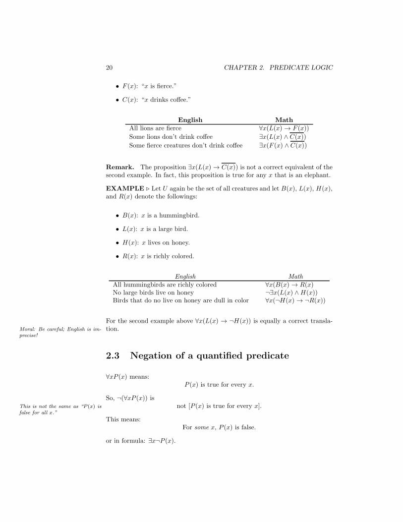
EXAMPLE ! Let the universe U be the set of all creatures and denote byL(x), F (x), and C(x) the followings:
• L(x): “x is a lion.”
20 CHAPTER 2. PREDICATE LOGIC
• F (x): “x is fierce.”
• C(x): “x drinks co"ee.”
English MathAll lions are fierce +x(L(x) & F (x))Some lions don’t drink co"ee .x(L(x) # C(x))Some fierce creatures don’t drink co"ee .x(F (x) #C(x))
Remark. The proposition .x(L(x)& C(x)) is not a correct equivalent of thesecond example. In fact, this proposition is true for any x that is an elephant.
EXAMPLE ! Let U again be the set of all creatures and let B(x), L(x), H(x),and R(x) denote the followings:
• B(x): x is a hummingbird.
• L(x): x is a large bird.
• H(x): x lives on honey.
• R(x): x is richly colored.
English MathAll hummingbirds are richly colored +x(B(x) & R(x)No large birds live on honey ¬.x(L(x) #H(x))Birds that do no live on honey are dull in color +x(¬H(x) & ¬R(x))
For the second example above +x(L(x) & ¬H(x)) is equally a correct transla-tion.Moral: Be careful; English is im-
precise!
2.3 Negation of a quantified predicate
+xP (x) means:P (x) is true for every x.
So, ¬(+xP (x)) isnot [P (x) is true for every x].This is not the same as “P (x) is
false for all x.”
This means:For some x, P (x) is false.
or in formula: .x¬P (x).

2.4. FREE AND BOUND VARIABLES 21
So, in general to negate universal quantifiers: Move the negation to theright, flipping the quantifiers from + to ..
.xP (x) means:P (x) is true for some x.
So, ¬(.xP (x)) isnot [P (x) is true for some x]. This is not the same as “P (x) is
false for some x.”
This means:P (x) is false for all x.
or in formula: +x¬P (x).
So, in general to negate existential quantifiers: Move the negation to theright, flipping the quantifiers from . to +.
EXAMPLE ! “No large birds live on honey.”
¬.x(L(x) #H(x)) ( +x¬(L(x) #H(x)) negation of quantifier rule
( +x(¬L(x) $ ¬H(x)) De Morgan
( +x(L(x) & ¬H(x)) p& q ( p $ q
2.4 Free and bound variables
Definition 12 A variable is bound if its value is known or is in the scope ofsome quantifier. A variable is free if it is not bound.
EXAMPLE ! In “P (x)”, x is free. However in “P (5)”, x is bound to 5.
EXAMPLE ! In “+xP (x)”, x is bound (has been quantified).
Remark. In propositions all variables must be bound (assigned or quantified).
Some predicates involve many variables and to bind them we use many quanti-fiers.
EXAMPLE ! Let P (x, y) = “x > y”. Then:
• “+xP (x, y)” is not a proposition (y is free).
• “+x+yP (x, y)” is a false proposition.
• “+x.yP (x, y)” is a true proposition.
• “+xP (x, 3)” is a false proposition (both x and y are bound).

22 CHAPTER 2. PREDICATE LOGIC
2.5 Meaning of multiply quantified predicates
1. “+x+yP (x, y)”: P (x, y) is true for every combination of x and y values.
2. “.x.yP (x, y)”: There is at least one choice of x and y, such that P (x, y)is true.
3. “+x.yP (x, y)”: For each x we can find at least one y (possibly a di"erenty for each x) such that P (x, y) is true.
4. “.x+yP (x, y)”: There is one x in particular (there may be more) suchthat for every y, P (x, y) is true.
Note that there is a big di"erence between 3, and 4.
EXAMPLE ! Let the universe U be people in this class and N(x, y) denote“x is sitting next to y.”
• .x.yN(x, y): There are two people next to each other.True.
• +x+yN(x, y): Everybody is sitting next to everybody.False.
• .x+yN(x, y): There is a particular person whom everybody is sitting nextto.False.
• +x.yN(x, y): Every person is sitting next to somebody.True?
EXAMPLE ! Let the universe U be the set of real numbers R.
• +m.n(n > 2m) (True). To show this, we need to show that for everynumber m there is a number (that can depend on m) that is greater than2m. Well, n = 2m + 1 is greater than 2m. So +m(n = 2m + 1 > 2m).Hence +m.n(n > 2m).
• .n+m(n > 2m). Is there a number n such that n > 2m regardless of m?! is not a number.
We show the answer to this question is “No” by showing its negation istrue.
¬(.n+m(n > 2m)) ( +n¬(+m(n > 2m)) ( +n.m¬(n > 2m) ( +n.m(n / 2m)
This is true by letting m = n. Clearly, n / 2n for all n.Check table 2 at page 31 of thetext.
EXAMPLE ! Let U = R and Q(x, y, z) = “x+ y = z”.
• +x+y.zQ(x, y, z): True.
• .z+x+yQ(x, y, z): False.
2.5. MEANING OF MULTIPLY QUANTIFIED PREDICATES 23
• +x.y.zQ(x, y, z): True.
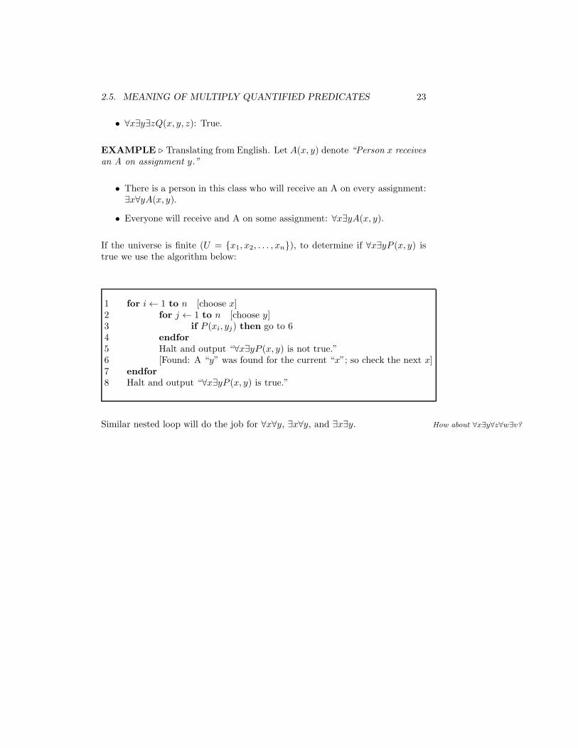
EXAMPLE ! Translating from English. Let A(x, y) denote “Person x receivesan A on assignment y.”
• There is a person in this class who will receive an A on every assignment:.x+yA(x, y).
• Everyone will receive and A on some assignment: +x.yA(x, y).
If the universe is finite (U = {x1, x2, . . . , xn}), to determine if +x.yP (x, y) istrue we use the algorithm below:
1 for i- 1 to n [choose x]2 for j - 1 to n [choose y]3 if P (xi, yj) then go to 64 endfor5 Halt and output “+x.yP (x, y) is not true.”6 [Found: A “y” was found for the current “x”; so check the next x]7 endfor8 Halt and output “+x.yP (x, y) is true.”
Similar nested loop will do the job for +x+y, .x+y, and .x.y. How about "x#y"z"w#v?

24 CHAPTER 2. PREDICATE LOGIC

Chapter 3
Proof Techniques
Definition 13 A theorem is a statement that can be shown to be true.
A proof is a sequence of statements, forming an argument to show that a theoremis true.
The statements used in a proof can include axioms or postulates, which arethe underlying assumptions about the mathematical structure, the hypothesesof the theorem to be proved, and previously proved theorems. The rules ofinference, which are the means used to draw conclusions from other assertions,tie together the steps of a proof.
EXAMPLE ! An ideal proof should look like the following:
1. 0 expression 1 1 Axiom 142. 0 expression 2 1 Axiom 233. 0 expression 3 1 Lines 1 and 2, and rule 284. 0 expression 4 1 Lines 2 and 3, and rule 45. 0 expression 5 1 Axiom 66. 0 expression 6 1 Lines 3, 5, and 6, and rule 2
...73. 0 expression 73 1 What we wanted to prove.
3.1 Rules of Inference
We use the following notation for a rule of inference:
25

26 CHAPTER 3. PROOF TECHNIQUES
Hypothesis 1Hypothesis 2
...Hypothesis n" Conclusion
The sign “"” is read “therefore”.
The most famous inference rule is Modus Ponens :
pp& q" q
Modus Ponens corresponds to [p # (p& q)]& q which is a tautology.
Fact 5 All our rules of inference should be tautologies.
EXAMPLE ! (Modus Ponens)
If I am Bonnie Blair then I win a gold medal.I am Bonnie Blair" I win a gold medal.
3.2 Important Rules of Inference
Rule Corresponding Tautology Name
p" p $ q
p& (p $ q) addition
p # q" p
(p # q)& p simplification
pp& q
" q[p # (p& q)]& q modus ponens
¬qp& q
" ¬p[¬q # (p& q)]& ¬p modus tollens
p& qq & r
" p& r[(p& q) # (q & r)]& (p& r) hypothetical syllogism
p $ q¬p
" q[(p $ q) # ¬p]& q disjunctive syllogism

3.2. IMPORTANT RULES OF INFERENCE 27
EXAMPLE ! (Modus Tollens)
If I am Bonnie Blair then I win a gold medal.I do not win a gold medal." I am not Bonnie Blair.
EXAMPLE ! (Hypothetical Syllogism)
If I am Bonnie Blair then I skate quickly.If I skate quickly then I win a gold medal." If I am Bonnie Blair then I win a gold medal.
EXAMPLE ! (Disjunctive Syllogism)
I am tired of talking or you are tired of listening.I am not tired of talking" You are tired of listening.
EXAMPLE ! Consider the following propositions:
• M : She is a math major.
• C: She is a CS major.
• D: She know discrete math.
• S: She is smart.
Now consider the following statements:
1. She is a math major or a CS major.
2. If she does not khnow discrete math, she is nota math major.
3. If she knows discrete math, she is smart.
4. She is not a CS major.
Now we can conclude that “She is smart” by first writing the above sentenceas logical propositions (lines 1–4) and then applying the inference rules (lines5–8).

28 CHAPTER 3. PROOF TECHNIQUES
1. M $ C
2. ¬D & ¬M .
3. D & S
4. ¬C
5. " M (By 1 and 4 — Disjunctive Syllogism).
6. " M & D (Contrapositive of 2).
7. " D (By 5 and 6 — Modus ponens).
8. " S (By 7 and 3 — Modus ponens).
EXAMPLE ! Consider the following set of propositions.
1. Rainy days make gardens grow.
2. Gardens don’t gro if it is not hot.
3. Whenever it is cold outside, it rains.
We rewrite the above setnence using the following variables:
• R: It rains.
• G: The gardens grow.
• H : It is hot (we use H for it is cold).
Thus we get the following translations:
1. R& G
2. H & G
3. H & R
Suppose we want to show that it is hot. We may try a proof by contradiction.
4. H (We assume).
5. " R (By 3 and 4 — Modus ponens).
6. " G (By 2 and 4 — Modus ponens).
7. " G (By 1 and 5 — Modus ponens).

3.3. FALLACIES 29
But 6 and 7 together say that “Gardens are growning and they are not growing,”a contradiction showing that our assumption was wrong and therefore “it is hot.”
Since we derive the conclusion in our proof methods from assumptions andinference rules, the conclusions are true only when both
1. the initial propositions (assumptions) are true, and
2. the rules of inference are tautologies.
Our conclusions however could be true of false if propositions used are false, orif inference rules used are fallacies.
3.3 Fallacies
Fallacies are non-rules of inference often used. Some famous fallacies are a!rm-ing the conclusion, denying the hypothesis, begging the question, and circularreasoning.
3.3.1 Fallacy of a!rming the conclusion
EXAMPLE ! Here is an example of a!rming the conclusion:
If I am Bonnie Blair then I skate fast.I skate fast." I am Bonnie Blair.
I can be Erk Heiden.
EXAMPLE ! Another one:
If you don’t give me $10, I will punch you in the nose.I punch you in the nose." You didn’t give me $10.
I can be sadist!
A!rming the conclusion is a fallacy because
[(p& q) # q] "& p.
This is because p might be false while q be true and this makes the wholeimplication false.

30 CHAPTER 3. PROOF TECHNIQUES
3.3.2 Fallacy of denying the hypothesis
EXAMPLE ! Here is an example of denying the hypothesis:
If it rains then it is cloudy.It does not rain." It is not cloudy.
What if it is cloudy but it doesn’train?
EXAMPLE ! Another one:
If it is a car, then it has 4 wheels.It is not a car." It does not have 4 wheels.
What if it is a 4-wheeled truck?
Denying the hypothesis is a fallacy because
[(p& q) # ¬p] "& ¬q.
This is because p might be false while q be true and this makes the wholeimplication false.
3.3.3 Other mistakes
To prove +xP (x): We must not rely on any special properties of x. We mustchoose x arbitrarily and show P (x) holds.
To prove .xP (x): We only need to find some value of x and show that P (x)holds for that value.
To prove .y+xP (x, y): We need to show that there is one single y such thatfor any x, P (x, y) is true. It is not su!cient to show that +x.yP (x, y).
3.4 Proof methods
3.4.1 Vacuous proof
To show that p& q is true, it is su!cient to show that p is false.
EXAMPLE ! p: Elephants are small.q: Bush likes to Quayle-hunt.Since p is false, p& q is true.

3.4. PROOF METHODS 31
3.4.2 Trivial Proof
To show that p& q is true, it is su!cient to show that q is true.
EXAMPLE ! p: Elephants are small.q: Bush likes to quail-hunt.
3.4.3 Direct Proof
To show that p & q is true, we assume that p is true, and use the inferencerules to conclude that q is true.
EXAMPLE ! (Direct Proof)To be proved: If n ( 3 mod 4 then n2 ( 1 mod 4.Proof. We assume that n ( 3 mod 4. This means that n = 4k + 3 for somek , Z. But then,
n2 = (4k + 3)2
= 16k2 + 24k + 9
= 16k2 + 24k + 8 + 1
= 4(4k2 + 6k + 2) + 1
= 4k! + 1 for some k! , Z
Hence n2 ( 1 mod 4.
3.4.4 Indirect proof
Instead of showing p& q is true, we can show that ¬q & ¬p (the contrapositive)is true. This establishes p& q as true since
p& q ( ¬q & ¬p.
3.4.5 Proof by contradiction
To prove that p is true, it is su!cient to prove that ¬p & q is true where q isclearly false. This is like saying “If ¬p & q is true, and q is false, then p mustbe true.” This is in fact that same as the the disjunctive syllogism
p $ q¬q
" p

32 CHAPTER 3. PROOF TECHNIQUES
Similar to indirect proof, to show that p & q is true, we show that ¬(p & q)results in a contradiction. That the same as showing that ¬(¬p $ q) ( p # ¬qresults in a contradiction. In fact, the latter is the most common form ofargument.
EXAMPLE ! Classic proof that22 is irrational by contradiction.
p:22 is irrational.
¬p:22 is rational.
We show that ¬pmakes a contradiction, i.e. we assume ¬p and derive somethingfalse.
If22 is rational, then .a, b : gcd(a, b) = 1, and
22 = a/b.This is the definition of a rational
numbers. By requiring a and b tobe relatively prime we look for thefraction a
b is in “lowest terms”.
Then it follows that 2 = a2/b2 or equivalently 2b2 = a2.
Since a2 is even (definition of even) we conclude that a is also even,i.e. .k , Z : a = 2k.Lemma. If a2 is even then a is
also even. [Prove this as an exer-cise.] Plugging this 2k instead of a in 2b2 = a2 we get 2b2 = (2k)2 = 4k2
or b2 = 2k2. Thus b2 is even and so b is even.
But now we have shown that a and b are both even, i.e. 2|a and 2|b.This contradicts the assumption that gcd(a, b) = 1.
3.4.6 Proof by cases
Suppose p ( p1 $ p2 $ . . . $ pn. Then proving p& q is equivalent to proving
[p1 $ p2 $ . . . $ pn]& q,
which is equivalent to
(p1 & q) # (p2 & q) # . . . # (pn & q).
Proof. We show the proof for n = 2. For larger n the proof is similar.
(p1 $ p2)& q ( ¬(p1 $ p2) $ q
( (¬p1 # ¬p2) $ q
( (¬p1 $ q) # (¬p2 $ q)
( (p1 & q) # (p2 & q)
Note. [p1 $ p2 $ . . . $ pn]& q "( (p1 & q) $ (p2 & q) $ . . . $ (pn & q).
3.4. PROOF METHODS 33
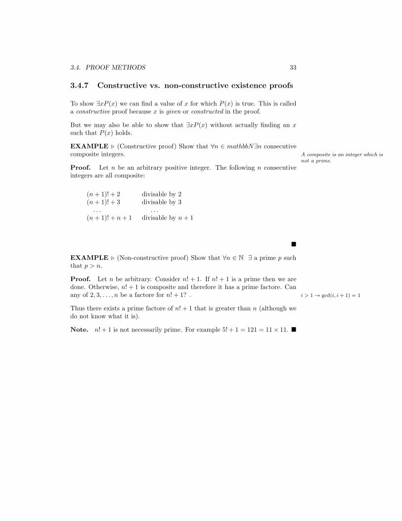
3.4.7 Constructive vs. non-constructive existence proofs
To show .xP (x) we can find a value of x for which P (x) is true. This is calleda constructive proof because x is given or constructed in the proof.
But we may also be able to show that .xP (x) without actually finding an xsuch that P (x) holds.
EXAMPLE ! (Constructive proof) Show that +n , mathbbN.n consecutivecomposite integers. A composite is an integer which is
not a prime.
Proof. Let n be an arbitrary positive integer. The following n consecutiveintegers are all composite:
(n+ 1)! + 2 divisable by 2(n+ 1)! + 3 divisable by 3. . . . . .
(n+ 1)! + n+ 1 divisable by n+ 1
!
EXAMPLE ! (Non-constructive proof) Show that +n , N . a prime p suchthat p > n.
Proof. Let n be arbitrary. Consider n! + 1. If n! + 1 is a prime then we aredone. Otherwise, n! + 1 is composite and therefore it has a prime factore. Canany of 2, 3, . . . , n be a factore for n! + 1? . i > 1 $ gcd(i, i+ 1) = 1
Thus there exists a prime factore of n! + 1 that is greater than n (although wedo not know what it is).
Note. n! + 1 is not necessarily prime. For example 5! + 1 = 121 = 113 11. !

34 CHAPTER 3. PROOF TECHNIQUES

Chapter 4
Set Theory
Definition 14 A set is an unordered collection of elements or objects. Primitive Notation
EXAMPLE ! {1, 2, 3} is a set containing 3 elements: “1”, “2”, and “3”.
EXAMPLE ! {1, 2, 3} = {3, 2, 1} (order irrelevant).
EXAMPLE ! {1, 1, 3, 2, 2} = {1, 2, 3} (number of occurrences irrelevant).
EXAMPLE ! {0, 1, 2, . . .} is the set of natural numbers N (infinite set).
EXAMPLE ! 4 = {} (empty set — contains no elements).
EXAMPLE ! 4 "= {4} = {{}}.
Definition 15 We denote
• “x is an element of the set S” by x , S.
• “x is not an element of the set S” by x ", S.
• “every element of the set A is also an element of the set B” by A 5 B,i.e. (+x)x , A& x , B.
The Venn diagram for A 5 B
35

36 CHAPTER 4. SET THEORY
Definition 16 A is a superset of B, denoted A 6 B if and only if B 5 A.
Definition 17 A = B if and only if A and B have exactly the same elements.
By the definition of equality of the sets A and B:
A = B i" +x(x , A' x , B)
i" A 5 B and A 6 B
i" A 5 B and B 5 A
Note. Showing two sets begin equal involves showing the following 2 things:If you show only one of these,you’re half done!
1. +x(x , A& x , B), which gives us A 5 B, and
2. +x(x , B & x , A), which gives us B 5 A.
4.1 Proper Subset
Definition 18 A is a proper subset of B, denoted A ! B, if A 5 B but notAlso written A % B by some au-thors, although this is misguidedbecause other (really misguided)authors use A % B to mean A &B.
B 5 A, i.e. A 5 B but A "= B.
A is a proper subset of B i":
+x(x , A& x , B) # ¬+x(x , B & x , A) (+x(x , A& x , B) # .x¬(¬(x , B) $ x , A) (+x(x , A& x , B) # .x(x , B # ¬(x , A)) (+x(x , A& x , B) # .x(x ", A # x , B).

4.2. WAYS TO DEFINE SETS 37
EXAMPLE ! {1, 2, 3} 5 {1, 2, 3, 5}{1, 2, 3} ! {1, 2, 3, 5}
Question: Is 4 5 {1, 2, 3}?Answer: Yes:
+x[(x , 4)& (x , {1, 2, 3})]
Since x , 4 is false, the implication is true.
Fact 6 4 is a subset of every set. 4 is a proper subset of every set except 4.
EXAMPLE ! Is 4 , {1, 2, 3}? No.
EXAMPLE ! Is 4 5 {4, 1, 2, 3}? Yes.
EXAMPLE ! Is 4 , {4, 1, 2, 3}? Yes.
4.2 Ways to Define Sets
1. List the elements explcitly (works only for finite sets).
EXAMPLE ! {John, Paul,George,Ringo}
2. List them “implicitly.”
EXAMPLE ! {1, 2, 3, . . .}
EXAMPLE ! {2, 3, 5, 7, 11, 13, 17, 19, 23, . . .}
3. Describe a property that defines the set (“set builder” notation).
EXAMPLE ! {x : x is prime }
EXAMPLE ! {x | x is prime }
EXAMPLE ! {x : P (x) is true. } (where P is a predicate). Let D(x, y) bethe predicate “x is divisible by y.” Then this set becomes D(x, y) ' #k(k.y = x).
{x : +y[(y > 1) # (y < x)]& ¬D(x, y)}

38 CHAPTER 4. SET THEORY
Question: Can we use any predicate P to define a set S = {x : P (x)}.
4.2.1 Russell’s Paradox
LetS = {x : x is a set such that x ", x}.
Is S , S?
• If S , S then by the definition of S, S ", S.
• If S ", S then by the definition of S, S , S.ARGHHH!!@#!
EXAMPLE ! There is a town with a barber who shaves all and only thepeople who don’t shave themselves.Question: Who shaves the barber?
4.3 Cardinality of a Set
Definition 19 IF S is finite, then the cardinality of S (written |S|) is thenumber of (distinct) elements in S.
EXAMPLE ! S = {1, 2, 5, 6} has cardinality |S| = 4.
EXAMPLE ! S = {1, 1, 1, 1, 1} has cardinality |S| = 1.
EXAMPLE ! |4| = 0.
EXAMPLE ! S = {4, {4}, {4, {4}}} has cardinality |S| = 3.
EXAMPLE ! The cardinality of N = {0, 1, 2, 3, . . .} is infinite.We will discuss infinite cardinal-ity later.
4.4 Power Set
Definition 20 If S is a set, then the power set of S, written 2S or P(S) orIn other words, the power set of Sis the set of all subsets of S P (S) is defined by:
2S = {x : x 5 S}
EXAMPLE ! S = {a} has the power set 2S = {4, {a}}.
EXAMPLE ! S = {a, b} has the power set 2S = {4, {a}, {b}, {a, b}}.

4.5. CARTESIAN PRODUCT 39
EXAMPLE ! S = 4 has the power set 2S = {4}.
EXAMPLE ! S = {4} has the power set 2S = {4, {4}}.
EXAMPLE ! S = {4, {4}} has the power set 2S = {4, {4}, {{4}}, {4, {4}}}.
Fact 7 If S is finite, then |2S | = 2|S|.
Question. Who cares if {4, {4, {4}}, {4}} is a subset of the powerset of
{{4}, 4, {4, {4}, {4, {4}}}}?
Answer. No body!
Question. Then why ask the question?
Answer. We must learn to pick nits.
4.5 Cartesian Product
Definition 21 The Cartesian product of two sets A and B is the set
A3B = {0a, b1 : a , A # b , B}
of ordered pairs. Similarly, the Cartesian product of n sets A1, . . . , An is the set
A1 3 · · ·3An = {0a1, . . . , an1 : a1 , A1 # . . . # an , An}
of ordered n-tuples.
EXAMPLE ! If A = {john,mary, fred} and B = {doe, rowe}, thenA( B = {)john, doe*, )mary,doe*, )fred,doe*, )john, roe*, )mary, roe*, )fred, roe*}
Fact 8 If A and B be finite, then |A3B| = |A|.|B|.
4.6 Set Operations
4.6.1 Union of Two Sets
Definition 22 For sets A and B, the union of A and B is the set A7B = {x :x , A $ x , B}.

40 CHAPTER 4. SET THEORY
4.6.2 Intersection of Two Sets
Definition 23 For sets A and B, the intersection of A and B is the set A8B ={x : x , A # x , B}.
EXAMPLE ! {presidents} 8 {deceased} = {deceased presidents}
EXAMPLE ! {US presidents} 8 {people in this room} = 4
Note. If for sets A and B, A 8B = 4, A and B are said to be disjoint.
4.6.3 Complement of a Set
Definition 24 Assume U be the universe of discourse (U contains all elementsunder consideration). Then the complement of a set A is the set A = {x , U :x ", A} which is the same as the set {x : x , U # x ", A} or {x : x ", A} whenU is understood implicitly.

4.6. SET OPERATIONS 41
Note. 4 = U and U = 4.
EXAMPLE ! IF U = {1, 2, 3} and A = {1} then A = {2, 3}.
4.6.4 Set Di"erence of two Sets
Definition 25 For sets A and B the set di"erence of A from B is defined asthe set A*B = {x : x , A # x ", B} = A 8B.
EXAMPLE ! {people in class}*{sleeping people} = {awake people in class}.
EXAMPLE ! {US presidents}* {baboons} = {US presidents}. ?
Note. A* A = A.
4.6.5 Symmeteric Di"erence (Exclusive-Or) of two Sets
Definition 26 For sets A and B, the symmetric di"erence of A and B is theset A%B = {x : (x , A # x ", B) $ (x ", A # x , B}.
From the definition:
A%B = {x : (x , A # x ", B) $ (x ", A # x , B}= {x : (x , A*B) $ (x , B *A)}= {x : x , (A*B) 7 (B *A)}= (A*B) 7 (B *A).
42 CHAPTER 4. SET THEORY
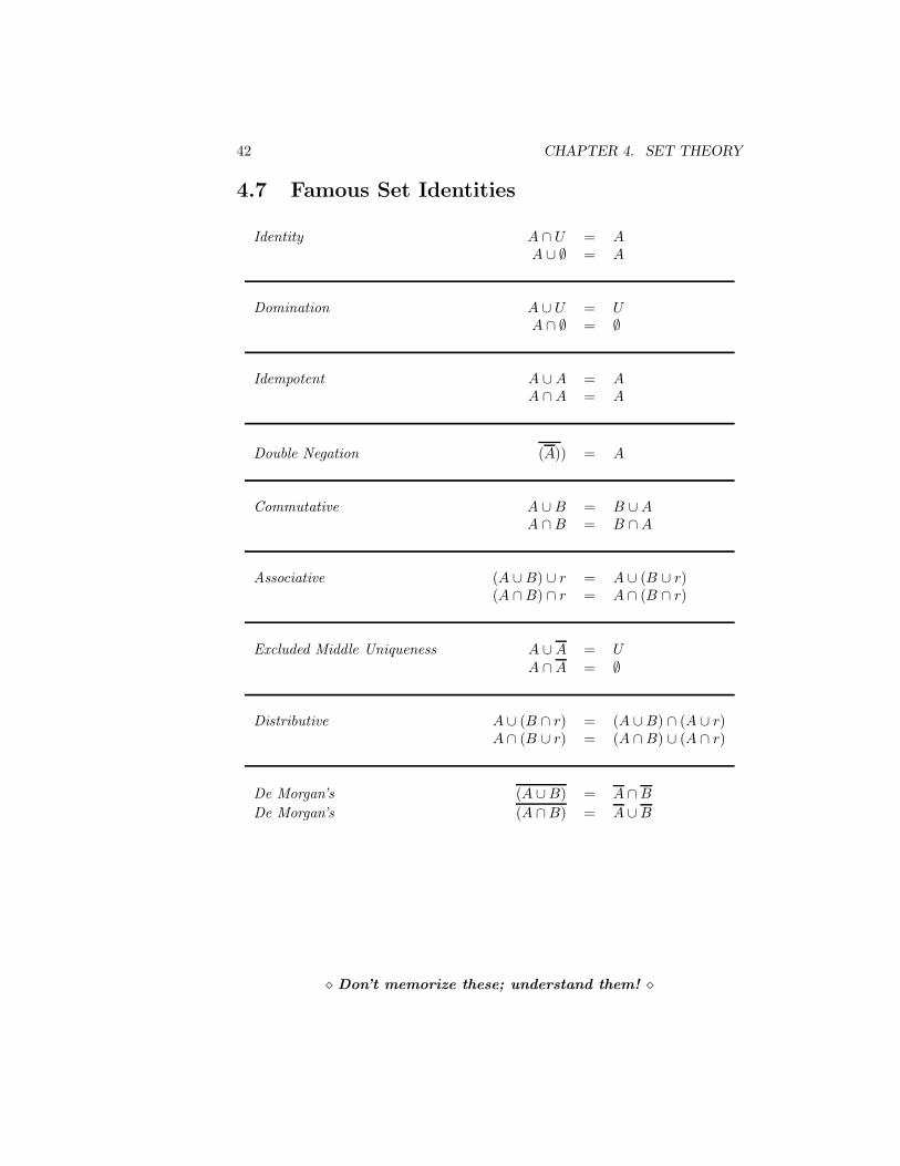
4.7 Famous Set Identities
Identity A 8 U = AA 7 4 = A
Domination A 7 U = UA 8 4 = 4
Idempotent A 7 A = AA 8 A = A
Double Negation (A)) = A
Commutative A 7B = B 7 AA 8B = B 8 A
Associative (A 7B) 7 r = A 7 (B 7 r)(A 8B) 8 r = A 8 (B 8 r)
Excluded Middle Uniqueness A 7 A = UA 8 A = 4
Distributive A 7 (B 8 r) = (A 7B) 8 (A 7 r)A 8 (B 7 r) = (A 8B) 7 (A 8 r)
De Morgan’s (A 7B) = A 8BDe Morgan’s (A 8B) = A 7B
9 Don’t memorize these; understand them! 9

4.8. 4 WAYS TO PROVE IDENTITIES 43
4.8 4 Ways to Prove Identities
To show that two sets A and B are equal we can use one of the following fourtechniques. 1. Show that A 5 B and B 5 A.
EXAMPLE ! We show that A 7B = A 8B (first proof).
(5) If x , A 7B, then x ", A 7B. So, x ", A and x ", B, and thus x , A 8B.
(6) If x , A8B then x ", A and x ", B. So, x ", A7B and therefor x , A 7B.
2. Use a “membership table”.Works the same way as a truth table in which we use 0s and 1s to indicate thefollowings.
0: x is not in the specified set.
1: x is in the specified set.
EXAMPLE ! We show that A 7B = A 8B (second proof).
A B A B A 7B A 7B A 8B1 1 0 0 1 0 01 0 0 1 1 0 00 1 1 0 1 0 00 0 1 1 0 1 1
3. Use previous identities.
EXAMPLE ! We show that A 7B = A 8B (third proof).
(A 7B) ( (A) 7 (B) by double complement
( (A) 8 (B) by De Morgan’s law 2
( (A) 8 (B) by double complement
( A 8B
4. Use logical equivalences of the defining propositions.
EXAMPLE ! We show that A 7B = A 8B (fourth proof).
44 CHAPTER 4. SET THEORY
A 7B = {x : ¬(x , A $ x , B)}= {x : (¬x , A) # (¬x , B)}= {x : (x , A) # (x , B)}= {x : (x , A 8B)}= A 8B
4.9 Generalized Union and Intersection
Definition 27n&
i=1
Ai = A1 7 A2 7 . . . 7 An
= {x : x , A1 $ x , A2 $ . . . x , An}
n'
i=1
Ai = A1 8 A2 8 . . . 8 An
= {x : x , A1 # x , A2 # . . . x , An}
4.10 Representation of Sets as Bit Strings
Definition 28 Let U = {x1, x2, . . . , xn} be the universe and A be some set inthis universe. Then we can represent A by a sequence of bits (0s and 1s) oflength n in which the i-th bit is 1 if xi , A and 0 otherwise. We call this stringthe characteristic vector of A.
EXAMPLE ! If U = {x1, x2, x3, x4, x5} and A = {x1, x2, x4}, then the char-acteristic vector of A will be 11010.
Fact 9 To find the characteristic vector for A 7 B we take the bitwise “or” ofthe characteristic vectors of A and B.
To find the characteristic vector for A 8 B we take the bitwise “and” of thecharacteristic vectors of A and B.
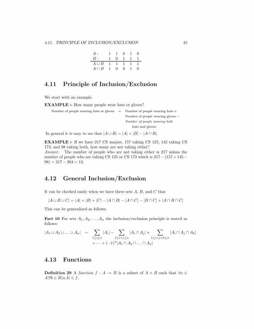
EXAMPLE ! If U = {x1, x2, x3, x4, x5} and A = {x1, x2, x4} and B ={x1, x3, x4, x5}, then the characteristic vector of A will be 11010 and the char-acteristic vector of B will be 10111. Then for the characteristic vector of A7Band A 8B we have get.
4.11. PRINCIPLE OF INCLUSION/EXCLUSION 45
A : 1 1 0 1 0B : 1 0 1 1 1A 7B 1 1 1 1 1A 8B 1 0 0 1 0
4.11 Principle of Inclusion/Exclusion
We start with an example.
EXAMPLE ! How many people wear hats or gloves?
Number of people wearing hats or gloves = Number of people wearing hats +
Number of people wearing gloves+Number of people wearing both
hats and gloves.
In general it is easy to see that |A 7B| = |A|+ |B|* |A 8B|.
EXAMPLE ! If we have 217 CS majors, 157 taking CS 125, 145 taking CS173, and 98 taking both, how many are not taking either?Answer: The number of people who are not taking either is 217 minus thenumber of people who are taking CS 125 or CS 173 which is 217* (157+ 145*98) = 217* 204 = 13.
4.12 General Inclusion/Exclusion
It can be checked easily when we have three sets A, B, and C that
|A 7B 7 C| = |A|+ |B|+ |C|* |A 8B|* |A 8 C|* |B 8C|+ |A 8B 8 C|
This can be generalized as follows.
Fact 10 For sets A1, A2, . . . , An the inclusion/exclusion principle is stated asfollows:
|A1 7A2 7 . . . 7 An| =(
1"i"n
|Ai|*(
1"i<j"n
|Ai 8Aj |+(
1"i<j<k"n
|Ai 8 Aj 8Ak|
+ · · ·+ (*1)n|A1 8 A2 8 . . . 8 An|
4.13 Functions
Definition 29 A function f : A & B is a subset of A 3 B such that +a ,A.!b , B0a, b1 , f .

46 CHAPTER 4. SET THEORY
From the above definition we cannot have 0a, b1 , f , and 0a, c1 , f for b "= c.Also there must be for each a, some b such that 0a, b1 , f .
Note. There can be 0a, b1 , f and 0c, b1 , f .Didn’t say that "b#!a)a, b* , f .
We write f(a) = b to indicate that b is the unique element of B such that0a, b1 , f .
Intuitively we can think of f as a rule, assigning to each a , A a b , B.though this intuition fails . . .morelater.
EXAMPLE ! A = {Latoya,Germaine,Michael,Teddy, John F.,Robert}B = {Mrs Jackson,Rose Kennedy,Mother Theresa}f : A& B, f(a) = mother(a)
f is a function because everyone has exactly one (biological) mother. Mrs Jack-son has more than 1 child. Functions do not require +b , B .!a , A f(a) = b.
Mother Theresa (paradoxically) is not a mother. Functions do not require +b ,B .a , A f(a) = b.
Definition 30 For a function f : A& B, A is called the domain of f and B iscalled the co-domain of f .
For a set S 5 A the image of A is defined as
image(A) = {f(a) : a , S}
Note. When I was a lad we used “range” instead of “co-domain”. Now rangeis used sometimes as “co-domain” and sometimes as “image”.
EXAMPLE ! In the previous example:
image({Latoya,Michael, John}) = {Mrs Jackson,Rose Kennedy}
andimage({Latoya,Michael}) = {Mrs Jackson}.

4.13. FUNCTIONS 47
Note.
image(S) = {f(a) : a , S} = {b , B : .a , A f(a) = b}
Definition 31 The range of a function f : A& B is image(A).
a , A is a pre-image of b , B if f(a) = b. For a set S 5 B, the pre-image of Sis defined as
pre-image(S) = {pre-image(b) : b , B}
The above concepts are represented pictorially below. Suppose f : A & B is afunction.
image(a) = f(a)
pre-image(b)
image(S)
pre-image(S)

48 CHAPTER 4. SET THEORY
Questions. What is the relationship between these two?
image(pre-image(S)) and pre-image(image(S))
Definition 32 A function f is one-to-one, or injective, or is an injection, if
+a, b, c (f(a) = b # f(c) = b)& a = c.
In other words each b , B has atmost one pre-image.
EXAMPLE ! The functions f(x) = mother(x) in the previous example wasnot one-to-one because f(Latoya) = f(Michael) = Mrs Jackson.
EXAMPLE ! f : R+ & R+, where f(x) = x2 is one-to-one, since each positivereal x has exactly one positive pre-image (
2x).
EXAMPLE ! f : R & R, where f(x) = x2 is not one-to-one. f(2) = 4 =f(*2).
Note. In terms of diagrams, one-to-one means that no more than one arrowgo to the same point in B.
Definition 33 A function f : A& B is onto, or surjective, or is a surjection if
+b , B .a , A f(a) = b
In other words, everything in Bhas at least one pre-image.
EXAMPLE ! In the mothers example, the function f(x) = mother(x) is notsurjective because Mother Theresa is not the mother of anyone in A.
EXAMPLE ! f : R & R, where f(x) = x2 is not surjective, since *1 has nosquared roots in R.
EXAMPLE ! f : R& R+, where f(x) = x2 is surjective, since every positivenumber has at least one squared root.In fact 2 squared roots.
4.14 Bijections
Definition 34 A function f : A& B is a bijection, or a one-to-one correspon-dence, if and only if f is one-to-one and onto (injective and surjective).
In other words, f : A& B is a bijection i":
• every b , B has exactly one pre-image, and
4.15. CARDINALITY OF INFINITE SETS 49
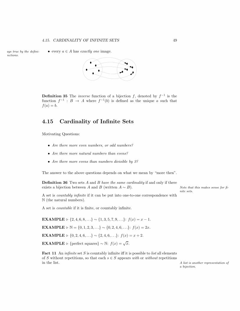
• every a , A has exactly one image.s always true by the defini-f a functions.
Definition 35 The inverse function of a bijection f , denoted by f#1 is thefunction f#1 : B & A where f#1(b) is defined as the unique a such thatf(a) = b.
4.15 Cardinality of Infinite Sets
Motivating Questions:
• Are there more even numbers, or odd numbers?
• Are there more natural numbers than evens?
• Are there more evens than numbers divisible by 3?
The answer to the above questions depends on what we mean by “more then”.
Definition 36 Two sets A and B have the same cardinality if and only if thereexists a bijection between A and B (written A ! B). Note that this makes sense for fi-
nite sets.
A set is countably infinite if it can be put into one-to-one correspondence withN (the natural numbers).
A set is countable if it is finite, or countably infinite.
EXAMPLE ! {2, 4, 6, 8, . . .} ! {1, 3, 5, 7, 9, . . .}: f(x) = x* 1.
EXAMPLE ! N = {0, 1, 2, 3, . . .} ! {0, 2, 4, 6, . . .}: f(x) = 2x.
EXAMPLE ! {0, 2, 4, 6, . . .} ! {2, 4, 6, . . .}: f(x) = x+ 2.
EXAMPLE ! {perfect squares} ! N: f(x) =2x.
Fact 11 An infinite set S is countably infinite i" it is possible to list all elementsof S without repetitions, so that each s , S appears with or without repetitionsin the list. A list is another representation of
a bijection.

50 CHAPTER 4. SET THEORY
EXAMPLE ! Evens: 0, 2, 4, 6, 10, 12, . . .
EXAMPLE ! Odds: 1, 3, 5, 7, 9, 11, . . .
EXAMPLE ! Squares: 0, 1, 2, 4, 9, 16, . . .
EXAMPLE ! Rationals: Hmmm, we’ll see!
EXAMPLE ! Reals: No! this can’t be done (not countably infinite).
Now consider the Motel Infinity shown below with no vacancy:
*1 can go to room 0 if everybody shifts down a room. Thus N 7 {*1} ! N.
Imagine instead of -1 we needed room for “camp:” (A countably infinite set).Still we could free up enough room by moving for every i the occupant of roomi to room 2i and giving the i-th person of the camp : bus the room 2i+ 1.
Fact 12 If A and B are countably infinite, then A 7B is countably infinite.
What happens if a countably infinite number of camp : buses need room inMotel Infinity?
4.15.1 Rational Numbers are Countably Infinite
By definition, rational numbers are those that can be written in the form pq
where p and q are natural numbers and q "= 0.
A naive attempt to enumerate all the rationals then can be to list them as
1
1,1
2,1
3,1
4,1
5, . . . ,
2
1,2
2,2
3,2
4,2
5, . . . ,
3
1,3
2,3
3,3
4,3
5, . . .
But this does not work because the first part of the list (11 ,12 ,
13 ,
14 ,
15 , . . .) never
finishes and therefore 21 is never reached.
A second approach will be to use the table below.

4.15. CARDINALITY OF INFINITE SETS 51
p&0 1 2 3 4 5 6 . . .
q ; 1 0 2 5 9 142 1 4 8 133 3 7 124 6 115 10 . . .67...
There is still a small problem with the above approach: some rationals are listedtwice or more.
Solution: Skip over those not in the “lowest term”. This way every positiverational appears in some box and we enumerate the boxes:
0
1,/02,1
1,/03,1
2,2
1,/04,1
3,/22,3
1, . . .
4.15.2 Real Numbers are NOT Countably Infinite
We will show that [0, 1] cannot be enumerated. This is due to George Cantor.
Recall that each real number in [0, 1] can be represented as an infinite decimal0.d1d2d3d4d5d6 . . ., where di’s are digits in {0, . . . , 9}.
EXAMPLE ! " * 3 = 0.1415926535897 . . .
EXAMPLE ! 12 = 0.5000000000000 . . .
Assume that there was an enumerate of reals in [0, 1]: r1, r2, r3, . . . such that allreals in [0, 1] would appear exactly once.
r1 0. 1 4 1 5 9 2 6 3 . . .
r2 0. 5 0 0 0 0 0 0 0 . . .
r3 0. 1 6 1 7 8 0 3 4 . . .
r4 0. 1 2 3 4 5 6 7 8 . . ....
. . .
rn 0. d1 d2 d3 d4 . . . dn dn+1 dn+2 . . .
Consider the real number r defined by diagonalizing.
r = .b1b2b3b4b4 . . .

52 CHAPTER 4. SET THEORY
where bi is 1 plus the i-th digit of ri (9 + 1 = 0).
EXAMPLE ! For the table above we get r = 0.2125 . . ..
r is a real number between 0 and 1 but was not listed becauser "= ri for any i.
Why? Because r and ri di!er in decimal position i.
Thus the enumeration wasn’t one after all, contradicting the existence of suchan enumeration.
4.15.3 Can All Functions Be Computed by Programs?
Suppose our alphabet have 1000 characters. We can list all strings of thisalphabet in order of their length.
• length 0 strings: 1
• length 1 strings: 1,000
• length 2 strings: 1,000,000
• length 3 strings: 109
• . . .
Some but not all of these strings are computer programs. The shortest computerprogram that looks like this
beginend.
requires 10 characters. Thus we can enumerate all programs (plus some mean-ingless strings) and therefore the set of programs is countably infinite, i.e.
{all programs} ! N.
We like to show that there exists a function f that no program can computer it.We show even the stronger statement that there is some function that outputsa single digit and still cannot be computed by any program. Let
F = {f : N& {0, 1, . . . , 9}} .
Let us give some examples of such functions.
4.15. CARDINALITY OF INFINITE SETS 53
EXAMPLE ! f(x) = 1 (The constant function).
EXAMPLE ! f(x) = x mod 10 (remainder of x divided by 10).
EXAMPLE ! f(x) = first digit of x.
EXAMPLE ! f(x) =
%0 if x is even1 if x is odd
How many such function do we have? Each function f : N & {0, . . . , 9}can be represented by a single real number in [0, 1]. This number is exactly0.f(0)f(1)f(2)f(3) . . ..
EXAMPLE ! The function f shown be the table below
x 0 1 2 3 4 5 6 7 8 . . .f(x) 1 4 1 5 9 2 6 5 3 . . .
can be represented by the real number 0.141592653 . . ..
Conversely, each number in [0, 1] can be thought of as a function from thenatural numbers to single digits.
EXAMPLE ! The number 0.72 corresponds to the function f where f(0) = 7,f(1) = 2, and f(x) = 0 for x / 2.
Thus we have shown thatF ! [0, 1] ! R.
This means that there are much more many functions as there are programsand therefore, some functions are not computed by any programs.

54 CHAPTER 4. SET THEORY

Chapter 5
Boolean Functions
5.1 Propositions vs. Boolean Functions
A proposition is really a special kind of function.
EXAMPLE ! f : {T,F}& {T,F} f(p) = ¬p.
p f(p)F TT F
EXAMPLE ! f(p, q, r) = (p # r) $ qf : {T,F}3 {T,F}3 {T,F}& {T,F} or f : {T,F}3 & {T,F}.f(F,F,F) = Tf(F,T,F) = F
5.2 New Notation
Old NewT 1F 0# .$ +¬ ¬
EXAMPLE ! f(p) = p
55

56 CHAPTER 5. BOOLEAN FUNCTIONS
p f(p)0 11 0
EXAMPLE ! f(p, q) = p+ q
p q p+ q0 0 00 1 11 0 11 1 1
EXAMPLE ! f(p, q) = pq
p q pq0 0 00 1 01 0 01 1 1
5.3 Boolean Functions of n variables
f : {0, 1}n & {0, 1}
EXAMPLE ! f(x1, x2, . . . , xn) = ((x1 + x2)x3 + x4)(x5 + x6x7)
x1 x2 x3 . . . xn f(x1, x2, . . . , xn)0 0 0 . . . 0 00 0 0 . . . 1 0...
......
. . ....
...1 1 1 . . . 1 1
Question. How many rows are needed to completely define a boolean functionof n variables?Of course, it is often much easier
(shorter) to describe th functionsymbolically. Answer. 2n
Question. How many di"erent functions f(x1, . . . , xn) can be defined?
If n = 1
x1 f0 f1 f2 f30 0 0 1 11 0 1 0 1

5.4. STANDARD SUM OF PRODUCTS 57
There are 2 rows and 4 di"erent columns.
If n = 2
x1 f0 f1 f2 f3 f4 f5 . . . f150 0 0 0 0 0 0 0 . . . 10 1 0 0 0 0 1 1 . . . 11 0 0 0 1 1 0 0 . . . 11 1 0 1 0 1 0 1 . . . 1
There are 4 rows and 16 di"erent columns. In general if there are k rows, therewill be as many columns as the number of rows a truth table with k variableswould need, i.e. 2k. Since k = 2n there will be 22
n
columns.
Question. Can we write all of them, using only +, ., and ¬, i.e. Is the operatorset {+, .,¬} functionally complete?
5.4 Standard Sum of Products
Also called Disjunctive Normal Form (DNF): Look at the rows which the valuesare 1. For each of these rows, construct the logical AND (#) to yield a 1. Then,OR ($) all of these products together to get a sum of products.
EXAMPLE ! For the following truth table,
p q r b minterms0 0 0 1 ¬p¬q¬r0 0 1 00 1 0 00 1 1 1 ¬pqr1 0 0 01 0 1 01 1 0 1 pq¬r1 1 1 1 qpr
we get:b = ¬p¬q¬r + ¬pqr + pq¬r + pqr.
5.5 Standard Product of Sums
Also called Conjunctive Normal Form (CNF): Look at the rows which the valuesare 0. For each of these rows, construct the logical OR of the negations to yielda 0. Then, AND all of these products together to get product of sums.
58 CHAPTER 5. BOOLEAN FUNCTIONS
EXAMPLE ! For the following truth table,
p q r b maxterms0 0 0 10 0 1 0 p+ q + ¬r0 1 0 0 p+ ¬q + r0 1 1 11 0 0 0 ¬p+ q + r1 0 1 0 ¬p+ q + ¬r1 1 0 11 1 1 1
we get:b = (p+ q + ¬r)(p + ¬q + r)(¬p + q + r)(¬p + q + ¬r).
Since
• Every boolean function is representable as a truth table, and
• Every table is representable using +, ., and ¬,
therefore Every boolean function is representable using +, ., and ¬, i.e.{+, .,¬} is functionally complete.
Homework. Show that {+,¬} and {.,¬} are also functionally complete but{+, .} is not.
5.6 Karnaugh Maps
The goal of this section is to find small sum-of-products for given boolean func-tions. There is a graphical technique for designing minimum sum-of-product ex-pressions from truth tables. This technique puts truth tables into two-dimensionalarrays called Karnaugh Maps.
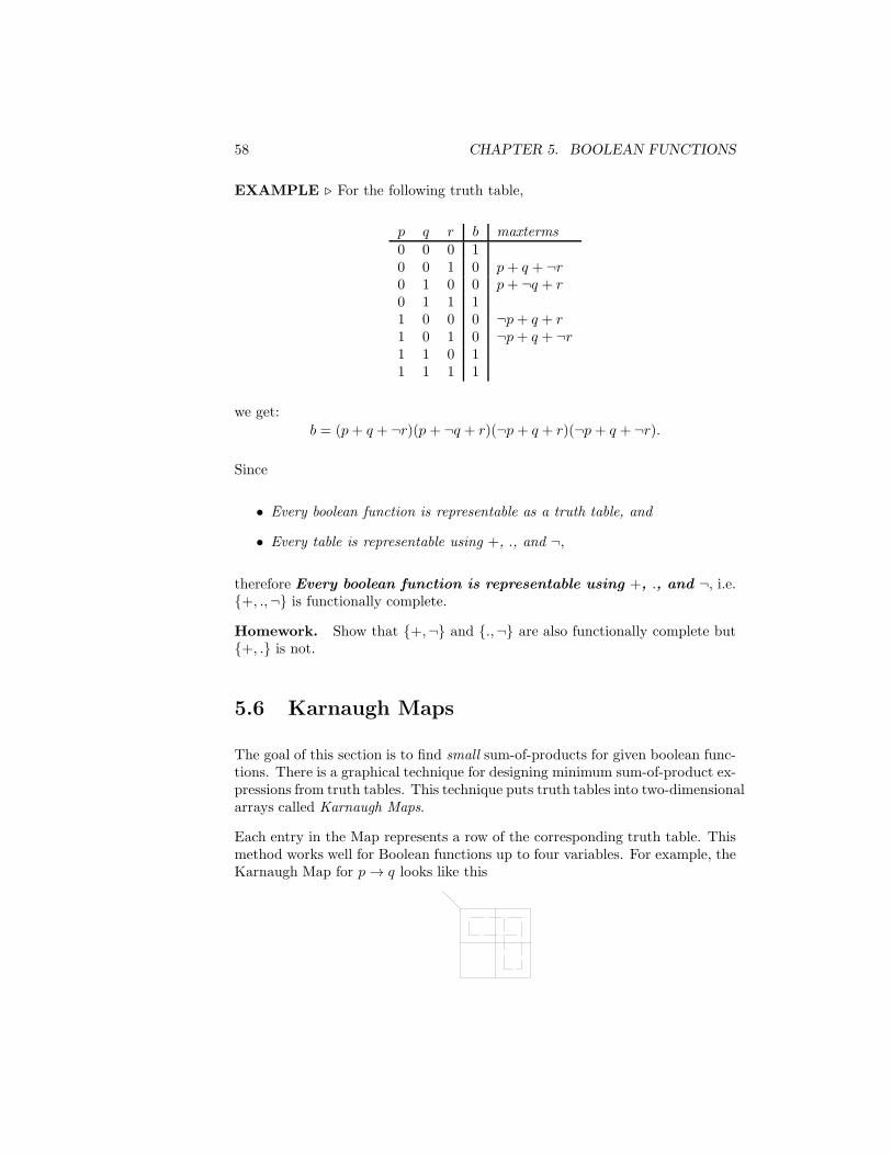
Each entry in the Map represents a row of the corresponding truth table. Thismethod works well for Boolean functions up to four variables. For example, theKarnaugh Map for p& q looks like this

5.6. KARNAUGH MAPS 59
• Each 13 1 cell containing 1 gives a minterm.
pq + pq + pq
• Two adjacent 1 cells gives a shorter term.
p+ pq
• The boxes can overlap and the goal is to cover the 1 cells with boxes.
p+ q
EXAMPLE ! Here is an example of a Karnaugh Map for three variables. Notethat the order of labels on the cells is selected in such a way that adjacent cellscorrespond to variable settings that di"er in exactly one position.
The table is for the following truth table.
p q r b0 0 0 00 0 1 10 1 0 10 1 1 11 0 0 01 0 1 11 1 0 01 1 1 0
The given map simplifies to pq + qr.
EXAMPLE ! Another three variable Karnaugh Map. The simplified functionby this map is yz + xz + xy.
EXAMPLE ! And this is a four variable Karnaugh Map that gives us thefunction ps+ qs+ pqrs.
60 CHAPTER 5. BOOLEAN FUNCTIONS
5.7 Design and Implementation of Digital Net-works
• 0: Low voltage (0V )
• 1: High voltage (6V or 2.5V )
The AND Gate
x y outputL L LL H LH L LH H H
The OR Gate
x y outputL L LL H HH L HH H H
The Inverter
x outputL HH L

5.7. DESIGN AND IMPLEMENTATION OF DIGITAL NETWORKS 61
EXAMPLE ! We want to activate a sound buzzer that if
1. temperature of engine exceeds 200 degrees, or
2. automobile is in gear and driver’s seat-belt is not buckled.
Let us represent the above signals with the following variables
• b: sound buzzer.
• p: temperature of the engine exceeds 200 degrees.
• q: automobile is in gear.
• r: driver’s seat-belt is buckled.
We want to in fact make a network for b = p+ qr.
5.7.1 One Bit Adder
0+ 0
0
0+ 1
1
1+ 0
1
1+ 11 0
a b ps c0 0 0 00 1 1 01 0 1 01 1 0 1
62 CHAPTER 5. BOOLEAN FUNCTIONS
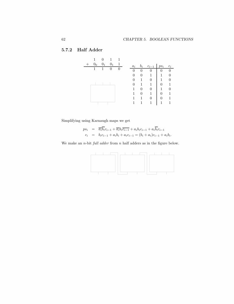
5.7.2 Half Adder
1 0 1 1+ 00 01 01 1
1 1 0 0ai bi ci#1 psi ci0 0 0 0 00 0 1 1 00 1 0 1 00 1 1 0 11 0 0 1 01 0 1 0 11 1 0 0 11 1 1 1 1
Simplifying using Karnaugh maps we get
psi = aibici#1 + aibici#1 + aibici#1 + aibici#1
ci = bici#1 + aibi + aici#1 = (bi + ai)ci#1 + aibi.
We make an n-bit full adder from n half adders as in the figure below.

Chapter 6
Familiar Functions andGrowth Rate
6.1 Familiar Functions
Polynomials
f(x) = a0xn + a1x
n#1 + · · ·+ anx0
EXAMPLE ! f(x) = x3 * 2x2 + 14.
Exponentials
f(x) = cdx
EXAMPLE ! f(x) = 310x.
EXAMPLE ! f(x) = ex.
Logarithms
log2 x = y such that 2y = x
Read Appendix 1
63

64 CHAPTER 6. FAMILIAR FUNCTIONS AND GROWTH RATE
Note. In this course lg is used for log2 and unless stated otherwise log is alsoused for log2.
lnx = loge x =
) x
1
1
tdt
Ceiling
<x= = least integer y such that x / y
EXAMPLE ! <1.7= = 2.
EXAMPLE ! <*1.7= = *1.
Floor
>x? = greatest integery such thaty / x
EXAMPLE ! >1.7? = 1.
EXAMPLE ! >*1.7? = *2.
6.2 Sequences
Definition 37 A sequence {ai} is a function f : N & R where we write ai toindicate f(i).
EXAMPLE ! The sequence {ai} where ai = i is: a1 = 1, a2 = 2, · · ·
EXAMPLE ! The sequence {ai} where ai = i2 is: a1 = 1, a2 = 4, a3 = 9, · · ·
6.3 Summation
Definition 38 We use the notation
k(
i=1
ai
to indicatea1 + a2 + · · ·+ ak.

6.3. SUMMATION 65
Similarly we use the notation$(
i=1
ai
to indicate
limn%$
n(
i=1
ai.
It is easy to verify the validity of the linearity in summation:
n(
k=1
cak + bk = cn(
k=1
ak +n(
k=1
bk.
6.3.1 Famous Sums
Question. What is S defined as the following sum?
S = 1 + 2 + 3 + 4 + 5 + 6 + · · ·+ 1000.
Answer. Let us add S to itself but in reverse order.
S = 1 + 2 + 3 + · · · + 1000+S = 1000 + 999 + 998 + · · · + 12S = 1001 + 1001 + 1001 + · · · + 1001
! "# $1000
Therefore 2S = 10003 1001 and S = 1000&10012 = 500, 500.
Let’s generalize this:
S = 1 + 2 + 3 + · · · + n+S = n + n* 1 + n* 2 + · · · + 12S = n+ 1 + n+ 1 + n+ 1 + · · · + n+ 1
! "# $n
Thus we get
S =n(
k=1
k =n(n+ 1)
2.
66 CHAPTER 6. FAMILIAR FUNCTIONS AND GROWTH RATE
EXAMPLE ! What is the sum 1 + 3 + 5 + 7 + · · ·+ 2n* 1?
n(
k=1
2k * 1 = 1 + 3 + 5 + 7 + · · ·+ 2n* 1
= 2 + 4 + 6 + · · ·+ 2n* n
= 2(1 + 2 + 3 + · · ·+ n)* n
= 2n(n+ 1)
2* n
= n(n+ 1)* n
= n2 + n* n
= n2
6.3.2 Geometric Series
n(
k=0
rk = 1 + r + r2 + r3 + · · ·+ rn
rn(
k=0
rk = r + r2 + r3 + r4 + · · ·+ rn+1
Subtracting top from bottom
(r * 1)n(
k=0
rk = rn+1 * 1
n(
k=0
rk =rn+1 * 1
r * 1
If r < 1 then the series converges as n approaches infinity.
$(
k=0
rk = 1 + r + r2 + r3 + · · ·+ rn + · · ·
r$(
k=0
rk = r + r2 + r3 + r4 + · · ·+ rn+1 + · · ·
Subtracting bottom from top
(1* r)$(
k=0
rk = 1
$(
k=0
rk =1
1* r

6.4. GROWTH OF FUNCTIONS 67
6.4 Growth of Functions
Running time of algorithms is defined by functions describing how many stepsthey take to complete in terms of input size.
EXAMPLE ! It might take 3n steps to add a list of n numbers, or 15n steps?or 1
100n2 steps?
f(x) = 3x
f(x) = 15x
f(x) = 1100n
2
x
y
• We would like to ignore constant factors (since di"erent machines run atdi"erent speeds/cycle).
• We would also like to ignore small values of x.
• In fact we want to see which function eventually is the largest.
Definition 39 The Big Oh Notation. For functions f and g, we write
f(x) = O(g(n))
to denote:
. c, k @ 0 such that + x > k f(x) / cg(x).
EXAMPLE ! 3n is O(15n) since +n > 0 3n / 13 15n.
EXAMPLE ! 15n is O(3n) since +n > 0 15n / 53 3n.
EXAMPLE ! x2 is O(x3) since +x > 1 x2 / x3.
EXAMPLE ! x2 is O( x2
1,000,000 ) since +x > 0 x2 / 1, 000, 000 x2
1,000,000 .

68 CHAPTER 6. FAMILIAR FUNCTIONS AND GROWTH RATE
EXAMPLE ! x2 + 100x+ 100 is O( 1100x
2 since +x > 2,
100x2 + 100x+ 100 / 23 (100)2 3 1
100x2
100x2 + 100x+ 100 / 200x2
100x+ 100 / 100x2
x+ 1 / x2
The last inequality is not true for x = 0 and x = 1 but is obviously true forx @ 2.
EXAMPLE ! We want to show that 5x + 100 is O(x/2). In other words wewant to fill in the blanks below
+x @ : 5x+ 100 / 3 x
2.
Attempt 1. Let c = 10, so that 10 3 x2 = 5x and then get rid of the 5x term.
But we we will be left with
+x @ : 5x+ 100 / 5x
and this obviously won’t work.
Insight. We must end up with something else on theright that is larger than100 (if x is large engough).
Let c = 11 (this way we will make an extra x/2 on the right).
+x @ : 5x+ 100 / 5x+x
2
and therefore we need to fill in the blank such that,
+x @ : 100 / x
2
and this is easy!
+x @ 200 : 100 / x
2
6.4.1 Guidlines
• In general, only the largest term in a sum matters. i.e.,
a0xn + a1x
n#1 + · · ·+ an#1x+ an is O(xn).
See proof of Theorem 3 of page 81in the text.
• n dominates lg n. So, as an example n5 lg n is O(n6).

6.4. GROWTH OF FUNCTIONS 69
• Here is a list of common functions in increasing O() order.
1 lgn n n lgn n2 n3 . . . 2n n!
EXAMPLE !*n
k=1 k = n(n+1)2 is O(n2).
EXAMPLE !*n
k=1 k2 = 12 + 22 + · · · + n2 /
n# $! "n2 + n2 + · · ·+ n2 = n3. So,*n
k=1 k2 is O(n3).
EXAMPLE ! For n! we have
n! = n(n* 1)(n* 2)(n* 3) · · · 3.2.1/ n3 n3 n3 n3 · · ·3 n! "# $
n
= nn
So, n! is O(nn).
EXAMPLE ! lgn! / lg nn / n lg n. So, lgn! is O(n lgn). We’ll see this later.
An important observation is that n3 is not O(100n2). If this were not true, thenfor some integers k and c we would have
+n @ k : n3 / c3 100n2.
But this would simplify to
+n @ k : n / c3 100
which is a contradiction.
Theorem 2 If f1 = O(g1) and f2 = O(g2), then f1(x)+f2(x) = O(max{g1(x), g2(x)}).
Proof. Let h(x) = max{g1(x), g2(x)}. Note that for di!erent values of x,h(x) can be g1(x) or g2(x).
Clearly, f1 = O(h) since g1(x) / h(x) for all x. Therefore,
.c1, k1 : f1(x) / c1h(x) +x @ k1.
Similarly f2 = O(h) and therefore
.c2, k2 : f2(x) / c2h(x) +x @ k2.
Let k = max{k1, k2} and c = c1 + c2. Then
f1(x) + f2(x) / c1h(x) + c2h(x) / ch(x) +x @ k.
!

70 CHAPTER 6. FAMILIAR FUNCTIONS AND GROWTH RATE
Corollary 1 If f1 is O(g) and f2 is O(g), then f1 + f2 is O(g).
A similar theorem can be proved for the product of two functions:
Theorem 3 If f1 = O(g1) and f2 = O(g2), then f1(x).f2(x) = O(g1(x).g2(x)).
Proof. From the assumptions we have
.c1, k1 : f1(x) / c1g1(x) +x @ k1.
And similarly for f2 we have
.c2, k2 : f2(x) / c2g2(x) +x @ k2.
But the we will have
+x @ max{k1, k2} : f1(x).f2(x) / c1.c2.g1(x).g2(x).
Therefore setting k = max{k1, k2} and c = c1.c2 we will have
+x @ k : f1(x).f2(x) / c.g1(x).g2(x)
as desired. !
Definition 40 For functions f and g, we write f = #(g) if g = O(f).
In other words, f = #(g) if
.k, c : +x @ k g(x) / cf(x)
or
.k, c! = 1
c+x @ k f(x) @ c!g(x).
Definition 41 For functions f and g, we write f = $(g) if f = O(g) andf = #(g) (or equivalently if f = O(g) and g = O(f)).This means that we can “trap” g
between some c!f and c!!f .
Intuitively,
When we write it is similar to
f = O(g) f / gf = #(g) f @ gf = $(g) f = g

6.4. GROWTH OF FUNCTIONS 71
6.4.2 Other Big-Oh Type Estimates
Definition 42 For functions f and g, f = o(g) if
+c > 0 .k f(x) / cg(x) when x @ k.
are to the definitions of
In other words, no matter how small c is, cg eventually dominates f . f = o(g)can alternatively be defined as
limn%$
f(n)
g(n)= 0.
EXAMPLE ! We want to show that n2 is o(n2 lg n). That will be to showthat
+c > 0 .k n2 / cn2 lgn if n @ k.
Proof. Let c be given (think of c as 11,000,000 ). How large does n have to be
to ensure thatn2 / cn2 lg n
or 1 / c lg n?
The answer is lgn @ 1c or n @ 2
1c (n @ 21,000,000). Therefore,
+c > 0 n2 / cn2 lgn when n @ 21c .
!
EXAMPLE ! We want to show that 10n2 = O(n3). Equivalently we want toshow that
+c > 0 .k 10n2 / cn3 when n @ k.
How large n must be so that 10n2 / cn3? Simplifying we get 10 / cn or 10c / n?
So,
+c > 0 .k =10
c10n2 / cn3 when n @ k.
Definition 43 For functions f and g, we write f = #(g) if g = o(f).
72 CHAPTER 6. FAMILIAR FUNCTIONS AND GROWTH RATE
Chapter 7
Mathematical Induction
Mathematical Inductin is an extremely important technique in proving theorems,especially in discrete mathematics and computer science. It is used often toprove that +n , N P (n) holds where P () is a predicate.
In general to show that +n , N P (n) is true, we can either
1. Let n , N be arbitrary and then show that P (n) is true, or This simultaneously proves P (n)for all n , N.
2. Show that P (0) # P (1) # P (2) # . . . (but this would take forever).
Mathematical Induction is a way to show that for each n,we could eventually prove that P (n) is true.
Definition 44 Principle of Mathematical Induction:
Let P () be a predicate defined on N. Then if
(1) P (0) is true, and
(2) +n , N [P (n)& P (n+ 1)],
then+n , N P (n) is true.
7.1 Why it works
Suppose (1) and (2) hold. Then
73

74 CHAPTER 7. MATHEMATICAL INDUCTION
P (0) By (1)P (0)& P (1) By (2)P (1) By Modus PonensP (1)& P (2) By (2)P (2) By Modus PonensP (2)& P (3) By (2)P (3) By Modus Ponens...
7.2 Well Ordering Property
Definition 45 A set S is said to have the well ordering property, if every non-empty subset of S has a least element.
EXAMPLE ! N is well-ordered.
Fact 13 We take the intuitive fact that the natural numbers are well-orderedas a “given axiom”.
EXAMPLE ! Are the integers (Z) well-ordered?Answer. No, the subset S = {. . . ,*3,*2,*1, 0} of Z has no least element.
EXAMPLE ! Are the non-negative reals well-ordered?Answer. No, the subset S = {x | x > 1} has no least element.
Fact 14 Any set can be well-ordered using a di"erent definition of “<”.
Proof. (of Mathematical Induction)Proof by contradiction: Assume that
(1) P (0) is true, and
(2) +n [p(n)& P (n+ 1)],
but NOT +n P (n).
Then .n , N such that ¬P (n). Let
S = {n , N : ¬P (n)}.
S is non-empty since by assumption .n , N ¬P (n). By well ordering propertyof N, S has a least element k. This means that

7.2. WELL ORDERING PROPERTY 75
• P (k) is false and k "= 0 because we already know by (1) that P (0) is true,and
• P (k * 1) is true, since k is the least element in S.
But then by (2), P (k * 1) & P (k) contradicting P (k * 1) true and P (k) false(Q.E.D). ! Homework: Show that Mathemat-
ical Induction Principle impliesWell Ordering Principle.EXAMPLE ! Sum of the first n odd numbers: What is the sum of the
first n odd numbers?1 + 3 + 5 + · · ·+ 2n* 1 =?
We first try to guess the answer.
1 = 1
1 + 3 = 4
1 + 3 + 5 = 9
1 + 3 + 5 + 7 = 16
1 + 3 + 5 + 7 + 9 = 25
· · · = · · ·1 + 3 + 5 + 7 + 9 + · · ·+ 2n* 1 = n2??
Now we prove it by induction. Let
P (n) = “The sum of the first n odd numbers is n2.”
We must show that (1) P (0) is true (base case), and (2) +n , N P (n)& P (n+1)(inductive step).
Base Case.
P (0) = “The sum of the first 0 odd numbers is 0.”
This is clearly true. We add noting and get 0.
Inductive Step.+n , N [P (n)& P (n+ 1)].
To show this, we do a direct proof. We assume P (n) and show that P (n + 1)holds.
Inductive Hypothesis: “The sum of the first n odd numbers is n2.”, i.e.
1 + 3 + 5 + · · ·+ 2n* 1 = n2.
To show: “The sum of the first n+ 1 odd numbers is (n+ 1)2.”, i.e.
1 + 3 + 5 + · · ·+ 2n* 1 + (2n+ 1) = (n+ 1)2.

76 CHAPTER 7. MATHEMATICAL INDUCTION
Sum of the first n+ 1 odds = 1 + 3 + 5 + · · ·+ 2n* 1 + (2n+ 1)
= n2 + (2n+ 1) (Applying the Induction Hypothesis)
= (n+ 1)2.
Thus, P (n+ 1) holds.
Important Notes.
• Book uses the following principle instead:
P (1)+n [P (n)& P (n+ 1)]" +n @ 1 P (n)
i.e. it starts at P (1). So, the text’s base case is P (1) not P (0).
• The following principle is also valid:
P (k)+n @ k [P (n)& P (n+ 1)]" +n @ k P (n)
EXAMPLE ! Prove that 1.1! + 2.2! + 3.3! + · · ·+ n.n! = (n+ 1)!* 1.Proof. Base Case. Show the above statement holds when n = 1.
1.1! = 1 = (1 + 1)!* 1.
Inductive Step. Show +n [P (n)& P (n+1)] where P (n) is the predicate statingthat the above equality holds.
Inductive Hypothesis:
1.1! + 2.2! + · · ·+ n.n! = (n+ 1)!* 1.
Now consider
1.1! + 2.2! + · · ·+ n.n!! "# $(n+1)!#1 by induction hypothesis
+(n+ 1).(n+ 1)! = (n+ 1)!* 1 + (n+ 1).(n+ 1)!
= [(n+ 1) + 1](n+ 1)!* 1
= (n+ 2)(n+ 1)!* 1
= (n+ 2)!* 1
= ((n+ 1) + 1)!* 1.
!
7.2. WELL ORDERING PROPERTY 77
EXAMPLE ! If S has n elements, then P(S) has 2n elements.Proof. Base Case. If S has 0 lements, then S = 4 and P(S) = {4} whichhas 1 = 20 elements.
Inductive Step. We want to show that
+n [(If |S| = n then |P(S)| = 2n)& (If |S| = n+ 1 then |P(S)| = 2n+1)].
Inductive Hypothesis. Assume that P(S) has 2n elements for any n-elementset S.
Let S! be any set with n+ 1 elements. Then S! = S 7 {a} for some a , S! andS 5 S! of cardinality n.
Every subset of S! either contains a, or does not. We will count separately thosesubsets of S! that don’t contain a, and those that do contain a.
Number of subsets of S! not containing a = Number of subsets of S
= 2n (by induction hypothesis)
On the other hand, subsets of S! containing a can all be made by taking somesubset of S! not containing a and adding a to it. Therefore, there are as manysubsets of S! containing a as there are subsets of S! not containing a. As everysubset of S! either contains a or not, and we just saw that the number of subsetsof S! not containing a is 2n, we conclude that the total number of subsets of S!
(containing or not containing a) is 2n + 2n = 2.2n = 2n+1. !
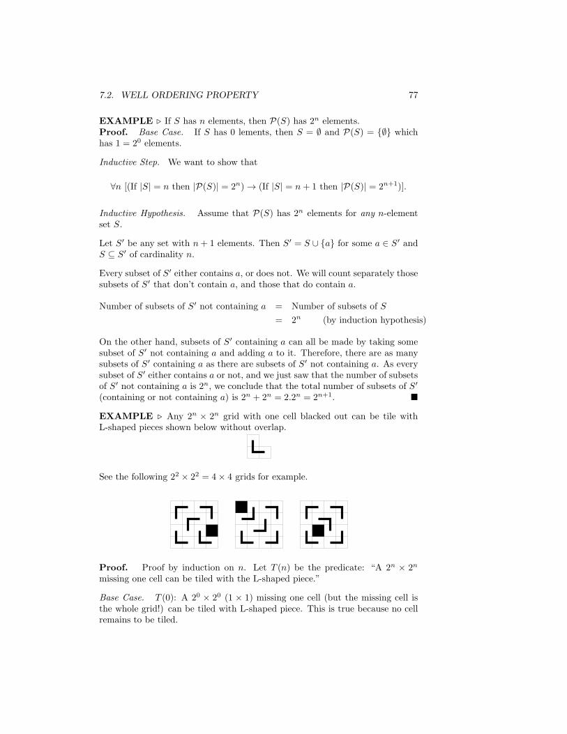
EXAMPLE ! Any 2n 3 2n grid with one cell blacked out can be tile withL-shaped pieces shown below without overlap.
See the following 22 3 22 = 43 4 grids for example.
Proof. Proof by induction on n. Let T (n) be the predicate: “A 2n 3 2n
missing one cell can be tiled with the L-shaped piece.”
Base Case. T (0): A 20 3 20 (1 3 1) missing one cell (but the missing cell isthe whole grid!) can be tiled with L-shaped piece. This is true because no cellremains to be tiled.

78 CHAPTER 7. MATHEMATICAL INDUCTION
T (1) (more satisfying): A 23 2 missing one cell can be tiled.
Inductive Step. Show that +n [T (n)& T (n+ 1)]. We assume inductively thata 2n 3 2n (missing one) can be tiled and show how to tile a 2n+1 3 2n+1 as inthe following figure.
!
Below is an example of tiling an 83 8 missing one.
7.3. STRONG MATHEMATICAL INDUCTION 79
7.3 Strong Mathematical Induction
Definition 46 Strong Mathematical Induction Principle
If P (0) and
+n @ 0 [(P (0) # P (1) # . . . # P (n))& P (n+ 1)]
then +n P (n).
Using the above (stronger) principle, to prove P (n+1) we can rely on inductivehypothesis that all of P (0), P (1), . . . , P (n) are true.
The reason this principle works, and the proof that it does (based on well-ordering principle) is identical to the weak induction.
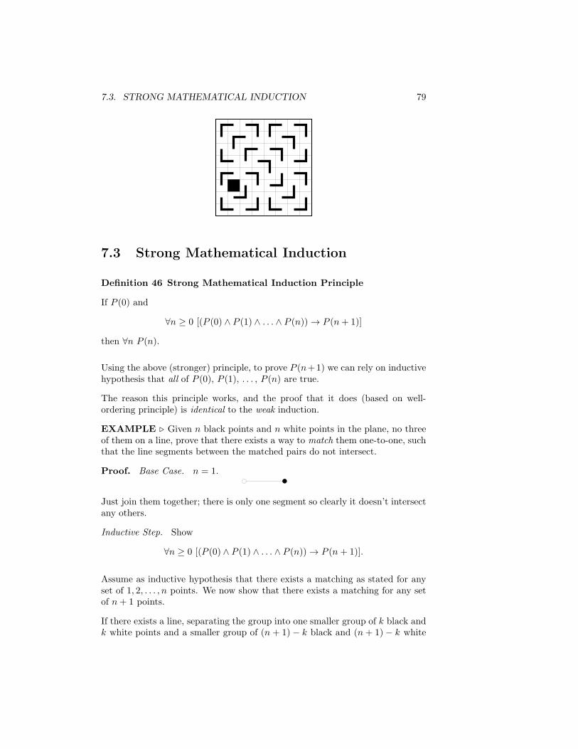
EXAMPLE ! Given n black points and n white points in the plane, no threeof them on a line, prove that there exists a way to match them one-to-one, suchthat the line segments between the matched pairs do not intersect.
Proof. Base Case. n = 1.
Just join them together; there is only one segment so clearly it doesn’t intersectany others.
Inductive Step. Show
+n @ 0 [(P (0) # P (1) # . . . # P (n))& P (n+ 1)].
Assume as inductive hypothesis that there exists a matching as stated for anyset of 1, 2, . . . , n points. We now show that there exists a matching for any setof n+ 1 points.
If there exists a line, separating the group into one smaller group of k black andk white points and a smaller group of (n + 1)* k black and (n+ 1)* k white

80 CHAPTER 7. MATHEMATICAL INDUCTION
points, then we can apply the inductive hypothesis to each side and note that apair from one side cannot interfere with a pair from the other side (why not?)
We now show that there is always such a separating line. For this consider theconvex hull of the points1. There are two possibilities:
• Case 1. There exists a black point and a white point on the convex hull.In this case, there exists an adjacent white and black points on the convexhull (why?) Then, we can separate this pair from the rest of the pointsand we are done.
• Case 2. The convex hull is all of the same color. Then take a line withslope unequal to the slope of any pair of points and sweep it across thefigure. There must be a place where k white and k black points fall onone side of the sweeping line and (n+ 1)* k white and (n+ 1)* k blackpoints fall on the other side of it.
This is because if for example the convex hull is all black, then the firstpoint the line passes is black. Also the last point that line passes is black.Somewhere in between this process, the white points must have “caughtup” to the black points behind the line.
1The convex hull of a set of points in plane is the smallest convex polygon containing allof the points (on or inside it).

7.4. INDUCTIVE (RECURSIVE) DEFINITIONS 81
!.
7.4 Inductive (recursive) Definitions
Similar to proving theorems inductively, we can sometimes define mathematicalstructures inductively (recursively).
EXAMPLE ! The non-recursive definition of factorial is
n! = 1.2.3. · · · .n.
But we can define factorial in the following (recursive) way as well.
n! =
%1 if n = 1n.(n* 1)! if n > 1
Note that this suggests an obviousrecursive algorithm.
An inductive or recursive definition has a base case which gives the definitionfor n = 0, and an induction step which gives the definition for n+1 in terms of1, 2, . . . , n.
EXAMPLE ! Fibonacci numbers.
f(n) =
+,
-
0 if n = 01 if n = 1f(n* 1) + f(n* 2) if n > 1
The first few numbers in the Fibonacci sequence (f(0), f(1), f(2), . . .) are then
0, 1, 1, 2, 3, 5, 8, 13, 21, . . . .
7.4.1 Sets can Be Defined Inductively
EXAMPLE ! Let S be the set of numbers divisible by 3: We define S asfollows
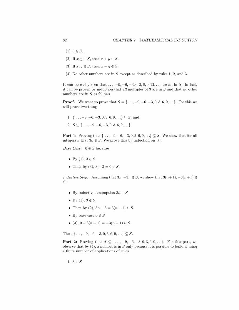
82 CHAPTER 7. MATHEMATICAL INDUCTION
(1) 3 , S.
(2) If x, y , S, then x+ y , S.
(3) If x, y , S, then x* y , S.
(4) No other numbers are in S except as described by rules 1, 2, and 3.
It can be easily seen that . . . ,*9,*6,*3, 0, 3, 6, 9, 12, . . . are all in S. In fact,it can be proven by induction that all multiples of 3 are in S and that no othernumbers are in S as follows.
Proof. We want to prove that S = {. . . ,*9,*6,*3, 0, 3, 6, 9, . . .}. For this wewill prove two things:
1. {. . . ,*9,*6,*3, 0, 3, 6, 9, . . .} 5 S, and
2. S 5 {. . . ,*9,*6,*3, 0, 3, 6, 9, . . .}.
Part 1: Proving that {. . . ,*9,*6,*3, 0, 3, 6, 9, . . .} 5 S. We show that for allintegers k that 3k , S. We prove this by induction on |k|.
Base Case. 0 , S because
• By (1), 3 , S
• Then by (3), 3* 3 = 0 , S.
Inductive Step. Assuming that 3n,*3n , S, we show that 3(n+1),*3(n+1) ,S.
• By inductive assumption 3n , S
• By (1), 3 , S.
• Then by (2), 3n+ 3 = 3(n+ 1) , S.
• By base case 0 , S
• (3), 0* 3(n+ 1) = *3(n+ 1) , S.
Thus, {. . . ,*9,*6,*3, 0, 3, 6, 9, . . .} 5 S.
Part 2: Proving that S 5 {. . . ,*9,*6,*3, 0, 3, 6, 9, . . .}. For this part, weobserve that by (4), a number is in S only because it is possible to build it usinga finite number of applications of rules
1. 3 , S

7.4. INDUCTIVE (RECURSIVE) DEFINITIONS 83
2. x, y , S & x+ y , S
3. x, y , S & x* y , S
For example
• To show that 3 , S we need to apply only a single rule (rule (1)).
• To show that 0 , S we need two rule applications 3 , Sand 3* 3 , S.
• To show that 9 , S we need three rule applications: rule (1) once and rule(2) twice.
We will prove by induction on the number of rules needed to show that x , Sthat x must be of the form 3k for some k , Z.
Base case. If x , S by one application of the rules, then it must be rule (1)(3 , S). Thus x = 3 and clearly x = 3k for k = 1.
Induction Step. We assume that the statement we want to prove holds forevery x whose membership in X can be shown by at most n application of thegiven rules.
Let x , S via n + 1 rule applications. Then suppose that the last applicationwas rule (2). Thus x = a + b where a, b are already known to be in S. Thena, b , S via less than or equal to n rule applications each and so a = 3ka andb = 3kb for some ka and kb. But then x = a + b = 3ka + 3kb = 3(ka + kb), amultiple of 3 as desired.
The case where the last rule-application is rule (3) is similar. !
EXAMPLE ! Recursive definition of Well-Formed-Formulas.
(1) T is a well-formed-formula, F is a well-formed-formula, and p is a well-formed-formula for any propositional variable p.
(2) If p is a well-formed-formula, then (¬p) is a well-formed-formula.
(3) If p and q are well-formed-formulas, then (p # q) and (p $ q) are well-formed-formulas.
Therefore, using the above definition, to see that ((p$q)#(¬r)) is a well-formed-formula, we show inductively that (p$q) and (¬r) are well-formed-formulas andapply rule (3).

84 CHAPTER 7. MATHEMATICAL INDUCTION
7.4.2 Strings and Recursive Definitions
Let % be a finite set. We will call % an alphabet. The set of strings over %denoted by %' is defined inductively as follows
(1) $ , %' where $ denotes the null or string.
(2) If x , % and w , %', then wx , %' where %' is the concatenation ofstrings w with symbol x.
EXAMPLE ! If % = {a, b, c}, then
%' = {$, a, b, c, aa, ab, ac, ba, bb, bc, ca, cb, cc, aaa, aab, . . .}.
Note that %' is infinite.Questions. 1. Does !" haveany strings of infinite length?2. Is there a bound on how largestrings in !" can be? (i.e. Is thata maximum-length string?)
EXAMPLE ! Inductive Definition of Length of Strings. We denote by|w| the length of the string w.
(1) |$| = 0.
(2) If w , %' and x , % then |wx| = |w| + 1.
EXAMPLE ! Inductive Definition of Reversal of Strings. By (w)R wedenote the string we get from w if list the symbols of w in the reverse order.For example (abc)R = cba. This is defined inductively as follows.
(1) ($)R = $.
(2) If w , %' and x , %, then (wx)R = x(w)R .
For example, by the given rules
(abc)R = ((ab)c)R
= c(ab)R
= c((a)b)R
= c(b(a)R)
= c(b(($)a)R)
= c(b(a($)R))
= c(b(a($)))
= cba
Theorem 4 +x, y , %'
(xy)R = yRxR
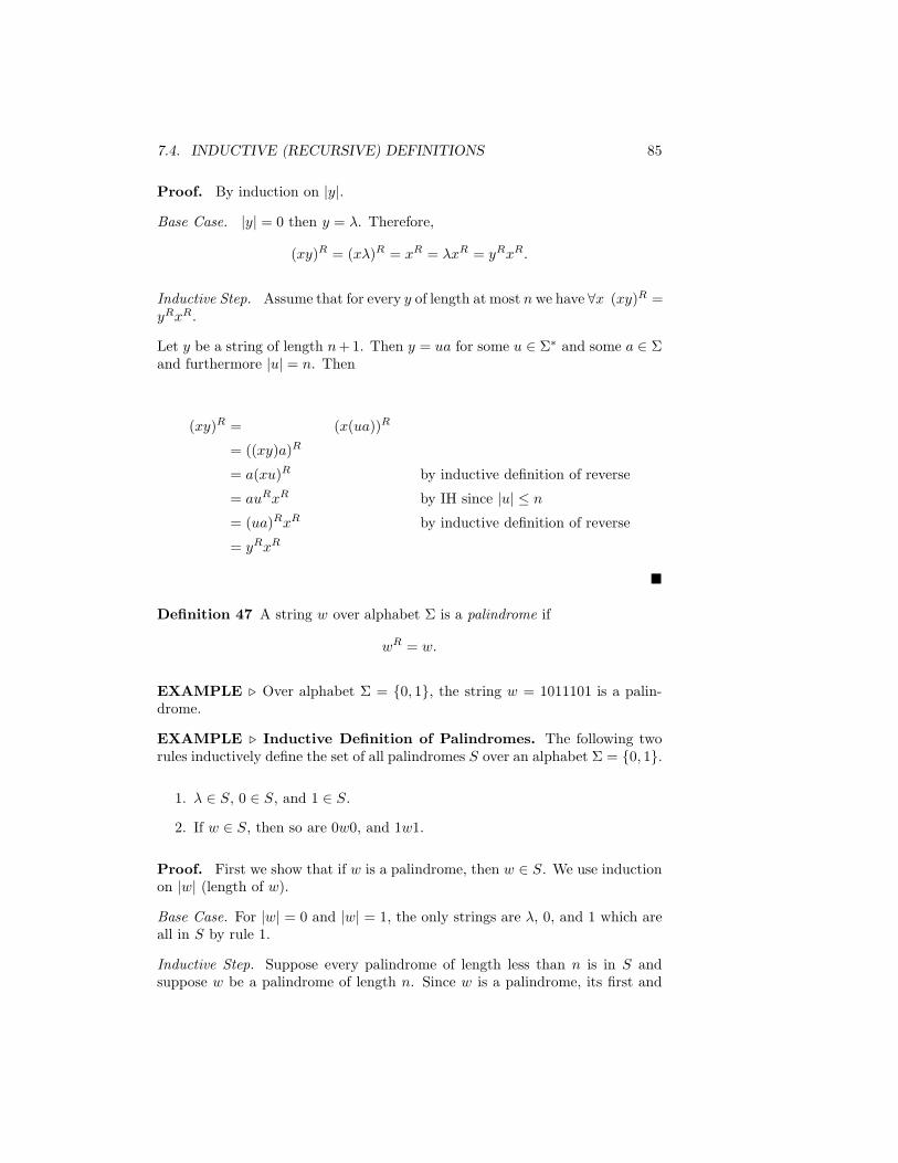
7.4. INDUCTIVE (RECURSIVE) DEFINITIONS 85
Proof. By induction on |y|.
Base Case. |y| = 0 then y = $. Therefore,
(xy)R = (x$)R = xR = $xR = yRxR.
Inductive Step. Assume that for every y of length at most n we have +x (xy)R =yRxR.
Let y be a string of length n+1. Then y = ua for some u , %' and some a , %and furthermore |u| = n. Then
(xy)R = (x(ua))R
= ((xy)a)R
= a(xu)R by inductive definition of reverse
= auRxR by IH since |u| / n
= (ua)RxR by inductive definition of reverse
= yRxR
!
Definition 47 A string w over alphabet % is a palindrome if
wR = w.
EXAMPLE ! Over alphabet % = {0, 1}, the string w = 1011101 is a palin-drome.
EXAMPLE ! Inductive Definition of Palindromes. The following tworules inductively define the set of all palindromes S over an alphabet % = {0, 1}.
1. $ , S, 0 , S, and 1 , S.
2. If w , S, then so are 0w0, and 1w1.
Proof. First we show that if w is a palindrome, then w , S. We use inductionon |w| (length of w).
Base Case. For |w| = 0 and |w| = 1, the only strings are $, 0, and 1 which areall in S by rule 1.
Inductive Step. Suppose every palindrome of length less than n is in S andsuppose w be a palindrome of length n. Since w is a palindrome, its first and

86 CHAPTER 7. MATHEMATICAL INDUCTION
last symbol shod be the same. Therefore, either w = 0w!0 or w = 1w!1 for somepalindrome w! of length less than n. Then by induction hypothesis, w! , S andthen by rule 2, w , S. This proves that every palindrome is in S.
Now we want to prove that every string in S is a palindrome. Note that everystring in S can be shown to be in S by applying a sequence of applications ofrules 1 and 2. We use induction on the number of applications of rules 1 and 2needed in showing that w , S to prove that w is a palindrome.
Base Case. The only strings that can be shown to be in S with a singleapplication of rules 1 and 2 are $, 0, and 1 which are derived using a singleapplication of rule 1 and are all palindromes.
Inductive Step. Suppose that every string derived by fewer than n applicationsof rules 1 and 2 is a palindrome and let w be a string that happens to be in S byn applications of rules 1 and 2. Clearly, the last rule applied to show that w , Smust have been rule 2 because rule 1 can be applied only once. Therefore, w isobtained by adding 0’s or 1’s to the beginning or end of a string w! , S whichcan be derived in n* 1 application of the above rules. By induction hypothesis,w! is a palindrome and since rule 2 adds either 0’s or 1’s to the beginning andend of the string, w is also a palindrome. !

Chapter 8
Running Time ofAlgorithms
Definition 48 An algorithm is a clearly defined, step-by-step procedure forsolving a problem. An algorithms has the following properties: We will use pseudo-codes for de-
scribing algorithms.
• The input and output are from specified domain.
• Each step is precisely described.
• Each step is executable in finite time.
• Is applicable to a large range of inputs, not just a particular one. Generality
• Must halt with output in finite time. Halting: This does not followfrom the finiteness of each step.
Note. It is a very di!cult (in fact unsolvable) problem to determine in generalif the last property , i.e. determining given an algorithm and an input to thealgorithm, weather the algorithm halts on its input.
EXAMPLE ! Nobody knows if the algorithm below halts for every input. Itis known that for input x up to billions, it halts.
87
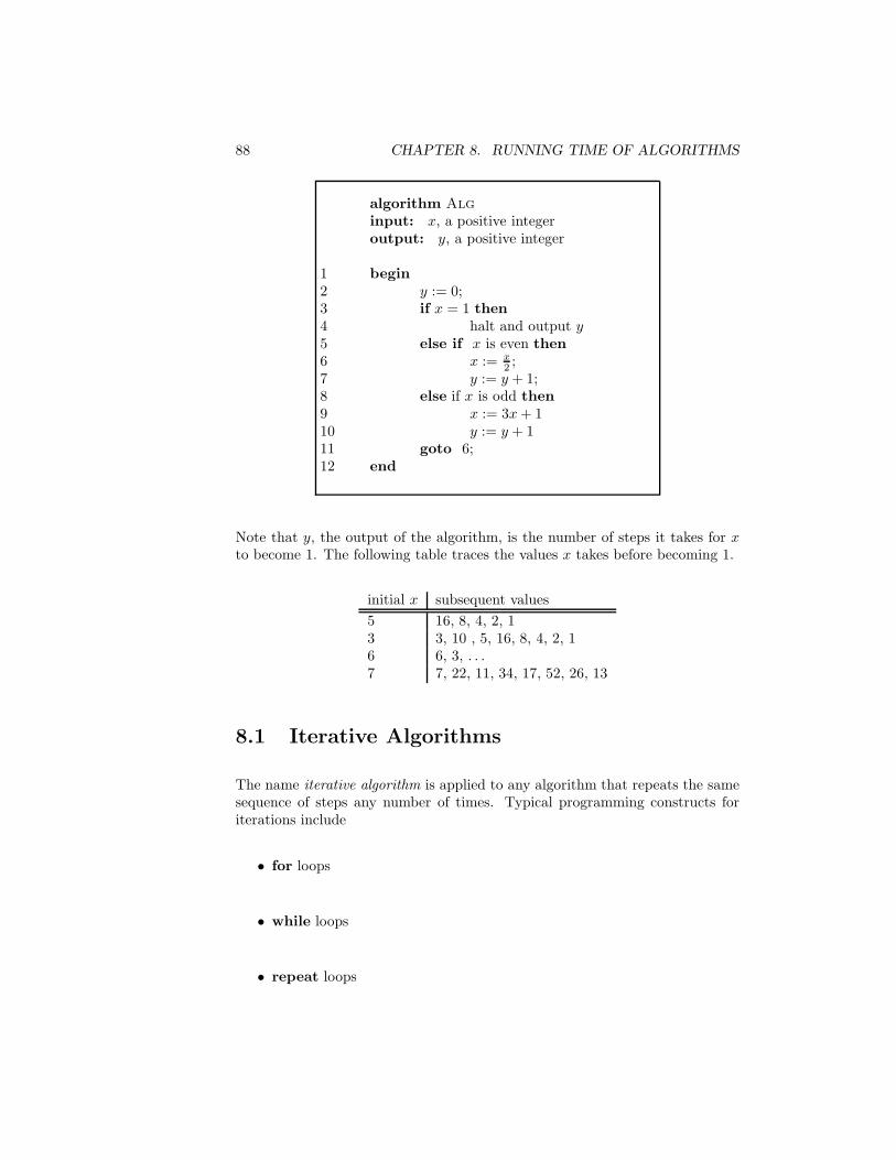
88 CHAPTER 8. RUNNING TIME OF ALGORITHMS
algorithm Alginput: x, a positive integeroutput: y, a positive integer
1 begin2 y := 0;3 if x = 1 then4 halt and output y5 else if x is even then6 x := x
2 ;7 y := y + 1;8 else if x is odd then9 x := 3x+ 110 y := y + 111 goto 6;12 end
Note that y, the output of the algorithm, is the number of steps it takes for xto become 1. The following table traces the values x takes before becoming 1.
initial x subsequent values
5 16, 8, 4, 2, 13 3, 10 , 5, 16, 8, 4, 2, 16 6, 3, . . .7 7, 22, 11, 34, 17, 52, 26, 13
8.1 Iterative Algorithms
The name iterative algorithm is applied to any algorithm that repeats the samesequence of steps any number of times. Typical programming constructs foriterations include
• for loops
• while loops
• repeat loops
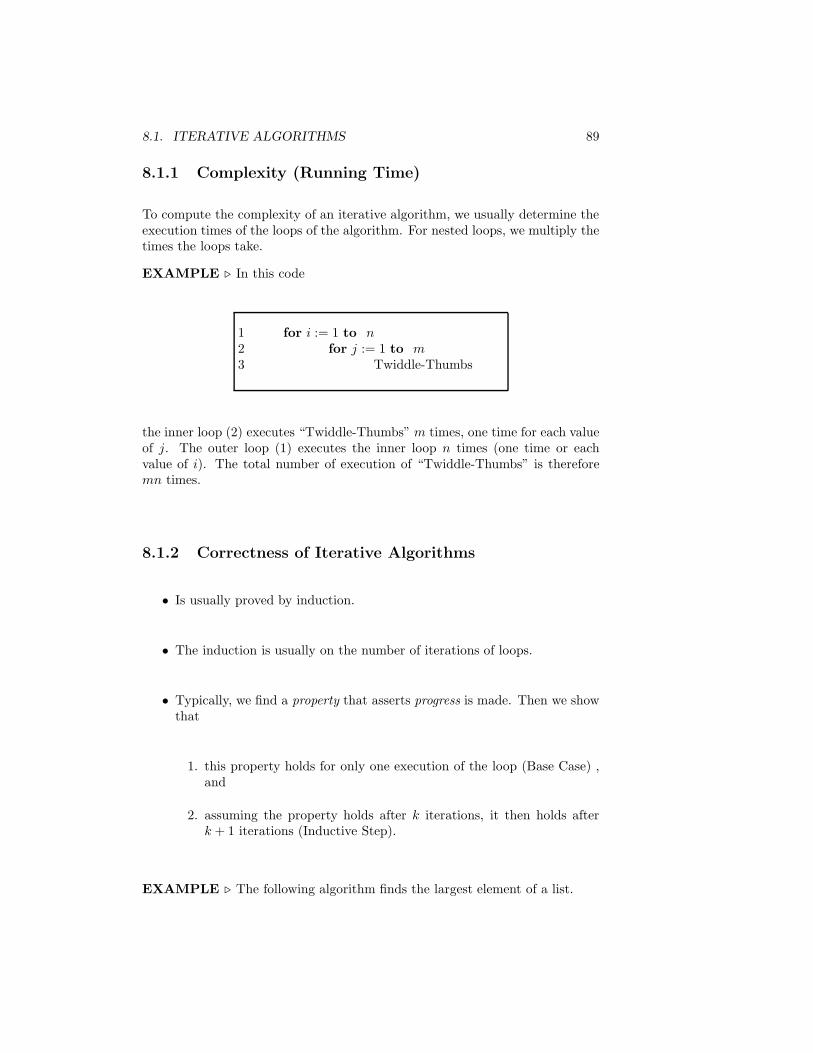
8.1. ITERATIVE ALGORITHMS 89
8.1.1 Complexity (Running Time)
To compute the complexity of an iterative algorithm, we usually determine theexecution times of the loops of the algorithm. For nested loops, we multiply thetimes the loops take.
EXAMPLE ! In this code
1 for i := 1 to n2 for j := 1 to m3 Twiddle-Thumbs
the inner loop (2) executes “Twiddle-Thumbs” m times, one time for each valueof j. The outer loop (1) executes the inner loop n times (one time or eachvalue of i). The total number of execution of “Twiddle-Thumbs” is thereforemn times.
8.1.2 Correctness of Iterative Algorithms
• Is usually proved by induction.
• The induction is usually on the number of iterations of loops.
• Typically, we find a property that asserts progress is made. Then we showthat
1. this property holds for only one execution of the loop (Base Case) ,and
2. assuming the property holds after k iterations, it then holds afterk + 1 iterations (Inductive Step).
EXAMPLE ! The following algorithm finds the largest element of a list.

90 CHAPTER 8. RUNNING TIME OF ALGORITHMS
algorithm Largestinput: x1, . . . , xn, a list (array) of positive integeroutput: xn, when done will contain the largest
1 begin2 for j := 1 to n* 13 if xj > xj+1 then [swap xj and xj+1]4 temp := xj ;5 xj := xj+1;6 xj+1 := temp;7 end
Below is an example of the execution of the above algorithm with 4 inputs. Thetwo %’s show the elements that are compared at each step.
variable initial value j = 1 j = 2 j = 3 after halting
x1 3 3 % 2 2 2x2 2 2 % 3 % 3 3x3 4 4 4 % 4 % 1x4 1 1 1 1 % 4
If we assume that
1. each comparison takes constant time c,
2. each addition takes constant time s, and
3. each assignment takes constant time a,
then the lines 3, 4, 5, and 6 of the above algorithm, take times c+s, a, a+s anda respectively. Adding these up, each execution of the loop of line (2) needs timeequal to & = c+3a+3s. Since the loop is executed n*1 times, the total runningtime of the above algorithm will be (c+ 3a+ 3s)(n* 1) = &.(n* 1) = O(n).Note that here, the constant ! de-
pends only on the machine thatruns the algorithm and not n. Now we give the proof of the correctness:
Proof. Assertion: After the j-th execution of the loop,
xj+1 = max{x1, x2, . . . , xj , xj+1}.
We prove the above claim by induction on j. Note that for j = n* 1, the aboveassertion states that the algorithm has successfully found the largest element ofthe input.
Base Case. j = 0, i.e. no iterations f the loop yet. Certainly x1 = max{x1}.
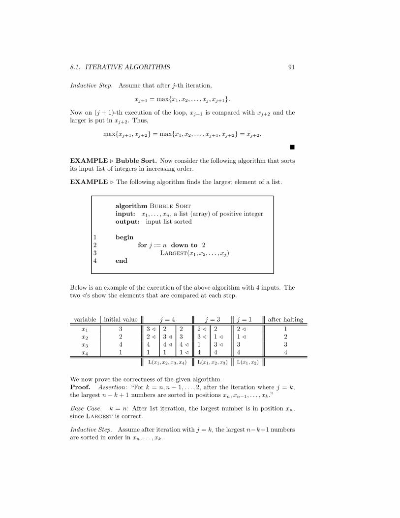
8.1. ITERATIVE ALGORITHMS 91
Inductive Step. Assume that after j-th iteration,
xj+1 = max{x1, x2, . . . , xj , xj+1}.
Now on (j + 1)-th execution of the loop, xj+1 is compared with xj+2 and thelarger is put in xj+2. Thus,
max{xj+1, xj+2} = max{x1, x2, . . . , xj+1, xj+2} = xj+2.
!
EXAMPLE ! Bubble Sort. Now consider the following algorithm that sortsits input list of integers in increasing order.
EXAMPLE ! The following algorithm finds the largest element of a list.
algorithm Bubble Sortinput: x1, . . . , xn, a list (array) of positive integeroutput: input list sorted
1 begin2 for j := n down to 23 Largest(x1, x2, . . . , xj)4 end
Below is an example of the execution of the above algorithm with 4 inputs. Thetwo %’s show the elements that are compared at each step.
variable initial value j = 4 j = 3 j = 1 after halting
x1 3 3 % 2 2 2 % 2 2 % 1x2 2 2 % 3 % 3 3 % 1 % 1 % 2x3 4 4 4 % 4 % 1 3 % 3 3x4 1 1 1 1 % 4 4 4 4
L(x1, x2, x3, x4) L(x1, x2, x3) L(x1, x2)
We now prove the correctness of the given algorithm.Proof. Assertion: “For k = n, n * 1, . . . , 2, after the iteration where j = k,the largest n* k + 1 numbers are sorted in positions xn, xn#1, . . . , xk.”
Base Case. k = n: After 1st iteration, the largest number is in position xn,since Largest is correct.
Inductive Step. Assume after iteration with j = k, the largest n*k+1 numbersare sorted in order in xn, . . . , xk.

92 CHAPTER 8. RUNNING TIME OF ALGORITHMS
Now the iteration with j = k * 1 calls Largest(x1, . . . , xk#1). So (by correct-ness of largest), the next largest is put into xk#1. Thus after this iteration, thelargest n* (k * 1) + 1 numbers are in positions xn, xn#1, . . . , xk, xk#1. !
8.2 Complexity
Often the running time of an algorithm depends not only on the number ofinputs (as with Bubble Sort), but also on what the particular inputs are (notlike Bubble sort).
Two common ways to analyze such algorithms are
1. Worst case complexity: Analyze what worst possible input could be.
2. Average case complexity : Consider the typical input.
EXAMPLE ! Linear Search Algorithm.The following algorithm finds the largest element of a list.
algorithm Linear Searchinput: Sorted list a1 < a2 < . . . < an of distinct integers and number xoutput: Position i that ai = x, if x is in the list.
1 begin2 i := 13 while (i / n and x "= ai)4 i := i + 15 if i = n+ 1 then6 output “x not in list”7 else8 output “x is in position i”9 end
Complexity (counting only comparisons with a!is): there will be i comparisonsonly if x = ai. However, if x = an or x is not in list at all, n comparisons willbe made.
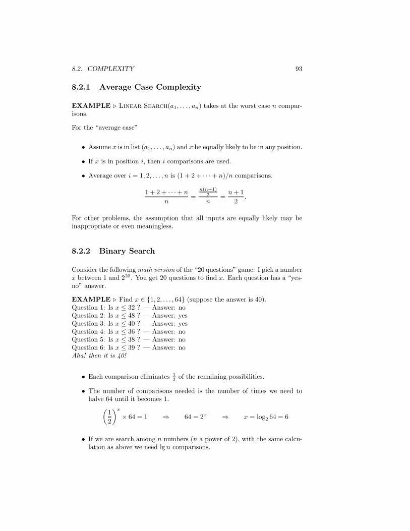
8.2. COMPLEXITY 93
8.2.1 Average Case Complexity
EXAMPLE ! Linear Search(a1, . . . , an) takes at the worst case n compar-isons.
For the “average case”
• Assume x is in list (a1, . . . , an) and x be equally likely to be in any position.
• If x is in position i, then i comparisons are used.
• Average over i = 1, 2, . . . , n is (1 + 2 + · · ·+ n)/n comparisons.
1 + 2 + · · ·+ n
n=
n(n+1)2
n=
n+ 1
2.
For other problems, the assumption that all inputs are equally likely may beinappropriate or even meaningless.
8.2.2 Binary Search
Consider the followingmath version of the “20 questions” game: I pick a numberx between 1 and 220. You get 20 questions to find x. Each question has a “yes-no” answer.
EXAMPLE ! Find x , {1, 2, . . . , 64} (suppose the answer is 40).Question 1: Is x / 32 ? — Answer: noQuestion 2: Is x / 48 ? — Answer: yesQuestion 3: Is x / 40 ? — Answer: yesQuestion 4: Is x / 36 ? — Answer: noQuestion 5: Is x / 38 ? — Answer: noQuestion 6: Is x / 39 ? — Answer: noAha! then it is 40!
• Each comparison eliminates 12 of the remaining possibilities.
• The number of comparisons needed is the number of times we need tohalve 64 until it becomes 1.
.1
2
/x
3 64 = 1 A 64 = 2x A x = log2 64 = 6
• If we are search among n numbers (n a power of 2), with the same calcu-lation as above we need lg n comparisons.
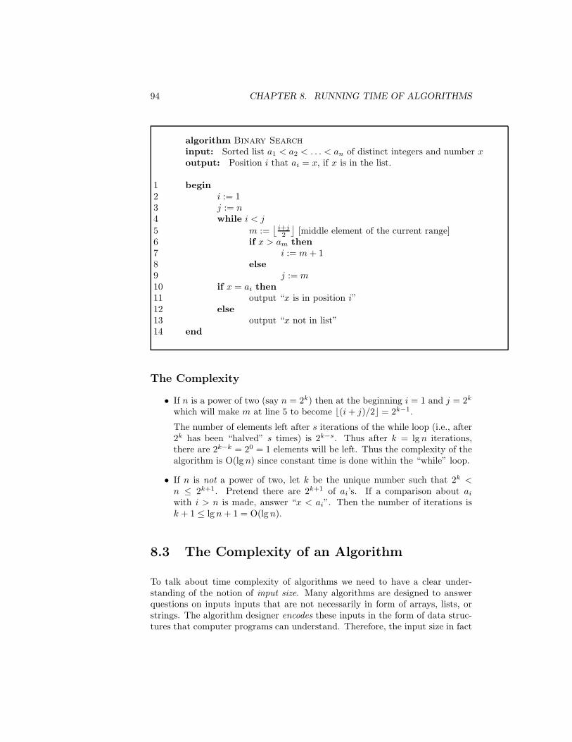
94 CHAPTER 8. RUNNING TIME OF ALGORITHMS
algorithm Binary Searchinput: Sorted list a1 < a2 < . . . < an of distinct integers and number xoutput: Position i that ai = x, if x is in the list.
1 begin2 i := 13 j := n4 while i < j5 m :=
0i+j2
1[middle element of the current range]
6 if x > am then7 i := m+ 18 else9 j := m10 if x = ai then11 output “x is in position i”12 else13 output “x not in list”14 end
The Complexity
• If n is a power of two (say n = 2k) then at the beginning i = 1 and j = 2k
which will make m at line 5 to become >(i+ j)/2? = 2k#1.
The number of elements left after s iterations of the while loop (i.e., after2k has been “halved” s times) is 2k#s. Thus after k = lg n iterations,there are 2k#k = 20 = 1 elements will be left. Thus the complexity of thealgorithm is O(lg n) since constant time is done within the “while” loop.
• If n is not a power of two, let k be the unique number such that 2k <n / 2k+1. Pretend there are 2k+1 of ai’s. If a comparison about aiwith i > n is made, answer “x < ai”. Then the number of iterations isk + 1 / lg n+ 1 = O(lgn).
8.3 The Complexity of an Algorithm
To talk about time complexity of algorithms we need to have a clear under-standing of the notion of input size. Many algorithms are designed to answerquestions on inputs inputs that are not necessarily in form of arrays, lists, orstrings. The algorithm designer encodes these inputs in the form of data struc-tures that computer programs can understand. Therefore, the input size in fact

8.3. THE COMPLEXITY OF AN ALGORITHM 95
depends on how we encode the input.
As a simple example suppose the input to the algorithm be a number. We canrepresent a number in decimal, binary or even unary. For example, number1024 has binary encoding 10000000000 or unary encoding
1111 . . .111! "# $1024 times
.
When we talk about the size of input, we consider a reasonably e!cient encodingof the input.
We will denote by worstA(n) the worst case time complexity of an algorithm Aon an input of size n.
EXAMPLE ! worstLinear Search(n) = O(n).
EXAMPLE ! worstBinary Search(n) = O(lg n).
The following table compare the amount of time that an algorithm with timecomplexity f(n) takes to complete if the computer that executes the algorithmruns at 1, 000, 000 steps per second.
Time Input Size nComplexity 10 20 30 40 50 60
n .00001s .00002s .00003s .00004s .00005s .00006sn2 .0001s .0004s .0009s .0016s .0025s .0036sn5 .1s 3.2s 24.3s 1.7m 5.2m 13m3n .059s 58m 6.5y 3855c 23 108c 1.33 1013c
s: seconds, m: minutes, y: years, c: centuries
One might ask the following questions: The computers are getting faster. Howmuch bigger of a problem can we solve if computers get faster?
The following table gives us some clue.
Time size of largest problem solvable in 1 hour using
Complexity todays’ technology 100 3 today’s technology
n N1 1003N1
n2 N2 103N2
n5 N3 2.53N3
3n N4 N4 + 4.19

96 CHAPTER 8. RUNNING TIME OF ALGORITHMS
8.3.1 Why Worst Case?
Advantages:
• Easy to analyze
• Gives guarantee about the running time, regardless of what input mightbe encountered
• Don’t have to assume or decide what typical inputs are
Disadvantages:
• Bizarre inputs could cause worst case performance to look awful, when infact most “typical” inputs cause the algorithm to terminate quickly.
8.4 Recursive Algorithms
Definition 49 A recursive algorithm is one which calls itself from within itsown body.
A recursive algorithm usually breaks the problem into one or more related sub-problems, solves (recursively) the sub-problems, and obtains the final solutionby some simple computation using the solution(s) to the sub-problem(s). Suchalgorithms are sometimes called “Divide And Conquer” algorithms.
These algorithms must satisfy two requirements:
1. The subproblems should be easier (smaller) than the original problem.
2. After a finite number of sub-divisions, we should reach a sub-problem thatcan be solved outright (terminating case).
EXAMPLE ! Calculating Factorial

8.4. RECURSIVE ALGORITHMS 97
algorithm Factorialinput: integer noutput: n!
1 begin2 if n = 1 then3 output “1”4 else5 output “n3 Factorial(n* 1)”6 end
Factorial(n)3
n Factorial(n#1)3
n* 1 Factorial(n#2)3
n* 2 Factorial(...)3
Factorial(2)3
2 Factorial(1) = 1
Below we give a proof of correctness for the given algorithm.Proof. By induction on n we show that Factorial(n) = n!
Base Case. Clearly on input 1, Factorial outputs 1 = 1!.
Inductive Step. We show that if the output of the algorithm for n*1 is (n*1)!,then its output for n is n!.
Assume inductively that Factorial(n * 1) = (n * 1)!. Then Factorial(n)outputs n3 Factorial(n* 1) = n3 (n* 1)! = n!. !
The correctness of a recursive algorithm is often easily proved by induction,since the algorithm itself has
• A base case (non-recursive) showing what to do if input is 1.

98 CHAPTER 8. RUNNING TIME OF ALGORITHMS
• An inductive (recursive) step, showing how to solve current problem as-suming that the recursive calls have correctly returned the solutions tothe subproblems. This of course looks like inductive step in a proof usinginduction.
EXAMPLE ! Merge-Sort. Recursive algorithm for sorting n numbers.
We first write a subroutine to merge two sorted list into one.
algorithm Mergeinput: Sorted lists a1, . . . , ak, b1, . . . , bloutput: Sorted list combining the inputs lists into one
1 begin2 i := 13 j := 14 while i+ j < k + l5 if i = k then6 append bj to the output list; j := j + 17 else if j = l then8 append ai to the output list; i := i+ 19 else if ai < bj then10 append ai to the output list; i := i+ 111 else12 append bj to the output list; j := j + 113 end
The following table shows howMerge works for input lists 1, 2, 5, 8 and 3, 4, 6, 9, 12.
output list a1, . . . , ak b1, . . . , bl1 % 2 5 8 3% 4 6 9 12
1 2% 5 8 3% 4 6 9 121, 2 5% 8 3% 4 6 9 121, 2, 3 5% 8 4% 6 9 121, 2, 3, 4 5% 8 6% 9 121, 2, 3, 4, 5 8% 6% 9 121, 2, 3, 4, 5, 6 8% 9% 121, 2, 3, 4, 5, 6, 8 9% 121, 2, 3, 4, 5, 6, 8, 9 12%1, 2, 3, 4, 5, 6, 8, 9, 12
Merge-Sort is a divide-and-conquer sorting algorithm. On input x1, . . . , xn,

8.4. RECURSIVE ALGORITHMS 99
we
• divide x1, . . . , xn into two groups,
• recursively Merge-Sort the two separate groups, and
• call Merge to merge the two sorted lists.
algorithm Merge-Sortinput: sub-list xl, . . . , xh
output: Sorted sub-list
1 begin2 if l @ h then3 return4 else5 Merge-Sort(xl , . . . , x> l+h
2 ?)6 Merge-Sort(x< l+h
2 =, . . . , xh)
7 Merge2(xl, . . . , x> l+h
2 ?), (x< l+h2 =, . . . , xh)
3
8 end
Recursion
+44444444444444,
44444444444444-
7 1 6 4 8 5 3 2
7 1 6 4
7 1
7 1
6 4
6 4
8 5 3 2
8 5
8 5
3 2
3 2

100 CHAPTER 8. RUNNING TIME OF ALGORITHMS
Merges
+44444444444444,
44444444444444-1 2 3 4 5 6 7 8
1 4 6 7
1 7
7 1
4 6
6 4
2 3 5 8
5 8
8 5
2 3
3 2
Correctness of Merge-Sort
Lemma 1 If Merge is given two sorted lists, then it correctly returns a singlesorted list containing elements of both lists.
The proof for the above lemma is omitted.This should be intuitive.
Now we prove the correctness of Merge-SortProof. We use induction on n.
Base Case. n = 1. If there is only one element to be sorted, then clearly thesingle element returned is in sorted order.
Inductive Assumption. For all n / k, Merge-Sort correctly sorts n numbers.
Inductive Step. To sort k+1 numbers, Merge-Sort divided into lists L1 andL2, each with approximately
0k+12
1/ k numbers.
By inductive assumption, the recursive calls to Merge-Sort return L1 and L2
in sorted order.
By the above lemma, Merge correctly combines these into a single, sorted lists,which is then output. !
EXAMPLE ! The towers of Hanoi.Rules:
1. Move only one disc at a time.
2. Can only put smaller on larger.
Goal: Transfer all n from A to B.

8.4. RECURSIVE ALGORITHMS 101
In the following algorithm Move(n,A,B,C) corresponds to move n discs fromA to B using C as spare.
algorithm Move(n,A,B,C)
1 begin2 if n = 1 then3 transfer the disc from A to B4 Move(n* 1, A, C,B)5 transfer n-th disc to B6 Move(n* 1, C,B,A)7 end
We now prove the correctness of the above algorithm.
Proof. Proof by induction on n.
Base Case. IF n = 1, it just moves the ring.
Inductive Hypothesis. Assume that Move(k,X, Y, Z) correctly moves k discsfrom X to Y using Z as a spare.
Inductive Step. Move(k + 1, A,B,C) calls Move(k,A,B,C). By inductivehypothesis, we have largest disc left on A, and the stack of k on pole C. Now thelargest disc is moved to B. Then Move(k, C,B,A) is called and by inductivehypothesis, the stack of k on C are moved onto B. !
8.4.1 Complexity of Recursive Algorithms
We usually use recurrence equations or recurrence relations to find the complex-ity of recursive algorithm. We won’t show you how to solve
these in this class — take CS 273,373, . . . .

102 CHAPTER 8. RUNNING TIME OF ALGORITHMS
To find a recurrence relation, we set up equations that express the complexityof a recursive algorithm.
• First, we write down boundary value(s): The running time for base casen = 1.
• Next, we express the time T (n) to solve a problem of size n in terms ofvalues T (k) where k < n.
• Finally, we can guess the solution, and prove it correct via induction.Otherwise, solve with techniques from CS 273, 373, . . . .
EXAMPLE ! Let T (n) be the time to do binary search on n elements (insorted order).
T (1) = 1
T (n) = c+ T (n/2)
where c is the time to determine which half x is in (some small constant) andT (n/2) is then time to search a sorted list of half size.
T (n) = c + T (n/2)# $! "
= c + c + T (n/4)# $! "
= c + c + c + T (n/8)...
......
= c + c + c + · · · + T (1)
54444444446
4444444447
depthof
recursion= lgn
Therefore, total time is c(lg n) = O(lg n).
EXAMPLE ! Let M(n) be the time to run Merge-Sort on n numbers.
M(1) = 1
M(n) = M(n/2) +M(n/2) + cn
where each M(n/2) is the time to sort half of the array and cn is the time tomerge the sorted half-arrays.
Again, intuitively this recurrence relation can be solved as follows.

8.4. RECURSIVE ALGORITHMS 103
M(n) = 2(M(n/2)) + cn
= 2(2(M(n/4)) + c(n/2)) + cn
= 4M(n/4) + cn+ cn
= 4(2(M(n/8) + c(n/4)) + cn+ cn
= 8M(n/8) + cn+ cn+ cn
...
= nM(n/n) + cn+ cn+ cn+ · · ·+ cn
544444444444444446
44444444444444447
depthof
recursion= lg n
Therefore, the total time is n+ cn(lg n) = O(n lg n)
EXAMPLE ! Let H(n) be the number of moves used by the towers of HanoiMove algorithm on n discs.
H(1) = 1
H(n) = H(n* 1) + 1 +H(n* 1)
= 2H(n* 1) + 1
Again by expanding we can intuitively find the answer to the recurrence relationabove.
H(n) = 2(H(n* 1)) + 1
= 2(2H(n* 2) + 1) + 1
= 4H(n* 2) + 2 + 1
= 4(2H(n* 3) + 1) + 2 + 1
= 8H(n* 3) + 4 + 2 + 1
...
= 2n#1(H(1)) + 2n#2 + · · ·+ 4 + 2 + 1
=n#1(
i=0
2i
= 2n * 1
544444444444444444444446
44444444444444444444447
depthof
recursion= n
The last equality is just the sum of a geometric series.
104 CHAPTER 8. RUNNING TIME OF ALGORITHMS
8.5 Typical Divide & Conquer Recurrences —Cheat Sheet
Fact 15 If you come up with the recurrence relation consisting of a base caseand the recurrence
T (n) = aT2nb
3+ cnd
then the solution to this recurrence relations is
T (n) =
+,
-
O(nd) if a < bd
O(nd lg n) if a = bd
O(nlogb a) if a > bd
Note that the above recurrence relation is usually obtained whenever solvingthe problem of size n can be done by
• breaking the problem into a sub-problems,
• with each sub-problem of size nb ,
• and we need cnd (typically d = 1) amount of work to put the results ofthe sub-problems into a solution for the original problem (of size n).
EXAMPLE ! Merge-Sort: T (n) = 2T (n/2)+ cn. Using the above fact, weobtain T (n) = O(n lgn).
EXAMPLE ! Binary-Search: T (n) = T (n/2) + cn0. Therefore, T (n) =O(n0 lgn) = O(lgn).
Chapter 9
Relations
Recall that for sets A and B, the Cartesian product of A and B is
A3B = {(a, b) : a , A and b , B}.
Definition 50 A relation R from A to B is a subset R 5 A3B.
Note that by the above definition, a relation is a set of ordered pairs.
EXAMPLE ! If A is the set of students and B is the set of courses, we candefine the relation R from A to B be
R = {(a, b) : student a taking course b }.
EXAMPLE ! Let A = B be the set of people. Then a relation R form A toB can be
R = {(a, b) : a and b have the same mother }.
Note. Whenever we define a relation R from a set A to the same set A, wesimply say that R is a relation on A.
EXAMPLE ! Any function f : A& B is a relation R defined as
R = {(a, b) : f(a) = b}.
Since f is a function, we know that this relation has the property that
+a , A .!b (a, b) , R
.
105

106 CHAPTER 9. RELATIONS
9.0.1 Properties of Relations on Sets
Definition 51 A relation R on set A is reflexive if
+a , A (a, a) , R.
EXAMPLE ! If A = {1, 2, 3, 4}, the relation R = {(1, 2), (3, 4), (1, 1), (3, 3)}on A is not reflexive but the relation R = {(1, 1), (2, 2), (3, 3), (4, 4), (1, 2), (3, 4)}is reflexive.
EXAMPLE ! Let A be the set of people. The the relation R defined on A as
R = {(a, b) : a and b have the same mother }
is reflexive because everybody has the same mother as himself!
Definition 52 A relation R on A is symmetric if
+a, b , A (a, b) , R& (b, a) , R.
EXAMPLE ! IfA is the set of people, thenR = {(a, b) : a and b have the same mother }is symmetric.
EXAMPLE ! On A = {1, 2}, the relation 4 is symmetric because for all pairs(a, b):
(a, b) , emptyset& (b, a) , emptyset
EXAMPLE ! The relation R = {(a, b) : a|b} is not symmetric on ".
Definition 53 A relation R on A is antisymmetric if
+a, b , A [(a, b) , R # (b, a) , R]& a = b.
EXAMPLE ! On A = N the “divides” relation R = {(a, b) : a|b} is anti-symmetric because if for integers a and b, a|b and b|a we can conclude thata = b.
EXAMPLE ! “divides” is not antisymmetric on Z because *1|a and 1| * 1but 1 "= *1.
EXAMPLE ! A = {1, 2, 3} and R = {(1, 1), (2, 2), (3, 3)} is both symmetricand antisymmetric.
Definition 54 A relation R on A is transitive if
+a, b, c , A [(a, b) , R # (b, c) , R]& (a, c) , R.

107
EXAMPLE ! If A is the set of people and R = {(a, b) : a and b are sisters },then clearly if a is a sister of b and b is a sister of c, then a is a sister of c andtherefore R is transitive but R is none of reflexive, symmetric, or antisymmetric(why?) .
EXAMPLE ! A = {1, 2, 3} and R = {(1, 2), (3, 1)}. Then R is not transitivebecause otherwise (3, 2) should be in.
EXAMPLE ! A = {1, 2, 3} and R = {(1, 2), (2, 1)}. Then R is not transitivebecause otherwise (1, 1) and (2, 2) should be in.
EXAMPLE ! A = {1, 2, 3} and R = {(1, 2)} is transitive (vacuously).
9.0.2 Combining Relations
Let R1 and R2 be two relations. Since relations are sets, R1 7 R2, R1 8 R2,R1 *R2, R2 *R1, and R1 are all subsets of A3B and hence relations.
Definition 55 Let R be a relation from A to B (i.e, R 5 A 3 B) and S bea relation from B to C (i.e, S 5 B 3 C). Then the composition of R and Sdenoted by R B S and defined as
S BR = {(a, c) : .B (a, b) , R and (b, c) , S}
EXAMPLE ! In the following figure, lines between elements of A and B showthe pairs in the relation R and those between B and C show the pairs in therelation S.
1
2
3
4
x
y
z
s
t
u
v
A B C
R S
Then S BR = {(1, u), (1, v), (2, t), (3, t), (4, u)}.
Definition 56 If R is a relation on A, then (inductively define)
R1 = R
Rn+1 = Rn BR
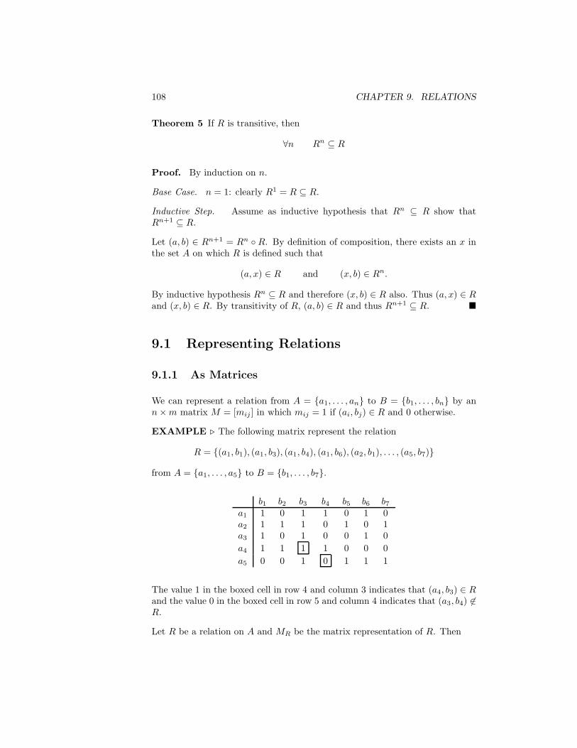
108 CHAPTER 9. RELATIONS
Theorem 5 If R is transitive, then
+n Rn 5 R
Proof. By induction on n.
Base Case. n = 1: clearly R1 = R 5 R.
Inductive Step. Assume as inductive hypothesis that Rn 5 R show thatRn+1 5 R.
Let (a, b) , Rn+1 = Rn B R. By definition of composition, there exists an x inthe set A on which R is defined such that
(a, x) , R and (x, b) , Rn.
By inductive hypothesis Rn 5 R and therefore (x, b) , R also. Thus (a, x) , Rand (x, b) , R. By transitivity of R, (a, b) , R and thus Rn+1 5 R. !
9.1 Representing Relations
9.1.1 As Matrices
We can represent a relation from A = {a1, . . . , an} to B = {b1, . . . , bn} by ann3m matrix M = [mij ] in which mij = 1 if (ai, bj) , R and 0 otherwise.
EXAMPLE ! The following matrix represent the relation
R = {(a1, b1), (a1, b3), (a1, b4), (a1, b6), (a2, b1), . . . , (a5, b7)}
from A = {a1, . . . , a5} to B = {b1, . . . , b7}.
b1 b2 b3 b4 b5 b6 b7a1 1 0 1 1 0 1 0a2 1 1 1 0 1 0 1a3 1 0 1 0 0 1 0
a4 1 1 1 1 0 0 0
a5 0 0 1 0 1 1 1
The value 1 in the boxed cell in row 4 and column 3 indicates that (a4, b3) , Rand the value 0 in the boxed cell in row 5 and column 4 indicates that (a3, b4) ",R.
Let R be a relation on A and MR be the matrix representation of R. Then
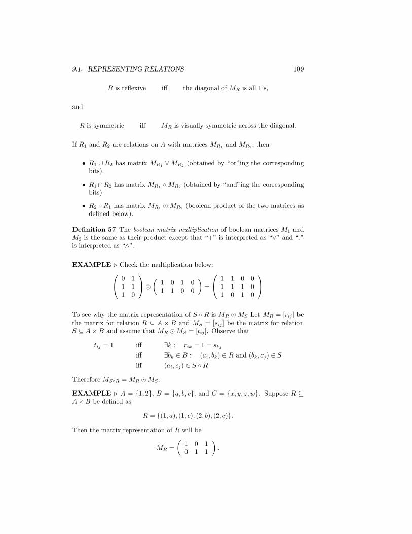
9.1. REPRESENTING RELATIONS 109
R is reflexive i" the diagonal of MR is all 1’s,
and
R is symmetric i" MR is visually symmetric across the diagonal.
If R1 and R2 are relations on A with matrices MR1 and MR2 , then
• R1 7 R2 has matrix MR1 $MR2 (obtained by “or”ing the correspondingbits).
• R1 8R2 has matrix MR1 #MR2 (obtained by “and”ing the correspondingbits).
• R2 BR1 has matrix MR1 CMR2 (boolean product of the two matrices asdefined below).
Definition 57 The boolean matrix multiplication of boolean matrices M1 andM2 is the same as their product except that “+” is interpreted as “$” and “.”is interpreted as “#”.
EXAMPLE ! Check the multiplication below:8
90 11 11 0
:
;C.
1 0 1 01 1 0 0
/=
8
91 1 0 01 1 1 01 0 1 0
:
;
To see why the matrix representation of S B R is MR CMS Let MR = [rij ] bethe matrix for relation R 5 A 3 B and MS = [sij ] be the matrix for relationS 5 A3B and assume that MR CMS = [tij ]. Observe that
tij = 1 i" .k : rik = 1 = skj
i" .bk , B : (ai, bk) , R and (bk, cj) , S
i" (ai, cj) , S BR
Therefore MS(R = MR CMS .
EXAMPLE ! A = {1, 2}, B = {a, b, c}, and C = {x, y, z, w}. Suppose R 5A3B be defined as
R = {(1, a), (1, c), (2, b), (2, c)}.
Then the matrix representation of R will be
MR =
.1 0 10 1 1
/.

110 CHAPTER 9. RELATIONS
Now suppose S 5 B 3 C be the relation
S = {(a, x), (a, y), (a, w), (b, y), (b, z), (c, x), (c, w)}
with the following matrix representation:
MS =
8
91 1 0 10 1 1 01 0 01
:
; .
Then S BR will have the matrix representation:
MR CMS =
.1 1 0 11 1 1 1
/
and therefore
S BR = {(1, x), (1, y), (1, w), (2, x), (2, y), (2, z), (2, w)}.
9.1.2 As Directed Graphs
Definition 58 A directed graph G = (V,E) consists of a set V (vertices) anda set E 5 V 3V (directed edges). In drawing a graph G = (V,E) we representsvertices with points and put directed and edge (an arrow) from vertex a tovertex b if (a, b) , E.
EXAMPLE ! The graph G = (V,E) where
V = {a, b, c, d}
andE = {(a, b), (a, d), (b, b), (b, d), (c, a), (c, b), (d, b)}
can be depicted as
a
d c
b

9.2. CLOSURE 111
Notice that a directed graph is a relation E on a set V .
Given a relation R on a set A, the corresponding directed graph is one withvertex set V = A and edge set E = R.
Let us denote by GR the graph of the relation R.
• R is reflexive if and only if every vertex in GR has a self-loop.
• R is symmetric if and only if all edges come in pairs (one in one directionand the other in the opposite direction).
• R is antisymmetric if and only if no edges come in pair (but self-loops areallowed).
• R is transitive if and only if all triangle are completed like this:
x
y
z
=A
x
y
z
9.2 Closure
Let R be a relation and P be a property (reflective, symmetric, transitive, etc.). If R has property P , then R is closed under P . If R does not have propertyP , we may want to “close” R, by adding as few pairs as possible to yield arelation R! such that R 5 R! and R! has property P .
Definition 59 Closure of R with respect to P is a relation R! such that
1. R 5 R!
2. R! has property P
3. +S such that (1) and (2) hold for S we have R! 5 S we have R! 5 S.
Note.
1. Closure of a relation with respect to a property may not exists.

112 CHAPTER 9. RELATIONS
2. If a relation R already has property P , then the closure of R with respectto P will be R itself.
EXAMPLE ! R a relation on A. We will denote by r(R) the reflexive closureof R.
r(R) = R 7 {(a, a) : a , A}.
Clearly,
1. R 5 r(R) is true,
2. r(R) is reflexive, and
3. If R 5 S and S reflexive then {(a, a) : a , A} 5 S, so r(R) 5 S.
EXAMPLE ! Let us denote by s(R) the symmetric closure of R. Then
s(R) = R 7 {(b, a) : (a, b) , R}! "# $R!1
.
Clearly,
1. R 5 s(R) is true,
2. s(R) is symmetric, and
3. If R 5 S with S symmetric then s(R) 5 S because R 5 S and everythingin s(R)*R must be in S also. Otherwise S will not be symmetric.
9.2.1 Transitive Closure
Using a similar technique as in the previous two examples we may come up withthe following definition for c(R), the transitive closure of R:
c(R) = R 7 {(a, c) : .b (a, b) , R, (b, c) , R}.
But this doesn’t work as shown in the following example.
EXAMPLE ! A = {1, 2, 3, 4, 5} and R = {(1, 2), (2, 3), (3, 4), 4, 5)}. Thenapplying the definition above, we get
c(R) = {(1, 2), (2, 3), (3, 4), (4, 5), (1, 3), (2, 4), (3, 5)}.
But this relation is not transitive because it contains (1, 3) and (3, 4) but doesnot contain (1, 4).
Solution. Do it over and over and over and . . . .

9.2. CLOSURE 113
Definition 60 A path in a directed graph is a sequence of edges
(x0, x1), (x1, x2), (x2, x3), . . . , (xn#1, xn).
The path as defined above:
• is from x0 to xn.
• has length n.
• if x0 = xn is a cycle or circuit.
• if all xi’s are di"erent is a simple path.
EXAMPLE ! In the graph of top of page 86, adb is a simple path, bdbb is acircuit, and abdbb is a path.
Since relations on a set are really graphs, the notion of path makes sense also.
Definition 61 A path in a relation R on set A from a to b is a sequence ofelements
a, x1, x2, . . . , xn#1, b
such that
(a, x1) , R+1 / i < n* 1 (xi, xi+1) , R(xn#1, b) , R
Lemma 2 If t(R) is the transitive closure of R and if R contains a path froma to b, then (a, b) , t(R).
Proof. Let R contain a path
a& x1 & x2 & . . .& xn#1 & b
from a to b. In other words R contains the pairs
(a, x1), (x1, x2), . . . , (xn#2, xn#1), (xn#1, b).
Then since R is transitive it will contain the other following pairs.

114 CHAPTER 9. RELATIONS
(a, b)
(a, xn#1)
...
(a, x4)
(a, x3)
(a, x2)
(a, x1) (x1, x2)
(x2, x3)
(x3, x4)
(xn#1, b)
!
EXAMPLE ! R = {(a, b), (a, c), (b, c), (c, d), (d, e), (d, b)}. Then abcde is apath and therefore by the above theorem (a, e) , t(R).
To determine the transitive closure of a relation:
1. Represent the relation as a graph.
2. For each pair of vertices (a, b), determine if there exists a path from a tob.
• If so, then (a, b) , t(R).
• If not, then (a, b) ", t(R).
Note.
1. The above method uses problem of checking whether there is a path be-tween a pair of vertices (or equivalently the graph connectivity problem).You will see e!cient algorithms for these problems in later classes.
2. There is a more e!cient, though more confusing method. Read aboutWarshall’s Algorithm in the text.
3. We can also use the Boolean Matrix Multiplication to solve this problem.The intuition is to compute R 7R2 7 . . . 7Rn.

Chapter 10
Equivalence Relations andPartial Orders
10.1 Equivalence Relations
The motivation to study equivalence relations is to focus only on properties ofobjects instead of objects themselves. All objects with the same property willbe “equivalent”.
Definition 62 An equivalence relation R on a set S is a relation that is
1. reflexive, i.e. +a , S aRa. we will use the notation aRbwhere R is a relation to denote(a, b) , R.2. symmetric, i.e. +a, b , S aRb' bRa.
3. transitive, i.e. +a, b, c , S aRb # bRc& aRc.
EXAMPLE ! Let S = { people in the class} and
R = {(a, b) : a has the same number of coins in pocket/purse as b }
Clearly R is reflexive, symmetric, and transitive and thus R is an equivalencerelation.
EXAMPLE ! S = Z and R = {(a, b) : a ( b mod 4}. Thus
• 0 ( 4 ( 8 ( 12 ( 16 · · · (all with remainder 0),
• 1 ( 5 ( 9 ( 13 ( 17 · · · (all with remainder 1),
115
116CHAPTER 10. EQUIVALENCE RELATIONS AND PARTIAL ORDERS
• 2 ( 6 ( 10 ( 14 ( 18 · · · (all with remainder 2),
• 3 ( 7 ( 11 ( 15 ( 19 · · · (all with remainder 3).
EXAMPLE ! Let S = {people of this class} and
R = {(a, b) : total cash on a is within $1.0 of total cash on b}
This relation is reflexive and symmetric by it is not transitive because a, b, andc can have $20, $21 and $22 respectively. Then we have aRb and bRc but a/Rb.
10.2 Equivalence Classes
Definition 63 Let R be an equivalence relation on S. The equivalence class ofa , S written [a]R is defined by
[a]R = {b , S : (a, b) , R}.
Thus [a]R is the set of all elements of S that a relates to, i.e. is equivalent to.
EXAMPLE ! Taking the equivalence relation on a few example ago based onthe number of coins in pocket/purse we have
[Prof. Pitt]R = {people with 5 coins in pocket/purse}.
Note that the collection of all equivalence classes for this relation are
• {people with 0 coins in pocket/purse}
• {people with 1 coins in pocket/purse}
• {people with 2 coins in pocket/purse}
• {people with 3 coins in pocket/purse}
• . . .
EXAMPLE ! S = Z and R = {(a, b) : a ( b mod 4}. Then [17]R ={. . . ,*7,*3, 1, 5, 9, 13, 17, . . .}. All classes are [0], [1], [2], and [3].
Definition 64 We call a a representative for equivalence class [a]R.
Note that if aRb (thus, if b , [a]R), then b is also a representative of [a]R.
EXAMPLE ! 17 is a representative of the class {. . . ,*7,*3, 1, 5, 9, 13, 17, . . .}.In fact every number of the form 4k + 1 is a representative for this class.

10.2. EQUIVALENCE CLASSES 117
Question. What do the equivalence classes of a a relation R on set S looklike?
We will show that they subdivide S into disjoint pieces. In particular, we can’thave two di!erent equivalence classes with non empty intersection.
To see this, consider the following lemma.
Lemma 3 Let R be an equivalence relation on a set S. Then
a) If aRb then [a]R = [b]R (the equivalence classes are identical).
b) If a/Rb then [a]R8[b]R = 4 (the equivalence classes are completely disjoint).
Proof. a) Suppose aRb. Now for x , S:
x , [a]R ) aRx definition of [a]R
) xRa symmetry of R
) xRb xRa and aRb
and R is transitive
) bRx symmetry of R
) x , [b]R definition of [b]R
Thus x , [a]R ) x , [b]R. So, [a]R = [b]R.
b) Proof by contradiction. Suppose to the contrary that
.x , [a]R 8 [b]R.
Then by the definition of [a]R and [b]R we know that aRx and bRx. By symme-try these become aRx and xRb. But then by transitivity of R we obtain aRbcontradicting the assumption that a/Rb. !
The two parts of the previous lemma together show that [a]R and [b]R are alwayseither identical or disjoint.
Note that if R is an equivalence relation on S then why?
S =&
a)S
[a]R.
Thus the equivalence classes of R “completely cover” S in the follow-ing way: S is the union of disjoint equivalence classes of R.

118CHAPTER 10. EQUIVALENCE RELATIONS AND PARTIAL ORDERS
S
[a]R
[b]R
[c]R
[d]R [e]R
· · ·
Such a cover of a set has a di"erent name.
Definition 65 A partition of a set S is a (perhaps infinite . . . perhaps uncount-ably infinite) collection of sets {Ai} such that
• each Ai is non-empty.
• each Ai 5 S.
• 7Ai = S.
• +i, j Ai 8 Aj = 4.
Each Ai is called a block of the partition.
EXAMPLE ! R = {rationals} 7 {irrationals} (2 blocks).
EXAMPLE ! R = {1} 7 {2} 7 {3} 7 {4} 7 { other reals}.
Theorem 6 a) If R is an equivalence relation on S, then
{[a]R : a , S}
is a partition of S, i.e., the equivalence classes of R partition S, and eachequivalence class is a block of this partition.
b) If {Ai} is any partition of S, then there exists an equivalence relation whoseequivalence classes are exactly the blocks Ai of S.
Proof. a) We’ve already noted that S = 7a)S [a]R, and each [a]R is nonempty(because it at least contains a itself) and [a]R 7 [b]R = 4 (unless aRb).
b) If {Ai} partitions S, then define the equivalence relation R on S by
R = {(a, b) : .i a , Ai and b , Ai}.
(Thus aRb if and only if a and b are both in the same block Ai together).Clearly, R is reflexive, symmetric. We now show that R is transitive as well.
Suppose aRb and bRc. Then by the definition of R given above:

10.3. PARTIAL ORDERS 119
1. There exists an i such that a and b are both in Ai, and
2. There exists a j such that b and c are both in Aj .
But b , Ai 8 Aj , so Ai must equal Aj (else wasn’t a partition). So, a, b, c , Ai
and in particular aRc. !
10.3 Partial Orders
Definition 66 If R is a relation on a set S, then (S,R) is a partial order andS is a called a partially ordered set (or a poset) if and only if R is
1. reflexive, i.e. +a aRa
2. transitive, i.e. +a, b, c aRb # bRc& aRc
3. antisymmetric, i.e. +a, b aRb # bRa& a = b.
EXAMPLE ! (/,R), i.e. the “less than or equal” relation on R is a partialorder.
EXAMPLE ! “divides” on Z+, i.e. (Z+, |) is a partial order. This because
• reflexive: a|a
• transitive: If a|b and b|c then a|c (easy)
• antisymmetric: If a|b and b|a, then there exist k1, k2 both positive suchthat k1a = b and k2b = a. Thus k1a = a/k2, or k1k2 = 1. So k1 = k2 = 1and thus a = b.
EXAMPLE ! (Z, |) is not a partial order because 1|* 1 and *1|1 but 1 "= *1.
EXAMPLE ! Let S be any set. Then (2S ,5) is a partial order.
Definition 67 Notation. The sign “/” will be used to define an arbitraryrelation that is reflexive, transitive, and antisymmetric. We will write a / b tomean aRb. We will also write a < b if a / b but a "= b.
EXAMPLE ! A standard partial order on {0, 1}n (the set of bit strings oflength n) is defined as
a1a2 . . . an / b1b2 . . . bn
120CHAPTER 10. EQUIVALENCE RELATIONS AND PARTIAL ORDERS
if and only if+i ai / bi.
Thus 0110 / 1110 and 0110 is incomparable to 1011. The above relation definesa partial order which corresponds exactly with the partial order of (2S ,5) fora set S of size n.
For example for a set S = {a, b} of size two, the power set of S consists of
4, {b}, {a}, {a, b}
Think of bit-strings as characteristic vectors of the elements of the power set.
00, 01, 10, 11
. In the relation we defined on bit strings 00 < 10 because each bit of 00 is lessthan or equal to the corresponding bit of 10. In other words 10 has at least allof the “1” bits as 00, and perhaps more.
So the set 10 represents contains the set represented by 00 and in fact we cancheck that 4 5 {a}.
Definition 68 Let (S,/) be a partial order. Then a and b are comparable ifeither a / b or b / a (or both).
Otherwise, they are incomparable.
EXAMPLE ! For (Z, |): 6 and 3 are comparable, 3 and 3 are comparable, 3and 5 are incomparable, and 8, 12 are incomparable.
In fact we call a partially order set so since not all things need to becomparable.
Definition 69 A total order is a partial order in which every pair of elementsare comparable.
EXAMPLE ! (Z,/) is a total order.
EXAMPLE ! Lexicographic ordering of strings. This is defined below.A total order used a lot in CS.
Definition 70 Having fixed a usual order on an alphabet %, for example theorder a < b < c < d < · · · < z if the alphabet are English letters, for any pair ofgiven strings & = x1x2 . . . xm and ' = y1y2 . . . yn in %' we define the followingordering:
To determine if & / ' let t = min{m,n} (shorter length). If
x1x2 . . . xt = y1y2 . . . yt

10.3. PARTIAL ORDERS 121
then shorter of & and ' comes first. Else let i / t be the smallest number suchthat xi "= yi (i is the first position where they di"er). If xi < yi then & < ' andotherwise ' < &.
EXAMPLE ! For the usual ordering on English alphabet we havediscreet < discreetness < discrete < discretion
10.3.1 Hasse Diagrams
We can represent posets as graphs. Consider the partial order ({1, 2, 3, 4},/).
1
2
3
4
In drawing Hasse diagrams
• We draw an edge from a to b if and only if a / b
• We do not draw the direction of the edges and assume that they all pointup.
• We do not draw self-loops, since we know they are there (all posets arereflexive).
• We do not bother drawing transitive edges (transitive edges are elimi-nated).
EXAMPLE ! (2{a,b,c},5) (same as bitwise / on {0, 1}3).

122CHAPTER 10. EQUIVALENCE RELATIONS AND PARTIAL ORDERS
000/4
010/{b}
011/{b, c}
100/{a}
101/{a, c}
001/{c}
110/{a, b}
Definition 71 Let (S,/) be a partial order. Then an element a , S is aminimal element if there exists no b such that b < a. Similarly, a , S is calleda maximal element if there exists no b such that a < b.
EXAMPLE ! Consider the poset represented by the following Hasse diagram
a b
c
f
d e
Maximal elements of the above poset are {a, b, c, f} and the minimal elementsare {d, e, f}.
Note. maximal and minimal elements need not be unique and a poset can haveseveral maxima and minima. Some points can be both maximal and minimal.
Question. Must there always exist some maximal or minimal elements?
Answer. Only if set is finite (consider (Z,/)).
Definition 72 In a poset S an element a is a minimum element if +b , S a / b.Similarly, an element a is a maximal element if +b , S b / a.
Note the di!erence of mum andmal.
Note. Intuitively when we say a is maximal it means that nothing beats a.But when we say that a is maximum it means that a beats everything.
EXAMPLE ! In the following poset a is maximum and b is minimum.

10.3. PARTIAL ORDERS 123
a
b
Question. Must maximum and minimum exist? Answer. No, same reason.
Note. If a is a maximum element, then a is a maximal element too (why?).Similarly, If a is a minimum element, then a is a minimal element too (why?).
Question. If maximum exists, is it unique i.e., can there be two di"erentmaximums?
Theorem 7 In every poset if the maximum element exists, it is unique. Simi-larly, in every poset if the minimum element exists, it is unique.
Proof. If a1 "= a2 and both are maximum, then a1 / a2 because a2 is maxi-mum and a2 / a1 because a1 is maximum. But then since “/” is antisymmetric,this implies that a1 = a2 contradicting a1 "= a2. So, only one maximum mayexist.
The argument for the uniqueness of minimum is similar. !
10.3.2 Upper and Lower Bounds
Definition 73 Let (S,/) be a partial order. If A 5 S, then an upper boundfor A is any element of S (perhaps in A also) such that +a , A a / x.
Similarly, a lower bound for A is a any x , S such that +a , A x / a.
EXAMPLE ! consider the following poset.

124CHAPTER 10. EQUIVALENCE RELATIONS AND PARTIAL ORDERS
a b
c
e
g h i
fj
d
Here the only upper bound of {g, j} is a, upper bounds of {g, i} are a, c, and e.The upper bounds of {i, j} are a, b, and d. The only upper bound of {a, d} isa and {a, b} have no upper bound.
The lower bounds of {a, b} are d, f , i, and j. The lower bounds of {c, d} are f ,and i. and {q, j} has no lower bounds.
Definition 74 Given a poset (S,/), and A 5 S, an element x , S is a greatestlower bound for A if x is a lower bound and for lower bound y of A, y / x.
Similarly, x is a least upper bound for A if x is an upper bound and if x / y forevery upper bound y of A.
EXAMPLE ! In the previous example lub(g, j) = a, lub(g, i) = e, lub(i, j) =d, glb(g, j) does not exist. glb(c, d) = f and glb(a, b) = d.
Note. Sometimes lub and glb don’t exist, even thought lower and upperbounds do exist.
EXAMPLE ! In the following poset
a b
c d
c and d are both lower bounds for {a, b} but neither is a glb. Also a and b areboth upper bounds for {c, d} but neither is a lub.

10.3. PARTIAL ORDERS 125
10.3.3 From Partial Orders to Total Orders
Consider the problem of getting dressed. Who said this course has no prac-tical applications?
Precedence constraints are modeled by a poset in which a / b if and only if youmust put on a before b.
socks
shoes
pants
uware
belt
jacket
overcoat
shirt
tie
Problem. how to get dressed, while respecting the constraints?
Clearly many solutions are possible. This is the problem of extending a partialorder to a total order.
Let (S,/) be a partial order with S finite. We show how to extend / to a totalorder on S. (i.e. can decide for all incomparable pair a and b whether to makea / b or vice versa, without violating transitivity, reflexivity, or antisymmetry.
Lemma 4 Every finite nonempty poset (S,/) has at least one minimal element.
Proof. Choose a0 , S. If a0 was not minimal, then there exists an a1 / a0,so choose a1. If this is not minimal, choose a2 / a1, and so on until a minimalelement is found. (why must this work?) !
Lemma 5 If (S,/) is a poset with a minimal, then (S*{a},/) is also a poset.
Proof. If you remove minimal a, reflexivity still holds and antisymmetry alsostill holds. If x, y, z , S * {a}, with x / y and y / z, then x / z also, since(S,/) was transitive. !
Think about Lemmas 1 and 2:

126CHAPTER 10. EQUIVALENCE RELATIONS AND PARTIAL ORDERS
1. Always there exists a minimal element.
2. If you remove it, you still have a poset.
This suggests:
algorithm Topological SortInput: poset (S,/)Output: elements of S in some total order.
1 begin2 Remove any minimal element from S and output it3 If S "= 4 goto 27 end
Depending on which minimal element is chosen at step 2 each time, a di"erenttotal order may be obtained. But all obtainable total orders will be consistentwith the original partial order.Probably an easy inductive proof
shows this.
EXAMPLE ! For the following poset
e f
gc d
a b
We first remove the minimal element e and obtain
f
gc d
a b
Then we remove the minimal element g and obtain
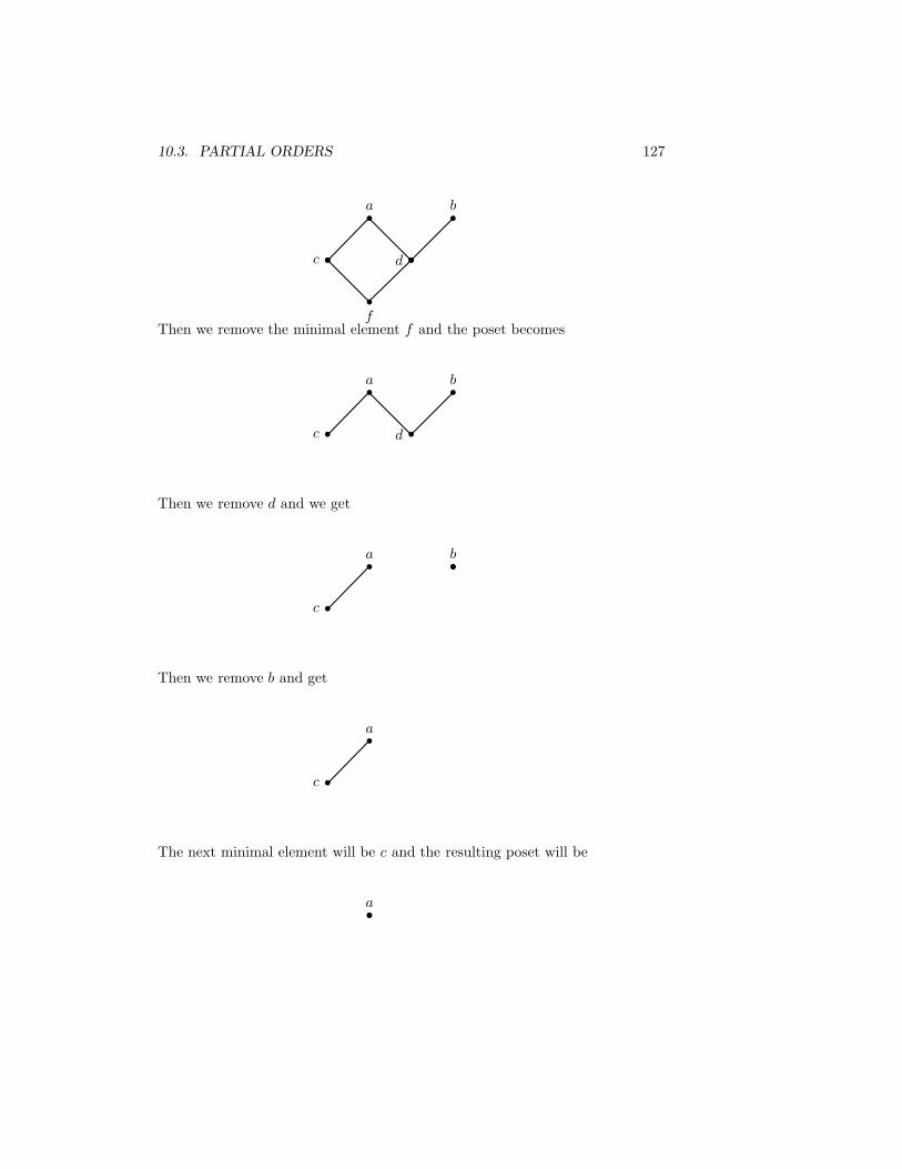
10.3. PARTIAL ORDERS 127
f
c d
a b
Then we remove the minimal element f and the poset becomes
c d
a b
Then we remove d and we get
c
a b
Then we remove b and get
c
a
The next minimal element will be c and the resulting poset will be
a

128CHAPTER 10. EQUIVALENCE RELATIONS AND PARTIAL ORDERS
Eventually we remove c and the algorithm terminates. The resulting total orderis then
e / g / f / d / b / c / a.