Computer Science Technical Report

A Practical Self-Stabilizing Leader

Election for Networks of

Resource-Constrained IoT DevicesMichael Conard and Ali Ebnenasir

Michigan Technological UniversityComputer Science Technical Report

CS-TR-21-01April 2021

Department of Computer ScienceHoughton, MI 49931-1295

www.cs.mtu.edu

A Practical Self-Stabilizing Leader Election for Networks of

Resource-Constrained IoT Devices

Michael Conard and Ali Ebnenasir

April 2021

Abstract. This paper presents a self-stabilizing and tunable leader election algorithm, called PraSLE, de-signed for real-world testbeds of resource-constrained devices in the Internet of Things (IoT). PraSLE is anextended version of the minimum finding algorithm that functions in a round-based asynchronous fashion.We provide a version of PraSLE for both reliable and unreliable networks. We show that PraSLE electsa unique leader in unreliable networks with probability 1. We also experimentally validate this result anddemonstrate that PraSLE outperforms existing methods in terms of average convergence time for ring, line,and mesh topologies up to 40 nodes, and for the clique topology up to 80 nodes. The tunable nature ofPraSLE enables engineers to optimize average convergence time, as well as communication and energy costs.PraSLE provides an important resource-efficient Distributed Computing Primitive (DCP) for unreliable net-works of low-end IoT devices based on which other DCPs (e.g., Paxos) can be developed for such networksin the domains of IoT and Cyber Physical Systems (CPS).

Keywords. Leader Election, Self-stabilization, Resource-constrained Devices, IoT

1

Contents

1 Introduction 3

2 Problem Statement 4

3 The PraSLE Algorithm 53.1 Correctness . . . . . . . . . . . . . . . . . . . . . . . . . . . . . . . . . . . . . . . . . . . . . . 5

4 Experimental Results 8

5 Tuning K and T 13

6 Related Work 18

7 Conclusion and Future Work 20

2

1 Introduction

The development of Distributed Computing Primitives (DCPs) for resource-constrained distributed systemsis an important challenge in the Internet of Things (IoT) and Cyber Physical Systems (CPSs) applications.Examples of such DCPs include leader election, consensus, spanning tree formation, distributed reset, etc.Developing lightweight DCPs that can be deployed in real-world unreliable networks (e.g., UDP/IP) is achallenging problem. More importantly, such networks are subject to transient faults such as bad initial-ization and loss of coordination, and they are expected to correctly execute DCPs despite the presence ofsuch faults. One of the important distributed algorithms that has applications in numerous settings (e.g.,broadcast, Paxos [16]) includes the Leader Election (LE) algorithm. While there are numerous algorithmsdeveloped for LE, it is desirable to have a resource-efficient, scalable, and self-stabilizing implementation ofLE that can provide a sub-linear average convergence time on unreliable networks and in the presence oftransient faults.

Numerous approaches exist for leader election in IoT and networks of resource-constrained devices, mostof which validate their protocol through simulation and lack evaluations on a real-world testbed. For example,Mendez et al. [18] implement the Bully algorithm [12] on a clique network where the process that has themaximum identifier (ID) becomes the leader. However, they provide little experimental results on a physicaltestbed. The Minimum Finding (MinFind) algorithm [21] extends the idea of the Bully algorithm, whereeach node broadcasts a randomly generated value (or its ID) and then enters a cycle of reading and relayingthe minimum value through broadcast. Bounceur et al. [3] present a Wait-Before-Send (WBS) protocolfor synchronous networks, where each node waits for min × t seconds before sending out its min value.Bounceur et al. [2] also present an energy-efficient algorithm for LE, Branch Optima to Global Optimum(BROGO), where a spanning tree is formed by flooding rooted at a specific node whose ID is known toeveryone. Sheshashayee et al. [23] put forward a protocol for electing the top k leaders in an asynchronousclique network with a broadcast primitive, and evaluate it through simulation and on a testbed of just 11nodes.

Most aforementioned approaches are evaluated through simulation or validation on small-scale testbedsof less than 30 nodes. Moreover, it is unclear if the underlying network is a UDP-based network. Someexisting methods assume a synchronous network. For example, the WBS method requires that all processesare synchronized at the start of the protocol, which is hard to ensure in large-scale distributed systems.Some approaches are asymmetric in that the code of some nodes are different from the rest of the nodes.Asymmetric LE algorithms are harder to implement and are more costly in terms of communication andenergy (e.g., BROGO [2]). Another restrictive assumption for a practical real-world LE implementationincludes the topology; where most existing methods assume a clique topology, we provide an efficient,tunable implementation and demonstrate it on ring, line, tree, mesh, and clique topologies. Last but notleast, our experiments show that PraSLE can easily scale up to networks of about 80 nodes with close tosub-linear increase in average convergence time, which is an important property for practical use in IoT andCPSs.Contributions. First, we present a practical, self-stabilizing and tunable version of the MinFind algorithm,called PraSLE1, that takes two parameters: maximum network latency and a diameter-proportional value.Mainstream engineers can use these parameters as knobs for tuning PraSLE to their platform, therebystriking a balance between robustness and resource efficiency. Second, our algorithm is self-stabilizing in thatit can recover to electing a unique leader from transient perturbations to arbitrary states. We provide variantsof PraSLE for both reliable and unreliable networks. We prove the correctness of PraSLE, and show thatit converges with probability 1 (in unreliable networks). Third, in contrast with most existing methods, weactually implement our algorithm (instead of just simulating it) on the RIOT operating system [1] in networksof up to 80 machines with Cortex-M3 processors in the IoT-Lab (www.iot-lab.info). Fourth, PraSLE issymmetric in that all nodes have the same piece of code up to variable renaming. Symmetry is an importantfeature for ease of use and energy consumption. Fifth, our communication model is timed asynchronous,where we have no synchronization assumption. We evaluate PraSLE using the unicast primitive on a UDP/IP

1Implementation source code available at https://github.com/maconard/cps-iot_leader-election

3

network (see Section 4). Sixth, while most existing methods consider a clique topology, we evaluate PraSLEon ring, line, tree, mesh, and clique topologies. Our experiments show that leader election on mesh is themost resilient and time, communication, and energy-efficient election. This is an interesting result for settingswhere engineers have the liberty of configuring their desired topology. Finally, we experimentally evaluatePraSLE with respect to three metrics: average convergence time, communication costs, and energy costs.Our experiments show that PraSLE’s average convergence time grows very slowly like a linear function (innetworks of up to 80 nodes) with a tiny slope that varies from 0.02 to 0.04 for different topologies. Theaverage number of messages exchanged grows linearly for all topologies (except clique), but significantlyslower for line and ring. The energy consumption of the entire network grows like a step function for line andring with a tiny step of 0.05J. For mesh and clique, energy costs grow linearly but with a tiny slope of 0.04for up to 40 nodes. Once the network scales beyond 40 nodes in clique the slope of the linear growth becomes0.07. We note that we created these topologies as overlay networks, and achieving such resource efficiencyon these overlay networks using a unicast primitive is a significant contribution by itself. In summary, ourexperiments show that PraSLE is a resilient, scalable, and resource-efficient leader election protocol for real-world networks of low-end devices. To the best of our knowledge, no other implementation of leader electionexhibits such characteristics on a wide range of topologies and in unreliable UDP networks.Organization. Section 2 states the LE problem. Section 3 present the PraSLE algorithm along with itsproof of correctness. Section 4 provides our experimental results. Section 5 expands on our experimentalresults in regards to the tunable values of PraSLE. Section 6 discusses related work. Finally, Section 7 makesconcluding remarks and discusses future extensions of this work.

2 Problem Statement

This section states the problem of Leader Election (LE) in a distributed system as well as presenting thepractical requirements under which we should solve the LE problem.

Given is a set of computing nodes/processes connected through a communication network. Doesthere exist an algorithm deployed on each process such that all processes collectively elect a uniqueprocess as the leader without reliance on any centralized authority?

While there are numerous methods for solving the LE problem under different settings (see Section 6), ourobjective is to provide a simple solution that is both self-stabilizing and can be deployed on practical networks(e.g., UDP/IP) for a large number of nodes. Thus, we first discuss the computation and communicationmodels under which we solve the LE problem.Computation model. The processes are symmetric in that the codes of any pair of processes are similarup to variable renaming/re-indexing. Each process pi has a unique identifier IDi, which can simply be itsassigned IPv6 address. Each instruction/action of the algorithm has a finite execution time. Actions areread-write atomic; that is, each read or write action is considered atomic. For example, checking the truthof a condition may not necessarily be atomic, but it contains atomic actions for reading the components ofthe condition. Each process has a ranking value, denoted mini (e.g., Line 4 in Figure 1), that defines thepotential of that process for becoming the leader. The lower the value of mini, the higher the likelihoodof pi becoming the leader. Such a ranking value could be randomly generated or may be a function (e.g.,getRankingValue() in Line 5 of Figure 1) of quantitative metrics such as battery life, processing power, availablememory, workload, etc. The variable leaderi in each process pi (e.g., Line 6 in Figure 1) holds the ID of theprocess that pi believes to be the leader.Communication model. The communication model of our algorithm is timed asynchronous, where mes-sages may be delivered by a maximum delay known by all nodes (denoted T in Figure 1). We consider bothreliable and unreliable networks, where messages may be lost. The underlying network topology determinesthe neighborhood of each process.Fault and failure models. The value of mini (representing the ranking function) may be perturbed bytransient faults, which could result in the perturbation of the global state of the system. Examples oftransient faults include soft errors (which cause random bit flips in memory), bad initialization, and loss of

4

coordination. Processes may also fail in a detectable manner (using a time out mechanism), and messagescould get lost in communication.

3 The PraSLE Algorithm

This section presents a self-stabilizing solution for the LE problem where starting from any arbitrary initialvalues of mini, the entire network will eventually elect a unique leader whose identity will be known foreach process. Since our main objective is to design an algorithm that can be implemented and deployedon real-world large-scale networks (e.g., the Internet), we call it Practical Self-stabilizing Leader Election(PraSLE). We also derive a probabilistic version of the proposed algorithm that will elect a leader withprobability 1 in unreliable networks.

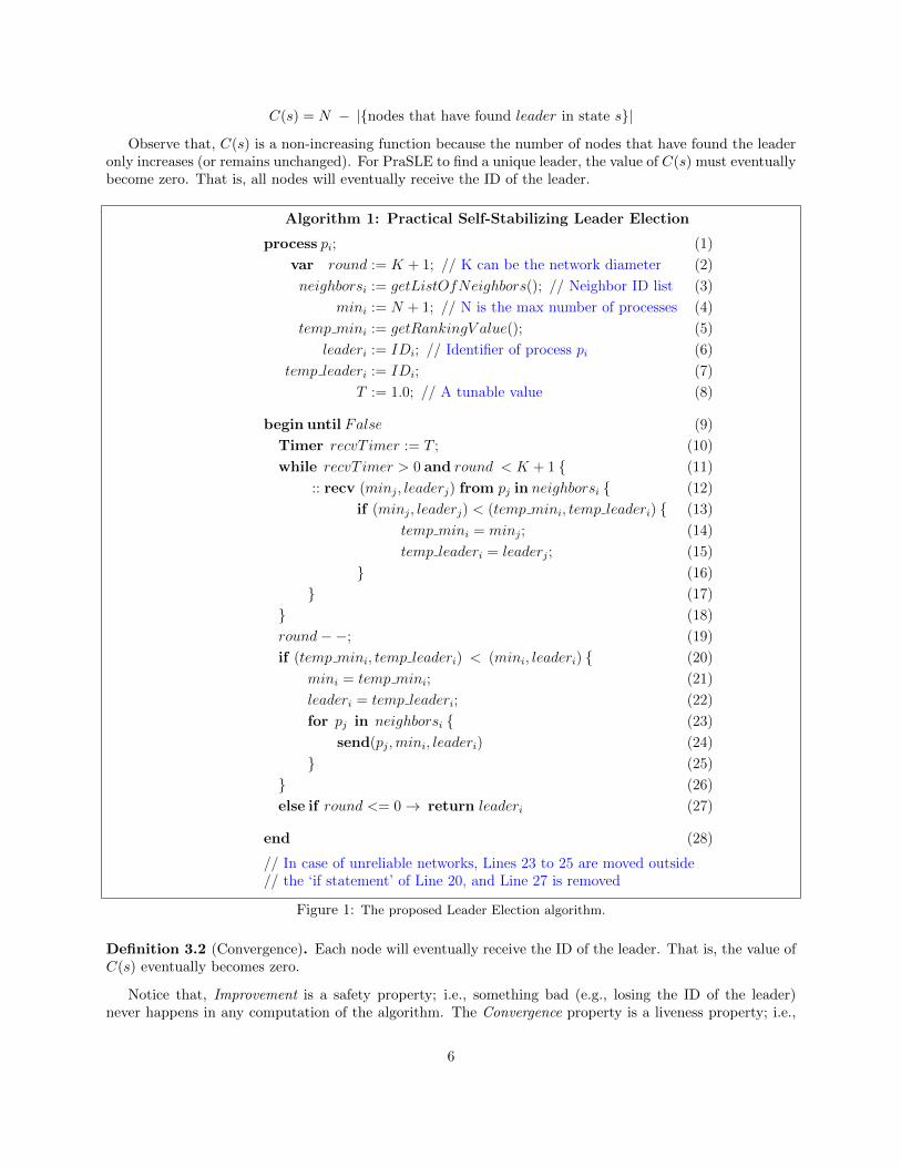
We first discuss a deterministic version of PraSLE where we assume reliable communication (i.e., messagesare delivered up to an upper bound delay known by each process). Figure 1 illustrates the pseudo code of arepresentative process in PraSLE. Each process executes in a round-based fashion and the rounds in differentprocesses need not be synchronized. However, we require that from the time a node sends a message untilthe message is received, the sender can perform a finite number of rounds. The algorithm runs for at least Krounds (Line 2 in Figure 1), where K can initially be the diameter of the network, denoted DLE , but couldbe initialized with other values too. In the first round, the condition of the while loop is false (because roundis equal to K + 1) and each process sends its mini and leaderi values to its immediate neighbors (Lines 20to 26). Starting from the second round, all processes go through repetitive execution of three main tasks:(1) collect information from neighbors for T seconds (Lines 11 to 18); (2) update local knowledge about whothe leader is (Lines 20 to 22), and (3) disseminate local knowledge to immediate neighbors (Lines 23 to 25).Note that any node can initiate the election and the nodes will propagate that event to their neighbors; thissnippet is excluded from Figure 1 for brevity.

Task 1 is to listen for T seconds to receive new information from neighbors which was sent out in theconclusion of the previous round (i.e.; the previous Task 3). When a message is received by process pi fromsome neighbor pj , process pi updates its local information with minj and leaderj if the pair (minj , leaderj)is smaller than the pair (temp mini, temp leaderi) (see Lines 14-15 in Figure 1). We say that (m, ID) <(m′, ID′) if and only if (iff) (m < m′) ∨ ((m = m′) ∧ (ID < ID′)). Even if process pi receives a messagefrom all of its neighbors it will still wait the full T seconds of the round duration before moving on.

Task 2 is simply a comparison between the most recent values of the leader and its ID in the currentround with the best values of the previous round. If the values of the current round (saved in the pair(temp mini, temp leaderi)) are a better choice then the pair (mini, leaderi) is updated (in Lines 21 and 22)to those values. Otherwise, no changes are made.

Task 3 is the dissemination of new best leader information to immediate neighbors. This can be imple-mented with a broadcast or uni-cast primitive. In a naive implementation the nodes can send their bestchoice of leader to their neighbors every round regardless of whether it is new information or not. However,a simple optimization is to have nodes track which neighbors already know the information they have andexclude them from the update, which significantly improves message complexity. This improvement is notdepicted in Algorithm 1 for simplicity, but we have implemented it in the code used for experimentation.

3.1 Correctness

This section defines the important requirements of PraSLE and then proves the correctness of the algorithmunder reliable and unreliable network assumptions. First, we define the improvement requirement as follows:

Definition 3.1 (Improvement). Once a process receives the ID of the global leader it will never lose it.Thus, once a unique leader is identified and every node has received its ID, it remains the leader of everyone.

In order to formalize the notion of improvement, we define the function C(s) from the set of global statesof the algorithm to {0, 1, · · · , N − 1}, where a global state is a global snapshot of the values of variables ofall processes:

5

C(s) = N − |{nodes that have found leader in state s}|Observe that, C(s) is a non-increasing function because the number of nodes that have found the leader

only increases (or remains unchanged). For PraSLE to find a unique leader, the value of C(s) must eventuallybecome zero. That is, all nodes will eventually receive the ID of the leader.

Algorithm 1: Practical Self-Stabilizing Leader Election

process pi; (1)

var round := K + 1; // K can be the network diameter (2)

neighborsi := getListOfNeighbors(); // Neighbor ID list (3)

mini := N + 1; // N is the max number of processes (4)

temp mini := getRankingV alue(); (5)

leaderi := IDi; // Identifier of process pi (6)

temp leaderi := IDi; (7)

T := 1.0; // A tunable value (8)

begin until False (9)

Timer recvT imer := T ; (10)

while recvT imer > 0 and round < K + 1 { (11)

:: recv (minj, leaderj) from pj in neighborsi { (12)

if (minj, leaderj) < (temp mini, temp leaderi) { (13)

temp mini = minj; (14)

temp leaderi = leaderj; (15)

} (16)

} (17)

} (18)

round−−; (19)

if (temp mini, temp leaderi) < (mini, leaderi) { (20)

mini = temp mini; (21)

leaderi = temp leaderi; (22)

for pj in neighborsi { (23)

send(pj,mini, leaderi) (24)

} (25)

} (26)

else if round <= 0→ return leaderi (27)

end (28)

// In case of unreliable networks, Lines 23 to 25 are moved outside// the ‘if statement’ of Line 20, and Line 27 is removed

Figure 1: The proposed Leader Election algorithm.

Definition 3.2 (Convergence). Each node will eventually receive the ID of the leader. That is, the value ofC(s) eventually becomes zero.

Notice that, Improvement is a safety property; i.e., something bad (e.g., losing the ID of the leader)never happens in any computation of the algorithm. The Convergence property is a liveness property; i.e.,

6

something good will eventually occur in every computation of the algorithm.Correctness in reliable networks. First, we prove the correctness of the algorithm (with respect toimprovement and convergence) under the assumption of a reliable network, where messages are delivered ina finite amount of time and no messages are lost.

Theorem 3.3. It is always the case that, starting from any state, PraSLE meets the improvement require-ment. Formally, �(C(si) ≥ C(si+1)), where � denotes the ‘always’ temporal operator, and (C(s) ≥ C(s+1))states that C(s) remains non-increasing when transitioning from a state si to its subsequent state si+1.

Proof. We will show that PraSLE satisfies the Improvement property via an induction on an arbitrarycomputation. Let c be a computation < s0, s1, ..., sm > of length m which starts in state s0 and where(si,si+1) is a state transition for i ≥ 0. We model the global state transition system of the algorithm as anon-deterministic finite state machine, where each state is a global snapshot of the local state of each node,and each transition captures message transmission, receipt of a message, or executing a local instruction onany node. Note that only Lines 21-22 of the algorithm are capable of impacting the value of C.

Base case. In the initial state s0, C(s0) ≥ C(s1) holds because at the start of the algorithm it is impossibleto update mini and leaderi, and messages are not sent or received yet.

Inductive hypothesis. Let C(sk−1) ≥ C(sk), for k ≥ 2.Inductive step. We must consider the different possible state transitions that could be performed from

any state sk and show that C(sk) ≥ C(sk+1) must hold. If the state transition (sk,sk+1) is the executionof any machine instruction other than those from Lines 21-22, then the value of C is unchanged and theinductive hypothesis holds as C(sk) = C(sk+1). If (sk, sk+1) is the execution of the instructions fromLines 21-22, then because of the condition on Line 20 the information being stored to mini and leaderimust be better than the previous values. If these new values are not the global leader’s then C remainsunchanged; i.e., C(sk) = C(sk+1). If these new values are the global leader’s then C is decremented byone and C(sk) > C(sk+1). Since the network forms a connected graph, at least one node must find theleader and decrement C this way in every round of the algorithm. There is no case where the value of C isincreased. Therefore, we have C(sk) ≥ C(sk+1); i.e., PraSLE satisfies the Improvement property.

Theorem 3.4 (Convergence). PraSLE will eventually elect a unique leader. That is, ♦(C(s) = 0) holds,where ♦ denotes the ‘eventually’ temporal operator.

Proof. Similar to the proof of Theorem 1, at least one node will obtain the global leader’s information ineach round which will reduce the value of C by at least 1. In the worst case, when the global leader is DLE

hops away from some node in the network, that node will receive the information in the DLE-th round.Since C was initialized with N − 1 (a finite value) and the network forms a connected graph, C must reach0 in finite time. Thus, the global state of the election must proceed closer to a unanimous decision where Cconverges to 0; i.e., PraSLE satisfies the Convergence property.

Correctness in unreliable networks. In the case of unreliable networks, we create a revised version ofPraSLE by moving Lines 23 to 25 outside the ‘if statement’ of Line 20, and by removing Line 27. Forsimplicity, we consider a worst case reliability 0 < α < 1 for the network. That is, the probability of amessage being delivered from a sender to a receiver is at least α. Note that when α = 1, we have a reliablenetwork, and when α = 0, the network is totally broken. For example, when a process pi executes a ‘recv’action in Line 12 of Figure 1, the message is received from pj with at least a probability α. Likewise, the‘send’ action in Line 24 would succeed in delivering the mini and leaderi to pj with at least a probabilityα. We follow the technique in [13] and show that Improvement and Convergence hold with probability 1.

Theorem 3.5. Let s0 be a state where C(s0) = L for some 0 < L < N . 2 We show that in any computationof the form 〈s0, s1, s2, · · · 〉, there is some k > 0 where C(sk) = L−1 with probability 1. Formally, ((C(s0) =L) ∧ (0 < L < N)) =⇒ Pr(∃k : k > 0 : (C(sk) = L− 1)) = 1.

2We assume L < N because there is at least one process that has the minimum ranking value.

7

Proof. First, observe that Pr(∃k : k > 0 : (C(sk) = L − 1)) = 1− Pr(∀k : k > 0 : (C(sk) = L)). We showthat Pr(∀k : k > 0 : (C(sk) = L)) = 0; hence, Pr(∃k : k > 0 : (C(sk) = L− 1)) = 1.

Let pi be the process that has the minimum ranking value globally. As such, pi sends mini and leaderito its immediate neighbors. Let ∆ denote the max degree of the underlying network topology. That is, pican have at most ∆ immediate neighbors. The probability that a single neighbor does not receive mini andleaderi is at most 1 − α, and the probability of none of the neighbors receiving mini and leaderi is equalto (1 − α)∆. Thus, the probability of the immediate neighbors of pi never receiving the values would belimk→∞(1−α)k∆. Since (1−α) < 1, we have that limk→∞(1−α)k∆ = 0. Thus, a neighbor must eventuallyreceive the values after some finite k steps of computation with probability 1 and at that time we will haveC(sk) = L − 1. This implies that Pr(∀k : k > 0 : (C(sk) = L)) = 0 and based on the above observationwe get Pr(∃k : k > 0 : (C(sk) = L − 1)) = 1 given (C(s0) = L) ∧ (0 < L < N). Thus, the revised PraSLEsatisfies the Improvement property in unreliable networks with probablity 1.

Theorem 3.6. Let s0 be a state where C(s0) = L for some 0 < L ≤ N . We show that in any computationof the form 〈s0, s1, s2, · · · 〉, there is some k > 0 where C(sk) = 0 with probability 1. Formally, ((C(s0) =L) ∧ (0 < L ≤ N)) =⇒ Pr(∃k : k > 0 : (C(sk) = 0)) = 1.

Proof. From some state s0 with C(s0) = L and (0 < L < N) the Improvement property gives that Pr(∃k :k > 0 : (C(sk) = L− 1)) = 1, where k is a finite number of computational steps. The Improvement propertycan be repeated for several rounds subsequently, each having another finite k steps of computation, until Lreaches 0. Since the initial value of L is finite, the total number of rounds will also be finite. Each roundcompletes with probability 1, thus having Pr(∃k : k > 0 : (C(sk) = 0)) = 1. Thus, the revised PraSLEsatisfies the Convergence property in unreliable networks with probability 1.

Theorem 3.7. In reliable networks, the worst case convergence time of PraSLE is O(D), where D is thenetwork diameter.

Proof. PraSLE has two phases: one includes Lines 11 to 18 where a node waits for T seconds to receiveupdates from its immediate neighbors, and the second phase contains Lines 20 to 26, where each node Pk

sends out local updates to its immediate neighbors. In a reliable network, we are sure that the neighborsof Pk will receive Pk’s updates. Now, let Pl be the node whose initial minl is the global minimum. Inthe first round of dissemination of minl the immediate neighbors of Pl receive minl and update their localmin values. The immediate neighbors of Pl will disseminate minl to their neighbors in their next round.Continuing thus, it will take at most the diameter hops away from Pl until every node has minl and the IDof Pl. Therefore, the convergence time to electing a leader is proportional to the diameter of the network;i.e., O(D).

Theorem 3.8. In reliable networks, the worst case message complexity of PraSLE is O(D∆N), where Drepresents the network diameter, N is the number of nodes, and ∆ denotes the max degree of the network.

Proof. In each round of message exchange between a node Pk and its immediate neighbors, Pk receives atmost ∆ message by executing Lines 11 to 18. Then, Pk may send at most ∆ messages to its immediateneighbors in Lines 20 to 26. Theorem 3.7 shows that each node will execute at most O(D) rounds. Thus,in the worst case, each node will exchange O(D∆) messages. Since we have N nodes in the network, theoverall worst case message complexity of PraSLE is O(D∆N).

4 Experimental Results

This section presents our results regarding the experimental evaluation of PraSLE on the ring, line, mesh,tree and clique topologies. We consider three major performance metrics: average convergence time, averagenumber of messages exchange and average energy consumption. We perform the experimental evaluation ofPraSLE on the IoT-Lab (www.iot-lab.info) system with iotlab-M3 nodes, which are physical IoT devicescomprised of Cortex M3 32-bit CPUs with a maximum clock speed of 72 MHz. These nodes have 64KB of

8

RAM and 256KB of ROM and communicate using the IEEE 802.15.4 standard in the 2.4GHZ frequencyband. Their maximum bandwidth is 256 kbits/s and they have a range of about 50 meters indoors. Thecommunication model is asynchronous and unreliable (UDP), which means there are delayed and lost packets.The energy monitoring is provided by the IoT-Lab platform via an INA226 hardware component with asampling period of 65.95 ms, which has maximum error of 0.1%.

We evaluate the reliable form of PraSLE, despite the fact that it is an unreliable environment. Eachtopology is evaluated for a range of the tuneable values K and T over the different network sizes. The datafor every configuration of K, T, and N is an average of 10 executions of PraSLE, or fewer for some of the moreaggressive configurations of K and T with a low probability of succeeding, particularly in larger networks.In the context of running the reliable form of PraSLE in an unreliable network, aggressive K and T valuesare those closest to or more strict than the optimal reliable values. Section 5 investigates the impact of thevalues of K and T on convergence time, messages, and energy consumption. Instances that fail due to thenature of an unreliable network are disregarded to collect results on instances that succeed, as if they werein a reliable network. That is, running the reliable version of PraSLE in an unreliable network does notalways succeed, and a new instance is launched until 10 successful results or 90 total minutes have passed.The graphs in Figures 2, 3, and 4 illustrate how increasing the size of the network in each topology impactsthose same metrics. The tree topology is depicted separately in Figure 5.Ring topology. We have evaluated the ring topology for 10 to 40 nodes (see left side of Figures 2, 3, and4). Since a ring is broken with only two failed nodes, it was not practical to evaluate more than 40 nodes onthe IoT-Lab as the odds of such a failure becomes too great. However, each of the segmented regions of thenetwork under such a failure do still elect a leader. The diameter of a ring network is N/2 so it follows thatthe optimal K value is also N/2, which indeed gave the best results for smaller network sizes. Larger networksizes feel the impact of the unreliable network more and required more robust K values, such as the ring ofsize 40 which began succeeding at K = 23 rather than the optimal K = 20. This is because when the packetscontaining the global leader’s information are dropped, that round results in no progress. In an unreliablenetwork of a larger size and small average degree this is bound to happen some times, so additional roundsare needed as a buffer to account for this.Line topology. We have evaluated the line topology for 10 to 30 nodes (see left side of Figures 2, 3, and4). Since a line is broken with only one failed node, which makes it even more likely to break than a ring,we could not evaluate networks greater than 30 nodes on the IoT-Lab platform. Similarly to the ring, eachof the segmented regions of the network under such a failure do still elect a leader. The diameter of a linenetwork is N so it follows that the optimal K value is also N , although we test more aggressive K valuesas well. These more aggressive tests with K less than the optimal value succeed with much lower frequency,but still provide valuable data points for approximating growth curves of the different metrics we consider.Mesh topology. We have evaluated the mesh topology for 10 to 40 nodes (see right side of Figures 2, 3,and 4). The mesh topology has an average degree greater than three (approaching four as N grows), soit exhibits significant robustness compared to line and ring topologies. Network sizes greater than 40 werenot evaluated only because of the uncertainty of availability regarding running experiments on the sharedIoT-Lab platform. The diameter of a mesh network is L + W − 2 where L is the length (or height) of thenetwork and W is the width of the network. For a mesh as square as possible, the values are L = d

√Ne and

W = round(√N); e.g. L = 7 and W = 6 for a mesh of size 40, which is six complete rows of six and one

partial row of four.Clique topology. We have evaluated the clique topology for 10 to 80 nodes (see right side of Figures 2, 3,and 4). This topology can be thought of as a complete graph; it has an average degree of N-1, so it exhibitssignificant robustness compared to the other topologies at the expense of an increased communication cost.Network sizes greater than 80 were not evaluated because of memory constraints on the low resource devices.We are currently working on optimizing the use of memory so we can scale up beyond 80 nodes. The diameterof a complete network is exactly one, which means the optimal K value is one. However, due to the largedegree of the network there are a significant number of messages exchanged, so a slightly larger K such astwo or three allows for improved robustness in unreliable networks with only a small impact to time.Tree topology. We have evaluated the tree topology for 10 to 40 nodes (Figure 5), for only one K and

9

T valuation. The binary tree network is constructed as complete as possible, where the layers of the treeare filled in left to right. The height of a binary tree of size N is O(lnN), so the diameter of the network(through the root node) is also O(lnN). Note that these results are with a conservative T value.

N (number of nodes)

Con

verg

ence

tim

e (s

ec)

0.0000

1.0000

2.0000

3.0000

4.0000

10 20 30 40

ring (best K,T) ring (K=N/2+3,T=0.1) line (best K,T) line (K=N,T=0.1)

Line/Ring: Convergence time (sec) as N Increases

N (number of nodes)

Con

verg

ence

tim

e (s

ec)

0.0000

1.0000

2.0000

3.0000

20 40 60 80

mesh (K=L+W-2,T=0.05) clique (K=1,T=0.05) clique (K=3,T=0.1)

Mesh/Clique: Convergence time (sec) as N Increases

Figure 2: Convergence time (sec) as network size grows

Figure 2 shows that the convergence time grows along a linear curve for the ring and line topologies. Thenumber of data points is relatively small, so the curves for mesh and clique do not represent their asymptotictime complexity well, as they also appear linear. The curves marked “(best K,T)” are made from the bestK and T pair available for each network size, which is why the yellow/long-dash curve in the left graph jutsupward after 20, as more aggressive parameters were used at N of 10 and 20 than at 30 for the line topology.

N (number of nodes)

Mes

sage

s

0.00

100.00

200.00

300.00

400.00

10 20 30 40

ring line

Line/Ring: Messages as N Increases

N (number of nodes)

Mes

sage

s

0.00

1000.00

2000.00

3000.00

4000.00

5000.00

20 40 60 80

mesh clique (K=1,T=0.05) clique (K=3,T=0.1)

Mesh/Clique: Messages as N Increases

Figure 3: Communication costs as network size grows

Figure 3 illustrates the growth in communication costs as the size of the network increases. The ring andline topologies shown in the left graph are similar, as the average degree is two for a ring and approachestwo as the network grows for a line. The mesh topology’s average degree approaches four as the networkgrows, so the growth is similar to ring and line but with a greater constant factor. The clique topology’saverage degree is N-1, so the worst case number of messages is N ∗ (N −1)∗K, which is quadratic unlike theother topologies which are linear. After N=40 the clique switches to linear growth because the nodes havereached the maximum number of messages they can process within the round duration. Note that the cliquetopology would benefit the most from a broadcast primitive but it is evaluated with unicast for consistencywith the other topologies.

10

N (number of nodes)

Ene

rgy

(Jou

les)

0.00

0.05

0.10

10 20 30 40

ring line

Line/Ring: Energy (J) as N Increases

N (number of nodes)

Ene

rgy

(Jou

les)

0.0

0.5

1.0

1.5

2.0

2.5

3.0

3.5

20 40 60 80

mesh clique (K=1,T=0.05) clique (K=3,T=0.1)

Mesh/Clique: Energy (J) as N Increases

Figure 4: Energy (J) costs as network size grows

Figure 4 presents the energy consumption of PraSLE as the network size grows. It is expected that thisshould be some combination of convergence time and message cost, as they are the two largest contributorsto total energy consumption. Some of the smaller sizes of the topologies are shown at 0 because energyconsumption with PraSLE running was not differentiable from the energy consumption of idle nodes, onaverage. The ring and line topologies are incredibly efficient in terms of energy given their low message cost.The clique topology consumes a significantly larger amount of energy as the network grows since the messagecost explodes (see Figure 3). The best middle ground is the mesh topology, which converges quickly, hasa reasonable message cost and energy consumption, and has increased reliability due to its higher averagedegree.

N

Con

verg

ence

(sec

)

0.0000

0.5000

1.0000

1.5000

2.0000

10 20 30 40

Tree: Convergence time as N Increases (K=2[ln(N)+1],T=0.1)

N

Mes

sage

s

0.00

100.00

200.00

300.00

400.00

10 20 30 40

Tree: Total Messages as N Increases (K=2[ln(N)+1],T=0.1)

N

Ene

rgy

(J)

0.000

0.025

0.050

0.075

0.100

0.125

10 20 30 40

Tree: Energy (J) as N Increases (K=2[ln(N)+1],T=0.1)

Figure 5: Average convergence time, communication costs, and energy costs for tree as network size grows

11

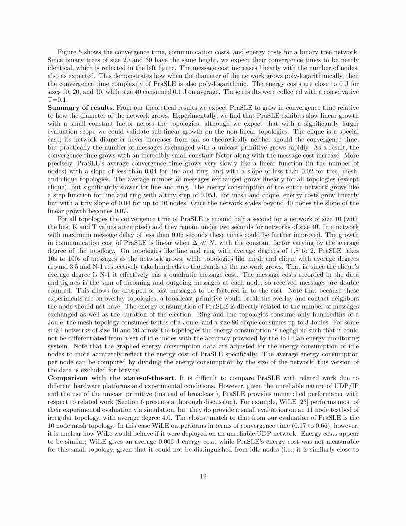
Figure 5 shows the convergence time, communication costs, and energy costs for a binary tree network.Since binary trees of size 20 and 30 have the same height, we expect their convergence times to be nearlyidentical, which is reflected in the left figure. The message cost increases linearly with the number of nodes,also as expected. This demonstrates how when the diameter of the network grows poly-logarithmically, thenthe convergence time complexity of PraSLE is also poly-logarithmic. The energy costs are close to 0 J forsizes 10, 20, and 30, while size 40 consumed 0.1 J on average. These results were collected with a conservativeT=0.1.Summary of results. From our theoretical results we expect PraSLE to grow in convergence time relativeto how the diameter of the network grows. Experimentally, we find that PraSLE exhibits slow linear growthwith a small constant factor across the topologies, although we expect that with a significantly largerevaluation scope we could validate sub-linear growth on the non-linear topologies. The clique is a specialcase; its network diameter never increases from one so theoretically neither should the convergence time,but practically the number of messages exchanged with a unicast primitive grows rapidly. As a result, theconvergence time grows with an incredibly small constant factor along with the message cost increase. Moreprecisely, PraSLE’s average convergence time grows very slowly like a linear function (in the number ofnodes) with a slope of less than 0.04 for line and ring, and with a slope of less than 0.02 for tree, mesh,and clique topologies. The average number of messages exchanged grows linearly for all topologies (exceptclique), but significantly slower for line and ring. The energy consumption of the entire network grows likea step function for line and ring with a tiny step of 0.05J. For mesh and clique, energy costs grow linearlybut with a tiny slope of 0.04 for up to 40 nodes. Once the network scales beyond 40 nodes the slope of thelinear growth becomes 0.07.

For all topologies the convergence time of PraSLE is around half a second for a network of size 10 (withthe best K and T values attempted) and they remain under two seconds for networks of size 40. In a networkwith maximum message delay of less than 0.05 seconds these times could be further improved. The growthin communication cost of PraSLE is linear when ∆ � N , with the constant factor varying by the averagedegree of the topology. On topologies like line and ring with average degrees of 1.8 to 2, PraSLE takes10s to 100s of messages as the network grows, while topologies like mesh and clique with average degreesaround 3.5 and N-1 respectively take hundreds to thousands as the network grows. That is, since the clique’saverage degree is N-1 it effectively has a quadratic message cost. The message costs recorded in the dataand figures is the sum of incoming and outgoing messages at each node, so received messages are doublecounted. This allows for dropped or lost messages to be factored in to the cost. Note that because theseexperiments are on overlay topologies, a broadcast primitive would break the overlay and contact neighborsthe node should not have. The energy consumption of PraSLE is directly related to the number of messagesexchanged as well as the duration of the election. Ring and line topologies consume only hundredths of aJoule, the mesh topology consumes tenths of a Joule, and a size 80 clique consumes up to 3 Joules. For somesmall networks of size 10 and 20 across the topologies the energy consumption is negligible such that it couldnot be differentiated from a set of idle nodes with the accuracy provided by the IoT-Lab energy monitoringsystem. Note that the graphed energy consumption data are adjusted for the energy consumption of idlenodes to more accurately reflect the energy cost of PraSLE specifically. The average energy consumptionper node can be computed by dividing the energy consumption by the size of the network; this version ofthe data is excluded for brevity.Comparison with the state-of-the-art. It is difficult to compare PraSLE with related work due todifferent hardware platforms and experimental conditions. However, given the unreliable nature of UDP/IPand the use of the unicast primitive (instead of broadcast), PraSLE provides unmatched performance withrespect to related work (Section 6 presents a thorough discussion). For example, WiLE [23] performs most oftheir experimental evaluation via simulation, but they do provide a small evaluation on an 11 node testbed ofirregular topology, with average degree 4.0. The closest match to that from our evaluation of PraSLE is the10 node mesh topology. In this case WiLE outperforms in terms of convergence time (0.17 to 0.66), however,it is unclear how WiLe would behave if it were deployed on an unreliable UDP network. Energy costs appearto be similar; WiLE gives an average 0.006 J energy cost, while PraSLE’s energy cost was not measurablefor this small topology, given that it could not be distinguished from idle nodes (i.e.; it is similarly close to

12

0). Lastly, PraSLE outperforms in messaging costs. Recall that our figures double count packets as outgoingmessages and incoming messages (to reflect lost packets), so PraSLE exchanged approximately 55-60 packetson average while WiLE exchanged 103.7 packets on average. Of course, it is worth noting that WiLE andPraSLE are evaluated on entirely different hardware. Bully LE [18] is evaluated on Cortex-M3 hardwaresimilarly to PraSLE, although with only 6 nodes. Unfortunately, as far as we are aware, the authors of [18]did not provide any convergence time, message cost, nor energy cost data to compare to. Resilient clusterLE [9] is evaluated on TelosB nodes in a cluster of size 50. Only the nodes above a certain energy thresholdcompete to become the leader, so not all 50 nodes are eligible like with PraSLE. The authors of [9] focuson security and do not provide any comparable metrics in terms of convergence time, messaging cost, andenergy cost, although they do state that their communication cost is “not a big problem.”

5 Tuning K and T

The values K and T used in PraSLE are tunable in that they can be raised and lowered to impact robustness(in an unreliable network) and efficiency. Recall that K is the number of rounds the protocol will run forand T is the duration of each round in seconds. Since the location of the global leader within the networkcannot be known in advance, K must be at least the diameter of the network. It can be increased furtherto account for dropped packets where the global leader’s information fails to propagate in some rounds.Increasing the value of K has a small impact on convergence time and energy consumed, so it is worth theexchange for added reliability in a practical environment. The value of T should be as small as possible whileallowing for essentially all messages to be delivered in time. By testing a range of values we found that thevalue of 0.05 seconds for T consistently gives fast convergence in Iot-Lab while allowing most messages to besuccessfully delivered in time, assuming they are not lost completely, for all topologies. A more aggressive Tthan 0.05 may be possible on other network configurations. Increasing the value of T has a large impact onconvergence time and therefore energy consumed, for the benefit of giving more time for messages to reachtheir destination. Neither increasing K nor T has any significant impact on the message complexity, sincenodes only send messages as needed in the first place. The best initial configuration to tune from is settingK to the diameter of the network and T to 0.05, increasing K by one until the desired reliability is achieved.Since increasing T has drastic impacts on time efficiency it is not recommended unless the communicationdelay of the network is significant, in which case fast convergence would already be challenging. As the sizeof the network grows so does the number of lost messages, so more robust K and T values may be needed.An example of such a case is the ring of size 40, where the best K value was 23 rather than the theoreticallyoptimal 20. Of course, in a reliable communication environment K should be set exactly to the diameter ofthe network and T should be set exactly to the network’s maximum message delay.

The graphs in this section portray the impacts of changing K and T on convergence time, communication,and energy costs on networks of fixed size. This is performed for line, ring, mesh, and clique networks ofsize 10, 20, and 30. The ring, mesh, and clique networks are also evaluated at size 40.

13

K

Con

verg

ence

Tim

e (s

ec)

0.0000

1.0000

2.0000

3.0000

4.0000

N/2 N/2 + 1 N/2 + 2 N/2 + 3 N/2 + 4 N/2 + 5

ring10 ring20 ring30 ring40

Ring: Convergence Time as K Increases (T=0.1)

T (sec)

Con

verg

ence

Tim

e (s

ec)

0.0000

2.0000

4.0000

6.0000

0.05 0.10 0.15 0.20

ring10 ring20 ring30 ring40

Ring: Convergence Time as T Increases (K=N/2 or best)

Figure 6: Average convergence time for ring as K and T change

Figure 6 illustrates the linear impact of increasing K or T in the ring network. The slope of the curvefrom increasing K is much less than the slope from increasing T. For example, in the N=40 ring network thecost of increasing K by 1 is approximately 0.1 seconds while the cost of increasing T by 0.05 is approximately1.3 seconds.

K

Mes

sage

s

0.00

100.00

200.00

300.00

400.00

N/2 N/2 + 1 N/2 + 2 N/2 + 3 N/2 + 4 N/2 + 5

ring10 ring20 ring30 ring40

Ring: Total Messages as K Increases (T=0.1)

T (sec)

Mes

sage

s

0.00

100.00

200.00

300.00

400.00

0.05 0.10 0.15 0.20

ring10 ring20 ring30 ring40

Ring: Total Messages as T Increases (K=N/2 or best)

Figure 7: Communication costs for ring as K and T change

Figure 7 shows how the values of K and T do not have any particular impact on message costs in the ringnetwork. This is because messages are only sent as needed in the first place, so neither redundant roundsnor extra time cause any additional messages.

K

Ene

rgy

(J)

0.00

0.05

0.10

0.15

0.20

N/2 N/2 + 1 N/2 + 2 N/2 + 3 N/2 + 4 N/2 + 5

ring10 ring20 ring30 ring40

Ring: Energy (J) as K Increases (T=0.1 or best)

T (sec)

Ene

rgy

(J)

0.0000

0.0500

0.1000

0.1500

0.2000

0.2500

0.05 0.10 0.15 0.20

ring10 ring20 ring30 ring40

Ring: Energy (J) as T Increases (K=N/2 or best)

Figure 8: Energy (J) costs for ring as K and T change

14

Figure 8 illustrates the energy consumption of the protocol across the entire network. As mentionedearlier in this section, some of the smaller network sizes showed a negligible consumption compared to idlenodes, so they are marked as 0 Joules. The experiments that consumed a non-negligible amount of energyshow a linear increase in consumption, which is related to the convergence time and message cost.

K

Con

verg

ence

Tim

e (s

ec)

0.0000

1.0000

2.0000

3.0000

4.0000

N/4 N/2 3N/4 N

line10 line20 line30

Line: Convergence Time as K Increases (T=0.1)

T (sec)

Con

verg

ence

Tim

e (s

ec)

0.0000

2.0000

4.0000

6.0000

8.0000

0.05 0.10 0.15 0.20

line10 line20 line30

Line: Convergence Time as T Increases (K=N/2 or best)

Figure 9: Average convergence time for line as K and T change

Figure 9 gives similar results to the ring topology (Figure 6), where increases in T have a much largerimpact on convergence time than K in a line topology. For example, in the N=30 line network the cost ofincreasing K by N/4 is approximately 0.83 seconds while the cost of increasing T by 0.05 is approximately1.64 seconds.

K

Mes

sage

s

0.00

50.00

100.00

150.00

200.00

250.00

N/4 N/2 3N/4 N

line10 line20 line30

Line: Total Messages as K Increases (T=0.1 or best)

T (sec)

Mes

sage

s

0.00

100.00

200.00

300.00

0.05 0.10 0.15 0.20

line10 line20 line30

Line: Total Messages as T Increases (K=N/2 or best)

Figure 10: Communication costs for line as K and T change

Similarly to the ring topology, Figure 10 shows that increases in K and T do not have any particularimpact on the number of messages exchanged.

15

K

Ene

rgy

(J)

0.00

0.05

0.10

0.15

0.20

N/4 N/2 3N/4 N

line10 line20 line30

Line: Energy (J) as K Increases (T=0.1 or best)

T (sec)

Ene

rgy

(J)

0.000

0.025

0.050

0.075

0.100

0.125

0.05 0.10 0.15 0.20

line10 line20 line30

Line: Energy (J) as T Increases (K=N/4 or best)

Figure 11: Energy (J) costs for line as K and T change

Figure 11 shows how little energy the line network consumes, such that it was only properly measurablefor the N=30 size. Increases in both K and T had little impact on energy.

K

Con

verg

ence

Tim

e (s

ec)

0.0000

0.5000

1.0000

1.5000

L+W-2 L+W-1 L+W

mesh10 mesh20 mesh30 mesh40

Mesh: Convergence Time as K Increases (T=0.05)

T (sec)

Con

verg

ence

Tim

e (s

ec)

0.0000

1.0000

2.0000

3.0000

4.0000

0.05 0.10 0.15 0.20

mesh10 mesh20 mesh30 mesh40

Mesh: Convergence Time as T Increases (K=L+W-2)

Figure 12: Average convergence time for mesh as K and T change

Figure 12 illustrates the efficiency of the mesh network. The linear (or better) growth in convergencetime from increases in K and T has an incredibly small constant factor, so increases in the parameters foradded reliability are not too costly. The increase in convergence time from adding one to K is only 0.07seconds, which is from the additional round duration of 0.05 seconds and some other minor delay factors.

K

Mes

sage

s

0.00

200.00

400.00

600.00

L+W-2 L+W-1 L+W

mesh10 mesh20 mesh30 mesh40

Mesh: Total Messages as K Increases (T=0.05)

T (sec)

Mes

sage

s

0.00

200.00

400.00

600.00

800.00

0.05 0.10 0.15 0.20

mesh10 mesh20 mesh30 mesh40

Mesh: Total Messages as T Increases (K=L+W-2)

Figure 13: Communication costs for mesh as K and T change

16

As with the other topologies, Figure 13 further demonstrates how changes in K and T have little impacton communication cost.

K

Ene

rgy

(J)

0.000

0.025

0.050

0.075

0.100

0.125

L+W-2 L+W-1 L+W

mesh10 mesh20 mesh30 mesh40

Mesh: Energy (J) as K Increases (T=0.05)

T (sec)

Ene

rgy

(J)

0.00

0.05

0.10

0.15

0.20

0.25

0.05 0.10 0.15 0.20

mesh10 mesh20 mesh30 mesh40

Mesh: Energy (J) as T Increases (K=L+W-2 or best)

Figure 14: Energy (J) costs for mesh as K and T change

Figure 14 shows the energy consumption of PraSLE in a mesh topology. The mesh30 curve in the leftfigure contains a measuring error, as there is no reasonable way for a lower K to consume so much moreenergy. Similarly in the right figure, it is a measuring error that the mesh40 curve is initially below themesh30 curve, although the trend corrects itself. We believe this is because with the smaller experiments orthose that last only a fraction of a second, the energy monitoring does not as accurately reflect the true cost.

K

Con

verg

ence

Tim

e (s

ec)

0.0000

0.5000

1.0000

1.5000

2.0000

1 2 3

clique10 clique20 clique30 clique40

Clique: Convergence Time as K Increases (T=0.05)

T (sec)

Con

verg

ence

Tim

e (s

ec)

0.0000

0.5000

1.0000

1.5000

2.0000

2.5000

0.05 0.10 0.15 0.20

clique10 clique20 clique30 clique40

Clique: Convergence Time as T Increases (K=1)

Figure 15: Average convergence time for clique as K and T change

The clique convergence times in Figure 15 appear similar to the mesh curves from Figure 12, with similarslopes. Considering the average degree of N-1, each node has a large number of messages to process eachround, and much of this processing time bleeds over the final round. This implies that the best averagedegree for a network to have would be somewhere closer to the the mesh’s 3.5-4 than the clique’s N-1.

17

K

Mes

sage

s

0.00

1000.00

2000.00

3000.00

1 2 3

clique10 clique20 clique30 clique40

Clique: Total Messages as K Increases (T=0.05)

T (sec)

Mes

sage

s

0.00

1000.00

2000.00

3000.00

4000.00

0.05 0.10 0.15 0.20

clique10 clique20 clique30 clique40

Clique: Total Messages as T Increases (K=1)

Figure 16: Communication costs for clique as K and T change

Figure 16 shows just how large the message cost is for a clique network, given that it’s high averagedegree brings the unicast messaging cost from linear to quadratic. Unlike the other topologies where K andT do not have any noticeable impact on communication cost, with the clique there is a slight up-trend incommunication cost following an increase in K or T. This is because there are so many messages being sent,a longer election allows for more of them to be received and processed.

K

Ene

rgy

(J)

0.0

0.2

0.4

0.6

0.8

1 2 3

clique10 clique20 clique30 clique40

Clique: Energy (J) as K Increases (T=0.05)

T (sec)

Ene

rgy

(J)

0.0

0.2

0.4

0.6

0.8

0.05 0.10 0.15 0.20

clique10 clique20 clique30 clique40

Clique: Energy (J) as T Increases (K=1)

Figure 17: Energy (J) costs for clique as K and T change

Figure 16 illustrates the energy consumption of the clique topology. The size 10 clique wasn’t distin-guishable from idle nodes. The outliers of K=2 and T=0.1 appear to be measuring errors, as there is not anexplainable reason for them to cost more than higher K and T values.

6 Related Work

This section discusses the strengths and weaknesses of existing methods while considering our researchobjectives of developing a practical self-stabilizing LE algorithm that can be deployed on UDP networkswith a unicast primitive. Specifically, we divide the literature into research that (i) explores the theoreticalboundaries of LE; (ii) approaches for LE in Wireless Sensor Networks and MANET, and (iii) studies focusedon LE in IoT and resource-constrained networks.

There are numerous methods that study LE from a theoretical point of view using different computationand communication models without being concerned with actual implementation issues. For example, Dotyand Soloveichik [10] present a population protocol for LE on a network of symmetric processes/nodes con-nected in a clique topology. They show that linear parallel time (in the number of nodes n) is a lower boundfor the convergence of constant-space population protocols. Sudo et al. [26] improve this lower bound to

18

Protocol Time Message Self- Topology Scale Communication

Complexity Complexity Stabilizing Devices Model

[23] Polynomial Polynomial Unstated Irregular 11 nodes Reliable(∆ = 4) MagoNode++ Asynchronous (TCP)

[18] Unstated Unstated Unstated Clique 6 nodes UnstatedCortex-M3

[9] Unstated Unstated Unstated Unstated 50 node cluster UnstatedTelosB

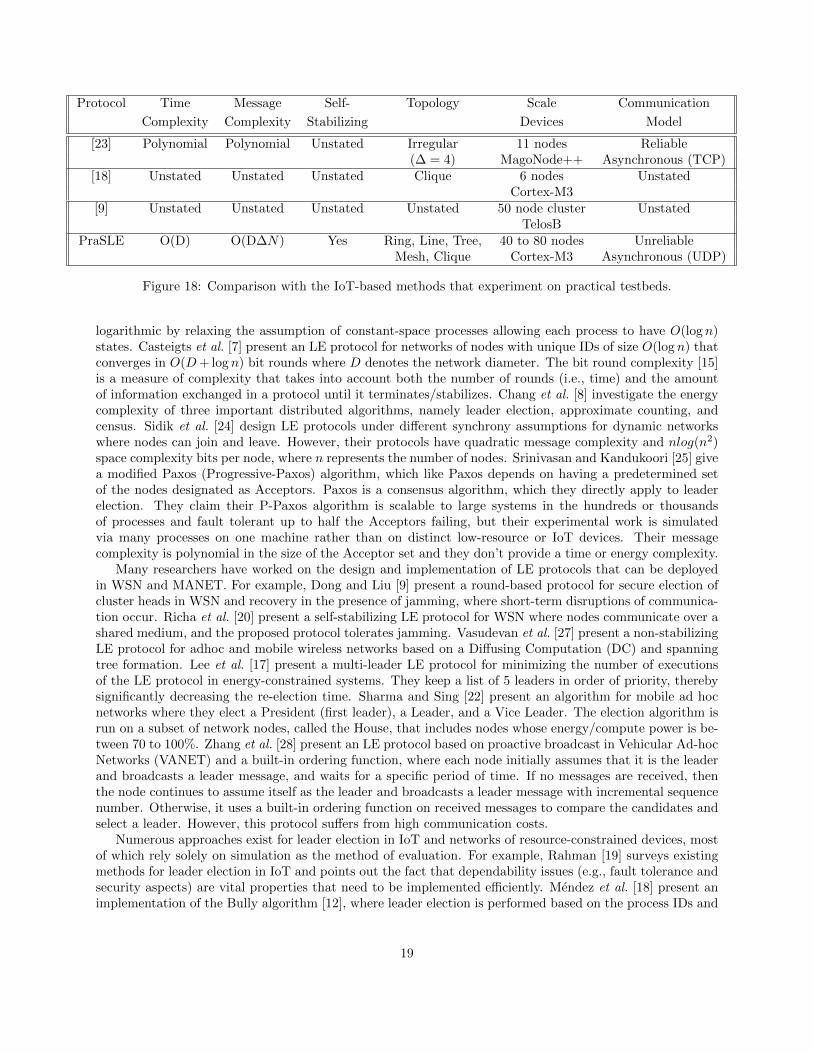
PraSLE O(D) O(D∆N) Yes Ring, Line, Tree, 40 to 80 nodes UnreliableMesh, Clique Cortex-M3 Asynchronous (UDP)

Figure 18: Comparison with the IoT-based methods that experiment on practical testbeds.

logarithmic by relaxing the assumption of constant-space processes allowing each process to have O(log n)states. Casteigts et al. [7] present an LE protocol for networks of nodes with unique IDs of size O(log n) thatconverges in O(D+ log n) bit rounds where D denotes the network diameter. The bit round complexity [15]is a measure of complexity that takes into account both the number of rounds (i.e., time) and the amountof information exchanged in a protocol until it terminates/stabilizes. Chang et al. [8] investigate the energycomplexity of three important distributed algorithms, namely leader election, approximate counting, andcensus. Sidik et al. [24] design LE protocols under different synchrony assumptions for dynamic networkswhere nodes can join and leave. However, their protocols have quadratic message complexity and nlog(n2)space complexity bits per node, where n represents the number of nodes. Srinivasan and Kandukoori [25] givea modified Paxos (Progressive-Paxos) algorithm, which like Paxos depends on having a predetermined setof the nodes designated as Acceptors. Paxos is a consensus algorithm, which they directly apply to leaderelection. They claim their P-Paxos algorithm is scalable to large systems in the hundreds or thousandsof processes and fault tolerant up to half the Acceptors failing, but their experimental work is simulatedvia many processes on one machine rather than on distinct low-resource or IoT devices. Their messagecomplexity is polynomial in the size of the Acceptor set and they don’t provide a time or energy complexity.

Many researchers have worked on the design and implementation of LE protocols that can be deployedin WSN and MANET. For example, Dong and Liu [9] present a round-based protocol for secure election ofcluster heads in WSN and recovery in the presence of jamming, where short-term disruptions of communica-tion occur. Richa et al. [20] present a self-stabilizing LE protocol for WSN where nodes communicate over ashared medium, and the proposed protocol tolerates jamming. Vasudevan et al. [27] present a non-stabilizingLE protocol for adhoc and mobile wireless networks based on a Diffusing Computation (DC) and spanningtree formation. Lee et al. [17] present a multi-leader LE protocol for minimizing the number of executionsof the LE protocol in energy-constrained systems. They keep a list of 5 leaders in order of priority, therebysignificantly decreasing the re-election time. Sharma and Sing [22] present an algorithm for mobile ad hocnetworks where they elect a President (first leader), a Leader, and a Vice Leader. The election algorithm isrun on a subset of network nodes, called the House, that includes nodes whose energy/compute power is be-tween 70 to 100%. Zhang et al. [28] present an LE protocol based on proactive broadcast in Vehicular Ad-hocNetworks (VANET) and a built-in ordering function, where each node initially assumes that it is the leaderand broadcasts a leader message, and waits for a specific period of time. If no messages are received, thenthe node continues to assume itself as the leader and broadcasts a leader message with incremental sequencenumber. Otherwise, it uses a built-in ordering function on received messages to compare the candidates andselect a leader. However, this protocol suffers from high communication costs.

Numerous approaches exist for leader election in IoT and networks of resource-constrained devices, mostof which rely solely on simulation as the method of evaluation. For example, Rahman [19] surveys existingmethods for leader election in IoT and points out the fact that dependability issues (e.g., fault tolerance andsecurity aspects) are vital properties that need to be implemented efficiently. Mendez et al. [18] present animplementation of the Bully algorithm [12], where leader election is performed based on the process IDs and

19

the process that has the max ID becomes the leader. Mendez et al. implement the Bully algorithm on anetwork with the clique topology where each node is an Arm Cortex-M3 managed by the FreeRTOS operatingsystem, however, their work lacks experimental results on how robust and efficient their implementation is.The Minimum Finding (MinFind) algorithm [21] extends the idea of the Bully algorithm, where each nodebroadcasts a randomly generated value (or its ID) and then enters a cycle of reading and relaying theminimum value (i.e., flooding the minimum value) through broadcast. Bounceur et al. [3] present a protocolfor synchronous networks based on the MinFind algorithm [21], where each node waits for m×t seconds, andif it receives nothing, then it broadcasts its m value and halts, called Wait-Before-Send (WBS). Otherwise,it broadcasts the value it has received and then halts. Bounceur et al. [2] also present an energy-efficientalgorithm for LE, called Branch Optima to Global Optimum (BROGO), where a spanning tree is formedby flooding rooted at a specific node whose ID is known to everyone. To address the issue of the failure ofthe root, the authors of [4] combine BROGO with WBS in order to automatically select a different root ifthe primary one fails. Another work by Bounceur et al. [5,6,14] extends the logic of the MinFind algorithmwhere the network is initially a forest and a tree routing protocol is used to flood the network with the IDof the leader of each tree (i.e., its local optima found by MinFind). Faika et al. [11] where they propose aleader election protocol for the Battery Management System (BMS) in electrical vehicles, where the rankingfunction represents the eligibility of node for becoming a leader based on its battery level. Nodes broadcastthe ranking value and wait for response. Moreover, nodes gradually increase their RF range if they do notreceive any responses. After receiving the response of its neighboring nodes, each node elects a local leader.The local leaders follow the same procedure to elect a global leader.

The closest work to ours includes Sheshashayee et al. [23] where they put forward a protocol for electingthe top k leaders, and evaluate it through simulation and on a testbed. In their LE protocol, each nodehas a rank between 1 and n, where n denotes the number of nodes in the network, a weight, and an ID.The communication primitive is a broadcast operation in an asynchronous clique network and the authorsconsider a time limit up to which messages are delivered. Initially, each node sets its rank to 1 and broadcastsa message containing its rank, its weight (which is a random value generated only once) and its ID. Then,the nodes engage in exchanging their local views, called progress view, of their locality and increase theirrank depending on the node weight and their progress view. The objective is to eventually have the progressview of the entire network in every node where the ranks are distinct. Reaching such a state ensures thatevery node in the network can sort all nodes based on their rank, and as a result know who the top k < nleaders are. The authors validate their method on the GreenCastalia simulator and implement and deploy iton real testbed of 11 MagoNode++ nodes, each having an 8-bit 16MHz CPU with 256 KB of ROM and 32KB of RAM, and communicating using an IEEE 802.15.4 compliant 2.4 GHz radio module. Their simulationand experimental results show that the convergence time and communication costs are reasonable. Theyalso show that packet size has an inverse relation with convergence time and energy consumption.

To the best of our knowledge, all aforementioned approaches are evaluated through simulation or vali-dation on small-scale testbeds of less than 30 nodes, with the exception of [9]. Moreover, it is unclear if theunderlying networks are UDP-based. The table in Figure 18 summarizes the related works that performexperimentation on real-world platforms. Some existing methods make assumptions about synchrony. Forexample, the WBS method [3] requires that all processes are synchronized at the start of the protocol, whichis hard to ensure in large scale distributed systems. Some approaches are asymmetric, which makes it hardto implement and more costly in terms of communication and energy (e.g., BROGO [2]). Another restrictiveassumption for a practical real-world LE implementation includes the topology, where most existing methodsassume a clique topology, whereas we provide an efficient, tunable implementation demonstrated for ring,line, tree, mesh, and clique. Last but not least, our experiments demonstrate that PraSLE can easily scaleup to networks of up to 80 nodes, which is an important property for practical use in IoT and CPS.

7 Conclusion and Future Work

We presented a practical self-stabilizing leader election algorithm, called PraSLE, supported by experimentalvalidation on the IoT-Lab platform. We provided two versions of PraSLE, one for reliable networks and

20

another for unreliable networks. We proved the correctness of PraSLE and showed that it converges to aunique leader with probability 1. We also experimentally demonstrated that PraSLE outperforms existingmethods in terms of average convergence time for ring, line, mesh, and clique topologies of up to 40 or 80nodes. Our current experimental results are promising and point to the direction of sub-linear convergencetime for non-linear topologies (which follows the asymptotic time complexity of PraSLE). However, we believethat we need to conduct more experiments with larger network sizes in order to verify this conjecture. Thetunable nature of PraSLE enables us to optimize average convergence time, as well as communication andenergy costs. Thus, PraSLE provides a resource-efficient primitive for distributed computing in unreliablenetworks of low-end IoT devices.

As an extension of this work, we are developing a variant of PraSLE where we elect the top k leadersinstead of just one unique leader. Additionally, we plan to develop and evaluate other distributed algorithms(such as Paxos) on IoT platforms. We would also like to expand the scope of our evaluation to networksgreater than 100 physical nodes and thoroughly evaluate more topologies such as grid.

Acknowledgment. We would like to thank David Hallberg for his help in the initial phases of this work,including algorithm brainstorming and scripting regarding energy consumption data. We’d also like to thankthe IoT-Lab team for their publicly accessible large-scale testbed, which made our experimental evaluationspossible.

References

[1] E. Baccelli, C. Gundogan, O. Hahm, P. Kietzmann, M. S. Lenders, H. Petersen, K. Schleiser, T. C.Schmidt, and M. Wahlisch. Riot: An open source operating system for low-end embedded devices inthe iot. IEEE Internet of Things Journal, 5(6):4428–4440, 2018.

[2] A. Bounceur, M. Bezoui, R. Euler, N. Kadjouh, and F. Lalem. Brogo: A new low energy consump-tion algorithm for leader election in wsns. In 2017 10th International Conference on Developments ineSystems Engineering (DeSE), pages 218–223. IEEE, 2017.

[3] A. Bounceur, M. Bezoui, R. Euler, and F. Lalem. A wait-before-starting algorithm for fast, fault-tolerantand low energy leader election in wsns dedicated to smart-cities and iot. In 2017 IEEE SENSORS, pages1–3. IEEE, 2017.

[4] A. Bounceur, M. Bezoui, R. Euler, F. Lalem, and M. Lounis. A revised brogo algorithm for leaderelection in wireless sensor and iot networks. In 2017 IEEE SENSORS, pages 1–3. IEEE, 2017.

[5] A. Bounceur, M. Bezoui, L. Lagadec, R. Euler, L. Abdelkader, and M. Hammoudeh. Dotro: A newdominating tree routing algorithm for efficient and fault-tolerant leader election in wsns and iot networks.In International Conference on Mobile, Secure, and Programmable Networking, pages 42–53. Springer,2018.

[6] A. Bounceur, M. Bezoui, M. Lounis, R. Euler, and C. Teodorov. A new dominating tree routing algo-rithm for efficient leader election in iot networks. In 2018 15th IEEE Annual Consumer Communications& Networking Conference (CCNC), pages 1–2. IEEE, 2018.

[7] A. Casteigts, Y. Metivier, J. M. Robson, and A. Zemmari. Deterministic leader election takes θ(d+log n)bit rounds. Algorithmica, 81(5):1901–1920, 2019.

[8] Y.-J. Chang, T. Kopelowitz, S. Pettie, R. Wang, and W. Zhan. Exponential separations in the energycomplexity of leader election. ACM Transactions on Algorithms (TALG), 15(4):1–31, 2019.

[9] Q. Dong and D. Liu. Resilient cluster leader election for wireless sensor networks. In 2009 6th AnnualIEEE Communications Society Conference on Sensor, Mesh and Ad Hoc Communications and Networks,pages 1–9. IEEE, 2009.

21

[10] D. Doty and D. Soloveichik. Stable leader election in population protocols requires linear time. Dis-tributed Computing, 31(4):257–271, 2018.

[11] T. Faika, T. Kim, and M. Khan. An internet of things (iot)-based network for dispersed and decentralizedwireless battery management systems. In 2018 IEEE Transportation Electrification Conference and Expo(ITEC), pages 1060–1064. IEEE, 2018.

[12] H. Garcia-Molina. Elections in a distributed computing system. IEEE transactions on Computers,(1):48–59, 1982.

[13] T. Herman. Probabilistic self-stabilization. Information Processing Letters, 35(2):63–67, 1990.

[14] N. Kadjouh, A. Bounceur, M. Bezoui, M. E. Khanouche, R. Euler, M. Hammoudeh, L. Lagadec, S. Jab-bar, and F. Al-Turjman. A dominating tree based leader election algorithm for smart cities iot infras-tructure. Mobile Networks and Applications, pages 1–14, 2020.

[15] K. Kothapalli, M. Onus, C. Scheideler, and C. Schindelhauer. Distributed coloring in O(√

log n) bits.In Proc. of IEEE International Parallel and Distributed Processing Symposium (IPDPS), 2006.

[16] L. Lamport et al. Paxos made simple. ACM Sigact News, 32(4):18–25, 2001.

[17] S. Lee, R. M. Muhammad, and C. Kim. A leader election algorithm within candidates on ad hoc mobilenetworks. In International Conference on Embedded Software and Systems, pages 728–738. Springer,2007.

[18] M. Mendez, F. G. Tinetti, A. M. Duran, D. A. Obon, and N. G. Bartolome. Distributed algorithmson iot devices: bully leader election. In 2017 International Conference on Computational Science andComputational Intelligence (CSCI), pages 1351–1355. IEEE, 2017.

[19] M. U. Rahman. Leader election in the internet of things: Challenges and opportunities. arXiv preprintarXiv:1911.00759, 2019.

[20] A. Richa, C. Scheideler, S. Schmid, and J. Zhang. Self-stabilizing leader election for single-hop wirelessnetworks despite jamming. In Proceedings of the Twelfth ACM International Symposium on Mobile AdHoc Networking and Computing, pages 1–10, 2011.

[21] N. Santoro. Design and analysis of distributed algorithms, volume 56. John Wiley & Sons, 2006.

[22] S. Sharma and A. K. Singh. An election algorithm to ensure the high availability of leader in large mobilead hoc networks. International Journal of Parallel, Emergent and Distributed Systems, 33(2):172–196,2018.

[23] A. V. Sheshashayee and S. Basagni. Wile: Leader election in wireless networks. Ad Hoc Sens. Wirel.Networks, 44(1-2):59–81, 2019.

[24] B. Sidik, R. Puzis, P. Zilberman, and Y. Elovici. Pale: Time bounded practical agile leader election.IEEE Transactions on Parallel and Distributed Systems, 31(2):470–485, 2019.

[25] S. Srinivasan and R. kandukoori. A synod based deterministic and indulgent leader election protocolfor asynchronous large groups. International Journal of Parallel, Emergent and Distributed Systems,pages 1–28, 2021.

[26] Y. Sudo, F. Ooshita, T. Izumi, H. Kakugawa, and T. Masuzawa. Time-optimal leader election inpopulation protocols. IEEE Transactions on Parallel and Distributed Systems, 2020.

[27] S. Vasudevan, J. Kurose, and D. Towsley. Design and analysis of a leader election algorithm for mobilead hoc networks. In Proceedings of the 12th IEEE International Conference on Network Protocols, 2004.ICNP 2004., pages 350–360. IEEE, 2004.

22

[28] R. Zhang, B. Jacquemot, K. Bakirci, S. Bartholme, K. Kaempf, B. Freydt, L. Montandon, S. Zhang,and O. Tonguz. Leader selection in vehicular ad-hoc network: a proactive approach. arXiv preprintarXiv:1912.06776, 2019.

23