Computer Sciences Department

Clustera: An Integrated Computation and Data Management System David DeWitt Eric Robinson Srinath Shankar Erik Paulson Jeffrey Naughton Joshua Royalty Andrew Krioukov Technical Report #1637 April 2007

1

Clustera: An Integrated Computation And Data Management System

David J. DeWitt, Eric Robinson, Srinath Shankar, Erik Paulson, Jeffrey Naughton, Joshua Royalty, Andrew Krioukov

Computer Sciences Department, University of Wisconsin-Madison

{dewitt, erobinso, srinath, epaulson, naughton, krioukov, royalty}@cs.wisc.edu

ABSTRACT

This paper introduces Clustera, an integrated computation and data management system. In contrast to traditional cluster-management systems that target specific types of workloads, Clustera is designed for extensibility, enabling the system to be easily extended to handle a wide variety of job types ranging from computationally-intensive, long-running jobs with minimal I/O requirements to complex SQL queries over massive relational tables. Another unique feature of Clustera is the way in which the system architecture exploits modern software building blocks including application servers and relational database systems in order to realize important performance, scalability, portability and usability benefits. Finally, experimental evaluation suggests that Clustera has good scale-up properties for SQL processing, that Clustera delivers performance comparable to Hadoop for MapReduce processing and that Clustera can support higher job throughput rates than previously published results for the Condor and CondorJ2 batch computing systems.

2

1. INTRODUCTION A little more than 25 years ago a cluster of computers was an exotic research commodity found only in a few universities and industrial research labs. At that point in time a typical cluster consisted of a couple of dozen minicomputers (e.g. VAX 11/750s or PDP 11s) connected by a local area network. By necessity clusters were small as the cost of a node was about the same as the annual salary of a staff member with an M.S. in computer science ($25K). Today, for a little more than the annual salary of a freshly minted M.S., one can purchase a cluster of about 100 nodes, each with 1,000 times more capacity in terms of CPU power, memory, disk, and network bandwidth than 25 years ago. Today clusters of 100 nodes are commonplace and many organizations have clusters of thousands of nodes. These clusters are used for various tasks including analyzing financial models, simulating circuit designs and physical processes, and analyzing massive data sets. The largest clusters - such as those used by Google, Microsoft, Yahoo and various defense laboratories - include over 10,000 nodes. Except for issues of power and cooling, one has to conclude that clusters of 100,000 or even one million nodes will be deployed in the not too distant future.

While it is always dangerous to generalize, clusters seem to be used today for three distinct types of applications:

• computationally intensive tasks • analyzing large data sets with techniques such as MapReduce • running SQL queries in parallel on structured data sets

Applications in the first class typically run as a single process on a single node. For example, a computer architect wishing to analyze a new chip design (e.g. an 8 core CPU with a split L2 cache design and a shared L3 cache) might want to explore the impact of various parameters (e.g. the relative sizes of the L2 and L3 caches) on the expected throughput of Oracle running the TPC-C benchmark. Each simulation run is very CPU intensive but consumes only a modest amount of disk bandwidth. Since there is a large parameter space to explore, the architect uses the nodes of the cluster to run many different simulations simultaneously. This style of cluster use is what Livny [1] refers to as “high throughput” computing. That is, instead of using the cluster nodes to run each simulation in parallel, many instances of the simulation are run concurrently, each exploring a different portion of the parameter space.

The second type of application is typified by Google’s Map/Reduce [2] software. This software has revolutionized the analysis of large data sets on clusters. A user of the Map/Reduce framework needs only to write map and reduce functions. The framework takes care of scheduling the map and reduce functions on the nodes of the cluster, moving intermediate data sets from the map functions to the reduce functions, providing fault tolerance in the event of software or hardware failures, etc. Since Map/Reduce is targeted towards analyzing large data sets, the overall framework also includes a distributed file system for storing the input and output files of a map/reduce computation on the nodes of the cluster.

There are two key differences between the class of jobs targeted by the MapReduce framework and those targeted by the first class of cluster software. First, MapReduce jobs run in parallel. For example, if the input data set is partitioned across the disks of 100 nodes, the framework might run 100 instances of the map function simultaneously. The second major difference is that MapReduce is targeted towards data intensive tasks while the former is targeted towards compute intensive tasks.

The third class of cluster applications is one for which the database community is most familiar: a SQL database system that uses the nodes of a cluster to run a SQL query in parallel. Like MapReduce, such systems are targeted towards running a single job (i.e., a SQL query) in parallel on large amounts of data. In contrast to MapReduce, the programming model is limited to that provided by SQL augmented, to a limited degree, by the use of user-defined functions and stored procedures.

All three types of cluster systems are, at the same time, both similar and different. All have a notion of a

3

job and a job scheduler. For Condor-like batch systems the job is an executable to be run on a single node. For MapReduce it is a pair of functions. For database systems the job is a SQL query. All three also have a job scheduler that is responsible for assigning jobs to nodes and monitoring their execution. In the case of MapReduce and SQL, the scheduler also is responsible for “parallelizing” the job so that it can run on multiple nodes concurrently.

Each system is also limited. None can run the other’s types of jobs. For example, the MapReduce framework cannot (currently at least) accept a SQL query as a job and run it. Likewise, no parallel database can accept a MapReduce job and run it, let alone a computationally intensive job such as a circuit simulator.

Having worked on clustering systems of various flavors since the early 1980s we strongly believe that cluster management is a database application. Clusters are “awash” in data including state and configuration information for each node in the cluster, information on users, files/tables, and jobs, accounting data to track usage, as well as the job queue itself. All this data must survive a crash and must be managed transactionally. For example, in the event of a crash submitted jobs must not be lost and completed jobs should not be rerun. Being able to query all this data is invaluable to both users and system administrators. For example, users need to be able to monitor their jobs - those that have been submitted but not yet run as well as those currently executing. System administrators need to be able to assess the health of the system, monitor usage, and produce summary reports. Having the data about the entire system stored centrally in one location in a form that can be easily accessed and queried makes essentially every aspect of building and running such a system simpler.

Some readers might assert that centralizing this information leaves the system vulnerable to failures. We believe that these concerns are groundless. While the information is logically centralized, in a modern database system it is physically replicated to provide robust behavior in the presence of failures.

With this background, we turn our attention to the focus of this paper, which is to present the design, implementation, and evaluation of a new cluster management system called Clustera. Clustera is different from all previous attempts to build a cluster management system in three important ways. First, it is designed to run the three classes of jobs described above efficiently. Second, its design leverages modern software components including database systems and application servers as its fundamental building blocks. Third, the Clustera framework is designed to be extensible, allowing new types of jobs and job schedulers to be added to the system in a straightforward fashion.

The remainder of this paper is organized as follows. In Section 2 we present related work. Section 3 describes Clustera’s software architecture including the three classes of abstract job schedulers we have implemented so far. In Section 4 we evaluate Clustera’s performance, including a comparison of Clustera’s implementation of MapReduce with that provided by Hadoop on a 100 node cluster. Finally, our conclusions and future research directions are presented in Section 5.

2. RELATED WORK 2.1 Cluster Management Systems The idea of using a cluster of computers for running computationally intensive tasks appears to have been conceived by Maurice Wilkes in the late 1970s [3]. Wilkes’ idea, which he termed a “processor bank,” was to use a pool of dedicated computers to provide additional cycles to users having only workstations of modest power. Users could “check out” a set of processors from the processor bank to run a computation.

Inspired by Wilkes we implemented such a processor bank as part of the Crystal project [4] in the early 1980s at Wisconsin. Known initially as “Remote Unix”, users could submit jobs to the cluster from their workstations. Jobs were linked with a library that trapped I/O calls, redirecting them to the submitting machine during execution. This was necessary because shared-file systems such as NFS did not yet exist. Over time, Remote Unix morphed into Condor and capabilities such as job checkpointing were added.

4

From its inception the primary focus of the Condor software has been computationally intensive tasks. Historically this occurred for two reasons. First, since I/O calls had to be redirected to the submitting machine, disk I/Os were quite slow. Second, disks were very small and expensive in those days, so when workstations were used to run Condor jobs workstation owners did not want their disks filled with someone else’s files. These two factors made it natural to focus the design of the system on managing computationally intensive tasks. Condor is installed on thousands of clusters around the world and is used to manage well in excess of 100,000 machines with the biggest known clusters composed of in excess of 10,000 nodes. Wilkes’ original vision has definitely been realized.

Many similar cluster management systems have been developed including LoadLeveler [5], LSF [6], PBS [7], and N1 Grid Engine (SGE) [8]. Like Condor, LoadLeveler, LSF and PBS use OS files for maintaining state information. SGE, optionally, allows the use of a database system for managing state information (i.e., job queue data, user data, etc.). In contrast to these “application-level” cluster management systems that sit on top of the OS, several vendors offer clustering solutions that are tightly integrated into the OS. One example of this class of system is Microsoft’s Compute Cluster Server [9] for Windows Server 2003. The focus of the GridMP [11] system is on providing a framework within which developers can “grid-enable,” or “port to the grid” pre-existing enterprise applications.

2.2 Parallel Database Systems Parallel database systems have their roots in early database machine efforts [11,12,13], which began soon after the relational data model was introduced. MUFFIN [14] was the first database system to propose using a cluster of standard computers for parallelizing queries, a configuration that Stonebraker later termed “shared-nothing”. Adopting the same shared-nothing paradigm, in the mid-1980s the Gamma [15] and Teradata [16] projects concurrently introduced the use of hash-based partitioning of relational tables across multiple cluster nodes and disks as well as the use of hash-based split functions as the basis of parallelizing the join and aggregate operators. Today parallel database systems are available from a variety of vendors including Teradata, Oracle, IBM, HP (Tandem), Greenplum, Netezza, and Vertica.

2.3 MapReduce Developed initially by Google [2], and now available as part of the open source system Hadoop [17], MapReduce has recently received very widespread attention for its ability to efficiently analyze large unstructured and structured data sets. The basic idea of MapReduce is straightforward and consists of two functions that a user writes called map and reduce plus a framework for executing a possibly large number of instances of each program on a compute cluster.

The map program reads a set of “records” from an input file, does any desired filtering and/or transformations and then outputs a set of records of the form (key, data). As the map program produces output records a “split” function partitions the records into M disjoint buckets by applying a function to the key of each output record. The map program terminates with M output files, one for each bucket. In general, there are multiple instances of the map program running on different nodes of a compute cluster. Each map instance is given a distinct portion of the input file by the MapReduce scheduler to process. If N nodes participate in the map phase, M files are produced at each of N nodes, for a total of N * M files.

The second phase executes M instances of the reduce program. Each reads one input file from each of the N nodes. After being collected by the MapReduce framework, the input records to a reduce instance are grouped on their keys (by sorting or hashing) and fed to the reduce program. Like the map program, the reduce program is an arbitrary computation in a general-purpose language. Each reduce instance can write records to an output file, which forms part of the “answer” to a MapReduce computation.

2.4 Dryad Drawing inspiration from cluster management systems like Condor, MapReduce, and parallel database systems, Dryad [18] is intended to be a general-purpose framework for developing coarse-grain data

5

parallel applications. Dryad applications consist of a data flow graph composed of vertices, corresponding to sequential computations, connected to each other by communication channels implemented via sockets, shared-memory message queues, or files. The Dryad framework provides support for scheduling the vertices constituting a computation on the nodes of a cluster, establishing communication channels between computations, and dealing with software and hardware failures.

In many ways the goals of the Clustera project and Dryad are quite similar to one another. Both are targeted toward handling a wide range of applications ranging from single process, computationally intensive jobs to parallel SQL queries. The two systems, however, employ radically different implementation strategies. Dyrad uses techniques similar to those first pioneered by the Condor project based on the use of daemon processes running on each node in the cluster to which the scheduler pushes jobs for execution.

3. Clustera Architecture 3.1 Introduction The goals of the Clustera project include efficient execution of a wide variety of job types ranging from computationally-intensive, long-running jobs with minimal I/O requirements to complex SQL queries over massive relational tables. Rather than “prewiring” the system to support a specific set of job types, Clustera is designed to be extensible, enabling the system to be easily extended to handle new types of jobs and their associated schedulers. Finally, the system is designed to scale to tens of 1000s of nodes by exploiting modern software building blocks including applications servers (e.g., JBoss) and relational database systems.

In designing and building this system we also wanted to answer the question of whether a general-purpose cluster management system could be competitive with one designed to execute a single type of job. As will be demonstrated in Section 4, we believe that the answer to this question is “yes”.

3.2 The Standard Cluster Architecture Figure 1 depicts the “standard” architecture that many cluster management systems use. Users submit their jobs to a job scheduler that “matches” submitted jobs to nodes as nodes become “available”. Examples of criteria that are frequently used to match a job to a node include the architecture for which the job has been compiled (e.g. Intel or Sparc) and the minimum amount of memory needed to run the job. From the set of “matching” jobs, the job scheduler will select which job to run according to some scheduling mechanism. Condor, for example, uses a combination of “fair-share” scheduling and job priorities. After a job is “matched” with a node, the scheduler sends the job to a daemon process on the node. This process assumes responsibility for starting the job and monitoring its execution until the job completes. How input and output files are handled varies from system to system. If, for example, the nodes in the cluster (as well as the submitting machines) have access to a shared file system such as NFS or AFS, jobs can access their input files directly. Otherwise, the job scheduler will push the input files needed by the job, along with the executable for the job, to the node. Output files are handled in an analogous fashion. We use the term “push” architecture in reference to the way jobs get “pushed” from the job scheduler to a waiting daemon process running on the node.

Figure 1: “Push” Cluster Architecture

6

Examples of this general class of architecture include Condor, LSF, IBM Loadleveler, PBS, and SunN1 Grid Engine. There are probably dozens of other similar systems. Despite this high-level similarity, there are differences between the systems, too. Condor, for example, uses a distributed job queue and file transfer to move files between the submitting machine and the node.

3.3 Clustera System Architecture Figure 2 depicts the architecture of Clustera. This architecture is unique in a number of ways. First, the Clustera server software is implemented using Java EE running inside the JBoss Application Server. As we will discuss in detail below, using an Application Server as the basis for the system provided us a number of important capabilities including scalability, fault tolerance, and multiplexing of the connections to the DBMS. The second unique feature is that the cluster nodes are web service clients of the Clustera server, using SOAP over HTTP to communicate and coordinate with the Clustera server. Third, all state information about jobs, users, nodes, files, job execution history, etc. is stored in a relational database system. Users and system administrators can monitor the state of their jobs and the overall health of the system through a web interface.

The Clustera server provides support for job management, scheduling and managing the configuration and state of each node in the cluster, concrete files, logical files, and relational tables, information on users including priorities, permissions, and accounting data, as well as a complete historical record of each job submitted to the system. The utility provided by maintaining a rich, complete record of job executions cannot be overstated. In addition to serving as the audit trail underlying the usage accounting information, maintaining these detailed historical records makes it possible, for example, to trace the lineage of a logical file or relational table (either of which typically is composed of a distributed set of physical files) back across all of the jobs and inputs that fed into its creation. Similarly it is possible to trace forward from a given file or table through all of the jobs that – directly or indirectly – read from the file or table in question to determine, for example, what computations need to be re-run if a particular data set needs to be corrected, updated or replaced.

Figure 2: Clustera Architecture

7

Users can perform essential tasks (e.g., submit and monitor jobs, reconfigure nodes, etc.) through either the web-service interface to the system or via a browser-based GUI. Additionally, users can access basic aggregate information about the system through a set of pre-defined, parameterized queries (e.g., How many nodes are in the cluster right now? How many jobs submitted by user X are currently waiting to be executed? Which files does job 123 depend on?). While pre-defined, parameterized queries are quite useful, efficiently administering, maintaining, troubleshooting and debugging a system like Clustera requires the ability to get real-time answers to arbitrary questions about system state that could not realistically be covered by even a very large set of canned reports. In these situations one big benefit of maintaining system state information in an RDBMS is clear – it provides users and administrators with the full power of SQL to pose queries and create ad-hoc reports. During development, we have found that our ability to employ SQL as, among other things, a very high-powered debugging tool has improved our ability to diagnose, and fix, both bugs and performance bottlenecks.

The Clustera node code is implemented as a web-service client in Java for portability (either Linux or Windows). The software runs in a JVM that is forked and monitored by a daemon process running on the node. Instead of listening on a socket (as with the “push” model described in the previous section), the Clustera node software periodically “pings” the Clustera server requesting work whenever it is available to execute a job. In effect, the node software “pulls” jobs from the server.

Since all communication with the server is via SOAP over HTTP, if the nodes are outside a firewall only a single hole in the firewall is needed (port 80). This capability turns out to be very important in corporate and campus settings when groups want to combine their departmental clusters into a larger “virtual” cluster.

While the use of a relational DBMS should be an obvious choice for storing all the data about the cluster, there are a number of benefits from also using an application server. First, applications servers (such as JBoss [20], BEA’s WebLogic, IBM’s WebSphere, and Oracle Application Server) are designed to scale to tens of 1000s of simultaneous web clients. Second, they are fault tolerant, multithreaded, and take care of pooling connections to the database server. Third, software written in Java EE is portable between different application servers. Finally, the Java EE environment presents an object-relationship model of the underlying tables in the database. Programming against this model provides a great deal of back-end database portability because the resulting Java EE application is, to a large extent, insulated from database-specific details such as query syntax differences, JDBC-SQL type-mappings, etc. We routinely run Clustera on both IBM’s DB2 and on PostgreSQL.

As illustrated in Figure 3, application servers can also be clustered on multiple machines for enhanced reliability and scalability. In a clustered environment the application server software can be configured to automatically manage the consistency of objects cached on two or more servers. In effect, the Java EE

Figure 3: Clustered Application Server

8

application is presented the image of a shared object cache.

3.4 Concrete Files, Concrete Jobs, Pipelines, and Concrete Job Scheduling Concrete jobs and concrete files are the primitives on which higher-level abstractions are constructed. Concrete files are the basic unit of storage in Clustera and correspond to a single operating system file. Concrete files are used to hold input, output, and executable files and are the building blocks for higher-level constructs, such as the logical files and relational tables described in the following section. Each concrete file is replicated a configurable number of times (three is the default) and the location for each replica is chosen in such a way to maximize the likelihood that a copy of the file will still be available even if a switch in the cluster fails. As concrete files are loaded into the system (or created as an output file) a checksum is computed over the file to insure that files are not corrupted.

As database practitioners we do the obvious thing and store the metadata about each concrete file in the database as illustrated in Figure 4. This includes ownership and permission information, the file’s checksum and the location of all replicas. Since nodes and disks fail, each node periodically contacts the server to synchronize the list of the files it is hosting with the list the server has. The server uses this information to monitor the state of the replicas of each file. If the number of replicas for a concrete file is below the desired minimum, the server picks a new node and instructs that node (the next time the node contacts the server) to obtain a copy of the file from one of the nodes currently hosting a replica.

A concrete job is the basic unit of execution in the Clustera system. A concrete job consists of a single arbitrary executable file that consumes zero or more files as input and produces zero or more output files. All information required to execute a concrete job is stored in the database including the name of the executable, the arguments to pass it, the minimum memory required, the processor type and the file IDs and expected runtime names of input and output files.

Figure 4: A four-node cluster illustrating the use of concrete files

9

A pipeline is the basic unit of scheduling. Though the name implies linearity, a pipeline is, in general, a DAG (directed acyclic graph) of one or more concrete jobs scheduled for co-execution on a single node; the nodes of the pipeline DAG are the concrete jobs to execute and the edges correspond to the inter-job data-dependencies. For large graphs of inter-dependent jobs, the concrete job scheduler will dynamically segment the graph into multiple pipelines. The pipelines themselves are often sized so that the number of executables in the pipeline matches the number of free processing cores on the node executing the pipeline.

The inputs to and the outputs from a pipeline are concrete files. During pipeline execution, the Clustera node software transparently enables the piping (hence the term “pipeline”) of intermediate files directly in memory from one executable to another without materializing them on disk. Note that the user need not tell the system which jobs to co-schedule or which files to pipe through memory – the system makes dynamic co-scheduling decisions based on the dependency graph and enables in-memory piping automatically at execution time. In the near future we plan to extend piping of intermediate files across pipelines/nodes.

The Clustera server makes scheduling decisions whenever a node “pings” the server requesting a pipeline to execute. Matching, in general, is a type of join between a set of idle nodes and a set of jobs that are eligible for execution [19]. The output of the match is a pairing of jobs with nodes that maximizes some benefit function. Typically this benefit function will incorporate job and user priorities while avoiding starvation. Condor, for example, incorporates the notion of “fair-share” scheduling to insure that every user gets his/her fair share of the available cycles [21]. In evaluating alternative matches, Clustera also includes a notion of what we term “placement-aware” scheduling which incorporates the locations of input, output, and executable files. The “ideal” match for a node is a pipeline for which it already has a copy of the executable files and all the input files. If such a match cannot be found then the scheduler will try to minimize the amount of data that must be transferred. For example, if a pipeline has a large input file, the scheduler will try to schedule that pipeline on a node that already has a copy of that file (while avoiding starvation).

Figure 5 shows a linear pipeline of n jobs in which the outputs of one job are consumed as the inputs to the successor job. For this very common type of pipeline, only the first job in the pipeline consumes any concrete files as input and only the last job in the pipeline produces any concrete files as output; the rest of the data is routed through in-memory pipes transparently to the executables.

Figure 6 shows a four-job DAG that runs as a single complex pipeline. In contrast to the Figure 5 pipeline, the Figure 6 pipeline illustrates that pipelines can be arbitrary DAGs. This single pipeline plan would likely be an excellent choice for execution on a four-core machine that already hosts copies of files LF1 and LF2.

Figure 5: A very common class of pipeline consisting of a linear chain

of n concrete jobs.

10

Figure 7 illustrates an alternative execution plan in which the four-job DAG of Figure 6 is segmented into three separate linear pipelines. In this example, the first two pipelines must materialize intermediate files LF4 and LF5 so that they can be used as the inputs to the third pipeline. Because they can run independently of each other, the first two pipelines are immediately eligible for execution. Since the third pipeline is dependent upon output files from the first two, though, it is only eligible for execution after those output files have been materialized (i.e., after both of the first two pipelines have completed successfully).

In contrast to Figure 6, the segmented plan of Figure 7 is potentially more suitable when files LF1 and LF2 are large and do not reside on the same host. In this situation, the first two pipelines can be executed without any data transfer required. Since the decision on where to schedule the third pipeline can be deferred until that pipeline is actually ready for execution, the concrete job scheduler can wait to see which of the two intermediate files (LF4 and LF5) is larger and minimize the network bandwidth usage and data transfer time by scheduling the third pipeline to run on that node. Alternatively, if the two intermediate files are small enough, the concrete job scheduler could choose a completely different node to run the last pipeline so that other pipelines (perhaps submitted by users with higher priority) requiring files LF1 or LF2 can immediately begin execution on one of the original two nodes.

Figure 7: Possible alternative set of pipelines resulting from segmenting the Figure 6

DAG into three separate linear pipelines with materialized intermediate files.

Figure 6: A four-job DAG that could be executed as a single complex pipeline.

11

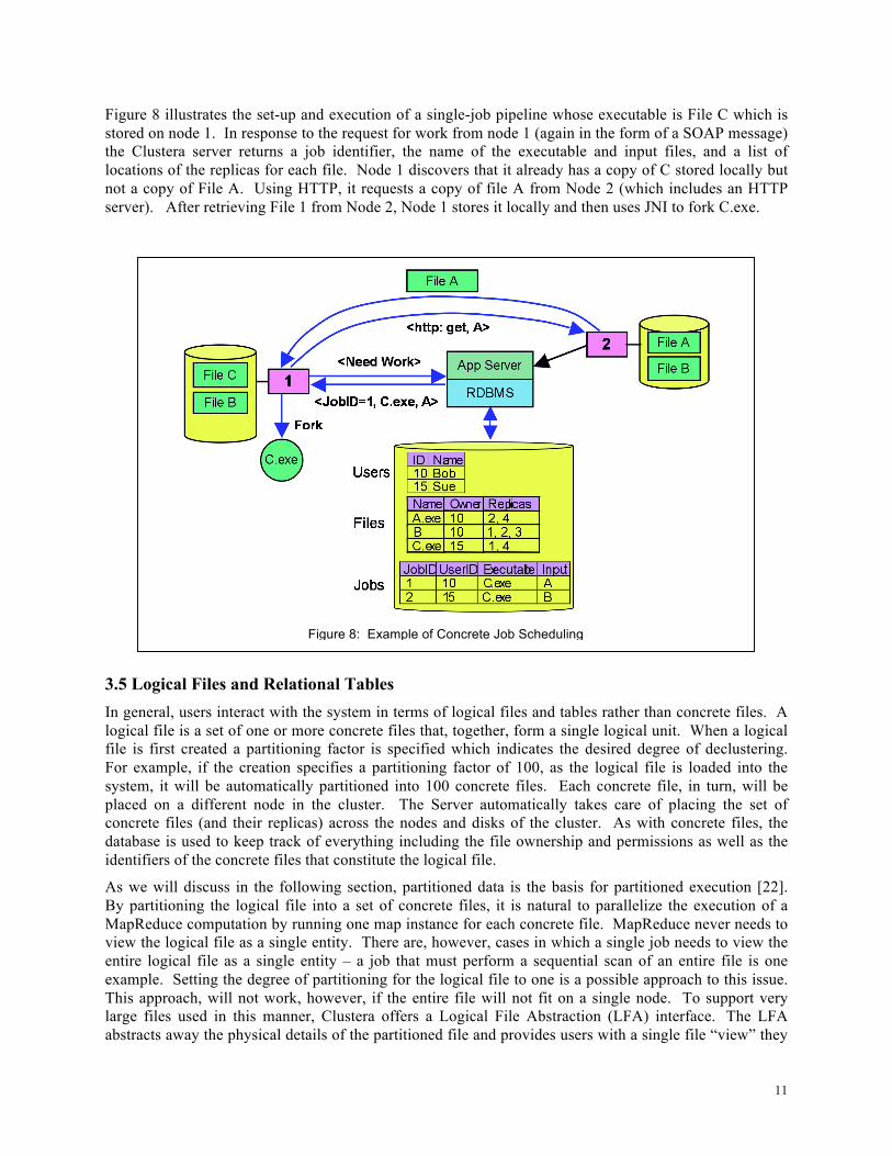
Figure 8 illustrates the set-up and execution of a single-job pipeline whose executable is File C which is stored on node 1. In response to the request for work from node 1 (again in the form of a SOAP message) the Clustera server returns a job identifier, the name of the executable and input files, and a list of locations of the replicas for each file. Node 1 discovers that it already has a copy of C stored locally but not a copy of File A. Using HTTP, it requests a copy of file A from Node 2 (which includes an HTTP server). After retrieving File 1 from Node 2, Node 1 stores it locally and then uses JNI to fork C.exe.

3.5 Logical Files and Relational Tables In general, users interact with the system in terms of logical files and tables rather than concrete files. A logical file is a set of one or more concrete files that, together, form a single logical unit. When a logical file is first created a partitioning factor is specified which indicates the desired degree of declustering. For example, if the creation specifies a partitioning factor of 100, as the logical file is loaded into the system, it will be automatically partitioned into 100 concrete files. Each concrete file, in turn, will be placed on a different node in the cluster. The Server automatically takes care of placing the set of concrete files (and their replicas) across the nodes and disks of the cluster. As with concrete files, the database is used to keep track of everything including the file ownership and permissions as well as the identifiers of the concrete files that constitute the logical file.

As we will discuss in the following section, partitioned data is the basis for partitioned execution [22]. By partitioning the logical file into a set of concrete files, it is natural to parallelize the execution of a MapReduce computation by running one map instance for each concrete file. MapReduce never needs to view the logical file as a single entity. There are, however, cases in which a single job needs to view the entire logical file as a single entity – a job that must perform a sequential scan of an entire file is one example. Setting the degree of partitioning for the logical file to one is a possible approach to this issue. This approach, will not work, however, if the entire file will not fit on a single node. To support very large files used in this manner, Clustera offers a Logical File Abstraction (LFA) interface. The LFA abstracts away the physical details of the partitioned file and provides users with a single file “view” they

Figure 8: Example of Concrete Job Scheduling

12

can read using the standard POSIX interface. The LFA first connects to the database via SOAP to obtain details on the relevant logical file (i.e., the names and locations of the constituent concrete files). Then, as the application needs them, the necessary concrete files are fetched. On Linux this is implemented through a device driver built on top of FUSE (Filesystem in Userspace).

A relation in Clustera is simply a logical file plus the associated schema information. We store the schema information in the Clustera database itself; an alternative approach is to store the schema information in a second logical file. We chose the first approach because it provides the SQL compiler with direct access to the required schema information, bypassing the need to access node-resident data in order to make scheduling decisions.

3.6 Abstract Jobs & Job Scheduler 3.6.1 Introduction Abstract jobs and abstract job schedulers are the key to Clustera’s flexibility and extensibility. Figure 9 illustrates the basic idea. Users express their work as an instance of some abstract job type. For example, a specific SQL query such as select * from students where gpa > 3.0 is an instance of the class of SQL Abstract Jobs. After optimization, the SQL Abstract Job Scheduler would compile this query into a set of concrete jobs, one for each concrete file of the corresponding students table.

Currently we have implemented three types of abstract jobs and their corresponding schedulers: one for complex workflows, one for MapReduce jobs, and one for running SQL queries. Each of these is described in more detail below.

3.6.2 Workflow Abstract Job Scheduler A workflow is a DAG of operations such as the one shown in Figure 6. Such workflows are common in many scientific applications. Workflows can be arbitrarily complex and are frequently used to take a relatively few base input files and pass them through a large number of discrete processing steps in order to produce relatively few final output files. It is not uncommon for the processing steps to use pre-existing executable files as building blocks. The true value of the workflow abstraction is that it provides end-users with a way to create new “programs” without having to write a single line of executable code. Instead of writing code, users can create new dataflow programs simply by recombining the base processing steps in new and interesting ways. Workflows can often generate a large number of intermediate files that are of little or no use to the end-user: only the final output really matters. Workflows can also benefit from parallelism, but keeping track of the large number of processing steps and the intermediate files they depend on is a tedious, error-prone process, which is why users often use workflow tools like Condor’s DAGMan [23].

The Clustera Workflow Abstract Scheduler (WAS) accepts a workflow specification as input and translates it into a graph of concrete jobs that are submitted to the system. The information contained in the workflow specification is similar to that required for any workflow scheduler –the executables to run,

Figure 9: Compilation of abstract job into concrete jobs

13

the input files they require, the jobs that they depend on, etc. For the WAS, the base input files and the output files are all specified as logical files – the WAS will translate the logical file references into the concrete file references required by the system. Since the WAS input is a DAG of jobs which the concrete job scheduler can deal with directly, little is required of the WAS beyond translating the file references and submitting the workflow to the scheduler.

Our current WAS does not assume it can parallelize the jobs in a workflow by instantiating one concrete job for each concrete file of a logical file. To clarify what this means, imagine that LF1 in Figure 6 consists of 100 concrete files. One interpretation of this workflow, then, is that the system should execute 100 instances of J2 - one for each concrete file composing LF1. The current WAS does not use this interpretation. Instead, the current WAS assumes that each executable (e.g. J2) in the workflow must consume its entire input file (e.g. LF1) as a unit and so will only execute one instance of J2. One of the issues at play here is that, since the executables are performing arbitrary functions on arbitrary data, there is no guarantee that the function can be parallelized and still return the correct results (or even execute correctly at all). For some workflows the parallelized approach is acceptable, while for others it is not. Another issue that arises is that LF1 and LF2 may have different partitioning factors making it difficult to determine, for example, how many instances of J1 to execute. Thus, to date, we have only implemented the single-instance-per-executable interpretation because it will always yield the correct results. In the near future we plan to enrich the workflow specification model in order to support the automatic parallelization case for those workflows that can benefit from it.

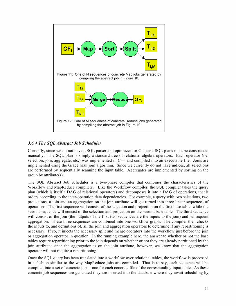
3.6.3 MapReduce Abstract Jobs and Job Scheduler A MapReduce abstract job consists of the name of the logical file to be used as input, the map and reduce functions, and the name to be assigned to the output logical file as shown in Figure 10. The Split, Sort (not shown), and Merge functions are provided by the system in the form of a permanently retained library of executables.

Given a MapReduce abstract job as input, the abstract scheduler will compile the abstract job into two sets of concrete jobs as shown in Figures 11 and 12. For the map phase (Figure 11) there will be one sequence of concrete jobs generated for each of the N concrete files of the input logical file. Each concrete job sequence CFi, 1≤ i ≤ N, will read its concrete file as input and apply the user supplied executable map function to produce output records that the Split function partitions among M concrete output files Ti,j 1≤ j ≤ N.

For the reduce phase (Figure 12), M concrete job sequences will be generated during the compilation process. M is picked based on an estimate of how much data the map phase will produce. Once generated, the concrete jobs for the map and reduce phases can all be submitted to the scheduler for execution. While the map jobs are immediately eligible for execution, the reduce jobs are not eligible until their input files have been produced.

Figure 10: MapReduce Abstract Job Example

14

3.6.4 The SQL Abstract Job Scheduler Currently, since we do not have a SQL parser and optimizer for Clustera, SQL plans must be constructed manually. The SQL plan is simply a standard tree of relational algebra operators. Each operator (i.e. selection, join, aggregate, etc.) was implemented in C++ and compiled into an executable file. Joins are implemented using the Grace hash join algorithm. Since we currently do not have indices, all selections are performed by sequentially scanning the input table. Aggregates are implemented by sorting on the group by attribute(s).

The SQL Abstract Job Scheduler is a two-phase compiler that combines the characteristics of the Workflow and MapReduce compilers. Like the Workflow compiler, the SQL compiler takes the query plan (which is itself a DAG of relational operators) and decomposes it into a DAG of operations, that it orders according to the inter-operation data dependencies. For example, a query with two selections, two projections, a join and an aggregation on the join attribute will get turned into three linear sequences of operations. The first sequence will consist of the selection and projection on the first base table, while the second sequence will consist of the selection and projection on the second base table. The third sequence will consist of the join (the outputs of the first two sequences are the inputs to the join) and subsequent aggregation. These three sequences are combined into one workflow graph. The compiler then checks the inputs to, and definitions of, all the join and aggregation operators to determine if any repartitioning is necessary. If so, it injects the necessary split and merge operators into the workflow just before the join or aggregation operator in question. In the running example here, the answer to whether or not the base tables require repartitioning prior to the join depends on whether or not they are already partitioned by the join attribute; since the aggregation is on the join attribute, however, we know that the aggregation operator will not require a repartitioning.

Once the SQL query has been translated into a workflow over relational tables, the workflow is processed in a fashion similar to the way MapReduce jobs are compiled. That is to say, each sequence will be compiled into a set of concrete jobs - one for each concrete file of the corresponding input table. As these concrete job sequences are generated they are inserted into the database where they await scheduling by

Figure 11: One of N sequences of concrete Map jobs generated by

compiling the abstract job in Figure 10.

Figure 12: One of M sequences of concrete Reduce jobs generated

by compiling the abstract job in Figure 10.

15

the concrete job scheduler.

3.6.5 Discussion As described above, pipelines of co-executing jobs are the fundamental units of scheduling in Clustera. This approach provides Clustera with two important opportunities for achieving run-time performance gains. First, the concrete job scheduler can take advantage of data-dependency information in order to make scheduling decisions that improve overall cluster efficiency. These decisions may, for example, help reduce network bandwidth consumption (by scheduling job executions on nodes where large input data files already reside) and disk I/O operations (by scheduling related executables to run on the same node so that intermediate files can be piped in memory rather than materialized in the file system) resulting in higher job throughput and reduced end-to-end execution times. Second, the concrete job scheduler can take advantage of multi-core nodes by dynamically segmenting the workload in order to match the number of executables in a pipeline to the number of available processing cores on the node.

One limitation of the current implementation, however, is that it does not support the piping of intermediate files across machines. Consider, for example, the DAG segmentation of Figure 7. Since the current implementation does not support cross-machine piping of intermediate data, the first two pipelines must materialize their intermediate data files so that the third pipeline, once it is scheduled, can pull the files to its local disk and begin execution. We are currently extending the system to support cross-machine piping of intermediate files. Once implemented, the concrete job scheduler could choose, for example, to have all three pipelines executing simultaneously so that the intermediate files are never written to disk at all, but rather are piped via a socket directly to the node executing the third pipeline.

Note that dynamic cross-node coordination is much more than a corner case performance booster. We believe that extending the system to support dynamically scheduled cross-node file piping is very important. This capability could prove useful, for example, whenever a data set is repartitioned during the course of processing - as occurs in Map/Reduce jobs between the map and reduce phases and as can occur in SQL jobs prior to joins and aggregation.

To illustrate this issue, consider a typical Map/Reduce job. Between the map phase and the reduce phase, the system needs to repartition the file on the key attribute of the map output records. These temporary “split files” are materialized on the node that ran the map computation and are later “pulled” to the nodes running the reduce computations. While [2] points out the fault-tolerance benefits of this approach, it is important to realize that this fault tolerance comes at a performance price. First, especially in the face of large intermediate files, nodes can end up spending a significant portion of their time and I/O bandwidth materializing files that will eventually just be thrown away. This is supported by the analysis of the sort experiment in [2] which points out that “the sort map tasks spend about half their time and I/O bandwidth writing intermediate output to their local disks.” Second, since every reduce task needs to pull input from every map task, each map node is going to be contacted by each reduce node at least once (and in the case that individual nodes run multiple map or reduce tasks, possibly multiple times) with a file transfer request. Since, except in the case of reduce-node failure, none of the intermediate files will ever be requested more than once, and since the files are, in general, unlikely to be requested in the order they were originally written, there will be little to no pattern to the requests. This lack of a pattern implies a significant spike in the number of random read requests during the repartitioning. Additionally, if, as is described in [2], the reduce tasks try to get a “head start” on the file transfer by requesting files (or pieces of files) as individual map tasks complete (as opposed to waiting until all of the map tasks have completed), there is significant potential that these random reads will now interfere with the writes being performed by the concurrently executing map tasks - potentially leading to map task performance degradation.

Note, however, that much of this problem could be ameliorated if the map tasks could “push” intermediate files to the reduce nodes via sockets. Reversing the communication flow like this fundamentally alters the performance dynamics. In this situation, the map nodes would not need to spend

16

any time or IO bandwidth on materializing files at all. They would, of course, spend time putting the intermediate data on the wire, but they must do this regardless of the approach. Additionally, since the map tasks would now be initiating “push” requests instead of responding to “pull” requests, they would be spared the potential random read interference highlighted in the previous paragraph. Furthermore, recall that, for the repartitioning, the reduce tasks are responsible for assembling a single file from multiple fragments, as opposed to the map tasks that are responsible for splitting a single file into multiple fragments. This difference is crucial because it means that the reduce tasks can convert a set of random network requests into a set of sequential file writes, as opposed to the map tasks (in the pull approach) for whom a set of random network requests translates into a set of random file reads. Thus, moving from a pull approach to a push approach holds out the opportunity of a) eliminating file writes on the map nodes and b) avoiding random reads on the map nodes in favor of sequential writes on the reduce nodes. The caveat, of course, is that skipping the map-node materialization of the intermediate files impairs fault-tolerance in the sense that the amount of work that must be redone in the event of reduce node failure is significantly higher. Clearly detailed experimentation and analysis is required to determine the performance characteristics of each approach and to understand how external factors (failure rate assumptions, for example) impact the overall expected performance of one approach compared the other. We plan to pursue this experimentation and analysis once we have completed implementing the cross-node file piping.

In terms of the implementation itself, while extending the system to support file piping via a socket will certainly present some challenges of its own, we believe the more interesting (and challenging) work will be in augmenting the concrete job scheduler to support this type of dynamic, cross-node schedule coordination in a volatile, high concurrency environment in an efficient, scalable manner. This challenge stems mainly from the fact that we believe it is impractical to rely on approaches that make simplifying assumptions (e.g., the system workload is fixed, one job/user can assume exclusive access to all the cluster nodes, we can rely on a static schedule and simply fail the job if one of the nodes in the schedule goes down, etc…) that are violated “in the wild” if Clustera is to fulfill the design goal of being a highly scalable, general purpose, multi-user, multi-job system.

3.7 Wrapup Before moving on to the performance analysis in Section 4, it is interesting to consider one other architectural aspect in which Clustera significantly differs from comparable systems – the handling of inter-job dependencies. As was described above, Clustera is aware of, and explicitly and internally manages, inter-job data dependencies. Condor, on the other hand, employs an external utility, DAGMan [23], for managing the inter-job dependency graph. Users submit their workflow DAGs to the DAGMan meta-scheduler utility. DAGMan analyzes the workflow graph to determine which jobs are eligible for submission and submits those to an underlying Condor process that performs job queue management – the schedd. DAGMan then “sniffs” the relevant schedd’s log files in order to monitor job progress. As submitted jobs complete, DAGMan updates the dependency graph in order to determine when previously ineligible jobs become eligible for execution. As these jobs become eligible DAGMan submits them to the Condor schedd. One of the benefits of this approach is that the workflow management logic runs as a separate process. Since the schedd is single-threaded, offloading the workflow management can reduce the load on the schedd.

For Clustera, probably the biggest benefit of managing the dependencies internally is that it provides the concrete job scheduler with the ability to do more intelligent scheduling. It is clearly impossible to enable in-memory (or cross-node) piping of intermediate data files if the jobs that would consume the piped data are not even visible to the system until after the jobs that produce that data have completed. One other noteworthy advantage of handling the dependencies internally is that it simplifies examining and/or manipulating a workflow as a unit. Finally, having all the information about the jobs that have been submitted and/or executed in one place significantly simplifies system administration. Additional information about our job scheduling algorithms can be found in [26].

17

4. Performance Experiments and Results As stated previously, a primary goal of the Clustera project is to enable efficient execution of a wide variety of job types on a potentially large cluster of compute nodes. To gauge our level of success in achieving this goal we ran a number of experiments designed to provide insight into the performance of the current prototype when executing three different types of jobs. Section 4.1 describes the experimental setup. The MapReduce results are presented in Section 4.2, the SQL results in Section 4.3, and arbitrary workflow results in Section 4.4. Section 4.5 explores the performance of the Clustera Server under load.

To give some additional context to the Clustera MapReduce and SQL performance numbers, we also ran comparable experiments using the latest stable release (version 0.16.0) of the open-source Hadoop system. There are four key reasons that we chose to compare Clustera numbers with Hadoop numbers for these workloads. The first reason, as laid out in the introduction, is to observe whether a general-purpose system like Clustera is capable of delivering MapReduce performance results that are even “in the same ballpark” as those delivered by a system, like Hadoop, that is specifically designed to perform MapReduce computations. The second reason is to understand how the relative performance of a moderately complex operation (e.g., a two-join SQL query) is affected by the rigidity of the underlying distributed execution paradigm; in substantially more concrete terms, this goal can be rephrased as trying to understand if it makes a difference whether a SQL query is translated to a set of MapReduce jobs or to an arbitrary tree of operators in preparation for parallel execution. The third reason is to understand if there are any structural differences between the two systems that lead to noticeably different performance or scalability properties. The fourth reason is to ascertain whether the benefit (if any) of enriching the data model for a parallel computing system (e.g., by making it partition-aware) is sufficient to justify the additional development and maintenance associated with the enriched model.

Note that providing a performance benchmark comparison between the two systems (or between Clustera and a parallel RDBMS) was not a goal of our experimentation. Parallel computation systems are very complex and, as will be noted in Section 4.1.1, can be sensitive to a variety of system parameters. While undoubtedly an interesting investigation in its own right, tuning either Hadoop or Clustera (much less both) to optimality for a particular workload is beyond the scope of this study and, along with a performance comparison including a parallel RDBMS, is deferred to future work. We are not attempting to make any claims about the optimally tuned performance of either system and the numbers should be interpreted with that in mind.

4.1 Experimental Setup We used a 100-node test cluster for our experiments. Each node has a single 2.40 GHz Intel Core 2 Duo processor running Red Hat Enterprise Linux 5 (kernel version 2.6.18) with 4GB RAM and two 250GB SATA-I hard disks. According to hdparm, the hard disks deliver ~7GB/sec for cached reads and ~74MB/sec for buffered reads. The 100 nodes are split across two racks of 50 nodes each. The nodes on each rack are connected via a Cisco C3560G-48TS switch. The switches have gigabit ethernet ports for each node and, according to the Cisco datasheet, have a forwarding bandwidth of 32Gbps. The two switches are connected via a single (full-duplex) gigabit ethernet link. In all our experiments the participating nodes are evenly split across this link.

For the Hadoop experiments we used an additional desktop machine with a single 2.40 GHz Intel Core 2 Duo processor and 2GB RAM to act as the Namenode and to host the MapReduce Job Tracker. For the Clustera experiments we used two additional machines - one to run the application server and one to run the backend database. For the application server we used JBoss 4.2.1.GA running on the same hardware configuration used for the Hadoop Namenode/Job Tracker. For the database we used DB2 v8.1 running on a machine with two 3.00 GHz Intel Xeon processors (with hyperthreading enabled) and 4GB RAM. The database bufferpool was ~1GB which was sufficient to maintain all of the records in memory.

18

As mentioned in Section 3, Clustera accepts an abstract description of a MapReduce job or SQL query and compiles it into a DAG of concrete jobs. For MapReduce jobs, the map and reduce functions are specified as part of the MapReduce specification, with the sort, split, and merge functions taken from a system-provided library. These library functions are re-used in the compilation of SQL queries. In addition SQL workflows also use select, project, hashJoin, aggregate and combine library functions. All MapReduce and SQL library functions are Linux binaries written in C.

4.1.1 A Note on Configuring Hadoop After getting up and running with Hadoop, we quickly realized that there were quite a few configuration parameters that we could adjust that would affect the observed performance. While a complete exploration of the effects of all 135 parameters is clearly beyond the scope of this paper, we did conduct a number of experiments to try to determine a good configuration for the workloads we were testing. Appendix I discusses the results of this experimentation in detail. For the current discussion, the key point to note is that we consistently observed the best performance when we used an HDFS block size of 128MB and permitted the nodes to execute two map tasks simultaneously. All of the Hadoop results presented in Sections 4.2 and 4.3 are based on this configuration.

4.2 MapReduce Scaleup Test This section presents the results of a series of scale-up experiments we ran to evaluate Clustera performance for MapReduce jobs. The base data for these experiments is the LINEITEM table of the TPC-H 100 scale dataset. The MapReduce job itself performs a group-by-aggregation on the first attribute (order-key) of the LINEITEM table. For each record in the input dataset the map function emits the first attribute as the key and the entire record as the value. After this intermediate data has been sorted and partitioned on the key (per the MapReduce contract), the reducer emits a row count for each unique key. If the goal were simply to calculate these row counts, then clearly this computation could be implemented more efficiently by having the map function emit, e.g., a “1” instead of the entire record as its output. For experimentation, however, the actual result of the computation is immaterial; observing the performance impact of large intermediate data files is, however, quite interesting and important.

As explained earlier, we ran a set of MapReduce scale-up experiments on both Clustera and Hadoop in order to try to understand, among other things, whether Clustera could deliver MapReduce performance results in the same general range as those delivered by Hadoop. For the scale-up experiments we varied the cluster size from 25 nodes up to 100 nodes and scaled up the size of the dataset to process accordingly.

For the Clustera MapReduce experiments, the input logical file is composed of a set of concrete files that each contain ~6 million records and are approximately 759 MB in size. In each experiment the number of concrete files composing the logical input file and the number of Reduce jobs is set to be equal to the number of nodes participating in the experiment; since the MapReduce abstract compiler generates one Map job per concrete file, the number of Map jobs, then, was always also equal to the number of nodes participating in the experiment.

Finally, we ran one additional experiment designed to see how performance of this computation is affected if the input data is hash-partitioned and the scheduler is aware of the partitioning. Since the “vanilla” MapReduce computation model does not distinguish between hash-partitioned and randomly partitioned input files, we could not run this experiment on Hadoop or via the Clustera MapReduce abstract compiler. We could, however, perform the same computation by recasting it as a Clustera-SQL job over a relational table containing the same underlying dataset (partitioned on the aggregation key) in which project and aggregate take the place of map and reduce. Since the SQL scheduler “knows” that the data is already hash-partitioned, it avoids a repartition and the resulting concrete workflow reduces to one project-sort-aggregate DAG for each concrete file in the table. To ensure comparability across results, the query’s project operator outputs the same intermediate values as the map functions of the

19

MapReduce jobs.

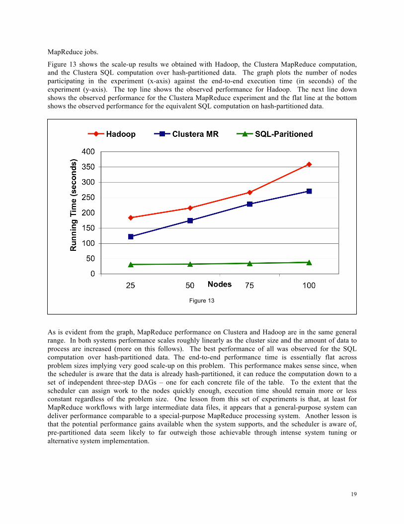
Figure 13 shows the scale-up results we obtained with Hadoop, the Clustera MapReduce computation, and the Clustera SQL computation over hash-partitioned data. The graph plots the number of nodes participating in the experiment (x-axis) against the end-to-end execution time (in seconds) of the experiment (y-axis). The top line shows the observed performance for Hadoop. The next line down shows the observed performance for the Clustera MapReduce experiment and the flat line at the bottom shows the observed performance for the equivalent SQL computation on hash-partitioned data.

As is evident from the graph, MapReduce performance on Clustera and Hadoop are in the same general range. In both systems performance scales roughly linearly as the cluster size and the amount of data to process are increased (more on this follows). The best performance of all was observed for the SQL computation over hash-partitioned data. The end-to-end performance time is essentially flat across problem sizes implying very good scale-up on this problem. This performance makes sense since, when the scheduler is aware that the data is already hash-partitioned, it can reduce the computation down to a set of independent three-step DAGs – one for each concrete file of the table. To the extent that the scheduler can assign work to the nodes quickly enough, execution time should remain more or less constant regardless of the problem size. One lesson from this set of experiments is that, at least for MapReduce workflows with large intermediate data files, it appears that a general-purpose system can deliver performance comparable to a special-purpose MapReduce processing system. Another lesson is that the potential performance gains available when the system supports, and the scheduler is aware of, pre-partitioned data seem likely to far outweigh those achievable through intense system tuning or alternative system implementation.

Figure 13

20

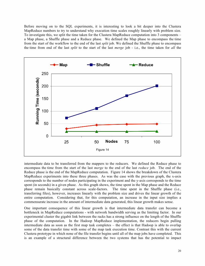
Before moving on to the SQL experiments, it is interesting to look a bit deeper into the Clustera MapReduce numbers to try to understand why execution time scales roughly linearly with problem size. To investigate this, we split the time taken for the Clustera MapReduce computation into 3 components – a Map phase, a Shuffle phase and a Reduce phase. We defined the Map phase to encompass the time from the start of the workflow to the end of the last split job. We defined the Shuffle phase to encompass the time from end of the last split to the start of the last merge job - i.e., the time taken for all the

intermediate data to be transferred from the mappers to the reducers. We defined the Reduce phase to encompass the time from the start of the last merge to the end of the last reduce job. The end of the Reduce phase is the end of the MapReduce computation. Figure 14 shows the breakdown of the Clustera MapReduce experiments into these three phases. As was the case with the previous graph, the x-axis corresponds to the number of nodes participating in the experiment and the y-axis corresponds to the time spent (in seconds) in a given phase. As this graph shows, the time spent in the Map phase and the Reduce phase remain basically constant across scale-factors. The time spent in the Shuffle phase (i.e., transferring files), however, increases linearly with the problem size and drives the linear growth of the entire computation. Considering that, for this computation, an increase in the input size implies a commensurate increase in the amount of intermediate data generated, this linear growth makes sense.

One important consequence of this linear growth is that intermediate data transfer can become a bottleneck in MapReduce computations - with network bandwidth serving as the limiting factor. In our experimental cluster the gigabit link between the racks has a strong influence on the length of the Shuffle phase of the computation. In the Hadoop MapReduce implementation, the reducers begin pulling intermediate data as soon as the first map task completes – the effect is that Hadoop is able to overlap some of the data transfer time with some of the map task execution time. Contrast this with the current Clustera prototype in which none of the file transfer begins until all of the map jobs have completed. This is an example of a structural difference between the two systems that has the potential to impact

Figure 14

21

performance and scalability. In the near future we plan to extend Clustera to enable this overlapping of data transfer time with map execution time, though by pushing data through a socket rather than by pulling it, and hope to see some performance gains as a result. Of course an even more important structural issue is exposed by the hash-partitioned version of this computation in which the partition-aware scheduler is able to avoid all data transfer costs and, as a result, display the best performance and scale-up properties.

4.2.1 MapReduce: Sensitivity to Intermediate Data This section explores in detail the sensitivity of Clustera MapReduce to varying amounts of intermediate data. In this set of experiments the input dataset (TPCH scale 100 LINEITEM table), the size of input data per map job (759 MB), the size of the output data per reduce job (19 MB), and the computation performed by the MapReduce workflows (group-by-aggregation) are identical to that in Section 4.2. Instead of emitting an entire input record as the value, however, in these experiments the map jobs emit a string with a specified length. By varying the length of this string, the amount of intermediate data produced, transferred and aggregated in the MapReduce workflow can be varied. We ran the group-by-aggregation MapReduce workflow on 25, 50, 75 and 100 nodes, with intermediate data sizes of 68 MB, 314 MB, 560 MB and 805 MB per node.

The results of these experiments are shown in Figure 15. In this figure, the x-axis corresponds to the amount of intermediate data generated on each node and the y-axis corresponds to the total running time for the computation. Each line corresponds to a different cluster size. The top line plots the results for a 100-node cluster, the second line down is for a 75-node cluster, the third line down is for a 50-node cluster and the bottom line is for a 25-node cluster. Note that for each cluster size in the experiments, the number of records processed and produced for all intermediate data sizes is the same - only the length of each record of the intermediate data files varies.

Figure 15

22

As shown in Figure 15, for all cluster sizes, the running time increases as the amount of intermediate data increases. One key point to observe, though, is that the rate of increase (i.e., the slope of the line) is greater for a 100-node cluster than for a 25-node cluster. To understand why this is so requires synthesizing two pieces of information. First, recall an insight derived from Figure 14 that, once the network is saturated, intermediate file transfer time grows linearly with the problem size. Second, recall that this is a scale-up experiment – i.e., the problem size is increased commensurately with the amount of resources devoted to solving the problem. The underlying factor, then, would appear to be the multiplicative effect that increasing the cluster size has on the total amount of intermediate data to transfer; in the 100-node case there is four times as much intermediate data to transfer as in the 25-node case simply because there is four times as much total intermediate data generated.

Figure 16 provides evidence that supports this supposition. The graph in Figure 16 shows, for each phase (Map, Shuffle, Reduce), the effect that varying the amount of intermediate data has on execution time for a 100-node cluster. In this graph, the x-axis plots the amount of intermediate data generated and the y-axis plots the observed execution time. The top line corresponds to the Shuffle phase, the middle line corresponds to the Map phase and the bottom line corresponds to the Reduce phase. As the amount of intermediate data increases, the time taken in the Shuffle phase grows at a much faster rate than the time taken in the Map and Reduce phases. Since the Shuffle phase, again, is driving the total execution time, it seems fair to conclude that the slope variance observed in Figure 15 is indeed being driven by the data transfer time.

As a final note, it is important to understand that, though the two graphs look almost identical, the Figure 14 graph and the Figure 16 graph are displaying two different, but related, phenomena. The Figure 16 graph shows that, for a given cluster size, the time it takes to complete a MapReduce computation with a large amount of intermediate data grows linearly with the problem size. The Figure 14 graph takes this one step further and demonstrates that, even if the resources devoted to the problem are increased

Figure 16

23

commensurately with the problem size, the time it takes to complete such a MapReduce computation still grows linearly with the problem size. Thus, it would appear that, for truly data-intensive problems, intermediate data transfer time is often the bottleneck of the computation and it is important to reduce this as much as possible in the Map phase. As the Partitioned-SQL experiment (Figure 13) shows, eliminating the Shuffle phase entirely by using pre-partitioned data is a particularly effective technique to reduce the workflow running time and provide much better scale-up properties.

4.4 SQL Scaleup Test This section presents the results of a series of scale-up experiments we ran to evaluate Clustera performance for SQL jobs. The base data for these experiments consists of the CUSTOMER, ORDERS and LINEITEM tables of the TPC-H dataset. The SQL query we ran was:

SELECT l.okey, o.date, o.shipprio, SUM(l.eprice) FROM lineitem l, orders o, customer c WHERE c.mkstsegment = ‘AUTOMOBILE’ and o.date < ‘1995-02-03’ and l.sdate > ‘1995-02-03’ and o.ckey = c.ckey and l.okey = o.okey GROUP BY l.okey, o.date, o.shipprio

We ran experiments on 25, 50, 75 and 100 nodes using appropriately scaled TPC-H datasets. For all the datasets, the size of the CUSTOMER, ORDERS and LINEITEM chunks on each node are 23MB, 169MB and 758 MB, respectively

For the Clustera experiments we used the SQL abstract scheduler. The query plan joined the CUSTOMER and ORDERS tables first (because they were the two smaller tables) and then joined that intermediate result with the LINEITEMS table. For the Clustera experiments we also varied the partitioning of the base tables. In one set of experiments the base tables were not hash-partitioned. For these experiments, each concrete file of a base table is first filtered through select and project operators, followed by a repartition according to the join key. Thus, there are four repartitions in the workflow – one for each of the base tables, and a fourth for the output of the first join (CUSTOMER-ORDERS). The final group-by-aggregation does not require a repartition since the final join key is okey. In the other set of experiments, the CUSTOMER and ORDERS tables are hash-partitioned by ckey and the LINEITEM table is hash-partitioned by okey. For these experiments, the base tables do not need to be repartitioned prior to the joins. The output of the CUSTOMER-ORDERS join, though, is partitioned on ckey, so it must be repartitioned on okey prior to the second join. The following table shows the total amount of intermediate data that is repartitioned in both cases.

Total Data Shuffled (MB) Num

Nodes Partitioned UnPartitioned 25 77 2122 50 154 4326 75 239 6537

100 316 8757

As was the case with the MapReduce experiments, we also ran the SQL experiments on Hadoop. While joining two tables may not fit “neatly” into the MapReduce paradigm, it can be done. In fact, it is precisely because a join does not fit neatly into the MapReduce paradigm that we thought that running the query on Hadoop would be interesting; we hoped that it would help us to understand if translating a SQL query into a series of MapReduce jobs (as opposed to a tree of operators) would have any noticeable impact on performance.

24

Rather than attempt to write our own MapReduce join code, we used the DataJoin contrib package that is included with Hadoop. In a DataJoin job in Hadoop, both join operands are treated as a single logical

input. The intermediate data is tagged with the base table name in the Map phase, and the join is enumerated in the Reduce phase with the help of these tags. As with the Clustera-SQL queries, for the DataJoin jobs we joined the CUSTOMER and ORDERS tables first and then joined this intermediate result with the LINEITEMS table before performing the final aggregation. Note that, in addition to tagging the data with the base table name, we also performed the necessary selections and projections in the Map phase. The total amount of intermediate data to be repartitioned during the DataJoin jobs, then, is just slightly larger than what is shown in the un-partitioned column in the table above – the excess is due to the per-record tags required to support the DataJoin. Since Hadoop does not support hash-partitioned files, we only ran un-partitioned DataJoins. For all DataJoin experiments we used the same Hadoop base configuration as described in the Section 4.2 MapReduce experiments.

On our generated datasets, the predicate on this query has a selectivity of approximately 50%; this selectivity factor significantly reduces the size of the intermediate files that are generated. We also experimented with another version of the query with no selection predicates to see if altering the selectivity had any impact on performance.

Figure 17 plots the number of nodes in the experiment (x-axis) against the observed run-time (in seconds, y-axis) of the computation. Looking at the right side of the graph, the top line is the DataJoin with no selection predicate, the second line is the Hadoop DataJoin with a selection predicate, the third line is the Clustera-SQL job on un-partitioned data with no selection predicate, the fourth line is the Clustera-SQL job on un-partitioned data with a selection predicate and the bottom line is the Clustera-SQL job on hash-partitioned data with no selection predicate. The Clustera-SQL job on partitioned data with a selection predicate performed on average about 30% better than the equivalent SQL job with no selection predicate, but we have not displayed it here in order to improve the readability of the figure.

Figure 17

25

As expected, observed performance and scalability on the hash-partitioned datasets is superior to all other approaches. Again, this would seem to suggest that, given the performance gains available, when implementing a parallel computation system it is probably worth the effort to enrich the data-model and scheduler to support and take advantage of partitioned data. For both of the Clustera SQL jobs over un-partitioned data, performance seems to scale roughly linearly with an increase in the problem size. Similar to the Clustera MapReduce results, the linear factor can be traced back to the data transfer when tables are repartitioned. Recall that in the current Clustera prototype none of the “merges” of a repartitioning are scheduled until all of the corresponding “splits” have completed. The result is that there is a spike in network activity when the merges are scheduled which causes the link between the racks to saturate (and become a bottleneck) leading to the linear growth in the data-transfer time and, by extension, the overall execution time. Compare this linear growth to that of the DataJoin job on un-partitioned data with a selection predicate (second line). This case still exhibits a linear component to the growth, but the linear growth here is damped relative to that of the Clustera SQL jobs just discussed; this dampening most likely occurs because, as described previously, the underlying Hadoop MapReduce jobs are able to overlap some of the data transfer time with some of the map task execution time. Again, in the near future we plan to apply this lesson by extending Clustera to support overlapping data-transfer time and execution time. Finally, the performance of the DataJoin with no selection predicate is interesting to consider. The run-time for the DataJoin with no selection predicate consistently ranges from approximately 2.2 to 2.3 times longer than the run-time for the DataJoin with a selection predicate. Compare this to the spread for the Clustera SQL jobs on un-partitioned data that consistently ranges from approximately 1.4 to 1.5 times longer. It is not entirely clear why the DataJoin spread is so much larger. One possible contributing factor is that perhaps less of the data-transfer time is overlapped with map task execution time. Another possible factor is that implementing a join in the MapReduce framework inherently incurs additional sorting overhead that can be avoided if a good plan using a hash-join is available. Unfortunately, despite some of their shared goals, the systems are sufficiently different that it appears that an in-depth investigation beyond the scope of this study is required to draw firm conclusions about the performance impact that the underlying parallel execution model has on join implementation. 4.5 Blast Workflow Speedup test Clustera also can run arbitrary workflows with user-defined data and programs. In this section we demonstrate the execution of the BLAST scientific workflow. BLAST is a sequence alignment program that searches a file of well-known proteins for similarities with a new sequence of proteins. A BLAST DAG consists of two jobs, blastall and javawrap. Blastall takes a sequence of acids seq and performs sequence alignment using the nr_db files, which document known proteins. Blastall produces a seq,blast file which is then processed by the javawrap program to produce csv and bin files for later use. A typical BLAST workflow consists of several such BLAST DAGs. Each DAG may operate on a different set of sequences, but all of them use the same nr_db and all_java.tar files. We ran a workflow of 1000 BLAST DAGs on 25, 50, 75 and 100 machines to test the speedup obtained. One copy of the input data (including the nr_db files and all_java.tar) is placed on either side of the switch. The average execution times for blastall and javawrap are 207s and 6s.

Figure 18 shows that as the number of nodes is increased, the actual speed-up obtained deviates slightly away from the ideal line. To understand this deviation, consider what is happening in the cluster while the workflow is executing. Before a blastall job can begin executing on a node, all of its required input data (the nr_db files) must be transferred to that node. As the number of nodes is increased, the amount of data that is transferred across the network increases, which delays the startup of the first blastall job on each node. Note that all of the file transfer time is spent before the execution of the first job. Also, once the first job on each node completes, the input data is essentially replicated throughout the cluster, and subsequent jobs do not incur any file transfer cost. This suggests that for workflows containing a large number of jobs with common input data, file transfer becomes a bottleneck as the number of nodes used to run the workflow is increased – for a given replication factor, when the number of nodes used is

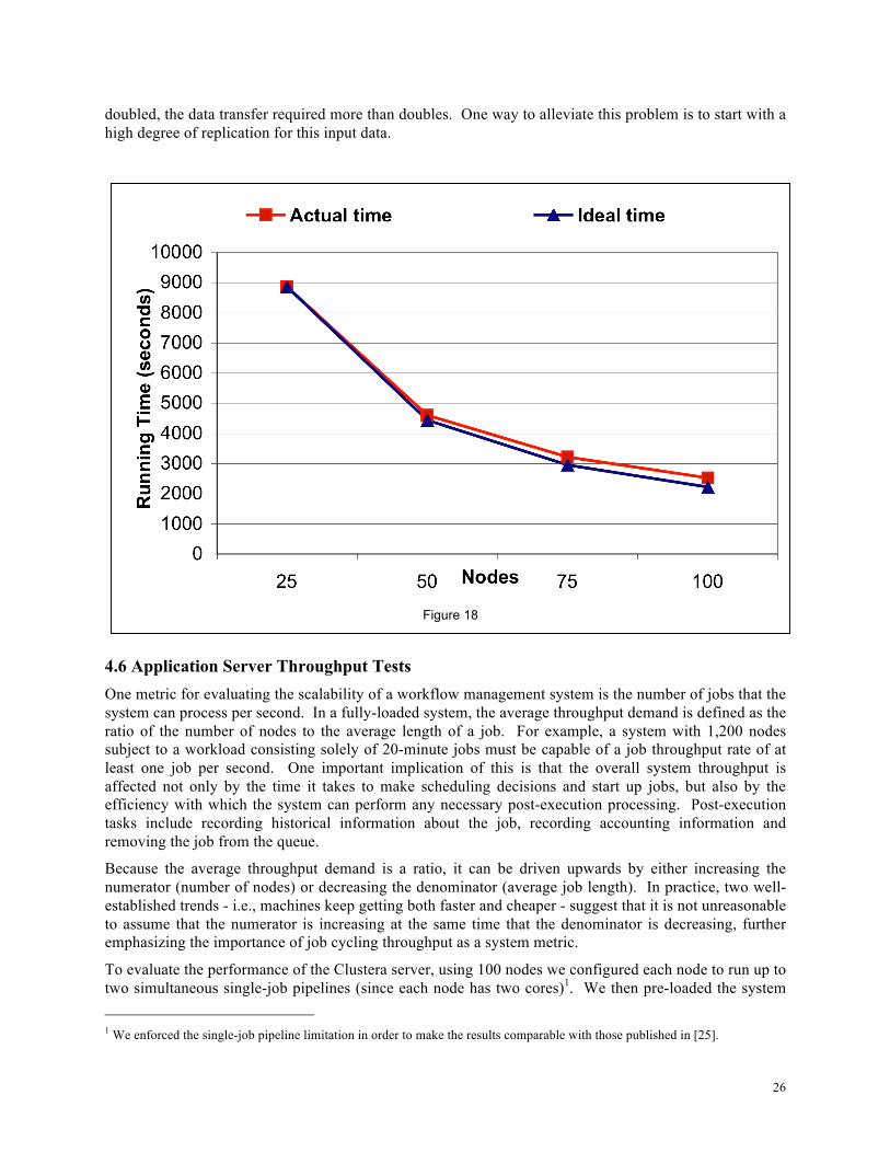
26

doubled, the data transfer required more than doubles. One way to alleviate this problem is to start with a high degree of replication for this input data.

4.6 Application Server Throughput Tests One metric for evaluating the scalability of a workflow management system is the number of jobs that the system can process per second. In a fully-loaded system, the average throughput demand is defined as the ratio of the number of nodes to the average length of a job. For example, a system with 1,200 nodes subject to a workload consisting solely of 20-minute jobs must be capable of a job throughput rate of at least one job per second. One important implication of this is that the overall system throughput is affected not only by the time it takes to make scheduling decisions and start up jobs, but also by the efficiency with which the system can perform any necessary post-execution processing. Post-execution tasks include recording historical information about the job, recording accounting information and removing the job from the queue.

Because the average throughput demand is a ratio, it can be driven upwards by either increasing the numerator (number of nodes) or decreasing the denominator (average job length). In practice, two well-established trends - i.e., machines keep getting both faster and cheaper - suggest that it is not unreasonable to assume that the numerator is increasing at the same time that the denominator is decreasing, further emphasizing the importance of job cycling throughput as a system metric.

To evaluate the performance of the Clustera server, using 100 nodes we configured each node to run up to two simultaneous single-job pipelines (since each node has two cores)1. We then pre-loaded the system 1 We enforced the single-job pipeline limitation in order to make the results comparable with those published in [25].

Figure 18

27

with a number of identical, fixed-length jobs whose lengths ranged from a maximum of 200 seconds down to a minimum of four seconds in order to cover a range from 1 job per second all the way up to 50 jobs per second.

Figure 19 plots the number of jobs cycled per second against the targeted throughput rate for the experiment. The top line shows the ideal throughput rate while the bottom line shows the observed results. The labels above the top line show the job length for that experiment. Since our cluster was configured to run 200 jobs concurrently the targeted throughput rate is simply 200 (the number of concurrent jobs) divided by the job length; the 200 second jobs correspond to a target of one job per second whereas the four second jobs correspond to a target of 50 jobs per second. For the jobs that were six seconds or longer, we observed the server achieving throughput rates very close to the ideal. For the five- and four-second jobs the observed rate is below the ideal.

Figure 20 shows a plot of the server’s CPU cycle consumption as a function of the number of jobs cycled per second. For each experiment we calculated the average throughput rate, excluding the ramp up and ramp down time.

Looking at the left side of the graph, the bottom line (square data points) in Figure 20 is “System” usage (cycles spent executing in “kernel” mode), the middle line (diamond data points) is “User” usage (cycles spent doing actual computation) and the top line (triangular data points) is idle cycles (spare computational capacity). These three categories sum up to approximately 100%; the time spent handling interrupts or waiting on IO was negligible and is not plotted here. As Figure 20 shows, the server still had at least 20% of its cycles to spare during all experiments.

One striking feature of Figure 20 is the apparent linear growth in cycle usage in response to increases in targeted throughput across experiments. This pattern changes at the right side of the chart as the observed throughput peaks just shy of 38 jobs cycled per second. Interestingly enough, the right-most data point

Figure 19

28

actually corresponds to the five-second job experiment (~37.9 jobs cycled per second with ~23.8% idle cycles remaining) and the second-from-the-right data point corresponds to the four-second job experiment (~36.9 jobs cycled per second with ~23.2% idle cycles). The server apparently saturates at around 38 jobs per second after which additional demand causes interference on the server leading to reduced performance.

The observed throughput rates presented here are an improvement over previously published results for CondorJ2 (a precursor to Clustera) and Condor [25]. This improvement comes despite the fact that Clustera is required to manage not only the same job, machine and configuration information managed by CondorJ2 (and Condor), but also to manage the logical and physical file information required to support data-aware scheduling.

A logical question to ask at this point is what can be done to push the throughput numbers up even higher? One answer is to throw more hardware at the problem – either by running a single server on a bigger machine (more CPUs and cores) or by moving to a clustered server configuration (e.g., Figure 3). Another approach is to reduce the amount of “work” required to cycle through a job in the system.

For any cluster management system cycling a job requires four steps: scheduling the job, starting the job, recording the job completion and “cleaning-up” after the job. Currently, in Clustera, scheduling the job and recording the job completion are reasonably fast operations. Starting the job and cleaning up after the job, however, are more involved operations that consume more of the CPU cycles. Starting the job involves working through a three-step protocol. In the first step the server informs the node of the job it has been scheduled to run. In the second step the node evaluates whether or not it will run the job and issues a web service call to the server informing the server of its decision. In the third step, assuming the node decided to run the job and after the node has collected all of the necessary input files and actually spawned the job in question, it sends a startup message to the server. This type of handshaking protocol is perfectly sensible for a system, like Condor, with a distributed job queue, but is probably more heavy-

Figure 20

29

weight than necessary in a system, like Clustera, with a centralized job queue. An alternative we are exploring is switch to a “Presumed Accept” protocol (in which the server assumes the node will run the job it has been assigned unless the node explicitly issues a reject call) with lazy-propagation of the startup data. This would remove two (out of four) web-service calls as well as two application-server and database transactions.

Cleaning up after the job requires removing the job from the queue and recording the historical information about the job. Our profiling indicates that much of the clean-up time is now spent on two operations – the lookup and deletion of the job and its related input file records and the creation of the historical records in the application server and their physical insertion into the database. Of these operations, the lookup and deletion of the job cannot be avoided. The creation and insertion of the historical records, however, could be skipped but doing so would reduce the usability and manageability of the system (and cluster) and make actions such as file lineage tracing essentially impossible. One of the trade-offs illustrated by this example pits manageability/usability against performance. So far we have consistently chosen to make usability and manageability high priorities.

5. Conclusions and Future Directions We are currently witnessing the early stages of the "cloud computing" revolution, in which large clusters of processors are exploited to perform various computing tasks on an "as needed" basis. To date the database community has played a minor role in this revolution in that (a) large-scale parallel database systems use a model of dedicated, single-use clusters very different from that adopted by cloud computing, and (b) cluster management systems for high-throughput and data intensive computing use database technology superficially if at all.

Our work on Clustera is an early step toward increasing the role of database systems in cloud computing in two ways. First, we have shown that cluster management is an ideal application for modern relational database system technology. Second, we have shown that a generic cluster management system like Clustera has potential as a platform upon which to execute massively parallel SQL queries. The potential in this second direction is huge --- it opens the door to integrated systems that can run SQL queries on the same platform used to run other data intensive and compute-intensive applications. A great deal of challenging research is needed before such systems are a reality, but if the database community does not work on building them, we fear the revolution will pass us by, and both parallel database systems and cloud computing will have missed a great opportunity.

6. References [1] Litzkow, M., Livny, M., and M. Mutka, “Condor – A Hunter of Idle Workstations”, Proc. of the 8th

ICDCS Conf., 1988.

[2] Dean, J. and S. Ghemawat, “MapReduce: Simplified Data Processing on Large Clusters,” Proc. of the 6th OSDI Conference, Dec. 2004

[3] Needham, R. M. and A. J. Herbert. 1982. The Cambridge Distributed Computing Systems, Addison-Wesley, MA.

[4] DeWitt, D., Finkel, R. and M. Solomon, “The Crystal Multicomputer: Design and Implementation Experience,” IEEE TSE, Vol 13. No. 8, 1987.

[5] IBM, “Tivoli Workload Scheduler LoadLeveler v3.3.2 Using and Administering,” April 2006.

[6] Platform Computing Corporation, “Administering Platform LSF”, Platform Computing Corporation, Feb. 2006.

[7] Urban, A (Ed.), “Portable Batch System Administrator Guide,” Altair Grid Technologies, April 2005.

[8] Sun Microsystems, Inc., “N1 Grid Engine 6 Administration Guide,” June 2004.

30

[9] Microsoft Corporation, “Windows Compute Cluster Server 2003 Reviewers Guide,” May 2006.

[10] United Devices, “Grid MP Platform Version 4.1 Application Developer’s Guide,” 2004.

[11] Schuster, S., Nguyen, H., Ozkarahan, and K. Smith, “RAP.2 – An Associative Processor for Databases,” Proc. of the 5th ISCA Conference, 1978.

[12] Su, S. and G. Lipovski, “CASSM: A Cellular System for Very Large Databases,” Proceedings of the 1st VLDB Conference, Framingham, MA, 1975.

[13] DeWitt, D., “DIRECT - A Multiprocessor Organization for Supporting Relational DBMS,” IEEE Trans. on Computers, Vol. C-28, No. 6, June 1979.

[14] Stonebraker, M., “Muffin: A Distributed Database Machine,” Proc. of the 1st ICDCS Conference, Oct. 1979.

[15] DeWitt, D., Gerber, B, Graefe, G., Heytens, M., Kumar, K. and M. Muralikrishna, “Gamma–A High Performance Dataflow Database Machine,” Proc. of the 1986 VLDB Conf.

[16] Teradata, “DBC/1012 Data Base Computer Concepts & Facilities,” Teradata Corp. Document No. C02-0001-00, 1983.

[17] http://hadoop.apache.org/

[18] Isard, M., Budiu, M, Yu, Y., Birrell, A., and D. Fetterly, “Dryad: Distributed Data-Parallel Programs from Sequential Building Blocks,” European Conference on Computer Systems (EuroSys), Lisbon, Portugal, March 21-23, 2007.

[19] Kini, A., Shankar, S., Naughton, J., and D. DeWitt, “Database support for matching: limitations and opportunities,” Proc. of the 2006 SIGMOD Conference, 2006.

[20]RedHat Enterprises, “JBoss Enterprise Application Platform,” http://www.jboss.com/products/platforms/application

[21] Mutka, M. and M. Livny, “Scheduling Remote Processing Capacity in a Workstation-Processor Bank Network,” In Proc. 7-th Int. Conf. on Distr. Comp. Systems, 1987.

[22] DeWitt, D. and J. Gray, “Parallel Database Systems: The Future of High Performance Database Systems,” CACM Vol. 34, No. 6, 1992.

[23] http://www.cs.wisc.edu/condor/dagman/

[24] Olson, C., Reed, B., Srivastava, U., Kumar, R. and A. Tomkins, “Pig Latin: A Not-So-Foreign Language for Data Processing,” Proceedings of the 2008 SIGMOD Conference.

[25] Robinson, E., and D. DeWitt, “Turning Cluster Management into Data Management: A System Overview,” Proceedings of the 2007 CIDR Conference, Asilomar, CA.

[26] Shankar, S. and DeWitt, D. J. 2007, “Data driven workflow planning in cluster management systems” In Proceedings of the 16th international Symposium on High Performance Distributed Computing, June 2007.

[27] Ghemawat, S., H. Gobioff, and S. Leung, “The Google File System,” Proceedings of the 19th ACM Symposium on Operating Systems Principles, 2003.

31

7. Appendix I – Hadoop Configuration Experiments Hadoop is still early in its development, and Hadoop cluster administrators are urged to customize their configuration to find the right balance of settings that perform well for their workloads. In this section, we present some basic background information on Hadoop as well as our experience with tuning Hadoop to improve performance. As stated in Section 4.1.1, the best-performing configurations observed here were what we used in comparisons to Clustera in Sections 4.2 and 4.3.

7.1 Background on Hadoop

The Hadoop Distributed File System (HDFS) implements many of the ideas from the Google File System [27]. Briefly, HDFS consists of a collection of data servers (the DataNodes) and a metadata server (the NameNode). Files in HDFS are broken up into blocks and are stored on the DataNodes. Clients contact the NameNode to translate between the HDFS namespace and learn the location of where to read or write blocks of a file. For redundancy, clients store data on multiple DataNodes, and the NameNode is responsible for ensuring that sufficient copies of the blocks are always available.

In Hadoop, DataNodes often serve simultaneously as execution nodes for MapReduce programs. Most MapReduce jobs are translated into one Java process per block of an input file, which then invokes the map() function on each record found in that block. Adjusting the block size of the file system is therefore a simple way to control the number of Map tasks launched by Hadoop for a given job (more sophisticated ways are, of course, possible.) In the usual case, Hadoop will chose to execute the Map task for a block on a machine where that block is already present, but in some cases it may transfer the block to another machine and perform the computation there. 7.1 Experimenting with Hadoop MapReduce

Our first experiment was the group-by aggregation, described in Section 4.2. In Hadoop we implemented this experiment by slightly modifying the “WordCount” example included in the Hadoop distribution.

Figure 21

32

Figure 21 shows the result of the experiments described in Section 4.2 with a number of different block sizes. Each machine was configured to run one map task and one reduce task simultaneously. As shown in Figure 21 we observed that a block size of 128 megabytes consistently exhibited the best performance. Smaller block sizes result in more map tasks, so one potential factor underlying the improvement when moving from 64MB blocks to 128MB blocks is that it may be possible that a 64MB block is processed too quickly to amortize the per-task overheads and startup costs. As blocks are completed, the reduce tasks can begin collecting intermediate results. This overlap can reduce the end-to-end time of the computation. Larger block sizes mean fewer completed map tasks are available to start collecting, which limits the potential parallelism. This could be a reason why block sizes larger than 128MB did not exhibit further performance gains.

Since our test bed is made up of dual-core machines, we also experimented with simultaneously running two map tasks on each node (along with a reduce task). The results are plotted in Figure 22. We found that, except for the 100-node case, running two map tasks per node with a 128MB block size always yielded better results than any other configuration. Note that as the cluster size increases, the network switch becomes the bottleneck leading to a reduction in the benefits of extra parallelism available when running two map tasks per node. Note also that the spike in the graph at 75 nodes with a 128MB block size and a single map task arises from significant variability for that particular data point. It is not clear why this data point exhibits such variability. We ran that particular experiment many times and consistently observed instability.

Figure 22

33

7.2 Experimenting with Hadoop DataJoin

We also ran the Hadoop DataJoin experiments with a number of different file system block sizes. Our joins included a 50% selection predicate to reduce the amount of intermediate data that had to be

Figure 23

Figure 24

34

transferred. As shown in Figure 23, with a single map task per node there appears to be little difference between 128, 256 and 512 MB block sizes. In Figure 24, we repeat the experiment with two map tasks per node. In these experiments, using two map tasks per node always outperformed using a single map task per node with a 128MB block size slightly outperforming a 256MB block size. In these experiments, the smaller intermediate data apparently prevents the network switch from becoming as narrow a bottleneck, which in turn allows for the performance gap between the single and dual map instances to remain pronounced for larger computations. Because a using two map tasks per node and a 128MB block size was consistently among the best (if not the best) configuration for all of our experiments, this is the configuration we reported results for in Sections 4.2 and 4.3.