Computer Simulation in Statistical Mechanicsand in Condensed Matter Physics

Pietro Ballone

Centre for Life NanoSciences @La Sapienza, Rome

Italian Institute of Technology, IIT

• Generalities on computer simulation;

• An introduction to molecular dynamics (MD);

• Basic elements of modelling;

• An introduction to Monte Carlo;

Figure 1: Ludwig Boltzmann

Textbooks on Simulation

D. Frenkel and B. Smit, Understanding Molecular Simulation, 2nd edn, Aca-demic Press, San Diego (2002).

J. P. Hansen and I. R. Mc Donald, Theory of Simple Liquids, Third Edition,Elsevier, Amsterdam (2006).

M. Tuckerman, Statistical Mechanics: Theory and Molecular Simulation,Oxford Graduate Texts, (2010).

Numerical Recipes, A series of books, many Authors, several editions, andversions devoted to different computer languages.

A bit obsolete, but still a useful introduction: M. P. Allen and D. J. Tildesley,Computer Simulation of Liquids; Clarendon Press: Oxford (1991).

Simulation:

”a method to reproduce and investigate the behaviour of a system on a

computer”

Carried out by:

• defining a set of equations that describe the relation between the parts ofthe system;

• solving the equations on a computer;

• analysing/interpreting the results to understand/predict the system proper-ties.

Extensively used in:

• physics;

• chemistry;

• engineering;

• finance and marketing;

• social sciences;

• strategy and military planning;

• biology (population biology; spread of diseases; ...)

• ...

• games (!!!!)

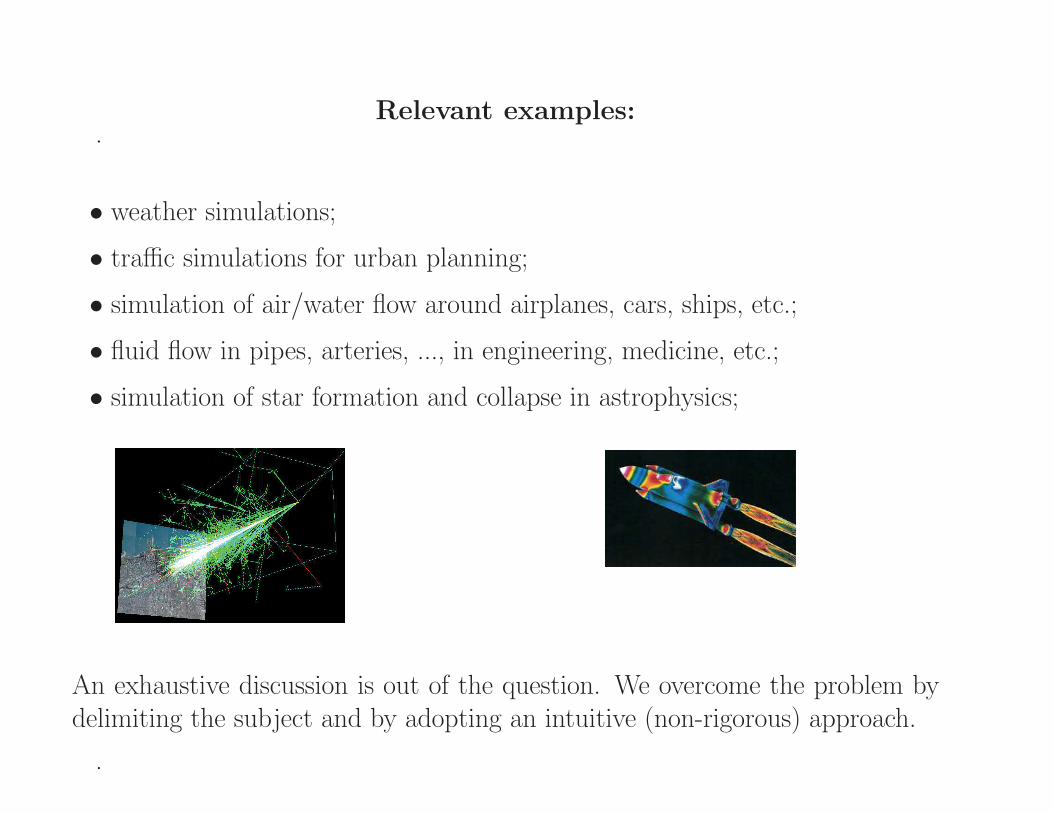
.Relevant examples:

• weather simulations;

• traffic simulations for urban planning;

• simulation of air/water flow around airplanes, cars, ships, etc.;

• fluid flow in pipes, arteries, ..., in engineering, medicine, etc.;

• simulation of star formation and collapse in astrophysics;

.

An exhaustive discussion is out of the question. We overcome the problem bydelimiting the subject and by adopting an intuitive (non-rigorous) approach.

In our lectures:

”a method to reproduce the behaviour of a

condensed matter system on a computer”

Figure 2: Computer Simulator

Applied to problems in:

• Physics

• Chemistry (including biochemistry)

• Materials science

More precisely, our few lectures are concerned withcomputer simulation based on classical particles.

We exclude, for instance:

• quantum systems;

• lattice models;

• fields;

• ...

In our case, computer simulation will be usedto compute equilibrium and non-equilibriumproperties of many-particle systems, startingfrom the microscopic interactions among these”particles”.

Often these particles will be identified with atoms.

Sometimes particles will represent whole molecules(CH4, PF

−6 , for instance), or groups of atoms

(coarse graining).

Figure 3: Methane

Figure 4: BPA-PC polycarbonate

Relevant applications include:

• the equilibrium properties of water from its molecular building block;

• the structure and dynamics of liquid or amorphous metals, semiconductorsor insulators;

• the structure and dynamics of lipids, proteins, nucleic acids, ...;

• ...

• the ionic dynamics in dense (astrophysics) plasmas;

• the properties of nuclear matter in neutron stars;

• ...

.many different flavours of simulation needed to cover the many size andtime scales of interest.

Figure 5: Figure from the Web

The multiplicity of scales is particularly apparent in the hierarchical organisationof bio-systems:

• Local Motions (0.01 to 5 A , 10−15 to 10−1 s)

– Atomic fluctuations

– Sidechain Motions

– Loop Motions

• Rigid Body Motions (1 to 10 A , 10−9 to 1s)

– Helix Motions

– Domain Motions (hinge bending)

– Subunit motions

• Large-Scale Motions (> 5 A , 10−7 to 104 s)

– Helix/coil transitions

– Dissociation/Association

– Folding and Unfolding

Historical Development (using digital computers)

• Fermi-Ulam-Pasta computational experiment (1953);

• Fermi, Metropolis, Ulam, von Neumann, introduced Monte Carlo (1948-1953);

• ”Equation of State Calculations by Fast Computing Machines” N. Metropo-lis, A.W.Rosenbluth, M.N.Rosenbluth, A.H.Teller and E. Teller, The Journalof Chemical Physics, 21, 1087 (1953);

• Alder and Wainwright: first MD of hard sphere fluids (1957-1959);

• A. Rahman, L. Verlet around 1964: first MD simulations of realistic systems;

• R. Car and M. Parrinello, ab-initio molecular dynamics (1985).

.

At that time, simulations were done on a single-CPU computer, starting fromENIAC:

Figure 6: ENIAC computer

.

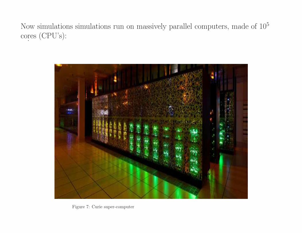
Now simulations simulations run on massively parallel computers, made of 105

cores (CPU’s):

Figure 7: Curie super-computer

Size and Performances (Curie, Commissariat a l’Energie Atomique):

• 100,000 cores (CPU’s);

• 2,000 Teraflops (2 Petaflops, i.e., 2× 1015) peak performance;

• Infiniband connectivity;

• 5 Petabytes disk storage (plus much more on slower access devices)

Problems and Limitations:

• high demand of electric power.

• massive and difficult dissipation of heat.

Fairly large computations on Curie take 107 core-hours to be completed.In this amount of time, we routinely simulate systems like this one:

Figure 8: POPC double bilayer

Crucial Algorithmic Advances:

• Efficient usage of parallel architecture: communications, shared memory,etc.;

• Linear scaling of FP operations / s up to large numbers of nodes/cores;

• Efficient usage of novel architectures (GPU);

• Efficient computation of long range forces: linear scaling with system size!

Outline of the Method(s)

•We assume that our systems are made of particles;

• evolving according classical mechanics;

• potential energy is a function of the atomic coordinates;

• we assume that the many-particle properties are already represented by sam-ples made of a number of atoms<<<<<<<NA = 6.022×1023 (Avogadro’snumber);

• we assume that the phenomena of interest occur on a microscopic time scale<<< s [to be specified below].

Basic choice:

In our simulations, either we assume equilibrium conditions or we need tospecify the operating conditions of an out-of-equilibrium phenomenon.

• equilibrium conditions:

– molecular dynamics;

– Monte Carlo;

• non-equilibrium conditions:

– molecular dynamics

Somewhat in between:

• kinetic Monte Carlo.

Typical system sizes range from 103 to 105 particles;

sometimes we exceed 106 particles.

Largest simulation could be: 4× 1012 particles (HLRZ, Juelich, Germany).

Not all simulation methods are driven by time.When time is relevant (MD for realistic models), typical simulation time scalescoves from 102 ps to 102 ns for systems of up to 106 particles.

Simulations in the µs range are fairly common, and a few ms simulations forsystems made of 105 particles have been made using a special-purpose machine.

[Anton super-computer: 17, 000 ns/day simulations of proteins in water].

Time limitations are more severe than size limitations.

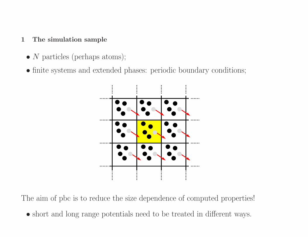
1 The simulation sample

• N particles (perhaps atoms);

• finite systems and extended phases: periodic boundary conditions;

The aim of pbc is to reduce the size dependence of computed properties!

• short and long range potentials need to be treated in different ways.

2 Generalities on systems

• N particles, {ri, i = 1, N}; {pi, i = 1, N};

• phase space: 6N -dimensional space spanned by the ri’s and pi’s;

• in classical statistical mechanics, we can restrict ourselves to the configura-tion space, spanned by the ri’s.

Everything that happens can be represented as a process taking place in phasespace.

Equilibrium state: characterised by its stationary probability distributionρeq(r

N ;pN) in phase space.

Crucial property - (Ergodicity): the equilibrium probability distributionshould not divide the phase space into disjoint portions!

Such a probability distribution, in turn, depends on the macroscopic variableschosen to identify the equilibrium (macroscopic) state.These can be:

• the number N of particles;

• the volume V ;

• the total energy E;

• the temperature T ;

• the pressure P ;

The choice of macroscopic variables has some limitations.The most common choices identify the ”ensembles” of statistical mechanics.

• microcanonical (NVE);

• canonical (NVT);

• isobaric (NPT);

• gran canonical (µPT);

• ...

.

A crucial role is played by the partition function corresponding to the rel-evant ensemble, which is the normalisation for the probability distributionρeq(r

N ;pN).

Example: Canonical ensemble NVT; the probability distribution is the Boltz-mann distribution:

ρeq({rN ,pN}) =

exp [−βHN ]

Z(1)

where HN is the Hamiltonian of the N -particle system, and β = 1/(KbT ).

The requirement:∫

ρeq(rN ;pN)drNdpN = 1 (2)

implies:

Z(N, V, T ) =

∫

exp [−βHN ]drNdpN (3)

In the NPT ensemble, we consider also fluctuations of the volume:

∆(N,P, T ) =βP

h3NN !

∫

V >0

exp [−β(HN + PV )]dV (4)

where h is Plank’s constant.

Equilibrium Systems

To compute properties, we need to sample the appropriate probability distribu-tion.

Two basic choices:

• compute the average properties of the system over the equilibrium distribu-tion in phase space (MC);

• visit a relevant portion of the phase space following the time evolution of arepresentative sample (MD);

These two choices are equivalent if the system is ”ergodic”, since in such a casetime averages are equal to ensemble averages. Given A(rN ,pN),

〈A〉ensemble = limt→∞

1

t

∫ t

0

A(rN(t′),pN(t′))dt′ (5)

Properties to be computed are:

• thermodynamics functions such as internal energy, enthalpy, entropy, etc.

• structural properties such as radial distribution function, structure factor,etc.

• properties of inhomogeneous systems such as surfaces and interfaces, finitesystems, etc.

• linear and non linear response to perturbation (that are still equilibriumproperties).Examples:

– isothermal compressibility;

– elastic constants

– thermal and electrical conductivities;

– ...

Two methods: molecular dynamics (MD) and Monte Carlo (MC).

.

Molecular Dynamics (MD):Basic version: Integrating Newton’s equations of motion

Let us assume that the simulated sample consists of N particles (atoms), rep-resenting a finite system, or a piece of an extended phase.

In the first case, we do not need to specify boundary conditions.In the second case, we usually adopt periodic boundary conditions.

Basic procedure (coarse-grained description):

1. setting up the system, initialising coordinates and velocities;

2. equilibrating the system (or carrying out a non-equilibrium computationalexperiment);

3. running the simulation;

4. analysing the data;

5. repeating (3)-(4) until collecting sufficient statistics.

Equilibrating the System

By necessity, we need to start from initial conditions that we cannot identify as”representative” or not.

Does the result depend on the initial conditions?Positions and momenta of all particles at time t are functions of their initialvalues at t = 0:

ri(t) = f [rN(0),pN(0); t] (6)

with a similar relation for the momenta.Let us change one or more initial conditions by a perturbation whose amplitudeis ǫ.The leading term in the deviation of coordinates and momenta is a growingexponential:

| ∆ri(t) |∼ ǫ exp (λt) (7)

where λ is the largest Lyapunov exponent. In ”real” systems made of 104

particles, λ can be as large as ∼ 0.1.

On the one hand:

no possibility of approaching ”ideal” trajectories( on a digital computer)

The round off error is enough to spoil the ”exact” result within a short time.However, global properties such as total energy, angular momentum, responsefunctions, etc., do not change. (← This is an ”experimental” observation, nota theorem).

On the other hand:

all starting conditions are equivalent(provided the system is ergodic)

Integrating Newton’s equations of motionSetting:

NVT ensemble; N particles, possibly with pbc.

A routine to compute potential energy and forces from the particle coordinates.

Newton’s equations of motion:

miri = Fi (8)

with initial conditions: {ri(t = 0)}.

”Ideal” Conservation laws are implicit in the form of the Hamiltonian:

No explicit dependence of the Hamiltonian on time −→ Energy is conserved.

Space isotropy: Angular momentum is conserved (finite and isolated systems).

Conservation laws provide an ideal tool to verify the accuracy of the integrationalgorithm and implementation.

Now integrating!

A task for Euler’s algorithm?Let us discretise the integral, and make a short time increment δt:

ri(t + δt) = ri(t) + δtvi(t) +1

2δt2

Fi

mi+ o(δt3) (9)

”Experimental” observation:Large deviations, and eventual breakdown of the integration unless δt is so shortto prevent covering a significant time interval.

What did go wrong?

Symmetries:

• Newton’s equations of motion are invariant under time reversal;

• time evolution conserves the volume in phase space. In other terms, thetransformation:

ri(t + δt)←− ri(t) (10)

has a Jacobian of one.The integration rule has to reflect the basic symmetries of the system dynamics.

Choices better than Euler: many possibilities, from ad-hoc integration rules, topredictor-corrector schemes

The Verlet AlgorithmThe algorithm developed and used for the first MD simulations is still a pop-

ular choice (upon suitable modifications). The simple exposition:

Forward evolution:

ri(t + δt) = ri(t) + δtvi(t) +1

2δt2

Fi(t)

mi+ o(δt3) (11)

Backward evolution:

ri(t− δt) = ri(t)− δtvi(t) +1

2δt2

Fi(t)

mi− o(δt3) (12)

Combining:

ri(t + δt) = 2ri(t)− ri(t− δt) + δt2Fi(t)

mi+ o(δt4) (13)

Choice of the time step: 1/100 of a characteristic (high frequency) vibrationalperiod.

.Properties:

• good long-time conservation of the global properties (total energy, angularmomentum, ..) that define the state;

• fairly large fluctuations on the time-step scale ← usually without conse-quences;

• very cheap and low RAM requirements (no longer so important).

It is a leap-frog algorithm

No consistent estimation of velocity at time t before time t + δt is computed:

vi(t) =[ri(t + δt)− ri(t− δt)]

2δt(14)

This is a problem when forces or other potentials depend on velocities.

Solution: velocity Verlet algorithm.

.For completeness: velocity Verlet.

It is a predictor-corrector integrator. One of its forms is:

• advance time by δt:

ri(t + δt)← ri(t) + δt vi(t) +1

2δt2ai(t) (15)

• predict velocities at t + δt:

vi(t + δt)← ri(t) + δtai(t) (16)

• compute forces FN(t + δt) at coordinates {rN(t + δt)}

• correct velocities:

vi(t + δt)← vi(t + δt) +1

2δt [ai(t + δt)− ai(t)] (17)

Figure 9: S-leaping Frog

Reasons of its success:

• simple and inexpensive (in time and storage);

• time reversible;

• it conserves the volume of the phase space.

.

A general framework to generate integration algorithms

Let us consider a function f [rN(t);pN(t); t].

Its time derivative is:

f = r∂f

∂r+ p

∂f

∂p≡ iLf (18)

We define in this way the operator L, which is known as the Liouville operator:

iL = r∂

∂r+ p

∂

∂p= iLr + iLp (19)

We can formally integrate in time:

f [rN(t);pN(t); t] = exp [iLt] f [rN(0);pN(0); 0] (20)

We see that the Liouville operator carries out an infinitesimal forward displace-ment of time.A more detailed analysis shows that iLr evolves the coordinates, while iLpevolves the momenta through an infinitesimal time increase.

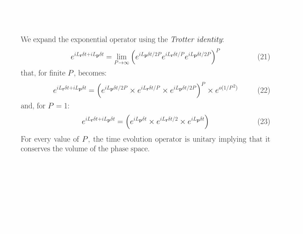
We expand the exponential operator using the Trotter identity:

eiLrδt+iLpδt = limP→∞

(

eiLpδt/2PeiLrδt/PeiLpδt/2P)P

(21)

that, for finite P , becomes:

eiLrδt+iLpδt =(

eiLpδt/2P × eiLrδt/P × eiLpδt/2P)P

× eo(1/P2) (22)

and, for P = 1:

eiLrδt+iLpδt =(

eiLpδt × eiLrδt/2 × eiLpδt)

(23)

For every value of P , the time evolution operator is unitary implying that itconserves the volume of the phase space.

Once developed, the expression:(

eiLpδt/2PeiLrδt/PeiLpδt/2P)P

= eiLpδt/2PeiLrδt/PeiLpδt/2P ... eiLpδt/2PeiLrδt/PeiLpδt/2P

(24)can be interpreted in terms of a precise sequence of coordinates and momentaevolutions through time, and can be translated into a precise integration algo-rithm.

Grouping or rearranging terms (when possible) in this expression provides a wayto develop new integration rules, that automatically correspond to unitary andtime reversible dynamics.

The P = 1 case, in particular, corresponds to velocity Verlet!

.

The minimal structure of a MD code

• Initialisation:

– read input (coordinates, velocities);

– compute initial forces;

– define auxiliary variables, counters, accumulators, etc.;

• Main loop:

– ”coordinates” part of the velocity Verlet;

– compute potential energy and forces;

– ”velocity” part of Verlet;

• Termination:

– output final configuration (coordinates, velocities and accelerations);

– compute and output properties and average quantities.

Most of the time (95%) is spent in the computation of forces.

Whatever the rule, the integration requires at most a few % of the CPU time.

.

Properties:

• temperature, pressure, internal energy;

• microscopic structure: the radial distribution function;

• compressibility; conductivity; etc. Green-Kubo fluctuation formulae.

A few examples:

Temperature:

KBT =〈2EK〉

3N(25)

where EK is the system kinetic energy.

Pressure (from the virial):

P = ρKBT +1

3V

⟨

N∑

i=1

Fi · ri

⟩

(26)

Specific heat:

cv =∂〈U〉

∂T=

1

KBT 2

[

〈U 2〉 − 〈U〉2]

(27)

U is the potential energy, and the cv computed in this way represents only theexcess contribution besides the trivial kinetic one.

Isothermal compressibility:

χT = −1

V

(

∂〈V 〉

∂P

)

T

=1

KBT 2

[

〈V 2〉 − 〈V 〉2]

(28)

where V is the system volume.

Summary of the previous lectureMolecular Dynamics:

Aim:

• compute equilibrium properties:Given A[rN ,pN ],

〈A〉ensemble = limt→∞

1

t

∫ t

0

A[rN(t′),pN(t′)]dt′ (29)

• reproduce the system evolution during a non-equilibrium transformation.

Achieved by integrating Newton’s equations of motion:

miri = Fi (30)

Integration carried out by discrete time steps of size δ, using a variety ofalgorithms.

The Verlet Algorithm

ri(t + δt) = 2ri(t)− ri(t− δt) + δt2Fi(t)

mi+ o(δt4) (31)

Leap-frog algorithm:

vi(t) =[ri(t + δt)− ri(t− δt)]

2δt(32)

This is a problem when forces or other potentials depend on velocities.

Solution: velocity Verlet algorithm.

.More often: Velocity Verlet integration

It is a predictor-corrector integrator. One of its forms is:

• advance time by δt:

ri(t + δt) = ri(t) + δt vi(t) +1

2δt2ai(t) (33)

• predict velocities at t + δt:

vi(t + δt) = ri(t) + δtai(t) (34)

• compute forces at {rN(t + δt)} (including velocities, if needed).

• correct velocities:

vi(t + δt) = vi(t + δt) +1

2δt [ai(t + δt)− ai(t)] (35)

A few practical considerations I

Equilibration

How long does it last?It depends on the relaxation times in the system.Easy for fluid systems not far from their triple pointDifficult or even impossible for amorphous systems, of for fluids close to theircritical point.

At the very least, there should be no observable drift in properties such as po-tential and kinetic energy; volume or pressure; local density and/or composition;etc.

In ”healthy” cases, equilibration takes from 10 to 20 % of the simulation time.

A few practical considerations IIStatistics

Quantities to be averages fluctuate because of the many interactions in the sys-tem.By the central limit theorem, the distribution of these fluctuations is Gaussian.The estimate of averages is affected by a standard error that decreases like theinverse square root of the simulation time → quick improvement at the begin-ning;more and more difficult to get a significant improvement at late stages!

Long relaxation times imply correlations in the estimate of properties.The error still decreases with time−1/2, but the prefactor might be large!Always necessary to check autocorrelation times.

Organise your runs into a modular sequence, in such a way that you can ex-clude/include segments to check/improve statistics, and to correct mistakes inthe identification of the equilibration to production turning point.

Molecular dynamics in different ensembles

The natural ensemble for MD is the NVE, or micro-canonical ensemble.However, we need / would like to run simulations in the canonical ensemble, orin the isobaric (NPT) ensemble.

Thermodynamic functions converge to the same value in the thermodynamiclimit.

Their fluctuations, however, are different in the different ensembles.

Because of the fluctuation-dissipation theorem, this implies that response func-tions are different in the different ensembles.

No surprise! We know, for instance, that Cv 6= Cp.

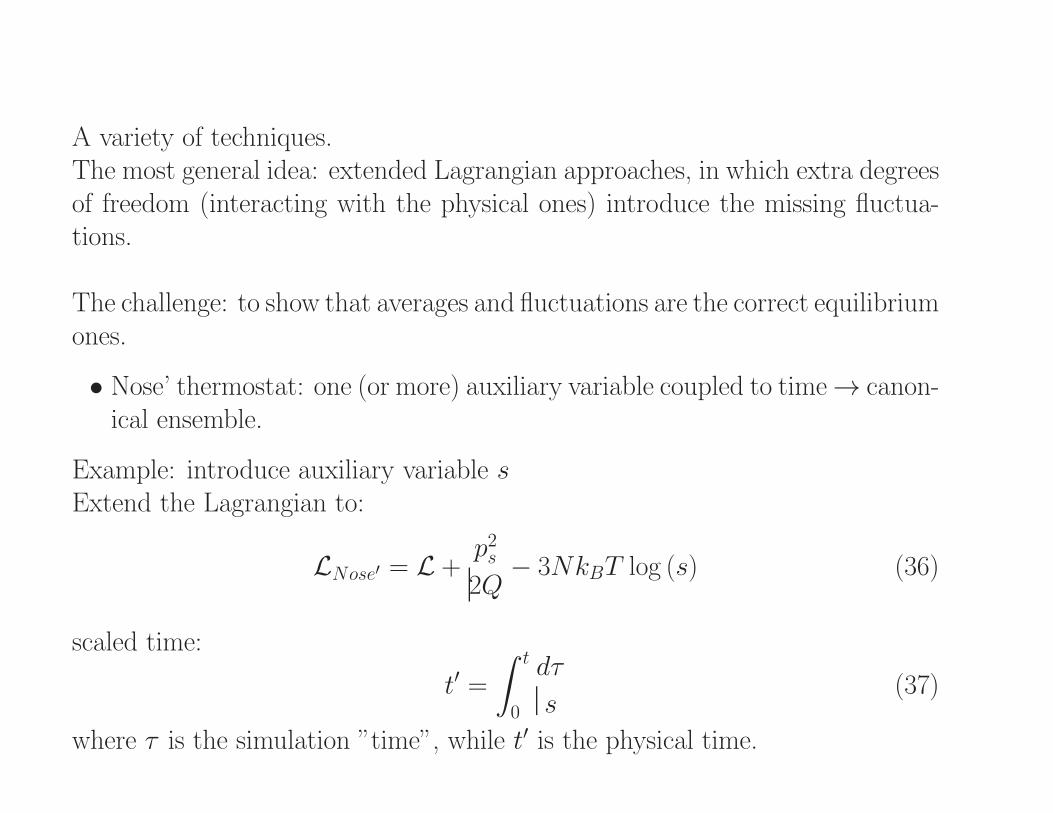
A variety of techniques.The most general idea: extended Lagrangian approaches, in which extra degreesof freedom (interacting with the physical ones) introduce the missing fluctua-tions.

The challenge: to show that averages and fluctuations are the correct equilibriumones.

• Nose’ thermostat: one (or more) auxiliary variable coupled to time→ canon-ical ensemble.

Example: introduce auxiliary variable sExtend the Lagrangian to:

LNose′ = L +p2s2Q− 3NkBT log (s) (36)

scaled time:

t′ =

∫ t

0

dτ

s(37)

where τ is the simulation ”time”, while t′ is the physical time.

• Parrinello-Rahman method: the sides of the simulation cell are auxiliaryvariables whose variations account for volume fluctuations at a pre-set pres-sure.

• Grand-canonical ensemble not relevant in MD, but several attempts havebeen made.

• ...

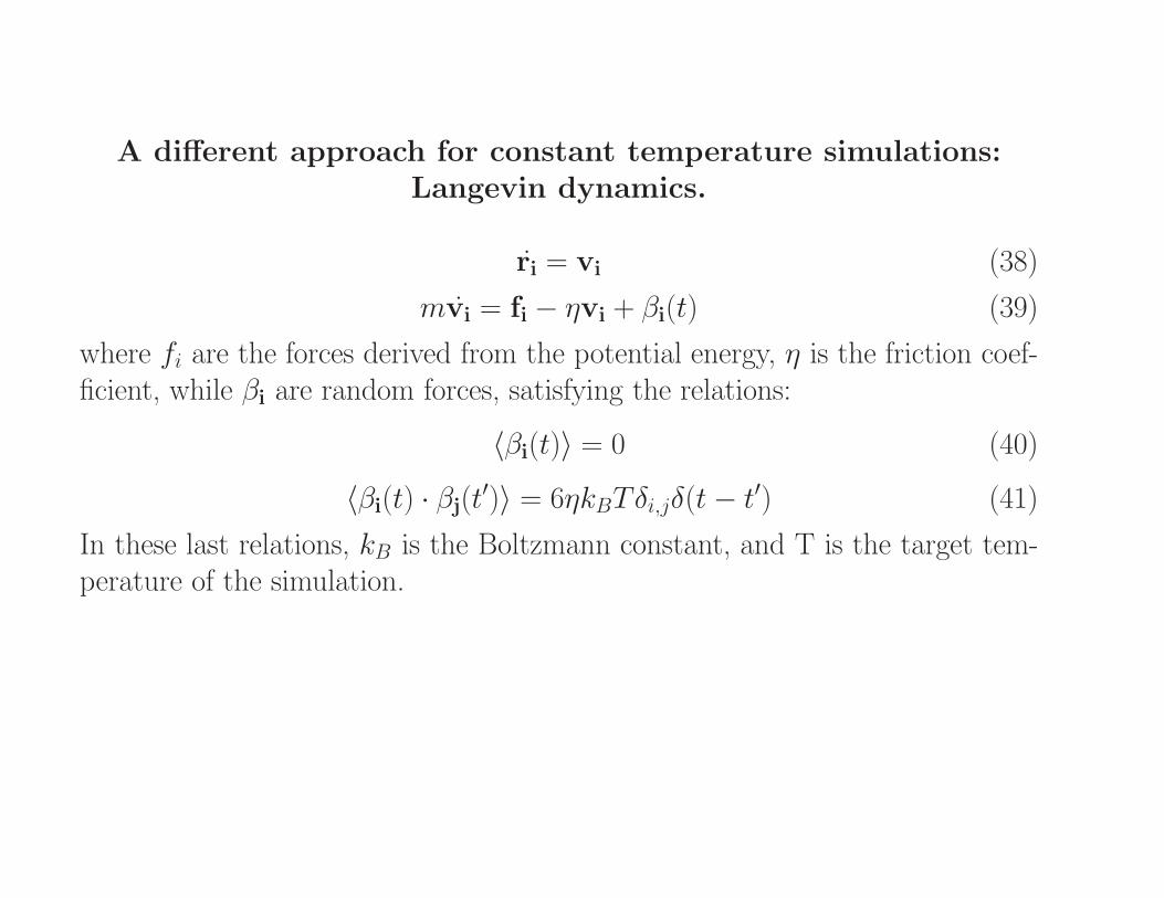
A different approach for constant temperature simulations:Langevin dynamics.

ri = vi (38)

mvi = fi − ηvi + βi(t) (39)

where fi are the forces derived from the potential energy, η is the friction coef-ficient, while βi are random forces, satisfying the relations:

〈βi(t)〉 = 0 (40)

〈βi(t) · βj(t′)〉 = 6ηkBTδi,jδ(t− t

′) (41)

In these last relations, kB is the Boltzmann constant, and T is the target tem-perature of the simulation.

.

Evaluation of Forces:

• Almost without exceptions, it represents the most time consuming portionof the computation;

• Time is spent computing distances and interactions. Different treatment of:

– short range forces;

– long range forces.

Interactions are long range when:∫

φ(r)dr −→∞ (42)

where φ is a representative interaction potential in the system.

.

Monte Carlo in the Canonical Ensemble

Equilibrium state defined by the probability distribution:

ρeq(rN ;pN) =

exp [−βHN(rN ;pN)]

∫

exp [−βH(rN ;pN)]drNdpN(43)

where HN(rN ;pN) is the system Hamiltonian:

HN(rN ;pN) =

N∑

i=1

p2i2mi

+ U (rN) = K(pN) + U (rN) (44)

Figure 10: Nicholas Metropolis

A(rN ;pN) operator defining a quantity of interest(examples: potential energy; virial)

Equilibrium value (canonical ensemble):

〈A〉 =

∫

ρeq(rN ;pN)A(rN ;pN)drNdpN = (45)

∫

A(rN ;pN) exp [−βHN(rN ;pN)]drNdpN

∫

exp [−βH(rN ;pN)]drNdpN

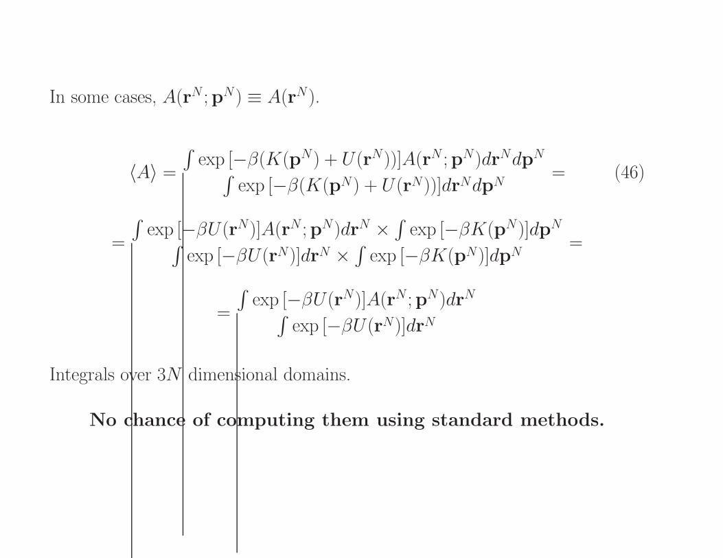
In some cases, A(rN ;pN) ≡ A(rN).

〈A〉 =

∫

exp [−β(K(pN) + U (rN))]A(rN ;pN)drNdpN∫

exp [−β(K(pN) + U (rN))]drNdpN= (46)

=

∫

exp [−βU (rN)]A(rN ;pN)drN ×∫

exp [−βK(pN)]dpN∫

exp [−βU (rN)]drN ×∫

exp [−βK(pN)]dpN=

=

∫

exp [−βU (rN)]A(rN ;pN)drN∫

exp [−βU (rN)]drN

Integrals over 3N dimensional domains.

No chance of computing them using standard methods.

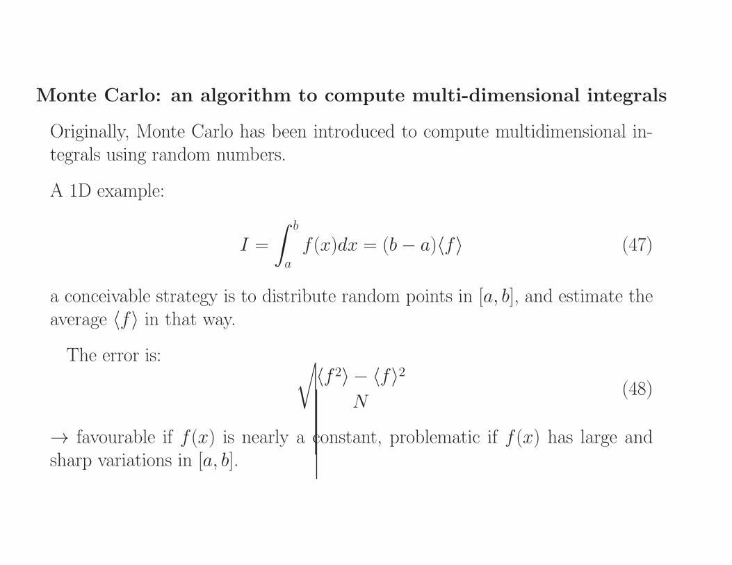
Monte Carlo: an algorithm to compute multi-dimensional integrals

Originally, Monte Carlo has been introduced to compute multidimensional in-tegrals using random numbers.

A 1D example:

I =

∫ b

a

f(x)dx = (b− a)〈f〉 (47)

a conceivable strategy is to distribute random points in [a, b], and estimate theaverage 〈f〉 in that way.

The error is:√

〈f 2〉 − 〈f〉2

N(48)

→ favourable if f(x) is nearly a constant, problematic if f(x) has large andsharp variations in [a, b].

Example: a function that is nearly zero everywhere, apart from one or a fewisolated peaks.

Figure 11: Example

.

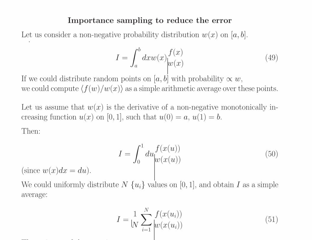
Importance sampling to reduce the error

Let us consider a non-negative probability distribution w(x) on [a, b].

I =

∫ b

a

dxw(x)f(x)

w(x)(49)

If we could distribute random points on [a, b] with probability ∝ w,we could compute 〈f(w)/w(x)〉 as a simple arithmetic average over these points.

Let us assume that w(x) is the derivative of a non-negative monotonically in-creasing function u(x) on [0, 1], such that u(0) = a, u(1) = b.

Then:

I =

∫ 1

0

duf(x(u))

w(x(u))(50)

(since w(x)dx = du).

We could uniformly distribute N {ui} values on [0, 1], and obtain I as a simpleaverage:

I =1

N

N∑

i=1

f(x(ui))

w(x(ui))(51)

The estimate of the error is:

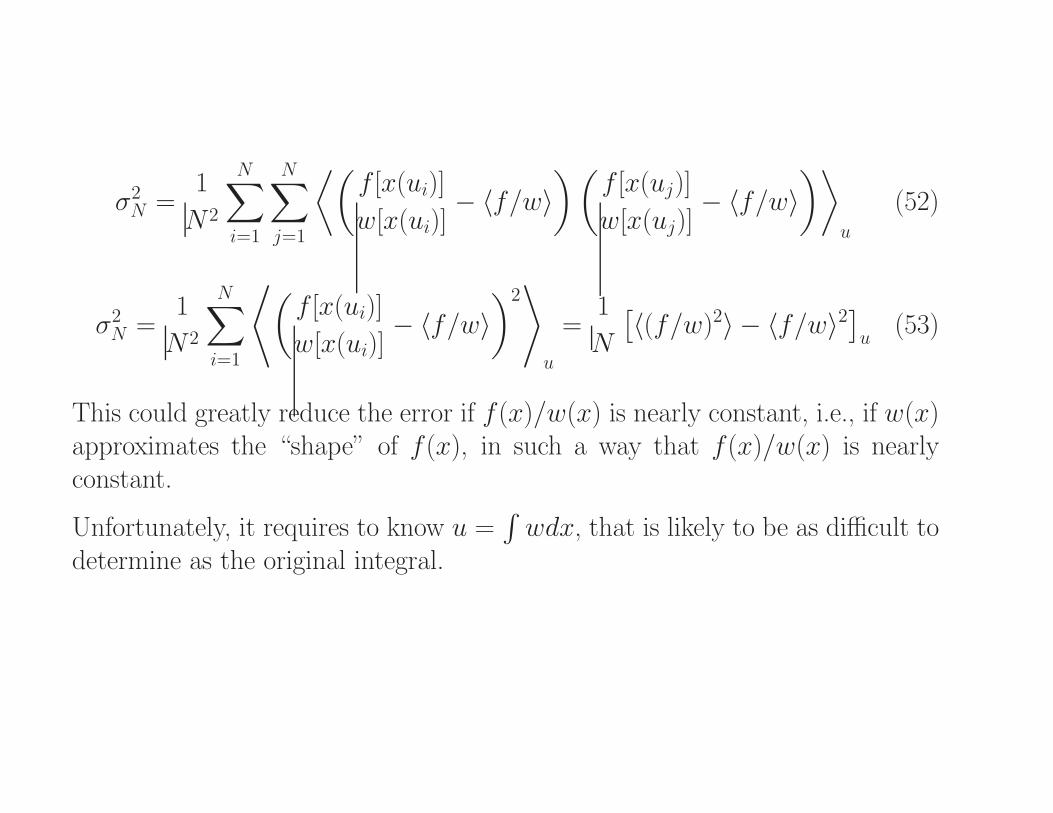
σ2N =1

N 2

N∑

i=1

N∑

j=1

⟨(

f [x(ui)]

w[x(ui)]− 〈f/w〉

)(

f [x(uj)]

w[x(uj)]− 〈f/w〉

)⟩

u

(52)

σ2N =1

N 2

N∑

i=1

⟨

(

f [x(ui)]

w[x(ui)]− 〈f/w〉

)2⟩

u

=1

N

[

〈(f/w)2〉 − 〈f/w〉2]

u(53)

This could greatly reduce the error if f(x)/w(x) is nearly constant, i.e., if w(x)approximates the “shape” of f(x), in such a way that f(x)/w(x) is nearlyconstant.

Unfortunately, it requires to know u =∫

wdx, that is likely to be as difficult todetermine as the original integral.

.

Monte Carlo in Statistical Mechanics (Metropolis)

Computing averages over probability distributions

Observation: we do not need to compute the integrals, but we need to computethe ratio of two integrals.Let us suppose that we are able to distribute points in the configuration space

with a density proportional to:

N (rN) ≡exp [−βU (rN)]

Z(54)

Then, again, we could compute:

〈A〉 =1

N

N∑

i=1

A[rNi ] (55)

.

Metropolis method is based on generating a sequence of configurations

Markov chain

constructed in such a way that their limiting distribution is the desired one (ρeq,in our case).Definition of Markov chain - Let us consider a set made of a finite (M) num-ber of elements (Γ1, ...., Γn, ..., ΓM).Markov chain is a sequence of these elements in which the i + 1-th choice de-pends only on the i-th choice.

The chain is defined by the probability πmn to go from element m to element nin the next step.Let us collect all the πmn in the matrix π.If the chain is at element m at step i, it has to go to some element n (includingn = m) at step i + 1. Hence:

∑

n

πmn = 1 (56)

with all the πmn being non-negative (since they are probabilities).This is the definition of a stochastic matrix.

.

The transition probability π defines an irreducible or ergodic chain if any state(element) can be reached from any other state along the sequence.

Let us start from a population of configurations distributed according to anarbitrary distribution ρ0 (ρ

0 is an M -dimensional vector).

The following step, the probability of being at configuration n will be:

ρ1n =∑

n

ρ0mπmn (57)

that we write as:ρ1 = ρ0π (58)

The equilibrium distribution will be:

ρ = limτ→∞

ρ0πτ (59)

It is easy to show that this implies:

ρ = πρ (60)

i.e., ρ is an eigenvector of π of eigenvalue 1.

Perron-Frobenius theorem states that an ergodic stochastic matrix has one andonly one eigenvector of unit eigenvalue → the limiting distribution is unique,and it is reached from any starting point.

All other eigenvalues are < than 1!

We know the limiting distribution, but we do not know π.How to build π?

It turns out that there is ample arbitrariness in constructing π.

Metropolis choice - Let us impose:

ρmπmn = ρnπnm (61)

known as the microscopic reversibility condition (sufficient but not necessary).

Then:∑

m

ρmπmn =∑

m

ρnπnm = ρn∑

m

πnm = ρn (62)

that is the unit eigenvalue condition!

Additional details - Metropolis again.

Let us introduce an auxiliary symmetric matrix αmn, that in the following willrepresent the uniform probability of moving in a volume element around thepresent configuration.

Then, for m 6= n, let us define:

πmn =

{

αmn if ρn ≥ ρmαmn × ρn/ρm if ρn < ρm

(63)

If m = n:πmm = 1−

∑

m6=n

πmn (64)

It is immediate to verify that this definition satisfies the microscopic reversibilitycondition.

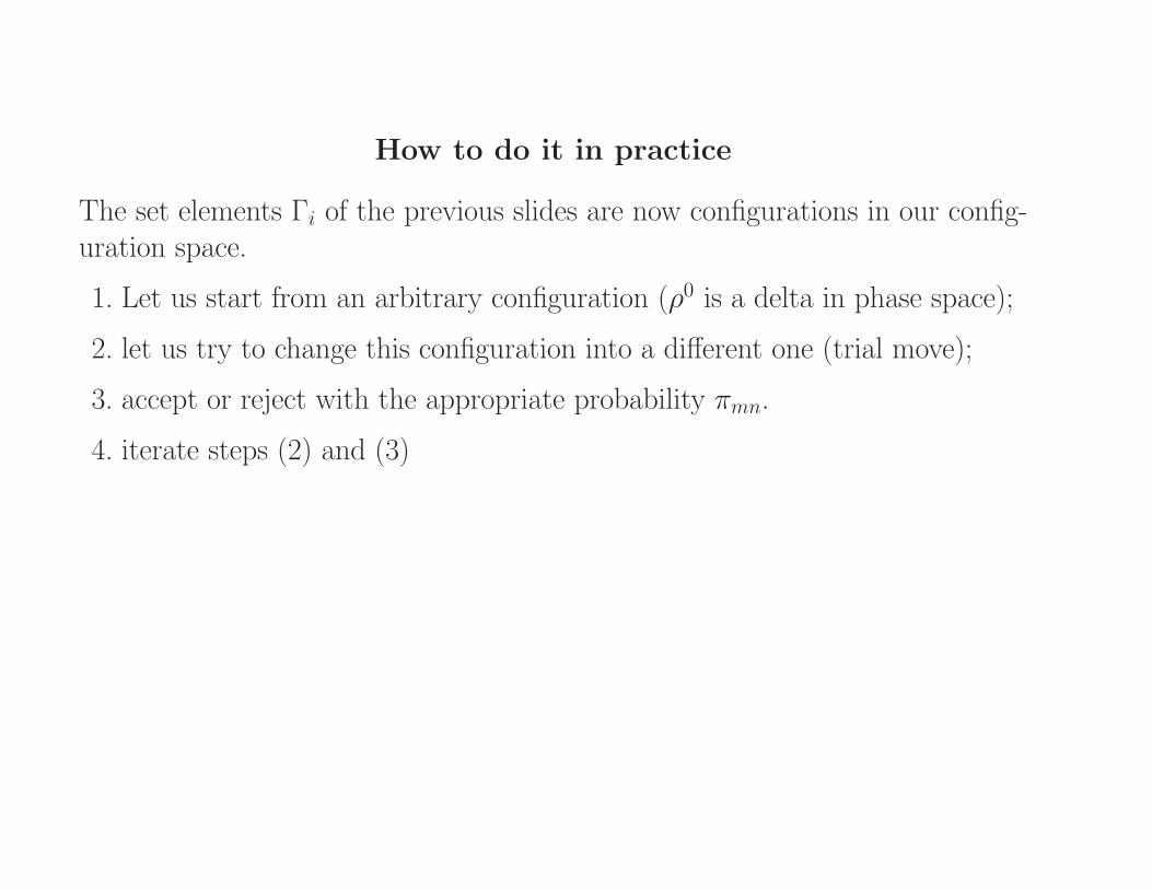
How to do it in practice

The set elements Γi of the previous slides are now configurations in our config-uration space.

1. Let us start from an arbitrary configuration (ρ0 is a delta in phase space);

2. let us try to change this configuration into a different one (trial move);

3. accept or reject with the appropriate probability πmn.

4. iterate steps (2) and (3)

.

Trial displacement

• select one particle at random

• displace each of its coordinates by a random displacement:

xi = xi + δ[rand()− 0.5]

yi = yi + δ[rand()− 0.5]

zi = zi + δ[rand()− 0.5]

where rand() is a function returning a random number uniformly distributedover ]0, 1[.

The transformation given above describes the random displacement of particlei in cube of side δ centred at the starting position.

We would like to make δ as big as possible, to sample independent configurations.

In practice, δ is small, otherwise the transition probability (to be discussed nextslide) is exceedingly small.→ high correlation among successive configurations, and slow decrease of thestatistical error.

Acceptance / Rejection stage

We tried a transition from the old (o) configuration to the new (n).

The probability of the o-configuration is:

ρeq(rNo ) ∝ exp [−βU (rNo )] (65)

The probability of the n-configuration is:

ρeq(rNn ) ∝ exp [−βU (rNn )] (66)

Hence their ratio is:

ρeq(new)

ρeq(old)= exp {−β[U (rNn )− U (r

No )} (67)

The ratio is > 1 if U (new) < U (old); < 1 if U (new) > U (old).

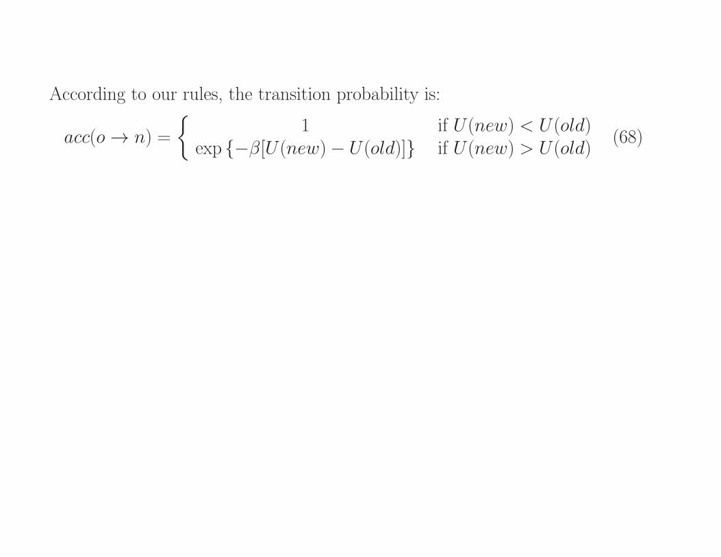
According to our rules, the transition probability is:

acc(o→ n) =

{

1 if U (new) < U (old)exp {−β[U (new)− U (old)]} if U (new) > U (old)

(68)

How to accept / reject with probability p?

By definition, p ≤ 1.

If p < 1, then:

• extract a random number ξ uniformly distributed over ]0, 1[;

• accept if ξ ≤ p;

• reject if ξ > p.

Random number generation: see Numerical Recipes

A few practical considerations

Each MC step changes the coordinate of just one particle

→ we need N -times more steps in MC than in MD.

MD requires the computations of forces; MC doesn’t→ MC simpler to implement than MD.

In MC it is possible to devise special trial moves to sample specific degrees offreedom

More importantly, in MC it is easy to sample different distribution functionscorresponding to other ensembles.

For instance: Isobaric Isothermal ensemble

ρeq(rn;pN) ∝ V N exp−β{U (rN) + PV } (69)

MC moves will try to:

• displace particles;

• change the volume

Other possibilities: grand canonical, micro-canonical, etc. (Gibbs ensemble).

Important practical consideration:

Most available packages implement MD, not MC!

.

Modelling in Condensed Matter Physics and Materials Science

• Atomistic models and molecular dynamics (MD) simulation.

• The system is made on N interacting atoms whose coordinates and momentaare {Rα, α = 1, ..., N}, {pα, α = 1, ..., N}.

– Assume classical mechanics

– System potential energy given by U ({Rα}).

– Forces on each atom:

Fα = −∇RαU ({Rα}) (70)

– Starting from a suitable set of coordinates and momenta at time t0

– Integration of Newton’s equations of motion discretised in time steps ofamplitude ∆t:

– Verlet algorithm:

Rα(t +∆t) = 2Rα(t)−Rα(t−∆t) +∆t2

MαFα(t) (71)

What is the meaning of U ({Rα})?

3 The potential energy surface (PES) of condensed matter systems

Ordinary matter −→ electrons and atomic nuclei.

N electrons {ri, i = 1, ..., N} {si, i = 1, ..., N} {pi}K nuclei {Rα, α = 1, ...,K} {Sα, α = 1, ...,K} {Pα}

Assumption: Non-relativistic Quantum Mechanics (QM); no spin-orbit interac-tions.

All properties determined by the many-body Hamiltonian:

H0 =K∑

α=1

Pα

2M+

N∑

i=1

p2i

2m+1

2

∑

α 6=β

ZαZβe2

|Rα −Rβ|−∑

i,α

Zαe2

|ri −Rα|+1

2

∑

i 6=j

e2

|ri − rj|,

(72)Shorthand notation:

H0 = Tion + +Uion−ion + Tele + Uion−ele + Uele−ele (73)

Units: Hartree atomic units h = e2 = m = 1

.

Full description: Many-body wave function Ψ(x1, ...,xN;R1, ...,Rk)where: xi = {ri, si} and we neglect the spin of the nuclei.

Time evolution:

ih∂Ψ({xi}, {Rα})

∂t= H0Ψ({xi}, {Rα}) (74)

Equivalent approach - determine all eigenvectors and stationary states ofH0:

H0Ψk({xi}, {Rα}) = EkΨk({xi}, {Rα}) (75)

No analytical solution but for the simplest cases.

In all other cases: computational solution of approximate models.

Major approximations are required to solve the problem even by numericalmethods.

The problem is due to the e− e interaction.

.

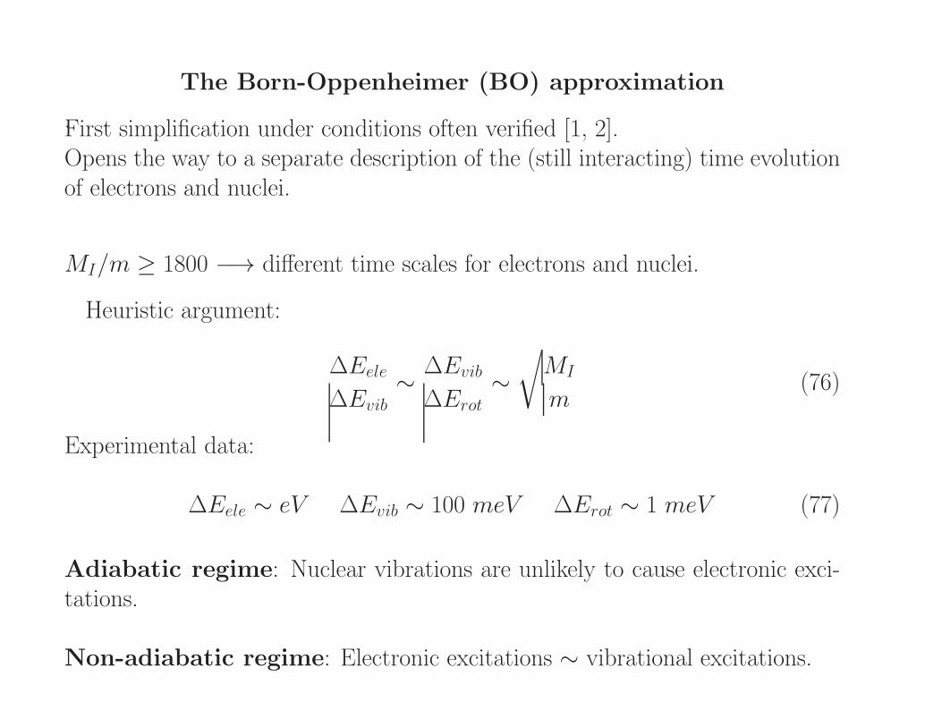
The Born-Oppenheimer (BO) approximation

First simplification under conditions often verified [1, 2].Opens the way to a separate description of the (still interacting) time evolutionof electrons and nuclei.

MI/m ≥ 1800 −→ different time scales for electrons and nuclei.

Heuristic argument:

∆Eele

∆Evib∼

∆Evib

∆Erot∼

√

MI

m(76)

Experimental data:

∆Eele ∼ eV ∆Evib ∼ 100 meV ∆Erot ∼ 1 meV (77)

Adiabatic regime: Nuclear vibrations are unlikely to cause electronic exci-tations.

Non-adiabatic regime: Electronic excitations ∼ vibrational excitations.

.

Electronic Hamiltonian:

Let us re-write H0 as:H0 = Tion + Hele (78)

where Hele = Tele + Vion−ion + Vion−ele + Vele−ele.

Clamped nuclear coordinates set at {Rα, α = 1, ...,K}.An eigenvalue problem for any choice of the atomic coordinates!

Heleψj({ri} | {Rα}) = Ej({Rα})ψj({ri} | {Rα}) (79)

Solve to provide a complete set of eigenvalues Ej({Rα}) and eigenfunctionsψj({ri} | {Rα}).ψj(ri | Rα) means: ψj explicit function of ri, parametrically dependent on{Rα}.Then:

Ψk({ri}, {Rα}) =∑

j

ψj({ri} | {Rα})χ(k)j (Rα) (80)

where χ(k)j (Rα) is the coefficient expressing the projection of Ψk on ψj:

χ(k)j ({Rα}) =

∫

ψ∗j ({ri} | {Rα})Ψk({ri}, {Rα})ΠNi=1dri (81)

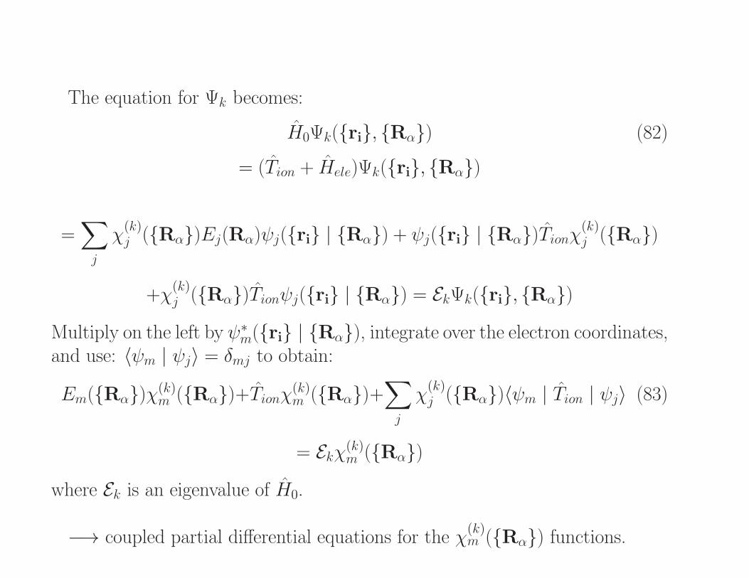
The equation for Ψk becomes:

H0Ψk({ri}, {Rα}) (82)

= (Tion + Hele)Ψk({ri}, {Rα})

=∑

j

χ(k)j ({Rα})Ej(Rα)ψj({ri} | {Rα}) + ψj({ri} | {Rα})Tionχ

(k)j ({Rα})

+χ(k)j ({Rα})Tionψj({ri} | {Rα}) = EkΨk({ri}, {Rα})

Multiply on the left by ψ∗m({ri} | {Rα}), integrate over the electron coordinates,and use: 〈ψm | ψj〉 = δmj to obtain:

Em({Rα})χ(k)m ({Rα})+Tionχ

(k)m ({Rα})+

∑

j

χ(k)j ({Rα})〈ψm | Tion | ψj〉 (83)

= Ekχ(k)m ({Rα})

where Ek is an eigenvalue of H0.

−→ coupled partial differential equations for the χ(k)m ({Rα}) functions.

.

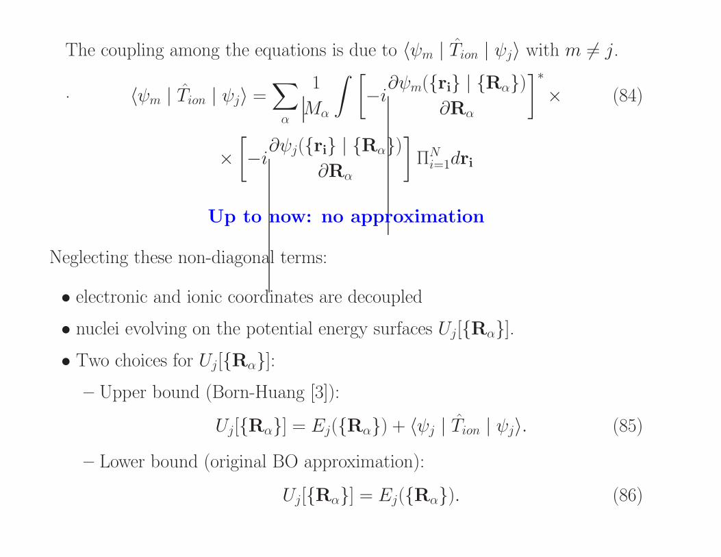
The coupling among the equations is due to 〈ψm | Tion | ψj〉 with m 6= j.

〈ψm | Tion | ψj〉 =∑

α

1

Mα

∫[

−i∂ψm({ri} | {Rα})

∂Rα

]∗

× (84)

×

[

−i∂ψj({ri} | {Rα})

∂Rα

]

ΠNi=1dri

Up to now: no approximation

Neglecting these non-diagonal terms:

• electronic and ionic coordinates are decoupled

• nuclei evolving on the potential energy surfaces Uj[{Rα}].

• Two choices for Uj[{Rα}]:

– Upper bound (Born-Huang [3]):

Uj[{Rα}] = Ej({Rα}) + 〈ψj | Tion | ψj〉. (85)

– Lower bound (original BO approximation):

Uj[{Rα}] = Ej({Rα}). (86)

Nuclear motion in the adiabatic regime:

• still quantum mechanical

• depending on initial conditions, it occurs on any of the Uj potential energysurfaces (PES’s).

• most cases but with noticeable exceptions, the relevant PES corresponds tothe electronic ground state

• the scale of times and energies of interest allows the usage of classical dy-namics [4].

When is the BO approximation valid?

Perturbative estimate of 〈ψm | Tion | ψj〉:

〈ψm | Tion | ψj〉 ∝1

Em − Ej〈ψm | [Pα, Hele] | ψj〉 (87)

The matrix elements of the commutator:

• depend primarily on the properties of individual atoms

• are moderately dependent on coordinates

• Then, the major factor is the energy gap Em − Ej.

Whenever (Em−Ej) becomes comparable to the typical energies of the atomicmotion:

• the BO decoupling is no longer valid

• the electronic and ionic motion are intimately intertwined

• both need to be treated quantum mechanically.

Figure 12: Conical intersection

Violations of the BO approximation are pervasive

• Occur often but not exclusively at conicalintersections [5]

• play a major role in chemical reactions

• challenge our ability to model catalysis [6]

• non-BO effects are routinely highlighted byexperiments [7].

• quantum mechanical features relevant in non-BO case go beyond delocal-isation and diffraction, but includes the appearance of geometric (Berry-Pancharatnam) phases [5].

Question: adiabatic motion in metals?

Answer: The relevant excitation is the plasmon (i.e., several eV).

Exceptions: Kohn anomalies; superconductivity; ...

Now we understand the meaning of U ({Rα})

Next step(s):

• how to compute / approximate U ({Rα}) and Fα = −∇RαU ({Rα})?

Immediate answer: solve the many-electron problemin eq. (82) for the ground state

• Is this the only choice?

• Is it really what you want to do?

• Can you do it in practice?

Figure 13: Computer-less Simula-tor

4 Choice I: models of PES based on intuition and chemistry

Basic entities: atoms (our choice).

Crucial features:

• excluded volume from Pauli principle at short distances;

• cohesion from chemical bonds;

• weak but pervasive attraction from dispersion forces(∼ r−6 in classical mechanics; ∼ r−7 in relativistic mechanics)

.

Most intuitive picture of atomic interactions, pair potentials:

U [{Rα}] =1

2

∑

α,β

φαβ(| Rα −Rβ |) (88)

A spherically symmetric potential has been assumed for the sake of simplicity.

Figure 14: Boscovitch intuition (1763)

Suitable for rare gases [28] and for simple ionic compounds [29].

Systems and models of this kind played a crucial role in early days of computersimulation.

Going beyond pair potentials

Three-body contributions:

U [{Rα}] =1

2!

∑

α,β

V2(Rα,Rβ) +1

3!

∑

α,βγ

V3(Rα,Rβ,Rγ) (89)

Even further:

U [{Rα}] =1

2!

∑

α,β

V2(Rα,Rβ) +1

3!

∑

α,βγ

V3(Rα,Rβ,Rγ)+ (90)

1

4!

∑

α,βγδ

V4(Rα,Rβ,Rγ, Rδ) + ...

You can always do it!

For instance:

The potential energy of two atoms defines V2;

Then, let us consider three atoms, whose potential energy is U [Rα,Rβ,Rγ]:

V3(R1,R2,R3) = U [R1,R2,R3]− V2(R1,R2)− V2(R2,R3)− V2(R1,R3)(91)

etc.

Practical? −→ Certainly not!

Meaningful? −→ Not really...

The many-particle expansion is an asymptotic expansion rather than a conver-gent series [30].

Bond-order potentials

Present days models of materials going beyond pair potential conform to thecluster potentials idea [31, 32], loosely based on the bond-order concept (Paul-ing [33])

• The system potential energy is expressed as the sum of n-atom contributions

• Each of the few terms describe low-order potentials whose strength dependson the local environment.

Approaches of this kind are used to simulate metals and metallic alloys, semi-conductors, and complex insulators such as transition metal oxides.

.Many-body interactions: metals and metal alloys

Physical metallurgy is currently one of the major area of application of atomisticsimulation [34].

Simplest picture of metals:ionic cores immersed in a sea of valence electronsdelocalised and fairly isotropic bonds

Basic ingredient: the homogeneous electron gas.

Potential energy obtained by second order perturbation theory.[35, 36]

System potential energy: sum of ion-ion pair interactions, and a volume term,due to the electron gas:

UN [{Rγ}] =1

2

∑

α,β

φ2(|Rα −Rβ|) + E[V,N ] (92)

The pair potential φ2(R) is:

• repulsive at short range;

• oscillating at long range(Friedel’s oscillations, λ ∼ 2kF ).

Good for simple (sp) metals (weak ion-electron interaction)inadequate for transition metals (strong ion-electron interaction, beyond secondorder perturbation).... but going beyond second order perturbation theory makes it intractable [37]

Good for homogeneous systemsunable to deal with surfaces and interfaces (the ”volume” term is undefined).

Mainly of historical interest.

No few-body potentials for metals:

First of all, no pair-potential. A pair potential model implies:

• symmetry relations for among elastic constantsfor instance: C12 6= C44 (Cauchy relation)

• the energy to create a vacancy equal to the cohesive energy

• crystal surfaces relax outwards.

In metals, instead:

• Cauchy anomaly C12 6= C44.

• vacancy formation energy

• Inward relaxation of free surfaces

Moreover: complex structures of some transition metals such as Mn, Cr, Hg,etc, defy any attempt to model them by few-body potentials.

.

Many-body potentials for metals: The embedded atom model

The widest used models for metals rely on the embedded atom idea [38, 39].

The origin can be traced to density functional theory [32, 41], tight-binding [40],or the bond-order model. Each metal ion i at position Ri:

• gains an energy E[ρe(Ri)] upon being immersed into the valence electrondistribution at density ρe(Ri)

• interacts with neighbouring ions by a short range repulsive pair potentialV2(R)

U [{Ri}] =1

2

N∑

i 6=j

V2(| Ri −Rj |) +N∑

i=1

E[ρe(Ri)] (93)

the electron density ρe at the position Ri of each atomic core is computed as:

ρe(Ri) =∑

j 6=i

tj(| Ri −Rj |) (94)

where the tj(R) describes the valence electron distribution of metal atoms.

.

Broad success of these models, due to their:

• fair description of a wide variety of metal properties.

• computational efficiency of EAM is due to the pair potential form of boththe repulsive contribution V2 and the embedding density expression

• MD simulations of 104 atoms covering ns times run on a laptop

0.0 0.25 0.5 0.75 1.00

2

4

6

8

[00z]

υ

[TH

z]

1.0 0.75 0.5 0.25 0.0

[0z1]

0.75 0.5 0.25 0.0

[0zz]

0.0 0.25 0.5

[zzz]

k a / 2 π

Pd

Figure 15: Phonon frequencies of fcc palladium from experiments (symbols, see [42]) and from the EAM model of Ref. [38].

An empirical and approximate approach such as EAM cannot provide the finalanswer to the problem of modelling metals, and transition metals in particular.

A step beyond EAM: the modified EAM (MEAM), including angular (three-and four-body) terms [39, 43].

.

Semiconductors and insulators

Silicon, germanium, gallium arsenide, etc.:

• characterised by fairly open and complex structures of relatively low coor-dination

• stabilised by sizeable angular forces, arising from the directionality of cova-lent bonds

• silicon and germanium turn into metals upon melting. Other semiconductorsbecome metals under pressure or at fairly high T (P, S, Se, ...).

Early models: three body interactions [44], only moderately successful (inter-actions beyond 3-body are important!)

bond-order concept [33] proved more fruitful [31, 45, 46]:The potential energy of an assembly of N atoms of coordinates {Ri} is given

by:

EN =∑

i 6=j

[A exp (−λ1Rij)−Bij exp (−λ2Rij)] (95)

The first term, representing the short range repulsion, is a genuine pair potential.The second term contains many-body contributions via the dependence of Bij

on the local environment.

Parallel to the EAM case for metals, potentials of this type replaced all previousmodels

Systematic improvement beyond the semi-empirical Tersoff and Brenner po-tentials relies on the analytical development of chemically accurate bond-ordermodels [47] −→ unusable in practice!

Major development: reactive force fields (Reaxx and REBO force fields) [48, 49],able to describe chemical transformations in the system under consideration.Used primarily for organic systems, but also for inorganic semi-conductors.Major difficulty: difficult parametrisation, cumbersome implementation in com-puter codes.

Organic molecular systems

The simulation of organic molecular systems, up to biological structures, isarguably the most important simulation activity

From the point of view of chemistry, organic materials are no different from anyother covalently bonded system

The most remarkable feature is the amazing transferability of C-C, C-H, C-N,and C-O bonding parameters from one molecule to another

It really makes sense to consider the system as a collection of atoms and bonds.

Figure 16:

Figure 17:

The PES of organic and biological systems is written as the sum of contributionsfrom bonded (Ub) and non-bonded (Unb) interactions:

U = Ub + Unb (96)

The bonded energy is given by the sum of two-, three-, and four-body termsfrom atoms joined by one ({ij}), two ({ijk}) and three ({ijkl}) consecutivecovalent bonds:

Ub =1

2

∑

{ij}

Ksij[Rij−Rij]

2+1

2

∑

{ijk}

Kbijb[θijk−θijk]

2+1

2

∑

{ijkl}

Kτijkl

[

1 + cos (nφijkl − φijkl)]

(97)Ksij, K

bijk and K

τijkl are suitable force constants, Rij, θijk, φijkl and n reflect the

length, bending and dihedral angles of unstrained bonds.Non bonded interactions are written as.

Unb =1

4πǫ0

∑

i 6=j

′qiqjRij

+∑

i 6=j

′4ǫij

[

(

σijRij

)12

−

(

σijRij

)6]

(98)

where the {qi} are atomic charges, σij and ǫij are coefficients for the dispersioninteraction.

Strong points:

• Validated potentials for broad categories of compounds.

• Generic potentials covering large classes of compounds and widely used bythe community include Amber [50], CHARMM [51], OPLS [52], Gromos [53].

Challenges:

• Attribution of charges to the atoms

• Polarisability

• Hydrogen bonding

Active research field: development of force fields for organo-metallic complexes−→ prosthetic groups in proteins, or active groups in a variety of organic opto-electronic devices, and are important also for homogeneous catalysis.

Challenges:

• variety of coordination numbers

• quantum features such as Jahn-Teller effects

• subtle features such as the it trans-influence [?]

These difficulties point to ab-initio methods for their solution.

Carbon systems such as fullerenes, carbon nanotubes and graphene lay at theboundary between inorganic and organic species, and blur the distinction be-tween covalent and metal character.Systems of this kind have been represented by a variety of models, from Tersoff-Brenner to molecular force field such as those described in this section.

Figure 18: Snapshot from a molecular dynamics simulation of a room temperature ionic liquid / water solution at 0.5 Mconcentration in contact with a POPC phospholipid bilayer [?]. Green balls: [Cl]−; gray-silver molecules: [bmim]+. wireframemolecules: POPC. Water has been removed to highlight the incorporation of [bmim]+ cations into the phospholipid bilayer.

Reasons to select ab-initio

1. Models for covalent systems are cumbersome to say the least.

2. Models to include polarisability are difficult to use.

3. Metals such as Ga, Mn, Cr, ... adopt complex structures difficult to repro-duce by manageable potentials.

4. We are unable to mix materials of different chemical bonding.

• interfaces

• composite materials

• metallo-organic

5. Hydrogen bonding is still somewhat problematic

6. hypothetical materials whose bonding is not known

7. In covalently bonded systems difficulty with breaking/forming bonds.

8. Need to extract information on electronic properties

All these problems of simulation point to ab-initio simulation as the method ofchoice to investigate difficult systems and systems on which there is little priorinformation.

Anticipation: why not to use ab-initio simulation?

• It is still fairly expensive, limited in time and size.

• It does not solve all problems

• Even in simple cases, the model might not be so accurate (examples: meltingof silicon, melting of ice).

• The description of the electronic properties in several cases is inadequate.

Nevertheless, it is the best we can do in many cases.

References

[1] Born, M.; Oppenheimer, R. Annalen der Physik 84, 457-484 (1927).

[2] Ziman, J.M. Electrons and phonons; Oxford Univ. Press: Oxford,UK, 1960; Chapter 5.

[3] Born, M.; Huang, K. Dynamical theory of crystal lattices OxfordUniversity Press: Oxford, UK, 1954.

[4] de Carvalho, F.F.; Bouduban, M.E.F.; Curchod, B.F.E.; Tavernelli,I. Nonadiabatic molecular dynamics based on trajectories. Entropy2013

[5] Yarkony, D.R. Diabolical conical intersections. Rev. Mod. Phys.

1996, 68, 985-1013.

[6] Kroes, G.J.; Gross, A.; Baerends, E.J.; Scheffler, M.; McCormack,D.A. Quantum theory of dissociative chemisorption on metal sur-faces. Acc. Chem. Res. 2002, 35, 193-200.

[7] Bowman, J.M. Beyond Born-Oppenheimer, Science 2008, 319, 40;White, J.D.; Chen, J.; Matsiev, D.; Auerbach, D.J.; Wodtke, A.M.Conversion of large-amplitude vibration to electron excitation at ametal surface. Nature 2005, 433, 503-505.

[8] Per semplicita’ non distingueremo i diversi tipi di nucleo presentinel sistema.

[9] Hellmann ; R. P. Feynman, Phys. Rev. 56, 340 (1939).

[10] P. Hohenberg and W. Kohn, Phys. Rev. 136, B864 (1964).

[11] W. Kohn and L. J. Sham, Phys. Rev. 140, 1133 (1965).

[12] A. William ..., atomi non sferici.

[13] F. Sottile and P. Ballone, Phys. Rev. B

[14] I. Shavitt

[15] T. L. Beck, Rev. Mod. Phys. 72, 1041 (2000).

[16] S. Goedecker, Rev. Mod. Phys.

[17] J. P. Perdew, R. G. Parr, M. Levy, and J. L. Balduz, Phys. Rev.Lett. 49, 1691 (1982).

[18] L. Kleinman, Phys. Rev. B 56, 12042 (1997).

[19] Numerical Recipes

[20] Allen, M. P.; Tildesley, D. J. Computer Simulation of Liquids;Clarendon Press: Oxford, 1987.

[22] N. Argaman and G. Makov, Am. J. Phys. 68, 69 (2000); Phys. Rev.B 66, 052413 (2002).

[23] Calculus of variations, I. M. Gelfand and S. V. Fomin, Prentice-Hall, Englewood Cliffs, N. J., (1963).

[24] W. M. C. Foulkes, L. Mitas, R. J. Needs, G. Rajagopal, Rev. Mod.Phys. 73, 33 (2001).

[25] C. Froese-Fischer, The Hartree-Fock Method for Atoms, Wiley,New York (1977).

[26] E. Clementi, J. Chem. Phys. 38, 2248 (1963).

[27] M. M. Morrell, R. G. Parr, and M. Levy, J. Chem. Phys. 62, 549(1975).

[28] Lennard-Jones, J.E. On the determination of molecular fields. Proc.R. Soc. Lond. A 1924, 106, 463-477.

[29] Fumi, F.G.; Tosi, M.P. Ionic sizes and Born repulsive parametersin the NaCl-type alkali halides. J. Phys. Chem. of Solids 1964,25, 31-43.

[30] Carlsson, A.E.; Ashcroft, N.W. Pair potentials from band theory:Application to vacancy-formation energies. Phys. Rev. B 1983,

[31] Abell, G.C. Empirical chemical pseudopotential theory of molecularand metallic bonding. Phys. Rev. B 1985, 31, 6184-6196.

[32] Carlsson, A.E. Beyond pair potentials in elemental transition met-als and semiconductors. in Solid State Physics: Advances in Re-

search and Applications, Ehrenreich, H., Turnbull, D., Eds.; Aca-demic Press: Boston, USA, 1990; Vol. 43, pp. 1-91.

[33] Pauling, L. The nature of the chemical bond; Cornell UniversityPress: Ithaca, USA, 1960, 3rd ed.

[34] Handbook of Materials Modeling, Ed. S. Yip; Springer: Berlin,Germany, 2005; Comprehensive Nuclear Materials, Vol. 1: BasicAspects of Radiation Effects in Solids/Basic Aspects of Multi-ScaleModeling, Ed. R. J.M. Konings; Elsevier: Amsterdam, Netherlands,2012.

[35] Dagens, L.; Rasolt, M.; Taylor, R. Charge densities and interionicpotentials in simple metals. Phys. Rev. B 1975, 11, 2726-2734.

[36] Hafner, J. From Hamiltonians to phase diagrams; Springer:Berlin, Germany, 1987.

[37] Moriarty, J.A. First-principles interatomic potentials in transitionmetals. Phys. Rev. Lett. 1985, 55, 1502-1505.

[38] Daw, M.S.; Baskes, M. I. Semiempirical, quantum mechanical cal-culation of hydrogen embrittlement in metals. Phys. Rev. Lett.

1983, 50, 1285-1288.

[39] Baskes, M. I. Application of the embedded-atom method to covalentmaterials: a semiempirical potential for silicon. Phys. Rev. Lett.1987, 59, 2666-2669.

[40] Rosato, V.; Guillope, M.; Legrand, B. Thermodynamical and struc-tural properties of f.c.c. transition metals using a simple tight-binding model. Philos. Mag. A 1989, 59, 321-336.

[41] Jacobsen, K.W.; Nørskov, J.K.; Puska, M.J. Interatomic interac-tions in the effective-medium theory. Phys. Rev. B 1987, 35, 7423-7442.

[42] Miiller, A.P.; Brockhouse, B.N. Crystal dynamics and electronicspecific heats of palladium and copper. Can. J. Phys. 1971, 49,704-723.

[43] Drautz, R.; Pettifor, D. G. Valence-dependent analytic bond-orderpotential for transition metals. Phys. Rev. B 2006, 74, 174117.

[44] Stillinger, F.; Weber, T. Computer simulation of local order in con-densed phases of silicon. Phys. Rev. B 1985, 31, 5262-5271.

[45] Tersoff, J. New empirical model for the structural properties of sili-con. Phys. Rev. Lett. 1986, 56, 632-635; Tersoff, J. New empiricalapproach for the structure and energy of covalent systems. Phys.Rev. B 1988, 37, 6991-7000.

[46] Brenner, D.W. Empirical potential for hydrocarbons for use in sim-ulating the chemical vapor deposition of diamond films. Phys. Rev.B 1990, 42, 9458-9471.

[47] Pettifor, D.G.; Oleinik, I.I. Analytic bond-order potentials beyondTersof-Brenner. I. Theory. Phys. Rev. B 1999, 59, 8487-8499.

[48] van Duin, A.C.T.; Dasgupta, S.; Lorant, F.; Goddard, W.A., III.ReaxFF: A reactive force field for hydrocarbons. J. Phys. Chem.

A 2001, 105, 9396-9409.

[49] Brenner, D.W.; Shenderova, O.A.; Harrison, J.A.; Stuart, S.J.; Ni,B.; Sinnott, S.B., A second-generation reactive empirical bond order(REBO) potential energy expression for hydrocarbons. J. Phys.:Condens. Matter 2002, 14, 783-802.

[50] Cornell, W.D.; Cieplak, P.; Bayly, C.I.; Gould, I.R.; Merz, K.M.,Jr; Ferguson, D.M.; Spellmeyer, D.C.; Fox, T.; Caldwell, J.W.;Kollman, P.A. A second generation force field for the simulation of

proteins, nucleic acids, and organic molecules. J. Am. Chem. Soc.

1995, 117 5179-5197.

[51] Patel, S.; Brooks, C.L.; III. CHARMM fluctuating charge force fieldfor proteins: I parameterization and application to bulk organicliquid simulations. J. Comput. Chem. 2004, 25, 1-16.

[52] Jorgensen, W.L.; Maxwell, D.S.; Tirado-Rives, J. Development andtesting of the OPLS all-atom force field on conformational energeticsand properties of organic liquids. J. Am. Chem. Soc. 1996, 118,11225-11236.

[53] Schuler, L.D.; Daura, X.; van Gunsteren, W.F. An improved GRO-MOS96 force field for aliphatic hydrocarbons in the condensedphase. J. Comp. Chem. 2001, 22, 1205-1218.