computer simulation of determinate and indeterminate...
TRANSCRIPT
COMPUTER SIMULATION OF DETERMINATE AND INDETERMINATE TRUSSES
BY FINITE ELEMENT METHODS IN MATLAB PROGRAMMING LANGUAGE
PROJECT REPORT BY:
RUNJI JOEL MURITHI
F18/1880/2007
SUPERVISOR: DR. HUSSEIN JAMA
A PROJECT SUBMITTED IN PARTIAL FULFILMENT FOR A BACHELORS
DEGREE IN BSC. MECHANICAL ENGINEERING IN UNIVERSITY OF NAIROBI
MAY, 2012
You created this PDF from an application that is not licensed to print to novaPDF printer (http://www.novapdf.com)

ii
DECLARATION
This research project is my original work and has not been presented for any award in any
institution whatsoever.
NAME: RUNJI JOEL MURITHI
SIGNATUTRE: ................................
DATE: ...............................................
This research project has been submitted for examination with my knowledge as the department
supervisor.
NAME: ..................................................
SIGNATURE: .....................................
DATE: ....................................................
You created this PDF from an application that is not licensed to print to novaPDF printer (http://www.novapdf.com)

iii
DEDICATION
This research project is dedicated to my late dad, mum and two sisters. They have all been
inspirational in my life and gave me the courage and determination to come this far.
You created this PDF from an application that is not licensed to print to novaPDF printer (http://www.novapdf.com)

iv
ACKNOWLEDGEMENT
I realize the profound truth that He who created all things inert as well as live is GOD. But many
things in this world are created through knowledge of some living beings and these living beings
are groomed by their teachers and through their own effort of self study and practice.
Those who are gifted by God are exceptions and those who are gifted by their teachers are lucky.
I am thankful to God as He has been grateful to me much more than I deserve and to my all
teachers from school level to University heights as I am product of their efforts and guidance and
hence this study.
I’m greatly indebted to the people and institution that made the writing of this project successful.
Special thanks go to my supervisor, Dr. Hussein Jama for his invaluable guidance, continuous
assistance and encouragement throughout the writing of this project report. I also acknowledge
my colleague Henry Orare for the sacrifice he made in offering Matlab software and necessary
training.
You created this PDF from an application that is not licensed to print to novaPDF printer (http://www.novapdf.com)

v
ABSTRACT
For any physical problem in engineering and science, there are traditionally two ways to deal
with it by either theoretical approach or experiments. The theoretical approach in terms of
mathematical modeling is an idealization and simplification of the real problems and the
theoretical models often extract the essential or major characteristics of the problem. The
mathematical equations obtained even for such over-simplified system are usually very difficult
for mathematical analysis. On the other hand, the experimental approach is usually expensive if
not impractical. It is now widely acknowledged that computational modeling and computer
simulations serve as a cost-effective alternative, bridging the gap or complementing the
traditional theoretical and experimental approaches to problem solving (Yang, 2006). This was
the justification for the research work.
The objective as highlighted in chapter one was to perform a computer simulation of determinate
and indeterminate trusses by finite element methods in Matlab programming language. Further,
this chapter contains the research questions that guided the research work, significance of the
study, scope of the study, limitations of the study, assumptions made and definition of terms
used. The literature review which summarizes the information from other researchers who have
carried out their research in the same field of study discusses the classical methods of analysis
trusses and details various aspects of finite element methods.
Matlab (Matrix laboratory) is an interactive software system for numerical computations and
graphics. Further discussions on Matlab are outlined in Chapter three including an overview of
Matlab programming language, Matlab system and advantages of programming using Matlab.
The Pseudo code followed in programming is also outlined within this chapter. Code validation
is outlined in chapter four using four examples using classical methods and finite element
methods.
Finally in conclusion it was possible to verify that in deed computer simulation of determinate
and indeterminate could be conducted using finite element analysis. The results were also
comparable with classical methods to accuracies of 99%.
You created this PDF from an application that is not licensed to print to novaPDF printer (http://www.novapdf.com)
vi
List of Figures
Figure 1: Truss Element......................................................................................................................... 27
Figure 2: Graphical user interface .......................................................................................................... 41
Figure 3: Ouput Sub function................................................................................................................. 43
Figure 4: Output sub function ................................................................................................................ 44
Figure 5: Output Function Continued ..................................................................................................... 45
Figure 6: Output Function continued...................................................................................................... 46
Figure 7: Output Function...................................................................................................................... 47
Figure 8: Pin-jointed idealization of example truss: (a) geometric and elastic properties, (b) support
conditions and applied loads. ................................................................................................................. 48
Figure 9: free body diagram Example 1 ................................................................................................. 49
Figure 10: free body diagram joint 1 ...................................................................................................... 50
Figure 11: free body diagram joint 2 ..................................................................................................... 50
Figure 12: Graphical User Interface for Example 1 ................................................................................ 51
Figure 13: Free body diagram example 2 ............................................................................................... 54
Figure 14: Free body diagram (a) Joint 1 (b) Joint 6 ............................................................................... 55
Figure 15: Free body diagram Joint 2 ..................................................................................................... 56
Figure 16: Free body diagram R4 unit force............................................................................................ 56
Figure 17: Graphical User Interface Example 2 ...................................................................................... 58
Figure 18: Example 3 ............................................................................................................................ 62
Figure 19: Free body diagram R4 redundant ........................................................................................... 62
Figure 20: Free body diagram Joint 1 ..................................................................................................... 63
Figure 22: Free body diagram Joint 2 ..................................................................................................... 64
Figure 21: Free body diagram Joint 5 ..................................................................................................... 64
Figure 23: Free body diagram joint 3 ..................................................................................................... 65
Figure 24: Free body diagram Joint 6 ..................................................................................................... 66
Figure 25: Free body diagram R4 redundant ........................................................................................... 67
Figure 26: Free body diagram Joint 1 ..................................................................................................... 68
Figure 27: Free body diagram Joint 5 ..................................................................................................... 68
Figure 28: Free body diagram Joint 2 ..................................................................................................... 69
You created this PDF from an application that is not licensed to print to novaPDF printer (http://www.novapdf.com)
vii
Figure 29: Free body diagram Joint 6 ..................................................................................................... 70
Figure 30: Graphical User Interface Example 3 ...................................................................................... 72
Figure 31: Comparison of Reaction Forces (FEM vs Classical) .............................................................. 75
Figure 32: Internal Stresses Results Comparison .................................................................................... 76
Figure 33: Example 4 ............................................................................................................................ 77
Figure 34: Graphical User Interface Example 4 ...................................................................................... 79
List of Tables
Table 1: FEM researchers ...................................................................................................................... 14
Table 2: Reaction Forces Example 1: ..................................................................................................... 53
Table 3: Internal Stresses Example 1 ..................................................................................................... 53
Table 4: Forces Analysis table ............................................................................................................... 57
Table 5: Computing R4 and Reactions ................................................................................................... 57
Table 6: Internal Stress Computation ..................................................................................................... 58
Table 7: Reaction Forces Example 2 ...................................................................................................... 61
Table 8: Internal Stress Example 2 ......................................................................................................... 61
Table 9: Analysis of Forces Example 3 .................................................................................................. 71
Table 10: R4 Computation and Reactions Forces .................................................................................... 71
Table 11: Internal Stress Computation ................................................................................................... 71
Table 12: Reaction Forces Example 3 .................................................................................................... 74
Table 13: Internal Stress Example 3 ....................................................................................................... 75
Table 14: Reaction Forces Example 4 .................................................................................................... 81
Table 15: Internal Stress Example 4 ....................................................................................................... 81
You created this PDF from an application that is not licensed to print to novaPDF printer (http://www.novapdf.com)
viii
Table of Contents
DECLARATION ....................................................................................................................... ii
DEDICATION .......................................................................................................................... iii
ACKNOWLEDGEMENT ......................................................................................................... iv
ABSTRACT ...............................................................................................................................v
List of Figures ........................................................................................................................... vi
List of Tables ........................................................................................................................... vii
CHAPTER ONE .........................................................................................................................1
1.0 INTRODUCTION .................................................................................................................1
1.1 Background of the Study .......................................................................................................1
1.2 Objectives of the study ..........................................................................................................3
1.2.1 General Objective ...........................................................................................................3
1.2.2 Specific Objectives .........................................................................................................3
1.3 Research Questions ...............................................................................................................3
1.4 Significance of the study .......................................................................................................4
1.5 Scope of the study .................................................................................................................4
1.6 Limitations of the study .........................................................................................................4
1.7 Assumptions of the study ......................................................................................................5
1.8 Definition of Terms ...............................................................................................................5
CHAPTER TWO ........................................................................................................................6
2.0 Literature Review ..................................................................................................................6
2.1 Introduction ...........................................................................................................................6
Theoretical Review .....................................................................................................................6
2.2 Trusses ..................................................................................................................................6
2.3 Statically determinate Vs Statistically Indeterminate Structures .............................................7
2.3.1 Statical Indeterminacy.....................................................................................................8
2.3.2 Kinematic Indeterminacy ................................................................................................8
2.3.3 Analysis of Determinate Trusses .....................................................................................8
2.3.4 Relation between number of members and joints for just rigid truss ................................9
2.3.5 Method of analysis of determinate trusses .......................................................................9
You created this PDF from an application that is not licensed to print to novaPDF printer (http://www.novapdf.com)
ix
2.5 Finite Element Methods....................................................................................................... 11
2.5.1 Introduction .................................................................................................................. 11
2.5.2 A Brief History of FEM ................................................................................................ 12
2.5.3 General Description of FEM ......................................................................................... 14
2.5.4 Principle of FEM .......................................................................................................... 15
2.5.5 Limitations of FEM....................................................................................................... 16
2.5.6 Advantages of Numerical Simulation ............................................................................ 16
2.5.7 Disadvantages of Numerical Simulation ........................................................................ 17
2.5.8 Distinction between finite element methods and classical methods ................................ 17
2.5.9 Classification of FEM ................................................................................................... 19
2.5.10 Mathematical Models .................................................................................................. 20
2.5.11 Design and Analysis of a component ........................................................................... 20
2.5.12 Types of Analysis ....................................................................................................... 22
2.5.13 Approximate method versus Exact method.................................................................. 22
2.5.14 Structural Analysis ...................................................................................................... 24
2.5.15 Plane Trusses .............................................................................................................. 25
2.5.16 Analysis of Trusses using FEM ................................................................................... 26
CHAPTER THREE ................................................................................................................... 32
3.0 Matlab Programming ........................................................................................................... 32
3.1 Introduction ......................................................................................................................... 32
3.2 Overview of the MATLAB Environment ............................................................................ 32
3.3 The MATLAB System ........................................................................................................ 33
3.4 Advantages of Matlab.......................................................................................................... 35
3.5 How the Program works ...................................................................................................... 35
3.5.1 M-File Functions .......................................................................................................... 35
3.5.2 Built-In Classes (Data Types) ....................................................................................... 36
3.5.3 A function handle.......................................................................................................... 36
3.5.4 Matrices ........................................................................................................................ 37
3.5.6 Program Control Statements ......................................................................................... 38
3.5.6 Types of Variables ........................................................................................................ 39
You created this PDF from an application that is not licensed to print to novaPDF printer (http://www.novapdf.com)
x
3.5.7 Graphical User Interface ............................................................................................... 40
3.5.8 Pseudo code .................................................................................................................. 41
CHAPTER FOUR ..................................................................................................................... 48
4.0 Code Validation .................................................................................................................. 48
4.1 Example 1 ........................................................................................................................... 48
4.1.1 Classical Method of joints ............................................................................................. 48
4.1.2 Finite Element Methods ................................................................................................ 51
4.2 Example 2 ........................................................................................................................... 53
4.2.1 Classical Method of Joints ............................................................................................ 53
4.2.2 Finite Element methods................................................................................................. 58
4.3 Example 3 ........................................................................................................................... 61
4.3.1 Classical Method of joints ............................................................................................. 61
4.3.2 Finite Element Method .................................................................................................. 72
4.4 Example 4 ........................................................................................................................... 76
4.4.1 Classical Strain Energy Method .................................................................................... 76
4.4.2 Finite element Methods ................................................................................................. 79
4.5 Discussion of Results .......................................................................................................... 81
CHAPTER FIVE ...................................................................................................................... 83
5.0 Conclusions and Recommendations ..................................................................................... 83
5.1 Conclusions ......................................................................................................................... 83
5.2 Recommendations ............................................................................................................... 84
References ................................................................................................................................ 85
Appendix .................................................................................................................................. 87
You created this PDF from an application that is not licensed to print to novaPDF printer (http://www.novapdf.com)
1
CHAPTER ONE
1.0 INTRODUCTION
1.1 Background of the Study
For any physical problem in engineering and science, there are traditionally two ways to deal
with it by either theoretical approach or experiments. The theoretical approach in terms of
mathematical modeling is an idealization and simplification of the real problems and the
theoretical models often extract the essential or major characteristics of the problem. The
mathematical equations obtained even for such over-simplified system are usually very difficult
for mathematical analysis. On the other hand, the experimental approach is usually expensive if
not impractical. Apart from financial limitation and limitation by physical scale, other
constraining factors include the range of physical parameters and time for carrying out various
experiments. As the computing speed and power have increased dramatically in the last few
decades, a practical third way or approach is emerging, which is the computational modeling and
numerical experimentation. It is now widely acknowledged that computational modeling and
computer simulations serve as a cost-effective alternative, bridging the gap or complementing
the traditional theoretical and experimental approaches to problem solving (Yang, 2006).
The essence of computational engineering, are the computational or numerical methods, (Yang,
2006). Numerical simulation of a process, means the solution of the governing equations (or
mathematical model) of the process using a numerical method and a computer. While the
derivation of the governing equations for most problems is not unduly difficult, their solution by
exact methods of analysis is a formidable task. In such cases, numerical methods of analysis
provide an alternative means of finding solutions (Reddy, 2004).
Where some computing has to be done and the objective would be to do simple simulations to
get correct or reasonably acceptable results the following limitations need to be overcome.
Limitations of computing time requiring use of efficient algorithms and high-speed computation
either by parallel computing or supercomputers. Further, almost all computations involve some
degree of approximation resulting in limitations as regards finite digit precision. This implies
You created this PDF from an application that is not licensed to print to novaPDF printer (http://www.novapdf.com)
2
results are only correct within a certain limit. In overcoming these limitations more versatile and
efficient methods are highly needed. In fact, according to (Yang, 2006) the finite element method
is one class of the most successful methods in computational engineering that has a wide range
of applications.
According to (Jin & Riley, 2009) the finite element method is a numerical procedure used to
obtain approximate solutions to boundary-value problems of mathematical physics with the aid
of an electronic computer. (Bhavikatti, 2004) describes finite element analysis as a numerical
technique where all the complexities of the problems, like varying shape, boundary conditions
and loads are maintained as they are but the solutions obtained are approximate. Because of its
diversity and flexibility as an analysis tool, it is receiving much attention in engineering. The
vast improvements in computer hardware technology and reduction of cost of computers have
boosted this method, since the computer is the basic need for the application of this method.
The Finite Element Method (FEM) is a product of the computer age and its application to solve
practical problems requires use of computer programs for analysis. Nowadays there are several
commercial finite element packages available that can solve varieties of problems. Some of these
packages are ANSYS, ALGOR, NISA, ABAQUS, NASTRAN etc. having pre and
postprocessors that give graphical interfaces of the structure before and after loading (Rao,
2007).
As a general rule FORTRAN codes are faster but more difficult to modify and are unable to
handle graphical operations, whereas Matlab allows for easy graphical interfaces. In addition,
Matlab’s graphical part and the computational part are kept completely separate, so as to allow a
more flexible utilization and avoid possible compatibility issues with different Matlab versions
(Pelosi, Cocciolli, & Selleri, 2009).
Skeletal structures can be analyzed by a variety of hand-oriented methods of structural analysis
taught in beginning Mechanics of Materials courses: the Displacement and Force methods. They
can also be analyzed by the computer-oriented FEM. That versatility makes those structures a
good choice to illustrate the transition from the hand-calculation methods taught in
You created this PDF from an application that is not licensed to print to novaPDF printer (http://www.novapdf.com)
3
undergraduate courses, to the fully automated finite element analysis procedures available in
commercial programs (Carlos, 2004).
1.2 Objectives of the study
The objectives of this study were:
1.2.1 General Objective
The general objective was to become familiar with finite element methods by use of Matlab
programming language.
1.2.2 Specific Objectives
The study was guided by the following specific objectives:
i) To conduct finite element analysis of two dimensional determinate and indeterminate
trusses
ii) To compare finite element analysis results for two dimensional determinate and
indeterminate trusses with classical methods
iii) To investigate whether finite element analysis of two dimensional determinate and
indeterminate trusses could be modeled in Matlab programming language
iv) To evaluate the efficiency and effectiveness of finite element analysis of two
dimensional determinate and indeterminate trusses modeled in Matlab Language
1.3 Research Questions
The research strived to answer the following questions:-
i. How do finite element methods analyze two dimensional determinate and indeterminate
trusses?
ii. Do results from finite element analysis of two dimensional determinate and indeterminate
trusses compare with classical methods?
You created this PDF from an application that is not licensed to print to novaPDF printer (http://www.novapdf.com)
4
iii. Is it possible to model finite element analysis of two dimensional determinate and
indeterminate trusses in Matlab programming language?
iv. How efficient and effective is computer modeling in finite element analysis of two
dimensional determinate and indeterminate trusses?
1.4 Significance of the study
The study is beneficial to engineers, as the study may be employed by, structural engineers in
assessing safety of structures. Due to increasing demand for safety assessment outside the
conventional code formats. Such assessment may be necessary for design purposes for critical
space structures or for the assessment of existing space structures for remaining life, particularly
where the safety or economic considerations are (Melchers & Hough, 2007). Hence, an efficient
and effective computerized structural analysis of trusses would aid in their assessment purpose.
The study would also benefit present students undertaking solid and structural mechanics as a
course as they would utilize the program to assess their understanding of the subject during their
private study. Hence it would act as a self assessment tool.
The study would benefit solid and structural mechanics lecturers as they would utilize the
program to analyze assessment questions set to students. The resulting program would save them
time to prepare for lectures and perform other responsibilities required of them.
1.5 Scope of the study
The main focus of this study was finite element analysis of two dimensional determinate and
indeterminate trusses through computer modeling in Matlab environment.
1.6 Limitations of the study
The study was limited to analysis of determinate and indeterminate trusses by finite element
methods. The computer program was limited to Matlab which employed numerical
programming. Further, the study was limited to duration of 30 weeks, where during this period
the researcher defined the research problem in the project proposal, prepared an algorithm in
You created this PDF from an application that is not licensed to print to novaPDF printer (http://www.novapdf.com)
5
Matlab Language for the two dimensional finite element analysis of determinate trusses and an
analysis of results obtained.
1.7 Assumptions of the study
The study made several assumptions. Specifically in this idealization, truss members carry only
axial loads, have no bending resistance, and are connected by frictionless pins (Da Silva, 2006).
1.8 Definition of Terms
Matrix: (Matloff, 2011) describes a matrix as a vector with two additional attributes: the number
of rows and the number of columns. Since matrices are vectors, they also have modes, such as
numeric and character.
Direct force structures: (Matloff, 2011) describes them as those structures where only one
internal force or stress resultant that is axial force may arise. Loads can be applied directly on the
members also but they are replaced by equivalent nodal loads. In the loaded members additional
internal forces such as bending moments, axial forces and shears are produced. Examples include
pin jointed plane frames and ball jointed space frames which are loaded and supported at the
nodes.
Plane frames: (Kalani, 1957) describes them as frames which all the members and applied
forces lie in same plane. The joints between members are generally rigid. The stress resultants
are axial force, bending moment and corresponding shear force.
Mathematical model: This is an idealization in which geometry, material properties, loads
and/or boundary conditions are simplified based on the analyst's understanding of what features
are important or unimportant in obtaining the results required (Narasaiah, 2008).
You created this PDF from an application that is not licensed to print to novaPDF printer (http://www.novapdf.com)
6
CHAPTER TWO
2.0 Literature Review
2.1 Introduction
This chapter summarizes the information from other researchers who have carried out their
research in the same field of study. The literature— that is, prior research that informs and
shapes the research question (Mohrman, 2011)— plays a crucial role in helping to keep these
elements working together for research purposes. The literature is an integrating force, helping to
shape research to make its best contribution. Familiarity with what has come before in a given
field that relates to a research question makes sure prior findings are integrated, elaborated, or
refuted in the current work (Mohrman, 2011). More specifically, with respect to understanding a
problem, finding out what others have done to understand that problem lowers the risk of
reinventing the wheel. Prior research in a field of inquiry informs and shapes one’s research
question, (Mohrman, 2011). In this regard the specific areas covered here are classical theories of
truss analysis, Finite Element Analysis of trusses and Matlab programming Language.
Theoretical Review
2.2 Trusses
(Da Silva, 2006) indicated that in a bar under pure axial loading the stress state may be
considered as uniform, irrespective of how the forces are applied, provided that the material
points under consideration are not close to the region of the member where the forces are applied
(Saint-Venant’s principle). In axially loaded slender members these regions are generally a small
part of the member, so that a uniform distribution of the stresses may be accepted when the
elongation of the bar is computed.
훥푙 = 푙 − 푙 = 휀푙 = (휎/퐸)푙 = (2.1)
Where 훥푙 = 퐶ℎ푎푛푔푒 푖푛 푙푒푛푔푡ℎ
You created this PDF from an application that is not licensed to print to novaPDF printer (http://www.novapdf.com)
7
휀 = strain
l = length
휎 = stress
E = Youngs Modulus
N = Normal Force
훺 = Area
2.3 Statically determinate Vs Statistically Indeterminate Structures
(Da Silva, 2006) indicates that a statically determinate structure only has internal force if
external forces are applied, which means that they are insensitive to temperature change, material
retraction, or any other actions that alter the dimensions of structural elements. Statically
indeterminate structures, on the other hand, may have internal forces in the absence of external
forces.
Statistically determinate structures are freely deformable, in the sense that their supports and
internal connections do not restrict the deformations. This means that a small change in the
geometry or size of the structural elements does not change the distribution of internal forces.
(Kalani, 1957) states that if skeletal structure is subjected to gradually increasing loads, without
distorting the initial geometry of structure, that is, causing small displacements, the structure is
said to be stable. If for the stable structure it is possible to find the internal forces in all the
members constituting the structure and supporting reactions at all the supports provided from
statical equations of equilibrium only, the structure is said to be determinate. If it is possible to
determine all the support reactions from equations of equilibrium alone the structure is said to be
externally determinate else externally indeterminate. If structure is externally determinate but it
is not possible to determine all internal forces then structure is said to be internally
indeterminate. Therefore according to (Kalani, 1957) a structural system may be:
i. Externally indeterminate but internally determinate
You created this PDF from an application that is not licensed to print to novaPDF printer (http://www.novapdf.com)
8
ii. Externally determinate but internally indeterminate
iii. Externally and internally indeterminate
iv. Externally and internally determinate
A system which is externally and internally determinate is said to be determinate system. A
system which is externally indeterminate, internally indeterminate or externally and internally
indeterminate is said to be indeterminate system.
If the total number of unknown internal and support reactions = to total number of independent
statical equations of equilibrium then the system is determinate. Else it is indeterminate.
2.3.1 Statical Indeterminacy
(Kalani, 1957) defines it as the difference of the unknown forces (internal forces plus external
reactions) and the equations of equilibrium.
2.3.2 Kinematic Indeterminacy
It is the number of possible relative displacements of the nodes in the directions of stress
resultants (Kalani, 1957).
2.3.3 Analysis of Determinate Trusses
The joints of the trusses are idealized for the purpose of analysis. In case of plane trusses the
joints are assumed to be hinged or pin connected. In case of space trusses ball and socket joint is
assumed which is called universal joint. If members are connected to a hinge in a plane or
universal joint in space, the system is equivalent to m members rigidly connected at the node
with hinges or socketed balls in (m-1) number of members at the nodes.
The plane truss requires supports equivalent of three reactions and determinate space truss
requires supports equivalent of six reactions in such a manner that supporting system is stable
and should not turn into a mechanism. For this it is essential that reactions should not be
concurrent and parallel so that system will not rotate and move. As regards loads they are
You created this PDF from an application that is not licensed to print to novaPDF printer (http://www.novapdf.com)
9
assumed to act on the joints or points of concurrency of members. If load is acting on member it
is replaced with equivalent loads applied to joints to which it is connected. Here the member
discharges two functions that is function of direct force member in truss and flexural member to
transmit its load to joints. For this member the two effects are combined to obtain final internal
stress resultants in this member.
The truss is said to be just rigid or determinate if removal of any one member destroys its rigidity
and turns it into a mechanism. It is said to be over rigid or indeterminate if removal of member
does not destroy its rigidity.
2.3.4 Relation between number of members and joints for just rigid truss
Let m = Number of members and j = Number of joints
Space truss
According to (Kalani, 1957) the number of equivalent links or members or reactive forces to
constrain the truss in space is 6 corresponding to equations of equilibrium in space ( Σ Fx = 0, Σ
Fy = 0, Σ FZ = 0, ΣMx = 0, ΣMy = 0, ΣMz = 0). For ball and socket (universal) joint the
minimum number of links or force components for support or constraint of joint in space is 3
corresponding to equations of equilibrium of concurrent system of forces in space ( Σ Fx = 0, Σ
Fy = 0, Σ FZ = 0). Each member is equivalent to one link or force.
Total number of links or members or forces which support j number of joints in space truss is (m
+ 6). Thus total number of unknown member forces and reactions is (m + 6). The equations of
equilibrium corresponding to j number of joints is 3j. Therefore for determinate space truss
system: (m + 6) = 3j. For a determinate plane truss system the relation is given as 2j-3 = m
2.3.5 Method of analysis of determinate trusses
There are two methods of analysis for determining axial forces in members of truss under point
loads acting at joints (Kalani, 1957) The forces in members are tensile or compressive. The first
step in each method is to compute reactions. Now we have system of members connected at
You created this PDF from an application that is not licensed to print to novaPDF printer (http://www.novapdf.com)
10
nodes and subjected to external nodal forces. The member forces can be determined by following
methods.
i. Method of joints
ii. Method of sections
i) Method of joints
The method of joints is used when forces in all the members are required. A particular joint is cut
out and its free body diagram is prepared by showing unknown member forces. Now by applying
equations of equilibrium the forces in the members meeting at this joint are computed.
Proceeding from this joint to next joint and thus applying equations of equilibrium to all joints
the forces in all members are computed. In case of space truss the number of unknown member
forces at a joint should not be more than three. For plane case number of unknowns should not
be more than two.
Equations for space ball and socket joint equilibrium: Σ Fx = 0, Σ Fy = 0, Σ FZ = 0
Equations for xy plane pin joint equilibrium: Σ Fx = 0, Σ Fy = 0
ii) Method of sections
This method is used when internal forces in some members are required. A section is passed to
cut the truss in two parts exposing unknown forces in required members. The unknowns are then
determined using equations of equilibrium. In plane truss not more than 3 unknowns should be
exposed and in case of space truss not more than six unknowns should be exposed.
Equations of equilibrium for space truss Σ Fx = 0, Σ Fy = 0, Σ FZ = 0 using method of sections:
ΣMx = 0, ΣMy = 0, ΣMZ = 0
Equations of equilibrium for xy-plane Σ Fx = 0, Σ Fy = 0, ΣMZ = 0 truss using method of
sections:
You created this PDF from an application that is not licensed to print to novaPDF printer (http://www.novapdf.com)
11
2.5 Finite Element Methods
2.5.1 Introduction
According to (Przemieniecki, 2009) the finite element method (FEM) for the analysis and design
of structures and mechanical components is based on the concept of replacing the actual
continuous structure by a mathematical model made up of elements of finite size (referred to as
finite elements) having known elastic and inertia properties that can be expressed in matrix form.
For this reason, early finite element methods were described as matrix methods of analysis, but
today FEM has become the accepted terminology. The matrices representing these properties are
considered as building blocks, which, when assembled together according to a set of rules
derived from the theory of elasticity, provide the static and dynamic properties of the actual
system.
Furthermore, the finite element analysis is a numerical technique. In this method all the
complexities of the problems, like varying shape, boundary conditions and loads are maintained
as they are but the solutions obtained are approximate. Because of its diversity and flexibility as
an analysis tool, it is receiving much attention in engineering. The fast improvements in
computer hardware technology and slashing of cost of computers have boosted this method,
since the computer is the basic need for the application of this method. A number of popular
brand of finite element analysis packages are now available commercially. Some of the popular
packages are STAAD-PRO, GT-STRUDEL, NASTRAN, NISA and ANSYS. Using these
packages one can analyse several complex structures (Bhavikatti, 2004).
The problems of structural mechanics such as deformation, trusses, stress analysis of automotive
aircraft, building and bridge structures, magnetic flux, seepage etc. have been reduced to a
system of linear simultaneous equations. Solution of these equations gives us the approximate
behaviour of the continuum. These facts suggest that we need to keep pace with the
developments by understanding the basic theory, modeling techniques, and computational
aspects of the finite element method. Applications range from problems relating to heat transfer,
fluid flow, lubrication, soil mechanics, electric and magnetic fields, structural engineering and
discussions related to structural analysis problems (Rao, 2007).
You created this PDF from an application that is not licensed to print to novaPDF printer (http://www.novapdf.com)
12
In order to use FEM packages properly, the user must know the following points clearly:
i) How to discretise the domain to get good results.
ii) Identification of variables.
iii) Which elements are to be used for solving the problems in hand?
iv) Incorporation of boundary conditions.
v) Solution of simultaneous equations.
vi) Choice of approximating functions.
vii) Identification of variables.
viii) How the element properties are developed and what are their limitations?
2.5.2 A Brief History of FEM
Engineers, physicists and mathematicians have developed finite element method independently.
In 1941, Hrenikoff found a solution of elasticity problems using the “framework method (Rao,
2007). In 1943 Courant R. made an effort to use piecewise continuous functions defined over
triangular domain (Bhavikatti, 2004).
In 1956, Turner et al. derived stiffness matrices for truss, beam, and other elements and
presented their new findings (Rao, 2007). Still in the fifties renewed interest in this field was
shown by Polya G, Hersh J and Weinberger H.F. Argyris and Kelsey who introduced the concept
of applying energy principles to the formation of structural analysis problems in 1960. In the
same year Clough R. W introduced the word ‘Finite Element Method’ (Bhavikatti, 2004).
The first book on finite elements by O.C. Zienkiewicz and Cheng was published in 1967. The
finite element method was applied to the problems which are non-linear and large deformations
in nature, appeared in the late 1960’s and early 1970’s. A book on nonlinear continua appeared
in 1972. It is curious to note that the mathematicians continue to put the finite element method on
sound theoretical ground whereas the engineers continue to find interesting extensions in various
branches of engineering. In 1959, Greenstadt utilised this technique to discretise cell. He defined
the unknowns through a series of functions for each cell, proper variational principle for them
You created this PDF from an application that is not licensed to print to novaPDF printer (http://www.novapdf.com)
13
and satisfied continuity requirements to tie together the cells giving fundamentalists of finite
element technique (Rao, 2007).
In sixties convergence aspect of the finite element method was pursued more rigorously. One
such study by Melosh R.J led to the formulation of the finite element method based on the
principles of minimum potential energy. Soon after that de Veubeke introduced equilibrium
elements based on the principles of minimum potential energy, Pian T. H. H introduced the
concept of hybrid element using the duel principle of minimum potential energy and minimum
complementary energy (Bhavikatti, 2004).
In Late 1960’s and 1970’s, considerable progress was made in the field of finite element
analysis. The improvements in the speed and memory capacity of computers largely contributed
to the progress and success of this method. In the field of solid mechanics from the initial
attention focused on the elastic analysis of plane stress and plane strain problems, the method has
been successfully extended to the cases of the analysis of three dimensional problems, stability
and vibration problems, non-linear analysis. A number of books [10 – 20] have appeared and
made this field interesting (Bhavikatti, 2004).
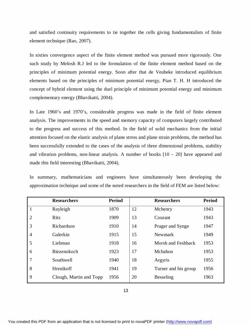
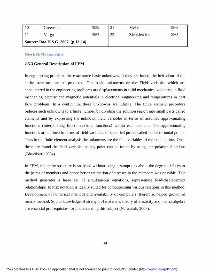
In summary, mathematicians and engineers have simultaneously been developing the
approximation technique and some of the noted researchers in the field of FEM are listed below:
Researchers Period Researchers Period
1 Rayleigh 1870 12 Mchenry 1943
2 Ritz 1909 13 Courant 1943
3 Richardson 1910 14 Prager and Synge 1947
4 Galerkin 1915 15 Newmark 1949
5 Liebman 1918 16 Morsh and Feshback 1953
6 Biezenokoch 1923 17 Mchahon 1953
7 Southwell 1940 18 Argyris 1955
8 Hrenikoff 1941 19 Turner and his group 1956
9 Clough, Martin and Topp 1956 20 Besseling 1963
You created this PDF from an application that is not licensed to print to novaPDF printer (http://www.novapdf.com)
14
10 Greenstadt 1959 21 Melosh 1963
11 Varga 1962 22 Zienkiewicz 1965
Source: Rao H.S.G. 2007, (p 13-14)
Table 1: FEM researchers
2.5.3 General Description of FEM
In engineering problems there are some basic unknowns. If they are found, the behaviour of the
entire structure can be predicted. The basic unknowns or the Field variables which are
encountered in the engineering problems are displacements in solid mechanics, velocities in fluid
mechanics, electric and magnetic potentials in electrical engineering and temperatures in heat
flow problems. In a continuum, these unknowns are infinite. The finite element procedure
reduces such unknowns to a finite number by dividing the solution region into small parts called
elements and by expressing the unknown field variables in terms of assumed approximating
functions (Interpolating functions/Shape functions) within each element. The approximating
functions are defined in terms of field variables of specified points called nodes or nodal points.
Thus in the finite element analysis the unknowns are the field variables of the nodal points. Once
these are found the field variables at any point can be found by using interpolation functions
(Bhavikatti, 2004).
In FEM, the entire structure is analysed without using assumptions about the degree of fixity at
the joints of members and hence better estimation of stresses in the members was possible. This
method generates a large set of simultaneous equations, representing load-displacement
relationships. Matrix notation is ideally suited for computerising various relations in this method.
Development of numerical methods and availability of computers, therefore, helped growth of
matrix method. Sound knowledge of strength of materials, theory of elasticity and matrix algebra
are essential pre-requisites for understanding this subject (Narasaiah, 2008).
You created this PDF from an application that is not licensed to print to novaPDF printer (http://www.novapdf.com)

15
2.5.4 Principle of FEM
FEM approach, which is based on minimum potential energy theorem, converges to the correct
solution from a higher value as the number of elements in the model increases. The number of
elements used in a model is selected by the engineer, based on the required accuracy of solution
as well as the availability of computer with sufficient memory. FEM has become popular as it
ensures usefulness of the results obtained even with lesser number of elements (Narasaiah,
2008).
Finite Element Analysis (FEA) based on FEM is a simulation, not reality, applied to the
mathematical model. Even very accurate FEA may not be good enough, if the mathematical
model is inappropriate or inadequate. A mathematical model is an idealisation in which
geometry, material properties, loads and/or boundary conditions are simplified based on the
analyst's understanding of what features are important or unimportant in obtaining the results
required. The error in solution can result from three different sources.
i. Modelling error - associated with the approximations made to the real problem.
ii. Discretisation error - associated with type, size and shape of finite elements used to
represent the mathematical model; can be reduced by modifying mesh.
iii. Numerical error - based on the algorithm used and the finite precision of numbers used to
represent data in the computer; most softwares use double precision for reducing
numerical error.
It is entirely possible for an unprepared software user to misunderstand the problem, prepare the
wrong mathematical model, discretise it inappropriately, fail to check computed output and yet
accept nonsensical results. FEA is a solution technique that removes many limitations of
classical solution techniques; but does not bypass the underlying theory or the need to devise a
satisfactory model. Thus, the accuracy of FEA depends on the knowledge of the analyst in
modelling the problem correctly (Narasaiah, 2008).
You created this PDF from an application that is not licensed to print to novaPDF printer (http://www.novapdf.com)
16
2.5.5 Limitations of FEM
The traditional method in finite element analysis is based on the assumed displacement field
within each element. These fields satisfy equation of compatibility of strains, but in general they
violate the equations of stress equilibrium within the element. Only the simple three-node
triangular plate element from among the family of isoparametric elements does not violate the
equations of stress equilibrium. Another method of determining the properties of finite elements
is to use stress fields that satisfy equations of stress equilibrium, but this approach is limited only
to some simple elements. For elements for which no stress fields are available, the displacement
field can be augmented by an additional displacement field vanishing on the element boundaries
and its magnitude determined from the principle of minimum potential energy in the element
(Bhavikatti, 2004).
2.5.6 Advantages of Numerical Simulation
(Jin & Riley, 2009) outlines the following advantages of numerical simulation
i. Because of their high predictive power and capability of dealing with complex
structures, numerical simulation tools can support a wide variety of engineering
applications, such as designing antennas analytically and predicting the impact of
platforms on antenna performance, and address more complex applications, including
calibration of antenna systems, estimating co-site interference of multiple-antenna
systems on a platform, and predicting scattering from low-observable antenna
installations.
Numerical simulation has four more distinctive advantages over traditional design by
experiment.
ii. The first advantage is low cost. When an item can be designed, analyzed, and
optimized on a computer, its design cost is reduced significantly compared to that of
constructing a prototype physically and measuring it.
You created this PDF from an application that is not licensed to print to novaPDF printer (http://www.novapdf.com)
17
iii. The second advantage is the short design cycle. It typically takes far less time to
simulate a structure on a computer than to actually build one and measure it in a
laboratory.
iv. The third advantage is the full exploration of the design space. Because of the low
cost and short design cycle, the designer can evaluate a large variety of design
parameters systematically to come up with an optimal design through numerical
simulation, which is simply impossible with laboratory experiments.
v. The last but not the least advantage of numerical simulation is the enormous amount
of physical insight it provides. With a numerical solution to Maxwell’s equations, the
designer can now use a computer visualization tool to “see” the current flow on an
antenna and field distributions around the antenna.
2.5.7 Disadvantages of Numerical Simulation
According to (Jin & Riley, 2009) the great advantages of numerical simulation are also
accompanied by a series of challenges. The main challenge is due to improper use of a numerical
simulation, such as insufficient discretization and use of a method outside its bounds. Such
improper use would yield either a poor or a completely erroneous design while wasting time and
resources. Therefore, it is very important to understand the basic principles, solution
technologies, and applicability and capabilities of numerical methods behind the numerical
simulation tools. Such knowledge can not only reduce the possibility of improper use of a
method, but also help in choosing from a suite of tools the technique best suited for a specific
problem, thus increasing the designer’s productivity.
2.5.8 Distinction between finite element methods and classical methods
In classical theory, the deformational behavior of continous media is considered on a
macroscopic scale without regard to size and shape of the elements within the prescribed
boundary of the structure. In finite element methods, elements are of finite size and have a
specified shape. These elements are specified arbitrarily in the process of defining the
mathematical model of the continuous structure. The properties of each element are calculated
using the theory of continuous elastic media, and the analysis of the entire structure is carried out
You created this PDF from an application that is not licensed to print to novaPDF printer (http://www.novapdf.com)
18
for the assembly of the individual elements. When the size of the elements is decreased, the
deformational behavior of the mathematical model converges to that of the continuous structure
(Przemieniecki, 2009).
(Bhavikatti, 2004) summarises the differences between finite element method vs classical
methods as follows
a) In classical methods exact equations are formed and exact solutions are obtained where
as in finite element analysis exact equations are formed but approximate solutions are
obtained.
b) Solutions have been obtained for few standard cases by classical methods, where as
solutions can be obtained for all problems by finite element analysis.
c) Whenever the following complexities are faced, classical method makes the drastic
assumptions’ and looks for the solutions:
i. Shape
ii. Boundary conditions
iii. Loading
To get the solution in the above cases, rectangular shapes, same boundary condition
along a side and regular equivalent loads are to be assumed. In FEM no such assumptions
are made. The problem is treated as it is.
d) When material property is not isotropic, solutions for the problems become very difficult
in classical method. Only few simple cases have been tried successfully by researchers.
FEM can handle structures with anisotropic properties also without any difficulty.
e) Problems with material and geometric non-linearities cannot be handled by classical
methods. There is no difficulty in FEM.
Hence FEM is superior to the classical methods only for the problems involving a number of
complexities which cannot be handled by classical methods without making drastic assumptions.
For all regular problems, the solutions by classical methods are the best solutions. Infact, to
You created this PDF from an application that is not licensed to print to novaPDF printer (http://www.novapdf.com)
19
check the validity of the FEM programs developed, the FEM solutions are compared with the
solutions by classical methods for standard problems (Bhavikatti, 2004).
2.5.9 Classification of FEM
The basic problem in any engineering design is to evaluate displacements, stresses and strains in
any given structure under different loads and boundary conditions. Several approaches of Finite
Element Analysis have been developed to meet the needs of specific applications. According to
(Narasaiah, 2008) the common methods are:
Displacement method - Here the structure is subjected to applied loads and/or specified
displacements. The primary unknowns are displacements, obtained by inversion of the stiffness
matrix, and the derived unknowns are stresses and strains. Stiffness matrix for any element can
be obtained by variational principle, based on minimum potential energy of any stable structure
and, hence, this is the most commonly used method.
Force method - Here the structure is subjected to applied loads and/or specified displacements.
The primary unknowns are member forces, obtained by inversion of the flexibility matrix, and
the derived unknowns are stresses and strains. Calculation of flexibility matrix is possible only
for discrete structural elements (such as trusses, beams and piping) and hence, this method is
limited in the early analyses of discrete structures and in piping analysis
Mixed method - Here the structure is subjected to applied loads and/or specified displacements.
The method deals with large stiffness coefficients as well as very small flexibility coefficients in
the same matrix. Analysis by this method leads to numerical errors and is not possible except in
some very special cases.
Hybrid method - Here the structure is subjected to applied loads and stress boundary conditions.
This deals with special cases, such as airplane dour frame which should be designed for stress-
free boundary, so that the door can be opened during flight, in cases of emergencies.
You created this PDF from an application that is not licensed to print to novaPDF printer (http://www.novapdf.com)
20
Displacement method is the most common method and is suitable for solving most of the
engineering problems.
2.5.10 Mathematical Models
One of the most important thing engineers and scientists do is to model natural phenomena. They
develop conceptual and mathematical models to simulate physical events, whether they are
aerospace, biological, chemical, geological, or mechanical. The mathematical models are
developed using laws of physics and they are often described in terms of algebraic, differential,
and/or integral equations relating various quantities of interest. A mathematical model can be
broadly defined as a set of relationships among variables that express the essential features of a
physical system or process in analytical terms (Reddy, 2004).
2.5.11 Design and Analysis of a component
(Narasaiah, 2008) Mechanical design is the design of a component for optimum size, shape, etc.,
against failure under the application of operational loads. A good design should also minimise
the cost of material and cost of production. Failures that are commonly associated with
mechanical components are broadly classified as:
a) Failure by breaking of brittle materials and subjected to repetitive loads) of ductile
materials.
b) Failure by yielding of ductile loads.
c) Failure by elastic deformation. materials, fatigue subjected to failure (when non-repetitive
The last two modes cause change of shape or size of the component rendering it useless and,
therefore, refer to functional or operational failure. Most of the design problems refer to one of
these two types of failures. Designing, thus, involves estimation of stresses and deformations of
the components at different critical points of a component for the specified loads and boundary
conditions, so as to satisfy operational constraints.
You created this PDF from an application that is not licensed to print to novaPDF printer (http://www.novapdf.com)
21
Design is associated with the calculation of dimensions of a component to withstand the applied
loads and perform the desired function. Analysis is associated with the estimation of
displacements or stresses in a component of assumed dimensions so that adequacy of assumed
dimensions is validated. Optimum design is obtained by many iterations of modifying
dimensions of the component based on the calculated values of displacements and/or stresses
vis-a-vis permitted values and re-analysis.
An analytic method is applied to a model problem rather than to an actual physical problem.
Even many laboratory experiments use models. A geometric model for analysis can be devised
after the physical nature of the problem has been understood. A model excludes superfluous
details such as bolts, nuts, rivets, but includes all essential features, so that analysis of the model
is not unnecessarily complicated and yet provides results that describe the actual problem with
sufficient accuracy. A geometric model becomes a mathematical "model” when its behaviour is
described or approximated by incorporating restrictions such as homogeneity, isotropy,
constancy of material properties and mathematical simplifications applicable for small
magnitudes of strains and rotations.
Several methods, such as method of joints for trusses, simple theory of bending, simple theory of
torsion, analyses of cylinders and spheres for axisymmetric pressure load etc., are available for
designing/analysing simple\ components of a structure. These methods try to obtain exact
solutions of second order partial differential equations and are based on several assumptions. on
sizes of the components, loads, end conditions, material properties, likely deformation pattern
etc. Also, these methods are not amenable for generalisation and effective utilisation of the
computer for repetitive jobs.
Strength of materials approach deals with a single beam member for different loads and end
conditions (free, simply supported and fixed). In a space -,. frame involving many such beam
members, each member is analysed independently by an assumed distribution of loads and end
conditions (Narasaiah, 2008).
You created this PDF from an application that is not licensed to print to novaPDF printer (http://www.novapdf.com)
22
2.5.12 Types of Analysis
According to (Narasaiah, 2008) mechanical engineers deal with two basic types of analyses for
discrete and continuum structures, excluding other applicatiion areas like fluid flow,
electromagnetics. FEM helps in modelling the component once and perform both the types of
analysis using the same model.
a) Thermal analysis - Deals with steady state or transient heat transfer by conduction and
convection, both being linear operations while radiation is a non-linear operation, and
estimation of temperature distribution in the component. This result can form one load
condition for the structural analysis
b) Structural analysis – Deals with estimation of stresses and displacements in discrete as
well as continuum structures under various types of loads such as gravity, wind, pressure
and temperature. Dynamic loads may also be considered.
2.5.13 Approximate method versus Exact method
An analytical solution is a mathematical expression that gives the values of the desired unknown
quantity at any location of a body and hence is valid for an infinite number of points in the
component. However, it is not possible to obtain analytical mathematical solutions for many
engineering problems.
For problems involving complex material properties and boundary conditions, numerical
approximate but acceptable solutions (with reasonable accuracy) for the unknown quantities -
only at discrete or finite number of points in the component.-Approximation is carried out in two
stages (Narasaiah, 2008):
a) In the formulation of the mathematical model, with respect to the physical behaviour of
the component. Example : Approximation of joint with multiple rivets at the junction of
any two members of a truss as a pin joint, assumption that the joint between a column and
a beam behaves like a simple support for the beam,.... The results are reasonably accurate
far away from the joint.
You created this PDF from an application that is not licensed to print to novaPDF printer (http://www.novapdf.com)

23
b) In obtaining numerical solution to the simplified mathematical model. The methods
usually involve approximation of a functional (such as Potential energy) in terms of
unknown functions (such as displacements) at finite number of points. There are two
broad categories
i. Weighted residual methods such as Galerkin Collocation method, Least squares
method, etc. method,
ii. Variational method (Rayleigh-Ritz method, FEM). FEM is an improvement of
Rayleigh-Ritz method by choosing a variational function valid over a small element
and not on the entire component, which will be discussed in detail later. These
methods also use the principle of minimum potential energy.
Principle of minimum potential energy
Among all possible kinematically admissible displacement fields (satisfying compatibility and
boundary conditions) of a conservative system, the one corresponding to stable equilibrium state
has minimum potential energy. For a component in static equilibrium, this principle helps in the
evaluation of unknown displacements of deformable solids (continuum structures).
Weighted Residual Methods
Most structural problems end up with differential equations. Closed form solutions are not
feasible in many of these problems. Different approaches are suggested to obtain approximate
solutions. One such category is the weighted residual technique.
Different methods are proposed based on how the residual is used in obtaining the best
(approximate) solution.
(a) called Galerkin Method
b) Collocation Method
c) Least Squares Method
You created this PDF from an application that is not licensed to print to novaPDF printer (http://www.novapdf.com)
24
In this method, integral of the residual over the entire component is minimised i.e
= 0 (2.2)
퐼 = ∫[푅({푎}, 푥)] . 푑푥 (2.3)
This method results in n algebraic simultaneous equations in unknown coefficients, which can be
easily evaluated.
2.5.14 Structural Analysis
Structural analysis is a most exciting field of activity, but it is clearly only a support activity in
the larger field of structural design. Analysis is a main part of the formulation and the solution of
any design problem, and it often must be repeated many times during the design process. The
analysis process helps to identify improved designs with respect to performance and cost
(Kirsch, 2002).
Referring to behavior under working loads, the objective of the analysis of a given structure is to
determine the internal forces, stresses and displacements under application of the given loading
conditions. In order to evaluate the response of the structure it is necessary to establish an
analytical model, which represents the structural behavior under application of the loadings. An
acceptable model must describe the physical behavior of the structure adequately, and yet be
simple to analyze. That is, the basic assumptions of the analysis will ensure that the model
represents the problem under consideration and that the idealizations and approximations used
result in a simplified solution. This latter property is essential particularly in the design of
complex or large systems. Two categories of mathematical models are often considered:
A. Lumped-parameter (discrete-system) models.
B. Continuum-mechanics-based (continuous-system) models
The solution of discrete analysis models usually involves the following steps:
You created this PDF from an application that is not licensed to print to novaPDF printer (http://www.novapdf.com)
25
i. Idealization of the system into a form that can be solved. The actual structure is idealized
as an assemblage of elements that are interconnected at the joints.
ii. Formulation of the mathematical model. The equilibrium requirements of each element
are first established in terms of unknown displacements, and the element interconnection
requirements are then used to establish the set of simultaneous analysis equations for the
unknown displacements.
iii. Solution of the model. The response is calculated by solving the simultaneous equations
for the unknown displacements; the internal forces and stresses of each element are
calculated by using the element equilibrium requirements.
The overall effectiveness of an analysis depends to a large degree on the numerical procedures
used for the solution of the equilibrium equations. The accuracy of the analysis can, in general,
be improved if a more refined model is used. In practice, there is a tendency to employ more and
more refined models to approximate the actual structure. This means that the cost of an analysis
and its practical feasibility depend to a considerable degree on the algorithms available for the
solution of the resulting equations. Because of the requirement that large systems be solved,
much research effort has been invested in equation solution algorithms. The time required for
solving the equilibrium equations can be a high percentage of the total solution time, particularly
in nonlinear analysis or in dynamic analysis, when the solution must be repeated many times. An
analysis may not be possible if the solution procedures are too costly or unstable.
2.5.15 Plane Trusses
The truss elements are part of a truss structure linked together by pinned joints that transmit only
axial force to the elements. Unlike an axial element, a truss element is two-dimensional, i.e. it
can displace both in x and y directions. Thus, we have two degrees of freedom at each node and
totally four degrees of freedom for a truss element (Rao, 2007). The geometry of the structure is
referred to a common Cartesian coordinate system {x, y}, which is called the global coordinate
system. Other names for it in the literature are structure coordinate system and overall
coordinate system. The key ingredients of the stiffness method of analysis are the forces and
displacements at the joints.
You created this PDF from an application that is not licensed to print to novaPDF printer (http://www.novapdf.com)
26
In a idealized pin-jointed truss, externally applied forces as well as reactions can act only at the
joints. All member axial forces can be characterized by the x and y components of these forces,
denoted by fx and fy , respectively. The components at joint i being identified as fxi and fyi ,
respectively.
2.5.16 Analysis of Trusses using FEM
The truss may be statically determinate or indeterminate. In the analysis all joints are assumed
pin connected and all loads act at joints only. These assumptions result into no bending of any
member. All members are subjected to only direct stresses– tensile or compressive (Bhavikatti,
2004).
The following steps illustrate how finite element analysis is conducted
Step 1: Selection of the Reference Origin for the Global Coordinate System
The reference origin is used for the coordinates of the element nodes and applied loads or
constraints on the structure (Bhavikatti, 2004).
Step 2: Selection of a Rigid Frame of Reference:
A rigid frame of reference is needed to calculate the node displacements. This is accomplished
by defining displacements u x and u y at all the nodes. This establishes a rigid frame of reference
with respect to which all other node displacements are calculated. This means that rigid-body
translations and rotations of the whole structure are eliminated. This is accomplished simply by
eliminating all rows and columns in the assembled stiffness, thermal stiffness, and/or mass
matrices corresponding to zero displacements defining the rigid frame of reference (Bhavikatti,
2004).
Step 3: Field Variables and Elements
Joint displacements are selected as basic field variables. Since there is no bending of the
members, we have to ensure only displacement continuity (C -continuity). Hence we select two
You created this PDF from an application that is not licensed to print to novaPDF printer (http://www.novapdf.com)
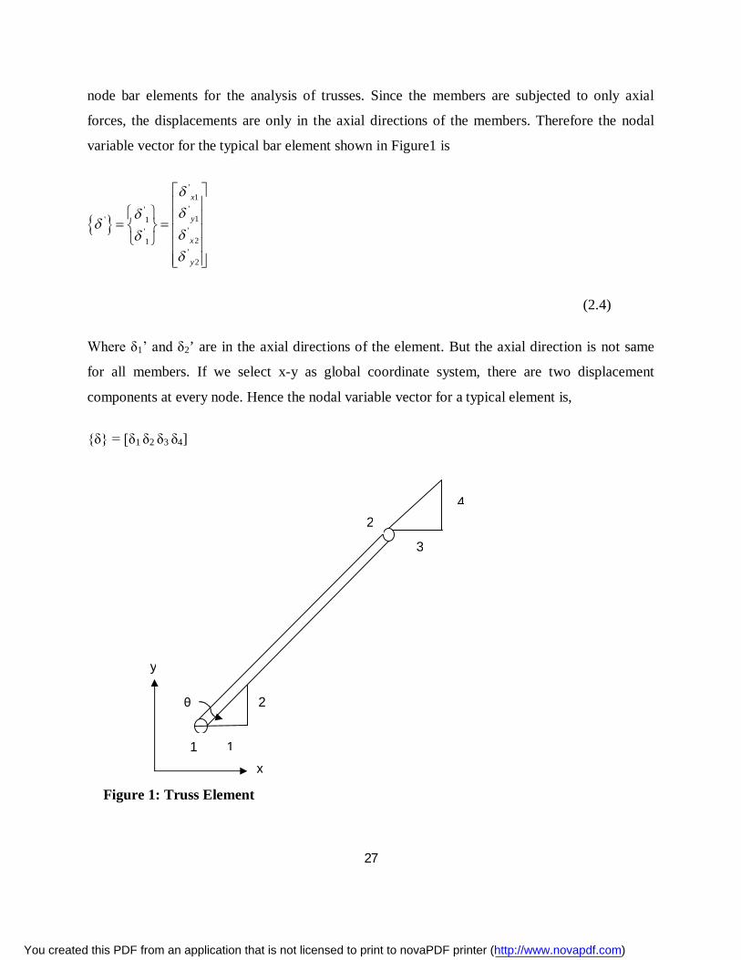
27
node bar elements for the analysis of trusses. Since the members are subjected to only axial
forces, the displacements are only in the axial directions of the members. Therefore the nodal
variable vector for the typical bar element shown in Figure1 is
'1
''1' 1
''21
'2
x
y
x
y
(2.4)
Where δ1’ and δ2’ are in the axial directions of the element. But the axial direction is not same
for all members. If we select x-y as global coordinate system, there are two displacement
components at every node. Hence the nodal variable vector for a typical element is,
{δ} = [δ1 δ2 δ3 δ4]
y
1
2
x
Figure 1: Truss Element
1
2
3
4
θ
You created this PDF from an application that is not licensed to print to novaPDF printer (http://www.novapdf.com)
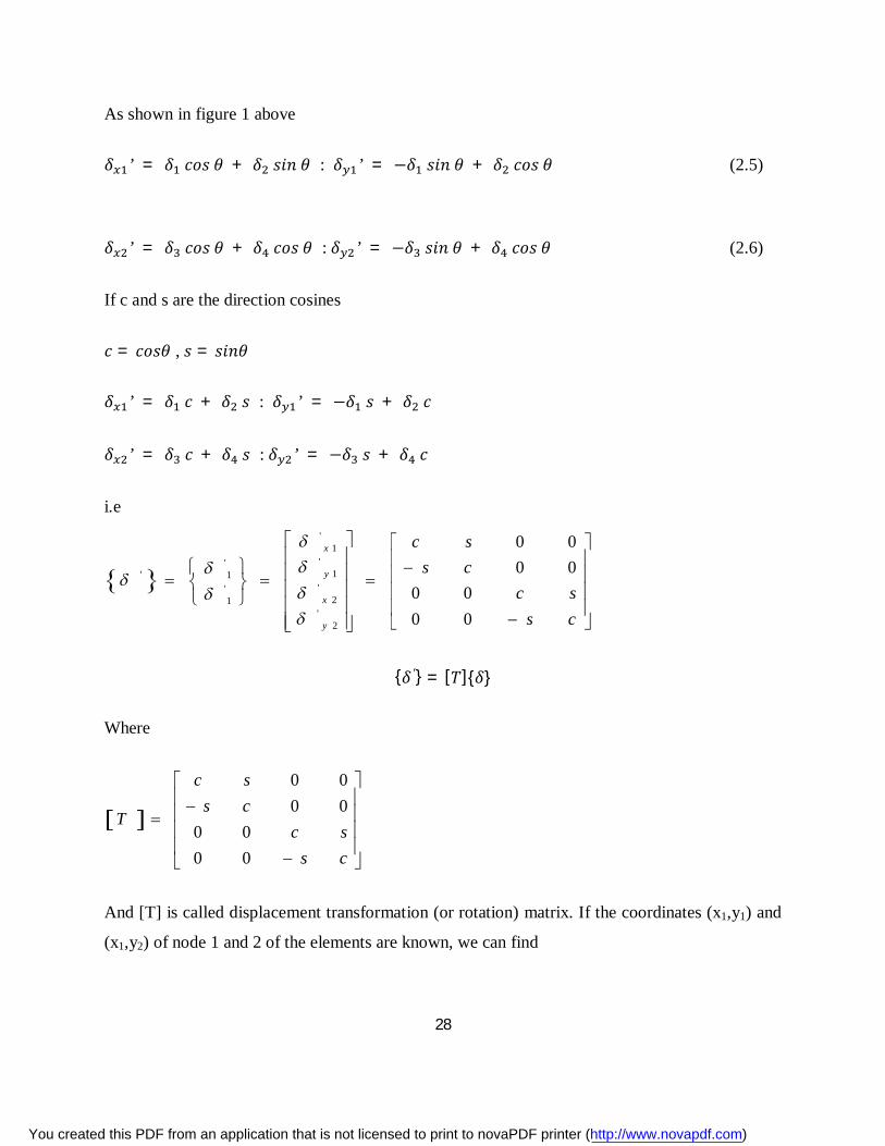
28
As shown in figure 1 above
훿 ’ = 훿 푐표푠 휃 + 훿 푠푖푛 휃 : 훿 ’ = −훿 푠푖푛 휃 + 훿 푐표푠 휃 (2.5)
훿 ’ = 훿 푐표푠 휃 + 훿 푐표푠 휃 : 훿 ’ = −훿 푠푖푛 휃 + 훿 푐표푠 휃 (2.6)
If c and s are the direction cosines
푐 = 푐표푠휃 , 푠 = 푠푖푛휃
훿 ’ = 훿 푐 + 훿 푠 : 훿 ’ = −훿 푠 + 훿 푐
훿 ’ = 훿 푐 + 훿 푠 : 훿 ’ = −훿 푠 + 훿 푐
i.e
'1
''1' 1
''21
'2
0 00 0
0 00 0
x
y
x
y
c ss c
c ss c
{훿 ′} = [푇]{훿}
Where
0 00 0
0 00 0
c ss c
Tc s
s c
And [T] is called displacement transformation (or rotation) matrix. If the coordinates (x1,y1) and
(x1,y2) of node 1 and 2 of the elements are known, we can find
You created this PDF from an application that is not licensed to print to novaPDF printer (http://www.novapdf.com)
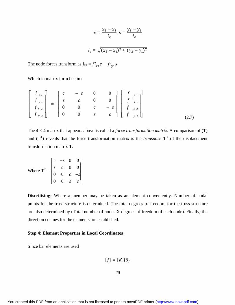
29
푐 =푥 − 푥푙 , 푠 =
푦 − 푦푙
푙 = (푥 − 푥 ) + (푦 − 푦 )
The node forces transform as fx1 = 푓′ 푐 − 푓′ 푠
Which in matrix form become
'1 1
'1 1
'2 2
'2 2
0 00 0
0 00 0
x x
y y
x x
y y
f fc sf fs cf fc sf fs c
(2.7)
The 4 × 4 matrix that appears above is called a force transformation matrix. A comparison of (T)
and (TT) reveals that the force transformation matrix is the transpose TT of the displacement
transformation matrix T.
Where TT =
0 00 0
0 00 0
c ss c
c ss c
Discritising: Where a member may be taken as an element conveniently. Number of nodal
points for the truss structure is determined. The total degrees of freedom for the truss structure
are also determined by (Total number of nodes X degrees of freedom of each node). Finally, the
direction cosines for the elements are established.
Step 4: Element Properties in Local Coordinates
Since bar elements are used
[푓] = [퐾]{훿}
You created this PDF from an application that is not licensed to print to novaPDF printer (http://www.novapdf.com)
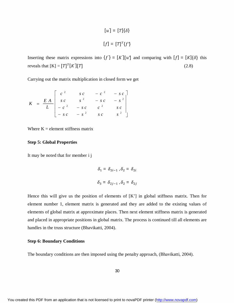
30
[푢′] = [푇]{훿}
[푓] = [푇] {푓′}
Inserting these matrix expressions into {푓 ′} = [퐾 ′][푢′] and comparing with [푓] = [퐾]{훿} this
reveals that [K] = [푇] [퐾 ′][푇] (2.8)
Carrying out the matrix multiplication in closed form we get
2 2
2 2
2 2
2 2
c s c c s cs c s s c sE AK
L c s c c s cs c s s c s
Where K = element stiffness matrix
Step 5: Global Properties
It may be noted that for member i j
훿 = 훿 ,훿 = 훿
훿 = 훿 , 훿 = 훿
Hence this will give us the position of elements of [K’] in global stiffness matrix. Then for
element number 1, element matrix is generated and they are added to the existing values of
elements of global matrix at approximate places. Then next element stiffness matrix is generated
and placed in appropriate positions in global matrix. The process is continued till all elements are
handles in the truss structure (Bhavikatti, 2004).
Step 6: Boundary Conditions
The boundary conditions are then imposed using the penalty approach, (Bhavikatti, 2004).
You created this PDF from an application that is not licensed to print to novaPDF printer (http://www.novapdf.com)

31
Step 7: Solution for the Global Node Displacements
Once the properties of Individual elements in the global coordinate system are calculated, they
are then assembled into the complete structure using the global coordinate system. This is
accomplished by a simple addition of the properties in the directions (i, j) to form the static load
displacement equation for the whole structure (Bhavikatti, 2004).
Assembly of the globalised matrices follows the relation that 푓 = ∑푓 = (∑퐾)푢 = 퐾푢
The resulting stiffness matrix is referred to as the Master stiffness matrix
Step 8: Computation of the Node Displacements
K is a singular matrix and therefore cannot be inverted to obtain a solution for U. Therefore in
this step all rows and columns corresponding to the rigid frame of reference, and any other rows
and columns corresponding to additional constraints (zero displacements) are eliminated from K.
In practice, however, in order to preserve the original numbering system the rows and columns in
K are not eliminated but are simply replaced with zeros except for the diagonal terms, which are
replaced with ones (Bhavikatti, 2004).
Step 9: Additional Calculations Analysts are interested in finding stresses and forces in the
members of the truss (Bhavikatti, 2004).
We know σ = Eeε (2.9)
But
= ε
' "
el
You created this PDF from an application that is not licensed to print to novaPDF printer (http://www.novapdf.com)
32
CHAPTER THREE
3.0 Matlab Programming
3.1 Introduction
Matlab (Matrix laboratory) is an interactive software system for numerical computations and
graphics. As the name suggests, Matlab is especially designed for matrix computations: solving
systems of linear equations, computing eigenvalues and eigenvectors, factoring matrices. In
addition, it has a variety of graphical capabilities, and can be extended through programs written
in its own programming language. Many such programs come with the system; a number of
these extend Matlab's capabilities to nonlinear problems, such as the solution of initial value
problems for ordinary differential equations. (http://www.math.mtu.edu)
Matlab is designed to solve problems numerically, that is, in finite-precision arithmetic.
Therefore it produces approximate rather than exact solutions, and should not be confused with a
symbolic computation system (SCS) such as Mathematica or Maple. It should be understood that
this does not make Matlab better or worse than an SCS; it is a tool designed for different tasks
and is therefore not directly comparable. (http://www.math.mtu.edu)
3.2 Overview of the MATLAB Environment
The MATLAB high-performance language for technical computing integrates computation,
visualization, and programming in an easy-to-use environment where problems and solutions are
expressed in familiar mathematical notation. Typical uses include
i. Math and computation
ii. Algorithm development
iii. Data acquisition
iv. Modeling, simulation, and prototyping
v. Data analysis, exploration, and visualization
vi. Scientific and engineering graphics
You created this PDF from an application that is not licensed to print to novaPDF printer (http://www.novapdf.com)

33
vii. Application development, including graphical user interface building
MATLAB is an interactive system whose basic data element is an array that does not require
dimensioning. It allows an individual to solve many technical computing problems, especially
those with matrix and vector formulations, in a fraction of the time it would take to write a
program in a scalar non interactive language such as C or FORTRAN
(http://www.mathwork.com).
MATLAB was originally written to provide easy access to matrix software developed by the
LINPACK and EISPACK projects. Today, MATLAB engines incorporate the LAPACK and
BLAS libraries, embedding the state of the art in software for matrix computation.
MATLAB has evolved over a period of years with input from many users. In university
environments, it is the standard instructional tool for introductory and advanced courses in
mathematics, engineering, and science. In industry, MATLAB is the tool of choice for high-
productivity research, development, and analysis Matlab Product help guide.
MATLAB features a family of add-on application-specific solutions called toolboxes. Very
important to most users of MATLAB, toolboxes allow an individual to learn and apply
specialized technology. Toolboxes are comprehensive collections of MATLAB functions (M-
files) that extend the MATLAB environment to solve particular classes of problems. One can
add on toolboxes for signal processing, control systems, neural networks, fuzzy logic, wavelets
and simulation Matlab Product help guide.
3.3 The MATLAB System
According to the (The Mathwork, Inc., 2008) MATLAB system consists of these main parts:
Desktop Tools and Development Environment
This is the set of tools and facilities that help a person to use and become more productive with
MATLAB functions and files. Many of these tools are graphical user interfaces. It includes the
MATLAB desktop and Command Window, a command history, an editor and debugger, a code
You created this PDF from an application that is not licensed to print to novaPDF printer (http://www.novapdf.com)
34
analyzer and other reports, and browsers for viewing help, the workspace, files, and the search
path.
Mathematical Function Library
This is a vast collection of computational algorithms ranging from elementary functions, like
sum, sine, cosine, and complex arithmetic, to more sophisticated functions like matrix inverse,
matrix eigen values, Bessel functions, and fast Fourier transforms.
The Language
This is a high-level matrix/array language with control flow statements, functions, data
structures, input/output, and object-oriented programming features. It allows both "programming
in the small" to rapidly create quick and dirty throw-away programs, and "programming in the
large" to create large and complex application programs.
Graphics
MATLAB has extensive facilities for displaying vectors and matrices as graphs, as well as
annotating and printing these graphs. It includes high-level functions for two-dimensional and
three-dimensional data visualization, image processing, animation, and presentation graphics. It
also includes low-level functions that allow a person to fully customize the appearance of
graphics as well as to build complete graphical user interfaces on MATLAB applications.
External Interfaces
This is a library that allows a person to write C and FORTRAN programs that interact with
MATLAB. It includes facilities for calling routines from MATLAB (dynamic linking), for
calling MATLAB as a computational engine, and for reading and writing MAT-files.
You created this PDF from an application that is not licensed to print to novaPDF printer (http://www.novapdf.com)
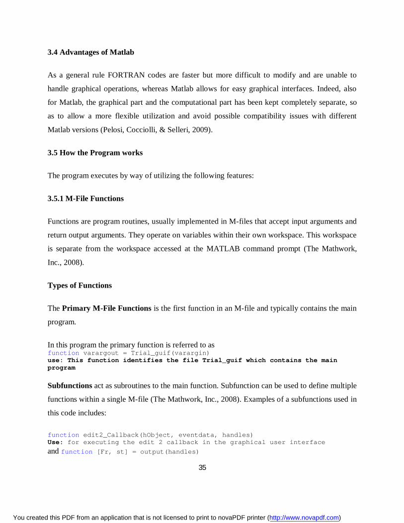
35
3.4 Advantages of Matlab
As a general rule FORTRAN codes are faster but more difficult to modify and are unable to
handle graphical operations, whereas Matlab allows for easy graphical interfaces. Indeed, also
for Matlab, the graphical part and the computational part has been kept completely separate, so
as to allow a more flexible utilization and avoid possible compatibility issues with different
Matlab versions (Pelosi, Cocciolli, & Selleri, 2009).
3.5 How the Program works
The program executes by way of utilizing the following features:
3.5.1 M-File Functions
Functions are program routines, usually implemented in M-files that accept input arguments and
return output arguments. They operate on variables within their own workspace. This workspace
is separate from the workspace accessed at the MATLAB command prompt (The Mathwork,
Inc., 2008).
Types of Functions
The Primary M-File Functions is the first function in an M-file and typically contains the main
program.
In this program the primary function is referred to as function varargout = Trial_guif(varargin) use: This function identifies the file Trial_guif which contains the main program
Subfunctions act as subroutines to the main function. Subfunction can be used to define multiple
functions within a single M-file (The Mathwork, Inc., 2008). Examples of a subfunctions used in
this code includes:
function edit2_Callback(hObject, eventdata, handles) Use: for executing the edit 2 callback in the graphical user interface and function [Fr, st] = output(handles)
You created this PDF from an application that is not licensed to print to novaPDF printer (http://www.novapdf.com)
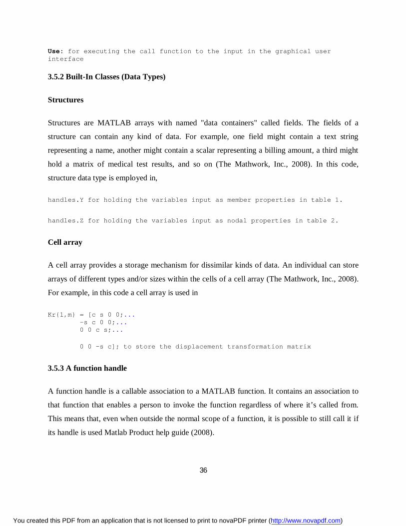
36
Use: for executing the call function to the input in the graphical user interface
3.5.2 Built-In Classes (Data Types)
Structures
Structures are MATLAB arrays with named "data containers" called fields. The fields of a
structure can contain any kind of data. For example, one field might contain a text string
representing a name, another might contain a scalar representing a billing amount, a third might
hold a matrix of medical test results, and so on (The Mathwork, Inc., 2008). In this code,
structure data type is employed in,
handles.Y for holding the variables input as member properties in table 1.
handles.Z for holding the variables input as nodal properties in table 2.
Cell array
A cell array provides a storage mechanism for dissimilar kinds of data. An individual can store
arrays of different types and/or sizes within the cells of a cell array (The Mathwork, Inc., 2008).
For example, in this code a cell array is used in
Kr{1,m} = [c s 0 0;... -s c 0 0;... 0 0 c s;...
0 0 -s c]; to store the displacement transformation matrix
3.5.3 A function handle
A function handle is a callable association to a MATLAB function. It contains an association to
that function that enables a person to invoke the function regardless of where it’s called from.
This means that, even when outside the normal scope of a function, it is possible to still call it if
its handle is used Matlab Product help guide (2008).
You created this PDF from an application that is not licensed to print to novaPDF printer (http://www.novapdf.com)
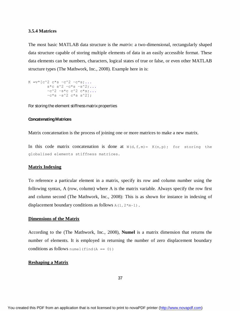
37
3.5.4 Matrices
The most basic MATLAB data structure is the matrix: a two-dimensional, rectangularly shaped
data structure capable of storing multiple elements of data in an easily accessible format. These
data elements can be numbers, characters, logical states of true or false, or even other MATLAB
structure types (The Mathwork, Inc., 2008). Example here in is:
K =v*[c^2 c*s -c^2 -c*s;... s*c s^2 -c*s -s^2;... -c^2 -s*c c^2 c*s;... -c*s -s^2 c*s s^2];
For storing the element stiffness matrix properties
Concatenating Matrices
Matrix concatenation is the process of joining one or more matrices to make a new matrix.
In this code matrix concatenation is done at W(d,f,m)= K(n,p); for storing the
globalised elements stiffness matrices.
Matrix Indexing
To reference a particular element in a matrix, specify its row and column number using the
following syntax, A (row, column) where A is the matrix variable. Always specify the row first
and column second (The Mathwork, Inc., 2008): This is as shown for instance in indexing of
displacement boundary conditions as follows A(1,2*m-1).
Dimensions of the Matrix
According to the (The Mathwork, Inc., 2008), Numel is a matrix dimension that returns the
number of elements. It is employed in returning the number of zero displacement boundary
conditions as follows numel(find(A == 0))
Reshaping a Matrix
You created this PDF from an application that is not licensed to print to novaPDF printer (http://www.novapdf.com)
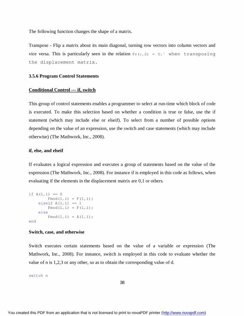
38
The following function changes the shape of a matrix.
Transpose - Flip a matrix about its main diagonal, turning row vectors into column vectors and
vice versa. This is particularly seen in the relation Fr(:,2) = U.' when transposing
the displacement matrix.
3.5.6 Program Control Statements
Conditional Control — if, switch
This group of control statements enables a programmer to select at run-time which block of code
is executed. To make this selection based on whether a condition is true or false, use the if
statement (which may include else or elseif). To select from a number of possible options
depending on the value of an expression, use the switch and case statements (which may include
otherwise) (The Mathwork, Inc., 2008).
if, else, and elseif
If evaluates a logical expression and executes a group of statements based on the value of the
expression (The Mathwork, Inc., 2008). For instance if is employed in this code as follows, when
evaluating if the elements in the displacement matrix are 0,1 or others.
if A(1,i) == 0 Fmod(1,i) = F(1,i); elseif A(1,i) == 1 Fmod(1,i) = F(1,i); else Fmod(1,i) = A(1,i); end
Switch, case, and otherwise
Switch executes certain statements based on the value of a variable or expression (The
Mathwork, Inc., 2008). For instance, switch is employed in this code to evaluate whether the
value of n is 1,2,3 or any other, so as to obtain the corresponding value of d.
switch n
You created this PDF from an application that is not licensed to print to novaPDF printer (http://www.novapdf.com)
39
case 1 d = n1-1; case 2 d = n1; case 3 d = n2-1; otherwise d =n2; end
Loop Control — for, while, continue, break
With loop control statements, one can repeatedly execute a block of code, looping back through
the block while keeping track of each iteration with an incrementing index variable. Use the for
statement to loop a specific number of times. The, while statement, is more suitable for basing
loop execution, on how long a condition continues to be true or false. The continue and break
statements give a person more control on exiting the loop.
for
The for loop executes a statement or group of statements a predetermined number of times.
for j=1:w D(i,j)=0; D(j,i)=0; D(i,i)=1;
end
For example, in the case above, the for loop executes w times before stopping.
3.5.6 Types of Variables
A MATLAB variable is essentially a tag assigned to a value while that value remains in memory.
The tag gives a way to reference the value in memory so that programs can read it, operate on it
with other data, and save it back to memory.
MATLAB provides three basic types of variables:
i. Local Variables
You created this PDF from an application that is not licensed to print to novaPDF printer (http://www.novapdf.com)
40
ii. Global Variables
iii. Persistent Variables
Local Variables
Each MATLAB function has its own local variables. These are separate from those of other
functions (except for nested functions), and from those of the base workspace. Variables defined
in a function do not remain in memory from one function call to the next, unless they are defined
as global or persistent (The Mathwork, Inc., 2008). Examples of local variables here include K
which is an element stiffness matrix local variable in the sub function Output.
3.5.7 Graphical User Interface
GUIDE, is the MATLAB graphical user interface development environment. Guide provides a
set of tools for creating graphical user interfaces (GUIs). These tools simplify the process of
designing and building GUIs (The Mathwork, Inc., 2008). GUIDE tools are used to:
i) Lay out the GUI.
Using the GUIDE Layout Editor, it is possible to lay out a GUI by clicking and dragging GUI
components—such as panels, buttons, text fields, sliders, menus, and so on—into the layout area.
GUIDE stores the GUI layout in a FIG-file Matlab Product Help (2008).
ii) Program the GUI.
GUIDE automatically generates an M-file that controls how the GUI operates. The M-file
initializes the GUI and contains a framework for the most commonly used callbacks for each
component—the commands that execute when a user clicks a GUI component. Using the M-file
editor, you can add code to the callbacks to perform the functions you want Matlab Product Help
(2008).
For this program guide tools were utilized in designing the GUI as seen in the first part of the
code in the appendix.
You created this PDF from an application that is not licensed to print to novaPDF printer (http://www.novapdf.com)

41
3.5.8 Pseudo code
START
Enter Number of Members
Numeric
Enter Member Properties
Enter Number of Nodes:
Numeric
Output
Function
Enter Nodal Properties
All Properties
Numeric
Display: Stress, Reaction Forces & Displacements
STOP
NO
NO
NO
YES
YES
YES
Figure 2: Graphical user interface
You created this PDF from an application that is not licensed to print to novaPDF printer (http://www.novapdf.com)

42
Explanation: Figure 1:
At the graphical user interface the user is required to enter numerical information on number of
members, corresponding member properties, number of nodes and corresponding properties at
the nodes. Where all the properties are entered correctly then they are passed by the checkbox to
the Output function.
Output Function
Explanation: Figure 2:
Once the output function is called, the number of members is passed to ‘for’ loop to control the
number of loops executed. The ‘for’ loop output’s the element stiffness matrix (K). The element
stiffness matrix is passed to the nested for loop which generates the globalised element stiffness
matrix. This is done with the help of the conditional switch statement that selects the index for
the global element stiffness matrix. The global element stiffness matrix is stored in the variable
W in concatenated form. The stored matrix is used in preparing the master stiffness matrix found
by summing all the global element stiffness matrices.
You created this PDF from an application that is not licensed to print to novaPDF printer (http://www.novapdf.com)
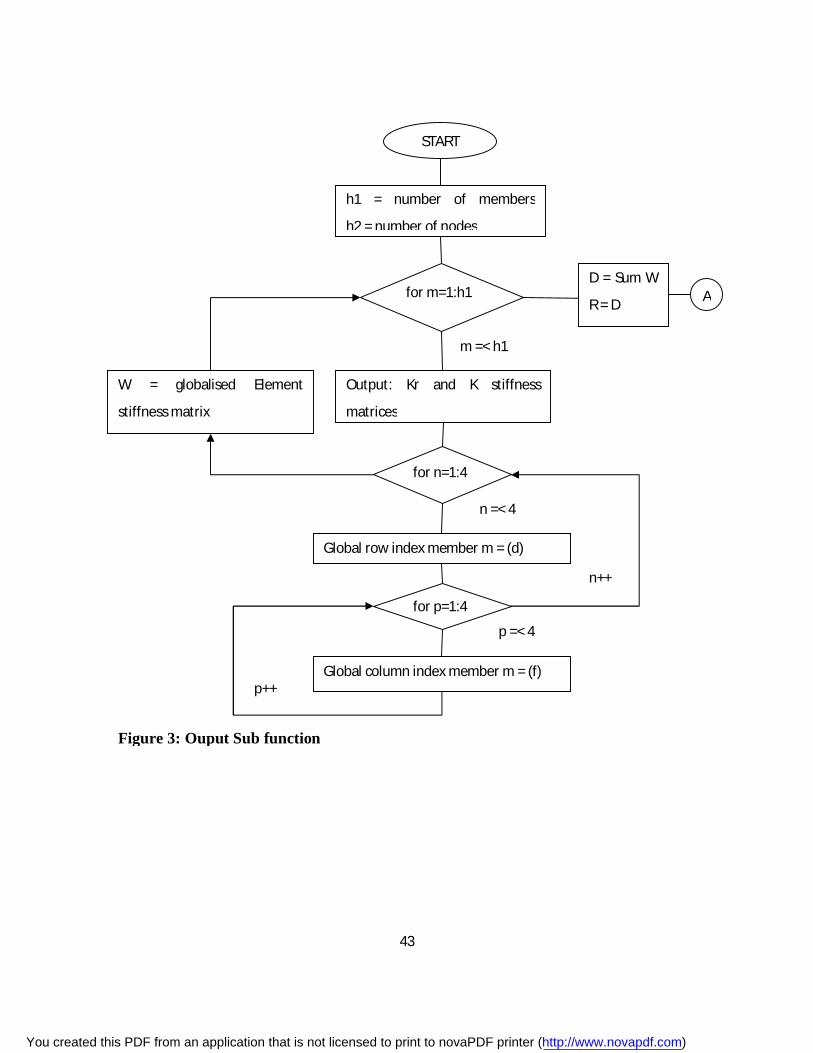
43
START
h1 = number of members
h2 = number of nodes
for m=1:h1
for n=1:4
Output: Kr and K stiffness
matrices
Global row index member m = (d)
for p=1:4
Global column index member m = (f)
W = globalised Element
stiffness matrix
m =< h1
n =< 4
p =< 4
p++
n++
D = Sum W
R = D A
Figure 3: Ouput Sub function
You created this PDF from an application that is not licensed to print to novaPDF printer (http://www.novapdf.com)
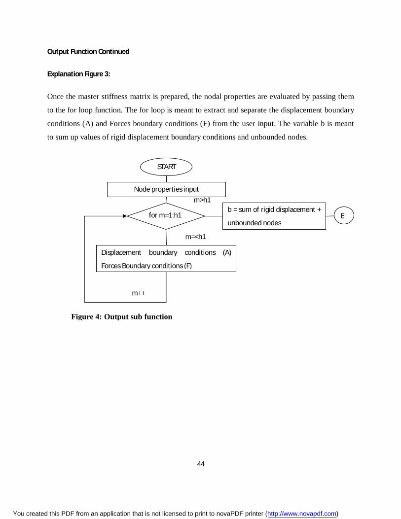
44
Output Function Continued
Explanation Figure 3:
Once the master stiffness matrix is prepared, the nodal properties are evaluated by passing them
to the for loop function. The for loop is meant to extract and separate the displacement boundary
conditions (A) and Forces boundary conditions (F) from the user input. The variable b is meant
to sum up values of rigid displacement boundary conditions and unbounded nodes.
START
for m=1:h1
Displacement boundary conditions (A)
Forces Boundary conditions (F)
m++
b = sum of rigid displacement +
unbounded nodes B
m=<h1
m>h1
Node properties input
Figure 4: Output sub function
You created this PDF from an application that is not licensed to print to novaPDF printer (http://www.novapdf.com)
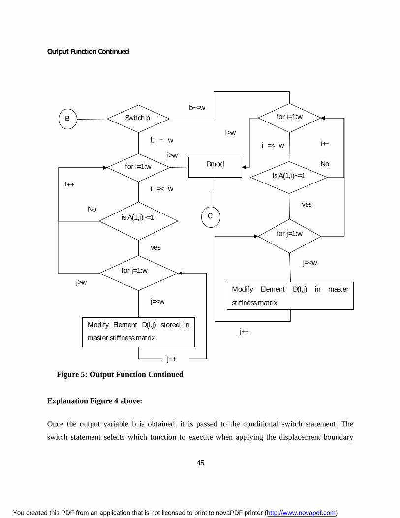
45
Output Function Continued
Explanation Figure 4 above:
Once the output variable b is obtained, it is passed to the conditional switch statement. The
switch statement selects which function to execute when applying the displacement boundary
B Switch b
for i=1:w
is A(1,i)~=1
for j=1:w
Modify Element D(I,j) stored in
master stiffness matrix
for i=1:w
Is A(1,i)~=1
for j=1:w
Modify Element D(I,j) in master
stiffness matrix
≠
b~=w
≠
j=<w
≠
No
≠
yes
≠
i =< w
≠
b = w
≠
j>w
≠
i++
≠
j++
≠
j++
≠
j=<w
≠
i++
≠
No
≠
yes
≠
i =< w
Dmod
i>w
C
i>w
Figure 5: Output Function Continued
You created this PDF from an application that is not licensed to print to novaPDF printer (http://www.novapdf.com)
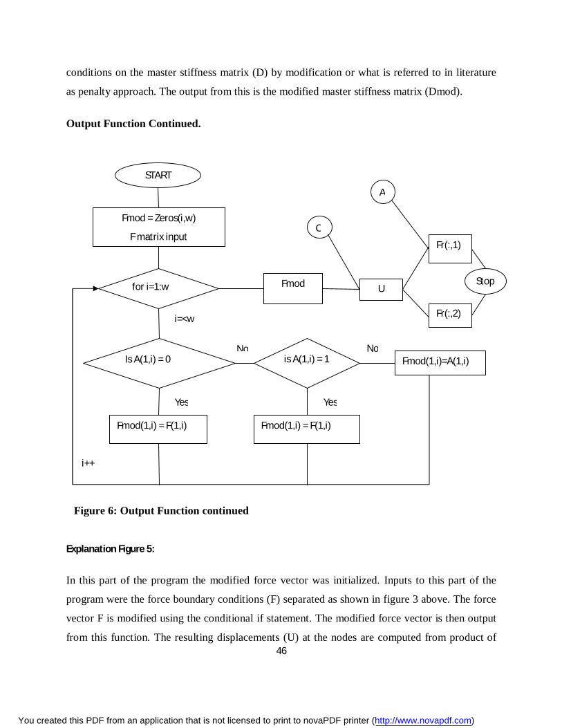
46
conditions on the master stiffness matrix (D) by modification or what is referred to in literature
as penalty approach. The output from this is the modified master stiffness matrix (Dmod).
Output Function Continued.
Explanation Figure 5:
In this part of the program the modified force vector was initialized. Inputs to this part of the
program were the force boundary conditions (F) separated as shown in figure 3 above. The force
vector F is modified using the conditional if statement. The modified force vector is then output
from this function. The resulting displacements (U) at the nodes are computed from product of
START
Fmod = Zeros(i,w)
F matrix input
for i=1:w
Is A(1,i) = 0
Fmod(1,i) = F(1,i) Fmod(1,i) = F(1,i)
is A(1,i) = 1 Fmod(1,i)=A(1,i)
i=<w
Yes
No No
Yes
i++
Fmod U
Fr(:,1)
Fr(:,2)
A
C
Stop
Figure 6: Output Function continued
You created this PDF from an application that is not licensed to print to novaPDF printer (http://www.novapdf.com)
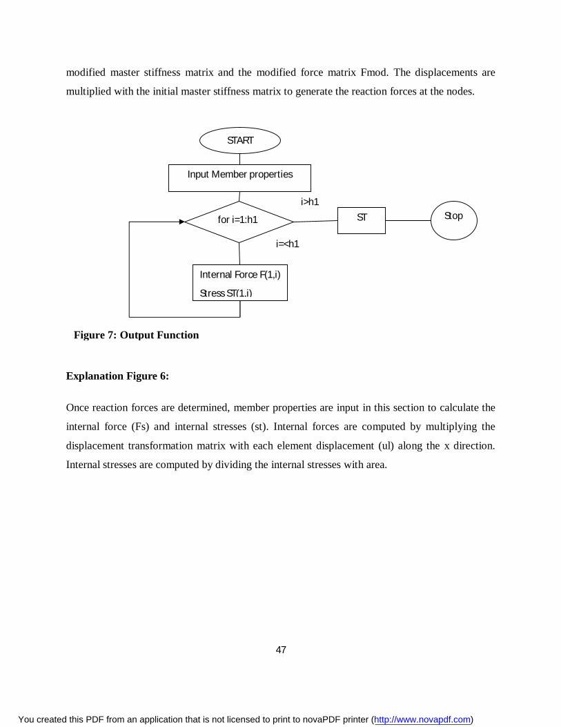
47
modified master stiffness matrix and the modified force matrix Fmod. The displacements are
multiplied with the initial master stiffness matrix to generate the reaction forces at the nodes.
Explanation Figure 6:
Once reaction forces are determined, member properties are input in this section to calculate the
internal force (Fs) and internal stresses (st). Internal forces are computed by multiplying the
displacement transformation matrix with each element displacement (ul) along the x direction.
Internal stresses are computed by dividing the internal stresses with area.
START
for i=1:h1
Internal Force F(1,i)
Stress ST(1,i)
i++
ST
i>h1 Stop
Input Member properties
i=<h1
Figure 7: Output Function
You created this PDF from an application that is not licensed to print to novaPDF printer (http://www.novapdf.com)
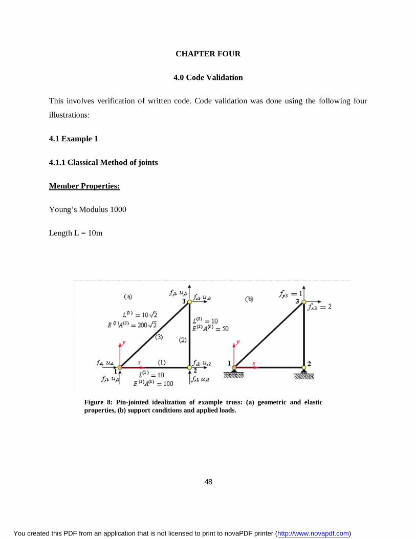
48
CHAPTER FOUR
4.0 Code Validation
This involves verification of written code. Code validation was done using the following four
illustrations:
4.1 Example 1
4.1.1 Classical Method of joints
Member Properties:
Young’s Modulus 1000
Length L = 10m
Figure 8: Pin-jointed idealization of example truss: (a) geometric and elastic properties, (b) support conditions and applied loads.
You created this PDF from an application that is not licensed to print to novaPDF printer (http://www.novapdf.com)
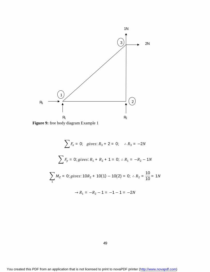
49
퐹 = 0; 푔푖푣푒푠: 푅 + 2 = 0; ∴ 푅 = −2푁
퐹 = 0;푔푖푣푒푠: 푅 + 푅 + 1 = 0; ∴ 푅 = −푅 − 1푁
푀 = 0;푔푖푣푒푠: 10푅 + 10(1)− 10(2) = 0; ∴ 푅 =1010 = 1푁
→ 푅 = −푅 − 1 = −1− 1 = −2푁
R1 R2
R3
2N
1N
1
3
2
Figure 9: free body diagram Example 1
You created this PDF from an application that is not licensed to print to novaPDF printer (http://www.novapdf.com)
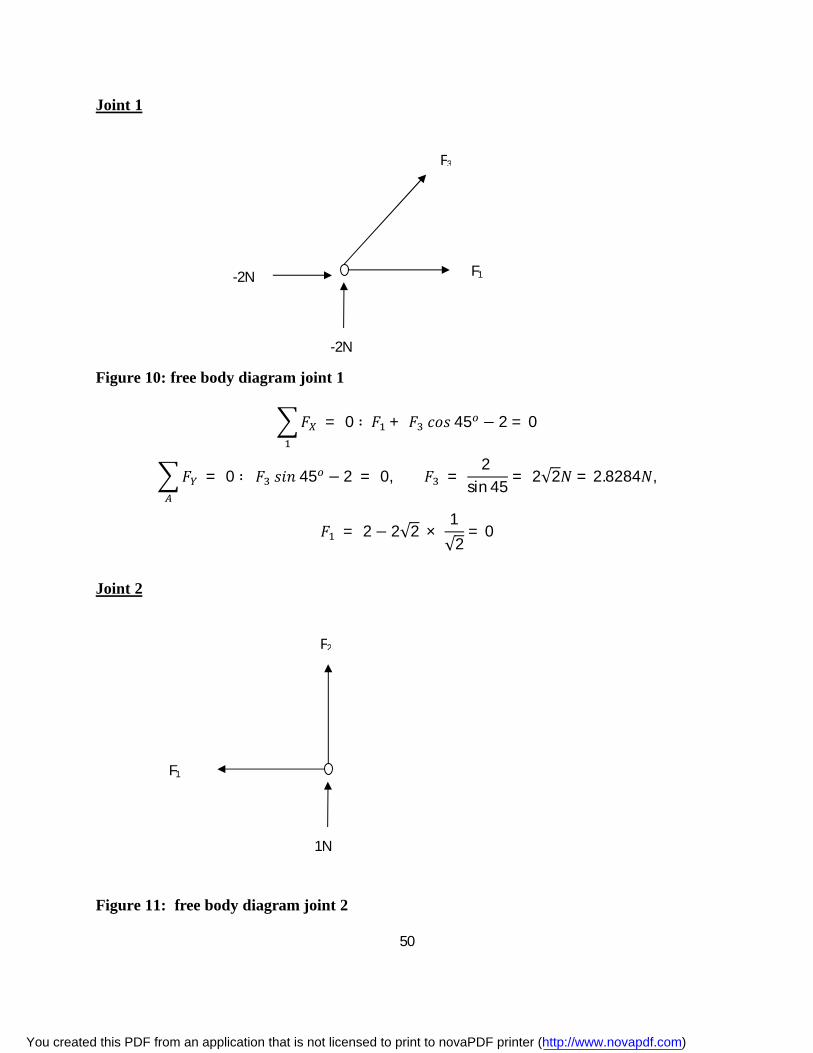
50
Joint 1
Figure 10: free body diagram joint 1
퐹 = 0 ∶ 퐹 + 퐹 푐표푠 45 − 2 = 0
퐹 = 0 ∶ 퐹 푠푖푛 45 − 2 = 0, 퐹 = 2
sin 45 = 2√2푁 = 2.8284푁,
퐹 = 2 − 2√2 × 1√2
= 0
Joint 2
Figure 11: free body diagram joint 2
1N
F1
F2
-2N
-2N
F1
F3
You created this PDF from an application that is not licensed to print to novaPDF printer (http://www.novapdf.com)
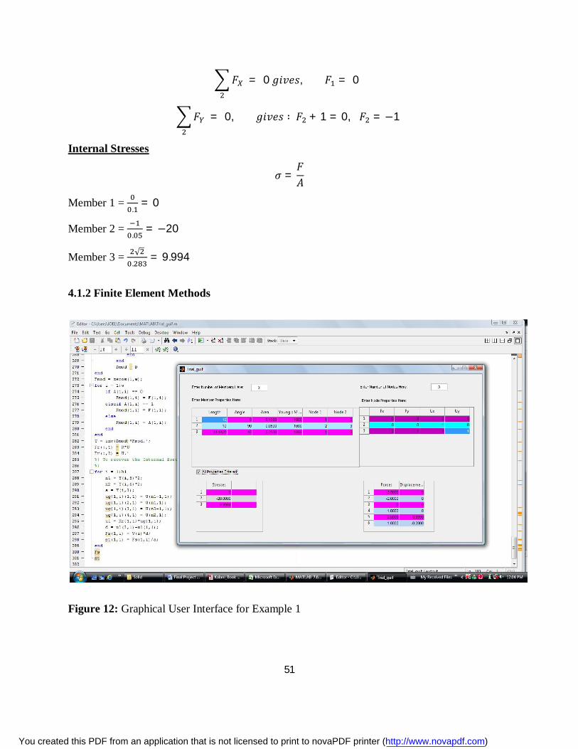
51
퐹 = 0 푔푖푣푒푠, 퐹 = 0
퐹 = 0, 푔푖푣푒푠 ∶ 퐹 + 1 = 0, 퐹 = −1
Internal Stresses
휎 =퐹퐴
Member 1 = .
= 0
Member 2 = .
= −20
Member 3 = √.
= 9.994
4.1.2 Finite Element Methods
Figure 12: Graphical User Interface for Example 1
You created this PDF from an application that is not licensed to print to novaPDF printer (http://www.novapdf.com)
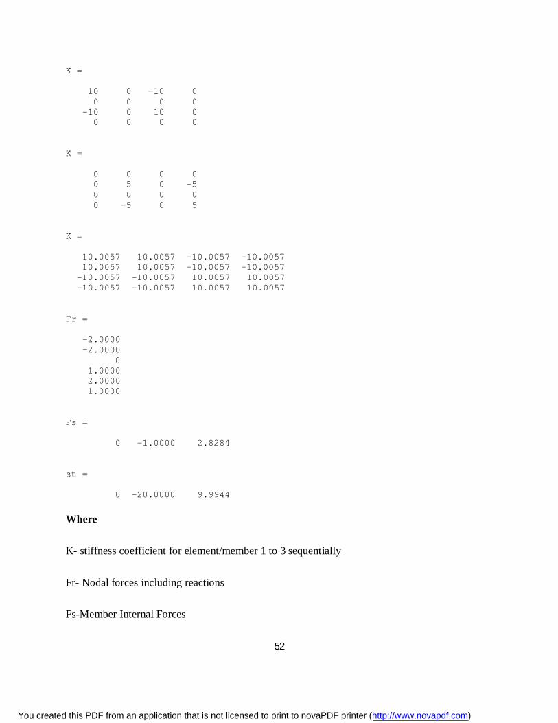
52
K = 10 0 -10 0 0 0 0 0 -10 0 10 0 0 0 0 0 K = 0 0 0 0 0 5 0 -5 0 0 0 0 0 -5 0 5 K = 10.0057 10.0057 -10.0057 -10.0057 10.0057 10.0057 -10.0057 -10.0057 -10.0057 -10.0057 10.0057 10.0057 -10.0057 -10.0057 10.0057 10.0057 Fr = -2.0000 -2.0000 0 1.0000 2.0000 1.0000 Fs = 0 -1.0000 2.8284 st = 0 -20.0000 9.9944
Where
K- stiffness coefficient for element/member 1 to 3 sequentially
Fr- Nodal forces including reactions
Fs-Member Internal Forces
You created this PDF from an application that is not licensed to print to novaPDF printer (http://www.novapdf.com)
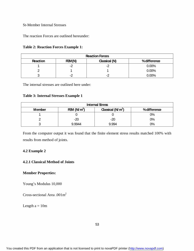
53
St-Member Internal Stresses
The reaction Forces are outlined hereunder:
Table 2: Reaction Forces Example 1:
Reaction Forces Reaction FEM(N) Classical (N) % difference
1 -2 -2 0.00% 2 1 1 0.00% 3 -2 -2 0.00%
The internal stresses are outlined here under:
Table 3: Internal Stresses Example 1
Internal Stress Member FEM (N/m2) Classical (N/m2) % difference
1 0 0 0% 2 -20 -20 0% 3 9.9944 9.994 0%
From the computer output it was found that the finite element stress results matched 100% with
results from method of joints.
4.2 Example 2
4.2.1 Classical Method of Joints
Member Properties:
Young’s Modulus 10,000
Cross-sectional Area .001m2
Length a = 10m
You created this PDF from an application that is not licensed to print to novaPDF printer (http://www.novapdf.com)
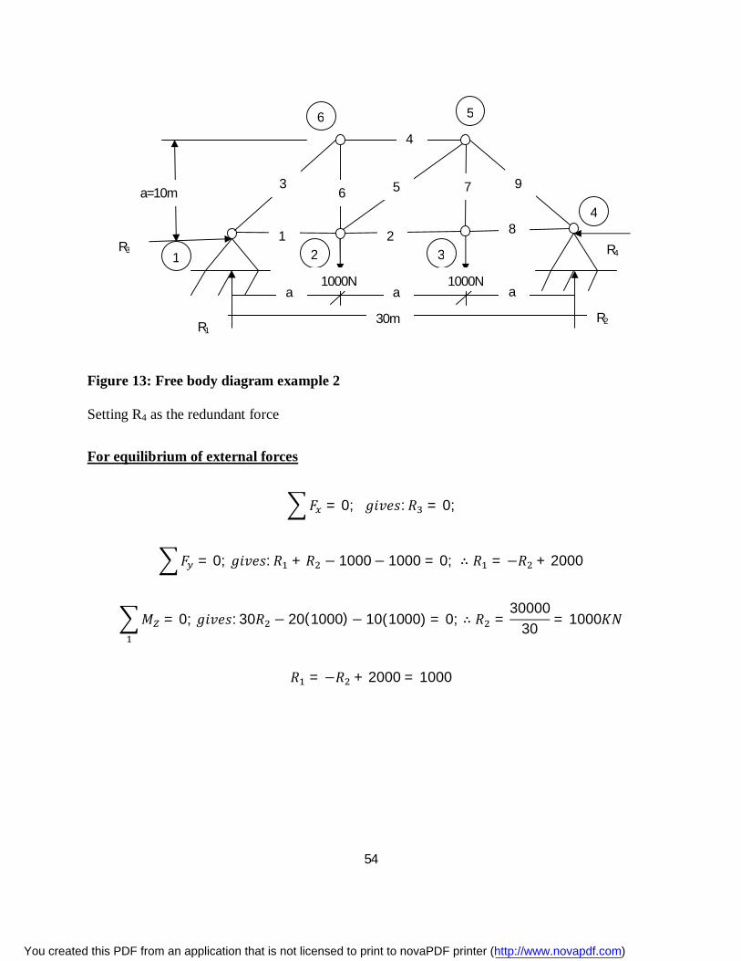
54
Figure 13: Free body diagram example 2
Setting R4 as the redundant force
For equilibrium of external forces
퐹 = 0; 푔푖푣푒푠: 푅 = 0;
퐹 = 0; 푔푖푣푒푠: 푅 + 푅 − 1000− 1000 = 0; ∴ 푅 = −푅 + 2000
푀 = 0; 푔푖푣푒푠: 30푅 − 20(1000)− 10(1000) = 0; ∴ 푅 =30000
30 = 1000퐾푁
푅 = −푅 + 2000 = 1000
6 5
4
3 2 1
3 6 7
4
5
2 1 8
9 a=10m
a a a
30m
R3
R2 R1
1000N 1000N
R4
You created this PDF from an application that is not licensed to print to novaPDF printer (http://www.novapdf.com)
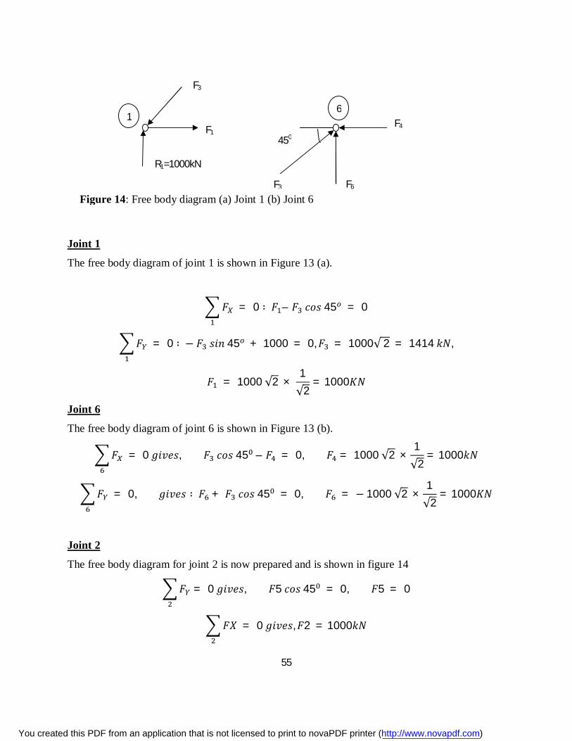
55
Joint 1
The free body diagram of joint 1 is shown in Figure 13 (a).
퐹 = 0 ∶ 퐹 – 퐹 푐표푠 45 = 0
퐹 = 0 ∶ − 퐹 푠푖푛 45 + 1000 = 0,퐹 = 1000√ 2 = 1414 푘푁,
퐹 = 1000 √2 × 1√2
= 1000퐾푁
Joint 6
The free body diagram of joint 6 is shown in Figure 13 (b).
퐹 = 0 푔푖푣푒푠, 퐹 푐표푠 45 – 퐹 = 0, 퐹 = 1000 √2 ×1√2
= 1000푘푁
퐹 = 0, 푔푖푣푒푠 ∶ 퐹 + 퐹 푐표푠 45 = 0, 퐹 = − 1000 √2 ×1√2
= 1000퐾푁
Joint 2
The free body diagram for joint 2 is now prepared and is shown in figure 14
퐹 = 0 푔푖푣푒푠, 퐹5 푐표푠 45 = 0, 퐹5 = 0
퐹푋 = 0 푔푖푣푒푠,퐹2 = 1000푘푁
450
F3
F3
F4
F6
F1
R1=1000kN
1 6
Figure 14: Free body diagram (a) Joint 1 (b) Joint 6
You created this PDF from an application that is not licensed to print to novaPDF printer (http://www.novapdf.com)
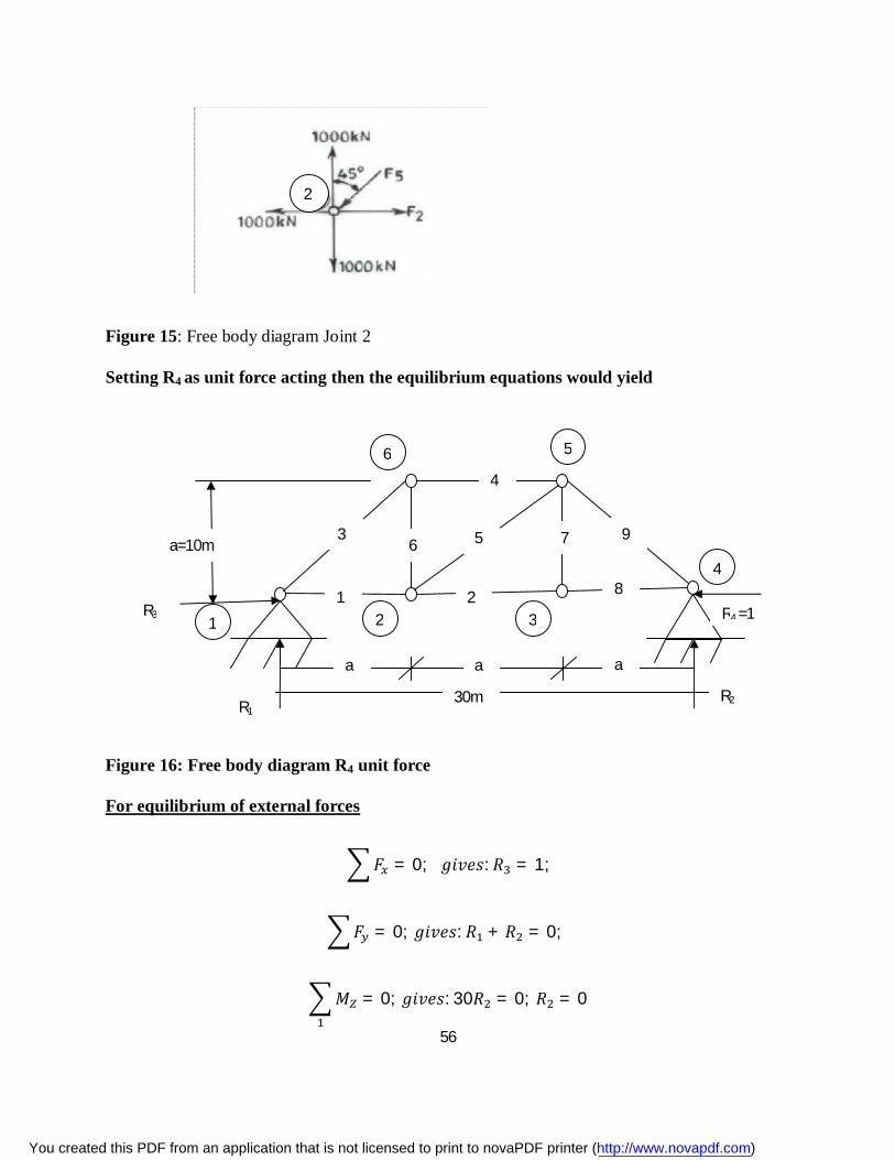
56
Figure 15: Free body diagram Joint 2
Setting R4 as unit force acting then the equilibrium equations would yield
Figure 16: Free body diagram R4 unit force
For equilibrium of external forces
퐹 = 0; 푔푖푣푒푠: 푅 = 1;
퐹 = 0; 푔푖푣푒푠: 푅 + 푅 = 0;
푀 = 0; 푔푖푣푒푠: 30푅 = 0; 푅 = 0
6 5
4
3 2 1
3 6 7
4
5
2 1 8
9 a=10m
a a a
30m
R3
R2 R1
R4 =1
2
You created this PDF from an application that is not licensed to print to novaPDF printer (http://www.novapdf.com)
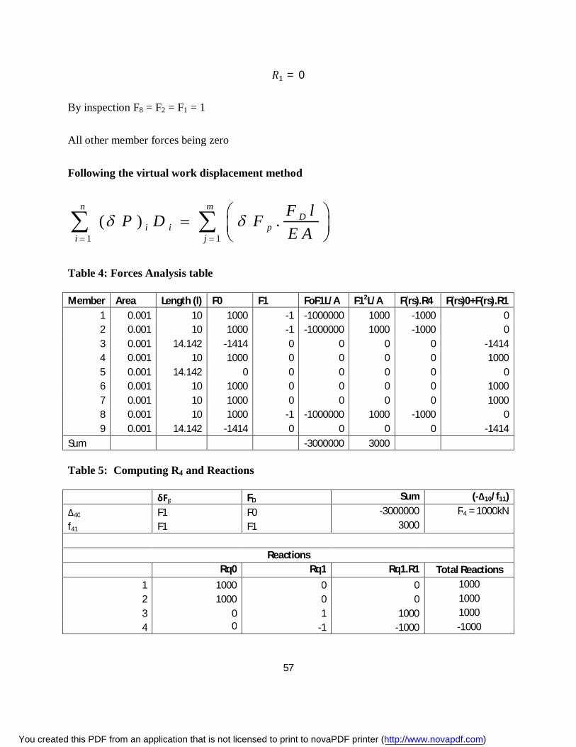
57
푅 = 0
By inspection F8 = F2 = F1 = 1
All other member forces being zero
Following the virtual work displacement method
1 1( ) .
n mD
i i pi j
F lP D FE A
Table 4: Forces Analysis table
Member Area Length (l) F0 F1 FoF1L/A F12L/A F(rs).R4 F(rs)0+F(rs).R1 1 0.001 10 1000 -1 -1000000 1000 -1000 0 2 0.001 10 1000 -1 -1000000 1000 -1000 0 3 0.001 14.142 -1414 0 0 0 0 -1414 4 0.001 10 1000 0 0 0 0 1000 5 0.001 14.142 0 0 0 0 0 0 6 0.001 10 1000 0 0 0 0 1000 7 0.001 10 1000 0 0 0 0 1000 8 0.001 10 1000 -1 -1000000 1000 -1000 0 9 0.001 14.142 -1414 0 0 0 0 -1414
Sum
-3000000 3000
Table 5: Computing R4 and Reactions
δFp FD Sum (-∆10/f11)
∆40 F1 F0 -3000000 R4 = 1000kN
f41 F1 F1 3000
Reactions Rq0 Rq1 Rq1.R1 Total Reactions
1 1000 0 0 1000
2 1000 0 0 1000
3 0 1 1000 1000
4 0 -1 -1000 -1000
You created this PDF from an application that is not licensed to print to novaPDF printer (http://www.novapdf.com)
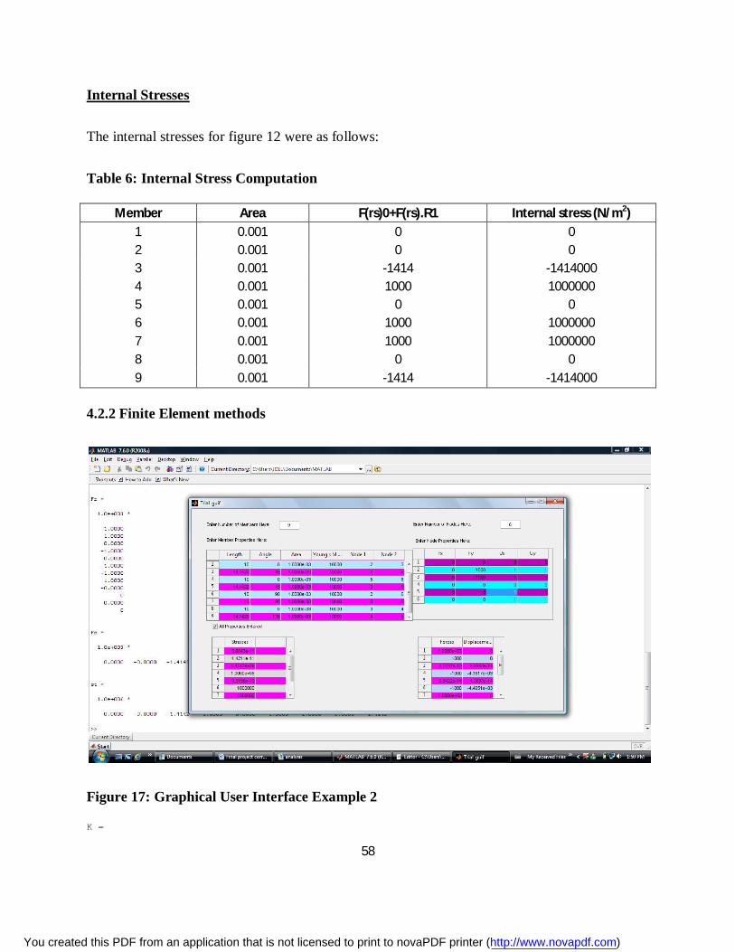
58
Internal Stresses
The internal stresses for figure 12 were as follows:
Table 6: Internal Stress Computation
Member Area F(rs)0+F(rs).R1 Internal stress (N/m2) 1 0.001 0 0 2 0.001 0 0 3 0.001 -1414 -1414000 4 0.001 1000 1000000 5 0.001 0 0 6 0.001 1000 1000000 7 0.001 1000 1000000 8 0.001 0 0 9 0.001 -1414 -1414000
4.2.2 Finite Element methods
Figure 17: Graphical User Interface Example 2
K =
You created this PDF from an application that is not licensed to print to novaPDF printer (http://www.novapdf.com)

59
1 0 -1 0 0 0 0 0 -1 0 1 0 0 0 0 0 K = 1 0 -1 0 0 0 0 0 -1 0 1 0 0 0 0 0 K = 0.3536 0.3536 -0.3536 -0.3536 0.3536 0.3536 -0.3536 -0.3536 -0.3536 -0.3536 0.3536 0.3536 -0.3536 -0.3536 0.3536 0.3536 K = 1 0 -1 0 0 0 0 0 -1 0 1 0 0 0 0 0 K = 0.3536 0.3536 -0.3536 -0.3536 0.3536 0.3536 -0.3536 -0.3536 -0.3536 -0.3536 0.3536 0.3536 -0.3536 -0.3536 0.3536 0.3536 K = 0 0 0 0 0 1 0 -1 0 0 0 0 0 -1 0 1 K = 0 0 0 0 0 1 0 -1 0 0 0 0 0 -1 0 1 K = 1 0 -1 0 0 0 0 0 -1 0 1 0 0 0 0 0 K = 0.3536 -0.3536 -0.3536 0.3536 -0.3536 0.3536 0.3536 -0.3536 -0.3536 0.3536 0.3536 -0.3536 0.3536 -0.3536 -0.3536 0.3536
You created this PDF from an application that is not licensed to print to novaPDF printer (http://www.novapdf.com)
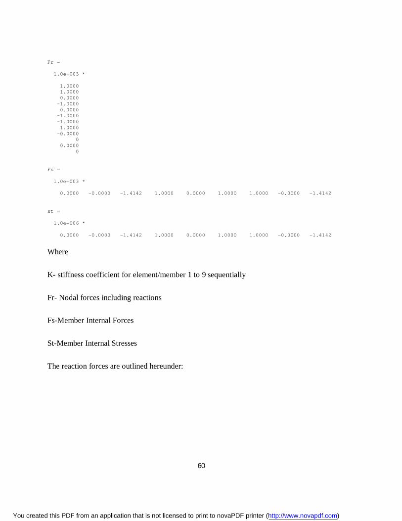
60
Fr = 1.0e+003 * 1.0000 1.0000 0.0000 -1.0000 0.0000 -1.0000 -1.0000 1.0000 -0.0000 0 0.0000 0 Fs = 1.0e+003 * 0.0000 -0.0000 -1.4142 1.0000 0.0000 1.0000 1.0000 -0.0000 -1.4142 st = 1.0e+006 * 0.0000 -0.0000 -1.4142 1.0000 0.0000 1.0000 1.0000 -0.0000 -1.4142
Where
K- stiffness coefficient for element/member 1 to 9 sequentially
Fr- Nodal forces including reactions
Fs-Member Internal Forces
St-Member Internal Stresses
The reaction forces are outlined hereunder:
You created this PDF from an application that is not licensed to print to novaPDF printer (http://www.novapdf.com)
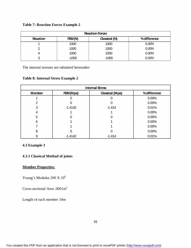
61
Table 7: Reaction Forces Example 2
Reaction Forces
Reaction FEM(N) Classical (N) % difference
1 1000 1000 0.00% 2 1000 1000 0.00% 4 1000 1000 0.00% 3 -1000 -1000 0.00%
The internal stresses are tabulated hereunder:
Table 8: Internal Stress Example 2
Internal Stress
Member FEM(Mpa) Classical (Mpa) % difference
1 0 0 0.00% 2 0 0 0.00% 3 -1.4142 -1.414 0.01% 4 1 1 0.00% 5 0 0 0.00% 6 1 1 0.00% 7 1 1 0.00% 8 0 0 0.00%
9 -1.4142 -1.414 0.01%
4.3 Example 3
4.3.1 Classical Method of joints
Member Properties:
Young’s Modulus 200 X 106
Cross-sectional Area .0001m2
Length of each member 10m
You created this PDF from an application that is not licensed to print to novaPDF printer (http://www.novapdf.com)

62
1
2
3
5
4
6
6
5
4
3
2
1
8
7
9 10KN
10KN
R3
R2
R1
600
10KN
Figure 19: Free body diagram R4 redundant
1 2
3
5
4
6
6
5
4
3
2
1
8
7
9 10KN
10KN
Figure 18: Example 3
R1
R2 10KN
You created this PDF from an application that is not licensed to print to novaPDF printer (http://www.novapdf.com)
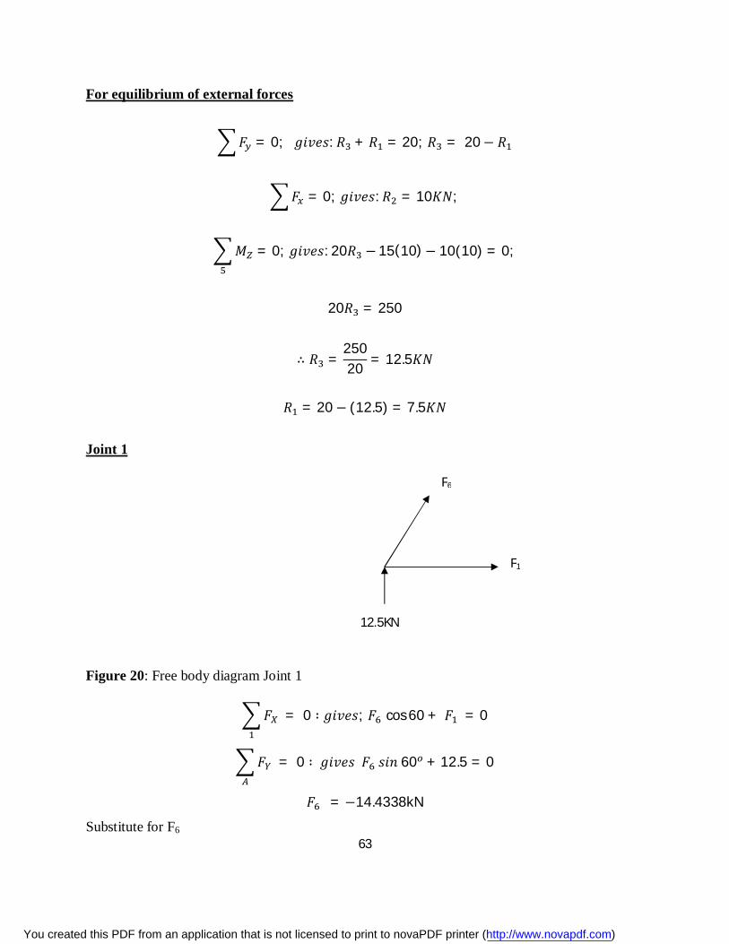
63
For equilibrium of external forces
퐹 = 0; 푔푖푣푒푠: 푅 + 푅 = 20; 푅 = 20− 푅
퐹 = 0; 푔푖푣푒푠: 푅 = 10퐾푁;
푀 = 0; 푔푖푣푒푠: 20푅 − 15(10)− 10(10) = 0;
20푅 = 250
∴ 푅 =25020 = 12.5퐾푁
푅 = 20 − (12.5) = 7.5퐾푁
Joint 1
Figure 20: Free body diagram Joint 1
퐹 = 0 ∶ 푔푖푣푒푠; 퐹 cos 60 + 퐹 = 0
퐹 = 0 ∶ 푔푖푣푒푠 퐹 푠푖푛 60 + 12.5 = 0
퐹 = −14.4338kN
Substitute for F6
F6
F1
12.5KN
You created this PDF from an application that is not licensed to print to novaPDF printer (http://www.novapdf.com)
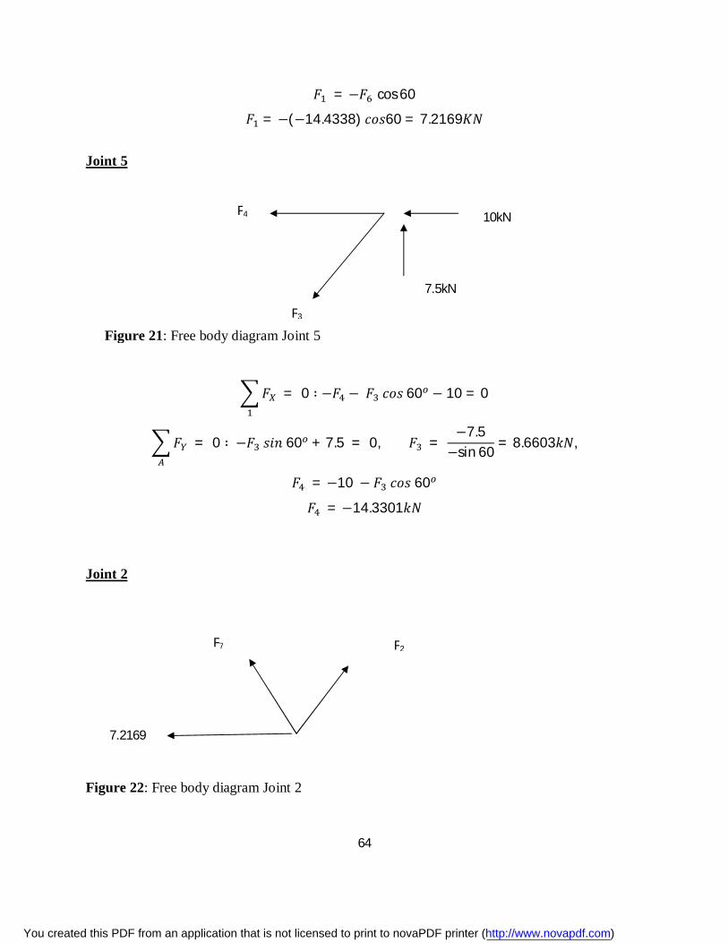
64
퐹 = −퐹 cos 60
퐹 = −(−14.4338) 푐표푠60 = 7.2169퐾푁
Joint 5
퐹 = 0 ∶ −퐹 − 퐹 푐표푠 60 − 10 = 0
퐹 = 0 ∶ −퐹 푠푖푛 60 + 7.5 = 0, 퐹 = −7.5−sin 60 = 8.6603푘푁,
퐹 = −10 − 퐹 푐표푠 60
퐹 = −14.3301푘푁
Joint 2
Figure 22: Free body diagram Joint 2
F7 F2
7.2169
F4
F3
Figure 21: Free body diagram Joint 5
10kN
7.5kN
You created this PDF from an application that is not licensed to print to novaPDF printer (http://www.novapdf.com)
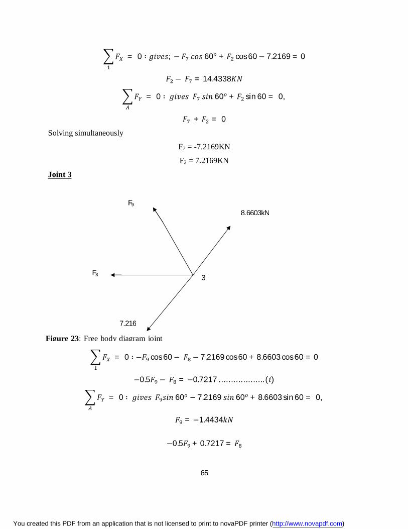
65
퐹 = 0 ∶ 푔푖푣푒푠; − 퐹 푐표푠 60 + 퐹 cos 60− 7.2169 = 0
퐹 − 퐹 = 14.4338퐾푁
퐹 = 0 ∶ 푔푖푣푒푠 퐹 푠푖푛 60 + 퐹 sin 60 = 0,
퐹 + 퐹 = 0
Solving simultaneously
F7 = -7.2169KN
F2 = 7.2169KN
Joint 3
퐹 = 0 ∶ −퐹 cos 60− 퐹 − 7.2169 cos 60 + 8.6603 cos 60 = 0
−0.5퐹 − 퐹 = −0.7217 … … … … … … . (푖)
퐹 = 0 ∶ 푔푖푣푒푠 퐹 푠푖푛 60 − 7.2169 푠푖푛 60 + 8.6603 sin 60 = 0,
퐹 = −1.4434푘푁
−0.5퐹 + 0.7217 = 퐹
7.216
3
8.6603kN
F8
F9
Figure 23: Free body diagram joint
You created this PDF from an application that is not licensed to print to novaPDF printer (http://www.novapdf.com)
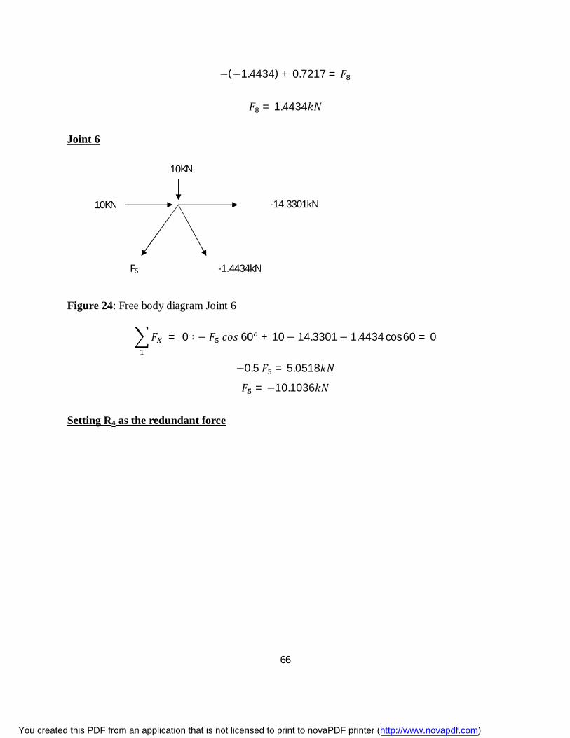
66
−(−1.4434) + 0.7217 = 퐹
퐹 = 1.4434푘푁
Joint 6
Figure 24: Free body diagram Joint 6
퐹 = 0 ∶ − 퐹 푐표푠 60 + 10− 14.3301− 1.4434 cos 60 = 0
−0.5 퐹 = 5.0518푘푁
퐹 = −10.1036푘푁
Setting R4 as the redundant force
10KN
-14.3301kN
-1.4434kN F5
10KN
You created this PDF from an application that is not licensed to print to novaPDF printer (http://www.novapdf.com)
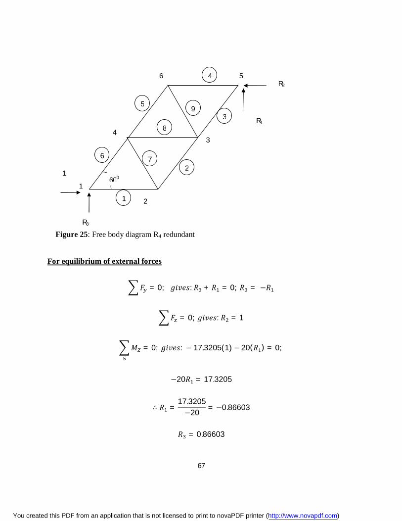
67
For equilibrium of external forces
퐹 = 0; 푔푖푣푒푠: 푅 + 푅 = 0; 푅 = −푅
퐹 = 0; 푔푖푣푒푠: 푅 = 1
푀 = 0; 푔푖푣푒푠: − 17.3205(1)−20(푅 ) = 0;
−20푅 = 17.3205
∴ 푅 =17.3205−20 = −0.86603
푅 = 0.86603
1
2
3
5
4
6
5
4
3
2
1
8
7
9
R3
R2
R1
600
Figure 25: Free body diagram R4 redundant
1
6
You created this PDF from an application that is not licensed to print to novaPDF printer (http://www.novapdf.com)
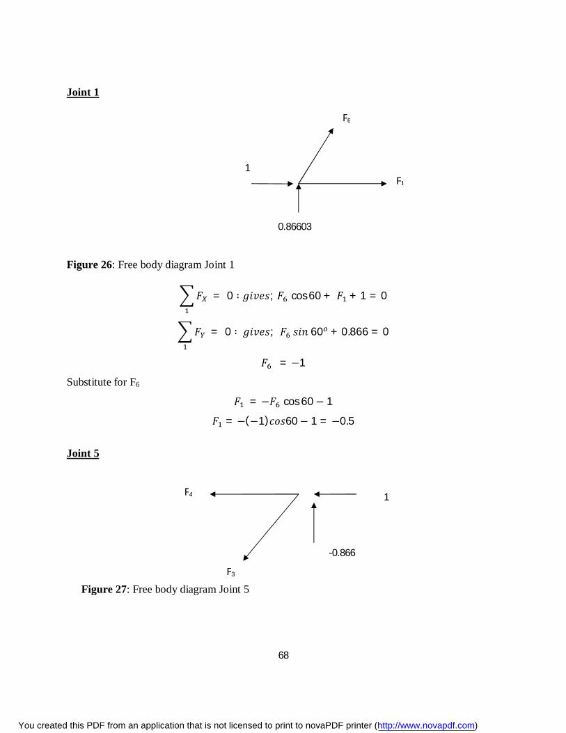
68
Joint 1
Figure 26: Free body diagram Joint 1
퐹 = 0 ∶ 푔푖푣푒푠; 퐹 cos 60 + 퐹 + 1 = 0
퐹 = 0 ∶ 푔푖푣푒푠; 퐹 푠푖푛 60 + 0.866 = 0
퐹 = −1
Substitute for F6
퐹 = −퐹 cos 60− 1
퐹 = −(−1)푐표푠60− 1 = −0.5
Joint 5
F4
F3
Figure 27: Free body diagram Joint 5
1
-0.866
F6
F1
0.86603
1
You created this PDF from an application that is not licensed to print to novaPDF printer (http://www.novapdf.com)
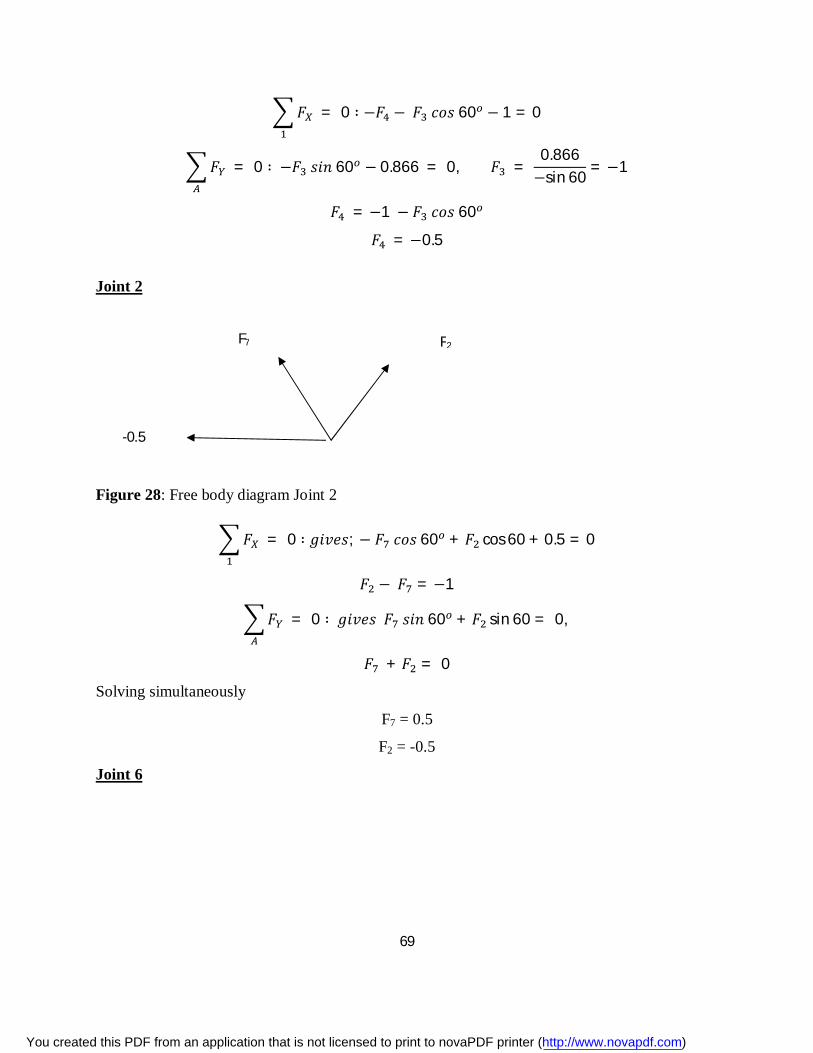
69
퐹 = 0 ∶ −퐹 − 퐹 푐표푠 60 − 1 = 0
퐹 = 0 ∶ −퐹 푠푖푛 60 − 0.866 = 0, 퐹 = 0.866−sin 60 = −1
퐹 = −1 − 퐹 푐표푠 60
퐹 = −0.5
Joint 2
Figure 28: Free body diagram Joint 2
퐹 = 0 ∶ 푔푖푣푒푠; − 퐹 푐표푠 60 + 퐹 cos 60 + 0.5 = 0
퐹 − 퐹 = −1
퐹 = 0 ∶ 푔푖푣푒푠 퐹 푠푖푛 60 + 퐹 sin 60 = 0,
퐹 + 퐹 = 0
Solving simultaneously
F7 = 0.5
F2 = -0.5
Joint 6
F7 F2
-0.5
You created this PDF from an application that is not licensed to print to novaPDF printer (http://www.novapdf.com)
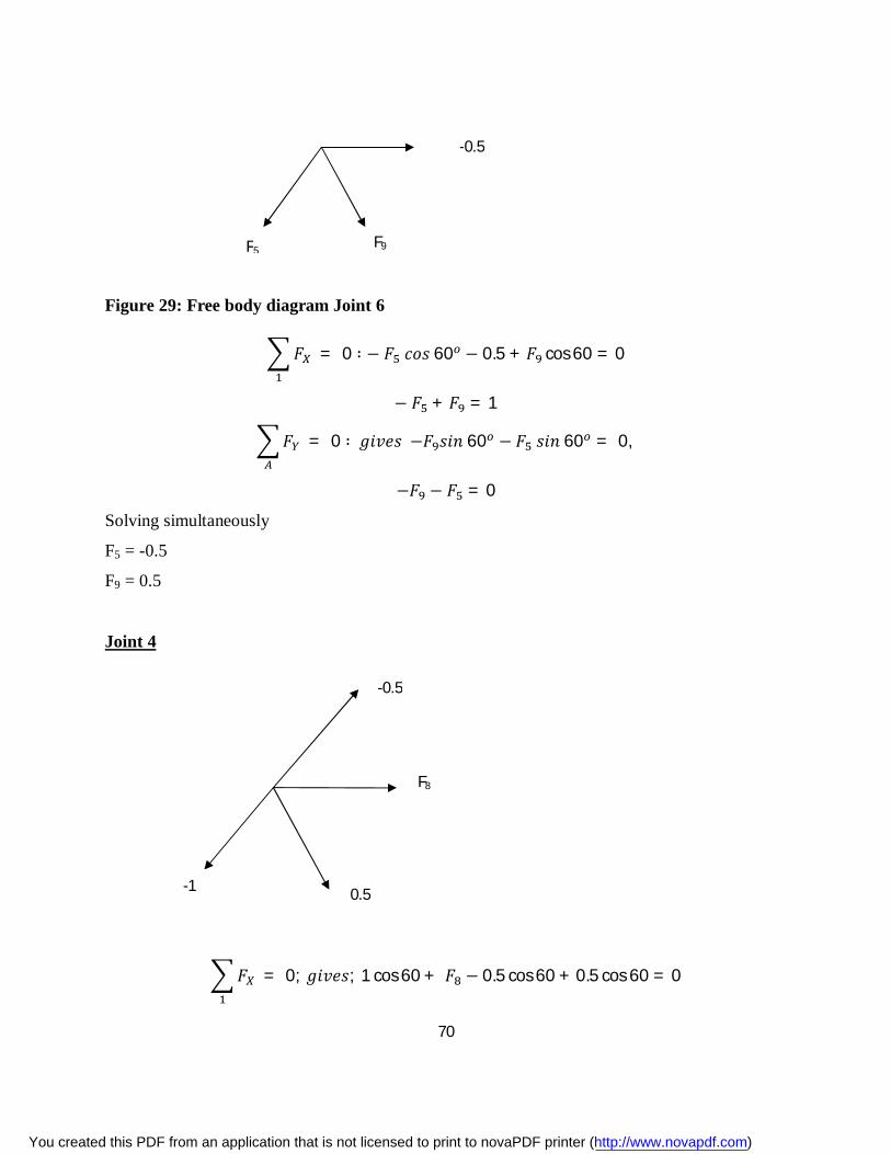
70
Figure 29: Free body diagram Joint 6
퐹 = 0 ∶ − 퐹 푐표푠 60 − 0.5 + 퐹 cos 60 = 0
− 퐹 + 퐹 = 1
퐹 = 0 ∶ 푔푖푣푒푠 −퐹 푠푖푛 60 − 퐹 푠푖푛 60 = 0,
−퐹 − 퐹 = 0
Solving simultaneously
F5 = -0.5
F9 = 0.5
Joint 4
퐹 = 0; 푔푖푣푒푠; 1 cos 60 + 퐹 − 0.5 cos 60 + 0.5 cos 60 = 0
-0.5
F8
0.5 -1
-0.5
F9 F5
You created this PDF from an application that is not licensed to print to novaPDF printer (http://www.novapdf.com)
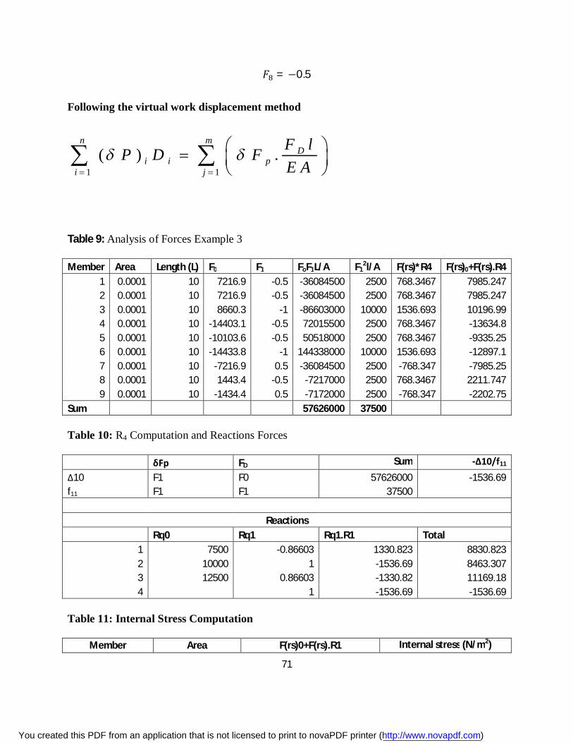
71
퐹 = −0.5
Following the virtual work displacement method
1 1( ) .
n mD
i i pi j
F lP D FE A
Table 9: Analysis of Forces Example 3
Member Area Length (L) F0 F1 FoF1L/A F12l/A F(rs)*R4 F(rs)0+F(rs).R4
1 0.0001 10 7216.9 -0.5 -36084500 2500 768.3467 7985.247 2 0.0001 10 7216.9 -0.5 -36084500 2500 768.3467 7985.247 3 0.0001 10 8660.3 -1 -86603000 10000 1536.693 10196.99 4 0.0001 10 -14403.1 -0.5 72015500 2500 768.3467 -13634.8 5 0.0001 10 -10103.6 -0.5 50518000 2500 768.3467 -9335.25 6 0.0001 10 -14433.8 -1 144338000 10000 1536.693 -12897.1 7 0.0001 10 -7216.9 0.5 -36084500 2500 -768.347 -7985.25 8 0.0001 10 1443.4 -0.5 -7217000 2500 768.3467 2211.747 9 0.0001 10 -1434.4 0.5 -7172000 2500 -768.347 -2202.75
Sum
57626000 37500
Table 10: R4 Computation and Reactions Forces
δFp FD Sum -∆10/f11
∆10 F1 F0 57626000 -1536.69 f11 F1 F1 37500
Reactions
Rq0 Rq1 Rq1.R1 Total
1 7500 -0.86603 1330.823 8830.823 2 10000 1 -1536.69 8463.307 3 12500 0.86603 -1330.82 11169.18 4
1 -1536.69 -1536.69
Table 11: Internal Stress Computation
Member Area F(rs)0+F(rs).R1 Internal stress (N/m2)
You created this PDF from an application that is not licensed to print to novaPDF printer (http://www.novapdf.com)
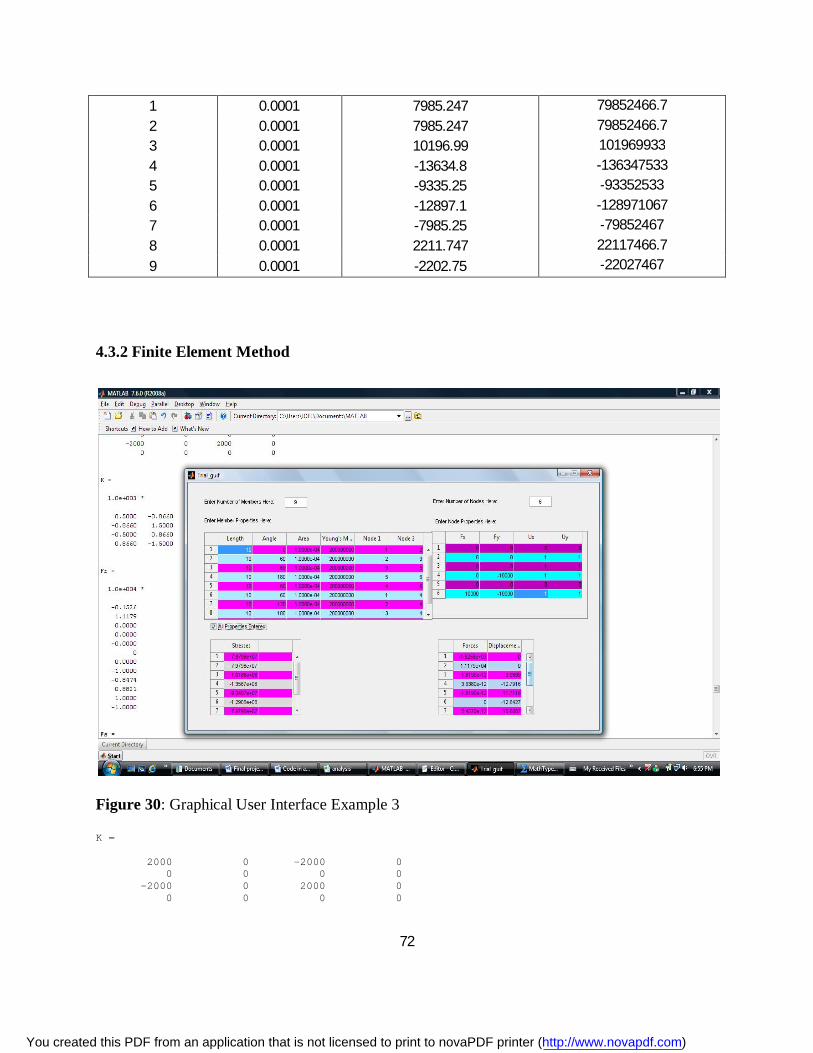
72
1 0.0001 7985.247 79852466.7
2 0.0001 7985.247 79852466.7 3 0.0001 10196.99 101969933
4 0.0001 -13634.8 -136347533 5 0.0001 -9335.25 -93352533
6 0.0001 -12897.1 -128971067 7 0.0001 -7985.25 -79852467
8 0.0001 2211.747 22117466.7
9 0.0001 -2202.75 -22027467
4.3.2 Finite Element Method
Figure 30: Graphical User Interface Example 3
K = 2000 0 -2000 0 0 0 0 0 -2000 0 2000 0 0 0 0 0
You created this PDF from an application that is not licensed to print to novaPDF printer (http://www.novapdf.com)

73
K = 1.0e+003 * 0.5000 0.8660 -0.5000 -0.8660 0.8660 1.5000 -0.8660 -1.5000 -0.5000 -0.8660 0.5000 0.8660 -0.8660 -1.5000 0.8660 1.5000 K = 1.0e+003 * 0.5000 0.8660 -0.5000 -0.8660 0.8660 1.5000 -0.8660 -1.5000 -0.5000 -0.8660 0.5000 0.8660 -0.8660 -1.5000 0.8660 1.5000 K = 2000 0 -2000 0 0 0 0 0 -2000 0 2000 0 0 0 0 0 K = 1.0e+003 * 0.5000 0.8660 -0.5000 -0.8660 0.8660 1.5000 -0.8660 -1.5000 -0.5000 -0.8660 0.5000 0.8660 -0.8660 -1.5000 0.8660 1.5000 K = 1.0e+003 * 0.5000 0.8660 -0.5000 -0.8660 0.8660 1.5000 -0.8660 -1.5000 -0.5000 -0.8660 0.5000 0.8660 -0.8660 -1.5000 0.8660 1.5000 K = 1.0e+003 * 0.5000 -0.8660 -0.5000 0.8660 -0.8660 1.5000 0.8660 -1.5000 -0.5000 0.8660 0.5000 -0.8660 0.8660 -1.5000 -0.8660 1.5000 K = 2000 0 -2000 0 0 0 0 0 -2000 0 2000 0 0 0 0 0 K = 1.0e+003 *
You created this PDF from an application that is not licensed to print to novaPDF printer (http://www.novapdf.com)
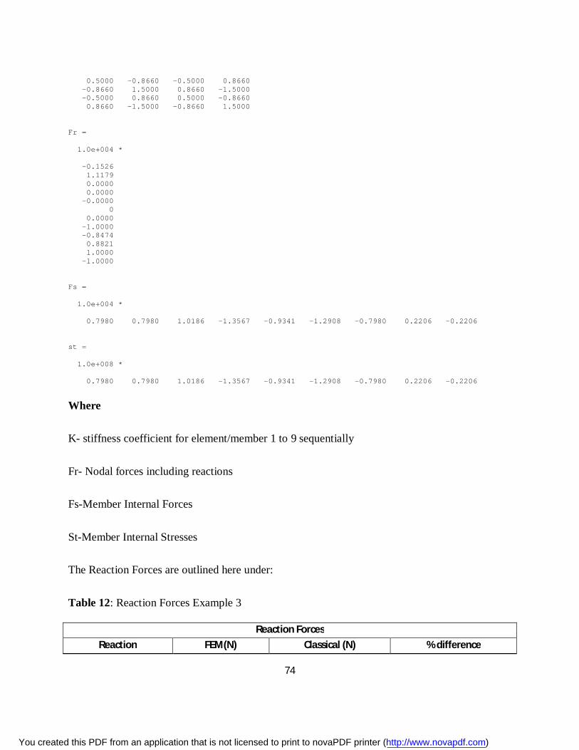
74
0.5000 -0.8660 -0.5000 0.8660 -0.8660 1.5000 0.8660 -1.5000 -0.5000 0.8660 0.5000 -0.8660 0.8660 -1.5000 -0.8660 1.5000 Fr = 1.0e+004 * -0.1526 1.1179 0.0000 0.0000 -0.0000 0 0.0000 -1.0000 -0.8474 0.8821 1.0000 -1.0000 Fs = 1.0e+004 * 0.7980 0.7980 1.0186 -1.3567 -0.9341 -1.2908 -0.7980 0.2206 -0.2206 st = 1.0e+008 * 0.7980 0.7980 1.0186 -1.3567 -0.9341 -1.2908 -0.7980 0.2206 -0.2206
Where
K- stiffness coefficient for element/member 1 to 9 sequentially
Fr- Nodal forces including reactions
Fs-Member Internal Forces
St-Member Internal Stresses
The Reaction Forces are outlined here under:
Table 12: Reaction Forces Example 3
Reaction Forces
Reaction FEM(N) Classical (N) % difference
You created this PDF from an application that is not licensed to print to novaPDF printer (http://www.novapdf.com)
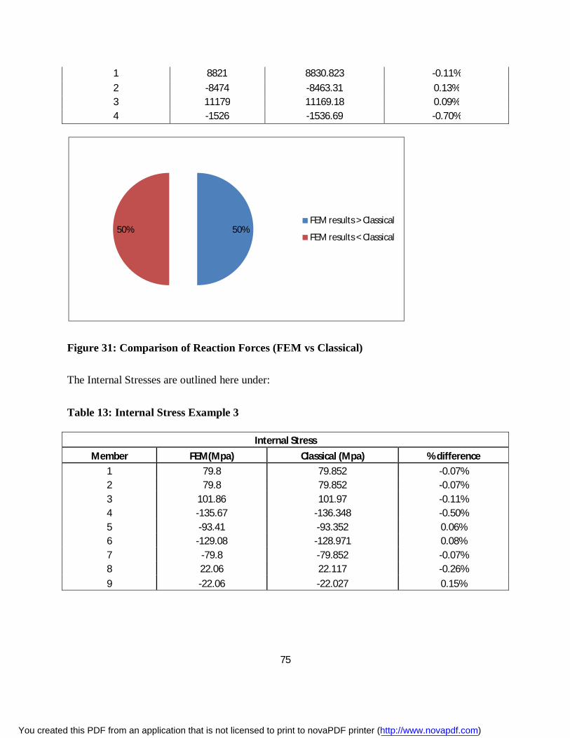
75
1 8821 8830.823 -0.11%
2 -8474 -8463.31 0.13% 3 11179 11169.18 0.09% 4 -1526 -1536.69 -0.70%
Figure 31: Comparison of Reaction Forces (FEM vs Classical)
The Internal Stresses are outlined here under:
Table 13: Internal Stress Example 3
Internal Stress
Member FEM(Mpa) Classical (Mpa) % difference
1 79.8 79.852 -0.07% 2 79.8 79.852 -0.07% 3 101.86 101.97 -0.11% 4 -135.67 -136.348 -0.50% 5 -93.41 -93.352 0.06% 6 -129.08 -128.971 0.08% 7 -79.8 -79.852 -0.07% 8 22.06 22.117 -0.26%
9 -22.06 -22.027 0.15%
50%50%FEM results > Classical
FEM results < Classical
You created this PDF from an application that is not licensed to print to novaPDF printer (http://www.novapdf.com)

76
Figure 32: Internal Stresses Results Comparison
4.4 Example 4
4.4.1 Classical Strain Energy Method
There are three members meeting at joint 2 and two equations of equilibrium, hence, static
indeterminacy is 1. Let 2-4 be redundant member. It is removed to obtain determinate system as
shown in figure 4.24 (b):
Properties
Youngs Modulus (E) 200 X 106
Cross-sectional area A = 0.001m2
Length L = 10m.
66.67%
33.33%
FEM results < Classical
FEM results > Classical
You created this PDF from an application that is not licensed to print to novaPDF printer (http://www.novapdf.com)
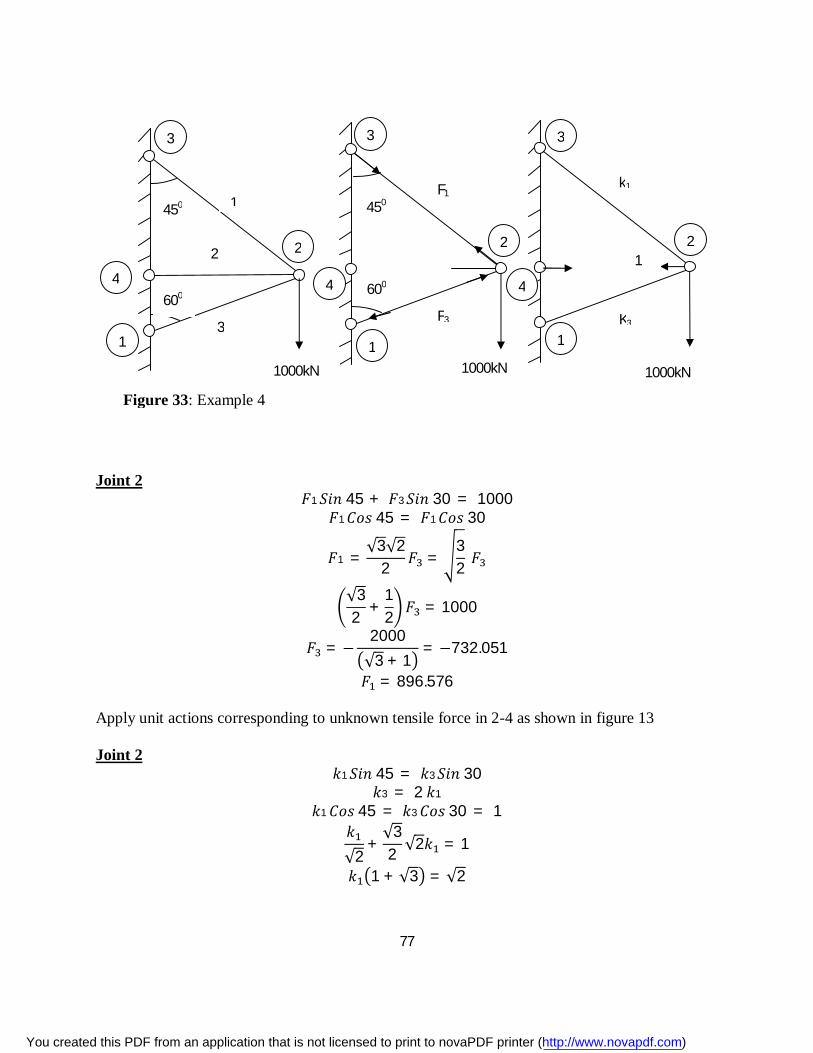
77
Joint 2 퐹1 푆푖푛 45 + 퐹3 푆푖푛 30 = 1000
퐹1 퐶표푠 45 = 퐹1 퐶표푠 30
퐹1 =√3√2
2 퐹 =32 퐹
√32 +
12 퐹 = 1000
퐹 = −2000√3 + 1
= −732.051
퐹 = 896.576 Apply unit actions corresponding to unknown tensile force in 2-4 as shown in figure 13 Joint 2
푘1 푆푖푛 45 = 푘3 푆푖푛 30
푘3 = 2 푘1
푘1 퐶표푠 45 = 푘3 퐶표푠 30 = 1 푘√2
+√32 √2푘 = 1
푘 1 + √3 = √2
1
3
2
1
4
3
2 2
1000kN 1000kN 1000kN
F1
F3 600
450
3 3
2
4 4
1 1
k1
1
K3
450
600
Figure 33: Example 4
You created this PDF from an application that is not licensed to print to novaPDF printer (http://www.novapdf.com)
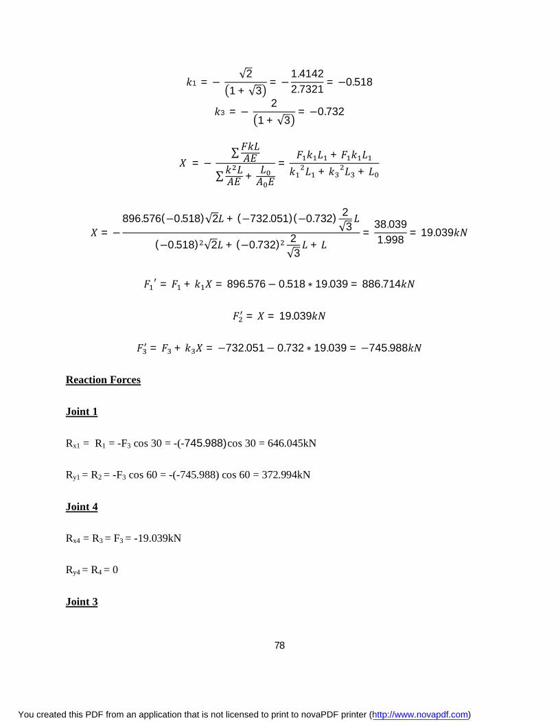
78
푘1 = − √2
1 + √3= −
1.41422.7321 = −0.518
푘3 = − 2
1 + √3= −0.732
푋 = − ∑퐹푘퐿퐴퐸
∑푘 퐿퐴퐸 + 퐿
퐴 퐸
=퐹 푘 퐿 + 퐹 푘 퐿
푘 퐿 + 푘 퐿 + 퐿
푋 = −896.576(−0.518)√2퐿 + (−732.051)(−0.732) 2
√3퐿
(−0.518) √2퐿 + (−0.732) 2√3
퐿 + 퐿=
38.0391.998 = 19.039푘푁
퐹 = 퐹 + 푘 푋 = 896.576− 0.518 ∗ 19.039 = 886.714푘푁
퐹 = 푋 = 19.039푘푁
퐹 = 퐹 + 푘 푋 = −732.051− 0.732 ∗ 19.039 = −745.988푘푁
Reaction Forces
Joint 1
Rx1 = R1 = -F3 cos 30 = -(-745.988)cos 30 = 646.045kN
Ry1 = R2 = -F3 cos 60 = -(-745.988) cos 60 = 372.994kN
Joint 4
Rx4 = R3 = F3 = -19.039kN
Ry4 = R4 = 0
Joint 3
You created this PDF from an application that is not licensed to print to novaPDF printer (http://www.novapdf.com)

79
Rx3 = R5 = -F1 Cos 45 = -(886.714) Cos 45 = -627.001kN
Ry3 = R6 = F1 sin 45 = 627.001kN
Member Stresses;
Member 1 = .
= −8667.14 푀푝푎
Member 2 = .
= 190.39 푀푝푎
Member 3 = .
= −7460푀푝푎
4.4.2 Finite element Methods
Figure 34: Graphical User Interface Example 4
K = 707.1136 -707.1136 -707.1136 707.1136 -707.1136 707.1136 707.1136 -707.1136 -707.1136 707.1136 707.1136 -707.1136 707.1136 -707.1136 -707.1136 707.1136
You created this PDF from an application that is not licensed to print to novaPDF printer (http://www.novapdf.com)
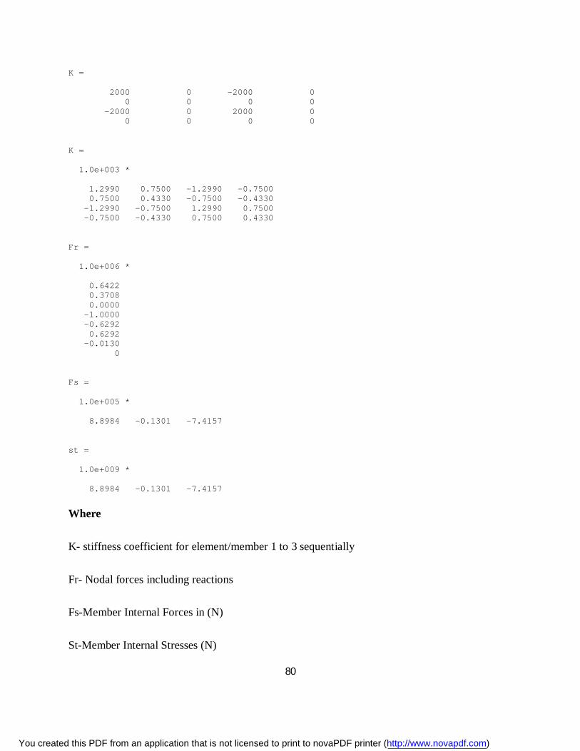
80
K = 2000 0 -2000 0 0 0 0 0 -2000 0 2000 0 0 0 0 0 K = 1.0e+003 * 1.2990 0.7500 -1.2990 -0.7500 0.7500 0.4330 -0.7500 -0.4330 -1.2990 -0.7500 1.2990 0.7500 -0.7500 -0.4330 0.7500 0.4330 Fr = 1.0e+006 * 0.6422 0.3708 0.0000 -1.0000 -0.6292 0.6292 -0.0130 0 Fs = 1.0e+005 * 8.8984 -0.1301 -7.4157 st = 1.0e+009 * 8.8984 -0.1301 -7.4157
Where
K- stiffness coefficient for element/member 1 to 3 sequentially
Fr- Nodal forces including reactions
Fs-Member Internal Forces in (N)
St-Member Internal Stresses (N)
You created this PDF from an application that is not licensed to print to novaPDF printer (http://www.novapdf.com)
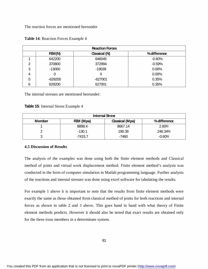
81
The reaction forces are mentioned hereunder
Table 14: Reaction Forces Example 4
Reaction Forces
FEM(N) Classical (N) % difference
1 642200 646045 -0.60% 2 370800 372994 -0.59% 3 -13000 -19039 0.00% 4 0 0 0.00% 5 -629200 -627001 0.35% 6 629200 627001 0.35%
The internal stresses are mentioned hereunder:
Table 15: Internal Stress Example 4
Internal Stress Member FEM (Mpa) Classical (Mpa) % difference
1 8898.4 8667.14 2.60% 2 -130.1 190.39 246.34% 3 -7415.7 -7460 -0.60%
4.5 Discussion of Results
The analysis of the examples was done using both the finite element methods and Classical
method of joints and virtual work displacement method. Finite element method’s analysis was
conducted in the form of computer simulation in Matlab programming language. Further analysis
of the reactions and internal stresses was done using excel software for tabulating the results.
For example 1 above it is important to note that the results from finite element methods were
exactly the same as those obtained from classical method of joints for both reactions and internal
forces as shown in table 2 and 3 above. This goes hand in hand with what theory of Finite
element methods predicts. However it should also be noted that exact results are obtained only
for the three truss members in a determinate system.
You created this PDF from an application that is not licensed to print to novaPDF printer (http://www.novapdf.com)
82
Example 2 above was a statically indeterminate truss structure. The study revealed that
differences of about 0.01% existed between internal stress results from finite element methods
and the classical method of joints and virtual work displacement method in the stress analysis as
shown in table 8. This difference could have been brought about by rounding off of values
during calculation. As regards external reactions the results were exact with no differences
observed as shown in table 7 above.
For example 3 above the study revealed percentage difference lying between 0.15% and -0.5%.
66.67% of the internal stresses estimated using FEM were below values estimated using classical
methods. 33.33% internal stress results being valued higher than those by classical methods as
shown in table 13 above. The study also revealed differences in values of reaction forces
estimated lying between -0.7% and 0.13%. 50% of the reaction forces were above values
estimated using classical methods while 50% lay below. This stress and reaction results
confirmed indeed that finite element method was an approximate method.
For example 4 above, which is a statically indeterminate system a significant difference of
246.34% existed in member 2. This was attributable to the orientation of internal forces in
member 2 as shown in figure 32. Else the magnitudes were comparable and results reliable for
design purposes. Other members’ results were comparable between the finite element methods
and classical method with a difference in stresses of magnitude below 2.6%. As regards external
reaction forces, differences existed to the extent of 0.6% as shown in table 14.
You created this PDF from an application that is not licensed to print to novaPDF printer (http://www.novapdf.com)

83
CHAPTER FIVE
5.0 Conclusions and Recommendations
5.1 Conclusions
As pertains whether finite element analysis could be conducted on two dimensional determinate
and indeterminate trusses, the study revealed that the finite element analysis for two dimensional
determinate and indeterminate trusses could be performed yielding approximate results.
As regards how finite element analysis results compare with classical methods, the study
indicated most differences being less than 1% magnitude. Hence the two methods were
comparable. This confirmed that finite element method was an approximate method and not an
exact method.
Furthermore, as pertains whether finite element analysis for two dimensional determinate and
indeterminate trusses could be modeled in Matlab programming language; it was possible to
confirm that Finite element analysis could be simulated using Matlab programming language.
All the results mentioned here-in were obtained through finite element analysis based on the
code attached here-in the appendix.
As regards the efficiency and effectiveness of finite element analysis of two dimensional
determinate and indeterminate trusses, computer simulation of the finite element analysis of
trusses revealed the following advantages:
i) High speed of executing the analysis task hence would save time for users. As compared
to the classical methods.
ii) Results obtained were accurate hence it improves reliability in the results obtained
especially when dealing with complex truss structures.
iii) Use of user friendly graphical interfaces would aid in minimizing errors in input and
hence reliable results obtained.
You created this PDF from an application that is not licensed to print to novaPDF printer (http://www.novapdf.com)

84
iv) It would be possible to conduct sensitivity analysis of various proposed designs at
minimal time and cost. Hence would be very useful to structural and mechanical
engineers during their designs.
5.2 Recommendations
Based on the study conducted the following recommendations were made:
i) The project could be extended to three dimensional truss structures by other students
willing to undertake the project using Matlab programming language or other numerical
software such as octave and Mathematica.
ii) The project could be extended by willing students in investigating the possibility of
integrating results directly from Drawing software such as AutoCad and Rhino to aid in
analysis while designing.
iii) The program could be extended by including a database of various materials and
corresponding yield stress values. Based on the output, the materials would then be
suggested to users while satisfying predesigned factor of safety.
iv) The program could also be improved upon by investigating possible ways of optimization
the program on computer hardware memory.
v) Following the fact that most users have access to mobile phones, willing students would
extend the project by configuring it to a phone application for ease of access and
convenience when carrying it.
You created this PDF from an application that is not licensed to print to novaPDF printer (http://www.novapdf.com)

85
References
Bhavikatti, S. (2004). Finite Element Analysis. Daryaganj, Delhi, IND: New Age International.
Carlos, A. (2004). The Direct Stiffness Method 1. Introduction to Finite Element Methods.
Boulder, Colorado, USA: Springer.
Da Silva, V. (2006). Mechanics and Strength of materials. Berlin, Heidelberg: Springer-Verlag.
Jin, J., & Riley, D. J. (2009). Finite Element Analysis of Antennas and Arrays. Hoboken, NJ,
USA: Wiley-IEEE Press.
Kalani, M. (1957). Basic Concepts and Conventional Methods of Structural Analysis. Mumbai,
India: IIT.
Kirsch, U. (2002). Design-Oriented Analysis of Structures: A Unified Approach. Secaucus, NJ,
USA: Kluwer Academic Publishers.
Matloff, N. (2011). Art of R Programming. In A Tour of Statistical Software design (p. 59). San
Francisco, CA, USA: No Starch Press.
Melchers, R., & Hough, R. (2007). Modelling Complex Engineering Structures (332 ed.).
Reston, VA, USA: American Society of civil Engineers.
Mohrman, S. (2011). Useful Research: Advancing Theory and Practive. Williston, AT, USA:
Berrett-Koehler Publishers.
Narasaiah, G. L. (2008). Finite Element Analysis. Hyderabad, IND: Global Media.
Pelosi, G., Cocciolli, R., & Selleri, S. (2009). Quick Finite Element Analysis for Electromagnetic
Waves. Norwood, MA, USA: Artech House.
Przemieniecki, J. S. (2009). Finite Element Structural Analysis: New Concepts. Reston, VA,
USA: American Institute of Aeronautics and Astronautics.
You created this PDF from an application that is not licensed to print to novaPDF printer (http://www.novapdf.com)

86
Rao, H. (2007). Finite Element Methods vs. Classical Methods. Daryaganj, Delhi, IND: New
Age International.
Reddy, J. N. (2004). Introduction to Nonlinear Finite Element Analysis. Cary, NC, USA: Oxford
University Press.
The Mathwork, Inc. (2008, March 1-30). Matlab Product help.
Yang, X.-S. (2006). Introduction to Computational Engineering with Matlab. Cambridge: GBR:
Cambridge International Science Publishing.
http://www.math.mtu.edu
You created this PDF from an application that is not licensed to print to novaPDF printer (http://www.novapdf.com)
87
Appendix
function varargout = Trial_guif(varargin) % TRIAL_GUIF M-file for Trial_guif.fig % TRIAL_GUIF, by itself, creates a new TRIAL_GUIF or raises the existing % singleton*. % % H = TRIAL_GUIF returns the handle to a new TRIAL_GUIF or the handle to % the existing singleton*. % % TRIAL_GUIF('CALLBACK',hObject,eventData,handles,...) calls the local % function named CALLBACK in TRIAL_GUIF.M with the given input arguments. % % TRIAL_GUIF('Property','Value',...) creates a new TRIAL_GUIF or raises the % existing singleton*. Starting from the left, property value pairs are % applied to the GUI before Trial_guif_OpeningFcn gets called. An % unrecognized property name or invalid value makes property application % stop. All inputs are passed to Trial_guif_OpeningFcn via varargin. % % *See GUI Options on GUIDE's Tools menu. Choose "GUI allows only one % instance to run (singleton)". % % See also: GUIDE, GUIDATA, GUIHANDLES % Edit the above text to modify the response to help Trial_guif % Last Modified by GUIDE v2.5 06-May-2012 00:42:31 % Begin initialization code gui_Singleton = 1; gui_State = struct('gui_Name', mfilename, ... 'gui_Singleton', gui_Singleton, ... 'gui_OpeningFcn', @Trial_guif_OpeningFcn, ... 'gui_OutputFcn', @Trial_guif_OutputFcn, ... 'gui_LayoutFcn', [] , ... 'gui_Callback', []); if nargin && ischar(varargin{1}) gui_State.gui_Callback = str2func(varargin{1}); end if nargout [varargout{1:nargout}] = gui_mainfcn(gui_State, varargin{:}); else gui_mainfcn(gui_State, varargin{:}); end % End initialization code - % --- Executes just before Trial_guif is made visible. function Trial_guif_OpeningFcn(hObject, eventdata, handles, varargin) % This function has no output args, see OutputFcn.
You created this PDF from an application that is not licensed to print to novaPDF printer (http://www.novapdf.com)
88
% hObject handle to figure % eventdata reserved - to be defined in a future version of MATLAB % handles structure with handles and user data (see GUIDATA) % varargin command line arguments to Trial_guif (see VARARGIN) % Choose default command line output for Trial_guif handles.output = hObject; % Update handles structure guidata(hObject, handles); % UIWAIT makes Trial_guif wait for user response (see UIRESUME) % uiwait(handles.figure1); % --- Outputs from this function are returned to the command line. function varargout = Trial_guif_OutputFcn(hObject, eventdata, handles) % varargout cell array for returning output args (see VARARGOUT); % hObject handle to figure % eventdata reserved - to be defined in a future version of MATLAB % handles structure with handles and user data (see GUIDATA) % Get default command line output from handles structure varargout{1} = handles.output; function edit1_Callback(hObject, eventdata, handles) % hObject handle to edit1 (see GCBO) % eventdata reserved - to be defined in a future version of MATLAB % handles structure with handles and user data (see GUIDATA) % Hints: get(hObject,'String') returns contents of edit1 as text % str2double(get(hObject,'String')) returns contents of edit1 as a double h = str2double(get(hObject,'String')); if isnan(h) errordlg('You must enter a numeric value','Bad Input','modal') return else handles.edit_text1 = h; A = zeros(h,6); set(handles.t1,'Data',A) set(handles.t1,'Enable','on') end guidata(hObject,handles) % --- Executes during object creation, after setting all properties. function edit1_CreateFcn(hObject, eventdata, handles) % hObject handle to edit1 (see GCBO) % eventdata reserved - to be defined in a future version of MATLAB % handles empty - handles not created until after all CreateFcns called % Hint: edit controls usually have a white background on Windows. % See ISPC and COMPUTER.
You created this PDF from an application that is not licensed to print to novaPDF printer (http://www.novapdf.com)
89
if ispc && isequal(get(hObject,'BackgroundColor'), get(0,'defaultUicontrolBackgroundColor')) set(hObject,'BackgroundColor','white'); end % --- Executes on button press in Confirm_checkbox. function Confirm_checkbox_Callback(hObject, eventdata, handles) % hObject handle to Confirm_checkbox (see GCBO) % eventdata reserved - to be defined in a future version of MATLAB % handles structure with handles and user data (see GUIDATA) % Hint: get(hObject,'Value') returns toggle state of Confirm_checkbox if get(hObject,'Value') == get(hObject,'Max') set(handles.t1,'Enable','inactive') set(handles.t5,'Enable','inactive') handles.Y = get(handles.t1,'Data'); handles.Z = get(handles.t5,'Data'); [Fr,st] = output(handles); set(handles.t2,'Enable','on','Visible','on') set(handles.t3,'Enable','on','Visible','on') set(handles.t2,'Data',st.') set(handles.t3,'Data',Fr) else end guidata(hObject,handles) function edit2_Callback(hObject, eventdata, handles) % hObject handle to edit2 (see GCBO) % eventdata reserved - to be defined in a future version of MATLAB % handles structure with handles and user data (see GUIDATA) % Hints: get(hObject,'String') returns contents of edit2 as text % str2double(get(hObject,'String')) returns contents of edit2 as a double x = str2double(get(hObject,'String')); if isnan(x) errordlg('You must enter a numeric value','Bad Input','modal') return else handles.edit_text2 = x; dat = zeros(x,4); A = zeros(x,4); for i = 1:x for j =1:4 if j>2 dat(i,j)= 1; else dat(i,j)= A(i,j); end end end set(handles.t5,'Data',dat) set(handles.t5,'Enable','on') end
You created this PDF from an application that is not licensed to print to novaPDF printer (http://www.novapdf.com)
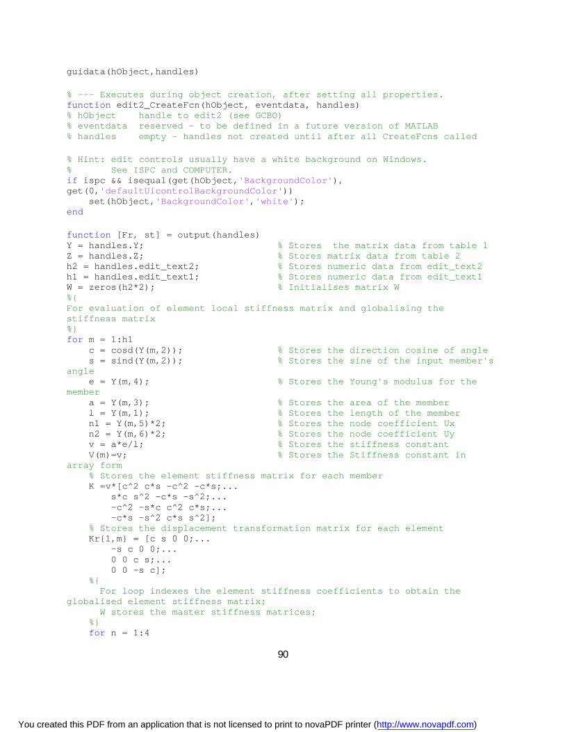
90
guidata(hObject,handles) % --- Executes during object creation, after setting all properties. function edit2_CreateFcn(hObject, eventdata, handles) % hObject handle to edit2 (see GCBO) % eventdata reserved - to be defined in a future version of MATLAB % handles empty - handles not created until after all CreateFcns called % Hint: edit controls usually have a white background on Windows. % See ISPC and COMPUTER. if ispc && isequal(get(hObject,'BackgroundColor'), get(0,'defaultUicontrolBackgroundColor')) set(hObject,'BackgroundColor','white'); end function [Fr, st] = output(handles) Y = handles.Y; % Stores the matrix data from table 1 Z = handles.Z; % Stores matrix data from table 2 h2 = handles.edit_text2; % Stores numeric data from edit_text2 h1 = handles.edit_text1; % Stores numeric data from edit_text1 W = zeros(h2*2); % Initialises matrix W %{ For evaluation of element local stiffness matrix and globalising the stiffness matrix %} for m = 1:h1 c = cosd(Y(m,2)); % Stores the direction cosine of angle s = sind(Y(m,2)); % Stores the sine of the input member's angle e = Y(m,4); % Stores the Young's modulus for the member a = Y(m,3); % Stores the area of the member l = Y(m,1); % Stores the length of the member n1 = Y(m,5)*2; % Stores the node coefficient Ux n2 = Y(m,6)*2; % Stores the node coefficient Uy v = a*e/l; % Stores the stiffness constant V(m)=v; % Stores the Stiffness constant in array form % Stores the element stiffness matrix for each member K =v*[c^2 c*s -c^2 -c*s;... s*c s^2 -c*s -s^2;... -c^2 -s*c c^2 c*s;... -c*s -s^2 c*s s^2]; % Stores the displacement transformation matrix for each element Kr{1,m} = [c s 0 0;... -s c 0 0;... 0 0 c s;... 0 0 -s c]; %{ For loop indexes the element stiffness coefficients to obtain the globalised element stiffness matrix; W stores the master stiffness matrices; %} for n = 1:4
You created this PDF from an application that is not licensed to print to novaPDF printer (http://www.novapdf.com)
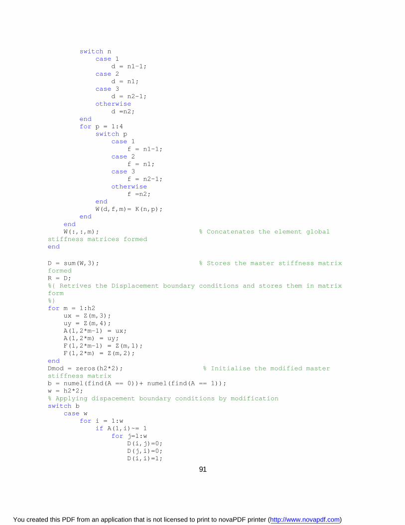
91
switch n case 1 d = n1-1; case 2 d = n1; case 3 d = n2-1; otherwise d =n2; end for p = 1:4 switch p case 1 f = n1-1; case 2 f = n1; case 3 f = n2-1; otherwise f =n2; end W(d,f,m)= K(n,p); end end W(:,:,m); % Concatenates the element global stiffness matrices formed end D = sum(W,3); % Stores the master stiffness matrix formed R = D; %{ Retrives the Displacement boundary conditions and stores them in matrix form %} for m = 1:h2 ux = Z(m,3); uy = Z(m,4); A(1,2*m-1) = ux; A(1,2*m) = uy; F(1,2*m-1) = Z(m,1); F(1,2*m) = Z(m,2); end Dmod = zeros(h2*2); % Initialise the modified master stiffness matrix b = numel(find(A == 0))+ numel(find(A == 1)); w = h2*2; % Applying dispacement boundary conditions by modification switch b case w for i = 1:w if A(1,i)~= 1 for j=1:w D(i,j)=0; D(j,i)=0; D(i,i)=1;
You created this PDF from an application that is not licensed to print to novaPDF printer (http://www.novapdf.com)
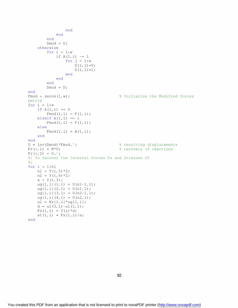
92
end end end Dmod = D; otherwise for i = 1:w if A(1,i) ~= 1 for j = 1:w D(i,j)=0; D(i,i)=1; end end end Dmod = D; end Fmod = zeros(1,w); % Initialize the Modified forces matrix for i = 1:w if A(1,i) == 0 Fmod(1,i) = F(1,i); elseif A(1,i) == 1 Fmod(1,i) = F(1,i); else Fmod(1,i) = A(1,i); end end U = inv(Dmod)*Fmod.'; % resulting displacements Fr(:,1) = R*U; % recovery of reactions Fr(:,2) = U.'; %{ To recover the Internal forces Fs and Stresses ST %} for i = 1:h1 n1 = Y(i,5)*2; n2 = Y(i,6)*2; a = Y(i,3); ug{1,i}(1,1) = U(n1-1,1); ug{1,i}(2,1) = U(n1,1); ug{1,i}(3,1) = U(n2-1,1); ug{1,i}(4,1) = U(n2,1); ul = Kr{1,i}*ug{1,i}; d = ul(3,1)-ul(1,1); Fs(1,i) = V(i)*d; st(1,i) = Fs(1,i)/a; end
You created this PDF from an application that is not licensed to print to novaPDF printer (http://www.novapdf.com)