computer simulations of emulsions stabilized by ...4 dynamics of the adsorption of a uniformly...
TRANSCRIPT

Computer simulations of emulsions stabilized by anisotropicparticlesCitation for published version (APA):Günther, F. S. (2017). Computer simulations of emulsions stabilized by anisotropic particles. Eindhoven:Technische Universiteit Eindhoven.
Document status and date:Published: 24/10/2017
Document Version:Publisher’s PDF, also known as Version of Record (includes final page, issue and volume numbers)
Please check the document version of this publication:
• A submitted manuscript is the version of the article upon submission and before peer-review. There can beimportant differences between the submitted version and the official published version of record. Peopleinterested in the research are advised to contact the author for the final version of the publication, or visit theDOI to the publisher's website.• The final author version and the galley proof are versions of the publication after peer review.• The final published version features the final layout of the paper including the volume, issue and pagenumbers.Link to publication
General rightsCopyright and moral rights for the publications made accessible in the public portal are retained by the authors and/or other copyright ownersand it is a condition of accessing publications that users recognise and abide by the legal requirements associated with these rights.
• Users may download and print one copy of any publication from the public portal for the purpose of private study or research. • You may not further distribute the material or use it for any profit-making activity or commercial gain • You may freely distribute the URL identifying the publication in the public portal.
If the publication is distributed under the terms of Article 25fa of the Dutch Copyright Act, indicated by the “Taverne” license above, pleasefollow below link for the End User Agreement:www.tue.nl/taverne
Take down policyIf you believe that this document breaches copyright please contact us at:[email protected] details and we will investigate your claim.
Download date: 23. May. 2020
Computer simulations of emulsions stabilizedby anisotropic particles
Florian Gunther

Cover illustration: VISUALIZATION by Florian Gunther, see Chapter 5.
This work was funded by the STW/NWO Vidi project 10787 of J. Harting entitledDense suspensions in medicine and industry.
c© Copyright 2017, Florian GuntherPrinted by Inkskamp Printing, proefschriften.net
CIP-DATA LIBRARY TECHNISCHE UNIVERSITEIT EINDHOVEN
Gunther, Florian
Computer simulations of emulsions stabilized by anisotropic particles / by FlorianGunther. - Eindhoven: Technische Universiteit Eindhoven, 2017. - Proefschrift.
A catalogue record is available from the Eindhoven University of Technology Library
ISBN: 978-90-386-4340-3NUR: 924

Computer simulations of emulsions stabilizedby anisotropic particles
PROEFSCHRIFT
ter verkrijging van de graad van doctor aan deTechnische Universiteit Eindhoven, op gezag van derector magnificus prof.dr.ir. F. P. T. Baaijens, voor een
commissie aangewezen door het College voorPromoties, in het openbaar te verdedigen
op 24 oktober 2017 om 16:00 uur
door
Florian Steffen Gunther
geboren te Stuttgart, Duitsland

Dit proefschrift is goedgekeurd door de promotoren en de samen-stelling van de promotiecommissie is als volgt:
voorzitter: prof.dr.ir. G. M. W. Kroesen1e promotor: prof.dr. J. D. R. Harting
(Helmholtz Institute Erlangen-Nurnberg for Renew-able Energy)
2e promotor: prof.dr. A. A. Darhuberleden: prof.dr.ir. E. H. van Brummelen
prof.dr.ir. J. van der Gucht (Wageningen University)prof.dr. R. H. H. G. van Roij (Utrecht University)prof.dr.ir. P. D. Anderson
Het onderzoek of ontwerp dat in dit proefschrift wordt beschreven is uitgevoerd inovereenstemming met de TU/e Gedragscode Wetenschapsbeoefening.


La libertad es el derecho que tienen las personas de actuarlibremente, pensar y hablar sin hipocresıa.Jose Julian Martı Perez


Contents
1 Introduction 31.1 Motivation . . . . . . . . . . . . . . . . . . . . . . . . . . . . . . . . . . . 31.2 State of current research . . . . . . . . . . . . . . . . . . . . . . . . . . . 41.3 Content of this thesis . . . . . . . . . . . . . . . . . . . . . . . . . . . . . 12
2 Theory of particle-stabilized interfaces and emulsions 132.1 Particle and system definition . . . . . . . . . . . . . . . . . . . . . . . . 132.2 A single particle at a fluid-fluid interface . . . . . . . . . . . . . . . . . . 15
2.2.1 Thermodynamics of a single particle at a fluid-fluid interface . 152.2.2 A single particle at a flat fluid-fluid interface . . . . . . . . . . . 17
2.3 Particle ensembles at a fluid-fluid interface . . . . . . . . . . . . . . . . 202.3.1 Interactions between colloidal particles: general discussion . . 202.3.2 Capillary interactions between particles . . . . . . . . . . . . . . 212.3.3 Capillary interactions between particles at a curved interface . 22
2.4 Emulsions . . . . . . . . . . . . . . . . . . . . . . . . . . . . . . . . . . . 222.4.1 Surfactant-stabilized emulsions . . . . . . . . . . . . . . . . . . . 222.4.2 Particle-stabilized emulsions . . . . . . . . . . . . . . . . . . . . 23
3 Simulation method 273.1 Hybrid lattice Boltzmann and molecular dynamics simulation method 27
3.1.1 The Boltzmann equation . . . . . . . . . . . . . . . . . . . . . . . 283.1.2 The lattice Boltzmann method . . . . . . . . . . . . . . . . . . . 30
3.1.2.1 The multicomponent lattice Boltzmann method . . . . 323.1.3 Suspended particles . . . . . . . . . . . . . . . . . . . . . . . . . 34
3.2 Implementation . . . . . . . . . . . . . . . . . . . . . . . . . . . . . . . . 37
4 Dynamics of the adsorption of a uniformly wetting ellipsoid to a fluid in-terface 394.1 Introduction . . . . . . . . . . . . . . . . . . . . . . . . . . . . . . . . . . 394.2 Theoretical model for a single particle adsorbing to a flat fluid interface 404.3 Adsorption trajectories in the ϑ-ξ space . . . . . . . . . . . . . . . . . . 424.4 Comparison of fully resolved simulations with the “flat interface” model 454.5 Parameter studies and adsorption dynamics . . . . . . . . . . . . . . . 464.6 Interface deformation caused by the adsorption . . . . . . . . . . . . . 584.7 Interface deformation: influence on the free energy . . . . . . . . . . . 644.8 Conclusion . . . . . . . . . . . . . . . . . . . . . . . . . . . . . . . . . . . 70
1

2 CONTENTS
5 Emulsions stabilized by uniformly wetting ellipsoids 715.1 Introduction . . . . . . . . . . . . . . . . . . . . . . . . . . . . . . . . . . 725.2 Phase behavior and parameter studies . . . . . . . . . . . . . . . . . . . 725.3 Long-term time evolution in emulsions due to particle anisotropy . . . 755.4 Single particle adsorption . . . . . . . . . . . . . . . . . . . . . . . . . . 795.5 Particle ensembles at a flat fluid-fluid interface . . . . . . . . . . . . . . 795.6 Particle ensemble at a spherical fluid-fluid interface . . . . . . . . . . . 85
5.6.1 Comparison between the influence of the flat and the sphericalinterface on the particle ensemble . . . . . . . . . . . . . . . . . 88
5.7 Conclusion . . . . . . . . . . . . . . . . . . . . . . . . . . . . . . . . . . . 89
6 Adsorption of a single Janus particle to a fluid interface 936.1 Introduction . . . . . . . . . . . . . . . . . . . . . . . . . . . . . . . . . . 93
6.1.1 The system of interest . . . . . . . . . . . . . . . . . . . . . . . . 956.2 A simplified free energy model for Janus particles . . . . . . . . . . . . 966.3 Improvement of the free energy model . . . . . . . . . . . . . . . . . . . 1016.4 Adsorption trajectories . . . . . . . . . . . . . . . . . . . . . . . . . . . . 1066.5 Conclusion . . . . . . . . . . . . . . . . . . . . . . . . . . . . . . . . . . . 110
7 Janus particle ensembles at fluid interfaces 1137.1 Introduction . . . . . . . . . . . . . . . . . . . . . . . . . . . . . . . . . . 1137.2 An ensemble of Janus particles at a flat fluid interface . . . . . . . . . . 1147.3 Emulsions stabilized by Janus particles . . . . . . . . . . . . . . . . . . 1217.4 Conclusion . . . . . . . . . . . . . . . . . . . . . . . . . . . . . . . . . . . 123
8 Conclusion and outlook 125
List of publications 149
Acknowledgments 151
Summary 153
Curriculum Vitae 155

Chapter 1
Introduction
Abstract
Here, we introduce the topic of the thesis. In section 1.1, we motivate the study ofemulsions stabilized by anisotropic colloidal particles as well as anisotropic colloidalparticles at fluid interfaces. In the subsequent section, a literature overview of thedevelopments of the field is given and the relation of our own study to the existingliterature is provided. Finally, a short overview of the structure of the thesis is given.
1.1 Motivation
It is poorly understood how the particle anisotropy influences properties of particlestabilized emulsions such as stabilization efficiency, emulsion lifetime, formation andaverage domain size of emulsions.
Particle stabilized emulsions play an important role in different fields such asfood and cosmetics industries, oil recovery and medicine [53, 65, 172]. One practicalexample for such an emulsion is mayonnaise, where mustard particles are adsorbedat the surface of oil droplets [157].
In this thesis, anisotropic particles in their role as stabilizers for emulsions arestudied. On the one hand, the particle anisotropy with respect to the shape is consid-ered. We use ellipsoids of revolution as simplest realization of an anisotropic shapeof the particle. On the other hand, the anisotropy of the particle surface wettabilityis studied. The so-called Janus particles consist of hydrophilic and hydrophobichemispheres.
Two types of particle stabilized emulsions are distinguished in this study: thePickering emulsion [152, 156], where discrete droplets of one fluid are immersed ina second fluid and the bijel (bicontinuous interfacially jammed emulsion gel) withtwo continuous fluid phases [91, 176]. Generally, particle stabilized emulsions areonly kinetically stable but thermodynamically unstable [10]. The cost of energy forcreating the unoccupied fluid interface is larger than the gain of entropy as comparedto the demixed state.
Colloidal particles are small particles with a radius in the range between 100nm
3

4 Introduction
and a few micrometers [34, 54, 183]. They are able to adsorb to a fluid-fluid interface.These particles in their function as stabilizers for emulsions act in a similar way assurfactants to stabilize emulsions of immiscible fluids. In both cases, the interfacialfree energy is reduced. The surfactant molecules reduce the interfacial tension byadsorbing to a fluid-fluid interface. In contrast, particles reduce the interfacial areabetween both fluids by occupying interfacial area.
Several studies of such emulsions were carried out using experiment, theory andsimulation [6, 7, 10, 14–17, 32, 34, 41, 46, 60, 95, 98, 102, 116, 134, 177, 187]. Most ofthe studies are undertaken for isotropic particles with respect to the particle shapeand the wettability. What can we say a priori by calculation before the executionof the simulation? How does the particle anisotropy influence or improve practicalproperties of emulsions? Can anisotropic particles be a more efficient stabilizer ofemulsions as compared to isotropic ones? Does the particle anisotropy influence thelife time of kinetically stable emulsions?
The ratio between the interface covered by the particle and the particle volumewhich is increased for anisotropic particles is supposed to influence the efficiency (thenumber of particles needed to stabilize a given interface area in an emulsion) andthe time development of the average domain size in an emulsion. An important stepwhich is used here to obtain a deeper understanding of the properties of emulsionsis the study of “model systems”. In the context of this thesis, these model systemsare the adsorption of a single particle to a fluid interface and the dynamics of particleensembles at a fluid interface.
1.2 State of current research
In this section, an overview is provided of the progress in the field of particle-stabilizedemulsions and related physical systems including the general behavior of particlesadsorbed at fluid-fluid interfaces. A more extensive review of theory and results isgiven in a recent book by Ngai and Bon [138]. Our focus is on particle anisotropy inthe sense of shape and surface wettability.
The simplest model system relevant for this thesis is the adsorption of a singleparticle to a flat fluid-fluid interface. Such an adsorption is usually irreversibleas the adsorption energy is several orders of magnitude larger than the thermalenergy [9, 10, 32].
An important parameter to classify a colloidal particle at a fluid interface is thecontact angle, a measurement for the surface wettability of the particle [27]. It dependson the interfacial tensions of the three interfaces: the one between the two fluids andbetween each of the fluids and the particle. It is usually measured inside the aqueousphase [148]. Typical values for the contact angle in emulsion systems are between 70
and 110 [104, 182]. Neutral wetting is reached for a contact angle of 90.Furthermore, the adsorption energy has a maximum for neutral wetting. It de-
creases if the difference of the surface wettability to the neutral wetting increases.The adsorption process can become reversible if the particle contact angle is far awayfrom the value of neutral wetting, i.e. close to 0 or 180 [10].
Several values of the interfacial tension for water in contact with different types ofoil as well as in contact with air are shown in Refs. [15, 131]. Furthermore, Ref. [131]

1.2. State of current research 5
lists contact angles of various particle types at different fluid-fluid interfaces.The adsorption process of a single particle to a fluid interface is investigated
many times. As the simplest case, the adsorption of a spherical particle is studied inRefs. [38, 58, 153, 158]. The equilibrium distance for the final state between the centerof the sphere and a flat interface is obtained by minimizing the free energy of therelated fluid-fluid and fluid-particle interfaces [153]. The dynamics of the adsorptionprocess is analyzed in Ref. [38] using the Langevin equation and molecular dynamics(MD) simulations. Capillarity and viscosity influence the process. Furthermore,the relaxation to the thermodynamic equilibrium is evaluated. The equation for apotential of a particle during the adsorption process to a fluid interface is derivedfrom the interfacial energy and an equation of motion is presented. For an exactlyspherical particle without roughness, the potential corresponds mathematically to theharmonic oscillator. In case of roughness of the surface, it becomes more complex [38].
Diffusion constants and drag forces of spherical particles adsorbed at fluid-fluidinterfaces for particle motion parallel to the flat interface are calculated in Ref. [58].The Stokes law for the drag force and the Stokes-Einstein relation are both correctedby an additional term which depends on the contact angle and the viscosity ratiobetween both fluid.
Compared to the case of a sphere, a particle with geometrical anisotropy has addi-tional rotational degrees of freedom. This renders the description of the adsorptionprocess and the final state of the particle at the interface more complex. The simplestrealization of particle shape anisotropy is the ellipsoid. For an ellipsoid, there areseveral studies available [44, 48, 57, 61, 77]. The final state or equilibrium state isfound to be the configuration, where the ellipsoid occupies as much interfacial areaas possible. For an oblate ellipsoid, it is the orientation of the particle main axisparallel to the interface. In Ref. [48], the free energy is calculated for different particleconfigurations characterized by the distance between particle center and flat interfaceas well as the orientation with respect to a flat interface. The interfacial areas arecalculated by a triangular tessellation technique. The force acting on the particle isobtained by the negative gradient of the free energy and used to obtain the adsorptiontrajectories.
In Ref. [158], the rotation of rough cylinders at a fluid interface is studied. Theroughness leads to energy barriers which can lock the particle to a given orientationaway from the equilibrium position.
Most of the theoretical or computational studies of particles at a fluid-fluid in-terface which are done so far, assume a perfectly flat fluid interface during theadsorption process and do not take the interface deformation caused by the particleinto account [16, 48]. The other extreme case of approximation is the case that the fluidis represented by a MD simulation [158]. In this case, a representation of the fluid byMD is unrealistic as the number of particles which can be studied is limited. In thisthesis, the following contribution for improvement is made: the lattice Boltzmannmethod, a mesoscopic method is used to describe the fluids. Instead of following themotion of single fluid molecules, only the dynamics of the single particle distributionfunctions is simulated. In this way, it is possible to obtain a realistic representationof the fluid with reasonable computational costs. Furthermore, the deformation ofinterfaces is properly taken into account.
Experimental studies of particles at fluid interfaces utilize for example a Langmuir

6 Introduction
trough [8, 9], the colloidal probe technique [72], the film-calliper method [94], the filmtrapping technique [82] or the gel trapping technique [148]. An overview of methodsto measure the particle contact angles is given in Refs. [29, 131].
Besides uniformly wetting particles, the adsorption of Janus particles to a fluid-fluid interface is studied [16, 144, 145]. The simplest case, the adsorption of a Janussphere is discussed and compared to the uniform wetting case in Ref. [16]. Theadsorption energy of a spherical Janus particle can be up to three times as strongas for a spherical uniformly wetting particle with neutral wettability [7]. There arealso studies of Janus particles with anisotropic shape. Examples are ellipsoids anddumbbells which are discussed in Refs. [144, 145]. The equilibrium state for a givenaspect ratio and a given wettability difference is obtained by minimizing the freeenergy function. Symmetric Janus particles with ellipsoidal and dumbbell shapeare discussed in Ref. [145]. A jump of the orientation angle from the orthogonalorientation to a tilted orientation is found for the ellipsoid, whereas for the dumbbellthere is a continuous transition between both orientations. For some values of aspectratio and contact angle difference, metastable configurations are found in additionto the stable state. The non-symmetric versions of ellipsoids and dumbbells arediscussed in Ref. [144]. The set of final states of non-symmetric Janus particles at thefluid interface depends on the aspect ratio and the wettability difference and is morecomplex as compared to the case of symmetric Janus particles.
Besides the surface tensions, another parameter can be important for the particleadsorption: the line tension of the three phase contact line can influence the freeenergy and in this way the equilibrium position [57, 61]. If the value of the linetension is sufficiently large, it even prevents the particle from adsorption to theinterface. Furthermore, the contact angle depends on the line tension and the lengthof the three phase contact line. For that reason, the particle radius influences thevalue of the contact angle as well as shown in Fig. 2 in Ref. [131]. Generally, the linetension is only relevant if the particle is sufficiently small. While it can be relevant fornanoparticles, for microparticles the line tension can usually be neglected.
The adsorption energy can be obtained by calculating the difference of the freeenergy for a particle in the bulk and at the interface or measuring the energy requiredfor detaching the particle from the interface. The detachment energy is obtainedby measuring the detachment force and integrating it. This is done in experiments(spherical particle) [154] and in simulations (including ellipsoids) [42].
A magnetic particle adsorbed at a fluid interface and under the influence of amagnetic field is studied in Refs. [26, 44, 137, 192]. The equilibrium orientationdepends on the magnetic field and the degree of anisotropy. A first order phasetransition with respect to the particle orientation is found. The interface deformabilityis found to be non-negligible [44].
A particle adsorbed at an interface generally causes the interface to deform. Theinterface deformation can be induced by forces acting on the particle (such as grav-ity), particle anisotropy in shape or wettability as well as non-constant interfacecurvature [19, 20, 59, 118, 174, 196]. In case of anisotropic particles and non-constantinterface curvature, the Young equation for the contact angle cannot be fulfilled bykeeping the shape which the interface had before the particle adsorption [118]. Theinterface deforms and the deformation can be characterized by the interface height,i.e. the difference in the position of the real and the ideal flat interface. It can be

1.2. State of current research 7
shown that the interface deformation can be described by a multipole expansion ofthe interface height [174].
If two colloidal particles are adsorbed at the interface, they generally interact bydirect and capillary interaction [141]. The following direct interactions can be found:electrostatic, van der Waals, magnetic or elastic potentials. A typical potential whichis often used is the DLVO (Derjaguin, Landau, Verwey, Overbeek) potential where ascreened electrostatic potential is combined with a van der Waals potential [49, 189].These direct interactions can be found between two colloids in the bulk. They can bealso found between two particles which are adsorbed at a fluid interface. Generally,they are different from those in the bulk as the fluids have different physical andchemical properties such as different dielectric constants. Detailed calculations of thedirect interaction between particles adsorbed at a fluid-fluid interface are presentedin Ref. [141].
In addition to these direct interactions, particles at a fluid interface feel capillaryinteractions. Capillary interactions can be explained as follows: we assume that twoparticles are adsorbed at a fluid interface and each particle causes an interface defor-mation. The overlap of these interface deformations causes the capillary interactionin the direction parallel to the interface [24].
Capillary interactions can be static or fluctuation induced [118]. The static onesare a result of the overlap of the static interface deformations described above. Theyare long ranged and act in the direction parallel to the interface. If a gravitationalforce normal to the interface acts on the particle, the attractive capillary interactionscales with the logarithm of the separation and the interaction range is given by thecapillary length [19]. The capillary length is a characteristic length for fluid interfacephenomena and depends on the interfacial tension. For the case of ellipsoids, itis calculated in Ref. [118] using a perturbative treatment. The capillary interactiondepends on the mutual orientation of the particles and has a quadrupolar shape. Fora particle with a radius parallel to the symmetry axis of the ellipsoidal particle with alength of 10µm, it has an amplitude of about 7 · 106kBT. The capillary interaction islarger than a typical electrostatic repulsion if the distance is small enough. The secondcontribution next to the static one are fluctuation induced capillary interactions.Those are a consequence of the Casimir effect which can be explained as follows:we consider two particles adsorbed at a flat interface. Thermal fluctuations in thefluids lead to capillary waves of the interface. Between the particles only fluctuationswith a wave length are allowed which fulfill Dirichlet boundary conditions, whereaselsewhere fluctuations with all wave lengths are allowed. The fact that there are morewaves outside than between the particles leads to an effective attraction between theparticles. The fluctuation induced capillary interactions are of the order of kBT andare therefore smaller than the shape induced capillary interactions. In some cases,there can be capillary repulsions as reported in Ref. [195]. The interaction for a smalldeviation from uniform wetting is calculated in Ref. [174].
In addition to the simple particle shapes such as spheres and ellipsoids, parti-cles with more complicated shape at fluid interfaces are studied. The shapes ofinterest can for example be cylinders which are studied by MD simulations [158],experiments [119] and analytical calculations [57], disk-shaped particles [139] orsuper-ellipsoidal hematite particles [135]. An experimental study for porous particlesand some realizations of anisotropic shapes (rod, rhomboid and microfiber particles)

8 Introduction
is given in in Ref. [171]. Many more final states are found as compared to ellipsoidsand the free energy landscape is more complex. Besides the influence of the particleshape, also the surface roughness of a spherical particle can lead to effects of capillaryinteraction [174].
In the previous paragraphs, single particles and particle pairs at interfaces arediscussed. Here, we discuss the behavior of a particle ensemble at an interface. Anoverview of the physics of particle laden interfaces is given in Refs. [24, 27, 109].Pioneering work is done by Pieranski in 1980 [153]. It is found that charged spheresadsorbed at an air-water interface form a triangular lattice due to repulsive dipole-dipole interactions between the particles. This electrical dipole is a result of theasymmetric charge distribution on the particle surface due to the fact that the particlesurface is in contact with two different fluids.
The simplest case with an ensemble of hard spheres at a flat interface is studied inseveral publications by e.g. Bleibel et al. [19, 20]. Capillary monopoles of the interfacedeformation are introduced by gravity-like forces normal to the interface. The forceinduced by the overlap of these interface deformation areas is attractive. The systembehaves in the same way as an ensemble of particles interacting with two-dimensionalscreened Newtonian gravity [19]. Different dynamical regimes are found dependingon the temperature and the capillary length [19].
Compared to spheres, an ensemble of ellipsoids at a flat fluid interface is morecomplex: among other things ellipsoidal particles differ from spherical ones bypacking effects. In a three dimensional system, spheres have a random (amorphous)jammed maximum packing density of about 0.64 whereas the corresponding valuefor anisotropic ellipsoids is larger [56]. The maximum for random packing for prolateellipsoids is reached for an aspect ratio of 1.5 and amounts to 0.72. For aspect ratioslarger than 1.5, it decreases. The number of contacts for ellipsoids is found to be about10 as compared to the 6 contacts in the case of spheres. A similar relation holds for atwo dimensional system [11].
If ellipsoids are adsorbed at a flat fluid interface, particles interact by shape-induced capillary interactions and influence mutual orientations. It is found inRef. [124] that side-to-side alignment as well as tip-to-tip alignment are possible.Which of them is found depends on the surface chemistry. The attraction of twoparticles caused by capillary interactions is measured. The time evolution of thecenter-to-center distance is given by a power law. This relation can be used to obtainthe magnitude of the interaction. The patterns created by ellipsoids at flat interfacesare investigated in Ref. [128]. They can form dense structures and side-by-sidealignments. Experiments with monolayers of ellipsoidal particles adsorbed at aflat fluid-fluid interface are done for different aspect ratios [11]. The compressionof monolayers including the influence of the aspect ratio is studied by comparingellipsoids with spheres [11]. The behavior of magnetic ellipsoidal particles at aflat interface is evaluated in Ref. [43]. The inter-particle interactions can be tuned bychanging the magnetic field. An ensemble of particles adsorbed at a single droplet andthe rheology of the particle-laden droplet are analyzed in Ref. [181] using differentmicroscopy methods. Ensembles of Janus particles at interfaces are explored inRefs. [126, 146, 159]. In contrast to a uniformly wetting sphere, a Janus sphere candeform the interface without additional external forces.
After having discussed systems with particles at an individual fluid interface,

1.2. State of current research 9
we discuss particle-stabilized emulsions of two immiscible fluids. As stated above,particles play a similar role as surfactants in stabilizing emulsions. They adsorb tothe interface and stabilize the emulsion in this way. A comparison of particles andsurfactants as stabilizers for emulsions is given in Ref. [15]. A general overview ofthe properties of particle-stabilized emulsions is provided in Refs. [10, 34, 95]. Wedistinguish two types of particle-stabilized emulsions which are important in thisthesis: the first one is the Pickering emulsion. It consists of discrete droplets of onefluid immersed in another one. It is firstly described by Ramsden in 1903 [156] andPickering in 1907 [152] who discovered this emulsion type independently from eachother. The droplet size is much larger than the size of a stabilizing particle. The secondemulsion type is the bicontinuous interfacially jammed emulsion gel (bijel) where bothfluids are continuous and separated by a particle laden fluid interface. It is predictedfor the first time by simulations in 2005 [176]. The first experimental realization iscarried into execution in 2007 [91] using a 2,6-lutidine-water mixture and neutrally-wetting particles. Several states of emulsions between Pickering emulsions and bijelsare found [36, 66, 191]: one example is presented in Ref. [36] where droplets areelongated. In Ref. [191], a structure is presented which is composed of a bicontinuousstructure like a bijel. In addition to the continuous phases, it contains a networkof colloid-bridged droplets. The stabilizing particles generally have a non-neutralwetting. As an example for a more complex composition of immiscible fluids, an oil-in-water-in-oil emulsion is presented in Ref. [14]. Similarly to the case of emulsions,particles can stabilize Pickering foams. Particles with high anisotropy lead to a highstability of foams [4, 75].
The formation process can be considered as follows: the initial state is the totallymixed state for both emulsions types. In case of a Pickering emulsion, the first stepof the emulsion formation is the nucleation of the droplets [164, 168], followed bydroplet growth, and the last one Ostwald ripening and coalescence. It can be shownthat the adsorption rate of particles to the interface is proportional to the number ofparticles in the bulk. The rate constant depends on the chemical composition of thecolloid [165]. If the surface of the droplets is not sufficiently well covered by particlesit leads to the coalescence of two droplets. The dynamics of coalescence is studiedin Ref. [6]. During the formation process, the average droplet radius in an emulsionincreases strongly. This increase slows down at a later time.
The formation of a bijel takes place in a different way. The bicontinuous structuredevelops by spinodal decomposition which is arrested when a sufficient numberof particles is adsorbed at the interface to stabilize the structure. It is shown thata bijel can be stable for at least seven months and the size of the domains staysapproximately constant [32].
In most cases, the two fluids forming an emulsion are water and a non-polar liquidsuch as oil, but there are also emulsions created by two immiscible oil types [15].Different types of non-polar liquids can be used for emulsions. Examples are cyclo-hexane and toluene [16]. An overview is given in Ref. [15]. There is a wide range ofparticles which can be used as emulsion stabilizers. Typical examples are hydroxides,iron oxide, metal sulfates, silica, clays, carbon [10] and polystyrene particles [41].More particle types stabilizing the emulsion can be found in table 1 in Ref. [10] and inRef. [15]. Also biological materials like particles synthesized from zein [45], bacterialcellulose nanocrystals [102], or whey can be used [52]. A general overview of the

10 Introduction
properties of particle stabilized emulsions is given in Refs. [10, 95].The effect of irreversible adsorption (discussed above) leads to the stability of the
emulsion. The most important parameter for stabilizing emulsions is the particlecoverage at the interface [60]. The type and the properties of a Pickering emulsiondepend on the choice of parameters such as particle size, salt concentration, particlewettability, fluid ratio and oil type. In general, hydrophobic particles tend to formoil-in-water (o/w) emulsions whereas hydrophilic particles tend to form water-in-oil (w/o) emulsions [10]. The optimal values of the contact angle are found to be70− 86 for o/w and 94− 110 for w/o [104, 182]. The effect of the particle size onthe emulsion is quite complicated [16]. In most cases, the droplet size increases withincreasing particle radius. However, there are situations where the particle radiusdecides if the emulsion is w/o or o/w as it is shown for a 1:1 water-toluene systemwith hydrophilic latex particles [16]. Different parameters can be used to control theemulsion for example for a controlled breakdown. Possible control parameters are forexample the pH value [69–71], the temperature [50, 51, 186] and an external magneticfield [134]. Some bijel properties can be controlled by the choice of parameters [32].For example, it can be shown that the domain size is inversely proportional to thevolume concentration of the stabilizing particles [98]. If the particles are magnetic, thedipole-dipole interaction as well as the dipole-field interaction can be used to controlthe structure during and after the formation [107].
Most investigations in theory and simulations are done for spherical particlesas stabilizer for emulsions [10, 16, 134, 177]. The effect of the particle shape forstabilizing emulsions is studied for hydrophilic polystyrene latex particles as wellas hydrophobic hermatite particles where the degree of anisotropy is varied [129].Emulsions stabilized by anisotropic particles are studied in Ref. [46, 102]. The shapesof interest in the experimental study are cubes and peanut shaped particles [46].Cubes are found to have an average packing density of 90% at the fluid interfaceand locally packing densities which are larger than the theoretical limit for spheres.The variation from 100% comes from the fact that the edges of the cubes are roundedand the ordering is not exactly cubic. This is realized by parallel orientation of thecubes. The droplet size depends linearly on the cube length. Emulsions stabilizedby nanorods are studied in Ref. [102]. The aspect ratio is varied from 13 to 160. Thecoverage ranges from 40% to the dense packing limit.
Emulsions usually have a kinetic stability, but they are thermodynamically unsta-ble. It might be that there are special cases where these emulsions are thermodynami-cally stable [161]. It can be shown that Janus particle stabilized emulsions can lead tothermodynamic stability of emulsions, but the difference between the two wettabilityareas has to be sufficiently large [7]. Note that Janus particles are discussed in moredetail below. The ordering of the particles at the interface of an emulsion droplet canbe aggregated or exhibit a lattice structure. It depends also on the electrostatic anddipole interactions between the colloids [41].
Pickering emulsions are used in the food industry, cosmetic industry, medicineor even for enhanced oil recovery [53, 65, 157, 170]. One example for applicationin the medical sector is the drug delivery. In Ref. [65], retinol as an example of alipophilic drug is discussed. Two types of o/w emulsions are compared, a Pickeringemulsion and a corresponding surfactant-stabilized emulsion as well as solutionof retinol in an oil. The Pickering emulsion is more efficient for the penetration

1.2. State of current research 11
through the skin as compared to the two other situations. A list of bio-mass particleswhich can be used for the production of food and cremes is given in Ref. [157]. Oneexample is the fine mustard particle which stabilizes mayonnaise. Other examples arereconstituted milk (o/w) and margarines/fatty spreads (w/o) [53]. An example for anapplication of particle-stabilized foams is the whipped dairy cream [53]. An overviewof emulsions and foams in food production is given in Ref. [53, 54, 162, 163, 173].One possible application of a bijel is a cross-flow reactor where each fluid componentflows in other direction [32]. The reactions take place at the remaining interface(not occupied by particles). The advantage as compared to a corresponding reactorbased on a Pickering emulsion is the fact that in the latter case the starting productof the chemical reaction which is located in the droplet phase, cannot be renewed.Furthermore, bijels can be used to create a porous medium which is studied bysimulation [66] and experiments [116]. The porous structure and its permeability canbe tuned by varying the particle wettability and concentration. The resulting porousmedium can be used for example for filters and reactors [66].
Several simulations are done related to particle-stabilized emulsions. In general,there are different classes of methods available to simulate emulsions as systems oftwo fluids and the interfacial stabilizer [187]. First, we distinguish between Eule-rian or Lagrangian methods representing the two fluids. The Lagrangian methodsare particle-based. One example is molecular dynamics (MD). Another method isdissipative particle dynamics (DPD) which is based on the Langevin equation. Itcan be used to simulate emulsions among other things [60, 93, 132]. Furthermore,there is the stochastic rotation dynamics (SRD) or multi-particle collision dynamics(MPC) [73, 89]. In the grid-based Eulerian representation such as the lattice Boltzmannmethod, the fluid is represented by a continuous field [33, 178]. Mesoscopic (andmacroscopic) scales are simulated. After having discussed the representation of fluids,the following step is the representation of the interface between the fluids which canbe sharp or diffuse [111]. In the case of a sharp interface, a separate representationof the interface is required. This is realized for example by the lattice Boltzmannmodel for Free Surface Flow (FSLBM) [108] or volume-of-fluid (VOF) which is thestandard method and the base for FSLBM [23, 99, 100]. It is usually complicated tosimulate sharp interfaces which are allowed to change their structure over time [22],but this change is important if the formation and stability of emulsions should bestudied. The diffuse interface representation uses the same representation for the bulkphases and the interface. A scalar order parameter (going from positive to negativevalues) indicates which of the bulk fluids can be found at a given point. The interfaceposition is given by the points where the order parameter has a value of 0. Examplesfor methods of diffuse interface representation in the context of lattice Boltzmannsimulations are the pseudo-potential or Shan-Chen method, the color gradient, thekinetic-theory-based model and free energy model [76, 86, 88, 101, 111, 117, 120–122, 143, 169, 179, 180, 187, 197]. Finally, the way of representing the stabilizingmaterial can be Eulerian or Lagrangian. In case of an Eulerian representation, asecond order parameter is needed to describe the concentration of the stabilizer. Thisorder parameter can be a scalar, vectorial or tensorial. It is appropriate to simulatemolecular stabilizers (surfactants), but it can also be used to simulate particles asstabilizers [3]. A Lagrange representation can be used if particles are the emulsionstabilizer. One possibility is the molecular dynamics (MD) method or the discrete

12 Introduction
element method (DEM). In the following, we refer to both methods as MD. The firstLB simulations using a diffuse interface representation and MD for the particles aredone by Stratford and collaborators [175, 176]. The first use of Shan-Chen in thiscontext is done in two dimensions by Joshi et al. in 2010 [101] and in three dimensionsby Jansen et al. in 2011 for emulsions stabilized by spheres [98]. It is shown thatboth Pickering emulsions and bijels can be studied with it. The work of this thesis isbased on the studies related to that publication. In the same class of representation,spinodal decomposition and bijels can be simulated by solving the Cahn-Hilliardequation and combining it with methods such as Brownian dynamics or an extendedfinite element method for particles [30, 35, 96]. Furthermore, droplets in a Pickeringemulsion can be represented as particles larger than the stabilizing particles usingBrownian dynamics simulations [64].
1.3 Content of this thesis
The remainder of this thesis is organized as follows: in chapter 2, the theoreticalbackground is presented. The theory of particles at interfaces and emulsions is con-sidered. Both, uniformly wetting particles (ellipsoids) and Janus particles (particleswith surface areas of different wettability) are discussed. Chapter 3 is an introductionto the simulation method, which is used for all results in the thesis. We explain thelattice Boltzmann method and the molecular dynamics method which are used tosimulate the fluid and the particles, respectively, and the coupling between them. Theresults are shown in chapter 4 to 7. The adsorption of a uniformly wetting particle toa flat interface is discussed in chapter 4. It includes some general aspects, parameterstudies and the study of the interface deformation and its influence on the adsorptionprocess. Emulsions stabilized by particles and particle ensembles at interfaces areconsidered in chapter 5. The first part of chapter 5 contains a parameter study ofemulsions stabilized by ellipsoids. The influence of the particle anisotropy is dis-cussed as well as the transition from a Pickering emulsion to a bijel. The long timedevelopment of timescales in emulsions is discussed in the second part of chapter 5.Model systems are used to explain the time behaviour of emulsions stabilized byanisotropic particles. We discuss the single particle adsorption of a Janus particlein chapter 6. Furthermore, we investigate a particle ensemble at a flat interface andprovide an outlook on emulsions stabilized by Janus particles in chapter 7.

Chapter 2
Theory of particle-stabilizedinterfaces and emulsions
Abstract
In this chapter, the theory required for understanding the results of this thesis is pre-sented. Furthermore, limitations of the available theoretical models and experimentalpossibilities are shown. Thus, the necessity of performing computer simulations asan alternative way to study the topic is motivated. We study the physics of emulsionsstabilized by anisotropic colloidal particles and their underlying building blocks. Theparticles can be anisotropic in shape and surface wettability. A single particle at afluid interface is the starting point of the description. The free energy function for thatsystem is used for the prediction of the final state. In the subsequent step, interactionsbetween particles as well as particle ensembles at interfaces are discussed. Finally,particle-stabilized emulsions are considered.
2.1 Particle and system definition
Our system of interest consists of two immiscible fluids (1, 2) and ellipsoidal particles.The ellipsoid of revolution is characterized by the radius R‖ of the main axis parallel tothe symmetry axis of the ellipsoid and the radius R⊥ of the two main axes orthogonalto the symmetry axis. The degree of anisotropy is characterized by the particle aspectratio
m =R‖R⊥
. (2.1)
The wetting properties of the particle surface can be characterized by the contactangle θ. As shown in the left sketch of Fig. 2.1, it is defined as the angle between thetangential plane of the particle surface and the one of the fluid-fluid interface at thepoint where the fluid-fluid interface meets the particle surface.
The particle position and orientation are characterized by ξ and ϑ, respectively. ξis the distance between the particle center and the undeformed interface. ϑ is defined
13

14 Theory of particle-stabilized interfaces and emulsions
θ
Fluid 2
Fluid 1
ϑ
ξ
xJanus
θP
αθA
Figure 2.1: Left: definition of the contact angle θ for a uniformly wetting particle.Center: definition of the positionξ and the orientational angle ϑ. Right: the parameterscharacterizing the Janus particle are the contact angles θA (apolar) and θP (polar)as well the parameters which characterize the size of the two regions: the distancebetween particle center and Janus separation line xJanus and the angle between particlemain axis and Janus separation lineα.
as the angle between the particle main axis and the normal of the (flat) interface(central sketch of Fig. 2.1).
Two particle types are considered, i.e. uniformly wetting particles and Janusparticles. A uniformly wetting particle is defined by the fact that θ is constant overthe whole particle surface. The second particle type is the Janus particle. The namefor that particle type comes from one of the oldest Roman gods called Janus who hastwo faces. This particle type was firstly mentioned by Casagrande in 1989 and deGennes in 1992 during his Nobel Prize lecture [31, 47]. In general, a Janus particleis defined as a particle with an anisotropy with respect to at least one physical orchemical surface property. The particle surface is divided in at least two differentareas where these particular properties differ. The surface property of interest forthis thesis is the particle wettability. In principle, the particle surface can have anywettability topology. For the discussion in this thesis, we limit ourselves to the case oftwo regions of different wettability separated by a plane. They are characterized bydifferent contact angles θA (apolar) and θP (polar). In case of parallel Janus particles(right sketch of Fig. 2.1), the plane is normal to the particle main axis and in case oforthogonal Janus particles the plane is normal to the orthogonal particle axis. The sizeof the regions is characterized byα and xJanus. xJanus is the distance between particlecenter and Janus separation line. α is the angle between particle main axis and Janus

2.2. A single particle at a fluid-fluid interface 15
separation line. The relation between them is given as
α = arctan
√
R2‖ − x2
Janus
mxJanus
and xJanus =R⊥R‖√
R2‖ tan2(α) + R2
⊥
. (2.2)
An ellipsoidal Janus particle with a hydrophilic part at the top and a hydrophobicpart at the bottom is shown in the right sketch of Fig. 2.1. The Janus particle can becharacterized by the Janus balance [112]
J =sin2α + 2 cosθP(cosα − 1)sin2α + 2 cosθA(cosα + 1)
. (2.3)
J plays an important role in the adsorption of a single particle at a fluid-fluid interface.J is related to the strength of the adsorption. The adsorption is strongest for J = 1.
A symmetric, parallel Janus particle as studied in this thesis is defined in thefollowing way: the particle surface is evenly divided into two areas of differentwettability so thatα = 90 and xJanus = 0. The contact angles θA and θP differ from90 by the same value. The two different contact angles are given as
θA = 90 + ∆θ and θP = 90 − ∆θ. (2.4)
This reduces the description to a single control parameter ∆θ to characterize wettingproperties of the particle. The average contact angle is given as 90 and J = 1.
2.2 A single particle at a fluid-fluid interface
2.2.1 Thermodynamics of a single particle at a fluid-fluid interface
In this subsection, we formulate a thermodynamic description of a single particlein contact with a fluid-fluid interface and follow Ref. [27]. The full informationof the thermodynamic system is contained in the thermodynamic potentials. Thethermodynamic potential used here is the free energy F . It is a function of tem-perature T, system volume V and some extensive variables related to the system:F = F (T, V, N1, N2, Ai, Li) [27]. Ai and Li are the interface areas and threephase contact lines, respectively, created by two fluids and the particle surface. N j isthe number of molecules of fluid j = 1, 2. The related intensive variables which areof interest are the interfacial tensionsσ j and the line tensions κ j. They can be obtainedfrom the free energy function as [27]
σ j =
(∂F∂A j
)T,V,Ni,Ai 6= j,Li
and κ j =
(∂F∂L j
)T,V,Ni,Ai,Li 6= j
. (2.5)
In the following, we assume T, V and Ni to be constant and do not consider themanymore. The free energy of a general particle adsorbed at the interface can be writtenas a summation over interface areas and contact lines [48, 77],
F (ξ , o) = ∑iσi Ai +∑
iκiLi. (2.6)

16 Theory of particle-stabilized interfaces and emulsions
ξ is the distance between the particle center and the undeformed flat interface. Theundeformed flat shape is the shape which the interface would have without theparticle. o is the unit vector related to the particle orientation. Ai and Li are functionsof ξ and o. In case of rotational symmetry, as it is the case for the ellipsoids ofrevolution studied here, the dependence on orientation reduces to the dependenceon the angle ϑ (see central sketch of Fig. 2.1) which is the angle between the particlemain axis and the normal of the undeformed interface.
We start with the discussion of uniformly wetting particles at a fluid interface. Forthat case Eq. (2.6) simplifies to [48, 77, 153]
F (ξ , o) = σ12 A12 +σ1p A1p +σ2p A2p +κL. (2.7)
p denotes the particle surface and 1,2 the two fluids. Equation (2.7) is used in thefollowing to study the adsorption of a single particle at a fluid-fluid interface. In orderto find the free energy gain of the adsorption, we consider the effective free energy∆F of adsorption compared to the case of the particle being completely immersed inthe bulk of fluid 2. Therefore, we define
F0 = σ12 Aflat +σ2p AS (2.8)
as the free energy where the particle is immersed completely in fluid 2 which is thereference fluid. Aflat = A12 + Aex is the interface area without an adsorbed particle.Aex is the interface area excluded by the adsorbed particle. AS = A1p + A2p is thetotal surface of the particle. Then, we can write the free energy difference as
∆F (ξ ,ϑ) = F −F0 = −σ12 Aex + (σ1p −σ2p)A1p +κL. (2.9)
The thermodynamic equilibrium for the system of interest can be obtained by mini-mizing F or ∆F with respect to ξ and o or ϑ. As F0 is a constant, it does not play arole which of them is minimized. The free energy of the equilibrium state is namedFeq or ∆Feq.
The relation between the contact angle θ and the interfacial tensions is given bythe Young equation as
σ12 cos(θ) = σ2p −σ1p. (2.10)
In case of non vanishing line tension, Eq. (2.10) changes for a general particle shapeto [5]
σ12 cos(θ) = σ2p −σ1p +κK. (2.11)
K is the geodesic curvature of the three-phase contact line [5]. For general particleshapes, the curvature K is not constant over the particle surface. For a sphere withradius R, it is, however, a constant given as [57]
K =cos(θ)
R sin(θ). (2.12)
The influence of κ in Eq. (2.11) leads to a change of θ as compared to Eq. (2.10) whichtakes into account only surface tensions. In order to quantify it, we define θ0 and θκas the contact angles which fulfill Eq. (2.10) and Eq. (2.11), respectively. The relation

2.2. A single particle at a fluid-fluid interface 17
between θ0 and θκ can be obtained by combining Eq. (2.10) and Eq. (2.11) togetherwith the relation for a spherical particle in Eq. (2.12),
cos(θ0) = cos(θκ)(
1− κ
Rσ12 sin(θκ)
). (2.13)
In the first step, we neglect κ for simplicity. Using Eq. (2.10), it is possible to simplifyEq. (2.9) to
∆F (ξ ,ϑ) = σ12(Aex + A1p cos(θ)). (2.14)
If a particle with two surface areas of different wettability is in contact with afluid-fluid interface the free energy is more complex than Eq. (2.7) for a uniformlywetting particle. Equation (2.6) can then be given as
F (ξ ,ϑ) = σ12 A12 + ∑i=A,P
∑j=1,2
σi j Ai j + ∑i=A,P
κiLi + ∑j=1,2
κ jL j. (2.15)
The first sum of the second summand runs over the two fluids (1,2) and the secondsum over the two wettability regions (A,P). The expression for the line tension ismore complicated than for the case of uniformly wetting: the third term stems fromthe three phase contact lines L j made from two fluids and each of the wettabilityareas. The last one comes from the three phase contact lines Li created from eachof the fluids and two solid wettability areas. Equation (2.15) has more componentscompared to Eq. (2.6). The expression for the free energy contains five intensivevariables related to the interfaces and four related to the contact lines. It is possible tosimplify Eq. (2.15) considering symmetries such as for symmetric Janus particles asdefined above.
For arbitrary particle shapes and orientations as well as for arbitrary interfaceshapes, it is generally difficult or even impossible to solve Eq. (2.6) (or one of thesimplifications discussed afterwards) analytically for different values of ξ and ϑ andto calculate the equilibrium value ∆Feq. It can be solved for some cases as discussedin the following. As the particles studied in this thesis have spherical or ellipsoidalshape, we restrict our consideration to these shapes.
2.2.2 A single particle at a flat fluid-fluid interface
Equation (2.7) and Eq. (2.9) are valid for any interface shape. In this section, weconsider them for the simplest case of a flat interface.
If the particle has a spherical shape, the free energy only depends on ξ . The inter-face does not deform (if no external forces act on the particle) and it is straightforwardto solve Eq. (2.14) analytically in order to find the equilibrium value as [17]
∆Feq = 2πR2σ12(1− cos(θ))2. (2.16)
After checking general formulae, we consider now realistic values for surface andline tensions and a spherical particle with radius R at a flat interface. It is assumedthat the particle is neutrally-wetting (θ = 90), and thus, Eq. (2.16) simplifies to∆Feq = 2πR2σ12. As an example for a typical value of a fluid-fluid interfacial tension,the value of a water-toluene interface is given as σ12 = 3.6 · 10−2 N m−1 [10]. The

18 Theory of particle-stabilized interfaces and emulsions
particle radius is assumed to be R = 10−8 m. This results in a value for the adsorptionenergy of ∆Feq ≈ 2.26 · 10−17 J ≈ 5.4 · 104kBT which is orders of magnitude largerthan the thermal energy. Thus, the adsorption is practically irreversible.
For the formulae above, we neglected the line tension κ. However, it was shownthat the line tension might play an important role in the particle adsorption process [57,61]. The value of κ can be positive or negative. Typical values for κ are in the range of10−12 · · · 10−6N [27]. A dimensionality analysis for simple fluids can be given by theestimation κ ∼ kBT/Ra with the atomic length scale Ra ∼ 0.1nm [27]. From Eq. (2.16)for neutral wetting and Eq. (2.9), we obtain
∆Feq = 4πR2σ12 + 2πκR. (2.17)
Both terms of Eq. (2.17) are comparable for κ ≈ 3.6 · 10−10 N (taking into accountthe numbers from above). The line tension can be neglected if the second term ofEq. (2.17) is much smaller than the first term.
For an ellipsoidal particle, the calculation of the free energy is more complicated.Compared to a sphere, an additional degree of freedom coming from the particleorientation has to be taken into account and interfacial areas are not easy to calculate.We consider an ellipsoid with a parallel radius R‖ and an orthogonal radius R⊥. Werestrict the orientations to those which are easiest to calculate such as parallel to the(undeformed) interface and neglect the interface deformation caused by the particle(discussed below in more detail).
The surface area of the ellipsoid can be written as [61]
Aell = 4πR2⊥G. (2.18)
Here, G is the geometrical aspect factor given as
G =
12 +
m2
4E ln( 1+E
1−E)
, for m < 112 +
12
mE arcsin E , for m > 1,
(2.19)
where m = R‖/R⊥ is the particle aspect ratio and E is the eccentricity of the ellipsoid,defined as
E =
√1−m2, for m ≤ 1√1−m−2, for m ≥ 1.
(2.20)
Note that for m = 1, the value for E is the same for the upper and lower line inEq. (2.20). In order to obtain the value of G for m = 1, the limit for m→ 1 has to betaken either from the upper line of Eq. (2.19) from below or from the lower line fromabove. In both cases, G = 1 is obtained and Aell shows in Eq. (2.18) the well knownvolume of a sphere [61].
If the particle is oriented parallel to the interface normal, Eq. (2.9) can be given as
∆F‖ = σ12πR2⊥Az + (σ1p −σ2p)A2p,‖, (2.21)
where Az ≡ 1− z2/R2‖. ∆F‖ is the free energy for a fixed particle orientation ϑ = 0.
A2p,‖ is given as A2p,‖(z) = Aell A2p,‖(z) with
A2p,‖(z) =
12 −
mzGR‖
√1 + E 2 z2
m2 R2‖− m2
GE , for m ≤ 1
12 −
m2 zGR‖
√1− E 2 z2
R2‖− m
GE , for m ≥ 1.(2.22)

2.2. A single particle at a fluid-fluid interface 19
For the case of particle orientations orthogonal to the interface normal, Eq. (2.9) leadsto the following relation for ∆F⊥, i.e. the equilibrium value for fixed orientationϑ = 90:
∆F⊥ = mσ12πR2⊥Az + (σ1p −σ2p)A2p,⊥. (2.23)
A2p,⊥ is given as A2p,⊥(z) = Aell A2p,⊥(z) with
A2p,⊥(z) =mπG
∫ 1
0dx′√
1−Azx′(1−m−2) arctan(
R‖z
√Az√
1− x′)
. (2.24)
The integral in this equation is not solvable analytically. It is much more compli-cated (or even impossible) to write down analytical equations for ∆F for particleorientations between the two extreme cases discussed above. The value of ξ whichminimizes the free energy for a given particle orientation, is ξmin. The free energiesfor that case are F‖,eq and F⊥,eq. The calculation shows that for spheres as well as forellipsoids, the free energy reduces when the particle adsorbs. Due to the reduced areaof fluid-fluid interface, the adsorbed state is energetically more favorable. In caseof anisotropic particles, the free energy minimum Feq also depends on the particleorientation towards the interface.
So far, the free energy is calculated based on interfacial areas and interfacialtensions. Equation (2.6) and Eq. (2.9) show that the line tension can matter as well. Wecan conclude from Eq. (2.9) that ∆F is not minimized anymore for the adsorbed state ifthe value of κ is positive and large enough. The critical value for spheres can be givenas κC = (Rσ12/2)(1− cos(θ)) sin(θ) [57]. For κ = κC, there is no energy differencebetween the adsorbed particle and the particle immersed in the reference fluid. Forκ > κC, it is more favorable for the particle to be in the reference fluid. Furthermore,for 0 < κ < κC, there is an energy barrier which the particle has to overcome duringthe adsorption process. For κ < 0, the free energy gain of the adsorption is evenincreased. For ellipsoids, the dependence ofκC is more complicated. There can also beenergy barriers if an ellipsoidal particle rotates at the interface [57]. A critical aspectratio mC can be found which depends on the contact angle and the line tension. Form ≥ mC, the particle does not adsorb anymore [61].
In general, if a non-spherical uniformly wetting particle is adsorbed at a fluidinterface which is flat before the adsorption, Eq. (2.10) or Eq. (2.11) cannot be fulfilledby a flat interface. This leads to deformation of the interface for general particleshapes. If the adsorbed particle is an ellipsoid there are just a few cases where theinterface is not deformed. These are shown in Table 2.1 for different values of m, ϑand θ as well as for ξ = ξmin [77]. ξmin is the value for ξ which minimizes the freeenergy (Eq. (2.7)) for given values of θ and ϑ.
In order to quantify the interface deformation, it is necessary to consider theboundary conditions: the flat interface far away from the particle and the contactangle at the particle surface. The interface fulfills the following equation in polarcoordinates for the undulation h [112]:
4h(r,φp) =
(1r× ∂
∂rr
∂
∂r+
1r2
∂2
∂2φp
)h(r,φp) = 0. (2.25)
φp is the azimuthal angle in the reference system of the particle. It can be solved by a

20 Theory of particle-stabilized interfaces and emulsions
m ϑ θ
1 any any> 1 0 any> 1 90 90
< 1 90 90
< 1 0 any
Table 2.1: Configurations where the flat interface is undeformed for a uniformlywetting ellipsoidal particle. In all cases, it is assumed that ξ = ξmin which is the valuethat minimizes Eq. (2.7) for given values of ϑ and θ. This table is taken from Ref. [77].
multipole-expansion. For an ellipsoid, it can be given as [118, 124, 174]
h(r,φp) =A0 lnr
r0(φp)
+∞∑
m=1
(r0(φp)
r
)m
(Am cos(m(φp − ∆φm)) + Bm sin(m(φp − ∆φm))).
(2.26)
Am and Bm are special parameters of the expansion. r0(φp) is the contact radius anddepends generally on φp for a non spherical particle. ∆φm is the phase shift of theangle φp. m is the order of the multipole. The monopole (m = 0) is only importantif the gravitational force acting on the particle is not negligible and in this mannerleads to an interfacial deformation [20, 141]. In most cases, the leading term is thequadrupole term (m = 2) [112].
So far, the static problem of a particle at a fluid interface was discussed. Equilib-rium states were studied by finding the free energy minima. It is more difficult todescribe the dynamics of adsorption to an interface. An approximation is made byderriving the dynamics of the particle from the free energy as given in Eq. (2.9) [48]assuming that the interface stays flat and ignoring hydrodynamical effects. For a fulldescription of that process, it is necessary to take the fluid drag force and the influenceof interfacial deformation into account. Experimental measurements might be difficultand an alternative to study such systems is provided by computer simulations.
2.3 Particle ensembles at a fluid-fluid interface
2.3.1 Interactions between colloidal particles: general discussion
Before we discuss the capillary interactions between particles at a fluid interface,we consider the full interaction potential in the static case. Generally, two colloidalparticles adsorbed at a fluid interface interact by direct and indirect interactions. Thefull potential is then given as
Ucol,if = Udirect + Ucap. (2.27)
The direct interactions Udirect are also found between particles in bulk, but they aredifferent for a particle adsorbed at a fluid-fluid interface [141]. Examples for Udirect

2.3. Particle ensembles at a fluid-fluid interface 21
are electrostatic, magnetic, elastic and hard core interactions. A typical model forelectrostatic interactions between colloids is the DLVO (Derjaguin, Landau, Verwey,Overbeek) potential [49, 189]. The hard core potential Uhc used in this thesis is givenas
Udirect = Uhc =
∞, for overlap0, else.
(2.28)
It vanishes if the particles do not overlap. A more detailed discussion of the possibili-ties for Udirect is given in Ref. [141].
If the particles move towards each other, lubrication interactions play a role.However, dynamical interactions such as lubrication forces do not influence thethermodynamics and the steady state and are therefore not discussed here.
2.3.2 Capillary interactions between particles
As shown in Table 2.1, the presence of particles at a fluid-fluid interface generallyleads to interface deformation. If more than one particle is adsorbed at the interfaceand the particles are close enough so that the deformation areas overlap it resultsin capillary interactions Ucap between the particles. The interaction type dependson the kind of deformation (see Eq. (2.26)). If a spherical particle is at the interfaceunder influence of a potential (e.g. gravity) the deformation is monopolar [19]. Wehave a dipolar deformation if a particle is in a tilted state and under the influenceof an external potential. This can be a uniformly wetting ellipsoidal particle duringthe flipping process i.e. during the rotation to its equilibrium state [48] or a Janusparticle [147] which can have an equilibrium state there [145]. We have a quadrupolardeformation, if an ellipsoidal particle has the appropriate orientation at the interfaceparallel to the interface. It was shown that already small deviations from the sphericalshape of the particle can lead to interface deformations resulting in strong capillaryinteractions [188]. The interaction potential between the particles decays usually asgiven by the scaling law Ucap ∝ rβ. It was measured experimentally that in most cases,it is given as β = −4 [28, 112, 142]. Ucap is usually much larger than kBT [124]. In caseof an ellipsoid with m > 1, it was found that the exponent depends on the mutualorientation of the particles. An experimental study showed the following values:β ≈ −4 for tip-to-tip alignment and β ≈ −3.1 for side-by-side alignment [124]. Ahexapolar deformation is present, if a Janus particle is in a tilted orientation withoutexternal field acting on the particle.
An analytical calculation for the capillary potential between two particles is shownin Ref. [174]. The two particles are assumed to be identical in all properties. Theinitial point is the interface deformation caused by each of the particles given inEq. (2.26). It is assumed that the quadrupolar term is the leading term and that B2
andφp vanish:( r0
r
)2 A2 cos(2(φp − ∆φm)). A relation for the energy depending onthe particle distance r is made by comparing the ideal flat interface with the interfacedeformation caused by the particle. The following dependence is obtained for theinteraction energy: Ucap ∝ σ12 A2
2r4 [174].

22 Theory of particle-stabilized interfaces and emulsions
2.3.3 Capillary interactions between particles at a curved interface
So far, we discussed the behavior of one or more particles at a flat interface, butgenerally the interface shape can be more complex. The simplest example of a curvedinterface with homogeneous curvature is a spherical interface. The shape of theinterface has to be taken into account for the calculation of the capillary interactionbetween the adsorbed particles [81]. If the curvature is non-uniform as it is the case forexample in bijels, even spherical particles at the interface cause interface deformationswhich lead to capillary interactions [59, 196]. In order to quantify this force, we startwith a characterization of the local geometry of the interface. The mean curvatureand the Gaussian curvature are defined as [196]
H(~x) =12(ζ1(~x) +ζ2(~x)) and G(~x) = ζ1(~x)ζ2(~x). (2.29)
ζ1(~x) and ζ2(~x) are the principal curvatures of the interface [18].The force acting on a spherical particle with radius R much smaller than the
capillary length can be obtained by a perturbation calculation for small interfacedeformation as [18]
Fcap,curved(~x) = −π
6σR4 sin4(θ)(1− 4RH(~x) cos(θ)∇G(~x)). (2.30)
2.4 Emulsions
An emulsion is generally a mixture of (at least) two immiscible fluids. The fluids havedifferent polarities. One fluid is polar and the other one apolar, for example waterand oil. As discussed below, there are several possibilities to stabilize emulsions: thestabilization by surfactant molecules and by colloidal particles.
2.4.1 Surfactant-stabilized emulsions
One possibility for the stabilization of emulsions is the stabilization by surfactantmolecules. A surfactant (surface active agent) is an amphiphilic molecule with a polarand an apolar part. This apolar tail is usually an organic side chain consisting ofcarbon and hydrogen atoms. The hydrophilic head group can be ionic or non-ionic.An example for a non-ionic hydrophilic part is the hydroxyl group. Surfactant-stabilized emulsions consist of droplets of one fluid immersed in the other fluid. Eachof the two parts of the molecule is immersed in the preferred fluid. The surfactantmolecules are characterized by the hydrophilic-lipophilic balance (HLB). It describesthe tendency of the molecule to water or oil. The value of the HLB can determine theemulsion type [151].
Microemulsions can be thermodynamically stable whereas nanoemulsions areonly kinetically stable [25]. In order to understand this, we look at the free energy forsurfactant stabilized emulsions [133]:
FS = Fentr +Fif. (2.31)
The interface term is given asFif = σred A12. (2.32)

2.4. Emulsions 23
A12 is the total area of all droplet surfaces. σred is the interfacial tension reduced bysurfactant and depends on the droplet curvature as
σred = σ0 + (σ∞ −σ0)
((Rdrop,0 − Rdrop)
2
R2drop,0 + R2
drop
). (2.33)
We assume that there is a uniform droplet size where all droplets have the radiusRdrop. σ∞ is the interfacial tension of a flat interface. σ0 and Rdrop,0 are the interfacialtension and the droplet radius at the point where surfactant monolayer is at itsoptimal curvature. σred is minimized at this point. Fif is always minimized by thedemixed states as the creation of area of the interfaces always costs energy. Thesecond contribution to the free energy is the entropy term Fentr = −TSS. The entropyis given as
SS = −nDkB
Φ(Φ ln Φ+ (1−Φ) ln(1−Φ)). (2.34)
nD is the number of droplets in a surfactant-stabilized emulsion, kB is the Boltzmannconstant and Φ is the volume fraction of the dispersed phase. It is shown in Ref. [133]that interface term is dominant. Thermodynamic stability can be found at a dropletradius of Rdrop ≈ Rdrop,0 where Fif is very small due to the low interfacial tension.Typical values of Rdrop,0 are in the range between few nm and 15nm.
2.4.2 Particle-stabilized emulsions
As discussed in the previous section, colloidal particles can be adsorbed to fluid-fluidinterfaces. They stabilize an emulsion as follows: the adsorbed particles act in asimilar way as surfactant molecules, but they do not need to be amphiphilic. Bothparticles and surfactants reduce the free energy (see Eq. (2.6) for a single particle ata fluid interface) of the interfacial contribution Fif by adsorbing to the fluid-fluidinterface, but they do it in different ways: the surfactants reduce the interfacial tensionwhereas adsorbed particles reduce the area of the fluid-fluid interface.
In the following, “ˇ” denotes variables which describe properties of particle-stabilized emulsions. In order to be able to discuss the formation process of emulsions,we define the following two variables: particle coverage fraction χav and the state ofthe total mixture of both fluids I. The particle coverage fraction is defined as
χav =Np Aex
A12,0. (2.35)
Np is the number of particles in the emulsion, Aex is the average area size of occupiedfluid interface per particle and A12,0 is the interface area without particles. Further-more, we define the state of total mixture of both fluids I. It is a metastable state withover-saturation. It is the starting point for the emulsion formation.
There are different types of particle-stabilized emulsions. In this thesis, we focuson Pickering emulsions (PE) and bicontinuous interfacially jammed emulsion gels(bijels) which are discussed in the following:
The Pickering emulsion consists of a continuous phase and a phase which exists inthe form of discrete droplets. The formation process of a Pickering emulsion starting

24 Theory of particle-stabilized interfaces and emulsions
from I can be sub-divided into three regimes: the nucleation, the droplet growth andat last the Ostwald ripening and the coalescence.
The nucleation is induced by thermal fluctuations. Under which conditions is anucleus stable and able to survive? We consider a nucleus with a radius Rnuc. Thenucleus will survive and grow for Rnuc > Rnuc,crit. Rnuc,crit is the critical radius of thenucleus and can be obtained as follows: the free energy of a nucleus is given as [168]
Fnuc = −4π3
R3nucρnuc∆µnuc + 4πR2
nucσnuc. (2.36)
ρnuc and ∆µnuc are number density and chemical potential of the nucleus, respectively,and σnuc is the interfacial tension between nucleus and supercritical mixture aroundthe nucleus. The survival of the nucleus is determined by the competition betweenthe two parts of Eq. (2.36): the volume energy (first term) and the surface energy ofthe droplet (second term) [164]. This effect leads to a relation for the critical radiusof the nucleus Rnuc,crit = 2σnuc/(ρnuc∆µnuc) where Fnuc has a maximum. During theOstwald ripening process, the mass transfer from small droplets to large ones reducesthe total surface area of all droplets. An overview of the kinetics of nucleation andtransition from nucleation to Ostwald ripening is given in Ref. [130]. The scalinglaw for Rdrop between nucleation and Ostwald ripening is given in Ref. [185]. Thetime development of the average droplet radius during Ostwald ripening can bedescribed as 〈Rdrop〉 ∝ t1/3 [164]. In the coalescence process, two droplets unify, andthe interfacial area of the new droplet is smaller than the sum of the interfacial areasof the two original droplets. Thus, χav increases. If a sufficient number of particles isadsorbed at the droplet surface and χav is large enough, the state is stabilized.
The bijel consists of two continuous fluid phases. The starting point of the emulsionformation process is again I. If the mixture is in the spinodal region of the phasediagram a spinodal decomposition starts [184]. A bicontinuous structure evolves andthe domains grow. Thereby, the particle concentration of the particle layer increases.The decomposition is stopped or at least strongly slowed down if the particles at theinterface reach the jammed state [55].
For both emulsion types the state stabilized by particles lasts at least for a finite timeperiod, but generally particle-stabilized emulsions are thermodynamically unstable.They are only kinetically stable.
In order to estimate the thermodynamic stability, we write down the free energyof an emulsion as
F = Fentr + Fif + Finteraction + Fpressure. (2.37)
It consists of four parts: the entropic contribution Fentr, the one from interfaces Fif,the pressure part Fpressure and Finteraction for the particle interactions. The entropiccontribution is given as Fentr = TS . S is the configuration entropy of the systemand is related to the mixing degree of the fluids (see Eq. (2.34)). Finteraction takes theinteraction between the particles into account and is given in a similar way as Ucolin Eq. (2.27) as a sum of direct and capillary interaction. Fpressure is a result of theLaplace pressure in the droplets of a Pickering emulsion. Inside a domain surroundedby an interface, the pressure P is increased by an amount δP given by the Laplace law
δP = 2σH(~x). (2.38)

2.4. Emulsions 25
In equilibrium and without external potentials, the pressure and thus,H(~x) is constantover the entire interface area. H is the mean curvature of the interface and givenin Eq. (2.29). The interfacial contribution for the general case of particles with twodifferent wettability areas is given as
Fif = σ12 A12,p + Np
(∑
i=1,2∑
j=A,Pσi j Ai j +∑
iκiLi
)(2.39)
and simplifies for uniformly wetting particles toFif = σ12 A12,p + Np(σ1p A1p +σ2p A2p +κL). In order to understand if the emulsionstate is thermodynamically stable, it is necessary to compare the free energy given inEq. (2.37) of the emulsion state and the totally demixed state. The energy cost fromthe contribution to the total free energy from the interface A12 which is not occupiedby particles (in general, particles cannot occupy the whole interfacial area) is largerthan the entropic gain of the mixed state of the fluids in the emulsion compared to thecompletely demixed state. In case of the last summand of Eq. (2.39), it depends on thesign of the line tension κ to which side it contributes. It turns out that for uniformlywetting particles the emulsion is generally thermodynamically unstable. Only fewspecial cases were found where such emulsions can be thermodynamic stable [105]. Incontrast to uniformly wetting particles, Janus particles have an additional possibilityto decrease the free energy of the emulsion: by having each of the two wetting areasin the preferred fluid. It was shown that this effect can cause an emulsion to becomethermodynamically stable [7].
After having discussed the thermodynamic stability, we consider the mechanismsof mechanical stability of the emulsion. As mentioned above, particle-stabilizedemulsions are only mechanically stable. For the case of a Pickering emulsion, there areseveral ways how the stabilized droplets can break leading to a total demixture in theend [17]. Possible mechanisms to break down emulsions are for example flocculation,Ostwald ripening, coagulation and coalescence. Gravity can cause creaming andsedimentation [17]. As gravity does not play a role in our consideration, it will not bediscussed further. There are several mechanisms to prevent particle laden dropletsfrom coalescence. If two particle laden droplets are close together we have a particledouble layer. Each particle layer consists of particles adsorbed at a fluid-fluid interfacebelonging to one of the droplets. There are several ways how this double layer canprevent the droplets from coalescence. The first one is the adsorption free energywhich can be obtained from Eq. (2.6) and usually orders of magnitudes larger thenthe thermal energy. It prevents the particles from desorption from the interface. Asseen above, the particle adsorption to a fluid interface is generally irreversible. Asthere is a densely packed two dimensional particle layer, the particles are limited withrespect to lateral motion. Sufficiently large lateral motion of the particles would allowcloser contact between the droplets which can lead to coalescence. Furthermore, thecapillary pressure of the thin fluid film created by particles at the interface of twodroplet approaching each other prevents the particles from touching each other sothat the droplets do not come too close.

26 Theory of particle-stabilized interfaces and emulsions

Chapter 3
Simulation method
Abstract
In this chapter, we describe the simulation method used to study particle-stabilizedemulsions and particles at fluid interfaces in this thesis: the lattice Boltzmann (LB)method combined with the molecular dynamics (MD) method. At first, the basicequation of the LB method is derived from the kinetic gas theory. Then, the LBmethod introduced. A focus is on the multicomponent implementation. Finally,the MD algorithm is discussed including the coupling to the LB method and theinter-particle interactions.
3.1 Hybrid lattice Boltzmann and molecular dynamicssimulation method
The systems of interest for this thesis are particle-stabilized emulsions and particlesat fluid interfaces. Therefore, it is necessary to simulate a system containing twoimmiscible fluids and particles (including a fluid-particle coupling and the interfacebetween the fluids). At the end of section 1.2, we provide a general overview ofavailable possible methods to represent the following components of emulsions: twoimmiscible fluids, their interface and the emulsion stabilizer.
For the investigation done for this thesis, we use an Eulerian representation forboth fluids including a diffuse interface representation. The LB method has theadvantage that it is straight forward to be parallelized.
For the simulation of the fluids, the lattice Boltzmann method is used [178]. Theaspects of the simulation method needed for the results of this thesis are summarizedon the following pages. A more detailed description of the LB method can be foundfor example in Ref. [33].
This chapter is partly based on the method description from Ref. [78, 79]
27

28 Simulation method
3.1.1 The Boltzmann equation
The basic equation of the LB method is based on the Boltzmann equation whichoriginates from the non-equilibrium thermodynamics and describes the dynamics ofan ideal gas. Here, the Boltzmann equation, the related gas theory and the route tothe LB method is described shortly. A more detailed description of the way from themicroscopic equation to the simulation method can be found for example in Ref. [84].
The starting point for the consideration is the probability distribution functionfor the gas particles f (~x,~v, t). The distribution function is defined in a way thatf (~x,~v, t)∆~x∆~v is the number of particles in the phase space volume ∆~x∆~v aroundposition ~x and microscopic velocity ~v of the gas particles at time t. f describes thesystem completely. If f is known, all macroscopic variables describing the systemcan be obtained from it. The time evolution of f follows a differential equation, theBoltzmann equation:(
∂
∂t+~v∇~x +
~Fp
Mp∇~v
)f (~x,~v, t) =
(∂ f∂t
)Coll
. (3.1)
∇~x and ∇~v are the spatial gradient and the velocity gradient, respectively. ~Fp is anexternal force acting on the particles and Mp is the mass of a gas particle. The lefthand side of the equation is related to the convection. It describes the change of fcaused by the particle velocity and external forces. The right hand side is the collisionterm and generally given as(
∂ f∂t
)Coll
=∫~v1
∫Ac
( f ′ f ′1 − f f1)(~v1 −~v)dAcd~v1. (3.2)
The molecules are assumed to be elastic hard spheres. Furthermore, Eq. (3.2) is re-stricted to binary collisions. Collisions between more than two particles are neglected.This is approximately fulfilled, if the mean free path λ f , the mean distance betweenone collision to the next one, is much larger than the range of inter-particle forces.Equation (3.2) considers the number of particles which are added to and removedfrom a phase space volume ∆~x∆~v around~x and~v and going to or coming from ∆~x∆~v1around velocity ~v1 caused by an elastic collision. The distribution functions for bothstates before the collision are given as f = f (~x,~v, t) and f1 = f1(~x,~v1, t). f ′ and f ′1are the corresponding distribution functions after the collision. As we are interestedin all particles entering or leaving our phase space volume ∆~x∆~v, we integrate thedistribution functions over ~v1. Ac is the cross section of the elastic collision and isrelated to the radius of the gas particles. For two spheres with the same radius, it isproportional to the square of the sphere radius [84]. The integration over Ac providesthe probability that a given collision takes place. The length of time of one collisionprocess is assumed to be short enough so that f is not changed significantly duringthe collision process. Note that this collision term (Eq. (3.2)) takes into account acollision between point-like particles. An extension which considers excluded volumeand long-range inter-particle interactions is given in Ref. [86], where a mean-fieldapproximation is used.
Equation (3.1) is valid for a wide range of Knudsen numbers between Kn 1(continuum fluid) and Kn 1 (free molecular flow). The Knudsen number is definedas Kn = λ f /l f , where l f is a typical length scale of the given problem.

3.1. Hybrid lattice Boltzmann and molecular dynamics simulation method 29
In general, f can be a non-equilibrium function and Eq. (3.1) can also describe astate of the fluid away from the thermodynamic equilibrium. One solution of Eq. (3.1)is the function for the equilibrium f eq, the Maxwell-Boltzmann distribution functionwhich is given for three dimensions i.e.
f eq =n
(2πkBT)3/2exp
(− ~c2
2kBT
)=
n(2πkBT)3/2
exp(− (~v−~u)2
2kBT
). (3.3)
Here, n is the number density of the fluid, ~u is the macroscopic velocity of the fluid,kB is the Boltzmann constant, T is the temperature and ~c = ~v−~u is the thermalvelocity of the fluid particles. It can be shown that Eq. (3.1) fulfills the second law ofthermodynamics and that the entropy increases or Boltzmann’s H-value decreases.Any starting distribution f (t = 0) = f0 develops after a sufficiently long time tof eq. f eq is the distribution function for the most probable state corresponding to themaximum entropy. This fact can be used to simplify the collision term from Eq. (3.1) asit is not easy or even impossible to obtain an exact analytical solution for the collisionterm as given in Eq. (3.2). There are several approximations for its calculation. Oneway to simplify the collision term is the Bhatnagar-Gross-Krook (BGK) approximationwhich is used here [13]. Then, Eq. (3.2) can be approximated as [87](
∂ f∂t
)Coll
= ω( f − f eq). (3.4)
ω is a molecular collision frequency and depends on the temperature and the particlenumber density. The time which f0 needs in this approximation to relax to f eq canbe estimated in the following way: if we consider a homogeneous system withoutexternal forces Eq. (3.1) together with Eq. (3.4) changes to the differential equation
∂ f∂t
= ω( f − f eq) (3.5)
and it can be solved with the initial condition f0 = f (t0) by
f (t) = ( f0 − f eq) exp(−ωt) + f eq. (3.6)
This provides a timescale τ = 1/ω for the relaxation process from the initial state f0to the equilibrium state f eq [84]. In the following, τ is called relaxation time. It can beshown that Eq. (3.1) with the BGK simplification still fulfills most of the characteristicscompared to the one with the full collision operator from Eq. (3.2).
If the collision time τ is much shorter than a typical macroscopic flow time, itcan be assumed that the system is always in a local equilibrium and f eq is a localequilibrium function which depends on the macroscopic variables n(~x, t), ~u(~x, t) andT(~x, t). These variables are given by the moments of the distribution function as
n =ρ
Mp=
1Mp
∫f d~v =
1Mp
∫f eqd~v,
ui =1ρ
∫vi f d~v =
1ρ
∫vi f eqd~v
and
e +Mpu2
i
2=
12ρ
∫v2
i f d~v =1
2ρ
∫v2
i f d~v.
(3.7)

30 Simulation method
ρ is the the mass density. e + Mpu2i /2 is the total kinetic energy per particle and
consists of the macroscopic kinetic energy per particle of the flow Mpu2i /2 and the
thermal energy per particle e which is related to the temperature as follows: e = cvT.cv is the specific heat capacity per particle. As mass, momentum and kinetic energyare invariants of the elastic collision, the same result is obtained if the momentumintegration is done with f at any time t or f eq at the final state. n(~x, t), ~u(~x, t) andT(~x, t) are then local functions. This changes Eq. (3.3) to the local equilibrium function
f eq(~x,~v, t) =n(~x, t)
(2πkBT(~x, t))3/2exp
(− (~v−~u(~x, t))2
2kBT(~x, t)
). (3.8)
It can be shown that the Navier-Stokes equations can be obtained from the Boltz-mann equation in the limit of continuous flow. Therefore, we consider a small Knud-sen number Kn 1 and a small deviation of f from the thermodynamic equilibrium.Then, f can be rewritten with the Chapman-Enskog expansion as
f =n
∑i=0
Kni f (i). (3.9)
f (0) is the equilibrium function given in Eq. (3.8) and f (i) is a function of the order i (i >0). By combining the moments from Eq. (3.7) with Eq. (3.1) and expanding them asgiven in Eq. (3.9), the Navier-Stokes equations can be obtained [84]. The microscopictheory described by the Boltzmann equation is consistent with the macroscopic theory.
3.1.2 The lattice Boltzmann method
The lattice Boltzmann method is based on the discrete form of the Boltzmann equationEq. (3.1) and the approximation for the collision term such as the one given in Eq. (3.4).The first step from the Boltzmann equation to the lattice Boltzmann method is thediscretization of the phase space. The continuous position space is replaced by a latticeof discrete points. The velocity space is discretized as follows: the fluid particles at agiven lattice node are only allowed to move to particular nodes in their neighborhood.In our case, it is a (three dimensional) simple cubic lattice and the surrounding pointsof interest are six nearest neighbors and 12 next nearest neighbors and such a latticeis called “D3Q19” [155]. The particles with zero velocity are also included in orderto obtain the correct values for macroscopic quantities such as density. The time isdiscretized by timesteps ∆t.
We assume to be in the hydrodynamic regime (Kn 1) and the collisions takeplace at the lattice points. Then, the mean free path λ f is given as the distance betweentwo neighboring lattice points ∆x. Furthermore, incompressibility of the fluid anda sufficiently small flow velocity are assumed so that Ma 1. Ma = vs/cs is theMach number, cs is the speed of sound playing the role of a reference velocity and vsis a typical macroscopic velocity of the fluid for the given problem. Ma is a scalingvariable and does not influence the macroscopic variables of the system. It is usuallychosen in the range between 0.1 and 0.01. If Ma is too small, the time step ∆t istoo small and the computing cost becomes too demanding, even though accuracyincreases with decreasing Ma. If Ma is too large, the fluid becomes compressibile.

3.1. Hybrid lattice Boltzmann and molecular dynamics simulation method 31
The discrete form of the Boltzmann equation can be obtained in the following way.If no external force acts on the fluid, the left hand side of Eq. (3.1) can be written as(
∂
∂t+~v∇~x
)fi = 0. (3.10)
f is a temporary function. Eq. (3.10) neglects the collision. This is a hyperbolic, partialdifferential equation and can be solved by In the following, x are the positions inthe discrete lattice in order to distinguish them from the positions ~x in the continousspace.
fi(x +~ci∆t, t + ∆t) = fi(x, t). (3.11)
This equation describes the transport of the value fi from one lattice point to theneighboring one in direction i during a time ∆t. This is the transport step, the first oftwo steps in the LB algorithm. The second step is the collision step. This step takesinto account the collision term from Eq. (3.1) discussed in subsection 3.1.1. It is givenas
fi(x +~ci∆t, t + ∆t) = fi(x +~ci∆t, t + ∆t) +Ω(x, t). (3.12)
Ω takes into account the collision from Eq. (3.2). The lattice Boltzmann equation canthen be obtained from Eq. (3.11) and Eq. (3.12) as
fi(x +~ci∆t, t + ∆t) = fi(x, t) +Ωi(x, t), (3.13)
where fi(x, t) is the single-particle distribution function with discrete lattice velocity~ci at time t located at lattice position x with i = 0 . . . Ni − 1, where Ni is the numberof directions. Equation (3.13) can be derived from Eq. (3.1) by time integration from 0to ∆t [87].
There are several ways to approximate Ω. In the single relaxation model,
Ωi(x, t) = − fi(x, t)− f eqi (ρ(x, t),~u(x, t))
τ∆t
(3.14)
is the Bhatnagar-Gross-Krook (BGK) collision operator corresponding to the definitionin Eq. (3.4) [13]. The macroscopic variables ρ and ~u are given by the discrete momentsof the distribution function in the same way as it was given for the continuous case inEq. (3.7): the density of the fluid is defined as
ρ(x, t) = ρ0 ∑i
fi(x, t), (3.15)
where ρ0 is a reference density and
~u =ρ0 ∑i fi(x, t)~ci
ρ(x, t)(3.16)
is the velocity of the fluid. τ is the relaxation time.Due to the fact that the energy is not an invariant in the lattice Boltzmann method,
a temperature cannot be defined directly. The LB method is an isothermal method.

32 Simulation method
For this reason, we use the isothermal speed of sound to replace the temperature asfollows: the isothermal speed of sound for an ideal gas is given as
cs =√
kBT (3.17)
=1√3∆x∆t
. (3.18)
1√3
is the prefactor for the lattice type used here. This relation is used to obtain areference velocity and to replace the temperature in Eq. (3.3). If the particle velocity ismuch smaller than cs, it is possible to expand Eq. (3.8) and to obtain with Eq. (3.17)
f eqi (ρ,~u) = ζiρ
[1 +
~ci ·~uc2
s+
(~ci ·~u)2
2c4s− (~u ·~u)
2c2s
](3.19)
which is the expansion for small velocities compared to the speed of sound for thesecond order equilibrium distribution function. ζi is a coefficient depending onthe direction and is given for “D3Q19” as follows: ζ0 = 1/3 for the zero velocity,ζ1,...,6 = 1/18 for the six nearest neighbors and ζ7,...,18 = 1/36 for the next nearestneighbors in diagonal direction. f eq
i is calculated after the transport step using f .The kinematic viscosity can be calculated as
ν = c2s∆t
(τ
∆t− 1
2
). (3.20)
In the following, we choose ∆x = ∆t = ρ0 = 1 for simplicity. In all simulations, therelaxation time is set to τ ≡ 1.
3.1.2.1 The multicomponent lattice Boltzmann method
Here, we consider extensions of the lattice Boltzmann method to simulate morethan a single fluid component. The distribution function, the fluid density, the BGKoperator and the fluid velocity of each component are represented by f c
i , ρc, Ωci and
~uc, respectively. c denotes the fluid component. There are different extensions for thelattice Boltzmann method to simulate multicomponent and multiphase systems [117,121, 143, 169, 180]. A general overview of the treatment of fluid-fluid interfaces isgiven in Ref. [111, 122, 187, 197]. Here, we provide a small overview of differentpossibilities to simulate immiscible fluids. The most important ones are the pseudo-potential, the color gradient method, the kinetic-theory-based model and the freeenergy model [76, 86, 88, 120, 169, 179].
The kinetic-theory-based model is based on the Boltzmann equation with BGKcollision operator [86, 88]. The interaction between the fluid particles is approximatedby a mean field potential. Its gradient is included as an effective external force inEq. (3.1).
The color gradient model is firstly developed by Gunstensen [76]. The operator Ωfrom Eq. (3.13) is divided into two contributions: the first one is the BGK contributionas given in Eq. (3.14). The second one takes into account the interface. It createssurface tension in the interface region and vanishes inside the bulk [39].

3.1. Hybrid lattice Boltzmann and molecular dynamics simulation method 33
Another relevant method is the free energy model. It is based on a free energyfunctional which depends on the fluid density [197]. Therefore, a free energy func-tional related to the van der Waals formulation for quasi-local thermodynamics for athermodynamic equilibrium of a two-component fluid and fixed temperature T isgiven as [33]
FMC =∫
Vdx(ψMC(T,ρ(x)) +
κMC
2(∇ρ(x))2). (3.21)
ψMC is the free energy density function in the bulk and κMC is a constant relatedto the surface tension. An advantage of that method is the thermodynamicallyconsistent description. It is incorporated in the equilibrium distribution as describedin Ref. [179].
Another possibility is the pseudo-potential method introduced by Shan and Chenwhich is used in this thesis [120, 169]. Every species has its own distribution functionfollowing Eq. (3.13). To obtain an interaction between the different components c, aforce
~Fc(x, t) = −Ψc(x, t)∑c′
gcc′ ∑x′Ψc′(x′, t)(x′ − x) (3.22)
is calculated locally and is included in the equilibrium distribution function. The forceis a mean-field approximation which mimics inter-particle interactions. It is summedover the different fluid species c′ and x′, the nearest neighbors of lattice positionsx. gcc′ is the coupling constant between the species. For our problem, it acts onlybetween different fluid species. A gcc acting within one component leads to a phaseseparation and can be used for example to simulate a gas-liquid system. Ψc(x, t) is amonotonous weight function representing an effective mass. For the results presentedhere, the form
Ψc(x, t) ≡ Ψ(ρc(x, t)) = 1− e−ρc(x,t)/ρ0 (3.23)
is used. The choice of Ψc has an influence on the equation of state of the simulatedfluid(s):
P = ρtotalc2s +
12
(∑cc′
gcc′c2sΨ
cΨc′)
. (3.24)
In this way, the choice of Ψc(x, t) allows to design the shape of the equation of state.P is the pressure. ρtotal = ∑c ρ
c is the total density of all fluid components. The firstterm of the right hand side in Eq. (3.24) represents the contribution from the ideal gaswhereas the second one comes from the interactions defined in Eq. (3.22). In principle,Ψc can be chosen arbitrarily to tune the equation of state into a desired shape but notall choices for Ψc enable stable simulations.
To incorporate ~Fc(x, t) in f eqi we define
∆~uc(x, t) =τ c~Fc(x, t)ρc(x, t)
. (3.25)
The macroscopic velocity included in f eqi is shifted by ∆~uc as
~uc(x, t) = ∑i f ci (x, t)~ci
ρc(x, t)− ∆~uc(x, t). (3.26)

34 Simulation method
Figure 3.1: Discretization of the particle on the lattice.
Here, we are interested in two immiscible fluids which will be referred to as “red”and “blue” fluids in the following, and the interaction parameter gcc′ for c 6= c′ iscalled gbr. In order to obtain two immiscible fluids, we choose a positive value whichleads to a repulsive interaction between the fluids. This interaction has to be strongenough to obtain two separate phases but it should not be too large in order to keepthe simulation stable. Therefore, we use the range of 0.08 ≤ gbr ≤ 0.14.
3.1.3 Suspended particles
Particles are simulated with molecular dynamics (MD) which is based on Newton’sequations for translational and rotational motion
~F = Mpar~upar and ~D = I ~ωpar. (3.27)
~F and ~D are the force and torque acting on the particle with mass Mpar and momentof inertia I. ~upar and ~ωpar are the velocity and the rotation vector of the particle.Equation (3.27) is solved by a leap frog integrator.
There are different methods to simulate particles immersed in a fluid and tocombine it with the LB method [127]. The first one is the method introduced byLadd and described below [113, 114]. The method of Ahlrichs and Dunweg couplespoint-like particles to the fluid [1]. It can be used for example to simulate polymerchains in fluid, where each point represents a monomer. An improvement of theDunweg method is given by Mackay [127]. The particles are point-like and compositeMD particles. A method which allows the representation of deformable particles isthe immersed boundary method [103, 111, 150]. The sharp interface is represented bya flexible mesh immersed in the fixed mesh of the LB method.
Here, we use the method introduced by Ladd and Aidun to simulate rigid parti-cles [2, 98, 113–115]. The particles are discretized on the lattice as shown in Fig. 3.1 asfollows: a defined number of lattice nodes are marked as occupied. The boundary ofthe particle is in the middle between an outer unoccupied and a neighboring occupied

3.1. Hybrid lattice Boltzmann and molecular dynamics simulation method 35
node. The fluid streaming from an unoccupied to a neighboring occupied node isreflected back to the unoccupied node. This kind of reflection makes sure that thevelocity at the particle boundary vanishes so that the no slip boundary condition isfulfilled. A mirror reflection would lead to a finite velocity parallel to the surface.The suspended particles are coupled to both fluid species by a modified bounce-backboundary condition. Equation (3.13) is changed in the following way:
f ci (x +~ci , t + 1) = f c
i (x +~ci , t) +Ωci (x +~ci , t) + C, (3.28)
where~ci is the velocity vector pointing to the next neighbor in direction i. C dependslinearly on the local particle velocity, i is defined in a way that~ci = −~ci is fulfilled.A change of the fluid momentum due to a particle leads to a change of the particlemomentum in order to keep the total momentum conserved,
~F(x, t) =(2 f c
i (x +~ci , t) + C)~ci. (3.29)
If the particle moves, some lattice nodes become free and others become occupied.The fluid on the newly occupied nodes is deleted and its momentum is transferred tothe particle as
~F(x, t) = −∑cρc(x, t)~uc(x, t). (3.30)
A newly freed node (located at x) is filled with the average density of the NFNneighboring fluid lattice nodes xiFN for each component c [98],
ρc(x, t) ≡ 1NFN
∑iFN
ρc(x +~ciFN , t). (3.31)
It has been shown that this refilling mechanism leads to an increase of the total massin the order of 1% in 107 time steps [98]. To counter this, the density of the system ismodified as
ρcnew = ρc
(1− C0
∑c ρcinit
ρcinit
∆ρc
N
). (3.32)
∆ρc is the mass error at the current timestep. C0 is a parameter and set for the resultsof this theses to C0 = 1000.
Hydrodynamics leads to a lubrication force between the particles. This force isreproduced automatically by the simulation for sufficiently large particle separations.If the distance between two particles is so small that no free lattice point exists betweenthem this reproduction fails. Therefore, we introduce a correction term as follows: ifthe smallest gap between two identical spheres with radius R is smaller than a criticalvalue ∆c = 2/3, the correction term is given as [115]
Fi j =3πµR2
2ri j(ri j(ui − u j))
(1
ri j − 2R− 1
∆c
). (3.33)
µ = νρtotal (3.34)
is the dynamic viscosity, ri j is the distance between the particle centers, ri j a unit vectorpointing from one particle center to the other one and ui and u j are the velocities of

36 Simulation method
particle i and j, respectively. To use this potential for ellipsoidal particles, Eq. (3.33) isgeneralized in a way proposed by Berne and Pechukas [12, 78, 97]. We define σ = 2Rand ε = 3πµσ/8. σ plays the role of a center-to-center distance when the particlestouch. Both are extended to the ellipsoidal case as
ε(oi , o j) =ε√
1− Υ2(oio j)2and
σ(oi , o j, ri j) =σ√
1− Υ2 (
(ri j oi+ri j o j)2
1+Υoi o j+
(ri j oi−ri j o j)2
1−Υoi o j)
,(3.35)
with σ = 2R⊥, ε = 3πµσ/8, Υ = (R2‖ − R2
⊥)/(R2‖ + R2
⊥) and ok the orientation unitvector of particle k = i, j. R‖ and R⊥ are the parallel and the orthogonal radius of theellipsoid. σ plays the role of the center-to-center distance for the given orientations oiand o j if the particles touch each other.
If the particles are orientated parallel to each other, the value ofσ is exact. If the par-ticles are oriented orthogonal to each other there is an error ofderr = σ/d⊥ =
√2√
R2‖ + R2
⊥/(R‖ + R⊥) =√
2√
m2 + 1/(m + 1). d⊥ = R‖ + R⊥ is
the exact distance between the particles if they touch for orthogonal orientation andm = R‖/R⊥ is the particle aspect ratio. For the spherical case (m = 1), the errorvanishes (derr = 1). If m goes to infinity, the extreme value of the error is given asd∞ =
√2. For m = 2 which is used for most of the simulations in this thesis, the error
is just about derr ≈ 1.054.Using Eq. (3.35), we can rewrite Eq. (3.33) and obtain
Fi j(oi , o j, ri j) = ε(oi , o j)Fi j
(ri j
σ(oi , o j, ri j)
). (3.36)
Fi j is a dimensionless function taking the specific form of the force into account and inthis example, it is given as Fi j(r) = ri j(ri j(ui − u j))(1/(r− 1)−σ/∆c). The effectivecenter-to-center distance is defined as r = ri j/σ . The particles overlap for r < 1.
The lubrication force (including the correction) already reduces the probabilitythat the particles come closely together and overlap. For the few cases, where thelubrication force cannot prevent the particles from overlap, we introduce the directpotential between the particles which is assumed to be a hard core potential. Toapproximate the hard core potential, we use the Hertz potential [90] which has thefollowing shape for two identical spheres with radius R:
φH = KH(2R− ri j)5/2 for ri j < 2R. (3.37)
For larger distances,φH vanishes. ri j is the distance between particle centers. KH is aforce constant and is chosen to be KH = 100 for all simulations. To use this potentialfor ellipsoidal particles, Eq. (3.37) is generalized in a similar way as the lubricationforce. Using Eq. (3.35), σ = 2R and ε = KHσ
5/2, we can rewrite Eq. (3.37) and obtain
φH(oi , o j, ri j) = ε(oi , o j)φH
(ri j
σ(oi , o j, ri j)
). (3.38)

3.2. Implementation 37
φH is a dimensionless function taking the specific form of the potential into accountand in this example, it is φH(r) = (1− r)5/2. Note that only the hard core interactionbetween the particles is considered here. More complex interactions such as Coulombinteraction and Dipole interaction (van der Waals) which act usually between colloidalparticles are neglected here.
The Shan-Chen forces (see Eq. (3.22)) also act between a node in the outer shellof a particle and its neighboring nodes outside of the particle. If the correspondinginner-particle node would be empty, this would lead to an increase of the fluiddensity around the particle duo to the missing repulsive Shan-Chen forces in thedirection away from the particle surface. Therefore, the nodes in the outer shell of theparticle are filled with a virtual fluid corresponding to the average of the value in theneighboring free nodes for each fluid component:
ρcvirt(x, t) = ρc(x, t) =
1NNP
∑iNP
ρc(x + ciNP , t). (3.39)
iNP denote the NNP neighboring non-particle lattice nodes. This can be used to controlthe wettability properties of the particle surface for the special case of two fluid specieswhich will be named red and blue. We define the control parameter ∆ρ and call itparticle color. With this parameter, it is possible to control the interaction between theparticle surface and the two fluids. This enables control the contact angle θ as it isdefined in Fig. 2.1 (in chapter 2). For positive values of ∆ρ, we add ∆ρ to the red fluidcomponent as
ρrvirt = ρr + ∆ρ. (3.40)
For negative values, we add absolute value of ∆ρ to the blue component as
ρbvirt = ρb + |∆ρ|. (3.41)
As it is shown in Fig. 3.2, there is a linear relation between ∆ρ and the three-phasecontact angle θ [78]. It is given as θ = aθ∆ρ+ bθ for moderate values of the contactangles (30 < θ < 150). The value of aθ depends on the choice of the interactionparameter between the fluids gbr. For gbr = 0.1, we obtain a value of aθ = 243.2. bθis set to 90 in order to make sure that ∆ρ = 0 produces neutral wetting.
The method of controlling particle wettability can be extended to Janus particles(defined in section 2.1). They are assumed to be parallel Janus particles as shownin Fig. 2.1. The particle surface is divided into two areas of different colors ∆ρt (top)and ∆ρb (bottom). ∆ρt and ∆ρb can be chosen independently. This results into twoareas with different contact angles [192]. The size of the areas can be determined bynJanus = xJanus/R‖ orα (xJanus andα defined in Fig. 2.1). These parameters are fixedto nJanus = 0 orα = 90 in this thesis.
3.2 Implementation
After having discussed the LB method, we shortly discuss the LB3D software usedfor the studies discussed in this thesis. The LB3D code used here is written inFORTRAN90 and is developed since 1999 in London, Stuttgart, Eindhoven andNuremberg [74, 167]. The code is suitable to be parallelized due to the high degree

38 Simulation method
70
80
90
100
110
120
-0.1 -0.05 0 0.05 0.1
co
nta
ct
an
gle
θ[°
]
particle color ∆ρ
Figure 3.2: The relation between the particle color ∆ρ and the contact angle θ isshown. A linear relation is found: θ = 243.2∆ρ+ 90.
of locality of the LB method. The Message Passing Interface (MPI) allows to runthe program efficiently on parallel architectures [85]. Each processor simulates asubdomain of the system. It can be shown that the simulation speed scales linearlywith the number of cores up to 218 ≈ 2.6 · 105 cores making it appropriate to runon supercomputers [78]. More details about the implementation can be found inRefs. [74, 78]. The code is able to simulate two immiscible fluids, suspended particlesand surfactant. The mass of each species is conserved separately. The particles canbe rigid particles like the ones discussed above or deformable particles calculatedwith the IBM (immersed boundary method) [111]. Furthermore, it can be chosenbetween SRT (single relaxation time) and MRT (multi relaxation time) and walls canbe included [166, 167]. Electrokinetic phenomena can be simulated. Therefore, theNernst-Planck equation is solved numerically. An open source version of LB3D ispublished on http://ccs.chem.ucl.ac.uk/lb3d and http://wwwmtp.phys.tue.nl/lb3d.

Chapter 4
Dynamics of the adsorption of auniformly wetting ellipsoid to afluid-fluid interface
Abstract
In this section, we study the adsorption of a single uniformly wetting ellipsoidalparticle to a fluid-fluid interface. This study is an important step towards a deeperunderstanding of the properties of particle stabilized emulsions.
We discuss the influence of the initial particle orientation, the influence of thehydrodynamics, especially of the interface deformation, and the effect of controlparameters such as the fluid-fluid interfacial tension, the particle contact angle (parti-cle wettability) and the particle aspect ratio. The trajectories in the phase space areobtained from lattice Boltzmann simulations (LB) combined with molecular dynamicsand the results are compared to a theoretical model based on the free energy whichneglects hydrodynamical effects completely. We conclude that hydrodynamical ef-fects such as bulk hydrodynamics as well as the influence of the deformable interfaceplay an important role for the single particle adsorption.
4.1 Introduction
Particles adsorbed at fluid-fluid interfaces (such as liquid-liquid and liquid-gas in-terfaces) are important in several situations. They can stabilize emulsions such asPickering emulsions and bijels [32, 34, 78, 79, 152] as well as foams [75]. These arestabilized by a monolayer of colloidal particles adsorbed at a fluid interface. Particlesact in a similar way as surfactants [67], but they do not need to be amphiphilic. Inboth cases, the free energy is decreased: in case of particles by the decrease of the
The results discussed in this chapter are based on Ref. [77] and on the single particle adsorption part ofRef. [79].
39

40 Dynamics of the adsorption of a uniformly wetting ellipsoid to a fluid interface
fluid-fluid interface area, whereas surfactants reduce the interfacial tension betweenboth fluids.
In order to understand these systems, it is useful to understand the basic processof single particle adsorption. The simplest case of an adsorption is the adsorptionof a single sphere with uniform wettability to a flat interface. In absence of externalforces such as gravity, the particle equilibrium position is determined by the particlewettability and the interface is undeformed. The binding energy is large enoughto make the adsorption irreversible. If the interface curvature is constant and theparticle wetting of a spherical particle is uniform the interface is not deformed by theadsorbed sphere. It can be shown that a non-constant interface curvature leads toan interface deformation if a spherical particle is adsorbed [196]. The non-constantinterface curvature can be induced by an external force acting on the particle. Thiscan influence the position of the particle at the interface [80].
In this thesis, we investigate the behavior of anisotropic particles at fluid interfaces.The first step is the investigation of a uniformly wetting particle with an ellipsoidalshape. The anisotropic particle shape leads to an additional degree of freedom forthe orientation (as compared to spheres). In order to gain a deeper understandingof emulsions, the single particle adsorption of an ellipsoidal particle to a flat fluid-fluid interface is studied here. The adsorption of an anisotropic particle is studied inRefs. [48, 57, 78, 79] for ellipsoidal shapes. In Ref. [48], an equation of motion for theadsorption of an ellipsoid is derived from the free energy function using Langevin dy-namics. Hydrodynamical effects and interface deformation are completely neglected.In Ref. [57], the equilibrium orientation of an ellipsoid and a cylinder at a fluid inter-face is calculated from the free energy. It is shown that it depends on the interfacialtensions and the line tension for a given particle shape. In Refs. [78, 79], the adsorp-tion of an ellipsoidal particle is studied by computer simulation. Furthermore, morecomplex particle shapes such as super-ellipsoidal hematite particles are studied [135].Most of the configurations of particles at the interface lead to deformations. The effectof particle anisotropy and forces acting on particles cause these deformations. Thebehavior of ellipsoidal particles adsorbed at a spherical fluid interface are studiedin Ref. [81]. It is found that the interaction between the particles can be repulsive orattractive depending on the distance between two particles and the symmetry of theinterface deformation induced by the particles.
4.2 Theoretical model for a single particle adsorbing toa flat fluid interface
Before starting to consider simulation results of the adsorption of a single particle to afluid interface, the equations needed for the evaluations are introduced. If the particleis neutrally-wetting and the line tension can be neglected, the free energy for a singleparticle at a flat fluid interface is given as
F (ξ ,ϑ) = σ12 A12(ξ ,ϑ). (4.1)
ξ is the distance between the particle center and the flat fluid interface, ϑ is the particleorientation (see central sketch in Fig. 2.1). σ12 and A12 are the interfacial tension andthe area of the remaining fluid-fluid interface, respectively.

4.2. Theoretical model for a single particle adsorbing to a flat fluid interface 41
For translation, the equation of motion is generally given as
Mparξ = Fcap + Fdrag, (4.2)
where Mpar is the mass of the adsorbed particle. Fcap(ξ ,ϑ(ξ)) is the force acting onthe particle caused by the change of the interface areas during the adsorption process:
Fcap = −dFdξ
= −∂F∂ξ− ∂F
∂ϑ
dϑdξ
,. (4.3)
If the particle does not rotate during the adsorption process, ∂F/∂ϑ vanishes andwith Eq. (4.1) and Eq. (4.3), we obtain
Fcap = −∂F∂ξ
= −σ12∂A12
∂ξ. (4.4)
The remaining interfacial area between the two fluids after the adsorption of theparticle is given as
A12 = Aflat − Aex. (4.5)
Aflat is the area of the flat fluid-fluid interface without the particle. Aex is the interfacearea excluded by the particle. For a particle with a spherical shape and withoutconsideration of interface deformations, it results in
A12 = Aflat − π(R2 −ξ2) = const−εξ2. (4.6)
A12 can be written as the sum of a constant and a term which is proportional to ξ2.The proportionality constant is the geometry constant ε and given for a sphere asε = π . It can be generalized to an ellipsoidal particle shape, is a measure of theinterface area occupation depending on the particle geometry and takes into accountthat the excluded interface area (circle or ellipse) is proportional to the square ofthe radius. ε depends on the orientation of the ellipsoid. With the capillary springconstant
kcap = 2σ12ε, (4.7)
Eq. (4.4) and Eq. (4.6), the capillary adsorption force is given as
Fcap = kcapξ . (4.8)
This is in agreement with Ref. [38] where it is found that Fcap ∝ ξ . Fdrag is the dragforce acting on the particle during the adsorption process. If the particle is in contactwith a fluid-fluid interface, the total drag coefficient is given as
cD = cD,b + cD,i, (4.9)
where cD,b is the bulk contribution. For a spherical particle with radius R in a bulkfluid with viscosity µ, the drag force coefficient cD,b is given by the Stokes’ lawcD,b = 6πµR. The relation is more complicated for an ellipsoidal particle, where itdepends on the orientation. Extensions to ellipsoids are discussed in Refs. [83, 140,149]. cD,i is the contribution to the total drag coefficient from the fluid interface. Note

42 Dynamics of the adsorption of a uniformly wetting ellipsoid to a fluid interface
that both fluids in our system of interest have the same viscosity µ and and therewiththe same value of cD,b. Here, the drag force is therefore given as
Fdrag = cDξ . (4.10)
With Eq. (4.8) and Eq. (4.10) in Eq. (4.2), the equation of motion for a harmonicoscillator is obtained as
Mparξ + cDξ + kcapξ = 0 or ξ + 2cDMξ +ω20ξ = 0, (4.11)
with the damping constant cDM = cD/(2Mpar) and the undamped oscillator fre-quency
ω0 =
√kcap
Mpar∝√σ12. (4.12)
For the solution of Eq. (4.11), two different cases can be distinguished: Eq. (4.11) canbe solved for the underdamped case (cDM < ω0) by
ξ(t) = ξ0 exp(−cDMt) cos(ωat), (4.13)
with ξ0 = ξ(t = 0) and the frequency of a damped harmonic oscillator
ωa = −i√
c2DM −ω2
0 =√ω2
0 − c2DM =
√kcap
Mpar− c2
DM =
√2σ12ε
Mpar− c2
DM
=√εMσ12 − c2
DM,
(4.14)
with the proportionality factor between the square of the frequency ω0 and theinterfacial tension between both fluids εM = 2ε/Mpar = ω2
0/σ12. For the overdampedcase (cDM > ω0), the solution of Eq. (4.11) is given as
ξ(t) =(ξ0
αHO
)exp(−cDMt)(αHO cosh(αHOt) + cDM sinh(αHOt))
andξ(t) = exp(−cDMt)(ξ+ exp(αHOt) +ξ− exp(−αHOt)),
(4.15)
with the frequency αHO =√
c2DM −ω2
0. ξ+ = ξ0/(2αHO)(αHO + cDM) andξ− = ξ0/(2αHO)(αHO − cDM) are the amplitudes with ξ+ +ξ− = ξ0. Note that thesolution for the critically damped case is disregarded here. εM and cDM generallydepend on the particle orientation ϑ and are thus time dependent. Equation (4.13)and Eq. (4.15) are only exactly valid for a particle adsorption without any particlerotation. The equations of motion for the rotating case are more complex than theones given in Eq. (4.13) and Eq. (4.15).
4.3 Adsorption trajectories in the ϑ-ξ space
In this section, we start with a general discussion of the adsorption of a single particleto a fluid interface. The focus lies on its basic properties such as the feature of the

4.3. Adsorption trajectories in the ϑ-ξ space 43
0
20
40
60
80
-1 -0.5 0 0.5 1
t=0t=1300
t=2500
t=3000
t=3200
t=3600
[]ϑ
°
[parallel particle radius]ξ
Figure 4.1: Outer plot: the adsorption trajectories for a single particle adsorption forneutral wetting (θ = 90), m = 2 and σ ≈ 0.041. A particle is placed as such thatit just touches the undeformed interface. The dashed lines denote the adsorptiontrajectories, the solid lines show the points where the particle touches the undeformedinterface. The circles depict the stable and the metastable point. The squares arerelated to the snapshots describing the adsorption process in the inset. For initialparticle orientations of ϑ0 6= 0 the particle ends in its stable configuration orientatedparallel to the interface. This figure is taken from Ref. [79].
adsorption trajectories. To characterize the particle orientation towards the interface,we introduce ϑ (see central sketch in Fig. 2.1 in section 2.1), the angle between theparticle main axis and the y-axis. The y-axis is oriented perpendicular to the flatfluid-fluid interface. We define ξ as the distance between the particle center andthe undeformed, flat interface in units of the long particle axis R‖. We consider thefollowing default parameters: the case of neutral wetting (θ = 90) and an aspect ratiom = R‖/R⊥ = 2. R‖ and R⊥ are the parallel and orthogonal radius of the ellipsoid,respectively (The parallel radius is chosen as R‖ = 8 if not defined otherwise.). Thefluid-fluid interaction parameter is set to gbr = 0.1 if not defined otherwise. Thiscorresponds to a fluid-fluid interfacial tension of σ12 ≈ 0.041.
We use a cubic system with 64 lattice nodes in each direction. A wall is placedat the top and bottom of the system in y-direction in order to keep the position ofthe interface in y-direction approximately constant. Periodic boundary conditionsare applied in the x- and z-direction parallel to the interface. In order to obtain a flatinterface, the system is filled with two equally sized cuboid shaped lamellae with aninterface orthogonal to the y-axis. The lamellae are mainly filled with red and bluefluid, respectively. The initial density for majority and minority species are set toρmaj = 0.7 and ρmin = 0.04. In the final state, both values stay approximately constantafter equilibrating for the chosen value of gbr = 0.1. The location of the fluid-fluidinterface with infinitesimal thickness is given by the points whereφ = ρr − ρb = 0 isfulfilled. In the following, we refer “flat interface” or “undeformed interface” as theundeformed, flat state of the interface.
If a particle comes close to the interface, the interface adsorbs the particle. In this

44 Dynamics of the adsorption of a uniformly wetting ellipsoid to a fluid interface
way, the total free energy given in Eq. (2.7) in subsection 2.2.1 is reduced [48]. Forthis study, a particle is placed at t = 0 such that it just touches the (undeformed flat)fluid-fluid interface. This is done for different initial orientations of the particle. In thefollowing, the initial orientation is denoted as ϑ0 = ϑ(t = 0). Five reference valuesfor the effective initial orientation ϑ0 are chosen:
ϑ0 = nϑ22.5, nϑ = 0, 1, 2, 3, 4. (4.16)
ϑ′0 = (10−4) is chosen as an additional orientation.
The inset in Fig. 4.1 shows snapshots of a typical adsorption process withϑ′0 = (10−4). In the first time steps, the particle moves towards the interface un-til the particle center is almost on the height of the flat interface (for neutrally wettingparticles) without changing the orientation. This translational motion lasts about 1300time steps. Then, the particle rotates towards an orientation parallel to the interface.The rotation is complete after 3600 time steps.
The outer plot in Fig. 4.1 shows a ϑ-ξ diagram of the adsorption with differenttrajectories for the different initial configurations. The points where the particle justtouches a flat interface with infinitesimal thickness are marked with two solid lines.These points are referred to in the following as ±ξ0(ϑ0) with ξ0 = |ξ(t = 0)| andϑ0 = ϑ(t = 0). The dashed lines indicate the adsorption trajectories. The dashedlines for ϑ0 6= 0 end in the upper circle at ξ = 0 and ϑ = 90 which correspondsto the stable point or equilibrium point where the free energy function shown inEq. (2.7) has a global minimum. Just the cases with an initial value of ϑ0 = 0 endat the metastable point at ϑ = 0 as shown by the circle at the bottom of Fig. 4.1.Equation (2.7) has a global maximum at this point. The angular deviation of the freeenergy function, the torque acting on the particle,
Dcap = −dFdϑ
, (4.17)
vanishes, so that there are no forces which cause the particle to rotate. This metastablepoint might not be found in experiments: on the one hand, thermal fluctuations ofthe fluid will cause the particle to rotate towards the stable point. On the other hand,it is impossible to place the particle exactly at ϑ0 = 0.
Furthermore, it becomes apparent that that the particle rotation during the ad-sorption process can be classified into two segments: the first regime is dominatedby a point-like force normal to the undeformed interface which acts on the particleat t = 0 of the adsorption process (see Fig. 4.2). This force causes a rotation towardsthe upright orientation (ϑ = 0). This effect is dominant in the beginning of theadsorption process. The second regime is dominated by the effect of decreasing ofthe interface area where the particle tends to a orientation parallel to the interface inorder to occupy as much interfacial area as possible. In the following, these regimeswill be referred as “point-like force rotation” and “interfacial area rotation”.

4.4. Comparison of fully resolved simulations with the “flat interface” model 45
Fpoint
Figure 4.2: Point-like force Fcap(t = 0) = Fpoint acting on the particle in the beginningof the adsorption process (when the particle is just touching the undeformed interface)causing a rotation towards the upright orientation ϑ = 0. The torque in the “pointlike force rotation” regime coming from Fpoint makes the particle rotating towards theupright orientation in the beginning of the adsorption process. This figure is takenfrom Ref. [79].
4.4 Comparison of fully resolved simulations with the“flat interface” model
In this section, we compare the adsorption trajectories obtained from our simulationswith a theoretical “flat interface” model. The latter one is based on the numericalsolution of Eq. (2.6) with an interface which is assumed to be constantly flat, unde-formable and infinitely thin. A detailed description is given in Ref. [48]. The theory isbased on the surface free energy which is minimized.
In order to be able to compare the simulation results with those of the “flatinterface” model, it is necessary to make sure that all parameters are set to the samevalues. One parameter which is difficult to handle in the simulation method usedin this thesis but included in Eq. (2.6) is the line tension. Since we cannot explicitlycontrol the three phase line tension κ in our simulations, the influence of the rescaledline tension κ = κ/(σ12
√A1p + A2p) is studied as a first step. Figure 4.3 shows the
diagrams for κ = −1, κ = 0 and κ = 1. The data are obtained from the method ofGraaf et al. The difference of the adsorption trajectories for the different values of κis sufficiently small, so that it is allowed to neglect the influence of κ and to do thiscomparison without considering it any further. Possible reasons for this behavior arethat translation and rotation are influenced in a similar way by κ and that the particleis large enough to be unaffected by line tension effects.
Note that the line tension κ is still an important parameter for the particle adsorp-tion at the interface even if the adsorption trajectories are insignificantly influencedby it [57]. If the line tension is too large an energy barrier is created for the particlewhen it adsorbs to the fluid interface. Since κ does not play a relevant role for thetrajectory shape in the ϑ-ξ-plot, we continue the comparison using κ = 0 in the “flatinterface” model and do not care about the parameter κ anymore.
Figure 4.4 compares adsorption trajectories obtained theoretically using the “flatinterface” model (dotted lines) and by simulations (dashed lines). There is a qualita-tive agreement, but there are some quantitative differences: the rotation of the particleduring “point like force rotation” in the beginning (discussed above) is more pro-

46 Dynamics of the adsorption of a uniformly wetting ellipsoid to a fluid interface
0
20
40
60
80
-1 -0.5 0 0.5 1
ϑ [
°]
ξ [parallel particle radius]
Figure 4.3: Study of the influence of the line tension on the theoretical results. Thedata of this plot are created with the model of de Graaf from Utrecht and not withour LB simulation. The comparison of the adsorption trajectories for κ = 0 (dottedlines), κ = −1 (solid lines) and κ = 1 (dashed lines) shows that the influence of theline tension on the shape of the ϑ-ξ trajectories can be neglected. This means thatwe are allowed to “compare” even if κ cannot be controlled independently in theLB simulation. This plot is produced using the data of the “flat interface” model incooperation with de Graaf et al. (Ref. [48]).
nounced in the theoretical model. For example, for the lines starting at ϑ0 = 22.5 themaximum difference between the values of the angle obtained from our simulation(ϑs) and the “flat interface” model (ϑt) is ∆ϑ = ϑs − ϑt ≈ 9.66 for ξ ≈ 0.54. The firstregime of the particle rotation is less pronounced.
The reason for the differences in the results obtained by the two mentionedapproaches is the inclusion of the hydrodynamics and thus, the possibility of interfacedeformation in our simulation model. If an anisotropic particle with homogeneouswettability rotates, the Young equation (see Eq. (2.10)) cannot be fulfilled by a flatinterface and this leads to an interface deformation around the particle. Exceptionscan be ϑ = 0 and ϑ = 90 at the equilibrium positions.
One possible explanation for the difference is the finite interface thickness. Itsinfluence is studied by comparing the trajectories in the ϑ-ξ diagram for differentvalues of R‖ (keeping the aspect ratio m and the interface thickness d constant). Inthis way, the ratio R‖/d is varied. We observe that this influence is small and cannotexplain the difference between theory and simulation. Another possible explanationis the deformability of the interface which is discussed below.
4.5 Parameter studies and adsorption dynamics
In this section, we discuss the dynamics of the particle adsorption as well as thedependency on different parameters. The theoretical model based on Eq. (2.6) istime independent. To include time dependence, we need a proper treatment of the

4.5. Parameter studies and adsorption dynamics 47
0
20
40
60
80
-1 -0.5 0 0.5 1
ϑ [
°]
ξ [parallel particle radius]
Figure 4.4: Comparison between the adsorption trajectories obtained from the theo-retical approach using Eq. (2.6) (dotted lines) and the simulation results (dashed lines).The solid lines show where the particle touches the undeformed interface. Thereis qualitative agreement but there are quantitative differences due to the interfacedeformation of the fluid interface which is properly described only by the simulations.A conclusion is that hydrodynamics is important. This plot is produced using thedata of the “flat interface” model in cooperation with de Graaf et al. (Ref. [48]). Thisfigure is taken from Ref. [77]
hydrodynamics, as it can be also seen in Eq. (4.11), where the damping constant (seeEq. (4.9)) is a result of the hydrodynamic influence.
Before starting the discussion of ξ(t) and ϑ(t) in the adsorption process for dif-ferent situations, we define three types of their time evolution: the overdampedregime shown in Fig. 4.5(a) related to Eq. (4.15), the underdamped regime shown inFig. 4.5(b) related to Eq. (4.13) and the regime with two steps of the adsorption shownin Fig. 4.5(c). The latter can be explained as follows: the drag coefficient cD for anellipsoidal particle depends on the orientation of the symmetry axis of the particle.The value is smallest for a motion directed parallel to the symmetry axis and thelargest for a motion directed orthogonal to it. A similar dependence for kcap can befound. Furthermore, the particle rotates during the translational motion. Thus, kcapdepends on the time as given in
dkcap
dt=
∂kcap
∂t︸ ︷︷ ︸=0
+∂kcap
∂ϑ
dϑdt
=∂kcap
∂ϑ
dϑdt
. (4.18)
The same relation is valid for cD. The first term vanishes as there is no explicit timedependence of kcap and cD and both variables remain constant without any particlerotation, for example for the initial orientations ϑ0 = 0 and ϑ0 = 90. If the timedependence in Eq. (4.18) plays a role, the differential equation in Eq. (4.11) becomesmore complex than for the case of a simple harmonic oscillator.
Figure 4.6 shows the time evolution of ξ and ϑ for different initial orientations.

48 Dynamics of the adsorption of a uniformly wetting ellipsoid to a fluid interface
t
ξ
(a)
10t
ξ
(b)
ξ
t
(c)
Figure 4.5: Sketches of the different types for the time evolution of a quantity suchas ξ : (a) The overdamped regime. (b) The underdamped regime. (c) The two-stepregime. Fig. (a) and (b) are related to the solutions of a damped harmonic oscillatorgiven in Eq. (4.13) and Eq. (4.15). Note that this is a schematic plot and thus, the unitsare disregarded here. This figure is taken from Ref. [77].
In the first step, we study the time evolution of ξ as shown in Fig. 4.6(a). The fivelines are related to the five initial orientations shown by the trajectories in Fig. 4.1 (seeEq. (4.16)). The starting value ±ξ0(ϑ0) for ξ depends on the related starting value ofϑ as shown by the solid line in Fig. 4.1. All the five lines end up in the value of thefinal position corresponding to the stable and metastable point. The upward pointingtriangle corresponds to a starting angle of ϑ0 = 0. For this starting orientation, theadsorption process takes about 10000 time steps to reach the final position (ξ = 0)and thus, it takes the longest time to reach the final state at ξ = 0 (this is longer thanthe time interval shown in this figure). Physical units can be obtained by assumingν = 10−6m2/s, the kinematic viscosity for water, and ∆x = 15.8nm. ∆x is chosenin a way that ∆xR⊥ and ∆xR‖ are the typical radii of a colloidal particle in physicalunits. We obtain ∆t = 4.2× 10⁻¹¹s. Thus, 10000 timesteps correspond to 420ns. Thesquares show the time evolution for the case of ϑ0 = 90. In this case as well, thereis no change of the orientation. This initial condition leads to the fastest adsorptionwhere the final state is already reached after less than 2000 time steps. Between theselines, there are three more lines for initial orientations of ϑ0 = 22.5 (downwardpointing triangle), ϑ0 = 45 (circle) and ϑ0 = 67.5 (diamond). Furthermore, it canbe seen that there is a transition between the underdamped and the overdampedregime dependent on the initial orientation. The lines for ϑ0 = 0, ϑ0 = 22.5 andϑ0 = 45 exhibit an overshoot related to the underdamped regime of the harmonicoscillator (see Fig. 4.5(b)). The line for ϑ0 = 90 can be fitted with Eq. (4.13) forthe underdamped case withωa = 4.49 · 10−3 and cDM = 3.31 · 10−3. In the case of

4.5. Parameter studies and adsorption dynamics 49
-1.0
-0.8
-0.6
-0.4
-0.2
0.0
0 400 800 1200 1600 2000
ξ [p
ara
llel p
art
icle
ra
diu
s]
t [timesteps]
ϑ0=0° ϑ0=22.5°ϑ0=45° ϑ0=67.5°ϑ0=90°
(a)
0
20
40
60
80
0 400 800 1200 1600 2000
ϑ [
°]
t [timesteps]
ϑ0=0° ϑ0=22.5°
ϑ0=45° ϑ0=67.5°
ϑ0=90°
(b)
Figure 4.6: (a) Time development of the distance between the particle center and theinterface ξ(t) for the same initial orientations as in Fig. 4.1. (b) Time development ofthe particle orientation ϑ(t) for different initial orientations. For ϑ(t = 0) 6= 0 andϑ(t = 0) = ϑ0 6= 90 the time development of ϑ can be classified into two regimes.The first one is related to dϑ/dt < 0 where a point like force acts on the particle asshown in Fig. 4.2 in the first few hundred time steps. The second one is related todϑ/dt > 0 which is dominated by free energy minimization. The transition timetrot,trans between both regimes decreases with increasing ϑ0. The time needed to bein the final orientation depends on the initial orientation. Fig. 4.6(b) is taken fromRef. [79]. Fig. 4.6(a) is taken from Ref. [77].

50 Dynamics of the adsorption of a uniformly wetting ellipsoid to a fluid interface
0
1
2
3
4
10 20 30 40 50 60 70 80 90
t e[1
03 times
teps
]
ϑ [ ]°
Figure 4.7: Outer plot: Time te which the particle needs to reach the final orientation(ϑ = 90) for different initial orientation angles ϑ0 = ϑ(t = 0) from ϑ = 0 to ϑ = 90.te diverges if ϑ0 approaches 0. The reason for the divergence is the approach of ϑ0 tothe orientation of the metastable point, as it is shown in the inset: if the starting angle(upper dotted line) approaches ϑ(t = 0) = 0 (lower dotted line) the time required toreach the equilibrium point it diverges. This figure is taken from Ref. [79].
rotation, the equations of the harmonic oscillator cannot describe the time behaviorany more and the equations can only be used for estimations. If ϑ0 decreases, kcapdecreases due to the decrease of the geometry constant ε. At some point,ω0 is smallerthan cDM and the underdamped case changes to the overdamped case as describedin Eq. (4.15). Note that the lines in Fig. 4.6(a) which are related to particle rotationcannot be fitted with Eq. (4.13) or Eq. (4.15) as parameters are time dependent due tothe rotation.
Figure 4.6(b) shows the time evolution of ϑ for different values of ϑ0. For ϑ0 = 0
and ϑ0 = 90 (upper and lower lines), the orientation remains unchanged and theadsorption to the interface causes only a translational particle motion. The trajectoriesfor the three other simulation runs start at ϑ0 = 22.5, ϑ0 = 45 and ϑ0 = 67.5. Theparticle rotates in these cases until the orientation parallel to the fluid interface isreached. As discussed in the end of section 4.3, the rotation can be divided into tworegimes, the “point like force rotation” and the “interfacial area rotation”. The “pointlike force rotation” regime with (dϑ/dt) < 0 is dominating in the first few 102 timesteps for all of the three trajectories. The duration of the “point like force rotation”regime ((dϑ/dt) > 0) increases for decreasing ϑ0. Furthermore, in all cases duringthe first time steps, ϑ decreases, but then it increases up to this final value. The timete is defined as the time the particle needs to reach the final orientation of ϑ = 90
depending on ϑ0. te is shown in the outer plot of Fig. 4.7. Due to the discretization ofthe particle on the lattice, its orientation shows small deviations from the theoreticalfinal value. Therefore, we measure te as the time when the angle reaches 98% ofthe theoretical final angle. The particle oscillates around this final value, but theseoscillations are very small and their magnitude falls below the threshold for themeasurement of te. te increases with decreasing ϑ0 and diverges for ϑ0 → 0. Thisdivergence can be understood using the inset of Fig. 4.7. If the starting angle ϑ0 comes

4.5. Parameter studies and adsorption dynamics 51
closer to ϑ = 0 (corresponding to the starting point for the metastable case where theparticle never flips) the initial torque from capillary forces Dcap(t = 0) causing theparticle rotation to become smaller and to vanish. This causes the divergence of te.
So far, the adsorption dynamics is discussed. The transition between the under-damped and the overdamped regime in the time evolution of ξ as predicted by theharmonic oscillator model in Eq. (4.11) and in section 4.2, the time divergence whileapproaching the transition of ϑfinal(ϑ0), the interplay between rotation and translationduring the adsorption process of the particle to the interface as well as the two rotationregimes.
After the discussion of the dynamics of the adsorption process, the influence ofsome control parameters on different properties of the adsorption of a single particleat a fluid interface will be discussed. The parameters of interest are the fluid-fluidinterfacial tension σ12, the particle contact angle θ and the particle aspect ratio m.
The influence of the interfacial tensionσ12 between both fluids is shown in Figs. 4.8and 4.9. Figure 4.8 depicts the influence on the shape of the trajectory whereasFig. 4.9 illustrates the influence on the dynamics. Figure 4.8(a) shows the adsorptiontrajectories in the plot of the adsorption trajectories for different values of σ12 (σ12 ≈0.014, σ12 ≈ 0.041 and σ12 ≈ 0.041). The opening angle of the trajectories decreasesfor increasing σ12. In the following, we quantify this effect and try to understandthe reason of this change. The opening angle is defined as the angle between apair of trajectories of the particle with the same initial orientation ϑ0, but differentinitial positions ξ(t = 0) = ξ0(ϑ0) and ξ(t = 0) = −ξ0(ϑ0). This is indicated bythe two circles in the inset of Fig. 4.8(b). To quantify the change of the shape ofthe adsorption trajectories and the opening angle of this pair, the distance whichthe particle moves during the first part of the adsorption process is measured andthe related parameter ξtrans,eff is defined in the following. The first part is mainlydominated by translation and given by the distance ξtrans = ξ(t = 0)−ξϑ betweenthe two red points in the inset of Fig. 4.8(b). The left circular pointξ(t = 0) = ±ξ0(ϑ0)is the starting point of the adsorption trajectory whereas the right one ξϑ is defined asthe position where the particle has the same orientation as in the beginning, given asϑ(t = tsp 6= 0) = ϑ(t = 0) = ϑ0. Here, tsp is the time, when the particle is at positionξϑ with orientation ϑ0. In this first part, the particle motion is mainly a translationalmotion with a small change of the orientation. This means that ξtrans is a measure forthe change of the opening angle by varying σ12. We define the rescaled length as thedimensionless quantity
ξtrans,eff =ξtrans
ξ(t = 0)=ξ(t = 0)−ξϑξ(t = 0)
= 1−ξϑ,eff. (4.19)
ξtrans,eff = 1 is related to a completely closed state of the opening angle. This meansthat, as a first step, the complete translation takes place and only thereafter therotation.ξtrans,eff is shown for different values ofσ12 in Fig. 4.8(b). A change ofσ12 influences
the relation between translation and rotation. The period in the beginning whichis mainly dominated by translation takes longer and the rotation starts at a laterpoint of the translation process. The outer set of Fig. 4.8(b) shows the value ofξtrans,eff in dependence on the surface tension σ12. For small values of σ12, there is astrong increase of ξtrans,eff whereas for higher values ofσ12 a saturation value of about
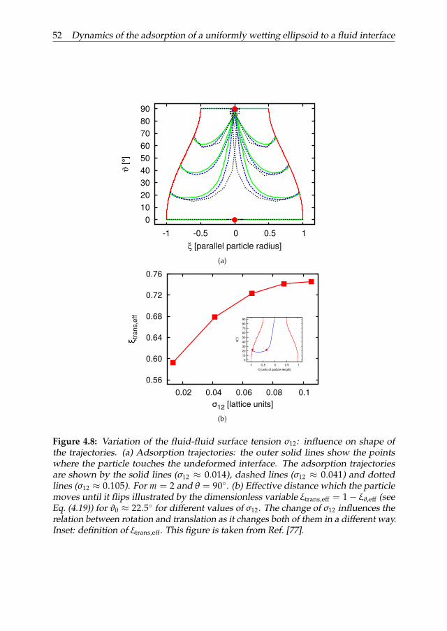
52 Dynamics of the adsorption of a uniformly wetting ellipsoid to a fluid interface
0
10
20
30
40
50
60
70
80
90
-1 -0.5 0 0.5 1
ϑ [
°]
ξ [parallel particle radius]
(a)
0.56
0.60
0.64
0.68
0.72
0.76
0.02 0.04 0.06 0.08 0.1
0102030405060708090
-1 -0.5 0 0.5 1
trans
,eff
ξ
12 [lattice units]σ
[] °
ϑ
[units of particle length]ξ
(b)
Figure 4.8: Variation of the fluid-fluid surface tension σ12: influence on shape ofthe trajectories. (a) Adsorption trajectories: the outer solid lines show the pointswhere the particle touches the undeformed interface. The adsorption trajectoriesare shown by the solid lines (σ12 ≈ 0.014), dashed lines (σ12 ≈ 0.041) and dottedlines (σ12 ≈ 0.105). For m = 2 and θ = 90. (b) Effective distance which the particlemoves until it flips illustrated by the dimensionless variable ξtrans,eff = 1−ξϑ,eff (seeEq. (4.19)) for ϑ0 ≈ 22.5 for different values of σ12. The change of σ12 influences therelation between rotation and translation as it changes both of them in a different way.Inset: definition of ξtrans,eff. This figure is taken from Ref. [77].

4.5. Parameter studies and adsorption dynamics 53
-1.0
-0.8
-0.6
-0.4
-0.2
0.0
0 1000 2000 3000 4000 5000 6000
ξ [p
ara
llel p
art
icle
ra
diu
s]
t [timesteps]
σ12=0.014σ12=0.041
σ12=0.06σ12=0.087σ12=0.105
(a)
400
600
800
1000
1200
1400
0.02 0.04 0.06 0.08 0.1
t sp [
tim
este
ps]
σ12 [lattice units]
lb3d HO, 1HO, 2
(b)
Figure 4.9: Variation of the fluid-fluid surface tension σ12: influence on dynamics. (a)ξ(t) for a starting angle of ϑ0 ≈ 22.5 and rescaled starting distanceξ(t = 0) ≈ −0.94.For different values of σ12: σ12 ≈ 0.014 (square), σ12 ≈ 0.041 (circle), σ12 ≈ 0.066(upward pointing triangle), σ12 ≈ 0.087 (downward pointing triangle), σ12 ≈ 0.105(diamond). m = 2, θ = 90. (b) Time tsp which the particle needs until it starts to flipfor different values of σ12. The dashed line is fitted to the relation obtained from theequation of the harmonic oscillator (Eq. (4.14), labeled in the plot as HO,1). The dotted
line is related to an improved relation (tsp = 1/√
aHOσ212 + bHOσ12 + cHO, labeled as
HO,2) with an additional parameter. This figure is taken from Ref. [77].

54 Dynamics of the adsorption of a uniformly wetting ellipsoid to a fluid interface
ξtrans,eff,s ≈ 0.7455 is reached. The increase of ξtrans,eff indicates the decrease of theopening angle. This indicates that the relation between translation and rotation ofthe particle in the adsorption process changes with changing σ12. The distance ofthe translation path which the particle moves before it starts to rotate, increases withincreasing σ12. This can be understood with Eq. (4.2): the translation is influencedby the two contributions Fcap and Fdrag. We consider the time in the beginning of theadsorption process and thus, in the “point like force rotation” regime. Both forcecontributions depend onσ12. From Eq. (4.7) and Eq. (4.8), it can be seen that Fcap ∝ σ12.Fdrag is proportional to the drag coefficient cD (see Eq. (4.10)) given in Eq. (4.9), butonly the contribution from the interface cD,i depends on σ12. The influence of σ12 onFdrag is dominant for the adsorption process. This means that the particle covers alarger distance until the “interfacial area rotation” regime begins and thus, the particlestarts to rotate.
The influence of the surface tension σ12 on the adsorption dynamics is shown inFig. 4.9. Figure 4.9(a) compares the time evolution of ξ for trajectories with an initialparticle orientation of ϑ0 ≈ 22.5 for different values of σ12 between 0.014 and 0.105.One can see that a larger value ofσ12 leads to a faster adsorption process (see diamondfor the largest value of σ12). For that value, it is shown in the plot that the line passesthe equilibrium point (ξ = 0) for a short time. The reason for that phenomenon is thatthe force acting on the particle is large enough for the particle to pass the equilibriumpoint and the system is in the underdamped regime of the harmonic oscillator. Thesquare showing the slowest adsorption corresponds to σ12 ≈ 0.014 which is thelowest value of the surface tensions studied here. The lines in Fig. 4.9(a) show thatthere is a transition from the overdamped to the underdamped harmonic oscillator.This can be understood as follows: it can be seen from the relationω0 =
√εMσ12 (see
Eq. (4.12)) that for low σ12, cDM > ω0 is fulfilled. This means that the system behavesas an overdamped oscillator. For higher values of σ12, cDM < ω0 is fulfilled leadingto the underdamped case.
The time tsp needed by the particle for the way from the point ξ(t = 0) to theinitial point ξϑ depending on σ12 is shown in Fig. 4.9(b). For larger values of σ12,the force which causes the particle adsorption increases, which leads to a fasteradsorption process. In order to understand this time behavior, we use the equationsof the harmonic oscillator (discussed in section 4.2) to get an estimation, and wecompare it with the results from the simulation. We assume that tsp is inverselyproportional to the oscillator frequency ωa as given in Eq. (4.14). This leads tothe relation tsp = 1/
√bHOσ12 + cHO. bHO and cHO are fit parameters related to the
capillary spring constant kcap and the damping constant cDM from Eq. (4.7) andEq. (4.9). The dashed line in Fig. 4.9(b) (labeled as HO,1) shows that this relationwith bHO = 7.95 · 10−5 and cHO = −9.33 · 10−7 describes the behavior quite well,but it is not yet the full description. There are deviations of the simulation resultsfrom the predictions of Eq. (4.14). Reasons for this deviation can be the following:cDM depends on σ12 via cD,i. The particle rotates during the period of interest so thatcDM and εM depend on ξ(ϑ) and the time as given in Eq. (4.18). There are possiblederivations from the relation tsp ∝ ω−1
a . Furthermore, the interface deformationcan possibly lead to a dependence kcap(ξ). The deviations are larger for smallervalues of σ12. The dependence of tsp from σ12 can be described more accurately by
the relation tsp = 1/√
aHOσ212 + bHOσ12 + cHO with an additional fit parameter aHO,

4.5. Parameter studies and adsorption dynamics 55
the correction term aHOσ212 and the values aHO = 3.51 · 10−4, bHO = 3.78 · 10−5 and
cHO = −6.74 · 10−8.
The influence of the contact angleθ on the particle adsorption to the fluid interfaceis shown in Fig. 4.10. Figure 4.10(a) presents the time development of ξ for differentvalues of the contact angle θ. There is a transition between the overdamped (forwettabilities close to the neutral wetting, see Fig. 4.5(a)) and the two-step regime (suf-ficiently far away from neutral wetting, see Fig. 4.5(c)). This is a result of an interplaybetween rotation and translation. An explanation for this is given by Fig. 4.10(b). Inthe case of 90, the largest part of the rotation starts when the translation is almostdone. On the other hand for 114.9, the rotation starts during the translation process.In this way, the translation is slowed down by the rotation. This leads to the two-stepregime.
The influence of the particle aspect ratio m in the range between 1.5 and 6 on theparticle adsorption is considered in Figs. 4.11 and 4.12. The values for the particleradii for the different values of m are calculated in a way that the particle volumeis constant. The adsorption trajectories for m = 6 are shown in Fig. 4.11(a). For themetastable point with ϑ0 = 0, the particle is supposed to end at ξfinal = 0. The factthat the particle stops earlier is a result of the effect of discretization of the particleon the lattice. One can see that the lines have a larger opening angle for m = 6 ascompared to m = 2 above. This aspect is shown in Fig. 4.12(a). The parameter ξtrans,effwhich is related to the opening angle, is plotted for different values of m between 1.5and 6. This behavior can be divided into two regimes: m ≤ 4 and m ≥ 4. For m ≤ 4,ξtrans,eff decreases with increasing m. This means that the rotation starts “earlier” forlarger aspect ratios. In the second regime, it increases. This can be explained bytwo competing effects. On the one hand, the capillary spring constant kcap decreaseswith increasing m. This leads to a decrease of ξtrans,eff. On the other hand, the dragcoefficient cD decreases with increasing m being related to an increase of ξtrans,eff. Theinfluence of the particle shape on the adsorption dynamics is shown in Fig. 4.11(b).The time evolution of ξres for an initial particle orientation of ϑ0 ≈ 22.5 for differentvalues of m is shown. ξres is defined as ξ/|ξ(t = 0)| where |ξ(t = 0)| is a parametermaking sure that all lines start at the same point ξres = −1 and depends on m. Allthree adsorption regimes presented in Fig. 4.5 are found in Fig. 4.11(b) dependingon the aspect ratio. The underdamped regime (Fig. 4.5(b)) is found for small aspectration (m = 1.5), the overdamped regime (Fig. 4.5(a)) for medium-sized aspect ratios(2 ≤ m ≤ 3) and the two-step regime (Fig. 4.5(c)) for aspect ratios of 4 and larger.Furthermore, we see that the time needed to reach the final point increases withincreasing m. This fact is shown in Fig. 4.12(b). In order to quantify this, we assume
tsp ∝ ωa and as shown in Eq. (4.14) the frequency is given byωa =√ω2
0 − c2DM. To
obtain an estimate, the following geometric consideration is made. We start witha sphere and increase m while the volume stays constant. This leads to followingrelation: R3 = R‖R2
⊥ with R‖ = Rma‖ and R⊥ = Rma⊥ . It turns out that a‖ = 2/3and a⊥ = −1/3. As the main axis is oriented perpendicular to the interface in thetime period of interest, the cross section can be estimated as Am ∝ R2
⊥ ∝ m−(2/3). Asthe perpendicular orientation is not exactly fulfilled: Am ∝ mdm , dm is supposed todeviate from −(2/3). The simulation data can be fitted as tsp = 1/
√bHOmdHO + cHO
with the following values: bHO = 7.63 · 10−06 and cHO = 3.36 · 10−7. The value of

56 Dynamics of the adsorption of a uniformly wetting ellipsoid to a fluid interface
-1.0
-0.8
-0.6
-0.4
-0.2
0.0
0 1 2 3 4 5 6
ξ [p
ara
llel p
art
icle
ra
diu
s]
t [103 timesteps]
θ=90° θ=95.8° θ=102.8°θ=107.0°θ=114.9°
(a)
-1.0
-0.8
-0.6
-0.4
-0.2
0.0
0 1 2 3 4 5 6
ξ re
s,
ϑre
s
t [103 timesteps]
ξres, 90° ϑres, 90° ξres, 114.9°ϑres, 114.9°
(b)
Figure 4.10: Variation of the contact angle θ. (a) ξ(t) for a starting angle ofϑ(t = 0) ≈ 22.5 and rescaled starting distance ξ(t = 0) ≈ −0.94. For differentvalues of θ: θ = 90 (square), θ ≈ 95.8 (circle), θ ≈ 102.8 (upward pointing trian-gle), θ ≈ 107.0 (downward pointing triangle), θ ≈ 114.9 (diamond). For m = 2,σ12 ≈ 0.041. There is a transition from the overdamped regime (see Fig. 4.5(a)) to thethe two-step regime (see Fig. 4.5(c)). (b) The transition from (a) can be explained bycomparing the relation between rotation and translation. The squares correspond toa contact angle of 90 whereas the circles correspond to 114.9. Full symbols corre-spond to translation and open symbols to rotation. In the case of 90, the largest partof the rotation starts when the translation is almost done. In contrast, for 114.9 therotation starts during the translation process. In this way, the translation is sloweddown by the rotation. This leads to the two-step regime. This figure is taken fromRef. [77].
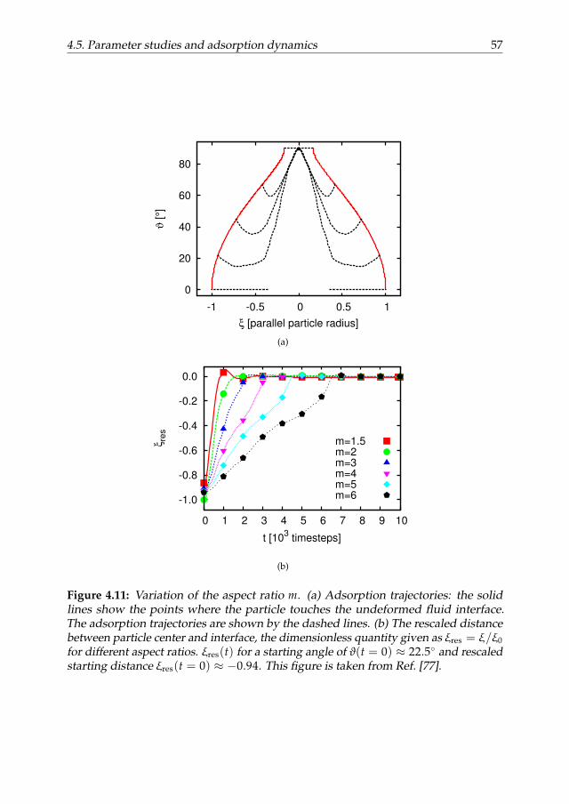
4.5. Parameter studies and adsorption dynamics 57
0
20
40
60
80
-1 -0.5 0 0.5 1
ϑ [
°]
ξ [parallel particle radius]
(a)
-1.0
-0.8
-0.6
-0.4
-0.2
0.0
0 1 2 3 4 5 6 7 8 9 10
ξ re
s
t [103 timesteps]
m=1.5m=2 m=3 m=4 m=5 m=6
(b)
Figure 4.11: Variation of the aspect ratio m. (a) Adsorption trajectories: the solidlines show the points where the particle touches the undeformed fluid interface.The adsorption trajectories are shown by the dashed lines. (b) The rescaled distancebetween particle center and interface, the dimensionless quantity given as ξres = ξ/ξ0for different aspect ratios. ξres(t) for a starting angle of ϑ(t = 0) ≈ 22.5 and rescaledstarting distance ξres(t = 0) ≈ −0.94. This figure is taken from Ref. [77].

58 Dynamics of the adsorption of a uniformly wetting ellipsoid to a fluid interface
0.55
0.60
0.65
0.70
0.75
2 3 4 5 6
ξ tra
ns,e
ff
m
(a)
1000
2000
3000
4000
2 3 4 5 6
t sp [
tim
este
ps]
m
(b)
Figure 4.12: (a) Effective distance which the particle moves until it flips, the dimen-sionless quantity ξtrans,eff = 1−ξϑ,eff for different values of m. (b) Time tsp which theparticle needs until it starts to flip for different values of m. The solid line is a fit withthe harmonic oscillator theory. This figure is taken from Ref. [77].
the exponent dHO differs from the expectations: instead of −(2/3), it is found to bedHO = −1.68 ≈ −(5/3).
4.6 Interface deformation caused by the adsorption
By comparing our simulation results with the ones of the “flat interface” model, itturns out that the interface deformation has an influence on the adsorption process.Here, we quantify the interface deformation.

4.6. Interface deformation caused by the adsorption 59
(a) (b) (c)
(d) (e) (f)
Figure 4.13: Snapshots of the simulation data showing the interface deformationduring the adsorption process. (a) t = 100. (b) t = 600. (c) t = 1200. (d) t = 4000. (e)t = 5800. (f) t = 6400. This figure is taken from Ref. [77].
If an anisotropic particle with a homogeneous wettability rotates, the fact that thecontact angle stays constant leads in most cases to an interface deformation aroundthe particle. The Young equation cannot be fulfilled by a flat interface anymore.The few cases where the interface is not deformed are shown in Table 2.1. If theadsorption process is sufficiently slow so that it can be assumed that the systemis close to equilibrium during the whole adsorption process, the contact angle isdefined. In order to illustrate this, the capillary number Ca for the system of interestis considered. Ca is defined as
Ca =µ~upar
σ12. (4.20)
µ is the dynamic viscosity given in Eq. (3.34). ~upar is the velocity of the particlecenter during the adsorption process. For the maximum and the average velocity ofthe particle in the adsorption process, we obtain capillary numbers of Ca ≈ 0.085and Ca ≈ 0.004, respectively. This value of Ca indicates that the contact angle is inequilibrium during the whole adsorption process.
In order to illustrate the interface deformation, we show some snapshots of theparticle during the adsorption process at different times in Fig. 4.13. These snapshotsare taken for an adsorption process with an initial orientation of ϑ0 = ϑ(t = 0) ≈0.0001. Figures 4.13(a) and 4.13(b) show the translational motion at the start ofthe simulation. The fluid interface starts to deform when the particle enters intothe interface. Figure 4.13(a) clearly shows a monopolar interface deformation. Therotation and the resulting dipolar interface deformation can be seen in Fig. 4.13(c) to4.13(e). Figure 4.13(f) depicts the final state where the interface deformation vanishes.
The following quantity can be used as a measure for the interface deformation(see Fig. 4.14): on the one hand, the position of the flat interface which we would

60 Dynamics of the adsorption of a uniformly wetting ellipsoid to a fluid interface
λif,0λif
Figure 4.14: The volume λ created by the interface deformation caused by a particleadsorbed at the fluid interface is shown. The undeformed flat interface yif,0 (asit would be the case without particles) is shown by the solid line. The interfacedeformation yif(ix, iz) is shown by the dashed line. This figure is taken from Ref. [77].
have without any particle is known a priori (solid line in Fig. 4.14). On the otherhand, the position of the real interface influenced by the particle can be obtained fromthe results of the simulation (dashed line in Fig. 4.14). The volume created by thedifference of these two interfaces is given by
λ =1λp
Nx
∑ix=1
Nz
∑iz=1|yif(ix, iz)− yif,0|. (4.21)
i j is the coordinate of a lattice node in j-direction (with j = x, z, the two directionsparallel to the interface) and N j is the number of lattice nodes in j-direction. yif(ix, iz)and yif,0 are the values of the y coordinate for the real interface for each x = ix andz = iz and the ideal flat interface, respectively. λp = (4/3)πR‖R2
⊥ is a normalizationfactor and corresponds to the particle volume. λ = 0 indicates an undeformedinterface, however, in most cases λ is different from zero. The only cases of generalellipsoidal particles with λ = 0 are shown in Table 2.1.
There are several contributions to λ which can be divided into two groups: (i)The static contribution due to the wettability: this contribution just depends on thephase space coordinates ξ and ϑ as well as the particle properties like θ and m. It isgiven by Eq. (2.26). (ii) Dynamic contributions: the moving particle causes capillarywaves. This contribution also comprises finite size effects. They stem from the factthat the range of the capillary wave is larger than the system size. Tests in whichthe system size was varied have shown that a convergence could not be found forsystem sizes that are realistic for our simulation method. Figure 4.15(a) depicts λfor an adsorption process with an initial orientation of ϑ0 = 45. λres shows a singlelarge peak after about 440 timesteps (peak A). It then decays because of a capillaryrestoring force (see Eq. (2.6)). This peak is caused by the translation and rotationwhich take place at about the same time. After this peak damped oscillations ofλ can be observed for the next few thousand timesteps. Figure 4.15(b) shows thesame scenario for ϑ(t = 0) ≈ 0.0001. Unlike in the previous case, the translationand the rotation take place at different times. They are completely decoupled. Thetranslation takes place mainly in the first 2000 timesteps and the largest deformationof this part is reached after about 460 timesteps. This peak is called peak B. Thedeformation decays during the following 1400 timesteps. The rotation of the particle

4.6. Interface deformation caused by the adsorption 61
starts after about 2000 timesteps and leads to a maximum of the deformation after3260 timesteps (peak C). The deformation caused by the translation is about 3.4 timeslarger than the deformation caused by the rotation: the translational motion pushesthe fluid much more than the rotation.
The time evolution of the rescaled deformation of the fluid interface λres = (4/3)λis shown by the squares in Fig. 4.15 for two different initial values of ϑ. The circlesand triangles show the rescaled values of ξres = ξ/ξ(t = 0) and ϑres = ϑ/90. λ, ξand ϑ are rescaled in order to keep them in a range between 0 and 1.
The influence of the fluid-fluid interfacial tension on the interface deformation isshown in Fig. 4.16. Figure 4.16(a) shows the rescaled time of the peak tp,res = tp/aresfor the peak B (squares, ares = 755) and C (circles, ares = 8904) of Fig. 4.15(a) and thepeak A of Fig. 4.15(b) (triangles, ares = 642). ares is a normalization factor and chosenin a way that tp,res forσ12 = 0.0138 (lowest value ofσ12) has a value of unity for everypeak. tp,res decreases with increasing σ12 for all cases.
In order to understand the behavior, we discuss some estimates from the consider-ations in section 4.2. As the particles have a contact angle of 90 and the line tensionis neglected, the starting point for the consideration of the free energy is Eq. (4.1).As shown in section 4.2, the system behaves like a damped harmonic oscillator and
as seen in Eq. (4.14) its frequency is given asωa =√εMσ12 − c2
DM. The time periodof the adsorption process can be estimated as tp ∝ 1/ωa which leads to a fit func-tion tp =
√bHOσ12 + cHO with fit parameters bHO and cHO related to εM and cDM.
εM is the proportionality factor between the frequency of the undamped harmonicoscillator and the interfacial tension between the two fluids. cDM is the dampingconstant. The inset of Fig. 4.16(a) shows that we can fit this function quite well (withbHO ≈ 1.27 · 10−4 and cHO ≈ −1.95 · 10−7).
Figure 4.16(b) shows the rescaled height λmax,res of the peak B (squares, ares =0.92), C (circles, ares = 0.19) and A (triangles, ares = 0.89). For lower values of σ12,we can see an almost linear relation between λmax,res and σ12 which is pronouncedfor peak A and B. This linearity comes from the fact that F and Fcap in Eq. (4.1)and Eq. (4.3) depend linearly on σ12. For higher values of σ12, there are deviationsfrom this linearity. Deviations from the prediction come from the fact that the realsystem is more complex than this idealized model. Fig. 4.17 shows the deformationintegrated over the time Λ =
∫λ(t)dt for different values of the fluid-fluid interfacial
tension between σ12 ≈ 0.0138 and σ12 ≈ 0.0873. The noise of the lines increasesfor increasing σ12. The larger as well as the smaller peak have higher values andmove to earlier times for increasing σ12. The reason for this is that larger values ofσ12 lead to larger forces acting on the particle which increases its velocity during theadsorption process. Furthermore, the restoring force is stronger for higher values ofσ12 which reduces the total interface deformations. The fact that it does not decreasemonotonously comes from fact that larger values of σ12 lead also to larger particlevelocities which increases the capillary waves leading to an increase of Λ.

62 Dynamics of the adsorption of a uniformly wetting ellipsoid to a fluid interface
0.0
0.2
0.4
0.6
0.8
1.0
0 1 2 3
λre
s,
ξ re
s,
ϑre
s
t [103 timesteps]
A
λresϑresξres
(a)
0.0
0.2
0.4
0.6
0.8
1.0
0 1 2 3 4 5
λre
s,
ξ re
s,
ϑre
s
t [103 timesteps]
B
C
λresϑresξres
(b)
Figure 4.15: (a) Time development of the rescaled interface deformation λres = (4/3)λ(see Eq. (4.21)) for ϑ(t = 0) = 45 is shown by the squares. For comparison, thetime development of the rescaled particle position ξres = ξ and rescaled orienta-tion ϑres = ϑ/90 are shown by the circles and triangles, respectively. Translationand rotation take place simultaneously. (b) The same situation as in (a) but forϑ(t = 0) ≈ 0.0001. Translation and rotation and their influence on the interface de-formation are completely decoupled. The comparison of (a) and (b) shows that thedeformation caused by translation is dominant. This figure is taken from Ref. [77].

4.6. Interface deformation caused by the adsorption 63
0.0
0.2
0.4
0.6
0.8
1.0
1.2
0.02 0.04 0.06 0.08
t p,res
400600800
0.04 0.08
t p
12 [lattice units]σ
12σ
(a)
0.6
0.7
0.8
0.9
1.0
0.02 0.04 0.06 0.08
λm
ax,r
es
σ12 [lattice units]
Peak BPeak CPeak A
(b)
Figure 4.16: Influence of the fluid-fluid interfacial tension σ12 on the interface defor-mation. (In both plots: peak A in Fig. 4.15: triangles, peak B in Fig. 4.15: squares, peakC: circles) (a) Rescaled peak time. tp,res decreases for increasing σ12 because a highervalue ofσ12 corresponds to a higher force acting on the particle, making the adsorptionfaster. Inset: for the purely translational mode it can be shown that it can be reason-ably well described as a harmonic oscillator and fitted by tp = 1/
√bHOσ12 + cHO.
(b) Rescaled height. λmax,res increases with increasing σ12. There is a linear increasefor small σ12 (σ12 ≤ 0.06) which can be explained by the equations of the harmonicoscillator (see Eq. (4.3)). This figure is taken from Ref. [77].

64 Dynamics of the adsorption of a uniformly wetting ellipsoid to a fluid interface
550
600
650
700
750
800
850
900
950
0.02 0.04 0.06 0.08
Λ
σ12 [lattice units]
ϑ(t=0)=(10-4
)°
ϑ(t=0)=45°
Figure 4.17: Influence of the fluid-fluid interfacial tension σ12 on the time integratedinterface deformation Λ =
∫λ(t)dt for the two initial angles from Fig. 4.15. Λ
is decreasing with increasing σ12 because a higher value of σ12 leads to a fasteradsorption and larger restoring force which reduces the interface deformation. Thisfigure is taken from Ref. [77].
4.7 Interface deformation: influence on the free energy
The final states of the adsorption of a uniformly wetting ellipsoid (the stable state(equilibrium) as well as the metastable state) to a flat fluid interface can be describedby finding local or global minima of the free energy. This has been done several timesassuming an ideally flat interfaces by neglecting interface deformation [26, 48]. Alsothe equation of motion for the adsorption including the force acting on the particlecoming from the interface can be derived from free energy as it is given in Eq. (4.2)and used in the “flat interface model”. In this section, we derive an expression for afree energy which takes into account the actual deformation of the interface.
The important variables for this situation are shown in Fig. 4.18. ∆ξ is the distanceof the undeformed interface and the plane created by the three-phase contact line.Note that this is generally not a plane for other particle orientations. h is the localinterface deformation and the zero-point is given at the 3-phase contact line createdby the fluid interface and the particle surface.
The starting point for this consideration is the free energy function as given inEq. (4.1). In order to show the influence of the interface deformation on the freeenergy, we split the total interfacial area A12 between the two fluids into the sumA12(ξ ,ϑ) = Aundef(ξ ,ϑ) + ∆Aifdef(ξ ,ϑ) and obtain
F (ξ ,ϑ) = σ12(Aundef(ξ ,ϑ) + ∆Aifdef(ξ ,ϑ)) = Fundef + ∆Fifdef
∆F (ξ ,ϑ) = F −F0 = σ12(−Aef(ξ ,ϑ) + ∆Aifdef(ξ ,ϑ)).(4.22)
∆Fifdef and ∆Aifdef are the correction terms to the free energy and the interface area,respectively, and take into account the deformation of the fluid interface inducedby the particle. They are functions of ξ and ϑ. Aundef is the area of a hypothetical

4.7. Interface deformation: influence on the free energy 65
ξh=0
r
R0
0
Δξ
Figure 4.18: The quantities needed to calculate the “new” free energy for an uprightorientation of the particle are shown here. The line at the bottom shows the unde-formed interface. The line above shows the deformed interface. ∆ξ is the heightof the deformed interface at the points where it meets the particle (3-phase contactline) above or below the undeformed interface. ξ is the distance between particlecenter and undeformed interface. r0 and R0 are the radius of the circle created by thedeformed and undeformed interface, respectively. This figure is taken from Ref. [77].
flat interface and Fundef is the corresponding free energy. Aef is the area of the flatinterface occupied by the particle.
Before calculating the interface areas, we define the following two radii
R0 =
√R2‖ −ξ2
mand r0 =
√R2‖ − (ξ − ∆ξ)2
m. (4.23)
As shown in Fig. 4.18, r0 and R0 are the radius of the circle created by the deformedand undeformed interface, respectively. They describe the respective three phasecontact line. Then, the exact solution for the excluded area from the undeformedinterface can be easily given as
Aef = πR20
Aundef = Aflat − Aef = Aflat − πR20.
(4.24)
With Eq. (4.24) and Eq. (4.23), we find
Aef = π
(R2‖
m2 −ξ2
m2
)= π
(R2⊥ −
ξ2
m2
). (4.25)
From the comparison between the two models in section 4.4, it turnes out that theinterface deformation influences the adsorption dynamics, but generally not the finalstate. Thus, the following requirements for the correction term ∆Aifdef are laid down:
∆Aifdef
= 0 for an undeformed interface> 0 for a deformed interface.
(4.26)

66 Dynamics of the adsorption of a uniformly wetting ellipsoid to a fluid interface
This makes sure that the minimum of F is not shifted. As seen in Table 2.1, theinterface is undeformed for ξ = 0 and otherwise deformed for the neutrally-wettingcase.
In order to obtain a function for ∆Aifdef, we start with the calculation similar to theone presented in Ref. [174] for small interface deformations: the infinitesimal elementof the undeformed interface is given as dS = dxdz and the one of the deformedinterface as dS∗ = dx∗dz∗. The relations are given as dx∗ = dx and
dz∗ =√
dz2 + dh2 ≈
√dz2 +
(dhdz
)2
dz2 = dz√
1 + (∇h)2 ≈ dz(
1 +12(∇h)2
).
(4.27)h is the height of the interface and vanishes at the point where the interface meets theparticle surface. The excess interface area can be obtained in the following way:
d(∆Aifdef) = dS∗ − dS = dxdz12(∇h)2. (4.28)
∆Aifdef is given as
∆Aifdef =12
∫ Rmax(φp)
r=r0(φp)
∫ 2π
φp=0(∇h)2rdφpdr. (4.29)
r0(φp) is the point where the interface touches the particle. It is a function ofφp for ageneral value of ϑ. In case of ϑ = 0, the three phase contact line is a circle as shownin Fig. 4.18, and thus, the dependence onφp vanishes. Rmax(φp) is the cutoff of theintegration.
For simplicity, we assume a constant orientation of ϑ = 0. This example is chosen,because it is simple to calculate. This corresponds to the adsorption trajectory of themetastable state.
The differential equation and the solution for h in form of a multipole expansionare given in Eq. (2.25) and Eq. (2.26). The important order for the situation of interesthere is the monopole
h(r) = A0 lnrr0
for r0 ≤ r ≤ Rmax, (4.30)
which does not depend on the directionφp. r is the distance from the particle center.r0 is the radius of the circle created by the deformed interface and the particle. Rmaxis defined as the value of r where
h(r = Rmax) = A0 lnRmax
r0= ∆ξ (4.31)
is fulfilled. It limits the range of the interface deformation. As h does not depend onthe angle in the monopole order in Eq. (4.30), the gradient is given by
∇h = er∂
∂rh = er A0
∂
∂rln
rr0
= erA0
r(4.32)
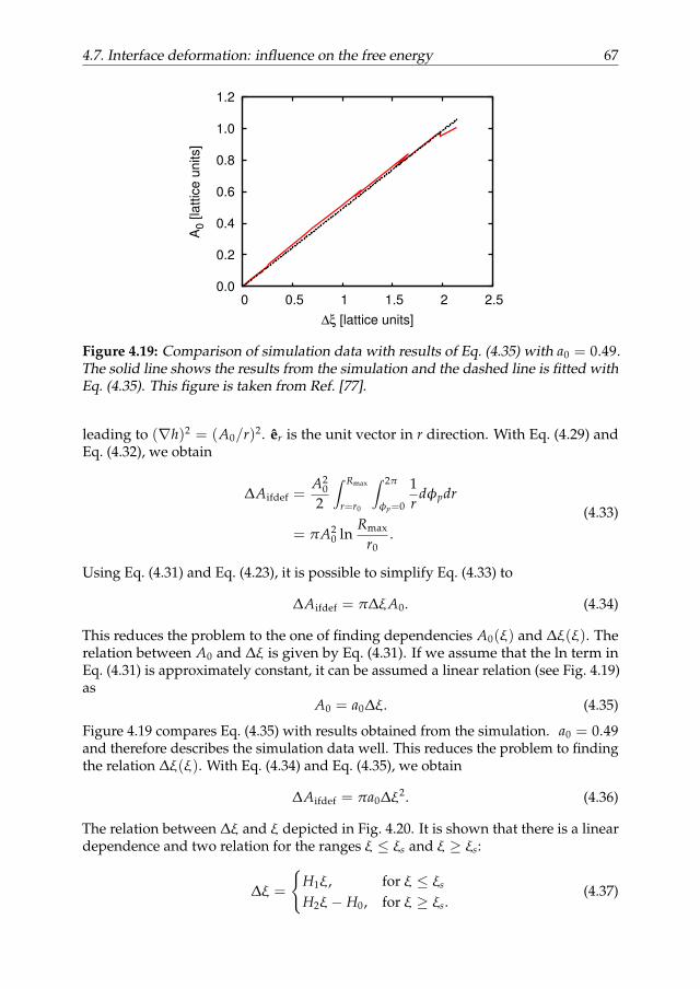
4.7. Interface deformation: influence on the free energy 67
0.0
0.2
0.4
0.6
0.8
1.0
1.2
0 0.5 1 1.5 2 2.5
A0 [
latt
ice
un
its]
∆ξ [lattice units]
Figure 4.19: Comparison of simulation data with results of Eq. (4.35) with a0 = 0.49.The solid line shows the results from the simulation and the dashed line is fitted withEq. (4.35). This figure is taken from Ref. [77].
leading to (∇h)2 = (A0/r)2. er is the unit vector in r direction. With Eq. (4.29) andEq. (4.32), we obtain
∆Aifdef =A2
0
2
∫ Rmax
r=r0
∫ 2π
φp=0
1r
dφpdr
= πA20 ln
Rmax
r0.
(4.33)
Using Eq. (4.31) and Eq. (4.23), it is possible to simplify Eq. (4.33) to
∆Aifdef = π∆ξA0. (4.34)
This reduces the problem to the one of finding dependencies A0(ξ) and ∆ξ(ξ). Therelation between A0 and ∆ξ is given by Eq. (4.31). If we assume that the ln term inEq. (4.31) is approximately constant, it can be assumed a linear relation (see Fig. 4.19)as
A0 = a0∆ξ . (4.35)
Figure 4.19 compares Eq. (4.35) with results obtained from the simulation. a0 = 0.49and therefore describes the simulation data well. This reduces the problem to findingthe relation ∆ξ(ξ). With Eq. (4.34) and Eq. (4.35), we obtain
∆Aifdef = πa0∆ξ2. (4.36)
The relation between ∆ξ and ξ depicted in Fig. 4.20. It is shown that there is a lineardependence and two relation for the ranges ξ ≤ ξs and ξ ≥ ξs:
∆ξ =
H1ξ , for ξ ≤ ξs
H2ξ − H0, for ξ ≥ ξs.(4.37)

68 Dynamics of the adsorption of a uniformly wetting ellipsoid to a fluid interface
0.0
0.5
1.0
1.5
2.0
2.5
0 1 2 3 4 5 6 7 8 9
∆ξ
[la
ttic
e u
nits]
ξ [lattice units]
Figure 4.20: Comparison of simulation data with results of Eq. (4.37). The solid lineshows the results from the simulation. The dashed lines are fitted with Eq. (4.37) withH0 = 0.58 and H2 = 0.37 for ξ ≤ ξs and H1 = 0.04 for ξ ≥ ξs. This figure is takenfrom Ref. [77].
-1
0
1
2
3
4
5
6
7
8
0 1 2 3 4 5 6 7 8
∆A
ifd
ef [la
ttic
e u
nits]
ξ [lattice units]
Figure 4.21: Comparison of simulation data with results of Eq. (4.38). The solid lineshows the results from the simulation. The dashed lines are fitted with Eq. (4.38) withA1 = 0.0023 for ξ ≤ ξs and B2 = 0.21, B1 = 0.66 and B0 = 0.52 for ξ ≥ ξs. Thisfigure is taken from Ref. [77].

4.7. Interface deformation: influence on the free energy 69
ξs = H0/(H2 − H1) is defined as the intersection of the two lines from Eq. (4.37). WithEq. (4.35), Eq. (4.37) and Eq. (4.34), we find
∆Aifdef =
πH1(a0 H1 − 2
m )ξ2 = A1ξ
2, for ξ ≤ ξs
π(H2ξ − H0)((a0 H2)ξ − a0 H0) = B2ξ2 + B1ξ + B0, for ξ ≥ ξs.
(4.38)
The coefficients are given as A1 = πH1(a0 H1), B0 = πa0 H20 , B1 = −πH0(2a0 H2) and
B2 = π(a0 H2)H2. Figure 4.21 shows the fit for the simulation data by this relation.Furthermore, Eq. (4.38) shows that ∆Aifdef vanishes for ξ = 0, i.e. the interfacedeformation and its influence vanish for the final position. This means that theinterface deformation influences the adsorption process but not the final state.
Finally, for the given orientation, we can write down explicitly the free energygiven in Eq. (4.22) using Eq. (4.24) and Eq. (4.38):
∆Fifdef(ξ ,ϑ = 0) = σ12(Aundef(ξ ,ϑ = 0) + ∆Aifdef(ξ ,ϑ = 0))
= σ12
(πR2
0 + π∆ξ
(A0 −
(2ξ − ∆ξ)
m
)).
(4.39)
With Eq. (4.23) and Eq. (4.38), we obtain the full dependence of Funiifdef from ξ as
∆Fifdef =
σ12((A1 −m−2)ξ2 + R⊥
), for ξ ≤ ξs
σ12((B2 −m−2)ξ2 + B1ξ + R⊥ + B0
), for ξ ≥ ξs.
(4.40)
The conditions of Eq. (4.26) are fulfilled by Eq. (4.39).Thus, the equation of motion from Eq. (4.2) can be given for this situation using
Eq. (4.39) as
Mparξ = −cDξ −
2σ12(A1 −m−2)ξ , for ξ ≤ ξs
2σ12(B2 −m−2)ξ +σ12B1, for ξ ≥ ξs.(4.41)
An additional term is added to Eq. (4.11) and we obtain
ξ + 2cDMξ +αHOξ = ξinh, (4.42)
withαHO = 2σ12(B2 −m−2)/Mpar. Thus, due to the interface deformation, an inho-mogeneous term is added to the differential equation of the harmonic oscillator. Thisadditional term is given as ξinh = −σ12B1/Mpar. cDM = cD/(2Mpar) is the dampingcoefficient. Figure 4.6(a) shows that the adsorption process in this example behaveslike an underdamped harmonic oscillator. It can be solved by
ξ(t) = ξhom(t) +ξinh
=
(ξhom,0
αHO
)exp(−cDMt)(αHO cosh(αHOt) + cDM sinh(αHOt)) +ξinh.
(4.43)
for ξ ≥ ξs. Thus, ξ(t) is given by a sum of the homogeneous solution of the harmonicoscillator ξhom and an inhomogeneous part ξinh. For ξ ≤ ξs, it reduces to Eq. (4.15).We saw that for a neutrally-wetting particle the interface deformation influences thedynamics but not the final state. The condition of Eq. (4.26) is fulfilled.

70 Dynamics of the adsorption of a uniformly wetting ellipsoid to a fluid interface
4.8 Conclusion
In this section, the final states and the dynamics of the adsorption of a single ellipsoidalparticle with a uniform wettability to a fluid interface is studied. In conclusion, onecan say that the equilibrium orientation of the particle is the orientation parallelto the interface. In this orientation, the particle occupies as much interface areaas possible and minimizes the free energy in this way. Furthermore, a metastablestate is found, where the particle has an upright orientation. The particle rotationduring the adsorption process of the particle can be divided into two regimes: in thebeginning, the particle rotates towards the upright orientation. This is caused by apoint-like force acting on the particle while it touches the interface. At a later stage,the particle rotates towards the orientation parallel to the interface. By comparing thesimulation results with the “flat interface” model, a simplified model which does notconsider any hydrodynamical effects, it can be concluded that the hydrodynamicsmust not be neglected. The two important hydrodynamical effects for the system ofinterest are the drag force and the interface deformation. The interface deformationcan be divided into a static and a dynamic contribution. The dynamic contributionfrom the translation is almost one order of magnitude larger than the one from therotation. It can be shown that the translation can be described by the equation of theharmonic oscillator, where the harmonic potential follows from the free energy andthe damping constant from the drag force of the bulk fluid and the interface. However,the deformation of the interface causes a deviation of the particle adsorption from theexact behavior of the harmonic oscillator. Therefore, it is necessary to add a correctionfactor to the free energy and the equation of motion in order to take into account theinterface deformation.

Chapter 5
Emulsions stabilized byuniformly wetting ellipsoids
Abstract
Particle-stabilized emulsions have received an enormous interest in the recent past,but our understanding of the dynamics of emulsion formation is still limited. Forsimple spherical particles, the time dependent growth of fluid domains is dominatedby the formation of droplets, particle adsorption and coalescence of droplets (Ost-wald ripening) which eventually can be almost fully blocked due to the presenceof the particles. Ellipsoidal particles are known to be more efficient stabilizers offluid interfaces than spherical particles and their anisotropic shape and the relatedadditional rotational degrees of freedom have an impact on the dynamics of emulsionformation. This leads to additional timescales in the long-term time evolution ofemulsion formation. In this chapter, we investigate these timescales by means of sim-ple model systems consisting of a single ellipsoidal particle or a particle ensemble at aflat interface as well as a particle ensemble at a spherical interface. It is demonstratedthat the anisotropic shape of ellipsoidal particles causes two additional timescales tobe of relevance in the dynamics of emulsion formation: a relatively short timescalecan be attributed to the adsorption of single particles and the involved rotation ofparticles towards the interface. As soon as the interface is jammed, however, capillaryinteractions between the particles cause a local reordering on very long timescalesleading to a continuous change in the interface configuration and a surprising in-crease of interfacial area. This effect can be utilized to counteract the thermodynamicinstability of particle-stabilized emulsions and thus offers the possibility to produceemulsions with exceptional stability. Furthermore, the influence of control parameterssuch as volume ratio of the fluids and contact angle on Pickering emulsions and bijelsis studied.
The results discussed in this chapter are based on Refs. [78, 79, 111].
71

72 Emulsions stabilized by uniformly wetting ellipsoids
5.1 Introduction
In the following, we consider emulsions stabilized by a large number of anisotropiccolloidal particles. To simulate a bulk system, we use a cubic volume with a sidelength of 256 lattice units and periodic boundary conditions in all directions. Toobtain a phase separation, the fluid-fluid interaction parameter between red and bluefluids (see Eq. (3.22)) is set to gbr = 0.08. The initial density distributions of the twofluids are chosen to be random.
As defined in section 2.4 and section 1.2, we distinguish between two differenttypes for these emulsions, the Pickering emulsion and the bicontinuous interfaciallyjammed emulsion gel (bijel). The bijel [176] consists of two continuous phases whereasthe Pickering emulsion [152, 156] is composed of discrete droplets of one fluid im-mersed in a second fluid phase. Bijels and Pickering emulsions stabilized by sphericalparticles have been investigated in Ref. [68, 98]. The emulsion type is found to dependon control parameters such as the volume ratio of the two fluid.
To characterize an emulsion, the time-dependent lateral domain size/droplet size
L(t) =13 ∑
i=x,y,zLi(t) (5.1)
is calculated. Its Cartesian components (i = x, y, z) are defined as
Li(t) =2π√〈k2
i (t)〉, 〈k2
i (t)〉 =∑k k2
i (t)s(k, t)∑k s(k, t)
. (5.2)
〈k2i (t)〉 is the second-order moment of the three-dimensional structure function
s(k, t) =1sn|φ′k(t)|. (5.3)
φ′ = φ− 〈φ〉 is the Fourier transform of the fluctuations of the order parameter
φ = ρr − ρb. (5.4)
ρr and ρb are the densities of the red and blue fluid, respectively, and defined inEq. (3.16).
The particle concentration is characterized by C = NpVp/V. Np is the number ofparticles in the emulsion, Vp and V are the volume of the particles and the system,respectively. The degree of anisotropy of a particle is given by the aspect ratiom = R‖/R⊥. R‖ and R⊥ are the parallel and orthogonal radius of the particles,respectively. The interaction parameter between the red and blue fluid (see Eq. (3.22))is chosen as gbr = 0.08 which corresponds to a fluid-fluid interfacial tension ofσ12 = 0.0138.
5.2 Phase behavior and parameter studies
In this section, we discuss the influence of control parameters on emulsions. Thechoice of the control parameters decides into which of the two phases the system

5.2. Phase behavior and parameter studies 73
evolves. Here, we look at the contact angle θ and the volume ratio of the fluids. θ isthe contact angle defined in chapter 2. The left plot in Fig. 5.1 shows the transitionfrom a bijel to a Pickering emulsion for an aspect ratio of m = 2 and a particle volumeconcentration of C ≈ 0.2. The squares show the configurations which lead to a bijelwhereas the circles denote a Pickering emulsion. If the amount of the two fluidspresent in the simulation is equal or not too different (e.g. a ratio of 4 : 3), we finda bijel for all considered contact angles. However, if the fluid ratio is increased, wefind a Pickering emulsion. For intermediate fluid ratios, the obtained phase dependson the chosen contact angle. For example for a ratio of 9 : 5, we obtain a bijel for acontact angle of 90 and a Pickering emulsion for all higher values of θ.
The right plot in Fig. 5.1 shows the dependence of the domain size on the vol-ume concentration of particles C for different concentrations between C = 0.08 andC = 0.24 for an emulsion with a fluid ratio of 1 : 1 and θ = 90.
The results for anisotropic particles (here: m = 2) and spheres (m = 1) arecompared. As can be seen in the left inset of Fig. 5.1, these parameters for the case ofm = 2 lead to a bijel. For too small volume concentrations such as C ≈ 0.04, there areinsufficient particles available to stabilize the emulsion. The system finally reaches afully demixed state. The simulation data is displayed by circles for m = 2 and squaresfor m = 1 (see [98]). L decreases with an increasing value of C. An increasing numberof particles stabilizing the emulsion leads to an increase of the total interfacial areaand thus to smaller domain sizes. The results can be fitted by the equation [98]
L(C) =aC+ b (5.5)
(see solid (m = 2) and dashed (m = 1) lines in the right plot in Fig. 5.1) with valuesb ≈ 11.08 for m = 2 and b ≈ 10.85 for m = 1. The offset b is due to the finite systemsize in our simulation and is approximately independent of the particle shape. Thefactor a depends on the shape of the particles. For spheres we find a value of a ≈ 3.86whereas for m = 2 we find a ≈ 2.20. The right plot in Fig. 5.1 shows that the domainsize L is larger for spherical particles than for the case of anisotropic particles. If aspherical particle with a radius R and a contact angle θ = 90 is adsorbed, it reducesthe interfacial area by an amount of A(m = 1) = 2πR2. If an anisotropic ellipsoid withaspect ratio m and the same volume as the sphere is adsorbed and reaches the stablepoint (see results of the single-particle adsorption in the previous chapter), the interfa-cial area is reduced by an amount of A(m) = 2πR‖R⊥ = 2πm1/3R2. For the exampleof m = 2, we obtain a reduction of the interface area of A(m = 2) ≈ 2.52πR2. Thus, ifthe particle anisotropy increases, the occupied area A(m) increases. This means thatif the particle number is kept constant and the anisotropy is increased, the particlescan stabilize a larger interface which leads to smaller domain sizes. As the structureof a bijel interface is quite complicated and the interfaces are generally curved, it isnot possible to utilize the relations given above to derive an exact dependence of thedomain size L on the particle aspect ratio m. However, the qualitative difference ofusing spheres or ellipsoids as emulsion stabilizers can be well understood.

74 Emulsions stabilized by uniformly wetting ellipsoids
90 110 130
Flu
id r
atio
Contact angle θ[°]
1:1
4:3
9:5
5:2
1:1
4:3
9:5
5:2
(a)
4
5
6
7
8
0.08 0.12 0.16 0.2 0.24
L [
latt
ice
un
its]
C [volume ratio]
m=2m=1
(b)
Figure 5.1: (a) Phase diagram demonstrating the transition from a bijel (circle) to aPickering emulsion (square) for m = 2. The contact angle θ and the volume ratiobetween the two fluids are varied. The squares show the configurations which leadto a bijel whereas the circles denote a Pickering emulsion. (b) Average domain sizeL in equilibrium versus the volume concentration of the particles C for a bijel withparticles of neutral wettability (θ = 90). The plot compares the data for spheres(m = 1, squares) [98] with ellipsoids (here: m = 2, circles). The behavior can beapproximated by L = a
C + b (see solid line (m = 2) and dashed line (m = 1)) where aand b are fit parameters. This figures are taken from Ref. [78].

5.3. Long-term time evolution in emulsions due to particle anisotropy 75
5.3 Long-term time evolution in emulsions due to parti-cle anisotropy
In this section, the long term-time evolution of both emulsion types is discussed. Wefind the two different types of emulsions in our simulations, namely the Pickeringemulsion (Fig. 5.2, left) and the bijel (Fig. 5.2, right). As shown in the previous subsec-tion, the choice of parameters (such as particle contact angle, particle concentration,fluid-fluid volume ratio, particle aspect ratio) determines the type of emulsions. Pa-rameter studies for emulsions have been discussed in Refs. [98] and [78] for sphericaland ellipsoidal particles, respectively. In the current section, we limit ourselves toanisotropy effects on the time dependence of the emulsion formation. We use thefollowing particle shapes: prolate ellipsoids (m = 2; Fig. 5.2, top), spheres (m = 1;Fig. 5.2, center) and oblate ellipsoids (m = 1/2; Fig. 5.2, bottom). For m = 1/2, wechoose R‖ = 5∆x and R⊥ = 10∆x. For the other values of m, the radii R‖ and R⊥ arechosen as such that the particle volume is kept constant, resulting in R‖ ≈ 12.6∆xand R⊥ ≈ 6.3∆x for m = 2 as well as R‖ = R⊥ ≈ 7.9∆x for spheres. The particlesare neutrally-wetting (contact angle θ = 90) and the particle volume concentrationis chosen as C = 0.24. The simulated systems of volume VS = L3
S have periodicboundary conditions in all three directions and a side length of LS = 256∆x. Initially,the particles are distributed randomly. At each lattice node, a random value for eachfluid component is chosen so that the designed fluid-fluid ratio is kept (1:1 for thebijels and 5:2 for the Pickering emulsions). When the simulation evolves in time, thefluids separate and droplets/domains with a majority of red or blue fluid form.
The time development of L(t) for the three different particle types (prolate, spher-ical and oblate (m = 2, 1 and 1/2) and for Pickering emulsions and bijels is shown inFig. 5.3. We can identify three regimes: in the first few hundred timesteps, the initialformation of the droplets/domains starts. Then, the growth of droplets/domainsis driven by Ostwald ripening. At even later times, droplets/domains grow due tocoalescence. When two droplets unify, the area coverage fraction of the particles at theinterface is increased, because the surface area of the new droplet is smaller than thatof the two smaller droplets before. At some point, the area coverage fraction of theparticles is sufficiently high to prevent further coalescence. The state which is reachedat that time is (at least kinetically) stabilized and one obtains a stable emulsion. Thevalues for L(t) are larger for bijels than for Pickering emulsions. This can be explainedby the way we calculate L(t) (see Eq. (5.1) and Eq. (5.2) together with related text)using a Fourier transformation of the order parameter field (see definition in Eq. (5.4)).
It can clearly be seen that anisotropic particles are more efficient in the interfacestabilization than spheres, since they can cover larger interfacial areas leading tosmaller fluid domains (note that the simulation volume is kept constant). However,the difference in L(t) for m = 2 and m = 1/2 is small. This can be understood asfollows: as mentioned above, if a neutrally-wetting prolate ellipsoid is adsorbed at aflat interface, it occupies an area AP,F(m > 1) = m1/3 Ap,s, where Ap,s is the occupiedinterface area for a sphere with the same volume. This corresponds in the case ofm = 2 to the occupied interface being larger by a factor of 1.26 as compared to spheres.For an oblate ellipsoid, the occupied interface area is AP,F(m < 1) = m−2/3 Ap,s whichfor m = 1/2 is by a factor of 1.59 larger than the area occupied by spheres. Sincein emulsions the interfaces are generally not flat, these formulae can only provide

76 Emulsions stabilized by uniformly wetting ellipsoids
Figure 5.2: Snapshots of typical simulated Pickering emulsions (left) and bijels (right)after 105 timesteps. The emulsions are stabilized by prolate ellipsoids (m = 2, top),spheres (m = 1, center) and oblate ellipsoids (m = 1/2, bottom). The parameterdetermining if one obtains a bijel or a Pickering emulsion is the fluid volume ratiowhich is chosen as 1:1 for the bijels and 5:2 for Pickering emulsions. This figure istaken from Ref. [79].

5.3. Long-term time evolution in emulsions due to particle anisotropy 77
0.5
1.0
1.5
2.0
2.5
3.0
3.5
0 2 4 6
L [para
llel part
icle
radiu
s]
t [105 timesteps]
bijel, m=2 bijel, m=1 bijel, m=1/2 Pickering, m=2 Pickering, m=1 Pickering, m=1/2
Figure 5.3: Pickering emulsion and bijel: Time development of the average domainsize L(t) (see Eq. (5.1)) for m = 1 and m = 2. At first view, a steady state is reachedafter about 105 timesteps. L(t) is larger for bijels than for Pickering emulsions which isdue to the measurement being based on the Fourier transform of the order parameter.Ellipsoids are able to stabilize larger interface areas than spheres leading to smallervalues for L(t). This figure is taken from Ref. [79].
a qualitative explanation of the behavior of L(t): if the interface curvature is notnegligible anymore, we lose some of the efficiency of interface stabilization which ismore pronounced for m < 1. This explains why the value of L(t) for m = 1/2 is onlyslightly smaller than for m = 2.
It seems that L(t) reaches a steady state after some 105 timesteps for both types ofemulsions and for all three values of m. However, if one zooms in one can observethat L(t) develops for a longer time period, if the particles have a non-spherical shape.As will be demonstrated below, the reason for this phenomenon is the additionalrotational degrees of freedom due to the particle anisotropy. Furthermore, the timedevelopment of L(t) for emulsions stabilized by prolate particles requires more timethan that for the oblate ones. If a particle changes its orientation as compared tothe interface or a neighboring particle, this generally changes the interface shape.In this way the domain sizes are influenced, leading to changes of L(t) – an effectwhich is not observed for m = 1. Figure 5.4 and Fig. 5.5 depict a zoom-in of the timedevelopment of L(t) for Pickering emulsions and bijels with m = 2 and m = 1/2,respectively. One observes that L(t) decays in all four cases. The kink in Fig. 5.4 afterabout 2.8 million timesteps is due to the coalescence of two droplets of the Pickeringemulsion. A substantial difference is the amplitude of the range of the decay. It islarger for the bijel since it consists of a single large interface whereas the Pickeringemulsion consists of many small interfaces. The large interface in the bijel is muchmore deformable. This explains the larger range of the decay of L(t) for the bijel. Thefluctuations are of the same order for Pickering emulsions and bijels. Furthermore,the range of the decay is larger for m = 2 than for m = 1/2. The time of reordering ismuch shorter for m = 1/2 as compared to m = 2. These effects can be explained by

78 Emulsions stabilized by uniformly wetting ellipsoids
0 5 10 15 20 25 30 35 40
L [para
llel part
icle
radiu
s]
t [105 timesteps]
2.35
2.40
2.45
2.50
2.55
m=2m=1/2
Figure 5.4: Pickering emulsion: zoom of the time dependent average domain sizeL(t) for m = 2, m = 1 and m = 1/2. The slow but continuous decrease of L(t) clearlyshows the occurrence of additional timescales in the domain growth. The kink in themeasurement for m = 2 can be attributed to the coalescence of two droplets. Thisfigure is taken from Ref. [79].
0 5 10 15 20 25 30 35 40
L [para
llel part
icle
radiu
s]
t [105 timesteps]
2.85
2.90
2.95
3.00
m=2m=1/2
Figure 5.5: Bijel: Zoom for m = 2 and m = 1/2: Time development of the averagedomain sizes depicting the impact of the additional timescales. The range of thevariation of L(t) is larger as compared to the Pickering emulsion due to the impact ofsmall deformations on the larger effective interface of the bijel. This figure is takenfrom Ref. [79].

5.4. Single particle adsorption 79
the presence of additional rotational degrees of freedom for the anisotropic particles.While oblate particles have only a single additional rotational degree of freedom ascompared to spheres, prolate particles show an even more complex behavior due totheir second additional rotational degree of freedom.
In this section, we demonstrated that particle anisotropy causes additional time-scales to influence the growth of domains in particle-stabilized emulsions. In thefollowing sections we discuss model systems in order to obtain a deeper under-standing of this effect. We will restrict ourselves to prolate particles with m = 2.Furthermore, the high resolution of the particles in the current section was only cho-sen to be able to sufficiently resolve the oblate objects. In order to reduce the requiredcomputational resources, we use smaller particles in the model systems studied belowand in the previous chapter (R‖ = 8∆x and R⊥ = 4∆x). It has been checked carefullythat the reduced particle size does not have a qualitative impact on the results.
5.4 Single particle adsorption
In the previous section, it is shown that there is an additional time developmentcaused by particle anisotropy. In this and in the following sections, we try to under-stand it with the help of model systems. The first model system is the adsorption of asingle particle to a flat fluid interface and discussed in the previous chapter. For allstarting orientations of the particle, it can be easily seen that the adsorption time takesup to the order of 104 timesteps and thus much shorter compared to the additionaltime evolution in the emulsions. The rotation of a particle towards the interface canbe related to one additional timescale, but it is not enough to understand the fulladditional time behavior.
5.5 Particle ensembles at a flat fluid-fluid interface
After having studied the adsorption of a single particle, we discuss the behavior of amany-particle ensemble at a flat interface. What is the influence of the hydrodynamicinteraction between many particles on the timescales involved in emulsion formation?For the case of the single-particle adsorption the particle orientation towards the inter-face (ϑ) is an important parameter. For prolate particles, also the mutual orientation(φ) of the particles is important and one has an additional degree of freedom leadingto particle orientational ordering. To characterize the ordering of the particles we usetwo order parameters and two correlation functions.
Measures for global ordering effects of the particles are the orientational orderparameters S and Q. We define the uniaxial order parameter S as [37, 110]
S =12⟨3 cos2 ϑ− 1
⟩, (5.6)
where 〈〉 denotes the averaging over particles. Originally, S is an order parameterfor studying liquid crystals which indicates the phase transition from the isotropic tothe anisotropic, nematic phase. Here, the parameter S is used as a measure for theorientation of the particle ensemble towards the interface. If all particles are oriented

80 Emulsions stabilized by uniformly wetting ellipsoids
Figure 5.6: Top left: Sketch of the initial condition for the many-particle system. Allparticles are oriented almost orthogonal to the interface corresponding to the initialconfiguration. Top right: Sketch of the final state. All particles are oriented parallel tothe interface. Bottom: Different constellations of mutual orientation of next neighbors.This figure is taken from Ref. [79].
orthogonal to the interface, we have S = S⊥ = 1 (see top right of Fig. 5.6). Theorientation of all particles parallel to the interface leads to S = S‖ = −0.5 (see top leftof Fig. 5.6).The biaxial order parameter Q is defined as [37]
Q =32⟨sin2 ϑ cos(2φ)
⟩. (5.7)
The parameter Q is a measure for the mutual orientation of the particles orientedparallel to the interface. If all particles lying parallel to the interface are oriented inthe same direction, it is Q = Qaniso = 1.5. Q = Qiso = 0 means that the particlesoriented parallel to the interface have a two-dimensional isotropic ordering.The local ordering effects are investigated by using two correlation functions. Thediscretized form of the pair correlation function g(r) is defined as (in the discreteform)
g(r) =1
2πgnNp
⟨∑
i, j 6=i
∫ r+ 12
r− 12
δ(r− ri j)dr
⟩, (5.8)
where Np is the number of particles, r and ri j are the distance from a reference particleand the distance between the two particle centers of particle i and j in units of R‖,respectively, and gn is a normalization factor chosen such that g(r) → 1 for r → ∞.g(r) gives a probability to find a particle at a distance r from a reference particle. It isa measure for the ordering of the particle centers and ignores the orientation. As ameasure for the local orientational ordering effects, the angular correlation function isdefined as (in the discrete form) [40]
g2l(r) =∫ r+ 1
2
r− 12
〈cos(2l(φ(0)−φ(r)))〉 dr. (5.9)
In the following, we choose l = 1 in order to have the appropriate values of this orderparameter for a given value of φ discussed below. It is referred to in the followingas g2. g2(r) gives a measure for the average orientation of particles at distance rfrom a reference particle. If the particles at distance r from the reference particleare all oriented parallel to the reference particle we have g2(r) = 1 (see right andleft configuration in the bottom of Fig. 5.6) and an orthogonal orientation leads to

5.5. Particle ensembles at a flat fluid-fluid interface 81
Figure 5.7: Zoomed snapshot after 104 timesteps of the state where the particles areflipped (Related to top right in Fig. 5.6). This figure is taken from Ref. [79].
g2(r) = −1 (see central configuration in the bottom of Fig. 5.6). In the following, weuse smoothed versions of g and g2 where we average over neighboring data points.The flat interface considered in this section is periodic in two dimensions parallelto the interface and each period has a size of AI = L2
I , with LI = 512 = 64R‖. Thesystem is confined by walls 40 lattice units distant from the interface in the thirddimension. The particle coverage fraction for N particles adsorbed at the interface isdefined as
χ(ξ ,ϑ) =NAP(ξ ,ϑ)
AI. (5.10)
AP(ξ ,ϑ) is the area which the particle would occupy at a hypothetical flat interfaceand depends on the distance between the particle center and the undeformed interfaceand the particle orientation relative to the flat interface. ξ is the distance between theparticle center and the undeformed interface. In the following, we relate the coveragefraction to the case of ξ = 0 and ϑ = 0 (χI) or ϑ = 90 (χF) corresponding to theinitial state and the equilibrium state for θ = 90 (see previous section). This leads toχI = NAP,I/AI and χF = NAP,F/AI with AP,I = πR2
⊥ and AP,F = πR‖R⊥.Initially, the particles are oriented almost orthogonally to the interface (see top left
of Fig. 5.6). The initial value for the polar angle is chosen as ϑ0 = ϑ(t = 0) ≈ 0.6
for all particles. This is close to the orientation orthogonal to the interface (ϑ = 0).The deviation from ϑ = 0 causes the rotation of the particles. The values for theazimuth angleφ and the particle positions are chosen randomly. This initial conditionensures that on the one hand, the particles are almost orthogonal to the interfaceand on the other hand the particles still flip. Analogously to the case of the single-particle adsorption, the particles flip to an orientation parallel to the interface (seeFig. 5.7). Figure 5.8 shows the time development of S for different values of χI

82 Emulsions stabilized by uniformly wetting ellipsoids
0 2000 4000 6000 8000 10000
S,Q
t [timesteps]
-0.6
-0.4
-0.2
0.0
0.2
0.4
0.6
0.8
1.0S, χI=0.08S, χI=0.38S, χI=0.46S, χI=0.52Q, χI=0.38
Figure 5.8: Time development of the two order parameters S(t) and Q(t) (see Eq. (5.6)and Eq. (5.7)) for m = 2, θ = 90,σ ≈ 0.041 in lattice units. Q(t) is shown for a singlevalue of χI only, since it stays at a value of approximately 0 for all χI . S(t) is shownfor different values of χI . In case of highly packed interfaces, i.e. for large values ofχI , not all particles are able to fully align with the interface. For larger values of χI , Sneeds a longer time to get into the equilibrium than shown here. This figure is takenfrom Ref. [79].
(χI ≈ 0.08 (squares), χI ≈ 0.38 (circles), χI ≈ 0.46 (upward pointing triangles)and χI ≈ 0.52 (downward pointing triangles)) and the time development of Q forχI ≈ 0.38 (diamonds). The parameter Q starts at 0 and ends at a small value(Qfinal ≈ 0.05 Qaniso) far away from the value of total ordering. A similar behavioris found for all values of χI . Figure 5.7 shows that there are smaller domains whereparticles are oriented in the same direction, but every domain has a different preferredparticle direction which might lead to small but still finite values of Q. Another reasonfor the finite value of Q can be the finite system size and finite particle number whichchange the parameter as follows [40]:
Q = Q∞ + O(
1√N
). (5.11)
Q∞ is the value of the biaxial order parameter that the corresponding infinitely ex-tended system with an infinite amount of particles would have, and the finite sizeeffect is of order of 1/
√N.
The time evolution of parameter S starts for all values of χI with a value ofS⊥ = 1. This corresponds to the initial configuration for all simulation runs. Forlower values of χI , the parameter S reaches S‖ = −0.5, corresponding to the case, thatthe particles flip completely. For larger values of χI , the final value of the parameteris Sfinal > S‖ = −0.5. This corresponds to the case where some particles cannotflip completely to the equilibrium orientation, because there is insufficient space.The final values of S (obtained after 105 timesteps) are shown in the outer plot of

5.5. Particle ensembles at a flat fluid-fluid interface 83
0.1 0.2 0.3 0.4 0.5 0.6
Sf
-0.52
-0.50
-0.48
-0.46
-0.44
-0.42
-0.40
-0.38
-0.36
0.2 0.4 0.6
t f[10
4 times
teps
]
02468
10
χI
χI
Figure 5.9: The final values of the order parameter S are plotted for different particledensities χI . As shown in 5.8 a transition from a fully ordered to a disordered statecan be found at a critical value of χI,C ≈ 0.42. Inset: the time the order parameter S(defined in Eq. 5.6) requires to reach the final value (time which particles need to flip).For small values of χI , t f is independent of χI but above a critical value of χI = χI,Ct f increases with increasing χ by almost one order of magnitude. This figure is takenfrom Ref. [79].
Fig. 5.9 as a function of χI . We find a transition point at χI,C ≈ 0.42 correspondingto χF,C ≈ 0.84. If all particles are oriented parallel to the interface, the systemcorresponds practically to a two dimensional system of ellipses. However, the valueof χI,C found is below the value of the closest packing density for a two-dimensionalsystem of ellipses with m = 2 which is χF,max ≈ 0.91. Such a system was also studiedin Ref. [40] with Monte Carlo (MC) simulations. For the case of an ellipse with anaspect ratio m2d = 2, a transition point of χ2dmc ≈ 0.78 from isotropy to a solidphase was found. The solid phase describes a state where the particle centers as wellas the orientations are ordered. We do not reach the limit of the solid phase. Thissuggests that hydrodynamic interactions and the absence of confinement in the thirddimension still play a dominant role. The biaxial order parameter in the MC systemgrows up to Q ≈ 1 (see Fig. 11 in Ref. [40]) corresponding to a global anisotropic statewith a quite high degree of ordering for χF > χ2dmc. This effect is not observed inour system. The reason for this difference is the method used to reach this state. Atwo-dimensional system of ellipses was studied in Ref. [40] whereas we simulatedthree-dimensional ellipsoids which form an effective two-dimensional system byflipping to the interface.
We can see that in the many-particle system and for small and moderate χI ,about 103 timesteps are required for the particles to flip which is the same order ofmagnitude as in the case of the single particle adsorption for small values of χI . Theinset in Fig. 5.9 shows the time the order parameter S needs to reach its final value.This corresponds to the time required for the whole particle ensemble to be flippedcompletely (χI < χc) or to reach the semi-flipped state for χI > χc. For χI < 0.38, t fstays almost constant at about 4500 timesteps. Here, t f is the time where S reached98% of its final value. In this regime, the distance between the particles is sufficiently

84 Emulsions stabilized by uniformly wetting ellipsoids
large such that the influence of hydrodynamic interactions on the flipping behaviorcan be neglected. For higher values, it increases very sharply and hydrodynamicinteractions between the particles must not be neglected anymore. Furthermore, thetime needed to flip completely for the very dense systems (jammed state) is aboutone order of magnitude larger.
The biaxial order parameter does not show any global ordering, but the snapshot inFig. 5.7 shows some local ordering effects. Hence, we need other ways to characterizethe local ordering effects and utilize the two local correlation functions g(r) and g2(r)defined above. The particles have a contact angle of 90, so there are no capillaryinteractions between them in the final state, when all of them have flipped completelyand the system has reached an equilibrium. However, there are dipolar interfacedeformations and thus, the interactions during the flipping process of the particlesand for χ > χc which causes capillary interactions at this time. After flipping there arestill some capillary waves going through the system, leading to interactions betweenthe particles. The pair correlation function g(r) is shown in Fig. 5.10(a) for threedifferent values of χI (χI ≈ 0.23, χI ≈ 0.31 and χI ≈ 0.38) after 105 timesteps. Thefirst peak is pronounced in all three cases. The distance r of this peak decreases forincreasing χI as well as the degree of ordering. For the highest χI , a depletion regionleading to a minimum after the peak is pronounced. To obtain a measure of the localorientational ordering effects, we investigate the orientational correlation functiong2(r) as shown in Fig. 5.10(b) for the same 3 values of χI . The first two positive peaksand the first negative peak can be explained with the drawings in the bottom ofFig. 5.6. The first positive peak is due to a side-to-side alignment of two particles.Fig. 5.7 shows several domains of side-to-side alignment. The first negative peakcomes from an alignment where the particles are oriented perpendicular to each otherand the second positive peak comes from a tip-to-tip alignment or second nearestneighbors of side-to-side orientation. The degree of translational and orientationalordering increases with increasing χI .
After having discussed the correlation functions, we investigate the time devel-opment of g(r) in order to understand the time development of the average domainsize L(t). Figure 5.11 shows g(r) at different times between 104 and 106 timesteps.The first peak decreases but at later times the following peaks are more pronounced.Thus, the degree of ordering increases. After 4 · 105 timesteps this development hasalmost come to an end. The reason for this remaining development is the particlereordering. The particles form domains where they align parallel to each other. Thesedomains become larger with time.
In this section, we have shown that the presence of many particles at an interfaceleads to two additional timescales in the reordering. The first one is the rotation ofthe particle towards the interface. The particle rotates towards its final orientationparallel to the interface. For lower values of χI , this process does not depend onχI and is not different from the single particle adsorption. For larger values of χI ,the time needed to come to its final orientation increases. Hydrodynamic as well asexcluded-volume effects become more important. Above a critical value, not everyparticle reaches its “final” orientation. The mutual reordering of the particles at theinterface (corresponding to g in Fig. 5.11) can also be observed. The first two peaksget more pronounced after several 105 timesteps as compared to the state after 104
timesteps shown in Fig. 5.10(b).

5.6. Particle ensemble at a spherical fluid-fluid interface 85
0.0
0.2
0.4
0.6
0.8
1.0
1.2
1.4
1.6
1 2 3 4 5 6
g
r [parallel particle radius]
χI=0.23χI=0.31χI=0.38
(a)
0 1 2 3 4
g2
r [parallel particle radius]
-0.04
0.00
0.04
0.08
0.12
-0.04
0.00
0.04
0.08
0.12
-0.04
0.00
0.04
0.08
0.12χI=0.23χI=0.31χI=0.38
(b)
Figure 5.10: (a) Pair correlation function g(r) (defined in Eq. (5.8)) (b) orientationcorrelation function g2(r) (defined in Eq. (5.9)). In both cases the ordering increaseswith increasing χI . This figure is taken from Ref. [79].
The rearrangement of the particles takes 106 timesteps. This can be related to asecond additional timescale for the emulsion formation.
5.6 Particle ensemble at a spherical fluid-fluid interface
In the previous section, the behavior of particle ensembles at a flat fluid-fluid interfacewas discussed. However, in emulsions the interfaces are generally not flat. Pickeringemulsions usually have (approximately) spherical droplets and bijels have an evenmore complicated structure of curved interfaces. The simplest realization of a curved

86 Emulsions stabilized by uniformly wetting ellipsoids
0.0
0.2
0.4
0.6
0.8
1.0
1.2
1.4
1.6
1 2 3 4 5 6
g
r [parallel particle radius]
.
.
.
.
.
.
t=1 104
t=2 105
t=4 105
t=1 106
Figure 5.11: Time development of g(r) for χI ≈ 0.38. The second peak is morepronounced at later timesteps. The particles reorder and the ordering increases. Thereordering process is almost done after 4 · 105 timesteps. This figure is taken fromRef. [79].
interface is a single droplet and as such this is studied in this section.
The simulated system is periodic and each period has a size of LS = 256 latticeunits. The droplet radius and the number of adsorbed particles are chosen to beRdrop = 0.6LS ≈ 76.8 and 600, respectively. In the beginning of the simulation, theparticles are placed orthogonal to the local interface tangential plane. As we haveseen already for the case of flat interfaces the particles flip to an orientation parallel tothis tangential plane. This state is shown in Fig. 5.12 after 2 · 105 timesteps. The timedevelopment of S is shown in Fig. 5.15. It has been found that the influence of theinterface curvature on the flipping process is larger than the influence of the particlecoverage. The time needed for the particles to flip is about a factor two smaller in thecase of the curved interface. Here, we investigate the particle correlation function(see Eq. (5.8)) for the particle ensemble. Figure 5.13 shows g for χI ≈ 0.27 at threedifferent times. After 104 timesteps it is still close to the correlation function of theinitial condition. After 105 timesteps some changes can be seen. The first peak isreduced but the second peak is more pronounced. There is no substantial changebetween 1 · 105 and 2 · 105 timesteps. Compared to the state at 105 timesteps, thecorrelation function shows pronounced peaks at longer distances from the particle(about 6R‖). The particles mostly reorder during the first 105 timesteps, since at latertimes only minor changes in the particle order can be observed. Similar to the caseof flat interfaces that was discussed in the previous section, the particle ensembleforms domains where the particles are ordered in a nematic fashion. The peaks in thecorrelation function are more pronounced in the case of droplets than in the case of aflat interface. The reason is given by the capillary interactions between the particleswhich are much stronger in the case of curved interfaces. In particular, non-zerocapillary interactions persist between spheroids even in the case of neutrally wettingparticles.

5.6. Particle ensemble at a spherical fluid-fluid interface 87
Figure 5.12: Snapshot of a particle ensemble at a spherical fluid interface after 2 · 105
timesteps. The Figure is taken from Ref. [111].
0.8
0.9
1.0
1.1
1.2
1.3
1 2 3 4 5 6 7 8
g
r [parallel particle radius]
.
.
.t=1 104
t=1 105
t=2 105
Figure 5.13: Time development of the order parameter g(r) for particles adsorbed ata spherical interface. The picture is taken from Ref. [111].

88 Emulsions stabilized by uniformly wetting ellipsoids
The time development of g(r) to a droplet as discussed in this section differs fromthe behavior in the case of a flat interface. For the droplet, g(r) arrives at its finalstructure after about 105 timesteps, whereas to a flat interface about four times asmany steps are required. In addition, for flat interfaces, g(r) only shows one or twopeaks (depending on χI), while for the particle covered droplet five peaks are founddue to a larger range of ordering of the particles. This is a result of the strongercapillary interactions between the particles due to the interface curvature.
We can understand one of the additional timescales with the behavior of the ellip-soidal particles to a single droplet. The particles reorder and it can be shown that thisleads to a small change of the shape of the droplet which is (almost) exactly sphericalin the beginning [106]. A change of the interface shape caused by reordering ofanisotropic particles leads to a change of L(t). The reordering of particle ensembles atflat as well as spherical interfaces takes of the order of 105 timesteps. This reorderingtakes place in idealized systems with constant interfaces which do not change theirshape considerably. In real emulsions, however, the interface geometry changes sub-stantially during their formation. For example, two droplets of a Pickering emulsioncan coalesce. After this unification the particle ordering starts anew. This explains thefact that the additional timescale we find in our emulsions is of the order of several106 timesteps.
5.6.1 Comparison between the influence of the flat and the spheri-cal interface on the particle ensemble
In the previous parts, particle ensembles at flat interface as well as spherical interfacewere discussed. Here, we discuss the differences between both cases.
In this subsection, we compare flat and spherical interface and its influence on theensemble of elongated ellipsoidal particles with aspect ratio m = 2. The results arecompared to the corresponding case of a flat interface. The initial particle orientationis such that the long axis is orthogonal to the local interface (cf. Fig. 5.14(a)). Asdiscussed above, for the case of a single prolate ellipsoidal particle at a flat interface,the equilibrium configuration is a particle orientation parallel to the interface. Wevary the coverage fraction χ = NAp/Ad which is defined as the ratio of the initialinterface area covered by the N particles orientated orthogonal to the interface andthe total surface area of the spherical droplet Ad. Ap is the area which is coveredby a single particle. Note that the covered area increases when the particles rotatetowards the interface. The simulations discussed in this section have been performedfor χ = 0.153 and χ = 0.305.
Figures 5.14(a) and (b) show the particle-laden droplet almost at the beginningof the simulation (after 103 time steps), where all particles are perpendicular to theinterface, for both values of χ. For the case of χ = 0.305, the particles are comparablyclose to each other so that capillary interactions lead to the clustering motion ofparticles. The reason for these capillary interactions is a deformation of the interfacecaused by particles rotating towards the interface. In addition the rotating particlescause a small deviation of the droplet from its originally spherical shape which alsoleads to capillary interactions [196]. In Fig. 5.14(c), at the end of the simulation, theparticles have completed a rotation towards the interface and stabilize the as muchinterfacial area as possible. However, their local dynamics and temporal re-ordering

5.7. Conclusion 89
is a continuous interplay between capillary interactions, hydrodynamic waves due tointerface deformations and particle collisions. Figure 5.16(a) shows the time evolutionof the order parameter S (as defined in Eq. (5.6)) for particles at a droplet interfacefor χ = 0.153 and χ = 0.305 and the corresponding cases for particles at a flatinterface. An ideal spherical shape of the droplet is assumed for the calculation ofS. Initially, the order parameter assumes the value S⊥ = 1 which corresponds toperfect alignment perpendicularly to the interface. In the case of flat interfaces, theorder parameter reaches the final value of S ≈ S‖ = −0.5. This corresponds tothe state where all particles are aligned with the interface plane. For particle ladendroplets (cf. Fig. 5.14(c)), a value of S ≈ −0.4 > S‖ is found which indicates thatthe particles are not entirely aligned with the interface. Furthermore, S fluctuatesin time. One possible reason for this deviation of S from S‖ is that the droplet doesnot have the exact spherical shape which is assumed for the calculation of S. Thiswould lead to an overestimated value of S. The fluctuation of S can be explained bydistortions of the droplet shape due to the dynamics of the particle rotations. Anotherdifference between the curved and the flat interface is the time scale for the particleflip. However, one cannot see a significant effect of χ on the time development of theorder parameter.
To measure the spatial short range ordering of the particles, we use the paircorrelation function as defined in Eq. (5.8). In Fig. 5.16(b), the time dependence ofg(r) is shown for a spherical interface and χ = 0.305. One notices that all maximadecrease in time. This means that the local ordering decreases, particularly in thefirst 104 time steps. Afterward, g(r) changes only slightly. Figure 5.16(c) comparesg(r) for χ = 0.153 and χ = 0.305 after 103 time steps and can be used to explain thedifferences of the snapshots in Fig. 5.14(a) and (b): the order is higher for a smallerconcentration χ. In the case of χ = 0.305, the ellipsoids are attracted by capillaryforces leading to a clustering of particles. This causes disorder which manifests itselfin smaller peak amplitudes of g(r).
In conclusion, the particle coverage χ has a marginal influence on the durationof the flipping towards the interface. However, the particles rotate faster when theinterface is spherical. For increasing χ, the spatial particle ordering is reduced sincethe average particle distance is sufficiently small to allow for attractive capillary forceswhich in turn cause particle clustering.
5.7 Conclusion
In this chapter, we have investigated the dynamics of the formation of Pickeringemulsions and bijels stabilized by ellipsoidal particles as well as the influence ofcontrol parameters on the final emulsion type. In contrast to emulsions stabilized byspherical particles, spheroids cause the average time dependent droplet or domainsize to slowly decrease even after very long simulation times corresponding to severalmillion simulation timesteps. The additional timescales related to this effect have beeninvestigated by detailed studies of simple model systems. At first, the adsorption ofsingle ellipsoidal particles was shown to happen on a comparably short timescale(≈ 104 timesteps). Second, particle ensembles at flat interfaces, however, mightrequire substantially more time in case of sufficiently densely packed interfaces.

90 Emulsions stabilized by uniformly wetting ellipsoids
(a) (b)
(c)
Figure 5.14: (a) and (b) Snapshots of the particle-laden droplet after 103 timesteps(close to the initial state) and the coverage fractions (a) χ = 0.153 and (b) χ =0.305. One observes a higher global spatial order for the more dilute system in (a)as compared to the denser case in (b). The particles are oriented orthogonal to theinterface in the initial state. (c) Final state after 2 · 104 timesteps and with χ = 0.305with an orientation of the particles parallel to the interface. The picture is taken fromRef. [111].
Here, local reordering effects induced by hydrodynamic interactions and interfacerearrangements prevent the system from attaining a steady state and add a furthertimescale to the emulsion formation (≈ 105 timesteps). Third, this reordering ispronounced in the case of curved interfaces, where the movement of the particlesleads to interface deformations and capillary interactions. During the formation of anemulsion, droplets might coalesce (Pickering emulsions) or domains might merge(bijels). After such an event the particles at the interface have to rearrange in order toadhere to the new interface structure. Due to this, the local reordering is practicallybeing “restarted” leading to an overall increase of the interfacial area on a timescaleof at least several 106 timesteps.
Our findings provide relevant insight in the dynamics of emulsion formationwhich is generally difficult to investigate experimentally due to the required hightemporal resolution of the measurement method and limited optical transparency ofthe experimental system. It is well known that in general particle-stabilized emulsionsare not thermodynamically stable and therefore the involved fluids will always phase

5.7. Conclusion 91
0 5000 10000 15000 20000
S
t [timesteps]
-0.6
-0.4
-0.2
0.0
0.2
0.4
0.6
0.8
1.0
1.2
-0.6
-0.4
-0.2
0.0
0.2
0.4
0.6
0.8
1.0
1.2sphere, χ=0.305sphere, χ=0.610
flat, χ=0.305flat, χ=0.610
Figure 5.15: Time evolution of the uniaxial order parameter S (defined in Eq. (5.6)):the order decreases faster for the case of a sphere, while the coverage fraction doesnot play an appreciable role. The Figure is taken from Ref. [111].
separate – even if this might take several months. Anisotropic particles, however,provide properties which might allow the generation of emulsions that are stableon substantially longer timescales. This is due to the continuous reordering of theparticles at liquid interfaces which leads to an increase in interfacial area and as suchcounteracts the thermodynamically driven reduction of interface area.

92 Emulsions stabilized by uniformly wetting ellipsoids
0 1 2 3 4 5 6 7 8 9
g
r [parallel particle radius]
0.0
0.5
1.0
1.5
2.0
0.0
0.5
1.0
1.5
2.0
0.0
0.5
1.0
1.5
2.0sphere, t=1000
sphere, t=10000sphere, t=20000
(a)
0 1 2 3 4 5 6 7 8 9
g
r [parallel particle radius]
0.0
0.5
1.0
1.5
2.0
2.5
3.0
3.5
0.0
0.5
1.0
1.5
2.0
2.5
3.0
3.5χ=0.305χ=0.610
(b)
Figure 5.16: (a) The time dependence of the pair correlation function g(r) (definedin Eq. (5.8)) for particles adsorbed at a spherical interface (χ = 0.305) is shown fordifferent times. (b) Pair correlation function for the spherical interface after 103 timesteps for different values of χ corresponding to Fig. 5.14(a) and (b). One can see thatthe order for the denser case is reduced due to capillary interactions which causethe particles to cluster causing a reduced long-range order. The Figure is taken fromRef. [111].

Chapter 6
Adsorption of a single Janusparticle to a fluid interface
Abstract
It is an unsolved problem how the interplay between the particle shape and theJanus effect influences the final state and the dynamics of the adsorption of a single,ellipsoidal Janus particle to a flat fluid interface. The particle shape and the Januseffect are characterized by the aspect ratio m and the wettability contrast ∆θ. Theunderstanding of the behavior of a Janus particle at a fluid interface is interestingfor scientific reasons and important in applications such as particle laden interfacesand particle stabilized emulsions. An analytical version of a simplified free energycalculation is presented. By comparing the final orientations from this calculationwith those from simulations, it turns out that there is qualitative agreement, but amore complete free energy model is needed for a full understanding of the behaviorof the Janus particle at the fluid interface. Therefore, a more detailed calculation ofthe free energy assisted by simulation results is presented.
6.1 Introduction
Here, as well as in the following chapter, different systems with one or more Janusparticles at fluid interfaces are discussed. They are named after the ancient Romangod Janus with two faces. In the context of fluid interfaces, Janus particles combinethe general colloidal properties (such as the role as emulsion stabilizer) with theproperties of amphiphilic molecules.
We restrict ourselves to symmetric, parallel Janus particles as defined in section 2.1and pictured in Fig. 6.1. The particle surface is divided into two equal proportions:a more apolar region with a contact angle θA = 90 + ∆θ and a more polar regionwith a contact angle θP = 90 − ∆θ. The Janus influence is given by the parameter∆θ ≥ 0 and defined in Eq. (2.4). Both areas of different wettability have exactly thesame size. The second control parameter of the Janus particle is the aspect ratio m ofthe ellipsoid (see Eq. (2.1)).
93

94 Adsorption of a single Janus particle to a fluid interface
θA
θP
Figure 6.1: Sketch of a symmetric, parallel Janus particle. The particle surface isdivided into two equally sized areas of wetting (characterized by θP (white area) andθA (dark area)).
A general overview on Janus particles is given in Ref. [190]. Furthermore, anoverview of their behavior at a fluid interface is provided by Fernandez-Rodriguez etal. [62, 63]. Janus particles at a fluid interface and a thin film are discussed in Ref. [136].There are several ways of the synthesis of Janus particles and of the treatment ofdifferent surface areas. The core can be an inorganic one such as silica or organicand the outside can be coated for example with Chromium(III) hydroxide or organicmolecules such as benzophenone methacrylate [123].
There are several studies involving a single Janus particle at a flat fluid-fluidinterface [16, 92, 144, 145]. A comparison between the free energy of homogeneousparticles and Janus particles, both with spherical shape, in contact with a fluid inter-face is presented in Ref. [16]. Park et al. used a “flat interface” model to calculate theconfigurations of ellipsoids and dumbbells for the symmetric [145] and the asymmet-ric case [144]. It is shown in Ref. [92] that the interfacial curvature matters, when aJanus particle is adsorbed at a curved fluid interface. To the best knowledge of theauthor, there is no study or publication yet investigating the adsorption dynamics ofa single Janus particle to a flat fluid interface.
In chapter 4, we discussed the adsorption of a single ellipsoid with a uniformlywetting surface at a flat fluid interface including the consideration of the interfacedeformation and its influence on the particle behavior. Here, we look at the adsorp-tion of an ellipsoidal Janus particle and include the influence of its heterogeneouswettability (Janus effect). Also here, a deformation of the fluid interface for some ofthe different configurations is expected.
Furthermore, the system discussed in this chapter can be related to similar systemsin the following way: we consider three properties, which can be used to influence theorientation of a single, ellipsoidal Janus particle at a flat fluid interface: the particleshape given by its aspect ratio, an external (e.g. magnetic) field acting on a particlewith a (magnetic) moment and the Janus character given by the wettability contrast.There are three possibilities to take two elements from a repertoire of the threeelements mentioned above. Two of these pairs are studied: the competition betweenthe particle shape and the magnetic field strength is studied with the assumption ofan undeformable interface [26] and in consideration of the interface deformation [44].The second choice is the concurrence between the Janus effect and a magnetic field

6.1. Introduction 95
strength [192, 193].Here, we focus on the third possibility, the interplay between the aspect ratio and
the Janus effect. The influence of both contributions on the adsorption process andthe final state is studied. If the effect of the interface deformation is included, the freeenergy of the system can be written as a sum of the following two contributions:
F = Fshape +FJanus. (6.1)
The geometrical contribution Fshape favors an orientation where as much interfacialarea as possible is occupied (orientation parallel to the interface as found in chapter 4),whereas the Janus contribution FJanus prefers an orientation where each wetting areais immersed in its preferred fluid (orientation perpendicular to the interface).
6.1.1 The system of interest
Here, we discuss the details of the system of interest for this chapter. The positionand the orientation of the particle with respect to the undeformed, flat interfaceare characterized by the variables ξ and ϑ, respectively, as shown in the center partof Fig. 2.1 and Fig. 4.18 and defined in section 4.3. ξ is the distance between theundeformed interface and the particle center in units of R‖ and ϑ is the polar angleand given as the angle between the main axis and the interface normal. The system ofinterest is composed of two equally sized fluid layers which consist of two immisciblefluids such as oil and water. They form a flat fluid-fluid interface. It is confined bywalls at the top and the bottom. Periodic boundary conditions apply in the other twodirections parallel to the interface (more details are given in section 4.3). The particleis initially placed in a way touching the flat interface with different initial orientationsϑ0 = ϑ(t = 0) and initial positions ξ0 = ξ(t = 0). ξ0 describes the points where theparticle touches the fluid interface and depends on ϑ0. Here, the range of values for ϑ0differs from the uniformly wetting case. There, the range was limited to 0 ≤ ϑ0 ≤ 90
due to the up-down symmetry of the ellipsoid with a uniformly wetting surface. Theexistence of two different wetting regions breaks this up-down symmetry. For thisreason, the range 0 ≤ ϑ0 ≤ 180 is chosen to cover the whole spectrum of initialorientations. The particle is placed in two different ways as shown in Fig. 6.2 andexplained in the following. The particle adsorbs to the interface between fluid 1 andfluid 2. There, fluid 1 is defined as the fluid where the particle is immersed at thestart of the simulation and fluid 2 is the fluid in which the particle enters duringthe adsorption process. The Janus particle is divided into the following two areas:the area which prefers fluid 1 (white area in Fig. 6.2) and the one preferring fluid 2(dark area in Fig. 6.2). This leads to two situations of the initial particle orientation forthe adsorbing process: the first orientation range is the “preferred initial orientation”(PIO) with 0 ≤ ϑ0 < 90 (left particle in Fig. 6.2), where the wetting area preferringfluid 2 touches the interface and enters fluid 2. The next one is the “unpreferredinitial orientation” (UIO) with 90 < ϑ0 ≤ 180 (right particle in Fig. 6.2), where theoppositely wetting area is at the interface. In case of ϑ0 = 90, the border betweenboth wetting areas touches the interface. ϑ′ is defined as the effective polar angle andgiven as
ϑ′ =
ϑ, for ϑ ≤ 90
180 − ϑ, for ϑ > 90.(6.2)

96 Adsorption of a single Janus particle to a fluid interface
Fluid 1
Fluid 2
Figure 6.2: The initial orientations ϑ0 of a symmetric Janus particle touching a flatinterface between two fluids. Fluid 1 is defined as the fluid in which the particle isimmersed in the beginning and fluid 2 is the fluid into which the particle enters. Thedark area of the Janus particle prefers fluid 2 whereas the white area prefers fluid1. Due to the missing up-down symmetry, the range of the initial orientation ϑ0 isextended from 0 ≤ ϑ0 ≤ 90 to 0 ≤ ϑ0 ≤ 180: the left particle is in the “preferredinitial orientation” (PIO, 0 ≤ ϑ0 < 90) and the right particle in the “unpreferredinitial orientation” (UIO, 90 < ϑ0 ≤ 180).
The parameter ϑ′ makes sure that the range of values for the angle in a ϑ′-ξ-plot staysthe same as in the case of a particle with a uniform wettability in chapter 4.
Similar to chapter 4, five reference values for the effective initial orientation ϑ′0 arechosen:
ϑ′0 = nϑ22.5, nϑ = 0, 1, 2, 3, 4. (6.3)
All these initial orientations ϑ′0 are taken for the PIO and the UIO. ϑ′0 = (10−4) ischosen as an additional orientation and only useful for the PIO as a hint if the uprightorientation (ϑ = 0) is a minimum of the free energy.
6.2 A simplified free energy model for Janus particles
In the first part of this section, a simplified free energy model for a single Janusparticle at a flat fluid interface is presented. The following two assumptions are made:the first one is that we consider an undeformable, flat interface. Furthermore, onlythe extreme particle orientations parallel and orthogonal to the interface are takeninto account. The upright orientation is the orientation, where each wetting area isfully immersed in its preferred fluid. This orientation is expected, if the Janus effectdominates. The parallel orientation is the orientation, where the particle occupiesas much interface area as possible. This orientation is expected if the shape of theparticle dominates. This model is referred to in the following as the “simplified Janusmodel”. The starting point is the free energy as given in Eq. (2.15). Neglecting theline tensions, it simplifies to
F (ξ ,ϑ) = σ12 A12 + ∑i=1,2
∑j=A,P
σi j Ai j. (6.4)
A and σ are the interface areas and the interfacial tensions, respectively. 1 and 2denote the two fluids whereas P and A denote the polar and apolar region of theparticle surface, respectively.

6.2. A simplified free energy model for Janus particles 97
We consider the initial state where the particle is fully immersed in fluid 1 whichchanges Eq. (6.4) to
F0 = σ12 Aflat + 0.5Aell(σ1A +σ1P). (6.5)
Aell is the total area of the ellipsoid surface. Aflat is the area of the flat fluid interface inabsence of the particle. F0 is the free energy of the reference state where the particleis immersed in the bulk and away from the interface.
For the final particle orientation parallel to the interface (ϑfinal = 90), Eq. (6.4)changes to
F‖ = (Aflat − A‖)σ12 + 0.25Aell
(∑
i=1,2(σiP +σiA)
). (6.6)
Aflat − A‖ is the remaining fluid-fluid interface after the particle adsorption and A‖is the area of the fluid-fluid interface excluded by the particle oriented parallel tothe interface. The free energy difference is given as ∆F‖ = F‖ − F0 = −A‖σ12 +0.25Aell(∑i=A,P(σ2i −σ1i)). Using Eq. (2.10) which holds for both of the two wettingareas of the particle independently, we obtain
∆F‖ = σ12
(0.25Aell
(∑
i=A,Pcosθi
)− A‖
). (6.7)
The symmetry from Eq. (2.4) and the addition theorem of the cosine function leads tothe following relation between the contact angles of the two wetting regions of theJanus particle:
cosθA = − cosθP. (6.8)
Using Eq. (6.8) to simplify Eq. (6.7), we obtain
∆F‖ = −σ12 A‖. (6.9)
For the particle orientation parallel to the interface normal, the free energy is givenas F⊥ = (Aflat − A⊥)σ12 + 0.5Aell(σ1A +σ2P). A⊥ is the excluded interfacial areadue to a particle with orthogonal orientation. In the same way as above, we obtain∆F⊥ = F⊥ −F0 = −A⊥σ12 + 0.5Aell(σ2P −σ1P). The following relation is obtained:
∆F⊥ = −σ12(0.5Aell cosθP + A⊥) = −σ12(0.5Aell sin ∆θ+ A⊥), (6.10)
with cosθP = sin ∆θ. This relation follows from Eq. (2.4) and from the additiontheorem of the cosine function. In order to find the orientation of the stable pointof the Janus particle at the interface, it is necessary to find the global minimum ofthe free energy. ∆θt is defined as the transition value of ∆θ above which the particleorientation parallel to the interface normal minimizes the free energy. ComparingEq. (6.9) and Eq. (6.10) leads to the following value of ∆θt for the transition point:
sin ∆θt =2(A‖ − A⊥)
Aell. (6.11)

98 Adsorption of a single Janus particle to a fluid interface
0
5
10
15
20
25
30
35
1 2 3 4 5 6m
Δθ
t[] °
Figure 6.3: The phase diagram (∆θt-m) obtained from the “simplified Janus model”.In the area above the line the upright orientation is the stable state whereas in theother region the particle orientation parallel to the interface is the stable state. Theline represents Eq. (6.13).
Thus, sin ∆θt depends on the aspect ratio via the three interfacial areas. The latterones are given as
0.5Aell = πR2⊥ +
πR⊥R2‖√
R2‖ − R2
⊥
arcsin
√
R2‖ − R2
⊥
R‖
= πR2
⊥
(1 +
m√m2 − 1
arcsin
(√m2 − 1
m
)),
A⊥ = πR2⊥, A‖ = πR⊥R‖ = πmR2
⊥ and A‖ = πR2⊥.
(6.12)
This changes Eq. (6.11) to the following relation for ∆θt(m):
sin ∆θt =m− 1(
1 + m√m2−1
arcsin(√
m2−1m
)) . (6.13)
It relates the Janus parameter at the transition point to the aspect ratio of the particle.As an example, for m = 2 (using Mathematica 9.0), we obtain ∆θt ≈ 17. The functiongiven in Eq. (6.13) is shown in Fig. 6.3 for the range of the aspect ratio which is usedin the simulation of the particle adsorption (1 ≤ m ≤ 6). The parallel orientationminimizes the free energy below the line and the upright orientation above.
In the following, the predictions from the “simplified Janus model” are comparedto the simulation results. Can we reproduce the upright orientation, the parallelorientation and the separation line between them by means of the simulations?Therefore, we follow several paths through the m-∆θ phase diagram from Fig. 6.3and compare the equilibrium orientation with the final particle orientations obtainedfrom the simulation. At first, we follow the lines along a constant aspect ratio m

6.2. A simplified free energy model for Janus particles 99
0102030405060708090
0 5 10 15 20 25
?ϑ
up[] °
[ ]Δθ °
Figure 6.4: Final orientation of a Janus particle for m = 1.5. A tilted (dashed line) andan upright (solid line) orientation of the particle are shown depending on the Janusparameter ∆θ. The vertical lines divide the range of ∆θ into three regions. In the leftregion, it can be concluded from the simulation results that the tilted orientation isthe global minimum. In the right region, the upright orientation is the only one whichis found. In the central region, both tilted and upright orientations are found in thesimulation results. It cannot be seen which one corresponds to the energetic minimum.The right sketch shows an upright orientation which is also there in the “simplifiedJanus model”. The left sketch shows a tilted orientation. This is in contradiction tothe exactly parallel orientation in the “simplified Janus model”. In the simulation theparallel orientation is only found in the limit of ∆θ = 0.
with a varying Janus parameter ∆θ. This corresponds to a vertical line throughthe phase diagram. It is shown for m = 1.5 in Fig. 6.4 and for several values ofm ≥ 2 in Fig. 6.5(a). As illustrated in Fig. 6.4, the values of the Janus parameter ∆θcan be divided into three ranges. The ranges are confined by dashed, vertical lines.In the left range, the tilted orientation is the stable point. In the centered range, itcannot be concluded from the simulation results directly, if the tilted orientation orthe upright orientation minimizes the free energy. In the right range, the uprightorientation is the only final orientation found from the simulation. The distinctionbetween the left and the centered range is done as follows by using the simulationresults: the adsorption trajectory of interest is the one with ϑ′0 = (10−4) (for the initialorientations see Eq. (6.3) and the accompanying text). If the adsorption trajectory forthis initial orientation ends up in a tilted orientation, it is assumed that this orientationrepresents the global minimum of the free energy. If this trajectory ends up in uprightorientation, then it is not possible to see directly from the simulation results which ofthe two orientations minimizes the free energy. The horizontal line through the phase

100 Adsorption of a single Janus particle to a fluid interface
60
65
70
75
80
85
90
95
100
0 5 10 15 20 25
ϑu
p[°
]
∆θ[°]
m=2m=3m=4
(a)
72
74
76
78
80
82
84
86
2 3 4 5 6
ϑu
p[°
]
m
∆θ=19.5°
(b)
Figure 6.5: (a) Final value of the angle ϑup of the particle after the adsorption to a fluidinterface in the tilted state is shown for a constant aspect ratio m and as a function ofthe Janus parameter ∆θ. It can be shown that the line of m = 2 follows the equationϑup = aϑ∆θ2 + bϑ∆θ+ cϑ with aϑ = (−2.18 · 10−2)/, bϑ = −5.31 · 10−1 and cϑ = 90.(b) The final angle ϑup of the particle after the adsorption to a fluid interface in thetilted state is shown for a constant ∆θ and depending on m.

6.3. Improvement of the free energy model 101
diagram corresponds to a constant ∆θ and is shown in Fig. 6.5(b). In the simulation,the Janus parameter is restricted to the range of 0 ≤ ∆θ ≤ 24.4.
At first, we consider the upright orientation where the Janus effect dominates.Fig. 6.4 shows that the upright state can be reproduced for m = 1.5 and ∆θ ≥ 15.6.This is indicated by the second black line in Fig. 6.4. In this range, the uprightorientation is the only orientation which is found, and thus, it can be concluded thatthis is the equilibrium orientation. The simulation results can reproduce the uprightorientation only for m = 1.5 exactly.
The following step is the reproduction of the parallel orientation ϑ = 90. Anorientation close to 90 is shown in the left range of Fig. 6.4 as well as in both plots inFig. 6.5. The lines in Fig. 6.4 and Fig. 6.5(a) show directly that the parallel orientationis exactly reached in the limit of ∆θ = 0. Instead of the parallel orientation, there isa range of tilted orientations which contains the parallel orientation in some limits.It can be assumed from Fig. 6.5(b) by extrapolation that the parallel orientation isreached in the limit of m = ∞.
Can the transition point between both orientations be reproduced from the sim-ulation results shown in Fig. 6.3 and in Eq. (6.13) for the “simplified Janus model”?The transition point is predicted by the “simplified Janus model” for m = 1.5 as∆θt ≈ 10.7 for this aspect ratio. This transition point cannot be explicitly reproduceddue to the extension of the centered range in Fig. 6.4. The value of 10.7 lies withinthe centered range. For m > 1.5 the range of area of a minimum with the uprightorientation cannot be seen. Therefore, it is not possible to reproduce a separation linethere.
6.3 Improvement of the free energy model
In section 6.2, a simplified approximation is used to estimate the particle orientationwhich minimizes the free energy. It turned out that the “simplified Janus model”is not sufficient to predict the final states of the particle at the interface. Now, weextend the free energy model to a completely free rotation of the particle and takeinto account the interface deformation. As it is not possible to calculate all areas ofthe fluid interface analytically, we use the Monte Carlo integration of those of theinterface areas from Eq. (6.4) which are not solvable analytically. The results of thesimulation for the particle configuration and the shape of the interface are used toobtain their value. m > 1 is assumed in the whole consideration.
The starting point is the free energy as given in Eq. (6.4) and Eq. (6.5). For thefollowing consideration, it is rewritten as
∆F (ξ ,ϑ) = F −F0 = −σ12 Aex + ∑i=A,P
A1i(σ1p −σ2p) (6.14)
= σ12
((∑
i=A,PA1i cos(θi)
)− Aex
)(6.15)
= σ12(sin(∆θ)(Aunpr − Apr)− Aex). (6.16)
Apr and Aunpr are the interfacial area between each wetting region on the one sideand its preferred and unpreferred fluid on the other side, respectively. Equation (2.10)

102 Adsorption of a single Janus particle to a fluid interface
is used for Eq. (6.15). Equation (6.16) makes use of Eq. (2.4). Aex is the interfacearea excluded by the adsorbed particle. It is split into a contribution from a flatinterface Aef and a contribution taking account to the difference caused by interfacedeformation ∆Aifdef as it is already done for the uniformly wetting case in Eq. (4.22):
∆F (ξ ,ϑ) = σ12(sin(∆θ)(Aunpr − Apr)− Aef + ∆Aifdef). (6.17)
In order to enable the comparison of these interfacial areas, all of them are consideredin units of R2
‖. The interfacial areas between a given wetting area of the particlesurface and a given fluid fulfill the following relation:
∑i=A,P
A1i =12
Aell = Apr + Aunpr. (6.18)
Aell is the area of the total surface of an ellipsoid (see Eq. (2.18) and the followingequations) and given for m > 1 as
Aell = 4πR2⊥
(12+
m2
4E ln(
1 + E1− E
))= π
R2‖
m2
(2 +
m2
E ln(
1 + E1− E
))= πR2
‖
(2
m2 +1E ln
(1 + E1− E
)).
(6.19)
E is the eccentricity from Eq. (2.20). Eq. (6.17) can be simplified with Eq. (6.18) as
∆F (ξ ,ϑ) = σ12
(Aell
(12− aell
)cos(θi)− Aef + ∆Aifdef
), (6.20)
with the fraction of the preferred interfacial area aell = 2Apr/Aell. This reduces theproblem to the calculation of the following three interfacial areas: aell, Aef and ∆Aifdef.
Aef is the excluded area of the flat fluid interface due to the adsorbed particle. Ithas the shape of an ellipse with the radii R⊥ andR and is given for ξ = 0 as
Aef = πR⊥R, (6.21)
with
R =R‖√
sin2(ϑ) + m2 cos2(ϑ). (6.22)
Equation (6.21) can be rewritten with Eq. (6.22) and Eq. (2.1) in order to be in units ofR2‖,
Aef =πR2‖
m√
sin2(ϑ) + m2 cos2(ϑ). (6.23)
The last contributing interfacial area ∆Aifdef depends on the interfacial deforma-tion indicated by h. h is the local level of the interface compared to the undeformedflat interface. The general shape of the interface deformation is given by Eq. (2.26).The final state of a symmetric Janus particle at a flat fluid interface is found to havea leading order of a hexapolar symmetry of the interface deformation around an

6.3. Improvement of the free energy model 103
ellipsoidal particle in a tilted orientation [160]. In this case, Eq. (2.26) with m = 3 andB3 = ∆φm(m = 3) = 0 reduces to
h(r,φp) =
(r0(φp)
r
)3
A3 cos(3φp) for r ≥ r0(φp). (6.24)
r0(φp) is the contact line, where the fluid interface touches the particle surface. It isrelated to the points where the interface touches the particle. For a flat interface, thefollowing relation can be obtained from a geometrical consideration as
r0(φp) =R√
sin2(φp)m2d + cos2(φp). (6.25)
m2d = R/R⊥ is the aspect ratio of the ellipse created by the three phase contact lineof the particle surface and the fluid-fluid interface and R and R⊥ are the two radiiof this ellipse. It is assumed that Eq. (6.25) is approximately fulfilled for particleconfigurations with an interface deformation.
In a manner similar to the one in section 4.7, ∆Aifdef is obtained from Eq. (4.29).According to Eq. (6.24), h depends on the angle φp, and thus, ∇h is more complexthan in Eq. (4.32) and given as
∇h = er∂
∂rh + eφp
1r
∂
∂φph
= −3r30
r4 (A3 cos(3φp))er −A3R3(1 + (1 + m2
2d) cos(2φp)) sin(φp)
r4(cos2(φp) + m22d sin2(φp))2.5
eφp .(6.26)
With the relation for the orthogonal unit vectors er · eφp = 0 and Eq. (6.25) for r0, thesquare of ∇h from Eq. (6.26) is given as
(∇h)2 =9r6
0
r8 (A3 cos(3φp))2 +
A23R6(1 + (1 + m2
2d) cos(2φp))2 sin2(φp)
r8(cos2(φp) + m22d sin2(φp))5
=A2
3R6
r8(sin2(φp)m22d + cos2(φp))3(
9(cos(3φp))2 +
(1 + (1 + m22d) cos(2φp))2 sin2(φp)
(cos2(φp) + m22d sin2(φp))2
)= ΥCΥrΥφp . (6.27)
ΥC ≡ A23R6 is a prefactor. Υr ≡ r−8 and Υφp ≡ (∇h)2/(ΥCΥr) take into account the

104 Adsorption of a single Janus particle to a fluid interface
dependences of r andφp, respectively. With Eq. (6.27) in Eq. (4.29), we obtain
∆Aifdef =12
∫ Rmax(φp)
r=r0(φp)
∫ 2π
φp=0(∇h)2rdφpdr (6.28)
=ΥC
2
∫ Rmax(φp)
r=r0(φp)
∫ 2π
φp=0ΥrΥφp rdφpdr (6.29)
= −ΥC
12
∫ 2π
φp=0Υφp
(1
R6max− 1
r0(φp)6
)dφp (6.30)
=ΥC
12
(1R6 −
1R6
max
) ∫ 2π
φp=0Υφp dφp (6.31)
=πΥC
12
(1R6 −
1R6
max
)Υint(m2d) (6.32)
=πA2
3
12
(1− R6
R6max
)Υint(m2d). (6.33)
The integration over r−7 runs from the interface-particle contact line r0(φp) to thecut-off radius Rmax(φp). The r−7 dependence is a consequence of the r−8 depen-dence from Υr and the r from the integration over the polar coordinates. Equa-tion (6.27) is used for Eq. (6.29). The spatial integration leads to a r−6 dependenceas shown in Eq. (6.30). Equation (6.31) makes use of the separation between thespacial and the angular dependence, Eq. (6.25) and the relation of the cutoff radius
Rmax = Rmax/√
sin2(φp)m22d + cos2(φp) with the parameterRmax. Υφp is defined as
Υφp = Υφp(sin2(φp)m22d + cos2(φp))3.
Υint(m2d) = π(9 + Υnum(m2d)), (6.34)
used in Eq. (6.32), is the result of the integration over φp. Υnum is the result of anumerical integration. A3 can be obtained from simulation results.
After the derivation of the necessary equations, we define dimensionless quanti-ties. A dimensionless expression for the free energy is defined as ∆Γ = ∆F/(πσ12R2
‖).The interfacial areas and the parameters of the interface deformation are made di-mensionless as Ai = Ai/R2
‖ and A3 = A3/R‖, respectively. Using these definitions,Eq. (6.20) changes to
∆Γ =∆F
σ12R2‖π
=1π
((12− aell
)Aell sin(∆θ)− Aef + ∆Aifdef
). (6.35)
Rmax is assumed to be ∞. With Eq. (6.19), Eq. (2.20), Eq. (6.23), Eq. (6.34) and Eq. (6.33),

6.3. Improvement of the free energy model 105
-0.6
-0.5
-0.4
-0.3
-0.2
0 5 10 15 20 25
∆Γ
∆θ[°]
tilted upright
Figure 6.6: The dimensionless free energy ∆Γ (see Eq. (6.35)) is shown for the tiltedstate as well for the upright state for m = 2. A transition point is found at ∆θt ≈ 20.For ∆θ < ∆θt the tilted state minimizes the free energy. The upright state minimizesthe free energy above ∆θt.
it can be rewritten as
∆Γ =
(12− aell
)sin(∆θ)
(2
m2 +1√
1−m−2ln
(1 +√
1−m−2
1−√
1−m−2
))
− 1
m√
sin2(ϑ) + m2 cos2(ϑ)+
A23
12Υint(m2d)
=
(12− aell
)sin(∆θ)
(2
m2 +1√
1−m−2ln
(1 +√
1−m−2
1−√
1−m−2
))
− 1
m√
sin2(ϑ) + m2 cos2(ϑ)+
A23
12(9 + Υnum(m2d)).
(6.36)
For the upright orientation, the free energy can be calculated exactly as shown inEq. (6.10). For the tilted orientation, the factor aell cannot be calculated analytically.It is calculated with the Monte Carlo method. The factor A3 is read out from theinterface deformation obtained by the simulation. The result of Eq. (6.36) for the tiltedorientation is compared with the one for the upright orientation in order to find theglobal minimum of the free energy.
Figure 6.6 shows the dimensionless free energy ∆Γ as a function of ∆θ for m = 2.It compares the values of ∆Γ for the tilted state and the upright state. A transitionpoint is found at ∆θt ≈ 20. For ∆θ < ∆θt the geometry dominates and the uprightorientation minimizes the free energy. For larger values of the Janus parameter,the wettability effect dominates and the upright orientation poses the free energyminimum.
The phase diagram depending on ∆θ and m is shown in Fig. 6.7. The results are

106 Adsorption of a single Janus particle to a fluid interface
0
5
10
15
20
25
1.5 2 2.5 3
∆θ[°
]
m
Figure 6.7: The regions in the m-∆θ phase diagram where the tilted and upright stateminimize the free energy are shown by squares and circles, respectively. The blackline separates both areas.
obtained from the simulation of a Janus particle adsorption to a flat interface andEq. (6.36). The study is done in the ranges of 0 ≤ ∆θ ≤ 25 and 1.5 ≤ m ≤ 6. Theregions where the shape dominates and the tilted state are shown by red squares. TheJanus dominated regions with the upright orientation as the free energy minimumare shown by blue circles. For m ≥ 3 the tilted state is found in the whole simulatedregion. For smaller aspect ratios transition points are found. The transition value of∆θ increases with an increasing aspect ratio m.
6.4 Adsorption trajectories
Up to here in this chapter, final states of the particle at the fluid interface werecalculated from the free energy and compared with results from the simulation. Toconclude the chapter, the trajectories of the adsorption of a single Janus particle to aflat fluid interface are shown in ϑ′-ξ diagrams. We present three different situationswhere the interplay between particle shape and wettability difference has a differentimpact. The three examples differ in the choice of the two parameters m and ∆θ.
The dashed and dotted lines show the adsorption trajectories for the PIO (“pre-ferred initial orientation”, see Fig. 6.2) and the UIO (“unpreferred initial orientation”),respectively. The square indicates the ending point of both dashed and dotted lines.The circle and blue triangles show the exclusive ending points of dashed and dottedlines, respectively. The solid lines indicate the points where the particle touches theinterface. This is the initial condition for the PIO and the UIO as shown in Fig. 6.2.The Roman numerals relate the points for the final states in Fig. 6.8(a) and Fig. 6.9 tothe sketches in Fig. 6.8(b) and Fig. 6.8(c).
The first situation with the parameters m = 2 and ∆θ ≈ 2 is presented inFig. 6.8(a). All trajectories with ϑ′0 > 0 end up in a tilted state (as shown by the squarein Fig. 6.8(a) and state “I” in Fig. 6.8(b)) characterized by the final position of ξup = 0.

6.4. Adsorption trajectories 107
0
20
40
60
80
-1 -0.5 0 0.5 1
I
II
III
IV
[parallel particle radius]ξ
[]ϑ°
(a)
Fluid 1
I
Fluid 2
(b)
Fluid 1
II IV
IIIFluid 2
(c)
Figure 6.8: (a) ϑ′-ξ-plot: the adsorption of a single Janus particle at a flat interfacefor m = 2 and ∆θ ≈ 2. The dashed and dotted lines represent the trajectories forthe PIO and UIO, respectively. The following types of ending points or final states(characterized by ξ and ϑ′) are shown here: The square indicates the ending pointof both dashed and dotted lines. The circle and triangles show the exclusive endingpoints of dashed and dotted lines, respectively. The Roman numerals relate thepoints for the final states to the following sketches: (b) Sketch of the tilted state (“I”,0 < ϑ′ < 90 and ξ = 0). It is related to the square (upper ending point in (a)). Theinterface is deformed in this configuration. (c) Sketch of the metastable states fordifferent versions of the upright orientation ϑ′ = 0 (“II”). Left particle: every wettingarea is immersed completely in the preferred fluid. ϑ = 0, ξ = 0 (related to the circle).Middle (“III”) and right (“IV”) particle: one wetting area is completely and the otherone partly in its unpreferred fluid. ϑ = 180, ±ξunpr (related to both triangles andgiven in Eq. (6.37)). The interface is flat for all three final states.

108 Adsorption of a single Janus particle to a fluid interface
The final orientation is tilted and close to the parallel orientation found for a particlewith a uniformly wetting surface. This is close to the state with the largest interfacialarea occupation. The latter was achieved in the case for a uniformly wetting particle,where the particle is oriented parallel to the interface. Even the line of ϑ0 = (10−4)
ends up in state “I”. This is an evidence that for this orientation the free energymaximum is there even for Janus particles, at least for this set of parameters.
For the trajectories of the initial orientation of ϑ′0 = 0, the particle does not rotateand stays in the upright orientation. There is a distinction to be made between thestates from the PIO (ϑ0 = 0) and the UIO (ϑ0 = 180). In the PIO, the particle endsat the point ϑ′0 = 0 and ξpr = 0. This state is indicated by the circle in Fig. 6.8(a) andthe left particle (state “II”) in Fig. 6.8(c). Each wetting area is completely immersedin its preferred fluid and the border between both wetting areas is exactly in contactwith the interface. The interface is undeformed in this state. In the UIO, the finalposition splits as ±ξunpr for the two adsorption trajectories coming from both sides ofthe interface. ξunpr is the absolute value of the position for the upright orientation inthe UIO. For a positive sign of ξ0, the particle ends up in a distance of ξunpr above theinterface and for a negative sign of ξ0 in a distance of ξunpr below the interface. Thisstate is indicated by the two triangles in Fig. 6.8(a) for both values of ξunpr and thecentered and right particle in Fig. 6.8(c). A relation for ξunpr can be obtained from thegeometrical consideration of an ellipsoidal particle as follows:
ξunpr =mR‖ tan(∆θ)√1 + m2 tan2(∆θ)
. (6.37)
In this configuration (ϑ0 = 180 and ±ξunpr), the Young equation (see Eq. (2.10)) canbe fulfilled by a flat fluid interface. In the recent example with m = 2, ∆θ = 1.95
and R‖ = 1 (the latter one due to the fact that ξunpr is like ξ in units of R‖), we obtainξunpr = 6.8 · 10−2 from Eq. (6.37). This is close to the value from the simulationξunpr ≈ 9.5 · 10−2 (the blue triangle from Fig. 6.8(a)). The deviation is a result of thediscretization of the particle on the lattice.
Figure 6.9(a) shows the adsorption trajectories for m = 2 and ∆θ ≈ 19.5. TheJanus effect is stronger as compared to the previous example. Furthermore, thestructure of ending points is more complex. Beside the upper point ϑup (state “I”)and the upright point ϑupright (states “II”, “III” and “IV”), there is an additional endpoint related to the orientation ϑmiddle (“second tilted orientation”, state “V”). It is atilted orientation similar to the one of state “I”, but with a different value of the angle.Its value is located between the two other orientations as ϑupright < ϑmiddle < ϑup.The final point of a given adsorption trajectory depends on the initial orientation asfollows: for the PIO, the final position is given as ξ = 0 for all initial orientations.The trajectories for the two upper starting angles (ϑ0 ≥ 67.5) end up in the upperfinal point (state “I”). The trajectory of ϑ0 = 45 ends up (as the only one from theconsidered initial orientations defined in Eq. (6.3)) in the “second tilted orientation”.The trajectories for the two lower values of ϑ0 end up in the upright orientationϑupright (state “II”). In contrast to the situation of Fig. 6.8(a), there is an extended rangeof initial orientations which end up finally in the upright orientation.
For the UIO, the ending point structure is completely different from the PIO. Thetrajectories for the reference orientations ϑ′0 ≤ 22.5 end up in the upper final point.For an initial orientation of ϑ0 = 180, the particle keeps its orientation during the
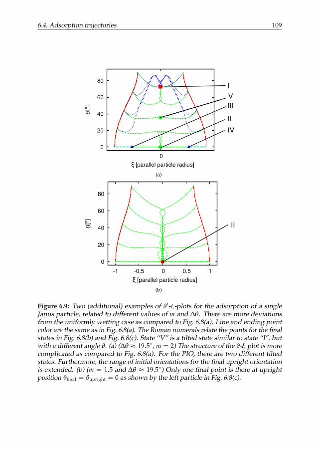
6.4. Adsorption trajectories 109
0
20
40
60
80
0
I
II
III
IV
V
[parallel particle radius]ξ
[]ϑ°
(a)
0
20
40
60
80
-1 -0.5 0 0.5 1
II
[parallel particle radius]ξ
[]ϑ°
(b)
Figure 6.9: Two (additional) examples of ϑ′-ξ-plots for the adsorption of a singleJanus particle, related to different values of m and ∆θ. There are more deviationsfrom the uniformly wetting case as compared to Fig. 6.8(a). Line and ending pointcolor are the same as in Fig. 6.8(a). The Roman numerals relate the points for the finalstates in Fig. 6.8(b) and Fig. 6.8(c). State “V” is a tilted state similar to state “I”, butwith a different angle ϑ. (a) (∆θ ≈ 19.5, m = 2) The structure of the ϑ-ξ plot is morecomplicated as compared to Fig. 6.8(a). For the PIO, there are two different tiltedstates. Furthermore, the range of initial orientations for the final upright orientationis extended. (b) (m = 1.5 and ∆θ ≈ 19.5) Only one final point is there at uprightposition ϑfinal = ϑupright = 0 as shown by the left particle in Fig. 6.8(c).

110 Adsorption of a single Janus particle to a fluid interface
adsorption process. The position is predicted from Eq. (6.37) ξunpr ≈ 5.78 · 10−1 andfrom the simulation results ξunpr = 6.22 · 10−1. All UIO trajectories of ϑ0 6= 180
end up in ξ = 0. Note that state “V” can be found in several regions in the m-∆θdiagram. It is shown in the calculations in section 6.3, that there is no region in them-∆θ diagram , where state “V” minimizes the free energy.
A fully Janus dominated case is shown in Fig. 6.9(b) for m = 1.5 and ∆θ ≈ 19.5.All studied trajectories end up in the upright orientation (state “II”). There is no tiltedstate found for any of the initial orientations. On the one hand, the anisotropy isso weak that the free energy gain due to the excluded interfacial area Aex for a finalorientation of ϑ > 0 is small. On the other hand, the Janus effect (∆θ) is strong enoughto force an orientation where each wetting area is in its preferred fluid.
In this section, three versions of ϑ-ξ plots for different sets of values of m and ∆θare shown. Figure 6.8(a) shows an example of shape domination and (at least for thePIO) similar to the case of the adsorption a particle with a homogeneous wettability.More deviations from the behavior as seen in the uniformly wetting case are foundin the two plots in Fig. 6.9. The plot in Fig. 6.9(a) exhibits a more complex structureof final states. Five final orientations are found, amongst them two tilted states withdifferent orientations. Fig. 6.9(b) shows an adsorption process which is dominatedcompletely by the Janus influence. The trajectories from all initial angles end up inthe upright orientation.
6.5 Conclusion
In this chapter, the adsorption of a single Janus particle to a flat fluid-fluid interfaceis studied. The focus is on the influence of the interplay between the geometryand the Janus effect. The final states of the particle at the fluid interface obtainedfrom the simulation are compared to the results from the free energy calculation.A simplified and fully analytical model, the “simplified Janus model”, is able topredict the simulation results within a specific range, but there are several limitations.The separation line between the areas which are dominated by the shape and theJanus effect, respectively, which is found in the “simplified Janus model” cannot bereproduced by the simulation results. The simulations show that there are differentfinal states, but they do not indicate the minimum of the free energy. Furthermore,the tilted orientation which is found in the simulation results is not included in the“simplified Janus model”. A better model for the free energy calculation is presentedin the second step. It takes into account the full rotation of the particle and thedeformability of the interface. It turns out that the equilibrium state determinedby the minimum of the free energy is a tilted orientation for large aspect ratios andsmall wettability differences, where the shape dominates. In case of small aspect ratioand large wettability difference, the Janus effect dominates and the particle is in anupright orientation. Thus, the equilibrium state of an ellipsoidal Janus particle ata fluid interface can be tuned by the choice of aspect ratio and wettability contrast.Furthermore, it is shown that the adsorption free energy decreases with a decreasingwettability contrast. The intensity of this decay is higher, if the wettability contrastis so large that the particle is in an upright orientation. Finally, it is shown that asymmetric, ellipsoidal Janus particle can have up to three metastable points whereas

6.5. Conclusion 111
the uniformly wetting counterpart has only one metastable point.

112 Adsorption of a single Janus particle to a fluid interface

Chapter 7
Janus particle ensembles at fluidinterfaces
Abstract
Particle laden fluid interfaces play an important role in different applications suchas the stabilization of emulsions. The interplay between the particle geometry andthe surface wettability contrast influences the collective behavior of an ensemble ofsymmetric, ellipsoidal Janus particles at a flat interface between two fluids. Therefore,the collective rotation of an ensemble of Janus particles adsorbed at a flat fluidinterface is studied for different values of the aspect ratio and the Janus parameter.This is one important step towards the understanding of the formation and theproperties of an emulsion stabilized by Janus particles with anisotropic shape. Theparticles are in an upright orientation at the beginning. Two types of rotation behaviorare found. The first type is the normal rotation, where the particles rotate towardsthe tilted state. If the aspect ratio and the wettability contrast are large enough, theparticle centers are pushed out of the interface. This slows down the flipping processconsiderably. In the extreme case, some particles are even expelled from the interface.In the end of the chapter, an outlook on emulsions stabilized by ellipsoidal Janusparticles is provided.
7.1 Introduction
In this section, we discuss the collective behavior of an ensemble of symmetric,parallel Janus particles at a flat fluid-fluid interface (see Fig. 6.1 for the definition ofa “Janus particle”). We investigate the influence of the interplay between the Januseffect and the particle geometry on the ensemble behavior.
This study is related to some of the previous parts of this thesis as follows: itis an extension of chapter 6, where the behavior of a single Janus particle at a flatinterface is studied and section 5.5, where an ensemble of uniformly wetting particlesis discussed. The adsorption of a single Janus particle turned out to be more complexthan the case of a uniformly wetting particle. This is depicted by the increased number
113

114 Janus particle ensembles at fluid interfaces
of possible ending points in the adsorption diagrams. Therefore, it can be expectedthat the collective behavior of an ensemble of Janus particles at a fluid interface isalso more complex as compared to an ensemble of uniformly wetting particles. It isalready discussed in chapter 5 for emulsions stabilized by uniformly wetting particlesthat the particle anisotropy leads to an additional time behavior of particle stabilizedemulsions in contrast to the case of a spherical particle shape. Model systems witha single or multiple particles at a fluid interface can explain this additional timebehavior. In this way, it can be expected that both, the adsorption of a single Janusparticle to a fluid interface from the previous chapter, and the behavior of an ensembleof Janus particles at a fluid interface discussed here improve our understanding ofemulsions stabilized by Janus particles. The question here is how the particle shapeand the Janus effect influence the collective rotation behavior of a Janus ensemble at aflat interface.
A recent overview of the behavior of Janus particle ensembles at a flat fluidinterface is provided in Ref. [63]. Several times, the capillary interaction between an-isotropic Janus particles at a flat fluid interface is studied [126, 147, 160]. In Ref. [160],the interaction between Janus ellipsoids at a flat, deformable fluid interface is cal-culated. Furthermore, it is found that a single Janus particle causes an interfacedeformation with hexapolar symmetry, if it is oriented in a tilted state and if no exter-nal field influences the particle. For Janus cylinders, a variety of assembly structuresis found [147]. Capillary interactions between spherical Janus particles can appearbecause of a diffuse boundary between the two wettability areas [146] or due to Janusparticles not being in their preferred orientation [159, 193]. An ensemble of Janusparticles at a spherical fluid interface is studied in Ref. [125]. Janus particles can beused to stabilize Pickering emulsions. The free energy is calculated for an emulsionstabilized by spherical Janus particles in Ref. [7]. The authors find that the Pickeringemulsion stabilized by Janus particles is thermodynamically stable if the wettabilitycontrast of the particles is sufficiently large.
7.2 An ensemble of Janus particles at a flat fluid inter-face
Here, we study a particle ensemble at a flat fluid interface. The particles are symmetri-cal and parallel Janus particles and have an ellipsoidal shape as shown in Fig. 6.1. Thesystem of interest is depicted in Fig. 7.1. They are characterized by the aspect ratio mand the Janus parameter ∆θ. For m = 2, the particle radii are given as R‖ = 12 andR⊥ = 6. For other aspect ratios, R‖ and R⊥ are changed in a way that the productR‖(m) · R⊥(m) stays constant. This implies that the interface area which the particleoccupies in an orientation parallel to the interface does not change for the differentaspect ratios. The simulations are performed for parameter ranges of 2 ≤ m ≤ 6and 0 ≤ ∆θ ≤ 24.4. The system size is 256∆x in each of the two directions parallelto the flat interface and 64∆x in the third direction. Then, the interfacial area inabsence of the particles is given as AI = 2562∆x2. In the beginning, the particlesare placed at the interface with an initial orientation of ϑ0 ≈ 179.4 in the “unpre-ferred initial orientation” (UIO, see definition in Fig. 6.2). This is the initial stateshown in the upper left snapshot in Fig. 7.1. In this orientation, each wetting area is

7.2. An ensemble of Janus particles at a flat fluid interface 115
Figure 7.1: Snapshot of an ensemble of Janus particles at a flat fluid-fluid interface(m = 2 and ∆θ = 24.4). Top left: side view of the initial state. All particles areoriented almost in the upright orientation. Each wetting area is in its unpreferredfluid. Bottom left: side view of the final state (after 40000 time steps). The particlesare oriented in a tilted orientation close to the parallel orientation. Right: top view ofthe final state (after 40000 time steps).
almost fully in contact with its unpreferred fluid, i.e. the hydrophobic region is incontact with the polar fluid and the hydrophilic region is in contact with the apolarfluid. In this way, a rotation of the particles should be induced. Np = 100 particlesare contained in the system. This corresponds to a coverage of the initial state ofχ = (Np Ap)/AI = (NpπR2
⊥)/AI ≈ 0.17 for m = 2. The azimuthal angle φ and theposition in the two directions parallel to the fluid interface of each particle are chosenrandomly. It is ensured that an overlap between the particles in avoided. The positionof each particle center in the direction orthogonal to the fluid interface is chosen suchthat the particle centers are at the same level as the fluid interface. Due to the missingup-down symmetry of the Janus particles and the resulting range of the polar angle(0 ≤ ϑ ≤ 180, discussed for Janus particles in chapter 6, see Fig. 6.2), the orderparameter S (used and defined in chapter 5 for the characterization of an ensemble ofuniformly wetting particles at a fluid interface) is not suitable to describe the system.Furthermore, ϑ′ used in the previous chapter is not suitable here since the particleorientation has to be fully resolved. Therefore, we track the average value of the polarangle ϑens(t) for all particles of the ensemble. It is defined as
ϑens(t) =1
Np
Np
∑i=1ϑi(t). (7.1)
ϑi is the orientation of particle i with respect to the interface.Figure 7.2 shows the time evolution of ϑens for different aspect ratios and the
following four Janus parameters: ∆θ = 0, ∆θ = 9.8, ∆θ = 19.5 and ∆θ = 24.4.The starting point in all cases is ϑens ≈ 179.4.

116 Janus particle ensembles at fluid interfaces
80
100
120
140
160
180
0 5000 10000 15000 20000
ϑe
ns[°
]
t [timesteps]
∆θ=0° ∆θ=9.8° ∆θ=19.5°
∆θ=24.4°
(a)
80
100
120
140
160
180
0 20000 40000 60000
ϑe
ns[°
]
t [timesteps]
∆θ=0° ∆θ=9.8° ∆θ=19.5°
∆θ=24.4°
(b)
Figure 7.2: Time evolution of the average orientation ϑens for different values of theJanus parameter ∆θ and aspect ratios (a) m = 2 and (b) m = 6.
Figure 7.2(a) depicts the situation the particles with an aspect ratio of m = 2. Inall examples, the particles flip from the upright orientation to a final orientation. Incase of vanishing Janus parameter, all particles are finally oriented in the parallelorientation ϑ = 90 with respect to the interface. The Janus particles end up in atilted orientation for the other values of ∆θ. The duration of the rotation processdecreases with increasing Janus parameter. This can be understood as follows: theforce which causes the particle to rotate increases with increasing wettability contrast.A dependence of the torque (defined in Eq. (4.17)) from the wetting contrast of a Janusparticle ∆θ can be obtained using Eq. (6.10) as
Dcap − Dcap,0 ∝ sin(∆θ). (7.2)

7.2. An ensemble of Janus particles at a flat fluid interface 117
Dcap is the torque for a given Janus parameter ∆θ and Dcap,0 is the reference valueof the torque for ∆θ = 0. The torque increases with increasing wettability contrast.Thereby, the rotation process is faster for larger values of the wettability contrast. Atypical rotation process is illustrated in Fig. 7.1. A side view of the initial state andthe final state are shown by the snapshot at the top and at the bottom of the left side,respectively. A top view of the final state is shown on the right side. The position ofthe particle centers in the direction normal to the interface stays constant during therotation process.
Figure 7.2(b) shows the time evolution of ϑens for m = 6. For the two lower valuesof ∆θ, there is a “direct rotation” process which is comparable to the one which isseen also for m = 2. “Direct rotation” denotes the fact that all particles rotate directlytowards the final orientation of the particles without delay. This is the expectedrotation behavior and also observed for the ensemble of uniformly wetting particlesin section 5.5. It is in agreement with Eq. (7.2) A different rotation behavior can beobserved for the upper two values of ∆θ. There is a delay in the collective rotation.This delay increases strongly with increasing ∆θ. For the largest value of ∆θ, therotation takes more time than the time period shown in the plot. This rotation type isreferred to in the following as “delayed rotation”.
The influence of the particle shape and the wetting contrast on the duration of therotation process te and the final average orientation ϑe are composed for the wholerange of m and ∆θ in both plots of Fig. 7.3. Figure 7.3(a) shows the time te which theaverage orientation ϑens needs to reach the final value. For a lower value of the aspectratio (m ≤ 4), a regular behavior can be found. te decreases, if the Janus parameter∆θ increases and it increases for an increasing aspect ratio. Note that it is difficult tocompare the process for different m directly as the coverage χ cannot have the samevalue for the different m in the whole range of possible particle orientations.
For m = 5 and small values of the Janus parameter ∆θ, the same behavior as form ≤ 4 can be observed. For m = 5 and large values of ∆θ as well as for m = 6, thebehavior is completely different. te increases with an increasing ∆θ. This increase ismuch stronger as compared to the decrease of te in the previous situation.
Figure 7.3(b) shows the behavior of ϑe, the final value of ϑens. The lines for allaspect ratios start at 90 for ∆θ = 0. This corresponds to the final parallel orientationwhich is found for uniformly wetting particles. For sufficiently small values of theaspect ratio (m ≤ 5), ϑe decreases for an increasing ∆θ. This decrease is strongestfor m = 2 and diminishes for an increasing aspect ratio. The same behavior can beobserved for m = 6 and small values of ∆θ. For m = 6 and large values of ∆θ, ϑeincreases.
In summary, both plots in Fig. 7.3 show that there is a complex dependence of theparticle rotation on the particle shape and the Janus parameter. It can be said thatthere are two different regimes in the particle rotation. The regimes have an impacton both dynamics and final state of the collective rotation. The first one is a “directrotation” regime. It can be found for sufficiently small values of the aspect ratio. Theparticles rotate until the tilted state is reached (as shown in Fig. 7.1) and the particlecenter does not move in the direction normal to the interface. The values of ϑe andte are determined by the interplay between the particle shape and the wettabilitycontrast in the following way: te decreases with increasing ∆θ and increases withincreasing m. This behavior is expected from free energy considerations (see Eq. (7.2)).

118 Janus particle ensembles at fluid interfaces
0
20
40
60
80
100
0 5 10 15 20 25
t e [
10
3 t
ime
ste
ps]
∆θ[°]
m=2m=3m=4m=5m=6
(a)
60
70
80
90
100
0 5 10 15 20 25
ϑe[°
]
∆θ[°]
m=2m=3m=4m=5m=6
(b)
Figure 7.3: (a) Time te needed to reach the final orientation. te decreases for increasing∆θ in the “direct rotation” regime (m ≤ 4 and m = 5 with a mall value of ∆θ). Aopposite behavior can be found in the “delayed rotation” (sufficiently large valuesof the Janus parameter and the aspect ratio), where te with increasing ∆θ. (b) Finalorientation ϑe (ϑe = ϑens(t) for t→ ∞). ϑe decreases for an increasing Janus parameter.There is an abnormal behavior for m = 6 and sufficiently large value of the Janusparameter.

7.2. An ensemble of Janus particles at a flat fluid interface 119
Figure 7.4: Snapshot of an ensemble of Janus particles at a flat fluid-fluid interface(m = 6 and ∆θ = 19.5) after 10000, 20000, 30000 and 40000 timesteps to understandthe “delayed rotation” regime in Fig. 7.2(b).
A second regime, the “delayed rotation”, is found for large values of the aspectratio and the Janus parameter. te is much larger compared to the previous regime.Furthermore, te increases with increasing ∆θ. This contradicts the expectation fromthe free energy consideration (see Eq. (7.2)) and indicates that the collective rotationprocess is more complex than in the “direct rotation” regime. In the following, we takea closer look at the rotation process in this regime. There, the particle rotation processtakes much longer and in the extreme case the average final orientation is differentfrom what is found in the first regime. Snapshots of the collective rotation processprovide a deeper insight in order to understand what happens during the rotationprocess in this regime. Figure 7.4 shows snapshots of the particle rotation process form = 6 and ∆θ = 19.5. A large number of particles is pushed away from the fluidinterface until they just touch the interface with the edge. Afterwards, most of theparticles or even all of them are slowly readsorbed to the fluid interface and rotate upto the tilted state. This procedure slows down the rotation process enormously.
In order to understand why particles are pushed away from the fluid interface,we study the early stage of the rotation process. Figure 7.5 shows snapshots of theparticle rotation process for m = 6 and ∆θ = 19.5 between 1000 and 6000 timesteps.At timesteps 2000 very few particles are already rotating. Their centers stay on thelevel oft the interface during the rotation process. As it is illustrated in Fig. 7.6, therotation of the few particles (Fig. 7.6(a)) leads to capillary shock waves. These shockwaves create a deflection of the Janus boundary of those of the particles which notyet started to rotate from the level of the fluid interface (Fig. 7.6(b)). This causes adisplacement of the center of these particles from the fluid interface. In the extremecase, one or few particles are even ejected completely from the interface. The motionof the particle center away from the interface can be understood by the free energyfunction as a function of the distance between the particle center and the flat interfacefor the upright orientation ϑ = 180 in the following way: each wetting area is in itsunpreferred fluid and the particle is close to this orientation. In the previous chapter,it is found that in this orientation there are two particle positions which minimize

120 Janus particle ensembles at fluid interfaces
Figure 7.5: Snapshot of an ensemble of Janus particles at a flat fluid-fluid interface(m = 6 and ∆θ = 19.5) in the initial phase of the rotation process. The snapshotsshow the positions of the particle ensemble after 1000, 2000, 3000, 4000, 5000 and 6000timesteps.
(a) (b)
Figure 7.6: Illustration of the situation which leads to the ejection of particles fromthe interface. (a) The particle is in the initial orientation at ϑ0 ≈ 179.4. This generatesa rotation of the particle until the particle reaches a final tilted orientation. Not allparticles start to rotate at the same time. (b) The particles which have not yet start torotate at a given time can be influenced by the rotating particles in the following way:If the rotation is strong enough, a deflection of the Janus boundary of those of theparticles which not yet started to rotate is created by capillary waves. These particleare pushed away from the interface or are even expelled completely.

7.3. Emulsions stabilized by Janus particles 121
the free energy where the center of the Janus particle is displaced by a distance ξunprabove or below the fluid interface. The position where the Janus boundary touchesthe interface is related to a maximum of the free energy with dF/dξ = 0. To leave thisposition, a small displacement from this position has to be induced. This is done bycapillary waves mentioned above. The displacement which minimizes the free energyis given by Eq. (6.37). For example, for the situation shown in Fig. 7.4 and Fig. 7.5(m = 6 and ∆θ = 19.5), the displacement is given as ξunpr ≈ 9.04 · 10−1 in units ofR‖. In this position, only the tip of the ellipsoid touches the interface. In the followingsnapshots in Fig. 7.5, it can be seen that more and more particles are ejected in thefollowing. In a later phase, most of the particles or even all of them are readsorbed.
Strong ordering effects of ellipsoidal particles with a magnetic moment at aflat fluid interface are found for the interplay between the magnetic field and theshape [43] and for the interplay between the magnetic field and the Janus effect [193].Such patterns are not found here for the following reason: we consider capillaryinteractions which have a position dependence of Ucap ∝ rβ. If an ellipsoidal particleis in a tilted orientation due to an external field, it causes a capillary deformation witha dipolar symmetry. This leads to an exponent of β = −2. In our system, the tiltedorientation of the ellipsoid without an external field causes an interface deformationwith a hexapolar symmetry and an exponent of β = −6. Therefore, the capillaryinteraction has a much shorter range in the system discussed here as compared to theother two examples.
7.3 Emulsions stabilized by Janus particles
To conclude the chapter, an outlook on emulsions stabilized by Janus particles isprovided. Here, we study the influence of the Janus effect on the formation of anemulsion. Fig. 7.7 shows a snapshot of an emulsion stabilized by Janus particles.
In section 5.3, we have studied the long term time evolution of the domain ordroplet size caused by the particle shape anisotropy. The properties such as thesystem size are defined there. The parameter of interest is the average domain sizeL(t) defined in Eq. (5.1) and Eq. (5.2). In order to investigate the influence of theJanus character on the formation of emulsions, we vary the Janus parameter ∆θ ofthe stabilizing particles.
Note that our simulation is limited with respect to the range of the Janus parameter,i.e. 0 ≤ ∆θ ≤ 5.48. The simulation becomes unstable for larger values whilesimulating the demixing process during emulsion formation. The forces and torques(see Eq. (7.2)) in the first timesteps of demixing for sufficiently large wettabilitycontrasts are too strong for having a stable simulation. In Ref. [7], it is found thatemulsions stabilized by Janus particles can be thermodynamically stable for values of∆θ which are sufficiently large. The range of values of ∆θ that can be achieved in oursimulation is not large enough to obtain thermodynamically stable emulsions. Fig. 7.8shows the long term time development of L(t) for a bijel with m = 2 for differentvalues of the Janus parameter: ∆θ = 2.74 and ∆θ = 5.48. Furthermore, the line forthe uniformly wetting case (∆θ = 0) is shown for comparison. There is just a smalldifference between these three lines. This means that there is no strong influence fromthe wettability difference of the stabilizing particles on the emulsion formation in

122 Janus particle ensembles at fluid interfaces
Figure 7.7: Snapshot of a Bijel after 400000 timesteps.
2.86
2.88
2.90
2.92
2.94
2.96
2.98
3.00
0 5 10 15 20 25 30 35 40
L [para
llel part
icle
radiu
s]
t [105 timesteps]
m=2, ∆θ=0° m=2, ∆θ=2.74°
m=2, ∆θ=5.48°
Figure 7.8: Long term time development of L(t) for a bijel with m = 2 for differentvalues of ∆θ.

7.4. Conclusion 123
the range of interest. However, there is a small decrease of L(t) with increasing ∆θ.The decrease of L(t) is related to an increase of the interfacial area stabilized by theparticles. In this way, there is a small tendency to increase the stabilizing efficiency ofthe Janus particles.
7.4 Conclusion
In this chapter, Janus particles at fluid interfaces are discussed. The first system ofinterest is an ensemble of Janus particles at a flat interface. The influence on theinterplay between the particle shape and the wettability contrast on the collectiverotation of the particles is studied. Generally, it is shown that the dependence of thecollective rotation on the particle shape and the wettability contrast is complex: therotation can be divided into two regimes with respect to m and ∆θ. In the “directrotation” regime the particles just rotate and the particle center constantly stays at theposition of the interface. The duration of the process and the final orientation dependon m and ∆θ as expected from the free energy considerations. In the second regime,the “delayed rotation”, the particle centers are pushed away from the interface andreadsorbed later. This slows down the adsorption process.
The chapter clauses with an outlook on emulsions stabilized by Janus particles. Asmall increase of the stabilization efficiency can be observed, if the wettability contrastincreases.
The next step in the study of emulsions stabilized by ellipsoidal Janus particlescan be the improvement of the simulation method in a way that larger wettabilitycontrasts can be simulated. Thermodynamically stable emulsions can be realized, ifthe wettability contrast is sufficiently large. Furthermore, also orthogonal Janus parti-cles are an interesting option as emulsion stabilizers because it is easier to minimizefree energy in the optimal orientation.

124 Janus particle ensembles at fluid interfaces
Chapter 8
Conclusion and outlook
Particle stabilized emulsions have been studied since the beginning of the last centuryand gained more attention in the last few decades. Most of the previous studiesare experimental. Few studies have been done by means of computer simulations.Computational studies may provide a deeper insight into the time dependent domainstructure of emulsions. The time evolution for domain sizes in the formation processis studied for spherical emulsion stabilizers [98]. Furthermore, some efforts havebeen made in the understanding of model systems with single particles or particleensembles at fluid interfaces. However, the understanding of these emulsions andmodel systems is still limited.
In the beginning of the thesis, the adsorption of a single ellipsoidal particle to a flatfluid interface is studied. The final state where the particle is oriented parallel to thefluid interface, is reproduced and thus, the simulation validated. By comparing oursimulation results with an approximation which neglects all hydrodynamical effects,we conclude that the deformation of the interface and generally hydrodynamicscannot be neglected for studying the adsorption process. The two important hydrody-namical effects for the system of interest are the drag force and the deformation of thefluid interface. It can be shown that the translational motion can be approximated bythe equation of the harmonic oscillator, with a harmonic potential obtained from thefree energy of the system and the damping constant from the drag force of the bulkfluid and the interface. However, the deformation of the interface causes a deviationof the particle adsorption from the exact behavior of the harmonic oscillator. Forcalculating the free energy, the influence of interfacial deformation on the interfacialareas has to be taken into account.
Related to emulsions stabilized by uniformly wetting particles, we investigate thedynamics of the formation of Pickering emulsions and bijels stabilized by ellipsoidalparticles as well as the influence of control parameters on the final emulsion type. Incontrast to emulsions stabilized by spherical particles, ellipsoidal particles cause theaverage time dependent droplet or domain size to slowly decrease even after verylong simulation times corresponding to several million timesteps. The additionaltimescales related to this effect are investigated by detailed studies of simple modelsystems. At first, the adsorption of single ellipsoidal particles is shown to happen
This text is partly based on Ref. [79].
125

126 Conclusion and outlook
on a comparably short timescale (≈ 104 timesteps). Second, particle ensembles atflat fluid-fluid interfaces, however, might require substantially more time in caseof sufficiently densely packed interfaces. Here, local reordering effects induced byhydrodynamic interactions and interface rearrangements prevent the system fromattaining a steady state and add a further timescale to the emulsion formation (≈ 105
timesteps). Third, this reordering is pronounced in the case of curved interfaceswhere the movement of the particles leads to interface deformations and capillaryinteractions. During the formation of an emulsion, droplets might coalesce (Pickeringemulsions) or domains might merge (bijels). After such an event, the particles at theinterface have to rearrange in order to adhere to the new interface structure. Due tothis, the local reordering is practically being “restarted” leading to an overall increaseof the interfacial area on a timescale of at least several 106 timesteps.
These findings provide relevant insight in the dynamics of emulsion formation,which is generally difficult to investigate experimentally due to the required hightemporal resolution of the measurement method and limited optical transparency ofthe experimental system. It is well known that in general particle-stabilized emulsionsare not thermodynamically stable and therefore the involved fluids will always phaseseparate – even if this might take several months. Anisotropic particles, however,provide properties, which might allow the generation of emulsions that are stableon substantially longer timescales. This is due to the continuous reordering of theparticles at liquid interfaces, which leads to an increase in interfacial area and as suchcounteracts the thermodynamically driven reduction of interface area.
After the discussion of homogeneous particles, we study Janus particles at fluidinterfaces. The wettability contrast at the particle surface improves the interfacialactivity. This can be a crucial factor for an improvement of the stabilization ofemulsions. The behavior of a single Janus particle at a flat fluid-fluid interfacedepends on the interplay between the particle shape and the wettability contrast. Thesimulation results of the adsorption of a single Janus particle to a flat fluid interfaceis compared with two different free energy models. It turns out that the full particlerotation and the interface deformation have to be taken into account. For weeklyanisotropic particles with a strong wettability contrast, the equilibrium orientationis an upright orientation with respect to the interface. For highly anisotropic Janusparticles, the equilibrium state is a tilted orientation. Furthermore, it is demonstratedthat a Janus particle at the interface can have up to three different final orientations.
The collective behavior of an ensemble of Janus particles at a flat fluid interfacedepending on particle shape and the wettability contrast is shown to be complex.Two types of a rotational behavior are found: the first one is the “direct rotation”. Theparticles rotate towards a tilted orientation and the particle centers do not move inthe direction normal to the interface. The influence of the wettability contrast is aspredicted from free energy considerations. This type is found for lower values of theaspect ratio. For larger values of the aspect ratio, a second type is found, the “delayedrotation”. The influence of the wettability contrast contradicts the predictions fromfree energy considerations which indicate a more complex rotation behavior. Some ofthe particle centers are pushed away from the interface and readsorbed later. Thisslows down the rotation process noticeably. In the end of the chapter, an outlook ofemulsions stabilized by Janus particles is provided. It is shown that the wettabilitycontrast has a small impact in the stabilization efficiency.

127
In summary, it is shown that particles with an anisotropic shape lead to an ad-ditional contribution to the time evolution of the emulsion formation. This can beunderstood by means of model systems and related to the particle orientation towardsthe interface as well as mutual orientation of the particles. This is a possible way toincrease the life time of particle stabilized emulsions. If a particle has an anisotropicshape and an inhomogeneous surface wettability the behavior of a single particle anda particle ensemble at the interface can be controlled by the interplay between aspectratio and wettability difference. Finally, it is demonstrated that hydrodynamics andespecially the interface deformability play an important role for the dynamics andthe final states of colloidal particles at the fluid interface.
There are different possibilities to continue the study of this thesis. The emulsionstabilizers in this thesis are colloidal particles interacting with a hard core potential(apart from hydrodynamic interactions). An interesting point is how other inter-particle potentials influence the different timescales of the emulsion formation. Possi-ble potentials are a screened Coulomb potential and a van der Waals potential. Thiscan include a different screening of the electrostatic Coulomb potential by differentfluid types (water and oil) for particles adsorbed at the fluid interface.
The investigations on Janus particles in this thesis are carried out with symmetricJanus particles. The next step can be a study of asymmetric Janus particles. Bothwetting areas can have a different size. Furthermore, the deviation of the contactangle of each wetting area from the neutrally wetting case can be generally different.It is shown for uniformly wetting particles that the optimal particle wettability forthe stabilization of a Pickering emulsion has a certain degree of preference for thecontinuous phase instead of a neutral wetting due to the curvature of the surface ofemulsion droplets. In the same way, it is interesting to see, if Janus particles with acertain degree of asymmetry are more efficient in stabilizing Pickering emulsions ascompared to symmetric Janus particles.
Another recommendation for future research is a study of the influence of the twotypes of rotation found for a Janus particle ensemble (as discussed in chapter 7) on theformation process of emulsions. It can be assumed that the second type of rotationhas an additional influence on the timescale there.

128 Conclusion and outlook

Bibliography
[1] P. Ahlrichs and B. Dunweg. Simulation of a single polymer chain in solution bycombining lattice Boltzmann and molecular dynamics. The Journal of ChemicalPhysics, 111(17):8225, 1999.
[2] C. Aidun, Y. Lu, and E. Ding. Direct analysis of particulate suspensions withinertia using the discrete Boltzmann equation. J. Fluid Mech., 373:287, 1998.
[3] S. Aland and A. Voigt. Simulation of common features and differences ofsurfactant-based and solid-stabilized emulsions. Colloids and Surfaces A: Physic-ochemical and Engineering Aspects, 413:298, 2012. 25th Meeting of the EuropeanColloid and Interface Society.
[4] R. Alargova, D. Warhadpande, V. Vesselin, and O. Velev. Foam superstabiliza-tion by polymer microrods. Langmuir, 20(24):10371, 2004.
[5] A. Amirfazli, S. Hanig, A. Muller, and A. W. Neumann. Measurements of linetension for solid-liquid-vapor systems using drop size dependence of contactangles and its correlation with solid-liquid interfacial tension. Langmuir, 16(4):2024, 2000.
[6] S. Arditty, C. Whitby, B. Binks, V. Schmitt, and F. Leal-Calderon. Some generalfeatures of limited coalescence in solid-stabilized emulsions. The EuropeanPhysical Journal E: Soft Matter and Biological Physics, 11:273, 2003.
[7] R. Aveyard. Can Janus particles give thermodynamically stable Pickeringemulsions? Soft Matter, 8:5233, 2012.
[8] R. Aveyard, J. Clint, D. Nees, , and N. Quirke. Structure and collapse of particlemonolayers under lateral pressure at the octane/aqueous surfactant solutioninterface. Langmuir, 16(23):8820, 2000.
[9] R. Aveyard, J. Clint, D. Nees, and N. Quirke. Structure and collapse of particlemonolayers under lateral pressure at the octane/aqueous surfactant solutioninterface. Langmuir, 16(23):8820, 2000.
[10] R. Aveyard, B. Binks, and J. Clint. Emulsions stabilised solely by colloidalparticles. Adv. Coll. Int. Sci., 100(0):503, 2003.
129

[11] M. Basavaraj, G. Fuller, J. Fransaer, and J. Vermant. Packing, flipping, andbuckling transitions in compressed monolayers of ellipsoidal latex particles.Langmuir, 22:6605, 2006.
[12] B. Berne and P. Pechukas. Gaussian model potentials for molecular interactions.J. Chem. Phys., 56:4213, 1972.
[13] P. Bhatnagar, E. Gross, and M. Krook. A model for collision processes in gases.I. Small amplitude processes in charged and neutral one-component systems.Phys. Rev., 94:511, 1954.
[14] B. Binks. Particles as surfactants-similarities and differences. Current Opinion inColloid & Interface Science, 7(1–2):21, 2002.
[15] B. Binks and J. Clint. Solid wettability from surface energy components: Rele-vance to Pickering emulsions. Langmuir, 18(4):1270, 2002.
[16] B. Binks and P. Fletcher. Particles adsorbed at the oil-water interface: A theo-retical comparison between spheres of uniform wettability and Janus particles.Langmuir, 17:4708, 2001.
[17] B. Binks and T. Horozov. Colloidal Particles at Liquid Interfaces. CambridgeUniversity Press, August 2008. ISBN 0521071313.
[18] C. Blanc, D. Fedorenko, M. Gross, M. In, M. Abkarian, Mohamed A. Gharbi,J. Fournier, P. Galatola, and M. Nobili. Capillary force on a micrometric spheretrapped at a fluid interface exhibiting arbitrary curvature gradients. Phys. Rev.Lett., 111:058302, 2013.
[19] J. Bleibel, S. Dietrich, A. Domınguez, and M. Oettel. Shock waves in capillarycollapse of colloids: a model system for two-dimensional screened Newtoniangravity. Phys. Rev. Lett., 107:128302, 2011.
[20] J. Bleibel, A. Domınguez, and M. Oettel. Colloidal particles at fluid interfaces:Effective interactions, dynamics and a gravitation–like instability. The EuropeanPhysical Journal Special Topics, 222(11):3071, 2013.
[21] J. Bleibel, A. Domınguez, F. Gunther, J. Harting, and M. Oettel. Hydrodynamicinteractions induce anomalous diffusion under partial confinement. Soft Matter,10:2945, 2014.
[22] S. Bogner, U. Rude, and J. Harting. Curvature estimation from a volume offluid indicator function for the simulation of surface tension and wetting witha free surface lattice Boltzmann method. Physical Review E, in press, 2016.
[23] S. Bogner, U. Rude, and J. Harting. Curvature estimation from a volume-of-fluid indicator function for the simulation of surface tension and wetting witha free-surface lattice boltzmann method. Phys. Rev. E, 93:043302, 2016.
[24] L. Botto, E. Lewandowski, M. Cavallaro, and K. Stebe. Capillary interactionsbetween anisotropic particles. Soft Matter, 8:9957, 2012.

[25] K. Bouchemal, S. Briancon, E. Perrier, and H. Fessi. Nano-emulsion formulationusing spontaneous emulsification: solvent, oil and surfactant optimisation.International Journal of Pharmaceutics, 280(1–2):241, 2004.
[26] F. Bresme and J. Faraudo. Orientational transitions of anisotropic nanoparticlesat liquid–liquid interfaces. Journal of Physics: Condensed Matter, 19(37):375110,2007.
[27] F. Bresme and M. Oettel. Nanoparticles at fluid interfaces. Journal of Physics:Condensed Matter, 19(41):413101, 2007.
[28] T. Brugarolas, B. Park, M. Lee, and D. Lee. Generation of amphiphilic Janusbubbles and their behavior at an air–water interface. Advanced FunctionalMaterials, 21(20):3924, 2011.
[29] S. Cappelli, Q. Xie, J. Harting, A. M. Jong, and M. W. J. Prins. Dynamic wetting:status and prospective of single particle based experiments and simulations.New Biotechnology, 32:420, 2015.
[30] J. Carmack and P. Millett. Numerical simulations of bijel morphology in thinfilms with complete surface wetting. The Journal of Chemical Physics, 143(15):154701, 2015.
[31] C. Casagrande, P. Fabre, E. Raphael, and M. Veyssie. ”Janus beads”: Realizationand behaviour at water/oil interfaces. Europhys. Lett., 9(3):251, 1989.
[32] M. Cates and P. Clegg. Bijels: a new class of soft materials. Soft Matter, 4:2132,2008.
[33] S. Chen and G. Doolen. Lattice Boltzmann method for fluid flows. Annu. Rev.Fluid Mech., 30:329, 1998.
[34] Y. Chevalier and M. Bolzinger. Emulsions stabilized with solid nanoparticles:Pickering emulsions. Colloids and Surfaces A: Physicochemical and EngineeringAspects, 439:23, 2013.
[35] Y. Choi and P. Anderson. Cahn–hilliard modeling of particles suspended intwo-phase flows. INTERNATIONAL JOURNAL FOR NUMERICAL METHODSIN FLUIDS, 69:995, 2011.
[36] P. Clegg, E. Herzig, A. Schofield, S. Egelhaaf, T. Horozov, B. Binks, M. Cates, andW. Poon. Emulsification of partially miscible liquids using colloidal particles:Nonspherical and extended domain structures. Langmuir, 23(11):5984, 2007.
[37] P. Collings, B. Ratna, and R. Shashidhar. Order parameter measurementsof dichroic dyes dissolved in smectic liquid crystals that tilt without layercontraction. Phys. Rev. E, 67:021705, 2003.
[38] C. Colosqui, J. Morris, and J. Koplik. Colloidal adsorption at fluid interfaces:regime crossover from fast relaxation to physical aging. Phys. Rev. Lett., 111:028302, 2013.

[39] K. Connington and T. Lee. A review of spurious currents in the lattice Boltz-mann method for multiphase flows. Journal of Mechanical Science and Technology,26(12):3857, 2012.
[40] J. Cuesta and D. Frenkel. Monte Carlo simulation of two-dimensional hardellipses. Phys. Rev. A, 42:2126, 1990.
[41] L. Dai, S. Tarimala, C.-Y. Wu, S. Guttula, and J. Wu. The structure and dynamicsof microparticles at Pickering emulsion interfaces. Scanning, 30:87, 2008.
[42] G. Davies, T. Kruger, P. Coveney, and J. Harting. Detachment energies ofspheroidal particles from fluid-fluid interfaces. The Journal of Chemical Physics,141(15):154902, 2014.
[43] G. Davies, T. Kruger, P. Coveney, J. Harting, and F. Bresme. Assembling ellip-soidal particles at fluid interfaces using switchable dipolar capillary interactions.Advanced Materials, 26(39):6715, 2014.
[44] G. Davies, T. Kruger, P. Coveney, J. Harting, and F. Bresme. Interface deforma-tions affect the orientation transition of magnetic ellipsoidal particles adsorbedat fluid-fluid interfaces. Soft Matter, 10:6742, 2014.
[45] J. de Folter, M. van Ruijven, and K. Velikov. Oil-in-water Pickering emulsionsstabilized by colloidal particles from the water-insoluble protein zein. SoftMatter, 8:6807, 2012.
[46] J. de Folter, E. Hutter, S. Castillo, Kira E. Klop, A. Philipse, and W. Kegel. Particleshape anisotropy in Pickering emulsions: cubes and peanuts. Langmuir, 30(4):955, 2014.
[47] Pierre-Gilles de Gennes. Soft matter (nobel lecture). Angewandte Chemie Interna-tional Edition in English, 31(7):842–845, 1992.
[48] J. de Graaf, M. Dijkstra, and R. van Roij. Adsorption trajectories and free-energyseparatrices for colloidal particles in contact with a liquid-liquid interface. J.Chem. Phys., 132(16):164902, 2010.
[49] B. Derjaguin and L. Landau. Theory of the stability of strongly charged lyopho-bic sols and of the adhesion of strongly charged particles in solutions of elec-trolytes. Acta Physico Chemica URSS, 14:633, 1941.
[50] M. Destribats, V. Schmitt, and R. Backov. Thermostimulable wax@sio2 core-shellparticles. Langmuir, 26(3):1734, 2010.
[51] M. Destribats, V. Lapeyre, E. Sellier, F. Leal-Calderon, V. Ravaine, and V. Schmitt.Origin and control of adhesion between emulsion drops stabilized by thermallysensitive soft colloidal particles. Langmuir, 28(8):3744, 2012.
[52] M. Destribats, M. Rouvet, C. Gehin-Delval, C. Schmitt, and Bernard P. Binks.Emulsions stabilised by whey protein microgel particles: towards food-gradePickering emulsions. Soft Matter, 10:6941, 2014.

[53] E. Dickinson. Food emulsions and foams: Stabilization by particles. Cur. Opin.Colloid Interface Sci., 15(1–2):40, 2010.
[54] E. Dickinson. Use of nanoparticles and microparticles in the formation andstabilization of food emulsions. Trends in Food Science & Technology, 24(1):4,2012.
[55] A. Dinsmore. Colloids: A useful boundary. Nature Materials, 6:921, 2007.
[56] A. Donev, I. Cisse, D. Sachs, E. Variano, F. Stillinger, R. Connelly, S. Torquato,and P. Chaikin. Improving the density of jammed disordered packings usingellipsoids. Science, 303(5660):990, 2004.
[57] L. Dong and D. Johnson. Adsorption of Acicular particles at liquid-fluid inter-faces and the influence of the line tension. Langmuir, 21:3838, 2005.
[58] A. Dorr, S. Hardt, H. Masoud, and H. Stone. Drag and diffusion coefficients ofa spherical particle attached to a fluid–fluid interface. 790:607, 2016.
[59] D. Ershov, J. Sprakel, J. Appel, M. Cohen Stuart, and J. van der Gucht.Capillarity-induced ordering of spherical colloids on an interface with an-isotropic curvature. 110:9220, 2013.
[60] H. Fan and A. Striolo. Mechanistic study of droplets coalescence in Pickeringemulsions. Soft Matter, 8:9533, 2012.
[61] J. Faraudo and F. Bresme. Stability of particles adsorbed at liquid/fluid inter-faces: Shape effects induced by line tension. The Journal of Chemical Physics, 118:6518, 2003.
[62] M. Fernandez-Rodriguez, M. Rodriguez-Valverde, M. Cabrerizo-Vilchez, andR. Hidalgo-Alvarez. Surface activity and collective behaviour of colloidallystable Janus-like particles at the air-water interface. Soft Matter, 10:3471, 2014.
[63] M. Fernandez-Rodriguez, M. Rodriguez-Valverde, M. Cabrerizo-Vilchez, andR. Hidalgo-Alvarez. Surface activity of Janus particles adsorbed at fluid–fluidinterfaces: Theoretical and experimental aspects. Advances in Colloid and InterfaceScience, 233:240, 2016.
[64] A. Fortini. Clustering and gelation of hard spheres induced by the Pickeringeffect. Phys. Rev. E, 85:040401, 2012.
[65] J. Frelichowska, M. Bolzinger, J. Pelletier, J. Valour, and Y. Chevalier. Topicaldelivery of lipophilic drugs from o/w Pickering emulsions. International Journalof Pharmaceutics, 371(1–2):56 – 63, 2009.
[66] S. Frijters and J. Harting. Self-assembled porous media from particle-stabilizedemulsions. Submitted for publication, 2016.
[67] S. Frijters, F. Gunther, and J. Harting. Effects of nanoparticles and surfactant ondroplets in shear flow. Soft Matter, 8:6542, 2012.

[68] S. Frijters, F. Gunther, and J. Harting. Domain and droplet sizes in emulsionsstabilized by colloidal particles. Physical Review E, 90:042307, 2014.
[69] S. Fujii, E. read, Binks b., and S. Armes. Stimulus-responsive emulsifiers basedon nanocomposite microgel particles. Advanced Materials, 17(8):1014–1018, 2005.
[70] S. Fujii, S. Armes, B. Binks, and R. Murakami. Stimulus-responsive particulateemulsifiers based on lightly cross-linked poly(4-vinylpyridine)-silica nanocom-posite microgels. Langmuir, 22(16):6818, 2006.
[71] F. Gautier, M. Destribats, R. Perrier-Cornet, J. Dechezelles, J. Giermanska,V. Heroguez, S. Ravaine, F. Leal-Calderon, and V. Schmitt. Pickering emul-sions with stimulable particles: from highly- to weakly-covered interfaces. Phys.Chem. Chem. Phys., 9:6455, 2007.
[72] G. Gillies, M. Kappl, and H. Butt. Direct measurements of particle–bubbleinteractions. Advances in Colloid and Interface Science, 114–115:165, 2005.
[73] G. Gompper, T. Ihle, D. M. Kroll, and R. G. Winkler. Advanced Computer Sim-ulation Approaches for Soft Matter Sciences III, chapter Multi-Particle CollisionDynamics: A Particle-Based Mesoscale Simulation Approach to the Hydro-dynamics of Complex Fluids, pages 1–87. Springer Berlin Heidelberg, Berlin,Heidelberg, 2009. ISBN 978-3-540-87706-6.
[74] D. Groen, O. Henrich, F. Janoschek, P. Coveney, and J. Harting. Lattice-Boltzmann methods in fluid dynamics: turbulence and complex colloidal fluids.In Wolfgang Frings Bernd Mohr, editor, Julich Blue Gene/P Extreme Scaling Work-shop 2011, page 17. Julich Supercomputing Centre, 52425 Julich, Germany, 2011.
[75] J. Guevara, A. Mejia, M. Shuai, Y. Chang, M. Mannan, and Z. Cheng. Stabiliza-tion of Pickering foams by high-aspect-ratio nano-sheets. Soft Matter, 9:1327,2013.
[76] A. Gunstensen, D. Rothman, S. Zaleski, and G. Zanetti. Lattice Boltzmannmodel of immiscible fluids. Phys. Rev. A, 43:4320, 1991.
[77] F. Gunther, J. de Graaf, M. Dijkstra, R. van Rooy, S. Frijters, and J. Harting.Dynamics of the adsorption of a uniformly wetting ellipsoid to a fluid-fluidinterface. To be published.
[78] F. Gunther, F. Janoschek, S. Frijters, and J. Harting. Lattice Boltzmann sim-ulations of anisotropic particles at liquid interfaces. Comp. Fluids, 80(0):184,2013.
[79] F. Gunther, S. Frijters, and J. Harting. Timescales of emulsion formation causedby anisotropic particles. Soft Matter, 10:4977, 2014.
[80] J. Guzowski, M. Tasinkevych, and S. Dietrich. Free energy of colloidal particlesat the surface of sessile drops. The European Physical Journal E, 33(3):219–242,2010. ISSN 1292-8941.

[81] J. Guzowski, M. Tasinkevych, and S. Dietrich. Capillary interactions in Pickeringemulsions. Phys. Rev. E, 84:031401, 2011.
[82] A. Hadjiiski, R. Dimova, N. Denkov, I. Ivanov, , and R. Borwankar. Filmtrapping technique: Precise method for three-phase contact angle determinationof solid and fluid particles of micrometer size. Langmuir, 12(26):6665, 1996.
[83] Y. Han, A. Alsayed, M. Nobili, J. Zhang, T. Lubensky, and A. Yodh. Brownianmotion of an ellipsoid. Science, 314(5799):626, 2006.
[84] Dieter Hanel. Molekulare Gasdynamik:. Springer, 2004. ISBN 9783540442479.
[85] J. Harting, J. Chin, M. Venturoli, and P. Coveney. Large-scale lattice Boltzmannsimulations of complex fluids: advances through the advent of computationalgrids. Philosophical Transactions of the Royal Society of London A: Mathematical,Physical and Engineering Sciences, 363(1833):1895, 2005.
[86] X. He and G. Doolen. Thermodynamic foundations of kinetic theory and latticeBoltzmann models for multiphase flows. Journal of Statistical Physics, 107(1-2):309, 2002.
[87] X. He and L. Luo. Theory of the lattice Boltzmann method: From the Boltzmannequation to the lattice Boltzmann equation. Phys. Rev. E, 56:6811, 1997.
[88] X. He, X. Shan, and G. Doolen. Discrete Boltzmann equation model for nonidealgases. Phys. Rev. E, 57:R13, 1998.
[89] M. Hecht, J. Harting, T. Ihle, and H. Herrmann. Simulation of claylike colloids.Phys. Rev. E, 72:011408, 2005.
[90] H. Hertz. Uber die Beruhrung fester elastischer Korper. Journal fur reine undangewandte Mathematik, 92:156, 1881.
[91] E. Herzig, K. White, A. Schofield, W. Poon, and P. Clegg. Bicontinuous emul-sions stabilized solely by colloidal particles. Nature Materials, 6:966, 2007.
[92] Y. Hirose, S. Komura, and Y. Nonomura. Adsorption of Janus particles tocurved interfaces. The Journal of Chemical Physics, 127(5):054707, 2007.
[93] M. Hore and M. Laradji. Microphase separation induced by interfacial segre-gation of isotropic, spherical nanoparticles. The Journal of Chemical Physics, 126(24):244903, 2007.
[94] T. Horozov, D. Braz, P. Fletcher, B. Binks, and J. Clint. Novel film-callipermethod of measuring the contact angle of colloidal particles at liquid interfaces.Langmuir, 24(5):1678, 2008.
[95] T. Hunter, R. Pugh, G. Franks, and G. Jameson. The role of particles in stabilisingfoams and emulsions. Advances in Colloid and Interface Science, 137(2):57, 2008.
[96] N. Jaensson, M. Hulsen, and P. Anderson. Stokes–Cahn–Hilliard formulationsand simulations of two-phase flows with suspended rigid particles. Computers& Fluids, 111:1, 2015.

[97] F. Janoschek, F. Toschi, and J. Harting. Simplified particulate model for coarse-grained hemodynamics simulations. Phys. Rev. E, 82:056710, 2010.
[98] F. Jansen and J. Harting. From bijels to Pickering emulsions: A lattice Boltzmannstudy. Phys. Rev. E, 83:046707, 2011.
[99] C. Janßen and M. Krafczyk. A lattice Boltzmann approach for free-surface-flowsimulations on non-uniform block-structured grids. Computers & Mathematicswith Applications, 59(7):2215, 2010.
[100] C. Janßen, S. Grilli, and M. Krafczyk. On enhanced non-linear free surfaceflow simulations with a hybrid lbm-vof model. Computers & Mathematics withApplications, 65(2):211, 2013.
[101] A. Joshi and Y. Sun. Numerical simulation of colloidal drop deposition dy-namics on patterned substrates for printable electronics fabrication. Journal ofDisplay Technology, 6(11):579, 2010.
[102] I. Kalashnikova, H. Bizot, P. Bertoncini, B. Cathala, and I. Capron. Cellulosicnanorods of various aspect ratios for oil in water Pickering emulsions. SoftMatter, 9:952, 2013.
[103] B. Kaoui, J. Harting, and C. Misbah. Two-dimensional vesicle dynamics undershear flow: Effect of confinement. Phys. Rev. E, 83:066319, 2011.
[104] G. Kaptay. On the equation of the maximum capillary pressure induced bysolid particles to stabilize emulsions and foams and on the emulsion stability di-agrams. Colloids and Surfaces A: Physicochemical and Engineering Aspects, 282–283:387, 2006.
[105] W. Kegel and J. Groenewold. Scenario for equilibrium solid-stabilized emul-sions. Phys. Rev. E, 80:030401, 2009.
[106] E. Kim, K. Stratford, R. Adhikari, and M.E. Cates. Arrest of fluid demixing bynanoparticles: A computer simulation study. Langmuir, 24:6549, 2008.
[107] E. Kim, K. Stratford, and M. Cates. Bijels containing magnetic particles: Asimulation study. Langmuir, 26(11):7928, 2010.
[108] C. Korner, M. Thies, T. Hofmann, N. Thurey, and U. Rude. Lattice Boltzmannmodel for free surface flow for modeling foaming. Journal of Statistical Physics,121(1):179.
[109] P. Kralchevsky and K. Nagayama. Capillary interactions between particlesbound to interfaces, liquid films and biomembranes. Advances in Colloid andInterface Science, 85(2–3):145, 2000.
[110] S. Kralj, S. Zumer, and D. Allender. Nematic-isotropic phase transition in aliquid-crystal droplet. Phys. Rev. A, 43:2943, 1991.
[111] T. Kruger, S. Frijters, F. Gunther, B. Kaoui, and J. Harting. Numerical simulationsof complex fluid-fluid interface dynamics. The European Physical Journal SpecialTopics, 222(1):177, 2013.

[112] A. Kumar, B. Park, F. Tu, and D. Lee. Amphiphilic Janus particles at fluidinterfaces. Soft Matter, 9:6604, 2013.
[113] A. Ladd. Numerical simulations of particulate suspensions via a discretizedBoltzmann equation. Part I. Theoretical foundation. J. Fluid Mech., 271:285, 1994.
[114] A. Ladd. Numerical simulations of particulate suspensions via a discretizedBoltzmann equation. Part II. Numerical results. J. Fluid Mech., 271:311, 1994.
[115] A. Ladd and R. Verberg. Lattice-Boltzmann simulations of particle-fluid sus-pensions. J. Stat. Phys., 104:1191, 2001.
[116] M. Lee and A. Mohraz. Bicontinuous macroporous materials from bijel tem-plates. Advanced Materials, 22(43):4836, 2010.
[117] T. Lee and P. Fischer. Eliminating parasitic currents in the lattice Boltzmannequation method for nonideal gases. Phys. Rev. E, 74:046709, 2006.
[118] H. Lehle, E. Noruzifar, and M. Oettel. Ellipsoidal particles at fluid interfaces.The European Physical Journal E: Soft Matter and Biological Physics, 26:151, 2008.
[119] E. Lewandowski, P. Searson, and K. Stebe. Orientation of a nanocylinder at afluid interface. The Journal of Physical Chemistry B, 110(9):4283, 2006.
[120] Q. Li, K. Luo, and X. Li. Forcing scheme in pseudopotential lattice Boltzmannmodel for multiphase flows. Phys. Rev. E, 86:016709, 2012.
[121] S. Lishchuk, C. Care, and I. Halliday. Lattice Boltzmann algorithm for surfacetension with greatly reduced microcurrents. Phys. Rev. E, 67:036701, 2003.
[122] H. Liu, Q. Kang, C. Leonardi, S. Schmieschek, A. Narvaez, B. Jones, J. Williams,A. Valocchi, and J. Harting. Multiphase lattice Boltzmann simulations forporous media applications. Computational Geosciences, 20(4):777, 2016.
[123] L. Liu, M. Ren, and W. Yang. Preparation of polymeric Janus particles bydirectional uv-induced reactions. Langmuir, 25(18):11048, 2009.
[124] J. Loudet, A. Alsayed, J. Zhang, and A. Yodh. Capillary interactions betweenanisotropic colloidal particles. Phys. Rev. Lett., 94:018301, 2005.
[125] X. Luu and A. Striolo. Ellipsoidal Janus nanoparticles assembled at sphericaloil/water interfaces. The Journal of Physical Chemistry B, 118(47):13737, 2014.
[126] X. Luu, J. Yu, and A. Striolo. Ellipsoidal Janus nanoparticles adsorbed at thewater-oil interface: Some evidence of emergent behavior. The Journal of PhysicalChemistry B, 117(44):13922, 2013.
[127] F. Mackay and C. Denniston. Coupling MD particles to a lattice-Boltzmannfluid through the use of conservative forces. Journal of Computational Physics,237(0):289, 2013.
[128] B. Madivala, J. Fransaer, and J. Vermant. Self-assembly and rheology of ellip-soidal particles at interfaces. Langmuir, 25(5):2718, 2009.

[129] B. Madivala, S. Vandebril, J. Fransaer, and J. Vermant. Exploiting particle shapein solid stabilized emulsions. Soft Matter, 5:1717, 2009.
[130] G. Madras and B. McCoy. Transition from nucleation and growth to Ostwaldripening. Chemical Engineering Science, 57(18):3809, 2002.
[131] A. Maestro, E. Guzman, F. Ortega, and R. Rubio. Contact angle of micro- andnanoparticles at fluid interfaces. Current Opinion in Colloid & Interface Science,19(4):355, 2014.
[132] A. Maiti and S. McGrother. Bead–bead interaction parameters in dissipativeparticle dynamics: Relation to bead-size, solubility parameter, and surfacetension. The Journal of Chemical Physics, 120(3):1594, 2004.
[133] D. McClements. Nanoemulsions versus microemulsions: terminology, differ-ences, and similarities. Soft Matter, 8:1719, 2012.
[134] S. Melle, M. Lask, and G.G. Fuller. Pickering emulsions with controllablestability. Langmuir, 21(6):2158, 2005.
[135] A. Morgan, N. Ballard, L. Rochford, G. Nurumbetov, T. Skelhon, and S. Bon.Understanding the multiple orientations of isolated superellipsoidal hematiteparticles at the oil-water interface. Soft Matter, 9:487, 2013.
[136] G. Morris, K. Hadler, and J. Cilliers. Particles in thin liquid films and at inter-faces. Current Opinion in Colloid & Interface Science, 20(2):98, 2015.
[137] B. Newton, K. Brakke, and D. Buzza. Influence of magnetic field on the orien-tation of anisotropic magnetic particles at liquid interfaces. Phys. Chem. Chem.Phys., 16:26051, 2014.
[138] T. Ngai and S. Bon, editors. Particle-Stabilized Emulsions and Colloids. RSC SoftMatter Series. The Royal Society of Chemistry, 2015. ISBN 978-1-84973-881-1.
[139] Y. Nonomura, S. Komura, , and K. Tsujii. Adsorption of disk-shaped janusbeads at liquid-liquid interfaces. Langmuir, 20(26):11821, 2004.
[140] B. O’Donnell and B. Helenbrook. Drag on ellipsoids at finite reynolds numbers.Atomization and Sprays, 15(4):363, 2005.
[141] M. Oettel and S. Dietrich. Colloidal interactions at fluid interfaces. Langmuir,24(4):1425, 2008.
[142] M. Oettel, A. Domınguez, and S. Dietrich. Attractions between charged colloidsat water interfaces. Journal of Physics: Condensed Matter, 17(32):L337, 2005.
[143] E. Orlandini, M. Swift, and J. Yeomans. A lattice Boltzmann model of binary-fluid mixtures. Europhys. Lett., 32(6):463, 1995.
[144] B. Park and D. Lee. Configuration of nonspherical amphiphilic particles at afluid-fluid interface. Soft Matter, 8:7690, 2012.

[145] B. Park and D. Lee. Equilibrium orientation of nonspherical Janus particles atfluid–fluid interfaces. ACS Nano, 6(1):782, 2012.
[146] B. Park, T. Brugarolas, and D. Lee. Janus particles at an oil-water interface. SoftMatter, 7:6413, 2011.
[147] B. Park, C. Choi, S. Kang, K. Tettey, C. Lee, and D. Lee. Geometrically andchemically anisotropic particles at an oil-water interface. Soft Matter, 9:3383,2013.
[148] V. Paunov. Novel method for determining the three-phase contact angle ofcolloid particles adsorbed at air-water and oil-water interfaces. Langmuir, 19(19):7970, 2003.
[149] F. Perrin. Mouvement brownien d’un ellipsoide - I. dispersion dielectrique pourdes molecules ellipsoidales. Le Journal de Physique et le Radium, 5(1):32, 1934.
[150] C. Peskin. The immersed boundary method. Acta Numerica, 11:479, 1 2002.
[151] R. Pichot, F. Spyropoulos, and I. Norton. O/W emulsions stabilised by bothlow molecular weight surfactants and colloidal particles: the effect of surfactanttype and concentration. Journal of Colloid and Interface Science, 352(1):128, 2010.
[152] S. Pickering. Emulsions. J. Chem. Soc., Trans., 91:2001, 1907.
[153] P. Pieranski. Two-dimensional interfacial colloidal crystals. Phys. Rev. Lett., 45:569, 1980.
[154] O. Pitois and X. Chateau. Small particle at a fluid interface: effect of contactangle hysteresis on force and work of detachment. Langmuir, 18(25):9751, 2002.
[155] Y. Qian, D. D’Humieres, and P. Lallemand. Lattice BGK models for Navier-Stokes equation. Europhys. Lett., 17:479, February 1992.
[156] W. Ramsden. Separation of solids in the surface-layers of solutions and ‘sus-pensions’. Proceedings of the Royal Society of London, 72:156, 1903.
[157] M. Rayner, D. Marku, M. Eriksson, M. Sjoo, P. Dejmek, and M. Wahlgren.Biomass-based particles for the formulation of Pickering type emulsions in foodand topical applications. Colloids and Surfaces A: Physicochemical and EngineeringAspects, 458:48 – 62, 2014.
[158] S. Razavi, I. Kretzschmar, J. Koplik, and C. Colosqui. Nanoparticles at liquidinterfaces: Rotational dynamics and angular locking. The Journal of ChemicalPhysics, 140(1):014904, 2014.
[159] H. Rezvantalab and S. Shojaei-Zadeh. Capillary interactions between sphericalJanus particles at liquid-fluid interfaces. Soft Matter, 9:3640, 2013.
[160] H. Rezvantalab and S. Shojaei-Zadeh. Role of geometry and amphiphilicity oncapillary-induced interactions between anisotropic Janus particles. Langmuir,29(48):14962, 2013.

[161] S. Sacanna, W. Kegel, and A. Philipse. Thermodynamically stable Pickeringemulsions. Phys. Rev. Lett., 98:158301, 2007.
[162] L. Sagis. Dynamic properties of interfaces in soft matter: Experiments andtheory. Rev. Mod. Phys., 83:1367, 2011.
[163] L. Sagis, editor. Microencapsulation and Microspheres. Academic Press, 2015.ISBN 978-0128003503.
[164] C. Sagui, D. O’Gorman, and M. Grant. Phase separation: from the initial nucle-ation stage to the final Ostwald ripening regime. In Symposium P – Science andTechnology of Semiconductor Surface Preparation, volume 481 of MRS Proceedings,1997.
[165] J. Salari, G. Mutsaers, J. Meuldijk, and B. Klumperman. Deformation of thewater/oil interface during the adsorption of sterically stabilized particles. Lang-muir, 30(25):7327, 2014.
[166] S. Schmieschek, A. Narvaez, and J. Harting. Multi relaxation time latticeBoltzmann simulations of multiple component fluid flows in porous media.page 39, 2013.
[167] S. Schmieschek, L. Shamardin, S. Frijters, T. Kruger, U. Schiller, J. Harting,and P. Coveney. Lb3d: A parallel implementation of the lattice-Boltzmannmethod for simulation of interacting amphiphilic fluids. Computer PhysicsCommunications, 217:149, 2017.
[168] R. Sear. Nucleation: theory and applications to protein solutions and colloidalsuspensions. Journal of Physics: Condensed Matter, 19(3):033101, 2007.
[169] X. Shan and H. Chen. Lattice Boltzmann model for simulating flows withmultiple phases and components. Phys. Rev. E, 47:1815, 1993.
[170] T. Sharma, G. Kumar, and J. Sangwai. Enhanced oil recovery using oil-in-water (o/w) emulsion stabilized by nanoparticle, surfactant and polymer in thepresence of NaCl. Geosystem Engineering, 17(3):195, 2014.
[171] E. Sharp, H. Al-Shehri, T. Horozov, S. Stoyanov, and V. Paunov. Adsorption ofshape-anisotropic and porous particles at the air-water and the decane-waterinterface studied by the gel trapping technique. RSC Adv., 4:2205, 2014.
[172] T. Skelhon, N. Grossiord, A. Morgan, and S. Bon. Quiescent water-in-oil Picker-ing emulsions as a route toward healthier fruit juice infused chocolate confec-tionary. J. Mater. Chem., 22:19289, 2012.
[173] J. Slattery, L. Sagis, and E. Oh, editors. Interfacial Transport Phenomena. Springer,2007.
[174] D. Stamou, C. Duschl, and D. Johannsmann. Long-range attraction betweencolloidal spheres at the air-water interface: The consequence of an irregularmeniscus. Phys. Rev. E, 62:5263, Oct 2000.

[175] K. Stratford, R. Adhikari, I. Pagonabarraga, and J. C. Desplat. Lattice Boltzmannfor binary fluids with suspended colloids. Journal of Statistical Physics, 121(1):163.
[176] K. Stratford, R. Adhikari, I. Pagonabarraga, J. Desplat, and M. Cates. Colloidaljamming at interfaces: A route to fluid-bicontinuous gels. Science, 309:2198,2005.
[177] H. Strohm and P. Lobmann. Porous TiO2 hollow spheres by liquid phasedeposition on polystyrene latex-stabilised Pickering emulsions. J. Mater. Chem.,14:2667, 2004.
[178] S. Succi. The Lattice Boltzmann Equation for Fluid Dynamics and Beyond. NumericalMathematics and Scientific Computation. Oxford University Press, Oxford,2001.
[179] M. Swift, W. Osborn, and J. Yeomans. Lattice boltzmann simulation of nonidealfluids. Phys. Rev. Lett., 75:830, 1995.
[180] M. Swift, E. Orlandini, W. Osborn, and J. Yeomans. Lattice Boltzmann simula-tions of liquid-gas and binary fluid systems. Phys. Rev. E, 54:5041, 1996.
[181] S. Tan, R. Tabor, L. Ong, G. Stevens, and R. Dagastine. Nano-mechanicalproperties of clay-armoured emulsion droplets. Soft Matter, 8:3112, 2012.
[182] J. Tang, P. Quinlan, and K. Tam. Stimuli-responsive Pickering emulsions: recentadvances and potential applications. Soft Matter, 11:3512, 2015.
[183] S. Tarimala, , and L. Dai. Structure of microparticles in solid-stabilized emul-sions. Langmuir, 20(9):3492, 2004.
[184] J. Tavacoli, J. Thijssen, and P. Clegg. Chapter 6 bicontinuous emulsions stabi-lized by colloidal particles. In Particle-Stabilized Emulsions and Colloids: Formationand Applications, pages 129–168. The Royal Society of Chemistry, 2015. ISBN978-1-84973-881-1.
[185] M. Tokuyama and Y. Enomoto. Dynamics of crossover phenomenon in phase-separating systems. Phys. Rev. Lett., 69:312, 1992.
[186] S. Tsuji and H. Kawaguchi. Thermosensitive Pickering emulsion stabilized bypoly(n-isopropylacrylamide)-carrying particles. Langmuir, 24(7):3300, 2008.
[187] R. van der Sman and M. Meinders. Mesoscale models of dispersions stabilizedby surfactants and colloids. Advances in Colloid and Interface Science, 211(0):63,2014.
[188] E. van Nierop, M. Stijnman, and S. Hilgenfeldt. Shape-induced capillary inter-actions of colloidal particles. Europhys. Lett., 72(4):671, 2005.
[189] E. Verwey and J. Overbeek. Theory of the stability of lyophobic colloids. Elsevier,New York, 1948.

142
[190] A. Walther and A. Muller. Janus particles: Synthesis, self-assembly, physicalproperties, and applications. Chemical Reviews, 113(7):5194, 2013.
[191] J. Witt, D. Mumm, and A. Mohraz. Bijel reinforcement by droplet bridging: aroute to bicontinuous materials with large domains. Soft Matter, 9:6773, 2013.
[192] Q. Xie, G. Davies, F. Gunther, and J. Harting. Tunable dipolar capillary defor-mations for magnetic Janus particles at fluid-fluid interfaces. Soft Matter, 11:3581, 2015.
[193] Q. Xie, G. Davies, and J. Harting. Controlled capillary assembly of magneticJanus particles at fluid-fluid interfaces. Soft Matter, 12:6566, 2016.
[194] Q. Xie, F. Gunther, and J. Harting. Mesoscale simulations of anisotropic particles atfluid-fluid interfaces, page 565. 2016.
[195] L. Yao, L. Botto, M. Cavallaro, Jr, B. Bleier, V. Garbin, and K. Stebe. Near fieldcapillary repulsion. Soft Matter, 9:779, 2013.
[196] C. Zeng, F. Brau, B. Davidovitch, and A. Dinsmore. Capillary interactionsamong spherical particles at curved liquid interfaces. Soft Matter, 8:8582, 2012.
[197] J. Zhang. Lattice Boltzmann method for microfluidics: models and applications.Microfluidics and Nanofluidics, 10(1):1, 2011.

Nomenclature
Acronyms
LB Lattice BoltzmannMD Molecular dynamicsPE Pickering emulsionBijel Bicontinuous interfacially jammed emulsion gel
Symbols
Latin
A Area of an interface between two fluids or one fluid and one solidAflat Area of a flat interface between two fluids in absence of particlesAef Area of the interface between two fluids occupied by a particle in the
flat interface approximationAundef Remaining interface between two fluids in the flat interface approxima-
tion∆Aifdef Correction term taking into account interface deformabilityAell Surface area of an ellipsoidAc Cross section of an elastic collisionaθ Parameter relating particle color ∆ρ to particle contact angle θaHO Parameter of the equation from the harmonic oscillator describing the
adsorption of a single particle to a fluid interfacebθ Parameter relating particle color ∆ρ to particle contact angle θbHO Parameter of the equation from the harmonic oscillator describing the
adsorption of a single particle to a fluid interfaceC Particle volume fraction in an emulsionC0 Parameter to control the mass correction in the LB methodCa Capillary number~c Thermal velocity of the fluid particlescv Specific heat capacity per fluid moleculecD Total drag coefficientcD,b Bulk contributioncD,i Contribution to the total drag coefficient from the fluid interface
143

144
cDM Damping constant of the harmonic oscillatorcs Speed of sound in the fluid~ci Discrete lattice velocity in LBcHO Parameter of the equation from the harmonic oscillator describing the
adsorption of a single particle to a fluid interface~D Torque acting on a colloidal particleDcap Torque acting on a colloidal particle due to a fluid interfaced Thickness of the interface between two fluids in the LB simulationdHO Parameter of the equation from the harmonic oscillator describing the
adsorption of a single particle to a fluid interface, exponente Thermal energy per particleE Eccentricity of an ellipsoid~F Force acting on a (colloidal) particle~Fp Force acting on a fluid moleculeFcap Capillary adsorption forceFdrag Drag forcef Probability distribution function for the gas particlesf eq Maxwell-Boltzmann distribution function, equilibrium of ffi Probability distribution function in LB simulation, component of direc-
tion if eqi Maxwell-Boltzmann distribution function, equilibrium of f , component
of direction iF Free energyF0 Free energy where the particle is immersed in one fluid, initial state,
reference state∆F Free energy differenceFnuc Free energy of a nucleusgcc′ Coupling constant between two fluid species (c and c′)gcc Coupling constant between particles of one fluid speciesgbr Coupling constant between two fluid species blue and redG Geometrical aspect factorG Gaussian curvature of a fluid interfaceg(r) Probability to find a particle at a distance r from a reference particleg2l The angular correlation function, a measure for local orientational order-
ing effectsg2 The angular correlation function for l = 1H Representation of the entropy in Boltzmann’s H-theoremH Mean curvature of a fluid interfaceh Local level of the fluid interface indicating the interface deformation,
undulation of the fluid interfaceI Moment of inertia of a colloidal particleI State of total mixture of both fluids, initial state of emulsion formationJ Janus balanceKH Force constant of the Hertz potentialKn Knudsen numberkcap Capillary spring constantkB Boltzmann constant

145
K Geodesic curvature of the three-phase contact lineL Average size of a domain or a droplet in an emulsionLi Average size of a domain or a droplet in an emulsion, component iLS System sizeL Length of the three phase contact linesMa Mach numberMp Mass of a fluid particle, fluid moleculeMpar Mass of a colloidal particlem Particle aspect ratio (ellipsoid)m2d Aspect ratio of a two dimensional ellipse (area of the fluid interface
excluded by an ellipsoidal particle)Np The number of particlesN j The number of molecules of a given fluidNFN Neighboring fluid nodes in the LB methodNp The number of particles in an emulsionn The number density of the fluido Unit vector of the particle orientationP Pressure of the fluidδP Pressure difference due to the Laplace pressureQ Biaxial order parameterR Radius of a spherical particleR‖ Parallel particle radiusR⊥ Orthogonal particle radiusRdrop Radius of a droplet in an emulsionRnuc Radius of a nucleus during the formation of the emulsionRmax Cut-off radius for the integration over the interface deformationr Distance between the centers of two colloidal particlesri j Distance between the centers of the colloidal particles i and jr0(φp) Radius of the three phase contact line created by fluid interface and
particle surfaceR Radius/one of the two radii of an ellipse (area of the fluid interface
excluded by an ellipsoidal particle)S Uniaxial order parameterS EntropySS Entropy of an emulsionT Temperaturet Timete Time which a single particle or an ensemble of particles needs to reach
the final state at a fluid interfacetsp Time which the particle needs until it starts to rotatetp Time scale of interface deformation during the adsorption of a single
particle to a fluid interface∆t Time step in the LB methodUcol,if Total interaction between two colloidal particles adsorbed at a fluid
interfaceUdirect Direct interactions between two colloidal particles adsorbed at a fluid
interface, interactions which can also be found in the bulk

146
Ucap Potential between two colloidal particles at a fluid interface due tocapillary interactions
~u Macroscopic velocity of the fluidui Macroscopic velocity of the fluid, component i~upar Velocity of the colloidal particleV System volume~v Microscopic velocity ~v of the gas particlesxJanus Janus distance~x Position∆x Distance between two neighboring lattice points in LByif Height of the real interface in the discrete latticeyif,0 Height of the ideally flat interface in the discrete lattice
Greek
α Janus angleαHO Frequency of the damped harmonic oscillator∆Γ Dimensionless free energyε Berne-Pechukas parameterε Geometry constant for the adsorption of a particle to a fluid interfaceεM Geometry constant per particle mass for the adsorption of a particle to a
fluid interfaceζi Principal curvature (component i) of the fluid interface (i = 1, 2)θ Particle contact angleθA Contact angle of the apolar region of a Janus particleθP Contact angle of the polar region of a Janus particleθ0 Particle contact angle from Young equation (depending only on the
interfacial tensions)θκ Particle contact angle from modified Young equation (depending on the
interfacial tensions and the line tension)∆θ Janus parameter, wettability contrast∆θt Value of ∆θ where the equilibrium orientation changes from the upright
orientation to the tilted or parallel orientationϑ Polar angle of a particle at a fluid interface,
measure for the particle orientation towards the interface,angle between particle main axis and interface normal
ϑ0 Polar angle of a particle at a fluid interface at t = 0ϑens Average value of the polar angle ϑ in a particle ensembleκ Line tensionΛ Volume created by the difference of the real and the flat interface, λ,
integrated over the timeλ Volume created by the difference of the real and the flat interface, a
measure for the interface deformationλ f Mean free pathµ Dynamic viscosityν Kinematic viscosityξ Distance between the particle center and the undeformed flat interface

147
ξtrans,eff Measure for the change of the opening angle of adsorption trajectoriesand for the point, where the particle starts to rotate
ρ Density of the fluidρc Density of component cρtotal Total density (sum of the densities of all fluid species)ρb Density blue of the fluidρr Density red of the fluidρ0 Reference density∆ρ Particle color, difference between blue and red density, LB parameter to
control the contact angleσ Berne-Pechukas parameter, plays the role of a center-to-center distance
if the particles touch each otherσ Interfacial tensionσ12 Interfacial tension between two fluidsσip Interfacial tension between fluid i and the surface of a particle (i = 1, 2)τ Relaxation time of the particle distribution function towards the equilib-
riumΦ Volume fraction of the dispersed phase in an emulsionφ Azimuth angle a particle at a fluid interfaceφp Azimuth angle in reference system of particleφH Hertz potential acting between colloidal particlesχ Fraction of the interface covered by adsorbed particlesΨc Monotonous weight function representing an effective mass of a fluid
component in the LB methodΩ Bhatnagar-Gross-Krook (BGK) collision operator for LBω Molecular collision frequencyω0 Frequency of an undamped harmonic oscillatorωa Frequency of a damped harmonic oscillator~ωpar Rotation vector of a colloidal particle

148

List of publications
This thesis is based on the following publications:
Peer-reviewed publications
Timescales of emulsion formation caused by anisotropic particlesF. Gunther, S. Frijters, J. HartingSoft Matter, 10, 4977-4989 (2014)→Chapter 4 and Chapter 5; Ref. [79]
Lattice Boltzmann simulations of anisotropic particles at liquid interfacesF. Gunther, F. Janoschek, S. Frijters, J. HartingComputers and Fluids, 80, 184-189 (2013)→ Section 5.2; Ref. [78]
Tunable dipolar capillary deformations for magnetic Janus particles at fluid-fluid interfacesQ. Xie, G. Davies, F. Gunther, J. HartingSoft Matter, 11, 3581-3588 (2015)→Ref. [192]
Domain and droplet sizes in emulsions stabilized by colloidal particlesS. Frijters, F. Gunther, J. HartingPhysical Review E, 90, 042307 (2014)→Ref. [68]
Hydrodynamic interactions induce anomalous diffusion under partial confinementJ. Bleibel, A. Domınguez, F. Gunther, J. Harting, M. OettelSoft Matter, 10, 2945-2948 (2014)→Ref. [21]
Numerical simulations of complex fluid-fluid interface dynamicsT. Kruger, S. Frijters, F. Gunther, B. Kaoui, J. HartingThe European Physical Journal Special Topics, 222, 177-198 (2013)→ Section 5.6; Ref. [111]
149

150 List of publications
Effects of nanoparticles and surfactant on droplets in shear flowS. Frijters, F. Gunther, J. HartingSoft Matter, 8, 6542-6556 (2012)→Ref. [67]
Conference proceedings and technical reports
Mesoscale simulation of anisotropic particles at fluid-fluid interfacesQ. Xie, F. Gunther, J. HartingHigh Performance Computing in Science and Engineering ’15, 565-577 (2016)→Chapter 4 and Chapter 5; Ref. [194]
Mesoscale simulations of fluid-fluid interfacesT. Kruger, S. Frijters, F. Gunther, B. Kaoui, J. HartingHigh Performance Computing in Science and Engineering ’14, 545-558 (2015)→ Section 5.6; Ref. [111]
Dynamic phase transitions and time dependent structuring effects in particle-stabilizedemulsionsS. Frijters, F. Gunther, J. HartingNIC Symposium 2014 Proceedings, NIC Series, 47, 279-286 (2014)
Coupled lattice Boltzmann and molecular dynamics simulations on massively parallel com-putersJ. Harting, S. Frijters, F. Janoschek, F. GuntherNIC Symposium 2012 Proceedings, NIC Series, 45, 243-250 (2012)
Nanoparticles as emulsion stabilizersJ. Harting, F. Jansen, S. Frijters, F. Janoschek, F. GuntherinSiDE, 9, 48 (2011)

Acknowledgments
This PhD thesis would not have been possible without support and fruitful discus-sions of different people.
First of all I would like to thank supervisor and promoter Jens Harting, who gaveme the opportunity to work on this interesting topic. I could always ask him for ad-vices related to technical and scientific problems and I had a lot of fruitful discussionswith him. Then, I would like to thank the head of our group and second promoter An-ton Darhuber. Furthermore, I would like to thank my colleagues from HIERN, MTPand WDY as well as the regular guests. Special thanks go to Florian Janoschek, StefanFrijters, Vitor Fernandes, Sebastian Schmieschek, Aniruddha Sarkar, Qingguang Xie,Simon Bogner, Othmane Aouane, Alexander Sukhov, Neehar Moharana, DebashishSaha and Humberto Bocanegra-Evans.
The simulations for this thesis have been performed on the following machines:grouch (own cluster, Eindhoven), Hermit (HLRS, Stuttgart), Juqueen (JSC, Julich),Juropa (JSC, Julich), Jugene (JSC, Julich), Cartesius (SARA, Amsterdam), and XC2(SCC, Karlsruhe). I would like to thank to everybody who administrated thesemachines and made it possible for me to use them. I acknowledge the substantialamount of computing time received through several large scale national and EUgrants. I would like to thank the Technology Foundation STW for the financialsupport of my project.
A special thank goes to the members of the doctoral committee prof.dr.ir. P.D.Anderson, prof.dr.ir. E.H. van Brummelen, prof.dr.ir. J. van der Gucht, prof. dr.R.H.H.G. van Roij for reviewing this thesis.
For fruitful cooperations on particles at interfaces I would like to thank Joost deGraaf, Rene van Roij, Marjolein Dijkstra, Johannes Bleibel, Martin Oettel, KonradSchwenke and Emanuela Del Gado.
Last but not least, I would like to thank my family. Special thank goes to myparents who made it possible for me to study physics. Without them, I could not havestarted my thesis.
151

152 Acknowledgments

Summary
Emulsions stabilized by colloidal particles have attracted considerable interest overthe past decades and are used in medicine, cosmetics, food and oil industry. Gener-ally, two emulsion types with particle-covered interfaces can be distinguished: thePickering emulsion with discrete droplets of one fluid immersed in a second fluidand the bijel (bicontinuous interfacially jammed emulsion gel) with two continuousfluid phases. Most studies are done for spherical particles with homogeneous wet-tability as stabilizers, while the influence of anisotropy of the stabilizing particles ispoorly understood. This thesis focuses on particles with anisotropic shape (ellipsoids)and inhomogeneous surface wettability (Janus particles) in their role as emulsionstabilizers. Model systems with particles at fluid interfaces are used to gain a deeperinsight into the behavior of anisotropic emulsion stabilizers. The simulation methodused for this investigation is the lattice Boltzmann method combined with moleculardynamics.
After an introduction to the topic and the simulation method, the adsorption ofa uniformly wetting ellipsoid to a flat fluid interface is discussed. In its final state,the particle is oriented parallel to the interface. The influence of the aspect ratio, thewettability and the interfacial tension between the fluids is investigated and explainedby a harmonic oscillator model. We find that the hydrodynamics including theinterface deformation during the adsorption process must not be neglected. Therefore,a correction term of the free energy for the particle at the interface, taking account tothe interface deformation, is presented.
Emulsions and particle ensembles at a fluid interface are discussed in the following.It is shown that control parameters such as the ratio of the fluid concentrations andthe contact angle have an influence on the emulsion type. Furthermore, we study theinfluence of the shape anisotropy of the particle on the long-term time behavior of theaverage domain size during the formation of the emulsion. It turns out that emulsionsstabilized by ellipsoidal particles show an additional time evolution as compared tothe ones stabilized by spheres. This behavior can be explained by particle adsorptionand rotation at the interface and a continuous reordering of adsorbed particles due tocapillary interactions. In summary, it is shown that particles with an anisotropic shapelead to two extra timescales in the emulsion formation process which can improvethe emulsion stability and increase the life time.
The last part of the thesis focuses on Janus particles at fluid interfaces. We discussthe influence of the interplay between particle shape and wettability contrast onthe final state of a single Janus particle at a flat fluid interface. The results arecompared with two different free energy models. It turns out that the full set of
153

154 Summary
particle orientations and the deformation of the interface both need to be considered.The set of final states (tilted orientation and orientation orthogonal to the interface)depends on the choice of the wettability difference and the aspect ratio. The influenceof the interplay between both parameters on the collective rotational behavior of aparticle ensemble at a flat fluid interface is then studied and two types of rotationalbehavior are found: for lower values of the aspect ratio the particles rotate up to atilted orientation and the particle center does not move in the direction orthogonal tothe fluid interface. For larger aspect ratios and larger wettability contrasts particlesare pushed away from the interface and can be readsorbed. This slows down therotation process noticeably. These results demonstrate that the behavior of a singleJanus particle and of a particle ensemble at a fluid interface can be well controlled bythe interplay between aspect ratio and wettability difference.

Curriculum Vitae
Last Name GuntherChristian Name Florian SteffenDate of Birth 20.04.1981Place of Birth Stuttgart1992 - 2001 Secondary school: Morike-Gymnasium, Ludwigsburg2001 - 2002 Civilian service at German Red Cross, Ludwigsburg2002 - 2004 Bachelor studies Computational Physics (Pre-Bachelor) at
University of Stuttgart2004 - 2009 Studies in Physics (German Diplom (MSc equivalent)) at
University of Stuttgart2008 - 2009 Thesis at Max Planck Institute for Intelligent Systems
(formerly Max Planck Institute for Metals Research)Title: “Colloidal rod fluids near geometrically structuredsubstrates”
2010 - 2017 Ph.D. student at Eindhoven University of TechnologyTitle: “Computer simulations of emulsions stabilized byanisotropic particles”Project title: “Dense suspension in medicine and industry”Project: “Vidi project 10787”
155