Computer Visioncmput 613

Sequential Sequential

3D Modeling from images 3D Modeling from images using epipolar geometry and Fusing epipolar geometry and F

Martin JagersandMartin Jagersand

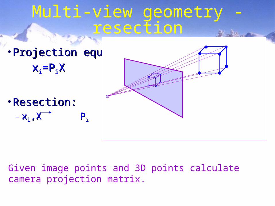
• Projection equationProjection equation

xxii=P=PiiXX

• Resection:Resection:– xxii,X P,X Pii

Multi-view geometry - resection

Given image points and 3D points calculate camera projection matrix.

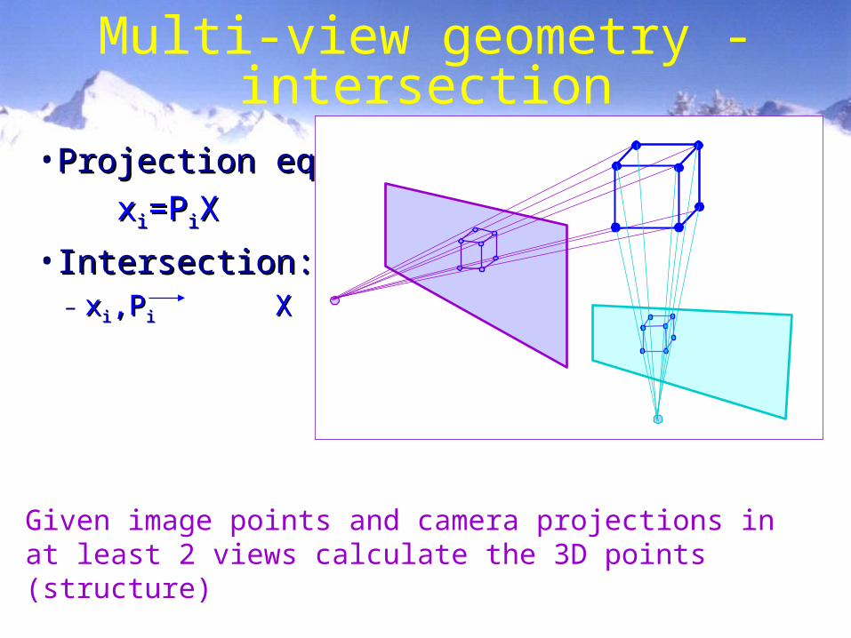
• Projection equationProjection equation

xxii=P=PiiXX

• Intersection:Intersection:– xxii,P,Pi i XX

Multi-view geometry - intersection

Given image points and camera projections in at least 2 views calculate the 3D points (structure)

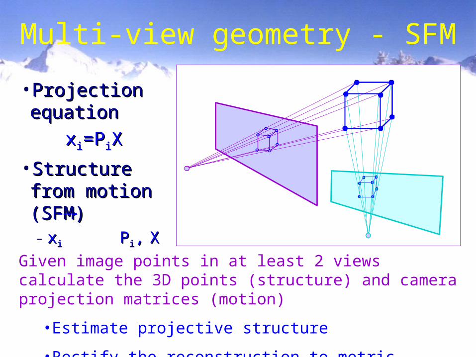
• Projection Projection equationequation

xxii=P=PiiXX

• Structure from Structure from motion (SFM)motion (SFM)– xxii P Pii,, XX

Multi-view geometry - SFM

Given image points in at least 2 views calculate the 3D points (structure) and camera projection matrices (motion)

•Estimate projective structure

•Rectify the reconstruction to metric (autocalibration)

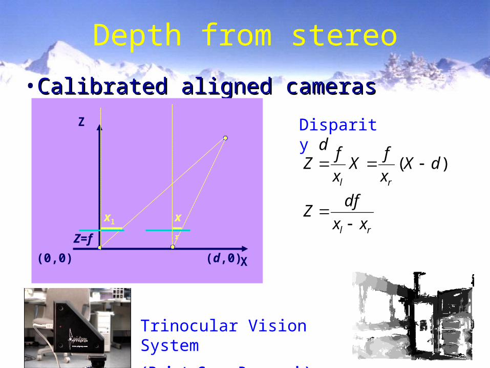
Depth from stereo

•Calibrated aligned camerasCalibrated aligned cameras

Z

X(0,0) (d,0)

Z=f

xl xrrl

rl

xx

dfZ

dXx

fX

x

fZ

)(

Disparity d

Trinocular Vision System

(Point Grey Research)

2 view geometry (Epipolar geometry)

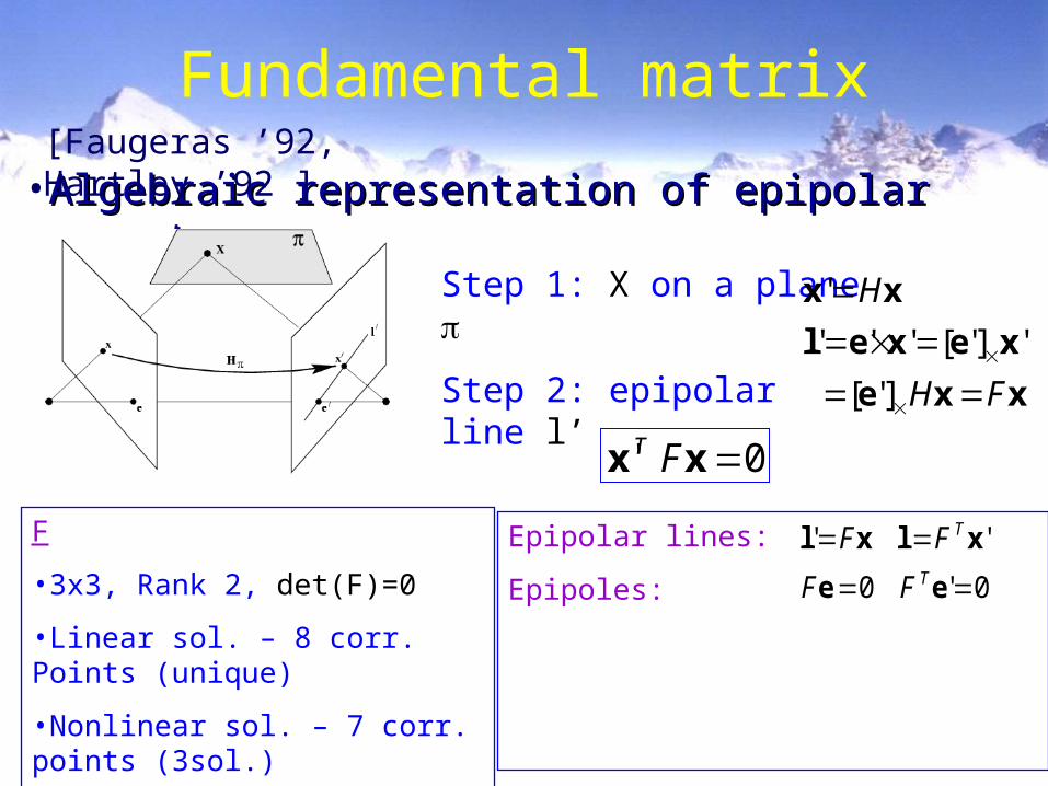
Fundamental matrix

• Algebraic representation of epipolar geometryAlgebraic representation of epipolar geometry

Step 1: X on a plane

Step 2: epipolar line l’xxe

xexel

xx

FH

H

]'[

']'['''

'

0' xx FT

F

•3x3, Rank 2, det(F)=0

•Linear sol. – 8 corr. Points (unique)

•Nonlinear sol. – 7 corr. points (3sol.)

•Very sensitive to noise & outliers

Epipolar lines:

Epipoles:

0'0

''

ee

xlxlT

T

FF

FF

[Faugeras ’92, Hartley ’92 ]

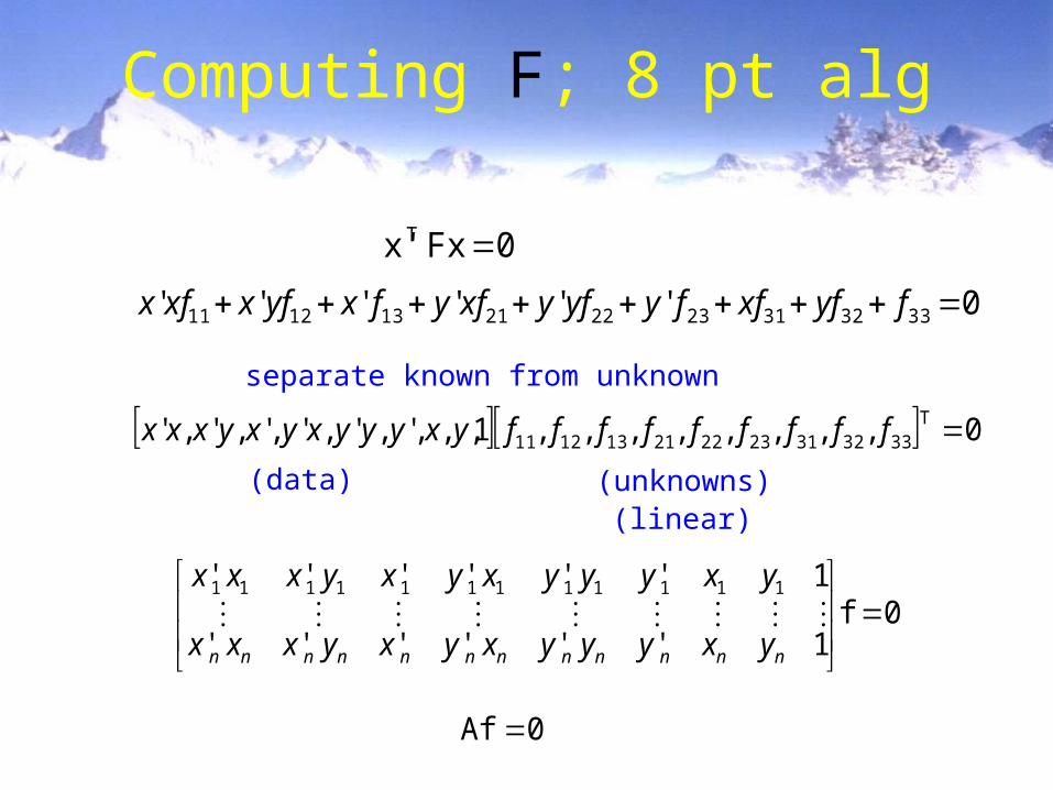
Computing F; 8 pt alg

0Fxx'T

separate known from unknown

0'''''' 333231232221131211 fyfxffyyfyxfyfxyfxxfx

0,,,,,,,,1,,,',',',',',' T333231232221131211 fffffffffyxyyyxyxyxxx

(data) (unknowns)(linear)

0Af

0f1''''''

1'''''' 111111111111

nnnnnnnnnnnn yxyyyxyxyxxx

yxyyyxyxyxxx

0

1´´´´´´

1´´´´´´

1´´´´´´

33

32

31

23

22

21

13

12

11

222222222222

111111111111

f

f

f

f

f

f

f

f

f

yxyyyyxxxyxx

yxyyyyxxxyxx

yxyyyyxxxyxx

nnnnnnnnnnnn

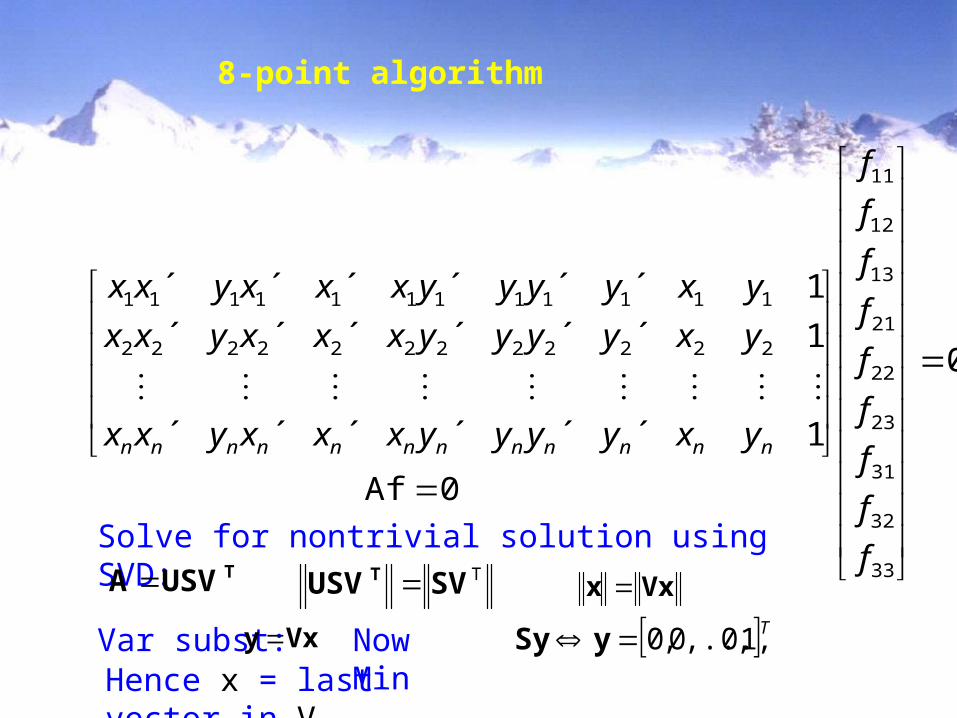
8-point algorithm

Solve for nontrivial solution using SVD:

0Af

TUSVA TSVUSVT Vxx

Var subst: Vxy Now Min T1,0,...,0,0 ySyHence x = last vector in V

Initial structure and motion

'' x2

1

eFeP

0IP

Epipolar geometry Projective calibration

012 FmmT

compatible with F

Yields correct projective camera setup(Faugeras´92,Hartley´92)

Obtain structure through triangulation

Use reprojection error for minimizationAvoid measurements in projective space

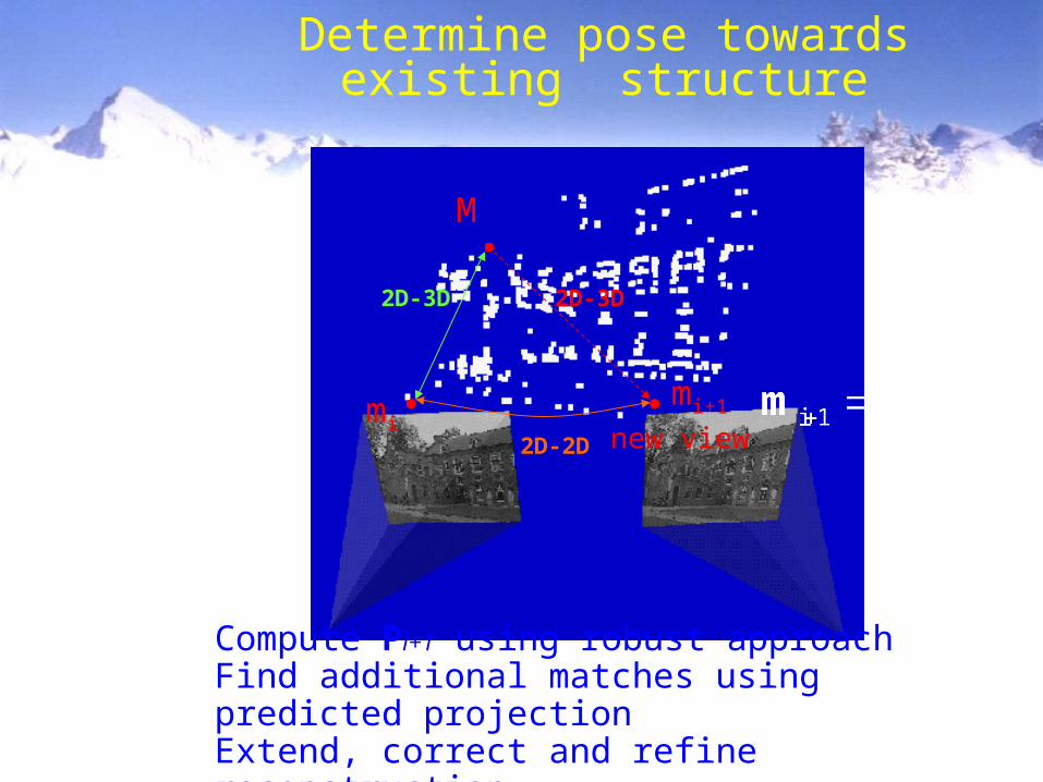
Compute Pi+1 using robust approachFind additional matches using predicted projectionExtend, correct and refine reconstruction

2D-2D

2D-3D 2D-3D

mimi+1

M

new view

Determine pose towards existing structure

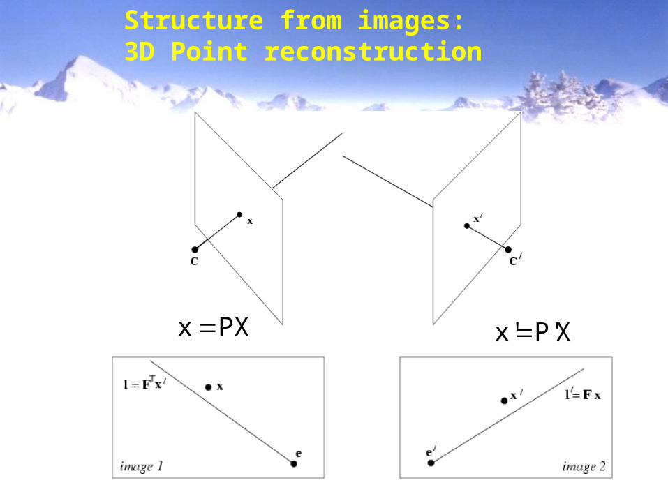
Structure from images:3D Point reconstruction

PXx XP'x'

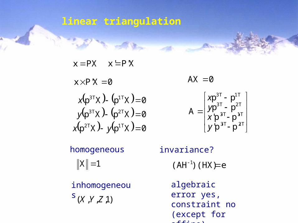
linear triangulation

XP'x'PXx

0XP'x

0XpXp

0XpXp

0XpXp

1T2T

2T3T

1T3T

yx

y

x

2T3T

1T3T

2T3T

1T3T

p'p''p'p''pppp

A

yxyx

0AX

homogeneous

1X

)1,,,( ZYX

inhomogeneous

invariance?

e)(HX)(AH-1

algebraic error yes, constraint no (except for affine)

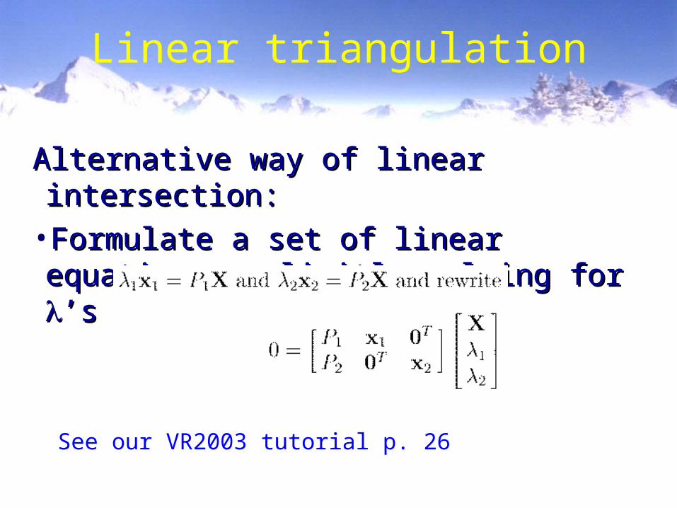
Linear triangulation

Alternative way of linear intersection:Alternative way of linear intersection:

•Formulate a set of linear equations explicitly Formulate a set of linear equations explicitly solving for solving for ’s’s

See our VR2003 tutorial p. 26

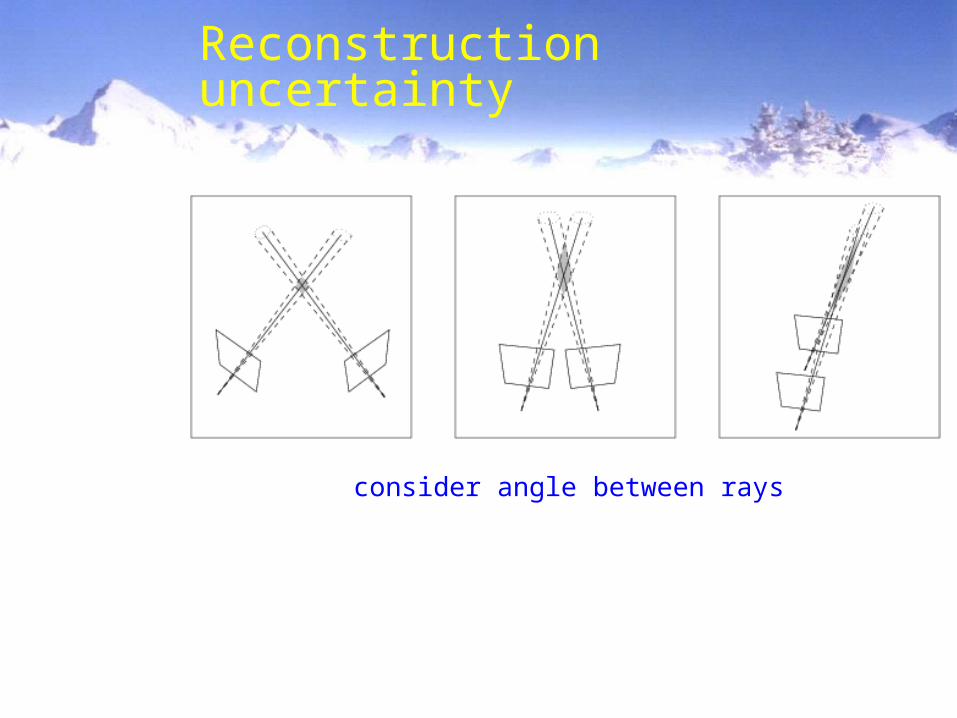
Reconstruction uncertainty

consider angle between rays

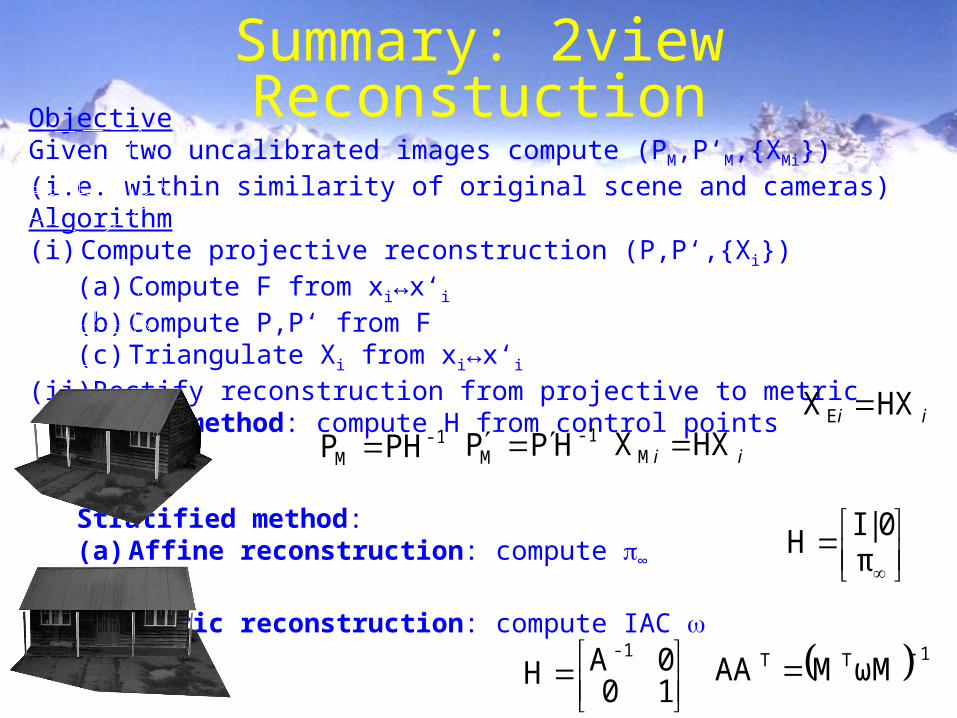
ObjectiveGiven two uncalibrated images compute (PM,P‘M,{XMi})(i.e. within similarity of original scene and cameras)Algorithm(i) Compute projective reconstruction (P,P‘,{Xi})

(a) Compute F from xi↔x‘i(b) Compute P,P‘ from F(c) Triangulate Xi from xi↔x‘i

(ii) Rectify reconstruction from projective to metricDirect method: compute H from control points

Stratified method:(a) Affine reconstruction: compute ∞

(b) Metric reconstruction: compute IAC

ii HXXE -1

M PHP -1M HPP ii HXXM

π0|I

H

100AH

-1 1TT ωMMAA

Summary: 2view Reconstuction

Sequential structure from motionusing 2 and 3 view geom

• Initialize structure and motion from two viewsInitialize structure and motion from two views• For each additional viewFor each additional view

– Determine poseDetermine pose– Refine and extend structureRefine and extend structure

• Determine correspondences robustly by jointly Determine correspondences robustly by jointly estimating matches and epipolar geometry estimating matches and epipolar geometry

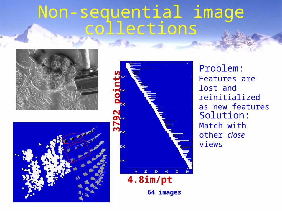
Non-sequential image collections

4.8im/pt64 images

3792

po

ints

Problem:Features are lost and reinitialized as new features

Solution:Match with other close views

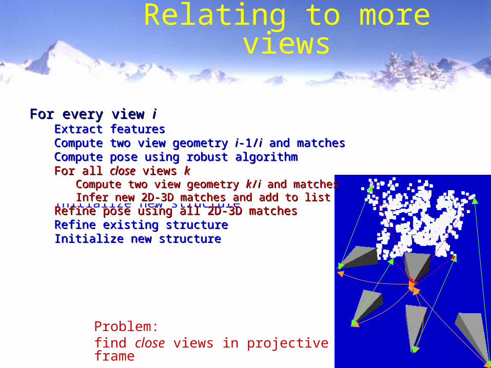
For every view iExtract featuresCompute two view geometry i-1/i and matches Compute pose using robust algorithmRefine existing structureInitialize new structure

Relating to more views

Problem: find close views in projective frame

For every view For every view iiExtract featuresExtract featuresCompute two view geometry Compute two view geometry ii-1/-1/ii and matches and matches Compute pose using robust algorithmCompute pose using robust algorithmFor all For all closeclose views views kk

Compute two view geometry Compute two view geometry kk//ii and matches and matchesInfer new 2D-3D matches and add to listInfer new 2D-3D matches and add to list

Refine pose using all 2D-3D matchesRefine pose using all 2D-3D matchesRefine existing structureRefine existing structureInitialize new structureInitialize new structure

Determining close views

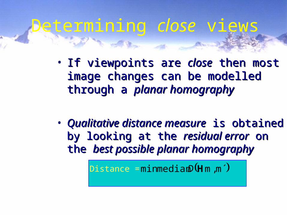
• If viewpoints are If viewpoints are closeclose then most image changes then most image changes can be modelled through a can be modelled through a planar homographyplanar homography

• Qualitative distance measureQualitative distance measure is obtained by is obtained by looking at the looking at the residual errorresidual error on the on the best possible best possible planar homographyplanar homography

Distance = m´,mmedian min HD

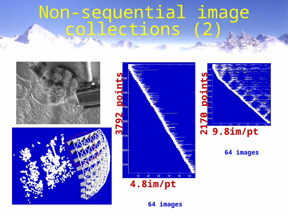
9.8im/pt

4.8im/pt

64 images

64 images

3792

po

ints

2170

po

ints

Non-sequential image collections (2)

Refining a captured model:Bundle adjustment

• Refine structure XRefine structure Xjj and motion P and motion Pii

• Minimize geometric errorMinimize geometric error• ML solution, assuming noise is GaussianML solution, assuming noise is Gaussian• Tolerant to missing dataTolerant to missing data

ji

ijj

iPd,

2),ˆˆ(min xX

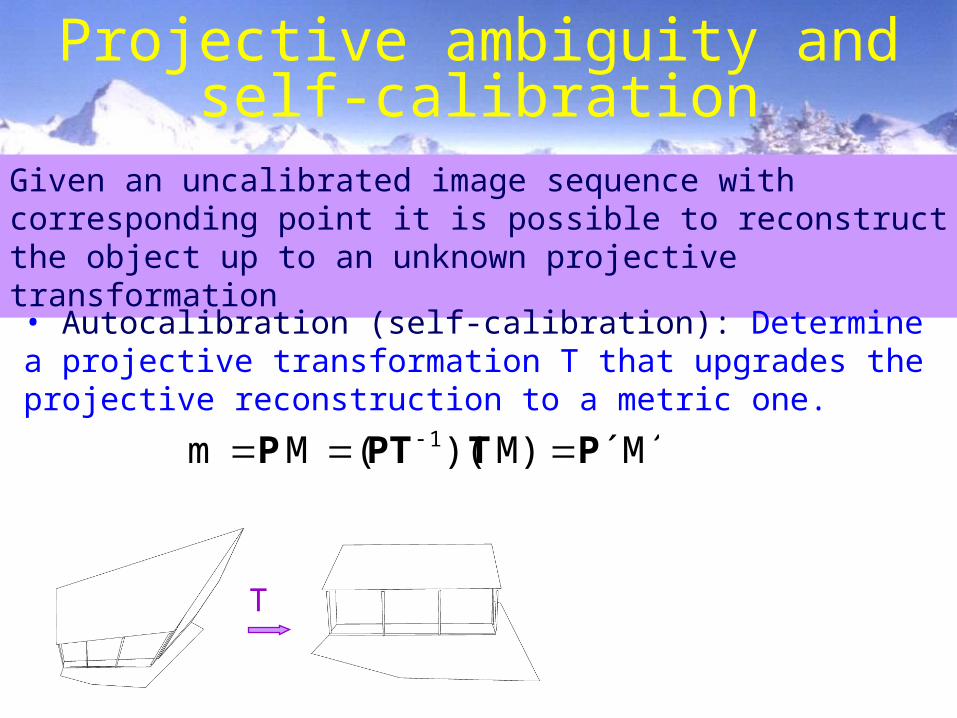
Projective ambiguity andself-calibration

Given an uncalibrated image sequence with corresponding point it is possible to reconstruct the object up to an unknown projective transformation

• Autocalibration (self-calibration): Determine a projective transformation T that upgrades the projective reconstruction to a metric one.

T

´M´M))((Mm 1 PTPTP

A complete modeling systemprojective

Sequence of frames scene structureSequence of frames scene structure

1.1. Get corresponding points (tracking).Get corresponding points (tracking).

2.2. 2,3 view geometry: 2,3 view geometry: compute F,T between consecutive frames compute F,T between consecutive frames (recompute correspondences).(recompute correspondences).

3.3. Initial reconstruction: Initial reconstruction: get an initial structure from a get an initial structure from a subsequence with big baseline (trilinear tensor, factorization …) subsequence with big baseline (trilinear tensor, factorization …) and bind more frames/points using resection/intersection.and bind more frames/points using resection/intersection.

4.4. Self-calibration.Self-calibration.

5.5. Bundle adjustment.Bundle adjustment.

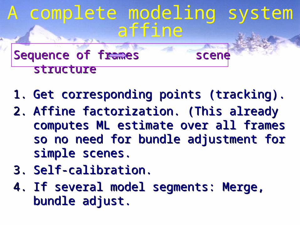
A complete modeling systemaffine

Sequence of frames scene structureSequence of frames scene structure

1.1. Get corresponding points (tracking).Get corresponding points (tracking).

2.2. Affine factorization. (This already computes ML Affine factorization. (This already computes ML estimate over all frames so no need for bundle estimate over all frames so no need for bundle adjustment for simple scenes.adjustment for simple scenes.

3.3. Self-calibration.Self-calibration.

4.4. If several model segments: Merge, bundle adjust.If several model segments: Merge, bundle adjust.

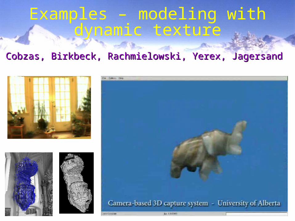
Examples – modeling with dynamic texture

Cobzas, Birkbeck, Rachmielowski, Yerex, JagersandCobzas, Birkbeck, Rachmielowski, Yerex, Jagersand

Examples: geometric modeling

Debevec and Taylor:Debevec and Taylor: Façade Façade

Examples: geometric modeling

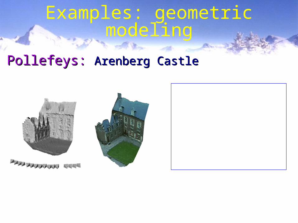
Pollefeys: Pollefeys: Arenberg CastleArenberg Castle

Examples: geometric modeling

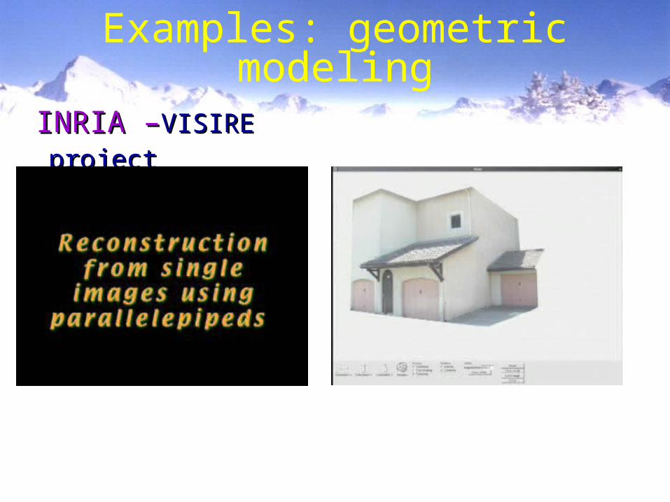
INRIA –INRIA –VISIRE projectVISIRE project

Examples: geometric modeling

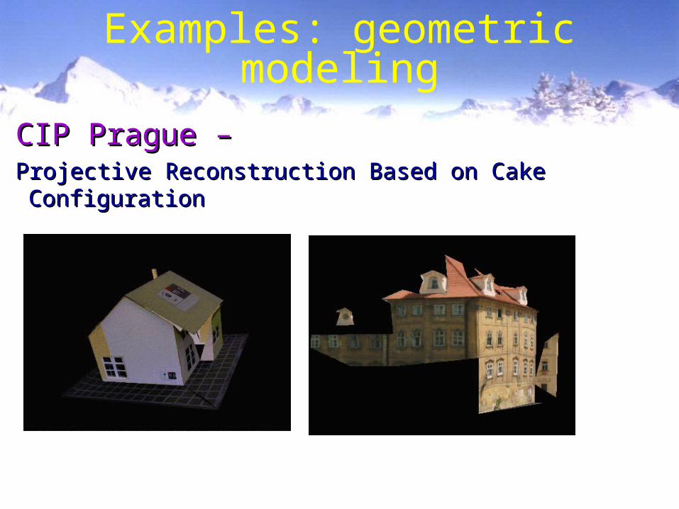
CIP Prague –CIP Prague –Projective Reconstruction Based on Cake ConfigurationProjective Reconstruction Based on Cake Configuration

Reading: FP Chapter 11.

• The Stereopsis Problem: Fusion and Reconstruction• Human Stereopsis and Random Dot Stereograms• Cooperative Algorithms• Correlation-Based Fusion• Multi-Scale Edge Matching• Dynamic Programming• Using Three or More Cameras

Dense stereo

•Go back to original images, do dense matching.Go back to original images, do dense matching.

•Try to get dense depth mapsTry to get dense depth maps

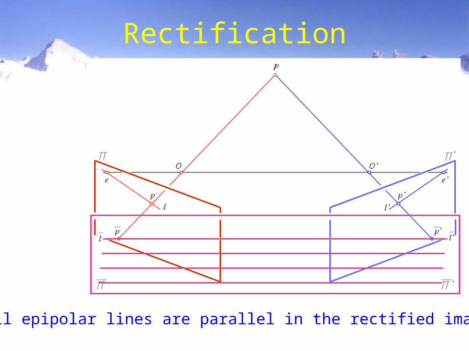
All epipolar lines are parallel in the rectified image plane.

Rectification

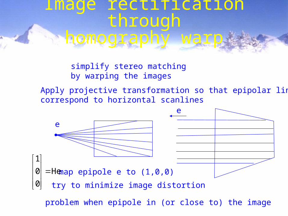
simplify stereo matching by warping the images

Apply projective transformation so that epipolar linescorrespond to horizontal scanlines

e

e

map epipole e to (1,0,0)

try to minimize image distortion

problem when epipole in (or close to) the image

He

0

0

1

Image rectification throughhomography warp

Stereo matching

Optimal path(dynamic programming )

Similarity measure(SSD or NCC)

Constraints• epipolar

• ordering

• uniqueness

• disparity limit

• disparity gradient limit

Trade-off

• Matching cost (data)

• Discontinuities (prior)

(Cox et al. CVGIP’96; Koch’96; Falkenhagen´97; Van Meerbergen,Vergauwen,Pollefeys,VanGool IJCV‘02)

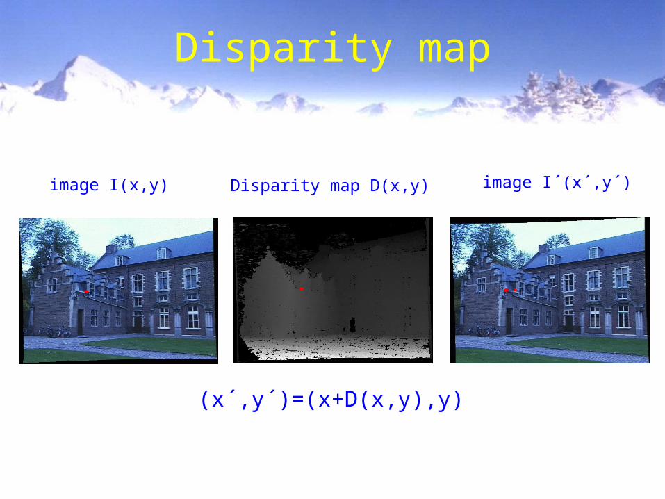
Disparity map

image I(x,y) image I´(x´,y´)Disparity map D(x,y)

(x´,y´)=(x+D(x,y),y)

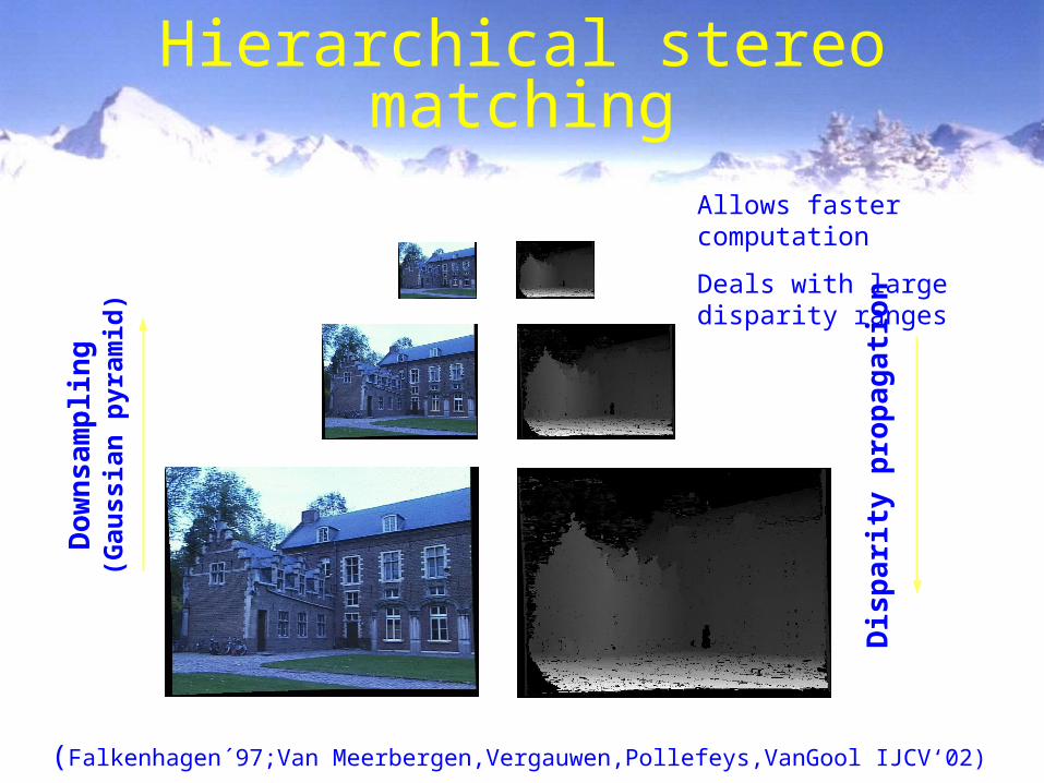
Hierarchical stereo matchingD

ow

nsam

plin

g

(Gau

ssia

n p

yra

mid

)

Dis

pari

ty p

rop

ag

ati

on

Allows faster computation

Deals with large disparity ranges

(Falkenhagen´97;Van Meerbergen,Vergauwen,Pollefeys,VanGool IJCV‘02)

Example: reconstruct image from neighboring images