Computerizing the Collins Method of determining Troposcatter Path Loss

by Roger Rehr, W3SZ5/8/2014

The Collins Method of determining Troposcatter Path Loss is described in "Tropospheric Scatter Principles and Applications", a training manual prepared by the Collins Radio Company under Signal Corps Contract No. DA36-039-sc-67491, Army Electronic Proving Ground, Fort Huachuca, Arizona. This document is dated 1 December, 1959.

The Collins method was, around the time of its publication, reported tobe a very accurate method for estimating troposcatter path loss (further discussion on this point will be near the end of this paper), but it suffers from the fact that it is a graphical method rather than a computational method. In order for it to be used as a computer-basedmethod, it must be converted from a graphical methodology to a computational methodology.

In this paper I describe a new, computational methodology derived from the original graphically-based Collins methodology, that will be used to develop a new software-based approach to the Collins model. I will then evaluate the accuracy of this method, using as a basis for comparison and as a “gold standard” the results of the original graphical Collins method applied to the same datasets.

Description of Collins method. With the original graphically-based Collins method, calculations of troposcatter loss are performed using figures 10.7, 10.8, 10.9, and 10.10 from the Collins publication. See Appendix to view copies of these figures.

Figure 10.7 is titled "Basic Propagation Loss Curve for 1000 Megacycles". It is a plot of "Loss Between Two Isotropic Radiators in dB vs Distance in Statute Miles". It is linear in y and log in x. Using the graph, one reads the loss in dB for a given distance in miles.

Figure 10.8 is "Frequency Correction Curve for Basic Propagation Loss".It is a plot of "Frequency Correction Factor in dB vs Frequency in Megacycles". It is linear in y and log in x. One reads the additional(or reduced) loss in dB due to frequency for a given frequency in MHz, as compared to the reference frequency of 1000 MHz.

Figure 10.9 is "Loss Due to Elevated Horizon Angles". It is a series ofcurves, for 50,75,100,150,200,250,300, and 350 miles for "Loss Due to Horizon Angles" in dB vs the sum of the horizon angles of the two communicating stations, in degrees. It is linear in y and x. One reads the loss in dB for a given total horizon angle by selecting the appropriate distance curve, or interpolating between curves if necessary.

Figure 10.10 is "Nomogram for Determining Aperture-to-Medium Coupling Loss". The leftmost scale is "Equivalent Smooth Earth Statue Miles andScatter Angle (Degrees)". The rightmost scale is "Antenna Beamwidth (Degrees)". The middle (result) scale is "Aperture to Medium Coupling Loss (dB)". None of these scales is linear. One selects the sum of scatter angle due to the combination of inter-station distance and take-off angles of the two stations on the left scale, and the antenna beamwidth on the right-hand scale. One then reads the aperture-to-medium coupling loss off the center scale where the line so drawn connecting the two points just described on the outer two scales intersects the middle scale. Note that this nomogram assumes identicalbeamwidths for the antennas at the two ends of the circuit, and this number, the “antenna beamwidth” on the right-hand scale of the nomogram

represents the beamwidth of a single antenna. To use this nomogram with a circuit where the antennas of the two stations do not have the same beamwidths, some assumptions or compromises must be made.

Description of proposed method for adapting the Collins model for calculation of troposcatter loss to a software-based model.

Data was digitized from figures 10.7 and 10.9 from the Collins paper byusing a program named GSYS2.4.6. This program was can be downloaded from http://www.jcprg.org/gsys/. It was developed by the staff of the Hokkaido University Nuclear Reaction Data Centre of Sapporo, Japan for their use in analysis of nuclear reaction data, and they have kindly made it available for general use. It was not necessary to digitize figure 10.8, as will be discussed below. Figure 10.10, the nomogram, was analyzed using a different technique, as will be described below. Digitizing the data contained in figures 10.7 and 10.9 of the original Collins manuscript proved to be an interesting proposition. No original paper copy of the article was available to me, and so all of my analysis was taken from digital copies. It turned out that there were some distortions in the graph images such that the grids on the graphs did not map smoothly into a digital grid that assumed consistentlinear (or log) mappings of the graph space over the entire extent of the graphs. I believe that this distortion of the mapped space was dueto distortions in the original figures due to their being created in 1959 using manual techniques rather than computer-based graphics techniques. As a result, there are, I believe distortions in the original graphs that were present in the original paper copies of this article. I do not believe that the distortions of the mapped space is a result of the digitial copying process used to create the digital images on which I based my models. Because of this distortion of the mapped graphical space, present in the original graphical data, I couldnot simply digitize the data from figures 10.7 and 10.9. I ended up after several iterations using an approach where I greatly magnified the graph in GSYS and used the GSYS digital coordinates to get me "in the ballpark" for the x and y coordinates. However, the least significant digit of the datapoints was determined by visual inspectionof the graphical space as mapped into GSYS rather than using the digital cooordinates determined by GSYS if it appeared that the GSYS coordinates were in error for the point in question when compared with the visual appearance of the relationship of the graphed curve and the gridlines on the graph in question. This approach was more time consuming than simply using the digital coordinates as determined by GSYS, but it gave many of the benefits of the fully digital approach without the error introduced by the geometric distortions in the mappedgraphical space noted above.

Software-derived curve fitting was done primarily using R-3.1.0 for Windows. The R Project Free Software Environment for Statistical Computing and Graphics compiles and runs on a wide variety of UNIX platforms as well as on Windows and MacOS. This software is produced by the R Project for Statistical Computing (http://www.r-project.org/).R-3.1.0 was also used for most of the statistical analysis of the modeldeveloped here. JKCFIT and POLYFIT (written and maintained by John Kennedy of the Mathematics Department at Santa Monica College, Santa Monica, California) were obtained from https://sites.google.com/site/johnkennedyshome/home/downloadable-software/abstracts and were used for simple curve fitting and initial exploration of possible models. JKCFIT will perform linear, log, exponential, and power curve-fitting, and POLYFIT will perform polynomial fits of degree 1 to 10. The website zunzun.com, authored byJames R. Phillips, has extensive curve-fitting facilities which were used to great advantage in the search for the optimum function to fit

the nomogram, figure 10.10. With this website, large numbers of potentially useful curve-fitting algorithms could be tested and compared quickly, allowing the best model to be chosen relatively quickly from among many “reasonable” possibilities. Zunzun.com also provided excellent graphics support facilities, producing animated gif and VRML (Virtual Reality Modeling Language; https://en.wikipedia.org/wiki/VRML) files of the datapoints and fitted surfaces. These figures were very helpful for confirming the integrityof the initial dataset and also for subjectively evaluating the "fit" of the models being evaluated. Some statistical analysis was performedusing the zunzun.com site, although this was primarily performed using the R Project software described above.

Figure 10.7 was fitted using a piecewise fit, with x (distance in miles) values below a cutpoint (named BRK) being fitted using a power function, and x values above BRK being fitted using a linear fit. The optimal value of BRK was chosen by minimizing the residual standard error when the function was evaluated for BRK values of 50-350 miles, at intervals of 1 mile. Results of the power fit are shown here for the optimal value of BRK, which turned out to be 329:

x y Min. : 35.16 Min. :159.3 Max. :541.83 Max. :262.7

> brk <- 329

Formula: y ~ I(x < brk) * alpha * x^beta + I(x > brk) * ((m * x) + b)

Parameters: Estimate Std. Error t value Pr(>|t|)alpha 87.0302349 0.1891146949 460.19816 3.043506e-242 ***beta 0.1723800 0.0004576264 376.68270 5.996901e-229 ***m 0.1199267 0.0019970923 60.05068 2.837331e-108 ***b 198.7430042 0.8478251608 234.41508 1.730651e-197 ***

Signif. codes: 0 ‘***’ 0.001 ‘**’ 0.01 ‘*’ 0.05 ‘.’ 0.1 ‘ ’ 1

Residual standard error: 0.684 on 153 degrees of freedom

Number of iterations to convergence: 3 Achieved convergence tolerance: 8.867e-06

For distances greater than or equal to 329 miles, the linear regressionused is: y = (0.120 * x) + 198.743.

The accuracy of the piecewise fit of the curve to the original data is excellent. The curve fit gives a Spearman correlation coefficient of 0.9997666 for the correlation of f(x) vs y in the original dataset.

The absolute error in dB of the Basic Propagation Loss calculated by the above method for the 157 datapoints digitized from Figure 10.7 as compared to the value of the basic propagation loss measured directly from Figure 10.7 is shown below:

Absolute Error (dB) of Model for Calculating Basic Propagation Loss

Min. 1st Qu. Median Mean 3rd Qu. Max.

0.01471 0.27400 0.59220 0.58420 0.81980 1.43600

Below is a plot of the optimal fit for Figure 10.7, with the regressionline (colored blue) calculated using this model superimposed on the

original datapoints (displayed as circles) obtained from the Collins figure:

A plot of the absolute error vs distance in miles is shown below:

The error analysis shows that the largest errors occur at distances of less than 100 miles. The only errors of absolute value more than 1 dB at distances of greater than 100 miles are an error of 1.005 dB at 100.7 miles, and and error of -1.08 dB at 226 miles. As is shown in the table above, the largest absolute error is 1.436 dB. This occurs at a distance of 36 miles, and is thus not of practical importance. Asis also shown in the table above, the median absolute error is only 0.59 dB, and the mean absolute error only 0.58 dB, both indicating excellent accuracy of this method of calculation of Basic Propagation Loss when compared with the values obtained directly from that Figure 7.

It was a simple matter to "code" the above algorithm into a useful program for calculating the basic propagation loss as a function of distance, using this extension of the Collins model.

Figure 10.8 does not require a curve fit. It is simply:Frequency Loss (dB) = 30 * Log10(frequency/1000)where the frequency is given in MHz, as was noted in the original Collins paper. Thus the frequency loss does not enter into a comparison of the results of the graphical and calculated Collins methods, as the frequency loss is the same for both methods.

Figure 10.9 was evaluated by determining the best fit for the individual dB-loss-vs-total-horizon-angle curves for each reference distance included in the Collins paper (50, 75, 100, 150, 200, 250, 300, and 350 miles). The best result was achieved by using a linear regression for horizon angles greater than or equal to 2.6 degrees, anda 4th order polynomial regression for total horizon angles of less than 2.6 degrees. This approach was chosen after extensive investigation ofhundreds of models, using zunzun.com for initial screening and then R for more detailed analysis. The breakpoint value of 2.6 degrees was determined by comparing the results of error analysis for choices for the breakpoint total horizon angle between 1 and 4 at 0.1 degree intervals, and then choosing the value for the breakpoint that gave thebest compromise between [1] minimizing the residual standard error (RSE) of the overall fit for all values of total horizon angle and [2] minimizing the standard error of the slope and intercept parameters of the linear portion of the fit, in order to provide for better accuracy when extrapolating the model to distances beyond 350 miles.

The model calculates the results for distances not exactly valued at the reference distances of 50, 75, 100, 150, 200, 250, 300, or 350 miles as follows. For distance values of less than 50 miles, the coefficients for the 50 mile reference distance are used. Troposcatteris not typically used at these very short distances. An alternative approach would have been to return “No Data” for distances of less than50 miles. For distance values between 50 and 350 miles, but with the distance not exactly valued at any of the reference distances, calculations are done for the closest two reference distance values, and a linear interpolation using these two results is used for the final result. The results obtained by this linear interpolation method for points immediately adjacent to the reference distances showed an excellent fit with the adjacent datapoints contained in the original dataset, confirming the accuracy of this interpolation.

For distances of greater than 350 miles, the regression coefficients tobe used at these larger distances were derived from a linear regressionof each of the coefficients of the applicable regression equations using the reference distances of 200, 250, 300, and 350 miles. These reference distances were chosen for inclusion in this calculation because they provided the best fit to the data. This method produced datapoints with an excellent fit when compared to the datapoints contained in the original Collins data set.

The linear regression coefficients for each of the reference distances for total horizon angle greater or equal to 2.6 are shown below:

miles slope intercept50 8.38 13.9375 7.96 10.93100 8.17 7.27150 7.58 7.30200 7.25 6.86250 7.03 6.21300 6.10 6.94350 5.76 5.88

The equation for dB loss for total horizon angles >= 2.6 is:dB loss = slope * total horizon angle + intercept.

The 4th order polynomial equation and coefficients for each of the reference distances for total horizon angles less than 2.6 are shown below:

Formula: y ~ a0 + a1 * x + a2 * x^2 + a3 * x^3 + a4 * x^4where y = db loss and x = total horizon angle in degrees.

The coefficients are given in the following table:

miles a0 a1 a2 a3 a450 -0.4020663 37.6010100 -24.2515196 8.8779426 -1.175177575 -0.8996337 29.5901500 -18.4272531 7.0375186 -0.9535724100 -0.8612149 22.4073235 -11.7325607 4.4854709 -0.6225285 150 -0.1604293 15.3438289 -4.0900476 1.2715630 -0.1694519 200 0.08274338 12.68992823 -1.68117170 0.31350178 -0.03621050250 0.08223525 12.12313270 -1.24670791 -0.02637818 0.03195288300 0.03456856 11.51170751 -1.43899133 0.17673472 -0.01488748 350 -0.01543547 10.53943957 -1.43080920 0.25360394 -0.03135268

For distances greater than 350 miles and total horizon angles greater than or equal to 2.6 the scattering loss in dB is determined by the equation:

dB loss = slope * total horizon angle + intercept

where

slope = -0.00851727357609711*(distance in miles) + 8.8491223155929

and

intercept = -0.00496 * (distance in miles) + 7.03933333333333

For distances greater than 350 miles and total horizon angles less than2.6, the dB loss equation is:

dB loss =

(-0.00068440648*miles + 0.234239712) + (-0.01412578234*miles + 15.600642146)*x + (0.00111760816*miles + -1.756762279)*x^2 + (4.683876E-5*miles + 0.166484906)*x^3 +(-6.45338E-5*miles + 0.00512235)*x^4

where x = total horizon angle in degrees.

Below is a graph of loss in dB vs total horizon angle. The green points are the original data from figure 10.9 of the Collins publication. The red points are scattering loss in dB calculated usingthe equations given above, for the reference distances of 50, 75, 100, 150, 200, 250,and 300 miles. The green points representing the original dataset are difficult to see, as they are hidden by the red points which are superimposed on them, because of the extremely good fit of the model data to the original datapoints. These calculated datapoints provide an extremely good fit to the original graphical datapoints.

The black points represent calculated datapoints for total horizon angles of -0.2, 0, 2.1, and 4.1 degrees, and distances of 351, 400, 500, 600, 700, 800, 900, and 1000 miles. These points are shown to

demonstrate the accuracy of the method of extrapolation used in the model for points with distances just beyond the reference range (upper limit 350 miles), and to show “reasonableness” of the datapoints as distances were extended to 400, 500, 600, 700, 800, 900, and 1000 miles. The fact that the points for 351 miles are superimposed on the original dataset points at 350 miles confirms the accuracy of the methods used here. However, the accuracy and validity of extrapolatingto distances outside the boundaries of the original Collins dataset arespeculative and there exist no confirmatory experimental data for distances of greater than 350 miles.

The blue points on the graph below represent calculated datapoints for 51, 76, 101, 151, 201, 251, and 301 miles and were derived as describedabove by performing linear interpolations from the reference distance data of the closest two reference distances for the same value of totalhorizon angle. The fact that these points are virtually superimposed on the adjacent reference datapoints at 50, 75 100, 150, 200, 250, and 300 miles provides some confirmation of the accuracy of this approach. Additional comparisons of the linear interpolation method for distancesjust below the reference distances as well as for points at various fractional distances between the reference distances were performed andall showed an excellent fit with the original dataset. These results are not shown here, in order to maintain brevity.

The above comparisons provide a “sanity” check of the method and confirmation that the method works for points within the boundary limits of the original Collins data set, but the comparisons do not provide any assurance of the accuracy of the method at distances above the maximum reference distance of 350 miles or for total horizon anglesoutside the data range of 0.2 – 4.0 degrees. As noted above, the positions of the black datapoints points for 400-1000 miles appear reasonable, but there is no “original data” with which to compare them.

Analysis of the error in the calculated scattering loss by comparing the calculated values for the loss to those obtained directly from Figure 10.9 shows the following for the absolute value of the error:

Min. 1st Qu. Median Mean 3rd Qu. Max. 0.00051 0.04756 0.10680 0.13660 0.19110 0.97870

So we see that the maximum absolute error for the scattering loss is just less than 1 dB, and the median and mean values for the absolute error are both on the order of 0.10 dB. This indicates excellent performance of the algorithm described. A plot of the absolute error vs total horizon angle is below:

It demonstrates the very acceptable errors achieved, and also shows what was noted above, that the greatest errors appear to occur at angles of less than zero.

Below is a plot of absolute scatter error loss in dB vs distance in miles.

It shows that the greatest absolute error of 0.98 occurs at the minimumreference distance of 40 miles, and that above 100 miles all errors arewell less than 0.5 dB.

Thus, the model derived from figure 10.9 in the Collins publication, like the model derived from figure 10.7, gives an excellent correlationwith the results obtained directly from the original graphs, with very acceptable absolute errors, as shown above.

This model was also easily "coded" into a software program for determining the total horizon angle scattering loss using this extension of the graphical Collins method.

Figure 10.10 in the Collins publication is a three-scale nomogram used to compute aperture-to-medium coupling loss in dB from antenna beamwidth in degrees and scatter angle in degrees. This nomogram represents the final step in the graphical Collins method for calculating troposcatter path loss. Note that the "scatter angle" usedfor this calculation is not the same parameter as the "total horizon angle" that was used in the calculations associated with figure 10.9. Scatter angle equals the total horizon angle plus the distance in miles * 0.010833.

As was noted near the beginning of this report, the antenna beamwidth on this nomogram represents the beamwidth for a single antenna, and in constructing the nomogram the Collins engineers made the assumption that the antennas at the two ends of the circuit have identical beamwidths. To use this nomogram for a circuit where the antennas at each end of the circuit do not have identical beamwidths, an assumption must be made. A reasonable assumption would be that the beamwidth used for the nomogram or nomogram-derived calculation is the average of the beamwidths of the two stations. This “detail” does not come into play with the construction and evaluation of the model presented in this paper, but would affect the “real world” use of both the original graphical Collins model and the model presented here, because it was derived from the Collins model.

The Collins nomogram is a 3-element parallel scale nomogram. A review of nomogram theory and practice shows that 3-element parallel scale nomograms are used when there are two independent variables and one dependent variable, and the variables can be represented by an equationof the form F1(x) + F2(y) + F3(z) = 0. Generally the nomogram scales are logarithmic, as this allows multiplication to be converted to addition, division to subtraction, etc. In the case of the nomogram infigure 10.10 of the original Collins publication, all 3 scales are logarithmic, as was verified by plotting the values of each scale vs the linear distance on that scale and then performing curve fitting andreviewing the error analysis of that fitting.

The first step in converting this nomogram to a formula that would allow automation of this calculation was to obtain 657 sets of scattering angle, beamwidth, and aperture-to-medium coupling loss datapoints from the nomogram. This data collection was computer-enhanced, in order to allow a more accurate data collection than could be achieved with a paper copy of the nomogram and a straightedge. The figure below helps to show how this was done. A computer-generated line was placed over a digitized image of the nomogram, with a rotational constraint (axis of rotation) placed on one of the three nomogram scales at the desired value of the parameter for that scale. The line was then rotated about the constraint (rotational axis) so that it intersected another scale at the desired parameter values for that scale, and then the values of scatter angle, aperture-to-medium coupling loss, and beamwidth could be determined from the points of intersection of this line with each of the three nomogram scales. Thisprocess was repeated in order to obtain 657 separate triplets of these three values.

For subsequent data analysis, the square root of the beamwidth was usedin curve fitting, rather than the beamwidth itself, in part because other investigators had suggested that the aperture-to-medium coupling loss is more directly related to the square root of the beamwidth than the beamwidth itself, but more importantly because modeling showed thatthis choice helped to further linearize the surface described by the raw datapoints, and improved the accuracy of the fit of the calculated data to the raw datapoints.

Because the nomogram scales were logarithmic, the logarithm of the scattering angle and coupling loss datapoints, and the logarithm of thesquare root of the beamwidth were used for curve fitting. The nomogram-derived dataset was viewed three-dimensionally using rotating animated gif and VRML files produced online at http://zunzun.com. Examining the data in this way showed that the above procedures did an excellent job of linearizing the relationship between the three variables, but that the relationship between variables still retained aslight sigmoid shape, as is shown below (although this shape is much more easily appreciated when one can view the rotating 3D dataset usingthe animated gif file or VRML file of this data, obtained as outlined above):

Because of the sigmoidal data shape it was likely that a sigmoidal function would likely provide the best fit to the data. In fact, a comparison of the accuracy (defined as minimizing the least squares error) of hundreds of functions at curve-fitting this data was performed using zunzun.com, and a sigmoid function provided the best fit of all of the functions evaluated. The function used is of the form

z = a0 + (a1 / (1.0 + exp(a2 * (x + a3 + a4 * y + a5 * x * y)))).

where:z = log10(aperture-to-medium-coupling loss) (in dB)x = log10(scattering angle) y = log10(beamwidth^0.5)

This function is attributed to Andrea Prunotto, a member of the Computational Biology Group in the Department of Medical Genetics at the University of Lausanne.

The values for the coefficients are:a0 = -1.3496735573765721E+00a1 = 2.8154539418053490E+00a2 = -1.8712895986060660E+00a3 = 2.6925289536049724E-01

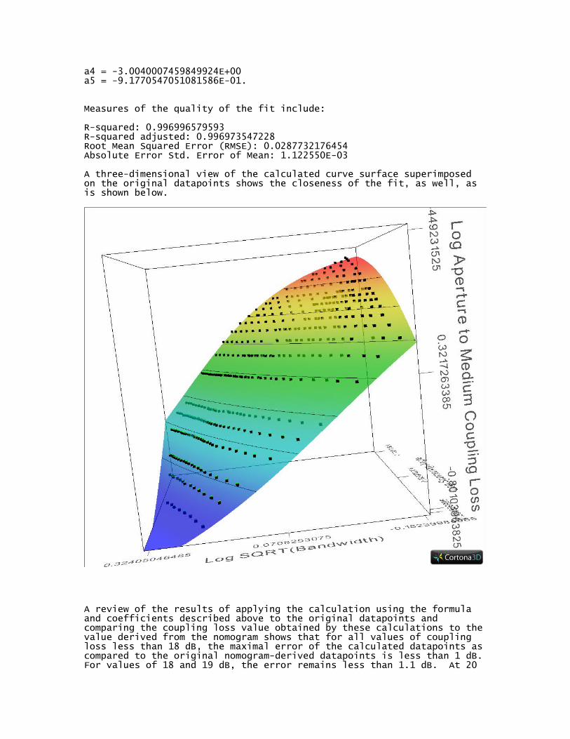
a4 = -3.0040007459849924E+00a5 = -9.1770547051081586E-01.

Measures of the quality of the fit include:

R-squared: 0.996996579593R-squared adjusted: 0.996973547228Root Mean Squared Error (RMSE): 0.0287732176454Absolute Error Std. Error of Mean: 1.122550E-03

A three-dimensional view of the calculated curve surface superimposed on the original datapoints shows the closeness of the fit, as well, as is shown below.

A review of the results of applying the calculation using the formula and coefficients described above to the original datapoints and comparing the coupling loss value obtained by these calculations to thevalue derived from the nomogram shows that for all values of coupling loss less than 18 dB, the maximal error of the calculated datapoints ascompared to the original nomogram-derived datapoints is less than 1 dB.For values of 18 and 19 dB, the error remains less than 1.1 dB. At 20

dB loss and above, the error has a maximal value of 1.758, but even in this range of loss above 20 dB, the mean error is only 1.3 dB. Note that the upper limit of loss that can be measured using the nomogram is22.5 dB. A significant portion of this higher error for values of 20 dB or more is likely the uncertainty in the nomogram-derived coupling loss, due to the extreme compression of the datapoints on the nomogram in that range. At the extremes of the nomogram, it was very difficult to get exactly the same result when reading the nomogram on two successive tries, even when using computer enhancement to improve the accuracy of the reading of the nomogram, due to this compression. There are similar but less extreme problems with nomogram accuracy at the upper ends of the ranges of scattering angle and beamwidth, as well. A plot of calculated vs nomogram-derived values of the aperture-to-medium coupling loss shows excellent agreement of the calculated anddirectly-nomogram-derived sets of datapoints, as is shown in the figurebelow.

The uncertainty noted of less than 1-2 dB is likely inconsequential in practice, given the much greater known uncertainties involved in

calculating troposcatter loss by the Collins method or any of the othermethods in current use. And as was just noted, this variability may well come predominantly from the nomogram itself, and does not suggest problems with the method of calculation presented here.

The absolute error is distributed as shown in the table below:

Absolute Error of Computed Aperture-to-Medium Coupling Loss

Min. 1st Qu. Median Mean 3rd Qu. Max. 0.0002 0.076 0.182 0.279 0.429 1.76

The chart shows that 25% of the calculated datapoints have an error of less than or equal to 0.08 dB. 50% of the calculated datapoints have an error of 0.18 dB or less. The average error is 0.28 dB. 75% of calculated datapoints have error of 0.43 dB or less. The distribution of error is nicely demonstrated on the plot of error vs nomographic coupling loss shown below:

The clustering of most of the 657 datapoints near the origin at the left of the graph is consistent with the very low values for the medianand mean error reported above. The larger (but still relatively small)errors for nomographic loss at the extreme upper end of the nomogram are also apparent.

The algorithms used for calculating the aperture-to-medium loss were

also easily "coded" in software so that this loss could be easily calculated by compter.

Determining Total Troposcatter Loss. For the original Collins model, total troposcatter loss equals the sum of the losses obtained by using figures 10.8, 10.8, 10.9, and 10.10 from the Collins publication. These losses represent, respectively, the basic propagation loss, the additional loss (or reduction in loss) due to frequency, the scatteringloss, and the aperture-to-medium coupling loss.

With the model described here, instead of using the graphs and the nomogram, one enters into the software program the values for take-off angle for each of the two stations, the distance between the stations in miles, the frequency, and the beamwidths of each of the stations' antennas. The total horizon angle is equal to the sum of the two take-off angles, and the total scattering angle is calculated from the distance and the take-off angles. Then the basic propagation loss, thefrequency loss, the scattering loss, and the aperture-to-medium coupling loss are calculated in software as described above, and added together to give the total troposcatter loss. Once the above algorithms were derived, it was a simple matter to put them into a working program, a screenshot of which is shown below:

The Collins article gave only two examples of results obtained using the graphical method. The computerized method described here was applied to those examples, which were described in sections 3.2 and 10.4.3.2 of the Collins publication, and the results of the method described here were compared with the results given in the Collins publication for these two examples.

The parameters given in the Collins publication for the example from section 3.2 were: frequency = 900 MHz, total horizon angle = 1.5

degrees, distance = 150 miles. The example in section 3.2 did not giveantenna gain or beamwidth information, and did not report aperture-to-medium coupling loss. A comparison of the results reported by the Collins paper for these parameters with the results obtained by the model described in this paper are given in the table below:

Result Result From Calculated by Collins Method Described

(All results are in dB) Paper In this paper

Basic Propagation Loss 206 206.4

Frequency Loss -1.5 -1.4

Total Horizon Angle Scatter Loss 18 17.1

Aperture-to-medium Coupling Loss ---- 8.37*

Total Troposcatter Loss 222.5 222.1

* Ignored in reported Total Troposcatter Loss, to main compatibility with result reported in Collins paper, which ignored this parameter in the result given (presumably to maintain simplicity, as the Collins example given in section 10.4.3.2 and shown below did include this parameter)

The parameters given in the Collins publication for the example from section 10.4.3.2 were: frequency = 2000 MHz, total horizon angle = 0.5,antenna gain = 15 dB (beamwidth = 2.2 degrees), distance = 100 miles. A comparison of the results reported by the Collins paper for these parameters with the results obtained by the model described in this paper are given in the table below:

Result Result From Calculated by Collins Method Described

(All results are in dB) Paper In this paper

Basic Propagation Loss 194 192.5

Frequency Loss 9 9.03

Total Horizon Angle Scatter Loss 8 7.93

Aperture-to-medium Coupling Loss 1 dB* 0.91

Total Troposcatter Loss 212 210.4

* The Collins paper reports this value as “approximately 1 db”.

By way of comparison with the above, the Yeh formula for toposcatter loss gives a total troposcatter loss of 228.6 dB for the first example,and 216.3 dB for the second example. The Yeh formula calculated the aperture-to-medium coupling loss as 7.6 dB for the first example and 3.8 dB for the second example. Subtracting the aperture-to-medium coupling loss from the Yeh result in the first case (because the Collins paper did not include that loss in the Example 1 calculation) gives a total troposcatter loss of 221 dB for the Yeh model, quite close to the Collins result of 222 dB. The Yeh result in the second case is 4-6 dB higher than the Collins-based results.

Additional Analysis of the model. Further analysis of the accuracy of the calculation method presented here was performed by creating 50 datapoints with randomly generated values of distance in the range of 50-350 miles, frequency between 432 and 10368 MHz, total horizon angle between -0.5 and +4 degrees, and beamwidth 0.5-4.0 degrees, and with the additional constraint that scattering angle (calculated from distance and total horizon angle as described above) be between 0.5 and5 degrees, the range covered by the nomogram in the original Collins paper. The geometric limits were chosen because they represent the limits of the original data and graphical tools presented in the Collins article. The frequency limits were chosen to represent the range of amateur radio allocations between 432 and 10368 MHz. Because the frequency is determined by an exact equation and did not require curve fitting, the frequency values chosen do not affect the analysis. The random datapoints were generated in the usual way using a computer algorithm, with a separate "seed" for each of the four parameters.

Once the randomly generated datapoints were created as noted above, they were used with the Collins figures to graphically determine sequentially the basic propagation loss, the scattering loss due to thetotal horizon angle, and the aperture-to-medium coupling loss, using figures 10.7, 10.9, and 10.10 respectively, as described above. The individual losses were then added to give the "Graphical Total Tropospheric Loss".

The computer calculation model was used by plugging the same randomly generated datapoints for distance, frequency, total horizon angle, and beamwidth into the formulas described earlier in this paper. This gavethe calculated, computer-software-generated results for the basic propagation loss, the scattering loss due to the total horizon angle, and the aperture-to-medium coupling loss. The frequency loss was againcalculated exactly. These losses were added together to give the "Calculated Total Tropospheric Loss".

Basic propagation loss ranged from 178 to 240 dB by the graphical method, and from 177 to 240 dB by the calculated model. The fit of thecalculated model results to the graphical results for the basic propagation loss was excellent, with an r value of 0.9999039. The graph of calculated vs graphical basic propagation loss is superimposedon the line of identity, as is shown in this figure:

The total horizon angle scattering loss ranged from -10.6 to +33.5 dB by both the graphical and the calculated methods. The calculated modeltotal horizon angle scatter loss values were also very well correlated with the corresponding graphical values, with an r value of 0.9993997 for the correlation, and with the plot of calculated vs graphical values also superimposed on the line of identity, as is shown in the figure below:

The aperture-to-medium coupling loss ranged from 0 to 16 db by both thegraphical and calculated methods. The calculated aperture-to-medium coupling loss results also fit very well to the graphically determined results, with an r value for the fit of 0.9982711, and with the points again superimposed on the line of identity, as is shown on the graph below:

Given the excellent fit of the calculated model data to the graphical model data for each of the three types of loss noted above, it was not surprising that the fit for total troposcatter loss between the calculated and graphical results was also extremely good. The total loss for the randomly generated datapoints ranged from 199 dB to 286 dBwith both methods. The r value for the correlation between these two data sets was 0.9981753. The plot of calculated model vs graphical results was again superimposed on the line of identity as is shown in the graph below:

When the graph is "zoomed" by limiting the x and y data ranges to 150-300 dB, the excellent fit on the line of identity is still noted:

The table below gives a closer look at the errors of the calculated method when compared to the graphical results:

Type of Loss Min. 1st Qu. Median Mean 3rd Qu. Max. Basic Propagation 0.0150 0.3320 0.6690 0.5861 0.7995 1.1000

Horizon Angle Scatter 0.0070 0.0785 0.1705 0.2246 0.3042 0.8230

Aperture To Medium 0.0010 0.0228 0.0615 0.1287 0.1635 0.5960

Total 0.0570 0.2690 0.5710 0.5636 0.8205 1.3100

The greatest contributor to the overall error is the basic propagation loss error, and the error in the aperture-to-medium coupling loss is the smallest contributor, with the horizon angle scatter loss error being intermediate in its contribution. When the errors in each type of loss are compared using the value of the maximal error for a given type of loss divided by the maximal value of that type of loss, i.e. when each type of error is expressed as a percent error, the results look somewhat different. The maximum basic propagation loss error is only 0.5% of the maximum basic propagation loss value. The maximum total loss error is only 0.5% of the maximum total loss. But the scatter loss error is 2.5% of the maximum scatter loss value, and the aperture-to-medium coupling loss error is 3.7% of the maximum aperture-to-medium coupling loss value. The fact that the percentage error for the aperture-to-medium coupling loss is the largest of all of the typesof error is not surprising, given the limitations of the nomogram itself, as described above.

A set of histograms of the individual error types provides some more insight into the results of the modeling presented in this paper:

Note that there is a bias of the apparent center point of the top 3 histograms, and that each of these histograms appears to be skewed towards negative values. If the differences between the graphical model and the calculated model were only due to inaccuracies of digitization, a symmetric distribution of the errors about the zero point without bias or skew would be expected. The fact that there is aslight bias and skew towards negative values suggests the presence of asmall systematic error in each of the models that demonstrates this skew.

It would be fair to say that the error of this model is likely sustantially less than the expected uncertainty inherent in applying any model of troposcatter path loss to a real-world path, so that the small errors in the method described here are likely to be inconsequential in actual use.

The analysis presented here does not and cannot address the accuracy ofthe graphical Collins model itself, on which this approach is based. A paper written by R. Larsen titled "A Comparison of Some Troposcatter Prediction Methods", and published in IEEE Conference Publication No. 48, Tropospheric Wave Propagation in 1959 ranked the Collins method as most accurate when compared with several other methods. It was followed in accuracy by the Yeh method, then the N.B.S. method, which was followed by the CCIR method, with the Rider method substantially less accurate than the others. Larsen noted that "of the four calculation methods, only Rider's method differs appreciably in performance from the others, being considerably inferior to them". In other words, the differences in accuracy between the first four methodswere small. Larsen also found that the inclusion of the surface refraction term in the Yeh and CCIR methods actually decreased the accuracy of those methods, and those models performed better when an arbitrary constant value of Ns was used. Unfortunately, Larsen did notindicate what value of the constant for Ns gave the best results with these formulas. The Collins method does not include a term for Ns. A total of 15 paths were evaluated in Larsen's paper, but the Collins formula dataset restrictions were satisfied by only of 11 of those paths. For those 11 paths, the rms error for the Collins method was only 2.5 dB, with a systematic bias of +0.5 dB. The mean absolute error was 2.1 dB. The Yeh method had an rms error of 7.4 dB, with a bias of -3.0 dB and a mean absolute error of 6 dB. The CCIR method hadan rms error of 8.1 dB, a bias of -4.5 dB, and a mean absolute error of6.0 dB. However, when the Collins results were expanded to include as well the 4 paths where extrapolation was necessary, its rms error more than doubled, to 5.1 dB. Its bias increased to + 0.9 dB, and its mean absolute error rose to 3.8 dB. In practical terms, these values are not importantly different from those obtained by the Yeh method when the Ns term of the Yeh method was converted to a constant term. Under those circumstances, the Yeh method had an rms error of 5.4 dB, with a bias of -0.3 dB and a mean absolute error of 4.3 dB. In general, the Collins method tended to give larger calculated path losses than eitherthe Yeh or CCIR methods.

Given the results of the Larsen article, it is interesting to compare the results of the Yeh model for the random dataset used in the analysis detailed above with those for the calculated and graphical Collins methods. The correlation between the Yeh method and the Collinsgraphical result is poorer than that between the two Collins methods, as would be expected, but the r value drops only a bit to 0.9758944. The r value for the correlation of the Yeh method and the calculated Collins method was 0.974934.

The table below shows the range of errors of the Yeh method for both correlations:

Comparison Min. 1st Qu. Median Mean 3rd Qu. Max. Yeh-Graphical Collins 0.233 0.9215 2.445 3.802 5.996 16.540Yeh-Calculated Collins 0.021 1.081 2.689 4.104 6.625 17.850The two Collins methods have similar correlations with the Yeh method.

You can see that the maximum difference in values between the Yeh method and the Collins methods (~17 dB) is more than 10 times greater than the maximum difference between the Collins methods noted earlier in this paper (1.31 dB).

The relationship between the Yeh results and the Collins results is shown in the graph below:

The Yeh method appears to sytematically overestimate loss (as compared to the Collins method) for lower values of total loss, and to underestimate loss for higher values of total loss. The linear regression describing this behavior is:

Yeh loss = 0.789 * Collins loss + 53.03.

This means that the "cross over" point where the Yeh and Collins methods give the same result is 251 dB, consistent with the appearance of the graph above.

Limitations of the Collins Model. There are limitations to the Collinsmethod that are intrinsic to the Collins dataset, and that are independent of the methods presented here, but which do impact on the decision of whether or not to use the method presented here for calculating troposcatter losses, because this method is based on the Collins dataset.

The first limitation is that the Collins data for basic propagation loss is limited to distances between 30 and 400 miles. Figure 10.7 of the Collins publication has a dotted line that extrapolates the data to530 miles, but no comment is made on the accuracy of this extrapolationin the text. The accuracy of any extrapolation beyond 400 miles is unknown, and so the accuracy of any use of the Collins model or any method based on the Collins model outside this range is unknown. The Larsen paper mentioned above did document a significant worsening of the Collins model when it was applied to troposcatter paths involving input values outside the range of its experimental data. As will be noted below, other portions of the Collins dataset are limited to distances of 50-350 miles, even further limiting the applicability of the Collins method for calculating troposcatter loss.

Also, the quantity and quality of the Collins data for scattering loss is limited when total horizon angles are less than zero (see figure 10.9 in the original publication). Additionally, there is no Collins data for total horizon angles of more than 4 degrees. Again, the accuracy of any extrapolation beyond this range is unknown, and so the accuracy of any use of the Collins model or any method based on the Collins model outside this range is unknown.

Furthermore, the Collins data for scattering loss was limited to specific distances of 50, 75, 100, 150,250, 300, and 350 miles. Once again, the accuracy of any extrapolation beyond this range is unknown, and so the accuracy of any use of the Collins model or any method basedon the Collins model outside this range is unknown.

Additionally, the Collins nomogram for antenna beamwidth in degrees only covers beamwidths of 0.5 to 4.0 degrees. This represents a gain range of 30 to 49 dBi for each station's antenna. If the assumption ismade that the beamwidth used for the nomogram-based calculations of theCollins method when the station antennas at the two ends of the circuitare not identical should be the average of the beamwidths of the two antennas, then the range of average gains would also be 30-49 dB. However, if the antennas are not identical, then the individual gains could be outside this range as long as the sum of their beamwidths was in this range. In any event, results for antenna gains outside the range of approximately 30 to 49 dB cannot be determined by the Collins method, and once again, the accuracy of any extrapolation beyond this range is unknown, and so the accuracy of any use of the Collins model or any method based on the Collins model outside this range is unknown.

Finally, the nomogram is limited to total scattering angles between 0.5and 5.0 degrees, and once again, the accuracy of any extrapolation beyond this range is unknown, and so the accuracy of any use of the Collins model or any method based on the Collins model outside this range is unknown.

Although the methods presented in this paper extending the Collins

method to computerized calculation do result in excellent correlation of the calculated datapoints with the experimental datapoints in the Collins dataset, the accuracy of the methods described here (and of theoriginal graphical Collins method itself) when applied to datapoints outside the boundaries of the Collins experimental dataset is unknown.

Summary. A computerized method derived from the original graphical Collins method for troposcatter loss has been developed and is presented here. Its accuracy has been confirmed for datapoints within the range of the original dataset. However, here are limitations and concerns regarding using any method derived from the Collins datapointsfor total horizon angles of less than zero or greater than 4 degrees, for distances less than 50 miles or greater than 350 miles, and for antenna gains that are less than 30 dB or greater than 49 dBi. While the Collins method has been reported in the paper by R. Larsen to be more accurate than the Yeh, CCIR, NBS.101,and Rider methods (as described above), Larsen demonstrated a significant worsening of the performance of the Collins method when it was used to extrapolate outside the limits of its dataset, although its accuracy remained at least as good as, and possibly better than, the accuracy of the Yeh formula under these circumstances.

In addition, the graphical methodology itself is a limitation, in termsof accuracy, reproducibility, and easy usability. Therefore, the extension of this method to a computer model significantly enhances theutility of the Collins method.

The author has written a simple program that allows entry of the necessary datapoints to evaluate a troposcatter path by either slider controls or by file entry, and which gives both Collins method and Yeh method results for the troposcatter loss. This software is available from the author on request, or you can download a zip file containing both executable and source files, from http://www.nitehawk.com/w3sz/YehCollins.zip

Another simple program that generates random datasets containing valuesall of which fall within the boundaries of the original Collins experimental dataset, and which can be used as I did to facilitate evaluation of this method, is also available on request, or you can download a zip file containing both executable and source files, fromhttp://www.nitehawk.com/w3sz/CollinsRandomDataGenerator.zip

Roger Rehr, W3SZ6/11/2014

Appendix

Figure 10.7:

Figure 10.8:

Figure 10.9:

Figure 10.10: