computing an ontological semantics for a natural language...
TRANSCRIPT
General rights Copyright and moral rights for the publications made accessible in the public portal are retained by the authors and/or other copyright owners and it is a condition of accessing publications that users recognise and abide by the legal requirements associated with these rights.
Users may download and print one copy of any publication from the public portal for the purpose of private study or research.
You may not further distribute the material or use it for any profit-making activity or commercial gain
You may freely distribute the URL identifying the publication in the public portal If you believe that this document breaches copyright please contact us providing details, and we will remove access to the work immediately and investigate your claim.
Downloaded from orbit.dtu.dk on: Jun 29, 2019
Computing an Ontological Semantics for a Natural Language Fragment
Szymczak, Bartlomiej Antoni
Publication date:2010
Document VersionPublisher's PDF, also known as Version of record
Link back to DTU Orbit
Citation (APA):Szymczak, B. A. (2010). Computing an Ontological Semantics for a Natural Language Fragment. Kgs. Lyngby,Denmark: Technical University of Denmark (DTU). IMM-PHD-2010, No. 242
Computing an Ontological Semanticsfor a Natural Language Fragment
Bart lomiej Antoni Szymczak
DTU InformaticsTechnical University of Denmark
International Language Studies and Computational LinguisticsCopenhagen Business School
Kongens Lyngby 2010IMM-PHD-2010-242

2
Abstract
The key objective of the research that has been carried out has been to establishtheoretically sound connections between the following two areas:
• Computational processing of texts in natural language by means of logicalmethods
• Theories and methods for engineering of formal ontologies
We have tried to establish a domain independent “ontological semantics”for relevant fragments of natural language. The purpose of this research isto develop methods and systems for taking advantage of formal ontologies forthe purpose of extracting the meaning contents of texts. This functionality isdesirable e.g. for future content–based search systems in contrast to today’skeyword based search systems (viz., Google) which rely chiefly on recognitionof stated keywords in the targeted text.
Logical methods were introduced into semantic theories for natural lan-guage already during the 60’s in what is today known as Montague semantics.However, this well–established tradition addresses mainly the domain indepen-dent logical structures of language such as quantifiers/determiners by meansof logic [18], such as type theory [2]. By contrast this project focuses on thedomain–specific parts of language (nouns, verbs, adjectives) introducing formalso–called generative ontologies as semantic target domains for noun– and verbphrases. Such a logico–semantic theory links the meaning of a sentence phrasesto nodes in the chosen ontology for the domain.
3

4

Resume
Den centrale malsætning for den forskning, der er blevet udført har været atetablere teoretisk velfunderet forbindelse mellem følgende to omrader:
• Maskinel behandling af tekster i naturlige sprog ved hjælp af logiskemetoder.
• Teorier og metoder til projektering af formelle ontologier.
Vi har forsøgt at etablere en domæneuafhængig “ontologisk semantik” forrelevante fragmenter af naturligt sprog. Formalet med denne forskning harværet at udvikle metoder og systemer til at drage fordel af formelle ontologiermed henblik pa udvinding af betydningsindholdet af tekster. Denne funktion-alitet er ønskelig f.eks for fremtidige indholdbaserede søgesystemer i modsætningtil dagens søgeordsbaserede søgesystemer (f.eks, Google), som er afhængige førstog fremmest af genkendelse af anførte nøgleord i de malrettede tekster.
Logisk metoder blev indført i semantiske teorier for naturligt sprog alleredei løbet af de 60erne i, hvad der i dag kendes som Montague semantik. Mendenne veletablerede tradition adresserer primært domæneuafhængige logiskestrukturer af sprog sasom kvantorer/artikler ved hjælp af logisk typeteori [2].Derimod fokuserer dette projekt pa den domænespecifikke del af sproget (sub-stantiver, verber, adjektiver) ved at indføre formelle sakaldte generative ontolo-gier som semantiske maldomæner for navne- og verbal fraser. Sadan en logico–semantisk teori knytter betydningen af en sætning fraser til knudepunkter i denvalgte ontologi for domænet.
5

6

Acknowledgements
The author would like to thank his supervisor, prof. Jørgen Fischer Nilsson andco–supervisor, prof. Per Anker Jensen for their help and guidance.
The author gratefully acknowledges the financial support with grants fromDTU Informatics, Technical University of Denmark and International LanguageStudies and Computational Linguistics, Copenhagen Business School.
7

8

Contents
Contents 9
List of Figures 15
1 Motivation 171.1 Goals . . . . . . . . . . . . . . . . . . . . . . . . . . . . . . . . . 171.2 Partners . . . . . . . . . . . . . . . . . . . . . . . . . . . . . . . . 191.3 More formal definitions . . . . . . . . . . . . . . . . . . . . . . . 201.4 Semantics of the keyword–based search and its deficiencies . . . . 20
1.4.1 Definition of keyword–based search . . . . . . . . . . . . . 201.4.2 Problems with keyword–based search . . . . . . . . . . . . 21
1.5 Comprehensive natural language semantics . . . . . . . . . . . . 231.6 Ontology–enabled browsing search . . . . . . . . . . . . . . . . . 251.7 Importance of fast information retrieval . . . . . . . . . . . . . . 251.8 Survey of the chapters . . . . . . . . . . . . . . . . . . . . . . . . 26
2 Logic and formalisms 292.1 First Order Predicate Logic . . . . . . . . . . . . . . . . . . . . . 29
2.1.1 Predication . . . . . . . . . . . . . . . . . . . . . . . . . . 302.1.2 Algebraic operations . . . . . . . . . . . . . . . . . . . . . 332.1.3 Distinction between classes and instances . . . . . . . . . 34
2.2 Lattices . . . . . . . . . . . . . . . . . . . . . . . . . . . . . . . . 342.2.1 Posets . . . . . . . . . . . . . . . . . . . . . . . . . . . . . 342.2.2 Top and bottom . . . . . . . . . . . . . . . . . . . . . . . 362.2.3 Upper and lower bounds . . . . . . . . . . . . . . . . . . . 362.2.4 Lattice as poset . . . . . . . . . . . . . . . . . . . . . . . . 372.2.5 Hasse diagrams . . . . . . . . . . . . . . . . . . . . . . . . 37
9

2.2.6 isa as partial order . . . . . . . . . . . . . . . . . . . . . . 37
2.2.7 Lattices as algebras . . . . . . . . . . . . . . . . . . . . . 38
2.2.8 Dual nature of lattices . . . . . . . . . . . . . . . . . . . . 40
2.2.9 Atoms . . . . . . . . . . . . . . . . . . . . . . . . . . . . . 40
2.2.10 Algebraic lattices and classifications . . . . . . . . . . . . 40
2.3 Description Logics . . . . . . . . . . . . . . . . . . . . . . . . . . 40
2.3.1 Restricting First Order Predicate Logic . . . . . . . . . . 40
2.3.2 TBox . . . . . . . . . . . . . . . . . . . . . . . . . . . . . 41
2.3.3 ABox . . . . . . . . . . . . . . . . . . . . . . . . . . . . . 42
2.3.4 Translating from Description Logics to First Order Pred-icate Logic . . . . . . . . . . . . . . . . . . . . . . . . . . 43
2.3.5 Examples . . . . . . . . . . . . . . . . . . . . . . . . . . . 44
2.3.6 Reasoning . . . . . . . . . . . . . . . . . . . . . . . . . . . 46
2.3.7 Peirce Algebra . . . . . . . . . . . . . . . . . . . . . . . . 47
2.4 Logic of Plurals and Mass Terms . . . . . . . . . . . . . . . . . . 47
2.4.1 “A boy and a girl played.” . . . . . . . . . . . . . . . . . . 47
2.4.2 “George and Martha met.” . . . . . . . . . . . . . . . . . 49
3 Introduction to ontologies 51
3.1 Classes and instances . . . . . . . . . . . . . . . . . . . . . . . . . 52
3.1.1 Distinction between class and instance . . . . . . . . . . . 52
3.1.2 Inheritance and isa . . . . . . . . . . . . . . . . . . . . . . 52
3.1.3 Relation instanceof . . . . . . . . . . . . . . . . . . . . . 53
3.1.4 Spanning objects . . . . . . . . . . . . . . . . . . . . . . . 54
3.2 Part-whole relation . . . . . . . . . . . . . . . . . . . . . . . . . . 55
3.3 Types of formal ontologies . . . . . . . . . . . . . . . . . . . . . . 56
3.3.1 Top–level ontologies . . . . . . . . . . . . . . . . . . . . . 56
3.3.2 Domain ontologies . . . . . . . . . . . . . . . . . . . . . . 56
3.3.3 Merging top–level and domain ontologies . . . . . . . . . 57
3.4 Querying Ontologies with Prolog . . . . . . . . . . . . . . . . . . 57
3.4.1 Pancreas Diagram . . . . . . . . . . . . . . . . . . . . . . 59
3.4.2 Binary relations . . . . . . . . . . . . . . . . . . . . . . . 59
3.4.3 isa defined on top of inst. . . . . . . . . . . . . . . . . . . 59
3.4.4 Knowledge base design . . . . . . . . . . . . . . . . . . . . 61
3.4.5 Well–formedness verification . . . . . . . . . . . . . . . . . 62
3.4.6 Inference . . . . . . . . . . . . . . . . . . . . . . . . . . . 63
3.4.7 Prolog querying . . . . . . . . . . . . . . . . . . . . . . . . 65
10

4 Type systems and programming languages for representing on-tologies 69
4.1 Logical types . . . . . . . . . . . . . . . . . . . . . . . . . . . . . 69
4.2 Types in programming languages . . . . . . . . . . . . . . . . . . 71
4.2.1 StandardML . . . . . . . . . . . . . . . . . . . . . . . . . 72
4.2.2 Prolog . . . . . . . . . . . . . . . . . . . . . . . . . . . . . 74
4.2.3 Mercury . . . . . . . . . . . . . . . . . . . . . . . . . . . . 75
4.3 Ontological types . . . . . . . . . . . . . . . . . . . . . . . . . . . 78
4.4 Grammatical ontotypes . . . . . . . . . . . . . . . . . . . . . . . 80
5 Ontological Semantics 83
5.1 Meaning of sentences . . . . . . . . . . . . . . . . . . . . . . . . . 83
5.2 Automatic meaning extraction . . . . . . . . . . . . . . . . . . . 84
5.3 Human language understanding . . . . . . . . . . . . . . . . . . . 84
5.4 Language as a protocol . . . . . . . . . . . . . . . . . . . . . . . . 85
5.4.1 Parts of speech . . . . . . . . . . . . . . . . . . . . . . . . 85
5.4.2 Necessity of part–of–speech tagging . . . . . . . . . . . . . 86
5.5 Grammar as the structure of English . . . . . . . . . . . . . . . . 87
5.5.1 Rules and structure . . . . . . . . . . . . . . . . . . . . . 87
5.5.2 Rules for natural languages . . . . . . . . . . . . . . . . . 87
5.5.3 Shallow context–free grammar for English . . . . . . . . . 88
5.6 Let us try various formalisms . . . . . . . . . . . . . . . . . . . . 91
5.7 Peirce–algebraic ontological semantics . . . . . . . . . . . . . . . 91
5.8 Semantic incompleteness . . . . . . . . . . . . . . . . . . . . . . . 94
5.9 Rephrasing . . . . . . . . . . . . . . . . . . . . . . . . . . . . . . 95
5.10 Relations vs. classes . . . . . . . . . . . . . . . . . . . . . . . . . 95
5.11 Plurals . . . . . . . . . . . . . . . . . . . . . . . . . . . . . . . . . 96
5.11.1 Collectives operator . . . . . . . . . . . . . . . . . . . . . 97
5.11.2 Multiple semantic roles . . . . . . . . . . . . . . . . . . . 97
5.11.3 Special nodes for representing collectives . . . . . . . . . . 98
5.12 Merging ontological semantics with categorial grammar . . . . . 98
5.12.1 Representing ontological semantics . . . . . . . . . . . . . 99
5.12.2 Modified Categorial Grammar . . . . . . . . . . . . . . . 100
5.12.3 Elimination rules . . . . . . . . . . . . . . . . . . . . . . . 102
5.12.4 Implementation outline . . . . . . . . . . . . . . . . . . . 104
5.13 Summary . . . . . . . . . . . . . . . . . . . . . . . . . . . . . . . 108
11
6 Comparison with state–of–the–art in ontological semantics 1096.1 Comparison to “Ontological Semantics” by Nirenburg and Raskin 1096.2 Framenet . . . . . . . . . . . . . . . . . . . . . . . . . . . . . . . 110
7 The computational view of the relation between the naturallanguage fragment and the ontological semantics 1137.1 Computation with Prolog vs. specification in First Order Predi-
cate Logic . . . . . . . . . . . . . . . . . . . . . . . . . . . . . . . 1147.2 Lists . . . . . . . . . . . . . . . . . . . . . . . . . . . . . . . . . . 1157.3 Computing with Definite Clause Grammars . . . . . . . . . . . . 1157.4 Ontograbbing with definite clauses . . . . . . . . . . . . . . . . . 116
7.4.1 Noun phrases . . . . . . . . . . . . . . . . . . . . . . . . . 1167.4.2 Handling prepositional phrases . . . . . . . . . . . . . . . 1177.4.3 Determiners . . . . . . . . . . . . . . . . . . . . . . . . . . 1197.4.4 Adjectives . . . . . . . . . . . . . . . . . . . . . . . . . . . 1197.4.5 Sentences . . . . . . . . . . . . . . . . . . . . . . . . . . . 1207.4.6 Ontology–based role recognition . . . . . . . . . . . . . . 1207.4.7 Expressing ontology using definite clauses . . . . . . . . . 1237.4.8 Ambiguities . . . . . . . . . . . . . . . . . . . . . . . . . . 1247.4.9 Expressing the lexicon using definite clauses . . . . . . . . 1247.4.10 Example . . . . . . . . . . . . . . . . . . . . . . . . . . . . 126
7.5 An extended version of the ontograbber . . . . . . . . . . . . . . 1267.5.1 Noun phrases . . . . . . . . . . . . . . . . . . . . . . . . . 1277.5.2 Prepositional phrases . . . . . . . . . . . . . . . . . . . . 1287.5.3 Genitives . . . . . . . . . . . . . . . . . . . . . . . . . . . 1307.5.4 Sentence level grammar . . . . . . . . . . . . . . . . . . . 1307.5.5 Verb phrases . . . . . . . . . . . . . . . . . . . . . . . . . 1307.5.6 Paraphrasing . . . . . . . . . . . . . . . . . . . . . . . . . 1327.5.7 Modified ontology representation . . . . . . . . . . . . . . 1327.5.8 Alternative role recognition for prepositional phrases . . . 1337.5.9 Examples . . . . . . . . . . . . . . . . . . . . . . . . . . . 133
7.6 Definite Clause Grammar Ontograbber . . . . . . . . . . . . . . . 1357.6.1 Example . . . . . . . . . . . . . . . . . . . . . . . . . . . . 137
7.7 Summary . . . . . . . . . . . . . . . . . . . . . . . . . . . . . . . 139
8 The computation of ontosemantics for unrestricted natural lan-guage 1418.1 Indexing . . . . . . . . . . . . . . . . . . . . . . . . . . . . . . . . 1428.2 Microontology for a sentence . . . . . . . . . . . . . . . . . . . . 142
12
8.3 Concept covers . . . . . . . . . . . . . . . . . . . . . . . . . . . . 1438.4 Grabbing . . . . . . . . . . . . . . . . . . . . . . . . . . . . . . . 1468.5 Combining explained . . . . . . . . . . . . . . . . . . . . . . . . . 1468.6 Grammar . . . . . . . . . . . . . . . . . . . . . . . . . . . . . . . 1488.7 Sample run . . . . . . . . . . . . . . . . . . . . . . . . . . . . . . 1498.8 Ontograbber from the parsing perspective . . . . . . . . . . . . . 1508.9 Capturing natural language . . . . . . . . . . . . . . . . . . . . . 1518.10 Termination . . . . . . . . . . . . . . . . . . . . . . . . . . . . . . 1518.11 Complexity issues . . . . . . . . . . . . . . . . . . . . . . . . . . . 1528.12 Building ontoterms . . . . . . . . . . . . . . . . . . . . . . . . . . 1528.13 Applied generative ontology for bio–domain . . . . . . . . . . . . 1538.14 Real life examples . . . . . . . . . . . . . . . . . . . . . . . . . . 1538.15 Conclusion . . . . . . . . . . . . . . . . . . . . . . . . . . . . . . 171
9 Further work 1739.1 Incorporation of a large scale lexicon and ontology . . . . . . . . 1739.2 Extending natural language coverage . . . . . . . . . . . . . . . . 1749.3 Ontological search engine . . . . . . . . . . . . . . . . . . . . . . 174
9.3.1 Ad–hoc concepts . . . . . . . . . . . . . . . . . . . . . . . 176
10 Conclusion 179
A Investigations of the conjunctions’ reading (distributive vs. col-lective) of Wikipedia Insulin sentences 181A.1 Sample sentences . . . . . . . . . . . . . . . . . . . . . . . . . . . 182A.2 Summary . . . . . . . . . . . . . . . . . . . . . . . . . . . . . . . 199
B Investigations of the type of relative clauses of the WikipediaInsulin article sentences 201B.1 Which . . . . . . . . . . . . . . . . . . . . . . . . . . . . . . . . . 201B.2 That . . . . . . . . . . . . . . . . . . . . . . . . . . . . . . . . . . 202B.3 Who . . . . . . . . . . . . . . . . . . . . . . . . . . . . . . . . . . 205
C Mercury implementation of the ontological semantics in cate-gorial grammar 207
D SML implementation of the Earley parser 213D.1 Signature . . . . . . . . . . . . . . . . . . . . . . . . . . . . . . . 213D.2 Implementation . . . . . . . . . . . . . . . . . . . . . . . . . . . . 214
13

E SML implementation of the generative ontology and the lexi-con 223E.1 Signature . . . . . . . . . . . . . . . . . . . . . . . . . . . . . . . 223E.2 Implementation . . . . . . . . . . . . . . . . . . . . . . . . . . . . 224
F SML implementation of the ontograbber 249
G Querying ontologies with Prolog – source code 257
H Open–source licensing of the ontograbber 263H.1 What is free software? . . . . . . . . . . . . . . . . . . . . . . . . 263H.2 Why is Ontograbber a good candidate for becoming a free software?264H.3 Community benefits . . . . . . . . . . . . . . . . . . . . . . . . . 264H.4 Why do free software communities form? . . . . . . . . . . . . . . 265H.5 Main types of open source software licenses . . . . . . . . . . . . 265H.6 Business models for free software and open source software . . . 266
H.6.1 Donations . . . . . . . . . . . . . . . . . . . . . . . . . . . 266H.6.2 Double licensing . . . . . . . . . . . . . . . . . . . . . . . 266H.6.3 Support . . . . . . . . . . . . . . . . . . . . . . . . . . . . 266H.6.4 Extra information . . . . . . . . . . . . . . . . . . . . . . 267H.6.5 Bounties . . . . . . . . . . . . . . . . . . . . . . . . . . . . 267
H.7 Conclusion . . . . . . . . . . . . . . . . . . . . . . . . . . . . . . 267
I Tests of the ontograbber algorithm on additional 27 sentences269
Bibliography 291
14

List of Figures
2.1 Abstract syntax of First Order Predicate Logic used throughoutthe text. . . . . . . . . . . . . . . . . . . . . . . . . . . . . . . . 31
2.2 Hasse diagram for ipo lattice. . . . . . . . . . . . . . . . . . . . . 382.3 Hasse diagram for isa lattice. . . . . . . . . . . . . . . . . . . . . 39
3.1 A sample ontology, created by merging the top–level Basic FormalOntology with common biomedical concepts. . . . . . . . . . . . 58
3.2 Pancreas diagram, created by Sine Zambach, Roskilde University,Denmark. . . . . . . . . . . . . . . . . . . . . . . . . . . . . . . . 60
4.1 Pancreas ontology translated into Description Logics. . . . . . . 794.2 Grammatical specification of a sample ontology. . . . . . . . . . 814.3 Sample sentencial form derivation for constructing nested onto-
logical types . . . . . . . . . . . . . . . . . . . . . . . . . . . . . . 82
5.1 A shallow context-free grammar for English, specified in BNF. . 90
8.1 The microontology presented in a graph form. . . . . . . . . . . . 1448.2 Sample run of the ontograbber . . . . . . . . . . . . . . . . . . . 1498.3 Sample top ontology taxonomy to be used as the input to the
ontograbbing algorithm . . . . . . . . . . . . . . . . . . . . . . . 154
15

16

Chapter 1
Motivation
1.1 Goals
Many future generation software systems offering common public and specializedservices are going to apply computational representation and processing of themeaning content of text and speech.
Representing such a semantics is a task that has been undertaken repeat-edly by linguists, computational linguists, philosophers, logicians, statisticians,mathematicians, computer scientists and software engineers. In addition tological and symbolic representations, meaning of language can be representedgeometrically with the help of vectors, or even physically with quantum statesand quantum mechanics. Such an approach is presented in [48].
However, rather than pursuing a geometric or non–symbolic approach, inthis work we have decided to explore and use a logico–algebraic approach. Thisis due to two main reasons. First of all, we would like to be able to describesemantics of large complex objects, such as phrases and sentences. This requiresthe compositionality for semantics, where meaning of complex phrases can beconstructed from meanings of smaller constituent phrases. This is relativelyeasily accomplished with symbolic and logic approach. The second reason isthat, we will use the so–called generative ontology to a large extent, and itis naturally represented in symbolic formalism. Also, we strive to achieve fullformalization and implementability of our methods, which is in general hardwith non–symbolic representations such as Conceptual Spaces [19].
A well-established and prominent theory for coping with natural language
17

meaning content is the type-logical framework devised in the Montague tradi-tion. However, this logical tradition tends to focus on closed word classes suchas determiners in order to account for the logical aspects of meaning formationindependent of context [13]. This is at the expense of open classes such as ad-jectives, nouns, and verbs which, by contrast, intuitively play the key role incarrying meaning and the ascription of meaning with respect to a domain ofdiscourse and a lexicon.
The word “Ontology” appeared thousands of years ago, where ancient philoso-phers tried to explain the essence of being. In such context, we use the capital-ized word “Ontology”. However, the current work deals with formal ontologies,or simply ontologies, written with lower–case “o”. Formal ontology can be un-derstood as specification of a conceptualization. It is crucial that the ontologyis specified in a formal way, so that it is machine–readable and understandable.A conceptualization can be thought of as a view of the world shared by somepeople. Of course none of the ontologies can describe a full conceptualization ofthe whole world. In most cases an ontology attempts to describe only a selectedpart of a specific domain. [17]
This work addresses the contextual and lexical meaning contributions andcompositions via the notion of formal ontologies. The latter have recently be-come a research focal point in domain modeling and knowledge engineering.Specifically, we try to develop theories and methodologies which bridge formalontologies and computational linguistics in a formal logical framework for “on-tological semantics”.
We would like to list some assumptions/requirements of this work:
• Formal logical methods form the basis for this work. This is in contrastto the fact that in natural language analysis and processing focus is com-monly put on statistical methods. We do not use any statistics.
• The project concentrates on written language only. Furthermore, we nar-row our attention to English texts in scientific domains.
• The project is intended to deal with search–oriented semantics for naturallanguage. The construction of an actual search engine is beyond the scopeof this study.
• We would like to achieve semantics that goes beyond keyword–seach, yetis not as rich as we usually tend to think when talking about naturallanguage semantics. This can be visually expressed as:
keywords < ontological semantics < natural language semantics
18
• The goal of the project is to investigate some possibilities of mergingnatural language semantics with formal ontologies. Hence, rather thanproviding one complete solution for doing it, the project presents variousattempts, using different formalisms, languages and methods.
1.2 Partners
This work is carried out as part of a PhD-project which was carried out inassociation with the SIABO project. SIABO addresses methods of engineeringand use of biomedical ontologies for content-based text search. From SIABOwebsite:
The approach used in SIABO introduces the notion of generativeontologies, that is, ontologies providing ever more specialized con-cepts reflecting the phrase structure of natural language. The projectseeks to set up a novel so–called “ontological semantics” mappingnoun phrases into points in the generative ontology. This enables anadvanced form of data mining of texts identifying paraphrases andconceptual relationships, and measuring distances between key con-cepts in texts. Thus, the project is unique in its attempt to provide aformal underpinning to conceptual similarity or relatedness of mean-ing. The project focuses on ontological engineering of biomedical on-tologies applying the notion of lattices and relation-algebras, whichfacilitates visualization of concepts as “ontoscapes”. The project hasclear affinities to contemporary research in the semantic web area,to description logic as well as XML approaches and gains its dis-tinct innovative scientific profile by means of the above mentionednotions.
SIABO is supported by the Danish NABIIT program. SIABO partnersinclude:
• DTU Informatics
• Group of Computational Linguistics at Copenhagen Business School
• Programming, Logic and Intelligent Systems research group at RoskildeUniversity
• NovoNordisk A/S Research Division, Copenhagen.
19
1.3 More formal definitions
Throughout the text we will use First Order Predicate Logic as the frameworkmetalanguage, in which other formalisms will be formally presented. We havechosen to do this mainly for the following reasons:
• People are usually familiar with First Order Predicate Logic, so that itbecomes a convenient formal inter–field language, just as English is aconvenient natural international language.
• The definitions become formal, as opposed to natural language descrip-tions in some sources.
• The implementation is usually presented in Prolog, which comes close toFirst Order Predicate Logic. This diminishes the distance between thetheoretical parts and the implementation.
1.4 Semantics of the keyword–based search and
its deficiencies
The big Internet boom of 1990s was followed by a huge increase in search engineresearch. Many successful companies emerged, most notably Google, whosesearch engine [11] has revolutionized the Internet.
1.4.1 Definition of keyword–based search
All of the current search engines in wide use are keyword–based. Informally, thismeans that the query is a collection of words, and the search returns a collectionof documents that contain (usually) all of the queried words. Formally we candescribe the behavior of keyword search using first order predicate logic1 asfollows.
We can represent an empty list using the constant nil. A non–empty listwill be constructed using binary functor l, whose first argument is a head of thelist, and second argument is the tail of the list, being itself a list.
We assume that the documents to be searched are stored in the documentfactual clause, which holds a list of keywords. A sample database of documentsD could look as follows:
1First order predicate logic is described in Section 2.1.
20
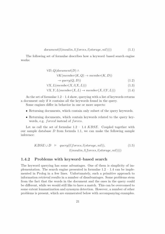
document(l(insulin, l(forces, l(storage, nil)))) (1.1)
The following set of formulae describes how a keyword–based search engineworks:
∀D,Q(document(D) ∧
∀K(member(K,Q)→ member(K,D))
→ query(Q,D)) (1.2)
∀X,L(member(X, l(X,L))) (1.3)
∀X,Y, L(member(X,L)→ member(X, l(Y, L))) (1.4)
As the set of formulae 1.2 – 1.4 show, querying with a list of keywords returnsa document only if it contains all the keywords found in the query.
Some engines differ in behavior in one or more aspects:
• Returning documents, which contain only subset of the query keywords.
• Returning documents, which contain keywords related to the query key-words, e.g. forced instead of forces.
Let us call the set of formulae 1.2 – 1.4 KBSE. Coupled together withour sample database D from formula 1.1, we can make the following sampleinference:
KBSE ∪D � query(l(forces, l(storage, nil)), (1.5)
l(insulin, l(forces, l(storage, nil))))
1.4.2 Problems with keyword–based search
The keyword querying has some advantages. One of them is simplicity of im-plementation. The search engine presented in formulae 1.2 – 1.4 can be imple-mented in Prolog in a few lines. Unfortunately, such a primitive approach toinformation retrieval results in a number of disadvantages. Some problems stemfrom the fact that the words in the document and the ones in the query couldbe different, while we would still like to have a match. This can be overcomed tosome extent lemmatization and synonym detection. However, a number of otherproblems is present, which are enumerated below with accompanying examples.
21

Scattered keywords
Let us consider the following query: insulin causes storage. The user isinterested in the concept of insulin forcing a storage of something.
Most search engines will return an article, in which insulin and storage
are present in one sentence, and causes is present in another sentence. Thisbehavior follows from the fact that the search engine does not recognize con-cepts appearing in the text, but rather relies on presence of words in the wholedocument.
Multiple queries
Most search engines have a feature which allows the user to search for a sequenceof keywords, which must appear contiguously in the returned document. Usu-ally, such a sequence must be enclosed in double quotes in the query. This allowsthe user to overcome the problem of scattered keywords to a certain extent. Onecould, e.g. search for ‘‘insulin causes storage’’, so that documents withthose keywords scattered around will not be shown in the result.
Unfortunately, the user is usually forced to pose multiple queries, as thedocument author might have written the text in a different way. The authorcould use different wording, phrased the document in a different manner, etc.
As an example, the user might be forced to query with the following se-quences of keywords:
• ‘‘insulin causes storage’’
• ‘‘insulin is causing storage’’
• ‘‘storage caused by insulin’’
• . . .
For each query different articles will be returned (if any).An ontological search engine should realize that all of those sequences of
keywords are paraphrases. It should therefore be necessary to simply fire onequery only. It is a key goal in our work to achieve such a functionality.
Lack of underlying ontology
Without an underlying ontology, the search engine will not be able to realizethat “forcing” is in fact a kind of “causing”. The user therefore needs to fire upadditional queries:
22

• ‘‘insulin forces storage’’
• ‘‘insulin is forcing storage’’
• ‘‘storage forced by insulin’’
• . . .
Language dependency
The deficiencies of keyword–based searching are due to the fact that the enginecompares text, not the semantics. If the engine was able to extract semanticsfrom the text and from the query and compare them, instead of comparing thetext itself, many problems could be easily overcome.
Comparing the ontological concepts instead of the words that describe themcould allow new ways of information retrieval, e.g. one could query in English,but get an article in Danish as a result.
1.5 Comprehensive natural language semantics
At one end of the spectrum we have the simple keyword functionality presentedin the previous section. At the other far end of the spectrum there is a very richsemantics, where the meaning of a sentence is presented as a logical formula inan expressive (usually undecidable) logic formalism. A common choice is theType Theory comprising simply–typed λ–calculus. [3] A very elaborate linguisticsystem based on it is presented in [46]. However, we focus on using ontologiesas basis for semantic domain, and we present one approach merging generativeontologies and type theory in Section 5.12 on page 98.
In this “rich” scenario the meaning of a sentece or a phrase is captured asa logical formula, which facilitates the use of logical consequence as the meansof establishing how the meaning of two sentences relate. There are, however,many problems with using such a semantics for search purposes.
Formalisms used in this scenario (e.g. First Order Predicate Logic, λ–calculus)use variables extensively, and therefore they focus a lot on quantifiers as meaning–carying elements (corresponding to determiners like “every”, “all”, “some”).They also put stress on logical connectives/operators. However, scientific textsin biomedical domain do not tend to convey meaning with quantifiers and con-nectives. The meaning in these texts is concentrated around nouns, verbs,adjectives and prepositions. Even if we find rare cases of quantifier–related
23
meaning in sentences, we claim that it is not important (maybe even unde-sired) to make use of that meaning for the purpose of search. Consider thesentence “All beta cells secrete insulin”. This could be translated to FirstOrder Predicate Logic as ∀X(betacell(X) → secrete(X, insulin)). Now con-sider “Many beta cells secrete insulin”. This would translate to the formula∃X(betacell(X) ∧ secrete(X, insulin)). We can observe how a lot of focus hasbeen put on quantification and operators. This seems irrelevant from the search–perspective, as it is hard to imagine a user query where one of these sentencesshould be returned as the result and the other should not. Also, deciding (evennon–automatically, i.e. by human) how to describe a meaning of a sentence inFirst Order Predicate Logic or Type Theory is very difficult. The textbooksare full of perfect examples, which seem to follow the building blocks of a givenlogic, so they can be translated easily. Unfortunately, it is not so easy with reallife sentences, let alone in an automatic manner.
The formalisms commonly used for representing natural language semanticscome with logical consequence, which can in principle be used for search. Thesearch engine can return all documents containing sentences such that theirmeaning entail the query. However, this approach suffers from multiple prob-lems. First Order Predicate Logic and Type Theory are undecidable formalisms,which means that sometimes we might not be able to conclude whether a givensentence should be included in the search results. Another problem is that aninconsistent sentence may appear in all search results (as anything follows fromit). Also, basing search on logical consequence seems to be a bad choice forsearch purposes, because it does not mirror the intentions of the user. Considertwo sentences: “All beta cells secrete insulin” and “Not all beta cells secreteinsulin”. Clearly, neither of these follow from the other (as a matter of fact theyare opposites). However, in search context, if one of them matches a query, wewould like the other one to match as well. This is because while searching we aremostly concerned with the “aboutness” of a sentence (what a sentence is about)rather than the propositional content that focuses on variables, quantifiers, andlogical connectives.
In the current work, we try to find a better semantic domain, which will besuitable for search. We will base it on a notion of generative ontologies, andwe will investigate the computational aspect of it. We would like to capturemore meaning than the keyword semantics, but less than the rich logic–basedsemantics. As a matter of fact, the keyword–semantics will be our fallbackmechanism, i.e. any phrase that is not understood well by our methods willproduce corresponding keywords as result.
24

1.6 Ontology–enabled browsing search
Basing the search semantics on a generative ontology has a big advantage, i.e. itenables search by browsing the indexed generative ontology.
Imagine that when processing the to–be–searched documents for every on-tological concept found we create a link from the generative ontology to thatdocument. We can now browse the generative ontology, which for every nodewould display the number of documents indexed under that node. It could ob-viously also list the links to the documents (or even sentences) that contain thisnode in their semantics. Example:
Let us say we want to find some documents about inhibiting the transport ofglucose. We start browsing the ontology at “inhibition”. The system says thatthere is 106 documents containing this concept. It also displays the most generalsubclasses, e.g. “inhibition of substance”, “inhibition of process”, etc. Weselect the latter, and we can see that there is 105 documents about “inhibitionof process”. This is still too many, so we browse down different processes,and we get to “inhibition of transport”, which has 104 documents. Again, wenarrow this concept down to “inhibition of (transport of substance)”, which has103 documents. We browse further down, so that we narrow our concept to“inhibition of (transport of glucose)”. At this point the system says there isonly 102 documents indexed. We could continue browsing down to even morespecific concepts (e.g. if we wanted the inhibition to happen in liver), but wedecide that we want to see the list of the documents.
This way of finding documents has some advantages compared to keywordquerying. The most important thing to notice is that the query is a concept inthe ontology, hence the query is not expressed in natural language. The sameconcept would correspond to a series of different noun phrases, verb phrases,sentences, or even languages.
Such a browsing is of course not free of drawbacks. The user needs to be adomain expert in order to browse the ontology efficiently.
We believe that the browsing search approach could become a useful tool inbiomedical domains, where large ontologies exist, and people are fairly familiarwith them.
1.7 Importance of fast information retrieval
In todays world, people increasingly depend on fast access to information. Wehave entered the era of “information society”, where Internet search engines are
25
the primary tool for each computer user.Subsequently, any improvement in the way people search for information
constitutes a big leap forward for computer users. People “google” 3 billiontimes a day[30]. Simple calculation shows that if by improving informationretrieval techniques we could save on average one second of person’s time persearch, this amounts to:
(timesavedpersearch) · (numberofsearchesperday)
= 1s · 3 · 109
= 3 · 109s
= 3 · 109s ·1min
60s
= 5 · 107min ·1h
60min
= 8.(3) · 105h ·1d
24h
≈ 34722d ·1y
365d≈ 95y
Thus, each day, we could save a century of humanity’s time (95 man–years)by one–second–per–person improvement. 2
In section 1.4 we explain why most people unnecessarily waste not one sec-ond, but much more time on machine–aided searching using today’s state–of–the–art technology.
Our hope is that by merging natural language semantics with formal on-tologies we could achieve semantic representation of text that could be used formore intelligent search than keyword–based one. Although we will not botherwith how to implement a search engine, we will devote this thesis to the devel-opment of an ontological semantics, including practical computational methodsof extracting it from natural language texts (in limited contexts).
1.8 Survey of the chapters
In Chapter 2 we introduce the reader to the formalisms that are useful for repre-senting either formal ontologies, natural language semantics, or both. Chapter 3
2Similar calculation shows that at the same time we save 100W · 8 · 105h ≈ 8 · 104kWh ofelectrical energy.
26

provides a general introduction to ontologies, both formal and informal ones. InChapter 4 we explain how the notion of “types” is used in logic, ontologies, andprogramming languages. We provide several approaches to the merging of theformal ontologies with natural language semantics in Chapter 5. We compareour point of view with that of the state of the art in Chapter 6. The question ofhow to approach the same problem from the computational point of view is dis-cussed in Chapter 7. In Chapter 8 we go one step further and try to use similarmethods for dealing with unrestricted natural language. We present some finalthoughts and the discussion of further work in Chapter 9. Finally, we concludethe work in Chapter 10.
27

28

Chapter 2
Logic and formalisms
Basic knowledge of various formalisms may be essential for understanding thefollowing chapters. Therefore we will try to make the reader familiar with a set offormalisms often used for representing ontologies, conceptual feature structures,semantics of natural language sentences and phrases, etc. Such an introductioncould be achieved in an alternativ fashion, i.e. by providing good references tothe material that describes the formalisms needed. However, it is feared thatthis would be at a cost of the lack of coherence of the current text.
In addition, the standard sources describing many of these formalisms areunfortunately not rich in relevant examples. Hence, we will try to introduce thenecessary background knowledge with the help of many examples.
In this chapter we will describe some of the formalisms useful for ontologyengineering and semantic representation for natural language:
• First Order Predicate Logic
• Lattices
• Description Logics
We will also have a brief look at the Logic of Plurals and Mass Terms.
2.1 First Order Predicate Logic
We assume that the reader is familiar with First Order Predicate Logic, as itis a basic tool for every computer scientist. Otherwise please consult a text onthe subject, e.g. [8].
29
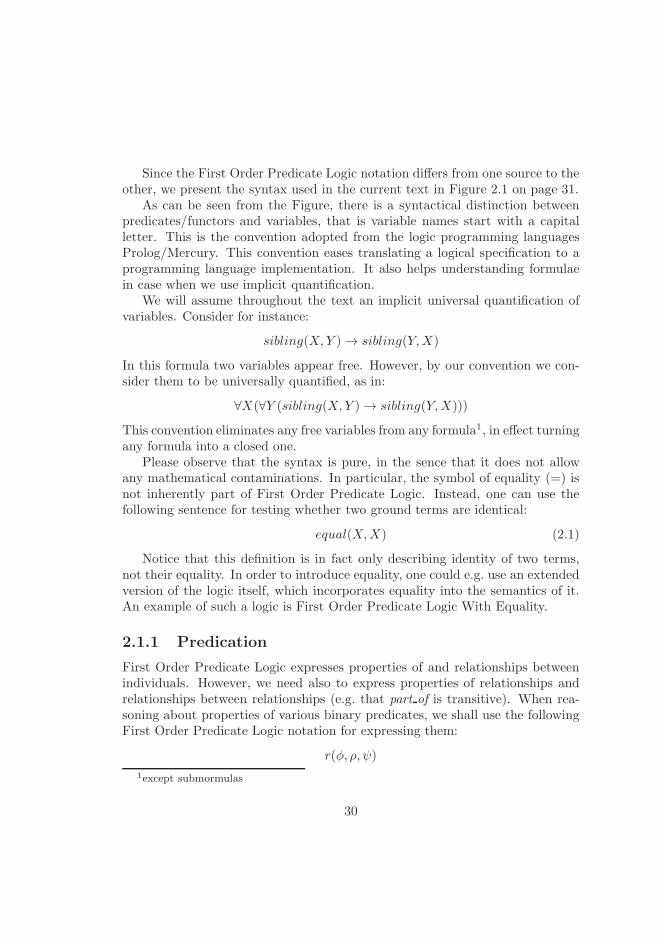
Since the First Order Predicate Logic notation differs from one source to theother, we present the syntax used in the current text in Figure 2.1 on page 31.
As can be seen from the Figure, there is a syntactical distinction betweenpredicates/functors and variables, that is variable names start with a capitalletter. This is the convention adopted from the logic programming languagesProlog/Mercury. This convention eases translating a logical specification to aprogramming language implementation. It also helps understanding formulaein case when we use implicit quantification.
We will assume throughout the text an implicit universal quantification ofvariables. Consider for instance:
sibling(X,Y )→ sibling(Y,X)
In this formula two variables appear free. However, by our convention we con-sider them to be universally quantified, as in:
∀X(∀Y (sibling(X,Y )→ sibling(Y,X)))
This convention eliminates any free variables from any formula1, in effect turningany formula into a closed one.
Please observe that the syntax is pure, in the sence that it does not allowany mathematical contaminations. In particular, the symbol of equality (=) isnot inherently part of First Order Predicate Logic. Instead, one can use thefollowing sentence for testing whether two ground terms are identical:
equal(X,X) (2.1)
Notice that this definition is in fact only describing identity of two terms,not their equality. In order to introduce equality, one could e.g. use an extendedversion of the logic itself, which incorporates equality into the semantics of it.An example of such a logic is First Order Predicate Logic With Equality.
2.1.1 Predication
First Order Predicate Logic expresses properties of and relationships betweenindividuals. However, we need also to express properties of relationships andrelationships between relationships (e.g. that part of is transitive). When rea-soning about properties of various binary predicates, we shall use the followingFirst Order Predicate Logic notation for expressing them:
r(φ, ρ, ψ)
1except submormulas
30

〈formula〉 ::= 〈predicate〉(〈termlist〉)
| 〈predicate〉
| ¬〈formula〉
| 〈formula〉 ∨ 〈formula〉
| 〈formula〉 ∧ 〈formula〉
| 〈formula〉 → 〈formula〉
| 〈formula〉 ← 〈formula〉
| 〈formula〉 ↔ 〈formula〉
| 〈quantifier〉〈variablelist〉(〈formula〉)
| (〈formula〉)
〈quantifier〉 ::= ∀|∃
〈term〉 ::= 〈variable〉
| 〈functor〉
| 〈functor〉(〈termlist〉)
〈termlist〉 ::= 〈term〉
| 〈term〉, 〈termlist〉
〈variablelist〉 ::= 〈variable〉
| 〈variable〉, 〈variablelist〉
〈lowercase〉 ::= a|b| . . . |x|y|z
〈uppercase〉 ::= A|B| . . . |X |Y |Z
〈letters〉 ::= ǫ
| 〈lowercase〉〈letters〉
| 〈uppercase〉〈letters〉
〈variable〉 ::= 〈uppercase〉〈letters〉
〈predicate〉 ::= 〈lowercase〉〈letters〉
〈functor〉 ::= 〈lowercase〉〈letters〉
Figure 2.1: Abstract syntax of First Order Predicate Logic used throughout thetext.
31
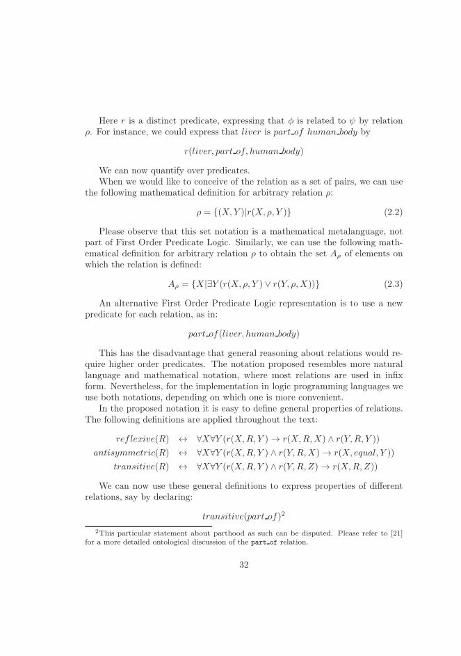
Here r is a distinct predicate, expressing that φ is related to ψ by relationρ. For instance, we could express that liver is part of human body by
r(liver, part of, human body)
We can now quantify over predicates.When we would like to conceive of the relation as a set of pairs, we can use
the following mathematical definition for arbitrary relation ρ:
ρ = {(X,Y )|r(X, ρ, Y )} (2.2)
Please observe that this set notation is a mathematical metalanguage, notpart of First Order Predicate Logic. Similarly, we can use the following math-ematical definition for arbitrary relation ρ to obtain the set Aρ of elements onwhich the relation is defined:
Aρ = {X |∃Y (r(X, ρ, Y ) ∨ r(Y, ρ,X))} (2.3)
An alternative First Order Predicate Logic representation is to use a newpredicate for each relation, as in:
part of(liver, human body)
This has the disadvantage that general reasoning about relations would re-quire higher order predicates. The notation proposed resembles more naturallanguage and mathematical notation, where most relations are used in infixform. Nevertheless, for the implementation in logic programming languages weuse both notations, depending on which one is more convenient.
In the proposed notation it is easy to define general properties of relations.The following definitions are applied throughout the text:
reflexive(R) ↔ ∀X∀Y (r(X,R, Y )→ r(X,R,X) ∧ r(Y,R, Y ))
antisymmetric(R) ↔ ∀X∀Y (r(X,R, Y ) ∧ r(Y,R,X)→ r(X, equal, Y ))
transitive(R) ↔ ∀X∀Y (r(X,R, Y ) ∧ r(Y,R, Z)→ r(X,R,Z))
We can now use these general definitions to express properties of differentrelations, say by declaring:
transitive(part of)2
2This particular statement about parthood as such can be disputed. Please refer to [21]for a more detailed ontological discussion of the part of relation.
32
Please observe that the following definition of reflexivity is deficient:
reflexive(R)↔ ∀X(r(X,R,X)) (2.4)
The problem is that we should require reflexivity to hold only for objects,which in fact engage in the relation, not for all objects in the universe.
2.1.2 Algebraic operations
Algebra plays an important role in representing the meaning of natural lan-guage. [28] We shall use the following First Order Predicate Logic notation forexpressing algebraic operations:
o(φ, ω, ψ, γ)
Here o is a distinct predicate intended for expressing that ω applied to φ andψ results in γ. E.g. we could express that Peirce product 3 of has color relationand green is green thing by:
o(has color, :, green, green thing)
We can use the following metalanguage definition for arbitrary operation ωto obtain the set Aω of elements on which the operation is defined:
Aω = {X |∃Y ∃Z(o(X, ρ, Y, Z) ∨ o(Y, ω,X,Z))} (2.5)
Similarly as for binary relations, it is easy to define general properties ofalgebraic operations. The following is assumed to hold throughout the text:
idempotent(O) ↔ ∀(o(X,O, Y, Z)→
o(X,O,X,X) ∧ o(Y,O, Y, Y ))
commutative(O) ↔ ∀(o(X,O, Y, Z)→ o(Y,O,X,Z))
associative(O) ↔ ∀(o(Y,O, Z,W ) ∧ o(X,O,W, V )
∧ o(X,O, Y, U)→ o(U,O,Z, V ))
absorptive(O1, O2) ↔ ∀(o(X,O2, Y, U)→ o(X,O1, U,X))
We can now use these general definitions to express properties of differentoperations, e.g. commutativity of set intersection:
commutative(∩)
3Peirce product algebraic operation is described in section 2.3.7 on page 47.
33
2.1.3 Distinction between classes and instances
In many knowledge domains, e.g. in the biomedical domain we do not seea clear need for distinguishing between classes (descriptions of groups of in-dividuals) and instances (individuals). For example, we could have a classliver, which represents a set of all possibly imaginable livers, and an instanceJohn Smith′s liver, representing a particular liver.
Since in the present framework we are concerned with understanding whatsentences in biomedical papers are about, we can forget about instances, asarticles rarely talk about some particulars. The general approach is to describethings more generally. Even if the article talks about a particular patient, hername will not be repeated in every sentence. Since we do not analyze thecontext, but analyze each sentence individually, the objects will still representclasses more than instances. Consider the following example:
This paper is about John Smith. His liver stores glucose. (2.6)
Even though the paper talks about some specific liver, our system will notbe able to notice that, because it analyzes each sentence independently.
Hence in the ontological analysis described later, we do not make any use ofinstances, or particulars, but we only use classes. Anyway, a particular objectcan be conceived as a singleton set comprising that object, so an instance canbe represented by a singleton class.
For further discussion of the notion of instances and classes, please referto [47, 32].
2.2 Lattices
One of the formalisms that can be used to represent the classification withinknowledge domains (and hence ontologies) is lattices. First we introduce nec-essary definitions, next we will present examples ilustrating the usefulness oflattices. We choose to present lattices within our chosen framework of FirstOrder Predicate Logic.
2.2.1 Posets
We call a binary relation R a poset (partially ordered set) iff it satisfies threeconditions:
poset(R)↔ reflexive(R) ∧ antisymmetric(R) ∧ transitive(R)
34
Following [38], from a mathematical point of view a poset is a pair (P,R)where P is a set and R is a relation (set of pairs: R ⊆ P × P ) such that R is apartial order (it is reflexive, antisymmetric and transitive).
We will however use the notion of a poset and partial order simultaneouslyfor a relation ρ, since we can always obtain such a mathematical view of a poset(Aρ, ρ) using definitions 2.3 and 2.2 on page 32.
Let us consider the following example defining the relation ipo (is part of),e.g. peru ipo southAmerika, but amazon ipo both peru and brasil:
r(peru, ipo, peru)
r(brasil, ipo, brasil)
r(southAmerika, ipo, southAmerika)
r(amazon, ipo, southAmerika)
r(brasil, ipo, southAmerika)
r(peru, ipo, southAmerika)
r(amazon, ipo, brasil)
r(amazon, ipo, amazon)
r(amazon, ipo, peru)
Using definition 2.3 we can obtain a mathematical view of the set Aipo onwhich the relation is defined:
Aipo = {amazon, peru, brasil, southAmerika}
Similarly, we can calculate the mathematical view of the relation ipo as aset of pairs using definition 2.2:
ipo = { (amazon, amazon), (peru, peru), (brasil, brasil),
(southAmerika, southAmerika),
(amazon, southAmerika), (brasil, southAmerika),
(peru, southAmerika), (amazon, brasil), (amazon, peru) }
Hence, we can refer to relation ipo as both a partial order and a poset.
It is easy to verify that:
poset(ipo)
35

2.2.2 Top and bottom
“Top” is the largest element in a given ordering, and “bottom” is the lowestone. We can define the top element T (denoted ⊤) for poset relation R as:
r(T, top,R)↔ ∀X,Y (r(X,R, Y )→ r(X,R, T ) ∧ r(Y,R, T ))
Similarly, the bottom element B (denoted ⊥) can be defined as:
r(B, bottom,R)↔ ∀X,Y (r(X,R, Y )→ r(B,R,X) ∧ r(B,R, Y ))
As an example for relation ipo defined in section 2.2.1, we have:
r(southAmerika, top, ipo) ∧ r(amazon, bottom, ipo)
There are poset relations R without ⊤ and ⊥ elements:
∃R(¬∃T (r(T, top,R)))
∃R(¬∃B(r(B, bottom,R)))
2.2.3 Upper and lower bounds
We say that elements X and Y in poset relation R have an upper bound U , aleast upper bound (supremum) S, lower bound L, and a greatest lower bound(infimum) I when:
upperBound(X,Y,R, U) ↔ r(X,R,U) ∧ r(Y,R, U)
supremum(X,Y,R, S) ↔ ∀U(upperBound(X,Y,R, U)→ r(S,R, U))
lowerBound(X,Y,R, L) ↔ r(L,R,X) ∧ r(L,R, Y )
infimum(X,Y,R, I) ↔ ∀L(lowerBound(X,Y,R, L)→ r(L,R, I))
36
Example:
upperBound(peru, amazon, ipo, southAmerika)
upperBound(peru, amazon, ipo, peru)
supremum(peru, amazon, ipo, peru)
¬supremum(peru, amazon, ipo, southAmerika)
lowerBound(brasil, southAmerika, ipo, amazon)
lowerBound(brasil, southAmerika, ipo, brasil)
infimum(brasil, southAmerika, ipo, brasil)
¬infimum(brasil, southAmerika, ipo, amazon)
2.2.4 Lattice as poset
We say that poset R is a lattice iff:
lattice(R)↔ ∀X,Y (r(X,R, Y )→ ∃S(supremum(X,Y,R, S))∧∃I(infimum(X,Y,R, I)))
We define boundedLattice as:
boundedLattice(R)↔ lattice(R) ∧ ∃T (r(T, top,R)) ∧ ∃B(r(B, bottom,R))
2.2.5 Hasse diagrams
The graphical representation of a poset known as Hasse diagram can be drawnin the following manner (from [38]): if x ≤ y then we place x below y and drawa line from x to y, except that lines following from reflexivity and transitivityare omitted.
The Hasse diagram of the poset ipo (which happens to be a lattice) is pre-sented in figure 2.2 on page 38.
2.2.6 isa as partial order
Of particular interest is the isa relation, which forms a poset when coupledwith arbitrary set of classes. We can hence easily represent the taxonomy of ourdomain using the Hasse diagram.
poset(isa)
37

Figure 2.2: Hasse diagram for ipo lattice.
We might insist that the isa relation is a lattice in order to enjoy the statedmathematical properties for our classification.
lattice(isa)
We present a sample Hasse diagram for the isa relation in our domain infigure 2.3 on page 39.
2.2.7 Lattices as algebras
As defined in [38], from mathematical point of view, lattice is a triple (L, J,M),where L is a nonempty set, J andM are binary operations defined on L, havingspecial properties. In our First Order Predicate Logic notation, however, theset L is implicitly defined and can be obtained using definition 2.5.
We shall call a pair of operations J,M a lattice, when:
lattice(J,M)↔idempotent(J) ∧ idempotent(M)∧
commutative(J) ∧ commutative(M)∧
associative(J) ∧ associative(M)∧
absorptive(J,M) ∧ absorptive(M,J)
We usually refer to the two operations as join (denoted ∨) and meet (denoted∧). Symbols ∨ and ∧ are reserved for disjunction and conjunction in First OrderPredicate Logic, hence we shall avoid them in our formulae.
38

Figure 2.3: Hasse diagram for isa lattice.
39
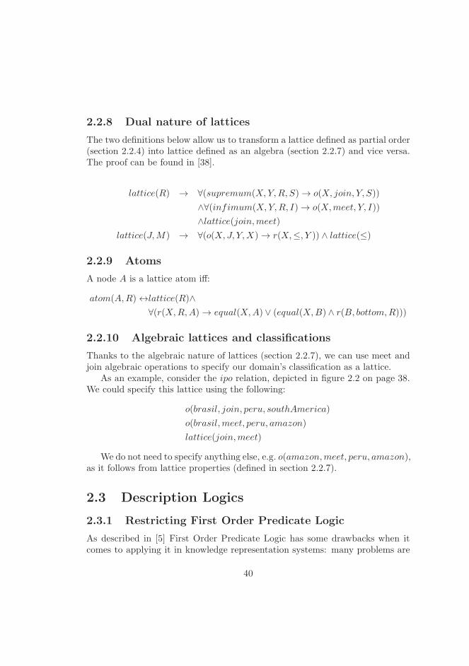
2.2.8 Dual nature of lattices
The two definitions below allow us to transform a lattice defined as partial order(section 2.2.4) into lattice defined as an algebra (section 2.2.7) and vice versa.The proof can be found in [38].
lattice(R) → ∀(supremum(X,Y,R, S)→ o(X, join, Y, S))
∧∀(infimum(X,Y,R, I)→ o(X,meet, Y, I))
∧lattice(join,meet)
lattice(J,M) → ∀(o(X, J, Y,X)→ r(X,≤, Y )) ∧ lattice(≤)
2.2.9 Atoms
A node A is a lattice atom iff:
atom(A,R)↔lattice(R)∧
∀(r(X,R,A)→ equal(X,A) ∨ (equal(X,B) ∧ r(B, bottom,R)))
2.2.10 Algebraic lattices and classifications
Thanks to the algebraic nature of lattices (section 2.2.7), we can use meet andjoin algebraic operations to specify our domain’s classification as a lattice.
As an example, consider the ipo relation, depicted in figure 2.2 on page 38.We could specify this lattice using the following:
o(brasil, join, peru, southAmerica)
o(brasil,meet, peru, amazon)
lattice(join,meet)
We do not need to specify anything else, e.g. o(amazon,meet, peru, amazon),as it follows from lattice properties (defined in section 2.2.7).
2.3 Description Logics
2.3.1 Restricting First Order Predicate Logic
As described in [5] First Order Predicate Logic has some drawbacks when itcomes to applying it in knowledge representation systems: many problems are
40
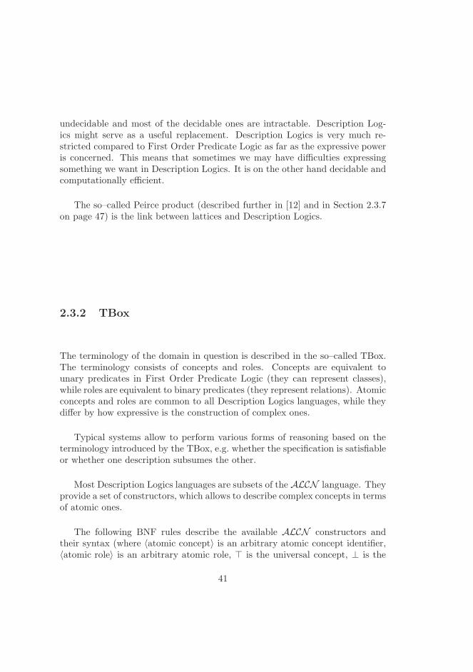
undecidable and most of the decidable ones are intractable. Description Log-ics might serve as a useful replacement. Description Logics is very much re-stricted compared to First Order Predicate Logic as far as the expressive poweris concerned. This means that sometimes we may have difficulties expressingsomething we want in Description Logics. It is on the other hand decidable andcomputationally efficient.
The so–called Peirce product (described further in [12] and in Section 2.3.7on page 47) is the link between lattices and Description Logics.
2.3.2 TBox
The terminology of the domain in question is described in the so–called TBox.The terminology consists of concepts and roles. Concepts are equivalent tounary predicates in First Order Predicate Logic (they can represent classes),while roles are equivalent to binary predicates (they represent relations). Atomicconcepts and roles are common to all Description Logics languages, while theydiffer by how expressive is the construction of complex ones.
Typical systems allow to perform various forms of reasoning based on theterminology introduced by the TBox, e.g. whether the specification is satisfiableor whether one description subsumes the other.
Most Description Logics languages are subsets of the ALCN language. Theyprovide a set of constructors, which allows to describe complex concepts in termsof atomic ones.
The following BNF rules describe the available ALCN constructors andtheir syntax (where 〈atomic concept〉 is an arbitrary atomic concept identifier,〈atomic role〉 is an arbitrary atomic role, ⊤ is the universal concept, ⊥ is the
41

bottom concept and 〈n〉 is a natural number):
〈concept〉 ::= 〈atomic concept〉
| ⊤
| ⊥
| ¬〈concept〉
| 〈concept〉 ⊓ 〈concept〉
| 〈concept〉 ⊔ 〈concept〉
| ∀〈atomic role〉.〈concept〉
| ∃〈atomic role〉.〈concept〉
| > 〈n〉〈atomic role〉
| 6 〈n〉〈atomic role〉
〈terminological axiom〉 ::= 〈concept〉 ⊑ 〈concept〉
| 〈concept〉 ≡ 〈concept〉
〈definition〉 ::= 〈atomic concept〉 ⊑ 〈concept〉
| 〈atomic concept〉 ≡ 〈concept〉
A set of 〈definition〉s is called a TBox if each symbolic name is defined atmost once. This limitation however seems to be abandoned in recent versionsof some Description Logics reasoning implementations.
2.3.3 ABox
The ABox provides set of assertions expressed in terms of terminology definedby the TBox. There are only two types of assertions one can make: conceptassertions of the form C(a) and role assertions of the form R(a, b), where C isa concept, R is a role, and a, b are names of individuals.
Existing systems allow checking whether assertions expressed by the ABoxare consistent and whether a particular individual is an instance of a givenconcept.
42
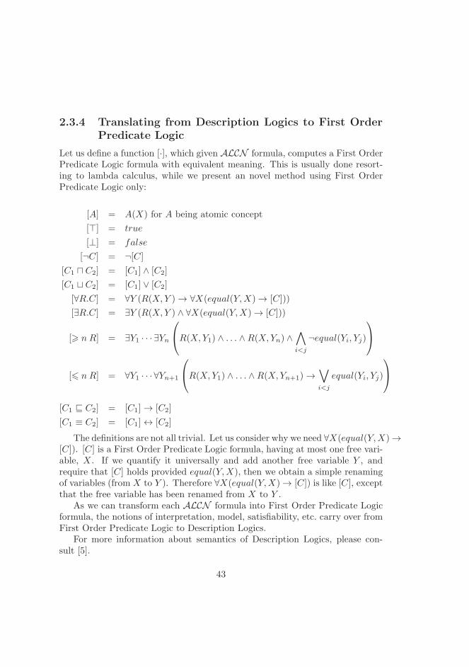
2.3.4 Translating from Description Logics to First OrderPredicate Logic
Let us define a function [·], which given ALCN formula, computes a First OrderPredicate Logic formula with equivalent meaning. This is usually done resort-ing to lambda calculus, while we present an novel method using First OrderPredicate Logic only:
[A] = A(X) for A being atomic concept
[⊤] = true
[⊥] = false
[¬C] = ¬[C]
[C1 ⊓ C2] = [C1] ∧ [C2]
[C1 ⊔ C2] = [C1] ∨ [C2]
[∀R.C] = ∀Y (R(X,Y )→ ∀X(equal(Y,X)→ [C]))
[∃R.C] = ∃Y (R(X,Y ) ∧ ∀X(equal(Y,X)→ [C]))
[> n R] = ∃Y1 · · · ∃Yn
R(X,Y1) ∧ . . . ∧R(X,Yn) ∧∧
i<j
¬equal(Yi, Yj)
[6 n R] = ∀Y1 · · · ∀Yn+1
R(X,Y1) ∧ . . . ∧R(X,Yn+1)→∨
i<j
equal(Yi, Yj)
[C1 ⊑ C2] = [C1]→ [C2]
[C1 ≡ C2] = [C1]↔ [C2]
The definitions are not all trivial. Let us consider why we need ∀X(equal(Y,X)→[C]). [C] is a First Order Predicate Logic formula, having at most one free vari-able, X . If we quantify it universally and add another free variable Y , andrequire that [C] holds provided equal(Y,X), then we obtain a simple renamingof variables (from X to Y ). Therefore ∀X(equal(Y,X)→ [C]) is like [C], exceptthat the free variable has been renamed from X to Y .
As we can transform each ALCN formula into First Order Predicate Logicformula, the notions of interpretation, model, satisfiability, etc. carry over fromFirst Order Predicate Logic to Description Logics.
For more information about semantics of Description Logics, please con-sult [5].
43

2.3.5 Examples
Below we present a TBox defining a taxonomy analogous to the Hasse dia-gram presented earlier in figure 2.3 on page 39. We assume that mountain,water, flowingWater, erupting are atomic base concepts and hasT ributary isan atomic role.
volcano ≡ mountain ⊓ erupting
geyser ≡ water ⊓ erupting
steadyWater ≡ water ⊓ ¬flowingWater ⊓ ¬geyser
lake ⊑ steadyWater
ocean ⊑ steadyWater
sea ⊑ steadyWater
river ≡ water ⊓ flowingWater ⊓ ∃hasT ributary.⊤
stream ≡ water ⊓ flowingWater ⊓ ∀hasT ributary.⊥
largeRiver ≡ river⊓ > 2 hasT ributary
Let us use the function f defined in section 2.3.4 in order to compute an
44
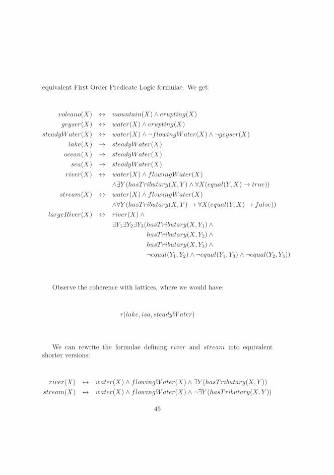
equivalent First Order Predicate Logic formulae. We get:
volcano(X) ↔ mountain(X) ∧ erupting(X)
geyser(X) ↔ water(X) ∧ erupting(X)
steadyWater(X) ↔ water(X) ∧ ¬flowingWater(X) ∧ ¬geyser(X)
lake(X) → steadyWater(X)
ocean(X) → steadyWater(X)
sea(X) → steadyWater(X)
river(X) ↔ water(X) ∧ flowingWater(X)
∧∃Y (hasT ributary(X,Y ) ∧ ∀X(equal(Y,X)→ true))
stream(X) ↔ water(X) ∧ flowingWater(X)
∧∀Y (hasT ributary(X,Y )→ ∀X(equal(Y,X)→ false))
largeRiver(X) ↔ river(X) ∧
∃Y1∃Y2∃Y3(hasT ributary(X,Y1) ∧
hasT ributary(X,Y2) ∧
hasT ributary(X,Y3) ∧
¬equal(Y1, Y2) ∧ ¬equal(Y1, Y3) ∧ ¬equal(Y2, Y3))
Observe the coherence with lattices, where we would have:
r(lake, isa, steadyWater)
We can rewrite the formulae defining river and stream into equivalentshorter versions:
river(X) ↔ water(X) ∧ flowingWater(X) ∧ ∃Y (hasT ributary(X,Y ))
stream(X) ↔ water(X) ∧ flowingWater(X) ∧ ¬∃Y (hasT ributary(X,Y ))
45
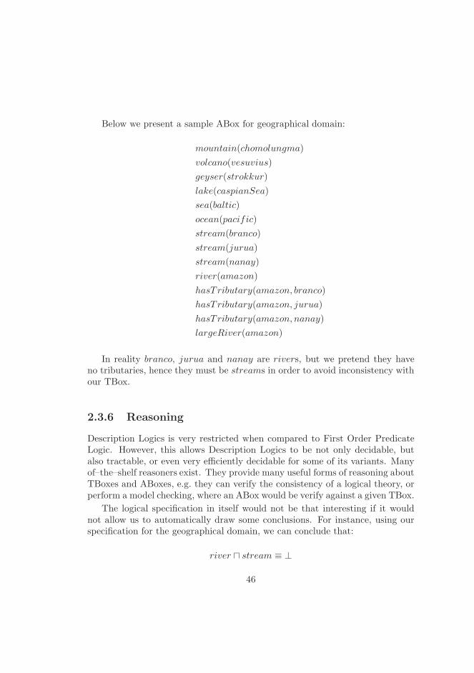
Below we present a sample ABox for geographical domain:
mountain(chomolungma)
volcano(vesuvius)
geyser(strokkur)
lake(caspianSea)
sea(baltic)
ocean(pacific)
stream(branco)
stream(jurua)
stream(nanay)
river(amazon)
hasT ributary(amazon, branco)
hasT ributary(amazon, jurua)
hasT ributary(amazon, nanay)
largeRiver(amazon)
In reality branco, jurua and nanay are rivers, but we pretend they haveno tributaries, hence they must be streams in order to avoid inconsistency withour TBox.
2.3.6 Reasoning
Description Logics is very restricted when compared to First Order PredicateLogic. However, this allows Description Logics to be not only decidable, butalso tractable, or even very efficiently decidable for some of its variants. Manyof–the–shelf reasoners exist. They provide many useful forms of reasoning aboutTBoxes and ABoxes, e.g. they can verify the consistency of a logical theory, orperform a model checking, where an ABox would be verify against a given TBox.
The logical specification in itself would not be that interesting if it wouldnot allow us to automatically draw some conclusions. For instance, using ourspecification for the geographical domain, we can conclude that:
river ⊓ stream ≡ ⊥
46

2.3.7 Peirce Algebra
Peirce algebra is a two–sorted algebra, which combines operations on sets andrelations. Hence, it is very useful for ontological applications, where classescan be conceived as sets, and where relations play major role. A very detailedintroduction is available in [12].
Of particular interest for us is the Peirce product, as the conceptual featurestructures used for representing parts of the ontological semantics are based onthe it. Peirce product (:) is defined as:
ρ : φ = {X |∃Y ((X,Y ) ∈ ρ ∧ Y ∈ φ)},
where ρ is a relation and φ is a class understood as a set. Notice that the Peirceproduct has an equivalent representation in Description Logics:
∃ρ.φ
Hence, the Peirce product can be considered to be the link between latticesand Description Logics.
2.4 Logic of Plurals and Mass Terms
The Logic of Plurals and Mass Terms is a variant of First Order Predicate Logic.It defines special facilities for describing plural formations. The most interestingof those is the collective operator (denoted ⊕), written by convention in an infixnotation. This operator takes two arguments and creates a collective object,representing the plural entity consisting of both arguments.
Let us have a look at some sentences, so that we can explain how ⊕ worksby example.
2.4.1 “A boy and a girl played.”
This sentence has two main readings:
• The collective reading, where the boy and the girl were engaged in acommon play.
• The distributive reading, where they both played, but individually.
47

Logic of Plurals and Mass Terms
In Logic of Plurals and Mass Terms we can utilize the collective operator torepresent the collective reading:
∃X∃Y (boy′(X) ∧ girl′(Y ) ∧ played′(X ⊕ Y ))
On the other hand, no special facilities are called for if we want to representthe distributive reading:
∃X∃Y (boy′(X) ∧ girl′(Y ) ∧ played′(X) ∧ played′(Y ))
Davidsonian view in First Order Predicate Logic
In the davidsonian view, we make use of an additional variable for representingthe event of playing. So the action of playing will not be represented by thepredicate played′(. . .) anymore. This has many advantages. We do not needto use the collective operator to represent the fact that more than one agenttook part in the action of playing, so we can stay within First Order PredicateLogic. Additionally, the arity of the played′ no longer needs to be decidedupon. E.g. if we also wanted to express the time at which the action tookplace, we would need to extend the unary predicate played′(who) to a binaryone play′(who,when). Such a problem is nonexistent with the davidsonianrepresentation of the meaning of the sentence.
The collective reading takes the form:
∃E∃X∃Y ∃T (playing(E)∧ boy(X) ∧ girl(Y )
∧ agt(E,X) ∧ agt(E, Y ) ∧ past(T ) ∧ tmp(E, T ))
The distributive reading will look as follows:
∃E1∃E2∃X∃Y ∃T1∃T2(playing(E1) ∧ boy(X) ∧ agt(E1, X) ∧ past(T1)
∧ playing(E2) ∧ girl(Y ) ∧ agt(E2, Y ) ∧ past(T2))
∧ tmp(E1, T1) ∧ tmp(E2, T2)
Description Logics
Finally, let us have a look at how such a semantics can be represented in De-scription Logics.
48

Here we will follow our previous representation using the davidsonian view.We chose our semantics to represent a concept rather than a terminologicalaxiom. The concept will be the one corresponding to the event that happened.
For the collective reading, we get the following single concept:
playing ⊓ ∃agt.boy ⊓ ∃agt.girl ⊓ ∃tmp.past
And for the distributive reading we get two separate semantics concepts (aswe have two different events):
playing ⊓ ∃agt.boy ⊓ ∃tmp.past
andplaying ⊓ ∃agt.girl ⊓ ∃tmp.past
2.4.2 “George and Martha met.”
This sentence has only the collective meaning. It is very hard to imagine thatsomebody would use such a sentence with the intention of saying that bothGeorge and Martha met somebody, but not each other.
Logic of Plurals and Mass Terms
The reading becomes (with the help of the collective operator):
met′(george ⊕martha)
Davidsonian view, First Order Predicate Logic
We can again utilize the davidsonian view for the purpose of representing thecollective reading within First Order Predicate Logic:
∃E∃X∃Y ∃T (meeting(E) ∧ george(X) ∧martha(Y )
∧ agt(E,X) ∧ agt(E, Y ) ∧ past(T ) ∧ tmp(E, T ))
Description Logics
Following our approach from the previous sentence, the reading becomes:
meeting ⊓ ∃agt.george ⊓ ∃agt.martha ⊓ ∃tmp.past
49

50

Chapter 3
Introduction to ontologies
This chapter provides a short general introduction to ontologies, both formaland informal ones. It is not the intention of the author that the chapter is arewrite of some books, but rather a brief introduction, which refers to certainsources. The aim of this chapter is specifically to establish how ontologicalnotions (such as classes, properties, relations, etc.) can be represented easily ina formal way.
In focus is the representation of ontologies in First Order Predicate Logic.This is due to the fact that if one can express ontological data in First OrderPredicate Logic, it is less difficult to adjust that representation to fit Prolog atthe implementation stage. Various First Order Predicate Logic representationscan be compared, so that it becomes evident how one can later implement theneeded reasoning machinery easily and efficiently.
This chapter also discusses various means of simplifying the view of theworld, e.g. lifting instances to singleton classes, etc.
A nice introduction and overview of ontologies and their various definitions isprovided in [23]. The word “Ontology” appeared thousands of years ago, whereancient philosophers tried to explain the essence of being. In such context, weuse the capitalized word “Ontology”. Please consult [23] for an overview of thefascinating problems that philosophers have been dealing with.
However, the current text focuses on formal ontologies, or simply ontologies,written with lower–case “o”. Formal ontology can be understood as specificationof a conceptualization. It is crucial that the ontology is specified in a formalway, so that it is machine–readable and understandable. A conceptualizationcan be thought of as a view of the world shared by some people. Of course none
51
of the ontologies can describe a full conceptualization of the whole world. Inmost cases an ontology attempts to describe only a specific domain.
3.1 Classes and instances
3.1.1 Distinction between class and instance
In most domains we clearly see the need for distinguishing between classes (de-scriptions of groups of individuals) and instances (individuals). For example, wecould have a class mountain, which represents a set of all possibly imaginablemountains, and an instance chomolungma, representing a particular mountain.
In concrete domains (as opposed to abstract ones), we insist that everyinstance represents an individual, which exists physically. On the other hand theclass mountain contains also non–existent objects. E.g. it comprises mountainshaving 9000m of height, even though no such mountains exist on Earth.1 If sucha mountain existed in history or will appear in the future, we may constructan instance representing it without modifying the class. Modifying the classmeans changing the relations in which the class engages, e.g. isa relation byadding or removing a pair of the form r(φ, isa, ψ) from the knowledge base, forarbitrary φ and ψ. Such a way of defining classes by their properties is known asintensional, as opposed to extensional manner, where classes are defined simplyby listing all elements.
Hence, once classes are defined and relations between them established, theyrepresent many different worlds. We can, by introducing specific instances,represent a particular world, e.g. planet Earth. We could represent a differentworld, e.g. planet Mars by using the same classes, yet different instances.
This is strongly related to the distinction between the TBox and the ABoxin Description Logics.
3.1.2 Inheritance and isa
Let us consider inheritance of properties from classes to subclasses. From inten-sional perspective, all elements in a subclass need to possess all the propertiespossessed jointly by all the members of parent class. Inheritance expressesthe fact that some classes are generalizations of other classes. The more gen-eral class is referred to as superclass or base class, and the less general one as
1Perhaps it also comprises the Meinong’s golden mountain – a common literature examplefor such non–existent objects. [14]
52

subclass or derived class. If the superclass represents a set of objects O, thesubclass represents a subset of O, which is in accord with the extensional viewof inheritance.
Inheritance is represented by the relation isa in the following manner:
r(flowingWaterObject, isa, waterObject)
We define isa to be a transitive relation:
transitive(isa)
Hence from the knowledge base, say:
r(flowingWaterObject, isa, waterObject)
r(river, isa, f lowingWaterObject)
we can deduce:r(river, isa, waterObject)
Hence, all rivers will need to possess the properties of water objects, e.g.that they are made of water, etc.
3.1.3 Relation instanceof
The relation between classes and instances is captured by the instanceof rela-tion. We have:
r(chomolungma, instanceof,mountain)2
It is important to distinguish between isa and instanceof relations. In thenatural language these are often confused, as in the following example:
r(river, isa, f lowingWaterObject)
r(orinoco, isa, river)
Such a usage is flawed, as river represents a class comprising all rivers andit can be instantiated. On the contrary orinoco is not a class, as it representsan individual, and it cannot be instantiated.
The examples in Section 3.1.4 also ilustrate that instanceof is not transitive(while isa is).
Furthermore, the following rule (defined as instance inference in [47]) applies:
∀(r(I, instanceof, C1) ∧ r(C1, isa, C2)→ r(I, instanceof, C2))
2Notice that we use lower–cased constants for geographic/politic names due to our con-vention in which upper–cased names are reserved for variables.
53

3.1.4 Spanning objects
In [47] we learn about the need for introducing spanning objects. A spanningobject is both a class and an instance of another class. In our sample geographydomain, the need for those is not apparent, because the domain is not abstract.We can add abstract concepts to the domain in order to discuss spanning objects.Let us consider the class typeOfGeographicObject. Instances of this class couldbe theRiver, theMountain, etc. On the other hand we have classmountain andsample instance chomolungma. The simplest representation for that situationwould be:
r(theMountain, instanceof, typeOfGeographicObject)
r(chomolungma, instanceof,mountain)
This representation, according to [47], is flawed, because the same concept(here mountain) needs an artificial split into an instance theMountain and aclass mountain.
We could express the correlation between theMountain and mountain interms of relation abstracts:
r(theMountain, abstracts,mountain)
In [47] we learn about problems arising from using relation abstracts. In-dividuals theMountain and chomolungma are fundamentaly different, becausechomolungma is a physical object in Geography domain, while theMountainis not. They do not exist in the same universe of discourse and this fact shouldbe explicitly modelled in our knowledge base.
Hence, the representation which makes use of spanning objects looks asfollows:
r(typeOfGeographicObject, classIn,metaGeographics)
r(mountain, instanceIn,metaGeographics)
r(mountain, classIn, geographics)
r(chomolungma, instanceIn, geographics)
r(mountain, instanceof, typeOfGeographicObject)
r(chomolungma, instanceof,mountain)
We have to introduce two universes of discourse: metaGeographics andgeographics. mountain is related to both of them, but using different relationsinstanceIn and classIn, respectively.
54

In order to enforce correct usage of those relations in the knowledge baseone could add the following conditions:
∀C,U1, U2(r(C, classIn, U1) ∧ r(C, classIn, U2)→ equal(U1, U2))
∀I, U1, U2(r(I, instanceIn, U1) ∧ r(I, instanceIn, U2)→ equal(U1, U2))
∀S,U1, U2(r(S, instanceIn, U1) ∧ r(S, classIn, U2)→ ¬equal(U1, U2))
∀I, C(r(I, instanceof, C)→ ∃U(r(I, instanceIn, U) ∧ r(C, classIn, U)))
3.2 Part-whole relation
Part-whole relations play an important role in scientific modeling. They expressthat some things are parts of other things. The graph of all part relations for agiven domain is refered to as partonomy.
Following [20], we define the supplementation property suppl of disjoint el-ements for a relation R:
suppl(R)↔ ∀A,B(r(A,R,B)→ ∃C(r(C,R,B) ∧ ¬∃X(r(X,R,A) ∧ r(X,R,C))))
Then we can define partof relation as a strict partial ordering relation, thushaving the following properties:
antisymmetric(partof)
transitive(partof)
suppl(partof)
Based on these properties a sample relation partof knowledge base couldlook as follows3:
r(zealand, partof, denmark)
r(jutland, partof, denmark)
r(denmark, partof, europe)
r(poland, partof, europe)
3We use lower–cased constants for geographic/politic names due to our convention in whichupper–cased names are reserved for variables.
55
3.3 Types of formal ontologies
Formal ontologies can be generally divided into lightweight and heavyweightontologies. The former are expressed using a very simple formalism, usuallyvariable–free one (like Description Logics and unlike First Order PredicateLogic), so that they serve as an overview of the conceptualization. The lattercall for more complicated formalism, as they usually model the conceptualiza-tion in a very detailed manner. In heavyweight ontologies a large amount of theinformation is implicit and is left to be inferred by the engine, hence the name.
Another categorization of ontologies focuses on the level of reality, whichthey describe. This division is presented in the following sections.
3.3.1 Top–level ontologies
Top–level ontologies, as the name suggests, are supposed to describe the mostgeneral view of the world. For a nice overview of different upper level ontologies,please refer to [23].
Out of many available top–level ontologies, we have decided to focus on BasicFormal Ontology (BFO). Like most top–level ontologies, BFO divides the worldinto enduring entities, called continuants (e.g. the body of a person), and 4–dimensional entities, called occurrents (e.g. the life of a person). A particularlygood description of BFO can be found in [43]:
BFO grows out of a philosophical orientation which overlaps withthat of DOLCE and SUMO. Unlike these, however, it is narrowlyfocused on the task of providing a genuine upper ontology which canbe used in support of domain ontologies developed for scientific re-search, as for example in biomedicine within the framework of theOBO Foundry.
3.3.2 Domain ontologies
Domain ontologies consist of classes characteristic for a given domain. Sincethe current text is concerned mainly with biomedical domain texts, we shall beinterested in biomedical ontologies.
There exists a large collection of biomedical ontologies, which are freelyavailable, called Open Biomedical Ontologies Foundry (OBO) [45]. It consistsof many domain–specific ontologies, gathered together in a unified format.
It is worth noticing that a domain ontology must be constructed by domainexperts, not by software engineers who want to use the ontology. Hence, in the
56
current project such an ontology is considered to be the input to the system,rather than a part of it. Various papers focus on the topic of creating a high–quality ontologies, e.g. [42].
3.3.3 Merging top–level and domain ontologies
Merging a top–level ontology with a particular domain ontology is not alwayseasy. Top–level ontologies are usually an attempt at a “perfect” categorizationof the world around us. They might be very abstract, in contrast to the domainontologies. The latter usually attempt to be as complete as possible, tryingto include all the concepts found in a particular domain. Therefore they tendto lose the perfectionistic view of the world. It might therefore be difficult tomerge the two into one, coherent ontology.
The reason why we would like to merge the two is that both are insufficientif used alone. Top–level ontologies are simply very small, normally having lessthan a hundred concepts. Therefore they cannot be used for analyzing naturallanguage, where much more concepts are found. The domain ontologies are, onthe other hand, relatively big, reaching even hundreds of thousands of concepts.Unfortunately, they are always focused on the domain, so they are missing theinter–domain concepts. Consider the sentence:
Insulin forces storage of glycogen. (3.1)
We can find three domain–specific concepts in the sentence: the chemical sub-stances insulin and glycogen, and the biological process of storing a substance.Unfortunately, the concept of action of forcing something cannot be present inthe biomedical ontology, as it is more of an inter–domain concept. If we canconstruct an ontology, which contains all of the above concepts, the ontologicalanalysis of the sentence will be more complete.
A sample ontology, created by merging the top–level Basic Formal Ontologywith common biomedical concepts is presented in Figure 3.1 on page 58.
3.4 Querying Ontologies with Prolog
Let us try to formalize an ontology with the goal of querying it in mind. We willuse First Order Predicate Logic as our formalism due to its closeness to Prolog.
Whenever a greek letter φ or ψ is encountered in a formula, it denotesa parameter and the formula itself is a parameterized formula, which can be
57

Figure 3.1: A sample ontology, created by merging the top–level Basic FormalOntology with common biomedical concepts.
58
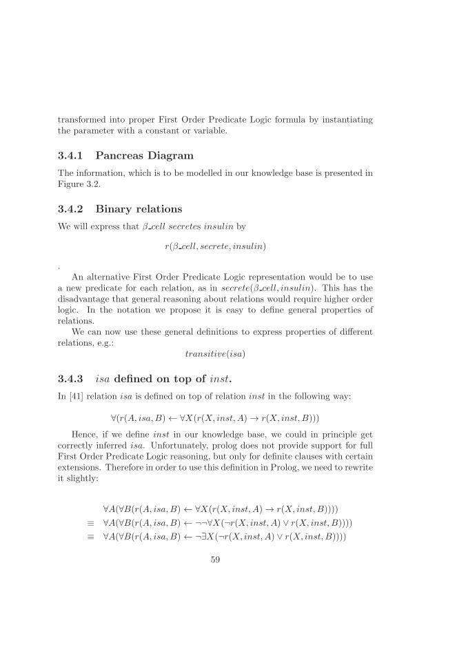
transformed into proper First Order Predicate Logic formula by instantiatingthe parameter with a constant or variable.
3.4.1 Pancreas Diagram
The information, which is to be modelled in our knowledge base is presented inFigure 3.2.
3.4.2 Binary relations
We will express that β cell secretes insulin by
r(β cell, secrete, insulin)
.An alternative First Order Predicate Logic representation would be to use
a new predicate for each relation, as in secrete(β cell, insulin). This has thedisadvantage that general reasoning about relations would require higher orderlogic. In the notation we propose it is easy to define general properties ofrelations.
We can now use these general definitions to express properties of differentrelations, e.g.:
transitive(isa)
3.4.3 isa defined on top of inst.
In [41] relation isa is defined on top of relation inst in the following way:
∀(r(A, isa,B)← ∀X(r(X, inst, A)→ r(X, inst, B)))
Hence, if we define inst in our knowledge base, we could in principle getcorrectly inferred isa. Unfortunately, prolog does not provide support for fullFirst Order Predicate Logic reasoning, but only for definite clauses with certainextensions. Therefore in order to use this definition in Prolog, we need to rewriteit slightly:
∀A(∀B(r(A, isa,B) ← ∀X(r(X, inst, A)→ r(X, inst, B))))
≡ ∀A(∀B(r(A, isa,B) ← ¬¬∀X(¬r(X, inst, A) ∨ r(X, inst, B))))
≡ ∀A(∀B(r(A, isa,B) ← ¬∃X(¬r(X, inst, A) ∨ r(X, inst, B))))
59

Figure 3.2: Pancreas diagram, created by Sine Zambach, Roskilde University,Denmark.
60
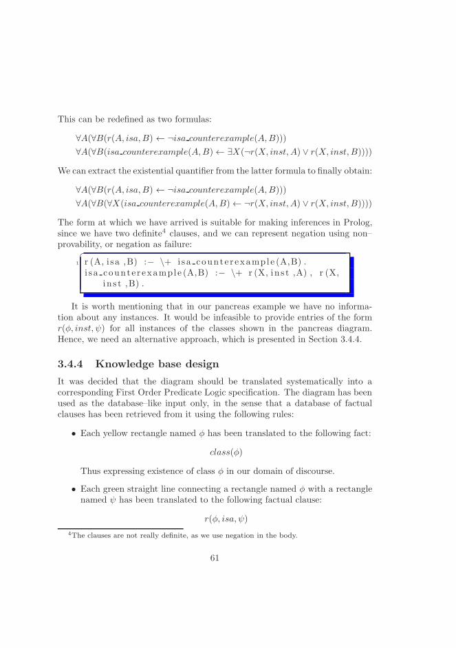
This can be redefined as two formulas:
∀A(∀B(r(A, isa,B) ← ¬isa counterexample(A,B)))
∀A(∀B(isa counterexample(A,B)← ∃X(¬r(X, inst, A) ∨ r(X, inst, B))))
We can extract the existential quantifier from the latter formula to finally obtain:
∀A(∀B(r(A, isa,B) ← ¬isa counterexample(A,B)))
∀A(∀B(∀X(isa counterexample(A,B)← ¬r(X, inst, A) ∨ r(X, inst, B))))
The form at which we have arrived is suitable for making inferences in Prolog,since we have two definite4 clauses, and we can represent negation using non–provability, or negation as failure:
�
1 r (A, i sa ,B) :− \+ isa counte r example (A,B) .i s a counte r example (A,B) :− \+ r (X, in s t ,A) , r (X,
in s t ,B) .
It is worth mentioning that in our pancreas example we have no informa-tion about any instances. It would be infeasible to provide entries of the formr(φ, inst, ψ) for all instances of the classes shown in the pancreas diagram.Hence, we need an alternative approach, which is presented in Section 3.4.4.
3.4.4 Knowledge base design
It was decided that the diagram should be translated systematically into acorresponding First Order Predicate Logic specification. The diagram has beenused as the database–like input only, in the sense that a database of factualclauses has been retrieved from it using the following rules:
• Each yellow rectangle named φ has been translated to the following fact:
class(φ)
Thus expressing existence of class φ in our domain of discourse.
• Each green straight line connecting a rectangle named φ with a rectanglenamed ψ has been translated to the following factual clause:
r(φ, isa, ψ)
4The clauses are not really definite, as we use negation in the body.
61

Those straight green lines do not have arrows indicating the direction, sothe convention assumed was that φ is below ψ in the picture, or in otherwords the parent class is higher up in the taxonomy.
• Each red zigzag line connecting a rectangle named φ with a rectanglenamed ψ has been translated to the following factual clause:
r(φ, partof, ψ)
Those red zigzag lines do not have arrows indicating the direction, so theconvention assumed was that φ is below ψ in the picture, or in other wordsψ class is higher up in the partonomy than φ.
In this way all the explicit knowledge visible on the pancreas diagram hasbeen transformed to First Order Predicate Logic and Prolog. Having no biolog-ical knowledge whatsoever, we have not modified the diagram in any way.
3.4.5 Well–formedness verification
In [41] we can find the following axioms governing relations in our knowledgebase:
• inst relation must hold between an instance and a class. We do not useinst in our system, but we use relations between classes that are definedon top of it in [41]. Hence, we can add the following axiom:
error() ← ∃R(∃X(∃Y ( (r(X,R, Y ) ∧ ¬db relation(R))
∨ (r(X,R, Y ) ∧ ¬db class(X))
∨ (r(X,R, Y ) ∧ ¬db class(Y )))))
This can be rewritten in Prolog as:�
e r r o r ( unde f i n ed r e l a t i o n (R) ) :− r ( ,R, ) ,\+ db r e l a t i o n (R) .
e r r o r ( unde f i n ed c l a s s (X) ) :− r (X, , ) , \+db c l a s s (X) .
3 e r r o r ( unde f i n ed c l a s s (X) ) :− r ( , ,X) , \+db c l a s s (X) .
Now, we can run the query asking for an error:
62
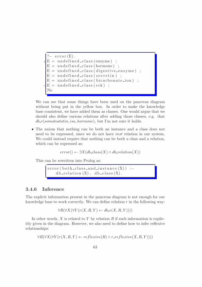
�
?− e r r o r (E) .2 E = unde f i n ed c l a s s ( enzyme ) ;E = unde f i n ed c l a s s ( hormone ) ;E = unde f i n ed c l a s s ( d i g e s t i v e enzyme ) ;E = unde f i n ed c l a s s ( s e c r e t i n ) ;E = unde f i n ed c l a s s ( b i ca rbona te i on ) ;
7 E = unde f i n ed c l a s s ( cck ) ;No
We can see that some things have been used on the pancreas diagramwithout being put in the yellow box. In order to make the knowledgebase consistent, we have added them as classes. One would argue that weshould also define various relations after adding those classes, e.g. thatdb r(somatostatin, isa, hormone), but I’m not sure it holds.
• The axiom that nothing can be both an instance and a class does notneed to be expressed, since we do not have inst relation in our system.We could instead require that nothing can be both a class and a relation,which can be expressed as:
error() ← ∃X(db class(X) ∧ db relation(X))
This can be rewritten into Prolog as:�
e r r o r ( bo th c l a s s and i n s t an c e (X) ) :−db r e l a t i o n (X) , db c l a s s (X) .
3.4.6 Inference
The explicit information present in the pancreas diagram is not enough for ourknowledge base to work correctly. We can define relation r in the following way:
∀R(∀X(∀Y (r(X,R, Y )← db r(X,R, Y ))))
In other words, X is related to Y by relation R if such information is explic-itly given in the diagram. However, we also need to define how to infer reflexiverelationships:
∀R(∀X(∀Y (r(X,R, Y )← reflexive(R) ∧ r reflexive(X,R, Y ))))
63

This says that we can use r reflexive to see whether reflexive behaviour canbe inferred, but only if the given relation is defined to be reflexive. r reflexiveis defined in the following way:
∀R(∀X(r reflexive(X,R,X)))
Transitivity is defined in the following way:
∀R(∀X(∀Y (r(X,R, Y )← transitive(R) ∧ r tr(X,R, Y ))))
This says that we can use r tr to see whether transitive behaviour can be in-ferred, but only if the given relation is defined to be transitive. r tr is definedin the following way:
∀R(∀X(∀Y (∀Z(r tr(X,R,Z) ← db r(X,R, Y ) ∧ db r(Y,R, Z)))))
∀R(∀X(∀Y (∀Z(r tr(X,R,Z) ← db r(X,R, Y ) ∧ r tr(Y,R, Z)))))
However, the Prolog implementation is slightly different for performance rea-sons.
We would also like to add inference of properties. We know that
r(acinar cell, isa, exocrine pancreatic cell)
Hence acinar cell should have all properties that exocrine pancreatic cell has.This is handled by:
∀R(∀X(∀Y (∀Z(r(X,R, Y )← inherited(R)∧r(X, isa, Z)∧diff(X,Z)∧r(Z,R, Y )))))
So now we can infer:�
?− r ( a c i n a r c e l l , par to f ,C) .C = exoc r ine panc r ea s ;C = pancreas ;
4 No
Another interesting question is: since r(PP cell, partof, pancreas) and weknow that r(PP cell, secrete, pancreatic polypeptide), should we conclude thatr(pancreas, secrete, pancreatic polypeptide)? In other words, would the rela-tion of secretion be copied up the partonomy? The answer is probably depen-dent on the view of what it really means to secrete something. If the secretedsubstance was only used internally within pancreas, we might not want to saythat pancreas secretes it, even though some part of pancreas does.
64

3.4.7 Prolog querying
If we are happy with the closed world assumption, we can use Prolog for queryingour knowledge base using simple language resembling English. The context–freegrammar of the language is presented below:
query ::= ”exist” class ”which” relation class
| ”every” class relation class
relation ::= ”isa” | ”partof” | ”secrete” | . . .
class ::= ”cell” | ”pancreas” | ”capillary” | . . .
The existential query resembles existential quantification in the sense thatone example is enough to get a positive answer. The following Prolog codeclarifies how the query is run:
�
1 ask ( [ ex i s t , Class1 , which , Relat ion , Clas s2 ] ,[ yes , fo r , ins tance ,X, Relat ion ,Y] ) :−
db c l a s s ( Clas s1 ) ,db r e l a t i o n ( Re la t ion ) ,db c l a s s ( Clas s2 ) ,
6 r (X, i sa , Clas s1 ) ,r (Y, i sa , Clas s2 ) ,r (X, Relat ion ,Y) .
We may be for instance interested to know whether there exists a stem cell,which secretes insulin. In such a case we would ask:
�
?− ask ( [ ex i s t , s t em ce l l , which , s e c r e t e , i n s u l i n ] ,A) .
2 No
But to see which cells at all secrete insulin, we can ask:�
?− ask ( [ ex i s t , c e l l , which , s e c r e t e , i n s u l i n ] ,A) .A = [ yes , fo r , ins tance , b e t a c e l l , s e c r e t e ,
i n s u l i n ]
Universal querying resembles universal quentification. We can define it inProlog in the following way:
65

�
ask ( [ every , Class1 , Relat ion , Clas s2 ] , [ yes , every ] ):−
db c l a s s ( Clas s1 ) ,3 db r e l a t i o n ( Re la t ion ) ,
db c l a s s ( Clas s2 ) ,\+ counterexample ( Class1 , Relat ion , Class2
, ) .
ask ( [ every , Class1 , Relat ion , Clas s2 ] ,E) :−8 db c l a s s ( Clas s1 ) ,
db r e l a t i o n ( Re la t ion ) ,db c l a s s ( Clas s2 ) ,counterexample ( Class1 , Relat ion , Class2 ,E)
.
13 counterexample ( Class1 , Relat ion , Class2 , [ no ,because ,X, not , Relat ion , Clas s2 ] ) :−
r (X, i sa , Clas s1 ) , d i f f (X, Clas s1 ) ,no t r (X, Relat ion , Clas s2 ) .
no t r (X,R,Y) :− \+ r (X,R,Y) .
We use negation as failure for finding a couterexample to our universal state-ment. If a counterexample can be found, the answere is “no” and the counterex-ample is returned. Otherwise, answer is “yes”. A sample interaction with thesystem may look as follows:
�
?− ask ( [ every , e n d o c r i n e p a n c r e a t i c c e l l , s e c r e t e ,i n s u l i n ] ,A) .
A = [ no , because , a l pha c e l l , not , s e c r e t e ,i n s u l i n ] ;
3 A = [ no , because , gamma cell , not , s e c r e t e ,i n s u l i n ] ;
A = [ no , because , pp c e l l , not , s e c r e t e , i n s u l i n] ;
No?− ask ( [ every , e n d o c r i n e p a n c r e a t i c c e l l , par to f ,
pancreas ] ,A) .
66

A = [ yes , every ] ;8 No
The full Prolog code is presented in Appendix G on page 257.
67

68
Chapter 4
Type systems andprogramming languages forrepresenting ontologies
This chapter serves as an investigation into programming languages and theirusefulness for representing formal ontologies and implementing ontology–basednatural language tools. One of the topics we will focus on is the notion of“type”. We will explain how this notion is used in logic and ontologies. Wewill further see how it is utilized in programming languages, where it is a keyconcept [36]. In other words, we will discuss what types of types there are.We will discuss the ontological usefulness of several programming languagesas far as their type systems and other related features are concerned. Theseconsiderations are important, as in the current work we are not only interestedin finding a link between natural language semantics and formal ontologies, butalso in establishing how to approach them in a practical way from the point ofview of computation.
4.1 Logical types
In First Order Predicate Logic there is no notion of types, or we can think ofit as having only one type, namely that of individuals. However, in the logicaltype theory types are the key concept. We have two elementary types:
69

• o – the type of truth values
• ι – the type of entities/objects
Those types are further combined by forming a function type in order torecursively form infinitely many possible types. For any two types τ1 and τ2 wecan construct a type of functions from τ1 to τ2, denoted either τ1 → τ2 or τ2τ1.We prefer the latter notation, as it is more compact.
For instance, type of the negation operation will be oo, that is negation is afunction that takes a truth value and produces another truth value.
Some very useful kinds of objects, e.g. sets can be represented with the helpof function types. We could represent the type of sets of individuals by oι, thatis a function that takes an individual as argument and returns a truth value asoutput. The intended working of such a function is that when an individual isin the set, the function returns true, and false otherwise.1
For instance the set{a, b}
can be represented by the following function:
f(X) = ⊤ if X = a or X = b, ⊥ otherwise.
However, this poses some restrictions on the use of such types from thecomputational point of view. One of the most famous undecidable problems isthe problem of equality of functions. There is no algorithm that could decidewhether two arbitrary functions (even of the same type) are equal or not.
Consider the following function as an illustration of this problem:
f(X) = ⊤ if (X = a ∧ ‘p=np’) or X = b, ⊥ otherwise.
In the above we added ‘p=np’, the famous computer science problem asone of the conditions as to what the function will answer when given a as theargument. Here for brevity we simply refer to it by the name ‘p=np’, but thinkof it as a long formula formalizing the problem and being either true or false.If ‘p=np’, the function will return ⊤, otherwise it will return ⊥. Hence, thisfunction is identical to the previous one if and only if ‘p=np’. This illustratesthat the problem of comparing two functions is at least as difficult as the ‘p=np’
problem, i.e. it is not easy to say the least.Hence, using type theory poses great difficulties for the implementation, as
most objects are represented by functions. Therefore, we would not be able to
1This commonly used function is known as the characteristic function of a set.
70

compare various objects (decide whether they are equal or not) in type theory.This is a huge disadvantage, taking computation into consideration.
4.2 Types in programming languages
Types for data in programming languages (sometimes called datatypes) are infact kinds of ontologies for objects created in computer’s operating memory.Some of them enable the representation of large taxonomies via the so–called“inheritance”. The main objective behind introduction of types in programminglanguages is to eliminate many programmingmistakes stemming from inter–typeconfusion. Those mistakes are very common in non–typed languages, but canbe easily detected by the compiler for typed languages. Let us now have a brieflook at the declarative programming languages.
Declarative languages describe what should be computed, rather than howsomething should be computed. This means they usually describe the computa-tion without state, side effects, and control flow. The type system of declarativelanguages is very well suited for expressing already specified logical theories.Some of the advantages of declarative languages include:
• Most declarative languages have a formal or semiformal semantics, whichallow for proving the correctness of the program.
• Declarative languages have a syntax which is very close to the standardmathematical notation. It is therefore easy to express formal ideas as aprogram.
• Because a declarative program describes what the solution is instead ofhow to compute it, the source code for the program is around 10 timesmore concise than one expressed in a imperative language.
• Strongly–typed declarative languages tend to have stronger type systemsthan strongly–typed imperative languages. Consider e.g. the Java im-perative language, where null is a member of any user–defined type, orC/C++, where compiler automatically casts between most primitive in-teger types, pointers, etc. While those features are often very useful forprogrammers, they also represent weakenings of the type system itself.
• Some declarative languages have support for nondeterministic computa-tion (returning multiple results), which at times proves to be very helpful.
71

It is however worth noting that the type system of a programming languagecannot be used easily for representing ontologies. The ontologies are usuallyrepresented in a program as data, not as types. With this approach, ontologicaltypes will take form of dynamic self–programmed types, which are taken careof by the program and not by the compiler or type checker.
Let us consider an example. In Java, a very popular language with object–oriented type system, we could declare the class of substances:
class Substance {}
Then, we could create a subclass of it, expressing that insulin is one of subtypesof substance:
class Insulin extends Substance {}
Java even provides a so–called reflection mechanism, where a program canlook into the type system during runtime. However, this approach is only suit-able for expressing fixed, bounded–size ontologies. The generative ontologiesthat we are going to work with are of unbounded size, as we can create complexclasses during the process of analyzing the text. We need to dynamically createnew ontological types as we go, and therefore we can’t use the programminglanguage’s type system directly for representing the ontology.
Next, let us have a brief look at some of the declarative programming lan-guages, together with their type system.
4.2.1 StandardML
StandardML is an established functional programming language. It is widelyused in academia, as it has a formal semantics. The following description [29]of StandardML [31] is a particularly concise description of the language:
Standard ML is a safe, modular, strict, functional, polymorphic pro-gramming language with compile–time type checking and type infer-ence, garbage collection, exception handling, immutable data typesand updatable references, abstract data types, and parametric mod-ules. It has efficient implementations and a formal definition with aproof of soundness.
Unfortunately, one can stumble upon an obstacle along the way. It turns outthat some of the operations which are necessary for natural language handling
72
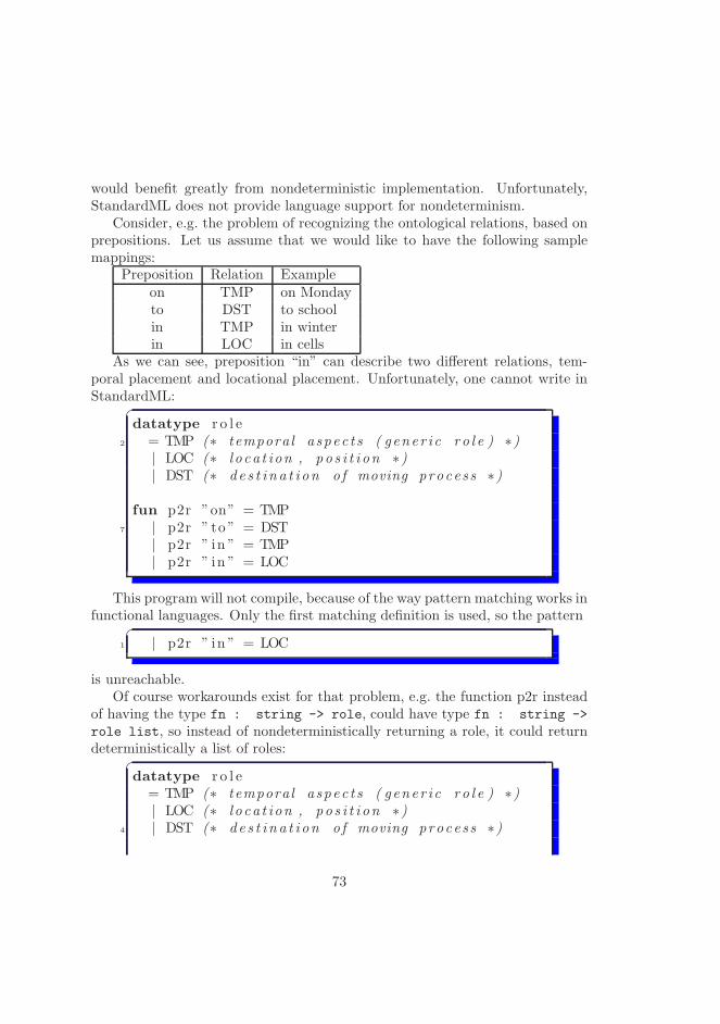
would benefit greatly from nondeterministic implementation. Unfortunately,StandardML does not provide language support for nondeterminism.
Consider, e.g. the problem of recognizing the ontological relations, based onprepositions. Let us assume that we would like to have the following samplemappings:
Preposition Relation Exampleon TMP on Mondayto DST to schoolin TMP in winterin LOC in cells
As we can see, preposition “in” can describe two different relations, tem-poral placement and locational placement. Unfortunately, one cannot write inStandardML:
�
datatype r o l e2 = TMP (∗ temporal aspec t s ( gener i c r o l e ) ∗)
| LOC (∗ l o ca t ion , po s i t i on ∗)| DST (∗ de s t i n a t i on o f moving proces s ∗)
fun p2r ”on” = TMP7 | p2r ” to ” = DST
| p2r ” in ” = TMP| p2r ” in ” = LOC
This program will not compile, because of the way pattern matching works infunctional languages. Only the first matching definition is used, so the pattern
�
1 | p2r ” in ” = LOC
is unreachable.Of course workarounds exist for that problem, e.g. the function p2r instead
of having the type fn : string -> role, could have type fn : string ->
role list, so instead of nondeterministically returning a role, it could returndeterministically a list of roles:
�
datatype r o l e= TMP (∗ temporal aspec t s ( gener i c r o l e ) ∗)| LOC (∗ l o ca t ion , po s i t i on ∗)
4 | DST (∗ de s t i n a t i on o f moving proces s ∗)
73
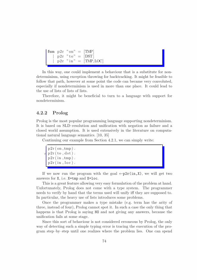
fun p2r ”on” = [TMP]| p2r ” to ” = [DST]| p2r ” in ” = [TMP,LOC]
In this way, one could implement a behaviour that is a substitute for non-determinism, using exception throwing for backtracking. It might be feasible tofollow that path, however at some point the code can became very convoluted,especially if nondeterminism is used in more than one place. It could lead tothe use of lists of lists of lists.
Therefore, it might be beneficial to turn to a language with support fornondeterminism.
4.2.2 Prolog
Prolog is the most popular programming language supporting nondeterminism.It is based on SLD–resolution and unification with negation as failure and aclosed world assumption. It is used extensively in the literature on computa-tional natural language semantics. [10, 35]
Continuing our example from Section 4.2.1, we can simply write:�
p2r ( on , tmp) .2 p2r ( to , ds t ) .p2r ( in , tmp) .p2r ( in , l o c ) .
If we now run the program with the goal ←p2r(in,X), we will get twoanswers for X, i.e. X=tmp and X=loc.
This is a great feature allowing very easy formulation of the problem at hand.Unfortunately, Prolog does not come with a type system. The programmerneeds to verify by hand that the terms used will unify iff they are supposed to.In particular, the heavy use of lists introduces some problems.
Once the programmer makes a type mistake (e.g. term has the arity ofthree, instead of four), Prolog cannot spot it. In such a case the only thing thathappens is that Prolog is saying NO and not giving any answers, because theunification fails at some stage.
Since this sort of behaviour is not considered erroneous by Prolog, the onlyway of detecting such a simple typing error is tracing the execution of the pro-gram step–by–step until one realizes where the problem lies. One can spend
74
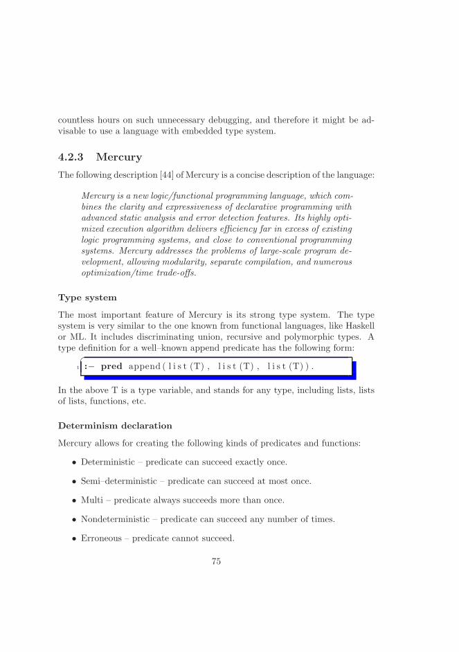
countless hours on such unnecessary debugging, and therefore it might be ad-visable to use a language with embedded type system.
4.2.3 Mercury
The following description [44] of Mercury is a concise description of the language:
Mercury is a new logic/functional programming language, which com-bines the clarity and expressiveness of declarative programming withadvanced static analysis and error detection features. Its highly opti-mized execution algorithm delivers efficiency far in excess of existinglogic programming systems, and close to conventional programmingsystems. Mercury addresses the problems of large-scale program de-velopment, allowing modularity, separate compilation, and numerousoptimization/time trade-offs.
Type system
The most important feature of Mercury is its strong type system. The typesystem is very similar to the one known from functional languages, like Haskellor ML. It includes discriminating union, recursive and polymorphic types. Atype definition for a well–known append predicate has the following form:
�
1 :− pred append ( l i s t (T) , l i s t (T) , l i s t (T) ) .
In the above T is a type variable, and stands for any type, including lists, listsof lists, functions, etc.
Determinism declaration
Mercury allows for creating the following kinds of predicates and functions:
• Deterministic – predicate can succeed exactly once.
• Semi–deterministic – predicate can succeed at most once.
• Multi – predicate always succeeds more than once.
• Nondeterministic – predicate can succeed any number of times.
• Erroneous – predicate cannot succeed.
75
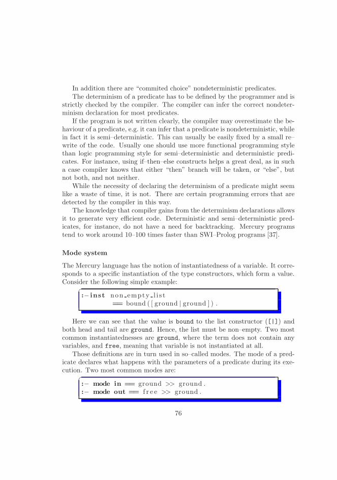
In addition there are “commited choice” nondeterministic predicates.The determinism of a predicate has to be defined by the programmer and is
strictly checked by the compiler. The compiler can infer the correct nondeter-minism declaration for most predicates.
If the program is not written clearly, the compiler may overestimate the be-haviour of a predicate, e.g. it can infer that a predicate is nondeterministic, whilein fact it is semi–deterministic. This can usually be easily fixed by a small re–write of the code. Usually one should use more functional programming stylethan logic programming style for semi–deterministic and deterministic predi-cates. For instance, using if–then–else constructs helps a great deal, as in sucha case compiler knows that either “then” branch will be taken, or “else”, butnot both, and not neither.
While the necessity of declaring the determinism of a predicate might seemlike a waste of time, it is not. There are certain programming errors that aredetected by the compiler in this way.
The knowledge that compiler gains from the determinism declarations allowsit to generate very efficient code. Deterministic and semi–deterministic pred-icates, for instance, do not have a need for backtracking. Mercury programstend to work around 10–100 times faster than SWI–Prolog programs [37].
Mode system
The Mercury language has the notion of instantiatedness of a variable. It corre-sponds to a specific instantiation of the type constructors, which form a value.Consider the following simple example:
�
:− inst non empty l i s t== bound ( [ ground | ground ] ) .
Here we can see that the value is bound to the list constructor ([|]) andboth head and tail are ground. Hence, the list must be non–empty. Two mostcommon instantiatednesses are ground, where the term does not contain anyvariables, and free, meaning that variable is not instantiated at all.
Those definitions are in turn used in so–called modes. The mode of a pred-icate declares what happens with the parameters of a predicate during its exe-cution. Two most common modes are:
�
:− mode in == ground >> ground .:− mode out == f r e e >> ground .
76

In other words, a variable is an input to a predicate, if its ground bothwhen the predicate is called, and when its finished. A variable is an output ofa predicate, if its free when the predicate is called, and it is ground when itsfinished.
The mode system is immensely helpful for avoiding common mistakes in logicprogramming. Consider for instance the well-known list appending predicate,where type, determinism, and mode declarations look as follows:
�
:− pred append ( l i s t (T) , l i s t (T) , l i s t (T) ) .:− mode append ( in , in , out ) i s det .
3 :− mode append (out , out , in ) i s nondet .
One needs to declare that all three arguments are lists of the same type ofelements. Additionally, we want to use append in two ways. First, given twoinput lists, we want to concatenate them to deterministically produce a resultinglist. Secondly, given a list, we want to nondeterministically produce two lists,which when concatenated, give us the supplied list.
Apart from serving as a nice overview of how the predicate works, such adeclaration allows the compiler to check for the following sample mistakes:
• Type errors – if the predicate tries to unify one of the arguments with alist of something else than the other arguments.
• Determinism errors – if the mode which we declared to work determinis-tically, is in fact nondeterministic.
• Mode errors – If the out variable is not instantiated to be ground by thepredicate.
Pure declarativeness
In most declarative languages there is a need for impure functions or predicateswhich introduce side–effects. Side–effects are things that happen outside of theformal semantics of a language. This is very often the case with e.g. input/out-put operations. In Mercury input and output is performed with preservationof purely declarative semantics. This can only be achieved thanks to the modedeclarations for predicates. Consider, e.g. the predicate for loading WordNetdatabase:
�
:−pred load wn ( s t r i n g : : in ,2 wn : : out ,
77
i o : : di ,i o : : uo) i s det .
The two last parameters represent input/output state before and after thepredicate was called. They have special modes. di means “destructive input”– the variable is dead after being passed to load wn, cannot be used again. uomeans “unique output” – the variable can be used only once after being outputfrom the predicate. Please observe that the predicate cannot be nondeterminis-tic, as it is impossible to backtrack over input/output operations. One cannot“undisplay text” or “unread from a file”. This is different than in Prolog, whereinput/output is performed in impure way, so one can perform input/outputoperations in backtracking predicates.
4.3 Ontological types
Having discussed some datatypes in some programming languages, we now re-turn to the issue of representing ontologies. From the point of view of theontologies, types take form of concepts or classes in the ontology. This meansthat the taxonomy of the domain in question defines what types of objects canexist in the domain.
Accordingly, the ontological types can be defined as a simple lattice, wherenodes represent classes. But we can also use some more heavy–weight types,where an inference engine would need to be employed for deciding whether someobject belongs to a given type. This can be achieved by using Description Logicswith a large and complicated TBox.
If we wish to base our ontological types on the pancreas diagram from Fig-ure 3.2 on page 60, then the snapshot of such a TBox could look as presentedin Figure 4.1 on page 79.
Notice that since in the biomedical domain we do not concern ourselves withindividuals, there is no need for the ABox.
In programming languages we usually have a finite number of types in agiven program. But from ontological perspective, types could be defined ina generative fashion, hence producing potentially infinitely many (unboundednumber of) available classes. This approach is followed in our ontological se-mantics prototypes with the Peirce product and infinite generative ontologiesdefined by means of conceptual feature structures.
78

pancreatic cell ⊑ cell ⊓ ∀located in.pancreas
exocrine cell ⊑ cell ⊓ ∀secretes.enzyme
endocrine cell ⊑ cell ⊓ ∀secretes.hormone
exocrine pancreas ⊑ ∀partof.pancreas
endocrine pancreas ⊑ ∀partof.pancreas
stem cell ⊑ cell
adult stem cell ⊑ stem cell
embrionic stem cell ⊑ stem cell
islet of Langerhans ⊑ ∀partof.endocrine pancreas
exocrine pancreatic cell ⊑ exocrine cell ⊓ pancreatic cell
⊓∀partof.exocrine pancreas
endocrine pancreatic cell ⊑ endocrine cell ⊓ pancreatic cell
⊓∀partof.islet of Langerhans
duct ⊑ ∀partof.exocrine pancreas
capilary ⊑ ∀partof.islet of Langerhans
α cell ⊑ endocrine pancreatic cell
⊓∀secretes.glucagon
β cell ⊑ endocrine pancreatic cell
⊓∀secretes.insulin
δ cell ⊑ endocrine pancreatic cell
⊓∀secretes.(gastrin ⊔ somatostatin)
PP cell ⊑ endocrine pancreatic cell
⊓∀secretes.pancreatic polypeptide
centroacinar cell ⊑ exocrine pancreatic cell
⊓∀secretes.digestive enzyme
⊓∀has primary signal.secretin
acinar cell ⊑ exocrine pancreatic cell
⊓∀secretes.bicarbonate ion
⊓∀has primary signal.cck
Figure 4.1: Pancreas ontology translated into Description Logics.
79

4.4 Grammatical ontotypes
It is possible to use the familiar notion of context–free grammars for representingontological types, as described in [1]. In such an application classes are repre-sented by nonterminal symbols and class subsumption relationship is replacedby the string derivation.
As an example, consider the following sample grammar, which representsan ontology created by combining Basic Formal Ontology with Gene Ontology.The grammar is presented in Figure 4.2 on page 81.
This grammar has the power of generating infinitely many ontological typesby means of deriving many various sentential forms. A sample derivation isshown in Figure 4.3 on page 82.
80

〈Entity〉 ::= 〈Continuant〉
| 〈Occurrent〉
〈Occurrent〉 ::= 〈Occurrent〉〈Occurrent role list〉
〈Occurrent role list〉 ::= ǫ
| [〈Occurrent role〉]〈Occurrent role list〉
〈Occurrent role〉 ::= CBY : 〈Occurrent〉
| LOC : 〈Continuant〉
| WRT : 〈Entity〉
| BMO : 〈Entity〉
| POF : 〈Occurrent〉
| . . .
〈Continuant〉 ::= 〈Continuant〉〈Continuant role list〉
〈Continuant role list〉 ::= ǫ
| [〈Continuant role〉]〈Continuant role list〉
〈Continuant role〉 ::= LOC : 〈Continuant〉
| POF : 〈Continuant〉
〈Occurrent〉 ::= 〈ProcessualEntity〉| . . .
〈ProcessualEntity〉 ::= 〈Process〉| . . .
〈Process〉 ::= 〈biological process〉
〈Continuant〉 ::= . . .
Figure 4.2: Grammatical specification of a sample ontology.
81
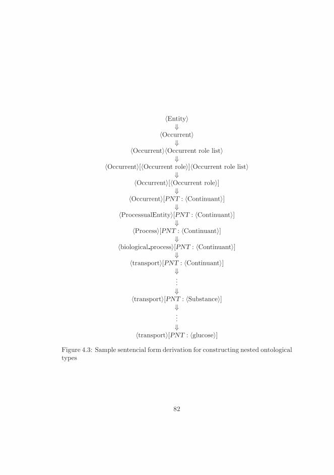
〈Entity〉⇓
〈Occurrent〉⇓
〈Occurrent〉〈Occurrent role list〉⇓
〈Occurrent〉[〈Occurrent role〉]〈Occurrent role list〉⇓
〈Occurrent〉[〈Occurrent role〉]⇓
〈Occurrent〉[PNT : 〈Continuant〉]⇓
〈ProcessualEntity〉[PNT : 〈Continuant〉]⇓
〈Process〉[PNT : 〈Continuant〉]⇓
〈biological process〉[PNT : 〈Continuant〉]⇓
〈transport〉[PNT : 〈Continuant〉]⇓...⇓
〈transport〉[PNT : 〈Substance〉]⇓...⇓
〈transport〉[PNT : 〈glucose〉]
Figure 4.3: Sample sentencial form derivation for constructing nested ontologicaltypes
82

Chapter 5
Ontological Semantics
In this chapter we will have a closer look at natural language, in particularEnglish. In particular we will discuss its grammar from a formal perspective.We will also try to establish how to formally represent the meaning of sentencesand phrases with the help of generative ontologies. Further, we will discusssome problems related to the extraction of that meaning.
Ontological phenomena visible most clearly in generative ontologies are mir-rored in the language. Our observation is that ontology should be language–independent, while language is perhaps ontology–dependent to a large extent.Hence, it is quite natural to base ontological semantics for a language on gen-erative ontologies.
5.1 Meaning of sentences
Let us use First Order Predicate Logic as a metalogic for describing relationbetween sentences and their meaning. We will write:
follows(Φ,Υ)
whenever Φ follows from sentence Υ. Υ is a natural language sentence repre-sented in arbitrary form, e.g. as a list of words. Φ is a formula in some chosenlogic representing partial meaning of the sentence Υ. We will say:
means(Υ,Φ)
83

whenever formula Φ is the full meaning of the sententence Υ. Let us define whatwe understand by “full meaning”:
∀S,M(means(S,M)↔ follows(M,S) ∧ ∀I(follows(I, S)→ entails(M, I)))
In other words formula M is the full meaning of sentence S if it follows fromS and if it entails all other formulas I, which also follow from S. So whenmeans(Υ,Φ), Φ is the perfect translation of natural language sentence Υ intodesirable logic, where no information is lost, and of course no new informationis introduced.
5.2 Automatic meaning extraction
When constructing a system for automatic meaning extraction, one cannot hopeto extract the full meaning of each sentence. There are several reasons for that:
• The reasoning necessary for full understanding is beyond computer’s abil-ities. It may be necessary to reference complicated real world knowledgeto understand the sentence.
• The target logic is unable to represent the full meaning of a sentence dueto its limited expressivity.
In any case, the system for natural language semantics extraction is sup-posed to understand as much of the sentence as possible. We are interested inextracting a meaning Φ, such that:
reading(Υ,Ψ) ∧ entails(Ψ,Φ)
5.3 Human language understanding
Human beings are exceptionally good at understanding language. It is by farthe most unique way of communicating found in nature, as it is tied to only onespecies.
Since our goal is to allow computer to understand language, we shall firstdiscuss what makes language understandable for us. Indeed, if we knew howour mind grasps the language, we could try to write a program, which wouldact in a similar manner.
Unfortunately, this task might be extremely difficult, or maybe even impos-sible. As a matter of fact we can only understand the brain on two levels:
84

1. A very low level: we know that impulses are being sent between cells andwe can observe that some regions of the brain are active while performinga particular task, such as speaking.
2. A very high level: we can observe the external behavior produced by ourmind.
The first understanding can be compared to how computer hardware func-tions. The second is similar to the output of a computer program, or its inter-face. We do not have any access to the “source code” for our mind.
5.4 Language as a protocol
When we want two machines to communicate, we need a protocol, which bothwill follow, so that they can understand each other. For human beings, thenatural language serves as a protocol.
The language, which we use today, and which has been evolving for tens ofthousands of years has one particular feature, which distinguishes it from otherprotocols used today, i.e. it is extremely complicated. This stems from the factthat language evolved to serve purposes of human mind, not that of a computer.
This might be conceived as an advantage in a various contexts, as the abilityof describing the same concept in so many different ways allows us to expressour emotions, it makes reading novels so pleasurable, etc.
Unfortunately, from the software engineering perspective the complexity oflanguage is a huge problem. No software system is capable of understanding itfully (or even to a large extent).
Luckily, language being a protocol, is not completely random, but rathersentences are built in a specific way. Language has been studied by linguists andthe knowledge about it is extremely useful when one tries to design a softwaresystem, which should take natural language sentences as the input.
In Sections 5.4.1 and 5.5 we explain the particularly interesting features ofnatural language, which might make it computer–understandable to a certaindegree.
5.4.1 Parts of speech
The English language consists of words, which can be grouped into certainclasses, called parts of speech or lexical categories. The most common ones are:
85

• common noun – names object class, e.g. the noun “cell” has the meaning,which covers all imaginable cells, not a particular cell.
• proper noun – names particular object, e.g. “Denmark” is a proper nounreferring to a particular country.
• verb – names actions, which are activities or interactions between things,e.g. “stored” is a verb, which names the action of storing something some-where.
• adjective – names properties ascribed to nouns, e.g. the phrase “hyper-glycemic symptoms” ascribes the property of being hyperglycemic to symp-toms.
• preposition – explains how different entities are related to each other.Very few prepositions exist. They tend to capture only the most commonrelations. E.g. the phrase “storage in cell” means that storage takes placeinside of a cell.
• adverb – plays similar role as adjective, except that it describes propertiesof concepts represented by other parts of speech than nouns.
5.4.2 Necessity of part–of–speech tagging
Let us consider the following sentence:insulin forces storage
Let us assume that the underlying ontology understands that the word “in-sulin” represents the concept c insulin and the word “storage” represents theconcept c storing. c insulin is defined as a chemical substance called insulin.c storing is defined as an action of storing something somewhere. Let us alsoassume that nothing in our ontology corresponds to the word “forces”.
In such a case understanding the whole phrase could be attempted by skip-ping the word “forces” and analyzing just “insulin storage”. Unfortunately, thiswould result in an incorrect understanding, as the original phrase was not reallytalking about insulin storage. It is not insulin that is in fact stored.
In order to remedy the situation, the algorithm could use part–of–speechtagging. This process assigns a list of lexical categories to each word of the sen-tence. The coverage of part–of–speech tagging is extensive, due to the existenceof large lexical resources, like WordNet. The size of todays lexical resources isfar superior to the size of any existing ontology. Almost any word of English
86

language can be assigned a lexical category, but only a small subset can befound in any ontology.
After the application of the part–of–speech tagging, we are faced with thefollowing information:
sentence insulin forces storagetagging noun verb nounontology c insulin ? c storing
At the moment the algorithm understands, that the sentence does not talkabout storage of insulin, as words “insulin” and “storage” appear on two sidesof a verb. Such a situation disallows the compound concept to be understoodas storage of insulin. Rather, insulin could be an agent and storage could be apatient of some action, described by the verb.
Observe that if the middle word is, e.g. a noun, we might be faced witha different situation. For instance: “insulin particles storage” sentence has adifferent structure, where the second word describes a patient for the actiondescribed by third word. In other words, we deal with the concept of storingsome particles.
5.5 Grammar as the structure of English
5.5.1 Rules and structure
All sentences of a language are similar. Even though completely different wordsare used, the structure of the sentence follows some rules. Recognizing thoserules is of utmost importance for understanding the sentence. If the sentenceis not constructed according to the rules, it will not be understood or it will bemisunderstood.
With artificial languages (e.g. programming languages), knowing the rulesis simple. When language is designed, a set of rules is invented, usually using avariant of Backus–Naur Form if the language is context–free. One might there-fore construct all the valid sentences of the language with the rules provided.
5.5.2 Rules for natural languages
The problem with natural languages is that they were not designed with anyrules in mind. The language evolved together with human brain, and we some-how know from the very childhood, which sentences are correct and which arenot (to some extent). We learn that by listening to sample correct sentences,rather than learning some rules and following them.
87
Hence, we are faced with a problem, which appears only for natural lan-guages. The problem is that we do not know the rules of the language. In asence the rules are hidden.
Why would we need the rules at all? It is because we would like to teachcomputers to understand natural language. Unfortunately, inputting all validsentences into a database is not an option. Such a set would probably be infinite,or in most optimistic estimation extremely huge. So we shall try to construct arelatively small set of rules, which could describe the structure of the languagein a satisfactory way.
In order to learn the rules, we might assume that we know which sentencesare correct and which are incorrect, and based on that we would like to analyzethe language, so that we can recognize the hidden rules.
Such a task, however, turns out to be extremely difficult.A substantial problem is that whatever set of rules one might come up with,
it is always relatively simple to find a counterexample. Such a counterexamplecould take two forms. It could either be a valid sentence, which cannot beproduced using the rules, or it could be an invalid sentence, which could beproduced using the set of rules provided.
For this very reason one cannot prove that English is a context–free language,hence it might not be describable using a context–free grammar.
Many linguistic problems that are faced if one tries to construct a context–free grammar for English are described in [40].
5.5.3 Shallow context–free grammar for English
This section describes the idea of a shallow grammar for English language.The problems described in Section 5.5.2 have to be dealt with somehow
if we want the system to understand the language. Fortunately, the system,which is to be designed in the current text, has some important properties. Thecrucial thing to realize is that the system has to analyze biomedical documents.Such documents are written using correct English language. Therefore, we canassume the absence of incorrect sentences in the analyzed text.
Such assumption has a major influence on the set of rules, which we shalldecide upon. Normally the rules should be very restrictive, so that they needto reject incorrect sentences. However, since we will not have any incorrectsentences, we do not need to reject them with the help of our rules.
As an example, consider the following simple rule1:
1Expressed in BNF.
88

〈sentence〉 ::= 〈noun〉〈verb〉〈noun〉 (5.1)
This rule expresses that a sentence can consist of a noun, followed by a verb,followed by a noun. Let us consider the following two sentences:
1. Insulin forces storage.
2. Insulin force storage.
Sentence 1 is a correct English sentence, while sentence 2 is not. Neverthe-less, sentence 1 will be accepted by our rule, as will sentence 2.
If we wanted to reject the second sentence, but accept the first one, we wouldneed to introduce more complicated rules. We can however observe, that thesecond sentence will not ever appear in the analyzed text, assuming that it is ahigh–quality material.
Hence, we can use a relatively simple shallow grammar for analyzing English.
As previously noted, English might not be describable by a context–freegrammar. However, taking into consideration the aforementioned observation,we can try to formulate a shallow grammar as a context–free grammar, sincewe do not need to reject incorrect sentences.
Such a grammar would not cover the whole English language, but this is nota problem. We shall note that the text, which is to be analyzed, is a scientifictext. As such it normally makes use of a specific subset of English languageonly.
As an example, we could consider the problem of questions. In a casualconversation, a novel, or a play, questions occur very often. This is howevernot a case for scientific articles, reports and texts. The Wikipedia entry for“Insulin”, which is our playground, does not contain even one question. Thatobservation allows us to construct a substantially simpler grammar for textanalysis, as the order of words in a question is not the same as in a statement.
In case a question appears in the analyzed text, we simply will not be ableto analyze such a sentence. Similarly if a sentence formulated in a less obviousway is encountered, which is rejected by the grammar, it will not be analyzed.
Taking all the considerations into account, we might design the a shallowcontext–free grammar for English, which is presented in Figure 5.5.3 on page 90.
Please observe that the grammar is ambiguous. The same sentence couldproduce different parse trees.
89

Figure 5.1: A shallow context-free grammar for English, specified in BNF.
〈s〉 ::= 〈d a cnp pp〉〈vp〉
〈vp〉 ::= 〈v〉〈pps〉|〈v〉〈d a cnp pp〉〈pps〉
〈pps〉 ::= ǫ|〈pp〉〈pps〉
〈pp〉 ::= 〈p〉〈d a cnp pp〉
〈d a cnp pp〉 ::= 〈d a cnp〉〈pps〉
〈d a cnp〉 ::= 〈d〉〈a cnp〉|〈a cnp〉
〈a cnp〉 ::= 〈adj〉〈a cnp〉|〈cnp〉
〈cnp〉 ::= 〈n〉〈cnp〉|〈n〉
〈v〉 ::= force|forces|cause|causes| . . .
〈n〉 ::= insulin|storage|cell|cells| . . .
〈d〉 ::= the|this|my| . . .
〈p〉 ::= in|with|by| . . .
〈adj〉 ::= pancreatic|recombinant|adipose|pineal| . . .
90
5.6 Let us try various formalisms
Instead of giving one final answer as to what formalism shall be used for rep-resenting ontological semantics, we would prefer to “play around” with some ofthem.
Initially one can try each of them separately and argue how well suited eachof them is for representing ontological semantics. Is Description Logics goodenough? How about First Order Predicate Logic? Lambda Calculus? Theproblems of tractability and decidability have to be taken into consideration asfar as search aspects are concerned, so the reader knows that semantics expressedin λ–calculus or First Order Predicate Logic cannot be searched for. Hence aneed arises for narrowing or combining some of them.
At this point let us have a look at the Peirce product2 based semanticsfor representing nodes in generative ontology, which is restrictive enough to betractable.
5.7 Peirce–algebraic ontological semantics
We are interested in “understanding” the language. This is a very complicatedproblem, and in the computational context it can be defined as capturing correctsemantics from the text.
There are various theories describing formal semantics for English, e.g. thealgebraic boolean semantics described in [26].
However, the most prominent example is the Montague semantics, whereone focuses on translating various English phrases into quantified formulae inFirst Order Predicate Logic3.
As an example, consider the following article from the Wikipedia entry on“Insulin”:
“Insulin is required for all animal life.” (5.2)
One could capture the semantics of this sentence in the following way:
∀X(life(X)∧ animal(X)→ requires(X, insulin))
This semantic representation is not particularly useful for the purpose ofcreating a search engine. One of the problems is that First Order Predicate
2The Peirce product has been introduced in section 2.3.7 on page 47.3Often higher–order logics are also used.
91
Logic is not decidable. Therefore it would be impossible to decide whethersemantics of some sentence in the text subsumes the semantics of the querysentence.
Additionally, such a focus on quantification is not something that the user ofthe search engine would expect. As a matter of fact the user is mostly concernedwith finding articles, which refer to a particular concept. Here the concept couldbe defined as requiring of insulin by animal life.
Peirce algebra (described in Section 2.3.7 on page 47) turns out to containa very useful operation, called Peirce product, which allows us to express theontological semantics of the sentence of interest as:
requiring ∩ agt : insulin∩ pnt : (animal ∩ life)
Note that Peirce product (:) binds stronger than intersection (∩).In order to explain this ontological semantics, let us go back to our running
example:
Insulin forces storage of glycogen. (5.3)
Its semantics can be expressed using Peirce algebra as:
forcing ∩ agt : insulin∩ pnt : (storage ∩ pnt : glycogen) (5.4)
Recall that Peirce algebra is an algebra of sets and relations between indi-viduals belonging to those sets [12]. In Equation 5.4, the sets, which representclasses in our ontology, are:
• forcing – A class (set) comprising all imaginable actions of forcing. E.g. “meforcing my younger brother yesterday to clean the room” is an example ofindividual belonging to this class.
• insulin – This class contains only one individual, being the chemical sub-stance called “insulin”. It is a singleton set.
• storage – A class (set) comprising all imaginable actions of storing.
• glycogen– This class contains only one individual, being the chemical sub-stance called “glycogen. It is a singleton set.
Similarly, the following ontological relations are present in Equation 5.4:
• agt – Agent relation, relating an action to its agent, which is usuallyinitiating the action and carrying it on.
92

• pnt – Patient relation, relating an action to its patient, which is usuallyinfluenced by the action, being modified, etc.
The problem of capturing the semantics presented in Equation 5.4 from thesample sentence is described in Chapter 7 on page 113.
In order to fully understand the semantics at hand, let us first translate itaccording to the definition of Peirce product:
forcing
∩ {X |∃Y ((X,Y ) ∈ agt ∧ Y ∈ insulin)}
∩ {X |∃Y ((X,Y ) ∈ pnt
∧ Y ∈ (storage ∩ {X |∃Y ((X,Y ) ∈ pnt ∧ Y ∈ glycogen)}))}
The resulting formula is quite complex. Let us try to explain part of it:
{X |∃Y ((X,Y ) ∈ agt ∧ Y ∈ insulin)} (5.5)
Equation 5.5 defines a set of all individuals X , which are agent–related tosome individual Y , such that Y is an instance of insulin. The resulting set willbe a class, comprising all entities, which have insulin as an agent.
Coming back to the full sentence, if we intersect all imaginable forcing actionswith all entities having insulin as an agent, we get a class containing all forcingactions, which have insulin as an agent.
Similarly, we narrow the forcing class by intersecting it with all entities,which have storage as a patient. A further, Peirce product restriction is appliedto the storage in a nested way, as we are only interested in the storage ofglycogen.
Hence, by using Peirce algebraic operations we can construct infinitely manycompound concepts, using a finite supply of primitive classes and relations. Itis worth noticing that such a representation allows us to capture most of thesubstantial information from the text.
This semantics is chosen as the best alternative for the ontological naturallanguage analyzers, which are described in Chapter 7.
A very useful property of the chosen semantics is that it is variable–free,hence quite simple to be dealt with computationally. It does not suffer from theproblems of First Order Predicate Logic, like undecidability. It is used in theworking implementation of the system, and allows it to work very efficiently.
93

5.8 Semantic incompleteness
If we consider sentence 5.3 and its semantics 5.4, we can notice that not all ofthe information that humans can retrieve from the sentence is captured by thesemantics. For instance, the tense of the verb is lost, so the semantics does nottell whether the action of forcing happens presently, in the past, etc.
In other words, we have:
[[Insulin forces storage of glycogen.]]
= [[Insulin forced storage of glycogen.]]
= forcing ∩ agt : insulin∩ pnt : (storage ∩ pnt : glycogen)
We should discuss whether such a behaviour is desired. We have to keep inmind that the semantics presented is supposed to be used by a search enginefor ontological querying.
Clearly, the search engine will give one of the sentences as the match for theother, as they have the same semantics. This is a desired behaviour, because thesentences talk about the same concepts, and we would probably like to neglectthe tense when we use the search engine.
On the other hand, we need to keep in mind that such a phenomenon cannotbe used as the main principle for the search engine’s matching. Also sentenceswith different semantics should be often found as answers to queries. Considere.g.:
[[Insulin forces storage of glycogen.]]
= forcing ∩ agt : insulin∩ pnt : (storage ∩ pnt : glycogen)
and:
[[Insulin causes storage of glycogen.]]
= causing ∩ agt : insulin∩ pnt : (storage ∩ pnt : glycogen)
Both sentences have different semantics, yet we would like to return one asthe match for the other one being the query. We can do it, because in theunderlying ontology we have:
isa(forcing, causing)
Knowing that the action of “forcing” is kind of a “causing”, the search engineshall in this case decide to return the sentence in question as a match.
We can conclude by saying that the incompleteness of the captured semanticscan in fact improve the end result of the search.
94
5.9 Rephrasing
One sentence might be reformulated in different ways. Usually words can bemoved around the sentence, in order to stress something, make the sentencefunny, etc. The sentence normally keeps similar meaning.
Rephrasing, however, poses a challenge for the ontological text analyzer.Clearly, we would like to achieve semantics, which is independent of the waythe sentence was phrased. This independence comes in most cases for free withthe commutativity of the set intersection operation. As an example, consider:
forcing ∩ agt : insulin∩ pnt : (storage ∩ pnt : glycogen)
= forcing ∩ pnt : (storage ∩ pnt : glycogen) ∩ agt : insulin
One could imagine that such two meanings are captured from different sen-tences. Nevertheless, they will be considered equal, as the set intersection (∩)is commutative.
Another type of rephrasing is illustrated by the following example:
[[Insulin forces storage of glycogen.]]
= [[Insulin forces glycogen storage.]]
= forcing ∩ agt : insulin∩ pnt : (storage ∩ pnt : glycogen)
The system is able to construct the same semantics for this example, becauseit looks for patient of an action both in prepositional phrase and in compondnoun phrase. This is the expected behaviour, as both sentences have the samemeaning.
5.10 Relations vs. classes
For some sentences we have the choice of extracting semantics in two differentways: using a relation or a class. For our sample sentence we could have:
[[Insulin forces storage of glycogen.]]
= forcing ∩ agt : insulin∩ pnt : (storage ∩ pnt : glycogen)
But we could also use the CBY relation, which relates an action to its cause.In such a case we would obtain:
[[Insulin forces storage of glycogen.]]
= storage ∩ pnt : glycogen∩ cby : insulin
95
Please observe how in one version the notion of forcing is represented by aclass and in the other by relation.
It should be decided which of the two semantics is preferable. In our opinionthe former is a better choice for the following reasons:
• By representing the action of forcing by the cby role we actually loose someuseful information. This is because few other verbs could trigger this role,e.g. “causes”.
• Since we did not introduce a subsumption relation between relations, butonly between classes, representing forcing as a class allows for some moreontology–based reasoning. E.g. we can easily see that “forcing” is below“causing” in the ontology, which is in turn below “action”, etc.
• One could argue that if we introduce a relation for representing the actionof causing, we should be consistent and do the same for other actions aswell. In our opinion it is preferable to keep the number of relations low.
• Relations also have the problem of requiring the inverse relations to betaken into consideration. Consider the following two semantics:
storage ∩ pnt : glycogen∩ cby : insulin
insulin∩ cau : (storage ∩ pnt : glycogen)
Both semantics are equivalent, as the relation cau4 is the inverse relationof cby5. For some reasoning engine, it must be explicitly defined thatthose relations are inverse, so that it could infer that the two presentedsemantics are the same.
5.11 Plurals
Sentences of our interest often involve plural constructions. Various construcionscan be used for constructing plurals. In the following, we will concentrate onthe “and” conjunction, which can form conjoined noun phrases, verb phrases,sentences, etc.
Let us consider the sentence:
A boy and a girl played. (5.6)
4r(φ, cau, ρ) means that phi causes ρ.5r(φ, cby, ρ) means that phi is caused by ρ.
96
The sentence has two Logic of Plurals and Mass Terms readings – the col-lective one:
∃x∃y[boy′(x) ∧ girl′(y) ∧ played′(x⊕ y)]
and the distributive one:
∃x[boy′(x) ∧ played′(x)] ∧ ∃y[girl′(y) ∧ played′(y)]
The distributive reading can be easily represented as two nodes in the generativeontology:
playing[agt : boy]
andplaying[agt : girl]
The collective reading is however problematic, as we need to decide how it shouldbe captured. The three alternatives are discussed in the following sections.
5.11.1 Collectives operator
We could use the operator ⊕ for constructing plural sums of two individuals, asin:
playing[agt : (boy ⊕ girl)]
The equivalent view in Peirce Algebra:
playing ∩ {X |∃Y ((X,Y ) ∈ agt ∧ Y ∈ (boy ⊕ girl))}
In this proposal the ⊕ operator takes two sets, representing classes, and con-structs a set representing collectives consisting of two individuals, each of whichbelongs to one of those two classes.
The advantage of this approach is that we can assume that relations have afunctional character. It means that the intended meaning of the agt relation isas follows: We say that event e and individual i are agt–related ((e, i) ∈ agt)iff i participates in e as its only agent. If an event has more than one agent, weneed to represent all of them as one collective agent, a plural.
5.11.2 Multiple semantic roles
We could simply use the same semantic role twice in a feature structure, as in:
playing[agt : boy, agt : girl]
97

The equivalent view in Peirce Algebra becomes:
playing ∩ {X |∃Y ((X,Y ) ∈ agt ∧ Y ∈ boy)} ∩ {X |∃Y ((X,Y ) ∈ agt ∧ Y ∈ girl)}
This means that the event which the sentence talks about is an intersection ofthree things:
• All events of playing;
• All events that have a boy as their agent;
• All events that have a girl as their agent.
We need to assume that relations do not have a functional character. It meansthat the intended meaning of the agt relation is as follows: We say that event eand individual i are agt–related ((e, i) ∈ agt) iff i participates in e as one of itsagents.
5.11.3 Special nodes for representing collectives
We may introduce special classes in the ontology for representing plurals. Say,we have a class sum, representing a very general collection of objects. Then wecan create the following node in the generative ontology as our representationof the sample sentence:
playing[agt : sum[cmp : boy, cmp : girl]]
We can think of this representation in the following way: the event belongs tothe class playing and it has an agent, which belongs to a class sum, comprisingtwo elements – a boy and a girl.
It is worth observing that this approach requires multiple semantic roles.The sum can be refined further into more specific classes, e.g. combination,mixture, etc.
5.12 Merging ontological semantics with catego-
rial grammar
Let us now investigate how one could merge the ontological semantics developedin this chapter with categorial grammar.6 The incorporation of ontologies can
6The combination of ontologies and categorial grammar has been presented previously byus in a paper at the International Multiconference on Computer Science and InformationTechnology – Computational Linguistics Applications.
98
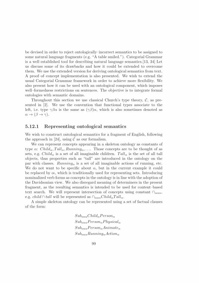
be devised in order to reject ontologically–incorrect semantics to be assigned tosome natural language fragments (e.g. “A table smiled.”). Categorial Grammaris a well established tool for describing natural language semantics.[13, 34] Letus discuss some of its drawbacks and how it could be extended to overcomethem. We use the extended version for deriving ontological semantics from text.A proof–of–concept implementation is also presented. We wish to extend theusual Categorial Grammar framework in order to achieve more flexibility. Wealso present how it can be used with an ontological component, which imposeswell–formedness restrictions on sentences. The objective is to integrate formalontologies with semantic domains.
Throughout this section we use classical Church’s type theory, C, as pre-sented in [2]. We use the convention that functional types associate to theleft, i.e. type γβα is the same as (γβ)α, which is also sometimes denoted asα→ (β → γ).
5.12.1 Representing ontological semantics
We wish to construct ontological semantics for a fragment of English, followingthe approach in [24], using C as our formalism.
We can represent concepts appearing in a skeleton ontology as constants oftype α: Childα, T allα, Runningα, . . .. Those concepts are to be thought of assets, e.g. Childα is a set of all imaginable children. Tallα is the set of all tallobjects, thus properties such as “tall” are introduced in the ontology on thepar with classes. Runningα is a set of all imaginable actions of running, etc.We do not want to be specific about α, but in the current example it couldbe replaced by oι, which is traditionally used for representing sets. Introducingnominalized verb forms as concepts in the ontology is in line with the adoption ofthe Davidsonian view. We also disregard meaning of determiners in the presentfragment, as the resulting semantics is intended to be used for content–basedtext search. We will represent intersection of concepts using constant ∩ααα,e.g. child ∩ tall will be represented as ∩αααChildαTallα.
A simple skeleton ontology can be represented using a set of factual clausesof the form:
SuboααChildαPersonα
SuboααPersonαPhysicalα
SuboααPersonαAnimateα
SuboααRunningαActionα
99
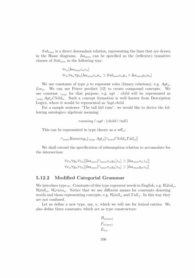
Suboαα is a direct descendant relation, representing the lines that are drawnin the Hasse diagrams. Isaoαα can be specified as the (reflexive) transitiveclosure of Suboαα in the following way:
∀cα[Isaoααcαcα]
∀cα∀aα∀pα[Isaoααcαaα ⊃ Suboααcαpα ∧ Isaoααpαaα]
We use constants of type ρ to represent roles (binary relations), e.g. Agtρ,Locρ. We can use Peirce product [12] to create compound concepts. Weuse constant :ααρ for that purpose, e.g. agt : child will be represented as:ααρ AgtρChildα. Such a concept formation is well–known from DescriptionLogics, where it would be represented as ∃agt.child.
For a sample sentence “The tall kid runs”, we would like to derive the fol-lowing ontologico–algebraic meaning:
running ∩ agt : (child ∩ tall)
This can be represented in type theory as a wffα:
∩αααRunningα[:ααρ Agtρ[∩αααChildαTallα]]
We shall extend the specification of subsumption relation to accomodate forthe intersection:
∀xα∀yα∀zα[[Isaoαα[∩αααxαyα]zα] ⊃ [Isaoααxαzα]]
∀xα∀yα∀zα[[Isaoαα[∩αααxαyα]zα] ⊃ [Isaoααyαzα]]
5.12.2 Modified Categorial Grammar
We introduce type ω. Constants of this type represent words in English, e.g.Wkidω,Wtallω, Wrunsω. Notice that we use different names for constants denotingwords and those representing concepts, e.g. Wtallω and Tallα. In this way theyare not confused.
Let us define a new type, say, κ, which we will use for lexical entries. Wealso define three constants, which act as type constructors:
Bκ(oκκ)
Fκ(oκκ)
Eκα
100
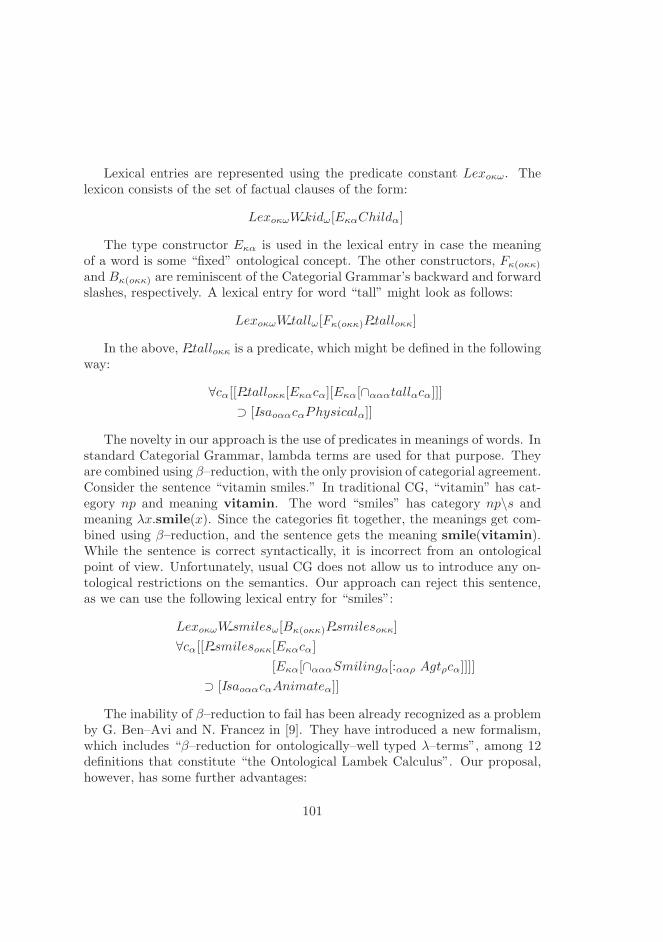
Lexical entries are represented using the predicate constant Lexoκω. Thelexicon consists of the set of factual clauses of the form:
LexoκωWkidω[EκαChildα]
The type constructor Eκα is used in the lexical entry in case the meaningof a word is some “fixed” ontological concept. The other constructors, Fκ(oκκ)
and Bκ(oκκ) are reminiscent of the Categorial Grammar’s backward and forwardslashes, respectively. A lexical entry for word “tall” might look as follows:
LexoκωWtallω[Fκ(oκκ)P talloκκ]
In the above, P talloκκ is a predicate, which might be defined in the followingway:
∀cα[[P talloκκ[Eκαcα][Eκα[∩αααtallαcα]]]
⊃ [IsaoααcαPhysicalα]]
The novelty in our approach is the use of predicates in meanings of words. Instandard Categorial Grammar, lambda terms are used for that purpose. Theyare combined using β–reduction, with the only provision of categorial agreement.Consider the sentence “vitamin smiles.” In traditional CG, “vitamin” has cat-egory np and meaning vitamin. The word “smiles” has category np\s andmeaning λx.smile(x). Since the categories fit together, the meanings get com-bined using β–reduction, and the sentence gets the meaning smile(vitamin).While the sentence is correct syntactically, it is incorrect from an ontologicalpoint of view. Unfortunately, usual CG does not allow us to introduce any on-tological restrictions on the semantics. Our approach can reject this sentence,as we can use the following lexical entry for “smiles”:
LexoκωWsmilesω[Bκ(oκκ)Psmilesoκκ]
∀cα[[Psmilesoκκ[Eκαcα]
[Eκα[∩αααSmilingα[:ααρ Agtρcα]]]]
⊃ [IsaoααcαAnimateα]]
The inability of β–reduction to fail has been already recognized as a problemby G. Ben–Avi and N. Francez in [9]. They have introduced a new formalism,which includes “β–reduction for ontologically–well typed λ–terms”, among 12definitions that constitute “the Ontological Lambek Calculus”. Our proposal,however, has some further advantages:
101

• It is very formal – it is formalized fully within C.
• It is very simple – it consists of a small number of formulae.
• It is very flexible – it allows adding arbitrary restrictions, e.g. one mightlike to use restrictions based on parthood relation rather than subsump-tion.
• It can be implemented in a straight–forward way, as presented in Sec-tion 5.12.4
For those reasons, rather than using β–reduction, we propose using a generalproof system, which is a machinery having inherently the notion of failure atdisposal. Now, desired semantic restriction can be handled by non–provabilityof a certain statement, e.g.:
K 0 ∃xκ[Psmilesoκκ[EκαV itaminα]xκ]
In the above K denotes a set of formulas consisting of lexical assertions andrules introduced throughout this section. So a vitamin cannot smile, but a childcertainly can:
K ⊢ ∃xκ[Psmilesoκκ[EκαChildα]xκ]
Not only are we interested in the provability of such a goal, but we would alsolike to know what is the resulting semantics. In this case it is: Eκα[∩αααSmilingα[:ααρAgtρChildα]]
In other words:
K ⊢ [Psmilesoκκ[EκαChildα]
[Eκα[∩αααSmilingα
[:ααρ AgtρChildα]]]]
5.12.3 Elimination rules
Recall that the forward sequent rule of the natural–deduction Lambek Calculustakes the form:
a⇒ Φ1 : A/B b⇒ Φ2 : B
a, b⇒ Φ1(Φ2) : A
102

and the backward rule:
a⇒ Φ1 : B b⇒ Φ2 : B\A
a, b⇒ Φ2(Φ1) : A
In the above a, b is the concatenation of a and b. Notice that the only pro-vision for the elimination to take place is the agreement of syntactic categories.This is because Φ1(Φ2) is always a well–formed λ–term, which can be β–reduced.
For the ease of reading, let us present the forward elimination rule of thegeneralized grammar in a similar, though quite informal way:
aθ ⇒ Fκ(oκκ)poκκ bθ ⇒ jκ K ⊢ poκκjκkκ
aθ, bθ ⇒ kκ
Let us formalize our generalized elimination rules in C. The derivation rela-tion (⇒) can be represented using a constant Roκθ. The sequences of meaningswill be represented using a well–known logic representation for lists. For theempty list we use the Nθ constant, and the list constructor is represented byLθθκ.
The list concatenation can be represented using the list appending well–known from logic programming, though here defined for non–empty lists only:
∀xκ∀yκ∀tθ[Aoθθθ[LθθκxκNθ]
[Lθθκyκtθ]
[Lθθκxκ[Lθθκyκtθ]]]
∀hκ∀lθ∀mθ∀tθ[[Aoθθθ[Lθθκhκlθ]mθ[Lθθκhκtθ]]
⊃ [Aoθθθlθmθtθ]]
The above use of Aoθθθ asserts that the concatenation of a and b yields g,or g is split into a and b. Now the forward elimination rule can be formalizedin C:
∀aθ∀bθ∀gθ∀jκ∀kκ∀poκκ[Roκθgθkκ]
⊃ [Aoθθθaθbθgθ]
∧ [Roκθaθ[Fκ(oκκ)poκκ]]
∧ [Roκθbθjκ]
∧ [poκκjκkκ]
103

Similarly, the backward elimination rule:
∀aθ∀bθ∀gθ∀jκ∀kκ∀poκκ[Roκθgθkκ]
⊃ [Aoθθθaθbθgθ]
∧ [Roκθaθjκ]
∧ [Roκθbθ[Bκ(oκκ)poκκ]]
∧ [poκκjκkκ]
We also need the following grammatical axiom, which expresses that if thelist of meanings contains only one element, that element is the resulting meaning:
∀kκ[Roκθ[LθθκkκNθ]kκ]
The English text can also be represented formally in C. We introduce a newtype ζ for that purpose. We will represent the text as a list of words. An emptylist of words will be represented by a constant Tnilξ and a list constructor by aconstant Tξξω.
5.12.4 Implementation outline
Using C instead of some kind of untyped logic as the underlying formalism hasimportant advantages regarding the implementation. It forces us to think of thetype of every formula, subformula and symbol. Thanks to that, the resultingformalization of the grammar is well–suited for implementation in a strongly–typed programming language. Using such a language (e.g. Mercury instead ofProlog) helps avoid very hard–to–find bugs and allows the compiler to generatemuch faster code.
We are interested in translating the formal specification given so far to aProlog–like logic programming language, so that we can execute specific queries.For that purpose, we have formalized the grammar in C using only definiteclauses. Furthermore, we perform the following steps:
• We write all the constants in lower–case
• We write all variables in upper–case
• We use i for intersection constant and p for the Peirce product constant
• We drop the subscripts indicating types in all formulas
• We replace ‘⊃’ and ‘∧’ with ‘:-’ and ‘,’, respectively.
104
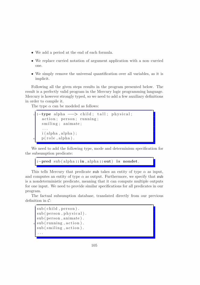
• We add a period at the end of each formula.
• We replace curried notation of argument application with a non–curriedone.
• We simply remove the universal quantification over all variables, as it isimplicit.
Following all the given steps results in the program presented below. Theresult is a perfectly valid program in the Mercury logic programming language.Mercury is however strongly typed, so we need to add a few auxiliary definitionsin order to compile it.
The type α can be modeled as follows:�
1 :−type alpha −−−> ch i l d ; t a l l ; phy s i c a l ;a c t i on ; person ; running ;smi l i ng ; animate ;. . .i ( alpha , alpha ) ;
6 p( ro l e , alpha ) .
We need to add the following type, mode and determinism specification forthe subsumption predicate:
�
:−pred sub ( alpha : : in , a lpha : : out ) i s nondet .
This tells Mercury that predicate sub takes an entity of type α as input,and computes an entity of type α as output. Furthermore, we specify that subis a nondeterministic predicate, meaning that it can compute multiple outputsfor one input. We need to provide similar specifications for all predicates in ourprogram.
The factual subsumption database, translated directly from our previousdefinition in C:
�
sub ( ch i ld , person ) .sub ( person , phy s i c a l ) .sub ( person , animate ) .
4 sub ( running , a c t i on ) .sub ( smi l ing , a c t i on ) .. . .
105
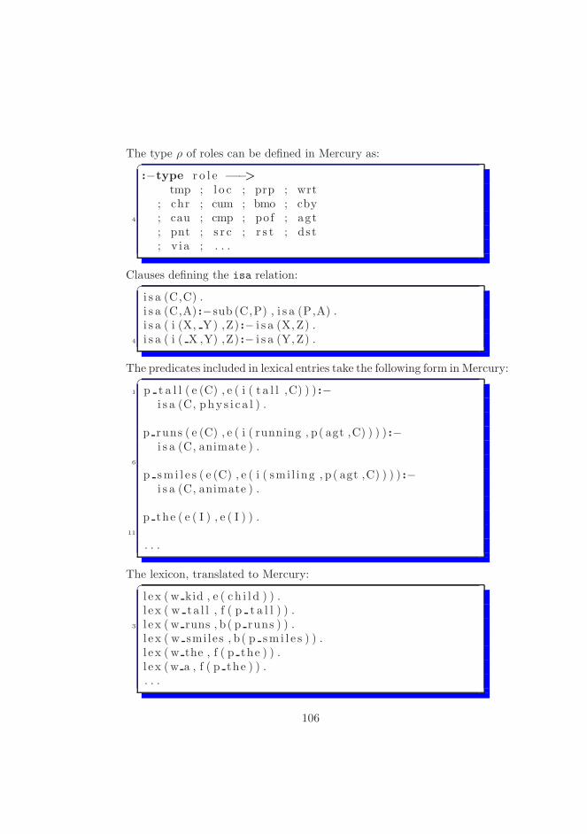
The type ρ of roles can be defined in Mercury as:�
:−type r o l e −−−>tmp ; l o c ; prp ; wrt
; chr ; cum ; bmo ; cby4 ; cau ; cmp ; pof ; agt
; pnt ; s r c ; r s t ; ds t; v ia ; . . .
Clauses defining the isa relation:�
i s a (C,C) .i s a (C,A) :−sub (C,P) , i s a (P,A) .i s a ( i (X, Y) ,Z) :− i s a (X, Z) .
4 i s a ( i ( X ,Y) ,Z) :− i s a (Y, Z) .
The predicates included in lexical entries take the following form in Mercury:�
1 p t a l l ( e (C) , e ( i ( t a l l ,C) ) ) :−i s a (C, phy s i c a l ) .
p runs ( e (C) , e ( i ( running , p( agt ,C) ) ) ) :−i s a (C, animate ) .
6
p sm i l e s ( e (C) , e ( i ( smi l ing , p ( agt ,C) ) ) ) :−i s a (C, animate ) .
p the ( e ( I ) , e ( I ) ) .11
. . .
The lexicon, translated to Mercury:�
l e x ( w kid , e ( ch i l d ) ) .l ex ( w ta l l , f ( p t a l l ) ) .
3 l e x ( w runs , b ( p runs ) ) .l ex ( w smiles , b( p sm i l e s ) ) .l ex ( w the , f ( p the ) ) .l ex (w a , f ( p the ) ) .. . .
106

The definition of non–empty list appending:�
a ( l (X, n ) , l (Y,T) , l (X, l (Y,T) ) ) .a ( l (H,L) ,M, l (H,T) ) :−a (L ,M,T) .
The rules formalized in C take the following form in Mercury:�
r ( l (X, n ) ,X) .
3 r (G, E1) :−a (G1 ,G2 ,G) ,r (G1 , f (P) ) ,r (G2 , E2) ,P(E2 , E1) .
8
r (G, E1) :−a (G1 ,G2 ,G) ,r (G1 , E2) ,r (G2 , b (P) ) ,
13 P(E2 , E1) .
The rules are the only place in the program, where we use higher–order predi-cates.
The following predicate assigns a meaning to English text:�
m(T,C) :−2 map lex (T,L) ,
r (L , e (C) ) .
Let us add an auxiliary predicate work for testing purposes:�
work (C) :−2 m( t ( w the ,
t ( w ta l l ,t ( w kid ,
t ( w smiles ,t n i l ) ) ) ) ,C) .
The map lex predicate is used for lexicon look–up of a list of words.
107

�
map lex ( tn i l , n) .map lex ( t (W,T) , l ( I ,MT) ) :−
l e x (W, I ) , map lex (T,MT) .
Notice that the program does not require higher order unification, exceptfor the simplest case where a variable is bound to a predefined predicate andsuch a predicate is called. Most logic programming languages provide a facilityfor such behaviour. We could change the syntax slightly and turn our code intoa valid Prolog program by utilizing the call library predicate.
The full listing of the program is given in Appendix C on page 207.Notice that the program is a direct implementation of the theory, hence
quite inefficient. Instead of the presented top–down approach, we could derivethe semantics in the bottom–up manner in order to avoid unneeded search.
For the sample query:�
? work (C) .
We get the following (exactly one) result:�
C = i ( smi l ing , p ( agt , i ( t a l l , c h i l d ) ) )
5.13 Summary
In this chapter we have introduced the notion of ontological semantics. Inparticular we will focus on the Peirce–algebraic ontological semantics, as it fitsperfectly with the generative ontology.
Furthermore, we have presented an example of how our ontological seman-tics can be utilized by merging it with Categorial Grammar. The functionalcomposition and β–reduction have been replaced with proof rule application.We have utilized it for constructing ontologico–algebraic meaning using onto-logical restrictions, dropping at the same time syntactic categories and syntacticrestrictions.
108

Chapter 6
Comparison withstate–of–the–art inontological semantics
In this brief chapter, as an interlude before we commence with developing sys-tems for ontological meaning extraction, let us have a look at the state–of–the–art and compare it to our approach.
One of the state–of–the–art approaches to ontological semantics utilizingLambek Calculus has been presented by G. Ben–Avi and N. Francez in [9]. Wehave previously presented a discussion of this work and suggested an alternativeapproach in Section 5.12 on page 98.
6.1 Comparison to “Ontological Semantics” byNirenburg and Raskin
Perhaps it is worth comparing our approach to the ontological semantics de-scribed in the previous chapter to that described in the book by the same titleby Nirenburg and Raskin [33].
• In our approach we use First Order Predicate Logic as the underlying for-mal metalanguage in order to maintain coherence between theory, specifi-cation, and implementation parts. Nirenburg and Raskin (N&R) dismiss
109

First Order Predicate Logic, as according to them it has failed “to havemade a historical impact”. We try to remain formal in our discussions,while they tend to be more philosophical and informal.
• N&R deal with textual natural language semantics in general. We con-cern ourselves only in general with scientific texts, particularly biomedicalones. This has large impact on the way ontologies are used in the seman-tics. Due to unrestricted domain, N&R’ semantics approaches issues ofaspect, detailed time, language style (formality, politeness, respect, force,simplicity, color, directness), modality, etc. These issues are not relevantfor our scientific text domains.
• The tasks that N&R’s text meaning representations have been used forinclude machine translation, information extraction, question answering,general human–computer dialog systems, and text summarization. Thisis a wide range of linguistic applications, while we focus ourselves on theproblem of semantic search.
• Our approach is unique in that we use the notion of generative ontologiesin order to establish a formal ontological semantics.
• We provide several concrete algorithms for extracting ontological seman-tics from text (and one for generating text given ontological semantics),with implementation. While N&R discuss how text meaning representa-tions can be extracted from text, they do not provide a specific algorithmor implementation thereof.
6.2 Framenet
Let us consider the Framenet project [6, 49, 7], centered around the idea ofsemantic frames.
In [15] we read:
The basic idea is that one cannot understand the meaning of a sin-gle word without access to all the essential knowledge that relates tothat word. For example, one would not be able to understand theword “sell” without knowing anything about the situation of com-mercial transfer, which also involves, among other things, a seller, abuyer, goods, money, the relation between the money and the goods,the relations between the seller and the goods and the money, therelation between the buyer and the goods and the money and so on.
110

This approach differs substantially from ours in various respects. As it ap-pears, frame semantics presuposes the need of quite large amount of real–worldknowledge. The quoted “knowing about the situation of commercial transfer”is very advanced and complicated task with a computer. Full formalization ofsuch a knowledge is an extremely difficult task – so difficult in fact, that nobodyhas ever come close to accomplishing it (for non–abstract concepts). All existingreal–world knowledge formalization attempts simplify the view of the problem,and describe only some relatively small (but usually most important) part ofit, leaving the less–important (or sometimes just more–difficult–to–model) el-ements out. Cf. e.g. CYC [27]. FrameNet serves as a simplified view of this“knowing”, where frames are used to encode some limited information aboutsituations like “commercial transfer”. However, comparing FrameNet to ourapproach, it still contains much more information in the frames than we doin our setup. This has both advantages and disadvantages. The advantage ofusing FrameNet for our purposes could be that the information available couldimprove the understanding of language. That’s the goal of FrameNet or anyother lexical resource – more knowledge allows better language comprehension.However, the downside is that one requires a large amount of frames. At thetime of writing FrameNet consists of close to 800 frames, which covers an im-presive amount of language. Nevertheless, still a lot more is needed to claima very large linguistic coverage. Projects like BioFrameNet [16] try to fill thegaps for some domains, but as with any knowlegde representation project, a lotis left to do.
In a sense, in our approach, we would like to have quite large languagecoverage. Therefore we only depend on a lexicon and a skeleton ontology, bothof which can support very large linguistic coverage, far beyond FrameNet’s 800frames.
The key difference, however, lies hidden in the underlying motivation andaspirations of the projects. Once again, frame semantics claims:
The basic idea is that one cannot understand the meaning of a singleword without access to all the essential knowledge that relates to thatword.
While we fully agree with this statement, the point to notice is that, asfar as our approach is concerned, we refrain from trying to “understand themeaning of a single word”. Instead of understanding the full meaning of aword, a phrase, or a sentence, we limit ourselves to capturing what the sentenceis about, i.e. extracting conceptual information from the sentence and linking tothe generative ontology. This comes from the fact that our ontological semantics
111

is supposed to be used for search, and for that purpose we do not need tounderstand the propositional content of a sentence. Hence, in our approach,understanding a word is limited to linking the word to a concept in the generativeontology.
Also, according to [39], FrameNet cannot be used as an ontology.Even though for the reasons explained above, we do not use FrameNet di-
rectly, some of its data could still be utilized while building a generative ontology.FrameNet contains semantic categories for frame elements, and those could bemanually1 turned into ontological affinities that define the generative ontology.However, we do not pursue this idea.
1It seems unlikely to achieve good results with automatic methods.
112

Chapter 7
The computational view ofthe relation between thenatural language fragmentand the ontologicalsemantics
This chapter gives an overview of how one could relate a fragment of the naturallanguage and the ontological semantics established in chapter 5 by computa-tional means. We call the process of extracting the ontological semantics fromtext “ontograbbing”. However, we also discuss the reverse problem of linguisticrealization, i.e. transforming a given ontological semantics into a linguistic form,such as a phrase or a sentence.
The chapter starts with a simple definite clause example of ontograbbing,which algorithmically relates text to its ontological semantics. This relationis supposed to be very formal, so the language is limited and narrowed downto selected language fragments. Further extensions are presented, in order ofincreasing complexity. In the next chapter we will present a more robust modelaccepting realistic text.
The algorithms presented in this chapter are not meant to be efficient, but toreflect closely the logical relation between language and its semantics established
113

in the previous chapter.
Since these simple ontograbbers are implemented in Prolog (including itsspecial Definite Clause Grammar notation), a short discussion about suitabilityof that system is provided.
7.1 Computation with Prolog vs. specification
in First Order Predicate Logic
In case of First Order Predicate Logic, we could use a Prolog system as aconvenient computational approximation that would allow us to reason in anefficient way. However, Prolog systems use most commonly some version of SLDresolution coupled with closed world assumption and negation as failure in orderto simulate the First Order Predicate Logic reasoning. The word “simulate” isused intentionally here. Let us have a look at how First Order Predicate Logicand Prolog logic programming differ. In the latter, due to the fact that SLDresolution is used, we are limited to writing our sentences as definite clauses.
This poses serious restrictions on our freedom to use arbitrary operatorsand quantifiers anywhere within our sentences. We are limited to using definiteclauses only, which are all built as universaly quantified implications with oneterm on the left hand side and a conjunction of arbitrary number of terms on theright hand side. Unfortunately, not every First Order Predicate Logic formulacan be translated to a set of definite clauses to be used by Prolog systems. Oneof the most noticeable problems with such translation is the fact that Prologuses negation as non–provability instead of classical negation.
Prolog systems often offer additional facilities, e.g. cut operation, whichgo beyond definite clauses. Such extensions modify the way SLD resolutionoperates, and hence logic programs containing them are referred to as impure.
However, even if the set of formulae is pure and exactly the same for FirstOrder Predicate Logic and Prolog, it is still not to be understood in the sameway. We have to keep in mind how Prolog executes the given logic program.The order of clauses is very important. Swapping the order of two clauses canturn a well–working program into a non–terminating one. We do not observesuch shortcomings with First Order Predicate Logic. Similar issue occurs withthe order of literals in the body of a given clause. While the order of literals ina conjunction is strictly arbitrary in First Order Predicate Logic, it matters alot with Prolog.
This situation means that while some First Order Predicate Logic specifi-
114
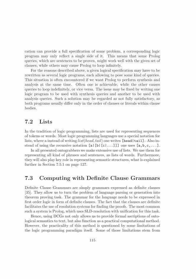
cation can provide a full specification of some problem, a corresponding logicprogram may only reflect a single side of it. This means that some Prologqueries, which are sentences to be proven, might work well with the given set ofclauses, while others may cause Prolog to loop infinitely.
For the reasons described above, a given logical specification may have to berewritten as several logic programs, each allowing to pose some kind of queries.This situation is often encountered if we want Prolog to perform synthesis andanalysis at the same time. Often one is achievable, while the other causesqueries to loop indefinitely, or vice versa. The issue may be fixed by writing onelogic program to be used with synthesis queries and another to be used withanalysis queries. Such a solution may be regarded as not fully satisfactory, asboth programs usually differ only in the order of clauses or literals within clausebodies.
7.2 Lists
In the tradition of logic programming, lists are used for representing sequencesof tokens or words. Most logic programming languages use a special notation forlists, where a instead of writing list(head, tail) one writes [head|tail]. Also in-stead of using the recursive notation [a|[b|[c|...]]] one uses [a,b,c,...].
In all presented ontograbbers we make extensive use of lists. We use them forrepresenting all kind of phrases and sentences, as lists of words. Furthermore,they will also play key role in representing semantic structures, what is explainedfurther in Section 7.5.1 on page 127.
7.3 Computing with Definite Clause Grammars
Definite Clause Grammars are simply grammars expressed as definite clauses[35]. They allow us to turn the problem of language parsing or generation intotheorem proving task. The grammar for the language needs to be expressed infirst order logic in form of definite clauses. The fact that the clauses are definitefacilitates the use of resolution systems for finding the proofs. The most commonsuch a system is Prolog, which uses SLD-resolution with unification for this task.
Hence, using DCGs not only allows us to provide formal ascriptions of onto-logical semantics to text, but also function as a practical computational method.However, the practicality of this method is questioned by some limitations ofthe logic programming paradigm itself. Some of those limitations stem from
115

the discrepancies between the underlying logic with its proof system and theinferential engine used to simulate it in logic programming in a computationalmanner.
7.4 Ontograbbing with definite clauses
We first present a simple grammar, which does not make use of the specialDCG notation available in Prolog. All definite clauses are “spelled out” fully.Additionally, for simplicity, we do not use difference lists, which would be hiddenbehind the special Prolog DCG notation.
In the course of analyzing the sentence the list of words needs to be dividedinto shorter sublists, corresponding to shorter phrases or words. For the purposeof (nondeterministically) dividing any list of tokens into two shorter lists we usethe split predicate:
�
s p l i t (X, [ H1 |T1 ] , [ H2 |T2 ] ):−append ( [ H1 |T1 ] , [ H2 |T2 ] ,X) .
The approach to parsing employed for this simplest ontograbber is by nomeans the fastest one. However, it allow us to provide a clean logical descriptionof how the ontological semantics is coupled with the grammar. Describing anefficient parsing process, e.g. utilizing the Earley1 parser would call for a verylarge number of formulae in First Order Predicate Logic.
7.4.1 Noun phrases
The np predicate defines the logical relation between noun phrases and corre-sponding ontological concepts. The singleton list containing only one token N
can be recognized as a noun phrase corresponding to the concept C if the lexiconcontains an entry for the noun N with an associated meaning C:
�
np ( [N] ,C) :−noun (N,C) .
For handling noun–noun compounds, we have the following rule:�
np (L ,C) :− s p l i t (L , L1 , L2) ,np (L1 ,C1) ,np (L2 ,C2) ,a nnc (C1 ,C2 ,C) .
1An SML implementation of the Earley parser is presented in Appendix D.
116
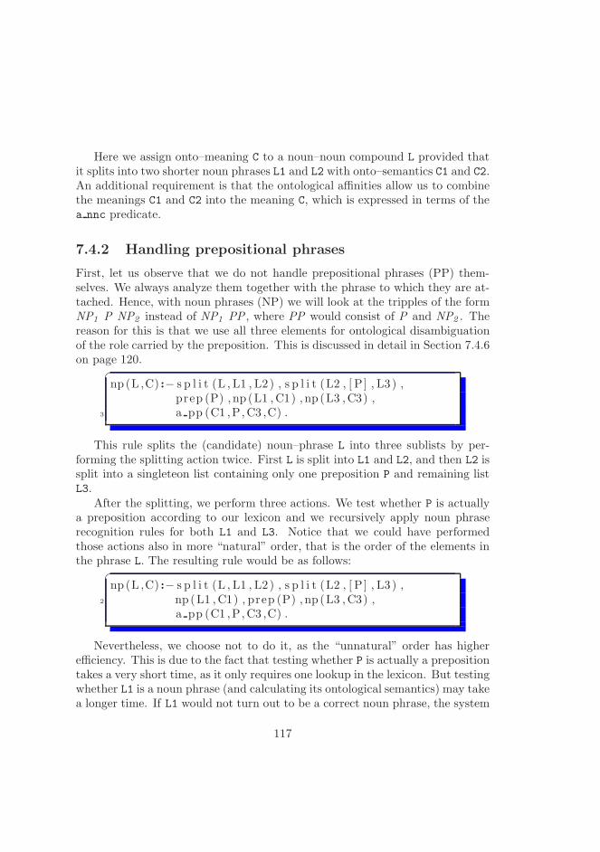
Here we assign onto–meaning C to a noun–noun compound L provided thatit splits into two shorter noun phrases L1 and L2 with onto–semantics C1 and C2.An additional requirement is that the ontological affinities allow us to combinethe meanings C1 and C2 into the meaning C, which is expressed in terms of thea nnc predicate.
7.4.2 Handling prepositional phrases
First, let us observe that we do not handle prepositional phrases (PP) them-selves. We always analyze them together with the phrase to which they are at-tached. Hence, with noun phrases (NP) we will look at the tripples of the formNP1 P NP2 instead of NP1 PP , where PP would consist of P and NP2 . Thereason for this is that we use all three elements for ontological disambiguationof the role carried by the preposition. This is discussed in detail in Section 7.4.6on page 120.
�
np (L ,C) :− s p l i t (L , L1 , L2) , s p l i t (L2 , [ P] , L3) ,prep (P) , np (L1 ,C1) , np (L3 ,C3) ,
3 a pp (C1 ,P,C3 ,C) .
This rule splits the (candidate) noun–phrase L into three sublists by per-forming the splitting action twice. First L is split into L1 and L2, and then L2 issplit into a singleteon list containing only one preposition P and remaining listL3.
After the splitting, we perform three actions. We test whether P is actuallya preposition according to our lexicon and we recursively apply noun phraserecognition rules for both L1 and L3. Notice that we could have performedthose actions also in more “natural” order, that is the order of the elements inthe phrase L. The resulting rule would be as follows:
�
np (L ,C) :− s p l i t (L , L1 , L2) , s p l i t (L2 , [ P] , L3) ,2 np (L1 ,C1) , prep (P) , np (L3 ,C3) ,
a pp (C1 ,P,C3 ,C) .
Nevertheless, we choose not to do it, as the “unnatural” order has higherefficiency. This is due to the fact that testing whether P is actually a prepositiontakes a very short time, as it only requires one lookup in the lexicon. But testingwhether L1 is a noun phrase (and calculating its ontological semantics) may takea longer time. If L1 would not turn out to be a correct noun phrase, the system
117

would need to backtrack only to find perhaps that in fact P is not a preposition.Hence, testing the preposition first improves the performance of the systemby avoiding a lot of unnecessary backtracking. After all, if we encounter apreposition in a sentence, a fairly good guess is that it follows a noun phrase.
Such a shuffling of atoms in the body of the clause is specific to practicallogic programming systems. We would never consider these two rules to beany different if we would be working with logical specification in First OrderPredicate Logic.
The question arises – what if there is more than one prepositional phraseattached to some noun phrase? In such a situation we observe ambiguity at thesyntactic level, i.e. the prepositional phrases can be either alligned or nested.However, it turns out that our rule for handling noun–preposition–noun tripletsis flexible enough to handle these cases. This stems from the fact that the ruleis recursive in nature. Let us investigate how the rule operates in such cases byconsidering the following example:
Blood flow through the liver after meals︸ ︷︷ ︸
NP0
The rule can split the phrase into three parts in two ways (as there are twoprepositions):
Blood flow︸ ︷︷ ︸
NP1
through︸ ︷︷ ︸
PREP1
the liver after meals︸ ︷︷ ︸
NP4︸ ︷︷ ︸
NP0
or
Blood flow through the liver︸ ︷︷ ︸
NP5
after︸︷︷︸
PREP2
meals︸ ︷︷ ︸
NP3︸ ︷︷ ︸
NP0
In both cases, after the splitting is performed, the rule is called recursivelyon the sublists, so that the noun phrases containing prepositions (NP4 andNP5) will be handled using the same rule, in effect splitting them again intothree parts each. So, after the second phase of splitting, we will be left with thefollowing two divisions:
118

Blood flow︸ ︷︷ ︸
NP1
through︸ ︷︷ ︸
PREP1
the liver︸ ︷︷ ︸
NP2
after︸︷︷︸
PREP2
meals︸ ︷︷ ︸
NP3︸ ︷︷ ︸
NP4︸ ︷︷ ︸
NP0
or
Blood flow︸ ︷︷ ︸
NP1
through︸ ︷︷ ︸
PREP1
the liver︸ ︷︷ ︸
NP2︸ ︷︷ ︸
NP5
after︸︷︷︸
PREP2
meals︸ ︷︷ ︸
NP3
︸ ︷︷ ︸
NP0
As we can observe, in both cases the final constituents to contribute to theontological semantics are the same, as could be expected. However, they arestructured differenctly at a higher level, via either NP4 or NP5 correspondingto either nested or alligned prepositional phrases, respectively.
7.4.3 Determiners
The following rule handles determiners. Notice that determiners do not con-tribute to the ascribed meaning:
�
np ( [D|L ] ,C) :−det (D) ,np (L ,C) .
Any determiners in the analyzed sentence are simply discarded. This hasan interesting side–effect. If the sentence contained determiners which are notsoundly placed according to the grammar, the analysis will continue withoutnoticing it. Usually a sentence containing e.g. a list of tokens “the the the”should be rejected, as being ungrammatical.
7.4.4 Adjectives
Adjectives can be analyzed in the following way, analogous to how we dealt withother phrases:
�
np (L ,C) :− s p l i t (L , [A] , L1) , adj (A,CA) ,np (L1 ,C1) ,a ad j (CA,C1 ,C) .
119

7.4.5 Sentences
Sentences built of a subject NP, a transitive verb, and an object NP, will beanalyzed as follows:
�
s (L ,C) :− s p l i t (L , L1 , L2) , s p l i t (L2 , [V] , L3) ,np (L1 ,C1) , tv (V,CV) , np (L3 ,C3) ,
3 a tv (C1 ,CV,C3 ,C) .
7.4.6 Ontology–based role recognition
Noun–noun compounds
An interesting problem is the recognition of a proper relation between conceptsin a noun–noun compound. While in prepositional phrases the preposition con-tains a hint as to what role should be ascribed in the resulting semantics, noun–noun compounds are more tricky. This recognition, in the current prototype,is made on the basis of where the concepts corresponding to the constituentnouns are placed in the ontology. E.g. if the meaning of the modifier noun isbelow “substance” in the ontology, and the meaning of the head noun is below“process”, we recognize the role to be “pnt”:
�
a nnc (X,Y, i (Y, p( pnt ,X) ) ) :− i s a (X, substance ) ,2 i s a (Y, pro ce s s ) .
Examples of this situation are: “glucose storage”, “insulin secretion”.Similarly, we can base the role recognition on the parthood relation:�
a nnc (X,Y, i (Y, p( loc ,X) ) ) :−pa r to f (X, body ) ,pa r to f (Y, body ) .
If both nouns represent parts of the body, we understand the hidden relationbetween them to be “loc”. E.g. “liver cell”.
Prepositional phrases
When used to represent compound concepts, prepositional phrases give us moreinformation about the intended role between the partial concepts than noun–noun compounds do. The clue is the preposition used. Nevertheless, preposi-tions still do not allow us to determine the role uniquely, as they are in general
120

ambiguous. We can, however, similarly as with noun–noun compounds, use theontology for the purpose of disambiguation. In the current theory, the predicateused for role disambiguation in prepositional phrases is called a pp.
It is worth noting that the disambiguation need not be absolute, i.e. wewill not always get one unique role. Out of n possible roles, we will get mdisambiguated ones, where 0 ≤ m ≤ n. Thus, we will usually get fewer roles,most commonly one or two. It can also happen that we do not get any roleat all in the disambiguation process. This happens if our ontological affinitiesare unable to “understand” a given prepositional prase type from ontologicalperspective. Such a situation is common in domain–specific texts, if the giventext falls outside of the domain considered, but the ontology is only defined forthe domain.
The a pp predicate might be defined as follows:�
a pp (X, of ,Y, i (X, p ( pnt ,Y) ) ):− i s a (Y, substance ) ,
3 i s a (X, pro ce s s ) .
Such a rule defines that if the noun phrase corresponding to concept X isaugmented with a prepositional phrase consisting of the preposition “of” and anounphrase corresponding to the concept Y, then the resulting role can be “pnt”,provided that X is below “process” in the ontology and Y is below “substance”.The resulting compound concept will be i(X,p(pnt,Y)), which can be writtenin the feature–structure notation as X [pnt : Y ].
As an example, let us consider the prepositional phrase “secretion of insulin”.According to the disambiguation rule above, we can understand the preposition“of” as representing the role pnt, due to the fact that “secretion” falls below“process” and “insulin” falls below “substance” in our ontology.
Note that it would be difficult to disambiguate the role represented by theprepositional phrase by looking at the phrase itself. That is why we also inves-tigate the noun phrase to which this prepositional phrase is attached. As anexample of why this is the case, consider the phrase “of insulin”. By looking atsuch a prepositional phrase itself, it is difficult to decide what role the prepo-sition denotes. If this phrase is attached to the noun “secretion”, we wouldunderstand it as pnt. However, if the noun would be “level”, thus forming thephrase “level of insulin”, then we would want to understand the role to be wrt.
Obviously, our role disambiguation for prepositional phrases can use arbi-trary definitions for any given preposition. We are not limited merely to tax-onomical inclusions. We could, for instance, also use parthood information for
121
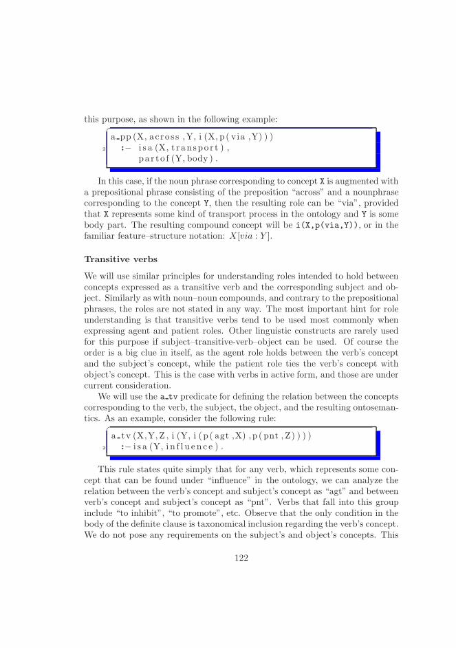
this purpose, as shown in the following example:�
a pp (X, acros s ,Y, i (X, p ( via ,Y) ) )2 :− i s a (X, t r anspo r t ) ,
pa r to f (Y, body ) .
In this case, if the noun phrase corresponding to concept X is augmented witha prepositional phrase consisting of the preposition “across” and a nounphrasecorresponding to the concept Y, then the resulting role can be “via”, providedthat X represents some kind of transport process in the ontology and Y is somebody part. The resulting compound concept will be i(X,p(via,Y)), or in thefamiliar feature–structure notation: X [via : Y ].
Transitive verbs
We will use similar principles for understanding roles intended to hold betweenconcepts expressed as a transitive verb and the corresponding subject and ob-ject. Similarly as with noun–noun compounds, and contrary to the prepositionalphrases, the roles are not stated in any way. The most important hint for roleunderstanding is that transitive verbs tend to be used most commonly whenexpressing agent and patient roles. Other linguistic constructs are rarely usedfor this purpose if subject–transitive-verb–object can be used. Of course theorder is a big clue in itself, as the agent role holds between the verb’s conceptand the subject’s concept, while the patient role ties the verb’s concept withobject’s concept. This is the case with verbs in active form, and those are undercurrent consideration.
We will use the a tv predicate for defining the relation between the conceptscorresponding to the verb, the subject, the object, and the resulting ontoseman-tics. As an example, consider the following rule:
�
a tv (X,Y,Z , i (Y, i (p ( agt ,X) ,p ( pnt , Z) ) ) )2 :− i s a (Y, i n f l u e n c e ) .
This rule states quite simply that for any verb, which represents some con-cept that can be found under “influence” in the ontology, we can analyze therelation between the verb’s concept and subject’s concept as “agt” and betweenverb’s concept and subject’s concept as “pnt”. Verbs that fall into this groupinclude “to inhibit”, “to promote”, etc. Observe that the only condition in thebody of the definite clause is taxonomical inclusion regarding the verb’s concept.We do not pose any requirements on the subject’s and object’s concepts. This
122
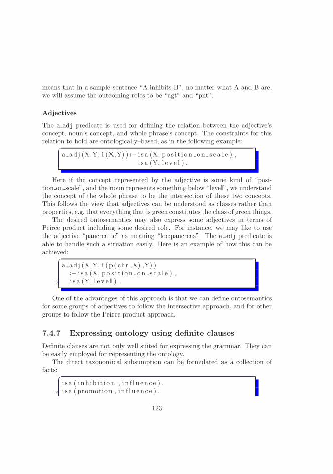
means that in a sample sentence “A inhibits B”, no matter what A and B are,we will assume the outcoming roles to be “agt” and “pnt”.
Adjectives
The a adj predicate is used for defining the relation between the adjective’sconcept, noun’s concept, and whole phrase’s concept. The constraints for thisrelation to hold are ontologically–based, as in the following example:
�
a ad j (X,Y, i (X,Y) ) :− i s a (X, p o s i t i o n o n s c a l e ) ,i s a (Y, l e v e l ) .
Here if the concept represented by the adjective is some kind of “posi-tion on scale”, and the noun represents something below “level”, we understandthe concept of the whole phrase to be the intersection of these two concepts.This follows the view that adjectives can be understood as classes rather thanproperties, e.g. that everything that is green constitutes the class of green things.
The desired ontosemantics may also express some adjectives in terms ofPeirce product including some desired role. For instance, we may like to usethe adjective “pancreatic” as meaning “loc:pancreas”. The a adj predicate isable to handle such a situation easily. Here is an example of how this can beachieved:
�
a ad j (X,Y, i (p ( chr ,X) ,Y) ):− i s a (X, p o s i t i o n o n s c a l e ) ,
3 i s a (Y, l e v e l ) .
One of the advantages of this approach is that we can define ontosemanticsfor some groups of adjectives to follow the intersective approach, and for othergroups to follow the Peirce product approach.
7.4.7 Expressing ontology using definite clauses
Definite clauses are not only well suited for expressing the grammar. They canbe easily employed for representing the ontology.
The direct taxonomical subsumption can be formulated as a collection offacts:
�
i s a ( i nh i b i t i o n , i n f l u e n c e ) .2 i s a ( promotion , i n f l u e n c e ) .
123
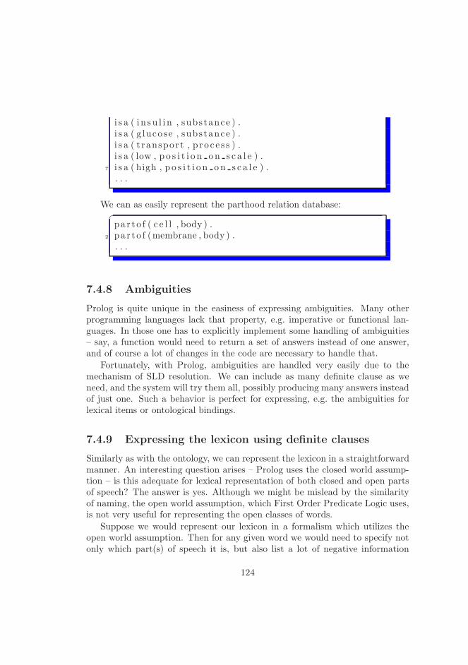
i s a ( i n s u l i n , substance ) .i s a ( g lucose , substance ) .i s a ( transpor t , p r o ce s s ) .i s a ( low , p o s i t i o n o n s c a l e ) .
7 i s a ( high , p o s i t i o n o n s c a l e ) .. . .
We can as easily represent the parthood relation database:�
pa r to f ( c e l l , body ) .2 pa r to f (membrane , body ) .
. . .
7.4.8 Ambiguities
Prolog is quite unique in the easiness of expressing ambiguities. Many otherprogramming languages lack that property, e.g. imperative or functional lan-guages. In those one has to explicitly implement some handling of ambiguities– say, a function would need to return a set of answers instead of one answer,and of course a lot of changes in the code are necessary to handle that.
Fortunately, with Prolog, ambiguities are handled very easily due to themechanism of SLD resolution. We can include as many definite clause as weneed, and the system will try them all, possibly producing many answers insteadof just one. Such a behavior is perfect for expressing, e.g. the ambiguities forlexical items or ontological bindings.
7.4.9 Expressing the lexicon using definite clauses
Similarly as with the ontology, we can represent the lexicon in a straightforwardmanner. An interesting question arises – Prolog uses the closed world assump-tion – is this adequate for lexical representation of both closed and open partsof speech? The answer is yes. Although we might be mislead by the similarityof naming, the open world assumption, which First Order Predicate Logic uses,is not very useful for representing the open classes of words.
Suppose we would represent our lexicon in a formalism which utilizes theopen world assumption. Then for any given word we would need to specify notonly which part(s) of speech it is, but also list a lot of negative information
124

about which parts of speech it is not. This would rather be an impracticalapproach.
The confusion arises from the fact that the word “open” in “open worldassumption” refers to the openness of the knowledge about a given word – wedo not know that it does not belong to some class unless we specify that. Butthe word “open” in “open word class” refers to the openness of the class as awhole, meaning that it does not have a fairly fixed amount of member words.
Determiners
The determiners are defined by the det predicate:�
det ( the s e ) .2 det ( the ) .
. . .
Prepositions
We take care of prepositions just as easily:�
prep ( o f ) .2 prep ( a c r o s s ) .
. . .
Nouns
The predicate for noun lexical entries will be binary, coupling the given nounwith its ontological class:
�
noun ( transpor t , t r anspo r t ) .2 noun ( i n s u l i n , i n s u l i n ) .
. . .
Verbs
Transitive verbs are stored in the lexicon together with the ontological classthey represent by means of the tv predicate:
125

�
tv ( i nh i b i t , i n h i b i t i o n ) .2 . . .
Adjectives
Lexical entries for adjectives are taken care of in the same way as nouns andverbs:
�
adj ( low , low ) .. . .
7.4.10 Example
Now, using Prolog’s SLD resolution, we can for instance ask the following query:�
:− s ( [ these , low , i n s u l i n , l e v e l , i nh i b i t ,the , t ranspor t , of , g lucose , acros s , c e l l ,
membrane ] ,3 C)
We will get only one answer:�
C = i ( i nh i b i t i o n ,2 i (p( agt , i ( low , i ( l e v e l ,
p(wrt , i n s u l i n ) ) ) ) ,p( pnt , i ( i ( t ranspor t ,
p ( pnt , g luco s e ) ) ,p( via , i (membrane ,
7 p( loc , c e l l ) ) ) ) ) ) )
7.5 An extended version of the ontograbber
We now present another ontograbber expressed with definite clauses to be usedwith the Prolog logic programming language.
This version uses similar basic principles as the previous one, except it isextended in many respects. Let us go step by step through the changes.
126
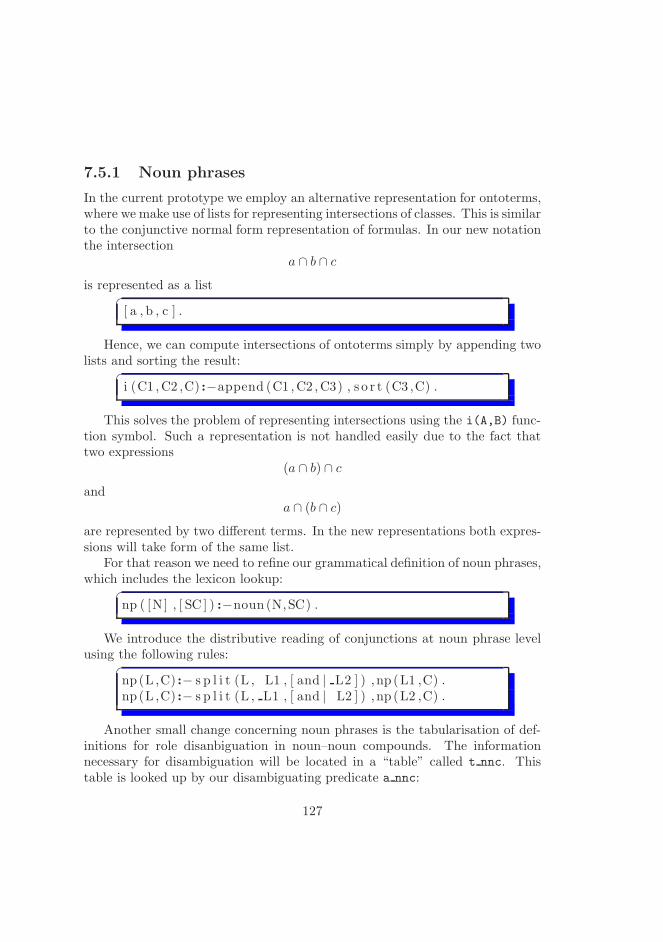
7.5.1 Noun phrases
In the current prototype we employ an alternative representation for ontoterms,where we make use of lists for representing intersections of classes. This is similarto the conjunctive normal form representation of formulas. In our new notationthe intersection
a ∩ b ∩ c
is represented as a list�
[ a , b , c ] .
Hence, we can compute intersections of ontoterms simply by appending twolists and sorting the result:
�
i (C1 ,C2 ,C) :−append (C1 ,C2 ,C3) , s o r t (C3 ,C) .
This solves the problem of representing intersections using the i(A,B) func-tion symbol. Such a representation is not handled easily due to the fact thattwo expressions
(a ∩ b) ∩ c
anda ∩ (b ∩ c)
are represented by two different terms. In the new representations both expres-sions will take form of the same list.
For that reason we need to refine our grammatical definition of noun phrases,which includes the lexicon lookup:
�
np ( [N] , [ SC ] ) :−noun (N,SC) .
We introduce the distributive reading of conjunctions at noun phrase levelusing the following rules:
�
np (L ,C) :− s p l i t (L , L1 , [ and | L2 ] ) ,np (L1 ,C) .np (L ,C) :− s p l i t (L , L1 , [ and | L2 ] ) ,np (L2 ,C) .
Another small change concerning noun phrases is the tabularisation of def-initions for role disanbiguation in noun–noun compounds. The informationnecessary for disambiguation will be located in a “table” called t nnc. Thistable is looked up by our disambiguating predicate a nnc:
127
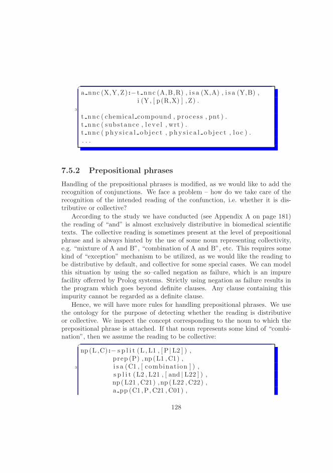
�
a nnc (X,Y,Z) :− t nnc (A,B,R) , i s a (X,A) , i s a (Y,B) ,i (Y, [ p(R,X) ] , Z) .
3
t nnc ( chemical compound , proces s , pnt ) .t nnc ( substance , l e v e l , wrt ) .t nnc ( phy s i c a l o b j e c t , phy s i c a l o b j e c t , l o c ) .. . .
7.5.2 Prepositional phrases
Handling of the prepositional phrases is modified, as we would like to add therecognition of conjunctions. We face a problem – how do we take care of therecognition of the intended reading of the confunction, i.e. whether it is dis-tributive or collective?
According to the study we have conducted (see Appendix A on page 181)the reading of “and” is almost exclusively distributive in biomedical scientifictexts. The collective reading is sometimes present at the level of prepositionalphrase and is always hinted by the use of some noun representing collectivity,e.g. “mixture of A and B”, “combination of A and B”, etc. This requires somekind of “exception” mechanism to be utilized, as we would like the reading tobe distributive by default, and collective for some special cases. We can modelthis situation by using the so–called negation as failure, which is an impurefacility offerred by Prolog systems. Strictly using negation as failure results inthe program which goes beyond definite clauses. Any clause containing thisimpurity cannot be regarded as a definite clause.
Hence, we will have more rules for handling prepositional phrases. We usethe ontology for the purpose of detecting whether the reading is distributiveor collective. We inspect the concept corresponding to the noun to which theprepositional phrase is attached. If that noun represents some kind of “combi-nation”, then we assume the reading to be collective:
�
np (L ,C) :− s p l i t (L , L1 , [ P |L2 ] ) ,prep (P) , np (L1 ,C1) ,
3 i s a (C1 , [ combination ] ) ,s p l i t (L2 , L21 , [ and | L22 ] ) ,np (L21 , C21) ,np (L22 , C22) ,a pp (C1 ,P, C21 , C01) ,
128

a pp (C1 ,P,C22 , C02) ,8 i (C01 , C02 ,C) .
Otherwise, the reading is understood to be distributive:�
np (L ,C) :− s p l i t (L , L1 , [ P |L2 ] ) ,2 prep (P) ,np (L1 ,C1) ,
\+i s a (C1 , [ combination ] ) ,np (L2 ,C2) ,a pp (C1 ,P,C2 ,C) .
Another extension in this version of the ontograbber is the tabularization ofthe ontological role disambiguation information.
We will store the many–to–many relation between prepositions and roles inthe p r predicate:
�
p r ( of , pnt ) .p r (by , agt ) .p r ( acros s , v ia ) .p r ( of , l o c ) .
5 p r ( of , wrt ) .p r ( through ,bmo) .p r ( of , cmp) .. . .
The information about possible roles between some top–level concepts hasbeen extracted into the t pp table:
�
a pp (X,P,Y, Z) :− t pp (A,R,B) , p r (P,R) , i s a (X,A) , i s a(Y,B) , i (X, [ p (R,Y) ] , Z) .
2
t pp ( proces s , pnt , substance ) .t pp ( i n f l u en c e , pnt , p r o ce s s ) .t pp ( proces s , agt , univ ) .t pp ( transpor t , via , univ ) .
7 t pp ( body part , loc , person ) .t pp ( property , wrt , univ ) .t pp ( i n f l u en c e , bmo, pro ce s s ) .t pp ( combination , cmp , univ ) .. . .
129

7.5.3 Genitives
In this extension of the ontograbber we introduce handling of genitives:�
np (L ,C) :− s p l i t (L , L1 , [ s |L2 ] ) ,np (L1 ,C1) ,np (L2 ,C2) ,
4 a gen (C1 ,C2 ,C) .
The role recognition for genitives is taken care of in the same way as fornoun–noun compounds:
�
1 a gen (X,Y,Z) :− t gen (A,B,R) ,i s a (X,A) ,i s a (Y,B) ,i (Y, [ p(R,X) ] , Z) .
6 t gen ( person , body part , pof ) .t gen ( univ , proces s , agt ) .. . .
7.5.4 Sentence level grammar
At the level of sentences, conjunctions have only distributive meaning and thefollowing rules model that:
�
s (L ,C) :− s p l i t (L , LS1 , [ and | LS2 ] ) , s (LS1 ,C) .2 s (L ,C) :− s p l i t (L , LS1 , [ and | LS2 ] ) , s (LS2 ,C) .
7.5.5 Verb phrases
Again we introduce two new rules to cope with distributive conjunctions, thistime at verb phrase level:
�
s (L ,C) :− s p l i t (L ,LNP1 , [VPH|VPT] ) , tv (VPH, ) ,s p l i t ( [VPH|VPT] ,LVP1 , [ and | LVP2 ] ) ,
130

3 append (LNP1,LVP1, L1) ,s (L1 ,C) .
s (L ,C) :− s p l i t (L ,LNP1 , [VPH|VPT] ) , tv (VPH, ) ,s p l i t ( [VPH|VPT] , LVP1 , [ and |LVP2 ] ) ,
8 append (LNP1,LVP2, L2) ,s (L2 ,C) .
We analyze verb phrases without conjunctions at the sentence level in thesame way as before:
�
1 s (L ,C) :− s p l i t (L ,LNP1 , [TV|LNP2 ] ) , tv (TV,TVC) ,np (LNP1,NPC1) , np (LNP2,NPC2) ,a tv (NPC1,TVC,NPC2,C) .
However, we introduce another extension, i.e. the possibility of attachingprepositional phrases at the verb phrase level through the following rules:
�
s (L ,C) :− s p l i t (L ,LNP1 , [TV| L2 ] ) ,2 tv (TV,TVC) ,
s p l i t (L2 ,LNP2 , [ LPPSH |LPPST ] ) ,prep (LPPSH) ,np (LNP1,NPC1) ,np (LNP2,NPC2) ,
7 pps (TVC, [ LPPSH |LPPST] ,TVC1) ,a tv (NPC1,TVC1,NPC2,C) .
pps (C , [ ] , C) .pps (C,LPPS,C2) :−
12 append ( [P |NPL] , LPPS1,LPPS) ,prep (P) ,pps (C,LPPS1,C1) ,np (NPL,NPC) ,a pp (C1 ,P,NPC,C2) .
We also tabularize the ontological information for role disambiguation andmake use of the more efficient representation for concept intersections:
�
a tv (X,Y, Z ,V) :− t t v (A,RS,RO) ,i s a (Y,A) ,i (Y, [ p(RS,X) ] ,W) ,
131

i (W, [ p (RO,Z) ] ,V) .5
t t v ( i n f l u en c e , agt , pnt ) .t t v ( proces s , agt , pnt ) .
7.5.6 Paraphrasing
Our rules allow us to ascribe ontoterms to sentences and phrases. This in turnenables us to define what paraphrasing is. We will cosider two sentences to beparaphrasing each other if both are realizations of the same ontoterm:
�
paraphrase (S1 , S2 ,C) :− s ( S1 ,C) , s ( S2 ,C) .
Similarly, a noun phrase could parahrase a sentence if both represent the sameontoterm:
�
paraphrase (S ,NP,C) :− s (S ,C) , np (NP,C) .
�
paraphrase (NP, S ,C) :−np (NP,C) , s (S ,C) .
Obviously, two noun phrases can be paraphrases of each other as well:�
paraphrase (NP1,NP2,C) :−np (NP1,C) , np (NP2,C) .
7.5.7 Modified ontology representation
The modified way of representing intersected concepts forces us to update ourontology definition. The new taxonomy has the following rules:
Anything is under “univ”, representing the universal concept:�
i s a ( , univ ) .
isa is the transitive closure of the direct subsumption relation sub:�
i s a (X, Z) :−sub (X,Y) , i s a (Y, Z) .
An intersection of some concepts is subsumed by some concept if any of theintersected concepts are subsumed by that concept:
132

�
i s a ( [X | T ] , Z) :− i s a (X, Z) .i s a ( [ X |T] , Z) :− i s a (T, Z) .
Due to the changes introduced we store now the taxonomical subsumptioninformation in relation called sub:
�
sub ( oxygen , substance ) .sub ( transpor t , p r o ce s s ) .
7.5.8 Alternative role recognition for prepositional phrases
The definition of the a pp predicate can be refined in order to make use of onlyone table for the role recognition in prepositional phrases:
�
a pp (X,P,Y, Z) :− t pp (A,P,B,R) , i s a (X,A) , i s a (Y,B) , i(X, [ p(R,Y) ] , Z) .
3 t pp ( proces s , of , substance , pnt ) .t pp ( i n f l u en c e , of , proces s , pnt ) .t pp ( proces s , by , univ , agt ) .t pp ( transpor t , acros s , univ , v ia ) .t pp ( body part , of , person , l o c ) .
8 t pp ( property , of , univ , wrt ) .t pp ( i n f l u en c e , through , proces s , bmo) .t pp ( combination , of , univ , cmp) .
7.5.9 Examples
Let us consider several examples of sentences and noun phrases and their cor-responding ontological semantics produced by the system.
The sentence�
[ these , low , i n s u l i n , l e v e l , i nh i b i t ,t ranspor t , of , g lucose , acros s , c e l l , membrane ]
results in the following ontological semantics:
133
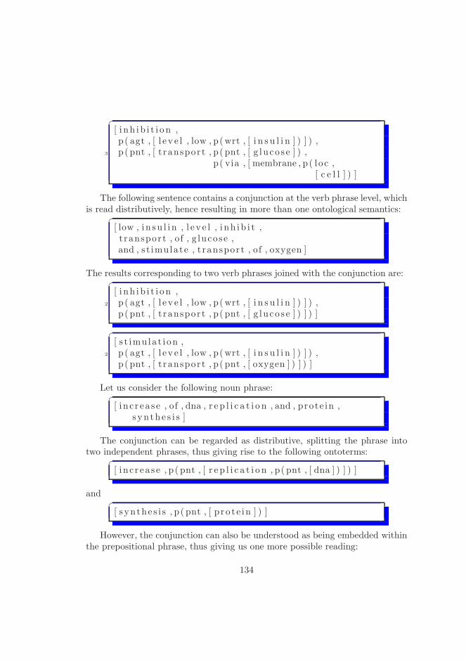
�
[ i nh i b i t i o n ,p ( agt , [ l e v e l , low , p(wrt , [ i n s u l i n ] ) ] ) ,
3 p( pnt , [ t ranspor t , p( pnt , [ g luco s e ] ) ,p( via , [ membrane , p ( loc ,
[ c e l l ] ) ]
The following sentence contains a conjunction at the verb phrase level, whichis read distributively, hence resulting in more than one ontological semantics:
�
[ low , i n s u l i n , l e v e l , i nh i b i t ,t ranspor t , of , g lucose ,and , s t imulate , t ranspor t , of , oxygen ]
The results corresponding to two verb phrases joined with the conjunction are:�
[ i nh i b i t i o n ,2 p( agt , [ l e v e l , low , p(wrt , [ i n s u l i n ] ) ] ) ,
p ( pnt , [ t ranspor t , p( pnt , [ g luco s e ] ) ] ) ]
�
[ s t imu la t i on ,2 p( agt , [ l e v e l , low , p(wrt , [ i n s u l i n ] ) ] ) ,
p ( pnt , [ t ranspor t , p( pnt , [ oxygen ] ) ] ) ]
Let us consider the following noun phrase:�
[ i n c r ea s e , of , dna , r e p l i c a t i o n , and , prote in ,s yn th e s i s ]
The conjunction can be regarded as distributive, splitting the phrase intotwo independent phrases, thus giving rise to the following ontoterms:
�
[ i n c r ea s e , p ( pnt , [ r e p l i c a t i o n , p( pnt , [ dna ] ) ] ) ]
and�
[ s ynthe s i s , p ( pnt , [ p r o te in ] ) ]
However, the conjunction can also be understood as being embedded withinthe prepositional phrase, thus giving us one more possible reading:
134
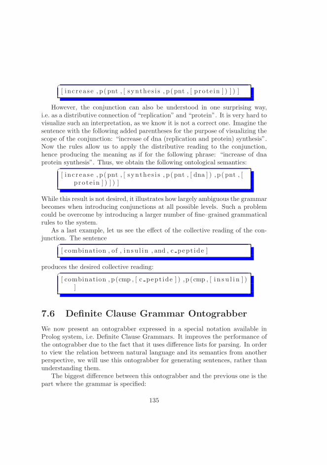
�
[ i n c r ea s e , p ( pnt , [ s ynthe s i s , p ( pnt , [ p r o te in ] ) ] ) ]
However, the conjunction can also be understood in one surprising way,i.e. as a distributive connection of “replication” and “protein”. It is very hard tovisualize such an interpretation, as we know it is not a correct one. Imagine thesentence with the following added parentheses for the purpose of visualizing thescope of the conjunction: “increase of dna (replication and protein) synthesis”.Now the rules allow us to apply the distributive reading to the conjunction,hence producing the meaning as if for the following phrase: “increase of dnaprotein synthesis”. Thus, we obtain the following ontological semantics:
�
[ i n c r ea s e , p ( pnt , [ s ynthe s i s , p ( pnt , [ dna ] ) ,p ( pnt , [p r o te in ] ) ] ) ]
While this result is not desired, it illustrates how largely ambiguous the grammarbecomes when introducing conjunctions at all possible levels. Such a problemcould be overcome by introducing a larger number of fine–grained grammaticalrules to the system.
As a last example, let us see the effect of the collective reading of the con-junction. The sentence
�
[ combination , of , i n s u l i n , and , c pept ide ]
produces the desired collective reading:�
[ combination , p (cmp , [ c pept ide ] ) ,p (cmp , [ i n s u l i n ] )]
7.6 Definite Clause Grammar Ontograbber
We now present an ontograbber expressed in a special notation available inProlog system, i.e. Definite Clause Grammars. It improves the performance ofthe ontograbber due to the fact that it uses difference lists for parsing. In orderto view the relation between natural language and its semantics from anotherperspective, we will use this ontograbber for generating sentences, rather thanunderstanding them.
The biggest difference between this ontograbber and the previous one is thepart where the grammar is specified:
135

�
np ( [ SC ] ) −−> [N] ,{ l e x (noun ,N,SC) } .
np (C) −−> {a nnc (C1 ,C2 ,C) } , np (C1) ,np (C2) .4
np (C) −−> {a pp (C1 ,P,C2 ,C) } , np (C1) , [P ] , np (C2) .
np (C) −−> { a gen (C1 ,C2 ,C) } , np (C1) , [ s ] , np (C2) .
9 np (C) −−> { a ad j (CA,CNP,C) } , a (CA) ,np (CNP) .
a ( [C] ) −−> [A] ,{ adj (A,C) } .
s (C) −−> { a tv (C1 ,TVC,C2 ,C) } , np (C1) ,14 tv (TVC) , np(C2) .
tv ( [C] ) −−> [V] ,{ l e x ( tv ,V,C) } .
The intersection of concepts is still represented using a list, except that ournew definition rejects empty lists for intersections:
�
i (C1 ,C2 ,C) :−append (C1 ,C2 ,C) ,nonempty (C1) ,nonempty (C2) .
4 nonempty ( [ | ] ) .
In the a nnc predicate we swap the order of literals in the body:�
1 a nnc (X,Y,Z) :− i (Y, [ p(R,X) ] , Z) ,t nnc (A,B,R) ,i s a (X,A) ,i s a (Y,B) .
We make similar operation with the a pp predicate:�
1 a pp ( [H|T] ,P,Y, Z):− i ( [H|T] , [ p(R,Y) ] , Z) ,
t pp (A,P,B,R) ,i s a chk ( [H|T] ,A) ,i s a chk (Y,B) .
136
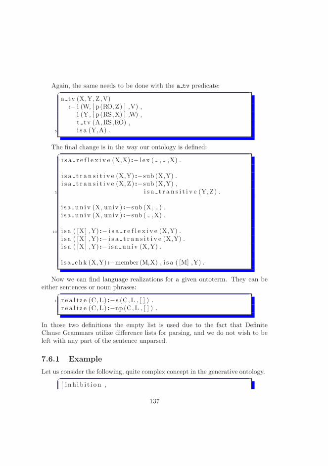
Again, the same needs to be done with the a tv predicate:�
a tv (X,Y, Z ,V):− i (W, [ p(RO,Z) ] ,V) ,
i (Y, [ p(RS,X) ] ,W) ,t t v (A,RS,RO) ,
5 i s a (Y,A) .
The final change is in the way our ontology is defined:�
i s a r e f l e x i v e (X,X) :− l e x ( , ,X) .
i s a t r a n s i t i v e (X,Y) :−sub (X,Y) .i s a t r a n s i t i v e (X, Z) :−sub (X,Y) ,
5 i s a t r a n s i t i v e (Y, Z) .
i s a un i v (X, univ ) :−sub (X, ) .i s a un i v (X, univ ) :−sub ( ,X) .
10 i s a ( [X] ,Y) :− i s a r e f l e x i v e (X,Y) .i s a ( [X] ,Y) :− i s a t r a n s i t i v e (X,Y) .i s a ( [X] ,Y) :− i s a un i v (X,Y) .
i s a chk (X,Y) :−member (M,X) , i s a ( [M] ,Y) .
Now we can find language realizations for a given ontoterm. They can beeither sentences or noun phrases:
�
1 r e a l i z e (C,L) :− s (C,L , [ ] ) .r e a l i z e (C,L) :−np (C,L , [ ] ) .
In those two definitions the empty list is used due to the fact that DefiniteClause Grammars utilize difference lists for parsing, and we do not wish to beleft with any part of the sentence unparsed.
7.6.1 Example
Let us consider the following, quite complex concept in the generative ontology.�
[ i nh i b i t i o n ,
137

p( agt , [ low ,3 l e v e l ,
p(wrt , [ i n s u l i n ] ) ] ) ,p ( pnt , [ t ranspor t ,
p( pnt , [ g luco s e ] ) ,p( via , [ membrane ,
8 p( loc , [ c e l l ] ) ] ) ] ) ]
Let us try to use our system for finding linguistic realizations of it. Belowwe present the list of produced phrases.
�
[ i nh i b i t i o n , by , low , i n s u l i n , l e v e l ,2 of , g lucose , t ranspor t , acros s , c e l l , membrane ]
[ i nh i b i t i o n , by , low , i n s u l i n , l e v e l ,of , t ranspor t , of , g lucose , acros s , c e l l , membrane ]
7 [ i nh i b i t i o n , by , low , i n s u l i n , s , l e v e l ,of , g lucose , t ranspor t , acros s , c e l l , membrane ]
[ i nh i b i t i o n , by , low , i n s u l i n , s , l e v e l ,of , t ranspor t , of , g lucose , acros s , c e l l , membrane ]
12
[ i nh i b i t i o n , by , low , l e v e l , of , i n s u l i n ,of , g lucose , t ranspor t , acros s , c e l l , membrane ]
[ i nh i b i t i o n , by , low , l e v e l , of , i n s u l i n ,17 of , t ranspor t , of , g lucose , acros s , c e l l , membrane ]
[ low , i n s u l i n , l e v e l , i nh i b i t ,g lucose , t ranspor t , acros s , c e l l , membrane ]
22 [ low , i n s u l i n , l e v e l , i nh i b i t ,t ranspor t , of , g lucose , acros s , c e l l , membrane ]
[ low , i n s u l i n , s , l e v e l , i nh i b i t ,g lucose , t ranspor t , acros s , c e l l , membrane ]
27
[ low , i n s u l i n , s , l e v e l , i nh i b i t ,
138
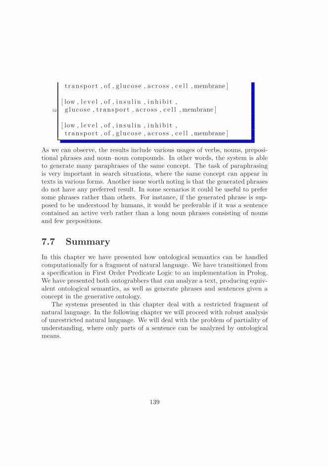
t ranspor t , of , g lucose , acros s , c e l l , membrane ]
[ low , l e v e l , of , i n s u l i n , i nh i b i t ,32 g lucose , t ranspor t , acros s , c e l l , membrane ]
[ low , l e v e l , of , i n s u l i n , i nh i b i t ,t ranspor t , of , g lucose , acros s , c e l l , membrane ]
As we can observe, the results include various usages of verbs, nouns, preposi-tional phrases and noun–noun compounds. In other words, the system is ableto generate many paraphrases of the same concept. The task of paraphrasingis very important in search situations, where the same concept can appear intexts in various forms. Another issue worth noting is that the generated phrasesdo not have any preferred result. In some scenarios it could be useful to prefersome phrases rather than others. For instance, if the generated phrase is sup-posed to be understood by humans, it would be preferable if it was a sentencecontained an active verb rather than a long noun phrases consisting of nounsand few prepositions.
7.7 Summary
In this chapter we have presented how ontological semantics can be handledcomputationally for a fragment of natural language. We have transitioned froma specification in First Order Predicate Logic to an implementation in Prolog.We have presented both ontograbbers that can analyze a text, producing equiv-alent ontological semantics, as well as generate phrases and sentences given aconcept in the generative ontology.
The systems presented in this chapter deal with a restricted fragment ofnatural language. In the following chapter we will proceed with robust analysisof unrestricted natural language. We will deal with the problem of partiality ofunderstanding, where only parts of a sentence can be analyzed by ontologicalmeans.
139

140
Chapter 8
The computation ofontosemantics forunrestricted naturallanguage
We now present the algorithm which associates ontological semantics with sen-tences. The retrieved ontological information takes the form of nodes in thegenerative ontology represented by so–called ‘concept covers’, to be describedin sect. 8.3. The result of the algoritmic analysis of a sentence is a collection ofontoterms.
The novel contribution of the present approach is that the natural languageparsing process is driven primarily by the ontology rather than by grammaticalproduction rules. Similarly to unification grammars, syntactic and semanticconstraints are utilized in parallel. However, in our approach, we do not con-struct a parse tree. Syntax plays a secondary role, taking the form of additionalconstraints, while ontological affinities play the primary role. The algorithmmakes use of a grammar, but it is a simplified, rudimentary grammar coveringfragments of English.
The algorithm described below proceeds in a bottom–up fashion, similarto forward chaining, robustly parsing complex sentences which are not fullycovered by the simplified grammar. It is reminiscent of the Earley parsing
141

algorithm (presented in Appendix D on page 213) in that it utilizes a similardynamic programming technique for backtracking and recomputation avoidance,although it does not make use of top–down constraints due to the lack of a formalgrammar for natural language in its entirety.
The algorithm presented goes beyond usual partial and shallow parsing tech-niques like chunking, which do not provide recursive phrase structure necessaryfor construction of nodes in the generative ontology.
8.1 Indexing
We index all the ontologically meaningful tokens of the input text. Considerthe sample sentence S1:
“These low0 insulin1 levels2 inhibit3 the transport4 of glucose5 across cell6membranes7.”
Only nouns, verbs and adjectives get indexed, as they correspond to some classin the ontology. Nouns, verbs and adjectives are the main building blocks carry-ing ontological meaning. Even though prepositions do not represent any classesin the ontology, they are utilized by the algorithm, as they usually determinehow classes should be combined into compound nodes in the generative ontology.
8.2 Microontology for a sentence
A microontology is the smallest fragment of the generative ontology which re-lates to the words in a sentence together with inherited ontological affinities.
The microontology for the sentence S1 is presented below:
142

c 2
c1
low
insulin
level
inhibition
transport
glucose
cell
mem
brane
lowinsulinlevel CHR WRT WRT
inhibition AGT AGT PNT PNT AGTtransport PNT PNT VIA VIAglucosecell LOC ,POF LOC ,POF
membrane LOC ,POF LOC ,POF
For each role r given in the table, the concept c1[r : c2] is a valid node in thegenerative ontology. This can be also represented by a graph, see Figure 8.1on page 144.
8.3 Concept covers
The algorithm manages sets of concept covers (covers for short), which representassociations between the text and nodes in the generative ontology.
Covers are of the following type:
N× N× syn×N × P
That means, a concept cover is a quintuple of:
• Two numbers m,n, such that m ≤ n, representing the spanning interval.The integers are indices of the words in the sentence
• The syntactic category representing what kind of word or phrase the coverrepresents (VP, NP, . . . )
• The node in the generative ontology that the cover represents
• The actual phrase covered
As an example, consider the following cover:
(4, 5,NP, transport[PNT : glucose], “transport of glucose”)
143

Figure 8.1: The microontology presented in a graph form.
144
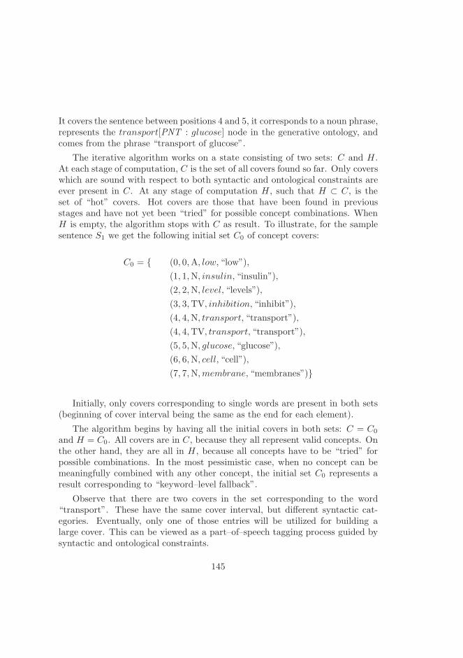
It covers the sentence between positions 4 and 5, it corresponds to a noun phrase,represents the transport[PNT : glucose] node in the generative ontology, andcomes from the phrase “transport of glucose”.
The iterative algorithm works on a state consisting of two sets: C and H .At each stage of computation, C is the set of all covers found so far. Only coverswhich are sound with respect to both syntactic and ontological constraints areever present in C. At any stage of computation H , such that H ⊂ C, is theset of “hot” covers. Hot covers are those that have been found in previousstages and have not yet been “tried” for possible concept combinations. WhenH is empty, the algorithm stops with C as result. To illustrate, for the samplesentence S1 we get the following initial set C0 of concept covers:
C0 = { (0, 0,A, low, “low”),
(1, 1,N, insulin, “insulin”),
(2, 2,N, level, “levels”),
(3, 3,TV, inhibition, “inhibit”),
(4, 4,N, transport, “transport”),
(4, 4,TV, transport, “transport”),
(5, 5,N, glucose, “glucose”),
(6, 6,N, cell, “cell”),
(7, 7,N,membrane, “membranes”)}
Initially, only covers corresponding to single words are present in both sets(beginning of cover interval being the same as the end for each element).
The algorithm begins by having all the initial covers in both sets: C = C0
and H = C0. All covers are in C, because they all represent valid concepts. Onthe other hand, they are all in H , because all concepts have to be “tried” forpossible combinations. In the most pessimistic case, when no concept can bemeaningfully combined with any other concept, the initial set C0 represents aresult corresponding to “keyword–level fallback”.
Observe that there are two covers in the set corresponding to the word“transport”. These have the same cover interval, but different syntactic cat-egories. Eventually, only one of those entries will be utilized for building alarge cover. This can be viewed as a part–of–speech tagging process guided bysyntactic and ontological constraints.
145
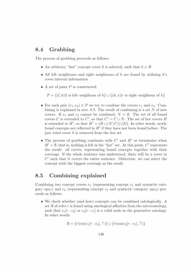
8.4 Grabbing
The process of grabbing proceeds as follows:
• An arbitrary “hot” concept cover h is selected, such that h ∈ H
• All left–neighbours and right–neighbours of h are found by utilizing h’scover interval information
• A set of pairs P is constructed:
P = {(l, h)|l is left–neighbour of h} ∪ {(h, r)|r is right–neighbour of h}
• For each pair (e1, e2) ∈ P we try to combine the covers e1 and e2. Com-bining is explained in sect. 8.5. The result of combining is a set N of newcovers. If e1 and e2 cannot be combined, N = ∅. The set of all foundcovers C is extended to C′, so that C′ = C ∪N . The set of hot covers His extended to H ′, so that H ′ = (H ∪ (N\C))\{h}. In other words, newlyfound concepts are reflected in H ′ if they have not been found before. Thejust–tried cover h is removed from the hot set
• The process of grabbing continues with C′ and H ′ or terminates whenH ′ = ∅, that is, nothing is left in the “hot” set. At this point, C′ representsthe result: all covers, representing found concepts together with theircoverage. If the whole sentence was understood, there will be a cover inC′ such that it covers the entire sentence. Otherwise, we can select theconcept with the biggest coverage as the result.
8.5 Combining explained
Combining two concept covers e1 (representing concept c1 and syntactic cate-gory syn1) and e2 (representing concept c2 and syntactic category syn2) pro-ceeds as follows:
• We check whether (and how) concepts can be combined ontologically. Aset R of roles r is found using ontological affinities from the microontology,such that c1[r : c2] or c2[r : c1] is a valid node in the generative ontology.In other words:
R = {r|isa(c1[r : c2],⊤)} ∪ {r|isa(c2[r : c1],⊤)}
146
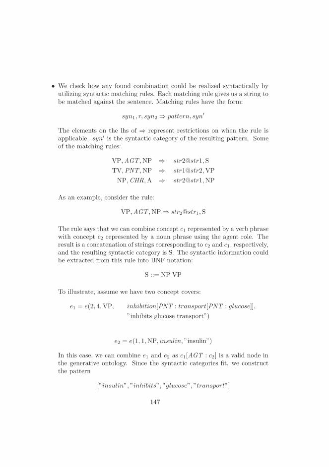
• We check how any found combination could be realized syntactically byutilizing syntactic matching rules. Each matching rule gives us a string tobe matched against the sentence. Matching rules have the form:
syn1, r, syn2 ⇒ pattern, syn′
The elements on the lhs of ⇒ represent restrictions on when the rule isapplicable. syn′ is the syntactic category of the resulting pattern. Someof the matching rules:
VP,AGT ,NP ⇒ str2@str1, S
TV,PNT ,NP ⇒ str1@str2,VP
NP,CHR,A ⇒ str2@str1,NP
As an example, consider the rule:
VP,AGT ,NP⇒ str2@str1, S
The rule says that we can combine concept c1 represented by a verb phrasewith concept c2 represented by a noun phrase using the agent role. Theresult is a concatenation of strings corresponding to c2 and c1, respectively,and the resulting syntactic category is S. The syntactic information couldbe extracted from this rule into BNF notation:
S ::= NP VP
To illustrate, assume we have two concept covers:
e1 = e(2, 4,VP, inhibition[PNT : transport[PNT : glucose]],
”inhibits glucose transport”)
e2 = e(1, 1,NP, insulin, ”insulin”)
In this case, we can combine e1 and e2 as c1[AGT : c2] is a valid node inthe generative ontology. Since the syntactic categories fit, we constructthe pattern
[”insulin”, ”inhibits”, ”glucose”, ”transport”]
147

which is successfully matched against the sentence. Hence, we add a newcover to the sets:
e(1, 4, S, inhibition[PNT : transport[PNT : glucose],AGT : insulin],
”insulin inhibits glucose transport”)
In addition to the matching rules mentioned above, we also have a highlyambiguous rule for noun–noun compounds:
N, ρ,N⇒ str2@str1,N
In the above, ρ can stand for any role, see also [22]. The high syntactic ambiguityof this rule is usually resolved with the help of ontological affinities.
Prepositions are related to roles by the following many–to–many relation:
Role Prepositionpnt ”of”agt ”by”via ”across”loc ”of”wrt ”of”bmo ”through”cmp ”of”...
...
For each related role ρ and preposition φ, we add one rule to our algorithm:
NP, ρ,NP⇒ str1@[φ]@str2,NP
In addition, the algorithm utilizes syntactic lifting rules which do not aim atcombining concepts but allow the lifting of syntactic categories, e.g., from nounto a noun phrase or from intransitive verb to a verb phrase.
8.6 Grammar
The purely syntactic parsing part of the algorithm could be achieved by fullrelaxation of ontological affinities, e.g., adding the role any:
isa(⊤[any : ⊤],⊤)
148

“These low insulin levels inhibit the transport of glucose across cell membranes.”
low insulin level inhibition transport glucose cell membrane⇓
low level[wrt : insulin] inhibition transport glucose cell membrane⇓
level[chr:lowwrt:insulin
]inhibition transport glucose cell membrane
⇓level
[chr:lowwrt:insulin
]inhibition transport glucose membrane[loc : cell]
⇓level
[chr:lowwrt:insulin
]inhibition transport[pnt : glucose] membrane[loc : cell]
⇓
level[chr:lowwrt:insulin
]inhibition transport
[pnt:glucosevia:membrane[loc:cell]
]
⇓
inhibition[agt : level[chr:lowwrt:insulin
]] transport
[pnt:glucosevia:membrane[loc:cell]
]
⇓
inhibition
[agt:level[chr:low
wrt:insulin]pnt:transport
[
pnt:glucose
via:membrane[loc:cell]
]
]
Figure 8.2: Sample run of the ontograbber
In such a case, any concept can be combined with any other from the ontologicalpoint of view, effectively making the algorithm use only syntactic constraints.
Since the formal grammar covers only fragments of the language, one cannot,in general, parse the sentence in its entirety. Therefore, we cannot assume anyparticular starting symbol, e.g., S. In many cases we might only be able tocapture a few phrases. In order to model that, we could introduce a modifiedgrammar, with production rules containing a distinguished nonterminal junkrepresenting any string. Instead, however, we simply parse the sentence in abottom–up manner, without any starting symbol.
8.7 Sample run
Figure 8.2 on page 149 presents a sample execution of the ontograbber algorithm.It abstracts from the details of concept covers, and only illustrates in what orderconcepts are combined and what is the resulting ontological semantics.
149

8.8 Ontograbber from the parsing perspective
The parsing performed by the algorithm is quite unusual, as it is executed as anadditional constraint on top of the ontological affinities. The ontological well-formedness of the ontoterms is the primary driving mechanism of the algorithm.
In order to describe the pure grammatical parsing performed by the al-gorithm, we could imagine a situation, where ontological constraints are fullyrelaxed. This is a very unlikely scenario, which constitutes the absolutely worstcase. In such a case, any two neighbouring concepts can be combined in a soundmanner according to the ontological affinities.
The grammatical constraints take the form of a restricted context free gram-mar. The restriction is that at most two nonterminals can appear in the righthand side of a production rule. This restriction comes from the fact that theanalysis is ontology–driven. The algorithm tries to put together two neighbour-ing concepts using the affinities, and each of those concepts represents a givengrammatical class. Therefore when viewed as a context free grammar, the righthand side of any rule will have at most two nonterminals corresponding to thetwo concepts being combined.
It is worth observing that the grammar is therefore similar to the CNF.Strictly, our grammar allows more expresive rules. CNF allows rules of theform where there is exactly two nonterminals on the right-hand side, withoutany terminal symbols. The grammar of our algorithm allows two nonterminalsaugmented by arbitrary number of terminal symbols. Hence, any valid CNFproduction rule is also a valid rule in the ontograbber’s grammar.
The allowance of an arbitrary number of terminal symbols in the rules isuseful for the purpose of writing rules involving closed word classes, e.g. prepo-sitions, determiners, etc.
Due to the fact that any CFG can be rewritten to an equivalent CNF rules,and the fact that CNF rules is a subset of the ontograbber’s grammatical rules,we conclude that CFG is not more expressive than our grammar.
The idea of introduction of full CFG production rules has been abandoned.This is because more than two nonterminals on the right hand side of a rule donot correspond well to the way that ontological affinities are defined. It is notclear at present how or why one would want to combine three or more conceptsat once. Three concepts can be easily combined in two steps: two of them arecombined, followed by the combination of the result with the third one.
Additionally, we are not interested in constructing a new parsing algorithm.There is a number of interesting approaches to parsing, many of which handlefull CFG productions. One example could be the Earley parsing algorithm.
150

One could easily use some of the so-called “of–the–shelf” parsers in order toparse with full CFG. We, however, consider the grammatical constraints tobe of secondary importance. We are more interested in the development of aontological analyzer, rather than grammatical parser.
The fact that full CFG rules are not allowed does not seem to be a largeobstacle. There exist also widely used algorithms that limit the grammar toCNF form, e.g. the CKY algorithm. The popularity of this algorithm lets us tobelieve that in practice the limitation on the form of the rules is not a severeproblem.
8.9 Capturing natural language
As we have discussed, the algorithm from grammatical point of view is able todescribe any context free language. The problem of capturing a given naturallanguage (or an interesting subset of it) can be reduced to the problem of sucha language (or its subset) being a context free language.
This question cannot be answered definitively. Nobody has ever proven oneway or the other. The general consensus is that natural languages are contextfree, although some parts of natural language might not be very convenientlymodeled using context–free production rules.
A general problem is that the grammar of natural languages is rarely de-scribed using fully formal methods. Natural languages are extremely compli-cated, constantly evolving, varying across regions. Any two native speakers willat times find a sentence, which one considers grammatical, and the other un-grammatical. For those reasons nobody has ever managed to fully formalize thegrammar of any written natural language.
Thus, the question of whether the ontograbber is able to handle any naturallanguage in its entirety boils down to whether the given language is actuallycontext–free.
8.10 Termination
The proof of the termination of the algorithm proceeds as follows:
When two neighbouring concepts are combined the first one covering posi-tions between a and b, the second one between b+1 and c, the result will coverpositions between a and c. Each cover is non–empty, so the result always coversmore than any of its constituents. Hence, the algorithm could not terminate
151
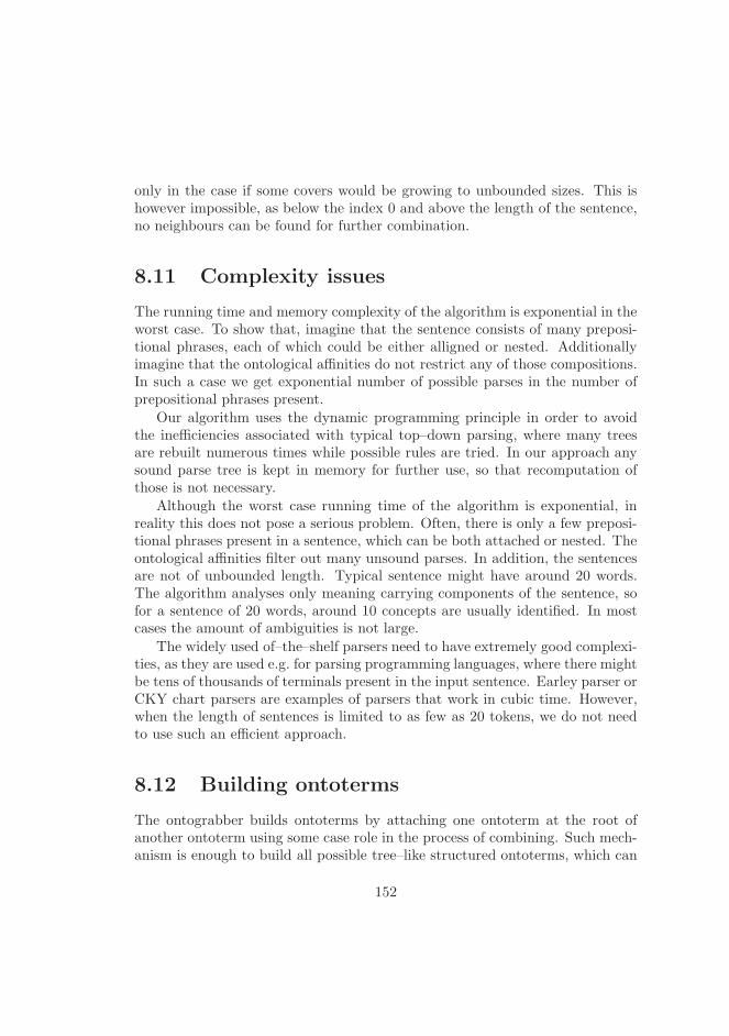
only in the case if some covers would be growing to unbounded sizes. This ishowever impossible, as below the index 0 and above the length of the sentence,no neighbours can be found for further combination.
8.11 Complexity issues
The running time and memory complexity of the algorithm is exponential in theworst case. To show that, imagine that the sentence consists of many preposi-tional phrases, each of which could be either alligned or nested. Additionallyimagine that the ontological affinities do not restrict any of those compositions.In such a case we get exponential number of possible parses in the number ofprepositional phrases present.
Our algorithm uses the dynamic programming principle in order to avoidthe inefficiencies associated with typical top–down parsing, where many treesare rebuilt numerous times while possible rules are tried. In our approach anysound parse tree is kept in memory for further use, so that recomputation ofthose is not necessary.
Although the worst case running time of the algorithm is exponential, inreality this does not pose a serious problem. Often, there is only a few preposi-tional phrases present in a sentence, which can be both attached or nested. Theontological affinities filter out many unsound parses. In addition, the sentencesare not of unbounded length. Typical sentence might have around 20 words.The algorithm analyses only meaning carrying components of the sentence, sofor a sentence of 20 words, around 10 concepts are usually identified. In mostcases the amount of ambiguities is not large.
The widely used of–the–shelf parsers need to have extremely good complexi-ties, as they are used e.g. for parsing programming languages, where there mightbe tens of thousands of terminals present in the input sentence. Earley parser orCKY chart parsers are examples of parsers that work in cubic time. However,when the length of sentences is limited to as few as 20 tokens, we do not needto use such an efficient approach.
8.12 Building ontoterms
The ontograbber builds ontoterms by attaching one ontoterm at the root ofanother ontoterm using some case role in the process of combining. Such mech-anism is enough to build all possible tree–like structured ontoterms, which can
152

be represented as feature structures.The limitation of this approach is that it is not possible to build general
graph–like ontoterms, that go beyond trees in their shape.
8.13 Applied generative ontology for bio–domain
In Figure 8.3 on page 154 we present a sample top ontology taxonomy thatcould be used as the input to the ontograbbing algorithm.
Similarly, the following ontological affinities could be used as the input tothe algorithm, coupled with the top ontology presented in Figure 8.3.
anatomical structure pof anatomical structureinfluence agt substanceinfluence agt levelinfluence pnt phenomenon or processphysical object loc anatomical structurephysical object pof physical objectproduction agt anatomical structureproduction pnt substancesubstance portion wrt substancetransport pnt substancetransport via anatomical structurelevel chr position on scalelevel wrt substance...
......
8.14 Real life examples
Let us now perform some experiments concerning how the algorithm presentedin this chapter performs on some sample sentences. Below we present a list ofsentences, which is a random sample from large biomedical corpora. Out ofmillions of sentences these specific sentences have been chosen only according tohow much of them is covered by our microscopic test lexicon. The lexicon is sosmall that it was difficult to find a large number of sentences to experiment with.Those presented here have not been preselected according to how well they arehandled by the algorithm. For each sentence we first give a set of three idealisticontological semantics, which have been created by hand by three experts:
153

activation
influence
natural_phenomenon_or_process
anatomical_structure
physical_objectentity
biologic_function
phenomenon_or_processbody_part_or_organ_or_organ_component
fully_formed_anatomical_structure
body_systemfunctional_concept
idea_or_concept
cell
conceptual_entity
univ
event
inhibition
insulinproteinsubstance
membrane
organ
substance_portion
transport
Figure
8.3:
Sample
top
ontologytaxonomy
tobeused
astheinputto
the
ontograbbingalgorith
m
154

• Bartlomiej Antoni Szymczak (abbreviated BAS) from Technical Univer-sity of Denmark
• Tine Lassen (abbreviated TL) from Roskilde University, Denmark
• Hanne Erdman Thomsen (abbreviated HET) from Copenhagen BusinessSchool, Denmark
All experts are members of the SIABO project and specialize in the use ofgenerative ontologies and ontological semantics.
The semantics prepared by experts is believed to be a “perfect answer”,which one would ideally like to get as the output of the algorithm. In addition tothose golden ontoterms we also list the ontoterm(s) produced by the algorithm.Due to ambiguities, there is often more than one ontosemantics produced (bothby experts and the algorithm).
Unfortunately, producing ontological semantics by hand is difficult and timeconsuming, and in addition requires expert knowledge. Therefore we did nothave resources to acquire hand–produced ontosemantics for more than ten sen-tences. We have rejected the option of producing golden standard semanticsexclusively ourselves, as it is difficult to create such semantics objectively whileknowing how the algorithm operates and what can be expected of it.
We have performed tests on 37 realistic sentences. Out of these we firstpresent 10 for which we managed to get experts’ golden standard. Next, wepresent the remaining 27 sentences, for which we do not have a golden standard.Adding a single sentence to the test set is not trivial, as both the lexicon andthe generative ontology need to be manually extended to incorporate the newwords and concepts.
The input sentence 1:�
the s e low i n s u l i n l e v e l s i n h i b i t the t r anspo r t o f g luco s ea c r o s s c e l l membranes t h e r e f o r e caus ing high blood
g luco s e l e v e l s
Golden ontosemantics (BAS):�
causa t i on [ agt : i n h i b i t i o n [ agt : [ l e v e l [ wrt : i n s u l i n ,chr : low ] ] ,
pnt : t r anspo r t [ pnt : g lucose ,
155
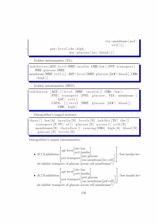
v ia : membrane [ pof :c e l l ] ] ] ,
5 pnt : l e v e l [ chr : high ,wrt : g luco s e [ l o c : blood ] ] ]
Golden ontosemantics (TL):�
i n h i b i t i o n [AGT: l e v e l [WRT: i n su l i n ,CHR: low ] ,PNT: t r anspo r t [WRT: g luco s e [WRT:
membrane [WRT: c e l l ] ] ] , RST: l e v e l [WRT: g luco s e [LOC: blood ] ,CHR: high ] ]
Golden ontosemantics (HET):�
i n h i b i t i o n [AGT: [ [ l e v e l [WRT: i n s u l i n ] ] CHR: low ] ;PNT: t r anspo r t [PNT: g luco s e ; VIA : membrane [
LOC: c e l l ] ;CAUS: [ [ [ l e v e l [WRT: g luco s e [LOC: blood ] ]
CHR: high ]
Ontograbber’s tagged sentence:�
the s e [ ] low [A] i n s u l i n [N] l e v e l s [N] i n h i b i t [TV] the [ ]t r anspo r t [N TV] o f [ ] g luco s e [N] a c r o s s [ ] c e l l [N]membranes [N] t h e r e f o r e [ ] caus ing [VBG] high [A] blood [N]g luco s e [N] l e v e l s [N]
Ontograbber’s output ontosemantics:
• (0,7,S,inhibition
agt: level
[chr: lowwrt: insulin
]
pnt: transport
[pnt: glucosevia: membrane
[loc: cell
]
]
,“low insulin lev-
els inhibit transport of glucose across cell membranes”)
• (0,7,S,inhibition
agt: level
[chr: lowwrt: insulin
]
pnt: transport
[pnt: glucosevia: membrane
[pof: cell
]
]
,“low insulin lev-
els inhibit transport of glucose across cell membranes”)
156
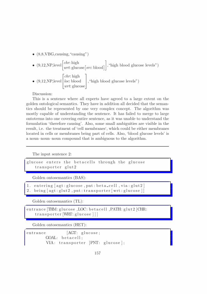
• (8,8,VBG,causing,“causing”)
• (9,12,NP,level
[chr: highwrt: glucose
[src: blood
]
]
,“high blood glucose levels”)
• (9,12,NP,level
chr: highloc: bloodwrt: glucose
,“high blood glucose levels”)
Discussion:This is a sentence where all experts have agreed to a large extent on the
golden ontological semantics. They have in addition all decided that the seman-tics should be represented by one very complex concept. The algorithm wasmostly capable of understanding the sentence. It has failed to merge to largeontoterms into one covering entire sentence, as it was unable to understand theformulation ‘therefore causing’. Also, some small ambiguities are visible in theresult, i.e. the treatment of ‘cell membranes‘, which could be either membraneslocated in cells or membranes being part of cells. Also, ‘blood glucose levels’ isa noun–noun–noun compound that is ambiguous to the algorithm.
The input sentence 2:�
g luco s e en t e r s the b e t a c e l l s through the g luco s et r an spo r t e r g lu t2
Golden ontosemantics (BAS):�
1 . en te r ing [ agt : g lucose , pnt : b e t a c e l l , v ia : g lu t2 ]2 . be ing [ agt : g lut2 , pnt : t r a n spo r t e r [ wrt : g luco s e ] ]
Golden ontosemantics (TL):�
entrance [THM: g lucose ,LOC: be t a c e l l ,PATH: g lu t2 [CHR:t r an spo r t e r [WRT: g luco s e ] ] ]
Golden ontosemantics (HET):�
entrance [AGT: g luco s e ;GOAL: b e t a c e l l ;VIA : t r an spo r t e r [PNT: g luco s e ] ;
157
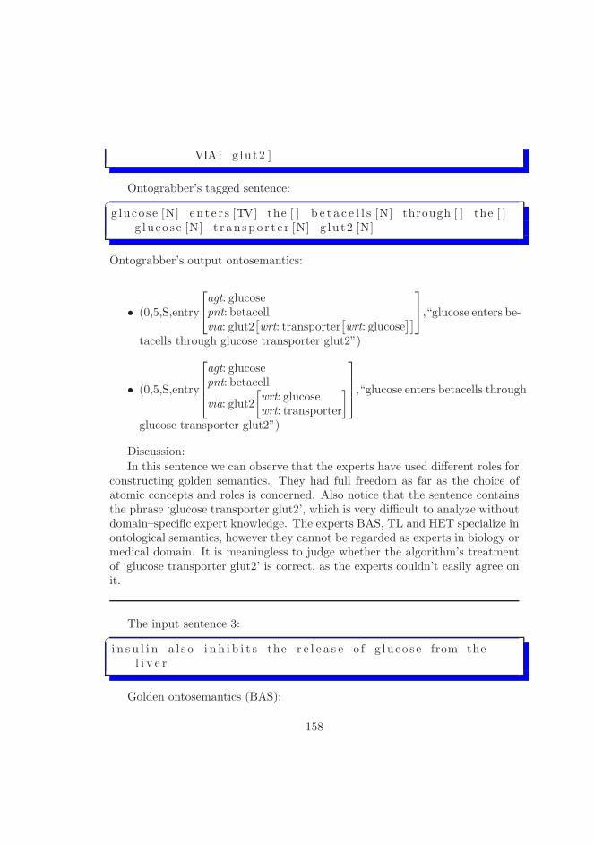
VIA : g lu t2 ]
Ontograbber’s tagged sentence:�
g luco s e [N] en t e r s [TV] the [ ] b e t a c e l l s [N] through [ ] the [ ]g luco s e [N] t r an spo r t e r [N] g lu t2 [N]
Ontograbber’s output ontosemantics:
• (0,5,S,entry
agt: glucosepnt: betacellvia: glut2
[wrt: transporter
[wrt: glucose
]]
,“glucose enters be-
tacells through glucose transporter glut2”)
• (0,5,S,entry
agt: glucosepnt: betacell
via: glut2
[wrt: glucosewrt: transporter
]
,“glucose enters betacells through
glucose transporter glut2”)
Discussion:
In this sentence we can observe that the experts have used different roles forconstructing golden semantics. They had full freedom as far as the choice ofatomic concepts and roles is concerned. Also notice that the sentence containsthe phrase ‘glucose transporter glut2’, which is very difficult to analyze withoutdomain–specific expert knowledge. The experts BAS, TL and HET specialize inontological semantics, however they cannot be regarded as experts in biology ormedical domain. It is meaningless to judge whether the algorithm’s treatmentof ‘glucose transporter glut2’ is correct, as the experts couldn’t easily agree onit.
The input sentence 3:�
i n s u l i n a l s o i n h i b i t s the r e l e a s e o f g luco s e from thel i v e r
Golden ontosemantics (BAS):
158

�
i n h i b i t i o n [ agt : i n s u l i n ,pnt : r e l e a s e [ pnt : g lucose , s r c : l i v e r ] ]
Golden ontosemantics (TL):�
i n h i b i t i o n [AGT: i n s u l i n ,PNT: r e l e a s e [WRT: g luco s e [SRC: l i v e r] ] ]
Golden ontosemantics (HET):�
i n h i b i t i o n [AGT: i n s u l i n ;PNT: r e l e a s e [PNT: g luco s e [SRC: l i v e r ] ] ]
Ontograbber’s tagged sentence:�
i n s u l i n [N] a l s o [ ] i n h i b i t s [TV] the [ ] r e l e a s e [N] o f [ ]g luco s e [N] from [ ] the [ ] l i v e r [N]
Ontograbber’s output ontosemantics:
• (0,4,S,inhibition
agt: insulin
pnt: release
[pnt: glucosesrc: liver
]
,“insulin inhibits release of glu-
cose from liver”)
• (0,4,S,inhibition
[agt: insulinpnt: release
[pnt: glucose
[src: liver
]]
]
,“insulin inhibits re-
lease of glucose from liver”)
Discussion:This is a relatively simple sentence, which uses only the most common lin-
guistic constructs. The experts were in agreement as to what ontosemanticsshould be produced. The algorithm has also successfully extracted the goldensemantics. However, it also produced one more result stemming from the ambi-guity of the phrase ‘release of glucose from liver’. It has found an extra, slightlysurprising meaning, where it is ‘glucose from liver’ that is released, but the re-lease process itself is not necessarily sourced in liver. Humans are very good atrejecting such an alternative. In fact, they reject it so well, that being presentedwith such an answer appears to be surprising.
159

The input sentence 4:�
the s e c r e t ed i n s u l i n promotes g luco s e u t i l i z a t i o n andi n h i b i t s product ion o f g luco s e by the l i v e r
Golden ontosemantics (BAS):�
1 . promotion [ agt : i n s u l i n [ chr : s e c r e t ed ] ,pnt : u t i l i z a t i o n [ pnt : g luco s e ] ]
2 . i n h i b i t i o n [ agt : i n s u l i n [ chr : s e c r e t ed ] ,pnt : product ion [ agt : l i v e r , pnt : g luco s e ] ]
Golden ontosemantics (TL):�
promotion [AGT: i n s u l i n [CHR: s e c r e t ed ] ,PNT: u t i l i z a t i o n [WRT:g luco s e ] ]
2 i n h i b i t i o n [AGT: i n s u l i n [CHR: s e c r e t ed ] ,PNT: product ion [AGT:l i v e r ,RST: g luco s e ] ]
Golden ontosemantics (HET):�
[ promotion [AGT: i n s u l i n [CHR: s e c r e t i o n ] ;PNT: u t i l i z a t i o n [PNT: g luco s e ] ] ;
i n h i b i t i o n [AGT: i n s u l i n [CHR: s e c r e t i o n ] ;4 PNT: product ion [AGT: l i v e r ; PNT: g luco s e ] ] ]
Ontograbber’s tagged sentence:�
the [ ] s e c r e t ed [VBD VBN] i n s u l i n [N] promotes [TV] g luco s e [N] u t i l i z a t i o n [N] and [ ] i n h i b i t s [TV] product ion [N] o f [ ]g luco s e [N] by [ ] the [ ] l i v e r [N]
Ontograbber’s output ontosemantics:
• (0,8,S,promotion
[agt: insulin
[pntof: secretion
]
pnt: utilization[pnt: glucose
]
]
,“ secreted insulin promotes
glucose utilization and inhibits production of glucose by liver”)
160
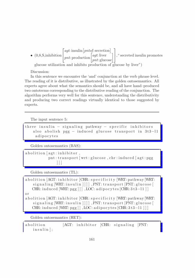
• (0,8,S,inhibition
agt: insulin[pntof: secretion
]
pnt: production
[agt: liverpnt: glucose
]
,“ secreted insulin promotes
glucose utilization and inhibits production of glucose by liver”)
Discussion:In this sentence we encounter the ‘and’ conjunction at the verb phrase level.
The reading of it is distributive, as illustrated by the golden ontosemantics. Allexperts agree about what the semantics should be, and all have hand–producedtwo ontoterms corresponding to the distributive reading of the conjunction. Thealgorithm performs very well for this sentence, understanding the distributivityand producing two correct readings virtually identical to those suggested byexperts.
The input sentence 5:�
th r e e i n s u l i n − s i g n a l i n g pathway − s p e c i f i c i n h i b i t o r sa l s o abo l i s h pgg − induced g luco s e t r anspo r t in 3t3−l 1ad ipocy te s
Golden ontosemantics (BAS):�
a b o l i t i o n [ agt : i nh i b i t o r ,pnt : t r anspo r t [ wrt : g lucose , chr : induced [ agt : pgg
] ] ]
Golden ontosemantics (TL):�
a b o l i t i o n [AGT: i n h i b i t o r [CHR: s p e c i f i c i t y [WRT: pathway [WRT:s i g n a l i n g [WRT: i n s u l i n ] ] ] ] , PNT: t r anspo r t [PNT: g luco s e [CHR: induced [WRT: pgg ] ] ] ,LOC: ad ipocy te s [CHR:3 t3−l 1 ] ]
ora b o l i t i o n [AGT: i n h i b i t o r [CHR: s p e c i f i c i t y [WRT: pathway [WRT:
s i g n a l i n g [WRT: i n s u l i n ] ] ] ] , PNT: t r anspo r t [PNT: g luco s e [CHR: induced [WRT: pgg ] ] ,LOC: ad ipocy te s [CHR:3 t3−l 1 ] ] ]
Golden ontosemantics (HET):�
a b o l i t i o n [AGT: i n h i b i t o r [CHR: s i g n a l i n g [PNT:i n s u l i n ] ;
161
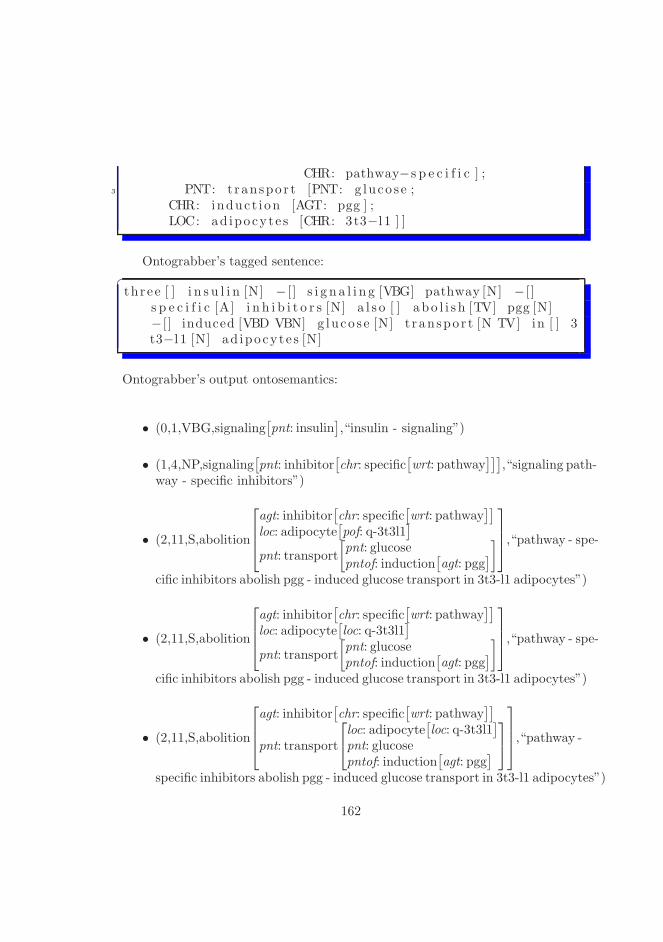
CHR: pathway−s p e c i f i c ] ;3 PNT: t r anspo r t [PNT: g luco s e ;
CHR: induc t i on [AGT: pgg ] ;LOC: ad ipocy te s [CHR: 3t3−l 1 ] ]
Ontograbber’s tagged sentence:�
th r e e [ ] i n s u l i n [N] − [ ] s i g n a l i n g [VBG] pathway [N] − [ ]s p e c i f i c [A] i n h i b i t o r s [N] a l s o [ ] a bo l i s h [TV] pgg [N]− [ ] induced [VBD VBN] g luco s e [N] t r anspo r t [N TV] in [ ] 3t3−l 1 [N] ad ipocy te s [N]
Ontograbber’s output ontosemantics:
• (0,1,VBG,signaling[pnt: insulin
],“insulin - signaling”)
• (1,4,NP,signaling[pnt: inhibitor
[chr: specific
[wrt: pathway
]]],“signaling path-
way - specific inhibitors”)
• (2,11,S,abolition
agt: inhibitor[chr: specific
[wrt: pathway
]]
loc: adipocyte[pof: q-3t3l1
]
pnt: transport
[pnt: glucosepntof: induction
[agt: pgg
]
]
,“pathway - spe-
cific inhibitors abolish pgg - induced glucose transport in 3t3-l1 adipocytes”)
• (2,11,S,abolition
agt: inhibitor[chr: specific
[wrt: pathway
]]
loc: adipocyte[loc: q-3t3l1
]
pnt: transport
[pnt: glucosepntof: induction
[agt: pgg
]
]
,“pathway - spe-
cific inhibitors abolish pgg - induced glucose transport in 3t3-l1 adipocytes”)
• (2,11,S,abolition
agt: inhibitor[chr: specific
[wrt: pathway
]]
pnt: transport
loc: adipocyte[loc: q-3t3l1
]
pnt: glucosepntof: induction
[agt: pgg
]
,“pathway -
specific inhibitors abolish pgg - induced glucose transport in 3t3-l1 adipocytes”)
162

• (2,11,S,abolition
agt: inhibitor[chr: specific
[wrt: pathway
]]
pnt: transport
loc: adipocyte[pof: q-3t3l1
]
pnt: glucosepntof: induction
[agt: pgg
]
,“pathway -
specific inhibitors abolish pgg - induced glucose transport in 3t3-l1 adipocytes”)
Discussion:This sentence proves to be very complicated. It requires a biological expert
knowledge to understand. The experts have suggested quite different goldensemantics for this sentence. There seems to be a lot of disagreement about whatthe sentence means and how small ontoterms should be combined to provide anontological meaning for the entire sentence. Hence, it is very difficult to judgehow successful the algorithm was, however it seems to be closest to the goldenstandard suggested by HET.
The input sentence 6:�
some anti−funga l agents func t i on as c e l l wa l l i n h i b i t o r sby i n h i b i t i n g g luco s e synthase
Golden ontosemantics (BAS):�
i n h i b i t i o n [ agt : agent [ chr : anti−funga l ] ,wrt : wa l l [ pof : c e l l ] ,pnt : synthase [ pnt : g luco s e ] ]
Golden ontosemantics (TL):�
func t i on [THM: agent [CHR: anti−funga l ] ,ATT: i n h i b i t o r [PNT:wa l l [WRT: c e l l ] ] ,MNR: i n h i b i t i o n [PNT: synthase [WRT:g luco s e ] ] ]
Golden ontosemantics (HET):�
func t i on [AGT: agent [CHR: anti−funga l ]THM: i n h i b i t i o n [AGT: i n h i b i t o r [XXX: wa l l [
POF: c e l l ] ] ;PNT: synthase [PNT: g luco s e ] ] ]
163
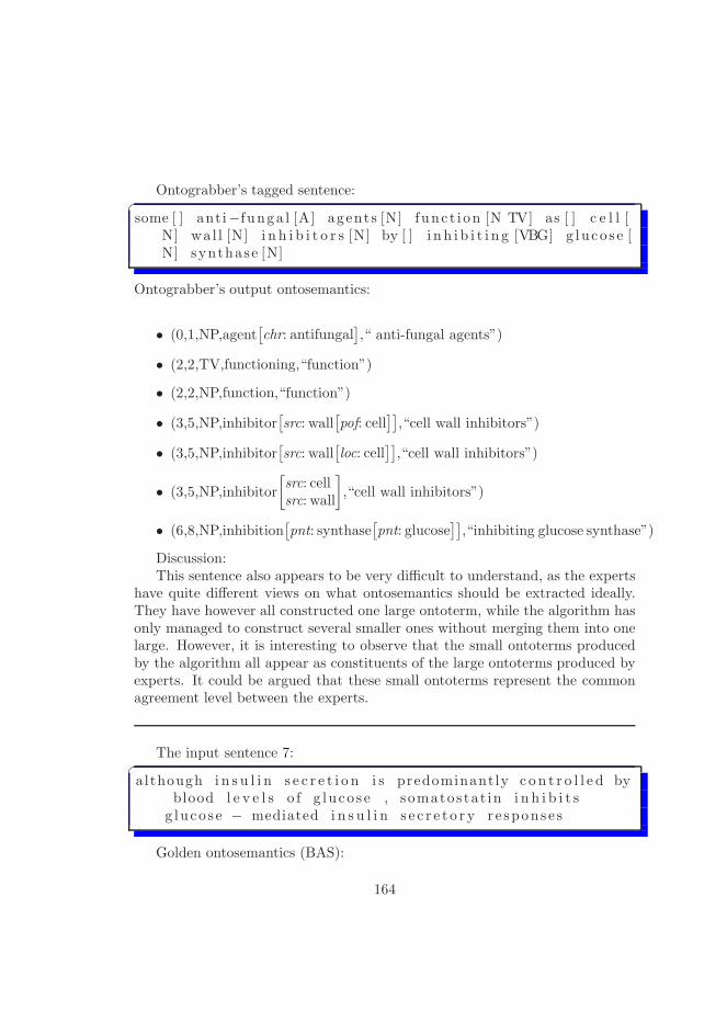
Ontograbber’s tagged sentence:�
some [ ] anti−funga l [A] agents [N] func t i on [N TV] as [ ] c e l l [N] wa l l [N] i n h i b i t o r s [N] by [ ] i n h i b i t i n g [VBG] g luco s e [N] synthase [N]
Ontograbber’s output ontosemantics:
• (0,1,NP,agent[chr: antifungal
],“ anti-fungal agents”)
• (2,2,TV,functioning,“function”)
• (2,2,NP,function,“function”)
• (3,5,NP,inhibitor[src: wall
[pof: cell
]],“cell wall inhibitors”)
• (3,5,NP,inhibitor[src: wall
[loc: cell
]],“cell wall inhibitors”)
• (3,5,NP,inhibitor
[src: cellsrc: wall
]
,“cell wall inhibitors”)
• (6,8,NP,inhibition[pnt: synthase
[pnt: glucose
]],“inhibiting glucose synthase”)
Discussion:This sentence also appears to be very difficult to understand, as the experts
have quite different views on what ontosemantics should be extracted ideally.They have however all constructed one large ontoterm, while the algorithm hasonly managed to construct several smaller ones without merging them into onelarge. However, it is interesting to observe that the small ontoterms producedby the algorithm all appear as constituents of the large ontoterms produced byexperts. It could be argued that these small ontoterms represent the commonagreement level between the experts.
The input sentence 7:�
although i n s u l i n s e c r e t i o n i s predominantly c o n t r o l l e d byblood l e v e l s o f g luco s e , somatostat in i n h i b i t s
g luco s e − mediated i n s u l i n s e c r e t o r y r e spons e s
Golden ontosemantics (BAS):
164

�
1 . c on t r o l [ agt : l e v e l [ wrt : g luco s e [ l o c : blood ] ] ,pnt : s e c r e t i o n [ pnt : i n s u l i n ] ]
2 . i n h i b i t i o n [ agt : somatostat in , pnt : r e sponse [ ? ? ] ]
Golden ontosemantics (TL):�
c on t r o l [AGT: l e v e l [WRT: g lucose ,LOC: blood ] ,PNT: s e c r e t i o n [WRT: i n s u l i n ]
2 i n h i b i t i o n [AGT: somatostat in ,PNT: response [CHR: s e c r e t o r y [WRT: i n s u l i n ] ,CHR: mediated ] ]
Golden ontosemantics (HET):�
c on t r o l [AGT: l e v e l [WRT: g luco s e ; LOC: blood ] ;PNT: s e c r e t i o n [THM: i n s u l i n ]
i n h i b i t i o n [AGT: somatostat in ;4 PNT: response [BMO: s e c r e t i o n [CHR: mediat ion [
AGT: g luco s e ] ;THM: i n s u l i n ] ]
Ontograbber’s tagged sentence:�
1 although [ ] i n s u l i n [N] s e c r e t i o n [N] i s [ IS ] predominantly [ ]c o n t r o l l e d [VBD VBN] by [ ] blood [N] l e v e l s [N] o f [ ]
g luco s e [N] , [ , ] somatostat in [N] i n h i b i t s [TV] g luco s e [N] − [ ] mediated [VBD VBN] i n s u l i n [N] s e c r e t o r y [A]r e spons e s [N]
Ontograbber’s output ontosemantics:
• (0,6,PSV,control
agt: level
[loc: bloodwrt: glucose
]
pnt: secretion[pnt: insulin
]
,“insulin secretion is controlled
by blood levels of glucose”)
• (7,7,,,nil,“,”)
• (8,8,NP,somatostatin,“somatostatin”)
165

• (9,9,TV,inhibition,“inhibits”)
• (10,10,NP,glucose,“glucose”)
• (11,11,VBD,mediation,“mediated”)
• (11,11,VBN,mediation,“mediated”)
• (12,12,NP,insulin,“insulin”)
• (13,14,NP,response[chr: secretory
],“secretory responses”)
Discussion:The experts seem to agree about the fact that the ontosemantics should be
split into two ontoterms, one corresponding to a large concept of ‘control’ andthe other to a large concept of ‘inhibition’. However, the experts had troubleunderstanding or agreeing upon how to represent the meaning of the phrase‘inhibits glucose–mediated insulin secretory responses’. The algorithm in factreflects this difficulty, as it has found a satisfactory answer for the ‘control’ part,but did not manage to go far beyond keywords for the ‘inhibition’ part.
The input sentence 8:�
the blood g luco s e l e v e l s may be f a s t i n g or fed g luco s el e v e l s , and blood g luco s e l e v e l s inc lude serum orplasma g luco s e l e v e l s
Golden ontosemantics (BAS):�
l e v e l [ wrt : g luco s e [ l o c : blood ] ]l e v e l [ wrt : g luco s e [ l o c : blood , chr : f ed ] ]l e v e l [ wrt : g luco s e [ l o c : blood , chr : f a s t i n g ] ]l e v e l [ wrt : g luco s e [ l o c : serum ] ]
5 l e v e l [ wrt : g luco s e [ l o c : plasma ] ]
Golden ontosemantics (TL):�
1 being [THM: l e v e l [WRT: g lucose ,LOC: blood ] , ATT: l e v e l [WRT:g lucose ,CHR: f a s t i n g ] , ATT: l e v e l [WRT: g lucose ,CHR: fed ] ]
be ing [THM: l e v e l [WRT: g lucose ,LOC: blood ] , ATT: l e v e l [WRT:g lucose ,LOC: serum ] , ATT: l e v e l [WRT: g lucose ,LOC: plasma ] ]
166

Golden ontosemantics (HET):�
l e v e l [WRT: g luco s e ; LOC: blood ]l e v e l [WRT: g luco s e ; CHR: f a s t i n g ]l e v e l [WRT: g luco s e ; CHR: f e ed i ng ]
4 i n c l u s i o n [AGT: l e v e l [WRT: g luco s e ; LOC: blood ]PNT: l e v e l [WRT: serum ] ;PNT: l e v e l [WRT: g luco s e [CHR: plasma ] ] ]
Ontograbber’s tagged sentence:�
the [ ] blood [N] g luco s e [N] l e v e l s [N] may [CAN] be [BE]f a s t i n g [VBG] or [ ] f ed [VBD VBN] g luco s e [N] l e v e l s [N], [ , ] and [ ] blood [N] g luco s e [N] l e v e l s [N] inc lude [TV]serum [N] or [ ] plasma [N] g luco s e [N] l e v e l s [N]
Ontograbber’s output ontosemantics:
• (0,2,NP,level[wrt: glucose
[src: blood
]],“ blood glucose levels”)
• (0,2,NP,level
[loc: bloodwrt: glucose
]
,“ blood glucose levels”)
• (3,3,CAN,can,“may”)
• (4,4,BE,nil,“be”)
• (5,5,VBG,fasting,“fasting”)
• (6,6,VBD,feeding,“fed”)
• (6,6,VBN,feeding,“fed”)
• (7,8,NP,level[wrt: glucose
],“glucose levels”)
• (9,9,,,nil,“,”)
• (10,12,NP,level[wrt: glucose
[src: blood
]],“ blood glucose levels”)
• (10,12,NP,level
[loc: bloodwrt: glucose
]
,“ blood glucose levels”)
167

• (13,13,TV,inclusion,“include”)
• (14,14,NP,serum,“serum”)
• (15,15,NP,plasma,“plasma”)
• (16,17,NP,level[wrt: glucose
],“glucose levels”)
Discussion:The sentence is quite difficult to understand, and the experts do not have a
common view of what the semantics should be. This is probably due to relativelyunusual nature of the sentence. Rather than providing describing observations,it provides a classification. This can be understood as the definition of thebiomedical ontology itself, which the algorithm uses as its input. The algorithmperforms quite well, as it captures most of the ontoterms common to all thosesuggested by experts.
The input sentence 9:�
the i n s u l i n s e c r e t i o n determined i s p r e f e r ab l y g luco s e −s t imulated i n s u l i n s e c r e t i o n
Golden ontosemantics (BAS):�
s e c r e t i o n [ pnt : i n s u l i n , chr : s t imulated [ agt : g luco s e ] ]
Golden ontosemantics (TL):�
f i nd i ng [THM: s e c r e t i o n [PNT: i n s u l i n ] ,ATT: s e c r e t i o n [PNT:i n s u l i n ,CHR: s t imu la t i on [AGT: g luco s e ] ] ]
Golden ontosemantics (HET):�
s e c r e t i o n [THM: i n s u l i n ; CHR: determinat ion ]s e c r e t i o n [THM: i n s u l i n ; CHR: s t imu la t i on [AGT: g luco s e ] ]
Ontograbber’s tagged sentence:�
the [ ] i n s u l i n [N] s e c r e t i o n [N] determined [VBD VBN] i s [ IS ]p r e f e r ab l y [ ] g luco s e [N] − [ ] s t imulated [VBD VBN]i n s u l i n [N] s e c r e t i o n [N]
168

Ontograbber’s output ontosemantics:
• (0,1,NP,secretion[pnt: insulin
],“ insulin secretion”)
• (2,2,VBD,determining,“determined”)
• (2,2,VBN,determining,“determined”)
• (3,5,PSV,stimulation[agt: glucose
],“is glucose - stimulated”)
• (4,7,NP,secretion
[pnt: insulinpntof: stimulation
[agt: glucose
]
]
,“glucose - stimulated in-
sulin secretion”)
Discussion:There was a medium–level agreement between the experts on this sentence.
One expert suggested two ontoterms, while other suggested one. The algorithmwas however unable to find any ontoterm covering entire sentence. It foundseveral ontoterms covering some parts of the sentence. It is worth noticing thattwo of these overlap, one representing the phrase ‘is glucose – stimulated’, andthe other ‘glucose – stimulated insulin secretion’.
The input sentence 10:�
in the l i v e r , i n s u l i n i n h i b i t s the product ion o f g luco s eby i n h i b i t i n g g luconeogene s i s and g l y c o g e n o l y s i s
Golden ontosemantics (BAS):�
causa t i on [ agt : i n h i b i t i o n [ agt : i n s u l i n ,pnt : g luconeogene s i s , pnt :
g l y c o g e n o l y s i s ]pnt : i n h i b i t i o n [ agt : i n s u l i n , l o c : l i v e r ,
pnt : product ion [ pnt : g luco s e ] ] ]
Golden ontosemantics (TL):�
i n h i b i t i o n [AGT: i n s u l i n , PNT: product ion [PNT: g luco s e ] , MNR:i n h i b i t i o n [PNT: g luconeogene s i s ,PNT: g l y c o g e n o l y s i s ] ,LOC: l i v e r ]
169

Golden ontosemantics (HET):�
i n h i b i t i o n [AGT: i n s u l i n ;PNT: product ion [PNT: g luco s e ] ;BMO: i n h i b i t i o n [PNT: g luconeogene s i s ; PNT:
g l y c o g e n o l y s i s ] ;LOC: l i v e r ]
Ontograbber’s tagged sentence:�
in [ ] the [ ] l i v e r [N] , [ , ] i n s u l i n [N] i n h i b i t s [TV] the [ ]product ion [N] o f [ ] g luco s e [N] by [ ] i n h i b i t i n g [VBG]g luconeogene s i s [N] and [ ] g l y c o g e n o l y s i s [N]
Ontograbber’s output ontosemantics:
• (0,0,NP,liver,“ liver”)
• (1,1,,,nil,“,”)
• (2,5,S,inhibition
[agt: insulinpnt: production
[pnt: glucose
]
]
,“insulin inhibits production
of glucose”)
• (6,8,NP,inhibition[pnt: glycogenolysis
],“inhibiting gluconeogenesis and glycogenol-
ysis”)
• (6,8,NP,inhibition[pnt: gluconeogenesis
],“inhibiting gluconeogenesis and glycogenol-
ysis”)
• (6,8,NP,glycogenolysis,“inhibiting gluconeogenesis and glycogenolysis”)
Discussion:
In this sentence the experts do not seem to agree what the ontosemanticsshould be. Thay have all produced quite different large ontoterms. However, itis worth observing that these large ontoterms, while different, have some smallcommon constituents. The algorithm has captured multiple ontoterms thatoverlap with these constituents. It also had a surprising approach as to how theconjunction should be interpreted.
170

8.15 Conclusion
The result of testing the remaining 27 sentences is presented in Appendix I onpage 269. The ten results presented and discussed here are of highest impor-tance, as we have been able to provide golden standard ontosemantics producedby three experts.
We believe that the results are very promising. The ontograbber was able toanalyze sentences for which it does not know a full grammar. Furthermore, thelexicon used as input to the ontograbber was tiny. In most sentences not all thewords have been found in the lexicon. However, despite those shortcomings, thesystem has managed to extract some ontological semantics for the sentences.The semantics in many cases is quite far from the golden one specified by ex-perts by hand. However, it is worth keeping in mind that the golden semanticsassumes perfect lexical and grammatical coverage of each sentence. With thetiny grammar employed in the system and the minute lexicon and ontology, webelieve that the extracted semantics is very promsing. It would certainly getmuch closer to the golden one if the lexicon, ontology, and grammar given asinput to the ontograbber would be extended.
In some cases the algorithm failed at merging middle–sized ontoterms intoone very large ontoterm covering the meaning of entire sentence. This mostoften stems from the fact that non–domain specific words are used as connec-tive entities for such meaning or linguistic constructs not covered by our smallgrammar are used. However, we regard this not to be a major problem, asthe middle–sized ontoterms (say, covering half of the sentence each) are soundmeaning representations, representing correctly the meaning of some phrases.
It is also important that in all sentences the resulting semantics providesmuch deeper understanding of meaning content than keyword–based search do.This hints that the resulting semantics could be used for constructing a success-ful search engine, at least for the domain of biomedical scientific texts.
171

172

Chapter 9
Further work
9.1 Incorporation of a large scale lexicon andontology
All of the ontograbbers presented in Chapters 7 and 8 use two main resourcesas input, i.e. the lexicon and the ontology. It would be very interesting to usesome large scale resources for that purpose, in an attempt to capture as muchof the natural language as possible. However, doing so poses many challengesdescribed below, and hence is beyond the scope of the current project.
The ontologies available today do not exhibit the generative character, nec-essary for our ontograbbers. Hence, they would need to be tailored manuallyin order to fit as the input to our systems. This generativity could be achievedby providing ontological affinities on the already–existing large taxonomies, ineffect creating a large generative ontology. The amount of work here would notbe as large as might be suspected, due to the fact that we only need to providethe affinities on the very top level of our ontology and allow the mechanics ofthe generative ontology to inherit the affinities deeper down. For an examplehow this is working in practice, see Figure 4.3 on page 82.
Adaptation of a large lexicon as the input to our ontograbber might provemore challenging. The lexicon needs to provide two main pieces of information toour ontograbbers, i.e. the possible parts of speech for every word and what nodein the ontology the word actually represents. Even though a large number oflexicons exist which provide the required information on word’s parts of speech1,
1Most dictionaries do so.
173

none of them is immediately ready for use with the generative ontology byproviding the information how words link to it. This could be worked aroundby using some of the lexicons available together with large ontologies availabletoday. Unfortunately, by following this path we would only get simple linksof words to the ontology, i.e. linking only to the basic concepts. Ideally, thelexicon would need to be modified to introduce the links of some words tocomplex ontoterms, which might require a substantial amount of work.
9.2 Extending natural language coverage
One interesting extension of most of the ontograbbers presented in Chapters 7and 8 is enlarging the grammar of those systems, in order to enable them tocapture more natural language constructs. This could be achieved fairly simplyfor many types of constructs, by following the same principles as with the con-structs already taken care of. For instance, the introduction of relative clauseswould be based on the same ideas as verb phrases and noun–noun compounds.There are also some constructs, which we have purposedly decided to omit, astheir contribution to the ontological semantics we search for is marginal. Theseinclude for instance determiners. However, there are some other interesting lin-guistic constructs that might be more difficult to introduce. An example of thatare phrasal verbs, where part of the verb is moved to the end of the sentence.Taking care of that would require some changes in the grammar of the ontograb-bers. We also have not discussed how to modify the methods presented in orderto deal with languages other than English.
9.3 Ontological search engine
While the problem of ontograbbing is quite well suited for formal description,which does not depart much from the logical specification, it is still important tokeep in mind that one wants to perform search based on the assigned ontologicalsemantics. Hence, there is a need for coming up with a mechanism for searchinghuge amounts of text.
The semantics extracted from the text could be used in a search engine. Asa matter of fact, the design was guided with such a possibility in mind. Thesemantics has been tailored, so that the search can be performed efficiently andeasily.
174

Consider the following semantics extracted from the text:
forcing ∩ agt : insulin
∩pnt : (storage ∩ pnt : glycogen
∩ loc : (cell ∩ wrt : liver))
Semantics of this form could be pre–extracted from multiple articles andstored in a database, which could be accessed by the search engine. If the userissues a query, we would simply perform the semantic analysis on it, and extractthe query semantics. Let us assume that the user is interested in the fact thatinsulin causes the storage of some substance and issues the following query:
Insulin caused storage of substance. (9.1)
This query would get the following semantics captured:
causing ∩ agt : insulin
∩pnt : (storage ∩ pnt : substance)
How would the search engine identify the sentence of interest as the answerto the query? It is worth observing that forcing is a subclass of causing andglycogen is a subclass of substance. One approach could use grammaticalproduction rules and in a few steps derive the text concept from the queryconcept. This approach has been presented in Figure 4.3 on page 82.
Another procedure can use a graph matching algorithm. Ontoterms can berepresented graphically in the form of direct acyclic tree graphs. In our case,we would need to match the query graph:
insulin[n] caused[v] storage[n] of[prep] substance[n]
c_causing
c_insulin
agt
c_storage
pnt
c_substance
pnt
175

against the article sentence graph:
insulin[n] forces[v] storage[n] of[prep] glycogen[n] in[prep] liver[n] cells[n]
c_forcing
c_insulin
agt
c_storage
pnt
c_glycogen
pnt
c_cell
loc
c_liver
wrt
Please observe that the underlying ontology with its class subsumption playsa vital role in such a matching, as we need to identify that forcing is a subclassof causing and glycogen is a subclass of substance for the graphs to match.
The graph matching has the advantage of respecting the commutativity ofset intersection. Additionally it can very easily deal with inverse relations bysimply honoring the direction of the arc in the graph.
The need of comparing the query graph to all graphs in the database canbe easily eliminated by indexing the database graphs by the primitive classesappearing in them, which are conceived in the current context as graph nodes.The query semantics would only need to be matched against those graphs, whichcontain all the concepts appearing in the query according to the index.
Even though the core of the engine would be relatively easy to implement,the amount of work would be substantial due to the need of downloading manyarticles, setting up a database for them, indexing them, etc. However, theSIABO project is currently working on an ontological search engine, which worksvery much along similar lines.
9.3.1 Ad–hoc concepts
A keyword–based search has a certain advantage over an ontological semanticsearch. If a given word does not correspond to any class in the ontology, the
176
keyword search will still be able to perform some search involving such a word.It is possible to add such a functionality to the ontological search engine quiteeasily.
This can be achieved by introducing ad–hoc concepts. If a word does notcorrespond to any class in the ontology, we can generate a new class on the fly.Such a class would be identified by the given word. Obviously, we would notknow where this class should be placed in the ontology. We may simply putit under the top concept. The ad–hoc class created in such a way allows theontological search engine to work as if it was a keyword, i.e. only exact matchwill be considered as a response to the query. While this approach is relativelyprimitive, it allows at least some search results to be returned in case that theontology does not contain what was queried about.
177

178
Chapter 10
Conclusion
In Chapter 1 we have outlined the motivation behind this work, including thefact that we would like to offer search–friendly semantics that surpasses thecapabilities of the keyword–based search. That should be achieved by mergingformal domain ontologies with natural language semantics.
In Chapter 2 we have presented formalisms that are useful for representingeither formal ontologies, natural language semantics, or both. We also gaveexamples about how they can be utilized. First Order Predicate Logic has beenused throughout the thesis as a common metalogical framework language, inwhich other ideas and formalisms have been presented. This has functioned asa glue between the logical methods presented and the computation proceduresdeveloped in later chapters, where we used logic programming.
Chapter 3 provided a general introduction to ontologies, with focus on formalones. In this chapter we have not yet dwelved into natural language semantics.Instead, we have presented how to use the logical framework of formal ontologiesto extract non–trivial information from them with the help of logic program-ming.
In Chapter 4 we explored the notion of types. We demonstrated how muchvariety exists between types as used in logic, ontologies, and programming lan-guages. Last but not least we have presented how generative ontologies work toprovide the infinitude of ontological types, or “ontoterms”.
In Chapter 5 we had a closer look at natural language – its grammar, mean-ing, and some problems related to extracting that meaning. We have presentedsome ways of how to merge the formal ontologies with natural language seman-tics.
179

In Chapter 6 we looked at the state–of–the–art in ontological semantics andwe have compared it to our approach.
In Chapter 7 we have answered the question of how to approach the problemof relating computationally the ontological semantics and a natural languagefragment. We have discussed how to use practical logic programming tools,such as Prolog, for that purpuse, while keeping as close to the underlying logicalspecification as possible. We have elaborated several approaches, each with itsown advantages, and described them in detail.
In Chapter 8 we went one step further and try to use similar methods asin Chapter 7 for dealing with unrestricted natural language. However, we havemoved further away from the pure logical specification in order to be able todeal with unrestricted versions of natural language. The approach presented inthis chapter introduces a novelty, i.e. the utilization of the ontological meaningearlier in the process understanding of the language than the grammar itself.
We have presented some final thoughts and the discussion of further workin Chapter 9.
180

Appendix A
Investigations of theconjunctions’ reading(distributive vs. collective)of Wikipedia Insulinsentences
The following is an investigation of the reading of conjunctions in a scientifictext, i.e. the Wikipedia entry on Insulin.
For each sentence:
• The conjunction has been identified with a frame
• The reading has been distinguished (whether it is collective or distributive)
• The syntactic level of the conjunction has been identified (NP level, sen-tence level, etc.)
• The relevance of the sentence has been decided (some sentences contribut-ing a lot to the given scientific text, and some not being interesting fromthat point of view)
A summary follows, where the findings of this study are presented.
181

A.1 Sample sentences
1: Insulin is a hormone with intensive effects on both metabolism andseveral other body systems.
The reading is distributive. Conjunction at NP level. Sentence is relevant.
2: Insulin causes most of the body’s cells to take up glucose from the blood,
storing it as glycogen in the liver and muscle, and stops use of fat as an energysource.
The reading is distributive. Conjunction at NP level. Sentence is relevant.
3: Insulin causes most of the body’s cells to take up glucose from the blood,
storing it as glycogen in the liver and muscle, and stops use of fat as an energysource.
The reading is distributive. Conjunction at VP level. Sentence is relevant.
4: When insulin is absent, glucose is not taken up by most body cells andthe body begins to use fat as an energy source.
The reading is distributive. Conjunction at VP level. Sentence is relevant.
5: Insulin is a peptide hormone composed of 51 amino acid residues andhas a molecular weight of 5808 Da.
The reading is distributive. Conjunction at VP level. Sentence is relevant.
6: Bovine insulin differs from human in only three amino acid residues, andporcine insulin in one.
The reading is distributive. Ellipsis. Sentence is irrelevant.
7: Insulin in some invertebrates is quite close to human insulin, has similar
effects inside cells, and is produced very similarly.The reading is distributive. Conjunction at VP level. Sentence is relevant.
8: Insulin is produced in the pancreas, and released when any of severalstimuli are detected.
The reading is distributive. Conjunction at VP level. Sentence is relevant.
9: These include protein ingestion, and glucose in the blood.
182

The reading is distributive. Conjunction at NP level. Sentence is irrelevant.
10: In target cells, they initiate a signal transduction which has the effect of
increasing glucose uptake and storage.
The reading is distributive. Conjunction at NP level. Sentence is relevant.
11: Production and secretion are largely independent; prepared insulin isstored awaiting secretion.
The reading is collective. Conjunction at NP level. Relevance is question-able.
12: Both C-peptide and mature insulin are biologically active.
The reading is distributive. Conjunction at NP level. Sentence is relevant.
13: Cell components and proteins in this image are not to scale.
The reading is distributive. Conjunction at NP level. Sentence is relevant.
14: These modifications of proinsulin remove the center portion of the
molecule, from the C- and N- terminal ends of proinsulin.
Conjunction at NP level. Relevance is questionable.
15: The remaining polypeptides, the B- and A- chains, are bound togetherby disulfide bonds/disulphide bonds.
The reading can be collective or distributive. Conjunction at NP level.Relevance is questionable.
16: Confusingly, the primary sequence of proinsulin goes in the order ”B-
C-A”, since B and A chains were identified on the basis of mass, and the Cpeptide was discovered after the others.
The reading can be collective or distributive. Conjunction at NP level.Relevance is questionable.
17: Confusingly, the primary sequence of proinsulin goes in the order ”B-
C-A”, since B and A chains were identified on the basis of mass, and the Cpeptide was discovered after the others.
The reading is distributive. Conjunction at S level. Sentence is relevant.
183
18: Glucose goes into the glycolysis and the respiratory cycle where mul-tiple high-energy ATP molecules are produced by oxidation
The reading is distributive. Conjunction at NP level. Sentence is relevant.
19: Dependent on ATP levels, and hence blood glucose levels, the ATP-controlled potassium channels close and the cell membrane depolarizes
The reading is distributive. Conjunction at NP level. Sentence is relevant.
20: Dependent on ATP levels, and hence blood glucose levels, the ATP-
controlled potassium channels close and the cell membrane depolarizesThe reading is distributive. Conjunction at S level. Sentence is relevant.
21: On depolarization, voltage controlled calcium channels open and cal-cium flows into the cells
The reading is distributive. Conjunction at S level. Sentence is relevant.
22: An increased calcium level causes activation of phospholipase C, whichcleaves the membrane phospholipid phosphatidyl inositol 4,5-bisphosphate into
inositol 1,4,5-triphosphate and diacylglycerol.The reading can be collective or distributive. Conjunction at NP level.
Relevance is questionable.
23: This allows the release of Ca2+ from the ER via IP3 gated channels,
and further raises the cell concentration of calcium.The reading is distributive. Conjunction at VP level. Sentence is relevant.
24: This is the main mechanism for release of insulin and regulation ofinsulin synthesis.
The reading is distributive. Conjunction at NP level. Sentence is relevant.
25: In addition some insulin synthesis and release takes place generally atfood intake, not just glucose or carbohydrate intake, and the beta cells are alsosomewhat influenced by the autonomic nervous system.
The reading is distributive. Conjunction at NP level. Sentence is relevant.
26: In addition some insulin synthesis and release takes place generally at
food intake, not just glucose or carbohydrate intake, and the beta cells arealso somewhat influenced by the autonomic nervous system.
184
The reading is distributive. Conjunction at S level. Sentence is relevant.
27: Other substances known to stimulate insulin release include amino acidsfrom ingested proteins, acetylcholine, released from vagus nerve endings, chole-
cystokinin, released by enteroendocrine cells of intestinal mucosa and glucose-dependent insulinotropic peptide.
The reading is distributive. Conjunction at NP level. Sentence is relevant.
28: This is thought to avoid downregulation of insulin receptors in target
cells and to assist the liver in extracting insulin from the blood.
The reading is distributive. Sentence is relevant.
29: Activation of insulin receptors leads to internal cellular mechanisms
that directly affect glucose uptake by regulating the number and operation ofprotein molecules in the cell membrane that transport glucose into the cell.
The reading is distributive. Conjunction at NP level. Sentence is relevant.
30: The genes that specify the proteins that make up the insulin receptor incell membranes have been identified and the structure of the interior, cell mem-
brane section, and now, finally after more than a decade, the extra-membranestructure of receptor.
Ellipsis. Relevance is questionable.
31: Two types of tissues are most strongly influenced by insulin, as far as
the stimulation of glucose uptake is concerned: muscle cells and fat cells.
The reading is distributive. Conjunction at NP level. Relevance is question-able.
32: The former are important because of their central role in movement,
breathing, circulation, etc, and the latter because they accumulate excess foodenergy against future needs.
Ellipsis. Relevance is questionable.
33: Effect of insulin on glucose uptake and metabolism.
The reading is distributive. Conjunction at NP level. Sentence is irrelevant.
185
34: These include: translocation of Glut-4 transporter to the plasma mem-
brane and influx of glucose, glycogen synthesis, glycolysis and fatty acid syn-thesis.
The reading is distributive. Conjunction at NP level. Relevance is question-able.
35: These include: translocation of Glut-4 transporter to the plasma mem-
brane and influx of glucose, glycogen synthesis, glycolysis and fatty acid syn-thesis.
The reading is distributive. Conjunction at NP level. Relevance is question-able.
36: Control of cellular intake of certain substances, most prominently glucose
in muscle and adipose tissue.The reading is distributive. Conjunction at NP level. Sentence is relevant.
37: Increase of DNA replication and protein synthesis via control of aminoacid uptake.
The reading is distributive. Conjunction at NP level. Sentence is relevant.
38: Increased glycogen synthesis - insulin forces storage of glucose in livercells in the form of glycogen; lowered levels of insulin cause liver cells to convert
glycogen to glucose and excrete it into the blood.The reading is distributive. Relevance is questionable.
39: Decreased gluconeogenesis - decreases production of glucose from non-sugar substrates, primarily in the liver ; lack of insulin causes glucose production
from assorted substrates in the liver and elsewhere.The reading is distributive. Conjunction at NP level. Sentence is irrelevant.
40: Once an insulin molecule has docked onto the receptor and effected itsaction, it may be released back into the extracellular environment or it may bedegraded by the cell.
The reading is collective. Relevance is questionable.
41: They do not require insulin to absorb glucose, unlike muscle and adi-pose tissue, and they have very small internal stores of glycogen.
The reading is distributive. Conjunction at NP level. Sentence is relevant.
186

42: They do not require insulin to absorb glucose, unlike muscle and adipose
tissue, and they have very small internal stores of glycogen.The reading is distributive. Conjunction at S level. Sentence is relevant.
43: Glycogen stored in liver cells can be converted to glucose, and releasedinto the blood, when glucose from digestion is low or absent, and the glycerolbackbone in triglycerides can also be used to produce blood glucose.
The reading is distributive. Relevance is questionable.
44: Glycogen stored in liver cells can be converted to glucose, and released
into the blood, when glucose from digestion is low or absent, and the glycerolbackbone in triglycerides can also be used to produce blood glucose.
The reading is distributive. Conjunction at S level. Sentence is relevant.
45: Sufficient lack of glucose and scarcity of these sources of glucose candramatically make itself manifest in the impaired functioning of the centralnervous system; dizziness, speech problems, and even loss of consciousness, canoccur.
The reading can be collective or distributive. Conjunction at NP level.Relevance is questionable.
46: Sufficient lack of glucose and scarcity of these sources of glucose candramatically make itself manifest in the impaired functioning of the central
nervous system; dizziness, speech problems, and even loss of consciousness,can occur.
The reading is distributive. Conjunction at NP level. Relevance is question-able.
47: Endogenous causes of insulin excess are very rare, and the overwhelm-ing majority of insulin-excess induced hypoglycemia cases are iatrogenic andusually accidental.
The reading is distributive. Conjunction at S level. Sentence is relevant.
48: Endogenous causes of insulin excess are very rare, and the overwhelm-
ing majority of insulin-excess induced hypoglycemia cases are iatrogenic andusually accidental.
Sentence is relevant. Sentence is irrelevant.
187

49: Metabolic syndrome - a poorly understood condition first called Syn-drome X by Gerald Reaven, Reaven’s Syndrome after Reaven, CHAOS in Aus-
tralia, and sometimes prediabetes.The reading is distributive. Conjunction at NP level. Sentence is irrelevant.
50: It is characterized by elevated blood pressure, dyslipidemia, and in-creased waist circumference.
The reading is distributive. Conjunction at NP level. Sentence is relevant.
51: Commonly, morbidities such as essential hypertension, obesity, Type 2
diabetes, and cardiovascular disease develop.The reading is distributive. Conjunction at NP level. Sentence is relevant.
52: Polycystic ovary syndrome - a complex syndrome in women in the re-
productive years where there is anovulation and androgen excess commonlydisplayed as hirsutism.
The reading is distributive. Conjunction at NP level. Relevance is question-able.
53: The host cells are then allowed to grow and reproduce normally, anddue to the inserted human DNA, they produce a synthetic version of humaninsulin.
The reading is distributive. Relevance is questionable.
54: The host cells are then allowed to grow and reproduce normally, anddue to the inserted human DNA, they produce a synthetic version of humaninsulin.
Relevance is questionable.
55: According to a survey that the International Diabetes Federation con-
ducted in 2002 on the access to and availability of insulin in its member coun-tries, approximately 70% of the insulin that is currently sold in the world isrecombinant, biosynthetic ’human’ insulin.
The reading is distributive. Ellipsis. Relevance is questionable.
56: Also, the International Diabetes Federation’s position statement is veryclear in stating that ”there is NO overwhelming evidence to prefer one species
188
of insulin over another” and ”[modern, highly-purified] animal insulins remaina perfectly acceptable alternative.
Sentence is irrelevant.
57: Selecting the ’right’ dose and timing.The reading is distributive. Conjunction at NP level. Relevance is question-
able.
58: Adjusting dosage and timing to fit food intake timing, amounts, andtypes.
The reading is distributive. Conjunction at NP level. Relevance is question-able.
59: Adjusting dosage and timing to fit exercise undertaken.The reading is distributive. Conjunction at NP level. Relevance is question-
able.
60: Adjusting dosage, type, and timing to fit other conditions, for instancethe increased stress of illness.
The reading is distributive. Conjunction at NP level. Relevance is question-able.
61: The dosage is non-physiological in that a subcutaneous bolus dose of
insulin alone is administered instead of combination of insulin and C-peptide
being released gradually and directly into the portal vein.The reading is collective. Conjunction at NP level. Sentence is relevant.
62: These delay absorption of the insulin, adjust the pH of the solution to
reduce reactions at the injection site, and so on.Sentence is irrelevant.
63: They have absorption and activity characteristics not currently possiblewith subcutaneously injected insulin proper.
The reading is distributive. Conjunction at NP level. Relevance is question-able.
64: Choosing insulin type and dosage/timing should be done by an expe-rienced medical professional working closely with the diabetic patient.
189

The reading is distributive. Conjunction at NP level. Relevance is question-able.
65: these begin to work within 5 to 15 minutes and are active for 3 to 4hours.
The reading is distributive. Conjunction at VP level. Relevance is question-able.
66: Short-acting, such as ”regular” insulin starts working within 30 minutes
and is active about 5 to 8 hours.The reading is distributive. Conjunction at VP level. Relevance is question-
able.
67: Intermediate-acting, such as ”NPH”, or ”lente” insulin starts working
in 1 to 3 hours and is active 16 to 24 hours.The reading is distributive. Conjunction at VP level. Relevance is question-
able.
68: Long-acting, such as ”ultralente” insulin starts working in 4 to 6 hours,
and is active 24 to 28 hours.The reading is distributive. Conjunction at VP level. Relevance is question-
able.
69: ”Insulin glargine” and ”Insulin detemir” both insulin analogs whichstart working within 1 to 2 hours and continue to be active, without majorpeaks or dips, for about 24 hours, although this varies in many individuals.
The reading is distributive. Conjunction at NP level. Relevance is question-able.
70: ”Insulin glargine” and ”Insulin detemir” both insulin analogs which
start working within 1 to 2 hours and continue to be active, without majorpeaks or dips, for about 24 hours, although this varies in many individuals.
The reading is distributive. Conjunction at VP level. Relevance is question-able.
71: A mixture of NPH and regular insulin - starts working in 30 minutesand is active 16 to 24 hours.
The reading is collective. Conjunction at NP level. Sentence is relevant.
190
72: A mixture of NPH and regular insulin - starts working in 30 minutes
and is active 16 to 24 hours.The reading is distributive. Conjunction at VP level. Relevance is question-
able.
73: 25 in India claiming it eliminates the risk of contracting diseases such as
BSE and CJD associated with insulin derived from pigs and cattle.The reading is distributive. Conjunction at NP level. Sentence is relevant.
74: 25 in India claiming it eliminates the risk of contracting diseases such as
BSE and CJD associated with insulin derived from pigs and cattle.The reading is distributive. Conjunction at NP level. Relevance is question-
able.
75: Hence, both a long-acting insulin and a short-acting insulin are typi-cally used.
The reading is distributive. Conjunction at NP level. Sentence is relevant.
76: Advantages to the patient are better control over background or ’basal’
insulin dosage, bolus doses calculated to fractions of a unit, and calculators inthe pump that may help with determining ’bolus’ infusion dosages.
The reading is distributive. Conjunction at NP level. Relevance is question-able.
77: The limitations are cost, the potential for hypoglycemic and hyper-glycemic episodes, catheter problems, and no ”closed loop” means of controllinginsulin delivery based on current blood glucose levels.
The reading is distributive. Conjunction at ADJ level. Sentence is relevant.
78: The limitations are cost, the potential for hypoglycemic and hyper-
glycemic episodes, catheter problems, and no ”closed loop” means of control-ling insulin delivery based on current blood glucose levels.
The reading is distributive. Conjunction at NP level. Relevance is question-able.
79: In addition, indwelling catheters pose the risk of infection and ulcer-ation, and some patients may also develop lipodystrophy due to the infusion
191
sets.The reading is distributive. Conjunction at NP level. Sentence is relevant.
80: In addition, indwelling catheters pose the risk of infection and ulceration,
and some patients may also develop lipodystrophy due to the infusion sets.The reading is distributive. Conjunction at S level. Sentence is relevant.
81: Insulin pumps require care and effort to use correctly.The reading is collective. Conjunction at NP level. Relevance is question-
able.
82: Food and Drug Administration approved the use of Exubera, the firstinhalable insulin.
Conjunction at name level. Relevance is questionable.
83: Inhaled insulin has similar efficacy to injected insulin, both in terms of
controlling glucose levels and blood half-life.The reading is distributive. Conjunction at NP level. Sentence is relevant.
84: Currently, inhaled insulin is short acting and is typically taken beforemeals; an injection of long-acting insulin at night is often still required.
The reading is distributive. Conjunction at VP level. Relevance is question-able.
85: Following its commercial launch in 2005 in the UK, it was not recom-
mended by National Institute for Health and Clinical Excellence for routineuse, except in cases where there is ””proven injection phobia diagnosed by apsychiatrist or psychologist””.
Conjunction at name level. Relevance is questionable.
86: Similarly, Eli Lilly and Company ended its efforts to develop its Airinhaled insulin in March 2008.
Conjunction at name level. Relevance is questionable.
87: Jet injection had different insulin delivery peaks and durations as com-pared to needle injection.
The reading can be collective or distributive. Conjunction at NP level.Relevance is questionable.
192
88: Both electricity using iontophoresis and ultrasound have been found tomake the skin temporarily porous.
The reading is distributive. Conjunction at NP level. Sentence is relevant.
89: Researchers have produced a watch-like device that tests for blood glu-
cose levels through the skin and administers corrective doses of insulin throughpores in the skin.
The reading is distributive. Conjunction at VP level. Sentence is relevant.
90: However, insulin is a protein, which are digested in the stomach andgut and in order to be effective at controlling blood sugar, can not be takenorally.
The reading can be collective or distributive. Conjunction at NP level.Sentence is relevant.
91: However, insulin is a protein, which are digested in the stomach and gut
and in order to be effective at controlling blood sugar, can not be taken orally.
The reading is distributive. Conjunction at S level. Sentence is relevant.
92: In a Phase I study, VIAtab delivered insulin to the blood stream quickly
and resembled the first-phase insulin release spike found in healthy individuals.
The reading is distributive. Conjunction at VP level. Sentence is relevant.
93: The company claims that an oral insulin therapy would be more con-
venient than currently available injectable or inhalable therapies, and theyexpect that convenience to result in increased insulin usage among the cur-rently underserved early-stage patients with Type 2 diabetes, thus helping tocreate better long-term outcomes for that patient population.
The reading is distributive. Conjunction at S level. Sentence is relevant.
94: Transplantation of an entire pancreas is difficult and relatively uncom-mon.
The reading is distributive. Conjunction at ADJ level. Sentence is irrelevant.
95: However, researchers at the University of Illinois at Chicago have slightly
modified the Edmonton Protocol procedure for islet cell transplantation and
193

achieved insulin independence in diabetes patients with fewer but better-functioningpancreatic islet cells.
The reading is distributive. Conjunction at VP level. Relevance is question-able.
96: The central problem for those requiring external insulin is picking the
right dose of insulin and the right timing.
The reading is distributive. Conjunction at NP level. Relevance is question-able.
97: The increased insulin level causes glucose absorption and storage incells, reduces glycogen to glucose conversion, reducing blood glucose levels, andso reducing insulin release.
The reading is distributive. Conjunction at NP level. Sentence is relevant.
98: The increased insulin level causes glucose absorption and storage in cells,
reduces glycogen to glucose conversion, reducing blood glucose levels, and soreducing insulin release.
Relevance is questionable.
99: The result is that the blood glucose level rises somewhat after eating,
and within an hour or so, returns to the normal ’fasting’ level.
Relevance is questionable.
100: In additions, fats and proteins cause delays in absorption of glucosefrom carbohydrate eaten at the same time.
The reading is distributive. Conjunction at NP level. Sentence is relevant.
101: Because of the complex and interacting factors, it is, in principle,impossible to know for certain how much insulin is needed to ’cover’ a particularmeal to achieve a reasonable blood glucose level within an hour or two aftereating.
The reading can be collective or distributive. Conjunction at ADJ level.Relevance is questionable.
102: Non-diabetics’ beta cells routinely and automatically manage this bycontinual glucose level monitoring and insulin release.
194
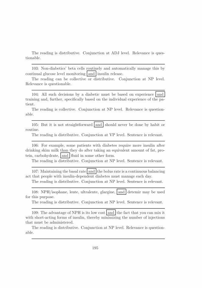
The reading is distributive. Conjunction at ADJ level. Relevance is ques-tionable.
103: Non-diabetics’ beta cells routinely and automatically manage this by
continual glucose level monitoring and insulin release.
The reading can be collective or distributive. Conjunction at NP level.Relevance is questionable.
104: All such decisions by a diabetic must be based on experience andtraining and, further, specifically based on the individual experience of the pa-tient.
The reading is collective. Conjunction at NP level. Relevance is question-able.
105: But it is not straightforward and should never be done by habit orroutine.
The reading is distributive. Conjunction at VP level. Sentence is relevant.
106: For example, some patients with diabetes require more insulin afterdrinking skim milk than they do after taking an equivalent amount of fat, pro-
tein, carbohydrate, and fluid in some other form.
The reading is distributive. Conjunction at NP level. Sentence is relevant.
107: Maintaining the basal rate and the bolus rate is a continuous balancingact that people with insulin-dependent diabetes must manage each day.
The reading is distributive. Conjunction at NP level. Sentence is relevant.
108: NPH/isophane, lente, ultralente, glargine, and detemir may be usedfor this purpose.
The reading is distributive. Conjunction at NP level. Sentence is relevant.
109: The advantage of NPH is its low cost and the fact that you can mix itwith short-acting forms of insulin, thereby minimizing the number of injectionsthat must be administered.
The reading is distributive. Conjunction at NP level. Relevance is question-able.
195
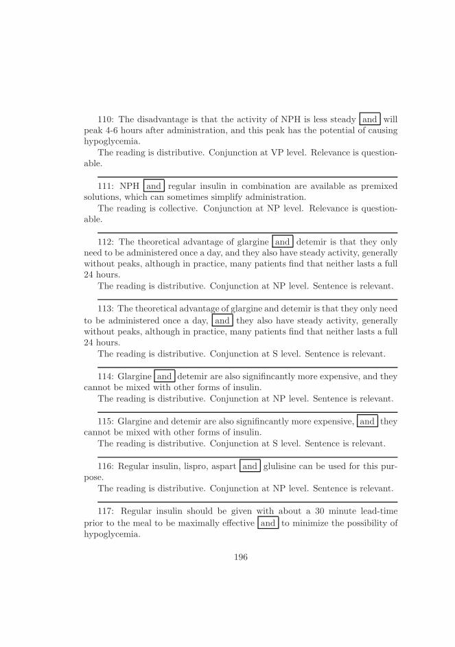
110: The disadvantage is that the activity of NPH is less steady and willpeak 4-6 hours after administration, and this peak has the potential of causinghypoglycemia.
The reading is distributive. Conjunction at VP level. Relevance is question-able.
111: NPH and regular insulin in combination are available as premixedsolutions, which can sometimes simplify administration.
The reading is collective. Conjunction at NP level. Relevance is question-able.
112: The theoretical advantage of glargine and detemir is that they onlyneed to be administered once a day, and they also have steady activity, generallywithout peaks, although in practice, many patients find that neither lasts a full24 hours.
The reading is distributive. Conjunction at NP level. Sentence is relevant.
113: The theoretical advantage of glargine and detemir is that they only need
to be administered once a day, and they also have steady activity, generallywithout peaks, although in practice, many patients find that neither lasts a full24 hours.
The reading is distributive. Conjunction at S level. Sentence is relevant.
114: Glargine and detemir are also signifincantly more expensive, and theycannot be mixed with other forms of insulin.
The reading is distributive. Conjunction at NP level. Sentence is relevant.
115: Glargine and detemir are also signifincantly more expensive, and theycannot be mixed with other forms of insulin.
The reading is distributive. Conjunction at S level. Sentence is relevant.
116: Regular insulin, lispro, aspart and glulisine can be used for this pur-pose.
The reading is distributive. Conjunction at NP level. Sentence is relevant.
117: Regular insulin should be given with about a 30 minute lead-time
prior to the meal to be maximally effective and to minimize the possibility ofhypoglycemia.
196

The reading is distributive. Sentence is relevant.
118: Lispro, aspart and glulisine are approved for dosage with the first biteof the meal, and may even be effective if given after completing the meal.
The reading is distributive. Conjunction at NP level. Relevance is question-able.
119: Lispro, aspart and glulisine are approved for dosage with the first bite
of the meal, and may even be effective if given after completing the meal.
The reading is distributive. Conjunction at VP level. Relevance is question-able.
120: Insulin prescriptions generally specify fixed amounts of long-acting in-
sulin to be given routinely, and fixed amounts of short-acting insulin prior toevery meal.
The reading is distributive. Conjunction at NP level. Relevance is question-able.
121: ”Sample regimen using insulin NPH and regular insulin”
The reading is distributive. Conjunction at NP level. Sentence is irrelevant.
122: ”Sample regimen using insulin glargine and insulin lispro”¡br /¿
The reading is distributive. Conjunction at NP level. Sentence is irrelevant.
123: A more complicated method that allows greater freedom with meal
times and snacks is carb counting.
The reading is distributive. Conjunction at NP level. Relevance is question-able.
124: The patient can use his or her total daily dose of insulin to estimate
how many grams of carbohydrates will be ”covered” by 1 unit of insulin, andusing this result, the patient can estimate how many units of insulin should beadministered depending on the carbohydrate concentration of their meal.
Sentence is irrelevant.
125: However, all dosages involve a fair degree of guesswork, and willseldom work consistently from one dosage to the next.
197
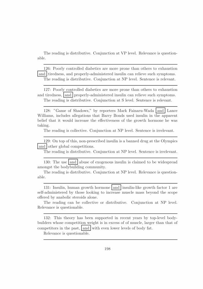
The reading is distributive. Conjunction at VP level. Relevance is question-able.
126: Poorly controlled diabetics are more prone than others to exhaustion
and tiredness, and properly-administered insulin can relieve such symptoms.
The reading is distributive. Conjunction at NP level. Sentence is relevant.
127: Poorly controlled diabetics are more prone than others to exhaustion
and tiredness, and properly-administered insulin can relieve such symptoms.
The reading is distributive. Conjunction at S level. Sentence is relevant.
128: ”Game of Shadows,” by reporters Mark Fainaru-Wada and LanceWilliams, includes allegations that Barry Bonds used insulin in the apparentbelief that it would increase the effectiveness of the growth hormone he wastaking.
The reading is collective. Conjunction at NP level. Sentence is irrelevant.
129: On top of this, non-prescribed insulin is a banned drug at the Olympics
and other global competitions.
The reading is distributive. Conjunction at NP level. Sentence is irrelevant.
130: The use and abuse of exogenous insulin is claimed to be widespreadamongst the bodybuilding community.
The reading is distributive. Conjunction at NP level. Relevance is question-able.
131: Insulin, human growth hormone and insulin-like growth factor 1 areself-administered by those looking to increase muscle mass beyond the scopeoffered by anabolic steroids alone.
The reading can be collective or distributive. Conjunction at NP level.Relevance is questionable.
132: This theory has been supported in recent years by top-level body-builders whose competition weight is in excess of of muscle, larger than that of
competitors in the past, and with even lower levels of body fat.
Relevance is questionable.
198

133: The abuse of exogenous insulin carries with it an attendant risk of
hypoglycemic coma and death when the amount used is in excess of thatrequired to handle ingested carbohydrate.
The reading is distributive. Conjunction at NP level. Sentence is relevant.
134: Acute risks include brain damage, paralysis, and death.The reading is distributive. Conjunction at NP level. Sentence is relevant.
135: Long-term risks may include development of type 2 diabetes, andpotentially a lifetime dependency on exogenous insulin.
The reading is distributive. Conjunction at NP level. Sentence is relevant.
136: In addition, overly high levels of insulin are seen only in those with
pathologies such as Type 2 diabetes mellitus, and only in some of those.Sentence is irrelevant.
137: The typical person cannot have insulin overload and still have bloodglucose levels which do not force symptoms of hypoglycemia.
The reading is collective. Relevance is questionable.
A.2 Summary
The reading can be collective or distributive: 15 16 22 45 87 90 101 103 131The reading is collective: 11 40 61 71 81 104 111 128 137The reading is distributive: 1 2 3 4 5 6 7 8 9 10 12 13 17 18 19 20 21 23 24
25 26 27 28 29 31 33 34 35 36 37 38 39 41 42 43 44 46 47 49 50 51 52 53 55 5758 59 60 63 64 65 66 67 68 69 70 72 73 74 75 76 77 78 79 80 83 84 88 89 91 9293 94 95 96 97 100 102 105 106 107 108 109 110 112 113 114 115 116 117 118119 120 121 122 123 125 126 127 129 130 133 134 135
Conjunction at S level: 17 20 21 26 42 44 47 80 91 93 113 115 127Conjunction at NP level: 1 2 9 10 11 12 13 14 15 16 18 19 22 24 25 27 29
31 33 34 35 36 37 39 41 45 46 49 50 51 52 57 58 59 60 61 63 64 69 71 73 74 7576 78 79 81 83 87 88 90 96 97 100 103 104 106 107 108 109 111 112 114 116 118120 121 122 123 126 128 129 130 131 133 134 135
Conjunction at ADJ level: 77 94 101 102Conjunction at VP level: 3 4 5 7 8 23 65 66 67 68 70 72 84 89 92 95 105 110
119 125Conjunction at name level: 82 85 86
199
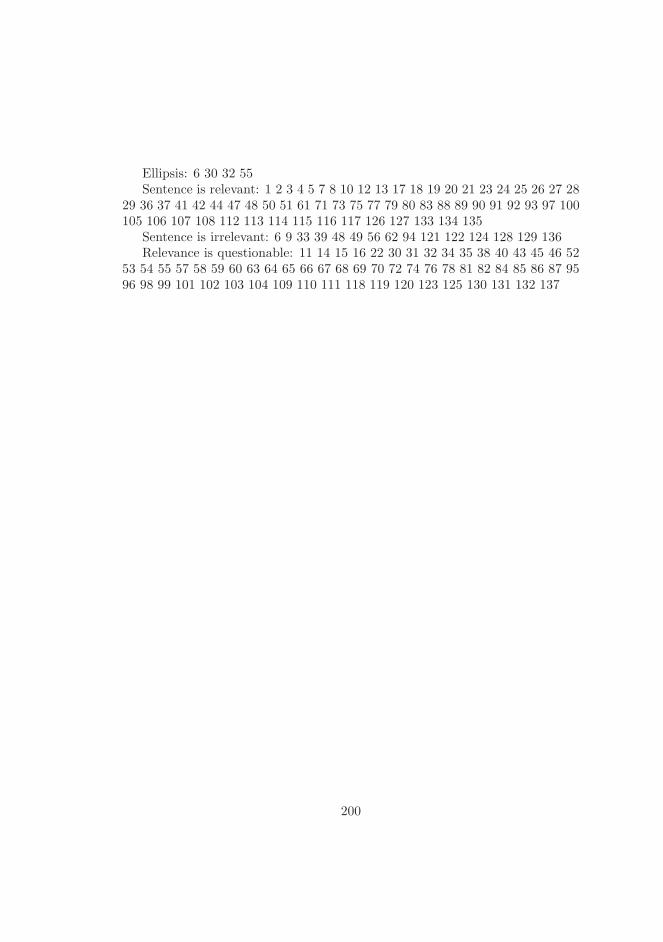
Ellipsis: 6 30 32 55Sentence is relevant: 1 2 3 4 5 7 8 10 12 13 17 18 19 20 21 23 24 25 26 27 28
29 36 37 41 42 44 47 48 50 51 61 71 73 75 77 79 80 83 88 89 90 91 92 93 97 100105 106 107 108 112 113 114 115 116 117 126 127 133 134 135
Sentence is irrelevant: 6 9 33 39 48 49 56 62 94 121 122 124 128 129 136Relevance is questionable: 11 14 15 16 22 30 31 32 34 35 38 40 43 45 46 52
53 54 55 57 58 59 60 63 64 65 66 67 68 69 70 72 74 76 78 81 82 84 85 86 87 9596 98 99 101 102 103 104 109 110 111 118 119 120 123 125 130 131 132 137
200
Appendix B
Investigations of the type ofrelative clauses of theWikipedia Insulin articlesentences
The following is an investigation of the type of relative clauses occuring in ascientific text, i.e. the Wikipedia entry on Insulin.
Insulin text had 172 sentences, of which: 13 had a ”which” relative clause.29 had a ”that” relative clause. 1 had a ”who” relative clause.
B.1 Which
These include protein ingestion, and glucose in the blood (from food whichproduces glucose when digested – characteristically this is carbohydrate, thoughnot all types produce glucose and so an increase in blood glucose levels).
In target cells, they initiate a signal transduction which has the effect ofincreasing glucose uptake and storage.
One million to three million islets of Langerhans (pancreatic islets) form theendocrine part of the pancreas, which is primarily an exocrine gland.
An increased calcium level causes activation of phospholipase C, which cleavesthe membrane phospholipid phosphatidyl inositol 4,5-bisphosphate into inositol
201

1,4,5-triphosphate and diacylglycerol.Metabolic syndrome a poorly understood condition first called Syndrome
X by Gerald Reaven, Reaven’s Syndrome after Reaven, CHAOS in Australia(from the signs which seem to travel together), and sometimes prediabetes.
Slight variations of the human insulin molecule are called insulin analogs,(technically ”insulin receptor ligands”) so named because they are not techni-cally insulin, rather they are analogs which retain the hormone’s glucose man-agement functionality.
”Insulin glargine” and ”Insulin detemir” both insulin analogs which startworking within 1 to 2 hours and continue to be active, without major peaks ordips, for about 24 hours, although this varies in many individuals.
However, insulin is a protein, which are digested in the stomach and gut andin order to be effective at controlling blood sugar, can not be taken orally.
Because of the complex and interacting factors, it is, in principle, impossibleto know for certain how much insulin (and which type) is needed to ’cover’ aparticular meal to achieve a reasonable blood glucose level within an hour ortwo after eating.
NPH and regular insulin in combination are available as premixed solutions,which can sometimes simplify administration.
The typical person cannot have insulin overload and still have blood glucoselevels which do not force symptoms of hypoglycemia.
Nicolae Paulescu, a professor of physiology at the University of Medicineand Pharmacy in Bucharest was the first one to isolate insulin, which he calledat that time pancrein, and published his work in 1921 that had been carried outin Bucharest.
Banting suggested that they try to use fetal calf pancreas, which had notyet developed digestive glands; he was relieved to find that this method workedwell.
B.2 That
Activation of insulin receptors leads to internal cellular mechanisms that di-rectly affect glucose uptake by regulating the number and operation of proteinmolecules in the cell membrane that transport glucose into the cell.
The genes that specify the proteins that make up the insulin receptor incell membranes have been identified and the structure of the interior, cell mem-brane section, and now, finally after more than a decade, the extra-membranestructure of receptor (Australian researchers announced the work 2Q 2006).
202

It is a protein that has been highly conserved across evolutionary time.
According to a survey that the International Diabetes Federation conductedin 2002 on the access to and availability of insulin in its member countries,approximately 70
Also, the International Diabetes Federation’s position statement is very clearin stating that ”there is NO overwhelming evidence to prefer one species ofinsulin over another” and ”[modern, highly-purified] animal insulins remain aperfectly acceptable alternative.
The dosage is non-physiological in that a subcutaneous bolus dose of insulinalone is administered instead of combination of insulin and C-peptide beingreleased gradually and directly into the portal vein.
Advantages to the patient are better control over background or ’basal’ in-sulin dosage, bolus doses calculated to fractions of a unit, and calculators in thepump that may help with determining ’bolus’ infusion dosages.
Researchers have produced a watch-like device that tests for blood glucoselevels through the skin and administers corrective doses of insulin through poresin the skin.
The company claims that an oral insulin therapy would be more convenientthan currently available injectable or inhalable therapies, and they expect thatconvenience to result in increased insulin usage among the currently underservedearly-stage patients with Type 2 diabetes, thus helping to create better long-term outcomes for that patient population.
The result is that the blood glucose level rises somewhat after eating, andwithin an hour or so, returns to the normal ’fasting’ level.
Maintaining the basal rate and the bolus rate is a continuous balancing actthat people with insulin-dependent diabetes must manage each day.
The advantage of NPH is its low cost and the fact that you can mix it withshort-acting forms of insulin, thereby minimizing the number of injections thatmust be administered.
The disadvantage is that the activity of NPH is less steady and will peak4-6 hours after administration, and this peak has the potential of causing hy-poglycemia.
The theoretical advantage of glargine and detemir is that they only needto be administered once a day, and they also have steady activity, generallywithout peaks, although in practice, many patients find that neither lasts a full24 hours.
A more complicated method that allows greater freedom with meal timesand snacks is ”carb counting.
203

”Game of Shadows,” by reporters Mark Fainaru-Wada and Lance Williams,includes allegations that Barry Bonds used insulin in the apparent belief thatit would increase the effectiveness of the growth hormone he was (also allegedto be) taking.
Their rationale is that since insulin and HGH act synergistically to promotegrowth, and since IGF-1 is a primary mediator of musculoskeletal growth, the’stacking’ of insulin, HGH and IGF-1 should offer a synergistic growth effect onskeletal muscle.
This theory has been supported in recent years by top-level bodybuilderswhose competition weight is in excess of of muscle, larger than that of competi-tors in the past, and with even lower levels of body fat.
The abuse of exogenous insulin carries with it an attendant risk of hypo-glycemic coma and death when the amount used is in excess of that required tohandle ingested carbohydrate.
In the non-diabetic, the feedback control mechanism connecting insulin re-lease and blood glucose level is very effective, and it is not possible to adjust itexcept that blood glucose levels rise slightly during digestion and absorption ofglucose.
The decrease in blood glucose levels is directly attributable to release ofinsulin, and that release ceases as blood glucose levels drop.
On testing the urine they found that there was sugar in the dog’s urine,establishing for the first time a relationship between the pancreas and diabetes.
Nicolae Paulescu, a professor of physiology at the University of Medicineand Pharmacy in Bucharest was the first one to isolate insulin, which he calledat that time pancrein, and published his work in 1921 that had been carried outin Bucharest.
In October 1920 Canadian Frederick Banting was reading one of Minkowski’spapers and concluded that it is the very digestive secretions that Minkowski hadoriginally studied that were breaking down the islet secretion(s), thereby makingit impossible to extract successfully.
Several weeks later it was clear the second run was also a success, and hehelped publish their results privately in Toronto that November.
Banting suggested that they try to use fetal calf pancreas, which had notyet developed digestive glands; he was relieved to find that this method workedwell.
However, the extract was so impure that Thompson suffered a severe allergicreaction, and further injections were canceled.
Banting, insulted that Best was not mentioned, shared his prize with Best,and Macleod immediately shared his with Collip.
204

Prior to that, insulin was sold in different strengths, including U-80 (80 unitsper milliliter) and U-40 formulations (40 units per milliliter), so the effort to”standardize” the potency aimed to reduce dosage errors and ease doctors’ jobof prescribing insulin for patients.
B.3 Who
Macleod, who was not entirely impressed with his idea so many before him hadtried and failed.
205

206
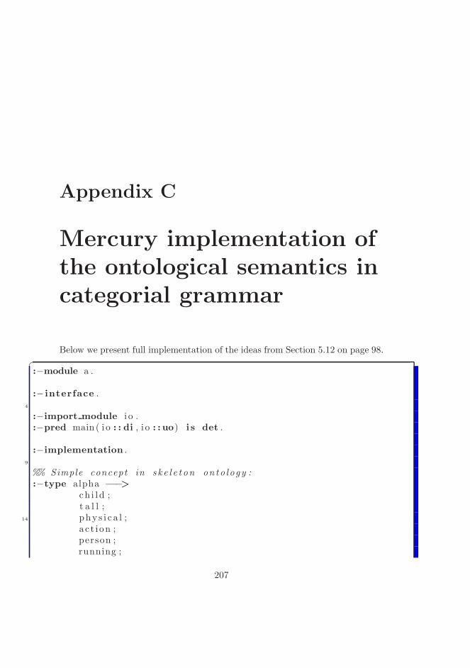
Appendix C
Mercury implementation ofthe ontological semantics incategorial grammar
Below we present full implementation of the ideas from Section 5.12 on page 98.�
:−module a .
:− interface .4
:−import module i o .:−pred main ( i o : : di , i o : : uo) i s det .
:−implementation .9
%% Simple concept in s k e l e t on on to logy ::−type alpha −−−>
ch i l d ;t a l l ;
14 phy s i c a l ;a c t i on ;person ;running ;
207
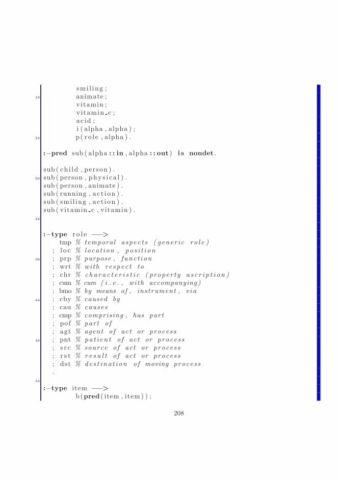
smi l i ng ;19 animate ;
v itamin ;v i tamin c ;ac id ;i ( alpha , alpha ) ;
24 p( ro l e , alpha ) .
:−pred sub ( alpha : : in , a lpha : : out ) i s nondet .
sub ( ch i ld , person ) .29 sub ( person , phy s i c a l ) .
sub ( person , animate ) .sub ( running , a c t i on ) .sub ( smi l ing , a c t i on ) .sub ( vitamin c , v itamin ) .
34
:−type r o l e −−−>tmp % temporal aspec t s ( gener i c r o l e )
; l o c % loca t ion , po s i t i on39 ; prp % purpose , func t ion
; wrt % with r e s pe c t to; chr % ch a r a c t e r i s t i c ( proper t y a s c r i p t i o n ); cum % cum ( i . e . , wi th accompanying ); bmo % by means of , instrument , v ia
44 ; cby % caused by; cau % causes; cmp % compris ing , has par t; pof % part o f; agt % agent o f ac t or proces s
49 ; pnt % pa t i en t o f ac t or proces s; s r c % source o f act or proces s; r s t % r e s u l t o f ac t or proces s; ds t % des t i n a t i on o f moving proces s.
54
:−type item −−−>b(pred ( item , item ) ) ;
208
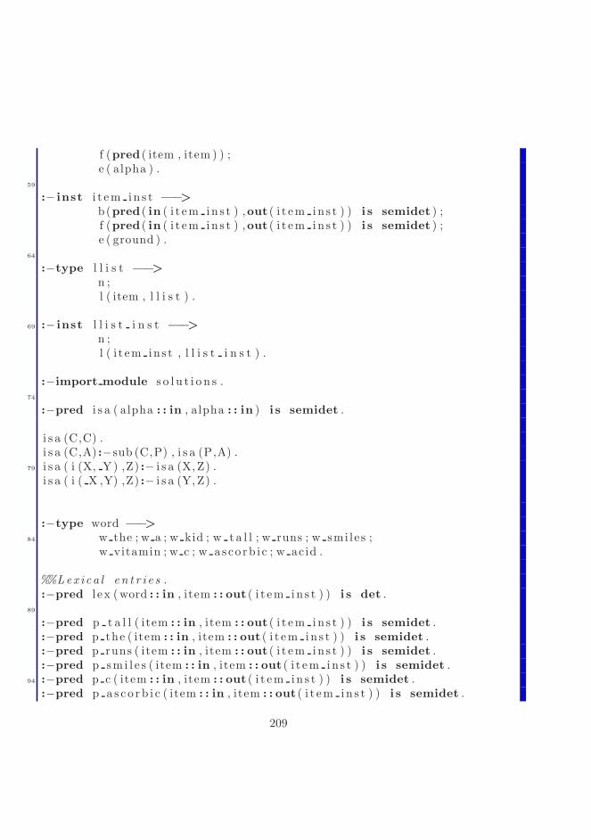
f (pred ( item , item ) ) ;e ( alpha ) .
59
:− inst i t em in s t −−−>b(pred ( in ( i t em in s t ) ,out ( i t em in s t ) ) i s semidet ) ;f (pred ( in ( i t em in s t ) ,out ( i t em in s t ) ) i s semidet ) ;e ( ground ) .
64
:−type l l i s t −−−>n ;l ( item , l l i s t ) .
69 :− inst l l i s t i n s t −−−>n ;l ( i t em ins t , l l i s t i n s t ) .
:−import module s o l u t i o n s .74
:−pred i s a ( alpha : : in , a lpha : : in ) i s semidet .
i s a (C,C) .i s a (C,A) :−sub (C,P) , i s a (P,A) .
79 i s a ( i (X, Y) ,Z) :− i s a (X, Z) .i s a ( i ( X ,Y) ,Z) :− i s a (Y, Z) .
:−type word −−−>84 w the ; w a ; w kid ; w t a l l ; w runs ; w smi le s ;
w vitamin ; w c ; w a s co rb i c ; w acid .
%%Lex i ca l e n t r i e s .:−pred l e x (word : : in , item : : out ( i t em in s t ) ) i s det .
89
:−pred p t a l l ( item : : in , item : : out ( i t em in s t ) ) i s semidet .:−pred p the ( item : : in , item : : out ( i t em in s t ) ) i s semidet .:−pred p runs ( item : : in , item : : out ( i t em in s t ) ) i s semidet .:−pred p sm i l e s ( item : : in , item : : out ( i t em in s t ) ) i s semidet .
94 :−pred p c ( item : : in , item : : out ( i t em in s t ) ) i s semidet .:−pred p a s c o r b i c ( item : : in , item : : out ( i t em in s t ) ) i s semidet .
209

p t a l l ( e (C) , e ( i ( t a l l ,C) ) ) :− i s a (C, phy s i c a l ) .99 p runs ( e (C) , e ( i ( running , p ( agt ,C) ) ) ) :− i s a (C, animate ) .
p sm i l e s ( e (C) , e ( i ( smi l ing , p ( agt ,C) ) ) ) :− i s a (C, animate ) .p the ( e ( I ) , e ( I ) ) .p c ( e (C) , e ( v i tamin c ) ) :− i s a (C, vitamin ) .p a s c o r b i c ( e (C) , e ( v i tamin c ) ) :− i s a (C, ac id ) .
104
l e x ( w kid , e ( ch i l d ) ) .l ex ( w ta l l , f ( p t a l l ) ) .l ex ( w runs , b( p runs ) ) .l ex ( w smiles , b ( p sm i l e s ) ) .
109 l e x ( w the , f ( p the ) ) .l ex (w a , f ( p the ) ) .l ex ( w vitamin , e ( v itamin ) ) .l ex (w c , b ( p c ) ) .l ex ( w acid , e ( ac id ) ) .
114 l e x ( w ascorb ic , f ( p a s c o r b i c ) ) .
:−pred r ( l l i s t : : in ( l l i s t i n s t ) , item : : out ( i t em in s t ) ) i s nondet .
:−pred a ( l l i s t ,119 l l i s t ,
l l i s t ) .
:−mode a (out ( l l i s t i n s t ) ,out ( l l i s t i n s t ) ,
124 in ( l l i s t i n s t ) ) i s nondet .
a ( l (X, n) , l (Y,T) , l (X, l (Y,T) ) ) .a ( l (H, L) ,M, l (H,T) ) :−a (L ,M,T) .
129 r ( l (X, n) ,X) .
r (G, E1) :−a (G1 ,G2 ,G) , r (G1 , f (P) ) , r (G2 , E2) ,P(E2 , E1) .
r (G, E1) :−a (G1 ,G2 ,G) , r (G1 , E2) , r (G2 , b (P) ) ,P(E2 , E1) .134
210
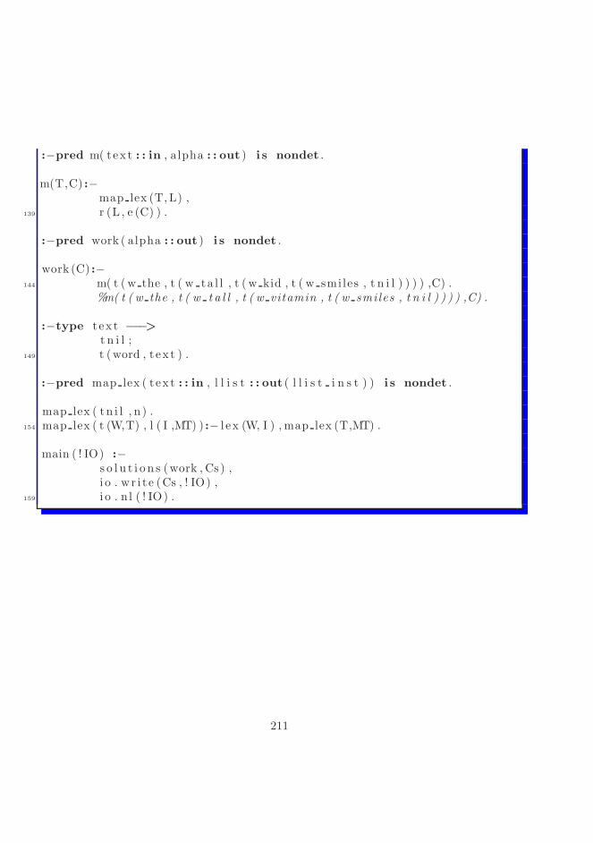
:−pred m( tex t : : in , a lpha : : out ) i s nondet .
m(T,C) :−map lex (T,L) ,
139 r (L , e (C) ) .
:−pred work ( alpha : : out ) i s nondet .
work (C) :−144 m( t ( w the , t ( w ta l l , t ( w kid , t ( w smiles , t n i l ) ) ) ) ,C) .
%m( t ( w the , t ( w t a l l , t ( w vitamin , t ( w smiles , t n i l ) ) ) ) ,C) .
:−type t ex t −−−>t n i l ;
149 t (word , t ex t ) .
:−pred map lex ( t ex t : : in , l l i s t : : out ( l l i s t i n s t ) ) i s nondet .
map lex ( tn i l , n ) .154 map lex ( t (W,T) , l ( I ,MT) ) :− l e x (W, I ) , map lex (T,MT) .
main ( ! IO) :−s o l u t i o n s (work , Cs ) ,i o . wr i t e (Cs , ! IO) ,
159 i o . n l ( ! IO) .
211

212

Appendix D
SML implementation of theEarley parser
Earley parser is an efficient polynomial time parser, with n3 time complexity [4](see also [25]). Below we present the implementation of it in the Standard MetaLanguage.
D.1 Signature
�
1 signature Earley =sig
(∗ Types o f t e rmina l s and nontermina ls∗)
6 type t = chartype n = s t r i n g
(∗ Terminals and nontermina ls are symbols ∗)
11 type symbol
val t : t −> symbolval n : n −> symbol
213
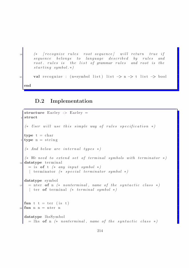
16 (∗ [ r ecogn i z e r u l e s root sequence ] w i l l re turn t rue i fsequence be longs to language de s c r i b ed by r u l e s androot . r u l e s i s the l i s t o f grammar r u l e s and root i s thes t a r t i n g symbol . ∗)
21 val r e c o gn i z e : (n∗ symbol l i s t ) l i s t −> n −> t l i s t −> bool
end
D.2 Implementation�
structure Earley :> Earley =2 struct
(∗ User w i l l use t h i s s imple way o f r u l e s s p e c i f i c a t i o n ∗)
type t = char7 type n = s t r i n g
(∗ And below are i n t e r n a l t ypes ∗)
(∗ We need to ex tend s e t o f t ermina l symbols wi th terminator ∗)12 datatype te rmina l
= i s of t (∗ any input symbol ∗)| te rminator (∗ s p e c i a l t erminator symbol ∗)
datatype symbol17 = nter of n (∗ nonterminal , name o f the s y n t a c t i c c l a s s ∗)
| t e r of te rmina l (∗ t ermina l symbol ∗)
fun t t = t e r ( i s t )22 fun n n = nter n
datatype lhsSymbol= lh s of n (∗ nonterminal , name o f the s y n t a c t i c c l a s s ∗)
214

| phi (∗ s p e c i a l symbol used in s t a r t i n g s e t ∗)27
type r u l e s= (n , symbol l i s t l i s t ) Polyhash . ha sh tab l e
exception notFound32
datatype s t a t e = s t a t e oflhsSymbol (∗ l h s o f the ru l e ∗)∗ ( symbol l i s t ) (∗ a l r eady parsed symbols ∗)∗ ( symbol l i s t ) (∗ not ye t parsed symbols ∗)
37 ∗ te rmina l (∗ one look−ahead symbol ∗)∗ i n t (∗ where par s ing s t a r t e d ∗)
fun makeStartState n= s ta t e ( phi ,
42 [ ] ,[ nter n ] ,terminator ,0)
47 (∗ t ype input = termina l Array . array ∗)
fun input t s= Array . f romLis t ( ( L i s t .map i s t s )@[ terminator ] )
52 (∗ We represen t s e t as map from se t e lements to un i t ∗)type s t a t eS e t = ( state , un i t ) Polyhash . ha sh tab l e
fun createEmptyStateSet ( ) =l e t
57 val emptyStateSet : s t a t eS e t= Polyhash . mkPolyTable (10 , notFound )
inemptyStateSet
end62
exception i n t e r na lE r r o r
215

fun c r ea teSta teSe tArray s i z e s t a r t S t a t e =l e t
67 val a = Array . a r ray ( s i z e , createEmptyStateSet ( ) )in
i f s i z e < 1then raise i n t e r na lE r r o relse ( Array . update a 0 s t a r t S t a t e ; a )
72 end
fun p r ed i c t o r ( nonterminal , lookAhead , ru l e s , s t a r t ed ) =l e t
fun aux ( nonterminal , [ ] , lookAhead , s t a r t ed )77 = [ ]
| aux ( nonterminal , rhs : : rhss , lookAhead , s t a r t ed )= s t a t e ( l h s nonterminal , [ ] , rhs , lookAhead , s t a r t ed )
: : aux ( nonterminal , rhss , lookAhead , s t a r t ed )val a l t e r n a t i v e s = Polyhash . f i nd r u l e s nonterminal
82 inaux ( nonterminal , a l t e r n a t i v e s , lookAhead , s t a r t ed )
end
(∗ i s S u b s t r i n g ( l , a , p ) checks i f l i s t l i s a s u b s t r i n g o f87 array a s t a r t i n g at po s i t i on p o f the array . ∗)
(∗ fun i s S u b s t r i n g ( [ ] , , ) = t rue| i s S u b s t r i n g ( terminator : : r e s t , input , po s i t i on )= pos i t i on >= Array . l en g t h input
92 | i s S u b s t r i n g ( ( l t ermina l ) : : r e s t , input , po s i t i on )= Array . sub ( input , po s i t i on ) = termina l
anda lso i s S u b s t r i n g ( re s t , input , po s i t i on +1)∗)
fun completer ( [ ] , ) = [ ]97 | completer ( ( s t a t e ( lhs1 ,
beforeDot ,( nter nonterminal ) : : afterDot ,lookAhead ,s t a r t ed ) ) : : s ta t e s ,
102 l h s 2 )= i f nonterminal = lhs2
216
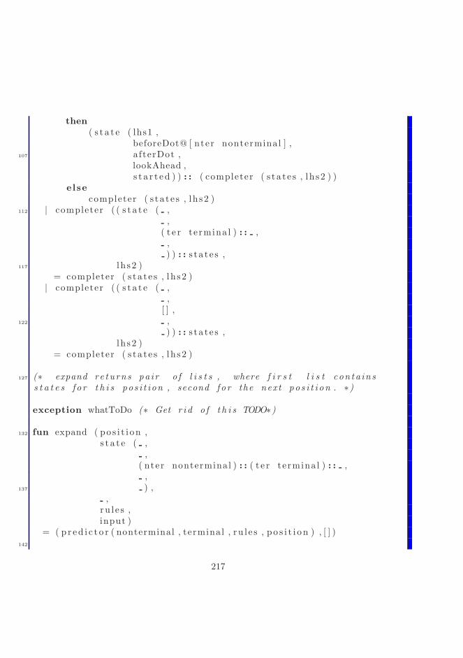
then( s t a t e ( lhs1 ,
beforeDot@ [ nter nonterminal ] ,107 afterDot ,
lookAhead ,s t a r t ed ) ) : : ( completer ( s ta t e s , l h s2 ) )
elsecompleter ( s ta t e s , l h s2 )
112 | completer ( ( s t a t e ( ,,
( t e r te rmina l ) : : ,,) ) : : s ta t e s ,
117 l h s 2 )= completer ( s ta t e s , l h s2 )| completer ( ( s t a t e ( ,
,[ ] ,
122 ,) ) : : s ta t e s ,
l h s2 )= completer ( s ta t e s , l h s2 )
127 (∗ expand re tu rns pa i r o f l i s t s , where f i r s t l i s t con ta in ss t a t e s f o r t h i s pos i t i on , second f o r the nex t po s i t i on . ∗)
exception whatToDo (∗ Get r i d o f t h i s TODO∗)
132 fun expand ( po s i t i on ,s t a t e ( ,
,( nter nonterminal ) : : ( t e r te rmina l ) : : ,,
137 ) ,,
r u l e s ,input )
= ( p r ed i c t o r ( nonterminal , terminal , r u l e s , p o s i t i o n ) , [ ] )142
217
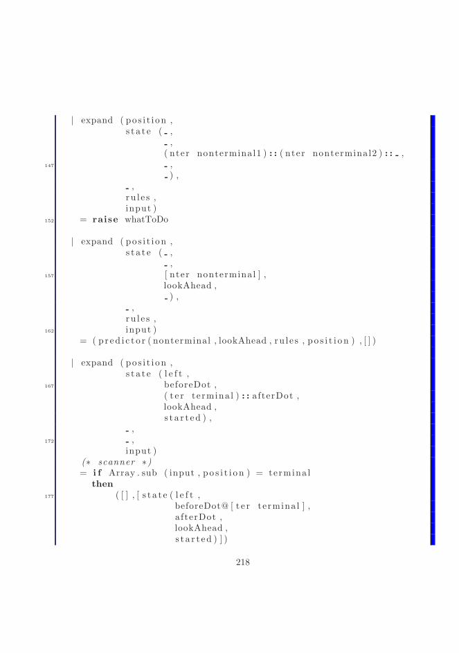
| expand ( po s i t i on ,s t a t e ( ,
,( nter nonterminal1 ) : : ( nter nonterminal2 ) : : ,
147 ,) ,
,r u l e s ,input )
152 = raise whatToDo
| expand ( po s i t i on ,s t a t e ( ,
,157 [ nter nonterminal ] ,
lookAhead ,) ,
,r u l e s ,
162 input )= ( p r ed i c t o r ( nonterminal , lookAhead , ru l e s , p o s i t i o n ) , [ ] )
| expand ( po s i t i on ,s t a t e ( l e f t ,
167 beforeDot ,( t e r te rmina l ) : : afterDot ,lookAhead ,s t a r t ed ) ,
,172 ,
input )(∗ scanner ∗)= i f Array . sub ( input , po s i t i o n ) = termina l
then177 ( [ ] , [ s t a t e ( l e f t ,
beforeDot@ [ t e r te rmina l ] ,a fterDot ,lookAhead ,s t a r t ed ) ] )
218
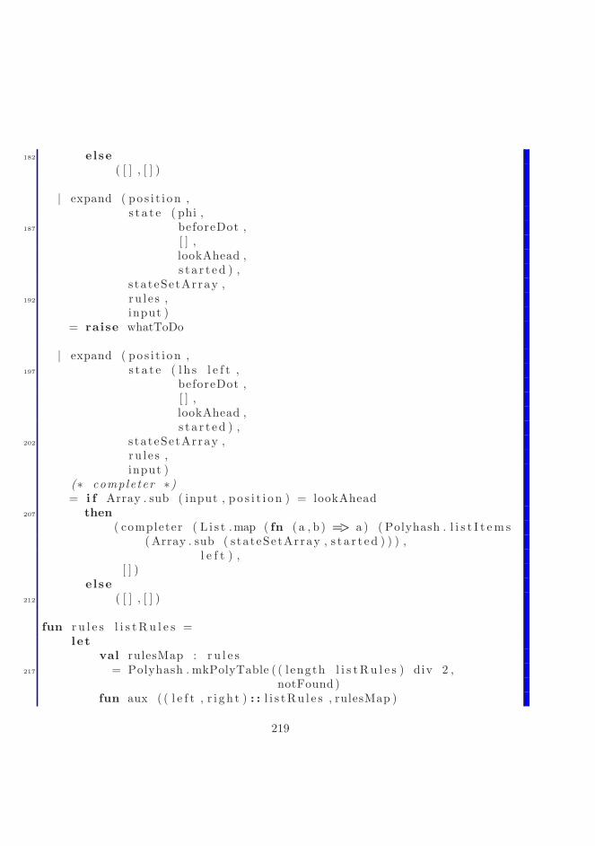
182 else( [ ] , [ ] )
| expand ( po s i t i on ,s t a t e ( phi ,
187 beforeDot ,[ ] ,lookAhead ,s t a r t ed ) ,
s ta teSetArray ,192 ru l e s ,
input )= raise whatToDo
| expand ( po s i t i on ,197 s t a t e ( l h s l e f t ,
beforeDot ,[ ] ,lookAhead ,s t a r t ed ) ,
202 s ta teSetArray ,ru l e s ,input )
(∗ comple ter ∗)= i f Array . sub ( input , po s i t i o n ) = lookAhead
207 then( completer ( L i s t .map ( fn ( a , b ) => a ) ( Polyhash . l i s t I t em s
(Array . sub ( s ta teSetArray , s t a r t ed ) ) ) ,l e f t ) ,
[ ] )else
212 ( [ ] , [ ] )
fun r u l e s l i s t R u l e s =l e t
val rulesMap : r u l e s217 = Polyhash . mkPolyTable ( ( l ength l i s tR u l e s ) div 2 ,
notFound )fun aux ( ( l e f t , r i g h t ) : : l i s tRu l e s , rulesMap )
219
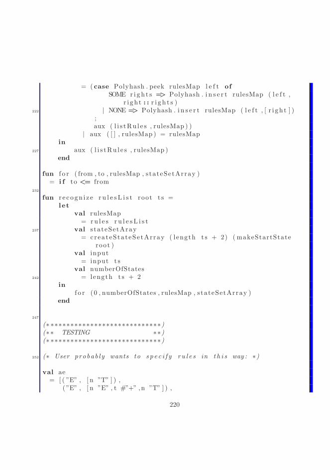
= ( case Polyhash . peek rulesMap l e f t ofSOME r i g h t s => Polyhash . i n s e r t rulesMap ( l e f t ,
r i g h t : : r i g h t s )222 | NONE => Polyhash . i n s e r t rulesMap ( l e f t , [ r i g h t ] )
;aux ( l i s tRu l e s , rulesMap ) )
| aux ( [ ] , rulesMap ) = rulesMapin
227 aux ( l i s tRu l e s , rulesMap )end
fun f o r ( from , to , rulesMap , s ta teSetArray )= i f to <= from
232
fun r e c o gn i z e r u l e s L i s t root t s =l e t
val rulesMap= r u l e s r u l e s L i s t
237 val s ta teSetAray= cr ea teSta teSe tArray ( length t s + 2) ( makeStartState
root )val input
= input t sval numberOfStates
242 = length t s + 2in
f o r (0 , numberOfStates , rulesMap , s ta teSetArray )end
247
(∗ ∗∗∗∗∗∗∗∗∗∗∗∗∗∗∗∗∗∗∗∗∗∗∗∗∗∗∗∗)(∗ ∗ TESTING ∗∗)(∗ ∗∗∗∗∗∗∗∗∗∗∗∗∗∗∗∗∗∗∗∗∗∗∗∗∗∗∗∗)
252 (∗ User probab l y wants to s p e c i f y r u l e s in t h i s way : ∗)
val ae= [ ( ”E” , [ n ”T” ] ) ,
( ”E” , [ n ”E” , t #”+” ,n ”T” ] ) ,
220

257 ( ”T” , [ n ”P” ] ) ,( ”T” , [ n ”T” , t #”∗” ,n ”P” ] ) ,( ”P” , [ t #”a” ] )]
262 val r e s= r e c o gn i z e ae ”E” ( explode ”a+a∗a” )
end
221

222

Appendix E
SML implementation of thegenerative ontology and thelexicon
Below we present an implementation of the generative ontology and the lexiconwritten in the Standard Meta Language.
E.1 Signature�
signature GenerativeOntology =sig
datatype s imp l e concept = s imple of s t r i n g
5 val s imple concept compare : s imp l e concept ∗ s imp l e concept −>order
datatype r o l e = r of s t r i n g
val ro le compare : r o l e ∗ r o l e −> order10
datatype concept= cc of s imp l e concept ∗ ( r o l e ∗ concept ) l i s t
223

(∗ Simple t e x t u a l r e p r e s en t a t i on o f a concept ∗)15 val c2s : concept −> s t r i n g
(∗ LaTeX tabu lar−based r ep r e s en t a t i on o f a concept ∗)val c 2 l a t e x : concept −> s t r i n g
20 (∗ TODO: Make i s a f a s t e r . ∗)(∗ ex cep t ion concep t no t found o f s t r i n g ∗)(∗ va l i s a : s imp l e concep t −> s imp l e concep t l i s t ∗)
datatype s yn ta c t i c c a t e g o r y = syn of s t r i n g25
val s c2 s : s yn t a c t i c c a t e g o r y −> s t r i n g
val synta c t i c ca tego ry compar e : s yn t a c t i c c a t e g o r y ∗s yn ta c t i c c a t e g o r y −> order
30 datatype l e x i c on i t em = l i of s yn ta c t i c c a t e g o r y ∗ concept
exception l e x no t found of s t r i n gval l e x : s t r i n g −> l e x i c on i t em l i s t
35 val a f f : s imp l e concept ∗ s imp l e concept −> r o l e l i s tend
E.2 Implementation�
structure GenerativeOntology :> GenerativeOntology =struct
4 fun poly compare ( x1 , x2 ) =Int . compare ( Polyhash . hash x1 , Polyhash . hash x2 )
datatype s imp l e concept = s imple of s t r i n g
9 fun s c2 s ( s imple x ) = x
224
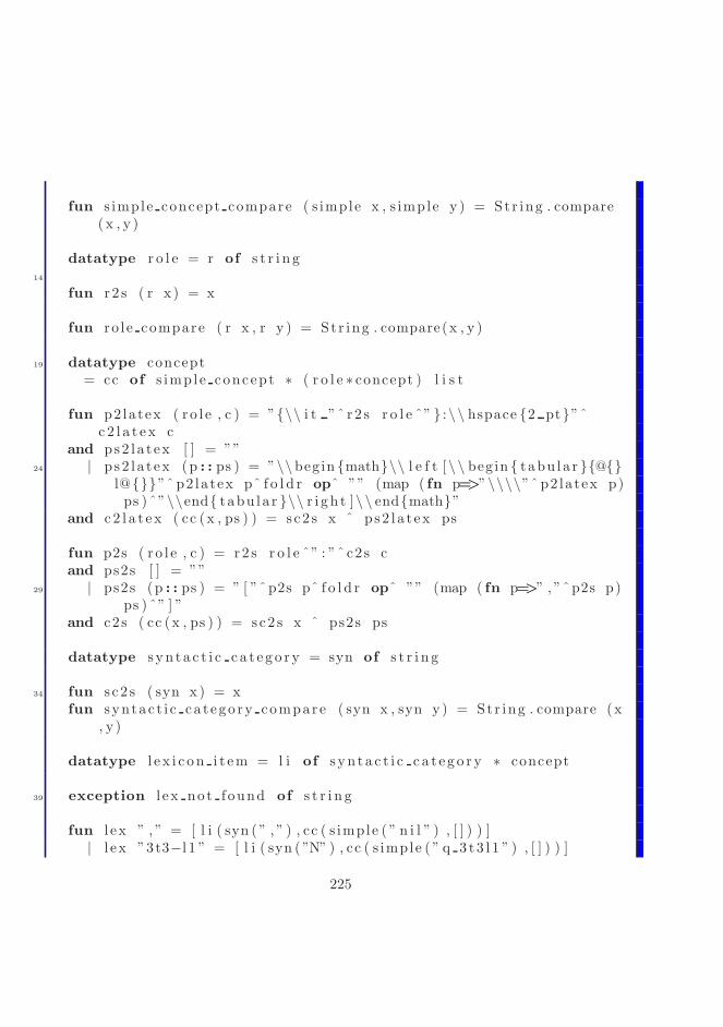
fun s imple concept compare ( s imple x , s imple y ) = Str ing . compare(x , y )
datatype r o l e = r of s t r i n g14
fun r 2 s ( r x ) = x
fun ro le compare ( r x , r y ) = Str ing . compare(x , y )
19 datatype concept= cc of s imp l e concept ∗ ( r o l e ∗ concept ) l i s t
fun p2 la tex ( r o l e , c ) = ”{\\ i t ”ˆ r 2 s r o l e ˆ” } :\\ hspace {2 pt}”ˆc 2 l a t e x c
and ps2 l a t ex [ ] = ””24 | ps2 l a t ex (p : : ps ) = ”\\begin {math}\\ l e f t [\\ begin { tabu la r }{@{}
l@{}}”ˆ p2 la tex pˆ f o l d r opˆ ”” (map ( fn p=>”\\\\”ˆ p2 la tex p)ps ) ˆ”\\end{ tabu la r }\\ r i g h t ]\\ end{math}”
and c 2 l a t e x ( cc (x , ps ) ) = sc2 s x ˆ ps2 l a t ex ps
fun p2s ( r o l e , c ) = r2 s r o l e ˆ” : ”ˆ c2s cand ps2s [ ] = ””
29 | ps2s (p : : ps ) = ” [ ”ˆp2s pˆ f o l d r opˆ ”” (map ( fn p=>” , ”ˆp2s p)ps ) ˆ” ] ”
and c2s ( cc (x , ps ) ) = sc2 s x ˆ ps2s ps
datatype s yn ta c t i c c a t e g o r y = syn of s t r i n g
34 fun s c2 s ( syn x ) = xfun synta c t i c ca tego ry compar e ( syn x , syn y) = Str ing . compare (x
, y )
datatype l e x i c on i t em = l i of s yn ta c t i c c a t e g o r y ∗ concept
39 exception l e x no t found of s t r i n g
fun l e x ” , ” = [ l i ( syn ( ” , ” ) , cc ( s imple ( ” n i l ” ) , [ ] ) ) ]| l e x ”3t3−l 1 ” = [ l i ( syn ( ”N” ) , cc ( s imple ( ” q 3 t 3 l 1 ” ) , [ ] ) ) ]
225

| l e x ” abo l i s h ” = [ l i ( syn ( ”TV” ) , cc ( s imple ( ” a b o l i t i o n ” ) , [ ] ) ) ]44 | l e x ” a c t i v a t i o n ” = [ l i ( syn ( ”N” ) , cc ( s imple ( ” a c t i v a t i o n ” ) , [ ] ) )
]| l e x ” a c t i v i t y ” = [ l i ( syn ( ”N” ) , cc ( s imple ( ” a c t i v i t y ” ) , [ ] ) ) ]| l e x ” ac t s ” = [ l i ( syn ( ”TV” ) , cc ( s imple ( ” a c t ing ” ) , [ ] ) ) ]| l e x ” add i t i on ” = [ l i ( syn ( ”N” ) , cc ( s imple ( ” add i t i on ” ) , [ ] ) ) ]| l e x ” adipocyte ” = [ l i ( syn ( ”N” ) , cc ( s imple ( ” ad ipocyte ” ) , [ ] ) ) ]
49 | l e x ” ad ipocy te s” = [ l i ( syn ( ”N” ) , cc ( s imple ( ” ad ipocyte ” ) , [ ] ) ) ]| l e x ”age” = [ l i ( syn ( ”N” ) , cc ( s imple ( ”age ” ) , [ ] ) ) ]| l e x ” agents ” = [ l i ( syn ( ”N” ) , cc ( s imple ( ” agent ” ) , [ ] ) ) ]| l e x ” a l l im in ” = [ l i ( syn ( ”N” ) , cc ( s imple ( ” a l l im in ” ) , [ ] ) ) ]| l e x ”am” = [ l i ( syn ( ” IS” ) , cc ( s imple ( ” i s ” ) , [ ] ) ) ]
54 | l e x ” anti−funga l ” = [ l i ( syn ( ”A” ) , cc ( s imple ( ” an t i f ung a l ” ) , [ ] )) ]
| l e x ” are ” = [ l i ( syn ( ” IS” ) , cc ( s imple ( ” i s ” ) , [ ] ) ) ]| l e x ”auc” = [ l i ( syn ( ”N” ) , cc ( s imple ( ”auc” ) , [ ] ) ) ]| l e x ”background” = [ l i ( syn ( ”N” ) , cc ( s imple ( ”background” ) , [ ] ) )
]| l e x ”be” = [ l i ( syn ( ”BE” ) , cc ( s imple ( ” n i l ” ) , [ ] ) ) ]
59 | l e x ” b e t a c e l l ” = [ l i ( syn ( ”N” ) , cc ( s imple ( ” b e t a c e l l ” ) , [ ] ) ) ]| l e x ” b e t a c e l l s ” = [ l i ( syn ( ”N” ) , cc ( s imple ( ” b e t a c e l l ” ) , [ ] ) ) ]| l e x ” b ind ing ” = [ l i ( syn ( ”N” ) , cc ( s imple ( ” b ind ing” ) , [ ] ) ) , l i (
syn ( ”VBG” ) , cc ( s imple ( ” b ind ing” ) , [ ] ) ) ]| l e x ”blood ” = [ l i ( syn ( ”N” ) , cc ( s imple ( ”blood ” ) , [ ] ) ) ]| l e x ” c a r r i e r ” = [ l i ( syn ( ”N” ) , cc ( s imple ( ” c a r r i e r ” ) , [ ] ) ) ]
64 | l e x ” caspase ” = [ l i ( syn ( ”N” ) , cc ( s imple ( ” caspase ” ) , [ ] ) ) ]| l e x ” ca spa s e s” = [ l i ( syn ( ”N” ) , cc ( s imple ( ” caspase ” ) , [ ] ) ) ]| l e x ” caus ing ” = [ l i ( syn ( ”VBG” ) , cc ( s imple ( ” caus ing ” ) , [ ] ) ) ]| l e x ” c e l l ” = [ l i ( syn ( ”N” ) , cc ( s imple ( ” c e l l ” ) , [ ] ) ) ]| l e x ” c e l l s ” = [ l i ( syn ( ”N” ) , cc ( s imple ( ” c e l l ” ) , [ ] ) ) ]
69 | l e x ” c e l l u l a r ” = [ l i ( syn ( ”A” ) , cc ( s imple ( ” c e l l u l a r ” ) , [ ] ) ) ]| l e x ” c en t r a l ” = [ l i ( syn ( ”A” ) , cc ( s imple ( ” c en t r a l ” ) , [ ] ) ) ]| l e x ” cha l l e ng e ” = [ l i ( syn ( ”N” ) , cc ( s imple ( ” cha l l e ng e” ) , [ ] ) ) ]| l e x ” c h a r a c t e r i z a t i o n” = [ l i ( syn ( ”N” ) , cc ( s imple ( ”
c h a r a c t e r i z a t i o n” ) , [ ] ) ) ]| l e x ” c l on ing ” = [ l i ( syn ( ”N” ) , cc ( s imple ( ” c l on ing ” ) , [ ] ) ) ]
74 | l e x ” combination ” = [ l i ( syn ( ”N” ) , cc ( s imple ( ” combination ” ), [ ] ) ) ]
| l e x ”compound” = [ l i ( syn ( ”N” ) , cc ( s imple ( ”compound” ) , [ ] ) ) ]
226
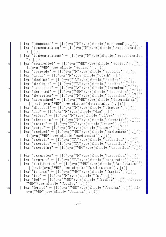
| l e x ”compounds” = [ l i ( syn ( ”N” ) , cc ( s imple ( ”compound” ) , [ ] ) ) ]| l e x ” concent r a t i on ” = [ l i ( syn ( ”N” ) , cc ( s imple ( ” concent r a t i on ”
) , [ ] ) ) ]| l e x ” concent r a t i ons ” = [ l i ( syn ( ”N” ) , cc ( s imple ( ” concent r a t i on
” ) , [ ] ) ) ]79 | l e x ” c o n t r o l l e d” = [ l i ( syn ( ”VBD” ) , cc ( s imple ( ” c on t r o l ” ) , [ ] ) ) ,
l i ( syn ( ”VBN” ) , cc ( s imple ( ” c on t r o l ” ) , [ ] ) ) ]| l e x ” cpept ide ” = [ l i ( syn ( ”N” ) , cc ( s imple ( ” cpept ide ” ) , [ ] ) ) ]| l e x ”death” = [ l i ( syn ( ”N” ) , cc ( s imple ( ”death” ) , [ ] ) ) ]| l e x ” d e c l i n e ” = [ l i ( syn ( ”TV” ) , cc ( s imple ( ” d e c l i n e ” ) , [ ] ) ) ]| l e x ” d e c l i n e s ” = [ l i ( syn ( ”TV” ) , cc ( s imple ( ” d e c l i n e ” ) , [ ] ) ) ]
84 | l e x ”dependent ” = [ l i ( syn ( ”A” ) , cc ( s imple ( ”dependent ” ) , [ ] ) ) ]| l e x ” detected ” = [ l i ( syn ( ”VBN” ) , cc ( s imple ( ” d e t e c t i o n” ) , [ ] ) ) ]| l e x ” d e t e c t i o n” = [ l i ( syn ( ”N” ) , cc ( s imple ( ” d e t e c t i o n ” ) , [ ] ) ) ]| l e x ”determined ” = [ l i ( syn ( ”VBD” ) , cc ( s imple ( ” determin ing” )
, [ ] ) ) , l i ( syn ( ”VBN” ) , cc ( s imple ( ” determin ing” ) , [ ] ) ) ]| l e x ” d i s po s a l ” = [ l i ( syn ( ”N” ) , cc ( s imple ( ” d i s po s a l ” ) , [ ] ) ) ]
89 | l e x ”dna” = [ l i ( syn ( ”N” ) , cc ( s imple ( ”dna” ) , [ ] ) ) ]| l e x ” e f f e c t ” = [ l i ( syn ( ”N” ) , cc ( s imple ( ” e f f e c t ” ) , [ ] ) ) ]| l e x ” e l e v a t i o n ” = [ l i ( syn ( ”N” ) , cc ( s imple ( ” e l e v a t i o n ” ) , [ ] ) ) ]| l e x ” en t e r s ” = [ l i ( syn ( ”TV” ) , cc ( s imple ( ” entry ” ) , [ ] ) ) ]| l e x ” entry” = [ l i ( syn ( ”N” ) , cc ( s imple ( ” entery ” ) , [ ] ) ) ]
94 | l e x ” ex c i t e d ” = [ l i ( syn ( ”VBD” ) , cc ( s imple ( ” excitement ” ) , [ ] ) ) ,l i ( syn ( ”VBN” ) , cc ( s imple ( ” excitement ” ) , [ ] ) ) ]
| l e x ” ex c r e t e ” = [ l i ( syn ( ”TV” ) , cc ( s imple ( ” ex c r e t i o n ” ) , [ ] ) ) ]| l e x ” ex c r e t e s ” = [ l i ( syn ( ”TV” ) , cc ( s imple ( ” ex c r e t i o n ” ) , [ ] ) ) ]| l e x ” ex c r e t i n g ” = [ l i ( syn ( ”VBG” ) , cc ( s imple ( ” ex c r e t i o n ” ) , [ ] ) )
]| l e x ” excur s i on” = [ l i ( syn ( ”N” ) , cc ( s imple ( ” excur s i on ” ) , [ ] ) ) ]
99 | l e x ” expr e s s ” = [ l i ( syn ( ”TV” ) , cc ( s imple ( ” expr e s s i on ” ) , [ ] ) ) ]| l e x ” f a c i l i t a t e d ” = [ l i ( syn ( ”VBD” ) , cc ( s imple ( ” f a c i l i t a t i o n ” )
, [ ] ) ) , l i ( syn ( ”VBN” ) , cc ( s imple ( ” f a c i l i t a t i o n ” ) , [ ] ) ) ]| l e x ” f a s t i n g ” = [ l i ( syn ( ”VBG” ) , cc ( s imple ( ” f a s t i n g ” ) , [ ] ) ) ]| l e x ” f a t ” = [ l i ( syn ( ”N” ) , cc ( s imple ( ” f a t ” ) , [ ] ) ) ]| l e x ” fed ” = [ l i ( syn ( ”VBD” ) , cc ( s imple ( ” f e ed i ng ” ) , [ ] ) ) , l i ( syn (
”VBN” ) , cc ( s imple ( ” f e ed i ng ” ) , [ ] ) ) ]104 | l e x ” formed” = [ l i ( syn ( ”VBD” ) , cc ( s imple ( ” forming” ) , [ ] ) ) , l i (
syn ( ”VBN” ) , cc ( s imple ( ” forming” ) , [ ] ) ) ]
227

| l e x ” func t i on ” = [ l i ( syn ( ”N” ) , cc ( s imple ( ” func t i on ” ) , [ ] ) ) , l i (syn ( ”TV” ) , cc ( s imple ( ” f un c t i o n i ng ” ) , [ ] ) ) ]
| l e x ” gene ra te s ” = [ l i ( syn ( ”TV” ) , cc ( s imple ( ” g ene ra t i on” ) , [ ] ) )]
| l e x ” glucagon” = [ l i ( syn ( ”N” ) , cc ( s imple ( ” g lucagon” ) , [ ] ) ) ]| l e x ” g lucok ina s e ” = [ l i ( syn ( ”N” ) , cc ( s imple ( ” g lucok ina s e ” )
, [ ] ) ) ]109 | l e x ” g luconeogene s i s ” = [ l i ( syn ( ”N” ) , cc ( s imple ( ”
g luconeogene s i s ” ) , [ ] ) ) ]| l e x ” g luco s e ” = [ l i ( syn ( ”N” ) , cc ( s imple ( ” g luco s e ” ) , [ ] ) ) ]| l e x ” g lucose−6−phosphatase” = [ l i ( syn ( ”N” ) , cc ( s imple ( ”
g luco s e 6 pho spha ta s e ” ) , [ ] ) ) ]| l e x ” g luco s ens ing ” = [ l i ( syn ( ”N” ) , cc ( s imple ( ” g luco s ens ing ” )
, [ ] ) ) ]| l e x ” g lu t2 ” = [ l i ( syn ( ”N” ) , cc ( s imple ( ” g lu t2 ” ) , [ ] ) ) ]
114 | l e x ” g lu t4 ” = [ l i ( syn ( ”N” ) , cc ( s imple ( ” g lu t4 ” ) , [ ] ) ) ]| l e x ” g lycogen” = [ l i ( syn ( ”N” ) , cc ( s imple ( ” g lycogen” ) , [ ] ) ) ]| l e x ” g l y c o g e n o l y s i s” = [ l i ( syn ( ”N” ) , cc ( s imple ( ”
g l y c o g e n o l y s i s ” ) , [ ] ) ) ]| l e x ” g l y c op r o t e i n” = [ l i ( syn ( ”N” ) , cc ( s imple ( ” g l y c op r o t e i n” )
, [ ] ) ) ]| l e x ”growth” = [ l i ( syn ( ”N” ) , cc ( s imple ( ”growth” ) , [ ] ) ) ]
119 | l e x ”high ” = [ l i ( syn ( ”A” ) , cc ( s imple ( ”high ” ) , [ ] ) ) ]| l e x ”hsp27” = [ l i ( syn ( ”N” ) , cc ( s imple ( ”hsp27” ) , [ ] ) ) ]| l e x ” impaired” = [ l i ( syn ( ”VBD” ) , cc ( s imple ( ” impairment” ) , [ ] ) )
, l i ( syn ( ”VBN” ) , cc ( s imple ( ” impairment ” ) , [ ] ) ) ]| l e x ” inc lude ” = [ l i ( syn ( ”TV” ) , cc ( s imple ( ” i n c l u s i o n ” ) , [ ] ) ) ]| l e x ” i n c o r po r a t i o n” = [ l i ( syn ( ”N” ) , cc ( s imple ( ” i n c o r po r a t i on”
) , [ ] ) ) ]124 | l e x ” i n c r e a s e ” = [ l i ( syn ( ”N” ) , cc ( s imple ( ” i n c r e a s e ” ) , [ ] ) ) ]
| l e x ” i n c r e a s ed” = [ l i ( syn ( ”VBD” ) , cc ( s imple ( ” i n c r e a s e ” ) , [ ] ) ) ,l i ( syn ( ”VBN” ) , cc ( s imple ( ” i n c r e a s ed” ) , [ ] ) ) ]
| l e x ” incubat ion ” = [ l i ( syn ( ”N” ) , cc ( s imple ( ” incubat ion ” ) , [ ] ) )]
| l e x ” i n d i c a t e s ” = [ l i ( syn ( ”TV” ) , cc ( s imple ( ” i n d i c a t i o n ” ) , [ ] ) )]
| l e x ” induce ” = [ l i ( syn ( ”TV” ) , cc ( s imple ( ” induc t i on ” ) , [ ] ) ) ]129 | l e x ” induced ” = [ l i ( syn ( ”VBD” ) , cc ( s imple ( ” induc t i on” ) , [ ] ) ) ,
l i ( syn ( ”VBN” ) , cc ( s imple ( ” induc t i on ” ) , [ ] ) ) ]
228

| l e x ” induces ” = [ l i ( syn ( ”TV” ) , cc ( s imple ( ” induc t i on ” ) , [ ] ) ) ]| l e x ” induc ing ” = [ l i ( syn ( ”VBG” ) , cc ( s imple ( ” induc t i on” ) , [ ] ) ) ]| l e x ” induc t i on” = [ l i ( syn ( ”N” ) , cc ( s imple ( ” induc t i on ” ) , [ ] ) ) ]| l e x ” i n h i b i t ” = [ l i ( syn ( ”TV” ) , cc ( s imple ( ” i n h i b i t i o n ” ) , [ ] ) ) ]
134 | l e x ” i n h i b i t e d ” = [ l i ( syn ( ”VBD” ) , cc ( s imple ( ” i n h i b i t i o n ” ) , [ ] )) , l i ( syn ( ”VBN” ) , cc ( s imple ( ” i n h i b i t i o n ” ) , [ ] ) ) ]
| l e x ” i n h i b i t i n g ” = [ l i ( syn ( ”VBG” ) , cc ( s imple ( ” i n h i b i t i o n ” ), [ ] ) ) ]
| l e x ” i n h i b i t i o n ” = [ l i ( syn ( ”N” ) , cc ( s imple ( ” i n h i b i t i o n ” ) , [ ] ) )]
| l e x ” i n h i b i t o r ” = [ l i ( syn ( ”N” ) , cc ( s imple ( ” i n h i b i t o r ” ) , [ ] ) ) ]| l e x ” i n h i b i t o r s ” = [ l i ( syn ( ”N” ) , cc ( s imple ( ” i n h i b i t o r ” ) , [ ] ) ) ]
139 | l e x ” i n h i b i t s ” = [ l i ( syn ( ”TV” ) , cc ( s imple ( ” i n h i b i t i o n ” ) , [ ] ) ) ]| l e x ” i n s u l i n ” = [ l i ( syn ( ”N” ) , cc ( s imple ( ” i n s u l i n ” ) , [ ] ) ) ]| l e x ” i n s u l i n o t r o p i c ” = [ l i ( syn ( ”A” ) , cc ( s imple ( ”
i n s u l i n o t r o p i c ” ) , [ ] ) ) ]| l e x ” invo lved ” = [ l i ( syn ( ”VBD” ) , cc ( s imple ( ” involvment ” ) , [ ] ) )
, l i ( syn ( ”VBN” ) , cc ( s imple ( ” involvment ” ) , [ ] ) ) ]| l e x ” i s ” = [ l i ( syn ( ” IS” ) , cc ( s imple ( ” i s ” ) , [ ] ) ) ]
144 | l e x ” john” = [ l i ( syn ( ”N” ) , cc ( s imple ( ” john” ) , [ ] ) ) ]| l e x ” k i t ” = [ l i ( syn ( ”N” ) , cc ( s imple ( ” k i t ” ) , [ ] ) ) ]| l e x ” l e v e l ” = [ l i ( syn ( ”N” ) , cc ( s imple ( ” l e v e l ” ) , [ ] ) ) ]| l e x ” l e v e l s ” = [ l i ( syn ( ”N” ) , cc ( s imple ( ” l e v e l ” ) , [ ] ) ) ]| l e x ” l i v e r ” = [ l i ( syn ( ”N” ) , cc ( s imple ( ” l i v e r ” ) , [ ] ) ) ]
149 | l e x ” low” = [ l i ( syn ( ”A” ) , cc ( s imple ( ” low” ) , [ ] ) ) ]| l e x ” lower s ” = [ l i ( syn ( ”TV” ) , cc ( s imple ( ” dec r ea s e ” ) , [ ] ) ) ]| l e x ” man i f e s t a t i on s” = [ l i ( syn ( ”N” ) , cc ( s imple ( ”man i f e s ta t i on
” ) , [ ] ) ) ]| l e x ”may” = [ l i ( syn ( ”CAN” ) , cc ( s imple ( ”can” ) , [ ] ) ) ]| l e x ”mediated ” = [ l i ( syn ( ”VBD” ) , cc ( s imple ( ”mediat ion” ) , [ ] ) ) ,
l i ( syn ( ”VBN” ) , cc ( s imple ( ”mediat ion” ) , [ ] ) ) ]154 | l e x ”mediator ” = [ l i ( syn ( ”N” ) , cc ( s imple ( ”mediator ” ) , [ ] ) ) ]
| l e x ”membrane” = [ l i ( syn ( ”N” ) , cc ( s imple ( ”membrane” ) , [ ] ) ) ]| l e x ”membranes” = [ l i ( syn ( ”N” ) , cc ( s imple ( ”membrane” ) , [ ] ) ) ]| l e x ”mixture ” = [ l i ( syn ( ”N” ) , cc ( s imple ( ”mixture ” ) , [ ] ) ) ]| l e x ”molecu la r” = [ l i ( syn ( ”A” ) , cc ( s imple ( ”molecu la r ” ) , [ ] ) ) ]
159 | l e x ”molecule ” = [ l i ( syn ( ”N” ) , cc ( s imple ( ”molecule ” ) , [ ] ) ) ]| l e x ”muscle” = [ l i ( syn ( ”N” ) , cc ( s imple ( ”muscle” ) , [ ] ) ) ]| l e x ”neurons ” = [ l i ( syn ( ”N” ) , cc ( s imple ( ”neuron” ) , [ ] ) ) ]
229

| l e x ” organism” = [ l i ( syn ( ”N” ) , cc ( s imple ( ” organism” ) , [ ] ) ) ]| l e x ” ox ida t i on ” = [ l i ( syn ( ”N” ) , cc ( s imple ( ” ox ida t i on ” ) , [ ] ) ) ]
164 | l e x ”oxygen” = [ l i ( syn ( ”N” ) , cc ( s imple ( ”oxygen” ) , [ ] ) ) ]| l e x ”pathway” = [ l i ( syn ( ”N” ) , cc ( s imple ( ”pathway” ) , [ ] ) ) ]| l e x ” p e r i ph e r a l ” = [ l i ( syn ( ”A” ) , cc ( s imple ( ” p e r i ph e r a l ” ) , [ ] ) )
]| l e x ”pgg” = [ l i ( syn ( ”N” ) , cc ( s imple ( ”pgg” ) , [ ] ) ) ]| l e x ” phosphory la t ion ” = [ l i ( syn ( ”N” ) , cc ( s imple ( ”
phosphory la t ion ” ) , [ ] ) ) ]169 | l e x ”pkc” = [ l i ( syn ( ”N” ) , cc ( s imple ( ”pkc” ) , [ ] ) ) ]
| l e x ”plasma” = [ l i ( syn ( ”N” ) , cc ( s imple ( ”plasma” ) , [ ] ) ) ]| l e x ” po lypept ide ” = [ l i ( syn ( ”N” ) , cc ( s imple ( ” po lypept ide ” )
, [ ] ) ) ]| l e x ” po t en t i a t e s ” = [ l i ( syn ( ”TV” ) , cc ( s imple ( ” po t en t i a t i o n ” )
, [ ] ) ) ]| l e x ” product ion” = [ l i ( syn ( ”N” ) , cc ( s imple ( ” product ion” ) , [ ] ) )
]174 | l e x ” pro longed ” = [ l i ( syn ( ”VBN” ) , cc ( s imple ( ” pro l onga t i on” )
, [ ] ) ) ]| l e x ”promote” = [ l i ( syn ( ”TV” ) , cc ( s imple ( ”promotion ” ) , [ ] ) ) ]| l e x ”promotes ” = [ l i ( syn ( ”TV” ) , cc ( s imple ( ”promotion ” ) , [ ] ) ) ]| l e x ” pro te in ” = [ l i ( syn ( ”N” ) , cc ( s imple ( ” pro te in ” ) , [ ] ) ) ]| l e x ” r e c epto r ” = [ l i ( syn ( ”N” ) , cc ( s imple ( ” r e c epto r ” ) , [ ] ) ) ]
179 | l e x ” r e gu l a t ab l e ” = [ l i ( syn ( ”A” ) , cc ( s imple ( ” r e gu l a t ab l e ” ), [ ] ) ) ]
| l e x ” r egu la t ed ” = [ l i ( syn ( ”VBD” ) , cc ( s imple ( ” r e gu l a t i o n ” ) , [ ] )) , l i ( syn ( ”VBN” ) , cc ( s imple ( ” r e gu l a t i o n ” ) , [ ] ) ) ]
| l e x ” r e gu l a t i o n ” = [ l i ( syn ( ”N” ) , cc ( s imple ( ” r e gu l a t i o n ” ) , [ ] ) )]
| l e x ” r e l e a s e ” = [ l i ( syn ( ”N” ) , cc ( s imple ( ” r e l e a s e ” ) , [ ] ) ) ]| l e x ” r e p l i c a t i o n ” = [ l i ( syn ( ”N” ) , cc ( s imple ( ” r e p l i c a t i o n ” )
, [ ] ) ) ]184 | l e x ” r e qu i r e ” = [ l i ( syn ( ”TV” ) , cc ( s imple ( ” requirement ” ) , [ ] ) ) ]
| l e x ” r e q u i r e s ” = [ l i ( syn ( ”TV” ) , cc ( s imple ( ” requirement ” ) , [ ] ) )]
| l e x ” r e s i s t a n c e ” = [ l i ( syn ( ”N” ) , cc ( s imple ( ” r e s i s t a n c e ” ) , [ ] ) )]
| l e x ” r e spons e s ” = [ l i ( syn ( ”N” ) , cc ( s imple ( ” response ” ) , [ ] ) ) ]
230
| l e x ” r e spons iv e ” = [ l i ( syn ( ”A” ) , cc ( s imple ( ” r e spons iv e ” ) , [ ] ) )]
189 | l e x ” r e s u l t i n g ” = [ l i ( syn ( ”VBG” ) , cc ( s imple ( ” r e s u l t ” ) , [ ] ) ) ]| l e x ” s e c r e t ed ” = [ l i ( syn ( ”VBD” ) , cc ( s imple ( ” s e c r e t i o n ” ) , [ ] ) ) ,
l i ( syn ( ”VBN” ) , cc ( s imple ( ” s e c r e t i o n ” ) , [ ] ) ) ]| l e x ” s e c r e t e s ” = [ l i ( syn ( ”TV” ) , cc ( s imple ( ” s e c r e t i o n ” ) , [ ] ) ) ]| l e x ” s e c r e t i n g ” = [ l i ( syn ( ”VBG” ) , cc ( s imple ( ” s e c r e t i o n ” ) , [ ] ) )
]| l e x ” s e c r e t i o n ” = [ l i ( syn ( ”N” ) , cc ( s imple ( ” s e c r e t i o n ” ) , [ ] ) ) ]
194 | l e x ” s e c r e t o r y ” = [ l i ( syn ( ”A” ) , cc ( s imple ( ” s e c r e t o r y ” ) , [ ] ) ) ]| l e x ” sensed” = [ l i ( syn ( ”VBD” ) , cc ( s imple ( ” s ens ing ” ) , [ ] ) ) , l i (
syn ( ”VBN” ) , cc ( s imple ( ” s ens ing ” ) , [ ] ) ) ]| l e x ” s e n s i t i v e ” = [ l i ( syn ( ”A” ) , cc ( s imple ( ” s e n s i t i v e ” ) , [ ] ) ) ]| l e x ”serum” = [ l i ( syn ( ”N” ) , cc ( s imple ( ”serum” ) , [ ] ) ) ]| l e x ” s i g n a l i n g ” = [ l i ( syn ( ”VBG” ) , cc ( s imple ( ” s i g n a l i n g ” ) , [ ] ) )
]199 | l e x ” sma l l e r ” = [ l i ( syn ( ”A” ) , cc ( s imple ( ” sma l l e r ” ) , [ ] ) ) ]
| l e x ” somatostat in ” = [ l i ( syn ( ”N” ) , cc ( s imple ( ” somatostat in ” ), [ ] ) ) ]
| l e x ” s p e c i f i c ” = [ l i ( syn ( ”A” ) , cc ( s imple ( ” s p e c i f i c ” ) , [ ] ) ) ]| l e x ” s t imu la te ” = [ l i ( syn ( ”TV” ) , cc ( s imple ( ” s t imu la t i on ” ) , [ ] )
) ]| l e x ” s t imulated ” = [ l i ( syn ( ”VBD” ) , cc ( s imple ( ” s t imu la t i on ” )
, [ ] ) ) , l i ( syn ( ”VBN” ) , cc ( s imple ( ” s t imu la t i on ” ) , [ ] ) ) ]204 | l e x ” s t imu l a t e s ” = [ l i ( syn ( ”TV” ) , cc ( s imple ( ” s t imu la t i on ” )
, [ ] ) ) ]| l e x ” s t imu la t ing ” = [ l i ( syn ( ”VBG” ) , cc ( s imple ( ” s t imu la t i on ” )
, [ ] ) ) ]| l e x ” synthase” = [ l i ( syn ( ”N” ) , cc ( s imple ( ” synthase” ) , [ ] ) ) ]| l e x ” s yn th e s i s ” = [ l i ( syn ( ”N” ) , cc ( s imple ( ” s yn th e s i s ” ) , [ ] ) ) ]| l e x ” t i s s u e s ” = [ l i ( syn ( ”N” ) , cc ( s imple ( ” t i s s u e ” ) , [ ] ) ) ]
209 | l e x ” t o l e r an c e ” = [ l i ( syn ( ”N” ) , cc ( s imple ( ” t o l e r an c e ” ) , [ ] ) ) ]| l e x ” t r a n s l o c a t i o n” = [ l i ( syn ( ”N” ) , cc ( s imple ( ” t r a n s l o c a t i o n”
) , [ ] ) ) ]| l e x ” t r anspo r t ” = [ l i ( syn ( ”N” ) , cc ( s imple ( ” t r anspo r t ” ) , [ ] ) ) ,
l i ( syn ( ”TV” ) , cc ( s imple ( ” t r anspo r t ” ) , [ ] ) ) ]| l e x ” t r an spo r t a t i o n” = [ l i ( syn ( ”N” ) , cc ( s imple ( ” t r anspo r t ” )
, [ ] ) ) ]
231

| l e x ” t r anspo r t ed” = [ l i ( syn ( ”VBD” ) , cc ( s imple ( ” t r anspo r t ” ), [ ] ) ) , l i ( syn ( ”VBN” ) , cc ( s imple ( ” t r anspo r t ” ) , [ ] ) ) ]
214 | l e x ” t r an spo r t e r ” = [ l i ( syn ( ”N” ) , cc ( s imple ( ” t r an spo r t e r ” ), [ ] ) ) ]
| l e x ” t r an spo r t e r s ” = [ l i ( syn ( ”N” ) , cc ( s imple ( ” t r an spo r t e r ” ), [ ] ) ) ]
| l e x ” t r anspo r t ing ” = [ l i ( syn ( ”VBG” ) , cc ( s imple ( ” t r anspo r t ” ), [ ] ) ) ]
| l e x ” t r an spo r t s ” = [ l i ( syn ( ”TV” ) , cc ( s imple ( ” t r anspo r t ” ) , [ ] ) )]
| l e x ” ty r o s i n e ” = [ l i ( syn ( ”N” ) , cc ( s imple ( ” ty r o s i n e ” ) , [ ] ) ) ]219 | l e x ”uptake ” = [ l i ( syn ( ”N” ) , cc ( s imple ( ”uptake ” ) , [ ] ) ) ]
| l e x ” u t i l i z a t i o n ” = [ l i ( syn ( ”N” ) , cc ( s imple ( ” u t i l i z a t i o n ” ), [ ] ) ) ]
| l e x ” va s op r e s s in” = [ l i ( syn ( ”N” ) , cc ( s imple ( ” va s op r e s s i n” ), [ ] ) ) ]
| l e x ”wa l l ” = [ l i ( syn ( ”N” ) , cc ( s imple ( ”wa l l ” ) , [ ] ) ) ]| l e x ”was” = [ l i ( syn ( ” IS” ) , cc ( s imple ( ” i s ” ) , [ ] ) ) ]
224 | l e x ”weigth ” = [ l i ( syn ( ”N” ) , cc ( s imple ( ”weigth ” ) , [ ] ) ) ]| l e x ”were” = [ l i ( syn ( ” IS” ) , cc ( s imple ( ” i s ” ) , [ ] ) ) ]| l e x ” z c y t o r 1 7 l i g ” = [ l i ( syn ( ”N” ) , cc ( s imple ( ” z c y t o r 1 7 l i g ” )
, [ ] ) ) ]| l e x w = raise l e x no t found w
229 fun i s a ( s imple ” a b o l i t i o n ” ) = [ s imple ” a b o l i t i o n ” , s imple ” event” , s imple ” i n f l u e n c e ” , s imple ” natura l phenomenon or proces s ” ,s imple ” phenomenon or process” , s imple ”univ ” ]| i s a ( s imple ” a c i n a r c e l l ” ) = [ s imple ” a c i n a r c e l l ” , s imple ”
ana tomica l s t ruc tur e ” , s imple ” c e l l ” , s imple ” en t i t y ” , s imple” e x o c r i n e c e l l ” , s imple ” e x o c r i n e p a n c r e a t i c c e l l ” , s imple ”fu l l y f o rmed ana tom i c a l s t r u c tu r e ” , s imple ” p a n c r e a t i c c e l l ”, s imple ” phy s i c a l o b j e c t ” , s imple ”univ ” ]
| i s a ( s imple ” a c t i v a t i o n ” ) = [ s imple ” a c t i v a t i o n ” , s imple ”event” , s imple ” i n f l u e n c e ” , s imple ”natura l phenomenon or proces s ” , s imple ”phenomenon or process” , s imple ”univ ” ]
| i s a ( s imple ” a c t i v i t y ” ) = [ s imple ” a c t i v i t y ” , s imple ” event” ,s imple ” natura l phenomenon or proces s ” , s imple ”phenomenon or process” , s imple ”univ ” ]
232
| i s a ( s imple ” add i t i on ” ) = [ s imple ” add i t i on ” , s imple ” event” ,s imple ” phenomenon or process” , s imple ”univ ” ]
234 | i s a ( s imple ” ad ipocyte ” ) = [ s imple ” ad ipocyte ” , s imple ”ana tomica l s t ruc tur e ” , s imple ” c e l l ” , s imple ” en t i t y ” , s imple” fu l l y f o rmed ana tom i c a l s t r u c tu r e ” , s imple ” phy s i c a l o b j e c t” , s imple ”univ ” ]
| i s a ( s imple ” a du l t s t em c e l l ” ) = [ s imple ” a du l t s t em c e l l ” ,s imple ” ana tomica l s t ruc tur e ” , s imple ” c e l l ” , s imple ” en t i t y ”, s imple ” fu l l y f o rmed ana tom i c a l s t r u c tu r e ” , s imple ”phy s i c a l o b j e c t ” , s imple ” s t em c e l l ” , s imple ”univ ” ]
| i s a ( s imple ” agent ” ) = [ s imple ” agent ” , s imple ”c onc ep tua l e n t i t y ” , s imple ” en t i t y ” , s imple ” substance” ,s imple ”univ ” ]
| i s a ( s imple ” a l l im in ” ) = [ s imple ” a l l im in ” , s imple ”c onc ep tua l e n t i t y ” , s imple ” en t i t y ” , s imple ” pro te in ” , s imple” substance” , s imple ”univ ” ]
| i s a ( s imple ” a l p h a c e l l ” ) = [ s imple ” a l p h a c e l l ” , s imple ”ana tomica l s t ruc tur e ” , s imple ” c e l l ” , s imple ” e nd o c r i n e c e l l ”, s imple ” e nd o c r i n e p a n c r e a t i c c e l l ” , s imple ” en t i t y ” , s imple” fu l l y f o rmed ana tom i c a l s t r u c tu r e ” , s imple ” p a n c r e a t i c c e l l” , s imple ” phy s i c a l o b j e c t ” , s imple ”univ ” ]
239 | i s a ( s imple ”aminoacid” ) = [ s imple ”aminoacid” , s imple ”c onc ep tua l e n t i t y ” , s imple ” en t i t y ” , s imple ” substance” ,s imple ”univ ” ]
| i s a ( s imple ” ana tomica l s t ruc tur e ” ) = [ s imple ”ana tomica l s t ruc tur e ” , s imple ” en t i t y ” , s imple ”phy s i c a l o b j e c t ” , s imple ”univ ” ]
| i s a ( s imple ” an t i f ung a l ” ) = [ s imple ” an t i f ung a l ” , s imple ”proper ty” , s imple ” subs tance prope r ty ” , s imple ”univ ” ]
| i s a ( s imple ” b e t a c e l l ” ) = [ s imple ” ana tomica l s t ruc tur e ” ,s imple ” b e t a c e l l ” , s imple ” c e l l ” , s imple ” e nd o c r i n e c e l l ” ,s imple ” e nd o c r i n e p a n c r e a t i c c e l l ” , s imple ” en t i t y ” , s imple ”fu l l y f o rmed ana tom i c a l s t r u c tu r e ” , s imple ” p a n c r e a t i c c e l l ”, s imple ” phy s i c a l o b j e c t ” , s imple ”univ ” ]
| i s a ( s imple ” b i o l o g i c f u n c t i o n ” ) = [ s imple ”b i o l o g i c f u n c t i o n ” , s imple ” event ” , s imple ”natura l phenomenon or proces s ” , s imple ”phenomenon or process” , s imple ”univ ” ]
233
244 | i s a ( s imple ”blood ” ) = [ s imple ” ana tomica l s t ruc tur e ” , s imple”blood ” , s imple ” body par t or organ or organ component ” ,
s imple ” en t i t y ” , s imple ” fu l l y f o rmed ana tom i c a l s t r u c tu r e ” ,s imple ”organ” , s imple ” phy s i c a l o b j e c t ” , s imple ”univ ” ]
| i s a ( s imple ” body par t or organ or organ component ” ) = [s imple ” ana tomica l s t ruc tur e ” , s imple ”body par t or organ or organ component ” , s imple ” en t i t y ” ,s imple ” fu l l y f o rmed ana tom i c a l s t r u c tu r e ” , s imple ”phy s i c a l o b j e c t ” , s imple ”univ ” ]
| i s a ( s imple ”body system” ) = [ s imple ”body system” , s imple ”c onc ep tua l e n t i t y ” , s imple ” en t i t y ” , s imple ”fun c t i o na l c on c ep t ” , s imple ” i d e a o r c on c ep t ” , s imple ”phy s i c a l o b j e c t ” , s imple ”univ ” ]
| i s a ( s imple ” c pept ide ” ) = [ s imple ” c pept ide ” , s imple ”c onc ep tua l e n t i t y ” , s imple ” en t i t y ” , s imple ” substance” ,s imple ”univ ” ]
| i s a ( s imple ” c a r r i e r ” ) = [ s imple ” c a r r i e r ” , s imple ”c onc ep tua l e n t i t y ” , s imple ” en t i t y ” , s imple ” substance” ,s imple ” t r an spo r t e r ” , s imple ”univ ” ]
249 | i s a ( s imple ” caspase ” ) = [ s imple ” caspase ” , s imple ”c onc ep tua l e n t i t y ” , s imple ” en t i t y ” , s imple ” pro te in ” , s imple” substance” , s imple ”univ ” ]
| i s a ( s imple ” caus ing ” ) = [ s imple ” caus ing ” , s imple ” event” ,s imple ” i n f l u e n c e ” , s imple ” natura l phenomenon or proces s ” ,s imple ” phenomenon or process” , s imple ”univ ” ]
| i s a ( s imple ” c e l l ” ) = [ s imple ” ana tomica l s t ruc tur e ” , s imple” c e l l ” , s imple ” en t i t y ” , s imple ”fu l l y f o rmed ana tom i c a l s t r u c tu r e ” , s imple ” phy s i c a l o b j e c t ”, s imple ”univ ” ]
| i s a ( s imple ” c en t r a l ” ) = [ s imple ” c en t r a l ” , s imple ” proper ty”, s imple ” s t r u c tu r e p r ope r t y ” , s imple ”univ ” ]
| i s a ( s imple ” c e n t r o a c i n a r c e l l ” ) = [ s imple ”ana tomica l s t ruc tur e ” , s imple ” c e l l ” , s imple ”c e n t r o a c i n a r c e l l ” , s imple ” en t i t y ” , s imple ” e x o c r i n e c e l l ” ,s imple ” e x o c r i n e p a n c r e a t i c c e l l ” , s imple ”fu l l y f o rmed ana tom i c a l s t r u c tu r e ” , s imple ” p a n c r e a t i c c e l l ”, s imple ” phy s i c a l o b j e c t ” , s imple ”univ ” ]
254 | i s a ( s imple ” cha l l e ng e ” ) = [ s imple ” cha l l e ng e” , s imple ” event” , s imple ”phenomenon or process” , s imple ”univ ” ]
234

| i s a ( s imple ” change” ) = [ s imple ” change” , s imple ” event” ,s imple ” natura l phenomenon or proces s ” , s imple ”phenomenon or process” , s imple ”univ ” ]
| i s a ( s imple ” c l on ing ” ) = [ s imple ” c l on ing ” , s imple ” event ” ,s imple ” phenomenon or process” , s imple ”univ ” ]
| i s a ( s imple ” combination ” ) = [ s imple ” combination ” ]| i s a ( s imple ”compound” ) = [ s imple ”compound” , s imple ”
c onc ep tua l e n t i t y ” , s imple ” en t i t y ” , s imple ” substance” ,s imple ”univ ” ]
259 | i s a ( s imple ” concent r a t i on ” ) = [ s imple ” concent r a t i on ” ,s imple ” l e v e l ” ]
| i s a ( s imple ” c onc ep tua l e n t i t y ” ) = [ s imple ”c onc ep tua l e n t i t y ” , s imple ” en t i t y ” , s imple ”univ ” ]
| i s a ( s imple ” c on t r o l ” ) = [ s imple ” c on t r o l ” , s imple ” event ” ,s imple ” i n f l u e n c e ” , s imple ” natura l phenomenon or proces s ” ,s imple ” phenomenon or process” , s imple ”univ ” ]
| i s a ( s imple ”death” ) = [ s imple ”death” , s imple ” event” , s imple” natura l phenomenon or proces s ” , s imple ”
phenomenon or process” , s imple ”univ ” ]| i s a ( s imple ” d e c l i n e ” ) = [ s imple ” change” , s imple ” d e c l i n e ” ,
s imple ” event” , s imple ” natura l phenomenon or proces s ” ,s imple ” phenomenon or process” , s imple ”univ ” ]
264 | i s a ( s imple ” dec r ea s e ” ) = [ s imple ” dec r ea s e ” , s imple ” event” ,s imple ” i n f l u e n c e ” , s imple ” natura l phenomenon or proces s ” ,s imple ” phenomenon or process” , s imple ”univ ” ]
| i s a ( s imple ”dependent ” ) = [ s imple ”dependent ” , s imple ”p r o c e s s p r op e r t y ” , s imple ” proper ty” , s imple ”univ ” ]
| i s a ( s imple ” d e t e c t i o n ” ) = [ s imple ” d e t e c t i o n ” , s imple ” event” , s imple ”medica l procedure ” , s imple ”phenomenon or process”, s imple ”univ ” ]
| i s a ( s imple ” d i s po s a l ” ) = [ s imple ” d i s po s a l ” , s imple ” event” ,s imple ” natura l phenomenon or proces s ” , s imple ”phenomenon or process” , s imple ” product ion” , s imple ”subs tance pro ce s s ” , s imple ”univ ” ]
| i s a ( s imple ”dna” ) = [ s imple ” c onc ep tua l e n t i t y ” , s imple ”dna” , s imple ” en t i t y ” , s imple ” substance” , s imple ”univ ” ]
269 | i s a ( s imple ” e f f e c t ” ) = [ s imple ” e f f e c t ” , s imple ” event” ,s imple ” phenomenon or process” , s imple ”univ ” ]
235
| i s a ( s imple ” embryon i c s t em ce l l ” ) = [ s imple ”ana tomica l s t ruc tur e ” , s imple ” c e l l ” , s imple ”embryon i c s t em ce l l ” , s imple ” en t i t y ” , s imple ”fu l l y f o rmed ana tom i c a l s t r u c tu r e ” , s imple ” phy s i c a l o b j e c t ”, s imple ” s t em c e l l ” , s imple ”univ ” ]
| i s a ( s imple ” e nd o c r i n e c e l l ” ) = [ s imple ”ana tomica l s t ruc tur e ” , s imple ” c e l l ” , s imple ” e nd o c r i n e c e l l ”, s imple ” en t i t y ” , s imple ” fu l l y f o rmed ana tom i c a l s t r u c tu r e ”, s imple ” phy s i c a l o b j e c t ” , s imple ”univ ” ]
| i s a ( s imple ” e nd o c r i n e p a n c r e a t i c c e l l ” ) = [ s imple ”ana tomica l s t ruc tur e ” , s imple ” c e l l ” , s imple ” e nd o c r i n e c e l l ”, s imple ” e nd o c r i n e p a n c r e a t i c c e l l ” , s imple ” en t i t y ” , s imple” fu l l y f o rmed ana tom i c a l s t r u c tu r e ” , s imple ” p a n c r e a t i c c e l l” , s imple ” phy s i c a l o b j e c t ” , s imple ”univ ” ]
| i s a ( s imple ” en t i t y ” ) = [ s imple ” en t i t y ” , s imple ”univ ” ]274 | i s a ( s imple ” entry ” ) = [ s imple ” entry ” , s imple ” event” , s imple
” phenomenon or process” , s imple ”univ ” ]| i s a ( s imple ”enzyme” ) = [ s imple ” c onc ep tua l e n t i t y ” , s imple ”
en t i t y ” , s imple ”enzyme” , s imple ” substance” , s imple ”univ ” ]| i s a ( s imple ” event ” ) = [ s imple ” event” , s imple ”univ ” ]| i s a ( s imple ” excitement ” ) = [ s imple ” event” , s imple ”
excitement ” , s imple ” i n f l u e n c e ” , s imple ”natura l phenomenon or proces s ” , s imple ”phenomenon or process” , s imple ”univ ” ]
| i s a ( s imple ” ex c r e t i o n ” ) = [ s imple ” event” , s imple ” ex c r e t i o n” , s imple ” natura l phenomenon or proces s ” , s imple ”phenomenon or process” , s imple ” product ion” , s imple ”subs tance pro ce s s ” , s imple ”univ ” ]
279 | i s a ( s imple ” excur s i on ” ) = [ s imple ” event” , s imple ” excur s i on” , s imple ” natura l phenomenon or proces s ” , s imple ”phenomenon or process” , s imple ” subs tance pro ce s s ” , s imple ”univ ” ]
| i s a ( s imple ” e x o c r i n e c e l l ” ) = [ s imple ” ana tomica l s t ruc tur e” , s imple ” c e l l ” , s imple ” en t i t y ” , s imple ” e x o c r i n e c e l l ” ,s imple ” fu l l y f o rmed ana tom i c a l s t r u c tu r e ” , s imple ”phy s i c a l o b j e c t ” , s imple ”univ ” ]
| i s a ( s imple ” e x o c r i n e p a n c r e a t i c c e l l ” ) = [ s imple ”ana tomica l s t ruc tur e ” , s imple ” c e l l ” , s imple ” en t i t y ” , s imple” e x o c r i n e c e l l ” , s imple ” e x o c r i n e p a n c r e a t i c c e l l ” , s imple ”
236
f u l l y f o rmed ana tom i c a l s t r u c tu r e ” , s imple ” p a n c r e a t i c c e l l ”, s imple ” phy s i c a l o b j e c t ” , s imple ”univ ” ]
| i s a ( s imple ” f a c i l i t a t i o n ” ) = [ s imple ” event” , s imple ”f a c i l i t a t i o n ” , s imple ” i n f l u e n c e ” , s imple ”natura l phenomenon or proces s ” , s imple ”phenomenon or process” , s imple ”univ ” ]
| i s a ( s imple ” f a t ” ) = [ s imple ” ana tomica l s t ruc tur e ” , s imple ”body par t or organ or organ component ” , s imple ” en t i t y ” ,s imple ” f a t ” , s imple ” fu l l y f o rmed ana tom i c a l s t r u c tu r e ” ,s imple ” phy s i c a l o b j e c t ” , s imple ” t i s s u e ” , s imple ”univ ” ]
284 | i s a ( s imple ” fu l l y f o rmed ana tom i c a l s t r u c tu r e ” ) = [ s imple ”ana tomica l s t ruc tur e ” , s imple ” en t i t y ” , s imple ”fu l l y f o rmed ana tom i c a l s t r u c tu r e ” , s imple ” phy s i c a l o b j e c t ”, s imple ”univ ” ]
| i s a ( s imple ” fun c t i o na l c on c ep t ” ) = [ s imple ”c onc ep tua l e n t i t y ” , s imple ” en t i t y ” , s imple ”fun c t i o na l c on c ep t ” , s imple ” i d e a o r c on c ep t ” , s imple ”univ ” ]
| i s a ( s imple ”gamma cell ” ) = [ s imple ” ana tomica l s t ruc tur e ” ,s imple ” c e l l ” , s imple ” e nd o c r i n e c e l l ” , s imple ”e nd o c r i n e p a n c r e a t i c c e l l ” , s imple ” en t i t y ” , s imple ”fu l l y f o rmed ana tom i c a l s t r u c tu r e ” , s imple ”gamma cell ” ,s imple ” p a n c r e a t i c c e l l ” , s imple ” phy s i c a l o b j e c t ” , s imple ”univ ” ]
| i s a ( s imple ” g en e r a l p r op e r t y ” ) = [ s imple ” g en e r a l p r op e r t y”]
| i s a ( s imple ” g lucagon” ) = [ s imple ” c onc ep tua l e n t i t y ” , s imple” en t i t y ” , s imple ” g lucagon” , s imple ” substance” , s imple ”univ
” ]289 | i s a ( s imple ” g lucok ina s e ” ) = [ s imple ” c onc ep tua l e n t i t y ” ,
s imple ” en t i t y ” , s imple ”enzyme” , s imple ” g lucok ina s e ” , s imple” substance” , s imple ”univ ” ]
| i s a ( s imple ” g luconeogene s i s ” ) = [ s imple ” event” , s imple ”g luconeogene s i s ” , s imple ” natura l phenomenon or proces s ” ,s imple ” phenomenon or process” , s imple ”univ ” ]
| i s a ( s imple ” g luco s e ” ) = [ s imple ” c onc ep tua l e n t i t y ” , s imple” en t i t y ” , s imple ” g luco s e ” , s imple ” substance” , s imple ”univ ” ]
| i s a ( s imple ” g luco s e 6 pho spha ta s e ” ) = [ s imple ”c onc ep tua l e n t i t y ” , s imple ” en t i t y ” , s imple ”g luco s e 6 pho spha ta s e ” , s imple ” substance” , s imple ”univ ” ]
237
| i s a ( s imple ” g l u c o s e e x c i t e d ” ) = [ s imple ” g l u c o s e e x c i t e d ” ,s imple ” proper ty” , s imple ” s t r u c tu r e p r ope r t y ” , s imple ”univ ”]
294 | i s a ( s imple ” g luco s ens ing ” ) = [ s imple ” event ” , s imple ”g luco s ens ing ” , s imple ” natura l phenomenon or proces s ” , s imple” phenomenon or process” , s imple ”univ ” ]
| i s a ( s imple ” g lu t2 ” ) = [ s imple ” c onc ep tua l e n t i t y ” , s imple ”en t i t y ” , s imple ” g lu t2 ” , s imple ” substance” , s imple ”t r an spo r t e r ” , s imple ”univ ” ]
| i s a ( s imple ” g lu t4 ” ) = [ s imple ” c onc ep tua l e n t i t y ” , s imple ”en t i t y ” , s imple ” g lu t4 ” , s imple ” substance” , s imple ”t r an spo r t e r ” , s imple ”univ ” ]
| i s a ( s imple ” g lycogen” ) = [ s imple ” c onc ep tua l e n t i t y ” , s imple” en t i t y ” , s imple ” g lycogen” , s imple ”molecule ” , s imple ”
substance” , s imple ”univ ” ]| i s a ( s imple ” g l y c o g e n o l y s i s ” ) = [ s imple ” event” , s imple ”
g l y c o g e n o l y s i s ” , s imple ” natura l phenomenon or proces s ” ,s imple ” phenomenon or process” , s imple ”univ ” ]
299 | i s a ( s imple ” g l y c op r o t e i n” ) = [ s imple ” c onc ep tua l e n t i t y ” ,s imple ” en t i t y ” , s imple ” g l y c op r o t e i n ” , s imple ” pro te in ” ,s imple ” substance” , s imple ”univ ” ]
| i s a ( s imple ”growth” ) = [ s imple ” b i o l o g i c f u n c t i o n ” , s imple ”event” , s imple ”growth” , s imple ”natura l phenomenon or proces s ” , s imple ”phenomenon or process” , s imple ”univ ” ]
| i s a ( s imple ”high ” ) = [ s imple ”high ” , s imple ”p o s i t i o n o n s c a l e ” ]
| i s a ( s imple ”hsp27” ) = [ s imple ” c onc ep tua l e n t i t y ” , s imple ”en t i t y ” , s imple ”hsp27” , s imple ” substance” , s imple ”univ ” ]
| i s a ( s imple ” i d e a o r c on c ep t ” ) = [ s imple ” c onc ep tua l e n t i t y ”, s imple ” en t i t y ” , s imple ” i d e a o r c on c ep t ” , s imple ”univ ” ]
304 | i s a ( s imple ” i n c o r po r a t i on” ) = [ s imple ” event” , s imple ”i n c o r po r a t i on” , s imple ” natura l phenomenon or proces s ” ,s imple ” phenomenon or process” , s imple ” subs tance pro ce s s ” ,s imple ”univ ” ]
| i s a ( s imple ” i n c r e a s e ” ) = [ s imple ” event” , s imple ” i n c r e a s e ” ,s imple ” i n f l u e n c e ” , s imple ” natura l phenomenon or proces s ” ,s imple ” phenomenon or process” , s imple ”univ ” ]
238
| i s a ( s imple ” i n c r e a s ed” ) = [ s imple ” i n c r e a s ed” , s imple ”p o s i t i o n o n s c a l e ” ]
| i s a ( s imple ” incubat ion ” ) = [ s imple ” event” , s imple ”incubat ion ” , s imple ” natura l phenomenon or proces s ” , s imple ”phenomenon or process” , s imple ”univ ” ]
| i s a ( s imple ” induc t i on ” ) = [ s imple ” event” , s imple ” induc t i on” , s imple ” i n f l u e n c e ” , s imple ” natura l phenomenon or proces s ”, s imple ” phenomenon or process” , s imple ”univ ” ]
309 | i s a ( s imple ” i n f l u e n c e ” ) = [ s imple ” event” , s imple ” i n f l u e n c e” , s imple ” natura l phenomenon or proces s ” , s imple ”phenomenon or process” , s imple ”univ ” ]
| i s a ( s imple ” i n h i b i t i o n ” ) = [ s imple ” event” , s imple ”i n f l u e n c e ” , s imple ” i n h i b i t i o n ” , s imple ”natura l phenomenon or proces s ” , s imple ”phenomenon or process” , s imple ”univ ” ]
| i s a ( s imple ” i n h i b i t o r ” ) = [ s imple ” c onc ep tua l e n t i t y ” ,s imple ” en t i t y ” , s imple ” i n h i b i t o r ” , s imple ” substance” ,s imple ”univ ” ]
| i s a ( s imple ” i n s u l i n ” ) = [ s imple ” c onc ep tua l e n t i t y ” , s imple” en t i t y ” , s imple ” i n s u l i n ” , s imple ” pro te in ” , s imple ”substance” , s imple ”univ ” ]
| i s a ( s imple ” i n s u l i n r e g u l a t a b l e ” ) = [ s imple ”i n s u l i n r e g u l a t a b l e ” , s imple ” proper ty” , s imple ”subs tance prope r ty” , s imple ”univ ” ]
314 | i s a ( s imple ” i n s u l i n o t r o p i c ” ) = [ s imple ” i n s u l i n o t r o p i c ” ,s imple ” proper ty” , s imple ” subs tance prope r ty” , s imple ”univ ”]
| i s a ( s imple ” i s ” ) = [ s imple ” i s ” ]| i s a ( s imple ” l e v e l ” ) = [ s imple ” l e v e l ” ]| i s a ( s imple ” l i v e r ” ) = [ s imple ” ana tomica l s t ruc tur e ” , s imple
” body par t or organ or organ component ” , s imple ” en t i t y ” ,s imple ” fu l l y f o rmed ana tom i c a l s t r u c tu r e ” , s imple ” l i v e r ” ,s imple ” organ” , s imple ” phy s i c a l o b j e c t ” , s imple ”univ ” ]
| i s a ( s imple ” low” ) = [ s imple ” low” , s imple ” p o s i t i o n o n s c a l e” ]
319 | i s a ( s imple ”medica l procedure ” ) = [ s imple ” event” , s imple ”medica l procedure ” , s imple ”phenomenon or process” , s imple ”univ ” ]
239
| i s a ( s imple ”membrane” ) = [ s imple ” ana tomica l s t ruc tur e ” ,s imple ” en t i t y ” , s imple ”membrane” , s imple ” phy s i c a l o b j e c t ” ,s imple ”univ ” ]
| i s a ( s imple ”mixture ” ) = [ s imple ” combination ” , s imple ”mixture ” ]
| i s a ( s imple ”molecu la r ” ) = [ s imple ”molecu la r” , s imple ”p r o c e s s p r op e r t y” , s imple ” proper ty” , s imple ”univ ” ]
| i s a ( s imple ”molecule ” ) = [ s imple ” c onc ep tua l e n t i t y ” , s imple” en t i t y ” , s imple ”molecule ” , s imple ” substance” , s imple ”univ
” ]324 | i s a ( s imple ”muscle” ) = [ s imple ” ana tomica l s t ruc tur e ” ,
s imple ” body par t or organ or organ component ” , s imple ”en t i t y ” , s imple ” fu l l y f o rmed ana tom i c a l s t r u c tu r e ” , s imple ”muscle” , s imple ” organ” , s imple ” phy s i c a l o b j e c t ” , s imple ”univ ” ]
| i s a ( s imple ” natura l phenomenon or proces s ” ) = [ s imple ”event” , s imple ” natura l phenomenon or proces s ” , s imple ”phenomenon or process” , s imple ”univ ” ]
| i s a ( s imple ” nervous system ” ) = [ s imple ”body system” , s imple” c onc ep tua l e n t i t y ” , s imple ” en t i t y ” , s imple ”
fun c t i o na l c on c ep t ” , s imple ” i d e a o r c on c ep t ” , s imple ”nervous system ” , s imple ” phy s i c a l o b j e c t ” , s imple ”univ ” ]
| i s a ( s imple ”neuron” ) = [ s imple ” ana tomica l s t ruc tur e ” ,s imple ” c e l l ” , s imple ” en t i t y ” , s imple ”fu l l y f o rmed ana tom i c a l s t r u c tu r e ” , s imple ”neuron” , s imple ”phy s i c a l o b j e c t ” , s imple ”univ ” ]
| i s a ( s imple ” neurona l s chwann ce l l ” ) = [ s imple ”ana tomica l s t ruc tur e ” , s imple ” c e l l ” , s imple ” en t i t y ” , s imple” fu l l y f o rmed ana tom i c a l s t r u c tu r e ” , s imple ”neurona l s chwann ce l l ” , s imple ” phy s i c a l o b j e c t ” , s imple ”univ ” ]
329 | i s a ( s imple ”organ” ) = [ s imple ” ana tomica l s t ruc tur e ” , s imple” body par t or organ or organ component ” , s imple ” en t i t y ” ,
s imple ” fu l l y f o rmed ana tom i c a l s t r u c tu r e ” , s imple ”organ” ,s imple ” phy s i c a l o b j e c t ” , s imple ”univ ” ]
| i s a ( s imple ”organism” ) = [ s imple ” ana tomica l s t ruc tur e ” ,s imple ” en t i t y ” , s imple ” fu l l y f o rmed ana tom i c a l s t r u c tu r e ” ,s imple ”organism” , s imple ” phy s i c a l o b j e c t ” , s imple ”univ ” ]
240

| i s a ( s imple ” ox ida t i on ” ) = [ s imple ” event” , s imple ”natura l phenomenon or proces s ” , s imple ” ox ida t i on ” , s imple ”phenomenon or process” , s imple ” subs tance pro ce s s ” , s imple ”univ ” ]
| i s a ( s imple ”oxygen” ) = [ s imple ” c onc ep tua l e n t i t y ” , s imple ”en t i t y ” , s imple ”oxygen” , s imple ” substance” , s imple ”univ ” ]
| i s a ( s imple ” p a n c r e a t i c c e l l ” ) = [ s imple ”ana tomica l s t ruc tur e ” , s imple ” c e l l ” , s imple ” en t i t y ” , s imple” fu l l y f o rmed ana tom i c a l s t r u c tu r e ” , s imple ” p a n c r e a t i c c e l l” , s imple ” phy s i c a l o b j e c t ” , s imple ”univ ” ]
334 | i s a ( s imple ”pathway” ) = [ s imple ” c onc ep tua l e n t i t y ” , s imple” en t i t y ” , s imple ”pathway” , s imple ”univ ” ]
| i s a ( s imple ”pgg” ) = [ s imple ” c onc ep tua l e n t i t y ” , s imple ”en t i t y ” , s imple ”pgg” , s imple ” substance” , s imple ”univ ” ]
| i s a ( s imple ”phenomenon or process” ) = [ s imple ” event” ,s imple ” phenomenon or process” , s imple ”univ ” ]
| i s a ( s imple ” phosphory la t ion ” ) = [ s imple ” event” , s imple ”natura l phenomenon or proces s ” , s imple ”phenomenon or process” , s imple ” phosphory la t ion ” , s imple ”univ ” ]
| i s a ( s imple ” phy s i c a l o b j e c t ” ) = [ s imple ” en t i t y ” , s imple ”phy s i c a l o b j e c t ” , s imple ”univ ” ]
339 | i s a ( s imple ”pkc” ) = [ s imple ” c onc ep tua l e n t i t y ” , s imple ”en t i t y ” , s imple ”pkc” , s imple ” substance” , s imple ”univ ” ]
| i s a ( s imple ” po l ynuc l e o t i d e” ) = [ s imple ” c onc ep tua l e n t i t y ” ,s imple ” en t i t y ” , s imple ” po l ynuc l e o t i d e” , s imple ” substance” ,s imple ”univ ” ]
| i s a ( s imple ” po lypept ide ” ) = [ s imple ” c onc ep tua l e n t i t y ” ,s imple ” en t i t y ” , s imple ” po lypept ide ” , s imple ” substance” ,s imple ”univ ” ]
| i s a ( s imple ” p o s i t i o n o n s c a l e ” ) = [ s imple ”p o s i t i o n o n s c a l e ” ]
| i s a ( s imple ” po t en t i a t i o n ” ) = [ s imple ” event” , s imple ”i n f l u e n c e ” , s imple ” natura l phenomenon or proces s ” , s imple ”phenomenon or process” , s imple ” po t en t i a t i o n ” , s imple ”univ ” ]
344 | i s a ( s imple ” pp c e l l ” ) = [ s imple ” ana tomica l s t ruc tur e ” ,s imple ” c e l l ” , s imple ” e nd o c r i n e c e l l ” , s imple ”e nd o c r i n e p a n c r e a t i c c e l l ” , s imple ” en t i t y ” , s imple ”fu l l y f o rmed ana tom i c a l s t r u c tu r e ” , s imple ” p a n c r e a t i c c e l l ”
241

, s imple ” phy s i c a l o b j e c t ” , s imple ” pp c e l l ” , s imple ”univ ” ]| i s a ( s imple ” p r o c e s s p r op e r t y” ) = [ s imple ” p r o c e s s p r op e r t y”
, s imple ” proper ty” , s imple ”univ ” ]| i s a ( s imple ” product ion” ) = [ s imple ” event” , s imple ”
natura l phenomenon or proces s ” , s imple ”phenomenon or process” , s imple ” product ion” , s imple ”subs tance pro ce s s ” , s imple ”univ ” ]
| i s a ( s imple ”promotion ” ) = [ s imple ” event” , s imple ” i n f l u e n c e” , s imple ” natura l phenomenon or proces s ” , s imple ”phenomenon or process” , s imple ”promotion ” , s imple ”univ ” ]
| i s a ( s imple ” proper ty” ) = [ s imple ” proper ty” , s imple ”univ ” ]349 | i s a ( s imple ” pro te in ” ) = [ s imple ” c onc ep tua l e n t i t y ” , s imple
” en t i t y ” , s imple ” pro te in ” , s imple ” substance” , s imple ”univ ” ]| i s a ( s imple ” q 3 t 3 l 1 ” ) = [ s imple ” ana tomica l s t ruc tur e ” ,
s imple ” c e l l ” , s imple ” en t i t y ” , s imple ”fu l l y f o rmed ana tom i c a l s t r u c tu r e ” , s imple ” phy s i c a l o b j e c t ”, s imple ” q 3 t 3 l 1 ” , s imple ”univ ” ]
| i s a ( s imple ” r e c epto r ” ) = [ s imple ” ana tomica l s t ruc tur e ” ,s imple ” en t i t y ” , s imple ” fu l l y f o rmed ana tom i c a l s t r u c tu r e ” ,s imple ” phy s i c a l o b j e c t ” , s imple ” r e c epto r ” , s imple ”univ ” ]
| i s a ( s imple ” r e gu l a t i o n ” ) = [ s imple ” event” , s imple ”i n f l u e n c e ” , s imple ” natura l phenomenon or proces s ” , s imple ”phenomenon or process” , s imple ” r e gu l a t i o n ” , s imple ”univ ” ]
| i s a ( s imple ” r e l e a s e ” ) = [ s imple ” event ” , s imple ”natura l phenomenon or proces s ” , s imple ”phenomenon or process” , s imple ” product ion” , s imple ” r e l e a s e ”, s imple ” subs tance pro ce s s ” , s imple ”univ ” ]
354 | i s a ( s imple ” r e p l i c a t i o n ” ) = [ s imple ” event ” , s imple ”natura l phenomenon or proces s ” , s imple ”phenomenon or process” , s imple ” product ion” , s imple ”r e p l i c a t i o n ” , s imple ” subs tance pro ce s s ” , s imple ”univ ” ]
| i s a ( s imple ” requirement ” ) = [ s imple ” event ” , s imple ”natura l phenomenon or proces s ” , s imple ”phenomenon or process” , s imple ” requirement ” , s imple ”subs tance pro ce s s ” , s imple ”univ ” ]
| i s a ( s imple ” r e s i s t a n c e ” ) = [ s imple ” b i o l o g i c f u n c t i o n ” ,s imple ” event ” , s imple ” natura l phenomenon or proces s ” ,s imple ” phenomenon or process” , s imple ” r e s i s t a n c e ” , s imple ”univ ” ]
242

| i s a ( s imple ” response ” ) = [ s imple ” event ” , s imple ”natura l phenomenon or proces s ” , s imple ”phenomenon or process” , s imple ” response ” , s imple ”univ ” ]
| i s a ( s imple ” s e c r e t i o n ” ) = [ s imple ” event” , s imple ”natura l phenomenon or proces s ” , s imple ”phenomenon or process” , s imple ” product ion” , s imple ”s e c r e t i o n ” , s imple ” subs tance pro ce s s ” , s imple ”univ ” ]
359 | i s a ( s imple ” s e c r e t o r y ” ) = [ s imple ” p r o c e s s p r op e r t y” , s imple” proper ty” , s imple ” s e c r e t o r y ” , s imple ”univ ” ]
| i s a ( s imple ” s ens ing ” ) = [ s imple ” event ” , s imple ”natura l phenomenon or proces s ” , s imple ”phenomenon or process” , s imple ” s ens ing ” , s imple ”subs tance pro ce s s ” , s imple ”univ ” ]
| i s a ( s imple ” s i g n a l ” ) = [ s imple ” c onc ep tua l e n t i t y ” , s imple ”en t i t y ” , s imple ” s i g n a l ” , s imple ”univ ” ]
| i s a ( s imple ” s i g n a l i n g ” ) = [ s imple ” event” , s imple ”natura l phenomenon or proces s ” , s imple ”phenomenon or process” , s imple ” s i g n a l i n g ” , s imple ”subs tance pro ce s s ” , s imple ”univ ” ]
| i s a ( s imple ” sma l l e r ” ) = [ s imple ” p o s i t i o n o n s c a l e ” , s imple” sma l l e r ” ]
364 | i s a ( s imple ” somatostat in ” ) = [ s imple ” c onc ep tua l e n t i t y ” ,s imple ” en t i t y ” , s imple ” somatostat in ” , s imple ” substance” ,s imple ”univ ” ]
| i s a ( s imple ” s p e c i f i c ” ) = [ s imple ” g en e r a l p r op e r t y ” , s imple” proper ty” , s imple ” s p e c i f i c ” , s imple ” subs tance prope r ty” ,s imple ”univ ” ]
| i s a ( s imple ” s t em c e l l ” ) = [ s imple ” ana tomica l s t ruc tur e ” ,s imple ” c e l l ” , s imple ” en t i t y ” , s imple ”fu l l y f o rmed ana tom i c a l s t r u c tu r e ” , s imple ” phy s i c a l o b j e c t ”, s imple ” s t em c e l l ” , s imple ”univ ” ]
| i s a ( s imple ” s t imu la t i on ” ) = [ s imple ” event” , s imple ”i n f l u e n c e ” , s imple ” natura l phenomenon or proces s ” , s imple ”phenomenon or process” , s imple ” s t imu la t i on ” , s imple ”univ ” ]
| i s a ( s imple ” s t r u c tu r e p r ope r t y ” ) = [ s imple ” proper ty” ,s imple ” s t r u c tu r e p r ope r t y ” , s imple ”univ ” ]
369 | i s a ( s imple ” substance” ) = [ s imple ” c onc ep tua l e n t i t y ” ,s imple ” en t i t y ” , s imple ” substance” , s imple ”univ ” ]
243
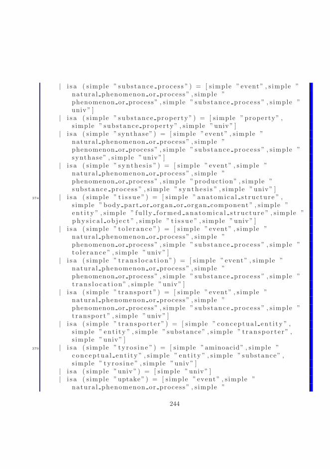
| i s a ( s imple ” subs tance pro ce s s ” ) = [ s imple ” event ” , s imple ”natura l phenomenon or proces s ” , s imple ”phenomenon or process” , s imple ” subs tance pro ce s s ” , s imple ”univ ” ]
| i s a ( s imple ” subs tance prope r ty ” ) = [ s imple ” proper ty” ,s imple ” subs tance prope r ty” , s imple ”univ ” ]
| i s a ( s imple ” synthase” ) = [ s imple ” event” , s imple ”natura l phenomenon or proces s ” , s imple ”phenomenon or process” , s imple ” subs tance pro ce s s ” , s imple ”synthase” , s imple ”univ ” ]
| i s a ( s imple ” s yn th e s i s ” ) = [ s imple ” event” , s imple ”natura l phenomenon or proces s ” , s imple ”phenomenon or process” , s imple ” product ion” , s imple ”subs tance pro ce s s ” , s imple ” s yn th e s i s ” , s imple ”univ ” ]
374 | i s a ( s imple ” t i s s u e ” ) = [ s imple ” ana tomica l s t ruc tur e ” ,s imple ” body par t or organ or organ component ” , s imple ”en t i t y ” , s imple ” fu l l y f o rmed ana tom i c a l s t r u c tu r e ” , s imple ”phy s i c a l o b j e c t ” , s imple ” t i s s u e ” , s imple ”univ ” ]
| i s a ( s imple ” t o l e r an c e ” ) = [ s imple ” event” , s imple ”natura l phenomenon or proces s ” , s imple ”phenomenon or process” , s imple ” subs tance pro ce s s ” , s imple ”t o l e r an c e ” , s imple ”univ ” ]
| i s a ( s imple ” t r a n s l o c a t i o n” ) = [ s imple ” event” , s imple ”natura l phenomenon or proces s ” , s imple ”phenomenon or process” , s imple ” subs tance pro ce s s ” , s imple ”t r a n s l o c a t i o n” , s imple ”univ ” ]
| i s a ( s imple ” t r anspo r t ” ) = [ s imple ” event” , s imple ”natura l phenomenon or proces s ” , s imple ”phenomenon or process” , s imple ” subs tance pro ce s s ” , s imple ”t r anspo r t ” , s imple ”univ ” ]
| i s a ( s imple ” t r an spo r t e r ” ) = [ s imple ” c onc ep tua l e n t i t y ” ,s imple ” en t i t y ” , s imple ” substance” , s imple ” t r an spo r t e r ” ,s imple ”univ ” ]
379 | i s a ( s imple ” ty r o s i n e ” ) = [ s imple ”aminoacid” , s imple ”c onc ep tua l e n t i t y ” , s imple ” en t i t y ” , s imple ” substance” ,s imple ” ty r o s i n e ” , s imple ”univ ” ]
| i s a ( s imple ”univ ” ) = [ s imple ”univ ” ]| i s a ( s imple ”uptake ” ) = [ s imple ” event ” , s imple ”
natura l phenomenon or proces s ” , s imple ”
244

phenomenon or process” , s imple ” subs tance pro ce s s ” , s imple ”univ ” , s imple ”uptake ” ]
| i s a ( s imple ” u t i l i z a t i o n ” ) = [ s imple ” event” , s imple ”natura l phenomenon or proces s ” , s imple ”phenomenon or process” , s imple ” subs tance pro ce s s ” , s imple ”univ ” , s imple ” u t i l i z a t i o n ” ]
| i s a ( s imple ” va s op r e s s i n” ) = [ s imple ” c onc ep tua l e n t i t y ” ,s imple ” en t i t y ” , s imple ” substance” , s imple ”univ ” , s imple ”va s op r e s s i n” ]
384 | i s a ( s imple ”wa l l ” ) = [ s imple ” ana tomica l s t ruc tur e ” , s imple” en t i t y ” , s imple ” fu l l y f o rmed ana tom i c a l s t r u c tu r e ” , s imple” phy s i c a l o b j e c t ” , s imple ”univ ” , s imple ”wa l l ” ]
| i s a ( s imple ”weigth ” ) = [ s imple ” proper ty” , s imple ”univ ” ,s imple ”weigth ” ]
| i s a ( s imple ” z c y t o r 1 7 l i g ” ) = [ s imple ” c onc ep tua l e n t i t y ” ,s imple ” en t i t y ” , s imple ” po l ynuc l e o t i d e” , s imple ” substance” ,s imple ”univ ” , s imple ” z c y t o r 1 7 l i g ” ]
| i s a ( s imple x ) = [ s imple x ]
389 fun i s a chk (x , y ) = L i s t . e x i s t s ( fn z=>z=y ) ( i s a x )
val a data = [ ( s imple ”DUMMY” , r ”dum” , s imple ”DUMMY” ) ,( s imple ” i n f l u e n c e ” , r ” agt” , s imple ” substance” ) ,( s imple ” subs tance pro ce s s ” , r ”pnt” , s imple ”
substance” ) ,394 ( s imple ” i n f l u e n c e ” , r ” agt” , s imple ” l e v e l ” ) ,
( s imple ” i n f l u e n c e ” , r ”pnt” , s imple ”phenomenon or process” ) ,
( s imple ” i n f l u e n c e ” , r ”pnt” , s imple ”ana tomica l s t ruc tur e ” ) ,
( s imple ” phy s i c a l o b j e c t ” , r ” l o c ” , s imple ”ana tomica l s t ruc tur e ” ) ,
( s imple ” phy s i c a l o b j e c t ” , r ” pof ” , s imple ”phy s i c a l o b j e c t ” ) ,
399 ( s imple ” product ion” , r ” agt” , s imple ”ana tomica l s t ruc tur e ” ) ,
( s imple ”phenomenon or process” , r ” l o c ” , s imple ”ana tomica l s t ruc tur e ” ) ,
245

( s imple ” substance” , r ” s r c ” , s imple ”ana tomica l s t ruc tur e ” ) ,
( s imple ” product ion” , r ” s r c ” , s imple ”ana tomica l s t ruc tur e ” ) ,
( s imple ” t r anspo r t ” , r ” v ia ” , s imple ”ana tomica l s t ruc tur e ” ) ,
404 ( s imple ” entry” , r ” agt” , s imple ” substance” ) ,( s imple ” entry” , r ”pnt” , s imple ”
ana tomica l s t ruc tur e ” ) ,( s imple ” entry” , r ” v ia ” , s imple ” t r an spo r t e r ” ) ,( s imple ” l e v e l ” , r ” chr ” , s imple ” p o s i t i o n o n s c a l e ”
) ,( s imple ” substance” , r ” chr ” , s imple ”
subs tance prope r ty ” ) ,409 ( s imple ”phenomenon or process” , r ” chr ” , s imple ”
p r o c e s s p r op e r t y” ) ,( s imple ” ana tomica l s t ruc tur e ” , r ” chr ” , s imple ”
s t r u c tu r e p r ope r t y ” ) ,( s imple ” l e v e l ” , r ”wrt” , s imple ” substance” ) ,( s imple ” l e v e l ” , r ” l o c ” , s imple ”blood ” ) ,( s imple ” t r an spo r t e r ” , r ”wrt” , s imple ” substance” ) ,
414 ( s imple ” g en e r a l p r op e r t y” , r ”wrt” , s imple ”univ ” ) ,( s imple ” i s ” , r ”qqq” , s imple ”univ ” ) ]
fun member (x , ys ) = L i s t . e x i s t s ( fn y=>y=x) ys
419 fun a f f ( sc1 , s c2 ) =l e t
val s c 1 anc e s t o r s = i s a sc1val temp0 = L i s t . f i l t e r ( fn (x , y , z )=>member (x ,
s c 1 anc e s t o r s ) ) a dataval temp1 = L i s t . f i l t e r ( fn (x , y , z )=>i s a chk ( sc2 , z ) )
temp0424 val r o l e s = L i s t .map ( fn (x , y , z )=>y) temp1
inBinaryset . l i s t I t em s ( Binaryset . addList ( Binaryset . empty
ro le compare , r o l e s ) )end
246

429 end
247

248
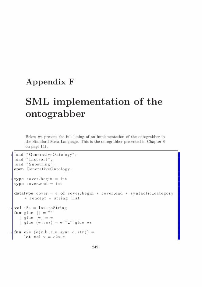
Appendix F
SML implementation of theontograbber
Below we present the full listing of an implementation of the ontograbber inthe Standard Meta Language. This is the ontograbber presented in Chapter 8on page 141.
�
1 load ”GenerativeOntology” ;load ” L i s t s o r t ” ;load ” Substr ing ” ;open GenerativeOntology ;
6 type cove r beg in = in ttype cover end = in t
datatype cover = e of cove r beg in ∗ cover end ∗ s yn ta c t i c c a t e g o r y∗ concept ∗ s t r i n g l i s t
11 val i 2 s = Int . toSt r ingfun g lue [ ] = ””| g lue [w] = w| g lue (w : :ws) = wˆ” ”ˆ g lue ws
16 fun e2s ( e ( c b , c e , synt , c , s t r ) ) =l e t val v = c2s c
249
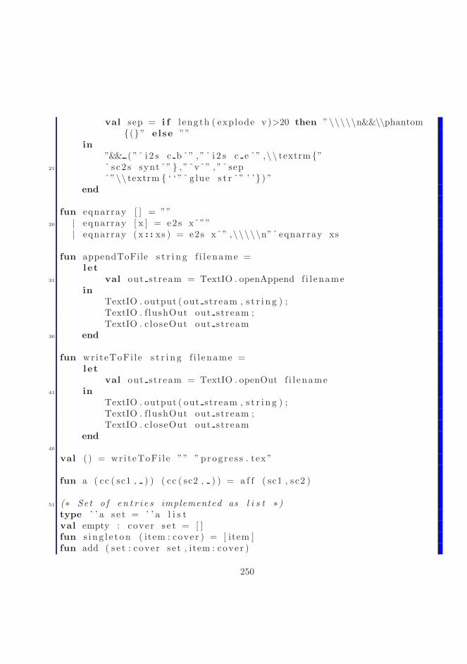
val sep = i f l ength ( explode v )>20 then ”\\\\\n&&\\phantom{(}” else ””
in”&& ( ”ˆ i 2 s c b ˆ” , ”ˆ i 2 s c e ˆ” ,\\ textrm {”
21 ˆ s c2 s synt ˆ” } , ”ˆvˆ” , ”ˆ sepˆ”\\ textrm { ‘ ‘ ”ˆ g lue s t r ˆ” ’ ’} ) ”
end
fun eqnarray [ ] = ””26 | eqnarray [ x ] = e2s xˆ””
| eqnarray (x : : xs ) = e2s xˆ” ,\\\\\n”ˆ eqnarray xs
fun appendToFile s t r i n g f i l ename =l e t
31 val out stream = TextIO . openAppend f i l enamein
TextIO . output ( out stream , s t r i n g ) ;TextIO . f lushOut out stream ;TextIO . c loseOut out stream
36 end
fun wr iteToFi l e s t r i n g f i l ename =l e t
val out stream = TextIO . openOut f i l ename41 in
TextIO . output ( out stream , s t r i n g ) ;TextIO . f lushOut out stream ;TextIO . c loseOut out stream
end46
val ( ) = wr i teToFi l e ”” ” prog r e s s . tex ”
fun a ( cc ( sc1 , ) ) ( cc ( sc2 , ) ) = a f f ( sc1 , s c2 )
51 (∗ Set o f e n t r i e s implemented as l i s t ∗)type ’ ’ a s e t = ’ ’ a l i s tval empty : cover s e t = [ ]fun s i n g l e t on ( item : cover ) = [ item ]fun add ( s e t : cover set , item : cover )
250

56 = i f L i s t . e x i s t s ( fn ( y : cover )=>y=item ) s e t then s e t else item : :s e t
fun addList ( s e t : cover set , [ ] ) = s e t| addList ( se t , ( x : cover ) : : xs ) = add ( addList ( se t , xs ) , x )
fun de l e t e ( se t , item : cover ) = L i s t . f i l t e r ( fn y=>y<>item ) s e tfun l i s t I t em s s e t = s e t
61 val isEmpty = L i s t . nu l lval f i nd = L i s t . f i nd
fun i n i t i a t e sen =l e t
66 fun i [ ] n ( s e t : cover s e t ) = s e t| i (w : :ws) n s e t =
l e tfun h ( ( l i ( synt , c ) ) : l e x i c on i t em ) = ( ( e (n , n , synt , c
, [ w] ) ) : cover )in
71 i ws (n+1) ( addList ( se t ,map h ( l ex w) ) )handle l e x no t found => i ws n s e t
endin
i sen 0 empty76 end
fun best ( cs : cover s e t ) = l e t val SOME(x) = f i nd ( fn =>t rue ) csin x end
fun addRole ( cc ( sc1 , ps1 ) , r o l e , c2 ) = cc ( sc1 , ( r o l e , c2 ) : : ps1 )81
val t a l l =[ fn ( s t r1 , syn ”VP” , c1 , r ” agt” , s t r2 , syn ”NP” , c2 )
=> ( s t r2@str1 , syn ”S” , addRole ( c1 , r ” agt” , c2 ) ) ,fn ( s t r1 , syn ”TV” , c1 , r ”pnt” , s t r2 , syn ”NP” , c2 )
86 => ( s t r1@str2 , syn ”VP” , addRole ( c1 , r ”pnt” , c2 ) ) ,fn ( s t r1 , syn ”N” , c1 , r o l e , s t r2 , syn ”N” , c2 )=> ( s t r2@str1 , syn ”N” , addRole ( c1 , r o l e , c2 ) ) ,
fn ( s t r1 , syn ”NP” , c1 , r ”pnt” , s t r2 , syn ”NP” , c2 )=> ( str1@ [ ” o f ” ] @str2 , syn ”NP” , addRole ( c1 , r ”pnt” , c2 ) ) ,
91 fn ( s t r1 , syn ”NP” , c1 , r ” agt” , s t r2 , syn ”NP” , c2 )
251
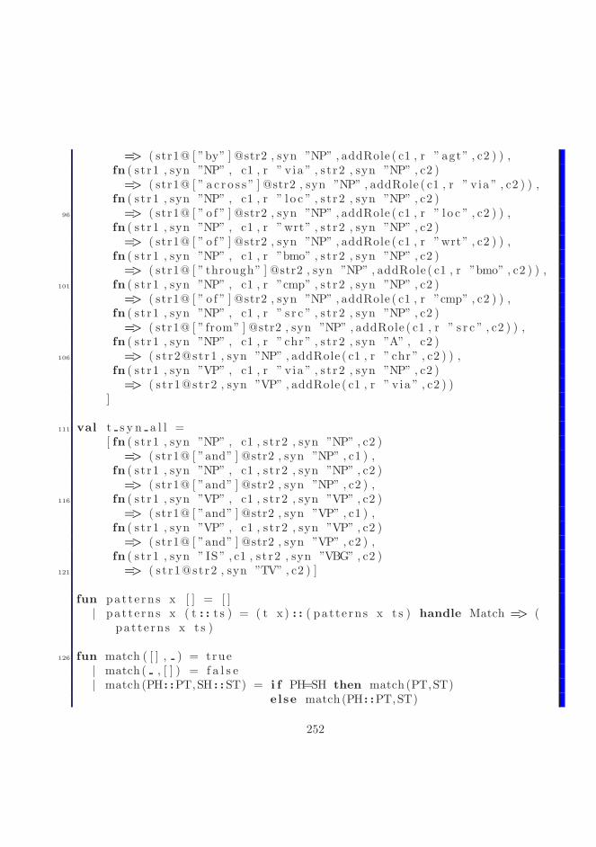
=> ( str1@ [ ”by” ] @str2 , syn ”NP” , addRole ( c1 , r ” agt” , c2 ) ) ,fn ( s t r1 , syn ”NP” , c1 , r ” v ia ” , s t r2 , syn ”NP” , c2 )=> ( str1@ [ ” a c r o s s ” ] @str2 , syn ”NP” , addRole ( c1 , r ” v ia ” , c2 ) ) ,
fn ( s t r1 , syn ”NP” , c1 , r ” l o c ” , s t r2 , syn ”NP” , c2 )96 => ( str1@ [ ” o f ” ] @str2 , syn ”NP” , addRole ( c1 , r ” l o c ” , c2 ) ) ,
fn ( s t r1 , syn ”NP” , c1 , r ”wrt” , s t r2 , syn ”NP” , c2 )=> ( str1@ [ ” o f ” ] @str2 , syn ”NP” , addRole ( c1 , r ”wrt” , c2 ) ) ,
fn ( s t r1 , syn ”NP” , c1 , r ”bmo” , s t r2 , syn ”NP” , c2 )=> ( str1@ [ ” through” ] @str2 , syn ”NP” , addRole ( c1 , r ”bmo” , c2 ) ) ,
101 fn ( s t r1 , syn ”NP” , c1 , r ”cmp” , s tr2 , syn ”NP” , c2 )=> ( str1@ [ ” o f ” ] @str2 , syn ”NP” , addRole ( c1 , r ”cmp” , c2 ) ) ,
fn ( s t r1 , syn ”NP” , c1 , r ” s r c ” , s t r2 , syn ”NP” , c2 )=> ( str1@ [ ” from” ] @str2 , syn ”NP” , addRole ( c1 , r ” s r c ” , c2 ) ) ,
fn ( s t r1 , syn ”NP” , c1 , r ” chr ” , s t r2 , syn ”A” , c2 )106 => ( s t r2@str1 , syn ”NP” , addRole ( c1 , r ” chr ” , c2 ) ) ,
fn ( s t r1 , syn ”VP” , c1 , r ” v ia ” , s t r2 , syn ”NP” , c2 )=> ( s t r1@str2 , syn ”VP” , addRole ( c1 , r ” v ia ” , c2 ) )
]
111 val t s y n a l l =[ fn ( s t r1 , syn ”NP” , c1 , s t r2 , syn ”NP” , c2 )
=> ( str1@ [ ”and” ] @str2 , syn ”NP” , c1 ) ,fn ( s t r1 , syn ”NP” , c1 , s t r2 , syn ”NP” , c2 )=> ( str1@ [ ”and” ] @str2 , syn ”NP” , c2 ) ,
116 fn ( s t r1 , syn ”VP” , c1 , s t r2 , syn ”VP” , c2 )=> ( str1@ [ ”and” ] @str2 , syn ”VP” , c1 ) ,
fn ( s t r1 , syn ”VP” , c1 , s t r2 , syn ”VP” , c2 )=> ( str1@ [ ”and” ] @str2 , syn ”VP” , c2 ) ,
fn ( s t r1 , syn ” IS” , c1 , s t r2 , syn ”VBG” , c2 )121 => ( s t r1@str2 , syn ”TV” , c2 ) ]
fun pa t te rns x [ ] = [ ]| pa t te rns x ( t : : t s ) = ( t x ) : : ( pa t t e rn s x t s ) handle Match => (
pa t t e rn s x t s )
126 fun match ( [ ] , ) = true| match ( , [ ] ) = f a l s e| match (PH: :PT,SH : :ST) = i f PH=SH then match (PT,ST)
else match (PH : :PT,ST)
252

131 fun combine sentence ( e ( c b1 , c e1 , s1 , c1 , s t r 1 ) ,e ( c b2 , c e2 , s2 , c2 , s t r 2 ) ) =
l e tfun n1 r o l e =
l e t136 val pats = pat te rns ( s tr1 , s1 , c1 , r o l e , s t r2 , s2 , c2 )
t a l lval matched = L i s t . f i l t e r ( fn ( pat , syn ’ , c )=> match
( pat , s entence ) ) patsin
map ( fn ( pat , syn ’ , c )=>e ( c b1 , c e2 , syn ’ , c , pat ) )matched
end141 fun n2 r o l e =
l e tval pats = pat te rns ( s tr2 , s2 , c2 , r o l e , s t r1 , s1 , c1 )
t a l lval matched = L i s t . f i l t e r ( fn ( pat , syn ’ , c )=> match
( pat , s entence ) ) patsin
146 map ( fn ( pat , syn ’ , c )=>e ( c b1 , c e2 , syn ’ , c , pat ) )matched
endin
L i s t . concat ( (map n1 ( a c1 c2 ) ) @ (map n2 ( a c2 c1 ) ) )end
151
fun syn combine sentence ( e ( c b1 , c e1 , s1 , c1 , s t r 1 ) ,e ( c b2 , c e2 , s2 , c2 , s t r 2 ) ) =
l e tval pats = pat te rns ( s tr1 , s1 , c1 , s t r2 , s2 , c2 ) t s y n a l l
156 val matched = L i s t . f i l t e r ( fn ( pat , syn ’ , c )=> match ( pat ,s entence ) ) pats
inmap ( fn ( pat , syn ’ , c )=>e ( c b1 , c e2 , syn ’ , c , pat ) ) matched
end
161 val l i f t r u l e = fn syn ”N” => syn ”NP” | => raise Match
253
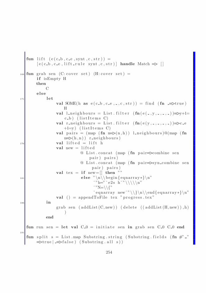
fun l i f t ( e ( c b , c e , synt , c , s t r ) ) =[ e ( c b , c e , l i f t r u l e synt , c , s t r ) ] handle Match => [ ]
166 fun grab sen (C: cover s e t ) (H: cover s e t ) =i f isEmpty Hthen
Celse
171 l e tval SOME(h as e ( c b , c e , , c , s t r ) ) = f i nd ( fn =>t rue )
Hval l n e i g hbou r s = L i s t . f i l t e r ( fn ( e ( , y , , , ) )=>y+1=
c b ) ( l i s t I t em s C)val r ne i ghbour s = L i s t . f i l t e r ( fn ( e (y , , , , ) )=>c e
+1=y) ( l i s t I t em s C)val pa i r s = (map ( fn n=>(n , h ) ) l n e i g hbou r s )@(map ( fn
n=>(h , n ) ) r ne i ghbour s )176 val l i f t e d = l i f t h
val new = l i f t e d@ L i s t . concat (map ( fn pa i r=>combine sen
pa i r ) pa i r s )@ L i s t . concat (map ( fn pa i r=>syn combine sen
pa i r ) pa i r s )val tex = i f new=[ ] then ””
181 else ”\n\\begin { eqnarray∗}\n”ˆ”h=”ˆ e2s hˆ”\\\\\n”ˆ”N=\\{”ˆ eqnarray newˆ”\\}\n\\end{ eqnarray∗}\n”
val ( ) = appendToFile tex ” prog r e s s . tex ”186 in
grab sen ( addList (C, new) ) ( d e l e t e ( ( addList (H, new) ) ,h))
end
fun run sen = l e t val C 0 = i n i t i a t e sen in grab sen C 0 C 0 end191
fun s p l i t s = L i s t .map Substr ing . s t r i n g ( Substr ing . f i e l d s ( fn #” ”=>t rue | =>f a l s e ) ( Substr ing . a l l s ) )
254
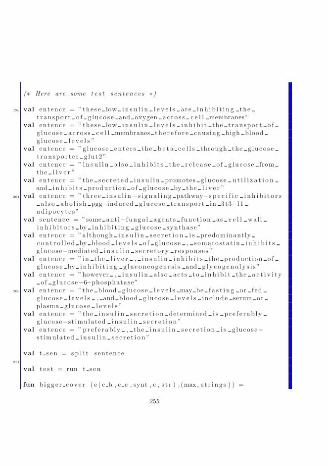
(∗ Here are some t e s t s en t ences ∗)
196 val entence = ” the s e low i n s u l i n l e v e l s a re i n h i b i t i n g thet r anspo r t o f g luco s e and oxygen a c r o s s c e l l membranes”
val entence = ” the s e low i n s u l i n l e v e l s i n h i b i t the t r anspo r t o fg luco s e a c r o s s c e l l membranes t h e r e f o r e caus ing high bloodg luco s e l e v e l s ”
val entence = ” g luco s e en t e r s the b e t a c e l l s through the g luco s et r an spo r t e r g lu t2 ”
val entence = ” i n s u l i n a l s o i n h i b i t s the r e l e a s e o f g luco s e fromthe l i v e r ”
val entence = ” the s e c r e t ed i n s u l i n promotes g luco s e u t i l i z a t i o nand i n h i b i t s product ion o f g luco s e by the l i v e r ”
201 val entence = ” thr e e i n s u l i n−s i g n a l i n g pathway−s p e c i f i c i n h i b i t o r sa l s o abo l i s h pgg−induced g luco s e t r anspo r t in 3 t3−l 1
ad ipocy te s”val sentence = ”some anti−funga l agents func t i on as c e l l wa l l
i n h i b i t o r s by i n h i b i t i n g g luco s e synthase”val entence = ”although i n s u l i n s e c r e t i o n i s predominantly
c o n t r o l l e d by blood l e v e l s o f g luco s e , somatostat in i n h i b i t sg lucose−mediated i n s u l i n s e c r e t o r y r e spons e s ”
val entence = ” in the l i v e r , i n s u l i n i n h i b i t s the product ion o fg luco s e by i n h i b i t i n g g luconeogene s i s and g l y c o g e n o l y s i s ”
val entence = ”however , i n s u l i n a l s o a c t s to i n h i b i t the a c t i v i t yo f g lucose−6−phosphatase”
206 val entence = ” the blood g luco s e l e v e l s may be f a s t i n g or fedg luco s e l e v e l s , and blood g luco s e l e v e l s inc lude serum orplasma g luco s e l e v e l s ”
val entence = ” the i n s u l i n s e c r e t i o n determined i s p r e f e r ab l yg lucose−s t imulated i n s u l i n s e c r e t i o n ”
val entence = ” p r e f e r ab l y , the i n s u l i n s e c r e t i o n i s g lucose−s t imulated i n s u l i n s e c r e t i o n ”
val t s e n = s p l i t s entence211
val t e s t = run t s en
fun b i g g e r c o v e r ( e ( c b , c e , synt , c , s t r ) , (max , s t r i n g s ) ) =
255
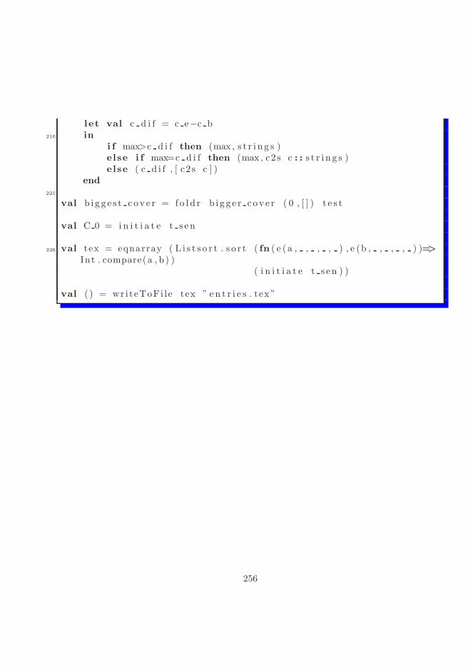
l e t val c d i f = c e−c b216 in
i f max>c d i f then (max , s t r i n g s )else i f max=c d i f then (max , c2s c : : s t r i n g s )else ( c d i f , [ c2 s c ] )
end221
val b i g g e s t c o v e r = f o l d r b i g g e r c o v e r ( 0 , [ ] ) t e s t
val C 0 = i n i t i a t e t s en
226 val tex = eqnarray ( L i s t s o r t . s o r t ( fn ( e ( a , , , , ) , e (b , , , , ) )=>Int . compare(a , b ) )
( i n i t i a t e t s en ) )
val ( ) = wr i teToFi l e tex ” e n t r i e s . tex ”
256

Appendix G
Querying ontologies withProlog – source code
Below the full Prolog code is presented for our “pancreas knowledge base”,together with querying facilities.
�
1 %% Ex p l i c i t in format ion from pancreas diagram :
db c l a s s ( c e l l ) .
db c l a s s ( nervous system ) .6
db c l a s s ( neurona l s chwann ce l l ) .db r ( neurona l s chwann ce l l , i sa , c e l l ) .db r ( neurona l s chwann ce l l , par to f , nervous system ) .
11 db c l a s s ( pancreas ) .
db c l a s s ( s t em c e l l ) .db r ( s t em ce l l , i sa , c e l l ) .
16 db c l a s s ( e x o c r i n e c e l l ) .db r ( e x o c r i n e c e l l , i sa , c e l l ) .db r ( e x o c r i n e c e l l , s e c r e t e , enzyme ) .
257

db c l a s s ( e nd o c r i n e c e l l ) .21 db r ( e nd o c r i n e c e l l , i sa , c e l l ) .
db r ( e nd o c r i n e c e l l , s e c r e t e , hormone ) .
db c l a s s ( p a n c r e a t i c c e l l ) .db r ( p a n c r e a t i c c e l l , i sa , c e l l ) .
26 db r ( p a n c r e a t i c c e l l , l o c a t ed i n , pancreas ) .
db c l a s s ( exoc r ine panc r ea s ) .db r ( exoc r ine panc r ea s , par to f , pancreas ) .
31 db c l a s s ( endoc r ine panc r ea s ) .db r ( endocr ine pancreas , par to f , pancreas ) .
db c l a s s ( a du l t s t em c e l l ) .db r ( adu l t s t em ce l l , i sa , a du l t s t em c e l l ) .
36
db c l a s s ( embryon i c s t em ce l l ) .db r ( embryonic s tem ce l l , i sa , s t em c e l l ) .
db c l a s s ( i s l e t o f l a n g e r h a n s ) .41 db r ( i s l e t o f l a n g e r h a n s , par to f , endoc r ine panc r ea s ) .
db c l a s s ( e x o c r i n e p a n c r e a t i c c e l l ) .db r ( e x o c r i n e p a n c r e a t i c c e l l , i sa , e x o c r i n e c e l l ) .db r ( e x o c r i n e p a n c r e a t i c c e l l , i sa , p a n c r e a t i c c e l l ) .
46 db r ( e x o c r i n e p a n c r e a t i c c e l l , par to f , exo c r ine panc r ea s ) .
db c l a s s ( duct ) .db r ( duct , par to f , exo c r ine panc r ea s ) .
51 db c l a s s ( e nd o c r i n e p a n c r e a t i c c e l l ) .db r ( e nd o c r i n e p a n c r e a t i c c e l l , i sa , e n d o c r i n e c e l l ) .db r ( e nd o c r i n e p a n c r e a t i c c e l l , i sa , p a n c r e a t i c c e l l ) .
db c l a s s ( c a p i l l a r y ) .56 db r ( c ap i l l a r y , par to f , i s l e t o f l a n g e r h a n s ) .
db c l a s s ( c e n t r o a c i n a r c e l l ) .
258

db r ( c e n t r o a c i n a r c e l l , i sa , e x o c r i n e p a n c r e a t i c c e l l ) .db r ( c e n t r o a c i n a r c e l l , s e c r e t e , d i g e s t i v e enzyme ) .
61 db r ( c e n t r o a c i n a r c e l l , p r imary s i gna l , s e c r e t i n ) .
db c l a s s ( a c i n a r c e l l ) .db r ( a c i n a r c e l l , i sa , e x o c r i n e p a n c r e a t i c c e l l ) .db r ( a c i n a r c e l l , s e c r e t e , b i ca rbona te i on ) .
66 db r ( a c i n a r c e l l , p r imary s i gna l , cck ) .
db c l a s s ( a l p h a c e l l ) .db r ( a l pha c e l l , i sa , e n d o c r i n e p a n c r e a t i c c e l l ) .db r ( a l pha c e l l , par to f , i s l e t o f l a n g e r h a n s ) .
71 db r ( a l pha c e l l , s e c r e t e , g lucagon ) .
db c l a s s ( b e t a c e l l ) .db r ( b e t a c e l l , i sa , e n d o c r i n e p a n c r e a t i c c e l l ) .db r ( b e t a c e l l , par to f , i s l e t o f l a n g e r h a n s ) .
76 db r ( b e t a c e l l , s e c r e t e , i n s u l i n ) .
db c l a s s ( gamma cell ) .db r ( gamma cell , i sa , e n d o c r i n e p a n c r e a t i c c e l l ) .db r ( gamma cell , par to f , i s l e t o f l a n g e r h a n s ) .
81 db r ( gamma cell , s e c r e t e , g a s t r i n ) .db r ( gamma cell , s e c r e t e , somatostat in ) .
db c l a s s ( p p c e l l ) .db r ( pp c e l l , i sa , e n d o c r i n e p a n c r e a t i c c e l l ) .
86 db r ( pp c e l l , par to f , i s l e t o f l a n g e r h a n s ) .db r ( pp c e l l , s e c r e t e , p anc r e a t i c po l yp ep t i d e ) .
db c l a s s ( g lucagon ) .
91 db c l a s s ( i n s u l i n ) .
db c l a s s ( g a s t r i n ) .
db c l a s s ( somatostat in ) .96
db c l a s s ( panc r e a t i c po l yp ep t i d e ) .
259
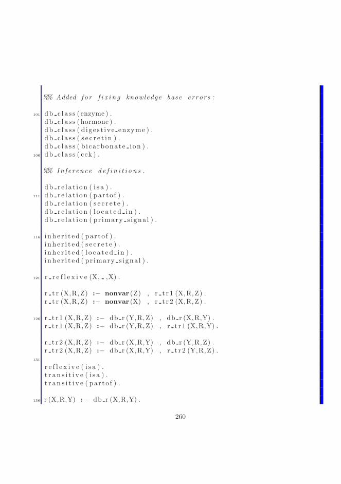
%% Added f o r f i x i n g knowledge base er ror s :
101 db c l a s s ( enzyme ) .db c l a s s ( hormone ) .db c l a s s ( d i g e s t i v e enzyme ) .db c l a s s ( s e c r e t i n ) .db c l a s s ( b i ca rbona te i on ) .
106 db c l a s s ( cck ) .
%% In ference d e f i n i t i o n s .
db r e l a t i o n ( i s a ) .111 db r e l a t i o n ( pa r to f ) .
db r e l a t i o n ( s e c r e t e ) .db r e l a t i o n ( l o c a t e d i n ) .db r e l a t i o n ( pr imary s i gna l ) .
116 i n h e r i t e d ( pa r to f ) .i n h e r i t e d ( s e c r e t e ) .i n h e r i t e d ( l o c a t e d i n ) .i n h e r i t e d ( pr imary s i gna l ) .
121 r r e f l e x i v e (X, ,X) .
r t r (X,R, Z) :− nonvar (Z) , r t r 1 (X,R, Z) .r t r (X,R, Z) :− nonvar (X) , r t r 2 (X,R, Z) .
126 r t r 1 (X,R,Z) :− db r (Y,R, Z) , db r (X,R,Y) .r t r 1 (X,R,Z) :− db r (Y,R, Z) , r t r 1 (X,R,Y) .
r t r 2 (X,R,Z) :− db r (X,R,Y) , db r (Y,R, Z) .r t r 2 (X,R,Z) :− db r (X,R,Y) , r t r 2 (Y,R, Z) .
131
r e f l e x i v e ( i s a ) .t r a n s i t i v e ( i s a ) .t r a n s i t i v e ( pa r to f ) .
136 r (X,R,Y) :− db r (X,R,Y) .
260
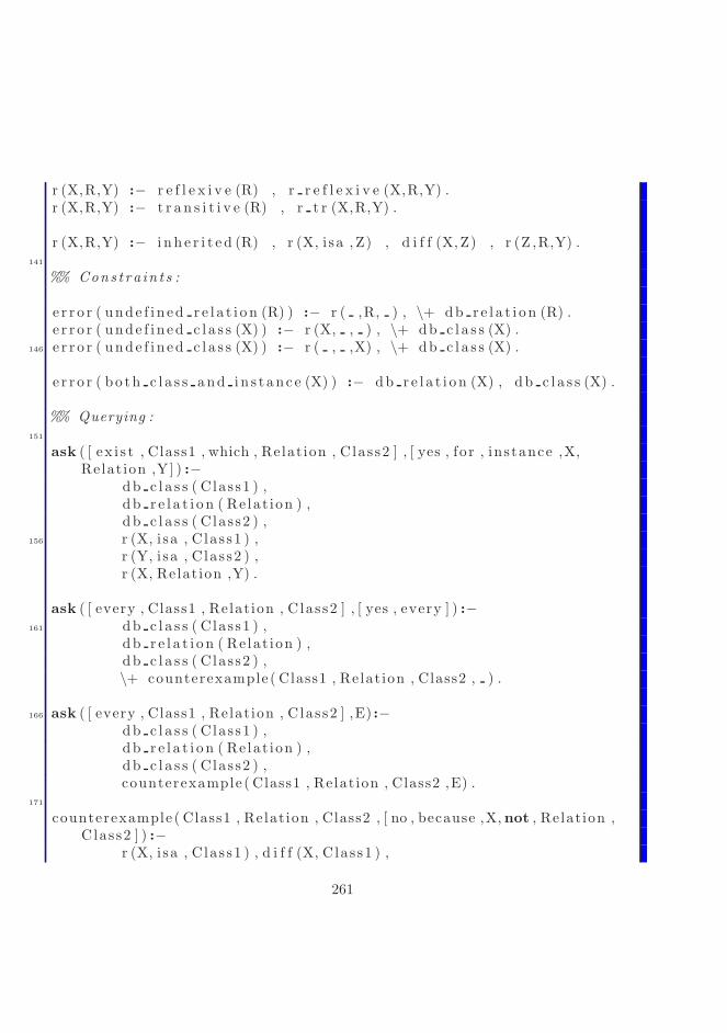
r (X,R,Y) :− r e f l e x i v e (R) , r r e f l e x i v e (X,R,Y) .r (X,R,Y) :− t r a n s i t i v e (R) , r t r (X,R,Y) .
r (X,R,Y) :− i n h e r i t e d (R) , r (X, i sa , Z) , d i f f (X, Z) , r (Z ,R,Y) .141
%% Cons t ra in t s :
e r r o r ( unde f i n ed r e l a t i o n (R) ) :− r ( ,R, ) , \+ db r e l a t i o n (R) .e r r o r ( unde f i n ed c l a s s (X) ) :− r (X, , ) , \+ db c l a s s (X) .
146 e r r o r ( unde f i n ed c l a s s (X) ) :− r ( , ,X) , \+ db c l a s s (X) .
e r r o r ( bo th c l a s s and i n s t an c e (X) ) :− db r e l a t i o n (X) , db c l a s s (X) .
%% Querying :151
ask ( [ ex i s t , Class1 , which , Relat ion , Clas s2 ] , [ yes , fo r , ins tance ,X,Relat ion ,Y] ) :−
db c l a s s ( Clas s1 ) ,db r e l a t i o n ( Re la t ion ) ,db c l a s s ( Clas s2 ) ,
156 r (X, i sa , Clas s1 ) ,r (Y, i sa , Clas s2 ) ,r (X, Relat ion ,Y) .
ask ( [ every , Class1 , Relat ion , Clas s2 ] , [ yes , every ] ) :−161 db c l a s s ( Clas s1 ) ,
db r e l a t i o n ( Re la t ion ) ,db c l a s s ( Clas s2 ) ,\+ counterexample ( Class1 , Relat ion , Class2 , ) .
166 ask ( [ every , Class1 , Relat ion , Clas s2 ] ,E) :−db c l a s s ( Clas s1 ) ,db r e l a t i o n ( Re la t ion ) ,db c l a s s ( Clas s2 ) ,counterexample ( Class1 , Relat ion , Class2 ,E) .
171
counterexample ( Class1 , Relat ion , Class2 , [ no , because ,X, not , Relat ion ,Clas s2 ] ) :−
r (X, i sa , Clas s1 ) , d i f f (X, Clas s1 ) ,
261

no t r (X, Relat ion , Clas s2 ) .
176 no t r (X,R,Y) :− \+ r (X,R,Y) .
d i f f (X,Y) :− \+ eq (X,Y) .eq (X,X) .
262

Appendix H
Open–source licensing ofthe ontograbber
The following is a discussion on the topic of possibility of releasing the ontograb-ber under an open–source license.
The Ontograbber is an algorithm which associates ontological semantics withsentences. The retrieved ontological information takes the form of nodes in thegenerative ontology represented by so–called ‘concept covers’. The result of thealgoritmic analysis of a sentence is a collection of ontoterms.
H.1 What is free software?
The Free Software Foundation has defined what a free software is:“Free software is a matter of the users’ freedom to run, copy, distribute,
study, change and improve the software. More precisely, it means that theprogram’s users have the four essential freedoms:
• The freedom to run the program, for any purpose (freedom 0).
• The freedom to study how the program works, and change it to make itdo what you wish (freedom 1). Access to the source code is a preconditionfor this.
• The freedom to redistribute copies so you can help your neighbor (freedom2).
263
• The freedom to distribute copies of your modified versions to others (free-dom 3). By doing this you can give the whole community a chance tobenefit from your changes. Access to the source code is a precondition forthis.”
H.2 Why is Ontograbber a good candidate forbecoming a free software?
The software developed in a academic environment, e.g. during a PhD studieshas some unique characteristics as compared to a commercially developed soft-ware. The internal workings of the software are usually a public knowledge,described in detail in scientific papers and the thesis itself. Companies, on theother hand try to hide as much information as possible concerning the internalworkings of the software they develop. They usually claim that this is to pro-tect their trade secrets. In reality many companies do not allow people to lookinto the source code of their products due to poor programming practices andquality of the underlying design.
Since there is usually nothing to hide with academic software, this paperexplores the possibility of releasing such a software as free software.
H.3 Community benefits
The free software enjoys a large community of people who use it. Those peoplefor historical reasons have mostly very high computer skills. Many of them getinvolved in the development of the software and its environment. The wayspeople get involved is usually one of the following:
• They use the software, and if they encounter a bug, they report it. Sincethese are usually highly skilled users, the bug reports tend to be verydetailed and of good quality. In return for reporting the bug, people canget a fix for it.
• They write documentation. This can e.g. take the form of a WIKI, whereusers themselves document the software. The motivation for doing thatmight be: “You (developers) better concentrate on developing the soft-ware, while we (users) will document it for you.” People realize that ifthey take the burden of writing the documentation off the developers, thesoftware will be developed more quickly.
264
• They discuss and support. It is much easier for users to get support for afree software product than for a closed alternative. This is because there isa lot of other users of the software that are ready to share their knowledgeand help when there are problems. This can take the form of a mailinglist, a forum website, Internet Relay Chat, or a local user group. Help isusually provided promptly, sometimes in minutes after a question is asked.At the Technical University of Denmark we have a “Linux User Group”,which meets at regular intervals.
• They develop the software. People with programming skills often will offerto fix a bug themselves. They might send a patch together with a bugreport. There is also a community of “bug squashers”, who follow the bugreports and donate their free time by fixing known issues.
H.4 Why do free software communities form?
The reasons people get involved in free software communities are the following:
• They get the software for free, based on hard work of others. They wantto contribute back in return.
• They want to learn. Getting involved in a open source project is a greatway of learning or mastering programming skills. One can also learnhow large software projects are managed successfully, e.g. those involvingthousands of programmers.
• They make money on the product. E.g. a company that uses the Linuxoperating system kernel as part of their commercial product might need toextend it in some way in order to use it successfully in their product. Theymay e.g. write a new device driver for hardware that they have developed.
• They want to be a part of a friendly community. People are social beings.They need to belong to some communities. People with high computerskills are very likely to feel well in a free software community.
H.5 Main types of open source software licenses
1. Freedom–preserving licenses. These licenses preserve the basic liberties ofthe free software. This means that the receipient of the software covered
265
by such a license cannot in any way turn it into non–free software. Themost commonly used license in this group is the GNU General PublicLicense.
2. Permissive licenses. These licenses allow the receipient of a open sourcesoftware to turn it into non-free software or even a completely closed soft-ware and distribute it further as such. Why would anybody need that?This commonly occurs when some company wants to use some open sourcesoftware product or library as part of their commercial product, withoutthe combining product becoming an open source product. The most com-mon licences of this group are GNU Lesser General Public License andBSD software license.
H.6 Business models for free software and open
source software
H.6.1 Donations
It is very common for free software to accept donations from users who wouldlike to support the project or the developers financially.
H.6.2 Double licensing
Many companies currently involved in the free software business make moneyon the so–called double licensing. This is a business model where exactly thesame product is provided as both a free–licensed one and as a closed–licensedone.
The free–licensed product is usually given away for free to anybody whowants it. This helps building a large community of users, wide–spreading andadvertising the software. The developers can also get a lot back from thoseusers, e.g. free documentation, free bug reports, or even fixes for them, and freesupport for other users of this software.
The closed–licensed product is sold to customers who need a closed licensefor some reason.
H.6.3 Support
Many companies developing free software are giving copies of the software andits source code for free, while charging users for optional support with respect
266
to the software. Many customers, including most corporate customers need aguarantee of professional support when they decide to use a product. Free soft-ware vendors may be selling time–limited access to such a support. Techniciansproviding such a support may solve it using on–line communication, telephone,or by visiting the customer.
H.6.4 Extra information
Many free software developers make money not on the product itself, but onthe information about it. It is quite common for a developer to write a bookdescribing a particular free software. Information vending can also take form ofconsulting, conducting courses or workshops, etc.
H.6.5 Bounties
Some free software developers propose to add a requested extension to an ex-isting product for some financial compensation, called a bounty. If a user is inneed of a particular fix/extension, she may consider paying such a bounty sothat the developers will solve her problems quickly.
H.7 Conclusion
We believe that the Ontograbber is well–fit for becoming a free software. Eventhough it would be released to any interested party for free, there still existbusiness models that allow the developing team to generate revenue.
267

268
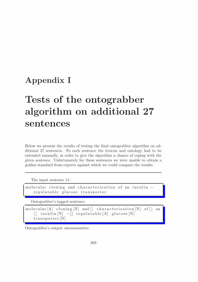
Appendix I
Tests of the ontograbberalgorithm on additional 27sentences
Below we present the results of testing the final ontograbber algorithm on ad-ditional 27 sentences. Fo each sentence the lexicon and ontology had to beextended manually, in order to give the algorithm a chance of coping with thegiven sentence. Unfortunately for these sentences we were unable to obtain agolden standard from experts against which we could compare the results.
The input sentence 11:�
molecu la r c l on ing and c h a r a c t e r i z a t i o n o f an i n s u l i n −r e gu l a t ab l e g luco s e t r an spo r t e r
Ontograbber’s tagged sentence:�
molecu la r [A] c l on ing [N] and [ ] c h a r a c t e r i z a t i o n [N] o f [ ] an[ ] i n s u l i n [N] − [ ] r e g u l a t ab l e [A] g luco s e [N]t r an spo r t e r [N]
Ontograbber’s output ontosemantics:
269

• (0,2,NP,cloning[chr: molecular
],“molecular cloning and characterization”)
• (0,2,NP,characterization,“molecular cloning and characterization”)
• (3,3,NP,insulin,“insulin”)
• (4,4,A,regulatable,“regulatable”)
• (5,6,NP,transporter[wrt: glucose
],“glucose transporter”)
The input sentence 12:�
g lucok ina s e i s the l i k e l y mediator o f g luco s ens ing inboth g luco s e − e x c i t e d and g luco s e − i n h i b i t e d c en t r a lneurons
Ontograbber’s tagged sentence:�
g lucok ina s e [N] i s [ IS ] the [ ] l i k e l y [ ] mediator [N] o f [ ]g luco s ens ing [N] in [ ] both [ ] g luco s e [N] − [ ] e x c i t e d [VBDVBN] and [ ] g luco s e [N] − [ ] i n h i b i t e d [VBD VBN] c en t r a l [
A] neurons [N]
Ontograbber’s output ontosemantics:
• (0,0,NP,glucokinase,“glucokinase”)
• (1,1,IS,is,“is”)
• (2,2,NP,mediator,“mediator”)
• (3,3,NP,glucosensing,“glucosensing”)
• (4,9,NP,neuron
[chr: centralpntof: inhibition
[agt: glucose
]
]
,“glucose - excited and glu-
cose - inhibited central neurons”)
• (4,9,NP,neuron
chr: central
pntof: inhibition
[agt: glucoseagt: glucose
]
,“glucose - excited and glu-
cose - inhibited central neurons”)
270

• (4,9,NP,neuron
[chr: centralpntof: excitement
[agt: glucose
]
]
,“glucose - excited and glu-
cose - inhibited central neurons”)
The input sentence 13:�
p r e f e r ab l y , the i n s u l i n s e c r e t i o n i s g luco s e −s t imulated i n s u l i n s e c r e t i o n
Ontograbber’s tagged sentence:�
p r e f e r ab l y [ ] , [ , ] the [ ] i n s u l i n [N] s e c r e t i o n [N] i s [ IS ]g luco s e [N] − [ ] s t imulated [VBD VBN] i n s u l i n [N]s e c r e t i o n [N]
Ontograbber’s output ontosemantics:
• (0,0,,,nil,“,”)
• (1,5,PSV,stimulation
[agt: glucosepnt: secretion
[pnt: insulin
]
]
,“ insulin secretion is glu-
cose - stimulated”)
• (3,7,PSV,stimulation
[agt: glucosepnt: secretion
[pnt: insulin
]
]
,“ insulin secretion is glu-
cose - stimulated”)
The input sentence 14:�
the entry o f g luco s e in to the ad ipocyte r e q u i r e s thea c t i v i t y o f the i n s u l i n s e n s i t i v e g luco s e t r an spo r t e r s
Ontograbber’s tagged sentence:�
the [ ] entry [N] o f [ ] g luco s e [N] in to [ ] the [ ] ad ipocyte [N]r e q u i r e s [TV] the [ ] a c t i v i t y [N] o f [ ] the [ ] i n s u l i n [N]s e n s i t i v e [A] g luco s e [N] t r an spo r t e r s [N]
271
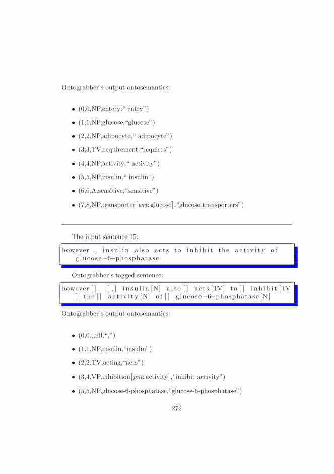
Ontograbber’s output ontosemantics:
• (0,0,NP,entery,“ entry”)
• (1,1,NP,glucose,“glucose”)
• (2,2,NP,adipocyte,“ adipocyte”)
• (3,3,TV,requirement,“requires”)
• (4,4,NP,activity,“ activity”)
• (5,5,NP,insulin,“ insulin”)
• (6,6,A,sensitive,“sensitive”)
• (7,8,NP,transporter[wrt: glucose
],“glucose transporters”)
The input sentence 15:�
however , i n s u l i n a l s o a c t s to i n h i b i t the a c t i v i t y o fg lucose−6−phosphatase
Ontograbber’s tagged sentence:�
however [ ] , [ , ] i n s u l i n [N] a l s o [ ] a c t s [TV] to [ ] i n h i b i t [TV] the [ ] a c t i v i t y [N] o f [ ] g lucose−6−phosphatase [N]
Ontograbber’s output ontosemantics:
• (0,0,,,nil,“,”)
• (1,1,NP,insulin,“insulin”)
• (2,2,TV,acting,“acts”)
• (3,4,VP,inhibition[pnt: activity
],“inhibit activity”)
• (5,5,NP,glucose-6-phosphatase,“glucose-6-phosphatase”)
272
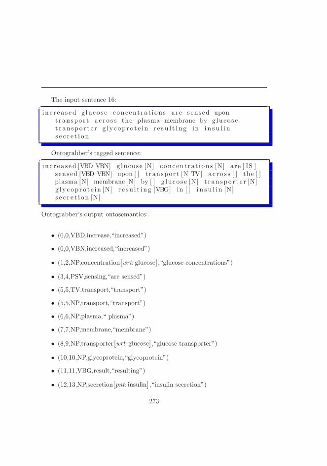
The input sentence 16:�
i n c r e a s ed g luco s e concent r a t i ons are sensed upont ranspo r t a c r o s s the plasma membrane by g luco s et r an spo r t e r g l y c op r o t e i n r e s u l t i n g in i n s u l i ns e c r e t i o n
Ontograbber’s tagged sentence:�
i n c r e a s ed [VBD VBN] g luco s e [N] concent r a t i ons [N] are [ IS ]s ensed [VBD VBN] upon [ ] t r anspo r t [N TV] a c r o s s [ ] the [ ]plasma [N] membrane [N] by [ ] g luco s e [N] t r an spo r t e r [N]g l y c op r o t e i n [N] r e s u l t i n g [VBG] in [ ] i n s u l i n [N]s e c r e t i o n [N]
Ontograbber’s output ontosemantics:
• (0,0,VBD,increase,“increased”)
• (0,0,VBN,increased,“increased”)
• (1,2,NP,concentration[wrt: glucose
],“glucose concentrations”)
• (3,4,PSV,sensing,“are sensed”)
• (5,5,TV,transport,“transport”)
• (5,5,NP,transport,“transport”)
• (6,6,NP,plasma,“ plasma”)
• (7,7,NP,membrane,“membrane”)
• (8,9,NP,transporter[wrt: glucose
],“glucose transporter”)
• (10,10,NP,glycoprotein,“glycoprotein”)
• (11,11,VBG,result,“resulting”)
• (12,13,NP,secretion[pnt: insulin
],“insulin secretion”)
273
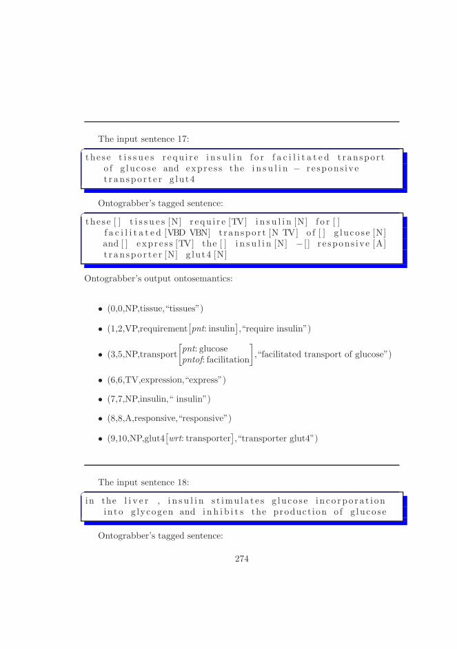
The input sentence 17:�
the s e t i s s u e s r e qu i r e i n s u l i n f o r f a c i l i t a t e d t r anspo r to f g luco s e and expr e s s the i n s u l i n − r e spons iv et r an spo r t e r g lu t4
Ontograbber’s tagged sentence:�
the s e [ ] t i s s u e s [N] r e qu i r e [TV] i n s u l i n [N] f o r [ ]f a c i l i t a t e d [VBD VBN] t r anspo r t [N TV] o f [ ] g luco s e [N]and [ ] expr e s s [TV] the [ ] i n s u l i n [N] − [ ] r e spons iv e [A]t r an spo r t e r [N] g lu t4 [N]
Ontograbber’s output ontosemantics:
• (0,0,NP,tissue,“tissues”)
• (1,2,VP,requirement[pnt: insulin
],“require insulin”)
• (3,5,NP,transport
[pnt: glucosepntof: facilitation
]
,“facilitated transport of glucose”)
• (6,6,TV,expression,“express”)
• (7,7,NP,insulin,“ insulin”)
• (8,8,A,responsive,“responsive”)
• (9,10,NP,glut4[wrt: transporter
],“transporter glut4”)
The input sentence 18:�
in the l i v e r , i n s u l i n s t imu l a t e s g luco s e i n c o r po r a t i onin to g lycogen and i n h i b i t s the product ion o f g luco s e
Ontograbber’s tagged sentence:
274
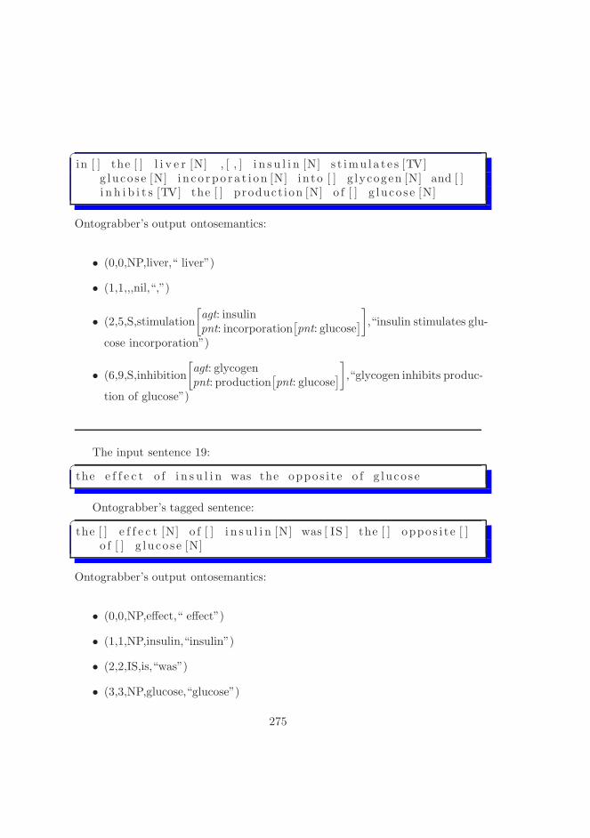
�
in [ ] the [ ] l i v e r [N] , [ , ] i n s u l i n [N] s t imu l a t e s [TV]g luco s e [N] i n c o r po r a t i on [N] in to [ ] g lycogen [N] and [ ]i n h i b i t s [TV] the [ ] product ion [N] o f [ ] g luco s e [N]
Ontograbber’s output ontosemantics:
• (0,0,NP,liver,“ liver”)
• (1,1,,,nil,“,”)
• (2,5,S,stimulation
[agt: insulinpnt: incorporation
[pnt: glucose
]
]
,“insulin stimulates glu-
cose incorporation”)
• (6,9,S,inhibition
[agt: glycogenpnt: production
[pnt: glucose
]
]
,“glycogen inhibits produc-
tion of glucose”)
The input sentence 19:�
the e f f e c t o f i n s u l i n was the oppo s i t e o f g luco s e
Ontograbber’s tagged sentence:�
the [ ] e f f e c t [N] o f [ ] i n s u l i n [N] was [ IS ] the [ ] oppo s i t e [ ]o f [ ] g luco s e [N]
Ontograbber’s output ontosemantics:
• (0,0,NP,effect,“ effect”)
• (1,1,NP,insulin,“insulin”)
• (2,2,IS,is,“was”)
• (3,3,NP,glucose,“glucose”)
275
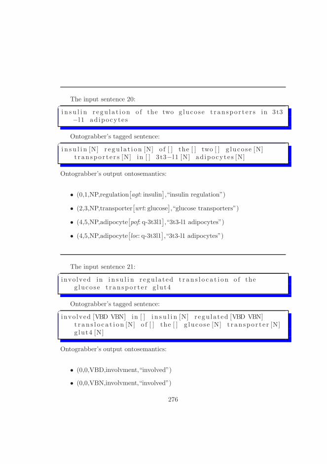
The input sentence 20:�
i n s u l i n r e gu l a t i o n o f the two g luco s e t r an spo r t e r s in 3t3−l 1 ad ipocy te s
Ontograbber’s tagged sentence:�
i n s u l i n [N] r e gu l a t i o n [N] o f [ ] the [ ] two [ ] g luco s e [N]t r an spo r t e r s [N] in [ ] 3 t3−l 1 [N] ad ipocy te s [N]
Ontograbber’s output ontosemantics:
• (0,1,NP,regulation[agt: insulin
],“insulin regulation”)
• (2,3,NP,transporter[wrt: glucose
],“glucose transporters”)
• (4,5,NP,adipocyte[pof: q-3t3l1
],“3t3-l1 adipocytes”)
• (4,5,NP,adipocyte[loc: q-3t3l1
],“3t3-l1 adipocytes”)
The input sentence 21:�
invo lved in i n s u l i n r egu la t ed t r a n s l o c a t i o n o f theg luco s e t r an spo r t e r g lu t4
Ontograbber’s tagged sentence:�
invo lved [VBD VBN] in [ ] i n s u l i n [N] r egu la t ed [VBD VBN]t r a n s l o c a t i o n [N] o f [ ] the [ ] g luco s e [N] t r an spo r t e r [N]g lu t4 [N]
Ontograbber’s output ontosemantics:
• (0,0,VBD,involvment,“involved”)
• (0,0,VBN,involvment,“involved”)
276
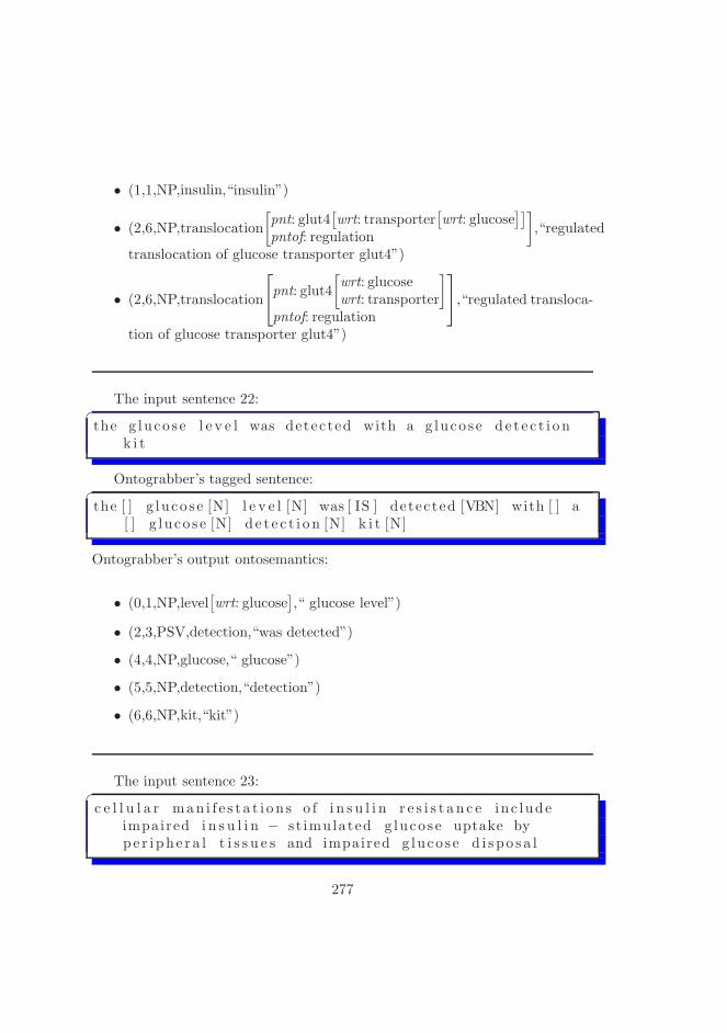
• (1,1,NP,insulin,“insulin”)
• (2,6,NP,translocation
[pnt: glut4
[wrt: transporter
[wrt: glucose
]]
pntof: regulation
]
,“regulated
translocation of glucose transporter glut4”)
• (2,6,NP,translocation
pnt: glut4
[wrt: glucosewrt: transporter
]
pntof: regulation
,“regulated transloca-
tion of glucose transporter glut4”)
The input sentence 22:�
the g luco s e l e v e l was detected with a g luco s e d e t e c t i o nk i t
Ontograbber’s tagged sentence:�
the [ ] g luco s e [N] l e v e l [N] was [ IS ] detected [VBN] with [ ] a[ ] g luco s e [N] d e t e c t i o n [N] k i t [N]
Ontograbber’s output ontosemantics:
• (0,1,NP,level[wrt: glucose
],“ glucose level”)
• (2,3,PSV,detection,“was detected”)
• (4,4,NP,glucose,“ glucose”)
• (5,5,NP,detection,“detection”)
• (6,6,NP,kit,“kit”)
The input sentence 23:�
c e l l u l a r man i f e s t a t i o n s o f i n s u l i n r e s i s t a n c e inc ludeimpaired i n s u l i n − s t imulated g luco s e uptake bype r i ph e r a l t i s s u e s and impaired g luco s e d i s po s a l
277
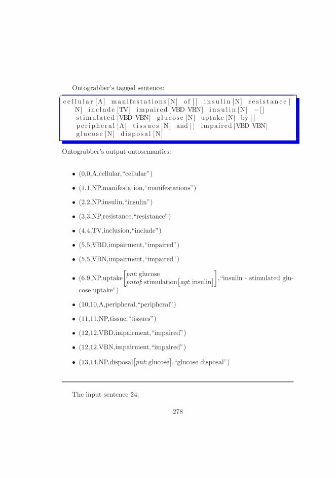
Ontograbber’s tagged sentence:�
c e l l u l a r [A] man i f e s t a t i o n s [N] o f [ ] i n s u l i n [N] r e s i s t a n c e [N] inc lude [TV] impaired [VBD VBN] i n s u l i n [N] − [ ]s t imulated [VBD VBN] g luco s e [N] uptake [N] by [ ]p e r i ph e r a l [A] t i s s u e s [N] and [ ] impaired [VBD VBN]g luco s e [N] d i s po s a l [N]
Ontograbber’s output ontosemantics:
• (0,0,A,cellular,“cellular”)
• (1,1,NP,manifestation,“manifestations”)
• (2,2,NP,insulin,“insulin”)
• (3,3,NP,resistance,“resistance”)
• (4,4,TV,inclusion,“include”)
• (5,5,VBD,impairment,“impaired”)
• (5,5,VBN,impairment,“impaired”)
• (6,9,NP,uptake
[pnt: glucosepntof: stimulation
[agt: insulin
]
]
,“insulin - stimulated glu-
cose uptake”)
• (10,10,A,peripheral,“peripheral”)
• (11,11,NP,tissue,“tissues”)
• (12,12,VBD,impairment,“impaired”)
• (12,12,VBN,impairment,“impaired”)
• (13,14,NP,disposal[pnt: glucose
],“glucose disposal”)
The input sentence 24:
278

�
high g luco s e l e v e l s promote i n s u l i n r e s i s t a n c e , andi n s u l i n r e s i s t a n c e g ene ra te s pro longed e l e v a t i o n s o fserum g luco s e concent r a t i on
Ontograbber’s tagged sentence:�
high [A] g luco s e [N] l e v e l s [N] promote [TV] i n s u l i n [N]r e s i s t a n c e [N] , [ , ] and [ ] i n s u l i n [N] r e s i s t a n c e [N]g ene ra te s [TV] pro longed [VBN] e l e v a t i o n s [ ] o f [ ] serum [N] g luco s e [N] concent r a t i on [N]
Ontograbber’s output ontosemantics:
• (0,2,NP,level
[chr: highwrt: glucose
]
,“high glucose levels”)
• (3,3,TV,promotion,“promote”)
• (4,4,NP,insulin,“insulin”)
• (5,5,NP,resistance,“resistance”)
• (6,6,,,nil,“,”)
• (7,7,NP,insulin,“insulin”)
• (8,8,NP,resistance,“resistance”)
• (9,9,TV,generation,“generates”)
• (10,10,VBN,prolongation,“prolonged”)
• (11,11,NP,serum,“serum”)
• (12,13,NP,concentration[wrt: glucose
],“glucose concentration”)
The input sentence 25:�
in the l i v e r , i n s u l i n i n h i b i t s the r e l e a s e o f g luco s efrom glycogen and the s yn th e s i s o f new g luco s e
279
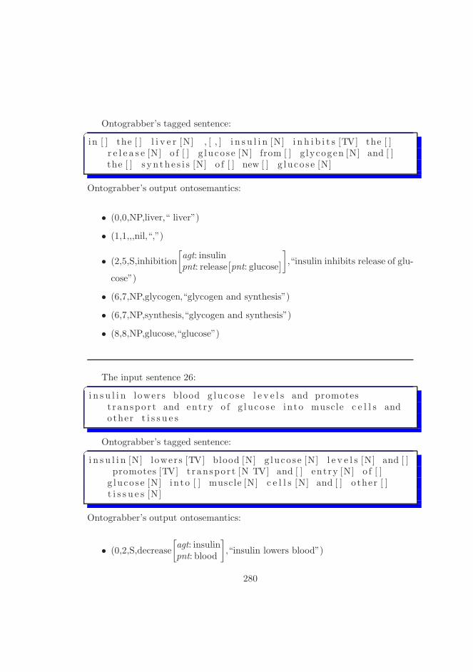
Ontograbber’s tagged sentence:�
in [ ] the [ ] l i v e r [N] , [ , ] i n s u l i n [N] i n h i b i t s [TV] the [ ]r e l e a s e [N] o f [ ] g luco s e [N] from [ ] g lycogen [N] and [ ]the [ ] s yn th e s i s [N] o f [ ] new [ ] g luco s e [N]
Ontograbber’s output ontosemantics:
• (0,0,NP,liver,“ liver”)
• (1,1,,,nil,“,”)
• (2,5,S,inhibition
[agt: insulinpnt: release
[pnt: glucose
]
]
,“insulin inhibits release of glu-
cose”)
• (6,7,NP,glycogen,“glycogen and synthesis”)
• (6,7,NP,synthesis,“glycogen and synthesis”)
• (8,8,NP,glucose,“glucose”)
The input sentence 26:�
i n s u l i n lower s blood g luco s e l e v e l s and promotest r anspo r t and entry o f g luco s e in to muscle c e l l s andother t i s s u e s
Ontograbber’s tagged sentence:�
i n s u l i n [N] lower s [TV] blood [N] g luco s e [N] l e v e l s [N] and [ ]promotes [TV] t r anspo r t [N TV] and [ ] entry [N] o f [ ]
g luco s e [N] in to [ ] muscle [N] c e l l s [N] and [ ] o ther [ ]t i s s u e s [N]
Ontograbber’s output ontosemantics:
• (0,2,S,decrease
[agt: insulinpnt: blood
]
,“insulin lowers blood”)
280
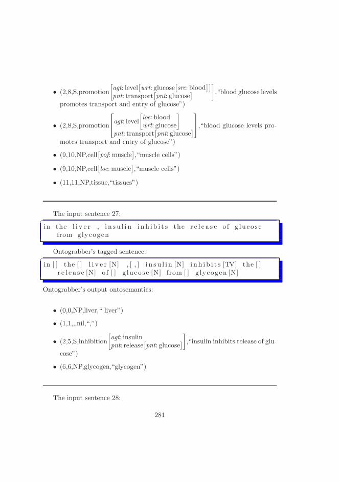
• (2,8,S,promotion
[agt: level
[wrt: glucose
[src: blood
]]
pnt: transport[pnt: glucose
]
]
,“blood glucose levels
promotes transport and entry of glucose”)
• (2,8,S,promotion
agt: level
[loc: bloodwrt: glucose
]
pnt: transport[pnt: glucose
]
,“blood glucose levels pro-
motes transport and entry of glucose”)
• (9,10,NP,cell[pof: muscle
],“muscle cells”)
• (9,10,NP,cell[loc: muscle
],“muscle cells”)
• (11,11,NP,tissue,“tissues”)
The input sentence 27:�
in the l i v e r , i n s u l i n i n h i b i t s the r e l e a s e o f g luco s efrom glycogen
Ontograbber’s tagged sentence:�
in [ ] the [ ] l i v e r [N] , [ , ] i n s u l i n [N] i n h i b i t s [TV] the [ ]r e l e a s e [N] o f [ ] g luco s e [N] from [ ] g lycogen [N]
Ontograbber’s output ontosemantics:
• (0,0,NP,liver,“ liver”)
• (1,1,,,nil,“,”)
• (2,5,S,inhibition
[agt: insulinpnt: release
[pnt: glucose
]
]
,“insulin inhibits release of glu-
cose”)
• (6,6,NP,glycogen,“glycogen”)
The input sentence 28:
281

�
add i t i on o f name to the incubat ion mixture i n h i b i t e d thei n s u l i n − mimicking e f f e c t o f a l l im in on both g luco s et r anspo r t and g luco s e ox ida t i on
Ontograbber’s tagged sentence:�
add i t i on [N] o f [ ] name [ ] to [ ] the [ ] incubat ion [N] mixture [N] i n h i b i t e d [VBD VBN] the [ ] i n s u l i n [N] − [ ] mimicking [ ]e f f e c t [N] o f [ ] a l l im in [N] on [ ] both [ ] g luco s e [N]
t r anspo r t [N TV] and [ ] g luco s e [N] ox ida t i on [N]
Ontograbber’s output ontosemantics:
• (0,0,NP,addition,“addition”)
• (1,1,NP,incubation,“ incubation”)
• (2,2,NP,mixture,“mixture”)
• (3,3,VBD,inhibition,“inhibited”)
• (3,3,VBN,inhibition,“inhibited”)
• (4,4,NP,insulin,“ insulin”)
• (5,5,NP,effect,“effect”)
• (6,6,NP,allimin,“allimin”)
• (7,10,NP,transport[pnt: glucose
],“glucose transport and glucose oxidation”)
• (7,10,NP,oxidation[pnt: glucose
],“glucose transport and glucose oxidation”)
The input sentence 29:�
the g luco s e formed i s then t r anspo r t ed by the g luco s ec a r r i e r o f the organism
Ontograbber’s tagged sentence:
282

�
the [ ] g luco s e [N] formed [VBD VBN] i s [ IS ] then [ ]t r anspo r t ed [VBD VBN] by [ ] the [ ] g luco s e [N] c a r r i e r [N]o f [ ] the [ ] organism [N]
Ontograbber’s output ontosemantics:
• (0,0,NP,glucose,“ glucose”)
• (1,1,VBD,forming,“formed”)
• (1,1,VBN,forming,“formed”)
• (2,3,PSV,transport,“is transported”)
• (4,5,NP,carrier[wrt: glucose
],“ glucose carrier”)
• (6,6,NP,organism,“ organism”)
The input sentence 30:�
a sma l l e r auc f o r g luco s e ( sma l l e r blood g luco s eexcur s i on a f t e r g luco s e cha l l e ng e ) i n d i c a t e s b e t t e rg luco s e t o l e r an c e
Ontograbber’s tagged sentence:�
a [ ] sma l l e r [A] auc [N] f o r [ ] g luco s e [N] ( [ ] sma l l e r [A]blood [N] g luco s e [N] excur s i on [N] a f t e r [ ] g luco s e [N]cha l l e ng e [N] ) [ ] i n d i c a t e s [TV] b e t t e r [ ] g luco s e [N]t o l e r an c e [N]
Ontograbber’s output ontosemantics:
• (0,0,A,smaller,“smaller”)
• (1,1,NP,auc,“auc”)
• (2,2,NP,glucose,“glucose”)
283
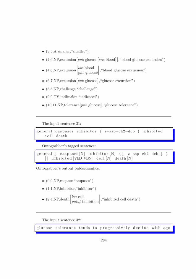
• (3,3,A,smaller,“smaller”)
• (4,6,NP,excursion[pnt: glucose
[src: blood
]],“blood glucose excursion”)
• (4,6,NP,excursion
[loc: bloodpnt: glucose
]
,“blood glucose excursion”)
• (6,7,NP,excursion[pnt: glucose
],“glucose excursion”)
• (8,8,NP,challenge,“challenge”)
• (9,9,TV,indication,“indicates”)
• (10,11,NP,tolerance[pnt: glucose
],“glucose tolerance”)
The input sentence 31:�
gene ra l ca spa s e s i n h i b i t o r ( z−asp−ch2−dcb ) i n h i b i t e dc e l l death
Ontograbber’s tagged sentence:�
gene ra l [ ] c a spa s e s [N] i n h i b i t o r [N] ( [ ] z−asp−ch2−dcb [ ] )[ ] i n h i b i t e d [VBD VBN] c e l l [N] death [N]
Ontograbber’s output ontosemantics:
• (0,0,NP,caspase,“caspases”)
• (1,1,NP,inhibitor,“inhibitor”)
• (2,4,NP,death
[loc: cellpntof: inhibition
]
,“inhibited cell death”)
The input sentence 32:�
g luco s e t o l e r an c e tends to p r o g r e s s i v e l y d e c l i n e with age
284
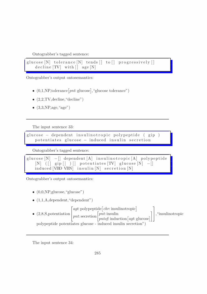
Ontograbber’s tagged sentence:�
g luco s e [N] t o l e r an c e [N] tends [ ] to [ ] p r o g r e s s i v e l y [ ]d e c l i n e [TV] with [ ] age [N]
Ontograbber’s output ontosemantics:
• (0,1,NP,tolerance[pnt: glucose
],“glucose tolerance”)
• (2,2,TV,decline,“decline”)
• (3,3,NP,age,“age”)
The input sentence 33:�
g luco s e − dependent i n s u l i n o t r o p i c po lypept ide ( g ip )po t en t i a t e s g luco s e − induced i n s u l i n s e c r e t i o n
Ontograbber’s tagged sentence:�
g luco s e [N] − [ ] dependent [A] i n s u l i n o t r o p i c [A] po lypept ide[N] ( [ ] g ip [ ] ) [ ] p o t en t i a t e s [TV] g luco s e [N] − [ ]induced [VBD VBN] i n s u l i n [N] s e c r e t i o n [N]
Ontograbber’s output ontosemantics:
• (0,0,NP,glucose,“glucose”)
• (1,1,A,dependent,“dependent”)
• (2,8,S,potentiation
agt: polypeptide[chr: insulinotropic
]
pnt: secretion
[pnt: insulinpntof: induction
[agt: glucose
]
]
,“insulinotropic
polypeptide potentiates glucose - induced insulin secretion”)
The input sentence 34:
285
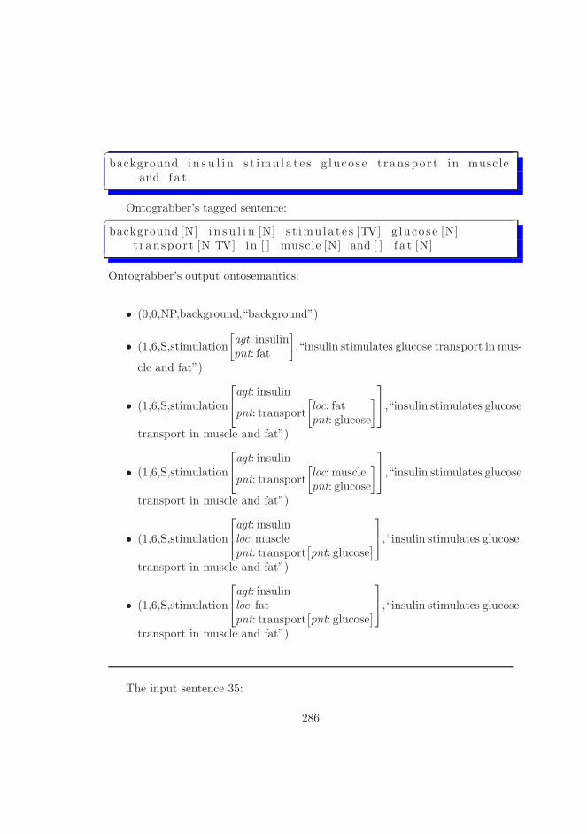
�
background i n s u l i n s t imu l a t e s g luco s e t r anspo r t in muscleand f a t
Ontograbber’s tagged sentence:�
background [N] i n s u l i n [N] s t imu l a t e s [TV] g luco s e [N]t r anspo r t [N TV] in [ ] muscle [N] and [ ] f a t [N]
Ontograbber’s output ontosemantics:
• (0,0,NP,background,“background”)
• (1,6,S,stimulation
[agt: insulinpnt: fat
]
,“insulin stimulates glucose transport in mus-
cle and fat”)
• (1,6,S,stimulation
agt: insulin
pnt: transport
[loc: fatpnt: glucose
]
,“insulin stimulates glucose
transport in muscle and fat”)
• (1,6,S,stimulation
agt: insulin
pnt: transport
[loc: musclepnt: glucose
]
,“insulin stimulates glucose
transport in muscle and fat”)
• (1,6,S,stimulation
agt: insulinloc: musclepnt: transport
[pnt: glucose
]
,“insulin stimulates glucose
transport in muscle and fat”)
• (1,6,S,stimulation
agt: insulinloc: fatpnt: transport
[pnt: glucose
]
,“insulin stimulates glucose
transport in muscle and fat”)
The input sentence 35:
286

�
most o f the compounds which i n h i b i t t y r o s i n ephosphory la t ion o f the i n s u l i n r e c epto r a l s o i n h i b i t e dg luco s e uptake in the same c e l l s
Ontograbber’s tagged sentence:�
most [ ] o f [ ] the [ ] compounds [N] which [ ] i n h i b i t [TV]ty r o s i n e [N] phosphory la t ion [N] o f [ ] the [ ] i n s u l i n [N]r e c epto r [N] a l s o [ ] i n h i b i t e d [VBD VBN] g luco s e [N]uptake [N] in [ ] the [ ] same [ ] c e l l s [N]
Ontograbber’s output ontosemantics:
• (0,0,NP,compound,“ compounds”)
• (1,1,TV,inhibition,“inhibit”)
• (2,2,NP,tyrosine,“tyrosine”)
• (3,3,NP,phosphorylation,“phosphorylation”)
• (4,4,NP,insulin,“ insulin”)
• (5,5,NP,receptor,“receptor”)
• (6,8,NP,uptake
[pnt: glucosepntof: inhibition
]
,“inhibited glucose uptake”)
• (9,9,NP,cell,“cells”)
The input sentence 36:�
i n h i b i t i o n o f z c y t o r 1 7 l i g a c t i v i t y could thus i n h i b i tgrowth o f such c e l l s
Ontograbber’s tagged sentence:�
i n h i b i t i o n [N] o f [ ] z c y t o r 1 7 l i g [N] a c t i v i t y [N] could [ ]thus [ ] i n h i b i t [TV] growth [N] o f [ ] such [ ] c e l l s [N]
287

Ontograbber’s output ontosemantics:
• (0,0,NP,inhibition,“inhibition”)
• (1,1,NP,zcytor17lig,“zcytor17lig”)
• (2,2,NP,activity,“activity”)
• (3,4,VP,inhibition[pnt: growth
],“inhibit growth”)
• (5,5,NP,cell,“cells”)
The input sentence 37:�
the t r anspo r t o f g luco s e a c r o s s a c e l l u l a r membrane i ss t imulated by i n s u l i n b ind ing to i t s i n s u l i n r e c epto ras part o f an i n s u l i n s i g n a l l i n g pathway
Ontograbber’s tagged sentence:�
the [ ] t r anspo r t [N TV] o f [ ] g luco s e [N] a c r o s s [ ] a [ ]c e l l u l a r [A] membrane [N] i s [ IS ] s t imulated [VBD VBN] by[ ] i n s u l i n [N] b ind ing [N VBG] to [ ] i t s [ ] i n s u l i n [N]r e c epto r [N] as [ ] part [ ] o f [ ] an [ ] i n s u l i n [N]s i g n a l l i n g [ ] pathway [N]
Ontograbber’s output ontosemantics:
• (0,1,NP,transport[pnt: glucose
],“ transport of glucose”)
• (2,2,A,cellular,“cellular”)
• (3,6,PSV,stimulation
[agt: insulinpnt: membrane
]
,“membrane is stimulated by insulin”)
• (7,7,VBG,binding,“binding”)
• (7,7,NP,binding,“binding”)
288

• (8,8,NP,insulin,“ insulin”)
• (9,9,NP,receptor,“receptor”)
• (10,10,NP,insulin,“ insulin”)
• (11,11,NP,pathway,“pathway”)
289

290
Bibliography
[1] Troels Andreasen and Jørgen Fischer Nilsson. Grammatical specificationof domain ontologies. Data Knowl. Eng., 48(2):221–230, 2004.
[2] P. Andrews. Classical type theory, 2001. Peter Andrews. Classical typetheory. In Alan Robinson and Andrei Voronkov, editors, Handbook of Au-tomated Reasoning,volume 2, chapter 15, pages 965-1007. North-Holland,2001. 43.
[3] Peter B. Andrews. An introduction to mathematical logic and type theory:to truth through proof. Academic Press Professional, Inc., San Diego, CA,USA, 1986.
[4] John Aycock and Nigel Horspool. Practical earley parsing, 2002.
[5] F. Baader and W. Nutt. Basic description logics, 2003.
[6] Collin F. Baker, Charles J. Fillmore, and John B. Lowe. The berkeleyframenet project. In Proceedings of the 17th international conference onComputational linguistics, pages 86–90, Morristown, NJ, USA, 1998. Asso-ciation for Computational Linguistics.
[7] Collin F. Baker and Hiroaki Sato. The framenet data and software. In ACL’03: Proceedings of the 41st Annual Meeting on Association for Computa-tional Linguistics, pages 161–164, Morristown, NJ, USA, 2003. Associationfor Computational Linguistics.
[8] M. Ben-Ari. Mathematical logic for computer science. Prentice-Hall, Inc.,Upper Saddle River, NJ, USA, 1993.
[9] Gilad Ben-Avi and Nissim Francez. Categorial grammar with ontology-refined types. In Proceedings of CG04, 2004.
291
[10] Patrick Blackburn and Johan Bos. Representation and Inference for Nat-ural Language. A First Course in Computational Semantics. CSLI Publi-cations, 2005.
[11] Sergey Brin and Lawrence Page. The anatomy of a large-scale hypertextualweb search engine. Computer Networks and ISDN Systems, 30(1–7):107–117, 1998.
[12] Chris Brink, Katarina Britz, and Renate A. Schmidt. Peirce algebras. For-mal Aspects of Computing, 6(3):339–358, April 1994. Also available asResearch Report MPI-I-92-229, Max-Planck-Institut fr Informatik, Saar-brcken, Germany (July 1992), and as Research Report RR 140, Depart-ment of Mathematics, University of Cape Town, Cape Town, South Africa(August 1992). An extended abstract appears in Nivat, M., Rattray, C.,Rus, T. and Scollo, G. (eds) , Algebraic Methodology and Software Tech-nology (AMAST’93): Proceedings of the 3rd International Conference onAlgebraic Methodology and Software Technology. Workshops in ComputingSeries, Springer-Verlag, London, 165-168 (1994).
[13] Bob Carpenter. Type-logical semantics. MIT Press, Cambridge, MA, USA,1998.
[14] Wikipedia contributors. Alexius meinong.http://en.wikipedia.org/wiki/Alexius Meinong.
[15] Wikipedia contributors. Frame semantics.http://en.wikipedia.org/wiki/Frame semantics (linguistics).
[16] Andrew Dolbey, Michael Ellsworth, and Jan Scheffczyk. Bioframenet: Adomain-specific framenet extension with links to biomedical ontologies. InOlivier Bodenreider, editor, KR-MED, volume 222 of CEUR WorkshopProceedings. CEUR-WS.org, 2006.
[17] Chris Fox. The Ontology of Language: properties, individuals and discourse.Lecture Notes of The Center for the Study of Language and Information(CSLI). The Center for the Study of Language and Information (CSLI),2000.
[18] L. T. F. Gamut. Logic, Language and Meaning, volume 1. University ofChicago Press, 1991.
292
[19] Peter Gardenfors. Conceptual Spaces: The Geometry of Thought. The MITPress, Cambridge, Massachusetts, 2000.
[20] Peter Gerstl and Simone Pribbeenow. Midwinters, end games, and bodyparts: a classification of part–whole relation. In Human-Computer Studies,pages 865–889, 1995.
[21] Peter Gerstl and Simone Pribbenow. Midwinters, end games, and bodyparts: a classification of part-whole relations. Int. J. Hum.-Comput. Stud.,43(5-6):865–889, 1995.
[22] Roxana Girju, Dan Moldovan, Marta Tatu, and Daniel Antohe. On thesemantics of noun compounds. Comput. Speech Lang., 19(4):479–496, 2005.
[23] Asuncion Gomez-Perez, Oscar Corcho, and Mariano Fernandez-Lopez. On-tological Engineering : with examples from the areas of Knowledge Man-agement, e-Commerce and the Semantic Web. First Edition (Advanced In-formation and Knowledge Processing). Springer, July 2004.
[24] P. A. Jensen and J. F. Nilsson. Ontology-based semantics for prepositions.In Syntax and Semantics of Prepositions, Text, Speech and Language Tech-nology, Vol. 29. Springer, 2006.
[25] Daniel Jurafsky and James H. Martin. Speech and Language Processing(2nd Edition) (Prentice Hall Series in Artificial Intelligence). PrenticeHall, 2 edition, 2008.
[26] Edward L. Keenan and Leonard M. Faltz. Boolean Semantics for NaturalLanguage. Reidel., Dordrecht, 1986.
[27] Douglas Lenat. Cyc: A large-scale investment in knowledge infrastructure.Communications of the ACM, 38(11):33–38, November 1995.
[28] Godehard Link. Algebraic semantics for natural language: some philosophy,some application. Int. J. Hum.-Comput. Stud., 43(5-6):765–784, 1995.
[29] Dave MacQueen. The standard ml of new jersey website.http://www.smlnj.org/index.html.
[30] Matt McGee. searchengineland.com. http://searchengineland.com/by-the-numbers-twitter-vs-facebook-vs-google-buzz-36709.
293

[31] Robin Milner, Mads Tofte, and Robert Harper. The Definition of StandardML. MIT Press, Cambridge, MA, USA, 1990.
[32] J. F. Nilsson. Ontological constitutions for classes and properties. InP. Øhrstrøm H. Schaerfe, P. Hitzler, editor, 14th Int. Conf. on Concep-tual Structures, ICCS 2006, Lecture Notes in Artificial Intelligence LNAI4068. Springer, 2006.
[33] Sergei Nirenburg and Victor Raskin. Ontological Semantics. Language,Speech, and Communication. MIT Press, Cambridge, Mass., 2004.
[34] R. T. Oehrle, E. Bach, and D. Wheeler. Categorial Grammars and NaturalLanguage Structures. Reidel, Dordrecht, 1988.
[35] F. Pereira and S. Shieber. Prolog and natural-language analysis. Stanford: Center for the Study of Language and Information, 1987.
[36] Benjamin C. Pierce. Types and programming languages. MIT Press, Cam-bridge, MA, USA, 2002.
[37] The Mercury Project. The mercury project benchmarks.http://www.mercury.cs.mu.oz.au/information/benchmarks.html.
[38] Jørgen Fischer Nilsson and Nikolaj Oldager. Introduction to orders andlattices. 2002.
[39] Josef Ruppenhofer, Michael Ellsworth, Miriam R. L. Petruck, Christo-pher R. Johnson, and Jan Scheffczyk. FrameNet II: Extended theory andpractice. Technical report, ICSI, 2005.
[40] Sag, T. Wasow, and E. Bender. Syntactic Theory: a formal introduction,Second Edition. 2003.
[41] B Smith and C Rosse. The role of foundational relations in the alignment ofbiomedical ontologies. In MEDINFO 2004. Proceedings of the 11th WorldCongress on Medical Informatics; 2004 Sep 7-11. IOS Press, 2004.
[42] Barry Smith. Beyond concepts: Ontology as reality representation.
[43] Holger Stenzhorn. Basic formal ontology website. http://www.ifomis.uni-saarland.de/bfo/.
[44] Author unknown. The mercury project introduction.http://www.cs.mu.oz.au/research/mercury/.
294

[45] Author unknown. Obo foundry website. http://obofoundry.org/.
[46] Jørgen Villadsen. Nabla: A Linguistic System based on Type Theory. Lit,2010.
[47] Christopher A. Welty and David A. Ferrucci. What’s in an instance?
[48] Dominic Widdows. Geometry and Meaning. CLSI Publications, Stanford,CA, USA, 2004.
[49] Mauhab Zareh. Framenet frequently asked questions.http://framenet.icsi.berkeley.edu/.
295