Artificial Intelligence 90 ( 1997) 13% 176

Artificial Intelligence

Computing answers with model elimination * Peter Baumgartner * , Ulrich Furbach I, Frieder Stolzenburg 2

Department of Computer Science, University of Koblenz, Rheinau 1, D-56075 Koblenz, Germany

Received November 1995; revised April 1996

Abstract

We demonstrate that theorem provers using model elimination (ME) can be used as answer- complete interpreters for disjunctive logic programming. More specifically, we introduce a family of restart variants of model elimination, and we introduce a mechanism for computing answers. Building on this, we develop a new calculus called ancestry restart ME. This variant admits a more restrictive regularity restriction than restart ME, and, as a side-effect, it is in particular attractive for computing definite answers. The presented calculi can also be used successfully in the context of automated theorem proving. We demonstrate experimentally that it is more difficult to compute nontrivial answers to goals than to prove the existence of answers. @ 1997 Elsevier Science B.V.

Keywords: Automated reasoning; Theorem proving; Model elimination; Logic programming; Computing answers

In first-order automatic theorem proving one is interested in the question whether a

given formula follows logically from a set of axioms. This is a rather artificial task; whenever one is interested in solving real problems it is often necessary to compute answers for given questions. It appears to us, that in automated theorem proving this

aspect has been pushed to the background. For instance, the statements of the puzzle problems in the TPTP library [33] also include their solutions in most cases, and the prover has only to verify them; however, it is much more interesting and more difficult

to find a solution than to prove correctness of a given one.

*This research was sponsored by the “Deutsche Forschungsgemeinschaft (DFG)” within the “Schwerpunktprogramm Deduktion”. A predecessor version of this paper appeared in Proceedings of the 14th International Joint Conference on ArtQicial Intelligence, Montreal, Que (1995) 335-340. * Corresponding author. E-mail: peter@informatik.uni-koblenzde. ’ E-mail: uli@informatik.uni-koblenzde. 2 E-mail: stolzen@informatik.uni-koblenz.de.

0004-3702/97/$17.00 @ 1997 Elsevier Science B.V. All rights reserved. PII SOOO4-3702( 96)00042-2

136 I? Baumgartner et al./Art@cial Intelligence 90 (1997) 135-I 76

In the early days, when automated theorem provers were understood as tools for real world problem solving, this problem was apparent: of course the textbook monkey was not interested whether there is a solution of the monkey and banana problem; it was merely interested in finding a way to reach the banana hanging on the ceiling. In [8] there is a whole chapter on question answering, where, for example, the work of Green

on question answering [ 131 is reviewed thoroughly. We feel that this aspect is not given sufficient attention in modern theorem proving literature.

In the logic programming area, the computation of answers has always been an im-

portant aspect. From there we learned that it is more difficult to prove a calculus to be answer-complete than only refutationally complete. Recently, there has been consid-

erable effort to use full first-order logic instead of only Horn clauses as the basis of logic programming [ 211. This (positive) disjunctive logic programming approach is in- vestigated from various directions. From the view of theorem proving one is concerned with modifying theorem provers such that they can be used as interpreters for logic programming purposes. The nonmonotonic reasoning community is working on finding appropriate semantics for disjunctive logic programs with negation, and from a database

viewpoint one is concerned with finding bottom-up approaches to computations. The aim of this paper is twofold: Firstly, we prove that theorem provers using model

elimination (ME) can be used as answer-complete interpreters for disjunctive logic pro-

gramming. Secondly, we demonstrate that in the context of automated theorem proving

it is more difficult to compute nontrivial answers to goals than to prove the existence of answers. We furthermore investigate mechanisms for finding most specific answers which give us the most concise information. Technically speaking this means, we are looking for the most definite or shortest disjunctive answers with the most general

variable substitutions. Concerning the first aspect, it is important to note that there is a lot of work towards

model theoretic semantics of positive disjunctive logic programs, and of course there

are numerous proposals for nonmonotonic extensions. However, with respect to proof theory, the situation is not so clear. At first glance one might be convinced that any first-

order theorem prover can be used for the interpretation of disjunctive logic programs,

since a program clause Al V . . . V A,, + B1 A . . . A B, is a representation of the clause

A1 V . . .V A,, V -Bl V . . .V TB,. The notions program and clause will be defined formally in Section 1.2. Indeed, in [ 181 SLI resolution is used as a calculus for disjunctive logic programming. From logic programming with Horn clauses, however, we learn that for

a procedural interpretation of program clauses it is crucial that clauses can only be accessed by the literals Ai, i.e., by the head literals. Technically, this means that only

those contrapositives are allowed to be used which contain a positive literal in the head. The approach from [ 181 completely ignores this aspect by using SLI resolution which requires all contrapositives.

There are proposals for first-order proof calculi using program clauses in only this procedural reading, e.g. Plaisted’s problem reduction formats [27], or the near-Horn Prolog family introduced by Loveland and his co-workers [22]. For a thorough discus-

sion we refer to [ 41. These approaches introduce new calculi or proof procedures, for which efficient implementations still have to be developed. Our aim is to modify ME such that it can be used for logic programming in the above sense. We introduce various

f? Baumgartner et al./Arttj?cial Intelligence 90 (1997) 135-176 137

refinements of restart model elimination and finally arrive at a calculus which supports a procedural reading of first-order program clauses.

This gives us the possibility to use existing theorem provers for disjunctive logic programming. As a first step towards this goal, we introduced in [4] the restart variant of ME and proved its refutational completeness. In this paper, we restate restart model elimination together with its variants. We furthermore give a ground completeness proof of its weakest variant, which gives us the basis of properly introducing an answer

computing mechanism into restart model elimination (RME). Furthermore we define

a variant called ancestry RME which allows extended regularity checking (i.e., loop

checking) w.r.t. the ordinary RME. Additionally this variant prefers proofs which permit definite answers.

For the second aspect, namely computing answers, we adapted our implementation of the RME variants-the PROTEIN system [ 51 -for answer computing as described below. We demonstrate with some of Smullyan’s puzzles [ 301 that it is more difficult to

compute answers than to prove unsatisfiability. Finally we give a comparative study of high performance theorem provers, including CYITER [ 251, SATCHMO [ 241, SETHEO

[ 161, and PROTEIN [5].

1. Model elimination and the restart variants

Model elimination, as originally introduced by Loveland in [ 191, plays a central role in our approach. We will introduce various variants, and especially we will use

as a formal starting point the restart model elimination calculus as introduced in [4].

Furthermore we will discuss how the calculus can be used for logic programming purposes by introducing refinements.

In the following subsection we informally describe a tableau-based variant of model elimination for the propositional case, and in the rest of this section we introduce our

calculi in a formal way for the first-order case.

1.1. Tableau model elimination

In this subsection we use the clause notation, mirroring the fact that we review a

calculus which is, as it stands, not suited for programming purposes. We use an ME calculus that differs from the original one presented in [ 191. It is described in [ 161 as

the base for the prover SETHEO. In [ 31 this calculus is discussed in detail by presenting it in a consolution style [ 111 and compared to various other calculi. ME, in this sense, manipulates trees by extension and reduction steps.

Example 1. In order to recall the calculus consider the clause set

A model elimination refutation is depicted in Fig. 1 (left side). It is obtained by successive fanning with clauses from the input set (extension steps). Additionally, it

138 P: Baumgarhler et al. /Artificial Intelligence 90 (1997) 135-l 76

P Q ;A * * A\

P Q TP Q * -k * *

,/7A /y

P Q /py * *

P Q I

,j \,

\ * * I Goal \

in ‘\ 1P -Q I * n,

Q -lP * *

Fig. I Model elimination (left side) versus restart model elimination (right side). In order not to overload the notation, positive Goal nodes are not displayed.

is required that every inner node is complementary to one of its sons. Such sons are annotated with a “A” in Fig. 1. A dashed arrow indicates a reduction step, i.e., the

closing of a branch due to a branch literal complementary to the leaf literal. Extension and reduction steps are allowed at any leaf of the tree and for extension steps any literal

from an input clause can be used to form a complementary pair of literals. For example, in the right subtree of Fig. 1 (left side) the clause {-P, Q} was used to extend the positive leaf P, i.e., we used the program clause Q +- P via the body literal P and hence dispensed with a procedural reading of the clause.

Now we show how restart model elimination treats Example 1. As a preliminary step,

the input clause set has to be transformed into what we call Goal normal form: every purely negative clause is conjoined with the new literal Goal. Thus, in the example, we replace (7P, TQ} by {Goal, TP, TQ}. Further, as query the unit clause TGoal is used.

Fig. 1 (right side) displays a restart model elimination refutation. Besides using the goal normal form, the only difference is that extension steps at positive literals are not

allowed; instead either a reduction step is carried out, or else the root literal-which is always -Goal-is copied, and then an extension follows.

These simple modifications obviously allow only extension steps with a positive, i.e., a head literal of a clause, and hence support a procedural reading of program clauses. In the following subsection we give a formal presentation of the calculus along the lines

of [3].

1.2. Restart model elimination (RME)

We will state some basic definitions. A clause is a multiset of literals, usually written as the disjunction L1 V . . ’ V L,. Clauses can be alternatively represented with an arrow. AIv. ’ -VA,,, +- BIA, ’ ./\B, is a representation of the clause AlV.. .VA,VlBlV. . *V-B,,, where the A and B are atoms. Clauses with m 2 1 are called program clauses with

P Baumgarmer et al./Artijicial Intelligence 90 (1997) 135-176 139

head literals Ai and body literals Bi, if present. Clauses of the form + BI A ’ ’ ’ A B, are called negative clauses in the sequel.

In Section 3 below we will restrict clause sets to programs, which consist of program clauses only; but this distinction is not needed now. However, from now on we assume our clause sets to be in Goal normal form, i.e., there exists only one negative clause which furthermore does not contain variables. Without loss of generality this can be achieved by introducing a new clause +-- Goal where Goal is a new predicate symbol, and by replacing every purely negative clause 7B1 V . . . V TB, by Goal +- B1, . . . , B,.

We are now turning towards the calculus. Throughout this paper, we consider a variant of ME which uses so-called ME tableaux as basic proof objects, see [ 151, rather than

ME chains [ 201.

Definition 2 (Literal tree, branch, etc. ) . A literal tree T is a pair (t, A) consisting of

a finite, ordered tree t and a labelling function A that assigns a literal to every node of t. Nodes are classified as positive or negative, as given by the polarity of the assigned literals. If 6 is a substitution, then T6 denotes the literal tree which is obtained from literal tree T by application of 6 to the labels of all nodes of T. That is, if T = (t, A) then TS = (t, A’), where A’(N) = (A(N) )S for every node N in T.

A branch of length n for a given literal T is a sequence [NO . Nt . . . . . N,,] (n > 0, written as indicated) of nodes in T such that NO is the root of T, Ni is the immediate

predecessor of Ni+t for 0 < i < n, and N, is a leaf of T; the functions First and Leaf return the first, respectively last node of a branch, i.e., First( [NO . Nt . . . . . N,,] ) = NO

andLeqf([Na.Nt...:N,])=N,.

Throughout this paper, the letter N is used for nodes, and the symbols P, q are used for branches; like branches, branch-valued variables are also written with brackets, as in

[PI. For our purposes it is useful also to use the branch representation of a literal tree

(t, A). That is, we identify (t, A) with (P,, A), where PI = {[p] 1 [p] is a branch of t}. If context allows we simply write P instead of (P,, A). Branch sets are typically denoted

by the letters P, Q, . . . . We write P, Q and mean P U Q (multiset union is intended

here). Similarly, [P],Q means { [p]},Q. We write N E [P] iff N occurs in [PI.

Now let [P] be a branch [No . Nt . . . . . N,,] . Any contiguous subsequence of [P] (possibly [P] itself) is called a partial branch (through [p] ). A partial branch [q] = [No.N1 -..: Nk] through [p] with k < n is also called a preJix of [p], written as [q] 6 [p] or [p] 2 [q]. The node Nk E [p] is a successor node of Nl E [p] iff k > 1; equivalently, we say that NI is an ancestor node of Nk. The concatenation of partial branches [p] and [q] is denoted by [p . q] ; similarly, [p . N] means the extension of [p] by the node N. We find it convenient to confuse a node with its label and write, for instance [p . L], where L is a literal, instead of [p . N], where A(N) = L; the meaning of L E [p] is obtained in the same way; also, we say node L instead of the node labelled with L.

In order to memorize the fact that a branch contains a contradiction, we allow to label a branch with a “*” as closed, we insist that if a branch is labelled as closed then its leaf is complementary to some of its ancestor nodes. Branches which are not labelled

140 I! Baumgarmer et al./Artificial Intelligence 90 (1997) 135-l 76

as closed are said to be open. A literal tree is closed if each of its branches is closed, otherwise it is open.

Equality on branch sets is defined with respect to the labels and the “closed” status. More precisely, define for branches [p]* =A,A~ [p’] * iff [p] =A,A~ [p’] where [No. . . . . Nn] =A,A’ [A$. . . . . NA] iff (A(&),. . .,A(N,)) = (A’(Ni),. ..,h’(NA)). For branch sets we define (P,, A) = (P,!, A’) iff I’, XA,A~ Pp, where MA,A~ is the usual multiset extension of =A,A~. Finally, we say that branch set (P,, A) is more general than branch

set (Ptt, A’) iff (P,, A)6 = (PP, h’), for some substitution 6. By the previous definition literal trees are introduced as static objects. We wish to

construct such literal trees in a systematic way. This is accomplished by, for instance,

the restart model elimination calculus.

Definition 3 (Brunch extension, connection). The extension of a branch [p] with clause C, written as [p] o C, is the branch set {[p + L] 1 L E C}. Equivalently, in tree view this operation extends the branch [p] by ICI new nodes which are labelled

with the literals from C. A pair of literals (K, L) is a connection with MGU u iff u is

a most general unifier for K and z.

Definition 4 (Restart model elimination). Given a clause set S in Goal normal form.

The inference rules extension step, reduction step and restart step on branch sets are

defined as in Fig. 2. The branch [p] is called selected branch in all three inference rules. A restart step followed immediately by an extension step is also called a restart extension step.

Note that like in the usual tableaux model elimination calculus (cf. Section 1.1)) an extension or a reduction step can be applicable to a negative leaf. To a positive leaf, a

reduction step or a restart step can be applicable, but never an extension step. We need one more definition before turning towards derivations:

Definition 5 (Computation rule). A computation rule is a total function c which maps

a tableau to one of its open branches. It is required that a computation rule is stable under lifting, which means that for any substitution (T, whenever c( Qcr) = [q]a then

c<Q> = [ql.

The role of a computation rule is to determine in a derivation the selected branch for the next inference step:

Definition 6 (Derivation). Let S be a clause set in Goal normal form and c be a computation rule. A restart model elimination derivation (RME derivation) of branch set P, with substitution (+I . . . CT, via c from S consists of a sequence (( [ YGoal] = PO),Pl,... , P,) of branch sets, where for i = 1,. . . , n:

(i) Pi is obtained from Pi-1 by means of an extension step with an appropriate variant C of some clause from S and MGU cri, or

(ii) Pi is obtained from Pi- 1 by means of a reduction step and MGU (+i, or (iii) Pi is obtained from Pi_ 1 by means of a restart step.

I? Baumgartner et al./Art$cial Intelligence 90 (1997) 135-176 141

r-

Restart mode1 elimination (RME)

Extension step:

[p],P A1 V-..VA,, c B, A...AB,

([p.Ai]*,[p] O(AlV*..VAi-lVAi+l V’..VA”,+Bl A..‘AB,),Z’)U

if (i) Al V...VA, + B1 A.. .AB, (withma l,nbOandi~{l,...,m}) isa

new variant (called extending clause) of a clause in S, and (ii) (Leaf( [p] ) , Ai) is a connection with MGU CT. In this context Ai is called the

extension literal.

Reduction step:

[Pl>P

([PI*, P)g

if (L, Leaf( [p] ) ) is a connection with MGU CT, for some node L E [p].

Restart step:

[PITP

[PI 0 First( [PI ), P

if Leaf( [p] ) is a positive literal.

Fig. 2. Inference rules for RME.

In each case the selected branch of the inference is determined by c. Quite often we will omit the term “via c” and mean that c is some arbitrary, given computation rule.

Finally, an RME refutation is an RME derivation such that P,, is closed. The term

“RME” is dropped if context allows. Notice that due to the construction of the inference rules, PI is obtained from PO by

an extension step with some clause Goal t BI , . . . , B, E S and with empty substitution. This clause is called the goal clause of the derivation.

Note that in extension steps we can connect only with the head literals of input clauses. Since in general this restriction is too strong, because it destroys completeness,

we have to “restart” the computation with a fresh copy of a negative clause. This is achieved by the restart rule, because refutations of clause sets in goal normal form always start with First( [p] ) s TGoal, and thus only extension steps are possible to TGoal, which in turn introduce a new copy of a negative clause (cf. Fig. 1, right side).

1.3. Refinement: head selection function

We have argued that the RME calculus can be used as a basis for logic programming with clauses which contain disjunctions in their head. By disallowing extension steps at positive leaf literals we assure that program clauses can only be used for an extension

142 f? Baumgartner et al./Artijicial Intelligence 90 (1997) 135-176

step such that one of the head literals is part of the connection. Hence our calculus supports the distinction into head and body literals: only head literals are used for “calling a program clause”. This is one important step towards a procedural reading of

disjunctive program clauses. We now go one step further, by introducing a head selection

function. This is a means to distinguish one single head literal, which is then the only one allowed to be used for an extension step. In Example 1, in the RME refutation from Fig. 1 we used the clause P V Q +- for an extension step at a leaf literal 7Q. Now assume that we had a head selection function that returns the literal P. Then this extension step would be impossible. This is a severe restriction of the calculus; we will

show later that we do not loose completeness.

Definition 7 (Head selection function). A head selection function f is a function that mapsaclauseA~V..~VA,cB~A.~.AB,withn~ltoanatomLE{A~,...,A,}.

L is called the selected ZiteraE of that clause by f. The head selection function f is required to be stable under lifting which means that if f selects Ly in the instance of

the clause (A1 V . . . V A,, +- BI A . . . A B,) y (for some substitution y) then f selects

L in A1 V.. . V A,, +- BI A. ‘. A B,,.

Note that this head selection function has nothing to do with the selection function from SLD resolution which selects subgoals. The latter corresponds in our setting to the computation rule from Definition 5.

Definition 8 (Derivation with head selection function). Let f be a head selection func- tion. An RME derivation is called a derivation with head selection function f if it is an

RME derivation such that in every extension step only the selected literal Ai from an

input clause Al V . ’ . V A,, t B1 A ’ . . A B,, is used for a connection (Leaf( [p]), Ai).

A head selection function obviously allows to distinguish one single head literal to be used as the only entry point during the whole derivation. Hence we arrive at a calculus

which does not need contrapositives at all. From the restart property we know that a

contrapositive which has a negative clause in its head can be discarded. In a derivation with head selection function we know that only the selected single positive literal has to be used. Our small derivation from the right side of Fig. 1 for Example 1 uses the clause P V Q + two times for an extension step. In both cases Q was used for the connection; hence if we assume a head selection function which gives Q as a selected literal, this tableau is a refutation with head selection function.

1.4. Rejinement: strictness

RME with head selection function allows a procedural reading of a single program clause. Extension steps use a clause Al V. . .VAiV. . .VA,, +- B1 A. . .AB, as a procedure

via the head Ai which is determined by the head selection function. Unfortunately, there is still a problem with the procedural interpretation, namely to explain how the remaining head literals are treated throughout a derivation. There are two possibilities to derive furtherly from a positive leaf literal: either the branch can be closed by performing a

R Baumgartner et al./Art$icial Intelligence 90 (I 997) 135-176 143

Fig. 3. RME (left side) versus strict RME (right side).

reduction step or a restart has to be done. In the right side of Fig. 1 both possibilities are contained. The literal P is used in a reduction step, hence it is the leaf of the leftmost

closed branch, and the rightmost path containing the P was extended by a restart step. In strict RME derivations we forbid reduction steps at positive leaf literals.

Definition 9 (Strict RME). An RME derivation is called a strict RIVE derivation iff in the connection (L, Leaf( [p] ) ) of every reduction step, Leuf( [p] ) is a negative literal.

In Fig. 3 we oppose our sample RME refutation to a strict RME refutation. Note that in a strict RME derivation, reduction steps still can be contained. However, they are only of one single kind, namely when a negative leaf literal is used for a connection

with a positive literal within the branch.

For a procedural interpretation of program clauses and its role in a refutation, we now can assume for strict RME refutations with head selection function, that all reduction steps close branches with a negative leaf literal. These reduction steps are interpreted very naturally by the following view to the restart concept. Let A1 V A2 c B be a

program clause and AI be the selected literal. Then a call to this clause can be done via Al within a refutation and, in addition, one has to prove the original goal with the

extra assumption A?. Instead of adding the fact A2 to the clause set for this additional proof strict RME allows the closing of a path by reduction steps to the path literal A2 which obviously has the same effect.

1.5. Rejnement: regularity

The regularity check for model elimination says that it is never necessary to construct a tableau where a literal occurs twice (or even more often) along a branch. Expressed operationally, it says that it is never necessary to repeat a previously derived subgoal

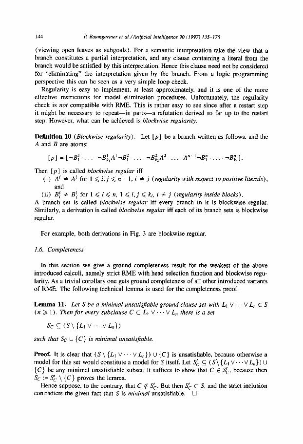
144 F! Baumgartner et al./Artijicial Intelligence 90 (1997) 135-l 76

(viewing open leaves as subgoals). For a semantic interpretation take the view that a branch constitutes a partial interpretation, and any clause containing a literal from the

branch would be satisfied by this interpretation. Hence this clause need not be considered

for “eliminating” the interpretation given by the branch. From a logic programming

perspective this can be seen as a very simple loop check. Regularity is easy to implement, at least approximately, and it is one of the more

effective restrictions for model elimination procedures. Unfortunately, the regularity

check is not compatible with RME. This is rather easy to see since after a restart step it might be necessary to repeat-in parts-a refutation derived so far up to the restart step. However, what can be achieved is blockwise regularity.

Definition 10 (Blockwise regularity). Let [p] be a branch written as follows, and the A and B are atoms:

[PI = r-B,’ . . . . . ~B;,A’TB:. . . . . 7Bi2A2. . . . . A”-‘7B; . . . . . TB;,,].

Then [p] is called blockwise regular iff (i) A’ # Aj for 1 < i, j < n - 1, i # j (regularity with respect to positive literals),

and (ii) Bf # Bj for 1 < 1 < n, 1 6 i, j < kr, i # j (regularity inside blocks).

A branch set is called blockwise regular iff every branch in it is blockwise regular. Similarly, a derivation is called blockwise regular iff each of its branch sets is blockwise

regular.

For example, both derivations in Fig. 3 are blockwise regular.

1.6. Completeness

In this section we give a ground completeness result for the weakest of the above

introduced calculi, namely strict RME with head selection function and blockwise regu- larity. As a trivial corollary one gets ground completeness of all other introduced variants

of RME. The following technical lemma is used for the completeness proof.

Lemma 11. Let S be a minimal unsatisjable ground clause set with L1 V . + . V L, E S (n > 1). Then for every subclause C c LI V . . . V L, there is a set

SC c (S\{Ll V...VL,})

such that SC U {C} is minimal unsatis$able.

Proof. It is clear that (S \ {LI V.. . V L,}) U {C} is unsatisfiable, because otherwise a model for this set would constitute a model for S itself. Let Sk C (S\ {LI V. . . V L,}) U

{C} be any minimal unsatisfiable subset. It suffices to show that C f Sk, because then

SC := S& \ {C} proves the lemma. Hence suppose, to the contrary, that C $! SL. But then SL C S, and the strict inclusion

contradicts the given fact that S is minimal unsatisfiable. 0

P Baumgartner et al./Artificial Intelligence 90 (1997) 135-176 145

Theorem 12 (Ground completeness). Let S be a minimal unsatis-able ground clause set in Goal normal form, c be a computation rule and f be a head selection function. Then there is a blockwise regular, strict RME refutation via c and f.

Proof. We will show the existence of the claimed refutation for some computation rule. Then, with a suitable switching lemma h la [ 171 this refutation can be reordered

according to c. Since this is straightforward for the ground case considered here, we

will omit the switching lemma and its proof. Let k(S) denote the number of occurrences of positive literals in S minus the number

of nonnegative clauses 3 in S (k(S) is a measure for the “Horn-ness” of S, it is related to the well-known excess literal parameter). Now we prove the claim by induction on

k(S). Base case: k(S) = 0. By well-known completeness results for ME (see e.g. [ 1,15,

201) there exists a regular ME refutation of S. It is also well known that ME is complete when restricted to negative goal clauses. Since the only negative clause in S is TGoal, it must also be the goal clause of this refutation. This refutation also trivially is strict.

Induction step: k(S) > 0. As the induction hypothesis assume the result to hold for

clause sets S’ satisfying the preconditions and k( S’) < k(S). Since k(S) > 0 there is in S a disjunctive clause

C=A, ,..., A,,+-Bl,,.., B, (m>2,n>O).

Suppose that the head selection function f selects Ai in C. By Lemma 11 there is a set

5°C ((S\{AI,...,A,,cB,,...,B,})U{AicB1,...,B,})

such that S’ is minimal unsatisfiable. S’ still is in Goal normal form. Hence, by the induction hypothesis there is a closed, blockwise regular, and strict RME refutation D’ of S’ and head selection function f’, where f’ is the same as f, but selects in

Ai + Bl,...y B, the head Ai (there is no other choice for f ‘> . Let P’ be the closed

tableau derived by D’. Now replace every extension step in D’ using the extending

clause Ai +. Bl, . . . . B, by Al ,..., A,, t Bl,..., B,. This leaves us with a derivation

from S and f, resulting in an open tableau whose open branches all end in a literal from

{A1,...,Ai-,,Ai+l,...,Am}. Now we delete from this tableau all subtrees below all positive inner nodes that do

not have any positive literals as ancestors. More formally, replace every branch of the form [p . A’. q] * by [p . A’], where [p] consists of negative nodes only, A’ is a positive node, and [q] is non-empty. Let P” be the resulting open tableau. P” can be thought of to be constructed in an RME derivation D” of S and f which does not further extend at the first positive nodes in each branch.

Every open branch in P” now takes the form [p . A’], for some [p] consisting of

negative nodes only, and A’ is a positive node, stemming from some disjunctive clause from S.

We will show how D” can be extended such that each branch [p . A’] is extended to a closed subtree below it. It suffices to show the construction for one of these branches,

’ A nonnegative clause is a clause containing at least one positive literal,

146 FY Baurngarhzer et al./Art$cial Intelligence 90 (1997) 135-176

because the construction can be applied to each of them, one after the other, which eventually leads to the desired refutation.

Hence let [p . A’] be one of those branches. The leaf literal A’ stems from a clause

A’, ,..., A;,, +-II;,.. .,I$ ES (m’22,n’>O),

whereA’EASforsomejE{l,..., m’}. Since S is given as minimal unsatisfiable, we can find by Lemma 11 a set

S”cS\{A; ,..., A;,, 48; ,..., II;,}

such that S” U {A’ c} is minimal unsatisfiable. Clearly, k(S” U {A’ c}) < k(S) (we replace a disjunctive clause by definite unit clause and possibly delete clauses). Since

S”U {A’ c} still is Goal normal form, we can find by the induction hypothesis a closed, blockwise regular and strict RME refutation D”’ of S” U {A’ c} and f", where f” is the same as f, except that it selects A’ in A’ +- (there is no other choice).

Next append D” with a restart step applied to [p . A’]. This results in a branch [p . A’ TGoal] . Then further append D”’ to this derivation, however each branch [ TGoal . q] in D”’ being replaced by [p . A’ . TGoaZ . q]. This leaves us with a

derivation D”” from SU {A’ +-} with head selection function f" and such that a closed

subtree below [p . A’] comes up. Now we have to turn D”” into a derivation from S alone. By construction, the clause

A’ c is used in D”” for extension steps only in the subtree below [p . A’], and always results in a closed branch of the form [p . A’ . TGoaZ . q’ . YA’ . A’]*. Hence we can

replace each of these extension steps by a reduction step, yielding a closed branch

[P.A’ . -Goal. q' . lA’]* instead. This gives us a strict derivation D from S alone using the head selection function f.

It remains to show that this construction preserves blockwise regularity. The regularity inside blocks trivially carries over from D”’ to D”“. For the regularity with respect to positive literals, the critical case is the node A’ which is with respect to positive nodes the only difference between the tableau derived in D”’ and D”“. However, recall that D”’ is a refutation of S” U {A’ +-}, which is minimal unsatisfiable. This implies that S” cannot contain a disjunctive clause with a head literal A’. But then, the literal A’ can

occur in the tableau derived in D”’ only at a leaf position, stemming from extension steps with A’ c. These usages, however, were eliminated in the transition from D”” to D’. Hence D is blockwise regular. 0

2. Computing answers

We now refine the RME calculus by one more concept, namely answer computation. By this, we mean the possibility to compute most general solutions to problem statements in the sense made popular for Horn clause logic programming.

In order to do so within the RME calculus, we have to presuppose a certain structure of the input clause set. More specifically, we assume as given a satisfiable clause set P, together with one single query, which is a clause of the form c Gt A . . . A G”, where

P Baumgartner et al./Arr$cial Intelligence 90 (1997) 135-176 147

the G are positive literals. Notice that we do not require P to be a program (i.e., a finite set of program clauses, cf. Section 1.2). While such a restriction would be unnecessary for the results of this section, it will be an issue again in Section 3 (cf. Note 1).

The restriction to one single query clause is a bit artificial, but supports the clarity of presentation. The generalization to more than one query clause is straightforward.

We will often abbreviate a query as +-- Q, where Q stands for the conjunction of Gs. The clause set S is the transformation of P U {+- Q} into goal normal form.

Definition 13 (Answers). If +- Q is a query, and 01, . . . ,8, are substitutions for the variables from Q, then QO, V. . . V Qf3,, is an answer (for S). An answer QOl V 1 . -V QO,,,

is a correct answer if P b V( Q& V . . . V QO,,,). Now let an RME refutation of S with

top clause +-- Goal and substitution u be given. Assume that this refutation contains m extension steps with the query, i.e., it contains m times an extension step with the clause

Goal t Qpi, where pi is the renaming substitution of this step. Let Ui = Pi(+ldon,(,,,).

Then Qal V . . . V QcT,?~ is a computed answer (for S).

That is, we simply collect applications of the query clause to obtain the answer. This idea is, of course, not new. For resolution, question answering was invented in the early paper [ 131; the idea is to attach answer literals to trace the usages of the query in the

resolution proof (see also [ 81 and Section 5.3 below).

Example 14. As an example take the following program P and query c Q (constants

and function symbols start with lower case letters and variables with upper case letters):

P: P(X) + Q<x>>Q(x> Q<a),Q(b) +

+-Q: +- P(X).

A refutation together with a computed answer is given in Fig. 4.

Before we prove answer-completeness we explicitly give a lifting theorem for restart

model elimination. The first part of the theorem can be regarded as a proof of refutational completeness (because equality among branch sets takes the “closed” status into account, cf. Definition 2), i.e., if P, is closed, then Pk is closed as well. The second part will be used in the proof of answer-completeness (Theorem 16).

2.1. Lifting

Theorem 15 (Lifting theorem for restart model elimination). Let S’ be a set of ground

instances of clauses taken from a clause set S in Goal normal form. Assume there exists a blockwise regular RME derivation D’ E (I$, Pi, . . . , Pk> from S’ with goal clause

CL E S’. Then there exists a blockwise regular RME derivation D z (PO, PI, . . . , P,) from S with some goal clause CO E S and substitution S such that P,6 = Pk.

Furthermore, there exists a substitution 6 such that Pi is obtained from Pi_, by an extension step with clause C’ E S’ if and only if Pi is obtained from Pi-1 by an

148 R Baumgartner et al./Art@cial Intelligence 90 (1997) 135-l 76

-Goal

-Q(X) -Q(X)

Q(a) Q(b) Q(a) Q(b)

I I -Goal YGoal

-Q(Y) -Q(Y) -Q(z) -Q(z)

Fig. 4. A refutation of the Goal normal form P U { +-- Goal, Goal 6 P(X) } of the clauses in Example 14, de- picted as a tree; the computed answer is P(n) V P(b) V P(b) where the substitution {X + a, Y + b, 2 + h) is applied.

extension step with a clause C E S such that CpiCrS = C’, where pi is the renaming substitution applied in that extension step.

Proof. The basic proof plan is to show by induction on n that P, can be mapped by application of a certain substitution S, to P’,. This approach would suffice to lift a derivation to the first-order level. However, as stated in the second part of the theorem,

we need moreover a lifting result for the clauses used in extension steps. In order to make things technically manageable we first define a clause set S, as

follows: S,, is a set of, say 1, pairwise variable disjoint clauses, and S,, contains for every ground instance Ckyk E S’ (k = 1,. . . , I) of a clause Ck E S a variant C&Q. Furthermore

Ckrk is supposed to be variable disjoint from S. At first we will show that there exists one single ground substitution y which can be

used instead of the individual yk. More precisely, we define first y; = r;lykIU&(rk), because then we have

(CkTkh’; = CkYk. (1)

Moreover, since the clauses in S, are assumed to be pairwise variable disjoint (by means of the 76) and because of the domain restriction of the yi it follows (Ckrk)yi =

(ckTk)y: . . . y;. But then, defining y = y{ . . . yi and using ( 1) we recognize more generally that S,,y = S’.

P Baumgartner et al./Art@cial Intelligence 90 (1997) 135-I 76 149

It follows with D’ being a derivation from S’ that D’ is also a derivation from S,,r. We will show how to lift D’ from S,y to the first-order level. In order to do so we have to define a slightly more general induction invariant Z(n) than the theorem gives us. In present notation it reads as follows:

Z(n): there exists an RME derivation (PO, P,, . . . , P,,) from S with substitution

c, . , . CT,, and there exists a substitution 8, such that l invariant 1: P,& = Pi and l invariant 2: whenever Pi (i = 1,. . . , n) is obtained from Pi_, by an extension

step with a clause C,y E S,,y, then Pi is obtained from Pi-, by an extension

step with some clause C E S such that

cpp, . . .U”& = c,y

where Pi is the renaming substitution used in the ith step to obtain a new

variant of C.

Clearly, Z(n) proves the theorem using the identity C’ = C,,y, and defining u := q . . . CT,, and S := 6,. The if-direction of the theorem’s statement (i.e., that D does not need more clauses for extension steps than D’) follows from the construction given below.

It thus remains to prove Z(n) (induction on n):

n = 0: Trivial, because with PO = [ TGoal] we can also set PO G [ TGoal] and define 80 = E (the empty substitution) ; invariant 2 holds vacuously.

(n-l) -+n:Letn>OandsupposeZ(n-1) toholdforthederivation(Po,P’,,..., Pk_, ) . Z (n - 1) gives us that there exists a substitution Si_, such that

P,-16,-i = P;_1, (2)

CPia, f . . uplSn-, = c,y (3)

under the provisos stated above in the definition of Z(n). In order to prove Z(n) we make a case analysis with respect to the inference rule applied to Pk_,:

Reduction step: PA_, contains a branch [p’] of the form [p’] = [. . . . A . . . . . A] to be closed, i.e., P’, contains [$I*. From the given invariant (2) we learn that P,+, in particular contains a branch [p] with [ pS,_, ] = [p’] . The branch [p] is of the form [p] = [ ..: K. ..: L], where KS,,_, = A = L&-l. In other words, a,,_, is a unifier for K and L. Since S,, is assumed to be a set of variants completely variable disjoint from S we can also assume that y neither acts on the variables from S nor on the variables occurring in the variants taken from S to build the derivation (PO,. . . , P,_,). But then P,,_, y = P,_, . Application of S,,_ 1 yields

P,_,yS,_, = P,_,6”_, ‘3 Pi_, = P/,_,ys,_,.

The last identity is trivial (Pk_, is ground) and is needed below. More specifically the following holds

(4)

KY&_, = KS,_, = A = LS,_, = LyS,,_,. (5)

150 I? Baumgartner et al./Artijicial Intelligence 90 (1997) 135-I 76

Next we turn to the clauses used in previous extension steps (cf. given invariant 2). Again, since y does not act on the variants taken from S it also holds cpiffr . . . an_,yGn_, = Cpp, . . . (+,,_I &__I. Thus we conclude

Cpi(Tt . . . gn-1Y8n-l = CpiUl 3 s . iT.n_,Sn_, ‘3 c,,y = c,ys,_, . (6)

The last identity holds trivially because C,,y is ground.

Eqs. (4)) (5)) (6) tell us that $,_I is a simultaneous unifier for the respective leftmost and rightmost terms in these equations. Hence there also exists an MGU u,,

and a substitution 6, such that

u”s” = y&-r. (7)

By construction, (T,, is an MGU for K and L. Hence we can apply a reduction step to [p] E P,_t with MGU gn to obtain P, = ((P,,_l \ {[p]}) U {[p]*})a,. Altogether we conclude

PA = ((Pn-I \ {bl)) U{[Pl*))~nhI

(7w4’((~n_l \ {WI)) u {Wl*))Yhl-1

(2) <(p’,_, \ {[P’l)) u {]p’l*)) = p’,.

The step (*) is justified by the fact that PL_, is ground. Note that this chain just proves invariant 1; the remaining invariant 2 is shown as follows:

Cpi(Tt . . . Ufl-l(+nSn ‘:I Cpic+* . . .(T,_,ysn_l ‘2 c,,y.

Extension step: Ph_, contains a branch [p’] of the form [p’] = [ . . . . A] to be

extended with a clause 2 V R E S,,y, i.e.,

P:, = (p’,_, \{[~‘l}) u{[~‘~~l*}‘J [p’l OR.

From the given invariant (2) we learn that P,._l in particular contains a branch [p] with [p&-l] = [p’]. The branch [p] is of the form [p] = [... . L], and thus, in particular A = LS,_ 1.

Let z V Q(, E S,. be the lifted version of 2 V R, i.e.,

(K, v Q,) y = x v R. (8)

Recall from the assumption stated at the beginning, that z V QU is a new variant by means of some renaming substitution 7, i.e., K V QU = (K V Q)T for some x V Q E S.

Let (TV Q)p,, be a new respective variant. We will show how to carry out an extension step with that variant.

From the last equation and (8) it follows

AvR=(K,VQ,)~=(KVQ)~Y=((KVQ)P,)P~~~~Y

= ((Kv Q)P~)P;:,~Y&,-1. (9)

F! Baumgartner et al./Artijicial Intelligence 90 (1997) 135-176 151

The last identity is justified by the fact that a,,_, is applied to a ground clause, and hence does not alter the clause.

The renaming substitution P,, introduces new variables; hence p;’ does not affect P,_l . Also, r does not affect P,,_l, because P,_l is built from new variants. Together

we obtain that P,,_I = Pn_lp;‘~. Further, as in the case of the reduction step, we can also assume that y does neither act on the variables from S nor on the variables occurring in the variants taken from S to build the derivation (PO, . . . , P,_l ) . But then

P,,_l y = P,,_I. Putting things together we obtain:

C-lP,‘V&-, = p _ 6 _ ‘A) P’ n 1 n 1 n-l = P’n_,P;lvs”-l. (10)

The last identity is trivial (I$_, is ground) and is needed below. Recall from above that we extended P’,_, at a branch [p’] with leaf A to obtain PL.

From A = I&_~, as given, we can now conclude with ( 10) even Lp;‘ryS,,_, = A. But then we have

Next we turn to the clauses used in previous extension steps (cf. given invariant 2).

By the same line of reasoning as for P,_l above we can assume that pi17 does not affect a clause C, whose ground instance C,,y is used in the ground derivation. Thus we

conclude

c,,y = c,,&y = c,,&ys,-I. (12)

The last identity holds because a,_, is applied to a ground clause.

Since the derivation from S uses new variants, and the MGUs used there can be supposed to introduce no new variables we have

C/&a, . . . (+n_, = Cpia, f . .Un_,p[‘r.

Again, since y does not act on the variants taken from S, Cpia, . . . a,,._,~ =

CpiCr] . . . g,,_, also holds. Using these identities and applying S,,_, we conclude

C/Iia, . . . gn_,Pn,rYSn-, = Cpi(T, . . . a*-,6n_,

‘2) c,y (2) CL,p,,7ySn-, . (13)

Eqs. ( lo), ( 11)) ( 13) tell us that ~;‘r$&_, is a simultaneous unifier for the respective leftmost and rightmost terms in these equations. Hence there also exists an MGU (+,, and a substitution 8, such that

ffil& = p,‘ry&-, . (14)

By ( 11) and ( 14)) CT,, is an MGU for L and Kp,. Hence we can apply an extension step to [p] E P,,_I with the variant clause (?? V Q)p,, and MGU g,, to obtain

P, = ((P,-I \ [PII u {b . (%)I*) u [PI ~Qpnb,.

Altogether we conclude

152 P Baumgartner et al./Art$cial Intelligence 90 (1997) 135-176

PtJn = ((Pn-1 \ [PI) U{b4~~,)l*}U [PI oQpn)un&

(‘4g10) ( ($I \ b’l) u {b’ . (&d I*} u [p’l 0 Qp,)a,&

(14ic9) ((Pn_, \ [p’]) U{[p’.A]*}U [p’] OR)

= PL.

Note that this chain of reasoning just proves invariant 1. We still have to prove invariant 2: first, invariant 2 has to be proved for all clauses

used up to, but not including this extension step:

cpiat . . . (+rt-lull& (5 cp$q . . .M&YLI (5 CL, y.

Second, invariant 2 has to be proved for the clause used in this extension step. For this note that P,, renames i&Q to a new variant. Hence ((xVQ)p,)q . . .un-l = (RVQ)pn.

From this it follows

Now invariants 1 and 2 have been shown, which concludes the proof of the extension

step. Restart step: Since in a restart step no substitution is applied we can take S,, := S,,_ 1.

Together with the induction hypothesis the result follows trivially.

To see the blockwise regularity of the lifted derivation D, assume to the contrary of the theorem, that the lifted version D’ is not blockwise regular. Then some branch [p]

along the refutation D’ is not globally regular. This means that one of the inequality constraints stated in the definition of blockwise regularity is violated. Thus [p] contains two occurrences of a literal B which violate one of these constraints. However, with the

branch [p] being a lifted version of a branch [p’] in D’ the inequality constraint must

be violated in [p’] as well. This plainly contradicts the assumption that D’ is blockwise regular. Hence D’ is also blockwise regular. 0

2.2. Answer-completeness

Theorem 16 (Answer-completeness of RME) . Let P be a satisjiable clause set, +- Q

be a query and Q6l V. . ’ V Q$l be a correct answer for P. Then there exists a blockwise

regular, strict RME refutation with head selection function from the Goal normal form

S of P U {- Q}, with computed answer QUA V . . . V QcT,,, such that Q(T) V . . . V Qun,

entails QOl V . . ’ V Q8l, i.e.,

3SVi E (1,. ..,m}IjE (1, . . . . l}Q(+iS=Qei.

Informally, the theorem states that for every given correct answer we can find a computed answer which can be instantiated by means of a single substitution S to a

l? Baumgartner et al./Artijicial Intelligence 90 (1997) 135-I 76 153

subclause of the given answer, and hence implies it. To obtain this result we have to demand one single substitution 6 which maps any of the clauses Cpia used in extension steps to the respective clause on the ground level.

Clearly, this result is harder to establish and more relevant than a lifting result for

SLI resolution in [ 181 which “moves the g-quantification inside”: in our words, they state that for every application of an input clause at the ground level there exists an application at the first-order level, and there exists a substitution to map this instance to

the ground level. As Example 17 shows, the approach of [ 181 cannot handle the case correctly if there are variable interdependencies in disjunctive answers.

Example 17. To see this, let us consider the clause set P = {P( f( X) > t} and the query t P(Z). Then according to [18], the singleton A = {P(Z) V P(f(Z))} is a correct and complete answer set, although A does not subsume P( f( X)). Thus we

would be incomplete. On the other hand, if we permit each literal to be substituted separately, in order to fix this problem, then we would be incorrect. For this let us

consider the clause set P’ = {P(X) V P( f( X) ) t}. Then we could get also the answer A with respect to the query +- P(Z) from above. But we could factor it to P(f( Z))

which is not entailed by P’.

Unfortunately, we can not obtain a result stating that the computed answer contains

less (or an equal number of) literals than the given answer. This behaviour sometimes

results in confusing answers. For instance, take again the clause set from Example 14:

P: P(X) + Qlx>,Q<x, Q(a>,Q<b> +

+- Q: + P(X).

The refutation from Fig. 4 computes the answer P(a) V P(b) V P(b) . Although P(a) V

P(b) is a correct answer, RME will not compute it. The reason for this is that two identical instances +- P(b) of the query have to be used. Now follow the proof of Theorem 16.

Proof. Given the correct answer Q&V. . -VQt$ we know by definition P b V( Qel V, . .V

Q&). Hence we conclude that PU{TV( Qti$ V. . .VQ&)} is unsatisfiable. By transforming this into CNF we get the unsatisfiable set of clauses S’ = P U {~Qb$q,. . . , lQe,r,} where each ri (1 < i < 1) substitutes new Skolem constants for the free variables of

Q4. With the abbreviation t9f = Biri for all 1 6 i < 1, we get an unsatisfiable set of clauses

s’ = P u {lee;, . . . , lee,‘}.

By the Herbrand-Lowenheim-Skolem theorem there exists an unsatisfiable ground clause set

S” = P’ u {lee;, . . . ) lee;}

154 R Baumgartner et al./Artificial Intelligence 90 (1997) 135-l 76

where P’ is a finite set of ground instances of clauses from P. From S” we select a minimal unsatisfiable subset

S”’ = P” U {-QO;, . . . , lQ&}

where P” & P’, and (without loss of generality) r 6 1. From ground completeness of RME (Theorem 12) we learn that there exists an RME refutation of the Goal normal form of S”‘, i.e., there exists an RME refutation D’ of

s I,,, = C’OOl U {Goal + et?{, . . . , Goal + Qf$} U {+- Goal}.

Here, a clause set ~~~~~ is obtained from a clause set P by replacing every purely

negative clause +t V . . .VTB, by GoalVTB1 V... V TB,. The minimality condition

ensures that each of the clauses {Goal c Qdi, . . . , Goal +- Qf3:) in S”” is used at least once for an extension step. Let m 2 Y be the total number of extension steps carried out

with clauses from that set. D’ is a refutation, i.e., a derivation of a closed branch set P,,. By the lifting theorem

there exists a blockwise regular RME derivation D of some more general branch set

P, from ~~~~~ U (Goal t Q} U { +-- Goal} since the second part of the lifting theorem assures that even single applications of extension steps are lifted, we conclude that the structure of the lifted tableau is invariant, i.e., strictness and head selection property lifts as well. Since only the empty branch set is more general than itself we conclude that P, is also a refutation. This proves refutational completeness.

Next we turn to answer-completeness, proper. The second part of the lifting theorem

gives us that for any extension step in D’ with clause Goal +- Qt9;,i, (where f is a

surjection from { 1,. . . , m} onto { 1,. . . , r)) there is exactly one extension step in D with the clause {Goal t Qpi} (i E { 1, . . . , m}), where pi is the renaming substitution

of that step. Furthermore (by the lifting theorem) there is a substitution 6’ such that

Goal +- Qpic+S’ = Goal + Qtlici,. (15)

This, however, is equivalent to the condition that every element in the disjunction

Ans = Qul V . . . v Qu’ v Qu,+~ v s . . v Qcr’,,

where (+i = Pi~ldom(p,) (for i = I,. . . , m), is mapped by application of 6’ into some element of QO{ V . . . V Q/3:. Note here that Ans is nothing but the computed answer

substitution. Recall that QOi = Q&rk (for k = 1, . , . , r), and hence with ( 15) we have

Qa4 = Qaf(i)Tf(i). (1’3)

However, in order to prove the theorem we have to find a substitution S such that Qai8 = Q/3f(i,. In order to define 6 recall that rk is a Skolemizing substitution and

hence can be written as

P Baumgarmer et al./Art$cial Intelligence 90 (I 997) 135-l 76 155

for some finite index set 0 and new constants a,. In this case we can treat in the refutation D the a, as new variables and define the substitutions

-I ‘k = a, + x, { 1 & + ‘h E Tk}.

Every rk introduces new Skolem constants. Hence the domains of the rkl are pairwise

disjoint. But then with defining 7-t := rF1 . . . 7;’ we get

7-11 -I

dom(~;‘) = 'k . (17)

Next define

6 :=87-l.

This is the desired substitution since

Qai8 = Q~iS’C’ (2) (QBf(i)~f(i))~-' (‘) (Qdf(i)Tf(i))Ty(lq = QOf(i).

Finally, with the fact that f is a suitable surjection the theorem is proved. 0

2.3. The minimal answer problem

Certainly it is interesting to tune our procedure such that it computes minimal answers

only. This means we want to be able to decide for a computed answer C of a clause set P, written P + C, whether there is no other answer C’ with P b C’ that is more general

than C. The decidability of this problem depends on the notion of “more general than” one wishes to implement. In the subsequent discussion, we will refer to the problem as the minimal answer problem.

We can interpret “more general than” as subsumption. A clause C’ subsumes the clause C, written C’ D C, iff there is a substitution 8 with C’8 G C. Subsumption of clauses is an NP-complete problem [ 141. Nevertheless it is decidable hence. However,

the minimal answer problem is essentially undecidable, i.e., not even semi-decidable,

because otherwise we could decide consistency, i.e., satisfiability of the clause set P as follows:

Consider the clause set P U {p} where p is a nullary predicate symbol which does not occur in P. Then clearly P is satisfiable iff P U {p} is. Since P U {p} b p trivially, p is a computed answer for P U {p}. Now we could ask whether there is another answer,

i.e., set of literals, which subsumes p. This is only possible for the empty clause. So we would be able to decide whether P U {p} k 0 does not hold, thus the satisfiability of P U {p} and hence of P itself. But the satisfiability problem is known to be essentially undecidable for first-order clause sets.

We can try it with logical implication instead of subsumption, i.e., we want to find out whether there is no answer C’ such that C’ + C. But in this case, the minimal answer problem is again essentially undecidable, since implication is a notion more general than

subsumption, i.e., C’ D C implies C’ * C. In contrast to the subsumption problem, already the implication problem for clauses is undecidable even for restricted cases; see

u91.

156 P Baumgartner et al./Artijicial Intelligence 90 (1997) 135-176

A condensation of a clause C is a minimum cardinality subset C’ 2 C such that C’ D C. It holds that any condensation of the clause C is logically equivalent to C, and

any two condensations of a clause are variants. This means we can restrict ourselves to computing only condensed answers C, i.e., C is its own condensation. Condensation is

a local property because it does not take the clause set P into account. Since the clause

condensation problem is decidable, the minimal answer problem becomes decidable too in this case. However, we refrained from implementing a condensation algorithm into

our system because of its appalling complexity. Deciding whether a clause is condensed

is co-NP-complete [ 121. Nevertheless our calculus is answer-complete, i.e., for all correct answers C of a

clause set P there is a subsuming computed answer C’ such that C’ D C, although it may be the case that not all answers in condensed form can be computed. To see this, look again at Example 14. However, in Section 3 below we will describe a calculus variant which is more optimal with respect to the length of the disjuncts.

3. Definite answers and regularity

From theorem proving with ME we know that the regularity check is an important means for improving efficiency. Regularity for ordinary ME means that it is never

necessary to construct a tableau where a literal occurs more than once along a branch. Expressed differently, it says that it is never necessary to repeat in a derivation a previously derived subgoal (viewing open leaves as subgoals). In this section we will present a variant of RME, the ancestry restart variant, which allows global regularity checks (see Definition 10). This variant is motivated by Loveland’s UnH-Prolog [23].

As an interesting side effect it turns out that this variant offers considerable benefits with respect to logic programming. Occasionally one is interested in the question whether

a given program with query admits a definite answer, i.e., an answer which is a single conjunction of atoms, but not a disjunction. Of course, in general, a non-definite program

does not always admit a definite answer, but some programs do. It is the latter class of

problems we are interested in now.

Example 18. Consider the program Poef = {P (X, a) V P (b, Y) -} and the query +-- P( X, Y). Note that, among others, P( b, a) and P( X, a) V P( b, Y) are correct answers. Now, by Theorem 16 strict RIME is answer-complete; hence we can find a refutation yielding a computed answer which entails P( b, a) (Fig. 5, left side). As noted after the statement of Theorem 16, RME will not always compute minimal (with respect to length) answers. It is easily verified that in this example the shortest computed answer

is P (X, a) V P ( b, Y) , which can be factored to P (b, a). This is due to repeated use of the query in the refutation.4

4 However, in this example we could find a non-strict RME using the query only once. Hence, one might

object that this example is vacuous. This, however, misses the point because there exists a more complicated example where this argumentation would not work.

R Baumgartner et al./Artificial Intelligence 90 (1997) 135-l 76 157

Restart ME refutation I

Ancestry restart ME refutation

-Goal

P(X’,a)

-Goal

Substitution: I

{X t x’, Y + a, +J(X”, Y”)

X” +- b, Y” + Y’} *

+(X3 Y) *

Substitution: {X - b,X’ + b,

Y-c&Y’+-a}

Answer: Answer: f(X’,a) v P(b,Y’) P(b,a)

Fig. 5. An RME (left side) and an ARME (right side) refutation of { P( X, a) V P( b, Y) +, + God,

Goal +- P (X, Y)} depicted as trees.

YGoal

P(X’, a) *

P(b, Y’)

I

The key idea to the direct computation of definite answers is to restrict the use of the

query to one single application in the refutation, namely at its top. Then, by definition, definite answers are obtained. However, such a restriction is incomplete. But if RME is modified such that every negative literal along a branch, not only the topmost literal, may be used for the restart step then completeness is recovered. This follows from a more general result which states that we can restrict our calculus to globally regular refutations (i.e., no literal except the literal used for the restart occurs more than once

along a branch). Let us now introduce all this more formally.

Definition 19 (Ancestry restart model elimination (ARME)). The calculus ancestry RME (ARME) is the same as strict RME (Definition 3), except that the inference

rule restart step is replaced by the inference rule ancestry restart step:

ancestry restart step: [Pl,P

,p, o ~A, p

if Leuf( [p] ) is a positive literal and 1A E [p] .

The term “ancestry” in the definition is explained by the use of ancestor literals for restart steps. Note that any reduction from a positive leaf literal to a negative ancestor

literal -IA can be simulated in ancestry RME by a restart step with -A, followed by a reduction step. Thus, non-strictness is “built into” ancestry RME. Note in addition,

that the ancestry restart rule includes the restart rule since the first literal of the branch, which is always ~Goal, can be used for the restart as well.

Fig. 5 (right side) shows an example ancestry RME refutation of Poef with query c P (X, Y) for Example 18. Note that no new copy of the query clause is used, but instead the present instance is copied by the ancestry restart rule, and then the resulting branch is closed by a reduction step. This example also demonstrates that-unlike in

158 P: Baumgartner et al./Art@cial Intelligence 90 (1997) 135-176

strict RME-it makes sense to apply a reduction step to a restart literal. This motivated us to change the definitions in [4] in now letting the restart step be an explicit inference

rule. Clearly, in terms of a proof procedure the ancestry restart rule induces a larger local

search space than the restart rule. On the other hand, refutations may become much shorter. In order to see this think of a derivation containing a branch [ 431. . . . . -B, . A]. It might be necessary in RME to repeat all the YBi in order to find a refutation. This derivationof [~B,...:~B,.A.lBl...: TB, ] can be abbreviated in ancestry RME

to [lB1 . . . . -B, . A . TB,,] by guessing the right -B, for the restart. Indeed, this is

the rationale for our proof procedure to search the restart literals from the leaf towards the top. As a further benefit of this search order note that a definite answer will be

enumerated before a non-definite answer, provided it allows for a shorter proof. Ancestry RME has some similarities to Plaisted’s modi$ed problem reduction format

(MPRF) [ 271. Expressed in our terminology, MPRF corresponds roughly to the non-

strict version of ancestry RME. As major differences we see that answer computation was not an issue in [27], and also that regularity refinements were not considered.

These differences justify the need for our new proofs. Now we proceed to an appropriate completeness result with respect to definite an-

swers. As mentioned above, this result shall be a consequence of a more general result concerning a regularity restriction. Let us define this notion precisely:

Definition 20 (Global regularity). Let [p] be a branch written as in Definition 10. The branch [p] is called globally regular iff it is blockwise regular (conditions (i) and (ii) in Definition lo), and additionally

(iii) Bf # By for 1 < 1 < m < n, 1 < i < kt, 2 6 j 6 k,, (global negative

regularity)

holds. The notion of global regularity is extended towards branch sets and derivations

as in Definition 10.

Hence we have three conditions, two from the definition of blockwise regularity and a third one from the above definition. Condition (i) states that all positive literals along a branch are pairwise different, and condition (ii) states that negative literals inside blocks

are pairwise different, where by a block we mean a smallest subbranch delimited by positive literals or the ends of the branch. Condition (iii) means that a negative literal

may be equal to one of its ancestors only if it follows a positive literal, i.e., if it is used

as a restart literal. Thus we have a global regularity condition, except for restart literals. In all example refutations given so far, all branches are blockwise regular. However, the refutation in Fig. 1 (right side) is not globally regular, as can be seen by the two occurrences of -Q in the rightmost branch. From this example we learn that RME is incompatible with the global regularity restriction. However we have:

Theorem 21 (Completeness of ARME). Let c be a computation rule, f be a head selection function and S be an unsatisJiable clause set in Goal normal form. Then there

exists a globally regular, ancestry RME refutation of S with computation rule c and

head selection function f.

F! Baumgartner et al./Art$cial Intelligence 90 (1997) 135-I 76 IS9

4Toal YGoal

-Goal +oal

YGoal

1B

/\ D’

*

Replace by l---- Restart

_-I

Fig. 6. Transformation step removing a violation of a global negative regularity constraint

Proof. The proof builds on the above answer-completeness Theorem 16, which in turn relies on the ground completeness Theorem 12. We can thus rely on this result, and

show how to transform a given blockwise regular refutation in RME on the ground level

to a globally regular refutation in ancestry RME (also on the ground level). This suffices to prove the theorem on the first-order level for the following reason:

suppose some unsatisfiable clause set in goal normal form is given. From the cited results we know that there exists a strict blockwise regular RME refutation, say D, which is

lifted from a strict blockwise regular RME refutation Dg on the ground level. By the transformation proposed below then there exists a globally regular ARME refutation

%K* It is straightforward to adapt the lifting theorem (Theorem 15) to take into account the ancestry restart step. The adaption to global regularity instead of blockwise regularity is straightforward as well. Hence DA,,~ is also globally regular.

It remains to prove the desired transformation. For this let Dg be the given strict,

blockwise regular RME refutation from above. Since by definition an ancestry restart step includes the possibility of a restart step, DR is also a blockwise regular ARME

refutation. Let n be the number of violations of the global negative regularity constraint (condition (iii) in Definition 20). Either n = 0 and we are done, or else Dg can be transformed to contain strictly less than n such violations, without sacrificing the

blockwise regularity constraints. Repeated application will eventually result in the desired refutation.

The transformation step can most easily be expressed using the tree view of ME. Fig. 6 (left) shows the general situation: assume Dg contains a branch

[p] =[~GoaZ~...~Ak~~Goal~..:~B~..:A’~~Goal~..:~B],

160 P Baumgartner et al./Art$cial Intelligence 90 (1997) 135-176

where A’ is the bottommost (rightmost) positive literal dominating --IB. Further, as indicated by the two occurrences of 1B in [p], the global negative regularity constraint

is violated for [p] . Let D’ be the tableau corresponding to the refutation of the branch

[PI. Now delete the subtree between A’ and 7B below (bounds excluded from deletion).

We arrive at a new tableau with branch

[p’] = [-~Goal. . . . . Ak. TGoal. . . . . -B . . . . . At. lB].

Next append D’ to [p’]. Since only negative literals have been deleted, and we assume that Ds is a strict RME refutation, in D’ no reduction steps from positive literals to

negative literals have occurred. Thus D’ is also a closed tableau below [p’] (right side

in Fig. 6). It is clear from the definition that this new tableau can be constructed by means of

an ancestry restart step, using 1B as restart literal. Furthermore, (at least) one violation of the global negative regularity constraint has been removed, and since we only have deleted some literals from p the blockwise regularity constraints will not be violated.

Thus we have found a suitable transformation step. 0

We can use this result to obtain the desired completeness result for definite answers.

Theorem 22 (Answer-completeness of ARME). Ancestry RME is answer-complete in the sense of Theorem 16. In particular, if Qt3 is a correct de$nite answerfor a program P then there exists an ARME refutation of P with computed answer Qo such that Qa6 = Qt3, for some substitution 6. Furthermore, the input clause Goal + Q is used exactly once, namely as the goal clause of the refutation.

This last theorem enables us to enumerate definite answers only, by simply restricting the use of Goal t Q to one extension step at the beginning. So we have the desirable properties of loop checking by regularity and the computation of definite answers.

Note 1 (Restriction to programs). Notice that in Theorem 22 we have one important

change now with respect to the results so far: for the special case of singleton definite answers we require our clause sets to be programs, i.e., no negative clauses are allowed

(except the query, of course). This restriction can be explained using the following

example.

Example 23. Consider the clause set P and the query +- Q:

P: P(XY),Q(XY>,Q(I:x> + + P(X,Y)

+ Q: +- Q(XY>.

It is clear that Q( X, X) is a correct (definite) answer. However, with the “wrong” head selection function which selects P(X, Y) in the first clause it is easy to see that neither an RME nor an ARME refutation of P with goal clause Q exists. The problem

P Baumgartner et al./Artifcial Intelligence 90 (1997) 135-l 76 161

is the incompatibility of the concepts “head selection function” and what could be called “independence of the goal clause”, i.e., that the goal clause can be chosen freely among all negative input clauses.

Of course, there exist refutations with the goal clause Goal t P( X, Y), stemming

from the second clause of P. However, the proof of Theorem 22 for the case of definite answers relies on the fact that the query is used as the goal clause of the ARME refutation (i.e., on top of the tree). However, in presence of negative clauses in the program this can in general not be achieved, and hence Theorem 22 does not hold in such a setting. Thus, restricting to programs solves the problem, because then there

is only one negative clause-the query-and thus we are forced to use it as the goal

clause. On the other side, if the “selection function” is given up, i.e., any positive literal in a

clause may be accessed as an entry point, then the “independence of the goal clause”

holds. Consequently, Theorem 22 can be recovered in this setting. However, a detailed treatment is beyong the scope of this paper and will be presented elsewhere.

Proof. The answer-completeness follows directly from the fact that the ancestry variant still permits restart steps with the goal, i.e., it allows for additional derivations. The proof of the last part is given by a careful analysis of the proof of Theorem 16. Recall from that proof that QO is a correct answer because P implies that S’ = P U {7Q&-}

is unsatisfiable, where r is some substitution introducing new Skolem constants for

the variables of Qe. Then we considered a set S”” of ground instances of the goal normal form of S’. It is important to recognize that the goal normal form S”” contains

exactly one instance of the query, namely Goal +-- Q&. Since we assume that P is a program, and hence consistent, it follows from the proof of Theorem 12 that there exists a strict RME refutation of S”” where the first extension step is done with the clause Goal +- Q&-. In other words, every branch in the refutation is of the form

where Qi is some literal in Q. Recall that Q is an abbreviation for Qt A . . . A Q,. Now suppose that GoaE +- Q& is used once again in the refutation. For syntactical reasons this can happen only if Goal c Q& is extended to a branch resulting from a restart step. This branch takes the form

[ TGoal . lQ#r . . . . . A . ~Goal]

where A is some positive literal. Extension with Goal c QLJr results (among possible others) in a branch

[ ~Gou~. TQ~OT. . . . ’ A . lGo~7.Z. YQih],

But now note that this extension step leads to a violation of the global negative regularity

restriction and thus will be eliminated by the transformation given in the proof of Theorem 21. To be more precise, the branch

162 F! Baumgarlner et al./Artijicial Intelligence 90 (1997) 135-176

will come up instead. Since every extension with Goal +- Q$r will be eliminated in this way, the query clause Goal +- Q& is used precisely once in this transformed refutation, namely for the first extension step. The lifting argument for this refutation then is the same as in Theorem 16. Thus we arrive at a refutation with computed answer QU which

is more general than Q6. This completes the proof. 0

4. Implementation

All variants and refinements of ME discussed so far are implemented in the PRO- TEIN system [ 51. PROTEIN is a first-order theorem proving system based on the PRO- LOG technology theorem proving (PTI’P) technique [ 321, implemented in ECLiPSe- PROLOG [ lo]. The general idea of the PTTP-implementation technique is to view

PROLOG as an almost complete theorem prover that has to be extended by only few ingredients in order to handle the non-Horn case. More precisely, the given clause set is compiled into a PROLOG program whose execution is a search for a refutation of the

given input clause set. We will now state some of PROTEIN’s features in more detail.

4.1. The PTTP technique

Since in general the input clause set is non-Horn, the resulting compiled PROLOG program will have some extra facilities corresponding to the deviation of the calculus under consideration from PROLOG’s SLD resolution. Two main extensions are the

introduction of negative predicates, in order to handle contrapositives whenever this is necessary, and the introduction of ancestry lists, which are used to store the information contained in branches. The latter allows the compiler to insert the code for reduction

and ancestry restart steps. By the PTTP technique we get a rapid and flexible, but nevertheless efficient system

which hosts both full predicate (clause) logic and answer computing. These properties-

flexibility and rapid prototyping-are the main advantages of the compilation to PRO- LOG over a dedicated extended WAM approach. So, the WAM technology and other

benefits of optimising PROLOG compilers are accessible to theorem proving and dis- junctive logic programming.

However, the use of a cut or other non-logical extensions of PROLOG should be avoided. Nevertheless it is possible to integrate plain PROLOG code. This is especially

useful if parts of the problem description do not need the full power of first-order predicate logic, or if one wants to exploit the procedural, non-logical capabilities of

PROLOG.

4.2. Computing answers with PROTEIN

Since ME is a goal-oriented, linear, and answer-complete calculus, it is really well

suited as an interpreter for disjunctive logic programming. PROTEIN facilitates comput- ing disjunctive and definite answers with respect to positive disjunctive logic programs.

F? Baumgartner et al./Artijcial Intelligence 90 (1997) 135-176 163

In the newest PROTEIN release there is a flag which allows us to look for definite answers only.

In our implementation, the definiteness of the answer can be guaranteed by the fact that all occurrences of answer literals during the proof search are unified with each other. This is the approach taken for resolution in [ 281. It is applicable in every variant of ME, not only in the ancestry variant. For this, coroutining techniques are used.

But it is also possible to force our system to use the query only once as the goal

clause according to Theorem 22. When using this setting for clause sets (as opposed to programs) such as those of the next section, the head selection function feature has to

be disabled in order to preserve completeness (cf. Note 1) .

4.3. Additional features

Different search strategies are built into PROTEIN, e.g. iterative deepening, depth-

first or more general weighted search. The restart, strict, and ancestry variants (possibly with selection function), loop checking by regularity and also factorization (which is

introduced in [20] ) are parts of the system. Another distinguished feature of PROTEIN is its theory interface (PROTEIN =

PROver with a Theory Extension INterface). PROTEIN includes theory reasoning [ 1,2,3 11 in a very general way. Theory reasoning allows a calculus to relieve from explicit reasoning in some domain (e.g. equality, partial orders, taxonomic reasoning)

by taking apart the domain knowledge and treating it by special inference rules. In an

implementation, this results in a universal “foreground” reasoner that calls a specialized “background” reasoner for theory reasoning.

Another instantiation of this approach allows us to plug in constraint reasoning com- ponents, thus making available the ECLiPSe-PROLOG constraint solving mechanism in a sound and complete manner for theorem proving [ 71.

5. Comparative theorem prover study

In the sequel, we want to relate our experiences in computing answers by using theorem provers. First of all, we had to overcome some technical problems because

theorem provers usually do not supply answers apart from “yes” or (possibly) “no”. We

will illustrate our experiences with a puzzle example which allows for both indefinite

and definite answers. We will discuss this example in detail, but we tested many other

examples. All considered examples are contained in the TPTP problem library [33] and were used without changes in our experiments.

5.1. Knights and knaves

Example 24. Our main example follows problem #36 in [ 301. A related example is studied in [ 261. The manner of formalizing problems there is similar to ours. The natural language description of our problem is given in Fig. 7.

164 I? Baumgartner et al. /Artificial Intelligence 90 (1997) 135-I 76

Natural language description:

(i) (ii)

(iii)

(iv)

(v)

(vi)

On an island, there live exactly two types of people: knights and knaves. Knights always tell the truth and knaves always lie. I landed on the island, met two inhabitants, asked one of them: “‘Is one of you a knight?” and he answered me. What can be said about the types of the asked and the other person depending on the answer I get? We assume, that either a proposition or its negation is true. If the disjunction of two propositions is true then at least one of them must be true.

Formulae set with two cases: (i) true(isa(Q,knight))i/true(isa(Q,knave)).

(ii) says(P,S) -+ (true(S) ts true(isa(P,knight))). (iii) (a) says( asked, l ) (“yes”),

(b) says(asked,not(o)) (“no”) where l = or( isa( asked, knight), isa (other, knight) > .

(iv) 1 (true( isa( asked, X) ) A true( isa( other, Y) ) ) . (v) true(not(C))Vtrue(C).

(vi) true(or(A,B)) cf (true(A) Vtrue(B))).

Possible answers: - knave/knave V knave/knight V knight/knave V knight/knight (trivial). - knave/knave V knight/knave V knight/knight (indefinite, case (a) only). - knave/knight (definite, case (b) only).

Fig. 7. Smullyan’s problem #36.

The reader may think about the problem for a while, before he looks at the solution

which is given next. The last two pieces of information (v) and (vi) explicitly state

some knowledge about inferencing. We need them in order to be able to cope with the

information in (ii) because our description language is only first-order. It is interesting

to note that a human being usually knows both these facts implicitly. We have to make a case distinction:

(a) Suppose, the asked person answers with “yes”. Then he may be a knight, because then of course it is true that one of them is a knight. In this case, the other person

can be a knight or a knave. We cannot even exclude that the asked person is a knave. Then it must be true that none of them is a knight, hence the other person is also a knave in this case.

(b) Let us now assume, the asked person answers with “no”. Then this person must be a knave, since a knight cannot answer with “no” honestly. It follows, that the

other person is a knight, because one of them must be a knight. So, in this case

we get a definite answer. In our formalization of the problem (also given in Fig. 7)) the formulae in (i) and (ii)

express the corresponding pieces of information from the natural language description.

P Baumgartner et al./Artijicial Intelligence 90 (1997) 135-176 165

-___-------------~__---------, 1 ltrue(isa(asked,X)) ~true(isa(orher, Y)) ’ _--______-_-----------~~~~-_--~

frue( isa( Q, knight) ) frue(isa(Q,knave)) I I

,___-____---____----_______-----_, I

; ltrue( isa( asked, X) ) ~rrue(isa(oUzer, Y) ) , +---___--’ _---_-___----___-----____---__I

frue(isa(Q, knight)) true ( isa ( Q, knave) ) (______-------__

A 1

----___-----____----_----_-__, i Ttrue(isa(asked, X))

I Tfrue(isa(other,Y)) ’ I

__---____-------___-- -------__I

true( isa( Q, knight) ) true( isa( Q, knave) )

; yrrue(isa(asked, X)) +rue(isa(o?her, Y)) ’ _----_-_------_-- ----- ----____I

Fig. 8. Derivation of the trivial answer.

Depending on the case considered, we choose exactly one of the formulae (iii) (a) or (iii) (b). This means, we actually split the problem into two formulae sets. We view the fact that a person denies a question as that he says that the thing in question is not

true using the binary predicate says (instead of a ternary predicate). Formula (iv) can be considered as the query; it is negated because we do refutation-based reasoning. We have to express the pieces of information (v) and (vi) explicitly by introducing the unary predicate true. The symbol i/ denotes exclusive or. The transformations of the formulae below into clausal form are straightforward and therefore omitted here. (But look at Fig. 11.) They consist of 11 clauses.

166 I? Bautngartner et al. /Artificial Intelligence 90 (1997) 13.5-l 76

--------------------_________l I +rue( isa (asked X) ) _------__I_ +rue(isa(other, Y)) ’ ------ -----_----___,

frue(isa(Q, knight)) true(isa(Q, knave) ) true(isa(Q,knight)) true(isu(Q,knave))

_-----__--__-----_--~-------_~ i ltrue( isu(asked X) ) --_---___1- +rue(isa(ofher, Y)) ’ ------___ --------__I

frue(isa(Q, knave)) frue(isa(Q, knight))

I --------_-------_--------__, I +xe(isa(asked, X))

I ltrue(isa(other, Y)) ’ I _--_-_----_-----_-___________J ,

--AA

I I I I I ,

frue( isa( P, knight) ) +rue( S) ysays( P, S)

true(or(A,B))

says(ask4 or(isa(asked, knight),isa(other, knight)))

Fig. 9. Derivation of the indefinite answer (case (a) only).

P Baumgartner et al./Ar@cial Intelligence 90 (1997) 135-l 76 167

,_____________--___----__-~~_~7

I +rue(isa(asked, X)) -true(isa(dwr, Y)) ’ _-_---- ____ ------__--------__J

true( isa( Q, knight) ) true( isa( Q. knave) ) true(A) wue( B) +rue(or(A, B))

I

,

I I I

1 A I

I true(nor(C)) true(C) I I I

I

I

I

;fi

L-------------) true(isa(P,knighr)) -true(S) -says( P, S)

true(S) +rue( isa( P, knight) ) -says(P,S)) <_---’

+rue(not(C)) -rrue( C)

true(or(A, B)) -true(A)

says(asked,not(or(isa(asked,knight),isa(other,knighr))))

Fig. 10. Derivation of the definite answer (case (b) only).

168 I? Baumgartner et al./Art@cial Intelligence 90 (1997) 135-I 76

We can prove the query in many different ways. As a consequence we get many trivial and hence useless answers. The (most) trivial one-a four part disjunction- can be obtained in both cases. We only need formula (i) and the query in order to infer it. But it only says that each of both persons are either knights or knaves. In

case (a) (if the asked person says “yes”) we can get an indefinite answer consisting of only three disjuncts. In the other case (b) (answer “no”) there exists a definite answer. Fig. 7 contains a list of these possible answers where X/Y is an abbreviation of

true( isu( asked, X) ) A true( isa( other, Y) ) . Figs. 8, 9 and 10 show tableaux for the derivations of the trivial, indefinite and

definite answer respectively. All occurrences of the query are emphasized with dashed

boxes. Substitutions are not annotated in order to keep the presentation clearer. Dashed upward links denote reduction steps. Dashed downward links abbreviate the presentation. They indicate proof parts that can be used repeatedly which can also be explained by factorization [20]. Before turning to our experiments we want to mention some interesting facts. They indicate the difficulties of finding the precise answers by means

of theorem proving systems. a Answer-completeness requires that we are able to compute the indefinite and defi-

nite answers in the respective cases for Example 24. In order to be able to derive

these answers we need a clause set which is not minimally unsatisfiable; note that the clauses of (i) and (iv) together are (minimally) unsatisfiable yielding the

trivial answer (see Fig. 8). l Nine steps are needed to derive the indefinite or the definite answer respectively,

while only seven steps are needed to derive the trivial answer (in both cases). So we expect the more precise answers to be found later during the proof search. This

turns out to be true for general resolution-based approaches, as the run time results

indicate. But our restart variants, especially ancestry RME, behave superior since they prefer shorter answers.

5.2. Experimental results

We tried to get the answers from Fig. 7 automatically by using the theorem proving

systems listed below. We used the clause ordering given by the problem description. Nevertheless our experiments show that the (run time) results depend on the ordering. All experiments have been performed on a Spare station lo/30 with 32 MB RAM and about 50 Mips processor rate. We investigated more puzzle examples from [30] as formulated in the TPTP problem library [33] that allow for definite answers. In

addition, we tried some planning examples and so-called blind hand problems, be-

cause both classes represent problems where answers besides “yes” or “no” are really desirable. A short description list of the theorem provers taken into consideration fol- lows.

l OTTER [ 251: resolution-style theorem proving program coded in C for first-order

logic (with equality). l SETHEO [ 161: top-down prover for first-order predicate logic based on the calculus

of the so-called connection tableaux which generalizes ME; it uses a WAM compiler similar to PROLOG, the resulting code is interpreted by a C program.

Table 1 Run time results I

P Baumgartner et al./Artijicial Intelligence 90 (1997) 13.5-176 169

TPTP NAME ANSWER SElTING OTTER SETHEO PROTEIN SATCHMO

binary hyper default ME RME ARME level

PUZO23- 1 knight/knave #27 definite

PUZO25- 1 knight/knave #35 definite

PUZO26- 1 knight/knave #39 definite

PUZO27- I knight/knave+?42 definite

PUZO35-1 knight/knave #36/l indefinite

PUZO35-2 knight/knave #36/ 1 indefinite

PUZO35-5 knight/knave #36/3( a) indefinite

PUZO35-6 knight/knave #36/3(b) definite

PUZa35-7 knight/knave #36 indefinite

trivial 0.12 0.13

general m t

special I I

trivial 323.79 0.43

general 320.47 t

special I /

trivial 72.52 2.10

general cc 2.05

special I f

trivial 0.53 0.70

general 0~) t

special I I

trivial 1.05 0.18

genera1 t t

special / I

trivial 0.92 0.21

general * t

special I I

trivial 0.62 0.06

general t co

special I /

trivial 16.67 0.99

general t t special I I

trivial 00 00

general DC) m

special I I

0.32

I

I I .40

0.25

I

9.32

1.53

I

II.73

I .67

I

6.73

0.04

t I

0.08

t !

/

0.15

M

0.18

/

0.72

I

I .83

cc

0.35 03 co

03 cc M

co m cc

0.87 10.68 12.35

cm 128.23 157.05

cc 119.57 47.40

m cc m

oc) cc cc

00 03 00

112.67 cm co

Co cc 00

m lx 00

0.30 0.48 I .27

0.13 0.35 0.45

! 00 co

0.77 0.55 1.10

0.17 0.50 0.58 , M m

co 00 46.27

1.97 414.77 308.90

m m co

4.27 12.48 15.67

co II.33 13.95

co 12.28 10.92

cu 192.92 189.17

m co co

00 co 00

M

0.30

0.30

00

768.60

766.07

*

I .68

1.70

Co

0.57

0.55

I

0.03

0.07

I

0.15

0.20

0.10

00

co

0.10 *

*

I 00 co

l SATCHMO [24]: theorem prover consisting of just a few lines of PROLOG code; it is based on a model generation paradigm and refutationally complete if used in

a level-saturation manner. l PROTEIN [ 51: as described in this paper; see especially Section 4. Tables 1 and 2 summarize our experiments. The tables give the TPTP description and

names of the problem; our Example 24 has the identifiers PUZO35-5 and PUZO35-6 for the cases (a) and (b), respectively. The next column shows what kind of answer we expect: a definite or an indefinite answer; the word “Horn” indicates pure Horn

problems which clearly allow definite answers only. Another column titled “setting”

contains three different entries: “general” means that a system setting is used which also derives indefinite answers, whereas “special” states settings which look for definite

answers only; the rows preceded with “trivial” show the run times until the first trivial (indefinite) answer is found. Then the run times themselves follow, all of them are

170 P Baumgartner et al./Artijcial Intelligence 90 (1997) 135-176

Table 2

Run time results 11

TPTP NAME ANSWER SETTING CYlTER SETHEO PROTEIN SATCHMO

binary hwer default ME RME ARME level

MSCOOl-1 blind hand #I

MSCOO2- 1 blind hand #2

MSCQO2-2 blind hand #2

PLAOOl-1 buying bread

PLA002- 1 all weather

PLA002-2 all weather definite

PLAOO3- I monkey-banana

PLAOOC 1 block’s world #l

PLAOO4-2 block’s world #I

Horn

Horn

Horn

PLAOOS- 1 block’s world #2 Horn

PLA005-2 block’s world #2 Horn

definite

definite

definite

Horn

definite

general

special

general

special

general

special

general

special

trivial

general

special

trivial

general

special

general

special

general

special

general

special

general

special

general

special

oc) 1.93

/ I

720.84 7.74

I I

660.89 1.54

I I 0.12

0.12

0.12 0.47

0.07 0.47

0.48

0.47

1.14 86.76 0.95 1.25 1.33 1.25

I I I .oo 1.27 1.33 1.28

0.17

t I

0.08 0.15 0.65 0.70

Co co co oa

Di) oc) co 00

M

00

I

0.63 cc 8.75 12.03

cc 00 00 Co

00 lxl co 00

0.16

I

0.95

co

I

Ix Co I

0.15

I

DC, I

00 I

co I

03 I

0.02

0.12

0.10 0.08

0.08 0.10

co I

00 I

co I

cc I

0.87 0.57 0.60

1.10 0.55 0.62

0.10 0.70 0.80

0.38 0.73 0.83

0.18

0.18

0.15

0.15

0.15 0.15

0.17 0.15

0.07 0.07

0.07 0.10

0.10

0.10

0.55

0.55

0.73

0.73

0.15

0.15

0.07

0.05

32.77 1.85 1.31 1.68

22.43 1.93 1.45 1.67

0.18 0.13 0.65 0.60

0.12 0.12 0.70 0.62

* *

* *

* *

DC,

00

*

*

*

*

co

co

0.07

11.77

*

*

*

*

*

*

*

*

percentage of solved problems in total 25% 30% 75% 60% 70% 70% 35%

given in seconds. “co” denotes the fact that we get no answer after 900s; a slash “/” means that the respective setting is not applicable; if the memory is exhausted then we write “*“. The other symbols will be explained in the sequel.

5.3. Resolution- and ME-based systems

We used OTTER in settings that are complete with respect to finding refutations,

namely binary and hyper-resolution (plus factorization). All clauses are put into the “set of support” [ 81. But OTTER has some problems with computing answers be-

cause it enumerates resolvents but not all (refutational) proofs. Especially during the

subsumption test, it did not take the answer literals into account which are provided for computing answers. That is the reason why UITER with (forward and backward) subsumption is not answer-complete.

P. Baumgarmer et al./Art@cial Intelligence 90 (1997) 135-176 171

An example which illustrates this, is case (b) (PUZO356) where the search stops after finding many times only the trivial answer with binary resolution. Such cases are marked with t. We got similar problems with case (a) (PUZO355) and binary resolu- tion. However, we find a proof by using hyper-resolution plus factorization immediately.

We also tried the autonomous mode of CYITER. But it does not solve more problems

than the other modes, and in autonomous mode, completeness is not guaranteed. In theory, there is a solution to the problem with subsumption. It can be shown that we

only have to take into account the answer literals during the subsumption steps. This can

easily be shown by extending the argument in the completeness proof of the resolution principle in [ 81 where the answer literals have to be treated explicitly. Unfortunately, it is not (yet) possible to test CYITER in this setting and find out whether this improves the behaviour, because it is not built in.

We generate answers with SETHEO by using global variables. The answers are kept in a list. By this and other technical tricks, we find the indefinite answer for case (a)

(PUZO355) within 0.15s and the definite answer within 0.18s. That is quite good and

may be explained by the subgoal reordering heuristics built into SETHEO, which are

not (yet) incorporated into our system. However, SETHEO also has constraints which are used in the default setting. Unfortunately, the anti-lemma constraints [ 151 destroy

answer-completeness in SETHEO. Examples for this are marked with a t, e.g. PUZO35-1 and PUZO35-2 (which will be discussed in Section 5.4).

PROTEIN is answer-complete; that has been stated in this paper. It finds the indefinite and definite answers for the respective case. We tried both, plain and restart ME. In the case of the restart variant we also tried its refinements: with or without ancestry restart or selection function (no contrapositives). We tried to compute the desired answers with settings where all solutions are computed in case (a) (indefinite answer). For the

case (b) (definite answer) we used the setting where only definite answers are searched for.

As one can see, using restart helps for case (b) (but it is not advantageous for case (a)), since plain ME does not find the desired answer, although it does so for

trivial answers. In most cases, trivial answers are found earlier than the other more specific ones. In some cases, we are able to find out that there is no definite answer

which is indicated with “!” (again for PUZO35-1 and PUZO35-2, also with SETHEO in the “special” setting). The reader may look at the rest of the table on his own.

5.4. Model elimination versus model generation

It seems that a model generation approach is very adequate for puzzles because they often allow for finite models. In this special case we can derive the answers from the models by the following non-deterministic procedure: generate all models of the

given clause set, e.g. with SATCHMO, extract from each of the (finitely many) models

one instance of the query, and combine them into one disjunctive answer. This is the “special” setting for SATCHMO. The proof that justifies this procedure is trivial for

the finite case and hence left out here. We use SATCHMO only with level-saturation, because the basic procedure is not refutationally complete and does not solve more puzzles.

172 E Baumgartner et al. /Artificial Intelligence 90 (1997) 135-l 76

It is important to notice that SATCHMO needs range-restricted input, i.e., any variable occurring in the head of a clause must also occur in the body. Any clause set can be translated into range-restricted form that is satisfiable iff the original one is so. For this purpose, an auxiliary predicate dom is introduced, and the following transformations are performed, according to [ 241:

l For each variable x which occurs not range restricted in some rule, the subgoal dam(x) is inserted in the body of this rule.

l For every nary (n > 0) function symbol f, we add the clause dom( f(xl , . . . , x,) ) c dom(x,) A . . . A dom(x,). If the clause set does not contain any constant, a single clause dam(a) is added where a is a new constant symbol.

However, if this transformation is performed literally on Smullyan’s puzzles #27, #35, #39 and #42, then we do loot find any of the answers at all. The reason is that the above-stated translation is very naive. It does not take into account that the problem domains are somehow naturally structured. Let us consider for example the first clause from Example 24:

true( isa( Q, knight) ) v true( isu( Q, knave) ) .

By inspection of the whole clause set, we realize that Q can only be instantiated with asked or other. But the naive transformation yields

true( isu( Q, knight) ) V tme( isu( Q, knave) ) + dom( Q)

where the dom predicate has to be defined as follows:

dom( asked). dom( other).

dom( knight). dom ( knave).

dom(isu(P,Q)) +- dom(P),dom(Q).

dom( not( C) ) + dam(C).

dom(or(A,B)) +- dam(A) Adorn(B).

By this, Q will be instantiated by compound terms, such as e.g. isu(usked, not( knave) ), which is obviously unnecessary and in addition semantically nonsense.

So we propose an extended procedure for automatically transforming clause sets into range-restricted form. The main idea is to replace the single dom predicate by a set of specialized dom predicates. Of course, the following procedure cannot decide which terms will occur on which argument positions, but it gives a safe approximation:

Definition 25 (Optimized range-restriction). Let 2,~ and Z:p be the sets of function and predicate symbols respectively, occurring in the given clause set S. Then we define _Z = _YF U {s.k 1 s E _ZF U SF, 1 < k < n} where n denotes the arity of the symbol s. Let now = denote the smallest equivalence relation on S which satisfies the following conditions:

0 If s(t1,. . . , t,,) is an atom or term occurring in S, and tk ( 1 < i < n) is a term with main functor f, then f = s. k.

P Baumgartner et al. /Artificial Intelligence 90 (1997) 13.5-I 76 173

(i>

(ii)

(iii)

(iv) (v)

(vi)

true( isa( Q, knight) ) V true( isu( Q, knave) ) +- domperson( Q) . + true( isa( Q, knight) ) A true( isa( Q, knave) ) . true(S) +- true( isu( P, knight) ) A suys( P, S) . true( isu( P, knight) ) +- true(S) A suys( P, S) . ( a) says ( asked, l ) ( “yes”). (b) suys( asked, not( 0) ) (“no”). where l = or( isa( asked, knight), isu( other, knight) ) . t true( isu(usked, X) ) A true( isu( other, Y) ) . true( not( C) ) V true(C) t dom_formulu( C). +- true(not(C)) A true(C). true(or(A,B)) +-true(A) Adornformula( true(or( A, B) ) +- true(B) A domformulu( A). true(A) Vtrue(B) +- true(or(A,B)). domperson( asked). domperson( other). dom_type( knight). dom_type( knave). dom_formulu( isu( P, Q) ) +-- domperson( P) , domqpe( Q). dom_formulu( not( C) ) +-- dom_formulu( C) . dom_formulu( or( A, B) ) t domformulu( A) A domformulu( B) .

Fig. I 1. Range-restricted form for Smullyan’s problem #36.

l If a variable x occurs in one clause of S as the ith argument of the symbol s and as the jth argument of the symbol t, then s.i 3 t.j.

Any equivalence class with constant symbol in it has to be extended by an artifi-

cial new constant. For each equivalence class [s] of =, we now introduce a pred- icate dom[s]. For each function symbol f E 2~ we add the predicate definition

dom[fl(f(xl,...,x,)) + dom[f.ll(xl),... ,dom[ f.n](x,) to S. If the variable x occurs only in the head of a rule, and x is the ith argument of the symbol s, then add

dom[ s.i] (x) in the body.

By this procedure, we can identify three equivalence classes of f for Example 24,

namely (i) person = {isu.l,usked,other,suys.l},

(ii) type = (isu.2, knight, knave}, and (iii) formula = { isu, not, not. 1, or, or. 1, or.2, suys.2, true. 1).

This means the optimized transformation into range-restricted form looks as in Fig. 11. In the ordinary transformation of this example, there is only one dom predicate. But as the subsequent discussion shows, the optimized transformation does not help for this

example to find the desired answers. With SATCHMO [24] and the optimization just presented, we get all answers for

the puzzle examples quite fast by using it with model generation since all considered puzzles allow for finite models-except #36. This is clear because in our formulations (PUZO355 and PUZO36-6) only infinite models exist. As soon as true(S) is valid for some expression S, it must hold true(not(not( S))) too; that means, we can derive facts

174 P. Baumgartner et al./Art@cial Intelligence 90 (1997) 135-l 76

with any number of double negations. This increases the search space to such a degree that the refutationally complete level-saturation version of SATCHMO is not able to find

the desired answers. Therefore, we investigated several other formalizations of Smullyan’s problem #36

(due to Franqois Bry) which have finite models and are a bit longer in formulation than

ours. Both versions permit the coding of the problem into one single clause set. Concern- ing version 1 (PUZO351 and PUZO35-2), SATCHMO finds the desired (disjunctive) answer within 0.03s. But PROTEIN also finds the answer within this time if we start in

proof tree depth 6. Version 2 (PUZO353 and PUZO35-4, not listed in our tables) is a

bit tricky since it uses the SATCHMO rule (@se t S) +- true( not( S) ) which mixes object- and meta-levels. On the one hand, this is an advantage for SATCHMO; but on

the other hand, it is not quite clear how then completeness can be assured. Ordinary first-order theorem provers need three additional lemmata in order to be able to find out

the solution. We developed a related variant of ME, called hyper-tableau [ 61. It combines ideas

from hyper-resolution and from analytic tableaux. It does not require range-restricted

input sets. Thus, it mostly avoids enumerating terms which is the effect of the dom predicate.

6. Conclusion

To conclude, it seems to be very promising to use ME as a base calculus for computing

answers in disjunctive logic programming. In this paper, we introduce (among others) the ancestry restart variant which is quite well suited for this purpose. We also give

some practical evidence. Nevertheless, further investigation is necessary in order to find yet more efficient calculi. All our experiments corroborate the following facts:

l Resolution has difficulties in solving puzzles because of some problems with sub- sumption. Because of this, OTTER is not answer-complete. Only 30% of the con-

sidered problems could be solved by OTTER. l Model elimination (which of course is related to resolution because it could be

seen as linear resolution plus reduction steps) is better suited although it could not solve all puzzles that we tested. Nevertheless, SETHEO solves more problems than PROTEIN. There may be several reasons for this: SETHEO is efficiently implemented in C and has some more refinements, such as folding-up and folding-

down [ 151, integrated in the system, whereas PROTEIN is an experimental system designed for rapid prototyping. In addition, SETHEO turned out not to be answer- complete as the examples PUZO35-1 and PUZO35-2 reveal.

l Model generation seems to be promising only for examples with finite domains (and hence finite models), whereas model elimination approaches are more robust for a wider range of applications.

Last but not least, we want to point out that OTTER, SETHEO, and SATCHMO do not support a procedural reading of program clauses-they all need contrapositives and provide little support for computing answers-but PROTEIN does. So, ancestry model elimination provides both an easy reading of problem descriptions as programs and

R Baumgartner et al./Ariificial Intelligence 90 (1997) 135-l 76 175

an efficient processing of them. And that is useful if we want to use logic as a real programming language.

Acknowledgements

We would like to thank Fragois Bry, Jtirgen Dix, Bertram Fronhofer, Ortrun Ibens, Reinhold Letz and William W. McCune for helpful discussions, Bruce Spencer and some anonymous referees for useful comments on this papers, and Olaf Menkens and Dorothea Schafer for their implementational work.

References

r21

131

I41

151

161

1

P. Baumgartner, A model elimination calculus with built-in theories, in: H.-J. Ohlbach, ed., Proceedings of the 16th German AI-Conference (GWAI-92), Lecture Notes in Artificial Intelligence 671 (Springer,

Berlin, 1992) 30-42.

P Baumgartner, Refinements of theory model elimination and a variant without contrapositives,

Proceedings ECAI-94, Amsterdam ( 1994); Long version: Research Rept. 8/93, Institute for Computer

Science, University of Koblenz, Koblenz ( 1993).

P. Baumgartner and U. Furbach, Consolution as a framework for comparing calculi, J. Symb. Comput.

16 (1993).

1101 1111

1121

P Baumgartner and U. Furbach, Model elimination without contrapositives and its application to PTTP,

J. Autom. Reasoning 13 ( 1994) 339-359; Short version in: Proceedings of CADE-12, Lecture Notes in

Artificial Intelligence 814 (Springer, Berlin, 1994) 87-101.

F? Baumgartner and U. Furbach, PROTEIN: a PROver with a Theory Extension INterface, in: A. Bundy,

ed., Proceedings of the 12th International Conference on Automated Deduction, Nancy, Lecture Notes

in Artificial Intelligence 814 (Springer, Berlin, 1994) 769-773.

P Baumgartner, U. Furbach and I. Niemell, Hyper tableaux, in: JELIA 96. European Workshop on Logic in AI, Lecture Notes in Artificial Intelligence 1126 (Springer, Berlin, 1996); Long version in:

Fachberichte Informatik, 8-96, Universitat Koblenz-Landau, Koblenz ( 1996).

I? Baumgartner and E Stolzenburg, Constraint model elimination and a PTTP-implementation, in:

P Baumgartner, R. HZhnle and J. Posegga, eds., Proceedings of the 4th Workshop on Theorem Proving with Analytic Tableaux and Related Methods, Lecture Notes in Artificial Intelligence 918 (Springer,

Berlin, 1995) 201-216.

C. Chang and R. Lee, Symbolic Logic and Mechanical Theorem Proving (Academic Press, New York,

1973).

R. Demolombe and T. Imielski, Nonstandard Queries and Nonstamdard Answers (Oxford University

Press, Oxford, 1994).

ECRC GmbH, Mtlnchen, ECLiPSe 3.5: User Manual-Extensions User Manual ( 1995).

E. Eder, Consolution and its relation with resolution, in: Proceedings IJCAI-91, Sydney, Australia

(1991).

G. Gottlob and C.G. Fermiiller, Removing redundancy from a clause, Arttf Intell. 61 (1993) 263-289. [ 131 CC. Green, Theorem-proving by resolution as a basis for question-answering systems, in: B. Meltzer

and D. Michie, eds., Machine Intelligence 4 (Elsevier, New York, 1969) 183-205.

I 141 D. Kapur and P Narendran, NP-completeness of the set unification and matching problems, in:

J.H. Siekmann, ed., Proceedings of the 8th International Conference on Automated Deduction, Oxford,

Lecture Notes in Artificial Intelligence 230 (Springer, Berlin, 1986) 489-495.

I 15 1 R. Letz, K. Mayr and C. Goller, Controlled integration of the cut rule into connection tableau calculi, J. Autom. Reasoning 13 (1994) 297-337.

I 16 I R. Letz, J. Schumann, S. Bayer1 and W. Bibel, SETHEO: a high-performance theorem prover, J. Autom. Reasoning 8 ( 1992)

176 P Baumgartner et al./Arttj?cial Intelligence 90 (1997) 135-I 76

] 17 1 J. Lloyd, Foundations of Logic Programming, Symbolic Computation (Springer, Berlin, 2nd extended ed., 1987).

[ 181 J. Lobo, J. Minker and A. Rajasekar, Foundations of Disjunctive Logic Programming (MIT Press, Cambridge, MA, 1992).

[ 191 D. Loveland, Mechanical theorem proving by model elimination, J. ACM 15 ( 1968). [ 201 D. Loveland, Automated Theorem Proving-A Logical Basis (North-Holland, Amsterdam, 1978). ]2 11 D.W. Loveland, Near-Horn Prolog, in: J.-L. Lassez, ed., Proceedings Fourth International Conference

on Logic Pragramming, Melbourne (1987) 456-469. 1221 D. Loveland, Near-Horn Prolog and beyond, J. Autom. Reasoning 7 (1991) l-26. ]23] D.W. Loveland and D.W. Reed, Near-Horn Prolog and the ancestry family of procedures, Tech. Rept.

CS-1992-20, Department of Computer Science, Duke University, Durham, NC ( 1992). ]24 I R. Manthey and E Bry, SATCHMO: a theorem prover implemented in Prolog, in: E. Lusk and

R. Overbeek, eds., Proceedings of the 9th International Conference on Automated Deduction, Argonne, IL, Lecture Notes in Computer Science 310 (Springer, Berlin, 1988) 415-434.

[ 251 W.W. McCune, OTTER 3.0 reference manual and guide, Tech. Rept. ANL-94/6, National Laboratory, Argonne, 1L ( 1994).

[26] H.J. Ohlbach, Predicate logic hacker tricks, J. Autom. Reasoning 1 (1985) 435-440. [ 271 D. Plaisted, Non-Horn clause logic programming without contrapositives, J. Autom. Reasoning 4 (1988)

287-325. [28] U.R. Schmerl, A resolution calculus giving definite answers, Tech. Rept. 9108, Universitat der

Bundeswehr, Miinchen (1991). ]29] M. Schmidt-SchauB, Implication of clauses is undecidable, Theoret. Comput. Sci. 59 (1991) 287-296. [ 301 Raymond M. Smullyan, What is the Name of this Book? The Riddle of Dracula and other Logical

Puzzles (Prentice-Hall, Englewood Cliffs, NJ, 1978). [31] M.E. Stickel, Automated deduction by theory resolution, J. Autom. Reasoning 1 (1985) 333-355. [ 321 M.E. Stickel, A Prolog technology theorem prover: implementation by an extended Prolog compiler, J.

Autom. Reasoning 4 (1988) 353-380. [33] G. Sutcliffe, C. Suttner and T. Yemenis, The TPTP problem library, in: A. Bundy, ed., Proceedings

CADE-12, Lecture Notes in Artificial Intelligence 814 (Springer, Berlin, 1994).