computing nmr parameters using the gipaw...

Computation of NMR properties, INSTN CEA Saclay, November 13-17 2017.

Computing NMR parameters using the GIPAW method

DFT and NMR with Quantum Espresso (QE)

[email protected] & [email protected]

Welcome to the hands-on session on the GIPAW method. The idea of these exercises is toget familiar with QE “standard” DFT calculations and computations of NMR tensors: the ElectricField Gradient – EFG- and magnetic shielding tensors. There are 6 exercises, some of them includesextra proposed who those who are already familiar with QE. These exercises illustrate the mainsteps in a GIPAW study : i) check the convergence of your calculation with respect to the plane-wave energy cutoff and the grid of k-points (and optionally the convergence threshold of the scfloop); ii) the optimization of your structure.

1. Basic NMR calculation

2. Converging the plane wave kinetic energy cutoff

3. Converging the k points grid

4. Relaxing a structure

5. Comparison of pseudopotentials performance

6. Sodium metasilicate : influence of the semi-core states

0. Practical information

At the end of this tutorial, notes are provided about the installation & compilation of the QEpackage on a standard linux distribution. If you wish to use your own computer (laptop), thisinstallation will require approximately 30 minutes.

From the output, you will be given the opportunity to simulate the NMR spectra (static and Magic Angle Spinning spectra) using simpson.

From now we assume that the following programs have been installed on your computer :

1. a MPI library & compiler :mpirun. The path to this command will be referred to as$MPIRUN in the remainder of this tutorial. For example :

MPIRUN=/usr/lib64/openmpi/bin/mpirun is most likely to be your command on a linuxsystem.

2. According to our choice for the installation (see also appendices) binary files (exe) of QEare :

DFT and NMR with Quantum Espresso /42

mailto:[email protected]

mailto:[email protected]


PW=/opt/qe.6.1/mkl/bin/pw.x (referred to as $PW below) for standard plane wave DFTcalculations : scf, relax and vc-relax;

GIPAW=/opt/qe.6.1/mkl/bin/gipaw.x ($GIPAW) is the gipaw module;

LD1=/opt/qe.6.1/mkl/bin/ld1.x ($LD1) is the pseudopotential generator;

To check this, simply run the command

ls /opt/qe.6.1/mkl/bin

If you don't find them, you can also try

locate pw.x

or better, you can specify the search directory

locate /opt/*pw.x

Copy the files

The files of this tutorial can be downloaded from the cea ftp site (anonymous login) :

ftp://ftp.cea.fr/incoming/y2k01/ NMRWinterSchool/Wednesday/gipaw_exercises.zip

Simply copy and paste this link (without gipaw_exercises.zip) in your web browser and you can download the files. Input files can the be expanded :

tar zxvf gipaw_exercises.tgz


ftp://ftp.cea.fr/incoming/y2k01/nmrprop/gipaw.tar.gz

ftp://ftp.cea.fr/incoming/y2k01/nmrprop/gipaw.tar.gz


1. Basic NMR calculation

The purpose of this exercise is to learn how to perform a basic NMR calculation. This isperformed in two or three steps in this order

1. a self-consistent calculation (SCF) with the pw.x code ;

2. an EFG tensor calculation from the quantities computed in step 1 ;1

3. a magnetic shielding (NMR) tensor calculation ;

Go into the directory 01_quartz and have a look at the input file quartz-scf.in for the scfcalculation :

&control title = 'quartz' calculation = 'scf' restart_mode = 'from_scratch' outdir = './scratch/' pseudo_dir = './ncpp/' , prefix = 'scf' tstress = .true. tprnfor = .true./

type of calculation : 'scf', 'relax', 'vc-relax ''from_scratch' or 'restart'working/scratch directorypseudopotentials foldername of files in the outdir folderprint stress tensorprint forces

&system ibrav = 0 celldm(1) = 1.0 nat = 9 ntyp = 2 ecutwfc = 80 nosym = .true. spline_ps = .true./

see the manual 2

length scaling factornumber of atomsnumber of atomic speciesplane wave cutoffuseful for NMR computationuseful for NMR computation

&electrons diago_thr_init = 1e-4 conv_thr = 1e-10 mixing_mode = 'plain' mixing_beta = 0.7 diagonalization = 'david'/

parameters that control the self-consistent loops.default valueSCF accuracy, smaller than the standard value (1e-6) as requiredfor a NMR computation (linear response)default value (control convergence of the scf loop)faster than the more robust 'cg'

ATOMIC_SPECIESSi 28.086 Si.pbe-tm-gipaw.UPFO 15.999 O.pbe-tm-gipaw.UPF

pseudopotential files (see pseudo_dir)atomic masses are not really needed (so fake values are ok...)

ATOMIC_POSITIONS crystalSi 0.4699 0.0000 0.33333333Si 0.0000 0.4699 0.66666667Si -0.4699 -0.4699 0.0000000O 0.413 0.2668 0.214O -0.2668 0.1462 0.54733333O -0.1462 -0.413 0.88066667O 0.2668 0.413 -0.214

crystal : fractional coordinatesalat: cartesian coord. in units of celldm(1)bohr : cartesian coord. in atomic unitsangstrom:cartesian coord. in Angstroem

1 This calculation is optional if you don't need the quadrupolar parameters.2 http://www.quantum-espresso.org/wp-content/uploads/Doc/INPUT_PW.html


http://www.quantum-espresso.org/wp-content/uploads/Doc/INPUT_PW.html


O -0.413 -0.1462 0.11933333O 0.1462 -0.2668 0.45266667

CELL_PARAMETERS alat 9.2861179 0.000000 0.000000 -4.6430589 8.042014 0.000000 0.0000000 0.000000 10.215864

unit cell parametersalat : in units of celldm(1)bohr : atomic unitsansgtrom : Angstroem

K_POINTS automatic2 2 2 1 1 1

grid of k pointsnk1 nk2 nk3 sk1 sk2 sk3

automatic : Monkhorst-Pack mesh nk1×nk2×nk3

shifted from (0,0,0) by (nk1,nk2,nk3).This is the standard scheme, usually with 000 or 111 shift.111 shift is better for most of structures except for hexagonal ones.

A complete description of the input parameters can be found at http://www.quantum-espresso.org/wp-content/uploads/Doc/INPUT_PW.html .

Let's run the SCF calculation on 4 cores, in an interactive mode first

$MPIRUN -n 4 $PW -in quartz-scf.in3

or you can send the output to a file a follows

$MPIRUN -n 4 $PW -in quartz-scf.in > quartz-scf.out

You can give a look at the output file4

Program PWSCF v.6.1 (svn rev. 13369) starts on 7Nov2017 at 17:56:11

This program is part of the open-source Quantum ESPRESSO suite for quantum simulation of materials; please cite "P. Giannozzi et al., J. Phys.:Condens. Matter 21 395502 (2009); URL http://www.quantum-espresso.org", in publications or presentations arising from this work. More details at http://www.quantum-espresso.org/quote

Parallel version (MPI), running on 4 processors R & G space division: proc/nbgrp/npool/nimage = 4 Reading input from quartz-scf.in

Current dimensions of program PWSCF are: Max number of different atomic species (ntypx) = 10 Max number of k-points (npk) = 40000 Max angular momentum in pseudopotentials (lmaxx) = 3

Subspace diagonalization in iterative solution of the eigenvalue problem: a serial algorithm will be used

VERSION of QE

PARALLELIZATIONEach k point calculation isperformed on 4 cores.

DIAGONALIZATION performedusing a serial algorithm

3 For example : /usr/lib64/openmpi/bin/mpirun -n 4 /opt/qe.6.1/mkl/bin/pw.x -i quartz-scf.in4 The calculation should be completed within 10-30 on 4 cores, you can compare with a run on 2 processors, or by

overloading the processors with 6 or 8 cores.





Parallelization info -------------------- sticks: dense smooth PW G-vecs: dense smooth PW Min 475 475 127 18426 18426 2605 Max 476 476 128 18428 18428 2608 Sum 1903 1903 511 73709 73709 10429

Title: quartz

bravais-lattice index = 0 lattice parameter (alat) = 1.0000 a.u. unit-cell volume = 762.9114 (a.u.)^3 number of atoms/cell = 9 number of atomic types = 2 number of electrons = 48.00 number of Kohn-Sham states= 24 kinetic-energy cutoff = 80.0000 Ry charge density cutoff = 320.0000 Ry convergence threshold = 1.0E-10 mixing beta = 0.7000 number of iterations used = 8 plain mixing Exchange-correlation = SLA PW PBX PBC ( 1 4 3 4 0 0)

celldm(1)= 1.000000 celldm(2)= 0.000000 celldm(3)= 0.000000 celldm(4)= 0.000000 celldm(5)= 0.000000 celldm(6)= 0.000000

crystal axes: (cart. coord. in units of alat) a(1) = ( 9.286118 0.000000 0.000000 ) a(2) = ( -4.643059 8.042014 0.000000 ) a(3) = ( 0.000000 0.000000 10.215864 )

reciprocal axes: (cart. coord. in units 2 pi/alat) b(1) = ( 0.107688 0.062173 -0.000000 ) b(2) = ( 0.000000 0.124347 0.000000 ) b(3) = ( 0.000000 -0.000000 0.097887 )

PseudoPot. # 1 for Si read from file: /opt/ncpp/Si.pbe-tm-gipaw.UPF MD5 check sum: 744ed8b2dc623e0d56f5dfff7afbe95f Pseudo is Norm-conserving, Zval = 4.0 Generated by new atomic code, or converted to UPF format Using radial grid of 1141 points, 2 beta functions with: l(1) = 0 l(2) = 1

PseudoPot. # 2 for O read from file: /opt/ncpp/O.pbe-tm-gipaw.UPF MD5 check sum: 12b6f10dd62b8d732352127d12073df4 Pseudo is Norm-conserving, Zval = 6.0 Generated by new atomic code, or converted to UPF format Using radial grid of 1095 points, 1 beta functions with: l(1) = 0

Some information about theplane wave basis

INPUT SUMMARY

ecutwfcecutrho

DFT functional code

CELL PARAMETERSin direct space

in reciprocal space

Pseudopontential details

pseudo atom Si4+

Pseudo atom O6+



atomic species valence mass pseudopotential Si 4.00 28.08600 Si( 1.00) O 6.00 15.99900 O ( 1.00)

No symmetry found

Cartesian axes

site n. atom positions (alat units) 1 Si tau( 1) = ( 4.3635468 0.0000000 3.4052880 ) 2 Si tau( 2) = ( -2.1817734 3.7789424 6.8105760 ) 3 Si tau( 3) = ( -2.1817734 -3.7789424 0.0000000 ) 4 O tau( 4) = ( 2.5963986 2.1456093 2.1861949 ) 5 O tau( 5) = ( -3.1563515 1.1757424 5.5914829 ) 6 O tau( 6) = ( 0.5599529 -3.3213518 8.9967709 ) 7 O tau( 7) = ( 0.5599529 3.3213518 -2.1861949 ) 8 O tau( 8) = ( -3.1563515 -1.1757424 1.2190931 ) 9 O tau( 9) = ( 2.5963986 -2.1456093 4.6243811 )

number of k points= 4 cart. coord. in units 2pi/alat k( 1) = ( 0.0269219 0.0466301 0.0244717), wk = 0.5000000 k( 2) = ( 0.0269219 0.0466301 -0.0244717), wk = 0.5000000 k( 3) = ( 0.0269219 -0.0155434 0.0244717), wk = 0.5000000 k( 4) = ( 0.0269219 -0.0155434 -0.0244717), wk = 0.5000000

Dense grid: 73709 G-vectors FFT dimensions: ( 54, 54, 60)

Estimated max dynamical RAM per process > 19.18MB

Estimated total allocated dynamical RAM > 76.72MB

Initial potential from superposition of free atoms

starting charge 40.41467, renormalised to 48.00000 Starting wfc are 51 randomized atomic wfcs

total cpu time spent up to now is 2.8 secs

per-process dynamical memory: 49.7 Mb

Self-consistent Calculation

iteration # 1 ecut= 80.00 Ry beta=0.70 Davidson diagonalization with overlap ethr = 1.00E-04, avg # of iterations = 4.0


total energy = -216.53319151 Ry Harris-Foulkes estimate = -216.65904942 Ry estimated scf accuracy < 0.40253335 Ry

iteration # 2 ecut= 80.00 Ry beta=0.70

ATOMIC SPECIES

because of nosym=.true.

ATOMIC COORDINATESCartesian in alat units

grid of k-pointsLIST of K-POINTS

SIZE and MEMORY information

SCF starts here !

First iteration

SCF accuracy

Second iteration



Davidson diagonalization with overlap ethr = 8.39E-04, avg # of iterations = 2.0


total energy = -216.57583771 Ry Harris-Foulkes estimate = -216.60973837 Ry estimated scf accuracy < 0.07741445 Ry

[...]



total energy = -216.59643806 Ry Harris-Foulkes estimate = -216.59643806 Ry estimated scf accuracy < 6.8E-09 Ry



End of self-consistent calculation

k = 0.0269 0.0466 0.0245 ( 9208 PWs) bands (ev):

-16.1632 -15.6913 -15.1392 -14.5250 -14.5072 -14.4595 -5.7167 -4.6092 -3.7580 -2.7984 -2.5035 -2.2150 -0.5817 -0.2982 -0.0804 0.3833 0.6260 0.8319 1.1950 1.3796 1.6110 1.9019 2.1552 2.4324

k = 0.0269 0.0466-0.0245 ( 9208 PWs) bands (ev):

-16.1632 -15.6914 -15.1392 -14.5250 -14.5072 -14.4595 -5.7167 -4.6092 -3.7580 -2.7984 -2.5035 -2.2150 -0.5817 -0.2982 -0.0804 0.3833 0.6260 0.8319 1.1950 1.3796 1.6110 1.9019 2.1552 2.4324

k = 0.0269-0.0155 0.0245 ( 9242 PWs) bands (ev):

-16.4066 -15.6816 -14.8652 -14.5020 -14.4824 -14.4408 -6.0903 -4.6612 -3.3624 -2.8587 -2.5677 -2.3647 -0.5806 -0.1192 0.0253 0.3195 0.6194 0.9713 1.0809 1.3137 1.6606 1.8590 2.2796 2.4752

k = 0.0269-0.0155-0.0245 ( 9242 PWs) bands (ev):

-16.4087 -15.6716 -14.8890 -14.4996 -14.4570 -14.4522 -6.0930 -4.6621 -3.3633 -2.8781 -2.5866 -2.3025 -0.5397 -0.0657 -0.0348 0.1927 0.5639 1.0796 1.1451 1.2947 1.7240 1.7755 2.1949 2.5553

highest occupied level (ev): 2.5553

! total energy = -216.59643806 Ry Harris-Foulkes estimate = -216.59643806 Ry

SCF accuracy

lower than conv_thr : STOP

Energies at each k-points

Fermi level

TOTAL SCF ENERGY



estimated scf accuracy < 9.4E-11 Ry

The total energy is the sum of the following terms:

one-electron contribution = -104.77105189 Ry hartree contribution = 78.07379578 Ry xc contribution = -50.90142391 Ry ewald contribution = -138.99775804 Ry

convergence has been achieved in 9 iterations

Forces acting on atoms (cartesian axes, Ry/au):

atom 1 type 1 force = 0.00182712 -0.00019089 0.00011915 atom 2 type 1 force = -0.00107881 0.00148724 -0.00011913 atom 3 type 1 force = -0.00101694 -0.00176161 -0.00000001 atom 4 type 2 force = -0.01113316 0.00225920 0.00437848 atom 5 type 2 force = 0.00410522 -0.01050994 0.00463504 atom 6 type 2 force = 0.00736133 0.00836878 0.00467166 atom 7 type 2 force = 0.00752324 -0.00851222 -0.00437861 atom 8 type 2 force = 0.00356739 0.01055947 -0.00467142 atom 9 type 2 force = -0.01115539 -0.00170004 -0.00463516

Total force = 0.029951 Total SCF correction = 0.000009

Computing stress (Cartesian axis) and pressure

total stress (Ry/bohr**3) (kbar) P= 69.19 0.00047347 -0.00000278 0.00000153 69.65 -0.41 0.22 -0.00000278 0.00047026 -0.00000088 -0.41 69.18 -0.13 0.00000153 -0.00000088 0.00046736 0.22 -0.13 68.75

Writing output data file scf.save

[...]

Parallel routines fft_scatter : 3.50s CPU 3.73s WALL ( 6773 calls)

PWSCF : 13.61s CPU 14.59s WALL

This run was terminated on: 17:56:25 7Nov2017

=------------------------------------------------------------------------------= JOB DONE.=------------------------------------------------------------------------------=

Final convergence error

Details of the energycontributions

Atomic FORCES

1 Ry/au = 13.6/0.529 eV/A = 25.71 eV/A

STRESS TENSOR

Internal pressure

TIMING INFORMATION(see the file)

TOTAL CPU TIME

Now, we are ready to go to the EFG calculation. Below is the efg.in input file :

&inputgipaw job = 'efg' prefix = 'scf' tmp_dir = './scratch/'

EFG calculationThe same as in the scf.in fileWhere the scf binary data are stored



diagonalization = 'cg' verbosity = 'high' q_gipaw = 0.01 spline_ps = .true. use_nmr_macroscopic_shape = .true. Q_efg(1) = 1.000 Q_efg(2) = -2.558/

or 'david', you can compare both options (speed)recommended to have detailsTypical valuerecommended for NMR calculation (must be also used in scf)not used for EFGQuadrupolar moment values can be declared (but this isoptional, default value is 1); respect the order of appearance inscf.in file (check scf.out). The output file will quickly tells you ifyou are right...Use 1.0 for I=1/2 nuclei, but the EFG existsanymay!)

The calculation should be quasi-instantaneous.

$MPIRUN -n 4 $GIPAW -in efg.in > quartz-efg.out5

The output file looks like

Program QE v.6.1 (svn rev. 13369) starts on 7Nov2017 at 18:50: 7


Parallel version (MPI), running on 4 processors R & G space division: proc/nbgrp/npool/nimage = 4

***** This is GIPAW svn revision unknown *****

Parallelizing q-star over 1 images

Reading data from directory: ./scratch/scf.save

Info: using nr1, nr2, nr3 values from input

Info: using nr1, nr2, nr3 values from input

IMPORTANT: XC functional enforced from input : Exchange-correlation = SLA PW PBX PBC ( 1 4 3 4 0 0) Any further DFT definition will be discarded Please, verify this is what you really want

Parallelization info -------------------- sticks: dense smooth PW G-vecs: dense smooth PW Min 475 475 127 18426 18426 2605 Max 476 476 128 18428 18428 2608

READING the SCF results

5 For example: /usr/lib64/openmpi/bin/mpirun -n 4 /opt/qe.6.1/mkl/bin/gipaw.x -i efg.in > quartz-efg.out



Sum 1903 1903 511 73709 73709 10429

Subspace diagonalization in iterative solution of the eigenvalue problem: a serial algorithm will be used

GIPAW projectors ----------------------------------------------- atom= Si l=0 rc= 2.0000 rs= 1.3333 atom= Si l=0 rc= 2.0000 rs= 1.3333 atom= Si l=1 rc= 2.0000 rs= 1.3333 atom= Si l=1 rc= 2.0000 rs= 1.3333 atom= Si l=2 rc= 2.0000 rs= 1.3333 atom= Si l=2 rc= 2.0000 rs= 1.3333 projs nearly linearly dependent: l=1 n1,n2= 1, 2 s= 0.99854623 projs nearly linearly dependent: l=2 n1,n2= 1, 2 s= 0.99998260

atom= O l=0 rc= 1.4500 rs= 0.9667 atom= O l=0 rc= 1.4500 rs= 0.9667 atom= O l=1 rc= 1.4500 rs= 0.9667 atom= O l=1 rc= 1.4500 rs= 0.9667 projs nearly linearly dependent: l=1 n1,n2= 1, 2 s= -0.99382826 -----------------------------------------------------------------

GIPAW integrals: ------------------------------------------- Atom i/j nmr_para nmr_dia epr_rmc epr_para epr_dia Si 1 1 0.12E+04 0.28E+00 0.91E+01 0.33E+05 0.89E+01 Si 2 1 -0.12E+04 -0.22E+00 -0.93E+01 -0.33E+05 -0.87E+01 Si 2 2 0.12E+04 0.12E+00 0.94E+01 0.34E+05 0.86E+01 Si 3 3 0.14E+02 0.32E+00 0.78E+01 0.36E+03 0.89E+01 Si 4 3 0.14E+02 0.31E+00 0.79E+01 0.36E+03 0.88E+01 Si 4 4 0.14E+02 0.30E+00 0.79E+01 0.37E+03 0.88E+01 Si 5 5 0.13E+00 0.19E-01 0.20E+00 0.40E+01 0.39E+00 Si 6 5 0.13E+00 0.19E-01 0.20E+00 0.41E+01 0.40E+00 Si 6 6 0.13E+00 0.20E-01 0.21E+00 0.42E+01 0.41E+00 O 1 1 0.94E+03 0.22E+00 0.82E+01 0.16E+05 0.59E+01 O 2 1 -0.11E+04 -0.25E+00 -0.99E+01 -0.19E+05 -0.75E+01 O 2 2 0.13E+04 0.29E+00 0.12E+02 0.22E+05 0.97E+01 O 3 3 0.43E+01 0.13E+00 0.12E+01 0.98E+02 0.24E+01 O 4 3 -0.53E+01 -0.19E+00 -0.16E+01 -0.12E+03 -0.33E+01 O 4 4 0.64E+01 0.26E+00 0.23E+01 0.14E+03 0.45E+01 ------------------------------------------------------------

alpha_pv= 37.9280 eV

Number of occupied bands for each k-point: k-point: 1 nbnd_occ= 24 k-point: 2 nbnd_occ= 24 k-point: 3 nbnd_occ= 24 k-point: 4 nbnd_occ= 24

q-space interpolation up to 88.00 Rydberg

GIPAW job: efg

ELECTRIC FIELD GRADIENTS TENSORS IN Hartree/bohrradius^2:

details of GIPAW pseudoHere 2 projectors for each l-component (l=0,1 and 2) for Si

the same for O (l=0, l=1) l=2 isused for the local potential part.

Some integrals in GIPAW theory.

Note the unit of the EFG tensor



----- bare term ----- Si 1 0.060937 0.000005 0.000056 Si 1 0.000005 -0.040040 0.017564 Si 1 0.000056 0.017564 -0.020897

[...]

O 9 0.048305 -0.072224 0.033289 O 9 -0.072224 -0.047070 0.082018 O 9 0.033289 0.082018 -0.001235

----- ionic term ----- Si 1 -0.051206 -0.000000 -0.000000 Si 1 -0.000000 0.032728 -0.015877 Si 1 -0.000000 -0.015877 0.018478

[...]

O 9 -0.175579 0.257844 -0.138514 O 9 0.257844 0.169749 -0.414051 O 9 -0.138514 -0.414051 0.005831

----- GIPAW term ----- Si 1 0.065084 0.001020 -0.000112 Si 1 0.001020 -0.052033 0.017596 Si 1 -0.000112 0.017596 -0.013050

[...]

O 9 -0.120534 0.171519 -0.099218 O 9 0.171519 0.115736 -0.307002 O 9 -0.099218 -0.307002 0.004798

----- total EFG ----- Si 1 0.074815 0.001025 -0.000055 Si 1 0.001025 -0.059345 0.019284 Si 1 -0.000055 0.019284 -0.015469

[...]

O 9 -0.247808 0.357139 -0.204443 O 9 0.357139 0.238415 -0.639036 O 9 -0.204443 -0.639036 0.009393

----- total EFG (symmetrized) ----- Si 1 0.074815 0.001025 -0.000055 Si 1 0.001025 -0.059345 0.019284 Si 1 -0.000055 0.019284 -0.015469

[...]

O 9 -0.247808 0.357139 -0.204443 O 9 0.357139 0.238415 -0.639036 O 9 -0.204443 -0.639036 0.009393

For each atom, the BARE term(see the GIPAW Theory), termnot involving reconstructionterms (inside the core)

IONIC TERM

Term that involves the PAWprojectors.

Final results

Not needed for EFG (tensor issymmetric by definition) but formagnetic shielding this isrequired.

Vxx Vxy Vxz

Vyx Vyy Vyz

Vzx Vzy Vzz



NQR/NMR SPECTROSCOPIC PARAMETERS: Si 1 Vxx= -0.0082 axis=( -0.003731 0.352726 0.935719) Si 1 Vyy= -0.0666 axis=( -0.006919 0.935694 -0.352745) Si 1 Vzz= 0.0748 axis=( -0.999969 -0.007791 -0.001050) Si 1 Q= 1.0000 1e-30 m^2 Cq= 0.1758 MHz eta= 0.78081

[...]

O 9 Vxx= -0.3607 axis=( 0.870038 0.007139 0.492933) O 9 Vyy= -0.5540 axis=( 0.366304 -0.678546 -0.636707) O 9 Vzz= 0.9147 axis=( -0.329933 -0.734523 0.592976) O 9 Q= -2.5580 1e-30 m^2 Cq= -5.4977 MHz eta= 0.21133

Initialization: gipaw_setup : 0.31s CPU 0.31s WALL ( 1 calls)

[...]

Plugins

GIPAW : 2.28s CPU 2.43s WALL ( 1 calls)

Result after diagonalization ofthe EFG tensorPrincipal components and axis(eigenvalues and eigenvectors)

CQ and η parameters

TIMING INFO

From this output you can easily extract the quadrupolar NMR parameters (slight differencescan be observed between the atoms because we disabled the symmetries). Orientation of the EFGtensor relative (Principal Axis System or PAS) to the crystallographic axes in terms of the Eulerangles can be obtained from the eigenvectors matrix. Those angles will be useful to relate the EFGPAS to the NMR PAS, parameters that are required to simulate the static (and MAS) NMRspectrum.

The magnetic shielding (ms) tensor can be calculated as well6 (the calculation is muchlonger)

$MPIRUN -n 4 $GIPAW -in nmr.in > quartz-nmr.out

The nmr.in file is very close the efg.in file:

&inputgipaw job = 'nmr' prefix = 'scf' tmp_dir = './scratch/' diagonalization = 'cg' verbosity = 'medium' q_gipaw = 0.01 spline_ps = .true. use_nmr_macroscopic_shape = .true./

NMR calculationThe same as in the scf.in fileWhere the scf binary data arestoredor 'david'recommended to have not toomuch detailsrecommended for NMRcalculation

The output looks like (identical parts have been suppressed for clarity).

6 Note that the EFG calculation, in contrast to the SCF one, is optional, i.e., not needed for the NMR calculation.



Program QE v.6.1 (svn rev. 13369) starts on 7Nov2017 at 19:21:33


Parallel version (MPI), running on 4 processors R & G space division: proc/nbgrp/npool/nimage = 4

***** This is GIPAW svn revision unknown *****

[...]

GIPAW job: nmr NMR macroscopic correction: yes 0.6667 0.0000 0.0000 0.0000 0.6667 0.0000 0.0000 0.0000 0.6667

Largest allocated arrays est. size (Mb) dimensions KS wavefunctions at k 0.85 Mb ( 2315, 24) KS wavefunctions at k+q 0.85 Mb ( 2315, 24) First-order wavefunctions 8.48 Mb ( 2315, 24, 10) Charge/spin density 0.33 Mb ( 43740, 1) Induced current 3.00 Mb ( 43740, 3,3,1) Induced magnetic field 3.00 Mb ( 43740, 3,3,1) NL pseudopotentials 0.64 Mb ( 2315, 18) GIPAW NL terms 3.60 Mb ( 2315, 102)

Computing the magnetic susceptibility isolve=0 ethr= 0.1000E-13

k-point # 1 of 4 pool # 1 cpu time: 1.5 compute_u_kq: q = ( 0.0000, 0.0000, 0.0000) Rotating WFCS compute_u_kq: q = ( 0.0016, 0.0000, 0.0000) Rotating WFCS compute_u_kq: q = ( -0.0016, 0.0000, 0.0000) Rotating WFCS compute_u_kq: q = ( 0.0000, 0.0016, 0.0000) Rotating WFCS compute_u_kq: q = ( 0.0000, -0.0016, 0.0000) Rotating WFCS compute_u_kq: q = ( 0.0000, 0.0000, 0.0016) Rotating WFCS compute_u_kq: q = ( 0.0000, 0.0000, -0.0016) Rotating WFCS k-point # 2 of 4 pool # 1 cpu time: 43.9 compute_u_kq: q = ( 0.0000, 0.0000, 0.0000) [...] k-point # 3 of 4 pool # 1 cpu time: 84.2 compute_u_kq: q = ( 0.0000, 0.0000, 0.0000) [...]

GIPAW NMR starts HERE

MEMORY (good to check forlarge system as GIPAW can bedemanding in terms of memory)

The k=0 term (see GIPAW theory)

First k pointRemember GIPAW Theory:uk,q are calculated in sixdirections (k±q) along x, y and z.

Second k-point

Third k-point



k-point # 4 of 4 pool # 1 cpu time: 122.5 compute_u_kq: q = ( 0.0000, 0.0000, 0.0000) [...] End of magnetic susceptibility calculation

f-sum rule (1st term): -47.9742 -0.0233 -0.0001 -0.0233 -48.0011 0.0001 -0.0001 0.0001 -48.0065

f-sum rule (2nd term): 0.0000 0.0000 0.0000 0.0000 0.0000 0.0000 0.0000 0.0000 0.0000

f-sum rule (should be -48.0000): -47.9742 -0.0233 -0.0001 -0.0233 -48.0011 0.0001 -0.0001 0.0001 -48.0065

chi_bare pGv (HH) in paratec units: -14.402760 -0.181152 -0.066495 -0.181568 -14.597872 0.048020 -0.074887 0.043140 -14.477278

-14.402760 -0.181152 -0.066495 -0.181568 -14.597872 0.048020 -0.074887 0.043140 -14.477278

chi_bare vGv (VV) in paratec units: -13.529023 -0.148687 -0.142035 -0.148767 -13.723251 0.094506 -0.142123 0.094751 -13.648461

-13.529023 -0.148687 -0.142035 -0.148767 -13.723251 0.094506 -0.142123 0.094751 -13.648461

chi_bare pGv (HH) in 10^{-6} cm^3/mol: -68.4433 -0.8608 -0.3160 -0.8628 -69.3705 0.2282 -0.3559 0.2050 -68.7974

chi_bare vGv (VV) in 10^{-6} cm^3/mol: -64.2912 -0.7066 -0.6750 -0.7070 -65.2142 0.4491 -0.6754 0.4503 -64.8588

Contributions to the NMR chemical shifts: -------------------------------

Macroscopic shape contribution in ppm: 8.47 8.4221 0.0000 0.0000 0.0000 8.5362 -0.0000 0.0000 -0.0000 8.4657

Core contribution in ppm:

Fourth k-point

IMPORTANT to check the f-sumrule for assessing the accuracyof the NMR calculation

f-sum should be a diagonalmatrix

Buck Magnetic Susceptibilitytensor

Isotropic contribution assuminga spherical sample.

Contribution from the forzen



Atom 1 Si pos: ( 4.363547 0.000000 3.405288) core sigma: 837.91 Atom 2 Si pos: ( -2.181773 3.778942 6.810576) core sigma: 837.91 Atom 3 Si pos: ( -2.181773 -3.778942 0.000000) core sigma: 837.91 Atom 4 O pos: ( 2.596399 2.145609 2.186195) core sigma: 270.67 Atom 5 O pos: ( -3.156351 1.175742 5.591483) core sigma: 270.67 Atom 6 O pos: ( 0.559953 -3.321352 8.996771) core sigma: 270.67 Atom 7 O pos: ( 0.559953 3.321352 -2.186195) core sigma: 270.67 Atom 8 O pos: ( -3.156351 -1.175742 1.219093) core sigma: 270.67 Atom 9 O pos: ( 2.596399 -2.145609 4.624381) core sigma: 270.67

Bare contribution in ppm:

Atom 1 Si pos: ( 4.363547 0.000000 3.405288) bare sigma: -27.96 -29.4601 -0.0406 -0.1152 -0.0647 -26.6954 0.3291 -0.1395 -1.1321 -27.7122

[...]

Atom 9 O pos: ( 2.596399 -2.145609 4.624381) bare sigma: 19.83 12.2751 13.5949 -4.4621 15.1486 29.7974 -18.5997 -2.5001 -15.9167 17.4153

Diamagnetic contribution in ppm:

Atom 1 Si pos: ( 4.363547 0.000000 3.405288) dia sigma: 5.40 5.4189 0.0002 -0.0000 0.0002 5.3935 0.0046 -0.0000 0.0046 5.4015

[...]

Atom 9 O pos: ( 2.596399 -2.145609 4.624381) dia sigma: 7.81 7.7593 0.0659 -0.0382 0.0659 7.8509 -0.1169 -0.0382 -0.1169 7.8076

Paramagnetic contribution in ppm:

Atom 1 Si pos: ( 4.363547 0.000000 3.405288) para sigma: -384.68 -382.8719 1.4411 1.6422 -0.0986 -384.4156 6.3052 -0.4322 -11.5934 -386.7532

[...]

Atom 9 O pos: ( 2.596399 -2.145609 4.624381) para sigma: -89.16 -95.4746 10.8945 -3.9622 12.1042 -80.9979 -15.2676 -2.3346 -13.0768 -91.0069

Total NMR chemical shifts in ppm: --------------------------------------- (adopting the Simpson convention for anisotropy and asymmetry)-----------

core electrons, independent ofthe environnement (depends onlyon the pseudopotentials). This donot contribute to the chemcalshift but the absolute chemicalshift only.

Bare : using only valenceelectrons

Term independent of the first-order induced current (seeGIPAW Theory)

Term dependent onf the first-order induced current (seeGIPAW theory).

Total Magnetic Shielding Tensor



Atom 1 Si pos: ( 4.363547 0.000000 3.405288) Total sigma: 439.16 439.4217 1.4008 1.5270 -0.1631 440.7313 6.6390 -0.5718 -12.7209 437.3144

Si 1 anisotropy: -5.63 eta: -0.8034 Si 1 sigma_11= 439.52 axis=( -0.979350 -0.006958 -0.202054) Si 1 sigma_22= 442.54 axis=( -0.095814 -0.864073 0.494163) Si 1 sigma_33= 435.40 axis=( -0.178028 0.503318 0.845563)

[...]

Atom 9 O pos: ( 2.596399 -2.145609 4.624381) Total sigma: 217.62 203.6507 24.5553 -8.4625 27.3187 235.8555 -33.9842 -4.8729 -29.1104 213.3505

O 9 anisotropy: 75.60 eta: -0.3555 O 9 sigma_11= 201.38 axis=( 0.698418 0.120156 0.705532) O 9 sigma_22= 183.46 axis=( 0.613837 -0.607446 -0.504196) O 9 sigma_33= 268.02 axis=( -0.367990 -0.785221 0.498007)

Initialization: gipaw_setup : 0.24s CPU 0.27s WALL ( 1 calls)

[...]

GIPAW : 149.53s CPU 162.23s WALL ( 1 calls)

Tensor in the crystal frameTotal sigma is the isotropic sigmashielding σiso in ppm

After diagonalization (PAS)

TIMING INFO

Note the GIPAW CPU timeversus SCF calculation

TODO : small program to get relative orientation between tensors

Extra 1: parallelisation

You can explore different parallelization options. For example using a parallel diagonalizationroutine (check however in your output file if it is not already used)

$MPIRUN -n 4 $PW -ndiag 4 -in quartz-scf.in

You should see

[…] Subspace diagonalization in iterative solution of the eigenvalue problem: one sub-group per band group will be used scalapack distributed-memory algorithm (size of sub-group: 2* 2 procs)[...]

And compare if your calculations is faster or not.

Similarly, you can ask for each k-point to be calculated using a single core as follows

$MPIRUN -n 4 $PW -npools 4 -in quartz-scf.in



You can try to find the best option for the NMR calculation for example.

Extra 2: use of crystal symmetries

In the input file, you can use the option nosym=.false. to force symmetry search (note that not allsymmetries are supported by the GIPAW calculations so it is safer to use nosym=.true. In the caseof hexagonal structures)

In the output file you will obtain :

[…] 6 Sym. Ops. (no inversion) found ( 4 have fractional translation)[...]

As well as an symmetry-adapted k points grid (3 k-points) that can make the calculation faster.

[…] number of k points= 3 cart. coord. in units 2pi/alat k( 1) = ( 0.0269219 0.0466301 0.0244717), wk = 1.0000000 k( 2) = ( 0.0269219 -0.0155434 0.0244717), wk = 0.5000000 k( 3) = ( -0.0269219 -0.0155434 -0.0244717), wk = 0.5000000[…]PWSCF : 10.24s CPU 11.21s WALL

Check if you obtain the same results in both cases. You can repeat the exercise later once you willhave determined the proper grid of k points (k-grid convergence).

2. Converging the plane-wave kinetic energy cutoff

When using new pseudopotential files, an important – if not crucial - point is to check theconvergence of your NMR computation with respect to the kinetic energy cutoff of the plane wavebasis (i.e, the size of your basis). For some library (pslibrary for example documented athttps://people.sissa.it/~dalcorso/pslibrary ), in the UPF file header (give a look at, this is an asciifile), you can find information but they are -theoretically- only valid for a SCF (and EFG)calculation. Indeed, NMR requires a linear reponse calculation and is therefore more demanding interm for accuracy (we will see that later). Once you have determined the cutoff energy (ecutwfc) ofa pseudo, as it is system-independent (thus you can use a representative tiny system), you can keepthe determined value for future studies. A second quantity that needs to be determined is the cutoffenergy for density terms (ecutrho) which is higher (but much less terms needs to be calculated). Asrule of thumb, you can let QE choose it for you: in the case of norm-conserving pseudopotentialsthe default value ecutrho=4*ecutwfc is good. For other pseudopotential type (PAW, USPP) youmust choose ecutrho=n*ecutwfc where n is between 8 and 12. These values are provided in the UPFfile, for example in O.pbe-n-kjpaw_psl.1.0.0.UPF:

<UPF version="2.0.1"> <PP_INFO> Generated using "atomic" code by A. Dal Corso v.6.1 svn rev. 13369 Author: ADC Generation date: 5Nov2017 DATE of GENERATION


https://people.sissa.it/~dalcorso/pslibrary

Pseudopotential type: PAW Element: O Functional: SLA PW PBX PBC

Suggested minimum cutoff for wavefunctions: 47. Ry Suggested minimum cutoff for charge density: 323. Ry The Pseudo was generated with a Scalar-Relativistic Calculation Local Potential by smoothing AE potential with Bessel fncs, cutoff radius:1.1000 Pseudopotential contains additional information for GIPAW reconstruction.

Valence configuration: nl pn l occ Rcut Rcut US E pseu 2S 1 0 2.00 1.000 1.300 -1.761149 2P 2 1 4.00 0.900 1.350 -0.663753 Generation configuration: 2S 1 0 2.00 1.000 1.300 -1.761143 2S 1 0 0.00 1.000 1.300 1.000000 2P 2 1 4.00 0.900 1.350 -0.663747 2P 2 1 0.00 0.900 1.350 0.050000

Pseudization used: troullier-martins<PP_INPUTFILE>&input title='O', zed=8., rel=1, config='[He] 2s2 2p4', iswitch=3, dft='PBE' / &inputp lpaw=.true., lgipaw_reconstruction=.true., use_paw_as_gipaw=.true., pseudotype=3, file_pseudopw='O.pbe-n-kjpaw_psl.1.0.0.UPF', author='ADC', lloc=-1, rcloc=1.1 which_augfun='PSQ', rmatch_augfun_nc=.true., nlcc=.true., new_core_ps=.true., rcore=0.7, tm=.true. /42S 1 0 2.00 0.00 1.00 1.30 0.02S 1 0 0.00 1.00 1.00 1.30 0.02P 2 1 4.00 0.00 0.90 1.35 0.02P 2 1 0.00 0.05 0.90 1.35 0.0</PP_INPUTFILE> </PP_INFO>   

TYPE

ecutwfcecutrho

VALENCE state used for thegeneration of the pseudo, here2s22p4

INPUT parameters (for ld1.x)

PAW typeGIPAW flagPAW~GIPAW

Parameters of the pseudizationof each valence orbital


[…] </PP_GIPAW_CORE_ORBITAL.1> </PP_GIPAW_CORE_ORBITALS> </PP_GIPAW></UPF>

The purpose of this exercise is to determine the correct value of ecutwfc for norm-conserving pseudopoentials.

Go into the 02_quartz_ecut directory. Repeat a NMR calculation by replacing the__ECUT__ field in quartz-scf.in by ecutwfc values ranging from 30 to 80 Ry (or even higher). Tomake the calculations faster you can use a single k-point by choosing (the convergence shouldn't bedependent of the k-points grid).

K_POINTS automatic1 1 1 1 1 1

Save each input file into a new file, for example quartz-scf_20.in, quartz-scf_30.in … and run eachcalculations

$MPIRUN -n 4 $PW -in quartz-scf_20.in > quartz-scf_20.out

$MPIRUN -n 4 $GIPAW -in efg.in > quartz-efg_20.out

$MPIRUN -n 4 $GIPAW -in nmr.in > quartz-nmr_20.out

You can automate the calculation with the following script (name it doit.sh for example)

#!/bin/bash

for Ec in 20 30 40 50 60 80 100 ; do

sed “s/__ECUT__/$Ec/g” quartz-scf.in > quartz-scf_$Ec.in

echo “ Ecut = $Ec Ry “

$MPIRUN -n 4 $PW -in quartz-scf_$Ec.in > quartz-scf_$Ec.out

$MPIRUN -n 4 $GIPAW -in efg.in > quartz-efg_$Ec.out

$MPIRUN -n 4 $GIPAW -in nmr.in > quartz-nmr_$Ec.out

done

exit 0;

Save the file and make it executable

chmod +x doit.sh



And run it

./doit.sh

To extract the total energy from all calculations, you can use the command

grep “! ” quartz-scf*.out

for the pressure (stress tensor)

grep “P= ” quartz-scf*.out

or for the force (select one Si atom and one O atom, respectively)

grep -A8 “Forces acting” quartz-scf*.out | grep “atom 1”

grep -A8 “Forces acting” quartz-scf*.out | grep “atom 4”

Below are the results computed for k-grid = 1 1 1 1 1 1 (few minutes).

Ecutwfc (Ry) Total energy (Ry) Pressure (kbar) Force_x @ Si1 Force_x @ O4

20 -205.47101647 -2006.61 0.01980554 -0.08681027

30 -212.35302546 -1583.39 0.00946773 -0.03102869

40 -215.30729384 -779.87 0.00510272 -0.00063238

50 -216.30805185 -235.19 0.00411164 0.00674735

60 -216.55612005 -4.36 0.00382403 0.00681681

70 -216.59896454 64.97 0.00379707 0.00745803

80 -216.60129327 72.22 0.00379937 0.00765175

90 -216.60310332 69.45 0.00377087 0.00749394

100 -216.60618239 68.69 0.00378040 0.00754162

110 -216.60872927 69.66 0.00377655 0.00764535

As you can see, the total energy changes by ~ 1mRy for Ec>100Ry which would be therequired value (but note that for a convergence of ~ 1mRy per atom 80Ry is ok). For the pressure,change of ~ 1 kbar is observed for 80Ry. Forces change by less than 1% for 80 Ry as well. Note thatforces and pressure do not decay monotonously because of the change of the basis set size with thecutoff energy.

Now we can look at the convergence of the EFG parameters, say 17O CQ and η.

grep Vxx quartz-efg*.out | grep “O 4”



grep Vyy quartz-efg*.out | grep “O 4”

grep Cq quartz-efg*.out | grep “O 4”

You should obtain something like:

Ecutwfc (Ry) Vxx Vyy CQ (MHz) η

20 -0.1837 -0.2127 -2.3828 0.07308

30 -0.3028 -0.3537 -3.9457 0.07751

40 -0.3999 -0.4405 -5.0509 0.04837

50 -0.4311 -0.4815 -5.4847 0.05523

60 -0.4465 -0.4913 -5.6365 0.04774

70 -0.4491 -0.4939 -5.6681 0.04751

80 -0.4498 -0.4942 -5.6734 0.04707

90 -0.4499 -0.4938 -5.6717 0.04651

100 -0.4496 -0.4936 -5.6688 0.04678

110 -0.4493 -0.4934 -5.6661 0.04672

Given the standard accuracy7 of 17O quadrupolar NMR parameters measurements (CQ~

0.1MHz and η~ 0.05), a cutoff value of 60-70 Ry would be sufficient.

Now we turn to the NMR parameters of 29Si and 17O nuclei.

grep "Total sigma:" quartz-nmr_*.out | grep "4 O"

grep "sigma_11" quartz-nmr_*.out | grep "O 4"

grep "sigma_22" quartz-nmr_*.out | grep "O 4"

And replace “O”,”4” by “Si” and 1, respectively to get the 29Si NMR parameters.

Ecutwfc (Ry) 29Si σ11 29Si σ22 29Si σ33 29Si σiso

20 402.29 437.96 359.32 399.86

30 435.47 452.52 393.17 427.05

40 437.15 451.13 398.41 428.90

50 439.60 453.00 404.04 432.22

60 439.51 452.68 404.00 432.06

7 This is an important point which is often ignored in publications: be aware of the accuracy of your experimental data before going to time-consuming calculations. Convergence of 0.01 ppm is really not necessary in solids !



70 439.48 452.65 404.06 432.06

80 439.46 452.63 404.01 432.03

90 439.47 452.64 404.02 432.04

100 439.49 452.66 404.05 432.09

110 439.51 452.67 404.08 432.06

Given the experimental accuracy (typically 0.2 ppm for 29Si), in this case, 70 Ry is fine.

Ecutwfc (Ry) 17O σ11 17O σ22 17O σ33 17O σiso

20 412.98 492.18 178.79 361.31

30 382.32 481.48 146.09 336.63

40 346.50 455.40 119.86 307.25

50 329.10 441.92 104.87 291.96

60 323.93 438.67 98.98 287.19

70 323.03 438.69 96.93 286.22

80 323.19 439.01 96.74 286.31

90 323.44 439.15 97.20 286.60

100 323.63 439.17 97.74 286.85

110 323.77 439.16 98.22 287.05Typicall error for 17O is 1-2 ppm, meaning that 70 Ry is entirely satisfactory.

Extra 1: Pseudopotentials influence. You can repeat the same calculations but now using softerpseudopotentials, especially for 17O using O.pbe-n-kjpaw_psl.1.0.0.UPF. (see in kjpaw folder andmodify the ATOMIC_SPECIES in the input file).

3. Converging the k points grid

Similarly to ecuwfc, the convergence with respect to the k-point grid (K_POINTS,i.e, thesampling of the reciprocal space) must be carefully checked. It worth to note that this convergenceis system-dependent. Theoretically you should check it for every system but as being mainlydependent on the cell size, you can determine a good estimate from your own experience (the largercell, the lesses k-point you need).

Go into the directory 03_quartz_kgrid and repeat the nmr calculation by substituting__KGRID__ for “1 1 1 1 1 1”, “2 2 2 1 1 1” “3 3 3 1 1 1”, “4 4 4 1 1 1” (and optionally up to n=5 orn=6 if you plan to have a coffee break meanwhile…). As done in the previous exercise, you canautomate the calculation with the following script (a string skc with no white spaces is introducedfor naming the input/output files)



#!/bin/bash

for kc in "1 1 1 1 1 1" "2 2 2 1 1 1" "3 3 3 1 1 1" "4 4 4 1 1 1" ; do

sed “s/__KGRID__/$kc/g” quartz-scf.in > quartz-scf_”$kc”.in

skc=${kc// /:}

echo " skc = $skc "

echo “SCF”

$MPIRUN -n 4 $PW -in quartz-scf_”$skc”.in > quartz-scf_”$skc”.out

echo “ EFG”

$MPIRUN -n 4 $GIPAW -in efg.in > quartz-efg_”$skc”.out

echo “NMR”

$MPIRUN -n 4 $GIPAW -in nmr.in > quartz-nmr_”$skc”.out

done

exit 0;

To analyse the outputs, you can use the unix commands based on “grep” from the previousexercises. Below are results (yours might be slightly different)

For the O#4.K_POINTS Vxx Vyy CQ (MHz) η

1 1 1 1 1 1 -0.4498 -0.4942 -5.6734 0.04707

2 2 2 1 1 1 -0.3641 -0.5538 -5.5170 0.20659

3 3 3 1 1 1 -0.3627 -0.5538 -5.5079 0.20853

4 4 4 1 1 1 -0.3626 -0.5537 -5.5077 0.20853

5 5 5 1 1 1 -0.3626 -0.5537 -5.5077 0.20852

6 6 6 1 1 1 -0.3626 -0.5537 -5.5077 0.20852

As you can see, K_POINTS=2 2 2 1 1 1 gives satisfactory results (remember: with respectsto the standard accuracy of NMR experiments).

For the magnetic shielding values, we obtain for 29Si:

K_POINTS 29Si σ11 29Si σ22 29Si σ33 29Si σiso

1 1 1 1 1 1 439.46 452.63 404.01 432.03

2 2 2 1 1 1 439.53 442.54 435.41 439.16



3 3 3 1 1 1 439.72 443.44 435.89 439.69

4 4 4 1 1 1 439.73 435.94 443.56 439.74

5 5 5 1 1 1 439.73 435.94 443.58 439.75

6 6 6 1 1 1 439.73 435.94 443.57 439.75

If you look carefully at the output files, you will realize that the convergence of the PASorientation (“axis”) have the same behavior. Here for 29Si, it can be concluded that K_POINTS 2 22 1 1 1 is good enough for both isotropic and anisotropic components of the CSA.

For 17O we obtain:K_POINTS 17O σ11 17O σ22 17O σ33 17O σiso

1 1 1 1 1 1 323.19 439.01 96.74 286.31

2 2 2 1 1 1 196.69 187.83 270.32 218.28

3 3 3 1 1 1 193.61 188.91 265.27 215.93

4 4 4 1 1 1 193.78 188.41 264.80 215.66

5 5 5 1 1 1 193.78 188.38 264.77 215.64

6 6 6 1 1 1 193.79 188.38 264.78 215.65

Now, in the case you need accuracy below 2 ppm, then K_POINTS 3 3 3 1 1 1 is required.This example points out that atoms may exhibit different convergence properties. We will see otherexamples below showing that the environment of the atom (chemical speciation) may also impactthe convergence properties, meaning that you may have to pay attention to the choice of yourreference compounds for setting up your input parameters; for example for large disordered systems(using supercell techniques), you should choose reference systems (crystals with known a structureand NMR properties) with a relevant composition and structure.

Extra 1. Now check the convergence of the NMR parameters with respect to the convergence of thescf loop (conv_thr). You can use K_POINTS = 1 1 1 1 1 1 for fast calculations.

4. Relaxing a structure

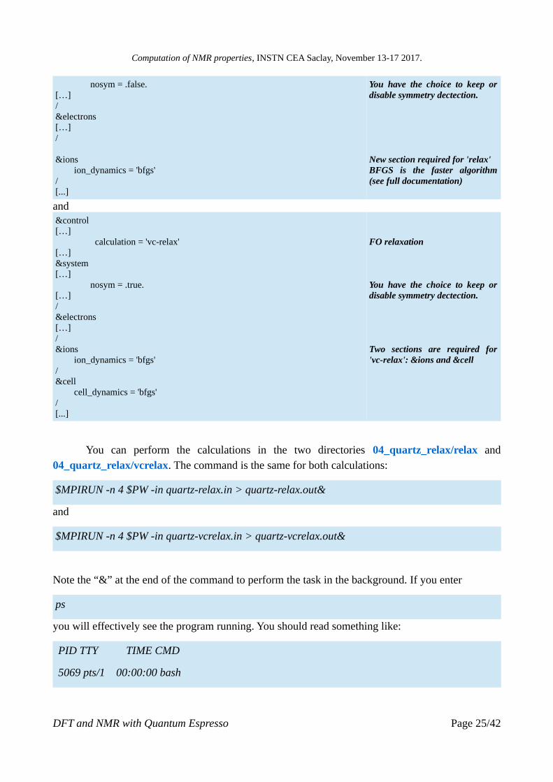
The basic idea behind the structure relaxation procedure (or structure optimization) is tominimize forces below a threshold (optimisation of atomic positions, APO) with or withoutminimization of the stress tensor (optimisation of the cell parameters, FO or Full Optimization).This minimization also forces the total energy to decrease. In the first case (APO) this calculation isreferred to as calculation='relax' in QE input file and calculation='vc-relax' in the second case(FO). Starting from the previous scf input files, this will give the two input files:

&control[…] calculation = 'relax'[…]&system[…]

APO relaxation



nosym = .false.[…]/&electrons[…]/

&ions ion_dynamics = 'bfgs'/[...]

You have the choice to keep ordisable symmetry dectection.

New section required for 'relax'BFGS is the faster algorithm(see full documentation)

and &control[…] calculation = 'vc-relax'[…]&system[…] nosym = .true.[…]/&electrons[…]/&ions ion_dynamics = 'bfgs'/&cell cell_dynamics = 'bfgs'/[...]

FO relaxation

You have the choice to keep ordisable symmetry dectection.

Two sections are required for'vc-relax': &ions and &cell

You can perform the calculations in the two directories 04_quartz_relax/relax and04_quartz_relax/vcrelax. The command is the same for both calculations:

$MPIRUN -n 4 $PW -in quartz-relax.in > quartz-relax.out&

and

$MPIRUN -n 4 $PW -in quartz-vcrelax.in > quartz-vcrelax.out&

Note the “&” at the end of the command to perform the task in the background. If you enter

ps

you will effectively see the program running. You should read something like:

PID TTY TIME CMD

5069 pts/1 00:00:00 bash



6077 pts/1 00:00:00 mpirun

6079 pts/1 00:00:26 pw.x

6080 pts/1 00:00:24 pw.x

6081 pts/1 00:00:24 pw.x

6082 pts/1 00:00:25 pw.x

6103 pts/1 00:00:00 ps

To follow the calculation, you can use the unix command tail as follows (CTRL^C to exit):

tail -f quartz-relax.out

The output file contains a series of SCF calculations, with in between:

[…]

BFGS Geometry Optimization

number of scf cycles = 1 number of bfgs steps = 0

energy new = -216.5964381506 Ry

new trust radius = 0.0121490964 bohr new conv_thr = 1.0E-10 Ry[...]

It ends with (note the default criteria for energy and force convergence, they can be specified in theinput file8)

[…]

bfgs converged in 10 scf cycles and 9 bfgs steps (criteria: energy < 1.0E-04 Ry, force < 1.0E-03 Ry/Bohr)

End of BFGS Geometry Optimization

Final energy = -216.5996153013 Ry[…]Begin final coordinates

ATOMIC_POSITIONS (crystal)[...]

End final coordinates

Final coordinates

HERE

8 It may be useful to check how accurately your structure must be optimized to have converged NMR properties.



You can choose your own criteria for convergence with the parameters etot_conv_thr andforce_conv_thr in the &control section. You can use the grep commands from exercises 2 and 3 tooutput the evolution of the total energy, pressure or forces. Note that there is generally a residualpressure in the system because we don't relax the unit cell volume.

For the 'vc-relax' calculation, it is generally recommended to use a higher ecutwfc value. Thereason is that you need to increase the basis set size and minimize some errors related change in thecell parameters (remember they determine the choice of the k-points thus of the basis set). Apartfrom this, the output is very similar but with some specific information (it is recommended tofollow the progression of the calculation with the tail command, at least the first time):

[…] number of scf cycles = 8 number of bfgs steps = 7

enthalpy old = -216.6032870361 Ry enthalpy new = -216.6034117117 Ry

CASE: enthalpy_new < enthalpy_old

new trust radius = 0.0200929722 bohr new conv_thr = 1.2E-12 Ry

new unit-cell volume = 806.77251 a.u.^3 ( 119.55135 Ang^3 ) density = 2.50366 g/cm^3[…]CELL_PARAMETERS (alat= 1.00000000)[…]

ATOMIC_POSITIONS (crystal)[…]

BFGS INFO

VOLUME VARIATION

CELL PARAMETERS

ATOMIC POSITIONS

with at the end the convergence criteria

[…]

End of BFGS Geometry Optimization

Final enthalpy = -216.6041146630 RyBegin final coordinates new unit-cell volume = 814.04208 a.u.^3 ( 120.62859 Ang^3 ) density = 2.48130 g/cm^3[…]

Followed by the optimized cell parameters and atomic positions. Howerver, in this case a finalcalculation is performed with a basis set determined from the new structure



[…]

A final scf calculation at the relaxed structure. The G-vectors are recalculated for the final unit cell Results may differ from those at the preceding step.[...]

So that total energy, forces and pressure might be slightly different from the last step of theminimization. If too much different, then you probably have to repeat the calculation with a highercutoff energy (starting from the final structure for example to save CPU time).

If you extract to the variation of the volume

grep volume quartz-vcrelax.out

you will generally observe an small increase (especially with PBE functional) in the finalvolume. This is a known effect that PBE functional tends to overestimate bond length (~1%) so thattypically the final unit cell volume overestimates the experimental value by 3-4%. If you trust yourinput data, you can use the celldm(1) parameter for example in the input file to scale the volumeback to its experimental value before the NMR calculation.

Extra: NMR calculation with relaxed structures

From the above outputs, extract the atomic positions (and cell parameters) and performcorresponding NMR calculation. Compare with results obtained with the experimental structure.Try using the scaled volume to its experimental value.

5. Sodium metasilicate : influence of semicore states

Now let's start with serious things. We consider a simple and small system : sodiummetasilicate. In order to make the calculation fast, we have chosen K-POINTS 2 2 2 1 1 1 (a densergrid is theoretically required, you can determine it as an extra) and nosym = .false. In this system,we have two environments for the oxygen atom : bridging-oxygen (BO) and non-bridging oxygen

(NBO).

First, you can compare NMRcalculations performed with K-POINTS 2 2 20 0 0 and K-POINTS 2 2 2 1 1 1. You canautomate you NMR calculation using thefollowing script (Note that the definitions ofMPIRUN, PW, GIPAW, NPROCS depends on



your system and installation) you can name run_nmr.sh

#!/bin/bash

MPIRUN=/usr/lib64/openmpi/bin/mpirun

PW=/opt/qe.6.1/openmpi/bin/pw.x

GIPAW=/opt/qe.6.1/openmpi/bin/gipaw.x

SEED=$1

If [ -f $SEED-scf.in ] ; then

NPROCS=4

echo “ SCF “

$MPIRUN -n $NPROCS $PW -i $SEED-scf.in > $SEED-scf.out

echo “EFG”

$MPIRUN -n $NPROCS $GIPAW -i efg.in > $SEED-efg.out

“NMR “

$MPIRUN -n $NPROCS $GIPAW -i nmr.in > $SEED-nmr.out

else

echo “ No SCF file found for $SEED. STOP”

fi

exit 0;

Then,

chmod +x run_nmr.sh [only once]

./run_nmr.sh metasilicate_1

if metasilicate_1-scf.in is your input file.

With nosym=.false. and K_POINTS 2 2 2 0 0 0 , 8 k-points are needed (making thecalculation relatively long) whereas with the shifted grid K_POINTS 2 2 2 1 1 1 only 2 k-points arenecessary. NMR outputs should be almost the same. With this grid, you can also compare withnosym=.true. .

For those first calculations, you can keep ecuwfc to 80 Ry to make them faster.9

You can first look at the plane wave cutoff energy, say from 20Ry to 80Ry (see ecut

9 I also observe a slight improvement using -nools 2. Make your own test. Bug : the number of k-point shows some dependencies with ecutwfc so that 60 Ry yields 4-k points. Make your own adjustment with a scf calculation.



subdirectory) for the BO (atom #11) and NBO (atom #7)

Ecutwfc Ry

17O CQ (BO)MHz

17O CQ (NBO)MHz

17O σiso (BO)ppm

17O σiso (NBO)ppm

20 -1.5942 -0.9369 331.91 355.46

30 -3.1553 -1.6026 276.41 300.35

40 -4.1519 -2.1777 232.04 257.15

50 -4.4605 -2.3929 209.82 237.68

60 -4.6025 -2.4747 202.55 230.77

70 -4.6284 -2.4848 200.81 229.26

80 -4.6370 -2.4902 200.75 229.25

For 29Si, we obtain (atom #5):Ecutwfc (Ry) 29Si σiso (ppm)

20 369.60

30 400.59

40 403.90

50 407.43

60 407.53

70 407.44

80 407.41

and for 23NaEcutwfc

Ry23Na CQ (MHz) 23Na σiso (ppm)

20 0.612 595.00

30 -1.068 595.13

40 -1.321 571.21

50 -1.358 552.84

60 -1.252 545.78

70 -1.239 544.04

80 -1.239 543.76

In conclusion, we observe similar convergence properties of the absolute magnetic shielding valuesfor all atoms.

Ecutwfc Ry

17O σiso (BO)ppm

17O σiso (NBO)ppm

17O △σiso ppm



20 331.91 355.46 23.55

30 276.41 300.35 23.94

40 232.04 257.15 25.11

50 209.82 237.68 27.86

60 202.55 230.77 28.22

70 200.81 229.26 28.45

80 200.75 229.25 28.5

What can be clearly observed from these data, is the fact that the relative shift convergefaster than absolute value. Because the experimental isotropic chemical shift is given by

δiso=−(σ iso−σref ) ,

for comparison with experimental data, only relative shifts counts. From a pratical point of view, itmeans that a reduced cutoff of 60 Ry is sufficient for the NMR spectroscopist (considering standardinaccuracies of experimental data). As an extra, you can perform the same exercise now with thesize of the k-point grid. Below are some results for magnetic shielding only:

K_POINTS 17O σiso (BO)ppm

17O σiso (NBO)ppm

17O △σiso ppm

29Si σiso ppm

23Na σiso ppm

1 1 1 1 1 1 301.51 259.27 -42.24 379.89 580.36

2 2 2 1 1 1 200.75 229.25 28.5 407.41 543.76

3 3 3 1 1 1 189.56 218.22 28.66 406.55 542.32

4 4 4 1 1 1 188.51 216.90 28.39 406.43 542.17

Here convergence of absolute / relative magnetic shieldings are clearly different. A k-grid of2 2 2 1 1 1 is therefore appropriate.

As a final point, we will now examine the influence of the choice of the valence states (hereNa), here for the sodium. Taking for example 80Ry and a 2 2 2 1 1 1 k-points grid, compare theNMR parameters using the Na pseudopotential Na.pbe-tm-gipaw.UPF (2s22p63s0 valenceconfiguration) and Na.pbe-tm-gipaw-dc.UPF (3s03p0 valence configuration).

Na psp 17O σiso (BO)ppm

17O σiso (NBO)ppm

17O △σiso ppm

29Si σiso ppm

23Na σiso ppm

2s22p63s0 200.75 229.25 28.5 407.41 543.76

2s22p63s0 / core 270.67 837.91 624.63

3s03p0 205.47 248.94 43.48 405.20 538.02

3s03p0 / core 270.67 837.91 377.28



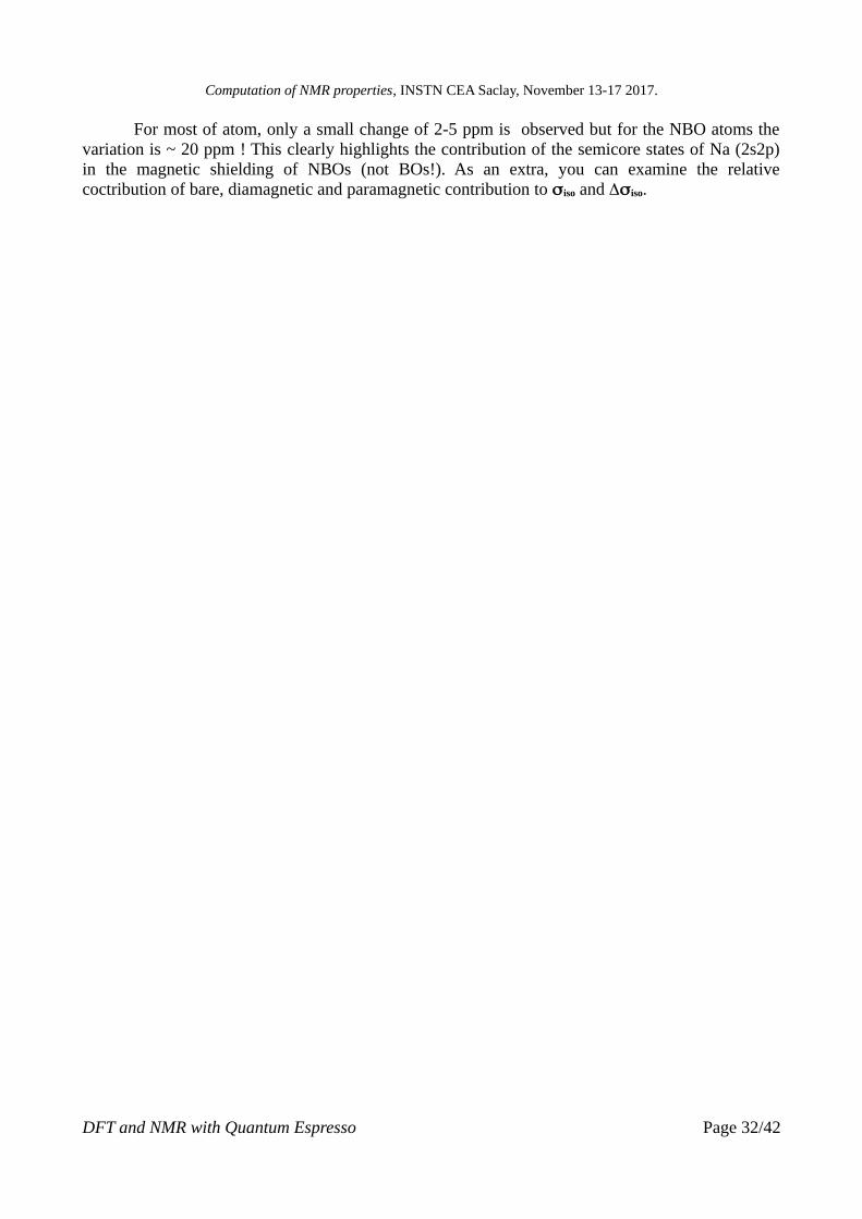
For most of atom, only a small change of 2-5 ppm is observed but for the NBO atoms thevariation is ~ 20 ppm ! This clearly highlights the contribution of the semicore states of Na (2s2p)in the magnetic shielding of NBOs (not BOs!). As an extra, you can examine the relativecoctribution of bare, diamagnetic and paramagnetic contribution to σiso and Δσiso.



Appendices

A. Installation

0) Installation of Quantum Espresso [optional]

~~~~~~~~~~~~~~~~~~~~~~~~~~~~~~~~~~~~~~~~~~~

Here are some notes describing the installation of QE (+ GIPAW)

version 6.1 on a linux CentOS 7 system. Installation on a different

distribution shouldn't be that different.

The following packages are assumed to be installed,

typically using the standard packager coming with

your distribution.

+ openmpi (or mpich) using your package manager (yum,yumex,...)

+ scalapack (preferentially using your package manager)

+ mkl (free version for academic usage can be downloaded upon registration)

As an alternative to mkl, you can install scalapack/lapack/atlas.

Below it is assumed that mkl is installed. Its installation is easy.

First get the package from Intel, current version is l_mkl_2018.0.128.tgz

>tar xvf l_mkl_2018.0.128.tgz

>cd l_mkl_2018.0.128

>sudo ./install.sh

To have the shared library accessible, the easiest is to add a file in /etc/ld.so.conf.d directory

Create a file /etc/ld.so.conf.d/mkl.conf (you need root access) with a single line

"/opt/intel/mkl/lib/intel64"

Then update the linker database

>sudo ldconfig



0.1) Get the qe 6.1 distribution files.

See http://qe-forge.org/gf/project and select Quantum ESPRESSO

Or go to http://qe-forge.org/gf/project/q-e/frs/

You should have the archive file qe-6.1.tar.gz

0.2) Extraction

Move the archive to a building directory, and then extract files

>tar xvf qe-6.1.tar.gz

>cd qe-6.1

0.3) Configuration

A good option is to install the qe program in the /opt/qe.6.1 directory. The configure scriptsprovided is sometimes able to find the intel library (/opt/intel). Just make first a try:

>./configure --enable-parallel --enable-shared --prefix=/opt/qe.6.1

If you obtain

[...]

The following libraries have been found:

BLAS_LIBS= -lblas

LAPACK_LIBS= -llapack -lblas

FFT_LIBS= -lfftw3

It means that the system will use built-in libraries (poor performances...): mkl libraries were not found.

To find where are installed MPI library, you can use the command

>locate mpirun

Below are some examples :

a) /opt/intel/compilers_and_libraries_2018.0.128/linux/mpi/intel64/bin/mpirun

b) /usr/lib64/openmpi/bin/mpirun

c) /usr/lib64/mpich/bin/mpirun


http://qe-forge.org/gf/project


a) is the Intel MPI library you can also download (l_mpi_2018.0.128.tgz)

b) is the standard openmpi library

c) is the standard mpich library

IF you've just installed one of the required library, o not hesitate to update the locate database so that it can be found by locate:

>sudo updatebp

Compilation with openmpi ("\" allows you to have a command on several lines in the terminal)

>BIN=/usr/lib64/openmpi/bin

>./configure --enable-parallel --enable-shared --prefix=/opt/qe.6.1/openmpi \

CC=$BIN/mpicc F77=$BIN/mpif90 FC=$BIN/mpif90 MPIF90=$BIN/mpif90 \

LIBDIRS="/opt/intel/mkl/lib/intel64"

At the end of the output, pay attention to the lines:

[...]

DFLAGS... -D__DFTI -D__MPI -D__SCALAPACK

[...]

The following libraries have been found:

BLAS_LIBS=-L/opt/intel/mkl/lib/intel64 -lmkl_gf_lp64 -lmkl_sequential -lmkl_core

LAPACK_LIBS=

SCALAPACK_LIBS=-lscalapack

FFT_LIBS=

BLAS_LIBS: mkl found.[Ok]

SCALAPACK_LIBS: SCALAPACK has been found.[Ok]



Note the option "--prefix=/opt/qe.6.1/openmpi" to have all programs installed in the/opt/qe.6.1/openmpi folder. You can also use /opt/qe.6.1 if don't plan to play with different libraries(Intel MPI, openmpi, mpich, atlas, ...)

0.4) Compilation

Using 8 cores for examples. To get the number ofcores, you can use the command

>nproc

Compilation of the two main programs

ld1 : for pseudopotential generation

pw : the main program (DFT Plane Wave calculation)

>make -j 8 ld1 pw

0.5) GIPAW module

the instruction

>make -j 8 gipaw

will force the download of qe-gipaw 6.1 in the archive folder. You should have the archive qe-gipaw-6.1.tar.gz in archive folder.

You will most probably meet an error (some bugs...), but it can be circumvent as follows:

>cd qe-gipaw-6.1

>./configure --with-qe-source=/home/charpent/NMRSchool/GIPAW_Tutorial/qe_install/qe-6.1

>make -j 8

/home/charpent/NMRSchool/GIPAW_Tutorial/qe_install is the folder where the compilation of thepackages is performed. Adpat to your own case.

0.6) Installation



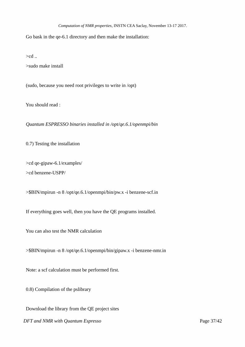
Go bask in the qe-6.1 directory and then make the installation:

>cd ..

>sudo make install

(sudo, because you need root privileges to write in /opt)

You should read :

Quantum ESPRESSO binaries installed in /opt/qe.6.1/openmpi/bin

0.7) Testing the installation

>cd qe-gipaw-6.1/examples/

>cd benzene-USPP/

>$BIN/mpirun -n 8 /opt/qe.6.1/openmpi/bin/pw.x -i benzene-scf.in

If everything goes well, then you have the QE programs installed.

You can also test the NMR calculation

>$BIN/mpirun -n 8 /opt/qe.6.1/openmpi/bin/gipaw.x -i benzene-nmr.in

Note: a scf calculation must be performed first.

0.8) Compilation of the pslibrary

Download the library from the QE project sites



http://qe-forge.org/gf/project/pslibrary/

Then on the left, click on ">>Files"

>tar zxvf pslibrary.1.0.0.tar.gz

>cd pslibrary.1.0.0/

First, you have to create some input files for have the GIPAW psp generated. I suggest to create thefollowing script (just copy/paste in a file named DoAll.sh)

~~~ script DoAll.sh

#!/bin/bash

for job in paw_ps_high.job paw_ps_low.job ; do

echo "=============================================="

echo " Collection $job "

echo "=============================================="

#psp=$(grep cat $job | awk '{print $3}')$

#echo " PSP = $psp "

sed 's/lpaw=.true.,/lpaw=.true., \

lgipaw_reconstruction=.true., \

use_paw_as_gipaw=.true.,/' $job > kj$job

done

exit 0;

~~~

Run it as follows:

>chmod +x DoAll.sh



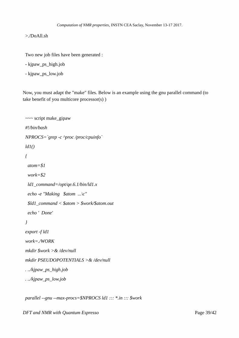
>./DoAll.sh

Two new job files have been generated :

- kjpaw_ps_high.job

- kjpaw_ps_low.job

Now, you must adapt the "make" files. Below is an example using the gnu parallel command (to take benefit of you multicore processor(s) )

~~~ script make_gipaw

#!/bin/bash

NPROCS=`grep -c ^proc /proc/cpuinfo`

ld1()

{

atom=$1

work=$2

ld1_command=/opt/qe.6.1/bin/ld1.x

echo -e "Making $atom ...\c"

$ld1_command < $atom > $work/$atom.out

echo ' Done'

}

export -f ld1

work=./WORK

mkdir $work >& /dev/null

mkdir PSEUDOPOTENTIALS >& /dev/null

. ../kjpaw_ps_high.job

. ../kjpaw_ps_low.job

parallel --gnu --max-procs=$NPROCS ld1 ::: *.in ::: $work



\mv *.UPF PSEUDOPOTENTIALS

\mv *.in WORK

~~~

If don't have "parallel" installed, then you can use a serial approach:

for fin in *.in ; do

ld1 fin $work

done

~~~ script make_gipaw

#!/bin/bash

NPROCS=`grep -c ^proc /proc/cpuinfo`

ld1()

{

atom=$1

work=$2

ld1_command=/opt/qe.6.1/bin/ld1.x

echo -e "Making $atom ...\c"

$ld1_command < $atom > $work/$atom.out

echo ' Done'

}

work=./WORK

mkdir $work >& /dev/null

mkdir PSEUDOPOTENTIALS >& /dev/null

. ../kjpaw_ps_high.job

. ../kjpaw_ps_low.job

for f_in in *.in ; do



ld1 $f_in $work

done

\mv *.UPF PSEUDOPOTENTIALS

\mv *.in WORK

~~~

Then to compile the psp, just go into the functional you need. For example, for pbe

>cd pbe

>../make_gipaw

>sudo mkdir -p /opt/pslibrary/1.0.0/pbe

>cp PSEUDOPOTENTIALS/* /opt/pslibrary/1.0.0/pbe

Here, all pseudo are installed in the directory "/opt/pslibrary/1.0.0/pbe"

You can also use the following scripts to install pseudos for all functionals.

First compilation:

~~~ script gen_upf.sh

#!/bin/bash

for fct in pbe pbesol wc revpbe rel-pbe rel-revpbe rel-pbesol rel-wc ; do

echo $fct ; cd $fct ; ../make_gipaw ; cd ..

done

~~~

>chmod +x gen_upf.sh

>./gen_upf.sh



Secondly, installtion:

~~~ scripts install_upf.sh

#!/bin/bash

for fct in pbe pbesol wc revpbe rel-pbe rel-revpbe rel-pbesol rel-wc ; do

opt=/opt/pslibrary/1.0.0/$fct

mkdir -p $opt

cp $fct/PSEUDOPOTENTIALS/* $opt

done

~~~

>chmod +x install_upf.sh

>sudo ./install_upf.sh

Pseudopotentials from the pslibrary use the "PAW" formalism, they are supposed to be softer than "Norm Conserving" (nc) ones.

NC ones, can be found at the home page of Davide Ceresoli:

https://sites.google.com/site/dceresoli/pseudopotentials

X.pbe-tm-gipaw.UPF : regular psp (Most designed by Ari Seitsonen)

X.pbe-tm-new-gipaw-dc.UPF : DC pseudo.

X.pbe-rkkj-gipaw-dc.UPF : Ultra Soft Pseudo (USPP), they are supposed


computing nmr parameters using the gipaw...

Documents