computing skylines on distributed data
TRANSCRIPT

Computing Skylines on Distributed Data
Haoyu ZhangIndiana University Bloomington
Bloomington,IN,[email protected]
Qin ZhangIndiana University Bloomington
Bloomington,IN,[email protected]
ABSTRACTIn this paper we study skyline queries in the distributedcomputational model, where we have s remote sites and acentral coordinator (the query node); each site holds a pieceof data, and the coordinator wants to compute the skylineof the union of the s datasets. The computation is in termsof rounds, and the goal is to minimize both the total com-munication cost and the round cost.
Viewing data objects as points in the Euclidean space, weconsider both the horizontal data partition case where eachsite holds a subset of points, and the vertical data partitioncase where each site holds one coordinate of all the points.We give a set of algorithms that have provable theoreticalguarantees, and complement them with information theo-retical lower bounds. We also demonstrate the superiorityof our algorithms over existing heuristics by an extensive setof experiments on both synthetic and real world datasets.
1. INTRODUCTIONSkyline computation, also known as the maximal vector
problem, is a useful database query for multi-criteria decisionmaking. If we view data objects as points in the Euclideanspace, then the skyline is defined to be the subset of pointsthat cannot be dominated by others, where we say a point ydominates a point x if y dominates x in all dimensions. Thisproblem was first studied in computational geometry in themid-1970’s [10], and was later introduced into databases asa query operator [4]. There is a vast literature on skylinecomputation and its variants, and we refer readers to [6] and[8] for excellent surveys.
Most work on skyline computation in the literature hasbeen conducted in the RAM (signal machine) model. Inrecently years, due to the large size of the datasets and thepopularity of map-reduce type of computation, a numberof parallel skyline algorithms have been proposed [19, 15,18, 17, 9, 1, 13, 14]. A common feature of these parallelalgorithms is that they use the divide-and-conquer approach,that is, they use central mechanisms to partition the whole
Permission to make digital or hard copies of all or part of this work forpersonal or classroom use is granted without fee provided that copies arenot made or distributed for profit or commercial advantage and that copiesbear this notice and the full citation on the first page. To copy otherwise, torepublish, to post on servers or to redistribute to lists, requires prior specificpermission and/or a fee.Copyright 20XX ACM X-XXXXX-XX-X/XX/XX ...$15.00.
point set into a number of subsets, and then assign eachsubset to a machine for local processing; finally the localresults are merged to form the global skyline. The art of thealgorithm design in this line of work lies in how to choosethe partition mechanism.
In this paper we study the skyline computation on dis-tributed data, which is different from parallel computationin that the data is inherently distributed in different loca-tions, and we cannot afford to repartition the whole datasetsince data repartition is communication prohibited over net-works, and may also cause local storage and data privacyissues which the query node cannot control.
Consider a global hotel search engine, where each hotelis represented as a point in the 2-dimensional Euclideanspace with the x-coordinate standing for the price and they-coordinate standing for the rate of the location. A usernaturally wants to find a hotel with the best location and thebest price, although in reality hotels in good locations usu-ally have higher prices. Thus a good search engine shouldrecommend the user with a list of candidates such that noother hotel has both cheaper price and better location. Thislist is exactly the skyline of the point set. Given a query, thesearch engine (e.g., kayak.com, hipmunk.com) needs to con-tact servers/providers in different locations worldwide. Thetotal bits of communication between the query node andservers and the communication rounds typically dominatethe engine’s response time, since sending messages throughnetwork is much slower than local computation, and the ini-tialization of a new communication round takes quite somesystem overhead.
The Coordinator Model and Previous Work. Westudy the skyline problem in the coordinator model whichcaptures the type of distributed computation mentioned above.In this model we have s remote sites each holding a piece ofdata, and a central coordinator which acts as the query node.We assume there is a two-way communication channel be-tween each site and the coordinator. The computation is interms of rounds: at the beginning of each round the coordi-nator sends a message to some of the sites, and then each ofthe contacted site sends a response back to the coordinator.The goal is to minimize the total bits of communication andthe number of the rounds of the computation. See Figure 1for a visualization of the model.
We differentiate two scenarios of data storage at sites:horizontal partition and vertical partition. In the formereach site contains an (arbitrary) subset of points. And inthe later each site contains one attribute of all points to-gether with their IDs which are used to restore the whole
arX
iv:1
611.
0042
3v1
[cs
.DB
] 1
Nov
201
6

· · ·Site 1
Coor
one round
Site 2 Site 3 Site s
Figure 1: The Coordinator Model
point vectors. Thus if points have d dimensions, we haved sites. The vertical partition corresponds to the settingswhere the information of each attribute has to be retrievedfrom a different server/provider. For example, we may wantto find the lowest prices of hotels from kayak.com, while thecustomers’ best ratings from TripAdvisor.
The coordinator model is equivalent to the models used inseveral previous works for distributed skyline computation[15, 20] (horizontal partition) and [2, 12] (vertical partition).However, all the existing skyline algorithms in this model areheuristic in nature. We will briefly describe these algorithmsin Section 4.1 (horizontal partition) and Section 3.2 (verticalpartition) respectively. In [16] the authors studied a generalversion of vertical partition where multiple columns can bestored in one site. In this paper we will give algorithmswith provable theoretical guarantees (for vertical partitionwe give a better heuristic, given a strong impossibility resultthat we will show). We will also compare our algorithmswith previous ones experimentally in Section 4.
The Skyline Problem. We now give the formal defini-tion of the skyline problem. In this paper we consider theproblem in the 2-dimensional Euclidean space. Given twodistinct points u = (xu, yu) and v = (xv, yv), we say u dom-inates v, denoted by u v, if xu ≥ xv and yu ≥ yv. For aset of distinct points S, the skyline of S is defined to be
sk(S) = u ∈ S | v ∈ S, if v u then v = u.
We next define the data partition of the skyline problemin the coordinator model. In the horizontal partition case,each site i holds a set Si ⊆ S. In the vertical partition case,we have two sites; the first site holds (xu, IDu) | u ∈ Swhere IDu denotes the ID (key) of point u, and the secondsite holds (IDu, yu) | u ∈ S. In both cases, the coordinatorneeds to output sk(S) at the end of the computation.
Our Contribution. We have made the following contribu-tions in this paper. Let n be the total number of points, kbe the number of skyline points (i.e., the output size), ands be the number of sites.
1. For the horizontal partition, we propose two algorithms.The first one achieves the theoretically optimal com-munication cost Θ(ks), but needs dk/2e communica-tion rounds. The second one gives a tradeoff betweenthe total communication cost and rounds: given around budget r the algorithm uses roughly O(skn2/r)communication (see Theorem 2 for the precise bound).We also prove that any one-round algorithm needslinear (i.e., Ω(n)) communication in the worst case.These are presented in Section 2.
2. For the vertical partition, we first prove that in theworst case, any algorithm needs linear communication,
regardless of the communication rounds. We then pro-pose a heuristic that works well in practical settings.These are presented in Section 3.
3. We have implemented our algorithms and relevant heuris-tic algorithms in the literature, and run them on bothsynthetic and real-world datasets. Our experimentshave demonstrated the superiority of our algorithmsover the existing ones in various aspects. We also no-ticed that for the horizontal partition and the datasetswe have tested, with only three communication roundsthe tradeoff algorithm can achieve similar communica-tion cost compared with the theoretically optimal one.The experimental results are presented in Section 4.
Preliminaries. Let [n] denote 1, 2, . . . , n.The φ-quantile of a set S is an element x such that at most
φ |S| elements of S are smaller than x and at most (1−φ) |S|elements of S are greater than x. If an ε-approximation isallowed (denoted by (φ, ε)-quantile), then we can return anyφ′-quantile of S such that φ− ε ≤ φ′ ≤ φ.
2. HORIZONTAL PARTITIONIn this section we give two algorithms for skyline compu-
tation in the horizontal partition case. We then complementthem by proving that the first algorithm is optimal in termsof the total communication cost (though it may need a largenumber of rounds). On the other extreme, if we want thecomputation to be done in one round then in the worst casethe sites need to send almost everything to the coordinator.Our second algorithm gives a tradeoff in between.
We also show that if data is sorted among the sites ac-cording to one of the coordinates, then there is a simplealgorithm that has much smaller communication cost anduses only two rounds.
2.1 AlgorithmsThere is a simple algorithm for computing the skyline
points in the coordinator model in one round: Each sitecomputes the skyline of its local data points and sends itto the coordinator, and then the coordinator computes theglobal skyline on top of the s local skylines. Unfortunatelythis algorithm has communication cost Ω(n); in other words,in the worse case almost all points in all sites need to be sentto the coordinator. We enclose a proof for this statement inSection 2.2.2. We thus try to explore if more rounds canhelp to reduce the communication cost.
2.1.1 Algorithm with Optimal Communication CostOur algorithm with communication costO(ks) is described
in Algorithm 1. We will show in Section 2.2.1 that thiscommunication cost is in fact optimal1 even if we allow aninfinite number of communication rounds.
Let us explain Algorithm 1 in words. At the beginning,each site computes its local skyline points since only thesepoints can possibly be the global skyline points. The restof the algorithm works as follows. At each round, the co-ordinator tries to find the (at most two) points with thelargest x-coordinate or y-coordinate in the remaining pointsheld by all sites. This is done by asking all sites to report
1Up to a logarithmic factor which counts the number of bitsused to represent a point.

Algorithm 1 Optimal Communication under HorizontalPartition
Input: Si is initialized as the point set held by Site iOutput: the global skyline1: Site i computes its local skyline points and discards the
other points in Si2: while ∃i ∈ [s] s.t. Si 6= ∅ do3: for each i s.t. Si 6= ∅ do4: Site i sends the point with the largest x-
coordinate and the point with the largest y-coordinateto the coordinator . the two points can be the samepoint
5: end for6: The coordinator computes new global skyline points
from the points received from all sites, and sends thenew global skyline points to each site
7: for each i s.t. Si 6= ∅ do8: Site i prunes Si by new global skyline points re-
ceived from the coordinator9: end for
10: end while
the local maximums of their remaining points (Line 3-5).Next, the coordinator computes new global skyline pointsfrom the received local maximums, and then sends the newglobal skyline points to all sites for another local pruningstep (Line 6-9).
We now show the correctness of Algorithm 1 and analyzeits costs. First, it is clear that the points with the largestx-coordinate or y-coordinate must be on the skyline. Af-ter the pruning, the points with the largest x-coordinate ory-coordinate in the remaining points also must be on theskyline since they cannot be dominated by the other re-maining points as well as the previous skyline points. Wethus can find one or two skyline points in each round (find-ing one skyline point may only happen in the last round).Since there are at most k skyline points, the algorithm willterminate after at most dk/2e rounds.
The running time at each site consists of two parts: thecomputation of the local skylines and the point prunings.The computation of local skyline at the i-th site needsO(ni logni)time [10], where ni = |Si| is the number of points at the i-th site. The time used for pruning is linear in ni at thei-th site: when pruning points using the new skyline pointwith the global maximum y-coordinate (Line 8), we scanthe points which are sorted increasingly according to theirx-coordinates after the local skyline computation. If a pointcannot be pruned in a particular round, then all the pointsafter it with larger x-coordinates cannot be pruned in thisround. Therefore every point will only be pruned once in thewhole computation. Same arguments hold for the pruningsusing the new skyline point with the global maximum x-coordinate. At the coordinator, for each round we only needto compute the maximums over at most 2s points. Thus thetotal running time is bounded by O(ks).
Theorem 1. There exists an algorithm for computing theskyline on n points in the 2-dimensional Euclidean spacein the coordinator model with s sites and horizontal datapartition that uses O(ks) communication and dk/2e rounds,where k is the output size, that is, the number of points in theskyline. The total running time at the i-th site is O(ni logni)
0 20 40 60 80 1006
7
8
9
10
11
12
13
14
Round
Com
mun
icat
ion
Cos
t (lo
g)
Tradeoff by Algorithm 2 Optimal communication cost by Algorithm 1
Figure 2: Theoretical Communication-Round Tradeoff
where ni is the number of points at the i-th site, and that atthe coordinator is O(ks).
2.1.2 A Communication-Round TradeoffIn the previous section we have shown an algorithm with
the optimal communication cost but needs dk/2e rounds; onthe other hand, there is a naive one-round algorithm but inthe worst case it needs Ω(n) bits of communication. Thenatural questions is:
Can we obtain a communication-round tradeoffto bridge the two extremes?
We try to address this question by proposing an algorithmthat allows the users to choose the number of the rounds ofthe communication in the computation. In this section weshow the following result.
Theorem 2. There exists an algorithm for computing theskyline on n points in the 2-dimensional Euclidean space inthe coordinator model with s sites and horizontal data par-tition that uses r (≥ 3) rounds and C = O(sk(n/s)1/dr/2e)communication, where k is the output size, that is, the num-ber of points in the skyline. The total running time at thei-th site is O(C/s+ni logni) where ni is the number of pointsat the i-th site, and the total running time at the coordinatoris O(C).
Figure 2 visualizes the communication-round tradeoff.
Let t = dr/2e. We describe our tradeoff algorithm in Al-gorithm 2. The algorithm again starts with a local skylinecomputation at each site. Similar to Algorithm 1, the restof the tradeoff algorithm still proceeds in rounds. The maindifference is that at each round, the parties (sites and thecoordinator) first jointly compute (1/d, 1/(2d))-quantiles topartition the Euclidean plane to a set of at most d verticalstrips, and then instead of computing the (at most 2) pointswith the global maximum x/y coordinates, the coordinatorcomputes for each non-empty strip the point with the max-imum y-coordinate by collecting information from the sites(Line 5-8); after that the parties use these points to com-pute new skyline points and prune each strip. We call thecombination of computing the quantiles and maximum y-coordinates, and finding new skyline points and performinglocal pruning, one step of the computation. The algorithmruns for (t − 1) steps, and after that the sites simply sendall the remaining points to the coordinator.

Algorithm 2 Communication-Round Tradeoff under Hori-zontal Partition
Input: Si is initialized as the point set held by Site i; r(#communication-rounds) is a user-chosen parameter;d is a parameter specified in the analysis.
Output: the global skyline1: Site i computes its local skyline points and prunes the
other (dominated) points in Si2: `← 0; t← dr/2e3: while (` ≤ t− 1) ∧ (∃i ∈ [s] s.t. Si 6= ∅) do4: All sites and the coordinator jointly compute
(1/d, 1/2d)-quantiles according to the x-coordinates ofpoints in
⋃i∈[s] Si . the quantile points naturally
partition the Euclidean plane to d strips5: for each i s.t. Si 6= ∅ do6: Site i, for each non-empty strip, sends the point
with the largest y-coordinate to the coordinator7: end for8: The coordinator, for each strip, finds the point with
the largest y-coordinate among points received fromsites; let Y denote the set of these points among allstrips
9: The coordinator computes new skyline points fromY and sends them to each site
10: for each i s.t. Si 6= ∅ do11: Site i prunes Si by new global skyline points re-
ceived from the coordinator12: end for13: `← `+ 114: end while15: ∀i ∈ [s], Site i sends Si to the coordinator16: The coordinator updates the global skyline using the
new points received from sites
We now show the correctness of Algorithm 2 and analyzeits costs. The high level intuition on the round efficiency ofAlgorithm 2 is that at each round, the point with the maxi-mum y-coordinate in each strip will either contribute to theglobal skyline or help to prune all the points in that strip.Compared with Algorithm 1, one can think that we are try-ing to prune the whole data set in parallel, that is, in eachstrip of the plane. This will reduce the round complexity atthe cost of mildly increasing the total communication cost.
Correctness. The correctness of Algorithm 2 is straight-forward: our skyline computation does not prune any pointthat is not dominated by others. Indeed, up to the (t−1)-thstep (or, (2t − 2)-th round), what Algorithm 2 does can besummarized as “sites send candidate global skyline points→ the coordinator computes new global skyline points fromthese candidates → sites use new skyline points to prunetheir local datasets”. At the (2t − 1)-th round, sites justsend all the remaining unpruned points to the coordinatorso that we will not miss any skyline points.
Communication cost. We count the communication costin two parts. The first part is the communication neededat the first (t − 1) steps, and the second part is the totalnumber of remaining points at all sites after the (t − 1)-thstep, which will be sent to the coordinator all at once at thefinal round.
We first analyze the cost of computing quantiles at eachstep. We can compute (ε, ε/2)-quantiles using the following
folklore algorithm: the i-th site (for all i ∈ [s]) sends thecoordinator the exact ε/2-quantiles Qi of its local point setSi. Using Q1, . . . , Qs, the coordinator can answer quantilequeries as follows: Given a query rank β, it returns thelargest v satisfying
β −∑i∈[s] ranki(v) ≥ 0,
where ranki(v) = ni(v) · (ε/2 · |Si|), and ni(v) is the numberof ε/2-quantiles in Qi that is smaller than v. It is easy tosee that 0 ≤ β − v ≤ ε/2 ·
∑i∈[s] |Si|. The following lemma
summarizes the communication cost of this algorithm.
Lemma 1. There is an algorithm that computes (ε, ε/2)-quantiles in the coordinator model using one round and O(s/ε)communication.
Thus the communication used for quantile computationcan be bounded by O(sd) at each step. The rest commu-nication at each step includes sending local maximums atall strips and new skyline points, which can be bounded byO(sd) we as well. To sum up the total communication inthe first part is bounded by O(sd(t− 1)).
The rest of the analysis is devoted to the second part, thatis, to bound the number of the remaining points after the(t− 1)-th step.
We first assume that the output size k is known, and dwill be chosen as a function of k. We will then show how toremove this assumption.
Let Y` ∈ [1, d] denote the number of new skyline points wefind at the `-th step. Observe that in each strip, if the pointwith the largest y-coordinate is not a skyline point, then therest of the points in that strip cannot be skyline points andthus are pruned. After the first step, there are at most Y1
strips having point and each strip has at most 2n/d points,so there are at most
Y1 · 2n/d = 2nY1/d
points left. After the second step, there are at most Y2 stripshaving point and each strip has at most 2(2nY1/d)/d points,so there are at most
Y2 · 2 (2nY1/d) /d = 4nY1Y2/d2 (Y1 + Y2 ≤ k)
points left. After the (t− 1)-th step, there are at most
2t−1n∏
`∈[t−1]
Y`/dt−1
∑`∈[t−1]
Y` ≤ k
(1)
≤ n
(2k
(t− 1)d
)t−1
(2)
points left, where from (1) to (2) we have used the AM-GMinequality and the equality holds when all Y` = k/(t− 1) (` =1, . . . , t−1). We thus have at most n(2k/((t−1)d))t−1 pointsleft at sites after (t−1)-th step, and the sites will send all ofthem in the final (i.e., (2t− 1)-th) round. Adding two partstogether, the total communication cost is bounded by
O(sd(t− 1)) + n
(2k
(t− 1)d
)t−1
. (3)
When
d =2k
t− 1·(n(t− 1)
2sk
)1/t
, (4)

Expression (3) simplifies to be O(sk(t−1)/t(n/s)1/t).
Dealing with unknown k. We now show how to dealwith the case that we do not know k at the beginning. Asimple idea is to guess k as powers of 2 (i.e., 1, 2, 4, 8, . . .),and for each guess, we run our algorithm, and report errorif∑Y` > k at some point, in which case we double the
value of k and rerun the algorithm. The correctness of thealgorithm still holds. The round complexity, however, mayblow up by a factor of log k in the worst case. We will showthat there is a way to preserve the round complexity evenwhen we do not know k at the beginning.
The new idea is to guess k progressively, based on thenumber of new skyline points found in the previous step.More precisely, we set the guess of k at the `-th step, denotedby k`, to be Y`−1 · (t − 1), for ` ≥ 2; and we set k1 = t − 1to begin with. Now at the `-th step we use
d = d` =2k`t− 1
·(n(t− 1)
2s
)1/t
(5)
strips for the pruning. Note that (5) is very similar to (4),where we have replaced the first k in (4) by k` and removedthe second k in (4).
Similar to (2), after (t− 1)-th step, there are at most
2t−1n∏
`∈[t−1]
(Y`/d`)
points left, and consequently the total communication costis bounded by
s∑
`∈[t−1]
d` + 2t−1n∏
`∈[t−1]
(Y`/d`). (6)
We now bound the two terms in (6) separately. We firsthave
s∑
`∈[t−1]
d` =2s∑`∈[t−1] k`
(t− 1)·(n(t− 1)
2s
)1/t
≤ 2sk ·(n(t− 1)
2s
)1/t
. (7)
where we have used the inequality
∑`∈[t−1]
k` = (t− 1)
1 +∑
`∈[t−2]
Y`
≤ (t− 1)k.
For the second term, we have
2t−1n∏
`∈[t−1]
(Y`/d`) = nY1Y2 · · ·Yt−1
Y1Y2 · · ·Yt−2
(n(t− 1)
2s
)t/(t−1)
= nYt−1 ·2s
n(t− 1)
(n(t− 1)
2s
)1/t
≤ 2sk
(t− 1)
(n(t− 1)
2s
)1/t
. (8)
By (7) and (8), the total cost is bounded by O(sk(n/s)1/t) =
O(sk(n/s)1/dr/2e), as claimed.
Running time. The time cost at each site involves threeparts: the computation of the local skyline, the computationof local quantiles, and the point prunings. Computing localskyline again cost O(ni logni) where ni is the number of
Yy1
y2
y3
y4
Site 1 Site 2 Site 3 Site 4 X
Figure 3: Algorithm for Sorted Dataset
points at the i-th site. The cost of point prunings can againbe made linear in ni for the same reason as that in Algo-rithm 1. Now we analysis the time cost of computing thelocal quantiles. Since points are sorted after the local sky-line computation, computing (exact) local quantiles needsO(d`) time at the `-th step. Thus the total time is bounded
by∑`∈[t−1] d` = O(k(n/s)1/t) = O(k(n/s)1/dr/2e).
The running time at the coordinator also consists of threeparts: the computation of approximate global quantiles ateach step, the computation of new skyline points from thefirst step to the (t − 1)-th step, and the computation ofskyline points (output) at the end. The observation is thatat each step, for each of the three tasks, the running at thecoordinator can be asymptotically bounded by the numberof points it receives from all sites in that step, and thusthe total running time at the coordinator is asymptoticallyupper bounded by the total communication cost.
2.1.3 An Algorithm for Sorted DatasetsIn this section we show that we can do much better if the
data points are partitioned to the s sites in a sorted orderwith respect to the x-coordinate (or, the y-coordinate). Inother words, let x1 ≤ x2 ≤ . . . ≤ xs−1 be (s − 1) splitpoints, and let x0 = −∞ and xs =∞. The i-th site gets allpoints between (xi−1, xi]. See Figure 3 for an illustration.As mentioned in the introduction, in the coordinator modelwe cannot afford to repartition the dataset. Therefore thealgorithm presented in this section is only useful for settingswhere the data has already been sorted among the sites.
Theorem 3. For n points in the 2-dimensional Euclideanspace partitioned among the s sites in the coordinator modelin the sorted manner according to their x-coordinates or y-coordinates, there exists an algorithm for computing the sky-line that uses O(k+ s) communication and 2 rounds, wherek is the output size, that is, the number of points in the sky-line. The total running time at the i-th site is O(ni logni)where ni is the number of points at the i-th site, and that atthe coordinator is O(k + s).
We described our algorithm for sorted datasets in Algo-rithm 3. Let us explain in words. Same as before, each sitefirst does a local pruning and computes its local skyline. Inthe first round, the i-th site sends the coordinator the pointwhich has the largest y-coordinate, denoted by yi. In thesecond round, the coordinator for each i ∈ [s] computes thevalue zi which is the maximum value among yi+1, . . . , ys,and sends zi to the i-th site. The i-th site then prunes allits local points with y-coordinate smaller than zi, and sendsthe rest of its points to the coordinator.
We now show the correctness of this algorithm and analyzeits costs. The claim is that the points in Si with y-coordinate

Algorithm 3 Sorted Datasets under Horizontal Partition
Input: Si is initialized as the point set held by Site iOutput: the global skyline1: Site i computes its local skyline points and discards the
other points in Si2: Site i sends the point with the largest y-coordinate, de-
noted by yi, to the coordinator3: The coordinator computes for ∀i ∈ [s], zi =
maxyi+1, . . . , ys, and sends zi to Site i4: Site i prunes Si using zi, and sends the rest points to
the coordinator5: The coordinator updates the global skyline using the
new points received from sites
larger than zi, denoted by Pi, must on the global skyline.Indeed, points in Pi can not be dominated by any point inS1, . . . , Si−1 since all points in Si have x-coordinates largerthan those points in S1, . . . , Si−1. On the other hand, pointsin Pi cannot be dominated by any point in Si+1, ..., Ss sinceall points in Pi have y-coordinates larger than the thosepoints in Si+1, . . . , Ss. The communication of the algorithmincludes sending yi and zi (costs 2s) plus sending skylinepoints (costs k). The running time at each site is dominatedby the local skyline computation, and the time cost at thecoordinator is clearly O(k+ s) (O(s) for the first round andO(k) for the second round).
2.2 Lower Bounds
2.2.1 Infinite RoundsWe prove a lower bound for the infinite-round case by
a reduction from a communication problem called s-DISJ.The lower bound matches the upper bound by Algorithm 1up to a logarithmic factor which counts the number of bitsused to represent a point in the Euclidean plane.
In s-DISJ, each of the s sites gets an m-bit vector. LetXi = (X1
i , . . . , Xmi ) be the vector the the i-th site gets.
We can view the whole input as an s × m matrix X withXi (i ∈ [s]) as rows. The s-DISJ problem is defined asfollows:
s-DISJ(X1, . . . , Xs) =
1, if there exists a j ∈ [m] s.t.
∀i ∈ [s], Xji = 1,
0, otherwise.
Lemma 2 ([5]). Any randomized algorithm for s-DISJthat succeeds with probability 0.51 has communication costΩ(sm). The lower bound holds even when we allow an infi-nite number of communication rounds.
The Reduction. Given the m-bit vector Xi for s-DISJ, thei-th site first converts it to a 2m-bit vector X ′i as follows:each 0 bit will be converted to 01, and each 1 bit will beconverted to 10. For example, when m = 5 and Xi = 10101,X ′i should be 1001100110. The next step is to convert X ′ito a staircase. This step is illustrated in Figure 4. We can“embed” the staircase into an m × m grid. The staircasestarts from the top-left point of the grid, and grows in 2msteps. In the `-th step, if the `-th coordinate of X ′i is 0,then the staircase grows one step horizontally rightwards;otherwise if the `-th coordinate is 1, then the staircase growsone step vertically downwards.
Figure 4: Translating vector X ′1 = 1001100110 (m = 5) toa staircase.
Figure 5: The solid red skyline corresponds to the case thats-DISJ(X1, . . . , Xs) = 0, and the dash blue skyline corre-sponds to the case that s-DISJ(X1, . . . , Xs) = 1.
The observation is that if we create s staircases usingX ′1, . . . , X
′s, then the skyline of the union of these s stair-
cases is closely related to the value of s-DISJ(X1, . . . , Xs):If s-DISJ(X1, . . . , Xs) = 0, then the skyline will be in theform of the red curve in Figure 5; otherwise, the skyline willbe different from the red curve (e.g., be the blue curve inFigure 5 if the 3rd coordinates of X1, . . . , Xs are all 1). Thisis because for each column j ∈ [m] in the grid, as long asthere is one i ∈ [s] such that the j-th coordinate of Xi is 0,or the (2j − 1)-th and (2j)-th coordinates of X ′i is 01, theskyline within the j-th column of the grid will be like “q”;otherwise if for all i ∈ [s] the j-th coordinate of Xi is 0, thenthe skyline within the j-th column of the grid will be like“x”. The other direction also holds, that is, if the skyline isin the form of the red curve, then s-DISJ(X1, . . . , Xs) = 0;otherwise, s-DISJ(X1, . . . , Xs) = 1.
When the size of the skyline is k, we set m = k accordingto our reduction, and obtain the following theorem.
Theorem 4. Any randomized protocol for computing sky-line in the coordinator model with horizontal partition thatsucceeds with probability 0.51 has communication cost Ω(sk)bits, where k is number of points in the skyline. The lowerbound holds even when we allow an infinite number of com-munication rounds.
2.2.2 One RoundWe now prove an Ω(n) communication lower bound for the
case that the algorithm needs to finish in one round. Thisproof is simpler than the infinite-round case – we only need

two sites to participate in the game. We assign Site 1 anm-bit vector u, which can be converted to a staircase in them×m grid just like the infinite-round case, and assign Site2 one bit v, which is translated to the upper-right connerpoint of the grid if v = 1 and the lower-left conner point ofthe grid if v = 0. We have the following simple observation,which holds because if we change one bit of the vector mfrom 0 to 1, we will change a “q” to “x” in the staircase, andthus change the skyline; same for replacing a bit 1 to 0.
Observation 1. If the coordinator needs to compute theglobal skyline, and v = 0, then it needs to learn the vector uexactly.
We immediately have the following lemma.
Lemma 3. Any one round randomized algorithm for thecoordinator to learn u exactly with probability 0.51 has com-munication cost Ω(m).
Note that when v = 1, the skyline only consists of a singlepoint in the upper right conner. Therefore the output sizek is not directly related to the value m; we thus can setm = Ω(n).
Theorem 5. Any one round randomized algorithm forcomputing skyline in the coordinator model with horizontalpartition that succeeds with probability 0.51 has communica-tion cost Ω(n) bits, where n is the total number of pointsheld by all sites.
3. VERTICAL PARTITIONIn the vertical partition, each site holds a single coordinate
of all the data points. Since we consider points in the 2-dimensional Euclidean space in this paper, we only havetwo sites, named Alice and Bob. We store the ID (key) ofeach point on both sites. More precisely, Alice has a setof tuples (xp1 , IDp1), (xp2 , IDp2), . . ., where xpi is the x-coordinate of point pi and IDpi is the ID of pi; and Bobhas a set of tuples (IDq1 , yq1), (IDq2 , yq2), . . ., where yqi isthe y-coordinate of point qi. We can join the two tables torecover the information of all points.
3.1 A Strong Lower BoundAs mentioned in the introduction, in the vertical par-
tition case there is a strong communication lower bound,which states that in the worst case sites have to send almosteverything to the coordinator. We prove the lower boundby a reduction from a classical problem in communicationcomplexity called two-party set-disjointness (denoted by 2-DISJ). In the 2-DISJ, we have two parties Alice and Bob.Alice holds a set of numbers A ⊆ [n], and Bob holds a setof numbers B ⊆ [n], and they want to jointly compute
2-DISJ(A,B) =
1, A ∩B 6= ∅,0, otherwise.
Fact 1 ([3]). Any randomized protocol for 2-DISJ thatsucceeds with probability 0.51 has communication cost Ω(n).
The Reduction. Alice uses her input A to create the x-coordinates of the n points as follows: for each a ∈ A, shecreates a point (2, a) where 2 is the x-coordinate and a is theID of the point; and for each a ∈ [n]\A, she creates a point
(1, a). Bob uses his input B to create the y-coordinates ofthe n points in a similar way: for each b ∈ B, he creates apoint (b, 2) where 2 is the y-coordinate and b is the ID ofthe point; and for each b ∈ [n]\B, he creates a point (b, 1).
It is easy to see that if A∩B 6= ∅, then there is at least onepoint in the (2, 2) position, which will be the only point inthe skyline; otherwise, the skyline will consist of two points(1, 2) and (2, 1). By Fact 1 we have
Theorem 6. Any randomized algorithm for computing sky-line in the distributed model with vertical partition that suc-ceeds with probability 0.51 has communication cost Ω(n), re-gardless how many rounds the algorithm uses.
3.2 A Simple HeuristicGiven the strong lower bound result in Section 3.1, we pro-
pose in this section a heuristic which is communication effi-cient on real-world datasets. Our algorithm can be thoughtas a batched pruning version of the Threshold-Algorithmbased approach [2, 12], but has been tailored for bounded-round distributed computation. We call our heuristic inter-active pruning; the pseudocode is described in Algorithm 4.
We now explain our algorithm in words. Let r be theround budget and ρ be the parameter denoting the numberof groups we use for the algorithm. We say a point p isrecovered at the coordinator if both the x and y coordinatesof p are known to the coordinator.
Alice and Bob first sort decreasingly all points accord-ing to the x-coordinates and y-coordinates respectively, andthen partition the points to ρ groups, denoted byGx1, . . . , GxρandGy1, . . . , Gyρ respectively. The coordinator tries to learnboth coordinates of the points that possibly lie in the sky-line progressively. It maintains four variables fx, fy, lx, ly:fx and fy stand for the indices of the next groups Alice andBob will send to the coordinator respectively; and groupswith indices at least lx and ly at Alice and Bob respec-tively have already been pruned. Observe that if fx ≥ lxor fy ≥ ly, then the coordinator must have recovered allthe skyline points, and thus the algorithm can terminate.Based on this fact, the coordinator always chooses the sitewith the smaller gap value lx − fx or ly − fy, and asks forthe information of its next group Gxfx or Gyfy .
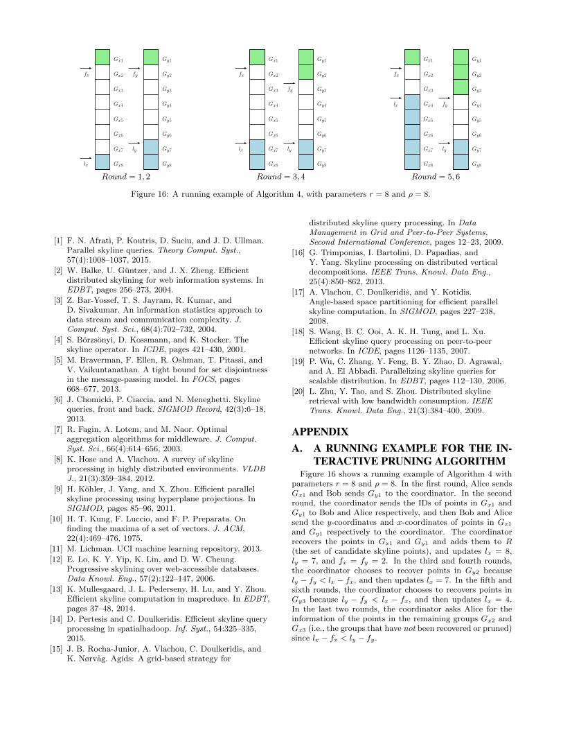
Algorithm 4 proceeds in three stages. The first stage con-sists of two rounds (Line 3 to 5). The goal of the first stageis to recover the first groups Gx1 and Gy1 at Alice and Bob,and update the variables lx and ly to determine the nextgroup to recover. The second stage consists of b(r − 4)/2csteps each of which consisting of two rounds (Line 6 to 10).The goal of the second stage is to recover points progressivelyfrom the site which has a smaller gap value. The algorithmwill stop early if at some step all points have been eitherpruned or recovered at a site. The goal of the third stage isto recover all groups that are still not recovered or prunedafter the first two stages. This is done at the coordinatorby first asking the site with the smaller gap value to get theIDs of points in these groups together with one of the twocoordinates, and then contacting the other site for the othercoordinates of these points. We include a running examplefor Algorithm 4 in Appendix A.
The correctness of the algorithm is straightforward sincewhen our algorithm stops, all points at one site are eitherrecovered or pruned. The local running time at each siteis dominated by the initial sorting which is O(n logn), and

Algorithm 4 Interactive Pruning under Vertical Partition
Input: S1 is the set of the x-coordinates of points heldby Alice, and S2 is the set of the y-coordinates of pointsheld by Bob. ρ (number of groups) and r (round budget)are two user-chosen parameters.
Output: the global skyline
1: Alice sorts S1 decreasingly and then partitions it to ρgroups of equal size, denoted by Gx = Gx1, . . . , Gxρ.Bob does the same thing on S2 and gets groups Gy =Gy1, . . . , Gyρ. Alice and Bob send the splitting coordi-nates of the group partitions to the coordinator. Givena point p, let gx(p) be the index of the group in Gx thatcontains p, and gy(p) be the index of the group in Gythat contains p
2: The coordinator maintains a set of points R denotingthe recovered points, and four variables: fx, fy, lx, ly.
3: The coordinator communicates with Alice and Bob tolearn both the x-coordinates and y-coordinates of pointsin Gy1 and Gx1, adds them to R, and then updateslx ← mingx(p) | p ∈ Gy1+1 and ly ← mingy(p) | p ∈Gx1+ 1
4: The coordinator sets fx ← 2, fy ← 25: j ← 1 . index of steps; one step uses two rounds6: while (2j ≤ r − 4) ∧ (lx > fx) ∧ (ly > fy) do7: If lx − fx ≤ ly − fy, the coordinator requests groupGxfx from Alice and updates fx ← fx+1, else it requestsGyfy from Bob and updates fy ← fy + 1
8: The coordinator recovers and adds points in Gxfx (orGyfy ) to R, and updates ly ← minly,mingy(p) | p ∈Gxfx+1 (or lx ← minlx,mingx(p) | p ∈ Gyfy+1)
9: j ← j + 110: end while11: if (lx > fx) ∧ (ly > fy) then12: The coordinator compares lx−fx and ly−fy; w.l.o.g.,
assume lx− fx is smaller. The coordinator sends fx andlx to Alice. Alice then sends the x-coordinates and IDsof points (denoted by P ) in Gxfx , . . . , Gx(lx−1) to thecoordinator.
13: The coordinator sends the IDs of points in P to Bob.Bob then sends the y-coordinates of points in P to thecoordinator. The coordinator adds points in P to R
14: end if15: The coordinator computes and outputs the skyline of R
the time cost at the coordinator is dominated by the finalskyline computation which is also O(n logn).
We comment that ρ is a parameter that we need to chooseat the beginning of the algorithm; we will discuss how tochoose ρ in the experiments in Section 4.
A comparison to previous algorithms. Our algorithm,the BDS algorithm and its improvement the IDS algorithmproposed in [2], and the PDS algorithm proposed [12] are allbased on the Threshold-Algorithm (TA) [7]. A clear differ-ence is that BDS, IDS and PDS recover one point in each stepat the coordinator, while we recover at least one group ofpoints in each step which helps to significantly reduce theround cost. The second major difference is that to improvethe basic TA-base algorithm BDS, both IDS and PDS sharethe idea of estimating the most probable terminating point,and then using it to decide which site to access next. IDS
finds the most probable terminating point by calculating the
score of each point which is the sum of the differences be-tween each of its coordinates and the coordinate of the lastpoint recovered by the sorted access at the respective site.PDS uses linear regression to estimate the rank of each point,and the point with the lowest rank is considered to be themost probable terminating point. In our algorithm, insteadof looking for the most probable terminating point, we focuson the number of unrecovered and unpruned groups remain-ing at each site. We choose to request a new group of pointsfrom the site with the smaller number of remaining groups,with the purpose of terminating the algorithm earlier.
It is well-known that the Threshold-Algorithm [7] is in-stance optimal in terms of number of points probed, and thusif we only measure the number of points recovered at the co-ordinator in the process, our batched pruning approach hasno advantage compared with the individual point pruningsin BDS, IDS and PDS. However, as we shall see in the experi-ments (Section 4), batched pruning can not only significantlyreduce the round cost, but also bring down the overall com-munication cost in some cases. This is because in each stepthe coordinator needs to send a message to request pointsfrom the sites in the sorted access, and consequently theround cost will influence the communication cost as well.
4. EXPERIMENTSIn this section we present the experimental studies of our
proposed algorithms. We have implemented all algorithmsin C++. All experiments were conducted on a laptop withInter Core i7 running Windows 7 with 4GB memory.
The Datasets. We use both synthetic and real-world datasets.We generated three synthetic datasets following the stan-dard literature [4]. The data partition among the sites willbe described in Section 4.1 (horizontal partition) and Sec-tion 4.2 (vertical partition) respectively.
• INDI(independent): We generate 20 million points. Foreach point we generate each of its coordinates indepen-dently uniformly at random from [0, 1]
• CORR(correlated): We select 200 thousand lines (de-noted by L1) perpendicular to the line from (0, 0) to(1, 1), where the intersections follow the standard nor-mal distribution. Next, for each line in L1 we pick 100points also following the standard normal distribution.We have 20 million points in total.
• ANTI(anti-correlated): We select 200 thousand lines(denoted by L2) perpendicular to the line from (0, 1) to(1, 0), where the intersections follow the standard nor-mal distribution. Next, for each line in L2 we pick 100points also following the standard normal distribution.We have 20 million points in total.
We make use of the following real-world datasets.
• Airline: this dataset contains 3 million the airlineitineraries and prices between 30 U.S. major cities in2015 first quarter.2 We choose (minus) fare and (mi-nus) fare-per-mile as the two attributes in x and ycoordinates. The skyline points are considered to beeconomic flights.
2Available at http://www.transtats.bts.gov.

• Household [11]: this dataset contains 2 million house-hold electric power consumption records gathered be-tween December 2006 and November 2010. We choosevoltage and intensity as the two attributes in x and ycoordinates. The skyline points represent those house-holds that are recommended to pay attention to theenergy efficiency.
• Covertype [11]: this dataset contains 500 thousandnatural statistics from four wilderness areas located inthe Roosevelt National Forest of northern Colorado.We choose elevation and slope as the two attributesin x and y coordinates. The skyline points representareas that may have interesting geological behaviors.
4.1 Horizontal PartitionAlgorithms. We compare the following algorithms in thecase of horizontal partition.
• Naive: the single round algorithm in which each sitecomputes and sends its local skyline to the coordinatorfor a merge.
• Optimal: Algorithm 1 in Section 2.1.1. The algorithmthat achieves the optimal communication cost.
• Tradeoff: Algorithm 2 in Section 2.1.2. The algorithmthat gives a smooth communication-round tradeoff.
• AGiDS: We use the AGiDS algorithm proposed in [15] asa comparison. To make AGiDS fit in our model, we usethe following version of the original algorithm: At thebeginning, the coordinator and sites share the infor-mation of a grid in which each cell represents a rangein the x/y-axes (equal width partition). In the firstround (the planing phase), sites send the informationof non-empty cells to the coordinator. In the secondround (the execution phase), the coordinator finds thecells that may contribute to global skyline and sendsthe information to sites, and then sites send points inthese cells to the coordinator. Finally the coordinatorcomputes the skyline of received points as the output.We comment that this algorithm is also very similarto the relaxed skyline algorithm proposed in [1]. Wechoose the grid to be 20 × 20 (total 400 cells) in ourexperiments which works the best under our settings.
• FDS: We use the FDS algorithm proposed in [20] as acomparison. The original algorithm proceeds in itera-tions. To make it fit in our model, we use three roundsfor each iteration: In the first round (the voluntaryphase), each site sends the top κ points with the largestscores (x+ y) to the coordinator. In the second round(the compulsory and computation phase), the coordi-nator calculates the minimum score (denoted by Fmin)from received points and sends it to each site. Each sitethen sends all its local points that have larger scoresthan Fmin to the coordinator. The coordinator updatesthe global skyline with points received in the first tworounds. In the third round (the feedback phase), thecoordinator calculates and sends each site a feedback,which consists of points that are guaranteed to domi-nate at least ` points in that site. And then each sitedoes a local pruning. κ and ` are two parameters inFDS; we choose the optimal values κ = 1 and ` = 1 asreported in [20].
Data Partition. For the three synthetic datasets, we par-tition points randomly to 20 sites. For Airline, we partitionthe data records in the same city to the same site; we thushave 30 sites. For Household, we partition the data collectedin every two consecutive months to the same site; 20 sites intotal. For Covertype, we just randomly partition the datarecords to 20 sites.
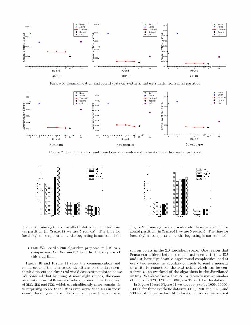
Results and Discussions. Figure 6 and Figure 7 show thecommunication and round costs of the five tested algorithmson the three synthetic datasets and three real-world datasetsmentioned above.
We observed that by using three rounds, the communi-cation cost of Tradeoff is 25%-44% of that of Naive onsynthetic datasets and 22%-31% on real-world datasets, andis also close to Optimal which uses more rounds. We no-ticed that the advantage of Tradeoff against Naive is largerin real-world datasets (even of smaller sizes) than syntheticones. This is because it is more likely in real-world datasetsthat a point in one site dominates most of the local skylinepoints in another site. We observe that in Household, by us-ing 5 rounds Tradeoff needs even less communication thanOptimal. This is possible since Optimal is just asymptoti-cally optimal in the worst case.
The communication cost of AGiDS, which uses two rounds,is similar to Naive on Airline and Household and evenworse on INDI, CORR, and Covertype, and is consequentlymuch worse than Tradeoff and Optimal. FDS uses the largestamount of rounds (even more than Optimal), but its com-munication is worse than both Tradeoff and Optimal on allsynthetic and real-world datasets.
Figure 8 and Figure 9 show the running time of the testedalgorithms (excluding the cost the common local skylinecomputation at the beginning) on synthetic and real-worlddatasets respectively.3 Generally speaking the running timeof all algorithms are similar. On the ANTI dataset, the run-ning time of Optimal and FDS are clearly worse than others.This is because they need many more rounds than otheralgorithms on ANTI.
Summary. Tradeoff achieves noticeable communicationcost reductions than AGiDS and Naive by using one or twomore rounds; its performance is very close to the theoreticaloptimal algorithm Optimal in the communication cost butis much more efficient in rounds. On the other hand, AGiDSdoes not have an advantage against Naive in communicationbut uses one more round, and the performance of FDS isclearly dominated by Tradeoff and Optimal. All algorithmshave similar time costs since the computation of the localskylines dominates the other costs.
4.2 Vertical PartitionWe compare the following algorithms in the vertical par-
tition case.
• Prune: Algorithm 4 in Section 3.2.
• BDS and IDS: We use the BDS and IDS algorithms pro-posed in [2] as comparisons. See Section 3.2 for a briefdescription of these two algorithms.
3The local skyline computation takes about 6 seconds on allthe three synthetic datasets and 1.1, 0.6, 0.2 seconds on theAirline, Household and Covertype respectively. This costin fact dominates the other time costs.
1 2 3 4 5Round
0.000
0.005
0.010
0.015
0.020
44 158
Naive
AGiDS
Trade-off
Optimal
FDS
Communication Cost(%
)
ANTI
1 2 3 4 5Round
0.000
0.002
0.004
0.006
0.008
0.010
13 22
Naive
AGiDS
Trade-off
Optimal
FDS
Communication C
ost(%
)
INDI
1 2 3 4 5Round
0.000
0.001
0.002
0.003
0.004
0.005
0.006
0.007
0.008
8 34
Naive
AGiDS
Trade-off
Optimal
FDS
Communication C
ost(%
)
CORR
Figure 6: Communication and round costs on synthetic datasets under horizontal partition
1 2 3 4 5Round
0.00
0.01
0.02
0.03
0.04
0.05
0.06
17 50
Naive
AGiDS
Trade-off
Optimal
FDS
Communication C
ost(%
)
Airline
1 2 3 4 5Round
0.00
0.01
0.02
0.03
0.04
0.05
0.06
0.07
0.08
19 50
Naive
AGiDS
Trade-off
Optimal
FDS
Co
mm
un
ica
tio
n Cost(%
)
Household
1 2 3 4 5Round
0.00
0.05
0.10
0.15
0.20
14 28
Naive
AGiDS
Trade-off
Optimal
FDS
Communication Cost(%
)
Covertype
Figure 7: Communication and round costs on real-world datasets under horizontal partition
Figure 8: Running time on synthetic datasets under horizon-tal partition (in Tradeoff we use 5 rounds). The time forlocal skyline computation at the beginning is not included.
• PDS: We use the PDS algorithm proposed in [12] as acomparison. See Section 3.2 for a brief description ofthis algorithm.
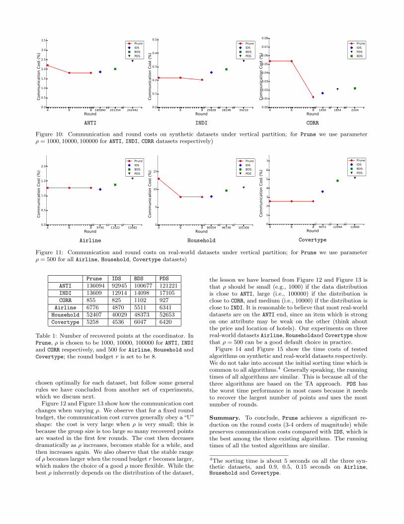
Figure 10 and Figure 11 show the communication andround costs of the four tested algorithms on the three syn-thetic datasets and three real-world datasets mentioned above.We observed that by using at most eight rounds, the com-munication cost of Prune is similar or even smaller than thatof BDS, IDS and PDS, which use significantly more rounds. Itis surprising to see that PDS is even worse then BDS in mostcases; the original paper [12] did not make this compari-
Figure 9: Running time on real-world datasets under hori-zontal partition (in Tradeoff we use 5 rounds). The time forlocal skyline computation at the beginning is not included.
son on points in the 2D Euclidean space. One reason thatPrune can achieve better communication costs is that IDS
and PDS have significantly larger round complexities, and atevery two rounds the coordinator needs to send a messageto a site to request for the next point, which can be con-sidered as an overhead of the algorithms in the distributedsetting. We also observe that Prune recovers similar numberof points as BDS, IDS, and PDS; see Table 1 for the details.
In Figure 10 and Figure 11 we have set ρ to be 1000, 10000,100000 for three synthetic datasets ANTI, INDI and CORR, and500 for all three real-world datasets. These values are not
4 6 8Round
0.0
0.5
1.0
1.5
2.0
2.5
3.0
3.5
185890 201354 242442
Prune
IDS
BDS
PDS
Communication Cost (%)
ANTI
4 6 8Round
0.0
0.1
0.2
0.3
0.4
0.5
25828 28196 34210
Prune
IDS
BDS
PDS
Communication Cost (%)
INDI
4 6 8Round
0.00
0.01
0.02
0.03
0.04
0.05
0.06
0.07
0.08
1650 1854 2204
Prune
IDS
PDS
BDS
Communication Cost (%)
CORR
Figure 10: Communication and round costs on synthetic datasets under vertical partition; for Prune we use parameterρ = 1000, 10000, 100000 for ANTI, INDI, CORR datasets respectively)
4 6 8Round
0.0
0.5
1.0
1.5
2.0
9740 11022 12682
Prune
IDS
BDS
PDS
Communication Cost (%)
Airline
4 6 8Round
0
5
10
15
80059 96746 105306
Prune
IDS
BDS
PDS
Communication Cost (%)
Household
4 6 8Round
0
1
2
3
4
5
6
7
9072 12094 12840
Prune
IDS
BDS
PDS
Communication Cost (%)
Covertype
Figure 11: Communication and round costs on real-world datasets under vertical partition; for Prune we use parameterρ = 500 for all Airline, Household, Covertype datasets)
Prune IDS BDS PDS
ANTI 136094 92945 100677 121221INDI 13609 12914 14098 17105CORR 855 825 1102 927
Airline 6776 4870 5511 6341Household 52407 40029 48373 52653Covertype 5258 4536 6047 6420
Table 1: Number of recovered points at the coordinator. InPrune, ρ is chosen to be 1000, 10000, 100000 for ANTI, INDIand CORR respectively, and 500 for Airline, Household andCovertype; the round budget r is set to be 8.
chosen optimally for each dataset, but follow some generalrules we have concluded from another set of experiments,which we discuss next.
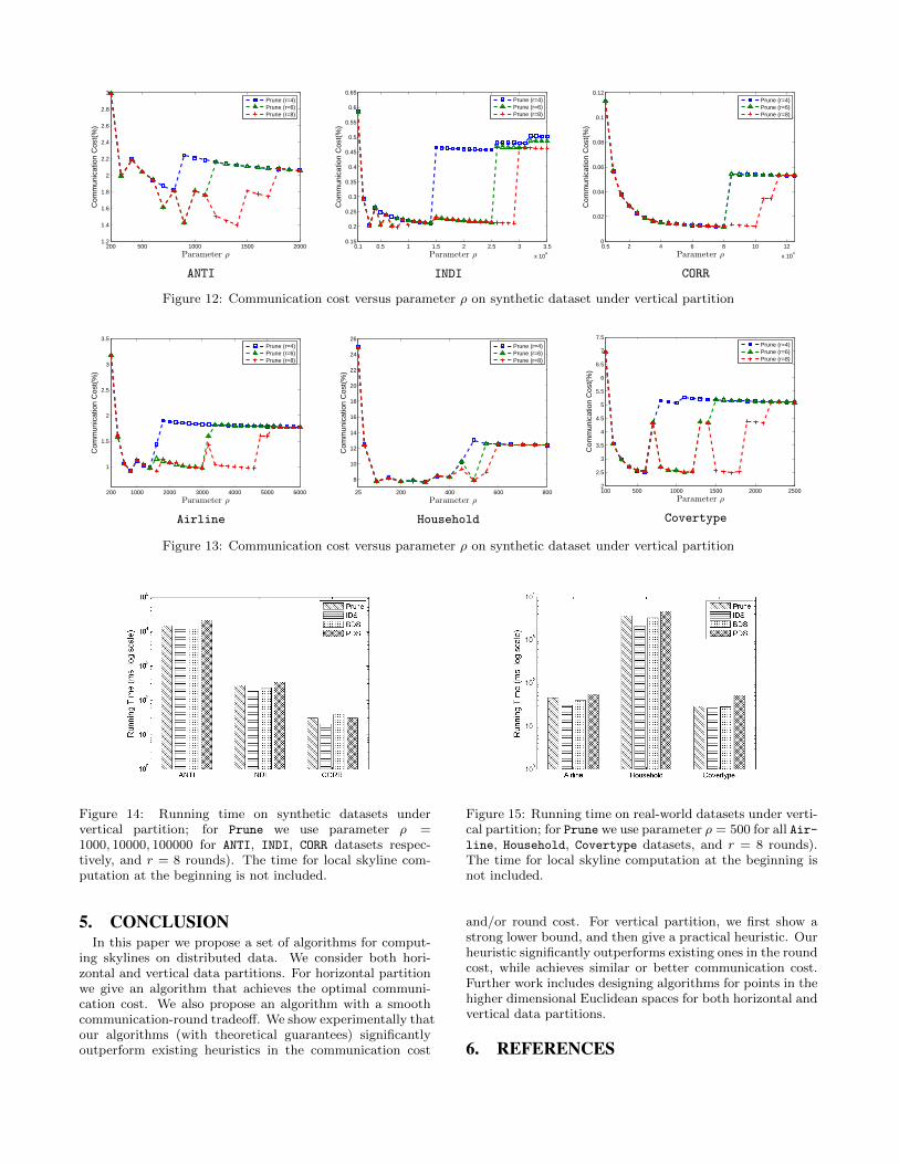
Figure 12 and Figure 13 show how the communication costchanges when varying ρ. We observe that for a fixed roundbudget, the communication cost curves generally obey a “U”shape: the cost is very large when ρ is very small; this isbecause the group size is too large so many recovered pointsare wasted in the first few rounds. The cost then deceasesdramatically as ρ increases, becomes stable for a while, andthen increases again. We also observe that the stable rangeof ρ becomes larger when the round budget r becomes larger,which makes the choice of a good ρ more flexible. While thebest ρ inherently depends on the distribution of the dataset,
the lesson we have learned from Figure 12 and Figure 13 isthat ρ should be small (e.g., 1000) if the data distributionis close to ANTI, large (i.e., 100000) if the distribution isclose to CORR, and medium (i.e., 10000) if the distribution isclose to INDI. It is reasonable to believe that most real-worlddatasets are on the ANTI end, since an item which is strongon one attribute may be weak on the other (think aboutthe price and location of hotels). Our experiments on threereal-world datasets Airline, Householdand Covertype showthat ρ = 500 can be a good default choice in practice.
Figure 14 and Figure 15 show the time costs of testedalgorithms on synthetic and real-world datasets respectively.We do not take into account the initial sorting time which iscommon to all algorithms.4 Generally speaking, the runningtimes of all algorithms are similar. This is because all of thethree algorithms are based on the TA approach. PDS hasthe worst time performance in most cases because it needsto recover the largest number of points and uses the mostnumber of rounds.
Summary. To conclude, Prune achieves a significant re-duction on the round costs (3-4 orders of magnitude) whilepreserves communication costs compared with IDS, which isthe best among the three existing algorithms. The runningtimes of all the tested algorithms are similar.
4The sorting time is about 5 seconds on all the three syn-thetic datasets, and 0.9, 0.5, 0.15 seconds on Airline,Household and Covertype.
200 500 1000 1500 20001.2
1.4
1.6
1.8
2
2.2
2.4
2.6
2.8
3
Parameter ρ
Com
mun
icat
ion
Cos
t(%
)
Prune (r=4)Prune (r=6)Prune (r=8)
ANTI
0.1 0.5 1 1.5 2 2.5 3 3.5
x 104
0.15
0.2
0.25
0.3
0.35
0.4
0.45
0.5
0.55
0.6
0.65
Parameter ρ
Com
mun
icat
ion
Cos
t(%
)
Prune (r=4)Prune (r=6)Prune (r=8)
INDI
0.5 2 4 6 8 10 12
x 104
0
0.02
0.04
0.06
0.08
0.1
0.12
Parameter ρ
Com
mun
icat
ion
Cos
t(%
)
Prune (r=4)Prune (r=6)Prune (r=8)
CORR
Figure 12: Communication cost versus parameter ρ on synthetic dataset under vertical partition
200 1000 2000 3000 4000 5000 6000
1
1.5
2
2.5
3
3.5
Parameter ρ
Com
mun
icat
ion
Cos
t(%
)
Prune (r=4)Prune (r=6)Prune (r=8)
Airline
25 200 400 600 800
8
10
12
14
16
18
20
22
24
26
Parameter ρ
Com
mun
icat
ion
Cos
t(%
)
Prune (r=4)Prune (r=6)Prune (r=8)
Household
100 500 1000 1500 2000 25002
2.5
3
3.5
4
4.5
5
5.5
6
6.5
7
7.5
Parameter ρ
Com
mun
icat
ion
Cos
t(%
)
Prune (r=4)Prune (r=6)Prune (r=8)
Covertype
Figure 13: Communication cost versus parameter ρ on synthetic dataset under vertical partition
Figure 14: Running time on synthetic datasets undervertical partition; for Prune we use parameter ρ =1000, 10000, 100000 for ANTI, INDI, CORR datasets respec-tively, and r = 8 rounds). The time for local skyline com-putation at the beginning is not included.
5. CONCLUSIONIn this paper we propose a set of algorithms for comput-
ing skylines on distributed data. We consider both hori-zontal and vertical data partitions. For horizontal partitionwe give an algorithm that achieves the optimal communi-cation cost. We also propose an algorithm with a smoothcommunication-round tradeoff. We show experimentally thatour algorithms (with theoretical guarantees) significantlyoutperform existing heuristics in the communication cost
Figure 15: Running time on real-world datasets under verti-cal partition; for Prune we use parameter ρ = 500 for all Air-line, Household, Covertype datasets, and r = 8 rounds).The time for local skyline computation at the beginning isnot included.
and/or round cost. For vertical partition, we first show astrong lower bound, and then give a practical heuristic. Ourheuristic significantly outperforms existing ones in the roundcost, while achieves similar or better communication cost.Further work includes designing algorithms for points in thehigher dimensional Euclidean spaces for both horizontal andvertical data partitions.
6. REFERENCES
fx
lx
ly
fy
Gx1
Gx2
Gx3
Gx4
Gx5
Gx6
Gx7
Gx8
Gy1
Gy2
Gy3
Gy4
Gy5
Gy6
Gy7
Gy8
Round = 1, 2
fx
lx ly
fy
Gx1
Gx2
Gx3
Gx4
Gx5
Gx6
Gx7
Gx8
Gy1
Gy2
Gy3
Gy4
Gy5
Gy6
Gy7
Gy8
Round = 3, 4
fx
lx
ly
fy
Gx1
Gx2
Gx3
Gx4
Gx5
Gx6
Gx7
Gx8
Gy1
Gy2
Gy3
Gy4
Gy5
Gy6
Gy7
Gy8
Round = 5, 6
Figure 16: A running example of Algorithm 4, with parameters r = 8 and ρ = 8.
[1] F. N. Afrati, P. Koutris, D. Suciu, and J. D. Ullman.Parallel skyline queries. Theory Comput. Syst.,57(4):1008–1037, 2015.
[2] W. Balke, U. Guntzer, and J. X. Zheng. Efficientdistributed skylining for web information systems. InEDBT, pages 256–273, 2004.
[3] Z. Bar-Yossef, T. S. Jayram, R. Kumar, andD. Sivakumar. An information statistics approach todata stream and communication complexity. J.Comput. Syst. Sci., 68(4):702–732, 2004.
[4] S. Borzsonyi, D. Kossmann, and K. Stocker. Theskyline operator. In ICDE, pages 421–430, 2001.
[5] M. Braverman, F. Ellen, R. Oshman, T. Pitassi, andV. Vaikuntanathan. A tight bound for set disjointnessin the message-passing model. In FOCS, pages668–677, 2013.
[6] J. Chomicki, P. Ciaccia, and N. Meneghetti. Skylinequeries, front and back. SIGMOD Record, 42(3):6–18,2013.
[7] R. Fagin, A. Lotem, and M. Naor. Optimalaggregation algorithms for middleware. J. Comput.Syst. Sci., 66(4):614–656, 2003.
[8] K. Hose and A. Vlachou. A survey of skylineprocessing in highly distributed environments. VLDBJ., 21(3):359–384, 2012.
[9] H. Kohler, J. Yang, and X. Zhou. Efficient parallelskyline processing using hyperplane projections. InSIGMOD, pages 85–96, 2011.
[10] H. T. Kung, F. Luccio, and F. P. Preparata. Onfinding the maxima of a set of vectors. J. ACM,22(4):469–476, 1975.
[11] M. Lichman. UCI machine learning repository, 2013.
[12] E. Lo, K. Y. Yip, K. Lin, and D. W. Cheung.Progressive skylining over web-accessible databases.Data Knowl. Eng., 57(2):122–147, 2006.
[13] K. Mullesgaard, J. L. Pederseny, H. Lu, and Y. Zhou.Efficient skyline computation in mapreduce. In EDBT,pages 37–48, 2014.
[14] D. Pertesis and C. Doulkeridis. Efficient skyline queryprocessing in spatialhadoop. Inf. Syst., 54:325–335,2015.
[15] J. B. Rocha-Junior, A. Vlachou, C. Doulkeridis, andK. Nørvag. Agids: A grid-based strategy for
distributed skyline query processing. In DataManagement in Grid and Peer-to-Peer Systems,Second International Conference, pages 12–23, 2009.
[16] G. Trimponias, I. Bartolini, D. Papadias, andY. Yang. Skyline processing on distributed verticaldecompositions. IEEE Trans. Knowl. Data Eng.,25(4):850–862, 2013.
[17] A. Vlachou, C. Doulkeridis, and Y. Kotidis.Angle-based space partitioning for efficient parallelskyline computation. In SIGMOD, pages 227–238,2008.
[18] S. Wang, B. C. Ooi, A. K. H. Tung, and L. Xu.Efficient skyline query processing on peer-to-peernetworks. In ICDE, pages 1126–1135, 2007.
[19] P. Wu, C. Zhang, Y. Feng, B. Y. Zhao, D. Agrawal,and A. El Abbadi. Parallelizing skyline queries forscalable distribution. In EDBT, pages 112–130, 2006.
[20] L. Zhu, Y. Tao, and S. Zhou. Distributed skylineretrieval with low bandwidth consumption. IEEETrans. Knowl. Data Eng., 21(3):384–400, 2009.
APPENDIXA. A RUNNING EXAMPLE FOR THE IN-
TERACTIVE PRUNING ALGORITHMFigure 16 shows a running example of Algorithm 4 with
parameters r = 8 and ρ = 8. In the first round, Alice sendsGx1 and Bob sends Gy1 to the coordinator. In the secondround, the coordinator sends the IDs of points in Gx1 andGy1 to Bob and Alice respectively, and then Bob and Alicesend the y-coordinates and x-coordinates of points in Gx1and Gy1 respectively to the coordinator. The coordinatorrecovers the points in Gx1 and Gy1 and adds them to R(the set of candidate skyline points), and updates lx = 8,ly = 7, and fx = fy = 2. In the third and fourth rounds,the coordinator chooses to recover points in Gy2 becausely − fy < lx − fx, and then updates lx = 7. In the fifth andsixth rounds, the coordinator chooses to recovers points inGy3 because ly − fy < lx − fx, and then updates lx = 4.In the last two rounds, the coordinator asks Alice for theinformation of the points in the remaining groups Gx2 andGx3 (i.e., the groups that have not been recovered or pruned)since lx − fx < ly − fy.