Parallel Computing 75 (2018) 41–60

Contents lists available at ScienceDirect

Parallel Computing

journal homepage: www.elsevier.com/locate/parco

Computing the expected makespan of task graphs in the

presence of silent errors

�

Henri Casanova

a , ∗, Julien Herrmann

b , Yves Robert c , d

a Dept. of Information and Computer Sciences, University of Hawai’i, M anoa, USA b School of Computational Science and Engineering, Georgia Tech, USA c École Normale Suérieure de Lyon, France d Dept. of Electrical Engineering and Computer Science, University of Tennessee, Knoxville, USA

a r t i c l e i n f o

Article history:

Received 4 October 2016

Revised 11 November 2017

Accepted 25 March 2018

Available online 27 March 2018

Keywords:

Task graphs

Scientific workflows

Fault-tolerance

Silent errors

Expected makespan

Scheduling

a b s t r a c t

Applications structured as Directed Acyclic Graphs (DAGs) of tasks occur in many domains,

including popular scientific workflows. DAG scheduling has thus received an enormous

amount of attention. Many of the popular DAG scheduling heuristics make scheduling deci-

sions based on path lengths. At large scale compute platforms are subject to various types

of failures with non-negligible probabilities of occurrence. Failures that have recently re-

ceived increased attention are “silent errors,” which cause data corruption. Tolerating silent

errors is done by checking the validity of computed results and possibly re-executing a

task from scratch. The execution time of a task then becomes a random variable, and

so do path lengths in a DAG. Unfortunately, computing the expected makespan of a DAG

(and equivalently computing expected path lengths in a DAG) is a computationally dif-

ficult problem. Consequently, designing effective scheduling heuristics in this context is

challenging. In this work, we propose an algorithm that computes a first order approxi-

mation of the expected makespan of a DAG when tasks are subject to silent errors. We

find that our proposed approximation outperforms previously proposed approaches both

in terms of approximation error and of speed.

© 2018 Elsevier B.V. All rights reserved.

1. Introduction

This paper introduces a new algorithm to approximate the expected makespan of a workflow application, i.e., an applica-

tion structured as a Directed Acyclic Graph (DAG) of tasks, in which tasks can fail and must be re-executed. A key question

when executing workflows on parallel platforms is the scheduling of tasks on the available compute resources, or proces-

sors. When not considering task failures, list scheduling algorithms are the de-facto standard [1] , and tools are available

that use such algorithms for scheduling workflow applications onto large-scale platforms in practice [2,3] . The prevalent list

scheduling heuristics prioritize tasks with large bottom levels. The bottom-level of a task is defined as the longest path from

that task to the end of the execution, assuming unlimited processors. This heuristic is known as CP-scheduling ( Critical Path

scheduling [4–6] ), and it has been extended to handle heterogeneous environments (see the HEFT algorithm [7] ).

� A preliminary version of this paper has appeared in the Proceedings of the 2016 IEEE International Workshop on Parallel Programming Models and

Systems Software for High-End Computing (P2S2). ∗ Corresponding author.

E-mail address: henric@hawaii.edu (H. Casanova).

https://doi.org/10.1016/j.parco.2018.03.004

0167-8191/© 2018 Elsevier B.V. All rights reserved.

42 H. Casanova et al. / Parallel Computing 75 (2018) 41–60

It is well-documented that large-scale platforms are increasingly subject to errors that can cause task failures. In par-

ticular, the occurrence of “silent errors” (or SDCs, for Silent Data Corruptions) has been recently identified as one of the

major challenges for Exascale [8] . Silent errors can be caused by external causes, including cosmic radiations or packag-

ing pollution. In addition, silent errors can occur when using DVFS (Dynamic Voltage Frequency Scaling) to reduce energy

consumption. For instance, at low voltage the probability that a task produces incorrect results increases [9,10] .

Regardless of their causes, an effective approach for avoiding propagating results corrupted by silent errors is to use a

verification mechanism after executing each task [11] . When an error is detected, the task is then re-executed. The verifi-

cation mechanism can be general-purpose (e.g., based on replication [12] , with re-execution only when the two outputs do

not match) or application-specific. Many application-specific error detection methods are available for classical High perfor-

mance Computing (HPC) applications, such as approximate re-execution for ODE and PDE solvers [13] , orthogonality checks

for Krylov-based sparse solvers [14,15] ), or Algorithm-Based Fault Tolerance (ABFT) for numerical linear algebra [16] .

Silent errors make it challenging to define efficient list scheduling algorithms to schedule task graphs. After the first

execution of a task, the error detector is used to check the result. If the result is correct, the task’s execution is marked

as successful, and its successor tasks are marked as ready. If the result is incorrect, then the task must be executed (and,

given that the first execution has failed, the second execution will typically succeed with very high probability). While this

scheme is conceptually simple, it greatly complicates the computation of the bottom-level of a task. And yet, computing the

expected length of the longest path in a DAG with unlimited processors (or equivalently the expected bottom-level of a task

in the DAG), is key to designing silent-error-aware versions of effective list scheduling heuristics (CP-scheduling, HEFT).

It is known that computing the expected length of the longest path in a DAG whose task weights are probabilistic is a

difficult problem [6] . Even in the case in which each task is re-executed at most once, i.e., when task weights are random

variables taking only two discrete values, the problem remains #P-complete [17] (see Section 2 for a detailed discussion). In

this work we develop an algorithm to compute an accurate first-order approximation of the expected length of the longest

path in a general DAG in which tasks are subject to silent errors, and whose execution lengths can take two different values,

depending upon there is a re-execution or not. More specifically, our contributions are:

• We develop an exact first-order approximation of the expected makespan of a general DAG, which can be computed in

polynomial time; • We compare our approach to two previously proposed approximations for DAGs for three sets of task graphs; • We quantify approximation errors via comparison to a brute-force Monte Carlo approach; and

• We show that our proposed approximation (i) leads to lower or similar error than previously proposed approximations

(and, importantly, to much lower error when the probability of task failure is low) and (ii) can be computed in practice

much faster than previously proposed approximations.

This paper is organized as follows. Section 2 reviews related work. Section 3 formalizes the problem that we address and

states assumptions. Section 4 describes our proposed approximation. Section 5 presents evaluation results. Section 6 con-

cludes with a brief summary of results and with perspectives on future work.

2. Related work

In this section we first review previous works on estimating the makespan of probabilistic DAGs, and then review rele-

vant literature on silent errors.

2.1. Expected makespan of probabilistic 2-state DAGs

Computing the expected makespan of a DAG whose task execution times obey arbitrary probability distributions is

known to be a difficult problem, even with unlimited processors. When task weights are fixed (deterministic), the makespan

is the length of the longest path in the graph (also called “critical path”). But assume instead a probabilistic 2-state DAG

where task weights obey a simple 2-state probability distribution: task T i has weight a i , 1 with probability p i and weight

a i , 2 with probability 1 − p i . Assume also that all the probability distributions of all tasks are independent. The makespan of

the DAG is now a random variable. It is known that computing its probability distribution, or even just its expected value,

is a #P-complete problem [17] . Recall that the class of #P problems is the class of counting problems corresponding to NP

decision problems [18–20] , and that #P-complete problems are at least as hard as NP-complete problems.

An informal explanation of why computing the expected makespan of probabilistic 2-state DAGs is a difficult combinato-

rial problem, is as follows. The main intuitive reason is that the expected value of the maximum of two random variables is

not the maximum of their expectations. As a result, when computing the length of a path in the DAG, one must keep track

of all possible values for the starting time of each task, together with their probabilities, and there may be an exponential

number of such values [21] .

In practice, there are three standard methods to compute the expected makespan of a probabilistic 2-state DAG, as de-

scribed hereafter.

2.1.1. Monte Carlo simulations

The Monte Carlo approach works as follows [22,23] : for each task in the DAG, a value of its weight is sampled from its

probability distribution. Once this is done, the DAG is deterministic and its longest path can be computed as explained in

H. Casanova et al. / Parallel Computing 75 (2018) 41–60 43

Section 3 . One then repeats this operation for a large number of trials, generating a new value at each trial. The set of these

values empirically approaches the actual distribution of the DAG makespan as the number of trials increases.

An interesting question is that of determining the number of trials to obtain a high confidence level in the result. We

refer the reader to the relevant discussion in [24] . A key drawback of the Monte Carlo approach is that it is compute-

intensive since the necessary number of trials is typically high. In this work, we only use Monte Carlo to compute a ground

truth so as to assess the accuracy of our and previously proposed algorithms that compute approximations of the expected

makespan. Hence, instead of determining a minimal number of trials, we conservatively use a very large number of trials so

as to guarantee that our ground truth is accurate.

2.1.2. Approximation by a series-parallel graph

Basic probability theory tells us how to compute the probability distribution of the sum of two random variables (by a

convolution) and of the maximum of two random variables (by taking the product of their cumulative density functions).

This simple consideration leads to an exact method to compute the expected makespan when the DAG is series-parallel

(see [25] for a definition of series-parallel graphs). The problem with probabilistic 2-state series-parallel graph remains NP-

complete in the weak sense and admits a pseudo-polynomial solution [21] .

When the DAG is not series-parallel, one approach is to approximate it by a series-parallel graph, which is constructed

iteratively, first by a sequence of reductions and then by duplicating some vertices. Dodin’s method [26] constructs such an

approximated series-parallel graph, whose expected makespan is used to estimate that of the original DAG. See [21,24] for

a detailed description of Dodin’s method. We include this method in our quantitative experiments in Section 5 .

2.1.3. Approximation with normality assumption

The central-limit theorem states that the sum of independent random variables tends to be normally distributed as the

number of variables increases. The expected makespan of the DAG is a combination of sums and maximums of the original

task weights, so a popular approach proposed by Sculli [27] is based on the normality assumption :

• Approximate the distribution of each task by a normal distribution of same mean and variance. This step has constant

cost per task for probabilistic 2-state DAGs. • Use Clarke’s formulas in [28] to compute the mean and variance of the sum and maximum of two (correlated) normal

distributions, and then assuming that they also follow normal distributions. • Traverse the original DAG and compute the mean and variance of the makespan.

See [24] for a full description of Sculli’s method, which we we also include in our quantitative experiments in Section 5 .

2.2. Silent errors

Considerable effort s have been directed at verification techniques to handle silent errors. A guaranteed, general-purpose

verification is only achievable with expensive techniques, such as process replication [12,29] or redundancy [30,31] . How-

ever, application-specific information can be exploited to decrease the verification cost. Algorithm-based fault tolerance

(ABFT) [16,32,33] is a well-known technique to detect errors in linear algebra kernels using checksums. Various techniques

have been proposed in other application domains. Benson et al. [13] compare a higher-order scheme with a lower-order one

to detect errors in the numerical analysis of ODEs. Sao and Vuduc [15] investigate self-stabilizing corrections after error de-

tection in the conjugate gradient method. Heroux and Hoemmen [34] design a fault-tolerant GMRES capable of converging

despite silent errors. Bronevetsky and de Supinski [35] provide a comparative study of detection costs for iterative methods.

Recently, detectors based on data analytics have been proposed to serve as partial verifications [36–38] . These detectors

use interpolation techniques, such as time series prediction and spatial multivariate interpolation, on scientific dataset to

offer lar ge error coverage at the expense of a negligible overhead. Although not perfect, the accuracy-to-cost ratios of these

techniques tend to be very high, which makes them attractive alternatives at large scale.

The rate of silent errors also depends upon the mode of execution. Temperature and power consumption are known to

have a high impact on silent error rates [39] . Furthermore, as mentioned in Section 1 , lowering the voltage/frequency is also

believed to have an adverse effect on system reliability [9,10] . Many papers (e.g., [10,40–42] ) have assumed the following

exponential silent error rate model:

λ(s ) = λ0 · 10

d(s max −s ) s max −s min , (1)

where λ0 denotes the average error rate at the maximum speed s max , d > 0 is a constant indicating the sensitivity of error

rate to voltage/frequency scaling, and s min is the minimum speed. In this model the error rate increases as processing speed

decreases. Overall, the main resilience concern is that the above studies suggest that minimizing energy consumption via

DVFS techniques call also lead to an increased number of silent errors.

A silent error must be detected for each task via some verification mechanism [11] . A naive but general-purpose veri-

fication technique would consist in re-running the task once so that an output mismatch indicates a silent error [12] . In

this case, the task can be re-executed one extra time so that the correct output can be picked via majority voting. Many

application-specific, and thus efficient, error detection methods have been proposed [13–16] . Because silent errors are not

detected when their occur, but only at the end of the execution of the task (by the verification mechanism), the task must be

44 H. Casanova et al. / Parallel Computing 75 (2018) 41–60

fully re-executed in case an error is detected. Assuming that the task re-execution allows a correct output to be produced,

we then need to consider probabilistic 2-state DAGs, in which each task has a weight for the no-error case, and another

(longer) weight for the error case. For simplicity, in this work we assume that the weight of a task T is a if there is no silent

error, and 2 a if a silent error is detected (which requires a re-execution). However, our work is immediately extensible to

arbitrary such two weights to account, for instance, for the overhead of the silent error detection mechanism.

Finally, this work assume that task failure arrival times are Exponentially distributed with Mean Time Between Failure

(MTBF) 1/ λ. Extensions to other probability distributions have been considered in [43,44] . These extensions apply in cases

when using the distribution’s MTBF as the (average) inverse of the failure rate and neglecting second order terms (i.e.,

terms proportional to the square of that failure rate) would lead to accurate approximations of the corresponding failure

probabilities.

3. Problem statement

We consider a general model of computation in which an application is structured as a Directed Acyclic Graph, in which

vertices represent tasks and edges represent task precedence. More formally, let G = (V, E) be a DAG, with V a set of tasks,

and E ⊂ V × V a set of edges. For each task i , let a i be its weight, i.e., its failure-free execution time. Let pa ( i, j ) denote the

length (as a sum of task weights) of the longest path from task i to task j , if such a path exists, otherwise let pa (i, j) = −∞ .

The longest path length in G is then defined as d(G ) = max i, j∈ V { pa (i, j) } . Let us call d ( G ) the failure-free makespan of G .

Because G is acyclic, we can compute d ( G ) in O (| V | + | E| ) time as follows: add two zero-weight vertices v 1 and v 2 to G ,

where v 1 represents a unique source task and v 2 a unique sink task. Also add an edge from v 1 to any entry task in G (a task

without predecessor), and an edge from any exit task in G (a task without successor) to v 2 . Then d(G ) = pa (s 1 , s 2 ) can be

computed in time O (| V | + | E| ) [45, Section 24.2] .

We consider that tasks fail independently and task failure arrival times are exponentially distributed with Mean Time

Between Failure (MTBF) 1/ λ. Therefore, the probability that task i fails during its first execution attempt is 1 − e −λa i , in

which case the task must be re-executed from scratch.

Our objective is to compute an approximation of the expected makespan of G , i.e., the longest path length in G taking

into accounts that tasks can fail and must be re-executed. The failure-free makespan defined above is a clear lower bound

on the expected makespan.

4. Approximating the expected makespan

In this section we compute a first-order approximation of the expected makespan of a DAG G , which we denote as E(G ) .

Our approximation relies on the fact that in practice λ is close to zero, which allows us to neglect O ( λ2 ) terms.

The probability that the first execution attempt of task i succeeds is:

p i = e −λa i = 1 − λa i + O (λ2 ) .

The probability that the first execution attempt of task i fails but that its second execution attempt succeeds is:

(1 − e −λa i ) e −λa i = λa i + O (λ2 ) = 1 − p i + O (λ2 ) .

Neglecting the O ( λ2 ) terms leads to the approximation that a task either takes time a i , with probability 1 − λa i , or time 2 a i ,

with probability λa i . In other terms, our first-order approximation consists in assuming that a task never fails more than

once. Hereafter when we say that a task fails, we mean that its first execution attempt fails and that its second execution

attempt succeeds.

For any S ⊂ V , let P ( S ) denote the probability that all tasks in S fail and that no task in V �S fails. Let also L ( S ) denote the

length of the longest path in G when all tasks in S fail and no task in V �S fails. E(G ) is thus defined as:

E(G ) =

∑

S⊂V

P (S) × L (S) .

We note that:

P (∅ ) =

∏

i ∈ V (1 − λa i + O (λ2 )) = 1 −

∑

i ∈ V λa i + O (λ2 ) ,

P ({ i } ) = (λa i + O (λ2 )) ×∏

j∈ V \{ i } (1 − λa j + O (λ2 ))

= λa i + O (λ2 ) , and

P (S) = O (λ2 ) if | S| > 1 .

Therefore:

H. Casanova et al. / Parallel Computing 75 (2018) 41–60 45

E(G ) = P (∅ ) × L (∅ ) +

∑

i ∈ V P ({ i } ) × L ({ i } ) + O (λ2 ) .

By definition, L (∅ ) = d(G ) ( G ’s failure-free makespan). Similarly, L ({ i } ) = d(G i ) , where G i a DAG identical to G but such that

task i has weight 2 a i instead of weight a i . We thus obtain:

E(G ) =

(

1 −∑

i ∈ V λa i

)

× d(G ) +

∑

i ∈ V (λa i ) ∗ d(G i ) + O (λ2 )

= d(G ) + λ∑

i ∈ V a i (d(G i ) − d(G )) + O (λ2 ) .

For a DAG G = (V, E) , d ( G ) can be computed in O (| V | + | E| ) time. Therefore, the above approximation can be computed

in O (| V | 2 + | V | . | E| ) time. Lower complexity can be achieved by exploiting the fact that G and the G i ’s differ in only the

weight of one task.

5. Evaluation

5.1. Makespan approximation techniques

In this section we evaluate three expected makespan approximations techniques:

1. First order – The approximation described in Section 4 ;

2. Dodin – The bound in [26] , which is computed by transforming any general DAG into an approximately equivalent

series-parallel graph and then computing the exact expected makespan of this graph using the approach explained in

Section 2.1.2 .

3. Normal – The approach that consists in approximating the discrete execution time of each task (i.e., a i with probability p iand 2 a i with probability 1 − p i ), by a continuous Normal distribution of same mean and standard deviation. The overall

expected makespan in the approximated as explained in Section 2.1.3 .

5.2. Application DAGs

We measure the error of the three makespan approximation techniques using 3 DAG datasets.

5.2.1. Linear algebra

This dataset consists of DAGs used in numerical linear algebra computations. More specifically, we consider 3 classical

factorizations of a k × k tiled matrix: Cholesky, LU, and QR factorization. Each tile has size b × b , where b is a platform-

dependent parameter. Hence the actual size of a k × k tiled matrix is N × N , where N = kb. For each factorization, the number

of vertices in the DAG depends on k as follows: the Cholesky DAG has 1 3 k

3 + O (k 2 ) tasks, while the LU and QR DAGs have2 3 k

3 + O (k 2 ) tasks (but the tasks in QR entail, on average, twice as many floating-point operations as in LU).

Figs. 1–3 show examples for k = 5 . The tasks in these DAGs are labeled by the corresponding BLAS kernels [46] , and their

weights are based on actual kernel execution times as reported in [47] for an execution on Nvidia Tesla M2070 GPUs with

tiles of size b = 960 .

For simplicity, in all that follows we call k the DAG size (i.e., the larger k the more tasks). For each DAG class we perform

experiments with k = 4 , 6 , 8 , 10 , 12 , for a total of 3 × 5 = 15 DAGs with up to 650 tasks.

5.2.2. Assembly trees

This dataset consists of assembly trees for a set of sparse matrices obtained from the University of Florida Sparse Matrix

Collection ( http://www.cise.ufl.edu/research/sparse/matrices/ ). These matrices satisfy the following assertions: not binary,

not corresponding to a graph, square, with a symmetric pattern, with between 20,0 0 0 and 2,0 0 0,0 0 0 rows, with an aver-

age number of non-zero elements per row at least equal to 2.5, and with a total number of non-zero elements at most

equal to 5,0 0 0,0 0 0. Among these matrices, for each group of matrix in the dataset we pick the one that has the largest

number of non-zero elements, resulting in 76 matrices (given the content of the dataset at the time this article is being

written). We first order the matrices using MeTiS [48] (through the MeshPart toolbox [49] ) and amd (available in Matlab),

and then build the corresponding elimination trees using the symbfact routine of Matlab. We also perform a relaxed node

amalgamation on these elimination trees to create assembly trees. We thus obtain a large set of instances by allowing 1, 2,

4, and 16 (if more than 1.6 × 105 nodes) relaxed amalgamations per node. Among these assembly trees, we selected four

of them for our experiments: ‘dump.1.1.amd.Goodwin.rim-447’ (a.k.a. ‘Goodwin’, 4079 nodes), ‘dump.1.1.amd.Li.li-732’ (a.k.a.

‘amd.Li.li’, 5139 nodes), ‘dump.1.1.amd.FEMLAB.sme3Dc-932’ (a.k.a. ‘FEMLAB’, 5707 nodes) and ‘dump.1.3.metis.Li.li-732’ (a.k.a.

‘metis.Li.li’, 2153 nodes).

46 H. Casanova et al. / Parallel Computing 75 (2018) 41–60

Fig. 1. DAG of a Cholesky factorization on a 5 × 5 tiled matrix.

Fig. 2. DAG of a LU factorization on a 5 × 5 tiled matrix.

H. Casanova et al. / Parallel Computing 75 (2018) 41–60 47

Fig. 3. DAG of a QR factorization on a 5 × 5 tiled matrix.

5.2.3. Random task graphs

This dataset consists random DAGs generated using the Directed Acyclic Graph GENerator (DAGGEN). 1 DAGGEN uses four

popular parameters to define the shape of a DAG: size, width, density and jumps .

• The size determines the number of tasks in the DAG (tasks are organized in levels). • The width determines the maximum parallelism in the DAG, that is the number of tasks in the largest level. A small

value leads to “chain” graphs and a large value to “fork-join” graphs. • The density denotes the number of edges between two levels of the DAG, with a low value leading to few edges and a

large value to many edges. • Random jump edges are added that go from level l to levels l + 1 . . . l + jumps .

The second and third parameters take values between 0 and 1. Our DAG generation procedure is similar to the one used

in [50] . Specifically, we generate three sets of random DAGs:

• Daggen1 : 100 randomly generated DAGs with size = 10 0 0 , width = 0 . 3 , density = 0 . 5 and jumps = 5 . A sample

Daggen1 DAG is depicted in Fig. 4 . • Daggen2 : 100 randomly generated DAGs with size = 10 0 0 , width = 0 . 3 , density = 0 . 9 and jumps = 7 . • Daggen3 : 100 randomly generated DAGs with size = 10 0 0 , width = 0 . 9 , density = 0 . 5 and jumps = 10 .

5.3. Experimental methodology

For each DAG, and for a given failure rate λ (see Section 3 ), we compute the First Order, Dodin, and Normal approxima-

tions of the expected makespan. To compute approximation errors one would ideally use the exact expected makespan (the

computation of which is a P#-complete problem). Instead, we resort to the brute-force Monte Carlo approach described in

Section 2.1.1 . We use 30 0,0 0 0 random trials. For each task in a trial, the task succeeds or fails as determined by sampling

a random time-to-next-failure value from an exponential distribution with parameter λ. We then approximate the expected

makespan as the average makespan over the 30 0,0 0 0 samples. This method is prohibitively expensive in practice, but pro-

vides us with a reasonable ground truth in our experiments. In all results hereafter we report on the relative error between

the approximations and this ground truth.

To allow for consistent comparisons of results across different DAGs (with different numbers of tasks and different task

weights), in our experiments we simply fix the probability that a task of average weight fails, which we denote as p fail , and

1 Code publicly available at https://github.com/frs69wq/daggen .

48 H. Casanova et al. / Parallel Computing 75 (2018) 41–60

Fig. 4. Sample Daggen1 DAG.

H. Casanova et al. / Parallel Computing 75 (2018) 41–60 49

Table 1

p fail values and corresponding

processor MTBF values assuming

a 10 0,0 0 0-processor platform.

p fail Processor MTBF

0.01 17.3 days

0.001 173.5 days

0.0 0 01 4.7 years

0.0 0 0 01 47.5 years

0.0 0 0 0 01 475.6 years

Fig. 5. Cholesky ( k = 4 , 6 , 8 , 10 , 12 ), p fail = 0 . 01 .

compute the failure rate. Formally, for a given DAG G = (V, E) and a given p fail value, we compute the average task weight

as a =

∑

i ∈ V a i / | V | and pick the failure rate λ such that

p fail = 1 − e −λa .

We evaluate the performance of our proposed approximation and compare it to its competitors for a range of p fail values.

We present results for a wide range of values, noting that the higher values correspond to error rates much higher than

those observed or expected on current and future large-scale computing platforms. The average execution time of a task

in our experiments is a = 0 . 15 s. So, for instance, p fail = 0 . 01 leads to an error rate λ = 0 . 067 . The corresponding MTBF

is μ = 1 /λ = 14 . 9 s. For a platform with 10 0,0 0 0 processors, this corresponds to an individual MTBF (per processor) of

17.3 days, quite an unrealistic value since individual processor MTBFs are typically estimated to be several years. Table 1

shows the p fail values used in our experiments and corresponding platform MTBF values (assuming 10 0,0 0 0 processors).

The results in the next section show that the lower p fail , the lower the error incurred by our proposed approximation. In

particular, our approximation outperforms its competitors for all realistic p fail values (i.e., p fail ≤ 0.001), and sometimes even

for unrealistically higher values.

5.4. Approximation error results

In this section we show relative error results, relative to expected makespans computed using the Monte Carlo method.

Negative values denote an underestimation, while positive values denote an overestimation. All figures use a logarithmic

scale on the vertical axis.

5.4.1. Linear algebra DAGs

Figs. 5–7 show relative error vs. graph size for Cholesky graphs and for p fail = 0 . 01 , 0 . 001 , and 0.0 0 01, respectively. The

data set has 5 graphs representing the Cholesky factorization of a k × k tiled matrix for k = 4 , 6 , 8 , 10 , 12 , as described in

Section 5.2.1 , which correspond to graphs with 20, 56, 120, 220 and 364 nodes. For p fail = 0 . 01 , we see that First Order leads

50 H. Casanova et al. / Parallel Computing 75 (2018) 41–60

Fig. 6. Cholesky ( k = 4 , 6 , 8 , 10 , 12 ), p fail = 0 . 001 .

Fig. 7. Cholesky ( k = 4 , 6 , 8 , 10 , 12 ), p fail = 0 . 0 0 01 .

to the lowest relative error for graphs sizes below 10, and that Normal leads to the lowest relative error for larger graphs.

Dodin leads to the largest relative error, but for the smallest graph size. Considering the largest graph size, First Order has

1.9% relative error while Normal has 0.3% relative error and Dodin has 8.7% relative error. For p fail = 0 . 001 , First Order leads

to dramatically lower error than its competitors (at least one order of magnitude lower). For instance, for the largest graph,

First Order has 0.03% relative error, compared to 5.8% for Dodin and 0.9% for Normal. These results are even more striking

for p fail = 0 . 0 0 01 . In this case, still for the largest graph, First Order has −0.0 0 06% relative error, compared to 3.7% for Dodin

and 0.4% for Normal. In this case, First Order is an underestimation of the expected makespan.

Figs. 8–10 show similar results for LU DAGs. The data set has 5 graphs representing the QR factorization of a k × k tiled

matrix for k = 4 , 6 , 8 , 10 , 12 , as described in Section 5.2.1 , which correspond to graphs with 30, 91, 204, 385 and 650 nodes.

The overall message from these results is the same, meaning that First Order leads to drastically lower error than its com-

H. Casanova et al. / Parallel Computing 75 (2018) 41–60 51

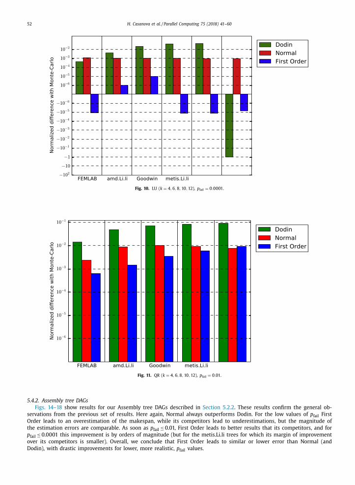
Fig. 8. LU ( k = 4 , 6 , 8 , 10 , 12 ), p fail = 0 . 01 .

Fig. 9. LU ( k = 4 , 6 , 8 , 10 , 12 ), p fail = 0 . 001 .

petitors as p fail decreases. Here again Dodin leads to the largest errors overall. For p fail = 0 . 01 , out approach leads to similar

errors of the same order of magnitude as the errors for Normal (and in this case Normal is most often an underestimation

while First Order is an overestimation).

Finally, Figs. 11–13 show results for QR DAGs and similar trends are observed. The data set has 5 graphs representing the

QR factorization of a k × k tiled matrix for k = 4 , 6 , 8 , 10 , 12 , as described in Section 5.2.1 , which correspond to graphs with

30, 91, 204, 385 and 650 nodes. First Order drastically improves on Dodin and Normal for p fail = 0 . 001 and p fail = 0 . 0 0 01 .

For p fail = 0 . 01 , First Order leads to similar or lower error than Normal. Here again, Dodin leads to the highest errors across

the board.

52 H. Casanova et al. / Parallel Computing 75 (2018) 41–60

Fig. 10. LU ( k = 4 , 6 , 8 , 10 , 12 ), p fail = 0 . 0 0 01 .

Fig. 11. QR ( k = 4 , 6 , 8 , 10 , 12 ), p fail = 0 . 01 .

5.4.2. Assembly tree DAGs

Figs. 14–18 show results for our Assembly tree DAGs described in Section 5.2.2 . These results confirm the general ob-

servations from the previous set of results. Here again, Normal always outperforms Dodin. For the low values of p fail First

Order leads to an overestimation of the makespan, while its competitors lead to underestimations, but the magnitude of

the estimation errors are comparable. As soon as p fail ≤ 0.01, First Order leads to better results that its competitors, and for

p fail ≤ 0.0 0 01 this improvement is by orders of magnitude (but for the metis.Li.li trees for which its margin of improvement

over its competitors is smaller). Overall, we conclude that First Order leads to similar or lower error than Normal (and

Dodin), with drastic improvements for lower, more realistic, p fail values.

H. Casanova et al. / Parallel Computing 75 (2018) 41–60 53

Fig. 12. QR ( k = 4 , 6 , 8 , 10 , 12 ), p fail = 0 . 001 .

Fig. 13. QR ( k = 4 , 6 , 8 , 10 , 12 ), p fail = 0 . 0 0 01 .

5.4.3. Randomly generated DAGs

Figs. 19–23 show results for randomly generated DAGs described in Section 5.2.3 . We observe similar trends as for the

two previous sets of DAGs. Normal outperforms Dodin across the board. For low values of p fail , First Order leads to error

comparable to that of Normal and Dodin. For p fail ≤ 0.0 0 01 error, it leads to orders of magnitude improvements over its com-

petitors. Our overall conclusion is that our proposed approximation approach improves over previously proposed approaches

in terms of accuracy, and drastically so for realistically low p fail values.

5.5. Scalability results

To assess the scalability of the three approximation methods, we run experiments with k = 20 for the LU DAG, i.e., 2,870

tasks, and p fail = 0 . 0 0 01 . Results for other DAGs show similar relative ranking of the three approximation results, and we

54 H. Casanova et al. / Parallel Computing 75 (2018) 41–60

Fig. 14. Results on the 4 assembly trees, p fail = 0 . 01 .

Fig. 15. Results on the 4 assembly trees, p fail = 0 . 001 .

picked this particular DAG for our scalability analysis because it is from a real-world application, because it is large enough

for a scalability study, and because it is small enough that the Monte Carlo method (which provides our ground truth)

can run in a reasonable amount of time. For this large graph, we ran the Monte Carlo for ten hours, so as to ensure the

accuracy of the ground truth. Error (normalized difference with Monte Carlo) and execution times are shown in Table 2 . We

see that for this large DAG, Dodin exhibits very large error. First Order is roughly two orders of magnitude more accurate

than Normal. We also see that First Order can be computed in under a second, while Normal requires about 20 min, i.e.,

about three orders of magnitude longer. All these experiments are performed on one core of a 2.1 GHz AMD Opteron(TM)

Processor 6272.

H. Casanova et al. / Parallel Computing 75 (2018) 41–60 55

Fig. 16. Results on the 4 assembly trees, p fail = 0 . 0 0 01 .

Fig. 17. Results on the 4 assembly trees, p fail = 0 . 0 0 0 01 .

5.6. Summary of results

Our results show that our proposed approximation, First Order, is accurate as long as the probability of task failure is

sufficiently low. In particular, the realistically low probability of task failures it is more accurate that its two competitors by

orders of magnitude. When the task failure probability is high, its accuracy is comparable to that of the Normal approxima-

tion. Across the board the Dodin approximation leads to the largest error. This is because the DAGs that we consider are far

from being series-parallel. As a result, the series-parallel graph constructed by Dodin is a poor approximation of the original

DAG, hence the large errors. Finally, not only is First Order more accurate, but it is also faster. Its computation for a large

DAG with 2870 tasks requires more than three orders of magnitude less time that Dodin and Normal.

56 H. Casanova et al. / Parallel Computing 75 (2018) 41–60

Fig. 18. Results on the 4 assembly trees, p fail = 0 . 0 0 0 01 .

Fig. 19. Results on the 3 sets of randomly generated graphs (of size 10 0 0 and various shapes), p fail = 0 . 01 .

Table 2

Results for a LU DAG with k = 20 (i.e., 2870 tasks) and p fail =

0 . 0 0 01 .

Dodin Normal First Order

Error −0 . 97 954 × 10 −6 7 × 10 −6

Execution time ∼ 2 min ∼ 20 min < 1 s

H. Casanova et al. / Parallel Computing 75 (2018) 41–60 57

Fig. 20. Results on the 3 sets of randomly generated graphs (of size 10 0 0 and various shapes), p fail = 0 . 001 .

Fig. 21. Results on the 3 sets of randomly generated graphs (of size 10 0 0 and various shapes), p fail = 0 . 0 0 01 .

58 H. Casanova et al. / Parallel Computing 75 (2018) 41–60

Fig. 22. Results on the 3 sets of randomly generated graphs (of size 10 0 0 and various shapes), p fail = 0 . 0 0 0 01 .

Fig. 23. Results on the 3 sets of randomly generated graphs (of size 10 0 0 and various shapes), p fail = 0 . 0 0 0 0 01 .

H. Casanova et al. / Parallel Computing 75 (2018) 41–60 59

6. Conclusion

We have proposed an algorithm to compute a first-order approximation of the expected makespan of a Directed Acyclic

Graph (DAG) of tasks in which tasks are subject to silent errors that may require task re-execution from scratch due to

corrupted results, which we term a failure. Our approximation can be computed in O (V 2 + V.E) time for a DAG with V

vertices and E edges. It is exact in the first order and neglects second order O ( λ2 ) terms, where λ is the exponential failure

rate. This amounts to assuming that each task may need to be re-executed at most once. The problem of computing the

expected makespan of a DAG of tasks with this assumption is actually a computationally difficult problem (#P-complete).

As a result, techniques to approximate the expected makespan have been proposed in previous works [24,26] . We have

evaluated our proposed approximation and these previously proposed techniques for three sets of DAGs (linear algebra DAGs,

assembly trees, and randomly generated DAGs). In our evaluations we quantify the approximation error via comparison to a

ground truth computed using a brute-force Monte Carlo method.

Our results show that our proposed approximation is more accurate than previously proposed approximations by sev-

eral orders of magnitude for realistically low failure rates. In addition, it can be computed much more quickly that these

previously proposed approximations, which is crucially important for solving problems at scale. Overall, we have proposed

a novel and improved approximation of the expected makespan of probabilistic DAGs in which tasks are subject to silent

errors that mandate task re-executions.

A possible future research direction would to use our general approach to compute a more complicated, but still tractable,

second order approximation (i.e., an approximation that does not neglect the O ( λ2 ) terms). While the improvement due to

including the second order terms would be likely insignificant for low failure rates, it may be significant for relatively high

failure rates, such as those observed for several recent systems [51–53] . These higher failure rates, however, may not be

relevant for the scale of current platforms and the failure probabilities of their processors. A broader and more promising

future direction is to adapt existing list scheduling scheduling algorithms, or to develop novel such algorithms, that rely on

our proposed approximation to make sound scheduling decisions.

Acknowledgments

This work was supported in part by the European project SCoRPiO, by the LABEX MILYON (ANR-10- LABX-0070) of Univer-

sité de Lyon, within the program “Investissements d’Avenir” ( ANR-11-IDEX-0 0 07 ) operated by the French National Research

Agency (ANR), by the PIA ELCI project, and by NSF awards SI2-SSE:1642369 and SHS:1563744 . The authors would like to

thank the reviewers, whose comments and suggestions have helped improve the final version.

References

[1] Y.-K. Kwok , I. Ahmad , Benchmarking and comparison of the task graph scheduling algorithms, J. Parallel Distrib. Comput. 59 (3) (1999) 381–422 .

[2] M. Wieczorek , R. Prodan , T. Fahringer , Scheduling of scientific workflows in the Askalon grid environment, SIGMOD Rec. 34 (3) (2005) 56–62 . [3] E. Deelman , D. Gannon , M. Shields , I. Taylor , Workflows and e-science: an overview of workflow system features and capabilities, Futur. Gen. Comput.

Syst. 25 (5) (2009) 528–540 . [4] P. Brucker , Scheduling Algorithms, Springer-Verlag, 2004 .

[5] Y. Robert, F. Vivien (Eds.), Introduction to Scheduling, Chapman and Hall/CRC Press, 2009. [6] M.L. Pinedo , Scheduling: Theory, Algorithms, and Systems, fifth, Springer, 2016 .

[7] H. Topcuoglu , S. Hariri , M.Y. Wu , Performance-effective and low-complexity task scheduling for heterogeneous computing, IEEE Trans. Parallel Distrib.

Syst. 13 (3) (2002) 260–274 . [8] F. Cappello , A. Geist , W. Gropp , S. Kale , B. Kramer , M. Snir , Toward exascale resilience: 2014 update, Supercomput. Front. Innov. 1 (1) (2014) 4–27 .

[9] A . Dixit , A . Wood , The impact of new technology on soft error rates, in: Proceedings of the 2011 IEEE International on Reliability Physics Symposium(IRPS), 2011, pp. 5B.4.1–5B.4.7 .

[10] D. Zhu , R. Melhem , D. Mosse , The effects of energy management on reliability in real-time embedded systems, in: Proceedings of the 2004 IEEE/ACMInternational Conference on Computer-Aided Design (ICCAD), 2004, pp. 35–40 .

[11] T. Hrault, Y. Robert (Eds.), Fault-Tolerance Techniques for High-Performance Computing, Computer Communications and Networks, Springer Verlag,

2015 . [12] D. Fiala , F. Mueller , C. Engelmann , R. Riesen , K. Ferreira , R. Brightwell , Detection and correction of silent data corruption for large-scale high-perfor-

mance computing, in: Proceedings of the 2012 ACM/IEEE SC International Conference, SC ’12, IEEE Computer Society Press, 2012 . [13] A.R. Benson , S. Schmit , R. Schreiber , Silent error detection in numerical time-stepping schemes., CoRR 29 (4) (2013) 403–421 . abs/1312.2674

[14] Z. Chen , Online-ABFT: an online algorithm based fault tolerance scheme for soft error detection in iterative methods, in: Proceedings of the EighteenthACM SIGPLAN Symposium on Principles and Practice of Parallel Programming, PPoPP ’13, ACM, 2013, pp. 167–176 .

[15] P. Sao , R. Vuduc , Self-stabilizing iterative solvers, in: Proceedings of the ScalA ’13, ACM, 2013 .

[16] G. Bosilca , R. Delmas , J. Dongarra , J. Langou , Algorithm-based fault tolerance applied to high performance computing, J. Parallel Distrib. Comput. 69(4) (2009) 410–416 .

[17] J.N. Hagstrom , Computational complexity of pert problems, Networks 18 (2) (1988) 139–147 . [18] L.G. Valiant , The complexity of enumeration and reliability problems, SIAM J. Comput. 8 (3) (1979) 410–421 .

[19] J.S. Provan , M.O. Ball , The complexity of counting cuts and of computing the probability that a graph is connected, SIAM J. Comput. 12 (4) (1983)777–788 .

[20] H.L. Bodlaender , T. Wolle , A note on the complexity of network reliability problems, IEEE Trans. Inf. Theory 47 (2004) 1971–1988 .

[21] R.H. Möhring , Scheduling under uncertainty: bounding the makespan distribution, in: H. Alt (Ed.), Computational Discrete Mathematics: AdvancedLectures, Springer, 2001, pp. 79–97 .

[22] M. Mitzenmacher , E. Upfal , Probability and Computing: Randomized Algorithms and Probabilistic Analysis, Cambridge University Press, 2005 . [23] R.M. van Slyke , Monte Carlo methods and the pert problem, Oper. Res. 11 (5) (1963) 839–860 .

[24] L.C. Canon, E. Jeannot, Correlation-aware heuristics for evaluating the distribution of the longest path length of a DAG with random weights, IEEETrans. Parallel Distrib. Syst. (2016) . Available at http://doi.ieeecomputersociety.org/10.1109/TPDS.2016.2528983 .

60 H. Casanova et al. / Parallel Computing 75 (2018) 41–60

[25] J. Valdes , R.E. Tarjan , E.L. Lawler , The recognition of series parallel digraphs, in: Proceedings of the Eleventh ACM Symposium on Theory of Computing,STOC ’79, ACM, 1979, pp. 1–12 .

[26] B. Dodin , Bounding the project completion time distribution in PERT networks, Oper. Res. 33 (4) (1985) 862–881 . [27] D. Sculli , The completion time of PERT networks, J. Oper. Res. Soc. 34 (2) (1983) 155–158 .

[28] C.E. Clark , The greatest of a finite set of random variables, Oper. Res. 9 (2) (1961) 145–162 . [29] X. Ni , E. Meneses , N. Jain , L.V. Kalé, ACR: automatic checkpoint/restart for soft and hard error protection, in: Proceedings of the 2013 ACM/IEEE SC

International Conference, SC ’13, ACM, 2013 .

[30] R.E. Lyons , W. Vanderkulk , The use of triple-modular redundancy to improve computer reliability, IBM J. Res. Dev. 6 (2) (1962) 200–209 . [31] J. Elliott , K. Kharbas , D. Fiala , F. Mueller , K. Ferreira , C. Engelmann , Combining partial redundancy and checkpointing for HPC, in: Proceedings of the

2012 International Conference on Distributed Computing Systems (ICDCS), IEEE, 2012 . [32] K.-H. Huang , J.A. Abraham , Algorithm-based fault tolerance for matrix operations, IEEE Trans. Comput. 33 (6) (1984) 518–528 .

[33] M. Shantharam , S. Srinivasmurthy , P. Raghavan , Fault tolerant preconditioned conjugate gradient for sparse linear system solution, in: Proceedings ofthe 2012 International Conference on Supercomputing (ICS ’12), ACM, 2012 .

[34] M. Heroux , M. Hoemmen , Fault-Tolerant Iterative Methods via Selective Reliability, Research report, Sandia National Laboratories, 2011 . [35] G. Bronevetsky , B. de Supinski , Soft error vulnerability of iterative linear algebra methods, in: Proceedings of the Twenty-Second International Confer-

ence on Supercomputing, ICS ’08, ACM, 2008, pp. 155–164 .

[36] E. Berrocal , L. Bautista-Gomez , S. Di , Z. Lan , F. Cappello , Lightweight silent data corruption detection based on runtime data analysis for HPC applica-tions, in: Proceedings of the 2015 HPDC, 2015 .

[37] L. Bautista Gomez , F. Cappello , Detecting silent data corruption through data dynamic monitoring for scientific applications, SIGPLAN Not. 49 (8) (2014)381–382 .

[38] L. Bautista Gomez , F. Cappello , Detecting and correcting data corruption in stencil applications through multivariate interpolation, in: Proceedings ofthe First International Workshop on Fault Tolerant Systems (FTS), 2015 .

[39] K. Tang , D. Tiwari , S. Gupta , P. Huang , Q. Lu , C. Engelmann , X. He , Power-capping aware checkpointing: On the interplay among power-capping,

temperature, reliability, performance, and energy, in: Proceedings of the 2016 Dependable Systems and Networks (DSN), IEEE Computer Society, 2016,pp. 311–322 .

[40] B. Zhao , H. Aydin , D. Zhu , Reliability-aware dynamic voltage scaling for energy-constrained real-time embedded systems, in: Proceedings of the 2008IEEE International Conference on Computer Design (ICCD), 2008, pp. 633–639 .

[41] G. Aupy , A. Benoit , Y. Robert , Energy-aware scheduling under reliability and makespan constraints, in: Proceedings of the 2012 International Conferenceon High Performance Computing (HiPC), 2012, pp. 1–10 .

[42] A . Das , A . Kumar , B. Veeravalli , C. Bolchini , A. Miele , Combined DVFS and mapping exploration for lifetime and soft-error susceptibility improvement

in MPSoCs, in: Proceedings of the 2014 Conference on Design, Automation & Test in Europe (DATE), 2014, pp. 61:1–61:6 . [43] D. Tiwari , S. Gupta , S.S. Vazhkudai , Lazy checkpointing: exploiting temporal locality in failures to mitigate checkpointing overheads on extreme-scale

systems, in: Proceedings of the 2014 Dependable Systems and Networks (DSN), IEEE, 2014, pp. 25–36 . [44] S. Gupta , D. Tiwari , C. Jantzi , J. Rogers , D. Maxwell , Understanding and exploiting spatial properties of system failures on extreme-scale HPC systems,

in: Proceedings of the 2016 Dependable Systems and Networks (DSN), IEEE Computer Society, 2016, pp. 38–43 . [45] T.H. Cormen , C.E. Leiserson , R.L. Rivest , C. Stein , Introduction to Algorithms, third, The MIT Press, 2009 .

[46] J. Choi , J. Dongarra , S. Ostrouchov , A. Petitet , D. Walker , R.C. Whaley , The design and implementation of the ScaLAPACK LU, QR, and Cholesky factor-

ization routines, Sci. Program 5 (1996) 173–184 . [47] C. Augonnet , S. Thibault , R. Namyst , P.-A. Wacrenier , StarPU: a unified platform for task scheduling on heterogeneous multicore architectures, Concurr.

Comput. Pract. Exp. 23 (2) (2011) 187–198 . [48] G. Karypis, V. Kumar, MeTiS: A Software Package for Partitioning Unstructured Graphs, Partitioning Meshes, and Computing Fill-Reducing Orderings

of Sparse Matrices Version 4.0, University of Minnesota, Department of Computer Science and Engineering, Army HPC Research Center, Minneapolis,1998.

[49] J.R. Gilbert , G.L. Miller , S.-H. Teng , Geometric mesh partitioning: implementation and experiments, SIAM J. Sci. Comput. 19 (6) (1998) 2091–2110 .

[50] F. Suter , Scheduling delta-critical tasks in mixed-parallel applications on a national grid, in: Proceedings of the International Conference on GridComputing (GRID 2007), IEEE, 2007 .

[51] J. Meza , Q. Wu , S. Kumar , O. Mutlu , Revisiting memory errors in large-scale production data centers: analysis and modeling of new trends from thefield, in: Proceedings of the 2015 Dependable Systems and Networks (DSN), IEEE Computer Society, 2015, pp. 415–426 .

[52] V. Sridharan , N. DeBardeleben , S. Blanchard , K.B. Ferreira , J. Stearley , J. Shalf , S. Gurumurthi , Memory errors in modern systems: the good, the bad,and the ugly, SIGARCH Comput. Archit. News 43 (1) (2015) 297–310 .

[53] B. Nie , D. Tiwari , S. Gupta , E. Smirni , J.H. Rogers , A large-scale study of soft-errors on GPUs in the field, in: Proceedings of the 2016 High Performance

Computer Architecture (HPCA), IEEE Computer Society, 2016, pp. 519–530 .