computing thousands of test statistics simultaneously in r
TRANSCRIPT

A joint newsletter of the Statistical Computing & Statistical Graphics Sections of the American Statistical Association
A Word from our 2007 Section Chairs JEFF SOLKA GRAPHICS
Hello statistical graphics and statistical computing community. We are all living in exciting times. There have been a number of exciting recent events and number one on my personal list is my own election as Fe l low of the ASA. I
consider this the greatest honor of my career.
On other less personal note, our section has recently provided support for the 2007 useR! Conference at Iowa State University. R continues to be an exciting language for the teaching, research, and specialized statistical graphics development. On a related note we all anxiously await the new book by Di Cook and Deborah Swayne entitled Interactive and Dynamic Graphics for Data Analysis: With R and GGobi (Use R ) . They have both been highly instrumental in shaping the vision of our section and their book provides a convenient tutorial/reference for both the educator and self-learner. Their book has an anticipated release date of July 2007.
Continues on Page 2..........
JOHN MONAHAN COMPUTING
Statistics as a Science: A Brief Rant
Four years ago, I participated in a panel discussion at JSM on what to teach in a graduate level course in statistical computing. I reported on the course that I had been
teaching for many years and how it had evolved. While there was substantial consensus among the panelists, everyone admitted some self-doubts on what they covered.
Continues on Page 2..........
Editorial Note 4Featured Article 5
Tools for Computing 11 History of Computing 17
JSM Program 23News 25
VOLUME 18, NO 1, JUNE 2007
PAGE 1
Computing, Continues !om Page 1.…In my own department at NC State, we have gone through another round of examination of what we should be teaching. We have tweaked the curriculum once more, designing a revised computing course to be required for doctoral students. I will have to admit that I’m a little nervous about teaching this revamped course in the Fall. Now some of the challenges that I am expecting don’t have me so worried. One familiar conceptual problem that seems to loom ever larger is programming. Before personal computers and the internet, most students’ first exposure to a computer was a programming class. Nowadays, most students think that working on a computer is pointing and clicking, and the concept of a dumb box that does ex-actly what you tell it to do -- and not what you want it to do -- is foreign to most students. Another concep-tual problem surrounds the conversion of character to numeric and finite precision arithmetic. I have faced that one for years and I’m prepared to dispel those mysteries.
The challenge that has me so concerned is the addition of the design and analysis of simulation experiments to this required course. Why the concern? We don’t do it well as a profession; we do not practice what we preach in our courses to the other sciences. We don’t design these experiments well, usually simple one- or two-factor experiments with those factors fully within our control. We overtax limited computing resources by performing many more replications than necessary. We rarely analyze the results properly. We measure the performance of both Method A and Method B on da-tasets 1, 2, 3, ..., N, and then we don’t include include datasets as a blocking factor (or analyze pairs). We of-ten fail to report standard errors in our results; we don’t properly execute tests or multiple comparisons. Standard analysis of simulation experiments published in statistics journals would be rejected by editors in biological journals without further review.
Reflecting more broadly, I have collaborated with a colleague in entomology for many years, and he has many students finishing up their research all at once, so lately I’ve been reading a lot about beetles, adelgids, and mites. The importance of the repeatability of experiments in that science is reflected in the atten-tion given to the details in the sections on Methods
and Materials. Good science means identifying Model XXy bucket and ZZ03 plastic bag. At first I found this practice amusing, but its importance became evi-dent upon hearing how a chemical now known as juvabione was once as just a mysterious effect given the name of ‘paper factor.’ In our profession we rarely de-scribe our simulation experiments in enough detail for anyone else to repeat our work. Years ago, reproducing a simulation study or comparing to another researcher ’s experiment was very difficult when random number generators and software were not portable. Now we have no such excuses.
So my challenge this fall is to ensure that the doctoral students in my department can perform experiments as good scientists. A very tall order. A challenge for us in the statistical computing community is to raise the standards of our profession so that we may be re-spected by our peers as a sound science.
Graphics, Continues !om Page 1.…
We look forward to the JSM in Salt Lake City Utah. Our program chair Simon Urbanek and our program chair-elect David Hunter have organized an exciting program of invited sessions, contributed sessions, and roundtables. Simon provides additional details later in this newsletter. Without stealing too much of his thunder I would like to mention a few highlights about the meeting.
The section is sponsoring a continuing education course, “Graphics of Large Datasets,” given by Antony Unwin and Heike Hofmann. Antony was recently elected Fellow of the ASA, congratulations Antony. We are also sponsoring a Topic Contributed Session, the Statistical Computing and Statistical Graphics Paper Competition and numerous roundtable activities including a luncheon with George Michailidis on “Graphical Data Mining of Network Data,” and a coffee roundtable on “Network Visualization,” with Deborah Swayne. The area of analysis/visualization of network data is very timely and highly relevant to a myriad of application areas. There will of course be our traditional joint mixer with the Statistical Computing
VOLUME 18, NO 1, JUNE 2007
PAGE 2

Graphics, Continues !om Page 2.…
section which if priors hold true should be highly entertaining. There are many other exciting session but discussions of these must be relegated to Simon’s article within this newsletter.
Before closing I would like to encourage the section members to help support the activities of their sister sections. During the winter of 2007 I, along with Ed Wegman, organized the Second Annual Conference on Quantitative Methods in Defense and National Security. This conference was sponsored by the ASA Section on Statistics in Defense and National Security and we had around 100 attendees at the conference which is not bad for Fairfax Virginia in the midst of a snow storm. There were a number of talks at the conference that illustrated how visualization can play a prominent role in this discipline area. You can learn more about this year’s conference by visiting http://www.galaxy.gmu.edu/QMDNS2007/. The location for next year’s conference is still being worked out.
Looking to the future, our program chair-elect, David Hunter will be looking for ideas for invited sessions for JSM 2008. David can be reached at [email protected]
Monday, July 30th, 7:30 PM Statistical Computing and Graphics Business
Meeting and Mixer Convention Center, Ba!room CWe expect to see you there
AADT95−05
SR 14
CalgroveLyons
McBeanValencia
MagicMountainRyeCanyonSR 126
HasleyCanyon
ParkerLakeHughes
Templin
VistaDelLago
SmokeyBear
SR 138SQuailLakeSR 138N
Gorman
FrazierMountain
Lebec
FortTejon
Grapevine
WheelerRidge
SR 99
Do you know what this graph represents? It was contributed by Jan Deleeuw, UCLA Stats. If you know what it is, contact the Editors of SCGN and let us know. The winner will be announced at the Statistical Computing and Graphics Mixer. The author of the graph can not participate in this competition
VOLUME 18, NO 1, JUNE 2007
PAGE 3
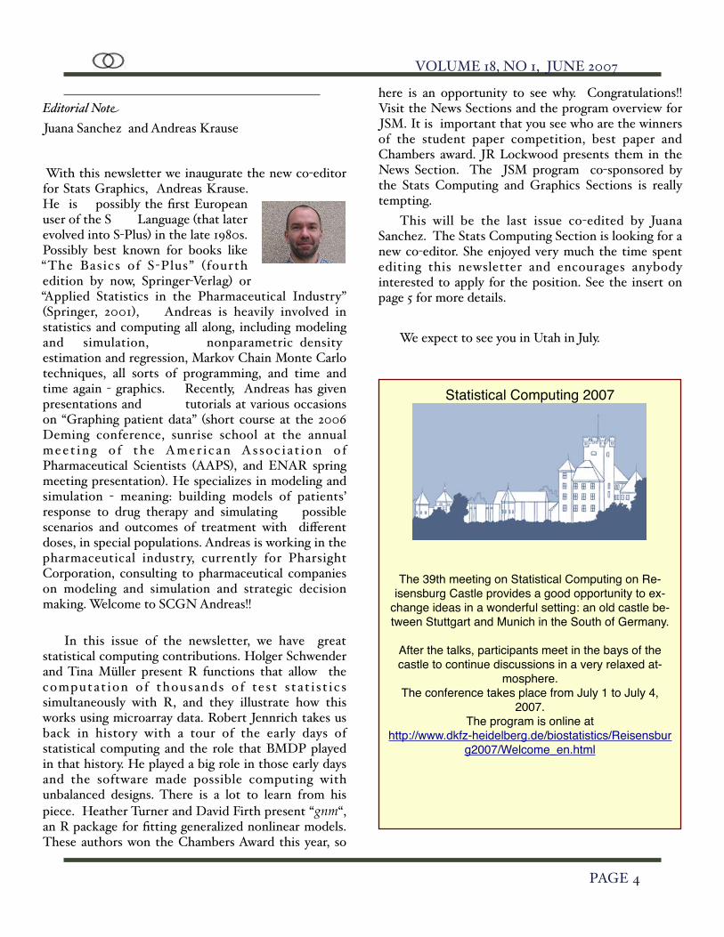
Editorial NoteJuana Sanchez and Andreas Krause
With this newsletter we inaugurate the new co-editor for Stats Graphics, Andreas Krause. He is possibly the first European user of the S Language (that later evolved into S-Plus) in the late 1980s. Possibly best known for books like “The Basics of S-Plus” (fourth edition by now, Springer-Verlag) or “Applied Statistics in the Pharmaceutical Industry” (Springer, 2001), Andreas is heavily involved in statistics and computing all along, including modeling and simulation, nonparametric density estimation and regression, Markov Chain Monte Carlo techniques, all sorts of programming, and time and time again - graphics. Recently, Andreas has given presentations and tutorials at various occasions on “Graphing patient data” (short course at the 2006 Deming conference, sunrise school at the annual meet ing o f the Amer ican Assoc ia t ion o f Pharmaceutical Scientists (AAPS), and ENAR spring meeting presentation). He specializes in modeling and simulation - meaning: building models of patients’ response to drug therapy and simulating possible scenarios and outcomes of treatment with different doses, in special populations. Andreas is working in the pharmaceutical industry, currently for Pharsight Corporation, consulting to pharmaceutical companies on modeling and simulation and strategic decision making. Welcome to SCGN Andreas!!
In this issue of the newsletter, we have great statistical computing contributions. Holger Schwender and Tina Müller present R functions that allow the computat ion of thousands of test s tat i s t ics simultaneously with R, and they illustrate how this works using microarray data. Robert Jennrich takes us back in history with a tour of the early days of statistical computing and the role that BMDP played in that history. He played a big role in those early days and the software made possible computing with unbalanced designs. There is a lot to learn from his piece. Heather Turner and David Firth present “gnm“, an R package for fitting generalized nonlinear models. These authors won the Chambers Award this year, so
here is an opportunity to see why. Congratulations!! Visit the News Sections and the program overview for JSM. It is important that you see who are the winners of the student paper competition, best paper and Chambers award. JR Lockwood presents them in the News Section. The JSM program co-sponsored by the Stats Computing and Graphics Sections is really tempting.
This will be the last issue co-edited by Juana Sanchez. The Stats Computing Section is looking for a new co-editor. She enjoyed very much the time spent editing this newsletter and encourages anybody interested to apply for the position. See the insert on page 5 for more details.
We expect to see you in Utah in July.
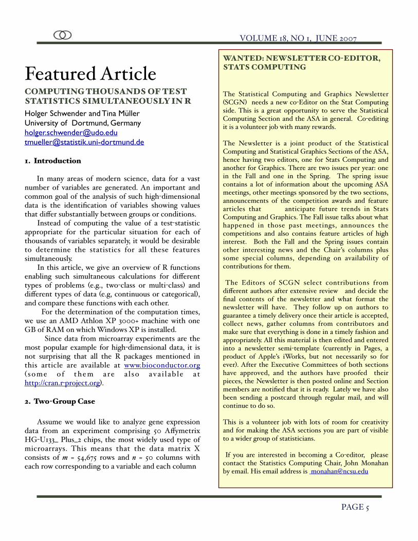
Statistical Computing 2007
The 39th meeting on Statistical Computing on Re-isensburg Castle provides a good opportunity to ex-
change ideas in a wonderful setting: an old castle be-tween Stuttgart and Munich in the South of Germany.
After the talks, participants meet in the bays of the castle to continue discussions in a very relaxed at-
mosphere.The conference takes place from July 1 to July 4,
2007.The program is online at
http://www.dkfz-heidelberg.de/biostatistics/Reisensburg2007/Welcome_en.html
VOLUME 18, NO 1, JUNE 2007
PAGE 4
Featured ArticleCOMPUTING THOUSANDS OF TEST STATISTICS SIMULTANEOUSLY IN RHolger Schwender and Tina MüllerUniversity of Dortmund, [email protected]@statistik.uni-dortmund.de
1. Introduction
In many areas of modern science, data for a vast number of variables are generated. An important and common goal of the analysis of such high-dimensional data is the identification of variables showing values that differ substantially between groups or conditions. Instead of computing the value of a test-statistic appropriate for the particular situation for each of thousands of variables separately, it would be desirable to determine the statistics for all these features simultaneously. In this article, we give an overview of R functions enabling such simultaneous calculations for different types of problems (e.g., two-class or multi-class) and different types of data (e.g, continuous or categorical), and compare these functions with each other. For the determination of the computation times, we use an AMD Athlon XP 3000+ machine with one GB of RAM on which Windows XP is installed. Since data from microarray experiments are the most popular example for high-dimensional data, it is not surprising that all the R packages mentioned in this article are available at www.bioconductor.org ( some of them are a l so a va i l ab le a t http://cran.r-project.org).
2. Two-Group Case
Assume we would like to analyze gene expression data from an experiment comprising 50 Affymetrix HG-U133_ Plus_2 chips, the most widely used type of microarrays. This means that the data matrix X consists of m = 54,675 rows and n = 50 columns with each row corresponding to a variable and each column
WANTED: NEWSLETTER CO-EDITOR, STATS COMPUTING The Statistical Computing and Graphics Newsletter (SCGN) needs a new co-Editor on the Stat Computing side. This is a great opportunity to serve the Statistical Computing Section and the ASA in general. Co-editing it is a volunteer job with many rewards.
The Newsletter is a joint product of the Statistical Computing and Statistical Graphics Sections of the ASA, hence having two editors, one for Stats Computing and another for Graphics. There are two issues per year: one in the Fall and one in the Spring. The spring issue contains a lot of information about the upcoming ASA meetings, other meetings sponsored by the two sections, announcements of the competition awards and feature articles that anticipate future trends in Stats Computing and Graphics. The Fall issue talks about what happened in those past meetings, announces the competitions and also contains feature articles of high interest. Both the Fall and the Spring issues contain other interesting news and the Chair’s columns plus some special columns, depending on availability of contributions for them.
The Editors of SCGN select contributions from different authors after extensive review and decide the final contents of the newsletter and what format the newsletter will have. They follow up on authors to guarantee a timely delivery once their article is accepted, collect news, gather columns from contributors and make sure that everything is done in a timely fashion and appropriately. All this material is then edited and entered into a newsletter semi-template (currently in Pages, a product of Apple’s iWorks, but not necessarily so for ever). After the Executive Committees of both sections have approved, and the authors have proofed their pieces, the Newsletter is then posted online and Section members are notified that it is ready. Lately we have also been sending a postcard through regular mail, and will continue to do so.
This is a volunteer job with lots of room for creativity and for making the ASA sections you are part of visible to a wider group of statisticians. If you are interested in becoming a Co-editor, please contact the Statistics Computing Chair, John Monahan by email. His email address is [email protected]
VOLUME 18, NO 1, JUNE 2007
PAGE 5

to a sample/observation. As the computation time does not depend on whether real or simulated data are used, this matrix is simulated by
> m <- 54675> n <- 50> X <- matrix(rnorm(m * n,10, 3), m)
Let’s further assume that the vector
> cl <- rep(0:1, e = n / 2)
contains the class labels of the observations.The “classical’’ way to compute the value of the
t-statistic for testing each of the variables is to call the R function t.test for each row of X separately, which can either be done by
> system.time(+ for(i in 1:m)+ t.test(X[i, ] ~ cl)$stat+ ) user system elapsed 252.38 0.09 252.52
or less time-consuming by
> system.time(+ for(i in 1:m)+ t.test(X[i, cl == 0],+ X[i, cl== 1])$stat+ ) user system elapsed 61.02 0.02 61.07
Another possibility is to use the function apply, i.e. to call
> compT <- function(x, cl){+ t.test(x[cl == 0], x[cl== + 1])$stat+ }> system.time(+ apply(X, 1, compT, cl = cl)+ ) user system elapsed 62.54 0.07 62.75
to apply compT to each row of X. (There are also other functions for applying a particular function to each element of an object. For example, lapply and sap-
ply access each element of a list – or each column of a data.frame object.)
Although the two latter ways for calculating the t-statistics save a lot of time, they are still very time-consuming – in particular if p-values should be computed based on a permutation method.
A possible solution to accelerate this process is to use the functions rowSums and rowMeans – that calculate the rowwise sums and means, respectively, of a matrix – to write your own function for determining the t-statistics for all rows of X simultaneously.As t.test by default computes Welch’s t-statistic, the corresponding rowwise function might be given by
rowtstat <- function(X, cl){ X0 <- X[, cl == 0] X1 <- X[, cl == 1] m0 <- rowMeans(X0) m1 <- rowMeans(X1) n0 <- sum(cl == 0) n1 <- sum(cl) sq <- function(x) x * x s0 <- rowSums(sq(X0 - m0)) s0 <- s0 / (n0 * (n0 - 1)) s1 <- rowSums(sq(X1 - m1)) s1 <- s1 / (n1 * (n1 - 1)) (m0 - m1) / sqrt(s0 + s1)}
Applying this function to X is about 130 times faster than employing t.test, as the computation time of rowtstat is 0.47 seconds.
> system.time(rowtstat(X, cl)) user system elapsed 0.46 0.01 0.47
A more convenient solution is to use the already existing functions rowttests and mt.teststat available in the packages genefilter and multtest, respectively. While in mt.teststat Welch’s t-statistic is computed by default, the ordinary t-statistic assuming equal group variances is determined in rowttests.
> library(genefilter)> cl2 <- as.factor(cl)> system.time(+ rowttests(X, cl2)$stat+ ) user system elapsed
VOLUME 18, NO 1, JUNE 2007
PAGE 6

0.18 0.00 0.18
> library(multtest)> system.time(+ mt.teststat(X, cl)+ ) user system elapsed 1.61 0.06 1.67
Additionally to Welch’s t-statistic, mt.teststat provides the possibility to employ the ordinary and the paired two-class t-statistic and the one-class t-statistic. The latter can also be determined using rowttests.
Table 1. Computation times (in seconds) of four functions for calculating t-statistics for different numbers of variables and observations.
50 Observations10,000 54,675 100,000
t.test 11.24 61.07 113.66rowtstat 0.06 0.47 0.80rowttests 0.02 0.18 0.24mt.teststat 0.20 1.67 3.07
100 Observations10,000 54,675 100,000
t.test 11.53 63.91 117.07rowtstat 0.12 0.91 1.54rowttests 0.04 0.24 0.32mt.teststat 0.37 3.23 5.10
In Table 1, the computation times for the above and other testing situations are summarized. This table shows that rowttests is less time-consuming than r o w t s t a t which in turn i s f a s ter than mt.teststat. In comparison to a one-by-one determination, all these functions lead to an immense reduction of computation time.
3. Wilcoxon Rank Sums
In addition to t-statistics, it is also possible to employ mt.teststat for computing (block) F-statistics (see Section 4) and standardized Wilcoxon rank sums. In-
stead of a t-test, a Wilcoxon rank sum test can thus be applied to the data described in Section 2 by calling
> system.time( mt.teststat(X, cl, test = + "wilcoxon")+ ) user system elapsed 11.64 0.06 11.74
However, this calculation takes almost seven times longer than the determination of the rowwise t-statistics. This relatively long computation time is due to the separate application of the function rank to each of the rows of X which requires more than 80% of the actual computation time.
> Xr <- X> system.time(+ for(i in 1:m)+ Xr[i, ] <- rank(Xr[i, ])+ ) user system elapsed 9.71 0.02 9.76
It would therefore be desirable to have a function enabling the determination of the ranks of all rows of X simultaneously. Unfortunately, such a function does not currently exist.
But the function rowQ in the package Biobase enables the rowwise computation of a specific quantile. For example,
> rowQ(X, i)
returns a vector of length nrow(X) containing the ith smallest value of each of the variables represented in X. Since typically the number of observations in high-dimensional data is much smaller than the number of variables, the use of rowQ in a function that calculates the ranks for all variables simultaneously might reduce the computation time. Such a function is given by
rowRanks <- function(X){ require(Biobase) Xr <- X for(i in 1:ncol(X)){ tmp <- rowQ(X, i) Xr[X == tmp] <- i } Xr
VOLUME 18, NO 1, JUNE 2007
PAGE 7

}
Figure 1. Computation times (in seconds) for the applications of three functions for determining the ranks of a matrix rowwise to different numbers of observations and variables, where for rowRanksWilc it is assumed that there are two equally sized groups of observations.
Figure 1, however, reveals that rowRanks only leads to an improved computation time if the number of observations is small.
Another idea is to count rowwise for each observation how many of the values of the respective variable are smaller than or equal to the value of this observation, i.e. to compute the ranks of each observation for all rows simultaneously. Furthermore, since the Wilcoxon rank sum is given by the sum over the ranks of the observations from one of the groups, it is only necessary to perform this calculation for the observations from one of the groups. This idea is im-plemented in the function
rowRanksWilc <- function(X,cl){ ids <- which(cl == 1) Xr <- matrix(0, nrow(X),
length(ids)) for(i in 1:length(ids)) Xr[ ,i] <- rowSums(X <= X[,ids[i]]) Xr}
which is available – along with the function rowWil-coxon for computing rowwise Wilcoxon rank sums or signed ranks – in siggenes version 1.11.1 and later. Figure 1 shows that in the case of equally sized groups rowRanksWilc leads to a lower computation time than applying the function rank to the rows of X if the number of observations is smaller than 100.
4. Multi-Group Case
Now we would like to generalize the two-class case to the k group case in which the F-statistic is an appropriate score for testing if a variable exhibits values that differ substantially between the k groups.
As mentioned in Section 3, mt.teststat provides the possibility to compute the values of the F-statistic for all rows of X simultaneously. Moreover, a function called rowFtests is available in the package gene-filter that also allows this calculation.The main difference between rowFtests and the other functions mentioned in this article is that rowFtests employs matrix algebra, whereas functions such as mt.teststat and rowttests are based on C-code. It is therefore not very surprising that mt.teststat is faster than rowFtests (see Table 2). Table 2 also reveals that contrary to rowFtests the computation time of mt.teststat does not seem to depend on the number of groups.
Table 2. Computation times (in seconds) for the ap-plications of both rowFtests and mt.teststat to a 54,675 x 50 matrix with varying numbers of groups (3, 4, 5, 10).
3 4 5 10mt.teststat 1.24 1.24 1.23 1.25rowFtests 1.83 1.92 2.00 2.59
VOLUME 18, NO 1, JUNE 2007
PAGE 8

5. Fitting Linear Models
Another interesting task is to fit a linear model for each of the variables represented in our 54,675 x 50 data matrix X (see Section 2). To simplify matters, assume that the vector
> cl <- rep(0:1, e = n / 2)
of the group labels is the only explanatory variable. Then, a linear model for each variable can be fitted by
> lLM <- vector("list", m)> system.time(+ for(i in 1:m)+ LM[[i]] <- lm(X[i,] ~ cl)+ ) user system elapsed 388.60 1.25 396.04
However, it is also possible to fit all 54,675 models at once, e.g., by employing matrix algebra: In the case of a single variable, the estimates for the coefficients can be determined by
where Z is the design matrix and y contains the values of the variable of interest. If we set
then all linear models are fitted at once, and
€
β∧
is a matrix containing the estimates for all coefficients of all models. Since transposing the high-dimensional matrix X is more time and memory consuming than
transposing ( ) ZZZA 1 ′′= − it is better to fit these models by computing
i.e. by
> system.time({+ A <- t(solve(t(Z) %*% Z) %*% t(Z))+ beta <- X %*% A+ }) user system elapsed 0.12 0.00 0.12
This reduces the computation time from more than six minutes to much less than one second. However, it only returns the estimates for the coefficients. Although most of the other statistics returned by lm can also be obtained by matrix calculation, it would be more convenient to use an already existing function that generates these values.
Fortunately, such a function does exist: lm. Taking a close look at the help file for lm reveals that if y in lm(y ~ x) is a matrix, a linear model will be fitted to each column of y. (Actually, we found this feature of lm while looking at the function lmFit of the package limma which has been particularly written for fitting linear models in high-dimensional data.) Thus, instead of calling lm for each row of X separately, all models can be fitted at once by
> system.time(+ lm.out <- lm(t(X) ~ cl)+ ) user system elapsed 3.31 0.20 3.51
6. Categorical Data
High-dimensional data is not necessarily continuous. The Affymetrix GeneChip Mapping 500K Array Set, e.g., provides data for calling the genotypes of about 500,000 SNPs (Single Nucleotide Polymorphisms), where a SNP is a single-base pair position in the DNA sequence at which different base alternatives exist. Since a SNP can typically take three forms called genotypes, Pearson’s χ2-statistic is an appropriate score for testing if the distribution of a SNP differs between several groups.
The package scrime which will be available at Bioconductor and/or CRAN in August or September 2007 (a pre-version of this package is available by request fromthe authors) contains the function rowChisqStats which cannot only be employed to identify variables showing a distribution that differs between several groups, but also to test each pair of rows of a matrix if the corresponding variables are independent.
The basic idea of rowChisqStats is to consider an indicator matrix for each level of the variables, and to use matrix algebra to compute the values of Pearson's χ2-statistic for all variables simultaneously (for details, see Schwender, 2007). Although this function has been written for a situation in which all variables exhibit the same number of categories and none of the values are
VOLUME 18, NO 1, JUNE 2007
PAGE 9
( ) yZZZ ′′= −1β̂
Ay ′′=′β̂
Xy ′=

missing, rowChisqStats can also cope with missing values and variables with differing numbers of levels.
Table 3. Computation times (in seconds) of both rowChisqStats and the individual calculation of Pearson’s χ2-statistics for different numbers of variables and observations. Each of the m variables can take three levels, and each of the n observations be-longs to one of two classes.
n = 200m rowChisqStats chisq.test
1,000 0.05 2.6410,000 0.63 26.74
100,000 6.16 274.96
n = 1,000m rowChisqStats chisq.test
1,000 0.40 3.3510,000 2.39 34.42
In Table 3, a comparison of the computation times of the applications of r o w C h i s q S t a t s and chisq.test to SNP data from case-control studies is presented. This table shows that rowChisqStats is much faster than applying chisq.test separately to each variable. Additionally, Table 4 reveals that the computation time of rowChisqStats depends on the (maximum) number of levels the variables can take, but not on the number of groups.
Table 4. Computation times (in seconds) of row-ChisqStats for different numbers of variables and different values of c, the number of levels a variable can take, and r, the number of classes to which the 200 observations belong.
1,000 10,000 100,000r = 2, c = 3 0.05 0.63 6.16r = 2, c = 5 0.07 1.03 9.98r =2, c = 10 0.15 2.04 61.82r = 3, c = 3 0.05 0.64 6.18r = 6, c= 3 0.05 0.62 6.46
7 Discussion
In this article, we have presented already existing as well as new functions for computing statistics for all rows of a data matrix simultaneously. We have also shown that employing these functions leads to a substantial reduction of the computation times in comparison to applying standard functions to each of the rows/variables separately.
However, there are more functions implemented for similar purposes: For most of the already existing functions with prefix row, a version is available enabling to determine the statistics columnwise. Other examples a re the funct ion mt.teststat.num.denum from the package multtest that returns the numerator and the denominator of the test statistics separately, or the functions rowpAUCs and rowSds from the package genefilter that allow rowwise calculations of, on the one hand, ROC curves and the partial areas under the curve, and on the other hand, the standard deviations.
Moreo ver, funct ions such a s mt.sample.teststat (from the multtest pack-age) or chisq.test can be applied to a single variable to determine the values of the test statistic for all permutations of the group labels simultaneously. There also exist combinations of these two types of simultaneous computations: The functions mt.maxT and mt.minP (again, from the multtest package), e.g., provide the possibility to calculate permutation based p-values for all rows of a matrix using the step-down multiple testing procedures described by West-fall and Young (1993).
AcknowledgementThe financial support of the Deutsche Forschungsge-meinschaft (SFB 475, “Reduction of Complexity in Multivariate Data Structures”) is gratefully acknow-ledged.ReferencesSchwender, H. (2007). A Note on the Simultaneous Computation of Thousands of Pearson’s χ2-Statistics. Technical Report, Collaborative Research Center 475, Department of Statistics, University of Dortmund.
Westfall, P.H. and Young, S.S. (1993). Resampling-Based Multiple Testing: Examples and Methods for P-Value Adjustments. Wiley, New York, NY.
VOLUME 18, NO 1, JUNE 2007
PAGE 10

THE SCOOP ON DATA VISUALIZATION
Highly recommended, rated M (Must see)!
Movies:
We have recently come across a wonderful piece of presenting interactive data analysis. Hans Rosling, a researcher of global health at Sweden’s Karolinska Institute, analyzes trends in global data like life expectancy and child mortality in a lively, entertaining and highly educational presentation.
We think that the movie is well worth your time (some 20 minutes), and it might well prove motivational for students to step into data analysis and statistics.The movie of the presentation can be downloaded from http://www.ted.com/index.php/talks/view/id/92
For those of you interested in what goes on outside academia, take a look also at what statistical offices of several countries are doing to improve statistical literacy and interest in data by citizens. Check this out.h t t p : / / w w w . o e c d . o r g / d o c u m e n t /12/0,2340,en_21571361_31938349_37725196_1_1_1_1,00.html
Books:
Michael Friendly's online book on visualization of Categorical data
http://www.math.yorku.ca/SCS/vcd/
http://www.uv.es/visualstats/Book/
We would like our readers to be aware of things going on in and outside academia. Send us unusual links, things that are not usually appearing in the main stream. As far as they deal with statistical graphics and computing we promise to submit it to thorough review.
Tools for ComputingGENERALIZED NONLINEAR MODELS IN RHeather L. Turner and David Firth, University of [email protected]@warwick.ac.uk http://go.warwick.ac.uk/heatherturner/gnm
1. Background
In this article we introduce the R package gnm, which provides tools for the specification, estimation and inspection of generalized nonlinear models. A generalized nonlinear model assumes that the variance of a response variable Y is equal to, or proportional to, a known function of its mean and that this mean is related to a nonlinear function of parameters via a link function, as follows:
€
g[E(y)] =η β( ) (1)
Thus a generalized nonlinear model may be considered as an extension of a generalized linear model, in which some terms are nonlinear in the parameters; or as an extension of a nonlinear least squares model, in which the variance of the response may be dependent on the mean.
The aim for gnm was to implement a much more gen-eral version of the Xlisp-Stat package Llama (Firth, 1998), which was designed to fit log-linear and multiplicative models for contingency tables. Hence the development of gnm has been strongly motivated by models with multiplicative terms, such as row-column association models (Goodman, 1979), UNIDIFF (uniform difference) models for social mobility (Xie, 1992; Erikson and Goldthorpe, 1992), GAMMI (generalized additive main effects and multiplicative interaction) models (e.g., van Eeuwijk, 1995) , Lee-Carter models for trends in age-specific mortality (Lee and Carter, 1992), diagonal-reference mode l s for dependence on a square or hyper-square classification (Sobel 1981, 1985), Rasch-type logit or probit models for legislative voting
VOLUME 18, NO 1, JUNE 2007
PAGE 11
(e.g., de Leeuw 2006), and stereotype multinomial regression models for ordinal response (Anderson, 1984). Nevertheless, the package provides a very general fitting algorithm with a simple, flexible inter-face that allows a wide range of generalized nonlinear models to be specified.
2. Implementation
The model-fitting function provided by the gnm package, also named gnm, has been patterned after glm --- the function provided in the base distribution of R for fitting generalized linear models. Therefore the manner in which models are specified and the majority of functions provided for model inspection will be familiar to users of R.
Models are specified in a symbolic form, with a special class of functions providing the mechanism for nonlinear terms to be included in the predictor. A number of these nonlin functions are distributed in the package, and user-defined nonlin functions are also supported. In principle any differentiable nonlinear term can be specified in this way.
With such generality, it would be difficult to define a set of rules by which identifiability constraints could be automatically applied, as they can be for linear models. This difficulty is circumvented in gnm by the use of a fitting algorithm that can work with over-parameterized representations of models. Model parameters are estimated via an iterative weighted least
squares a lgorithm, using the Moore -Penrose pseudoinverse to handle the rank-deficient design matrix. By default therefore, gnm applies only minimal identifiability constraints. An arbitrary parameterization -determined at random - is used for nonlinear terms which involve parameter redundancy. Inference on identifiable parameter contrasts can be conducted after the model has been fitted, by using supporting functions in the package.
3. Multiplicative Interaction Models
As noted earlier, there are several examples of generalized nonlinear models that have been proposed for the analysis of contingency tables. Here we con-sider the uniform difference (UNIDIFF) model (Xie, 1992; Erikson and Goldthorpe, 1992) for three-way contingency tables:
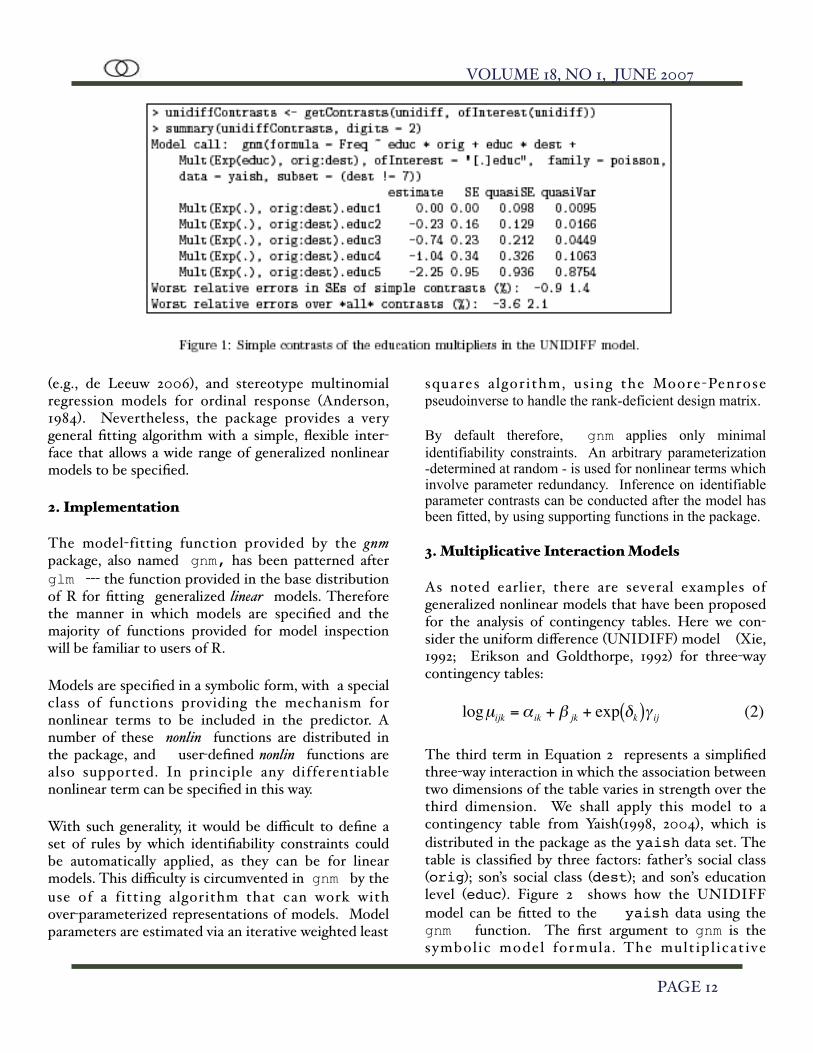
The third term in Equation 2 represents a simplified three-way interaction in which the association between two dimensions of the table varies in strength over the third dimension. We shall apply this model to a contingency table from Yaish(1998, 2004), which is distributed in the package as the yaish data set. The table is classified by three factors: father’s social class (orig); son’s social class (dest); and son’s education level (educ). Figure 2 shows how the UNIDIFF model can be fitted to the yaish data using the gnm function. The first argument to gnm is the symbol ic model formula . The mult ip l icat ive
VOLUME 18, NO 1, JUNE 2007
PAGE 12
€
logµijk =α ik + β jk + exp δk( )γ ij (2)
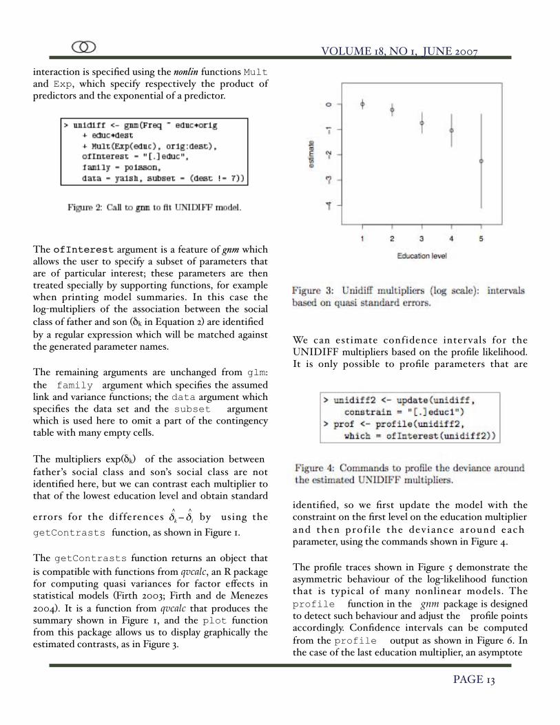
interaction is specified using the nonlin functions Mult and Exp, which specify respectively the product of predictors and the exponential of a predictor.
The ofInterest argument is a feature of gnm which allows the user to specify a subset of parameters that are of particular interest; these parameters are then treated specially by supporting functions, for example when printing model summaries. In this case the log-multipliers of the association between the social class of father and son (δk in Equation 2) are identifiedby a regular expression which will be matched against the generated parameter names.
The remaining arguments are unchanged from glm: the family argument which specifies the assumed link and variance functions; the data argument which specifies the data set and the subset argument which is used here to omit a part of the contingency table with many empty cells.
The multipliers exp(δk) of the association between father’s social class and son’s social class are not identified here, but we can contrast each multiplier to that of the lowest education level and obtain standard
errors for the differences
€
δk∧
−δi∧
by using the getContrasts function, as shown in Figure 1.
The getContrasts function returns an object that is compatible with functions from qvcalc, an R package for computing quasi variances for factor effects in statistical models (Firth 2003; Firth and de Menezes 2004). It is a function from qvcalc that produces the summary shown in Figure 1, and the plot function from this package allows us to display graphically the estimated contrasts, as in Figure 3.
We can estimate confidence intervals for the UNIDIFF multipliers based on the profile likelihood. It is only possible to profile parameters that are
identified, so we first update the model with the constraint on the first level on the education multiplier and then prof i le the dev iance around each parameter, using the commands shown in Figure 4.
The profile traces shown in Figure 5 demonstrate the asymmetric behaviour of the log-likelihood function that is typical of many nonlinear models. The profile function in the gnm package is designed to detect such behaviour and adjust the profile points accordingly. Confidence intervals can be computed from the profile output as shown in Figure 6. In the case of the last education multiplier, an asymptote
VOLUME 18, NO 1, JUNE 2007
PAGE 13

has been detected and the lower confidence limit is therefore shown as negative infinity.
4. Multinomial Regression
Multinomial response models may be fitted with gnm by using the well-known equivalence between multinomial and (conditional) Poisson likelihoods. We illustrate this here by applying the stereotype
model proposed by Anderson (1984) for ordered categorical data. This model is a special case of the multinomial logistic model, in which the probability that a response belongs to category c given values of the covariates x is defined as:
VOLUME 18, NO 1, JUNE 2007
PAGE 14
€
pr(yi = c | xi) =exp βoc + γ cβ
T xi( )exp βor + γ rβ
T xi( )r∑ (3)
We shall use one of the example data sets from Anderson (1984), taken from a study of patients with back pain. The data are observations of three prognos-tic variables and an ordered factor quantifying the progress of each patient. These data are available in the gnm package as the data set backPain.
€
loguic =α i + βoc + γ c βrr∑ xir (4)
We can fit the stereotype model to the backPain data by re-expressing the categorical data as counts and fitting the log-linear model
The g nm package provides a uti l ity function expandCategorical to perform the required data manipulation: Figure 7 demonstrates its use.
The parameters of interest in the stereotype model are the category-specific multipliers (γc in Equation 3). In order to make these parameters identifiable, we need to constrain both their location and scale. The location may be const ra ined by se t t ing one o f the category-specific multipliers to zero. As we have
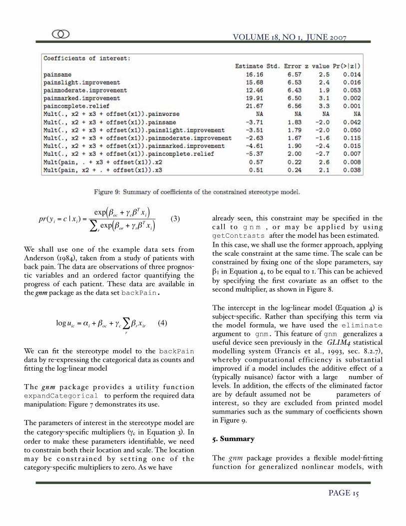
already seen, this constraint may be specified in the ca l l to g n m , o r may be app l ied by us ing getContrasts after the model has been estimated. In this case, we shall use the former approach, applying the scale constraint at the same time. The scale can be constrained by fixing one of the slope parameters, say β1 in Equation 4, to be equal to 1. This can be achieved by specifying the first covariate as an offset to the second multiplier, as shown in Figure 8.
The intercept in the log-linear model (Equation 4) is subject-specific. Rather than specifying this term via the model formula, we have used the eliminate argument to gnm. This feature of gnm generalizes a useful device seen previously in the GLIM4 statistical modelling system (Francis et al., 1993, sec. 8.2.7), whereby computational efficiency is substantial improved if a model includes the additive effect of a (typically nuisance) factor with a large number of levels. In addition, the effects of the eliminated factor are by default assumed not be parameters of interest, so they are excluded from printed model summaries such as the summary of coefficients shown in Figure 9.
5. Summary
The gnm package provides a flexible model-fitting function for generalized nonlinear models, with
VOLUME 18, NO 1, JUNE 2007
PAGE 15
supporting functions for model inspection and inference. The package is distributed with a comprehensive manual, that provides plenty of examples based on practical applications. This manual can also be downloaded from the gnm webpage{http://go.warwick.ac.uk/heatherturner/gnm}.
References
J. A. Anderson. Regression and ordered categorical variables. J. R. Statist. Soc. B, 46 (1):1-30, 1984.
J. de Leeuw. Principal component analysis of binary data by iterated singular value decomposition. Comp. Stat. Data Anal., 50(1): 21--39, 2006.
R.~Erikson and J.~H. Goldthorpe. The Constant Flux. Oxford: Clarendon Press, 1992.
D.~Firth. Overcoming the reference category problem in the presentation of statistical models. Sociological Methodology, 33: 1--18, 2003.
D.~Firth. Llama: An object-oriented system for log multiplicative models. In R.~Payne and P.~Green, editors, COMPSTAT 1998, Proceedings in Computational Statistics, pages 305--310. Heidelberg: Physica-Verlag, 1998.
D.~Firth and R.~X. {de Menezes}. Quasi-variances. Biometrika, 91: 65--80, 2004.
B.~J. Francis, M.~Green, and C.~D. Payne, editors. The GLIM System, Release 4 Manual. Oxford: Clarendon Press, 1993.
L.~A. Goodman. Simple models for the analysis of as-sociation in cross-classifications having ordered categories. J. Amer. Statist. Assoc., 74: 537--552, 1979.
R.~D. Lee and L.~Carter. Modelling and forecasting the time series of US mortality. Journal of the American Statistical Association, 87: 659--671, 1992.
M.~E. Sobel. Diagonal mobility models: A substan-tively motivated class of designs for the analysis of mobility effects. Amer. Soc. Rev., 46: 893--906, 1981.
M.~E. Sobel. Social mobility and fertility revisited: Some new models for the analysis of the mobility effects hypothesis. Amer. Soc. Rev., 50:699--712, 1985.
F.~A. van Eeuwijk. Multiplicative interaction in generalized linear models. Biometrics, 51: 1017--1032, 1995.
Y.~Xie. The log-multiplicative layer effect model for comparing mobility tables. American Sociological Re-view, 57: 380--395, 1992.
M.~Yaish. Class Mobility Trends in Israeli Society, 1974-1991 Edwin Mellen Press, Lewiston, 2004.
M.~Yaish. Opportunities, Little Change. Class Mobility in Israel: Society, 1974--1991. PhD thesis, Nuffield College, University of Oxford, 1998.
VOLUME 18, NO 1, JUNE 2007
PAGE 16
History of Statistical Computing BMDP and Some Statistical Computing History Robert Jennrich, University of California, Los [email protected]
The first package of BMDP statistical programs appeared in 1961. For at least a decade this was the most extensively used statistical package. The early development of statistical software is discussed here from the perspective of BMDP during the 60’s and 70’s.
The discussion will illustrate the use of a number of important statistical computing tools including Beaton sweeps, dummy variables, the FFT, problem definition, lattice driven balanced mixed model computation, and unbalanced incomplete mixed model analysis.
Only a limited number of BMDP programs are discussed. The choice was made to illustrate tools and is rather arbitrary. In the interest of some historical accuracy the programs are those best known to the author.
1. The first manual
A natural place to begin is with the BIMD manual complied by Lynn Hayward in 1961. BIMD stands for ``biomedical’’ and the Biomedical Data Processing Group at UCLA. The manual documented a collection of 35 programs produced in just two years by students and staff in the Division of Biostatistics at UCLA under the direction of Wilfrid Dixon, Frank Massey, and Jean Dunn. In most cases the programs were created for specific medical research projects.
There were 8 regression programs, 6 multivariate analysis programs, 6 analysis of variance programs, 9 tabulating, screening, and plotting programs, and 6 miscellaneous programs.
While primitive by today’s standards these programs covered a broad spectrum of analyses including multiple and stepwise regression, factor analysis, discriminant analysis, balanced and to some extent unbalanced analysis of variance and covariance, and cross tabulation.
The BIMD programs later became the BMD programs and eventually the BMDP programs. BMD was simply an alternate spelling of BIMD. The letter P in BMDP stood for the parameter language which represented a major advance that greatly simplified program use and output readability. Here these programs will be referred to generically as the BMDP programs. Until the mid 70’s, when generous federal support ended, the BMDP programs were free.
As an historical note the first manual had three stepwise regression programs. One used a residual sum of squares, one an F-to-enter, and one a partial correlation variable selection rule. While asserted to be distinct these rules are in fact equivalent, something that might have been discovered empirically if not theoretically.
2. The Beaton sweep operator
The BMDP programs made extensive use of the Beaton sweep operator. The Beaton sweep is a matrix operator introduced in Albert Beaton’s thesis supervised by John Tukey. His thesis became an Educational Testing Service Research Bulletin in 1964. Jennrich (1977) may be a more useful reference here. Today the Beaton sweep is a well known and extensively used statistical computing tool. BMDP used a minor modification of Beaton’s operator called the Gauss-Jordan pivot. This modification had the advantage that it was its own inverse making it unnecessary to write and use a separate inversion subroutine. In the discussion here the Beaton sweep will refer to the modified operator. Actually there is a sweep operator for each non zero diagonal element of the matrix to which it is applied. The choice is an operator parameter.
The sweep operator was very easy to implement. It required just 11 lines of Fortran code.
VOLUME 18, NO 1, JUNE 2007
PAGE 17

To describe the use of the operator consider a multivariate regression model of the form
and the partitioned matrix
This matrix is called the regression tableau (RT) corresponding to the model (1). In it
€
B∧
is the matrix
of least squares estimates of B, S=(Y-X
€
B∧
)’(Y-X
€
B∧
) is a matrix of residual cross products, and (X’X)-1 is useful for computing standard errors and evaluating test sta-tistics.
Consider the modified regression model obtained by moving the i-th column of Y into X. The new RT is obtained by simply applying the sweep operator defined by the i-th diagonal element of S to the current RT.
Moving the i-th column of X into Y is also very easy. One simply applies the sweep operator defined by the i-th diagonal element of (X’X)-1 to the current RT.
In stepwise regression when variables are entered or removed the current RT is updated using the sweep operator. The last diagonal element of S is the residual sum of squares for the current stepwise regression model. The independent variable entered is the one that makes the largest reduction in this element and the independent variable removed is the one that makes the smallest increase. In either case finding these variables is easy because the amount of change is a simple function of just two values in the current RT. After a variable is selected for entry or removal the RT is updated using the sweep operator defined by the diagonal element corresponding to the variable to be moved.
One argument in support of stepwise regression is that by using the sweep operator the cost of a stepwise regression is no more than that of an ordinary regression and the incomplete regressions produced along the way may lead to interesting insights.
In addition to stepwise regression the sweep operator has been used for best subset regression, for stepwise discriminant analysis and other stepwise analyses, for unbalanced fixed and mixed analyses of variance and covariance and other methods using categorical vari-ables, and for nonlinear regression and other methods using coordinate constraints.
3. Problem definition
In 1969 BMDP introduced a parameter control language developed by Laszlo Engelman that greatly simplified problem definiton.
Problem definition parameters were given explicit names that could be used to specify their values. Moreover, using them made it possible to assign default values. This not only greatly simplified problem definition it made the definition and output much easier to read.
Rather than punching (yes, punching) a numeric parameter value in specified columns of control cards, one for each parameter with no defaults, using the parameter control language one could punch
INPUT VARIABLES = 3. FORMAT = '(F2.0,2F3.0)'./VARIABLE NAMES = FOOD , WEIGHT , GAIN. GROUPING = FOOD./DESIGN DEPENDENT = GAIN./END. {Data here}
to specify a simple one way analysis of covariance.
Before the introduction of the parameter language the definition for the same problem was
VOLUME 18, NO 1, JUNE 2007
PAGE 18
€
Y = XB + E (1)
€
X 'X( )−1 B∧
−B∧
' S
PROBLM__0400038010300003{29-68blank}0001SAMSIZ010010010008(F2.0,2F3.0){Data here}CVRSEL020102
which is clearly much more difficult to read and much more difficult to punch because all of the numbers and letters had to appear and appear in specified columns. This required the explicit specification of 22 parameter values rather than 7 when using the parameter control language.
The parameter control language also simplified variable generation. For example the parameter language command
/TRANSFORM RATIO = WEIGHT/HEIGHT.
replaced the equivalent transgeneration command
__614_____2_____4
where 14 is the division command and 6, 2, and 4 are the variable numbers for RATIO, WEIGHT, and HEIGHT.
Because programs shared many problem definition parameters it became appropriate to view BMDP as a statistical software system rather than simply a collection of programs.
4. FFT, the fast Fourier transform
An important contribution to statistical computing and to computing in general was the re-discovery by Cooley and Tukey (1965) of the FFT. Although discovered several times earlier it was Tukey who identified the wide applicability and importance of this algorithm.
BMDP was the first general statistical software system to use the FFT to produce efficient frequency domain time series analysis programs. The programs estimated power and cross spectra, amplitudes, phases, and coherences for multiple series. The cross spectra were
used to estimate multiple coherences and frequency response functions for a set of input and output series.
5. Computer generated dummy variables
BMDP made extensive use of computer generated dummy variables. The main ideas can be described in terms of the two-way analysis of variance (anova) model
The terms αi, βj, and γijk sum to zero on each of their subscripts.
Let nij be the number of levels of k in the cell defined by i and j. The fitting is greatly simplified if all of the nij are equal. Such models are called balanced. In the unbalanced case linear regression was used for fitting. The linear regression model corresponding to (2) had the form
where Dμ, Dα, Dβ, and D γ are dummy variable matrices for the anova components and θμ, θα, θβ and θγ are parameter vectors of appropriate lengths.
The dummy variable matrices were generated as follows. A main effect table was created for each single index (main effect) component of the anova model. If the index i had three values the table for the α i component in (2) was
VOLUME 18, NO 1, JUNE 2007
PAGE 19
€
yijk = µ +α i +β j +γ ij +eijk (2)
€
y = Dµθµ + Dαθα + Dβθβ + Dγθγ + e (3)
The columns in the matrix on the lower right sum to zero and are a basis for the space of all functions of i that sum to zero.
The input data for each subject contained values for the anova indices i and j. Dummy variable matrices were constructed from these as follows.
Dummy variable values for a main effect were generated by reading from its main effect table. The values for the main effect αi for a subject with i=2 are 0 and -1, the values in the second line of the αi main effect table. Dummy variable values for the βj term were generated similarly. Dummy variable values for the interaction term γij were simply the Kronecker product of those for the two main effect terms. The dummy variable matrices, one for each term in the anova model, were formed one line at a time from the index values i and j for each subject. The dummy variable matrix Dµ for the intercept term µ was simply a column of ones.
Let D=(Dµ,Dα,Dβ,Dγ) be the dummy variable matrix formed by adjoining those for each of the anova com-ponents. The regression model (3) takes the form Y=Dθ +e. Let
be the RT for this regression model. The sum of squares for testing any component in the anova model is the increase in RSS after sweeping on all the diagonal elements of (D’D)-1 corresponding to the component.
In general there could be more than two main effects and one interaction. The anova model need not be a full factorial, interactions and for that matter any terms in the model could be dropped. Analysis of covariance models were handled by simply adjoining a matrix X of covariate values to the anova dummy vari-able matrix D.
Before the introduction of computer generated dummy variables users were required to create these by hand and enter them as part of an expanded input data set.Few had the knowledge or anywhere near the patience required to do this even if they were paid assistants or graduate students. Computer generated dummy variable matrices greatly simplified the use of unbalanced analysis of variance and covariance mod-els.
5. Lattices and balanced mixed model analysis of variance
When BMDP began writing analysis of variance pro-grams for mixed models the literature contained many examples, but little in the way of general methods that could be applied to a wide variety of models. A notable exception was the work of Cornfield and Tukey (1956) that expressed expected mean squares for very general balanced mixed models as weighted sums of the variance components defined by the models.
In their very general balanced mixed model program P8V, BMDP used models defined by lattices and computing schemes based on lattices. More specifically models were defined by a sequence of subscript sets. For example a repeated measures model with groups g, treatments t, subjects s, and data ygts can be defined by the sequence g, t, sg of subscript sets. The last subscript set is often written s(g) and read as subjects nested within groups, but the parentheses are not needed. Using set union and intersection the first step was to form the lattice generated by the specified subscript sets. For the repeated measures example the lattice is as displayed below
VOLUME 18, NO 1, JUNE 2007
PAGE 20

where φ is the empty subset. Each node in the lattice corresponds to a term in the anova model defined by the lattice. To compute a sum of squares (SS) for each term in the anova model, P8V began by computing a marginal SS, Mn for each node n in the lattice. For the gt term in the repeated measures model this would be
where ls is the number of levels of the index s and
Mode l sums o f squares Sn, one for each node n in the lattice, were computed recursively using
where the sum is over all nodes m in the lattice that are proper subsets of n. The nodes n must be processed in order of node size. Nodes with equal sizes may be processed in any order. This produces a model SS for each term in the anova model.
Degrees of freedom (df) for each term in the anova model were computed in a similar manner. Each node n was assigned the df of its marginal sum of squares Mn. For the gt node in the repeated measures model this is lg lt. Degrees of freedom for each term in the anova model were obtained from their marginal df using the same lattice driven subtraction process used to obtain model SS from marginal SS. Actually the model SS and df were computed simultaneously by applying the lattice subtraction process to marginal (SS,df) pairs.
An analysis of variance table was produced by giving a df, mean square MS=SS/df, and expected mean square EMS for each term in the anova model. The EMS were produced using the methods of Cornfield and Tukey. Finally F statistics were produced, where possible, by
matching EMS. Many different anova models can be defined by specifying an appropriate and usually very brief collection of subscript sets.
6. General mixed model analysis of variance and covariance
In 1977 BMDP introduced a mixed model analysis of variance and covariance program that did not require balance or completeness. This program P3V was a precursor to SAS (MIXED), SPSS (MIXED), and Stata (xtmixed) all of which appeared much later. An example of a mixed model is
Except for the xijk the subscripted Roman letters on the right side are uncorrelated random variables with mean zero and for those sharing the same Roman letter, common variance. For example the
for all i and j. The Greek terms in the model are called fixed effects and the random terms random effects.
In P3V this model is defined by a DESIGN paragraph with the sentences
FIX = I. RAND = J. RAND = I,J. COV = X.
Using a variety of FIX and RAND specifications a wide variety of mixed models could be specified. These included random coefficients factorial models, nested models, and repeated measures models.
Because the models were not required to be complete or balanced computer generated dummy variables were used to reformulate them as a fixed and random coefficients model. These had the form
VOLUME 18, NO 1, JUNE 2007
PAGE 21
€
Mgt = ls ygt2.
t∑
g∑
€
ygt2
= ygtss∑ / ls.
€
Sn = Mn − Smm⊂n∑
€
yijk = µ +α i + bj + cij + βxijk + eijk
€
Var cij( ) =σ c2
€
y = Xα +U1b1 + ........+Ucbc + e

where b1………. bc are uncorrelated random vectors with covariance matrices
€
σ12I1,.........,σ c
2Ic . In the example the second random component cij became U2b2.
Two methods of estimation were used, maximum likelihood (ML) and restricted maximum likelihood (REML). Also two algorithms were used, Fisher scoring (FS) and Newton-Raphson (NR). For the ML and FS pair the algorithm had the form
where θ is a vector containing the mean and variance parameters, I(θ) is the information matrix for the ML model,and s(θ) is the score vector. Partial sweeping
was used to keep the variance components
€
σ i2 ≥ 0 . All
tests were likelihood ratio tests. Computing formulas and the partial sweeping strategy are discussed by Jennrich and Sampson (1976, 1968).
Unfortunately P3V had a number of weaknesses. Rather than being automatic, all tests of significance for the terms in the model had to be explicitly requested. Moreover, the output was much too ver-bose. BMDP didn’t seem to appreciate the importance of this program. Rather than making easy fixes for its shortcomings, they encouraged the use of their much less general P2V program.
7. People
Many contributed to the development of the BMDP programs. It is difficult to name all who made significant contributions. Some who played a major role in the early development of BMDP include: Wilfrid J. Dixon who supervised the development of the BMDP system and served as editor or co-editor of all BMDP manuals after the first. His NIH grants were the source of financial support.
Robert I. Jennrich who developed algorithms for regression, analysis of variance, factor analysis, stepwise discriminant analysis, and time series analysis
as part of his half time appointment in the Depart-ment of Bio-mathematics at UCLA from 1962-79.
Morton B. Brown who developed the frequency table programs including a log-linear model program and methods for dealing with structural zeros. He also reorganized the BMDP manuals and co-edited two of them.
Laszlo Engelman who created the parameter language, developed many of the programs, and supervised the other programmers.
Paul F. Sampson who from the beginning was BMDP’s secret weapon used to write many of their programs.
MaryAnn H. Hill who produced most of program write-ups.
Two who during extended visits made significant con-tributions were Richard L. Anderson who helped develop the mixed model analysis of variance programs and John A. Hartigan who developed the block and k-means cluster analysis programs.
8. SPSS and SAS
Two additional statistical software systems SPSS and SAS were introduced in the late 60’s and early 70’s. They were similar to BMDP and undoubtedly benefitted from the BMDP development during the previous decade. SPSS and SAS became increasingly popular in part due to there becoming commercial enterprises early on. Their usage probably surpassed that of BMDP by the beginning of the 80’s.
BMDP was supported primarily by NIH grants until 1980 when it too became a commercial, but less successful, enterprise. In 1995 it was sold to SPSS and slowly dropped out of sight. The BMDP software, however, can still be obtained from Statistical Solu-tions Ltd., http://www.statsol.ie.
VOLUME 18, NO 1, JUNE 2007
PAGE 22
€
Δθ = I θ( )−1s θ( )

References
Beaton, A.E. (1964). The use of special matrix operators in statistical calculus. Research Bu!etin RB-64-51, Educational Testing Service, Princeton, New Jersey. Instructions on how to obtain this thesis may be found a t h t tp : / /www.es t .org / re search / reseacher / RB-64-51.html. Cooley, J.W. & Tukey, J.W. (1965). An algorithm for machine calculation of complex Fourier series. Mathematics of Computation, 19}, 297-301.
Cornfield, J. & Tukey, J.W. (1956). Average values of mean squares in factorials. Annals of Mathematical Statistics, 27, 907-949.
Jennrich, R.I. (1977). Stepwise regression. InStatistical Methods for Digital Computers, Enslein, K., Ralston, A., & Wilf, H.S, eds. New York: Wiley. Jennr ich , R .I . & Sampson , P.F. ( 1976 ) . Newton-Raphson and related algorithms for variance component estimation. Technometrics, 18, 11-17.
Jennrich, R.I. & Sampson, P.F. (1968). Application of stepwise regression to non-linear estimation. Technometrics, 10}, 63-72.
56th Session of the ISI INTERNATIONAL STATISTICAL INSTITUTE 22 - 29 AUG, Lisboa 2007
http://www.isi2007.com.pt/
The Graphics program at JSMJEFF SOLKA (for Simon Urbanek)
The Statistical Graphics Section has two invited session during JSM2007. These are l isted in chronological order below.
•Mon, 7/30 8:30 AM to 10:20 AM, Exploring Models Interactively •Tue, 7/31 2:00 PM to 3:50 PM, Scagnostics, We also have two topic contributed session and a topic contributed panel.•Mon, 7/30 10:30 AM to 12:20 PM, Applications of Visualization for Web 2.0 •Tue, 7/31 8:30 AM to 10:20 AM, Statistical Graphics for Everyday Use?, Topic Contributed Panel•Wed, 8/1 2:00 PM to 3:50 PM, Statistical Graphics for Analysis of Drug Safety and Efficacy
We have a regular contributed session.
•Thu, 8/2 10:30 AM to 12:20 PM, Statistical Graphics - Methods and Applications
We have several interesting roundtable luncheons/coffees.
•7/30 12:30 PM to 1:50 PM, Graphical Data Mining of Network Data, Luncheon•Tue, 7 /31 7 :00 AM to 8 :15 AM, Network Visualization, Coffee•Wed, 8/1 7:00 AM to 8:15 AM, Introducing Multivariate Statistics through Graphics and Geometry, Coffee•Wed, 8/1 12:30 PM to 1:50 PM, Visualizing Model and Parameter Uncertainty, Luncheon
We also have a continuing education course.
•Sat, 7/28 8:30 AM to 5:00 PM, Graphics of LargeDatasets
Stat Graphics also co-sponsors 19 other sessions including the invited session
VOLUME 18, NO 1, JUNE 2007
PAGE 23
•Dimens ion Reduct ion and Informat ion Visualization, Thu, 8/2 10:30 AM to 12:20 PM.
In this session the third talk seems highly relevant to the interests of our section. It is scheduled for 11:35 AM and is entitled
“Matrix Visualization for High-dimensional Categorical Data Structure with a Cartography Link .”
So a careful perusal of the online JSM2007 program is in order. I am sure that there are numerous other graphical nuggets to be found within the program. See you all in Salt Lake City
The Computing program at JSM
The Circle Gameby John Monahan
Whenever I have to speak about the past in some way that may reveal my age, I have a well-reheared gesture to rub my mouth with my hand, mumbling so that the only words discernable are ‘...years ago,’ leaving the listener to speculate about what was mumbled. I recently had the need to look at an old issue of the Proceedings of the Statistical Computing Section (when the ASA sections published their own).
Since that same mumbling gesture won’t work in print, the year was 1975, the first year I had gone to JSM as a wet-behind-the-ears graduate student. Contrary to speculation, the language was not Latin, but the names of some of the computer languages that were discussed make it seem as ancient.
The topics included in that issue reflect the worries of that time, and, because of the nature of research, also
the dreams. Among those topics were: arithmetic, testing, debugging, and comparing software, algorithms for Monte Carlo, trying to get different software to talk to each other. Following some success in the progression of regression software, one dream of that era was to develop software to automatically do variable selection in regression. “Dreams have lost their grandeur coming true....” And now as we look at the invited sessions sponsored by the Statistical Computing Section for the coming JSM in Salt Lake City, we see the development of the descendants of those dreams. There are three invited sessions on statistical machine learning: one with the ‘New Devel-opments,’ clearly to distinguish from the ‘Old,’ a second session on ‘Robust’ and a third on ‘Recent Advances.’ “There will be new dreams, maybe better dreams...” Thirty years ago, thousands of observations were enough to constitute a large data problem. Today, as seen in the ‘Harnessing Data Streams’ continuing education course, the statistical analysis cannot wait for all of the data, as mundane concepts such as ‘sam-ple size’ become obsolete. Back then, most statistical techniques that relied on combinatorial computations were often limited in their application to toy problems with sample sizes in single digits. But in Tim Hesterberg’s continuing education course at JSM, permutation tests and bootstrap methods are now able to take their places as standard statistical methodology.
One would expect that the most recent dreams should come from researchers least unencumbered by the past. For those, the session for the winning submissions in the Statistical Computing and Statisti-cal Graphics Student Paper Competition should be a good place to look.
______________________________________
VOLUME 18, NO 1, JUNE 2007
PAGE 24

News ANNUAL COMPETITIONS 2007 WINNERS JR Locklwood, Awards Officer, 2007Statistical Computing Section The Statistical Computing Section of ASA sponsors three annual competitions aimed at promoting the development and dissemination of novel statistical computing methods and tools: the Student Paper competition (jointly with the Statistics Graphics Section), the John M. Chambers Award, and the Best Contributed Paper competition. Winners of all three awards are selected prior to the Joint Statistical Meetings (JSM), being officially announced at the Monday night business meeting of the Statistical Computing and Statistical Graphics Sections at JSM.
The Student Paper competition is open to all who are registered as a student (undergraduate or graduate) on or after September 1st of the previous year when the results are announced. Details on submission requirements are provided in the competition’s announcement, which went out in September and is available at the Statistical Computing website at http://www.statcomputing.org.
The four winners of the Student Paper competition are selected by a panel of judges formed by the Council of Sections Representatives (COS- REPs) of the Statistical Computing and Statistical Graphics Sections, who work hard to get the results announced by the last week of January. As part of the award, the winners receive a plaque, have their JSM registration covered by the sponsoring sections and are reimbursed up to US $1,000 for their travel and housing expenses to attend the meetings. The winning papers are presented at a special Topics Contributed session at JSM, which typically takes place on Tuesday, but this year is taking place on Sunday. The winners of the 2007 Student Paper competition, presented in alphabetical order, were:
•Andrew Finley (advisors Sudipto Banerjee and Alan R. Ek), “spBayes: An R Package for Univariate and
Multivariate Hierarchical Point-referenced Spatial Models”
•Alexander Pearson (advisor Derick R. Peterson), “A Flexible Model Selection Algorithm for the Cox Model with High-Dimensional Data”
•Sijian Wang (advisor Ji Zhu), “Improved Centroids Estimation for the Nearest Shrunken Centroid Classifier”
•Hadley Wickham (advisors Di Cook and Heike Hofmann), “Exploratory Model Analysis”
The John M. Chambers Award is endowed by Dr. Chambers generous donation of the prestigious Software System Award of the Association for Computing Machinery presented to him in 1998 for the design and development of the S language. The competition is open to small teams of developers (which must include at least one student or recent graduate) that have designed and implemented a piece of statistical software, with the winner being selected by a panel of three judges, indicated by the section’s awards officer. Further details on the requirements for submission and eligibility criteria are provided in the competition’s announcement, which is distributed in early October, and at the Statistics Computing website (see above). The prize includes a plaque, a cash award of US $1,000, plus a US $1,000 allowance for travel and hotel expenses to attend JSM (with registration fee covered by the section.) The winner of the 2007 John M Chambers Award was:
Heather Turner and David Firth (University of Warwick Department of Statistics) for “gnm”, an R package for fitting generalized nonlinear models
Final ly, the Best Contributed Paper award is determined on the basis of the evaluations filled out by the attendees and session chairs of the Contributed and Topics Contributed sessions of JSM which have the Statistical Computing Section as first sponsor. All presenters in those sessions are automatically entered in the competition. The prize includes a US $100 cash award and a plaque. The winner of the Best Contributed Paper Award from JSM 2006 was: Adam
VOLUME 18, NO 1, JUNE 2007
PAGE 25
Petrie and Thomas R. Wil lemain (Rensselaer Polytechnic Institute), “Spanning Trees as Data Analysis Tools”
I want to thank the judges of both the Student Paper Competition and the John M. Chambers Award for their dedication and efforts to see that the competitions were run fairly and on time. I also want to extend special thanks to Jose Pinheiro, who patiently answered many procedural questions as I waded through my first year as Awards Chair. Congratulations to all of this year’s winners and I look forward to next year’s competitions.
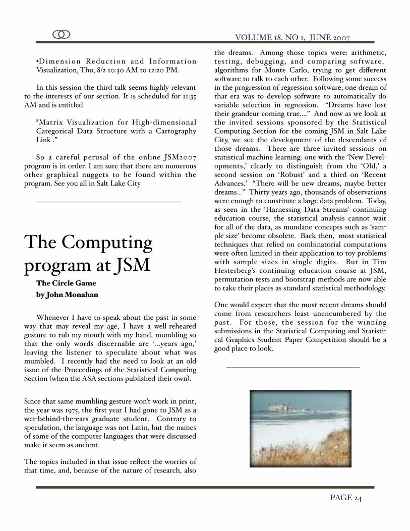
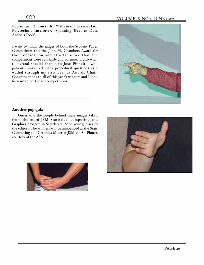
Another pop quizGuess who the people behind these images taken
from the 2006 JSM Statistical computing and Graphics program in Seattle are. Send your guesses to the editors. The winners will be announced at the Stats Computing and Graphics Mixer at JSM 2008. Photos courtesy of the ASA.
VOLUME 18, NO 1, JUNE 2007
PAGE 26

Statistical Computing Section Officers 2006John F. Monahan, [email protected] (919)515-1917Deborah A. Nolan, [email protected](510) 643-7097Stephan R. Sain, Past [email protected](303)556-8463Ed Wegman, Program Chair [email protected] (703)993-1691Wolfang S. Jank, Program Chair [email protected] (301) 405-1118David J. Poole, Secretary/[email protected] (973)360-7337Vincent Carey, COS Rep. 05-07 [email protected] (617) 525-2265Juana Sanchez, COS Rep. 06-08 and Newsletter [email protected] (310)825-1318Thomas F. Devlin, Electronic Communication Liaison [email protected] (973) 655-7244 J.R. Lockwood, Awards Officer [email protected] 4941R. Todd Ogden, Publications Offi-cer [email protected] J. Miller, Continuing Education Liaison [email protected] (703) 993-1690
Statistical Graphics Section Officers 2007Jeffrey L. Solka, [email protected](540) 653-1982Daniel J. Rope, [email protected](703) 740-2462Paul J. Murrell, Past Chair [email protected] 9 3737599Simon Urbanek, Program [email protected](973)360-7056Daniel R. Hunter , Program [email protected](814) 863-0979John Castelloe, [email protected] (919) 677-8000Daniel B. Carr, COS Rep [email protected] (703) 993-1671Edward J. Wegman, COS Rep [email protected] (703) 993-1680Linda W. Pickel, COS Rep 07-09 [email protected](301) 402-9344Andreas Krause, Newsletter [email protected]
Brooks Friedly, Publications Officer [email protected](507) 538-3646Monica D. Clark, ASA Staff [email protected](703) 684-1221
T
The Statistical Computing & Statis-tical Graphics Newsletter is a publi-cation of the Statistical Computing and Statistical Graphics Sections of the ASA. Until a new Co-editor for the Statistical Graphics Section comes in to replace Di Cook, all communications regarding the publi-cation should be addressed to:
Juana Sanchez, Editor Statistical Computing Section. Department of Statistics University of California, 8125 MS Building, Los Angeles, CA90095 (310) 825-1218 [email protected] www.stat.ucla.edu/~jsanchez
Andreas Krause, Editor Statistical Graphics Section [email protected] http://www.elmo.ch
All communications regarding ASA membership and the Statistical Computing and Statistical Graphics Section, including change of address, should be sent to American Statisti-cal Association, 1429 Duke Street Alexandria, VA 22314-3402 USA (703)684-1221, fax (703)684-2036 [email protected]
VOLUME 18, NO 1, JUNE 2007
PAGE 27