comsol multiphysics · his comsol multiphysics modeling guide provides an in-depth examination ....
TRANSCRIPT
COMSOLMultiphysics ®
V E R S I O N 3 . 4
MODELING GUIDE
How to contact COMSOL:
BeneluxCOMSOL BV Röntgenlaan 19 2719 DX Zoetermeer The Netherlands Phone: +31 (0) 79 363 4230 Fax: +31 (0) 79 361 [email protected] www.femlab.nl
Denmark COMSOL A/S Diplomvej 376 2800 Kgs. Lyngby Phone: +45 88 70 82 00 Fax: +45 88 70 80 90 [email protected] www.comsol.dk
Finland COMSOL OY Arabianranta 6FIN-00560 Helsinki Phone: +358 9 2510 400 Fax: +358 9 2510 4010 [email protected] www.comsol.fi
France COMSOL France WTC, 5 pl. Robert Schuman F-38000 Grenoble Phone: +33 (0)4 76 46 49 01 Fax: +33 (0)4 76 46 07 42 [email protected] www.comsol.fr
Germany FEMLAB GmbHBerliner Str. 4 D-37073 Göttingen Phone: +49-551-99721-0Fax: +49-551-99721-29 [email protected]
Italy COMSOL S.r.l. Via Vittorio Emanuele II, 22 25122 Brescia Phone: +39-030-3793800 Fax: [email protected]
Norway COMSOL AS Søndre gate 7 NO-7485 Trondheim Phone: +47 73 84 24 00 Fax: +47 73 84 24 01 [email protected] www.comsol.no Sweden COMSOL AB Tegnérgatan 23 SE-111 40 Stockholm Phone: +46 8 412 95 00 Fax: +46 8 412 95 10 [email protected] www.comsol.se
SwitzerlandFEMLAB GmbH Technoparkstrasse 1 CH-8005 Zürich Phone: +41 (0)44 445 2140 Fax: +41 (0)44 445 2141 [email protected] www.femlab.ch
United Kingdom COMSOL Ltd. UH Innovation CentreCollege LaneHatfieldHertfordshire AL10 9AB Phone:+44-(0)-1707 284747Fax: +44-(0)-1707 284746 [email protected] www.uk.comsol.com
United States COMSOL, Inc. 1 New England Executive Park Suite 350 Burlington, MA 01803 Phone: +1-781-273-3322 Fax: +1-781-273-6603 COMSOL, Inc. 10850 Wilshire Boulevard Suite 800 Los Angeles, CA 90024 Phone: +1-310-441-4800 Fax: +1-310-441-0868
COMSOL, Inc. 744 Cowper Street Palo Alto, CA 94301 Phone: +1-650-324-9935 Fax: +1-650-324-9936
For a complete list of international representatives, visit www.comsol.com/contact
Company home pagewww.comsol.com
COMSOL user forumswww.comsol.com/support/forums
COMSOL Multiphysics Modeling Guide © COPYRIGHT 1994–2007 by COMSOL AB. All rights reserved
Patent pending
The software described in this document is furnished under a license agreement. The software may be used or copied only under the terms of the license agreement. No part of this manual may be photocopied or reproduced in any form without prior written consent from COMSOL AB.
COMSOL, COMSOL Multiphysics, COMSOL Reaction Engineering Lab, and FEMLAB are registered trademarks of COMSOL AB. COMSOL Script is a trademark of COMSOL AB.
Other product or brand names are trademarks or registered trademarks of their respective holders.
Version: October 2007 COMSOL 3.4
C O N T E N T S
C h a p t e r 1 : I n t r o d u c t i o n
Overview of the COMSOL Multiphysics Application Modes 2
Application Modes in COMSOL Multiphysics . . . . . . . . . . . . 2
Selecting an Application Mode . . . . . . . . . . . . . . . . . . 5
Modeling Guidelines 7
Using Symmetries . . . . . . . . . . . . . . . . . . . . . . 7
Effective Memory Management . . . . . . . . . . . . . . . . . 8
Selecting an Element Type . . . . . . . . . . . . . . . . . . . 9
Analyzing Model Convergence and Accuracy . . . . . . . . . . . . 9
Achieving Convergence When Solving Nonlinear Equations. . . . . . . 10
Avoiding Strong Transients . . . . . . . . . . . . . . . . . . . 11
Typographical Conventions . . . . . . . . . . . . . . . . . . . 11
C h a p t e r 2 : U s i n g t h e P h y s i c s M o d e s
The Physics Modes 14
Defining the Physics for a Model . . . . . . . . . . . . . . . . . 14
The Physics Modes . . . . . . . . . . . . . . . . . . . . . . 15
Physics Mode Documentation . . . . . . . . . . . . . . . . . . 16
C h a p t e r 3 : A c o u s t i c s
Fundamentals of Acoustics 20
What is Acoustics? . . . . . . . . . . . . . . . . . . . . . . 20
Five Standard Acoustics Problems . . . . . . . . . . . . . . . . 20
Mathematical Models for Acoustic Analysis . . . . . . . . . . . . . 21
The Acoustics Application Mode 23
Variables and Space Dimensions . . . . . . . . . . . . . . . . . 23
C O N T E N T S | i

ii | C O N T E N T S
PDE Formulation . . . . . . . . . . . . . . . . . . . . . . . 23
Subdomain Settings . . . . . . . . . . . . . . . . . . . . . . 24
Boundary Conditions . . . . . . . . . . . . . . . . . . . . . 25
Scalar Variables . . . . . . . . . . . . . . . . . . . . . . . 28
Application Mode Variables . . . . . . . . . . . . . . . . . . . 29
Units . . . . . . . . . . . . . . . . . . . . . . . . . . . 31
2D . . . . . . . . . . . . . . . . . . . . . . . . . . . . 31
2D Axisymmetric. . . . . . . . . . . . . . . . . . . . . . . 32
Example—Reactive Muffler 34
Introduction . . . . . . . . . . . . . . . . . . . . . . . . 34
Model Definition . . . . . . . . . . . . . . . . . . . . . . . 34
Results and Discussion. . . . . . . . . . . . . . . . . . . . . 36
Reference . . . . . . . . . . . . . . . . . . . . . . . . . 37
Modeling Using the Graphical User Interface . . . . . . . . . . . . 37
C h a p t e r 4 : D i f f u s i o n
The Diffusion Application Mode 46
PDE Formulation . . . . . . . . . . . . . . . . . . . . . . . 46
Subdomain Settings . . . . . . . . . . . . . . . . . . . . . . 46
Boundary Conditions . . . . . . . . . . . . . . . . . . . . . 47
Application Mode Variables . . . . . . . . . . . . . . . . . . . 49
The Convection and Diffusion Application Mode 51
PDE Formulation . . . . . . . . . . . . . . . . . . . . . . . 51
Subdomain Settings . . . . . . . . . . . . . . . . . . . . . . 52
Boundary Conditions . . . . . . . . . . . . . . . . . . . . . 53
Application Mode Variables . . . . . . . . . . . . . . . . . . . 54
Effective Diffusivity in Porous Materials 56
Introduction . . . . . . . . . . . . . . . . . . . . . . . . 56
Model Definition . . . . . . . . . . . . . . . . . . . . . . . 57
Results and Discussion. . . . . . . . . . . . . . . . . . . . . 58
Modeling in COMSOL Multiphysics . . . . . . . . . . . . . . . . 61
Modeling Using the Graphical User Interface . . . . . . . . . . . . 62
C h a p t e r 5 : E l e c t r o m a g n e t i c s
The Electromagnetics Application Modes 76
Fundamentals of Electromagnetics 77
Electromagnetic Force for Particle Tracing . . . . . . . . . . . . . 81
The Conductive Media DC Application Mode 83
PDE Formulation . . . . . . . . . . . . . . . . . . . . . . . 83
Boundary Conditions . . . . . . . . . . . . . . . . . . . . . 84
Line Sources . . . . . . . . . . . . . . . . . . . . . . . . 87
Point Sources . . . . . . . . . . . . . . . . . . . . . . . . 87
Application Mode Variables . . . . . . . . . . . . . . . . . . . 87
The Electrostatics Application Mode 89
PDE Formulation . . . . . . . . . . . . . . . . . . . . . . . 89
Application Scalar Variables . . . . . . . . . . . . . . . . . . . 90
Boundary Conditions . . . . . . . . . . . . . . . . . . . . . 90
Line Sources . . . . . . . . . . . . . . . . . . . . . . . . 92
Point Sources . . . . . . . . . . . . . . . . . . . . . . . . 92
Application Mode Variables . . . . . . . . . . . . . . . . . . . 92
Magnetostatics Application Mode 95
PDE Formulation . . . . . . . . . . . . . . . . . . . . . . . 95
Application Mode Property . . . . . . . . . . . . . . . . . . . 96
Application Scalar Variable . . . . . . . . . . . . . . . . . . . 96
Boundary and Interface Conditions . . . . . . . . . . . . . . . . 96
Point Sources . . . . . . . . . . . . . . . . . . . . . . . . 98
Application Mode Variables . . . . . . . . . . . . . . . . . . . 98
AC Power Electromagnetics 105
PDE Formulation . . . . . . . . . . . . . . . . . . . . . . 105
Application Scalar Variables . . . . . . . . . . . . . . . . . . 106
Boundary and Interface Conditions . . . . . . . . . . . . . . . 106
Point Sources . . . . . . . . . . . . . . . . . . . . . . . 108
Application Mode Variables . . . . . . . . . . . . . . . . . . 108
C O N T E N T S | iii

iv | C O N T E N T S
Example: Electric Sensor 118
Model Definition . . . . . . . . . . . . . . . . . . . . . . 118
Results and Discussion. . . . . . . . . . . . . . . . . . . . 118
Modeling Using the Graphical User Interface . . . . . . . . . . . 119
Example: A Permanent Magnet 123
Modeling Using the Graphical User Interface . . . . . . . . . . . 123
Alternative Modeling Approach . . . . . . . . . . . . . . . . 127
References . . . . . . . . . . . . . . . . . . . . . . . . 128
C h a p t e r 6 : F l u i d M e c h a n i c s
The Navier-Stokes Application Mode 130
Variables and Space Dimension . . . . . . . . . . . . . . . . 130
PDE Formulation and Equations . . . . . . . . . . . . . . . . 130
Subdomain Settings . . . . . . . . . . . . . . . . . . . . . 131
Boundary Conditions . . . . . . . . . . . . . . . . . . . . 132
Point Settings . . . . . . . . . . . . . . . . . . . . . . . 140
Numerical Stability—Artificial Diffusion . . . . . . . . . . . . . 140
Corner Smoothing . . . . . . . . . . . . . . . . . . . . . 144
Application Mode Variables . . . . . . . . . . . . . . . . . . 145
General Solver Settings . . . . . . . . . . . . . . . . . . . 147
Solver Settings . . . . . . . . . . . . . . . . . . . . . . . 147
Khan and Richardson Force for Particle Tracing . . . . . . . . . . 147
References . . . . . . . . . . . . . . . . . . . . . . . . 148
Example: Steady Incompressible Flow 150
Introduction . . . . . . . . . . . . . . . . . . . . . . . 150
Model Definition . . . . . . . . . . . . . . . . . . . . . . 150
Results. . . . . . . . . . . . . . . . . . . . . . . . . . 152
References . . . . . . . . . . . . . . . . . . . . . . . . 154
Modeling Using the Graphical User Interface . . . . . . . . . . . 155
C h a p t e r 7 : H e a t T r a n s f e r
Heat Transfer Fundamentals 164
What is Heat Transfer? . . . . . . . . . . . . . . . . . . . 164
The Heat Equation . . . . . . . . . . . . . . . . . . . . . 165
The Conduction Application Mode 167
Variables and Space Dimensions . . . . . . . . . . . . . . . . 167
PDE Formulation . . . . . . . . . . . . . . . . . . . . . . 167
Subdomain Settings . . . . . . . . . . . . . . . . . . . . . 168
Boundary Condition Types . . . . . . . . . . . . . . . . . . 169
Boundary Settings . . . . . . . . . . . . . . . . . . . . . 172
Application Mode Variables . . . . . . . . . . . . . . . . . . 173
The Convection and Conduction Application Mode 175
Variables and Space Dimensions . . . . . . . . . . . . . . . . 175
PDE Formulation . . . . . . . . . . . . . . . . . . . . . . 175
Subdomain Settings . . . . . . . . . . . . . . . . . . . . . 176
Boundary Conditions . . . . . . . . . . . . . . . . . . . . 177
Application Mode Variables . . . . . . . . . . . . . . . . . . 178
Examples of Heat Transfer Models 180
1D Steady-State Heat Transfer with Radiation . . . . . . . . . . . 180
Model Definition . . . . . . . . . . . . . . . . . . . . . . 180
Results. . . . . . . . . . . . . . . . . . . . . . . . . . 181
Modeling Using the Graphical User Interface . . . . . . . . . . . 181
2D Steady-State Heat Transfer with Convection . . . . . . . . . . 184
Model Definition . . . . . . . . . . . . . . . . . . . . . . 184
Results. . . . . . . . . . . . . . . . . . . . . . . . . . 185
Modeling Using the Graphical User Interface . . . . . . . . . . . 185
2D Axisymmetric Transient Heat Transfer . . . . . . . . . . . . 188
Model Definition . . . . . . . . . . . . . . . . . . . . . . 188
Results. . . . . . . . . . . . . . . . . . . . . . . . . . 189
Modeling Using the Graphical User Interface . . . . . . . . . . . 190
References . . . . . . . . . . . . . . . . . . . . . . . . 194
C O N T E N T S | v
vi | C O N T E N T S
C h a p t e r 8 : S t r u c t u r a l M e c h a n i c s
The Structural Mechanics Application Modes 196
Theory Background 197
Strain-Displacement Relationship . . . . . . . . . . . . . . . . 197
Stress-Strain Relationship. . . . . . . . . . . . . . . . . . . 197
Implementation . . . . . . . . . . . . . . . . . . . . . . 199
Application Mode Descriptions 202
Application Mode Properties . . . . . . . . . . . . . . . . . 202
Material Properties . . . . . . . . . . . . . . . . . . . . . 204
Constraints . . . . . . . . . . . . . . . . . . . . . . . . 205
Loads . . . . . . . . . . . . . . . . . . . . . . . . . . 206
Damping . . . . . . . . . . . . . . . . . . . . . . . . . 207
The Solid, Stress-Strain Application Mode 208
Variables and Space Dimensions . . . . . . . . . . . . . . . . 208
PDE Formulation . . . . . . . . . . . . . . . . . . . . . . 208
Application Mode Variables . . . . . . . . . . . . . . . . . . 209
The Plane Stress Application Mode 212
Material . . . . . . . . . . . . . . . . . . . . . . . . . 212
PDE Formulation . . . . . . . . . . . . . . . . . . . . . . 212
Application Mode Variables . . . . . . . . . . . . . . . . . . 213
The Plane Strain Application Mode 217
Material Properties . . . . . . . . . . . . . . . . . . . . . 217
PDE Formulation . . . . . . . . . . . . . . . . . . . . . . 218
Application Mode Variables . . . . . . . . . . . . . . . . . . 218
The Axial Symmetry, Stress-Strain Application Mode 221
PDE Formulation . . . . . . . . . . . . . . . . . . . . . . 222
Application Mode Variables . . . . . . . . . . . . . . . . . . 222
Examples of Structural Mechanics Models 226
Tapered Membrane End Load . . . . . . . . . . . . . . . . . 226
Modeling in COMSOL Multiphysics . . . . . . . . . . . . . . . 227
Results. . . . . . . . . . . . . . . . . . . . . . . . . . 227
Modeling Using the Graphical User Interface . . . . . . . . . . . 228
Tapered Cantilever Gravity Load . . . . . . . . . . . . . . . . 231
Modeling in COMSOL Multiphysics . . . . . . . . . . . . . . . 231
Results. . . . . . . . . . . . . . . . . . . . . . . . . . 232
Modeling Using the Graphical User Interface . . . . . . . . . . . 232
Reference . . . . . . . . . . . . . . . . . . . . . . . . 235
C h a p t e r 9 : P D E M o d e s f o r E q u a t i o n - B a s e d M o d e l i n g
The PDE Modes 238
Using the PDE Modes 239
Starting a Model Using a PDE Mode. . . . . . . . . . . . . . . 239
Using the Coefficient Form PDEs. . . . . . . . . . . . . . . . 239
Using the General Form PDE . . . . . . . . . . . . . . . . . 249
Solving Time-Dependent Problems . . . . . . . . . . . . . . . 256
Solving Eigenvalue Problems. . . . . . . . . . . . . . . . . . 258
Interpreting PDE Coefficients . . . . . . . . . . . . . . . . . 259
Classical PDEs . . . . . . . . . . . . . . . . . . . . . . . 260
Equation Variables . . . . . . . . . . . . . . . . . . . . . 261
Boundary-Coupled Equation Variables . . . . . . . . . . . . . . 262
Ideal and non-Ideal Constraints . . . . . . . . . . . . . . . . 265
Variables for PDEs in Weak Form . . . . . . . . . . . . . . . 266
Application Mode Variables . . . . . . . . . . . . . . . . . . 269
PDE Coefficients and Boundary Conditions with Time Derivatives . . . 271
Using Equation Contributions on Interior Mesh Boundaries 273
Specifying Equation Contributions . . . . . . . . . . . . . . . 273
Specifying Interior Mesh Boundary Expressions. . . . . . . . . . . 274
Examples—Equation-Based Modeling 275
Poisson’s Equation on the Unit Disk. . . . . . . . . . . . . . . 275
Results. . . . . . . . . . . . . . . . . . . . . . . . . . 276
Modeling Using the Graphical User Interface . . . . . . . . . . . 277
C O N T E N T S | vii
viii | C O N T E N T S
Implementing a Point Source . . . . . . . . . . . . . . . . . 279
Modeling Using the Graphical User Interface . . . . . . . . . . . 280
C h a p t e r 1 0 : G l o b a l E q u a t i o n s a n d O D E s
Solving ODEs and Global Equations 286
Adding ODEs and Other Global Equations . . . . . . . . . . . . 286
The Global Equations Dialog Box. . . . . . . . . . . . . . . . 286
Solving ODEs—the Lotka-Volterra Equations . . . . . . . . . . . 287
Solving Algebraic and Transcendental Equations . . . . . . . . . . 288
Adding an ODE to a Boundary . . . . . . . . . . . . . . . . 289
C h a p t e r 1 1 : T h e W e a k F o r m
Weak Form Modeling 293
Adding Weak Form Contributions . . . . . . . . . . . . . . . 293
Modeling with PDEs on Boundaries, Edges, and Points . . . . . . . . 294
Using Weak Coefficients or the Weak Modes . . . . . . . . . . . 294
Example: Variational Calculus 296
Model Definition . . . . . . . . . . . . . . . . . . . . . . 296
Results. . . . . . . . . . . . . . . . . . . . . . . . . . 297
Modeling in COMSOL Multiphysics . . . . . . . . . . . . . . . 297
Modeling Using the Graphical User Interface . . . . . . . . . . . 298
Modeling Using the Programming Language . . . . . . . . . . . . 299
Using Weak Constraints 300
Specifying Weak Constraints . . . . . . . . . . . . . . . . . 301
Weak Constraints in Assemblies . . . . . . . . . . . . . . . . 302
Limitations of Weak Constraints . . . . . . . . . . . . . . . . 303
Example—Coupling Variables and Boundary Constraints 304
Boundary Constraints in a Heat Transfer Model . . . . . . . . . . 304
No Weak Constraints . . . . . . . . . . . . . . . . . . . . 308
Weak Ideal Constraints . . . . . . . . . . . . . . . . . . . 308
Weak Non-Ideal Constraints . . . . . . . . . . . . . . . . . 308
Theoretical Background 310
Deriving the Weak Form . . . . . . . . . . . . . . . . . . . 310
Weak Form Application Modes . . . . . . . . . . . . . . . . 311
Entering a PDE in Coefficient Form Using the Weak Form . . . . . . 315
C h a p t e r 1 2 : M u l t i p h y s i c s M o d e l i n g
Creating Multiphysics Models 318
Multiphysics Modeling Approaches . . . . . . . . . . . . . . . 318
Using Predefined Multiphysics Couplings . . . . . . . . . . . . . 318
Adding Physics Sequentially . . . . . . . . . . . . . . . . . . 326
Building a Coupled Multiphysics Model Directly . . . . . . . . . . 326
Removing Application Modes . . . . . . . . . . . . . . . . . 327
Multiphysics Model Properties . . . . . . . . . . . . . . . . . 327
Managing the Solver and Solution Components . . . . . . . . . . 328
Deactivating Physics or Equations . . . . . . . . . . . . . . . 331
Using the Model Navigator for Multiphysics Models . . . . . . . . . 331
Specifying Settings for Multiphysics Models . . . . . . . . . . . . 332
Example: Resistive Heating 334
Introduction . . . . . . . . . . . . . . . . . . . . . . . 334
Model Definition . . . . . . . . . . . . . . . . . . . . . . 334
Modeling in COMSOL Multiphysics . . . . . . . . . . . . . . . 335
Modeling Using the Graphical User Interface . . . . . . . . . . . 335
Working with Components 347
The Component Library . . . . . . . . . . . . . . . . . . . 347
Adding Components . . . . . . . . . . . . . . . . . . . . 348
Merging Components . . . . . . . . . . . . . . . . . . . . 348
C O N T E N T S | ix
x | C O N T E N T S
C h a p t e r 1 3 : U s i n g A s s e m b l i e s
Creating Assemblies 352
The Analyzed Geometry—Assembly vs. Composite Geometry . . . . 352
Creating Pairs . . . . . . . . . . . . . . . . . . . . . . . 353
Identity Pairs 356
The Identity Pair Dialog Box . . . . . . . . . . . . . . . . . 357
Selection Colors for Pairs . . . . . . . . . . . . . . . . . . 359
Specifying Physics Settings on Pairs 361
Controlling the Use of Pairs. . . . . . . . . . . . . . . . . . 362
Edge and Point Pairs . . . . . . . . . . . . . . . . . . . . 363
Slit Boundary Conditions . . . . . . . . . . . . . . . . . . . 363
Meshing Assemblies 365
Example—Meshing a Composite Geometry or an Assembly . . . . . 365
Thin-Film Resistance Model 368
Model Definition . . . . . . . . . . . . . . . . . . . . . . 368
Results. . . . . . . . . . . . . . . . . . . . . . . . . . 370
Modeling Using the Graphical User Interface . . . . . . . . . . . 372
Comparing the Thin-Film Approximation with the Full 3D Model . . . 375
Using Identity Conditions 376
Creating Identity Conditions . . . . . . . . . . . . . . . . . 376
Thin-Layer Diffusion Model 380
Modeling Using the Graphical User Interface . . . . . . . . . . . 381
C h a p t e r 1 4 : D e f o r m e d M e s h e s
Deformed Mesh Fundamentals 392
Mathematical Description of the Mesh Movement . . . . . . . . . 392
Derivatives . . . . . . . . . . . . . . . . . . . . . . . . 394

Frames for Deformed Meshes 396
Frames in the Model Navigator . . . . . . . . . . . . . . . . 396
Settings for Frames . . . . . . . . . . . . . . . . . . . . . 400
Frame Selection for Coupling Variables . . . . . . . . . . . . . 400
The Moving Mesh Application Mode 401
Subdomain Settings . . . . . . . . . . . . . . . . . . . . . 401
Boundary Conditions . . . . . . . . . . . . . . . . . . . . 403
Smoothing Methods. . . . . . . . . . . . . . . . . . . . . 404
Remeshing . . . . . . . . . . . . . . . . . . . . . . . . 405
Example: Electrochemical Polishing 414
Introduction . . . . . . . . . . . . . . . . . . . . . . . 414
Model Definition . . . . . . . . . . . . . . . . . . . . . . 414
Modeling in COMSOL Multiphysics . . . . . . . . . . . . . . . 415
Results. . . . . . . . . . . . . . . . . . . . . . . . . . 415
Modeling Using the Graphical User Interface . . . . . . . . . . . 416
The Parameterized Geometry Application Mode 421
Subdomain Settings . . . . . . . . . . . . . . . . . . . . . 421
Boundary Conditions . . . . . . . . . . . . . . . . . . . . 422
Point Settings . . . . . . . . . . . . . . . . . . . . . . . 424
Example: Eigenmode Analysis of an L-Shaped Membrane with
Rounded Corner 425
Introduction . . . . . . . . . . . . . . . . . . . . . . . 425
Model Definition . . . . . . . . . . . . . . . . . . . . . . 425
Modeling in COMSOL Multiphysics . . . . . . . . . . . . . . . 425
Results. . . . . . . . . . . . . . . . . . . . . . . . . . 426
Reference . . . . . . . . . . . . . . . . . . . . . . . . 426
Modeling Using the Graphical User Interface . . . . . . . . . . . 427
C O N T E N T S | xi
xii | C O N T E N T S
Retrieving the Deformed Mesh 431
Limitations of the Deformed Mesh Feature 432
C h a p t e r 1 5 : S t a b i l i z a t i o n T e c h n i q u e s
Numerical Stabilization 434
Introduction . . . . . . . . . . . . . . . . . . . . . . . 434
Application Modes and Artificial Diffusion . . . . . . . . . . . . 435
Selecting an Artificial Diffusion Method . . . . . . . . . . . . . 438
Adding Artificial Diffusion Manually . . . . . . . . . . . . . . . 438
Artificial Diffusion Types 439
Isotropic Diffusion . . . . . . . . . . . . . . . . . . . . . 439
Streamline Diffusion. . . . . . . . . . . . . . . . . . . . . 440
Crosswind Diffusion . . . . . . . . . . . . . . . . . . . . 445
Pressure Stabilization . . . . . . . . . . . . . . . . . . . . 446
References . . . . . . . . . . . . . . . . . . . . . . . . 447
INDEX 449
1
I n t r o d u c t i o n
This COMSOL Multiphysics Modeling Guide provides an in-depth examination of the application modes in COMSOL Multiphysics and how to use them to model different types of physics and to perform equation-based modeling using PDEs.
This chapter gives an overview of the available application modes as well as some general guidelines for effective modeling.
1
2 | C H A P T E R
Ove r v i ew o f t h e COMSOL Mu l t i p h y s i c s App l i c a t i o n Mode s
Solving PDEs generally means you must take the time to set up the underlying equations, material properties, and boundary conditions for a given problem. COMSOL Multiphysics, however, relieves you of much of this work. The package provides a number of application modes that consist of predefined templates and user interfaces already set up with equations and variables for specific areas of physics. Special properties allow the selection of, for instance, analysis type and model formulations. The application mode interfaces consist of customized dialog boxes for the physics in subdomains and on boundaries, edges, and points along with predefined PDEs. A set of application-dependent variables makes it easy to visualize and postprocess the important physical quantities using conventional terminology and notation. Adding even more flexibility, the equation system view provides the possibility to examine and modify the underlying PDEs in the case where a predefined application mode does not exactly match the application you want to model.
Note: Suites of application modes that are optimized for specific disciplines together with large model libraries are available in a group of optional products: the AC/DC Module, the Acoustics Module, the Chemical Engineering Module, the Earth Science Module, the Heat Transfer Module, the MEMS Module, the RF Module, and the Structural Mechanics Module.
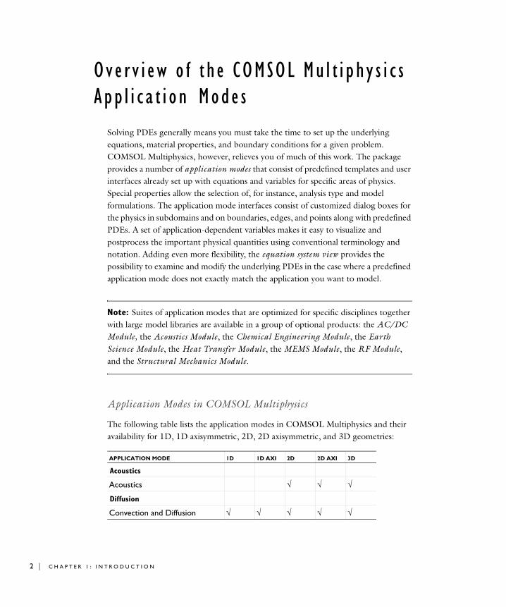
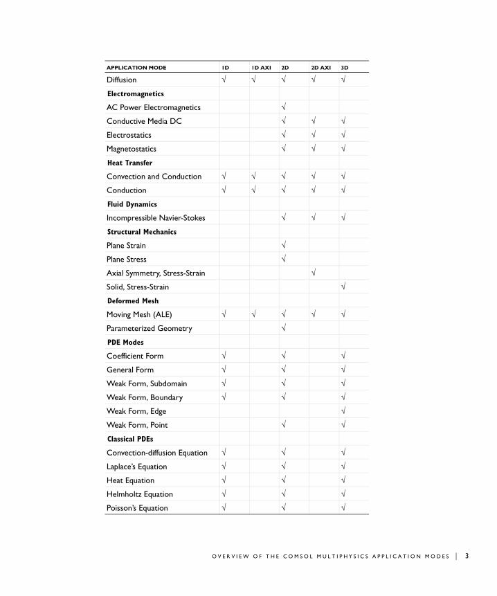
Application Modes in COMSOL Multiphysics
The following table lists the application modes in COMSOL Multiphysics and their availability for 1D, 1D axisymmetric, 2D, 2D axisymmetric, and 3D geometries:
APPLICATION MODE 1D 1D AXI 2D 2D AXI 3D
Acoustics
Acoustics √ √ √
Diffusion
Convection and Diffusion √ √ √ √ √
1 : I N T R O D U C T I O N
Diffusion √ √ √ √ √
Electromagnetics
AC Power Electromagnetics √
Conductive Media DC √ √ √
Electrostatics √ √ √
Magnetostatics √ √ √
Heat Transfer
Convection and Conduction √ √ √ √ √
Conduction √ √ √ √ √
Fluid Dynamics
Incompressible Navier-Stokes √ √ √
Structural Mechanics
Plane Strain √
Plane Stress √
Axial Symmetry, Stress-Strain √
Solid, Stress-Strain √
Deformed Mesh
Moving Mesh (ALE) √ √ √ √ √
Parameterized Geometry √
PDE Modes
Coefficient Form √ √ √
General Form √ √ √
Weak Form, Subdomain √ √ √
Weak Form, Boundary √ √ √
Weak Form, Edge √
Weak Form, Point √ √
Classical PDEs
Convection-diffusion Equation √ √ √
Laplace’s Equation √ √ √
Heat Equation √ √ √
Helmholtz Equation √ √ √
Poisson’s Equation √ √ √
APPLICATION MODE 1D 1D AXI 2D 2D AXI 3D
O V E R V I E W O F T H E C O M S O L M U L T I P H Y S I C S A P P L I C A T I O N M O D E S | 3
4 | C H A P T E R
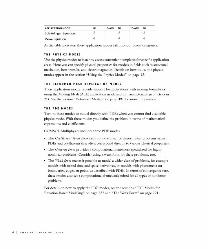
As the table indicates, these application modes fall into four broad categories:
T H E P H Y S I C S M O D E S
Use the physics modes to instantly access convenient templates for specific application areas. Here you can specify physical properties for models in fields such as structural mechanics, heat transfer, and electromagnetics. Details on how to use the physics modes appear in the section “Using the Physics Modes” on page 13.
T H E D E F O R M E D M E S H A P P L I C A T I O N M O D E S
These application modes provide support for applications with moving boundaries using the Moving Mesh (ALE) application mode and for parameterized geometries in 2D. See the section “Deformed Meshes” on page 391 for more information.
T H E P D E M O D E S
Turn to these modes to model directly with PDEs when you cannot find a suitable physics mode. With these modes you define the problem in terms of mathematical expressions and coefficients.
COMSOL Multiphysics includes three PDE modes:
• The Coefficient form allows you to solve linear or almost linear problems using PDEs and coefficients that often correspond directly to various physical properties.
• The General form provides a computational framework specialized for highly nonlinear problems. Consider using a weak form for these problems, too.
• The Weak form makes it possible to model a wider class of problems, for example models with mixed time and space derivatives, or models with phenomena on boundaries, edges, or points as described with PDEs. In terms of convergence rate, these modes also set a computational framework suited for all types of nonlinear problems.
For details on how to apply the PDE modes, see the sections “PDE Modes for Equation-Based Modeling” on page 237 and “The Weak Form” on page 291.
Schrödinger Equation √ √ √
Wave Equation √ √ √
APPLICATION MODE 1D 1D AXI 2D 2D AXI 3D
1 : I N T R O D U C T I O N
C L A S S I C A L P D E S
The Classical PDEs folder contain application modes that describe a suite of well-known PDEs. They are special cases of the coefficient form PDE and are not meant to serve as templates.
Selecting an Application Mode
When creating a model in COMSOL Multiphysics, you can select a single application mode that describes one type of physics or select several application modes for multiphysics modeling and coupled-field analyses.
M O D E L I N G U S I N G A S I N G L E A P P L I C A T I O N M O D E
Most of the physics application modes contain stationary, eigenvalue, and dynamic (time-dependent) analysis types. As already mentioned, these modes provide a modeling interface where you can create models using material properties, boundary conditions, and initial conditions. Each of these modes comes with a template that automatically supplies the appropriate underlying PDE.
If you cannot find a physics mode that matches a given problem, try one of the PDE modes, which allow you to define a custom model in general mathematical terms. Indeed, COMSOL Multiphysics can model virtually any scientific phenomenon or engineering problem that originates from the laws of science.
M U L T I P H Y S I C S M O D E L I N G U S I N G M U L T I P L E A P P L I C A T I O N M O D E S
When modeling real-world systems, you often need to include the interaction between different kinds of physics. For instance, the properties of an electronic component such as an inductor vary with temperature. To solve such a problem, combine two or several application modes into a single model using the multiphysics features of COMSOL Multiphysics. For the example just mentioned, combine the Conductive Media DC and Heat Transfer by Conduction application modes. In this way you create a system of two PDEs with two dependent variables: V for the electric potential and T for the temperature. There are also predefined multiphysics couplings that provide two coupled application modes for some common multiphysics applications.
Combining physics modes and PDE modes also works well. Assume, for instance, that you want to model the fluid-structure interactions due to the vibrations of yoghurt in a cardboard container as it rides on a conveyor belt. You could start with the Plane Stress mode for structural mechanics to model the container walls and then add a PDE to model the irrotational flow of the fluid. This approach also creates a system of two
O V E R V I E W O F T H E C O M S O L M U L T I P H Y S I C S A P P L I C A T I O N M O D E S | 5
6 | C H A P T E R
PDEs but requires that you define one of them from scratch, in this case using the general PDE formulation.
To summarize the proposed strategy for modeling processes that involve several types of physics: Look for application modes suitable for the phenomena of interest. If you find them among the physics modes, use them; if not, add one or more PDE modes.
The approach when coupling multiple application modes is to use the dependent variables or their derivatives directly, or to use expressions containing the dependent variables. The coupling can occur in subdomains and on boundaries.
1 : I N T R O D U C T I O N
Mode l i n g Gu i d e l i n e s
To allow you to model large-scale problems, COMSOL Multiphysics lets you tune solver settings and use symmetries and other model properties to reach a solution or—failing that—interrupt the solution process to retrieve a partial solution.
Using Symmetries
By using symmetries in a model you can reduce its size by one-half or more, making this an efficient tool for solving large problems. This applies to the cases where the geometries and modeling assumptions include symmetries.
The most important types of symmetries are axial symmetry and symmetry and antisymmetry planes or lines:
• Axial Symmetry is common for cylindrical and similar 3D geometries. If the geometry is axisymmetric, there are variations in the radial (r) and vertical (z) direction only and not in the angular (θ) direction. You can then solve a 2D problem in the rz-plane instead of the full 3D model, which can save considerable memory and computation time. Many COMSOL Multiphysics application modes are available in axisymmetric versions.
• Symmetry and Antisymmetry Planes or Lines are common in both 2D and 3D models. Symmetry means that a model is identical on either side of a dividing line or plane. For a scalar field, the normal flux is zero across the symmetry line. In structural mechanics, the symmetry conditions are different. Antisymmetry means that the loading of a model is oppositely balanced on either side of a dividing line or plane. For a scalar field, the dependent variable is 0 along the antisymmetry plane or line. Structural mechanics applications have other antisymmetry conditions. Many application modes have symmetry conditions directly available in the Boundary
Settings dialog box.
To take advantage of symmetry planes and symmetry lines, all of the geometry, material properties, and boundary conditions must be symmetric, and any loads or sources must be symmetric or antisymmetric. You can then build a model of the symmetric portion, which can be half, a quarter, or an eighth of the full geometry, and apply the appropriate symmetry (or antisymmetry) boundary conditions.
M O D E L I N G G U I D E L I N E S | 7
8 | C H A P T E R
Effective Memory Management
Especially in 3D modeling, extensive memory usage dictates some extra precautions. First, check that you have selected an iterative linear system solver. Normally you do not need to worry about which solver to use, because the application mode makes an appropriate default choice. In some situations, though, it might be necessary to make additional changes to the solver settings and the model.
E S T I M A T I N G T H E M E M O R Y U S E F O R A M O D E L
Out-of-memory messages occur when COMSOL Multiphysics tries to allocate an array that does not fit sequentially in memory. It is common that the amount of available memory seems large enough for an array, but there might not be a contiguous block of that size due to memory fragmentation. The only solver that requires a single large contiguous memory block is the UMFPACK direct solver.
In estimating how much memory it takes to solve a specific model, the following factors are the most important:
• The number of node points
• The number of dependent and independent variables
• The element order
• The sparsity pattern of the system matrices. The sparsity pattern, in turn, depends on the shape of the geometry and the mesh. For example, an extended ellipsoid gives sparser matrices than a sphere.
C R E A T I N G A M E M O R Y - E F F I C I E N T G E O M E T R Y
A first step when dealing with large models is to try to reduce the model geometry as much as possible. Often you can find symmetry planes and reduce the model to a half, a quarter or even an eighth of the original size. Memory usage does not scale linearly but rather polynomially (Cnk, k > 1), which means that the model needs less than half the memory if you find a symmetry plane and cut the geometry size by half. Other ways to create a more memory-efficient geometry include:
• Avoiding small geometry objects where not needed and using Bézier curves instead of polygon chains.
1 : I N T R O D U C T I O N
• Making sure that the mesh elements are of a high quality. Mesh quality is important for an iterative linear system solver. Convergence is faster and more robust if the element quality is high.
• Avoiding geometries with sharp, narrow corners. Mesh elements get thin when they approach sharp corners, leading to poor element quality in the adjacent regions.
Selecting an Element Type
As the default element type for most application modes, COMSOL Multiphysics uses second-order Lagrange elements or shape functions (see “Finite Elements” on page 452 in the COMSOl Multiphysics Reference Guide for an overview of the available element types). These and other higher-order elements add additional degrees of freedom on midpoint and interior nodes in the mesh elements. These added degrees of freedom provide a more accurate solution but also require more memory due to the reduced sparsity of the discretized system. For many application areas, such as stress analysis in structural and solid mechanics, the increased accuracy of a second-order element is important. In fluid-flow modeling using the incompressible Navier-Stokes equations, a combination of element types using an element for the velocity components of a higher order than that for the pressure usually provides the best result. The default element for the Incompressible Navier-Stokes application mode is the P2-P1 element using second-order elements for the velocity components and linear elements for the pressure. For other applications you can select a first-order element instead of a second-order element, or reduce the element order in general, to reduce memory use.
Analyzing Model Convergence and Accuracy
It is important that the finite element model accurately captures local variations in the solution such as stress concentrations. In some cases you can compare your results to values from handbooks, measurements, or other sources of data. Many examples in the COMSOL Multiphysics Modeling Guide and the COMSOL Multiphysics Model Library include comparisons to established results or analytical solutions. Look for these benchmark models as a means of checking results.
If a model has not been verified by other means, a convergence test is useful for determining if the mesh density is sufficient. Here you refine the mesh and run the analysis again, and then you see if the solution is converging to a stable value as the mesh is refined. If the solution changes when you refine the mesh, the solution is mesh dependent, so the model requires a finer mesh. You can use adaptive mesh refinement
M O D E L I N G G U I D E L I N E S | 9
10 | C H A P T E R
(see “Avoiding Inverted Mesh Elements” on page 356 of the COMSOL Multiphysics User’s Guide), which adds mesh elements based on an error criterion to resolve those areas where the error is large.
For convergence, it is important to avoid singularities in the geometry (see “Avoiding Singularities and Degeneracies in the Geometry” on page 94 of the COMSOL Multiphysics User’s Guide for more information).
Achieving Convergence When Solving Nonlinear Equations
Nonlinear problems are often difficult to solve. In many cases, no unique solution exists. COMSOL Multiphysics uses a Newton-type iterative method to solve nonlinear systems of PDEs. This solution method can be sensitive to the initial estimate of the solution. If the initial conditions are too far from the desired solution, convergence might be impossible, even though it might be simple from a different starting value.
You can do several things to improve the chances for finding the relevant solutions to difficult nonlinear problems:
• Provide the best possible initial values.
• Solve sequentially and iterate between single-physics equations; finish by solving the fully coupled multiphysics problem when you have obtained better starting guesses.
• Ensure that the boundary conditions are consistent with the initial solution and that neighboring boundaries have compatible conditions that do not create singularities.
• Refine the mesh in regions of steep gradients.
• For convection-type problem, introduce artificial diffusion to improve the problem’s numerical properties (see “Stabilization Techniques” on page 433).
• Scaling can be an issue when one solution component is zero. In those cases, the automatic scaling might not work. See “Scaling of Variables and Equations” on page 497 of the COMSOL Multiphysics Reference Guide for more information.
• Turn a stationary nonlinear PDE into a time-dependent problem. Making the problem time dependent generally results in smoother convergence. By making sure to solve the time-dependent problem for a time span long enough for the solution to reach a steady state, you solve the original stationary problem.
• Use the parametric solver and vary a material property or a PDE coefficient starting from a value that makes the equations less nonlinear to the value at which you want to compute the solution. This way you solve a series of increasingly difficult
1 : I N T R O D U C T I O N
nonlinear problems. The solution of a slightly nonlinear problem that is easy to solve serves as the initial value for a more difficult nonlinear problem.
Avoiding Strong Transients
If you start solving a time-dependent problem with initial conditions that are inconsistent, or if you use boundary settings or subdomain settings that switch instantaneously at a certain time, you induce strong transient signals in a system. The time-stepping algorithm then takes very small steps to resolve the transient, and the solution time might be very long, or the solution process might even stop. Stationary problems can run into mesh-resolution issues such as overshooting and undershooting of the solution due to infinite flux problems.
Unless you want to know the details of these transients, start with initial conditions that lead to a consistent solution to a stationary problem. Only then turn on the boundary values, sources, or driving fluxes over a time interval that is realistic for your model.
In most cases you should turn on your sources using a smoothed step over a finite time. What you might think of as a step function is, in real-life physics, often a little bit smoothed because of inertia. The step or switch does not happen instantaneously. Electrical switches take milliseconds, and solid-state switches take microseconds. See “Specifying Discontinuous Functions” on page 149 of the COMSOL Multiphysics User’s Guide for information about smoothed step functions to try out.
Typographical Conventions
All COMSOL manuals use a set of consistent typographical conventions that should make it easy for you to follow the discussion, realize what you can expect to see on the screen, and know which data you must enter into various data-entry fields. In particular, you should be aware of these conventions:
• A boldface font of the shown size and style indicates that the given word(s) appear exactly that way on the COMSOL graphical user interface (for toolbar buttons in the corresponding tooltip). For instance, we often refer to the Model Navigator, which is the window that appears when you start a new modeling session in COMSOL; the corresponding window on the screen has the title Model Navigator. As another example, the instructions might say to click the Multiphysics button, and the boldface font indicates that you can expect to see a button with that exact label on the COMSOL user interface.
M O D E L I N G G U I D E L I N E S | 11

12 | C H A P T E R
• The names of other items on the graphical user interface that do not have direct labels contain a leading uppercase letter. For instance, we often refer to the Draw toolbar; this vertical bar containing many icons appears on the left side of the user interface during geometry modeling. However, nowhere on the screen will you see the term “Draw” referring to this toolbar (if it were on the screen, we would print it in this manual as the Draw menu).
• The symbol > indicates a menu item or an item in a folder in the Model Navigator. For example, Physics>Equation System>Subdomain Settings is equivalent to: On the Physics menu, point to Equation System and then click Subdomain Settings. COMSOL Multiphysics>Heat Transfer>Conduction means: Open the COMSOL
Multiphysics folder, open the Heat Transfer folder, and select Conduction.
• A Code (monospace) font indicates keyboard entries in the user interface. You might see an instruction such as “Type 1.25 in the Current density edit field.” The monospace font also indicates COMSOL Script codes.
• An italic font indicates the introduction of important terminology. Expect to find an explanation in the same paragraph or in the Glossary. The names of books in the COMSOL documentation set also appear using an italic font.
1 : I N T R O D U C T I O N
2
U s i n g t h e P h y s i c s M o d e s
This chapter provides an overview of the physics application modes within COMSOL Multiphysics. It goes on to describe how these application modes make modeling various types of physics easier, faster, and more efficient. Later chapters review each physics mode in detail, including step-by-step examples of how to build and solve models for that particular physics application.
13
14 | C H A P T E R
T h e Phy s i c s Mod e s
One convenient way to solve a physics problem is to set it up with the assistance of templates that COMSOL Multiphysics provides in the form of its physics modes. The software computes the PDE coefficients based on application-specific parameters and material properties that you supply, such as Young’s modulus for a structural-mechanics model or the heat capacity for a heat-transfer model.
Defining the Physics for a Model
When working with a physics mode, you have access to all necessary settings for material properties, boundary conditions, and other modeling parameters through the Physics menu.
S U B D O M A I N S E T T I N G S A N D M A T E R I A L P R O P E R T I E S
Enter application-specific subdomain properties by choosing Subdomain Settings from the Physics menu or double-clicking a subdomain in the subdomain selection mode, which you enter by opening the Subdomain Settings dialog box, by clicking the Subdomain Mode button on the Main toolbar, or on the Physics menu by first pointing to Selection Mode and then clicking Subdomain Mode. For a complete description of the material properties available within each application mode, see the following chapters.
B O U N D A R Y S E T T I N G S
To set up boundary conditions, choose Boundary Settings from the Physics menu or double-click a boundary in the boundary selection mode, which you enter by opening the Boundary Settings dialog box, by clicking the Boundary Mode button on the Main toolbar, or on the Physics menu by first pointing to Selection Mode and then click Boundary Mode. The Boundary Settings dialog box is slightly different for application mode and provides the appropriate boundary conditions. For a complete description of the boundary conditions available for the physics modes, see the following chapters.
P O I N T S E T T I N G S
Some models include point sources or use a point in the geometry to fix the value of a variable. To access the point settings, choose Point Settings from the Physics menu or double-click a point in the point selection mode, which you enter by opening the Point Settings dialog box, by clicking the Point Mode button on the Main toolbar, or on the
2 : U S I N G T H E P H Y S I C S M O D E S
Physics menu by first pointing to Selection Mode and then click Point Mode. The Point
Settings dialog box is not available in all application modes.
PO S T P R O C E S S I N G U S I N G A P P L I C A T I O N M O D E V A R I A B L E S
With the postprocessing mode you can visualize any variable or expression of variables by working with the Plot Parameters, Cross-Section Plot Parameters, and Domain Plot
Parameters dialog boxes. You can also have COMSOL Multiphysics compute integrated values with the help of the Subdomain Integration and Boundary Integration dialog boxes.
Each application mode provides a special set of application-specific variables called application mode variables. Lists of these variables for each application mode appear in the following chapters.
Note: For all application modes you have access to shape-function variables and equation variables for the corresponding PDE solution form (coefficient, general, or weak). For further details, please refer to Ref. “Using Variables and Expressions” on page 138 in the COMSOL Multiphysics User’s Guide.
The Physics Modes
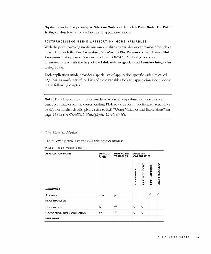
The following table lists the available physics modes:
TABLE 2-1: THE PHYSICS MODES
APPLICATION MODE DEFAULT
SuffixDEPENDENT VARIABLES
ANALYSIS CAPABILITIES
ST
AT
ION
AR
Y
TIM
E D
EP
EN
DE
NT
TIM
E H
AR
MO
NIC
EIG
EN
FRE
QU
EN
CY
ACOUSTICS
Acoustics aco p √ √HEAT TRANSFER
Conduction ht T √ √
Convection and Conduction cc T √ √DIFFUSION
T H E P H Y S I C S M O D E S | 15

16 | C H A P T E R
Physics Mode Documentation
Chapters 3–8 in this manual give detailed descriptions of each physics mode, typically broken down into the following sections:
V A R I A B L E S A N D S P A C E D I M E N S I O N S
The Variables and Space Dimensions section describes the dependent and independent variables or space dimensions (1D, 2D, 3D, or axisymmetric) you can use in the application mode.
Convection and Diffusion cd c √ √
Diffusion di c √ √ELECTROMAGNETICS
AC Power Electromagnetics qa Az √
Conductive Media DC dc V √
Electrostatics es V √
Magnetostatics qa Az √STRUCTURAL MECHANICS
Solid, Stress-Strain sld u, v, w √ √ √
Plane Stress ps u, v √ √ √
Plane Strain pn u, v √ √ √
Axial Symmetry, Stress-Strain axi uor, w √ √ √INCOMPRESSIBLE NAVIER STOKES
Incompressible Navier-Stokes, 2D ns u, v, p √ √
Incompressible Navier-Stokes, 3D ns u, v, w, p √ √
TABLE 2-1: THE PHYSICS MODES
APPLICATION MODE DEFAULT
SuffixDEPENDENT VARIABLES
ANALYSIS CAPABILITIES
ST
AT
ION
AR
Y
TIM
E D
EP
EN
DE
NT
TIM
E H
AR
MO
NIC
EIG
EN
FRE
QU
EN
CY
2 : U S I N G T H E P H Y S I C S M O D E S
P D E F O R M U L A T I O N
The PDE Formulation section presents the equations the physics mode solves. It also lists the material properties, sources, and coefficients in the COMSOL Multiphysics formulation.
A P P L I C A T I O N S C A L A R V A R I A B L E S
The Application Scalar Variables section lists nongeometric variables specific to the application mode. The default values are physical constants such as the permittivity of vacuum or arbitrary values, for example, the frequency 50 Hz for the AC Power Electromagnetics application mode. Not every application mode has application scalar variables.
S U B D O M A I N S E T T I N G S
The Subdomain Settings section lists the subdomain properties in the application mode such as material properties and sources and sinks.
B O U N D A R Y C O N D I T I O N S
The Boundary Conditions section lists the available boundary conditions while explaining their physical interpretation and the quantities that you specify to define the boundary settings.
L I N E A N D P O I N T S E T T I N G S
In some application modes there are line and point settings for defining line and point sources, pressure constraints, and other properties.
A P P L I C A T I O N M O D E V A R I A B L E S
The Application Mode Variables section lists all the variables available to you when formulating the equation and performing postprocessing. You can create functions of these variables for postprocessing and visualizing the analysis and when expressing physical properties. The Predefined quantities lists in the dialog boxes for visualization and postprocessing do not always include all the variables; if a variable does not appear in the list, simply type its name in the Expression edit field.
Application mode variables are defined on the following geometric domains:
• Subdomains: S
• Boundary segments: B
• Edges: E
• Points: P
T H E P H Y S I C S M O D E S | 17
18 | C H A P T E R
In the tables that review the application mode variables for each case, the Domain column indicates the top level where the variables are defined. Many variables that are available on subdomains are also available on boundaries, edges, and points, but they then take the average value of the values in the subdomains around the boundary, edge, or point (for the subdomains in which the variable is present). In addition to the letters above, indicating the domains where the application mode variable is valid, a V indicates that it is a vector-valued variable.
In some cases the table also lists the solution form for which a variable is available:
• Coefficient form: c
• General form: g
• Weak form: w
The Name column in the table of application mode variables lists the variables available for use, whereas the Expression column lists the implementation of the application mode variables in terms of other variables. The italic i and j in the variable names can refer to any of the space coordinates. For example, Ti can mean either Tx, Ty, or Tz in 3D where the space coordinates are x, y, and z. In 2D axisymmetry, Ti stands for either Tr or Tz. Further, you construct the variable names of vector components and tensor components using the names of the space coordinates. For example, if an application mode uses x1, y1, z1, then the variables for the vector components of the temperature gradient are Tx1, Ty1, Tz1.
Note: All application mode variables include a suffix indicating which application mode they belong to. Table 2-1 on page 15 lists the default suffix for the physics modes. For example, the default suffix added to application mode variable names for an Incompressible Navier-Stokes application mode is _ns.
Note: The default space coordinate names are x, y, z for Cartesian coordinate systems and r, (phi), and z for cylindrical coordinate systems. It is possible to change these names when defining a new geometry in the Model Navigator. The variable t represents the time for time-dependent models.
ϕ
2 : U S I N G T H E P H Y S I C S M O D E S
3
A c o u s t i c s
This chapter describes how to use the Acoustics application mode for modeling and simulation of acoustics and vibrations. It consists of three major sections:
• An overview of acoustics modeling
• A description of the Acoustics application mode
• A step-by-step review of how to model a reactive muffler
19
20 | C H A P T E R
Fundamen t a l s o f A c ou s t i c s
What is Acoustics?
Acoustics is the physics of sound. Sound is the sensation, as detected by the ear, of very small rapid changes in the air pressure above and below a static value. This static value is atmospheric pressure (about 100,000 pascals), which varies slowly. Associated with a sound pressure wave is a flow of energy. Physically, sound in air is a longitudinal wave where the wave motion is in the direction of the energy flow. The wave crests are the pressure maxima, while the troughs represent the pressure minima.
Sound results when the air is disturbed by some source. An example is a vibrating object, such as a speaker cone in a hi-fi system. It is possible to see the movement of a bass speaker cone when it generates sound at a very low frequency. As the cone moves forward, it compresses the air in front of it, causing an increase in air pressure. Then it moves back past its resting position and causes a reduction in air pressure. This process continues, radiating a wave of alternating high and low pressure at the speed of sound.
Five Standard Acoustics Problems
Five standard problems or scenarios occur frequently when analyzing acoustics:
• The radiation problem—A vibrating structure (a speaker, for example) radiates sound into the surrounding space. A far-away boundary condition is necessary to model the unbounded domain.
• The scattering problem—An incident wave impinges on a body and creates a scattered wave. A far-away radiation boundary condition is necessary.
• The sound field in an interior space (such as a room)—The acoustic waves stay in a finite volume so no radiation condition is necessary.
• Coupled fluid-elastic structure interaction (structural acoustics)—If the radiating or scattering structure consists of an elastic material, then you must consider the interaction between the body and the surrounding fluid. In the multiphysics coupling, the acoustic analysis provides a load (the sound pressure) to the structural analysis, and the structural analysis provides accelerations to the acoustic analysis.
• The transmission problem—The incident sound wave propagates into a body, which can have different acoustic properties. Pressure and acceleration are continuous on the boundary.
3 : A C O U S T I C S
Mathematical Models for Acoustic Analysis
Sound waves in a lossless medium are governed by the following equation for the (differential) pressure p (with SI unit N/m2):
Here ρ0 (kg/m3) refers to the density and cs (m/s) denotes the speed of sound. The dipole source q (N/m3) and the monopole source Q (1/s2) are both optional. The combination ρ0 cs
2 is called the bulk modulus, commonly denoted β (N /m2).
A special case is a time-harmonic wave, for which the pressure varies with time as
where ω = 2π f (rad/s) is the angular frequency, f (Hz) as usual denoting the frequency. Assuming the same harmonic time-dependence for the source terms, the wave equation for acoustic waves reduces to an inhomogeneous Helmholtz equation:
(3-1)
With the source terms removed, you can also treat this equation as an eigenvalue PDE to solve for eigenmodes and eigenfrequencies.
Typical boundary conditions are:
• Sound-hard boundaries (walls)
• Sound-soft boundaries
• Impedance boundary conditions
• Radiation boundary conditions
These are described in more detail below.
In lossy media, an additional term of first order in the time derivative needs to be introduced to model attenuation of the sound waves:
1
ρ0 cs2
--------------t2
2
∂
∂ p ∇ 1ρ0------– ∇p q–( )⎝ ⎠
⎛ ⎞⋅+ Q=
p x t,( ) p x( ) eiωt=
∇ 1ρ0------– ∇p q–( )⎝ ⎠
⎛ ⎞⋅ ω2p
ρ0 cs2
--------------– Q=
1
ρ0 cs2
-------------t2
2
∂∂ p da t∂
∂p– ∇ 1
ρ0------– ∇p q–( )⎝ ⎠
⎛ ⎞⋅+ Q=
F U N D A M E N T A L S O F A C O U S T I C S | 21

22 | C H A P T E R
The damping term is absent from the standard PDE formulations in the Acoustics application mode. However, in line with COMSOL Multiphysics’ general modeling philosophy, the da coefficient is accessible from the user interface through the Subdomain Settings - Equation System dialog box.
Note also that even when the sound waves propagate in a lossless medium, attenuation frequently occurs by interaction with the surroundings at the boundaries of the system. The tutorial model “Example—Reactive Muffler” on page 34 provides an example of this.
3 : A C O U S T I C S
Th e A c ou s t i c s App l i c a t i o n Mode
The Acoustics application mode in COMSOL Multiphysics is designed for the analysis of various types of acoustics problems, all concerning pressure waves in a fluid. An acoustics model can be part of a larger multiphysics model that describes, for example, the interactions between structures and acoustic waves.
Variables and Space Dimensions
The Acoustics application mode solves for the acoustic pressure, p. It is available for 2D, 2D axisymmetric, and 3D geometries.
PDE Formulation
COMSOL Multiphysics supplies two PDE formulations—or analysis types—for the Acoustics application mode from which you can choose:
• Time-harmonic analysis
• Eigenfrequency analysis
T I M E - H A R M O N I C A N A L Y S I S
The time-harmonic—or frequency-domain—formulation is based on the inhomogeneous Helmholtz equation given in Equation 3-1 on page 21 and repeated here for convenience:
With this formulation you can compute the frequency response using the parametric solver to sweep over a frequency range using a harmonic load.
E I G E N F R E Q U E N C Y A N A L Y S I S
In the eigenfrequency formulation the source terms are absent and you solve for the eigenmodes and the eigenvalues or eigenfrequencies:
(3-2)
∇ 1ρ0------– ∇p q–( )⎝ ⎠
⎛ ⎞⋅ ω2p
ρ0 cs2
---------------– Q=
∇ 1ρ0------– ∇p⎝ ⎠
⎛ ⎞⋅ λ2 p
ρ0 cs2
-------------+ 0=
T H E A C O U S T I C S A P P L I C A T I O N M O D E | 23
24 | C H A P T E R
The eigenvalue λ introduced in this equation is related to the eigenfrequency, f, through λ = −i2π f.
You can switch between specifying the eigenfrequencies and the eigenvalues by choosing Properties from the Physics menu and changing the value of the property Specify eigenvalues using in the Application Mode Properties dialog box. There you can also change the analysis type.
Equations 3-1 and 3-2 are both defined in three space dimensions. Because they are given in coordinate-independent notation, the equations apply to 2D, 2D axisymmetric, and 3D models alike. However, upon expanding the operators, the extra symmetries possessed by 2D and 2D axisymmetric models imply that the equations can be further adapted to the case at hand. For this reason, the general discussion that follows immediately below applies in all its details only to the 3D case, while the particularities of the remaining cases are presented in two separate subsections.
Subdomain Settings
The application-mode characteristic quantities defined on subdomains are:
• In the Fluid density edit field you enter the density of the fluid in which the acoustic waves propagate. The default value is 1.25 kg/m3, the density of air expressed in SI units.
• The Speed of sound edit field takes the speed of the sound wave. The default value is 343 m/s, the speed of sound in air at approximately 20 degrees Celsius.
• The Dipole source edit fields contain the individual components of the dipole source vector, q, one for each space dimension. The dipole source has the SI unit N/m3. Its default value is 0.
• The monopole source term Q in the Monopole source edit field has the SI unit 1/s2. It has the default value 0.
QUANTITY VARIABLE DESCRIPTION
ρ0 rho0 Fluid density
cs cs Speed of sound
q qx, qy, qz Dipole source
Q Q Monopole source
∇
3 : A C O U S T I C S
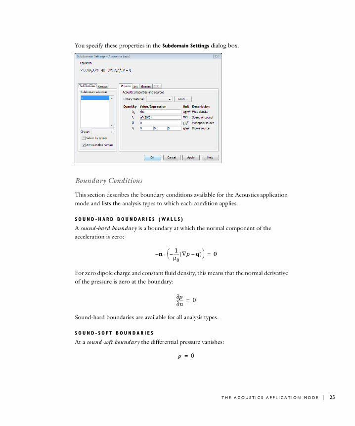
You specify these properties in the Subdomain Settings dialog box.
Boundary Conditions
This section describes the boundary conditions available for the Acoustics application mode and lists the analysis types to which each condition applies.
S O U N D - H A R D B O U N D A R I E S ( WA L L S )
A sound-hard boundary is a boundary at which the normal component of the acceleration is zero:
For zero dipole charge and constant fluid density, this means that the normal derivative of the pressure is zero at the boundary:
Sound-hard boundaries are available for all analysis types.
S O U N D - S O F T B O U N D A R I E S
At a sound-soft boundary the differential pressure vanishes:
n–1ρ0------– ∇p q–( )⎝ ⎠
⎛ ⎞⋅ 0=
n∂∂p 0=
p 0=
T H E A C O U S T I C S A P P L I C A T I O N M O D E | 25
26 | C H A P T E R
Sound-soft boundaries are also available for all analysis types.
P R E S S U R E S O U R C E
This boundary condition means that you specify a constant acoustic pressure to be maintained at the boundary:
The pressure-source condition is available only for time-harmonic analysis.
I M P E D A N C E B O U N D A R Y C O N D I T I O N
The impedance boundary condition is a generalization of the sound-hard and sound-soft boundary conditions:
Here Z (SI unit Pa s/m ) is the acoustic input impedance of the external domain. From a physical point of view, the acoustic input impedance is the ratio between pressure and normal particle velocity. It can be expressed in terms of the characteristic impedance inside the domain, Z0 = ρ c, as Z = ζ Z0, where the dimensionless quantity ζ is called the specific acoustic impedance.
The impedance boundary condition is a good approximation for a locally reacting surface—a surface for which the normal velocity at any point depends only on the pressure at that exact point.
Note that in the two opposite limits and , the sound-hard and sound-soft boundary conditions are recovered. Impedance boundary conditions are available for time-harmonic and transient analysis.
R A D I A T I O N B O U N D A R Y C O N D I T I O N S
The radiation boundary conditions allow an outgoing wave to leave the modeling domain with minimal reflections. In specifying a boundary condition of this kind you have the choice between three wave types: plane, cylindrical, or spherical. You can thus adapt the condition to the geometry of your modeling domain.
The radiation boundary conditions read
p p0=
n 1ρ0------– ∇p q–( )⎝ ⎠
⎛ ⎞⋅ iωpZ
----------– 0=
Z ∞→ Z 0→
n–1ρ0------– ∇p q–( )⎝ ⎠
⎛ ⎞⋅ ik κ r( )+( ) pρ0------+ ik κ r( ) i k n⋅( )–+( )
p0ρ0------e
i k r⋅( )–=
3 : A C O U S T I C S
where k is the wave number (a predefined application-mode variable; see Table 3-1 on page 30) and κ ( r ) is a function whose form depends on the wave type:
• Plane wave: κ( r ) = 0
• Cylindrical wave: κ( r ) = 1 / (2 r)
• Spherical wave: κ( r ) = 1 / r
In the latter two cases, r is the shortest distance from the point r = (x, y, z) on the boundary to the source. The right-hand side of the equation represents an optional incoming plane pressure wave with amplitude p0 and wave vector k = k nk, where nk denotes the unit vector in the direction of propagation.
To define a radiation boundary condition, select a plane, cylindrical, or spherical wave from the Wave type list. In addition, you must specify:
• p0—the pressure source amplitude
• nk—the wave direction vector
• r0 = (x0, y0, z0)—a point on the source axis (for a cylindrical wave) or the source location (for a spherical wave)
• raxis—the source axis direction (only for cylindrical waves)
The default value of nk is the inward normal vector, −n, which is the natural direction for waveguides and similar structures. For wave propagation in open space, k can point in any direction.
Note: You do not have to normalize the vector whose components you enter in the Wave direction edit fields; the software explicitly normalizes the components to make nk a unit vector in the direction that you specify.
Radiation boundary conditions are available for time-harmonic analysis only.
S P E C I F I E D N O R M A L A C C E L E R A T I O N
The inward normal acceleration an represents an external source term. You can also use it for coupling your acoustics model to a structural analysis. The specified normal acceleration is available for time-harmonic analysis.
n–1ρ0------– ∇p q–( )⎝ ⎠
⎛ ⎞⋅ an=
T H E A C O U S T I C S A P P L I C A T I O N M O D E | 27
28 | C H A P T E R
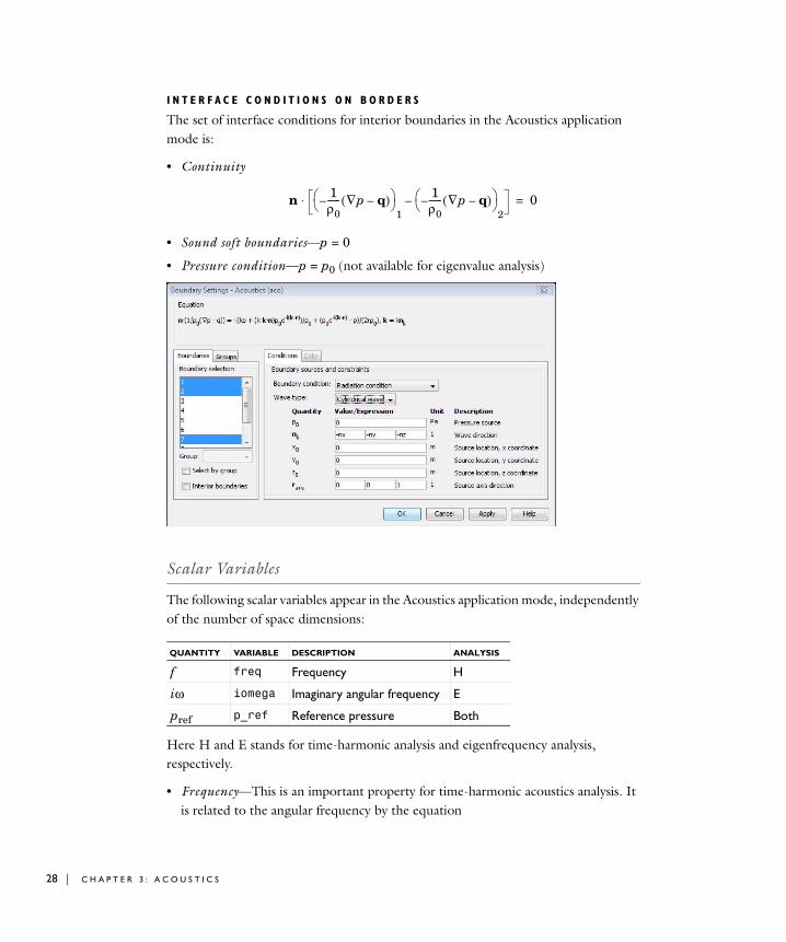
I N T E R F A C E C O N D I T I O N S O N B O R D E R S
The set of interface conditions for interior boundaries in the Acoustics application mode is:
• Continuity
• Sound soft boundaries—p = 0
• Pressure condition—p = p0 (not available for eigenvalue analysis)
Scalar Variables
The following scalar variables appear in the Acoustics application mode, independently of the number of space dimensions:
Here H and E stands for time-harmonic analysis and eigenfrequency analysis, respectively.
• Frequency—This is an important property for time-harmonic acoustics analysis. It is related to the angular frequency by the equation
QUANTITY VARIABLE DESCRIPTION ANALYSIS
f freq Frequency H
iω iomega Imaginary angular frequency E
pref p_ref Reference pressure Both
n 1ρ0------– ∇p q–( )⎝ ⎠
⎛ ⎞1
1ρ0------– ∇p q–( )⎝ ⎠
⎛ ⎞2
–⋅ 0=
3 : A C O U S T I C S
The wavelength is given by λ = cs / f. Therefore, the higher the frequency, the shorter the wavelength. To resolve a wave, it is important that the mesh size be smaller than the wavelength. As a rule of thumb, use a minimum mesh resolution of a few elements per wavelength with the default second-order Lagrange elements.
Another important acoustics property is the wave number, k, which is defined as
• Imaginary angular frequency—For the eigenfrequency analysis type the quantity iω is used as a scalar variable in place of the frequency, f. By default, it is related to the eigenvalue, λ, by the equation
(Note that the symbol λ is used here in a different meaning than in the previous paragraph.)
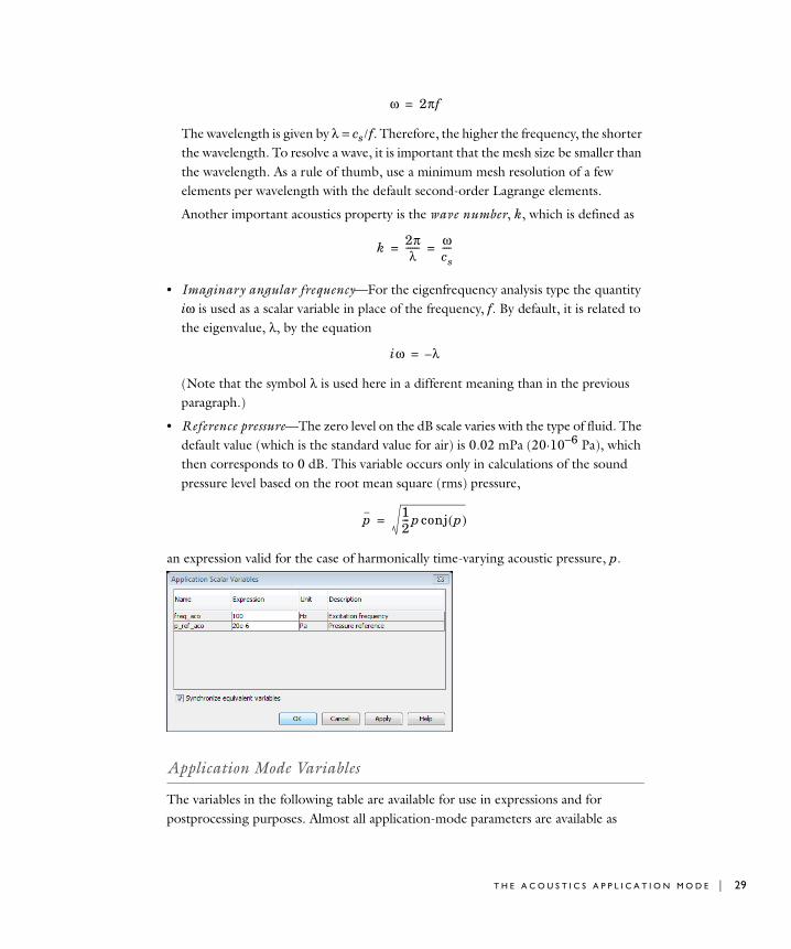
• Reference pressure—The zero level on the dB scale varies with the type of fluid. The default value (which is the standard value for air) is 0.02 mPa (20·10−6 Pa), which then corresponds to 0 dB. This variable occurs only in calculations of the sound pressure level based on the root mean square (rms) pressure,
an expression valid for the case of harmonically time-varying acoustic pressure, p.
Application Mode Variables
The variables in the following table are available for use in expressions and for postprocessing purposes. Almost all application-mode parameters are available as
ω 2πf=
k 2πλ
------ ωcs----= =
iω λ–=
p 12--- p conj p( )=
T H E A C O U S T I C S A P P L I C A T I O N M O D E | 29

30 | C H A P T E R
variables. Some variables are available only in certain analysis types as indicated in the Analysis column, where an H means that the variable is available only for time-harmonic analysis. The table uses an index convention where a single index i denotes any one of the global space variables (x, y, z) while a summation over i runs over all three space dimensions.
TABLE 3-1: ACOUSTICS APPLICATION MODE VARIABLES
NAME SYMBOL NAME ANALYSIS DOMAIN DESCRIPTION EXPRESSION
p p Both All pressure p
Lp Lp Both S sound pressure level
rho0 ρ0 Both S fluid density ρ0
cs cs Both S speed of sound cs
k k Both S wave number ω /cs
qi qi Both S dipole source, xi component
qi
normq |q| Both S dipole source, norm
ai ai Both S local acceleration, xi component
norma |a| Both S local acceleration, norm
na an Both B outward normal acceleration
vi vi H S local velocity, xi component
ai/(iω)
normv |v| Both S local velocity, norm
nv vn H B outward normal velocity
an/(iω)
10 p2
p02
------⎝ ⎠⎜ ⎟⎛ ⎞
log
qi2
i∑
1ρ0------–
xi∂∂p qi–⎝ ⎠⎛ ⎞
ai2
i∑
n 1ρ0------– ∇p q–( )⎝ ⎠
⎛ ⎞⋅
vi2
i∑
3 : A C O U S T I C S
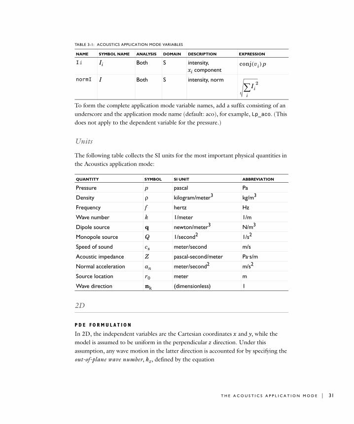
To form the complete application mode variable names, add a suffix consisting of an underscore and the application mode name (default: aco), for example, Lp_aco. (This does not apply to the dependent variable for the pressure.)
Units
The following table collects the SI units for the most important physical quantities in the Acoustics application mode:
2D
P D E F O R M U L A T I O N
In 2D, the independent variables are the Cartesian coordinates x and y, while the model is assumed to be uniform in the perpendicular z direction. Under this assumption, any wave motion in the latter direction is accounted for by specifying the out-of-plane wave number, kz, defined by the equation
Ii Ii Both S intensity, xi component
normI I Both S intensity, norm
QUANTITY SYMBOL SI UNIT ABBREVIATION
Pressure p pascal Pa
Density ρ kilogram/meter3 kg/m3
Frequency f hertz Hz
Wave number k 1/meter 1/m
Dipole source q newton/meter3 N/m3
Monopole source Q 1/second2 1/s2
Speed of sound cs meter/second m/s
Acoustic impedance Z pascal-second/meter Pa·s/m
Normal acceleration an meter/second2 m/s2
Source location r0 meter m
Wave direction nk (dimensionless) 1
TABLE 3-1: ACOUSTICS APPLICATION MODE VARIABLES
NAME SYMBOL NAME ANALYSIS DOMAIN DESCRIPTION EXPRESSION
conj vi( ) p
Ii2
i∑
T H E A C O U S T I C S A P P L I C A T I O N M O D E | 31

32 | C H A P T E R
(3-3)
Time-Harmonic AnalysisUsing Equation 3-3 and expanding the 3D operators in Equation 3-1, the equation for the pressure, p(x , y), becomes
where the ’s denote 2D differential operators.
Eigenfrequency AnalysisIdentical reasoning as for the time-harmonic case leads to the equation
S C A L A R V A R I A B L E S
In addition to the scalar variables available in the three-dimensional case, in 2D you can also specify the value of the out-of-plane wave number, kz:
The default value of kz is 0.
A P P L I C A T I O N M O D E V A R I A B L E S
With the interpretation that the index i stands for either x or y and that summations run over these two values, all variables listed in Table 3-1 on page 30 are defined also in the 2D case.
2D Axisymmetric
P D E F O R M U L A T I O N
In the 2D axisymmetric case, the independent variables are the radial coordinate, r, and the axial coordinate, z. The only dependence of the azimuthal coordinate, , allowed is through a phase factor:
QUANTITY VARIABLE DESCRIPTION ANALYSIS TYPE
f freq Frequency (time-harmonic) H
iω iomega Imaginary angular frequency E
kz kz Out-of-plane wave number Both
pref p_ref Reference pressure Both
p x y z t, , ,( ) p x y,( )ei ωt kz– z( )=
∇
∇ 1ρ0------– ∇p q–( )⋅ ω
cs------⎝ ⎠⎛ ⎞ 2
kz2
–pρ0------– Q=
∇
∇ 1ρ0------– ∇p⎝ ⎠
⎛ ⎞⋅ λcs------⎝ ⎠⎛ ⎞ 2
kz2
+pρ0------+ 0=
ϕ
3 : A C O U S T I C S
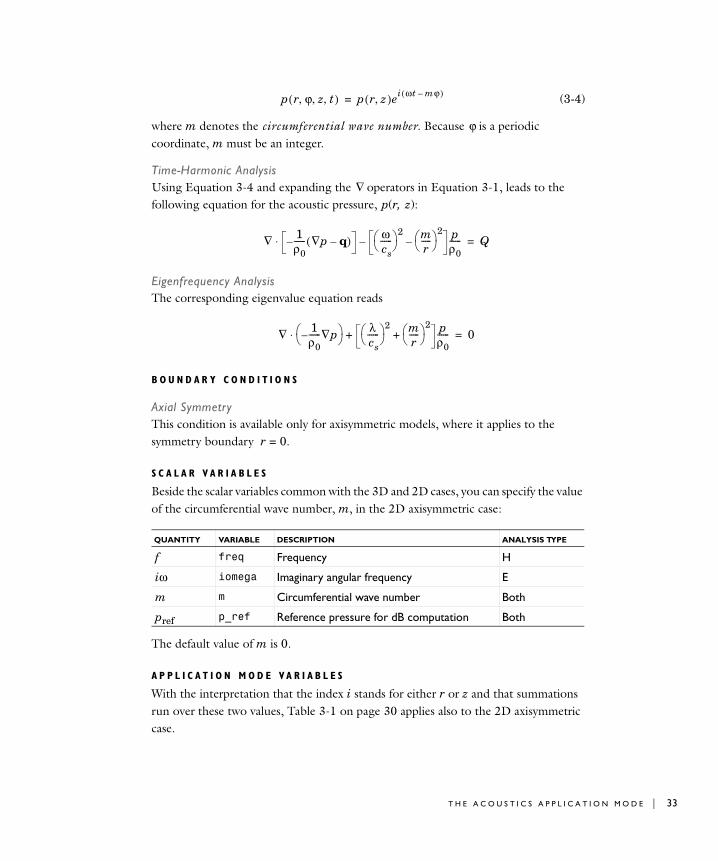
(3-4)
where m denotes the circumferential wave number. Because is a periodic coordinate, m must be an integer.
Time-Harmonic AnalysisUsing Equation 3-4 and expanding the operators in Equation 3-1, leads to the following equation for the acoustic pressure, p(r , z):
Eigenfrequency AnalysisThe corresponding eigenvalue equation reads
B O U N D A R Y C O N D I T I O N S
Axial SymmetryThis condition is available only for axisymmetric models, where it applies to the symmetry boundary r = 0.
S C A L A R V A R I A B L E S
Beside the scalar variables common with the 3D and 2D cases, you can specify the value of the circumferential wave number, m, in the 2D axisymmetric case:
The default value of m is 0.
A P P L I C A T I O N M O D E V A R I A B L E S
With the interpretation that the index i stands for either r or z and that summations run over these two values, Table 3-1 on page 30 applies also to the 2D axisymmetric case.
QUANTITY VARIABLE DESCRIPTION ANALYSIS TYPE
f freq Frequency H
iω iomega Imaginary angular frequency E
m m Circumferential wave number Both
pref p_ref Reference pressure for dB computation Both
p r ϕ z t, , ,( ) p r z,( )ei ωt mϕ–( )=
ϕ
∇
∇ 1ρ0------– ∇p q–( )⋅ ω
cs------⎝ ⎠⎛ ⎞ 2 m
r-----⎝ ⎠⎛ ⎞ 2
–pρ0------– Q=
∇ 1ρ0------– ∇p⎝ ⎠
⎛ ⎞⋅ λcs------⎝ ⎠⎛ ⎞2 m
r-----⎝ ⎠⎛ ⎞ 2
+pρ0------+ 0=
T H E A C O U S T I C S A P P L I C A T I O N M O D E | 33
34 | C H A P T E R
Examp l e—Rea c t i v e Mu f f l e r
Introduction
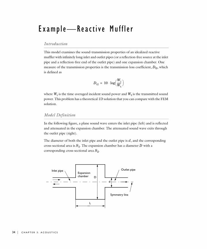
This model examines the sound-transmission properties of an idealized reactive muffler with infinitely long inlet and outlet pipes (or a reflection-free source at the inlet pipe and a reflection-free end of the outlet pipe) and one expansion chamber. One measure of the transmission properties is the transmission-loss coefficient, Dtl, which is defined as
where Wi is the time-averaged incident sound power and Wt is the transmitted sound power. This problem has a theoretical 1D solution that you can compare with the FEM solution.
Model Definition
In the following figure, a plane sound wave enters the inlet pipe (left) and is reflected and attenuated in the expansion chamber. The attenuated sound wave exits through the outlet pipe (right).
The diameter of both the inlet pipe and the outlet pipe is d, and the corresponding cross-sectional area is S1. The expansion chamber has a diameter D with a corresponding cross-sectional area S2.
Dtl 10WiWt-------⎝ ⎠⎛ ⎞log⋅=
Expansion
L
dD
Inlet pipe Outlet pipe
chamber
Symmetry line
3 : A C O U S T I C S

According to Ref. 1, the 1D theoretical solution for the transmission loss to this problem is
where k is the wave number; S1 and S2 are the areas of the pipes and expansion chamber; and L gives the length of the expansion chamber.
The model computes the pressure, p, for the fluid in the region defined by the above geometry. This is a time-harmonic problem so you can use the Helmholtz equation defined in the axisymmetric Acoustics application mode:
where ω = 2π f is the angular frequency, ρ0 is the fluid density, and cs is the speed of sound. The q term is a dipole source with the dimension of force per volume.
Because this is an axisymmetric model, you need to include only half of the geometry as indicated in the following figure:
You must apply axial symmetry boundary conditions on the line of symmetry.
Assume the walls are rigid, and thus use sound-hard (wall) boundary conditions,
which means that the normal derivative of the pressure is zero at the boundaries.
Radiation boundary conditions describe the inlet and outlet boundaries:
Dtl 10 1S1
2 S2⋅--------------
S22 S1⋅--------------–⎝ ⎠
⎛ ⎞2
kL( )2sin( )⋅+log⋅=
∇ 1ρ0------– ∇p q–( )⎝ ⎠
⎛ ⎞⋅ ω2p
ρ0 cs2
---------------– 0=
Expansion Inlet pipe Outlet pipechamber
Line of symmetry
n∂∂p 0=
n–1ρ0------– ∇p q–( )⎝ ⎠
⎛ ⎞⋅ ikρ0------⎝ ⎠
⎛ ⎞p+ik i k n⋅( )–( ) p0 e
i k r⋅( )–
ρ0------------------------------------------------------------------=
E X A M P L E — R E A C T I V E M U F F L E R | 35
36 | C H A P T E R
The radiation boundary condition is useful when the surroundings are merely a continuation of the domain, which is the case in this model. The term on the right-hand side represents an incoming pressure wave with an amplitude p0 and a direction given by the wave vector, k. In this model, an incoming pressure wave with the amplitude p0 = 1 Pa enters at the inlet boundary.
To determine the transmission loss in the model, you must first calculate the incident and transmitted time-averaged sound intensities and the corresponding sound power values. The equation
gives the time-averaged sound intensities where p is equal to p0 at the inlet and the computed solution at the outlet.
Using the boundary integration tool, you can evaluate the incident and transmitted sound powers, W, as:
Results and Discussion
Figure 3-1 shows the theoretical transmission loss (square markers) and the COMSOL Multiphysics solution (triangle markers) as a function of frequency. The theoretical solution has an upper frequency limit for its validity. This limit is the cut-on frequency, which defines the frequency range where only plane waves can propagate; above this frequency, also higher modes can propagate.
According to Ref. 1, the first cut-on frequency for a pipe is
.
Its value in this case is approximately 332 Hz, but it is evident from the above figure that a discrepancy exists between the theoretical and the FEM solution, even below the cut-on frequency. The discrepancy also increases with frequency between the 1D theoretical model and a 3D analysis, as you can see in Ref. 1. In the lower frequency range, however, there is good agreement between the theoretical solution and the FEM solution.
I p2
2ρ0 c-------------=
W I 2πr⋅( ) rd∫=
f01 1.841 cπD--------=
3 : A C O U S T I C S
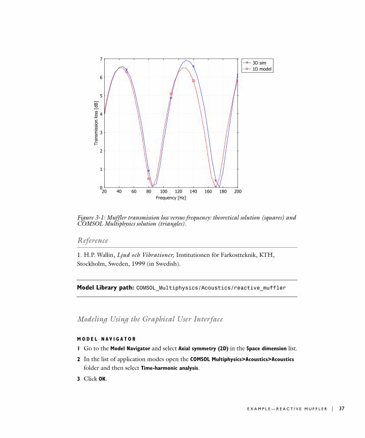
Figure 3-1: Muffler transmission loss versus frequency: theoretical solution (squares) and COMSOL Multiphysics solution (triangles).
Reference
1. H.P. Wallin, Ljud och Vibrationer, Institutionen för Farkostteknik, KTH, Stockholm, Sweden, 1999 (in Swedish).
Model Library path: COMSOL_Multiphysics/Acoustics/reactive_muffler
Modeling Using the Graphical User Interface
M O D E L N A V I G A T O R
1 Go to the Model Navigator and select Axial symmetry (2D) in the Space dimension list.
2 In the list of application modes open the COMSOL Multiphysics>Acoustics>Acoustics
folder and then select Time-harmonic analysis.
3 Click OK.
E X A M P L E — R E A C T I V E M U F F L E R | 37
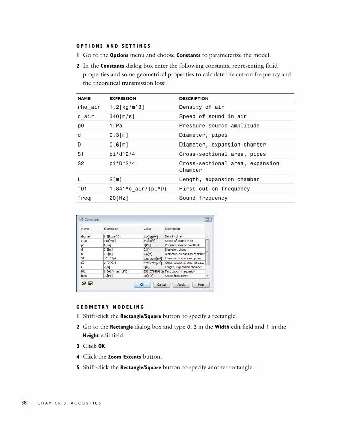
38 | C H A P T E R
O P T I O N S A N D S E T T I N G S
1 Go to the Options menu and choose Constants to parameterize the model.
2 In the Constants dialog box enter the following constants, representing fluid properties and some geometrical properties to calculate the cut-on frequency and the theoretical transmission loss:
G E O M E T R Y M O D E L I N G
1 Shift-click the Rectangle/Square button to specify a rectangle.
2 Go to the Rectangle dialog box and type 0.3 in the Width edit field and 1 in the Height edit field.
3 Click OK.
4 Click the Zoom Extents button.
5 Shift-click the Rectangle/Square button to specify another rectangle.
NAME EXPRESSION DESCRIPTION
rho_air 1.2[kg/m^3] Density of air
c_air 340[m/s] Speed of sound in air
p0 1[Pa] Pressure-source amplitude
d 0.3[m] Diameter, pipes
D 0.6[m] Diameter, expansion chamber
S1 pi*d^2/4 Cross-sectional area, pipes
S2 pi*D^2/4 Cross-sectional area, expansion chamber
L 2[m] Length, expansion chamber
f01 1.841*c_air/(pi*D) First cut-on frequency
freq 20[Hz] Sound frequency
3 : A C O U S T I C S
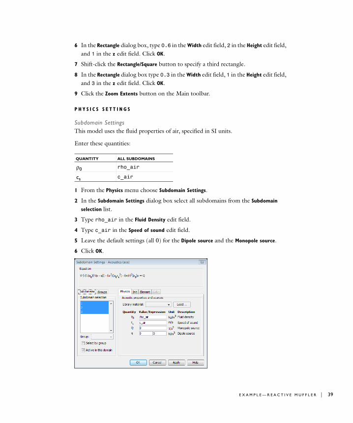
6 In the Rectangle dialog box, type 0.6 in the Width edit field, 2 in the Height edit field, and 1 in the z edit field. Click OK.
7 Shift-click the Rectangle/Square button to specify a third rectangle.
8 In the Rectangle dialog box type 0.3 in the Width edit field, 1 in the Height edit field, and 3 in the z edit field. Click OK.
9 Click the Zoom Extents button on the Main toolbar.
P H Y S I C S S E T T I N G S
Subdomain SettingsThis model uses the fluid properties of air, specified in SI units.
Enter these quantities:
1 From the Physics menu choose Subdomain Settings.
2 In the Subdomain Settings dialog box select all subdomains from the Subdomain
selection list.
3 Type rho_air in the Fluid Density edit field.
4 Type c_air in the Speed of sound edit field.
5 Leave the default settings (all 0) for the Dipole source and the Monopole source.
6 Click OK.
QUANTITY ALL SUBDOMAINS
ρ0 rho_air
cs c_air
E X A M P L E — R E A C T I V E M U F F L E R | 39
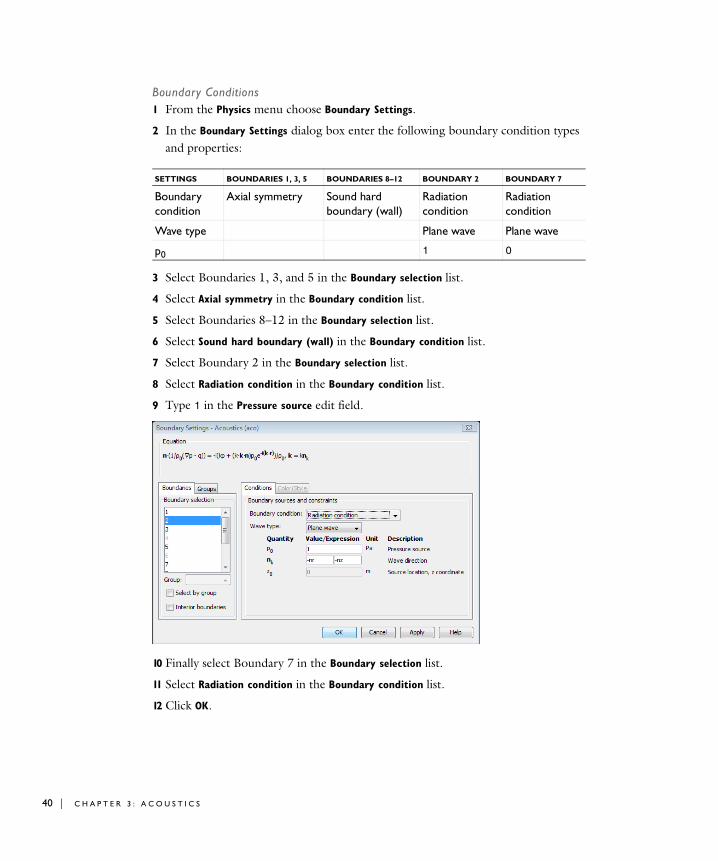
40 | C H A P T E R
Boundary Conditions1 From the Physics menu choose Boundary Settings.
2 In the Boundary Settings dialog box enter the following boundary condition types and properties:
3 Select Boundaries 1, 3, and 5 in the Boundary selection list.
4 Select Axial symmetry in the Boundary condition list.
5 Select Boundaries 8–12 in the Boundary selection list.
6 Select Sound hard boundary (wall) in the Boundary condition list.
7 Select Boundary 2 in the Boundary selection list.
8 Select Radiation condition in the Boundary condition list.
9 Type 1 in the Pressure source edit field.
10 Finally select Boundary 7 in the Boundary selection list.
11 Select Radiation condition in the Boundary condition list.
12 Click OK.
SETTINGS BOUNDARIES 1, 3, 5 BOUNDARIES 8–12 BOUNDARY 2 BOUNDARY 7
Boundary condition
Axial symmetry Sound hard boundary (wall)
Radiation condition
Radiation condition
Wave type Plane wave Plane wave
p0 1 0
3 : A C O U S T I C S
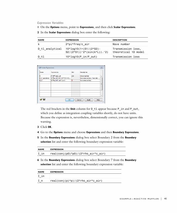
Expression Variables1 On the Options menu, point to Expressions, and then click Scalar Expressions.
2 In the Scalar Expressions dialog box enter the following:
The red brackets in the Unit column for D_tl appear because P_in and P_out, which you define as integration coupling variables shortly, do not have units. Because the expression is, nevertheless, dimensionally correct, you can ignore this warning.
3 Click OK.
4 Go to the Options menu and choose Expressions and then Boundary Expressions.
5 In the Boundary Expressions dialog box select Boundary 2 from the Boundary
selection list and enter the following boundary expression variable:
6 In the Boundary Expressions dialog box select Boundary 7 from the Boundary
selection list and enter the following boundary expression variable:
NAME EXPRESSION DESCRIPTION
k 2*pi*freq/c_air Wave number
D_tl_analytical 10*log10(1+(S1/(2*S2)- S2/(2*S1))^2*(sin(k*L)).^2)
Transmission loss, theoretical 1D model
D_tl 10*log10(P_in/P_out) Transmission loss
NAME EXPRESSION
I_in real(conj(p0)*p0)/(2*rho_air*c_air)
NAME EXPRESSION
I_in
I_n real(conj(p)*p)/(2*rho_air*c_air)
E X A M P L E — R E A C T I V E M U F F L E R | 41
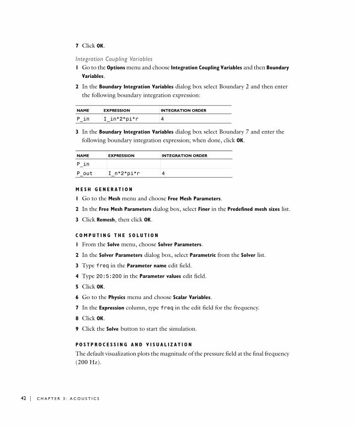
42 | C H A P T E R
7 Click OK.
Integration Coupling Variables1 Go to the Options menu and choose Integration Coupling Variables and then Boundary
Variables.
2 In the Boundary Integration Variables dialog box select Boundary 2 and then enter the following boundary integration expression:
3 In the Boundary Integration Variables dialog box select Boundary 7 and enter the following boundary integration expression; when done, click OK.
M E S H G E N E R A T I O N
1 Go to the Mesh menu and choose Free Mesh Parameters.
2 In the Free Mesh Parameters dialog box, select Finer in the Predefined mesh sizes list.
3 Click Remesh, then click OK.
C O M P U T I N G T H E S O L U T I O N
1 From the Solve menu, choose Solver Parameters.
2 In the Solver Parameters dialog box, select Parametric from the Solver list.
3 Type freq in the Parameter name edit field.
4 Type 20:5:200 in the Parameter values edit field.
5 Click OK.
6 Go to the Physics menu and choose Scalar Variables.
7 In the Expression column, type freq in the edit field for the frequency.
8 Click OK.
9 Click the Solve button to start the simulation.
P O S T P R O C E S S I N G A N D V I S U A L I Z A T I O N
The default visualization plots the magnitude of the pressure field at the final frequency (200 Hz).
NAME EXPRESSION INTEGRATION ORDER
P_in I_in*2*pi*r 4
NAME EXPRESSION INTEGRATION ORDER
P_in
P_out I_n*2*pi*r 4
3 : A C O U S T I C S
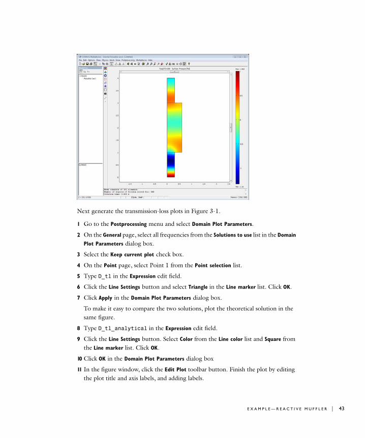
Next generate the transmission-loss plots in Figure 3-1.
1 Go to the Postprocessing menu and select Domain Plot Parameters.
2 On the General page, select all frequencies from the Solutions to use list in the Domain
Plot Parameters dialog box.
3 Select the Keep current plot check box.
4 On the Point page, select Point 1 from the Point selection list.
5 Type D_tl in the Expression edit field.
6 Click the Line Settings button and select Triangle in the Line marker list. Click OK.
7 Click Apply in the Domain Plot Parameters dialog box.
To make it easy to compare the two solutions, plot the theoretical solution in the same figure.
8 Type D_tl_analytical in the Expression edit field.
9 Click the Line Settings button. Select Color from the Line color list and Square from the Line marker list. Click OK.
10 Click OK in the Domain Plot Parameters dialog box
11 In the figure window, click the Edit Plot toolbar button. Finish the plot by editing the plot title and axis labels, and adding labels.
E X A M P L E — R E A C T I V E M U F F L E R | 43

44 | C H A P T E R
3 : A C O U S T I C S
4
D i f f u s i o n
This chapter explains how to use both the Diffusion application mode and the Diffusion and Convection application mode to model and simulate various types of transport problems. It concludes with a step-by-step example that introduces the concept of effective diffusivity in porous media.
45
46 | C H A P T E R
Th e D i f f u s i o n App l i c a t i o n Mode
The Diffusion application mode treats a specific mechanism of mass transport, the simplest one to describe in mathematical terms, namely diffusion. This application mode is available in 1D, 2D, and 3D as well as in axisymmetric formulations in 1D and 2D.
The dependent variable is the concentration of mass, c.
Note: The optional Chemical Engineering Module provides an application mode for the diffusion of several species as well as an application mode for problems that involve potential flow. It also supports modeling using pseudo-2D and pseudo-3D geometries.
PDE Formulation
Heat transfer is a diffusion process, so the generic diffusion equation has the same structure as the heat equation. Diffusion is governed by the equation
where c is the concentration, D is the diffusion coefficient, and R is a reaction rate. The diffusion process can be anisotropic, in which case D is a tensor.
Subdomain Settings
The diffusion equation coefficients to specify on the subdomains are:
COEFFICIENT VARIABLE DESCRIPTION
δts Dts_c Time-scaling coefficient
D D_c Diffusion coefficient, diffusion coefficient tensor
Dij Dxixj_c Diffusion coefficient tensor, xixj component
R R_c Reaction rate
δtsc∂t∂
----- ∇ D– ∇c( )⋅+ R=
4 : D I F F U S I O N
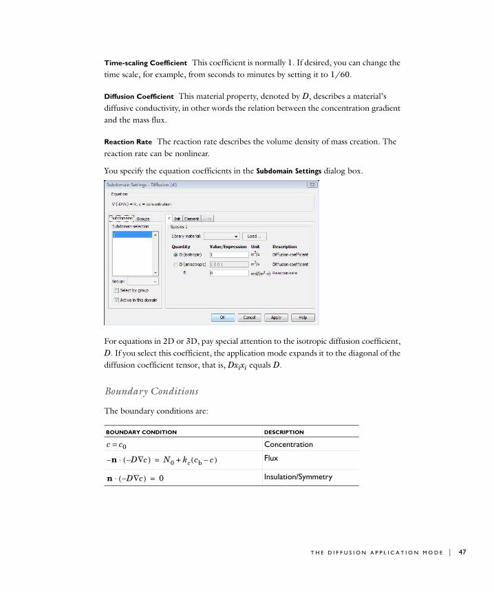
Time-scaling Coefficient This coefficient is normally 1. If desired, you can change the time scale, for example, from seconds to minutes by setting it to 1/60.
Diffusion Coefficient This material property, denoted by D, describes a material’s diffusive conductivity, in other words the relation between the concentration gradient and the mass flux.
Reaction Rate The reaction rate describes the volume density of mass creation. The reaction rate can be nonlinear.
You specify the equation coefficients in the Subdomain Settings dialog box.
For equations in 2D or 3D, pay special attention to the isotropic diffusion coefficient, D. If you select this coefficient, the application mode expands it to the diagonal of the diffusion coefficient tensor, that is, Dxixi equals D.
Boundary Conditions
The boundary conditions are:
BOUNDARY CONDITION DESCRIPTION
c = c0 Concentration
Flux
Insulation/Symmetry
n– D– c∇( )⋅ N0 kc cb c–( )+=
n D– c∇( )⋅ 0=
T H E D I F F U S I O N A P P L I C A T I O N M O D E | 47
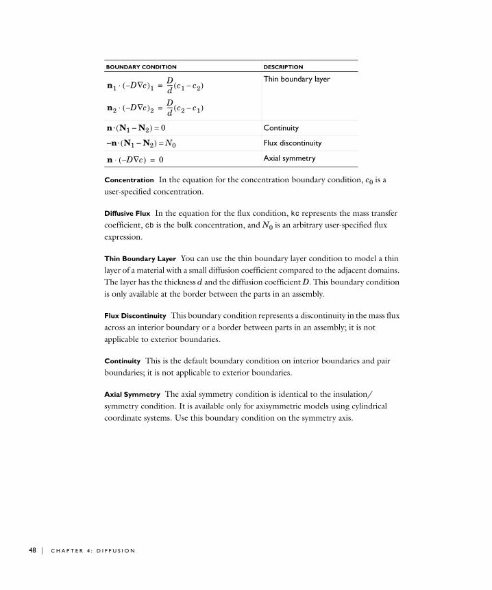
48 | C H A P T E R
Concentration In the equation for the concentration boundary condition, c0 is a user-specified concentration.
Diffusive Flux In the equation for the flux condition, kc represents the mass transfer coefficient, cb is the bulk concentration, and N0 is an arbitrary user-specified flux expression.
Thin Boundary Layer You can use the thin boundary layer condition to model a thin layer of a material with a small diffusion coefficient compared to the adjacent domains. The layer has the thickness d and the diffusion coefficient D. This boundary condition is only available at the border between the parts in an assembly.
Flux Discontinuity This boundary condition represents a discontinuity in the mass flux across an interior boundary or a border between parts in an assembly; it is not applicable to exterior boundaries.
Continuity This is the default boundary condition on interior boundaries and pair boundaries; it is not applicable to exterior boundaries.
Axial Symmetry The axial symmetry condition is identical to the insulation/symmetry condition. It is available only for axisymmetric models using cylindrical coordinate systems. Use this boundary condition on the symmetry axis.
Thin boundary layer
n · ( N1 − N2 ) = 0 Continuity
−n · ( N1 − N2 ) = N0 Flux discontinuity
Axial symmetry
BOUNDARY CONDITION DESCRIPTION
n1 D– c∇( )1⋅ Dd---- c1 c2–( )=
n2 D– c∇( )2⋅ Dd---- c2 c1–( )=
n D– c∇( )⋅ 0=
4 : D I F F U S I O N
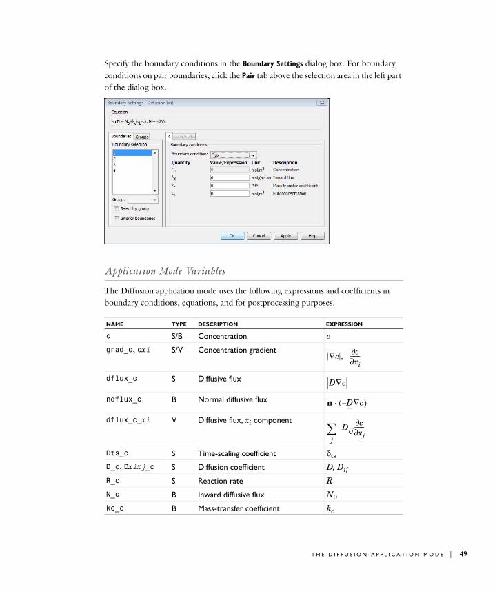
Specify the boundary conditions in the Boundary Settings dialog box. For boundary conditions on pair boundaries, click the Pair tab above the selection area in the left part of the dialog box.
Application Mode Variables
The Diffusion application mode uses the following expressions and coefficients in boundary conditions, equations, and for postprocessing purposes.
NAME TYPE DESCRIPTION EXPRESSION
c S/B Concentration c
grad_c, cxi S/V Concentration gradient
dflux_c S Diffusive flux
ndflux_c B Normal diffusive flux
dflux_c_xi V Diffusive flux, xi component
Dts_c S Time-scaling coefficient δts
D_c, Dxixj_c S Diffusion coefficient D, Dij
R_c S Reaction rate R
N_c B Inward diffusive flux N0
kc_c B Mass-transfer coefficient kc
∇c , c∂xi∂
-------
D∇c
n D∇c–( )⋅
Dijc∂xj∂
-------–
j∑
T H E D I F F U S I O N A P P L I C A T I O N M O D E | 49
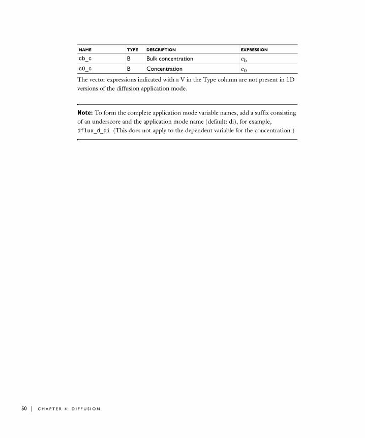
50 | C H A P T E R
The vector expressions indicated with a V in the Type column are not present in 1D versions of the diffusion application mode.
Note: To form the complete application mode variable names, add a suffix consisting of an underscore and the application mode name (default: di), for example, dflux_d_di. (This does not apply to the dependent variable for the concentration.)
cb_c B Bulk concentration cb
c0_c B Concentration c0
NAME TYPE DESCRIPTION EXPRESSION
4 : D I F F U S I O N
Th e Con v e c t i o n and D i f f u s i o n App l i c a t i o n Mode
This application mode models the most common type of transport in chemical systems: transport by convection and diffusion. You can simulate transport by convection and diffusion in 1D, 2D, and 3D as well as for axisymmetric systems in 1D and 2D.
The dependent variable in the application mode is the concentration of mass, c.
Note: The optional Chemical Engineering Module contains an application mode for the convection and diffusion of several species. It also supports modeling using pseudo-2D and pseudo-3D geometries.
PDE Formulation
The equations for the nonconservative and conservative formulations for a species, c, are:
nonconservative
conservative
The nonconservative formulation is the default for advection and diffusion types of equations in COMSOL Multiphysics because the software assumes an incompressible fluid. Thus the term equals zero and gets dropped from the nonconservative formulation. This ensures that no nonphysical source term arises from a flow field where the incompressibility constraint, , is not absolutely fulfilled.
For stationary analysis the term with the time derivative gets dropped.
δtsc∂t∂
----- ∇ D c∇–( )⋅+ R u ∇c⋅–=
δtsc∂t∂
----- ∇ D c cu+∇–( )⋅+ R=
c∇ u⋅
∇ u⋅ 0=
T H E C O N V E C T I O N A N D D I F F U S I O N A P P L I C A T I O N M O D E | 51
52 | C H A P T E R
Subdomain Settings
The various coefficients used in the equations are:
For equations in 2D or 3D, pay special attention to the isotropic diffusion coefficient, D. If you select this coefficient, the application mode expands it to the diagonal of the diffusion coefficient tensor, that is, Dxixi equals D.
You specify the equation coefficients in the Subdomain Settings dialog box.
A R T I F I C I A L D I F F U S I O N
The Convection and Diffusion application mode supports artificial diffusion using the following methods:
• Isotropic diffusion
• Streamline diffusion
• Crosswind diffusion
To specify and activate artificial diffusion:
1 Open the Subdomain Settings dialog box.
2 Click the Physics tab.
3 With at least one subdomain selected, click the Artificial Diffusion button.
See “Stabilization Techniques” on page 433 in the COMSOL Multiphysics Modeling Guide for more information about artificial diffusion.
COEFFICIENT VARIABLE DESCRIPTION
δts Dts_c Time-scaling coefficient
D D_c Diffusion coefficient or tensor
Dij Dxixj_c Diffusion coefficient tensor, xixj component
R R_c Reaction rate
u, v, w u_c, v_c, w_c Velocity in the x1, x2, and x3 directions
4 : D I F F U S I O N
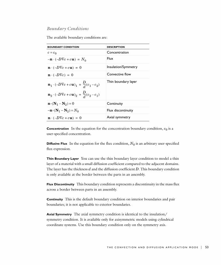
Boundary Conditions
The available boundary conditions are:
Concentration In the equation for the concentration boundary condition, c0 is a user-specified concentration.
Diffusive Flux In the equation for the flux condition, N0 is an arbitrary user-specified flux expression.
Thin Boundary Layer You can use the thin boundary layer condition to model a thin layer of a material with a small diffusion coefficient compared to the adjacent domains. The layer has the thickness d and the diffusion coefficient D. This boundary condition is only available at the border between the parts in an assembly.
Flux Discontinuity This boundary condition represents a discontinuity in the mass flux across a border between parts in an assembly.
Continuity This is the default boundary condition on interior boundaries and pair boundaries; it is not applicable to exterior boundaries.
Axial Symmetry The axial symmetry condition is identical to the insulation/symmetry condition. It is available only for axisymmetric models using cylindrical coordinate systems. Use this boundary condition only on the symmetry axis.
BOUNDARY CONDITION DESCRIPTION
c = c0 Concentration
Flux
Insulation/Symmetry
Convective flow
Thin boundary layer
n · ( N1 − N2 ) = 0 Continuity
−n · ( N1 − N2 ) = N0 Flux discontinuity
Axial symmetry
n– D c cu+∇–( )⋅ N0=
n D c cu+∇–( )⋅ 0=
n D– c∇( )⋅ 0=
n1 D– c cu+∇( )1⋅ Dd---- c1 c2–( )=
n2 D– c∇ cu+( )2⋅ Dd---- c2 c1–( )=
n D c cu+∇–( )⋅ 0=
T H E C O N V E C T I O N A N D D I F F U S I O N A P P L I C A T I O N M O D E | 53
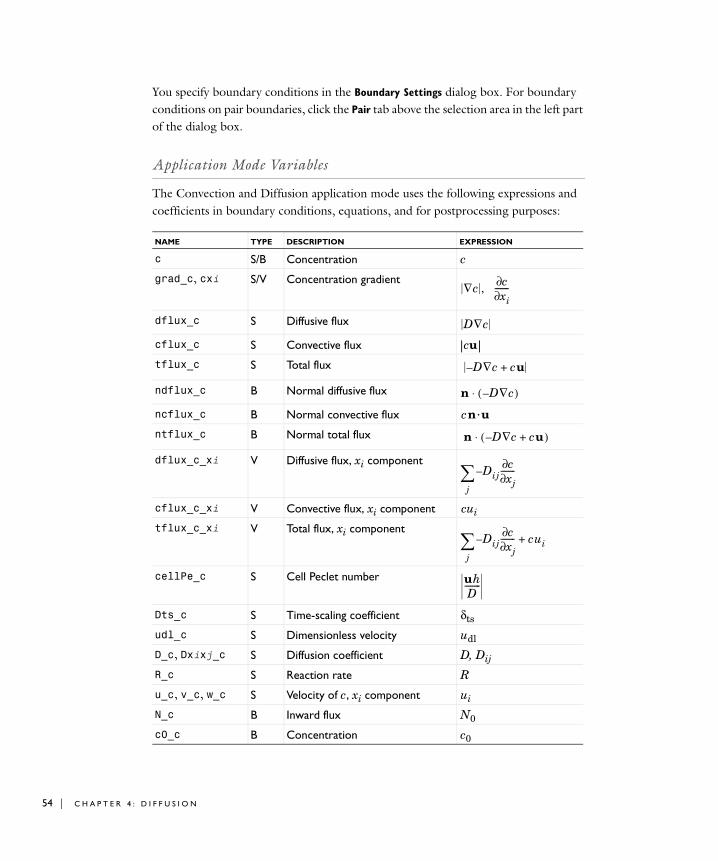
54 | C H A P T E R
You specify boundary conditions in the Boundary Settings dialog box. For boundary conditions on pair boundaries, click the Pair tab above the selection area in the left part of the dialog box.
Application Mode Variables
The Convection and Diffusion application mode uses the following expressions and coefficients in boundary conditions, equations, and for postprocessing purposes:
NAME TYPE DESCRIPTION EXPRESSION
c S/B Concentration c
grad_c, cxi S/V Concentration gradient
dflux_c S Diffusive flux
cflux_c S Convective flux | cu |tflux_c S Total flux
ndflux_c B Normal diffusive flux
ncflux_c B Normal convective flux c n · u
ntflux_c B Normal total flux
dflux_c_xi V Diffusive flux, xi component
cflux_c_xi V Convective flux, xi component cui
tflux_c_xi V Total flux, xi component
cellPe_c S Cell Peclet number
Dts_c S Time-scaling coefficient δts
udl_c S Dimensionless velocity udl
D_c, Dxixj_c S Diffusion coefficient D, Dij
R_c S Reaction rate R
u_c, v_c, w_c S Velocity of c, xi component ui
N_c B Inward flux N0
c0_c B Concentration c0
∇c , c∂xi∂
-------
D∇c
D– ∇c cu+
n D∇c–( )⋅
n D– ∇c cu+( )⋅
Dijc∂xj∂
-------–
j∑
Dijc∂xj∂
-------–
j∑ cui+
uhD
--------
4 : D I F F U S I O N
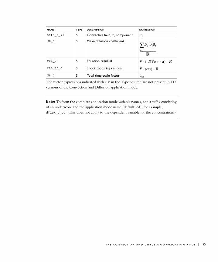
The vector expressions indicated with a V in the Type column are not present in 1D versions of the Convection and Diffusion application mode.
Note: To form the complete application mode variable names, add a suffix consisting of an underscore and the application mode name (default: cd), for example, dflux_d_cd. (This does not apply to the dependent variable for the concentration.)
beta_c_xi S Convective field, xi component ui
Dm_c S Mean diffusion coefficient
res_c S Equation residual
res_sc_c S Shock capturing residual
da_c S Total time-scale factor δts
NAME TYPE DESCRIPTION EXPRESSION
Dijβiβj
i j,∑
β--------------------------
∇ D– ∇c cu+( )⋅ R–
∇ cu( )⋅ R–
T H E C O N V E C T I O N A N D D I F F U S I O N A P P L I C A T I O N M O D E | 55
56 | C H A P T E R
E f f e c t i v e D i f f u s i v i t y i n Po r ou s Ma t e r i a l s
This model introduces the concept of effective diffusivity in porous media by comparing the transport through an artificial porous structure described in a detailed model with a simplified homogeneous porous media approach using effective transport properties.
The exercise consists of two parts. The first part describes how to create the model with a detailed geometry. The second part shows how to define a homogeneous model for porous media using an effective diffusivity calculated using the detailed model from the first part.
Introduction
Transport through porous structures is usually treated using simplified homogeneous models with effective transport properties. This is in most cases a necessity, since the typical dimensions of the pores and particles making up the porous structure are several orders of magnitude smaller than the size of the subdomain that is to be modeled.
However, it might be interesting to investigate the assumptions and simplifications done when homogenizing a porous structure by comparing a homogeneous model with a model defined using the detailed structure.
4 : D I F F U S I O N

The artificial porous structure used in this model is depicted in Figure 4-1 below.
Figure 4-1: Artificial porous structure. The domain colored in red is accessible for diffusion.
Model Definition
The model equation in the modeled domain shown in Figure 4-1 is the time-dependent equation
where c denotes concentration (mol/m3 using SI units) and D the diffusion coefficient (m2/s) of the solute.
The boundary conditions are of three different types. The so-called concentration boundary condition is set at the left vertical boundary in Figure 4-1 and is expressed as
where c0 is a given concentration.
The right vertical boundary in Figure 4-1 is set according to
where km is the mass transfer coefficient (m/s) and c1 the concentration in a bulk solution outside of the porous structure.
All other boundaries are insulating boundaries according to
Concentrationboundary
Fluxboundaries
∂c∂t----- ∇+ D c∇–( )⋅ 0=
c c0=
D c∇–( ) n⋅ km c c1–( )=
E F F E C T I V E D I F F U S I V I T Y I N P O R O U S M A T E R I A L S | 57
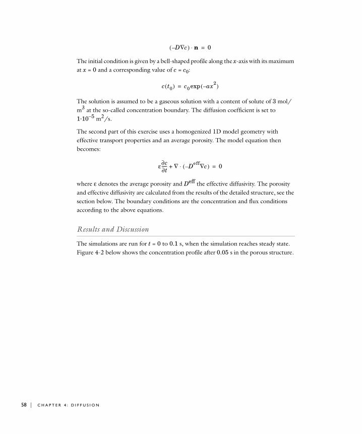
58 | C H A P T E R
The initial condition is given by a bell-shaped profile along the x-axis with its maximum at x = 0 and a corresponding value of c = c0:
The solution is assumed to be a gaseous solution with a content of solute of 3 mol/m3 at the so-called concentration boundary. The diffusion coefficient is set to 1·10−5 m2/s.
The second part of this exercise uses a homogenized 1D model geometry with effective transport properties and an average porosity. The model equation then becomes:
where ε denotes the average porosity and Deff the effective diffusivity. The porosity and effective diffusivity are calculated from the results of the detailed structure, see the section below. The boundary conditions are the concentration and flux conditions according to the above equations.
Results and Discussion
The simulations are run for t = 0 to 0.1 s, when the simulation reaches steady state. Figure 4-2 below shows the concentration profile after 0.05 s in the porous structure.
D c∇–( ) n⋅ 0=
c t0( ) c0 ax2–( )exp=
ε∂c∂t----- ∇+ Deff c∇–( )⋅ 0=
4 : D I F F U S I O N
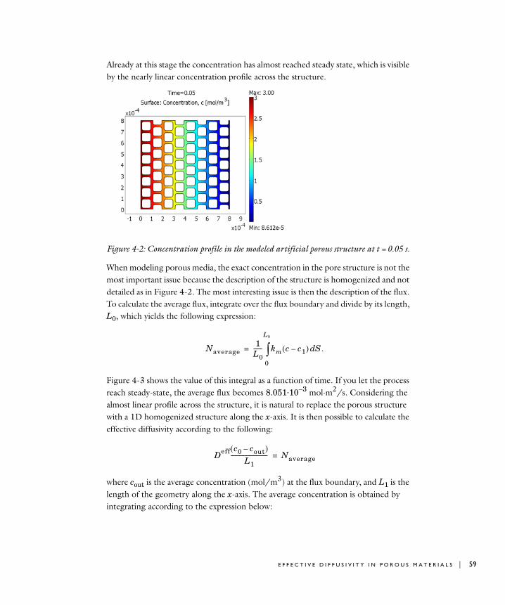
Already at this stage the concentration has almost reached steady state, which is visible by the nearly linear concentration profile across the structure.
Figure 4-2: Concentration profile in the modeled artificial porous structure at t = 0.05 s.
When modeling porous media, the exact concentration in the pore structure is not the most important issue because the description of the structure is homogenized and not detailed as in Figure 4-2. The most interesting issue is then the description of the flux. To calculate the average flux, integrate over the flux boundary and divide by its length, L0, which yields the following expression:
Figure 4-3 shows the value of this integral as a function of time. If you let the process reach steady-state, the average flux becomes 8.051·10−3 mol·m2/s. Considering the almost linear profile across the structure, it is natural to replace the porous structure with a 1D homogenized structure along the x-axis. It is then possible to calculate the effective diffusivity according to the following:
where cout is the average concentration (mol/m3) at the flux boundary, and L1 is the length of the geometry along the x-axis. The average concentration is obtained by integrating according to the expression below:
Naverage1
L0------ km c c1–( ) S.d
0
L0
∫=
Deff c0 cout–( )L1
-------------------------- Naverage=
E F F E C T I V E D I F F U S I V I T Y I N P O R O U S M A T E R I A L S | 59

60 | C H A P T E R
This gives and average concentration cout = 1.61·10−3 mol/m3 and using L1 = 8·10−4 m gives the effective diffusivity according to the following:
which yields a value for the effective diffusivity of 2.15·10−6 m2/s compared to the “free” diffusivity of 1·10−5 m2/s. The effective and “free” diffusivities are usually related according to the equation
where ε is the porosity of the structure and τ the so-called tortuosity, which is a measure of the actual length per unit effective length a molecule has to diffuse in a porous structure. To calculate the porosity of the modeled structure, you integrate the value 1 over the structure and then divide this by the length and width of the structure:
resulting in a value of 0.382. The value of τ can then be calculated to 1.78. In addition, the tortuosity is usually expressed as a power of the porosity, resulting in an expression for the effective diffusivity according to
If you use the calculated values for porosity and effective diffusivity, the value for p is 1.60. The experimental values for p for porous structures used for transport in catalysts, soils, and other porous structures is usually in the range 1.5–2.
Using the value of the effective diffusivity, a simple homogenized 1D model provides the possibility to compare the value of the flux using a homogenized model to the value using the detailed 2D structure. Figure 4-3 shows that there is an excellent agreement between the model using a detailed geometry and the homogenized model.
cout1
L0------ c S.d
0
L0
∫=
Deff 8.051 10 3– 8.0 10 4–⋅×⋅3 1.61 10 3–⋅–( )
--------------------------------------------------------------=
Deff Dετ--=
ε 1L0L1-------------- 1 xd yd
0
L0
∫0
L1
∫=
Deff Dεp=
4 : D I F F U S I O N
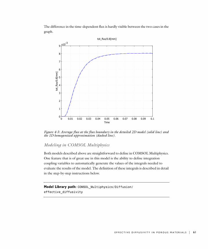
The difference in the time-dependent flux is hardly visible between the two cases in the graph.
Figure 4-3: Average flux at the flux boundary in the detailed 2D model (solid line) and the 1D homogenized approximation (dashed line).
Modeling in COMSOL Multiphysics
Both models described above are straightforward to define in COMSOL Multiphysics. One feature that is of great use in this model is the ability to define integration coupling variables to automatically generate the values of the integrals needed to evaluate the results of the model. The definition of these integrals is described in detail in the step-by-step instructions below.
Model Library path: COMSOL_Multiphysics/Diffusion/effective_diffusivity
E F F E C T I V E D I F F U S I V I T Y I N P O R O U S M A T E R I A L S | 61
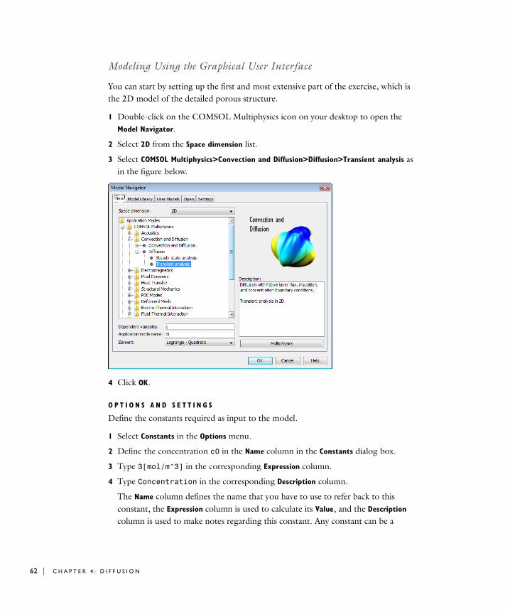
62 | C H A P T E R
Modeling Using the Graphical User Interface
You can start by setting up the first and most extensive part of the exercise, which is the 2D model of the detailed porous structure.
1 Double-click on the COMSOL Multiphysics icon on your desktop to open the Model Navigator.
2 Select 2D from the Space dimension list.
3 Select COMSOL Multiphysics>Convection and Diffusion>Diffusion>Transient analysis as in the figure below.
4 Click OK.
O P T I O N S A N D S E T T I N G S
Define the constants required as input to the model.
1 Select Constants in the Options menu.
2 Define the concentration c0 in the Name column in the Constants dialog box.
3 Type 3[mol/m^3] in the corresponding Expression column.
4 Type Concentration in the corresponding Description column.
The Name column defines the name that you have to use to refer back to this constant, the Expression column is used to calculate its Value, and the Description column is used to make notes regarding this constant. Any constant can be a
4 : D I F F U S I O N
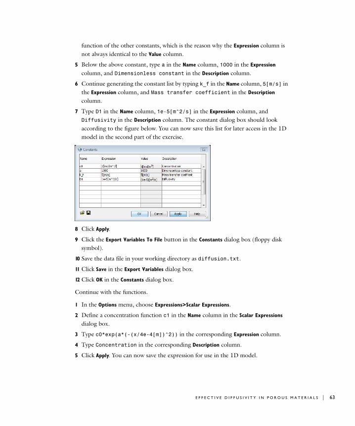
function of the other constants, which is the reason why the Expression column is not always identical to the Value column.
5 Below the above constant, type a in the Name column, 1000 in the Expression column, and Dimensionless constant in the Description column.
6 Continue generating the constant list by typing k_f in the Name column, 5[m/s] in the Expression column, and Mass transfer coefficient in the Description column.
7 Type D1 in the Name column, 1e-5[m^2/s] in the Expression column, and Diffusivity in the Description column. The constant dialog box should look according to the figure below. You can now save this list for later access in the 1D model in the second part of the exercise.
8 Click Apply.
9 Click the Export Variables To File button in the Constants dialog box (floppy disk symbol).
10 Save the data file in your working directory as diffusion.txt.
11 Click Save in the Export Variables dialog box.
12 Click OK in the Constants dialog box.
Continue with the functions.
1 In the Options menu, choose Expressions>Scalar Expressions.
2 Define a concentration function c1 in the Name column in the Scalar Expressions dialog box.
3 Type c0*exp(a*(-(x/4e-4[m])^2)) in the corresponding Expression column.
4 Type Concentration in the corresponding Description column.
5 Click Apply. You can now save the expression for use in the 1D model.
E F F E C T I V E D I F F U S I V I T Y I N P O R O U S M A T E R I A L S | 63
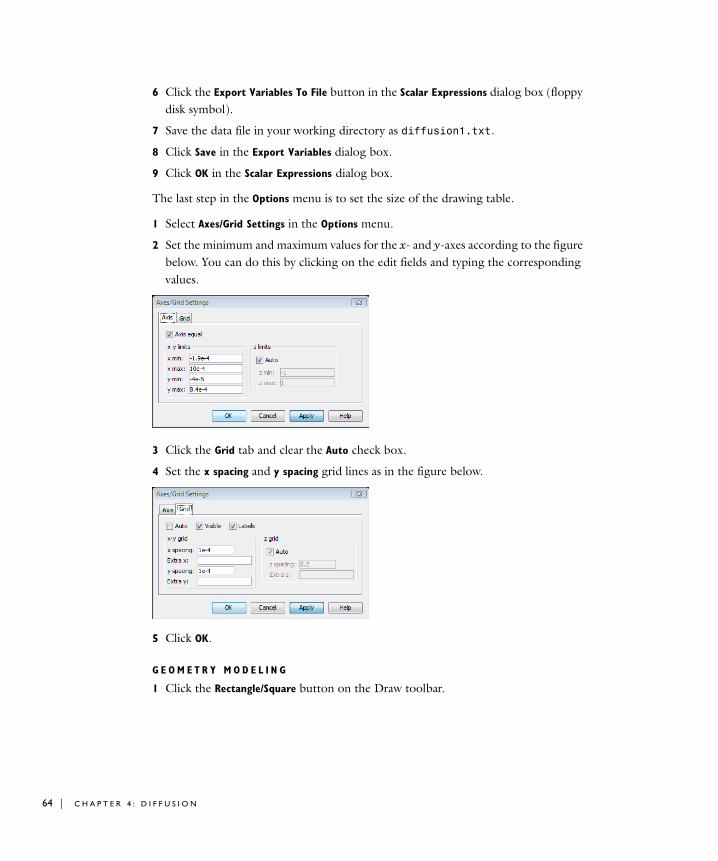
64 | C H A P T E R
6 Click the Export Variables To File button in the Scalar Expressions dialog box (floppy disk symbol).
7 Save the data file in your working directory as diffusion1.txt.
8 Click Save in the Export Variables dialog box.
9 Click OK in the Scalar Expressions dialog box.
The last step in the Options menu is to set the size of the drawing table.
1 Select Axes/Grid Settings in the Options menu.
2 Set the minimum and maximum values for the x- and y-axes according to the figure below. You can do this by clicking on the edit fields and typing the corresponding values.
3 Click the Grid tab and clear the Auto check box.
4 Set the x spacing and y spacing grid lines as in the figure below.
5 Click OK.
G E O M E T R Y M O D E L I N G
1 Click the Rectangle/Square button on the Draw toolbar.
4 : D I F F U S I O N
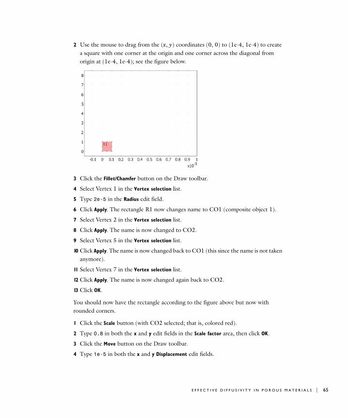
2 Use the mouse to drag from the (x, y) coordinates (0, 0) to (1e-4, 1e-4) to create a square with one corner at the origin and one corner across the diagonal from origin at (1e-4, 1e-4); see the figure below.
3 Click the Fillet/Chamfer button on the Draw toolbar.
4 Select Vertex 1 in the Vertex selection list.
5 Type 2e-5 in the Radius edit field.
6 Click Apply. The rectangle R1 now changes name to CO1 (composite object 1).
7 Select Vertex 2 in the Vertex selection list.
8 Click Apply. The name is now changed to CO2.
9 Select Vertex 5 in the Vertex selection list.
10 Click Apply. The name is now changed back to CO1 (this since the name is not taken anymore).
11 Select Vertex 7 in the Vertex selection list.
12 Click Apply. The name is now changed again back to CO2.
13 Click OK.
You should now have the rectangle according to the figure above but now with rounded corners.
1 Click the Scale button (with CO2 selected; that is, colored red).
2 Type 0.8 in both the x and y edit fields in the Scale factor area, then click OK.
3 Click the Move button on the Draw toolbar.
4 Type 1e-5 in both the x and y Displacement edit fields.
E F F E C T I V E D I F F U S I V I T Y I N P O R O U S M A T E R I A L S | 65
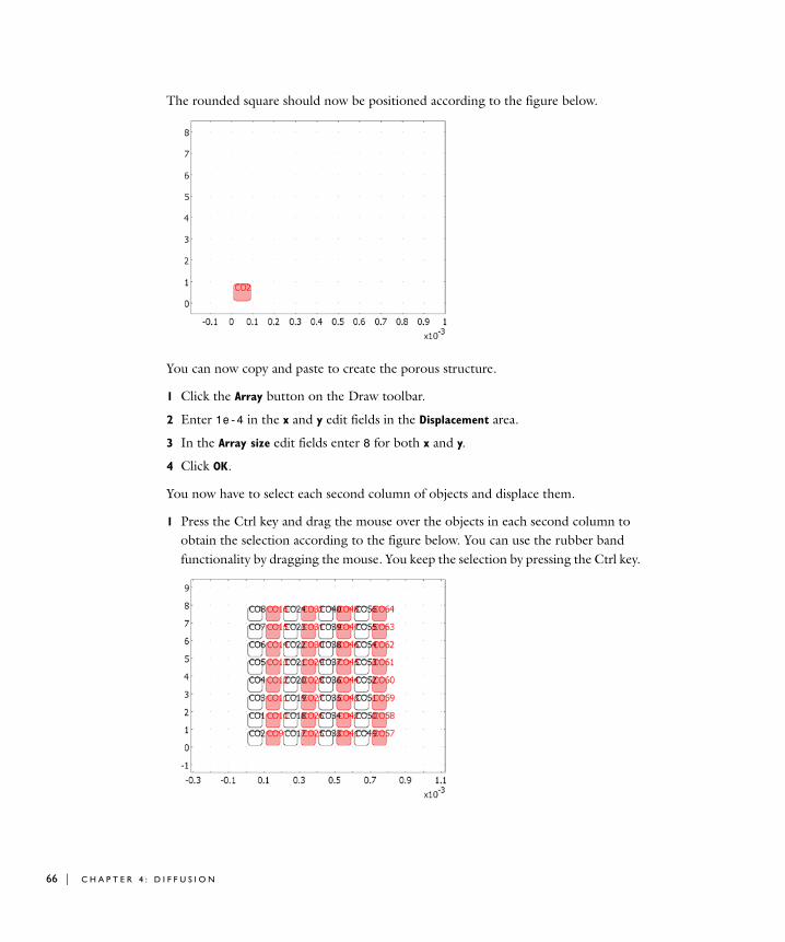
66 | C H A P T E R
The rounded square should now be positioned according to the figure below.
You can now copy and paste to create the porous structure.
1 Click the Array button on the Draw toolbar.
2 Enter 1e-4 in the x and y edit fields in the Displacement area.
3 In the Array size edit fields enter 8 for both x and y.
4 Click OK.
You now have to select each second column of objects and displace them.
1 Press the Ctrl key and drag the mouse over the objects in each second column to obtain the selection according to the figure below. You can use the rubber band functionality by dragging the mouse. You keep the selection by pressing the Ctrl key.
4 : D I F F U S I O N
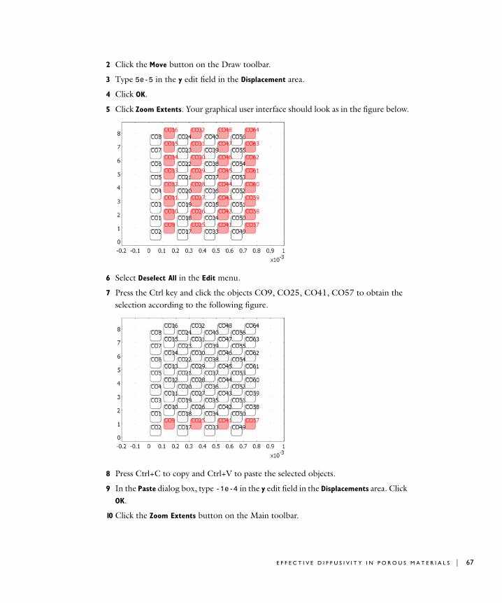
2 Click the Move button on the Draw toolbar.
3 Type 5e-5 in the y edit field in the Displacement area.
4 Click OK.
5 Click Zoom Extents. Your graphical user interface should look as in the figure below.
6 Select Deselect All in the Edit menu.
7 Press the Ctrl key and click the objects CO9, CO25, CO41, CO57 to obtain the selection according to the following figure.
8 Press Ctrl+C to copy and Ctrl+V to paste the selected objects.
9 In the Paste dialog box, type -1e-4 in the y edit field in the Displacements area. Click OK.
10 Click the Zoom Extents button on the Main toolbar.
E F F E C T I V E D I F F U S I V I T Y I N P O R O U S M A T E R I A L S | 67
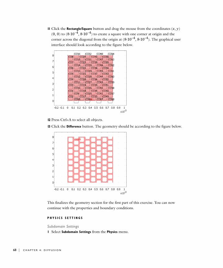
68 | C H A P T E R
11 Click the Rectangle/Square button and drag the mouse from the coordinates (x, y) (0, 0) to (8·10−4, 8·10−4) to create a square with one corner at origin and the corner across the diagonal from the origin at (8·10−4, 8·10−4). The graphical user interface should look according to the figure below.
12 Press Ctrl+A to select all objects.
13 Click the Difference button. The geometry should be according to the figure below.
This finalizes the geometry section for the first part of this exercise. You can now continue with the properties and boundary conditions.
P H Y S I C S S E T T I N G S
Subdomain Settings1 Select Subdomain Settings from the Physics menu.
4 : D I F F U S I O N
2 Select Subdomain 1 from the Subdomain selection list.
3 Type D1 in the Diffusion coefficient edit field. Note that you have defined D1 in the Constants dialog box in the Options menu.
4 Click the Init tab to set the initial condition.
5 Type c1 in the Concentration, c edit field (c(t0)). Note that you have defined c1 as a scalar expression variable.
6 Click OK.
Boundary Conditions1 Select Boundary Settings from the Physics menu.
2 Select Boundary 1 in the Boundary selection list.
3 Select Concentration from the Boundary condition list.
4 Type c0 in the Concentration edit field.
5 Select Boundary 276 from the Boundary selection list.
6 Select Flux from the Boundary condition list.
7 Type k_f in the Mass transfer coefficient edit field. The bulk concentration in the Bulk concentration edit field should be 0.
8 Click OK.
All other boundaries, except for the two boundaries that you have altered above, should remain at the default Insulation/Symmetry boundary condition.
M E S H G E N E R A T I O N
Click the Initialize Mesh button on the Main toolbar.
C O M P U T I N G T H E S O L U T I O N
1 Click the Solver Parameters button on the Main toolbar.
2 Type 0:2e-3:0.1 in the Times edit field to define the Time stepping. This gives an integration from 0 to 0.1 s with 2 ms increments between each output.
3 Select Direct (SPOOLES) from the Linear system solver list. The SPOOLES solver makes use of the symmetry in the diffusion equation, which the solver detects automatically, thus saving memory.
4 Click OK.
5 Click the Solve button on the Main toolbar.
E F F E C T I V E D I F F U S I V I T Y I N P O R O U S M A T E R I A L S | 69
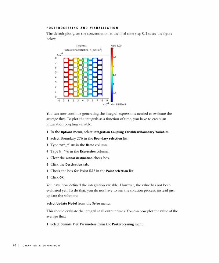
70 | C H A P T E R
P O S T P R O C E S S I N G A N D V I S U A L I Z A T I O N
The default plot gives the concentration at the final time step 0.1 s; see the figure below.
You can now continue generating the integral expressions needed to evaluate the average flux. To plot the integrals as a function of time, you have to create an integration coupling variable.
1 In the Options menu, select Integration Coupling Variables>Boundary Variables.
2 Select Boundary 276 in the Boundary selection list.
3 Type tot_flux in the Name column.
4 Type k_f*c in the Expression column.
5 Clear the Global destination check box.
6 Click the Destination tab.
7 Check the box for Point 532 in the Point selection list.
8 Click OK.
You have now defined the integration variable. However, the value has not been evaluated yet. To do that, you do not have to run the solution process; instead just update the solution:
Select Update Model from the Solve menu.
This should evaluate the integral at all output times. You can now plot the value of the average flux:
1 Select Domain Plot Parameters from the Postprocessing menu.
4 : D I F F U S I O N
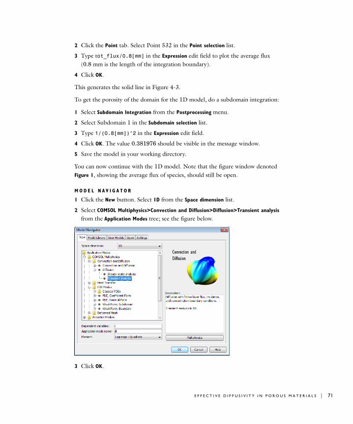
2 Click the Point tab. Select Point 532 in the Point selection list.
3 Type tot_flux/0.8[mm] in the Expression edit field to plot the average flux (0.8 mm is the length of the integration boundary).
4 Click OK.
This generates the solid line in Figure 4-3.
To get the porosity of the domain for the 1D model, do a subdomain integration:
1 Select Subdomain Integration from the Postprocessing menu.
2 Select Subdomain 1 in the Subdomain selection list.
3 Type 1/(0.8[mm])^2 in the Expression edit field.
4 Click OK. The value 0.381976 should be visible in the message window.
5 Save the model in your working directory.
You can now continue with the 1D model. Note that the figure window denoted Figure 1, showing the average flux of species, should still be open.
M O D E L N A V I G A T O R
1 Click the New button. Select 1D from the Space dimension list.
2 Select COMSOL Multiphysics>Convection and Diffusion>Diffusion>Transient analysis from the Application Modes tree; see the figure below.
3 Click OK.
E F F E C T I V E D I F F U S I V I T Y I N P O R O U S M A T E R I A L S | 71
72 | C H A P T E R
O P T I O N S A N D S E T T I N G S
You can now load the constants from the 2D model above.
1 Select Constants from the Options menu.
2 Click the Import Variables From File button in the lower left corner of the Constants
dialog box (open-catalog symbol).
3 Select the file diffusion.txt that you have previously created in your working directory in the Import Variables dialog box.
4 Click Open.
5 Define a new constant in the Constants dialog box by typing epsilon in the Name column, 0.381976 in the Expression column, and Porosity in the Description column.
6 Change the diffusivity D1 to 2.15e-6 in the corresponding Expression field.
7 Click OK in the Constants dialog box.
You can continue by loading the scalar expression from the 2D model.
1 Select Expressions>Scalar Expressions from the Options menu.
2 Click the Import Variables From File button in the lower left corner of the Scalar Expressions dialog box (open-catalog symbol).
3 Select the file diffusion1.txt that you have previously created in your working directory in the Import Variables dialog box.
4 Click Open.
5 Click OK in the Scalar Expressions dialog box.
G E O M E T R Y M O D E L I N G
1 Select Specify Objects, Line from the Draw menu.
2 Type 0 8e-4 in the Coordinates, x edit field to create a line from x = 0 to x = 8·10−4.
3 Click the Zoom Extents button on the Main toolbar.
P H Y S I C S
Subdomain Settings1 Select Subdomain Settings from the Physics menu.
2 Select Subdomain 1 from the Subdomain selection list.
3 Type epsilon in the Time-scaling coefficient edit field.
4 Type D1 in the Diffusion coefficient edit field.
4 : D I F F U S I O N
5 Click the Init tab.
6 Type c1 in the Concentration, c edit field (c(t0)). This sets the initial condition.
7 Click OK.
Boundary Settings1 Select Boundary Settings from the Physics menu.
2 Select Boundary 1 in the Boundary selection list.
3 Select Concentration in the Boundary condition drop-down list.
4 Type c0 in the Concentration edit field.
5 Select Boundary 2 in the Boundary selection list.
6 Select Flux from the Boundary condition list.
7 Type k_f in the Mass transfer coefficient edit field.
8 Click OK.
M E S H G E N E R A T I O N
Click the Refine Mesh button on the Main toolbar to create a fine mesh.
C O M P U T I N G T H E S O L U T I O N
1 Click the Solver Parameters button on the Main toolbar.
2 Type 0:2e-3:0.1 in the Times edit field to define the Time stepping.
3 Click OK.
4 Click the Solve button on the Main toolbar.
PO S T P R O C E S S I N G A N D V I S U A L I Z A T I O N
1 Select Domain Plot Parameters in the Postprocessing menu.
2 Click the Point tab. Select Point 2 in the Point selection list.
3 Type k_f*c in the Expression edit field.
4 Click the Line Settings button.
5 Select Dashed line from the Line style list, then click OK.
6 Click the General tab. Select the Keep current plot check box.
7 Select Figure 1 in the Plot in list, then click OK.
You should now get a plot according to Figure 4-3 above.
E F F E C T I V E D I F F U S I V I T Y I N P O R O U S M A T E R I A L S | 73

74 | C H A P T E R
4 : D I F F U S I O N
5
E l e c t r o m a g n e t i c s
This chapter explains the application modes in COMSOL Multiphysics for electromagnetics and how to use them for electromagnetic field simulations. Specifically, it takes a detailed look at the Conductive Media DC application mode, the Electrostatics application mode, the Magnetostatics application mode, and the AC Power Electromagnetics application mode. It concludes by presenting three step-by-step examples using the Conductive Media application mode DC to model a copper plate, the Electrostatics application mode to model an electric sensor, and the Magnetostatics application mode to model a permanent magnet.
75
76 | C H A P T E R
Th e E l e c t r omagne t i c s App l i c a t i o n Mode s
For simulating electromagnetic fields, COMSOL Multiphysics offers four application modes.
The first three perform static simulations:
• Electrostatics
• Conductive media DC
• Magnetostatics
With static problems you solve for either electric properties, as is the case for the first two modes, or magnetic properties, as in magnetostatics.
In time-varying electromagnetic fields the electric and magnetic quantities are coupled, so you simulate them with the fourth application modes of interest here: AC Power Electromagnetics.
This section of the manual begins with a brief introduction to electromagnetics and a definition of the electromagnetic quantities. Then it discusses each of the four application modes in detail.
Note: The optional AC/DC Module contains specialized and extended application modes and models for electromagnetic simulations, for example, for computations of inductors and capacitors. The optional RF Module includes application modes for wave-propagation simulations that are especially useful in microwave engineering and photonics.
5 : E L E C T R O M A G N E T I C S
Fundamen t a l s o f E l e c t r omagne t i c s
The problem of electromagnetic analysis on a macroscopic level is that of solving Maxwell’s equations subject to certain boundary conditions. Maxwell’s equations are a set of equations, written in differential or integral form, stating the relationships between the fundamental electromagnetic quantities. These quantities are:
• The electric field intensity, E
• The electric displacement or electric flux density, D
• The magnetic field intensity, H
• The magnetic flux density, B
• The current density, J
• The electric charge density, ρ
You can formulate the equations in differential or integral form. This discussion presents them in differential form because it leads to differential equations that the finite element method can be handle.
For general time-varying fields, Maxwell’s equations are
The first two equations are also referred to as Maxwell-Ampère’s law and Faraday’s law, respectively. The last two are forms of Gauss’ law in the electric and magnetic form, respectively.
Another fundamental relationship is the equation of continuity:
Out of these five equations only three are independent. The first two combined with either the electric form of Gauss’ law or the equation of continuity form an independent system.
∇ H× J D∂t∂
-------+=
∇ E× B∂t∂
-------–=
∇ D⋅ ρ=
∇ B⋅ 0=
∇ J⋅ ρ∂t∂
------–=
F U N D A M E N T A L S O F E L E C T R O M A G N E T I C S | 77
78 | C H A P T E R
C O N S T I T U T I V E R E L A T I O N S H I P S
To obtain a closed system, you need the constitutive relationships describing the macroscopic properties of the medium. They are
(5-1)
where ε0 is the permittivity of vacuum, µ0 is the permeability of vacuum, and σ is the electric conductivity. In the SI system the permeability of a vacuum is 4π·10−7 H/m. The velocity of an electromagnetic wave in a vacuum is given as c0, and you can derive the permittivity of a vacuum from the relationship
The electric polarization vector P describes how a material is polarized when an electric field E is present. It can be interpreted as the volume density of electric dipole moments. P is generally a function of E. Some materials can have a nonzero P in the absence of an electric field.
The magnetization vector M similarly describes how a material is magnetized when a magnetic field H is present. It can be interpreted as the volume density of magnetic dipole moments. M is generally a function of H. One use of the magnetization vector is to describe permanent magnets, which have a nonzero M when no magnetic field is present.
For linear materials the polarization is directly proportional to the electric field, P = ε0 χe E, where χe is the electric susceptibility. Similarly, in linear materials the magnetization is directly proportional to the magnetic field, M = χm H, where χm is the magnetic susceptibility. For such materials the constitutive relations are
where εr is the material’s relative permittivity, and µr is its relative permeability. Usually these are scalar properties but can, in the general case, be 3-by-3 tensors when the material is anisotropic. The properties ε and µ (without subscripts) are the material’s permittivity and permeability.
D ε0E P+=
B µ0 H M+( )=
J σE=
ε01
c02µ0
---------- 8.854 10 12– F/m 136π--------- 10 9– F/m⋅≈⋅= =
D ε0 1 χe+( )E ε0εrE εE= = =
B µ0 1 χm+( )H µ0µrH µH= = =
5 : E L E C T R O M A G N E T I C S
Generalized Constitutive RelationshipsFor nonlinear materials, a generalized form of the constitutive relationships is useful. The relationship used for electric fields is
The field Dr is the remanent displacement, which is the displacement when no electric field is present.
Similarly, a generalized form of the constitutive relationship for the magnetic field is
where Br is the remanent magnetic flux density, which is the magnetic flux density when no magnetic field is present.
You can generalize the third line in Equation 5-1 by introducing an externally generated current Je. This relationship is then
PO T E N T I A L S
Under certain circumstances it can be helpful to formulate a problem in terms of the electric scalar potential V and magnetic vector potential A. They are given by the equalities
which are direct consequences of the magnetic case of Gauss’ law and Faraday’s law, respectively.
M A T E R I A L P R O P E R T I E S
This discussion has so far only formally introduced the constitutive relationships. These seemingly simple relationships can be quite complicated at times. In fact, these relationships require some special considerations when working with four main groups of materials:
• Inhomogeneous materials
• Anisotropic materials
D ε0εrE Dr+=
B µ0µrH Br+=
J σE Je+=
B ∇ A×=
E ∇V–A∂t∂
-------–=
F U N D A M E N T A L S O F E L E C T R O M A G N E T I C S | 79
80 | C H A P T E R
• Nonlinear materials
• Dispersive materials
A material can belong to one or more of these groups.
Inhomogeneous materials are the least complicated. An inhomogeneous medium is one in which the constitutive parameters vary with the space coordinates so that different field properties prevail at different parts of the material structure.
For anisotropic materials the field relationships at any point differ for different directions of propagation. This means that a 3x3 tensor is necessary to properly define the constitutive relationships. If this tensor is symmetric, the material is often referred to as reciprocal. In these cases you can rotate the coordinate system such that a diagonal matrix results. If two of the diagonal entries are equal, the material is uniaxially anisotropic; if none of the elements have the same value, the material is biaxially anisotropic (Ref. 2). You need anisotropic parameters, for instance, to examine permittivity in crystals (Ref. 2) and when working with conductivity in solenoids.
In some nonlinear materials the permittivity or permeability depend on the intensity of the electromagnetic field. Nonlinearity also includes hysteresis effects where not only the existing field intensities influence a material’s physical properties but the history of the field distribution also plays a role.
Finally, dispersion describes changes in a wave’s velocity with wavelength. In the frequency domain you can express dispersion with a frequency dependence of the constitutive laws.
B O U N D A R Y A N D I N T E R F A C E C O N D I T I O N S
To get a full description of an electromagnetic problem, you must also specify boundary conditions at material interfaces and physical boundaries. At interfaces between two media, you can mathematically express the boundary conditions as
where ρs and Js denote the surface charge density and surface current density, respectively, and n2 is the outward normal from medium 2. Of these four equations,
n2 E1 E2–( )× 0=
n2 D1 D2–( )⋅ ρs=
n2 H1 H2–( )× Js=
n2 B1 B2–( )⋅ 0=
5 : E L E C T R O M A G N E T I C S
only two are independent. This is an overdetermined system of equations, so you would like to reduce it. First select either equation one or equation four. Then select either equation two or equation three. Together these selections form a set of two independent conditions.
From these relationships, you can derive the interface condition for the current density,
Interface Between a Dielectric and a Perfect ConductorA perfect conductor has infinite electrical conductivity and as such has no internal electric field. Otherwise it would produce an infinite current density according to the third fundamental constitutive relationship. At an interface between a dielectric and a perfect conductor, the boundary conditions for the E and D fields are simplified. Assume that subscript 1 corresponds to a perfect conductor; then D1 = 0 and E1 = 0 in the relationships just given. If, in addition, you are dealing with a time-varying case, then B1 = 0 and H1 = 0, as well, as a consequence of Maxwell’s equations. The result is the following set of boundary conditions for the fields in the dielectric medium for the time-varying case:
Electromagnetic Force for Particle Tracing
The electromagnetic force is available for particle tracing plots in the Conductive Media DC application mode and the Electrostatics application mode in the COMSOL Multiphysics products.
The following expression is used to describe the electromagnetic force on a particle with the charge q moving through the electric and magnetic fields with the velocity v:
U S I N G T H E E L E C T R O M A G N E T I C F O R C E F O R P A R T I C L E T R A C I N G
The electromagnetic force is the default selection in the Predefined forces list on the Particle Tracing page.
n2 J1 J2–( )⋅ρs∂t∂
--------–=
n– 2 E2× 0=
n– 2 H2× Js=
n– 2 D2⋅ ρs=
n– 2 B2⋅ 0=
F q E v B×+( )=
F U N D A M E N T A L S O F E L E C T R O M A G N E T I C S | 81
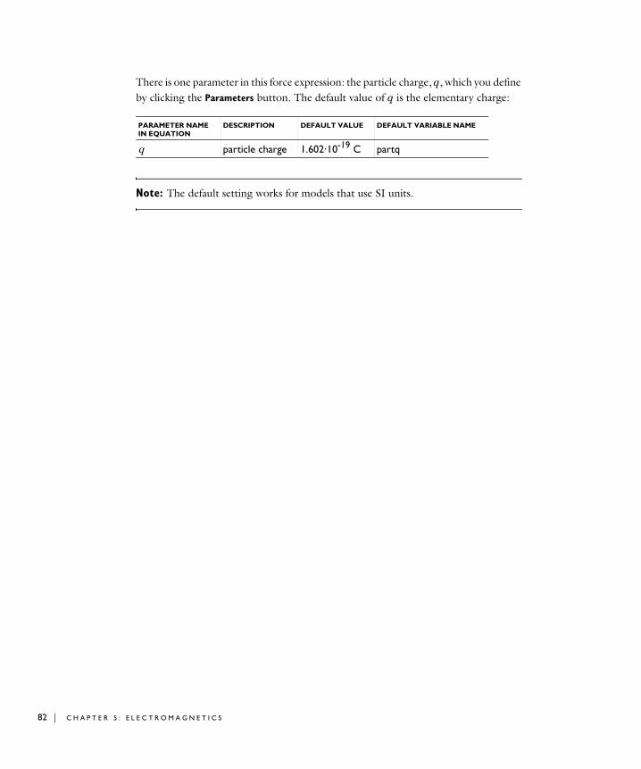
82 | C H A P T E R
There is one parameter in this force expression: the particle charge, q, which you define by clicking the Parameters button. The default value of q is the elementary charge:
Note: The default setting works for models that use SI units.
PARAMETER NAME IN EQUATION
DESCRIPTION DEFAULT VALUE DEFAULT VARIABLE NAME
q particle charge 1.602·10-19 C partq
5 : E L E C T R O M A G N E T I C S
Th e Condu c t i v e Med i a DC App l i c a t i o n Mode
Electrolysis and the computation of resistances of grounding plates involves a medium with electric conductivity σ and a steady current.
You can use the Conductive Media DC application mode for 3D, 2D in-plane, and 2D axisymmetric models.
PDE Formulation
When handling conductive media you must consider the equation of continuity. In a stationary coordinate system, the point form of Ohm’s law states that
where Je is an externally generated current density. The static form of the equation of continuity then gives
To handle current sources, generalize the equation to
The in-plane Conductive Media DC application mode assumes that your model has a symmetry where the electric potential varies only in the x and y directions and is constant in the z direction. This implies that the electric field, E, is tangential to the xy-plane. The application mode solves the following equation where d is the thickness in the z direction:
The axisymmetric Conductive Media DC application mode considers the situation where the fields and geometry are axially symmetric. In this case the electric potential is constant in the direction, which implies that the electric field is tangential to the rz-plane.
J σE Je+=
∇ J⋅ ∇– σ V∇ Je–( )⋅ 0= =
∇– σ V∇ Je–( )⋅ Qj=
∇– d σ V∇ Je–( )⋅ dQj=
ϕ
T H E C O N D U C T I V E M E D I A D C A P P L I C A T I O N M O D E | 83
84 | C H A P T E R
Writing the generalized equation for Qj in cylindrical coordinates and multiplying it by r to avoid singularities at r = 0 results in
S P E C I F Y I N G T H E C O N D U C T I V I T Y
You can provide the conductivity in three different ways:
• Isotropic conductivity: a scalar number or expression
• Anisotropic conductivity: several components of a conductivity tensor to define an anisotropic material
• Temperature-dependent conductivity (which occurs in, for example, Joule heating, which is also called resistive heating). In this case the following equation describes the conductivity:
where ρ0 is the resistivity at the reference temperature T0. α is the temperature coefficient of resistivity, which describes how the resistivity varies with temperature. T is the current temperature, which can be a value that you specify or the temperature from a heat transfer application mode (in the Joule Heating predefined multiphysics coupling, this is the default setting).
Boundary Conditions
The relevant interface condition at interfaces between different media for this application mode is
This is fulfilled by the natural boundary condition
C U R R E N T F L O W
The current-flow boundary condition
r∂∂
z∂∂
T
– rσ r∂∂V
z∂∂V
rJe–
⎝ ⎠⎜ ⎟⎜ ⎟⎜ ⎟⎜ ⎟⎛ ⎞
⋅ rQj=
σ 1ρ0 1 α T T0–( )+( )-----------------------------------------------=
n2 J1 J2–( )⋅ 0=
n σ V∇ Je–( )1 σ V∇ Je
–( )2–[ ]⋅ n– J1 J2–( )⋅ 0= =
5 : E L E C T R O M A G N E T I C S
specifies the normal component of the current density for the current flowing across the boundary.
I N W A R D C U R R E N T F L O W
The inward-current flow boundary condition
is similar to the previous current-flow boundary condition except this case specifies the normal component of the current density rather than the complete vector. When the normal component Jn is positive then the current flows inwards towards the boundary.
D I S T R I B U T E D R E S I S T A N C E
You can use the distributed resistance boundary condition
to model a thin sheet of a resistive material. The sheet has the thickness d and is connected to the potential Vref.
E L E C T R I C I N S U L A T I O N
The electric-insulation boundary condition
specifies that no current flows across the boundary.
This boundary condition is also applicable at symmetric boundaries where the potential is known to be symmetric with respect to the boundary.
E L E C T R I C P O T E N T I A L
The electric-potential boundary condition
specifies the voltage at a boundary. Because you are solving for the potential in this application mode, you generally define the value of the potential at some boundary in the geometry.
n J⋅ n J0⋅=
n J⋅– Jn=
n J⋅ σd--- V Vref–( ),= n J1 J2–( )⋅ σ
d--- V Vref–( )=
n J⋅ 0=
V V0=
T H E C O N D U C T I V E M E D I A D C A P P L I C A T I O N M O D E | 85
86 | C H A P T E R
G R O U N D
The ground boundary condition
is a special case of the previous one but specifies zero potential. This boundary condition is also applicable at symmetry boundaries where the potential is known to be antisymmetric with respect to the boundary.
C U R R E N T S O U R C E
You can apply the current-source boundary condition
to interior boundaries that represent either a current source or sink.
C O N T I N U I T Y
The continuity boundary condition
specifies that the normal components of the electric current are continuous across the interior boundary.
C O N T A C T R E S I S T A N C E
You can use the contact resistance boundary condition
to model a thin layer of a resistive material. The layer has the thickness d and the conductivity σ. This boundary condition is only available at the border between the parts in an assembly.
A X I A L S Y M M E T R Y
In axisymmetric models, use the boundary condition for axial symmetry at the symmetry axis r = 0.
V 0=
n J1 J2–( )⋅ Jn=
n J1 J2–( )⋅ 0=
n J1⋅ σd--- V1 V2–( )=
n J2⋅ σd--- V2 V1–( )=
5 : E L E C T R O M A G N E T I C S
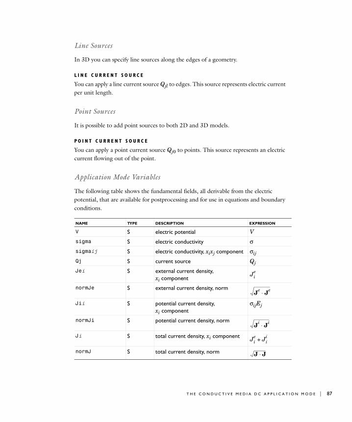
Line Sources
In 3D you can specify line sources along the edges of a geometry.
L I N E C U R R E N T S O U R C E
You can apply a line current source Qjl to edges. This source represents electric current per unit length.
Point Sources
It is possible to add point sources to both 2D and 3D models.
PO I N T C U R R E N T S O U R C E
You can apply a point current source Qj0 to points. This source represents an electric current flowing out of the point.
Application Mode Variables
The following table shows the fundamental fields, all derivable from the electric potential, that are available for postprocessing and for use in equations and boundary conditions.
NAME TYPE DESCRIPTION EXPRESSION
V S electric potential V
sigma S electric conductivity σsigmaij S electric conductivity, xixj component σij
Qj S current source Qj
Jei S external current density, xi component
normJe S external current density, norm
Jii S potential current density, xi component
σijEj
normJi S potential current density, norm
Ji S total current density, xi component
normJ S total current density, norm
Jie
Je Je⋅
Ji Ji⋅
Jie Ji
i+
J J⋅
T H E C O N D U C T I V E M E D I A D C A P P L I C A T I O N M O D E | 87
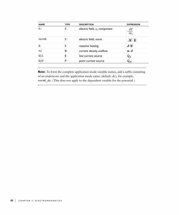
88 | C H A P T E R
Note: To form the complete application mode variable names, add a suffix consisting of an underscore and the application mode name (default: dc), for example, normE_dc. (This does not apply to the dependent variable for the potential.)
Ei S electric field, xi component
normE S electric field, norm
Q S resistive heating J · E
nJ B current density outflow n · J
Qjl E line current source Qjl
Qj0 P point current source Qj0
NAME TYPE DESCRIPTION EXPRESSION
V∂xi∂
-------–
E E⋅
5 : E L E C T R O M A G N E T I C S
Th e E l e c t r o s t a t i c s App l i c a t i o n Mode
Applications involving electrostatics include high-voltage apparatus, electronic devices, and capacitors. The term “statics” means that the time rate of change of the electric field is slow, and that wavelengths are very large compared to the size of the domain of interest.
The Electrostatics application mode is available for 3D, 2D in-plane, and 2D axisymmetric models.
PDE Formulation
COMSOL Multiphysics carries out the modeling of static electric fields using the electric potential V. By combining the definition of potential with Gauss’ law and the equation of continuity, it is possible to derive the classic Poisson’s equation.
Specifically, under static conditions the electric potential, V, is defined by the relationship
Combining this equation with the constitutive relationship D = ε0 E + P between D and E, it is possible to represent Gauss’ law as Poisson’s equation
The In-plane Electrostatics application mode assumes a symmetry where the electric potential varies only in the x and y directions and is constant in the z direction. This implies that the electric field, E, is tangential to the xy-plane. Given this symmetry, you solve the same equation as in the 3D case.
The Axisymmetric Electrostatics application mode considers the situation where the fields and geometry are axially symmetric. In this case the electric potential is constant in the direction, which implies that the electric field is tangential to the rz-plane.
Writing the previous equation for ρ in cylindrical coordinates and multiplying it by r to avoid singularities at r = 0, the equation becomes
E V∇–=
∇– ε0 V∇ P–( )⋅ ρ=
ϕ
T H E E L E C T R O S T A T I C S A P P L I C A T I O N M O D E | 89
90 | C H A P T E R
Application Scalar Variables
There is one application-specific scalar variable in this mode:
Boundary Conditions
The relevant interface condition at interfaces between different media for this mode is
In the absence of surface charges, this condition is fulfilled by the natural boundary condition
E L E C T R I C D I S P L A C E M E N T
The electric-displacement boundary condition
specifies the normal component of the electric displacement at a boundary.
S U R F A C E C H A R G E
The surface-charge boundary condition
specifies the surface charge density at an outer boundary or at an interior boundary between two nonconducting media.
Z E R O C H A R G E / S Y M M E T R Y
The zero charge/symmetry boundary condition
PROPERTY NAME DEFAULT DESCRIPTION
ε0 epsilon0 8.854187817·10-12 F/m Permittivity of vacuum
r∂∂
z∂∂
T
– rε0r∂
∂V
z∂∂V
rP–
⎝ ⎠⎜ ⎟⎜ ⎟⎜ ⎟⎜ ⎟⎛ ⎞
⋅ rρ=
n2 D1 D2–( )⋅ ρs=
n ε0 V∇ P–( )1 ε0 V∇ P–( )2–[ ]⋅ n– D1 D2–( )⋅ 0= =
n D⋅ n D0⋅=
n– D⋅ ρs,= n D1 D2–( )⋅ ρs=
5 : E L E C T R O M A G N E T I C S

specifies that the normal component of the electric displacement equals zero.
This boundary condition is also applicable at symmetry boundaries where the potential is known to be symmetric with respect to the boundary.
E L E C T R I C P O T E N T I A L
The electric-potential boundary condition
specifies the voltage at a boundary. Because you are solving for the potential in this application mode, you generally define the value of the potential at some boundary in the geometry.
G R O U N D
The ground boundary condition
is a special case of the previous one but specifying zero potential. This boundary condition is also applicable at symmetry boundaries where the potential is known to be antisymmetric with respect to the boundary.
C O N T I N U I T Y
The continuity boundary condition
specifies that the normal component of the electric displacement is continuous across the boundary.
T H I N L OW P E R M I T T I V I T Y G A P
You can use the thin low permittivity gap condition
n D⋅ 0=
V V0=
V 0=
n D1 D2–( )⋅ 0=
n D1⋅ εd--- V1 V2–( )=
n D2⋅ εd--- V2 V1–( )=
T H E E L E C T R O S T A T I C S A P P L I C A T I O N M O D E | 91
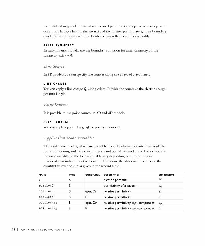
92 | C H A P T E R
N
to model a thin gap of a material with a small permittivity compared to the adjacent domains. The layer has the thickness d and the relative permittivity εr. This boundary condition is only available at the border between the parts in an assembly.
A X I A L S Y M M E T R Y
In axisymmetric models, use the boundary condition for axial symmetry on the symmetry axis r = 0.
Line Sources
In 3D models you can specify line sources along the edges of a geometry.
L I N E C H A R G E
You can apply a line charge Ql along edges. Provide the source as the electric charge per unit length.
Point Sources
It is possible to use point sources in 2D and 3D models.
P O I N T C H A R G E
You can apply a point charge Q0 at points in a model.
Application Mode Variables
The fundamental fields, which are derivable from the electric potential, are available for postprocessing and for use in equations and boundary conditions. The expressions for some variables in the following table vary depending on the constitutive relationship as indicated in the Const. Rel. column; the abbreviations indicate the constitutive relationship as given in the second table.
NAME TYPE CONST. REL. DESCRIPTION EXPRESSIO
V S electric potential V
epsilon0 S permittivity of a vacuum ε0
epsilonr S epsr, Dr relative permittivity εr
epsilonr S P relative permittivity 1
epsilonrij S epsr, Dr relative permittivity, xixj component εrij
epsilonrij S P relative permittivity, xixj component 1
5 : E L E C T R O M A G N E T I C S
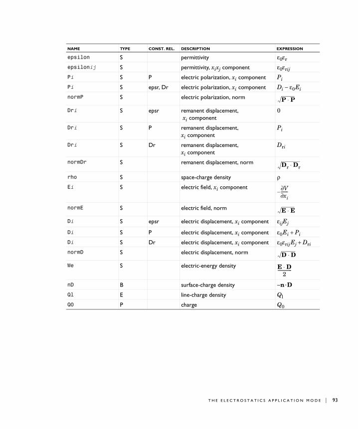
i
i
+ Dri
N
r
epsilon S permittivity ε0εr
epsilonij S permittivity, xixj component ε0εrij
Pi S P electric polarization, xi component Pi
Pi S epsr, Dr electric polarization, xi component Di − ε0 E
normP S electric polarization, norm
Dri S epsr remanent displacement, xi component
0
Dri S P remanent displacement, xi component
Pi
Dri S Dr remanent displacement, xi component
Dri
normDr S remanent displacement, norm
rho S space-charge density ρEi S electric field, xi component
normE S electric field, norm
Di S epsr electric displacement, xi component εijEj
Di S P electric displacement, xi component ε0 Ei + PDi S Dr electric displacement, xi component ε0εrij Ej normD S electric displacement, norm
We S electric-energy density
nD B surface-charge density −n · D
Ql E line-charge density Ql
Q0 P charge Q0
NAME TYPE CONST. REL. DESCRIPTION EXPRESSIO
P P⋅
Dr D⋅
V∂xi∂
-------–
E E⋅
D D⋅
E D⋅2
--------------
T H E E L E C T R O S T A T I C S A P P L I C A T I O N M O D E | 93
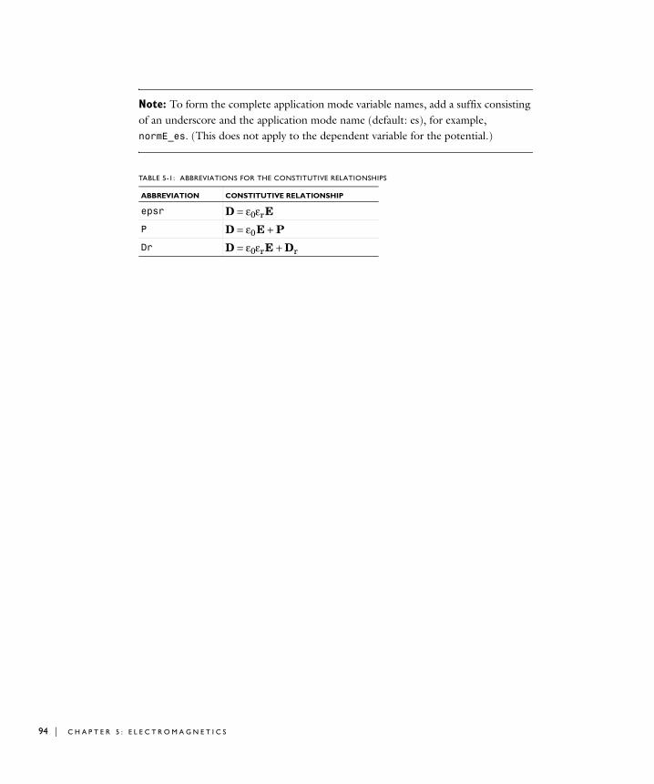
94 | C H A P T E R
Note: To form the complete application mode variable names, add a suffix consisting of an underscore and the application mode name (default: es), for example, normE_es. (This does not apply to the dependent variable for the potential.)
TABLE 5-1: ABBREVIATIONS FOR THE CONSTITUTIVE RELATIONSHIPS
ABBREVIATION CONSTITUTIVE RELATIONSHIP
epsr D = ε0εr E
P D = ε0 E + PDr D = ε0εr E + Dr
5 : E L E C T R O M A G N E T I C S
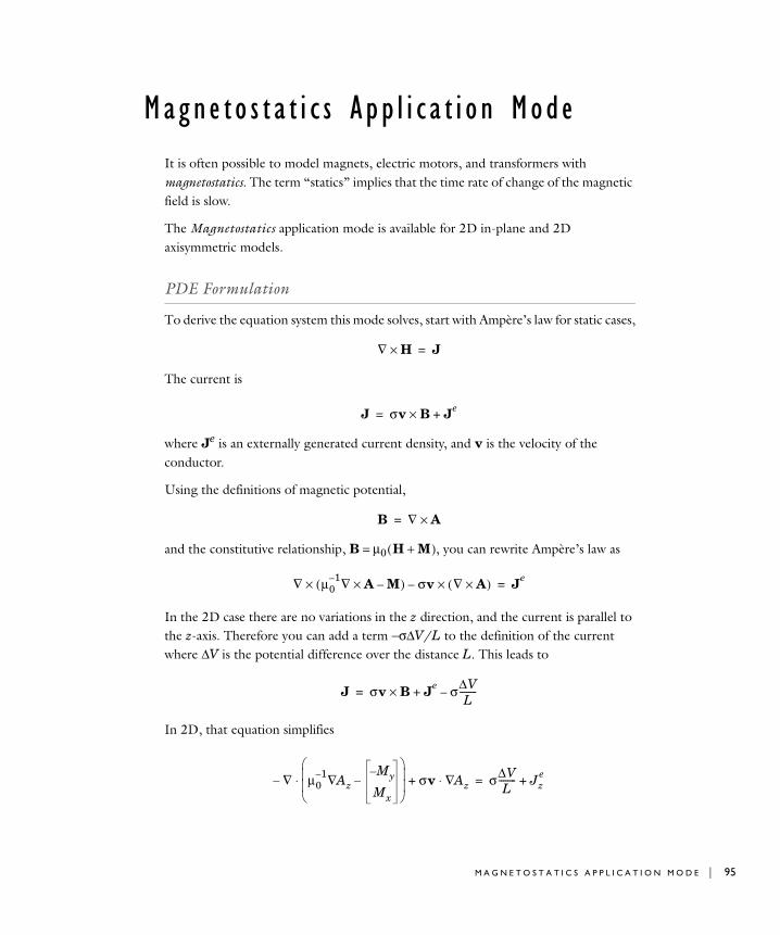
Magne t o s t a t i c s App l i c a t i o n Mode
It is often possible to model magnets, electric motors, and transformers with magnetostatics. The term “statics” implies that the time rate of change of the magnetic field is slow.
The Magnetostatics application mode is available for 2D in-plane and 2D axisymmetric models.
PDE Formulation
To derive the equation system this mode solves, start with Ampère’s law for static cases,
The current is
where Je is an externally generated current density, and v is the velocity of the conductor.
Using the definitions of magnetic potential,
and the constitutive relationship, B = µ0 ( H + M ), you can rewrite Ampère’s law as
In the 2D case there are no variations in the z direction, and the current is parallel to the z-axis. Therefore you can add a term −σ∆V/L to the definition of the current where ∆V is the potential difference over the distance L. This leads to
In 2D, that equation simplifies
∇ H× J=
J σv B× Je+=
B ∇ A×=
∇ µ01– ∇ A× M–( )× σv ∇ A×( )×– Je
=
J σv B× Je σ∆VL
--------–+=
∇ µ01– Az∇
M– y
Mx
–⎝ ⎠⎜ ⎟⎜ ⎟⎛ ⎞
⋅– σv Az∇⋅+ σ∆VL
-------- Jze
+=
M A G N E T O S T A T I C S A P P L I C A T I O N M O D E | 95
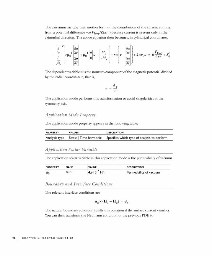
96 | C H A P T E R
The axisymmetric case uses another form of the contribution of the current coming from a potential difference −σ ( Vloop / (2π r )) because current is present only in the azimuthal direction. The above equation then becomes, in cylindrical coordinates,
The dependent variable u is the nonzero component of the magnetic potential divided by the radial coordinate r, that is,
The application mode performs this transformation to avoid singularities at the symmetry axis.
Application Mode Property
The application mode property appears in the following table:
Application Scalar Variable
The application scalar variable in this application mode is the permeability of vacuum.
Boundary and Interface Conditions
The relevant interface conditions are
The natural boundary condition fulfills this equation if the surface current vanishes. You can then transform the Neumann condition of the previous PDE to
PROPERTY VALUES DESCRIPTION
Analysis type Static | Time-harmonic Specifies which type of analysis to perform
PROPERTY NAME VALUE DESCRIPTION
µ0 mu0 4π·10-7 H/m Permeability of vacuum
r∂∂
z∂∂
T
rµ01– r∂
∂u
z∂∂u
µ01– 2
0u
Mz
M– r
–+
⎝ ⎠⎜ ⎟⎜ ⎟⎜ ⎟⎜ ⎟⎛ ⎞
– rσ v r∂∂u
z∂∂u
⋅
⎝ ⎠⎜ ⎟⎜ ⎟⎜ ⎟⎜ ⎟⎛ ⎞
2σvru+ + σVloop2πr
------------- Jϕe
+=
uAϕr
-------=
n2 H1 H2–( )× Js=
5 : E L E C T R O M A G N E T I C S
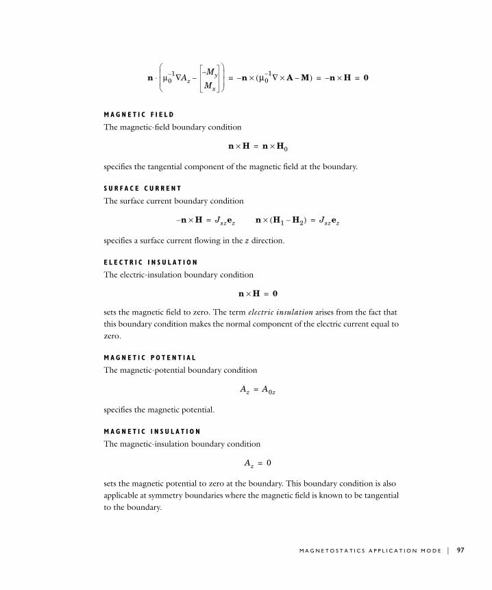
M A G N E T I C F I E L D
The magnetic-field boundary condition
specifies the tangential component of the magnetic field at the boundary.
S U R F A C E C U R R E N T
The surface current boundary condition
specifies a surface current flowing in the z direction.
E L E C T R I C I N S U L A T I O N
The electric-insulation boundary condition
sets the magnetic field to zero. The term electric insulation arises from the fact that this boundary condition makes the normal component of the electric current equal to zero.
M A G N E T I C P O T E N T I A L
The magnetic-potential boundary condition
specifies the magnetic potential.
M A G N E T I C I N S U L A T I O N
The magnetic-insulation boundary condition
sets the magnetic potential to zero at the boundary. This boundary condition is also applicable at symmetry boundaries where the magnetic field is known to be tangential to the boundary.
n µ01– Az∇
M– y
Mx
–⎝ ⎠⎜ ⎟⎜ ⎟⎛ ⎞
⋅ n µ01– ∇ A× M–( )×– n H×– 0= = =
n H× n H0×=
n H×– Jszez= n H1 H2–( )× Jszez=
n H× 0=
Az A0z=
Az 0=
M A G N E T O S T A T I C S A P P L I C A T I O N M O D E | 97
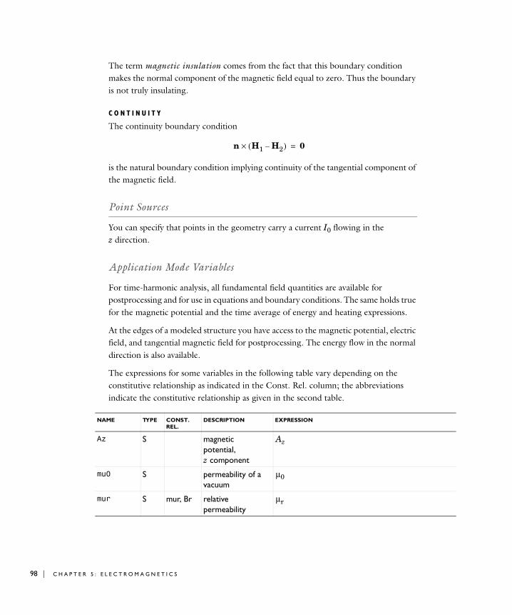
98 | C H A P T E R
The term magnetic insulation comes from the fact that this boundary condition makes the normal component of the magnetic field equal to zero. Thus the boundary is not truly insulating.
C O N T I N U I T Y
The continuity boundary condition
is the natural boundary condition implying continuity of the tangential component of the magnetic field.
Point Sources
You can specify that points in the geometry carry a current I0 flowing in the z direction.
Application Mode Variables
For time-harmonic analysis, all fundamental field quantities are available for postprocessing and for use in equations and boundary conditions. The same holds true for the magnetic potential and the time average of energy and heating expressions.
At the edges of a modeled structure you have access to the magnetic potential, electric field, and tangential magnetic field for postprocessing. The energy flow in the normal direction is also available.
The expressions for some variables in the following table vary depending on the constitutive relationship as indicated in the Const. Rel. column; the abbreviations indicate the constitutive relationship as given in the second table.
n H1 H2–( )× 0=
NAME TYPE CONST. REL.
DESCRIPTION EXPRESSION
Az S magnetic potential, z component
Az
mu0 S permeability of a vacuum
µ0
mur S mur, Br relative permeability
µr
5 : E L E C T R O M A G N E T I C S
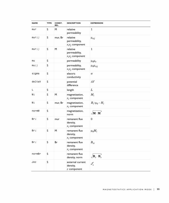
mur S M relative permeability
1
murij S mur, Br relative permeability, xixj component
µrij
murij S M relative permeability, xixj component
1
mu S permeability µ0µr
muij S permeability, xixj component
µ0µrij
sigma S electric conductivity
σ
deltaV S potential difference
∆V
L S length L
Mi S M magnetization, xi component
Mi
Mi S mur, Br magnetization, xi component
Bi / µ0 − Hi
normM S magnetization, norm
Bri S mur remanent flux density, xi component
0
Bri S M remanent flux density, xi component
µ0Mi
Bri S Br remanent flux density, xi component
Bri
normBr S remanent flux density, norm
Jez S external current density, z component
NAME TYPE CONST. REL.
DESCRIPTION EXPRESSION
M M*⋅
Br Br*⋅
Jze
M A G N E T O S T A T I C S A P P L I C A T I O N M O D E | 99
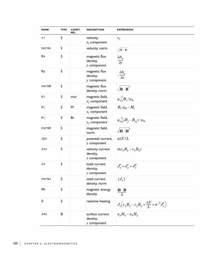
100 | C H A P T E
vi S velocity, xi component
vi
normv S velocity, norm
Bx S magnetic flux density, x component
By S magnetic flux density, y component
normB S magnetic flux density, norm
Hi S mur magnetic field, xi component
Hi S M magnetic field, xi component
Bi / µ0 − Mi
Hi S Br magnetic field, xi component
normH S magnetic field, norm
Jpz S potential current, z component
σ∆V/L
Jvz S velocity current density, z component
σ(vx By − vy Bx)
Jz S total current density, z component
normJ S total current density, norm
|Jz|
Wm S magnetic energy density
Q S resistive heating
Jsz B surface current density, z component
ny Hx − nx Hy
NAME TYPE CONST. REL.
DESCRIPTION EXPRESSION
v v⋅
Az∂y∂
---------
Az∂x∂
---------–
B B*⋅
µrij1– Bj µ0⁄
µrij1– Bj Brj–( ) µ0⁄
H H*⋅
Jze Jz
v Jzp
+ +
H B⋅2
--------------
Jz vxBy vyBx–∆VL
-------- σ 1– Jze
+ +⎝ ⎠⎛ ⎞
R 5 : E L E C T R O M A G N E T I C S
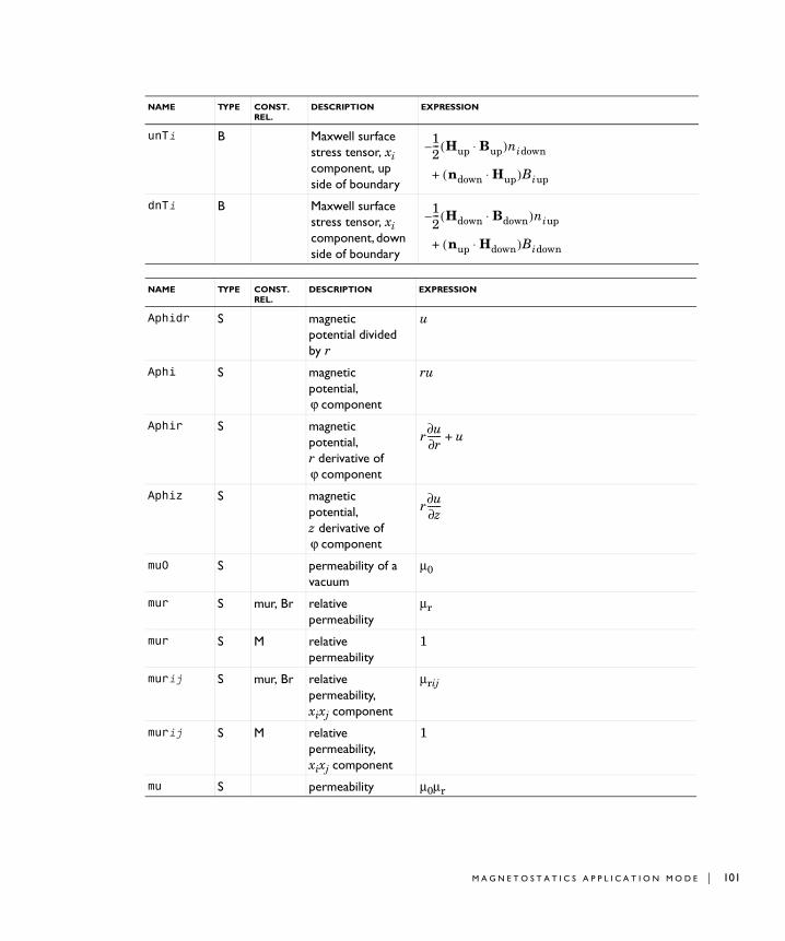
unTi B Maxwell surface stress tensor, xi component, up side of boundary
dnTi B Maxwell surface stress tensor, xi component, down side of boundary
NAME TYPE CONST. REL.
DESCRIPTION EXPRESSION
Aphidr S magnetic potential divided by r
u
Aphi S magnetic potential,
component
ru
Aphir S magnetic potential, r derivative of
component
Aphiz S magnetic potential, z derivative of
component
mu0 S permeability of a vacuum
µ0
mur S mur, Br relative permeability
µr
mur S M relative permeability
1
murij S mur, Br relative permeability, xixj component
µrij
murij S M relative permeability, xixj component
1
mu S permeability µ0µr
NAME TYPE CONST. REL.
DESCRIPTION EXPRESSION
12--- Hup Bup⋅( )nidown–
ndown Hup⋅( )Biup+
12--- Hdown Bdown⋅( )niup–
nup Hdown⋅( )Bidown+
ϕ
ϕ
r u∂r∂
------ u+
ϕ
r u∂z∂
------
M A G N E T O S T A T I C S A P P L I C A T I O N M O D E | 101
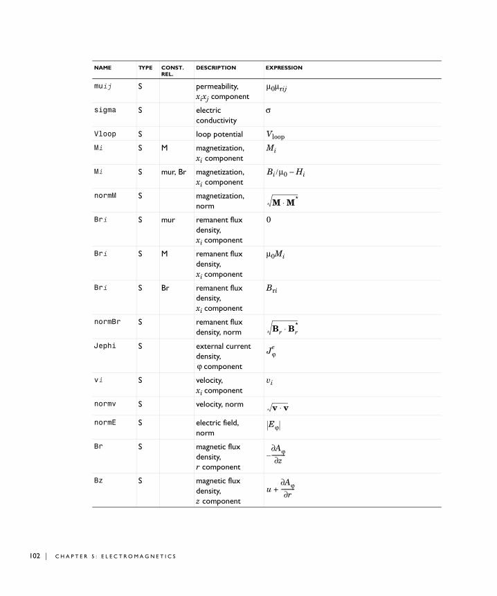
102 | C H A P T E
muij S permeability, xixj component
µ0µrij
sigma S electric conductivity
σ
Vloop S loop potential Vloop
Mi S M magnetization, xi component
Mi
Mi S mur, Br magnetization, xi component
Bi / µ0 − Hi
normM S magnetization, norm
Bri S mur remanent flux density, xi component
0
Bri S M remanent flux density, xi component
µ0Mi
Bri S Br remanent flux density, xi component
Bri
normBr S remanent flux density, norm
Jephi S external current density,
component
vi S velocity, xi component
vi
normv S velocity, norm
normE S electric field, norm
Br S magnetic flux density, r component
Bz S magnetic flux density, z component
NAME TYPE CONST. REL.
DESCRIPTION EXPRESSION
M M*⋅
Br Br*⋅
ϕ
Jϕe
v v⋅
Eϕ
Aϕ∂z∂
----------–
uAϕ∂r∂
----------+
R 5 : E L E C T R O M A G N E T I C S

normB S magnetic flux density, norm
Hi S mur magnetic field, xi component
Hi S M magnetic field, xi component
Bi / µ0 − Hi
Hi S Br magnetic field, xi component
normH S magnetic field, norm
Jpphi S loop current, component
σVloop/2πr
Jiphi S induced current density,
component
Jvphi S velocity current density,
component
σ(vz Br − vr Bz)
Jphi S total current density,
component
normJ S total current density, norm
Wm S magnetic energy density
Q S resistive heating
Jsphi B surface current density,
component
nr Hz − nz Hr
NAME TYPE CONST. REL.
DESCRIPTION EXPRESSION
B B*⋅
µrij1– Bj µ0⁄
µrij1– Bj Brj–( ) µ0⁄
H H*⋅
ϕ
ϕ
σEϕ
ϕ
ϕ
Jϕe Jϕ
v Jϕp
+ +
Jϕ
H B⋅2
--------------
Jϕ vrBz vzBr–Vloop2πr
------------- σ 1– Jϕe
+ +⎝ ⎠⎛ ⎞
ϕ
M A G N E T O S T A T I C S A P P L I C A T I O N M O D E | 103
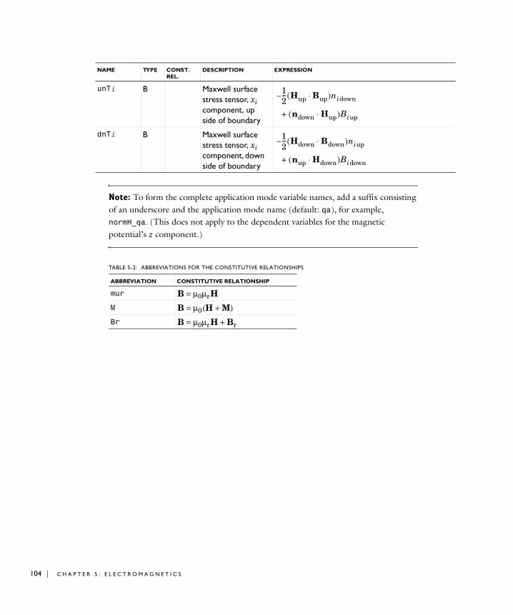
104 | C H A P T E
Note: To form the complete application mode variable names, add a suffix consisting of an underscore and the application mode name (default: qa), for example, normH_qa. (This does not apply to the dependent variables for the magnetic potential’s z component.)
unTi B Maxwell surface stress tensor, xi component, up side of boundary
dnTi B Maxwell surface stress tensor, xi component, down side of boundary
NAME TYPE CONST. REL.
DESCRIPTION EXPRESSION
12--- Hup Bup⋅( )nidown–
ndown Hup⋅( )Biup+
12--- Hdown Bdown⋅( )niup–
nup Hdown⋅( )Bidown+
TABLE 5-2: ABBREVIATIONS FOR THE CONSTITUTIVE RELATIONSHIPS
ABBREVIATION CONSTITUTIVE RELATIONSHIP
mur B = µ0µr H
M B = µ0 (H + M)Br B = µ0µr H + Br
R 5 : E L E C T R O M A G N E T I C S
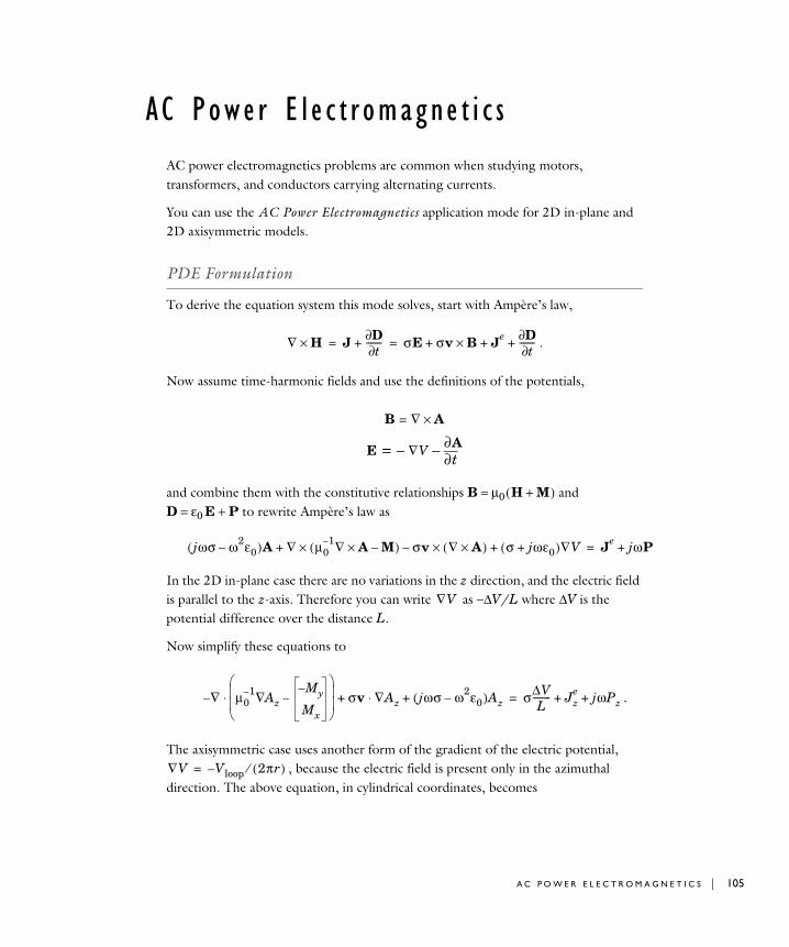
AC Powe r E l e c t r omagne t i c s
AC power electromagnetics problems are common when studying motors, transformers, and conductors carrying alternating currents.
You can use the AC Power Electromagnetics application mode for 2D in-plane and 2D axisymmetric models.
PDE Formulation
To derive the equation system this mode solves, start with Ampère’s law,
.
Now assume time-harmonic fields and use the definitions of the potentials,
and combine them with the constitutive relationships B = µ0 ( H + M ) and D = ε0 E + P to rewrite Ampère’s law as
In the 2D in-plane case there are no variations in the z direction, and the electric field is parallel to the z-axis. Therefore you can write as −∆V/L where ∆V is the potential difference over the distance L.
Now simplify these equations to
.
The axisymmetric case uses another form of the gradient of the electric potential, , because the electric field is present only in the azimuthal
direction. The above equation, in cylindrical coordinates, becomes
∇ H× J D∂t∂
-------+ σE σv B× Je D∂t∂
-------+ + += =
B ∇ A×=
E ∇V–t∂
∂A–=
jωσ ω2ε0–( )A ∇ µ01– ∇ A M–×( )× σv ∇ A×( ) σ jωε0+( )∇V+×–+ Je jωP+=
∇V
∇– µ01– Az∇
M– y
Mx
–⎝ ⎠⎜ ⎟⎜ ⎟⎛ ⎞
⋅ σv+ ∇Az⋅ jωσ ω2ε0–( )Az+ σ∆VL
-------- Jze
+ jωPz+=
∇V Vloop 2πr( )⁄–=
A C P O W E R E L E C T R O M A G N E T I C S | 105

106 | C H A P T E
ru
The dependent variable u is the nonzero component of the magnetic potential divided by the radial coordinate r, so that
The application mode performs this transformation to avoid singularities on the symmetry axis.
Application Scalar Variables
The application scalar variables in this application mode are:
The frequency occurs as a variable in time-harmonic problems.
Boundary and Interface Conditions
The relevant interface condition is
The natural boundary condition fulfills this equation if the surface current vanishes. You can transform the Neumann condition of this PDE into
PROPERTY NAME DEFAULT DESCRIPTION
µ0 mu0 4π·10-7 H/m Permeability of vacuum
ε0 epsilon0 8.854187817·10-12 F/m Permittivity of vacuum
ν nu 50 Hz Frequency
r∂∂
z∂∂ rµ0
1– r∂∂u
z∂∂u
µ01– 2
0u
Mz
M– r
–+
⎝ ⎠⎜ ⎟⎜ ⎟⎜ ⎟⎜ ⎟⎛ ⎞
⋅
⎝ ⎠⎜ ⎟⎜ ⎟⎜ ⎟⎜ ⎟⎛ ⎞
– rσ v r∂∂u
z∂∂u
⋅
⎝ ⎠⎜ ⎟⎜ ⎟⎜ ⎟⎜ ⎟⎛ ⎞
r σjω ω2ε0–( )u 2σv+ + +
σVloop2πr
-------------- Jϕe
+ jωPϕ+=
uAϕr
-------=
n2 H1 H2–( )× Js=
R 5 : E L E C T R O M A G N E T I C S
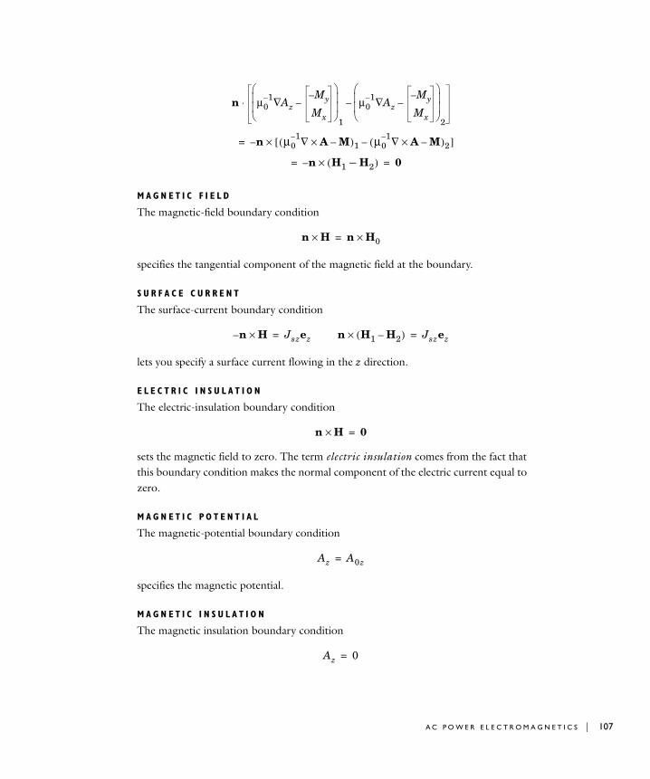
M A G N E T I C F I E L D
The magnetic-field boundary condition
specifies the tangential component of the magnetic field at the boundary.
S U R F A C E C U R R E N T
The surface-current boundary condition
lets you specify a surface current flowing in the z direction.
E L E C T R I C I N S U L A T I O N
The electric-insulation boundary condition
sets the magnetic field to zero. The term electric insulation comes from the fact that this boundary condition makes the normal component of the electric current equal to zero.
M A G N E T I C P O T E N T I A L
The magnetic-potential boundary condition
specifies the magnetic potential.
M A G N E T I C I N S U L A T I O N
The magnetic insulation boundary condition
n µ01– Az∇
M– y
Mx
–⎝ ⎠⎜ ⎟⎜ ⎟⎛ ⎞
1
µ01– Az∇
M– y
Mx
–⎝ ⎠⎜ ⎟⎜ ⎟⎛ ⎞
2
–⋅
n µ01– ∇ A× M–( )1 µ0
1– ∇ A× M–( )2–[ ]×–=
n H1 H2–( )×– 0= =
n H× n H0×=
n H×– Jszez= n H1 H2–( )× Jszez=
n H× 0=
Az A0z=
Az 0=
A C P O W E R E L E C T R O M A G N E T I C S | 107
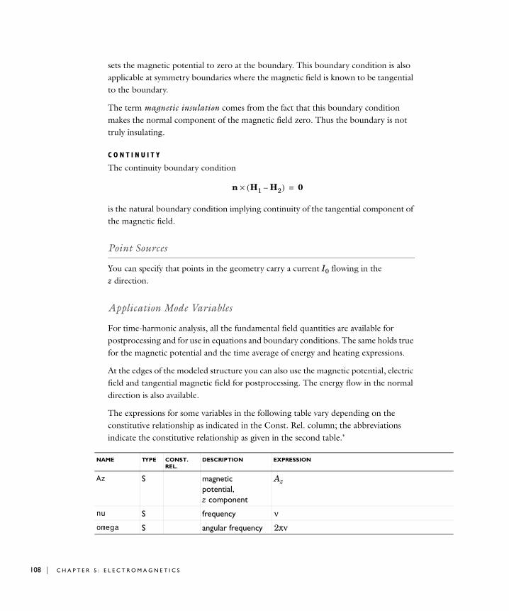
108 | C H A P T E
sets the magnetic potential to zero at the boundary. This boundary condition is also applicable at symmetry boundaries where the magnetic field is known to be tangential to the boundary.
The term magnetic insulation comes from the fact that this boundary condition makes the normal component of the magnetic field zero. Thus the boundary is not truly insulating.
C O N T I N U I T Y
The continuity boundary condition
is the natural boundary condition implying continuity of the tangential component of the magnetic field.
Point Sources
You can specify that points in the geometry carry a current I0 flowing in the z direction.
Application Mode Variables
For time-harmonic analysis, all the fundamental field quantities are available for postprocessing and for use in equations and boundary conditions. The same holds true for the magnetic potential and the time average of energy and heating expressions.
At the edges of the modeled structure you can also use the magnetic potential, electric field and tangential magnetic field for postprocessing. The energy flow in the normal direction is also available.
The expressions for some variables in the following table vary depending on the constitutive relationship as indicated in the Const. Rel. column; the abbreviations indicate the constitutive relationship as given in the second table.’
n H1 H2–( )× 0=
NAME TYPE CONST. REL.
DESCRIPTION EXPRESSION
Az S magnetic potential, z component
Az
nu S frequency νomega S angular frequency 2πν
R 5 : E L E C T R O M A G N E T I C S
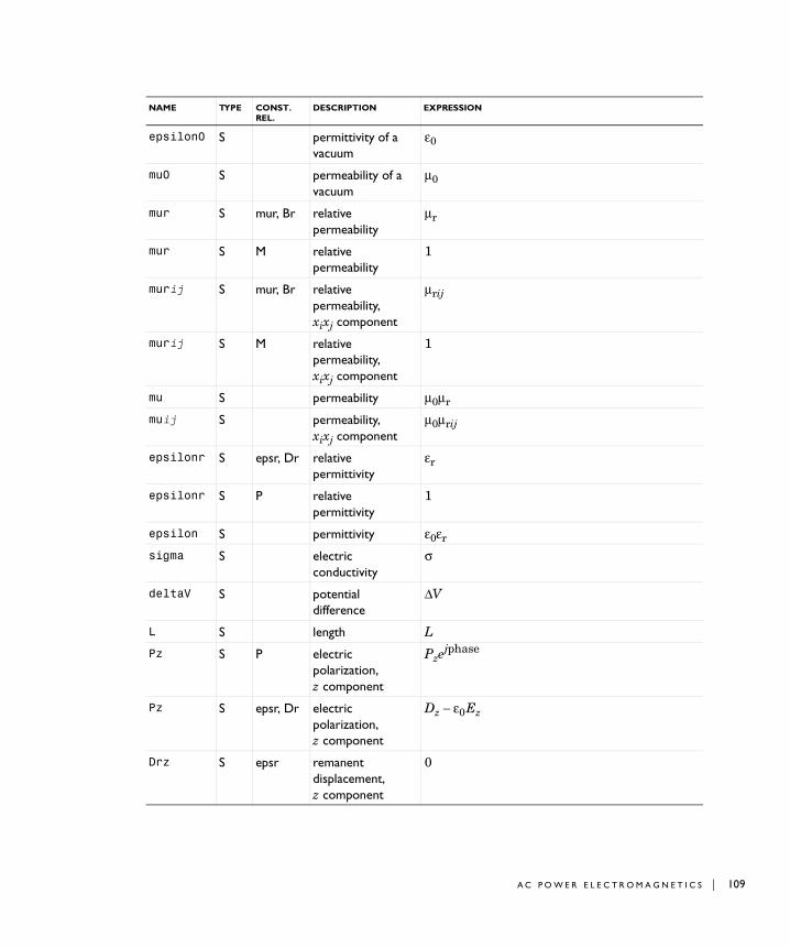
epsilon0 S permittivity of a vacuum
ε0
mu0 S permeability of a vacuum
µ0
mur S mur, Br relative permeability
µr
mur S M relative permeability
1
murij S mur, Br relative permeability, xixj component
µrij
murij S M relative permeability, xixj component
1
mu S permeability µ0µr
muij S permeability, xixj component
µ0µrij
epsilonr S epsr, Dr relative permittivity
εr
epsilonr S P relative permittivity
1
epsilon S permittivity ε0εr
sigma S electric conductivity
σ
deltaV S potential difference
∆V
L S length L
Pz S P electric polarization, z component
Pzejphase
Pz S epsr, Dr electric polarization, z component
Dz − ε0 Ez
Drz S epsr remanent displacement, z component
0
NAME TYPE CONST. REL.
DESCRIPTION EXPRESSION
A C P O W E R E L E C T R O M A G N E T I C S | 109
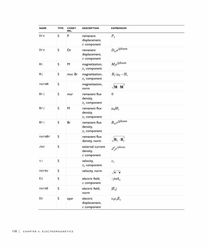
110 | C H A P T E
Drz S P remanent displacement, z component
Pz
Drz S Dr remanent displacement, z component
Drzejphase
Mi S M magnetization, xi component
Miejphase
Mi S mur, Br magnetization, xi component
Bi / µ0 − Hi
normM S magnetization, norm
Bri S mur remanent flux density, xi component
0
Bri S M remanent flux density, xi component
µ0Mi
Bri S Br remanent flux density, xi component
Bri ejphase
normBr S remanent flux density, norm
Jez S external current density, z component
vi S velocity, xi component
vi
normv S velocity, norm
Ez S electric field, z component
−jωAz
normE S electric field, norm
|Ez|
Dz S epsr electric displacement, z component
ε0εrEz
NAME TYPE CONST. REL.
DESCRIPTION EXPRESSION
M M*⋅
Br Br*⋅
Jzeejphase
v v⋅
R 5 : E L E C T R O M A G N E T I C S
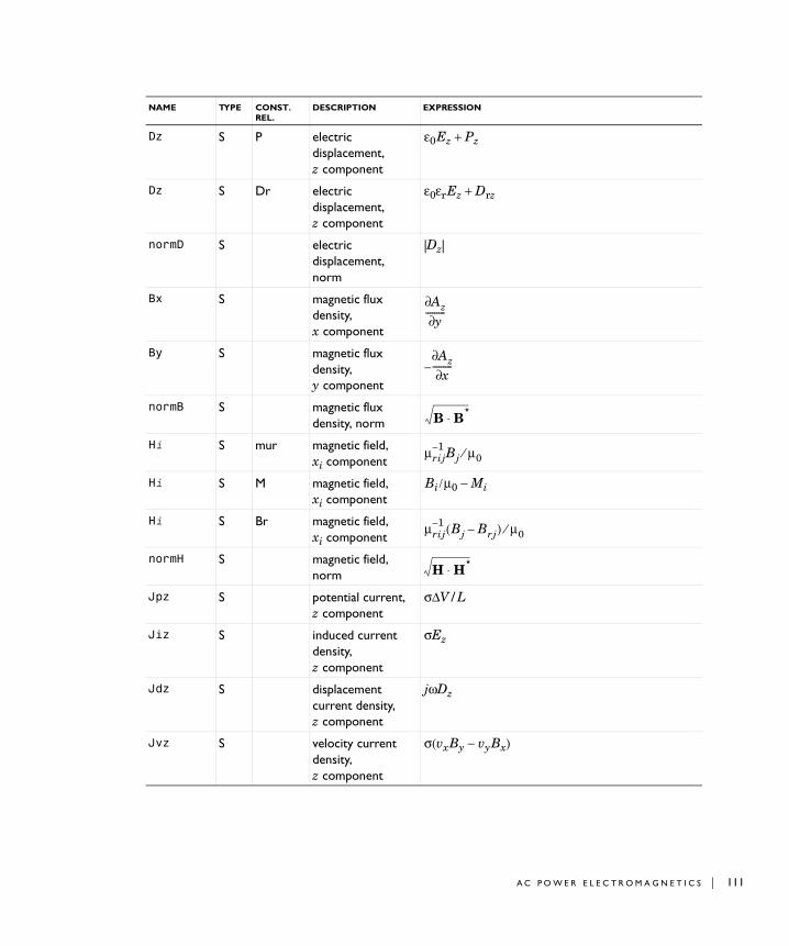
Dz S P electric displacement, z component
ε0 Ez + Pz
Dz S Dr electric displacement, z component
ε0εr Ez + Drz
normD S electric displacement, norm
|Dz|
Bx S magnetic flux density, x component
By S magnetic flux density, y component
normB S magnetic flux density, norm
Hi S mur magnetic field, xi component
Hi S M magnetic field, xi component
Bi / µ0 − Mi
Hi S Br magnetic field, xi component
normH S magnetic field, norm
Jpz S potential current, z component
σ∆V/L
Jiz S induced current density, z component
σEz
Jdz S displacement current density, z component
jωDz
Jvz S velocity current density, z component
σ(vx By − vy Bx)
NAME TYPE CONST. REL.
DESCRIPTION EXPRESSION
Az∂y∂
---------
Az∂x∂
---------–
B B*⋅
µrij1– Bj µ0⁄
µrij1– Bj Brj–( ) µ0⁄
H H*⋅
A C P O W E R E L E C T R O M A G N E T I C S | 111
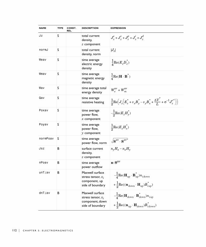
112 | C H A P T E
ze*⎠⎞⎠⎞
Jz S total current density, z component
normJ S total current density, norm
|Jz|
Weav S time average electric energy density
Wmav S time average magnetic energy density
Wav S time average total energy density
Qav S time average resistive heating
Poxav S time average power flow, x component
Poyav S time average power flow, y component
normPoav S time average power flow, norm
Jsz B surface current density, z component
ny Hx − nx Hy
nPoav B time average power outflow
n · Sav
unTiav B Maxwell surface stress tensor, xi component, up side of boundary
dnTiav B Maxwell surface stress tensor, xi component, down side of boundary
NAME TYPE CONST. REL.
DESCRIPTION EXPRESSION
Jze Jz
v Jzp Jz
i Jzd
+ + + +
14---Re EzDz
*( )
14---Re H B*⋅( )
Weav Wm
av+
12---Re Jz Ez
* vxBy* vyBx
*–
∆V*
L----------- σ 1– J+ + +⎝
⎛⎝⎛
12---Re EzHy
*( )–
12---Re EzHx
*( )
Sav Sav*⋅
14---Re Hup Bup
*⋅( )nidown–
12---Re ndown Hup⋅( )Biup
*( )+
14---Re Hdown Bdown
*⋅( )niup–
12---Re nup Hdown⋅( )Bidown
*( )+
R 5 : E L E C T R O M A G N E T I C S
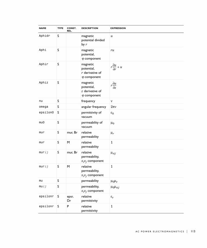
NAME TYPE CONST. REL.
DESCRIPTION EXPRESSION
Aphidr S magnetic potential divided by r
u
Aphi S magnetic potential,
component
ru
Aphir S magnetic potential, r derivative of
component
Aphiz S magnetic potential, z derivative of
component
nu S frequency νomega S angular frequency 2πνepsilon0 S permittivity of
vacuum ε0
mu0 S permeability of vacuum
µ0
mur S mur, Br relative permeability
µr
mur S M relative permeability
1
murij S mur, Br relative permeability, xixj component
µrij
murij S M relative permeability, xixj component
1
mu S permeability µ0µr
muij S permeability, xixj component
µ0µrij
epsilonr S epsr, Dr
relative permittivity
εr
epsilonr S P relative permittivity
1
ϕ
ϕ
r u∂r∂
------ u+
ϕ
r u∂z∂
------
A C P O W E R E L E C T R O M A G N E T I C S | 113
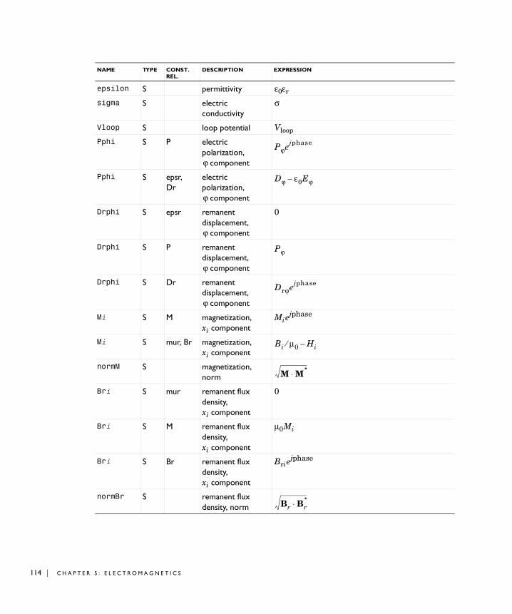
114 | C H A P T E
epsilon S permittivity ε0εr
sigma S electric conductivity
σ
Vloop S loop potential Vloop
Pphi S P electric polarization,
component
Pphi S epsr, Dr
electric polarization,
component
Drphi S epsr remanent displacement,
component
0
Drphi S P remanent displacement,
component
Drphi S Dr remanent displacement,
component
Mi S M magnetization, xi component
Mi ejphase
Mi S mur, Br magnetization, xi component
normM S magnetization, norm
Bri S mur remanent flux density, xi component
0
Bri S M remanent flux density, xi component
µ0 Mi
Bri S Br remanent flux density, xi component
Bri ejphase
normBr S remanent flux density, norm
NAME TYPE CONST. REL.
DESCRIPTION EXPRESSION
ϕ
Pϕejphase
ϕ
Dϕ ε0Eϕ–
ϕ
ϕ
Pϕ
ϕ
Drϕejphase
Bi µ0⁄ Hi–
M M*⋅
Br Br*⋅
R 5 : E L E C T R O M A G N E T I C S
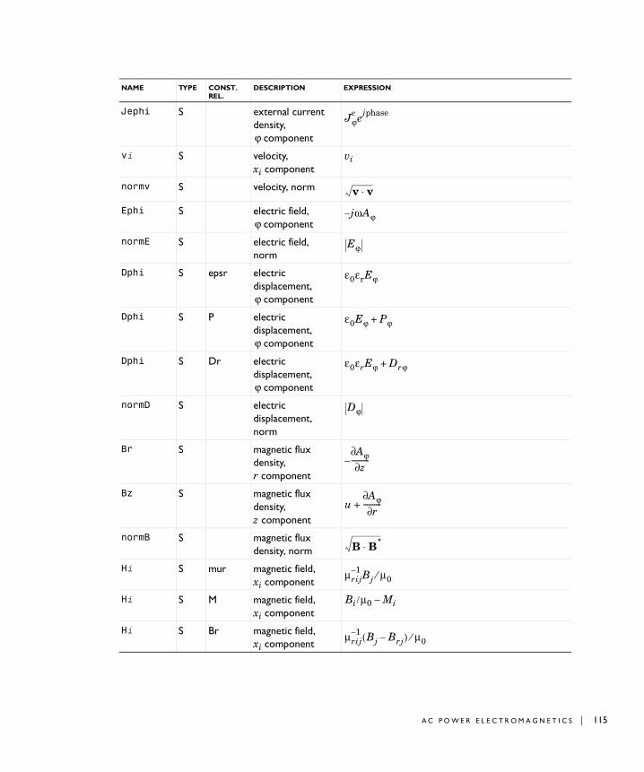
Jephi S external current density,
component
vi S velocity, xi component
vi
normv S velocity, norm
Ephi S electric field, component
normE S electric field, norm
Dphi S epsr electric displacement,
component
Dphi S P electric displacement,
component
Dphi S Dr electric displacement,
component
normD S electric displacement, norm
Br S magnetic flux density, r component
Bz S magnetic flux density, z component
normB S magnetic flux density, norm
Hi S mur magnetic field, xi component
Hi S M magnetic field, xi component
Bi / µ0 − Mi
Hi S Br magnetic field, xi component
NAME TYPE CONST. REL.
DESCRIPTION EXPRESSION
ϕ
Jϕe ejphase
v v⋅
ϕjωAϕ–
Eϕ
ϕ
ε0εrEϕ
ϕ
ε0Eϕ Pϕ+
ϕ
ε0εrEϕ Drϕ+
Dϕ
Aϕ∂z∂
----------–
uAϕ∂r∂
----------+
B B*⋅
µrij1– Bj µ0⁄
µrij1– Bj Brj–( ) µ0⁄
A C P O W E R E L E C T R O M A G N E T I C S | 115
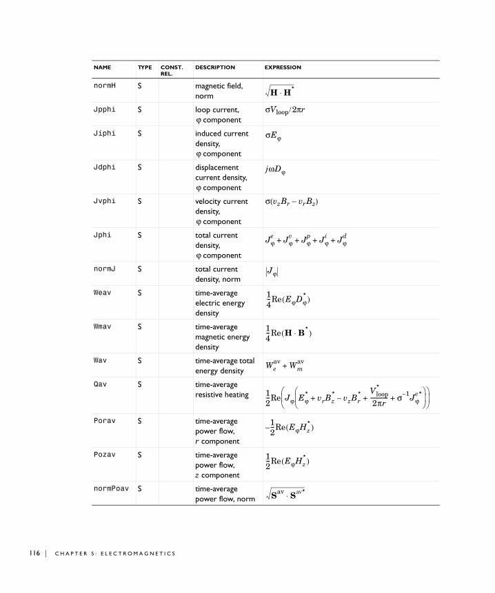
116 | C H A P T E
ϕe*
⎠⎟⎞
⎠⎟⎞
normH S magnetic field, norm
Jpphi S loop current, component
σVloop / 2πr
Jiphi S induced current density,
component
Jdphi S displacement current density,
component
Jvphi S velocity current density,
component
σ(vz Br − vr Bz)
Jphi S total current density,
component
normJ S total current density, norm
Weav S time-average electric energy density
Wmav S time-average magnetic energy density
Wav S time-average total energy density
Qav S time-average resistive heating
Porav S time-average power flow, r component
Pozav S time-average power flow, z component
normPoav S time-average power flow, norm
NAME TYPE CONST. REL.
DESCRIPTION EXPRESSION
H H*⋅
ϕ
ϕ
σEϕ
ϕ
jωDϕ
ϕ
ϕ
Jϕe Jϕ
v Jϕp Jϕ
i Jϕd
+ + + +
Jϕ
14---Re EϕDϕ
*( )
14---Re H B*⋅( )
Weav Wm
av+
12---Re Jϕ Eϕ
* vrBz* vzBr
*–
Vloop*
2πr------------- σ 1– J+ + +
⎝⎜⎛
⎝⎜⎛
12---Re EϕHz
*( )–
12---Re EϕHz
*( )
Sav Sav*⋅
R 5 : E L E C T R O M A G N E T I C S
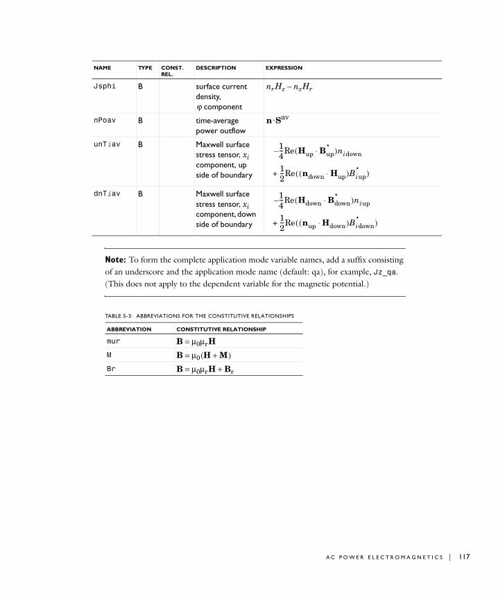
Note: To form the complete application mode variable names, add a suffix consisting of an underscore and the application mode name (default: qa), for example, Jz_qa. (This does not apply to the dependent variable for the magnetic potential.)
Jsphi B surface current density,
component
nr Hz − nz Hr
nPoav B time-average power outflow
n · Sav
unTiav B Maxwell surface stress tensor, xi component, up side of boundary
dnTiav B Maxwell surface stress tensor, xi component, down side of boundary
NAME TYPE CONST. REL.
DESCRIPTION EXPRESSION
ϕ
14---Re Hup Bup
*⋅( )nidown–
12---Re ndown Hup⋅( )Biup
*( )+
14---Re Hdown Bdown
*⋅( )niup–
12---Re nup Hdown⋅( )Bidown
*( )+
TABLE 5-3: ABBREVIATIONS FOR THE CONSTITUTIVE RELATIONSHIPS
ABBREVIATION CONSTITUTIVE RELATIONSHIP
mur B = µ0µr H
M B = µ0 (H + M )Br B = µ0µr H + Br
A C P O W E R E L E C T R O M A G N E T I C S | 117
118 | C H A P T E
Examp l e : E l e c t r i c S e n s o r
This is a model from electric impedance tomography, a method of imaging the interior permittivity distribution of an object by measuring current and voltage at the surface. The technique is used in, for example, medical diagnosis. Because different organs have different properties, you can “see” the organs and their movement from the outside.
The model shows how you can determine the shape and the placement of small objects with different material properties inside a closed box from outside. Applying a potential difference on the boundaries of the box gives rise to a surface charge density that varies depending on the permittivity distribution inside the box. By looking at the surface charge density you can therefore see the shape of the different materials inside the box.
Model Definition
This model solves Gauss’ law with ρ = 0.
The box contains air with εr equal to 1 and the different objects are made of material with different values of the relative permittivity, εr: 1, 2, and 3.
To get a voltage difference, set V = 0 on the bottom and V = 1 on top of the box. On all the other boundaries, use an electric insulation condition:
Results and Discussion
The surface charge density is higher above material with higher permittivity as expected. You can clearly see the shape of the figures inside the box on the top surface in the following plot.
∇ ε0εr∇V( )⋅– ρ=
n D⋅ 0=
R 5 : E L E C T R O M A G N E T I C S
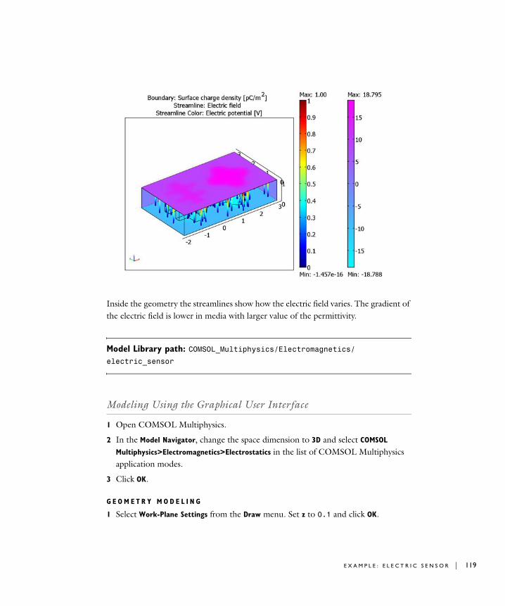
Inside the geometry the streamlines show how the electric field varies. The gradient of the electric field is lower in media with larger value of the permittivity.
Model Library path: COMSOL_Multiphysics/Electromagnetics/electric_sensor
Modeling Using the Graphical User Interface
1 Open COMSOL Multiphysics.
2 In the Model Navigator, change the space dimension to 3D and select COMSOL
Multiphysics>Electromagnetics>Electrostatics in the list of COMSOL Multiphysics application modes.
3 Click OK.
G E O M E T R Y M O D E L I N G
1 Select Work-Plane Settings from the Draw menu. Set z to 0.1 and click OK.
E X A M P L E : E L E C T R I C S E N S O R | 119
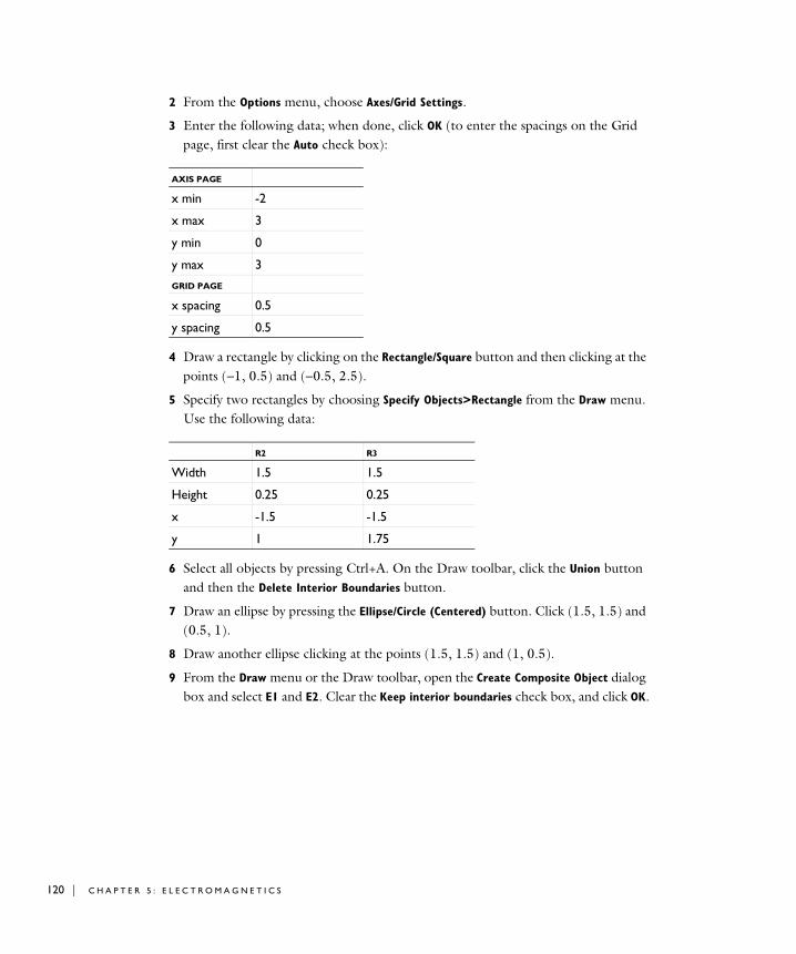
120 | C H A P T E
2 From the Options menu, choose Axes/Grid Settings.
3 Enter the following data; when done, click OK (to enter the spacings on the Grid page, first clear the Auto check box):
4 Draw a rectangle by clicking on the Rectangle/Square button and then clicking at the points (−1, 0.5) and (−0.5, 2.5).
5 Specify two rectangles by choosing Specify Objects>Rectangle from the Draw menu. Use the following data:
6 Select all objects by pressing Ctrl+A. On the Draw toolbar, click the Union button and then the Delete Interior Boundaries button.
7 Draw an ellipse by pressing the Ellipse/Circle (Centered) button. Click (1.5, 1.5) and (0.5, 1).
8 Draw another ellipse clicking at the points (1.5, 1.5) and (1, 0.5).
9 From the Draw menu or the Draw toolbar, open the Create Composite Object dialog box and select E1 and E2. Clear the Keep interior boundaries check box, and click OK.
AXIS PAGE
x min -2
x max 3
y min 0
y max 3
GRID PAGE
x spacing 0.5
y spacing 0.5
R2 R3
Width 1.5 1.5
Height 0.25 0.25
x -1.5 -1.5
y 1 1.75
R 5 : E L E C T R O M A G N E T I C S
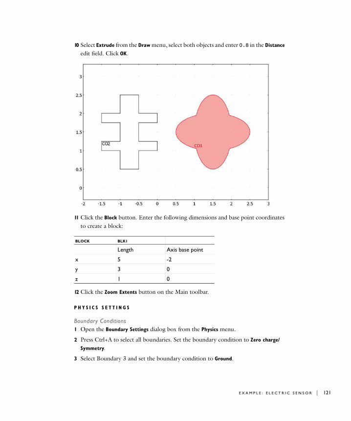
10 Select Extrude from the Draw menu, select both objects and enter 0.8 in the Distance edit field. Click OK.
11 Click the Block button. Enter the following dimensions and base point coordinates to create a block:
12 Click the Zoom Extents button on the Main toolbar.
P H Y S I C S S E T T I N G S
Boundary Conditions1 Open the Boundary Settings dialog box from the Physics menu.
2 Press Ctrl+A to select all boundaries. Set the boundary condition to Zero charge/
Symmetry.
3 Select Boundary 3 and set the boundary condition to Ground.
BLOCK BLK1
Length Axis base point
x 5 -2
y 3 0
z 1 0
E X A M P L E : E L E C T R I C S E N S O R | 121
122 | C H A P T E
4 Select Boundary 4 and set the boundary condition to Electric potential and V0 to 1.
5 Click OK.
Subdomain SettingsIn the Subdomain Settings dialog box, set the following values of εr:
M E S H G E N E R A T I O N
1 Open the Free Mesh Parameters dialog box and select Fine from the Predefined mesh
sizes list on the General tab. Click OK to close the dialog box.
2 Click the Initialize Mesh button on the Main toolbar to initialize the mesh.
C O M P U T I N G T H E S O L U T I O N
Solve the model by clicking the Solve button on the Main toolbar.
P O S T P R O C E S S I N G A N D V I S U A L I Z A T I O N
1 Open the Plot Parameters dialog box.
2 On the General page clear the Slice check box and select the Boundary and Streamline check boxes.
3 Click the Boundary tab. In the Boundary data area, select Surface charge density from the Predefined quantities list. In the Unit edit field, type pC/m^2.
4 In the Boundary color area, select cool from the Colormap list.
5 On the Streamline page, click the Line Color tab.
6 Click the Use expression button. Then click the Color Expression button and set the color data to Electric potential in the Predefined quantities list. Click OK.
7 Click the Start Points tab. Type 100 in the Number of start points edit field.
8 Select Tube from the Line type list.
9 Click the Tube Radius button and set the Radius data to Electric field, norm. Click OK.
10 Click OK.
To see the streamlines inside the box you must suppress some of the boundaries:
1 On the Options menu, point to Suppress and then click Suppress Boundaries.
2 In the dialog box select Boundaries 1, 2, and 6–37. Click OK.
3 Open the Plot Parameters dialog box and click OK.
SETTING SUBDOMAIN 1 SUBDOMAIN 2 SUBDOMAIN 3
εr (isotropic) 1 2 3
R 5 : E L E C T R O M A G N E T I C S

Examp l e : A Pe rmanen t Magne t
As an example of a magnetostatics problem, consider how to model a horseshoe-shaped permanent magnet. It consists of a ferromagnetic material, but the two end sections, often painted red and white, are premagnetized in opposite directions. The magnetic field pattern around such a permanent magnet is well known.
The domain consists of four regions:
• Three parts of the permanent magnet—the two premagnetized ends and the curved midsection
• The air surrounding the magnet
The permeability µ in air equals µ0 = 4π·10−7 H/m. Because the magnet is made of a ferromagnetic material, its relative permeability normally depends on the strength of the magnetic field, but in this model it is a constant with a value of 5000. The premagnetization adds a magnetization vector, pointing in the positive x direction at the upper end and in the negative x direction in the lower end. The magnitude of the magnetization is 750 kA/m.
It is reasonable to neglect the field at the boundaries of the computational domain, thus leading to the Dirichlet boundary condition A = 0 on the exterior boundary.
Model Library path: COMSOL_Multiphysics/Electromagnetics/permanent_magnet
Modeling Using the Graphical User Interface
M O D E L N A V I G A T O R
1 Go to the Model Navigator and select 2D in the Space dimension list.
2 Open the COMSOL Multiphysics>Electromagnetics folder and then select Magnetostatics in the list of application modes.
3 Use the default quadratic Lagrange elements.
4 Click OK.
E X A M P L E : A P E R M A N E N T M A G N E T | 123
124 | C H A P T E
O P T I O N S A N D S E T T I N G S
1 Enter the following values in the Axes/Grid Settings dialog box. To set the grid spacing, click the Grid tab and clear the Auto check box.
2 Enter these names and expressions in the Constants dialog box:
G E O M E T R Y M O D E L I N G
Start by modeling the upper and the lower premagnetized parts of the magnet.
1 Click the Rectangle/Square button and draw a rectangle from (0, 0.2) to (0.4, 0.4).
2 Click the Rectangle/Square button and draw a rectangle from (0, −0.4) to (0.4, −0.2).
Next draw the rest of the magnet using boundary modeling:
3 Click the Line button, and click the points (0.4, 0.2), (0.4, 0.4), and (0.6, 0.4).
4 Click the 2nd Degree Bézier Curve button, then click at the points (1, 0.4), (1, 0), (1, −0.4), and (0.6, −0.4).
5 Click Line and then click at the points (0.4, -0.4), (0.4, −0.2), and (0.6, -0.2).
6 Click 2nd Degree Bézier Curve and then click at the points (0.8, −0.2), (0.8, 0), (0.8, 0.2), and (0.6, 0.2).
7 Close the region with the right mouse button.
The last step in creating the geometry is to model the surrounding air.
8 Draw a rectangle from (−3, −2) to (3, 2).
AXIS GRID
x min -3 x spacing 0.2
x max 3 Extra x
y min -2 y spacing 0.2
y max 2 Extra y
NAME EXPRESSION
murFe 5000
Mpre 750000
R 5 : E L E C T R O M A G N E T I C S
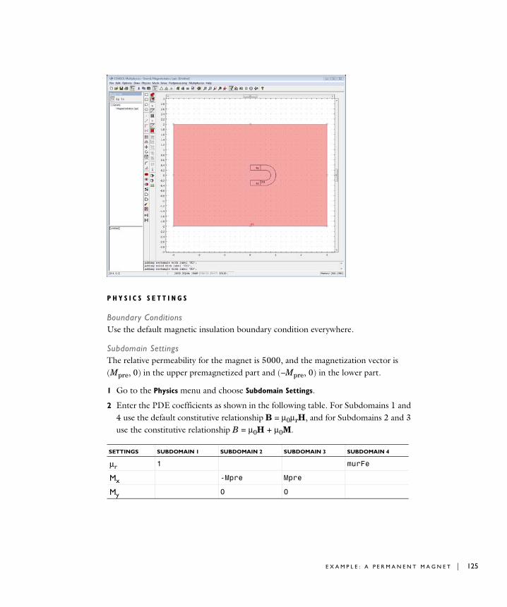
P H Y S I C S S E T T I N G S
Boundary ConditionsUse the default magnetic insulation boundary condition everywhere.
Subdomain SettingsThe relative permeability for the magnet is 5000, and the magnetization vector is (Mpre, 0) in the upper premagnetized part and (−Mpre, 0) in the lower part.
1 Go to the Physics menu and choose Subdomain Settings.
2 Enter the PDE coefficients as shown in the following table. For Subdomains 1 and 4 use the default constitutive relationship B = µ0µrH, and for Subdomains 2 and 3 use the constitutive relationship B = µ0H + µ0M.
SETTINGS SUBDOMAIN 1 SUBDOMAIN 2 SUBDOMAIN 3 SUBDOMAIN 4
µr 1 murFe
Mx -Mpre Mpre
My 0 0
E X A M P L E : A P E R M A N E N T M A G N E T | 125

126 | C H A P T E
M E S H G E N E R A T I O N
To resolve the field at the ends of the magnets, use a smaller mesh size at those boundaries:
1 From the Mesh menu, choose Free Mesh Parameters.
2 Click the Boundary tab.
3 Select Boundaries 4 and 7 (the ends of the magnet).
4 Type 0.01 in the Maximum element size edit field.
5 Click OK.
6 Click the Initialize Mesh button on the Main toolbar to create the mesh.
C O M P U T I N G T H E S O L U T I O N
Use the adaptive solver to improve the solution accuracy.
1 Go to the Solve menu and choose Solver Parameters.
2 In the Solver Parameters dialog box, select the Adaptive mesh refinement check box underneath the Solver list.
3 Click OK.
4 Click the Solve button.
P O S T P R O C E S S I N G A N D V I S U A L I Z A T I O N
Use the streamline plot to visualize the magnetic field using field lines where the distance between the lines is inversely proportional to the magnetic field strength.
1 Open the Plot Parameters dialog box.
2 Select the Streamline check box.
3 Click the Streamline tab.
4 Select Magnitude controlled from the Streamline plot type list.
5 Type 50 in the Density edit field.
6 Click the Line Color tab.
7 Click the Color button, and then select a white color from the palette in the Streamline Color dialog box. Click OK.
8 Click OK.
R 5 : E L E C T R O M A G N E T I C S
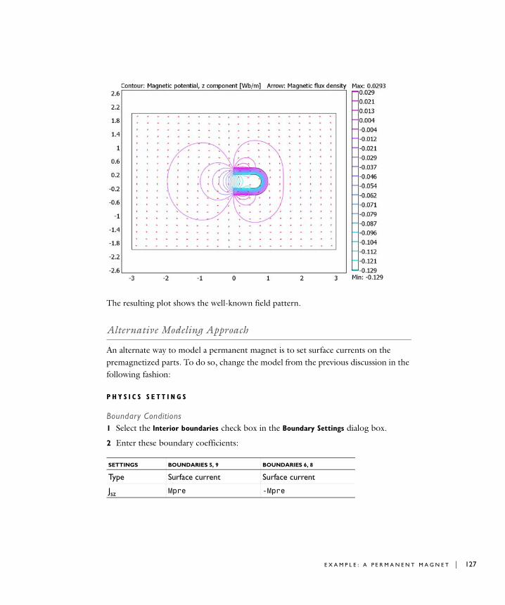
The resulting plot shows the well-known field pattern.
Alternative Modeling Approach
An alternate way to model a permanent magnet is to set surface currents on the premagnetized parts. To do so, change the model from the previous discussion in the following fashion:
P H Y S I C S S E T T I N G S
Boundary Conditions1 Select the Interior boundaries check box in the Boundary Settings dialog box.
2 Enter these boundary coefficients:
SETTINGS BOUNDARIES 5, 9 BOUNDARIES 6, 8
Type Surface current Surface current
Jsz Mpre -Mpre
E X A M P L E : A P E R M A N E N T M A G N E T | 127
128 | C H A P T E
Subdomain SettingsModify the subdomain settings to remove the magnetization:
C O M P U T I N G T H E S O L U T I O N
Go to the Solver Parameters dialog box and clear the Adaptive mesh refinement check box to turn off the adaptive solver. Simply use the mesh obtained by solving the previous problem. Solve the problem again.
P O S T P R O C E S S I N G A N D V I S U A L I Z A T I O N
The solution plot reveals a result identical to the one where you modeled the premagnetization using a magnetization vector.
References
1. D.K. Cheng, Field and Wave Electromagnetics. Addison-Wesley. Reading, MA, 1989.
2. J. Jin, The Finite Element Method in Electromagnetics, John Wiley & Sons, New York, 1993.
3. B.D. Popovic, Introductory Engineering Electromagnetics, Addison-Wesley, Reading, MA, 1971.
SETTING SUBDOMAINS 2, 3
Mx 0
R 5 : E L E C T R O M A G N E T I C S
6
F l u i d M e c h a n i c s
This chapter explains how to use the Incompressible Navier-Stokes application mode for the modeling and simulation of fluid mechanics and fluid statics. Note that the engineering community often uses the term CFD, computational fluid dynamics, to refer to the numerical simulation of fluids. This chapter concludes with step-by-step instructions on how to model a common benchmark problem: flow over a backward step in the absence of external forces.
129
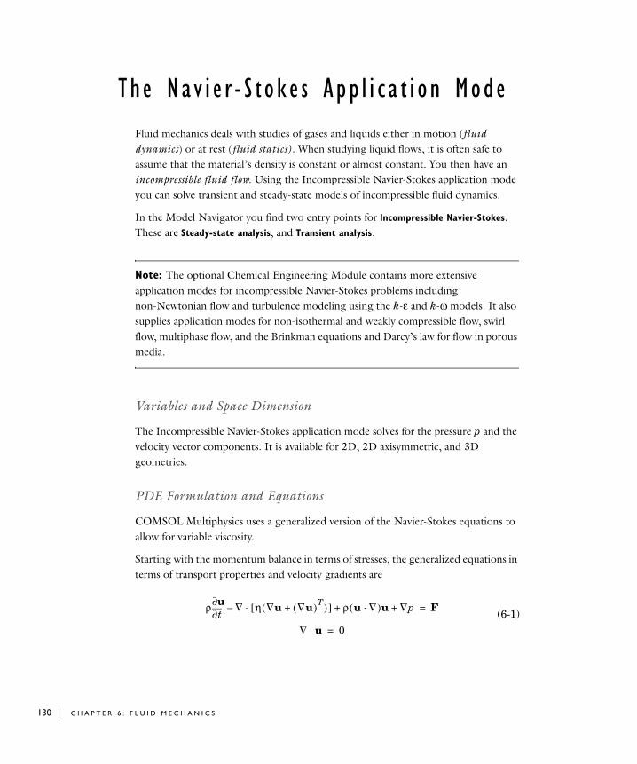
130 | C H A P T E
Th e Na v i e r - S t o k e s App l i c a t i o n Mode
Fluid mechanics deals with studies of gases and liquids either in motion (fluid dynamics) or at rest (fluid statics). When studying liquid flows, it is often safe to assume that the material’s density is constant or almost constant. You then have an incompressible fluid flow. Using the Incompressible Navier-Stokes application mode you can solve transient and steady-state models of incompressible fluid dynamics.
In the Model Navigator you find two entry points for Incompressible Navier-Stokes. These are Steady-state analysis, and Transient analysis.
Note: The optional Chemical Engineering Module contains more extensive application modes for incompressible Navier-Stokes problems including non-Newtonian flow and turbulence modeling using the k-ε and k-ω models. It also supplies application modes for non-isothermal and weakly compressible flow, swirl flow, multiphase flow, and the Brinkman equations and Darcy’s law for flow in porous media.
Variables and Space Dimension
The Incompressible Navier-Stokes application mode solves for the pressure p and the velocity vector components. It is available for 2D, 2D axisymmetric, and 3D geometries.
PDE Formulation and Equations
COMSOL Multiphysics uses a generalized version of the Navier-Stokes equations to allow for variable viscosity.
Starting with the momentum balance in terms of stresses, the generalized equations in terms of transport properties and velocity gradients are
(6-1)ρ
t∂∂u ∇ η ∇u ∇u( )T
+( )[ ]⋅– ρ u ∇⋅( )u ∇p+ + F=
∇ u⋅ 0=
R 6 : F L U I D M E C H A N I C S
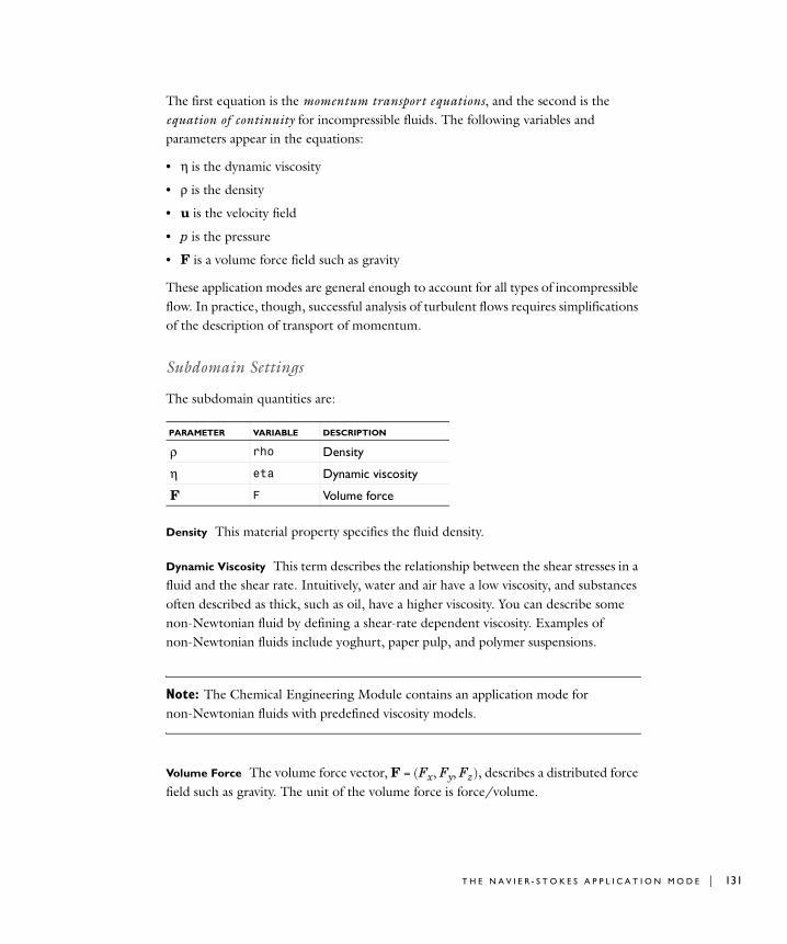
The first equation is the momentum transport equations, and the second is the equation of continuity for incompressible fluids. The following variables and parameters appear in the equations:
• η is the dynamic viscosity
• ρ is the density
• u is the velocity field
• p is the pressure
• F is a volume force field such as gravity
These application modes are general enough to account for all types of incompressible flow. In practice, though, successful analysis of turbulent flows requires simplifications of the description of transport of momentum.
Subdomain Settings
The subdomain quantities are:
Density This material property specifies the fluid density.
Dynamic Viscosity This term describes the relationship between the shear stresses in a fluid and the shear rate. Intuitively, water and air have a low viscosity, and substances often described as thick, such as oil, have a higher viscosity. You can describe some non-Newtonian fluid by defining a shear-rate dependent viscosity. Examples of non-Newtonian fluids include yoghurt, paper pulp, and polymer suspensions.
Note: The Chemical Engineering Module contains an application mode for non-Newtonian fluids with predefined viscosity models.
Volume Force The volume force vector, F = (Fx, Fy, Fz), describes a distributed force field such as gravity. The unit of the volume force is force/volume.
PARAMETER VARIABLE DESCRIPTION
ρ rho Density
η eta Dynamic viscosity
F F Volume force
T H E N A V I E R - S T O K E S A P P L I C A T I O N M O D E | 131
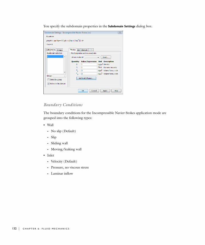
132 | C H A P T E
You specify the subdomain properties in the Subdomain Settings dialog box.
Boundary Conditions
The boundary conditions for the Incompressible Navier-Stokes application mode are grouped into the following types:
• Wall
- No slip (Default)
- Slip
- Sliding wall
- Moving/leaking wall
• Inlet
- Velocity (Default)
- Pressure, no viscous stress
- Laminar inflow
R 6 : F L U I D M E C H A N I C S

• Outlet
- Velocity
- Pressure
- Pressure, no viscous stress (Default)
- No viscous stress
- Normal stress
- Laminar outflow
• Symmetry boundary
- Symmetry (Default)
- Axial symmetry
• Open boundary
- Normal stress (Default)
- No viscous stress
• Stress
- General stress (Default)
- Normal stress
- Normal stress, normal flow
T H E N A V I E R - S T O K E S A P P L I C A T I O N M O D E | 133
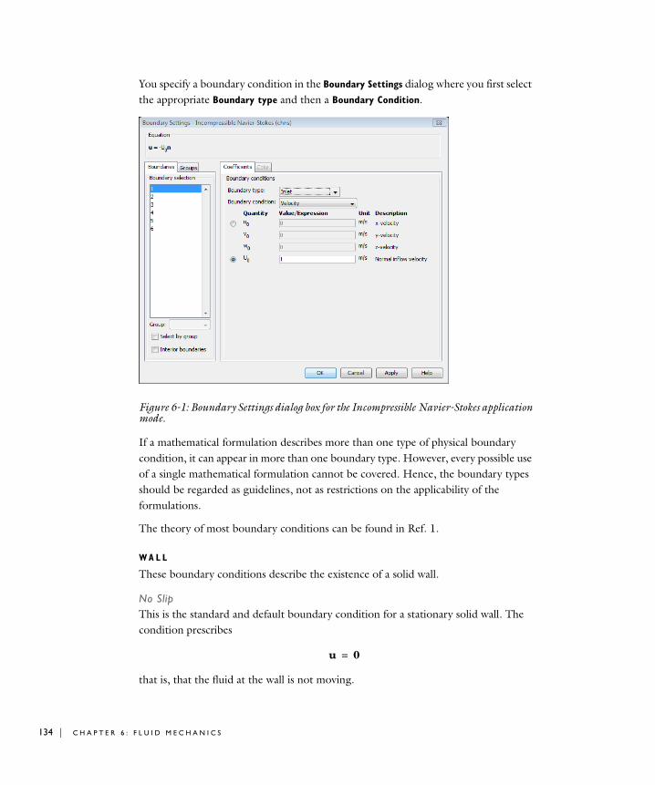
134 | C H A P T E
You specify a boundary condition in the Boundary Settings dialog where you first select the appropriate Boundary type and then a Boundary Condition.
Figure 6-1: Boundary Settings dialog box for the Incompressible Navier-Stokes application mode.
If a mathematical formulation describes more than one type of physical boundary condition, it can appear in more than one boundary type. However, every possible use of a single mathematical formulation cannot be covered. Hence, the boundary types should be regarded as guidelines, not as restrictions on the applicability of the formulations.
The theory of most boundary conditions can be found in Ref. 1.
WA L L
These boundary conditions describe the existence of a solid wall.
No SlipThis is the standard and default boundary condition for a stationary solid wall. The condition prescribes
that is, that the fluid at the wall is not moving.
u 0=
R 6 : F L U I D M E C H A N I C S
Moving/Perforated WallIf the wall moves, so must the fluid. Hence, this boundary condition prescribes
Note that setting this boundary condition does not automatically cause the associated wall to move. The section “The Moving Mesh Application Mode” on page 401 of the COMSOL Multiphysics Modeling Guide describes how to set up a model with moving boundaries.
You can also use the Moving/perforated wall boundary condition to simulate a wall where fluid is leaking into or leaving through a perforated wall.
Sliding WallIf you use this boundary condition, the wall is assumed to behave like a conveyor belt, that is, that the surface is sliding in its tangential direction. The wall does not have to actually move in the coordinate system.
In two space dimensions (2D), the tangential direction is unambiguously defined by the direction of the boundary. However, the situation becomes more complicated in 3D. For this reason, this boundary condition has slightly different definitions in the different space dimensions.
2D and Axial Symmetry The velocity is given as a scalar Uw and the condition prescribes
where t = (−ny , nx) for 2D and t = (−nz , nr) for axial symmetry.
3D The velocity is set equal to a given vector uw projected onto the boundary plane:
SlipThe slip condition assumes that there are no viscous effects at the slip wall and hence, no boundary layer develops. From a modeling point of view, this may be a reasonable approximation if the important effect of the wall is to prevent fluid from leaving the domain. Mathematically, the constraint can be formulated as:
u uw=
u n⋅ 0=
u t⋅ Uw=
u uw n uw⋅( )n–=
u n⋅ 0= , t pI– η ∇u ∇u( )T+( )+( )n⋅ 0=
T H E N A V I E R - S T O K E S A P P L I C A T I O N M O D E | 135
136 | C H A P T E
where t is a tangential vector to the boundary.
I N L E T
This boundary type contains different ways to specify conditions on a boundary where the fluid is supposed to enter the domain. Notice that the formulations contained in this boundary type all appear, some of them slightly modified, in the Outflow boundary type as well. Hence, there is nothing in the mathematical formulations that prevents a fluid from leaving the domain through boundaries where you have specified the Inlet boundary type.
VelocityThis boundary condition offers two ways to specify an inlet velocity. The first is to set the velocity equal to a given vector u0:
The other is to specify a normal inflow velocity:
Note that the boundary normal, n, is pointing out of the domain.
Pressure, No Viscous StressThis boundary condition specifies vanishing viscous stress along with a Dirichlet condition on the pressure:
It is a numerically stable boundary condition that admits total control of the pressure level along the entire boundary. However, if the inflow is not normal to the boundary, this condition is an overspecification. In the case that your solution turns out to have a non-normal inflow velocity, there are two choices. Either, move the boundary farther away to a location where the inflow is normal to the boundary or, use a stress type boundary condition described on page 139.
Note that this condition is identical to the Pressure, no viscous stress condition for Outflow boundaries. Hence, depending on the pressure field in the rest of the subdomain, a boundary with this condition can very well become an outflow boundary.
u u0=
u nU0–=
η ∇u ∇u( )T+( )n 0,= p p0=
R 6 : F L U I D M E C H A N I C S
O U T F L O W
This boundary type contains different ways to specify conditions on a boundary where the fluid exits the domain. Note that all of the formulations in this type can be found, possibly slightly modified, in other boundary types as well. Hence, there is nothing in the mathematical formulations that prevent a fluid from entering the domain through boundaries where you have set the Outflow boundary type.
Setting outlet conditions for the Navier-Stokes equations is not a trivial task. A general rule of thumb, however, is that if there is something interesting happening at an outflow boundary, extend the computational domain to include this phenomenon.
VelocityThis boundary condition offers two ways to specify an outlet velocity. The first is to set the velocity equal to a given vector u0:
The other is to specify a normal outlet velocity:
Observe that the boundary normal, n, is pointing out of the domain.
Pressure, No Viscous StressThis boundary condition specifies vanishing viscous stress along with a Dirichlet condition on the pressure:
It is a numerically stable boundary condition that admits total control of the pressure level at the whole boundary. However, if the outflow is not normal to the boundary, this condition is an overspecification. In the case that your solution turns out to have a non-normal outflow velocity, there are two choices. Either move the boundary farther away to a location where the outflow is normal to the boundary or use a stress type boundary condition described on page 139.
Observe that this condition is identical to the Pressure, no viscous stress condition for Inflow boundaries. Hence, depending on the pressure field in the rest of the subdomain, a boundary with this condition can very well become an inflow boundary.
PressureThis boundary condition prescribes only a Dirichlet condition for the pressure:
u u0=
u nU0=
η ∇u ∇u( )T+( )n 0,= p p0=
T H E N A V I E R - S T O K E S A P P L I C A T I O N M O D E | 137
138 | C H A P T E
Use this boundary condition only for high Reynolds number outflow boundaries, that is Rec = ρ | u | h / (2η) >>1. It is far less stable than the Pressure, no viscous stress boundary condition, but it is consistent with a non-normal outflow velocity.
No Viscous StressPrescribes vanishing viscous stress:
This condition can be useful in some situations because it does not impose any constraint on the pressure. A typical example is a model with volume forces that give rise to pressure gradients that are hard to prescribe in advance. It should however be combined with a point constraint on the pressure to be numerically stable (see “Point Settings” on page 140).
Normal StressThe total stress on the boundary is set equal to a stress vector of magnitude, f0, oriented in the negative normal direction:
This implies that the total stress in the tangential direction is zero. This boundary condition implicitly sets a constraint on the pressure that for 2D flows can be written
(6-2)
If ∂un / ∂n is small, Equation 6-2 can be interpreted as .
S Y M M E T R Y B O U N D A R Y
Prescribes no penetration and vanishing shear stresses:
In 2D Axial Symmetry, the above formulation is called Symmetry.
Axial SymmetryThis boundary condition is only available in 2D Axial Symmetry. Use it on all boundaries with coordinate r = 0. It prescribes ur = 0 and vanishing stresses in the z direction.
p p0=
η ∇u ∇u( )T+( )n 0=
pI– η ∇u ∇u( )T+( )+( )n f0n–=
p 2η∂un
∂n---------- f0+=
p f0≈
u n⋅ 0= , t pI– η ∇u ∇u( )T+( )+( )n⋅ 0=
R 6 : F L U I D M E C H A N I C S
O P E N B O U N D A R Y
You can use this boundary type on boundaries that are open to large volumes of fluid. Fluid can both enter and leave the domain on boundaries with this type of condition.
No Viscous StressPrescribes vanishing viscous stress:
This condition can be useful in some situations because it does not impose any constraint on the pressure. A typical example is a model with volume forces that give rise to pressure gradients that are hard to prescribe in advance. It should however be combined with a point constraint on the pressure to be numerically stable (see “Point Settings” on page 140).
Normal StressThe total stress on the boundary is set equal to a stress vector of magnitude, f0, oriented in the negative normal direction:
This implies that the total stress in the tangential direction is zero. This boundary condition implicitly sets a constraint on the pressure that for 2D flows can be written
(6-3)
If ∂un / ∂n is small, Equation 6-3 can be interpreted as .
S T R E S S
This type of boundary condition represents a very general class of conditions also known as traction boundary conditions.
General StressThe total stress on the boundary is set equal to a given stress F:
This boundary condition implicitly sets a constraint on the pressure that for 2D flows can be written
(6-4)
η ∇u ∇u( )T+( )n 0=
pI– η ∇u ∇u( )T+( )+( )n f0n–=
p 2η∂un
∂n---------- f0+=
p f0≈
pI– η ∇u ∇u( )T+( )+( )n F=
p 2η∂un
∂n---------- n F⋅–=
T H E N A V I E R - S T O K E S A P P L I C A T I O N M O D E | 139
140 | C H A P T E
If ∂un / ∂n is small, Equation 6-4 can be interpreted as .
Normal StressThe total stress on the boundary is set equal to a stress vector of magnitude, f0, oriented in the negative normal direction:
This implies that the total stress in the tangential direction is zero. This boundary condition implicitly sets a constraint on the pressure that for 2D flows can be written
(6-5)
If ∂un / ∂n is small, Equation 6-5 can be interpreted as .
Normal Stress, Normal FlowIn addition to the stress condition set in the Normal stress condition, this condition also prescribes that there must be no tangential velocities on the boundary:
Also this boundary condition implicitly sets a constraint on the pressure that for 2D flows can be written
(6-6)
If ∂un / ∂n is small, Equation 6-6 can be interpreted as .
Point Settings
If it is not possible to specify the pressure level using a boundary condition, the pressure must be set in some other way, for example, by specifying a fixed pressure at a point. You find a dialog box for Point Settings on the Physics menu.
Numerical Stability—Artificial Diffusion
The momentum equations (Equation 5-7) are of convection-diffusion type. It is well known that if standard Galerkin discretization is used, such equations become unstable for an element Peclet number (Pe) larger than one (Ref. 2):
p n F⋅–≈
pI– η ∇u ∇u( )T+( )+( )n f0n–=
p 2η∂un
∂n---------- f0+=
p f0≈
pI– η ∇u ∇u( )T+( )+( )n f0n–= , t u⋅ 0=
p 2η∂un∂n
---------- f0+=
p f0≈
R 6 : F L U I D M E C H A N I C S
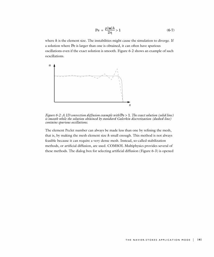
(6-7)
where h is the element size. The instabilities might cause the simulation to diverge. If a solution where Pe is larger than one is obtained, it can often have spurious oscillations even if the exact solution is smooth. Figure 6-2 shows an example of such ocscillations.
Figure 6-2: A 1D convection diffusion example with Pe > 1. The exact solution (solid line) is smooth while the solution obtained by standard Galerkin discretization (dashed line) contains spurious oscillations.
The element Peclet number can always be made less than one by refining the mesh, that is, by making the mesh element size h small enough. This method is not always feasible because it can require a very dense mesh. Instead, so-called stabilization methods, or artificial diffusion, are used. COMSOL Multiphysics provides several of these methods. The dialog box for selecting artificial diffusion (Figure 6-3) is opened
Pe ρ u h2η
---------------- 1>=
x
u
T H E N A V I E R - S T O K E S A P P L I C A T I O N M O D E | 141
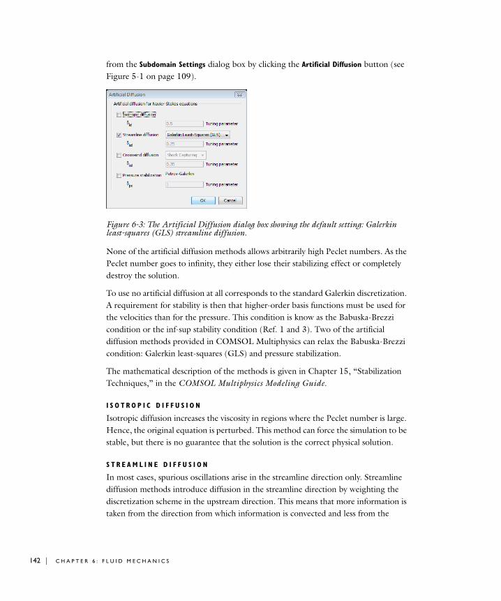
142 | C H A P T E
from the Subdomain Settings dialog box by clicking the Artificial Diffusion button (see Figure 5-1 on page 109).
Figure 6-3: The Artificial Diffusion dialog box showing the default setting: Galerkin least-squares (GLS) streamline diffusion.
None of the artificial diffusion methods allows arbitrarily high Peclet numbers. As the Peclet number goes to infinity, they either lose their stabilizing effect or completely destroy the solution.
To use no artificial diffusion at all corresponds to the standard Galerkin discretization. A requirement for stability is then that higher-order basis functions must be used for the velocities than for the pressure. This condition is know as the Babuska-Brezzi condition or the inf-sup stability condition (Ref. 1 and 3). Two of the artificial diffusion methods provided in COMSOL Multiphysics can relax the Babuska-Brezzi condition: Galerkin least-squares (GLS) and pressure stabilization.
The mathematical description of the methods is given in Chapter 15, “Stabilization Techniques,” in the COMSOL Multiphysics Modeling Guide.
I S O T R O P I C D I F F U S I O N
Isotropic diffusion increases the viscosity in regions where the Peclet number is large. Hence, the original equation is perturbed. This method can force the simulation to be stable, but there is no guarantee that the solution is the correct physical solution.
S T R E A M L I N E D I F F U S I O N
In most cases, spurious oscillations arise in the streamline direction only. Streamline diffusion methods introduce diffusion in the streamline direction by weighting the discretization scheme in the upstream direction. This means that more information is taken from the direction from which information is convected and less from the
R 6 : F L U I D M E C H A N I C S
direction in which the information is traveling. Streamline-diffusion methods are closely related to the upwind methods in finite difference and finite volume methods.
Anisotropic Streamline DiffusionThis method projects the extra diffusion onto the streamlines and is therefore much less brutal than the isotropic diffusion. Still, the method is not consistent, meaning that the exact solution does not solve the discrete system. Therefore, the accuracy of the solution cannot be guaranteed.
Streamline Upwind Petrov-Galerkin (SUPG)The Streamline Upwind Petrov-Galerkin method is a consistent method, which means that it does not perturb the equations. A model that converges with this method can be considered to be a solution to the discrete counterpart of Equation 5-6 and Equation 5-7. This method is somewhat less stabilizing than the anisotropic streamline diffusion because the terms that differ between the methods are mainly destabilizing.
Streamline Upwind Petrov-Galerkin (SUPG), CompensatedThis version of SUPG turns off the diffusion in regions with element Peclet number less than one.
Galerkin Least-Squares (GLS)The Galerkin least-squares (GLS) method is a consistent method that circumvents the Babuska-Brezzi condition, that is, it is possible to use equal-order elements for the velocities and the pressure.
For the momentum equations, GLS has many of its stability properties in common with SUPG. The superior stability of GLS can often be explained by the stabilizing terms on the continuum equation, terms that SUPG lacks.
GLS is activated per default even though it is more expensive to assemble than SUPG. The extra cost is often more than compensated for by the superior stability properties of GLS.
C R O S S W I N D D I F F U S I O N
In some cases, diffusion in the streamline direction is not enough to enforce stability. This is the situation in thin boundary layers and shear layers where there are large gradients in directions orthogonal to the streamline direction.
Ordo h3/2
The Ordo h3/2 method is an efficient and inexpensive method with good convergence properties. It is not consistent but has good accuracy compared to methods of similar complexity. However, the method is constructed exclusively for linear elements and it
T H E N A V I E R - S T O K E S A P P L I C A T I O N M O D E | 143
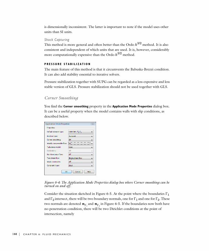
144 | C H A P T E
is dimensionally inconsistent. The latter is important to note if the model uses other units than SI units.
Shock CapturingThis method is more general and often better than the Ordo h3/2 method. It is also consistent and independent of which units that are used. It is, however, considerably more computationally expensive than the Ordo h3/2 method.
P R E S S U R E S T A B I L I Z A T I O N
The main feature of this method is that it circumvents the Babuska-Brezzi condition. It can also add stability essential to iterative solvers.
Pressure stabilization together with SUPG can be regarded as a less expensive and less stable version of GLS. Pressure stabilization should not be used together with GLS.
Corner Smoothing
You find the Corner smoothing property in the Application Mode Properties dialog box. It can be a useful property when the model contains walls with slip conditions, as described below.
Figure 6-4: The Application Mode Properties dialog box where Corner smoothing can be turned on and off.
Consider the situation sketched in Figure 6-5. At the point where the boundaries Γ1 and Γ2 intersect, there will be two boundary normals, one for Γ1 and one for Γ2. These two normals are denoted and in Figure 6-5. If the boundaries now both have no-penetration condition, there will be two Dirichlet conditions at the point of intersection, namely
nΓ1nΓ2
R 6 : F L U I D M E C H A N I C S
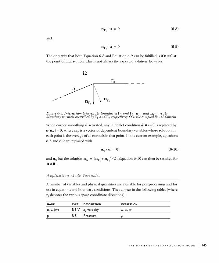
(6-8)
and
(6-9)
The only way that both Equation 6-8 and Equation 6-9 can be fulfilled is if u ≡ 0 at the point of intersection. This is not always the expected solution, however.
Figure 6-5: Intersection between the boundaries Γ1 and Γ2. and are the boundary normals prescribed by Γ1 and Γ2 respectively. Ω is the computational domain.
When corner smoothing is activated, any Dirichlet condition d(n) = 0 is replaced by d(nw) = 0, where nw is a vector of dependent boundary variables whose solution in each point is the average of all normals in that point. In the current example, equations 6-8 and 6-9 are replaced with
(6-10)
and nw has the solution . Equation 6-10 can then be satisfied for .
Application Mode Variables
A number of variables and physical quantities are available for postprocessing and for use in equations and boundary conditions. They appear in the following tables (where xi denotes the various space coordinate directions):
NAME TYPE DESCRIPTION EXPRESSION
u, v, (w) B S V xi velocity u, v, w
p B S Pressure p
nΓ1u⋅ 0=
nΓ2u⋅ 0=
ΩΓ2
Γ1
nΓ1nΓ2
nΓ1nΓ2
nw u⋅ 0=
nw nΓ1nΓ2
+( ) 2⁄=
u 0≠
T H E N A V I E R - S T O K E S A P P L I C A T I O N M O D E | 145
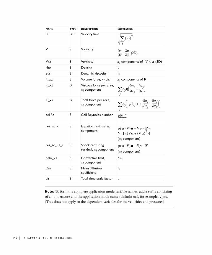
146 | C H A P T E
Note: To form the complete application mode variable names, add a suffix consisting of an underscore and the application mode name (default: ns), for example, V_ns. (This does not apply to the dependent variables for the velocities and pressure.)
U B S Velocity field
V S Vorticity (2D)
Vxi S Vorticity xi components of (3D)
rho S Density ρ
eta S Dynamic viscosity η
F_xi S Volume force, xi dir. xi components of F
K_xi B Viscous force per area, xi component
T_xi B Total force per area, xi component
cellRe S Cell Reynolds number
res_ui_c S Equation residual, ui component
(ui component)
res_sc_ui_c S Shock capturing residual, ui component
(ui component)
beta_xi S Convective field, xi component
ρui
Dm S Mean diffusion coefficient
η
da S Total time-scale factor ρ
NAME TYPE DESCRIPTION EXPRESSION
ui( )2
i∑
x∂∂v
y∂∂u
–
∇ u×
nj
j∑ η
ui∂xj∂
--------uj∂xi∂
--------+⎝ ⎠⎛ ⎞
nj
j∑ p– δij η
ui∂xj∂
--------uj∂xi∂
--------+⎝ ⎠⎛ ⎞+
ρ u hη
--------------
ρ u ∇⋅( )u ∇p F–
∇ η ∇u ∇u( )T+( )[ ]⋅
–+
ρ u ∇⋅( )u ∇p F–+
R 6 : F L U I D M E C H A N I C S
General Solver Settings
For a flow that is parallel to a coordinate axis, the automatic scaling feature in COMSOL Multiphysics does not work if you use the nonlinear stationary solver. For such cases, turn off the scaling feature or use manual scaling; see “Scaling of Variables and Equations” on page 497 in the COMSOL Multiphysics Reference Guide. The problem occurs when one solution component is identically zero.
Solver Settings
The recommended solver type for small and medium-sized fluid-flow problems is a direct solver, and the PARDISO direct solver is the default solver for 1D and 2D models. It is not as robust as UMFPACK or SPOOLES but is more memory efficient.
3D problems are often too large to solve using a direct solver. The default solver is GMRES with the geometric multigrid (GMG) preconditioner. The GMG preconditioner uses the Vanka preconditioner/smoother as the presmoother and postsmoother.
For more information about the solvers, see Chapter 6, “Solving the Model,” on page 359 in the COMSOL Multiphysics User’s Guide.
For a flow that is parallel to a coordinate axis, the automatic scaling feature in COMSOL Multiphysics does not work if you use the nonlinear stationary solver. For such cases, turn off the scaling feature or use manual scaling; see “Scaling of Variables and Equations” on page 497 in the COMSOL Multiphysics Reference Guide. The problem occurs when one solution component is close to zero
Khan and Richardson Force for Particle Tracing
The Khan and Richardson force is available for particle tracing plots in the Incompressible Navier-Stokes application mode and other application modes for fluid dynamics in the COMSOL Multiphysics products.
B A C K G R O U N D
The force expression that the software uses is derived partly using experimental results, and it is valid for a wide range of Reynolds numbers, stretching from creeping flow toward the turbulent regime (Ref. 4).
The following equation describes the total force that a fluid exerts on an immersed spherical particle:
T H E N A V I E R - S T O K E S A P P L I C A T I O N M O D E | 147

148 | C H A P T E
where the definition of the particle Reynolds number, Rep, is
.
The orientation of a given force component (for example, positive or negative x-component) is determined by the sign of the corresponding component in the vector difference , because this determines whether the fluid is accelerating or slowing down the particle in that direction.
U S I N G T H E K H A N A N D R I C H A R D S O N F O R C E F O R P A R T I C L E T R A C I N G
Thew Khan and Richardson force is the default selection in the Predefined forces list on the Particle Tracing tab.
There is one parameter in this force expression: the particle radius rp, which you defined by clicking the Parameters button. Table 6-1 shows the default values for this parameter:
The particle mass appears in the force equation, and you enter its value in the m edit field.The default value for the particle mass is mp = (4π / 3)·10−9 kg, which is the mass of a particle with the same density as water and a radius of 10−4 m, which is the default radius.
Note: The default settings work for models that use SI units.
References
1. P.M. Gresho and R.L. Sani, Incompressible Flow and the Finite Element Method, Volume 2: Isothermal Laminar Flow, John Wiley and Sons, LTD, 2000.
2. O.C. Zienkiewicz, R.L. Taylor, and P. Nithiarasu, The Finite Element Method for Fluid Dynamics, Sixth edition, Elsevier, 2005.
TABLE 6-1: PARAMETER FOR THE KHAN AND RICHARDSON FORCE
PARAMETER NAME IN EQUATION
DESCRIPTION DEFAULT VALUE DEFAULT VARIABLE NAME
rp particle radius 10-4 m partrad
F πrp2ρ u up–( )2 1.84 Rep( ) 0.31– 0.293 Rep( )0.06+( )3.45=
Rep u up– 2rpρ( ) η⁄=
u up–
R 6 : F L U I D M E C H A N I C S
3. C. Johnson, Numerical solution of partial differential equations by the finite element method, Studentlitteratur, 1987.
4. J.M. Coulson and J.F. Richardson, “Particle Technology and Separation Processes,” Chemical Engineering, vol. 2, Butterworth-Heinemann.
T H E N A V I E R - S T O K E S A P P L I C A T I O N M O D E | 149
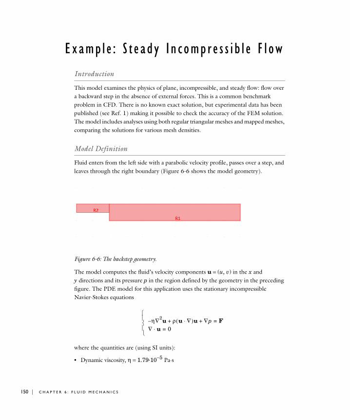
150 | C H A P T E
Examp l e : S t e a d y I n c omp r e s s i b l e F l ow
Introduction
This model examines the physics of plane, incompressible, and steady flow: flow over a backward step in the absence of external forces. This is a common benchmark problem in CFD. There is no known exact solution, but experimental data has been published (see Ref. 1) making it possible to check the accuracy of the FEM solution. The model includes analyses using both regular triangular meshes and mapped meshes, comparing the solutions for various mesh densities.
Model Definition
Fluid enters from the left side with a parabolic velocity profile, passes over a step, and leaves through the right boundary (Figure 6-6 shows the model geometry).
Figure 6-6: The backstep geometry.
The model computes the fluid’s velocity components u = (u, v) in the x and y directions and its pressure p in the region defined by the geometry in the preceding figure. The PDE model for this application uses the stationary incompressible Navier-Stokes equations
where the quantities are (using SI units):
• Dynamic viscosity, η = 1.79·10−5 Pa·s
η– ∇2u ρ u ∇⋅( )u ∇p+ + F=
∇ u⋅ 0=⎩⎪⎨⎪⎧
R 6 : F L U I D M E C H A N I C S
• Density, ρ = 1.23 kg/m3
• A force field, F, absent in this model
The first equation is the balance of momentum from Newton’s second law. The other relationship is the equation of continuity, where zero on the right-hand side states that the fluid is incompressible.
The shape of the flow pattern depends only on the Reynolds number.
In this model, you choose boundary conditions so that the average velocity at the inlet is Vmean = 0.544 m/s. To obtain a corresponding parabolic velocity profile, set (u, v) = (6Vmean s(1 − s), 0), where s is a boundary parameterization variable that runs from 0 to 1 along the boundary. The fluid is always stationary at the walls, so (u, v) = (0, 0) is the appropriate boundary condition. At the exit boundary, assume a constant static pressure p = 0.
For such a fluid flow you can expect a velocity field with a boundary layer of thickness approximately equal to 1/ at the walls. To resolve this steep solution gradient you need a few rows of elements across the layer. For a flow with a large Reynolds number, elements in the interior of the channel can be much larger than those near the walls.
U S I N G T H E I N C O M P R E S S I B L E N A V I E R - S T O K E S A P P L I C A T I O N M O D E
Start by setting up a model and solve this problem on a fixed isotropic mesh. The given input data correspond to a Reynolds number of
Even though you are working with a steady flow model, it needs initial conditions because the incompressible Navier-Stokes equations are nonlinear. To achieve a numerical solution, the nonlinear solver solves the equations iteratively.
Re
Re 0.544 2 0.0052 1.23⋅ ⋅ ⋅
1.79 10 5–⋅------------------------------------------------------------- 389≈=
E X A M P L E : S T E A D Y I N C O M P R E S S I B L E F L O W | 151
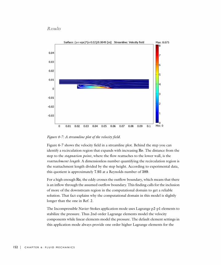
152 | C H A P T E
Results
Figure 6-7: A streamline plot of the velocity field.
Figure 6-7 shows the velocity field in a streamline plot. Behind the step you can identify a recirculation region that expands with increasing Re. The distance from the step to the stagnation point, where the flow reattaches to the lower wall, is the reattachment length. A dimensionless number quantifying the recirculation region is the reattachment length divided by the step height. According to experimental data, this quotient is approximately 7.93 at a Reynolds number of 389.
For a high enough Re, the eddy crosses the outflow boundary, which means that there is an inflow through the assumed outflow boundary. This finding calls for the inclusion of more of the downstream region in the computational domain to get a reliable solution. That fact explains why the computational domain in this model is slightly longer than the one in Ref. 2.
The Incompressible Navier-Stokes application mode uses Lagrange p2-p1 elements to stabilize the pressure. Thus 2nd-order Lagrange elements model the velocity components while linear elements model the pressure. The default element settings in this application mode always provide one order higher Lagrange elements for the
R 6 : F L U I D M E C H A N I C S
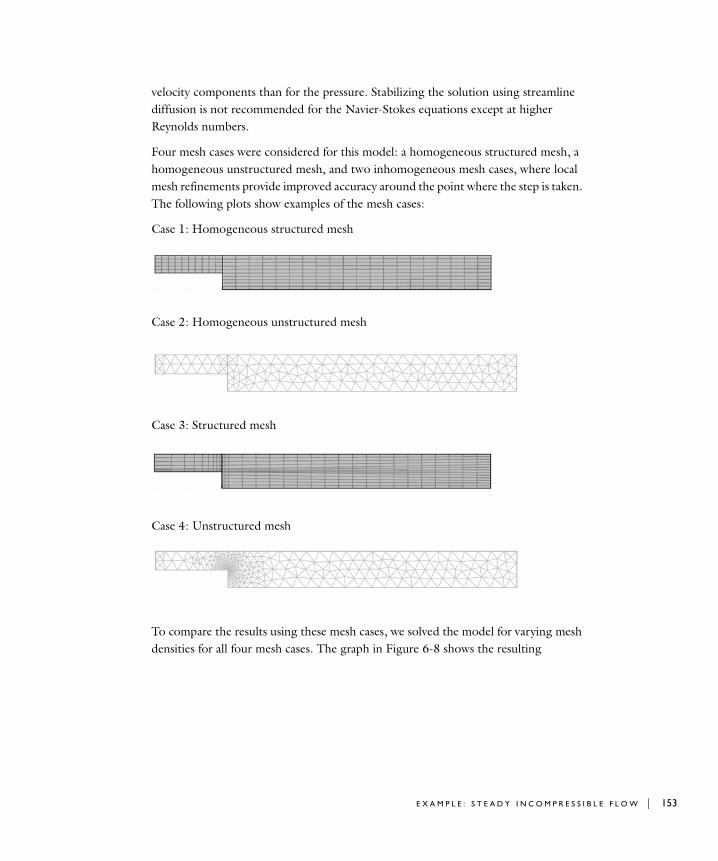
velocity components than for the pressure. Stabilizing the solution using streamline diffusion is not recommended for the Navier-Stokes equations except at higher Reynolds numbers.
Four mesh cases were considered for this model: a homogeneous structured mesh, a homogeneous unstructured mesh, and two inhomogeneous mesh cases, where local mesh refinements provide improved accuracy around the point where the step is taken. The following plots show examples of the mesh cases:
Case 1: Homogeneous structured mesh
Case 2: Homogeneous unstructured mesh
Case 3: Structured mesh
Case 4: Unstructured mesh
To compare the results using these mesh cases, we solved the model for varying mesh densities for all four mesh cases. The graph in Figure 6-8 shows the resulting
E X A M P L E : S T E A D Y I N C O M P R E S S I B L E F L O W | 153
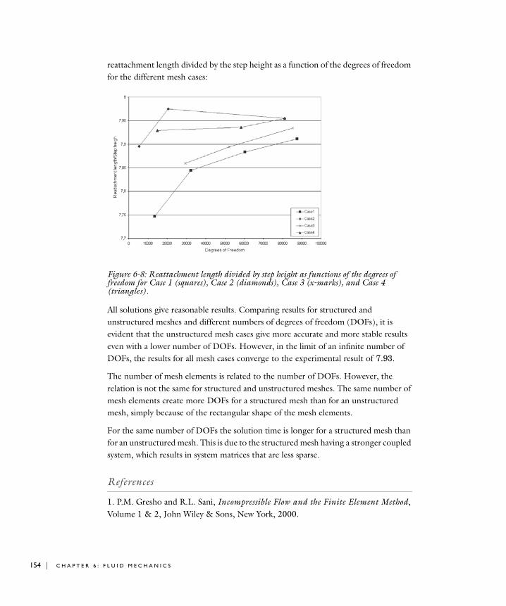
154 | C H A P T E
reattachment length divided by the step height as a function of the degrees of freedom for the different mesh cases:
Figure 6-8: Reattachment length divided by step height as functions of the degrees of freedom for Case 1 (squares), Case 2 (diamonds), Case 3 (x-marks), and Case 4 (triangles).
All solutions give reasonable results. Comparing results for structured and unstructured meshes and different numbers of degrees of freedom (DOFs), it is evident that the unstructured mesh cases give more accurate and more stable results even with a lower number of DOFs. However, in the limit of an infinite number of DOFs, the results for all mesh cases converge to the experimental result of 7.93.
The number of mesh elements is related to the number of DOFs. However, the relation is not the same for structured and unstructured meshes. The same number of mesh elements create more DOFs for a structured mesh than for an unstructured mesh, simply because of the rectangular shape of the mesh elements.
For the same number of DOFs the solution time is longer for a structured mesh than for an unstructured mesh. This is due to the structured mesh having a stronger coupled system, which results in system matrices that are less sparse.
References
1. P.M. Gresho and R.L. Sani, Incompressible Flow and the Finite Element Method, Volume 1 & 2, John Wiley & Sons, New York, 2000.
R 6 : F L U I D M E C H A N I C S
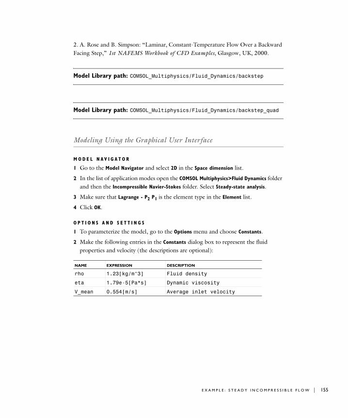
2. A. Rose and B. Simpson: “Laminar, Constant-Temperature Flow Over a Backward Facing Step,” 1st NAFEMS Workbook of CFD Examples, Glasgow, UK, 2000.
Model Library path: COMSOL_Multiphysics/Fluid_Dynamics/backstep
Model Library path: COMSOL_Multiphysics/Fluid_Dynamics/backstep_quad
Modeling Using the Graphical User Interface
M O D E L N A V I G A T O R
1 Go to the Model Navigator and select 2D in the Space dimension list.
2 In the list of application modes open the COMSOL Multiphysics>Fluid Dynamics folder and then the Incompressible Navier-Stokes folder. Select Steady-state analysis.
3 Make sure that Lagrange - P2 P1 is the element type in the Element list.
4 Click OK.
O P T I O N S A N D S E T T I N G S
1 To parameterize the model, go to the Options menu and choose Constants.
2 Make the following entries in the Constants dialog box to represent the fluid properties and velocity (the descriptions are optional):
NAME EXPRESSION DESCRIPTION
rho 1.23[kg/m^3] Fluid density
eta 1.79e-5[Pa*s] Dynamic viscosity
V_mean 0.554[m/s] Average inlet velocity
E X A M P L E : S T E A D Y I N C O M P R E S S I B L E F L O W | 155
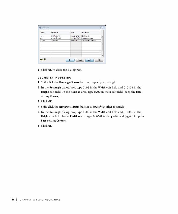
156 | C H A P T E
3 Click OK to close the dialog box.
G E O M E T R Y M O D E L I N G
1 Shift-click the Rectangle/Square button to specify a rectangle.
2 In the Rectangle dialog box, type 0.08 in the Width edit field and 0.0101 in the Height edit field. In the Position area, type 0.02 in the x edit field (keep the Base
setting Corner).
3 Click OK.
4 Shift-click the Rectangle/Square button to specify another rectangle.
5 In the Rectangle dialog box, type 0.02 in the Width edit field and 0.0052 in the Height edit field. In the Position area, type 0.0049 in the y edit field (again, keep the Base setting Corner).
6 Click OK.
R 6 : F L U I D M E C H A N I C S
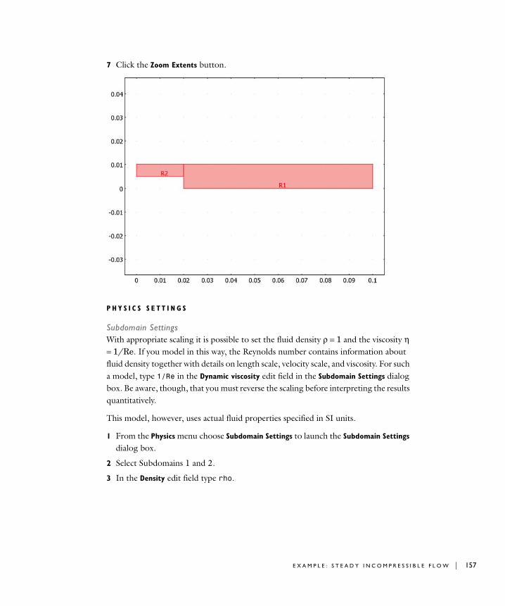
7 Click the Zoom Extents button.
P H Y S I C S S E T T I N G S
Subdomain SettingsWith appropriate scaling it is possible to set the fluid density ρ = 1 and the viscosity η = 1/Re. If you model in this way, the Reynolds number contains information about fluid density together with details on length scale, velocity scale, and viscosity. For such a model, type 1/Re in the Dynamic viscosity edit field in the Subdomain Settings dialog box. Be aware, though, that you must reverse the scaling before interpreting the results quantitatively.
This model, however, uses actual fluid properties specified in SI units.
1 From the Physics menu choose Subdomain Settings to launch the Subdomain Settings dialog box.
2 Select Subdomains 1 and 2.
3 In the Density edit field type rho.
E X A M P L E : S T E A D Y I N C O M P R E S S I B L E F L O W | 157

158 | C H A P T E
4 In the Dynamic viscosity edit field type eta.
The nonlinear solver also requires an initial value. With a low Reynolds number a simple constant expression is sufficient:
5 With both subdomains still selected, click the Init tab.
6 Enter the initial value V_mean in the edit field for u(t0); this value corresponds to a uniform x-velocity of magnitude Vmean throughout the domain. Leave the initial values for the y-velocity and the pressure at their default zero values.
7 Click OK.
R 6 : F L U I D M E C H A N I C S

Boundary ConditionsThe relevant boundary conditions for the model are:
The no-slip condition is the default setting, so you only need to modify the settings for Boundaries 1 and 8.
1 From the Physics menu, choose Boundary Settings.
2 Select Boundary 1.
3 In the Boundary type list select Inlet
4 In the U0 edit field type V_mean*6*s*(1-s).
5 Select Boundary 8.
6 In the Boundary type list select Outlet.
7 Click OK.
SETTINGS BOUNDARY 1 BOUNDARIES 2–5, 7 BOUNDARY 8
Boundary type Inlet Wall Outlet
Boundary condition Velocity No slip Pressure, no viscous stress
u0 V_mean*6*s*(1-s)
v0 0
p0 0
E X A M P L E : S T E A D Y I N C O M P R E S S I B L E F L O W | 159
160 | C H A P T E
M E S H G E N E R A T I O N
Because the Navier-Stokes equations are computationally difficult, it is important to use an appropriate mesh. If the mesh is too coarse, the solution might not converge at all or errors might be large. Conversely, if the mesh is too fine, the solution time for the nonlinear system of equations might be unnecessarily long. In this case, solve the model with two different types of mesh, first using a mapped mesh and later using a conventional unstructured triangular mesh.
Mesh Case 1—Mapped mesh1 From the Mesh menu, choose Mapped Mesh Parameters.
2 In the Mapped Mesh Parameters dialog box, click the Boundary tab.
3 Specify the numbers of mesh elements according to the following table by first selecting the appropriate boundaries in the Boundary selection list, then selecting the Constrained edge element distribution check box, and finally entering the number of elements in the Number of edge elements edit field.
4 Click Remesh, then click OK.
Mesh Case 2—Triangular mesh1 From the Mesh menu, choose Free Mesh Parameters.
2 On the Global page, click the Custom mesh size option button, then type 9e-4 in the Maximum element size edit field.
3 Click Remesh, then click OK.
C O M P U T I N G T H E S O L U T I O N
Click the Solve button on the Main toolbar to start the simulation.
SETTINGS BOUNDARIES 1–4, 6 BOUNDARIES 5, 7
Number of mesh elements 34 62
R 6 : F L U I D M E C H A N I C S
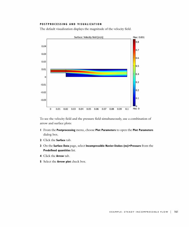
PO S T P R O C E S S I N G A N D V I S U A L I Z A T I O N
The default visualization displays the magnitude of the velocity field.
To see the velocity field and the pressure field simultaneously, use a combination of arrow and surface plots:
1 From the Postprocessing menu, choose Plot Parameters to open the Plot Parameters dialog box.
2 Click the Surface tab.
3 On the Surface Data page, select Incompressible Navier-Stokes (ns)>Pressure from the Predefined quantities list.
4 Click the Arrow tab.
5 Select the Arrow plot check box.
E X A M P L E : S T E A D Y I N C O M P R E S S I B L E F L O W | 161
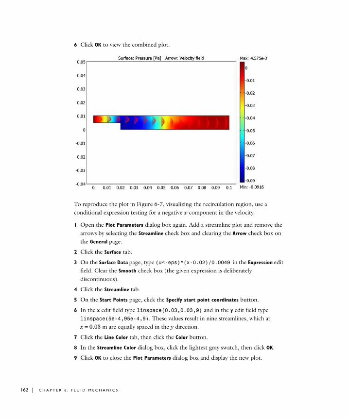
162 | C H A P T E
6 Click OK to view the combined plot.
To reproduce the plot in Figure 6-7, visualizing the recirculation region, use a conditional expression testing for a negative x-component in the velocity.
1 Open the Plot Parameters dialog box again. Add a streamline plot and remove the arrows by selecting the Streamline check box and clearing the Arrow check box on the General page.
2 Click the Surface tab.
3 On the Surface Data page, type (u<-eps)*(x-0.02)/0.0049 in the Expression edit field. Clear the Smooth check box (the given expression is deliberately discontinuous).
4 Click the Streamline tab.
5 On the Start Points page, click the Specify start point coordinates button.
6 In the x edit field type linspace(0.03,0.03,9) and in the y edit field type linspace(5e-4,95e-4,9). These values result in nine streamlines, which at x = 0.03 m are equally spaced in the y direction.
7 Click the Line Color tab, then click the Color button.
8 In the Streamline Color dialog box, click the lightest gray swatch, then click OK.
9 Click OK to close the Plot Parameters dialog box and display the new plot.
R 6 : F L U I D M E C H A N I C S
7
H e a t T r a n s f e r
This chapter covers heat transfer application modes. It starts with some background on heat transfer. It then reviews specifics of the Conduction application mode and then the Convection and Conduction application mode. It concludes with COMSOL Multiphysics models of three heat-transfer examples taken from a NAFEMS (National Agency for Finite Element Methods and Standards) benchmark collection.
163
164 | C H A P T E
Hea t T r a n s f e r F undamen t a l s
What is Heat Transfer?
From the kitchen toaster to the latest high-performance microprocessor, heat is ubiquitous and of great importance in the engineering world. To optimize thermal performance and reduce costs, engineers and researchers are making use of finite element analysis. Because most material properties are temperature-dependent, the effects of heat enter many other disciplines and drive the requirement for multiphysics modeling.
For instance, both the toaster and the microchip contain electrical conductors that generate thermal energy as electric current passes through them. As these conductors release thermal energy, system temperature increases as does that of the conductors. If the electric conductivity is temperature dependent, it changes accordingly and, in turn, affects the electric field in the conductor. Other examples of multiphysics couplings that involve heat transfer are thermal stresses, thermal-fluid convection, and induction heating.
Heat transfer is defined as the movement of energy due to a temperature difference. It is characterized by the following three mechanisms:
• Conduction is heat transfer by diffusion in a stationary medium due to a temperature gradient. The medium can be a solid or a liquid.
• Convection is heat transfer between either a hot surface and a cold moving fluid or a cold surface and a hot moving fluid. Convection occurs in fluids (liquids and gases).
• Radiation is heat transfer via electromagnetic waves between two surfaces (A and B) with different temperatures TA and TB, provided that Surface A is visible to an infinitesimally small observer on Surface B.
Note: The Heat Transfer Module supports simulations of all three types of heat transfer mechanism, including surface-to-surface and surface-to-ambient radiation.
The examples later in this chapter shows transient heat transfer by conduction, convection, and radiation. For an introductory example of a multiphysics coupling of a heat balance to a momentum balance through the Navier-Stokes equations, see “Free
R 7 : H E A T TR A N S F E R
Convection” on page 357 in the COMSOL Multiphysics Model Library. In that model the heat flux accounts for transport by convection and conduction. The system consists of heated tubes subjected to a stream of a fluid perpendicular to the main axis of the tubes. The tubes heat the streaming medium as it travels from the bottom to the top of the domain.
The Heat Equation
The mathematical model for heat transfer by conduction is the heat equation:
Quickly review the variables and quantities in this equation:
• T is the temperature.
• ρ is the density.
• C is the heat capacity.
- Cp is the heat capacity at a constant pressure.
- Cv is the heat capacity for a constant volume.
• k is thermal conductivity.
• Q is a heat source or a heat sink.
For a steady-state model, temperature does not change with time, and the first term containing ρ and C vanishes.
If the thermal conductivity is anisotropic, k becomes the thermal conductivity tensor k:
To model heat conduction and convection through a fluid, the heat equation also includes a convective term. COMSOL Multiphysics represents this formulation in the Convection and Conduction application mode as:
ρC∂T∂t------- ∇– k∇T( )⋅ Q=
k
kxx kxy kxz
kyx kyy kyz
kzx kzy kzz
=
ρCp t∂∂T ∇ k T ρCpTu )+∇–(⋅+ Q=
H E A T TR A N S F E R F U N D A M E N T A L S | 165
166 | C H A P T E
where u is the velocity field. This field can either be provided as a mathematical expression of the independent variables or calculated by a coupling to the velocity field from an application mode such as Incompressible Navier-Stokes.
The heat flux vector is defined by the expression within the parentheses in the equation above. For transport through conduction and convection, this equation yields
where q is the heat flux vector. If the heat transfer is by conduction only, q is determined by
For a detailed discussion of the fundamentals of heat transfer, see Ref. 1.
Note: Heat capacity here refers to the quantity that represents the amount of heat required to change one unit of mass of a substance by one degree. It has units of energy per mass per degree (J/kg/K in SI units). This quantity is also called specific heat or specific heat capacity.
q k T ρ Cp T u+∇–=
q k T∇–=
R 7 : H E A T TR A N S F E R
Th e Condu c t i o n App l i c a t i o n Mode
This application mode models heat transfer by conduction. It also includes convection and radiation effects around edges and boundaries. The Conduction application mode is suitable for modeling of heat transfer in solids. To start modeling with this application mode, go to the Model Navigator and select Heat Transfer and then Conduction.
Variables and Space Dimensions
The Conduction application mode is available in 1D, 2D, and 3D as well as for axisymmetric models using cylindrical coordinates in 1D and 2D. The dependent variable is the temperature, T.
PDE Formulation
The mathematical model for heat transfer by conduction is the following version of the heat equation
with the following material properties:
• δts is a time-scaling coefficient.
• ρ is the density.
• Cp is the heat capacity.
• k is the thermal conductivity tensor.
• Q is the heat source (or sink).
For a steady-state problem the temperature does not change with time and the first term disappears.
In rare cases you might decide to add domain-specific transversal convection or radiation in 1D planar and axisymmetric models and 2D planar models. Represent this by adding the two terms on the right:
δtsρCp∂T∂t------- ∇– k∇T( )⋅ Q=
δtsρCp∂T∂t------- ∇– k∇T( )⋅ Q
htransdA
----------------+ Text T–( )Ctrans
dA----------------- Tambtrans
4 T4–( )+=
T H E C O N D U C T I O N A P P L I C A T I O N M O D E | 167
168 | C H A P T E
where:
• htrans is the transversal convective heat transfer coefficient.
• Text is the transversal external temperature.
• Ctrans is a user-defined constant.
• Tambtrans is the transversal ambient temperature.
• dA is the thickness in 2D and area in 1D.
Note: When using transversal convection or radiation, the heat equation must be modified to accommodate the area dA. For all practical purposes the use of this feature is a rare exception, and the terms htrans and Ctrans are usually set to zero.
Subdomain Settings
The subdomain quantities are:
Time-scaling coefficient This coefficient is normally 1, but you can change the time scale, for example, from seconds to minutes by setting it to 1/60.
Density It specifies the material’s density. Enter this quantity as mass per volume.
QUANTITY VARIABLE DESCRIPTION
δts Dts Time-scaling coefficient
ρ rho Density
Cp C Heat capacity
k k Thermal conductivity
Thermal conductivity tensor
kij kxixj Thermal conductivity tensor, xixj component
Q Q Heat source
htrans htrans Transversal convective heat transfer coefficient
Text Text Transversal external temperature
Ctrans Ctrans User-defined constant
Tambtrans Tambtrans Transversal ambient temperature
k
R 7 : H E A T TR A N S F E R
Heat capacity The heat capacity C describes the amount of heat energy required to produce a unit temperature change in a unit mass.
Thermal conductivity The thermal conductivity k describes the relationship between the heat flux vector q and the temperature gradient as in
,
which is Fourier’s law of heat conduction. Enter this quantity as power per length and temperature.
Heat source The heat source describes heat generation within the domain. Express heating and cooling with positive and negative values, respectively. Enter the quantity Q as unit power per unit volume (W/m3 in SI units).
Boundary Condition Types
The available boundary conditions are:
H E A T F L U X
COMSOL Multiphysics supplies only one generalized boundary condition for heat flux, but it accounts for general heat flux as well as heat flux from convection and radiation.
BOUNDARY CONDITION DESCRIPTION
Heat flux
Insulation or symmetry
T = T0 Prescribed temperature
T = 0 Zero temperature
Thin thermally resistive layer (pair boundaries only)
T∇
q k T∇–=
n k∇T( )⋅ q0 h+ Tinf T–( ) Cconst Tamb4 T4
–( )+=
n k∇T( )⋅ 0=
n1 k1∇T1( )⋅ kd--- T2 T1–( )=
n2 k2∇T2( )⋅ kd--- T1 T2–( )=
n k∇T( )⋅ q0 h+ Tinf T–( ) Cconst Tamb4 T4
–( )+=
T H E C O N D U C T I O N A P P L I C A T I O N M O D E | 169
170 | C H A P T E
The application mode interprets the heat flux q0 in the direction of the inward normal. It interprets the convection and radiation terms in the direction of the outward normal.
• Specify q0 to represent a heat flux that enters the domain. For instance, any electric heater is well represented by this condition, and you can omit its geometry. Enter the quantity q0 as unit power per unit area (W/m2 using SI units). While this is directly applicable to 3D, unit depth and unit area are assumed in 2D and 1D applications, respectively.
• h(Tinf – T) models convective heat transfer with the surrounding environment, where h is the heat transfer coefficient and Tinf is the ambient bulk temperature. The value of h depends on the geometry and the ambient flow conditions. For a thorough introduction on how to calculate heat transfer coefficients see Ref. 1.
• Cconst (T4
amb– T4) models radiation heat transfer with the surrounding environment. Tamb is the temperature of the surrounding radiation environment, which might differ from Tinf. Cconst is the product of the surface emissitivity ε and the Stefan-Boltzmann constant σ = 5.669·10−8 W/(m2·K4) (with the same unit as the Stefan-Boltzmann constant):
The surface emissivity is a material property discussed and tabulated in Ref. 1.
Note: A problem with radiation boundaries is nonlinear, so you must work with absolute (thermodynamical) temperature units. See “Using Units” on page 183 in the COMSOL Multiphysics User’s Guide.
I N S U L A T I O N O R S Y M M E T R Y
This condition specifies where the domain is well insulated, or it reduces model size by taking advantage of symmetry. Intuitively this equation says that the gradient across the boundary must be zero. For this to be true, the temperature on one side of the boundary must equal the temperature on the other side. Because there is no temperature difference across the boundary, heat cannot transfer across it.
An interesting numerical check for convergence is the numerical evaluation of the above condition along the boundary, something easily accomplished with the
Cconst εσ=
n k∇T( )⋅ 0=
R 7 : H E A T TR A N S F E R
postprocessing features of COMSOL Multiphysics. Another check is to plot the temperature field as a contour plot. Ideally the contour lines are perpendicular to any insulated boundary.
A X I A L S Y M M E T R Y
This boundary condition is available only for axisymmetric versions of the heat transfer application models. Use it only on the symmetry axis r = 0.
P R E S C R I B E D T E M P E R A T U R E
This boundary prescribes the temperature T0. This condition means that the finite element solution returns a solution in which the above condition is either true or minimally approximated.
P R E S C R I B E D Z E R O TE M P E R A T U R E
This boundary specifies a zero boundary temperature.
C O N T I N U I T Y
The default setting for interior boundaries is Continuity, which is a special case of the above Heat source/sink condition. In the absence of sources or sinks, that condition becomes −n1· ( q1 − q2 ) = 0. This means that the heat flux in the normal direction is continuous across the boundary. This is the default boundary condition on interior boundaries.
The temperature is naturally continuous on an internal boundary following the continuity of the finite element field. Therefore, the Continuity boundary condition is identical to the condition that applies between any two neighboring elements in the mesh. In fact, as long as you have not selected Enable interior boundaries in the Boundary Settings dialog box, the interior boundaries are not in any way different from any other mesh element boundaries, where the Continuity condition effectively applies.
The Continuity boundary condition is available on interior boundaries and assembly pairs only.
H E A T F L U X D I S C O N T I N U I T Y
The Heat flux discontinuity condition is available on interior boundaries and pairs representing borders between parts in an assembly:
T T0=
T 0=
T H E C O N D U C T I O N A P P L I C A T I O N M O D E | 171
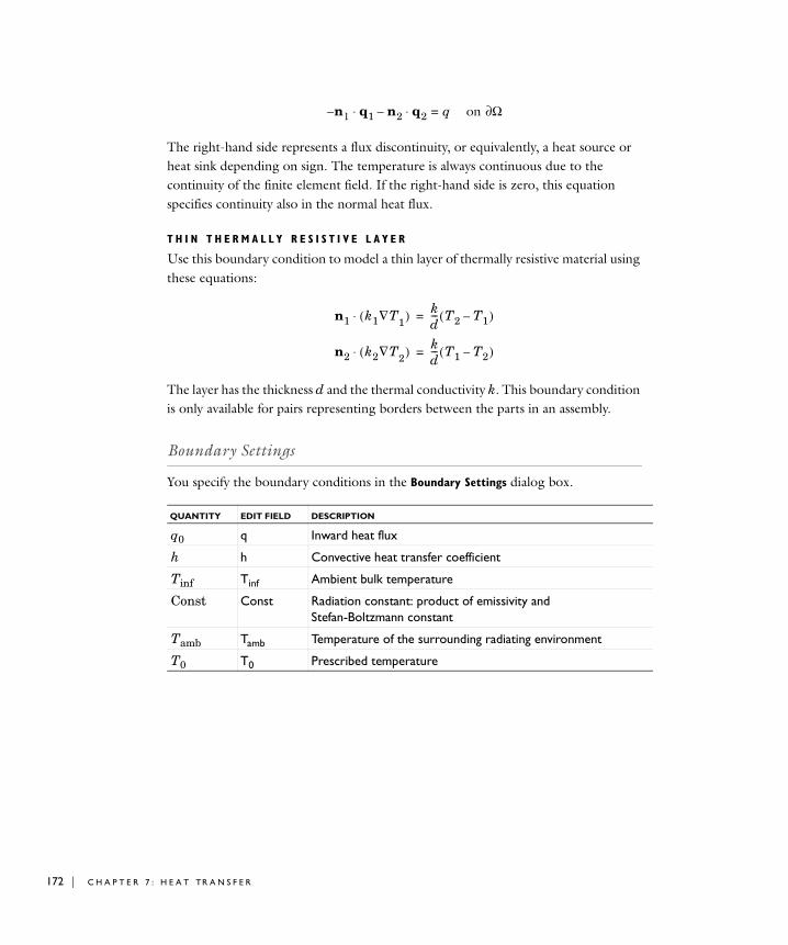
172 | C H A P T E
The right-hand side represents a flux discontinuity, or equivalently, a heat source or heat sink depending on sign. The temperature is always continuous due to the continuity of the finite element field. If the right-hand side is zero, this equation specifies continuity also in the normal heat flux.
T H I N T H E R M A L L Y R E S I S T I V E L A Y E R
Use this boundary condition to model a thin layer of thermally resistive material using these equations:
The layer has the thickness d and the thermal conductivity k. This boundary condition is only available for pairs representing borders between the parts in an assembly.
Boundary Settings
You specify the boundary conditions in the Boundary Settings dialog box.
QUANTITY EDIT FIELD DESCRIPTION
q0 q Inward heat flux
h h Convective heat transfer coefficient
Tinf Tinf Ambient bulk temperature
Const Const Radiation constant: product of emissivity and Stefan-Boltzmann constant
Tamb Tamb Temperature of the surrounding radiating environment
T0 T0 Prescribed temperature
n1– q1⋅ n2 q2⋅– q= on Ω∂
n1 k1∇T1( )⋅ kd--- T2 T1–( )=
n2 k2∇T2( )⋅ kd--- T1 T2–( )=
R 7 : H E A T TR A N S F E R
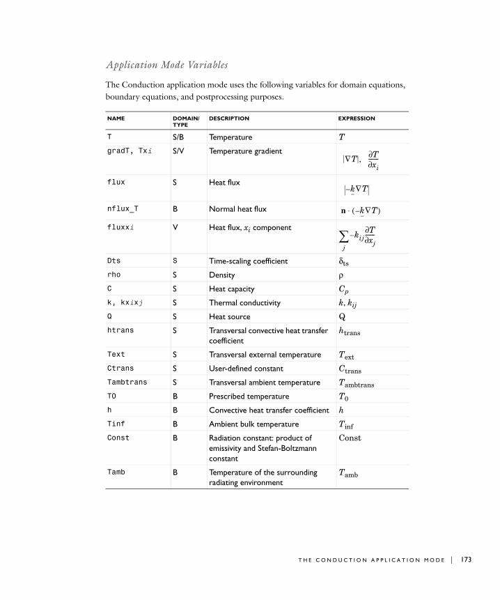
Application Mode Variables
The Conduction application mode uses the following variables for domain equations, boundary equations, and postprocessing purposes.
NAME DOMAIN/TYPE
DESCRIPTION EXPRESSION
T S/B Temperature T
gradT, Txi S/V Temperature gradient
flux S Heat flux
nflux_T B Normal heat flux
fluxxi V Heat flux, xi component
Dts S Time-scaling coefficient δts
rho S Density ρC S Heat capacity Cp
k, kxixj S Thermal conductivity k, kij
Q S Heat source Q
htrans S Transversal convective heat transfer coefficient
htrans
Text S Transversal external temperature Text
Ctrans S User-defined constant Ctrans
Tambtrans S Transversal ambient temperature Tambtrans
T0 B Prescribed temperature T0
h B Convective heat transfer coefficient h
Tinf B Ambient bulk temperature Tinf
Const B Radiation constant: product of emissivity and Stefan-Boltzmann constant
Const
Tamb B Temperature of the surrounding radiating environment
Tamb
∇T , T∂xi∂
-------
k∇T–
n k∇T–( )⋅
kijT∂xj∂
-------–
j∑
T H E C O N D U C T I O N A P P L I C A T I O N M O D E | 173
174 | C H A P T E
Note: To form the complete application mode variable names, add a suffix consisting of an underscore and the application mode name (default: ht), for example, flux_ht. (This does not apply to the dependent variable for the temperature.)
Note: The vector expressions V are not present in the 1D formulation of the Conduction application mode.
R 7 : H E A T TR A N S F E R
Th e Con v e c t i o n and Condu c t i o n App l i c a t i o n Mode
In addition to heat transfer by conduction, the Convection and Conduction application mode includes heat transfer by convection. In the convection term for the equation that defines this application mode you can specify the velocity vector as an analytical expression. Alternatively, you can connect it directly to the solution of the equations of motion, for example, through a multiphysics coupling to the Incompressible Navier-Stokes application mode. The Convection and Conduction application mode is suitable for modeling of heat transfer in fluids.
Variables and Space Dimensions
The Convection and Conduction application mode is available in 1D, 2D, 3D, Axial symmetry 1D, and Axial symmetry 2D.
Note: The optional Chemical Engineering Module also contains this Convection and Conduction application mode. In addition to the above-mentioned space dimensions, it features pseudo-2D and pseudo-3D geometry options in which it uses time as a second or third spatial dimension. This feature is useful in situations where convection in the direction of the flow is large. This often applies to reactors and equipment for unit operations.
PDE Formulation
This application mode supports the following nonconservative formulation of the transient PDE for heat transfer by convection and conduction:
The nonconservative formulation assumes an incompressible fluid, which means that . This ensures that no unphysical source term arises from a flow field where
the incompressibility constraint, , is not absolutely fulfilled. The convective
δtsρCp t∂∂T ∇ k T∇–( )⋅+ Q ρC– pu ∇T⋅=
∇ u⋅ 0=
∇ u⋅ 0=
T H E C O N V E C T I O N A N D C O N D U C T I O N A P P L I C A T I O N M O D E | 175
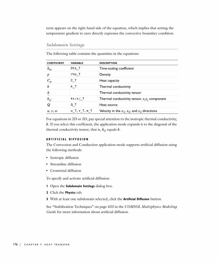
176 | C H A P T E
term appears on the right-hand side of the equation, which implies that setting the temperature gradient to zero directly expresses the convective boundary condition.
Subdomain Settings
The following table contains the quantities in the equations:
For equations in 2D or 3D, pay special attention to the isotropic thermal conductivity, k. If you select this coefficient, the application mode expands it to the diagonal of the thermal conductivity tensor, that is, kii equals k.
A R T I F I C I A L D I F F U S I O N
The Convection and Conduction application mode supports artificial diffusion using the following methods:
• Isotropic diffusion
• Streamline diffusion
• Crosswind diffusion
To specify and activate artificial diffusion:
1 Open the Subdomain Settings dialog box.
2 Click the Physics tab.
3 With at least one subdomain selected, click the Artificial Diffusion button.
See “Stabilization Techniques” on page 433 in the COMSOL Multiphysics Modeling Guide for more information about artificial diffusion.
COEFFICIENT VARIABLE DESCRIPTION
δts Dts_T Time-scaling coefficient
ρ rho_T Density
Cp C_T Heat capacity
k k_T Thermal conductivity
Thermal conductivity tensor
kij kxixj_T Thermal conductivity tensor, xixj component
Q Q_T Heat source
u, v, w u_T, v_T, w_T Velocity in the x1, x2, and x3 directions
k
R 7 : H E A T TR A N S F E R
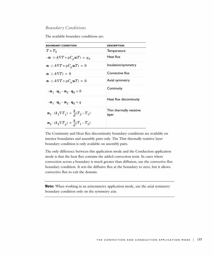
Boundary Conditions
The available boundary conditions are:
The Continuity and Heat flux discontinuity boundary conditions are available on interior boundaries and assembly pairs only. The Thin thermally resistive layer boundary condition is only available on assembly pairs.
The only difference between this application mode and the Conduction application mode is that the heat flux contains the added convection term. In cases where convection across a boundary is much greater than diffusion, use the convective flux boundary condition. It sets the diffusive flux at the boundary to zero, but it allows convective flux to exit the domain.
Note: When working in an axisymmetry application mode, use the axial symmetry boundary condition only on the symmetry axis.
BOUNDARY CONDITION DESCRIPTION
T = T0 Temperature
Heat flux
Insulation/symmetry
Convective flux
Axial symmetry
Continuity
Heat flux discontinuity
Thin thermally resistive layer
n– k T ρCpuT+∇–( )⋅ q0=
n k T ρCpuT+∇–( )⋅ 0=
n k– T∇( )⋅ 0=
n k T ρCpuT+∇–( )⋅ 0=
n1– q1⋅ n2 q2⋅– 0=
n1– q1⋅ n2 q2⋅– q=
n1 k1∇T1( )⋅ kd--- T2 T1–( )=
n2 k2∇T2( )⋅ kd--- T1 T2–( )=
T H E C O N V E C T I O N A N D C O N D U C T I O N A P P L I C A T I O N M O D E | 177
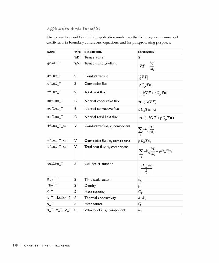
178 | C H A P T E
Application Mode Variables
The Convection and Conduction application mode uses the following expressions and coefficients in boundary conditions, equations, and for postprocessing purposes.
NAME TYPE DESCRIPTION EXPRESSION
T S/B Temperature T
grad_T S/V Temperature gradient
dflux_T S Conductive flux
cflux_T S Convective flux
tflux_T S Total heat flux
ndflux_T B Normal conductive flux
ncflux_T B Normal convective flux
ntflux_T B Normal total heat flux
dflux_T_xi V Conductive flux, xi component
cflux_T_xi V Convective flux, xi component ρ Cp Tui
tflux_T_xi V Total heat flux, xi component
cellPe_T S Cell Peclet number
Dts_T S Time-scale factor δts
rho_T S Density ρC_T S Heat capacity Cp
k_T, kxixj_T S Thermal conductivity k, kij
Q_T S Heat source Q
u_T, v_T, w_T S Velocity of c, xi component ui
∇T , T∂xi∂
-------
k∇T
ρCpTu
k∇T– ρCpTu+
n k∇T–( )⋅
ρCpTn u⋅
n k∇T– ρCpTu+( )⋅
kijT∂xj∂
-------–
j∑
kijT∂xj∂
-------–
j∑ ρCpTui+
ρCpuhk
-------------------
R 7 : H E A T TR A N S F E R
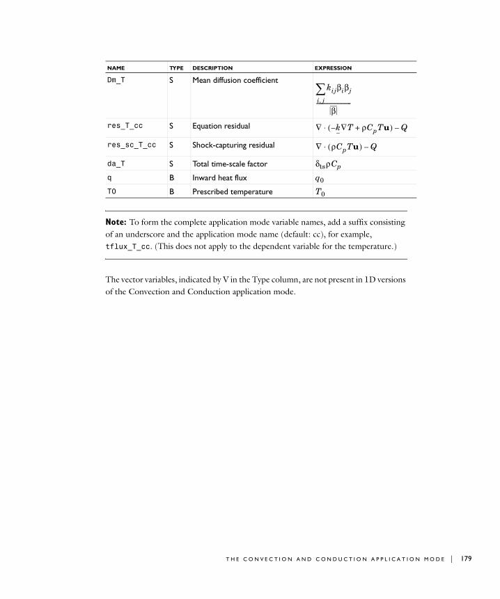
Note: To form the complete application mode variable names, add a suffix consisting of an underscore and the application mode name (default: cc), for example, tflux_T_cc. (This does not apply to the dependent variable for the temperature.)
The vector variables, indicated by V in the Type column, are not present in 1D versions of the Convection and Conduction application mode.
Dm_T S Mean diffusion coefficient
res_T_cc S Equation residual
res_sc_T_cc S Shock-capturing residual
da_T S Total time-scale factor δts ρ Cp
q B Inward heat flux q0
T0 B Prescribed temperature T0
NAME TYPE DESCRIPTION EXPRESSION
kijβiβj
i j,∑
β-------------------------
∇ k– ∇T ρCpTu+( )⋅ Q–
∇ ρCpTu( )⋅ Q–
T H E C O N V E C T I O N A N D C O N D U C T I O N A P P L I C A T I O N M O D E | 179
180 | C H A P T E
Examp l e s o f H ea t T r a n s f e r Mode l s
The following three heat transfer benchmark examples show how to model heat transfer using:
• Steady-state and transient analysis
• Temperature, heat flux, convective cooling, and radiation boundary conditions
• Thermal conductivity as a function of temperature
All examples are taken from a NAFEMS benchmark collection (Ref. 2).
1D Steady-State Heat Transfer with Radiation
The first example shows a 1D steady-state thermal analysis including radiation to a prescribed ambient temperature.
Model Definition
This 1D model has a domain of length 0.1 m. The left end is kept at 1000 K, and at the right end there is radiation to 300 K. For the radiation, the model properties are:
• The emissivity, ε, is 0.98.
• The Stefan-Boltzmann constant, σ, is 5.67·10−8 W/(m·K4).
In the domain, use the following material property:
• The thermal conductivity is 55.563 W/(m·°C).
R 7 : H E A T TR A N S F E R
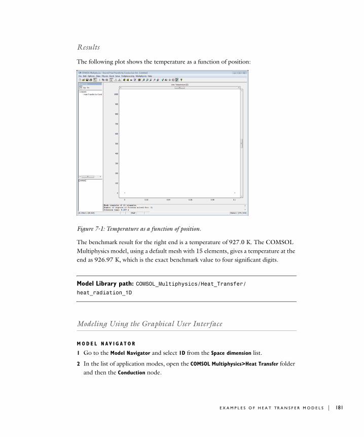
Results
The following plot shows the temperature as a function of position:
Figure 7-1: Temperature as a function of position.
The benchmark result for the right end is a temperature of 927.0 K. The COMSOL Multiphysics model, using a default mesh with 15 elements, gives a temperature at the end as 926.97 K, which is the exact benchmark value to four significant digits.
Model Library path: COMSOL_Multiphysics/Heat_Transfer/heat_radiation_1D
Modeling Using the Graphical User Interface
M O D E L N A V I G A T O R
1 Go to the Model Navigator and select 1D from the Space dimension list.
2 In the list of application modes, open the COMSOL Multiphysics>Heat Transfer folder and then the Conduction node.
E X A M P L E S O F H E A T TR A N S F E R M O D E L S | 181
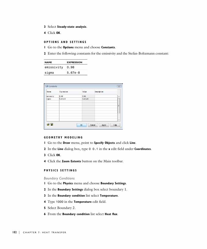
182 | C H A P T E
3 Select Steady-state analysis.
4 Click OK.
O P T I O N S A N D S E T T I N G S
1 Go to the Options menu and choose Constants.
2 Enter the following constants for the emissivity and the Stefan-Boltzmann constant:
G E O M E T R Y M O D E L I N G
1 Go to the Draw menu, point to Specify Objects and click Line.
2 In the Line dialog box, type 0 0.1 in the x edit field under Coordinates.
3 Click OK.
4 Click the Zoom Extents button on the Main toolbar.
P H Y S I C S S E T T I N G S
Boundary Conditions1 Go to the Physics menu and choose Boundary Settings.
2 In the Boundary Settings dialog box select boundary 1.
3 In the Boundary condition list select Temperature.
4 Type 1000 in the Temperature edit field.
5 Select Boundary 2.
6 From the Boundary condition list select Heat flux.
NAME EXPRESSION
emissivity 0.98
sigma 5.67e-8
R 7 : H E A T TR A N S F E R
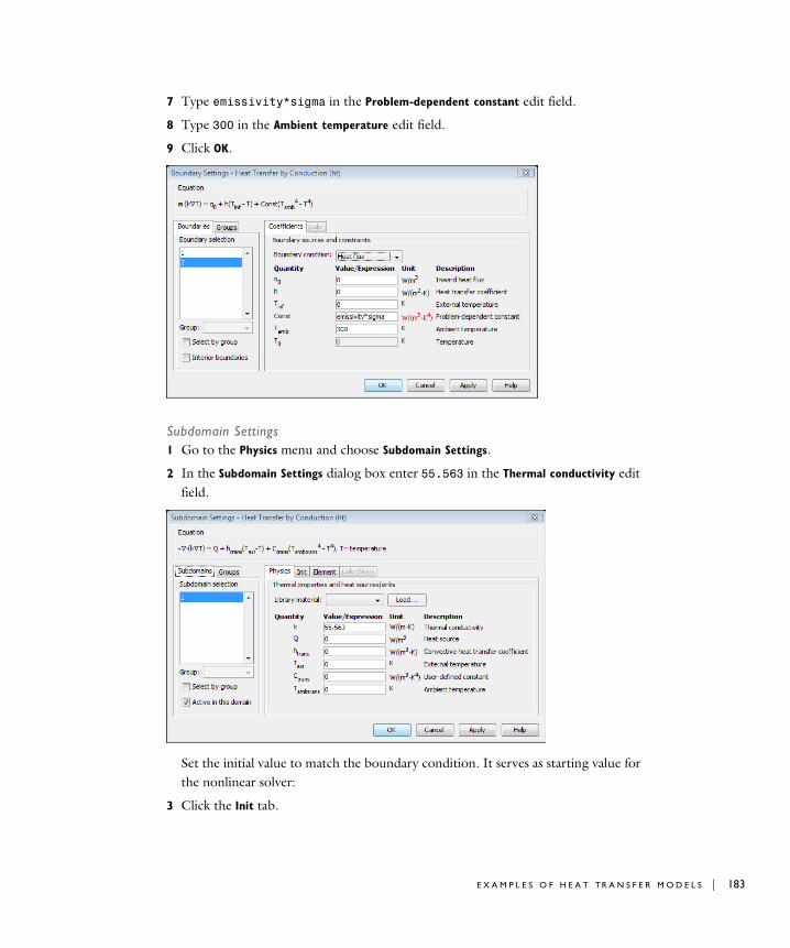
7 Type emissivity*sigma in the Problem-dependent constant edit field.
8 Type 300 in the Ambient temperature edit field.
9 Click OK.
Subdomain Settings1 Go to the Physics menu and choose Subdomain Settings.
2 In the Subdomain Settings dialog box enter 55.563 in the Thermal conductivity edit field.
Set the initial value to match the boundary condition. It serves as starting value for the nonlinear solver:
3 Click the Init tab.
E X A M P L E S O F H E A T TR A N S F E R M O D E L S | 183
184 | C H A P T E
4 Type 1000 as the initial value in the Temperature edit field.
5 Click OK.
M E S H G E N E R A T I O N
Initialize the mesh by clicking the Initialize Mesh button on the Main toolbar.
C O M P U T I N G T H E S O L U T I O N
Click the Solve button on the Main toolbar.
P O S T P R O C E S S I N G A N D V I S U A L I Z A T I O N
Figure 7-1 on page 181 shows the temperature distribution in the domain. Use the zoom tools to focus on the temperature at the right end.
2D Steady-State Heat Transfer with Convection
This example shows a 2D steady-state thermal analysis including convection to a prescribed external (ambient) temperature.
Model Definition
This model domain is 0.6-by-1.0 meters. For the boundary conditions:
• The left boundary is insulated.
• The lower boundary is kept at 100 °C.
• The upper and right boundaries are convecting to 0 °C with a heat transfer coefficient of 750 W/(m2·°C).
In the domain use the following material property:
• The thermal conductivity is 52 W/(m·°C).
R 7 : H E A T TR A N S F E R
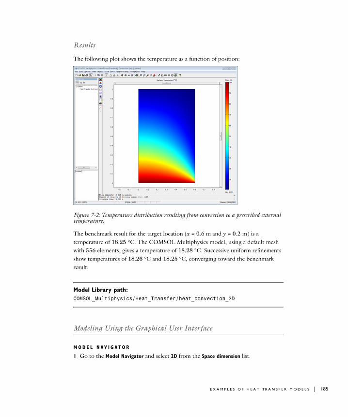
Results
The following plot shows the temperature as a function of position:
Figure 7-2: Temperature distribution resulting from convection to a prescribed external temperature.
The benchmark result for the target location (x = 0.6 m and y = 0.2 m) is a temperature of 18.25 °C. The COMSOL Multiphysics model, using a default mesh with 556 elements, gives a temperature of 18.28 °C. Successive uniform refinements show temperatures of 18.26 °C and 18.25 °C, converging toward the benchmark result.
Model Library path:
COMSOL_Multiphysics/Heat_Transfer/heat_convection_2D
Modeling Using the Graphical User Interface
M O D E L N A V I G A T O R
1 Go to the Model Navigator and select 2D from the Space dimension list.
E X A M P L E S O F H E A T TR A N S F E R M O D E L S | 185
186 | C H A P T E
2 In the list of application modes, open the COMSOL Multiphysics>Heat Transfer folder and then the Conduction node.
3 Select Steady-state analysis.
4 Click OK.
G E O M E T R Y M O D E L I N G
1 On the Draw menu point to Specify Objects and click Rectangle.
2 In the Rectangle dialog box, find the Size area and type 0.6 in the Width edit field, then type 1 in the Height edit field.
3 Click OK.
4 Click the Zoom Extents button.
P H Y S I C S S E T T I N G S
Boundary ConditionsThe default boundary condition is thermal insulation, so you must set boundary conditions for only three of the boundaries.
1 Go to the Physics menu and choose Boundary Settings.
2 In the Boundary Settings dialog box select Boundary 2.
3 In the Boundary condition list select Temperature.
4 Type 100[degC] in the Temperature edit field to specify a temperature in degrees Celsius (the default unit for temperature in the SI base unit system is kelvin).
5 Select Boundaries 3 and 4.
6 In the Boundary condition list select Heat flux.
7 Type 750 in the Heat transfer coefficient edit field.
8 Type 0[degC] in the External temperature edit field.
R 7 : H E A T TR A N S F E R
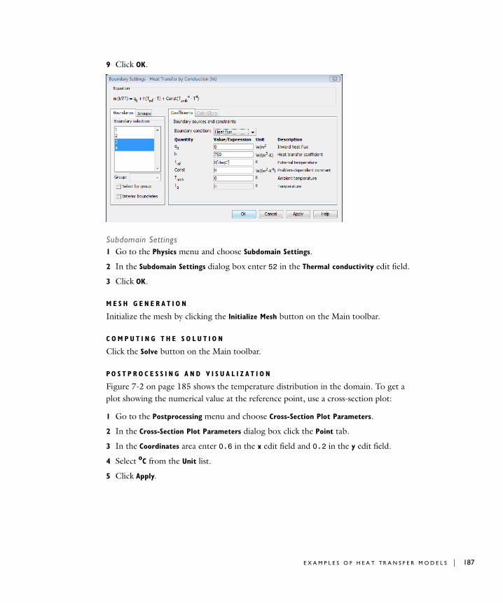
9 Click OK.
Subdomain Settings1 Go to the Physics menu and choose Subdomain Settings.
2 In the Subdomain Settings dialog box enter 52 in the Thermal conductivity edit field.
3 Click OK.
M E S H G E N E R A T I O N
Initialize the mesh by clicking the Initialize Mesh button on the Main toolbar.
C O M P U T I N G T H E S O L U T I O N
Click the Solve button on the Main toolbar.
PO S T P R O C E S S I N G A N D V I S U A L I Z A T I O N
Figure 7-2 on page 185 shows the temperature distribution in the domain. To get a plot showing the numerical value at the reference point, use a cross-section plot:
1 Go to the Postprocessing menu and choose Cross-Section Plot Parameters.
2 In the Cross-Section Plot Parameters dialog box click the Point tab.
3 In the Coordinates area enter 0.6 in the x edit field and 0.2 in the y edit field.
4 Select oC from the Unit list.
5 Click Apply.
E X A M P L E S O F H E A T TR A N S F E R M O D E L S | 187
188 | C H A P T E
2D Axisymmetric Transient Heat Transfer
This example shows an axisymmetric transient thermal analysis with a step change to 1000 °C at time 0.
Model Definition
This model domain is 0.3-by- 0.4 meters. For the boundary conditions:
• The left boundary is the symmetry axis.
• The other boundaries have a temperature of 1000 °C. The entire domain is at 0 °C at the start, which represents a step change in temperature at the boundaries.
In the domain use the following material properties:
• The density, ρ, is 7850 kg/m3
• The heat capacity is 460 J/(kg·°C)
• The thermal conductivity is 52 W/(m·°C)
R 7 : H E A T TR A N S F E R
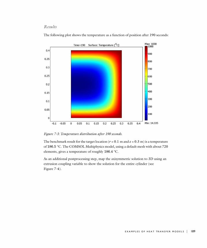
Results
The following plot shows the temperature as a function of position after 190 seconds:
Figure 7-3: Temperature distribution after 190 seconds.
The benchmark result for the target location (r = 0.1 m and z = 0.3 m) is a temperature of 186.5 °C. The COMSOL Multiphysics model, using a default mesh with about 720 elements, gives a temperature of roughly 186.4 °C.
As an additional postprocessing step, map the axisymmetric solution to 3D using an extrusion coupling variable to show the solution for the entire cylinder (see Figure 7-4).
E X A M P L E S O F H E A T TR A N S F E R M O D E L S | 189
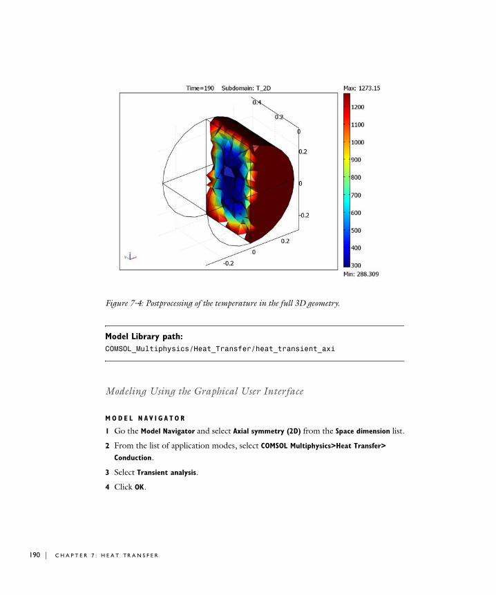
190 | C H A P T E
Figure 7-4: Postprocessing of the temperature in the full 3D geometry.
Model Library path: COMSOL_Multiphysics/Heat_Transfer/heat_transient_axi
Modeling Using the Graphical User Interface
M O D E L N A V I G A T O R
1 Go the Model Navigator and select Axial symmetry (2D) from the Space dimension list.
2 From the list of application modes, select COMSOL Multiphysics>Heat Transfer>
Conduction.
3 Select Transient analysis.
4 Click OK.
R 7 : H E A T TR A N S F E R
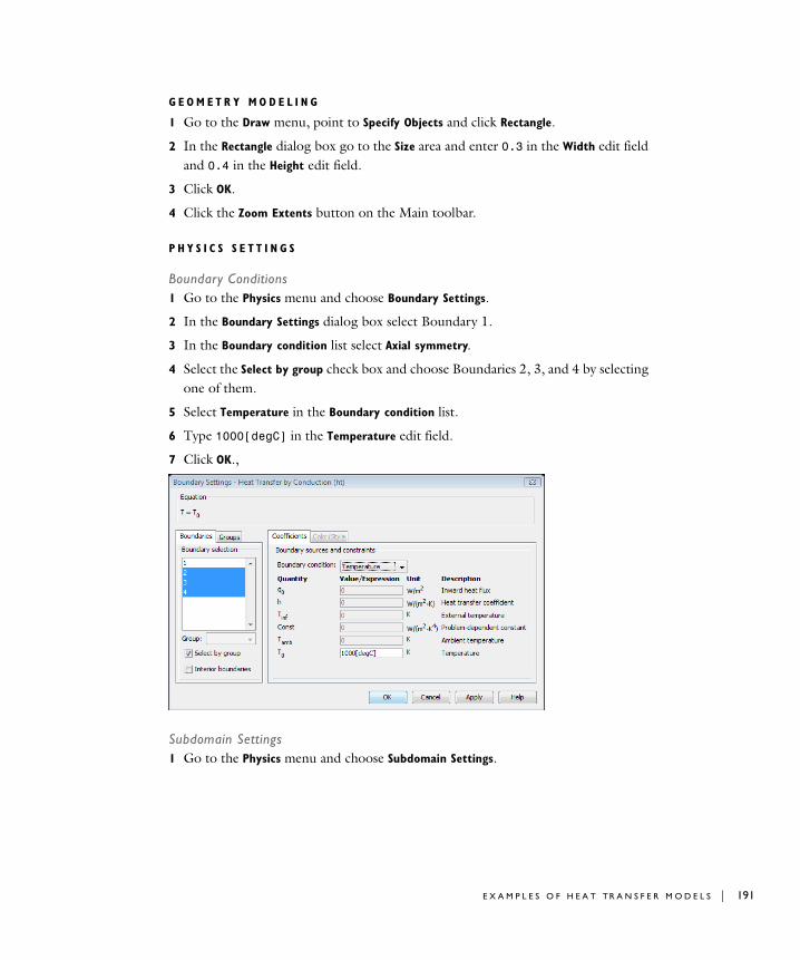
G E O M E T R Y M O D E L I N G
1 Go to the Draw menu, point to Specify Objects and click Rectangle.
2 In the Rectangle dialog box go to the Size area and enter 0.3 in the Width edit field and 0.4 in the Height edit field.
3 Click OK.
4 Click the Zoom Extents button on the Main toolbar.
P H Y S I C S S E T T I N G S
Boundary Conditions1 Go to the Physics menu and choose Boundary Settings.
2 In the Boundary Settings dialog box select Boundary 1.
3 In the Boundary condition list select Axial symmetry.
4 Select the Select by group check box and choose Boundaries 2, 3, and 4 by selecting one of them.
5 Select Temperature in the Boundary condition list.
6 Type 1000[degC] in the Temperature edit field.
7 Click OK.,
Subdomain Settings1 Go to the Physics menu and choose Subdomain Settings.
E X A M P L E S O F H E A T TR A N S F E R M O D E L S | 191
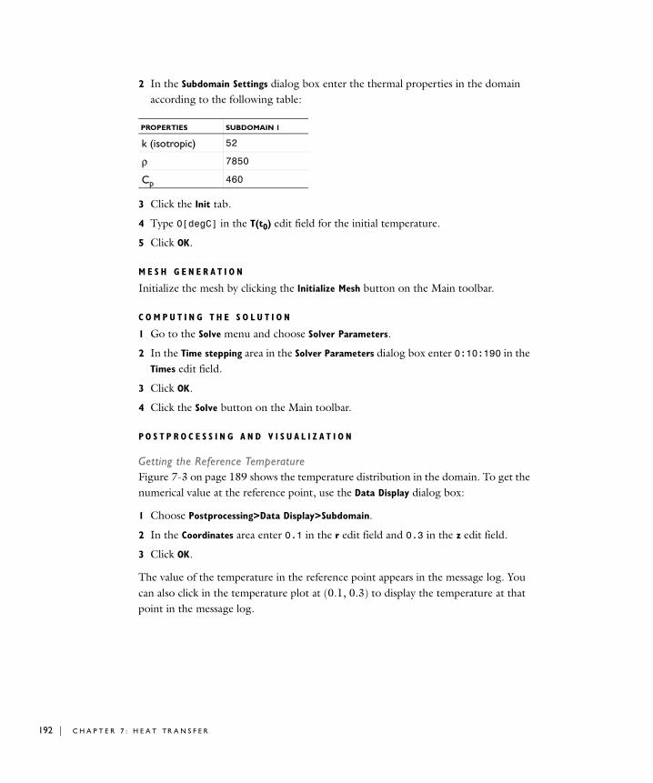
192 | C H A P T E
2 In the Subdomain Settings dialog box enter the thermal properties in the domain according to the following table:
3 Click the Init tab.
4 Type 0[degC] in the T(t0) edit field for the initial temperature.
5 Click OK.
M E S H G E N E R A T I O N
Initialize the mesh by clicking the Initialize Mesh button on the Main toolbar.
C O M P U T I N G T H E S O L U T I O N
1 Go to the Solve menu and choose Solver Parameters.
2 In the Time stepping area in the Solver Parameters dialog box enter 0:10:190 in the Times edit field.
3 Click OK.
4 Click the Solve button on the Main toolbar.
P O S T P R O C E S S I N G A N D V I S U A L I Z A T I O N
Getting the Reference TemperatureFigure 7-3 on page 189 shows the temperature distribution in the domain. To get the numerical value at the reference point, use the Data Display dialog box:
1 Choose Postprocessing>Data Display>Subdomain.
2 In the Coordinates area enter 0.1 in the r edit field and 0.3 in the z edit field.
3 Click OK.
The value of the temperature in the reference point appears in the message log. You can also click in the temperature plot at (0.1, 0.3) to display the temperature at that point in the message log.
PROPERTIES SUBDOMAIN 1
k (isotropic) 52
ρ 7850
Cp 460
R 7 : H E A T TR A N S F E R
Postprocessing in 3DTo postprocess the solution in 3D, first revolve the geometry into a cylinder in a 3D geometry and then map the axisymmetric solution to the cylinder using an extrusion coupling variable:
1 From the Draw menu, choose Revolve.
2 In the Revolve dialog box, leave the default settings and click OK. This creates a cylinder in 3D. Note that the axis of revolution in 3D is the y-axis, which means that the plane that you map the radial coordinate r to is the xz-plane.
3 Click the Geom1 tab at the top of the drawing area to return to the 2D axisymmetric geometry.
4 Choose Options>Extrusion Coupling Variables>Subdomain Variables.
5 In the Subdomain Extrusion Variables dialog box, select Subdomain 1 and then type T_2D in the first row of the Name column and T is the first row of the Expression column. This creates an extrusion coupling variable T_2D that represents the temperature (the variable T).
6 Click the General transformation button. The default source transformation (x: r and y: z) is correct.
7 Click the Destination tab.
8 Select Geom2 from the Geometry list, select Subdomain from the Level list, and finally select the 1 check box for Subdomain 1 in the Subdomain selection list. The variable T_2D is the only extrusion coupling variable and the software selects it automatically.
9 In the Destination transformation area, type sqrt(x^2+z^2) in the x edit field, and leave the value y in the y edit field. This transforms r and z in the axisymmetric geometry to and y, respectively, in the 3D geometry.
10 Click OK.
11 From the Solve menu, choose Update Model to map the solution to the 3D geometry.
12 From the Postprocessing menu, choose Plot Parameters.
13 To plot the temperature in the cylinder as a subdomain plot, clear the Slice check box and select the Subdomain check box in the Plot type area on the General page.
14 Select the Element selection check box and type x>0 in the Logical expression edit field to “look inside” by removing all elements with a negative x coordinate.
15 Click the Subdomain tab, and then type T_2D in the Expression edit field.
16 Click OK to generate Figure 7-4 on page 190.
x2 z2+
E X A M P L E S O F H E A T TR A N S F E R M O D E L S | 193
194 | C H A P T E
References
1. Frank P. Incropera and David P. DeWitt, Fundamentals of Heat and Mass Transfer, 4th edition, John Wiley & Sons, New York, 1996.
2. A.D. Cameron, J. A. Casey, and G.B. Simpson: NAFEMS Benchmark Tests for Thermal Analysis (Summary), NAFEMS Ltd., Glasgow, 1986.
R 7 : H E A T TR A N S F E R
8
S t r u c t u r a l M e c h a n i c s
This chapter explains how to use the Structural Mechanics application modes to simulate and analyze applications involving solid mechanics. It begins with a brief theoretical backgrounder on structural mechanics, after which subsequent sections give details of the application modes.
195
196 | C H A P T E
Th e S t r u c t u r a l Me c h an i c s App l i c a t i o n Mode s
COMSOL Multiphysics includes four application modes for stress analysis and general structural mechanics simulation:
• The Solid, Stress-Strain application mode (for 3D geometries)
• The Plane Stress application mode (for 2D geometries)
• The Plane Strain application mode (for 2D geometries)
• The Axial Symmetry Stress-Strain application mode (for 2D axisymmetric geometries)
The last three cases are 2D simplifications of the full 3D equations, simplifications that are valid under certain assumptions.
Note: The optional Structural Mechanics Module contains application modes and models that allow for extended, specialized analyses of structural and solid mechanics problems.
R 8 : S T R U C T U R A L M E C H A N I C S
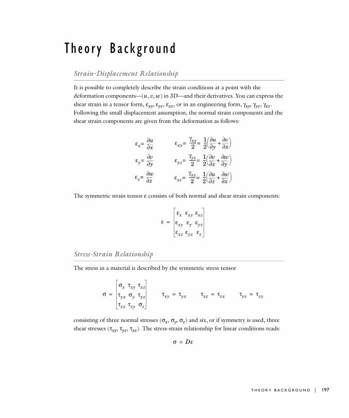
Th eo r y Ba c k g r ound
Strain-Displacement Relationship
It is possible to completely describe the strain conditions at a point with the deformation components—(u, v, w) in 3D—and their derivatives. You can express the shear strain in a tensor form, εxy, εyz, εxz, or in an engineering form, γxy, γyz, γxz. Following the small-displacement assumption, the normal strain components and the shear strain components are given from the deformation as follows:
The symmetric strain tensor ε consists of both normal and shear strain components:
Stress-Strain Relationship
The stress in a material is described by the symmetric stress tensor
consisting of three normal stresses (σx, σy, σz) and six, or if symmetry is used, three shear stresses (τxy, τyz, τxz). The stress-strain relationship for linear conditions reads:
εx x∂∂u
=
εy y∂∂v
=
εz z∂∂w
=
εxyγxy2
-------=12---
y∂∂u
x∂∂v
+⎝ ⎠⎛ ⎞=
εyzγyz
2-------=
12---
z∂∂v
y∂∂w
+⎝ ⎠⎛ ⎞=
εxzγxz
2-------=
12---
z∂∂u
x∂∂w
+⎝ ⎠⎛ ⎞=
εεx εxy εxz
εxy εy εyz
εxz εyz εz
=
σσx τxy τxz
τyx σy τyz
τzx τzy σz
= τxy τyx= τxz τzx= τyz τzy=
σ Dε=
T H E O R Y B A C K G R O U N D | 197
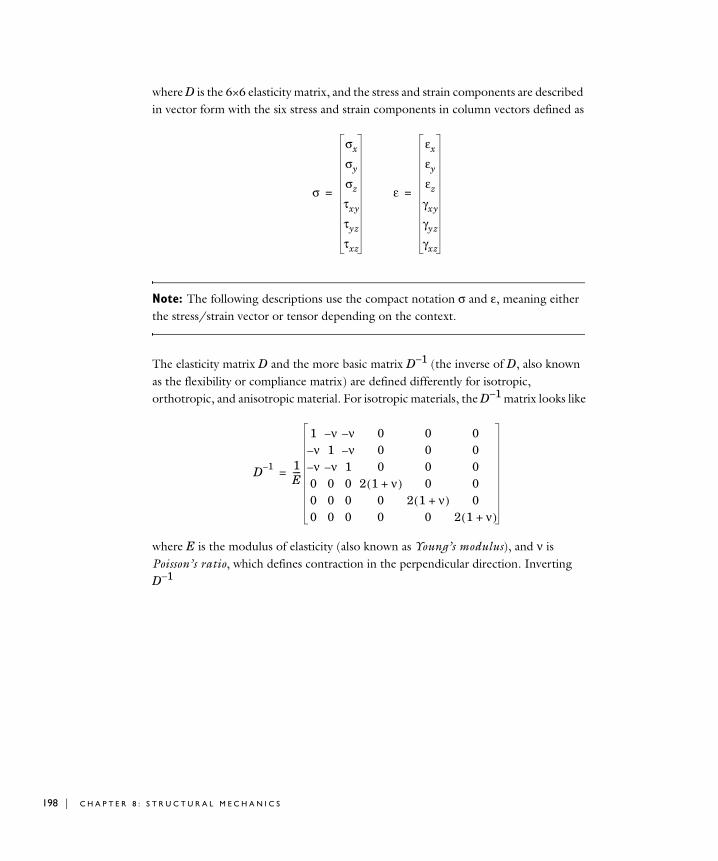
198 | C H A P T E
where D is the 6×6 elasticity matrix, and the stress and strain components are described in vector form with the six stress and strain components in column vectors defined as
Note: The following descriptions use the compact notation σ and ε, meaning either the stress/strain vector or tensor depending on the context.
The elasticity matrix D and the more basic matrix D−1 (the inverse of D, also known as the flexibility or compliance matrix) are defined differently for isotropic, orthotropic, and anisotropic material. For isotropic materials, the D−1 matrix looks like
where E is the modulus of elasticity (also known as Young’s modulus), and ν is Poisson’s ratio, which defines contraction in the perpendicular direction. Inverting D−1
σ
σx
σy
σz
τxy
τyz
τxz
= ε
εx
εy
εz
γxy
γyz
γxz
=
D 1– 1E----
1 ν– ν– 0 0 0ν– 1 ν– 0 0 0ν– ν– 1 0 0 0
0 0 0 2 1 ν+( ) 0 00 0 0 0 2 1 ν+( ) 00 0 0 0 0 2 1 ν+( )
=
R 8 : S T R U C T U R A L M E C H A N I C S
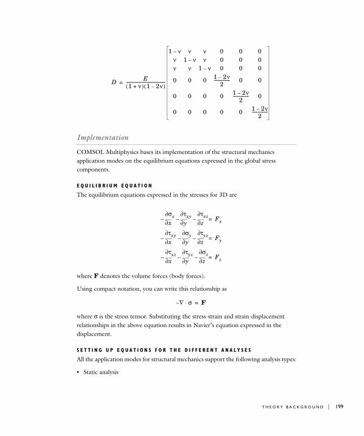
Implementation
COMSOL Multiphysics bases its implementation of the structural mechanics application modes on the equilibrium equations expressed in the global stress components.
E Q U I L I B R I U M E Q U A T I O N
The equilibrium equations expressed in the stresses for 3D are
where F denotes the volume forces (body forces).
Using compact notation, you can write this relationship as
where σ is the stress tensor. Substituting the stress-strain and strain-displacement relationships in the above equation results in Navier’s equation expressed in the displacement.
S E T T I N G U P E Q U A T I O N S F O R T H E D I F F E R E N T A N A L Y S E S
All the application modes for structural mechanics support the following analysis types:
• Static analysis
D E1 ν+( ) 1 2ν–( )
---------------------------------------
1 ν– ν ν 0 0 0ν 1 ν– ν 0 0 0ν ν 1 ν– 0 0 0
0 0 0 1 2ν–2
---------------- 0 0
0 0 0 0 1 2ν–2
---------------- 0
0 0 0 0 0 1 2ν–2
----------------
=
x∂∂σx–
y∂∂τxy–
z∂∂τxz Fx=–
x∂∂τxy–
y∂∂σy–
z∂∂τyz Fy=–
x∂∂τxz–
y∂∂τyz–
z∂∂σz Fz=–
∇– σ⋅ F=
T H E O R Y B A C K G R O U N D | 199
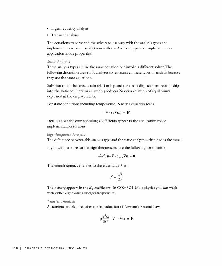
200 | C H A P T E
• Eigenfrequency analysis
• Transient analysis
The equations to solve and the solvers to use vary with the analysis types and implementations. You specify them with the Analysis Type and Implementation application mode properties.
Static AnalysisThese analysis types all use the same equation but invoke a different solver. The following discussion uses static analyses to represent all these types of analysis because they use the same equations.
Substitution of the stress-strain relationship and the strain-displacement relationship into the static equilibrium equation produces Navier’s equation of equilibrium expressed in the displacements.
For static conditions including temperature, Navier’s equation reads
Details about the corresponding coefficients appear in the application mode implementation sections.
Eigenfrequency AnalysisThe difference between this analysis type and the static analysis is that it adds the mass.
If you wish to solve for the eigenfrequencies, use the following formulation:
The eigenfrequency f relates to the eigenvalue λ as
The density appears in the da coefficient. In COMSOL Multiphysics you can work with either eigenvalues or eigenfrequencies.
Transient AnalysisA transient problem requires the introduction of Newton’s Second Law.
∇– c u∇( )⋅ F=
λd– au ∇– csta u = 0∇⋅
f λ2π-------=
ρ∂2u∂t2---------- ∇– c u∇⋅ F=
R 8 : S T R U C T U R A L M E C H A N I C S
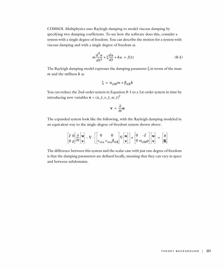
COMSOL Multiphysics uses Rayleigh damping to model viscous damping by specifying two damping coefficients. To see how the software does this, consider a system with a single degree of freedom. You can describe the motion for a system with viscous damping and with a single degree of freedom as
(8-1)
The Rayleigh damping model expresses the damping parameter ξ in terms of the mass m and the stiffness k as
You can reduce the 2nd-order system in Equation 8-1 to a 1st-order system in time by introducing new variables v = (u_t, v_t, w_t)t
The expanded system look like the following, with the Rayleigh damping modeled in an equivalent way to the single-degree-of-freedom system shown above:
The difference between this system and the scalar case with just one degree of freedom is that the damping parameters are defined locally, meaning that they can vary in space and between subdomains.
md2udt2---------- ξdu
dt------- ku+ + f t( )=
ξ αdMm βdKk+=
v ∂∂t-----u=
I 00 ρ
∂∂t----- u
v∇ 0 0
csta cstaβdK∇ u
v0 I–
0 αdMρuv
+⋅– 0K
=
T H E O R Y B A C K G R O U N D | 201
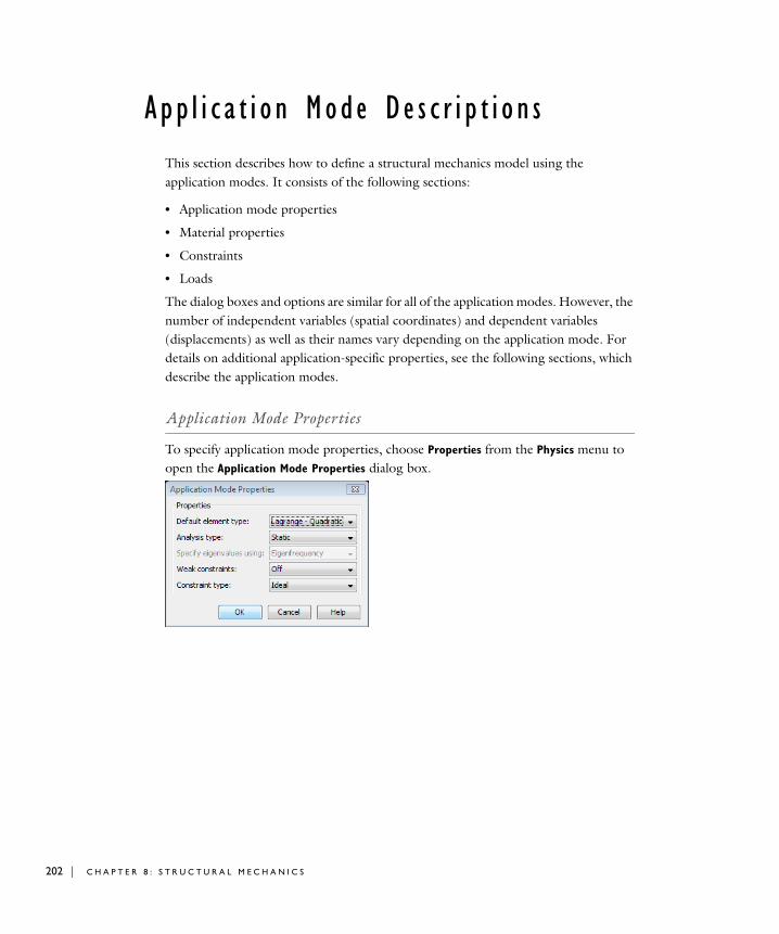
202 | C H A P T E
App l i c a t i o n Mode De s c r i p t i o n s
This section describes how to define a structural mechanics model using the application modes. It consists of the following sections:
• Application mode properties
• Material properties
• Constraints
• Loads
The dialog boxes and options are similar for all of the application modes. However, the number of independent variables (spatial coordinates) and dependent variables (displacements) as well as their names vary depending on the application mode. For details on additional application-specific properties, see the following sections, which describe the application modes.
Application Mode Properties
To specify application mode properties, choose Properties from the Physics menu to open the Application Mode Properties dialog box.
R 8 : S T R U C T U R A L M E C H A N I C S
In this dialog box you can specify different global settings for the model:
• Make a selection from the Default element type list. This selection becomes the default on all subdomains. Available elements are:
- Lagrange - Linear, 1st-order Lagrange elements
- Lagrange - Quadratic, 2nd-order Lagrange elements
- Lagrange - Cubic, 3rd-order Lagrange elements
- Lagrange - Quartic, 4th-order Lagrange elements
- Lagrange - Quintic, 5th-order Lagrange elements
• Make a selection from the Analysis type list; the default is static analysis. Your choice affects the equations and which solver COMSOL Multiphysics uses if you previously selected the Auto select solver check box in the Solver Parameters dialog box.
• Indicate how you prefer to specify eigenvalues—using eigenvalues themselves or eigenfrequencies—by selecting from the Specify eigenvalues using list. This property is applicable only to eigenfrequency analyses.
• Control whether or not weak constraints should be available in the Weak constraints list by selecting On or Off.
Use weak constraints for accurate computation of reaction forces, solving for the reaction force, which is equal to the Lagrange multiplier that the weak constrain introduces as an additional dependent variable. When weak constraints are enabled, all constraints are weak constraints by default, but it is possible to change this setting for individual domains.
• Choose the type of constraint. Select Ideal or Non-ideal from the Constraint type list. See “Ideal vs. Non-Ideal Constraints” on page 301 for more information about these constrain types.
A P P L I C A T I O N M O D E D E S C R I P T I O N S | 203
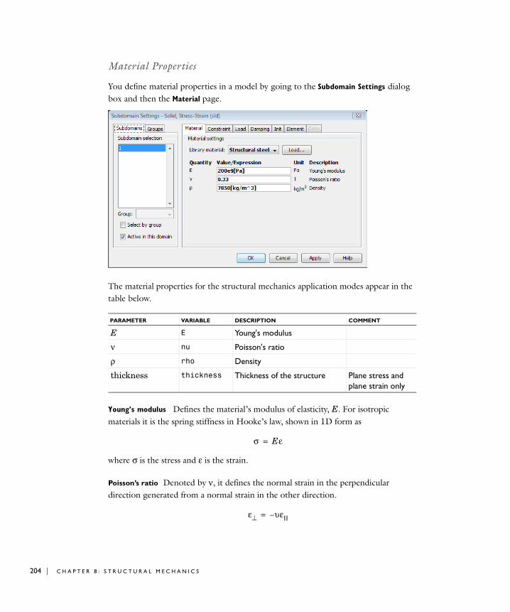
204 | C H A P T E
Material Properties
You define material properties in a model by going to the Subdomain Settings dialog box and then the Material page.
The material properties for the structural mechanics application modes appear in the table below.
Young’s modulus Defines the material’s modulus of elasticity, E. For isotropic materials it is the spring stiffness in Hooke’s law, shown in 1D form as
where σ is the stress and ε is the strain.
Poisson’s ratio Denoted by ν, it defines the normal strain in the perpendicular direction generated from a normal strain in the other direction.
PARAMETER VARIABLE DESCRIPTION COMMENT
E E Young's modulus
ν nu Poisson's ratio
ρ rho Density
thickness thickness Thickness of the structure Plane stress and plane strain only
σ Eε=
ε⊥ υεl l–=
R 8 : S T R U C T U R A L M E C H A N I C S

Density This property, ρ, specifies the material’s density.
The COMSOL Multiphysics materials library contains values for many of these properties for common materials such as steel, copper, or aluminum. See “Using the Materials/Coefficients Library” on page 223 in the COMSOL Multiphysics User’s Guide.
Constraints
A constraint specifies the displacement of certain parts of a structure. You can define constraints on all domain levels:
• Points, edges, boundaries (faces), and subdomains in 3D
• Points, boundaries, and subdomains in 2D.
To specify them, go to the Constraint page in the Subdomain Settings, Boundary Settings, Edge Settings, or Point Settings dialog boxes. The following image shows the Boundary
Settings dialog box for the Solid, Stress-Strain application mode, but this page looks the same on all domain levels in all structural mechanics application modes.
You can describe a constraint using standard or general notation, an option you control using the Standard notation and the General notation, Hu=R buttons.
S T A N D A R D N O T A T I O N F O R C O N S T R A I N T S
Using standard notation, you constrain each displacement direction independently:
1 Select the check boxes in front of Rx, Ry, and Rz to activate the constraint.
A P P L I C A T I O N M O D E D E S C R I P T I O N S | 205
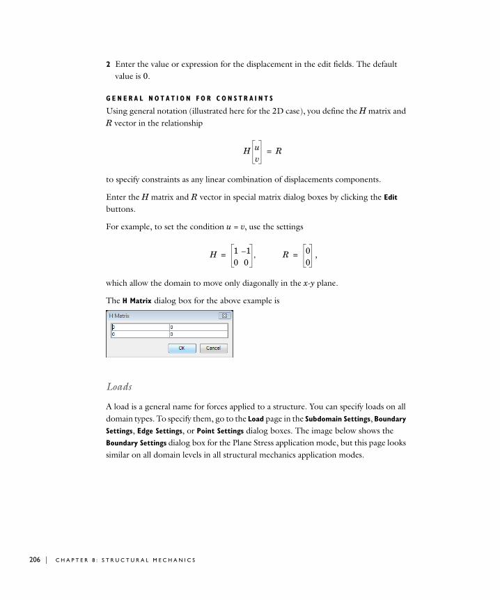
206 | C H A P T E
2 Enter the value or expression for the displacement in the edit fields. The default value is 0.
G E N E R A L N O T A T I O N F O R C O N S T R A I N T S
Using general notation (illustrated here for the 2D case), you define the H matrix and R vector in the relationship
to specify constraints as any linear combination of displacements components.
Enter the H matrix and R vector in special matrix dialog boxes by clicking the Edit buttons.
For example, to set the condition u = v, use the settings
,
which allow the domain to move only diagonally in the x-y plane.
The H Matrix dialog box for the above example is
Loads
A load is a general name for forces applied to a structure. You can specify loads on all domain types. To specify them, go to the Load page in the Subdomain Settings, Boundary
Settings, Edge Settings, or Point Settings dialog boxes. The image below shows the Boundary Settings dialog box for the Plane Stress application mode, but this page looks similar on all domain levels in all structural mechanics application modes.
H uv
R=
H 1 1–
0 0,= R 0
0=
R 8 : S T R U C T U R A L M E C H A N I C S
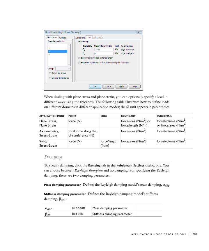
(N/m3) (N/m2)
(N/m3)
(N/m3)
When dealing with plane stress and plane strain, you can optionally specify a load in different ways using the thickness. The following table illustrates how to define loads on different domains in different application modes; the SI unit appears in parentheses.
Damping
To specify damping, click the Damping tab in the Subdomain Settings dialog box. You can choose between Rayleigh damping and no damping. For specifying the Rayleigh damping, there are two damping parameters:
Mass damping parameter Defines the Rayleigh damping model’s mass damping, αdM.
Stiffness damping parameter Defines the Rayleigh damping model’s stiffness damping, βdK.
APPLICATION MODE POINT EDGE BOUNDARY SUBDOMAIN
Plane Stress, Plane Strain
force (N) force/area (N/m2) or force/length (N/m)
force/volumeor force/area
Axisymmetry, Stress-Strain
total force along the circumference (N)
force/area (N/m2) force/volume
Solid, Stress-Strain
force (N) force/length (N/m)
force/area (N/m2) force/volume
αdM alphadM Mass damping parameter
βdK betadK Stiffness damping parameter
A P P L I C A T I O N M O D E D E S C R I P T I O N S | 207
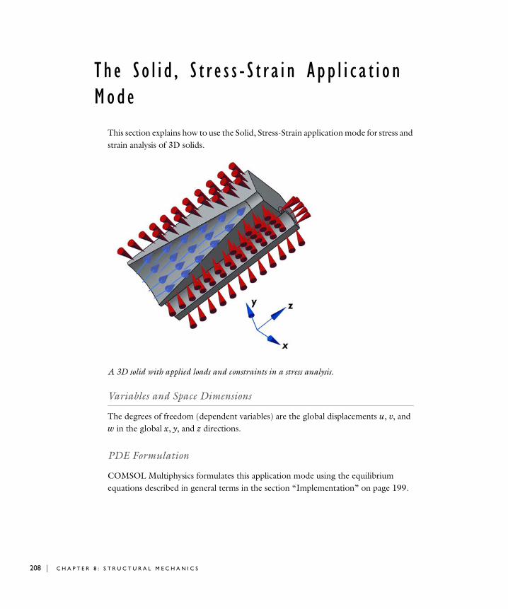
208 | C H A P T E
T h e S o l i d , S t r e s s - S t r a i n App l i c a t i o n Mode
This section explains how to use the Solid, Stress-Strain application mode for stress and strain analysis of 3D solids.
A 3D solid with applied loads and constraints in a stress analysis.
Variables and Space Dimensions
The degrees of freedom (dependent variables) are the global displacements u, v, and w in the global x, y, and z directions.
PDE Formulation
COMSOL Multiphysics formulates this application mode using the equilibrium equations described in general terms in the section “Implementation” on page 199.
R 8 : S T R U C T U R A L M E C H A N I C S
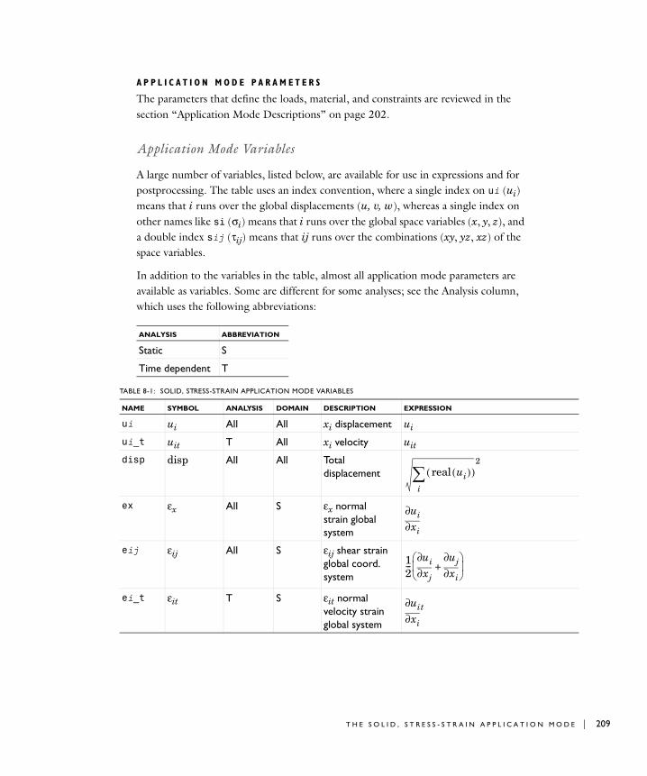
A P P L I C A T I O N M O D E P A R A M E T E R S
The parameters that define the loads, material, and constraints are reviewed in the section “Application Mode Descriptions” on page 202.
Application Mode Variables
A large number of variables, listed below, are available for use in expressions and for postprocessing. The table uses an index convention, where a single index on ui (ui) means that i runs over the global displacements (u, v, w), whereas a single index on other names like si (σi) means that i runs over the global space variables (x, y, z), and a double index sij (τij) means that ij runs over the combinations (xy, yz, xz) of the space variables.
In addition to the variables in the table, almost all application mode parameters are available as variables. Some are different for some analyses; see the Analysis column, which uses the following abbreviations:
ANALYSIS ABBREVIATION
Static S
Time dependent T
TABLE 8-1: SOLID, STRESS-STRAIN APPLICATION MODE VARIABLES
NAME SYMBOL ANALYSIS DOMAIN DESCRIPTION EXPRESSION
ui ui All All xi displacement ui
ui_t uit T All xi velocity uit
disp disp All All Total displacement
ex εx All S εx normal strain global system
eij εij All S εij shear strain global coord. system
ei_t εit T S εit normal velocity strain global system
ui( )real( )i∑
2
xi∂∂ui
12---
xj∂∂ui
xi∂∂uj+
⎝ ⎠⎜ ⎟⎛ ⎞
xi∂∂uit
T H E S O L I D , S T R E S S - S T R A I N A P P L I C A T I O N M O D E | 209
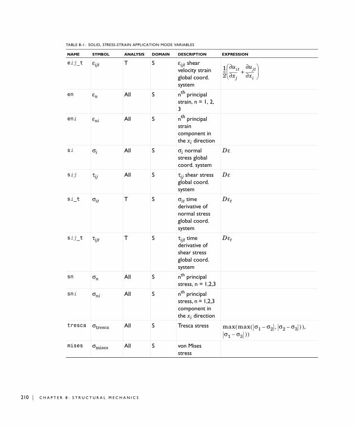
210 | C H A P T E
) ),
eij_t εijt T S εijt shear velocity strain global coord. system
en εn All S nth principal strain, n = 1, 2, 3
eni εni All S nth principal strain component in the xi direction
si σi All S σi normal stress global coord. system
D ε
sij τij All S τij shear stress global coord. system
D ε
si_t σit T S σit time derivative of normal stress global coord. system
D εt
sij_t τijt T S τijt time derivative of shear stress global coord. system
D εt
sn σn All S nth principal stress, n = 1,2,3
sni σni All S nth principal stress, n = 1,2,3 component in the xi direction
tresca σtresca All S Tresca stress
mises σmises All S von Mises stress
TABLE 8-1: SOLID, STRESS-STRAIN APPLICATION MODE VARIABLES
NAME SYMBOL ANALYSIS DOMAIN DESCRIPTION EXPRESSION
12---
xj∂∂uit
xi∂∂ujt+
⎝ ⎠⎜ ⎟⎛ ⎞
max max σ1 σ2– σ2 σ3–,(σ1 σ3– )
()
R 8 : S T R U C T U R A L M E C H A N I C S
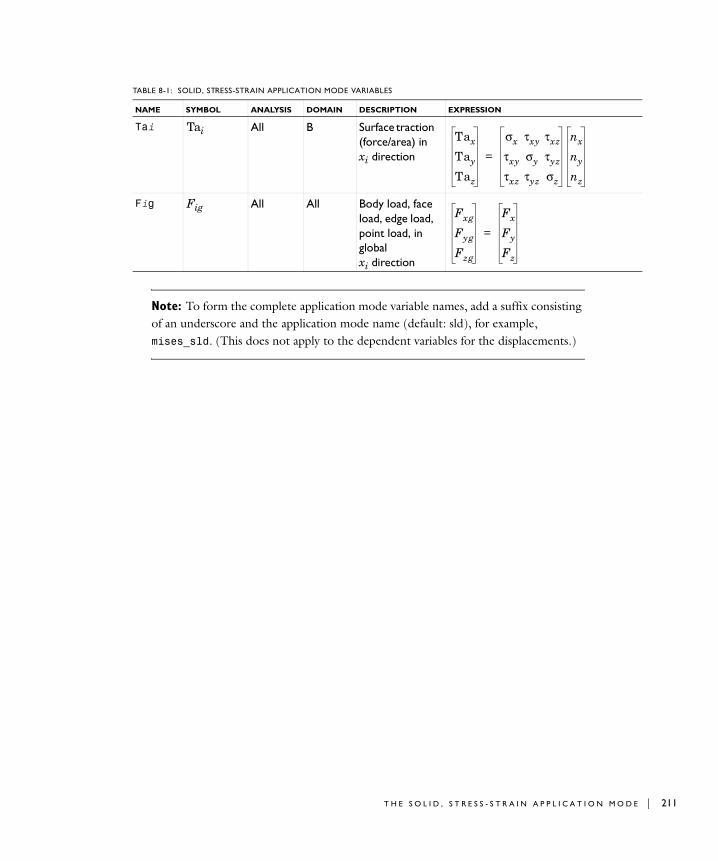
Note: To form the complete application mode variable names, add a suffix consisting of an underscore and the application mode name (default: sld), for example, mises_sld. (This does not apply to the dependent variables for the displacements.)
Tai Tai All B Surface traction (force/area) in xi direction
Fig Fig All All Body load, face load, edge load, point load, in global xi direction
TABLE 8-1: SOLID, STRESS-STRAIN APPLICATION MODE VARIABLES
NAME SYMBOL ANALYSIS DOMAIN DESCRIPTION EXPRESSION
Tax
Tay
Taz
σx τxy τxz
τxy σy τyz
τxz τyz σz
nx
ny
nz
=
Fxg
Fyg
Fzg
Fx
Fy
Fz
=
T H E S O L I D , S T R E S S - S T R A I N A P P L I C A T I O N M O D E | 211
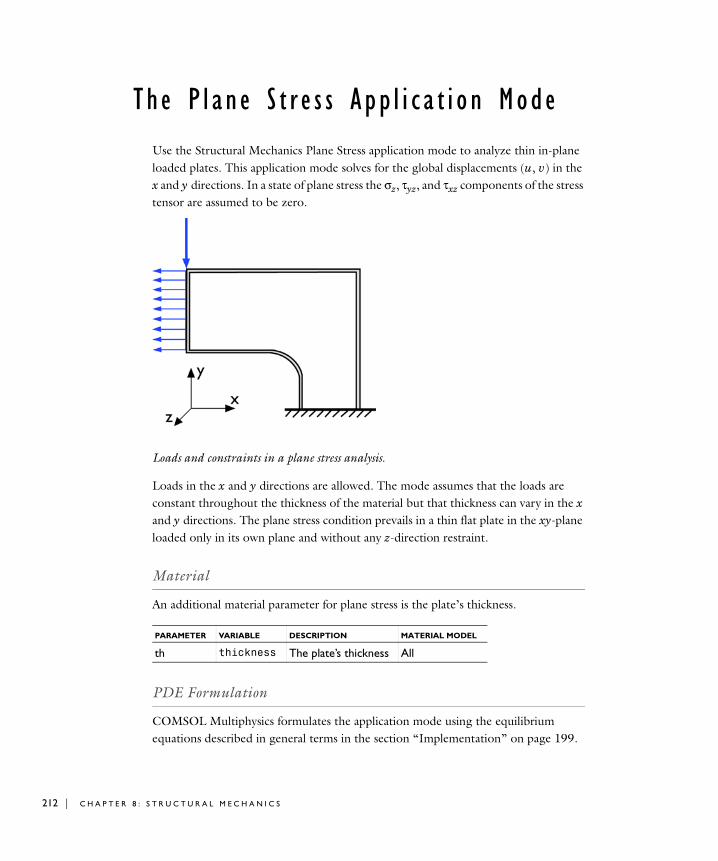
212 | C H A P T E
Th e P l a n e S t r e s s App l i c a t i o n Mode
Use the Structural Mechanics Plane Stress application mode to analyze thin in-plane loaded plates. This application mode solves for the global displacements (u, v) in the x and y directions. In a state of plane stress the σz, τyz, and τxz components of the stress tensor are assumed to be zero.
Loads and constraints in a plane stress analysis.
Loads in the x and y directions are allowed. The mode assumes that the loads are constant throughout the thickness of the material but that thickness can vary in the x and y directions. The plane stress condition prevails in a thin flat plate in the xy-plane loaded only in its own plane and without any z-direction restraint.
Material
An additional material parameter for plane stress is the plate’s thickness.
PDE Formulation
COMSOL Multiphysics formulates the application mode using the equilibrium equations described in general terms in the section “Implementation” on page 199.
PARAMETER VARIABLE DESCRIPTION MATERIAL MODEL
th thickness The plate’s thickness All
R 8 : S T R U C T U R A L M E C H A N I C S
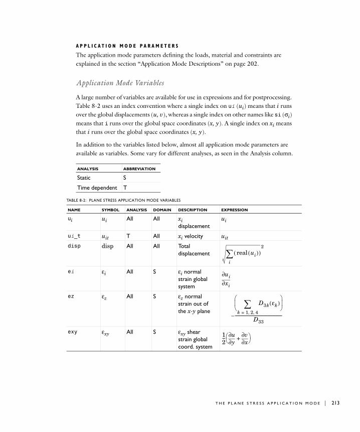
A P P L I C A T I O N M O D E P A R A M E T E R S
The application mode parameters defining the loads, material and constraints are explained in the section “Application Mode Descriptions” on page 202.
Application Mode Variables
A large number of variables are available for use in expressions and for postprocessing. Table 8-2 uses an index convention where a single index on ui (ui) means that i runs over the global displacements (u, v), whereas a single index on other names like si (σi) means that i runs over the global space coordinates (x, y). A single index on xi means that i runs over the global space coordinates (x, y).
In addition to the variables listed below, almost all application mode parameters are available as variables. Some vary for different analyses, as seen in the Analysis column.
ANALYSIS ABBREVIATION
Static S
Time dependent T
TABLE 8-2: PLANE STRESS APPLICATION MODE VARIABLES
NAME SYMBOL ANALYSIS DOMAIN DESCRIPTION EXPRESSION
ui ui All All xi displacement
ui
ui_t uit T All xi velocity uit
disp disp All All Total displacement
ei εi All S εi normal strain global system
ez εz All S εz normal strain out of the x-y plane
exy εxy All S εxy shear strain global coord. system
ui( )real( )i∑
2
xi∂∂ui
D3k εk( )k 1 2 4, ,=∑⎝ ⎠
⎜ ⎟⎛ ⎞
D33-----------------------------------------------–
12---
y∂∂u
x∂∂v
+⎝ ⎠⎛ ⎞
T H E P L A N E S T R E S S A P P L I C A T I O N M O D E | 213
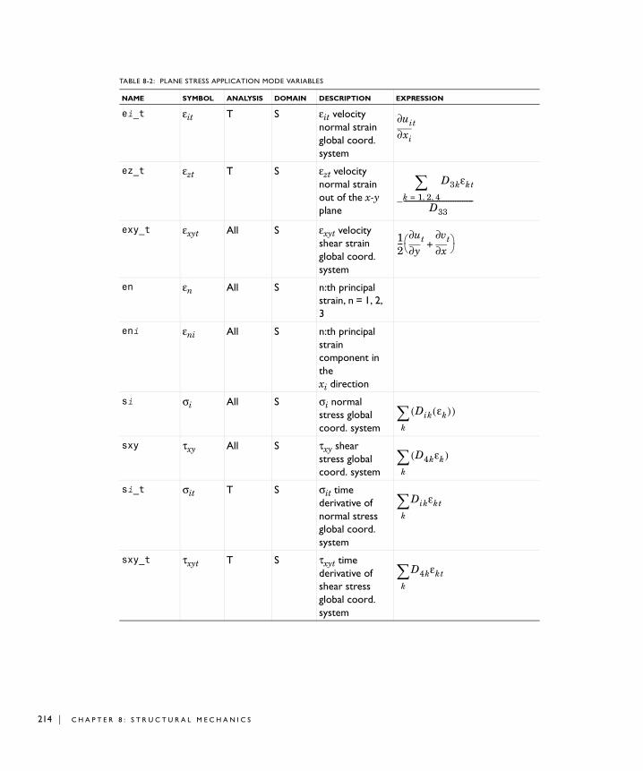
214 | C H A P T E
ei_t εit T S εit velocity normal strain global coord. system
ez_t εzt T S εzt velocity normal strain out of the x-y plane
exy_t εxyt All S εxyt velocity shear strain global coord. system
en εn All S n:th principal strain, n = 1, 2, 3
eni εni All S n:th principal strain component in the xi direction
si σi All S σi normal stress global coord. system
sxy τxy All S τxy shear stress global coord. system
si_t σit T S σit time derivative of normal stress global coord. system
sxy_t τxyt T S τxyt time derivative of shear stress global coord. system
TABLE 8-2: PLANE STRESS APPLICATION MODE VARIABLES
NAME SYMBOL ANALYSIS DOMAIN DESCRIPTION EXPRESSION
xi∂∂uit
D3kεkt
k 1 2 4, ,=∑
D33---------------------------------------–
12---
y∂∂ut
x∂∂vt+⎝ ⎠
⎛ ⎞
Dik εk( )( )k∑
D4kεk( )k∑
Dikεkt
k∑
D4kεkt
k∑
R 8 : S T R U C T U R A L M E C H A N I C S
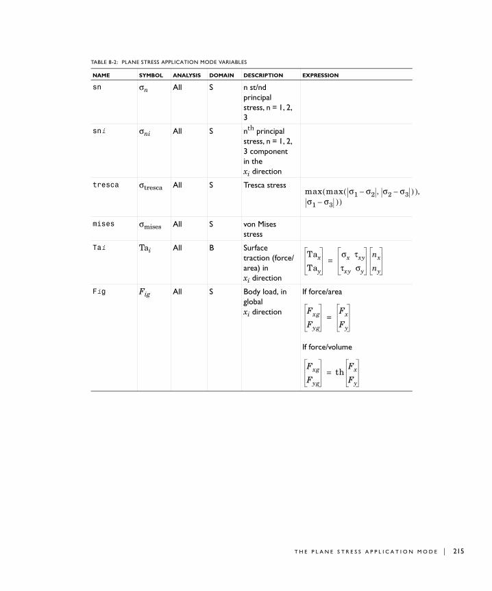
) ),
sn σn All S n st/nd principal stress, n = 1, 2, 3
sni σni All S nth principal stress, n = 1, 2, 3 component in the xi direction
tresca σtresca All S Tresca stress
mises σmises All S von Mises stress
Tai Tai All B Surface traction (force/area) in xi direction
Fig Fig All S Body load, in global xi direction
If force/area
If force/volume
TABLE 8-2: PLANE STRESS APPLICATION MODE VARIABLES
NAME SYMBOL ANALYSIS DOMAIN DESCRIPTION EXPRESSION
max max σ1 σ2– σ2 σ3–,(σ1 σ3– )
()
Tax
Tay
σx τxy
τxy σy
nx
ny
=
Fxg
Fyg
Fx
Fy
=
Fxg
Fyg
thFx
Fy
=
T H E P L A N E S T R E S S A P P L I C A T I O N M O D E | 215
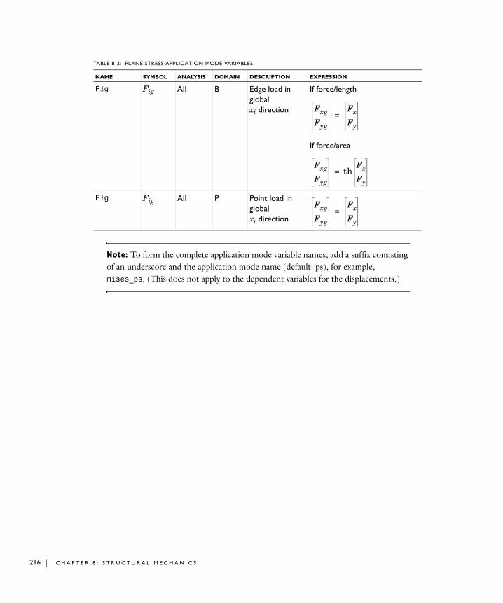
216 | C H A P T E
Note: To form the complete application mode variable names, add a suffix consisting of an underscore and the application mode name (default: ps), for example, mises_ps. (This does not apply to the dependent variables for the displacements.)
Fig Fig All B Edge load in global xi direction
If force/length
If force/area
Fig Fig All P Point load in global xi direction
TABLE 8-2: PLANE STRESS APPLICATION MODE VARIABLES
NAME SYMBOL ANALYSIS DOMAIN DESCRIPTION EXPRESSION
Fxg
Fyg
Fx
Fy
=
Fxg
Fyg
thFx
Fy
=
Fxg
Fyg
Fx
Fy
=
R 8 : S T R U C T U R A L M E C H A N I C S
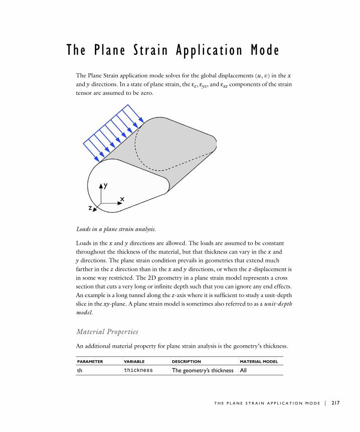
Th e P l a n e S t r a i n App l i c a t i o n Mode
The Plane Strain application mode solves for the global displacements (u, v) in the x and y directions. In a state of plane strain, the εz, εyz, and εxz components of the strain tensor are assumed to be zero.
Loads in a plane strain analysis.
Loads in the x and y directions are allowed. The loads are assumed to be constant throughout the thickness of the material, but that thickness can vary in the x and y directions. The plane strain condition prevails in geometries that extend much farther in the z direction than in the x and y directions, or when the z-displacement is in some way restricted. The 2D geometry in a plane strain model represents a cross section that cuts a very long or infinite depth such that you can ignore any end effects. An example is a long tunnel along the z-axis where it is sufficient to study a unit-depth slice in the xy-plane. A plane strain model is sometimes also referred to as a unit-depth model.
Material Properties
An additional material property for plane strain analysis is the geometry’s thickness.
PARAMETER VARIABLE DESCRIPTION MATERIAL MODEL
th thickness The geometry’s thickness All
T H E P L A N E S T R A I N A P P L I C A T I O N M O D E | 217

218 | C H A P T E
PDE Formulation
COMSOL Multiphysics formulates the application mode using the equilibrium equations described in general terms in the section “Implementation” on page 199.
A P P L I C A T I O N M O D E P A R A M E T E R S
The application mode parameters defining the loads, material, and constraints are explained in the section “Application Mode Descriptions” on page 202.
Application Mode Variables
A large number of variables are available for use in expressions and for postprocessing. In addition to the variables listed below, almost all application mode parameters are available as variables. Some vary for different analyses as seen in the Analysis column.
Table 8-3 uses an index convention where a single index on ui (ui) means that i runs over the global displacements (u, v), whereas a single index on other names like si (σi) means that i runs over the global spatial coordinates (x, y). A single index on xi means that i runs over the global spatial coordinates (x, y).
ANALYSIS ABBREVIATION
Static S
Time dependent T
TABLE 8-3: PLANE STRAIN APPLICATION MODE VARIABLES
NAME SYMBOL ANALYSIS DOMAIN DESCRIPTION EXPRESSION
ui ui All All xi displacement ui
ui_t uit T All xi velocity uit
disp disp All All Total displacement
ei εi All S εi normal strain global system
exy εxy All S εxy shear strain global coord. system
ui( )real( )i∑
2
xi∂∂ui
12---
y∂∂u
x∂∂v
+⎝ ⎠⎛ ⎞
R 8 : S T R U C T U R A L M E C H A N I C S
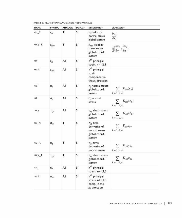
ei_t εit T S εit velocity normal strain global system
exy_t εxyt T S εxyt velocity shear strain global coord. system
en εn All S nth principal strain, n=1,2,3
eni εni All S nth principal strain component in the xi direction
si σi All S σi normal stress global coord. system
sz σz All S σz normal stress
sxy τxy All S τxy shear stress global coord. system
si_t σit T S σit time derivative of normal stress global coord. system
sz_t σz T S σzt time derivative of normal stress
sxy_t τxy T S τxy shear stress global coord. system
sn σn All S nth principal stress, n=1,2,3
sni σni All S nth principal stress, n=1,2,3 comp. in the xi direction
TABLE 8-3: PLANE STRAIN APPLICATION MODE VARIABLES
NAME SYMBOL ANALYSIS DOMAIN DESCRIPTION EXPRESSION
xi∂∂uit
12---
y∂∂ut
x∂∂vt+⎝ ⎠
⎛ ⎞
Dik εk( )k 1 2 4, ,=∑
D3k εk( )k 1 2 4, ,=∑
D4k εk( )k 1 2 4, ,=∑
Dikεkt
k 1 2 4, ,=∑
D3kεkt
k 1 2 4, ,=∑
D4kεkt
k 1 2 4, ,=∑
T H E P L A N E S T R A I N A P P L I C A T I O N M O D E | 219
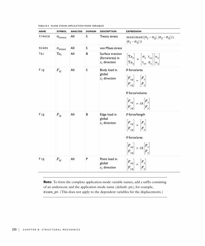
220 | C H A P T E
) ),
Note: To form the complete application mode variable names, add a suffix consisting of an underscore and the application mode name (default: pn), for example, mises_pn. (This does not apply to the dependent variables for the displacements.)
tresca σtresca All S Tresca stress
mises σmises All S von Mises stress
Tai Tai All B Surface traction (force/area) in xi direction
Fig Fig All S Body load in global xi direction
If force/area
If force/volume
Fig Fig All B Edge load in global xi direction
if force/length
if force/area
Fig Fig All P Point load in global xi direction
TABLE 8-3: PLANE STRAIN APPLICATION MODE VARIABLES
NAME SYMBOL ANALYSIS DOMAIN DESCRIPTION EXPRESSION
max max σ1 σ2– σ2 σ3–,(σ1 σ3– )
()
Tax
Tay
σx τxy
τxy σy
nx
ny
=
Fxg
Fyg
Fx
Fy
=
Fxg
Fyg
thFx
Fy
=
Fxg
Fyg
Fx
Fy
=
Fxg
Fyg
thFx
Fy
=
Fxg
Fyg
Fx
Fy
=
R 8 : S T R U C T U R A L M E C H A N I C S
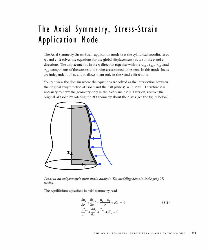
Th e A x i a l S ymme t r y , S t r e s s - S t r a i n App l i c a t i o n Mode
The Axial Symmetry, Stress-Strain application mode uses the cylindrical coordinates r, , and z. It solves the equations for the global displacement (u, w) in the r and z
directions. The displacement v in the direction together with the , , , and components of the stresses and strains are assumed to be zero. In this mode, loads
are independent of , and it allows them only in the r and z directions.
You can view the domain where the equations are solved as the intersection between the original axisymmetric 3D solid and the half plane , r ≥ 0. Therefore it is necessary to draw the geometry only in the half plane r ≥ 0. Later on, recover the original 3D solid by rotating the 2D geometry about the z-axis (see the figure below).
Loads in an axisymmetric stress-strain analysis. The modeling domain is the gray 2D section.
The equilibrium equations in axial symmetry read
(8-2)
ϕϕ τrϕ τϕz γrϕ
γϕzϕ
ϕ 0=
r∂∂σr
z∂∂τrz σr σθ–
r------------------ Kr+ + + 0
r∂∂τrz
z∂∂σz τrz
r------- Kz+ + + 0=
=
T H E A X I A L S Y M M E T R Y , S T R E S S - S T R A I N A P P L I C A T I O N M O D E | 221
222 | C H A P T E
The strain-displacement relationships for the axial symmetry case for small displacements are
To avoid division by r in the equilibrium equations (which causes problems on the axis, where r = 0), the COMSOL Multiphysics application mode transforms the equations. It multiplies the first equation by r2 and the second by r. This transformation is a natural choice because it appears in the principle of virtual work. Integrating over the volume, you must multiply the integrand by 2πr. The application mode introduces and solves for a new dependent variable
which replaces the true radial displacement u.
Note: r = 0 is the symmetry axis. In the Axial Symmetry, Stress-Strain application mode the r-axis is in the x direction (horizontal), and the z-axis is in the y direction (vertical).
PDE Formulation
COMSOL Multiphysics formulates this application mode by using the equilibrium equation (see Equation 8-2) described in general terms in the section “Implementation” on page 199.
A P P L I C A T I O N M O D E P A R A M E T E R S
The application mode parameters defining the loads, material, and constraints are explained in the section “Application Mode Descriptions” on page 202.
Application Mode Variables
A large number of variables are available for use in expressions and for postprocessing. In addition to the variables listed in Table 8-4, almost all application mode parameters
εr r∂∂u
= εϕur---= εz z∂
∂w= γrz z∂
∂ur∂
∂w+=
uor ur---=
R 8 : S T R U C T U R A L M E C H A N I C S
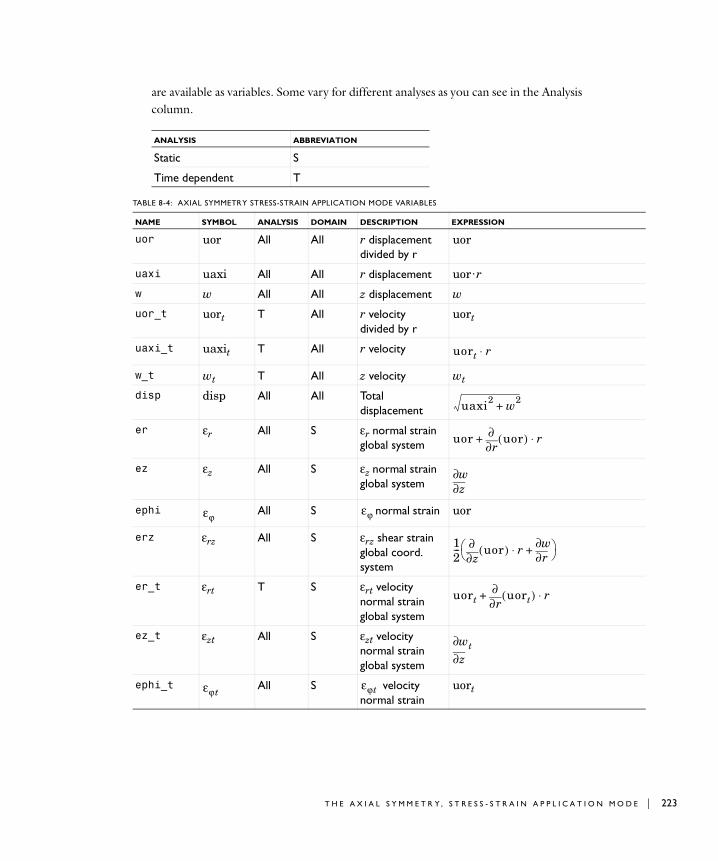
are available as variables. Some vary for different analyses as you can see in the Analysis column.
ANALYSIS ABBREVIATION
Static S
Time dependent T
TABLE 8-4: AXIAL SYMMETRY STRESS-STRAIN APPLICATION MODE VARIABLES
NAME SYMBOL ANALYSIS DOMAIN DESCRIPTION EXPRESSION
uor uor All All r displacement divided by r
uor
uaxi uaxi All All r displacement uor · r
w w All All z displacement w
uor_t uort T All r velocity divided by r
uort
uaxi_t uaxit T All r velocity
w_t wt T All z velocity wt
disp disp All All Total displacement
er εr All S εr normal strain global system
ez εz All S εz normal strain global system
ephi All S normal strain uor
erz εrz All S εrz shear strain global coord. system
er_t εrt T S εrt velocity normal strain global system
ez_t εzt All S εzt velocity normal strain global system
ephi_t All S velocity normal strain
uort
uort r⋅
uaxi2 w2+
uorr∂
∂ uor( ) r⋅+
z∂∂w
εϕεϕ
12---
z∂∂ uor( ) r⋅
r∂∂w
+⎝ ⎠⎛ ⎞
uort r∂∂ uort( ) r⋅+
z∂∂wt
εϕtεϕt
T H E A X I A L S Y M M E T R Y , S T R E S S - S T R A I N A P P L I C A T I O N M O D E | 223
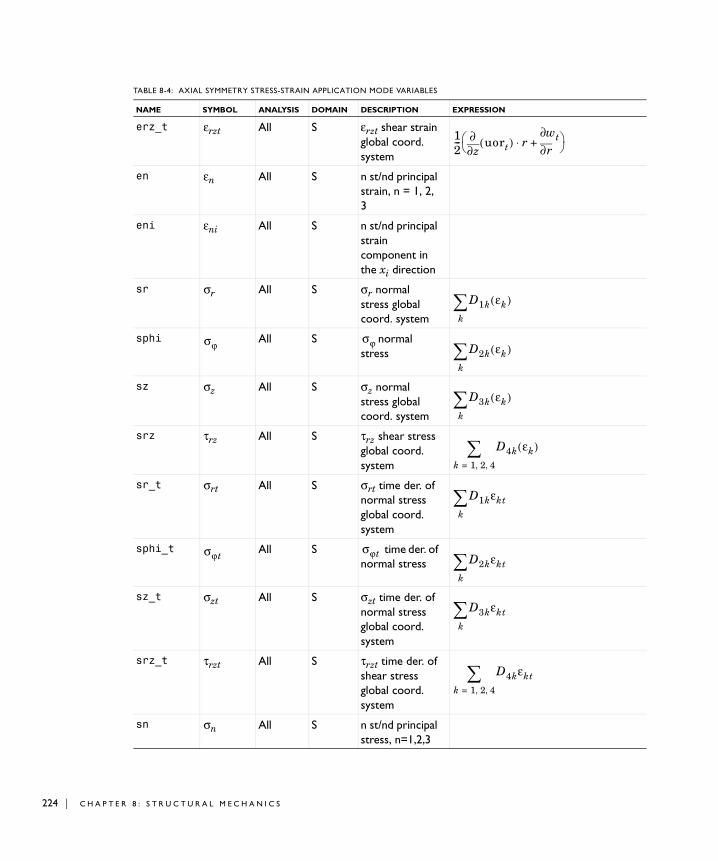
224 | C H A P T E
erz_t εrzt All S εrzt shear strain global coord. system
en εn All S n st/nd principal strain, n = 1, 2, 3
eni εni All S n st/nd principal strain component in the xi direction
sr σr All S σr normal stress global coord. system
sphi All S normal stress
sz σz All S σz normal stress global coord. system
srz τrz All S τrz shear stress global coord. system
sr_t σrt All S σrt time der. of normal stress global coord. system
sphi_t All S time der. of normal stress
sz_t σzt All S σzt time der. of normal stress global coord. system
srz_t τrzt All S τrzt time der. of shear stress global coord. system
sn σn All S n st/nd principal stress, n=1,2,3
TABLE 8-4: AXIAL SYMMETRY STRESS-STRAIN APPLICATION MODE VARIABLES
NAME SYMBOL ANALYSIS DOMAIN DESCRIPTION EXPRESSION
12---
z∂∂ uort( ) r⋅
r∂∂wt+⎝ ⎠
⎛ ⎞
D1k εk( )k∑
σϕσϕ D2k εk( )
k∑
D3k εk( )k∑
D4k εk( )k 1 2 4, ,=∑
D1kεkt
k∑
σϕtσϕt D2kεkt
k∑
D3kεkt
k∑
D4kεkt
k 1 2 4, ,=∑
R 8 : S T R U C T U R A L M E C H A N I C S
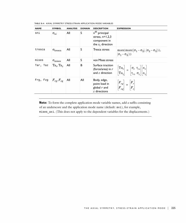
3 ) ),
Note: To form the complete application mode variable names, add a suffix consisting of an underscore and the application mode name (default: axi), for example, mises_axi. (This does not apply to the dependent variables for the displacements.)
sni σni All S nth principal stress, n=1,2,3 component in the xi direction
tresca σtresca All S Tresca stress
mises σmises All S von Mises stress
Tar, Taz Tar, Taz All B Surface traction (force/area) in r and z direction
Frg, Fzg Frg, Fzg All All Body, edge, point load in global r and z directions
TABLE 8-4: AXIAL SYMMETRY STRESS-STRAIN APPLICATION MODE VARIABLES
NAME SYMBOL ANALYSIS DOMAIN DESCRIPTION EXPRESSION
max max σ1 σ2– σ2 σ–,(σ1 σ3– )
()
Tar
Taz
σr τrz
τrz σz
nr
nz
=
Frg
Fzg
Fr
Fz
=
T H E A X I A L S Y M M E T R Y , S T R E S S - S T R A I N A P P L I C A T I O N M O D E | 225
226 | C H A P T E
Examp l e s o f S t r u c t u r a l Me chan i c s Mode l s
Two structural mechanics benchmark models show how to perform a linear static stress analysis using:
• A uniformly distributed horizontal load along an outer edge
• A gravity load
The examples are taken from a NAFEMS benchmark collection (Ref. 1).
Tapered Membrane End Load
The first example shows a 2D plane stress model of a membrane with a thickness of 0.1 m. The load is a uniformly distributed horizontal load of 10 MN/m (that is, a pressure of 100 MPa) along the right end. At the left end, there is no displacement in the x direction. Also, at a midpoint location, the left end is fixed in the y direction.
The model uses the following material properties:
• The material is isotropic.
• The Young’s modulus (elasticity modulus) is 210·103 MPa.
• The Poisson ratio is 0.3.
R 8 : S T R U C T U R A L M E C H A N I C S
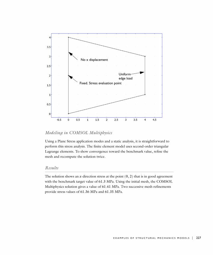
Modeling in COMSOL Multiphysics
Using a Plane Stress application modes and a static analysis, it is straightforward to perform this stress analysis. The finite element model uses second-order triangular Lagrange elements. To show convergence toward the benchmark value, refine the mesh and recompute the solution twice.
Results
The solution shows an x-direction stress at the point (0, 2) that is in good agreement with the benchmark target value of 61.3 MPa. Using the initial mesh, the COMSOL Multiphysics solution gives a value of 61.41 MPa. Two successive mesh refinements provide stress values of 61.36 MPa and 61.35 MPa.
No x displacement
Fixed. Stress evaluation point
Uniformedge load
E X A M P L E S O F S T R U C T U R A L M E C H A N I C S M O D E L S | 227
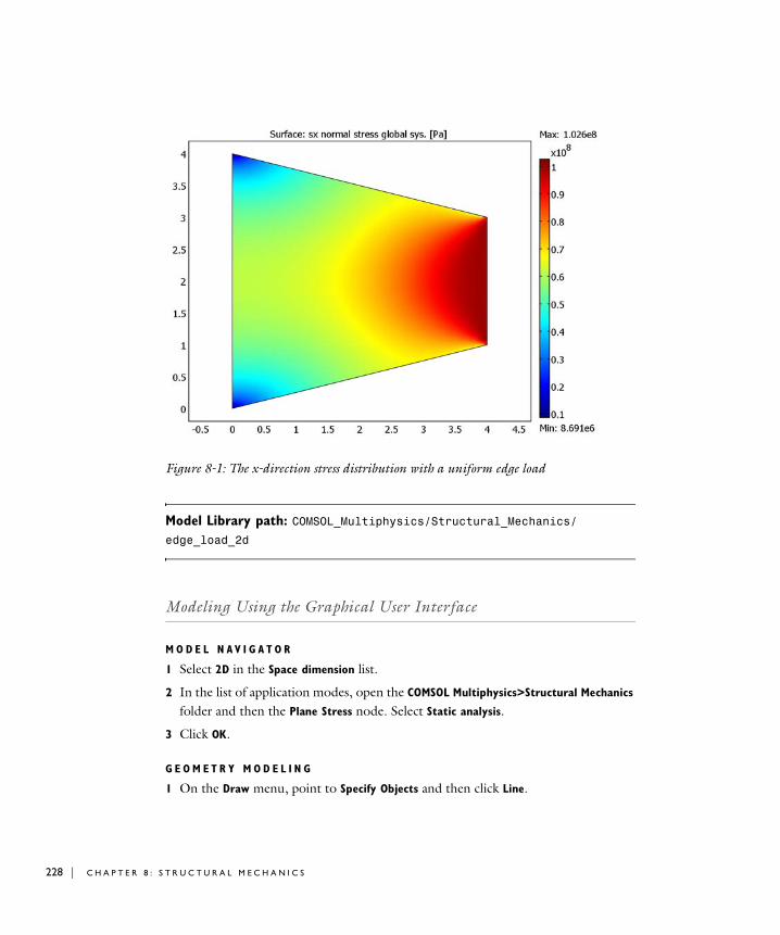
228 | C H A P T E
Figure 8-1: The x-direction stress distribution with a uniform edge load
Model Library path: COMSOL_Multiphysics/Structural_Mechanics/edge_load_2d
Modeling Using the Graphical User Interface
M O D E L N A V I G A T O R
1 Select 2D in the Space dimension list.
2 In the list of application modes, open the COMSOL Multiphysics>Structural Mechanics folder and then the Plane Stress node. Select Static analysis.
3 Click OK.
G E O M E T R Y M O D E L I N G
1 On the Draw menu, point to Specify Objects and then click Line.
R 8 : S T R U C T U R A L M E C H A N I C S
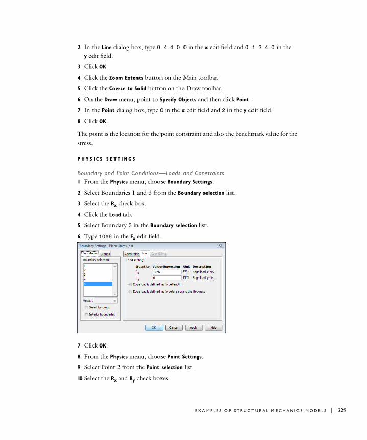
2 In the Line dialog box, type 0 4 4 0 0 in the x edit field and 0 1 3 4 0 in the y edit field.
3 Click OK.
4 Click the Zoom Extents button on the Main toolbar.
5 Click the Coerce to Solid button on the Draw toolbar.
6 On the Draw menu, point to Specify Objects and then click Point.
7 In the Point dialog box, type 0 in the x edit field and 2 in the y edit field.
8 Click OK.
The point is the location for the point constraint and also the benchmark value for the stress.
P H Y S I C S S E T T I N G S
Boundary and Point Conditions—Loads and Constraints1 From the Physics menu, choose Boundary Settings.
2 Select Boundaries 1 and 3 from the Boundary selection list.
3 Select the Rx check box.
4 Click the Load tab.
5 Select Boundary 5 in the Boundary selection list.
6 Type 10e6 in the Fx edit field.
7 Click OK.
8 From the Physics menu, choose Point Settings.
9 Select Point 2 from the Point selection list.
10 Select the Rx and Ry check boxes.
E X A M P L E S O F S T R U C T U R A L M E C H A N I C S M O D E L S | 229
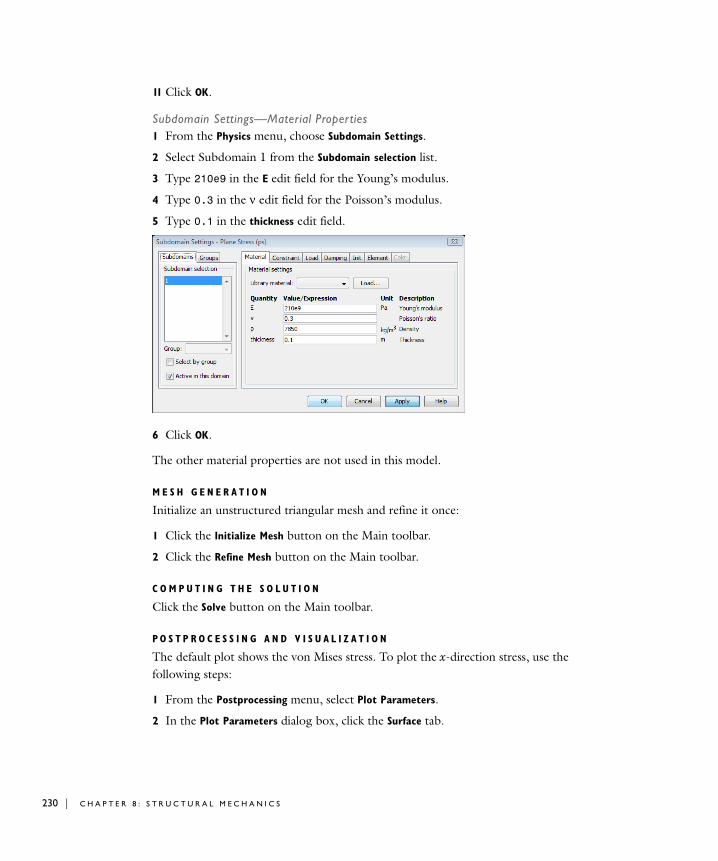
230 | C H A P T E
11 Click OK.
Subdomain Settings—Material Properties1 From the Physics menu, choose Subdomain Settings.
2 Select Subdomain 1 from the Subdomain selection list.
3 Type 210e9 in the E edit field for the Young’s modulus.
4 Type 0.3 in the ν edit field for the Poisson’s modulus.
5 Type 0.1 in the thickness edit field.
6 Click OK.
The other material properties are not used in this model.
M E S H G E N E R A T I O N
Initialize an unstructured triangular mesh and refine it once:
1 Click the Initialize Mesh button on the Main toolbar.
2 Click the Refine Mesh button on the Main toolbar.
C O M P U T I N G T H E S O L U T I O N
Click the Solve button on the Main toolbar.
P O S T P R O C E S S I N G A N D V I S U A L I Z A T I O N
The default plot shows the von Mises stress. To plot the x-direction stress, use the following steps:
1 From the Postprocessing menu, select Plot Parameters.
2 In the Plot Parameters dialog box, click the Surface tab.
R 8 : S T R U C T U R A L M E C H A N I C S
3 On the Surface Data tab, select sx normal stress global sys. from the Predefined quantities list.
4 Click OK.
To get a better look at the value of the x-direction stress at the point (0,2), use the Cross-Section Plot Parameters dialog box:
1 From the Postprocessing menu, select Cross-Section Plot Parameters.
2 Click the Point tab.
3 Select sx normal stress global sys. from the Predefined quantities list.
4 Type 0 in the x edit field and 2 in the y edit field.
5 Click OK.
This plot shows a straight line representing the value of the x-direction stress at the point (0, 2). You can also click at that point in the results plot. That prints the numeric value in the message log.
Tapered Cantilever Gravity Load
The second example shows another 2D plane stress model of a membrane with a thickness of 0.1 m. The load is a gravity load that acts in the negative y direction with an acceleration of 9.81 m/s2. The left end boundary is fully fixed (no displacements).
The model uses the following material properties:
• The material is isotropic.
• The Young’s modulus (elasticity modulus) is 210·103 MPa.
• The Poisson ratio is 0.3.
• The density is 7000 kg/m3.
Modeling in COMSOL Multiphysics
Using a Plane Stress application modes and a static analysis, it is straightforward to perform this stress analysis. You enter the gravity load as force/volume. COMSOL Multiphysics then computes the load using the thickness of the material. The finite element model uses second-order triangular Lagrange elements. For postprocessing, use a cross-section plot to show the value of the shear stress at the location (0,2).
E X A M P L E S O F S T R U C T U R A L M E C H A N I C S M O D E L S | 231
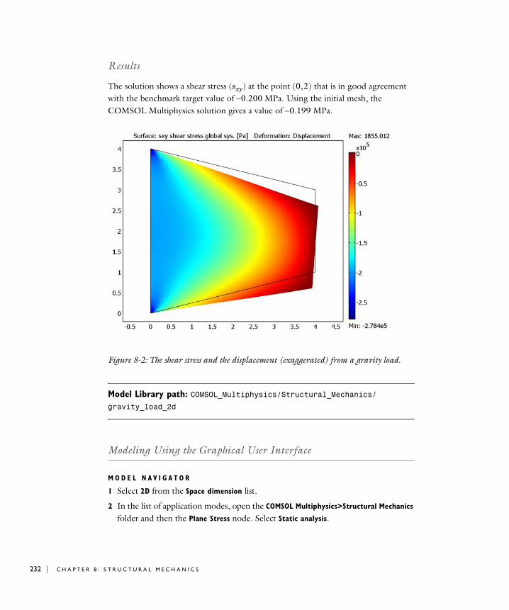
232 | C H A P T E
Results
The solution shows a shear stress (sxy) at the point (0, 2) that is in good agreement with the benchmark target value of −0.200 MPa. Using the initial mesh, the COMSOL Multiphysics solution gives a value of −0.199 MPa.
Figure 8-2: The shear stress and the displacement (exaggerated) from a gravity load.
Model Library path: COMSOL_Multiphysics/Structural_Mechanics/gravity_load_2d
Modeling Using the Graphical User Interface
M O D E L N A V I G A T O R
1 Select 2D from the Space dimension list.
2 In the list of application modes, open the COMSOL Multiphysics>Structural Mechanics folder and then the Plane Stress node. Select Static analysis.
R 8 : S T R U C T U R A L M E C H A N I C S
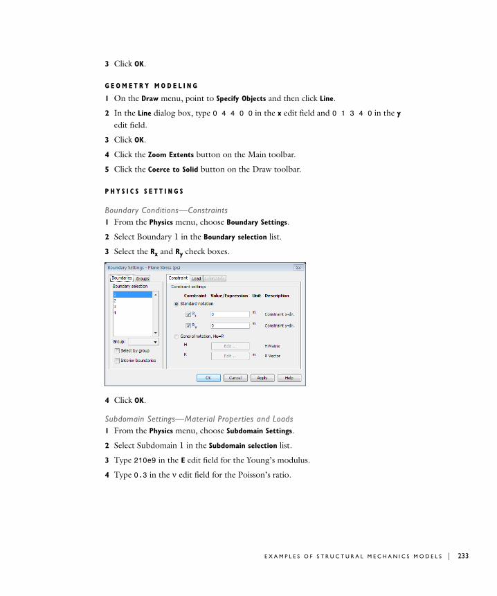
3 Click OK.
G E O M E T R Y M O D E L I N G
1 On the Draw menu, point to Specify Objects and then click Line.
2 In the Line dialog box, type 0 4 4 0 0 in the x edit field and 0 1 3 4 0 in the y edit field.
3 Click OK.
4 Click the Zoom Extents button on the Main toolbar.
5 Click the Coerce to Solid button on the Draw toolbar.
P H Y S I C S S E T T I N G S
Boundary Conditions—Constraints1 From the Physics menu, choose Boundary Settings.
2 Select Boundary 1 in the Boundary selection list.
3 Select the Rx and Ry check boxes.
4 Click OK.
Subdomain Settings—Material Properties and Loads1 From the Physics menu, choose Subdomain Settings.
2 Select Subdomain 1 in the Subdomain selection list.
3 Type 210e9 in the E edit field for the Young’s modulus.
4 Type 0.3 in the ν edit field for the Poisson’s ratio.
E X A M P L E S O F S T R U C T U R A L M E C H A N I C S M O D E L S | 233
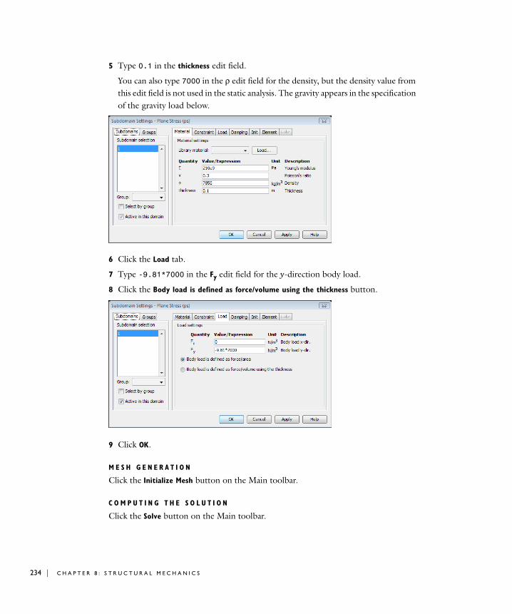
234 | C H A P T E
5 Type 0.1 in the thickness edit field.
You can also type 7000 in the ρ edit field for the density, but the density value from this edit field is not used in the static analysis. The gravity appears in the specification of the gravity load below.
6 Click the Load tab.
7 Type -9.81*7000 in the Fy edit field for the y-direction body load.
8 Click the Body load is defined as force/volume using the thickness button.
9 Click OK.
M E S H G E N E R A T I O N
Click the Initialize Mesh button on the Main toolbar.
C O M P U T I N G T H E S O L U T I O N
Click the Solve button on the Main toolbar.
R 8 : S T R U C T U R A L M E C H A N I C S

PO S T P R O C E S S I N G A N D V I S U A L I Z A T I O N
The default plot shows the von Mises stress. To plot the shear stress and also the deformed shape (displacements), use the following steps:
1 From the Postprocessing menu, select Plot Parameters.
2 In the Plot Parameters dialog box, click the Surface tab.
3 On the Surface Data tab, select sxy shear stress global sys. from the Predefined quantities list.
4 Click the Deform tab.
5 Select the Deformed shape plot check box. The deformation data is the x and y displacements by default.
6 Click OK.
The deformed shape plot uses a scaling factor to clearly show the deformation. The actual displacements are small compared to the model geometry. Click the Deform tab too see the scale factor or to enter a different scale factor.
To get a better look at the value of the shear stress at the point (0, 2), use the Cross-Section Plot Parameters dialog box:
1 From the Postprocessing menu, select Cross-Section Plot Parameters.
2 Click the Point tab.
3 Select sxy shear stress global sys. from the Predefined quantities list.
4 Type 0 in the x edit field and 2 in the y edit field.
5 Click OK.
The plot shows a straight line at the value of the shear stress at (0, 2). You can also click at that point in the results plot. That prints the numeric value in the message log.
Reference
1. D. Hitchings, A. Kamoulakos, G. A. O. Davies: Linear Statics Benchmarks Vol. 1, NAFEMS Ltd., Glasgow, 1987.
E X A M P L E S O F S T R U C T U R A L M E C H A N I C S M O D E L S | 235

236 | C H A P T E
R 8 : S T R U C T U R A L M E C H A N I C S
9
P D E M o d e s f o r E q u a t i o n - B a s e d M o d e l i n g
This chapter describes the use of the PDE modes for equation-based modeling. A step-by-step example illustrates the use of the PDE modes for solving Poisson’s equation.
237
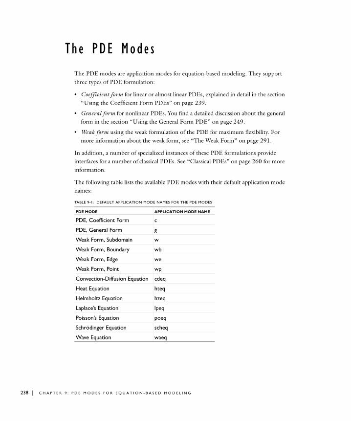
238 | C H A P T E
Th e PDE Mode s
The PDE modes are application modes for equation-based modeling. They support three types of PDE formulation:
• Coefficient form for linear or almost linear PDEs, explained in detail in the section “Using the Coefficient Form PDEs” on page 239.
• General form for nonlinear PDEs. You find a detailed discussion about the general form in the section “Using the General Form PDE” on page 249.
• Weak form using the weak formulation of the PDE for maximum flexibility. For more information about the weak form, see “The Weak Form” on page 291.
In addition, a number of specialized instances of these PDE formulations provide interfaces for a number of classical PDEs. See “Classical PDEs” on page 260 for more information.
The following table lists the available PDE modes with their default application mode names:
TABLE 9-1: DEFAULT APPLICATION MODE NAMES FOR THE PDE MODES
PDE MODE APPLICATION MODE NAME
PDE, Coefficient Form c
PDE, General Form g
Weak Form, Subdomain w
Weak Form, Boundary wb
Weak Form, Edge we
Weak Form, Point wp
Convection-Diffusion Equation cdeq
Heat Equation hteq
Helmholtz Equation hzeq
Laplace’s Equation lpeq
Poisson’s Equation poeq
Schrödinger Equation scheq
Wave Equation waeq
R 9 : P D E M O D E S F O R E Q U A T I O N - B A S E D M O D E L I N G
U s i n g t h e PDE Mode s
Starting a Model Using a PDE Mode
Do as follows to create a new model using one of the PDE modes:
1 Start COMSOL Multiphysics or click New in the COMSOL Multiphysics window.
2 In the Model Navigator make a selection from the Space dimension list.
3 Go to the folder Application Modes>COMSOL Multiphysics>PDE Modes.
4 Open either the PDE, Coefficient Form folder, the PDE, General Form folder, or one of the weak form folders, and make a further selection between the analysis types available.
Alternatively, open the Classical PDEs folder to select from a list of classical PDEs, which are all special cases of the coefficient form formulation.
5 Click OK.
S P E C I F Y I N G A S Y S T E M O F P D E S
COMSOL Multiphysics allows the creation of PDEs with more than one dependent variable. To add variables, follow steps 1 through 4 above and then enter all the variable names as space-separated entries in the Dependent variables edit field before clicking OK. (For the classical PDEs, you can change the name of the dependent variable but not add new ones.) The number of equations in the model equals the number of dependent variables. For example, to start a model with three dependent variables u1, u2, and u3, enter:
u1 u2 u3
You can also couple several scalar PDEs using a multiphysics approach.
Using the Coefficient Form PDEs
The coefficient form PDE mode covers many well-known PDEs. This section covers the formulation and settings pertaining to the coefficient form, as well as the general PDE terminology used in COMSOL Multiphysics.
U S I N G T H E P D E M O D E S | 239
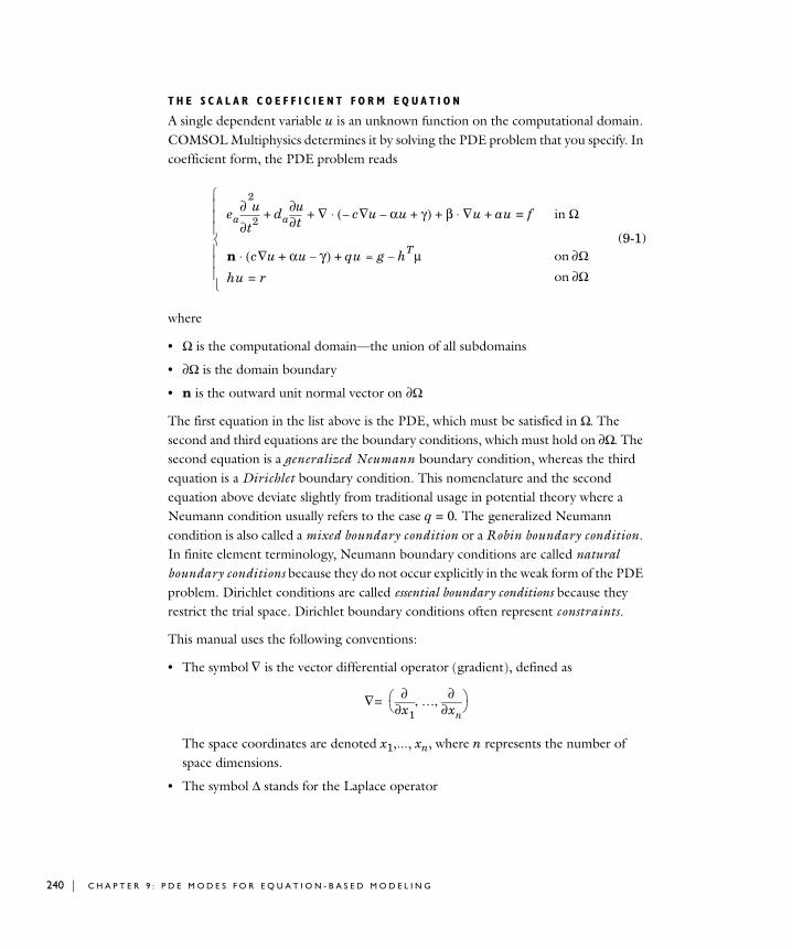
240 | C H A P T E
T H E S C A L A R C O E F F I C I E N T F O R M E Q U A T I O N
A single dependent variable u is an unknown function on the computational domain. COMSOL Multiphysics determines it by solving the PDE problem that you specify. In coefficient form, the PDE problem reads
(9-1)
where
• Ω is the computational domain—the union of all subdomains
• ∂Ω is the domain boundary
• n is the outward unit normal vector on ∂Ω
The first equation in the list above is the PDE, which must be satisfied in Ω. The second and third equations are the boundary conditions, which must hold on ∂Ω. The second equation is a generalized Neumann boundary condition, whereas the third equation is a Dirichlet boundary condition. This nomenclature and the second equation above deviate slightly from traditional usage in potential theory where a Neumann condition usually refers to the case q = 0. The generalized Neumann condition is also called a mixed boundary condition or a Robin boundary condition. In finite element terminology, Neumann boundary conditions are called natural boundary conditions because they do not occur explicitly in the weak form of the PDE problem. Dirichlet conditions are called essential boundary conditions because they restrict the trial space. Dirichlet boundary conditions often represent constraints.
This manual uses the following conventions:
• The symbol is the vector differential operator (gradient), defined as
The space coordinates are denoted x1,..., xn, where n represents the number of space dimensions.
• The symbol ∆ stands for the Laplace operator
eat2
2
∂∂ u da+
t∂∂u ∇+ c u∇– αu– γ+( )⋅ β ∇u au+⋅+ f= in Ω
n c u αu γ–+∇( )⋅ qu = g hTµ–+ on Ω∂
hu r= on Ω∂⎩⎪⎪⎪⎨⎪⎪⎪⎧
∇
∇x1∂∂ …
xn∂∂, ,⎝ ⎠
⎛ ⎞=
R 9 : P D E M O D E S F O R E Q U A T I O N - B A S E D M O D E L I N G
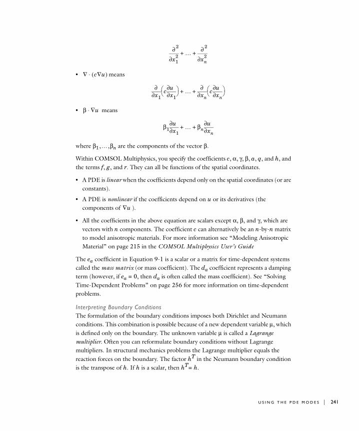
• means
• means
where β1 , … , βn are the components of the vector β.
Within COMSOL Multiphysics, you specify the coefficients c, α, γ, β, a, q, and h, and the terms f, g, and r. They can all be functions of the spatial coordinates.
• A PDE is linear when the coefficients depend only on the spatial coordinates (or are constants).
• A PDE is nonlinear if the coefficients depend on u or its derivatives (the components of ).
• All the coefficients in the above equation are scalars except α, β, and γ, which are vectors with n components. The coefficient c can alternatively be an n-by-n matrix to model anisotropic materials. For more information see “Modeling Anisotropic Material” on page 215 in the COMSOL Multiphysics User’s Guide
The ea coefficient in Equation 9-1 is a scalar or a matrix for time-dependent systems called the mass matrix (or mass coefficient). The da coefficient represents a damping term (however, if ea = 0, then da is often called the mass coefficient). See “Solving Time-Dependent Problems” on page 256 for more information on time-dependent problems.
Interpreting Boundary ConditionsThe formulation of the boundary conditions imposes both Dirichlet and Neumann conditions. This combination is possible because of a new dependent variable µ, which is defined only on the boundary. The unknown variable µ is called a Lagrange multiplier. Often you can reformulate boundary conditions without Lagrange multipliers. In structural mechanics problems the Lagrange multiplier equals the reaction forces on the boundary. The factor hT in the Neumann boundary condition is the transpose of h. If h is a scalar, then hT= h.
x12
2
∂∂ …
xn2
2
∂∂
+ +
∇ c u∇( )⋅
x1∂∂ c
x1∂∂u
⎝ ⎠⎛ ⎞ …
xn∂∂ c
xn∂∂u
⎝ ⎠⎛ ⎞+ +
β u∇⋅
β1 x1∂∂u … β+ n xn∂
∂u+
u∇
U S I N G T H E P D E M O D E S | 241
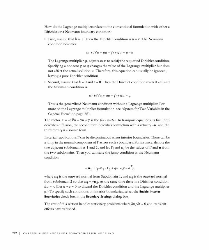
242 | C H A P T E
How do the Lagrange multipliers relate to the conventional formulation with either a Dirichlet or a Neumann boundary condition?
• First, assume that h = 1. Then the Dirichlet condition is u = r. The Neumann condition becomes:
The Lagrange multiplier, µ, adjusts so as to satisfy the requested Dirichlet condition. Specifying a nonzero g or q changes the value of the Lagrange multiplier but does not affect the actual solution u. Therefore, this equation can usually be ignored, leaving a pure Dirichlet condition.
• Second, assume that h = 0 and r = 0. Then the Dirichlet condition reads 0 = 0, and the Neumann condition is
This is the generalized Neumann condition without a Lagrange multiplier. For more on the Lagrange multiplier formulation, see “System for Two Variables in the General Form” on page 251.
The vector is the flux vector. In transport equations its first term describes diffusion, the second term describes convection with a velocity −α, and the third term γ is a source term.
In certain applications Γ can be discontinuous across interior boundaries. There can be a jump in the normal component of Γ across such a boundary. For instance, denote the two adjacent subdomains as 1 and 2, and let Γi and ni be the values of Γ and n from the two subdomains. Then you can state the jump condition as the Neumann condition
where n1 is the outward normal from Subdomain 1, and n2 is the outward normal from Subdomain 2 so that n1 = −n2. At the same time there is a Dirichlet condition hu = r. (Let h = r = 0 to discard the Dirichlet condition and the Lagrange multiplier µ.) To specify such conditions on interior boundaries, select the Enable Interior
Boundaries check box in the Boundary Settings dialog box.
The rest of this section handles stationary problems where ∂u/∂t = 0 and transient effects have vanished.
n c u αu γ–+∇( )⋅ qu = g µ–+
n c u αu γ–+∇( )⋅ qu = g+
Γ c u∇–= αu– γ+
n1 Γ1 n2 Γ2⋅–⋅– qu = g hTµ–+
R 9 : P D E M O D E S F O R E Q U A T I O N - B A S E D M O D E L I N G
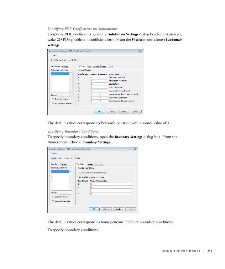
Specifying PDE Coefficients on SubdomainsTo specify PDE coefficients, open the Subdomain Settings dialog box for a stationary, scalar 2D PDE problem in coefficient form. From the Physics menu, choose Subdomain
Settings.
The default values correspond to Poisson’s equation with a source value of 1.
Specifying Boundary ConditionsTo specify boundary conditions, open the Boundary Settings dialog box. From the Physics menu, choose Boundary Settings.
The default values correspond to homogeneous Dirichlet boundary conditions.
To specify boundary conditions:
U S I N G T H E P D E M O D E S | 243
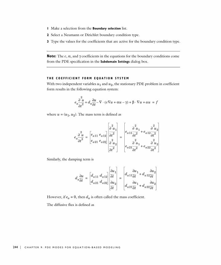
244 | C H A P T E
1 Make a selection from the Boundary selection list.
2 Select a Neumann or Dirichlet boundary condition type.
3 Type the values for the coefficients that are active for the boundary condition type.
Note: The c, α, and γ coefficients in the equations for the boundary conditions come from the PDE specification in the Subdomain Settings dialog box.
T H E C O E F F I C I E N T F O R M E Q U A T I O N S Y S T E M
With two independent variables u1 and u2, the stationary PDE problem in coefficient form results in the following equation system:
where u = (u1, u2). The mass term is defined as
Similarly, the damping term is
However, if ea = 0, then da is often called the mass coefficient.
The diffusive flux is defined as
eat2
2
∂∂ u da t∂
∂u ∇ c u αu γ–+∇( )⋅– β ∇u⋅ au+ ++ f=
eat2
2
∂∂ u ea11 ea12
ea21 ea22
t2
2
∂
∂ u1
t2
2
∂
∂ u2
ea11t2
2
∂
∂ u1 ea12t2
2
∂
∂ u2+
ea21t2
2
∂
∂ u1 ea22t2
2
∂
∂ u2+
= =
da t∂∂u da11 da12
da21 da22
t∂∂u1
t∂∂u2
da11 t∂∂u1 da12 t∂
∂u2+
da21 t∂∂u1 da22 t∂
∂u2+
= =
R 9 : P D E M O D E S F O R E Q U A T I O N - B A S E D M O D E L I N G
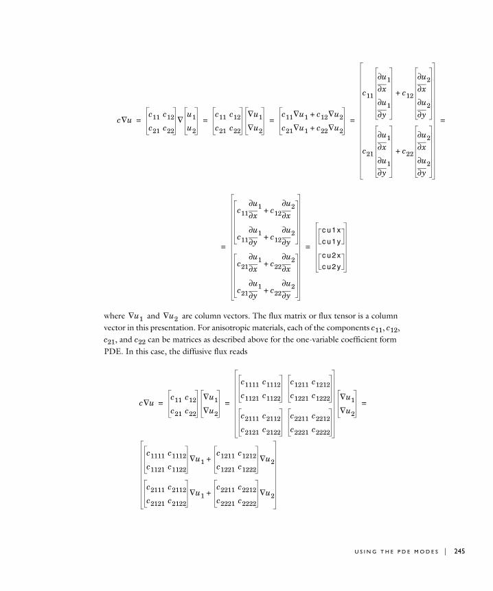
x∂∂u2
y∂∂u2
x∂∂u2
y∂∂u2
=
where and are column vectors. The flux matrix or flux tensor is a column vector in this presentation. For anisotropic materials, each of the components c11, c12, c21, and c22 can be matrices as described above for the one-variable coefficient form PDE. In this case, the diffusive flux reads
c u∇c11 c12
c21 c22
u1
u2
∇c11 c12
c21 c22
u1∇
u2∇
c11 u1∇ c12 u2∇+
c21 u1∇ c22 u2∇+
c11x∂
∂u1
y∂∂u1
c12+
c21x∂
∂u1
y∂∂u1
c22+
= = = =
c11 x∂∂u1 c12 x∂
∂u2+
c11 y∂∂u1 c12 y∂
∂u2+
c21 x∂∂u1 c22 x∂
∂u2+
c21 y∂∂u1 c22 y∂
∂u2+
cu1x
cu1y
cu2x
cu2y
= =
u1∇ u2∇
c u∇c11 c12
c21 c22
u1∇
u2∇
c1111 c1112
c1121 c1122
c1211 c1212
c1221 c1222
c2111 c2112
c2121 c2122
c2211 c2212
c2221 c2222
u1∇
u2∇
c1111 c1112
c1121 c1122
u1∇c1211 c1212
c1221 c1222
u2∇+
c2111 c2112
c2121 c2122
u1∇c2211 c2212
c2221 c2222
u2∇+
= = =
U S I N G T H E P D E M O D E S | 245
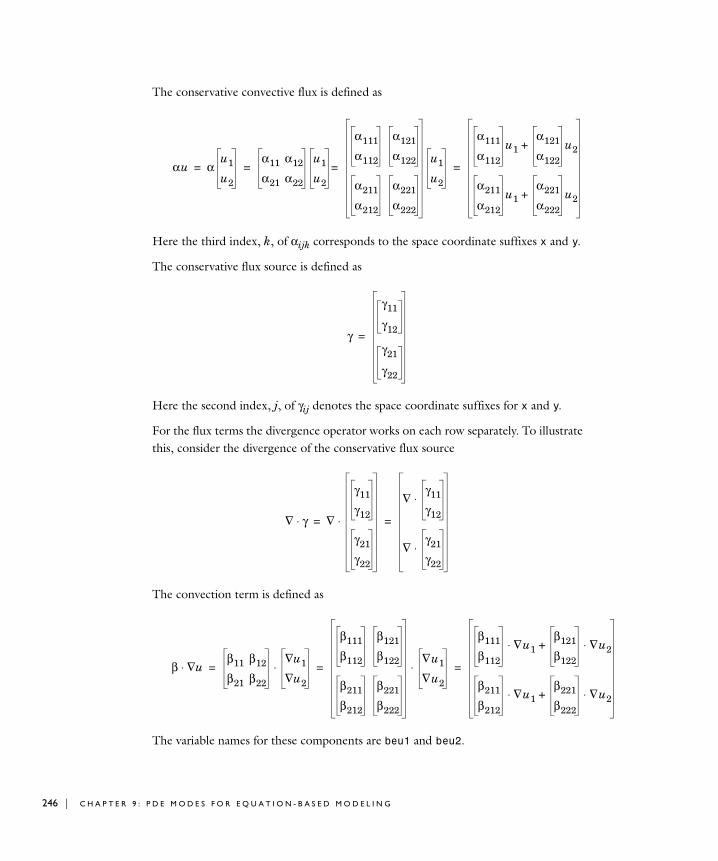
246 | C H A P T E
u2
u2
The conservative convective flux is defined as
Here the third index, k, of αijk corresponds to the space coordinate suffixes x and y.
The conservative flux source is defined as
Here the second index, j, of γij denotes the space coordinate suffixes for x and y.
For the flux terms the divergence operator works on each row separately. To illustrate this, consider the divergence of the conservative flux source
The convection term is defined as
The variable names for these components are beu1 and beu2.
αu αu1
u2
α11 α12
α21 α22
u1
u2
α111
α112
α121
α122
α211
α212
α221
α222
u1
u2
=
α111
α112
u1α121
α122
u2+
α211
α212
u1α221
α222
u2+
= = =
γ
γ11
γ12
γ21
γ22
=
∇ γ⋅ ∇
γ11
γ12
γ21
γ22
⋅
∇γ11
γ12
⋅
∇γ21
γ22
⋅
= =
β u∇⋅β11 β12
β21 β22
u1∇
u2∇⋅
β111
β112
β121
β122
β211
β212
β221
β222
∇u1
∇u2
⋅
β111
β112
∇u1⋅β121
β122
∇⋅+
β211
β212
∇u1⋅β221
β222
∇⋅+
= = =
R 9 : P D E M O D E S F O R E Q U A T I O N - B A S E D M O D E L I N G

The absorption term is defined as
The variable names for these components are au1 and au2.
The source term is defined as
The variable names for these components are f1 and f2.
The Boundary Condition TermsThe Dirichlet boundary condition, in expanded form, reads
If you choose the Dirichlet condition, you also get the generalized Neumann boundary condition, which reads
The normal vector n = (nx, ny) operates on the flux vector in the same way as the divergence operator as explained earlier. If h has full rank (as in the default identity matrix, for example) only the constraints from the Dirichlet condition are active.
If you choose the Neumann condition, you get only the boundary condition
The normal component of the diffusive flux is defined as
The normal component of the conservative convective flux is defined as
aua11 a12
a21 a22
u1
u2
a11u1 a12u2+
a21u1 a22u2+= =
ff1
f2
=
h11 h12
h21 h22
u1
u2
r1
r2
=
n c u αu γ–+∇( )⋅ qu+ g hTµ–=
n c u αu γ–+∇( )⋅ qu+ g=
n c u∇⋅ nc11 c12
c21 c22
u1∇
u2∇⋅
n c11 u1∇ c12 u2∇+( )⋅
n c21 u1∇ c22 u2∇+( )⋅= =
U S I N G T H E P D E M O D E S | 247
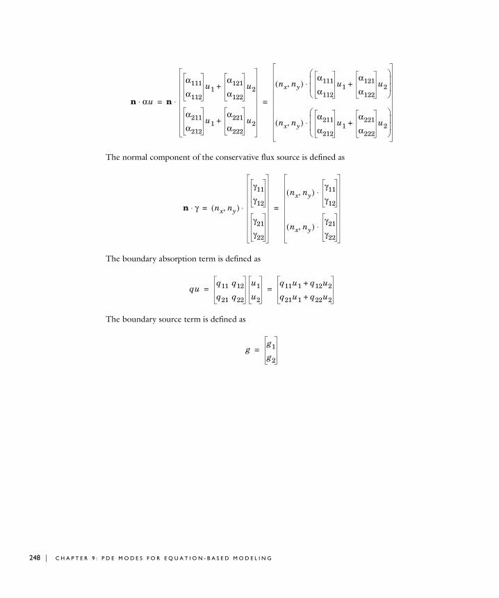
248 | C H A P T E
The normal component of the conservative flux source is defined as
The boundary absorption term is defined as
The boundary source term is defined as
n αu⋅ n
α111
α112
u1α121
α122
u2+
α211
α212
u1α221
α222
u2+
⋅
nx ny,( )α111
α112
u1α121
α122
u2+⎝ ⎠⎜ ⎟⎜ ⎟⎛ ⎞
⋅
nx ny,( )α211
α212
u1α221
α222
u2+⎝ ⎠⎜ ⎟⎜ ⎟⎛ ⎞
⋅
= =
n γ⋅ nx ny,( )
γ11
γ12
γ21
γ22
⋅
nx ny,( )γ11
γ12
⋅
nx ny,( )γ21
γ22
⋅
= =
quq11 q12
q21 q22
u1
u2
q11u1 q12u2+
q21u1 q22u2+= =
gg1
g2
=
R 9 : P D E M O D E S F O R E Q U A T I O N - B A S E D M O D E L I N G
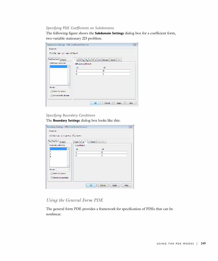
Specifying PDE Coefficients on SubdomainsThe following figure shows the Subdomain Settings dialog box for a coefficient form, two-variable stationary 2D problem.
Specifying Boundary ConditionsThe Boundary Settings dialog box looks like this:
Using the General Form PDE
The general form PDE provides a framework for specification of PDEs that can be nonlinear.
U S I N G T H E P D E M O D E S | 249
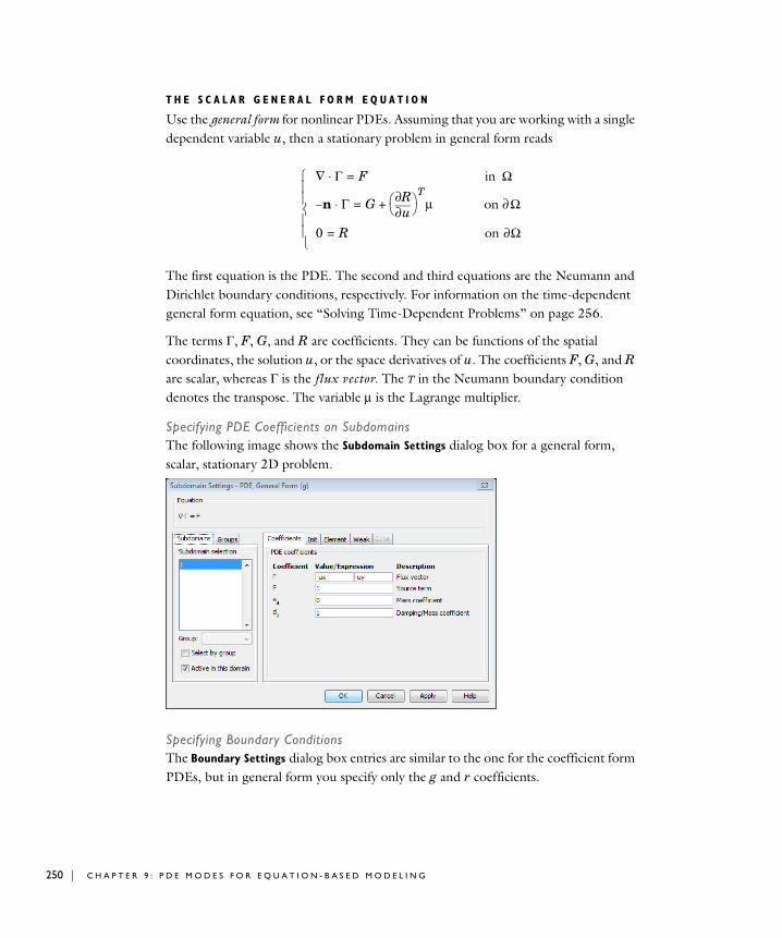
250 | C H A P T E
T H E S C A L A R G E N E R A L F O R M E Q U A T I O N
Use the general form for nonlinear PDEs. Assuming that you are working with a single dependent variable u, then a stationary problem in general form reads
The first equation is the PDE. The second and third equations are the Neumann and Dirichlet boundary conditions, respectively. For information on the time-dependent general form equation, see “Solving Time-Dependent Problems” on page 256.
The terms Γ, F, G, and R are coefficients. They can be functions of the spatial coordinates, the solution u, or the space derivatives of u. The coefficients F, G, and R are scalar, whereas Γ is the flux vector. The T in the Neumann boundary condition denotes the transpose. The variable µ is the Lagrange multiplier.
Specifying PDE Coefficients on SubdomainsThe following image shows the Subdomain Settings dialog box for a general form, scalar, stationary 2D problem.
Specifying Boundary ConditionsThe Boundary Settings dialog box entries are similar to the one for the coefficient form PDEs, but in general form you specify only the g and r coefficients.
∇ Γ⋅ F= in Ω
n– Γ⋅ Gu∂
∂R⎝ ⎠⎛ ⎞
Tµ+= on ∂Ω
0 R= on ∂Ω⎩⎪⎪⎨⎪⎪⎧
R 9 : P D E M O D E S F O R E Q U A T I O N - B A S E D M O D E L I N G
T H E G E N E R A L F O R M E Q U A T I O N S Y S T E M
In the case of several dependent variables u1, u2, …, uN, the following system of equations represents a stationary problem in the general form:
The equation index l ranges from 1 to N, while the constraint index m ranges from 1 to M. This discussion uses the summation convention. Fl, Gl, and Rm are scalars, whereas Γl is a vector. In this case there are several Lagrange multipliers: µ1, µ2,…, µM.
For a more compact form, let u be a vector with components uk, let Γ be a vector with components Γl, and so on. Then the system of equations takes on the same form as given above for a single dependent variable.
It is possible to rewrite the system to introduce the components Γlj of the vector Γl and the components nj of the normal vector n. Then the system of equations becomes
System for Two Variables in the General FormThe following example of a PDE in the general form is a stationary system for N = 2 solution components in n = 2 space dimensions with M = 2 constraints:
with the generalized Neumann boundary conditions
∇ Γl⋅ Fl= in Ω
n– Γl⋅ Gl ul∂∂Rmµm+= on ∂Ω
0 Rm= on ∂Ω⎩⎪⎪⎪⎨⎪⎪⎪⎧
xj∂∂Γlj Fl= in Ω
nj– Γlj Gl ul∂∂Rmµm+= on ∂Ω
0 Rm= on ∂Ω⎩⎪⎪⎪⎪⎨⎪⎪⎪⎪⎧
∇ Γ1⋅ F1= in Ω
∇ Γ2⋅ F2= in Ω⎩⎪⎨⎪⎧
U S I N G T H E P D E M O D E S | 251
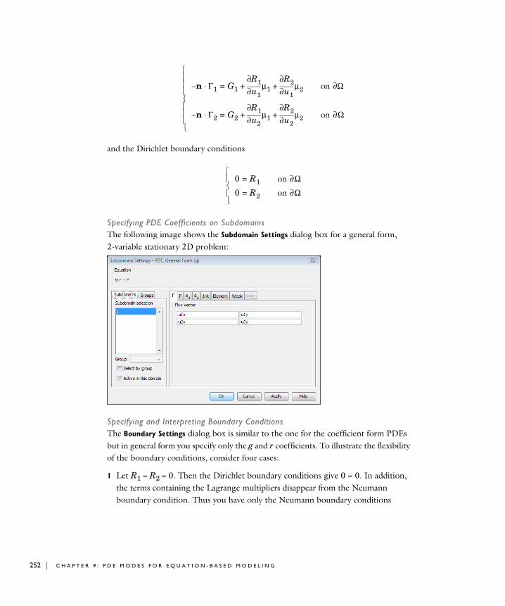
252 | C H A P T E
and the Dirichlet boundary conditions
Specifying PDE Coefficients on SubdomainsThe following image shows the Subdomain Settings dialog box for a general form, 2-variable stationary 2D problem:
Specifying and Interpreting Boundary ConditionsThe Boundary Settings dialog box is similar to the one for the coefficient form PDEs but in general form you specify only the g and r coefficients. To illustrate the flexibility of the boundary conditions, consider four cases:
1 Let R1 = R2 = 0. Then the Dirichlet boundary conditions give 0 = 0. In addition, the terms containing the Lagrange multipliers disappear from the Neumann boundary condition. Thus you have only the Neumann boundary conditions
n– Γ1⋅ G1 u1∂∂R1µ1 u1∂
∂R2µ2+ += on Ω∂
n– Γ2⋅ G2 u2∂∂R1µ1 u2∂
∂R2µ2+ += on ∂Ω⎩⎪⎪⎪⎨⎪⎪⎪⎧
0 R1= on ∂Ω
0 R2= on ∂Ω⎩⎪⎨⎪⎧
R 9 : P D E M O D E S F O R E Q U A T I O N - B A S E D M O D E L I N G
2 Let R1 = r1 − u1 and R2 = r2 − u2. Then the Dirichlet conditions are the usual u1 = r1 and u2 = r2. The Neumann boundary conditions become
These equations impose no restrictions on u1 or u2, because the Lagrange multipliers µ1 and µ2 always adjust so as to fulfill the Dirichlet conditions. In this case, you can therefore ignore the Neumann boundary conditions.
3 Let R1 = r1 − u1 and R2 = 0. Then the Dirichlet conditions are
and the Neumann conditions are
The first Neumann condition can be ignored because it imposes no restriction on u1 or u2. You effectively have only the Dirichlet condition on u1 together with the second Neumann condition.
4 The same as case 3 above but with the two PDEs interchanged (Γ1 and Γ2 as well as F1 and F2). Then the PDEs are
The Dirichlet condition is similar to that in Case 3: u1 = r1. The Neumann conditions then become
n– Γ1⋅ G1= on Ω∂
n– Γ2⋅ G2= on ∂Ω⎩⎪⎨⎪⎧
n– Γ1⋅ G1 µ1–= on Ω∂
n– Γ2⋅ G2 µ2–= on ∂Ω⎩⎪⎨⎪⎧
0 r1 u1–= on ∂Ω
0 0= on ∂Ω⎩⎨⎧
n– Γ1⋅ G1 µ1–= on Ω∂
n– Γ2⋅ G2= on ∂Ω⎩⎪⎨⎪⎧
∇ Γ2⋅ F2= in Ω
∇ Γ1⋅ F1= in Ω⎩⎪⎨⎪⎧
U S I N G T H E P D E M O D E S | 253
254 | C H A P T E
Effectively, you have only the Neumann condition . In comparison with case 3 above, the PDEs and the Dirichlet conditions are identical, while the Neumann conditions are different. Thus, when mixing Dirichlet and Neumann conditions, the ordering of the equations and the dependent variables are important. However, the ordering of the Dirichlet conditions does not matter since the different Lagrange multipliers are for all practical purposes indistinguishable from each other.
5 Finally, let R1 = u2 − u1 and R2 = 0. Then the Dirichlet conditions are
and the Neumann conditions are
Note that the same Lagrange multiplier now appears in both Neumann conditions, which can have different definitions of Γ and G. Therefore, contrary to Cases 2 and 3 above, the Neumann conditions cannot be ignored. Instead, adding the two conditions, it becomes apparent that the solution and flux on the boundary must fulfill
In these examples, the values of the Lagrange multipliers do not matter. However, they often have a physical significance. In structural mechanics, the term
,
n– Γ2⋅ G2 µ1–= on Ω∂
n– Γ1⋅ G1= on ∂Ω⎩⎪⎨⎪⎧
n– Γ1⋅ G1=
0 u2 u1–= on ∂Ω
0 0= on ∂Ω⎩⎨⎧
n– Γ1⋅ G1 µ1–= on Ω∂
n– Γ2⋅ G2 µ1+= on ∂Ω⎩⎪⎨⎪⎧
0 u2 u1–= on Ω∂
n– Γ2⋅ n Γ2⋅– G1 G2+= on ∂Ω⎩⎪⎨⎪⎧
u∂∂R
⎝ ⎠⎛ ⎞
Tµ
R 9 : P D E M O D E S F O R E Q U A T I O N - B A S E D M O D E L I N G
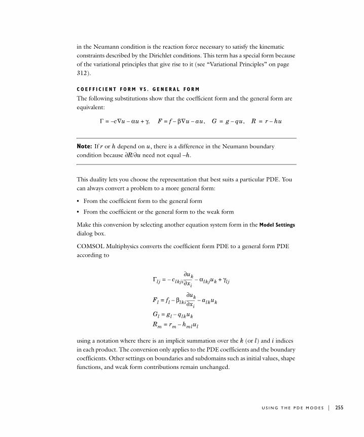
in the Neumann condition is the reaction force necessary to satisfy the kinematic constraints described by the Dirichlet conditions. This term has a special form because of the variational principles that give rise to it (see “Variational Principles” on page 312).
C O E F F I C I E N T F O R M V S . G E N E R A L F O R M
The following substitutions show that the coefficient form and the general form are equivalent:
Note: If r or h depend on u, there is a difference in the Neumann boundary condition because ∂R/∂u need not equal −h.
This duality lets you choose the representation that best suits a particular PDE. You can always convert a problem to a more general form:
• From the coefficient form to the general form
• From the coefficient or the general form to the weak form
Make this conversion by selecting another equation system form in the Model Settings dialog box.
COMSOL Multiphysics converts the coefficient form PDE to a general form PDE according to
using a notation where there is an implicit summation over the k (or l) and i indices in each product. The conversion only applies to the PDE coefficients and the boundary coefficients. Other settings on boundaries and subdomains such as initial values, shape functions, and weak form contributions remain unchanged.
Γ c u∇–= αu– γ F f β∇u– au G,–=,+ g qu R,– r hu–= =
Γlj clkji xi∂∂uk– αlkjuk– γlj+=
Fl fl βlki xi∂∂uk– alkuk–=
Gl gl qlkuk–=
Rm rm hmlul–=
U S I N G T H E P D E M O D E S | 255
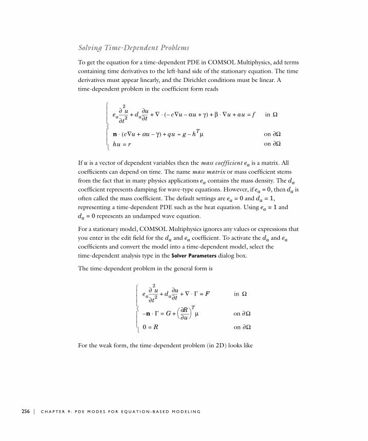
256 | C H A P T E
Solving Time-Dependent Problems
To get the equation for a time-dependent PDE in COMSOL Multiphysics, add terms containing time derivatives to the left-hand side of the stationary equation. The time derivatives must appear linearly, and the Dirichlet conditions must be linear. A time-dependent problem in the coefficient form reads
If u is a vector of dependent variables then the mass coefficient ea is a matrix. All coefficients can depend on time. The name mass matrix or mass coefficient stems from the fact that in many physics applications ea contains the mass density. The da coefficient represents damping for wave-type equations. However, if ea = 0, then da is often called the mass coefficient. The default settings are ea = 0 and da = 1, representing a time-dependent PDE such as the heat equation. Using ea = 1 and da = 0 represents an undamped wave equation.
For a stationary model, COMSOL Multiphysics ignores any values or expressions that you enter in the edit field for the da and ea coefficient. To activate the da and ea coefficients and convert the model into a time-dependent model, select the time-dependent analysis type in the Solver Parameters dialog box.
The time-dependent problem in the general form is
For the weak form, the time-dependent problem (in 2D) looks like
eat2
2
∂
∂ u da+t∂
∂u ∇+ c u∇– αu– γ+( )⋅ β ∇u au+⋅+ f= in Ω
n c u αu γ–+∇( )⋅ qu = g hTµ–+ on Ω∂
hu r= on Ω∂⎩⎪⎪⎪⎨⎪⎪⎪⎧
eat2
2
∂∂ u da+
t∂∂u ∇+ Γ⋅ F= in Ω
n– Γ⋅ Gu∂
∂R⎝ ⎠⎛ ⎞
Tµ+= on ∂Ω
0 R= on ∂Ω⎩⎪⎪⎪⎨⎪⎪⎪⎧
R 9 : P D E M O D E S F O R E Q U A T I O N - B A S E D M O D E L I N G
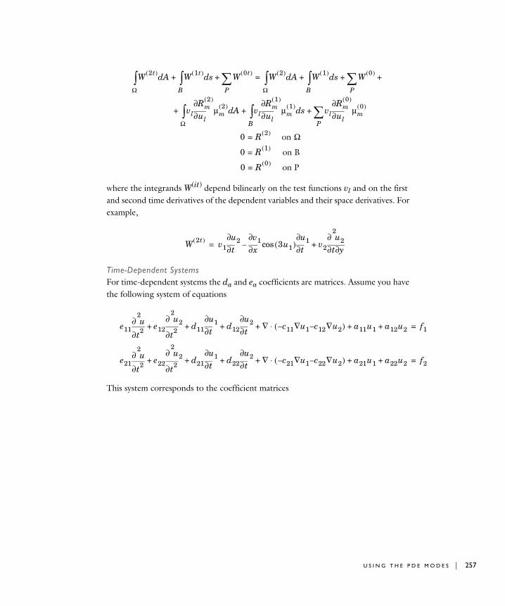
f1
f2
where the integrands W(it) depend bilinearly on the test functions vl and on the first and second time derivatives of the dependent variables and their space derivatives. For example,
Time-Dependent SystemsFor time-dependent systems the da and ea coefficients are matrices. Assume you have the following system of equations
This system corresponds to the coefficient matrices
W 2t( ) AdΩ∫ W 1t( ) sd
B∫ W 0t( )
P∑+ + W 2( ) Ad
Ω∫ W 1( ) sd
B∫ W 0( )
+
P∑+ +=
vl ul∂∂Rm
2( )
µm2( ) Ad
Ω∫ vl ul∂
∂Rm1( )
µm1( ) sd
B∫ vl ul∂
∂Rm0( )
µm0( )
P∑+ + +
0 R 2( )= on Ω
0 R 1( )= on B
0 R 0( )= on P
W 2t( ) v1 t∂∂u2
x∂∂v1 3u1( )
t∂∂u1 v2 t y∂
2
∂∂ u2+cos–=
e11t2
2
∂∂ u e12
t2
2
∂
∂ u2 d11+ +t∂
∂u1 d12 t∂∂u2 ∇ c11– u1∇ c12∇u2–( ) a11u1 a12u2+ +⋅+ + =
e21t2
2
∂
∂ u e22t2
2
∂
∂ u2 d21+ +t∂
∂u1 d22 t∂∂u2 ∇ c21– u1∇ c22∇u2–( ) a21u1 a22u2+ +⋅+ + =
U S I N G T H E P D E M O D E S | 257
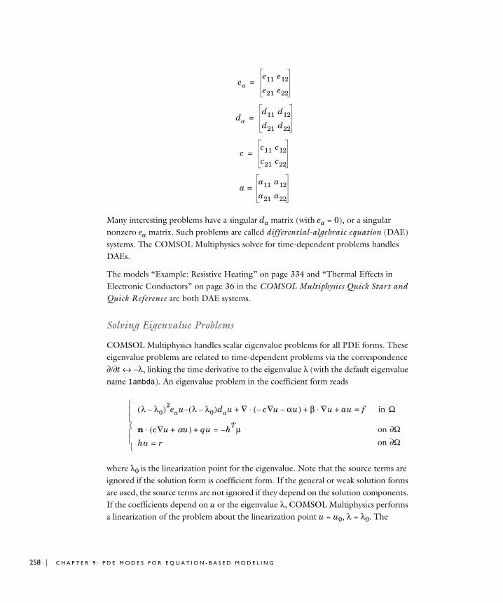
258 | C H A P T E
Many interesting problems have a singular da matrix (with ea = 0), or a singular nonzero ea matrix. Such problems are called differential-algebraic equation (DAE) systems. The COMSOL Multiphysics solver for time-dependent problems handles DAEs.
The models “Example: Resistive Heating” on page 334 and “Thermal Effects in Electronic Conductors” on page 36 in the COMSOL Multiphysics Quick Start and Quick Reference are both DAE systems.
Solving Eigenvalue Problems
COMSOL Multiphysics handles scalar eigenvalue problems for all PDE forms. These eigenvalue problems are related to time-dependent problems via the correspondence ∂/∂t ↔ −λ, linking the time derivative to the eigenvalue λ (with the default eigenvalue name lambda). An eigenvalue problem in the coefficient form reads
where λ0 is the linearization point for the eigenvalue. Note that the source terms are ignored if the solution form is coefficient form. If the general or weak solution forms are used, the source terms are not ignored if they depend on the solution components. If the coefficients depend on u or the eigenvalue λ, COMSOL Multiphysics performs a linearization of the problem about the linearization point u = u0, λ = λ0. The
eae11 e12
e21 e22
=
dad11 d12
d21 d22
=
cc11 c12
c21 c22
=
aa11 a12
a21 a22
=
λ λ0–( )2eau λ λ0–( )d– au ∇+ c u∇– αu–( )⋅ β ∇u au+⋅+ f= in Ω
n c u αu+∇( )⋅ qu = hTµ–+ on Ω∂
hu r= on Ω∂⎩⎪⎪⎨⎪⎪⎧
R 9 : P D E M O D E S F O R E Q U A T I O N - B A S E D M O D E L I N G
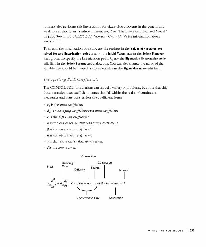
software also performs this linearization for eigenvalue problems in the general and weak forms, though in a slightly different way. See “The Linear or Linearized Model” on page 366 in the COMSOL Multiphysics User’s Guide for information about linearization.
To specify the linearization point u0, use the settings in the Values of variables not
solved for and linearization point area on the Initial Value page in the Solver Manager dialog box. To specify the linearization point λ0 use the Eigenvalue linearization point edit field in the Solver Parameters dialog box. You can also change the name of the variable that should be treated as the eigenvalue in the Eigenvalue name edit field.
Interpreting PDE Coefficients
The COMSOL PDE formulations can model a variety of problems, but note that this documentation uses coefficient names that fall within the realm of continuum mechanics and mass transfer. For the coefficient form:
• ea is the mass coefficient
• da is a damping coefficient or a mass coefficient.
• c is the diffusion coefficient.
• α is the conservative flux convection coefficient.
• β is the convection coefficient.
• a is the absorption coefficient.
• γ is the conservative flux source term.
• f is the source term.
Diffusion
Convection
Source
Convection
Absorption
Source
eat2
2
∂∂ u da+
t∂∂u ∇ c u αu γ–+∇( )⋅– β ∇u⋅ au+ + f=
Conservative Flux
Damping/MassMass
U S I N G T H E P D E M O D E S | 259
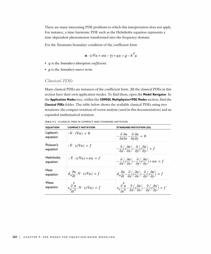
260 | C H A P T E
There are many interesting PDE problems to which this interpretation does not apply. For instance, a time-harmonic PDE such as the Helmholtz equation represents a time-dependent phenomenon transformed into the frequency domain.
For the Neumann boundary condition of the coefficient form
• q is the boundary absorption coefficient.
• g is the boundary source term.
Classical PDEs
Many classical PDEs are instances of the coefficient form. All the classical PDEs in this section have their own application modes. To find them, open the Model Navigator. In the Application Modes tree, within the COMSOL Multiphysics>PDE Modes section, find the Classical PDEs folder. The table below shows the available classical PDEs using two notations: the compact notation of vector analysis (used in this documentation) and an expanded mathematical notation.
TABLE 9-2: CLASSICAL PDES IN COMPACT AND STANDARD NOTATION
EQUATION COMPACT NOTATION STANDARD NOTATION (2D)
Laplace’s equation
Poisson’s equation
Helmholtz equation
Heat equation
Wave equation
n c u α u γ–+∇( )⋅ qu = g hTµ–+
∇ u∇( )⋅– 0=
x∂∂
x∂∂u
–y∂
∂y∂
∂u– 0=
∇ c u∇( )⋅– f=
x∂∂ c
x∂∂u
⎝ ⎠⎛ ⎞
y∂∂ c
y∂∂u
⎝ ⎠⎛ ⎞–– f=
∇ c u∇( )⋅– au+ f=
x∂∂ c
x∂∂u
⎝ ⎠⎛ ⎞
y∂∂ c
y∂∂u
⎝ ⎠⎛ ⎞–– au+ f=
da t∂∂u ∇ c u∇( )⋅– f= da t∂
∂ux∂
∂ cx∂
∂u⎝ ⎠⎛ ⎞
y∂∂ c
y∂∂u
⎝ ⎠⎛ ⎞–– f=
eat2
2
∂∂ u ∇ c u∇( )⋅– f= ea
t2
2
∂∂ u
x∂∂ c
x∂∂u
⎝ ⎠⎛ ⎞
y∂∂ c
y∂∂u
⎝ ⎠⎛ ⎞–– f=
R 9 : P D E M O D E S F O R E Q U A T I O N - B A S E D M O D E L I N G
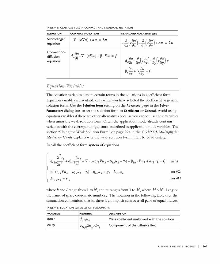
Equation Variables
The equation variables denote certain terms in the equations in coefficient form. Equation variables are available only when you have selected the coefficient or general solution form. Use the Solution form setting on the Advanced page in the Solver
Parameters dialog box to set the solution form to Coefficient or General. Avoid using equation variables if there are other alternatives because you cannot use these variables when using the weak solution form. Often the application mode already contains variables with the corresponding quantities defined as application mode variables. The section “Using the Weak Solution Form” on page 294 in the COMSOL Multiphysics Modeling Guide explains why the weak solution form might be of advantage.
Recall the coefficient form system of equations
where k and l range from 1 to N, and m ranges from 1 to M, where . Let y be the name of space coordinate number j. The notation in the following table uses the summation convention, that is, there is an implicit sum over all pairs of equal indices.
Schrödinger equation
Convection- diffusion equation
TABLE 9-3: EQUATION VARIABLES ON SUBDOMAINS
VARIABLE MEANING DESCRIPTION
daul dalkuk Mass coefficient multiplied with the solution
culy Component of the diffusive flux
TABLE 9-2: CLASSICAL PDES IN COMPACT AND STANDARD NOTATION
EQUATION COMPACT NOTATION STANDARD NOTATION (2D)
∇ c u∇( )⋅– au+ λu=
x∂∂ c
x∂∂u
⎝ ⎠⎛ ⎞
y∂∂ c
y∂∂u
⎝ ⎠⎛ ⎞–– au+ λu=
da t∂∂u ∇ c u∇( )⋅– β u∇⋅+ f=
da t∂∂u
x∂∂ c
x∂∂u
⎝ ⎠⎛ ⎞
y∂∂ c
y∂∂u
⎝ ⎠⎛ ⎞–– +
βx x∂∂u βy y∂
∂u+ f=
ea lkt2
2
∂
∂ uk da lk t∂∂uk ∇+ clk uk∇– αlkuk– γl+( )⋅ βlk ∇uk alkuk+⋅+ fl=+ in Ω
n clk uk αlkuk γl–+∇( )⋅ qlkuk = gl hmlµm–+ on Ω∂
hmkuk rm= on Ω∂⎩⎪⎪⎪⎨⎪⎪⎪⎧
M N≤
clkji uk xi∂⁄∂
U S I N G T H E P D E M O D E S | 261
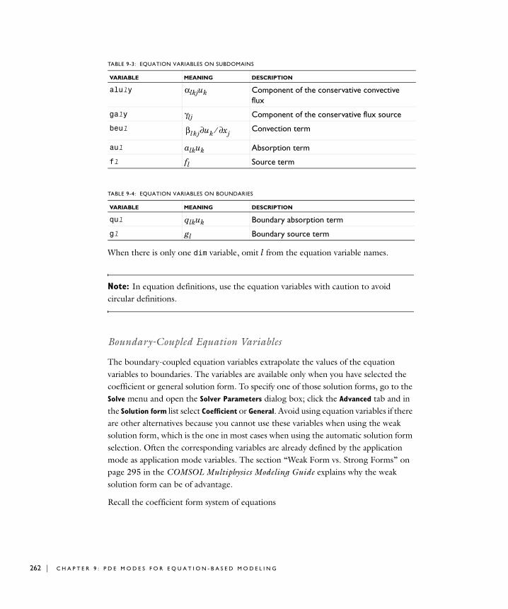
262 | C H A P T E
When there is only one dim variable, omit l from the equation variable names.
Note: In equation definitions, use the equation variables with caution to avoid circular definitions.
Boundary-Coupled Equation Variables
The boundary-coupled equation variables extrapolate the values of the equation variables to boundaries. The variables are available only when you have selected the coefficient or general solution form. To specify one of those solution forms, go to the Solve menu and open the Solver Parameters dialog box; click the Advanced tab and in the Solution form list select Coefficient or General. Avoid using equation variables if there are other alternatives because you cannot use these variables when using the weak solution form, which is the one in most cases when using the automatic solution form selection. Often the corresponding variables are already defined by the application mode as application mode variables. The section “Weak Form vs. Strong Forms” on page 295 in the COMSOL Multiphysics Modeling Guide explains why the weak solution form can be of advantage.
Recall the coefficient form system of equations
aluly αlkjuk Component of the conservative convective flux
galy γlj Component of the conservative flux source
beul Convection term
aul alkuk Absorption term
fl fl Source term
TABLE 9-4: EQUATION VARIABLES ON BOUNDARIES
VARIABLE MEANING DESCRIPTION
qul qlkuk Boundary absorption term
gl gl Boundary source term
TABLE 9-3: EQUATION VARIABLES ON SUBDOMAINS
VARIABLE MEANING DESCRIPTION
βlkj uk xj∂⁄∂
R 9 : P D E M O D E S F O R E Q U A T I O N - B A S E D M O D E L I N G
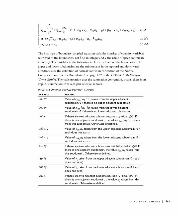
The first type of boundary-coupled equation variables consists of equation variables restricted to the boundaries. Let l be an integer and y the name of space coordinate number j. The variables in the following table are defined on the boundaries. The upper and lower subdomains are the subdomains in the upward and downward directions (see the definition of normal vectors in “Direction of the Normal Component on Interior Boundaries” on page 167 in the COMSOL Multiphysics User’s Guide). The table notation uses the summation convention, that is, there is an implicit summation over each pair of equal indices.
TABLE 9-5: BOUNDARY-COUPLED EQUATION VARIABLES
VARIABLE MEANING
uculy Value of clkji ∂uk / ∂xi taken from the upper adjacent subdomain. 0 if there is no upper adjacent subdomain.
dculy Value of clkji ∂uk / ∂xi taken from the lower adjacent subdomain. 0 if there is no lower adjacent subdomain.
culy If there are two adjacent subdomains, (uculy+dculy)/2. If there is one adjacent subdomain, the value clkji ∂uk / ∂xi taken from this subdomain. Otherwise undefined.
ualuly Value of αlkjuk taken from the upper adjacent subdomain (0 if such does not exist)
daluly Value of αlkjuk taken from the lower adjacent subdomain (0 if such does not exist)
aluly If there are two adjacent subdomains, (ualuly+daluly)/2. If there is one adjacent subdomain, the value αlkjuk taken from this subdomain. Otherwise undefined.
ugaly Value of γlj taken from the upper adjacent subdomain (0 if such does not exist)
dgaly Value of γlj taken from the lower adjacent subdomain (0 if such does not exist)
galy If there are two adjacent subdomains, (ugaly+dgaly)/2. If there is one adjacent subdomain, the value γlj taken from this subdomain. Otherwise undefined.
ea lkt2
2
∂
∂ uk da lk t∂∂uk ∇+ clk uk∇– αlkuk– γl+( )⋅ βlk ∇uk alkuk+⋅+ fl=+ in Ω
n clk uk αlkuk γl–+∇( )⋅ qlkuk = gl hmlµm–+ on Ω∂
hmkuk rm= on Ω∂⎩⎪⎪⎪⎨⎪⎪⎪⎧
U S I N G T H E P D E M O D E S | 263
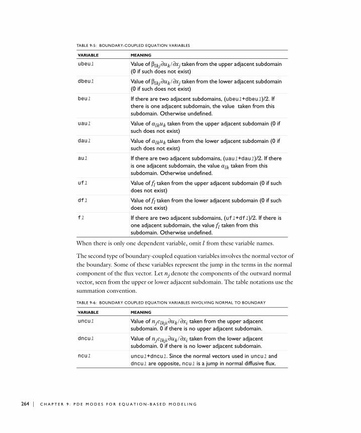
264 | C H A P T E
When there is only one dependent variable, omit l from these variable names.
The second type of boundary-coupled equation variables involves the normal vector of the boundary. Some of these variables represent the jump in the terms in the normal component of the flux vector. Let nj denote the components of the outward normal vector, seen from the upper or lower adjacent subdomain. The table notations use the summation convention.
ubeul Value of βlkj ∂uk / ∂xj taken from the upper adjacent subdomain (0 if such does not exist)
dbeul Value of βlkj ∂uk / ∂xj taken from the lower adjacent subdomain (0 if such does not exist)
beul If there are two adjacent subdomains, (ubeul+dbeul)/2. If there is one adjacent subdomain, the value taken from this subdomain. Otherwise undefined.
uaul Value of alkuk taken from the upper adjacent subdomain (0 if such does not exist)
daul Value of alkuk taken from the lower adjacent subdomain (0 if such does not exist)
aul If there are two adjacent subdomains, (uaul+daul)/2. If there is one adjacent subdomain, the value alk taken from this subdomain. Otherwise undefined.
ufl Value of fl taken from the upper adjacent subdomain (0 if such does not exist)
dfl Value of fl taken from the lower adjacent subdomain (0 if such does not exist)
fl If there are two adjacent subdomains, (ufl+dfl)/2. If there is one adjacent subdomain, the value fl taken from this subdomain. Otherwise undefined.
TABLE 9-6: BOUNDARY COUPLED EQUATION VARIABLES INVOLVING NORMAL TO BOUNDARY
VARIABLE MEANING
uncul Value of nj clkji ∂uk / ∂xi taken from the upper adjacent subdomain. 0 if there is no upper adjacent subdomain.
dncul Value of nj clkji ∂uk / ∂xi taken from the lower adjacent subdomain. 0 if there is no lower adjacent subdomain.
ncul uncul+dncul. Since the normal vectors used in uncul and dncul are opposite, ncul is a jump in normal diffusive flux.
TABLE 9-5: BOUNDARY-COUPLED EQUATION VARIABLES
VARIABLE MEANING
R 9 : P D E M O D E S F O R E Q U A T I O N - B A S E D M O D E L I N G

When there is only one dependent variable, omit l from the above variable names.
Note: In equation definitions, use boundary-coupled equation variables with caution to avoid circular definitions.
Ideal and non-Ideal Constraints
Constraints formulated through the coefficients h and r in the PDE, Coefficient Form application mode and through the coefficient R in the PDE, General Form application mode, give rise to constraints called ideal. An ideal constraint dictates exactly how the the flux conditions (or Neumann boundary conditions) are influenced by the constraint force. For the coefficent form, the flux condition is
,
and for the general form, the flux condition is
.
The last term on the right-hand side in both expressions is the ideal constraint force. Thus, with ideal constraints you cannot enforce a flux condition independently of the constraints. In mathematics as well as in multiphysics modeling it is often necessary to enforce Neumann conditions and Dirichlet conditions more freely than what is possible through ideal constraints. As an example, consider again the general form
unalul Value of njαlkjuk taken from the upper adjacent subdomain (0 if such does not exist)
dnalul Value of njαlkjuk taken from the lower adjacent subdomain (0 if such does not exist)
nalul unalul+dnalul
ungal Value of njγlj taken from the upper adjacent subdomain (0 if such does not exist)
dngal Value of njγlj taken from the lower adjacent subdomain (0 if such does not exist)
ngal ungal+dngal
TABLE 9-6: BOUNDARY COUPLED EQUATION VARIABLES INVOLVING NORMAL TO BOUNDARY
VARIABLE MEANING
n c u αu+∇( )⋅ qu = g hTµ–+
n– Γ⋅ Gu∂
∂R⎝ ⎠⎛ ⎞
Tµ+=
U S I N G T H E P D E M O D E S | 265
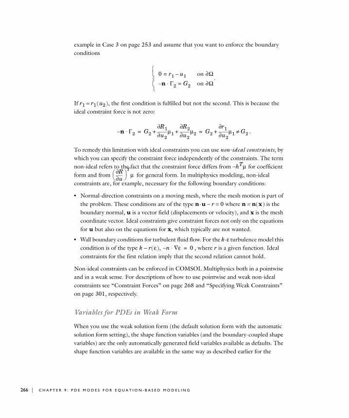
266 | C H A P T E
example in Case 3 on page 253 and assume that you want to enforce the boundary conditions
.
If r1 = r1 ( u2 ), the first condition is fulfilled but not the second. This is because the ideal constraint force is not zero:
.
To remedy this limitation with ideal constraints you can use non-ideal constraints, by which you can specify the constraint force independently of the constraints. The term non-ideal refers to the fact that the constraint force differs from −hTµ for coefficient form and from for general form. In multiphysics modeling, non-ideal constraints are, for example, necessary for the following boundary conditions:
• Normal-direction constraints on a moving mesh, where the mesh motion is part of the problem. These conditions are of the type n · u − r = 0 where n = n( x ) is the boundary normal, u is a vector field (displacements or velocity), and x is the mesh coordinate vector. Ideal constraints give constraint forces not only on the equations for u but also on the equations for x, which typically are not wanted.
• Wall boundary conditions for turbulent fluid flow. For the k-ε turbulence model this condition is of the type k − r( ε ), , where r is a given function. Ideal constraints for the first relation imply that the second relation cannot hold.
Non-ideal constraints can be enforced in COMSOL Multiphysics both in a pointwise and in a weak sense. For descriptions of how to use pointwise and weak non-ideal constraints see “Constraint Forces” on page 268 and “Specifying Weak Constraints” on page 301, respectively.
Variables for PDEs in Weak Form
When you use the weak solution form (the default solution form with the automatic solution form setting), the shape function variables (and the boundary-coupled shape variables) are the only automatically generated field variables available as defaults. The shape function variables are available in the same way as described earlier for the
0 r1 u1–= on ∂Ω
n– Γ2⋅ G2= on ∂Ω⎩⎪⎨⎪⎧
n– Γ2⋅ G2 u2∂∂R1µ1 u2∂
∂R2µ2+ + G2 u2∂∂r1 µ1+ G2≠= =
u∂∂R⎝ ⎠⎛ ⎞
Tµ
n– ε∇⋅ 0=
R 9 : P D E M O D E S F O R E Q U A T I O N - B A S E D M O D E L I N G
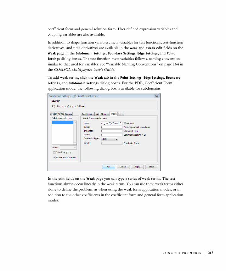
coefficient form and general solution form. User-defined expression variables and coupling variables are also available.
In addition to shape function variables, meta variables for test functions, test-function derivatives, and time derivatives are available in the weak and dweak edit fields on the Weak page in the Subdomain Settings, Boundary Settings, Edge Settings, and Point
Settings dialog boxes. The test function meta variables follow a naming convention similar to that used for variables; see “Variable Naming Conventions” on page 164 in the COMSOL Multiphysics User’s Guide.
To add weak terms, click the Weak tab in the Point Settings, Edge Settings, Boundary
Settings, and Subdomain Settings dialog boxes. For the PDE, Coefficient Form application mode, the following dialog box is available for subdomains.
In the edit fields on the Weak page you can type a series of weak terms. The test functions always occur linearly in the weak terms. You can use these weak terms either alone to define the problem, as when using the weak form application modes, or in addition to the other coefficients in the coefficient form and general form application modes.
U S I N G T H E P D E M O D E S | 267
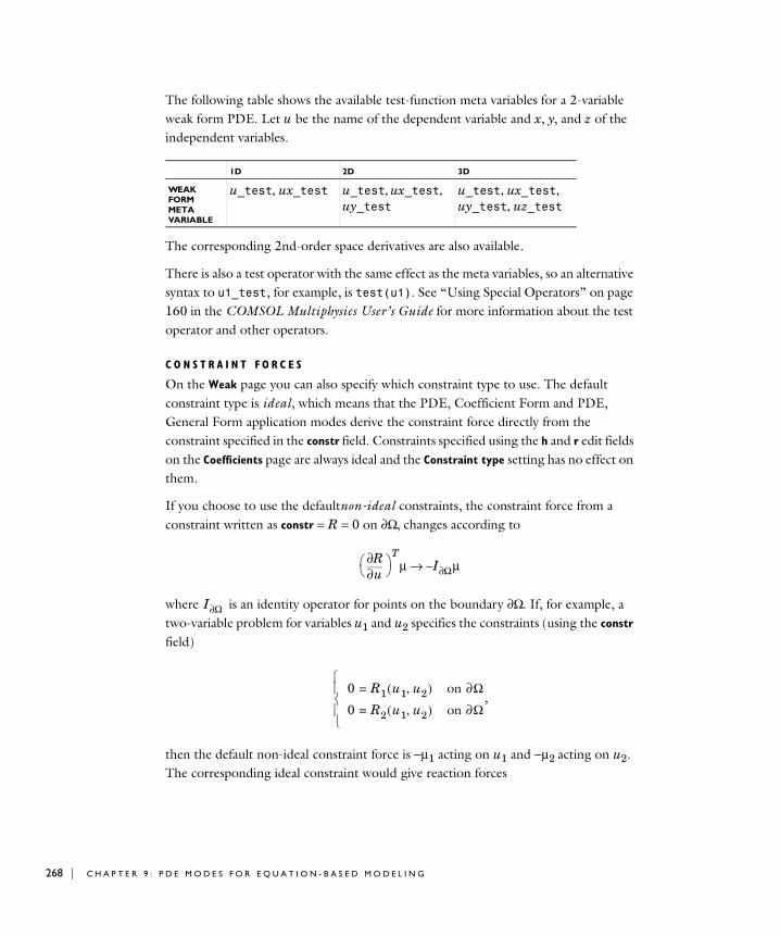
268 | C H A P T E
The following table shows the available test-function meta variables for a 2-variable weak form PDE. Let u be the name of the dependent variable and x, y, and z of the independent variables.
The corresponding 2nd-order space derivatives are also available.
There is also a test operator with the same effect as the meta variables, so an alternative syntax to u1_test, for example, is test(u1). See “Using Special Operators” on page 160 in the COMSOL Multiphysics User’s Guide for more information about the test operator and other operators.
C O N S T R A I N T F O R C E S
On the Weak page you can also specify which constraint type to use. The default constraint type is ideal, which means that the PDE, Coefficient Form and PDE, General Form application modes derive the constraint force directly from the constraint specified in the constr field. Constraints specified using the h and r edit fields on the Coefficients page are always ideal and the Constraint type setting has no effect on them.
If you choose to use the defaultnon-ideal constraints, the constraint force from a constraint written as constr = R = 0 on ∂Ω, changes according to
where is an identity operator for points on the boundary ∂Ω. If, for example, a two-variable problem for variables u1 and u2 specifies the constraints (using the constr field)
,
then the default non-ideal constraint force is −µ1 acting on u1 and −µ2 acting on u2. The corresponding ideal constraint would give reaction forces
1D 2D 3D
WEAK FORM META VARIABLE
u_test, ux_test u_test, ux_test, uy_test
u_test, ux_test, uy_test, uz_test
u∂∂R⎝ ⎠⎛ ⎞
Tµ I Ω∂ µ–→
I Ω∂
0 R1 u1 u2,( )= on ∂Ω
0 R2 u1 u2,( )= on ∂Ω⎩⎪⎨⎪⎧
R 9 : P D E M O D E S F O R E Q U A T I O N - B A S E D M O D E L I N G
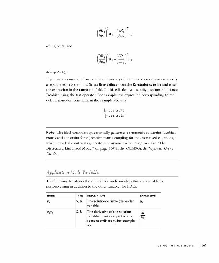
acting on u1 and
acting on u1.
If you want a constraint force different from any of these two choices, you can specify a separate expression for it. Select User defined from the Constraint type list and enter the expression in the constf edit field. In this edit field you specify the constraint force Jacobian using the test operator. For example, the expression corresponding to the default non-ideal constraint in the example above is
.
Note: The ideal constraint type normally generates a symmetric constraint Jacobian matrix and constraint force Jacobian matrix coupling for the discretized equations, while non-ideal constraints generate an unsymmetric coupling. See also “The Discretized Linearized Model” on page 367 in the COMSOL Multiphysics User’s Guide.
Application Mode Variables
The following list shows the application mode variables that are available for postprocessing in addition to the other variables for PDEs:
NAME TYPE DESCRIPTION EXPRESSION
ui S, B The solution variable (dependent variable)
ui
uixj S, B The derivative of the solution variable ui with respect to the space coordinate xj, for example, uy
u1∂∂R1
⎝ ⎠⎜ ⎟⎛ ⎞
T
µ1 u1∂∂R2
⎝ ⎠⎜ ⎟⎛ ⎞
T
µ2+
u2∂∂R1
⎝ ⎠⎜ ⎟⎛ ⎞
T
µ1 u2∂∂R2
⎝ ⎠⎜ ⎟⎛ ⎞
T
µ2+
test u1( )–test u2( )–⎩
⎨⎧
ui∂xi∂
--------
U S I N G T H E P D E M O D E S | 269

270 | C H A P T E
uixjxk S, B The second derivative of the solution variable ui with respect to the space coordinates xj and xk, for example, uxx, uxy.
uit S, B The derivative of the solution variable ui with respect to time
uitt S, B The second derivative of the solution variable ui with respect to time
uixjt S, B The mixed derivative of the solution variable ui with respect to time and the space coordinate xj.
absuixi S, B Gradient of solution
abscuix S Value of the c*grad(ui) vector (Coefficient Form only). Only available when solving using coefficient form as solution form.
absgaix S Value of the Gamma vector (General Form only). Only available when solving using general form as solution form.
|Γ|
cuix S, B c*grad(ui) vector components (Coefficient Form only). Only available when solving using coefficient form as solution form.
ga1xj S, B Gamma vector components (General Form only). Only available when solving using general form as solution form.
γx
NAME TYPE DESCRIPTION EXPRESSION
xj xk∂
2
∂∂ ui
t∂∂ui
t2
2
∂
∂ ui
xj t∂
2
∂∂ ui
∇u ,ui∂xi∂
--------
c∇ u( )
cui∂x∂
--------
R 9 : P D E M O D E S F O R E Q U A T I O N - B A S E D M O D E L I N G
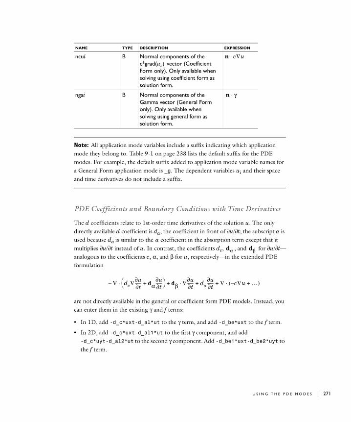
Note: All application mode variables include a suffix indicating which application mode they belong to. Table 9-1 on page 238 lists the default suffix for the PDE modes. For example, the default suffix added to application mode variable names for a General Form application mode is _g. The dependent variables ui and their space and time derivatives do not include a suffix.
PDE Coefficients and Boundary Conditions with Time Derivatives
The d coefficients relate to 1st-order time derivatives of the solution u. The only directly available d coefficient is da, the coefficient in front of ∂u/∂t; the subscript a is used because da is similar to the a coefficient in the absorption term except that it multiplies ∂u/∂t instead of u. In contrast, the coefficients dc, , and for ∂u/∂t—analogous to the coefficients c, α, and β for u, respectively—in the extended PDE formulation
are not directly available in the general or coefficient form PDE models. Instead, you can enter them in the existing γ and f terms:
• In 1D, add -d_c*uxt-d_al*ut to the γ term, and add -d_be*uxt to the f term.
• In 2D, add -d_c*uxt-d_al1*ut to the first γ component, and add -d_c*uyt-d_al2*ut to the second γ component. Add -d_be1*uxt-d_be2*uyt to the f term.
ncui B Normal components of the c*grad(ui) vector (Coefficient Form only). Only available when solving using coefficient form as solution form.
ngai B Normal components of the Gamma vector (General Form only). Only available when solving using general form as solution form.
NAME TYPE DESCRIPTION EXPRESSION
n c∇u⋅
n γ⋅
dα dβ
∇ dc∇∂u∂t------ dα
∂u∂t------+⎝ ⎠
⎛ ⎞⋅– dβ ∇∂u∂t------⋅ da
∂u∂t------ ∇ c– ∇u …+( )⋅+ + +
U S I N G T H E P D E M O D E S | 271
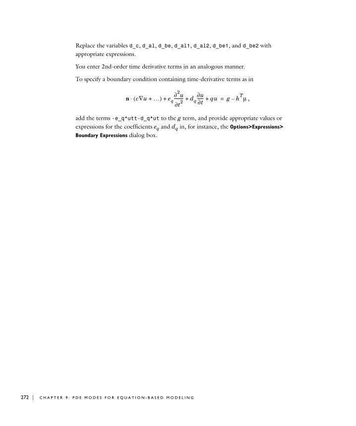
272 | C H A P T E
Replace the variables d_c, d_al, d_be, d_al1, d_al2, d_be1, and d_be2 with appropriate expressions.
You enter 2nd-order time derivative terms in an analogous manner.
To specify a boundary condition containing time-derivative terms as in
,
add the terms -e_q*utt-d_q*ut to the g term, and provide appropriate values or expressions for the coefficients eq and dq in, for instance, the Options>Expressions>
Boundary Expressions dialog box.
n c∇u …+( )⋅ eq∂2u
∂t2--------- dq+
∂u∂t------ qu+ + g hTµ–=
R 9 : P D E M O D E S F O R E Q U A T I O N - B A S E D M O D E L I N G

U s i n g Equa t i o n Con t r i b u t i o n s on I n t e r i o r Me s h Bounda r i e s
In COMSOL Multiphysics it is possible to have equation contributions also from mesh element boundaries that does not lie on a geometry boundary. This makes additional finite element formulations possible like, for example, the discontinuous Galerkin method in space for some transport and flow problems, and the ultraweak variational formulation for wave problems driven by a single frequency.’
Note: The Acoustics Module provides a predefined interface for modeling pressure acoustics using the ultraweak variational formulation.
You specify these interior mesh boundary equation contributions on the corresponding subdomains. It is also possible to define expression variables to use on the interior mesh boundaries. Useful applications typically use discontinuous elements and the up and down operators in expressions to access values on elements adjacent to the interior mesh boundaries.
Specifying Equation Contributions
1 Open the Subdomain Settings dialog box from the Physics menu for any of the PDE Modes. For models with other application modes, choose Equation System>
Subdomain Settings.
2 Select the subdomain where you want to enter an equation contribution on the interior mesh boundaries.
3 Click the Weak tab or the bnd.weak tab depending on the equation system form.
4 Enter your equation contributions in the bnd.weak edit field or the edit fields in the bnd.weak terms area.
5 Click the Element tab.
6 Enter the desired integration order for the ultraweak equation contributions in the bnd.gporder text field.
7 Click OK.
U S I N G E Q U A T I O N C O N T R I B U T I O N S O N I N T E R I O R M E S H B O U N D A R I E S | 273
274 | C H A P T E
Specifying Interior Mesh Boundary Expressions.
To specify expression variables on the interior mesh boundaries, select Interior Mesh Boundary Expressions from the Expressions submenu on the Options menu.
The example in section “Upwinding Using Discontinuous Basis Functions” on page 112 in the COMSOL Multiphysics Model Library shows how to implement the discontinuous Galerkin method with upwinding stabilization using equation contributions on interior mesh boundaries.
R 9 : P D E M O D E S F O R E Q U A T I O N - B A S E D M O D E L I N G
Examp l e s—Equa t i o n -Ba s e d Mode l i n g
The models in this section solves Poisson’s equation and compares the solution to the exact solution and implements a point source. They serve as introductions to equation-based modeling using PDEs in COMSOL Multiphysics. You find many more equation-based models in the chapter “Equation-Based Models” in the COMSOL Multiphysics Model Library.
Poisson’s Equation on the Unit Disk
A classic PDE with a well-known behavior is Poisson’s equation
on the unit disk Ω with f = 1. The exact solution is
which makes it possible to compare the COMSOL Multiphysics solution with the values of the exact solution at the node points on the mesh.
∇ ∇u( )⋅– f= Ωu 0= ∂Ω⎩
⎨⎧
u x y,( ) 1 x2– y2
–4
---------------------------,=
E X A M P L E S — E Q U A T I O N - B A S E D M O D E L I N G | 275
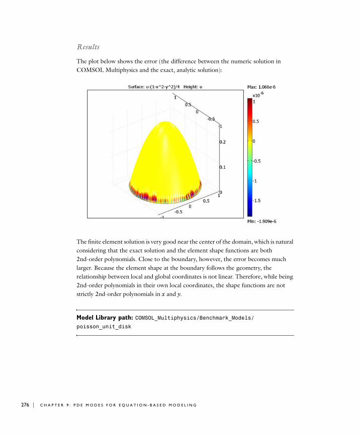
276 | C H A P T E
Results
The plot below shows the error (the difference between the numeric solution in COMSOL Multiphysics and the exact, analytic solution):
The finite element solution is very good near the center of the domain, which is natural considering that the exact solution and the element shape functions are both 2nd-order polynomials. Close to the boundary, however, the error becomes much larger. Because the element shape at the boundary follows the geometry, the relationship between local and global coordinates is not linear. Therefore, while being 2nd-order polynomials in their own local coordinates, the shape functions are not strictly 2nd-order polynomials in x and y.
Model Library path: COMSOL_Multiphysics/Benchmark_Models/poisson_unit_disk
R 9 : P D E M O D E S F O R E Q U A T I O N - B A S E D M O D E L I N G
Modeling Using the Graphical User Interface
The following section explains how to derive the above plot using the graphical user interface.
M O D E L N A V I G A T O R
1 In the Model Navigator, select 2D from the Space dimension list.
2 In the list of application modes, open the COMSOL Multiphysics>PDE Modes folder and then the Classical PDEs folder.
3 Select Poisson’s Equation.
4 Select Lagrange - Quadratic in the Element list (the default element type).
5 Click OK.
O P T I O N S A N D S E T T I N G S
1 Go to the Options menu and choose Axes/Grid Settings.
2 Enter the axis limits from the following table.
3 Click the Grid tab.
4 Clear the Auto check box and enter the following values for the grid spacings and extra grid points:
G E O M E T R Y M O D E L I N G
1 Find the Draw toolbar and click the Ellipse/Circle (Centered) button.
2 Using the right mouse button, draw a circle centered at (0, 0) with a radius of 1.
P H Y S I C S S E T T I N G S
Boundary ConditionsThe default boundary condition in this mode is u = 0, so no changes are necessary.
Subdomain SettingsBy default f is set to 1. Again, no changes are necessary.
AXIS GRID
x min -2 x spacing 0.5
x max 2 Extra x
y min -1.5 y spacing 0.5
y max 1.5 Extra y
E X A M P L E S — E Q U A T I O N - B A S E D M O D E L I N G | 277
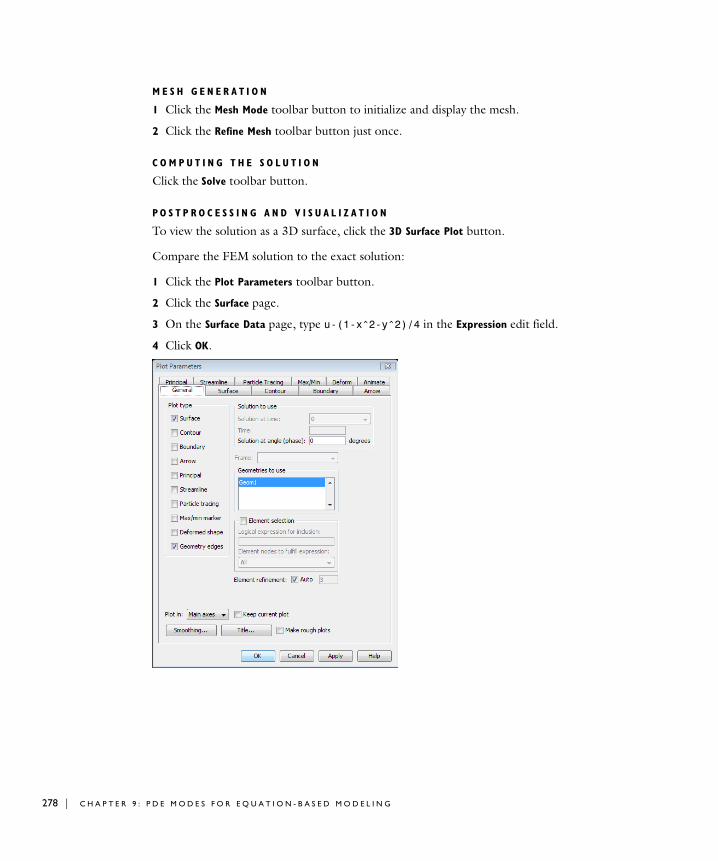
278 | C H A P T E
M E S H G E N E R A T I O N
1 Click the Mesh Mode toolbar button to initialize and display the mesh.
2 Click the Refine Mesh toolbar button just once.
C O M P U T I N G T H E S O L U T I O N
Click the Solve toolbar button.
P O S T P R O C E S S I N G A N D V I S U A L I Z A T I O N
To view the solution as a 3D surface, click the 3D Surface Plot button.
Compare the FEM solution to the exact solution:
1 Click the Plot Parameters toolbar button.
2 Click the Surface page.
3 On the Surface Data page, type u-(1-x^2-y^2)/4 in the Expression edit field.
4 Click OK.
R 9 : P D E M O D E S F O R E Q U A T I O N - B A S E D M O D E L I N G
Implementing a Point Source
Consider Poisson’s equation on the unit circle with a point source at the origin. Its formal expression is:
where δ is the Dirac δ distribution located at the origin. The exact solution is , which has a singularity at the origin.
The easiest way to describe a point source is with an extra weak term. Understanding why requires some basic knowledge of FEM theory and the weak formulation of PDEs. To obtain the weak formulation of the general Poisson equation (where f is any source term), multiply it with a test function utest and integrate over the domain Ω:
Integrate by parts and introduce the Lagrange multiplier λ to account for the constraint on the boundary. This results in the weak formulation:
Most terms in these equations are sums of integrals over the domain, Ω, or over the domain boundary, ∂Ω. You can explicitly add extra weak terms to the equations. In addition to handling terms integrated over Ω or ∂Ω, COMSOL Multiphysics also handles contributions from integrals over edges and from single points. The software does not integrate contributions from points but instead collects them and adds them directly to the equations.
∇ ∇u( )⋅– δ= Ωu 0= ∂Ω⎩
⎨⎧
u 12π------– r( )log=
∇ ∇u( )⋅– utestΩ∫ futest
Ω∫=
uutest∂Ω∫ 0=
utest∀,
⎩⎪⎪⎪⎨⎪⎪⎪⎧
∇u ∇utest⋅Ω∫ λutest
∂Ω∫+ futest
Ω∫=
uutest∂Ω∫ 0=
utest∀,
⎩⎪⎪⎪⎨⎪⎪⎪⎧
E X A M P L E S — E Q U A T I O N - B A S E D M O D E L I N G | 279
280 | C H A P T E
COMSOL Multiphysics discretizes the integral equations just given as long as the source term f is a function of the space coordinates, solution variables, and time. Unfortunately, you cannot express the Dirac δ distribution as a function that COMSOL Multiphysics can integrate numerically. The solution lies in noting that by the definition of the Dirac δ distribution, the following equality holds true:
Therefore, setting f to zero and adding utest as a weak term for a point at the origin provides the problem’s correct weak formulation. The following model handles the resolution of the singularity at the origin using local mesh refinement.
Model Library path: COMSOL_Multiphysics/Benchmark_Models/point_source
Modeling Using the Graphical User Interface
M O D E L N A V I G A T O R
1 In the Model Navigator, select 2D in the Space dimension list.
2 In the list of application modes, open the COMSOL Multiphysics>PDE Modes folder and then Classical PDEs.
δutestΩ∫ utest 0( )=
R 9 : P D E M O D E S F O R E Q U A T I O N - B A S E D M O D E L I N G
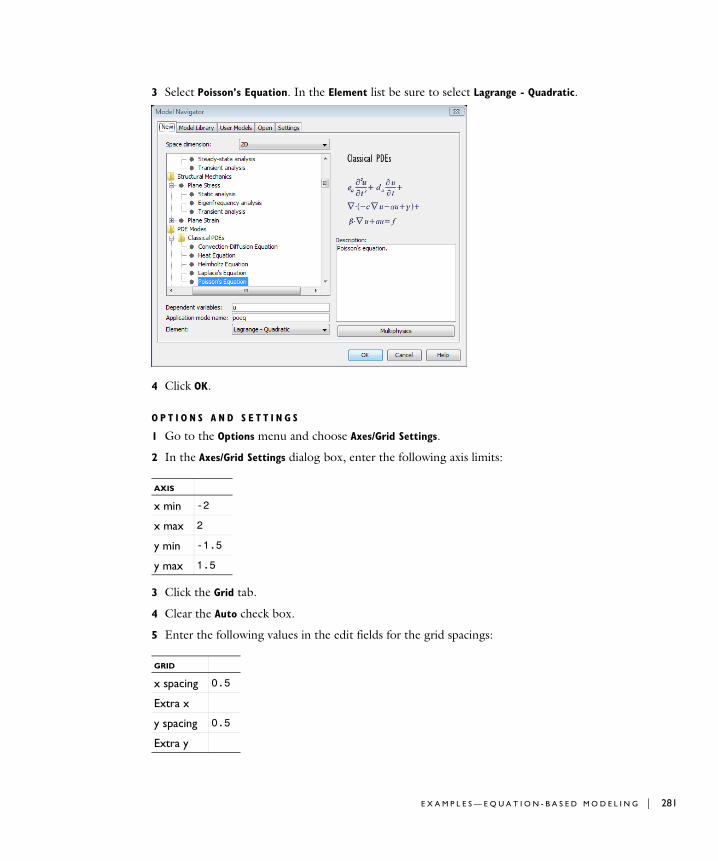
3 Select Poisson’s Equation. In the Element list be sure to select Lagrange - Quadratic.
4 Click OK.
O P T I O N S A N D S E T T I N G S
1 Go to the Options menu and choose Axes/Grid Settings.
2 In the Axes/Grid Settings dialog box, enter the following axis limits:
3 Click the Grid tab.
4 Clear the Auto check box.
5 Enter the following values in the edit fields for the grid spacings:
AXIS
x min -2
x max 2
y min -1.5
y max 1.5
GRID
x spacing 0.5
Extra x
y spacing 0.5
Extra y
E X A M P L E S — E Q U A T I O N - B A S E D M O D E L I N G | 281
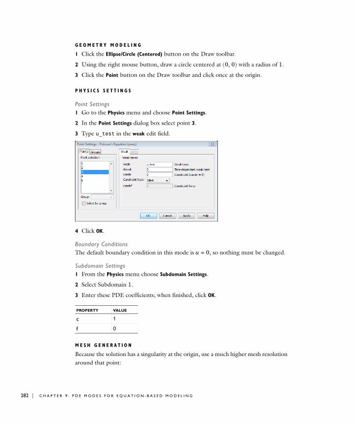
282 | C H A P T E
G E O M E T R Y M O D E L I N G
1 Click the Ellipse/Circle (Centered) button on the Draw toolbar.
2 Using the right mouse button, draw a circle centered at (0, 0) with a radius of 1.
3 Click the Point button on the Draw toolbar and click once at the origin.
P H Y S I C S S E T T I N G S
Point Settings1 Go to the Physics menu and choose Point Settings.
2 In the Point Settings dialog box select point 3.
3 Type u_test in the weak edit field.
4 Click OK.
Boundary ConditionsThe default boundary condition in this mode is u = 0, so nothing must be changed.
Subdomain Settings1 From the Physics menu choose Subdomain Settings.
2 Select Subdomain 1.
3 Enter these PDE coefficients; when finished, click OK.
M E S H G E N E R A T I O N
Because the solution has a singularity at the origin, use a much higher mesh resolution around that point:
PROPERTY VALUE
c 1
f 0
R 9 : P D E M O D E S F O R E Q U A T I O N - B A S E D M O D E L I N G
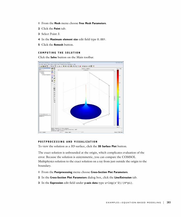
1 From the Mesh menu choose Free Mesh Parameters.
2 Click the Point tab.
3 Select Point 3.
4 In the Maximum element size edit field type 0.001.
5 Click the Remesh button.
C O M P U T I N G T H E S O L U T I O N
Click the Solve button on the Main toolbar.
PO S T P R O C E S S I N G A N D V I S U A L I Z A T I O N
To view the solution as a 3D surface, click the 3D Surface Plot button.
The exact solution is unbounded at the origin, which complicates evaluation of the error. Because the solution is axisymmetric, you can compare the COMSOL Multiphysics solution to the exact solution on a ray from just outside the origin to the boundary.
1 From the Postprocessing menu choose Cross-Section Plot Parameters.
2 In the Cross-Section Plot Parameters dialog box, click the Line/Extrusion tab.
3 In the Expression edit field under y-axis data type u+log(x^2)/(4*pi).
E X A M P L E S — E Q U A T I O N - B A S E D M O D E L I N G | 283

284 | C H A P T E
4 In the Cross-section line data area, type 0.02 in the x0 edit field and type 1 in the x1 edit field. Leave both y0 and y1 at the default value of 0.
5 Click OK.
Another way to check the solution’s accuracy is to integrate the difference between the exact solution and the FEM solution over the domain. The result shows that although the local error close to the origin is quite large, the global error in the L2 norm is small.
R 9 : P D E M O D E S F O R E Q U A T I O N - B A S E D M O D E L I N G

10
G l o b a l E q u a t i o n s a n d O D E s
This chapter describes the use of COMSOL Multiphysics to solve global equations such as ODEs, algebraic equations, and transcendental equations. You can solve such equations separately or coupled to a full finite-element model. Quick examples show how to specify and solve these types of equations.
285

286 | C H A P T E
S o l v i n g ODE s and G l oba l Equa t i o n s
Adding ODEs and Other Global Equations
When working on complex models, you frequently need to introduce single named degrees of freedom, or states, which are not logically related to any particular point in space, and their corresponding equations. In particular, such situations arise when modeling physics in interaction with an external system, for example, a controller or an electrical circuit built from standard components. It is often possible to describe such systems by a system of ordinary differential equations, ODEs, with a limited number of degrees of freedom.
The Global Equations dialog box is designed for implementing this type of external equation, tightly coupled to a PDE model in a physical domain. You can use it for ODEs, differential algebraic equations, purely algebraic equations and conditions, and transcendental equations, or to add degrees of freedom to a PDE using the introduced states. Possible uses include:
• Controllers (see “Process Control Using a PID Controller” on page 317 in the COMSOL Multiphysics Model Library)
• Rigid-body mechanics (see “Terminal Falling Velocity of a Sand Grain” on page 237 in the COMSOL Multiphysics Model Library)
• Nonlinear eigenvalue problems (see “Example: Eigenmode Analysis of an L-Shaped Membrane with Rounded Corner” on page 425)
• Continuation
• Integral constraints (see “Example: Eigenmode Analysis of an L-Shaped Membrane with Rounded Corner” on page 425 of this book and “The Two-Term Boltzmann Equation” on page 171 in the COMSOL Multiphysics Model Library)
• Augmented or generalized equations (see “Stress-Optical Effects with Generalized Plane Strain” on page 615 in the Structural Mechanics Module Model Library, also available in the RF Module Model Library)
The Global Equations Dialog Box
To add a space-independent equation such as an ODE, choose Global Equations from the Physics menu. On the States page, each row corresponds to a named state, that is, a single degree of freedom. Fill in the name of the state variable in the first column
R 1 0 : G L O B A L E Q U A T I O N S A N D O D E S
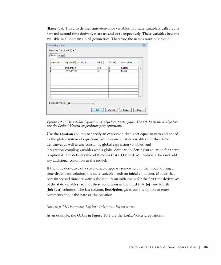
(Name (u)). This also defines time-derivative variables. If a state variable is called u, its first and second time derivatives are ut and utt, respectively. These variables become available in all domains in all geometries. Therefore the names must be unique.
Figure 10-1: The Global Equations dialog box, States page. The ODEs in the dialog box are the Lotka-Volterra or predator-prey equations.
Use the Equation column to specify an expression that is set equal to zero and added to the global system of equations. You can use all state variables and their time derivatives as well as any constants, global expression variables, and integration-coupling variables with a global destination. Setting an equation for a state is optional. The default value of 0 means that COMSOL Multiphysics does not add any additional condition to the model.
If the time derivative of a state variable appears somewhere in the model during a time-dependent solution, the state variable needs an initial condition. Models that contain second time derivatives also require an initial value for the first time derivatives of the state variables. You set these conditions in the third (Init (u)) and fourth (Init (ut)) columns. The last column, Description, gives you the option to enter comments about the state or the equation.
Solving ODEs—the Lotka-Volterra Equations
As an example, the ODEs in Figure 10-1 are the Lotka-Volterra equations:
S O L V I N G O D E S A N D G L O B A L E Q U A T I O N S | 287
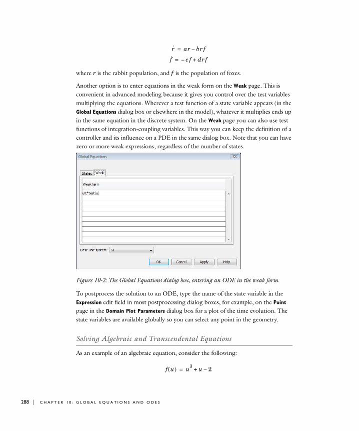
288 | C H A P T E
where r is the rabbit population, and f is the population of foxes.
Another option is to enter equations in the weak form on the Weak page. This is convenient in advanced modeling because it gives you control over the test variables multiplying the equations. Wherever a test function of a state variable appears (in the Global Equations dialog box or elsewhere in the model), whatever it multiplies ends up in the same equation in the discrete system. On the Weak page you can also use test functions of integration-coupling variables. This way you can keep the definition of a controller and its influence on a PDE in the same dialog box. Note that you can have zero or more weak expressions, regardless of the number of states.
Figure 10-2: The Global Equations dialog box, entering an ODE in the weak form.
To postprocess the solution to an ODE, type the name of the state variable in the Expression edit field in most postprocessing dialog boxes, for example, on the Point page in the Domain Plot Parameters dialog box for a plot of the time evolution. The state variables are available globally so you can select any point in the geometry.
Solving Algebraic and Transcendental Equations
As an example of an algebraic equation, consider the following:
r· ar br f–=
f· c f– dr f+=
f u( ) u3 u 2–+=
R 1 0 : G L O B A L E Q U A T I O N S A N D O D E S
This equation has a single root at u = 1. To enter it into the Global Equations dialog box, type u in the Name (u) column and u^3+u-2 in the Equation column (both entries on the same row). Then click the Solve button on the Main toolbar to compute the solution. To display the solution in the message log, choose Postprocessing>
Data Display>Global and type u in the Expression edit field in the Global Data Display dialog box. Click Apply, and Value: 1, Expression: u appears in the message log.
As an example of a transcendental equation, consider the following:
A root to this equation is approximately 0.56714. To enter it into the Global Equations dialog box, type u in the Name (u) column and exp(-u)-u in the Equation column (both entries on the same row). Then click the Solve button on the Main toolbar to compute the solution. To display the solution in the message log, choose Postprocessing>Data Display>Global and type u in the Expression edit field in the Global
Data Display dialog box. Click Apply, and Value: 0.567143, Expression: u appears in the message log.
Adding an ODE to a Boundary
Sometimes a boundary equation is coupled to a PDE in an adjacent subdomain. For example, adding an ODE for v on a boundary such that
where u is the dependent variable in an adjacent subdomain. To implement an ODE on a boundary, do the following:
1 Add a Weak Form, Boundary application mode.
2 Go to the Physics menu and choose Boundary Settings. In the Boundary Settings dialog box, click the Weak tab and type v_test*u in the weak edit field and v_test*v_time in the dweak edit field. This is the weak formulation of the ODE.
f u( ) e u– u–=
∂v∂t------ u=
S O L V I N G O D E S A N D G L O B A L E Q U A T I O N S | 289

290 | C H A P T E
R 1 0 : G L O B A L E Q U A T I O N S A N D O D E S
11
T h e W e a k F o r m
This chapter explains weak form modeling, its purpose, and how to use it. The weak form in COMSOL Multiphysics is a particular way of specifying a model, one in which you use a more general syntax to describe the problem. The discussion concludes with a section giving some theoretical background.
Do not be misled by the term “weak:” the weak form is very powerful and flexible. We have borrowed the term weak form from mathematics, but in this context it has a slightly different meaning; this implementation incorporates features in addition to those defined in the mathematical weak form. Moreover, knowledge of the mathematical weak form is not prerequisite to using the COMSOL Multiphysics implementation.
The distinguishing features of the weak form in COMSOL Multiphysics are that it makes it possible to:
• Solve strongly nonlinear and nonlocal models that need an exact Jacobian for convergence.
• Enter certain equations which can be derived from an energy principle in a very compact and convenient form. Such equations, for example, arise in structural mechanics.
291

292 | C H A P T E
• Add and modify nonstandard constraints, such as various contact and friction models.
• Build models with PDEs on boundaries, edges, and points.
• Use the test operator to conveniently work with problems in variational calculus and parametric optimization.
COMSOL Multiphysics provides two different ways of modeling with the weak form:
• Weak form application modes
• Weak form contributions
In addition, you can add weak constraints, which, for example, provide accurate fluxes and reaction forces.
There are many additional benefits of the weak form, and we mention some of them in the context of specific models in other books in this documentation set.
R 1 1 : T H E W E A K F O R M
Weak Fo rm Mode l i n g
The weak form application modes enable all of the weak form features outlined above. In particular, you need to use these application modes for models with separate PDEs on boundaries, edges, or points. However, modeling with the weak form does not always require using the weak form application modes; sometimes adding weak form contributions is sufficient, as described below.
By default, all models are converted to the weak solution form before solving. Although this feature is a part of the solution technique rather than part of the modeling process, it nonetheless belongs in this discussion because it is based on the weak form implementation. Using the weak solution form gives you the most important benefit of the weak form—the exact Jacobian necessary for fast convergence of strongly nonlinear problems—while you can still do the modeling and view the equations in the equation form of your choice.
The discussion in this chapter reviews the easiest ways to work with the weak form before going on to describe the weak form application modes.
Adding Weak Form Contributions
To add weak contributions to a model you are describing in a physics mode, follow these steps:
1 In the Physics menu, point to Equation System and then select Subdomain Settings, Boundaries Settings, Edge Settings, or Points settings depending on where you need to add the contributions.
2 In the corresponding dialog box, click the Weak tab.
3 Enter the weak contribution in the weak or dweak edit fields.
To add weak contributions to a model you are describing in a coefficient form or general form PDE mode, use the Subdomain Settings dialog box and other settings directly available in the Physics menu.
A D D I N G E D G E A N D P O I N T S O U R C E S A N D C O N S T R A I N T S
Using weak form contributions, you can also add sources and constraints on edges and points. The section “Specifying Point and Edge Settings” on page 242 in the COMSOL Multiphysics User’s Guide describes the procedure.
W E A K F O R M M O D E L I N G | 293
294 | C H A P T E
A D D I N G WE A K C O N S T R A I N T S
The weak form can assist in making accurate flux or reaction-force computations. The section “Using Weak Constraints” on page 300 describes how to use weak constraints for this purpose.
V A R I A T I O N A L C A L C U L U S
Use the test operator to conveniently work with problems in variational calculus and optimization theory. See the minimal-surface example on page 296 for an example of this technique.
Modeling with PDEs on Boundaries, Edges, and Points
The weak form makes it possible to do PDE modeling on boundaries, edges, and points, thus opening up a wider class of models than the other application modes. This is the only type of modeling where you need the weak form application modes.
Using weak form application modes is also a smart way of handling thin layers; COMSOL Multiphysics then solves the problem by modeling rather than meshing. This approach reduces the solution time, and is sometimes what makes a solution possible at all.
The model “Transport and Adsorption” on page 30 in the COMSOL Multiphysics Model Library shows how to use the weak form boundary mode to model a thin adsorbtion layer with diffusion as a PDE on the boundary of a convection-diffusion problem. Another model using tangential derivative variables is “Shell Diffusion” on page 150 in the COMSOL Multiphysics Model Library.
Using Weak Coefficients or the Weak Modes
U S I N G T H E WE A K S O L U T I O N F O R M
By using the weak solution form (the default solution form) you can model with one of the strong forms of the PDE using, for example, the PDE application modes, yet still take advantage of some of the abilities of the weak form. COMSOL Multiphysics converts all your equations to the weak form before solving the problem.
R 1 1 : T H E W E A K F O R M
WE A K F O R M V S . S T R O N G F O R M S
Some features in COMSOL Multiphysics are available only in either strong or weak form. When a feature is available in the weak form but not in a strong form, you can always
• Display and modify the equations in the weak form using the weak equation system form
• Convert to the weak form when solving using the weak solution form (this is the default behavior)
When a feature is available only in a strong form, however, you must model using this form.
Strong Form Features• When using residual method Coefficient, the adaptive mesh refinement considers
only the strong form coefficients when computing the error estimators. The default residual method Weak accounts for all contributions, on weak and strong form.
• The equation variables and coupled boundary equation variables are available only for the strong forms.
Weak Form FeaturesThe weak form automatically computes the Jacobian contributions for all variables, including coupling variables. The strong forms only consider Jacobian contributions from coefficients. Thus, to get an accurate Jacobian when dealing with for example coupling variables and mixed time-space derivatives you might have to use the weak solution form
W E A K F O R M M O D E L I N G | 295
296 | C H A P T E
Examp l e : V a r i a t i o n a l C a l c u l u s
Variational calculus is a branch of mathematics where you want to find the function that extremizes some functional and often also determine the extremal value of the functional in question in the process. According to a fundamental result in the calculus of variations, the integral
has a stationary value if the Euler-Lagrange equation
is satisfied. Use the test operator to conveniently handle certain problems from variational calculus as it implements the Euler-Lagrange equation. See Chapter 4, “The Test Operator.” in the COMSOL Multiphysics User’s Guide for its definition.
Model Definition
The area of the surface z = u(x, y) | (x, y) ∈ Ω is equal to
Given the values of the function u on the boundary ∂Ω, the task is to determine u inside Ω such that the area is minimized. Solving this minimal-surface problem is related to finding the shape of a soap film with a prescribed boundary.
In this example, let with u = x2 on the boundary ∂Ω. Using the Euler-Lagrange equation, you can derive the equation for the minimal-surface problem as:
Simplify the problem by using the test operator to let COMSOL Multiphysics derive the minimal surface problem automatically. Typing in
F x u ∇u, ,( ) ΩdΩ∫
u∂∂F ∇
∇u∂∂F⋅– 0=
A u[ ] 1 ∇u 2+ Ωd
Ω∫=
Ω x y,( ) x2 y2 1≤+ =
∇–1
1 ∇u 2+
----------------------------∇u⎝ ⎠⎜ ⎟⎛ ⎞
⋅ 0=
R 1 1 : T H E W E A K F O R M
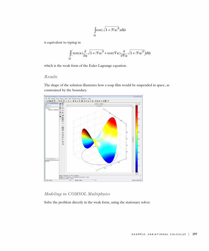
is equivalent to typing in
which is the weak form of the Euler-Lagrange equation.
Results
The shape of the solution illustrates how a soap film would be suspended in space, as constrained by the boundary.
Modeling in COMSOL Multiphysics
Solve the problem directly in the weak form, using the stationary solver.
test 1 ∇u 2+( ) Ωd
Ω∫
test u( )u∂
∂ 1 ∇u 2+ test ∇u( )
∇u∂∂ 1 ∇u 2
++⎝ ⎠⎛ ⎞ Ωd
Ω∫
E X A M P L E : V A R I A T I O N A L C A L C U L U S | 297
298 | C H A P T E
Model Library path: COMSOL_Multiphysics/Benchmarks/minimal_surface
Modeling Using the Graphical User Interface
M O D E L N A V I G A T O R
1 Select 2D from the Space dimension list.
2 In the application mode list, open COMSOL Multiphysics>PDE Modes and then select Weak Form, Subdomain. Make sure Lagrange - Quadratic elements are selected.
3 Click OK.
G E O M E T R Y M O D E L I N G
The problem domain is a unit circle. Draw a circle centered at (0, 0) with a radius of 1.
P H Y S I C S S E T T I N G S
Boundary Conditions1 From the Physics menu, choose Boundary Settings.
2 Enter the following boundary coefficients:
3 Click OK.
Subdomain Settings1 From the Physics menu, open the Subdomain Settings dialog box and enter the PDE
coefficients:
2 Click OK.
SETTINGS ALL BOUNDARIES
weak 0
dweak 0
constr x^2-u
SETTINGS SUBDOMAIN 1
weak test(sqrt(1+ux^2+uy^2))
dweak 0
constr 0
R 1 1 : T H E W E A K F O R M
M E S H G E N E R A T I O N
Click the Initialize Mesh button to create a mesh.
C O M P U T I N G T H E S O L U T I O N
Click the Solve button on the Main toolbar to solve the problem.
PO S T P R O C E S S I N G A N D V I S U A L I Z A T I O N
Click the 3D Surface Plot button and the Scene Light button to create an illuminated 3D plot.
Modeling Using the Programming Language
Run the model from COMSOL Script or MATLAB:
1 Create the geometry and a standard mesh:
clear femfem.geom = circ2(0,0,1);fem.mesh = meshinit(fem);
2 Set up the minimization problem that characterizes the minimal surface. Use second order Lagrange elements:
fem.shape = 2;fem.sshape = 2;fem.bnd.constr = 'x^2-u';fem.equ.weak = 'test(sqrt(1+ux^2+uy^2))';
3 Create the extended mesh, solve the nonlinear problem, and plot the solution:
fem.xmesh = meshextend(fem);fem.sol = femstatic(fem);postsurf(fem,'u','u');
4 Compute the area of the minimal surface:
postint(fem,'sqrt(1+ux^2+uy^2)')
E X A M P L E : V A R I A T I O N A L C A L C U L U S | 299
300 | C H A P T E
U s i n g Weak Con s t r a i n t s
The weak constraints feature in COMSOL Multiphysics implements constraints by using finite elements on the constrained domain for the Lagrange multipliers, and by solving for the Lagrange multipliers along with the original problem. The weak constraints have a number of distinct advantages. They can:
• Provide very accurate flux computations—the Lagrange multipliers along the constraints optimally balance the finite element projection of the applied loads (reaction forces). See “Computing Accurate Fluxes” on page 253 in the COMSOL Multiphysics User’s Guide for more information and an example.
• Handle nonlinear constraints—the nonlinear solver does not store the Lagrange multipliers arising from standard constraints from one step to the next, which affects the convergence when constraints are nonlinear. Weak constraints can handle general nonlinearities because the Lagrange multipliers are updated as a part of the solution vector and give correct contributions to the stiffness matrix.
• Implement constraints including derivatives—constraints only on the tangential component of the derivative work when using standard constraints, whereas you must use weak constraint to be able to handle nontangential constraints. Note that boundary conditions involving the normal component of the derivative can almost always be reformulated as a Neumann condition, which is usually preferable.
Weak constraints also come with the following drawbacks:
• Because extra unknowns are introduced for the Lagrange multipliers the problem size increases compared to when eliminating the constraints.
• The formulation normally implies that a so-called saddle-point problem is introduced with zeros on the main diagonal of the Jacobian of the discretized equations. This class of problems is often more difficult to solve. Because iterative methods for linear systems are sensitive to the eigenvalue distribution of the system matrix, a weak constraint formulation can be much more difficult to solve than the corresponding pointwise constraint formulation.
• Discontinuous constraints result in (theoretically) infinite Lagrange multipliers. In practice you get large oscillations.
R 1 1 : T H E W E A K F O R M
Specifying Weak Constraints
In the graphical user interface you can add weak constraints using the Weak constraints application mode property. The following procedure applies to the physics modes:
1 From the Physics menu select Properties.
2 In the Application Mode Properties dialog box, select On from the Weak constraints list.
3 Select Ideal or Non-ideal from the Constraint type list (see “Ideal vs. Non-Ideal Constraints” on page 301)
4 Click OK.
The variable names in the application modes using weak constraints, such as lm1, correspond to the Lagrange multipliers. The weak constraints supersede the original constraints and implement them using a weak formulation. By default, weak constraints are active on all boundaries. To control the use of weak constraints on individual boundaries, open the Boundary Settings dialog box and click the Weak
Constr. tab. On this tab, which appears when you add weak constraints, you can select boundaries and then select or clear the Use weak constraints check box to include or turn off the weak constraints for the selected boundaries. You can also set element type, shape function, and initial values for the weak constraint variables (Lagrange multipliers).
I D E A L V S . N O N - I D E A L C O N S T R A I N T S
Ideal weak constraints in theory implement the same boundary conditions as the standard, pointwise, constraints. In some cases, the result may differ slightly, but this is only due to the different discretization. Using non-ideal constraints, on the other hand, modifies the way boundary conditions are interpreted. Switching from pointwise constraints to non-ideal weak constraints therefore can modify the physics of the model, while using ideal weak constraints only affects the numerics.
The difference between ideal and non-ideal constraints is the way the Lagrange multipliers—which can be interpreted as generalized reaction forces—are applied. In an ideal constraint, the Lagrange multipliers are applied symmetrically on all dependent variables involved in the constraint so as to keep symmetric problems symmetric. In a non-ideal constraint, the reaction forces are applied only on the application mode’s dependent variable at the boundary where the constraint is specified.
U S I N G W E A K C O N S T R A I N T S | 301
302 | C H A P T E
Imagine a model with two application modes A and B, with dependent variables u and v, respectively. If application mode A specifies a standard constraint as R = 2u−3v = 0, COMSOL Multiphysics implements the ideal weak boundary constraint by adding the weak term
where µ and are the Lagrange multiplier and corresponding test function, and and are the test functions corresponding to u and v, respectively. Since µ multiplies both
test functions in the second integral, both u and v are affected by the constraint, which is therefore bidirectional.
The corresponding non-ideal weak constraint adds the weak form contribution
Here, the Lagrange multiplier µ only multiplies the test function . All reaction forces therefore apply only to u, while v is left unaffected by the constraint. This makes the non-ideal constraint unidirectional. Note also that the non-ideal constraint does not consider the factor 2 in front of u when applying the forces. Even if the constraint would contain spatial derivatives, the Lagrange multiplier would still be applied only directly on the dependent variable itself.
For more information on the effects of ideal and non-ideal constraints, see “Example—Coupling Variables and Boundary Constraints” on page 304. For a model that uses ideal weak constraints for accurate outward normal current densities, see “Semiconductor Diode” on page 442 in the COMSOL Multiphysics Model Library. For a model that uses non-ideal weak constraints to get the correct reaction forces, see “Sloshing Tank” on page 247 in the COMSOL Multiphysics Model Library.
Weak Constraints in Assemblies
When using assemblies, the application modes add a constraint on the dependent variables on the destination domains of the identity pairs. If you use weak constraints, the application modes also turn these constraints into weak constraints. Unlike other physics settings on pairs you do not control the use of weak constraints on pairs on the Pair tab in the Boundary Settings dialog box. If you would like to change the settings for the weak constraints on the destination boundaries of a pair go to the Boundaries
µ 2u 3v–( )⋅B∫ ds µ 2u 3v–( ) sd⋅
B∫+
µ uv
µ 2u 3v–( )⋅B∫ ds µ u sd⋅
B∫+
u
R 1 1 : T H E W E A K F O R M
tab and change the settings there. See the section “Specifying Physics Settings on Pairs” on page 361 for general information about physics settings on pairs.
The constraints on pairs, which makes sure that the dependent variables are continuous across the pair boundary, are always implemented as ideal constraints. This because the non-ideal constraints do not conserve the flux from the source side to the destination side of the pair.
Limitations of Weak Constraints
Weak constraints are more difficult to use than conventional pointwise constraints. Consider the following tips when using them:
• Pointwise and weak constraints on the same set of variables on adjacent boundaries (boundaries that share common node points in the mesh) do not work. This means that if you must constrain all boundaries on a solid and want to use a weak constraint on one boundary segment (one face), you must use the weak constraint on the entire boundary of the solid (if the boundary is connected).
• You must always have a nontrivial constraint (that is, a Dirichlet condition) on the boundaries where you enable the weak constraint for the constraint to take effect.
• Problems with the scaling of linear systems sometimes arise in conjunction with weak constraints. The Lagrange multiplier variables always have a different unit than the main system variables, and can therefore be of a completely different order of magnitude. Usually the automatic variable scaling in the solvers is sufficient, but there are cases when you may want to consider manual scaling.
• Always use the same shape function type for the weak constraint as for the variables that you constrain, possibly with lower-order elements for the weak constraint. In some cases, for example when constraining derivatives, the system of equations may become singular. The reason is usually that there are redundant Lagrange multiplier degrees of freedom in the model. Try to lower the order of the Lagrange multiplier variables, or use constraints on the Lagrange multiplier to remove some degrees of freedom.
• If you want to use iterative methods for the linear system and if the weak constraint formulation gives zero’s on the diagonal of the system matrix, the SOR class of preconditioners and smoothers will not work. Instead try use the Vanka algorithm with the Lagrange multipliers as the Vanka variables, or use the incomplete LU factorization algorithm.
U S I N G W E A K C O N S T R A I N T S | 303

304 | C H A P T E
Examp l e—Coup l i n g V a r i a b l e s and Bounda r y Con s t r a i n t s
Boundary Constraints in a Heat Transfer Model
This example describes the difference between different boundary constraints when using a coupling variable to map a function of a solution from one boundary to another.
Consider the following example:
M O D E L N A V I G A T O R
1 In the Model Navigator, select 2D in the Space Dimension list.
2 In the list of application modes, select COMSOL Multiphsyics>Heat
Transfer>Conduction>Steady-state analysis.
G E O M E T R Y M O D E L I N G
1 Draw a rectangle with diagonal corners at (0, 0) and (2, 1).
2 Draw a circle with center at (1, 0.5) and radius 0.1.
3 Subtract the circle from the rectangle to create a hole: Press Ctrl+A to select both objects and click the Difference button.
P H Y S I C S S E T T I N G S
Boundary Conditions1 From the Physics menu, open the Boundary Settings dialog box.
2 Select the boundaries of the circle (Boundaries 5–8) and select Temperature in the Boundary condition list. Type 300 in the Temperature edit field to specify the value of the fixed temperature (in kelvin). The circle then acts as a heat sink.
3 Select boundary 3 (the top boundary) and then select Heat flux in the Boundary
condition list. Type 10000*x in the Inward heat flux edit field. This creates a heat flux of 0 to 20,000 W/m2, which increases linearly from left to right.
4 The other boundaries are thermally insulated, which is the default setting. Click OK to close the Boundary Settings dialog box.
R 1 1 : T H E W E A K F O R M
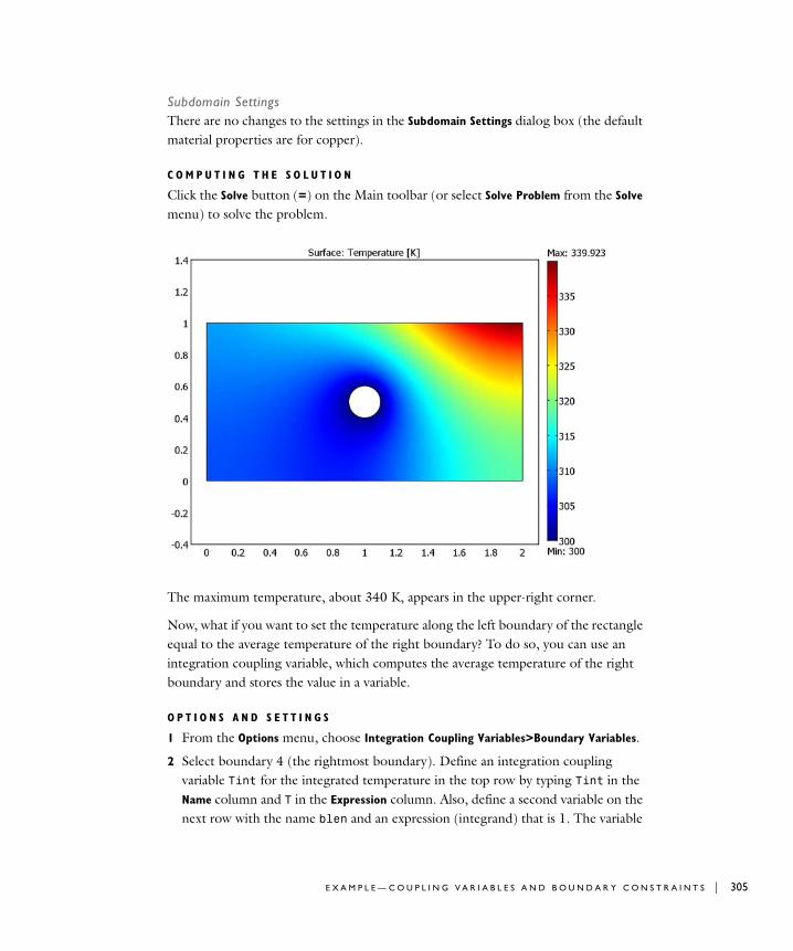
Subdomain SettingsThere are no changes to the settings in the Subdomain Settings dialog box (the default material properties are for copper).
C O M P U T I N G T H E S O L U T I O N
Click the Solve button (=) on the Main toolbar (or select Solve Problem from the Solve menu) to solve the problem.
The maximum temperature, about 340 K, appears in the upper-right corner.
Now, what if you want to set the temperature along the left boundary of the rectangle equal to the average temperature of the right boundary? To do so, you can use an integration coupling variable, which computes the average temperature of the right boundary and stores the value in a variable.
O P T I O N S A N D S E T T I N G S
1 From the Options menu, choose Integration Coupling Variables>Boundary Variables.
2 Select boundary 4 (the rightmost boundary). Define an integration coupling variable Tint for the integrated temperature in the top row by typing Tint in the Name column and T in the Expression column. Also, define a second variable on the next row with the name blen and an expression (integrand) that is 1. The variable
E X A M P L E — C O U P L I N G V A R I A B L E S A N D B O U N D A R Y C O N S T R A I N T S | 305
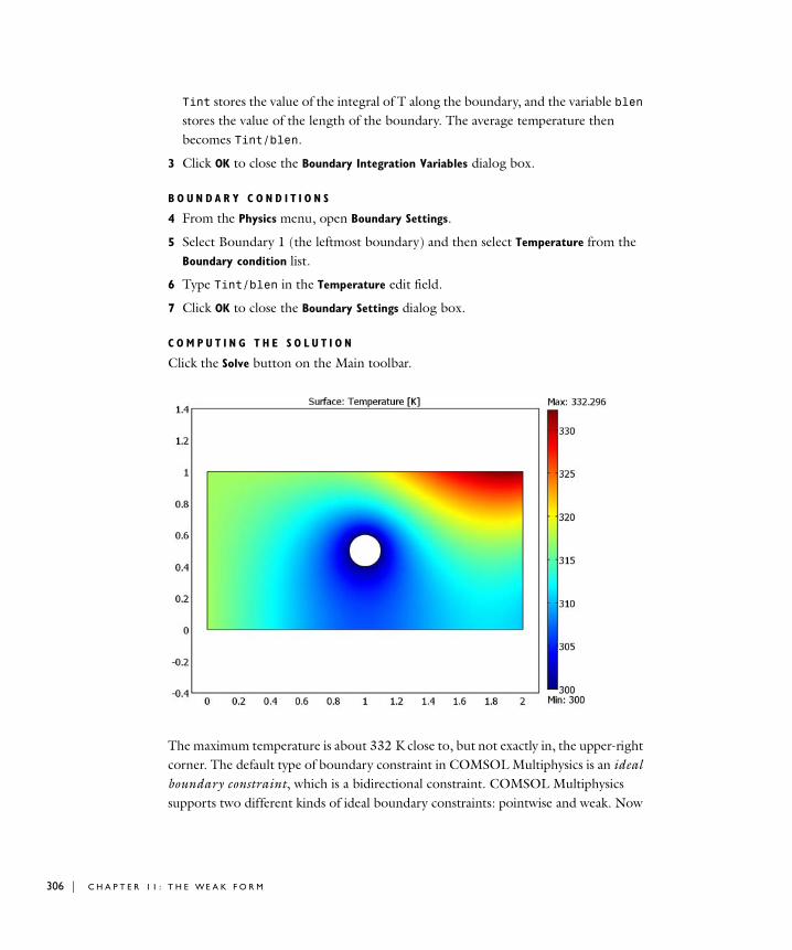
306 | C H A P T E
Tint stores the value of the integral of T along the boundary, and the variable blen stores the value of the length of the boundary. The average temperature then becomes Tint/blen.
3 Click OK to close the Boundary Integration Variables dialog box.
B O U N D A R Y C O N D I T I O N S
4 From the Physics menu, open Boundary Settings.
5 Select Boundary 1 (the leftmost boundary) and then select Temperature from the Boundary condition list.
6 Type Tint/blen in the Temperature edit field.
7 Click OK to close the Boundary Settings dialog box.
C O M P U T I N G T H E S O L U T I O N
Click the Solve button on the Main toolbar.
The maximum temperature is about 332 K close to, but not exactly in, the upper-right corner. The default type of boundary constraint in COMSOL Multiphysics is an ideal boundary constraint, which is a bidirectional constraint. COMSOL Multiphysics supports two different kinds of ideal boundary constraints: pointwise and weak. Now
R 1 1 : T H E W E A K F O R M
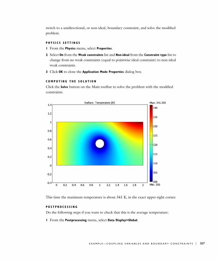
switch to a unidirectional, or non-ideal, boundary constraint, and solve the modified problem.
P H Y S I C S S E T T I N G S
1 From the Physics menu, select Properties.
2 Select On from the Weak constraints list and Non-ideal from the Constraint type list to change from no weak constraints (equal to pointwise ideal constraint) to non-ideal weak constraints.
3 Click OK to close the Application Mode Properties dialog box.
C O M P U T I N G T H E S O L U T I O N
Click the Solve button on the Main toolbar to solve the problem with the modified constraints.
This time the maximum temperature is about 341 K, in the exact upper-right corner.
PO S T P R O C E S S I N G
Do the following steps if you want to check that this is the average temperature:
1 From the Postprocessing menu, select Data Display>Global.
E X A M P L E — C O U P L I N G V A R I A B L E S A N D B O U N D A R Y C O N S T R A I N T S | 307
308 | C H A P T E
2 For the Expression to evaluate, type Tint/blen. Click OK.
This displays the average temperature value, about 327 K, in the message log. To compare this with the values in the plot, just click close to the left boundary. This displays the solution at the grid locations of the background grid, which you can see in the Draw mode. The same value appears for all points on the left boundary.
The subsequent sections explain the differences between the different types of boundary constraints.
No Weak Constraints
The pointwise ideal boundary constraint is what you get if you select Off from the Weak
constraints list and Ideal from the Constraint type list. These are the default settings and correspond to the most common type of boundary constraint for virtually all boundary conditions of the Dirichlet type. In the previous example, when using the pointwise ideal boundary constraint together with the integrated coupling variables, the coupling is bidirectional.
Weak Ideal Constraints
The weak ideal boundary constraint gives the same result as if the weak constraints are turned off, except that using weak ideal constraints adds an additional dependent variable (a so-called Lagrange multiplier), which you can use for extremely accurate postprocessing.
If you select Ideal from the Constraint type list in the previous example, you get the same solution. If you then open the Solver Manager and click the Solve For tab, the list of variables to solve for contains an additional dependent variable. The name of this Lagrange multiplier variable is lm1. The Lagrange multiplier is available for postprocessing via boundary integration on boundaries and provides an accurate value for the integrated flux.
Weak Non-Ideal Constraints
The weak non-ideal boundary constraints gives a different solution. In this case the coupling is unidirectional, and it provides information transfer from the right boundary to the left boundary but not the other way around. The left boundary and the solution in the vicinity of the left boundary do not affect the solution at the right boundary. This type of unidirectional constraint can be explained intuitively as a
R 1 1 : T H E W E A K F O R M
controller that senses the average temperature at the right boundary and forces the temperature at the left boundary to take this value. The left boundary has, however, no way of telling the right boundary of its temperature.
In general, use non-ideal boundary constraints for automatic control design and similar applications, where values from one part of the solution are “forced upon” another part of the solution. On the other hand, use ideal boundary constraints for problems where the model is “left by itself,” and the laws of nature balance the solution to an energy minimum (or, for problems with no well-defined energy, a saddle point).
Whenever using coupling variables in constraint expressions as in this example, make sure you do not use a different constraint at an adjacent boundary, because this would most likely create an ill-posed problem with no well-defined solution.
E X A M P L E — C O U P L I N G V A R I A B L E S A N D B O U N D A R Y C O N S T R A I N T S | 309
310 | C H A P T E
T h e o r e t i c a l B a c k g r ound
The mathematical weak form gives you direct access to the terms of the weak equation and provides maximum freedom in defining finite element problems. This section provides a theoretical background to the weak form in COMSOL Multiphysics.
Deriving the Weak Form
Before describing what the weak form is, this discussion first looks at the conversion of a simple problem in general form to the weak form.
Consider a stationary PDE problem for a single dependent variable, u, in two space dimensions:
Now let v be an arbitrary function on Ω, and call it the test function (v should of course belong to a suitably chosen well-behaved class of functions, V). Multiplying the PDE with this function and integrating leads to
where dA is the area element. Now use Green’s formula (Gauss’ formula) to integrate by parts:
where ds is the length element. Now use the Neumann boundary condition
to arrive at the following equation:
∇ Γ⋅ F in Ω=
v∇ Γ⋅ AdΩ∫ vF Ad
Ω∫=
vΓ n⋅ sdΩ∂∫ v∇ Γ⋅ Ad
Ω∫– vF Ad
Ω∫=
n Γ⋅– Gu∂
∂Rµ+=
0 v∇ Γ⋅ vF+( ) AdΩ∫ v G
u∂∂Rµ+⎝ ⎠
⎛ ⎞ sdΩ∂∫+=
R 1 1 : T H E W E A K F O R M
Together with the Dirichlet condition, this is a weak reformulation of the original PDE problem. Note that the requirement is that the above weak equation should hold for all test functions v. You can reverse the steps of the derivation to show that if the functions u and µ satisfy the weak formulation, then they also satisfy the original formulation. However, this holds true only if the solutions and coefficients are sufficiently smooth. For instance, in the case of discontinuities in material properties, you can have a solution of the weak formulation while the strong formulation has no meaning. The names “weak” and “strong” stem from this distinction: the weak formulation is a weaker condition on the solution than the strong formulation. A benefit of the weak formulation is that it requires less regularity of Γ. This is important in the finite element method.
For the most part, the weak reformulation of a system of equations in general form is
where you use the summation convention. If the boundary conditions are given on interior boundaries, ∂Ω can be enlarged to include these. You now have several test functions v1, v2, …, vN, one for each of the original PDEs. The weak equation is required to hold for all test functions (in the suitably chosen function space V). Of course, in three dimensions, for dA and ds you must substitute the volume and surface area elements, respectively. In one dimension, for dA substitute the length element, and interpret the boundary integral as a sum over the boundary points.
Weak Form Application Modes
In COMSOL Multiphysics you can add weak form PDEs on all domain levels. From the PDE Modes folder in the Model Navigator, select from:
• Weak Form, Subdomain
• Weak Form, Boundary
• Weak Form, Edge (3D only)
• Weak Form, Point
The Weak Form, Boundary application modes are of great use when you must define a PDE on a boundary and couple this equation to an equation in a subdomain. A
0 vl∇ Γl⋅ vlFl+( ) AdΩ∫ vl Gl ul∂
∂Rmµm+⎝ ⎠⎜ ⎟⎛ ⎞
sdΩ∂∫+=
0 Rm on ∂Ω=⎩⎪⎪⎨⎪⎪⎧
T H E O R E T I C A L B A C K G R O U N D | 311
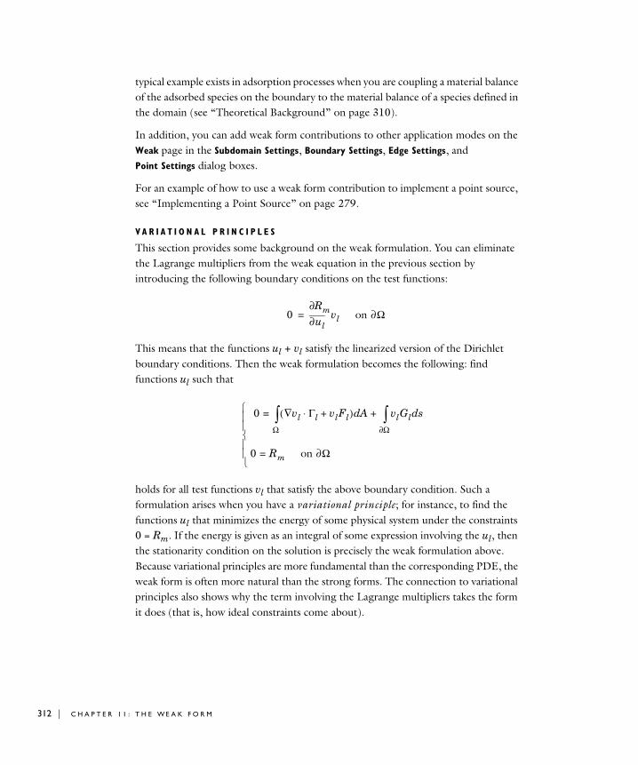
312 | C H A P T E
typical example exists in adsorption processes when you are coupling a material balance of the adsorbed species on the boundary to the material balance of a species defined in the domain (see “Theoretical Background” on page 310).
In addition, you can add weak form contributions to other application modes on the Weak page in the Subdomain Settings, Boundary Settings, Edge Settings, and Point Settings dialog boxes.
For an example of how to use a weak form contribution to implement a point source, see “Implementing a Point Source” on page 279.
V A R I A T I O N A L P R I N C I P L E S
This section provides some background on the weak formulation. You can eliminate the Lagrange multipliers from the weak equation in the previous section by introducing the following boundary conditions on the test functions:
This means that the functions ul + vl satisfy the linearized version of the Dirichlet boundary conditions. Then the weak formulation becomes the following: find functions ul such that
holds for all test functions vl that satisfy the above boundary condition. Such a formulation arises when you have a variational principle; for instance, to find the functions ul that minimizes the energy of some physical system under the constraints 0 = Rm. If the energy is given as an integral of some expression involving the ul, then the stationarity condition on the solution is precisely the weak formulation above. Because variational principles are more fundamental than the corresponding PDE, the weak form is often more natural than the strong forms. The connection to variational principles also shows why the term involving the Lagrange multipliers takes the form it does (that is, how ideal constraints come about).
0ul∂
∂Rmvl on ∂Ω=
0 vl∇ Γl⋅ vlFl+( ) AdΩ∫ vlGl sd
Ω∂∫+=
0 Rm on ∂Ω=⎩⎪⎪⎨⎪⎪⎧
R 1 1 : T H E W E A K F O R M
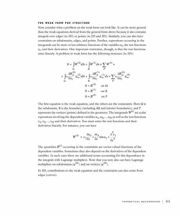
T H E W E A K F O R M P D E S T R U C T U R E
Now consider what a problem on the weak form can look like. It can be more general than the weak equations derived from the general form above because it also contains integrals over edges (in 3D) or points (in 2D and 3D). Similarly, you can also have constraints on subdomains, edges, and points. Further, expressions occurring in the integrands can be more or less arbitrary functions of the variables ul, the test functions vl, and their derivatives. One important restriction, though, is that the test functions enter linearly. A problem in weak form has the following structure (in 2D):
The first equation is the weak equation, and the others are the constraints. Here Ω is the subdomain, B is the boundary (including ∂Ω and interior boundaries), and P represents the vertices (points) defined in the geometry. The integrands W(i) are scalar expressions involving the dependent variables u1, u2,..., uN as well as the test functions v1, v2,..., vN and their derivatives. You must enter the test functions and their derivatives linearly. For instance, you can have
The quantities R(i) occurring in the constraints are vector-valued functions of the dependent variables. Sometimes they also depend on the derivatives of the dependent variables. In such cases there are additional terms accounting for this dependence in the integrals with Lagrange multipliers. Note that you now also can have Lagrange multipliers on subdomains (µ(2)) and on vertices (µ(0)).
In 3D, contributions to the weak equation and the constraints can also come from edges (curves).
0 W 2( ) AdΩ∫ W 1( ) sd
B∫ W 0( )
+
P∑+ +=
vl ul∂∂Rm
2( )
µm2( ) Ad
Ω∫ vl ul∂
∂Rm1( )
µm1( ) sd
B∫ vl ul∂
∂Rm0( )
µm0( )
P∑+ + +
0 R 2( )= on Ω
0 R 1( )= on B
0 R 0( )= on P
W 2( ) v1 x∂∂u2
x∂∂v2 u1sin
y2
2
∂
∂ v1+ +=
T H E O R E T I C A L B A C K G R O U N D | 313
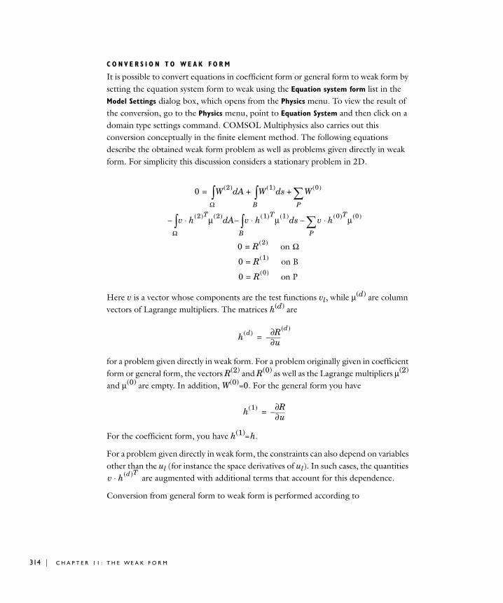
314 | C H A P T E
C O N V E R S I O N T O WE A K F O R M
It is possible to convert equations in coefficient form or general form to weak form by setting the equation system form to weak using the Equation system form list in the Model Settings dialog box, which opens from the Physics menu. To view the result of the conversion, go to the Physics menu, point to Equation System and then click on a domain type settings command. COMSOL Multiphysics also carries out this conversion conceptually in the finite element method. The following equations describe the obtained weak form problem as well as problems given directly in weak form. For simplicity this discussion considers a stationary problem in 2D.
Here v is a vector whose components are the test functions vl, while µ(d) are column vectors of Lagrange multipliers. The matrices h(d) are
for a problem given directly in weak form. For a problem originally given in coefficient form or general form, the vectors R(2) and R(0) as well as the Lagrange multipliers µ(2) and µ(0) are empty. In addition, W(0)=0. For the general form you have
For the coefficient form, you have h(1)= h.
For a problem given directly in weak form, the constraints can also depend on variables other than the ul (for instance the space derivatives of ul). In such cases, the quantities
are augmented with additional terms that account for this dependence.
Conversion from general form to weak form is performed according to
0 W 2( ) AdΩ∫ W 1( ) sd
B∫ W 0( )
P∑+ +=
v h⋅ 2( )Tµ 2( ) AdΩ∫– v h⋅ 1( )Tµ 1( ) sd
B∫– v h 0( )Tµ 0( )⋅
P∑–
0 R 2( )= on Ω
0 R 1( )= on B
0 R 0( )= on P
h d( )u∂
∂R d( )–=
h 1( )u∂
∂R–=
v h⋅ d( )T
R 1 1 : T H E W E A K F O R M
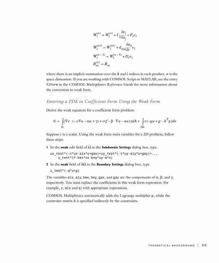
where there is an implicit summation over the k and i indices in each product. n is the space dimension. If you are working with COMSOL Script or MATLAB, see the entry flform in the COMSOL Multiphysics Reference Guide for more information about the conversion to weak form.
Entering a PDE in Coefficient Form Using the Weak Form
Derive the weak equation for a coefficient form problem:
Suppose c is a scalar. Using the weak form meta variables for a 2D problem, follow these steps:
1 In the weak edit field of Ω in the Subdomain Settings dialog box, type
ux_test*(-c*ux-alx*u+gax)+uy_test*(-c*uy-aly*u+gay)+... u_test*(f-bex*ux-bey*uy-a*u)
2 In the weak field of ∂Ω in the Boundary Settings dialog box, type
u_test*(-q*u+g)
The variables alx, aly, bex, bey, gax, and gay are the components of α, β, and γ, respectively. You must replace the coefficients in this weak form expression (for example, c, alx and q) with appropriate expressions.
COMSOL Multiphysics automatically adds the Lagrange multiplier µ, while the constraint matrix h is specified indirectly by the constraints.
Wln( ) Wl
n( ) Γlj xj∂∂vl Flvl+ +=
Wlnt( ) Wl
nt( ) dalk t∂∂ukvl+=
Wln 1–( ) Wl
n 1–( ) Glvl+=
Rmn( ) Rm=
0 v∇ c u∇– αu– γ+( )⋅ v f β ∇u au–⋅–( )+( ) AdΩ∫ v qu g hTµ–+–( ) sd
Ω∂∫+=
T H E O R E T I C A L B A C K G R O U N D | 315

316 | C H A P T E
R 1 1 : T H E W E A K F O R M
12
M u l t i p h y s i c s M o d e l i n g
This chapter covers the use of COMSOL Multiphysics for multiphysics modeling and coupled-field analyses. It first describes the various ways of building multiphysics models. Then a step-by-step example shows how to model Joule heating (also called resistive heating) taking into account thermal-electric couplings.
317
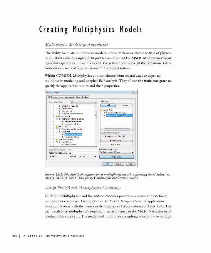
318 | C H A P T E
C r e a t i n g Mu l t i p h y s i c s Mod e l s
Multiphysics Modeling Approaches
The ability to create multiphysics models—those with more than one type of physics or equation such as coupled-field problems—is one of COMSOL Multiphysics’ most powerful capabilities. In such a model, the software can solve all the equations, taken from various areas of physics, as one fully coupled system.
Within COMSOL Multiphysics you can choose from several ways to approach multiphysics modeling and coupled-field analysis. They all use the Model Navigator to specify the application modes and their properties.
Figure 12-1: The Model Navigator for a multiphysics model combining the Conductive Media DC and Heat Transfer by Conduction application modes.
Using Predefined Multiphysics Couplings
COMSOL Multiphysics and the add-on modules provide a number of predefined multiphysics couplings. They appear in the Model Navigator’s list of application modes, in folders with the names in the Category/Folder column in Table 12-1. For each predefined multiphysics coupling, there is an entry in the Model Navigator in all products that support it. The predefined multiphysics couplings consist of two or more
R 1 2 : M U L T I P H Y S I C S M O D E L I N G
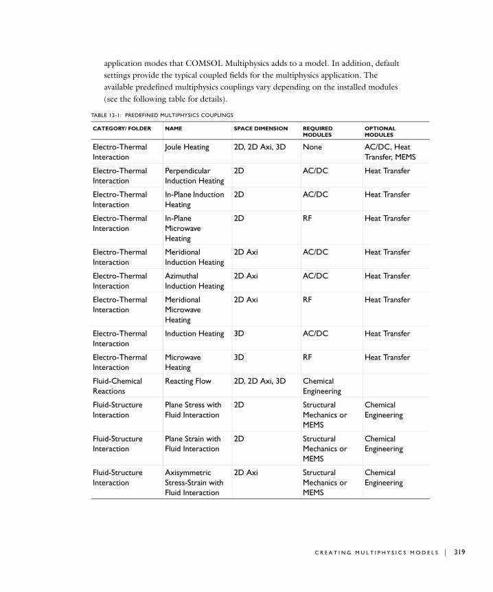
S
application modes that COMSOL Multiphysics adds to a model. In addition, default settings provide the typical coupled fields for the multiphysics application. The available predefined multiphysics couplings vary depending on the installed modules (see the following table for details).
TABLE 12-1: PREDEFINED MULTIPHYSICS COUPLINGS
CATEGORY/ FOLDER NAME SPACE DIMENSION REQUIRED MODULES
OPTIONAL MODULES
Electro-Thermal Interaction
Joule Heating 2D, 2D Axi, 3D None AC/DC, HeatTransfer, MEM
Electro-Thermal Interaction
Perpendicular Induction Heating
2D AC/DC Heat Transfer
Electro-Thermal Interaction
In-Plane Induction Heating
2D AC/DC Heat Transfer
Electro-Thermal Interaction
In-Plane Microwave Heating
2D RF Heat Transfer
Electro-Thermal Interaction
Meridional Induction Heating
2D Axi AC/DC Heat Transfer
Electro-Thermal Interaction
Azimuthal Induction Heating
2D Axi AC/DC Heat Transfer
Electro-Thermal Interaction
Meridional Microwave Heating
2D Axi RF Heat Transfer
Electro-Thermal Interaction
Induction Heating 3D AC/DC Heat Transfer
Electro-Thermal Interaction
Microwave Heating
3D RF Heat Transfer
Fluid-Chemical Reactions
Reacting Flow 2D, 2D Axi, 3D Chemical Engineering
Fluid-Structure Interaction
Plane Stress with Fluid Interaction
2D Structural Mechanics or MEMS
Chemical Engineering
Fluid-Structure Interaction
Plane Strain with Fluid Interaction
2D Structural Mechanics or MEMS
Chemical Engineering
Fluid-Structure Interaction
Axisymmetric Stress-Strain with Fluid Interaction
2D Axi Structural Mechanics or MEMS
Chemical Engineering
C R E A T I N G M U L T I P H Y S I C S M O D E L S | 319
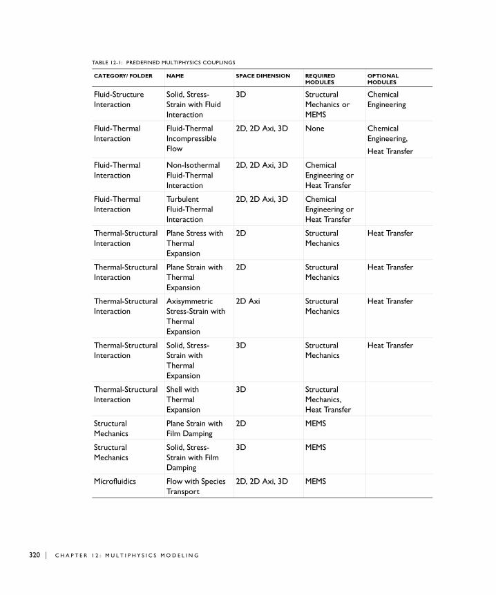
320 | C H A P T E
Fluid-Structure Interaction
Solid, Stress- Strain with Fluid Interaction
3D Structural Mechanics or MEMS
Chemical Engineering
Fluid-Thermal Interaction
Fluid-Thermal Incompressible Flow
2D, 2D Axi, 3D None Chemical Engineering,
Heat Transfer
Fluid-Thermal Interaction
Non-Isothermal Fluid-Thermal Interaction
2D, 2D Axi, 3D Chemical Engineering or Heat Transfer
Fluid-Thermal Interaction
Turbulent Fluid-Thermal Interaction
2D, 2D Axi, 3D Chemical Engineering or Heat Transfer
Thermal-Structural Interaction
Plane Stress with Thermal Expansion
2D Structural Mechanics
Heat Transfer
Thermal-Structural Interaction
Plane Strain with Thermal Expansion
2D Structural Mechanics
Heat Transfer
Thermal-Structural Interaction
Axisymmetric Stress-Strain with Thermal Expansion
2D Axi Structural Mechanics
Heat Transfer
Thermal-Structural Interaction
Solid, Stress- Strain with Thermal Expansion
3D Structural Mechanics
Heat Transfer
Thermal-Structural Interaction
Shell with Thermal Expansion
3D Structural Mechanics, Heat Transfer
Structural Mechanics
Plane Strain with Film Damping
2D MEMS
Structural Mechanics
Solid, Stress- Strain with Film Damping
3D MEMS
Microfluidics Flow with Species Transport
2D, 2D Axi, 3D MEMS
TABLE 12-1: PREDEFINED MULTIPHYSICS COUPLINGS
CATEGORY/ FOLDER NAME SPACE DIMENSION REQUIRED MODULES
OPTIONAL MODULES
R 1 2 : M U L T I P H Y S I C S M O D E L I N G
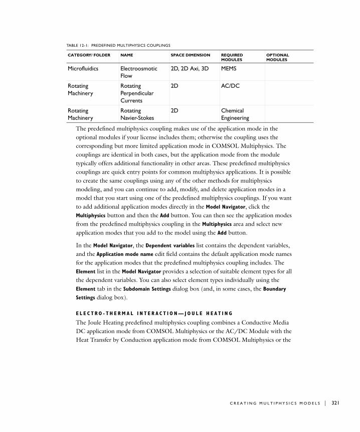
The predefined multiphysics coupling makes use of the application mode in the optional modules if your license includes them; otherwise the coupling uses the corresponding but more limited application mode in COMSOL Multiphysics. The couplings are identical in both cases, but the application mode from the module typically offers additional functionality in other areas. These predefined multiphysics couplings are quick entry points for common multiphysics applications. It is possible to create the same couplings using any of the other methods for multiphysics modeling, and you can continue to add, modify, and delete application modes in a model that you start using one of the predefined multiphysics couplings. If you want to add additional application modes directly in the Model Navigator, click the Multiphysics button and then the Add button. You can then see the application modes from the predefined multiphysics coupling in the Multiphysics area and select new application modes that you add to the model using the Add button.
In the Model Navigator, the Dependent variables list contains the dependent variables, and the Application mode name edit field contains the default application mode names for the application modes that the predefined multiphysics coupling includes. The Element list in the Model Navigator provides a selection of suitable element types for all the dependent variables. You can also select element types individually using the Element tab in the Subdomain Settings dialog box (and, in some cases, the Boundary
Settings dialog box).
E L E C T R O - T H E R M A L I N T E R A C T I O N — J O U L E H E A T I N G
The Joule Heating predefined multiphysics coupling combines a Conductive Media DC application mode from COMSOL Multiphysics or the AC/DC Module with the Heat Transfer by Conduction application mode from COMSOL Multiphysics or the
Microfluidics Electroosmotic Flow
2D, 2D Axi, 3D MEMS
Rotating Machinery
Rotating Perpendicular Currents
2D AC/DC
Rotating Machinery
Rotating Navier-Stokes
2D Chemical Engineering
TABLE 12-1: PREDEFINED MULTIPHYSICS COUPLINGS
CATEGORY/ FOLDER NAME SPACE DIMENSION REQUIRED MODULES
OPTIONAL MODULES
C R E A T I N G M U L T I P H Y S I C S M O D E L S | 321
322 | C H A P T E
General Heat Transfer application mode from the Heat Transfer Module. The interaction is fully coupled in both directions:
• In the heat transfer application mode, resistive heating appears as a heat source (the resistive heating variable Q_es (or Q_emes) appears in the Q edit field).
• In the Conductive Media DC application mode, the definition of the conductivity σ uses the thermal heating model 1/(ρ0(1+α(T−T0))), where T is the dependent variable for temperature from the heat transfer application mode. The values for ρ0 (resistivity at reference temperature), α (temperature coefficient), and T0 (reference temperature) are default values that you can change to match your modeling situation.
You can select a steady-state or a transient analysis.
For an example of a model using the Joule Heating predefined multiphysics coupling, see “Example: Resistive Heating” on page 334.
E L E C T R O - T H E R M A L I N T E R A C T I O N — I N D U C T I O N H E A T I N G
The Induction Heating predefined multiphysics coupling combines an application mode for induction currents from the AC/DC Module with the Heat Transfer by Conduction application mode from COMSOL Multiphysics or the General Heat Transfer application mode from the Heat Transfer Module. The predefined interaction adds the resistive heating from the induction currents as a heat source in the application mode for the heat transfer.
For more information, see the AC/DC Module User’s Guide.
E L E C T R O - T H E R M A L I N T E R A C T I O N — M I C R O W AV E H E A T I N G
The Microwave Heating predefined multiphysics coupling combines an application mode for electromagnetic waves from the RF Module with the Heat Transfer by Conduction application mode from COMSOL Multiphysics or the General Heat Transfer application mode from the Heat Transfer Module. The predefined interaction adds the resistive heating from the electromagnetic waves as a heat source in the application mode for the heat transfer.
For more information, see the RF Module User’s Guide.
F L U I D - C H E M I C A L R E A C T I O N S I N T E R A C T I O N — R E A C T I N G F L O W
The Reacting Flow predefined multiphysics coupling requires the Chemical Engineering Module. Reacting Flow combines a Convection and Diffusion mass balance application mode with an Incompressible Navier-Stokes application mode,
R 1 2 : M U L T I P H Y S I C S M O D E L I N G

both from the Chemical Engineering Module. The interaction is a one-way coupling using the velocity described by the Navier-Stokes equations as part of the convective mass transfer. The components of the velocity vector u from the Incompressible Navier-Stokes application mode appear in the u, v, and w edit fields in the Subdomain
Settings dialog box for the Convection and Diffusion application mode.
By default, COMSOL Multiphysics solves for the velocity field, pressure, and species concentrations simultaneously. For large problems, you can take advantage of the one-way coupling and solve the problem sequentially (unless there are fluid-flow properties that depend on the species concentrations): First solve for velocities and pressures, and then solve the mass balance equation using the computed velocities from the Navier-Stokes equation. See “Solving for a Subset of the Dependent Variables” on page 329 on how to select which variables to solve for.
F L U I D - S T R U C T U R E I N T E R A C T I O N ( F S I )
The Fluid-Structure Interaction (FSI) predefined multiphysics coupling is available in the MEMS Module and the Structural Mechanics Module. FSI combines fluid flow with structural mechanics, using a Moving Mesh (ALE) application mode to capture the fluid movement. Predefined groups of boundary settings help to define the fluid loads on the solid domain and the structural velocities affect on the fluid. For more information and example models, see the Structural Mechanics Module and MEMS Module documentation.
F L U I D - T H E R M A L I N T E R A C T I O N — F L U I D - T H E R M A L I N C O M P R . F L O W
The Fluid-Thermal Incompressible Flow predefined multiphysics coupling combines an Incompressible Navier-Stokes application mode from COMSOL Multiphysics with the Heat Transfer by Convection and Conduction application mode from COMSOL Multiphysics. The interaction is a one-way coupling using the velocity described by the Navier-Stokes equations as part of the convective heat transfer. The components of the velocity vector u from the Incompressible Navier-Stokes application mode appear in the u, v, and w edit fields in the Subdomain Settings dialog box for the heat transfer application mode.
By default, COMSOL Multiphysics solves for the velocity field, pressure, and species concentrations simultaneously. For large problems, you can take advantage of the one-way coupling and solve the problem sequentially (unless there are fluid-flow properties that depend on the temperature): first solve for velocities and pressures and then solve the heat transfer equation using the computed velocities from the Navier-Stokes equation. See “Solving for a Subset of the Dependent Variables” on page 329 on how to select which variables to solve for.
C R E A T I N G M U L T I P H Y S I C S M O D E L S | 323
324 | C H A P T E
The Chemical Engineering Module and the Heat Transfer Module also include the Non-Isothermal Fluid-Thermal Interaction and Turbulent Fluid-Thermal Interaction predefined multiphysics couplings, which are similar but model non-isothermal fluids and turbulent fluid flow instead of incompressible, laminar fluid flow. For more information about these predefined couplings, see the Chemical Engineering Module and Heat Transfer Module documentation.
T H E R M A L - S T R U C T U R A L I N T E R A C T I O N — T H E R M A L E X P A N S I O N
The predefined multiphysics couplings for structural mechanics with thermal expansion requires the Structural Mechanics Module. They combine the Heat Transfer by Conduction application mode from COMSOL Multiphysics or the General Heat Transfer application mode from the Heat Transfer Module with the following application modes from the Structural Mechanics Module:
• Plane Stress in 2D
• Plane Strain in 2D
• Axial Symmetry, Stress-Strain in 2D axisymmetry
• Solid, Stress-Strain in 3D
• Shell in 3D
The interaction is a one-way coupling using the temperature described by a heat transfer application mode to define the strain temperature. On the Load page in the Subdomain Settings dialog box in the structural mechanics application mode, the Include thermal expansion check box is selected, and the dependent variable for temperature from the heat transfer application mode appears in the Temp edit field for the strain temperature. The Tempref edit field contains a default value (0) for the strain reference temperature. If necessary, adjust the strain reference temperature to a suitable value for your model.
By default, COMSOL Multiphysics solves for the temperature and displacements simultaneously. For large problems, you can take advantage of the one-way coupling and solve the problem sequentially (unless there are thermal properties that depend on the displacements): first solve for temperature and then perform the stress-strain analysis using the computed temperature field from the heat transfer equation. See “Solving for a Subset of the Dependent Variables” on page 329 on how to select which variables to solve for.
R 1 2 : M U L T I P H Y S I C S M O D E L I N G
S T R U C T U R A L M E C H A N I C S I N C L U D I N G F I L M D A M P I N G
The MEMS Module includes the Plane Strain with Film Damping and Solid, Stress-Strain with Film Damping predefined multiphysics couplings. The couple the structural mechanics application mode with the Film Damping application mode, for transient and frequency-response analysis of microsystems that include film damping. The Film Damping application mode models film damping on boundaries, and the predefined multiphysics coupling sets the boundary deformation to the displacement variables from the structural mechanics application mode.
For more information, see the MEMS Module documentation.
M I C R O F L U I D I C S — F L O W W I T H S P E C I E S T R A N S P O R T
This suite of predefined multiphysics couplings combines the application modes for microfluidics (General Laminar Flow, Incompressible Navier-Stokes, Non-Isothermal Flow, Stokes Flow, and Non-Isothermal Stokes Flow) with the Convection and Diffusion application mode. The coupling is similar to the one in the Reacting Flow predefined multiphysics coupling (see “Fluid-Chemical Reactions Interaction—Reacting Flow” on page 322), combining fluid flow with species (mass) transport.
For more information, see the MEMS Module documentation.
M I C R O F L U I D I C S — E L E C T R O O S M O T I C F L O W
This suite of predefined multiphysics couplings for electroosmotic flow modeling combines the application modes for microfluidics (General Laminar Flow, Incompressible Navier-Stokes, Non-Isothermal Flow, Stokes Flow, and Non-Isothermal Stokes Flow) with the Conductive Media DC application mode.
Using the Electroosmotic Flow predefined multiphysics coupling, both application modes include boundary groups for defining boundaries as electrodes, ground, electroosmosis, inlets, and outlets.
For more information, see the MEMS Module documentation.
R O T A T I N G M A C H I N E R Y — R O T A T I N G P E R P E N D I C U L A R C U R R E N T S
For modeling of rotating machinery such as motors and generators, the Rotating Perpendicular Currents predefined multiphysics coupling combines the Perpendicular Induction Currents application mode with a Moving Mesh (ALE) application mode. The Moving Mesh (ALE) application mode, which captures the rotation, contains predefined groups with settings for fixed parts and parts that rotate clockwise or counterclockwise.
C R E A T I N G M U L T I P H Y S I C S M O D E L S | 325
326 | C H A P T E
For more information, see the AC/DC Module documentation.
R O T A T I N G M A C H I N E R Y — R O T A T I N G N A V I E R - S TO K E S
For modeling of rotating machinery with fluids (such as stirrers), the Rotating Navier-Stokes predefined multiphysics coupling combines the Incompressible Navier-Stokes application mode with a Moving Mesh (ALE) application mode. The Moving Mesh (ALE) application mode, which captures the rotation, contains predefined groups with settings for fixed parts and parts that rotate clockwise or counterclockwise.
For more information, see the Chemical Engineering Module documentation.
Adding Physics Sequentially
With this approach you can verify that each type of physics or PDE gives the expected results before adding more complexity to the model by adding another physics or coupling fields.
Use these steps to add one application mode at the time:
1 Select an application mode.
2 Draw the geometry.
3 Define the physics settings.
4 Solve and visualize the results.
Then add another application mode:
5 Go to the Multiphysics menu and choose Model Navigator.
6 Select a new application mode.
7 In the Multiphysics area, click the Add button.
8 Click OK.
9 Add and modify settings in the Physics menu, including couplings between the physics.
Building a Coupled Multiphysics Model Directly
Another approach is to include multiple application modes when you start creating the model in the Model Navigator:
1 Select an application mode for the model.
R 1 2 : M U L T I P H Y S I C S M O D E L I N G
2 Click the Multiphysics button.
3 In the Multiphysics area, click the Add button.
4 Continue selecting application modes and adding them to the model by clicking Add.
5 Click OK.
Removing Application Modes
To remove an application mode from a model:
1 Choose Model Navigator from the Multiphysics menu.
2 Select the application mode from the list under Multiphysics. You can also select a geometry in the list to remove the entire geometry and all application modes that it contains.
3 Click Remove.
4 Click OK.
Multiphysics Model Properties
When you add or remove application modes, COMSOL Multiphysics updates some model properties to:
• Include all dependent variables in the added application modes in the list of variables to solve for.
• Update all application-dependent dialog boxes.
A C T I V E A P P L I C A T I O N M O D E
The application mode selected under Multiphysics becomes the active application mode when you begin modeling.
To shift between the different application modes during modeling, select one from the Multiphysics menu to make it active.
R U L I N G A P P L I C A T I O N M O D E
The ruling application mode determines the global settings for the multiphysics model from its application mode properties. For example, if the analysis type is different for two application modes in the same model, the software takes the analysis type from the ruling application mode. You select the ruling application mode for a multiphysics model in the Model Navigator.
C R E A T I N G M U L T I P H Y S I C S M O D E L S | 327
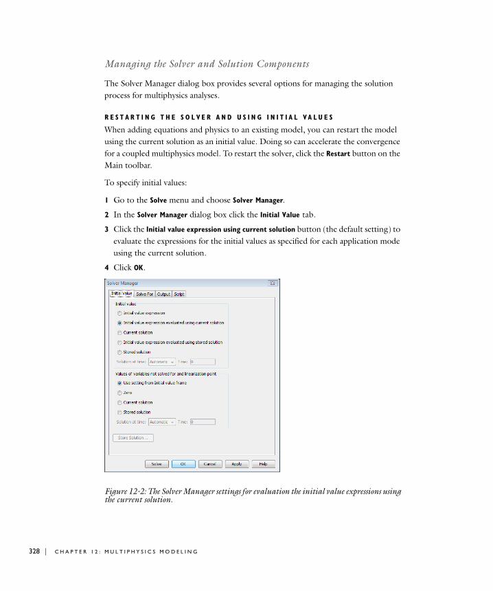
328 | C H A P T E
Managing the Solver and Solution Components
The Solver Manager dialog box provides several options for managing the solution process for multiphysics analyses.
R E S T A R T I N G T H E S O L V E R A N D U S I N G I N I T I A L V A L U E S
When adding equations and physics to an existing model, you can restart the model using the current solution as an initial value. Doing so can accelerate the convergence for a coupled multiphysics model. To restart the solver, click the Restart button on the Main toolbar.
To specify initial values:
1 Go to the Solve menu and choose Solver Manager.
2 In the Solver Manager dialog box click the Initial Value tab.
3 Click the Initial value expression using current solution button (the default setting) to evaluate the expressions for the initial values as specified for each application mode using the current solution.
4 Click OK.
Figure 12-2: The Solver Manager settings for evaluation the initial value expressions using the current solution.
R 1 2 : M U L T I P H Y S I C S M O D E L I N G
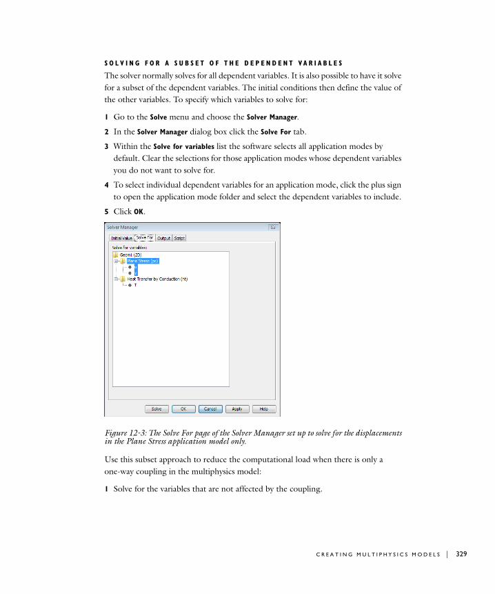
S O L V I N G F O R A S U B S E T O F T H E D E P E N D E N T V A R I A B L E S
The solver normally solves for all dependent variables. It is also possible to have it solve for a subset of the dependent variables. The initial conditions then define the value of the other variables. To specify which variables to solve for:
1 Go to the Solve menu and choose the Solver Manager.
2 In the Solver Manager dialog box click the Solve For tab.
3 Within the Solve for variables list the software selects all application modes by default. Clear the selections for those application modes whose dependent variables you do not want to solve for.
4 To select individual dependent variables for an application mode, click the plus sign to open the application mode folder and select the dependent variables to include.
5 Click OK.
Figure 12-3: The Solve For page of the Solver Manager set up to solve for the displacements in the Plane Stress application model only.
Use this subset approach to reduce the computational load when there is only a one-way coupling in the multiphysics model:
1 Solve for the variables that are not affected by the coupling.
C R E A T I N G M U L T I P H Y S I C S M O D E L S | 329
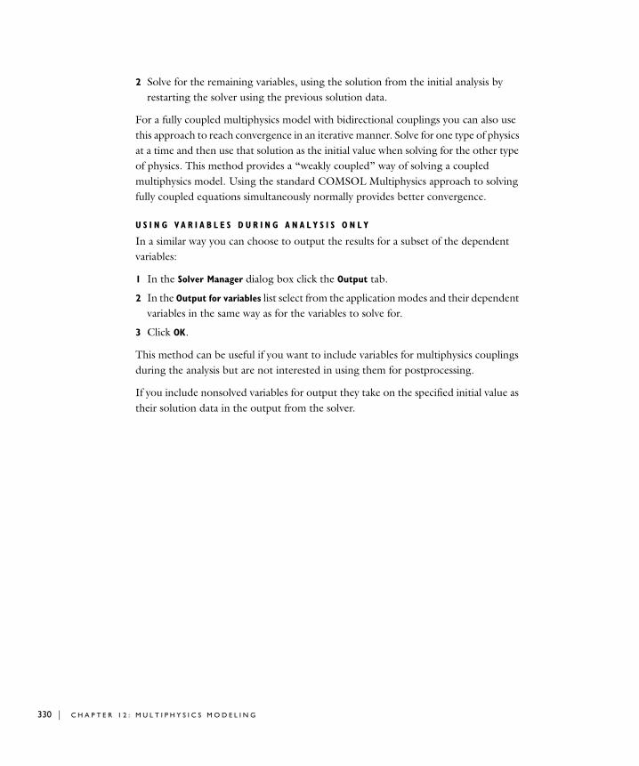
330 | C H A P T E
2 Solve for the remaining variables, using the solution from the initial analysis by restarting the solver using the previous solution data.
For a fully coupled multiphysics model with bidirectional couplings you can also use this approach to reach convergence in an iterative manner. Solve for one type of physics at a time and then use that solution as the initial value when solving for the other type of physics. This method provides a “weakly coupled” way of solving a coupled multiphysics model. Using the standard COMSOL Multiphysics approach to solving fully coupled equations simultaneously normally provides better convergence.
U S I N G V A R I A B L E S D U R I N G A N A L Y S I S O N L Y
In a similar way you can choose to output the results for a subset of the dependent variables:
1 In the Solver Manager dialog box click the Output tab.
2 In the Output for variables list select from the application modes and their dependent variables in the same way as for the variables to solve for.
3 Click OK.
This method can be useful if you want to include variables for multiphysics couplings during the analysis but are not interested in using them for postprocessing.
If you include nonsolved variables for output they take on the specified initial value as their solution data in the output from the solver.
R 1 2 : M U L T I P H Y S I C S M O D E L I N G
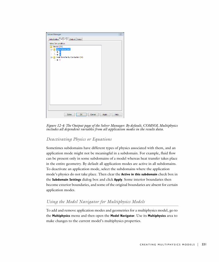
Figure 12-4: The Output page of the Solver Manager. By default, COMSOL Multiphysics includes all dependent variables from all application modes in the results data.
Deactivating Physics or Equations
Sometimes subdomains have different types of physics associated with them, and an application mode might not be meaningful in a subdomain. For example, fluid flow can be present only in some subdomains of a model whereas heat transfer takes place in the entire geometry. By default all application modes are active in all subdomains. To deactivate an application mode, select the subdomains where the application mode’s physics do not take place. Then clear the Active in this subdomain check box in the Subdomain Settings dialog box and click Apply. Some interior boundaries then become exterior boundaries, and some of the original boundaries are absent for certain application modes.
Using the Model Navigator for Multiphysics Models
To add and remove application modes and geometries for a multiphysics model, go to the Multiphysics menu and then open the Model Navigator. Use its Multiphysics area to make changes to the current model’s multiphysics properties.
C R E A T I N G M U L T I P H Y S I C S M O D E L S | 331
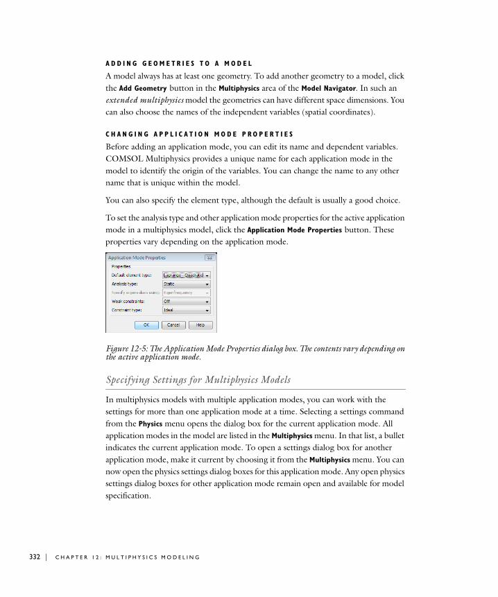
332 | C H A P T E
A D D I N G G E O M E T R I E S T O A M O D E L
A model always has at least one geometry. To add another geometry to a model, click the Add Geometry button in the Multiphysics area of the Model Navigator. In such an extended multiphysics model the geometries can have different space dimensions. You can also choose the names of the independent variables (spatial coordinates).
C H A N G I N G A P P L I C A T I O N M O D E P R O P E R T I E S
Before adding an application mode, you can edit its name and dependent variables. COMSOL Multiphysics provides a unique name for each application mode in the model to identify the origin of the variables. You can change the name to any other name that is unique within the model.
You can also specify the element type, although the default is usually a good choice.
To set the analysis type and other application mode properties for the active application mode in a multiphysics model, click the Application Mode Properties button. These properties vary depending on the application mode.
Figure 12-5: The Application Mode Properties dialog box. The contents vary depending on the active application mode.
Specifying Settings for Multiphysics Models
In multiphysics models with multiple application modes, you can work with the settings for more than one application mode at a time. Selecting a settings command from the Physics menu opens the dialog box for the current application mode. All application modes in the model are listed in the Multiphysics menu. In that list, a bullet indicates the current application mode. To open a settings dialog box for another application mode, make it current by choosing it from the Multiphysics menu. You can now open the physics settings dialog boxes for this application mode. Any open physics settings dialog boxes for other application mode remain open and available for model specification.
R 1 2 : M U L T I P H Y S I C S M O D E L I N G
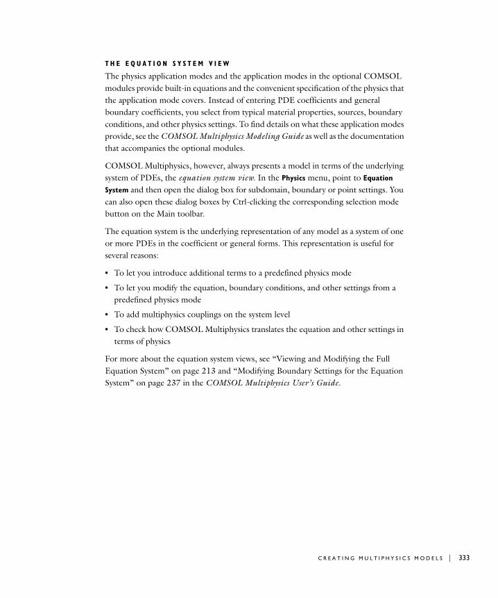
T H E E Q U A T I O N S Y S T E M V I E W
The physics application modes and the application modes in the optional COMSOL modules provide built-in equations and the convenient specification of the physics that the application mode covers. Instead of entering PDE coefficients and general boundary coefficients, you select from typical material properties, sources, boundary conditions, and other physics settings. To find details on what these application modes provide, see the COMSOL Multiphysics Modeling Guide as well as the documentation that accompanies the optional modules.
COMSOL Multiphysics, however, always presents a model in terms of the underlying system of PDEs, the equation system view. In the Physics menu, point to Equation
System and then open the dialog box for subdomain, boundary or point settings. You can also open these dialog boxes by Ctrl-clicking the corresponding selection mode button on the Main toolbar.
The equation system is the underlying representation of any model as a system of one or more PDEs in the coefficient or general forms. This representation is useful for several reasons:
• To let you introduce additional terms to a predefined physics mode
• To let you modify the equation, boundary conditions, and other settings from a predefined physics mode
• To add multiphysics couplings on the system level
• To check how COMSOL Multiphysics translates the equation and other settings in terms of physics
For more about the equation system views, see “Viewing and Modifying the Full Equation System” on page 213 and “Modifying Boundary Settings for the Equation System” on page 237 in the COMSOL Multiphysics User’s Guide.
C R E A T I N G M U L T I P H Y S I C S M O D E L S | 333
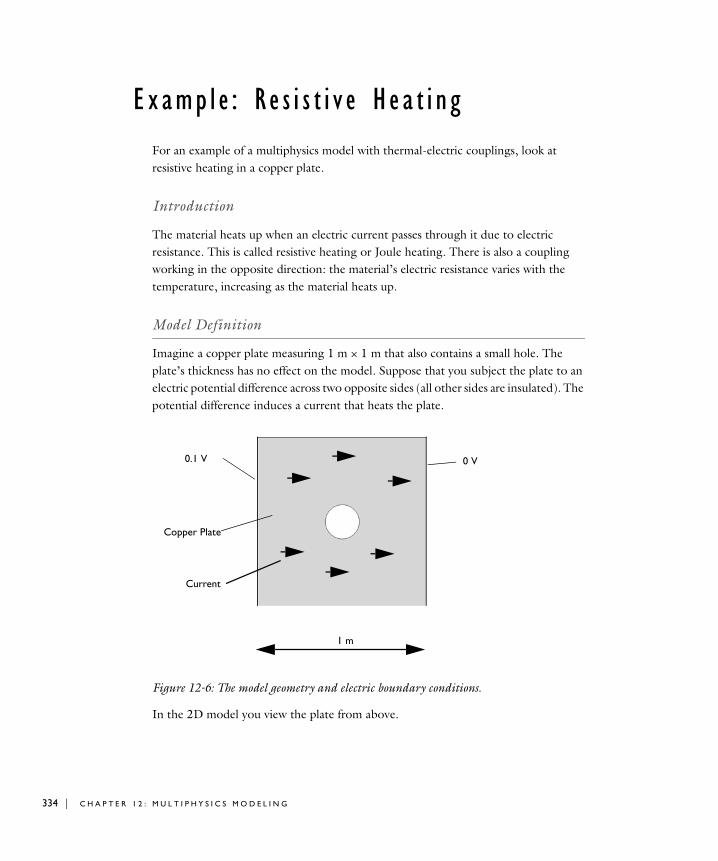
334 | C H A P T E
Examp l e : R e s i s t i v e Hea t i n g
For an example of a multiphysics model with thermal-electric couplings, look at resistive heating in a copper plate.
Introduction
The material heats up when an electric current passes through it due to electric resistance. This is called resistive heating or Joule heating. There is also a coupling working in the opposite direction: the material’s electric resistance varies with the temperature, increasing as the material heats up.
Model Definition
Imagine a copper plate measuring 1 m × 1 m that also contains a small hole. The plate’s thickness has no effect on the model. Suppose that you subject the plate to an electric potential difference across two opposite sides (all other sides are insulated). The potential difference induces a current that heats the plate.
Figure 12-6: The model geometry and electric boundary conditions.
In the 2D model you view the plate from above.
0.1 V
Copper Plate
0 V
Current
1 m
R 1 2 : M U L T I P H Y S I C S M O D E L I N G
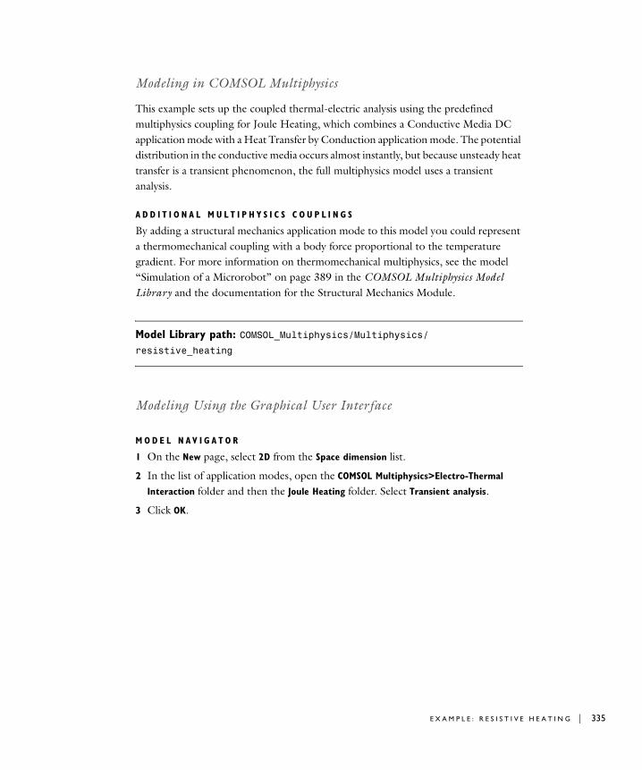
Modeling in COMSOL Multiphysics
This example sets up the coupled thermal-electric analysis using the predefined multiphysics coupling for Joule Heating, which combines a Conductive Media DC application mode with a Heat Transfer by Conduction application mode. The potential distribution in the conductive media occurs almost instantly, but because unsteady heat transfer is a transient phenomenon, the full multiphysics model uses a transient analysis.
A D D I T I O N A L M U L T I P H Y S I C S C O U P L I N G S
By adding a structural mechanics application mode to this model you could represent a thermomechanical coupling with a body force proportional to the temperature gradient. For more information on thermomechanical multiphysics, see the model “Simulation of a Microrobot” on page 389 in the COMSOL Multiphysics Model Library and the documentation for the Structural Mechanics Module.
Model Library path: COMSOL_Multiphysics/Multiphysics/resistive_heating
Modeling Using the Graphical User Interface
M O D E L N A V I G A T O R
1 On the New page, select 2D from the Space dimension list.
2 In the list of application modes, open the COMSOL Multiphysics>Electro-Thermal
Interaction folder and then the Joule Heating folder. Select Transient analysis.
3 Click OK.
E X A M P L E : R E S I S T I V E H E A T I N G | 335
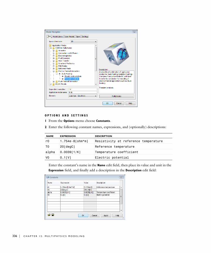
336 | C H A P T E
O P T I O N S A N D S E T T I N G S
1 From the Options menu choose Constants.
2 Enter the following constant names, expressions, and (optionally) descriptions:
Enter the constant’s name in the Name edit field, then place its value and unit in the Expression field, and finally add a description in the Description edit field:
NAME EXPRESSION DESCRIPTION
r0 1.754e-8[ohm*m] Resistivity at reference temperature
T0 20[degC] Reference temperature
alpha 0.0039[1/K] Temperature coefficient
V0 0.1[V] Electric potential
R 1 2 : M U L T I P H Y S I C S M O D E L I N G
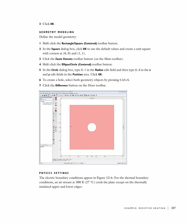
3 Click OK.
G E O M E T R Y M O D E L I N G
Define the model geometry:
1 Shift-click the Rectangle/Square (Centered) toolbar button.
2 In the Square dialog box, click OK to use the default values and create a unit square with corners at (0, 0) and (1, 1).
3 Click the Zoom Extents toolbar button (on the Main toolbar).
4 Shift-click the Ellipse/Circle (Centered) toolbar button.
5 In the Circle dialog box, type 0.1 in the Radius edit field and then type 0.5 in the x and y edit fields in the Position area. Click OK.
6 To create a hole, select both geometry objects by pressing Ctrl+A.
7 Click the Difference button on the Draw toolbar.
P H Y S I C S S E T T I N G S
The electric boundary conditions appear in Figure 12-6. For the thermal boundary conditions, an air stream at 300 K (27 °C) cools the plate except on the thermally insulated upper and lower edges:
E X A M P L E : R E S I S T I V E H E A T I N G | 337
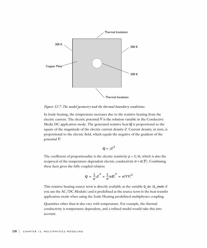
338 | C H A P T E
Figure 12-7: The model geometry and the thermal boundary conditions.
In Joule heating, the temperature increases due to the resistive heating from the electric current. The electric potential V is the solution variable in the Conductive Media DC application mode. The generated resistive heat Q is proportional to the square of the magnitude of the electric current density J. Current density, in turn, is proportional to the electric field, which equals the negative of the gradient of the potential V:
The coefficient of proportionality is the electric resistivity ρ = 1/σ, which is also the reciprocal of the temperature-dependent electric conductivity σ = σ(T). Combining these facts gives the fully coupled relation
This resistive heating source term is directly available as the variable Q_dc (Q_emdc if you use the AC/DC Module) and is predefined as the source term in the heat transfer application mode when using the Joule Heating predefined multiphysics coupling.
Quantities other than σ also vary with temperature. For example, the thermal conductivity is temperature dependent, and a refined model would take this into account.
300 K
Copper Plate
300 K
300 K
Thermal Insulation
Thermal Insulation
Q J 2∝
Q 1σ--- J
2 1σ--- σE
2σ V∇ 2
= = =
R 1 2 : M U L T I P H Y S I C S M O D E L I N G
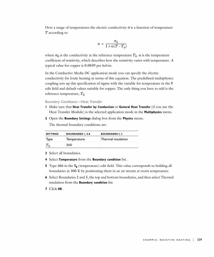
Over a range of temperatures the electric conductivity σ is a function of temperature T according to
where σ0 is the conductivity at the reference temperature T0. α is the temperature coefficient of resistivity, which describes how the resistivity varies with temperature. A typical value for copper is 0.0039 per kelvin.
In the Conductive Media DC application mode you can specify the electric conductivity for Joule heating in terms of this equation. The predefined multiphysics coupling sets up this specification of sigma with the variable for temperature in the T edit field and default values suitable for copper. The only thing you have to add is the reference temperature, T0.
Boundary Conditions—Heat Transfer1 Make sure that Heat Transfer by Conduction or General Heat Transfer (if you use the
Heat Transfer Module) is the selected application mode in the Multiphysics menu.
2 Open the Boundary Settings dialog box from the Physics menu.
The thermal boundary conditions are:
3 Select all boundaries.
4 Select Temperature from the Boundary condition list.
5 Type 300 in the T0 (temperature) edit field. This value corresponds to holding all boundaries at 300 K by positioning them in an air stream at room temperature.
6 Select Boundaries 2 and 3, the top and bottom boundaries, and then select Thermal insulation from the Boundary condition list.
7 Click OK.
SETTINGS BOUNDARIES 1, 4–8 BOUNDARIES 2, 3
Type Temperature Thermal insulation
T0 300
σσ0
1 α T T0–( )+-----------------------------------=
E X A M P L E : R E S I S T I V E H E A T I N G | 339
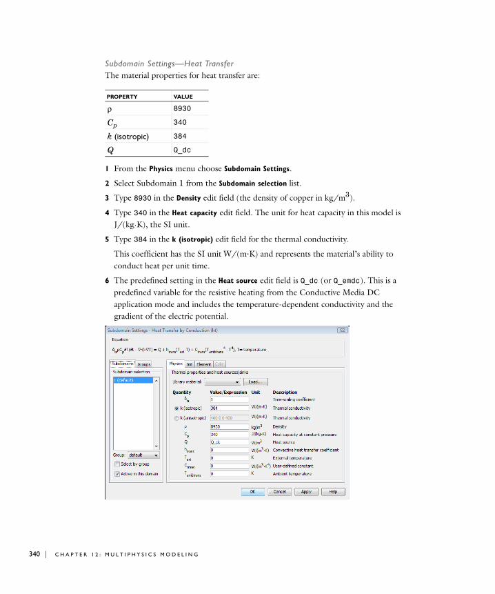
340 | C H A P T E
Subdomain Settings—Heat TransferThe material properties for heat transfer are:
1 From the Physics menu choose Subdomain Settings.
2 Select Subdomain 1 from the Subdomain selection list.
3 Type 8930 in the Density edit field (the density of copper in kg/m3).
4 Type 340 in the Heat capacity edit field. The unit for heat capacity in this model is J/(kg·K), the SI unit.
5 Type 384 in the k (isotropic) edit field for the thermal conductivity.
This coefficient has the SI unit W/(m·K) and represents the material’s ability to conduct heat per unit time.
6 The predefined setting in the Heat source edit field is Q_dc (or Q_emdc). This is a predefined variable for the resistive heating from the Conductive Media DC application mode and includes the temperature-dependent conductivity and the gradient of the electric potential.
PROPERTY VALUE
ρ 8930
Cp 340
k (isotropic) 384
Q Q_dc
R 1 2 : M U L T I P H Y S I C S M O D E L I N G
Initial Conditions—Heat TransferAlso enter the initial value for the temperature, which is 300 K just as the boundary condition:
1 Click the Init tab in the Subdomain Settings dialog box.
2 Type 300 as the initial value in the edit field for T(t0).
3 Click OK.
Application Mode SelectionTo define the settings for the copper plate’s electric properties, switch to the Conductive Media DC application mode, selecting it from the Multiphysics menu or using the Model Tree.
Boundary Conditions—Conductive Media DC1 Open the Boundary Settings dialog box by choosing Boundary Settings from the
Physics menu. The boundary conditions for the Conductive Media DC application mode in this example are:
2 Press Ctrl+A to select all boundaries.
3 From the Boundary condition list select Electric insulation.
Change the conditions on Boundaries 1 and 4:
4 From the Boundary selection list select Boundary 1, the left boundary.
5 From the Boundary condition list select Electric potential and type V0 in the V0 edit field.
6 Select Boundary 4.
7 From the Boundary condition list select Ground.
8 Click OK.
Subdomain Settings—Conductive Media DC1 From the Physics menu choose Subdomain Settings.
2 Select Subdomain 1 from the Subdomain selection list.
3 From the Conductivity relation list, select Linear temperature relation.
4 Make sure that the T edit field contains the field variable for temperature, T.
5 Type r0 in the ρ0 edit field for the resistivity at the reference temperature.
SETTINGS BOUNDARY 1 BOUNDARY 4 BOUNDARIES 2, 3, 5–8
Type Electric potential Ground Electric insulation
V V0
E X A M P L E : R E S I S T I V E H E A T I N G | 341
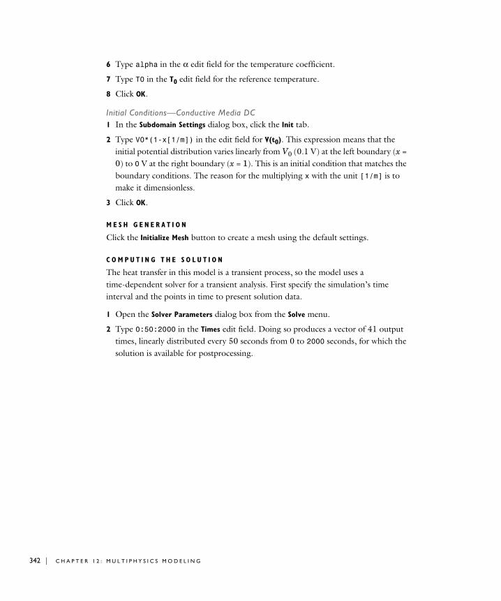
342 | C H A P T E
6 Type alpha in the α edit field for the temperature coefficient.
7 Type T0 in the T0 edit field for the reference temperature.
8 Click OK.
Initial Conditions—Conductive Media DC1 In the Subdomain Settings dialog box, click the Init tab.
2 Type V0*(1-x[1/m]) in the edit field for V(t0). This expression means that the initial potential distribution varies linearly from V0 (0.1 V) at the left boundary (x = 0) to 0 V at the right boundary (x = 1). This is an initial condition that matches the boundary conditions. The reason for the multiplying x with the unit [1/m] is to make it dimensionless.
3 Click OK.
M E S H G E N E R A T I O N
Click the Initialize Mesh button to create a mesh using the default settings.
C O M P U T I N G T H E S O L U T I O N
The heat transfer in this model is a transient process, so the model uses a time-dependent solver for a transient analysis. First specify the simulation’s time interval and the points in time to present solution data.
1 Open the Solver Parameters dialog box from the Solve menu.
2 Type 0:50:2000 in the Times edit field. Doing so produces a vector of 41 output times, linearly distributed every 50 seconds from 0 to 2000 seconds, for which the solution is available for postprocessing.
R 1 2 : M U L T I P H Y S I C S M O D E L I N G

3 Click OK.
C O M P U T I N G T H E S O L U T I O N
You can now run the transient analysis. To do so, click the Solve button on the Main toolbar.
PO S T P R O C E S S I N G A N D V I S U A L I Z A T I O N
The default plot from this analysis shows the temperature or the potential distribution.
E X A M P L E : R E S I S T I V E H E A T I N G | 343
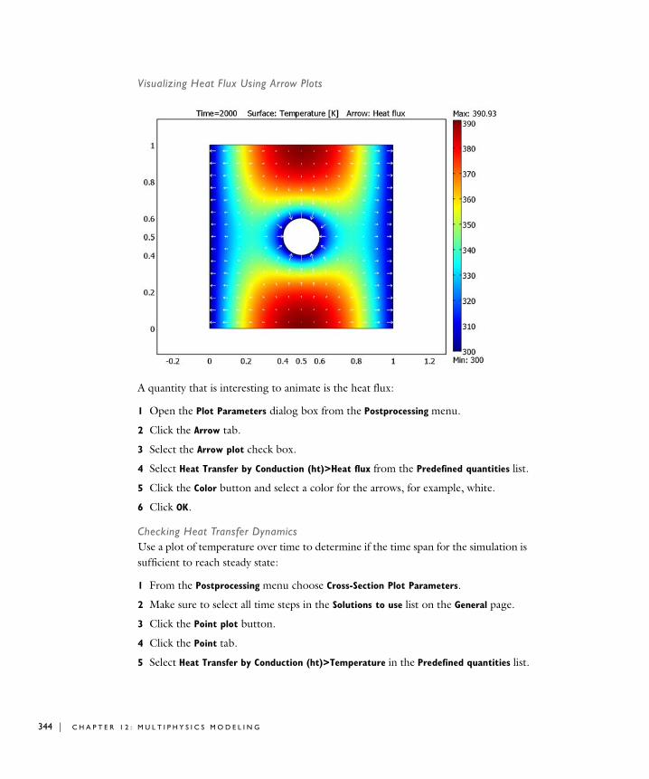
344 | C H A P T E
Visualizing Heat Flux Using Arrow Plots
A quantity that is interesting to animate is the heat flux:
1 Open the Plot Parameters dialog box from the Postprocessing menu.
2 Click the Arrow tab.
3 Select the Arrow plot check box.
4 Select Heat Transfer by Conduction (ht)>Heat flux from the Predefined quantities list.
5 Click the Color button and select a color for the arrows, for example, white.
6 Click OK.
Checking Heat Transfer DynamicsUse a plot of temperature over time to determine if the time span for the simulation is sufficient to reach steady state:
1 From the Postprocessing menu choose Cross-Section Plot Parameters.
2 Make sure to select all time steps in the Solutions to use list on the General page.
3 Click the Point plot button.
4 Click the Point tab.
5 Select Heat Transfer by Conduction (ht)>Temperature in the Predefined quantities list.
R 1 2 : M U L T I P H Y S I C S M O D E L I N G

6 In the Coordinates area, type 0.5 in the x edit field and 0.75 in the y edit field.
7 Click OK.
The plot of temperature as a function of time shows that it has reached a steady state. The temperature hardly increases at all if you extend the simulation over a longer time span.
Figure 12-8: Heat transfer dynamics visualized as temperature versus time.
C O M P U T I N G T H E S O L U T I O N U S I N G A S E G R E G A T E D S T A T I O N A R Y S O L V E R
You can also solve this model for the steady-state condition. There is no problem solving this coupled multiphysics model using the standard stationary solver because the model is small. For large models, a segregated solver approach can be beneficial. This example shows how to solve a multiphysics model using the segregated stationary solver. You continue with the Resistive Heating model, adding the following steps:
1 From the Solve menu, choose Solver Parameters.
2 Select Stationary from the Analysis list.
3 Select Stationary segregated from the Solver list. COMSOL Multiphysics has two predefined groups, one for each application mode (the temperature T and the electric potential V). All you need to do is to specify the tolerances so that the
E X A M P L E : R E S I S T I V E H E A T I N G | 345
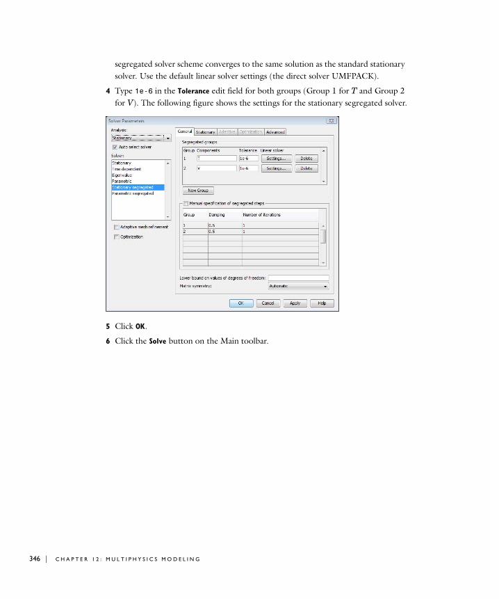
346 | C H A P T E
segregated solver scheme converges to the same solution as the standard stationary solver. Use the default linear solver settings (the direct solver UMFPACK).
4 Type 1e-6 in the Tolerance edit field for both groups (Group 1 for T and Group 2 for V). The following figure shows the settings for the stationary segregated solver.
5 Click OK.
6 Click the Solve button on the Main toolbar.
R 1 2 : M U L T I P H Y S I C S M O D E L I N G
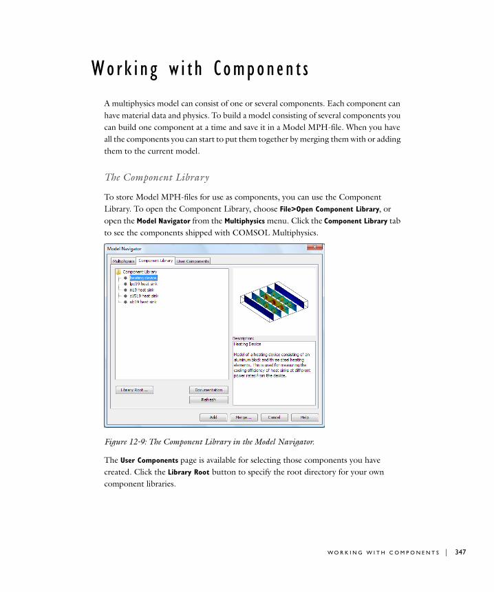
Work i n g w i t h Componen t s
A multiphysics model can consist of one or several components. Each component can have material data and physics. To build a model consisting of several components you can build one component at a time and save it in a Model MPH-file. When you have all the components you can start to put them together by merging them with or adding them to the current model.
The Component Library
To store Model MPH-files for use as components, you can use the Component Library. To open the Component Library, choose File>Open Component Library, or open the Model Navigator from the Multiphysics menu. Click the Component Library tab to see the components shipped with COMSOL Multiphysics.
Figure 12-9: The Component Library in the Model Navigator.
The User Components page is available for selecting those components you have created. Click the Library Root button to specify the root directory for your own component libraries.
W O R K I N G W I T H C O M P O N E N T S | 347

348 | C H A P T E
Adding Components
To add a component to a model on which you are working, select Add Component from the File menu; alternately, select the component you want to add in the Component Library and click the Add button. You can also add a component from the Model Tree when you choose the Detail and Inspect views. Right-click the top node with the model’s name, and then select Add Component.
COMSOL Multiphysics creates a new geometry page and adds the component to this geometry. If the component has several geometries, the software adds all the geometries to the model. Adding a component includes the component’s physics and mesh but not the solution.
Merging Components
To merge a component to the model on which you are working, either select Merge
Component from the File menu or select the component you want to merge in the Component Library and click the Merge button. You can also add a component from the Model Tree. Right-click the geometry node where you want to merge a component with the current mode, and then select Merge Component.
When merging a component the Merge Component dialog box appears.
In the Geometry list you can find the geometries in the component. Select the geometry you want to merge into the model. Clicking Merge merges the geometry objects in the selected geometry into the current geometry in your model. The resulting geometry becomes an assembly.
When you select a geometry in the dialog box, the application modes in this geometry appear in a list. If application modes of the same type as the selected one already exist
R 1 2 : M U L T I P H Y S I C S M O D E L I N G
in the model, you can choose to merge the component’s application mode with one of the application modes in the model. Select the model’s application mode from the Merge application mode with list. The resulting application mode then includes the physics settings for the component.
If you want the component application mode to exist as a new application mode, select None in the Merge application mode with list. If you do not want to merge the application modes, you must make sure that the application mode names are unique. The program suggests unique names for the dependent variables and the application mode in the corresponding edit fields. If there are no application modes to merge with, or if None is selected, COMSOL Multiphysics adds a new application mode to the model. This application mode is only active in the domains belonging to the component.
When you have application modes in the model that the software does not merge with application modes from the component, they are active only in the domains that belonged to the model before the merge.
Because of geometry changes the merge does not include the mesh and the solution. Also, coupling variables that have other destinations than global are not merged.
For an example of how to work with components and merging them into a model, see “Heat-Sink Experiments Using the Component Library” on page 289 in the COMSOL Multiphysics Model Library.
W O R K I N G W I T H C O M P O N E N T S | 349

350 | C H A P T E
R 1 2 : M U L T I P H Y S I C S M O D E L I N G
13
U s i n g A s s e m b l i e s
This chapter explains how to model using assemblies where the geometry consists of separate parts. There are special considerations and possibilities during meshing as well as setting up the boundary conditions for an assembly model.
351
352 | C H A P T E
C r e a t i n g A s s emb l i e s
The Analyzed Geometry—Assembly vs. Composite Geometry
When you leave Draw mode COMSOL Multiphysics analyzes the geometry to find all subdomains, boundaries, edges, and points in the geometry. When doing this COMSOL Multiphysics creates an analyzed geometry that you apply the physics on. You can choose between two types of analyzed geometries:
• A composite geometry. The analyzed geometry object that the software creates is a single object (that typically consists of several subdomains), which effectively is the same object you would get if you select all objects in Draw mode and create the union of them. This is the default type of analyzed geometries, for which COMSOL Multiphysics automatically connects the geometry, mesh, and physics at the interior interfaces.
• An assembly. In this case you get an analyzed geometry that consists of several parts (disjoint composite geometries), each object in Draw mode becoming a part of the assembly. For an assembly, you must manually connect the geometry, mesh, and physics at the part interfaces.
If there are no problems using a composite geometry this is usually to prefer, because it automatically provides continuity in the physical fields at part interfaces and material discontinuities as well as accurate solutions and conforming mesh elements and nodes at part interfaces. There are some cases, however, when an assembly is the best choice:
• Sometimes the software fails to create a composite geometry. In those cases you can choose to use an assembly. It is a simpler operation to create an assembly, and it often succeeds even if creating a composite geometry fails.
• Each part in an assembly gets separate meshes. This can make it easier to mesh a complicated geometry, where the mesh generator creates at too dense mesh or even fails to create a mesh for the composite geometry. Bear in mind that having separate meshes means that the meshes may not be compatible at the two sides of a border between two parts. This can give you a less accurate solution.
• Assemblies make it possible to apply boundary conditions where the dependent variable is discontinuous at the interface between two parts. One example is a contact resistance boundary condition for electric currents where the electric potential is discontinuous.
R 1 3 : U S I N G A S S E M B L I E S
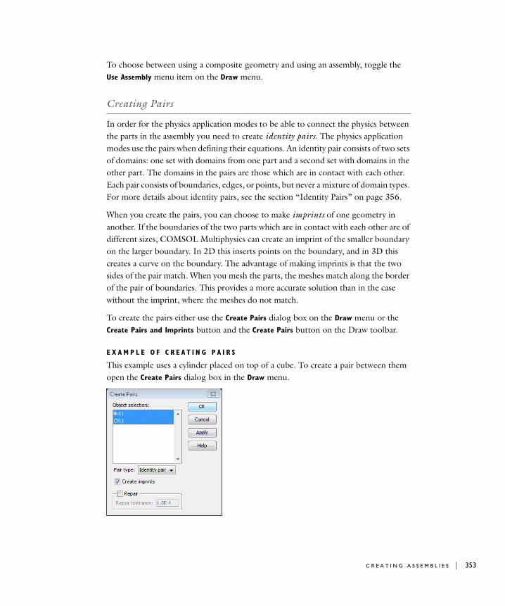
To choose between using a composite geometry and using an assembly, toggle the Use Assembly menu item on the Draw menu.
Creating Pairs
In order for the physics application modes to be able to connect the physics between the parts in the assembly you need to create identity pairs. The physics application modes use the pairs when defining their equations. An identity pair consists of two sets of domains: one set with domains from one part and a second set with domains in the other part. The domains in the pairs are those which are in contact with each other. Each pair consists of boundaries, edges, or points, but never a mixture of domain types. For more details about identity pairs, see the section “Identity Pairs” on page 356.
When you create the pairs, you can choose to make imprints of one geometry in another. If the boundaries of the two parts which are in contact with each other are of different sizes, COMSOL Multiphysics can create an imprint of the smaller boundary on the larger boundary. In 2D this inserts points on the boundary, and in 3D this creates a curve on the boundary. The advantage of making imprints is that the two sides of the pair match. When you mesh the parts, the meshes match along the border of the pair of boundaries. This provides a more accurate solution than in the case without the imprint, where the meshes do not match.
To create the pairs either use the Create Pairs dialog box on the Draw menu or the Create Pairs and Imprints button and the Create Pairs button on the Draw toolbar.
E X A M P L E O F C R E A T I N G P A I R S
This example uses a cylinder placed on top of a cube. To create a pair between them open the Create Pairs dialog box in the Draw menu.
C R E A T I N G A S S E M B L I E S | 353
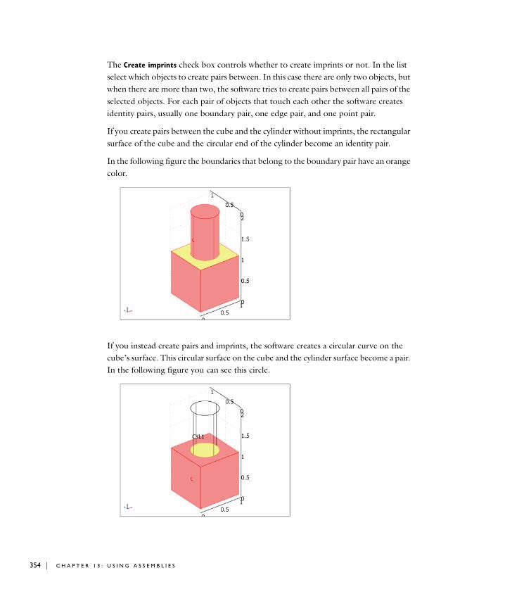
354 | C H A P T E
The Create imprints check box controls whether to create imprints or not. In the list select which objects to create pairs between. In this case there are only two objects, but when there are more than two, the software tries to create pairs between all pairs of the selected objects. For each pair of objects that touch each other the software creates identity pairs, usually one boundary pair, one edge pair, and one point pair.
If you create pairs between the cube and the cylinder without imprints, the rectangular surface of the cube and the circular end of the cylinder become an identity pair.
In the following figure the boundaries that belong to the boundary pair have an orange color.
If you instead create pairs and imprints, the software creates a circular curve on the cube’s surface. This circular surface on the cube and the cylinder surface become a pair. In the following figure you can see this circle.
R 1 3 : U S I N G A S S E M B L I E S

If your license includes the Structural Mechanics Module or the MEMS Module you can also create contact pairs using the Create Pairs dialog box. To do this select Contact
pair in the Pair type list. This list is absent in the dialog box if you do not have any of these two modules. Contact pairs are used when modeling structural contact. You can read about this topic in the Structural Mechanics Module User’s Guide.
C R E A T I N G A S S E M B L I E S | 355
356 | C H A P T E
I d e n t i t y Pa i r s
When making models with assemblies you need to define identity pairs, which define where the parts of the assemblies are connected. The application modes use the pairs to put constraints on the equations such that the solution becomes continuous across the border between the parts. An identity pair consists of two sets of domains, either two sets of boundaries, two sets of edges, or two sets of points. Such pairs are called identity boundary pairs, identity edge pairs, and identity point pairs, respectively. The two sets of domains are the source domains and the destination domains. The application modes put a constraint on the dependent variables on the destination domains, forcing them to be equal to the value on the source domains. When the source and destination do not match each other completely you obtain the best numerical result if you let the destination be the smaller of the two. When creating pairs either using the Create Pairs dialog box or any of the Create Pairs and Imprints button or the Create Pairs button on the Draw toolbar, the smaller side always becomes the destination. The easiest way to create the identity pairs is to use the dialog box or the toolbar buttons. For details see the section “Creating Pairs” on page 353; it describes how to manually define the pairs, which becomes necessary if the automatic generation fails, or if you need to adjust the pairs which the automatic generation created.
R 1 3 : U S I N G A S S E M B L I E S

The Identity Pair Dialog Box
To define identity pairs, choose any of the menu items on the Physics>Identity Pairs menu. This opens the dialog box for the identity pairs of the selected domain type, for example, the Identity Boundary Pairs dialog box.
Each pair has a name. The application modes use this name to refer to the pair. The names must be unique for each domain level, but pairs on different domain levels can have the same name. For example, two boundary pairs cannot have the name “Pair 1,” while there can be both a boundary pair and a point pair called “Pair 1.”
The two domain lists show the source and destination domains of the pair selected in the list to the left. The check boxes beside the domain numbers indicate which domains belong to the source and which to the destination.
Clicking the buttons Check Selected below the lists selects the check boxes of the domains highlighted in the list. This is equivalent to selecting the individual check boxes and is a quick way to select multiple check boxes. Clicking the button Clear
Selected similarly clears the check boxes of the selected domains.
Use the buttons Select Source and Select Destination to select the source and destination domains in the main window and in the selection lists.
Clicking the arrow button between the selection lists interchanges the source and destination domains.
I D E N T I T Y P A I R S | 357
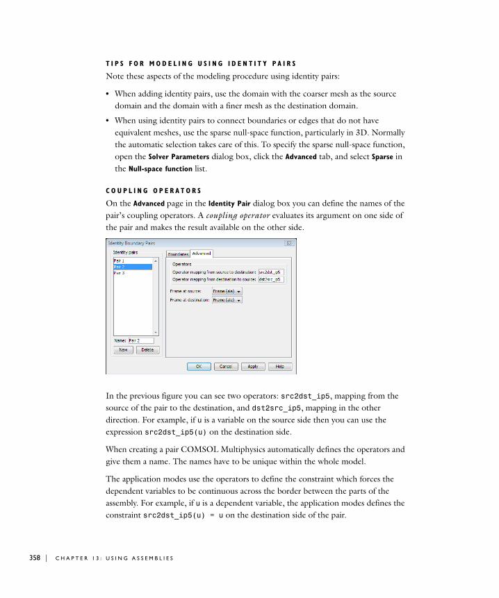
358 | C H A P T E
T I P S F O R M O D E L I N G U S I N G I D E N T I T Y P A I R S
Note these aspects of the modeling procedure using identity pairs:
• When adding identity pairs, use the domain with the coarser mesh as the source domain and the domain with a finer mesh as the destination domain.
• When using identity pairs to connect boundaries or edges that do not have equivalent meshes, use the sparse null-space function, particularly in 3D. Normally the automatic selection takes care of this. To specify the sparse null-space function, open the Solver Parameters dialog box, click the Advanced tab, and select Sparse in the Null-space function list.
C O U P L I N G O P E R A T O R S
On the Advanced page in the Identity Pair dialog box you can define the names of the pair’s coupling operators. A coupling operator evaluates its argument on one side of the pair and makes the result available on the other side.
In the previous figure you can see two operators: src2dst_ip5, mapping from the source of the pair to the destination, and dst2src_ip5, mapping in the other direction. For example, if u is a variable on the source side then you can use the expression src2dst_ip5(u) on the destination side.
When creating a pair COMSOL Multiphysics automatically defines the operators and give them a name. The names have to be unique within the whole model.
The application modes use the operators to define the constraint which forces the dependent variables to be continuous across the border between the parts of the assembly. For example, if u is a dependent variable, the application modes defines the constraint src2dst_ip5(u) = u on the destination side of the pair.
R 1 3 : U S I N G A S S E M B L I E S
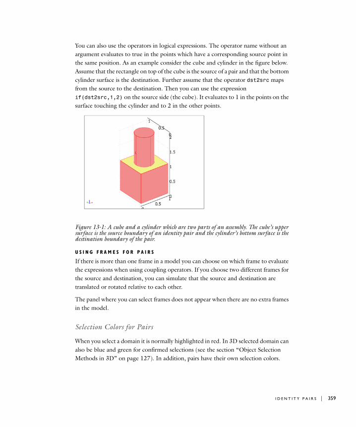
You can also use the operators in logical expressions. The operator name without an argument evaluates to true in the points which have a corresponding source point in the same position. As an example consider the cube and cylinder in the figure below. Assume that the rectangle on top of the cube is the source of a pair and that the bottom cylinder surface is the destination. Further assume that the operator dst2src maps from the source to the destination. Then you can use the expression if(dst2src,1,2) on the source side (the cube). It evaluates to 1 in the points on the surface touching the cylinder and to 2 in the other points.
Figure 13-1: A cube and a cylinder which are two parts of an assembly. The cube’s upper surface is the source boundary of an identity pair and the cylinder’s bottom surface is the destination boundary of the pair.
U S I N G F R A M E S F O R P A I R S
If there is more than one frame in a model you can choose on which frame to evaluate the expressions when using coupling operators. If you choose two different frames for the source and destination, you can simulate that the source and destination are translated or rotated relative to each other.
The panel where you can select frames does not appear when there are no extra frames in the model.
Selection Colors for Pairs
When you select a domain it is normally highlighted in red. In 3D selected domain can also be blue and green for confirmed selections (see the section “Object Selection Methods in 3D” on page 127). In addition, pairs have their own selection colors.
I D E N T I T Y P A I R S | 359
360 | C H A P T E
In Draw mode the domains belonging to a pair have an orange color. This is true whether they are selected or not.
In the Subdomain, Boundary, Edge, and Point selection modes the pair domains have three possible selection colors. When you select a source domain it becomes highlighted in cyan. A destination domain which you select becomes highlighted in magenta. If a domain is a source domain to one pair and a destination domain to another pair it is highlighted in orange. These specific selection colors for pairs override the red selection colors but not the green and blue colors for confirmed selections.
You can deactivate the pair colors and use only the red selection color. To do so open the Preferences dialog box, and on the Visualization tab clear the Pair colors check box. This also turns off the orange color for the pairs in Draw mode.
R 1 3 : U S I N G A S S E M B L I E S
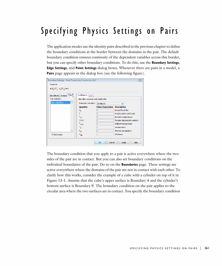
S p e c i f y i n g Ph y s i c s S e t t i n g s on Pa i r s
The application modes use the identity pairs described in the previous chapter to define the boundary conditions at the border between the domains in the pair. The default boundary condition ensures continuity of the dependent variables across this border, but you can specify other boundary conditions. To do this, use the Boundary Settings, Edge Settings, and Point Settings dialog boxes. Whenever there are pairs in a model, a Pairs page appears in the dialog box (see the following figure).
The boundary condition that you apply to a pair is active everywhere where the two sides of the pair are in contact. But you can also set boundary conditions on the individual boundaries of the pair. Do so on the Boundaries page. These settings are active everywhere where the domains of the pair are not in contact with each other. To clarify how this works, consider the example of a cube with a cylinder on top of it in Figure 13-1. Assume that the cube’s upper surface is Boundary 4 and the cylinder’s bottom surface is Boundary 9. The boundary condition on the pair applies to the circular area where the two surfaces are in contact. You specify the boundary condition
S P E C I F Y I N G P H Y S I C S S E T T I N G S O N P A I R S | 361
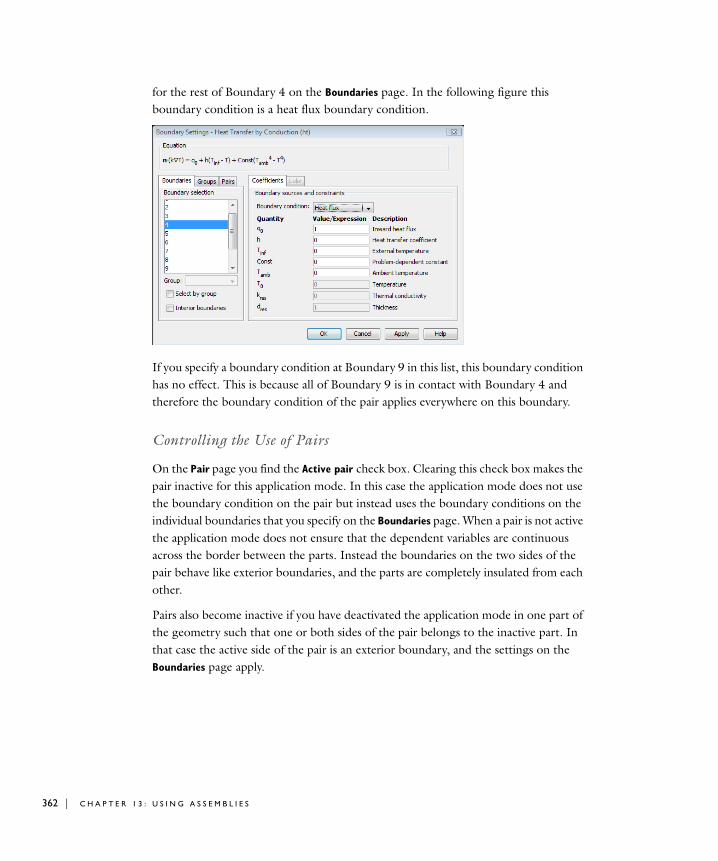
362 | C H A P T E
for the rest of Boundary 4 on the Boundaries page. In the following figure this boundary condition is a heat flux boundary condition.
If you specify a boundary condition at Boundary 9 in this list, this boundary condition has no effect. This is because all of Boundary 9 is in contact with Boundary 4 and therefore the boundary condition of the pair applies everywhere on this boundary.
Controlling the Use of Pairs
On the Pair page you find the Active pair check box. Clearing this check box makes the pair inactive for this application mode. In this case the application mode does not use the boundary condition on the pair but instead uses the boundary conditions on the individual boundaries that you specify on the Boundaries page. When a pair is not active the application mode does not ensure that the dependent variables are continuous across the border between the parts. Instead the boundaries on the two sides of the pair behave like exterior boundaries, and the parts are completely insulated from each other.
Pairs also become inactive if you have deactivated the application mode in one part of the geometry such that one or both sides of the pair belongs to the inactive part. In that case the active side of the pair is an exterior boundary, and the settings on the Boundaries page apply.
R 1 3 : U S I N G A S S E M B L I E S
Edge and Point Pairs
You specify the settings for edge and point pairs in the same ways as for boundary pairs. But most application modes do not use the edge and point pairs. The application modes that define their equations on subdomain level use boundary pairs only. The reason is that because the setting on the boundary pair ensures that the dependent variables are continuous between the boundaries, this also ensures that they are continuous between the edges and points adjacent to the boundaries in contact. Putting constraints on the edges and points is therefore unnecessary.
The application modes which define their equations on the boundary level use the pairs on edges in 3D or on points in 2D. The dependent variables of these application modes need a constraint on the edges (or points) to be continuous.
Similarly, the application modes that define their equations on the edge level use the point pairs.
Slit Boundary Conditions
On the borders between pairs in an assembly, you can specify special “slit boundary conditions,” which represent a discontinuity in the field due to, for example, contact resistance. The following application modes include a boundary condition of this type:
These boundary conditions are available in the Boundary Settings dialog box by clicking the Pairs tab and selecting the pairs where you want to apply the boundary condition. In addition to the physical quantity listed in Table 13-1, you must also enter the thickness of the layer or gap. For an example model, see “Thin-Film Resistance Model” on page 368.
TABLE 13-1: SLIT BOUNDARY CONDITIONS
APPLICATION MODE BOUNDARY CONDITION PHYSICAL QUANTITY
Conductive Media DC Contact resistance Electric conductivity
Electrostatics Thin highly capacitive layer Permittivity
Diffusion, Convection and Diffusion, Electrokinetic Flow
Thin boundary layer Diffusion coefficient
Heat Transfer by Conduction, Convection and Conduction, General Heat Transfer
Thin thermally resistive layer Thermal conductivity
Magnetostatics, No Currents Thin low permeability gap Permeability
S P E C I F Y I N G P H Y S I C S S E T T I N G S O N P A I R S | 363

364 | C H A P T E
Note: The General Heat Transfer application mode is only available in the Heat Transfer Module, and the Magnetostatics, No Currents application mode is only available in the AC/DC Module. The Electrokinetic Flow application mode is only available in the MEMS Module and the Chemical Engineering Module.
R 1 3 : U S I N G A S S E M B L I E S
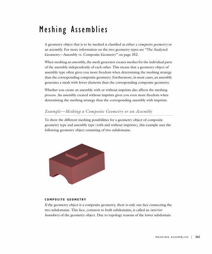
Me sh i n g A s s emb l i e s
A geometry object that is to be meshed is classified as either a composite geometry or an assembly. For more information on the two geometry types see “The Analyzed Geometry—Assembly vs. Composite Geometry” on page 352.
When meshing an assembly, the mesh generator creates meshes for the individual parts of the assembly independently of each other. This means that a geometry object of assembly type often gives you more freedom when determining the meshing strategy than the corresponding composite geometry. Furthermore, in most cases, an assembly generates a mesh with fewer elements than the corresponding composite geometry.
Whether you create an assembly with or without imprints also affects the meshing process. An assembly created without imprints gives you even more freedom when determining the meshing strategy than the corresponding assembly with imprints.
Example—Meshing a Composite Geometry or an Assembly
To show the different meshing possibilities for a geometry object of composite geometry type and assembly type (with and without imprints), this example uses the following geometry object consisting of two subdomains.
C O M P O S I T E G E O M E T R Y
If the geometry object is a composite geometry, there is only one face connecting the two subdomains. This face, common to both subdomains, is called an interior boundary of the geometry object. Due to topology reasons of the lower subdomain
M E S H I N G A S S E M B L I E S | 365
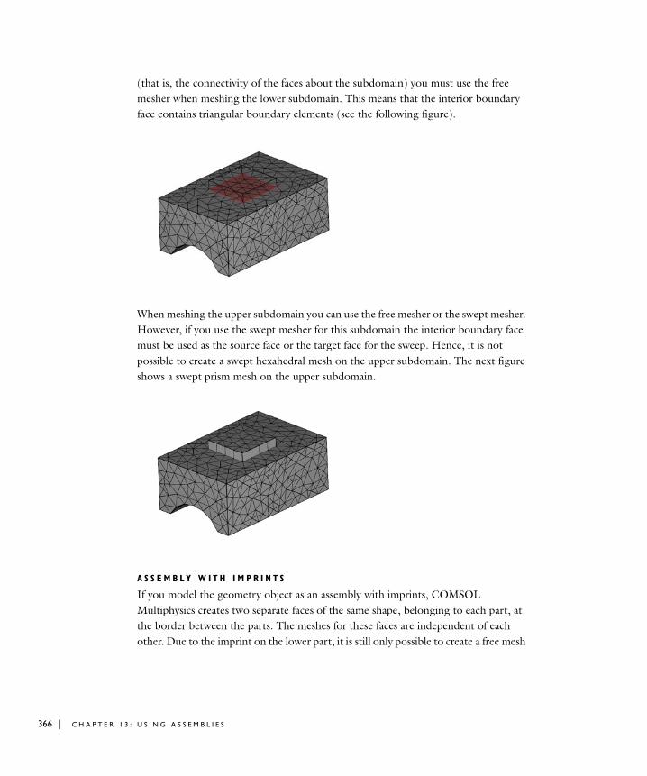
366 | C H A P T E
(that is, the connectivity of the faces about the subdomain) you must use the free mesher when meshing the lower subdomain. This means that the interior boundary face contains triangular boundary elements (see the following figure).
When meshing the upper subdomain you can use the free mesher or the swept mesher. However, if you use the swept mesher for this subdomain the interior boundary face must be used as the source face or the target face for the sweep. Hence, it is not possible to create a swept hexahedral mesh on the upper subdomain. The next figure shows a swept prism mesh on the upper subdomain.
A S S E M B L Y W I T H I M P R I N T S
If you model the geometry object as an assembly with imprints, COMSOL Multiphysics creates two separate faces of the same shape, belonging to each part, at the border between the parts. The meshes for these faces are independent of each other. Due to the imprint on the lower part, it is still only possible to create a free mesh
R 1 3 : U S I N G A S S E M B L I E S
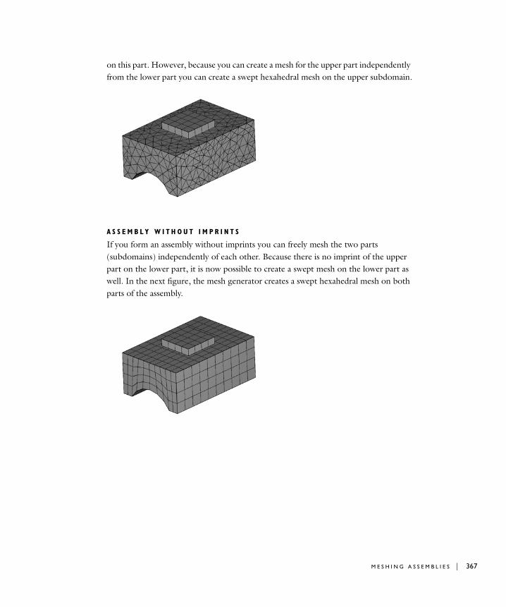
on this part. However, because you can create a mesh for the upper part independently from the lower part you can create a swept hexahedral mesh on the upper subdomain.
A S S E M B L Y W I T H O U T I M P R I N T S
If you form an assembly without imprints you can freely mesh the two parts (subdomains) independently of each other. Because there is no imprint of the upper part on the lower part, it is now possible to create a swept mesh on the lower part as well. In the next figure, the mesh generator creates a swept hexahedral mesh on both parts of the assembly.
M E S H I N G A S S E M B L I E S | 367
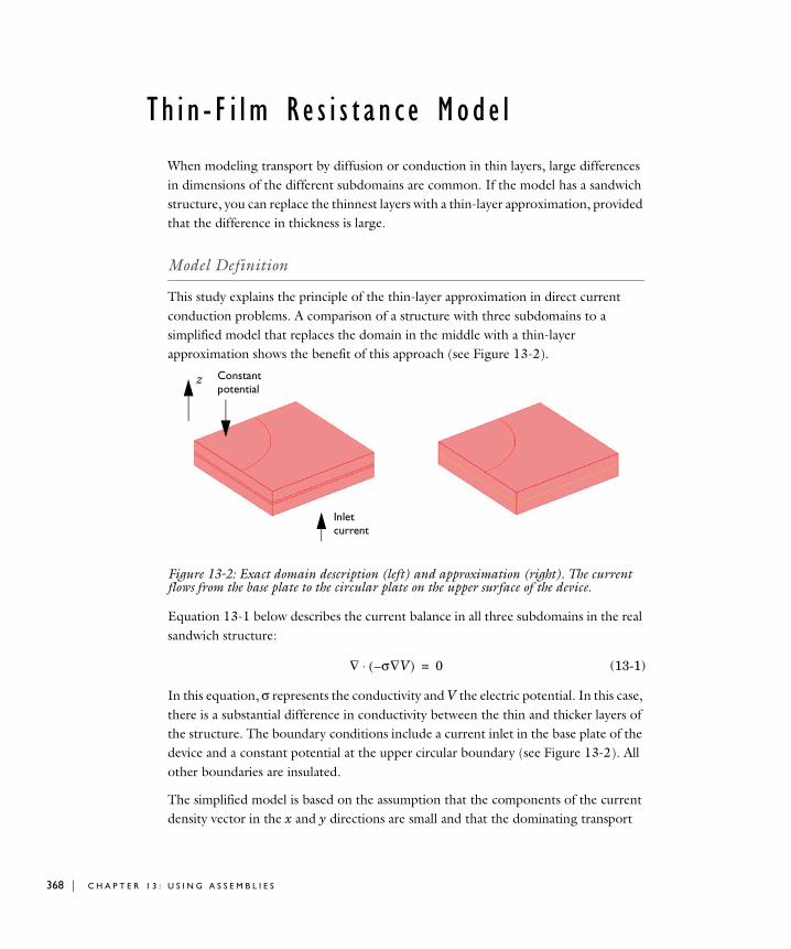
368 | C H A P T E
Th i n - F i lm Re s i s t a n c e Mode l
When modeling transport by diffusion or conduction in thin layers, large differences in dimensions of the different subdomains are common. If the model has a sandwich structure, you can replace the thinnest layers with a thin-layer approximation, provided that the difference in thickness is large.
Model Definition
This study explains the principle of the thin-layer approximation in direct current conduction problems. A comparison of a structure with three subdomains to a simplified model that replaces the domain in the middle with a thin-layer approximation shows the benefit of this approach (see Figure 13-2).
Figure 13-2: Exact domain description (left) and approximation (right). The current flows from the base plate to the circular plate on the upper surface of the device.
Equation 13-1 below describes the current balance in all three subdomains in the real sandwich structure:
(13-1)
In this equation, σ represents the conductivity and V the electric potential. In this case, there is a substantial difference in conductivity between the thin and thicker layers of the structure. The boundary conditions include a current inlet in the base plate of the device and a constant potential at the upper circular boundary (see Figure 13-2). All other boundaries are insulated.
The simplified model is based on the assumption that the components of the current density vector in the x and y directions are small and that the dominating transport
z Constantpotential
Inletcurrent
∇ σ∇V–( )⋅ 0=
R 1 3 : U S I N G A S S E M B L I E S
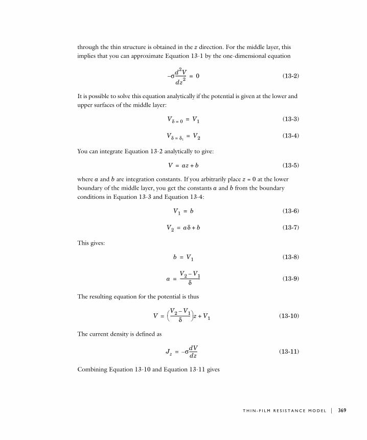
through the thin structure is obtained in the z direction. For the middle layer, this implies that you can approximate Equation 13-1 by the one-dimensional equation
(13-2)
It is possible to solve this equation analytically if the potential is given at the lower and upper surfaces of the middle layer:
(13-3)
(13-4)
You can integrate Equation 13-2 analytically to give:
(13-5)
where a and b are integration constants. If you arbitrarily place z = 0 at the lower boundary of the middle layer, you get the constants a and b from the boundary conditions in Equation 13-3 and Equation 13-4:
(13-6)
(13-7)
This gives:
(13-8)
(13-9)
The resulting equation for the potential is thus
(13-10)
The current density is defined as
(13-11)
Combining Equation 13-10 and Equation 13-11 gives
σd2V
dz2-----------– 0=
Vδ 0= V1=
Vδ δ1= V2=
V az b+=
V1 b=
V2 aδ b+=
b V1=
aV2 V1–
δ--------------------=
VV2 V1–
δ--------------------⎝ ⎠⎛ ⎞ z V1+=
Jz σdVdz--------–=
T H I N - F I L M R E S I S T A N C E M O D E L | 369
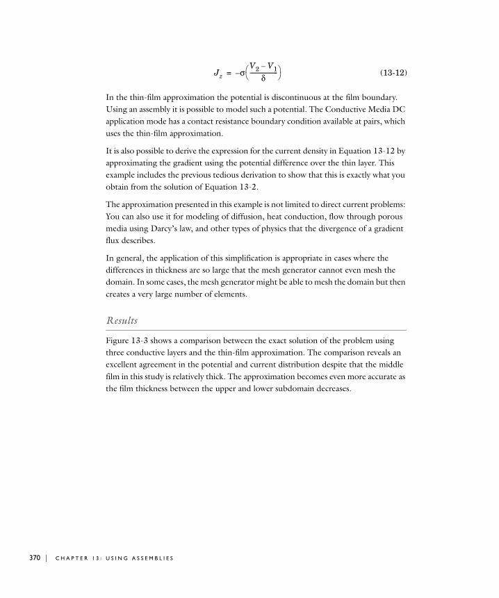
370 | C H A P T E
(13-12)
In the thin-film approximation the potential is discontinuous at the film boundary. Using an assembly it is possible to model such a potential. The Conductive Media DC application mode has a contact resistance boundary condition available at pairs, which uses the thin-film approximation.
It is also possible to derive the expression for the current density in Equation 13-12 by approximating the gradient using the potential difference over the thin layer. This example includes the previous tedious derivation to show that this is exactly what you obtain from the solution of Equation 13-2.
The approximation presented in this example is not limited to direct current problems: You can also use it for modeling of diffusion, heat conduction, flow through porous media using Darcy’s law, and other types of physics that the divergence of a gradient flux describes.
In general, the application of this simplification is appropriate in cases where the differences in thickness are so large that the mesh generator cannot even mesh the domain. In some cases, the mesh generator might be able to mesh the domain but then creates a very large number of elements.
Results
Figure 13-3 shows a comparison between the exact solution of the problem using three conductive layers and the thin-film approximation. The comparison reveals an excellent agreement in the potential and current distribution despite that the middle film in this study is relatively thick. The approximation becomes even more accurate as the film thickness between the upper and lower subdomain decreases.
Jz σV2 V1–
δ--------------------⎝ ⎠⎛ ⎞–=
R 1 3 : U S I N G A S S E M B L I E S
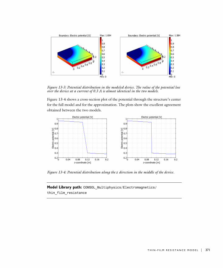
Figure 13-3: Potential distribution in the modeled device. The value of the potential loss over the device at a current of 0.3 A is almost identical in the two models.
Figure 13-4 shows a cross-section plot of the potential through the structure’s center for the full model and for the approximation. The plots show the excellent agreement obtained between the two models.
Figure 13-4: Potential distribution along the z direction in the middle of the device.
Model Library path: COMSOL_Multiphysics/Electromagnetics/thin_film_resistance
T H I N - F I L M R E S I S T A N C E M O D E L | 371
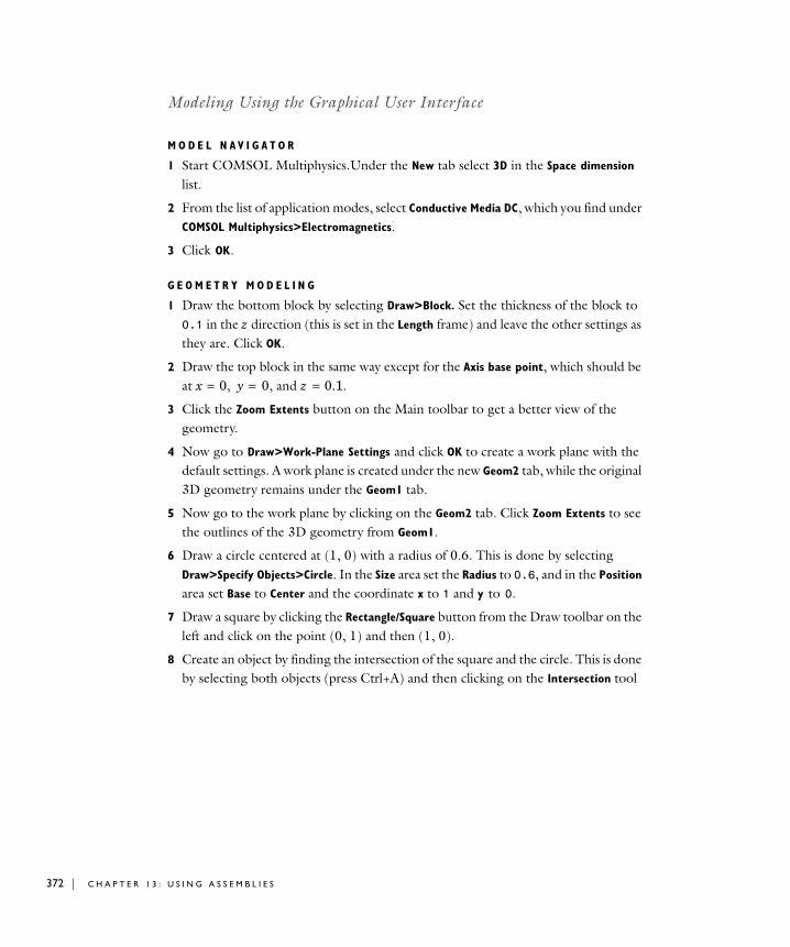
372 | C H A P T E
Modeling Using the Graphical User Interface
M O D E L N A V I G A T O R
1 Start COMSOL Multiphysics.Under the New tab select 3D in the Space dimension list.
2 From the list of application modes, select Conductive Media DC, which you find under COMSOL Multiphysics>Electromagnetics.
3 Click OK.
G E O M E T R Y M O D E L I N G
1 Draw the bottom block by selecting Draw>Block. Set the thickness of the block to 0.1 in the z direction (this is set in the Length frame) and leave the other settings as they are. Click OK.
2 Draw the top block in the same way except for the Axis base point, which should be at x = 0, y = 0, and z = 0.1.
3 Click the Zoom Extents button on the Main toolbar to get a better view of the geometry.
4 Now go to Draw>Work-Plane Settings and click OK to create a work plane with the default settings. A work plane is created under the new Geom2 tab, while the original 3D geometry remains under the Geom1 tab.
5 Now go to the work plane by clicking on the Geom2 tab. Click Zoom Extents to see the outlines of the 3D geometry from Geom1.
6 Draw a circle centered at (1, 0) with a radius of 0.6. This is done by selecting Draw>Specify Objects>Circle. In the Size area set the Radius to 0.6, and in the Position area set Base to Center and the coordinate x to 1 and y to 0.
7 Draw a square by clicking the Rectangle/Square button from the Draw toolbar on the left and click on the point (0, 1) and then (1, 0).
8 Create an object by finding the intersection of the square and the circle. This is done by selecting both objects (press Ctrl+A) and then clicking on the Intersection tool
R 1 3 : U S I N G A S S E M B L I E S
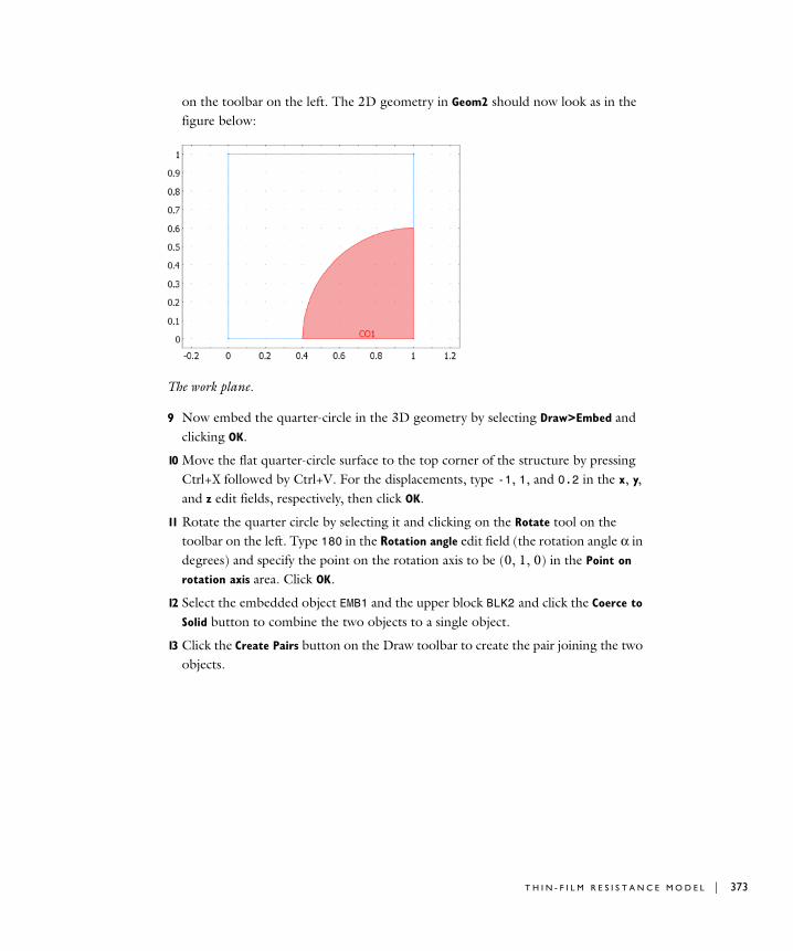
on the toolbar on the left. The 2D geometry in Geom2 should now look as in the figure below:
The work plane.
9 Now embed the quarter-circle in the 3D geometry by selecting Draw>Embed and clicking OK.
10 Move the flat quarter-circle surface to the top corner of the structure by pressing Ctrl+X followed by Ctrl+V. For the displacements, type -1, 1, and 0.2 in the x, y, and z edit fields, respectively, then click OK.
11 Rotate the quarter circle by selecting it and clicking on the Rotate tool on the toolbar on the left. Type 180 in the Rotation angle edit field (the rotation angle α in degrees) and specify the point on the rotation axis to be (0, 1, 0) in the Point on
rotation axis area. Click OK.
12 Select the embedded object EMB1 and the upper block BLK2 and click the Coerce to
Solid button to combine the two objects to a single object.
13 Click the Create Pairs button on the Draw toolbar to create the pair joining the two objects.
T H I N - F I L M R E S I S T A N C E M O D E L | 373
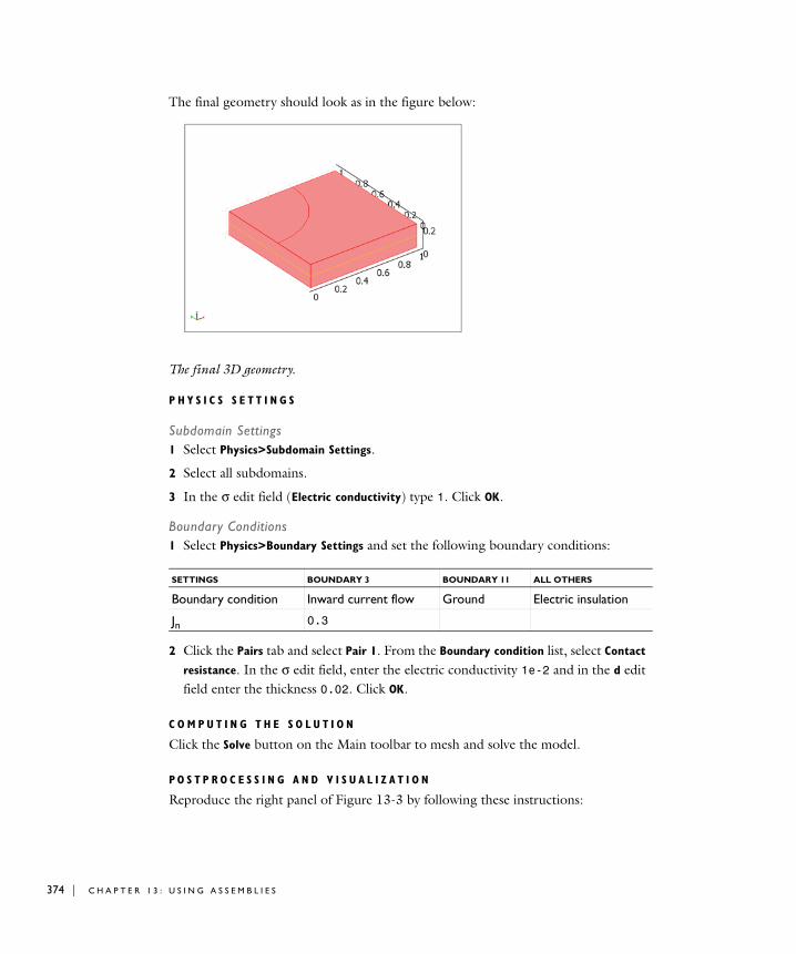
374 | C H A P T E
The final geometry should look as in the figure below:
The final 3D geometry.
P H Y S I C S S E T T I N G S
Subdomain Settings1 Select Physics>Subdomain Settings.
2 Select all subdomains.
3 In the σ edit field (Electric conductivity) type 1. Click OK.
Boundary Conditions1 Select Physics>Boundary Settings and set the following boundary conditions:
2 Click the Pairs tab and select Pair 1. From the Boundary condition list, select Contact
resistance. In the σ edit field, enter the electric conductivity 1e-2 and in the d edit field enter the thickness 0.02. Click OK.
C O M P U T I N G T H E S O L U T I O N
Click the Solve button on the Main toolbar to mesh and solve the model.
P O S T P R O C E S S I N G A N D V I S U A L I Z A T I O N
Reproduce the right panel of Figure 13-3 by following these instructions:
SETTINGS BOUNDARY 3 BOUNDARY 11 ALL OTHERS
Boundary condition Inward current flow Ground Electric insulation
Jn 0.3
R 1 3 : U S I N G A S S E M B L I E S
1 Click the Plot Parameters button on the Main toolbar.
2 On the General page, clear the Slice check box and select the Boundary check box.
3 Click the Boundary tab.
4 From the Predefined quantities list, select Conductive Media DC (dc)>Electric potential.
5 Clear the Smooth check box.
6 Click OK.
To generate the plot in the right panel of Figure 13-4, proceed with the following steps:
1 From the Postprocessing menu, select Cross-Section Plot Parameters.
2 On the Line/Extrusion page, verify that the selection in the Predefined quantities list in the y-axis data area is Potential.
3 In the x-axis data area, click first the lower option button and then the Expression button.
4 In the X-Axis Data dialog box, type z in the Expression edit field. Click OK.
5 In the Cross-section line data area, enter the following settings:
6 Click OK to close the Cross-Section Plot Parameters dialog box and generate the plot.
Comparing the Thin-Film Approximation with the Full 3D Model
You can easily reproduce the full 3D model that served as a reference model for comparison in this example. To do so, move the upper block, CO1, a distance 0.02 in the z direction, then add a thin block with the height 0.02 in between the top and bottom block. Here it is not necessary to use an assembly, so you can clear Use Assembly in the Draw menu. Set the conductivity to 0.01 in this thin middle subdomain (leave it at 1 in the top and bottom subdomains). Let the boundary conditions for the top and bottom of the thin layer be inactive, which means that the solution is continuous across the interfaces. Let the outer boundary conditions be the same as they were in the above description (that is, electric insulation), and compute the solution for this model.
It should now be apparent that the two solutions show good agreement and that the first approach consumes significantly less time and memory.
x0 0.5 x1 0.5
y0 0.5 y1 0.5
z0 0 z1 0.2
T H I N - F I L M R E S I S T A N C E M O D E L | 375
376 | C H A P T E
U s i n g I d e n t i t y C ond i t i o n s
To connect the fields of physics across different geometries, you can use identity conditions that make the physical quantities equal across the different parts. The identity boundary conditions and identity conditions on other domain types define a constraint that makes two quantities equal on two separate (but usually equally-shaped) domains in two different geometries where you do not need a coordinate transformation between the source and destination domains. That is, the source and the destination domains must lie in the same place in the coordinate space.
Note: Using an assembly and identity pairs, you can work with a geometry that consists of several parts without using multiple geometries and identity conditions.
Creating Identity Conditions
When you do not need a transformation, you specify a identity condition in the same way as you specify a periodic condition:
1 Select the source geometry for the coupling variable.
2 On the Options menu point to Identity Conditions, then click on the domain type: Identity Subdomain Conditions, Identity Boundary Conditions, Identity Edge Conditions (3D only), or Identity Point Conditions.
3 In the dialog box for the identity conditions, start by specifying the source geometry on the Source page. Enter the expression that you wish to use in the identity coupling for the source. Refer to each constraint in the identity coupling by a name. A default name appears for the constraint that implements the identity coupling. To
R 1 3 : U S I N G A S S E M B L I E S
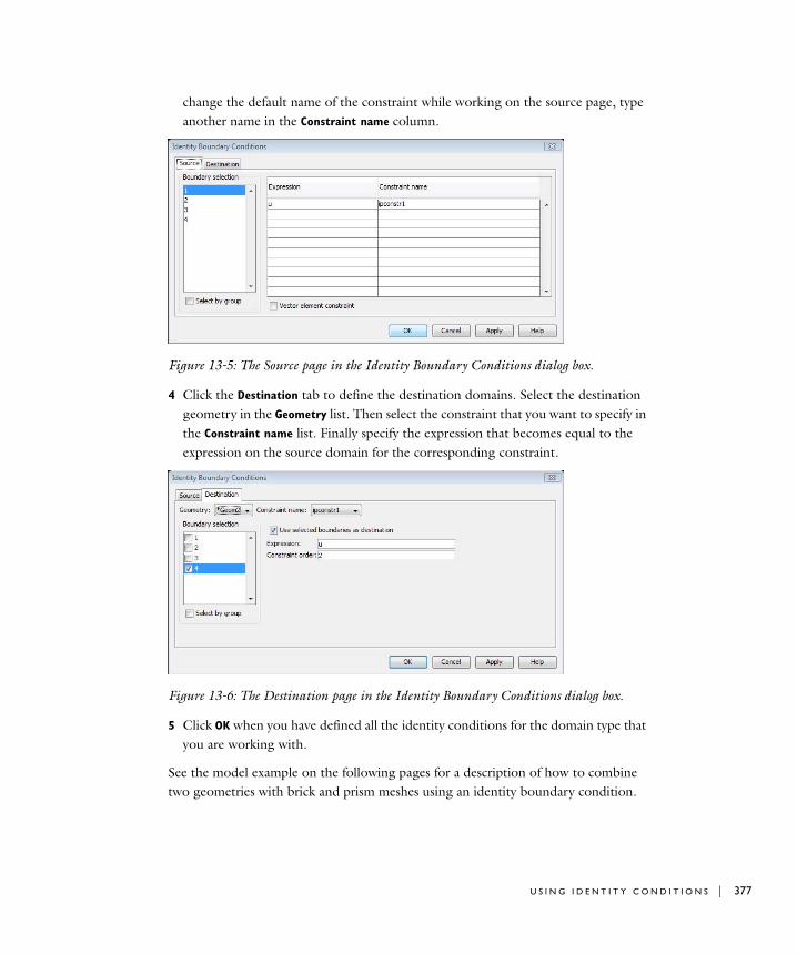
change the default name of the constraint while working on the source page, type another name in the Constraint name column.
Figure 13-5: The Source page in the Identity Boundary Conditions dialog box.
4 Click the Destination tab to define the destination domains. Select the destination geometry in the Geometry list. Then select the constraint that you want to specify in the Constraint name list. Finally specify the expression that becomes equal to the expression on the source domain for the corresponding constraint.
Figure 13-6: The Destination page in the Identity Boundary Conditions dialog box.
5 Click OK when you have defined all the identity conditions for the domain type that you are working with.
See the model example on the following pages for a description of how to combine two geometries with brick and prism meshes using an identity boundary condition.
U S I N G I D E N T I T Y C O N D I T I O N S | 377
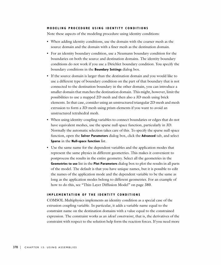
378 | C H A P T E
M O D E L I N G P R O C E D U R E U S I N G I D E N T I T Y C O N D I T I O N S
Note these aspects of the modeling procedure using identity conditions:
• When adding identity conditions, use the domain with the coarser mesh as the source domain and the domain with a finer mesh as the destination domain.
• For an identity boundary condition, use a Neumann boundary condition for the boundaries on both the source and destination domains. The identity boundary conditions do not work if you use a Dirichlet boundary condition. You specify the boundary conditions in the Boundary Settings dialog box.
• If the source domain is larger than the destination domain and you would like to use a different type of boundary condition on the part of that boundary that is not connected to the destination boundary in the other domain, you can introduce a smaller domain that matches the destination domain. This might, however, limit the possibilities to use a mapped 2D mesh and then also a 3D mesh using brick elements. In that case, consider using an unstructured triangular 2D mesh and mesh extrusion to form a 3D mesh using prism elements if you want to avoid an unstructured tetrahedral mesh.
• When using identity-coupling variables to connect boundaries or edges that do not have equivalent meshes, use the sparse null-space function, particularly in 3D. Normally the automatic selection takes care of this. To specify the sparse null-space function, open the Solver Parameters dialog box, click the Advanced tab, and select Sparse in the Null-space function list.
• Use the same name for the dependent variables and the application modes that represent the same physics in different geometries. This makes it convenient to postprocess the results in the entire geometry. Select all the geometries in the Geometries to use list in the Plot Parameters dialog box to plot the results in all parts of the model. The default is that you have unique names, but it is possible to edit the names of the application mode and the dependent variable to be the same as long as the application modes belong to different geometries. For an example of how to do this, see “Thin-Layer Diffusion Model” on page 380.
I M P L E M E N T A T I O N O F T H E I D E N T I T Y C O N D I T I O N S
COMSOL Multiphysics implements an identity condition as a special case of the extrusion coupling variable. In particular, it adds a variable name equal to the constraint name on the destination domains with a value equal to the constrained expression. The constraint works as an ideal constraint, that is, the derivatives of the constraint with respect to the solution help form the reaction forces. If you need more
R 1 3 : U S I N G A S S E M B L I E S
freedom in specifying how the reaction forces are applied, use the extrusion coupling variable directly and specify the reaction force and constraint as weak contributions.
Note: It is normally much easier to work with an assembly that consists of two or more geometrical parts. You can then use identity pairs and interactive meshing to create a model where the physics is connected and where you can use different types of meshes in each part.
M O D E L I N G P R O C E D U R E F O R M U L T I G E O M E T R Y L I N K I N G
The following list shows the main steps you must take to make a model with a continuous field that you link between two or more geometries:
1 Create the full geometry using separate geometries (parts) in the COMSOL Multiphysics model. Use the View All 3D Geometries/View All 2D Geometries button in the Visualization/Selection toolbar or the View Geometries dialog box to show other geometries than the current geometry during modeling. This helps to see that the geometries are spatially connected and that the total geometry looks right.
2 Create the meshes for the different geometries. These can be of different kinds, which is not possible using a single geometry. This is the main advantage with this multigeometry approach.
3 Add the physics to the different geometries. It is typically the same type of physics, and the field is continuous across the geometries. For this purpose, use the same name for the field variables (dependent variables) and the application modes. You can then visualize and postprocess the solution on the entire geometry using the same variable names for both dependent variables and application mode variables that use the application mode name as a suffix.
Note: The default names for the application modes and dependent variables are different for each application mode that you add. Make sure to edit these to make all names the same.
4 Use identity boundary conditions to link the physics across the different geometries.
5 Compute the solution.
6 For visualization plot the results in all geometries simultaneously. To do so, select all the geometries in the Geometries to use list in the Plot Parameters dialog box.
U S I N G I D E N T I T Y C O N D I T I O N S | 379
380 | C H A P T E
Th i n - L a y e r D i f f u s i o n Mode l
The following example shows how to link two separate geometries into a 3D thin-layer diffusion model using identity boundary conditions. It also illustrates the use of different mesh element types; the brick and prism elements provide a large reduction in the number of degrees of freedom (DOFs) for this thin geometry. For more information about mesh elements and meshing options, see “Meshing” on page 285 in the COMSOL Multiphysics User’s Guide.
In this model you can significantly reduce the number of DOFs—and thus the solution time—by taking advantage of the geometry shape using brick and prism meshes instead of an unstructured tetrahedral mesh. The total model has only about 2300 DOFs using this approach. Using a default tetrahedral mesh on the same geometry leads to a problem with roughly 18,000 DOFs.
The physics in this model is a single-species diffusion. The dependent variable is the concentration, c. All boundaries are insulated except the inlet and the outlet. At the inlet boundary the concentration is c0. At the outflow boundary (the bottom surface) there is an outward flux of −rsurf c/c0 (COMSOL Multiphysics defines the inward flux as positive), where rsurf is the reaction rate at the surface. An effective diffusion coefficient takes the porous material in the thin bottom plate into account. Table 13-2 on page 387 lists all material properties in the model.
The interface condition at the connection between the top and bottom parts is that the concentration c is equal on both sides.
R 1 3 : U S I N G A S S E M B L I E S
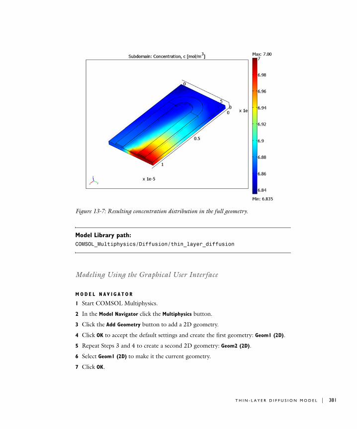
Figure 13-7: Resulting concentration distribution in the full geometry.
Model Library path:
COMSOL_Multiphysics/Diffusion/thin_layer_diffusion
Modeling Using the Graphical User Interface
M O D E L N A V I G A T O R
1 Start COMSOL Multiphysics.
2 In the Model Navigator click the Multiphysics button.
3 Click the Add Geometry button to add a 2D geometry.
4 Click OK to accept the default settings and create the first geometry: Geom1 (2D).
5 Repeat Steps 3 and 4 to create a second 2D geometry: Geom2 (2D).
6 Select Geom1 (2D) to make it the current geometry.
7 Click OK.
T H I N - L A Y E R D I F F U S I O N M O D E L | 381
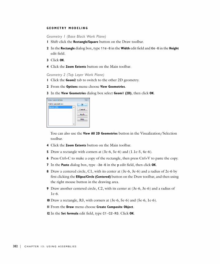
382 | C H A P T E
G E O M E T R Y M O D E L I N G
Geometry 1 (Base Block Work Plane)1 Shift-click the Rectangle/Square button on the Draw toolbar.
2 In the Rectangle dialog box, type 11e-6 in the Width edit field and 6e-6 in the Height edit field.
3 Click OK.
4 Click the Zoom Extents button on the Main toolbar.
Geometry 2 (Top Layer Work Plane)1 Click the Geom2 tab to switch to the other 2D geometry.
2 From the Options menu choose View Geometries.
3 In the View Geometries dialog box select Geom1 (2D), then click OK.
You can also use the View All 2D Geometries button in the Visualization/Selection toolbar.
4 Click the Zoom Extents button on the Main toolbar.
5 Draw a rectangle with corners at (3e-6, 5e-6) and (1.1e-5, 4e-6).
6 Press Ctrl+C to make a copy of the rectangle, then press Ctrl+V to paste the copy.
7 In the Paste dialog box, type -3e-6 in the y edit field, then click OK.
8 Draw a centered circle, C1, with its center at (3e-6, 3e-6) and a radius of 2e-6 by first clicking the Ellipse/Circle (Centered) button on the Draw toolbar, and then using the right mouse button in the drawing area.
9 Draw another centered circle, C2, with its center at (3e-6, 3e-6) and a radius of 1e-6.
10 Draw a rectangle, R3, with corners at (3e-6, 5e-6) and (5e-6, 1e-6).
11 From the Draw menu choose Create Composite Object.
12 In the Set formula edit field, type C1-C2-R3. Click OK.
R 1 3 : U S I N G A S S E M B L I E S
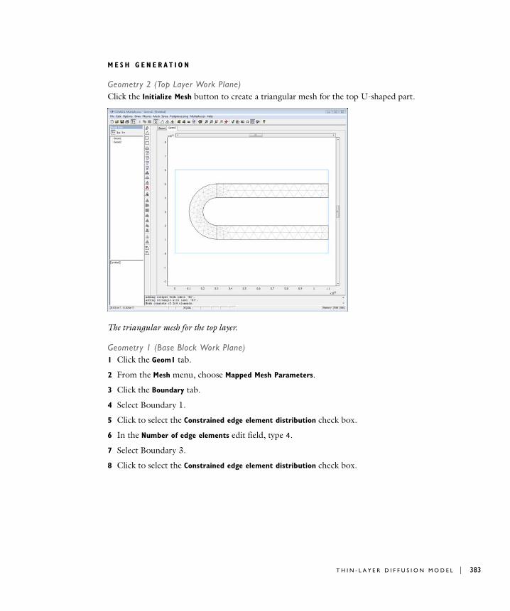
M E S H G E N E R A T I O N
Geometry 2 (Top Layer Work Plane)Click the Initialize Mesh button to create a triangular mesh for the top U-shaped part.
The triangular mesh for the top layer.
Geometry 1 (Base Block Work Plane)1 Click the Geom1 tab.
2 From the Mesh menu, choose Mapped Mesh Parameters.
3 Click the Boundary tab.
4 Select Boundary 1.
5 Click to select the Constrained edge element distribution check box.
6 In the Number of edge elements edit field, type 4.
7 Select Boundary 3.
8 Click to select the Constrained edge element distribution check box.
T H I N - L A Y E R D I F F U S I O N M O D E L | 383
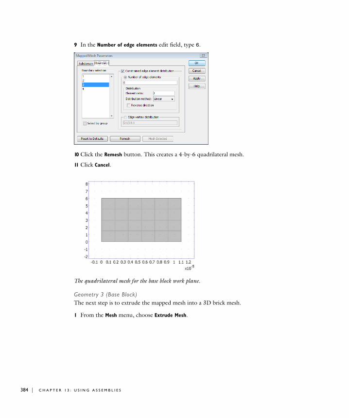
384 | C H A P T E
9 In the Number of edge elements edit field, type 6.
10 Click the Remesh button. This creates a 4-by-6 quadrilateral mesh.
11 Click Cancel.
The quadrilateral mesh for the base block work plane.
Geometry 3 (Base Block)The next step is to extrude the mapped mesh into a 3D brick mesh.
1 From the Mesh menu, choose Extrude Mesh.
R 1 3 : U S I N G A S S E M B L I E S
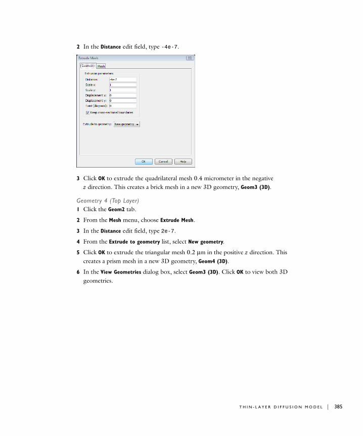
2 In the Distance edit field, type -4e-7.
3 Click OK to extrude the quadrilateral mesh 0.4 micrometer in the negative z direction. This creates a brick mesh in a new 3D geometry, Geom3 (3D).
Geometry 4 (Top Layer)1 Click the Geom2 tab.
2 From the Mesh menu, choose Extrude Mesh.
3 In the Distance edit field, type 2e-7.
4 From the Extrude to geometry list, select New geometry.
5 Click OK to extrude the triangular mesh 0.2 µm in the positive z direction. This creates a prism mesh in a new 3D geometry, Geom4 (3D).
6 In the View Geometries dialog box, select Geom3 (3D). Click OK to view both 3D geometries.
T H I N - L A Y E R D I F F U S I O N M O D E L | 385
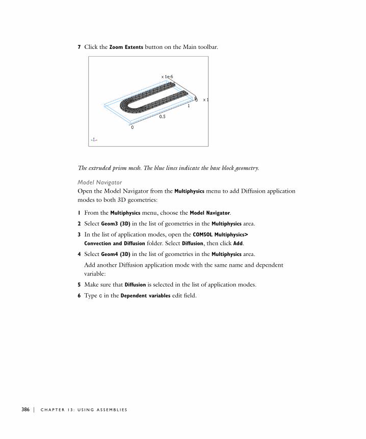
386 | C H A P T E
7 Click the Zoom Extents button on the Main toolbar.
The extruded prism mesh. The blue lines indicate the base block geometry.
Model NavigatorOpen the Model Navigator from the Multiphysics menu to add Diffusion application modes to both 3D geometries:
1 From the Multiphysics menu, choose the Model Navigator.
2 Select Geom3 (3D) in the list of geometries in the Multiphysics area.
3 In the list of application modes, open the COMSOL Multiphysics> Convection and Diffusion folder. Select Diffusion, then click Add.
4 Select Geom4 (3D) in the list of geometries in the Multiphysics area.
Add another Diffusion application mode with the same name and dependent variable:
5 Make sure that Diffusion is selected in the list of application modes.
6 Type c in the Dependent variables edit field.
R 1 3 : U S I N G A S S E M B L I E S
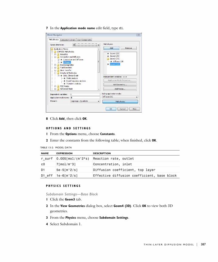
7 In the Application mode name edit field, type di.
8 Click Add, then click OK.
O P T I O N S A N D S E T T I N G S
1 From the Options menu, choose Constants.
2 Enter the constants from the following table; when finished, click OK.
P H Y S I C S S E T T I N G S
Subdomain Settings—Base Block1 Click the Geom3 tab.
2 In the View Geometries dialog box, select Geom4 (3D). Click OK to view both 3D geometries.
3 From the Physics menu, choose Subdomain Settings.
4 Select Subdomain 1.
TABLE 13-2: MODEL DATA
NAME EXPRESSION DESCRIPTION
r_surf 0.005[mol/(m^2*s) Reaction rate, outlet
c0 7[mol/m^3] Concentration, inlet
D1 5e-5[m^2/s] Diffusion coefficient, top layer
D1_eff 1e-6[m^2/s] Effective diffusion coefficient, base block
T H I N - L A Y E R D I F F U S I O N M O D E L | 387
388 | C H A P T E
5 Type D1_eff in the D (isotropic) edit field for the isotropic diffusion coefficient.
6 Click the Init tab.
7 In the c(t0) edit field, type c0.
8 Click OK.
Boundary Conditions—Base Block1 From the Physics menu, choose Boundary Settings.
2 Select Boundary 3 (the bottom boundary).
3 From the Boundary condition list, select Flux.
4 Type -r_surf*c/c0 in the N0 edit field for the inward flux to define an outward flux.
5 Click OK.
Subdomain Settings—Top Layer1 Click the Geom4 tab.
2 In the View Geometries dialog box, select Geom3 (3D). Click OK to view both 3D geometries.
3 From the Physics menu, choose Subdomain Settings.
4 Press Ctrl+A to select all subdomains.
5 Type D1 in the D (isotropic) edit field for the isotropic diffusion coefficient.
6 Click the Init tab.
7 In the c(t0) edit field, type c0.
8 Click OK.
Boundary Conditions—Top Layer1 From the Physics menu, choose Boundary Settings.
2 Select Boundary 18 (the top inflow boundary).
3 Select Concentration in the Boundary condition list.
4 In the c0 edit field for concentration, type c0.
5 Click OK.
Identity Boundary ConditionsTo couple the concentration values from the base block to the top layer, use an identity boundary condition.
1 Click the Geom3 tab.
R 1 3 : U S I N G A S S E M B L I E S
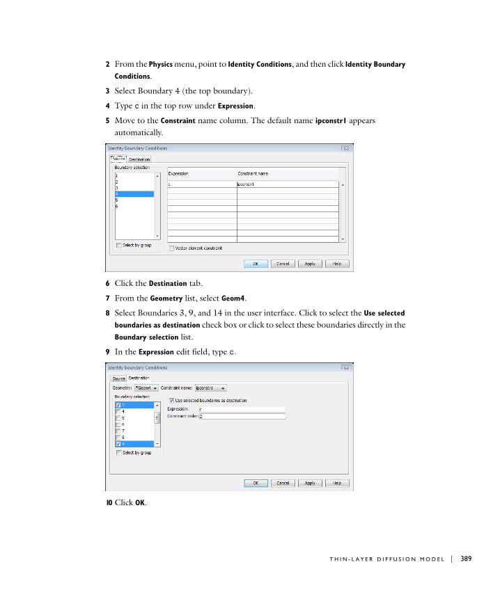
2 From the Physics menu, point to Identity Conditions, and then click Identity Boundary
Conditions.
3 Select Boundary 4 (the top boundary).
4 Type c in the top row under Expression.
5 Move to the Constraint name column. The default name ipconstr1 appears automatically.
6 Click the Destination tab.
7 From the Geometry list, select Geom4.
8 Select Boundaries 3, 9, and 14 in the user interface. Click to select the Use selected
boundaries as destination check box or click to select these boundaries directly in the Boundary selection list.
9 In the Expression edit field, type c.
10 Click OK.
T H I N - L A Y E R D I F F U S I O N M O D E L | 389
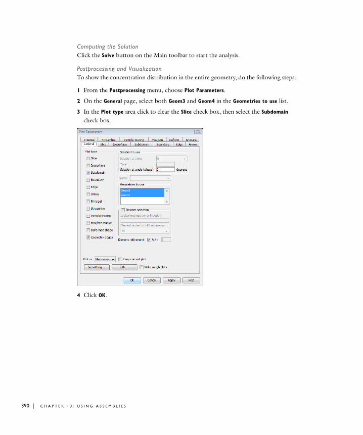
390 | C H A P T E
Computing the SolutionClick the Solve button on the Main toolbar to start the analysis.
Postprocessing and VisualizationTo show the concentration distribution in the entire geometry, do the following steps:
1 From the Postprocessing menu, choose Plot Parameters.
2 On the General page, select both Geom3 and Geom4 in the Geometries to use list.
3 In the Plot type area click to clear the Slice check box, then select the Subdomain check box.
4 Click OK.
R 1 3 : U S I N G A S S E M B L I E S
14
D e f o r m e d M e s h e s
This chapter explains how to use the application modes that control mesh deformation: the Moving Mesh (ALE) application mode and the Parameterized Geometry application mode.
391
392 | C H A P T E
De f o rmed Me s h Fundamen t a l s
A deformed mesh can be useful if the boundaries of your computational domain are moving in time or as a function of a parameter. The point is that a new mesh need not be generated for each configuration of the boundaries—instead, the software simply perturbs the mesh nodes so they conform with the moved boundaries.
In COMSOL Multiphysics, you can control the movement of the interior nodes in three ways:
• By propagating the moving boundary displacement throughout the domain to obtain a smooth mesh deformation everywhere — this is done by solving PDEs for the mesh displacements (a Laplace or Winslow smoothing PDE) with boundary conditions given by the movement of the boundaries.
• By specifying an explicit formula for the mesh deformation.
• By letting the mesh movement be determined by some physical deformation variables, such as the displacement components of structural mechanics.
The technique for mesh movement is called an arbitrary Lagrangian-Eulerian (ALE) method. In the special case of a Lagrangian method, the mesh movement follows the movement of the physical material. Such a method is often used in solid mechanics, where the displacements often are relatively small.
When the material motion is more complicated, like in a fluid flow model, the Lagrangian method is not appropriate. For such models, an Eulerian method, where the mesh is fixed, is often used—except that this method cannot account for moving boundaries.
The ALE method is an intermediate between the Lagrangian and the Eulerian method, and it combines the best features of both—it allows moving boundaries without the need for the mesh movement to follow the material.
Mathematical Description of the Mesh Movement
Though moving meshes are also possible in 3D, consider a 2D geometry for simplicity. First denote the spatial coordinates as (x, y) and then let (X, Y) be the coordinates of a mesh node in the initial, undeformed configuration. To describe the spatial coordinates (x, y) of the same mesh node in the deformed configuration, you can use the functions
R 1 4 : D E F O R M E D M E S H E S
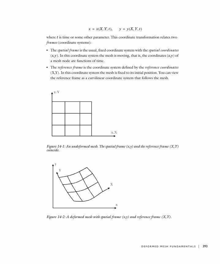
where t is time or some other parameter. This coordinate transformation relates two frames (coordinate systems):
• The spatial frame is the usual, fixed coordinate system with the spatial coordinates (x,y). In this coordinate system the mesh is moving, that is, the coordinates (x,y) of a mesh node are functions of time.
• The reference frame is the coordinate system defined by the reference coordinates (X,Y). In this coordinate system the mesh is fixed to its initial position. You can view the reference frame as a curvilinear coordinate system that follows the mesh.
Figure 14-1: An undeformed mesh. The spatial frame (x,y) and the reference frame (X,Y) coincide.
Figure 14-2: A deformed mesh with spatial frame (x,y) and reference frame (X,Y).
x x X Y t, ,( ) y, y X Y t, ,( )= =
D E F O R M E D M E S H F U N D A M E N T A L S | 393
394 | C H A P T E
Some geometric variables that the software defines are available for both the spatial and the reference frames (see “Geometric Variables” on page 165 in the COMSOL Multiphysics User’s Guide).
Derivatives
S P A T I A L D E R I V A T I V E S
For a dependent variable u, there are two kinds of spatial derivatives:
• ux and uy, the derivatives in the spatial frame. That is, u is considered as a function of x and y (and t). These are typically denoted ux and uy in the software.
• uX and uY, the derivatives in the reference frame. That is, u is considered as a function of X and Y (and t). These are typically denoted uX and uY in the software.
In COMSOL Multiphysics, it is only possible to use one of these types of derivatives depending on the frame associated with the application mode that defines u.
T I M E D E R I V A T I V E S
There are two kinds of time derivatives related to the two frames:
• The common spatial time derivative is related to the spatial frame:
The spatial coordinates (x, y) are fixed when computing this derivative; that is, you consider a fixed point in space. This derivative is often denoted ut in the software (see page 399).
• The reference time derivative (or mesh time derivative) is related to the reference frame:
The reference coordinates (X,Y) are fixed when computing this derivative; that is, you consider a point that follows the moving mesh, for instance a mesh node. This derivative is denoted uTIME in the software.
The two derivatives are related by the chain rule:
ut t∂∂u
x y,=
uTIME t∂∂u
X Y,=
ut uTIME uxxTIME– uyyTIME–=
R 1 4 : D E F O R M E D M E S H E S
where (xTIME,yTIME) is the mesh velocity. The reference time derivative is often less important from the user point view because its value depends on the mesh movement, which has no physical significance. However, for the special case when the mesh follows the material’s motion (the Lagrangian method), the reference time derivative is physically significant and is also called the material time derivative.
The solvers assemble the discretized model on the deformed mesh, using the reference time derivative of the solution as input. They also compute the spatial time derivative by the preceding formula. This implies that the PDEs do not have to be reformulated when you use a deformed mesh. However, if you use a Lagrangian method, some material properties might depend on the material deformation (which is then the same as the mesh deformation).
D E F O R M E D M E S H F U N D A M E N T A L S | 395
396 | C H A P T E
F r ame s f o r De f o rmed Me s h e s
When modeling deformed meshes you need two frames. A frame is a coordinate system, and it includes a set of coordinate names. The two frames are:
• The reference frame, which is the frame in which the mesh is fixed. This is the frame in which you draw the geometry and gives the shape of the geometry before it is deformed. This frame is associated with the geometry, and it exists even when you do not use deformed meshes.
• The spatial frame, which is the usual coordinate system that is fixed in space. In this frame the mesh is moving according to the settings in the deformed mesh application mode. The spatial frame is associated with the deformed mesh application mode.
Frames in the Model Navigator
Before you have added a deformed mesh application mode, there is only one frame, the reference frame. The reference coordinates are the independent variables in the
R 1 4 : D E F O R M E D M E S H E S
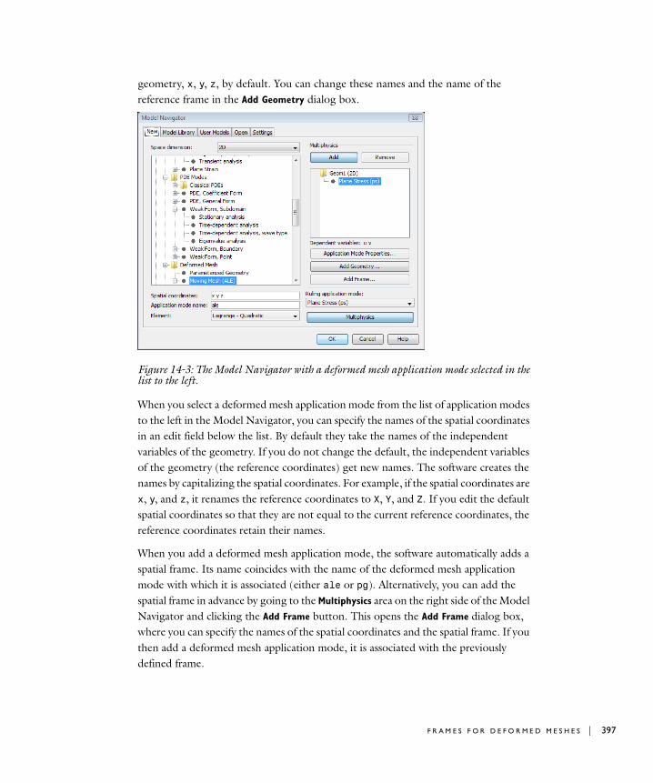
geometry, x, y, z, by default. You can change these names and the name of the reference frame in the Add Geometry dialog box.
Figure 14-3: The Model Navigator with a deformed mesh application mode selected in the list to the left.
When you select a deformed mesh application mode from the list of application modes to the left in the Model Navigator, you can specify the names of the spatial coordinates in an edit field below the list. By default they take the names of the independent variables of the geometry. If you do not change the default, the independent variables of the geometry (the reference coordinates) get new names. The software creates the names by capitalizing the spatial coordinates. For example, if the spatial coordinates are x, y, and z, it renames the reference coordinates to X, Y, and Z. If you edit the default spatial coordinates so that they are not equal to the current reference coordinates, the reference coordinates retain their names.
When you add a deformed mesh application mode, the software automatically adds a spatial frame. Its name coincides with the name of the deformed mesh application mode with which it is associated (either ale or pg). Alternatively, you can add the spatial frame in advance by going to the Multiphysics area on the right side of the Model Navigator and clicking the Add Frame button. This opens the Add Frame dialog box, where you can specify the names of the spatial coordinates and the spatial frame. If you then add a deformed mesh application mode, it is associated with the previously defined frame.
F R A M E S F O R D E F O R M E D M E S H E S | 397
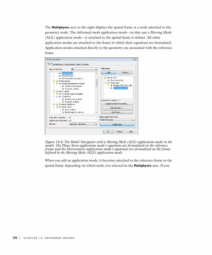
398 | C H A P T E
The Multiphysics area to the right displays the spatial frame as a node attached to the geometry node. The deformed mesh application mode—in this case a Moving Mesh (ALE) application mode—is attached to the spatial frame it defines. All other application modes are attached to the frame in which their equations are formulated. Application modes attached directly to the geometry are associated with the reference frame.
Figure 14-4: The Model Navigator with a Moving Mesh (ALE) application mode in the model. The Plane Stress application mode’s equations are formulated on the reference frame and the Electrostatics application mode’s equations are formulated on the frame defined by the Moving Mesh (ALE) application mode.
When you add an application mode, it becomes attached to the reference frame or the spatial frame depending on which node you selected in the Multiphysics area. If you
R 1 4 : D E F O R M E D M E S H E S
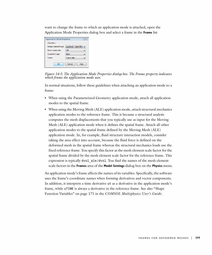
want to change the frame to which an application mode is attached, open the Application Mode Properties dialog box and select a frame in the Frame list
Figure 14-5: The Application Mode Properties dialog box. The Frame property indicates which frame the application mode uses.
In normal situations, follow these guidelines when attaching an application mode to a frame:
• When using the Parameterized Geometry application mode, attach all application modes to the spatial frame.
• When using the Moving Mesh (ALE) application mode, attach structural mechanics application modes to the reference frame. This is because a structural analysis computes the mesh displacements that you typically use as input for the Moving Mesh (ALE) application mode when it defines the spatial frame. Attach all other application modes to the spatial frame defined by the Moving Mesh (ALE) application mode. In, for example, fluid-structure interaction models, consider taking the area effect into account, because the fluid force is defined on the deformed mesh in the spatial frame whereas the structural mechanics loads use the fixed reference frame. You specify this factor as the mesh element scale factor for the spatial frame divided by the mesh element scale factor for the reference frame. This expression is typically dvol_ale/dvol. You find the names of the mesh element scale factors in the Frames area of the Model Settings dialog box on the Physics menu.
An application mode’s frame affects the names of its variables. Specifically, the software uses the frame’s coordinate names when forming derivatives and vector components. In addition, it interprets a time derivative ut as a derivative in the application mode’s frame, while uTIME is always a derivative in the reference frame. See also “Shape Function Variables” on page 171 in the COMSOL Multiphysics User’s Guide.
F R A M E S F O R D E F O R M E D M E S H E S | 399
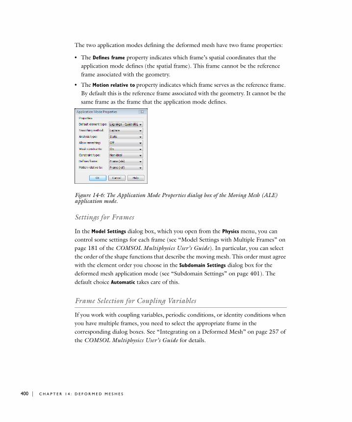
400 | C H A P T E
The two application modes defining the deformed mesh have two frame properties:
• The Defines frame property indicates which frame’s spatial coordinates that the application mode defines (the spatial frame). This frame cannot be the reference frame associated with the geometry.
• The Motion relative to property indicates which frame serves as the reference frame. By default this is the reference frame associated with the geometry. It cannot be the same frame as the frame that the application mode defines.
Figure 14-6: The Application Mode Properties dialog box of the Moving Mesh (ALE) application mode.
Settings for Frames
In the Model Settings dialog box, which you open from the Physics menu, you can control some settings for each frame (see “Model Settings with Multiple Frames” on page 181 of the COMSOL Multiphysics User’s Guide). In particular, you can select the order of the shape functions that describe the moving mesh. This order must agree with the element order you choose in the Subdomain Settings dialog box for the deformed mesh application mode (see “Subdomain Settings” on page 401). The default choice Automatic takes care of this.
Frame Selection for Coupling Variables
If you work with coupling variables, periodic conditions, or identity conditions when you have multiple frames, you need to select the appropriate frame in the corresponding dialog boxes. See “Integrating on a Deformed Mesh” on page 257 of the COMSOL Multiphysics User’s Guide for details.
R 1 4 : D E F O R M E D M E S H E S
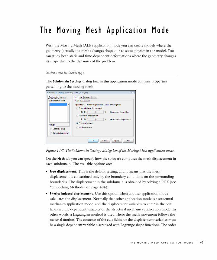
Th e Mov i n g Me s h App l i c a t i o n Mode
With the Moving Mesh (ALE) application mode you can create models where the geometry (actually the mesh) changes shape due to some physics in the model. You can study both static and time-dependent deformations where the geometry changes its shape due to the dynamics of the problem.
Subdomain Settings
The Subdomain Settings dialog box in this application mode contains properties pertaining to the moving mesh.
Figure 14-7: The Subdomain Settings dialog box of the Moving Mesh application mode.
On the Mesh tab you can specify how the software computes the mesh displacement in each subdomain. The available options are:
• Free displacement. This is the default setting, and it means that the mesh displacement is constrained only by the boundary conditions on the surrounding boundaries. The displacement in the subdomain is obtained by solving a PDE (see “Smoothing Methods” on page 404).
• Physics induced displacement. Use this option when another application mode calculates the displacement. Normally that other application mode is a structural mechanics application mode, and the displacement variables to enter in the edit fields are the dependent variables of the structural mechanics application mode. In other words, a Lagrangian method is used where the mesh movement follows the material motion. The contents of the edit fields for the displacement variables must be a single dependent variable discretized with Lagrange shape functions. The order
T H E M O V I N G M E S H A P P L I C A T I O N M O D E | 401
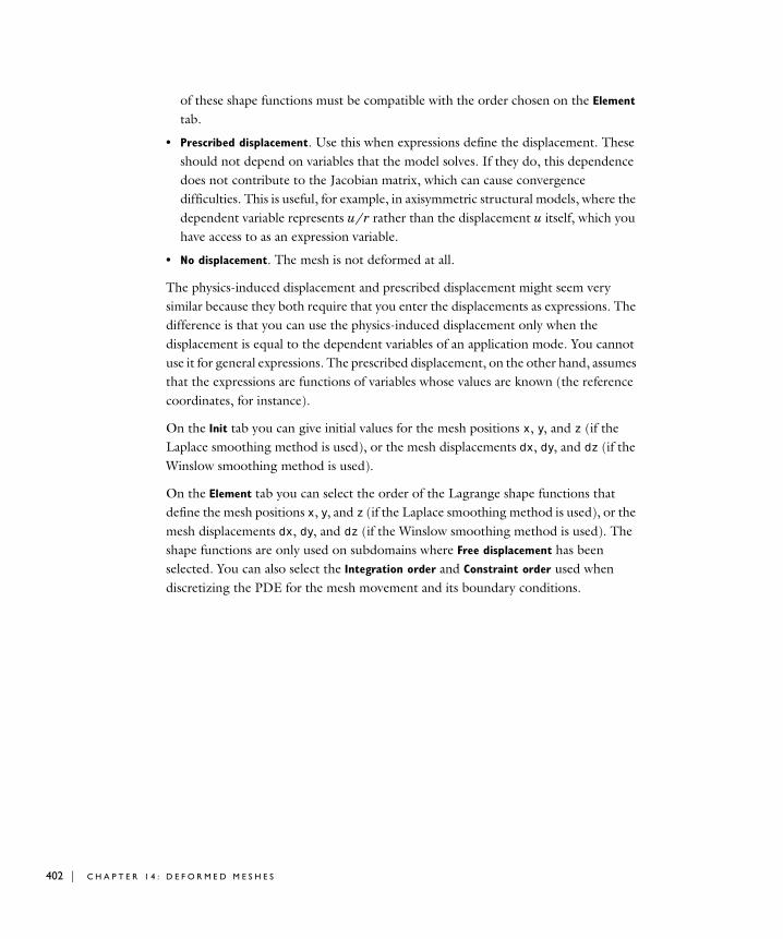
402 | C H A P T E
of these shape functions must be compatible with the order chosen on the Element tab.
• Prescribed displacement. Use this when expressions define the displacement. These should not depend on variables that the model solves. If they do, this dependence does not contribute to the Jacobian matrix, which can cause convergence difficulties. This is useful, for example, in axisymmetric structural models, where the dependent variable represents u/r rather than the displacement u itself, which you have access to as an expression variable.
• No displacement. The mesh is not deformed at all.
The physics-induced displacement and prescribed displacement might seem very similar because they both require that you enter the displacements as expressions. The difference is that you can use the physics-induced displacement only when the displacement is equal to the dependent variables of an application mode. You cannot use it for general expressions. The prescribed displacement, on the other hand, assumes that the expressions are functions of variables whose values are known (the reference coordinates, for instance).
On the Init tab you can give initial values for the mesh positions x, y, and z (if the Laplace smoothing method is used), or the mesh displacements dx, dy, and dz (if the Winslow smoothing method is used).
On the Element tab you can select the order of the Lagrange shape functions that define the mesh positions x, y, and z (if the Laplace smoothing method is used), or the mesh displacements dx, dy, and dz (if the Winslow smoothing method is used). The shape functions are only used on subdomains where Free displacement has been selected. You can also select the Integration order and Constraint order used when discretizing the PDE for the mesh movement and its boundary conditions.
R 1 4 : D E F O R M E D M E S H E S
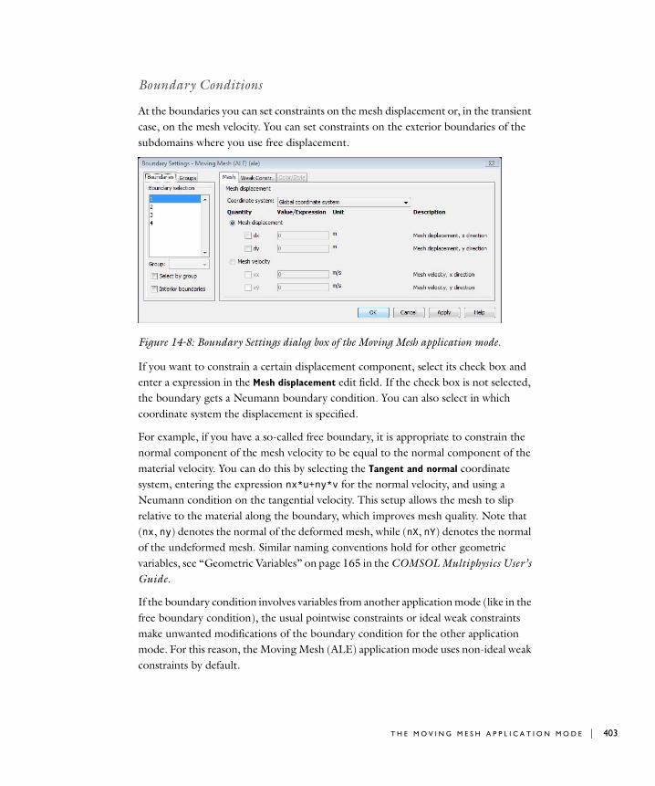
Boundary Conditions
At the boundaries you can set constraints on the mesh displacement or, in the transient case, on the mesh velocity. You can set constraints on the exterior boundaries of the subdomains where you use free displacement.
Figure 14-8: Boundary Settings dialog box of the Moving Mesh application mode.
If you want to constrain a certain displacement component, select its check box and enter a expression in the Mesh displacement edit field. If the check box is not selected, the boundary gets a Neumann boundary condition. You can also select in which coordinate system the displacement is specified.
For example, if you have a so-called free boundary, it is appropriate to constrain the normal component of the mesh velocity to be equal to the normal component of the material velocity. You can do this by selecting the Tangent and normal coordinate system, entering the expression nx*u+ny*v for the normal velocity, and using a Neumann condition on the tangential velocity. This setup allows the mesh to slip relative to the material along the boundary, which improves mesh quality. Note that (nx, ny) denotes the normal of the deformed mesh, while (nX, nY) denotes the normal of the undeformed mesh. Similar naming conventions hold for other geometric variables, see “Geometric Variables” on page 165 in the COMSOL Multiphysics User’s Guide.
If the boundary condition involves variables from another application mode (like in the free boundary condition), the usual pointwise constraints or ideal weak constraints make unwanted modifications of the boundary condition for the other application mode. For this reason, the Moving Mesh (ALE) application mode uses non-ideal weak constraints by default.
T H E M O V I N G M E S H A P P L I C A T I O N M O D E | 403
404 | C H A P T E
It is important that the boundary conditions are consistent with the settings in the adjacent subdomains. If the subdomain settings define a certain displacement, the boundary must be displaced in the same way.
Smoothing Methods
In the domains with free displacement, the Moving Mesh (ALE) application mode solves an equation for the mesh displacement. This equation smoothly deforms the mesh given the constraints you place on the boundaries. You can choose between Laplace smoothing and Winslow smoothing. To specify the smoothing methods, use the Application Mode Properties dialog box, which you access from the Multiphysics area in the Model Navigator or from the Physics menu.
To see how these smoothing methods differ, let x and y be the spatial coordinates of the frame which the application mode defines, and let X and Y be the reference coordinates of the reference frame. If you choose Laplace smoothing, the software introduces deformed mesh positions x and y as degrees of freedom in the model. In the static case, it solves the equation
and in the transient case it solves the equation
Similar equations hold for the y coordinate.
If you choose Winslow smoothing, the software solves the equation
and does the same for Y. Equivalently, X and Y satisfy Laplace equations as functions of the x and y coordinates.
C O M P A T I B I L I T Y W I T H 3 . 2 M O D E L S
COMSOL Multiphysics 3.2 used a different implementation of the Winslow smoothing. The old implementation used mesh displacements instead of mesh positions as degrees of freedom. For backward compatibility, 3.2 models that use
∂2x
X2∂---------- ∂2x
Y2∂---------+ 0=
X2
2
∂∂ x∂
t∂-----
Y2
2
∂∂ x∂
t∂-----+ 0=
∂2X
x2∂---------- ∂2X
y2∂----------+ 0=
R 1 4 : D E F O R M E D M E S H E S
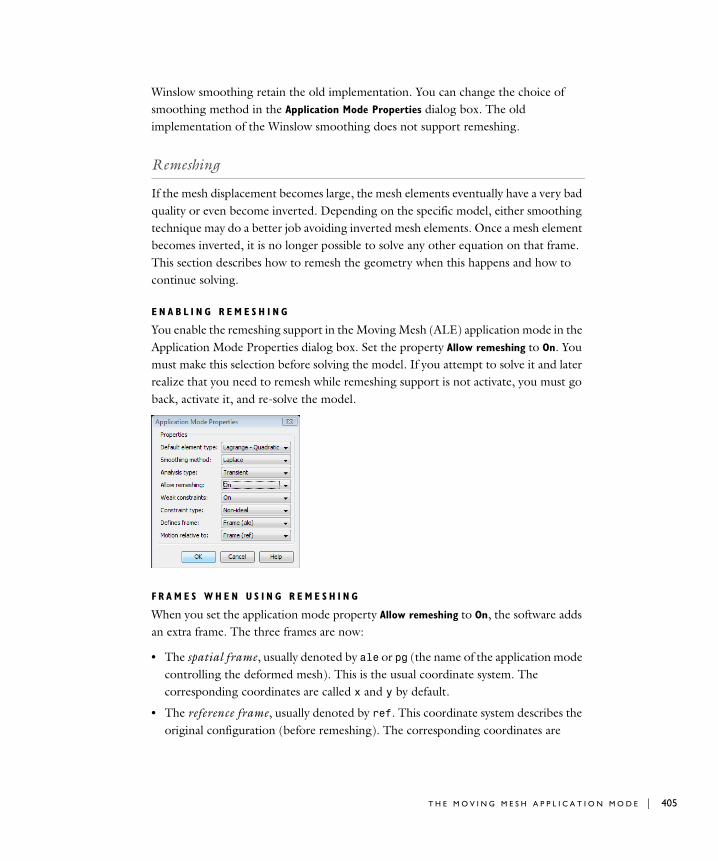
Winslow smoothing retain the old implementation. You can change the choice of smoothing method in the Application Mode Properties dialog box. The old implementation of the Winslow smoothing does not support remeshing.
Remeshing
If the mesh displacement becomes large, the mesh elements eventually have a very bad quality or even become inverted. Depending on the specific model, either smoothing technique may do a better job avoiding inverted mesh elements. Once a mesh element becomes inverted, it is no longer possible to solve any other equation on that frame. This section describes how to remesh the geometry when this happens and how to continue solving.
E N A B L I N G R E M E S H I N G
You enable the remeshing support in the Moving Mesh (ALE) application mode in the Application Mode Properties dialog box. Set the property Allow remeshing to On. You must make this selection before solving the model. If you attempt to solve it and later realize that you need to remesh while remeshing support is not activate, you must go back, activate it, and re-solve the model.
F R A M E S W H E N U S I N G R E M E S H I N G
When you set the application mode property Allow remeshing to On, the software adds an extra frame. The three frames are now:
• The spatial frame, usually denoted by ale or pg (the name of the application mode controlling the deformed mesh). This is the usual coordinate system. The corresponding coordinates are called x and y by default.
• The reference frame, usually denoted by ref. This coordinate system describes the original configuration (before remeshing). The corresponding coordinates are
T H E M O V I N G M E S H A P P L I C A T I O N M O D E | 405
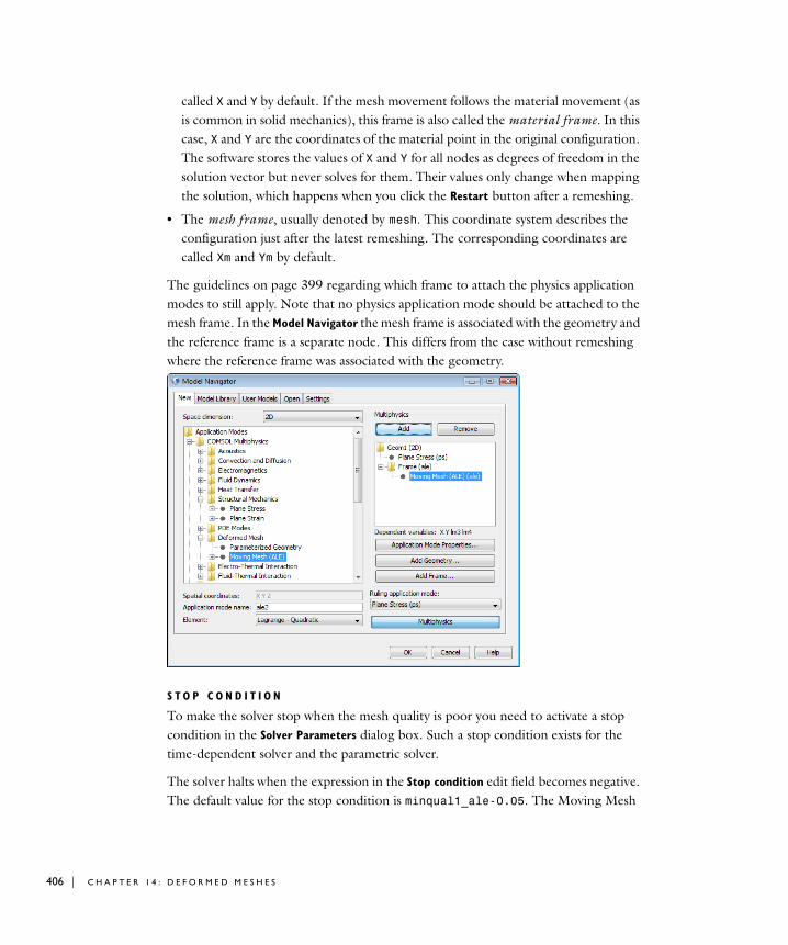
406 | C H A P T E
called X and Y by default. If the mesh movement follows the material movement (as is common in solid mechanics), this frame is also called the material frame. In this case, X and Y are the coordinates of the material point in the original configuration. The software stores the values of X and Y for all nodes as degrees of freedom in the solution vector but never solves for them. Their values only change when mapping the solution, which happens when you click the Restart button after a remeshing.
• The mesh frame, usually denoted by mesh. This coordinate system describes the configuration just after the latest remeshing. The corresponding coordinates are called Xm and Ym by default.
The guidelines on page 399 regarding which frame to attach the physics application modes to still apply. Note that no physics application mode should be attached to the mesh frame. In the Model Navigator the mesh frame is associated with the geometry and the reference frame is a separate node. This differs from the case without remeshing where the reference frame was associated with the geometry.
S T O P C O N D I T I O N
To make the solver stop when the mesh quality is poor you need to activate a stop condition in the Solver Parameters dialog box. Such a stop condition exists for the time-dependent solver and the parametric solver.
The solver halts when the expression in the Stop condition edit field becomes negative. The default value for the stop condition is minqual1_ale-0.05. The Moving Mesh
R 1 4 : D E F O R M E D M E S H E S
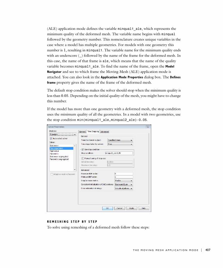
(ALE) application mode defines the variable minqual1_ale, which represents the minimum quality of the deformed mesh. The variable name begins with minqual followed by the geometry number. This nomenclature creates unique variables in the case where a model has multiple geometries. For models with one geometry this number is 1, resulting in minqual1. The variable name for the minimum quality ends with an underscore (_) followed by the name of the frame for the deformed mesh. In this case, the name of that frame is ale, which means that the name of the quality variable becomes minqual1_ale. To find the name of the frame, open the Model
Navigator and see to which frame the Moving Mesh (ALE) application mode is attached. You can also look in the Application Mode Properties dialog box. The Defines
frame property gives the name of the frame of the deformed mesh.
The default stop condition makes the solver should stop when the minimum quality is less than 0.05. Depending on the initial quality of the mesh, you might have to change this number.
If the model has more than one geometry with a deformed mesh, the stop condition uses the minimum quality of all the geometries. In a model with two geometries, use the stop condition min(minqual1_ale,minqual2_ale)-0.05.
R E M E S H I N G S T E P B Y S T E P
To solve using remeshing of a deformed mesh follow these steps:
T H E M O V I N G M E S H A P P L I C A T I O N M O D E | 407
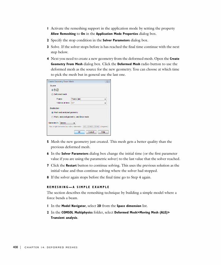
408 | C H A P T E
1 Activate the remeshing support in the application mode by setting the property Allow Remeshing to On in the Application Mode Properties dialog box.
2 Specify the stop condition in the Solver Parameters dialog box.
3 Solve. If the solver stops before is has reached the final time continue with the next step below.
4 Next you need to create a new geometry from the deformed mesh. Open the Create
Geometry From Mesh dialog box. Click the Deformed Mesh radio button to use the deformed mesh as the source for the new geometry. You can choose at which time to pick the mesh but in general use the last one.
5 Mesh the new geometry just created. This mesh gets a better quality than the previous deformed mesh.
6 In the Solver Parameters dialog box change the initial time (or the first parameter value if you are using the parametric solver) to the last value that the solver reached.
7 Click the Restart button to continue solving. This uses the previous solution as the initial value and thus continue solving where the solver had stopped.
8 If the solver again stops before the final time go to Step 4 again.
R E M E S H I N G — A S I M P L E E X A M P L E
The section describes the remeshing technique by building a simple model where a force bends a beam.
1 In the Model Navigator, select 2D from the Space dimension list.
2 In the COMSOL Multiphysics folder, select Deformed Mesh>Moving Mesh (ALE)>
Transient analysis.
R 1 4 : D E F O R M E D M E S H E S

3 Click the Multiphysics button and then the Add button to add the Moving Mesh application mode to the model.
4 In the list of application modes, select Structural Mechanics>Plane Stress>Transient
analysis. In the Multiphysics area select the node Geom1 (2D). Then click Add to add the Plane Stress application mode.
5 Click OK to close the Model Navigator.
Geometry Modeling1 Draw a rectangle with a width of 1.6, height of 1.2, and with its lower left corner at
(−0.6, −0.4).
2 Draw a second rectangle with a width of 1.4, height of 0.2, and its lower left corner at (−0.6, −0.2).
Physics Settings1 In the Subdomain Settings dialog box of the Plane Stress application mode clear the
Active in this domain check box for Subdomain 1 (the air). Click OK to close the dialog box.
2 In the Boundary Settings dialog box select Boundary 3 and activate the constraints Rx and Ry by selecting the corresponding check boxes. Go to the Load tab and select Boundaries 4, 6, and 8. Enter a force that increases with time by setting Fy to -1e6*t. Click OK to close the dialog box.
3 Select the Moving Mesh (ALE) application mode from the Multiphysics menu.
4 In the Subdomain Settings dialog box of the Moving Mesh application mode select Subdomain 2 and click the Physics induced displacement button. Enter the displacement variables u and v in the dx, dy edit fields. Click OK to close the dialog box.
5 In the Boundary Settings dialog box select Boundaries 4, 6, and 8. Select the dx and dy check boxes and then enter the mesh displacement u and v in the corresponding edit fields.
6 Select Boundaries 1, 2, 5, 7, and 9, and select the dx and dy check boxes to prevent these boundaries from moving. Click OK to close the dialog box.
T H E M O V I N G M E S H A P P L I C A T I O N M O D E | 409
410 | C H A P T E
Note: To obtain a correct solution, you should use the support for large deformations in the Plane Stress application mode, but that feature is available only in the extended Plane Stress application mode in the Structural Mechanics and MEMS modules.
The next step is to activate support for remeshing in the Moving Mesh application mode:
1 Open the Application Mode Properties dialog box by selecting Properties from the Physics menu.
2 Select On from the Allow remeshing list and click OK.
You must make this selection before solving the model. If you attempt to solve it and later realize that you need to remesh while remeshing support is not activate, you must go back, activate it, and re-solve the model.
Mesh Generation1 Initialize the mesh.
2 Refine it once.
Computing the SolutionTo make the solver stop when the mesh quality becomes poor, first enable a stop condition in the Solver Parameters dialog box.
1 From the Solve menu open the Solver Parameters dialog box. In the Times edit field enter 0:0.01:0.3.
R 1 4 : D E F O R M E D M E S H E S
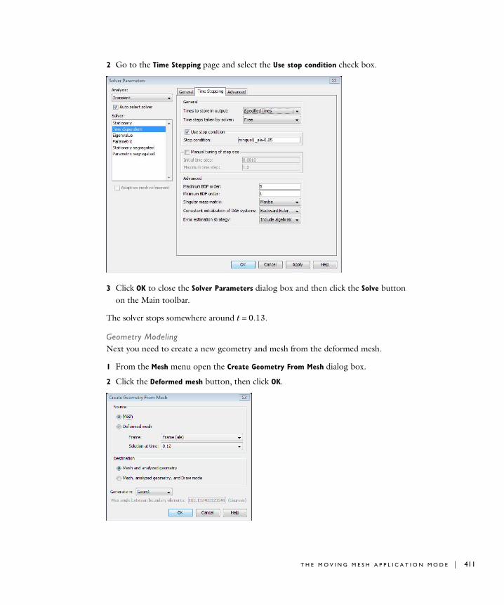
2 Go to the Time Stepping page and select the Use stop condition check box.
3 Click OK to close the Solver Parameters dialog box and then click the Solve button on the Main toolbar.
The solver stops somewhere around t = 0.13.
Geometry ModelingNext you need to create a new geometry and mesh from the deformed mesh.
1 From the Mesh menu open the Create Geometry From Mesh dialog box.
2 Click the Deformed mesh button, then click OK.
T H E M O V I N G M E S H A P P L I C A T I O N M O D E | 411
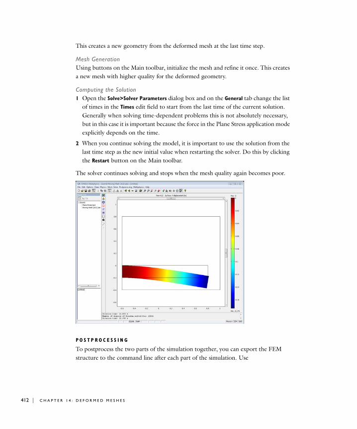
412 | C H A P T E
This creates a new geometry from the deformed mesh at the last time step.
Mesh GenerationUsing buttons on the Main toolbar, initialize the mesh and refine it once. This creates a new mesh with higher quality for the deformed geometry.
Computing the Solution1 Open the Solve>Solver Parameters dialog box and on the General tab change the list
of times in the Times edit field to start from the last time of the current solution. Generally when solving time-dependent problems this is not absolutely necessary, but in this case it is important because the force in the Plane Stress application mode explicitly depends on the time.
2 When you continue solving the model, it is important to use the solution from the last time step as the new initial value when restarting the solver. Do this by clicking the Restart button on the Main toolbar.
The solver continues solving and stops when the mesh quality again becomes poor.
P O S T P R O C E S S I N G
To postprocess the two parts of the simulation together, you can export the FEM structure to the command line after each part of the simulation. Use
R 1 4 : D E F O R M E D M E S H E S
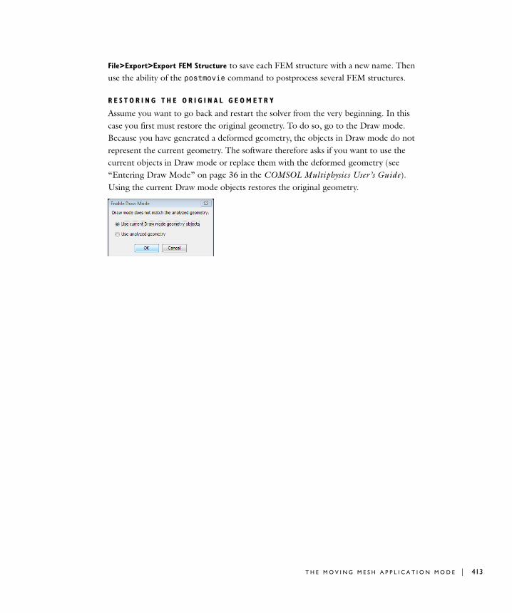
File>Export>Export FEM Structure to save each FEM structure with a new name. Then use the ability of the postmovie command to postprocess several FEM structures.
R E S T O R I N G T H E O R I G I N A L G E O M E T R Y
Assume you want to go back and restart the solver from the very beginning. In this case you first must restore the original geometry. To do so, go to the Draw mode. Because you have generated a deformed geometry, the objects in Draw mode do not represent the current geometry. The software therefore asks if you want to use the current objects in Draw mode or replace them with the deformed geometry (see “Entering Draw Mode” on page 36 in the COMSOL Multiphysics User’s Guide). Using the current Draw mode objects restores the original geometry.
T H E M O V I N G M E S H A P P L I C A T I O N M O D E | 413
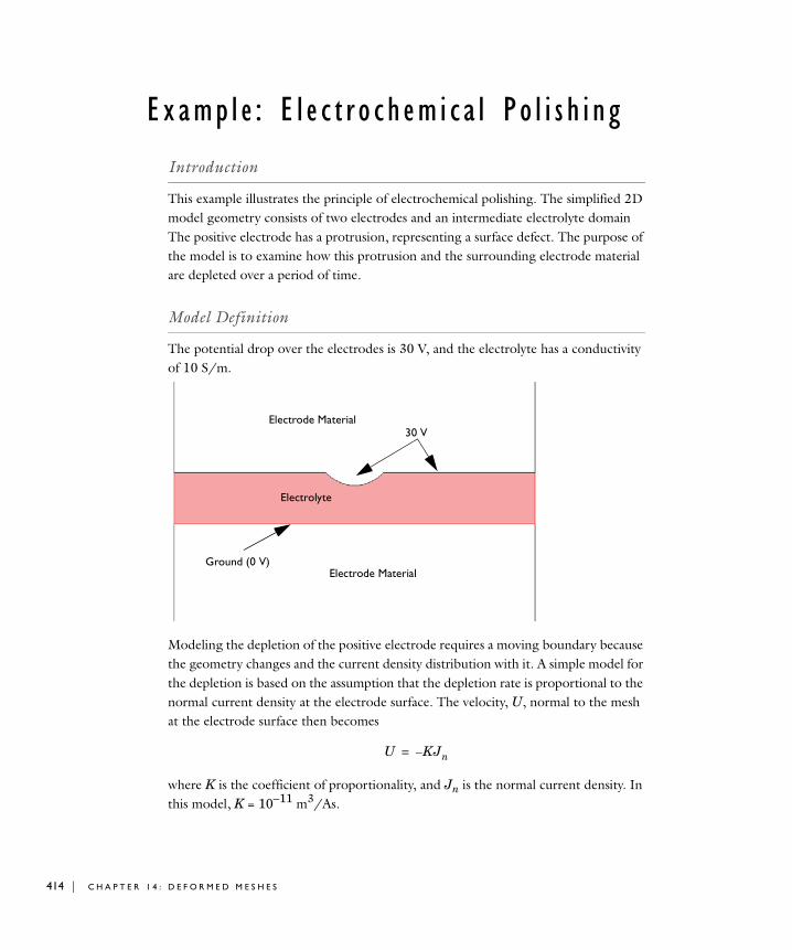
414 | C H A P T E
Examp l e : E l e c t r o c h em i c a l Po l i s h i n g
Introduction
This example illustrates the principle of electrochemical polishing. The simplified 2D model geometry consists of two electrodes and an intermediate electrolyte domain The positive electrode has a protrusion, representing a surface defect. The purpose of the model is to examine how this protrusion and the surrounding electrode material are depleted over a period of time.
Model Definition
The potential drop over the electrodes is 30 V, and the electrolyte has a conductivity of 10 S/m.
Modeling the depletion of the positive electrode requires a moving boundary because the geometry changes and the current density distribution with it. A simple model for the depletion is based on the assumption that the depletion rate is proportional to the normal current density at the electrode surface. The velocity, U, normal to the mesh at the electrode surface then becomes
where K is the coefficient of proportionality, and Jn is the normal current density. In this model, K = 10−11 m3/As.
Electrode Material
Electrode Material
30 V
Ground (0 V)
Electrolyte
U KJn–=
R 1 4 : D E F O R M E D M E S H E S
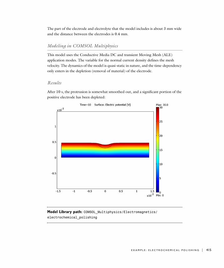
The part of the electrode and electrolyte that the model includes is about 3 mm wide and the distance between the electrodes is 0.4 mm.
Modeling in COMSOL Multiphysics
This model uses the Conductive Media DC and transient Moving Mesh (ALE) application modes. The variable for the normal current density defines the mesh velocity. The dynamics of the model is quasi-static in nature, and the time-dependency only enters in the depletion (removal of material) of the electrode.
Results
After 10 s, the protrusion is somewhat smoothed out, and a significant portion of the positive electrode has been depleted:
Model Library path: COMSOL_Multiphysics/Electromagnetics/electrochemical_polishing
E X A M P L E : E L E C T R O C H E M I C A L P O L I S H I N G | 415
416 | C H A P T E
Modeling Using the Graphical User Interface
M O D E L N A V I G A T O R
1 Select 2D in the Space dimension list. (This model can easily be generalized to 3D.)
2 In the application mode list, open COMSOL Multiphysics>Deformed Mesh and then Moving Mesh (ALE)>Transient analysis.
3 Click the Multiphysics button and then the Add button.
4 In the application mode list, open COMSOL Multiphysics>
Electromagnetics>Conductive Media DC.
5 Click the Add button. This adds the Conductive Media DC application mode to the moving mesh frame.
6 Click OK to close the Model Navigator.
O P T I O N S
1 From the Options menu, open the Constants dialog box.
2 Enter a constant with the name K, the expression 1e-11[m^3/(A*s)], and the description Coefficient of proportionality (the description is optional).
3 Click OK to close the Constants dialog box.
G E O M E T R Y M O D E L I N G
1 Click the Rectangle/Square button on the Draw toolbar, and draw a rectangle with corners at x = −1.4, y = 0 and x = +1.4, y = 0.4.
2 Shift-click the Ellipse/Circle (Centered) button.
3 In the Circle dialog box, type 0.3 in the Radius edit field and set the center coordinates to (0, 0.6) by typing 0 in the X edit field and 0.6 in the Y edit field.
4 Click OK.
5 Select both objects by using the keyboard shortcut Ctrl+A. Both objects are now highlighted in red.
6 Click the Difference button on the Draw toolbar to remove the circle object from the rectangle. This creates the protruding part of the electrode.
7 The model needs to be the order of mm and not m. Click to select the object and then click the Scale button on the Draw toolbar.
8 Enter a scale factor of 10−3 by typing 1e-3 in both the X and Y edit fields in the Scale factor area. Click OK.
9 Click the Zoom Extents button on the Main toolbar.
R 1 4 : D E F O R M E D M E S H E S
The geometry is now ready.
P H Y S I C S S E T T I N G S
Subdomain Settings—Conductive Media DC1 From the Multiphysics menu, select the Conductive Media DC application mode.
2 From the Physics menu, select Subdomain Settings.
3 In the Subdomain Settings dialog box, select Subdomain 1 (the only one) and type 10 in the Electric conductivity edit field.
4 Click OK to close the Subdomain Settings dialog box.
Boundary Settings—Conductive Media DC1 From the Physics menu, select Boundary Settings.
2 For Boundaries 3, 4, 6, and 7, select the Electric potential in the Boundary condition list and type 30 in the Electric potential edit field.
3 For Boundaries 1 and 5, select Electric insulation in the Boundary condition list. Electric insulation is a good approximation if you want to simulate that the electrodes are extended indefinitely in both directions.
4 For Boundary 2, select Ground as the boundary condition.
5 Click OK to close the Boundary Settings dialog box.
Boundary Settings—Moving Mesh (ALE)1 From the Multiphysics menu, select the Moving Mesh (ALE) application mode.
2 From the Physics menu, select Boundary Settings.
3 In the Boundary Settings dialog box, for boundary 2, click the Mesh displacement button and set the mesh displacement in both directions to 0 by selecting the dx and dy check boxes.
4 For Boundaries 1 and 5, click the Mesh velocity button and set the mesh velocity, in the x direction to 0 by selecting the vx check box.
5 Select Boundaries 3, 4, 6, and 7, and select Tangent and normal coord. sys. in
deformed mesh in the Coordinate system list. Click the Mesh velocity button. Then select the vn check box and type -K*nJ_dc in the Mesh velocity, n direction edit field. This makes the normal mesh velocity equal to −K Jn (nJ_dc is the variable for the current density outflow from the Conductive Media DC application mode).
6 Click OK.
E X A M P L E : E L E C T R O C H E M I C A L P O L I S H I N G | 417
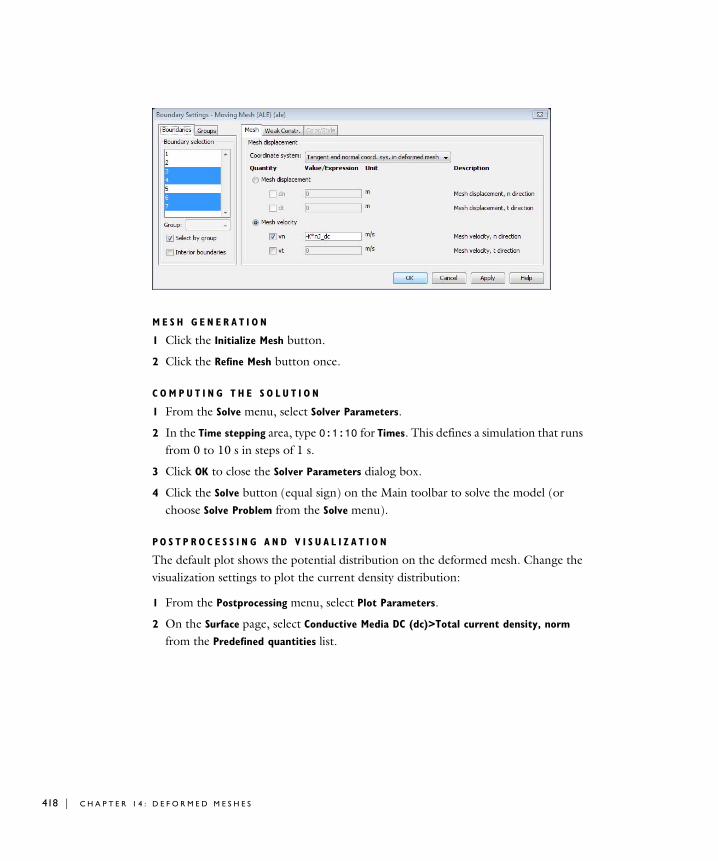
418 | C H A P T E
M E S H G E N E R A T I O N
1 Click the Initialize Mesh button.
2 Click the Refine Mesh button once.
C O M P U T I N G T H E S O L U T I O N
1 From the Solve menu, select Solver Parameters.
2 In the Time stepping area, type 0:1:10 for Times. This defines a simulation that runs from 0 to 10 s in steps of 1 s.
3 Click OK to close the Solver Parameters dialog box.
4 Click the Solve button (equal sign) on the Main toolbar to solve the model (or choose Solve Problem from the Solve menu).
P O S T P R O C E S S I N G A N D V I S U A L I Z A T I O N
The default plot shows the potential distribution on the deformed mesh. Change the visualization settings to plot the current density distribution:
1 From the Postprocessing menu, select Plot Parameters.
2 On the Surface page, select Conductive Media DC (dc)>Total current density, norm
from the Predefined quantities list.
R 1 4 : D E F O R M E D M E S H E S
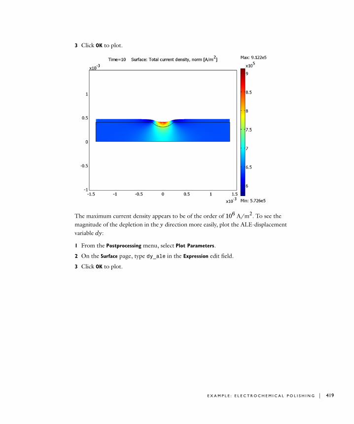
3 Click OK to plot.
The maximum current density appears to be of the order of 106 A/m2. To see the magnitude of the depletion in the y direction more easily, plot the ALE-displacement variable dy:
1 From the Postprocessing menu, select Plot Parameters.
2 On the Surface page, type dy_ale in the Expression edit field.
3 Click OK to plot.
E X A M P L E : E L E C T R O C H E M I C A L P O L I S H I N G | 419
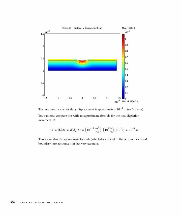
420 | C H A P T E
The maximum value for the y-displacement is approximately 10−4 m (or 0.1 mm).
You can now compare this with an approximate formula for the total depletion increment, d:
This shows that the approximate formula (which does not take effects from the curved boundary into account) is in fact very accurate.
d U ∆t K Jn ∆t 10 11– m3
As-------⎝ ⎠
⎛ ⎞ 106 Am-----⎝ ⎠
⎛ ⎞ 101s( )⋅ ⋅ 10 4– m= = = =
R 1 4 : D E F O R M E D M E S H E S
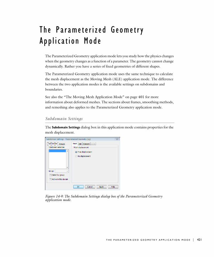
Th e Pa r ame t e r i z e d Geome t r y App l i c a t i o n Mode
The Parameterized Geometry application mode lets you study how the physics changes when the geometry changes as a function of a parameter. The geometry cannot change dynamically. Rather you have a series of fixed geometries of different shapes.
The Parameterized Geometry application mode uses the same technique to calculate the mesh displacement as the Moving Mesh (ALE) application mode. The difference between the two application modes is the available settings on subdomains and boundaries.
See also the “The Moving Mesh Application Mode” on page 401 for more information about deformed meshes. The sections about frames, smoothing methods, and remeshing also applies to the Parameterized Geometry application mode.
Subdomain Settings
The Subdomain Settings dialog box in this application mode contains properties for the mesh displacement.
Figure 14-9: The Subdomain Settings dialog box of the Parameterized Geometry application mode.
T H E P A R A M E T E R I Z E D G E O M E T R Y A P P L I C A T I O N M O D E | 421
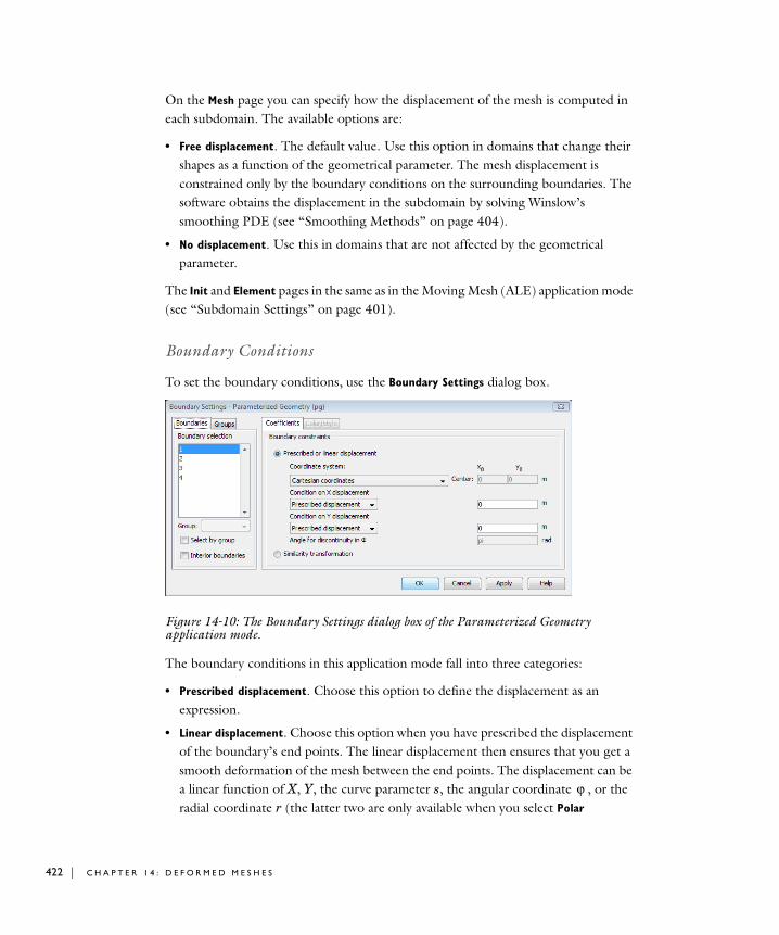
422 | C H A P T E
On the Mesh page you can specify how the displacement of the mesh is computed in each subdomain. The available options are:
• Free displacement. The default value. Use this option in domains that change their shapes as a function of the geometrical parameter. The mesh displacement is constrained only by the boundary conditions on the surrounding boundaries. The software obtains the displacement in the subdomain by solving Winslow’s smoothing PDE (see “Smoothing Methods” on page 404).
• No displacement. Use this in domains that are not affected by the geometrical parameter.
The Init and Element pages in the same as in the Moving Mesh (ALE) application mode (see “Subdomain Settings” on page 401).
Boundary Conditions
To set the boundary conditions, use the Boundary Settings dialog box.
Figure 14-10: The Boundary Settings dialog box of the Parameterized Geometry application mode.
The boundary conditions in this application mode fall into three categories:
• Prescribed displacement. Choose this option to define the displacement as an expression.
• Linear displacement. Choose this option when you have prescribed the displacement of the boundary’s end points. The linear displacement then ensures that you get a smooth deformation of the mesh between the end points. The displacement can be a linear function of X, Y, the curve parameter s, the angular coordinate , or the radial coordinate r (the latter two are only available when you select Polar
ϕ
R 1 4 : D E F O R M E D M E S H E S
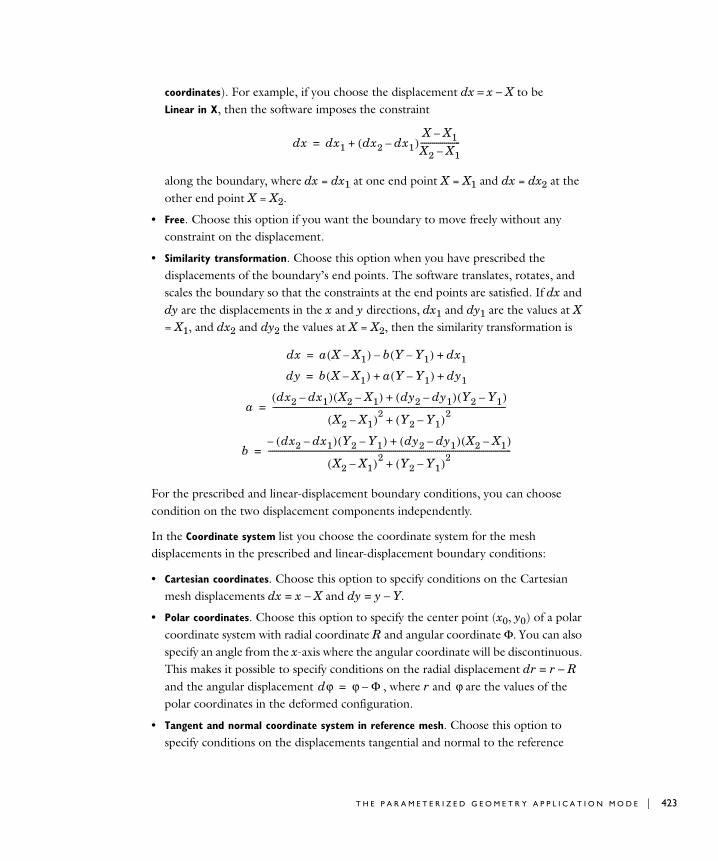
coordinates). For example, if you choose the displacement dx = x − X to be Linear in X, then the software imposes the constraint
along the boundary, where dx = dx1 at one end point X = X1 and dx = dx2 at the other end point X = X2.
• Free. Choose this option if you want the boundary to move freely without any constraint on the displacement.
• Similarity transformation. Choose this option when you have prescribed the displacements of the boundary’s end points. The software translates, rotates, and scales the boundary so that the constraints at the end points are satisfied. If dx and dy are the displacements in the x and y directions, dx1 and dy1 are the values at X = X1, and dx2 and dy2 the values at X = X2, then the similarity transformation is
For the prescribed and linear-displacement boundary conditions, you can choose condition on the two displacement components independently.
In the Coordinate system list you choose the coordinate system for the mesh displacements in the prescribed and linear-displacement boundary conditions:
• Cartesian coordinates. Choose this option to specify conditions on the Cartesian mesh displacements dx = x − X and dy = y − Y.
• Polar coordinates. Choose this option to specify the center point (x0, y0) of a polar coordinate system with radial coordinate R and angular coordinate Φ. You can also specify an angle from the x-axis where the angular coordinate will be discontinuous. This makes it possible to specify conditions on the radial displacement dr = r − R and the angular displacement , where r and are the values of the polar coordinates in the deformed configuration.
• Tangent and normal coordinate system in reference mesh. Choose this option to specify conditions on the displacements tangential and normal to the reference
dx dx1 dx2 dx1–( )X X1–
X2 X1–--------------------+=
dx a X X1–( ) b Y Y1–( )– dx1+=
dy b X X1–( ) a Y Y1–( ) dy1+ +=
adx2 dx1–( ) X2 X1–( ) dy2 dy1–( ) Y2 Y1–( )+
X2 X1–( )2 Y2 Y1–( )2+
---------------------------------------------------------------------------------------------------------------------=
bdx2 dx1–( ) Y2 Y1–( )– dy2 dy1–( ) X2 X1–( )+
X2 X1–( )2 Y2 Y1–( )2+
--------------------------------------------------------------------------------------------------------------------------=
dϕ ϕ Φ–= ϕ
T H E P A R A M E T E R I Z E D G E O M E T R Y A P P L I C A T I O N M O D E | 423
424 | C H A P T E
boundary. That is, you can specify conditions on the tangential displacement tX*dx+tY*dy and the normal displacement nX*dx+nY*dy.
• Tangent and normal coordinate system in deformed mesh. Choose this option to specify conditions on the displacements tangential and normal to the deformed boundary. That is, you can specify conditions on the tangential displacement tx*dx+ty*dy and the normal displacement nx*dx+ny*dy.
Point Settings
In the Point Settings dialog box it is possible to constrain the displacement of points in the geometry. You can choose to specify the displacements in Cartesian or polar coordinates.
R 1 4 : D E F O R M E D M E S H E S
Examp l e : E i g e nmode Ana l y s i s o f an L - S h ap ed Memb r a n e w i t h Rounded Co r n e r
Introduction
Cleve Moler studied the eigenvalues of the L-shaped membrane in his Ph.D. thesis (Ref. 1). Extend the problem by introducing a rounded corner in the concave corner and plot the radius versus the eigenvalue of the rounded corner. COMSOL Multiphysics makes it possible to easily parameterize the problem in terms of the radius of the rounded corner.
Model Definition
This model is a study of how the eigenvalues of the eigenvalue problem
change as a function of the radius of the rounded corner. To use the nonlinear parametric solver you need to add a normalizing condition that determines the size of the solution. In this model, it is the integral condition
Modeling in COMSOL Multiphysics
Use an integration coupling variable to compute the norm and an ordinary differential equation (ODE) to enter the equation for the constraint on the norm. The value of the Lagrange multiplier λ corresponds to the eigenvalue of the problem. You can also use this technique to solve nonlinear eigenvalue problems such as ∆u = λ sin (u).
Parameterize the radius of the rounded corner by a parameter p. Initially draw the geometry with a rounded corner with radius 0.5. Scale the straight boundaries adjacent to the rounded corner in the x and y directions, respectively. Scale the rounded corner
∆u– λu= on Ωu 0= on ∂Ω⎩
⎨⎧
u 2 xd ydΩ∫ 1=
E X A M P L E : E I G E N M O D E A N A L Y S I S O F A N L - S H A P E D M E M B R A N E W I T H R O U N D E D C O R N E R | 425
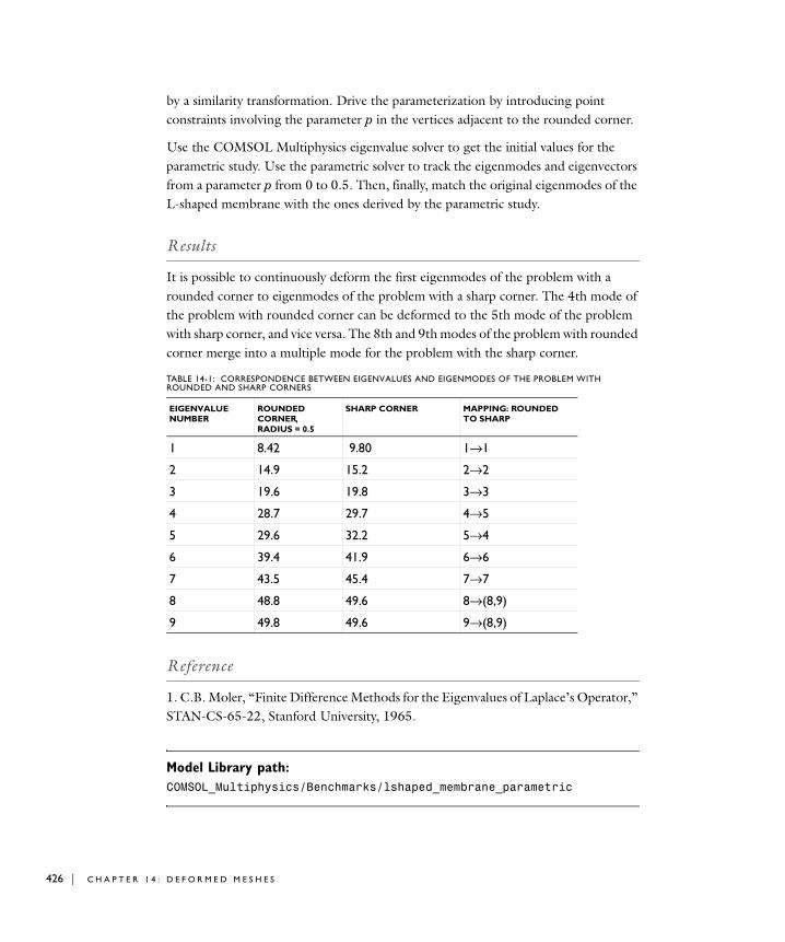
426 | C H A P T E
by a similarity transformation. Drive the parameterization by introducing point constraints involving the parameter p in the vertices adjacent to the rounded corner.
Use the COMSOL Multiphysics eigenvalue solver to get the initial values for the parametric study. Use the parametric solver to track the eigenmodes and eigenvectors from a parameter p from 0 to 0.5. Then, finally, match the original eigenmodes of the L-shaped membrane with the ones derived by the parametric study.
Results
It is possible to continuously deform the first eigenmodes of the problem with a rounded corner to eigenmodes of the problem with a sharp corner. The 4th mode of the problem with rounded corner can be deformed to the 5th mode of the problem with sharp corner, and vice versa. The 8th and 9th modes of the problem with rounded corner merge into a multiple mode for the problem with the sharp corner.
Reference
1. C.B. Moler, “Finite Difference Methods for the Eigenvalues of Laplace’s Operator,” STAN-CS-65-22, Stanford University, 1965.
Model Library path: COMSOL_Multiphysics/Benchmarks/lshaped_membrane_parametric
TABLE 14-1: CORRESPONDENCE BETWEEN EIGENVALUES AND EIGENMODES OF THE PROBLEM WITH ROUNDED AND SHARP CORNERS
EIGENVALUE NUMBER
ROUNDED CORNER, RADIUS = 0.5
SHARP CORNER MAPPING: ROUNDED TO SHARP
1 8.42 9.80 1→1
2 14.9 15.2 2→2
3 19.6 19.8 3→3
4 28.7 29.7 4→5
5 29.6 32.2 5→4
6 39.4 41.9 6→6
7 43.5 45.4 7→7
8 48.8 49.6 8→(8,9)
9 49.8 49.6 9→(8,9)
R 1 4 : D E F O R M E D M E S H E S
Modeling Using the Graphical User Interface
M O D E L N A V I G A T O R
1 Select 2D from the Space dimension list.
2 In the application mode list, open COMSOL Multiphysics>Deformed Mesh and then Parameterized Geometry.
3 Click the Multiphysics button and then the Add button.
4 In the application mode list, open COMSOL Multiphysics>PDE Modes and then double-click PDE, Coefficient Form. Make sure that the PDE, Coefficient Form application mode appears together with the Parameterized Geometry application mode under Frame (pg).
5 Click OK.
O P T I O N S A N D S E T T I N G S
1 From the Options menu, choose Axes/Grid Settings.
2 Click the Grid tab, clear the Auto check box, and add Extra x: -0.5 and Extra y: 0.5.
3 Click OK.
G E O M E T R Y M O D E L I N G
1 On the Draw toolbar, click Line.
2 Click (-1, 0), (-1, -1), (1, -1), (1, 1), (0, 1), (0, 0.5).
3 On the Draw toolbar, click 2nd Degree Bézier Curve.
4 Click (0, 0), (-0.5, 0).
5 Close the geometry object by right clicking the mouse.
6 Click the Zoom Extents button on the Main toolbar.
P H Y S I C S S E T T I N G S
Subdomain Settings1 Make sure the PDE, Coefficient Form (c) application mode is selected on the
Multiphysics menu.
2 On the Physics menu, open the Subdomain Settings dialog box.
3 Select Subdomain 1.
4 Enter the source term lm*u in the f coefficient edit field.
5 On the Init tab, enter the initial value u in the u(t0) edit field.
E X A M P L E : E I G E N M O D E A N A L Y S I S O F A N L - S H A P E D M E M B R A N E W I T H R O U N D E D C O R N E R | 427
428 | C H A P T E
Coupling Variables1 From the Options menu, choose Integration Coupling Variables>Subdomain Variables
to open the Subdomain Integration Variables dialog box.
2 On Subdomain 1, define the variable uint as the expression u^2 using integration order 4. Make sure the Global destination check box is selected.
3 Click OK.
Global Equations1 On the Physics menu, open the Global Equations dialog box.
2 On the first row in the table on the States tab, type lm in the Name (u) column and 1-uint in the Equation column. Set its initial value to lambda in the Init (u) column.
3 Click OK.
Boundary Conditions1 In the Multiphysics menu, select the Parameterized Geometry (pg) application mode.2 Open the Boundary Settings dialog box on the Physics menu.
3 Keep the default setting on Boundaries 1, 2, 5, and 6.
4 On Boundary 3, select Prescribed or linear displacement, Linear in X for Condition on
X displacement, and Prescribed displacement, 0, for Condition on Y displacement.
5 On Boundary 4, select Prescribed or linear displacement, Prescribed displacement, 0, for Condition on X displacement, and Linear in Y for Condition on Y displacement.
6 Select Similarity transformation for the rounded corner, Boundary 7.
7 Click OK.
Point Settings1 Open the Point Settings dialog box on the Physics menu.2 Select Point 3, and check X-displacement, and set p as its value.
3 Select Point 4, and check Y-displacement, and set -p as its value.
4 Click OK.
P O S T P R O C E S S I N G A N D V I S U A L I Z A T I O N
1 Open the Plot Parameters dialog box.
2 Click the Surface tab. Select PDE, Coefficient Form (c)>u from the Predefined
quantities list on the Surface Data page.
3 Click OK.
R 1 4 : D E F O R M E D M E S H E S
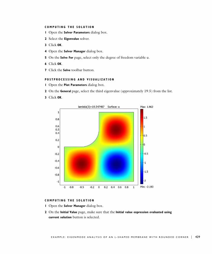
C O M P U T I N G T H E S O L U T I O N
1 Open the Solver Parameters dialog box.
2 Select the Eigenvalue solver.
3 Click OK.
4 Open the Solver Manager dialog box.
5 On the Solve For page, select only the degree of freedom variable u.
6 Click OK.
7 Click the Solve toolbar button.
PO S T P R O C E S S I N G A N D V I S U A L I Z A T I O N
1 Open the Plot Parameters dialog box.
2 On the General page, select the third eigenvalue (approximately 19.5) from the list.
3 Click OK.
C O M P U T I N G T H E S O L U T I O N
1 Open the Solver Manager dialog box.
2 On the Initial Value page, make sure that the Initial value expression evaluated using
current solution button is selected.
E X A M P L E : E I G E N M O D E A N A L Y S I S O F A N L - S H A P E D M E M B R A N E W I T H R O U N D E D C O R N E R | 429
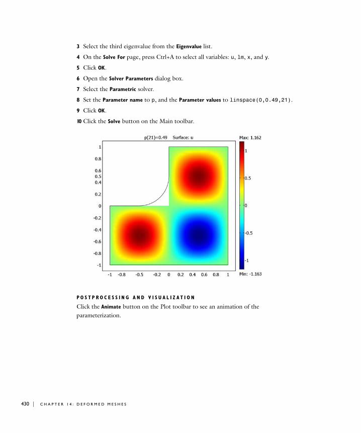
430 | C H A P T E
3 Select the third eigenvalue from the Eigenvalue list.
4 On the Solve For page, press Ctrl+A to select all variables: u, lm, x, and y.
5 Click OK.
6 Open the Solver Parameters dialog box.
7 Select the Parametric solver.
8 Set the Parameter name to p, and the Parameter values to linspace(0,0.49,21).
9 Click OK.
10 Click the Solve button on the Main toolbar.
P O S T P R O C E S S I N G A N D V I S U A L I Z A T I O N
Click the Animate button on the Plot toolbar to see an animation of the parameterization.
R 1 4 : D E F O R M E D M E S H E S
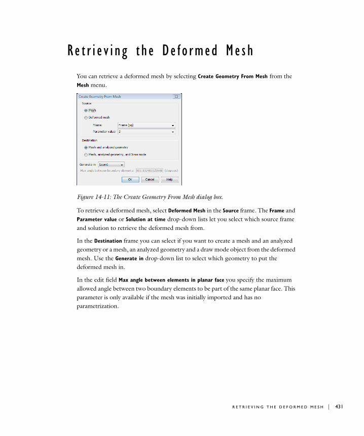
Re t r i e v i n g t h e De f o rmed Me s h
You can retrieve a deformed mesh by selecting Create Geometry From Mesh from the Mesh menu.
Figure 14-11: The Create Geometry From Mesh dialog box.
To retrieve a deformed mesh, select Deformed Mesh in the Source frame. The Frame and Parameter value or Solution at time drop-down lists let you select which source frame and solution to retrieve the deformed mesh from.
In the Destination frame you can select if you want to create a mesh and an analyzed geometry or a mesh, an analyzed geometry and a draw mode object from the deformed mesh. Use the Generate in drop-down list to select which geometry to put the deformed mesh in.
In the edit field Max angle between elements in planar face you specify the maximum allowed angle between two boundary elements to be part of the same planar face. This parameter is only available if the mesh was initially imported and has no parametrization.
R E T R I E V I N G T H E D E F O R M E D M E S H | 431
432 | C H A P T E
L im i t a t i o n s o f t h e De f o rmed Me s h F e a t u r e
The following limitations apply to the deformed mesh feature:
• The connectivity of the mesh remains unchanged during the mesh deformation, which means that topological changes in the geometry are not allowed.
• When the mesh deformation becomes large, the quality of the mesh can deteriorate. If this happens, the solver runs into convergence problems. Sometimes you see the warning Inverted mesh element in the Progress window for the solver, which means that a mesh element has (partially) warped inside-out. Use a smaller mesh deformation if you get these problems.
• If you work with finite elements of types other than Lagrange, solving for the mesh deformation coupled to the non-Lagrange elements can result in convergence problems. However, solving first for the mesh deformation and then for the physics in a one-way coupled fashion works. The reason for this is that if u is discretized with non-Lagrange elements, first-order spatial derivatives like ux does not give a contribution to the Jacobian matrix from the dependence on the mesh motion. Moreover, second-order spatial derivatives never make such Jacobian contributions.
• Solving time-dependent wave equations on a moving mesh does not work, because the formula for the second-order spatial time derivative utt in terms of reference time derivatives is not implemented.
• When using second-order (or higher-order) elements in the deformed mesh application modes, the mesh moving techniques often produce elements with distorted shapes. The measure of mesh quality does not capture these distorted shapes because it is computed from the positions of the corners of the mesh element (ignoring mid-side nodes, for instance). For these reasons, it is often best to use linear elements for the mesh positions in the deformed mesh application modes. You can select element type on the Element tab in the Subdomain Settings dialog box for the Moving Mesh (ALE) and Parameterized Geometry application modes. You must also open the Model Settings dialog box from the Physics menu and select the ALE frame (typically Frame (ale)) in the Frames list and select the appropriate element order (typically Linear) in the Geometry shape order list.
R 1 4 : D E F O R M E D M E S H E S
15
S t a b i l i z a t i o n T e c h n i q u e s
This chapter explains the different stabilization techniques that are available to stabilize the solution to convection-dominated transport problems.
433
434 | C H A P T E
Nume r i c a l S t a b i l i z a t i o n
Modeling transport phenomena for complex geometries usually requires numerical solutions based on some kind of discretization, and in COMSOL Multiphysics’ case in the form of finite elements. The discretization of convection-dominated transport problems can introduce instabilities in the solution. You might detect these instabilities as oscillations in the studied fields, primarily where steep gradients are present. The oscillations can even be large enough to prevent the solution from converging. To address these problems, COMSOL Multiphysics includes several stabilization techniques. This section explains these techniques and their modes of operation.
Introduction
Consider a typical scalar transport problem of a convection and diffusion type governed by the following equation and boundary conditions:
This formulation can represent a mass balance or energy balance in a fluid. You can derive some information on the general nature of the solution from dimensionless numbers that describe the relative influence of the different terms in the equation:
• The Peclet number, Pe, is a dimensionless number that describes the relationship between the convective and diffusive terms in a convection and diffusion equation.
• For fluid mechanics problems, where diffusive terms are introduced through the viscosity, the same information is contained in the Reynolds number, Re.
The definitions of both numbers also contain a typical length scale.
You can calculate the Peclet and Reynolds numbers both locally and globally, depending on which length scale is used in their definition. In the same way that the global Peclet and Reynolds numbers influence the solution’s global properties and stability, their local counterparts affect the stability of the numerical solution scheme.
The local definition of the Peclet number includes the product of the local mesh size, h, and the magnitude of the convective velocity, β, divided by the diffusivity, c, that is:
∇ c– ∇u βu+( )⋅ 0= in Ωn– c– ∇u βu+( )⋅ g= on Ω1∂
u r= on Ω2∂
R 1 5 : S T A B I L I Z A T I O N TE C H N I Q U E S
The local Reynolds number is the ratio of inertia to viscosity, multiplied by the local mesh size:
Where applicable, these dimensionless numbers are available as postprocessing variables, for example, cellRe_ns, which is the cell Reynolds number in the Incompressible Navier-Stokes application mode, if you use the default application mode name. As mentioned earlier, the Pe and Re numbers are measures of the relation between directed convection and diffusion. Oscillations can occur where any of the following conditions exist and the Pe or Re number exceeds 2:
• A Dirichlet boundary condition can force the solution to take on a steep gradient near the boundary forming a boundary layer. If the mesh cannot resolve the boundary layer, this creates a local disturbance.
• An initial condition varying in space (one that the mesh does not resolve) causes a local initial disturbance that over time propagates through the computational domain.
• A small initial diffusion term close to a varying source term or varying Dirichlet boundary condition can result in a local disturbance.
• Transport of a varying field or layer that the mesh does not resolve causes a transient under-resolved area.
Clearly all of these problems result from the poor discretization of the continuous equations and are not general properties of the equations themselves. As long as any diffusion is present in the problem, there is—at least in theory—a mesh resolution beyond which the discretization is stable. In most cases the mesh size is determined by available memory in the computer used for the simulation, which implies that a given mesh cannot always properly resolve small-scale effects.
Application Modes and Artificial Diffusion
In COMSOL Multiphysics and the Chemical Engineering Module, Earth Science Module, Heat Transfer Module, and MEMS Module, the application modes for fluid dynamics, convective heat transfer, and convective mass transfer provide predefined stabilization through artificial diffusion.
Pecellh β
c----------=
Recellhρ v
η-------------=
N U M E R I C A L S T A B I L I Z A T I O N | 435
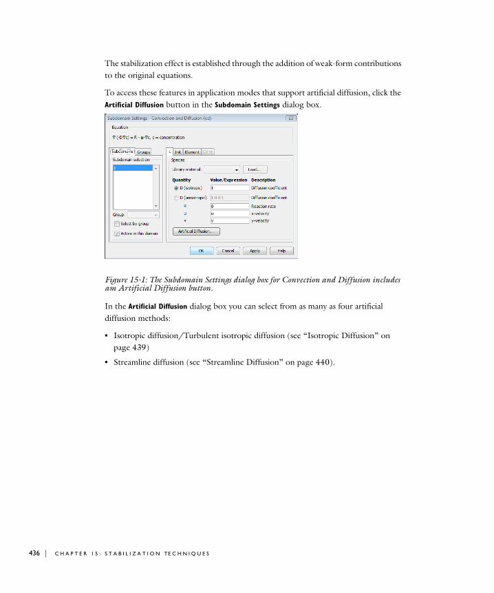
436 | C H A P T E
The stabilization effect is established through the addition of weak-form contributions to the original equations.
To access these features in application modes that support artificial diffusion, click the Artificial Diffusion button in the Subdomain Settings dialog box.
Figure 15-1: The Subdomain Settings dialog box for Convection and Diffusion includes am Artificial Diffusion button.
In the Artificial Diffusion dialog box you can select from as many as four artificial diffusion methods:
• Isotropic diffusion/Turbulent isotropic diffusion (see “Isotropic Diffusion” on page 439)
• Streamline diffusion (see “Streamline Diffusion” on page 440).
R 1 5 : S T A B I L I Z A T I O N TE C H N I Q U E S
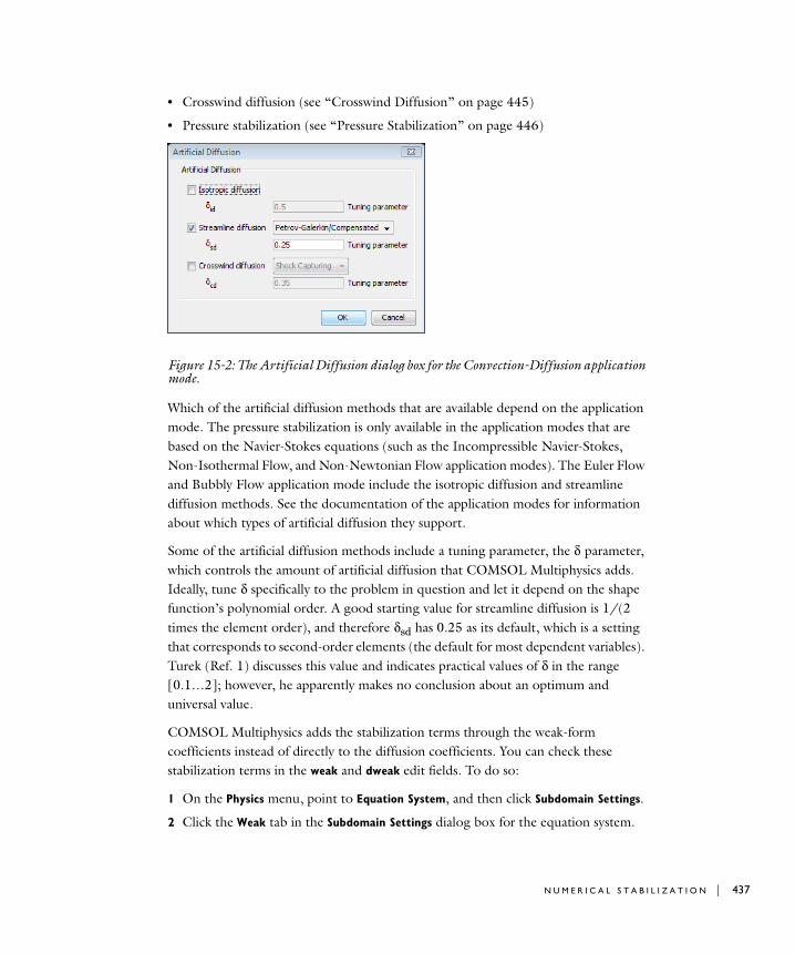
• Crosswind diffusion (see “Crosswind Diffusion” on page 445)
• Pressure stabilization (see “Pressure Stabilization” on page 446)
Figure 15-2: The Artificial Diffusion dialog box for the Convection-Diffusion application mode.
Which of the artificial diffusion methods that are available depend on the application mode. The pressure stabilization is only available in the application modes that are based on the Navier-Stokes equations (such as the Incompressible Navier-Stokes, Non-Isothermal Flow, and Non-Newtonian Flow application modes). The Euler Flow and Bubbly Flow application mode include the isotropic diffusion and streamline diffusion methods. See the documentation of the application modes for information about which types of artificial diffusion they support.
Some of the artificial diffusion methods include a tuning parameter, the δ parameter, which controls the amount of artificial diffusion that COMSOL Multiphysics adds. Ideally, tune δ specifically to the problem in question and let it depend on the shape function’s polynomial order. A good starting value for streamline diffusion is 1/(2 times the element order), and therefore δsd has 0.25 as its default, which is a setting that corresponds to second-order elements (the default for most dependent variables). Turek (Ref. 1) discusses this value and indicates practical values of δ in the range [0.1…2]; however, he apparently makes no conclusion about an optimum and universal value.
COMSOL Multiphysics adds the stabilization terms through the weak-form coefficients instead of directly to the diffusion coefficients. You can check these stabilization terms in the weak and dweak edit fields. To do so:
1 On the Physics menu, point to Equation System, and then click Subdomain Settings.
2 Click the Weak tab in the Subdomain Settings dialog box for the equation system.
N U M E R I C A L S T A B I L I Z A T I O N | 437
438 | C H A P T E
3 Examine the weak-form contributions from the artificial diffusion in the weak and dweak edit fields.
Selecting an Artificial Diffusion Method
A general guideline when using artificial diffusion is to first use streamline diffusion using the Galerkin least-squares (GLS) method. The GLS method is active by default in most fluid-flow application modes in COMSOL Multiphysics, the Chemical Engineering Module, and the Heat Transfer Module.
Streamline diffusion can produce very sharp solutions but cannot prevent undershoots and overshoots at sharp gradients. Crosswind diffusion, preferably with shock capturing, addresses exactly this.
If all else fails, try pure isotropic diffusion, which stabilizes most problems of the convection-diffusion type.
Use the pressure stabilization option only when you want to use equal-order interpolation for Stokes type of problems, thus circumventing the Babuska-Brezzi condition (the Inf-Sup stability criterion). Some tuning might be required to get the incompressibility constraint satisfactorily fulfilled.
Adding Artificial Diffusion Manually
Sometimes you might need to use stabilization techniques even though no application mode with this functionality is available. Examples of such situations appear in the COMSOL Multiphysics Model Library in “A Transport Problem” on page 111 and “Shock Tube” on page 230.
R 1 5 : S T A B I L I Z A T I O N TE C H N I Q U E S
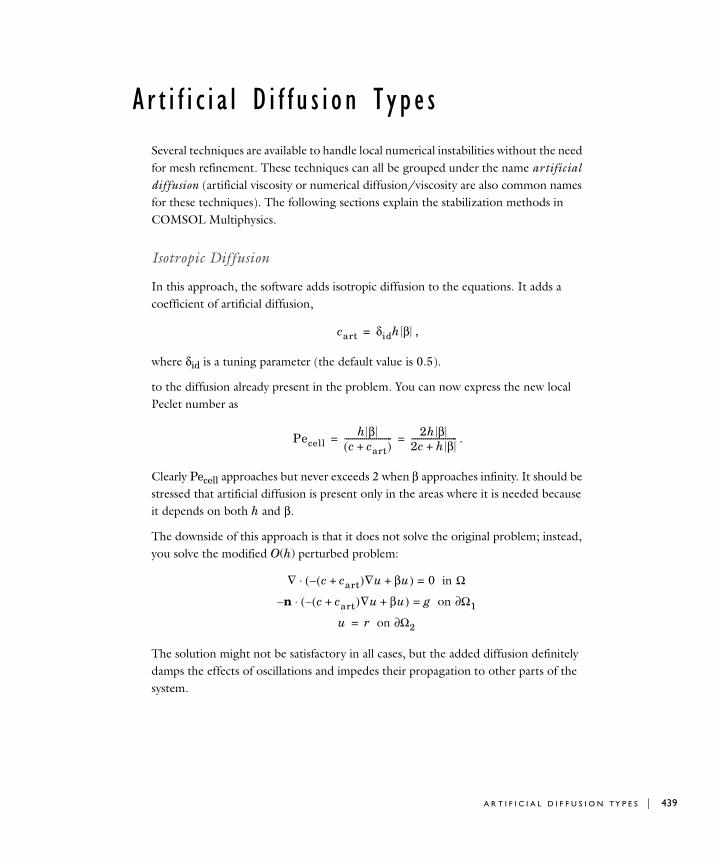
A r t i f i c i a l D i f f u s i o n T yp e s
Several techniques are available to handle local numerical instabilities without the need for mesh refinement. These techniques can all be grouped under the name artificial diffusion (artificial viscosity or numerical diffusion/viscosity are also common names for these techniques). The following sections explain the stabilization methods in COMSOL Multiphysics.
Isotropic Diffusion
In this approach, the software adds isotropic diffusion to the equations. It adds a coefficient of artificial diffusion,
,
where δid is a tuning parameter (the default value is 0.5).
to the diffusion already present in the problem. You can now express the new local Peclet number as
.
Clearly Pecell approaches but never exceeds 2 when β approaches infinity. It should be stressed that artificial diffusion is present only in the areas where it is needed because it depends on both h and β.
The downside of this approach is that it does not solve the original problem; instead, you solve the modified O(h) perturbed problem:
The solution might not be satisfactory in all cases, but the added diffusion definitely damps the effects of oscillations and impedes their propagation to other parts of the system.
cart δidh β=
Pecellh β
c cart+( )------------------------ 2h β
2c h β+-----------------------= =
∇ c cart+( )– ∇u βu+( )⋅ 0= in Ω
n– c cart+( )– ∇u βu+( )⋅ g= on Ω1∂
u r on Ω2∂=
A R T I F I C I A L D I F F U S I O N TY P E S | 439
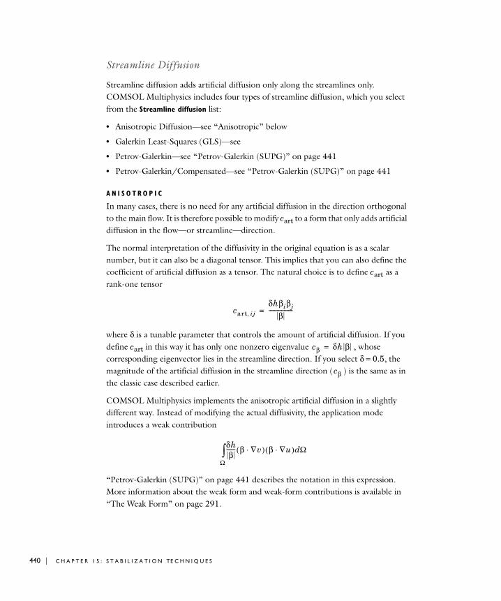
440 | C H A P T E
Streamline Diffusion
Streamline diffusion adds artificial diffusion only along the streamlines only. COMSOL Multiphysics includes four types of streamline diffusion, which you select from the Streamline diffusion list:
• Anisotropic Diffusion—see “Anisotropic” below
• Galerkin Least-Squares (GLS)—see
• Petrov-Galerkin—see “Petrov-Galerkin (SUPG)” on page 441
• Petrov-Galerkin/Compensated—see “Petrov-Galerkin (SUPG)” on page 441
A N I S O T R O P I C
In many cases, there is no need for any artificial diffusion in the direction orthogonal to the main flow. It is therefore possible to modify cart to a form that only adds artificial diffusion in the flow—or streamline—direction.
The normal interpretation of the diffusivity in the original equation is as a scalar number, but it can also be a diagonal tensor. This implies that you can also define the coefficient of artificial diffusion as a tensor. The natural choice is to define cart as a rank-one tensor
where δ is a tunable parameter that controls the amount of artificial diffusion. If you define cart in this way it has only one nonzero eigenvalue , whose corresponding eigenvector lies in the streamline direction. If you select δ = 0.5, the magnitude of the artificial diffusion in the streamline direction ( ) is the same as in the classic case described earlier.
COMSOL Multiphysics implements the anisotropic artificial diffusion in a slightly different way. Instead of modifying the actual diffusivity, the application mode introduces a weak contribution
“Petrov-Galerkin (SUPG)” on page 441 describes the notation in this expression. More information about the weak form and weak-form contributions is available in “The Weak Form” on page 291.
cart ij,δhβiβj
β-----------------=
cβ δh β=
cβ
δhβ
------ β ∇v⋅( ) β ∇u⋅( ) ΩdΩ∫
R 1 5 : S T A B I L I Z A T I O N TE C H N I Q U E S

Analogous to the case of classic artificial diffusion, a problem stabilized with anisotropic diffusion is not identical to the original problem. In fact, the exact solution to the original equations does not solve the modified problem. However, the errors introduced by the anisotropic artificial diffusion are far less serious than the ones created by classic artificial diffusion.
PE T R O V - G A L E R K I N ( S U P G )
Because COMSOL Multiphysics bases the discretization of the equations on the finite element method, it provides an elegant way of adding artificial diffusion without actually perturbing the original equations. This method is more commonly known as the streamline upwind Petrov-Galerkin method. Its origin stems from the weak form of the equations.
The weak formulation of the convection and diffusion equation is
where v is an arbitrary function called a test function. In the absence of streamline diffusion, the test function belongs to the same function space as the solution, u.
Now replace the test function v with
(15-1)
where the primed delta, δ', is
and δ is a tuning parameter. This introduces artificial diffusion through the test function itself. Because you can choose this function arbitrarily, there is no explicit perturbation of the original equations whatsoever. This is all true in theory, but in practice the solutions might be somewhat smeared out along the streamlines. Even so, solutions obtained by this method are usually far better than those obtained by any of the methods already mentioned.
The following equation gives the weak formulation of a problem with streamline diffusion:
∇vΩ∫ c∇u Ωd ∇v β⋅
Ω∫– u Ωd vg sd
Ω1∂∫=
u r on Ω2∂=
v δ'β ∇v⋅+
δ'δhβ
------=
A R T I F I C I A L D I F F U S I O N TY P E S | 441
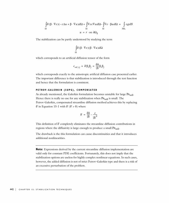
442 | C H A P T E
The stabilization can be partly understood by studying the term
which corresponds to an artificial diffusion tensor of the form
which corresponds exactly to the anisotropic artificial diffusion case presented earlier. The important difference is that stabilization is introduced through the test function and hence that the formulation is consistent.
P E T R O V - G A L E R K I N ( S U P G ) , C O M P E N S A T E D
As already mentioned, the Galerkin formulation becomes unstable for large Pecell. Hence there is really no use for any stabilization when Pecell is small. The Petrov-Galerkin, compensated streamline diffusion method achieves this by replacing δ' in Equation 15-1 with δ' (δ' > 0) where
This definition of δ’ completely eliminates the streamline-diffusion contributions in regions where the diffusivity is large enough to produce a small Pecell.
The drawback is the this formulation can cause discontinuities and that it introduces additional nonlinearities.
Note: Expressions derived by the current streamline diffusion implementation are valid only for constant PDE coefficients. Fortunately, this does not imply that the stabilization options are useless for highly complex nonlinear equations. In such cases, however, the added diffusion is not of strict Petrov-Galerkin type and there is a risk of an excessive perturbation of the problem.
δ' β ∇v⋅( ) c∆u– β ∇u⋅+( ) ΩdΩ∫ ∇v
Ω∫+ c∇u Ωd ∇v β⋅
Ω∫– u Ωd vg Sd
Ω1∂∫=
u r on Ω2∂=
δ' β ∇v⋅( ) β ∇u⋅( ) ΩdΩ∫
csd ij, δ'βiβjδhβ
------βiβj= =
δ'δhβ
------ c
β 2---------–=
R 1 5 : S T A B I L I Z A T I O N TE C H N I Q U E S

G A L E R K I N L E A S T - S Q U A R E S S T A B I L I Z A T I O N ( G L S )
During the years, the Petrov-Galerkin method has been developed and also given rise to new and often superior methods. One of them is the Galerkin least-squares (GLS) stabilization technique.
GLS is a general stabilization technique applicable to a wide range of problems (see Ref. 1). Its theoretical background is that the test function should be chosen to minimize the square of the residual of the equations. By working with matrices rather than only scalar equations, GLS can be formulated for systems of transport equations.
General Formulation of GLS StabilizationIt is possible to formulate GLS stabilization for any set of independent variables for any set of equations of convection-diffusion type. In conservative variables, the system has the form
, (15-2)
where U is the vector of conservative variables, Kj is the convective flux in the jth direction, Fj is the diffusive flux in the jth direction, and B is the source vector. The length of the vectors is the number of equations. Reformulated in primitive variables, V, Equation 15-2 can be written as
, (15-3)
where , , and the four-dimensional tensor Dij is such that
. (15-4)
Written in operator formulation, Equation 15-3 becomes
(15-5)
where
(15-6)
Applying the Galerkin least-squares technique, the weak formulation of Equation 15-3 gets the following left-side contribution:
∂U∂t--------
∂Kj
∂xj---------+
∂Fj
∂xj--------- B+=
A0∂Vk∂t
---------- Aj∂V∂xj--------+
∂∂xi-------- Dij
∂V∂xj--------⎝ ⎠
⎛ ⎞ B+=
A0 ∂U ∂V⁄= Aj ∂Kj ∂V⁄=
Dij∂V∂xj-------- Fi=
ϒV B=
ϒ AO∂∂t----- Aj
∂∂xj-------- ∂
∂xj--------– Dji
∂∂xj--------⎝ ⎠
⎛ ⎞+=
A R T I F I C I A L D I F F U S I O N TY P E S | 443
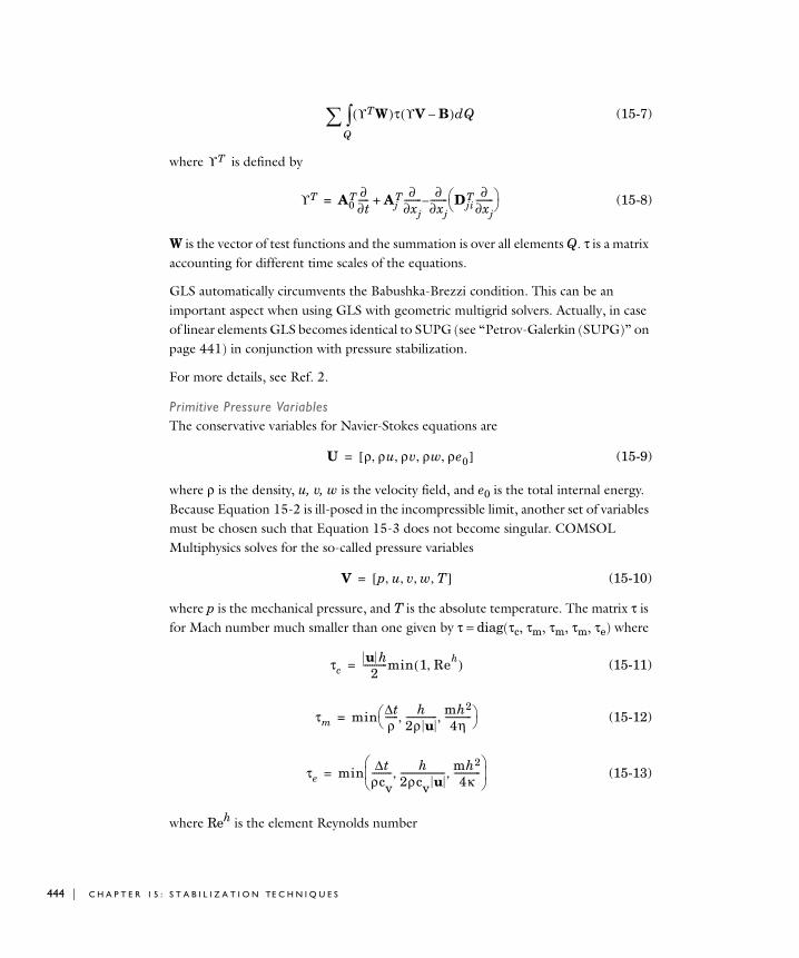
444 | C H A P T E
(15-7)
where is defined by
(15-8)
W is the vector of test functions and the summation is over all elements Q. τ is a matrix accounting for different time scales of the equations.
GLS automatically circumvents the Babushka-Brezzi condition. This can be an important aspect when using GLS with geometric multigrid solvers. Actually, in case of linear elements GLS becomes identical to SUPG (see “Petrov-Galerkin (SUPG)” on page 441) in conjunction with pressure stabilization.
For more details, see Ref. 2.
Primitive Pressure VariablesThe conservative variables for Navier-Stokes equations are
(15-9)
where ρ is the density, u, v, w is the velocity field, and e0 is the total internal energy. Because Equation 15-2 is ill-posed in the incompressible limit, another set of variables must be chosen such that Equation 15-3 does not become singular. COMSOL Multiphysics solves for the so-called pressure variables
(15-10)
where p is the mechanical pressure, and T is the absolute temperature. The matrix τ is for Mach number much smaller than one given by τ = diag(τc, τm, τm, τm, τe) where
(15-11)
(15-12)
(15-13)
where Reh is the element Reynolds number
ϒTW( )Q∫ τ ϒV B–( )dQ∑
ϒT
ϒT A0T ∂
∂t----- Aj
T ∂∂xj-------- ∂
∂xj--------– Dji
T ∂∂xj--------⎝ ⎠
⎛ ⎞+=
U ρ ρu ρv ρw ρe0,,,,[ ]=
V p u v w T, , , ,[ ]=
τcu h2
-----------min 1 Reh,( )=
τm min ∆tρ------ h
2ρ u-------------- mh2
4η------------, ,⎝ ⎠
⎛ ⎞=
τe min ∆tρcv--------- h
2ρcv u-------------------- mh2
4κ------------, ,
⎝ ⎠⎜ ⎟⎛ ⎞
=
R 1 5 : S T A B I L I Z A T I O N TE C H N I Q U E S
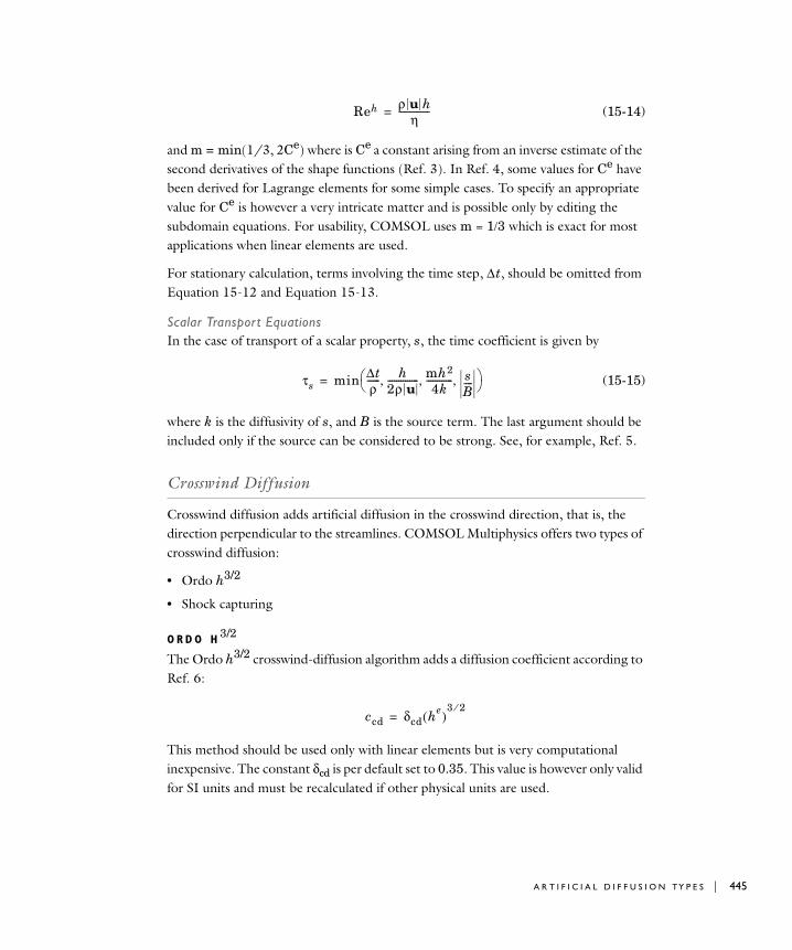
(15-14)
and m = min(1/3, 2Ce) where is Ce a constant arising from an inverse estimate of the second derivatives of the shape functions (Ref. 3). In Ref. 4, some values for Ce have been derived for Lagrange elements for some simple cases. To specify an appropriate value for Ce is however a very intricate matter and is possible only by editing the subdomain equations. For usability, COMSOL uses m = 1/3 which is exact for most applications when linear elements are used.
For stationary calculation, terms involving the time step, ∆ t, should be omitted from Equation 15-12 and Equation 15-13.
Scalar Transport EquationsIn the case of transport of a scalar property, s, the time coefficient is given by
(15-15)
where k is the diffusivity of s, and B is the source term. The last argument should be included only if the source can be considered to be strong. See, for example, Ref. 5.
Crosswind Diffusion
Crosswind diffusion adds artificial diffusion in the crosswind direction, that is, the direction perpendicular to the streamlines. COMSOL Multiphysics offers two types of crosswind diffusion:
• Ordo h3/2
• Shock capturing
O R D O H 3/2
The Ordo h3/2 crosswind-diffusion algorithm adds a diffusion coefficient according to Ref. 6:
This method should be used only with linear elements but is very computational inexpensive. The constant δcd is per default set to 0.35. This value is however only valid for SI units and must be recalculated if other physical units are used.
Reh ρ u hη
--------------=
τs min ∆tρ------ h
2ρ u-------------- mh2
4k------------ s
B----, , ,⎝ ⎠
⎛ ⎞=
ccd δcd he( )3 2⁄
=
A R T I F I C I A L D I F F U S I O N TY P E S | 445
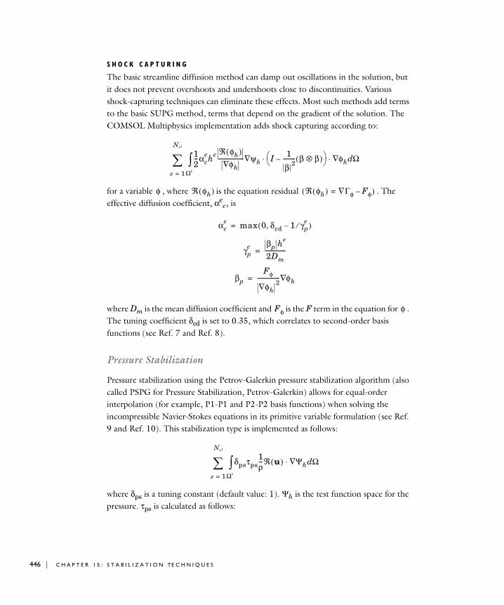
446 | C H A P T E
S H O C K C A P T U R I N G
The basic streamline diffusion method can damp out oscillations in the solution, but it does not prevent overshoots and undershoots close to discontinuities. Various shock-capturing techniques can eliminate these effects. Most such methods add terms to the basic SUPG method, terms that depend on the gradient of the solution. The COMSOL Multiphysics implementation adds shock capturing according to:
for a variable , where is the equation residual . The effective diffusion coefficient, αe
c, is
where Dm is the mean diffusion coefficient and is the F term in the equation for . The tuning coefficient δcd is set to 0.35, which correlates to second-order basis functions (see Ref. 7 and Ref. 8).
Pressure Stabilization
Pressure stabilization using the Petrov-Galerkin pressure stabilization algorithm (also called PSPG for Pressure Stabilization, Petrov-Galerkin) allows for equal-order interpolation (for example, P1-P1 and P2-P2 basis functions) when solving the incompressible Navier-Stokes equations in its primitive variable formulation (see Ref. 9 and Ref. 10). This stabilization type is implemented as follows:
where δps is a tuning constant (default value: 1). Ψh is the test function space for the pressure. τps is calculated as follows:
12---αc
ehe ℜ φh( )φh∇
------------------- ψh∇ I 1
β 2--------- β β⊗( )–⎝ ⎠
⎛ ⎞ φh∇⋅ ⋅ Ωd
Ωe
∫e 1=
Nel
∑
φ ℜ φh( ) ℜ φh( ) ∇Γφ Fφ–=( )
αce max 0 δcd 1 γp
e⁄–,( )=
γpe βp he
2Dm---------------=
βpFφ
φh∇ 2---------------- φh∇=
Fφ φ
δpsτps1ρ---ℜ u( ) Ψh∇⋅ Ωd
Ωe
∫e 1=
Nel
∑
R 1 5 : S T A B I L I Z A T I O N TE C H N I Q U E S
References
1. S. Turek, Efficient Solvers for Incompressible Flow Problems: An Algorithmic Approach in View of Computational Aspects. In: LNCSE 6, Springer-Verlag, 1999.
2. G. Hauke and T.J.R. Hughes, “A comparative study of different sets of variables for solving compressible and incompressible flows,” Computer Methods in Applied Mechanics and Engineering, vol. 153, pp. 1–44, 1998.
3. L. Franca and S. Frey, “Stabilized finite element methods: II. The incompressible Navier-Stokes equations,” Computer Methods in Applied Mechanics and Engineering, vol. 99, pp 209–233, 1992.
4. I. Hariri and T.J.R. Hughes, “What are C and h?: Inequalities for the analysis and design of finite element methods,” Computer Methods in Applied Mechanics and Engineering, vol. 97, pp. 157–192, 1992.
5. J.-H. Kim, K.E. Jansen, and M.K. Jensen, “Simulation of three-dimensional incompressible turbulent flow inside tubes with helical fins,” Numerical Heat Transfer, Part B, vol. 46, pp. 195–221, 2004.
6. C. Johnson, A. Schatz, and L. Wahlbin, “Crosswind Smear and Pointwise Error in Streamline Diffusion Finite Element Methods,” Math. Comp., vol. 49, pp. 25–38, 1987.
7. R. Codina, “A Discontinuity-Capturing Crosswind Dissipation for the Finite Element Solution of the Convection-Diffusion Equation,” Comput. Methods Appl. Mech. Engrg., vol. 110, pp. 325–342, 1993.
8. R. Codina, “A Shock-Capturing Anisotropic Diffusion for the Finite Element Solution of the Diffusion-Convection-Reaction Equation,” VIII International Conference on Finite Elements in Fluids, vol. 1, pp. 67–75.
9. T.E. Tezduyar, R. Shih, S. Mittal, and S.E. Ray, “Incompressible Flow Computations with Stabilized Bilinear and Linear Equal-Order-Interpolation Velocity-Pressure Element,” University of Minnesota Supercomputer Institute Research Report UMSI90/165, September, 1990.
τpsu
he-------⎝ ⎠⎛ ⎞ 2 3η
ρ he( )2
-----------------⎝ ⎠⎜ ⎟⎛ ⎞ 2
+
12---–
=
A R T I F I C I A L D I F F U S I O N TY P E S | 447
448 | C H A P T E
10. T.J.R. Hughes, L.P. Franca, and M. Becestra, “A New Finite-Element Formulation for Computational Fluid Dynamics, V. Circumventing the Babuska-Brezzi Condition, A Stable Petrov-Galerkin Formulation of the Stokes Problem Accommodating Equal-Order Interpolations,” Comput. Methods Appl. Mech. Engrg., vol. 59, pp. 85–99, 1986.
11. F. Shakib, T.J.R. Hughes, and Z. Johan, “A new finite element formulation for computational fluid dynamics: X. The compressible Euler and Navier-Stokes equations,” Comp. Methods. Appl. Mech. Engrg., vol. 89, pp. 141–219, 1991.
R 1 5 : S T A B I L I Z A T I O N TE C H N I Q U E S
I N D E X
A absorption coefficient 259
absorption term 247
absorption term, variable for 262
AC Power Electromagnetics application
mode 105
AC/DC Module 2, 76
accuracy of results 9
acoustics
application mode for 23
boundary conditions for 21
mathematical models for 21
standard problems in 20
Acoustics Module 2
active application mode 327
Add Frame dialog box 397
adsorption
modeling using the weak form 310
ALE method 392
algebraic equations 288
alu boundary coupled equation variable
263
alu equation variable 262
Ampère’s law 77, 105
analysis
eigenfrequency 200
static 200
time-dependent 200
transient 200
analysis types
in structural mechanics 199
anisotropic diffusion 440
anisotropic material 245
in electromagnetics 79
antisymmetry conditions 7
application mode
AC Power Electromagnetics 105
Acoustics 23
active 327
Axial Symmetry, Stress-Strain 221
Conduction 167
Conductive Media DC 83
Convection and Conduction 175
Convection and Diffusion 51
Diffusion 46
Electrostatics 89
for physics 15
for weak form 293
Magnetostatics 95
Plane Strain 217
Plane Stress 212
Poisson’s equation 277
ruling 327
Solid, Stress-Strain 208
application mode names
for PDE modes 238
application mode properties
changing 332
application mode variable
for fluid mechanics 145
application mode variables 17
for PDE modes 269
application modes 2
in COMSOL Multiphysics 2
removing from model 327
selecting 5
arbitrary Lagrangian-Eulerian method
392
area effects, across frames in ALE models
399
artificial diffusion 434, 439
adding manually 438
for convective heat transfer 176
I N D E X | 449

450 | I N D E X
for the Navier-Stokes equations 52
in application modes 435
using pressure stabilization 434
artificial diffusion method
crosswind diffusion 445
isotropic diffusion 439
pressure stabilization 446
selecting 438
streamline diffusion 440
artificial viscosity 439
assemblies
meshing 365
assembly 352
au boundary coupled equation variable
264
au equation variable 262
average temperature 305
axial symmetry 7
in acoustics 33
in Conductive Media DC models 86
in diffusion 48
in diffusion and convection 53
in Electrostatics models 92
in heat transfer 171
Axial Symmetry, Stress-Strain application
mode 221
axisymmetric solution, mapping to 3D
189
B Babushka-Brezzi condition 444
Babuska-Brezzi condition 142
backstep model 150
benchmark models 9
benchmark problem 150
beu boundary coupled equation variable
264
beu equation variable 262
body forces 199
boundary absorption coefficient 260
boundary absorption term 248
boundary condition
Neumann 240
boundary conditions
continuity 171
Dirichlet 240
for parameterized geometries 422
for PDEs 240
generalized Neumann 240
heat flux discontinuity 171
specification of 14
symmetric 170
thin thermally resistive layer 172
with time derivatives 272
boundary coupled equation variables
262, 263
boundary layer 363
boundary source term 248, 260
bulk modulus 21
C CFD 130
Chemical Engineering Module 2
Convection and Diffusion application
mode in 51
diffusion application modes in 46
for fluid dynamics 130
circumferential wave number 33
classical PDEs 260
Classical PDEs application mode
Poisson’s equation 277
coefficient form 4, 256
Component Library 347
components 347
composite geometry 352
computational fluid dynamics 130
concentration
boundary condition for 48
of mass 46
Conduction
application mode 167
conduction
in heat transfer 164
Conductive Media DC
application mode 83
conductivity 78
in Joule heating 84
temperature-dependent 84, 339
thermal 169
conductor
perfect 81
connecting geometries
model example 380
conservative convective flux
for two-variable PDE 246
normal component of 247
variables for 262
conservative flux 259
source term 246
conservative flux convection coefficient
259
conservative flux source
normal component of 248
conservative flux source term 259
conservative formulation
for convection and diffusion 51
constitutive relations
generalized 79
in electromagnetics 78
constraints
general notation for 206
ideal 265
ideal vs. non-ideal 301
non-ideal 265, 266
specification of 205
contact pair 355
contact resistance 86, 363
contiguous memory block 8
continuity 172
continuity boundary condition 171
convection
in heat transfer 164
Convection and Conduction
application mode 175
Convection and Diffusion
application mode 51
convection coefficient 259
convection term
for two-variable PDE 246
variable for 262
convection-diffusion equation 261
convective flux
boundary condition for 177
convergence
for nonlinear equations 10
testing 9
coordinate system 393
copper
resistive heating of 334
coupling
in resistive heating model 334, 338
coupling operator 358
coupling variable
integration 425
crosswind diffusion 445
cu boundary coupled equation variable
263
cu equation variable 261
current
steady 83
current density 77
current flow 84
cut-on frequency 36
cylindrical coordinates 221
cylindrical wave 27
D DAE. See differential-algebraic equation.
I N D E X | 451
452 | I N D E X
dalu boundary coupled equation varia-
ble 263
damping 207
damping coefficient 259
damping term 241, 244
dau boundary coupled equation variable
264
dau equation variable 261
dbeu boundary coupled equation varia-
ble 264
dcu boundary coupled equation variable
263
deactivating
physics or equations 331
deformed mesh 392
limitations 432
minimum quality of 407
deformed mesh application mode
adding 397
deformed meshes
limitations when using 432
density 165
in fluids 131
in structural mechanics 204
dependent variables
editing names of 332
df boundary coupled equation variable
264
dga boundary coupled equation variable
263
dielectric
conductor 81
differential-algebraic equation 258
Diffusion
application mode 46
diffusion
thin-layer model 380
diffusion coefficient 46, 259
diffusive flux 48, 177
for two-variable PDEs 244
normal component 247
variables for 261
dipole source 21
Dirac function 279
Dirichlet boundary condition 240
for two-variable PDE 247
discontinuities
when using streamline diffusion 442
discontinuity in fields 363
discontinuous flux
across interior boundaries 242
discontinuous Galerkin method 273
dispersive materials
in electromagnetics 80
distorted shapes of mesh elements 432
distributed resistance 85
divergence operator 246
dnalu boundary coupled equation varia-
ble 265
dncu boundary coupled equation varia-
ble 264
dnga boundary coupled equation varia-
ble 265
documentation
for the physics modes 16
dynamic viscosity 39, 131, 158
E Earth Science Module 2
eigenfrequency analysis 200
eigenvalue 200
eigenvalue analysis
in acoustics 23
eigenvalue problem 258, 425
nonlinear 425
electric charge density 77
electric conductivity 78, 338, 339
electric current 338
electric dipole moment 78
electric displacement 77
electric field 77
electric flux density 77
electric insulation 85, 97, 107
electric polarization 78
electric potential
boundary condition for 85, 91
electric resistance 338
electric scalar potential 79
electric sensor
model of 118
electric susceptibility 78
electrochemical polishing 414
electromagnetic forces 81
electromagnetics
fundamental quantities in 77
Electrostatics application mode 89
electro-thermal interaction 321
element Peclet number 140
element types
selecting 9
equation of continuity
in electromagnetics 77
equation system
applications for 333
viewing 333
equation system view 2
equation variables 261
equation-based modeling 275
equations
deactivating in subdomains 331
equilibrium equations 199
essential boundary condition 240
Eulerian method 392
Euler-Lagrange equation 296
extended multiphysics 332
external current 79
F f boundary coupled equation variable
264
f equation variable 262
Faraday’s law 77
fluid mechanics 130
fluid-chemical reactions interaction 322
fluid-structure interaction 323
fluid-thermal interaction 323
flux 259
conservative 259
diffusive 48
vector 250
flux discontinuity 48, 53
flux vector 242
Fourier’s law of heat conduction 169
frames
attaching application modes to 399
for deformed meshes 396
selecting for coupling variables 400
settings for 400
types of 393
when using remeshing 405
free boundary 403
free displacement 401, 422, 423
frequency
in AC Power Electromagnetics models
106
G g equation variable on boundary 262
ga boundary coupled equation variable
263
ga equation variable 262
Gauss’ formula 310
Gauss’ law 77, 118
general form 4, 251
for PDEs 250
of time-dependent problem 256
generalized Neumann boundary condi-
tion 240
I N D E X | 453
454 | I N D E X
generalized Neumann boundary condi-
tions
for coefficient form PDE 247
geometries
adding to model 332
memory-efficient modeling of 8
geometry
assembly 352
composite 352
parameterized 425
global equations 286
gradient
temperature 169
gravity load 231
Green’s formula 310
ground
boundary condition for 91
ground potential 86
H heat capacity 165, 167, 169, 340
heat equation 165, 167, 260
heat flux 169
boundary condition for 170
heat flux discontinuity 171
heat sink 165
heat source 165, 169, 338, 340
heat transfer
application modes for 163
by conduction 164
by convection 164
by radiation 164
coefficient 170
model examples 180
heat transfer coefficient
for transversal convective heat trans-
fer 168
Heat Transfer Module 2, 164
Helmholtz equation 260
Hooke’s law 204
I ideal boundary constraint 306
Ideal constraints 265
ideal constraints 265, 301, 312
in identity conditions 378
identity boundary conditions 376
example using 380
modeling procedure using 378
identity pair 353, 356
identity pairs
tips for modeling using 358
imprints 353, 366
when meshing 365
incompressible flow 130
modeling 150
Incompressible Navier-Stokes
application mode 155
induction heating 322
inf-sup stability condition 142
inhomogeneous materials
in electromagnetics 79
initial value 341
initial values
specifying 328
integration coupling variable 425
integration coupling variables
for computing average temperature
305
interface conditions
for Conductive Media DC models 84
interior boundaries 365
inward current flow
boundary condition for 85
isotropic artificial diffusion 439
isotropic diffusion 439
isotropic material 197, 198
J Joule heating 84, 321, 334
K Khan and Richardson force 147
L L2 error norm 284
Lagrange multipliers 308
in boundary conditions 241
variable names for 301
Lagrange p2-p1 elements 152
Lagrangian method 392
Laplace operator 240
Laplace smoothing 404
Laplace’s equation 260
line charge
in Electrostatics models 92
line source
in Conductive Media DC models 87
linear displacement 422
linear problem 241
Lotka-Volterra equation 287
L-shaped membrane 425
M magnet, permanent 123
magnetic dipole moment 78
magnetic field 77
boundary condition for 97, 107
magnetic flux density 77
magnetic insulation 97, 108
magnetic potential
boundary condition for 97, 107
magnetic susceptibility 78
magnetic vector potential 79
magnetization 78
Magnetostatics application mode 95
mass coefficient 241, 256, 259
mass damping 207
mass matrix 241, 256
mass term 244
mass transfer coefficient 48
material model
isotropic 197
material properties
specification of 14
material time derivative 395
Maxwell’s equations 77
Maxwell-Ampère’s law 77
memory use, for COMSOL Multiphysics
models 8
MEMS Module 2
mesh frames 406
mesh quality
stopping when poor 406
mesh time derivative 394
meshing
assemblies 365
meta variable
test function 267
microwave heating 322
minimal surface 296
minimal-surface 296
minimum quality of deformed mesh 407
mixed boundary condition 240
modeling approaches
for multiphysics 318
modulus of elasticity 198
moving boundaries 392, 414
moving mesh 392
Moving Mesh application mode 401
multigeometry linking
modeling procedure 379
multiphysics model 334
multiphysics modeling
combining application modes for 5
multiphysics models
specifying settings for 332
N NAFEMS
benchmark models from 180, 226
nalu boundary coupled equation varia-
ble 265
natural boundary condition 240
Navier’s equation 199, 200
I N D E X | 455
456 | I N D E X
Navier-Stokes equations 130
ncu boundary coupled equation variable
264
Neumann boundary condition 240, 252
Neumann boundary conditions
for coefficient form PDE 247
generalized 247
Newton’s second law 200
nga boundary coupled equation variable
265
no displacement 402, 422
nonconservative formulation
for convection and diffusion 51
non-ideal constraints 265, 266, 301
nonlinear eigenvalue problem 425
nonlinear equations
solving 10
nonlinear material
in electromagnetics 80
nonlinear problem 241
non-Newtonian fluid 131
normal acceleration 27
normal components
of conservative convection term 247
of conservative source term 248
of diffusive flux 247
normal heat flux continuity 172
normal stress 197
numerical diffusion 439
numerical viscosity 439
O ODEs
implementing integral constraints 425
on boundaries 289
solving 286
Ohm’s law 83
ordinary differential equations 286
oscillations in the solution 435
P p2-p1 elements 152
pair
contact 355
creating 353
identity 353
parameterized geometry 425
Parameterized Geometry application
mode 421
particle charge 82
particle Reynolds number 148
particle tracing 81
PDE
classical 260
coefficient names for 259
on boundaries, edges, and points 294
PDE formulation
coefficient form vs. general form 255
PDE modes 2
PDE system 251
Peclet number 140, 434
local 439
perfect conductor 81
permanent magnet 123
permeability 123
anisotropic 78
of vacuum 78
relative 78
permeability of vacuum 96
permittivity
anisotropic 78
of vacuum 78
relative 78
permittivity of vacuum
in electrostatics 90
Petrov-Galerkin pressure stabilization
446
physics
deactivating in subdomains 331
physics induced displacement 401
physics mode
AC Power Electromagnetics 105
Acoustics 23
Conduction 167
Conductive Media DC 83
Convection and Conduction 175
Convection and Diffusion 51
Diffusion 46
Electrostatics 89
Magnetostatics 95
physics modes 2, 15
Plane Strain application mode 217
plane stress
model using 226, 231
Plane Stress application mode 212
plane wave 27
point settings
specification of 14
point source 276, 279
in AC Power Electromagnetics models
108
in Conductive Media DC models 87
in Electrostatics models 92
in Magnetostatics models 98
Poisson’s equation 260, 275
application mode 277
on unit disk 275
Poisson’s ratio 198, 204
polarization 78
predefined multiphysics couplings 318
prescribed displacement 402, 422
pressure 131
reference value for 29
pressure source 26
pressure stabilization
Petrov-Galerkin 434, 446
PSPG. See pressure stabilization
Q qu equation variable on boundary 262
R radiation
in acoustics 26
in heat transfer 164
Rayleigh damping 201, 207
reaction force 203
reaction rate 47
in diffusion models 46
reactive muffler
model of 34
reattachment length 152
reference coordinates 393
reference frames 393, 396, 405
reference time derivative 394
relative permeability 78
relative permittivity 78
remanent displacement 79
remanent magnetic flux density 79
remeshing 405
resistance, in thin layers 368
resistive heating 84, 334
restarting solver 328
Reynolds number 151, 434
for a particle 148
RF Module 2, 76
Robin boundary condition 240
ruling application mode 327
S Schrödinger equation 261
segregated stationary solver 345
shear strain 197
shear stress 197
shear-rate dependent viscosity 131
shock capturing
using crosswind diffusion 446
similarity transformation 423, 426
slit boundary conditions 363
smoothing methods
for moving meshes 404
soap film model 296
I N D E X | 457
458 | I N D E X
Solid, Stress-Strain application mode 208
solution form 261, 262
coefficient 261, 262
general 261, 262
weak 293, 294
solver
restarting 328
sound hard boundary 25
sound soft boundary 25
source term 259
for two-variable PDE 247
variable for 262
spatial coordinates 393
spatial frames 393, 396, 405
spatial time derivative 394
specific heat 165
speed of sound 24
spherical wave 27
stabilization techniques 434
stagnation point 152
states 286
static analysis 200
steady current 83
Stefan-Boltzmann constant 170
stiffness damping 207
stop condition for solver 406
strain 197
shear 197
strain-displacement relations 197
streamline diffusion 440
for Navier-Stokes equations 153
streamline upwind 441
streamline upwind Petrov-Galerkin 441
stress 197
normal 197
shear 197
tensor 197
strong formulation
versus weak formulation 311
strongly coupled model 330
structural mechanics
application modes for 196
Structural Mechanics Module 2, 196
subdomain settings
specification of 14
subset of variables
solving for 329
suffixes
for application mode variables 18, 271
SUPG. See streamline upwind
Petrov-Galerkin
surface charge 80
boundary condition for 90
surface current 80, 97, 107
boundary condition for 97, 107
surface emissivity 170
susceptibility
electric 78
magnetic 78
symmetry boundary condition 170
T temperature
boundary condition for 171
temperature coefficient 84, 339
temperature continuity 172
temperature dependent quantity 338
temperature gradient 169
temperature-dependent conductivity 84
test function 310, 313
meta variables for 267
test function derivatives
meta variable for 267
test operator 268, 296
thermal analysis
model examples 180
thermal conductivity 165, 167, 169
temperature dependent 338
thermal expansion 324
thermal insulation 170
thermal-structural interaction 324
thickness 217
in plane strain models 217
in plane stress models 212
thin boundary layer 363
for convection-diffusion 53
for diffusion 48
thin highly capacitive layer 363
thin low permeability gap 363
thin structures
modeling using prism and brick meshes
380
thin thermally resistive layer 172, 363
thin-film resistance 368
time derivative 394
time derivatives
boundary conditions with 272
meta variables for 267
TIME suffix 399
time-dependent analysis 200
time-dependent coefficient form equa-
tion 256
time-dependent general form equation
250
time-dependent problem 241, 256
in general form 256
time-dependent problems
in weak form 256
time-dependent system 241, 257
time-harmonic model 260
time-scaling coefficient
for diffusion models 47
in the heat equation 168
transcendental equations 288
transient analysis 200
transients, avoiding 11
typographical conventions 11
U ualu boundary coupled equation varia-
ble 263
uau boundary coupled equation variable
264
ubeu boundary coupled equation varia-
ble 264
ucu boundary coupled equation variable
263
uf boundary coupled equation variable
264
uga boundary coupled equation variable
263
ultraweak variational formulation 273
UMFPACK direct solver
contiguous memory block for 8
unalu boundary coupled equation varia-
ble 265
unconstrained displacement 423
uncu boundary coupled equation varia-
ble 264
unga boundary coupled equation varia-
ble 265
unit-depth model. See Plane Strain appli-
cation mode
V Vanka preconditioner/smoother
for Navier-Stokes 147
variables
boundary coupled equation 263
for multiphysics couplings only 330
variational calculus 296
variational principle 312
vector differential operator 240
velocity
in fluids 131
viscosity
dynamic 131
shear-rate dependent 131
I N D E X | 459
460 | I N D E X
viscous damping 201
volume force field 131, 147
volume forces 199
W wave direction cosines 27
wave equation 256, 260
wave number 29
weak constraint
in structural mechanics 203
weak constraints
applications for 300
in assembly geometries 302
limitations when using 303
specifying 301
weak form 4
application modes for 293, 311
definition of 310
edit fields for specifying 267
of time-dependent problem 256
theoretical background for 310
usage of 291
weak form contributions
adding 293
weak formulation
versus strong formulation 311
weak ideal constraints 308
weak non-ideal constraints 308
weak solution form 293, 294
weak terms
for implementing point sources 279
using 267
weakly coupled model 330
Winslow smoothing 404
Y Young’s modulus 198, 204