concentration of measure and the compact classical matrix ... · concentration of measure and the...

Concentration of Measure and the CompactClassical Matrix Groups

Elizabeth Meckes

Program for Women and Mathematics 2014

Institute for Advanced Studyand

Princeton University

Lecture 1

Introduction to the compact classicalmatrix groups

1.1 What is an orthogonal/unitary/symplectic matrix?The main question addressed in this lecture is “what is a random orthogonal/unitary/symplecticmatrix?”, but first, we must address the preliminary question: “What is an orthogonal/unitary/sympleticmatrix?”

Definition.1. An n× n matrix U over R is orthogonal if

UUT = UTU = In, (1.1)

where In denotes the n× n identity matrix, and UT is the transpose of U . The set ofn× n orthogonal matrics over R is denoted O (n).

2. An n× n matrix U over C is unitary if

UU∗ = U∗U = In, (1.2)

where U∗ denotes the conjugate transpose of U . The set of n × n unitary matricesover C is denoted U (n).

3. An 2n× 2n matrix U over C is symplectic1 if U ∈ U (2n) and

UJU∗ = U∗JU = J, (1.3)

where

J :=

[0 In−In 0

].

The set of 2n× 2n symplectic matrices over C is denoted Sp (2n).1Alternatively, you can define the symplectic group to be n × n matrices U with quaternionic entries,

such that UU∗ = In, where U∗ is the (quaternionic) conjugate transpose. You can represent quaternions as2 × 2 matrices over C, and then these two definitions should be the same. Honestly, I got sick of it before Imanaged to grind it out, but if you feel like it, go ahead.

1

LECTURE 1. INTRODUCTION 2

Note that it is immediate from the definitions that U is orthogonal if and only if UT isorthogonal, and U is unitary or symplectic if and only if U∗ is.

The algebraic definitions given above are the most standard and the most compact.However, it’s often more useful to view things more geometrically. (Incidentally, fromnow on in these lectures, we’ll mostly follow the nearly universal practice in this area ofmathematics of ignoring the symplectic group most, if not all, of the time.)

One very useful viewpoint is the following.

Lemma 1.1. Let M be an n × n matrix over R. Then M is orthogonal if and only if thecolumns of M form an orthonormal basis of Rn. Similarly, if M is an n × n matrix overC, then M is unitary if and only if the columns of M form an orthonormal basis of Cn.

Proof. Note that the (i, j)th entry of UTU (if U has real entries) or U∗U (if U has complexentries) is exactly the inner product of the ith and jth columns of U . So UTU = In orU∗U = In is exactly the same thing as saying the columns of U form an orthonormal basisof Rn or Cn.

If we view orthogonal (resp. unitary) matrices as maps on Rn (resp. Cn), we see evenmore important geometric properties.

Lemma 1.2.1. For U an n×n matrix over R, U ∈ O (n) if and only if U acts as an isometry on Rn;

that is,〈Uv, Uw〉 = 〈v, w〉 for all v, w ∈ Rn.

2. For U an n×n matrix over C, U ∈ U (n) if and only if U acts as an isometry on Cn:

〈Uv, Uw〉 = 〈v, w〉 for all v, w ∈ Cn.

Proof. Exercise.

Another important geometric property of matrices in O (n) and U (n) is the following.

Lemma 1.3. If U is an orthogonal or unitary matrix, then | det(U)| = 1.

Proof. If U ∈ O (n), then

1 = det(I) = det(UUT ) = det(U) det(UT ) =[

det(U)]2.

If U ∈ U (n), then

1 = det(I) = det(UU∗) = det(U) det(U∗) =∣∣ det(U)

∣∣2.We sometimes restrict our attention to the so-called “special” counterparts of the or-

thogonal and unitary groups, defined as follows.


Definition. The set SO (n) ⊆ O (n) of special orthogonal matrices is defined by

SO (n) := U ∈ O (n) : det(U) = 1.

The set SU (n) ⊆ U (n) of special unitary matrices is defined by

SU (n) := U ∈ U (n) : det(U) = 1.

A final (for now) important observation is that the sets O (n), U (n), Sp (2n), SO (n),and SU (n) are compact Lie groups; that is, they are groups (with matrix multiplication asthe operation), and they are manifolds. For now we won’t say much about their structureas manifolds, but right away we will need to see that they can all be seen as subsets ofEuclidean space – O (n) and SO (n) can be thought of as subsets of Rn2; U (n) and SU (n)can be seen as subsets of Cn2 and Sp (2n) can be seen as a subset of C(2n)2 . You could seethis by just observing that there are n2 entries in an n×n matrix and leave it at that, but it’shelful to say a bit more. No matter how we organize the entries of, say, a matrix A ∈ O (n)in a vector of length n2, it will be the case that if A,B ∈ O (n) with entries aij and bij,and ~A and ~B denote the vectors in Rn2 to which we have associated A and B, then⟨

~A, ~B⟩

=n∑

i,j=1

aijbij = Tr(ABT ).

So rather than fuss about how exactly to write a matrix as a vector, we often talk insteadabout the Euclidean spaces Mn(R) (resp. Mn(C)) of n×n matrices over R (resp. C), withinner products

〈A,B〉 := Tr(ABT )

for A,B ∈Mn(R), and〈A,B〉 := Tr(AB∗)

forA,B ∈Mn(C). These inner products are called the Hilbert-Schmidt inner products onmatrix space. The norm induced by the Hilbert-Schmidt inner product is sometimes calledthe Frobenius norm or the Schatten 2-norm.

Notice that the discussion above presents us with two ways to talk about distance withinthe compact classical matrix groups: we can use the Hilbert-Schmidt inner product anddefine the distance between two matrices A and B by

dHS(A,B) := ‖A−B‖HS :=√〈A−B,A−B〉HS =

√Tr[(A−B)(A−B)∗

]. (1.4)

On the other hand, since for example A,B ∈ U (n) can be thought of as living in a sub-manifold of Euclidean space Mn(C), we could consider the geodesic distance dg(A,B)between A and B; that is, the length, as measured by the Hilbert-Schmidt metric, of theshortest path lying entirely in U (n) betweenA andB. In the case of U (1), this is arc-lengthdistance, whereas the Hilbert-Schmidt distance defined in Equation (1.4) is the straight-linedistance between two points on the circle. It doesn’t make much difference which of thesetwo distances you use, though:


Lemma 1.4. Let A,B ∈ U (n). Then

dHS(A,B) ≤ dg(A,B) ≤ π

2dHS(A,B).

Exercise 1.5. Prove Lemma 1.4:1. Observe that dHS(A,B) ≤ dg(A,B) trivially.2. Show that dg(A,B) ≤ π

2dHS(A,B) for A,B ∈ U (1); that is, that arc-length on the

circle is bounded above by π2

times Euclidean distance.3. Show that both dHS(·, ·) and dg(·, ·) are translation-invariant; that is, if U ∈ U (n),

then

dHS(UA,UB) = dHS(A,B) and dg(UA,UB) = dg(A,B).

4. Show that it suffices to assume that A = In.5. If A = In and B = U

[diag(eiθ1 , . . . , eiθn)

]V for U, V ∈ U (n) (that is, write the

singular value decomposition for B), compute the length of the geodesic from A toB given by U(t) := U

[diag(eitθ1 , . . . , eitθn)

]V , for 0 ≤ t ≤ 1.

6. Combine parts 2, 4, and 5 to finish the proof.

We observed above that orthogonal and unitary matrices act as isometries on Rn andCn; it is also true that they act as isometries on their respective matrix spaces, via matrixmultiplication.

Lemma 1.6. If U ∈ O (n) (resp. U (n)), then the map TU : Mn(R) → Mn(R) (resp.TU : Mn(C)→Mn(C)) defined by

TU(M) = UM

is an isometry on Mn(R) (resp. Mn(C)) with respect to the Hilbert-Schmidt inner product.

Proof. Exercise.

1.2 What is a random O (n)/U (n)/Sp (2n) matrix?The most familiar kind of random matrix is probably one described as something like:“take an empty n × n matrix, and fill in the entries with independent random variables,with some prescribed distributions”. Thinking of matrices as the collections of their entriesis very intuitive and appealing in some contexts, but less so in ours. Since orthogonalmatrices are exactly the linear isometries of Rn, they are inherently geometric objects, andthe algebraic conditions defining orthogonality, etc., are about the relationships among theentries that create that natural geometric property.

The situation is analogous to thinking about, say, a point on the circle in R2 (it’s ageneralization of that, actually, since S1 ⊆ C is exactly U (1)). We can think of a point onthe circle as z = x + iy with the condition that x2 + y2 = 1, but that’s a bit unwieldy, and


definitely doesn’t lead us directly to any ideas about how to describe a “uniform randompoint” on the circle. It’s much more intuitive to think about the circle as a geometric object:what we should mean by a “uniform random point on the circle” should be a complexrandom variable taking values in S1 ⊆ C, whose distribution is rotation invariant; thatis, if A ⊆ S1, the probability of our random point lying in A should be the same as theprobability that it lies in eiθA := eiθa : a ∈ A.

The story with the matrix groups is similar: if G is one of the matrix groups definedin the last section, a “uniform random element” of G should be a random U ∈ G whosedistribution is translation invariant; that is, if M ∈ G is any fixed matrix, then we shouldhave the equality in distribution

MUd= UM

d= U.

Alternatively, the distribution of a uniform random element of G should be a translationinvariant probability measure µ on G: for any subset A ⊆ G and any fixed M ∈ G,

µ(MA) = µ(AM) = µ(A),

where MA := MU : U ∈ A and AM := UM : U ∈ A.It turns out that there is one, and only one, way to do this.

Theorem 1.7. Let G be any of O (n), SO (n), U (n), SU (n), or Sp (2n). Then there is aunique translation-invariant probability measure (called Haar measure) on G.

The theorem is true in much more generality (in particular, any compact Lie grouphas a Haar probability measure), but we won’t worry about that, or the proof of the the-orem. Also, in general one has to worry about invariance under left-translation or right-translation, since they could be different. In the case of compact Lie groups, left-invarianceimplies right-invariance and vice versa, so I will rather casually just talk about “translation-invariance” without specifying the side, and using both sides if it’s convenient.

Exercise 1.8.1. Prove that a translation-invariant probability measure on O (n) is invariant under

transposition: if U is Haar-distributed, so is UT .2. Prove that a translation-invariant probability measure on U (n) is invariant under

transposition and under conjugation: if U is Haar-distributed, so are both UT andU∗.

The theorem above is an existence theorem which doesn’t itself tell us how to describeHaar measure in specific cases. In the case of the circle, you already are very familiar withthe right measure: (normalized) arc length. That is, we measure an interval on the circleby taking its length and dividing by 2π, and if we’re feeling fussy we turn the crank ofmeasure theory to get a bona fide probability measure.

In the case of the matrix groups, we will describe three rather different-seeming con-structions that all lead back to Haar measure. We’ll specialize to the orthogonal group forsimplicity, but the constructions for the other groups are similar.


The Riemannian approachWe’ve already observed that O (n) ⊆ Rn2 , and that it is a compact submanifold.

Quick Exercise 1.9. What is O (1)?

Incidentally, as you’ve just observed in the n = 1 case, O (n) is not a connected man-ifold – it splits into two pieces: SO (n) and what’s sometimes called SO− (n), the set ofmatrices U ∈ O (n) with det(U) = −1.

Exercise 1.10. Describe both components of O (2).

Because O (n) sits inside of the Euclidean matrix space Mn(R) (with the Hilbert-Schmidt inner product), it has a Riemannian metric that it inherits from the Euclideanmetric. Here’s how that works: a Riemannian metric is a gadget that tells you how to takeinner products of two vectors which both lie in the tangent space to a manifold at a point.For us, this is easy to understand, because our manifold O (n) lies inside Euclidean space:to take the inner products of two tangent vectors at the same point, we just shift the twovectors to be based at the origin, and then take a dot product the usual way. An importantthing to notice about this operation is that it is invariant under multiplication by a fixedorthogonal matrix: if U ∈ O (n) is fixed and I apply the map TU from Lemma 1.6 (i.e.,multiply by U ) to Mn(R) and then take the dot product of the images of two tangent vec-tors, it’s the same as it was before. The base point of the vectors changes, but the fact thatTU is an isometry exactly means that their dot product stays the same. (Incidentally, this isessentially the solution to the second half of part 3 of Exercise 1.5.)

Now, on any Riemannian manifold, you can use the Riemannian metric to define anatural notion of volume, which you can write a formula for in coordinates if you want.The discussion above means that the volume form we get on O (n) is translation-invariant;that is, it’s Haar measure.

An explicit geometric constructionRecall that Lemma 1.1 said that U was an orthogonal matrix if and only if its columns wereorthonormal. One way to construct Haar measure on O (n) is to add entries to an emptymatrix column by column (or row by row), as follows. First choose a random vector U1

uniformly from the sphere Sn−1 ⊆ Rn (that is, according to the probability measure definedby normalized surface area). Make U1 the first column of the matrix; by construction,‖U1‖ = 1. The next column will need to be orthogonal to U1, so consider the unit spherein the orthogonal complement of U1; that is, look at the submanifold of Rn defined by(

U⊥1)∩ Sn−1 =

x ∈ Rn : ‖x‖ = 1, 〈x, U1〉 = 0

.

QA1.9:±1


This is just a copy of the sphere Sn−2 sitting inside a (random) n − 1-dimensional sub-space of Rn, so we can choose a random vector U2 ∈

(U⊥1)∩ Sn−1 according to nor-

malized surface area measure, and let this be the second column of the matrix. Now wecontinue in the same way; we pick each column to be uniformly distributed in the unitsphere of vectors which are orthogonal to each of the preceding columns. The resulting

matrix

| |U1 . . . Un| |

is certainly orthogonal, and moreover, it turns out that is also Haar-

distributed.Observe that if M is a fixed orthogonal matrix, then

M

| |U1 . . . Un| |

=

| |MU1 . . . MUn| |

.So the first column of M

| |U1 . . . Un| |

is constructed by choosing U1 uniformly from

Sn−1 and then multiplying by M . But M ∈ O (n) means that M acts as a linear isometryof Rn, so it preserves surface area measure on Sn−1. (If you prefer to think about calculus,if you did a change of variables y = Mx, where x ∈ Sn−1, then you would have y ∈ Sn−1

too and the Jacobian of the change of variables is |det(M)| = 1.) That is, the distributionof MU1 is exactly uniform on Sn−1.

Now, since M is an isometry, 〈MU2,MU1〉 = 0 and, by exactly the same argument asabove, MU2 is uniformly distributed on

(MU1)⊥ ∩ Sn−1 := x ∈ Rn : |x| = 1, 〈MU1, x〉 = 0 .

So the second column of M[U1 . . . Un

]is distributed uniformly in the unit sphere of the

orthogonal complement of the first column.Continuing the argument, we see that the distribution of M

[U1 . . . Un

]is exactly the

same as the distribution of[U1 . . . Un

], so this construction is left-invariant. By uniqueness

of Haar-measure, this means that our construction is Haar measure.

The Gaussian approachThis is probably the most commonly used way to describe Haar measure, and also onethat’s easy to implement on a computer.

We start with an empty n×nmatrix, and fill it with independent, identically distributed(i.i.d.) standard Gaussian entries xi,j to get a random matrix X . That is, the joint density(with respect to

∏ni,j=1 dxij) of the n2 entries of X is given by

1

(2π)n2

n∏i,j=1

e−x2ij2 =

1

(2π)n2 exp

−1

2

n∑i,j=1

x2i,j

.


The distribution of X is invariant under multiplication by an orthogonal matrix: by thechange of variables yij :=

[MX

]ij

=∑n

k=1 Mikxkj , the density of the entries of MX

with respect to∏dyij is

| det(M−1)|(2π)2

exp

−1

2

n∑i,j=1

[M−1y]2ij

=

1

(2π)n2 exp

−1

2

n∑i,j=1

y2i,j

,

since M−1 is an isometry.So filling a matrix with i.i.d. standard Gaussians gives us something invariant under

left-multiplication by an orthogonal matrix, but this isn’t a Haar-distributed orthogonalmatrix, because it’s not orthogonal! To take care of that, we make it orthogonal: we usethe Gram-Schmit process. Fortunately, performing the Gram-Schmidt process commuteswith multiplication by a fixed orthogonal matrix M : let Xi denote the columns of X .Then, for example, when we remove the X1 component from X2, we replace X2 withX2 − 〈X1, X2〉X2. If we then multiply by M , the resulting second column is

MX2 − 〈X1, X2〉MX2.

If, on the other hand, we first multiplyX byM , we have a matrix with columnsMX1, . . . ,MXn.If we now remove the component in the direction of column 1 from column 2, our new col-umn 2 is

MX2 − 〈MX1,MX2〉MX1 = MX2 − 〈X1, X2〉MX2,

since M is an isometry.What we have then, is that if we fill a matrix X with i.i.d. standard normal random

variables, perform the Gram-Schmidt process, and then multiply by M , that is the sameas applying the Gram-Schmidt process to MX , which we saw above has the same distri-bution as X itself. In other words, the probability measure constructed this way gives usa random orthogonal matrix whose distribution is invariant under left-multiplication by afixed orthogonal matrix: we have constructed Haar measure (again).

Note: if you’re more familiar with the terminology, it may help to know that what wechecked above is that if you fill a matrix with i.i.d. standard Gaussian entries and write itsQR-decomposition, the Q part is exactly a Haar-distributed random orthogonal matrix.

Haar measure on SO (n) and SO− (n)

The constructions above describe how to choose a uniform random matrix from O (n), butas we noted above, O (n) decomposes very neatly into two pieces, those matrices withdeterminant 1 (SO (n)) and those with determinant −1 (SO− (n)). Theorem 1.7 says thatSO (n) has a unique translation-invariant probability measure; it’s easy to see that it’s ex-actly what you get by restricting Haar measure on O (n).


There is also a measure that we call Haar measure on SO− (n), which is what you getby restricting Haar measure from O (n). The set SO− (n) isn’t a group, it’s a coset ofthe subgroup SO (n) in the group O (n); we continue to use the name Haar measure onSO− (n) even though we don’t have a translation-invariant measure on a group, becausewhat we have instead is a probability measure which is invariant under translation withinSO− (n) by any matrix from SO (n). There is a neat connection between Haar measureon SO (n) and Haar measure on SO− (n): if U is Haar-distributed in SO (n) and U is anyfixed matrix in SO− (n), then UU is Haar-distributed in SO− (n).

Exercise 1.11. Carefully check the preceding claim.

1.3 Who cares?“Random matrices” are nice buzz-words, and orthogonal or unitary matrices sound naturalenough, but why invest one’s time and energy in developing a theory about these objects?

Much of the original interest in random matrices from the compact classical groups(mainly the unitary group) stems from physics. One big idea is that, in quantum mechan-ics, the energy levels of a quantum system are described by the eigenvalues of a Hermitianoperator (the Hamiltonian of the system). If we can understand some important thingsabout the operator by considering only finitely many eigenvalues (that is, working on afinite-dimensional subspace of the original domain), we’re led to think about matrices.These matrices are too complicated to compute, but a familiar idea from statistical physicswas that under such circumstances, you could instead think probabilistically – consider arandom matrix assumed to have certain statistical properties, and try to understand what theeigenvalues are typically like, and hope that this is a good model for the energy levels ofquantum systems. Some of the most obvious statistical models for random matrices lackedcertain symmetries that seemed physically reasonable, so Freeman Dyson proposed con-sidering random unitary matrices. They were not meant to play the role of Hamiltonians,but rather to encode the same kind of information about the quantum system, at least in anapproximate way.

A somewhat more recent and initially rather startling connection is between randomunitary matrices and number theory, specifically, properties of the zeroes of the Riemannzeta function. Remarkably enough, this connection was noticed through physics. Thestory goes that Hugh Montgomery gave a talk at Princeton about some recent work onconjectures about the pair correlations of the zeroes of the Riemann zeta function. Dysoncouldn’t attend, but met Montgomery for tea, and when Montgomery started to tell Dysonhis conjecture, Dyson said, “Do you think it’s this?” and proceeded to write Montgomery’sconjecture on the board. He explained that this was what you would get if the eigenvaluesof a large random unitary matrix could model the zeroes of zeta. Since then, a huge liter-ature has been built up around understanding the connection and using it and facts aboutrandom unitary matrices in order to understand the zeta zeroes. There’s been far too muchactivity to pretend to survey here, but some notable developments were Odlyzko’s compu-


tational work, which shows that the connection between zeta zeroes and eigenvalues passesevery statistical test anyone’s thrown at them (see in particular the paper of Persi Diaconisand Marc Coram), Keating and Snaith’s suggestion that the characteristic polynomial of arandom unitary matrix can model zeta itself, which has led to a remarkable series of con-jectures on the zeta zeroes, and Katz and Sarnak’s discovery (and rigorous proof!) of theconnection between the eigenvalues of random matrices from the compact classical groupsand other L-functions.

Finally, we’ve talked already about some geometric properties of orthogonal and uni-tary matrices; they encode orthonormal bases of Rn and Cn. As such, talking about ran-dom orthogonal and unitary matrices lets us talk about random bases and, maybe moreimportantly, random projections onto lower-dimensional subspaces. This leads to beauti-ful results about the geometry of high-dimensional Euclidean space, and also to importantpractical applications. In Lecture 4, we’ll see how deep facts about Haar measure on theorthogonal group yield powerful randomized algorithms in high-dimensional data analysis.

Lecture 2

Some properties of Haar measure on thecompact classical matrix groups

2.1 Some simple observationsThere are a few useful and important properties of Haar measure on O (n), etc., that we canget easily from translation invariance and the orthogonality (unitarity? unitariness?) of thematrices themselves. The first was actually Exercise 1.8, which said that the distributionof a Haar random matrix is invariant under taking the transpose (and conjugate transpose).The next is an important symmetry of Haar measure which will come up constantly.

Lemma 2.1. Let U be distributed according to Haar measure in G, where G is one ofO (n), U (n), SO (n), and SU (n). Then all of the entries of U are identically distributed.

Proof. Recall that permutations can be encoded by matrices: to a permutation σ ∈ Sn,associate the matrix Mσ with entries in 0, 1, such that mij = 1 if and only if σ(i) = j.Such a permutation matrixMσ is inG (check!). Moreover, multiplication on the left byMσ

permutes the rows by σ and multiplication on the right byMσ permutes the columns by σ−1.We can thus move any entry of the matrix into, say, the top-left corner by multiplication onthe right and/or left by matrices in G. By the translation invariance of Haar measure, thismeans that all entries have the same distribution.

Exercise 2.2. If U is Haar-distributed in U (n), the distributions of Re(U11) and Im(U11)are identical.

In addition to making the distribution of our random matrices reassuringly symmetric,the lemma makes some computations quite easy. For example, now that we know that theentries of U all have the same distributions, a natural thing to do is to try to calculate a fewthings like Eu11 and Var(u11). We could use one of the contructions from the last lecture,but that would be overkill; putting the symmetries we have to work is much easier, as inthe following example.

11

LECTURE 2. PROPERTIES OF HAAR MEASURE 12

Example. Let U be Haar distributed in G, for G as above.1. E[u11] = 0: note that Haar measure is invariant under multiplication on the left by

−1 0 00 1

. . .0 1

;

doing so multiplies the top row (so in particular u11) of U by −1, but doesn’t changethe distribution of the entries. So u11

d= −u11 ( d= means “equals in distribution”),

and thus E[u11] = 0.2. E|u11|2 = 1

n: because U ∈ G, we know that

∑nj=1 |u1j|2 = 1, and because all the

entries have the same distribution, we can write

E|u11|2 =1

n

n∑j=1

E|u1j|2 =1

nE

(n∑j=1

|u1j|2)

=1

n.

Exercise 2.3. For U =[uij]nj=1

, compute Cov (uij, uk`) and Cov(u2ij, u

2k`

)for all i, j, k, `.

Understanding the asymptotic distribution of the individual entries of Haar-distributedmatrices is of course more involved than just calculating the first couple of moments, butfollows from classical results. Recall that our geometric construction of Haar measureon O (n) involves filling the first column with a random point on the sphere (the sameconstruction works for U (n), filling the first column with a uniform random point in thecomplex sphere z ∈ Cn : |z| = 1.) That is, the distribution of u11 is exactly that of x1,where x = (x1, . . . , xn) is a uniform random point of Sn−1 ⊆ Rn. The asymptotic distri-bution of a single coordinate of a point on the sphere has been known for over a hundredyears; the first rigorous proof is due to Borel in 1906, but it was recognized by Maxwelland others decades earlier. It is also often referred to as the “Poincare limit”, although ap-parently without clear reasons (Diaconis and Freedman’s paper which quantifies this resulthas an extensive discussion of the history.)

Theorem 2.4 (Borel’s lemma). Let X = (X1, . . . , Xn) be a uniform random vector inSn−1 ⊆ Rn. Then

P[√nX1 ≤ t

] n→∞−−−→ 1√2π

∫ t

−∞e−

x2

2 dx;

that is,√nX1 converges weakly to a Gaussian random variable, as n→∞.

There are various ways to prove Borel’s lemma; one way is by the method of moments.The following proposition taken from [5] gives a general formula for integrating polyno-mials over spheres.


Proposition 2.5. Let P (x) = |x1|α1|x2|α2 · · · |xn|αn . Then if X is uniformly distributed on√nSn−1,

E[P (X)

]=

Γ(β1) · · ·Γ(βn)Γ(n2)n( 1

2

Pαi)

Γ(β1 + · · ·+ βn)πn/2,

where βi = 12(αi + 1) for 1 ≤ i ≤ n and

Γ(t) =

∫ ∞0

st−1e−sds = 2

∫ ∞0

r2t−1e−r2

dr.

(The proof is essentially a reversal of the usual trick for computing the normalizingconstant of the Gaussian distribution – it’s not a bad exercise to work it out.)

Proof of Borel’s lemma by moments. To prove the lemma, we need to show that if we con-sider the sequence of random variables Yn distributed as the first coordinate of a uniformrandom point on

√nSn−1, that for m fixed,

limn→∞

E[Y mn

]= E

[Zm], (2.1)

where Z is a standard Gaussian random variable. Recall that the moments of the standardGaussian distribution are

E[Zm]

=

(m− 1)(m− 3)(m− 5) . . . (1), m = 2k;

0, m = 2k + 1.(2.2)

The expression (m − 1)(m − 3) . . . (1) is sometimes called “(m − 1) skip-factorial” anddenoted (m− 1)!!.

To prove (2.1), first note that it follows by symmetry that E[X2k+11 ] = 0 for all k ≥ 0.

Next, specializing Proposition 2.5 to P (X) = X2k1 gives that the even moments of X1 are

E[X2k

1

]=

Γ(k + 1

2

)Γ(

12

)n−1Γ(n2

)nk

Γ(k + n

2

)πn2

.

Using the functional equation Γ(t + 1) = tΓ(t) and the fact that Γ(

12

)=√π, this

simplifies to

E[X2k

1

]=

(2k − 1)(2k − 3) . . . (1)nk

(n+ 2k − 2)(n+ 2k − 4) . . . (n). (2.3)

Equation (2.1) follows immediately.

We’ve learned a lot in the last century, even about this rather classical problem. In par-ticular, we can give a much more precise statement that quantifies the central limit theoremof Borel’s lemma. In order to do this, we will first need to explore some notions of distancebetween measures.


2.2 Metrics on probability measuresWhat is generally meant by quantifying a theorem like Borel’s lemma is to give a rate ofconvergence of Yn to Z in some metric; that is, to give a bound in terms of n on the distancebetween Yn and Z, for some notion of distance. The following are some of the more widelyused metrics on probability measures on Rn. The definitions can be extended to measureson other spaces, but for now we’ll stick with Rn.

1. Let µ and ν be probability measures on Rn. The total variation distance between µand ν is defined by

dTV (µ, ν) := 2 supA⊆Rn

|µ(A)− ν(A)| ,

where the supremum is over Borel measurable sets. Equivalently, one can define

dTV (µ, ν) := supf :Rn→R

∣∣∣∣∫ fdµ−∫fdν

∣∣∣∣ ,where the supremum is over functions f which are continuous, such that ‖f‖∞ ≤ 1.The total variation distance is a very strong metric on probability measures; in par-ticular, you cannot approximate a continuous distribution by a discrete distributionin total variation.

Exercise 2.6.(a) Prove that these two definitions are equivalent.

Hint: The Hahn decomposition of Rn corresponding to the signed measure µ−νis useful here.

(b) Prove that the total variation distance between a discrete distribution and a con-tinuous distribution is always 2.

2. The bounded Lipschitz distance is defined by

dBL(µ, ν) := sup‖g‖BL≤1

∣∣∣∣∫ g dµ−∫g dν

∣∣∣∣ ,where the bounded-Lipschitz norm ‖g‖BL of g : Rn → R is defined by

‖g‖BL := max

‖g‖∞ , sup

x 6=y

|g(x)− g(y)|‖x− y‖

and ‖·‖ denotes the standard Euclidean norm on Rn. The bounded-Lipschitz distanceis a metric for the weak topology on probability measures (see, e.g., [4, Theorem11.3.3]).


3. The Lp Wasserstein distance for p ≥ 1 is defined by

Wp(µ, ν) := infπ

[∫‖x− y‖p dπ(x, y)

] 1p

,

where the infimum is over couplings π of µ and ν; that is, probability measures π onR2n such that π(A× Rn) = µ(A) and π(Rn × B) = ν(B). The Lp Wasserstein dis-tance is a metric for the topology of weak convergence plus convergence of momentsof order p or less. (See [7, Section 6] for a proof of this fact, and a lengthy discus-sion of the many fine mathematicians after whom this distance could reasonably benamed.)

When p = 1, there is the following alternative formulation:

W1(µ, ν) := sup|f |L≤1

∣∣∣∣∫ f dµ−∫f dν

∣∣∣∣ ,where |f |L denotes the Lipschitz constant of f . That this is the same thing as W1

defined above is the Kantorovich-Rubenstein theorem.

As a slight extension of the notation defined above, we will also write things likedTV (X, Y ), where X and Y are random vectors in Rn, to mean the total variation distancebetween the distributions of X and Y .

2.3 More refined properties of the entries of Haar-distributedmatrices

We saw in Section 2.1 that ifU =[uij]ni,j=1

is a Haar-distributed random orthogonal matrix,then the asymptotic distribution of

√nu11 is the standard Gaussian distribution. Moreover,

this followed from the classical result (Borel’s lemma) that the first coordinate of a uniformrandom point on

√nSn−1 converges weakly to Gaussian, as n → ∞. Borel’s lemma has

been strengthened considerably, as follows.

Theorem 2.7 (Diaconis-Freedman). Let X be a uniform random point on√nSn−1, for

n ≥ 5. Then if Z is a standard Gaussian random variable,

dTV (X1, Z) ≤ 4

n− 4.

This theorem is fine as far as it goes (it is in fact sharp in the dependence on n), butit’s very limited as a means of understanding Haar measure on O (n), since it’s only aboutthe distribution of individual entries and not about their joint distributions. You will see (oralready have seen) in Exercise 2.3 that the covariances between the squares of the entries arequite small; much smaller than the variances of individual entries. It’s natural to conjecture


then that you could approximate some of the entries of a large random orthogonal matrixby a collection of independent Gaussian random variables. Diaconis and Freedman in factshowed rather more about the coordinates of a random point on the sphere:

Theorem 2.8 (Diaconis-Freedman). Let X be a uniform random point on√nSn−1, for

n ≥ 5, and let 1 ≤ k ≤ n− 4. Then if Z is a standard Gaussian random vector in Rk,

dTV((X1, . . . , Xk), Z

)≤ 2(k + 3)

n− k − 3.

This means that one can approximate k entries from the same row or column of U byindependent Gaussian random variables, as long as k = o(n). Persi Diaconis then raisedthe question: How many entries of U can be simultaneously approximated by independentnormal random variables? A non-sharp answer was given by Diaconis, Eaton and Lauritsonin [3]; the question was definitively answered (in two ways) by Tiefeng Jiang, as follows.

Theorem 2.9 (Jiang’s Theorem 1). Let Un be a sequence of random orthogonal matriceswith Un ∈ O (n) for each n, and suppose that pn, qn = o(

√n). Let L(

√nU(pn, qn))

denote the joint distribution of the pnqn entries of the top-left pn × qn block of√nUn, and

let Φ(pn, qn) denote the distribution of a collection of pnqn i.i.d. standard normal randomvariables. Then

limn→∞

dTV (L(√nU(pn, qn)),Φ(pn, qn)) = 0.

That is, a pn × qn principle submatrix can be approximated in total variation by aGaussian random matrix, as long as pn, qn

√n. The theorem is sharp in the sense

that if pn ∼ x√n and qn ∼ y

√n for x, y > 0, then dTV (L(

√nU(pn, qn)),Φ(pn, qn)) does

not tend to zero.As we said above, total variation distance is a very strong metric on the space of prob-

ability measures. Jiang also proved the following theorem, which says that if you accepta much weaker notion of approximation, then you can approximate many more entries ofU by i.i.d. Gaussians. Recall that a sequence of random variables Xn tends to zero inprobability (denoted Xn

P−−−→n→∞

0) if for all ε > 0,

limn→∞

P [|Xn| > ε] = 0.

Theorem 2.10 (Jiang’s Theorem 2). For each n, let Yn =[yij]ni,j=1

be an n × n matrixof independent standard Gaussian random variables and let Γn =

[γij]ni,j=1

be the matrixobtained from Yn by performing the Gram-Schmidt process; i.e., Γn is a random orthogonalmatrix. Let

εn(m) = max1≤i≤n,1≤j≤m

∣∣√nγij − yij∣∣.Then

εn(mn)P−−−→

n→∞0

if and only if mn = o(

nlog(n)

).


That is, in an “in probability” sense, o(

n2

log(n)

)entries of U (so nearly all of them!) can

be simultaneously approximated by independent Gaussians.

2.4 A first look at eigenvaluesSuppose U is a random orthogonal or unitary matrix. Then U has eigenvalues (U is normalby definition), all of which lie on the unit circle S1 ⊆ C. Since U is random, its set ofeigenvalues is a random point process; that is, it is a collection of n random points on S1.The eigenvalue process of a random orthogonal or unitary matrix has many remarkableproperties, the first of which is that there is an explicit formula (due to H. Weyl) for itsdensity. The situation is simplest for random unitary matrices.

Lemma 2.11 (Weyl density formula). The unordered eigenvalues of an n × n randomunitary matrix have eigenvalue density

1

n!(2π)n

∏1≤j<k≤n

|eiθj − eiθk |2,

with respect to dθ1 · · · dθn on (2π)n.That is, for any central function g : U (n) → R (g is central if g(U) = g(V UV ∗) for

any U, V ∈ U (n), or alternatively, if g depends on U only through its eigenvalues),∫U(n)

gdHaar =1

n!(2π)n

∫[0,2π)n

g(θ1, . . . , θn)∏

1≤j<k≤n

|eiθj − eiθk |2dθ1 · · · dθn,

where g : [0, 2π)n → R is the expression of g(U) as a function of the eigenvalues of U .Note that any g arising in this way is therefore invariant under permutations of coordinateson [0, 2π)n: g(θ1, . . . , θn) = g(θσ(1), . . . , θσ(n)) for any σ ∈ Sn.

More concretely, let eiφjnj=1 be the eigenvalues of a Haar-distributed random orthog-onal matrix, with 0 ≤ φ1 < φ2 < · · · < φn < 2π. Let σ ∈ Sn be a random permutation,independent of U . Then for any measurable A ⊆ [0, 2π)n,

P[(eiφσ(1) , . . . , eiφσ(n)) ∈ A

]=

1

n!(2π)n

∫· · ·∫

A

∏j<k

|eiθj − eiθk |2dθ1 . . . dθn.

Equivalently, if A is a measureable subset of 0 ≤ θ1 < θ2 < · · · < θn < 2π ⊆[0, 2π)n, then

P[(eiφ1 , . . . , eiφn) ∈ A

]=

1

(2π)n

∫· · ·∫

A

∏j<k

|eiθj − eiθk |2dθ1 . . . dθn.


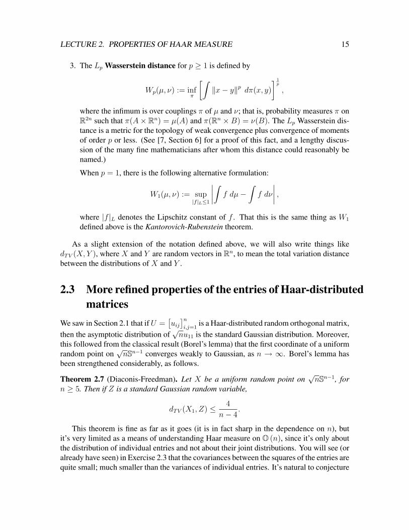
Figure 2.1: On the left are the eigenvalues of a 100 × 100 random unitary matrix; on theright are 100 i.i.d. uniform random points. Figures courtesy of E. Rains.

The factor∏

1≤j<k≤n |eiθj − eiθk |2 is the norm-squared of a Vandermonde determinant,which means one can also write it as∏

1≤j<k≤n

|eiθj − eiθk |2 =∣∣∣det

[eiθj(k−1)

]nj,k=1

∣∣∣2 =∑σ,τ∈Sn

sgn(στ)∏

1≤k≤n

eiθk(σ(k)−τ(k)).

(2.4)

This last expression can be quite useful in computations.

Either expression for the eigenvalue density is pretty hard to look at, but one thing tonotice right away is that for any given pair (j, k), |eiθk − eiθj |2 is zero if θj = θk (and smallif they are close), but |eiθk − eiθj |2 is 4 if θj = θk + π (and in that neighborhood if θj andθk are roughly antipodal). This produces the effect known as “eigenvalue repulsion”: theeigenvalues really want to spread out. You can see this pretty dramatically in pictures, evenfor matrices which aren’t really that large.

In the picture on the right in Figure 2.4, where 100 points were dropped uniformly andindependently, there are several large clumps of points close together, and some biggishgaps. In the picture on the right, this is much less true: the eigenvalues are spread prettyevenly, and there are no big clumps.

Things are similar for the other matrix groups, just a little fussier. Each matrix inSO (2N + 1) has 1 as an eigenvalue, each matrix in SO− (2N + 1) has −1 as an eigen-value, and each matrix in SO− (2N + 2) has both−1 and 1 as eigenvalues; we refer to all ofthese as trivial eigenvalues. The remaining eigenvalues of matrices in SO (N) or Sp (2N)occur in complex conjugate pairs. For this reason, when discussing SO (N), SO− (N), orSp (2N), the eigenvalue angles corresponding to the eigenvalues in the open upper half-circle are the nontrivial ones and we generally restrict our attention there. For U (N), allthe eigenvalue angles are considered nontrivial; there are no automatic symmetries in theeigenvalue process in this case.


In the case of the orthogonal and symplectic groups, one can give a similar formula forthe density of the non-trivial eigenangles as in the unitary case, although it is not as easy towork with because it doesn’t take the form of a norm squared. The densities are as follows.

Theorem 2.12. Let U be a Haar-distributed random matrix in S, where S is one ofSO (2n+ 1), SO (2n), SO− (2n+ 1), SO− (2n+ 2), Sp (2n). Then a function g of Uwhich is invariant under conjugation of U by a fixed orthogonal (in all but the last case) orsymplectic (in the last case) matrix is associated as above with a function g : [0, π)n → R(of the non-trivial eigenangles) which is invariant under permutations of coordinates, and∫

G

gdHaar =

∫[0,π)n

gdµG,

where the measures µG on [0, π)n have densities with respect to dθ1 · · · dθn as follows.

G µG

SO (2n)2

n!(2π)n

∏1≤j<k≤n

(2 cos(θk)− 2 cos(θj)

)2

SO (2n+ 1) , SO− (2n+ 1)2n

n!πn

∏1≤j≤n

sin2

(θj2

) ∏1≤j<k≤n


)2

Sp (2n) ,SO− (2N + 2)2n

n!πn

∏1≤j≤n

sin2 (θj)∏

1≤j<k≤n


)2

One of the technical tools that is commonly used to study the ensemble of eigenvaluesof a random matrix is the empirical spectral measure. Given a random matrix U witheigenvalues λ1, . . . , λn, the empirical spectral measure of U is the random measure

µU :=1

n

n∑j=1

δλj .

The empirical spectral measure is a handy way to encode the ensemble of eigenvalues.In particular, it lets us formalize the idea that the eigenvalues are evenly spread out onthe circle, and indeed more so than i.i.d. points are, by comparing the empirical spectralmeasure to the uniform measure on the circle. In dealing with convergence of randommeasures, one notion that comes up a lot is that of convergence “weakly in probability”,although it is seldom actually defined. This is an unfortunate practice, with which we willbreak. However, we will specialize to the situation that the random measures are definedon S1, since that is where our empirical spectral measures live.

Definition. A sequence of random probability measures µn on S1 converge weakly in prob-ability to a measure µ on S1 (written µn

P=⇒ µ) if for each continuous f : S1 → R,∫

fdµnP−−−→

n→∞

∫fdµ.


There are many equivalent viewpoints:

Lemma 2.13. For j ∈ Z and µ a probability measure on [0, 2π), let µ(j) =∫ 2π

0eijθdµ(θ)

denote the Fourier transform of µ at j. The following are equivalent:1. µn

P=⇒ µ;

2. for each j ∈ Z, µn(j)P−−−→

n→∞µ(j);

3. for every subsequence n′ in N there is a further subsequence n′′ such that with prob-ability one, µn′′ =⇒ µ as n→∞.

The first result showing that the eigenvalues of a Haar-distributed matrix evenly fill outthe circle was proved by Diaconis and Shahshahani.

Theorem 2.14 (Diaconis–Shahshahani). Let Gn be one of the sequences O (n), U (n),or Sp (2n) of groups, and let µn be the empirical spectral measure of Un, where Un isHaar-distributed in Gn. Then as n → ∞, µn converges, weakly in probability, to theuniform measure ν on S1.

In fact, it is possible to show that the measures µn converge quite quickly to the uni-form measure on the circle, and indeed more quickly than the empirical measure of n i.i.d.uniform points on the circle.

Theorem 2.15 (E. Meckes-M. Meckes). Suppose that for each n, Un is Haar distributed inGn, where Gn is one of O (n), SO (n), SO− (n), U (n), SU (n), or Sp (2n). Let ν denotethe uniform measure on S1. There is an absolute constant C such that with probability 1,for all sufficiently large n, and all 1 ≤ p ≤ 2,

Wp(µn, ν) ≤ C

√log(n)

n.

By way of comparison, it is known (cf. [2]) that if µn is the empirical measure of n i.i.d.uniform points on S1, then Wp(µn, ν) is typically of order 1√

n.

The above result gives one explicit demonstration that there is important structure tothe eigenvalue processes of these random matrices; in at least some ways, they are quitedifferent from collections of independent random points. There are indeed many beautifulpatterns to be found; a particularly striking example is the following.

Theorem 2.16 (Rains). Let m ∈ N be fixed and let m := minm,N. If ∼ denotesequality of eigenvalue distributions, then

U (N)m ∼⊕

0≤j<emU(⌈

N − jm

⌉)That is, if U is a uniform N × N unitary matrix, the eigenvalues of Um are distributed asthose of m independent uniform unitary matrices of sizes⌊

N

m

⌋:= max

k ∈ N | k ≤ N

m

and

⌈N

m

⌉:= min

k ∈ N | k ≥ N

m

,


such that the sum of the sizes of the matrices is N . In particular, if m ≥ N , the eigenvaluesof Um are distributed exactly as N i.i.d. uniform points on S1.

We conclude this lecture by mentioning a special algebraic structure of the eigenvalueprocesses of the compact classical groups. These processes are what’s known as determi-nantal point processes. The definition is a little complicated, but it turns out that processesthat satisfy it have very special (very useful) properties, as we’ll see.

Firstly, a point process X in a locally compact Polish space Λ is a random discretesubset of Λ. Abusing notation, we denote by X(D) the number of points of X in D. Apoint process may or may not have k-point correlation functions, defined as follows.

Definition. For a point process X in Λ, suppose there exist functions ρk : Λk → [0,∞)such that, for pairwise disjoint subsets D1, . . . , Dk ⊆ Λ,

E

[k∏j=1

X(Di)

]=

∫· · ·∫

D1 Dk

ρk(x1, . . . , xk)dx1 · · · dxk.

Then the ρk are called the k-point correlation functions (or joint intensities) of X.

A determinantal point process is a point process whose k-point correlation functionshave a special form:

Definition. Let K : Λ× Λ→ [0, 1]. A point process X is a determinantal point processwith kernel K if for all k ∈ N,

ρk(x1, . . . , xk) = det[K(xi, xj)

]ki,j=1

.

Proposition 2.17. The nontrivial eigenvalue angles of uniformly distributed random matri-ces in any of SO (N), SO− (N), U (N), Sp (2N) are a determinantal point process, withrespect to uniform measure on Λ, with kernels as follows.

KN(x, y) Λ

SO (2N) 1 +N−1∑j=1

2 cos(jx) cos(jy) [0, π)

SO (2N + 1) ,SO− (2N + 1)N−1∑j=0

2 sin

((2j + 1)x

2

)sin

((2j + 1)y

2

)[0, π)

U (N)N−1∑j=0

eij(x−y) [0, 2π)

Sp (2N) , SO− (2N + 2)N∑j=1

2 sin(jx) sin(jy) [0, π)


For some purposes, the following alternatives can be more convenient. In all but theunitary case, they are the same functions; for the unitary case, the kernels are different butdefine the same point processes.

First define

SN(x) :=

sin(Nx2

)/ sin

(x2

)if x 6= 0,

N if x = 0.

Proposition 2.18. The nontrivial eigenvalue angles of uniformly distributed random matri-ces in any of SO (N), SO− (N), U (N), Sp (2N) are a determinantal point process, withrespect to uniform measure on Λ, with kernels as follows.

LN(x, y) Λ

SO (2N)1

2

(S2N−1(x− y) + S2N−1(x+ y)

)[0, π)

SO (2N + 1) ,SO− (2N + 1)1

2

(S2N(x− y)− S2N(x+ y)

)[0, π)

U (N) SN(x− y) [0, 2π)

Sp (2N) ,SO− (2N + 2)1

2

(S2N+1(x− y)− S2N+1(x+ y)

)[0, π)

One thing that is convenient about determinantal point processes is that there are easy-to-use (in principle, at least) formulas for computing things like means and variances of thenumber of points in a given set, such as those given in the following lemma.

Lemma 2.19. Let K : I × I → R be a continuous kernel on an interval I such that thecorresponding operator

K(f)(x) :=

∫I

K(x, y)f(y)dµ(y)

on L2(µ), where µ is the uniform measure on I , is an orthogonal projection. For a subin-terval D ⊆ I , denote by ND the number of particles of the determinantal point processwith kernel K which lie in D. Then

END =

∫D

K(x, x) dµ(x)

andVar ND =

∫D

∫I\D

K(x, y)2 dµ(x) dµ(y).

Lecture 3

Concentration of Haar measure

3.1 The concentration of measure phenomenonThe phenomenon of concentration of measure has poked its head out of the water in manyplaces in the history of mathematics, but was first explicitly described and used by VitaliMilman in the 1970’s in his probabilistic proof of Dvoretzky’s theorem. Milman stronglyadvocated that the phenomenon was both fundamental and useful, and its study and appli-cation has become a large and influential field since then. The basic idea is that functionswith small local fluctuations are often essentially constant, where “essentially” means thatwe consider a function on a probability space (i.e., a random variable) and it is close to aparticular value with probability close to 1.

An example of a concentration phenomenon in classical probability theory is the fol-lowing.

Theorem 3.1 (Bernstein’s inequality). Let Xjnj=1 be independent random variables such

that, for each i, |Xj| ≤ 1 almost surely. Let σ2 = Var(∑n

j=1Xj

). Then for all t > 0,

P

[∣∣∣∣∣ 1nn∑j=1

Xj − E

(1

n

n∑j=1

Xj

)∣∣∣∣∣ > t

]≤ C exp

(−min

n2t2

2σ2,nt

2

).

That is, the average of independent bounded random variables is essentially constant,in that it is very likely to be close to its mean. We can reasonably think of the average ofn random variables as a statistic with small local fluctuations, since if we just change thevalue of one (or a few) of the random variables, the average can only change on the order1n

.In a more geometric context, we have the following similar statement about Lipschitz

functions of a random point on the sphere.

Theorem 3.2 (Levy’s lemma). Let f : Sn−1 → R be Lipschitz with Lipschitz constantL, and let X be a uniform random vector in Sn−1. Let M be the median of f ; that is,

23

LECTURE 3. CONCENTRATION OF HAAR MEASURE 24

P[f(X) ≥M ] ≥ 12

and P[f(X) ≤M ] ≥ 12. Then

P[∣∣f(X)−M

∣∣ ≥ Lt]≤ 2e−(n−2)t2 .

Again, this says that if the local fluctions of a function on the sphere are controlled (thefunction is Lipschitz), then the function is essentially constant.

We often prefer to state concentration results about the mean rather than the median, asfollows.

Corollary 3.3. Let f : Sn−1 → R be Lipschitz with Lipschitz constant L, and let X bea uniform random vector in Sn−1. Then for Mf denoting the median of f with respect touniform measure on Sn−1, |Ef(X)−Mf | ≤ L

√πn−2

and

P[|f(X)− Ef(X)| ≥ Lt] ≤ eπ−nt2

4 .

That is, a Lipschitz function on the sphere is essentially constant, and we can take thatconstant value to be either the median or the mean of the function.

Proof. First note that Levy’s lemma and Fubini’s theorem imply that∣∣Ef(X)−Mf

∣∣ ≤ E∣∣f(X)−Mf

∣∣=

∫ ∞0

P[∣∣f(X)−Mf

∣∣ > t]dt ≤

∫ ∞0

2e−(n−2)t2

L2 dt = L

√π

n− 2.

If t > 2√

πn−2

, then

P [|f(X)− Ef(X)| > Lt] ≤ P [|f(X)−Mf | > Lt− |Mf − Ef(X)|]

≤ P[|f(X)−Mf | > L

(t−√

π

n− 2

)]≤ 2e−

(n−2)t2

4 .

On the other hand, if t ≤ 2√

πn−2

, then

eπ−(n−2)t2

4 ≥ 1,

so the statement holds trivially.

3.2 Log-Sobolev inequalities and concentrationKnowing that a metric probability space possesses a concentration of measure propertyalong the lines of Levy’s lemma opens many doors; however, it is not a priori clear how toshow that such a property holds or to determine what the optimal (or even good) constantsare. In this section we discuss one approach to obtaining measure concentration, which isin particular one way to prove Levy’s lemma.

We begin with the following general definitions for a metric space (X, d) equipped witha Borel probability measure P.


Definition.1. The entropy of a measurable function f : X → [0,∞) with respect to P is

Ent(f) := E[f log(f)

]− (Ef) log (Ef) .

2. For a locally Lipschitz function g : X → R,

|∇g| (x) := lim supy→x

|g(y)− g(x)|d(y, x)

.

Exercise 3.4. Show that Ent(f) ≥ 0 and that for c > 0, Ent(cf) = cEnt(f).

Definition. We say that (X, d,P) satisfies a logarithmic Sobolev inequality (or log-Sobolevinequality or LSI) with constant C > 0 if, for every locally Lipschitz f : X → R,

Ent(f 2) ≤ 2CE(|∇f |2

). (3.1)

The reason for our interest in log-Sobolev inequalities is that they imply measure con-centration for Lipschitz functions, via the “Herbst argument”. The argument was outlinedby Herbst in a letter to Len Gross, who was studying something called “hypercontractiv-ity”. The argument made it into folklore, and then books (e.g., [6]) without most of thepeople involved ever having seen the letter (Gross kept it, though, and if you ask nicelyhe’ll let you see it).

Specifically, the following result holds.

Theorem 3.5. Suppose that (X, d,P) satisfies a log-Sobolev inequality with constant C >0. Then for every 1-Lipschitz function F : X → R, E|F | <∞, and for every r ≥ 0,

P[∣∣F − EµF

∣∣ ≥ r]≤ 2e−r

2/2C .

Proof (the Herbst argument).We begin with the standard observation that for any λ > 0,

P [F ≥ EF + r] = P[eλF−EλF ≥ eλr

]≤ e−λrEeλF−EλF , (3.2)

assuming that EeλF <∞. For now, assume that F is bounded as well as Lipschitz, so thatthe finiteness is assured. Also, observe that we can always replace F with F − EF , so wemay assume that EF = 0.

That is, given a bounded, 1-Lipschitz function F : X → R with EF = 0, we need toestimate EeλF under the assumption of an LSI with constant C; a natural thing to do is toapply the LSI to the function f with

f 2 := eλF .

For notational convenience, let H(λ) := EeλF . Then

Ent(f 2) = E[λFeλF

]−H(λ) logH(λ),


whereas

|∇f(x)| ≤ eλF (x)

2

(λ

2

)|∇F (x)|,

because the exponential function is smooth and F is 1-Lipschitz, and so

E|∇f |2 ≤ λ2

4E[|∇F |2eλF

]≤ λ2

4E[eλF]

=λ2

4H(λ)

(since |∇F | ≤ 1). Applying the LSI with constant C to this f thus yields

E[λFeλF

]−H(λ) logH(λ) = λH ′(λ)−H(λ) logH(λ) ≤ Cλ2

2H(λ),

or rearranging,H ′(λ)

λH(λ)− logH(λ)

λ2≤ C

2.

Indeed, if we define K(λ) := logH(λ)λ

, then the right-hand side is just K ′(λ), and so wehave the simple differential inequality

K ′(λ) ≤ C

2.

Now, H(0) = 1, so

limλ→0

K(λ) = limλ→0

H ′(λ)

H(λ)= lim

λ→0

E[FeλF

]E [eλF ]

= EF = 0,

and thus

K(λ) =

∫ λ

0

K ′(s)ds ≤∫ λ

0

C

2ds =

Cλ

2.

In other words,H(λ) = E

[eλF]≤ e

Cλ2

2 .

It follows from (3.2) that for F : X → R which is 1-Lipschitz and bounded,

P [F ≥ EF + r] ≤ e−λr+Cλ2

2 .

Now choose λ = rC

and the statement of the result follows under the assumption that F isbounded.

In the general case, let ε > 0 and define the truncation Fε by

Fε(x) :=

−1ε, F (x) ≤ −1

ε;

F (x), −1ε≤ F (x) ≤ 1

ε;

1ε, F (x) ≥ 1

ε.


Then Fε is 1-Lipschitz and bounded so that by the argument above,

E[eλFε

]≤ eλEFε+Cλ2

2 .

The truncation Fε approaches F pointwise as ε→ 0, so by Fatou’s lemma,

E[eλF]≤ elim infε→0 λEFεe

Cλ2

2 .

It remains to show that EFεε→0−−→ EF ; we can then complete the proof in the unbounded

case exactly as before.Now, we’ve already proved the concentration inequality

P [|Fε − EFε| > t] ≤ 2e−t2

2C (3.3)

and Fε converges pointwise (hence also in probability) to F , which has some finite value ateach point in X , so there is a constant K such that

P [|F | ≤ K] ≥ 3

4,

and the convergence of Fε in probability to F means that there is some K ′ such that forε < εo,

P [|Fε − F | > K ′] <1

4.

It follows that for ε < εo,E|Fε| < K +K ′.

It also follows from (3.3) and Fubini’s theorem that

E |Fε − EFε|2 =

∫ ∞0

tP [|Fε − EFε| > t] dt ≤∫ ∞

0

2te−t2

2C dt = 2C,

so that in fact EF 2ε ≤ 2C +K +K ′. Using Fatou’s lemma again gives that

EF 2 ≤ lim infε→0

EF 2ε ≤ 2C +K +K ′.

We can then use convergence in probability again

|EF − EFε| =≤ δ + E|Fε − F |1|Fε−F |>δ ≤ δ +√

E|Fε − F |2P [|Fε − F | > δ]ε→0−−→ 0.

One of the reasons that the approach to concentration via log-Sobolev inequalities isso nice is that log-Sobolev inequalities tensorize; that is, if one has the same LSI on eachof some finite collection of spaces, one can get the same LSI again on the product space,independent of the number of factors. Specifically, we have the following.


Theorem 3.6 (see [6]). Suppose that each of the metric probability spaces (Xi, di, µi)(1 ≤ i ≤ n) satisifes a log-Sobolev inequality: for each i there is a Ci > 0 such that forevery locally Lipschitz function f : Xi → R,

Entµi(f2) ≤ 2Ci

∫|∇Xif |2dµi.

Let X = X1 × · · · ×Xn, and equip X with the L2-sum metric

d((x1, . . . , xn), (y1, . . . , yn)

):=

√√√√ n∑i=1

d2i (xi, yi)

and the product probability measure µ := µ1 ⊗ · · · ⊗ µn. Then (X, d, µ) satisfies a log-Sobolev inequality with constant C := max1≤i≤nCi.

Note that with respect to the L2-sum metric, if f : X → R, then

|∇f |2 =n∑i=1

|∇Xif |2,

where

|∇Xif(x1, . . . , xn)| = lim supyi→xi

|f(x1, . . . , xi−1, yi, xi+1, . . . , xn)− f(x1, . . . , xn)|di(yi, xi)

.

A crucial point to notice above is that the constant C doesn’t get worse with the numberof factors; that is, the lemma gives dimension-free tensorization.

The theorem follows immediately from the following property of entropy.

Proposition 3.7. Let X = X1 × · · · ×Xn and µ = µ1 ⊗ · · · ⊗ µn as above, and supposethat f : X → [0,∞). For x1, . . . , xn \ xi fixed, write

fi(xi) = f(x1, . . . , xn),

thought of as a function of xi. Then

Entµ(f) ≤n∑i=1

∫Entµi(fi)dµ.

Proof. The proof is a good chance to see a dual formulation of the definition of entropy.Given a probability space (Ω,F,P), we defined entropy for a function f : Ω→ R by

EntP(f) :=

∫f log(f)dP−

(∫fdP

)log

(∫fdP

).


It turns out to be equivalent to define

EntP(f) := sup

∫fgdP

∣∣∣∣ ∫ egdP ≤ 1

,

which can be seen as follows.First, for simplicity we may assume that

∫fdP = 1, since both expressions we’ve given

for the entropy are homogeneous of degree 1. Then our earlier expression becomes

EntP(f) =

∫f log(f)dP.

Now, if g := log(f), then∫eg =

∫f = 1, and so we have that∫

f log(f)dP =

∫fgdP ≤ sup

∫fgdP

∣∣∣∣ ∫ egdP ≤ 1

.

On the other hand, Young’s inequality says that for u ≥ 0 and v ∈ R,

uv ≤ u log(u)− u+ ev;

applying this to u = f and v = g and integrating shows that

sup

∫fgdP

∣∣∣∣ ∫ egdP ≤ 1

≤∫f log(f)dP.

With this alternative definition of entropy, given g such that∫egdµ ≤ 1, for each i

define

gi(x1, . . . , xn) := log

(∫eg(y1,...,yi−1,xi,...,xn)dµ1(y1) · · · dµi−1(yi−1)∫eg(y1,...,yi,xi+1,...,xn)dµ1(y1) · · · dµi(yi)

),

(note that gi only actually depends on xi, . . . , xn). Thenn∑i=1

gi(x1, . . . , xn) = log

(eg(x1,...,xn)∫

eg(y1,...,yn)dµ1(y1) · · · dµn(yn)

)≥ g(x1, . . . , xn),

and by construction,∫e(gi)idµi =

∫ (∫eg(y1,...,yi−1,xi,...,xn)dµ1(y1) · · · dµi−1(yi−1)∫eg(y1,...,yi,xi+1,...,xn)dµ1(y1) · · · dµi(yi)

)dµi(xi) = 1.

Applying these two estimates together with Fubini’s theorem yields∫fgdµ ≤

n∑i=1

∫fgidµ =

n∑i=1

∫ (∫fi(g

i)idµi

)dµ ≤

n∑i=1

∫Entµi(fi)dµ.


The optimal (i.e., with smallest constants) log-Sobolev inequalities on most of the com-pact classical matrix groups were proved using the Bakry-Emery curvature criterion. Tostate it, we need to delve a little bit into the world of Riemannian geometry and define somequantities on Riemannian manifolds, most notably, the Ricci curvature.

Recall that a Riemannian manifold (M, g) is a smooth manifold (every point has anopen neighborhood which is diffeomorphic to an open subset of Euclidean space) togetherwith a Riemannian metric g. The metric g is a family of inner products: at each pointp ∈ M , gp : TpM × TpM → R defines an inner product on the tangent space TpM to Mat p. Our manifolds are all embedded in Euclidean space already, and the metrics are justthose inherited from the ambient Euclidean space (this came up briefly in our discussion ofthe Riemannian construction of Haar measure in Lecture 1).

A vector field X on M is a smooth (infinitely differentiable) map X : M → TM suchthat for each p ∈ M , X(p) ∈ TpM . To have a smooth Riemannian manifold, we requirethe metric g to be smooth, in the sense that for any two smooth vector fields X and Y onM , the map

p 7−→ gp(X(p), Y (p))

is a smooth real-valued function on M .In Riemannian geometry, we think of vector fields as differential operators (think of

them as directional derivatives): given a smooth function f : M → R and a vector field Xon M , we define the function X(f) by the requirement that for any curve γ : [0, T ] → Mwith γ(0) = p and γ′(0) = X(p) (here, γ′(0) denotes the tangent vector to the curve γ atγ(0) = p),

X(f)(p) =d

dtf(γ(t))

∣∣∣∣t=0

.

Given two vector fields X and Y on M , there is a unique vector field [X, Y ], called theLie Bracket of X and Y , such that

[X, Y ](f) = X(Y (f))− Y (X(f)).

It is sometimes convenient to work in coordinates. A local frame Li is a collectionof vector fields defined on an open set U ⊆ M such that at each point p ∈ U , the vectorsLi(p) ⊆ TpM form a basis of TpM . The vector fields Li are called a local orthonor-mal frame if at each point in U , the Li are orthonormal with repect to g. Some manifoldsonly have local frames, not global ones; that is, you can’t define a smooth family of vectorfields over the whole manifold which forms a basis of the tangent space at each point. Thisis true, for example of S2 ⊆ R3.

We need a few more notions in order to get to curvature. Firstly, a connection ∇ onM is a way of differentiating one vector field in the direction of another: a connection ∇is a bilinear form on vector fields that assigns to vector fields X and Y a new vector field∇XY , such that for any smooth function f : M → R,

∇fXY = f∇XY and ∇X(fY ) = f∇X(Y ) +X(f)Y.


A connection is called torsion-free if∇XY−∇YX = [X, Y ]. There is a special connectionon a Riemannian manifold, called the Levi-Civita connection, which is the unique torsion-free connection with the property that

X(g(Y, Z)) = g(∇XY, Z) + g(Y,∇XZ).

This property may look not obviously interesting, but geometrically, it is a compatibilitycondition of the connection ∇ with g. There is a notion of transporting a vector field ina “parallel way” along a curve, which is defined by the connection. The condition abovemeans (this is not obvious) that the inner product defined by g of two vector fields at a pointis unchanged if you parallel-transport the vector fields (using ∇ to define “parallel”) alongany curve.

Finally, we can define the Riemannian curvature tensor R(X, Y ): to each pair ofvector fields X and Y on M , we associate an operator R(X, Y ) on vector fields defined by

R(X, Y )(Z) := ∇X(∇YZ)−∇Y (∇XZ)−∇[X,Y ]Z.

The Ricci curvature tensor is the function Ric(X, Y ) on M which, at each point p ∈ M ,is the trace of the linear map on TpM defined by Z 7→ R(Z, Y )(X). In orthonormal localcoordinates Li,

Ric(X, Y ) =∑i

g(R(X,Li)Li, Y ).

(Note that seeing that this coordinate expression is right involves using some of the sym-metries of R.) The Bakry-Emery criterion can be made more general, but for our purposesit suffices to formulate it as follows.

Theorem 3.8 (Bakry–Emery). Let (M, g) be a compact, connected, m-dimensional Rie-mannian manifold with normalized volume measure µ. Suppose that there is a constantc > 0 such that for each p ∈M and each v ∈ TpM ,

Ricp(v, v) ≥ 1

cgp(v, v).

Then µ satisfies a log-Sobolev inequality with constant c.

3.3 Concentration for the compact classical groupsTheorem 3.9. The matrix groups and cosets SO (n), SO− (n), SU (n), U (n), and Sp (2n)with Haar probability measure and the Hilbert–Schmidt metric, satisfy logarithmic Sobolevinequalities with constants


G CG

SO (n), SO− (n) 4n−2

SU (n) 2n

U (n) 6n

Sp (2n) 12n+1

We saw in Lecture 1 (Lemma 1.4) that the the geodesic distance on U (n) is boundedabove by π/2 times the Hilbert–Schmidt distance. Thus Theorem 3.9 implies, for examplethat U (n) equipped with the geodesic distance also satisfies a log-Sobolev inequality, withconstant 3π2/2n.

Exercise 3.10. Prove that Theorem 3.9 does indeed imply a LSI for the geodesic distancewith constant 3π2/n.

The proof of Theorem 3.9 for each G except U (n) follows immediately from theBakry–Emery Theorem, by the following curvature computations.

Proposition 3.11. If Gn is one of SO (n), SO− (n) SU (n), or Sp (2n), then for eachU ∈ Gn and each X ∈ TUGn,

RicU(X,X) = cGngU(X,X),

where gU is the Hilbert-Schmidt metric and cGn is given by

G cG

SO (n), SO− (n) n−24

SU (n) n2

Sp (2n) 2n+ 1

This gives us the concentration phenomenon we’re after on all of the Gn except O (n)and U (n). Now, on O (n) we can’t actually expect more and indeed more is not true,because O (n) is disconnected. We have the best we can hope for already, namely concen-tration on each of the pieces. In the case of U (n), though, we in fact do have the samekind of concentration that we have on SU (n). There is no non-zero lower bound on theRicci curvature on U (n), but the log-Sobolev inequality there follows from the one onSU (n). The crucial observation is the following coupling of the Haar measures on SU (n)and U (n).

Lemma 3.12. Let θ be uniformly distributed in[0, 2π

n

]and let V ∈ SU (n) be uniformly

distributed, with θ and V independent. Then eiθV is uniformly distributed in U (n).


Proof. Let X be uniformly distributed in [0, 1), K uniformly distributed in 0, . . . , n− 1,and V uniformly distributed in SU (n) with (X,K, V ) independent. Consider

U = e2πiX/ne2πiK/nV.

On one hand, it is easy to see that (X + K) is uniformly distributed in [0, n], so thate2πi(X+K)/n is uniformly distributed on S1. Thus U d

= ωV for ω uniform in S1 and indepen-dent of V . One can then show that the distribution of ωV is translation-invariant on U (n),and thus yields Haar measure.

On the other hand, if In is the n × n identity matrix, then e2πiK/nIn ∈ SU (n). By thetranslation invariance of Haar measure on SU (n) this implies that e2πiK/nV

d= V , and so

e2πiX/nVd= U .

Exercise 3.13. Prove carefully that if ω is uniform in S1 and U is Haar-distributed in SU (n)with ω, U independent, then ωU is Haar-distributed in U (n).

Using this coupling lets us prove the log-Sobolev inequality on U (n) via the tensoriza-tion property of LSI.

Proof of Theorem 3.9. First, for the interval [0, 2π] equipped with its standard metric anduniform measure, the optimal constant in (3.1) for functions f with f(0) = f(2π) is knownto be 1, see e.g. [8]. This fact completes the proof — with a better constant than stated above— in the case n = 1; from now on, assume that n ≥ 2.

Suppose that f : [0, π]→ R is locally Lipschitz, and define a function f : [0, 2π]→ Rby reflection:

f(x) :=

f(x), 0 ≤ x ≤ π;

f(2π − x), π ≤ x ≤ 2π.

Then f is locally Lipschitz and f(2π) = f(0), so f satisfies a LSI for uniform measure on[0, 2π] with constant 1. If µ[a,b] denotes uniform (probability) measure on [a, b], then

Entµ[0,2π](f 2) = Entµ[0,π]

(f 2),

and1

2π

∫ 2π

0

|∇f(x)|2dx =1

π

∫ π

0

|∇f(x)|2dx,

so f itself satisfies a LSI for uniform measure on [0, π] with constant 1 as well. In fact, theconstant 1 here is optimal (see Exercise 3.14).

It then follows by a scaling argument that the optimal logarithmic Sobolev constant on[0, π

√2√n

)is 2/n (for g :

[0, π

√2√n

)→ R, apply the LSI to g

(√2nx)

and rearrange it to get

the LSI on[0, π

√2√n

).)


By Theorem 3.9 SU (n) satisfies a log-Sobolev inequality with constant 2/n whenequipped with its geodesic distance, and hence also when equipped with the Hilbert–Schmidt metric. By the tensorization property of log-Sobolev inequalities in Euclideanspaces (Lemma 3.6), the product space

[0, π

√2√n

)×SU (n), equipped with the L2-sum met-

ric, satisfies a log-Sobolev inequality with constant 2/n as well.Define the map F :

[0, π

√2√n

)× SU (n) → U (n) by F (t, V ) = e

√2it/√nV . By Lemma

3.12, the push-forward via F of the product of uniform measure on[0, π

√2√n

)with uniform

measure on SU (n) is uniform measure on U (n). Moreover, this map is√

3-Lipschitz:∥∥∥e√2it1/√nV1 − e

√2it2/

√nV2

∥∥∥HS≤∥∥∥e√2it1/

√nV1 − e

√2it1/

√nV2

∥∥∥HS

+∥∥∥e√2it1/

√nV2 − e

√2it2/

√nV2

∥∥∥HS

= ‖V1 − V2‖HS +∥∥∥e√2it1/

√nIn − e

√2it2/

√nIn

∥∥∥HS

≤ ‖V1 − V2‖HS +√

2 |t1 − t2|

≤√

3

√‖V1 − V2‖2

HS + |t1 − t2|2.

Since the map F is√

3-Lipschitz, its image U (n) with the (uniform) image measuresatisfies a logarithmic Sobolev inequality with constant (

√3)2 2

n= 6

n.

Exercise 3.14. Prove that the optimal log-Sobolev constant for uniform measure on [0, π]is 1. Here are two possible approaches:

1. Suppose uniform measure on [0, π] satisfied a LSI with constant C < 1. Let f :[0, 2π] be locally Lipschitz with f(0) = f(2π). Decompose all of the integrals in theexpression for the entropy of f 2 w.r.t. uniform measure on [0, 2π] into the part on[0, π] and the part on [π, 2π]. Use the concavity of the logarithm and your assumedLSI to get an estimate for the entropy of f 2 on [0, 2π]. Now obtain a contraditctionby observing that whether or not the crucial inequality holds is invariant under thetransformation f(x) 7−→ f(2π − x), and so you may use whichever version of f ismore convenient.

2. Consider the function f(x) = 1 + ε cos(x) on [0, π]. Suppose you had an LSI on[0, π] with constant C < 1. Apply it to this f and expand Entµ[0,π]

(f 2) in powers ofε to get a contradiction.

From our log-Sobolev inequalities, we finally get the concentration we want on thecompact classical groups, as follows.

Corollary 3.15. Given n1, . . . , nk ∈ N, let X = Gn1×· · ·×Gnk , where for each of the ni,Gni is one of SO (ni), SO− (ni), SU (ni), U (ni), or Sp (2ni). Let X be equipped with theL2-sum of Hilbert–Schmidt metrics on the Gni . Suppose that F : X → R is L-Lipschitz,


and that Uj ∈ Gnj : 1 ≤ j ≤ k are independent, Haar-distributed random matrices.Then for each t > 0,

P[F (U1, . . . , Uk) ≥ EF (U1, . . . , Uk) + t

]≤ e−(n−2)t2/12L2

,

where n = minn1, . . . , nk.

Proof. By Theorem 3.9 and Lemma 3.6, X satisfies a log-Sobolev inequality with constant6/(n−2). The stated concentration inequality then follows from the Herbst argument.

Lecture 4

Applications of Concentration

4.1 The Johnson-Lindenstrauss LemmaA huge area of application in computing is that of dimension-reduction. In this day andage, we are often in the situation of having (sometimes large, sometimes not so large) datasets that live in very high-dimension. For example, a digital image can be encoded as a ma-trix, with each entry corresponding to one pixel, and the entry specifying the color of thatpixel. So if you had a small black and white image whose resolution was, say 100 × 150pixels, you would encode it as a vector in 0, 115,000. An issue that causes problems is thatmany algorithms for analyzing such high-dimensional data have their run-time increasevery quickly as the dimension of the data increases, to the point that analyzing the data inthe most obvious way becomes computationally infeasible. The idea of dimension reduc-tion is that in many situations, the desired algorithm can be at least approximately carriedout in a much lower-dimensional setting than the one the data come to you in, and that canmake computationally infeasible problems feasible.

A motivating problemSuppose you have a data set consisting of black and white images of hand-written examplesof the numbers 1 and 2. So you have a reference collection X of n points in Rd, where dis the number of pixels in each image. You want to design a computer program so that onecan input an image of a hand-written number, and the computer can tell whether it’s a 1or a 2. So the computer will have a query point q ∈ Rd, and the natural thing to do is toprogram it to find the closest point in the reference set X to q; the computer then reportsthat the input image was of the same number as that closest point in X.

36

LECTURE 4. APPLICATIONS OF CONCENTRATION 37

P. Indyk

The naıve approach would be for the computer to calculate the distance from q to eachof the points of X in turn, keeping track of which point in X has so far been the closest.Such an algorithm runs in O(nd) steps. Remember that d can be extremely large if ourimages are fairly high resolution, so nd steps might be computationally infeasible. Manymathematicians’ first remark at this point is that the problem only has to be solved withinthe span of the points of X and q, so that one can a priori replace d by n. Actually doingthis, though, means you have to find an orthonormal basis for the subspace you plan towork in, so in general you can’t save time this way.

The idea of dimension reduction is to find a way to carry out the nearest point algorithmwithin some much lower-dimensional space, in such a way that you are guarranteed (or tobe more realistic, very likely) to still find the closest point, and without having to do muchwork to figure out which lower-dimensional space to work in. This sounds impossible,but the geometry of high-dimensional spaces often turns out to be surprising. An impor-tant result about high-dimensional geometry that has inspired many randomized algorithmsincorporating dimension-reduction is the following.

Lemma 4.1 (The Johnson–Lindenstrauss Lemma). There are absolute constants c, C suchthat the following holds.

Let xjnj=1 ⊆ Rd, and let P be a random k× d matrix, consisting of the first k rows ofa Haar-distributed random matrix in O (d). Fix ε > 0 and let k = a log(n)

ε2. With probability

1− Cn2−ac

(1− ε)‖xi − xj‖2 ≤(d

k

)‖Pxi − Pxj‖2 ≤ (1 + ε)‖xi − xj‖2 (4.1)

for all i, j ∈ 1, . . . , n.

What the lemma says is that one can take a set of n points in Rd and project them ontoa random subspace of dimension on the order of log(n) so that, after appropriate rescaling,the pairwise distances between the points hardly changes. The practical conclusion of thisis that if your problem is about the metric structure of the data (finding the closest point asabove, finding the most separated pair of points, finding the minimum length spanning tree


of a graph,etc.), there is no need to work in the high-dimensional space that the data natu-rally live in, and that moreover there is no need to work hard to pick a lower-dimensionalsubspace onto which to project: a random one should do.

Exercise 4.2. Verify that for x ∈ Rd and P as above, dkE‖Px‖2 = ‖x‖2.

Getting an almost-solution, with high probabilityThe discussion above suggests that we try to solve the problem of finding the closest pointto q in X by choosing a random k × d matrix P to be the first k rows of a Haar-distributedU ∈ O (d), then finding the closest point in Px :∈ X to Pq. There are two obviousissues here. One is that we might have the bad luck to choose a bad matrix P that doesn’tsatisfy (4.1). But that is very unlikely, and so we typically just accept the risk and figure itwon’t actually happen.

There is a second issue, though, which is that it’s possible that we choose P that doessatisfy (4.1), but that the closest point in Px :∈ X to Pq is Py, whereas the closest pointin X to q is z, with y 6= z. In that case, although our approach will yield the wrong valuefor the closest point (y instead of z), we have by choice of y and (4.1) that

‖q − y‖ ≤

√d

k(1− ε)‖Pq − Py‖ ≤

√d

k(1− ε)‖Pq − Pz‖ ≤

√1 + ε

1− ε‖q − z‖.

So even though z is the true closest point to q, y is almost as close. In our example ofrecognizing whether a hand-written number is a 1 or a 2, it seems likely that even if wedon’t find the exact closest point in the reference set, we’ll still manage to correctly identifythe number, which is all we actually care about.

For being willing to accept an answer which may be not quite right, and accept the(tiny) risk that we’ll choose a bad matrix, we get a lot in return. The naıve algorithm wementioned at the beginning now runs in O(n log(n)) steps.

Proof of Johnson-LindenstraussGiven xini=1 ⊆ Rd, ε > 0, and U a Haar-distributed random matrix in O (d), let P be thek × d matrix consisting of the first k rows of U . We want to show that for each pair (i, j),

(1− ε)‖xi − xj‖2 ≤(d

k

)∥∥Pxi − Pxj∥∥2 ≤ (1 + ε)‖xi − xj‖2

with high probability, or equivalently,

√1− ε ≤

√d

k

∥∥Pxi,j∥∥ ≤ √1 + ε

for xi,j :=xi−xj‖xi−xj‖ .


For notational convenience, fix i and j for the moment and let x = xi,j . For such anx ∈ Sd−1 fixed, consider the function Fx : O (d)→ R defined by

Fx(U) =

√d

k

∥∥∥Px∥∥∥.Let U,U ′ ∈ O (d), and let P, P ′ denote the matrices of the first k rows of U and U ′.

Then ∣∣∣Fx(U)− Fx(U ′)∣∣∣ =

√d

k

∣∣∣‖Px‖ − ‖P ′x‖∣∣∣ ≤√d

k

∥∥(P − P ′)x∥∥.

Exercise 4.3. Prove that∥∥(P − P ′)x

∥∥ ≤ dH,S(U,U ′).Hint: First show

∥∥(P − P ′)x∥∥ ≤ ∥∥(U − U ′)x

∥∥.

That is, the function Fx is√

dk-Lipschitz on O (d) with respect to dHS(·, ·) In particular,

Fx is also√

dk-Lipschitz when restricted to either SO (d) or SO− (d).

The idea is to apply concentration of measure to the function Fx. We want a concentra-tion inequality on the full orthogonal group, which we will get from similar inequalities onthe two components.

Haar measure on O (d) can be described in terms of Haar measure on SO (d) andSO− (d) as follows. Let U1 be Haar-distributed in SO (d) and let U2 be the matrix obtainedfrom U by swapping the last two rows. Then we saw in Lecture 1 that U2 is Haar-distributedin SO− (d), and so if U is equal to U1 with probability 1

2and equal to U2 with probability

12, then U is Haar distributed on O (d). Note that as long as k ≤ d− 2, the matrix P1 of the

first k rows of U1 is the same as the matrix P2 of the first k rows of U2. It follows that

EFx(U) = EFx(U1) = EFx(U2).

Because Fx is√

dk-Lipschitz when restricted to either SO (d) or SO− (d), concentration of

measure implies that, for j = 1, 2,

P [|Fx(Uj)− EFx(Uj)| ≥ ε] ≤ Ce−ckε2

.

It then follows by conditioning on whether U = U1 or U = U2 that

P [|Fx(U)− EFx(U)| ≥ ε] ≤ Ce−ckε2

. (4.2)

To complete the proof, we need to show that EFx(U) ≈ 1.

By the invariance of Haar measure under translation,

Pxd= Pe1 = (U11, . . . , Uk1),


where e1 is the first standard basis vector in Rd. It follows that

Fx(U)d=

√(d

k

)(U2

11 + · · ·+ U2k1).

We saw in the first lecture that EU2i1 = 1

dfor each i, so E

[Fx(U)

]2= 1; written slightly

differently,

1 = Var(Fx(U)) +(EFx(U)

)2.

By Fubini’s theorem and the concentration inequality (4.2),

Var(Fx(U)) =

∫ ∞0

P[|Fx(U)− EFx(U)|2 ≥ t

]dt ≤

∫ ∞0

Ce−cktdt =C

ck,

so that √1− C

ck≤ EFx(U) ≤ 1.

Recall that k = a log(n)ε2

. As long as ε < ca log(n)C+ca log(n)

, this means that 1 − ε2≤ EFx(U) ≤ 1,

and soP[∣∣Fx(U)− 1

∣∣ > ε]≤ Ce−

ckε2

4 ; (4.3)

that is, with probability at least 1− Ce− ckε2

4 ,

1− ε ≤√d

k‖Px‖ ≤ 1 + ε.

Returning to the original formulation, for each pair (i, j), there is a set of probability atleast 1− Ce−ckε2 such that

(1− ε)2‖xi − xj‖2 ≤(d

k

)∥∥Uxi − Uxj∥∥2 ≤ (1 + ε)2‖xi − xj‖2.

There are fewer than n2 pairs (i, j), so a simple union bound gives that the abovestatement holds for all pairs (i, j) with probability at least 1− C

nac−2 .

Exercise 4.4. In the course of the proof, we assumed that k ≤ d − 2 for convenience.While we certainly expect this to be true in applications, show that this wasn’t necessaryby checking the cases k = d− 1 and k = d.


4.2 Uniform approximation of the empirical spectral mea-sure of powers of random unitary matrices

In this section we give the proof of Theorem 2.15 on the rate of convergence of the em-pirical spectral measure of a Haar random matrix to the uniform distribution. The resultquoted there is a corollary of the following.

Theorem 4.5. Let µn,m be the spectral measure of Um, where 1 ≤ m ≤ n and U ∈ U (n)is distributed according to Haar measure, and let ν denote the uniform measure on S1.Then for each p ≥ 1,

EWp(µn,m, ν) ≤ Cp

√m[log(nm

)+ 1]

n,

where C > 0 is an absolute constant.Moreover, for each t > 0,

P

Wp(µn,m, ν) ≥ C

√m[log(nm

)+ 1]

n+ t

≤ exp

[−n

2t2

24m

]

for 1 ≤ p ≤ 2 and

P

Wp(µn,m, ν) ≥ Cp

√m[log(nm

)+ 1]

n+ t

≤ exp

[−n

1+2/pt2

24m

]

for p > 2, where C > 0 is an absolute constant.

This kind of change in behavior at p = 2 is typical for the Wasserstein distances.By a simple application of the Borel-Cantelli lemma, one gets an almost sure rate of

convergence, as follows.

Corollary 4.6. Suppose that for each n, Un ∈ U (n) is Haar-distributed and 1 ≤ mn ≤ n.Let ν denote the uniform measure on S1. There is an absolute constant C such that givenp ≥ 1, with probability 1, for all sufficiently large n,

Wp(µn,mn , ν) ≤ C

√mn log(n)

n

if 1 ≤ p ≤ 2 and

Wp(µn,mn , ν) ≤ Cp

√mn log(n)

n12

+ 1p

if p > 2.


Exercise 4.7. Prove Corollary 4.6

The first step in proving Theorem 4.5 is to prove a concentration result for the num-ber N

(m)θ of eigenangles of Um in [0, θ). We get such a result as a concenquence of the

following remarkable property of determinantal point processes.

Proposition 4.8. Let K : Λ × Λ → C be a kernel on a locally compact Polish space Λsuch that the corresponding integral operator K : L2(µ)→ L2(µ) defined by

K(f)(x) =

∫K(x, y)f(y) dµ(y)

is self-adjoint, nonnegative, and locally trace-class with eigenvalues in [0, 1]. For D ⊆ Λmeasurable, letKD(x, y) = 1D(x)K(x, y)1D(y) be the restriction ofK toD. Suppose thatD is such that KD is trace-class; denote by λkk∈A the eigenvalues of the correspondingoperator KD on L2(D) (A may be finite or countable) and denote by ND the number ofparticles of the determinantal point process with kernel K which lie in D. Then

NDd=∑k∈A

ξk,

where “ d=” denotes equality in distribution and the ξk are independent Bernoulli random

variables with P[ξk = 1] = λk and P[ξk = 0] = 1− λk.

This result is quite valuable for us, because it tells us (once we’ve checked the condi-tions; see Exercise 4.9) that N

(1)θ is distributed exactly as a sum of n independent Bernoulli

random variables. Moreover, thanks to Rains’ Theorem (Theorem 2.16), N(m)θ is equal

in distribution to the total number of eigenvalue angles in [0, θ) of each of U0 . . . , Um−1,where U0, . . . , Um−1 are independent and Uj is Haar-distributed in U

(⌈n−jm

⌉); that is,

N(m)θ

d=

m−1∑j=0

Nj,θ,

where the Nj,θ are the independent counting functions corresponding to U0, . . . , Um−1. Itis therefore also true that N

(m)θ is distributed exactly as a sum of n independent Bernoulli

random variables.

Exercise 4.9. Show that the operator K : L2([0, 2π))→ L2([0, 2π)) defined by

K(f)(x) =1

2π

∫ 2π

0

KN(x− y)f(y)dy,

for KN(z) =∑N−1

j=0 eijz is self-adjoint, nonnegative, and trace-class.


Classical probability has quite a few things to say about sums of independent Bernoullirandom variables; in particular, an application of Bernstein’s inequality (Theorem 3.1) willgive us the concentration we need for the eigenvalue counting function. Specifically, foreach t > 0 we have

P[∣∣∣N(m)

θ − EN(m)θ

∣∣∣ > t]≤ 2 exp

(−min

t2

4σ2,t

2

), (4.4)

where σ2 = Var N(m)θ .

Of course, in order to apply (4.4), it is necessary to estimate EN(m)θ and σ2. Rains’

Theorem again means we only need to do any real work in the case m = 1. To do thecomputations, we use the kernel of the eigenvalue process given in Theorem 2.18 togetherwith the formulae from Lemma 2.19.

Proposition 4.10. Let U be uniform in U (N). Then for all θ ∈ [0, 2π),

EN(1)θ =

nθ

2π,

andVar N

(1)θ ≤ log n+ 1.

Proof. Computing EN(1)θ is trivial, either by symmetry or by Lemma 2.19.

To compute Var N(1)θ , note first that if θ ∈ (π, 2π), then Nθ

d= N − N2π−θ, and so it

suffices to assume that θ ≤ π. By Proposition 2.18 and Lemma 2.19,

Var Nθ =1

4π2

∫ θ

0

∫ 2π

θ

Sn(x− y)2 dx dy =1

4π2

∫ θ

0

∫ 2π−y

θ−y

sin2(nz2

)sin2

(z2

) dz dy

=1

4π2

[∫ θ

0

z sin2(nz2

)sin2

(z2

) dz +

∫ 2π−θ

θ

θ sin2(nz2

)sin2

(z2

) dz +

∫ 2π

2π−θ

(2π − z) sin2(nz2

)sin2

(z2

) dz

]

=1

2π2

[∫ θ

0

z sin2(nz2

)sin2

(z2

) dz +

∫ π

θ

θ sin2(nz2

)sin2

(z2

) dz

].

For the first integral, since sin(z2

)≥ z

πfor all z ∈ [0, θ], if θ > 1

n, then∫ θ

0

z sin2(nz2

)sin2

(z2

) dz ≤∫ 1

n

0

(πn)2z

4dz +

∫ θ

1n

π2

zdz = π2

(1

8+ log(n) + log(θ)

).

If θ ≤ 1n

, there is no need to break up the integral and one simply has the bound (πnθ)2

8≤ π2

8.

Similarly, if θ < 1n

, then∫ π

θ

θ sin2(nz2

)sin2

(z2

) dz ≤∫ 1

n

θ

θ(πn)2

4dz +

∫ π

1n

π2θ

z2dz

=π2θn

4(1− nθ) + π2nθ − πθ ≤ 5π2

4;


if θ ≥ 1n

, there is no need to break up the integral and one simply has a bound of π2.All together,

Var Nθ ≤ log(n) +11

16.

Corollary 4.11. Let U be uniform in U (n) and 1 ≤ m ≤ n. For θ ∈ [0, 2π), let N(m)θ be

the number of eigenvalue angles of Um in [0, θ). Then

EN(m)θ =

nθ

2πand Var N

(m)θ ≤ m

(log( nm

)+ 1).

Proof. This follows immediately from Theorem 2.16; note that the n/m in the variancebound, as opposed to the more obvious dn/me, follows from the concavity of the logarithm.

Putting these estimates together with Equation (4.4) gives that for all t > 0,

P[∣∣∣∣N(m)

θ − nθ

2π

∣∣∣∣ > t

]≤ 2 exp

(−min

t2

4m(log(nm

)+ 1) , t

2

). (4.5)

It’s fairly straighforward to use this inequality to obtain concentration for the individualeigenangles around their predicted values, as follows.

Lemma 4.12. Let 1 ≤ m ≤ n and let U ∈ U (n) be uniformly distributed. Denote by eiθj ,1 ≤ j ≤ n, the eigenvalues of Um, ordered so that 0 ≤ θ1 ≤ · · · ≤ θn < 2π. Then for eachj and u > 0,

P[∣∣∣∣θj − 2πj

n

∣∣∣∣ > 4π

nu

]≤ 4 exp

[−min

u2

m(log(nm

)+ 1) , u] . (4.6)

Proof. For each 1 ≤ j ≤ n and u > 0, if j + 2u < n then

P[θj >

2πj

n+

4π

nu

]= P

[N

(m)2π(j+2u)

n

< j

]= P

[j + 2u−N

(m)2π(j+2u)

n

> 2u

]≤ P

[∣∣∣∣N(m)2π(j+2u)

n

− EN(m)2π(j+2u)

n

∣∣∣∣ > 2u

].

If j + 2u ≥ n then

P[θj >

2πj

n+

4π

nu

]= P [θj > 2π] = 0,

and the above inequality holds trivially. The probability that θj < 2πjn− 4π

nu is bounded in

the same way. Inequality (4.6) now follows from (4.5).


We are now in a position to bound the expected distance between the empirical spectralmeasure of Um and uniform measure. Let θj be as in Lemma 4.12. Then by Fubini’stheorem,

E∣∣∣∣θj − 2πj

n

∣∣∣∣p =

∫ ∞0

ptp−1P[∣∣∣∣θj − 2πj

n

∣∣∣∣ > t

]dt

=(4π)pp

np

∫ ∞0

up−1P[∣∣∣∣θj − 2πj

n

∣∣∣∣ > 4π

nu

]du

≤ 4(4π)pp

np

[∫ ∞0

up−1e−u2/m[log(n/m)+1] du+

∫ ∞0

up−1e−u du

]=

4(4π)p

np

[(m[log( nm

)+ 1])p/2

Γ(p

2+ 1)

+ Γ(p+ 1)

]≤ 8Γ(p+ 1)

(4π

n

√m[log( nm

)+ 1])p

.

Observe that in particular,

Var θj ≤ Cm[log(nm

)+ 1]

n2.

Let νn be the measure which puts mass 1n

at each of the points e2πij/n, 1 ≤ j ≤ n. Then

EWp(µn,m, νn)p ≤ E

[1

n

n∑j=1

∣∣eiθj − e2πij/n∣∣p] ≤ E

[1

n

n∑j=1

∣∣∣∣θj − 2πj

n

∣∣∣∣p]

≤ 8Γ(p+ 1)

(4π

n

√m[log( nm

)+ 1])p

.

It is easy to check that Wp(νn, ν) ≤ πn

, and thus

EWp(µn,m, ν) ≤ EWp(µn,m, νn) +π

n≤ (EWp(µn,m, νn)p)

1p +

π

n. (4.7)

Applying Stirling’s formula to bound Γ(p+ 1)1p completes the proof.

To prove the rest of the main theorem, namely the concentration of Wp(µn,m, ν) at itsmean, the idea is essentially to show that Wp(µn,m, ν) is a Lipschitz function of U andapply concentration of measure.

The following lemma gives the necessary Lipschitz estimates for the functions to whichthe concentration property will be applied.

Lemma 4.13. Let p ≥ 1. The map A 7→ µA taking an n× n normal matrix to its spectralmeasure is Lipschitz with constant n−1/maxp,2 with respect to Wp. Thus if ρ is any fixedprobability measure on C, the mapA 7→ Wp(µA, ρ) is Lipschitz with constant n−1/maxp,2.


Proof. If A and B are n × n normal matrices, then the Hoffman–Wielandt inequality [1,Theorem VI.4.1] states that

minσ∈Σn

n∑j=1

∣∣λj(A)− λσ(j)(B)∣∣2 ≤ ‖A−B‖2

HS , (4.8)

where λ1(A), . . . , λn(A) and λ1(B), . . . , λn(B) are the eigenvalues (with multiplicity, inany order) of A and B respectively, and Σn is the group of permutations on n letters.Defining couplings of µA and µB given by

πσ =1

n

n∑j=1

δ(λj(A),λσ(j)(B))

for σ ∈ Σn, it follows from (4.8) that

Wp(µA, µB) ≤ minσ∈Σn

(1

n

n∑j=1

∣∣λj(A)− λσ(j)(B)∣∣p)1/p

≤ n−1/maxp,2 minσ∈Σn

(n∑j=1

∣∣λj(A)− λσ(j)(B)∣∣2)1/2

≤ n−1/maxp,2 ‖A−B‖HS .

Now, by Rains’ Theorem, µn,m is equal in distribution to the spectral measure of ablock-diagonal n × n random matrix U1 ⊕ · · · ⊕ Um, where the Uj are independent anduniform in U

(⌊nm

⌋)and U

(⌈nm

⌉). Identify µn,m with this measure and define the function

F (U1, . . . , Um) = Wp(µU1⊕···⊕Um , ν); the preceding discussion means that if U1, . . . , Um

are independent and uniform in U(⌊

nm

⌋)and U

(⌈nm

⌉)as necessary, then F (U1, . . . , Um)

d=

Wp(µn,m, ν).Applying the concentration inequality in Corollary 3.15 to the function F gives that

P[F (U1, . . . , Um) ≥ EF (U1, . . . , Um) + t

]≤ e−nt

2/24mL2

,

where L is the Lipschitz constant of F , and we have used the trivial estimate⌊nm

⌋≥ n

2m.

Inserting the estimate of EF (U1, . . . , Um) from Equation (4.7) and the Lipschitz estimatesof Lemma 4.13 completes the proof.

Bibliography

[1] R. Bhatia. Matrix Analysis, volume 169 of Graduate Texts in Mathematics. Springer-Verlag, New York, 1997.

[2] E. del Barrio, E. Gine, and C. Matran. Central limit theorems for the Wassersteindistance between the empirical and the true distributions. Ann. Probab., 27(2):1009–1071, 1999.

[3] Persi W. Diaconis, Morris L. Eaton, and Steffen L. Lauritzen. Finite de Finetti theoremsin linear models and multivariate analysis. Scand. J. Statist., 19(4):289–315, 1992.

[4] R. M. Dudley. Real Analysis and Probability, volume 74 of Cambridge Studies in Ad-vanced Mathematics. Cambridge University Press, Cambridge, 2002. Revised reprintof the 1989 original.

[5] G. Folland. How to integrate a polynomial over a sphere. Amer. Math. Monthly,108(5):446–448, 2001.

[6] M. Ledoux. The Concentration of Measure Phenomenon, volume 89 of MathematicalSurveys and Monographs. American Mathematical Society, Providence, RI, 2001.

[7] C. Villani. Optimal Transport: Old and New, volume 338 of Grundlehren derMathematischen Wissenschaften [Fundamental Principles of Mathematical Sciences].Springer-Verlag, Berlin, 2009.

[8] F. B. Weissler. Logarithmic Sobolev inequalities and hypercontractive estimates on thecircle. J. Funct. Anal., 37(2):218–234, 1980.

47

concentration of measure and the compact classical matrix ... · concentration of measure and the...

Documents