concepts and methods of mathematical physics - fachbereich mathematik
TRANSCRIPT
Concepts and Methods of Mathematical Physics
Winston Fairbairn 1 and Catherine Meusburger 2
Department Mathematik, Bereich AZ
Universitat Hamburg
Bundesstraße 55, Geomatikum
D - 20146 Hamburg
Germany
December 3, 2010
[email protected]@uni-hamburg.de

2
Disclaimer
This is a preliminary draft version of the lecture notes for the course “Concepts and Methodsof Mathematical Physics”, which was held as an intensive course for Master level studentsOctober 5-16 2009 and October 4-15 2010 at Hamburg University.
The lecture notes still contain many typos and mistakes, which we will try to correct gradually.However, we decline responsibility for any confusion that arises from them in the meantime.We are grateful for information about mistakes and also for suggestions and comments aboutthese notes. These can be emailed to:
[email protected], [email protected].
December 3, 2010, Winston Fairbairn and Catherine Meusburger
——————————————————————————————————————W. Fairbairn, C. Meusburger Lecture notes: Concepts and Methods of Mathematical Physics
PRELIMINARY DRAFT VERSION December 3, 2010
Contents
1 Tensors and differential forms 7
1.1 Vector spaces . . . . . . . . . . . . . . . . . . . . . . . . . . . . . . . . . . . . 7
1.1.1 Notation and conventions . . . . . . . . . . . . . . . . . . . . . . . . . 7
1.1.2 Constructions with vector spaces . . . . . . . . . . . . . . . . . . . . . 8
1.1.3 (Multi)linear forms . . . . . . . . . . . . . . . . . . . . . . . . . . . . . 12
1.2 Tensors . . . . . . . . . . . . . . . . . . . . . . . . . . . . . . . . . . . . . . . 15
1.3 Alternating forms and exterior algebra . . . . . . . . . . . . . . . . . . . . . . 21
1.4 Vector fields and differential forms . . . . . . . . . . . . . . . . . . . . . . . . 26
1.5 Electrodynamics and the theory of differential forms . . . . . . . . . . . . . . 35
2 Groups and Algebras 41
2.1 Groups, algebras and Lie algebras . . . . . . . . . . . . . . . . . . . . . . . . 41
2.2 Lie algebras and matrix Lie groups . . . . . . . . . . . . . . . . . . . . . . . . 45
2.3 Representations . . . . . . . . . . . . . . . . . . . . . . . . . . . . . . . . . . . 50
2.3.1 Representations and maps between them . . . . . . . . . . . . . . . . 50
2.3.2 (Ir)reducibility . . . . . . . . . . . . . . . . . . . . . . . . . . . . . . . 54
2.3.3 (Semi)simple Lie algebras, Casimir operators and Killing form . . . . 55
2.4 Duals, direct sums and tensor products of representations . . . . . . . . . . . 62
2.4.1 Groups and Lie groups . . . . . . . . . . . . . . . . . . . . . . . . . . . 62
2.4.2 Hopf algebras . . . . . . . . . . . . . . . . . . . . . . . . . . . . . . . . 65
2.4.3 Tensor product decomposition . . . . . . . . . . . . . . . . . . . . . . 69
3 Special Relativity 73
3.1 Minkowski metric and Lorentz group . . . . . . . . . . . . . . . . . . . . . . . 73
3.2 Minkowski space . . . . . . . . . . . . . . . . . . . . . . . . . . . . . . . . . . 78
3.3 The theory of special relativity . . . . . . . . . . . . . . . . . . . . . . . . . . 80
3
4 CONTENTS
4 Topological Vector Spaces 89
4.1 Types of topological vector spaces . . . . . . . . . . . . . . . . . . . . . . . . 89
4.1.1 Topological vector spaces, metric spaces and normed spaces . . . . . . 89
4.1.2 Topological vector spaces with semi-norms . . . . . . . . . . . . . . . . 93
4.1.3 Banach spaces and Hilbert spaces . . . . . . . . . . . . . . . . . . . . . 95
4.1.4 Summary . . . . . . . . . . . . . . . . . . . . . . . . . . . . . . . . . . 101
4.2 Distributions . . . . . . . . . . . . . . . . . . . . . . . . . . . . . . . . . . . . 102
4.3 Fourier transforms . . . . . . . . . . . . . . . . . . . . . . . . . . . . . . . . . 108
4.4 Hilbert spaces . . . . . . . . . . . . . . . . . . . . . . . . . . . . . . . . . . . . 111
5 Quantum mechanics 117
5.1 Operators on Hilbert spaces . . . . . . . . . . . . . . . . . . . . . . . . . . . . 117
5.2 Axioms of quantum mechanics . . . . . . . . . . . . . . . . . . . . . . . . . . 129
5.3 Quantum mechanics - the C∗-algebra viewpoint . . . . . . . . . . . . . . . . . 133
5.4 Canonical Quantisation . . . . . . . . . . . . . . . . . . . . . . . . . . . . . . 137
——————————————————————————————————————W. Fairbairn, C. Meusburger Lecture notes: Concepts and Methods of Mathematical Physics
PRELIMINARY DRAFT VERSION December 3, 2010
Contents 5
References and further reading
Chapter 1
• Frank Warner, Foundations of differentiable manifolds and Lie groups, Chapter 2
• R. Abraham, J. E. Marsden, R. Ratiu, Tensor Analysis, manifolds and applications,Chapter 5,6
• Theodor Brocker, Lineare Algebra und analytische Geometrie: Ein Lehrbuch fur Physikerund Mathematiker, Chapter 7
• Otto Forster, Analysis 3: Integralrechnung im Rn mit Anwendungen
• Henri Cartan, Differential forms
• Harley Flanders, Differential forms with applications to the physical sciences
• Jean A. Dieudonne, Treatise on Analysis 1, Appendix Linear Algebra
Chapter 2
• Andrew Baker, Matrix groups: an introduction to Lie group theory
• Brian C. Hall, Lie groups, Lie algebras, and representations: an elementary introduction
• Jurgen Fuchs, Christoph Schweigert, Symmetries, Lie Algebras and Representations: AGraduate Course for Physicists
Chapter 3
• Domenico Giulini, Algebraic and geometric structures of Special Relativity,http://arxiv.org/abs/math-ph/0602018
• Domenico Giulini, The Rich Structure of Minkowski Space, http://arxiv.org/abs/0802.4345
Chapter 4
• Otto Forster, Analysis 3: Integralrechnung im Rn mit Anwendungen
• Jean A. Dieudonne, Treatise on Analysis 1
• Jean A. Dieudonne, Treatise on Analysis 2
Chapter 5
• Jean A. Dieudonne, Treatise on Analysis 2
• William Averson: A short course on spectral theory
• John v. Neumann, Mathematical Foundations of Quantum Mechanics
• N. P. Landsman, Lecture notes on C*-algebras, Hilbert C*-modules, and quantummechanics, http://arxiv.org/abs/math-ph/9807030
• Domenico Giulini, That strange procedure called quantisation,http://arxiv.org/abs/quant-ph/0304202
——————————————————————————————————————W. Fairbairn, C. Meusburger Lecture notes: Concepts and Methods of Mathematical Physics
PRELIMINARY DRAFT VERSION December 3, 2010

6 CONTENTS
——————————————————————————————————————W. Fairbairn, C. Meusburger Lecture notes: Concepts and Methods of Mathematical Physics
PRELIMINARY DRAFT VERSION December 3, 2010
Chapter 1
Tensors and differential forms
1.1 Vector spaces
1.1.1 Notation and conventions
Vector spaces and related structures play an important role in physics because they arisewhenever physical systems are linearised, i.e. approximated by linear structures. Linearityis a very strong tool. Non-linear systems such as general relativity or the fluid dynamicsgoverned by Navier Stokes equation are very difficult to handle.
In this section, we consider finite dimensional vector spaces over the field k = R or k = C andlinear maps between them. Vectors x ∈ V are characterised uniquely by their coefficientswith respect to a basis B = e1, ...en of V
x =n∑
i=1
xiei. (1.1)
The set of linear maps φ : V → W between vector spaces V and W over k, denotedHom(V,W ), also has the structure of a vector space with scalar multiplication and vectorspace addition given by
(φ+ ψ)(v) = φ(v) + ψ(v) (tφ)(v) = tφ(v) ∀ψ, φ ∈ Hom(V,W ), t ∈ k. (1.2)
A linear map φ ∈ Hom(V,W ) is called a homomorphism of vector spaces. It is called
• monomorphism if it is injective: φ(x) = φ(y) implies x = y
• epimorphism if it is surjective: ∀x ∈W there exists a y ∈ V such that Φ(y) = x
• isomorphism if it is bijective, i.e. injective and surjective. If an isomorphism betweenV and W exists, dim(V ) = dim(W ) and we write V ∼= W
• endomorphism if V = W . We denote the space of endomorphisms of V by End(V )
• automorphism if it is a bijective endomorphism. We denote the space of automorphismsof V by Aut(V ).
7
8 CHAPTER 1. TENSORS AND DIFFERENTIAL FORMS
Linear maps φ ∈ Hom(V,W ) are characterised uniquely by their matrix elements with respectto a basis B = e1, ..., en of V and a basis B′ = f1, ..., fm of W
φ(ei) =n∑
i=1
φ ji fj. (1.3)
The matrix Aφ = (φi j) is called the representing matrix of the linear map φ with respectto B and B′. The transformation of the coefficients of a vector x ∈ V under a linear mapφ ∈ Hom(V,W ) is given by
x′ = φ(x) =
m∑
j=1
x′jfj x′j =
n∑
i=1
φ ji x
i. (1.4)
1.1.2 Constructions with vector spaces
We will now consider the basic constructions that allow us to create new vector spaces fromgiven ones. The first is the quotient of a vector space V by a linear subspace U . It allowsone to turn a linear map into an injective linear map.
Definition 1.1.1: (Quotients of vector spaces)
Let U be a linear subspace of V . This is a subset U ⊂ V that contains the null vector andis closed under the addition of vectors and under multiplication with k and therefore has thestructure of a vector space.
We set v ∼ w is there exists an u ∈ U such that w = u + v. Then ∼ defines an equivalencerelation on V , i. e. it satisfies
1. reflexivity: w ∼ w for all w ∈ V
2. symmetry: v ∼ w ⇒ w ∼ v for all v,w ∈ V
3. transitivity: u ∼ v, v ∼ w ⇒ u ∼ w for all u,v,w ∈ V .
The quotient V/U is the set of equivalence classes [v] = v + U = w ∈ V | w ∼ v. It hasthe structure of a vector space with null vector [0] = 0+U = U and with addition and scalarmultiplication
[v] + [w] = [v + w] t[v] = [tv] ∀v,w ∈ V, t ∈ R.
Remark 1.1.2: It is important to show that the addition and scalar multiplication ofequivalence classes are well-defined, i.e. that the result does not depend on the choice ofthe representative. In other words, we have to show that [v] = [v′] implies t[v] = t[v′] and[v] = [v′], [w] = [w′] implies [v + w] = [v′ + w′].
If [v] = [v′], we have v − v′ ∈ U . As U is a linear subspace of V this implies t(v − v′) =tv − tv′ ∈ U for all t ∈ R and therefore [tv] = [tv′].
If [v] = [v′] and [w] = [w′], we have v−v′ ∈ U , w−w′ ∈ U . As U is a linear subspace of V ,this implies (v−v′)+(w−w′) = (v+w)−(v′+w′) ∈ U . Hence, we have [v+w] = [v′+w′].The vector space addition and scalar multiplication on V/U are therefore well-defined andV/U has the structure of a vector space with null vector [0] = U .
——————————————————————————————————————W. Fairbairn, C. Meusburger Lecture notes: Concepts and Methods of Mathematical Physics
PRELIMINARY DRAFT VERSION December 3, 2010
1.1. Vector spaces 9
Example 1.1.3: We consider the vector space V = R2 and the linear subspace U =Span(x) = tx | t ∈ R, where x ∈ R2\0. Then, an equivalence class [y] = y+tx | t ∈ Ris a line through y ∈ R2 with “velocity vector” x. The quotient space R2/U is the set of linesthrough points y ∈ R2. The sum [y + z] of two lines [y], [z] is a line through y + z and thescalar multiplication of a line [y] with t ∈ R is the line [ty] through ty.
Example 1.1.4: Consider a linear map φ ∈ Hom(V,W ). Then ker(φ) = v ∈ V | φ(v) = 0is a linear subspace of V . We can define a linear map φ : V/ker(φ) →W by setting
φ([v]) = φ(v) ∀v ∈ V.
This map is well defined since [v] = [v′] if and only if there exists a u ∈ ker(φ) suchthat v′ = v + u. In this case, we have φ(v′) = φ(v) + φ(u) = φ(v). It is linear sinceφ([v]+[w]) = φ([v+w]) = φ(v+w) = φ(v)+φ(w) = φ([v])+ φ([w]) and φ(t[v]) = φ([tv]) =φ(tv) = tφ(v) = tφ([v]). The quotient construction therefore allows one to construct aninjective map φ′ ∈ Hom(V/ker(φ),W ) from a linear map φ ∈ Hom(V,W ).
Exercise 1: Show that for any vector space V and any linear map φ ∈ End(V ), we haveV ∼= ker(φ) ⊕ Im(φ). Show that V/ker(φ) ∼= Im(φ).
Hint: Choose a basis B1 = e1, .., ek, ei = φ(gi) of Im(φ) and complete it to a basisB = B1 ∪ f1, ..., fn−k of V . By subtracting suitable linear combinations from the basisvectors f1, ..., fn, you can construct vectors that lie in ker(φ).
We now consider the dual of a vector space. Dual vector spaces play an important role inphysics. Among others, they encode the relations between particles and anti-particles. Inparticle physics, elementary particles are given by representations of certain Lie algebras onvector spaces. The duals of those vector spaces correspond to the associated anti-particles.
Definition 1.1.5: (Dual of a vector space, dual basis)
1. The dual of a vector space V over k, denoted V ∗, is the space Hom(V, k) of linear formson V , i.e. of linear maps
α : V → k α(tx + sy) = tα(x) + sα(y) ∀t, s ∈ k,x,y ∈ V. (1.5)
We have dim(V ) = dim(V ∗) and (V ∗)∗ ∼= V for any finite dimensional vector space V .
2. For any basis B = e1, ..., en of V there is a dual basis B∗ = e1, ..., en of V ∗ char-acterised by ei(ej) = δij. Any element of V ∗ can be expressed as linear combination ofthe basis elements as
α =
n∑
i=1
αiei αi ∈ k. (1.6)
The choice of a basis and its dual gives rise to an isomorphism φ : V → V ∗ defined by
v =
n∑
i=1
viei 7→ φ(v) =
n∑
i,j=1
δijviej =
n∑
i=1
viei.
——————————————————————————————————————W. Fairbairn, C. Meusburger Lecture notes: Concepts and Methods of Mathematical Physics
PRELIMINARY DRAFT VERSION December 3, 2010
10 CHAPTER 1. TENSORS AND DIFFERENTIAL FORMS
Remark 1.1.6: Note that the identification between a vector space and its dual is notcanonical, as it makes use of the choice of a basis and depends on this choice. With adifferent choice of a basis one obtains a different isomorphism φ : V → V ∗.
Note also that (V ∗)∗ ∼= V does in general not hold for infinite dimensional vector spaces.This is due to the fact that there is no good isomorphism V → V ∗.
Definition 1.1.7: (Dual of a linear map)
For any linear map φ ∈ Hom(V,W ) there is a dual linear map φ∗ ∈ Hom(W ∗, V ∗) defined by
φ∗(α) = α φ ∀α ∈W ∗. (1.7)
If the transformation of a basis B and of the coefficients under a linear map φ ∈ Hom(V,W )are given by, respectively, (1.3) and (1.4), the transformation of the dual basis B∗ and of thecoefficients under the dual φ∗ takes the form
φ∗(f j) =n∑
i=1
φ ji f
i φ∗(α)i =n∑
j=1
φ ji αj. (1.8)
The representing matrix Aφ∗ of the dual map φ∗ is the transpose of the representing matrixof φ: Aφ∗ = ATφ .
Lemma 1.1.8: The duals φ∗ of linear maps φ ∈ Hom(V,W ) satisfy the relations:
(idV )∗ = idV ∗ (1.9)
(tφ+ sψ)∗ = tφ∗ + sψ∗ ∀φ,ψ ∈ Hom(V,W ), t, s ∈ R
(φ ψ)∗ = ψ∗ φ∗ ∀ψ ∈ Hom(V,W ), φ ∈ Hom(W,U )
Remark 1.1.9: (Covariant and contravariant quantities, Einstein summation convention)
1. Under a linear map φ ∈ End(V ), quantities with lower indices such as the the basisvectors ei ∈ B and the coefficients with respect to the dual basis B∗ transform as in(1.3), (1.8)
ei 7→n∑
j=1
φ ji ej αi 7→
n∑
j=1
φ ji αj .
They are said to transform contravariantly or to be contravariant quantities. Quantitieswith upper indices such as the coefficients with respect to a basis B or the basis vectorsei ∈ B∗ of the dual basis, transform as in (1.4), (1.8).
ei 7→n∑
j=1
φ ij e
j xi 7→n∑
j=1
φ ij x
j.
They are said to transform covariantly or to be covariant quantities.
2. In physics the sum symbols are often omitted and quantities are expressed in Einstein
summation convention: all indices that occur twice in an expression, once as anupper and once as a lower index, are summed over. Equations (1.1), (1.3), (1.6) and(1.8) then take the form
x = xiei φ(ei) = φ ji ej α = αie
i φ∗(ei) = φ ij e
j . (1.10)
——————————————————————————————————————W. Fairbairn, C. Meusburger Lecture notes: Concepts and Methods of Mathematical Physics
PRELIMINARY DRAFT VERSION December 3, 2010
1.1. Vector spaces 11
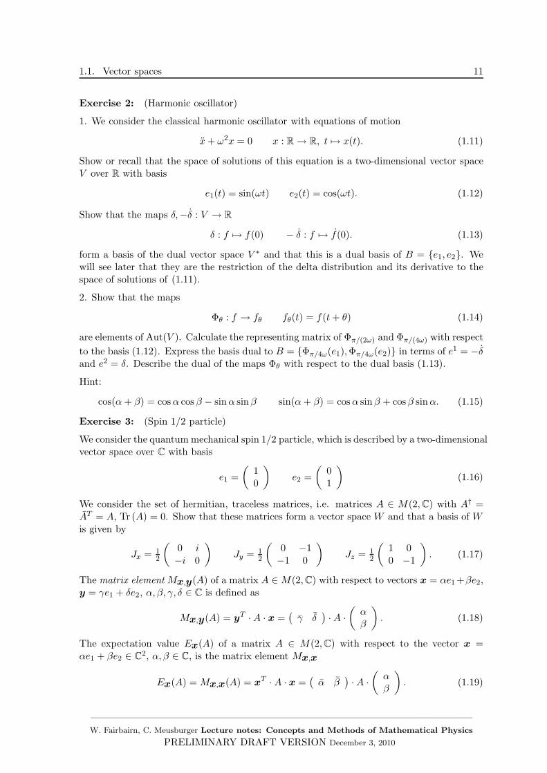
Exercise 2: (Harmonic oscillator)
1. We consider the classical harmonic oscillator with equations of motion
x+ ω2x = 0 x : R → R, t 7→ x(t). (1.11)
Show or recall that the space of solutions of this equation is a two-dimensional vector spaceV over R with basis
e1(t) = sin(ωt) e2(t) = cos(ωt). (1.12)
Show that the maps δ,−δ : V → R
δ : f 7→ f(0) − δ : f 7→ f(0). (1.13)
form a basis of the dual vector space V ∗ and that this is a dual basis of B = e1, e2. Wewill see later that they are the restriction of the delta distribution and its derivative to thespace of solutions of (1.11).
2. Show that the maps
Φθ : f → fθ fθ(t) = f(t+ θ) (1.14)
are elements of Aut(V ). Calculate the representing matrix of Φπ/(2ω) and Φπ/(4ω) with respect
to the basis (1.12). Express the basis dual to B = Φπ/4ω(e1),Φπ/4ω(e2) in terms of e1 = −δand e2 = δ. Describe the dual of the maps Φθ with respect to the dual basis (1.13).
Hint:
cos(α+ β) = cosα cos β − sinα sinβ sin(α+ β) = cosα sin β + cosβ sinα. (1.15)
Exercise 3: (Spin 1/2 particle)
We consider the quantum mechanical spin 1/2 particle, which is described by a two-dimensionalvector space over C with basis
e1 =
(10
)e2 =
(01
)(1.16)
We consider the set of hermitian, traceless matrices, i.e. matrices A ∈ M(2,C) with A† =AT = A, Tr (A) = 0. Show that these matrices form a vector space W and that a basis of Wis given by
Jx = 12
(0 i−i 0
)Jy = 1
2
(0 −1−1 0
)Jz = 1
2
(1 00 −1
). (1.17)
The matrix element Mx,y(A) of a matrix A ∈M(2,C) with respect to vectors x = αe1 +βe2,y = γe1 + δe2, α, β, γ, δ ∈ C is defined as
Mx,y(A) = yT ·A · x =(γ δ
)·A ·
(αβ
). (1.18)
The expectation value Ex(A) of a matrix A ∈ M(2,C) with respect to the vector x =αe1 + βe2 ∈ C2, α, β ∈ C, is the matrix element Mx,x
Ex(A) = Mx,x(A) = xT · A · x =(α β
)·A ·
(αβ
). (1.19)
——————————————————————————————————————W. Fairbairn, C. Meusburger Lecture notes: Concepts and Methods of Mathematical Physics
PRELIMINARY DRAFT VERSION December 3, 2010

12 CHAPTER 1. TENSORS AND DIFFERENTIAL FORMS
Show that for any x,y ∈ C2, the expectation value Ex : A 7→ Ex(A) and the real andimaginary part of the matrix elements Mx,y : A 7→ Ex,y(A) are elements of W ∗. Determinevectors x,y,z such that the expectation values Ex, Ey, Ez form a dual basis for Jx, Jy, Jz.Hint: Show first that for x = (α, β)T , α, β ∈ C, we have
Ex(Jx) = −Im(αβ) Ex(Jy) = −Re(αβ) Ex(Jz) = 12(|α|2 − |β|2).
We will now investigate constructions that allow us to build a new vector space out of twogiven ones. The first is the direct sum of two vector spaces. It allows one to combine familiesof linear maps φi : Vi →Wi, i = 1, ..., n into a single linear map φ = φ1⊕...⊕φi : V1⊕...⊕Vn →W1 ⊕ ...⊕Wn.
Definition 1.1.10: (Direct sum of vector spaces)
The direct sum V ⊕W of two vector spaces V and W is the set of tuples (x,y) | x ∈ V,y ∈W, equipped with the vector space addition and scalar multiplication
(x1,y1) + (x2,y2) = (x1 + x2,y1 + y2) t · (x,y) = (tx, ty) (1.20)
for all x,x1,x2 ∈ V , y,y1,y2 ∈ W and t ∈ k. If BV = e1, .., en is a basis of V andBW = f1, ..., fm a basis of W , a basis of V ⊕W is given by
BV⊕W = (ei, 0) | ei ∈ BV ∪ (0, fj) | fj ∈ BW . (1.21)
The maps ıV : V → V ⊕W , ıW : W → V ⊕W
ıV (v) = (v, 0) ıW (w) = (0,w) ∀v ∈ V,w ∈W
are called the canonical injections of V and W into V ⊕W . In the following we often omitthe tuple notation and write x + y for ıV (v) + ıW (w) = (x,y).
The direct sum of two linear maps φ ∈ Hom(V, V ′), ψ ∈ Hom(W,W ′) is the linear mapφ⊕ ψ ∈ Hom(V ⊕W,V ′ ⊕W ′) defined by
φ⊕ ψ(v,w) = (φ(v), ψ(w)) ∀v ∈ V,w ∈W.
An alternative but equivalent definition of the direct sum is via a universality property.
Definition 1.1.11: The direct sum of two vector spaces V,W over k is a vector space,denoted V ⊕W together with two linear maps ıV : V → V ⊕W , iW : W → V ⊕W suchthat for any pair of linear maps β : V → X, γ : W → X there exists a unique bilinear mapφβ,γ : V ⊕W → X such that φβ,γ ıV = β, φβ,γ iW = γ.
1.1.3 (Multi)linear forms
Definition 1.1.12: (Multilinear forms)
1. A n-linear form on a vector space V is a map α : V × ...× V → k that is linear in allarguments
α(.., ty + sz, ...) = t α(...,y, ...) + s α(...,z, ...) ∀t, s ∈ k,xi,y,z ∈ V.
2. For n = 2, the form is called bilinear. The representing matrix of a bilinear form α :V × V → k with respect to a basis B = e1, ..., en of V is the matrix Aα = (αij)i,j=1,...,n
with αij = α(ei, ej). A bilinear form α : V × V → k is called
——————————————————————————————————————W. Fairbairn, C. Meusburger Lecture notes: Concepts and Methods of Mathematical Physics
PRELIMINARY DRAFT VERSION December 3, 2010
1.1. Vector spaces 13
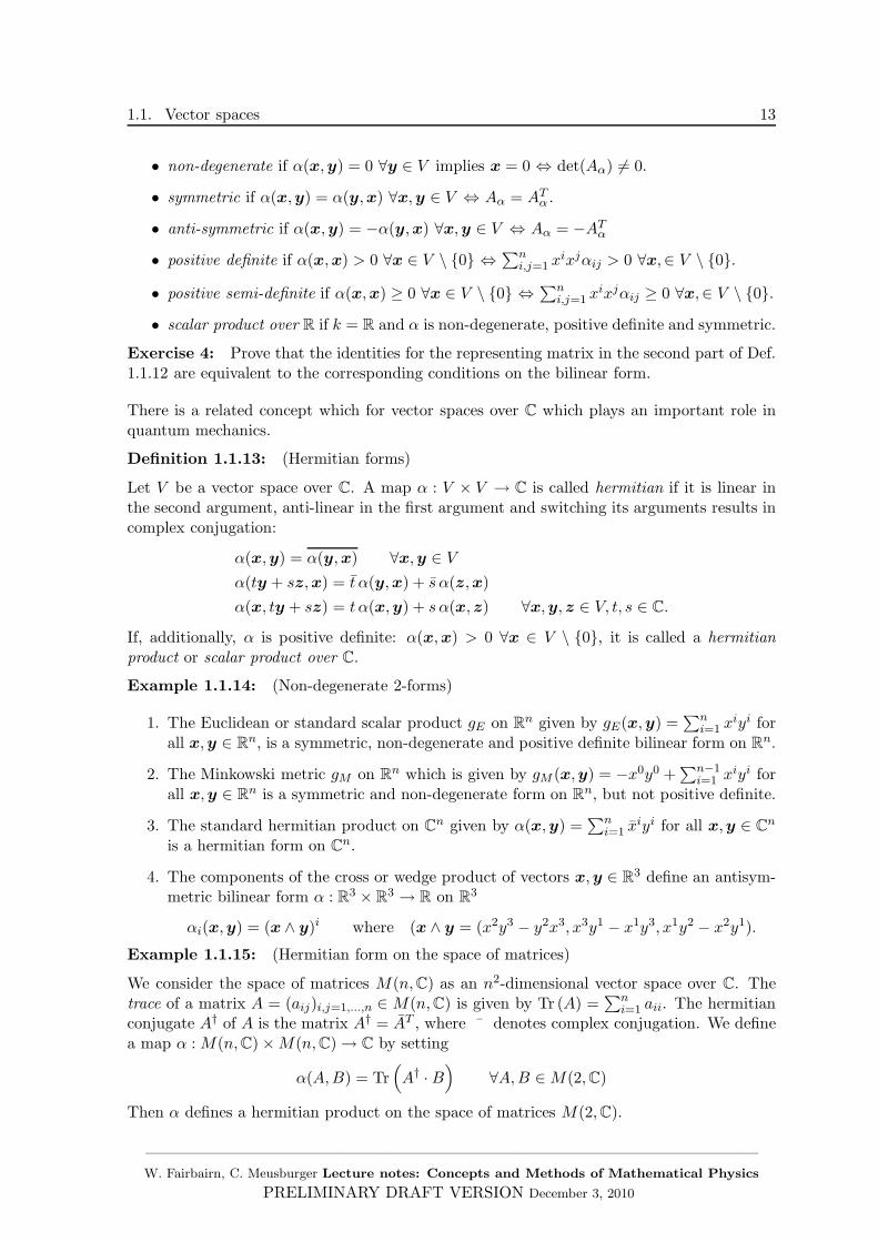
• non-degenerate if α(x,y) = 0 ∀y ∈ V implies x = 0 ⇔ det(Aα) 6= 0.
• symmetric if α(x,y) = α(y,x) ∀x,y ∈ V ⇔ Aα = ATα .
• anti-symmetric if α(x,y) = −α(y,x) ∀x,y ∈ V ⇔ Aα = −ATα• positive definite if α(x,x) > 0 ∀x ∈ V \ 0 ⇔ ∑n
i,j=1 xixjαij > 0 ∀x,∈ V \ 0.
• positive semi-definite if α(x,x) ≥ 0 ∀x ∈ V \ 0 ⇔ ∑ni,j=1 x
ixjαij ≥ 0 ∀x,∈ V \ 0.
• scalar product over R if k = R and α is non-degenerate, positive definite and symmetric.
Exercise 4: Prove that the identities for the representing matrix in the second part of Def.1.1.12 are equivalent to the corresponding conditions on the bilinear form.
There is a related concept which for vector spaces over C which plays an important role inquantum mechanics.
Definition 1.1.13: (Hermitian forms)
Let V be a vector space over C. A map α : V × V → C is called hermitian if it is linear inthe second argument, anti-linear in the first argument and switching its arguments results incomplex conjugation:
α(x,y) = α(y,x) ∀x,y ∈ V
α(ty + sz,x) = t α(y,x) + s α(z,x)
α(x, ty + sz) = t α(x,y) + s α(x,z) ∀x,y,z ∈ V, t, s ∈ C.
If, additionally, α is positive definite: α(x,x) > 0 ∀x ∈ V \ 0, it is called a hermitianproduct or scalar product over C.
Example 1.1.14: (Non-degenerate 2-forms)
1. The Euclidean or standard scalar product gE on Rn given by gE(x,y) =∑n
i=1 xiyi for
all x,y ∈ Rn, is a symmetric, non-degenerate and positive definite bilinear form on Rn.
2. The Minkowski metric gM on Rn which is given by gM (x,y) = −x0y0 +∑n−1
i=1 xiyi for
all x,y ∈ Rn is a symmetric and non-degenerate form on Rn, but not positive definite.
3. The standard hermitian product on Cn given by α(x,y) =∑n
i=1 xiyi for all x,y ∈ Cn
is a hermitian form on Cn.
4. The components of the cross or wedge product of vectors x,y ∈ R3 define an antisym-metric bilinear form α : R3 × R3 → R on R3
αi(x,y) = (x ∧ y)i where (x ∧ y = (x2y3 − y2x3, x3y1 − x1y3, x1y2 − x2y1).
Example 1.1.15: (Hermitian form on the space of matrices)
We consider the space of matrices M(n,C) as an n2-dimensional vector space over C. Thetrace of a matrix A = (aij)i,j=1,...,n ∈ M(n,C) is given by Tr (A) =
∑ni=1 aii. The hermitian
conjugate A† of A is the matrix A† = AT , where ¯ denotes complex conjugation. We definea map α : M(n,C) ×M(n,C) → C by setting
α(A,B) = Tr(A† · B
)∀A,B ∈M(2,C)
Then α defines a hermitian product on the space of matrices M(2,C).
——————————————————————————————————————W. Fairbairn, C. Meusburger Lecture notes: Concepts and Methods of Mathematical Physics
PRELIMINARY DRAFT VERSION December 3, 2010
14 CHAPTER 1. TENSORS AND DIFFERENTIAL FORMS
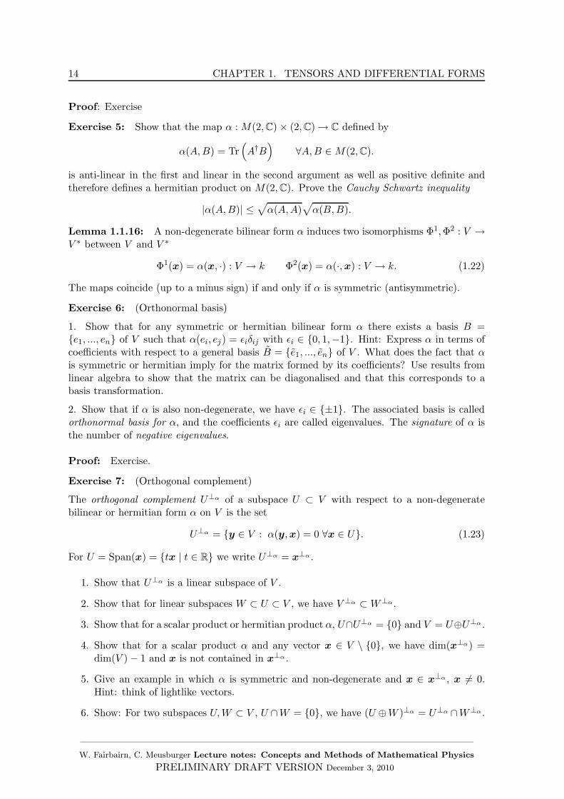
Proof: Exercise
Exercise 5: Show that the map α : M(2,C) × (2,C) → C defined by
α(A,B) = Tr(A†B
)∀A,B ∈M(2,C).
is anti-linear in the first and linear in the second argument as well as positive definite andtherefore defines a hermitian product on M(2,C). Prove the Cauchy Schwartz inequality
|α(A,B)| ≤√α(A,A)
√α(B,B).
Lemma 1.1.16: A non-degenerate bilinear form α induces two isomorphisms Φ1,Φ2 : V →V ∗ between V and V ∗
Φ1(x) = α(x, ·) : V → k Φ2(x) = α(·,x) : V → k. (1.22)
The maps coincide (up to a minus sign) if and only if α is symmetric (antisymmetric).
Exercise 6: (Orthonormal basis)
1. Show that for any symmetric or hermitian bilinear form α there exists a basis B =e1, ..., en of V such that α(ei, ej) = ǫiδij with ǫi ∈ 0, 1,−1. Hint: Express α in terms ofcoefficients with respect to a general basis B = e1, ..., en of V . What does the fact that αis symmetric or hermitian imply for the matrix formed by its coefficients? Use results fromlinear algebra to show that the matrix can be diagonalised and that this corresponds to abasis transformation.
2. Show that if α is also non-degenerate, we have ǫi ∈ ±1. The associated basis is calledorthonormal basis for α, and the coefficients ǫi are called eigenvalues. The signature of α isthe number of negative eigenvalues.
Proof: Exercise.
Exercise 7: (Orthogonal complement)
The orthogonal complement U⊥α of a subspace U ⊂ V with respect to a non-degeneratebilinear or hermitian form α on V is the set
U⊥α = y ∈ V : α(y,x) = 0 ∀x ∈ U. (1.23)
For U = Span(x) = tx | t ∈ R we write U⊥α = x⊥α .
1. Show that U⊥α is a linear subspace of V .
2. Show that for linear subspaces W ⊂ U ⊂ V , we have V ⊥α ⊂W⊥α.
3. Show that for a scalar product or hermitian product α, U∩U⊥α = 0 and V = U⊕U⊥α .
4. Show that for a scalar product α and any vector x ∈ V \ 0, we have dim(x⊥α) =dim(V ) − 1 and x is not contained in x⊥α .
5. Give an example in which α is symmetric and non-degenerate and x ∈ x⊥α , x 6= 0.Hint: think of lightlike vectors.
6. Show: For two subspaces U,W ⊂ V , U ∩W = 0, we have (U ⊕W )⊥α = U⊥α ∩W⊥α.
——————————————————————————————————————W. Fairbairn, C. Meusburger Lecture notes: Concepts and Methods of Mathematical Physics
PRELIMINARY DRAFT VERSION December 3, 2010
1.2. Tensors 15
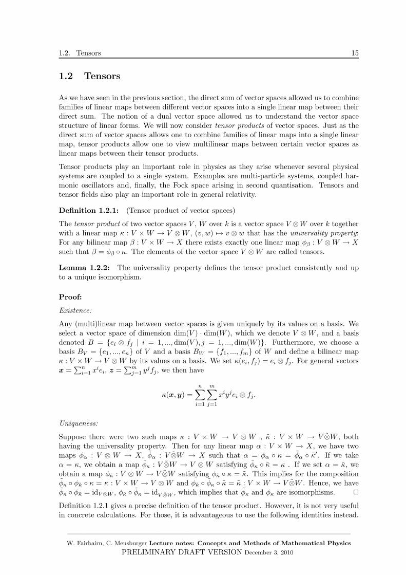
1.2 Tensors
As we have seen in the previous section, the direct sum of vector spaces allowed us to combinefamilies of linear maps between different vector spaces into a single linear map between theirdirect sum. The notion of a dual vector space allowed us to understand the vector spacestructure of linear forms. We will now consider tensor products of vector spaces. Just as thedirect sum of vector spaces allows one to combine families of linear maps into a single linearmap, tensor products allow one to view multilinear maps between certain vector spaces aslinear maps between their tensor products.
Tensor products play an important role in physics as they arise whenever several physicalsystems are coupled to a single system. Examples are multi-particle systems, coupled har-monic oscillators and, finally, the Fock space arising in second quantisation. Tensors andtensor fields also play an important role in general relativity.
Definition 1.2.1: (Tensor product of vector spaces)
The tensor product of two vector spaces V , W over k is a vector space V ⊗W over k togetherwith a linear map κ : V ×W → V ⊗W , (v,w) 7→ v ⊗ w that has the universality property:For any bilinear map β : V ×W → X there exists exactly one linear map φβ : V ⊗W → Xsuch that β = φβ κ. The elements of the vector space V ⊗W are called tensors.
Lemma 1.2.2: The universality property defines the tensor product consistently and upto a unique isomorphism.
Proof:
Existence:
Any (multi)linear map between vector spaces is given uniquely by its values on a basis. Weselect a vector space of dimension dim(V ) · dim(W ), which we denote V ⊗W , and a basisdenoted B = ei ⊗ fj | i = 1, ...,dim(V ), j = 1, ...,dim(W ). Furthermore, we choose abasis BV = e1, ..., en of V and a basis BW = f1, ..., fm of W and define a bilinear mapκ : V ×W → V ⊗W by its values on a basis. We set κ(ei, fj) = ei ⊗ fj. For general vectorsx =
∑ni=1 x
iei, z =∑m
j=1 yjfj, we then have
κ(x,y) =n∑
i=1
m∑
j=1
xiyjei ⊗ fj.
Uniqueness:
Suppose there were two such maps κ : V × W → V ⊗ W , κ : V × W → V ⊗W , bothhaving the universality property. Then for any linear map α : V ×W → X, we have twomaps φα : V ⊗ W → X, φα : V ⊗W → X such that α = φα κ = φα κ′. If we takeα = κ, we obtain a map φκ : V ⊗W → V ⊗W satisfying φκ κ = κ . If we set α = κ, weobtain a map φκ : V ⊗W → V ⊗W satisfying φκ κ = κ. This implies for the compositionφκ φκ κ = κ : V ×W → V ⊗W and φκ φκ κ = κ : V ×W → V ⊗W . Hence, we haveφκ φκ = idV⊗W , φκ φκ = idV ⊗W , which implies that φκ and φκ are isomorphisms. 2
Definition 1.2.1 gives a precise definition of the tensor product. However, it is not very usefulin concrete calculations. For those, it is advantageous to use the following identities instead.
——————————————————————————————————————W. Fairbairn, C. Meusburger Lecture notes: Concepts and Methods of Mathematical Physics
PRELIMINARY DRAFT VERSION December 3, 2010
16 CHAPTER 1. TENSORS AND DIFFERENTIAL FORMS
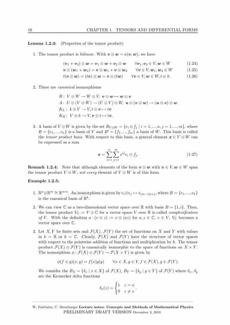
Lemma 1.2.3: (Properties of the tensor product)
1. The tensor product is bilinear. With v ⊗ w = κ(v,w), we have
(v1 + v2) ⊗ w = v1 ⊗ w + v2 ⊗ w ∀v1,v2 ∈ V,w ∈W (1.24)
v ⊗ (w1 + w2) = v ⊗ w1 + v ⊗ w2 ∀v ∈ V,w1,w2 ∈W (1.25)
t(v ⊗ w) = (tv) ⊗ w = v ⊗ (tw) ∀v ∈ V,w ∈W, t ∈ k. (1.26)
2. There are canonical isomorphisms
R : V ⊗W → W ⊗ V, v ⊗ w 7→ w ⊗ v
A : U ⊗ (V ⊗W ) → (U ⊗ V ) ⊗W, u ⊗ (v ⊗ w) → (u ⊗ v) ⊗ w
KL : k ⊗ V → V, t⊗ v 7→ tv
KR : V ⊗ k → V,v ⊗ t 7→ tv.
3. A basis of V ⊗W is given by the set BV⊗W = ei⊗ fj | i = 1, ..., n, j = 1, ...,m, whereB = e1, ..., en is a basis of V and B′ = f1, ..., fm a basis of W . This basis is calledthe tensor product basis. With respect to this basis, a general element x ∈ V ⊗W canbe expressed as a sum
x =
n∑
i=1
m∑
j=1
xijei ⊗ fj. (1.27)
Remark 1.2.4: Note that although elements of the form v ⊗ w with v ∈ V,w ∈ W spanthe tensor product V ⊗W , not every element of V ⊗W is of this form.
Example 1.2.5:
1. Rn⊗Rm ∼= Rm·n. An isomorphism is given by ei⊗ej 7→ e(m−1)i+j , whereB = e1, ..., ekis the canonical basis of Rk.
2. We can view C as a two-dimensional vector space over R with basis B = 1, i. Then,the tensor product VC := V ⊗ C for a vector space V over R is called complexificationof V . With the definition a · (v ⊗ z) := v ⊗ (az) for a, z ∈ C, v ∈ V , VC becomes avector space over C.
3. Let X,Y be finite sets and F(X), F(Y ) the set of functions on X and Y with valuesin k = R or k = C. Clearly, F(X) and F(Y ) have the structure of vector spaceswith respect to the pointwise addition of functions and multiplication by k. The tensorproduct F(X) ⊗ F(Y ) is canonically isomorphic to the space of functions on X × Y .The isomorphism φ : F(X) ⊗F(Y ) → F(X × Y ) is given by
φ(f ⊗ g)(x, y) = f(x)g(y) ∀x ∈ X, y ∈ Y, f ∈ F(X), g ∈ F(Y ).
We consider the BX = δx | x ∈ X of F(X), BY = δy | y ∈ Y of F(Y ) where δx, δyare the Kronecker delta functions
δx(z) =
1 z = x
0 z 6= x.
——————————————————————————————————————W. Fairbairn, C. Meusburger Lecture notes: Concepts and Methods of Mathematical Physics
PRELIMINARY DRAFT VERSION December 3, 2010
1.2. Tensors 17
Clearly, we have for any f ∈ F(X), f =∑
x∈X f(x)δx and similarly for Y . In terms ofthese bases, the isomorphism φ takes the form
φ(δx ⊗ δy) = δ(x,y) δ(x,y)(v,w) =
1 x = v and y = w
0 otherwise.
Its inverse is given by
φ−1 : F(X × Y ) → F(X) ⊗F(Y ), δ(x,y) 7→ δx ⊗ δy.
As the linear maps between vector spaces also form a vector space, we can consider the tensorproduct of vector spaces of linear maps. We obtain the following lemma.
Lemma 1.2.6: (Tensor product of linear maps, functoriality)
For vector spaces U, V,W,Z over k the tensor product Hom(U, V ) ⊗ Hom(W,Z) is canoni-cally isomorphic to Hom(U ⊗W,V ⊗ Z). The isomorphism τ : Hom(U, V ) ⊗ Hom(W,Z) →Hom(U ⊗W,V ⊗ Z) is given by
τ(ψ ⊗ φ)(u ⊗ v) = ψ(u) ⊗ φ(v) ∀ψ ∈ Hom(U, V ), φ ∈ Hom(W,Z),u ∈ U,v ∈ V.
In terms of the maps κV⊗Z : V × Z → V ⊗ Z, κU⊗W : U ×W → U ⊗W introduced in Def.1.2.1, we have
κV⊗Z (ψ, φ) = (ψ ⊗ φ) κU⊗W ∀ψ ∈ Hom(U, V ), φ ∈ Hom(W,Z). (1.28)
We say the tensor product is functorial.
Lemma 1.2.7: (Transformation behaviour of coefficients)
If we characterise ψ ∈ Hom(U, V ), φ ∈ Hom(W,Z) by their matrix coefficients with respectto bases BU = e1, ..., en, BV = f1, ..., fm,BW = g1, ..., gp, BZ = h1, ..., hs
ψ(ei) =m∑
j=1
ψ ji fj φ(gk) =
s∑
l=1
φ lk hl, (1.29)
the matrix coefficients of the tensor product ψ ⊗ φ with respect to the bases BU⊗W =ei⊗ gk | i = 1, ..., n, k = 1, ..., p and BV⊗Z = fj ⊗hl | j = 1, ...,m, l = 1, ..., s are given by
(ψ ⊗ φ)(ei ⊗ gk) =
m∑
j=1
s∑
l=1
ψ ji φ
lk fj ⊗ hl (1.30)
Alternatively, we can characterise the linear map ψ ⊗ φ by its action on the coefficients. For
x =
n∑
i=1
p∑
k=1
xikei ⊗ gk (φ⊗ ψ)(x) =
m∑
j=1
s∑
l=1
x′jlfj ⊗ hl, (1.31)
we have
x′jl =
n∑
i=1
p∑
k=1
ψ ji φ
lk x
ik.
——————————————————————————————————————W. Fairbairn, C. Meusburger Lecture notes: Concepts and Methods of Mathematical Physics
PRELIMINARY DRAFT VERSION December 3, 2010
18 CHAPTER 1. TENSORS AND DIFFERENTIAL FORMS
Exercise 8: (Two spin 1/2 particles)
We consider a system of two spin 1/2 particles as in Example 3. The vector space associatedwith the combined system is the tensor product C2⊗C2 ∼= C4. A basis of C2⊗C2, the tensorproduct basis, is given by
B = e1 ⊗ e1, e1 ⊗ e2, e2 ⊗ e1, e2 ⊗ e2 (1.32)
with e1, e2 as in (1.16). We consider the total spin or total angular momentum
J2tot :=
3∑
a=1
(1 ⊗ Ja + Ja ⊗ 1)(1 ⊗ Ja + Ja ⊗ 1) =
3∑
a=1
J2a ⊗ 1 + 1 ⊗ J2
a + 2Ja ⊗ Ja ∈ End(C2 ⊗ C2)
and the total spin or total angular momentum in the z-direction
J totz = 1 ⊗ Jz + Jz ⊗ 1 ∈ End(C2 ⊗ C2).
Determine the matrix coefficients of J2tot and J totz with respect to the tensor product basis.
Show that another basis of C2 ⊗ C2 is given by
B′ = e1 ⊗ e1, e2 ⊗ e2,1√2(e1 ⊗ e2 − e2 ⊗ e1),
1√2(e1 ⊗ e2 + e2 ⊗ e1). (1.33)
Determine the matrix coefficients of J2tot and J totz with respect to this basis.
After defining the tensor product, we are now ready to investigate the relation betweentensors and multilinear forms. We start by considering the relation between tensor productsand dual vector spaces.
Theorem 1.2.8: (Tensor products and duals)
1. For vector spaces V,W over k, the tensor product of their duals is canonically isomorphicto the dual of their tensor product: V ∗ ⊗W ∗ ∼= (V ⊗W )∗. The isomorphism is given by
τ : α⊗ β 7→ τ(α ⊗ β) τ(α⊗ β)(v ⊗ w) = α(v)β(w) ∀v ∈ V,w ∈W. (1.34)
2. For vector spaces V,W over k, we have V ∗ ⊗W ∼= Hom(V,W ). The isomorphism is
µ :α⊗ w 7→ µ(α⊗ w) µ(α⊗ w)(v) = α(v)w ∀v ∈ V,w ∈W. (1.35)
Corollary 1.2.9: The n-fold tensor product V ∗ ⊗ ...⊗ V ∗ can be identified with the spaceof n-forms α : V × ...× V → k. The identification is given by
µ(α1 ⊗ ...⊗ αn)(v1, ...,vn) = α1(v1) · · ·αn(vn) ∀v1, ...,vn ∈ V, α1, ..., αn ∈ V ∗. (1.36)
In the following, we will often omit the isomorphisms µ, τ in theorem 1.2.8 and write α ⊗β(v ⊗ w) = α(v)β(w) for (1.34) and (α⊗ w)(v) = α(v)w for (1.35).
These relations between the tensor product of vector spaces, their duals and multilinearforms extend to multiple tensor products of vector spaces and their duals. To define this, weintroduce the tensor algebra.
——————————————————————————————————————W. Fairbairn, C. Meusburger Lecture notes: Concepts and Methods of Mathematical Physics
PRELIMINARY DRAFT VERSION December 3, 2010
1.2. Tensors 19
Definition 1.2.10: (Tensor algebra)
1. For a vector space V and r, s ≥ 0, we define the tensor space of type (r,s)
⊗
r,s
V := V ⊗ ...⊗ V︸ ︷︷ ︸r×
⊗V ∗ ⊗ ...⊗ V ∗︸ ︷︷ ︸
s×
⊗
0,0
V = k. (1.37)
elements of⊗
r,s V are called homogeneous tensors of type (r,s).
2. The tensor algebra T (V ) is the direct sum
T (V ) =⊕
r,s≥0
⊗
r,s
V. (1.38)
We define a multiplication ⊗ : T (V ) ⊗ T (V ) → T (V ) via its action on the homogeneoustensors and extend it bilinearly to T (V ). For u1 ⊗ ... ⊗ ur ⊗ α1 ⊗ ... ⊗ αs ∈ ⊗r,s V andx1 ⊗ ...⊗ xp ⊗ β1 ⊗ ...⊗ βq ∈
⊗p,q V we set
(u1 ⊗ ...⊗ ur ⊗ α1 ⊗ ...⊗ αs) ⊗ (x1 ⊗ ...⊗ xp ⊗ β1 ⊗ ...⊗ βq) (1.39)
:= u1 ⊗ ...⊗ ur ⊗ x1 ⊗ ...⊗ xp ⊗ α1 ⊗ ...⊗ αs ⊗ β1 ⊗ ...⊗ βp ∈⊗
r+p,s+q
V. (1.40)
Remark 1.2.11: With the multiplication defined in (1.2.10), the tensor algebra becomesan associative, graded algebra.
• associative means (a⊗ b) ⊗ c = a⊗ (b⊗ c) for all a, b, c ∈ T (V ).
• graded means that T (V ) can be expressed as a direct sum of homogeneous spaces as in(1.38) and the multiplication adds their degrees ⊗ :
⊗r,s V ×⊗p,q V →⊗
r+p,s+q V .
Remark 1.2.12: The tensor algebra plays an important role in quantum field theory. TheFock spaces constructed in the formalism of second quantisation are tensor algebras of certainvector spaces.
Remark 1.2.13: (Interpretation of (r, s)-tensors)
Together, Theorem 1.2.8 and Definition 1.2.10 imply that we can interpret an (r, s) tensorv1 ⊗ ...⊗ vr ⊗ α1 ⊗ ...⊗ αs ∈
⊗r,s V as
• a multilinear map
V × ...× V︸ ︷︷ ︸s×
→⊗
r,0
V
(x1, ...,xs) 7→ α1(x1) · · ·αs(xs)v1 ⊗ ...⊗ vr
• a multilinear map
V ∗ × ...× V ∗︸ ︷︷ ︸
r×→⊗
0,s
V
(β1, ..., βr) 7→ β1(v1) · · · βr(vr)α1 ⊗ ...⊗ αs
——————————————————————————————————————W. Fairbairn, C. Meusburger Lecture notes: Concepts and Methods of Mathematical Physics
PRELIMINARY DRAFT VERSION December 3, 2010

20 CHAPTER 1. TENSORS AND DIFFERENTIAL FORMS
• a linear map
⊗
s,0
V →⊗
r,0
V
x1 ⊗ ...⊗ xs 7→ α1(x1) · · ·αs(xs)v1 ⊗ ...⊗ vr
• a linear map
⊗
0,r
→⊗
0,s
V
β1 ⊗ ...⊗ βr 7→ β1(v1) · · · βr(vr)α1 ⊗ ...⊗ αs
• a linear form on⊗
s,r V
⊗
s,r
V → k
x1 ⊗ ...⊗ xs ⊗ β1 ⊗ ...⊗ βr 7→ α1(x1) · · ·αs(xs)β1(v1) · · · βr(vr).
Example 1.2.14: Vectors are (1, 0)-tensors. Linear forms are (0, 1)-tensors. Linear mapsare (1, 1)-tensors. Bilinear forms are (0, 2)-tensors.
Lemma 1.2.15: (Coefficients and transformation behaviour)
1. With respect to a basis B = e1, ..., en of V and dual basis B∗ = e1, ..., en, a generalelement in
⊗r,s V can be expressed as
x =n∑
i1,...,ir,j1,...,js=1
xi1...isj1...jsei1 ⊗ ...⊗ eir ⊗ ej1 ⊗ ...⊗ ejs (1.41)
The upper indices are called covariant indices and lower indices contravariant indices.
2. We consider linear maps φ1, .., φr , ψ1, ...ψs ∈ End(V ) with matrix elements
φk(ei) =
n∑
j=1
(φk)ji ej ψl(ei) =
n∑
j=1
(ψl)ji ej (1.42)
Then, the transformation of a (r, s) tensor under φ1 ⊗ ...⊗ φr ⊗ ψ1 ⊗ ...⊗ ψs is given by
φ1 ⊗ ...⊗ φr ⊗ ψ1 ⊗ ...⊗ ψs(ei1 ⊗ ...⊗ eir ⊗ ej1 ⊗ ...⊗ ejs) = (1.43)n∑
k1,...,kr,l1,...ls=1
(φ1)k1i1
· · · (φr) krir
(ψ1)j1l1
· · · (ψs) jsls
ek1 ⊗ ...⊗ ekr ⊗ el1 ⊗ ...⊗ els .
and the coefficients transform according to
xi1...isj1...js7→
n∑
k1,...,kr,l1,...ls=1
(φ1)k1i1
· · · (φr) krir
(ψ1)j1l1
· · · (ψs) jsls
xl1...lsk1...kr(1.44)
——————————————————————————————————————W. Fairbairn, C. Meusburger Lecture notes: Concepts and Methods of Mathematical Physics
PRELIMINARY DRAFT VERSION December 3, 2010
1.3. Alternating forms and exterior algebra 21
Definition 1.2.16: (Trace and contraction of tensors)
The trace is the canonical linear map Tr : End(V ) ∼= V ⊗ V ∗ → k
Tr : v ⊗ α 7→ α(v) ∀v ∈ V, α ∈ V ∗. (1.45)
When expressed in terms of the coefficients with respect to a basis B = e1, ..., en of V andits dual basis B∗ = e1, ..., en, the trace coincides with the matrix trace.
Tr
n∑
i,j=1
xijei ⊗ ej
=
n∑
i=1
xii (1.46)
Exercise 9:
Suppose that the following quantities denote the coefficients of a (r, s)-tensor, i.e. an elementof⊗
r,s V , with respect to a basis B = e1, ..., en of V and its dual B∗ = e1, ..., en
gij xijmn yijik zijk. (1.47)
Determine (r, s) for each of them and give expressions for the five maps in remark 1.2.13 interms of B and B∗ and in terms of the coefficients. Use Einstein summation convention.
Example:
wkij is the coefficient of a (1,2)-tensor. The associated map ϕ : V × V → V is given by
ϕ(ei, ej) = wkijek, ϕ(x,y)k = wkijxiyj.
The associated map φ : V ∗ → V ∗ ⊗ V ∗ is given by
φ(ek) = wkijei ⊗ ej φ(α)ij = wkijαk.
The associated map ψ : V ⊗ V → V is given by
ψ(ei ⊗ ej) = wkijek ψ(x ⊗ y)k = wkijxiyj.
1.3 Alternating forms and exterior algebra
We will now consider a special type of multilinear forms, namely the ones that are alternatingor anti-symmetric, and we will construct the associated dual object.
Definition 1.3.1: (Alternating or exterior k-form)
An alternating (or exterior) k-form on V is a k-form on V such that
σα(v1, ...,vk) = α(vσ(1), ...,vσ(k)) = sig(σ)α(v1, ...,vk) ∀v1, ...,vk ∈ V, σ ∈ S(k),
where the sign sig(σ) of the permutation σ ∈ S(k) is sig(σ) = (−1)n, where n is the numberof elementary transpositions, i.e. exchanges of neighbouring elements needed to obtain σ or,equivalently, the number of pairs (i, j), i, j ∈ 1, ..., k with i < j and σ(i) > σ(j). Explicitly,
sig(σ) = Πi<ji− j
σ(i) − σ(j). (1.48)
The alternating k-forms on V form a vector space which we denote by Altk(V ). The vectorspace Alt(V ) of alternating forms on V is the direct sum Alt(V ) =
⊕∞k=0 Altk(V ).
——————————————————————————————————————W. Fairbairn, C. Meusburger Lecture notes: Concepts and Methods of Mathematical Physics
PRELIMINARY DRAFT VERSION December 3, 2010
22 CHAPTER 1. TENSORS AND DIFFERENTIAL FORMS
Example 1.3.2: For σ ∈ S(3), σ : (1, 2, 3) 7→ (3, 1, 2) sig(σ) = 1, since there are two pairs,(1, 3) and (2, 3), whose order is inverted by sigma and two elementary transpositions areneeded to obtain sigma
(1, 2, 3) 7→ (1, 3, 2) 7→ (3, 1, 2).
For σ ∈ S(4), σ : (1, 2, 3, 4) 7→ (2, 4, 1, 3), we have sig(σ) = −1 since there are three pairs,(1, 2), (1, 4) and (3, 4), with i < j and σ(i) > σ(j) and three elementary transpositions areneeded to obtain σ
(1, 2, 3, 4) 7→ (1, 2, 4, 3) 7→ (2, 1, 4, 3) 7→ (2, 4, 1, 3).
Example 1.3.3: We have Alt1(V ) = V ∗. Alternating one-forms are one-forms. Alternatingtwo-forms are antisymmetric bilinear forms on V .
Lemma 1.3.4: (Properties of Altk(V ))
1. An alternating k-form vanishes on (v1, ...,vk) if are v1, ...,vk linearly dependent.
2. This implies in particular that it is antisymmetric
α(v1, ...,vj , ...,vi, ...vn) = −α(v1, ...,vi, ...,vj, ...,vn). (1.49)
3. Altk(V ) = 0 for all k > dim(V ).
As we have seen in the previous section, there is a duality between n-forms on V and tensorproducts ⊗nV , that allows us to interpret n-forms as elements of
⊗n V ∗ and led to thedefinition of the tensor algebra. We would now like to specialise this definition to alternatingk-forms and construct an object that takes the role of tensor algebra for alternating forms.This object is the exterior algebra of a vector space V . To define it, we have to introduce thealternator.
Definition 1.3.5: (Alternator, k-fold exterior product of V )
The alternator is the bilinear map
ak :⊗
k,0
V →⊗
k,0
V (1.50)
v1 ⊗ ....⊗ vk 7→ ak(v1 ⊗ ...⊗ vk) = 1k!
∑
σ∈S(k)
sig(σ) vσ(1) ⊗ ...⊗ vσ(k). (1.51)
Its image Im(ak) ⊂ ⊗k,0V is called the k-fold exterior product and denoted ΛkV .
Lemma 1.3.6: The alternator is a projector from⊗
k,0 V onto its image ΛkV : akak = ak.
Proof: Exercise.
Lemma 1.3.7: Altk(V ) = Λk(V ∗). ΛkV has properties analogous to those in Lemma 1.3.4:
1. x ∈ Λk(V ) ⇒ x(α1, ..., αk) = 0 if α1, ..., αk linearly dependent.
2. ΛkV = 0 for k > dim(V ).
——————————————————————————————————————W. Fairbairn, C. Meusburger Lecture notes: Concepts and Methods of Mathematical Physics
PRELIMINARY DRAFT VERSION December 3, 2010
1.3. Alternating forms and exterior algebra 23
Definition 1.3.8: (Exterior algebra, wedge product)
1. The exterior algebra or Grassmann algebra is the vector space given as the direct sum
ΛV =
dim(V )⊕
k=0
ΛkV. (1.52)
2. The wedge product ∧ : ΛkV × ΛlV → Λk+lV is the unique bilinear map that satisfies
ak(x) ∧ al(y) = (k+l)!k!l! ak+l(x ⊗ y) ∀x ∈ ΛkV,y ∈ ΛlV. (1.53)
3. By extending the wedge product bilinearly to ΛV , we obtain a bilinear map ∧ : ΛV ×ΛV → ΛV . This gives ΛV the structure of an associative, graded algebra.
Remark 1.3.9: Equation (1.53) defines the wedge product consistently and uniquely.
Lemma 1.3.10: (Properties of the wedge product)
The wedge product is
1. bilinear:α ∧ (tβ + sγ) = tα∧ β + sα∧ γ, (tβ + sγ)∧ α = tβ ∧ α+ sγ ∧ α ∀t, s ∈ k, α, β, γ ∈ ΛV
2. associative: (α ∧ β) ∧ γ = α ∧ (β ∧ γ) for all α, β, γ ∈ ΛV
3. graded anti-commutative (skew): For α ∈ ΛkV, β ∈ ΛlV : α ∧ β = (−1)klβ ∧ α.
4. natural: φ∗(α ∧ β) = φ∗(α) ∧ φ∗(β) for all φ ∈ End(V ), α, β ∈ Λ(V ∗) = Alt(V ).
5. related to the determinant:
α1 ∧ ... ∧ αk(v1, ..., vk) = det (αi(vj))i,j∈1,...,k ∀α1, ..., αk ∈ Λ1V ∗ (1.54)
6. given by the identity
x1 ∧ ... ∧ xl =(k1 + ...+ kl)!
k1!k2! · · · kl!ak1+...+kl
(x1 ⊗ ...⊗ xl) xi ∈ ΛkiV. (1.55)
Theorem 1.3.11: (Basis of ΛkV )
For any basis B = e1, ..., en of V , a basis of ΛkV is given by the ordered k-fold wedgeproducts of elements in B
BΛkV = ei1 ∧ ei2 ... ∧ eik , 0 < i1 < i2 < ... < ik ≤ n. (1.56)
This implies dim(ΛkV ) =
(nk
)= n!
k!(n−k)! . In particular, ΛnV is one-dimensional and
spanned by e1 ∧ e2 ∧ ... ∧ en.Exercise 10: (Transformation under linear maps)
Show that for any linear map φ ∈ End(V ) with det(φ) = 1 and associated matrix Aφ =(φi j)i,j∈1,...,n, we have
φ∗(e1) ∧ ... ∧ φ∗(en)(v1, ...,vn) = e1 ∧ ... ∧ en(φ(v1), ..., φ(vn)) = det(Aφ). (1.57)
——————————————————————————————————————W. Fairbairn, C. Meusburger Lecture notes: Concepts and Methods of Mathematical Physics
PRELIMINARY DRAFT VERSION December 3, 2010
24 CHAPTER 1. TENSORS AND DIFFERENTIAL FORMS
The fact that the dimension of ΛkV is dim(ΛkV ) = n!k!(n−k)! = dim(Λn−kV ) suggests that
there should be an identification between the vector spaces ΛkV and Λn−kV . Note, however,that this identification is not canonical, since it requires additional structure, namely a non-degenerate symmetric (or hermitian) bilinear form on V .
Lemma 1.3.12: (Hodge operator)
1. Consider a vector space V over k and let α be a non-degenerate symmetric or hermitianbilinear form on V . We obtain a symmetric, non-degenerate bilinear form on ΛkV bychoosing a basis B = e1, ..., en of V and setting
α : ΛkV × ΛkV → R α(ei1 ∧ ... ∧ eik , ej1 ∧ ... ∧ ejk) = α(ei1 , ej1) · · ·α(eik , ejk)
for 0 < i1 < i2 < ... < ik ≤ n, 0 < j1 < j2 < ... < jn ≤ n.
By Exercise 6 there exists a basis in which α(ei, ej) = ǫiδij with ǫi ∈ ±1. For thisbasis, we have
α(ei1 ∧ ... ∧ eik , ej1 ∧ ... ∧ ejk) = ǫi1 · · · ǫikδi1,j1 · · · δik ,jk (1.58)
for 0 < i1 < i2 < ... < ik ≤ n, 0 < j1 < j2 < ... < jn ≤ n.
2. There is a unique bilinear map ∗α : ΛkV → Λn−kV the Hodge operator or Hodge starthat satisfies x∧ (∗αy) = α(x,y)e1 ∧ ...∧ en for all x,y ∈ ΛkV . It is given by its valueson a basis of ΛkV
∗α(ei1 ∧ ... ∧ eik) = (−1)sgn(σ)ǫi1 · · · ǫikej1 ∧ ... ∧ ejn−k,
where 0 < i1 < i2 < ... < ik ≤ n, 0 < j1 < ... < jn−k ≤ n, i1, ..., ik ∪ j1, ..., jn−k =1, ..., n and σ ∈ Sn is the permutation
σ > (i1, ..., ik , j1, ..., jn−k) → (1, ..., n).
The Hodge operator satisfies
(a) ∗α(e1 ∧ ... ∧ en) = (−1)ǫ1...ǫn, ∗α1 = e1 ∧ ... ∧ en(b) For all x ∈ ΛkV , y ∈ Λn−kV : α(x, ∗αy) = (−1)k(n−k)α(∗αx,y)
(c) For all x ∈ ΛkV : ∗α(∗αx) = (−1)k(n−k)+ǫ1···ǫnx.
Example 1.3.13: (Angular momentum, wedge product)
We consider R3 with the standard scalar product α = gE . For vectors x =∑3
i=1 xiei,
p =∑n
i=1 piei, we set
l =3∑
i=1
liei = ∗α(x ∧ p). (1.59)
Then, the components of l =∑3
i=1 liei are given by
l1 = x2p3 − p2x3 l2 = x3p1 − x1p3 l3 = x1p2 − x2p1. (1.60)
We recover the usual expression for the angular momentum. This also explains the use ofthe symbol ∧ for the wedge or cross product of two vectors in R3.
——————————————————————————————————————W. Fairbairn, C. Meusburger Lecture notes: Concepts and Methods of Mathematical Physics
PRELIMINARY DRAFT VERSION December 3, 2010
1.3. Alternating forms and exterior algebra 25
We now consider the transformation of l under the linear map φ : R3 → R3, y → −y. Whilethe vectors x and p transform as x → −x, p → −p, we have x ∧ p → x ∧ p. with thedefinition l′ = ∗α(φ(x) ∧ φ(p)), we find l′ = l. This is due to the fact that the bilinear formα is not invariant under the linear map φ, as can be shown using Exercise 10.
The angular momentum therefore does not transform as a usual vector under the map φ.One says that l transforms as a pseudovector or axial vector. Similarly, one can define apseudoscalar s by setting s = ∗αx ∧ p ∧ k, where x,p,k are three linearly independentvectors in R3. Under the map φ, s transforms as s→ s′ = ∗α(x′ ∧ p′ ∧ k′) = −s.
We generalise this observation to the following definition and lemma
Definition 1.3.14: (Pseudovector, pseudoscalar)
Let V be a vector space of odd dimension over R, α a non-degenerate bilinear form as inLemma 1.3.12 with associated orthonormal basis B = e1, ..., en and exterior algebra ΛV .Then:
• elements of Λ0V = k are called scalars
• elements of Λ1V = V are called vectors
• elements of Λn−1V ∼= V are called pseudovectors
• elements of ΛnV ∼= k are called pseudoscalars.
Lemma 1.3.15: An oriented vector space V is a vector space V over R together with thechoice of an ordered basis B. Two ordered bases are said to induce the same orientation if theyare related by a linear map φ ∈ Aut(V ) with positive determinant. A linear map φ ∈ Aut(V )is called orientation preserving if detφ > 0 and orientation reversing if detφ < 0.
Let V be a vector space over R of odd dimension. Under an orientation reversing linear mapφ ∈ Aut(φ), detφ = −1 with matrix coefficients φ(ei) =
∑nj=1 φ
ji ej scalars, pseudoscalars,
vectors and pseudovectors transform according to
• scalars s ∈ Λ0V : s→ s
• vectors x =∑n
i=1 xiei ∈ Λ1V : xi → φ i
j xj
• pseudovectors y =∑n
i=1 yie1 ∧ ...ei... ∧ en: yi → −φ i
j yj
• pseudoscalars r · e1 ∧ ... ∧ en ∈ ΛnV : r → −r.
Definition 1.3.14 and Lemma 1.3.15 solve the puzzle about the transformation behaviour ofpseudovectors and pseudoscalars. They are not really vectors or scalars, but, respectively, thetuple of coefficients of n − 1-forms and n-forms. In odd-dimensional spaces, an orientationreversing map changes the sign of the form which spans the space of n-forms and leavesinvariant the sign of the basis vectors which span the space of n− 1-forms. This explains theresulting transformation behaviour of the coefficients.
——————————————————————————————————————W. Fairbairn, C. Meusburger Lecture notes: Concepts and Methods of Mathematical Physics
PRELIMINARY DRAFT VERSION December 3, 2010
26 CHAPTER 1. TENSORS AND DIFFERENTIAL FORMS
1.4 Vector fields and differential forms
Definition 1.4.1: (Submanifolds of Rn)
A subset M ⊂ Rn is called a submanifold of dimension k of Rn if for all points ∀p ∈M thereexist open neighbourhoods U ⊂ Rn and functions f1, ..., fn−k : U → R ∈ C∞(Rn) such that
1. M ∩ U = x ∈ U : f1(x) = ... = fn−k(x) = 0.
2. The gradients gradf1(p),... ,gradfn(p) are linearly independent, where gradf =∑n
i=1 ∂ifei.
Example 1.4.2: (Submanifolds of Rn)
1. Any open subset U ⊂ Rn is a n-dimensional submanifold of Rn.
2. Linear subspaces V ⊂ Rn are submanifolds of Rn.
3. The (n−1)-sphere Sn−1 = x =∑n
i=1 xiei ∈ Rn | ∑n
i=1(xi)2 = 1 is a n−1-dimensional
submanifold of Rn.
4. The (n − 1)-dimensional hyperbolic space Hn−1 = x =∑n−1
i=0 xiei ∈ Rn | − (x0)2 +∑n−1
i=1 (xi)2 = −1 is a n− 1-dimensional submanifold of Rn.
Definition 1.4.3: (Tangent vector, tangent space)
A vector v ∈ Rn is called a tangent vector in p at a submanifold M ⊂ Rn if there exists asmooth curve c :] − ǫ, ǫ[→M , c(0) = p, c(0) = v.
The tangent space on M at p is the set TpM = v ∈ Rn | v tangent vector at M in p. It isa k-dimensional linear subspace of Rn. The dual vector space T ∗
pM is called the cotangentspace on M at p.
The set TM =⋃p∈M TpM is called tangent bundle, the set T ∗M =
⋃p∈M (TpM)∗ the cotan-
gent bundle of M . The tangent bundle TM and the cotangent bundle T ∗M are equippedwith canonical projections πM : TM → M , v ∈ TpM 7→ p ∈ M and πM : T ∗M → M ,α ∈ (TMp )∗ 7→ p ∈M .
Example 1.4.4:
1. For open subsets U ⊂ Rn, we have TpU = Rn for all p ∈ U .
2. If V ⊂ Rn is linear subspace, we have TpV = V for all p ∈ V .
3. For all p ∈ Sn−1 the tangent space in p is given by TpSn−1 = p⊥ = x ∈ Rn :∑n
i=1 xipi = 0.
4. For all p ∈ Hn−1, we have TpHn−1 = p⊥ = x ∈ Rn : x0p0 −∑n−1
i=1 xipi = 0.
Proof: The first two examples are trivial. In the case of Sn−1, curves c :] − ǫ, ǫ[→ M withc(0) = p must satisfy
∑ni=1 ci(t)
2 = 1. This implies
d
dt|t=0
(n∑
i=1
ci(t)2
)= 2
n∑
i=1
ci(0)ci(0) = 2
n∑
i=1
ci(0)pi = 0
and therefore c(0) ∈ p⊥. The proof for Hn−1 is analogous. 2
——————————————————————————————————————W. Fairbairn, C. Meusburger Lecture notes: Concepts and Methods of Mathematical Physics
PRELIMINARY DRAFT VERSION December 3, 2010
1.4. Vector fields and differential forms 27
Definition 1.4.5: (Vector fields, tensor fields and differential forms)
1. We consider a submanifold M ⊂ Rn. A vector field on M is a map
Y :M → TM p 7→ Y (p) ∈ TpM.
The set of all vector fields on M , denoted Vec(M), is a vector space over R with respectto pointwise addition and multiplication by R.
2. A (r, s)-tensor field on M is a map
g : M →⊗
r,s
TM p 7→ g(p) ∈⊗
r,s
TpM.
The set of all tensor fields on M is a vector space over R with respect to pointwiseaddition and multiplication by R.
3. A differential form of order k on M (or k-form on M) is a map
ω : M →⋃
p∈MΛk(T ∗
pM) p 7→ ω(p) ∈ ΛkT ∗p (M).
The set of all k-forms on M , denoted Ωk(M), is a vector space on M with respect topointwise addition and multiplication by R. 0-forms are functions on M .
In the following we will mostly restrict attention to submanifolds U ⊂ Rn that are opensubsets. However, most of the statements that follow generalise to the situation where U isa general submanifold of Rn or, generally, a manifold.
Lemma 1.4.6: (Expression in coordinates)
Let U ⊂ Rn be an open subset and x1, ..., xn be the canonical coordinates on Rn with respectto its standard basis B = e1, ..., en. We denote by B∗ = e1, ..., en the dual basis. Thebasis vector fields associated with these coordinates are
∂i :U → TU p 7→ ∂i(p) = ei ∀p ∈ U, i ∈ 1, ..., n. (1.61)
The associated basis one-forms are
dxi :U → T ∗U p 7→ dxi(p) = ei ∀p ∈ U, i ∈ 1, ..., n. (1.62)
1. A vector field on U can be expressed as a linear combination of the basis vector fieldswith coefficients that are functions on U
Y =
n∑
i=1
yi∂i yi : U → R. (1.63)
A vector field is called continuous, differentiable, smooth etc. if all coefficient functionsare continuous, differentiable, smooth etc. We denote by Vec(U) the vector space ofsmooth vector fields on U .
——————————————————————————————————————W. Fairbairn, C. Meusburger Lecture notes: Concepts and Methods of Mathematical Physics
PRELIMINARY DRAFT VERSION December 3, 2010
28 CHAPTER 1. TENSORS AND DIFFERENTIAL FORMS
2. A k-form ω : U → ΛkT ∗U on U can be expressed as:
ω =∑
1≤i1<...<ik≤nfi1...ikdx
i1 ∧ ... ∧ dxik fi1...ik : U → R. (1.64)
A k-form ω is called continuous, differentiable, smooth etc. if all coefficient functionsfi1...ik : U → R are continuous, differentiable, smooth etc. We denote by Ωk(U) thevector space of smooth k-forms on U .
3. A (r, s)-tensor field g : U → ⊗r,s TM can be expressed in terms of the basis vector
fields and the basis of one-forms as
g =n∑
i1,...,ir,j1,...,js=1
gi1···irj1···js∂i1 ⊗ ...⊗ ∂ir ⊗ dxj1 ⊗ ...⊗ dxjs gi1···irj1···js : U → R.
A (r, s)-tensor field is called continuous, differentiable, smooth etc. if all coefficientfunctions gi1···irj1···js : U → R are continuous, differentiable, smooth etc.
Definition 1.4.7: (Action of a vector field on a function)
The action of a smooth vector field X ∈ Vec(U) on functions f ∈ C∞(U) defines a mapC∞(U) → C∞(U), f → X.f given by
X.f(p) :=d
dt|t=0f(p+ tX(p)). (1.65)
For X =∑n
i=1 xi∂i, x
i ∈ C∞(U), we have
Xf(p) =n∑
i=1
xi(p)∂if(p). (1.66)
In particular, the basis vector fields ∂i act by partial derivatives ∂i.f(p) = ddt |t=0f(p+ tei).
We can thus interpret vector fields as differential operators on the vector space C∞(M) ofsmooth functions on a manifold M . Moreover, the preceding definitions imply that we canthink of a vector field as something that attaches an element of a vector space V to every pointof a submanifold M ⊂ Rn and of a differential form as something that attaches an elementof the dual vector space V ∗ to each point of M . All structures that we have encountered inthe previous sections - duality, exterior algebra - will give rise to corresponding structures forvector fields and differential forms. These structures are obtained by defining them pointwise.
Definition 1.4.8: (Operations on k-forms)
1. Sum of k-forms and products with functions: For k-forms ω,α ∈ Ωk(U) and functionsf ∈ C∞(U), the sum ω+α ∈ Ωk(U) and the product f ·ω ∈ Ωk(U) are defined pointwise
(ω + α)(p) = ω(p) + α(p) (fω)(p) = f(p)ω(p) ∀p ∈ U. (1.67)
2. Wedge product: The wedge product of differential forms ω ∈ Ωk(U), α ∈ Ωl(U), is the(k + l)-form ω ∧ α ∈ Ωk+l defined pointwise as
(ω ∧ α)(p) = ω(p) ∧ α(p) ∀p ∈ U. (1.68)
——————————————————————————————————————W. Fairbairn, C. Meusburger Lecture notes: Concepts and Methods of Mathematical Physics
PRELIMINARY DRAFT VERSION December 3, 2010
1.4. Vector fields and differential forms 29
Remark 1.4.9: All properties and identities we derived previously for the exterior algebrahold pointwise. In particular, the wedge product satisfies identities analogous to the ones inLemma 1.3.10.
To generalise the Hodge star to k-forms, we need additional structure, namely an assignmentof a non-degenerate symmetric bilinear form on TpU to every point p ∈ U . This turns Uinto a pseudo-Riemannian manifold or, if the form is positive definite, into a Riemannianmanifold.
Definition 1.4.10: (Riemannian and pseudo-Riemannian manifold)
A submanifold M ⊂ Rn is called a pseudo-Riemannian manifold if it is equipped with asmooth symmetric non-degenerate (0, 2)-tensor field, i.e. a smooth map
g : M → T ∗pM ⊗ T ∗
pM p 7→ g(p) ∈ T ∗pM ⊗ T ∗
pM (1.69)
that assigns to every point p ∈ M a symmetric, non-degenerate bilinear form g(p) on TpM .The (0, 2)-tensor field g is called a pseudo-Riemannian metric on M . If g(p) is positivedefinite for all p ∈M , g is called a Riemannian metric on M and M is called a Riemannianmanifold.
In local coordinates the metric g takes the form
g =
n∑
i,j=1
gijdxi ⊗ dxj gij = gji : M → R smooth. (1.70)
Definition 1.4.11: (Hodge operator)
Let U ⊂ Rn be an open subset of Rn, g a pseudo-Riemannian metric on U . Then there existvector fields E1, ..., En ∈ Vec(U), the orthonormal basis for g, such that E1(p), ..., En(p) arelinearly independent for all p ∈ U and
gp(Ei(p), Ej(p)) = ǫiδij ǫi ∈ ±1 ∀p ∈ U.
In terms of the basis vector fields ∂1, ..., ∂n ∈ Vec(U), these vector fields are given by coefficientfunctions U j
i ∈ C∞(U)
Ei =
n∑
j=1
U ji ∂j
such that the matrix U ji (p) is invertible for all p ∈ U . We denote by (U−1) j
i ∈ C∞(U) the
components of its inverse, i.e. the functions characterised by the condition∑n
j=1 Uj
i (U−1) kj =
δki . Then the one-forms dXi defined by
dXi =
n∑
j=1
(U−1) ij dx
j
are dual to the vector fields Ei: dXj(Ei) = δji . We define a non-degenerate symmetric bilinear
form g on Ωk(U) by setting
g(dXi, dXj) = ǫiδij (1.71)
g(dXi1 ∧ ... ∧ dXik , dXj1 ∧ ... ∧ dXjk) = g(dXi1 , dXj1) · · · g(dXik , dXjk)
——————————————————————————————————————W. Fairbairn, C. Meusburger Lecture notes: Concepts and Methods of Mathematical Physics
PRELIMINARY DRAFT VERSION December 3, 2010
30 CHAPTER 1. TENSORS AND DIFFERENTIAL FORMS
for i1 < i2 < ... < ik, j1 < ... < jk, ik, jk ∈ 1, ..., n. The Hodge operator is the unique map∗g : Ωk(U) → Ωn−k(U) defined by
ω ∧ ∗gη = g(ω, η) · dx1 ∧ ... ∧ dxn. (1.72)
In terms of the one-forms dXi, we have
∗g(dXi1 ∧ . . . ∧ dXik ) = (−1)sgn(σ)ǫi1 · · · ǫikdXj1 ∧ . . . ∧ dXjn−k ,
where 0 < i1 < · · · < ik ≤ n, 0 < j1 < · · · < jn−k ≤ n, i1, ..., ik ∪ j1, ..., jn−k = 1, ..., nand sgn(σ) is the sign of the permutation
σ : (i1, ..., ik , j1, ..., jn−k) 7→ (1, ..., n).
Remark 1.4.12: The properties and identities in Lemma 1.3.12 generalise to this situation.What is different is that the orthonormal basis of g(p) changes with p ∈ U . The vector fieldsEi that diagonalise g and the associated one-forms dXi are therefore not a constant linearcombination of the basis vector fields ∂i and one-forms dxi, but a linear combination withcoefficients that are functions on U .
It remains to investigate how differential forms behave under functions that map the manifoldM or the open subset U ⊂ Rn to other manifolds. The concept which characterises theirbehaviour under such transformations is the pull-back.
Definition 1.4.13: (Pull-back of differential forms)
Let U ⊂ Rn, V ⊂ Rm be open subsets and let ω ∈ Ωk(U) be a k-form that is given by
ω =∑
1≤i1<...<ik≤nfi1...ik dx
i1 ∧ ... ∧ dxin . (1.73)
Suppose there exists a continuously differentiable map φ = (φ1, ..., φn) : V ⊂ Rm → U ⊂ Rn.Then, the pull-back of ω with φ is the differential form φ∗ω ∈ Ωk(V ) defined by
φ∗ω(p)(v1, ...,vn) = ω(φ(p)) (dpφv1, ..., dpφvn) ∀v1, ...,vn ∈ TpU,
where dpφ is the matrix dpφ = (∂iφj(p))ij . In local coordinates, we have
φ∗ω =∑
1≤i1<...<ik≤nfi1...ik φ dφi1 ∧ ... ∧ dφik dφi =
n∑
j=1
∂jφi dxj (1.74)
Lemma 1.4.14: (Properties of the pull-back)
The pull-back of differential forms
1. is linear: φ∗(tω1 + sω2) = tφ∗ω1 + sφ∗ω2 for all ω1, ω2 ∈ Ωk(U), t, s ∈ R
2. commutes with the wedge product: φ∗(ω ∧ σ) = (φ∗ω) ∧ (φ∗σ)for all ω ∈ Ωk(M), σ ∈ Ωl(M)
3. satisfies (φ ψ)∗ω = ψ∗(φ∗ω).
——————————————————————————————————————W. Fairbairn, C. Meusburger Lecture notes: Concepts and Methods of Mathematical Physics
PRELIMINARY DRAFT VERSION December 3, 2010
1.4. Vector fields and differential forms 31
After generalising the structures encountered for alternating forms and the exterior algebra todifferential forms, we will now investigate the new structures which arise from the dependenceon the points p ∈M . The first is the exterior differential of a differential form.
Definition 1.4.15: (Exterior Differential)
Let U ⊂ Rn be an open subset of Rn. The exterior differential is a map d : Ω(U) → Ω(U),d(Ωk(U)) ⊂ Ωk+1(U), defined by
dω =∑
1≤i1<...<ik≤ndfi1....ik ∧ dxi1 ∧ ... ∧ dxik =
∑
1≤i1<...<ik≤n,j 6=i1,...,ik∂jfi1...ik dx
j ∧ dxi1 ∧ ... ∧ dxik
for ω =∑
1≤i1<...<ik≤nfi1....ik ∧ dxi1 ∧ ... ∧ dxik ∈ Ωk(U) fi1···ik ∈ C∞(U). (1.75)
Remark 1.4.16: Note that this definition is independent of the choice of coordinates. Theexterior differential depends only on the k-form ω itself and is therefore well-defined.
Lemma 1.4.17: (Properties of exterior differential)
The exterior differential
1. is linear: d(tω1 + sω2) = tdω1 + sdω2 ∀ω1, ω2 ∈ Ωk(U), t, s ∈ R
2. is graded anti-commutative (skew)
d(ω ∧ σ) = (dω) ∧ σ + (−1)kω ∧ dσ ∀ω ∈ Ωk(U), σ ∈ Ωl(U)
3. satisfies d2ω = d(dω) = 0
4. Commutes with the pull-back: For any continuously differentiable map φ = (φ1, ..., φn) :V ⊂ Rm → U ⊂ Rn, we have d(φ∗ω) = φ∗(dω) for all ω ∈ Ωk(U).
Proof: Exercise.
Remark 1.4.18: The compatibility between exterior differential and pull-back d(φ∗)ω =Φ∗(dω) and the identity d2ω = 0 arise from the fact that the exterior derivative and differentialforms are antisymmetric. Roughly speaking, the antisymmetry of differential forms and ofthe exterior derivative kills all second order derivatives which arise when one applies theexterior differential to the pull-back or to the differential form dω.
Exercise 11:
1. Show that the exterior differential is well-defined and independent of the choice of co-ordinates. Consider first its transformation under a linear map φ : Rn → Rn and showthat d(φ∗)ω = Φ∗(dω) in that case. Prove now the identity d(φ∗)ω = Φ∗(dω) for a general(continuously differentiable) map φ = (φ1, ..., φn) : V ⊂ Rm → U ⊂ Rn.
2. We consider an open subset U ⊂ Rn and attempt to define a symmetric exterior differentialby setting
df =n∑
i=1
∂ifdxi ∀f ∈ C∞(U) (1.76)
dω =
n∑
j=1
12∂jf
i(dxi ⊗ dxj + dxj ⊗ dxi) for ω =
n∑
i=1
fidxi ∈ Ω1(U).
——————————————————————————————————————W. Fairbairn, C. Meusburger Lecture notes: Concepts and Methods of Mathematical Physics
PRELIMINARY DRAFT VERSION December 3, 2010
32 CHAPTER 1. TENSORS AND DIFFERENTIAL FORMS
Show that this differential does not satisfy d2f = 0 for all f ∈ C∞(U). Investigate how itchanges under the pull-back. Does the identity d(φ∗ω) = φ∗(dω) hold for ω?
Example 1.4.19: (Gradient, divergence, curl)
1. The exterior differential of a function f ∈ Ω0(U) is the gradient
df =n∑
i=1
∂if dxi =
n∑
i=1
(gradf)i dxi ∀f ∈ Ω0(U) (1.77)
Note that the gradient defined in this way is a one-form. In order to obtain a gradientwhich is a vector field on U , we need an identification (TpU)∗ ∼= TpU for all p ∈ U .Such an identification is obtained via a Riemannian metric or via the choice of a basisof TpU and a dual basis of (TpU)∗ for all p ∈ U .
2. The exterior differential of a one-form ω ∈ Ω1(U) is the curl:
dω = 12
n∑
i,j=1
(∂ifj − ∂jfi)dxi ∧ dxj ∀ω =
n∑
i=1
fi dxi ∈ Ω1(U) (1.78)
For U ⊂ R3, we can set dω = g1 dx2 ∧ dx3 + g2 dx
3 ∧ dx1 + g3 dx1 ∧ dx2 and recover the
familiar expression for the curl:
gi = (~∇×~f)i = ǫ jki (∂jfk − ∂kfj),
where ǫ jki is the totally antisymmetric tensor with ǫ 23
1 = 1.
3. The exterior differential of a n− 1-form is related to the divergence div~f =∑n
i=1 ∂ifi.We consider a (n− 1)-form
ω =
n∑
i=1
(−1)i−1fi dx1 ∧ dx2 ∧ ... ∧ dxi ∧ ... ∧ dxn = ∗gE
(n∑
i=1
fi dxi
)
where ∗gEis the Hodge operator associated with the Euclidean metric gE on Rn. The
differential of ω is given by
dω =
(n∑
i=1
∂ifi
)· dx1 ∧ ... ∧ dxn = div~f · dx1 ∧ · · · ∧ dxn ∈ Ωn(U) (1.79)
Exercise 12: Consider an open subset U ⊂ R3.
1. Show that for a function f ∈ C∞(U), the identity d2f = 0 can be reformulated as
~∇× (gradf) = 0.
2. Show that for a one-form ω =∑3
i=1 fi dxi, the identity d2ω = 0 can be reformulated as
div(~∇× ~f) = 0.
——————————————————————————————————————W. Fairbairn, C. Meusburger Lecture notes: Concepts and Methods of Mathematical Physics
PRELIMINARY DRAFT VERSION December 3, 2010
1.4. Vector fields and differential forms 33
Lemma 1.4.20: (Co-differential)
Let U ⊂ Rn be an open subset of Rn, g a pseudo-Riemannian metric of signature s ≤ n withassociated Hodge star ∗g. Then, the co-differential δ = − ∗g d ∗g : Ωk+1(U) → Ωk(U) hasproperties analogous to the ones in lemma 1.4.17. In particular: δ2 = ∗g d∗g ∗g d∗g = 0
Definition 1.4.21: (closed, exact)
A k-form ω ∈ Ωk(U) is called closed if dω = 0. It is called exact if there exists a (k− 1)-formθ ∈ Ωk−1(U) such that ω = dθ.
Clearly, due to the identity d2 = 0, all exact differential forms on an open subset U ⊂ Rn
are closed. The answer to the question if the converse is also true is in general negative.However, it can be shown that for subsets U ⊂ Rn which are star-shaped, every closed formis exact. This is the content of Poincare’s lemma.
Theorem 1.4.22: (Poincare lemma)
Let U ⊂ Rn be open and star-shaped, i.e. such that there exists a point p ∈ U such that forany q ∈ U , the segment [p, q] = (1− t)p+ tq | t ∈ [0, 1] lies in U : [p, q] ⊂ U . Let ω ∈ Ωk(U)be closed. Then ω is exact.
Remark 1.4.23: Do not confuse star-shaped with convex. Star-shaped means that thereexists a point p ∈ U such that the segments connecting it to any other point in U lie in U .Convex means that this is the case for all points p ∈ U . Convex therefore implies star-shaped,but not the other way around.
Exercise 13: (Uniqueness of the exterior differential)
The exterior differential d is a linear map d : Ωk(U) → Ωk+1(U) that satisfies d2 = 0. Inthis exercise, we investigate how unique such a structure is. Given the structures we haveintroduced so far, we attempt to construct other linear maps d : Ωk(U) → Ωk+1(U) thatdiffer from d non-trivially and satisfy d2 = 0.
1. As a first guess, we could consider modifying d by multiplying it with a function f ∈ Ω0(M).Show that the map df : Ωk(M) → Ωk+1(M), ω 7→ f · dω does not satisfy d2
f = 0 unless f isconstant. Multiplying d by a function therefore does not yield a new differential.
2. As a second guess, we could consider modifying d by using a one-form θ ∈ Ω1(U). As weneed a map d : Ωk(U) → Ωk+1(U), the canonical way of implementing this would be to define
dθ(ω) := dω + θ ∧ ω ∀ω ∈ Ωk(U). (1.80)
Show that we have d2θ = 0 if and only if θ is closed. Given a closed θ ∈ Ω1(U), we call the
associated map dθ : Ωk(U) → Ωk+1(U) the covariant derivative with respect to θ.
3. We now consider a vector space V with basis B = e1, .., en and one-forms ω ∈ Ωk(U, V )which take values in the vector space V . With respect to the basis B = e1, .., en, suchvector space valued one-forms can be expressed as
ω =
n∑
a=1
ωa ea with ωa ∈ Ωk(U) ∀a ∈ 1, ..., n. (1.81)
To define a covariant derivative, we use one-forms θ ∈ Ω1(U,End(V )) which take values in thevector space End(V ) of endomorphisms of V . With respect to the basis B, such one-forms
——————————————————————————————————————W. Fairbairn, C. Meusburger Lecture notes: Concepts and Methods of Mathematical Physics
PRELIMINARY DRAFT VERSION December 3, 2010
34 CHAPTER 1. TENSORS AND DIFFERENTIAL FORMS
can be expressed as
θ(ea) =
n∑
b=1
θ ba eb with θ b
a ∈ Ω1(U) ∀a, b ∈ 1, ..., n. (1.82)
We define the covariant derivative with respect to θ as
dθωa = dωa +
n∑
b=1
θ ba ∧ ωb. (1.83)
Show that d2θωa = 0 for all ω ∈ Ωk(U, V ), a = 1, ..., n, if and only if θ is flat:
dθ ba +
n∑
c=1
θ ca ∧ θ b
c = 0. (1.84)
Remark 1.4.24: Such generalised derivatives play an important role in gauge and field the-ories. The one-forms θ used to construct the generalised derivatives dθ corresponds to gaugefields. One-forms θ ∈ ω1(U) correspond to abelian gauge theories such as electromagnetism.One-forms θ ∈ Ω1(U,End(V )) with values in the set of endomorphisms End(V ) correspondto non-abelian gauge theories.
We will now investigate the interaction of vector fields and differential forms. As we haveseen in the context of (multi)linear forms, we can interpret a bilinear form or (0, 2)-tensorg ∈ V ∗ ⊗ V ∗ on a vector space V as a bilinear map g : V × V → R or as a linear mapg : V → V ∗. In the context of vector fields and differential forms, we consider (0, 2)-tensor fields on an open subset U ⊂ Rn, which assign to every point p ∈ U a bilinear formω(p) : TpU × TpU → R. An example are the (pseudo-) Riemannian metrics in Definition1.4.10, which correspond to symmetric non-degenerate (0,2)-tensor fields.
We will now investigate what structures are obtained from anti-symmetric non-degenerate(0,2)-tensor fields or 2-forms on U . One finds that every non-degenerate 2-form on U givesrise to a map Vec(U) × Vec(U) → C∞(U) and to an identification of Vec(U) and Ω1(U).If one combines these structures with the exterior differential of functions f ∈ C∞(U), oneobtains a map C∞(U)× C∞(U) → C∞(U). If the 2-form is also closed, this map is a Poissonbracket.
Lemma 1.4.25: (Identification of vector fields and forms: the Poisson bracket)
Let U ⊂ Rn be open and ω ∈ Ω2(U) a closed, non-degenerate 2-form on U . Such a 2-formis also called a symplectic form on U . The non-degenerate 2-form ω induces an isomorphismbetween Vec(U) and Ω1(U)
Φω : Vec(U) → Ω1(U) X 7→ ω(X, ·). (1.85)
It therefore gives rise to a map
X· : C∞(U) → Vec(U) f 7→ Xf = Φ−1ω (df) (1.86)
and a map
, : C∞(U) × C∞(U) → C∞(U) (1.87)
(f, g) 7→ f, g = df(Xg) = −dg(Xf ) = ω(Xf ,Xg)
The latter has the properties of a Poisson bracket.
——————————————————————————————————————W. Fairbairn, C. Meusburger Lecture notes: Concepts and Methods of Mathematical Physics
PRELIMINARY DRAFT VERSION December 3, 2010
1.5. Electrodynamics and the theory of differential forms 35
1. It is bilinear: tf + sg, h = tf, h + sg, h for all f, g, h ∈ C∞(U), t, s ∈ R.
2. It is antisymmetric: f, g = −g, f for all f, g ∈ C∞U .
3. It satisfies the Leibnitz identity or, in other words, it is a derivation:
f · g, h = f · g, h + g · f, h ∀f, g, h ∈ C∞(U).
4. It satisfies the Jacobi identity:
f, g, h + h, f, g + g, h, f = 0 ∀f, g, h ∈ C∞(U).
If U is star-shaped, there exists a one form θ such that ω = dθ. Such a one-form is called asymplectic potential.
Proof: The bilinearity and antisymmetry follow from the fact that all maps involved inthe definition are linear and from the antisymmetry of the two-form ω. The Leibnitz identityfollows from the identity d(f · g) = f · dg + g · df . The Jacobi identity follows from the factthat ω is closed and the existence of the symplectic potential from Poincare’s lemma. 2
Remark 1.4.26: The Poisson bracket is well known from classical mechanics. There itoften arises from a canonical symplectic form associated with the action that characterises aphysical system. The functions in C∞(U) correspond to the functions on phase space.
1.5 Electrodynamics and the theory of differential forms
An electrodynamical system is described by two fields:
• the electrical field ~E : R4 → R3 which assigns to each point ~x in space and each time tthe value of the electrical field ~E(t, x) ∈ R3 at ~x at time t .
• the magnetic field ~B : R4 → R3 which assigns to each point ~x in space and each time tthe value ~B(t, x) ∈ R3 of the magnetic field at ~x at time t.
together with two densities that describe the behaviour of the electrical charges:
• the charge density ρ : R4 → R which assigns to each point ~x in space and each time tthe density ρ(t, ~x) of the electrical charge at ~x at time t.
• the current density ~ : R4 → R3 which assigns to each point ~x in space and each time tthe density ~(t, ~x) of the electrical current at ~x at time t.
The behaviour of the electromagnetic system is described by the Maxwell equations.
Definition 1.5.1: (Maxwell equations)
We consider an electrical field ~E : R4 → R3, a magnetic field ~B : R4 → R a charge densityρ : R4 → R and a current density ~ : R4 → R3. In units in which the speed of light, thedielectric and the magnetic constant are one: ǫ0 = µ0 = c = 1, the Maxwell equations read
div~E = ρ div ~B = 0 (1.88)
~∇× ~E = −∂t ~B ~∇× ~B =~ + ∂t ~E. (1.89)
——————————————————————————————————————W. Fairbairn, C. Meusburger Lecture notes: Concepts and Methods of Mathematical Physics
PRELIMINARY DRAFT VERSION December 3, 2010
36 CHAPTER 1. TENSORS AND DIFFERENTIAL FORMS
The Maxwell equation div ~B = 0 is often paraphrased as the absence of magnetic sources,while ~∇× ~E = −∂t ~B is known as Faraday’s law. The equation div~E = ρ is often referred toas Gauss’ law and ~∇× ~B =~ + ∂t ~E as Ampere’s law.
In addition to the Maxwell equations, we have the charge conservation law
∂tρ+ div~ = 0. (1.90)
Remark 1.5.2: The Maxwell equations (1.88) can be viewed as consistency conditions onthe electrical and magnetic field ~E(t, ·), ~B(t, ·) at a given time t. The charge conservationlaw describes the time evolution of the charge density, and the Maxwell equations (1.89) thetime evolution of the electrical and magnetic field.
If the electrical field ~E(t, ·), the magnetic field ~B(t, ·) and the charge and current densitiesρ(t, ·),~(t, ·) are known for a given time t, the Maxwell equations uniquely determine theirvalues for all t′ > t.
We will now show that the Maxwell equations can be reformulated in terms of differentialforms and that this formulation is useful for understanding their properties. We consider thevector space R4 with Basis B = e0, e1, e2, e3 and a symmetric non-degenerate bilinear formg, the Minkowski metric, characterised by
g(e0, e0) = −1 g(ei, ei) = 1 for i = 1, 2, 3 g(eµ, eν) = 0 µ, ν ∈ 0, 1, 2, 3, µ 6= ν.
We denote by ∗ the associated Hodge star and by δ = ∗ d ∗ the associated co-differential.To keep the convention most widespread in physics, we will label indices with Greek lettersif they take values µ, ν, ... ∈ 0, 1, 2, 3 and reserve Latin indices i, j, k, ... ∈ 1, 2, 3 for thespatial indices. The time coordinate t therefore corresponds to x0.
By combining the components of the electrical and magnetic field into a two-form and thecurrent and charge density into a one-form, we obtain the following definition.
Definition 1.5.3: (Electrodynamics in formulation with forms)
The field strength tensor is the two-form F ∈ Ω2(R4)
F = −3∑
i=1
Ei dx0 ∧ dxi +B1 dx
2 ∧ dx3 +B2 dx3 ∧ dx1 +B3 dx
1 ∧ dx2.
Its Hodge dual is the two-form ∗F ∈ Ω2(R4), often referred to as dual field strength tensor
∗F = −3∑
i=1
Bi dx0 ∧ dxi − E1 dx
2 ∧ dx3 − E2 dx3 ∧ dx1 −E3 dx
1 ∧ dx2. (1.91)
The four-current J ∈ Ω1(R4) is the one-form
J = −ρ dx0 + j1 dx1 + j2 dx
2 + j3 dx3. (1.92)
with Hodge dual ∗J ∈ Ω3(R4)
∗ J = ρ dx1 ∧ dx2 ∧ dx3 − j1 dx0 ∧ dx2 ∧ dx3 − j2 dx
0 ∧ dx3 ∧ dx1 − j3 dx0 ∧ dx1 ∧ dx2.
——————————————————————————————————————W. Fairbairn, C. Meusburger Lecture notes: Concepts and Methods of Mathematical Physics
PRELIMINARY DRAFT VERSION December 3, 2010
1.5. Electrodynamics and the theory of differential forms 37
Remark 1.5.4: Note that the electrical fields
E =
n∑
i=1
Ei dxi
and the magnetic field
B =n∑
j,k=1
ǫijkBi dxj ∧ dxk
enter the expression for the field strength tensor in a different way. This is related to the factthat the magnetic field B is a pseudovector, i.e. a two-form, while the electrical field E is avector or one-form.
Lemma 1.5.5: (Maxwell equations and charge conservation)
In terms of field strength tensor and four-current, the Maxwell equations take the form
dF = 0 δF = ∗d ∗ F = J. (1.93)
The charge conservation law is given by
δJ = ∗d ∗ J = 0. (1.94)
Proof:
We have
dF =(div ~B
)dx1 ∧ dx2 ∧ dx3 + (∂0B1 + ∂2E3 − ∂3E2) dx
0 ∧ dx2 ∧ dx3
+ (∂0B2 + ∂3E1 − ∂1E3) dx0 ∧ dx3 ∧ dx1 + (∂0B3 + ∂2E1 − ∂1E2) dx
0 ∧ dx1 ∧ dx2.
dF = 0 is therefore equivalent to the absence of magnetic sources and Faraday’s law
dF = 0 ⇔ div ~B = 0, ∂0B + ~∇× ~E = 0. (1.95)
Similarly, we can determine the co-differential δF = ∗d ∗ F . This yields
∗d ∗ F = − div ~E dx0 + (−∂0E1 + ∂2B3 − ∂3B2) dx1 + (−∂0E2 + ∂3B1 − ∂1B3) dx
2
+ (−∂0E3 + ∂1B2 − ∂2B1) dx3.
The equation δF = ∗d ∗ F = 0 is therefore equivalent to Gauss law and Ampere’s law
δF = ∗d ∗ F = J ⇔ div ~E = ρ, ~∇× ~B − ∂t ~E =~. (1.96)
Finally, we determine the co-differential δJ and find that the equation δJ = 0 is equivalentto the current conservation law
δJ = ∗d ∗ J = 0 ⇔ ∂0ρ+ div~ = 0. (1.97)
We will now use Poincare’s lemma to obtain the gauge potentials of electrodynamics. Theseare the vector potential ~A : R4 → R3 and the scalar potential φ : R4 → R from which theelectrical and magnetic field are obtained as
~B = ~∇× ~A ~E = grad φ− ∂0~A, (1.98)
or, equivalently, in coordinates,
Bi = ǫ jki ∂jAk ei = ∂iφ− ∂0Ai.
——————————————————————————————————————W. Fairbairn, C. Meusburger Lecture notes: Concepts and Methods of Mathematical Physics
PRELIMINARY DRAFT VERSION December 3, 2010
38 CHAPTER 1. TENSORS AND DIFFERENTIAL FORMS
Lemma 1.5.6: (Poincare’s lemma ⇒ existence of gauge potentials)
As dF = 0 and R4 star-shaped, Poincare’s lemma implies the existence of a one-form A ∈Ω1(R4), the gauge potential, such that F = dA. With the definition
A = −φdx0 +
3∑
i=1
Aidxi = −φdx0 +A1 dx
1 +A2 dx2 +A3 dx
3, (1.99)
where φ is the scalar potential and Ai are the components of the vector potential, the equationF = dA reproduces (1.98)
F = dA ⇔ ~B = ~∇× ~A ~E = grad φ− ∂0~A. (1.100)
Remark 1.5.7: Note that the gauge potential A is defined only up to addition of an exactone-form dχ ∈ Ω1(R4), χ ∈ Ω0(R4). As d2 = 0, we have: d(A + dχ) = dA + d2χ = dA. Atransformation A 7→ A+dχ corresponds to a transformation of the scalar and vector potential
φ 7→ φ− ∂0χ ~A 7→ ~A+ gradχ (1.101)
and is called a gauge transformation. It can be used to bring the potentials ~A and φ into aform that is suited to the problem under consideration. This is called fixing a gauge.
Exercise 14: (Covariant formulation of electrodynamics in local coordinates)
We express the gauge potential, the field strength tensor and the four-current current usingEinstein’s summation convention
A = Aµdxµ F = 1
2Fµνdxµ ∧ dxν J = jµdx
µ, (1.102)
where all indices µ, ν, ... run from 0 to 3. We set gµν = g(eµ, eν) and denote by gµν its inversegµνg
νρ = δρµ.
1. Show that in these coordinates the equation F = dA takes the form
Fµν = ∂µAν − ∂µAν (1.103)
and the equation dF = 0 reads
∂µFνρ + ∂ρFµν + ∂νFρµ = 0. (1.104)
2. Let now ǫµνρσ be the totally antisymmetric tensor in four indices with the conventionǫ0123 = 1. Note that the totally antisymmetric tensor with four indices satisfies
ǫµνρσǫµντκ = 2(gρτ gσκ − gρκgστ ).
We denote the components of ∗F by ∗F = 12Fµνdxµ ∧ dxν . Show that the components
of ∗F are given by
Fρσ = 12ǫρστκg
τµgκνFµν = 12ǫρστκF
τκ F τκ = gτµgκνFµν (1.105)
and that the equation δF = J reads
∂ρFρσ = jσ with ∂ρ = gµρ∂µ. (1.106)
——————————————————————————————————————W. Fairbairn, C. Meusburger Lecture notes: Concepts and Methods of Mathematical Physics
PRELIMINARY DRAFT VERSION December 3, 2010
1.5. Electrodynamics and the theory of differential forms 39
3. Show that the charge conservation law takes the form
∂σjσ = 0 with ∂ρ = gµρ∂µ. (1.107)
Exercise 15: (Gauge fixing)
1. Coulomb gauge and static Maxwell equations
Show that one can use the gauge freedom A 7→ A + dχ to impose the Coulomb gaugecondition
div ~A = 0. (1.108)
Show that the residual gauge freedom is A 7→ A + dχ, where χ satisfies the Laplaceequation ∆χ =
∑3i=1 ∂
2i χ = 0.
We now consider the electrostatic and magnetostatic case of the Maxwell equations,i.e. a situation where the fields and the charge density are independent of time ∂0
~E =∂0~B = 0, ∂0ρ = 0. Show that the Maxwell equations take the form
div~E = ρ div ~B = 0 (1.109)
~∇× ~E = 0 ~∇× ~B =~ (1.110)
and tat the charge conservation law becomes div~ = 0. Show that if A satisfies thecondition of the Coulomb gauge, the Maxwell equations can be re-formulated as
∆φ = −ρ ∆ ~A =
3∑
i=1
∂2i~A = −~. (1.111)
The potentials φ, ~A are thus solutions of the inhomogeneous Laplace equation.
2. Lorentz gauge and electromagnetic waves
Show that the gauge freedom A 7→ A+dχ can also be used to impose the Lorentz gauge
div ~A+ ∂0φ = 0 (1.112)
and that the residual gauge freedom of this gauge are gauge transformations A 7→ A+dχwhere χ satisfies the wave equation 2χ = ∂2
0χ− ∆χ = 0.
We now consider the Maxwell equations without sources, i.e. a situation with vanishingcharge and current density ρ =~ = 0, in which the Maxwell equations take the form
div ~E = 0 div ~B = 0 (1.113)
~∇×~E = −∂0~B ~∇× ~B = ∂0
~E. (1.114)
Show that in the Lorentz gauge the Maxwell equations
div ~E = 0 ~∇× ~B = ∂0~E. (1.115)
can be expressed as
2φ = 0 2A = 0, (1.116)
while the other two Maxwell equations are satisfied automatically. The potentials φ, ~Aare therefore solutions of the wave equation - they correspond to electromagnetic waves,non-trivial electrical and magnetic fields in the absence of sources and currents.
Hint: Prove and then use the identities
~∇×gradF = 0 ~∇×(~∇× ~G) = grad(div ~G) − 2 ~G. (1.117)
——————————————————————————————————————W. Fairbairn, C. Meusburger Lecture notes: Concepts and Methods of Mathematical Physics
PRELIMINARY DRAFT VERSION December 3, 2010

40 CHAPTER 1. TENSORS AND DIFFERENTIAL FORMS
——————————————————————————————————————W. Fairbairn, C. Meusburger Lecture notes: Concepts and Methods of Mathematical Physics
PRELIMINARY DRAFT VERSION December 3, 2010
Chapter 2
Groups and Algebras
2.1 Groups, algebras and Lie algebras
Groups and algebras play a fundamental role in physics because they are the mathematicalstructures which describe symmetries and observables of physical systems.
Classical symmetries such as rotation or translation symmetry in classical mechanics andLorentz symmetry in special relativity are described by groups. This is due to the fact thecomposition of two symmetries should yield another symmetry, that each symmetry shouldhave an inverse and that there should be a neutral or trivial symmetry. This leads to thedefinition of a group.
One distinguishes ”continuous” symmetries (such as rotations, Lorentz transformations ortranslations), which correspond to Lie groups, and discrete symmetries such as permutationsor time reversal. The former can be differentiated, which leads to the concept of Lie algebras.Lie algebras correspond to infinitesimal symmetries of physical systems and are associatedwith additive quantum numbers in the quantum theory.
(Associative) algebras, often equipped with additional structures, describe observables ofphysical systems. Examples are the Poisson algebras which correspond to phase spaces ofclassical physical systems theory and algebras of observables in the quantum theory.
Definition 2.1.1: (Associative unital algebra, subalgebra, abelian algebra)
1. An (associative) algebra is a vector space A over k = R or k = C together with abilinear map : A×A→ A, the multiplication, that is associative (a b) c = a (b c)for all a, b, c ∈ A. If there exists an element e such that e a = a e = a ∀a ∈ A, thiselement is called the unit and A is called a unital algebra.
2. A (unital) subalgebra of a unital associative algebra A is a linear subspace B ⊂ A thatis a (unital) algebra, i.e. that is closed under the multiplication: b b′ ∈ B ∀b, b′ ∈ B(and that contains the unit: e ∈ B). An algebra is called abelian or commutative ifa b = b a for all a, b ∈ A.
Remark 2.1.2: If a unit exists, it is unique.
Example 2.1.3: (Associative algebras)
41
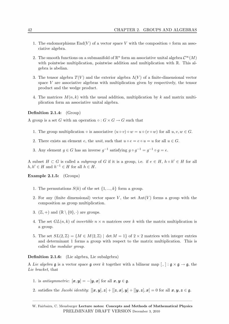
42 CHAPTER 2. GROUPS AND ALGEBRAS
1. The endomorphisms End(V ) of a vector space V with the composition form an asso-ciative algebra.
2. The smooth functions on a submanifold of Rn form an associative unital algebra C∞(M)with pointwise multiplication, pointwise addition and multiplication with R. This al-gebra is abelian.
3. The tensor algebra T (V ) and the exterior algebra Λ(V ) of a finite-dimensional vectorspace V are associative algebras with multiplication given by respectively, the tensorproduct and the wedge product.
4. The matrices M(n, k) with the usual addition, multiplication by k and matrix multi-plication form an associative unital algebra.
Definition 2.1.4: (Group)
A group is a set G with an operation : G×G→ G such that
1. The group multiplication is associative (u v) w = u (v w) for all u, v,w ∈ G.
2. There exists an element e, the unit, such that u e = e u = u for all u ∈ G.
3. Any element g ∈ G has an inverse g−1 satisfying g g−1 = g−1 g = e.
A subset H ⊂ G is called a subgroup of G if it is a group, i.e. if e ∈ H, h h′ ∈ H for allh, h′ ∈ H and h−1 ∈ H for all h ∈ H.
Example 2.1.5: (Groups)
1. The permutations S(k) of the set 1, ..., k form a group.
2. For any (finite dimensional) vector space V , the set Aut(V ) forms a group with thecomposition as group multiplication.
3. (Z,+) and (R \ 0, ·) are groups.
4. The set GL(n, k) of invertible n × n matrices over k with the matrix multiplication isa group.
5. The set SL(2,Z) = M ∈ M(2,Z) | detM = 1 of 2 × 2 matrices with integer entriesand determinant 1 forms a group with respect to the matrix multiplication. This iscalled the modular group.
Definition 2.1.6: (Lie algebra, Lie subalgebra)
A Lie algebra g is a vector space g over k together with a bilinear map [ , ] : g × g → g, theLie bracket, that
1. is antisymmetric: [x,y] = −[y,x] for all x,y ∈ g.
2. satisfies the Jacobi identity: [[x,y],z] + [[z,x],y] + [[y,z],x] = 0 for all x,y,z ∈ g.
——————————————————————————————————————W. Fairbairn, C. Meusburger Lecture notes: Concepts and Methods of Mathematical Physics
PRELIMINARY DRAFT VERSION December 3, 2010
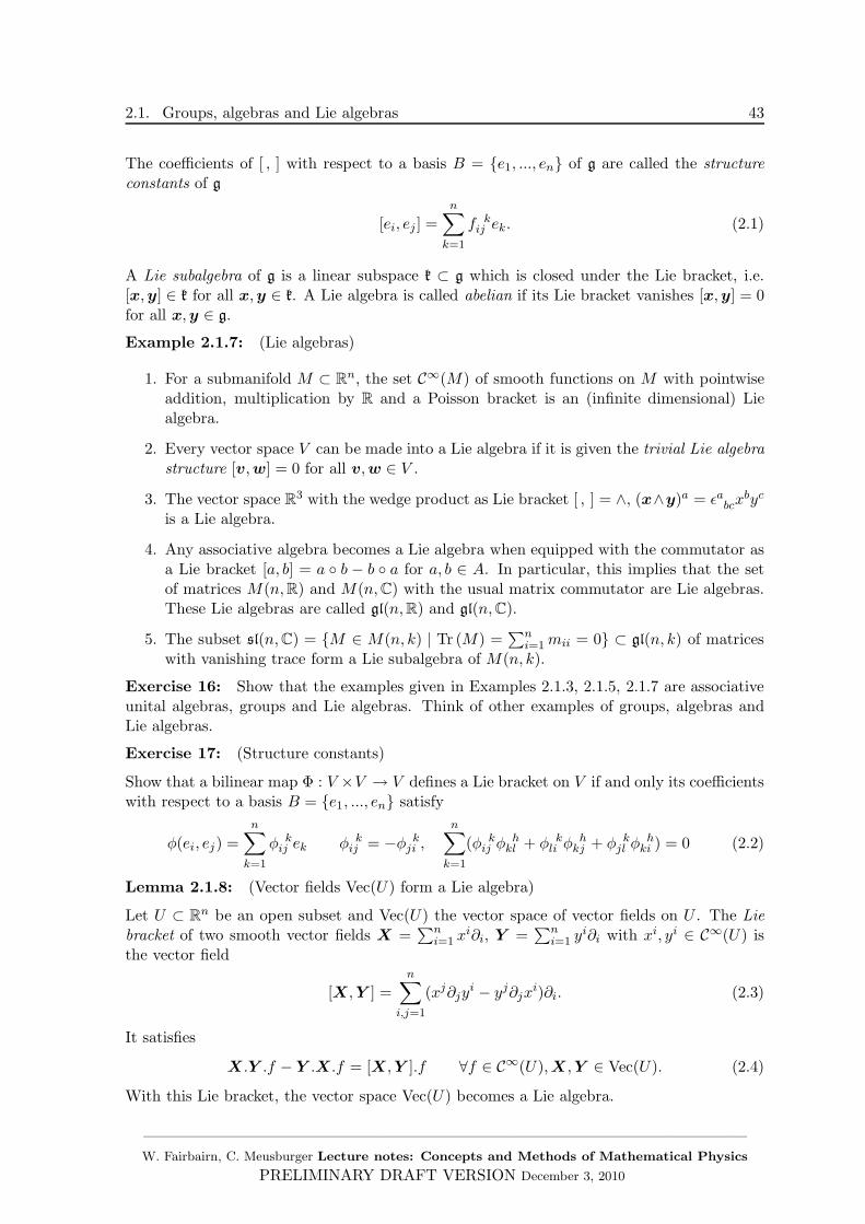
2.1. Groups, algebras and Lie algebras 43
The coefficients of [ , ] with respect to a basis B = e1, ..., en of g are called the structureconstants of g
[ei, ej ] =n∑
k=1
f kij ek. (2.1)
A Lie subalgebra of g is a linear subspace k ⊂ g which is closed under the Lie bracket, i.e.[x,y] ∈ k for all x,y ∈ k. A Lie algebra is called abelian if its Lie bracket vanishes [x,y] = 0for all x,y ∈ g.
Example 2.1.7: (Lie algebras)
1. For a submanifold M ⊂ Rn, the set C∞(M) of smooth functions on M with pointwiseaddition, multiplication by R and a Poisson bracket is an (infinite dimensional) Liealgebra.
2. Every vector space V can be made into a Lie algebra if it is given the trivial Lie algebrastructure [v,w] = 0 for all v,w ∈ V .
3. The vector space R3 with the wedge product as Lie bracket [ , ] = ∧, (x∧y)a = ǫabcxbyc
is a Lie algebra.
4. Any associative algebra becomes a Lie algebra when equipped with the commutator asa Lie bracket [a, b] = a b − b a for a, b ∈ A. In particular, this implies that the setof matrices M(n,R) and M(n,C) with the usual matrix commutator are Lie algebras.These Lie algebras are called gl(n,R) and gl(n,C).
5. The subset sl(n,C) = M ∈ M(n, k) | Tr (M) =∑n
i=1mii = 0 ⊂ gl(n, k) of matriceswith vanishing trace form a Lie subalgebra of M(n, k).
Exercise 16: Show that the examples given in Examples 2.1.3, 2.1.5, 2.1.7 are associativeunital algebras, groups and Lie algebras. Think of other examples of groups, algebras andLie algebras.
Exercise 17: (Structure constants)
Show that a bilinear map Φ : V ×V → V defines a Lie bracket on V if and only its coefficientswith respect to a basis B = e1, ..., en satisfy
φ(ei, ej) =
n∑
k=1
φ kij ek φ k
ij = −φ kji ,
n∑
k=1
(φ kij φ
hkl + φ k
li φhkj + φ k
jl φhki ) = 0 (2.2)
Lemma 2.1.8: (Vector fields Vec(U) form a Lie algebra)
Let U ⊂ Rn be an open subset and Vec(U) the vector space of vector fields on U . The Liebracket of two smooth vector fields X =
∑ni=1 x
i∂i, Y =∑n
i=1 yi∂i with xi, yi ∈ C∞(U) is
the vector field
[X,Y ] =
n∑
i,j=1
(xj∂jyi − yj∂jx
i)∂i. (2.3)
It satisfies
X .Y .f − Y .X.f = [X,Y ].f ∀f ∈ C∞(U),X ,Y ∈ Vec(U). (2.4)
With this Lie bracket, the vector space Vec(U) becomes a Lie algebra.
——————————————————————————————————————W. Fairbairn, C. Meusburger Lecture notes: Concepts and Methods of Mathematical Physics
PRELIMINARY DRAFT VERSION December 3, 2010
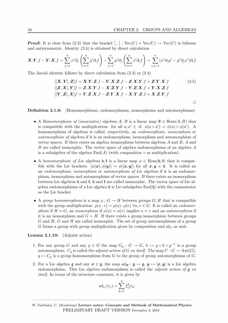
44 CHAPTER 2. GROUPS AND ALGEBRAS
Proof: It is clear from (2.3) that the bracket [ , ] : Vec(U) × Vec(U) → Vec(U) is bilinearand antisymmetric. Identity (2.4) is obtained by direct calculation
X.Y .f − Y .X .f =
n∑
j=1
xj∂j
(n∑
i=1
yi∂if
)−
n∑
j=1
yj∂j
(n∑
i=1
xi∂if
)=
n∑
i,j=1
(xj∂iyi − yj∂jx
i)∂if.
The Jacobi identity follows by direct calculation from (2.3) or (2.4)
[[X ,Y ],Z]f = X.Y .Z.f − Y .X .Z.f − Z.X.Y .f + Z.Y .X.f (2.5)
[[Z ,X],Y ]f = Z.X.Y .f − X.Z.Y .f − Y .Z.X .f + Y .X .Z.f
[[Y ,Z],X]f = Y .Z.X.f − Z.Y .X.f − X.Y .Z.f + X.Z.Y .f
2
Definition 2.1.9: (Homomorphisms, endomorphisms, isomorphisms and automorphisms)
• A Homomorphism of (associative) algebras A, B is a linear map Φ ∈ Hom(A,B) thatis compatible with the multiplication: for all a, a′ ∈ A: φ(a a′) = φ(a) φ(a′). Ahomomorphism of algebras is called, respectively, an endomorphism, isomorphism orautomorphism of algebras if it is an endomorphism, isomorphism and automorphism ofvector spaces. If there exists an algebra isomorphism between algebras A and B, A andB are called isomorphic. The vector space of algebra endomorphisms of an algebra Ais a subalgebra of the algebra End(A) (with composition as multiplication).
• A homomorphism of Lie algebras h, k is a linear map φ ∈ Hom(h, k) that is compat-ible with the Lie brackets: [φ(x), φ(y)] = φ([x,y]) for all x,y ∈ h. It is called anan endomorphism, isomorphism or automorphism of Lie algebras if it is an endomor-phism, isomorphism and automorphism of vector spaces. If there exists an isomorphismbetween Lie algebras h and k, h and k are called isomorphic. The vector space of Lie al-gebra endomorphisms of a Lie algebra h is Lie subalgebra End(h) with the commutatoras the Lie bracket.
• A group homomorphism is a map ρ : G → H between groups G,H that is compatiblewith the group multiplication: ρ(u · v) = ρ(u) · ρ(v) ∀u, v ∈ G. It is called an endomor-phism if H = G, an isomorphism if φ(u) = φ(v) implies u = v and an automorphism ifit is an isomorphism and G = H. If there exists a group isomorphism between groupsG and H, G and H are called isomorphic. The set of group automorphisms of a groupG forms a group with group multiplication given by composition and idG as unit.
Lemma 2.1.10: (Adjoint action)
1. For any group G and any g ∈ G the map Gg : G → G, h 7→ g h g−1 is a groupautomorphism. Cg is called the adjoint action of G on itself. The map C : G→ Aut(G),g 7→ Cg is a group homomorphism from G to the group of group automorphisms of G.
2. For a Lie algebra g and any x ∈ g, the map adx : g → g, y 7→ [x,y] is a Lie algebraendomorphism. This Lie algebra endomorphism is called the adjoint action of g onitself. In terms of the structure constants, it is given by
adei(ej) =n∑
k=1
fkijek.
——————————————————————————————————————W. Fairbairn, C. Meusburger Lecture notes: Concepts and Methods of Mathematical Physics
PRELIMINARY DRAFT VERSION December 3, 2010
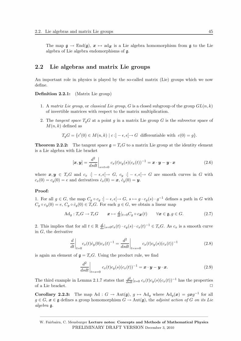
2.2. Lie algebras and matrix Lie groups 45
The map g → End(g), x 7→ adx is a Lie algebra homomorphism from g to the Liealgebra of Lie algebra endomorphisms of g.
2.2 Lie algebras and matrix Lie groups
An important role in physics is played by the so-called matrix (Lie) groups which we nowdefine.
Definition 2.2.1: (Matrix Lie group)
1. A matrix Lie group, or classical Lie group, G is a closed subgroup of the group GL(n, k)of invertible matrices with respect to the matrix multiplication.
2. The tangent space TgG at a point g in a matrix Lie group G is the subvector space ofM(n, k) defined as
TgG = c′(0) ∈M(n, k) | c :] − ǫ, ǫ[→ G differentiable with c(0) = g.
Theorem 2.2.2: The tangent space g = TeG to a matrix Lie group at the identity elementis a Lie algebra with Lie bracket
[x,y] =d2
dsdt
∣∣∣∣s=t=0
cx(t)cy(s)(cx(t))−1 = x · y − y · x (2.6)
where x,y ∈ TeG and cx :] − ǫ, ǫ[→ G, cy :] − ǫ, ǫ[→ G are smooth curves in G withcx(0) = cy(0) = e and derivatives cx(0) = x, cy(0) = y.
Proof:
1. For all g ∈ G, the map Cg cy :] − ǫ, ǫ[→ G, s 7→ g · cy(s) · g−1 defines a path in G withCg cy(0) = e, Cg cy(0) ∈ TeG. For each g ∈ G, we obtain a linear map
Adg : TeG→ TeG x 7→ ddt |t=0Cg cx(t) ∀x ∈ g, g ∈ G. (2.7)
2. This implies that for all t ∈ R dds |s=0cx(t) · cy(s) · cx(t)−1 ∈ TeG. As cx is a smooth curve
in G, the derivative
d
dt
∣∣∣∣t=0
cx(t)cy(0)cx(t)−1 =
d2
dsdt
∣∣∣∣t=s=0
cx(t)cy(s)(cx(t))−1 (2.8)
is again an element of g = TeG. Using the product rule, we find
d2
dsdt
∣∣∣∣t=s=0
cx(t)cy(s)(cx(t))−1 = x · y − y · x. (2.9)
The third example in Lemma 2.1.7 states that d2
dsdt |t=0 cx(t)cy(s)(cx(t))−1 has the properties
of a Lie bracket. 2
Corollary 2.2.3: The map Ad : G → Aut(g), g 7→ Adg where Adg(x) = gxg−1 for allg ∈ G, x ∈ g defines a group homomorphism G→ Aut(g), the adjoint action of G on its Liealgebra g.
——————————————————————————————————————W. Fairbairn, C. Meusburger Lecture notes: Concepts and Methods of Mathematical Physics
PRELIMINARY DRAFT VERSION December 3, 2010
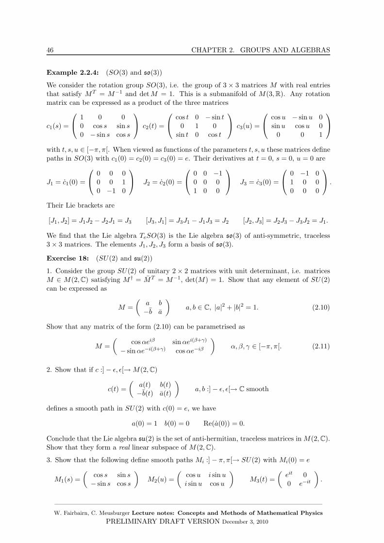
46 CHAPTER 2. GROUPS AND ALGEBRAS
Example 2.2.4: (SO(3) and so(3))
We consider the rotation group SO(3), i.e. the group of 3 × 3 matrices M with real entriesthat satisfy MT = M−1 and detM = 1. This is a submanifold of M(3,R). Any rotationmatrix can be expressed as a product of the three matrices
c1(s) =
1 0 00 cos s sin s0 − sin s cos s
c2(t) =
cos t 0 − sin t0 1 0
sin t 0 cos t
c3(u) =
cosu − sinu 0sinu cos u 0
0 0 1
with t, s, u ∈ [−π, π[. When viewed as functions of the parameters t, s, u these matrices definepaths in SO(3) with c1(0) = c2(0) = c3(0) = e. Their derivatives at t = 0, s = 0, u = 0 are
J1 = c1(0) =
0 0 00 0 10 −1 0
J2 = c2(0) =
0 0 −10 0 01 0 0
J3 = c3(0) =
0 −1 01 0 00 0 0
.
Their Lie brackets are
[J1, J2] = J1J2 − J2J1 = J3 [J3, J1] = J3J1 − J1J3 = J2 [J2, J3] = J2J3 − J3J2 = J1.
We find that the Lie algebra TeSO(3) is the Lie algebra so(3) of anti-symmetric, traceless3 × 3 matrices. The elements J1, J2, J3 form a basis of so(3).
Exercise 18: (SU(2) and su(2))
1. Consider the group SU(2) of unitary 2 × 2 matrices with unit determinant, i.e. matricesM ∈ M(2,C) satisfying M † = MT = M−1, det(M) = 1. Show that any element of SU(2)can be expressed as
M =
(a b−b a
)a, b ∈ C, |a|2 + |b|2 = 1. (2.10)
Show that any matrix of the form (2.10) can be parametrised as
M =
(cosαeiβ sinαei(β+γ)
− sinαe−i(β+γ) cosαe−iβ
)α, β, γ ∈ [−π, π[. (2.11)
2. Show that if c :] − ǫ, ǫ[→M(2,C)
c(t) =
(a(t) b(t)−b(t) a(t)
)a, b :] − ǫ, ǫ[→ C smooth
defines a smooth path in SU(2) with c(0) = e, we have
a(0) = 1 b(0) = 0 Re(a(0)) = 0.
Conclude that the Lie algebra su(2) is the set of anti-hermitian, traceless matrices in M(2,C).Show that they form a real linear subspace of M(2,C).
3. Show that the following define smooth paths Mi :] − π, π[→ SU(2) with Mi(0) = e
M1(s) =
(cos s sin s− sin s cos s
)M2(u) =
(cos u i sinui sinu cos u
)M3(t) =
(eit 00 e−it
).
——————————————————————————————————————W. Fairbairn, C. Meusburger Lecture notes: Concepts and Methods of Mathematical Physics
PRELIMINARY DRAFT VERSION December 3, 2010
2.2. Lie algebras and matrix Lie groups 47
Show that the derivatives of these paths are given by
K1 = M1(0) =
(0 1−1 0
)K2 = M2(0) =
(0 ii 0
)K3 = M3(0) =
(i 00 −i
)
and that they form a basis of the set of traceless, anti-hermitian matrices in M(2,C). Showthat their Lie bracket is given by
[K1,K2] = K3 [K3,K1] = K2 [K2,K3] = K1. (2.12)
3. Define a linear map Φ : su(2) → so(3) by setting Φ(K1) = J1, Φ(K2) = J2, Φ(K3) = J3
where J1, J2, J3 are the matrices in Example 2.2.4. Show that this map is a Lie algebraisomorphism and therefore so(3) ∼= su(2) as Lie algebras.
Remark: As they can be expressed as Lie algebras with structure constants in R, bothso(3) and su(2) are Lie algebras over R. Note that this does not mean that the matricescorresponding to these elements are matrices with entries in R. The anti-hermitian matricesare only a real liner subspace, but not a complex linear subspace of M(n,C).
Remark: As a submanifold of R4 ∼= C2, the group SU(2) is diffeomorphic to the three-sphereS3. The identification is given by
M =
(cosαeiβ sinαei(β+γ)
− sinαe−i(β+γ) cosαe−iβ
)7→ (cosα, sinα cos β, sinα sin β cos γ, sinα sin β sin γ)
α, β ∈ [−π, π[, γ ∈ [0, 2π[.
Theorem 2.2.5: (Exponential map)
Let g be a Lie algebra that is a Lie subalgebra of the Lie algebra gl(n, k). Then, the series
exp(M) =
∞∑
k=0
Mk
k!(2.13)
converges absolutely for all M ∈ M(n, k) and hence defines a map exp : g → M(n, k). Theimage exp(g) is a matrix Lie group.
Proof:
1. We first need to show that the exponential map exp : M(n, k) → M(n, k) is well-defined, i.e. that the series converges absolutely. For this, we consider the norm ||M || =√
Tr (M †M) =√∑n
i,j=1 |mij |2 introduced in Exercise 1.1.15. Using the Cauchy Schwartz
inequality |Tr(A†B
)| ≤ ||A||||B||, one can show by induction that ||Mk|| ≤ ||M ||k for all
k ∈ N. This implies
n∑
k=0
Mk
k!≤
n∑
k=0
||M ||kk!
(2.14)
As∑∞
n=0xk
k! converges for all x ∈ R, the series∑n
k=0Mk
k! converges absolutely, and theexponential map for matrices is well-defined.
——————————————————————————————————————W. Fairbairn, C. Meusburger Lecture notes: Concepts and Methods of Mathematical Physics
PRELIMINARY DRAFT VERSION December 3, 2010
48 CHAPTER 2. GROUPS AND ALGEBRAS
2. We now need to show that the image of exp has the structure of a group. For this, wenote that exp(0) = 1n, where 1n is the n× n unit matrix. Furthermore, we have
exp(M) · exp(−M) =
∞∑
k,l=0
(−1)lMk
k!
M l
l!(2.15)
After a change of variables s = k + l and reordering the sum (which can be done because itconverges absolutely), we obtain
exp(M) exp(−M) =∞∑
s=0
M s
s!
(s∑
l=0
s!
l!(s − l)!(−1)l
)=
∞∑
s=0
M s
s!
(s∑
l=0
(−1)l(sl
))(2.16)
Using the binomial formula (x+ y)s =∑s
l=0
(sl
)xlys−l, we find
exp(M) · exp(−M) =
∞∑
s=0
M s
s!(1 + (−1))s = 1n. (2.17)
This proves the existence of inverses. It remains to show that the image of exp is closedunder the multiplication, i.e. if g = exp(M), h = exp(N) there exists a P ∈ g such thatg · h = exp(P ). This can be shown using the formula of Baker Campbell and Hausdorff, whoshowed that such a P exists and gave an explicit expression for P in terms of M and N
P =∞∑
n=1
(−1)n
n!
∞∑
k1,j1,...,kn,jn=0ki+ji>0 ∀i=1,...,n
1
(∑n
l=1(kl + jl)) k1!j1! · · · kn!jn![Mk1N j1Mk2N j2 · · ·MknN jn ]
[Mk1N j1Mk2N j2 · · ·MknN jn ] := [M, [M, ..., [M︸ ︷︷ ︸k1×
, [N, [N, ..., [N︸ ︷︷ ︸j1×
, ... [M, [M, ...[M︸ ︷︷ ︸kn×
, [N, [N, ...N ]]]...]︸ ︷︷ ︸jn×
.
Note that this multiple commutator vanishes f jn > 1 or jn = 0 and kn > 1. 2
Remark 2.2.6: If g ⊂ M(n, k) is a Lie subalgebra, the Lie algebra of the Lie group G =exp(g) is TeG = g. This follows from the fact that for all g ∈ exp(g), there exists a M ∈ g
such that g = exp(M) and the paths cM :] − ǫ, ǫ[→ G, cM (t) = exp(tM) satisfy cM (0) = e,cM (0) = M . However, given a matrix Lie group G ⊂ M(n, k) with Lie algebra g = TeG, theexponential map exp : g → G is not necessarily surjective. In general, its image is either Gor a proper subgroup of G.
Example 2.2.7: (sl(n, k) and SL(n, k))
We consider the set sl(n, k) of matrices with vanishing trace and entries in k. We claim thatthe image of this Lie algebra under the exponential map exp : M(n,K) → GL(n, k) is thesubgroup SL(n, k) = g ∈ GL(n, k) | det(M) = 1. To show this, we prove the identity
det(exp(K)) = eTr(K) ∀K ∈M(n, k). (2.18)
We set M = tK, t ∈ R, K = (kij)i,j=1,...,n ∈M(n, k) and note that
d
dteTr(tK) = Tr (K) eTr(K).
——————————————————————————————————————W. Fairbairn, C. Meusburger Lecture notes: Concepts and Methods of Mathematical Physics
PRELIMINARY DRAFT VERSION December 3, 2010
2.2. Lie algebras and matrix Lie groups 49
Using the formula for the determinant, we obtain
d
dtdet etK =
d
dt
∑
σ∈Sn
(−1)sgn(σ)(etK)1σ(1) · · · (etK)nσ(n)
=
n∑
l,m=1
∑
σ∈Sn
klm(etK)mσ(l)
(etK)lσ(l)(−1)sgn(σ)(etK)1σ(1) · · · (etK)nσ(n).
From the antisymmetry of the determinant it follows that all terms except the ones withm = l vanish. This yields
d
dtdet etK =
n∑
l=1
∑
σ∈Sn
kll(etK)lσ(l)
(etK)lσ(l)(−1)sgn(σ)(etK)1σ(1) · · · (etK)nσ(n) = det etKTr (K) .
Hence, we have
d
dtln(det etK
)=
Tr (K) · det etK
det etK= Tr (K) =
Tr (K) · etTr(K)
etTr(K)=
d
dtln(etTr(K)
).
This implies det etK = C · etTr(K), where C ∈ C constant. As we have det e0 = det(1n) = 1 =e0, the contant is c = 1, which proves identity (2.18).
Using (2.18), one then finds that the image of a traceless matrix under the exponentialmap is a matrix with unit determinant. This implies that exp(sl(n, k)) is either SL(n, k) aproper subgroup of SL(n, k). To show that it is the whole group, one can select a set ofmultiplicative generators of SL(n, k), i.e. a set of matrices such that any element of SL(n, k)can be expressed as a product in these generators and show that these generators can beobtained via the exponential map. (See Exercise 19) 2.
Exercise 19: (M(n,R) and GL(n,R))
We consider the set GL(n,R) of invertible matrices in M(n,R), i.e. matrices M ∈ M(n,R)with detM 6= 0. As this is an open subset of M(n,R), it is a submanifold of M(n,R) andtherefore a Lie group.
1. To determine TeGL(n,R), we consider the matrices Eij whose only non-zero entry is a1 in row i and column j: (Eij)kl = δi,kδj,l . Show that for i 6= j, Mij(t) = 1n + tEij isinvertible with M−1
ij (t) = 1 − tEij. Show that for all i = 1, ..., n, Mii(t) = 1n + (et − 1)Eii
is invertible with M−1ii (t) = 1n + (e−t − 1)Eii. Conclude that the matrices Mij define paths
Mij :] − ǫ, ǫ[→ GL(n,R) with Mij(0) = 1n, Mij(0) = Eij for all i, j = 1, ..., n. Show that theelements Mij(0) = Eij form a basis of M(n,R) and therefore TeG = M(n,R).
Hint: Show first that E2ij = 0 for i 6= j, E2
ii = Eii.
2. We now consider the exponential map exp : M(n,R) →M(n,R). Use the identity
det(eM ) = exp(Tr (M))
to conclude that exp(M(n,R)) is a subgroup of the group of invertible matrices M ∈ GL(n, k)with det(M) > 0. Although TeGL(n,R) = M(n,R), the image of the exponential mapexp : M(n,R) →M(n,R) is therefore not GL(n,R) but only a subgroup of it.
——————————————————————————————————————W. Fairbairn, C. Meusburger Lecture notes: Concepts and Methods of Mathematical Physics
PRELIMINARY DRAFT VERSION December 3, 2010
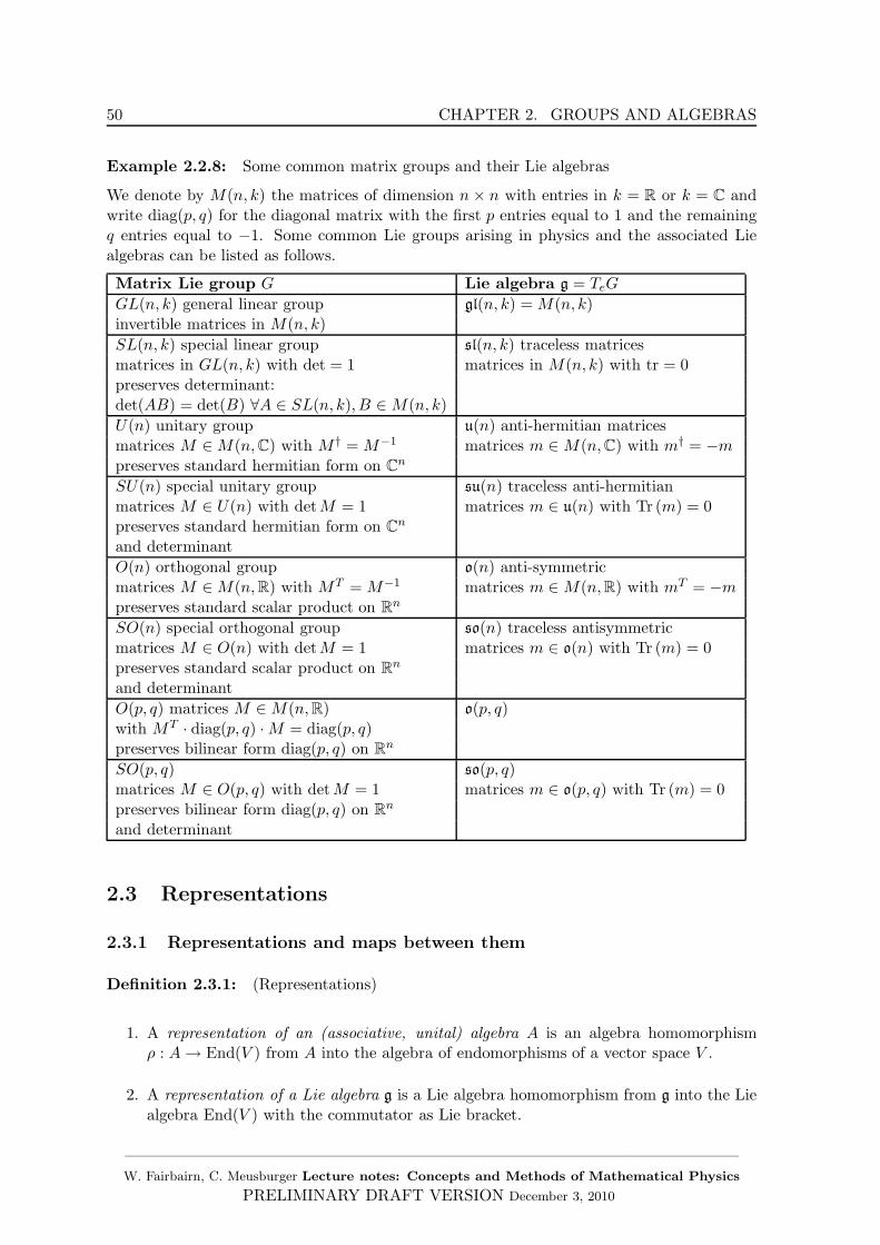
50 CHAPTER 2. GROUPS AND ALGEBRAS
Example 2.2.8: Some common matrix groups and their Lie algebras
We denote by M(n, k) the matrices of dimension n × n with entries in k = R or k = C andwrite diag(p, q) for the diagonal matrix with the first p entries equal to 1 and the remainingq entries equal to −1. Some common Lie groups arising in physics and the associated Liealgebras can be listed as follows.
Matrix Lie group G Lie algebra g = TeG
GL(n, k) general linear group gl(n, k) = M(n, k)invertible matrices in M(n, k)
SL(n, k) special linear group sl(n, k) traceless matricesmatrices in GL(n, k) with det = 1 matrices in M(n, k) with tr = 0preserves determinant:det(AB) = det(B) ∀A ∈ SL(n, k), B ∈M(n, k)
U(n) unitary group u(n) anti-hermitian matricesmatrices M ∈M(n,C) with M † = M−1 matrices m ∈M(n,C) with m† = −mpreserves standard hermitian form on Cn
SU(n) special unitary group su(n) traceless anti-hermitianmatrices M ∈ U(n) with detM = 1 matrices m ∈ u(n) with Tr (m) = 0preserves standard hermitian form on Cn
and determinant
O(n) orthogonal group o(n) anti-symmetricmatrices M ∈M(n,R) with MT = M−1 matrices m ∈M(n,R) with mT = −mpreserves standard scalar product on Rn
SO(n) special orthogonal group so(n) traceless antisymmetricmatrices M ∈ O(n) with detM = 1 matrices m ∈ o(n) with Tr (m) = 0preserves standard scalar product on Rn
and determinant
O(p, q) matrices M ∈M(n,R) o(p, q)with MT · diag(p, q) ·M = diag(p, q)preserves bilinear form diag(p, q) on Rn
SO(p, q) so(p, q)matrices M ∈ O(p, q) with detM = 1 matrices m ∈ o(p, q) with Tr (m) = 0preserves bilinear form diag(p, q) on Rn
and determinant
2.3 Representations
2.3.1 Representations and maps between them
Definition 2.3.1: (Representations)
1. A representation of an (associative, unital) algebra A is an algebra homomorphismρ : A→ End(V ) from A into the algebra of endomorphisms of a vector space V .
2. A representation of a Lie algebra g is a Lie algebra homomorphism from g into the Liealgebra End(V ) with the commutator as Lie bracket.
——————————————————————————————————————W. Fairbairn, C. Meusburger Lecture notes: Concepts and Methods of Mathematical Physics
PRELIMINARY DRAFT VERSION December 3, 2010
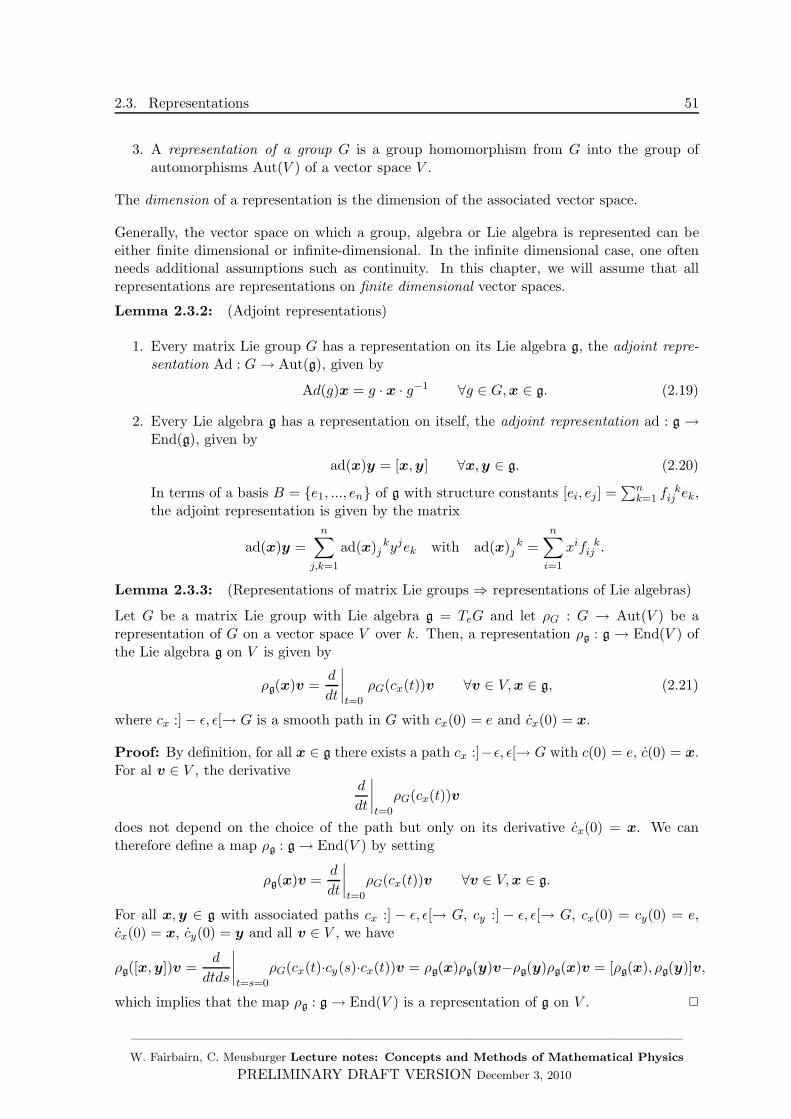
2.3. Representations 51
3. A representation of a group G is a group homomorphism from G into the group ofautomorphisms Aut(V ) of a vector space V .
The dimension of a representation is the dimension of the associated vector space.
Generally, the vector space on which a group, algebra or Lie algebra is represented can beeither finite dimensional or infinite-dimensional. In the infinite dimensional case, one oftenneeds additional assumptions such as continuity. In this chapter, we will assume that allrepresentations are representations on finite dimensional vector spaces.
Lemma 2.3.2: (Adjoint representations)
1. Every matrix Lie group G has a representation on its Lie algebra g, the adjoint repre-sentation Ad : G→ Aut(g), given by
Ad(g)x = g · x · g−1 ∀g ∈ G,x ∈ g. (2.19)
2. Every Lie algebra g has a representation on itself, the adjoint representation ad : g →End(g), given by
ad(x)y = [x,y] ∀x,y ∈ g. (2.20)
In terms of a basis B = e1, ..., en of g with structure constants [ei, ej ] =∑n
k=1 fk
ij ek,the adjoint representation is given by the matrix
ad(x)y =n∑
j,k=1
ad(x) kj y
jek with ad(x) kj =
n∑
i=1
xif kij .
Lemma 2.3.3: (Representations of matrix Lie groups ⇒ representations of Lie algebras)
Let G be a matrix Lie group with Lie algebra g = TeG and let ρG : G → Aut(V ) be arepresentation of G on a vector space V over k. Then, a representation ρg : g → End(V ) ofthe Lie algebra g on V is given by
ρg(x)v =d
dt
∣∣∣∣t=0
ρG(cx(t))v ∀v ∈ V,x ∈ g, (2.21)
where cx :] − ǫ, ǫ[→ G is a smooth path in G with cx(0) = e and cx(0) = x.
Proof: By definition, for all x ∈ g there exists a path cx :]−ǫ, ǫ[→ G with c(0) = e, c(0) = x.For al v ∈ V , the derivative
d
dt
∣∣∣∣t=0
ρG(cx(t))v
does not depend on the choice of the path but only on its derivative cx(0) = x. We cantherefore define a map ρg : g → End(V ) by setting
ρg(x)v =d
dt
∣∣∣∣t=0
ρG(cx(t))v ∀v ∈ V,x ∈ g.
For all x,y ∈ g with associated paths cx :] − ǫ, ǫ[→ G, cy :] − ǫ, ǫ[→ G, cx(0) = cy(0) = e,cx(0) = x, cy(0) = y and all v ∈ V , we have
ρg([x,y])v =d
dtds
∣∣∣∣t=s=0
ρG(cx(t)·cy(s)·cx(t))v = ρg(x)ρg(y)v−ρg(y)ρg(x)v = [ρg(x), ρg(y)]v,
which implies that the map ρg : g → End(V ) is a representation of g on V . 2
——————————————————————————————————————W. Fairbairn, C. Meusburger Lecture notes: Concepts and Methods of Mathematical Physics
PRELIMINARY DRAFT VERSION December 3, 2010
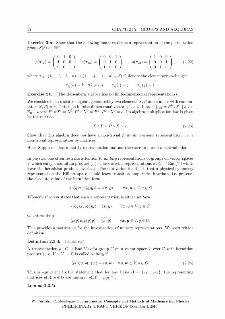
52 CHAPTER 2. GROUPS AND ALGEBRAS
Exercise 20: Show that the following matrices define a representation of the permutationgroup S(3) on R3
ρ(π12) =
0 1 01 0 00 0 1
ρ(π13) =
0 0 10 1 01 0 0
ρ(π23) =
1 0 00 0 10 1 0
, (2.22)
where πij : (1, ..., i, ...j, ...n) → (1, ..., j, ..., i, ...n) ∈ S(n) denote the elementary exchanges
πij(k) = k ∀k 6= i, j πij(i) = j πij(j) = i.
Exercise 21: (The Heisenberg algebra has no finite-dimensional representations)
We consider the associative algebra generated by two elements X,P and a unit e with commu-tator [X,P ] = e. This is an infinite-dimensional vector space with basis ekl = P k X l | k, l ∈N0, where P 0 X l = X l, P k X0 = P k, P 0 X0 = e. Its algebra multiplication law is givenby the relation
X P − P X = e. (2.23)
Show that this algebra does not have a non-trivial finite dimensional representation, i.e. anon-trivial representation by matrices.
Hint: Suppose it has a matrix representation and use the trace to obtain a contradiction.
In physics, one often restricts attention to unitary representations of groups on vector spacesV which carry a hermitian product 〈 , 〉. These are the representations ρ : G→ End(V ) whichleave the hermitian product invariant. The motivation for this is that a physical symmetryrepresented on the Hilbert space should leave transition amplitudes invariant, i.e. preservethe absolute value of the hermitian form.
|〈ρ(g)x, ρ(g)y〉| = |〈x,y〉| ∀x,y ∈ V, g ∈ G
Wigner’s theorem states that such a representation is either unitary
〈ρ(g)x, ρ(g)y〉 = 〈x,y〉 ∀x,y ∈ V, g ∈ G
or anti-unitary〈ρ(g)x, ρ(g)y〉 = 〈x,y〉 ∀x,y ∈ V, g ∈ G.
This provides a motivation for the investigation of unitary representations. We start with adefinition.
Definition 2.3.4: (Unitarity)
A representation ρ : G → End(V ) of a group G on a vector space V over C with hermitianproduct 〈 , 〉 : V × V → C is called unitary if
〈ρ(g)v, ρ(g)w〉 = 〈v,w〉 ∀v,w ∈ V, g ∈ G. (2.24)
This is equivalent to the statement that for any basis B = e1, ..., en, the representingmatrices ρ(g), g ∈ G are unitary: ρ(g)† = ρ(g)−1.
Lemma 2.3.5:
——————————————————————————————————————W. Fairbairn, C. Meusburger Lecture notes: Concepts and Methods of Mathematical Physics
PRELIMINARY DRAFT VERSION December 3, 2010
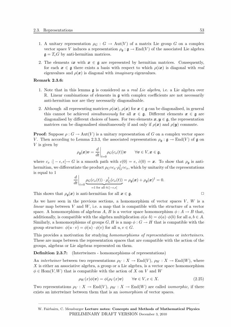
2.3. Representations 53
1. A unitary representation ρG : G → Aut(V ) of a matrix Lie group G on a complexvector space V induces a representation ρg : g → End(V ) of the associated Lie algebrag = TeG by anti-hermitian matrices.
2. The elements ix with x ∈ g are represented by hermitian matrices. Consequently,for each x ∈ g there exists a basis with respect to which ρ(ix) is diagonal with realeigenvalues and ρ(x) is diagonal with imaginary eigenvalues.
Remark 2.3.6:
1. Note that in this lemma g is considered as a real Lie algebra, i.e. a Lie algebra overR. Linear combinations of elements in g with complex coefficients are not necessarilyanti-hermitian nor are they necessarily diagonalisable.
2. Although all representing matrices ρ(ix), ρ(x) for x ∈ g can be diagonalised, in generalthis cannot be achieved simultaneously for all x ∈ g. Different elements x ∈ g arediagonalised by different choices of bases. For two elements x,y ∈ g, the representationmatrices can be diagonalised simultaneously if and only if ρ(x) and ρ(y) commute.
Proof: Suppose ρ : G→ Aut(V ) is a unitary representation of G on a complex vector spaceV . Then according to Lemma 2.3.3, the associated representation ρg : g → End(V ) of g onV is given by
ρg(x)v =d
dt
∣∣∣∣t=0
ρG(cx(t))v ∀v ∈ V,x ∈ g,
where cx :] − ǫ, ǫ[→ G is a smooth path with c(0) = e, c(0) = x. To show that ρg is anti-
hermitian, we differentiate the product ρGcx·ρ†Gcx, which by unitarity of the representationsis equal to 1
d
dt
∣∣∣∣t=0
ρG(cx(t)) · ρ†G(cx(t))︸ ︷︷ ︸=1 for all t∈]−ǫ,ǫ[
= ρg(x) + ρg(x)† = 0.
This shows that ρg(x) is anti-hermitian for all x ∈ g. 2
As we have seen in the previous sections, a homomorphism of vector spaces V , W is alinear map between V and W , i.e. a map that is compatible with the structure of a vectorspace. A homomorphism of algebras A, B is a vector space homomorphism φ : A→ B that,additionally, is compatible with the algebra multiplication φ(a ·b) = φ(a) ·φ(b) for all a, b ∈ A.Similarly, a homomorphisms of groups G,H is a map φ : G→ H that is compatible with thegroup structure: φ(u · v) = φ(u) · φ(v) for all u, v ∈ G.
This provides a motivation for studying homomorphisms of representations or intertwiners.These are maps between the representation spaces that are compatible with the action of thegroups, algebras or Lie algebras represented on them.
Definition 2.3.7: (Intertwiners - homomorphisms of representations)
An intertwiner between two representations ρV : X → End(V ), ρW : X → End(W ), whereX is either an associative algebra, a group or a Lie algebra, is a vector space homomorphismφ ∈ Hom(V,W ) that is compatible with the action of X on V and W
ρW (x)φ(v) = φ(ρV (x)v) ∀v ∈ V, x ∈ X. (2.25)
Two representations ρV : X → End(V ), ρW : X → End(W ) are called isomorphic, if thereexists an intertwiner between them that is an isomorphism of vector spaces.
——————————————————————————————————————W. Fairbairn, C. Meusburger Lecture notes: Concepts and Methods of Mathematical Physics
PRELIMINARY DRAFT VERSION December 3, 2010
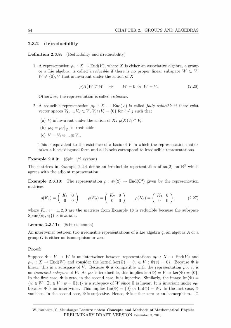
54 CHAPTER 2. GROUPS AND ALGEBRAS
2.3.2 (Ir)reducibility
Definition 2.3.8: (Reducibility and irreducibility)
1. A representation ρV : X → End(V ), where X is either an associative algebra, a groupor a Lie algebra, is called irreducible if there is no proper linear subspace W ⊂ V ,W 6= 0, V that is invariant under the action of X
ρ(X)W ⊂W ⇒ W = 0 or W = V. (2.26)
Otherwise, the representation is called reducible.
2. A reducible representation ρV : X → End(V ) is called fully reducible if there existvector spaces V1, ..., Vn ⊂ V , Vi ∩ Vi = 0 for i 6= j such that
(a) Vi is invariant under the action of X: ρ(X)Vi ⊂ Vi
(b) ρVi = ρV∣∣Vi
is irreducible
(c) V = V1 ⊕ ...⊕ Vn.
This is equivalent to the existence of a basis of V in which the representation matrixtakes a block diagonal form and all blocks correspond to irreducible representations.
Example 2.3.9: (Spin 1/2 system)
The matrices in Example 2.2.4 define an irreducible representation of su(2) on R3 whichagrees with the adjoint representation.
Example 2.3.10: The representation ρ : su(2) → End(C4) given by the representationmatrices
ρ(K1) =
(K1 00 0
)ρ(K2) =
(K2 00 0
)ρ(K3) =
(K3 00 0
), (2.27)
where Ki, i = 1, 2, 3 are the matrices from Example 18 is reducible because the subspaceSpan(e3, e4) is invariant.
Lemma 2.3.11: (Schur’s lemma)
An intertwiner between two irreducible representations of a Lie algebra g, an algebra A or agroup G is either an isomorphism or zero.
Proof:
Suppose Φ : V → W is an intertwiner between representations ρV : X → End(V ) andρW : X → End(W ) and consider the kernel ker(Φ) = v ∈ V : Φ(v) = 0. Because Φ islinear, this is a subspace of V . Because Φ is compatible with the representation ρV , it isan invariant subspace of V . As ρV is irreducible, this implies ker(Φ) = V or ker(Φ) = 0.In the first case, Φ is zero, in the second case, it is injective. Similarly, the image Im(Φ) =w ∈ W : ∃v ∈ V : w = Φ(v) is a subspace of W since Φ is linear. It is invariant under ρWbecause Φ is an intertwiner. This implies Im(Φ) = 0 or Im(Φ) = W . In the first case, Φvanishes. In the second case, Φ is surjective. Hence, Φ is either zero or an isomorphism. 2
——————————————————————————————————————W. Fairbairn, C. Meusburger Lecture notes: Concepts and Methods of Mathematical Physics
PRELIMINARY DRAFT VERSION December 3, 2010
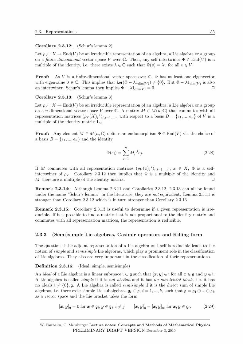
2.3. Representations 55
Corollary 2.3.12: (Schur’s lemma 2)
Let ρV : X → End(V ) be an irreducible representation of an algebra, a Lie algebra or a groupon a finite dimensional vector space V over C. Then, any self-intertwiner Φ ∈ End(V ) is amultiple of the identity, i.e. there exists λ ∈ C such that Φ(v) = λv for all v ∈ V .
Proof: As V is a finite-dimensional vector space over C, Φ has at least one eigenvectorwith eigenvalue λ ∈ C. This implies that ker(Φ − λ1dim(V )) 6= 0. But Φ − λ1dim(V ) is alsoan intertwiner. Schur’s lemma then implies Φ − λ1dim(V ) = 0. 2
Corollary 2.3.13: (Schur’s lemma 3)
Let ρV : X → End(V ) be an irreducible representation of an algebra, a Lie algebra or a groupon a n-dimensional vector space V over C. A matrix M ∈ M(n,C) that commutes with allrepresentation matrices (ρV (X) j
i )i,j=1,...,n with respect to a basis B = e1, ..., en of V is amultiple of the identity matrix 1n.
Proof: Any element M ∈M(n,C) defines an endomorphism Φ ∈ End(V ) via the choice ofa basis B = e1, ..., en and the identity
Φ(ei) =n∑
j=1
M ji ej . (2.28)
If M commutes with all representation matrices (ρV (x) ji )i,j=1,...,n, x ∈ X, Φ is a self-
intertwiner of ρV . Corollary 2.3.12 then implies that Φ is a multiple of the identity andM therefore a multiple of the identity matrix. 2
Remark 2.3.14: Although Lemma 2.3.11 and Corollaries 2.3.12, 2.3.13 can all be foundunder the name “Schur’s lemma” in the literature, they are not equivalent. Lemma 2.3.11 isstronger than Corollary 2.3.12 which is in turn stronger than Corollary 2.3.13.
Remark 2.3.15: Corollary 2.3.13 is useful to determine if a given representation is irre-ducible. If it is possible to find a matrix that is not proportional to the identity matrix andcommutes with all representation matrices, the representation is reducible.
2.3.3 (Semi)simple Lie algebras, Casimir operators and Killing form
The question if the adjoint representation of a Lie algebra on itself is reducible leads to thenotion of simple and semisimple Lie algebras, which play a prominent role in the classificationof Lie algebras. They also are very important in the classification of their representations.
Definition 2.3.16: (Ideal, simple, semisimple)
An ideal of a Lie algebra is a linear subspace i ⊂ g such that [x,y] ∈ i for all x ∈ g and y ∈ i.A Lie algebra is called simple if it is not abelian and it has no non-trivial ideals, i.e. it hasno ideals i 6= 0, g. A Lie algebra is called semisimple if it is the direct sum of simple Liealgebras, i.e. there exist simple Lie subalgebras gi ⊂ g, i = 1, ..., k, such that g = g1 ⊕ ...⊕ gkas a vector space and the Lie bracket takes the form
[x,y]g = 0 for x ∈ gi,y ∈ gj, i 6= j [x,y]g = [x,y]gi for x,y ∈ gi. (2.29)
——————————————————————————————————————W. Fairbairn, C. Meusburger Lecture notes: Concepts and Methods of Mathematical Physics
PRELIMINARY DRAFT VERSION December 3, 2010

56 CHAPTER 2. GROUPS AND ALGEBRAS
Corollary 2.3.17:
The adjoint representation of a Lie algebra g is irreducible if and only if g is simple.
Theorem 2.3.18: A Lie algebra is semisimple if and only if it has no non-trivial abelianideals.
Proof: The proof can be found in many textbooks on Lie algebras.
We now construct a class of Lie algebras which are neither simple nor semisimple, the Liealgebras associated with semi-direct product groups.
Example 2.3.19: (Semidirect products)
1. Let G be a matrix Lie group with Lie algebra g = TeG and denote by [ , ]g the Liebracket on g. Let ρG : G→ Aut(V ) be a representation of G on a vector space V overk and ρg : g → End(V ) the associated representation of g.
We consider the set G × V = (g,v) | g ∈ G,v ∈ V and define a multiplication· : (G× V ) × (G× V ) → (G× V ) by setting
(g,v) · (h,w) = (gh,v + ρG(g)w) ∀g, h ∈ G,v,w ∈ V.
Then, the set G× V with the multiplication · is a group, called the semidirect productof G and V and denoted G⋉ V .
2. Its Lie algebra, denoted g ⋉ V , is the set g × V = (x,v) | x ∈ g,v ∈ V with thevector space structure of the direct sum
(x,v) + (y,w) = (x + y,v + w) t(x,v) = (tx, tv) ∀x,y ∈ g,v,w ∈ V, t ∈ k.
and with Lie bracket
[(x,v), (y,w)] = ([x,y]g, ρg(x)w − ρg(y)v) ∀x,y ∈ g,v,w ∈ V.
3. This Lie algebra is neither simple nor semi-simple. The linear subspaces V = (0,v) | v ∈V ⊂ g ⋉ V and g = (x, 0) | x ∈ g are ideals of g
[(x,v), (0,w)] = (0, ρg(x)w) ∀x ∈ g,v,w ∈ V
[(x,v), (y, 0)] = ([x,y]g, 0) ∀x,y ∈ g,v ∈ V.
This implies that g ⋉ V cannot be simple, unless G is the trivial Lie group: G = eor V is the trivial vector space of dimension 0: V = 0. Moreover, one finds that thevector space V ⊂ g ⋉ V is an abelian ideal of g ⋉ V
[(0,v), (0,w)] = 0 ∀v,w ∈ V.
By Theorem 2.3.18, a semisimple Lie algebra cannot have any non-trivial abelian ideals,which implies that the semidirect product g ⋉ V cannot be semisimple. 2
Remark 2.3.20: Many groups that are important in physics are semidirect products. Ex-amples are the Euclidean group SO(3) ⋉ R3 and the Poincare group SO(3, 1) ⋉ R4.
——————————————————————————————————————W. Fairbairn, C. Meusburger Lecture notes: Concepts and Methods of Mathematical Physics
PRELIMINARY DRAFT VERSION December 3, 2010
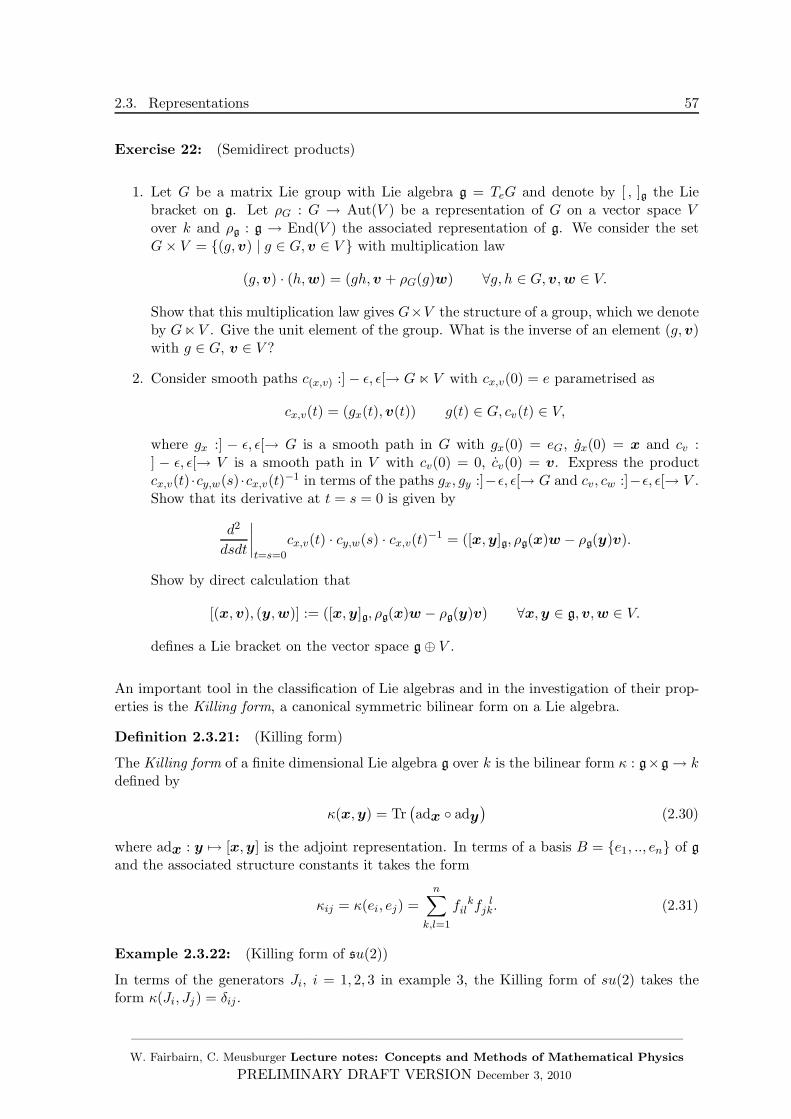
2.3. Representations 57
Exercise 22: (Semidirect products)
1. Let G be a matrix Lie group with Lie algebra g = TeG and denote by [ , ]g the Liebracket on g. Let ρG : G → Aut(V ) be a representation of G on a vector space Vover k and ρg : g → End(V ) the associated representation of g. We consider the setG× V = (g,v) | g ∈ G,v ∈ V with multiplication law
(g,v) · (h,w) = (gh,v + ρG(g)w) ∀g, h ∈ G,v,w ∈ V.
Show that this multiplication law gives G×V the structure of a group, which we denoteby G⋉V . Give the unit element of the group. What is the inverse of an element (g,v)with g ∈ G, v ∈ V ?
2. Consider smooth paths c(x,v) :] − ǫ, ǫ[→ G⋉ V with cx,v(0) = e parametrised as
cx,v(t) = (gx(t),v(t)) g(t) ∈ G, cv(t) ∈ V,
where gx :] − ǫ, ǫ[→ G is a smooth path in G with gx(0) = eG, gx(0) = x and cv :] − ǫ, ǫ[→ V is a smooth path in V with cv(0) = 0, cv(0) = v. Express the productcx,v(t) ·cy,w(s) ·cx,v(t)−1 in terms of the paths gx, gy :]−ǫ, ǫ[→ G and cv, cw :]−ǫ, ǫ[→ V .Show that its derivative at t = s = 0 is given by
d2
dsdt
∣∣∣∣t=s=0
cx,v(t) · cy,w(s) · cx,v(t)−1 = ([x,y]g, ρg(x)w − ρg(y)v).
Show by direct calculation that
[(x,v), (y,w)] := ([x,y]g, ρg(x)w − ρg(y)v) ∀x,y ∈ g,v,w ∈ V.
defines a Lie bracket on the vector space g ⊕ V .
An important tool in the classification of Lie algebras and in the investigation of their prop-erties is the Killing form, a canonical symmetric bilinear form on a Lie algebra.
Definition 2.3.21: (Killing form)
The Killing form of a finite dimensional Lie algebra g over k is the bilinear form κ : g×g → kdefined by
κ(x,y) = Tr(adx ady
)(2.30)
where adx : y 7→ [x,y] is the adjoint representation. In terms of a basis B = e1, .., en of g
and the associated structure constants it takes the form
κij = κ(ei, ej) =n∑
k,l=1
f kil f
ljk. (2.31)
Example 2.3.22: (Killing form of su(2))
In terms of the generators Ji, i = 1, 2, 3 in example 3, the Killing form of su(2) takes theform κ(Ji, Jj) = δij .
——————————————————————————————————————W. Fairbairn, C. Meusburger Lecture notes: Concepts and Methods of Mathematical Physics
PRELIMINARY DRAFT VERSION December 3, 2010
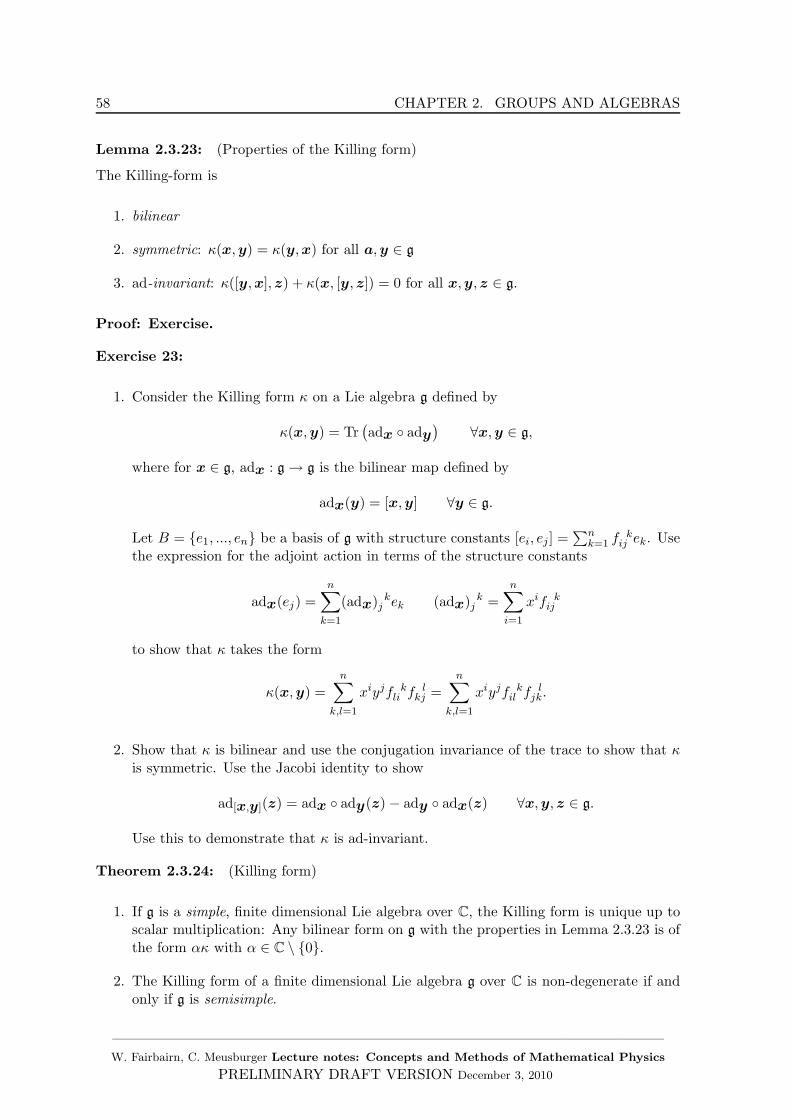
58 CHAPTER 2. GROUPS AND ALGEBRAS
Lemma 2.3.23: (Properties of the Killing form)
The Killing-form is
1. bilinear
2. symmetric: κ(x,y) = κ(y,x) for all a,y ∈ g
3. ad-invariant: κ([y,x],z) + κ(x, [y,z]) = 0 for all x,y,z ∈ g.
Proof: Exercise.
Exercise 23:
1. Consider the Killing form κ on a Lie algebra g defined by
κ(x,y) = Tr(adx ady
)∀x,y ∈ g,
where for x ∈ g, adx : g → g is the bilinear map defined by
adx(y) = [x,y] ∀y ∈ g.
Let B = e1, ..., en be a basis of g with structure constants [ei, ej ] =∑n
k=1 fk
ij ek. Usethe expression for the adjoint action in terms of the structure constants
adx(ej) =
n∑
k=1
(adx) kj ek (adx) k
j =
n∑
i=1
xif kij
to show that κ takes the form
κ(x,y) =n∑
k,l=1
xiyjf kli f
lkj =
n∑
k,l=1
xiyjf kil f
ljk.
2. Show that κ is bilinear and use the conjugation invariance of the trace to show that κis symmetric. Use the Jacobi identity to show
ad[x,y](z) = adx ady(z) − ady adx(z) ∀x,y,z ∈ g.
Use this to demonstrate that κ is ad-invariant.
Theorem 2.3.24: (Killing form)
1. If g is a simple, finite dimensional Lie algebra over C, the Killing form is unique up toscalar multiplication: Any bilinear form on g with the properties in Lemma 2.3.23 is ofthe form ακ with α ∈ C \ 0.
2. The Killing form of a finite dimensional Lie algebra g over C is non-degenerate if andonly if g is semisimple.
——————————————————————————————————————W. Fairbairn, C. Meusburger Lecture notes: Concepts and Methods of Mathematical Physics
PRELIMINARY DRAFT VERSION December 3, 2010

2.3. Representations 59
Proof:
1. The first statement follows from Schur’s lemma. If β : g × g → k is a bilinear form withthe properties of Lemma 2.3.23, then its representing matrix βij = β(ei, ej) with respect toa basis B = e1, ..., en is symmetric and commutes with all matrices (adx) k
i . By Schur’slemma, it is therefore a multiple of the identity.
2. The second statement can be proved as follows: To show that the Killing form is non-degenerate if g is semisimple, we express g as a direct sum g = g1⊕...⊕gk, where gi, k = i, .., kare simple subalgebras and [gi, gj ] = 0 for i 6= j. We select bases Bi = ei1, ..., eisi
of gi. Then
the representing matrix (κij)i,k=1,...,n of κ with respect to the basis B =⋃ki=1Bi takes a block
diagonal form with blocks corresponding to the restrictions κi = κ∣∣gi
. As gi is simple, κi is
a multiple of the identity matrix κi = λi1si with λi 6= 0. Hence, the matrix (κij)i,k=1,...,n isdiagonal with eigenvalues λi 6= 0. This implies that κ is non-degenerate.
3. To show that g is semisimple if its Killing form is non-degenerate, we suppose that i ⊂ g
is an ideal in g. Then i⊥ = x ∈ g | κ(x,y) = 0 ∀y ∈ i is also an ideal of g sinceκ([y,x],z) = −κ(x, [y,z]) = 0 if x ∈ i⊥,z ∈ g, y ∈ i. Hence g = i ⊕ i⊥, where both i, i⊥
are ideals and therefore subalgebras of g. If they are both simple, the proof is complete.Otherwise, one of them, say i contains an ideal j ⊂ i. We then repeat the argument and findi = j ⊕ j⊥, where the orthogonal complement is taken with respect to the restriction of theKilling form to i. After a finite number of steps, we obtain a decomposition of g as a directsum of simple subalgebras. 2
Definition 2.3.25: (Quadratic Casimir)
The quadratic Casimir for a finite-dimensional simple matrix Lie algebra g with basis B =e1, ..., en is the matrix
C =
n∑
i,j=1
κijei · ej where κij = κ(ei, ej) κijκjk = δji , (2.32)
where κ is the Killing form and the product is the matrix multiplication. Note that thequadratic Casimir is not an element of the Lie algebra g.
Example 2.3.26: (Quadratic Casimir for su(2))
The quadratic Casimir of su(2) is given by
J2 = J21 + J2
2 + J23 , (2.33)
where Ji are the generators of su(2) in example 3.
Lemma 2.3.27: The quadratic Casimir is independent of the choice of basis and its matrixcommutator with all elements of g vanishes.
Proof:
When expressed in terms of structure constants, the ad-invariance of the Killing form reads
n∑
j=1
κijfj
kl + κljfj
ki = 0, (2.34)
——————————————————————————————————————W. Fairbairn, C. Meusburger Lecture notes: Concepts and Methods of Mathematical Physics
PRELIMINARY DRAFT VERSION December 3, 2010
60 CHAPTER 2. GROUPS AND ALGEBRAS
which implies for its inverse
n∑
j=1
κijf ljk + κjlf i
jk = 0. (2.35)
The Lie bracket of the quadratic Casimir element with an element of the basis is given by
[C, ek] =
n∑
i,j,l=1
κij(f ljkeiel + f l
ik elej) =
n∑
i,j,l=1
eiel(κijf l
jk + κjlf ijk) = 0. (2.36)
Under a change of basis e′i =∑n
j=1 aji ej , A ∈ GL(n, k) the Killing form changes according
to
κ′ij = κ(e′i, e′j) =
n∑
k,l=1
A ki A
lj κ(ek, el) =
n∑
k,l=1
A ki A
lj κkl.
Its inverse therefore transforms according to
κ′ij =
n∑
k,l=1
(A−1) ik (A−1) j
l κkl.
The quadratic Casimir is therefore invariant and does not depend on the choice of basis
C ′ =
n∑
i,j=1
κ′ije′ie′j =
n∑
i,j,k,l,m,n=1
(A−1) ik (A−1) j
l κklA m
i A nj en · em =
n∑
i,j,k,l,m,n=1
δmk δnl κ
klemen
=
n∑
k,l=1
κklekel = C.
2
Corollary 2.3.28: In any finite-dimensional, irreducible representation of a simple Liealgebra on a vector space over C, the matrix representing the quadratic Casimir element is amultiple of the identity.
Proof: This follows from Schur’s lemma (version 3) 2
Example 2.3.29: (Irreducible unitary representations of su(2))
We determine the finite-dimensional irreducible unitary representations of su(2). Let ρ :su(2) → End(V ) be a representation of su(2) on a vector space V over C with hermitianproduct 〈 , 〉. The Lie algebra su(2) has a basis B = J1, J2, J3 with Lie bracket
[Ji, Jj ] = i3∑
k=1
ǫ kij Jk. (2.37)
Unitarity of the representation means that the adjoint of the action of the generators Ji onV agrees with the action of Ji
ρ(Ji)† = ρ(Ji) or, equivalently 〈ρ(x)w, v〉 = 〈w, ρ(x)v〉 ∀v,w ∈ V. (2.38)
——————————————————————————————————————W. Fairbairn, C. Meusburger Lecture notes: Concepts and Methods of Mathematical Physics
PRELIMINARY DRAFT VERSION December 3, 2010
2.3. Representations 61
1. We introduce the new basis
J± = J1 ± iJ2 Jz = J3 (2.39)
in which the Lie bracket and unitarity condition take the form
[Jz , J±] = ±J± [J+, J−] = 2Jz ρ(Jz)† = ρ(Jz), ρ(J±)† = ρ(J∓). (2.40)
2. We now consider a maximal abelian and semisimple Lie subalgebra of su(2), also calledCartan subalgebra of su(2), i.e. a maximal set of matrices that can be diagonalised simul-taneously. The Lie bracket implies that this maximal abelian subalgebra can only be one-dimensional. We select it to be the one-dimensional subspace spanned by Jz. As ρ(Jz) ishermitian, it can be diagonalised over C with real eigenvalues. Hence, we obtain a basisBV = v1, ..., vn of V spanned by eigenvectors
ρ(Jz)vk = λkvk λk ∈ R. (2.41)
We now note the identity
ρ(Jz)ρ(J±)kv = (λ± k)ρ(J±)kv, (2.42)
which can be proved by induction using the Lie bracket of the generators J± and Jz:
ρ(Jz)ρ(J±)v = ρ(J±)ρ(Jz)v ± ρ(J±)v = (λ± 1)ρ(J±)v. (2.43)
Identity (2.42) implies that for any eigenvector v of ρ(Jz) with eigenvalue λ, ρ(J±)v is eitheran eigenvector with eigenvalue λ ± 1 or vanishes. Suppose now that the basis is orderedsuch that λn is the biggest eigenvalue or highest weight of ρ(Jz). Then ρ(J+)vn = 0, and weobtain a sequence of eigenvectors wk = ρ(Jk−)vn satisfying ρ(Jz)wk = (λn − k)wk. As therepresentation is finite dimensional, there exists a s ∈ N such that ρ(J−)kvn = 0 for k > s,ρ(Js−)vn 6= 0.
3. We will now show that the vectors ρ(Jk−)vn for 0 ≤ k ≤ s form a basis of V . Thatthey are linearly independent follows from the fact that they are eigenvectors with differenteigenvalues. To show that they span V , we use the identity
ρ(J+)wk = (2kλn − k(k − 1))wk−1, (2.44)
which can be proved by induction:
ρ(J+)w1 = ρ(J+)ρ(J−)vn = 2Jzvn = 2λnvn = 2λnw0
ρ(J+)wk+1 = ρ(J−)ρ(J+)wk + 2Jzwk = (2kλn − k(k − 1))ρ(J−)wk−1 + 2(λn − k)wk
= (2kλn − k(k − 1) + 2(λn − k))wk = (2(k + 1)λn − (k + 1)k)wk
ws ws − 1 ws − 2 · · · w1 w0
•J+
)) •J−
ii
J+
** •J−
jj
J+,, • · · · •
J−
jj
J+
)) •J−
ll
J+
(( •J−
hh
Hence, we have
ρ(Jz)wk = (λn − k)wk ρ(J−)wk = wk+1 ρ(J+)wk = (2kλn − k(k − 1))wk−1, (2.45)
——————————————————————————————————————W. Fairbairn, C. Meusburger Lecture notes: Concepts and Methods of Mathematical Physics
PRELIMINARY DRAFT VERSION December 3, 2010
62 CHAPTER 2. GROUPS AND ALGEBRAS
which implies that Span(w0, ..., ws) is an invariant subspace of V . As ρ is irreducible,Span(w0, ..., ws) = V and dim(V ) = s + 1. the irreducible representations are labelled bytheir dimension s ∈ N.
4. Normalisation of eigenstates. From the basis w0, ..., ws of V , we construct an orthonor-mal basis, whose elements we denote by |j,m〉 with j = λn ∈ Z/2, m ∈ −j,−j+1, ..., j−1, j.Supposing vn = |j, j〉 is normalised such that 〈j, j|j, j〉 = 1, we find
〈wk+1|wk+1〉 = 〈wk|ρ(J+)wk+1〉 = 2jk − k(k − 1)〈wk|wk〉 (2.46)
This implies after some further calculations that the action of su(2) on the normalised statesis given by
Jz |j,m〉 = m|j,m〉 J±|j,m〉 =√j(j + 1) −m(m± 1) |j,m± 1〉 (2.47)
5. Finally, we determine the eigenvalues of the quadratic Casimir ρ(J2) of su(2)
J2 = J21 + J2
2 + J23 = J2
z + 12(J+J− + J−J+). (2.48)
In any irreducible, finite dimensional representation ρ(J2) must be proportional to the unitmatrix, ρ(J2) = τ1 with a proportionality constant τ that characterises the representation.This implies
ρ(J2)w0 = ρ(Jz)2w0 + 1
2ρ(J+)ρ(J−)w0 = λ2nw0 + 1
2ρ(J+)w1 = λn(λn + 1)w0 (2.49)
ρ(J2)ws = ρ(Jz)2ws + 1
2ρ(J−)ρ(J+)ws = (λn − s)2ws + sλn − 12s(s− 1)ws (2.50)
We have
τ = λ2n + λn = (λn − s)2 + sλn − 1
2s(s− 1) ⇒ λn = 12s. (2.51)
and find that the eigenvalues of ρ(Jz) are s2 ,
s2 − 1, ...,− s
2 + 1,− s2 .
In physics, Lie algebra symmetries such as the su(2) symmetry in this example correspondto observables. Therefore, their eigenvalues in a representation are quantum numbers. Theeigenvalues j of the Casimir operator J2, which correspond to the absolute value of theangular momentum or spin vector are called the principal angular momentum or spin quantumnumber. The eigenvalues m of Jz , which correspond to the z-component of the angularmomentum, are referred to as magnetic quantum numbers.
2.4 Duals, direct sums and tensor products of representations
2.4.1 Groups and Lie groups
Given a representation of a Lie algebra on a vector space V , one can construct new represen-tations using the associated vector spaces investigated in Chapter 1 - the dual V ∗, the directsum V ⊕W and tensor product V ⊗W . We obtain the following definition.
Definition 2.4.1: (Representations of Lie algebras - constructions)
——————————————————————————————————————W. Fairbairn, C. Meusburger Lecture notes: Concepts and Methods of Mathematical Physics
PRELIMINARY DRAFT VERSION December 3, 2010
2.4. Duals, direct sums and tensor products of representations 63
1. Dual of a representation: The dual of the representation ρV on a on vector spaces V isthe representation ρV ∗ : g → End(V ∗) on the dual vector space V ∗ defined via
ρV ∗(x)α = α ρV (−x) ∀α ∈ V ∗,x ∈ g (2.52)
or, in terms of a basis BV = e1, ..., en and its dual
ρV ∗(x)ei =
n∑
k=1
(ρV (−x)) ik e
k ∀x ∈ g. (2.53)
2. Direct sum of representations: The direct sum of the representations ρV : g → End(V ),ρW : g → End(W ) is the representation ρV⊕W : g → End(V ⊕W ) on the direct sum ofthe associated vector spaces defined by
ρV⊕W (x)(v + w) = ρV (x)v + ρW (x)w ∀x ∈ g, v ∈ V ⊂ V ⊕W,w ∈W ⊂ V ⊕W.
3. Tensor product of representations: The tensor product of the representations ρV : g →End(V ), ρW : g → End(W ) is the representation ρV⊗W : g → End(V ⊗W ) on thetensor product of the associated vector spaces defined by
ρV⊗W (x)(v ⊗ w) = (ρV (x)v) ⊗w + v ⊗ (ρW (x)w) ∀x ∈ g, v ∈ V,w ∈W. (2.54)
Remark 2.4.2: In particle physics, elementary particles are described by irreducible repre-sentations of Lie algebras. Examples are quarks, electrons, neutrinos etc. The duals of theserepresentations describe the associated anti-particle. Composite particles such as the hadrons(including the proton and the neutron) and the mesons are described by tensor products ofirreducible representations.
It can be shown that for a semisimple Lie algebra, the tensor product of irreducible, finitedimensional representations is always fully reducible, i.e. decomposable into irreducible rep-resentations. An irreducible representation that arises in such a decomposition is called amultiplet or, if the dimension of the representation is one, a singlet. More precisely, onespeaks of a doublet if the associated irreducible representation has dimension two, a tripletif it has dimension three, a quadruplet for dimension four etc. The composite particles whichcorrespond to such multiplets have similar masses and similar behaviour with respect to thefundamental interactions modelled by these representations.
The construction of a representations on dual vector spaces and tensor products of vectorspaces for Lie algebras can be performed analogously for groups if we replace g ↔ G, End(·) ↔Aut(·), −x ∈ g ↔ g−1 ∈ G and sums with products in (2.54) in Def. 2.4.1.
This is corresponds to the concepts of additive and multiplicative quantum numbers. Additivequantum numbers are eigenvalues of Lie algebra elements in representations on a Hilbert space.If one considers two copies of a quantum mechanical system, which corresponds to taking thetensor product of two representations, the corresponding eigenvalue in the tensor product ofthe representations is the sum of the eigenvalues in the individual representations.
Multiplicative quantum numbers are eigenvalues of group elements in a representation of agroup on a Hilbert space. When considering two copies of the system, i.e. taking the tensorproduct, the corresponding eigenvalue in the tensor product of the representations is theproduct of the eigenvalues in the individual representations.
——————————————————————————————————————W. Fairbairn, C. Meusburger Lecture notes: Concepts and Methods of Mathematical Physics
PRELIMINARY DRAFT VERSION December 3, 2010
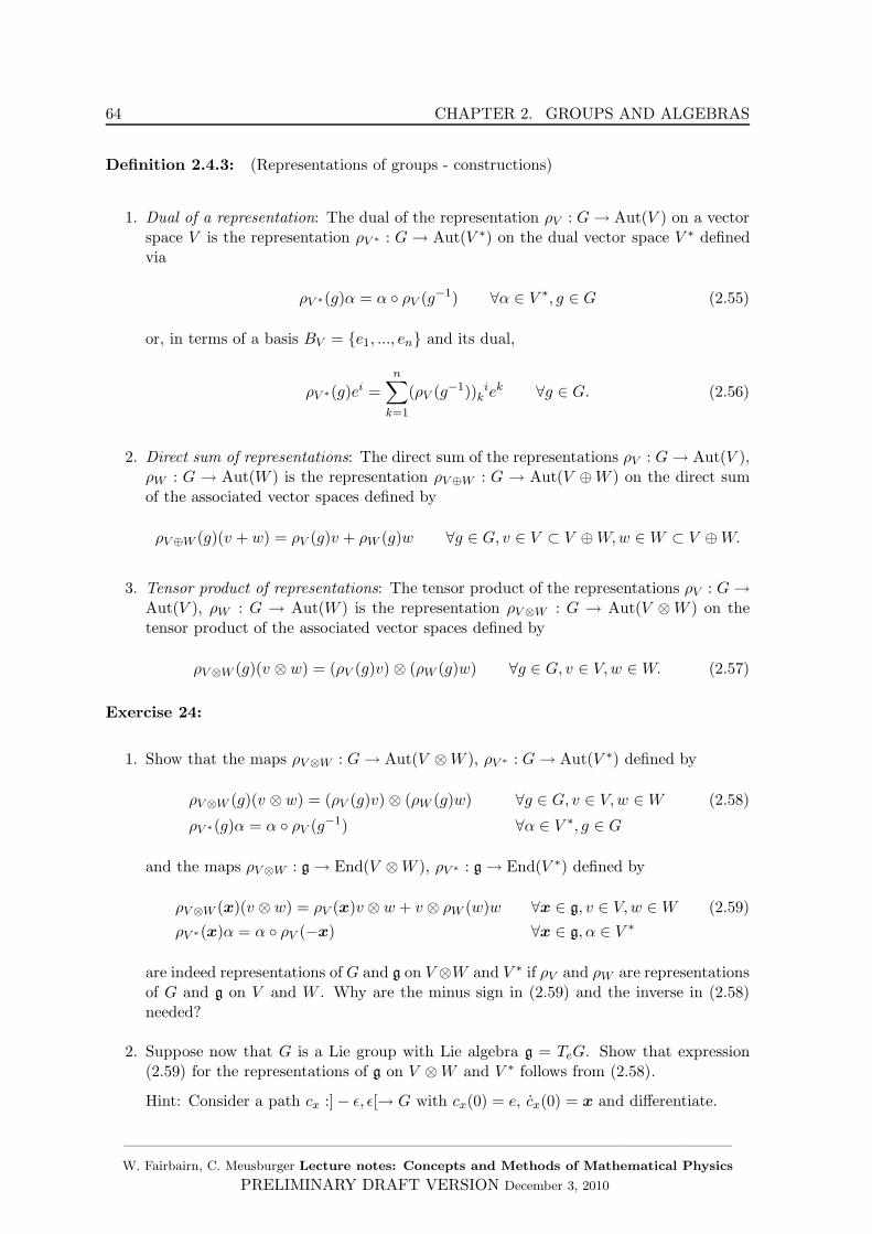
64 CHAPTER 2. GROUPS AND ALGEBRAS
Definition 2.4.3: (Representations of groups - constructions)
1. Dual of a representation: The dual of the representation ρV : G→ Aut(V ) on a vectorspace V is the representation ρV ∗ : G → Aut(V ∗) on the dual vector space V ∗ definedvia
ρV ∗(g)α = α ρV (g−1) ∀α ∈ V ∗, g ∈ G (2.55)
or, in terms of a basis BV = e1, ..., en and its dual,
ρV ∗(g)ei =n∑
k=1
(ρV (g−1)) ik e
k ∀g ∈ G. (2.56)
2. Direct sum of representations: The direct sum of the representations ρV : G→ Aut(V ),ρW : G → Aut(W ) is the representation ρV⊕W : G → Aut(V ⊕W ) on the direct sumof the associated vector spaces defined by
ρV⊕W (g)(v + w) = ρV (g)v + ρW (g)w ∀g ∈ G, v ∈ V ⊂ V ⊕W,w ∈W ⊂ V ⊕W.
3. Tensor product of representations: The tensor product of the representations ρV : G→Aut(V ), ρW : G → Aut(W ) is the representation ρV⊗W : G → Aut(V ⊗W ) on thetensor product of the associated vector spaces defined by
ρV⊗W (g)(v ⊗ w) = (ρV (g)v) ⊗ (ρW (g)w) ∀g ∈ G, v ∈ V,w ∈W. (2.57)
Exercise 24:
1. Show that the maps ρV⊗W : G→ Aut(V ⊗W ), ρV ∗ : G→ Aut(V ∗) defined by
ρV⊗W (g)(v ⊗ w) = (ρV (g)v) ⊗ (ρW (g)w) ∀g ∈ G, v ∈ V,w ∈W (2.58)
ρV ∗(g)α = α ρV (g−1) ∀α ∈ V ∗, g ∈ G
and the maps ρV⊗W : g → End(V ⊗W ), ρV ∗ : g → End(V ∗) defined by
ρV⊗W (x)(v ⊗ w) = ρV (x)v ⊗ w + v ⊗ ρW (w)w ∀x ∈ g, v ∈ V,w ∈W (2.59)
ρV ∗(x)α = α ρV (−x) ∀x ∈ g, α ∈ V ∗
are indeed representations of G and g on V ⊗W and V ∗ if ρV and ρW are representationsof G and g on V and W . Why are the minus sign in (2.59) and the inverse in (2.58)needed?
2. Suppose now that G is a Lie group with Lie algebra g = TeG. Show that expression(2.59) for the representations of g on V ⊗W and V ∗ follows from (2.58).
Hint: Consider a path cx :] − ǫ, ǫ[→ G with cx(0) = e, cx(0) = x and differentiate.
——————————————————————————————————————W. Fairbairn, C. Meusburger Lecture notes: Concepts and Methods of Mathematical Physics
PRELIMINARY DRAFT VERSION December 3, 2010
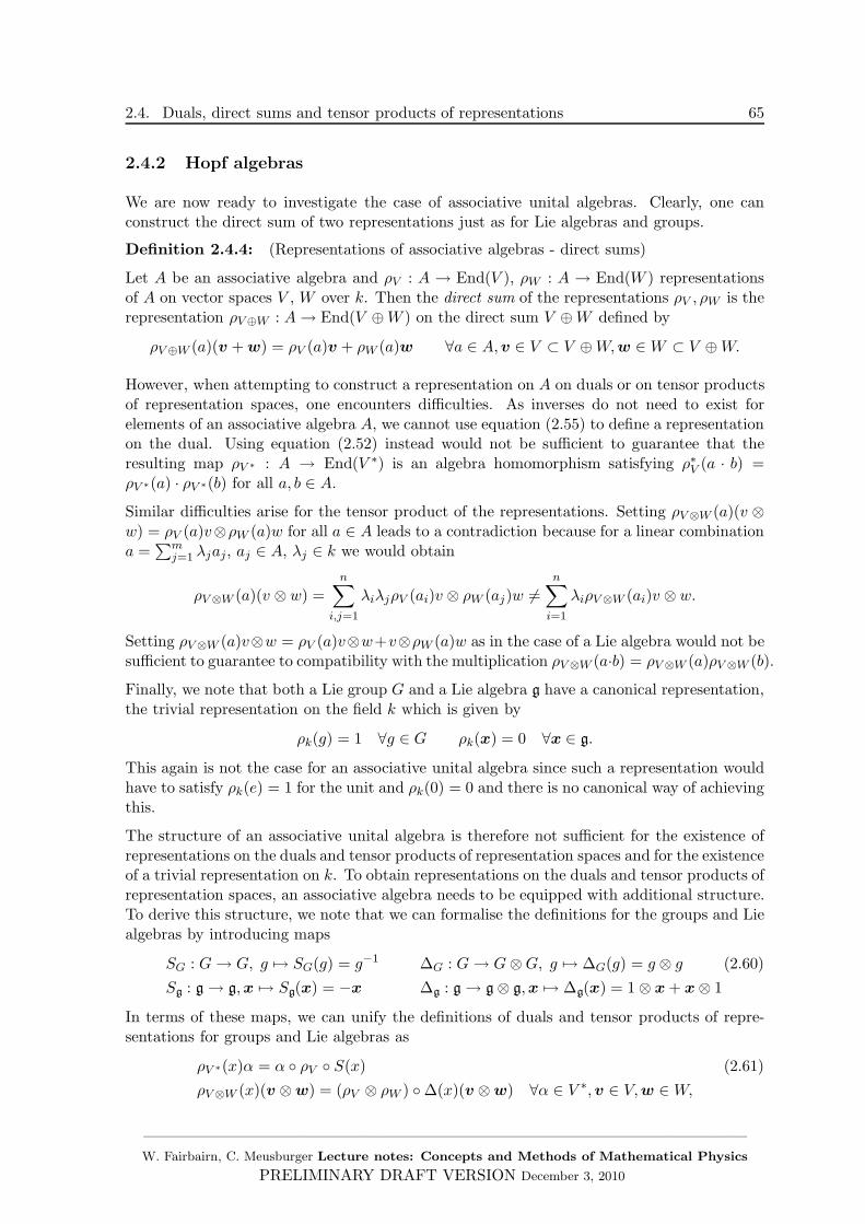
2.4. Duals, direct sums and tensor products of representations 65
2.4.2 Hopf algebras
We are now ready to investigate the case of associative unital algebras. Clearly, one canconstruct the direct sum of two representations just as for Lie algebras and groups.
Definition 2.4.4: (Representations of associative algebras - direct sums)
Let A be an associative algebra and ρV : A → End(V ), ρW : A → End(W ) representationsof A on vector spaces V , W over k. Then the direct sum of the representations ρV , ρW is therepresentation ρV⊕W : A→ End(V ⊕W ) on the direct sum V ⊕W defined by
ρV⊕W (a)(v + w) = ρV (a)v + ρW (a)w ∀a ∈ A,v ∈ V ⊂ V ⊕W,w ∈W ⊂ V ⊕W.
However, when attempting to construct a representation on A on duals or on tensor productsof representation spaces, one encounters difficulties. As inverses do not need to exist forelements of an associative algebra A, we cannot use equation (2.55) to define a representationon the dual. Using equation (2.52) instead would not be sufficient to guarantee that theresulting map ρV ∗ : A → End(V ∗) is an algebra homomorphism satisfying ρ∗V (a · b) =ρV ∗(a) · ρV ∗(b) for all a, b ∈ A.
Similar difficulties arise for the tensor product of the representations. Setting ρV⊗W (a)(v ⊗w) = ρV (a)v⊗ρW (a)w for all a ∈ A leads to a contradiction because for a linear combinationa =
∑mj=1 λjaj, aj ∈ A, λj ∈ k we would obtain
ρV⊗W (a)(v ⊗ w) =n∑
i,j=1
λiλjρV (ai)v ⊗ ρW (aj)w 6=n∑
i=1
λiρV⊗W (ai)v ⊗ w.
Setting ρV⊗W (a)v⊗w = ρV (a)v⊗w+v⊗ρW (a)w as in the case of a Lie algebra would not besufficient to guarantee to compatibility with the multiplication ρV⊗W (a·b) = ρV⊗W (a)ρV ⊗W (b).
Finally, we note that both a Lie group G and a Lie algebra g have a canonical representation,the trivial representation on the field k which is given by
ρk(g) = 1 ∀g ∈ G ρk(x) = 0 ∀x ∈ g.
This again is not the case for an associative unital algebra since such a representation wouldhave to satisfy ρk(e) = 1 for the unit and ρk(0) = 0 and there is no canonical way of achievingthis.
The structure of an associative unital algebra is therefore not sufficient for the existence ofrepresentations on the duals and tensor products of representation spaces and for the existenceof a trivial representation on k. To obtain representations on the duals and tensor products ofrepresentation spaces, an associative algebra needs to be equipped with additional structure.To derive this structure, we note that we can formalise the definitions for the groups and Liealgebras by introducing maps
SG : G→ G, g 7→ SG(g) = g−1 ∆G : G→ G⊗G, g 7→ ∆G(g) = g ⊗ g (2.60)
Sg : g → g,x 7→ Sg(x) = −x ∆g : g → g ⊗ g,x 7→ ∆g(x) = 1 ⊗ x + x ⊗ 1
In terms of these maps, we can unify the definitions of duals and tensor products of repre-sentations for groups and Lie algebras as
ρV ∗(x)α = α ρV S(x) (2.61)
ρV⊗W (x)(v ⊗ w) = (ρV ⊗ ρW ) ∆(x)(v ⊗ w) ∀α ∈ V ∗,v ∈ V,w ∈W,
——————————————————————————————————————W. Fairbairn, C. Meusburger Lecture notes: Concepts and Methods of Mathematical Physics
PRELIMINARY DRAFT VERSION December 3, 2010
66 CHAPTER 2. GROUPS AND ALGEBRAS
where x is either an element of a group G or of a Lie algebra g, and S and ∆ are the mapsgiven by (2.60). Note that in order to yield representations, of groups and Lie algebras, themaps S and ∆ must satisfy
S(x ⋄ y) = S(y) ⋄ S(x) ∆(x ⋄ y) = ∆(x) ⋄ ∆(y),
where x ⋄ y = [x, y] for x, y ∈ g and x ⋄ y = x · y for x, y ∈ G. In other words, ∆ mustbe a homomorphism of groups or Lie algebras and S an anti-endomorphism of groups orLie algebras. Note also that the fact that the map ∆ consistently defines representations onmultiple tensor products U ⊗V ⊗W is due to the fact that for both, the case of a group anda Lie algebra, it satisfies the co-associativity condition
(∆ ⊗ id) ∆ = (id ⊗ ∆) ∆.
Moreover, we note that in both, the case of a group and the Lie algebra, the trivial represen-tation on the field k is given by a map
ǫg : g → k ǫ(x) = 0 ∀x ∈ g (2.62)
ǫG : G→ k ǫ(g) = 1 ∀g ∈ G.
Note that in order to give rise to representations, the map ǫ must be a homomorphism ofgroups or Lie algebras, i.e. satisfy
ǫ(x ⋄ y) = ǫ(x) · ǫ(y),
where again x ⋄ y = [x, y] for x, y ∈ g and x ⋄ y = x · y for x, y ∈ G. Moreover, themap ǫ which defines the trivial representations must be compatible with with the fact thatk⊗V ∼= V ∼= V ⊗k for all vector spaces V over k. More precisely, the canonical isomorphismsφL : k⊗ V → V , t⊗ v 7→ tv and φR : V ⊗ k → V , v ⊗ t 7→ tv should be intertwiners betweenthe representations on k ⊗ V , V ⊗ k constructed from a representation on V via the maps ǫand ∆ and the representation on V . This translates into the condition
(ǫ⊗ id) ∆ = (id ⊗ ǫ) ∆ = id,
which is satisfied trivially for both the case of the group and the Lie algebra.
Finally, we note that for both, groups and Lie algebras the evaluation maps evL : V ∗ ⊗ V →k, α ⊗ v 7→ α(v) and evR : V ⊗ V ∗ → k, v ⊗ α 7→ α(v) are intertwiners between therepresentations on V ⊗ V ∗ and V ∗ ⊗ V constructed via the maps ∆ and S and between thetrivial representation given by the map ǫ. The former are given by
ρV ∗⊗V (x)α⊗ v = (ρV ∗ ⊗ ρV )(∆(x))α ⊗ v ρV⊗V ∗(x)v ⊗ α = (ρV ⊗ ρV ∗)(∆(x))v ⊗ α
where the representation ρV ∗ is defined as in (2.61), α ∈ V ∗ and v ∈ V . The require-ment that the evaluation map is an intertwiner between these representations and the trivialrepresentation on k defined via the map ǫ translates into the condition
m (S ⊗ id) ∆(x) = m (id ⊗ S) ∆(x) = ǫ(x)e,
where e is the unit (e=1 for groups and e = 0 for Lie algebras). The map m : x⊗ y 7→ x ⋄ yis the group multiplication m : g ⊗ h 7→ g · h in the case of a group G and the Lie bracket
——————————————————————————————————————W. Fairbairn, C. Meusburger Lecture notes: Concepts and Methods of Mathematical Physics
PRELIMINARY DRAFT VERSION December 3, 2010

2.4. Duals, direct sums and tensor products of representations 67
m : x ⊗ y 7→ [x,y] in the case of a Lie algebra. Clearly, the maps (2.60) and (2.62) satisfythis condition.
We can summarise this discussion as follows:
We consider a structure X which is either a group, a Lie algebra or an associative, unitalalgebra with a multiplication map ⋄ : X ×X → X which is either the group multiplication,or the Lie bracket or the multiplication of the associative algebra and with a unit e satisfyinge⋄x = x⋄e = x for all x ∈ X. Representations of X are X-homomorphisms ρV : X → End(V )into the set of endomorphisms of a vector space V .
In order to construct
1. representations ρV⊗W : X → End(V ⊗W ) on the tensor products V ⊗W of represen-tation spaces for all representations ρV : X → End(V ), ρW : X → End(W )
2. a trivial representation on the field k
such that the following consistency conditions are satisfied
1. The representations ρU⊗(V⊗W ), ρ(U⊗V )⊗W : X → End(U ⊗ V ⊗W ) are identical
2. The canonical isomorphisms k ⊗ V ∼= V , V ⊗ k ∼= V are intertwiners between therepresentations ρk⊗V : X → End(k ⊗ V ), ρV⊗k : X → End(V ⊗ k) and ρV
we need X-homomorphisms ∆ : X → X ⊗X and ǫ : X → k and an anti-X-endomorphismS : X → X that satisfy the following conditions
1. Co-associativity: (∆ ⊗ idX) ∆ = (idX ⊗ ∆) ∆.
2. Compatibility between ǫ and ∆: (ǫ⊗ idX) ∆ = (idX ⊗ ǫ) ∆ = idX
If additionally we require
3. The existence of representations ρV ∗ : X → End(V ∗) on the dual vector spaces V ∗ of allrepresentations ρV : X → End(V ).
such that
3. The evaluation maps evL : V ∗ ⊗ V → k, α ⊗ v 7→ α(v) and evR : V ⊗ V ∗ → k,v⊗α 7→ α(v) are intertwiners between the representations ρV ∗⊗V : X → End(V ∗ ⊗ V ),ρV⊗V ∗ : X] → End(V ∗ ⊗ V ) and ρk : X → End(k)
we also need an anti-X-endomorphism S : X → X that is compatible with ∆, ǫ and ⋄:m (S ⊗ idX) ∆ = m (idX ⊗ S) ∆ = ǫ · e, where m : x⊗ y → x ⋄ y corresponds to themultiplication map and e is the unit.
By applying these requirements to an associative algebra, we obtain the definition of a Bial-gebra and of a Hopf algebra.
——————————————————————————————————————W. Fairbairn, C. Meusburger Lecture notes: Concepts and Methods of Mathematical Physics
PRELIMINARY DRAFT VERSION December 3, 2010
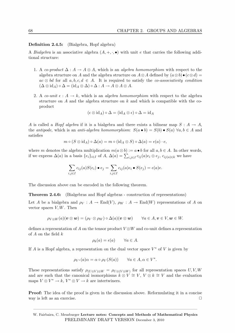
68 CHAPTER 2. GROUPS AND ALGEBRAS
Definition 2.4.5: (Bialgebra, Hopf algebra)
A Bialgebra is an associative algebra (A,+, ·, •) with unit e that carries the following addi-tional structure:
1. A co-product ∆ : A → A ⊗ A, which is an algebra homomorphism with respect to thealgebra structure on A and the algebra structure on A⊗A defined by (a⊗ b)• (c⊗d) =ac ⊗ bd for all a, b, c, d ∈ A. It is required to satisfy the co-associativity condition(∆ ⊗ idA) ∆ = (idA ⊗ ∆) ∆ : A→ A⊗A⊗A.
2. A co-unit ǫ : A → k, which is an algebra homomorphism with respect to the algebrastructure on A and the algebra structure on k and which is compatible with the co-product
(ǫ⊗ idA) ∆ = (idA ⊗ ǫ) ∆ = idA
A is called a Hopf algebra if it is a bialgebra and there exists a bilinear map S : A → A,the antipode, which is an anti-algebra homomorphism: S(a • b) = S(b) • S(a) ∀a, b ∈ A andsatisfies
m (S ⊗ idA) ∆(a) = m (idA ⊗ S) ∆(a) = ǫ(a) · e,
where m denotes the algebra multiplication m(a⊗ b) := a • b for all a, b ∈ A. In other words,if we express ∆(a) in a basis eii∈I of A, ∆(a) =
∑i,j∈I cij(a)ei ⊗ ej , cij(a)∈k we have
∑
i,j∈Icij(a)S(ei) • ej =
∑
i,j∈Icij(a)ei • S(ej) = ǫ(a)e.
The discussion above can be encoded in the following theorem.
Theorem 2.4.6: (Bialgebras and Hopf algebras - construction of representations)
Let A be a bialgebra and ρV : A → End(V ), ρW : A → End(W ) representations of A onvector spaces V,W . Then
ρV⊗W (a)(v ⊗ w) = (ρV ⊗ ρW ) ∆(a)(v ⊗ w) ∀a ∈ A,v ∈ V,w ∈W.
defines a representation of A on the tensor product V ⊗W and co-unit defines a representationof A on the field k
ρk(a) = ǫ(a) ∀a ∈ A.
If A is a Hopf algebra, a representation on the dual vector space V ∗ of V is given by
ρV ∗(a)α = α ρV (S(a)) ∀a ∈ A,α ∈ V ∗.
These representations satisfy ρ(U⊗V )⊗W = ρU⊗(V⊗W ) for all representation spaces U, V,Wand are such that the canonical isomorphisms k ⊗ V ∼= V , V ⊗ k ∼= V and the evaluationmaps V ⊗ V ∗ → k, V ∗ ⊗ V → k are intertwiners.
Proof: The idea of the proof is given in the discussion above. Reformulating it in a conciseway is left as an exercise. 2
——————————————————————————————————————W. Fairbairn, C. Meusburger Lecture notes: Concepts and Methods of Mathematical Physics
PRELIMINARY DRAFT VERSION December 3, 2010

2.4. Duals, direct sums and tensor products of representations 69
2.4.3 Tensor product decomposition
Example 2.4.7: (Tensor product for su(2), Clebsch Gordan coefficients)
We consider the tensor product of two representations ρV : su(2) → End(V ), ρW : su(2) →End(W ). We characterise these representations by the dimensions dV , dW or, equivalently,by the eigenvalue of the quadratic Casimir operator ρV (J2) = 1
2jV (jV + 1) · 1V , ρW (J2) =12jW (jW + 1) · 1W with dV = 2jV + 1, dW = 2jW + 1.
A basis of V is then given by the eigenvectors of Jz: BV = |jV ,mV 〉 | mV = −jV , ..., jV ,ρV (Jz)|jV ,mV 〉 = mV |jV ,mV 〉 and similarly for W BW = |jW ,mW 〉 | mW = −jW , ..., jW ,ρW (Jz)|jW ,mW 〉 = mW |jV ,mW 〉.1. Tensor product of representations
All elements of the tensor product basis |jV ,mV 〉 ⊗ |jW ,mW 〉 are eigenstates of ρV⊗W (Jz)
ρV⊗W (Jz)|jV ,mV 〉 ⊗ |jW ,mW 〉 =(ρV (Jz)|jV ,mV 〉) ⊗ |jW ,mW 〉 + |jV ,mV 〉 ⊗ (ρW (Jz)|jW ,mW 〉)=(mV +mW )|jV ,mV 〉 ⊗ |jW ,mW 〉
However, they are in general not eigenstates of the quadratic Casimir operator:
ρV⊗W (J2)|jV ,mV 〉 ⊗ |jW ,mW 〉 =
=∑
i=x,y,z
(ρV (Ji) ⊗ 1 + 1 ⊗ ρW (Ji))(ρV (Ji) ⊗ 1 + 1 ⊗ ρW (Ji))|jV ,mV 〉 ⊗ |jW ,mW 〉 (2.63)
= 12 (jV (jV + 1) + jW (jW + 1) + 2mWmV )|jV ,mV 〉 ⊗ |jW ,mW 〉+ 1
2
√jV (jV + 1) −mV (mV + 1)
√jW (jW + 1) −mw(mw − 1)|jV ,mV + 1〉 ⊗ |jW ,mW − 1〉
+ 12
√jV (jV + 1) −mV (mV − 1)
√jW (jW + 1) −mw(mw + 1)|jV ,mV − 1〉 ⊗ |jW ,mW + 1〉
With Schur’s lemma, this implies that the representation ρV⊗W is reducible.
2. Tensor product decomposition
We now want to decompose the tensor product ρV⊗W into irreducible representations. Inother words, we want to find a basis of V ⊗W that consists of eigenvectors |J,M 〉 of ρV⊗W (J2)and ρV⊗W (Jz) satisfying
ρV⊗W (J2)|J,M〉 = 12J(J + 1)|J,M 〉 ρV⊗W |J,M〉 = M |J,M 〉 M =∈ −J, ..., J.
From the action of J2, one can see that the states in the tensor product basis are eigenstates ofJ2 if and only if either mV = jV , mW = jW or mV = −jV , mW = −jW and the correspondingeigenvalues are M = ±(jV + jW ), J = jV + jW .
As the states in the tensor product basis are eigenstates of ρV⊗W (Jz) with eigenvalues M =mV + mW and mV ∈ −jV , ..., jV − 1, JV , mW ∈ −jW , ..., jW − 1, JW , we have M ∈−(jV + jW ), ..., jV + jW − 1, jV + jW . Moreover, equation (2.63) implies
〈jV ,mV |⊗ 〈jWmW |ρV⊗W (J2)|jV ,mV 〉⊗ |jW ,mW 〉 = 12(jV (jV +1)+ jW (jW +1)+2mVmW )
and therefore
12(|jV −jW |)(|jV −jW |+1) ≤ 1
2(jV (jV +1)+jW (jW +1)+2mVmW ) ≤ 12(jV +jW )(jV +jW +1).
——————————————————————————————————————W. Fairbairn, C. Meusburger Lecture notes: Concepts and Methods of Mathematical Physics
PRELIMINARY DRAFT VERSION December 3, 2010
70 CHAPTER 2. GROUPS AND ALGEBRAS
This implies that the expectation value of J2 in the representation ρV⊗W takes values in
〈J,M |ρV⊗W (J2)J,M 〉 ∈ [12 (|jV − jW |)(|jV − jW | + 1), 12(jV + jW )(jV + jW + 1)],
and therefore J ∈ −|jV − jW |,−|jV + jW |+ 1, ..., jV + jW − 1, jV + jW . One can show thateach value J ∈ −|jV − jW |,−|jV + jW |+1, ..., jV + jW − 1, jV + jW arises exactly once andthe tensor product decomposition of the representations ρV and ρW is given by
V ⊗W =
jV +jW⊕
J=−|jV −jW |VJ ,
where VJ are linear subspaces of V ⊗W which are invariant under the action ρV⊗W of su(2)and carry an irreducible representation of su(2) of dimension dJ = 2J + 1.
3. Clebsch Gordan coefficients
We will now determine the basis transformation from the tensor product basis |jV ,mV 〉 ⊗|jW ,mW 〉 to the basis |J,M〉. As the states in the tensor product basis are eigenstates ofρV⊗W (Jz), the eigenstate |J,M〉 must be given as a linear combination of vectors in
BJ,M = |jV ,mV 〉 ⊗ |jW ,mW 〉 | mV ∈ −jV , ..., jV ,mW ∈ −jW , ..., jW ,mV +mW = M.
This implies in particular that the eigenvalue of the quadratic Casimir operator in the tensorproduct takes values 1
2J(J + 1) with
J ∈ |jV − jW |, |jV + jW | + 1, ..., jV + jW − 1, jV + jW .
The coefficients in this linear combination are called Clebsch-Gordan coefficients and areusually denoted 〈jV ,mV , jW ,mW |J,M〉.
|J,M〉 =
jV∑
mV =−jV
jW∑
mW =−jW〈jV ,mV , jW ,mW |J,M〉 |jV ,mV 〉 ⊗ |jW ,mW 〉. (2.64)
Clearly, the Clebsch Gordan coefficients satisfy
〈jV ,mV , jW ,mW |J,M 〉 = δM,mV +mW〈jV ,mV , jW ,mW |J,mV +mW 〉
〈jV ,mV , jW ,mW |J,M 〉 = 0 if J /∈ |jV − jW |, |jV − jW | + 1, ..., jV + jW.
By applying ρV⊗W (J±) to both sides of the equation, we find the following recursion relation
√J(J + 1) −M(M ± 1)|J,M ± 1〉 =
√jV (jV + 1) −mV (mV ∓ 1)〈jV ,mV ∓ 1, jW ,mW |J,M 〉
+√jW (jW + 1) −mW (mW ∓ 1)〈jV ,mV , jW ,mW ∓ 1|J,M〉.
Together with a phase convention, namely that the Clebsch Gordan coefficients 〈jV , jV , jW , jV−J |JJ〉 are real and positive for all J ∈ |jV − jW |, |jV − jW | + 1, ..., jV + jW , this recursionrelation determines the Clebsch Gordan coefficients uniquely, and one finds that they are allreal.
We also note that the Clebsch-Gordan coefficients are a basis transformation between twoorthonormal bases of the representation space V ⊗W , the tensor product basis |jV ,mV 〉 ⊗|jW ,mW 〉 and the basis |J,M〉. They are therefore coefficients of a unitary matrix which,
——————————————————————————————————————W. Fairbairn, C. Meusburger Lecture notes: Concepts and Methods of Mathematical Physics
PRELIMINARY DRAFT VERSION December 3, 2010
2.4. Duals, direct sums and tensor products of representations 71
by the choice of the phase convention, has only real entries. The relation A†A = ATA = 1for a unitary matrix with real entries is equivalent to the orthogonality relations for Clebsch-Gordan coefficients
jV∑
mV =−jV
jW∑
mW =−jW〈jV ,mV , jW ,mW |J,M〉〈jV ,mV , jW ,mW |J ′,M ′〉 = δJJ ′δMM ′
jV +jW∑
J=|jV −jW |
J∑
M=−J〈jV ,mV , jW ,mW |J,M〉〈jV ,m′
V , jW ,m′W |J,M〉 = δmV ,m
′VδmW ,m′
W.
——————————————————————————————————————W. Fairbairn, C. Meusburger Lecture notes: Concepts and Methods of Mathematical Physics
PRELIMINARY DRAFT VERSION December 3, 2010

72 CHAPTER 2. GROUPS AND ALGEBRAS
——————————————————————————————————————W. Fairbairn, C. Meusburger Lecture notes: Concepts and Methods of Mathematical Physics
PRELIMINARY DRAFT VERSION December 3, 2010
Chapter 3
Special Relativity
3.1 Minkowski metric and Lorentz group
Definition 3.1.1: (Minkowski metric)
We consider the vector space R4 with standard basis B = e0, e1, e2, e3
e0 =
1000
e1 =
0100
e2 =
0010
e3 =
0001
.
The Minkowski metric is the non-degenerate bilinear form g : R4 × R4 → R of signature(−1, 1, 1, 1) given by
g(e0, e0) = −1 g(ei, ei) = 1 ∀i ∈ 1, 2, 3 g(ei, ej) = 0 ∀i, j ∈ 0, 1, 2, 3, i 6= j. (3.1)
In the following, we will use the notation Mg for the matrix with entries (Mg)ij = g(ei, ej).We also write x · y for g(x,y) and x2 for g(x,x).
Definition 3.1.2: (Timelike, spacelike lightlike, future directed, past directed)
A vector x ∈ R4 is called timelike if g(x,x) < 0, lightlike if g(x,x) = 0, x 6= 0 and spacelikeif g(x,x) > 0. A timelike or lightlike vector x ∈ M4 is called future directed (past directed) ifg(x, e0) < 0 (g(x, e0) > 0).
Exercise 25: (Cauchy Schwartz inequality for Lorentzian signature)
1. Show that for any two future directed, timelike vectors x,y ∈ R4, we have x · y < 0.|x · y| ≥
√|x2|
√|y2| and |x · y| =
√|x2|
√|y2| if and only if x = αy, α ∈ R+.
2. Show that for any two spacelike vectors x,y ∈ R4, the Cauchy Schwartz inequalityholds in its usual form |x · y| ≤
√x2√
y2 and equality holds if and only if x,y arelinearly dependent x = αy, α ∈ R \ 0.
3. Show that for any two lightlike vectors x,y ∈ R4, we have x · y ≤ 0 if and only if bothare future directed or both are past directed and x · y ≥ 0 if and only if one is pastdirected and one future directed.
73
74 CHAPTER 3. SPECIAL RELATIVITY
Definition 3.1.3: (Lorentz group)
The Lorentz group SO(3, 1) is the group of matrices B ∈M(4,R) that preserve the Minkowskimetric
g(Bx, By) = g(x,y) ∀x,y ∈ R. (3.2)
Lemma 3.1.4: Any element of the Lorentz group can be expressed uniquely as
M±(R, ~w) =
±√
1 + |~w|2 ±(RT ~w)T
~w
(√1+|~w|2−1
|~w|2 ~w · ~wT + 13
)· R
(3.3)
=
±√
1 + |~w|2 ±~wT
~w
(√1+|~w|2−1
|~w|2 ~w · ~wT + 13
) ·
(1 00 R
)
with R ∈ O(3), ~w ∈ R3, |~w|2 =
3∑
i=1
(wi)2.
1. An element of the Lorentz group parametrised as in (3.3) is called time orientationpreserving if it has m00 =
√1 + |~w|2. Otherwise it is called time orientation reversing.
The element T = diag(−1, 1, 1, 1) is called time reversal.
2. An element of the Lorentz group parametrised as in (3.3) is called orientation preservingif detR = 1, i.e. R ∈ SO(3). Otherwise it is called orientation reversing. The elementP = diag(1,−1,−1,−1) is called parity transformation.
3. The elements which are both orientation and time orientation preserving form a sub-group SO+,↑(3, 1) ⊂ SO(3, 1) which is a connected component of SO(3, 1). This sub-group is called the proper orthochronous Lorentz group.
4. An element M+(1, ~w) ∈ SO+,↑(3, 1) parametrised as in (3.3) with R = 1 is called aboost in the direction of ~w. The parameter θ defined by |~w| = sinh θ is called the rapidityof the boost.
5. An element M+(R, 0) ∈ SO+,↑(3, 1) parametrised as in (3.3) is called a rotation if ~w = 0and R ∈ SO(3). The rotations form the subgroup SO(3) ⊂ SO+,↑(3, 1).
6. Any element L ∈ SO(3, 1) of the Lorentz group can be expressed uniquely as L =T pP qBR, where p, q ∈ 0, 1, T is the time reversal, P the parity transformation B aboost and R ∈ SO(3) a rotation.
7. Any element L ∈ SO+,↑(3, 1) of the proper orthochronous Lorentz group can be ex-pressed uniquely as a product L = BR, where B is a boost and R a rotation. This iscalled the polar decomposition.
Proof: Exercise 2
Remark 3.1.5: The Lorentz group is not compact. In physics, this statement correspondsto the fact that one cannot boost a massive particle to the velocity of light. By considering
the norm ||M || = Tr(M †M
)=√∑3
i,j=0m2ij and a sequence of boosts Bn = M+(1, n · e1) ∈
——————————————————————————————————————W. Fairbairn, C. Meusburger Lecture notes: Concepts and Methods of Mathematical Physics
PRELIMINARY DRAFT VERSION December 3, 2010
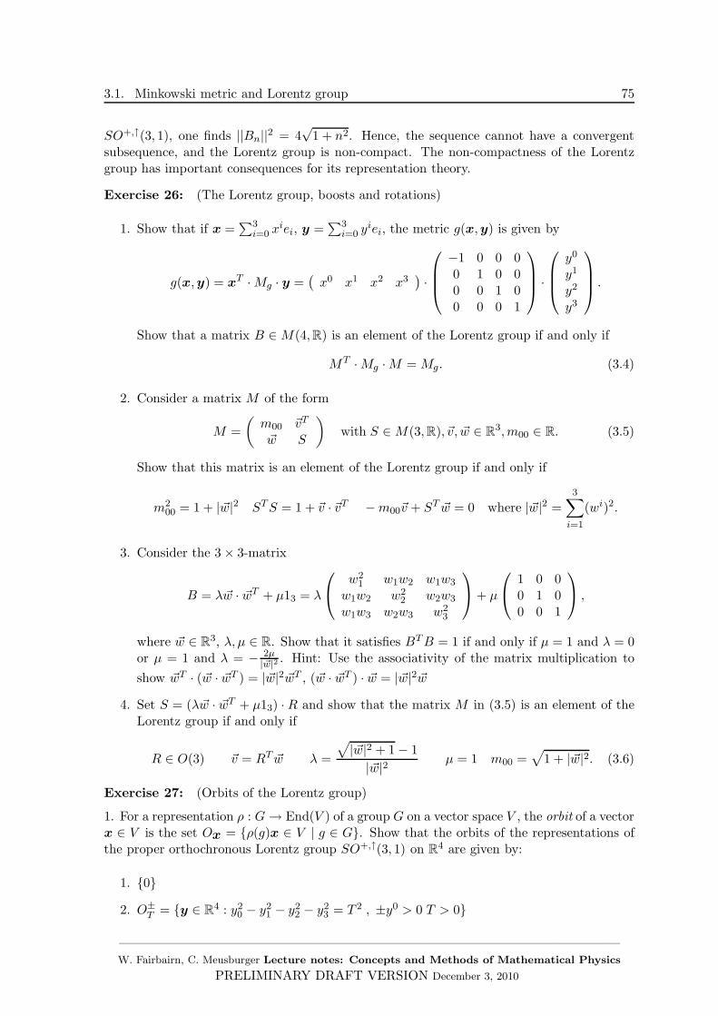
3.1. Minkowski metric and Lorentz group 75
SO+,↑(3, 1), one finds ||Bn||2 = 4√
1 + n2. Hence, the sequence cannot have a convergentsubsequence, and the Lorentz group is non-compact. The non-compactness of the Lorentzgroup has important consequences for its representation theory.
Exercise 26: (The Lorentz group, boosts and rotations)
1. Show that if x =∑3
i=0 xiei, y =
∑3i=0 y
iei, the metric g(x,y) is given by
g(x,y) = xT ·Mg · y =(x0 x1 x2 x3
)·
−1 0 0 00 1 0 00 0 1 00 0 0 1
·
y0
y1
y2
y3
.
Show that a matrix B ∈M(4,R) is an element of the Lorentz group if and only if
MT ·Mg ·M = Mg. (3.4)
2. Consider a matrix M of the form
M =
(m00 ~vT
~w S
)with S ∈M(3,R), ~v, ~w ∈ R3,m00 ∈ R. (3.5)
Show that this matrix is an element of the Lorentz group if and only if
m200 = 1 + |~w|2 STS = 1 + ~v · ~vT −m00~v + ST ~w = 0 where |~w|2 =
3∑
i=1
(wi)2.
3. Consider the 3 × 3-matrix
B = λ~w · ~wT + µ13 = λ
w21 w1w2 w1w3
w1w2 w22 w2w3
w1w3 w2w3 w23
+ µ
1 0 00 1 00 0 1
,
where ~w ∈ R3, λ, µ ∈ R. Show that it satisfies BTB = 1 if and only if µ = 1 and λ = 0or µ = 1 and λ = − 2µ
|~w|2 . Hint: Use the associativity of the matrix multiplication to
show ~wT · (~w · ~wT ) = |~w|2 ~wT , (~w · ~wT ) · ~w = |~w|2 ~w
4. Set S = (λ~w · ~wT + µ13) · R and show that the matrix M in (3.5) is an element of theLorentz group if and only if
R ∈ O(3) ~v = RT ~w λ =
√|~w|2 + 1 − 1
|~w|2 µ = 1 m00 =√
1 + |~w|2. (3.6)
Exercise 27: (Orbits of the Lorentz group)
1. For a representation ρ : G→ End(V ) of a group G on a vector space V , the orbit of a vectorx ∈ V is the set Ox = ρ(g)x ∈ V | g ∈ G. Show that the orbits of the representations ofthe proper orthochronous Lorentz group SO+,↑(3, 1) on R4 are given by:
1. 0
2. O±T = y ∈ R4 : y2
0 − y21 − y2
2 − y23 = T 2 , ±y0 > 0 T > 0
——————————————————————————————————————W. Fairbairn, C. Meusburger Lecture notes: Concepts and Methods of Mathematical Physics
PRELIMINARY DRAFT VERSION December 3, 2010
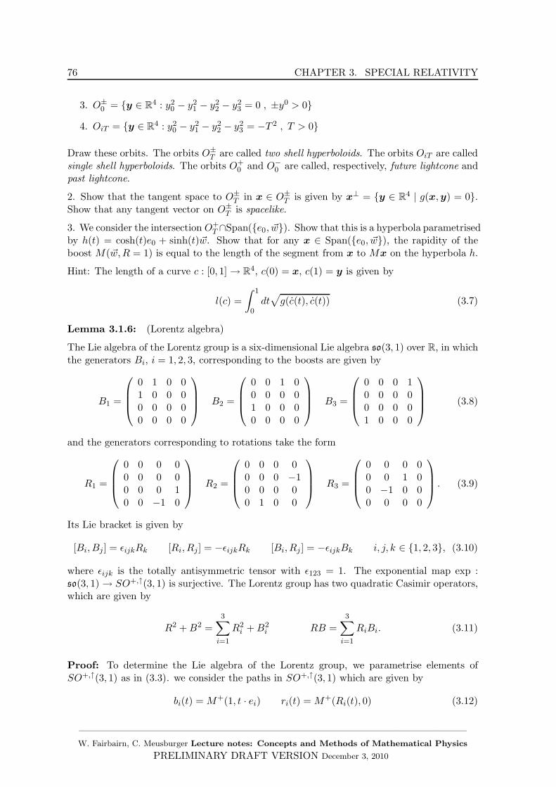
76 CHAPTER 3. SPECIAL RELATIVITY
3. O±0 = y ∈ R4 : y2
0 − y21 − y2
2 − y23 = 0 , ±y0 > 0
4. OiT = y ∈ R4 : y20 − y2
1 − y22 − y2
3 = −T 2 , T > 0
Draw these orbits. The orbits O±T are called two shell hyperboloids. The orbits OiT are called
single shell hyperboloids. The orbits O+0 and O−
0 are called, respectively, future lightcone andpast lightcone.
2. Show that the tangent space to O±T in x ∈ O±
T is given by x⊥ = y ∈ R4 | g(x,y) = 0.Show that any tangent vector on O±
T is spacelike.
3. We consider the intersection O+T ∩Span(e0, ~w). Show that this is a hyperbola parametrised
by h(t) = cosh(t)e0 + sinh(t)~w. Show that for any x ∈ Span(e0, ~w), the rapidity of theboost M(~w,R = 1) is equal to the length of the segment from x to Mx on the hyperbola h.
Hint: The length of a curve c : [0, 1] → R4, c(0) = x, c(1) = y is given by
l(c) =
∫ 1
0dt√g(c(t), c(t)) (3.7)
Lemma 3.1.6: (Lorentz algebra)
The Lie algebra of the Lorentz group is a six-dimensional Lie algebra so(3, 1) over R, in whichthe generators Bi, i = 1, 2, 3, corresponding to the boosts are given by
B1 =
0 1 0 01 0 0 00 0 0 00 0 0 0
B2 =
0 0 1 00 0 0 01 0 0 00 0 0 0
B3 =
0 0 0 10 0 0 00 0 0 01 0 0 0
(3.8)
and the generators corresponding to rotations take the form
R1 =
0 0 0 00 0 0 00 0 0 10 0 −1 0
R2 =
0 0 0 00 0 0 −10 0 0 00 1 0 0
R3 =
0 0 0 00 0 1 00 −1 0 00 0 0 0
. (3.9)
Its Lie bracket is given by
[Bi, Bj ] = ǫijkRk [Ri, Rj ] = −ǫijkRk [Bi, Rj ] = −ǫijkBk i, j, k ∈ 1, 2, 3, (3.10)
where ǫijk is the totally antisymmetric tensor with ǫ123 = 1. The exponential map exp :so(3, 1) → SO+,↑(3, 1) is surjective. The Lorentz group has two quadratic Casimir operators,which are given by
R2 +B2 =3∑
i=1
R2i +B2
i RB =3∑
i=1
RiBi. (3.11)
Proof: To determine the Lie algebra of the Lorentz group, we parametrise elements ofSO+,↑(3, 1) as in (3.3). we consider the paths in SO+,↑(3, 1) which are given by
bi(t) = M+(1, t · ei) ri(t) = M+(Ri(t), 0) (3.12)
——————————————————————————————————————W. Fairbairn, C. Meusburger Lecture notes: Concepts and Methods of Mathematical Physics
PRELIMINARY DRAFT VERSION December 3, 2010
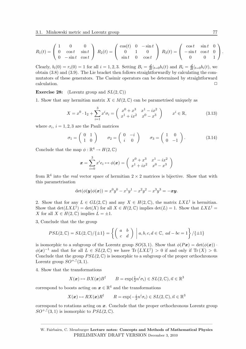
3.1. Minkowski metric and Lorentz group 77
R1(t) =
1 0 00 cos t sin t0 − sin t cos t
R2(t) =
cos(t) 0 − sin t0 1 0
sin t 0 cos t
R3(t) =
cos t sin t 0− sin t cos t 0
0 0 1
.
Clearly, bi(0) = ri(0) = 1 for all i = 1, 2, 3. Setting Bi = ddt |t=0bi(t) and Ri = d
dt |t=0bi(t), weobtain (3.8) and (3.9). The Lie bracket then follows straightforwardly by calculating the com-mutators of these generators. The Casimir operators can be determined by straightforwardcalculation. 2
Exercise 28: (Lorentz group and SL(2,C))
1. Show that any hermitian matrix X ∈M(2,C) can be parametrised uniquely as
X = x0 · 12 +
3∑
i=1
xiσi =
(x0 + x3 x1 − ix2
x1 + ix2 x0 − x3
)xi ∈ R, (3.13)
where σi, i = 1, 2, 3 are the Pauli matrices
σ1 =
(0 11 0
)σ2 =
(0 −ii 0
)σ3 =
(1 00 −1
). (3.14)
Conclude that the map φ : R4 → H(2,C)
x =
3∑
i=0
xiei 7→ φ(x) =
(x0 + x3 x1 − ix2
x1 + ix2 x0 − x3
)
from R4 into the real vector space of hermitian 2 × 2 matrices is bijective. Show that withthis parametrisation
det(φ(y)φ(x)) = x0y0 − x1y1 − x2y2 − x3y3 = −xy.
2. Show that for any L ∈ GL(2,C) and any X ∈ H(2,C), the matrix LXL† is hermitian.Show that det(LXL†) = det(X) for all X ∈ H(2,C) implies det(L) = 1. Show that LXL† =X for all X ∈ H(2,C) implies L = ±1.
3, Conclude that the the group
PSL(2,C) = SL(2,C)/±1 =
(a bc d
) ∣∣∣∣ a, b, c, d ∈ C, ad− bc = 1
/±1
is isomorphic to a subgroup of the Lorentz group SO(3, 1). Show that φ(Px) = det(φ(x)) ·φ(x)−1 and that for all L ∈ SL(2,C) we have Tr
(LXL†) > 0 if and only if Tr (X) > 0.
Conclude that the group PSL(2,C) is isomorphic to a subgroup of the proper orthochronousLorentz group SO+,↑(3, 1).
4. Show that the transformations
X(x) 7→ BX(x)B† B = exp(12n
iσi) ∈ SL(2,C), ~n ∈ R3
correspond to boosts acting on x ∈ R4 and the transformations
X(x) 7→ RX(x)R† R = exp(− i2n
iσi) ∈ SL(2,C), ~n ∈ R3
correspond to rotations acting on x. Conclude that the proper orthochronous Lorentz groupSO+,↑(3, 1) is isomorphic to PSL(2,C).
——————————————————————————————————————W. Fairbairn, C. Meusburger Lecture notes: Concepts and Methods of Mathematical Physics
PRELIMINARY DRAFT VERSION December 3, 2010
78 CHAPTER 3. SPECIAL RELATIVITY
3.2 Minkowski space
Definition 3.2.1: (Affine space)
An affine space A over a vector space V is a set A together with a vector space V and a mapφ : A × V → A, (a,v) 7→ φ(a,v) such that
1. For all a ∈ A, the map φa = φ(a, ·) : V → A, v 7→ φ(a,v) is a bijection.
2. For all a ∈ A, v,w ∈ V , φ(φ(a,v),w) = φ(a,v + w). In other words: the mapφ : A × V → A gives rise to an action of the abelian group (V,+) on A.
Lemma 3.2.2: (Vector spaces and affine spaces)
1. Let A,B affine spaces over a vector space V with maps φA : A × V → A and φB :B × V → B. Then there exists a bijection f : A → B such that
φB(f(a),v) = f(φA(a,v)) ∀a ∈ A,v ∈ V. (3.15)
2. For any vector space V , V becomes an affine space over itself if we set φ : V × V → V ,φ(v,w) = v + w for all v,w ∈ V .
Proof: Exercise.
Remark 3.2.3: (Affine spaces and vector spaces)
The first condition in Definition 3.2.1 tells us that the choice of an element a ∈ A allows us toidentify A and V via the map φ(a, ·) : V → A. As a consequence of this, any two affine spacesover a vector space V can be identified via bijections defined as in (3.15). Note, however,that this identification is not canonical.
The second statement in Lemma 3.2.2 then tells us that we can identify any affine space withthe set Rn or Cn viewed as an affine space over the vector space Rn or Cn. The fundamentaldifference between a vector space and an affine space is that a vector space has a distinguishedelement, the null vector, whereas an affine space does not. Roughly speaking: “an affine spaceis a vector space who has forgotten about its origin”.
In the following, we omit the map φ : A × V → A and write a+ v for φ(a,v) for any a ∈ A,v ∈ V . We write a− b for the unique element v ∈ V such that b = φ(a,v).
Remark 3.2.4: Via its identification with the underlying vector space and the identificationof the vector space with Rn, any affine space A over a vector space V , dim(V ) = n can beviewed as a manifold isomorphic to Rn. The tangent space at any point a ∈ A is isomorphicto V ∼= Rn.
Definition 3.2.5: (Affine subspaces, hyperplanes, lines)
Let A be an affine space over a vector space V . An affine subspace or k-dimensional affinehyperplane of A is a subset B ⊂ A of the form
B = a+W = a+ w | a ∈ A,w ∈W ⊂ V
where W ⊂ V is a linear subspace of V of dimension k. An affine subspace is called straightline if it is an affine hyperplane of dimension 1, i.e. W = Span(w), w ∈ V \ 0.
——————————————————————————————————————W. Fairbairn, C. Meusburger Lecture notes: Concepts and Methods of Mathematical Physics
PRELIMINARY DRAFT VERSION December 3, 2010

3.2. Minkowski space 79
The transformations which preserve the structure of a vector space V are linear maps f : V →V . The transformations which preserve affine spaces are affine maps or affine transformations.
Definition 3.2.6: (Affine transformation)
Let A be an affine space over a vector space V . An affine transformation is a map f : A → A
for which there exists an a ∈ A, M ∈ End(V ) and v ∈ V such that
f(b) = a+ v +M(b− a) ∀b ∈ A. (3.16)
Bijective linear transformations of a vector space V are characterised by the fact that theymap linear subspaces of dimension one to linear subspaces of dimension one. A similarcharacterisation exists for bijective affine transformations.
Theorem 3.2.7: A map f : A → A is called a collineation if for all a, b, c ∈ A which lie on astraight line, f(a), f(b), f(c) lie on a straight line. A map f : A → A is a bijective collineationif and only if f is a bijective affine transformation, i.e. there exists an a ∈ A, M ∈ Aut(V ),v ∈ V such that
f(b) = a+ v +M(b− a) ∀b ∈ A.
Remark 3.2.8: Note that for any affine transformation characterised as in (3.16), we havef(a) = a+ v. Given another element c ∈ A, we can reexpress (3.16) as
f(b) = a+ v +M(b− a) = c+ v′ +M(b− c) v′ = M(c− a) − (c− a) + v ∀b ∈ A.
Hence it is possible to choose a fixed element a ∈ A and express all affine transformations withrespect to this element. With the choice of such an element a ∈ A an affine transformationis then characterised uniquely by the associated linear map M ∈ End(V ) and the vectorv ∈ V . Hence, we can identify the set of affine transformations with the set of tuples (M,v),M ∈ End(V ), v ∈ V .
We are now ready to investigate the structure of the set of bijective affine transformationsand find that they form a group.
Lemma 3.2.9: The affine bijections form a group with respect to their composition, namelythe semidirect product Aut(V ) ⋉ V . In other words: given an element a ∈ A and twoaffine transformations f1, f2 : A → A characterised with respect to a ∈ A by linear mapsM1,M2 ∈ Aut(V ) and v1,v2 ∈ V , the composition f1 f2 : A → A is given by
f1 f2(b) = a+ (M1M2)(b− a) + v1 +M1v2 ∀b ∈ A.
Denoting fi by a tuple (Mi,vi), we can express the multiplication law as
(M1,v1) (M2,v2) = (M1 M2,v1 +M1v2).
Affine spaces can be equipped with additional structure if additional structures such as bi-linear forms are present on the underlying vector spaces. Affine bijections then should berestricted to those affine transformations which preserve this additional structure. If oneconsiders an affine space over the vector space R4 equipped with the Minkowski metric, oneobtains Minkowski space. The affine bijections which preserve the structure of Minkowskispace are the Poincare transformations.
——————————————————————————————————————W. Fairbairn, C. Meusburger Lecture notes: Concepts and Methods of Mathematical Physics
PRELIMINARY DRAFT VERSION December 3, 2010
80 CHAPTER 3. SPECIAL RELATIVITY
Definition 3.2.10: (Minkowski space)
Minkowski space M4 is an affine space over the vector space R4 equipped with the Minkowskimetric. The Poincare group is the set of bijective affine transformations which preserve theMinkowski metric. It is the semidirect product P3 = SO(3, 1)⋉R4 with group multiplication
(L1,w1) (L2,w2) = (L1 · L2,w1 + L1w2) ∀L1, L2 ∈ SO(3, 1),w1,w2 ∈ R4. (3.17)
Straight lines and, more generally, paths c : R → M4 in Minkowski space can now be inves-tigated with respect to their behaviour with respect to the Minkowski metric. In particular,we have the following definitions.
Definition 3.2.11: (Worldline, eigentime, arclength, geodesic)
1. A smooth curve x : R → M4 is called future directed (past directed) if x(t) is futuredirected (past directed) for all t ∈ R.
2. It is called timelike (lightlike, spacelike) if for all t ∈ R the velocity vector x(t) ∈ R4 istimelike (lightlike, spacelike).
3. It is called geodesic if its image is a straight line in Minkowski space.
4. A future directed, timelike curve x : R → M4 is called a worldline. It is calledparametrised according to eigentime if x(t)2 = −c2 for all t ∈ R, where c ∈ R+ isa fixed constant. The vector
v(t) = cx(t)√|x(t)2|
is called four velocity of the worldline x at time t.
Remark 3.2.12:
Any smooth lightlike curve is a geodesic and either future directed or past directed.
3.3 The theory of special relativity
The axioms of special relativity are usually stated in the following form.
Axiom 1 Spacetime is homogeneous and isotropic
Axiom 2 Relativity: The laws of physics take the same form for all inertial observers. Withrespect to inertial observers, particles which are not subject to forces move on straight linesand with constant speed.
Axiom 3 There exists a universal velocity c ∈ R which is the same for all inertial observersand cannot be reached by any massive observer.
One can show that, together and interpreted correctly, these axioms uniquely characteriseMinkowski space. We will not give the full derivation, but show how these axioms can berecast in a mathematically precise form.
We start with the first axiom. The statement that spacetime is homogeneous means that itis described by an affine space A4 over the vector space R4. Additionally, to give rise to a
——————————————————————————————————————W. Fairbairn, C. Meusburger Lecture notes: Concepts and Methods of Mathematical Physics
PRELIMINARY DRAFT VERSION December 3, 2010
3.3. The theory of special relativity 81
notion of lengths, angles and time, one requires that R4 is equipped with a non-degeneratesymmetric bilinear form g.
Spacetime transformations or symmetry transformations must form a subgroup of the groupof affine bijections GL(4,R) ⋉ R4. As time and space are homogenous, this subgroup mustcontain all translations and therefore be of the form G⋉R4. The requirement that spacetimeis isotropic amounts to imposing that the rotation group SO(3) should be contained in thegroup of symmetry transformations: SO(3) ⊂ G. Moreover, we require that spacetimetransformations are orientation and volume preserving. In other words: the group G shouldbe a subgroup G ⊂ SL(4,R). We can thus rephrase the first axiom as follows:
Axiom 1’ Time and space are described by an affine space A4 over the vector space R4 witha non-degenerate, symmetric bilinear form g. Spacetime symmetries which relate differentobservers form a subgroupG⋉R4 of the group of affine bijections with SO(3) ⊂ G ⊂ SL(4,R).
In order to give a precise formulation of the second axiom we must develop a notion ofinertial observer and of forces. Intuitively, it seems plausible to translate this statement intothe requirement that inertial observers and particles which are not subjected to forces shouldbe associated with certain lines in the affine space A4. The set of all inertial observers shouldbe invariant under spacetime symmetries, and any two inertial observers should be related bya spacetime symmetry. (Otherwise, there would be several non-equivalent types of inertialobservers). This yields the following reformulation of Axiom 2:
Axiom 2’ 1: Inertial observers and the motion of massive particles not subjected to forcesare described by certain lines in A4. The set of inertial observers forms an orbit under theaction of the group of symmetry transformations S = G ⋉ R4. In other words: a line in A4
corresponds to an observer if and only if it is of the form a+w in A4, where a ∈ A4, w = Le0,L ∈ G and e0 is a fixed vector in R4.
In order to determine precisely which subgroup G ⊂ SL(4,R) describes the spacetime sym-metries between observers, we need to make more precise statements about the form of thesetransformations. While the rotation group SO(3) is contained in G as a subgroup, G shouldcontain additional transformations, the velocity transformations, which relate observers mov-ing with constant velocities with respect to each other.
We require that these velocity transformations are parametrised uniquely by velocity vectors~v ∈ R3, that ~v = 0 corresponds to the identity and that the dependence on ~v is contin-uous. This amounts to the statement that the group of symmetry transformations is asix-dimensional Lie subgroup of G. Moreover, one requires that the velocity transformationsare compatible with rotations which encode the isotropy of spacetime and that velocity trans-formations in a fixed direction form a subgroup of G. This leads to the following condition.
Axiom 2’ 2: The group of symmetry transformations is of the form G ⋉ R4 where G ⊂SL(4,R) is a six-dimensional Lie group which contains SO(3). In addition to rotations, Gcontains velocity transformations L(~v) ∈ G which satisfy
L(−~v) = L(~v)−1 R · L(~v) ·R−1 = L(R~v) ∀R ∈ SO(3).
Velocity transformations L(αw), α ∈ R in a fixed direction w ∈ R4 form a subgroup of G.
Axiom 3 can be reformulated as follows
——————————————————————————————————————W. Fairbairn, C. Meusburger Lecture notes: Concepts and Methods of Mathematical Physics
PRELIMINARY DRAFT VERSION December 3, 2010
82 CHAPTER 3. SPECIAL RELATIVITY
Axiom 3’ The set of all admissible velocity vectors ~v is the closed three-ball Bc(0) ⊂ R3. Forany v, v′ ∈ [−c, c] and any ~e ∈ S2 ⊂ R3, there exists a unique v′′ ∈ [−c, c] such that
L(v~e) · L(v′~e) = L(v′′~e).
It can be shown that together, Axioms 1, 2 and 3 fix the group G ⊂ SL(4,R) uniquely. Theyimply G = SO+,↑(3, 1) and that the affine space which describes the spacetime is Minkowskispace M4. We can summarise the resulting description of space and time, i.e. the theory ofspecial relativity in the following postulates.
Postulate 1: (Spacetime and observers)
Space and time are described by Minkowski space M4. Each inertial observer corresponds toa timelike straight line in Minkowski space. The admissible symmetry transformations whichrelate different observers form the group of affine transformations SO(3, 1)+,↑ ⋉ R4, i.e. theproper orthochronous Poincare group.
Postulate 2: (Time and space as perceived by observers)
For an inertial observer whose motion is given by a timelike line a+Span(w), the velocity unitvector is the unique future directed, timelike vector w satisfying w2 = −1 and Span(w) =Span(w).
The time interval elapsed between two events x, y ∈ M4 as perceived by this observer isgiven by ∆tw(x, y) = |w(x − y)|, where w is the velocity unit vector of the observer. Theevents x, y are perceived as simultaneous if w(x − y) = 0. Event x occurs before event y ifw(x− y) < 0 and after event y if w(x− y) > 0. The set of events occurring simultaneouslywith an event x ∈ M4 with respect to the observer given by w is the affine plane x + w⊥.This gives rise to a foliation of spacetime by affine hyperplanes b + w⊥, b ∈ a + Span(w)through points on the observer’s worldline.
The relative position between two simultaneous events x, y ∈ a + w⊥ as perceived by theobserver is the spacelike vector x− y.
Postulate 3: (Motion of massive particles and of light)
Point particles of mass m 6= 0 move on worldlines. The eigentime of the worldline coincideswith the time perceived by the particle, i.e. the time shown on a clock moving with theparticle. Particles with mass m 6= 0 that are not subjected to any forces moves on futuredirected, timelike geodesics. Light moves along future directed, lightlike geodesics.
In order to formulate the fourth postulate, we need to introduce a notion of future and past.
Definition 3.3.1: (Future, past, lightcone)
The future I+(x) and past I−(x) of a point x ∈ M4 are the sets
I±(x) = y ∈ M4 | (y − x)2 ≤ 0 , y − x future (past) directed.
They are called the future (past) lightcone at x ∈ M4.
The future (past) of a subset S ∈ M4 is the set
I±(S) = y ∈ M4 | ∃x ∈ S : (x− y)2 ≤ 0 , y − x future (past) directed =⋃
x∈SI±(x).
——————————————————————————————————————W. Fairbairn, C. Meusburger Lecture notes: Concepts and Methods of Mathematical Physics
PRELIMINARY DRAFT VERSION December 3, 2010
3.3. The theory of special relativity 83
Using this notion of future and past, we can state the fourth postulate as follows:
Postulate 4: (Causality)
Each physical event corresponds to a unique point in Minkowski space M4. An event x ∈ M4
can influence an event y ∈ M4 or a signal can be sent from x to y if and only if y lies in thefuture of x. If x /∈ I+(y) and y /∈ I+(x), x and y are called causally disconnected and nosignal can be passed between them.
We now have to show that Postulate 2 gives rise to a sensible notion of time for each inertialobserver, which is compatible with the notion of past, future and causality introduced inPostulate 4. This is guaranteed by the following lemma.
Lemma 3.3.2: For any inertial observer whose worldline is characterised by a velocity unitvector w and any events x, y, z ∈ M4, we have:
1. x and y simultaneous implies y − x spacelike
2. x ∈ I+(y) implies that y happens before x with respect to the observer, x ∈ I−(y)implies that x happens before y.
3. If x happens before y and y happens before z, then x happens before z.
Proof: Exercise.
This lemma shows that for a single observer, the assignment of time makes sense and iscompatible with the notion of past, future and causality. However, it is clear that it dependson the observer. Time and space are no longer absolute as in Newtonian mechanics butbecome observer-dependent.
In order to ensure that the notion of time is physically sensible, we now need to make surethat assignments of time made by different observers are compatible and that the secondaxiom holds. This is guaranteed by the content of the following lemma.
Lemma 3.3.3: (Relativity of simultaneity)
For any two inertial observers whose velocity unit vectors w, v, w 6= v are not equal, thereexist events x, y such that x happens before y with respect to the observer characterised byw and y happens before x with respect to the observer characterised by v. Such events arealways causally disconnected.
Proof: Exercise. 2
Remark 3.3.4: Note that the existence of events whose order in time is reversed withrespect to two observers is not in contradiction with Axiom 2. As such events are alwayscausally disconnected, neither of them can affect the other. Although two observers coulddisagree about which event happens before the other, they would agree on the fact thatneither of the two events can influence the other or, equivalently, that there is no light rayemitted at event x and received at event y or vice versa. The fact that two observers assigndifferent times to events therefore does not mean that they perceive different laws of physics.
Exercise 29: (Relativity of simultaneity)
——————————————————————————————————————W. Fairbairn, C. Meusburger Lecture notes: Concepts and Methods of Mathematical Physics
PRELIMINARY DRAFT VERSION December 3, 2010
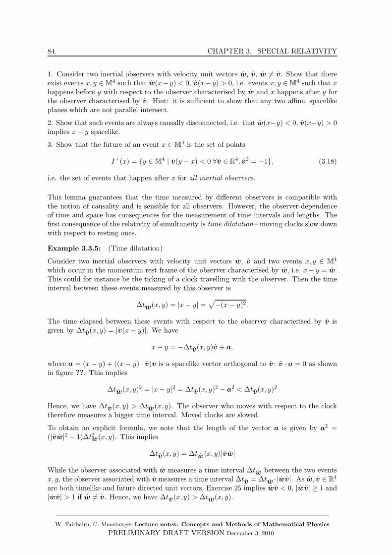
84 CHAPTER 3. SPECIAL RELATIVITY
1. Consider two inertial observers with velocity unit vectors w, v, w 6= v. Show that thereexist events x, y ∈ M4 such that w(x−y) < 0, v(x−y) > 0, i.e. events x, y ∈ M4 such that xhappens before y with respect to the observer characterised by w and x happens after y forthe observer characterised by v. Hint: it is sufficient to show that any two affine, spacelikeplanes which are not parallel intersect.
2. Show that such events are always causally disconnected, i.e. that w(x−y) < 0, v(x−y) > 0implies x− y spacelike.
3. Show that the future of an event x ∈ M4 is the set of points
I+(x) = y ∈ M4 | v(y − x) < 0 ∀v ∈ R4, v2 = −1, (3.18)
i.e. the set of events that happen after x for all inertial observers.
This lemma guarantees that the time measured by different observers is compatible withthe notion of causality and is sensible for all observers. However, the observer-dependenceof time and space has consequences for the measurement of time intervals and lengths. Thefirst consequence of the relativity of simultaneity is time dilatation - moving clocks slow downwith respect to resting ones.
Example 3.3.5: (Time dilatation)
Consider two inertial observers with velocity unit vectors w, v and two events x, y ∈ M4
which occur in the momentum rest frame of the observer characterised by w, i.e. x− y = w.This could for instance be the ticking of a clock travelling with the observer. Then the timeinterval between these events measured by this observer is
∆tw(x, y) = |x− y| =√−(x− y)2.
The time elapsed between these events with respect to the observer characterised by v isgiven by ∆tv(x, y) = |v(x− y)|. We have
x− y = −∆tv(x, y)v + a,
where a = (x− y) + ((x − y) · v)v is a spacelike vector orthogonal to v: v · a = 0 as shownin figure ??. This implies
∆tw(x, y)2 = |x− y|2 = ∆tv(x, y)2 − a2 < ∆tv(x, y)2
Hence, we have ∆tv(x, y) > ∆tw(x, y). The observer who moves with respect to the clocktherefore measures a bigger time interval. Moved clocks are slowed.
To obtain an explicit formula, we note that the length of the vector a is given by a2 =(|vw|2 − 1)∆t2w(x, y). This implies
∆tv(x, y) = ∆tw(x, y)|vw|
While the observer associated with w measures a time interval ∆tw between the two eventsx, y, the observer associated with v measures a time interval ∆tv = ∆tw · |wv|. As w, v ∈ R4
are both timelike and future directed unit vectors, Exercise 25 implies wv < 0, |wv| ≥ 1 and|wv| > 1 if w 6= v. Hence, we have ∆tv(x, y) > ∆tw(x, y).
——————————————————————————————————————W. Fairbairn, C. Meusburger Lecture notes: Concepts and Methods of Mathematical Physics
PRELIMINARY DRAFT VERSION December 3, 2010
3.3. The theory of special relativity 85
The second consequence of the relativity of simultaneity is the Lorentz contraction - movingrods appear shortened.
Lemma 3.3.6: (Lorentz contraction)
Consider two inertial observers with velocity unit vectors w, v and a rod which is at restwith respect to the observer w. The worldlines of its ends are therefore of the form
e1(t) = tw + z1 e2(t) = tw + z2 z1, z2 ∈ M4, w · (z1 − z2) = 0 (3.19)
The relative position ~p of the ends of the rod as measured by observer w is therefore givenby ~p = z1 − z2 and its length is (z1 − z2)
2.
When the observer v measures the relative position of the ends of the rod, the result is thevector u between intersection of the worldlines associated with the ends of the rod with anaffine plane a+ v⊥ of events simultaneous with respect to v
u = z2 − z1 −(z2 − z1) · v
vww
If we decompose the vector z1 − z2 into a component a orthogonal to both v and w and intoa component c = α(v + (vw)w) in the plane spanned by v, w and orthogonal to w but notto v, we have
u = a + c − vc
vww.
The length of u is given by
u2 = a2 + c2 − (vc)2
(vw)2= a2 +
c2
(vw)2.
The observer v therefore assigns to the rod the length l(v) with l(v)2 = u2 = a2 +c2/(vw)2,while the observer associated with w measures its length as l(w) = a2 + c2.
From Exercise 25, we have |wv| > 1 if v 6= w , which implies l(v) ≤ l(w) and l(v) < l(w) ifthe vector c 6= 0. The rod therefore appears shortened for an observer who moves with respectto the rod and whose velocity relative to the rod is not orthogonal to it. The shortening effectis maximal if the observer moves parallel to the rod (a = 0).
Exercise 30:
1. Consider an observer with worldline
e(t) = tx + x0 with x0 ∈ M4,x ∈ R4,x2 = −c2, e0 · x < 0
and a future directed geodesic y : R → M4. Use the time intervals and position vectors withrespect to observers to show that the relative velocity of y with respect to the observer withworldline e is given by
~v(t) = −c y(t) + (x · y(t))x
x · y(t).
Show that ~v(t)2 < c2 if y is timelike and ~v(t)2 = c2 if y is lightlike. Show that the velocityfour vector associated with y can be written as
y(t) =1√
1 − ~v2(t)/c2(c · e0 + ~v(t)),
——————————————————————————————————————W. Fairbairn, C. Meusburger Lecture notes: Concepts and Methods of Mathematical Physics
PRELIMINARY DRAFT VERSION December 3, 2010
86 CHAPTER 3. SPECIAL RELATIVITY
where ~v(t) is the velocity of y with respect to the observer with worldline e(t) = te0 + x0.
2. Show that for an inertial observer with four velocity x = 1√1−~v2(t)/c2
(ce0 +~v), ~ve0 = 0 and
an internal observer with four velocity y = ce0, the formulas for time dilatation and Lorentzcontraction take the form
∆t′ =∆t√
1 − ~v2/c2l′ = l
√1 − ~v2/c2.
Exercise 31: (Addition of velocities)
Consider two boosts in the e1 direction.
B(θ1) =
cosh θ1 sinh θ1 0 0sinh θ1 cosh θ1 0 0
0 0 1 00 0 0 1
B(θ2) =
cosh θ2 sinh θ2 0 0sinh θ2 cosh θ2 0 0
0 0 1 00 0 0 1
Show that the product B1(θ1) · B(θ2) = B(θ2) · B(θ1) = B(θ3) is another boost in thee1-direction with
θ3 = θ1 + θ2.
Show that the velocity of the observer with four velocity c·B(θ)e0 with respect to the observerwith four velocity c · e0 is given by ~v = v · e1, v = c · tanh θ. Show that the relativistic velocityaddition law takes the form
v3 =v1 + v2
1 + v1v2/c.
Example 3.3.7: (Appearance of the night sky)
We consider an inertial observer at a point x ∈ M4 and his past lightcone
I−(x) = x+ y ∈ M4 | y2 = 0, e0 · y > 0,
which is the set of all lightrays sent out in Minkowski space which reach the observer at theevent x. The map
f : I−(x) → S2, y = (|~y|, ~y) 7→ f(y) = (1, ~y/|~y|)
maps the backward lightcone to the two-sphere S2 and is invariant under y → αy, α ∈ R+.It therefore induces a map from the set of past lightrays at x to S2. Each point p ∈ S2
corresponds to a point in the sky as seen by the observer.
By combining this map with the stereographic projection P : S2 → C ∪ ∞
P (~k) =
k1−ik2
1−k3 k3 6= 1
∞ k3 = 1∀~k ∈ S2
we obtain a map ρ = P f : R4 → C ∪ ∞
ρ(y) =
y1−iy2y0−y3 y0 6= y3
∞ y0 = y3
which is again invariant under rescalings y 7→ αy, α ∈ R+0 and therefore induces a map from
the set of past lightrays to C∪∞. Note that by definition, the stereographic projection maps
——————————————————————————————————————W. Fairbairn, C. Meusburger Lecture notes: Concepts and Methods of Mathematical Physics
PRELIMINARY DRAFT VERSION December 3, 2010
3.3. The theory of special relativity 87
circles on S2 to circles or lines in C ∪ ∞. More precisely, any circle in S2 which does notcontain the point (0, 0, 1) is mapped to a circle in C∪∞ and any circle through (0, 0, 1) toa line.
We will now use this map to see how the appearance of the night sky changes if a boost orrotation is applied to the observer. For this, it is convenient to use the identification of R4
with the set of hermitian matrices as in Exercise 28
x ∈ R4 7→ φ(x) = x0 +
3∑
i=1
xiσi =
(x0 + x3 x1 − ix2
x1 + ix2 x0 − x3
), (3.20)
in which the Minkowski metric is given by x ·y = − det(φ(x) ·φ(y)). With this identification,lightlike past oriented vectors are given by hermitian matrices M ∈ M(2,C), M † = M withvanishing determinant.
Applying this map to the past lightcone, we obtain
φ(y) =
(y0 + y3 y1 − iy2
y1 + iy2 y0 − y3
)= (y0 − y3) ·
(|z|2 zz 1
)with z = ρ(y). (3.21)
As shown in Exercise 28, the proper orthochronous Lorentz group is isomorphic to PSL(2,C) =SL(2,C)/±1, and the action of a Lorentz transformation L on v ∈ R4 agrees with the ac-tion of the associated element L ∈ SL(2,C) on the hermitian matrix φ(v)
L · φ(v) · L† = φ(Lv) ∀v ∈ R4, L ∈ SO+,↑(3, 1).
We now consider the transformation of the hermitian matrix (3.21) associated with a back-ward lightray under a Lorentz transformation given by a matrix L ∈ SL(2,C)
L =
(a bc d
)∈ SL(2,C).
This yields
L · φ(y) · L† = (y0 − y3)|cz + d|2 ·
∣∣∣az+bcz+d
∣∣∣2
az+bcz+d
az+bcz+d
1
.
A Lorentz transformation acting on the past lightcone therefore corresponds to a Mobiustransformation acting on C ∪ ∞
L =
(a bc d
)∈ SL(2,C) z 7→ az + b
cz + d.
The defining characteristic of Mobius transformations is that they map circles and lines inC∪∞ to circles and lines in C∪∞. Due to the properties of the stereographic projection,circles and lines in C∪∞ correspond to circles on the night sky as perceived by the observer.Lorentz transformations acting on the backward lightcone therefor map circles on the nightsky to circles in the night sky. This implies in particular that the Lorentz contraction isinvisible.
——————————————————————————————————————W. Fairbairn, C. Meusburger Lecture notes: Concepts and Methods of Mathematical Physics
PRELIMINARY DRAFT VERSION December 3, 2010

88 CHAPTER 3. SPECIAL RELATIVITY
——————————————————————————————————————W. Fairbairn, C. Meusburger Lecture notes: Concepts and Methods of Mathematical Physics
PRELIMINARY DRAFT VERSION December 3, 2010
Chapter 4
Topological Vector Spaces
4.1 Types of topological vector spaces
Infinite dimensional vector spaces play an important role in quantum mechanics . Thisfollows already from the fact that the Heisenberg algebra, which encodes two of the mostimportant observables in physics, namely the positions and momenta, has no non-trivialfinite-dimensional representations. One can show this by taking the trace, which leads to acontradiction. In the infinite-dimensional case, this contradiction disappears, because thereare operators of which one cannot take the trace, i.e. whose trace is ill-defined.
Quantum mechanics therefore forces one to consider representations on infinite-dimensionalvector spaces. However, it turns out that the structure of a vector space alone is too weak.To have the desired properties, infinite dimensional vector spaces need to be equipped withadditional structure, namely with a topology that is compatible with the structure of a vectorspace. This leads to the notion of topological vector spaces.
Infinite dimensional vector spaces arising in physics are topological vector spaces, often withfurther structures such as norms, semi-norms or hermitian products. In this chapter, we willstudy different examples of such vector spaces which play an important role in physics andand investigate their properties.
Throughout this chapter, we will make extensive use of the Lebesgue measure. All integralsconsidered in the following are Lebesgue integrals. We will assume familiarity with Lebesgueintegration and elementary measure theory. A concise introduction is given in J. Dieudonne,Treatise on Analysis 1.
4.1.1 Topological vector spaces, metric spaces and normed spaces
We start by introducing the notion of topological spaces and topological vector spaces.
Definition 4.1.1: (Topology, continuity)
A topology on a set E is a family T of subsets F ⊂ E, called open sets in E such that
1. ∅,X ∈ T
2. General unions of open sets are open sets: If Fi ∈ T ∀i ∈ I ⇒ ⋃i∈I Fi ∈ T
89
90 CHAPTER 4. TOPOLOGICAL VECTOR SPACES
3. Finite intersections of open sets are open sets: If Fi ∈ T , ∀i ∈ 1, ..., n ⇒ ⋂ni=1 Fi ∈ T .
A set E with a topology is called a topological space.
A function f : E → G between topological spaces E and G is called continuous if for everyopen set F ⊂ G the preimage f−1(F ) = x ∈ E | f(x) ∈ F is open.
Example 4.1.2: If X, Y are topological spaces with topologies TX , TY , then the directproduct X × Y is a topological space with topology TX×Y = U × V | U ∈ TX , V ∈ TY .
A topological vector space is a vector space whose topology is compatible with the vectorspace structure:
Definition 4.1.3: (Topological vector space, isomorphisms of topological vector spaces)
A topological vector space E over k = R or k = C is a vector space E over k with a topology Tsuch that the vector space addition + : E×E → E and the scalar multiplication · : k×E → Eare continuous with respect to T . In other words: the preimage of each open set in E is openwith respect to the induced topologies on E × E and k × E (where k is equipped with thestandard topology).
When considering isomorphisms of topological vector spaces and their duals, one imposes thatthese structures are compatible with the topology on E. In other words: they are requiredto be continuous.
Definition 4.1.4: (Isomorphisms of topological vector spaces, continuous duals)
An isomorphism of topological vector spaces E, G is a bijective, linear map L : E → G thatis a homeomorphism, i.e. continuous with respect to the topologies on E, G and invertiblesuch that L−1 continuous with respect to the topologies on E, G.
The continuous dual E∗ of a topological vector space E over k is the set of continuous linearfunctionals E → k, i.e. linear maps E → k which are continuous with respect to the topologyon E.
An important concept which allows one to classify topologies and hence topological vectorspaces is the notion of Hausdorff. It also plays a crucial role in the notion of manifolds.
Definition 4.1.5: (Neighbourhood, Hausdorff)
A topological vector space is called Hausdorff if for any two elements x, y ∈ E there existopen sets Ux, Uy with x ∈ Ux, y ∈ Uy such that Ux ∩ Uy = ∅.A subset V ⊂ E is called a neighbourhood of x ∈ E if there exists an open set U ⊂ V withx ∈ U .
It turns out that in the finite-dimensional case the requirement that the topology is Hausdorffis strong enough to determine the topology of a topological vector space completely. Note,however, that this is not true for infinite dimensional topological vector spaces.
Lemma 4.1.6: On any finite-dimensional vector space V there is a unique topology, thecanonical topology, which is Hausdorff and turns V into a topological vector space.
——————————————————————————————————————W. Fairbairn, C. Meusburger Lecture notes: Concepts and Methods of Mathematical Physics
PRELIMINARY DRAFT VERSION December 3, 2010
4.1. Types of topological vector spaces 91
If V is a finite-dimensional topological vector space over k and B = e1, ..., en a basis of V ,then the map φ : kn → V
(x1, ..., xn) 7→n∑
i=1
xiei
is an isomorphism of topological vector spaces.
An important class of topologies are those defined by distance functions. This leads to theconcept of metric spaces.
Definition 4.1.7: (Metric space, distance function, metrisable space)
A metric space is a set E together with a distance function d : E × E → R that has thefollowing properties:
1. Positivity: d(x, y) ≥ 0 for all x, y ∈ E and d(x, y) = 0 implies x = y.
2. Symmetry: d(x, y) = d(y, x) for all x, y ∈ E
3. Triangle inequality: d(x, z) ≤ d(x, y) + d(y, z) for all x, y, z ∈ E
Any metric space is a topological space. The topology T induced by the distance function isthe family of sets generated by r-balls Br(x) = y ∈ E | d(y, x) < r, r ∈ R, i.e. the familyof sets which can be expressed as general union or finite intersection of r-balls.
A topological vector space is called metrisable if its topology agrees with a topology inducedby a distance function on E.
Remark 4.1.8: Metric spaces and metrizable spaces are Hausdorff.
Example 4.1.9: Consider kn (k = R or k = C) with the standard basis B = e1, ..., en.A distance function on kn is given by
d(x,y) =n∑
i=1
|xi − yi| ∀x =n∑
i=1
xiei,y =n∑
i=1
yiei ∈ kn.
A special class of metric spaces are metric spaces whose distance function is induced by anorm
Definition 4.1.10: (Norm, semi-norm)
A semi-norm on a vector space E over k is a map || || : E → R which
• is positive semi-definite ||x|| ≥ 0 for all x ∈ E
• satisfies ||λx|| = |λ|||x|| for all x ∈ E, λ ∈ k.
• satisfies the triangle inequality: ||x+ y|| ≤ ||x|| + ||y|| for al x, y ∈ E.
A norm on E is a semi-norm which is positive definite ||x|| > 0 for all x 6= 0.
——————————————————————————————————————W. Fairbairn, C. Meusburger Lecture notes: Concepts and Methods of Mathematical Physics
PRELIMINARY DRAFT VERSION December 3, 2010
92 CHAPTER 4. TOPOLOGICAL VECTOR SPACES
Lemma 4.1.11: (Normed vector spaces are metric spaces)
A norm || || : E → R on a vector space E over k = R or k = C defines a distance functiond : E × E → R on E via
d(x, y) = ||x− y|| ∀x, y ∈ E.The distance function is translation invariant, i.e. satisfies d(x + z, y + z) = d(x, y) for allx, y, z ∈ E and d(λx, λy) = |λ|d(x, y) for all x, y ∈ E, λ ∈ R.
Example 4.1.12: Consider kn (k = R or k = C) with the standard basis B = e1, ..., en.A norm on kn is given by
||x|| =n∑
i=1
|xi| ∀x =n∑
i=1
xiei, xi ∈ k.
The distance function induced by this norm is the one from example 4.2.1.
Example 4.1.13: Let f : V → k be a linear form on a vector space V over k. Then
||x|| = |f(x)| ∀x ∈ V
defines a norm on V .
The fact that normed vector spaces are metric spaces implies in particular that they areequipped with a topology induced by the distance function. It turns out that this topologyis always compatible with the vector space structure and turns the vector space E into atopological space.
Lemma 4.1.14: For any normed vector space E over k = R or k = C, the vector spaceaddition + : E × E → E, (x,y) 7→ x + y and the scalar multiplication ·λ : E → E, x 7→ λx
with λ ∈ k are uniformly continuous.
To classify norms on vector spaces, one needs a concept of equivalence of norms. It is naturalto call two norms on a vector space equivalent if they induce the same topology. One canshow that this is the case if and only if sequences that converge with respect to one normalso converge with respect to the other norm. This leads to the following definition.
Definition 4.1.15: (Equivalence of norms)
Two norms || ||1, || ||2 : E → R on a vector space E are equivalent if there exist a, b > 0such that
a||x||1 ≤ ||x||2 ≤ b||x||1 ∀x ∈ E.
Remark 4.1.16: One can show that on a finite-dimensional vector space, all norms areequivalent. This is not the case for infinite-dimensional topological vector spaces. A counterexample is given in Example 4.1.29.
Exercise 32: Consider the vector space kn, where k = R or k = C, with standard basisB = e1, ..., en and express vectors x ∈ kn with respect to this basis as x =
∑ni=1 x
iei. Showthat the following norms are equivalent:
1. ||x|| =√∑n
i=1 |xi|2
2. ||x|| =∑n
i=1 |xi|
3. ||x|| = max|xi| |i ∈ 1, ..., n.
——————————————————————————————————————W. Fairbairn, C. Meusburger Lecture notes: Concepts and Methods of Mathematical Physics
PRELIMINARY DRAFT VERSION December 3, 2010
4.1. Types of topological vector spaces 93
4.1.2 Topological vector spaces with semi-norms
The existence of a semi-norm is not enough to turn a vector space into a metric space.However, it is possible to construct normed vector spaces and hence metric spaces fromtopological vector spaces with semi-norms by taking a quotient. This is similar to of asituation in Example ??, in which quotients of vector spaces are used to turn linear mapsbetween vector spaces V and W into injective linear maps V/ker(φ) → W . Note, however,that a norm is not a linear map, although the basic idea of the construction is similar.
Lemma 4.1.17: (Quotients of vector spaces with semi-norms)
If E is a topological vector space with a semi-norm || ||, the set N = x ∈ E | ||x|| = 0is a linear subspace of E. The quotient space E/N is a normed vector space with norm||[x]|| = ||x+N || := ||x||.
Proof: Exercise. 2
Exercise 33: Consider a topological vector space E over k = R or k = C with a semi-norm|| ||. Show that the set N = x ∈ E | ||x|| = 0 is a linear subspace of E. Consider thequotient space E/N . Show that the definition
|| [x] || = ||x|| ∀x ∈ E
where [x] = x + N = y ∈ E | ||y − x|| = 0 are the equivalence classes of elements x ∈ Edefines a norm on E/N .
Hint: Show first that this definition is consistent, i.e. that for x, y ∈ E with [x] = [y], we have|| [x] || = || [y] ||. Then you know that this defines a map || || : E/N → k and you can showthat this map has the properties of a norm.
Another important situation in which semi-norms give rise to topological vector spaces arevector spaces which carry a family of semi-norms. These vector spaces play an importantrole in the theory of distributions.
Definition 4.1.18: (Topology defined by semi-norms, locally convex)
Let (|| ||α)α∈I , || ||α : E → R be a family of semi-norms on a vector space E. The family ofsemi-norms induces a topology on E. In this topology, the class T of open sets is the class ofsubsets U ⊂ E such that for all x ∈ U there exists a finite family of semi-norms (|| ||αi)i=1,...,n
and positive numbers (rj)j=1,...,n such that
K(x; (αj), (rj)) := y ∈ E | ||y − x||αj < rj ∀j ∈ 1, ..., n ⊂ U.
This topology is compatible with the vector space structure and turns E into a topologicalvector space.
A vector space E whose topology is given by a family of semi-norms is called a locally convexvector space. A sequence xnn∈N, xn ∈ E in a locally convex vector space E is said toconverge towards an element x ∈ E with respect to a family of semi-norms if ||xn−x||α → 0for all α ∈ I.
We will now show that the space of smooth functions with compact support (also often calledtest functions in the physics literature) is an example of a locally convex vector space.
——————————————————————————————————————W. Fairbairn, C. Meusburger Lecture notes: Concepts and Methods of Mathematical Physics
PRELIMINARY DRAFT VERSION December 3, 2010
94 CHAPTER 4. TOPOLOGICAL VECTOR SPACES
Definition 4.1.19: (Smooth functions with compact support)
A smooth function with compact support on Rn is a smooth function ϕ : Rn → C whosesupport Supp(ϕ) = x ∈ Rn : ϕ(x) 6= 0 is compact. The set of functions with compactsupport is denoted C∞
c (Rn). With pointwise addition and multiplication by C it becomes aninfinite dimensional vector space.
A family of semi-norms on the space of smooth functions with compact support is obtainedby considering the supremum of general derivatives. The motivation for defining these semi-norms is the wish to control derivatives of functions.
Lemma 4.1.20: (Semi-norms on C∞c (Rn))
We consider general multi-indices α = (j1, ..., jn) ∈ Nn, n ∈ N and set Dαf = ∂j1 · · · ∂jnf .Then, a family of semi-norms (|| ||α)α∈NN is given by
||f ||α = supx∈Rn|Dαf(x)| f ∈ C∞c (Rn), α ∈ NN.
The space C∞c (Rn) with the topology induced by this family of semi-norms is a locally convex
vector space.
Proof: Exercise. 2
Remark 4.1.21: The locally convex vector space C∞c (Rn) is not metrizable.
We now define a notion of convergence on the vector space C∞c (Rn) equipped with this family
of semi-norms.
Definition 4.1.22: (Convergence in C∞c (Rn))
A sequence ϕii∈N, ϕi ∈ C∞c (Rn) converges towards a function ϕ ∈ C∞
c (Rn), ϕiC∞
c (Rn)−−−−−→ ϕ,with respect to this family of semi-norms if
1. There exists a compact subset K ⊂ Rn such that Supp(ϕ) ⊂ K, Supp(ϕi) ⊂ K ∀i ∈ N
2. For all α = (j1, ..., jn) ∈ Nn, the sequence of derivatives Dαϕi = ∂j1 · · · ∂jnϕi convergesuniformly to Dαϕ = ∂j1 · · · ∂jnϕ. In other words: for any multi-index α ∈ Nn and anyǫ > 0 there exists an iαǫ ∈ N such that for all x ∈ Rn, i > iǫ |Dαϕi(x) −Dαϕ(x)| < ǫ.
One can show that the requirement that a function f : C∞c (Rn) → C is continuous in the sense
of Definition 4.1.3 if and only if f(ϕn)n→∞−−−→ f(ϕ) for all sequences ϕnn∈N, ϕn ∈ C∞
c (Rn)
with ϕnC∞
c (Rn)−−−−−→ ϕ, ϕ ∈ C∞c (Rn). Using this notion of convergence, one finds that the
continuous dual of the topological vector space C∞c (Rn) is the vector space of distributions.
Definition 4.1.23: (Distribution)
A distribution is a linear map T : C∞c (Rn) → C, ϕ 7→ T [ϕ] that is continuous with respect to
convergence in D(Rn):
ϕiC∞
c (Rn)−−−−−→ ϕ ⇒ T [ϕi] → T [ϕ] (4.1)
The space of distributions on Rn, denoted D∗(Rn) is an infinite dimensional vector spacewith respect to pointwise addition and multiplication by C.
——————————————————————————————————————W. Fairbairn, C. Meusburger Lecture notes: Concepts and Methods of Mathematical Physics
PRELIMINARY DRAFT VERSION December 3, 2010
4.1. Types of topological vector spaces 95
Lemma 4.1.24: (Topology on D∗(Rn), convergence of distributions)
The space of distributions D∗(Rn) becomes a locally convex topological vector space whenequipped with the topology defined by the family of semi-norms (||T ||ϕ)ϕ∈C∞
c (Rn), ||T ||ϕ =|T [φ]|.A sequence Tii∈N, Ti ∈ D∗(Rn) of distributions converges towards a distribution T ∈D∗(Rn), Ti
D∗
−−→ T if Ti[ϕ] → T [ϕ] for all ϕ ∈ C∞c (Rn).
4.1.3 Banach spaces and Hilbert spaces
We return to normed topological vector spaces. A special class of normed topological vectorspaces are Banach spaces, which are characterised by the fact that they are complete withrespect to their norm.
Definition 4.1.25: (Banach space)
A Banach space is a normed vector space E over k = C or k = R which is complete withrespect to the norm || || : E → R, i.e. any Cauchy sequence xnn∈N, ||xn − xm|| < ǫ for alln,m ≥ n0 converges towards an element x ∈ E.
A map Φ : E → F between Banach spaces (E, || ||E) and (F, || ||F ) is called continuous iffor all convergent sequences xnn∈N, xn ∈ E with ||xn − x||E → 0 the sequence of imagesconverges ||Φ(xn) − Φ(x)||F → 0.
For any Banach space, the continuous dual is also a Banach space:
Lemma 4.1.26: If E is a Banach space with norm || || then the continuous dual of E is aBanach space with the operator norm || ||E∗ : E∗ → R, ||f ||E∗ = sup|f(x)| | x ∈ E, ||x|| ≤ 1.
Example 4.1.27: The space C(I) of continuous functions with values in R on a closedinterval I = [0, 1] with norm
||f || =
∫ b
a|f(t)|dt (4.2)
is a normed space, but not a Banach space. The sequence fnn≥3
fn(t) =
1 0 ≤ t ≤ 12
0 12 + 1
n ≤ t ≤ 1
1 − n(t− 12) 1
2 < t < 12 + 1
n
(4.3)
is a Cauchy sequence with respect to the norm (4.2), but does not converge towards a functionin C(I).
Example 4.1.28: We consider the set lp, 1 ≤ p < ∞ of absolutely p-summable seriesx = xnn∈N, xn ∈ k, in k = R or k = C, i.e. series x = xnn∈N, xn ∈ k such that∑∞
n=1 |xk|p < ∞. These sets are vector spaces with respect to the addition and scalarmultiplication
xnn∈N + yny∈N = xn + ynn∈N txnn∈N = txnn∈N ∀t ∈ R.
——————————————————————————————————————W. Fairbairn, C. Meusburger Lecture notes: Concepts and Methods of Mathematical Physics
PRELIMINARY DRAFT VERSION December 3, 2010
96 CHAPTER 4. TOPOLOGICAL VECTOR SPACES
These vector spaces are Banach spaces when equipped with the norm
||x||p =
( ∞∑
n=1
|xk|p)1/p
.
The space l∞ of bounded series x = xnn∈N, xn ∈ k, supn∈N|xn| < ∞ is a Banach spacewith norm
||x||∞ = supn∈N|xn|.Example 4.1.29: We consider the vector space l1∞ = l1 ∩ l∞ of sequences which are bothabsolutely summable and bounded. The norms || ||1 and || ||∞ on l1∞ are not equivalent. Thiscan be seen by considering the sequences x = xnn∈N with x ∈]0, 1[. We have ||x||∞ = xand
||x||1 =
∞∑
k=1
xk =1
1 − x− 1 =
x
1 − x.
If we set xk = (1 − 1k )nn∈N for k ∈ N, k ≥ 2 we have ||xk||∞ = 1 − 1
kk→∞−−−→ 1 and
||xk||1 =1 − 1
k1k
= k − 1k→∞−−−→ ∞.
This implies that the norms || ||∞ and || ||1 are not equivalent.
Exercise 34: (Banach spaces of series)
1. We consider the set l∞ of all bounded sequences in k = R or k = C, i.e. sequencesx = xkk∈N, xk ∈ k for which supk∈N|xk| < ∞. Show that l∞ is a vector space withrespect to pointwise addition xkk∈N + ykk∈N = xk + ykk∈N and scalar multiplicationαxkk∈N = αxkk∈N for α ∈ k. Show that
||x||∞ = supn∈N|xn| x = xkk∈N ∈ l∞
defines a norm on l∞ and turns l∞ into a Banach space.
2. For 1 ≤ p < ∞, we consider the set lp of p-summable sequences in k, i.e. the set ofsequences xkk∈N, xk ∈ k with
∑∞k=1 |xk|p <∞. For xkk∈N ∈ lp, we define
||xk||p =
( ∞∑
k=1
|xk|p)1/p
.
Sequences in l1 are called absolutely convergent sequences, sequences in l2 square summablesequences.
Show that lp has the structure of a vector space with respect to pointwise addition xkk∈N +ykk∈N = xk + ykk∈N and scalar multiplication αxkk∈N = αxkk∈N for α ∈ k. Showthat || ||p defines a norm on lp.
Hint: To prove the triangle inequality, proceed as follows
• Show that for all sequences xkk∈N, ykk∈N ∈ lp :
||xk + yk||pp =
∞∑
k=1
|xk + yk|p ≤∞∑
k=1
|xk||xk + yk|p−1 +
n∑
k=1
|yk||xk + yk|p−1
——————————————————————————————————————W. Fairbairn, C. Meusburger Lecture notes: Concepts and Methods of Mathematical Physics
PRELIMINARY DRAFT VERSION December 3, 2010
4.1. Types of topological vector spaces 97
• Apply Holder’s inequality
∞∑
k=1
|xkyk| ≤( ∞∑
k=1
|xk|p)1/p( ∞∑
k=1
|yk|q)1/q
∀p, q ≥ 1,1
p+
1
q= 1
to each of the summands to show
||xk + yk||pp =
∞∑
k=1
|xk + yk|p ≤ (||xk||p + ||yk||p)||xn + yn||pp||xn + yn||p
• Derive the triangle inequality.
One can show that (lp, || ||p) is a Banach space, i.e. complete with respect to the norm || ||p.3. We now consider the continuous dual of the Banach spaces (lp, || ||p), 1 ≤ p ≤ ∞. Westart by considering the case p = ∞. For sequences x = xkk∈N ∈ l∞, y = ykk∈N ∈ l1, weset
L(x,y) =∞∑
k=1
xkyk.
Show that that the series∑∞
k=1 xkyk is absolutely convergent for all absolutely convergentsequences y = ykk∈N ∈ l1 and bounded sequences x = xkk∈N hence defines linear mapsLx = L(x, ·) : l1 → k and Ly = L(·,y) : l∞ → k . Hint: We have |xkyk| ≤ |yk|supk∈N|xk|.Show that Lx : l1 → k is continuous for all x = xkk∈N ∈ l∞ and Ly : l∞ → k is continuousfor all y = ykk∈N ∈ l1. Conclude that the assignment x 7→ Lx defines a linear map froml∞ into the continuous dual of l1 and that the assignment y 7→ Ly : l∞ → R defines a linearmap from l1 into the continuous dual of l∞.
4. We now consider the case 1 < p <∞. For sequences x = xkk∈N ∈ lp and y = ykk∈N ∈lq with 1
p + 1q = 1 we set
L(x,y) =
∞∑
k=1
xkyk
Use Holder’s inequality to show that the series L(x,y) is absolutely convergent for all x =xkk∈N ∈ lp and y = ykk∈N ∈ lq with 1
p + 1q = 1. Show that it defines continuous linear
maps Lx = L(x, ·) : lq → k and Ly = L(·,y) : lp → k. Conclude that the assignmentx 7→ Lx defines a linear map from lp into the continuous dual of lq and that the assignmenty 7→ Ly : l∞ → R defines a linear map from lq into the continuous dual of lp.
Remark 4.1.30: One can show that the maps x → Lx define vector space isomorphismsfrom l∞ into the continuous dual of l1 and from lp, 1 < p < ∞ into the continuous dual of
l1+1
p−1 . The continuous duals of l1 and l∞ can therefore be identified, respectively, with the
vector spaces l∞ and l1, and the continuous dual of lp, 1 < p <∞ with l1+1
p−1
An important set of Banach spaces are the Lebesgue spaces or Lp-spaces, which are related toLebesgue integrals. To construct these spaces, we need to introduce the concepts of functionsdefined almost everywhere and of identities that hold almost everywhere. These are functionsthat are defined or identities that old everywhere on Rn except in a set of points which is sosmall that it cannot affect Lebesgue integrals. More precisely, these are functions that aredefined and identities that hold everywhere in Rn except on a set of Lebesgue measure zero.
——————————————————————————————————————W. Fairbairn, C. Meusburger Lecture notes: Concepts and Methods of Mathematical Physics
PRELIMINARY DRAFT VERSION December 3, 2010
98 CHAPTER 4. TOPOLOGICAL VECTOR SPACES
Definition 4.1.31: (Almost everywhere)
An identity I is said to hold almost everywhere if the set of points for which it does not holdp ∈ Rn | I not true in p is of Lebesgue measure zero.
A function is said to be defined almost everywhere if it is defined on a subset U ⊂ Rn suchthat Rn \U is of Lebesgue measure zero. If f is a function defined almost everywhere on Rn
which takes values in C we write f : Rn → C ∪ ∞.Two functions f, g : Rn → C ∪ ∞ are called equal almost everywhere if the set x ∈ Rn :f(x) 6= g(x) is of Lebesgue measure zero.
Example 4.1.32: (Zero sets for the Lebesgue measure)
1. If A ⊂ B, A,B ⊂ Rn and B is a set of Lebesgue measure zero, A is a set of Lebesguemeasure zero.
2. Any set S ⊂ Rk contained in a k-dimensional subspace of Rn, k < n is a zero set forthe Lebesgue measure on Rn.
3. If Aii∈N, Ai ∈ Rn are subsets of measure zero,⋃∞i=1Ai is a subset of measure zero
4. If f, g ∈ C0(Rn) and f = g almost everywhere, then f(x) = g(x) for all x ∈ Rn.
Using the notion of functions defined almost everywhere, we can define p-integrable andbounded functions.
Definition 4.1.33: (p-integrable functions, locally integrable functions, bounded functions)
1. For 1 ≤ p <∞, Lp(Rn) is the set of functions f : Rn → C ∪ ∞, for which
||f ||p =
(∫
Rn
dnx|f(x)|p) 1
p
<∞. (4.4)
Functions in L1(Rn) are called integrable, functions in L2(Rn) square integrable andfunctions in Lp(Rn) p-integrable.
2. A function f : Rn → C ∪ ∞ is called locally integrable if∫K |f(x)|dnx exists for all
compact K ⊂ Rn. The set of locally integrable functions is denoted L1loc(R
n).
3. L∞(Rn) is the set of locally integrable functions f : Rn → C ∪ ∞ for which
||f ||∞ = infc ≥ 0 | |f | ≤ c almost everywhere on Rn <∞. (4.5)
Elements of L∞(Rn) are called bounded almost everywhere or bounded.
Example 4.1.34: (Integrable, locally integrable, p-integrable)
1. The function f : Rn → R, f(x) = 1 for all x ∈ Rn is bounded and locally integrable,but not p-integrable: f ∈ L1
loc(Rn), f ∈ L∞(Rn), f /∈ Lp(Rn) for all p ∈ [0,∞[.
——————————————————————————————————————W. Fairbairn, C. Meusburger Lecture notes: Concepts and Methods of Mathematical Physics
PRELIMINARY DRAFT VERSION December 3, 2010

4.1. Types of topological vector spaces 99
2. The function f : R → R
f(x) =
x−α x ∈]0, 1[
0 x ≤ 0 or x ≥ 1α ∈ R+ (4.6)
is not bounded: f /∈ L∞(R). It is in Lp(R), p ∈ [1,∞[ if and only if pα < 1. It is locallyintegrable and integrable if and only if α < 1.
3. The function f : R → R
f(x) =
x−α x ≥ 1
0 x < 1α ∈ R+ (4.7)
is bounded and locally integrable: f ∈ L∞(Rn), f ∈ L1loc(R
n). It is in Lp(Rn), p ∈ [1,∞[if and only if pα > 1.
4. f ∈ C∞c (Rn) ⇒ f ∈ Lp(Rn) for all p ∈ [1,∞].
5. f ∈ C0(Rn), f bounded ⇒ f ∈ L1loc(R
n).
Clearly, the sets Lp(Rn), 1 ≤ p ≤ ∞ are vector spaces with respect to pointwise additionof functions and multiplication by C. Also, it is clear that || || : Lp(Rn) → R is positivesemi-definite and satisfies ||λf ||p = |λ|||f ||p. It can also be shown that it satisfies the triangleinequality. However, it does not define a norm on Lp(Rn) because it fails to be positive-definite.
Lemma 4.1.35: For 1 ≤ p ≤ ∞, the spaces Lp(Rn) with pointwise addition of functionsand multiplication by C are vector spaces. || · ||p defines a semi-norm on Lp(Rn). It satisfies||f ||p = 0 if and only if f = 0 almost everywhere on Rn.
Hence, in order to obtain a normed vector space, we have to take the quotient of Lp withrespect to the linear subspace of functions which vanish almost everywhere on Rn as in lemma4.1.17. This leads to the definition of Lp-spaces of Lebesgue spaces.
Definition 4.1.36: (Lp-spaces, Lebesgue spaces)
The Lp-space or Lebesgue space Lp(Rn), 1 ≤ p ≤ ∞, is the quotient vector space Lp(Rn)/N ,N = f : Rn → C∪∞, f = 0 almost everywhere on Rn. Its elements are equivalenceclasses [f ] = f +N with respect to the equivalence relation f ∼ g if f = g almost everywhereon Rn or, equivalently, f − g ∈ N . The semi-norm || ||p on Lp(Rn) induces a norm onLp(Rn).
With this definition, one obtains a class of normed vector spaces (Lp(Rn), || ||p) whichadditionally, are complete with respect to the norm || ||p and therefore Banach spaces.
Theorem 4.1.37: (Lebesgue spaces are Banach spaces)
For all 1 ≤ p ≤ ∞ the Lebesgue spaces Lp(Rn) with the Lp-norm || ||p : Lp(Rn) → R areBanach spaces.
The vector space of equivalence classes C∞c (Rn)/N is dense in Lp(Rn), i.e. for any f ∈ Lp(Rn),
there exists a sequence ϕnn∈N, ϕ ∈ C∞c (Rn)/N with ||ϕn − f ||p n→∞−−−→ 0
——————————————————————————————————————W. Fairbairn, C. Meusburger Lecture notes: Concepts and Methods of Mathematical Physics
PRELIMINARY DRAFT VERSION December 3, 2010
100 CHAPTER 4. TOPOLOGICAL VECTOR SPACES
Theorem 4.1.38: The continuous dual of the Banach spaces Lp(Rn) with 1 ≤ p ≤ ∞ isisomorphic to the Banach space Lq(Rn), where 1
p + 1q = 1. (For p = ∞ interpret this equation
as q = 1.). The isomorphism φp : Lq(Rn) → Lp(Rn)∗ is given by
f ∈ Lq(Rn) 7→ Lf : Lp(Rn) → C, Lf (g) :=
∫
Rn
f(x)g(x)dnx.
A special class of Banach spaces are Hilbert spaces, which are Banach spaces E whose normis induced by a hermitian product on E.
Definition 4.1.39: (Scalar product, Hilbert space, Pre-Hilbert space)
A scalar product or hermitian product on a vector space E over k = R or k = C is a positivedefinite hermitian form on E, i.e. a map 〈 , 〉 : E × E → C that satisfies
1. 〈x + y,z〉 = 〈x,z〉 + 〈y,z〉, 〈z,x + y〉 = 〈z,x〉 + 〈z,y〉 for all x,y,z ∈ E.
2. 〈λx,y〉 = λ〈x,y〉, 〈x, λy〉 = λ〈x,y〉 for all x,y ∈ E and λ ∈ C
3. 〈y,x〉 = 〈x,y〉 for all x,y ∈ E
4. 〈x,x〉 ≥ 0 for all x ∈ E, 〈x,x〉 = 0 if and only if x = 0
A vector space E together with a scalar product is called a Pre-Hilbert space. It is calleda Hilbert space if it is complete with respect to the norm ||x|| =
√〈x,x〉, i.e. any Cauchy
sequence with respect to this norm converges towards an element of H.
One can show that all Hilbert spaces are Banach spaces, but not the other way around.
Lemma 4.1.40: If (E, 〈 , 〉) is a pre-Hilbert space, the map || · || : E → R+0 , ||x|| =
√〈x,x〉
defines a norm on E. If (E, 〈 , 〉) is a Hilbert space, (E, || · ||) is a Banach space.
Proof: Exercise. 2
Exercise 35: Let E with scalar product 〈 , 〉 : E × E → C be a Pre-Hilbert space anddenote by ||x|| =
√〈x,x〉 the associated norm. Prove the following identities
1. Cauchy Schwartz inequality |〈x,y〉| ≤ ||x|| · ||y|| ∀x,y ∈ E
2. Triangle inequality: ||x + y|| ≤ ||x|| + ||y||
3. 〈x,y〉 = 12 (||x + y||2 − ||x||2 − ||y||2)
4. ||x||2 + ||y||2 = 12 ||x + y||2 + 1
2 ||x − y||2
Hints: To prove the Cauchy Schwartz inequality, consider the cases ||x||, ||y|| 6= 0 and thecase where ||x|| = 0 or ||y|| = 0 separately. For ||y|| 6= 0, consider the norm squared of the
vector x − 〈x,y〉||y||2 y. To prove the triangle inequality, square both sides of the equation, and
use the Cauchy Schwartz inequality.
We will now consider some important examples of Hilbert spaces as well as an example ofPre-Hilbert spaces, which is not a Hilbert space.
——————————————————————————————————————W. Fairbairn, C. Meusburger Lecture notes: Concepts and Methods of Mathematical Physics
PRELIMINARY DRAFT VERSION December 3, 2010

4.1. Types of topological vector spaces 101
Example 4.1.41: (Hilbert spaces)
1. The vector space Cn with scalar product 〈x,y〉 =∑n
i=1 yixi is a Hilbert space
2. The vector space L2(Rn) is a is Hilbert space with the scalar product
〈f, g〉 =
∫
Rn
f(x)g(x)dnx. (4.8)
3. The space l2 = xnn∈N | ∑∞n=0 |xn|2 <∞ of square summable sequences is a Hilbert
space with the scalar product
〈x,y〉 =∞∑
n=1
xnyn x = (xn)n∈N,y = (yn)n∈N. (4.9)
Remark 4.1.42: The Hilbert space of absolutely convergent series can be viewed as theinfinite-dimensional analogue of the vector spaces Cn. We will see later that any separa-ble Hilbert space can be identified with this space via the choice of a (countably infinite)orthonormal basis.
Example 4.1.43: (Pre-Hilbert space but not Hilbert space) We consider the space C(I)from example 4.1.27 with scalar product
〈f, g〉 =
∫ b
af(t)g(t) (4.10)
and associated norm || || =√
〈 , 〉. This is a pre-Hilbert space, but not a Hilbert space sincethe sequence (4.3) given in example 4.1.27 is a Cauchy sequence but does not converge.
We will now investigate the continuous duals of Hilbert spaces. We start with the observationthat for the Hilbert spaces l2 of square summable series and the Hilbert space L2(Rn) of squareintegrable functions, the continuous duals were determined already in the previous sections.There, we found that these Hilbert spaces are self-dual, i.e. that their continuous dual isisomorphic to the spaces itself l2∗ = l2, L2(Rn)∗ = L2(Rn). Riesz’s theorem asserts that thatthis is a general pattern for all Hilbert spaces. Hilbert spaces are self-dual.
Theorem 4.1.44: (Continuous dual of Hilbert spaces, Riesz’s theorem)
Let E be a Hilbert space with hermitian product 〈 , 〉 : E × E → C. Then, the continuousdual E∗ of E is isomorphic to E. More precisely, the linear map
R : E → E∗ , x 7→ 〈x, ·〉
is a continuous and bijective and satisfies ||Rx||E∗ = ||x||, where the norm || ||E∗ on E∗ isgiven by ||f || = sup|f(x)| | x ∈ E, ||x|| ≤ 1.
4.1.4 Summary
In this section, we considered examples of topological vector spaces, which included locallyconvex vector spaces associated with distributions, metric and metrizable spaces as well asnormed spaces, which as special cases included Banach and Hilbert spaces.
——————————————————————————————————————W. Fairbairn, C. Meusburger Lecture notes: Concepts and Methods of Mathematical Physics
PRELIMINARY DRAFT VERSION December 3, 2010
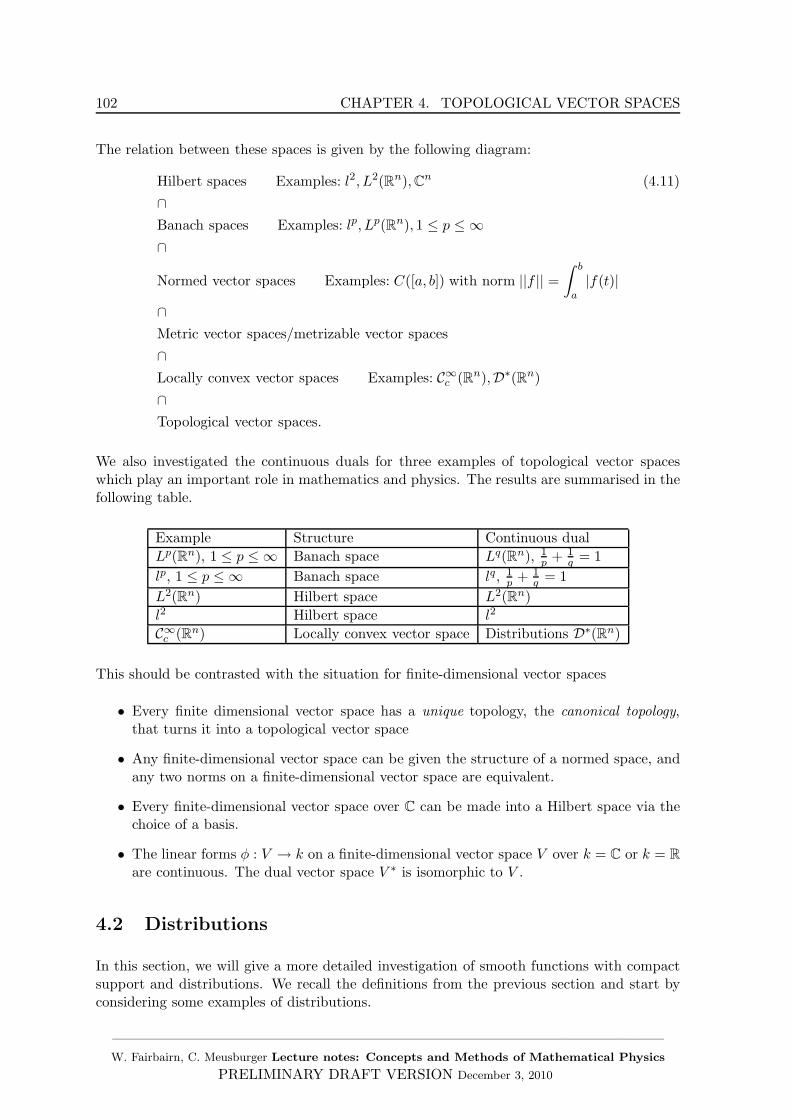
102 CHAPTER 4. TOPOLOGICAL VECTOR SPACES
The relation between these spaces is given by the following diagram:
Hilbert spaces Examples: l2, L2(Rn),Cn (4.11)
∩Banach spaces Examples: lp, Lp(Rn), 1 ≤ p ≤ ∞∩
Normed vector spaces Examples: C([a, b]) with norm ||f || =
∫ b
a|f(t)|
∩Metric vector spaces/metrizable vector spaces
∩Locally convex vector spaces Examples: C∞
c (Rn),D∗(Rn)
∩Topological vector spaces.
We also investigated the continuous duals for three examples of topological vector spaceswhich play an important role in mathematics and physics. The results are summarised in thefollowing table.
Example Structure Continuous dual
Lp(Rn), 1 ≤ p ≤ ∞ Banach space Lq(Rn), 1p + 1
q = 1
lp, 1 ≤ p ≤ ∞ Banach space lq, 1p + 1
q = 1
L2(Rn) Hilbert space L2(Rn)
l2 Hilbert space l2
C∞c (Rn) Locally convex vector space Distributions D∗(Rn)
This should be contrasted with the situation for finite-dimensional vector spaces
• Every finite dimensional vector space has a unique topology, the canonical topology,that turns it into a topological vector space
• Any finite-dimensional vector space can be given the structure of a normed space, andany two norms on a finite-dimensional vector space are equivalent.
• Every finite-dimensional vector space over C can be made into a Hilbert space via thechoice of a basis.
• The linear forms φ : V → k on a finite-dimensional vector space V over k = C or k = R
are continuous. The dual vector space V ∗ is isomorphic to V .
4.2 Distributions
In this section, we will give a more detailed investigation of smooth functions with compactsupport and distributions. We recall the definitions from the previous section and start byconsidering some examples of distributions.
——————————————————————————————————————W. Fairbairn, C. Meusburger Lecture notes: Concepts and Methods of Mathematical Physics
PRELIMINARY DRAFT VERSION December 3, 2010
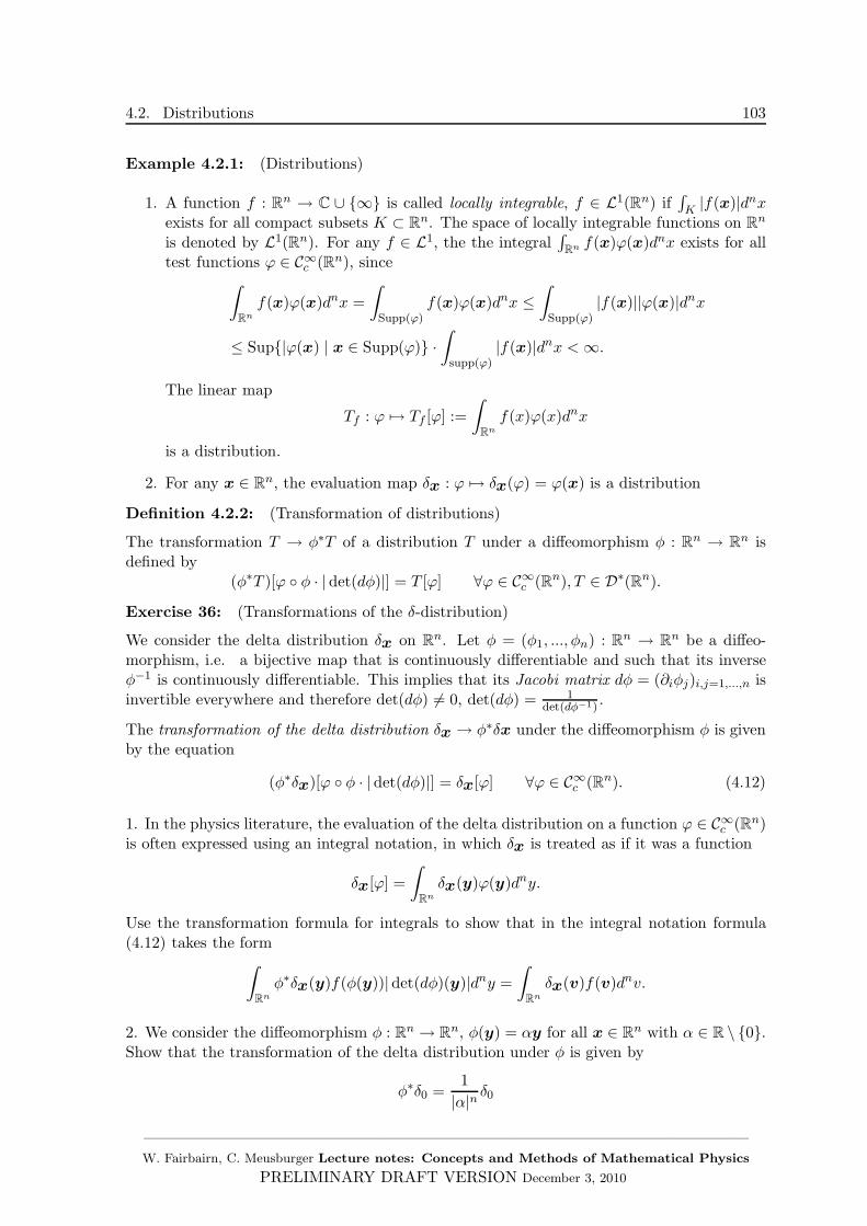
4.2. Distributions 103
Example 4.2.1: (Distributions)
1. A function f : Rn → C ∪ ∞ is called locally integrable, f ∈ L1(Rn) if∫K |f(x)|dnx
exists for all compact subsets K ⊂ Rn. The space of locally integrable functions on Rn
is denoted by L1(Rn). For any f ∈ L1, the the integral∫
Rn f(x)ϕ(x)dnx exists for alltest functions ϕ ∈ C∞
c (Rn), since∫
Rn
f(x)ϕ(x)dnx =
∫
Supp(ϕ)f(x)ϕ(x)dnx ≤
∫
Supp(ϕ)|f(x)||ϕ(x)|dnx
≤ Sup|ϕ(x) | x ∈ Supp(ϕ) ·∫
supp(ϕ)|f(x)|dnx <∞.
The linear map
Tf : ϕ 7→ Tf [ϕ] :=
∫
Rn
f(x)ϕ(x)dnx
is a distribution.
2. For any x ∈ Rn, the evaluation map δx : ϕ 7→ δx(ϕ) = ϕ(x) is a distribution
Definition 4.2.2: (Transformation of distributions)
The transformation T → φ∗T of a distribution T under a diffeomorphism φ : Rn → Rn isdefined by
(φ∗T )[ϕ φ · |det(dφ)|] = T [ϕ] ∀ϕ ∈ C∞c (Rn), T ∈ D∗(Rn).
Exercise 36: (Transformations of the δ-distribution)
We consider the delta distribution δx on Rn. Let φ = (φ1, ..., φn) : Rn → Rn be a diffeo-morphism, i.e. a bijective map that is continuously differentiable and such that its inverseφ−1 is continuously differentiable. This implies that its Jacobi matrix dφ = (∂iφj)i,j=1,...,n isinvertible everywhere and therefore det(dφ) 6= 0, det(dφ) = 1
det(dφ−1).
The transformation of the delta distribution δx → φ∗δx under the diffeomorphism φ is givenby the equation
(φ∗δx)[ϕ φ · |det(dφ)|] = δx[ϕ] ∀ϕ ∈ C∞c (Rn). (4.12)
1. In the physics literature, the evaluation of the delta distribution on a function ϕ ∈ C∞c (Rn)
is often expressed using an integral notation, in which δx is treated as if it was a function
δx[ϕ] =
∫
Rn
δx(y)ϕ(y)dny.
Use the transformation formula for integrals to show that in the integral notation formula(4.12) takes the form
∫
Rn
φ∗δx(y)f(φ(y))|det(dφ)(y)|dny =
∫
Rn
δx(v)f(v)dnv.
2. We consider the diffeomorphism φ : Rn → Rn, φ(y) = αy for all x ∈ Rn with α ∈ R \ 0.Show that the transformation of the delta distribution under φ is given by
φ∗δ0 =1
|α|n δ0
——————————————————————————————————————W. Fairbairn, C. Meusburger Lecture notes: Concepts and Methods of Mathematical Physics
PRELIMINARY DRAFT VERSION December 3, 2010
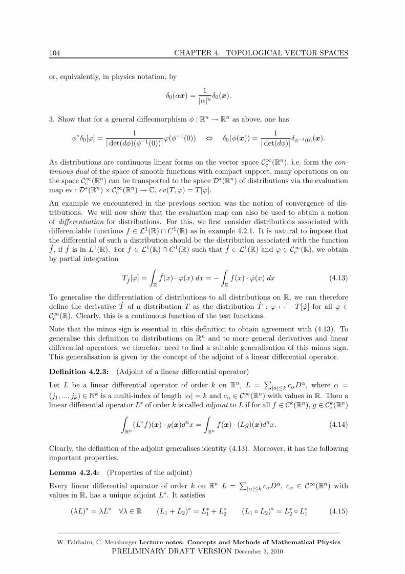
104 CHAPTER 4. TOPOLOGICAL VECTOR SPACES
or, equivalently, in physics notation, by
δ0(αx) =1
|α|n δ0(x).
3. Show that for a general diffeomorphism φ : Rn → Rn as above, one has
φ∗δ0[ϕ] =1
|det(dφ)(φ−1(0))|ϕ(φ−1(0)) ⇔ δ0(φ(x)) =1
|det(dφ)|δφ−1(0)(x).
As distributions are continuous linear forms on the vector space C∞c (Rn), i.e. form the con-
tinuous dual of the space of smooth functions with compact support, many operations on onthe space C∞
c (Rn) can be transported to the space D∗(Rn) of distributions via the evaluationmap ev : D∗(Rn) × C∞
c (Rn) → C, ev(T,ϕ) = T [ϕ].
An example we encountered in the previous section was the notion of convergence of dis-tributions. We will now show that the evaluation map can also be used to obtain a notionof differentiation for distributions. For this, we first consider distributions associated withdifferentiable functions f ∈ L1(R) ∩ C1(R) as in example 4.2.1. It is natural to impose thatthe differential of such a distribution should be the distribution associated with the functionf , if f is in L1(R). For f ∈ L1(R) ∩ C1(R) such that f ∈ L1(R) and ϕ ∈ C∞
c (R), we obtainby partial integration
Tf [ϕ] =
∫
R
f(x) · ϕ(x) dx = −∫
R
f(x) · ϕ(x) dx (4.13)
To generalise the differentiation of distributions to all distributions on R, we can thereforedefine the derivative T of a distribution T as the distribution T : ϕ 7→ −T [ϕ] for all ϕ ∈C∞c (R). Clearly, this is a continuous function of the test functions.
Note that the minus sign is essential in this definition to obtain agreement with (4.13). Togeneralise this definition to distributions on Rn and to more general derivatives and lineardifferential operators, we therefore need to find a suitable generalisation of this minus sign.This generalisation is given by the concept of the adjoint of a linear differential operator.
Definition 4.2.3: (Adjoint of a linear differential operator)
Let L be a linear differential operator of order k on Rn, L =∑
|α|≤k cαDα, where α =
(j1, ..., jk) ∈ Nk is a multi-index of length |α| = k and cα ∈ C∞(Rn) with values in R. Then alinear differential operator L∗ of order k is called adjoint to L if for all f ∈ Ck(Rn), g ∈ Ckc (Rn)
∫
Rn
(L∗f)(x) · g(x)dnx =
∫
Rn
f(x) · (Lg)(x)dnx. (4.14)
Clearly, the definition of the adjoint generalises identity (4.13). Moreover, it has the followingimportant properties.
Lemma 4.2.4: (Properties of the adjoint)
Every linear differential operator of order k on Rn L =∑
|α|≤k cαDα, cα ∈ C∞(Rn) with
values in R, has a unique adjoint L∗. It satisfies
(λL)∗ = λL∗ ∀λ ∈ R (L1 + L2)∗ = L∗
1 + L∗2 (L1 L2)
∗ = L∗2 L∗
1 (4.15)
——————————————————————————————————————W. Fairbairn, C. Meusburger Lecture notes: Concepts and Methods of Mathematical Physics
PRELIMINARY DRAFT VERSION December 3, 2010
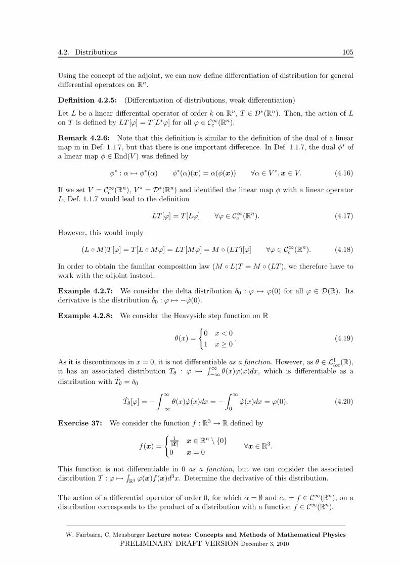
4.2. Distributions 105
Using the concept of the adjoint, we can now define differentiation of distribution for generaldifferential operators on Rn.
Definition 4.2.5: (Differentiation of distributions, weak differentiation)
Let L be a linear differential operator of order k on Rn, T ∈ D∗(Rn). Then, the action of Lon T is defined by LT [ϕ] = T [L∗ϕ] for all ϕ ∈ C∞
c (Rn).
Remark 4.2.6: Note that this definition is similar to the definition of the dual of a linearmap in in Def. 1.1.7, but that there is one important difference. In Def. 1.1.7, the dual φ∗ ofa linear map φ ∈ End(V ) was defined by
φ∗ : α 7→ φ∗(α) φ∗(α)(x) = α(φ(x)) ∀α ∈ V ∗,x ∈ V. (4.16)
If we set V = C∞c (Rn), V ∗ = D∗(Rn) and identified the linear map φ with a linear operator
L, Def. 1.1.7 would lead to the definition
LT [ϕ] = T [Lϕ] ∀ϕ ∈ C∞c (Rn). (4.17)
However, this would imply
(L M)T [ϕ] = T [L Mϕ] = LT [Mϕ] = M (LT )[ϕ] ∀ϕ ∈ C∞c (Rn). (4.18)
In order to obtain the familiar composition law (M L)T = M (LT ), we therefore have towork with the adjoint instead.
Example 4.2.7: We consider the delta distribution δ0 : ϕ 7→ ϕ(0) for all ϕ ∈ D(R). Itsderivative is the distribution δ0 : ϕ 7→ −ϕ(0).
Example 4.2.8: We consider the Heavyside step function on R
θ(x) =
0 x < 0
1 x ≥ 0. (4.19)
As it is discontinuous in x = 0, it is not differentiable as a function. However, as θ ∈ L1loc(R),
it has an associated distribution Tθ : ϕ 7→∫∞−∞ θ(x)ϕ(x)dx, which is differentiable as a
distribution with Tθ = δ0
Tθ[ϕ] = −∫ ∞
−∞θ(x)ϕ(x)dx = −
∫ ∞
0ϕ(x)dx = ϕ(0). (4.20)
Exercise 37: We consider the function f : R3 → R defined by
f(x) =
1|x| x ∈ Rn \ 00 x = 0
∀x ∈ R3.
This function is not differentiable in 0 as a function, but we can consider the associateddistribution T : ϕ 7→
∫R3 ϕ(x)f(x)d3x. Determine the derivative of this distribution.
The action of a differential operator of order 0, for which α = ∅ and cα = f ∈ C∞(Rn), on adistribution corresponds to the product of a distribution with a function f ∈ C∞(Rn).
——————————————————————————————————————W. Fairbairn, C. Meusburger Lecture notes: Concepts and Methods of Mathematical Physics
PRELIMINARY DRAFT VERSION December 3, 2010
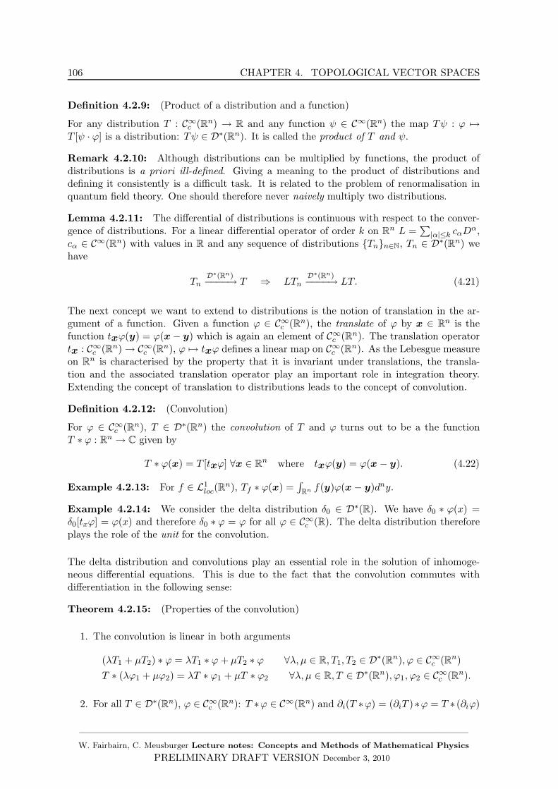
106 CHAPTER 4. TOPOLOGICAL VECTOR SPACES
Definition 4.2.9: (Product of a distribution and a function)
For any distribution T : C∞c (Rn) → R and any function ψ ∈ C∞(Rn) the map Tψ : ϕ 7→
T [ψ · ϕ] is a distribution: Tψ ∈ D∗(Rn). It is called the product of T and ψ.
Remark 4.2.10: Although distributions can be multiplied by functions, the product ofdistributions is a priori ill-defined. Giving a meaning to the product of distributions anddefining it consistently is a difficult task. It is related to the problem of renormalisation inquantum field theory. One should therefore never naively multiply two distributions.
Lemma 4.2.11: The differential of distributions is continuous with respect to the conver-gence of distributions. For a linear differential operator of order k on Rn L =
∑|α|≤k cαD
α,cα ∈ C∞(Rn) with values in R and any sequence of distributions Tnn∈N, Tn ∈ D∗(Rn) wehave
TnD∗(Rn)−−−−→ T ⇒ LTn
D∗(Rn)−−−−→ LT. (4.21)
The next concept we want to extend to distributions is the notion of translation in the ar-gument of a function. Given a function ϕ ∈ C∞
c (Rn), the translate of ϕ by x ∈ Rn is thefunction txϕ(y) = ϕ(x − y) which is again an element of C∞
c (Rn). The translation operatortx : C∞
c (Rn) → C∞c (Rn), ϕ 7→ txϕ defines a linear map on C∞
c (Rn). As the Lebesgue measureon Rn is characterised by the property that it is invariant under translations, the transla-tion and the associated translation operator play an important role in integration theory.Extending the concept of translation to distributions leads to the concept of convolution.
Definition 4.2.12: (Convolution)
For ϕ ∈ C∞c (Rn), T ∈ D∗(Rn) the convolution of T and ϕ turns out to be a the function
T ∗ ϕ : Rn → C given by
T ∗ ϕ(x) = T [txϕ] ∀x ∈ Rn where txϕ(y) = ϕ(x − y). (4.22)
Example 4.2.13: For f ∈ L1loc(R
n), Tf ∗ ϕ(x) =∫
Rn f(y)ϕ(x − y)dny.
Example 4.2.14: We consider the delta distribution δ0 ∈ D∗(R). We have δ0 ∗ ϕ(x) =δ0[txϕ] = ϕ(x) and therefore δ0 ∗ ϕ = ϕ for all ϕ ∈ C∞
c (R). The delta distribution thereforeplays the role of the unit for the convolution.
The delta distribution and convolutions play an essential role in the solution of inhomoge-neous differential equations. This is due to the fact that the convolution commutes withdifferentiation in the following sense:
Theorem 4.2.15: (Properties of the convolution)
1. The convolution is linear in both arguments
(λT1 + µT2) ∗ ϕ = λT1 ∗ ϕ+ µT2 ∗ ϕ ∀λ, µ ∈ R, T1, T2 ∈ D∗(Rn), ϕ ∈ C∞c (Rn)
T ∗ (λϕ1 + µϕ2) = λT ∗ ϕ1 + µT ∗ ϕ2 ∀λ, µ ∈ R, T ∈ D∗(Rn), ϕ1, ϕ2 ∈ C∞c (Rn).
2. For all T ∈ D∗(Rn), ϕ ∈ C∞c (Rn): T ∗ϕ ∈ C∞(Rn) and ∂i(T ∗ϕ) = (∂iT )∗ϕ = T ∗ (∂iϕ)
——————————————————————————————————————W. Fairbairn, C. Meusburger Lecture notes: Concepts and Methods of Mathematical Physics
PRELIMINARY DRAFT VERSION December 3, 2010
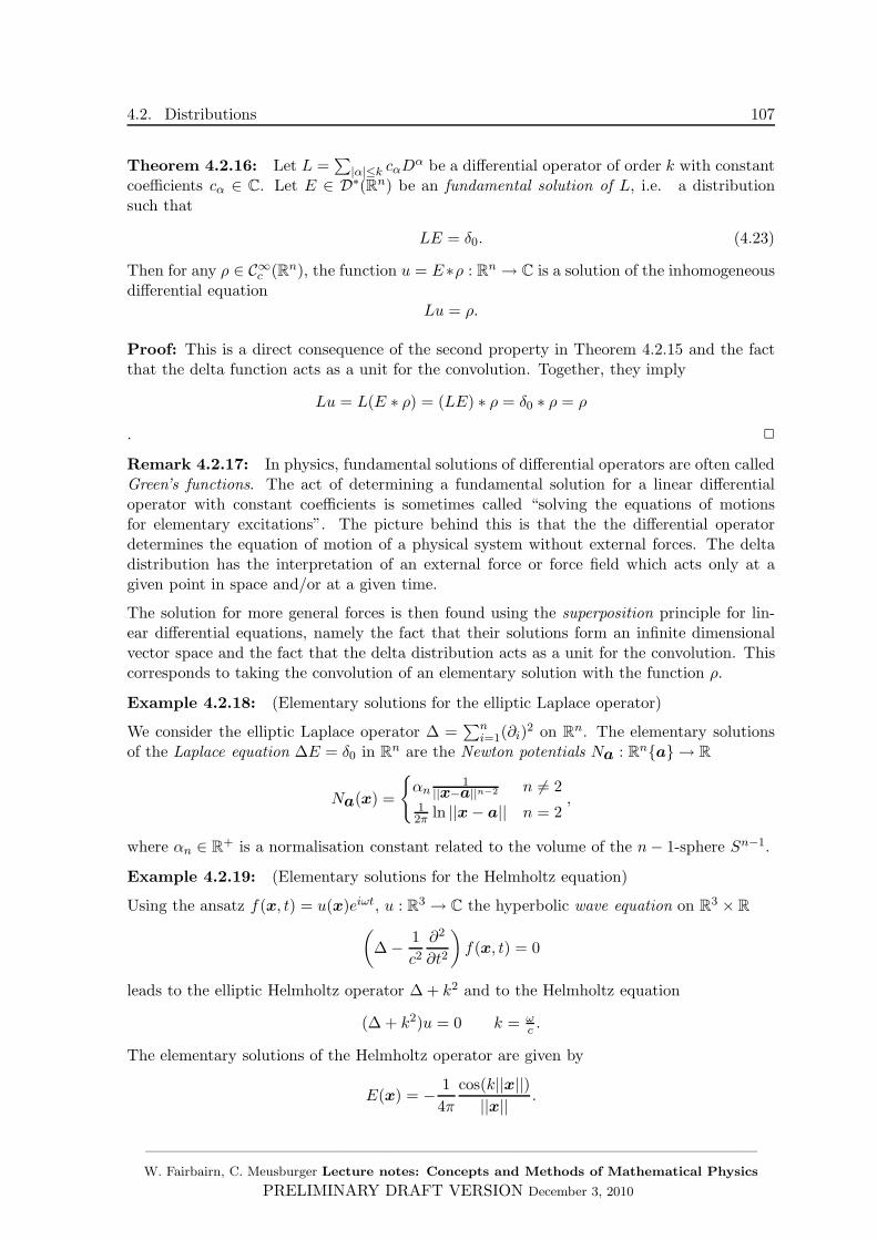
4.2. Distributions 107
Theorem 4.2.16: Let L =∑
|α|≤k cαDα be a differential operator of order k with constant
coefficients cα ∈ C. Let E ∈ D∗(Rn) be an fundamental solution of L, i.e. a distributionsuch that
LE = δ0. (4.23)
Then for any ρ ∈ C∞c (Rn), the function u = E∗ρ : Rn → C is a solution of the inhomogeneous
differential equationLu = ρ.
Proof: This is a direct consequence of the second property in Theorem 4.2.15 and the factthat the delta function acts as a unit for the convolution. Together, they imply
Lu = L(E ∗ ρ) = (LE) ∗ ρ = δ0 ∗ ρ = ρ
. 2
Remark 4.2.17: In physics, fundamental solutions of differential operators are often calledGreen’s functions. The act of determining a fundamental solution for a linear differentialoperator with constant coefficients is sometimes called “solving the equations of motionsfor elementary excitations”. The picture behind this is that the the differential operatordetermines the equation of motion of a physical system without external forces. The deltadistribution has the interpretation of an external force or force field which acts only at agiven point in space and/or at a given time.
The solution for more general forces is then found using the superposition principle for lin-ear differential equations, namely the fact that their solutions form an infinite dimensionalvector space and the fact that the delta distribution acts as a unit for the convolution. Thiscorresponds to taking the convolution of an elementary solution with the function ρ.
Example 4.2.18: (Elementary solutions for the elliptic Laplace operator)
We consider the elliptic Laplace operator ∆ =∑n
i=1(∂i)2 on Rn. The elementary solutions
of the Laplace equation ∆E = δ0 in Rn are the Newton potentials Na : Rna → R
Na(x) =
αn
1||x−a||n−2 n 6= 2
12π ln ||x − a|| n = 2
,
where αn ∈ R+ is a normalisation constant related to the volume of the n− 1-sphere Sn−1.
Example 4.2.19: (Elementary solutions for the Helmholtz equation)
Using the ansatz f(x, t) = u(x)eiωt, u : R3 → C the hyperbolic wave equation on R3 × R
(∆ − 1
c2∂2
∂t2
)f(x, t) = 0
leads to the elliptic Helmholtz operator ∆ + k2 and to the Helmholtz equation
(∆ + k2)u = 0 k = ωc .
The elementary solutions of the Helmholtz operator are given by
E(x) = − 1
4π
cos(k||x||)||x|| .
——————————————————————————————————————W. Fairbairn, C. Meusburger Lecture notes: Concepts and Methods of Mathematical Physics
PRELIMINARY DRAFT VERSION December 3, 2010
108 CHAPTER 4. TOPOLOGICAL VECTOR SPACES
4.3 Fourier transforms
In this section, we will investigate the Fourier transform as a continuous linear map ondifferent vector spaces. We start by considering the space L1(Rn).
Definition 4.3.1: (Fourier transform)
For f ∈ L1(Rn), the integral
f(y) =1
(2π)n/2
∫
Rn
f(x)e−i〈x,y〉dnx 〈x,y〉 =
n∑
i=1
xiyi (4.24)
exists. The function f : Rn → C, y 7→ f(y) is called the Fourier transform of f .
Example 4.3.2:
We determine the Fourier transform of the function f : Rn → R, f(x) = e−x2/2.
f(y) = 1(2π)n/2
∫
Rn
e−x2/2e−ix·ydnx =
n∏
i=1
∫ ∞
−∞1√2πe−x
2i /2−ixiyidxi
=
n∏
i=1
∫ ∞
−∞1√2πe−
12 (xi+iyi)
2−12y
2i dxi = e−
12y2
(1√2π
∫ ∞
−∞e−x
2/2dx
)n= e−
12y2
. (4.25)
Example 4.3.3:
We determine the Fourier transform of the function f : R → R, f(x) = e−|x|.
f(y) = 1√2π
∫ ∞
−∞e−|x|e−ixydx = 1√
2π
∫ ∞
0e−|x|(e−ixy + eixy)dx
= 1√2π
limR→∞
[−e
−x(1+iy)
1 + iy− e−x(1−iy)
1 − iy
]x=R
x=0
=√
2π
1
1 + y2(4.26)
Exercise 38: Show that for the characteristic function χ[−1,1] : R → R the Fourier trans-form is given by
χ[−1,1](x) =
1 |x| ≤ 1
0 |x| > 1⇒ χ[−1,1](x) =
√2
π
sinx
x(4.27)
Note that χ is not in L1(R) although χ ∈ L1(R).
Lemma 4.3.4: (Properties of the Fourier transform)
The Fourier transform f has the following properties:
1. It is continuous: f ∈ C0(Rn) for all f ∈ L1(Rn).
2. It is linear: αf + βg = αf + βg for all α, β ∈ C, f, g ∈ L1(Rn).
3. It is bounded: ||f ||∞ ≤ 1(2π)n/2 ||f ||1 for all f ∈ L1(Rn).
4. If f ∈ L1 vanishes almost everywhere, f = 0.
——————————————————————————————————————W. Fairbairn, C. Meusburger Lecture notes: Concepts and Methods of Mathematical Physics
PRELIMINARY DRAFT VERSION December 3, 2010
4.3. Fourier transforms 109
Corollary 4.3.5:
The Fourier transformation defines a linear, continuous map F : L1(Rn) → C0(Rn).
Lemma 4.3.6: (Identities for the Fourier transform)
The Fourier transform satisfies the following identities
1. For all f ∈ L1(Rn) and g(x) = f(λx) almost everywhere, λ ≥ 0 ⇒ g(y) = 1λn f(y/λ).
2. For f ∈ L1(Rn) and g(x) = f(−x) almost everywhere ⇒ g(y) = f(y).
3. For f ∈ L1(Rn), fx(y) = txf(y) = f(y)e−i〈x,y〉
4. For f ∈ C1c (R
n) = f ∈ C1(Rn) | x ∈ Rn | f(x) 6= 0 compact: (∂jf)(y) = iyj f(y).
5. If the function x 7→ xjf is integrable, f is continuously differentiable with respect to
yj and (xjf) = i∂j f .
6. For f, g ∈ L1(Rn), the functions fg and gf are integrable and
∫
Rn
f(x)g(x)dnx =
∫
Rn
f(y)g(y)dny. (4.28)
7. For any f ∈ C∞c (Rn), the Fourier transform is integrable: f ∈ L1(Rn).
Proof: Identities 1.), 2.), 3.), 4.) can be proved by substitution of integration variables andare left as an exercise. 7.) follows from integration theory.
To prove 5.), we need to use integration theory to show that f is differentiable and differen-tiation commutes with the integral in the definition of the Fourier transformation. We thenobtain
∂j f(y) =∂
∂yj
(y 7→ 1
(2π)n/2
∫
Rn
f(x)e−i〈x,y〉dnx
)=
−i(2π)n/2
∫
Rn
xjf(x)e−i〈x,y〉dnx = −ixjf(y).
6.): As f , g are continuous and bounded, fg and gf are integrable. Using Fubini’s theoremone obtains
∫
Rn
f(x)g(x)dnx =1
(2π)n/2
∫
Rn
∫
Rn
f(x)g(y)e−i〈x,y〉dnxdny
=1
(2π)n/2
∫
Rn
(∫
Rn
f(x)e−i〈x,y〉dnx
)g(y)dny =
∫
Rn
f(y)g(y)dny
2
As in the case of distributions, one can define a convolution on the space L1(Rn). It turnsout that the Fourier transform has special properties with respect to the convolution, namelythat it transforms the convolution of functions to the product of convolutions. To see this,we start by defining the convolution of functions in L1(Rn).
——————————————————————————————————————W. Fairbairn, C. Meusburger Lecture notes: Concepts and Methods of Mathematical Physics
PRELIMINARY DRAFT VERSION December 3, 2010
110 CHAPTER 4. TOPOLOGICAL VECTOR SPACES
Definition 4.3.7: (Convolution)
For f, g ∈ L1(Rn), the convolution of f and g is the function f ∗ g : Rn → C defined by
f ∗ g(y) =
∫
Rn
f(x)g(y − x)dnx. (4.29)
If g vanishes almost everywhere, f ∗ g = 0 = g ∗ f for all f ∈ L1(Rn). The convolutiontherefore induces a bilinear map ∗ : L1(Rn) × L1(Rn) → L1(Rn).
Remark 4.3.8: Note that this definition of the convolution coincides with the one fordistributions Tf : C∞
c (Rn) → C associated with a functions f ∈ L1(Rn). If Tf : C∞c (Rn) → C
is the distribution associated with a function f ∈ L1(Rn) and g is a function g ∈ C∞c (Rn), we
have Tf ∗ g = f ∗ g.Lemma 4.3.9: (Properties of the convolution)
The convolution induces a continuous bilinear map ∗ : L1(Rn)×L1(Rn) → L1(Rn). It satisfies
1. ||f ∗ g||1 ≤ ||f ||1||g||1 for all f, g ∈ L1(Rn).
2. (f ∗ g) = (2π)n/2f · g for all f, g ∈ L1(Rn).
3. f ∗ g(x) = g ∗ f(x) ∀x ∈ Rn, f, g ∈ L1(Rn)
4. (f ∗ g) ∗ h = f ∗ (g ∗ h) ∀x ∈ Rn, f, g, h ∈ L1(Rn).
Proof: Exercise. 2
To work with a notion of Fourier transform that is defined for locally integrable functionsor as a continuous linear map from L1(Rn) to C0(Rn) will not be sufficient in the following.Firstly, we would like to construct the inverse of a Fourier transform, which is complicated ifwe view the Fourier transform as a continuous linear map F : L1(Rn) → C0(Rn). Secondly,many applications of the Fourier transform such as its role in quantum mechanics involvefunctions in L2(Rn), not L1(Rn). We will see in the following that it is possible to extendthe Fourier transform to L2(Rn) and that this is closely related to constructing its inverse.
As a first step, we note that the Fourier transform is injective in the following sense:
Theorem 4.3.10: (Uniqueness and Inversion of Fourier transform)
1. If f ∈ L1(Rn) such that f ∈ L1(Rn), we have
f(x) =1
(2π)n/2
∫
Rn
f(y)ei〈y,x〉 almost everywhere. (4.30)
2. For all f, g ∈ L1(Rn) with f = g, we have f(x) = g(x) for almost all x ∈ Rn.
Hence, the Fourier transformation is injective in the sense that two functions in L1(Rn) whoseFourier transformations agree must be equal almost everywhere. However, the inversionformula given in the preceding theorem is only valid for functions that are such that theirFourier transform is also in L1(Rn). As the Fourier transform does not preserve the L1- norm|| ||1, there is in general no guarantee that the Fourier transformation of a function in L1(Rn)is in L1(Rn). However, it turns out that the Fourier transform preserves the L2-norm || ||2.
——————————————————————————————————————W. Fairbairn, C. Meusburger Lecture notes: Concepts and Methods of Mathematical Physics
PRELIMINARY DRAFT VERSION December 3, 2010
4.4. Hilbert spaces 111
Theorem 4.3.11: For all f ∈ L1(Rn) ∩ L2(Rn), f ∈ L2(Rn) and ||f ||2 = ||f ||2.
Hence, the Fourier transformation is defined for functions in L1(Rn) and is injective forthose functions, but preserves the L2-norm. This suggests that in order to obtain a Fouriertransformation which is an isomorphism of Banach or Hilbert spaces, we should extend it toL2(Rn). That this is possible is shown by Plancherel’s theorem, whose proof makes use of thefact that the smooth functions with compact support and hence the intersection L1(Rn) ∩L2(Rn) are dense in L2(Rn).
Corollary 4.3.12: (Plancherel’s theorem)
There exists a unique isomorphism F : L2(Rn) → L2(Rn) such that
1. ||F(f)||L2= ||f ||L2
for all f ∈ L2(Rn)
2. F(f) = f for all f ∈ L1(Rn) ∩ L2(Rn)
3. F−1(f)(y) = 1(2π)n/2
∫Rn f(x)ei〈x,y〉dnx for all f ∈ L1(Rn) ∩ L2(Rn).
4.4 Hilbert spaces
We will now focus on Hilbert spaces, which play an important role in quantum mechanics.Throughout this section, we denote by H a Hilbert space with scalar product or hermitianproduct 〈 , 〉 : H×H → C.
Many of the constructions that are possible for finite-dimensional vector spaces such as pro-jections on linear subspaces and decomposition of vectors with respect to a basis are alsopossible for (separable) Hilbert spaces. We start by considering the projection on a closedlinear subspace.
Theorem 4.4.1: (Orthogonal projection on a closed subspace)
Let H be a Hilbert space and F ⊂ H a closed subspace of H, i.e. a linear subspace F ⊂ Hsuch that any Cauchy sequence with elements in F converges towards an element of F . Thenfor each x ∈ H there exists a unique y ∈ F , the projection of x on F denoted y = PF (x),such that ||x − y|| = d(x, F ) = inf||x − z|| | z ∈ F. The projection map PF : H → F ,x 7→ PF (x) has the following properties:
1. It is linear and continuous.
2. It satisfies: PF PF = PF
3. 〈x − PF (x),z〉 = 0 for all z ∈ F .
4. Any element x ∈ H can be expressed uniquely as a sum of its projection on F and anelement of the orthogonal complement F⊥ = y ∈ H | 〈z,y〉 = 0 ∀z ∈ F.
x = PF (x) + z z ∈ F⊥. (4.31)
Proof:
——————————————————————————————————————W. Fairbairn, C. Meusburger Lecture notes: Concepts and Methods of Mathematical Physics
PRELIMINARY DRAFT VERSION December 3, 2010
112 CHAPTER 4. TOPOLOGICAL VECTOR SPACES
1. Uniqueness: To prove that y is unique, we select a sequence (xn)n∈N with ||xn − x|| →d(x, F ) = inf||x − z|| | z ∈ F. The last identity in exercise (35) implies
||xn − xk||2 = 2(||x − xn||2 + ||x − xk||2) − 4 ||x 12(xn + xm)||2︸ ︷︷ ︸≥d(x,F )2
(4.32)
and therefore ||xn − xk||2 < ǫ2 if ||x − xk||2, ||x − xn||2 < d(x, F )2 + ǫ2
4 . This shows thatxnn∈N is a Cauchy sequence. As F is closed, this sequence converges to an element y ∈ Fwith ||x − y|| = d(x, F ). For any element z ∈ F with ||x − z|| = d(x, F ), we obtain usingagain the last identity in exercise (35)
||y − z||2 = 4d(x, F )2 − 4 ||x − 12(y + z)||︸ ︷︷ ︸
≥d(x,F )2
≤ 0 (4.33)
and therefore z = y. This shows that y = PF (x) is unique.
2. Let y = PF (x) for a general x ∈ H. Then, y ∈ F and d(y, F ) = 0 = ||y − y||. Theuniqueness of the projection then implies PF (y) = y and therefore PF PF = PF .
3. To prove that 〈x − PF (x),z〉 = 0 for all z ∈ F , we use the third identity in (35) and findfor all t ∈ R+
||x − (PF (x) − tz)||2 = t2||z||2 + d(x, F )2 − 2t〈x − PF (x),z〉 ≥ d(x, F )2, (4.34)
which implies t(〈x − PF (x),z〉− t2 ||z||2) ≤ 0 for all t ∈ R+. Hence, we must have 〈x − PF (x),z〉−
t2 ||z||2 ≤ 0 for all t ∈ R+. By letting t tend to zero, we obtain 〈x − PF (x),z〉 = 0. Set-ting x = PF (x) + (x − PF (x)) for any x ∈ H therefore defines a unique decompositionx = PF (x) + z with z ∈ F⊥.
4. To show linearity of PF : H → F , we use
〈x + y − PF (x + y),z〉 = 〈x + y − PF (x) − PF (y),z〉 = 0 ∀z ∈ F. (4.35)
This implies
〈PF (x + y)−PF (x)−PF (y), PF (x + y)−PF (x)−PF (y)〉 = ||PF (x + y)−PF (x)−PF (y)||2 = 0
and therefore PF (x+y) = PF (x)+PF (y). To show that PF is continuous, we take a sequence(yn)n∈N with ||yn−y|| → 0. The decomposition y = PF (y)+y−PF (y) with y−PF (y) ∈ F⊥
implies
||y − yn||2 = ||PF (y) − PF (yn)||2 + ||y − PF (y) − yn + PF (yn)||2 ≥ ||PF (y) − PF (yn)||2
||y − yn|| → 0 therefore implies ||PF (y) − PF (yn)|| → 0 and hence continuity of PF . 2.
Corollary 4.4.2:
For any A ⊂ H Span(A) = ∑ni=1 λiai | λi ∈ k,ai ∈ A is dense in H if and only if the
orthogonal complement A⊥ is trivial A⊥ = x ∈ H | 〈x,a〉 = 0 ∀a ∈ A = 0.
Proof: Clearly, Span(A) is a closed subspace of H and A⊥ = Span(A)⊥. By theorem 4.4.1,
any element x ∈ H can be decomposed uniquely as x = PSpan(A)(x) + z with z ∈ A⊥. If A⊥
is trivial, this implies x ∈ Span(A) and hence density of Span(A) in H.
Conversely, if Span(A) is dense in H, then for every element x ∈ A⊥ there exists a sequencexnn∈N, xn ∈ Span(A) with xn → x. As we have 〈xn,x〉 = 0 for all n ∈ N, this implies〈x,x〉 = 0. We have x = 0 and therefore A⊥ = 0. 2
——————————————————————————————————————W. Fairbairn, C. Meusburger Lecture notes: Concepts and Methods of Mathematical Physics
PRELIMINARY DRAFT VERSION December 3, 2010
4.4. Hilbert spaces 113
Definition 4.4.3: (Separable Hilbert space)
A Hilbert space H is called separable if there exists a countably infinite set (xn)n∈N withxn ∈ H for all n ∈ N and whose Span is dense in H: Span(xn | n ∈ N) = H. In otherwords, for every y ∈ H and every ǫ > 0 there exists a finite set of indices n1, ..., nk ∈ N andcoefficients α1, ..., αk ∈ C such that
||k∑
i=1
αixni − y|| < ǫ. (4.36)
Example 4.4.4: (Separable Hilbert spaces)
1. The Hilbert space l2 of square summable series is separable.
2. L2(Rn) with the scalar product (4.8) is separable.
Example 4.4.5: (Non-separable Hilbert space)
The vector space
H = f : R → R | ∃c ∈ R+ :∑
t∈I|f(t)|2 < c for all finite I ⊂ R 〈f, g〉 =
∑
t∈R
f(t)g(t)
is a Hilbert space but not separable.
Proof:
1. For all f ∈ H, the set I(f) = t ∈ R | f(t) 6= 0 is countable. To demonstrate this, weconsider the sets In(f) = t ∈ R : | |f(t)| ≥ 1
n, n ∈ N. In must be finite, because otherwise
one could construct a sequence tii∈N, ti ∈ N with∑k
i=1 |f(ti)|2 ≥ k2
n → ∞ with k → ∞.Clearly, I(f) =
⋃n∈N
In(f) and therefore I(f) is countable.
2. Suppose Span(A) ⊂ H is dense in H. As the functions gs : R → R
gs(t) =
1 t = s
0 t 6= s
are elements of H for all s ∈ R, for all s ∈ R there must exist a sequence f snn∈N, fn ∈Span(A) with ||f sn−gs|| → 0. This implies |f sn(t)−gs(t)| → 0 for all t ∈ N and hence f sn(s) 6= 0for n ≥ n0 for some n0 ∈ N.
Hence, for any s ∈ R, A must contain a function fs ∈ H with fs(s) 6= 0. This implies that Acannot be a countable infinite set, since for every f ∈ H, I(f) is countable and a countableunit of countable sets must be countable, whereas R is not countable. 2
Definition 4.4.6: (Hilbert basis)
A Hilbert basis of a Hilbert space H is a finite or countably infinite sequence (ei)i∈N, ei ∈ H,of elements in H that are
1. orthonormal: 〈ei, ej〉 = δij for all i, j ∈ N
2. dense in H: Span(ei | i ∈ N) = H.
——————————————————————————————————————W. Fairbairn, C. Meusburger Lecture notes: Concepts and Methods of Mathematical Physics
PRELIMINARY DRAFT VERSION December 3, 2010

114 CHAPTER 4. TOPOLOGICAL VECTOR SPACES
Lemma 4.4.7: A Hilbert space admits a Hilbert basis if and only if it is separable.
Proof: Clearly, if H admits a Hilbert basis, it is separable, and if H = 0 the statement istrivial. We need to prove that if H 6= 0 is separable, it admits a Hilbert basis. This is theinfinite-dimensional counterpart of Gram Schmidt orthogonalisation.
If H is separable, there exists a dense set of elements B = xn | n ∈ N. Let i1 be i1 =minn ∈ N | xn 6= 0 xk = 0∀k < n and set e1 = xi1/||xi1 ||. If xk ∈ Span(e1) for all k ≥ i1,we have H = Span(e1) and the proof is complete. Otherwise, there exists an index i2 ∈ N,i2 > i1 such that xi2 /∈ Span(e1) and xk ∈ Spane1 for all k ∈ [i1, i2[. Set
e2 =xi2 − 〈xi2, e1〉e1
||xi2 − 〈xi2, e1〉e1||(4.37)
If xk ∈ Span(e1, e2) for all k ≥ i2, we have H = Span(e1, e2) and the proof is complete.Otherwise, there exists an index i3 ∈ N, i3 > i2 such that xi3 /∈ Span(e1, e2) and xk ∈Spane1, e2 for all k ∈ [i2, i3[. Set
e3 =xi3 − 〈xi3 , e1〉e1 − 〈xi3 , e2〉e2
||xi3 − 〈xi2 , e1〉e1 − 〈xi3 , e2〉e2||(4.38)
and continue in this way.
If H is finite dimensional, the procedure stops after a finite number of steps. Otherwise, we ob-tain a sequence (ei)i∈N with 〈ei, ej〉 = δij . In this case, we need to show that Span(ei | i ∈ N) =H. This follows with Corollary 4.4.2 if we can show that Span(ei | i ∈ N)⊥ = 0. Consideran element x with 〈x, e〉i = 0 for all i ∈ N. By construction of the elements ei, this implies〈x,x〉n = 0 for all n ∈ N. As Span(xn | n ∈ N) is dense in H, this implies x = 0. 2
Theorem 4.4.8: (Decomposition with respect to a Hilbert basis)
Let H be a separable Hilbert space with a Hilbert basis B = ei | i ∈ N. For any vectorx ∈ H we have the identities
x =∞∑
i=1
〈ei,x〉ei (4.39)
||x||2 = 〈x,x〉 =
∞∑
i=1
|〈ei,x〉|2 (Parseval’s equation). (4.40)
In other words: The series Sn(x) =∑n
i=1 〈ei,x〉ei and Rn(x) =∑n
i=1 |〈ei,x〉|2 convergeabsolutely towards x and ||x||2. If (ai)i∈N is a sequence such that
∑∞i=1 |ai|2 < ∞, then
a =∑∞
i=1 aiei exists (i.e. the series converges) and ai = 〈ei,a〉.
Proof:
As we can write x = x − Sn(x) + Sn(x) with 〈x − Sn(x), ek〉 = 0 for all k ≤ n, we have
||x||2 = ||x − Sn(x)||2 + ||Sn(x)||2 ⇒ ||Sn(x)||2 =
n∑
k=1
|〈x, ek〉| ≤ ||x||2. (4.41)
This implies that for all ǫ > 0 there exists an nǫ ∈ N such that
Rm(x) −Rn(x) = ||Sn(x) − Sm(x)||2 = ||m∑
k=n+1
〈ek,x〉ek||2 =
m∑
k=n+1
|〈ek,x〉|2 < ǫ ∀n,m ≥ nǫ.
——————————————————————————————————————W. Fairbairn, C. Meusburger Lecture notes: Concepts and Methods of Mathematical Physics
PRELIMINARY DRAFT VERSION December 3, 2010
4.4. Hilbert spaces 115
Hence, the sequence (Sn(x))n∈N is a Cauchy sequence and converges towards a unique elementy ∈ H. For any ǫ > 0 there exists n ∈ N such that ||y − Sn(x)|| < ǫ. We then have
|〈y − x, ek〉| ≤ |〈y − Sn(x), ek〉| + |〈x − Sn(x), ek〉| ≤ ||y − Sn(x)|| < ǫ ∀k ≤ n. (4.42)
With ǫ → 0, n → ∞, we therefore obtain |〈y − x, ek〉| = 0 for all k ∈ N. This implies
y − x ∈ Span(B)⊥ = Span(B)⊥. As B is dense in H, Corollary 4.4.2 implies x = y and
||x||2 = limn→∞
||Sn(x)||2 =
∞∑
k=1
|〈x, ei〉|2. (4.43)
Conversely, if (ai)i∈N is a sequence such that∑∞
i=1 |ai|2 <∞, then for each ǫ > 0 there existsnǫ such that
||m∑
k=n+1
akek||2 =
m∑
k=n+1
|ak|2 < ǫ ∀n,m > nǫ. (4.44)
This implies that An =∑n
k=0 akek is a Cauchy sequence and converges towards a uniqueelement a ∈ H. We have
|〈a, ei〉 − ai| ≤ |〈a −An, ei〉| + |〈An, ei〉 − ai| ≤ ||a −An|| n→∞−−−→ 0 (4.45)
with n→ ∞, we therefore obtain 〈a, ei〉 = ai. 2
Corollary 4.4.9: For any separable Hilbert space H with scalar product 〈 , 〉, there is aunitary isomorphism φ : H → l2, i.e. an isomorphism φ : H → l2 which preserves the scalarproduct 〈φ(x), φ(y)〉l2 = 〈x,y〉 for all x,y ∈ H.
Proof: This is simply a rephrasing of Theorem 4.4.8. To obtain such a unitary isomorphismφ : H → l2, one chooses a Hilbert basis B = ei | i ∈ N of H and sets φ(x) = 〈x, ei〉i∈N.2
Remark 4.4.10: A Hilbert basis is the infinite-dimensional analogue of an orthonormalbasis for finite-dimensional vector spaces. The Hilbert space of absolutely convergent series inExample 4.1.28 is the infinite-dimensional analogue of the vector spaces Rn and Cn. Theorem4.4.8 can therefore be viewed as the infinite-dimensional analogue of the identification offinite-dimensional vector spaces with Cn or Rn.
As in the finite dimensional case, this identification is not canonical because it requires thechoice of a basis. Moreover, in the infinite dimensional case, the vector space structure aloneis not enough for the identification. Instead, one needs the stricter requirement that thevector space is a separable Hilbert space.
——————————————————————————————————————W. Fairbairn, C. Meusburger Lecture notes: Concepts and Methods of Mathematical Physics
PRELIMINARY DRAFT VERSION December 3, 2010

116 CHAPTER 4. TOPOLOGICAL VECTOR SPACES
——————————————————————————————————————W. Fairbairn, C. Meusburger Lecture notes: Concepts and Methods of Mathematical Physics
PRELIMINARY DRAFT VERSION December 3, 2010
Chapter 5
Quantum mechanics
5.1 Operators on Hilbert spaces
Definition 5.1.1: (Bounded operator, compact operator)
A linear operator O : B → B on a Banach space B is called bounded if there exists a c ∈ R+
such that ||Ov|| ≤ c||v|| ∀v ∈ B. It is called compact if O(U) is compact for every boundedU ⊂ B.
Lemma 5.1.2: A linear operator O on a Banach space B is bounded if and only if it iscontinuous, i. e. for all sequences xnn∈N , xn ∈ B with ||xn − x|| → 0 we have ||Oxn −Ox|| → 0. The vector space of bounded linear operators on a Hilbert space B with norm||O|| = sup||Ox|| | x ∈ E, ||x|| = 1 is a Banach space. It will be denoted B(B) in thefollowing.
Proof: Let xnn∈N, xn ∈ B be a sequence with ||xn−x|| n→∞−−−→ 0, x ∈ H. If O is bounded,we have ||Oxn − Ox|| ≤ c||xn − x|| n→∞−−−→ 0, hence O is continuous. If O is continuous, it iscontinuous in 0 and there exists a δ > 0 such that ||Ox|| < 1 for all x ∈ B with ||x|| < δ.This implies
||Oy|| =
∣∣∣∣∣∣∣∣||y||δ
O
(δy
||y||
)∣∣∣∣∣∣∣∣ =
||y||δ
∣∣∣∣∣∣∣∣O(δy
||y||
)∣∣∣∣∣∣∣∣ ≤
||y||δ
∀y ∈ H.
2
Example 5.1.3: (Bounded operators)
1. The identity operator on a Banach space B is bounded. It is compact if and only if Bis finite-dimensional.
2. If H is a Hilbert space, projectors on a closed subspace F ⊂ H are bounded.
Many of the linear operators which we will consider in the following will be bounded operatorsdefined on a Banach space B or a Hilbert space H. However, there are operators which areimportant in physics and that are unbounded or not even defined on everywhere on B orH. Examples are the momentum and position operators and the Hamiltonian operators ofsystems whose energy is not bounded.
117
118 CHAPTER 5. QUANTUM MECHANICS
Example 5.1.4: (Unbounded operators)
1. For H = L2(Rn), the position operator Xi(ψ)(x) = xi · ψ(x) and the momentumoperator Piψ(x) = i ∂
∂xiψ(x) are not bounded, and there exist elements ψ ∈ L2(Rn) for
which Xψ, Pψ /∈ L2(Rn).
2. Let α = (j1, ..., jn) ∈ Nn a multi-index, Dα = ∂j1 · · · ∂jn and D =∑
|α|≤k cαDα, cα ∈
C∞(Rn) a linear differential operator on the Hilbert space H = L2(Rn). Then D is ingeneral not bounded and there exist ψ ∈ L2(Rn) for which Dψ /∈ L2(Rn).
In both of the examples above, one finds that the unbounded operators become bounded andmap elements of the Hilbert space L2(Rn) to elements of L2(Rn) if one restricts attentionto the linear subspace C∞
c (Rn) of smooth functions with compact support. However, notethat this space is not a Banach space. It is dense in L2(Rn) but not normed, since it is notmetrisable. One therefore has to give up the restriction to bounded linear operators definedon the whole Hilbert or Banach space and to consider also operators which are only definedon linear subspaces of a Banach space B or Hilbert space H. This leads to the notion ofdomain and range.
Definition 5.1.5: (Domain, range, densely defined)
Let A be a linear operator acting on a Banach space B. The domain dA ⊂ B of A is thelinear subspace spanned by elements x ∈ B on which A is defined as a continuous linear mapA : dA → B. The range rA ⊂ B is the set rA = x ∈ B | ∃y ∈ dA : x = Ay. An operator Ais called densely defined if its domain dA is dense in B: dA = B.
Example 5.1.6: (Position and momentum operator)
We consider the Hilbert space H = L2(R). Let X : ψ 7→ Xψ, Xψ(x) = xψ(x) the positionoperator and P : ψ 7→ Pψ, Pψ(x) = i ∂∂xψ(x) the momentum operator on L2(R). Then thedomains dX , dP are the linear subspaces of L2(Rn) defined by the conditions
dX = ψ ∈ L2(R) |∫ ∞
−∞x2|ψ(x)|2dx <∞ (5.1)
dP = ψ ∈ L2(R) |∫ ∞
−∞
∣∣∣∣∂
∂xψ(x)
∣∣∣∣2
dx <∞.
Clearly, dX , dP 6= H since for ψ, φ ∈ L2(R)
ψ(x) =
0 x < 11√x
x ≥ 1φ(x) =
0 x ∈] −∞, 0] ∪ [1,∞[
1x1/4
x ∈]0, 1[
∫ ∞
−∞x2|ψ(x)|2 =
∫ ∞
1xdx = ∞
∫ ∞
−∞
∣∣∣∣∂
∂xφ(x)
∣∣∣∣2
dx =
∫ 1
0
1
16x5/2dx = ∞.
However, the operators X,P are densely defined. We have
∫ ∞
−∞x2|ϕ(x)|2dx <∞
∫ ∞
−∞
∣∣∣∣∂
∂xϕ(x)
∣∣∣∣2
dx <∞ ∀ϕ ∈ C∞c (R).
As C∞c (R) is dense in L2(R), this implies dX , dP dense in H = L2(R).
——————————————————————————————————————W. Fairbairn, C. Meusburger Lecture notes: Concepts and Methods of Mathematical Physics
PRELIMINARY DRAFT VERSION December 3, 2010
5.1. Operators on Hilbert spaces 119
Remark 5.1.7: The domain of an operator is not a mathematical subtlety but an essentialpart of the definition of a linear operator and has a physical meaning. One can show - forinstance by considering the momentum operator on the interval [0, 1] - that there are severalpossibilities of extending a given operator to larger domains and these different extensionsdiffer in their spectrum. The domain is also important when one discusses the question iftwo operators on a Hilbert space are equal: Two operators A : dA → rA, B : dB → rB areequal A = B if they satisfy dA = dB and A = B on dA = dB .
The role of domain of an operator gives rise to another important distinction, namely thatof a self-adjoint operator on a Hilbert space from an hermitian operator.
Definition 5.1.8: (Adjoint, hermitian, self-adjoint operators)
Let A : dA → rA be a linear operator on a Hilbert space H whose domain dA ⊂ H is dense inH. The adjoint of the operator A is the operator A† : dA† → rA† defined by
〈x, Ay〉 = 〈A†x,y〉 ∀y ∈ dA,x ∈ dA† (5.2)
where dA† = x ∈ H | ∃z ∈ H : 〈x, Ay〉 = 〈z,y〉 ∀y ∈ dA.A linear operator A on H is called hermitian if dA ⊂ dA† and Ax = A†x for all x ∈ dA. It iscalled self-adjoint if it is hermitian and dA = dA† .
Example 5.1.9:
1. For H = L2(R), the position and momentum operator are self-adjoint, but dX , dP 6= H.
2. An orthogonal projector P on a closed linear subspace F ⊂ H of a Hilbert space H hasdP = H and satisfies P † = P . Projection operators are self-adjoint. Conversely, anylinear continuous operator P on H with dP = H, P † = P and P P = P is a projectionoperator on a closed subspace F ⊂ H.
Remark 5.1.10:
1. The condition that dA is dense in H is needed for the uniqueness of the adjoint. If thereexists a z ∈ H such that 〈x, Ay〉 = 〈z,y〉 for all y ∈ dA, the fact that dA is dense in Hguarantees that z is unique.
2. The distinction between hermitian and self-adjoint is essential and physically meaning-ful. The spectral theorem exists only for self-adjoint operators, and only self-adjointHamiltonians give rise to a unitary time evolution.
3. In order to be interpreted as a physical observable, operators on a Hilbert space needto be self-adjoint. Hermitian is not enough.
Theorem 5.1.11: (Hellinger Toeplitz)
If a linear operator A is defined everywhere on a Hilbert space H: dA = H and 〈Ax,y〉 =〈x, Ay〉 for all x,y ∈ H, then A is bounded.
The Hellinger Toeplitz theorem implies that no unbounded operator that is a physical ob-servable (and therefore self-adjoint) can be defined on the whole Hilbert space. This confirmsthe importance of considering operators whose domain is not the whole Hilbert space.
We now return to the bounded operators that are defined on the whole Hilbert space. Wedistinguish the following important cases.
——————————————————————————————————————W. Fairbairn, C. Meusburger Lecture notes: Concepts and Methods of Mathematical Physics
PRELIMINARY DRAFT VERSION December 3, 2010
120 CHAPTER 5. QUANTUM MECHANICS
Definition 5.1.12: (Normal, unitary, positive operator)
A bounded linear operator A ∈ B(H) on a Hilbert space H is called normal if A†A = AA†. Itis called unitary, if it is invertible and A†A = AA† = 1. It is called positive, if it is self-adjointand 〈x, Ax〉 ≥ 0 for all x ∈ H.
Example 5.1.13:
1. If A is self-adjoint, it is normal.
2. For all operators A ∈ B(H), the operators AA†, A†A are positive.
3. If A is self-adjoint and U unitary, UAU † is self-adjoint.
4. If A is positive and U unitary UAU † is positive.
Exercise 39:
Let H be a Hilbert space. Show that if A ∈ B(H) is self-adjoint, then the exponential
exp(iA) =∞∑
k=0
(iA)k
k!
exists and is unitary.
Hint:
1. Show that if A ∈ B(H) there exists a constant c > 0 such that
n∑
k=0
||ikAk||k!
≤n∑
k=0
ck
k!
where ||A|| = sup||Ax|| | x ∈ H, ||x|| = 1. The series∑n
k=0ikAk
k! therefore converges
absolutely towards on element exp(iA) =∑∞
k=0ikAk
k! ∈ B(H). Show that ||(iA)†|| = ||A|| andtherefore exp((iA)†) exists.
2. Show by reordering the series that
exp(iA) · exp((iA)†) = exp(iA) exp(−iA) = e.
Definition 5.1.14: (Hilbert Schmidt operator)
A Hilbert Schmidt operator on an infinite-dimensional separable Hilbert space H is an operatorO for which the series
∑∞i=1 ||O ei||2 converges for a Hilbert basis eii∈N. For a Hilbert
Schmidt operator O, the limit
||O||HS =
√√√√∞∑
i=1
||Oei||2 (5.3)
is called the Hilbert Schmidt norm of O (with respect to the Hilbert basis eii∈N).
Lemma 5.1.15:
——————————————————————————————————————W. Fairbairn, C. Meusburger Lecture notes: Concepts and Methods of Mathematical Physics
PRELIMINARY DRAFT VERSION December 3, 2010
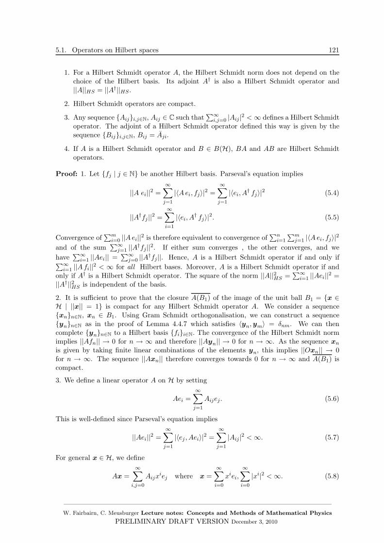
5.1. Operators on Hilbert spaces 121
1. For a Hilbert Schmidt operator A, the Hilbert Schmidt norm does not depend on thechoice of the Hilbert basis. Its adjoint A† is also a Hilbert Schmidt operator and||A||HS = ||A†||HS .
2. Hilbert Schmidt operators are compact.
3. Any sequence Aiji,j∈N, Aij ∈ C such that∑∞
i,j=0 |Aij |2 <∞ defines a Hilbert Schmidtoperator. The adjoint of a Hilbert Schmidt operator defined this way is given by thesequence Biji,j∈N, Bij = Aji.
4. If A is a Hilbert Schmidt operator and B ∈ B(H), BA and AB are Hilbert Schmidtoperators.
Proof: 1. Let fj | j ∈ N be another Hilbert basis. Parseval’s equation implies
||A ei||2 =
∞∑
j=1
|〈Aei, fj〉|2 =
∞∑
j=1
|〈ei, A† fj〉|2 (5.4)
||A†fj ||2 =
∞∑
i=1
|〈ei, A† fj〉|2. (5.5)
Convergence of∑m
i=0 ||Aei||2 is therefore equivalent to convergence of∑n
i=1
∑mj=1 |〈Aei, fj〉|2
and of the sum∑∞
j=1 ||A†fj||2. If either sum converges , the other converges, and we
have∑∞
i=1 ||Aei|| =∑∞
j=0 ||A†fj||. Hence, A is a Hilbert Schmidt operator if and only if∑∞i=1 ||Afi||2 < ∞ for all Hilbert bases. Moreover, A is a Hilbert Schmidt operator if and
only if A† is a Hilbert Schmidt operator. The square of the norm ||A||2HS =∑∞
i=1 ||Aei||2 =||A†||2HS is independent of the basis.
2. It is sufficient to prove that the closure A(B1) of the image of the unit ball B1 = x ∈H | ||x|| = 1 is compact for any Hilbert Schmidt operator A. We consider a sequencexnn∈N, xn ∈ B1. Using Gram Schmidt orthogonalisation, we can construct a sequenceynn∈N as in the proof of Lemma 4.4.7 which satisfies 〈yn,ym〉 = δnm. We can thencomplete ynn∈N to a Hilbert basis fii∈N. The convergence of the Hilbert Schmidt normimplies ||Afn|| → 0 for n → ∞ and therefore ||Ayn|| → 0 for n → ∞. As the sequence xnis given by taking finite linear combinations of the elements yn, this implies ||Oxn|| → 0for n → ∞. The sequence ||Axn|| therefore converges towards 0 for n → ∞ and A(B1) iscompact.
3. We define a linear operator A on H by setting
Aei =
∞∑
j=1
Aijej . (5.6)
This is well-defined since Parseval’s equation implies
||Aei||2 =
∞∑
j=1
|〈ej , Aei〉|2 =
∞∑
j=1
|Aij |2 <∞. (5.7)
For general x ∈ H, we define
Ax =
∞∑
i,j=0
Aijxiej where x =
∞∑
i=0
xiei,
∞∑
i=0
|xi|2 <∞. (5.8)
——————————————————————————————————————W. Fairbairn, C. Meusburger Lecture notes: Concepts and Methods of Mathematical Physics
PRELIMINARY DRAFT VERSION December 3, 2010
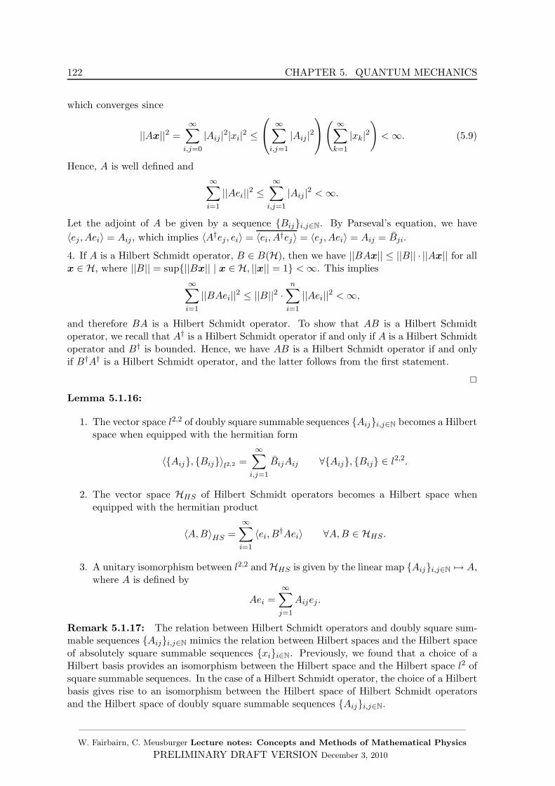
122 CHAPTER 5. QUANTUM MECHANICS
which converges since
||Ax||2 =
∞∑
i,j=0
|Aij |2|xi|2 ≤
∞∑
i,j=1
|Aij |2( ∞∑
k=1
|xk|2)<∞. (5.9)
Hence, A is well defined and
∞∑
i=1
||Aei||2 ≤∞∑
i,j=1
|Aij |2 <∞.
Let the adjoint of A be given by a sequence Biji,j∈N. By Parseval’s equation, we have
〈ej , Aei〉 = Aij , which implies 〈A†ej , ei〉 = 〈ei, A†ej〉 = 〈ej , Aei〉 = Aij = Bji.
4. If A is a Hilbert Schmidt operator, B ∈ B(H), then we have ||BAx|| ≤ ||B|| · ||Ax|| for allx ∈ H, where ||B|| = sup||Bx|| | x ∈ H, ||x|| = 1 <∞. This implies
∞∑
i=1
||BAei||2 ≤ ||B||2 ·n∑
i=1
||Aei||2 <∞,
and therefore BA is a Hilbert Schmidt operator. To show that AB is a Hilbert Schmidtoperator, we recall that A† is a Hilbert Schmidt operator if and only if A is a Hilbert Schmidtoperator and B† is bounded. Hence, we have AB is a Hilbert Schmidt operator if and onlyif B†A† is a Hilbert Schmidt operator, and the latter follows from the first statement.
2
Lemma 5.1.16:
1. The vector space l2,2 of doubly square summable sequences Aiji,j∈N becomes a Hilbertspace when equipped with the hermitian form
〈Aij, Bij〉l2,2 =
∞∑
i,j=1
BijAij ∀Aij, Bij ∈ l2,2.
2. The vector space HHS of Hilbert Schmidt operators becomes a Hilbert space whenequipped with the hermitian product
〈A,B〉HS =∞∑
i=1
〈ei, B†Aei〉 ∀A,B ∈ HHS .
3. A unitary isomorphism between l2,2 and HHS is given by the linear map Aiji,j∈N 7→ A,where A is defined by
Aei =∞∑
j=1
Aijej .
Remark 5.1.17: The relation between Hilbert Schmidt operators and doubly square sum-mable sequences Aiji,j∈N mimics the relation between Hilbert spaces and the Hilbert spaceof absolutely square summable sequences xii∈N. Previously, we found that a choice of aHilbert basis provides an isomorphism between the Hilbert space and the Hilbert space l2 ofsquare summable sequences. In the case of a Hilbert Schmidt operator, the choice of a Hilbertbasis gives rise to an isomorphism between the Hilbert space of Hilbert Schmidt operatorsand the Hilbert space of doubly square summable sequences Aiji,j∈N.
——————————————————————————————————————W. Fairbairn, C. Meusburger Lecture notes: Concepts and Methods of Mathematical Physics
PRELIMINARY DRAFT VERSION December 3, 2010
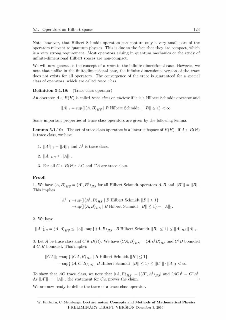
5.1. Operators on Hilbert spaces 123
Note, however, that Hilbert Schmidt operators can capture only a very small part of theoperators relevant to quantum physics. This is due to the fact that they are compact, whichis a very strong requirement. Most operators arising in quantum mechanics or the study ofinfinite-dimensional Hilbert spaces are non-compact.
We will now generalise the concept of a trace to the infinite-dimensional case. However, wenote that unlike in the finite-dimensional case, the infinite dimensional version of the tracedoes not exists for all operators. The convergence of the trace is guaranteed for a specialclass of operators, which are called trace class.
Definition 5.1.18: (Trace class operator)
An operator A ∈ B(H) is called trace class or nuclear if it is a Hilbert Schmidt operator and
||A||1 = sup|〈A,B〉HS | B Hilbert Schmidt , ||B|| ≤ 1 <∞.
Some important properties of trace class operators are given by the following lemma.
Lemma 5.1.19: The set of trace class operators is a linear subspace of B(H). If A ∈ B(H)is trace class, we have
1. ||A†||1 = ||A||1 and A† is trace class.
2. ||A||HS ≤ ||A||1.
3. For all C ∈ B(H): AC and CA are trace class.
Proof:
1. We have 〈A,B〉HS = 〈A†, B†〉HS for all Hilbert Schmidt operators A,B and ||B†|| = ||B||.This implies
||A†||1 =sup|〈A†, B〉HS | B Hilbert Schmidt ||B|| ≤ 1=sup|〈A,B〉HS | B Hilbert Schmidt ||B|| ≤ 1 = ||A||1.
2. We have
||A||2HS = 〈A,A〉HS ≤ ||A|| · sup|〈A,B〉HS | B Hilbert Schmidt ||B|| ≤ 1 ≤ ||A||HS ||A||1.
3. Let A be trace class and C ∈ B(H). We have 〈CA,B〉HS = 〈A, c†B〉HS and C†B boundedif C,B bounded. This implies
||CA||1 =sup|〈CA,B〉HS | B Hilbert Schmidt ||B|| ≤ 1=sup|〈A,C†B〉HS | B Hilbert Schmidt ||B|| ≤ 1 ≤ ||C†|| · ||A||1 <∞.
To show that AC trace class, we note that |〈A,B〉HS| = |〈B†, A†〉HS| and (AC)† = C†A†.As ||A†||1 = ||A||1, the statement for CA proves the claim. 2
We are now ready to define the trace of a trace class operator.
——————————————————————————————————————W. Fairbairn, C. Meusburger Lecture notes: Concepts and Methods of Mathematical Physics
PRELIMINARY DRAFT VERSION December 3, 2010
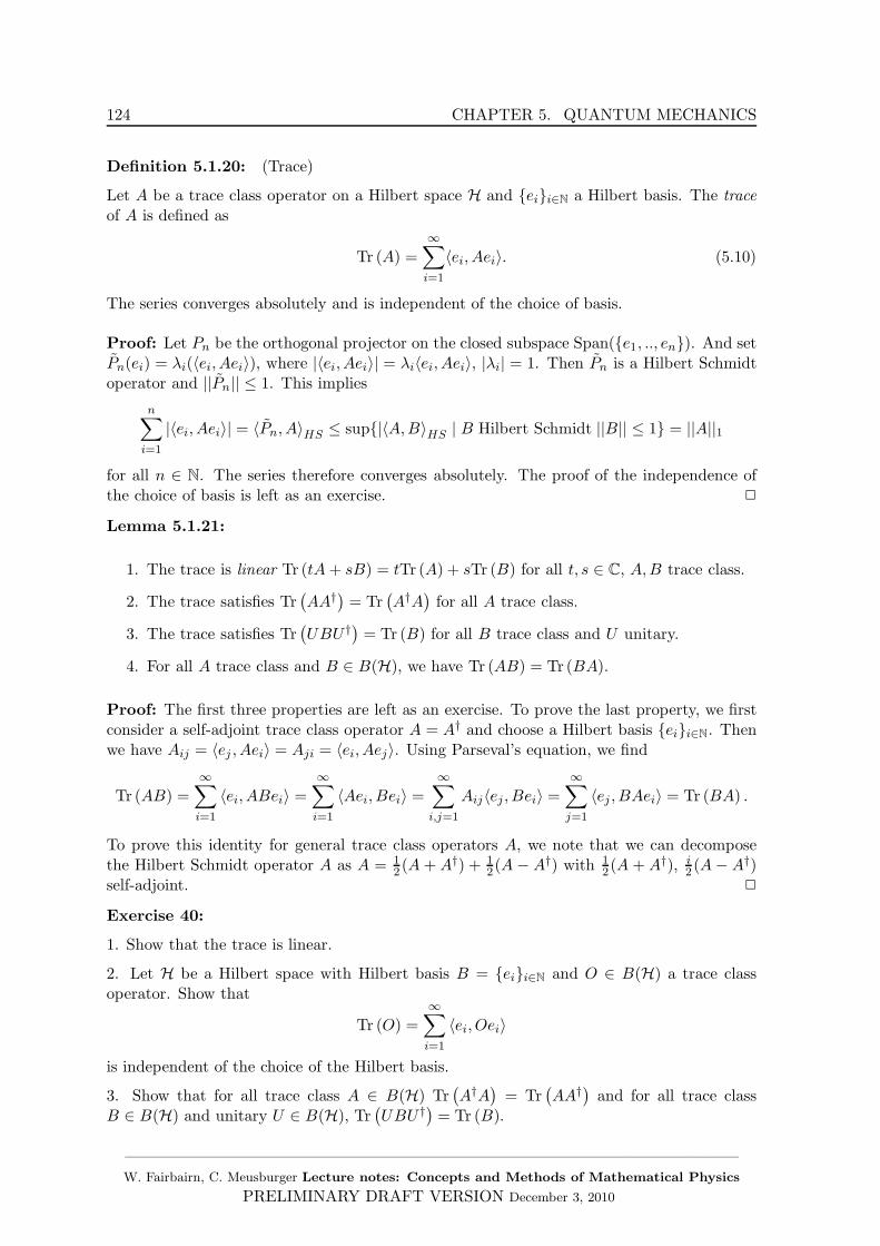
124 CHAPTER 5. QUANTUM MECHANICS
Definition 5.1.20: (Trace)
Let A be a trace class operator on a Hilbert space H and eii∈N a Hilbert basis. The traceof A is defined as
Tr (A) =
∞∑
i=1
〈ei, Aei〉. (5.10)
The series converges absolutely and is independent of the choice of basis.
Proof: Let Pn be the orthogonal projector on the closed subspace Span(e1, .., en). And setPn(ei) = λi(〈ei, Aei〉), where |〈ei, Aei〉| = λi〈ei, Aei〉, |λi| = 1. Then Pn is a Hilbert Schmidtoperator and ||Pn|| ≤ 1. This implies
n∑
i=1
|〈ei, Aei〉| = 〈Pn, A〉HS ≤ sup|〈A,B〉HS | B Hilbert Schmidt ||B|| ≤ 1 = ||A||1
for all n ∈ N. The series therefore converges absolutely. The proof of the independence ofthe choice of basis is left as an exercise. 2
Lemma 5.1.21:
1. The trace is linear Tr (tA+ sB) = tTr (A) + sTr (B) for all t, s ∈ C, A,B trace class.
2. The trace satisfies Tr(AA†) = Tr
(A†A
)for all A trace class.
3. The trace satisfies Tr(UBU †) = Tr (B) for all B trace class and U unitary.
4. For all A trace class and B ∈ B(H), we have Tr (AB) = Tr (BA).
Proof: The first three properties are left as an exercise. To prove the last property, we firstconsider a self-adjoint trace class operator A = A† and choose a Hilbert basis eii∈N. Thenwe have Aij = 〈ej , Aei〉 = Aji = 〈ei, Aej〉. Using Parseval’s equation, we find
Tr (AB) =
∞∑
i=1
〈ei, ABei〉 =
∞∑
i=1
〈Aei, Bei〉 =
∞∑
i,j=1
Aij〈ej , Bei〉 =
∞∑
j=1
〈ej , BAei〉 = Tr (BA) .
To prove this identity for general trace class operators A, we note that we can decomposethe Hilbert Schmidt operator A as A = 1
2 (A+ A†) + 12(A − A†) with 1
2(A + A†), i2 (A− A†)
self-adjoint. 2
Exercise 40:
1. Show that the trace is linear.
2. Let H be a Hilbert space with Hilbert basis B = eii∈N and O ∈ B(H) a trace classoperator. Show that
Tr (O) =
∞∑
i=1
〈ei, Oei〉
is independent of the choice of the Hilbert basis.
3. Show that for all trace class A ∈ B(H) Tr(A†A
)= Tr
(AA†) and for all trace class
B ∈ B(H) and unitary U ∈ B(H), Tr(UBU †) = Tr (B).
——————————————————————————————————————W. Fairbairn, C. Meusburger Lecture notes: Concepts and Methods of Mathematical Physics
PRELIMINARY DRAFT VERSION December 3, 2010
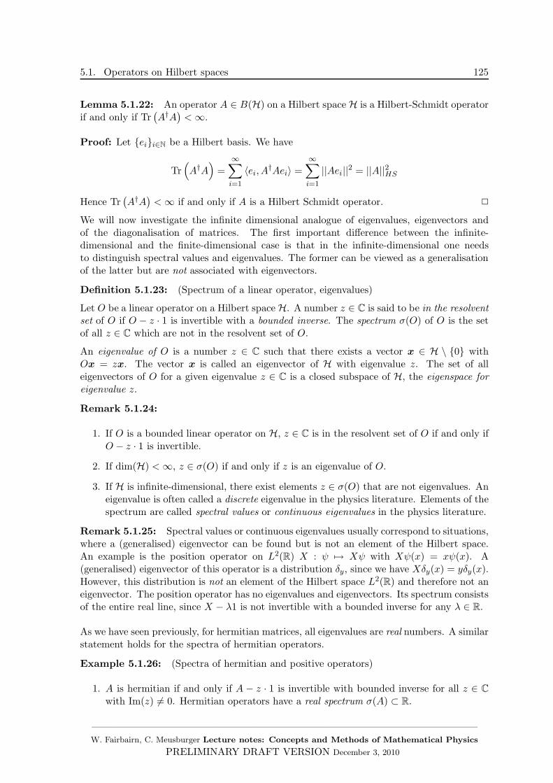
5.1. Operators on Hilbert spaces 125
Lemma 5.1.22: An operator A ∈ B(H) on a Hilbert space H is a Hilbert-Schmidt operatorif and only if Tr
(A†A
)<∞.
Proof: Let eii∈N be a Hilbert basis. We have
Tr(A†A
)=
∞∑
i=1
〈ei, A†Aei〉 =
∞∑
i=1
||Aei||2 = ||A||2HS
Hence Tr(A†A
)<∞ if and only if A is a Hilbert Schmidt operator. 2
We will now investigate the infinite dimensional analogue of eigenvalues, eigenvectors andof the diagonalisation of matrices. The first important difference between the infinite-dimensional and the finite-dimensional case is that in the infinite-dimensional one needsto distinguish spectral values and eigenvalues. The former can be viewed as a generalisationof the latter but are not associated with eigenvectors.
Definition 5.1.23: (Spectrum of a linear operator, eigenvalues)
Let O be a linear operator on a Hilbert space H. A number z ∈ C is said to be in the resolventset of O if O − z · 1 is invertible with a bounded inverse. The spectrum σ(O) of O is the setof all z ∈ C which are not in the resolvent set of O.
An eigenvalue of O is a number z ∈ C such that there exists a vector x ∈ H \ 0 withOx = zx. The vector x is called an eigenvector of H with eigenvalue z. The set of alleigenvectors of O for a given eigenvalue z ∈ C is a closed subspace of H, the eigenspace foreigenvalue z.
Remark 5.1.24:
1. If O is a bounded linear operator on H, z ∈ C is in the resolvent set of O if and only ifO − z · 1 is invertible.
2. If dim(H) <∞, z ∈ σ(O) if and only if z is an eigenvalue of O.
3. If H is infinite-dimensional, there exist elements z ∈ σ(O) that are not eigenvalues. Aneigenvalue is often called a discrete eigenvalue in the physics literature. Elements of thespectrum are called spectral values or continuous eigenvalues in the physics literature.
Remark 5.1.25: Spectral values or continuous eigenvalues usually correspond to situations,where a (generalised) eigenvector can be found but is not an element of the Hilbert space.An example is the position operator on L2(R) X : ψ 7→ Xψ with Xψ(x) = xψ(x). A(generalised) eigenvector of this operator is a distribution δy, since we have Xδy(x) = yδy(x).However, this distribution is not an element of the Hilbert space L2(R) and therefore not aneigenvector. The position operator has no eigenvalues and eigenvectors. Its spectrum consistsof the entire real line, since X − λ1 is not invertible with a bounded inverse for any λ ∈ R.
As we have seen previously, for hermitian matrices, all eigenvalues are real numbers. A similarstatement holds for the spectra of hermitian operators.
Example 5.1.26: (Spectra of hermitian and positive operators)
1. A is hermitian if and only if A − z · 1 is invertible with bounded inverse for all z ∈ C
with Im(z) 6= 0. Hermitian operators have a real spectrum σ(A) ⊂ R.
——————————————————————————————————————W. Fairbairn, C. Meusburger Lecture notes: Concepts and Methods of Mathematical Physics
PRELIMINARY DRAFT VERSION December 3, 2010
126 CHAPTER 5. QUANTUM MECHANICS
2. A hermitian operator A is positive if and only if σ(A) ⊂ R+0 .
Exercise 41:
Show that the only possible eigenvalues of a projection operator are 0 and 1.
We are now ready to investigate the decomposition of Hilbert spaces into linear subspaces ofeigenvectors associated with eigenvalues. As it can be expected that spectral values whichare not eigenvalues are associated with complications, we start with the simplest situation,namely the one of compact, normal operators. In this case, it turns out that there is at mostone spectral value which is not an eigenvalue.
Theorem 5.1.27: (Spectral decomposition for compact, normal operators)
Let A ∈ B(H) compact and normal. Then 0 ∈ σ(A) and σ(A) is either finite or of the formσ(A) = 0, λ1, λ2, ... where λnn∈N, λi ∈ C \ 0 is a sequence that converges to 0 withn → ∞. For each λi, i ∈ N the eigenspace Ei = x ∈ H | Ax = λix is of finite dimension0 < dim(Ei) <∞. The eigenspaces Ei are orthogonal: 〈x,y〉 = 0 for all x ∈ Ei, y ∈ Ej withi 6= j. The operator A can be expressed in terms of the projection operators PEi on Ei as
A =
∞∑
i=1
λiPEi . (5.11)
Remark 5.1.28: In the physics literature identity (5.11) is often expressed in bra-ket no-tation as
A =
∞∑
i=1
λi|ei〉〈ei|.
Corollary 5.1.29: (Spectrum of compact, positive operators)
If A is a compact, positive operator, it is in particular self-adjoint, which implies normal andall eigenvalues are positive or zero. Hence, the spectrum of a compact, positive operator iseither finite with 0 ∈ σ(A) or takes the form σ(A) = 0, λ1, λ2, ... where (λn)n∈N, λn ∈ R+ isa sequence that converges to 0. The eigenspaces Ei, i ∈ N are orthogonal, and the operatorA is given by
A =∞∑
i=1
λiPEi . (5.12)
Theorem 5.1.27 provides us with a rather straightforward generalisation of the diagonalisationof complex matrices. However, its disadvantage is that it is only valid for a very specific classof of operators- most operators relevant to physics are not compact. In particular, identityoperators, projectors on infinite-dimensional subspaces and Hamilton operators of systemswhose energy is not bounded are non-compact operators. We therefore need a generalisationof this theorem. This forces us to deal with spectral values which are not eigenvalues and tointroduce the notion of a spectral measure.
Definition 5.1.30: (Spectral measure)
A Borel set in k = C or k = R is a subset E ⊂ k that can be expressed as a countableunion
⋃∞i=1Ei or countable intersection
⋂∞i=1Ei of open subsets of k, their complements and
countable unions and intersections thereof. We denote by Bor(k) the Borel sets in k.
——————————————————————————————————————W. Fairbairn, C. Meusburger Lecture notes: Concepts and Methods of Mathematical Physics
PRELIMINARY DRAFT VERSION December 3, 2010
5.1. Operators on Hilbert spaces 127
A spectral measure on k is a function P : E ∈ Bor(k) → P (E) ∈ B(H) which assigns to eachBorel set in k a projection operator P (E) ∈ B(H) such that
1. P (∅) = 0
2. P (k) = 1
3. P (⋃∞i=1Ei) =
∑∞i=1 P (Ei) for mutually disjoint Borel sets: Ei ⊂ k, Ei ∩Ej = ∅ ∀i 6= j.
Lemma 5.1.31: (Properties of spectral measures)
A spectral measure P : Bor(k) → B(H) has the following properties
1. Monotonicity: E1 ⊂ E2 ⇒ P (E1) ≤ P (E2).
2. (Orthogonality): E1∩E2 = ∅ ⇒ P (E1)⊥P (E2), i.e. P (E2)P (E1) = P (E1)P (E2) = 0.
3. For all E1, E2 ∈ Bor(k): P (E1 ∩ E2) = P (E1)P (E2).
Proof: Exercise.
We will now use the concept of spectral measure to define integrals of operators. For this weneed the following lemma.
Lemma 5.1.32: Let P : Bor(k) → B(H) be a spectral measure. Then for all x,y ∈ H,the function µx,y : Bor(k) → C defined by µx,y(E) = 〈P (E)x,y〉 is a measure on k, i.e. itsatisfies
1. µx,y(∅) = 0
2. A ⊂ ⋃∞j=1Aj , Aj ∈ Bor(k) for all j ∈ N ⇒ µx,y(A) ≤∑∞
i=1 µx,y(Aj).
Lemma 5.1.33: The measure µx,y is of bounded variation. For all E ∈ Bor(k) we have
||µx,y(E)|| = sup∞∑
n=1
|µ(Ei)| | E =∞⋃
i=1
Ei , Ei ∈ Bor(k), Ei ∩ Ej = ∅ for i 6= j ≤ ||x||||y||
In order to define the integral of operators associated with measures µx,y, x,y ∈ H we needthe notion of the generalised Lebesgue Stieltjes integral.
Definition 5.1.34: (Lebesgue Stieltjes integral)
Let µ be a measure of bounded variation on k, i.e. a measure µ on k for which there existsa constant c ∈ R+ such that
||µ(E)|| = sup∞∑
n=1
|µ(Ei)| | E =∞⋃
i=1
Ei , Ei ∈ Bor(k), Ei∩Ej = ∅ for i 6= j ≤ c ∀E ∈ Bor(k).
Let f : k → R be a Borel function or measurable function, i.e. a function such that thepreimage f−1(T ) is a Borel set for all Borel sets T ⊂ R. Suppose that f is non-negative:f ≥ 0 almost everywhere, and bounded, ||f ||∞ = supx∈k|f(x)| < ∞. Then the generalisedLebesgue Stieltjes integral of f over a Borel set E with respect to µ is defined as
∫
Efdµ := sup
n∑
i=1
inff(x) | x ∈ Eiµ(Ei) | E =∞⋃
i=1
Ei , Ei ∈ Bor(k), Ei ∩ Ej = ∅ for i 6= j
.
——————————————————————————————————————W. Fairbairn, C. Meusburger Lecture notes: Concepts and Methods of Mathematical Physics
PRELIMINARY DRAFT VERSION December 3, 2010
128 CHAPTER 5. QUANTUM MECHANICS
If f : k → C is a complex valued, bounded Borel function, then the functions Re(f)± : k →R+
0 , Im(f)± : k → R+0 defined by
Re(f)+(z) = maxRe(f)(z), 0 Re(f)−(z) = −minRe(f)(z), 0Im(f)+(z) = maxIm(f)(z), 0 Im(f)−(z) = −minIm(f)(z), 0 ∀z ∈ k (5.13)
are non-negative, bounded Borel functions. The generalised Lebesgue Stieltjes integral of fover a Borel set E is defined as
∫
Efdµ :=
∫
ERe(f)+dµ−
∫
ERe(f)−dµ+ i
∫
EIm(f)+dµ− i
∫
EIm(f)−dµ. (5.14)
Remark 5.1.35: The integral∫E fdµ is well defined. If f : k → R is non-negative, bounded
Borel function with ||f ||∞ = c and µ a measure of bounded variation, we have
0 ≤ inff(x) | x ∈ Eiµ(Ei) ≤ c · µ(Ei) ∀Ei ∈ Bor(k)
and therefore
∫
Efdµ =sup
n∑
i=1
inff(x) | x ∈ Eiµ(Ei) | E =
∞⋃
i=1
Ei , Ei ∈ Bor(k), Ei ∩ Ej = ∅ for i 6= j
≤c · sup
∞∑
n=1
|µ(Ei)| | E =
∞⋃
i=1
Ei , Ei ∈ Bor(k), Ei ∩ Ej = ∅ for i 6= j
= c||µ|| <∞.
We can now use the Lebesgue Stieltjes integral for the measure µx,y to define a boundedhermitian form on H and to obtain an associated operator via Riesz’s theorem.
Lemma 5.1.36: Let f : k → C be a bounded Borel function Then its integral with respectto the measure µx,y exists and the map g : H × H → C g(x,y) =
∫k fdµx,y defines a
bounded hermitian form on H. We have
|g(x,y)| ≤ ||x||||y||||f ||∞ ∀x,y ∈ H.
By Riesz’s theorem there exists a unique operator F ∈ B(H) with 〈Fx,y〉 =∫
Cfdµxy. we
denote this operator by F =:∫k f(z)dP (z).
This allows us to formulate the spectral theorem for self-adjoint operators.
Theorem 5.1.37: (Spectral decomposition for self-adjoint operators)
For a densely defined self-adjoint operator A on H there exists a unique spectral measurePA : Bor(R) → B(H) such that
A =
∫
R
x dPA(x).
Conversely, any operator defined by a spectral measure in this way is self-adjoint.
With the definition f(A) :=∫
Rf(x)dPA(x) for bounded Borel functions f : R → C, we have
PA(E) = χE(A), where χE is the characteristic function of a Borel set E
χE(x) =
1 x ∈ E
0 x /∈ E. (5.15)
——————————————————————————————————————W. Fairbairn, C. Meusburger Lecture notes: Concepts and Methods of Mathematical Physics
PRELIMINARY DRAFT VERSION December 3, 2010

5.2. Axioms of quantum mechanics 129
In many books on quantum mechanics, this theorem is presented in terms of spectral sequencesor resolutions of the identity. One can show that spectral sequences are equivalent to spectralmeasures on R.
Definition 5.1.38: (Resolution of the identity )
A resolution of the identity is a function λ ∈ R → Pλ ∈ B(H) into the set of orthogonalprojection operators on H such that
1. λ ≤ µ ⇒ Pλ ≤ Pµ
2. limλ→−∞ Pλ, limλ→∞ Pλ exist and satisfy
P−∞ = limλ→−∞
Pλ = 0 P∞ := limλ→∞
Pλ = idH.
3. limǫ→0,ǫ>0 Pλ+ǫ = Pλ.
Here, all limits are taken with respect to the norm ||O|| = sup||Ox|| | x ∈ H, ||x|| = 1 forbounded operators on H. The resolution of the identity is called constant in a point x ∈ R ifthere exists an interval ]a, b[⊂ R), a < x < b, such that Pay = Pby for all y ∈ H. Otherwiseit is called discontinuous in x ∈ R.
Exercise 42: Let P : Bor(R) → B(H) a spectral measure on the Borel sets of R. Showthat the function Pλ = P (] −∞, λ]), λ ∈ R defines a resolution of the identity. Show thattwo spectral measures P,Q : Bor(R) → B(H) give rise to the same resolution of the identitysatisfy P = Q.
5.2 Axioms of quantum mechanics
Axiom 1: The observables, i.e. the measurable quantities of a physical system, are inone-to-one correspondence with self-adjoint operators on a separable Hilbert space. Thepossible results of measurements of an observable are given by the spectrum of the associatedself-adjoint operator.
To formulate the second axiom of quantum mechanics, we have to introduce the notion of adensity operator and of a pure state.
Definition 5.2.1: (Density operator)
A density operator on a Hilbert space H is a trace class, positive operator ρ ∈ B(H) suchthat ρ O is trace class for all observables O.
Remark 5.2.2: Note that the fact that ρ is trace class implies directly that ρ O is traceclass for all bounded operators O ∈ B(H) by Lemma 5.1.19.
Lemma 5.2.3: For any density operator ρ, the associated normalised density operatorρ = ρ/Tr (ρ) can be expressed as
ρ :=ρ
Tr (ρ)=
∞∑
i=1
λiPei 0 ≤ λi ≤ 1,∑
i
λi = 1, (5.16)
where eii∈N is a Hilbert basis and Pei the projector on Span(ei),
——————————————————————————————————————W. Fairbairn, C. Meusburger Lecture notes: Concepts and Methods of Mathematical Physics
PRELIMINARY DRAFT VERSION December 3, 2010
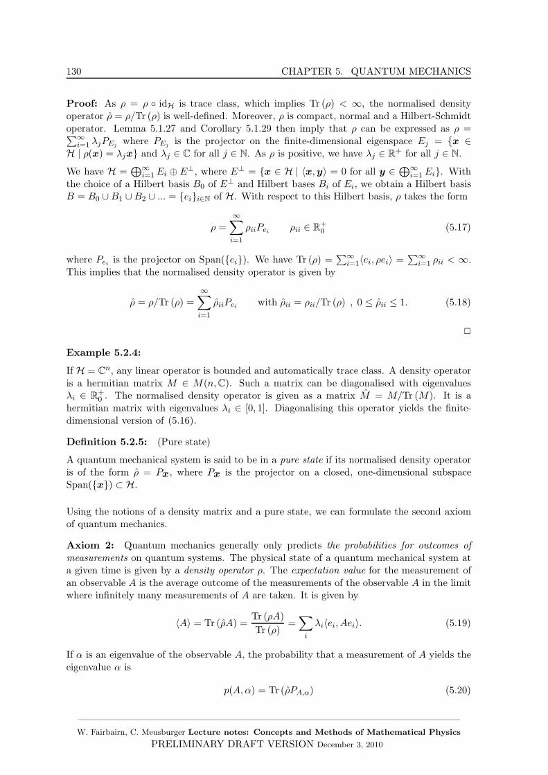
130 CHAPTER 5. QUANTUM MECHANICS
Proof: As ρ = ρ idH is trace class, which implies Tr (ρ) < ∞, the normalised densityoperator ρ = ρ/Tr (ρ) is well-defined. Moreover, ρ is compact, normal and a Hilbert-Schmidtoperator. Lemma 5.1.27 and Corollary 5.1.29 then imply that ρ can be expressed as ρ =∑∞
i=1 λjPEj where PEj is the projector on the finite-dimensional eigenspace Ej = x ∈H | ρ(x) = λjx and λj ∈ C for all j ∈ N. As ρ is positive, we have λj ∈ R+ for all j ∈ N.
We have H =⊕∞
i=1Ei ⊕ E⊥, where E⊥ = x ∈ H | 〈x,y〉 = 0 for all y ∈ ⊕∞i=1Ei. With
the choice of a Hilbert basis B0 of E⊥ and Hilbert bases Bi of Ei, we obtain a Hilbert basisB = B0 ∪B1 ∪B2 ∪ ... = eii∈N of H. With respect to this Hilbert basis, ρ takes the form
ρ =
∞∑
i=1
ρiiPei ρii ∈ R+0 (5.17)
where Pei is the projector on Span(ei). We have Tr (ρ) =∑∞
i=1〈ei, ρei〉 =∑∞
i=1 ρii < ∞.This implies that the normalised density operator is given by
ρ = ρ/Tr (ρ) =∞∑
i=1
ρiiPei with ρii = ρii/Tr (ρ) , 0 ≤ ρii ≤ 1. (5.18)
2
Example 5.2.4:
If H = Cn, any linear operator is bounded and automatically trace class. A density operatoris a hermitian matrix M ∈ M(n,C). Such a matrix can be diagonalised with eigenvaluesλi ∈ R+
0 . The normalised density operator is given as a matrix M = M/Tr (M). It is ahermitian matrix with eigenvalues λi ∈ [0, 1]. Diagonalising this operator yields the finite-dimensional version of (5.16).
Definition 5.2.5: (Pure state)
A quantum mechanical system is said to be in a pure state if its normalised density operatoris of the form ρ = Px, where Px is the projector on a closed, one-dimensional subspaceSpan(x) ⊂ H.
Using the notions of a density matrix and a pure state, we can formulate the second axiomof quantum mechanics.
Axiom 2: Quantum mechanics generally only predicts the probabilities for outcomes ofmeasurements on quantum systems. The physical state of a quantum mechanical system ata given time is given by a density operator ρ. The expectation value for the measurement ofan observable A is the average outcome of the measurements of the observable A in the limitwhere infinitely many measurements of A are taken. It is given by
〈A〉 = Tr (ρA) =Tr (ρA)
Tr (ρ)=∑
i
λi〈ei, Aei〉. (5.19)
If α is an eigenvalue of the observable A, the probability that a measurement of A yields theeigenvalue α is
p(A,α) = Tr (ρPA,α) (5.20)
——————————————————————————————————————W. Fairbairn, C. Meusburger Lecture notes: Concepts and Methods of Mathematical Physics
PRELIMINARY DRAFT VERSION December 3, 2010
5.2. Axioms of quantum mechanics 131
where PA,α is the projector on the eigenspace of A for eigenvalue α. If α ∈ σ(A) is a spectralvalue but not an eigenvalue, and [α− ǫ, α+ ǫ] ⊂ σ(A) does not contain any eigenvalues, theprobability that a measurement of A yields a result in [α− ǫ, α+ ǫ] is given by
pA,[α−ǫ,α+ǫ] = Tr
(ρ ·∫ α+ǫ
α−ǫdPA
)= Tr (ρ · PA([α− ǫ, α+ ǫ])) (5.21)
where PA is the spectral measure associated with A.
A definite prediction for the outcome of a measurement of an observable A is possible if andonly if the density operator is of the form ρ = PA,α, where PA,α is the projector on a subspaceof the eigenspace of eigenvalue α ∈ σ(A). In this case, the expectation value is 〈A〉 = α, theprobability of measuring α is p(A,α) = 1 and the variance vanishes 〈(A− 〈A〉)2〉 = 0. Moregenerally, if f is a polynomial with coefficients in C, we have
〈f(A)〉 − f(〈A〉) = 0
Exercise 43: (Expectation values)
Suppose that a quantum system is in a pure state with a normalised density operator ρ = Pxthat is a projector on a one-dimensional subspace Span(x) with x ∈ H. Show that for allobservables A the expectation value 〈A〉 = Tr (ρA) can be expressed in terms of the hermitianproduct 〈 , 〉 on H as
〈A〉 = 〈x, Ax〉.
Axiom 3: (Preparation and measurements)
The density operator ρ for the description of a quantum mechanical system is given by theexperimental conditions under which the system was prepared. If the preparation of thesystem involved the measurement of an observable A with outcome α ∈ σ(A), where α is aneigenvalue of A, the normalised density operator after preparation satisfies
Tr (ρPA,α) = 1, (5.22)
where PA,α is the projector on the eigenspace associated with eigenvalue α of A. If thesystem before preparation is described by a density operator ρ1, the density operator afterpreparation is given by
ρ2 = PA,αρ1PA,α ρ2 =PA,αρ1PA,α
Tr (PA,αρ1PA,α). (5.23)
This postulate is also known under the name collapse of the wave function. After a measure-ment of an observable A with outcome α ∈ σ(A) is performed, the wave function is said tocollapse to a linear combination of eigenvectors of O with eigenvalue α.
Note that the eigenspace of an observable A with eigenvalue α is not necessarily one-dimensionaland therefore does not specify a unique element of H. This corresponds to the fact that usu-ally measurements of several observables are needed to determine the state of a physicalsystem. A set of observables that can be measured simultaneously and whose measurementsgive all the information that can be gained about the state of the system is called a completeset of commuting observables.
——————————————————————————————————————W. Fairbairn, C. Meusburger Lecture notes: Concepts and Methods of Mathematical Physics
PRELIMINARY DRAFT VERSION December 3, 2010

132 CHAPTER 5. QUANTUM MECHANICS
Definition 5.2.6: (Complete set of commuting observables)
A complete set of commuting observables is a finite set of observables Oii=1,...n whichcommute [Oi, Oj ] = Oi Oj −Oj Oi = 0 ∀i, j ∈ 1, ..., n and are such that the intersection∩ni=1Eαi of the eigenspaces Eiαi
of observable Oi with eigenvalue αi is a one-dimensionalsubspace of H. In other words, there exists an x ∈ H such that
n⋂
i=1
Eiαi= Span(x).
Example 5.2.7: For the hydrogen atom (when the spins of electron and proton are ne-glected), a complete set of commuting observables is given by the Hamiltonian H, the totalangular momentum J2 and the angular momentum Lz in the z-direction.
Remark 5.2.8: The requirement that the set is finite is motivated by the fact that otherwiseinfinitely many measurements would be needed to determine the physical state of the system,which would be impossible in practice. However, it is clear that this requirement of finitenessmust be dropped in quantum field theory.
There is no mathematical proof that a complete set of observables exists for all quantum me-chanical system satisfying the axioms of quantum mechanics. However, a quantum mechanicalsystem without a complete set of commuting observables would be difficult to interpret. Inparticular, it would not be possible to prepare such a system in a way that it is in a purestate by performing a finite number of measurements.
Axiom 4: (Time development)
The time development of a quantum mechanical system is described by a unitary operatorUt with continuous time dependence, the time evolution operator, which is determined by thedifferential equation
Ut = 1i~HtUt U0 = idH. (5.24)
where Ht is the Hamiltonian at time t, which gives the energy of the system. The timeevolution of the physical state is given by
〈A〉t = Tr(UtρU
†t A). (5.25)
Note that this time development of the system can be interpreted in two ways. The firstinterpretation is that of a time development of the density operator, while the observablesremain constant and undergo no time evolution.
〈A〉t = Tr (ρtA) ρt = UtρU†t . (5.26)
Note that as U is unitary, Tr(UtρU
†t
)= Tr (ρ) and therefore ρt = UtρU
†t . Unitary opera-
tors preserve probability. In view of expression (5.16) for the density operator, this can be
interpreted as a time development of each projector Pi → UtPiU†t and hence as a time devel-
opment of the vectors in the Hilbert space x 7→ Utx for all x ∈ H. This is the Schrodingerpicture of time development.
——————————————————————————————————————W. Fairbairn, C. Meusburger Lecture notes: Concepts and Methods of Mathematical Physics
PRELIMINARY DRAFT VERSION December 3, 2010
5.3. Quantum mechanics - the C∗-algebra viewpoint 133
The second interpretation of formula (5.26) is due to the fact that the cyclic invariance ofthe trace, one can rewrite (5.26) as
〈A〉t = Tr(PU †
tAUt
)= Tr (ρAt) At = U †
t AUt. (5.27)
In this viewpoint, the density operators (and therefore the elements of H) remain constantand undergo no time development. Instead, it is the observables of the system which developwith time. This is called the Heisenberg picture of time development.
Exercise 44: (Time development)
Consider a quantum system with normalised density operator ρ, time evolution operatorUt and Hamiltonian Ht. Let A be an observable. Show that the time development of theexpectation value 〈A〉t is given by
d
dt〈A〉t = 1
i~〈[A,Ht]〉t.
Consider now a quantum system that is given by the Heisenberg algebra and equipped witha Hamilton operator of the form
Ht =P 2
2m+ Vt(X),
where P is the momentum operator, X the position operator and Vt(X) a tie-dependentfunction of X. Suppose that X and P satisfy the commutation relations of the Heisenbergalgebra [X,P ] = i~ 1. Show that the time development of the expectation values 〈X〉t, 〈P 〉tis given by
d
dt〈X〉t = 1
m〈P 〉td
dt〈P 〉t = −〈V ′
t (X)〉t where V ′t (x) =
d
dxVt(x).
Show that if we interpret the derivative Ft(x) := −V ′t (x) = − d
dxVt(x) as the force arisingfrom the time-dependent potential Vt, the expectation value of X satisfies
md2
dt2〈X〉t = 〈F (X)〉t.
The “acceleration” of the expectation value of the position is therefore given by the expecta-tion value of the force. This statement is known under the name of Ehrenfest’s theorem.
5.3 Quantum mechanics - the C∗-algebra viewpoint
The postulates of quantum mechanics introduced in the last section give a clear frameworkfor the formulation and interpretation of quantum theories. However, it has the disadvantagethat it is based on the notion of a Hilbert space. Hilbert spaces have no counterparts inthe classical theory and cannot be directly accessed by measurements. Measurements canonly be associated with observables of the theory. Only the observables have counterparts inthe classical theory and a clear physical interpretation. Moreover, the notion of states in aHilbert space becomes problematic in quantum field theory in curved spacetimes.
——————————————————————————————————————W. Fairbairn, C. Meusburger Lecture notes: Concepts and Methods of Mathematical Physics
PRELIMINARY DRAFT VERSION December 3, 2010
134 CHAPTER 5. QUANTUM MECHANICS
This raises the question if it is possible to give a formulation of quantum mechanics basedon the algebra of observables alone, in which Hilbert spaces either do not appear at all or arederived from the algebra of observables. The answer to this question is positive and given bythe theory of C∗-algebras.
Definition 5.3.1: (Banach algebra, C∗-algebra)
A (unital) Banach algebra is a (unital) associative algebra A that as a vector space has thestructure of a Banach space with norm || || and satisfies
1. ||x · y|| ≤ ||x|| · ||y|| for all x,y ∈ A
2. ||e|| = 1.
A (unital) C∗-algebra is a (unital) Banach algebra with an involution ∗ : A→ A, ∗2 = 1 that
1. is an anti-linear anti-algebra homomorphism
(xy)∗ = y∗x∗ (tx + sy)∗ = tx∗ + sy∗ ∀x,y ∈ A, t, s ∈ C. (5.28)
2. satisfies ||xx∗|| = ||x||2 for all x ∈ A.
A ∗-subalgebra of a C∗-algebra A is a subalgebra B ⊂ A which is closed with respect to thenorm || || and satisfies x∗ ∈ B for all x ∈ B.
Example 5.3.2: (C∗-algebras)
1. The space B(H) of bounded linear operators on a Hilbert space H with norm ||A|| =sup||Ax|| | x ∈ H, ||x|| = 1 is a Banach algebra. With the involution ∗ : O 7→ O† itbecomes a C∗-algebra.
2. Hilbert Schmidt operators form a C∗ − algebra without unit, where the norm is theHilbert Schmidt norm and the involution is the adjoint O∗ = O†
3. The space L1(Rn) with pointwise addition, multiplication by C, norm || · ||1 and theconvolution as product is a Banach algebra.
Exercise 45: Show that the properties of the involution in a C∗-algebra A imply
||e|| = 1 ||x∗|| = ||x|| ||x · y|| ≤ ||x||||y|| ∀x,y ∈ A. (5.29)
Definition 5.3.3: (Self adjoint, normal and unitary elements of a C∗-algebra)
An element x ∈ A of a C∗-algebra A is called hermitian or self adjoint if x∗ = x. It is callednormal if x∗x = xx∗. It is called unitary if xx∗ = e.
Exercise 46: Show that for all elements x ∈ A of a C∗-algebra A, the elements 12(x + x∗)
and 12i(x − x∗) are self-adjoint. Show that the unitary elements of A form a group. Show
that an element x ∈ A is normal if and only if 12(x + x∗), 1
2i(x − x∗) commute.
Definition 5.3.4: (Spectrum, regular value, spectral values)
Let A be a Banach algebra and x ∈ A. A complex number z ∈ C is a regular value of a ifx − z · e has an inverse. Otherwise it is called a spectral value. The spectrum σ(x) is the setof spectral values of elements x ∈ A.
——————————————————————————————————————W. Fairbairn, C. Meusburger Lecture notes: Concepts and Methods of Mathematical Physics
PRELIMINARY DRAFT VERSION December 3, 2010
5.3. Quantum mechanics - the C∗-algebra viewpoint 135
Example 5.3.5: If A = B(H) is the set of bounded linear operators on a Hilbert space H,this definition coincides with Definition 5.1.23.
Definition 5.3.6: (State)
A positive linear form of a unital C∗-algebra A is a linear form ψ ∈ A∗ such that ψ(xx∗) ≥ 0for all x ∈ A. A state on A is a positive linear form on A that satisfies ψ(e) = e.
Exercise 47: Show that the set of states of a unital C∗-algebra A is convex, i.e. if ψ1, ψ2
are states of A, ψt = tψ1 + (1 − t)ψ2 is a state of A for all t ∈ [0, 1].
Definition 5.3.7: (Pure state)
A state ψ of a unital C∗-algebra A is pure if ψ = tφ+ (1 − t)η with t ∈ [0, 1] and states φ, ηimplies t = 1 and ψ = φ or t01 and ψ = η.
Theorem 5.3.8: (Krein Mil’man)
Pure states exist for any unital C∗-algebra A and the set of states of A is the closed convexhull of its pure states. In other words: Any state ψ of A can be expressed as
ψ =n∑
i=1
λiψi λi ∈ [0, 1],n∑
i=1
λi = 1, (5.30)
where ψi, i ∈ 1, .., n are pure states. Pure states are characterised by λj = 1 for a singlej ∈ 1, ..., n and λi = 0 for all i 6= j.
Definition 5.3.9: (Complete set of commuting observables)
A set of commuting observables of a a unital C∗-algebra A is a finite set of commuting self-adjoint elements x1, ...,xn ∈ A, x∗
i = xi, xixj = xjxi for all i, j ∈ 1, ..., n . A complete setof commuting observables of A is a finite set of commuting observables of A such that thereexists a set of pure states ψ1, ..., ψn whose convex hull is the set of states of A and whichsatisfy
ψi(x2j − ψi(xj)
2e) = 0 ∀i, j ∈ 1, .., n. (5.31)
Remark 5.3.10: As in the standard description, the requirement that the complete setof commuting observables is finite is a condition that arises from physics. An infinite set ofcommuting observables would imply that an infinite number of measurements is needed todetermine the physical state of the system. There is a priori no guarantee that such a set ofobservables exists. However, it would be difficult to give a physical interpretation to a systemwithout a complete set of commuting observables.
Example 5.3.11: We consider the C∗-algebra B(H) of bounded linear operators on H. Ifρ is a density operator for B(H), then
ψρ : A 7→ ψρ(A) =Tr (ρA)
Tr (ρ)(5.32)
is a state. If ρ is a projector on a one-dimensional subspace of H, it is a pure state.
Proof: Exercise
——————————————————————————————————————W. Fairbairn, C. Meusburger Lecture notes: Concepts and Methods of Mathematical Physics
PRELIMINARY DRAFT VERSION December 3, 2010

136 CHAPTER 5. QUANTUM MECHANICS
Example 5.3.12: We consider the C∗-algebra of matrices A = M(n,C) with norm ||M || =
Tr(M †M
)=√∑n
i,j=1 |mij |2 and involution M∗ = M †. Then, ψM : A 7→ Tr (AM) /Tr (M) is
a state for any hermitian matrix M ∈M(n,C). It is a pure state if and only if the eigenvalues(λ1, ..., λn) of M are such that λi = 0 for all i 6= j, λj ∈ R \ 0 for exactly one j ∈ 1, ..., n.
Exercise 48: Show that for a state ψ : A→ C, the map φ : A×A→ C, φ : (x,y) 7→ ψ(y∗x)is a positive hermitian linear form on A, i.e. it satisfies
φ(x∗y) = φ(y∗x) |φ(y∗x)|2 ≤ |φ(x∗x)||φ(y∗y)| φ(x∗) = φ(x∗e) = φ(x)
|φ(ex)|≤φ(e)φ(x∗x) ∀x,y ∈ A.
Hint: consider the bilinear form ϕ : A× A → C, (x,y) 7→ ψ(x + y,x + y) and show that ittakes values in R. Show also that it satisfies ϕ(xy,z) = ϕ(y,x∗z) for all x,y,z ∈ A.
Remark 5.3.13: By comparing with formula (5.19), we see that the choice of a densityoperator on B(H) gives rise to a state on the C∗-algebra B(H). A state in the sense of thissection is a linear functional on a C∗-algebra of quantum observables that assigns to everyobservable its expectation value. This expectation value is given by the density operator.
Hence, we can define expectation values without making use of Hilbert spaces. They aregiven as positive linear functionals on the C∗-algebra which contains the observables. Thedefinition is elegant, but also worrying. It raises the question, if such expectation valuesautomatically give rise to representations on Hilbert spaces or if, instead, there is a wholeset of quantum systems which does not have a Hilbert space and which escaped the originalformulation. We will see in the following that the answer to this is the first alternative and thetwo formulations of quantum mechanics are equivalent. For this, we introduce the conceptof a representation of a C∗-algebra.
Definition 5.3.14: (Representation of C∗-algebra)
A representation of a (unital) C∗-algebra A is an algebra homomorphism π : A→ B(H) intothe the set of bounded linear operators on a Hilbert space H which is continuous with respectto the norm || || on A and the norm ||O|| = sup||Ox|| | x ∈ H, ||x|| = 1 on B(H) suchthat π(x∗) = π(x)† for all x ∈ A (and π(e) = e).
It can be shown that every state on a C∗-algebra A gives rise to a representation of A on aHilbert space. This is called the GNS construction.
Definition 5.3.15: (GNS pair)
Let ψ be a positive linear functional on a C∗-algebra A. A GNS pair for ψ is a pair (π,x),where π is a representation of A on a Hilbert space H and x ∈ H a vector such that
• x is cyclic: π(a)x | a ∈ A = H
• ψ(a) = 〈x|π(a)x〉 for all a ∈ A.
Two GNS pairs (π,x), (π′,x′) are called equivalent if there exists a unitary operator U :H → H′ such that x′ = Ux and U π(a) = π′(a) U for all a ∈ A. In other words: TwoGNS pairs are equivalent if they are related by a unitary intertwiner between the associatedrepresentations.
——————————————————————————————————————W. Fairbairn, C. Meusburger Lecture notes: Concepts and Methods of Mathematical Physics
PRELIMINARY DRAFT VERSION December 3, 2010

5.4. Canonical Quantisation 137
Theorem 5.3.16: Every positive linear functional ψ on a unital C∗-algebra A has a GNSpair (π,x) and any two GNS pairs for ψ are equivalent. A positive linear functional on A isa pure state if and only if the representation π is irreducible.
Proof: see p123 ff, p129 in Arveson: A Short Course on spectral theory. We only sketch theidea of the proof.
As the C∗-algebra A is the only vector space available in this definition, it seems plausibleto construct the Hilbert space H from A. More precisely, one defines the Hilbert space H asthe quotient A/Nψ where Nψ = a ∈ A | ψ(a∗a) = 0. If we denote by [a] = a + Nψ theequivalence class [a] = a + y | y ∈ Nψ, we can define the scalar product on H by setting〈a+Nψ,y +Nψ〉 = ψ(y∗a), a,y ∈ A. The cyclic vector x is the equivalence class x = e+N .The representation is given by π(a)(y +Nψ) = a · y +Nψ. The rest of the proof consists ofchecking that these objects are well-defined and have the required properties. 2
Thus, we find that every state on a C∗-algebra gives rise to a representation of A on a Hilbertspace such that the state is realised as an expectation value in this representation. To showthat the formulation of quantum mechanics in terms of C∗-algebras is indeed equivalent tothe traditional formulation, it remains to show that states on A exist. This is the content ofthe theorem by Gelfand-Naimark. For a proof see for example section 4.8. in Arveson: AShort Course on spectral theory.
Theorem 5.3.17: (Gelfand-Naimark)
For every element a ∈ A, there is a state ψa : A→ C such that ψa(a∗a) = ||a||2. Every C∗-
algebra A can be represented as the algebra of bounded linear operators B(H) on a Hilbertspace H such that for any state ψ : A → C, 〈π(a)x|x〉 = ψ(a) and π(a∗)x = π(a)†x for allx ∈ H.
Remark 5.3.18: Note that this theorem does not assert that H is a separable Hilbert space.It can be shown, however, that for a C∗-algebra which is generated as a C∗-algebra by a finiteor countably infinite set of elements, the Hilbert space is separable.
This shows that the two formulations of quantum mechanics - the one based on Hilbert spacesand the one based on C∗-algebras - are indeed equivalent. The concept of a Hilbert space istherefore not necessary as a starting point for the the formulation of a quantum theory. Itis possible to formulate the quantum theory based on the observables. In this formulation,physical states appear as positive linear functionals of the observables and Hilbert spaces areobtained from their representations.
5.4 Canonical Quantisation
After investigating the formulation of quantum mechanics from two different viewpoints, wewill now look at the construction of quantum theories from classical theories. It should benoted that this construction - usually referred to as quantisation is in general neither analgorithm nor an existence theorem. While it can often be shown that quantisations with therequired physical properties exist in specific cases, this existence is not guaranteed a priori orin general. Moreover, the question of what constitutes an admissible quantum theory for agiven classical theory is subtle. We will see in the following that even in the simplest possible
——————————————————————————————————————W. Fairbairn, C. Meusburger Lecture notes: Concepts and Methods of Mathematical Physics
PRELIMINARY DRAFT VERSION December 3, 2010

138 CHAPTER 5. QUANTUM MECHANICS
case - the two-dimensional Heisenberg algebra, which describes the motion of a particle inone-dimensional space - the construction of a quantum theory and its existence is not asstraightforward as it seems.
We start our investigation with the classical theory. The classical observables which parametrisethe phase space form a Poisson algebra.
Definition 5.4.1: A Poisson algebra is an associative unital algebra A together with abilinear map , : A×A→ A, the Poisson bracket which
1. is antisymmetric: f, g = −g, f for all f, g ∈ A
2. satisfies the Leibnitz identity: f · g, h = fg, h + gf, h for all f, g, h ∈ A
3. satisfies the Jacobi identity: f, g, h + h, f, g + g, h, f = 0 ∀f, g, h ∈ A.
Remark 5.4.2: Any Poisson algebra (A,+, ·, , ) is also a Lie algebra with Lie bracket , as well as a commutative associative algebra.
Example 5.4.3: For an open subset U ⊂ Rn, the vector space C∞(U) of smooth functionswith pointwise multiplication is a commutative associative algebra. If U ⊂ Rn is equippedwith a symplectic form ω ∈ Ω2(U), the vector space C∞(U) has the structure of a Poissonalgebra (see Lemma 1.4.25).
Example 5.4.4: For any submanifold U ⊂ Rn, the cotangent bundle T ∗U has the struc-ture of a Poisson algebra. In terms of coordinate functions qi, i = 1, ...,dim(U) on U andcoordinates pi : TqU → R, i = 1, ...,dim(U) which are the one-forms dual to the basis vectorfields ∂i : q ∈ U → TqU , pi(∂j) = δij , the Poisson structure takes the form
pi, qj = δij qi, qj = pi, pj = 0 i, j ∈ 1, ...,dim(U).
The coordinates qi are called positions, the coordinates pi conjugate momenta.
It can be shown that any Poisson structure on a submanifold U ⊂ Rn of even dimensionwhich is given by a symplectic form looks like the Heisenberg algebra locally. This is thecontent of Darboux’s theorem.
Lemma 5.4.5: (Darboux’s theorem)
Let ω ∈ Ω2(U) be a symplectic two-form on a submanifold U ⊂ Rn of even dimensiondim(U) = 2n. By Poincare’s lemma, for any star-shaped neighbourhood V ⊂ U there existsa one-form θ ∈ Ω1(V ), the symplectic potential, with ω = dθ. Then, there exists a set ofcoordinates qi, p
i : V → R such that
θ =∑
i=1
qi dpi,
and the Poisson structure on V takes the form
pi, qj = δij qi, qj = pi, pj = 0 i, j ∈ 1, ...,dim(U).
Such coordinates are called Darboux coordinates. The coordinates qi are called positions, thecoordinates pi conjugate momenta.
——————————————————————————————————————W. Fairbairn, C. Meusburger Lecture notes: Concepts and Methods of Mathematical Physics
PRELIMINARY DRAFT VERSION December 3, 2010
5.4. Canonical Quantisation 139
Remark 5.4.6: Darboux’s theorem asserts that locally, all Poisson structures that are givenby symplectic forms look alike. This is a consequence of the antisymmetry of the Poissonbracket or, equivalently, the antisymmetry of the symplectic form. In contrast, a symmetricpositive definite bilinear form on the tangent bundle TU of a submanifold U ⊂ Rn correspondsto a Riemannian metric. It can be shown that such metrics can be brought into a standardform given by the Riemannian coordinates. However, this does not lead to an analogue ofDarboux’s theorem since the second order derivatives and higher order derivatives of themetric do not vanish.
Darboux’s theorem provides a strong motivation for the study of the Heisenberg Poissonalgebra.
Definition 5.4.7: (Heisenberg algebra)
The Heisenberg algebra Hn is the Poisson algebra C∞(T ∗Rn) with coordinates qi on Rn andconjugate coordinates pi on TqR
n ∼= Rn and Poisson bracket
pi, pj = qi, qj = 0 ∀i, j = 1, ..., n pj , qi = δij . (5.33)
The algebra Pol(pi, qi) of polynomials in the coordinates pi, qj is a Poisson subalgebra of Hn,i.e. it is a subalgebra with respect to the associative algebra structure and Pol(pi, qi),Pol(pi, qi) ⊂Pol(pi, qi).
We will now investigate the canonical quantisation of the Heisenberg algebra, which - at leastlocally - tells us something about the quantisation of physical phase spaces. It should benoted that canonical quantisation is not an algorithm or a theorem. Rather, it has the statusof an idea or a principle. As we will see in the following, one needs to be precise in definingwhat quantisation means as well as in its implementation, and there is no guarantee that amathematical object with the desired properties exists.
The basic idea or principle of canonical quantisation is the following: A Poisson algebra com-bines the structure of a (commutative, unital) algebra with the structure of a Lie algebra.The compatibility of these structures is given by the Leibnitz identity. In canonical quantisa-tion this Poisson algebra is to be replaced by an (non-commutative) associative algebra suchthat both, the multiplicative structure and the Lie algebra structure of the Poisson algebraare obtained from its multiplication (the latter via the commutator).
In physics, this principle is often states as the requirement that there should be a one-to-onecorrespondence between multiplicative generators of these algebras (classical and quantumobservables) and a relation between the Poisson bracket of the Poisson algebra and thecommutator of the associative algebra
, → 1i~[ , ]
Moreover, in order to obtain self-adjoint and unitary operators, one demands that the asso-ciative algebra has the structure of a C∗-algebra and is represented on a Hilbert space. Thisis referred to as canonical quantisation. To make this notion precise, we use the followingdefinition.
Definition 5.4.8: (Perfect quantisation)
A perfect quantisation of a commutative Poisson algebra A is a vector space homomorphismQ : A→ A into an associative, unital C∗-algebra A ⊂ B(H) of operators on a Hilbert spaceH such that:
——————————————————————————————————————W. Fairbairn, C. Meusburger Lecture notes: Concepts and Methods of Mathematical Physics
PRELIMINARY DRAFT VERSION December 3, 2010
140 CHAPTER 5. QUANTUM MECHANICS
1. Q is a Lie algebra homomorphism between the Lie algebras (A, , ) and (A, , ~),where the Lie bracket on A is given by x,y~ = 1
i~[x,y] = 1i~(x y − y x). In other
words:
Q(f, g) = 1i~[Q(f), Q(g)] = 1
i~(Q(f) Q(g) −Q(g) Q(f)) ∀f, g ∈ A. (5.34)
2. The unit of the Poisson algebra is mapped to the unit of the C∗-algebra: Q(1) = e.
3. Q induces an irreducible representation of A via the inclusion Q(A) ⊂ B(H).
In the following, we will often omit the map Q and write f instead of Q(f) for all f ∈ A.
Remark 5.4.9: It is often useful to modify this definition to allow also unbounded operatorswith domains that are dense in H.
We will now show that a perfect quantisation does not exist for the Heisenberg Poissonalgebra. We consider the simplest case, namely the Heisenberg algebra H1 of dimension two.As a first step, we obtain the following lemma.
Lemma 5.4.10: In any perfect quantisation Q of the Heisenberg algebra H1, one has
q2 = q2 p2 = p2 qp = 12(pq + qp). (5.35)
Proof:
As q2, q = 0, we have [q2, q] = 0. Condition (5.34) together with the condition that the
representation on the Hilbert space H is irreducible implies that the operator q2 ∈ B(H) isa function A(q), which depends only on q but not on p. As p, q2 = −2q, we have
[p, A(q)] = −i~A(q) = −2i~q.
This implies that q2 = A(q) is of the form q2 = q2 − 2e−, where e− is a hermitian operatorwhich does not depend on q, p.
An analogous argument for p, p implies p2 = p2+2e+, where e+ is a hermitian operator whichdoes not depend on p, q. The identity q2, p2 = 4pq implies
4i~pq = [q2, p2] = [q2, p2] − 4[e−, e+] = 2i~(qp+ pq) − 4i~h,
where i~h = [e−, e+] is a hermitian operator which does not depend on p, q. One can thenshow that the operators e±, h satisfy
[e−, e+] = i~ h [h, e±] = ±2i~ e±.
This is the Lie bracket of sl(2,C) that we encountered in the section on Lie algebras. However,there we found that the corresponding operators (matrices) were anti-hermitian. One canshow that sl(2,C) does not have a non-trivial representation in which these commutationrelations hold for hermitian operators. Hence, the operators e±, h must be trivial, and wehave
q2 = q2 p2 = p2 qp = 12(pq + qp).
2
——————————————————————————————————————W. Fairbairn, C. Meusburger Lecture notes: Concepts and Methods of Mathematical Physics
PRELIMINARY DRAFT VERSION December 3, 2010
5.4. Canonical Quantisation 141
This lemma determines the quantisation map Q for polynomials of order one and two inthe variables p, q. We can now use the correspondence between commutators and Poissonbrackets to determine the quantisation map for polynomials of higher order. However, whendoing this one obtains contradictions and finds that it is not possible to extend the perfectquantisation in this way. This is known as the Gronewold van Hove paradox.
Theorem 5.4.11: (Gronewold van Hove paradox)
A perfect quantisation does not exist for any Lie subalgebra of the Heisenberg algebra H1
which contains polynomials in p and q of degree greater than two.
Proof:
Using the correspondence between Poisson bracket and commutator, we show that
q3 = q3 p3 = p3 q2p = 12 (q2p+ pq2) qp2 = 1
2 (p2q + qp2)
By induction, it then follows that for any real polynomial P
P (q) = P (q) P (p) = P (p) P (q)p = 12(P (q)p+ pP (q)) P (p)q = 1
2(P (p)q + qP (p)).
This leads to a contradiction with the Poisson bracket.
q3, p3 = 3q2p, p2q.
Applying the correspondence to the left-hand side yields
[q3, p3] = i~(9q2p2 − 18i~pq − 6~2)
while the right-hand side gives
3[q2p, p2q] = i~(9p2q2 − 18i~pq − 3~2)
This contradicts the identity Q(f, g) = 1i~(Q(g) Q(g) = Q(g) Q(f)). 2
Exercise 49: 1. Use the correspondence principle f, g = 1i~[f , g] and the Poisson bracket
of the Heisenberg Poisson algebra
p, p = q, q = 0 p, q = 1.
to show that the quadratic relations
q2 = q2 p2 = p2 qp = 12(pq + qp).
imply
P (q) = P (q) P (p) = P (p) P (q)p = 12(P (q)p+ pP (q)) P (p)q = 1
2(P (p)q + qP (p)).
for all polynomials P with real coefficients.
2. Determine the commutators [q3, p3], [q2p, p2q] and the associated Poisson brackets q3, p3,q2p, p2q. Show that this leads to a contradiction with the correspondence principle.
——————————————————————————————————————W. Fairbairn, C. Meusburger Lecture notes: Concepts and Methods of Mathematical Physics
PRELIMINARY DRAFT VERSION December 3, 2010
142 CHAPTER 5. QUANTUM MECHANICS
Remark 5.4.12: Roughly speaking, what goes wrong when one tries to construct a perfectquantisation that contains higher order polynomials in the variables p, q is that each identityof the form f(p, q), g(p, q) = h(p, q), where f, g, h are polynomials in p and q correspondsto several identities in the associative algebra. These identities are related by commuting thevariables q, p. As the commutator of p and q is not trivial, this leads to a contradiction.
The essence of the Gronewold van Hove paradox is that demanding the existence of a perfectquantisation is too rigid for most physical systems. Instead of imposing that the identity
Q(f, g) = 1i~[Q(f), Q(g)] = 1
i~(Q(f) Q(g) −Q(g) Q(f)) (5.36)
holds for all f, g ∈ A, one usually only demands that this condition holds only for a linearsubspace A′ ⊂ A, which forms a Lie subalgebra of A and which is such that elements of A′
generate A multiplicatively. In other words: A′, A′ ⊂ A′ and polynomials in A′ should bedense in A.
Definition 5.4.13: (Quantisation)
An (imperfect) quantisation of a commutative Poisson algebra A is a vector space homomor-phism Q : A→ A into an associative, unital C∗-algebra A ⊂ B(H) of operators on a Hilbertspace H such that:
1. The unit of the Poisson algebra is mapped to the unit of the C∗-algebra: Q(1) = e.
2. Q induces an irreducible representation of A via Q(A) ⊂ B(H).
3. There exists a linear subspace A′ ⊂ A which is a Lie subalgebra with respect to thePoisson bracket A′, A′ ⊂ A′ and is such that the polynomials Pol(BA′) in the elementsof a Basis BA′ of A′ are dense in A. The restriction of quantisation map to A′, Q|A′ :A′ → Q(A′), is a Lie algebra isomorphism from A′ to a Lie subalgebra Q(A′) ⊂ A
Q(f, g) = 1i~[Q(f), Q(g)] = 1
i~(Q(f) Q(g) −Q(g) Q(f)) ∀f, g ∈ A′. (5.37)
Remark 5.4.14: If the correspondence requirement is weakened in this way, quantisationscan be shown to exist for most physical systems. Note however, that for higher order polyno-mials in the elements of the basis BA′ , the correspondence condition only holds in a weakenedform
[Q(f), Q(g)] = i~Q(f, g) +O(~2) (5.38)
where O(~2) denotes linear combinations involving elements of A which are preceded byfactors ~k with k ≥ 2.
——————————————————————————————————————W. Fairbairn, C. Meusburger Lecture notes: Concepts and Methods of Mathematical Physics
PRELIMINARY DRAFT VERSION December 3, 2010