concerns about a - forest products laboratory · concerns about a variance approach to ... in this...
TRANSCRIPT

Concerns about a Variance Approach to the X-ray Diffractometric Estimation of Microfibril Angle in Wood Steve P. VerrillDavid E. KretschmannVictoria L. HerianMichael WiemannHarry A. Alden
United StatesDepartment ofAgriculture
Forest Service
ForestProductsLaboratory
ResearchPaperFPL–RP–658

October 2010
Verrill, Steve P.; Kretschmann, David E.; Herian, Victoria L.; Wiemann, Michael. 2010. Concerns about a variance approach to the x-ray diffractometric estimation of microfibril angle in wood. Research Paper FPL-RP-658. Madison, WI: U.S. Department of Agriculture, Forest Service, Forest Products Laboratory. 92 p.
A limited number of free copies of this publication are available to the public from the Forest Products Laboratory, One Gifford Pinchot Drive, Madison, WI 53726–2398. This publication is also available online at www.fpl.fs.fed.us. Laboratory publications are sent to hundreds of libraries in the United States and elsewhere.
The Forest Products Laboratory is maintained in cooperation with the University of Wisconsin.
The use of trade or firm names in this publication is for reader information and does not imply endorsement by the United States Department of Agriculture (USDA) of any product or service.
The USDA prohibits discrimination in all its programs and activities on the basis of race, color, national origin, age, disability, and where applicable, sex, marital status, familial status, parental status, religion, sexual orienta-tion, genetic information, political beliefs, reprisal, or because all or a part of an individual’s income is derived from any public assistance program. (Not all prohibited bases apply to all programs.) Persons with disabilities who require alternative means for communication of program informa-tion (Braille, large print, audiotape, etc.) should contact USDA’s TARGET Center at (202) 720–2600 (voice and TDD). To file a complaint of discrimi-nation, write to USDA, Director, Office of Civil Rights, 1400 Independence Avenue, S.W., Washington, D.C. 20250–9410, or call (800) 795–3272 (voice) or (202) 720–6382 (TDD). USDA is an equal opportunity provider and employer.
AbstractIn this paper we raise three technical concerns about Evans’s 1999 Appita Journal “variance approach” to estimating microfibril angle. The first concern is associated with the approximation of the variance of an X-ray intensity half-profile by a function of the microfibril angle and the natural variability of the microfibril angle, S2 ≈ µ2/2 + σ2. The sec-ond concern is associated with the approximation of the nat-ural variability of the microfibril angle by a function of the microfibril angle, σ2 ≈ f(µ). The third concern is associated with the fact that the variance approach was not designed to handle tilt in the fiber orientation. All three concerns are as-sociated with potential biases in microfibril angle estimates. We raise these three concerns so that other researchers in-terested in understanding, implementing, or extending the variance approach or in comparing the approach to other methods of estimating MFA will be aware of them.
Keywords: SilviScan, microfibril angle, bias, cell cross-section
Contents1 Introduction ....................................................................... 1
2 The Variance Approach ..................................................... 2
3 Our Simulation Tools and Results .................................... 3
4 Problems with Several of the Variance Approach Approximations .................................................................... 4
5 Effect of Tilt ...................................................................... 8
6 Sources of Rotation and Tilt ........................................... 10
7 Estimating σ2 as a function of MFA ................................ 11
8 Summary ........................................................................ 14
9 Acknowledgments ........................................................... 15
10 References .................................................................... 15
11 Appendix A - An Extension to Cave’s Equation .......... 17
12 Appendix B - The Simulation Tables .......................... 24
13 Appendix C - The Partial Derivative Approach to Estimating the Bright Spot Broadening Standard Deviations .......................................................................... 26
14 Appendix D - The Effects of a Change in Tilt Sign or in Rotation Sign on the Pattern of Eight Bright Spots Associated with a Rectangular Cross Section .................... 29
15 Appendix E - The Effects of a Change in Tilt Sign or inRotation Sign on the Pattern of 12 Bright Spots Associatedwith a Hexagonal Cross Section ........................................ 30
16 Appendix F - The Effect of a Rotation Greater Than π/2 on the Pattern of Eight Bright Spots Associated with a Rectangular Cross Section ................................................. 32
17 Appendix G - The Effect of a Rotation Greater Than π/2 on the Pattern of 12 Bright Spots Associated with a Hexagonal Cross Section ................................................... 33
18 Appendix H - Natural Variability in Cell Rotation ...... 34
Figures ............................................................................... 37

Concerns about a Variance Approach to the X-ray Diffrac-tometric Estimation of Microfibril Angle in Wood
Steve P. Verrill, Mathematical StatisticianDavid E. Kretschmann, Research General EngineerVictoria L. Herian, StatisticianMichael Wiemann, Wood AnatomistForest Products Laboratory, Madison, Wisconsin
Harry A. Alden, Professor of BotanyCollege of Southern Maryland
1 Introduction
Microfibril angle (MFA) is the angle between the direction of crystalline cellulose fibrils in the cellwall and the longitudinal direction of the cell. There is a strong belief that the MFA of the S2 layerof the woody cell wall is a critical factor in the mechanical behavior of wood (Megraw 1986). The S2MFA appears to have a significant influence on the tensile strength, stiffness, and shrinkage of wood(Harris and Meylan 1965, Cave and Walker 1994, Evans and Ilic 2001). Thus, rapid estimationof MFA from the scanning of cores has been developed as a method for comparing and improvingsilvicultural practices, and as a technique for identifying superior trees.
Evans (1999) provides the theoretical justification for a “variance approach” to estimatingMFA from X-ray diffraction patterns. In this paper we raise concerns about three aspects of thatapproach:
1. We believe that the justification for the base approximation
S2 ≈ µ2/2 + σ2
is not strong. (Here, µ denotes the MFA, σ denotes the natural variability of the MFA, andS2 is defined in Section 2.)
2. An implementor of the approach must choose a function of µ with which to model σ. In the1999 paper, Evans proposed the general model
σ2 = (k × µ)2 + σ2add
and suggested that 1/3 and 6 might be reasonable choices for k and σadd. We demonstratethat biases in the MFA estimate can be sensitive to the choice of the model for σ2.
3. The 1999 variance approach was not designed to handle fiber tilt. We show that the methodcan perform poorly in the presence of tilt. (We note that some implementors of the varianceapproach have apparently developed extensions to the method that are intended to handletilt. However, these methods have not yet been detailed in the open literature.)
We raise these three concerns so that other researchers interested in understanding, imple-menting, or extending the variance approach or in comparing the approach to other methods ofestimating MFA will be aware of them.
1

2 The Variance Approach
Evans (1999) proposed the variance approach to estimating MFA and gave a detailed descriptionof the method. Here we give a quick synopsis.
The procedure is based on X-ray diffraction techniques. The radial wall of a machined core isirradiated by a 0.2-mm-diameter X-ray beam, which produces a diffraction pattern on a back plane.In general, due to reflections from the 002 crystallographic planes in the cellulose microfibrils, twoback plane bright spots are produced per wood cell face. Thus, cells with rectangular cross sectionsyield 8 back plane bright spots while those with hexagonal cross sections produce 12 bright spots.These bright spot patterns are broadened by (among other factors) MFA variability and variabilitiesin cell rotation and tilt. These broadened intensity patterns can be evaluated along the 2θ circle onthe back plane (where θ is the Bragg angle). In Figure 1 we provide an example of such an intensityprofile. These profiles contain left and right halves that are more or less symmetric, depending onwood cell rotation and tilt.
Evans (1999) argued thatS2 ≈ µ2/2 + σ2 (1)
where S2 is the variability of either of the profile halves, µ is MFA, and σ is the variability of theMFA angle in the path of the beam. Evans proposed the additional approximation
σ2 ≈ f(µ) (2)
for some function f .Taken together, approximations (1) and (2) yield
S2 ≈ µ2/2 + f(µ) (3)
which, in principle, can be solved for µ. To implement this procedure in practice requires a detailedassumption about f(µ).
Evans (1999) suggested that σ2 could be replaced by
f(µ) = σ2mult + σ2add = (k × µ)2 + σ2add
Evans went on to suggest that reasonable values for k might be 1/4 or 1/5 or Cave’s (1966) 1/3,and a reasonable value for σadd might “lie in the range 6 – 10” degrees. He further stated that (asof 1999) he used k = 1/3 and σadd = 6. In a personal communication (Evans 2008), he stated thathe continued to use
σ2 ≈ f(µ) = (µ/3)2 + 62 (4)
Combining approximations (1) and (4), we obtain (Evans’ (1999) equation [34])√18/11
√S2 − 62 ≈ µ (5)
This is the MFA estimate that we evaluated in our simulations. Other variance approach estimateswould be obtained if other values for f(µ) were used.
We have developed analytical and simulation tools that permit us to evaluate the quality ofvariance approach estimates. In the next section we describe our simulation tools, and report theresults of simulation experiments that were performed with these tools. These experiments help usidentify conditions under which the 1999 algorithm does not perform well.
In Section 4 we look at the theoretical basis for approximation (1), and identify two weak-nesses in its derivation. In Section 5, we evaluate the biases that can occur when wood cells are
2

tilted. In Section 6 we identify good experimental practices that new implementors of the approachcan employ to guard against poor performance. We also identify naturally occurring sources ofvariability that can cause problems for the unmodified 1999 algorithm, and that cannot be easilycircumvented. In Section 7 we consider approximation (2) and biases that can occur when theapproximation is inadequate.
3 Our Simulation Tools and Results
In the course of developing MFA X-ray diffraction techniques (Verrill et al. 2001, 2006, 2011),we have developed computational tools that permit us to calculate the backplane locations ofthe unbroadened bright spots for rectangular and hexagonal wood cell cross sections and manyMFA/rotation/tilt combinations. Our methods are based on extensions of an equation first derivedby Cave (1966). For rectangular cross sections, the techniques are described in appendix A ofVerrill et al. (2006). For hexagonal cross sections, the techniques are described in Appendix Aof the current paper. We have made use of these methods to evaluate the performance of thevariance approach algorithm. Under the assumption of Gaussian MFA variability, and given thestandard deviation of the Gaussian distribution (we use approximation (4) to obtain the value forthe MFA variance), we perform Monte Carlo draws from the MFA distribution, and then calculatethe corresponding azimuthal coordinates of the bright spots on the back plane.
Given 10,000 Monte Carlo draws, we obtain back-plane X-ray intensity profiles. (In, for example,the rectangular case, each draw of an MFA yields the angular locations of eight bright spots onthe backplane of the X-ray apparatus. See appendix A of Verrill et al. (2006) for details. Theseangles are accumulated in a frequency diagram (histogram) over the 10,000 draws, and this diagramconstitutes the simulated X-ray intensity profile.) We can use these profiles to calculate varianceapproach estimates of the MFAs and then compare them to the true generating MFAs. Thispermits us to estimate the biases associated with the variance approach. In addition, we can breakthe variability of the profile into between peak (in the rectangular case there are eight intensitypeaks associated with the mean locations of the eight bright spots) and within peak portions andthus analyze the quality of the approximations that lead to Evans’s (1999) equation [29].
We can also calculate the standard deviations associated with the peaks and compare these tothe values obtained from Evans’s equation [14].
The FORTRAN code that forms the basis for these simulations can be found athttp://www1.fpl.fs.fed.us/varapp sim.html.
The results from these simulations are reported in Tables 1 – 50. These tables are so extensivethat they are not included in this report. Instead, they can be viewed and/or downloaded athttp://www1.fpl.fs.fed.us/varapp tables.html. We do give detailed descriptions of the tablesin Appendix B. The biases in the variance approach estimates are reported in Tables 21 – 25(rectangular cross-sections) and Tables 46 – 50 (hexagonal cross-sections). The biases are plottedin Figures 2 – 29.
For larger cell tilts and larger MFAs, these biases are significant. For example, for a rectangularcross-section, a 15 degree rotation, 20 degree tilt, and 40 degree MFA, the full-profile bias (usingboth sets of peaks)1 is 5.9 degrees, a 15% upward bias. The left half-profile bias (using only theleft set of peaks) is 10.1 degrees, a 25% bias. For a hexagonal cross-section, a 0 degree rotation,20 degree tilt, and 40 degree MFA, the bias (both full-profile and half-profile) is 7.1 degrees, an18% bias. In general, biases increase as tilt and MFA increase.
1S2 in (1) is replaced by (S2L + S2
R)/2 where S2L is the left half-profile variance and S2
R is the right half-profilevariance.
3
As part of a more general simulation study, Saren and Serimaa (2006) approximated the biasin the variance approach estimate of MFA for µ = 10, and tilt = 2, 5, 10, 20, and 45 degrees. Theirestimated bias values are larger than ours.
We note that our simulations are not complete. Our methods permit a tilt of the original zaxis of a cell toward the x axis followed by a rotation around the original z axis (see Figure 30).This permits the longitudinal axis of the cell to point in any direction, but it does not permit freerotation of the cell around that axis. We were led to this model by physical considerations associatedwith our X-ray apparatus (Verrill et al., 2006). However, our model does not cover all possibleconfigurations. Further, in reality, cell cross sections are mixtures of quadrilateral, pentagonal,hexagonal, elliptical, and other forms. (And we have modeled only regular hexagons.) In addition,in some circumstances, tangential and radial cell walls can differ significantly in thickness. In suchcircumstances, bright spots associated with thicker walls should be accentuated. In the currentsimulation, we have assumed that cell walls are equal in thickness. Still, for the purposes of thispaper, our simulations are sufficient to highlight possible problems with the 1999 algorithm.
4 Problems with Several of the Variance Approach Approxima-tions
The biases in the variance approach estimates result from approximations that were made in thecourse of the method’s development, and from the fact that the variance approach algorithm wasnot designed to handle tilt. In this section we focus on approximation (1). In the next section wefocus on tilt. In Section 7 we focus on approximation (2).
In this section we revisit a portion of the theoretical development in Evans (1999). We willfocus on equations [14] – [29] of that paper.
Evans assumes that a wood cell has J faces at angles 90 + α0 + 2πj/J , j = 0, . . . , J − 1, tothe incoming X-ray beam (so α0 is the rotation of the front face away from perpendicular to theincoming beam). He further assumes (his equation [12]) that the contribution of the jth face tothe (left or right half of the) back plane intensity profile is
Ij =1√2π
1
δjexp
((φ− φj)2/(2δ2j )
)(6)
where φ denotes azimuthal angle, φj is the bright spot associated with the jth face for the half-profile (left or right) under consideration, and δj is the standard deviation of the broadened peakassociated with the jth bright spot.
This normality assumption is presumably only approximately appropriate. Peura et al. (2005,2008a,b) and Saren et al. (2001) found that MFA distributions both within single cells and acrosscells in a growth ring are right skewed. (They restricted their attention to earlywood.) We havefound (see, for example, Figure 31) that even if the generating MFA distribution for a face isnormal, in general the resulting back plane intensity distribution associated with that face is not.However, as we will see below, the normality assumption is not needed for the development of avariance approach to MFA estimation.
Given Equation (6), Evans notes that the mean bright spot location associated with the left orright back plane half-profile under consideration is (his equation [17])
φ ≡J−1∑j=0
∫ ∞−∞
φIj/Jdφ (7)
4

The variance of the half-profile is (his equation [16])
S2 ≡J−1∑j=0
∫ ∞−∞
(φ− φ)2Ijdφ/J (8)
Evans makes an argument in his equations [18] through [25] that yields
S2 =J−1∑j=0
(φj − π/2)2/J +J−1∑j=0
δ2j /J (9)
Here we present a standard statistical argument that yields a similar conclusion:Suppose that, for a given half-profile (left or right), yi1, . . . , yiJ are the bright spot locations
associated with a draw of an MFA from the assumed MFA distribution (Evans assumes a distribu-tion with mean µ and variance σ2). Note that in cases of large MFA/tilt, a yij might be missing.That is, there might be no reflections from a face.
Assume that there are n draws from the MFA distribution and that there are nj yij ’s forj = 1, . . . , J . For many tilt, rotation, MFA combinations, we will have n1 = . . . = nJ = n. But insome cases, because of the lack of reflections from a face in some draws, we will have nj < n forsome j.
Define
y·j ≡nj∑i=1
yij/nj
This is the mean bright spot location for the jth peak in the half-profile.The mean bright spot location for the half-profile will be
y·· ≡J∑j=1
nj y·j/ntot
where ntot = n1 + . . .+ nJ .The variance of the bright spot locations around this mean will be
S2 ≡J∑j=1
nj∑i=1
(yij − y··)2 /ntot
=
J∑j=1
nj∑i=1
(yij − y·j + y·j − y··)2 /ntot
=J∑j=1
nj∑i=1
((yij − y·j)2 + 2× (yij − y·j)(y·j − y··) + (y·j − y··)2
)/ntot
=J∑j=1
( nj∑i=1
(yij − y·j)2 + 2× (y·j − y··)nj∑i=1
(yij − y·j) +
nj∑i=1
(y·j − y··)2)/ntot
=
J∑j=1
( nj∑i=1
(yij − y·j)2 + 2× (y·j − y··)× 0 +
nj∑i=1
(y·j − y··)2)/ntot
=J∑j=1
( nj∑i=1
(yij − y·j)2 + nj (y·j − y··)2)/ntot
5

=
J∑j=1
(nj − 1)s2j/ntot +
J∑j=1
nj (y·j − y··)2 /ntot (10)
where
s2j ≡nj∑i=1
(yij − y·j)2 /(nj − 1)
is the sample standard deviation of the jth peak.This corresponds to Evans’s equation [25]. (Our first term, the mean within peak sum of squares,
corresponds to his second. Our second term, the mean between peak sum of squares, correspondsto his first.) However, we do not assume that the expectation of the jth distribution is the jthbright spot location; we do not conclude that the average of the expectations of the distributionsfor the j faces is a constant (π/2 for the right half-profile in his coordinate system); and we handlethe case of non-reflection.
Evans argues that the first term on the right hand side (RHS) of Equation (10) can be approxi-mated by σ2/ cos(µ), where µ is the MFA and σ2 is the variability of the MFA. He also argues thatthe second term on the RHS of Equation (10) can be approximated by µ2/2. These approximationsare flawed and can lead to biased MFA estimates.
Consider the first term on the RHS of Equation (10). To approximate it, Evans makes useof his equation [14]2. His equation [14] can yield seriously inflated estimates of δj . This can beestablished heuristically, by simulation, and analytically.
To understand the heuristic explanation, consider Figure 32. It provides the locations of theeight bright spots on the back plane for a cell with rectangular cross section in the no rotation, notilt case. It is clear from this figure that as MFA varies, the locations of the bright spots associatedwith the front and back faces of the wood cell vary much more than do the locations of the brightspots associated with the right and left faces. However, as Evans notes, his equation [14] predictsthat the bright spots associated with the right and left faces will be broadened more than the brightspots associated with the front and back faces.
Our simulation estimates of the variabilities of each of the broadened bright spots are reportedin Tables 6 – 10 and 31 – 35, and support our heuristic understanding. Estimates of the δj ’s basedon Evans’s equation [14] frequently significantly exceed the simulation estimates.
Finally, it is possible to obtain analytic estimates of the δj ’s. This approach is described inAppendix C of this paper. It is based on a Taylor series approximation and will be most accuratefor smaller MFAs. These analytic estimates of the δj ’s are also reported in Tables 6 – 10 and31 – 35, and they agree with our simulation estimates for smaller MFAs.
The resulting upward bias in σ2/ cos(µ) as an estimate of∑J
j=1(nj − 1)s2j/ntot is reported inTables 11 – 15 and 36 – 40. This bias can be quite large. For example, for a rectangular cell crosssection, 0 degree rotation, and 0 degree tilt, the percent bias ranges from 89% to 123% as MFAranges from 2 degrees to 55 degrees. For a hexagonal cell cross section, 0 degree rotation, and0 degree tilt, the percent bias ranges from 95% to 39% as MFA ranges from 2 degrees to 55 degrees.
Now consider the second term on the RHS of Equation (10). Evans argues that it is approxi-mately equal to µ2/2. (It might be argued that the term Evans is approximating,
∑Jj=1(φj− φ)2/J ,
differs from our∑J
j=1 nj(y·j − y··)2/ntot. However, in our simulations we show that µ2/2 is also a
2His equation [14] is δj = σ sec(µ sin(αj − θ)) where θ is the Bragg angle, δj is the standard deviation of the jthintensity peak in the half-profile, µ is the mean of the MFA distribution, σ is the standard deviation of the MFAdistribution, and for the jth face of the cell, j = 0, 1, . . . J − 1, αj = α0 + 2πj/J where α0 is the rotation of thefront face of the cell away from perpendicular to the incoming X-ray beam. (Thus, α0 = 0 for a front face that isperpendicular to the incoming X-ray beam.)
6
poor approximation to∑J
j=1(φj − φ)2/J .) In fact, µ2/2 almost always underestimates the secondterm on the RHS of Equation (10), sometimes severely. Again, it is possible to obtain an intuitivefeel for this underestimation. It is well known (see, for example, Cave 1966, or Verrill et al. 2006)that for cells with rectangular cross section in the no rotation, no tilt case, the azimuthal angles(in our coordinate system3) of the bright spot locations for the front and back faces in the lefthalf-profile are −µ and µ, and the azimuthal angle of the center of the bright spots is 0. Thus wewould expect that
J∑j=1
nj(y·j − y··)2/ntot
is at least equal to
((−µ− 0)2 + (µ− 0)2)/4 = µ2/2
However, as we can see from Figure 32, the bright spots associated with the right and left faces aresymmetric around 0 and not equal to 0. Thus,
J∑j=1
nj(y·j − y··)2/ntot
is inflated above µ2/2 by approximately the amount φ2RL/2 where the bright spots associated withthe right and left faces are located at ±φRL (for the left half-profile). In Tables 16 – 20 and 41 – 45we supplement this heuristic argument with simulation results that indicate that µ2/2 can seriouslyunderestimate the second term on the RHS of (10). For example, for a rectangular cross section,45 degree rotation, and 0 degree tilt, the percent biases range from −5% to −35% as MFA rangesfrom 2 degrees to 55 degrees. For a hexagonal cross section, 0 degree rotation, and 0 degree tilt,the percent biases range from −7% to −30% as MFA ranges from 2 degrees to 55 degrees.
We note that there are two additional indications that the theory that leads to Equation (1) isnot fully satisfactory. First, the theory draws no distinction between the left half-profile (LHP) andthe right half-profile (RHP). That is, according to the theory, it should not matter whether the S2
used in Equation (1) is the variance of the LHP, the variance of the RHP, or their average. However,it does matter. For example, for a rectangular cross section, 0 degree tilt, 15 degree rotation (Table21), there is a 4.1 degree difference between the LHP and RHP biases for a 40 degree MFA, and a10.5 degree difference for a 50 degree MFA. Second, in the final approximation for S2, cell rotationis not included as a predictor. That is, according to the theory, the rotation of the cell shouldnot matter. However, it does matter. For example (see Table 21), for a rectangular cross section,0 degree tilt, and an MFA of 40 degrees, as the rotation increases from 0 degrees to 45 degrees,the MFA bias increases from −.1 degrees to 4 degrees. For an MFA of 50 degrees, as the rotationincreases from 0 degrees to 45 degrees, the MFA bias increases from 1.7 degrees to 9.2 degrees.
The net result of the variance approach’s overestimate (in general) of the first term on the RHSof (10) and its underestimate (in general) of the second term on the RHS of (10) is that as MFAincreases, the bias in the variance approach estimate of MFA increases. See Tables 21 – 25 and46 – 50 and Figures 2 through 29. For rectangular cross sections, in the no cell rotation, no tilt case,the bias is always reasonable. (In our simulation the bias increased from −2 degrees to 1.8 degrees
3In our 2006 paper we define φ = 0 to correspond to the eastern direction on the back plane (as does Cave, 1966).Evans takes the northern direction as φ = 0. In our coordinate system the center of the left intensity half-profile(corresponding to the right side of the back plane) will tend to be located near our φ = 0 and the center of the rightintensity half-profile (corresponding to the left side of the back plane) will tend to be located near our φ = π. InEvans’s coordinate system these centers will be at approximately −π/2 and +π/2.
7

as MFA increased from 2 to 55 degrees.) However, in other cases, it is not. For example, for arectangular cross section, a 15 degree rotation, 20 degree tilt, and 40 degree MFA, the full-profilebias is 5.9 degrees, a 15% upward bias. The left half-profile bias (using only the left set of peaks)is 10.1 degrees, a 25% bias. For a hexagonal cross section, a 0 degree rotation, 20 degree tilt, and40 degree MFA, the bias (both full-profile and half-profile) is 7.1 degrees, an 18% bias.
However, the variance approach was not designed to handle tilt. Thus, to be fair to it, in thissection we should focus only on the biases in those cases in which tilt was set to 0 degrees. As canbe seen in Table 21 and Figures 2 – 8, in the 0 tilt case, for rectangular cross sections and trueMFAs between 2 and 55 degrees, the full-profile biases increase as MFA increases, do not exceed11.7 degrees in absolute value, and are largest for a rotation of 45 degrees. Further, it could beargued that the only “significant” biases are associated with MFAs that are 40 degrees or larger.
5 Effect of Tilt
As noted above, the variance approach was not designed to handle tilt. Evans (1999) writes:
If the fibre axis is not perpendicular to the X-ray beam, the azimuthal diffraction profileis distorted and MFA is overestimated. Simple methods for the determination of thedirection of the fibre axis from the diffraction pattern, and for the correction of theMFA will be presented in a future paper.
Buksnowitz et al. (2008) states that “X-ray diffractometry has long been used to estimate grainangle” and it references Evans et al. (1996, 1999, 2000). Evans et al. (2000) states that “wemeasure the distortion [in the diffraction pattern] to correct the MFA results for the effects of fibretilt in the beam direction . . . A description of the method will be presented in a future report.” Italso states that the “relative orientations of the fibres within the samples were measured using X-ray diffractometry (R. Evans, manuscript in preparation).” Thus, Evans and others claim to havedeveloped extensions to the variance approach algorithm that permit tilt to be properly handled.However, no paper has yet appeared in the literature that details these methods.
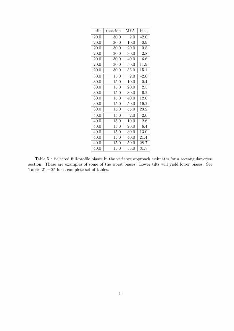
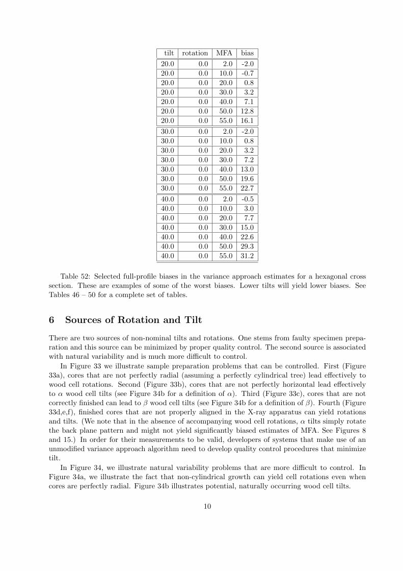
In the absence of publicly available algorithms for correcting the variance approach method fortilt, it is worthwhile to investigate the effect of tilt on the bias in the estimates. In Tables 21 – 25and 46 – 50, and Figures 2 – 8 and 16 – 22, we see that the bias in full-profile variance approachestimates increases as tilt increases and that it can be quite large. We present a subset of thesebiases in Tables 51 and 52. These biases are among the worst that appear in the full set of tables.
We note that other diffractometric methods of estimating MFA are also likely to perform poorlyin the presence of larger tilt if they are not corrected for tilt.
8
tilt rotation MFA bias
20.0 30.0 2.0 -2.0
20.0 30.0 10.0 -0.9
20.0 30.0 20.0 0.8
20.0 30.0 30.0 2.8
20.0 30.0 40.0 6.6
20.0 30.0 50.0 11.9
20.0 30.0 55.0 15.1
30.0 15.0 2.0 -2.0
30.0 15.0 10.0 0.4
30.0 15.0 20.0 2.5
30.0 15.0 30.0 6.2
30.0 15.0 40.0 12.0
30.0 15.0 50.0 19.2
30.0 15.0 55.0 23.2
40.0 15.0 2.0 -2.0
40.0 15.0 10.0 2.6
40.0 15.0 20.0 6.4
40.0 15.0 30.0 13.0
40.0 15.0 40.0 21.4
40.0 15.0 50.0 28.7
40.0 15.0 55.0 31.7
Table 51: Selected full-profile biases in the variance approach estimates for a rectangular crosssection. These are examples of some of the worst biases. Lower tilts will yield lower biases. SeeTables 21 – 25 for a complete set of tables.
9
tilt rotation MFA bias
20.0 0.0 2.0 -2.0
20.0 0.0 10.0 -0.7
20.0 0.0 20.0 0.8
20.0 0.0 30.0 3.2
20.0 0.0 40.0 7.1
20.0 0.0 50.0 12.8
20.0 0.0 55.0 16.1
30.0 0.0 2.0 -2.0
30.0 0.0 10.0 0.8
30.0 0.0 20.0 3.2
30.0 0.0 30.0 7.2
30.0 0.0 40.0 13.0
30.0 0.0 50.0 19.6
30.0 0.0 55.0 22.7
40.0 0.0 2.0 -0.5
40.0 0.0 10.0 3.0
40.0 0.0 20.0 7.7
40.0 0.0 30.0 15.0
40.0 0.0 40.0 22.6
40.0 0.0 50.0 29.3
40.0 0.0 55.0 31.2
Table 52: Selected full-profile biases in the variance approach estimates for a hexagonal crosssection. These are examples of some of the worst biases. Lower tilts will yield lower biases. SeeTables 46 – 50 for a complete set of tables.
6 Sources of Rotation and Tilt
There are two sources of non-nominal tilts and rotations. One stems from faulty specimen prepa-ration and this source can be minimized by proper quality control. The second source is associatedwith natural variability and is much more difficult to control.
In Figure 33 we illustrate sample preparation problems that can be controlled. First (Figure33a), cores that are not perfectly radial (assuming a perfectly cylindrical tree) lead effectively towood cell rotations. Second (Figure 33b), cores that are not perfectly horizontal lead effectivelyto α wood cell tilts (see Figure 34b for a definition of α). Third (Figure 33c), cores that are notcorrectly finished can lead to β wood cell tilts (see Figure 34b for a definition of β). Fourth (Figure33d,e,f), finished cores that are not properly aligned in the X-ray apparatus can yield rotationsand tilts. (We note that in the absence of accompanying wood cell rotations, α tilts simply rotatethe back plane pattern and might not yield significantly biased estimates of MFA. See Figures 8and 15.) In order for their measurements to be valid, developers of systems that make use of anunmodified variance approach algorithm need to develop quality control procedures that minimizetilt.
In Figure 34, we illustrate natural variability problems that are more difficult to control. InFigure 34a, we illustrate the fact that non-cylindrical growth can yield cell rotations even whencores are perfectly radial. Figure 34b illustrates potential, naturally occurring wood cell tilts.
10

Saren et al. (2006) found that in Norway spruce the α tilt in Figure 34b tended to graduallyincrease from small negative angles (−6 to 0 degrees) near the pith towards small positive angles(0 to 6 degrees) near the bark, and that the β tilt (spiral grain) can be cyclical with absolutevalues ranging from 0 to 30 degrees. Buksnowitz et al. (2008) have found that in Norway sprucethe β tilt can vary from −11 to +12 degrees. For Eucalyptus nitens (H. Deane & Maiden) Maidentrees, Evans et al. (2000) report a “standard deviation of fibre axial orientation” that ranges fromapproximately 13 to 16.5 degrees. Given that their fiber axial orientation included both “roll” (α)and “pitch” (β), it is unclear how “standard deviation of fibre axial orientation” was calculated.However, it appears that the β range could have been quite large. (They remark that “Fibre pitchvariation was consistently greater than roll variation.”) Gindl and Teischinger (2002) studied blocksfrom 12 larch trees and found spiral grain angles that ranged from 0 to 40 degrees. Angles between0 and 5 degrees were most common, but angles above 20 degrees were not uncommon. See theirFigure 2. (However, the authors note that the “material was selected specifically to represent anoptimum variability of grain angle.”) Northcott (1957) found spiral grain angles that varied from−16 to +19 degrees in Douglas-fir. Houkal (1982) found that the absolute value of spiral grainranged from 0 to 16 degrees in Pinus oocarpa Schiede ex Schltdl. Martley (1920) studied 19 Indianhardwoods and found spiral grain angles that varied from −33 to +35 degrees. Noskowiak (1963)observed spiral grain angles as high as 40 degrees in mature foxtail pine (Pinus balfouriana Grev.and Balf.).
We have performed exploratory studies (described in detail in Appendix H) that indicate thatin samples from Pinus lambertiana Dougl. and Pinus monticola Dougl. ex D. Don., the naturalvariability in cell rotation has mean roughly equal to 0 degrees and standard deviation roughlyequal to 5 degrees. In a sample of 220 cells from Pinus lambertiana, the range of rotations wasfrom −17 degrees to +15 degrees. In a sample of 243 cells from Pinus monticola, the range ofrotations was from −25 degrees to +14 degrees. We observed no trend in mean rotation as weprogressed from pith to bark.
In this study we also found that cells were primarily quadrilateral (40.2%), hexagonal (34.1%),elliptical (16.8%), and pentagonal (8.6%) in cross section. (Earlywood percentages differ fromlatewood percentages. See Appendix H.)
Also note that for hexagonal cells viewed from the tangential face, the default rotation is 0,while for hexagonal cells viewed from the radial face, the default rotation is 30 degrees.
7 Estimating σ2 as a function of MFA
As noted in Section 2, the variance approach is based on two approximations. First,
S2 ≈ µ2/2 + σ2 (11)
where µ denotes the MFA and σ2 denotes the natural variability of the MFA. Second,
σ2 ≈ f(µ) (12)
for some function f . Combining the two approximations, we obtain
S2 ≈ µ2/2 + f(µ)
and we can, at least in principle, solve for µ.In Sections 4 and 5, we established in our simulations that approximation (11) can lead to
significantly biased estimates of µ even if we know exactly the best f in approximation (12). (Inour simulations we knew that the generating variance of the MFAs was σ2 = (µ/3)2 + 62.)
11

In this section, we discuss possible choices for f(µ) and demonstrate that, as one would expect,additional biases can occur if the f that one chooses for a variance approach analysis does notmatch the generating f(µ).
As noted in Section 2, Evans (1999, 2008) suggested that σ2 could be replaced by
σ2 ≈ f(µ) = (µ/3)2 + 62 (13)
What is the source of approximation (13)?Cave (1966) found that he could obtain a good match between X-ray and iodine stain estimates
of microfibril angle if he tookσ2 = (µ/3)2
Evans (1999) noted that the MFA variance was non-zero even when the MFA was approximatelyequal to zero. This led him to propose the addition of a constant to (µ/3)2. He argued thatexperience suggests that 62 is a reasonable value for this constant. Thus, approximation (13) isempirical rather than theoretical in nature.
Is there evidence for other forms of f(µ)?In a personal communication, Evans (2009) wrote: “It should be noted that there are cases
in which residual variance decreases with increasing microfibril angle (when compression woodforms, the microfibril angle is high but its variability tends to be lower than in normal wood —unpublished.)”
Cave and Robinson (1998) report results for seven specimens in which their estimates of MFAranged from 1 degree to 29 degrees while their estimates of σ ranged from 10 to 14 degrees (11 de-grees for the 1 degree MFA, 12 degrees for the 29 degree MFA). This suggests that σ does notdepend upon µ.
Donaldson (1998) finds that ring number (1, 5, 10, 15) has no effect on microfibril angle rangein tracheid samples of size 25 in radiata pine. Because microfibril angle tends to decline as ringnumber increases, and population standard deviation is proportional to sample range (for samplesof constant size), this suggests that σ does not decrease as µ decreases.
Alden and Kretschmann (reported in Verrill et al. 2011) used iodine crystallization techniquesto obtain optical estimates of microfibril angle from 833 prepared slides. Each slide contained cellsobtained from the earlywood or the latewood of a single ring. The first eight rings from two boltsfrom each of two trees at each of 26 loblolly pine plantations were evaluated in the study. Aldenand Kretschmann measured 10 microfibril angles on each slide. In Figure 35 we plot the standarddeviations of the 10 replicates versus the means of the 10 replicates for all 833 slides. We also plotthe σ =
√(µ/3)2 + 62 line in the figure, and the regression line through Alden and Kretschmann’s
data. There is a clear discrepancy. Of course, the variability encountered by X-ray devices can beassociated with many hundreds of cells so it would be reasonable for it to be inflated above thatmeasured on the surface of a specimen. Note, however, the lack of a significant increase in σ as afunction of µ in Alden and Kretschmann’s data. The slope coefficient in the regression is only 0.04(with a standard error of 0.009).
Peura et al. (2008a) used synchrotron X-ray microdiffraction to investigate the distribution ofmicrofibril angle in single cells. In Figure 36 we plot the standard deviations (calculated as 0.425times their full width at half maximum (FWHM) values) versus the mode values for the 17 samplesin their table 3. We also plot the σ =
√(µ/3)2 + 62 line in the figure, and the regression line
through the Peura et al. data. In this case, it appears that approximation (13) underestimates σ,especially given that the standard deviations plotted in Figure 36 are from single cells. On the otherhand, there is some support for the idea that σ increases as MFA increases. The slope coefficientfor the regression line in the figure is 0.19 (with a standard error of 0.08).
12
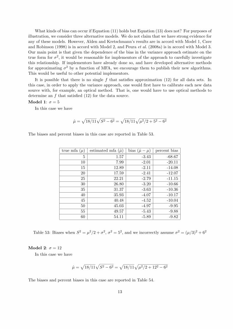
What kinds of bias can occur if Equation (11) holds but Equation (13) does not? For purposes ofillustration, we consider three alternative models. We do not claim that we have strong evidence forany of these models. However, Alden and Kretschmann’s results are in accord with Model 1, Caveand Robinson (1998) is in accord with Model 2, and Peura et al. (2008a) is in accord with Model 3.Our main point is that given the dependence of the bias in the variance approach estimate on thetrue form for σ2, it would be reasonable for implementors of the approach to carefully investigatethis relationship. If implementors have already done so, and have developed alternative methodsfor approximating σ2 by a function of MFA, we encourage them to publish their new algorithms.This would be useful to other potential implementors.
It is possible that there is no single f that satisfies approximation (12) for all data sets. Inthis case, in order to apply the variance approach, one would first have to calibrate each new datasource with, for example, an optical method. That is, one would have to use optical methods todetermine an f that satisfied (12) for the data source.
Model 1: σ = 5
In this case we have
µ =√
18/11√S2 − 62 =
√18/11
√µ2/2 + 52 − 62
The biases and percent biases in this case are reported in Table 53.
true mfa (µ) estimated mfa (µ) bias (µ− µ) percent bias
5 1.57 -3.43 -68.67
10 7.99 -2.01 -20.11
15 12.89 -2.11 -14.08
20 17.59 -2.41 -12.07
25 22.21 -2.79 -11.15
30 26.80 -3.20 -10.66
35 31.37 -3.63 -10.36
40 35.93 -4.07 -10.17
45 40.48 -4.52 -10.04
50 45.03 -4.97 -9.95
55 49.57 -5.43 -9.88
60 54.11 -5.89 -9.82
Table 53: Biases when S2 = µ2/2 + σ2, σ2 = 52, and we incorrectly assume σ2 = (µ/3)2 + 62
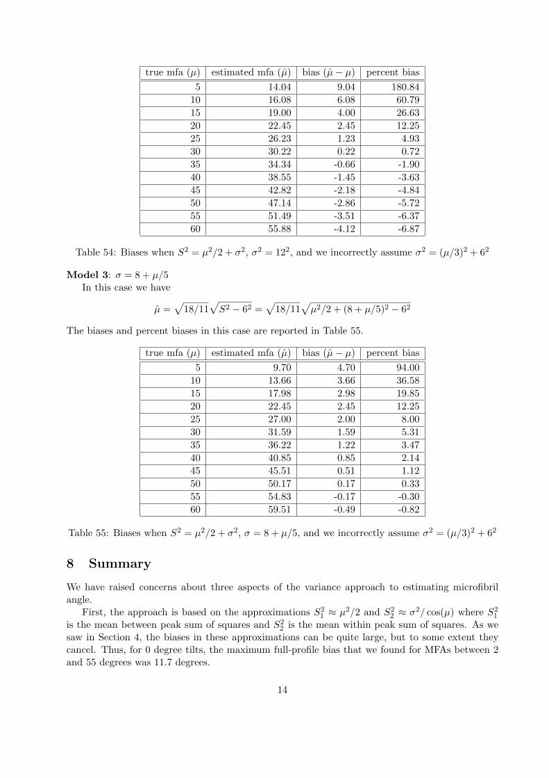
Model 2: σ = 12
In this case we have
µ =√
18/11√S2 − 62 =
√18/11
√µ2/2 + 122 − 62
The biases and percent biases in this case are reported in Table 54.
13
true mfa (µ) estimated mfa (µ) bias (µ− µ) percent bias
5 14.04 9.04 180.84
10 16.08 6.08 60.79
15 19.00 4.00 26.63
20 22.45 2.45 12.25
25 26.23 1.23 4.93
30 30.22 0.22 0.72
35 34.34 -0.66 -1.90
40 38.55 -1.45 -3.63
45 42.82 -2.18 -4.84
50 47.14 -2.86 -5.72
55 51.49 -3.51 -6.37
60 55.88 -4.12 -6.87
Table 54: Biases when S2 = µ2/2 + σ2, σ2 = 122, and we incorrectly assume σ2 = (µ/3)2 + 62
Model 3: σ = 8 + µ/5In this case we have
µ =√
18/11√S2 − 62 =
√18/11
√µ2/2 + (8 + µ/5)2 − 62
The biases and percent biases in this case are reported in Table 55.
true mfa (µ) estimated mfa (µ) bias (µ− µ) percent bias
5 9.70 4.70 94.00
10 13.66 3.66 36.58
15 17.98 2.98 19.85
20 22.45 2.45 12.25
25 27.00 2.00 8.00
30 31.59 1.59 5.31
35 36.22 1.22 3.47
40 40.85 0.85 2.14
45 45.51 0.51 1.12
50 50.17 0.17 0.33
55 54.83 -0.17 -0.30
60 59.51 -0.49 -0.82
Table 55: Biases when S2 = µ2/2 + σ2, σ = 8 + µ/5, and we incorrectly assume σ2 = (µ/3)2 + 62
8 Summary
We have raised concerns about three aspects of the variance approach to estimating microfibrilangle.
First, the approach is based on the approximations S21 ≈ µ2/2 and S2
2 ≈ σ2/ cos(µ) where S21
is the mean between peak sum of squares and S22 is the mean within peak sum of squares. As we
saw in Section 4, the biases in these approximations can be quite large, but to some extent theycancel. Thus, for 0 degree tilts, the maximum full-profile bias that we found for MFAs between 2and 55 degrees was 11.7 degrees.
14

Second, in Section 5 we noted that the variance approach was not designed to handle tilt, and,consequently, in the presence of tilt, the method can yield estimates that are highly biased. (Wealso noted that there may be algorithmic fixes for this, but that they have not yet appeared in theliterature.)
Third, as we saw in Section 7, there is some doubt about a proper model for σ2. One modelproposed by Evans in the 1999 paper was σ2 = (µ/3)2 + 62. In Section 7, we considered threeother models that have some data support and found that there can be large (percent) biases ifone of these models is true but σ2 = (µ/3)2 + 62 is assumed. This suggests that in order to applythe variance approach in a new situation, it might be necessary to use optical methods to firstdetermine an appropriate f in the approximation σ2 ≈ f(µ).
On the other hand, it is important to keep these concerns in perspective. In our simulations wefound that if approximation (4) holds and is used, and if tilts are restricted to 10 degrees or less,and MFAs are restricted to 40 degrees or less, the biases in MFA estimates increase with MFA anddo not exceed 4.6 degrees in absolute value.
We raise the three concerns so that other researchers interested in understanding, implementing,or extending the variance approach or in comparing the approach to other methods of estimatingMFA will be aware of them.
9 Acknowledgments
The authors gratefully acknowledge the very valuable comments and suggestions of the reviewers.
10 References
Buksnowitz, C., Muller, U., Evans, R., Teischinger, A., and Grabner, M. (2008). “The potential ofSilviScan’s X-ray diffractometry method for the rapid assessment of spiral grain in softwood,evaluated by goniometric measurements.” Wood Sci Technol. 42. Pages 95-102.
Cave, I.D. (1966). “X-ray measurement of microfibril angle.” Forest Products Journal. 16(10).Pages 37-42.
Cave, I.D., and Robinson, W. (1998). “Interpretation of (002) diffraction arcs by means of a mini-malist model.” Microfibril Angle in Wood. B.G. Butterfield editor. International Associationof Wood Anatomists. University of Canterbury. New Zealand. Pages 108-115.
Cave, I.D. and Walker, J.C.F. (1994). “Stiffness of wood in fast-grown plantation softwoods: theinfluence of microfibril angle.” Forest Products Journal. 44(5). Pages 43-48.
Donaldson, L.A. (1998). “Between-tracheid variability of microfibril angles in radiata pine.”Microfibril Angle in Wood. B.G. Butterfield editor. International Association of WoodAnatomists. University of Canterbury. New Zealand. Pages 206-224.
Evans, R.E. (1999). “A variance approach to the X-ray diffractometric estimation of microfibrilangle in wood.” Appita Journal. 52(4). Pages 283-289,294.
Evans, R.E. (2008). Personal communication.
Evans, R.E. (2009). Personal communication.
15
Evans, R.E. and Illic, J. (2001). “Rapid prediction of wood stiffness from microfibril angle anddensity.” Forest Products Journal. 51. Pages 53-57.
Evans, R., Stuart, S.A., and Van der Touw, J. (1996). “Microfibril angle scanning of incrementcores by X-ray diffractometry.” Appita Journal. 49(6). Pages 411-414.
Evans, R., Hughes, M., and Menz, D. (1999). “Microfibril angle variation by scanning X-raydiffractometry.” Appita Journal. 52(5). Pages 363-367.
Evans, R., Stringer, S., and Kibblewhite, R.P. (2000). “Variation of microfibril angle, densityand fibre orientation in twenty-nine Eucalyptus nitens trees.” Appita Journal. 53(5). Pages450-457.
Gindl, W. and Teischinger, A. (2002). “The potential of Vis- and NIR-spectroscopy for thenondestructive evaluation of grain-angle in wood.” Wood and Fiber Science 34(4). Pages651-656.
Harris, J.M. and Meylan, B.A. (1965). “The influence of microfibril angle on longitudinal andtangential shrinkage in Pinus radiata.” Holzforschung. 19(5). Pages 144-153.
Houkal, D. (1982). “Spiral grain in Pinus Oocarpa.” Wood and Fiber Science. 14(4). Pages320-330.
Martley, J.F. (1920). “Double cross grain.” Annals Appl. Biol. 7(2,3). Pages 224-268.
Megraw, R.A. (1986). “Wood quality factors in loblolly pine: the influence of tree age, position inthe tree, and cultural practice on wood specific gravity, fiber length and fibril angle.” TAPPIPress. Pages 1-88.
Northcott, P.L. (1957). “Is spiral grain the normal growth pattern?” For. Chron. 33(4). Pages335-352.
Noskowiak, A.F. (1963). “Spiral Grain in Trees . . . A Review.” Forest Products Journal. Pages266-275.
Peura, M., Muller, M., Serimaa, R., M., Vainio, U., Saren, M., Saranpaa, P., and Burghammer,M. (2005). “Structural studies of single wood cell walls by synchrotron X-ray microdiffractionand polarised light microscopy.” Nuclear Instruments and Methods in Physics Research B.238. Pages 16-20.
Peura, M., Muller, M., Vainio, U., Saren, M., Saranpaa, P., and Serimaa, R. (2008a). “X-ray microdiffraction reveals the orientation of cellulose microfibrils and the size of cellulosecrystallites in single Norway spruce tracheids.” Trees. 22. Pages 49-61.
Peura, M., Saren, M., Laukkanen, J., Nygard, K., Andersson, S., Saranpaa, P., Paakkari, T.,Hamalainen, K., and Serimaa, R. (2008b). “The elemental composition, the microfibril angledistribution and the shape of the cell cross-section in Norway spruce xylem.” Trees. 22.Pages 499-510.
Saren, M. and Serimaa, R. (2006). “Determination of microfibril angle distribution by X-raydiffraction,” Wood Sci Technol, 40. Pages 445-460.
16

Saren, M., Serimaa, R., Andersson, S., Paakkari, T., Saranpaa, P., and Pesonen, E. (2001).“Structural Variation of Tracheids in Norway Spruce (Picea abies [L.] Karst.),” Journal ofStructural Biology, 136. Pages 101-109.
Saren, M., Serimaa, R., and Tolonen, Y. (2006). “Determination of fiber orientation in Norwayspruce using X-ray diffraction and laser scattering,” Holz als Roh- und Werkstoff, 64. Pages183-188.
Verrill, S.P., Kretschmann, D.E., and Herian, V.L. (2001). JMFA — A graphically interactiveJava program that fits microfibril angle X-ray diffraction data. Res. Note FPL-RN-0283.Madison, WI: U.S. Department of Agriculture, Forest Service, Forest Products Laboratory.44 p.
Verrill, S.P., Kretschmann, D.E., and Herian, V.L. (2006). JMFA 2 — A graphically interactiveJava program that fits microfibril angle X-ray diffraction data. Res. Paper 635. Madison,WI: U.S. Department of Agriculture, Forest Service, Forest Products Laboratory. 70 p.
Verrill, S.P., Kretschmann, D.E., Herian, V.L., and Alden, H. (2011). JMFA 3 — A graphicallyinteractive Java program that fits microfibril angle X-ray diffraction data. Manuscript inpreparation.
11 Appendix A — An Extension to Cave’s Equation
Cave (1966) derived an equation for the locations of the spots of high X-ray intensity on the backplane of the X-ray apparatus. This equation applies to cells with rectangular cross sections. It doesnot account for cell tilt. See the appendix to Verrill et al. (2001) for a detailed derivation of Cave’sequation. In appendix A of Verrill et al. (2006) we extended Cave’s analysis to the case in whichthe cell can be tilted. Here we extend it to include a tilted, rotated cell of hexagonal cross section.
11.1 Microfibril Directions
To derive the six equations (one for each of the cell’s six sides) we first need the microfibril angledirections. Let θ denote the Bragg angle (11.35 degrees for light of wavelength 1.54 angstroms),µ denote the microfibril angle, η denote the tilt of the vertical axis in the wood cell down towardthe positive x axis, α equal 90 degrees plus the counterclockwise rotation of the cell around theoriginal z axis (after the tilt), and φ equal the angle (measured counterclockwise from the east) ofthe bright spot on the “2θ circle” on the back plane. See Figures 30, 37, and 38.
11.1.1 Front Face
See Figure 39 for our definition of the front, right 1, right 2, back, left 1, and left 2 faces of a cellwith a hexagonal cross section.
Before tilt and rotation, the direction of a microfibril on the front face is 0sin(µ)cos(µ)
17

After a tilt of the top of the cell down toward the positive x axis, the direction becomes cos(µ) sin(η)sin(µ)
cos(µ) cos(η)
Now, the mathematical tranformation that corresponds to a physical rotation through angle
rot of the cell about the original z axis is the matrix cos(−rot) sin(−rot) 0− sin(−rot) cos(−rot) 0
0 0 1
which equals sin(α) cos(α) 0
− cos(α) sin(α) 00 0 1
where α = π/2 + rot.
Thus the direction of the microfibril angle after tilt and rotation is
b =
sin(α) cos(α) 0− cos(α) sin(α) 0
0 0 1
cos(µ) sin(η)sin(µ)
cos(µ) cos(η)
=
sin(α) cos(µ) sin(η) + cos(α) sin(µ)− cos(α) cos(µ) sin(η) + sin(α) sin(µ)
cos(µ) cos(η)
(14)
11.1.2 Right 1 Face
Before tilt, the direction of a microfibril on the right 1 face is cos(−60) sin(−60) 0− sin(−60) cos(−60) 0
0 0 1
0sin(µ)cos(µ)
=
−√3
2 sin(µ)12 sin(µ)cos(µ)
After a tilt of the top of the cell down toward the positive x axis through an angle η, the directionbecomes cos(η) 0 sin(η)
0 1 0− sin(η) 0 cos(η)
−√3
2 sin(µ)12 sin(µ)cos(µ)
=
−√3
2 sin(µ) cos(η) + cos(µ) sin(η)12 sin(µ)√
32 sin(µ) sin(η) + cos(µ) cos(η)
The direction of the microfibril angle after tilt and rotation is thus
b =
sin(α) cos(α) 0− cos(α) sin(α) 0
0 0 1
−
√3
2 sin(µ) cos(η) + cos(µ) sin(η)12 sin(µ)√
32 sin(µ) sin(η) + cos(µ) cos(η)
(15)
=
−√3
2 sin(α) sin(µ) cos(η) + sin(α) cos(µ) sin(η) + 12 cos(α) sin(µ)√
32 cos(α) sin(µ) cos(η)− cos(α) cos(µ) sin(η) + 1
2 sin(α) sin(µ)√32 sin(µ) sin(η) + cos(µ) cos(η)
18

11.1.3 Right 2 Face
Before tilt, the direction of a microfibril on the right 2 face is cos(−120) sin(−120) 0− sin(−120) cos(−120) 0
0 0 1
0sin(µ)cos(µ)
=
−√3
2 sin(µ)−1
2 sin(µ)cos(µ)
After a tilt of the top of the cell down toward the positive x axis through an angle η, the directionbecomes cos(η) 0 sin(η)
0 1 0− sin(η) 0 cos(η)
−√3
2 sin(µ)−1
2 sin(µ)cos(µ)
=
−√3
2 sin(µ) cos(η) + cos(µ) sin(η)−1
2 sin(µ)√32 sin(µ) sin(η) + cos(µ) cos(η)
The direction of the microfibril angle after tilt and rotation is thus
b =
sin(α) cos(α) 0− cos(α) sin(α) 0
0 0 1
−
√3
2 sin(µ) cos(η) + cos(µ) sin(η)−1
2 sin(µ)√32 sin(µ) sin(η) + cos(µ) cos(η)
(16)
=
−√3
2 sin(α) sin(µ) cos(η) + sin(α) cos(µ) sin(η)− 12 cos(α) sin(µ)√
32 cos(α) sin(µ) cos(η)− cos(α) cos(µ) sin(η)− 1
2 sin(α) sin(µ)√32 sin(µ) sin(η) + cos(µ) cos(η)
11.1.4 Back Face
Before tilt and rotation, the direction of a microfibril on the back face is 0− sin(µ)cos(µ)
After a tilt of the top of the cell down toward the positive x axis, the direction becomes cos(µ) sin(η)
− sin(µ)cos(µ) cos(η)
The direction of the microfibril angle after tilt and rotation is thus
b =
sin(α) cos(µ) sin(η)− cos(α) sin(µ)− cos(α) cos(µ) sin(η)− sin(α) sin(µ)
cos(µ) cos(η)
(17)
11.1.5 Left 1 Face
Before tilt, the direction of a microfibril on the left 1 face is cos(−240) sin(−240) 0− sin(−240) cos(−240) 0
0 0 1
0sin(µ)cos(µ)
=
√32 sin(µ)−1
2 sin(µ)cos(µ)
19

After a tilt of the top of the cell down toward the positive x axis through an angle η, the directionbecomes cos(η) 0 sin(η)
0 1 0− sin(η) 0 cos(η)
√32 sin(µ)−1
2 sin(µ)cos(µ)
=
√32 sin(µ) cos(η) + cos(µ) sin(η)
−12 sin(µ)
−√32 sin(µ) sin(η) + cos(µ) cos(η)
The direction of the microfibril angle after tilt and rotation is thus
b =
sin(α) cos(α) 0− cos(α) sin(α) 0
0 0 1
√32 sin(µ) cos(η) + cos(µ) sin(η)
−12 sin(µ)
−√32 sin(µ) sin(η) + cos(µ) cos(η)
(18)
=
√32 sin(α) sin(µ) cos(η) + sin(α) cos(µ) sin(η)− 1
2 cos(α) sin(µ)
−√32 cos(α) sin(µ) cos(η)− cos(α) cos(µ) sin(η)− 1
2 sin(α) sin(µ)
−√32 sin(µ) sin(η) + cos(µ) cos(η)
11.1.6 Left 2 Face
Before tilt, the direction of a microfibril on the left 2 face is cos(−300) sin(−300) 0− sin(−300) cos(−300) 0
0 0 1
0sin(µ)cos(µ)
=
√32 sin(µ)12 sin(µ)cos(µ)
After a tilt of the top of the cell down toward the positive x axis through an angle η, the directionbecomes cos(η) 0 sin(η)
0 1 0− sin(η) 0 cos(η)
√32 sin(µ)12 sin(µ)cos(µ)
=
√32 sin(µ) cos(η) + cos(µ) sin(η)
12 sin(µ)
−√32 sin(µ) sin(η) + cos(µ) cos(η)
The direction of the microfibril angle after tilt and rotation is thus
b =
sin(α) cos(α) 0− cos(α) sin(α) 0
0 0 1
√32 sin(µ) cos(η) + cos(µ) sin(η)
12 sin(µ)
−√32 sin(µ) sin(η) + cos(µ) cos(η)
(19)
=
√32 sin(α) sin(µ) cos(η) + sin(α) cos(µ) sin(η) + 1
2 cos(α) sin(µ)
−√32 cos(α) sin(µ) cos(η)− cos(α) cos(µ) sin(η) + 1
2 sin(α) sin(µ)
−√32 sin(µ) sin(η) + cos(µ) cos(η)
11.2 The Six Equations
There are two conditions that a 002 reflecting plane must meet to reflect a beam coming in alongthe x axis. First, b is in the 002 crystallographic planes of the cellulose crystals associated withthe microfibrils so the normal, p, to the 002 plane that succeeds in reflecting the beam must beperpendicular to b. Second (the Bragg condition), the normal to the 002 reflecting plane mustmake a 90− θ angle to the x axis, where θ is the Bragg angle for the X-ray wavelength being used.Given these two conditions, we want to be able to determine the location at which the reflectedbeam intersects the back plane of the X-ray apparatus.
20

The second condition gives us
p1 =
100
· p = cos(90− θ) = sin(θ) (20)
We also havep21 + p22 + p23 = 1 (21)
Making use of Equations (20) and (21), we obtain
p22 + p23 = cos2(θ) (22)
The first condition and Equation (20) give us sin(θ)p2p3
· b = 0 (23)
Thus the solutions for (p2, p3) will be the 0, 1, or 2 points represented by the intersectionof line (23) with circle (22). Circle (22) has radius cos(θ) and a point on circle (22) has form(cos(φ) cos(θ), sin(φ) cos(θ)) for some angle φ. That is,
p2 = cos(φ) cos(θ) (24)
p3 = sin(φ) cos(θ)
From Equations (23) and (24) and Equations (14) – (19), after dividing by cos(θ), we obtainsix versions of the equation
d1 + d2 × cos(φ) + d3 × sin(φ) = 0 (25)
(In the next section we relate the φ in Equations (24) and (25) to the angle (counterclockwise fromthe east) of the bright spot on the back plane.)
For the front face, we have
d1 = (sin(α) cos(µ) sin(η) + cos(α) sin(µ)) tan(θ)
d2 = − cos(α) cos(µ) sin(η) + sin(α) sin(µ) (26)
d3 = cos(µ) cos(η)
For the right 1 face, we have
d1 =
(−√
3
2sin(α) sin(µ) cos(η) + sin(α) cos(µ) sin(η) +
1
2cos(α) sin(µ)
)tan(θ)
d2 =
√3
2cos(α) sin(µ) cos(η)− cos(α) cos(µ) sin(η) +
1
2sin(α) sin(µ) (27)
d3 =
√3
2sin(µ) sin(η) + cos(µ) cos(η)
For the right 2 face, we have
d1 =
(−√
3
2sin(α) sin(µ) cos(η) + sin(α) cos(µ) sin(η)− 1
2cos(α) sin(µ)
)tan(θ)
d2 =
√3
2cos(α) sin(µ) cos(η)− cos(α) cos(µ) sin(η)− 1
2sin(α) sin(µ) (28)
d3 =
√3
2sin(µ) sin(η) + cos(µ) cos(η)
21
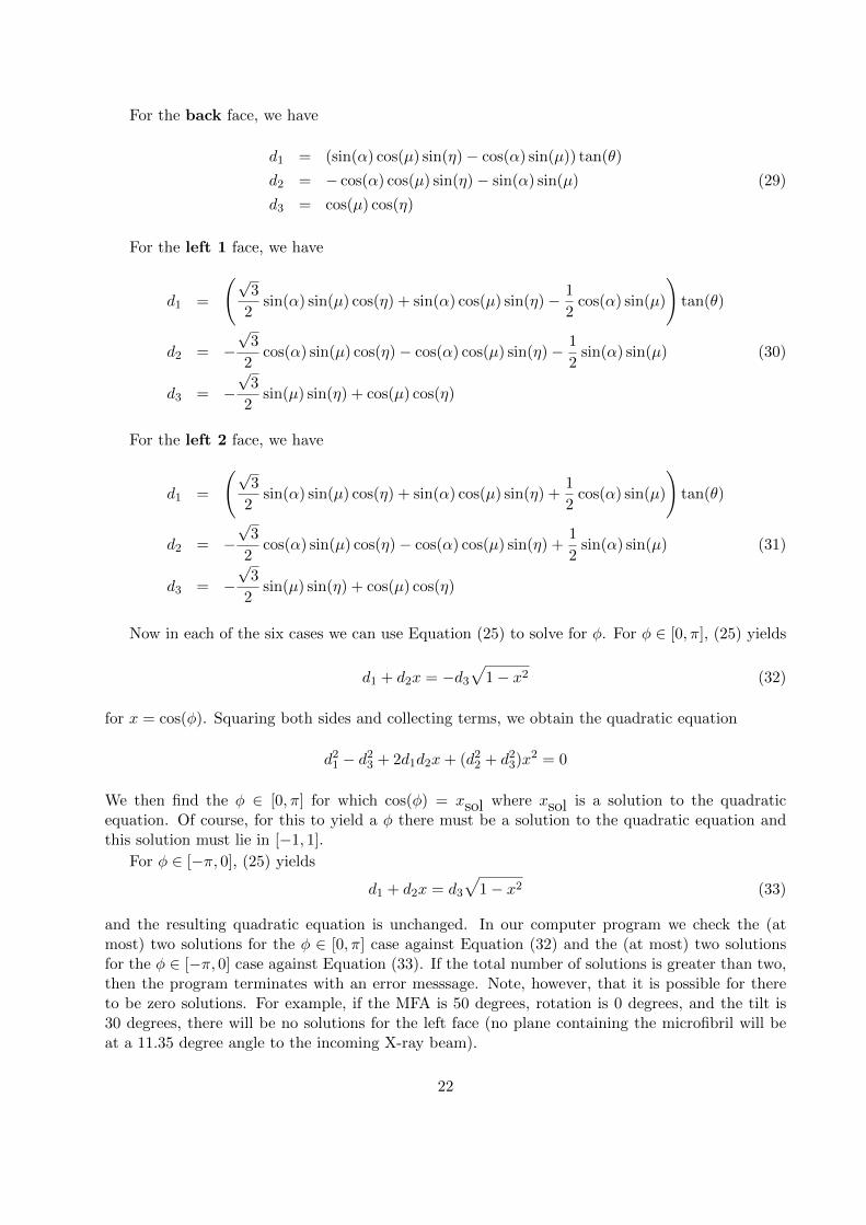
For the back face, we have
d1 = (sin(α) cos(µ) sin(η)− cos(α) sin(µ)) tan(θ)
d2 = − cos(α) cos(µ) sin(η)− sin(α) sin(µ) (29)
d3 = cos(µ) cos(η)
For the left 1 face, we have
d1 =
(√3
2sin(α) sin(µ) cos(η) + sin(α) cos(µ) sin(η)− 1
2cos(α) sin(µ)
)tan(θ)
d2 = −√
3
2cos(α) sin(µ) cos(η)− cos(α) cos(µ) sin(η)− 1
2sin(α) sin(µ) (30)
d3 = −√
3
2sin(µ) sin(η) + cos(µ) cos(η)
For the left 2 face, we have
d1 =
(√3
2sin(α) sin(µ) cos(η) + sin(α) cos(µ) sin(η) +
1
2cos(α) sin(µ)
)tan(θ)
d2 = −√
3
2cos(α) sin(µ) cos(η)− cos(α) cos(µ) sin(η) +
1
2sin(α) sin(µ) (31)
d3 = −√
3
2sin(µ) sin(η) + cos(µ) cos(η)
Now in each of the six cases we can use Equation (25) to solve for φ. For φ ∈ [0, π], (25) yields
d1 + d2x = −d3√
1− x2 (32)
for x = cos(φ). Squaring both sides and collecting terms, we obtain the quadratic equation
d21 − d23 + 2d1d2x+ (d22 + d23)x2 = 0
We then find the φ ∈ [0, π] for which cos(φ) = xsol where xsol is a solution to the quadraticequation. Of course, for this to yield a φ there must be a solution to the quadratic equation andthis solution must lie in [−1, 1].
For φ ∈ [−π, 0], (25) yields
d1 + d2x = d3√
1− x2 (33)
and the resulting quadratic equation is unchanged. In our computer program we check the (atmost) two solutions for the φ ∈ [0, π] case against Equation (32) and the (at most) two solutionsfor the φ ∈ [−π, 0] case against Equation (33). If the total number of solutions is greater than two,then the program terminates with an error messsage. Note, however, that it is possible for thereto be zero solutions. For example, if the MFA is 50 degrees, rotation is 0 degrees, and the tilt is30 degrees, there will be no solutions for the left face (no plane containing the microfibril will beat a 11.35 degree angle to the incoming X-ray beam).
22

11.3 Relation between φ and the Angle (Counterclockwise from the East) ofthe Bright Spot on the Back Plane
Let us now consider the issue of where the reflected beam intersects the back plane. We know thatthe beam comes in along the x axis and reflects off a plane whose normal is given by Equations(20) and (24). Consider now a canonical situation in which a beam reflects off a plane with normal(0,0,1) (the z axis). In this case the direction vector of the reflected beam is the same as thedirection vector of the incident beam except that the sign of the z coordinate is reversed.
To make use of this result, we first find the transform that takes the p vector to the z vector.This requires a rotation of 90 − φ degrees of the z axis towards the y axis (to bring the z axis inline with the projection of p onto the y, z plane), followed by a rotation of θ degrees of the z axistowards the x axis (to bring the z axis into line with p). These two rotations can be representedby the transform
T ≡
cos(θ) 0 − sin(θ)0 1 0
sin(θ) 0 cos(θ)
1 0 00 sin(φ) − cos(φ)0 cos(φ) sin(φ)
One can check that
T (p) = T ·
sin(θ)cos(φ) cos(θ)sin(φ) cos(θ)
=
001
Now in the original coordinate system, the X-ray incident direction is −1
00
In the coordinate system in which the p vector has been transformed to the z vector, this incidentdirection becomes
T ·
−100
=
− cos(θ)0
− sin(θ)
so the beam reflects off in the − cos(θ)
0sin(θ)
direction. Transformed back into the original coordinate system, this direction vector is 1 0 0
0 sin(φ) − cos(φ)0 cos(φ) sin(φ)
−1 cos(θ) 0 − sin(θ)0 1 0
sin(θ) 0 cos(θ)
−1 − cos(θ)0
sin(θ)
=
− cos(2θ)cos(φ) sin(2θ)sin(φ) sin(2θ)
We extend a beam in this direction to its intersection with a back plane that is perpendicular
to the x axis and x0 units behind the specimen by multiplying by a factor of x0/ cos(2θ). Thus the
23

beam intersects the back plane at the point −x0cos(φ) sin(2θ)x0/(cos(2θ))sin(φ) sin(2θ)x0/(cos(2θ))
=
−x0cos(φ) tan(2θ)x0sin(φ) tan(2θ)x0
Looking face on at the back plane, this is the point that is on the circle of radius tan(2θ)x0 (the“2θ circle”) and φ degrees in a counterclockwise direction from the y axis. So a φ that is a solutionto Equation (25) is also the angle (counterclockwise from the east) of a point of maximum X-rayintensity.
12 Appendix B — The Simulation Tables
We describe Tables 1 through 50 in this appendix. The tables can be viewed and/or downloadedat http://www1.fpl.fs.fed.us/varapp tables.html.
Tables 1 – 25 are associated with cells of rectangular cross section. Tables 26 – 50 are thecorresponding tables for cells of hexagonal cross section.
For cells of rectangular cross section, Tables 1 through 5 list the 8 bright spot locations fortilts of 0, 10, 20, 30, and 40 degrees, rotations of 0, 15, 30, 45, 60, 75, and 90 degrees, and MFAsof 2, 10, 20, 30, 40, 50, and 55 degrees. Tables 26 through 30 list the corresponding informationfor the 12 bright spot locations generated by a hexagonal cross section. (In Appendices D – G weestablish symmetries that permit us reasonably to restrict our simulation to the tilts and rotationsconsidered.) These tables also list the corresponding mean bright spot locations, φ, for each of thetwo half-profiles. (If there is no tilt, these means are 0 degrees and 180 degrees.)
In the rectangular case, plots of bright spot locations for 0 and 15 degree tilts, 0, 10, 20, 22.5,30, 40, 45, 50, 60, 67.5, 70, 80, and 90 degree rotations, and 10, 20, 30, 40, 50, and 60 degree MFAsare displayed in Figures 6 through 18 and 20 through 32 of Verrill et al. (2006).
In the hexagonal case, plots of bright spots for 0 and 20 degree tilts, 0, 15, 30, 45, 60, 75, and90 degree rotations, and 10, 20, 30, 40, 50, and 55 degree MFAs appear as Figures 40 through 53of the current paper.
Tables 6 – 25 and 31 – 50 are associated with the relation
S2 =J∑j=1
(nj − 1)s2j/ntot +J∑j=1
nj (y·j − y··)2 /ntot (34)
that we developed in Section 5. Here
s2j ≡nj∑i=1
(yij − y·j)2 /(nj − 1)
is the standard deviation of the jth peak.Recall that in our simulation we draw MFAs from a Gaussian distribution centered at µ with
standard deviation given by σ =√
(µ/3)2 + 62. The ith draw leads to bright spot locationsyij , j = 1, . . . , J corresponding to φj , j = 1, . . . , J .
Tables 6 – 10 and 31 – 35 provide three estimates of the δj ’s — our simulation estimates(the s2j ’s), our “analytic” estimates (see Appendix C), and the estimates based on Evans’s (1999)equation [14]. The tables provide these estimates for both the left and the right half-profiles. Inboth the rectangular and hexagonal cases, the tables demonstrate that Evans’s equation [14] yieldspoor estimates of the δj ’s (even in the no-tilt, no-rotation case).
24

Tables 11 – 15 and 36 – 40 compare our∑J
j=1(nj − 1)s2j/ntot value with Evans’s σ2/ cos(µ),
which is his approximation to his∑J
j=1 δ2j /J . Given the differences between our s2j ’s and the δ2j ’s
from Evans’s equation [14], we would expect significant differences between the∑J
j=1(nj−1)s2j/ntotand σ2/ cos(µ) values. A glance at the tables makes clear that the differences are indeed significant.It should also be noted that the Evans value,
∑Jj=1 δ
2j /J , does not depend on the half-profile, while,
in fact, as can be seen from the tables, for non-zero rotations the mean within peak variability candiffer significantly between the left and right half-profiles.
Tables 16 – 20 and 41 – 45 compare our∑J
j=1 nj (y·j − y··)2 /ntot (the SS1 column in the table)
with Evans’s µ2/2. We also compare∑J
j=1(φj− φ)2/J (the SS2 column),∑J
j=1(φj−0)2/J (the SS3
column, left half-profile rows), and∑J
j=1(φj −π)2/J (the SS3 column, right half-profile rows) with
µ2/2. The Evans result consistently underestimates the other measures of between peak variability.Again, the Evans value does not depend on the half-profile, while, in fact, for non-zero rotations,the between peak variability can differ significantly between the left and right half-profiles.
Tables 21 – 25 and 46 – 50 list the biases in the variance approach estimate of MFA as a functionof tilt, rotation, MFA, half-profile, and cell cross section. Plots of a subset of these results appearas Figures 2 through 29. It is important to note that the figures plot the biases in the case in whichboth half-profiles are used to estimate the MFA. If only a single half-profile is used, the biasescan be significantly inflated (or deflated) depending upon the tilt, rotation, MFA, cross section,and half-profile. For example, from Table 21 we can see that for 0 tilt, 15 degree rotation, and arectangular cross section, when the variabilities of the two half-profiles are averaged, the theoreticalbiases for MFAs 40, 50, and 55 are 1.2, 4.9, and 8.1. However, when only the variance of the lefthalf-profile is used in the estimate, the corresponding biases are 3.2, 9.9, and 15.2.
One feature of these tables needs to be explained. The tables contain two super-columnslabeled “theoretical” and “practical”. The “practical” columns were calculated by assuming thatthe intensity between −90 degrees and 90 degrees on the back plane corresponds to the left half-profile and the intensity between 90 degrees and 270 degrees on the back plane corresponds to theright half-profile. (Here the 0 degree direction on the back plane is East and the positive azimuthaldirection is counterclockwise.) The “theoretical” columns were obtained by determining the four(or six) φj ’s that corresponded to each of the two half-profiles, and then allocating the two brightpoints from a face in a draw to the appropriate peaks and thus the appropriate half-profiles. Forsmall tilts and MFAs, the two approaches will yield the same results. However, for larger tilts andMFAs, broadened bright spots from an MFA draw can appear in the “wrong” half of the back plane.See, for example, Figure 53. For a tilt of 20 degrees and an MFA of 50, it is clear that the broadenedpeak of the bright spot that is at an angle of −70.7 degrees would be expected to be broadened insuch a manner that part of its peak would lie below −90 degrees. For the “practical” estimate of S2
the half-profile is truncated at −90 degrees (and at +90 degrees). For the “theoretical” estimate,the half-profile is not truncated.
We note a problem with the current implementation of our simulation. For very large MFAs(50 or 55 degrees in our simulation), it is possible for misallocations to be made. Our algorithmcompares
ss1 = (y1 − φL)2 + (y2 − φR)2
and
ss2 = (y1 − φR)2 + (y2 − φL)2
where φL and φR are the unbroadened left and right half-profile bright spots for a particular face,and y1, y2 are the bright spots associated with that face for a particular draw of a broadened MFA.
25
If ss1 < ss2, our algorithm allocates y1 to the φL peak and y2 to the φR peak. If ss1 > ss2, itallocates y1 to the φR peak and y2 to the φL peak. This algorithm yields simulation s2j ’s that matchanalytic estimates of peak variabilities for smaller (and many larger) MFAs. It yields theoreticalbias estimates that match practical bias estimates for smaller MFAs. However, for the highest MFAvalues, it yields larger bias estimates than does the practical approach. We expect that the practicalapproach will underestimate the true S2 for larger MFAs as it truncates at −90 and 90 degrees (or,for the right half-profile, 90 and 270 degrees). Thus it is reasonable that the theoretical estimatesof MFA will be larger than the practical for larger MFAs. However, it is also possible that, forlarger MFAs, some of the positive bias of the theoretical MFA estimates is due to misallocations.
13 Appendix C — The Partial Derivative Approach to Estimatingthe Bright Spot Broadening Standard Deviations
As established in Appendix A, the defining equation for azimuthal angles is
d1 + d2 cos(φ) + d3 sin(φ) = 0 (35)
where φ is the azimuthal angle of a bright spot on the back plane (read counterclockwise from theeast), and d1, d2, d3 are known values that depend on the Bragg angle, MFA, cell face, rotation,and tilt.
Taking partial derivatives of both sides of this equation with respect to MFA we obtain
∂d1∂µ
+∂d2∂µ
cos(φ) + d2(− sin(φ))∂φ
∂µ+∂d3∂µ
sin(φ) + d3 cos(φ)∂φ
∂µ= 0
or, solving for ∂φ∂µ ,
∂φ
∂µ=
(∂d1∂µ
+∂d2∂µ
cos(φ) +∂d3∂µ
sin(φ)
)/ (d2 sin(φ)− d3 cos(φ)) (36)
Next, we have the Taylor series approximation
φ(µ) ≈ φ(µ0) +∂φ(µ0)
∂µ× (µ− µ0)
Assuming that µ is a random variable with mean µ0 and standard deviation σ, this implies that
Var(φ(µ)) ≈(∂φ(µ0)
∂µ
)2
× σ2 (37)
Results (36) and (37) permit us to obtain an analytic estimate of the standard deviation asso-ciated with a bright spot.
To complete this approach, we need expressions for the partial derivatives of the four or sixfaces of the wood cell:
13.1 Rectangular Cross Section
13.1.1 Front Face
From result (26) we have
∂d1∂µ
= (− sin(α) sin(µ) sin(η) + cos(α) cos(µ)) tan(θ)
26

∂d2∂µ
= cos(α) sin(µ) sin(η) + sin(α) cos(µ) (38)
∂d3∂µ
= − sin(µ) cos(η)
13.1.2 Right Face
In Verrill et al. (2006) we established that for the right face,
d1 = − sin(α) sin(µ− η) tan(θ)
d2 = cos(α) sin(µ− η) (39)
d3 = cos(µ− η)
Thus,
∂d1∂µ
= − sin(α) cos(µ− η) tan(θ)
∂d2∂µ
= cos(α) cos(µ− η) (40)
∂d3∂µ
= − sin(µ− η)
13.1.3 Back Face
From result (29) we have
∂d1∂µ
= (− sin(α) sin(µ) sin(η)− cos(α) cos(µ)) tan(θ)
∂d2∂µ
= cos(α) sin(µ) sin(η)− sin(α) cos(µ) (41)
∂d3∂µ
= − sin(µ) cos(η)
13.1.4 Left Face
In Verrill et al. (2006) we established that for the left face,
d1 = sin(α) sin(µ+ η) tan(θ)
d2 = − cos(α) sin(µ+ η) (42)
d3 = cos(µ+ η)
Thus,
∂d1∂µ
= sin(α) cos(µ+ η) tan(θ)
∂d2∂µ
= − cos(α) cos(µ+ η) (43)
∂d3∂µ
= − sin(µ+ η)
27

13.2 Hexagonal Cross Section
13.2.1 Front Face
See result (38) above.
13.2.2 Right 1 Face
From result (27) we have
∂d1∂µ
=
(−√
3
2sin(α) cos(µ) cos(η)− sin(α) sin(µ) sin(η) +
1
2cos(α) cos(µ)
)tan(θ)
∂d2∂µ
=
√3
2cos(α) cos(µ) cos(η) + cos(α) sin(µ) sin(η) +
1
2sin(α) cos(µ) (44)
∂d3∂µ
=
√3
2cos(µ) sin(η)− sin(µ) cos(η)
13.2.3 Right 2 Face
From result (28) we have
∂d1∂µ
=
(−√
3
2sin(α) cos(µ) cos(η)− sin(α) sin(µ) sin(η)− 1
2cos(α) cos(µ)
)tan(θ)
∂d2∂µ
=
√3
2cos(α) cos(µ) cos(η) + cos(α) sin(µ) sin(η)− 1
2sin(α) cos(µ) (45)
∂d3∂µ
=
√3
2cos(µ) sin(η)− sin(µ) cos(η)
13.2.4 Back Face
See result (41) above.
13.2.5 Left 1 Face
From result (30) we have
∂d1∂µ
=
(√3
2sin(α) cos(µ) cos(η)− sin(α) sin(µ) sin(η)− 1
2cos(α) cos(µ)
)tan(θ)
∂d2∂µ
= −√
3
2cos(α) cos(µ) cos(η) + cos(α) sin(µ) sin(η)− 1
2sin(α) cos(µ) (46)
∂d3∂µ
= −√
3
2cos(µ) sin(η)− sin(µ) cos(η)
13.2.6 Left 2 Face
From result (31) we have
∂d1∂µ
=
(√3
2sin(α) cos(µ) cos(η)− sin(α) sin(µ) sin(η) +
1
2cos(α) cos(µ)
)tan(θ)
28
∂d2∂µ
= −√
3
2cos(α) cos(µ) cos(η) + cos(α) sin(µ) sin(η) +
1
2sin(α) cos(µ) (47)
∂d3∂µ
= −√
3
2cos(µ) sin(η)− sin(µ) cos(η)
14 Appendix D — The Effects of a Change in Tilt Sign or inRotation Sign on the Pattern of Eight Bright Spots Associatedwith a Rectangular Cross Section
In appendix B of Verrill et al. (2006), we established the following eight claims.
14.1 A Change in Tilt Sign
Given a change in tilt sign, bright spot locations are reflected across the horizontal west to eastline (see Figure 38). Also front, back IDs are exchanged, and right, left IDs are exchanged.
This effect is embodied in the following four claims.
Claim 1
If φ is a solution for a front bright spot under tilt η, then −φ is a solution for a back brightspot under tilt −η.
Claim 2
If φ is a solution for a back bright spot under tilt η, then −φ is a solution for a front brightspot under tilt −η.
Claim 3
If φ is a solution for a right bright spot under tilt η, then −φ is a solution for a left bright spotunder tilt −η.
Claim 4
If φ is a solution for a left bright spot under tilt η, then −φ is a solution for a right bright spotunder tilt −η.
14.2 A Change in Rotation Sign
Given a change in rotation sign, bright spot locations are reflected across the vertical south to northline (see Figure 38). Also front, back IDs are exchanged. Right, left IDs remain unchanged.
This effect is embodied in the following four claims.
Claim 5
If π/2− β is a solution for a front bright spot under rotation rot, then π/2 + β is a solution fora back bright spot under rotation −rot.
Claim 6
If π/2− β is a solution for a back bright spot under rotation rot, then π/2 + β is a solution fora front bright spot under rotation −rot.
Claim 7
If π/2− β is a solution for a right bright spot under rotation rot, then π/2 + β is a solution fora right bright spot under rotation −rot.
Claim 8
If π/2− β is a solution for a left bright spot under rotation rot, then π/2 + β is a solution fora left bright spot under rotation −rot.
29

15 Appendix E — The Effects of a Change in Tilt Sign or inRotation Sign on the Pattern of 12 Bright Spots Associatedwith a Hexagonal Cross Section
15.1 A Change in Tilt Sign
Given a change in tilt sign, bright spot locations are reflected across the horizontal west to eastline (see Figure 38). Also front and back IDs are exchanged, right 1 and left 1 IDs are exchanged,and right 2 and left 2 IDs are exchanged.
This effect is embodied in the following six claims.
Claim 9
If φ is a solution for a front bright spot under tilt η, then −φ is a solution for a back brightspot under tilt −η.
Claim 10
If φ is a solution for a back bright spot under tilt η, then −φ is a solution for a front brightspot under tilt −η.
Claim 11
If φ is a solution for a right 1 bright spot under tilt η, then −φ is a solution for a left 1 brightspot under tilt −η.
Claim 12
If φ is a solution for a left 1 bright spot under tilt η, then −φ is a solution for a right 1 brightspot under tilt −η.
Claim 13
If φ is a solution for a right 2 bright spot under tilt η, then −φ is a solution for a left 2 brightspot under tilt −η.
Claim 14
If φ is a solution for a left 2 bright spot under tilt η, then −φ is a solution for a right 2 brightspot under tilt −η.
Equations (26) – (31) can be used in a straightforward manner to establish these claims. Here,for the purposes of illustration, we establish Claim 11.
From Equations (25) and (27) we have(−√
3
2sin(α) sin(µ) cos(η) + sin(α) cos(µ) sin(η) +
1
2cos(α) sin(µ)
)tan(θ) +(√
3
2cos(α) sin(µ) cos(η)− cos(α) cos(µ) sin(η) +
1
2sin(α) sin(µ)
)cos(φ) +(√
3
2sin(µ) sin(η) + cos(µ) cos(η)
)sin(φ) = 0
Multiplying this equation by −1 we obtain(√3
2sin(α) sin(µ) cos(η)− sin(α) cos(µ) sin(η)− 1
2cos(α) sin(µ)
)tan(θ) +(
−√
3
2cos(α) sin(µ) cos(η) + cos(α) cos(µ) sin(η)− 1
2sin(α) sin(µ)
)cos(φ) +
30
(−√
3
2sin(µ) sin(η)− cos(µ) cos(η)
)sin(φ) = 0
or
(√3
2sin(α) sin(µ) cos(−η) + sin(α) cos(µ) sin(−η)− 1
2cos(α) sin(µ)
)tan(θ) +(
−√
3
2cos(α) sin(µ) cos(−η)− cos(α) cos(µ) sin(−η)− 1
2sin(α) sin(µ)
)cos(−φ) +(
−√
3
2sin(µ) sin(−η) + cos(µ) cos(−η)
)sin(−φ) = 0
which is what we needed to establish (see Equations (25) and (30)).
15.2 A Change in Rotation Sign
Given a change in rotation sign, bright spot locations are reflected across the vertical south to northline (see Figure 38). Also front back IDs are exchanged, right 1 and right 2 IDs are exchanged, andleft 1 and left 2 IDs are exchanged.
This effect is embodied in the following six claims.
Claim 15
If π/2− β is a solution for a front bright spot under rotation rot, then π/2 + β is a solution fora back bright spot under rotation −rot.
Claim 16
If π/2− β is a solution for a back bright spot under rotation rot, then π/2 + β is a solution fora front bright spot under rotation −rot.
Claim 17
If π/2− β is a solution for a right 1 bright spot under rotation rot, then π/2 + β is a solutionfor a right 2 bright spot under rotation −rot.
Claim 18
If π/2− β is a solution for a right 2 bright spot under rotation rot, then π/2 + β is a solutionfor a right 1 bright spot under rotation −rot.
Claim 19
If π/2− β is a solution for a left 1 bright spot under rotation rot, then π/2 + β is a solution fora left 2 bright spot under rotation −rot.
Claim 20
If π/2− β is a solution for a left 2 bright spot under rotation rot, then π/2 + β is a solution fora left 1 bright spot under rotation −rot.
Equations (26) – (31) can be used in a straightforward manner to establish these claims. Here,for the purposes of illustration, we establish Claim 17.
From Equations (25) and (27) we have (recall that α = π/2 + rot so cos(α) = − sin(rot) andsin(α) = cos(rot))(
−√
3
2cos(rot) sin(µ) cos(η) + cos(rot) cos(µ) sin(η)− 1
2sin(rot) sin(µ)
)tan(θ) +
31

(−√
3
2sin(rot) sin(µ) cos(η) + sin(rot) cos(µ) sin(η) +
1
2cos(rot) sin(µ)
)sin(β) + (48)(√
3
2sin(µ) sin(η) + cos(µ) cos(η)
)cos(β) = 0
or
(−√
3
2cos(−rot) sin(µ) cos(η) + cos(−rot) cos(µ) sin(η) +
1
2sin(−rot) sin(µ)
)tan(θ) +(
−√
3
2sin(−rot) sin(µ) cos(η) + sin(−rot) cos(µ) sin(η)− 1
2cos(−rot) sin(µ)
)sin(−β) +(√
3
2sin(µ) sin(η) + cos(µ) cos(η)
)cos(β) = 0
which is what we needed to establish (see Equations (25) and (28)).
16 Appendix F — The Effect of a Rotation Greater Than π/2 onthe Pattern of Eight Bright Spots Associated with a Rectan-gular Cross Section
We note that we use some potentially confusing notation here. In Appendix E, π/2−β and π/2+βwere examples of φ (azimuthal) values. In this appendix, we use them to reference rotation values.
The bright spot locations for an η tilt and a π/2 + β rotation are the same as the bright spotlocations for a −η tilt and a −(π/2 − β) rotation. Labels, however, do change — front and backbright spots exchange labels, and right and left bright spots exchange labels.
This effect is embodied in the following four claims.
Claim 21
If φ is a solution for a front bright spot under rotation π/2 + β and tilt η, then φ is a solutionfor a back bright spot under rotation −(π/2− β) and tilt −η.
Claim 22
If φ is a solution for a back bright spot under rotation π/2 + β and tilt η, then φ is a solutionfor a front bright spot under rotation −(π/2− β) and tilt −η.
Claim 23
If φ is a solution for a right bright spot under rotation π/2 + β and tilt η, then φ is a solutionfor a left bright spot under rotation −(π/2− β) and tilt −η.
Claim 24
If φ is a solution for a left bright spot under rotation π/2 + β and tilt η, then φ is a solutionfor a right bright spot under rotation −(π/2− β) and tilt −η.
Equations (15) through (19) in Verrill et al. (2006) can be used in a straightforward manner toestablish these claims. Here, for the purposes of illustration, we establish Claim 21.
From equations (15) and (16) in Verrill et al. (2006) (the α in equation (16) equals π/2+rotation)and the facts that cos(π/2 + β) = − sin(β) and sin(π/2 + β) = cos(β), we have
(− sin(β) cos(µ) sin(η)− cos(β) sin(µ)) tan(θ) +
32
(cos(β) cos(µ) sin(η)− sin(β) sin(µ)) cos(φ) +
cos(µ) cos(η) sin(φ) = 0
or
(sin(β) cos(µ) sin(−η)− cos(β) sin(µ)) tan(θ) +
(− cos(β) cos(µ) sin(−η)− sin(β) sin(µ)) cos(φ) +
cos(µ) cos(−η) sin(φ) = 0
or
(cos(−(π/2− β)) cos(µ) sin(−η) + sin(−(π/2− β)) sin(µ)) tan(θ) +
(sin(−(π/2− β)) cos(µ) sin(−η)− cos(−(π/2− β)) sin(µ)) cos(φ) +
cos(µ) cos(−η) sin(φ) = 0
which is what we needed to establish.
17 Appendix G — The Effect of a Rotation Greater Than π/2 onthe Pattern of 12 Bright Spots Associated with a HexagonalCross Section
We note that we use some potentially confusing notation here. In Appendix E, π/2−β and π/2+βwere examples of φ (azimuthal) values. In this appendix, we use them to reference rotation values.
The bright spot locations for an η tilt and a π/2 + β rotation are the same as the bright spotlocations for a −η tilt and a −(π/2 − β) rotation. Labels, however, do change — front and backbright spots exchange labels, right 1 and left 1 bright spots exchange labels, and right 2 and left 2bright spots exchange labels.
This effect is embodied in the following six claims.Claim 25If φ is a solution for a front bright spot under rotation π/2 + β and tilt η, then φ is a solution
for a back bright spot under rotation −(π/2− β) and tilt −η.Claim 26If φ is a solution for a back bright spot under rotation π/2 + β and tilt η, then φ is a solution
for a front bright spot under rotation −(π/2− β) and tilt −η.Claim 27If φ is a solution for a right 1 bright spot under rotation π/2 +β and tilt η, then φ is a solution
for a left 1 bright spot under rotation −(π/2− β) and tilt −η.Claim 28If φ is a solution for a left 1 bright spot under rotation π/2 + β and tilt η, then φ is a solution
for a right 1 bright spot under rotation −(π/2− β) and tilt −η.Claim 29If φ is a solution for a right 2 bright spot under rotation π/2 +β and tilt η, then φ is a solution
for a left 2 bright spot under rotation −(π/2− β) and tilt −η.
33

Claim 30If φ is a solution for a left 2 bright spot under rotation π/2 + β and tilt η, then φ is a solution
for a right 2 bright spot under rotation −(π/2− β) and tilt −η.Equations (25) – (31) can be used in a straightforward manner to establish these claims. Here,
for the purposes of illustration, we establish Claim 27.From Equations (25) and (48) and the facts that cos(π/2 + β) = − sin(β) and sin(π/2 + β) =
cos(β), we have(−√
3
2(− sin(β)) sin(µ) cos(η) + (− sin(β)) cos(µ) sin(η)− 1
2cos(β) sin(µ)
)tan(θ) +(
−√
3
2cos(β) sin(µ) cos(η) + cos(β) cos(µ) sin(η) +
1
2(− sin(β)) sin(µ)
)cos(φ) +(√
3
2sin(µ) sin(η) + cos(µ) cos(η)
)sin(φ) = 0
or
(√3
2sin(β) sin(µ) cos(−η) + sin(β) cos(µ) sin(−η)− 1
2cos(β) sin(µ)
)tan(θ) +(√
3
2(− cos(β)) sin(µ) cos(−η) + (− cos(β)) cos(µ) sin(−η)− 1
2sin(β) sin(µ)
)cos(φ) +(
−√
3
2sin(µ) sin(−η) + cos(µ) cos(−η)
)sin(φ) = 0
or
(√3
2cos(−(π/2− β)) sin(µ) cos(−η) + cos(−(π/2− β)) cos(µ) sin(−η)
+1
2sin(−(π/2− β)) sin(µ)
)tan(θ) +(√
3
2sin(−(π/2− β)) sin(µ) cos(−η) + sin(−(π/2− β)) cos(µ) sin(−η)
−1
2cos(−(π/2− β)) sin(µ)
)cos(φ) +(
−√
3
2sin(µ) sin(−η) + cos(µ) cos(−η)
)sin(φ) = 0
which is what we needed to establish.
18 Appendix H — Natural Variability in Cell Rotation
Because cell rotation affects the bias in variance approach MFA estimates, we wanted to perform aquick first look at the natural cell rotations that might be present in a sample. (We distinguish these
34

rotations from rotations that might be introduced in the course of the collection and preparationof a sample. See Figure 33.) We do not claim that our results are definitive.
The cross sections of two professionally prepared slides of gymnosperms were used to obtainmicrographs. One of these was prepared from the wood of Pinus lambertiana Dougl., the other fromthe wood of Pinus monticola Dougl. ex D. Don. Serial micrographs were taken across the entirecross sections in the radial direction; the micrographs were printed, then taped together to producea magnified image of a continuous radial strip. A micrograph was also taken of a stage micrometerto be used to determine final magnification. The micrographs were taken on an Olympus BX40microscope with a Spot 2 Insight Firewire camera, using 10× oculars and objectives, and the imageswere stored in a computer file prior to printing.
The Pinus lambertiana slide was 6.7 mm wide (radial direction) and contained nine latewoodrings, two of which appeared to be false rings. The Pinus monticola slide was 7.6 mm wide(radial direction) and contained six latewood rings. Although the slides were taken from matureportions of the stems, there was enough ring curvature to determine pith and bark sides of theslides. Comparing the wood micrographs with the stage micrometer micrograph gave a final printedmagnification of 2300×.
Each micrograph was saved as a .tif file, resulting in 9 files for Pinus lambertiana and 10 filesfor Pinus monticola. Each micrograph had a slight overlap from the previous one to maintain acontinuous line. The .tif files were then opened with SigmaScan Pro R© software(http://systat.us/sc/index.html). A 20 by 20 grid was electronically overlayed on each imageand used as a reference to locate individual cells and to measure cell rotation angles. The SigmaScanPro software also opens a blank spreadsheet when measurements begin.
For each of the 19 images, 25 grid locations on the 20 by 20 grid were randomly chosen. Thecells at the 25 locations were measured. The angle reported is the angle between the pith-sidetangential face of the cell and a ray in the image. The angle measurements were made by clickingon the pith-side tangential face, dragging the mouse to the ray in a direction parallel to the face,clicking on the ray, and then moving toward the pith on the ray and clicking a third time. Theangle measurement was then automatically generated and recorded in the spreadsheet.
The majority of the measurements were made by clicking on the closest ray to the right of thecell (assuming that one is looking radially from the pith to the bark), but when the location ofthe ray did not allow this, the measurement was made to the left. In this case, the final angle wasobtained by subtracting the physical measurement from 180 degrees.
Earlywood and latewood were noted, as well as the shape of the cell being measured. Spread-sheets and images with overlaid angles were saved for each .tif file.
Because the sampling was uniform with respect to area, earlywood cells were sampled muchmore frequently than latewood cells. We analyzed the earlywood and latewood cells separately.
SAS R© (http://www.sas.com) was used to analyze the data. There was no trend across themicrograph from pith to bark. The sample sizes, pooled means and standard deviations, andminimum and maximum rotation values for the two species and the two types of cells are providedin Tables 56 and 57. For both species, the earlywood angle data was nonnormal. For lambertiana,the latewood angle data was nonnormal.
Species sample size mean standard deviation minimum maximum
lambertiana 197 87.7 5.60 72.9 104.9
monticola 220 88.5 4.06 65.2 103.8
Table 56: Angles between the tangential faces of cells and rays, earlywood
35
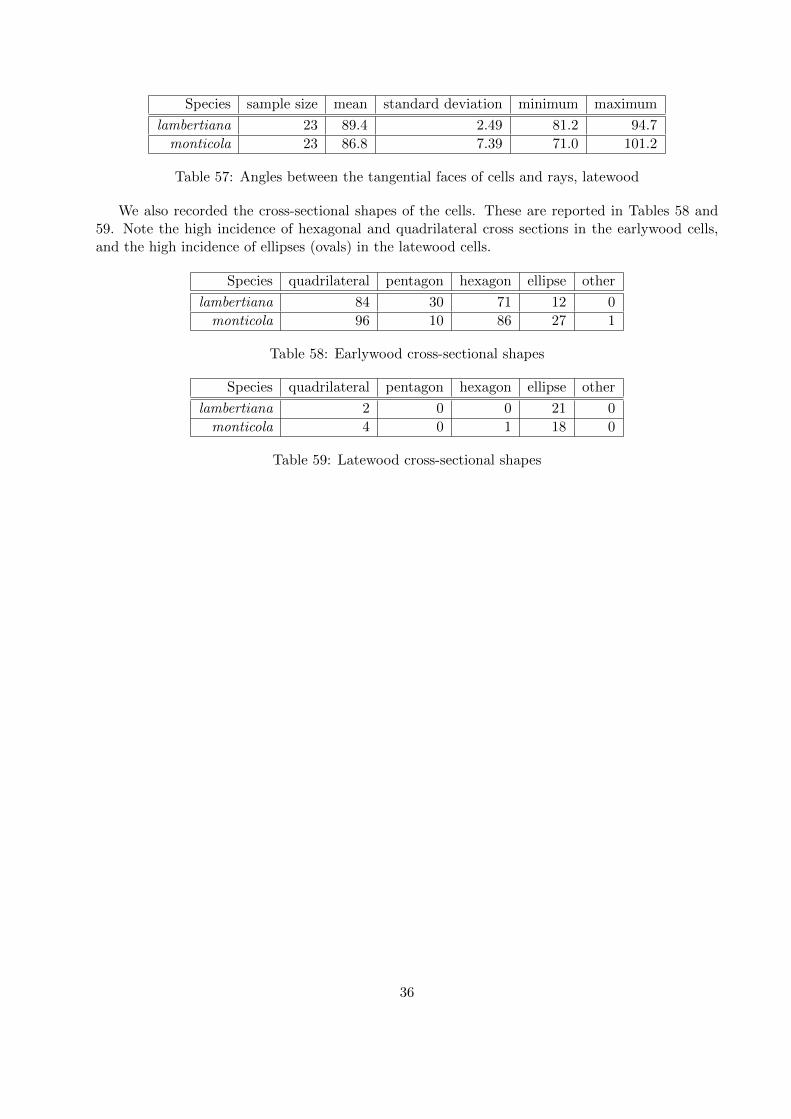
Species sample size mean standard deviation minimum maximum
lambertiana 23 89.4 2.49 81.2 94.7
monticola 23 86.8 7.39 71.0 101.2
Table 57: Angles between the tangential faces of cells and rays, latewood
We also recorded the cross-sectional shapes of the cells. These are reported in Tables 58 and59. Note the high incidence of hexagonal and quadrilateral cross sections in the earlywood cells,and the high incidence of ellipses (ovals) in the latewood cells.
Species quadrilateral pentagon hexagon ellipse other
lambertiana 84 30 71 12 0
monticola 96 10 86 27 1
Table 58: Earlywood cross-sectional shapes
Species quadrilateral pentagon hexagon ellipse other
lambertiana 2 0 0 21 0
monticola 4 0 1 18 0
Table 59: Latewood cross-sectional shapes
36
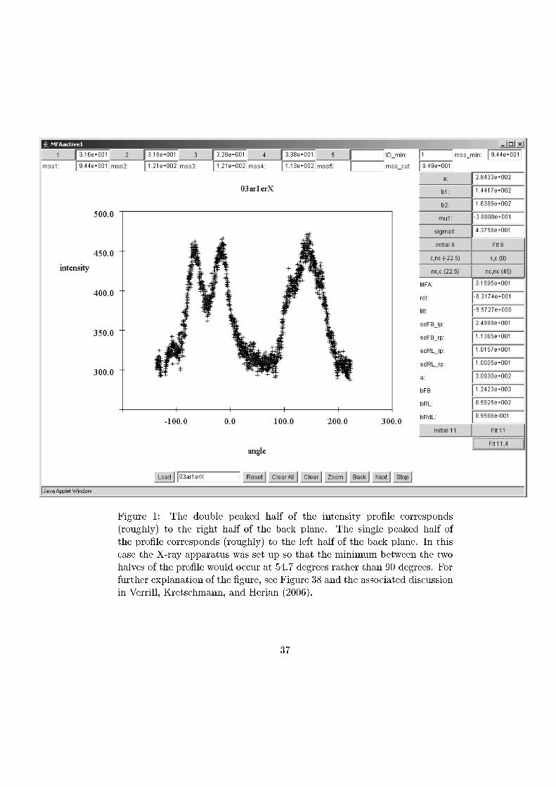
������ �� � ��� �� ������ ��� �� �� ��������� ������ �����������
�������� �� �� ���� ��� �� �� ��� ������ � ������ ������ ��� ��
�� ������ ����������� �������� �� �� ���� ��� �� �� ��� ������ �� ���
���� �� ����� ��������� ��� ��� �� �� ��� �� ��� � ������ �� ���
��!�� �� �� ������ ����� ����� �� "#�$ ������� ����� ��� %& �������� ���
������ �'��������� �� �� �����( ��� ������ )* ��� �� ���������� ����������
�� +������( ,����� ���( ��� -����� �.&&/��
)$

0 0 0 00
0 0
microfibril angle
varia
nce
appr
oach
bia
s
0 10 20 30 40 50
010
2030
1 1 1 1 11
1
22
22
22 2
3
33
33
4
4
4
4
������ �� ����� ���� ��� ������ ���� ���������� ����� � ������
������� � � � ������ ����� � � �� ������ ����� � � �� ������ ����� � � �� ������
����� � � �� ������ ����� ���������� ������ ������� ��������� ��������
���� �������������� ���� �� ������� !�� �� ������ ����" #� �� ## ������
$�%�" �� �� ������ ����" ��" #�" �� ## ������ $�%� ������ ����� �� ��
��&������� !��� ��� ��!� !�� �� ����� �����
�'
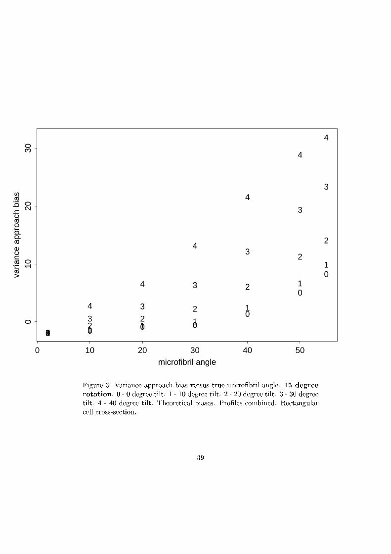
0 0 0 00
0
0
microfibril angle
varia
nce
appr
oach
bia
s
0 10 20 30 40 50
010
2030
1 1 1 1
1
1
1
22
22
2
2
2
3
3
3
3
3
3
3
4
4
4
4
4
4
4
������ �� ����� ���� ��� ������ ���� ���������� ����� �� ������
������� � � � ������ ����� � � �� ������ ����� � � �� ������ ����� � � �� ������
����� � � �� ������ ����� ���������� ������ ������� ��������� ��������
���� ��������������
�(

0 00
0
0
0
0
microfibril angle
varia
nce
appr
oach
bia
s
0 10 20 30 40 50
010
2030
1 11
1
1
1
1
22
22
2
2
2
3
3
3
3
3
3
3
4
4
4
4
4
4
4
������ �� ����� ���� ��� ������ ���� ���������� ����� � ������
������� � � � ������ ����� � � �� ������ ����� � � �� ������ ����� � � �� ������
����� � � �� ������ ����� ���������� ������ ������� ��������� ��������
���� ��������������
��
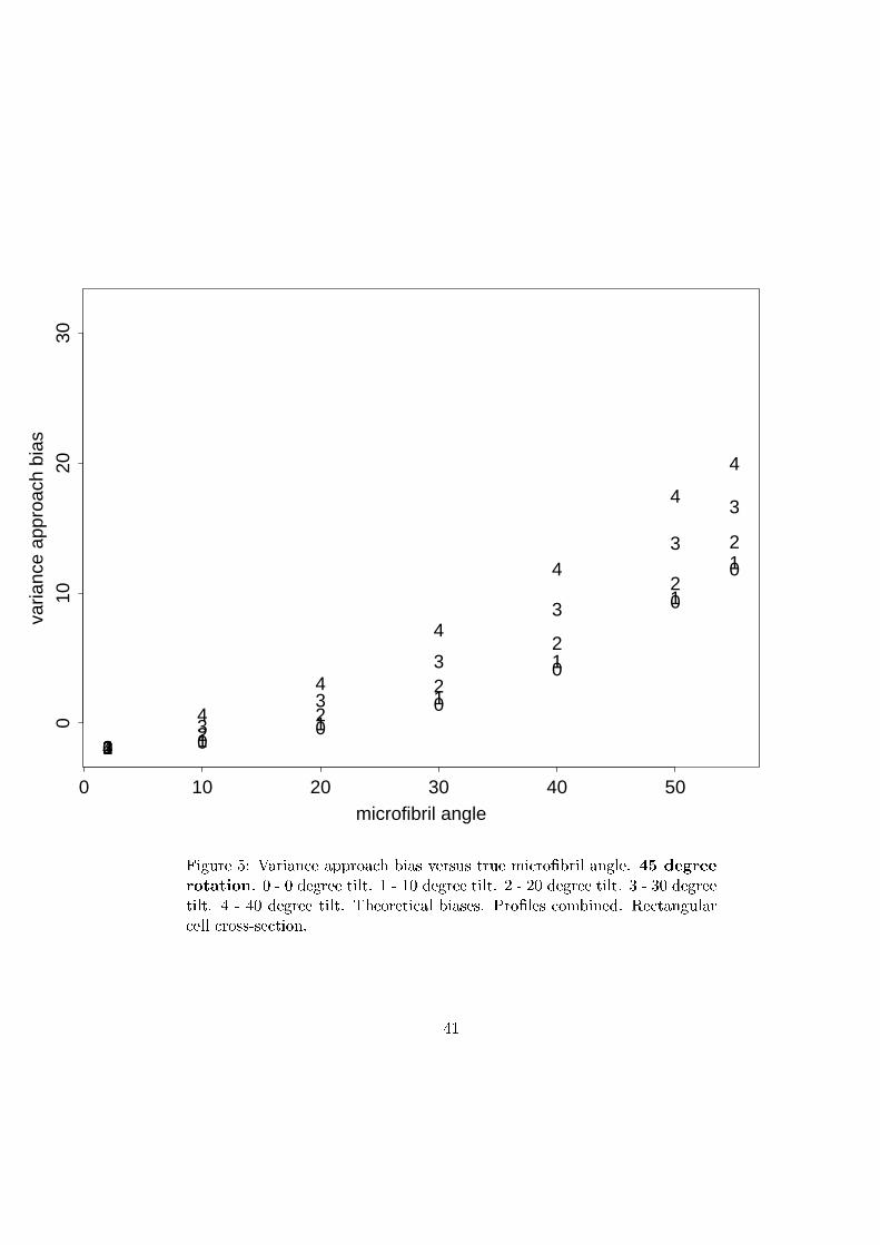
0 00
0
0
0
0
microfibril angle
varia
nce
appr
oach
bia
s
0 10 20 30 40 50
010
2030
1 11
1
1
1
1
22
2
2
2
2
2
33
3
3
3
3
3
4
4
4
4
4
4
4
������ #� ����� ���� ��� ������ ���� ���������� ����� �� ������
������� � � � ������ ����� � � �� ������ ����� � � �� ������ ����� � � �� ������
����� � � �� ������ ����� ���������� ������ ������� ��������� ��������
���� ��������������
��

0 00
0
0
00
microfibril angle
varia
nce
appr
oach
bia
s
0 10 20 30 40 50
010
2030
1 11
1
1
1
1
2 22
2
2
2
2
3 33
3
3
3
3
44
44
4
4
4
������ )� ����� ���� ��� ������ ���� ���������� ����� �� ������
������� � � � ������ ����� � � �� ������ ����� � � �� ������ ����� � � �� ������
����� � � �� ������ ����� ���������� ������ ������� ��������� ��������
���� ��������������
��

0 0 0 00
0
0
microfibril angle
varia
nce
appr
oach
bia
s
0 10 20 30 40 50
010
2030
1 1 1 11
1
1
2 22 2
2
2
2
3 3 3 33
3
3
4 4 4 44
4
4
������ *� ����� ���� ��� ������ ���� ���������� ����� �� ������
������� � � � ������ ����� � � �� ������ ����� � � �� ������ ����� � � �� ������
����� � � �� ������ ����� ���������� ������ ������� ��������� ��������
���� ��������������
��

0 0 0 0 0
00
microfibril angle
varia
nce
appr
oach
bia
s
0 10 20 30 40 50
010
2030
1 1 1 11
11
2 2 2 2 22
2
3 3 3 3 33
3
4 4 4 44
44
������ '� ����� ���� ��� ������ ���� ���������� ����� �� ������
������� � � � ������ ����� � � �� ������ ����� � � �� ������ ����� � � �� ������
����� � � �� ������ ����� ���������� ������ ������� ��������� ��������
���� ��������������
��

0 00 0
0
0 0
microfibril angle
varia
nce
appr
oach
bia
s
0 10 20 30 40 50
05
1015
1 11 1
1
11
22
22
2
2 2
3
3
3
3
33
3
4
4
4
4
4
4
4
������ (� ����� ���� ��� ������ ���� ���������� ����� � ������
������� � � � ������ ����� � � �� ������ ����� � � �� ������ ����� � � �� ������
����� � � �� ������ ����� �������� ������ ������� ��������� ��������
���� ��������������
�#

0 00 0
0
00
microfibril angle
varia
nce
appr
oach
bia
s
0 10 20 30 40 50
05
1015
11
11
1
11
2
2
2
2
2
2 2
3
3
3
3
3 3
3
4
4
4
4
4
4
4
������ ��� ����� ���� ��� ������ ���� ���������� ����� �� ������
������� � � � ������ ����� � � �� ������ ����� � � �� ������ ����� � � �� ������
����� � � �� ������ ����� �������� ������ ������� ��������� ��������
���� ��������������
�)

0 00
0
0
00
microfibril angle
varia
nce
appr
oach
bia
s
0 10 20 30 40 50
05
1015
11
1
1
1
1
1
2
2
2
2
2
22
3
3
3
3
3
33
4
4
4
4
4
4
4
������ ��� ����� ���� ��� ������ ���� ���������� ����� � ������
������� � � � ������ ����� � � �� ������ ����� � � �� ������ ����� � � �� ������
����� � � �� ������ ����� �������� ������ ������� ��������� ��������
���� ��������������
�*
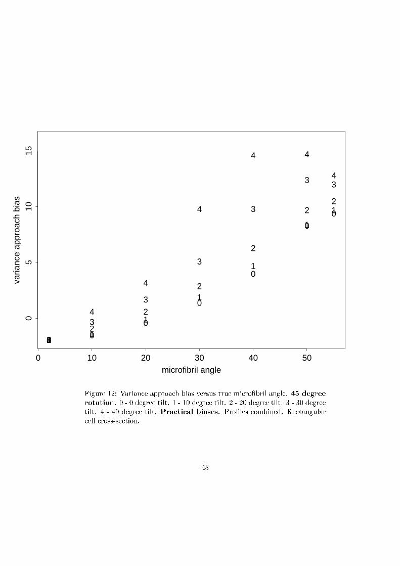
0 0
0
0
0
00
microfibril angle
varia
nce
appr
oach
bia
s
0 10 20 30 40 50
05
1015
11
1
1
1
1
1
22
2
2
2
22
3
3
3
3
3
3 3
4
4
4
4
4 4
4
������ ��� ����� ���� ��� ������ ���� ���������� ����� �� ������
������� � � � ������ ����� � � �� ������ ����� � � �� ������ ����� � � �� ������
����� � � �� ������ ����� �������� ������ ������� ��������� ��������
���� ��������������
�'

0 00
0
0
0 0
microfibril angle
varia
nce
appr
oach
bia
s
0 10 20 30 40 50
05
1015
1 11
1
1
11
22
2
2
2
22
33
3
3
3
3 3
4
4
4
4
44
4
������ ��� ����� ���� ��� ������ ���� ���������� ����� �� ������
������� � � � ������ ����� � � �� ������ ����� � � �� ������ ����� � � �� ������
����� � � �� ������ ����� �������� ������ ������� ��������� ��������
���� ��������������
�(

0 00
0
0
00
microfibril angle
varia
nce
appr
oach
bia
s
0 10 20 30 40 50
05
1015
1 11
1
1
11
2 22
2
2
2 2
3 33
3
3
3 3
44
4
4
44
4
������ ��� ����� ���� ��� ������ ���� ���������� ����� �� ������
������� � � � ������ ����� � � �� ������ ����� � � �� ������ ����� � � �� ������
����� � � �� ������ ����� �������� ������ ������� ��������� ��������
���� ��������������
#�

0 00 0 0
00
microfibril angle
varia
nce
appr
oach
bia
s
0 10 20 30 40 50
05
1015
1 11 1
1
11
2 22 2
2
22
3 33
3
3
3 3
4 44
4
44
4
������ �#� ����� ���� ��� ������ ���� ���������� ����� �� ������
������� � � � ������ ����� � � �� ������ ����� � � �� ������ ����� � � �� ������
����� � � �� ������ ����� �������� ������ ������� ��������� ��������
���� ��������������
#�

0 0 00
0
0
0
microfibril angle
varia
nce
appr
oach
bia
s
0 10 20 30 40 50
010
2030
1 11
1
1
1
1
22
2
2
2
2
2
3
3
3
3
3
3
3
4
4
4
4
4
44
������ �� ����� � ������ � ���� ������ ���� �� ������� ������ � ������
������� � � � ������ ����� � � �� ������ ����� � � �� ������ ����� � � �� ������
����� � � �� ������ ����� �������� �� ������� ������ �������� !�"������
��� ������� �����
#�

0 00
0
0
0
0
microfibril angle
varia
nce
appr
oach
bia
s
0 10 20 30 40 50
010
2030
1 11
1
1
1
1
22
22
2
2
2
3
3
3
3
3
3
3
4
4
4
4
4
������ �$ ����� � ������ � ���� ������ ���� �� ������� ������ �� ������
������� � � � ������ ����� � � �� ������ ����� � � �� ������ ����� � � �� ������
����� � � �� ������ ����� �������� �� ������� ������ �������� !�"������
��� ������� ����� ����� ��� ������� %�� �� ������ ����& #� ��� ## ������
'�(� �� ���� ����� ��� �� ��)� ����� %��� ��� ��%� � %� � �� ����� �����
#�

0 00
00
00
microfibril angle
varia
nce
appr
oach
bia
s
0 10 20 30 40 50
010
2030
1 11
11
1
1
22
22
2
22
33
3
3
3
3
4
4
4
4
4
������ �* ����� � ������ � ���� ������ ���� �� ������� ������ � ������
������� � � � ������ ����� � � �� ������ ����� � � �� ������ ����� � � �� ������
����� � � �� ������ ����� �������� �� ������� ������ �������� !�"������
��� ������� ����� ����� ��� ������� %�� �� ������ ����& ## ������ '�(& ���
�� ������ ����& #� ��� ## ������ '�(� �� ���� ����� ��� �� ��)� ����� %���
��� ��%� � %� � �� ����� �����
#�
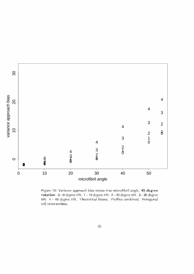
0 0 00
0
0
0
microfibril angle
varia
nce
appr
oach
bia
s
0 10 20 30 40 50
010
2030
1 11 1
1
1
1
2 22
2
2
2
2
33
3
3
3
3
3
4
4
4
4
4
4
4
������ �+ ����� � ������ � ���� ������ ���� �� ������� ������ �� ������
������� � � � ������ ����� � � �� ������ ����� � � �� ������ ����� � � �� ������
����� � � �� ������ ����� �������� �� ������� ������ �������� !�"������
��� ������� �����
##

0 00
0
0
0
0
microfibril angle
varia
nce
appr
oach
bia
s
0 10 20 30 40 50
010
2030
1 11
1
1
1
1
2 22
2
2
2
2
33
33
3
3
3
44
44
4
4
4
������ �� ����� � ������ � ���� ������ ���� �� ������� ������ �� ������
������� � � � ������ ����� � � �� ������ ����� � � �� ������ ����� � � �� ������
����� � � �� ������ ����� �������� �� ������� ������ �������� !�"������
��� ������� �����
#�

0 00 0
0
0
0
microfibril angle
varia
nce
appr
oach
bia
s
0 10 20 30 40 50
010
2030
1 11 1
1
1
1
2 22 2
2
2
2
3 33 3
3
3
3
4 44
4
4
4
4
������ �� ����� � ������ � ���� ������ ���� �� ������� ������ �� ������
������� � � � ������ ����� � � �� ������ ����� � � �� ������ ����� � � �� ������
����� � � �� ������ ����� �������� �� ������� ������ �������� !�"������
��� ������� �����
#$
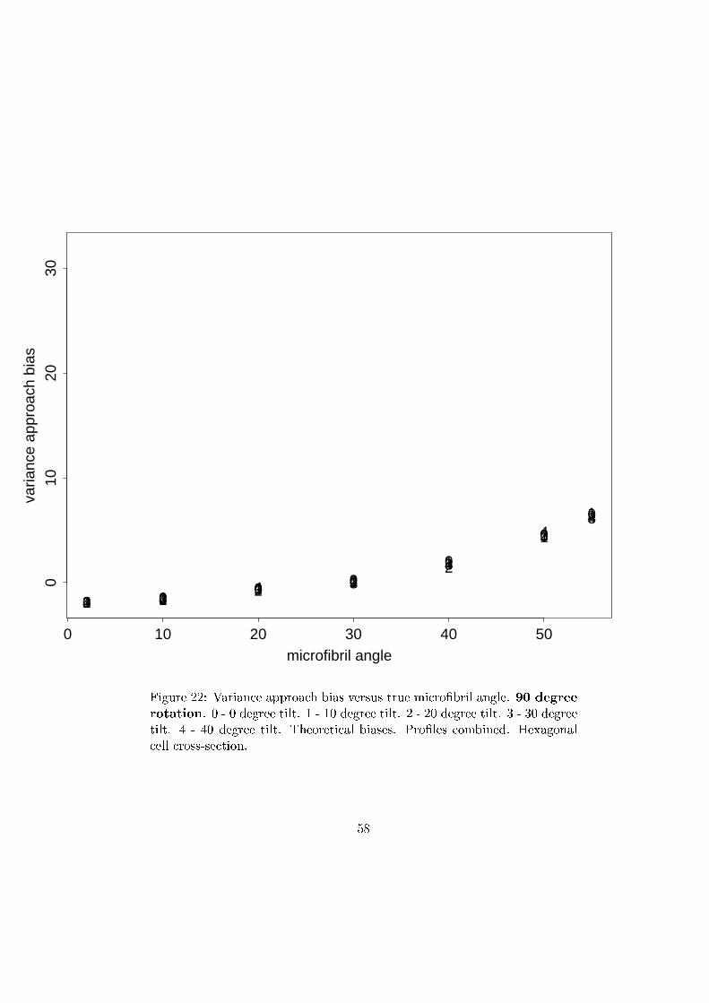
0 00 0
0
00
microfibril angle
varia
nce
appr
oach
bia
s
0 10 20 30 40 50
010
2030
1 11 1
1
1
1
2 2 22
2
22
3 33 3
3
33
4 44 4
4
44
������ �� ����� � ������ � ���� ������ ���� �� ������� ������ �� ������
������� � � � ������ ����� � � �� ������ ����� � � �� ������ ����� � � �� ������
����� � � �� ������ ����� �������� �� ������� ������ �������� !�"������
��� ������� �����
#*
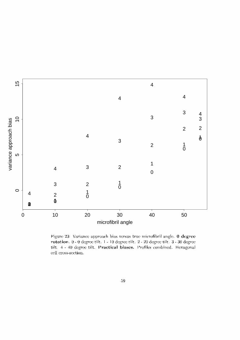
0 00
0
0
0
0
microfibril angle
varia
nce
appr
oach
bia
s
0 10 20 30 40 50
05
1015
11
1
1
1
11
2
2
2
2
2
2 2
3
3
3
3
33
3
4
4
4
4
4
4
4
������ �� ����� � ������ � ���� ������ ���� �� ������� ������ � ������
������� � � � ������ ����� � � �� ������ ����� � � �� ������ ����� � � �� ������
����� � � �� ������ ����� �������� ������ ������ �������� !�"������
��� ������� �����
#+

0 00
0
0
00
microfibril angle
varia
nce
appr
oach
bia
s
0 10 20 30 40 50
05
1015
11
1
1
1
11
2
2
2
2
2
2 2
3
3
3
3
33
3
4
4
4
4
4 4
4
������ �� ����� � ������ � ���� ������ ���� �� ������� ������ �� ������
������� � � � ������ ����� � � �� ������ ����� � � �� ������ ����� � � �� ������
����� � � �� ������ ����� �������� ������ ������ �������� !�"������
��� ������� �����
��

0 00
0
0
00
microfibril angle
varia
nce
appr
oach
bia
s
0 10 20 30 40 50
05
1015
1 1
11
1
1
1
22
2
2
2
2 2
3
3
3
3
3
33
4
4
4
4
44
4
������ �# ����� � ������ � ���� ������ ���� �� ������� ������ � ������
������� � � � ������ ����� � � �� ������ ����� � � �� ������ ����� � � �� ������
����� � � �� ������ ����� �������� ������ ������ �������� !�"������
��� ������� �����
��

0 00
0
0
0
0
microfibril angle
varia
nce
appr
oach
bia
s
0 10 20 30 40 50
05
1015
1 1
11
1
11
22
2
2
2
22
3
3
3
3
3
33
4
4
4
4
4 4
4
������ �� ����� � ������ � ���� ������ ���� �� ������� ������ �� ������
������� � � � ������ ����� � � �� ������ ����� � � �� ������ ����� � � �� ������
����� � � �� ������ ����� �������� ������ ������ �������� !�"������
��� ������� �����
��
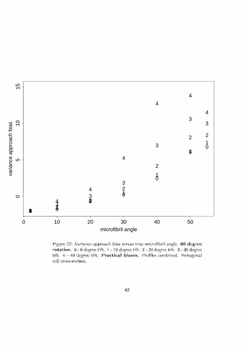
0 0
00
0
00
microfibril angle
varia
nce
appr
oach
bia
s
0 10 20 30 40 50
05
1015
1 11
1
1
1
1
22
2
2
2
2 2
33
3
3
3
33
4
4
4
4
4
4
4
������ �$ ����� � ������ � ���� ������ ���� �� ������� ������ �� ������
������� � � � ������ ����� � � �� ������ ����� � � �� ������ ����� � � �� ������
����� � � �� ������ ����� �������� ������ ������ �������� !�"������
��� ������� �����
��
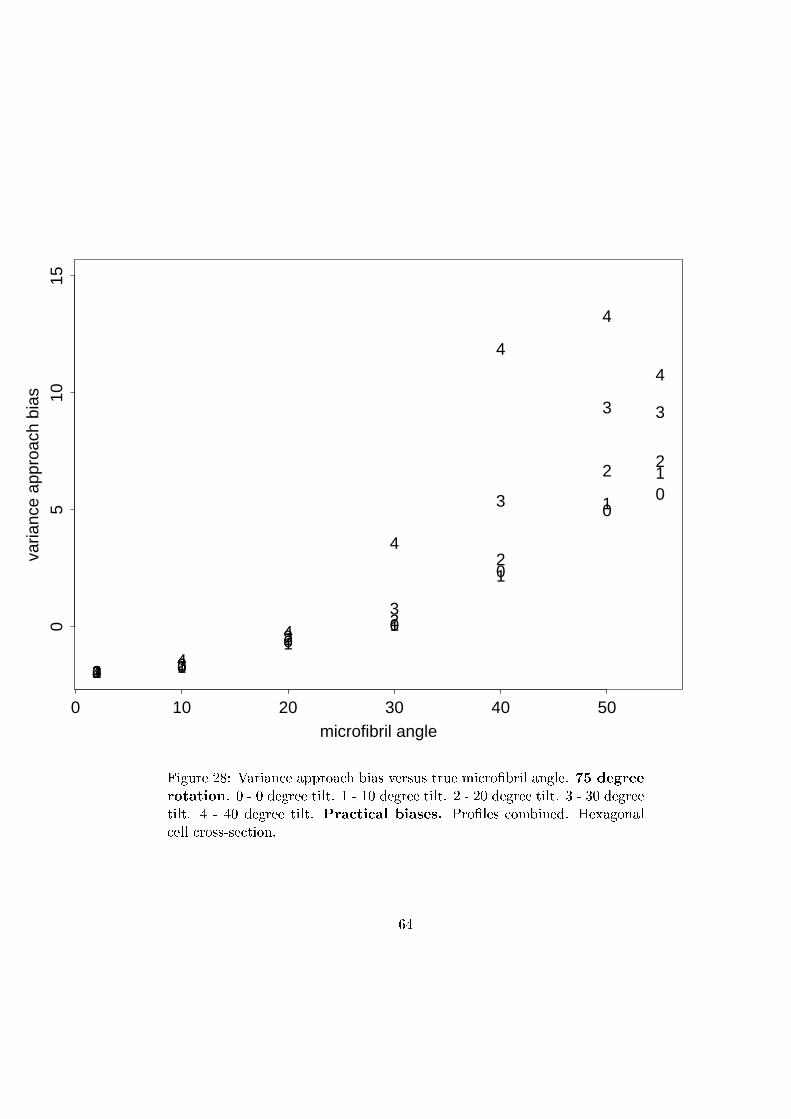
0 0
00
0
00
microfibril angle
varia
nce
appr
oach
bia
s
0 10 20 30 40 50
05
1015
1 11
1
1
1
1
2 2
22
2
2 2
3 3
3
3
3
3 3
44
4
4
4
4
4
������ �* ����� � ������ � ���� ������ ���� �� ������� ������ �� ������
������� � � � ������ ����� � � �� ������ ����� � � �� ������ ����� � � �� ������
����� � � �� ������ ����� �������� ������ ������ �������� !�"������
��� ������� �����
��
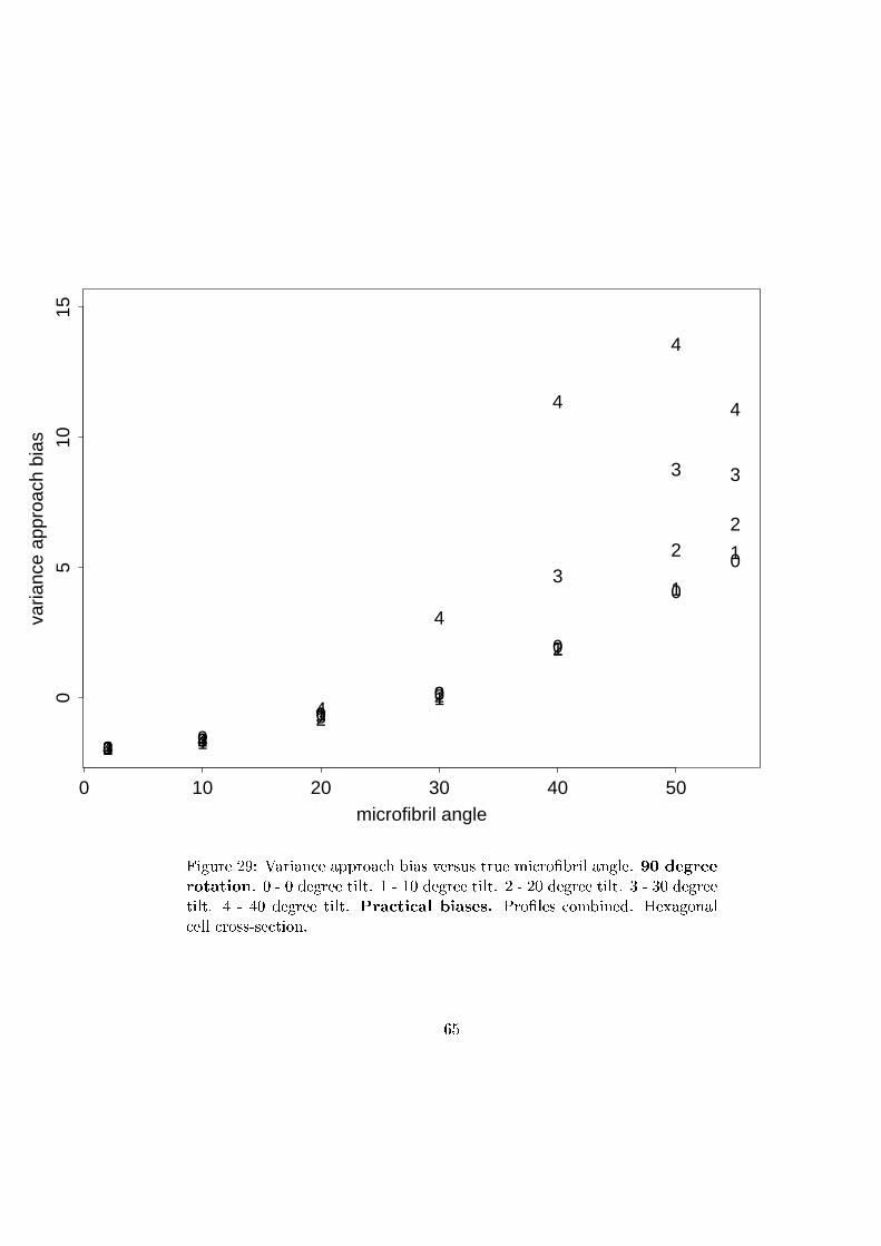
0 00
0
0
0
0
microfibril angle
varia
nce
appr
oach
bia
s
0 10 20 30 40 50
05
1015
1 1
11
1
1
1
2 22
2
2
22
3 33
3
3
3 3
4 4
4
4
4
4
4
������ �+ ����� � ������ � ���� ������ ���� �� ������� ������ �� ������
������� � � � ������ ����� � � �� ������ ����� � � �� ������ ����� � � �� ������
����� � � �� ������ ����� �������� ������ ������ �������� !�"������
��� ������� �����
�#
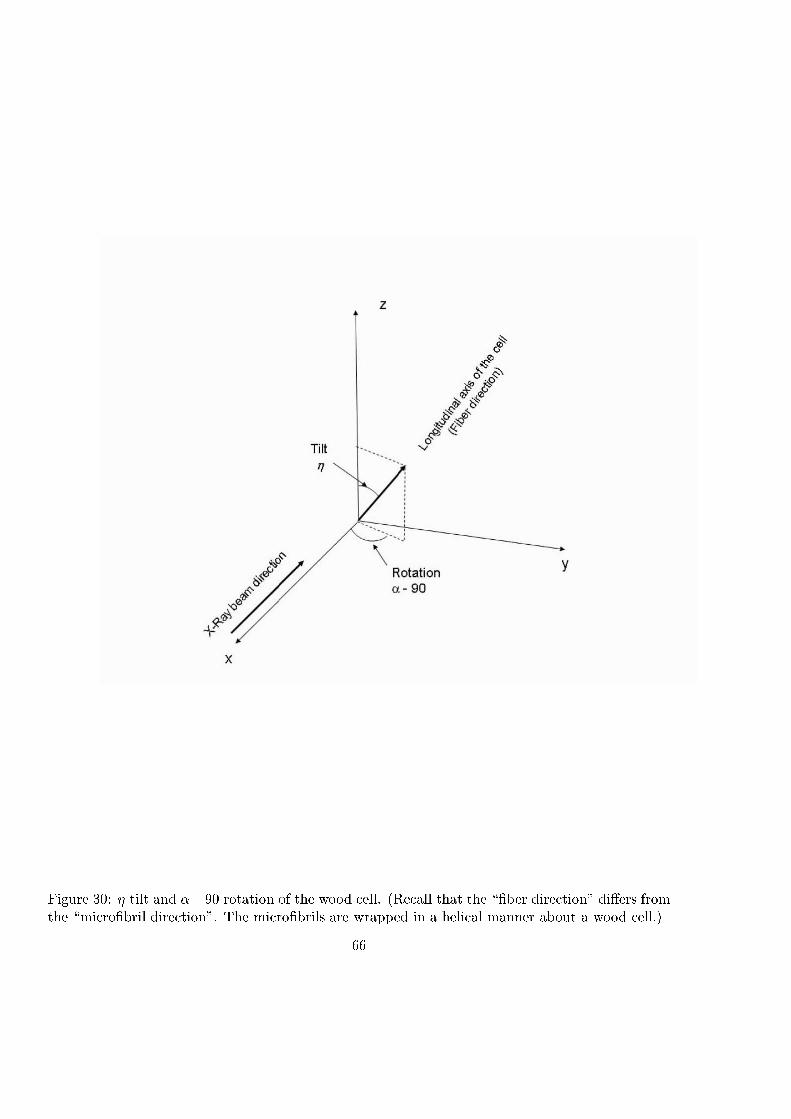
������ �� � �� � � ���� ����� �� �� ���� ����� ������� �� �� ����� ������� � ������ ������ ����������� ������� �� ��� ����������� ��� ��� �� � � ������� �� �� ���� � ���� �����!
""
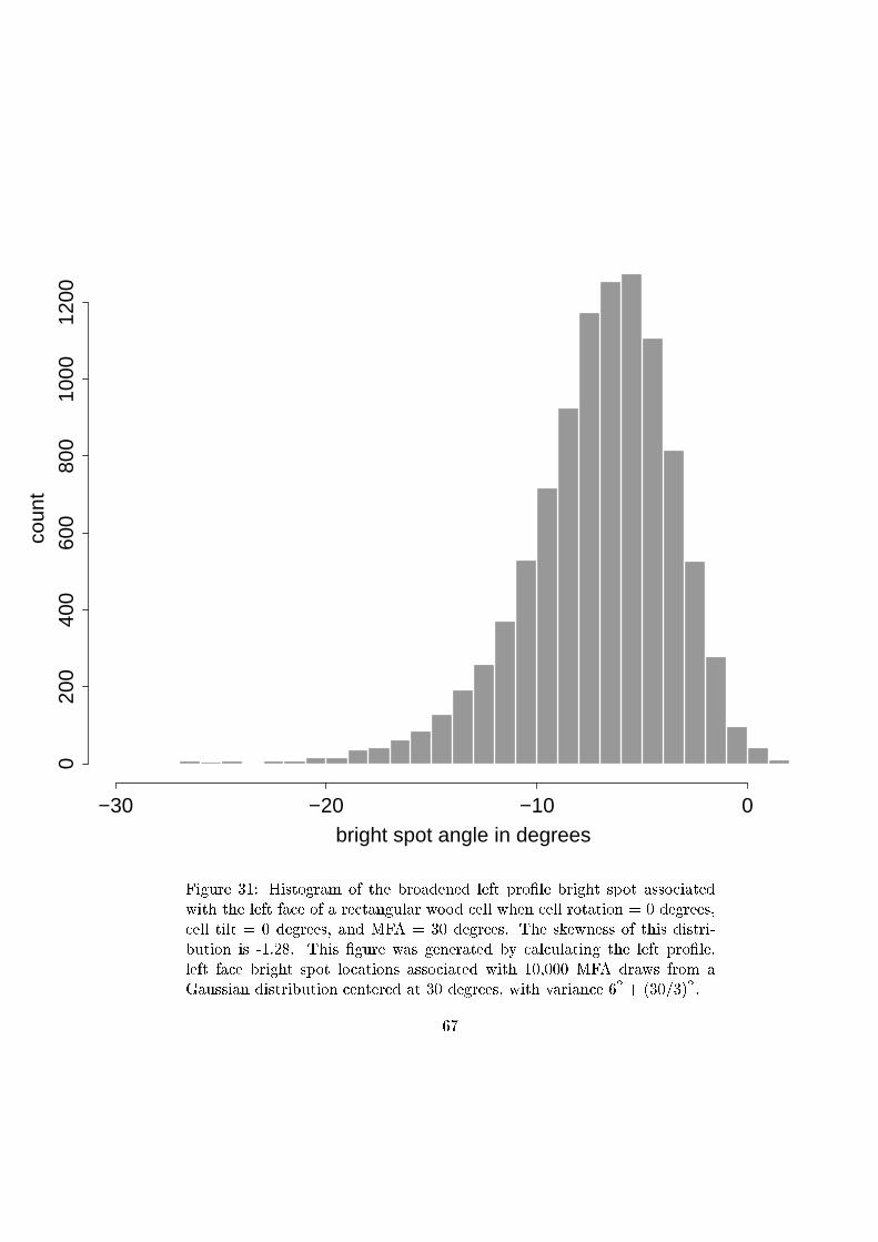
−30 −20 −10 0
020
040
060
080
010
0012
00
bright spot angle in degrees
coun
t
������ �� ��� ���� � ��� �� ������ ���� �� ��� ������ �� � ��� ������
���� ��� ���� ���� � � ����������� � � ���� ���� ���� � ���� � � � ��������
���� ���� � � �������� ��� ��� � �� �������� �� �!������ � ���� ������"
���� � �� "��#$� ��� ����� ��� ��������� �% ����������� ��� ���� �� ����
���� ���� ������ �� � � ���� �� ��� ������ ���� ������ ��� ����� �� � �
&������� ���������� � �������� �� �� �������� ���� '������� (� ) *����+��
(,

10 deg MFA 20 deg MFA
30 deg MFA 40 deg MFA
50 deg MFA 60 deg MFA
������ �# - ���� �� � ���� ��������% ."��% �� �� � ��� ���! ����� � �
� � ���� ���� � � ������� ��� � � ���� � ���� � � � �������
� / �� �� ��� � ��� ����� *��� �� ���� ��� � ���� �+ ����
� / �� �� ��� � ��� ��� ����
� / �� �� ��� � ��� ���� ����
� / �� �� ��� � ��� ��� ����($

������ ��� ���� � ��� � ����� �� � ����������� ���� � ��
��

������ ��� � ���� ��� ���� ��� � � ����������� � ��� ��� � ��
��

������ ��� ��� ���� � ��� � �� ��� �� ��� ����� ����� �� ��� ����� �� ������� � ��� � ���� �� ������������ � ��� �� ������ � ��
��

������ � � ���� � ��� � ����� �� � ������������ �� !��
�"

������ � � � #���� ��� �� ��� $����� �� !�� �����
��
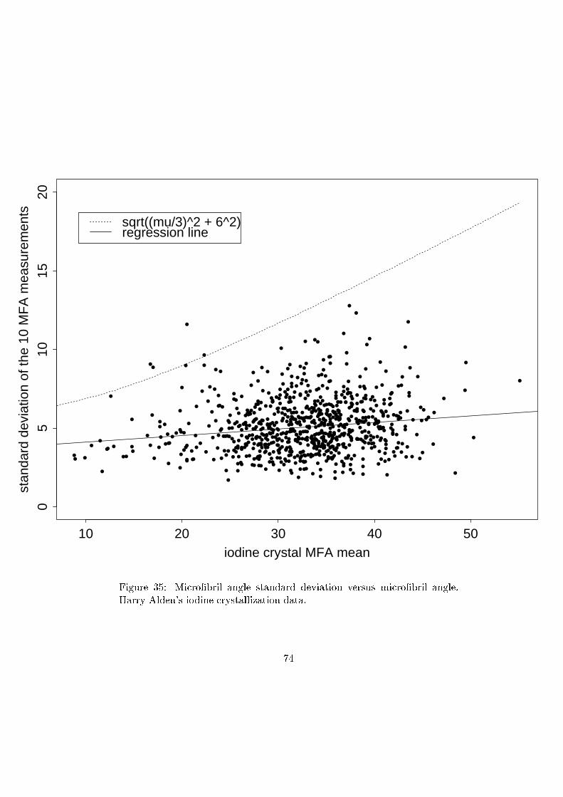
•• •
•
••
••
•••
••
•••
•
•• •
•
••
• •
•
•
•
•••
•••
•
••
•
••
•
•
•
•
•
•
•
•
•
•
•
•
•
•
•
•
•
•
•
••
• •
•
• •
•
•
•
•
•••
•
•
•
•
•
••
••
•
• •••
•
•
••
•••
••
•
•
•
•
••
•
•
••
•
• •• ••
•• •• •
•
•
••
• •
•
•
•
•
••
••
•••
••
•• •
••
•
•
•
•
•
•
•
•
••
•
•
•
••••
•
•
••
• ••
•
•
•
•
•
•
••
•
•
••
•
•
•
•
•
•
•
•
•
••
•
•
•
•
•
•
•
•
•
•
••••
•
•
•
•
•
••
•
••
•
••
••
•
•
•
•••
•
•
•
•
•
••
••
••
•
••
•
•
••
•••
••
•
•
••
•
••• •
•
•
•
•
•
•• •
• •
••
•
••
••••
• ••
•
•
•
•
•
••
•
••
•
•
••
•
•
•
•••
•
•
•
•
•
•
•
•••
• ••
••
•• •
••
•
•
•
•
•
•
• •
•
••
••
•
•
•
••
•
• • •
•
•
•
•• •• ••
•
•
••
• •
•
•
••
•
•
•
•
•
•
•
• •
•
•
•
•
•
•
•
•
•
•
•
•
•
•
•
•
•
••
•
•
•
•
•
• ••
•
•
•
••
• •
•• ••• ••
••
•••
•
•• ••
•
•
••
•• •
••
•
••
•
• •
•
••
•
••
•
•
• •
••
••
•
••
•••
•••
••
•
•
•
•
•
•
•• •
•
•• •
••
•
•
••• •
•
•
•
•
•
•• •
•
•
••• •
•
•
•
•
•
•
•
•
•
••
•
•
•
• ••
•
•
•
••
•
•
••
••
• •
•
•
•
•
•
••
•
• ••
•
• •
•
•
•
•• ••
•
•
••
• •
•••
•
•
•
•
•
•
•
••
••
•
•
•
• ••
•
• •••
••
•
••••
•
• ••
••
•
•
•• •
•
•
•
••
•
••
••
••
•
•
• •
••
•••
•
•
•
•
•
• •• •
••
•
•
•
••
••
•• ••
•
• •• ••
••
••
•
• ••
•
•
••
•••
•
•
•
•
•
•
•
•
•
••
•
•
•••
• ••
••
•
•
••
••
••
•
•
•••
•
•
•
•
• •
•• ••
• •
•
•
•••
•
• •
•
•
•
•
••
•
•••
• •
•
••••
•
•
•• •
•
•
•
•
•
••
•
•
•
•
•
•
•
•
•
•
•
• ••
•
•
•
•
•• •
• •
•
•
•••
•
•
•••
•
••
•
••
•
•
• ••
••
•
•
••
•
••
•
•••
••
• ••
•
••
• •• ••
••
•
•
•• •
•
•
••
••
•
•
•
•
•
•
•
••
iodine crystal MFA mean
stan
dard
dev
iatio
n of
the
10 M
FA
mea
sure
men
ts
10 20 30 40 50
05
1015
20
sqrt((mu/3)^2 + 6^2)regression line
������ �� ���� ���� ����� �������� ��������� ������ ����� ���� ������
����� ������� ������ ��������������� �����
��
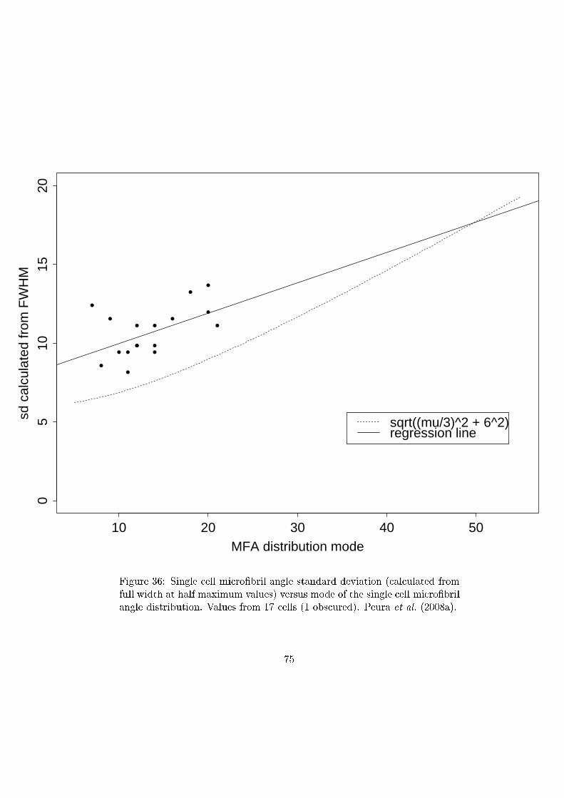
•
•
•
•
•
•• •
•
•
•
• • •
•
•
•
MFA distribution mode
sd c
alcu
late
d fr
om F
WH
M
10 20 30 40 50
05
1015
20
sqrt((mu/3)^2 + 6^2)regression line
������ �� ����� ���� ����� ���� ����� �������� ��������� !���������� "���
"��� #���$ �� $��" ��%���� ������& ������ ���� �" �$� ������ ���� ����� ����
����� ������������� '����� "��� (� ����� !( ��������&� )���� �� ��� !*++,�&�
��

������ �� -������� �" �$� ./��� ��0�������� 1$� ����� ���� �����2 �2 ���
�$� ��������2 � � 3+ ��� ���/���� �� �$�� ����2 ��� �$� ����2 �2 �� ����� ��
������ �+ "�� � ���/���� �����
��
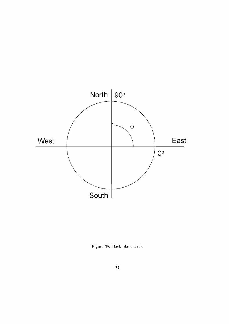
������ �, 4��5 6���� ������
��
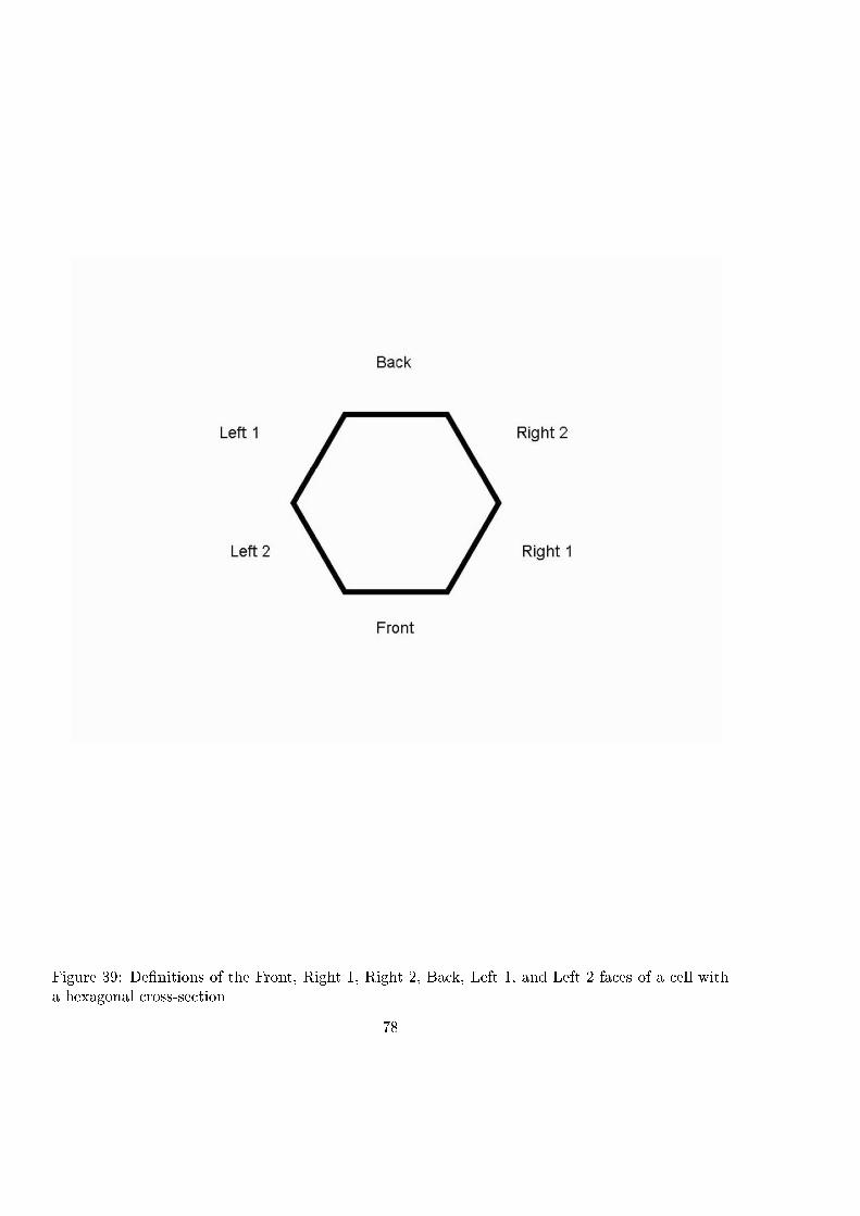
������ �� ���� ���� �� �� ���� � ���� �� ���� �� ����� ��� �� ��� ��� � ����� �� � ���� �� �
� ��������� ��������� ���
!

10 deg MFA 20 deg MFA
30 deg MFA 40 deg MFA
50 deg MFA 55 deg MFA
������ �� �� ����� �� �������������� ��� � ����� �� ��� � �� �� �� ���
��� ��� � ����� �������� ���� ���� ���� �� � �������� �� ���� ����
������ � ��������
� � ����� ��� �� ��� ����� ������� ���� �� ��� ���� � ��
� � ����� ��� �� ��� ��� � ��
� � ����� ��� �� ��� ���� � � ��
� � ����� ��� �� ��� ���� � � ��
� � ����� ��� �� ��� ���� � � ��
� � ����� ��� �� ��� ���� � � ��

10 deg MFA 20 deg MFA
30 deg MFA 40 deg MFA
50 deg MFA 55 deg MFA
������ �! �� ����� �� �������������� ��� � ����� �� ��� � �� �� �� ���
��� ��� � ����� �������� ���� ���� ���� �� � �������� �� ���� ����
������ � �� ��������
� � ����� ��� �� ��� ����� ������� ���� �� ��� ���� � ��
� � ����� ��� �� ��� ��� � ��
� � ����� ��� �� ��� ���� � � ��
� � ����� ��� �� ��� ���� � � ��
� � ����� ��� �� ��� ���� � � ��
� � ����� ��� �� ��� ���� � � ��

10 deg MFA 20 deg MFA
30 deg MFA 40 deg MFA
50 deg MFA 55 deg MFA
������ �" �� ����� �� �������������� ��� � ����� �� ��� � �� �� �� ���
��� ��� � ����� �������� ���� ���� ���� �� � �������� �� ���� ����
������ � � ��������
� � ����� ��� �� ��� ����� ������� ���� �� ��� ���� � ��
� � ����� ��� �� ��� ��� � ��
� � ����� ��� �� ��� ���� � � ��
� � ����� ��� �� ��� ���� � � ��
� � ����� ��� �� ��� ���� � � ��
� � ����� ��� �� ��� ���� � � ��

10 deg MFA 20 deg MFA
30 deg MFA 40 deg MFA
50 deg MFA 55 deg MFA
������ �# �� ����� �� �������������� ��� � ����� �� ��� � �� �� �� ���
��� ��� � ����� �������� ���� ���� ���� �� � �������� �� ���� ����
������ � �� ��������
� � ����� ��� �� ��� ����� ������� ���� �� ��� ���� � ��
� � ����� ��� �� ��� ��� � ��
� � ����� ��� �� ��� ���� � � ��
� � ����� ��� �� ��� ���� � � ��
� � ����� ��� �� ��� ���� � � ��
� � ����� ��� �� ��� ���� � � ��

10 deg MFA 20 deg MFA
30 deg MFA 40 deg MFA
50 deg MFA 55 deg MFA
������ �� �� ����� �� �������������� ��� � ����� �� ��� � �� �� �� ���
��� ��� � ����� �������� ���� ���� ���� �� � �������� �� ���� ����
������ � � ��������
� � ����� ��� �� ��� ����� ������� ���� �� ��� ���� � ��
� � ����� ��� �� ��� ��� � ��
� � ����� ��� �� ��� ���� � � ��
� � ����� ��� �� ��� ���� � � ��
� � ����� ��� �� ��� ���� � � ��
� � ����� ��� �� ��� ���� � � ��

10 deg MFA 20 deg MFA
30 deg MFA 40 deg MFA
50 deg MFA 55 deg MFA
������ �$ �� ����� �� �������������� ��� � ����� �� ��� � �� �� �� ���
��� ��� � ����� �������� ���� ���� ���� �� � �������� �� ���� ����
������ � �� ��������
� � ����� ��� �� ��� ����� ������� ���� �� ��� ���� � ��
� � ����� ��� �� ��� ��� � ��
� � ����� ��� �� ��� ���� � � ��
� � ����� ��� �� ��� ���� � � ��
� � ����� ��� �� ��� ���� � � ��
� � ����� ��� �� ��� ���� � � ��

10 deg MFA 20 deg MFA
30 deg MFA 40 deg MFA
50 deg MFA 55 deg MFA
������ �% �� ����� �� �������������� ��� � ����� �� ��� � �� �� �� ���
��� ��� � ����� �������� ���� ���� ���� �� � �������� �� ���� ����
������ � � ��������
� � ����� ��� �� ��� ����� ������� ���� �� ��� ���� � ��
� � ����� ��� �� ��� ��� � ��
� � ����� ��� �� ��� ���� � � ��
� � ����� ��� �� ��� ���� � � ��
� � ����� ��� �� ��� ���� � � ��
� � ����� ��� �� ��� ���� � � ��

10 deg MFA 20 deg MFA
30 deg MFA 40 deg MFA
50 deg MFA 55 deg MFA
������ �� �� ����� �� �������������� ��� � ����� �� ��� � �� �� �� ���
��� ��� � ����� �������� ���� ���� ���� �� �� �������� �� ���� ����
������ � ��������
� ����� ��� �� ��� ����� !������ ���� �� ��� ����" � ��
� ����� ��� �� ��� ��� � ��
� ����� ��� �� ��� ���� � � ��
� ����� ��� �� ��� ���� � � ��
� ����� ��� �� ��� ���� � � ��
� ����� ��� �� ��� ���� � � ��

10 deg MFA 20 deg MFA
30 deg MFA 40 deg MFA
50 deg MFA 55 deg MFA
������ �# �� ����� �� �������������� ��� � ����� �� ��� � �� �� �� ���
��� ��� � ����� �������� ���� ���� ���� �� �� �������� �� ���� ����
������ � �� ��������
� ����� ��� �� ��� ����� !������ ���� �� ��� ����" � ��
� ����� ��� �� ��� ��� � ��
� ����� ��� �� ��� ���� � � ��
� ����� ��� �� ��� ���� � � ��
� ����� ��� �� ��� ���� � � ��
� ����� ��� �� ��� ���� � � ��

10 deg MFA 20 deg MFA
30 deg MFA 40 deg MFA
50 deg MFA 55 deg MFA
������ �$ �� ����� �� �������������� ��� � ����� �� ��� � �� �� �� ���
��� ��� � ����� �������� ���� ���� ���� �� �� �������� �� ���� ����
������ � � ��������
� ����� ��� �� ��� ����� !������ ���� �� ��� ����" � ��
� ����� ��� �� ��� ��� � ��
� ����� ��� �� ��� ���� � � ��
� ����� ��� �� ��� ���� � � ��
� ����� ��� �� ��� ���� � � ��
� ����� ��� �� ��� ���� � � ��
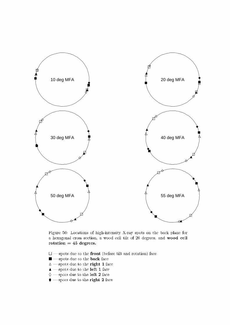
10 deg MFA 20 deg MFA
30 deg MFA 40 deg MFA
50 deg MFA 55 deg MFA
������ %� �� ����� �� �������������� ��� � ����� �� ��� � �� �� �� ���
��� ��� � ����� �������� ���� ���� ���� �� �� �������� �� ���� ����
������ � �� ��������
� ����� ��� �� ��� ����� !������ ���� �� ��� ����" � ��
� ����� ��� �� ��� ��� � ��
� ����� ��� �� ��� ���� � � ��
� ����� ��� �� ��� ���� � � ��
� ����� ��� �� ��� ���� � � ��
� ����� ��� �� ��� ���� � � ��

10 deg MFA 20 deg MFA
30 deg MFA 40 deg MFA
50 deg MFA 55 deg MFA
������ %& �� ����� �� �������������� ��� � ����� �� ��� � �� �� �� ���
��� ��� � ����� �������� ���� ���� ���� �� �� �������� �� ���� ����
������ � � ��������
� ����� ��� �� ��� ����� !������ ���� �� ��� ����" � ��
� ����� ��� �� ��� ��� � ��
� ����� ��� �� ��� ���� � � ��
� ����� ��� �� ��� ���� � � ��
� ����� ��� �� ��� ���� � � ��
� ����� ��� �� ��� ���� � � ��
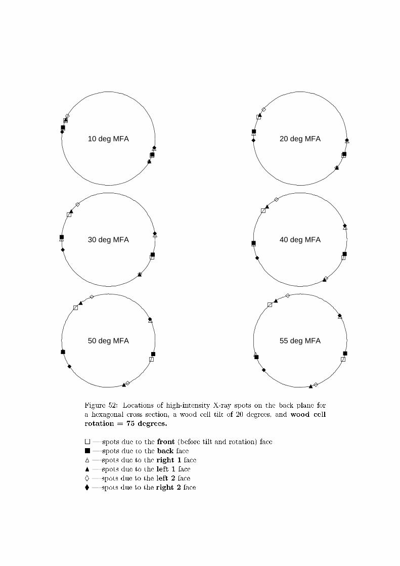
10 deg MFA 20 deg MFA
30 deg MFA 40 deg MFA
50 deg MFA 55 deg MFA
������ %� �� ����� �� �������������� ��� � ����� �� ��� � �� �� �� ���
��� ��� � ����� �������� ���� ���� ���� �� �� �������� �� ���� ����
������ � �� ��������
� ����� ��� �� ��� ����� !������ ���� �� ��� ����" � ��
� ����� ��� �� ��� ��� � ��
� ����� ��� �� ��� ���� � � ��
� ����� ��� �� ��� ���� � � ��
� ����� ��� �� ��� ���� � � ��
� ����� ��� �� ��� ���� � � ��

10 deg MFA 20 deg MFA
30 deg MFA 40 deg MFA
50 deg MFA 55 deg MFA
������ %' �� ����� �� �������������� ��� � ����� �� ��� � �� �� �� ���
��� ��� � ����� �������� ���� ���� ���� �� �� �������� �� ���� ����
������ � � ��������
� ����� ��� �� ��� ����� !������ ���� �� ��� ����" � ��
� ����� ��� �� ��� ��� � ��
� ����� ��� �� ��� ���� � � ��
� ����� ��� �� ��� ���� � � ��
� ����� ��� �� ��� ���� � � ��
� ����� ��� �� ��� ���� � � ��