condition assessment of medium voltage cable joints

Condition Assessment of Medium Voltage Cable JointsDielectric Spectroscopy of field grading

materials

Mai-Linn Sanden

Master of Energy and Environmental Engineering

Supervisor: Frank Mauseth, ELKRAFTCo-supervisor: Sverre Hvidsten, SINTEF Energy Research

Department of Electric Power Engineering

Submission date: June 2015

Norwegian University of Science and Technology

- iii -

Project description

A significant part of the Norwegian medium voltage cable distributionnet is older than the expected lifetime of 30 years. Cable joints have a shorterexpected lifetime than the cable. In case of heat-shrink joints installed in the80's, many service failures have occurred due to over-heating of the metallicconnector. In general, the condition of the insulation of the joints can beassessed by partial discharge measurements or dielectric spectroscopy.

For joints and terminations, field grading materials (FGM) are oftenused to achieve the wanted field distribution to avoid local field enhancementand partial discharges. The dielectric properties of the FGM will also beinfluenced by the frequency of the applied voltage, but also humidity andtemperature will influence the resulting field distribution.

The project work will be mainly experimental. Field grading materialwill be characterized as function of frequency and electric field. The influenceof humidity is also important and will also be investigated during the masterwork.

- iv -

- v -

Preface

This master thesis is written during spring semester of 2015. The thesisis a final assignment of a five years M.Sc. in Energy and Environmentalengineering at the Norwegian University of Science and Technology. The thesisis carried out at the Department of Electric Power Engineering incollaboration with SINTEF Energy Research.

The master work has mostly been experimental, with numerous hoursspent in the laboratory. A parallel experiment was performed at SINTEFEnergy research, with measurements performed on the same test objectsutilized in this thesis. Measurement results found by SINTEF Energy Researchis thereby to be used in this thesis for analysis of the obtained values here.

Trondheim, June 2015

Mai-Linn Sanden

- vi -

- vii -

Acknowledgement

I would like to thank my supervisor Frank Mauseth at NTNU and co-supervisor Sverre Hvidsten at SINTEF Energy Research. For guidance andhelp throughout the master work, insightful advises and practical assistancein laboratory.

Thanks to Henrik Enoksen for help with preparing and conditioningthe test objects correctly before measurements, in addition to helpfulinformation through the master work. I would also thank Torbjørn AndersenVe for help in the laboratory when performing water uptake measurements,and Jorunn Hølto with guidance during differential scanning calorimetrymeasurements.

I must thank my fellow students at NTNU, especially my four closestgirlfriends, for good times and many wonderful memories during these fiveyears.

I would wish to express my deepest appreciation to Yngve, for yoursupport and patience throughout the semester. For encouraging and helpingme when I needed it and for all those hours you have spent reading andcorrecting my thesis. I valuable your advices and critical comments.

At last, I would like express a sincere gratitude to my family. For loveand support throughout the years, and all the possibilities you have providedme.

(PS: Frank, I still got my long nails.)

- viii -

- ix -

Abstract

This thesis examines the electrical properties of a commonly usedstress control tube for medium voltage heat-shrink joints using non-destructive methods in laboratory. The electrical properties of the tube weredetermined by use of dielectric spectroscopy while changing the temperature,AC electric field and humidity level. In order to characterize the material,both differential scanning calorimetry and water uptake measurements wasperformed on samples of stress control tube.

Two similar test objects were used in order to obtain a higher electricfield strength at the same applied AC voltage. A Raychem stress control tubewas shrunk on the outside of a cylindrical shape consisting of two metalelectrodes and a PTFE rod separating them. The length of the PTFE rod was100 mm for Object L, while only 20 mm for Object S providing a higher fieldstrength.

Water uptake measurement was performed in order to determine thestress control tube’s ability to diffuse water. Measurement results imply thatthe water uptake is dependent of both the degree of shrinkage and thetemperature. The highest water content is observed for a virgin stress controltube kept at 90 ℃, with a concentration of 8 % after 105 days. None on thetest samples reached saturation during the experimental work.

Differential scanning calorimetry measurement was performed in orderto examine if the stress control tube had any phase transitions changing theelectrical properties of the stress control tube. Samples of stress control tubewere examined in the temperature range of 20 ℃ to 200 ℃. Results indicatethat the stress control tube, independent of the degree of shrinkage, has anendothermic melting transition in the temperature range of 94 ℃ to 114 ℃.Dielectric response measurements show that the thermal transition of thestress control tube will provide an increased conductivity. This is likely causedby a change from semi-crystalline to amorphous state, releasing trapped chargecarriers and providing the material to become more electrical conductive.

- x -

Dielectric spectroscopy was performed on both test objects in theelectric field range from 0.025 – 1.0 kVpeak/mm for Object S and 0.005 – 0.01kVpeak/mm for Object L. Frequency was varied from 100 Hz to 1 mHz.

A temperature dependence was observed for dielectric loss tangent, inaddition to large values up to 1000. At higher temperatures, the dielectric losstangent was observed independent of the electric field. For measurements at40 ℃, an electric field dependence is observed for field strengths above 0.5kVpeak/mm.

The results show that the conductivity is dependent of thetemperature. After exposed to 150 ℃, the temperature is decreased to 40 ℃and a new measurement is performed. Hysteresis effect is then observed as theconductivity attains a higher value than before exposed to high temperatures.

The conductivity is found independent at the electrical field at hightemperatures. At low temperatures, the electrical field dependence is observedfor field strengths above 0.5 kVpeak/mm.

Observations made imply that the conductivity is strongly dependentof the humidity level. When performing dielectric response measurement on awet test object, the conductivity experienced a significant increase from 10-11

to 10-5 S/m.Wet stress control tube was dissected after complete dielectric response

measurement. There was not observed signs of tracking, causing the electrodesto be short-circuited during measurements.

- xi -

Sammendrag

Denne masteroppgaven vil ta for seg laboratorieundersøkelser av deelektriske egenskapene til kommersiell feltstyrende strømpe brukt imellomspenningskabelskjøter. Dielektrisk responsmåling i frekvensdomenetble brukt for å bestemme de elektriske egenskapene til strømpen som enfunksjon av temperatur, AC elektrisk felt og fuktighet. For å karakteriserestrømpen ble det utført differensiell skannings-kalorimetri ogvannopptaksmålinger.

Testobjektet brukt i oppgaven bestod av to metallelektroder montertsammen med en PTFE stav. På utsiden var det krympet på en Raychemfeltstyrende strømpe. Det var valgt to ulike lengder, 100 mm og 20 mm, påPTFE staven for å oppnå høyere feltstyrker.

Fra vannopptaksmålingene ble det observert at vannopptaket varavhengig av både temperatur og grad av krymping. Det høyeste vanninnholder observert for en ukrympet strømpe ved en temperatur på 90 ℃, hvorkonsentrasjonen etter 105 dager hadde økt med 8 % av tørrvekten. Ingen avprøvene gikk i metning under det eksperimentelle arbeidet.

Differensiell skannings-kalorimetri ble utført for å undersøke om denfeltstyrende strømpen hadde noen faseoverganger som kunne endre deelektriske egenskapene under dielektrisk spektroskopi målingene. Resultatetfra målingene indikerer at strømpen, uavhengig av krympenivå, har etsmeltepunkt i temperaturområdet fra 94 til 114 ℃. Dielektriskeresponsmålinger viser at faseovergangen gir økt ledningsevne. Dette ersannsynligvis forårsaket av en endring fra semi-krystallinsk til amorf tilstandsom vil frigjøre ladningsbærere og øke ledningsevnen til strømpen.

Dielektrisk spektroskopi ble utført på begge testobjektene. Denelektriske feltstyrken påtrykket Objekt S og Objekt L er henholdsvis 0,025 -1,0 kVpeak/mm og 0,005 - 0,01 kVpeak/mm. Frekvensen ble variert fra 100 Hztil 1 mHz.

- xii -

En temperaturavhengighet ble observert for den dielektrisktapstangenten, og ved 1 mHz ble det målt verdier opp til 1000. Tapstangentener vil være uavhengig av feltstyrken ved høye temperaturer. Målinger utførtved 40 ℃ indikerer en elektrisk feltavhengighet for feltstyrker over 0,5 kVpeak/mm.

Resultatene viser at ledningsevnen er avhengig av temperaturen. Etterå ha blitt påtrykket temperatur opp til 150 ℃, blir temperaturen redusert til40 ℃ og en ny måling utført. En hysterese-effekt blir så observert, hvorkonduktiviteten holder en høyere verdi enn før utsatt for høy temperatur.

Konduktiviteten er funnet at uavhengig av feltstyrken ved høyetemperaturer. Målinger ved lavere temperaturer vil en feltavhengighet væresynlig for feltstyrker over 0,5 kVpeak/ mm.

Observasjoner antyder at konduktiviteten er sterkt avhengig avfuktnivået i strømpen. Sammenlikning av resultater for tørt og vått objektviser en betydelig økning i ledningsevnen, fra 10-11 til 10-5 S / m.

Etter måling blir det våte objektet dissekert. Det blir ikke observerttegn som indikerer at elektrodene har vært kortsluttes i løpet av målingene.

- xiii -

Abbreviations

DSC Differential scanning calorimetry

FD Frequency domain

FGM Field grading material

PTFE Polytetrafluoroethylene

SCT Stress control tube

TD Time domain

XLPE Crossed linked polyethylene

- xiv -

Table of contents

Project description ...................................................................................................... iii

Preface ........................................................................................................................... v

Acknowledgement .......................................................................................................vii

Abstract ........................................................................................................................ix

Abbreviations ............................................................................................................ xiii

1 Introduction .......................................................................................................... 31.1 Background ................................................................................... 31.2 Hypothesis ....................................................................................5

2 Theory ................................................................................................................... 72.1 XLPE-cable systems .....................................................................72.2 Basic electrostatic theory ............................................................ 142.3 Non-destructive diagnostic methods ............................................ 232.4 Material characteristic analysis ................................................... 30

3 Method ................................................................................................................ 353.1 Diffusion ..................................................................................... 353.2 Differential scanning calorimetry ................................................ 393.3 Dielectric response measurement ................................................. 423.4 Measurement sequence ................................................................ 49

4 Results ................................................................................................................. 514.1 Diffusion ..................................................................................... 514.2 Differential scanning calorimetry ................................................ 574.3 Dielectric spectroscopy ................................................................ 63

- 2 -

5 Discussion ............................................................................................................ 895.1 Diffusion ..................................................................................... 895.2 Differential scanning calorimetry ................................................ 905.3 Dielectric spectroscopy ................................................................ 915.4 Sources of errors ......................................................................... 95

6 Conclusion ........................................................................................................... 976.1 Further work .............................................................................. 98

7 Bibliography ........................................................................................................ 99

Appendix A – Diffusion.............................................................................................. IIIA1 – Test procedure for Mass Uptake Measurement ...................................... IIIA2 – Curves for diffusion .............................................................................. VII

Appendix B – Differential scanning calorimetry....................................................... XIB1 – Test procedure DSC .............................................................................. XIB2 – DSC measurement results .................................................................... XIII

Appendix C – Results from dielectric response measurements ...........................XVIIIC1 – Measurement result, Object L ............................................................. XIXC2 – Measurement result, Object S .......................................................... XXIIIC3 – Results at DSC temperatures .......................................................... XXVIIC4 – Measurements results examine effect of increased humidity............XXXIII

Appendix D – Formulas used for calculation of the conductivity..................... XXXVI

Appendix E - Dissection of the wet test object ............................................... XXXVIII

Appendix F – List of figures ..................................................................................... XL

Appendix G – List of tables ............................................................................... XLVIII

- 3 -

Chapter 1

1 Introduction

1.1 Background

In Norway, a significant part of the medium voltage (12 and 24 kV) cabledistribution systems have reached its expected lifetime. Observations indicate thatseveral cable sections containing heat shrink joints have suffered from overheating.Observations imply that these joints still seems to withstand the service conditions.However, if the current loading in the cable network increases, additional jointscan experience critical overheating. [1]

This overheating is probably caused by a high contact resistance in themetallic connector. Overheating can be expected to increase the temperature withinthe cable section to temperatures well above the rated temperature. It has beenproposed that such joints have a very low electrical resistance. [1]

Joints and terminations are considered as the weakest parts of the cablesystem. In order to avoid field enhancement, leading to partial discharges andpossible premature failure, these sections can be equipped with a field grading tube.The function of this tube is to obtain a more uniform field distribution along thecable length and further reduce the probability of an enhancement.

This thesis will examine a field grading tube is commonly used in jointsthat have experienced overheating. The aim is to examine how the tube behavesas the temperature is increased up to 150 ℃. Analysis will mainly concern if suchhigh temperatures can cause critical changes in the electrical properties of thematerial. The paper is part of a larger work trying to elucidate the mechanismscausing low insulation resistance in medium voltage cable joints.

- 4 -

1.1.1 Condition assessment

In order to determine in which state the cable system is, several non-destructive tests can be performed. The collective term of this investigation is calledcondition assessment, and has the past decade managed to achieve a high focusand great priority in the industry. A proper understanding of the power systemand its failure characteristics is desirable knowledge. This can be used to providea comprehensive estimate of the condition and the remaining lifetime of the system.

If condition assessment is performed throughout the lifetime and theobtained information is used properly, an increased reliability of the system can beachieved. This information provides an opportunity to schedule maintenance andreplacement at the most suitable time. Additionally, the assessment can statewhich component in need for a replacement and thus avoiding changing of a healthycomponent and unnecessary costs.

The challenge regarding condition assessment is to determine the indicatorsthat reveal a critical system state. Efforts have been put into the discovery of thefailure indicators and which of the parameters that differ from the normal conditionand thus can be used in evaluations. Laboratory tests are performed with an aimto develop a recommended diagnostic method with an interpretation of theevaluation criteria. This will provide realistic replacement measures for the cablesystem.

For a cable system, the two most common non-destructive tests performedare dielectric response and partial discharge measurement. Dielectric responsemeasurements are based on the changes in dielectric properties and are dependenton several factor. These factors can be frequency or time, temperature and chemicalcomposition of the dielectric [2]. Partial discharge measurements can thus be usedto find internal weak spots, e.g. voids, cracks and impurities.

However, when measuring dielectric loss tangent for a cable sectioncontaining cable joint, large values can be observed. This can lead to erroneousassessment of the cable condition, e.g. stating that the cable suffer from severelywater treeing. [3]

- 5 -

1.2 Hypothesis

This master thesis will examine the temperature, humidity and electric fielddependence of a commercial field grading tube used in medium voltage XLPE cableinstalled in the 80s. Both measurement of the diffusion and differential scanningcalorimetry is performed to characterize the material, while the main focus of thisthesis will be on dielectric response measurements. Experimental work has beenperformed in order to test the following hypothesis.

1. Diffusion

i. Both the temperature and degree of shrinkage effects thestress control tube’s ability to diffuse water.

ii. Samples of stress control tube will reach saturation duringmaster work. This result can further be used in order toconditioning the test object into having a humidity level of>90 %.

2. Differential scanning calorimetry

i. The stress control tube does not have any phase transitionat temperatures below 150 ℃, which causes the electricalproperties of the stress control tube to change.

3. Dielectric response measurements

i. Dielectric loss tangent, tan , for the stress control tube hasa high value that can cause erroneous assessment of cablecondition containing a cable joint.

ii. When increasing the temperature, the stress control tube’sconductivity will increase.

iii. Hysteresis effects are not present in the stress control tube.The material has a reversibly change of the conductivityafter being subjected to high temperatures.

iv. Having an increased humidity of the test object, the stresscontrol tube’s conductivity will increase.

- 7 -

Chapter 2

2 Theory

2.1 XLPE-cable systems

Cross-linked polyethylene, often referred to as XLPE or PEX, arethermosetting polymers that has been through a vulcanization process. The processestablishes crosslinks between the molecules which removes the material’s plasticitywhen heated. This type of polymer will not reshape during overheating such asthermoplastic polymers does. Thus, a higher operation temperature can be achievedfor XLPE than for ordinary polyethylene (PE).

Thus, the continuous operation temperatures of the cables are ininternational norms set to be 70 ℃ for PE, and 90 ℃ for XLPE. After XLPE cableswere introduced, it has been the most commonly used material in cable insulation.[4]

PE and XLPE cables are on the other hand sensitive to partial discharges,which can have a considerable influence on the cable’s lifetime. Great effort istherefore focused on preventing voids and protrusions. [5]

XLPE cables were introduced in 1968 in Norway. These cables were notwater tight, causing them to be vulnerable to water tree degradation. In thebeginning of 1980s, the cables were produced with a dry vulcanization, but stillwithout a watertight design. From 1990, XLPE cables were produced to be bothaxially and radially watertight and are the design used today. [6]

The failure rate of XLPE cables is relatively low, but when considering theentire system, including terminations and joints, the failure rate increases [3].

- 8 -

2.1.1 Cable joints

Cables are manufactured in factories under a clean and controlledenvironment. Several factors limit the length of cables during manufacturing, andlong cables are therefore produced in several sections. Dividing the cable intosections also eases the process of service and repair. Installation of those twosections is performed at site and they are connected with a joint providing aprotected and insulated connection.

The cables are stripped down to the conductors by removing the insulationand are electrically connected by e.g. a metal connector. By screwing or pressing,the connector tightens and creates an electrical connection between the two cablesections. Outside the metal connector, the cable layers are connected to make aprotected and insulated layer. A moisture barrier should also be added to avoidwater diffusion into the joint.

When joining cables at site, a clean environment and experienced personnelare required. Caution must be taken to avoid improperly installation, as poorworkmanship tends to increase local stress. Examples of poor workmanship are cutson the cable during the shield cutback operation, contaminations or weakconnection between the conductors.

The weak connection in the metal connector provides a high transitionresistance and an increased heat generation inside the joint. If the heat generatedexceeds the heat dissipated to the environment the temperature will increase. Asthe temperature becomes higher than the rated temperature of the cable system,degradation of the insulation material will increase rapidly. Degradation weakensthe electrical and mechanical properties of the material and initiates partialdischarges that might lead to breakdown. For this reason, jointing two cablesshould be performed with caution. [5]

Heat-shrink joints made of shrinkable plastic are commonly used and areespecially useful when re-insulating jointed cables. They have the advantage to bemade in a different size from the conductors and can be applied in a short timeand adjusted to fit the conductors [7]. However, many medium voltage cablesections with these joints have suffered from overheating, especially XLPE cablesinstalled in the 1980s. [3]

- 9 -

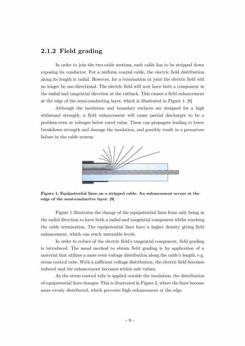
2.1.2 Field grading

In order to join the two cable sections, each cable has to be stripped downexposing its conductor. For a uniform coaxial cable, the electric field distributionalong its length is radial. However, for a termination or joint the electric field willno longer be one-directional. The electric field will now have both a component inthe radial and tangential direction at the cutback. This causes a field enhancementat the edge of the semi-conducting layer, which is illustrated in Figure 1. [8]

Although the insulation and boundary surfaces are designed for a highwithstand strength, a field enhancement will cause partial discharges to be aproblem even at voltages below rated value. These can propagate leading to lowerbreakdown strength and damage the insulation, and possibly result in a prematurefailure in the cable system.

Figure 1: Equipotential lines on a stripped cable. An enhancement occurs at theedge of the semi-conductive layer. [9]

Figure 1 illustrates the change of the equipotential lines from only being inthe radial direction to have both a radial and tangential component whilst reachingthe cable termination. The equipotential lines have a higher density giving fieldenhancement, which can reach untenable levels.

In order to reduce of the electric field’s tangential component, field gradingis introduced. The usual method to obtain field grading is by application of amaterial that utilizes a more even voltage distribution along the cable’s length, e.g.stress control tube. With a sufficient voltage distribution, the electric field becomesreduced and the enhancement becomes within safe values.

As the stress control tube is applied outside the insulation, the distributionof equipotential lines changes. This is illustrated in Figure 2, where the lines becomemore evenly distributed, which prevents high enhancement at the edge.

- 10 -

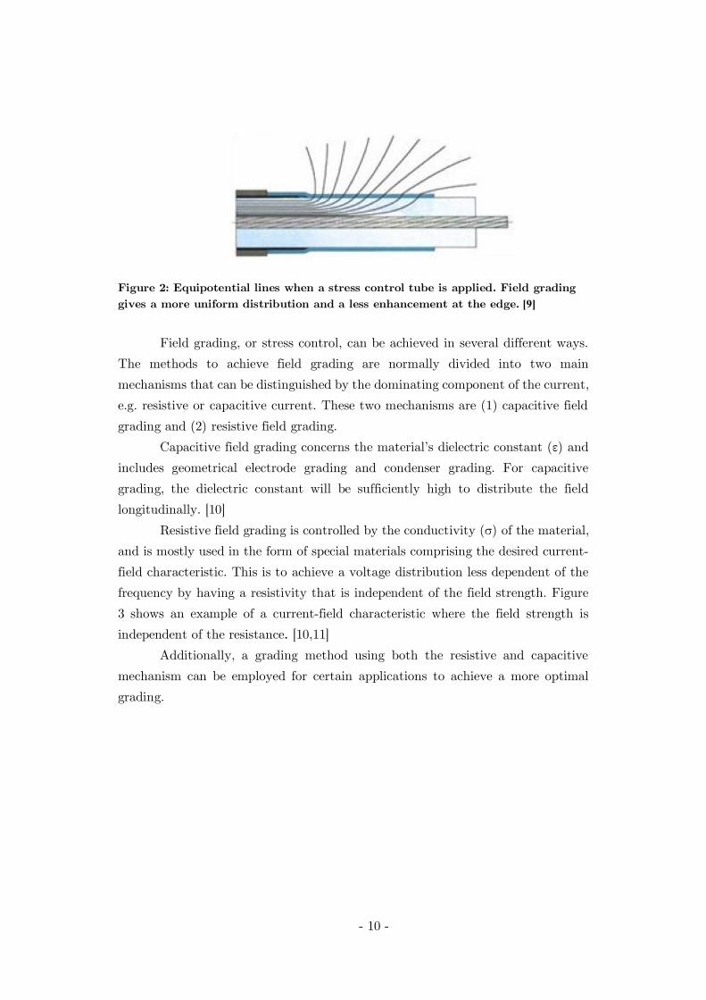
Figure 2: Equipotential lines when a stress control tube is applied. Field gradinggives a more uniform distribution and a less enhancement at the edge. [9]

Field grading, or stress control, can be achieved in several different ways.The methods to achieve field grading are normally divided into two mainmechanisms that can be distinguished by the dominating component of the current,e.g. resistive or capacitive current. These two mechanisms are (1) capacitive fieldgrading and (2) resistive field grading.

Capacitive field grading concerns the material’s dielectric constant (ε) andincludes geometrical electrode grading and condenser grading. For capacitivegrading, the dielectric constant will be sufficiently high to distribute the fieldlongitudinally. [10]

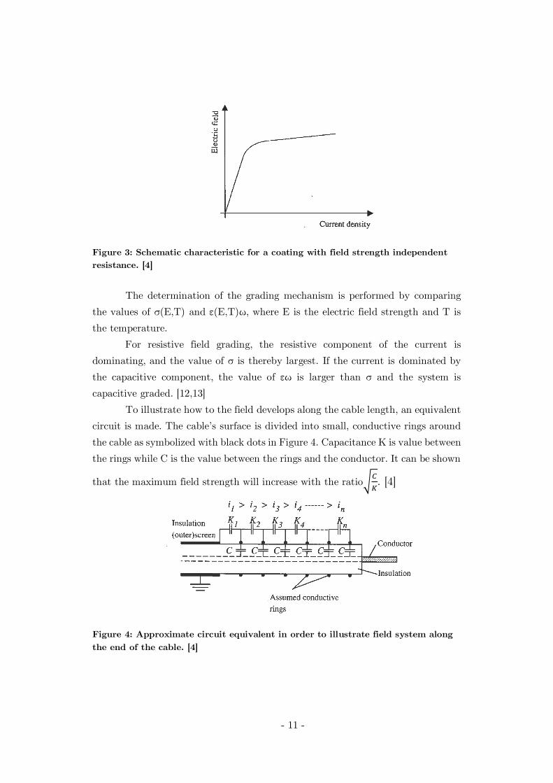
Resistive field grading is controlled by the conductivity (σ) of the material,and is mostly used in the form of special materials comprising the desired current-field characteristic. This is to achieve a voltage distribution less dependent of thefrequency by having a resistivity that is independent of the field strength. Figure3 shows an example of a current-field characteristic where the field strength isindependent of the resistance. [10,11]

Additionally, a grading method using both the resistive and capacitivemechanism can be employed for certain applications to achieve a more optimalgrading.

- 11 -

Figure 3: Schematic characteristic for a coating with field strength independentresistance. [4]

The determination of the grading mechanism is performed by comparingthe values of σ(E,T) and ε(E,T)ω, where E is the electric field strength and T isthe temperature.

For resistive field grading, the resistive component of the current isdominating, and the value of σ is thereby largest. If the current is dominated bythe capacitive component, the value of εω is larger than σ and the system iscapacitive graded. [12,13]

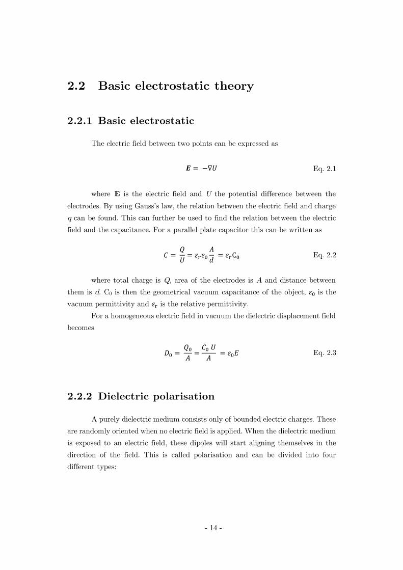
To illustrate how to the field develops along the cable length, an equivalentcircuit is made. The cable’s surface is divided into small, conductive rings aroundthe cable as symbolized with black dots in Figure 4. Capacitance K is value betweenthe rings while C is the value between the rings and the conductor. It can be shown

that the maximum field strength will increase with the ratio . [4]

Figure 4: Approximate circuit equivalent in order to illustrate field system alongthe end of the cable. [4]

- 12 -

In order to keep the magnitude of the longitudinal field stress below criticalvalues, the value of C should be decreased or K increased. However, the value ofC cannot easily be changed as it is given by the potential between thesemiconductor and the conductor. In order to reduce the maximum field strength,the value of K should rather be increased. Various techniques utilize this connectionin order to improve the field distribution, e.g. resistive and refractive field control.[4]

Stress control tube

To achieve a satisfactory field distribution in a cable joint, it is common toapply a stress control tube (SCT). A frequently used type is heat-shrinkable tube,which can fit a large range of sizes and are shrink-heated onto the cable, to makea close fitting.

The heat-shrinkable SCT is made of semi-crystalline polymers compoundedwith additives making it possible to shrink. The material is made with cross-linkingwhile it is in its original shape, which is the shape the material will remember.After a cross-linking, the material is heated above its crystalline meltingtemperature and expanded to a larger size and then cooled down in that position.When the tube is applied to a cable, it will remember its original shape whenheated and form a tight fit to the cable section. [14]

The heat-shrinkable polymers are often used in combination with hot-meltadhesives and have field grading as nonlinear resistive, refractive or resistive-refractive [15].

Linear resistive grading is conversely rarely used. The field distribution forsuch materials is frequency dependent, and thus hard to give an acceptable fielddistribution both at impulse and operation voltage without high losses. A highconductivity is necessary in such cases and a consequence of this is that it createshigh losses. To avoid this, non-linear material might be more suitable. By usingsuch a material, the field grading can be efficient during both conditions. [11]

For resistive field grading a resistive coat are applied. Capacitance K willthen be in parallel with the resistance R, giving an equivalent impedance. This isillustrated in Figure 5.

- 13 -

Figure 5. Equivalent circuit of an impedance stress control material (dark bluelayer) applied to the cable. [10]

Resistive grading reduces the field enhancement by bringing a critical highfield region to a conductive state. This will make the space charge within the tubechange forms, and create a counter field reducing the enhancement. [10]

In addition, a non-linear resistive field grading material has a conductivitythat is field dependent, σ(E). This gives that it typically changes from a low to ahigh conductive value in narrow electric field region. Based on this, the materialmust have a reversibly change from highly conductive to resistive in order to havelow losses. [10]

The highly conductive state provides a greater part of the current passingthrough the tube, increasing the resistive losses. If these losses exceed the dissipatedenergy to the environment, an overheating can be the result.

- 14 -

2.2 Basic electrostatic theory

2.2.1 Basic electrostatic

The electric field between two points can be expressed as

= −∇ Eq. 2.1

where E is the electric field and U the potential difference between theelectrodes. By using Gauss’s law, the relation between the electric field and chargeq can be found. This can further be used to find the relation between the electricfield and the capacitance. For a parallel plate capacitor this can be written as

= = = C Eq. 2.2

where total charge is Q, area of the electrodes is A and distance betweenthem is d. C0 is then the geometrical vacuum capacitance of the object, is thevacuum permittivity and is the relative permittivity.

For a homogeneous electric field in vacuum the dielectric displacement fieldbecomes

= == Eq. 2.3

2.2.2 Dielectric polarisation

A purely dielectric medium consists only of bounded electric charges. Theseare randomly oriented when no electric field is applied. When the dielectric mediumis exposed to an electric field, these dipoles will start aligning themselves in thedirection of the field. This is called polarisation and can be divided into fourdifferent types:

- 15 -

1. Electronic polarizationThe electrons in the orbit of an atom will be distorted when exposed to anelectric field, giving a higher concentration of electrons at one side of theatom. The distortion results in a temporarily dipole, which is extremelyrapid and proportional to the applied field. [5]

2. Ionic polarizationMolecules consisting of negative and positive ions in a symmetrical arrayare not dipoles. When subjected to an electric field the negative and positiveions are pulled in different direction giving a temporarily dipole, whichvanish when the electric field disappears. [5]

3. Orientation polarizationMolecules that are permanent dipoles, e.g. water, have random directionwhen not exposed to an electric field. The effect of an applied field givesthe permanent dipoles to line up in the same direction of the field. [5]

4. Interface polarizationIn dielectric materials there exist areas where the atoms, molecules and ionsare not ideal arranged, in addition to impurities and free electrons. Whenan electric field is applied to the material, electrons start moving towardsthese areas. This will create a local electric field. [5]

2.2.3 Time dependent polarisation

The alignment of the dipoles in a dielectric medium is time dependent.Immediately after an electric field is applied the two first mechanisms, electronicand ionic polarisation, will happen momentary. The two last mechanisms,orientation and interface polarisation, are time dependent and will use some timeto align themselves with the field. These two is commonly denoted as relaxationmechanism.

If a DC voltage is applied to a parallel plate condenser with dielectricinsulation medium, all the dipoles will align themselves in the same direction. Thisresults in a reduction of the net charge between the plates. The reduction is due to

- 16 -

the cancellation by the adjacent dipole and gives a lower voltage potentialdifference between the electrodes. The phenomenon is illustrated in Figure 6.

Figure 6: Parallel plate condenser. [16]a) with vacuum. b) with dielectric medium.c) Resulting net free charge on the surface of the plates when having a dielectricmedium.

When the vacuum is replaced with a dielectric material, the dielectricdisplacement field will increase with the polarisation ( )

( ) = ε ( ) + ( ) = (1 + ) ( ) Eq. 2.4

where is the electric susceptibility of the dielectric material.An equivalent circuit can be established based on the mechanisms present

in a dielectric medium when a step voltage is applied. The current flowing throughthe dielectric can be divided into the following three contributions: conduction,momentary polarisation, and relaxation polarisation. These have each a differenttime constants, and the relation is used in the establishment of the circuitillustrated in Figure 7. The current i(t) indicated in the figure will then be thesame as the current measured during an application of a DC step voltage.

- 17 -

Figure 7: Equivalent circuit of a dielectric medium with conduction, momentarypolarisation and relaxation mechanism.

Each of the components can be related to one of the three contributions tothe current. Conduction is modelled with a resistance Ro and gives the stationarypart of the current. This component will arise if the dielectric material issignificantly conductive and is related to the materials conductivity σ.

Momentary polarisation gives a high current-spike immediately afterapplying a step voltage, and is modelled as a condenser Cm.

Relaxation polarisation is slow process and very temperature dependent andis modelled as a RC-unit with Rd and Cd. The mechanism will then have a time-constant τ equal for both polarisation and depolarisation state. [5]

The relation of the current through a dielectric medium is given in thefollowing equations.

( ) = ( ) + ( )

= ( ) + ( + )

Eq. 2.5

( ) = ( ) +(∞)

⋅ + ( ) Eq. 2.6

Eq. 2.6 shows that the current is a summation of the momentarypolarisation, the relaxation polarisation and the materials conduction ability.

Jδ is the current density of the momentary polarisation given as a highcurrent-spike immediately after applying a step voltage.

Cm R0Rd

Cd

DC

i(t)

- 18 -

Pd presents the relaxation mechanism where its value initially high, butstarts decreasing as the dipoles align themselves with the field. How fast this occursis dependent on the time constant .

When both the momentary and relaxation mechanism has decayed, thecurrent will stabilize at the conductive current. This current is dependent on thematerial’s ability to conduct a current and is proportional with the conductivity.The shape of the current is illustrated in Figure 8.

Figure 8. The current’s shape for both polarisation and depolarisation timeperiod. [5]

- 19 -

2.2.4 Frequency

Since dielectric relaxation is a slow mechanism, it will cause a contributionto the dielectric loss as well as cause a relative permittivity that varies withfrequency, ( ).

When the dielectric medium is subjected to an AC voltage, the electric fieldwill be alternating and the dipoles will try to follow the polarity of the voltage.How fast the electric field changes direction is proportional to the frequency.

If the dielectric is subjected to a low frequency ( ≪ 1), the dipoles willwithout difficulty manage to follow the electric field. However, when the frequencyis increased, the dipoles will struggle to keep up with the alternating field. Thiswill create a phase shift between alignment of the dipole and the field. When thefrequency gets sufficiently high, ≫ 1, the dipoles will no longer be able tofollow. The result of an increasing frequency is a reduction in polarisation hence areduction in relative permittivity. [5]

The phase shift created will cause the electrical flux density D to lag theapplied electric field with an angle δ. Using this relation, the relative permittivitycan be divided into a real ( ) and imaginary ( ) part where both are functionsof the frequency. The real part is commonly known as dielectric constant. Theimaginary part is known as the dielectric loss factor, and represents the phase shiftcausing losses.

When assuming that the conductivity, σ, is zero, the relative permittivity,, can be expressed as

( ) = ⋅ = | | = − Eq. 2.7

where describes how the capacitance C increases with regards to C0.At very low and very high frequencies, it can be assumed that the dielectric

loss factor can be neglected, ≈ 0 [5]. In such cases the Eq. 2.7 can then beexpressed as

( ) = − ≈ Eq. 2.8

- 20 -

The relation of the real and imaginary permittivity is illustrated in Figure9. At high and low frequencies the imaginary part is approximately zero and themaximum value appears when = 1, i.e. at frequency with = .

Figure 9: Real and imaginary part of the permittivity as a function of frequency.

The ratio between and is denoted as the dielectric loss tangent,tan .This is the most commonly used parameter to characterize an insulation materialwhen considering the dielectric loss [5].

tan ( ) =( )( ) Eq. 2.9

For dielectric materials the parts of the relative permittivity can beconsidered to be ≥ 0 and ≫ . The dielectric constant and dielectric lossfactor are dependent on the frequency, material homogeneity, anisotropy, moistureand temperature. [17]

As the temperature increases, the dipoles respond faster to frequency changethus giving a decrease in the relaxation time constant .

In a semiconductor, the conductivity is dependent of two different factors:the concentration of free charge carriers and their mobility. The charge carriers areformed by thermal activation and mobility increases with temperature, whichprovides a temperature dependency by both factors. The conductivity willexperience an increase when the temperature is raised.

If the object is affected by humidity, water molecules might give anadditional contribution to the charge carriers. For a joint without a watertightdesign, the conductivity can have a significant increase and be dependent of theelectric field. [3,18]

- 21 -

Dielectric losses

When measuring the losses during application of an AC voltage, losses canno longer be divided into dielectric and conductivity parts when measuring. Thedielectric loss tangent, tan , is therefore commonly used for express the total lossesand characterization of the insulation system. [5]

= ωε ε tanδ Eq. 2.10

The total loss, P, within a system depends upon the electrical stress (E),frequency (ω), permittivity (ε) and the dielectric loss tangent

Due to the presence of both dielectric and conductivity losses, the total losscan be denoted as

= (ωε ε tan + σ) Eq. 2.11

As the losses are difficult to separate, a new expression is made fortan asa function of both the dielectric and conductive losses.

tan = tan + = + Eq. 2.12

When the conductivity is included, the new expression for dielectric losstangent will be inverse proportional with the frequency, → 0 provides thattan → ∞.

In most cases, the relation | | ≫ | | will apply. This provides a goodapproximation to use ≈ . Based on this, the dielectric loss tangent can besimplified to

tan ≈ Eq. 2.13

When modelling the dielectric losses, a resistor can be represented in eitherparallel or series with an ideal and lossless capacitance. A cable is often modelledas a capacitor due to its capacitive connection between the conductor andsemiconductor. In addition, the parallel model commonly represents the cablesystem [5].

- 22 -

The lossless capacitance C is therefore placed in parallel with a voltagedependent resistance R that represents the heat generated due to dielectric lossesin the capacitor. The current will then be divided into a current IC and IR as shownin Figure 10.

The current IR is in phase with the applied voltage, while IC has a 90° phaseshift. The resistive and capacitive current provides the resultant current I (Figure11). The angle represents the displacement of the current I from IC, where thecapacitor have no losses. Additionally, the amplitude of IR is much less than theone for IC.

Figure 10: Equivalent circuit for parallelcircuit.

Figure 11: Phasor diagram for parallelcircuit.

Using the geometric relation from the figure, the value of tan δ can beexpressed as the ratio of the resistive and capacitive current.

tan = =1

Eq. 2.14

- 23 -

2.3 Non-destructive diagnostic methods

In order to perform condition assessment on cable accessorises, severalmethods are based on measurement of the dielectric response [19]. Dielectricresponse analysis is to be performed in either the time or the frequency domain,with respectively DC or AC voltages.

Time domain analysis is used to measure of the current response or returnvoltage as a function of time when either applying a step voltage or removing thevoltage [20].

During frequency domain measurements, the test object is subjected to anAC voltage at a specified frequency [21]. The quantities measured are the dielectricloss tangent, changes in capacitance and the dielectric loss factor as a function offrequency.

2.3.1 Time domain analysis

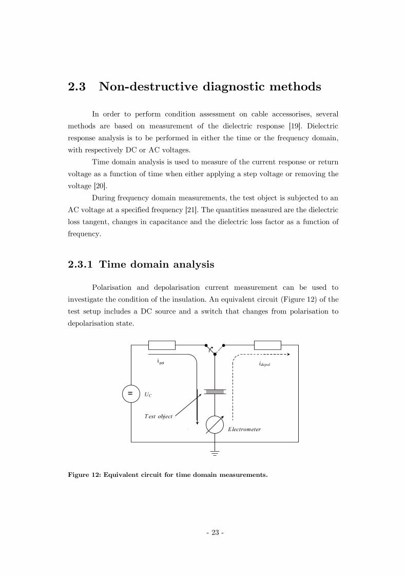
Polarisation and depolarisation current measurement can be used toinvestigate the condition of the insulation. An equivalent circuit (Figure 12) of thetest setup includes a DC source and a switch that changes from polarisation todepolarisation state.

Figure 12: Equivalent circuit for time domain measurements.

Electrometer

UC

T est object

=

idepoli pol

- 24 -

The test object is subjected to step-voltage of U0 for a time period tpol. Theresponse of the current will immediately have a spike, but strongly decrease beforereaching a steady-state value.

After time period tpol, the circuit is short-circuited to earth. A depolarisationcurrent will flow as the dipoles align back to their original position. The currentresponse is illustrated in Figure 13. [22]

Figure 13: Polarisation and depolarisation current as a function of time. [18]

The polarisation and depolarisation current can expressed as

( ) = + ( ) Eq. 2.15

( ) = [ ( ) − ( + )] Eq. 2.16

where ( ) is the dielectric response function of the test object. If thecharging time of the test object is sufficiently long, the value of ( + ) could bedisregarded and set to zero.

By combining Eq. 2.15 and Eq. 2.16, an approximated equation for theconductivity of the object can be found

≈

( ) − ( ) Eq. 2.17

- 25 -

2.3.2 Frequency domain analysis

Non-destructive methods when applying a sinusoidal voltage have beendeveloped as a diagnostics method for cable systems [23].

Dielectric response measurements can be used as a measurement techniqueto determine the dielectric properties of the material that can be used for analysisof the dielectric material. The method used is dielectric spectroscopy, wheremeasurements of the capacitance and the loss are given as a function of thefrequency.

When applying a sinusoidal voltage to the test object, a sinusoidal currentwill start to flow though the object. Measurement of both the voltage and currentenables calculation of the impedance. Furthermore, the impedance can be used tofind several parameters that can be used for the analysis of the dielectric. Figure14 shows the equivalent circuit used during dielectric spectroscopy measurements.

Figure 14: Principle for measuring dielectric response in frequency domain. Objectis subjected to a high voltage source. The current and voltage is measured withamplitude and angle. Parameters can be calculated with these values.

For diagnostic purposes, several relevant dielectric parameters areestablished and are summarized in Table 1 [23,24].

- 26 -

Table 1: Diagnostic parameters

Parameter Description

( ) Real part of the relative permittivity

Δ ( ) Changes in the real permittivity part

( ) Imaginary part of the relative permittivity (Dielectric loss factor)

tan Dielectric loss tangent

Δ(Δ ( )) Change in the real part of the permittivity with voltage

Δ ( ) Changes in the dielectric loss factor with voltage

Δ tan ( ) Changes in the dielectric loss tangent

Active power losses in a dielectric medium, while subjected to an ACvoltage (Eq. 2.18), is a function of both the conductivity and the dielectric lossfactor.

= + = + Eq. 2.18

In order to be able to distinguish the losses, measurements over a largerange of frequencies might be necessary. At low frequencies, the DC losses will bethe dominating making it possible to provide a sufficient estimate of theconductivity. In most case, the relation | | ≫ | | will apply, returning ≈ asa valid approximation.

The measurement executed on the test object can be performed with anInsulation Diagnostic System. Several measurements are performed on a suitablefrequency range and for several voltages. This will provide a more comprehensiveresult where both frequency and voltage dependence can be determined.

- 27 -

2.3.3 Relation between time and frequencyanalysis

For a material responding linearly, i.e. independent of the applied voltage,time domain and frequency domain can be mathematically related. They are theFourier transformation of one another [22,25]:

( ) = ( ) cos Eq. 2.19

( ) = ( ) sin Eq. 2.20

and

( ) =2

(ω) cos(ωt)

Eq. 2.21

=2

(ω) sin(ωt)

The dielectric response function ( ) is related to the polarisationmechanism in time domain. The function is associated to the change in currentwith time and is therefore a real value.

For frequency domain, the function has to be defined by a real andimaginary component ( ) and− ( ). The variation is both a function of thephase and quadrature with respect to the driving harmonic signal [25].

The relation can be written as:

χ( ) = χ (ω) − jχ (ω) = ( )e Eq. 2.22

The response function will be different for each dielectric material andchange differently depending on the time period for the material that is studied.Different types of dielectric response function are illustrated in Figure 15.

- 28 -

Figure 15: Different types of dielectric response function [26]

The most common relation is Debye and is a sufficient approximation forliquids. However, it is not typical for solid materials [22].

Curie-von Schweidler is more common when modelling a solid dielectric andwill be valid for a wide range of different materials and time domains. The dielectricresponse function in a Curie-von Schweidler model is defined as: [26]

( ) = Eq. 2.23

The Hamon approximation is the Curie-von Schweidler model for a limitedrange of n. Using 0.3 < < 1.2, have been found to fit the measured current withthis approximation quite well.

For a XLPE cable, the depolarisation current will typically be timedependent according to the Hamon approximation. This relation yields a loss factorexpressed as [22,27]

(ω) ≈( ) ∙

2π ⋅ 0.1 Eq. 2.24

- 29 -

A new expression for the loss tangent can be derived when combining theresult inn Eq. 2.21 with Eq. 2.25.

( ) ≈ + ( ) Eq. 2.25

tan ( ) =( )( )

≈( ) ∙

2 ∙ 0.1+ Eq. 2.26

- 30 -

2.4 Material characteristic analysis

2.4.1 Diffusion

Materials have different degrees of porosity. A porous material consists ofpores, voids and cracks that make it possible for liquids and gasses to beaccumulated. In order for the molecules to be transported within the material, thisfree volume has to be connected into channels. The degree of which the materialallows a molecular transportation is called permeability.

If a material is exposed to e.g. water, its ability to absorb the water fromthe surroundings can be determined by investigating the permeability coefficient,Pe. From Eq. 2.1, the coefficient is defined as the product of the diffusion coefficientD, and solubility coefficient S.

= ∙ Eq. 2.27

The diffusion coefficient gives the kinetic driven absorption where themolecules are transported within the material. The solubility coefficient is thethermodynamically component presenting the amount of molecules the materialcan absorb under defined conditions [28].

If a material is immersed in water, it is reasonable to assume that its surfacereaches saturation immediately [28]. The water uptake by the material willtherefore depend on the diffusion of water from the surface into the material. Aftera time period, the absorption will reach equilibrium given by the diffusionbehaviour and the materials dimension.

The diffusion behaviour, or transport mechanism, can follow three differentcases dependent on the relative mobility of the penetrant and polymer. [29]

1. Fickian diffusion, n = 0.5.2. Non-Fickian diffusion, n=1.0.3. Anomalous diffusion, 0.5 < n < 1.0.

A common practice to distinguish the different diffusion behaviour is to adjust thesorption results by the use of Eq. 2.28. The value of n can then be found and usedfor determination of the transport mechanism. [21,29]

- 31 -

= Eq. 2.28

where is the mass uptake at time t, is the mass uptake when equilibrium isreached, k is a constant and n is given by the transport mechanism.

For an experimental determination of the diffusion, a method called MassUptake Measurement can be performed [28,30]. The method provides the material’sgained moisture weight in percentage as a function of time, M(t).

( ) = −

100% Eq. 2.29

The time dependent mass uptake can be approximated to Eq. 2.30 if thethree following conditions are satisfied. Firstly, the situation can be regarded asone-dimensional with the edge effect neglected. Secondly, the material initially hasa uniform temperature and moisture distribution inside. Last, the moisture andtemperature in the environment is constant. [30]

This yields the moisture content in the material as a function of themaximum moisture content, , and the initial moisture content, .

( ) = ( − ) + Eq. 2.30

The time dependent parameter can then be approximated to

( ) =( ) −−

≈ 1 − −7.3 ⋅ ⋅

.

Eq. 2.31

Where is the diffusion coefficient in the one-dimensional situation, and is related to the thickness of the medium. If the material is exposed at both sides, becomes equal to the thickness. If only one side of the material is exposed,

become equal to twice the thickness.The permeability coefficient of the gas through the polymer is dependent of

several factors: The polymer nature, the gas, pressure and temperature willinfluence its value when changed [28,29]. At a given pressure, an increase in thetemperature will increase the free volume of the material. As the free volume

- 32 -

increase, the materials ability to absorb water increases, as well as the permeabilitycoefficient.

Another factor that can give an altered characteristic of moisture absorptionis filler particles. When a material contains filler particles, the diffusion behaviourmight differ from the Fickian diffusion.

The solubility of the filler particles can have solubility different from thepolymer, resulting in two-stage diffusion. First, the diffusion is dominated by thepolymer’s sorption. Then the filler particles in the polymer will contribute to thesorption. This can give two different diffusion coefficients for the material.

Whether the total absorption will increase or decrease is dependent on thefiller particles. [28]

2.4.2 Differential scanning calorimetry

Differential scanning calorimetry (DSC) is a technique used forinvestigation of the thermal transitions of a polymer. The sample can be heated,cooled or held at constant temperature, and its response is monitored.

The level of heat required to achieve a constant temperature increase isdependent of the specimen. When reaching the transition temperature, the materialcan both absorb and release heat, changing the required heat delivered from thegauge. The changes are monitored and can later be used for analysis of the testspecimen.

The measurement is performed as a comparison of the test specimen and areference sample. A small piece of specimen is placed in in a crucible, while anempty crucible is used as a reference. As the temperature increases, the two samplesmight react differently. For the crucible containing a test specimen, a non-uniformheat flow might be necessary for achieving the same increase in temperature as thereference.

The experiment is performed under an atmosphere of nitrogen gas. Thenitrogen gas will provide a dry environment as the measurement is executed. Inaddition, the gas flow can provide a better heat transfer that contributes to a fasterresponse time.

Figure 16 illustrates how the heat flow to the test specimen might changewhen the temperature is increased. When reaching a transition temperature, the

- 33 -

material can experience phase changes, glass transitions, melts or curing. The typeof transition can be determined by analysis of the shape of the curve. The responsecould be either exothermic (delivering energy) or endothermic (consuming energy).

Figure 16: Typical curve received from the DSC measurement. [31]

Heat flow in mW

Temperature

exothermic

endothermic

- 34 -

- 35 -

Chapter 3

3 Method

3.1 Diffusion

Dielectric response measurements are to be performed with bothtemperature and humidity as variable parameters. As the humidity is introduced,a better knowledge of the SCT’s ability to diffuse water is required.

Measurements performed on pieces of SCT can provide saturation curves,which further can be used to conditioning the test object to a desired humiditylevel.

If the level is selected to be >90 % of the maximum water content, this willprovide a good criterion for to evaluation, as the object is entirely wet. Bycomparing the measurements on an entirely wet object to that of a dry object, theeffect of humidity may be determined.

For examination of the diffusion mechanism, Water Uptake Measurementis performed on pieces of SCT. The essence behind the method is to measure therelative water uptake as a function of time. The result can then be presented as acurve with relative mass uptake versus time, and can be used to find the diffusioncoefficient Dx.

By the use of Eq. 2.31, these two equations can be used to make two distinctcurves. The first curve is made from the measured quantities giving Gmeasured, whileGcalculated is made for a defined Dx, shown in Eq. 3.1 and Eq. 3.2.

( ) =( ) −− Eq. 3.1

- 36 -

( ) = 1 − −7.3 ⋅ ⋅

.Eq. 3.2

The value of Dx is then changed with the purpose of achieving Gcalculated tobe a good approximation to Gmeasured. The value of Dx, which gives the bestapproximation is then be defined as the SCT’s diffusion coefficient. As the value ofDx is determined, new curves can be made with different value of the geometricconstant s, e.g. whether the situation is one or two-sided.

In order to make a curve to illustrate the water uptake in a SCT shrunk ona PTFE cylinder during conditioning, the value of s is set to 2h as the water uptakeis limited to be one-sided.

Water uptake measurements

The diffusion characteristics were investigated at three differenttemperatures, 30, 60 and 90 ℃, in addition to three different degrees of shrinking

i) Not shrunk (Virgin)ii) Partially shrunk to fit the PTFE rodsiii) Fully shrunk to its minimum size

As a result, it is possible to examine how the water uptake changes withboth variations in the temperature and the degrees of shrinking.

The measurement required preparation in advance of the execution. Threeidentical pieces with length 100 mm was shrunk to the three different degrees. Asthe measurement device, Mettler Toledo UMX2, is highly sensitive, the weight ofeach pieces was required to be below 2 grams.

The pieces of SCT were cut into 16 smaller samples with an individualweight around 1.5 grams. Figure 82 illustrates the preferable geometry of the testspecimen. The size of n and l should be much larger than h, resulting in adominating diffusion through the nl –surface. The diffusion is then considered tohave one-dimensional conditions, D(t) = Dx(t). [30]

The samples were thus cut in such a way to achieve smooth surface on theedges, and therefore avoid roughness where water droplets can attach easier.

- 37 -

Figure 17: Geometry of test specimen.

Afterwards, the pieces were placed in a vacuum drying oven at 70 ℃ forone week in order to obtain dry-weight. Prior to the measurement, the temperaturein the vacuum drying oven was decreased to 25 ℃, giving a sample temperatureapproximately equal to the room temperature.

The sample’s initial (dry) weight, Mi, was measured immediately afterremoval from the vacuum drying oven, avoiding interaction with the surrounding.Afterwards, the sample is immersed in distillate water, which was preheated to theexperimental temperature.

The sample should be kept immersed in water with a limited time in contactwith the surroundings to avoid interactions influencing the experiment.

Continuously measurements of the sample are carried out with theequipment illustrated in Figure 18. A computer is connected to the measuringdevice, Mettler Toledo UMX2, where the date, time and weight automatically arestored in Excel.

Figure 18: Equipment used when performing Mass Uptake Measurement.A computer connected to the measurement instrument Mettler Toledo UMX2.An electrostatic precipitator removes the surface charge.

h

l

n

- 38 -

Cold distillate water is used in order to remove convection currents andlock the water content in the sample before weight measurement. Placing the objectin room temperate water gives the same basis for all measurements.

Paper sheets are used in order to remove the surface water, ensuring thatthe weight increase is due to the diffusion. Before placing the sample on the weight,it is moved through an electrostatic precipitator removing the surface charge. Themeasurement instrument sends the information to Excel, while the sample is placedback in its container for continuous exposure to water.

The preparation and measurement procedure used in for experiment isdescribed in more detail and can be found in Appendix A1.

- 39 -

3.2 Differential scanning calorimetry

Dielectric response measurements are to be performed at temperatures from40 ℃up to 150 ℃. In order to be able to compare measurement at differenttemperatures, the material should not experience any changes within thattemperature range.

DSC is used for investigation of the thermal transition of the SCT for aselected temperature interval. The stress control tube thereby checked for thermaltransitions giving changes in the material. The measuring device used for theexamination was Mettler Toledo High-Pressure Differential Scanning Calorimetrywith nitrogen gas.

The specimen was prepared and placed in a crucible pan, while the referencewas kept empty. Both of the crucibles pans were placed in the DSC-device, atemperature program was selected and started. During the measurement thecrucibles was kept in an atmosphere consisted of nitrogen gas giving a better heattransfer.

The temperature program was selected as the temperature interval from 20℃ to 200 ℃. The temperature program with a length of 97 minutes, are shown inFigure 19.

The temperature program starts with a temperature stabilization at 20 ℃.It is then linearly increased up to 200 ℃, where it is kept for a small period beforedecreasing linearly back to its starting point.

This program is executed twice in a row. The two parallels are identical,causing period 2 and 6 in Figure 19 to be equal.

Figure 19: Temperature program for DSC measurement.

1

2

3

4

5

6

7

8

°C

50

100

150

min0 10 20 30 40 50 60 70 80 90

- 40 -

Table 2: Temperature program used for the differential scanning calorimetry.

Interval Start temperature End temperature Duration Slope

1 | 5 20 ℃ 20 ℃ 10 min 0 ℃/min2 | 6 20 ℃ 200 ℃ 20 min 10 ℃/min3 | 7 200 ℃ 200 ℃ 5 min 0 ℃/min4 | 8 200 ℃ 20 ℃ 20 min -10 ℃/min

The aim of the experiment is thus to examine the changes as thetemperature increases to 200 ℃. For this reason, the analysis is limited to concernonly interval 2 and 6.

Measurement procedure

DSC measurement was to be performed at each of the three differentdegrees of shrinking. Pieces of stress control tube is shrunk into the three degreesbefore they are cut into smaller pieces and placed in a vacuum drying oven. Thesamples were dried at 70 ℃ for a week in prior to the measurement.

As the volume of the crucible pan is only 40 µL, the SCT had to be cut intosmaller test samples to fit into the crucibles. In order to avoid temperaturegradients over the sample, the height h should be kept small in addition to be keptuniform over its area (Figure 20).

Figure 20: Illustration of the test samples used for DSC measurement.

A more detailed description of the preparation procedure for the test sampleis found in Appendix B2.

l

h

- 41 -

Analysis of measured data

The measurement results in a heat flow curve, which presents the requiredpower from the heat pan in order to follow the temperature program. The curvecan be analysed by the usage of software program STARe Excellent.

The purpose of the DSC measurement is to determine if there is anoccurrence of transition phases within the specified temperature range. Analysis isreduced to find the onset-, minimum- and maximum temperature.

Onset is defined as the temperature in the beginning of a transition change,i.e. the knee point where the curve has a significant change from the baseline.

Minimum temperature is where the curve has its lowest demand for heattransfer, yielding the melting peak. Maximum temperature describes the pointwhere heat flow required is back to its baseline where it is approximately uniform.

- 42 -

3.3 Dielectric response measurement

Dielectric response measurements were to be performed on a commerciallyavailable heat-shrink stress control tube installed on a PTFE rod. Thesemeasurements were performed with purpose to characterize the electrical propertiesof the stress control tube when changing the temperature and humidity level.

3.3.1 Test object

The test object used in this study is a simple cylinder with metal electrodesand insulation material made of polytetrafluoroethylene (PTFE).

To achieve higher electric field strengths using the same voltage source, twodifferent dimensions of PTFE was used. The largest object had an insulationdimension of 100 mm and is referred to as Object L whilst Object S is the shorterobject with an insulation length of 20 mm.

Figure 21: Cylinder consisting of metal electrodes assembled together with aPTFE rod.

In order to consider the properties of a stress control tube, the cylinder waschosen to be made of PTFE. By the reason that it has extremely good electricalproperties; the value of tan δ, for all frequencies, is one of the lowest known forsolid insulation and the material has a dielectric constant as low as 2 [5].

The cylinder had an outer diameter of 25 mm before installing the SCT,and 29 mm after installation of the SCT. The diameter of the tube is within therecommended range when installing the stress control tube in a real joint. [1]

The stress control tube to be characterized is Raychem JSCR 42/16.Previous experiments on this tube indicate that the conductivity has a non-linearfield dependence. [32]

- 43 -

When installing the tube on the PTFE rod, some caution must be takeninto account. In order to avoid impurities at the interface between the insulationand the tube, the test object should be properly cleaned before application.

When shrinking the tube, the heating should start at the rod’s midpointand performed outward toward each end separately. This will avoid that voidsfilled with air are trapped beneath the tube, resulting in reduced breakdownstrength. The finished test object is illustrated in Figure 22.

Figure 22. Cylinder consisting of PTFE rod, two metal electrodes and heat shrinkstress control tube.

Before placing the test object in the experimental circuit, the followingadjustment was performed as shown in Figure 23:

Corona rings (1) were attached in both ends, in order to avoid coronadischarge. A PTFE ring (2), is attached at one end of the object to avoid that themeasuring electrode is connected to the grounded corona-ring. Metallic clams (5)were used on both electrodes to ensure good electric contact between the electrodeand stress control tube. This will provide a better and more uniform contact as thetemperature increases.

Figure 23. Illustration of test object; (1) Corona rings, (2) PTFE ring insulatingthe measuring electrode from the grounded corona ring, (3) stress control tube,(4) PTFE rod, and (5) metallic clamps. [1]

- 44 -

3.3.2 Dielectric spectroscopy

Measurements of dielectric response, dielectric spectroscopy, performedusing an Insulation Diagnostic System, IDA 200 [33]. IDA 200 utilizes low voltages,up to 200 Vpeak, with a frequency range of 0.1 mHz to 1 kHz.

To achieve higher voltages, an external voltage unit is added providing anoutput voltage up to 30 kVpeak. This will however limit the upper limit of thefrequency range to 100 Hz.

IDA 200 can measure capacitanceranging from 10 pF to 100 mF. Dielectric losstangent is within the range of 0 – 10 when theaccuracy of the capacitance is retained,otherwise, the value can be higher. [34]

The measurement inaccuracies for IDA200 are given in Figure 24 as a function of thesample capacitance and the measurementfrequency.

IDA 200 produces a sinusoidal voltagewith different frequencies, which produce acurrent though the sample, illustrated in Figure25. Both the current and voltage is measuredwith amplitude and angle, and enables theimpedance Z to be calculated. This could be usedin order to determine the different diagnosticparameters (Table 1).

The impedance can be presented directly with rectangular or polar form, orby using different impedance models. The four different models are

1. RC circuit in series or parallel. (R and C)2. Complex C ( ′, andΔ ′)3. Dielectric ( , , Δ and tan )4. Resistive ( , and )

Figure 24. Measurementinaccuracies for IDA 200 atdifferent values of capacitance anddielectric loss tangent. [34]

- 45 -

Figure 25. Measurement of electrical impedance. [33]

This thesis will use the complex and dielectric model, to examine thedielectric loss tangents and complex capacitances. Analysis of these parameters isperformed with regard to the change in voltage, frequency, temperature andhumidity. These parameters can further be used for calculation of the stress controltube’s conductivity.

The measured complex capacitance can be related to the complexpermittivity by:

= = ( − ) = − Eq. 3.3

Dielectric spectroscopy can be performed with a grounded or ungroundedspecimen, in addition to either with or without a guard. The two differentconnection diagrams are shown in Figure 26 and Figure 27.

Figure 26. Connection diagram forUngrounded Specimen Test (UST).

Figure 27. Connection diagram for GroundedSpecimen Test (GST).

VA1

A2

Cx

Cs1

Cs2

Hi

Lo

Ground

VA1

A2

Cx

Cs1

Cs2

Hi

Lo

Ground

- 46 -

This experiment will perform measurement with the connection illustratedin Figure 26, i.e. ungrounded specimen without a guard. The test object fromFigure 23 is placed within a heating cabinet, which provide a stable temperatureduring measurement. The final experimental setup is shown in Figure 28.

IDA 200 is connected to an external high voltage unit (HVU) and furtherto a termination box. Two separate connections, referred to as “Hi” and “Lo”, areconnected between the termination box and the specimen.

“Hi” is connected to the high voltage electrode of the test object by thehigh-voltage supply. Corona rings are attached at the connection point in order toavoid corona discharges. “Lo” is connected to the opposite electrode, which isseparated from the grounded corona ring.

Due to large temperatures inside the heating cabinet, both the measuring-and high voltage cable had to be rated for temperatures above 150 ℃.

Figure 28. Measurement diagram for the experiment using UST without a guard.

- 47 -

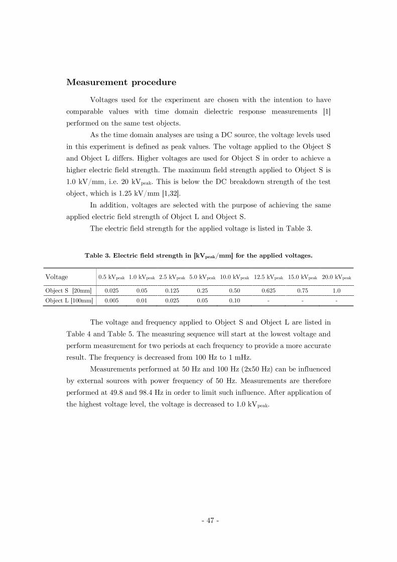
Measurement procedure

Voltages used for the experiment are chosen with the intention to havecomparable values with time domain dielectric response measurements [1]performed on the same test objects.

As the time domain analyses are using a DC source, the voltage levels usedin this experiment is defined as peak values. The voltage applied to the Object Sand Object L differs. Higher voltages are used for Object S in order to achieve ahigher electric field strength. The maximum field strength applied to Object S is1.0 kV/mm, i.e. 20 kVpeak. This is below the DC breakdown strength of the testobject, which is 1.25 kV/mm [1,32].

In addition, voltages are selected with the purpose of achieving the sameapplied electric field strength of Object L and Object S.

The electric field strength for the applied voltage is listed in Table 3.

Table 3. Electric field strength in [kVpeak/mm] for the applied voltages.

Voltage 0.5 kVpeak 1.0 kVpeak 2.5 kVpeak 5.0 kVpeak 10.0 kVpeak 12.5 kVpeak 15.0 kVpeak 20.0 kVpeak

Object S [20mm] 0.025 0.05 0.125 0.25 0.50 0.625 0.75 1.0Object L [100mm] 0.005 0.01 0.025 0.05 0.10 - - -

The voltage and frequency applied to Object S and Object L are listed inTable 4 and Table 5. The measuring sequence will start at the lowest voltage andperform measurement for two periods at each frequency to provide a more accurateresult. The frequency is decreased from 100 Hz to 1 mHz.

Measurements performed at 50 Hz and 100 Hz (2x50 Hz) can be influencedby external sources with power frequency of 50 Hz. Measurements are thereforeperformed at 49.8 and 98.4 Hz in order to limit such influence. After application ofthe highest voltage level, the voltage is decreased to 1.0 kVpeak.

- 48 -

Table 4. Measurement program for Object S.

Voltage [kVpeak] 0.5 1.0 2.5 5.0 10.0 12.5 15.0 20.0 1.0

Frequency [Hz] 98.4 49.8 20 10 5 2 1 0.5 0.2 0.1 0.01 0.001

Table 5. Measurement program for Object L.

Voltage [kVpeak] 0.5 1.0 2.5 5.0 10.0 1.0

Frequency [Hz] 98.4 49.8 20 10 5 2 1 0.5 0.2 0.1 0.01 0.001

Temperature

Measurements is to be performed at three different temperatures: 40 °C, 90°C (rated temperature) and 150 °C (temperature during failure). The sequence ofthe measurements is to be 40 °C, 90 °C, 150 °C and then repeated at 40 °C.

This measurement is to examine whether the measurement has changed theelectrical properties after a high voltage application. Such change can be caused byan anomalous (hysteresis) effect or desorption of volatiles during application ofhigh temperatures.

Humidity

In order to increase the water content within the stress control tube thetest object is immersed in distillate water at 90 °C. The object is kept at theseconditions for 39 days. Preparation of the test object is required before performingdielectric response measurement.

The test object was immediately placed in circulating cold water (4 ℃) for5 minutes, in order to quickly cool the object and lock the water inside the tube.The sample was paper-dried to remove water on the object’s surface. Layers ofplastic foil applied tight to avoid air bubbles form between the layers, and last,insulation tape was applied to cover the plastic foil.

This application was performed in order to avoid the moisture to diffuseout of the test object during the measurement.

- 49 -

Conditioning of the test object

The test object was pre-conditioned in a vacuum drying oven at 70 °C forthree days. After three days, the test object is connected to the experimental setup.In order for the test object to achieve a stable temperature, the object wastemperature conditioned for about one hour before performing measurements.

3.4 Measurement sequence

The measurement sequence for this thesis is:

1. Diffusion measurements

Measurement on three degrees of shrinkage of the stress controltube, at 30 °C, 60 °C and 90 °C.

2. Differential scanning calorimetry

Measurement of three degrees of shrinkage of the stress control tube.

3. Dielectric response measurementsi. Measurement 40 °C – 90 °C – 150 °C – 40 °Cii. Measurements at temperatures results found by differential

scanning calorimetry.

Measurements described in i. and ii. are performed for both Object Sand Object L.

iii. PTFE rod (100 mm) without application of a stress controltube at 40, 90 and 150 °C.

iv. Object S2 at 20 °C before placed in distillate water.v. Object S1 with plastic foil and insulating tape.vi. Object S2 in wet condition with plastic foil and insulating

tape at 20 °C.vii. Dissection of Object S2 after measurements.

- 50 -

- 51 -

Chapter 4

4 Results

4.1 Diffusion

Water uptake measurements were performed according to the descriptionin chapter 3. Small pieces of stress control tube, holding three different degrees ofshrinkage, were examined. The purpose of the experiment was to determine theirwater uptake characteristic as a function of both degree of shrinkage andtemperature.

Test measurements were first performed on three objects for determinationof a suitable measurement sequence. As water uptake is most rapid in thebeginning, measurements were performed more frequently the first hours.Measurements indicate that the stress control tube has a slow water uptake. Onthis basis, the measurement sequence was performed less frequently after the firsttwo hours.

At each measurement, the test sample’s weight in addition to the time anddate was noted. Eq. 2.29 can then be used to find the material’s gained moistureas a percentage of the dry weight, which is plotted as a function of time.

Figures made from the measurement indicate that the stress control tubekeeps absorbing water, and the test samples do not reach saturation during thisexperiment.

In addition, the measurements show signs on having two stages of diffusion.A steeper slope is visible in the beginning, and after a period, the water uptakecurve shifts towards a new and linear slope. This seems to be applicable formeasurements performed at 90 ℃ and 60 ℃, but also in some extent for themeasurement at 30 ℃.

- 52 -

4.1.1 Water absorption affected by the degree ofshrinkage

Analyses performed at samples kept at the same temperature shows thatthe water uptake by the stress control tube is dependent on the degree of shrinkage.When the shrinking increases, water uptake by the tube decreases.

A virgin stress control tube has the highest water uptake, while the fullyshrunk tube has the lowest. For a partially shrunk stress control tube, the wateruptake will lie in between the value for virgin and fully shrunk stress control tube.

After closer examination, partially shrunk samples appear to be unevenlyshrunk. A 10 cm tube was shrunken on a PTFE rod, and cut into 16 samples.Comparison of those samples shows that some have areas with higher degree ofshrinkage, while other have lower. This variation provides curves of the wateruptake that differs.

For both samples of virgin and fully shrunk SCT, the thickness of the tubeis uniform over its whole area. This provides a water uptake by the samples to beapproximately the same for the given degree of shrinkage.

Water uptake at 30 ℃

Figure 29 show the water concentration in percentage of the total weightas a function of days for the different degrees of shrinkage.

Water uptake for samples at 30 ℃ indicates that none of the samples hasreached saturation after 100 days. The water uptake seems to rather be increasing,than stagnate.

After reaching 100 days, the water concentration weight can be found to be1.15 % (virgin), 0.89 % (partially shrunk) and 0.82 % (fully shrunk).

- 53 -

Figure 29. Water content at 30 ℃, given as percentage of the total mass. Onesample of each degree of shrinkage is shown in the figure.


Measurements on samples held at 60 ℃, provides three curves havingsimilar shape. Water uptake by the stress control tubes will still not reachsaturation.

After being immersed in water for 95 days, the water concentration in thetube will be 3 % for virgin SCT, 2.4 % for partially shrunk SCT and 1.95 % forfully shrunk SCT.


- 54 -


Test samples kept at 90 ℃ provides the highest water uptake by the stresscontrol tube. Still, there is no sign of saturation in the test samples, but rather alinearly increase.


The water uptake by the stress control tubes seems to have two differentphases of diffusion. The first phase follows a typical saturation curve, while thesecond phase has a water uptake following an approximate linear increase.

The daily increase in water uptake during second phase will almost beidentical for the three samples. Theslope of the curve can be graphicallyfound as shown in Figure 32. Theincrease is given as the percentageincrease per day.

Values of the increase in wateruptake can thereby be found to be0.046 %/day (virgin), 0.045 %/day(partially shrunk) and 0.040 %/day(fully shrunk).

Because the water uptake hastwo phases, the diffusion coefficient Dx

is difficult to determine by use of

Figure 32. Graphically determination of thewater increase per day.

0.00

1.00

2.00

3.00

4.00

5.00

6.00

7.00

8.00

9.00

0 10 20 30 40 50 60 70 80 90 100 110

Con

cent

ratio

n[%

]

Time [days]

Water Uptake at 90 ℃Virgin P art ially shrunken Fully shrunken

0.046 %/ day

0.045 %/ day

0.04 %/ day

- 55 -

equation for Gmeasured and Gcalculated (Eq. 3.1 and Eq. 3.2). Using the formulas willnot provide a good curve fitting.

Due to the unknown value of the diffusion coefficient, the water content inthe test object used for dielectric response measurement cannot be mathematicallycalculated. An approximated value of the water content is found graphicallyinstead.

4.1.2 Water absorption affected by temperature

Results show that the water uptake increases with temperature. The slopeof the water uptake is also highest at 90 ℃, presenting the highest increase inconcentration.

Figure 33 gives water uptake curves for partially shrunk stress control tubeat the three temperatures. At each temperature, two test samples are used andthus providing two different curves. The two curves indicate that the samples havedifferent water uptake, as the concentration differs through the whole experiment.

After closer examination, the stress control tube is found to be unevenlyshrunk, giving different thickness of the samples. The sample with the highestdegree of shrinking, i.e. the thickest, have the lowest water uptake.

For virgin and fully shrunk stress control tube, the water uptake isapproximately identical for both measurement. Figures illustrating this are foundin Appendix A2.

Figure 33. Water uptake for partially shrunk stress control tube at 30, 60 and 90℃. Results from two test samples at each temperature are shown.

- 56 -

The curves for water uptake at 30 and 60 ℃ seems to have reached theirmaximum water content, however, this is not the case. A small increase in wateruptake at 30 ℃ and 60 ℃ is visible in respectively Figure 29 and Figure 30.

Water content for six different partially shrunk test samples after 80 days,is listed in Table 6. The water uptake at 90 ℃ is approximately three times higherthan for 60 ℃ and approximately seven times higher than samples at 30 ℃.

Table 6. Water content for six test samples of partially shrunk SCT after beingimmersed for 80 days.

Temperature

Sample 1 Sample 2

30 ℃ 6.75 % 6.28 %60 ℃ 2.29 % 2.00 %90 ℃ 1.00 % 0.82 %

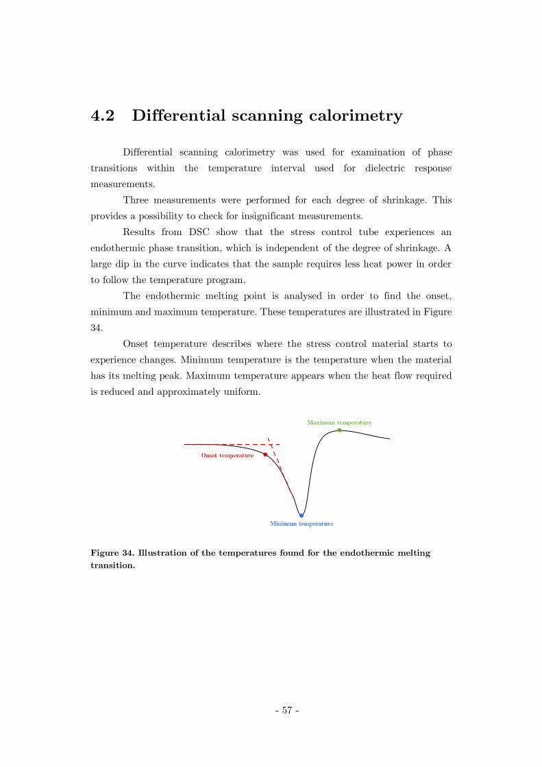
- 57 -


Differential scanning calorimetry was used for examination of phasetransitions within the temperature interval used for dielectric responsemeasurements.

Three measurements were performed for each degree of shrinkage. Thisprovides a possibility to check for insignificant measurements.

Results from DSC show that the stress control tube experiences anendothermic phase transition, which is independent of the degree of shrinkage. Alarge dip in the curve indicates that the sample requires less heat power in orderto follow the temperature program.

The endothermic melting point is analysed in order to find the onset,minimum and maximum temperature. These temperatures are illustrated in Figure34.

Onset temperature describes where the stress control material starts toexperience changes. Minimum temperature is the temperature when the materialhas its melting peak. Maximum temperature appears when the heat flow requiredis reduced and approximately uniform.

Figure 34. Illustration of the temperatures found for the endothermic meltingtransition.

- 58 -

4.2.1 Virgin

The results from DSC analysis of the endothermic melting peak are listedin Table 7. The results indicate that the onset temperature of the melting transitionoccurs at a temperature slightly above the rated temperature for XLPE cables (90℃).

Mean value of the onset temperature for a virgin stress control tube is foundto be 93 ℃. Mean value of the minimum temperature is 104.8 ℃ and for maximumtemperature 118.3 ℃.

Table 7. DSC analysis of maximum endothermic phase transition for a virginstress control tube.

Measurement 1 Measurement 2 Measurement 3Mean value

First run Second run First run Second run First run Second run

Onset 96.6 ℃ 90.1 ℃ 94.4 ℃ 90.6 ℃ 94.8 ℃ 91.9 ℃ 93.0 ℃

Minimum 103.1 ℃ 105.5 ℃ 104.4 ℃ 105.6 ℃ 103.4 ℃ 106.9 ℃ 104.8 ℃

Maximum 118.4 ℃ 119.1 ℃ 114.1 ℃ 119.8 ℃ 117.0 ℃ 121.2℃ 118.3 ℃

Figure 35 shows the curves for DSC measurement 2. The blue curve presentsthe first run, which has a local endothermic peak at 80 ℃. During the second run(red curve), this local peak disappears and less power is required from the samplesto follow the temperature program.

Figures for the first and third measurement can be found in Appendix B2.Both have similar curves as for the second measurement, with a local peak atapproximately 80 ℃. The first measurement shows a more unstable powerconsumption, with both endothermic and exothermic peaks.

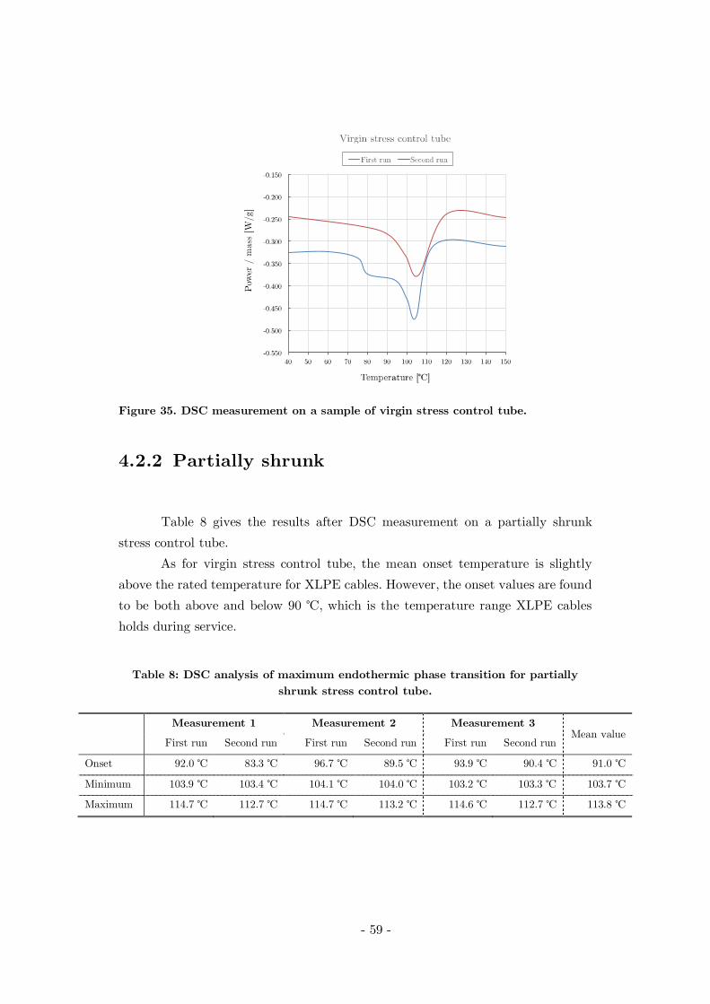
- 59 -

Figure 35. DSC measurement on a sample of virgin stress control tube.

4.2.2 Partially shrunk

Table 8 gives the results after DSC measurement on a partially shrunkstress control tube.

As for virgin stress control tube, the mean onset temperature is slightlyabove the rated temperature for XLPE cables. However, the onset values are foundto be both above and below 90 ℃, which is the temperature range XLPE cablesholds during service.

Table 8: DSC analysis of maximum endothermic phase transition for partiallyshrunk stress control tube.



Onset 92.0 ℃ 83.3 ℃ 96.7 ℃ 89.5 ℃ 93.9 ℃ 90.4 ℃ 91.0 ℃

Minimum 103.9 ℃ 103.4 ℃ 104.1 ℃ 104.0 ℃ 103.2 ℃ 103.3 ℃ 103.7 ℃

Maximum 114.7 ℃ 112.7 ℃ 114.7 ℃ 113.2 ℃ 114.6 ℃ 112.7 ℃ 113.8 ℃

- 60 -

Mean value for the minimum temperature is found to be 103.8 ℃, while themaximum temperature’s mean value is 113.8 ℃. During the first run, the onsettemperature is slightly higher than the second run, with respectively 94.2 ℃ and87.7 ℃.

Figure 35 shows the curves for the first DSC measurement. The blue curvepresents the first run, and the second run is represented by the red curve.

Figure 36. DSC measurement for a partially shrunk stress control tube sample.

The partially shrunk sample has, in similar to a virgin sample, a localendothermic peak at approximately 80 ℃. This local peak disappeared during thesecond run, and also here the sample requires less power to follow the temperatureprogram.

Figures for the second and third measurement can be found in AppendixB2.

- 61 -

4.2.3 Fully shrunk

Table 8 gives the results after DSC measurement on a fully shrunk stresscontrol tube. The results are similar to the partially shrunk tube; however, the firstrun does not have a local peak. The curve for the first and second run is almostidentical, except that the second run has a slightly smaller power consumption.

The mean values are similar to both virgin and partially shrunken, withonset temperature of 92 ℃, minimum temperature of 103.8 ℃ and maximumtemperature of 114 ℃.

Figures for second and third measurement are found in Appendix B2.

Table 9. DSC analysis of maximum endothermic phase transition for fully shrunkstress control tube.



Onset 91.9 ℃ 89.9 ℃ 92.0 ℃ 91.7 ℃ 97.3 ℃ 89.6 ℃ 92.0 ℃

Minimum 103.0 ℃ 103.2 ℃ 105.0 ℃ 104.7 ℃ 103.6 ℃ 103.3 ℃ 103.8 ℃

Maximum 113.8 ℃ 112.5 ℃ 114.8 ℃ 114.7 ℃ 114.5 ℃ 113.8 ℃ 114.0 ℃

Figure 37. DSC measurement for a fully shrunk stress control tube sample.

- 62 -

4.2.4 Results from differential scanningcalorimetry

DSC measurement for the three degrees of shrinkage are separated into firstand second run, and then combined in Figure 38. The result show that both virginand partially shrunk stress control tube experience a local peak at approximately80 ℃, but such local peak are not visible for the fully shrunken. The local peak istherefore likely due to incomplete shrinking.

Figure 38. Curves from DSC measurement of the three degrees of shrinkage, divided introfirst and second run.

The curves for partially and fully shrunk SCT are similar in both the firstand second run, except for the local peak. Results from DSC measurement of thevirgin sample show a smaller specific power consumption, and a smallerendothermic peak.

Results from DSC measurement show an endothermic peak within thetemperature interval used for dielectric response measurement. Further analysis isto be performed in order to examine if this phase transition changes the electricalproperties of the material.

The test object used in dielectric response measurement has a partiallyshrunken tube. Temperatures used for further investigations have been chosen tobe 94 ℃, 104 ℃ and 114 ℃.

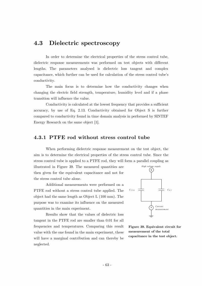
- 63 -

4.3 Dielectric spectroscopy

In order to determine the electrical properties of the stress control tube,dielectric response measurements was performed on test objects with differentlengths. The parameters analysed is dielectric loss tangent and complexcapacitance, which further can be used for calculation of the stress control tube’sconductivity.

The main focus is to determine how the conductivity changes whenchanging the electric field strength, temperature, humidity level and if a phasetransition will influence the value.

Conductivity is calculated at the lowest frequency that provides a sufficientaccuracy, by use of Eq. 2.13. Conductivity obtained for Object S is furthercompared to conductivity found in time domain analysis in performed by SINTEFEnergy Research on the same object [1].

4.3.1 PTFE rod without stress control tube

When performing dielectric response measurement on the test object, theaim is to determine the electrical properties of the stress control tube. Since thestress control tube is applied to a PTFE rod, they will form a parallel coupling asillustrated in Figure 39. The measured quantities arethen given for the equivalent capacitance and not forthe stress control tube alone.

Additional measurements were performed on aPTFE rod without a stress control tube applied. Theobject had the same length as Object L (100 mm). Thepurpose was to examine its influence on the measuredquantities in the main experiment.

Results show that the values of dielectric losstangent in the PTFE rod are smaller than 0.01 for allfrequencies and temperatures. Comparing this resultvalue with the one found in the main experiment, thesewill have a marginal contribution and can thereby beneglected.

Figure 39. Equivalent circuit formeasurement of the totalcapacitance in the test object.

A

↯High voltage supply

C P T FE C SC T

Curren tm easurem en t

- 64 -

The dielectric loss tangent for a PTFE rod is illustrated Figure 40. A largedispersion can be observed, but the losses have a minor change as the temperatureincreases.

Figure 40. Dielectric loss tangent for a PTFE rod without a stress control tube.

Analysis of the complex permittivity depicts that it has an approximatelyconstant value of 5, with small variations from 4.8 to 5.2, for all measurements(Figure 41). It appears to be independent of frequency, voltage and partlytemperature. Results from measurements show that an increase in temperatureyields a slightly smaller value of .

Figure 41. Complex permittivity, , for a PTFE rod a stress control tube.

Complex capacitances for the PTFE rod have a similar shape as found fordielectric loss tangent and complex permittivity. As is connected to by theconstant C0, its value will be constant and independent of the frequency, electricfield and temperature. Comparing this value to the ones measured at Object L, itsinfluence can be assumed negligible (Figure 42).

0.000001

0.00001

0.0001

0.001

0.01

0.1

1

0.01 0.1 1 10 100

Die

lect

ric

loss

tang

ent,

tanδ

Frequency [H z]

40 ℃ 90 ℃ 150 ℃

1

3

5

7

9

0.01 0.1 1 10 100

Com

plex

per

mit

tivi

ty,�

'

Frequency [H z]

40 ℃ 90 ℃ 150 ℃

- 65 -

Figure 42. Real value of complex capacitance for Object L and PTFE rod.

The values of , has a large dispersion of values as found for andthe curves will be similar as found in Figure 40. Its value is compared to the onemeasured on Object L (Figure 43) and is also assumed negligible.

Figure 43. Imaginary value of complex capacitance for Object L and PTFE rod.

1.0E-14

1.0E-13

1.0E-12

1.0E-11

1.0E-10

1.0E-09

0.01 0.1 1 10 100

Com

plex

capa

cita

nce,

C'

[F]

Frequency [Hz]

40 ℃ 90 ℃ 150 ℃ PT FE

1.0E-17

1.0E-16

1.0E-15

1.0E-14

1.0E-13

1.0E-12

1.0E-11

1.0E-10

1.0E-09

1.0E-08

1.0E-07

1.0E-06

1.0E-05

0.001 0.01 0.1 1 10 100

Com

plex

capa

cita

nce,

C''

[F]

Frequency [Hz]

40 ℃ 90 ℃ 150 ℃ PT FE

- 66 -

4.3.2 Measurement on Object L

Measurement on Object L provides analysis in the electric field range of0.005–0.01 kV/mm. Dielectric response measurements were performed atfrequencies from 100 Hz to 1 mHz.

However, when the temperature was increased to 90 ℃ and 150 ℃, thelosses became substantial at the lowest frequencies. Losses at 1 mHz would thenexceed range at where the measuring instrument, IDA 200, can detect precisely.

The result can be observed as large spread in measured values, where IDA200 gives both positive and negative measurement results.

For that reason, analysis at these temperatures provides a restraint in thefrequency range to be from 100 Hz to 10 mHz at the highest temperatures.

The results in this section will be presented as a function of the frequency.All measurements at different temperatures are combined into one figure thatprovides an opportunity to compare the effect of changes in the frequency, electricfield and temperature. Electric field dependency for a parameter is detected wherethe curves at the same temperature have a deviation.

Curves with results from dielectric response measurement on Object L, isfound in Appendix C1.

Dielectric loss tangent,

Values for the dielectric loss tangent for measurements on Object L arepresented in Figure 44. Results show that the losses increases with temperature.

Furthermore, the dielectric loss tangent increases with decreasingfrequency. The highest dielectric loss tangent is thus observed at 150 ℃, at thehighest electric field and lowest frequency. At 10 mHz, tan have gained a valueabove 100, which is above the measuring range of IDA 200. Inaccuracies canthereby be expected for both complex capacitance and the dielectric loss tangent.

- 67 -

Figure 44. Dielectric loss tangent for measurement at Object L. All fields areincluded with a lower frequency limitation of 10 mHz.

The dielectric loss tangent for 40 ℃ and 90 ℃ has a significant lower valueand will for both be below 10 at 10 mHz. However, as the frequency is decreasedto 1 mHz, their value will be doubled.

For measurements at 150 ℃, a minor field dependence is observed forfrequencies below 10 Hz and is illustrated in Figure 45.

Figure 45. Dielectric loss tangent as a function of the electric field for 150 ℃.

0.01

0.1

1

10

100

1000

0.01 0.1 1 10 100

Die

lect

ric

loss

tan

gent

,ta

nδ

Frequency [Hz]

40 ℃ 90 ℃ 150 ℃

1

10

100

0.01 0.01 0.03 0.05 0.10

Die

lect

ric

loss

tang

ent,

tand

Electric field [kV/ mm]

10 mHz 100 mHz 1 Hz 10 Hz

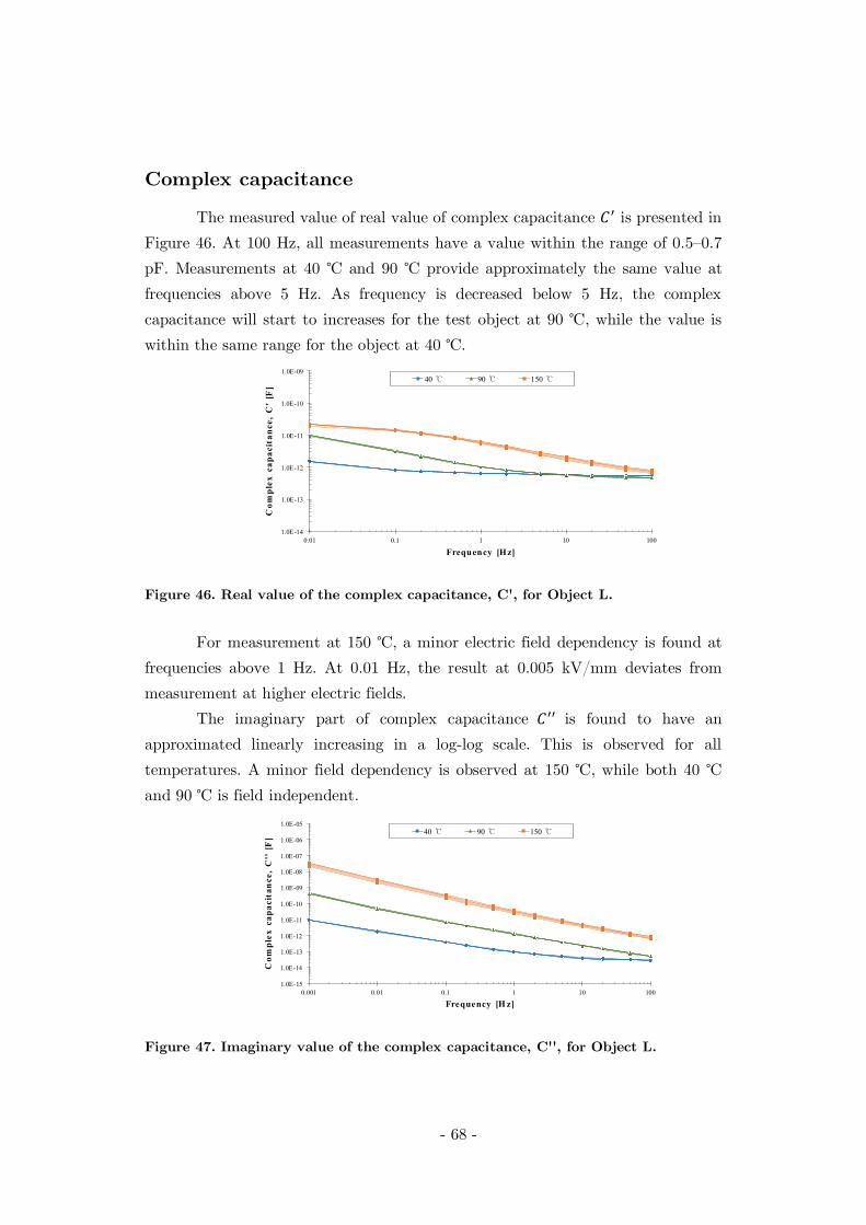
- 68 -

Complex capacitance

The measured value of real value of complex capacitance is presented inFigure 46. At 100 Hz, all measurements have a value within the range of 0.5–0.7pF. Measurements at 40 ℃ and 90 ℃ provide approximately the same value atfrequencies above 5 Hz. As frequency is decreased below 5 Hz, the complexcapacitance will start to increases for the test object at 90 ℃, while the value iswithin the same range for the object at 40 ℃.

Figure 46. Real value of the complex capacitance, C', for Object L.

For measurement at 150 ℃, a minor electric field dependency is found atfrequencies above 1 Hz. At 0.01 Hz, the result at 0.005 kV/mm deviates frommeasurement at higher electric fields.

The imaginary part of complex capacitance is found to have anapproximated linearly increasing in a log-log scale. This is observed for alltemperatures. A minor field dependency is observed at 150 ℃, while both 40 ℃and 90 ℃ is field independent.

Figure 47. Imaginary value of the complex capacitance, C'', for Object L.

1.0E-14

1.0E-13

1.0E-12

1.0E-11

1.0E-10

1.0E-09

0.01 0.1 1 10 100

Com

plex

capa

cita

nce,

C'

[F]

Frequency [Hz]

40 ℃ 90 ℃ 150 ℃

1.0E-15

1.0E-14

1.0E-13

1.0E-12

1.0E-11

1.0E-10

1.0E-09

1.0E-08

1.0E-07

1.0E-06

1.0E-05

0.001 0.01 0.1 1 10 100

Com

plex

capa

cita

nce,

C''

[F]

Frequency [H z]

40 ℃ 90 ℃ 150 ℃

- 69 -

4.3.3 Measurement on Object S

As the length of the PTFE rod is decreased from 100 mm to 20 mm, higherelectric field strengths are obtained during measurement on Object S.Measurements provide analysis of the material’s electrical properties in the electricfield range of 0.025 to 1.0 kV/mm with frequency varying from 100 Hz to 1 mHz.

As for measurement at Object L, the losses became substantial when thefrequency is decreased to 1 mHz, and is specially observed for measurement at 150℃. Here, the losses exceeded the range where IDA 200 can detect accurately. Theconsequence is a large variety in the value of the dielectric loss tangent. This isespecially true for the highest electric fields where the value is observed to bedecreasing. This is can be seen in Figure 48.

Figure 48. Dielectric loss tangent for Object S when including the entirefrequency range from 1 mHz to 100 Hz.

During the first measurement at 40 ℃, observations made indicated thatthe current had a deformation as the frequency was decreased. In addition, largecurrent peaks were noticed during application of the highest electric fields, i.e. 0.75kV/mm and 1.0 kV/mm.

During the measurement at 0.75 kV/mm, i.e. 15 kV, the experimentexperienced a malfunction at 20 Hz where IDA200 kept measuring for several hourswithout altering voltage or frequency. The measurement was stopped and newmeasurements were performed at 0.75, 1.0 and 0.05 kV/mm, i.e. 15, 20 and 1 kV.

0.01

0.1

1

10

100

1000

10000

0.001 0.01 0.1 1 10 100

Die

lect

ric

loss

tang

ent,

tanδ

Frequency [Hz]

40 ℃ 90 ℃ 150 ℃

- 70 -

Dielectric loss tangent,

When analysing of the results from the two measurements at 40 ℃, a fielddependence is observed. Figure 49 illustrates the dielectric loss tangent for bothlow electric fields, i.e. red curves, and the highest electric fields, i.e. blue curves.

Figure 49. Dielectric loss tangent at 40 ℃. Red curves illustrate the firstmeasurement, while the blue presents the second measurement.

A field dependence is observed for theelectric fields in the range from 0.5 – 1.0kV/mm. This dependence will increase as thefield increases and is illustrated in Figure 50.

Analysis of the dielectric loss tangent formeasurement at 90 ℃ and 150 ℃ is performedby examination of the curves in Figure 48.

Observations made indicate that bothhave a field dependence at low frequencies.However, as the value exceeds the value of 10,the accuracy of the measurement at 1 mHz canbe seen as insignificant.

For 90 ℃, dielectric loss tangent will exceed the value of 10 at 10 mHz,while 0.5 Hz for measurements at 150 ℃. At these frequencies, field dependencycan be observed.

A minor field dependence is observed at 50 Hz and 100 Hz for measurementsperformed at 90 ℃. This is likely due to measurements performed at their exactvalues. Measurement at these values can be influenced by external sources withpower frequency of 50 Hz.

0.01

0.1

1

10

100

0.001 0.01 0.1 1 10 100

Die

lect

ric

loss

tang

ent,

tand

Frequency [Hz]

0.025 - 0.625 kV/ mm 0.750 - 1.000 kV/ mm

Figure 50. Dielectric loss tangent as afunction of electric field strength.

0.01

0.1

1

10

100

0.000 0.250 0.500 0.750 1.000

Die

lect

ric

loss

tang

ent,

tand

Electrical field strength [kV/ mm]

1 mHz 10 mHz 100 mHz

1 Hz 10 Hz 100 Hz

- 71 -

Complex capacitance

Results indicate that increases when the frequency is decreased. Whenexamining results at 40 ℃, a minor field dependence is observed for measurementwhen applying the two highest electric field strengths. The deviation is most likelycaused by the two separate measurements, where measurement at the two highestfield strengths was delayed several hours.

For both 90 ℃ and 150 ℃, an electric field dependence is observed as forthe dielectric loss tangent. When the dielectric loss tangent exceeds 10, the valueof capacitance may not be retained. The field dependence is then likely caused byexceeding region where the measurement is given with good accuracy.

Figure 51. Complex capacitance C’ from measurement at Object S

The imaginary value the complex capacitance will, for all temperatures,increase when the frequency is decreased. At 90 ℃ and 150 ℃, the capacitance willbe independent of the electric field. Measurement results at 40 ℃ imply a fielddependence. This dependence is comparable to the one found for dielectric losstangent, as the curves in Figure 48 and Figure 52 are similar.

Figure 52. Complex capacitance C’’ from measurements on Object S.

1.0E-12

1.0E-11

1.0E-10

1.0E-09

1.0E-08

0.001 0.01 0.1 1 10 100

Com

plex

cap

acit

ance

,C

'[F

]

Frequency [Hz]

40 ℃ 90 ℃ 150 ℃

1.0E-14

1.0E-13

1.0E-12

1.0E-11

1.0E-10

1.0E-09

1.0E-08

1.0E-07

1.0E-06

0.001 0.01 0.1 1 10 100

Com

plex

capa

ciat

ance

,C

''[F

]

Frequency [H z]

40 ℃ 90 ℃ 150 ℃

- 72 -

4.3.4 Comparison of measurement at 40 ℃

Measurement on Object L

Two distinct measurement was performed at 40 ℃, one before increasingthe temperature to 150 ℃ and one after. A higher value is observed for the secondmeasurement, i.e. after being subjected to higher temperatures. Field independenceis found for both first and second run.

The difference between in the first and second run increases whendecreasing the frequency (Figure 53). At the highest frequencies, values of thecapacitances are both in the same range. When reaching the lowest frequencies,the capacitance in the second run have increased with one order of magnitude.

The value of the imaginary part is found to be higher during the secondrun for all frequencies. The value is six times higher at 1 mHz, but only 1.15 timeshigher at 100 Hz.

Figure 53. Real part of complex capacitance. Figure 54. Imaginary part of the complexcapacitance.

Values of the dielectric loss tangent are presented in Figure 55. Resultsshow that the losses during the second run are higher than observed during thefirst run. The deviation changes over the frequency range, and the highest deviationis found around 1 Hz. Here the value is 6 times higher than found in the first run.

Figure 56 show the calculated conductivity for the whole frequency range.However, the material’s conductivity will be most accurate if using values found at

1.00E-13

1.00E-12

1.00E-11

1.00E-10

0.001 0.01 0.1 1 10 100

Com

plex

capa

cita

nce,

C'[

F]

Frequency [Hz]

First run Second run

1.00E-14

1.00E-13

1.00E-12

1.00E-11

1.00E-10

1.00E-09

0.001 0.01 0.1 1 10 100

Com

plex

capa

cita

nce,

C''

[F]

Frequency [Hz]


- 73 -

the lowest frequency. Here, the losses in the object will dominated by theconductivity.

Results show that the conductivity increases after the test object has beensubjected to high temperatures. At 1 mHz, the conductivity in the first run is foundto be 33 pS/m. After being subjected to 150 ℃, the conductivity in the stresscontrol tube increases to 680 pS/m.

Figure 55. Dielectric loss tangent, for firstand second measurement at 40 ℃.

Figure 56. Conductivity, σ, for first andsecond measurement on Object L at 40 ℃.

Measurement on Object S

As for Object L, two distinct measurement was performed at 40 ℃, onebefore increasing the temperature to 150 ℃ and one afterwards. For the firstmeasurement, the second run (0.625 and 1.0 kV/mm) provides higher values forthe parameters. This is assumed to be caused by the two separate measurementand is disregarded in this analysis.

Comparison shows that the has a slightly higher value during the secondmeasurement for frequencies below 2 Hz, while a lower value for frequencies above5 Hz. In the range of 2 – 5 Hz, the value is approximately equal. The electric fielddependence found during the first measurements is not present in the result fromthe second measurement. The imaginary part, , has a marginally larger valueduring the second measurement.

0.01

0.1

1

10

0.001 0.01 0.1 1 10 100

Die

lect

ric

loss

tang

ent,

tand

Frequency [Hz]

F irst run Second run

1.00E-11

1.00E-10

1.00E-09

1.00E-08

1.00E-07

0.001 0.01 0.1 1 10 100

Com

duct

ivit

y,s

[S/m

]

Frequency [Hz]


- 74 -

Figure 57. Real value of complexcapacitance, C’, for Object S at 40 ℃.

Figure 58. Imaginary part of the complexcapacitance, C’’, for Object S at 40 ℃.

Figure 59 presents the dielectric loss tangent for the two measurements.The losses will have a minor increase in the second measurement for lowestfrequencies. At frequencies higher than 10 Hz, the value of dielectric loss tangentwill be in the same range.

The calculated conductivity is given by Figure 60 for the whole frequencyrange. The material’s conductivity is determined at 1 mHz, and will be largestduring the second run. The conductivity of the stress control tube will increasesfrom 11 to 31 nS/m, after being subjected to 150 ℃.

Figure 59. Dielectric loss tangent for ObjectS at 40 ℃.

Figure 60. Conductivity, σ, for Object S at40 ℃.

1.00E-12

1.00E-11

1.00E-10

0.001 0.01 0.1 1 10 100

Com

plex

capa

cita

nce,

C'[

F]

Frequency [Hz]


1.00E-13

1.00E-12

1.00E-11

1.00E-10

1.00E-09

1.00E-08

0.001 0.01 0.1 1 10 100

Com

plex

capa

cita

nce,

C''

[F]

Frequency [Hz]


0.01

0.1

1

10

100

0.001 0.01 0.1 1 10 100

Die

lect

ric

loss

tang

ent,

tand

Frequency [Hz]


1.00E-11

1.00E-10

1.00E-09

1.00E-08

1.00E-07

0.001 0.01 0.1 1 10 100

Con

duct

ivity

,s[S

/m]

Frequency [Hz]


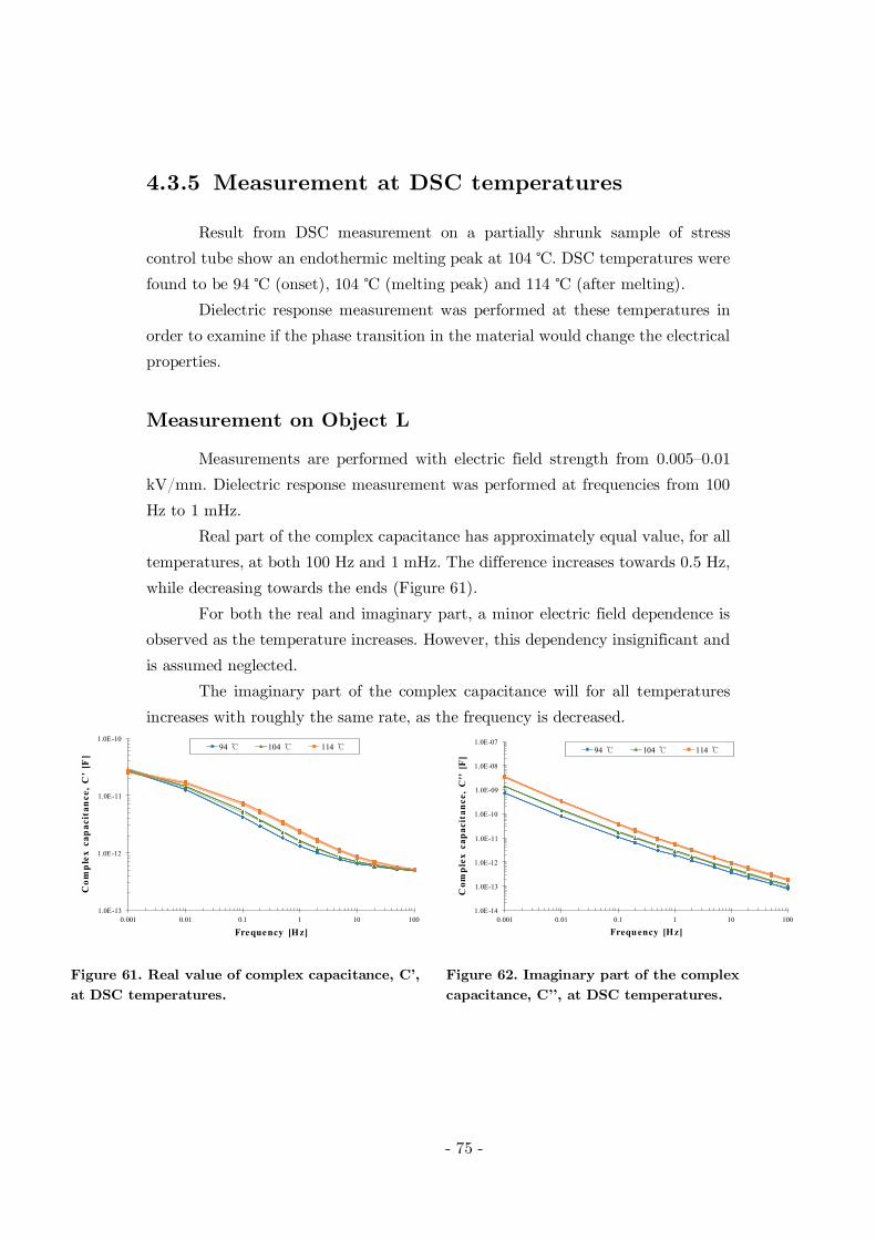
- 75 -

4.3.5 Measurement at DSC temperatures

Result from DSC measurement on a partially shrunk sample of stresscontrol tube show an endothermic melting peak at 104 ℃. DSC temperatures werefound to be 94 ℃ (onset), 104 ℃ (melting peak) and 114 ℃ (after melting).

Dielectric response measurement was performed at these temperatures inorder to examine if the phase transition in the material would change the electricalproperties.

Measurement on Object L

Measurements are performed with electric field strength from 0.005–0.01kV/mm. Dielectric response measurement was performed at frequencies from 100Hz to 1 mHz.

Real part of the complex capacitance has approximately equal value, for alltemperatures, at both 100 Hz and 1 mHz. The difference increases towards 0.5 Hz,while decreasing towards the ends (Figure 61).

For both the real and imaginary part, a minor electric field dependence isobserved as the temperature increases. However, this dependency insignificant andis assumed neglected.

The imaginary part of the complex capacitance will for all temperaturesincreases with roughly the same rate, as the frequency is decreased.

Figure 61. Real value of complex capacitance, C’,at DSC temperatures.

Figure 62. Imaginary part of the complexcapacitance, C’’, at DSC temperatures.

1.0E-13

1.0E-12

1.0E-11

1.0E-10

0.001 0.01 0.1 1 10 100

Com

plex

capa

cita

nce,

C'

[F]

Frequency [Hz]

94 ℃ 104 ℃ 114 ℃

1.0E-14

1.0E-13

1.0E-12

1.0E-11

1.0E-10

1.0E-09

1.0E-08

1.0E-07

0.001 0.01 0.1 1 10 100

Com

plex

capa

cita

nce,

C''

[F]

Frequency [Hz]

94 ℃ 104 ℃ 114 ℃

- 76 -

Dielectric loss tangent has a slight increase when increasing thetemperature. All measurement has the same curved shape, and no field dependenceis observed.

Calculation of the conductivity is performed and the result is presented inFigure 64. The material’s conductivity is found at 1 mHz, is observed increasingwhen temperature is increased.

Field dependence is observed for measurement performed after meltingtransition of the material, i.e. at 114 ℃. The conductivity of the stress control tubeis found increasing when the electric field strength is increased.

Figure 63. Dielectric loss tangent for Object L atDSC temperatures.

Figure 64. Calculated conductivity for Object L atDSC temperatures and all frequencies.

0.1

1

10

100

0.01 0.1 1 10 100

Die

lect

ric

loss

tang

ent,

tanδ

Frequency [Hz]

94 ℃ 104 ℃ 114 ℃

1.0E-09

1.0E-08

1.0E-07

0.001 0.01 0.1 1 10 100

Con

duct

ivit

y,σ

[S/m

]

Frequency [H z]

94 ℃ 104 ℃ 114 ℃

- 77 -

Measurements on Object S

Measurements on Object S is performed with electric field strength from0.025 – 1.0 kV/mm with frequencies in the range of 100 Hz to 10 mHz. Frequencyof 1 mHz was excluded, due to inaccuracies found when measuring at 40, 90 and150 ℃.

Real part of the complex capacitance will increase when decreasingfrequency or increasing the temperature. At 10 mHz, the value of the capacitancehas a large spread as the accuracy is decreased. This is illustrated in Figure 65.

Field dependence is not observed for the measurements, however, a smallervalue can be detected for the first measurement at 94 ℃.

The imaginary part of the conductivity will increase as frequency isdecreased, and is observed for all temperatures. A minor field dependence is foundat 50 Hz and 100 Hz, and is likely due to measurement at its exact value.

As observed for C’, the first measurement at 94 ℃ have a slightly smallervalue than found for higher electric fields. This might be caused by not reached auniform temperature before dielectric measurement was performed.

Figure 65. Real value of complex capacitance, C’,at DSC temperatures.

Figure 66. Imaginary part of the complexcapacitance, C’’, at DSC temperatures.

1.0E-12

1.0E-11

1.0E-10

1.0E-09

0.01 0.1 1 10 100

Com

plex

cap

acit

ance

,C

'[F

]

Frequency [Hz]

94 ℃ 104 ℃ 114 ℃

1.0E-12

1.0E-11

1.0E-10

1.0E-09

1.0E-08

1.0E-07

0.01 0.1 1 10 100

Com

plex

capa

ciat

ance

,C

''[F

]

Frequency [Hz]

94 ℃ 104 ℃ 114 ℃

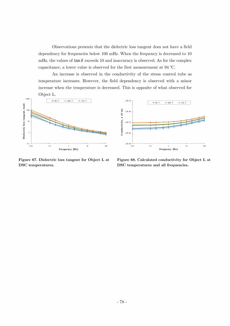
- 78 -

Observations presents that the dielectric loss tangent does not have a fielddependency for frequencies below 100 mHz. When the frequency is decreased to 10mHz, the values of tan exceeds 10 and inaccuracy is observed. As for the complexcapacitance, a lower value is observed for the first measurement at 94 ℃.

An increase is observed in the conductivity of the stress control tube astemperature increases. However, the field dependency is observed with a minorincrease when the temperature is decreased. This is opposite of what observed forObject L.

Figure 67. Dielectric loss tangent for Object L atDSC temperatures.

Figure 68. Calculated conductivity for Object L atDSC temperatures and all frequencies.

0.1

1

10

100

1000

0.01 0.1 1 10 100

Die

lect

ric

loss

tang

ent,

tanδ

Frequency [Hz]

94 ℃ 104 ℃ 114 ℃

1.0E-09

1.0E-08

1.0E-07

1.0E-06

1.0E-05

0.01 0.1 1 10 100

Con

duct

ivit

y,σ

[S/m

]

Frequency [Hz]

94 ℃ 104 ℃ 114 ℃

- 79 -

4.3.6 Conductivity

The conductivity of the test object can be calculated with the parametersfound in dielectric spectroscopy measurements. The relationship between dielectricloss tangent, permittivity and conductivity is seen in Eq. 2.3, and can be rewrittenas in Eq. 4.1.

This equation is an approximation and will apply when the relation | | ≫| | is fulfilled. At low frequencies, the losses in the test object will be dominatedby the conductivity. Using this relation the conductivity of the stress control tubecan be calculated when using tan and found at the lowest frequencies. A moredetailed description for calculation of the conductivity can be found in AppendixD.

The value of PTFE’s complex permittivity is in the calculations used as2.1. During measurement of a PTFE rod, the complex permittivity was measuredto have a value of 5. However, an increase from 2.1 to 5 will scarcely influence theresult of the conductivity.

The percentage increase or decrease when changing relative permittivityfrom 2.1 to 5.0 is presented in Table 10. The prevalent change is observed forObject L with only a 2.85 % decrease when increasing the complex permittivity.Due to minor changes, this is considered as insignificant for this thesis.

Table 10. Percentage change in conductivity when increasing the complexpermittivity from 2.1 to 5.0 in the calculations of conductivity.

Object L Object S

40 ℃ -2.85 % -1.64 %90 ℃ -0.83 % -0.68 %

150 ℃ +1.04 % -0.72 %

≈ tan ⋅ Eq. 4.1

- 80 -

Conductivity calculated for Object L

Calculation of the conductivity is performed for values obtained at 1 mHz.As the dielectric loss tangent can be assumed to have a good accuracy here.

Results show that the conductivity willincrease linear with the temperature. Theconductivity obtained at an electric fieldstrength of 0.1 kV/mm is presented as afunction of the temperature in Figure 69.

The transition phase at 94 ℃ – 114 ℃does not indicate a change in the electricalproperties of the material, as there is a linearincrease in the conductivity.

From Figure 69, the conductivity isobserved independent of the electric field in thefield range from 0.005 kV/mm to 0.1 kV/mm.

A hysteresis effect is observed, as the conductivity has increased whenperforming the second measurement at 40 ℃. The conductivity will then be 20times higher than during first measurement, however, only 2 timer less than theconductivity at 90 ℃.

Figure 70. Conductivity calculated for Object L with values obtained at 1 mHz.

1.00E-11

1.00E-10

1.00E-09

1.00E-08

1.00E-07

1.00E-06

0.00 0.03 0.05 0.08 0.10

Con

duct

ivity

,σ[S

/m]


Conduct ivity at 1 mHz

40 40 (2) 90 94 104 114 150

Figure 69. Conductivity obtainedat an electric field strength of 0.1kV/mm calculated at frequency of1 mHz.

1.00E-11

1.00E-10

1.00E-09

1.00E-08

1.00E-07

1.00E-06

20 40 60 80 100 120 140 160

Con

duct

ivity

,s[S

/m]

Temperature [℃]

- 81 -

Conductivity calculated for Object S

The conductivity is calculated for values obtained at 10 mHz.Measurements at 1 mHz provided inaccurate values, while the accuracy is assumedto be good for the results gained at 10 mHz.

For Object L, i.e. low electric fieldstrengths, the conductivity will increase linearwith temperature. Figure 71 presents theconductivity obtained at an electric fieldstrength of 1.0 kV/mm. The conductivity willno longer increase linearly with temperature.

Observations made indicates that thetransition phase at 94 ℃ – 114 ℃ will affect theconductivity. A larger increase discovered forthe transition phase.

Figure 73 presents the conductivity forall temperatures as a function of the electricfield applied. The figure indicates that the conductivity for Object S will beindependent of the electric field for all measurements except the first measurementat 40 ℃. Here, a field dependence is observed for field strengths above 0.5 kV/mm.

Figure 72. Conductivity calculated for Object S with values obtained at 10 mHz.

1.00E-11

1.00E-10

1.00E-09

1.00E-08

1.00E-07

1.00E-06

0.00 0.25 0.50 0.75 1.00

Con

duct

ivity

,s[S

/m]


Conduct ivit y at 10 mHz

40 ℃ 40 ℃ (2) 90 ℃ 94 ℃ 104 ℃ 114 ℃ 150 ℃

Figure 71. Conductivity obtainedat an electric field strength of 0.1kV/mm calculated at frequency of1 mHz.

1.00E-10

1.00E-09

1.00E-08

1.00E-07

1.00E-06

20 40 60 80 100 120 140 160

Con

duct

ivity

,s[S

/m]

Temperature [℃]

- 82 -

A hysteresis effect is also observed for Object S, with an increase in theconductivity after being exposed to 150 ℃. The conductivity will be 2.3 times largerduring the second run, which is much smaller than found for Object L. A fielddependence is observed for first measurement, which disappears during secondmeasurement. This field dependence makes the conductivity at 1.0 kV/mm to havea higher value during the first than the second measurement.

Comparison of the conductivity from measurement in timedomain and frequency domain

Time domain measurements on the object are performed in [1]. The samevoltages are used in both measurements in order to make comparison possible.

Conductivity calculated from time domain (TD) measurements have aslightly smaller than the value calculated in frequency domain (FD). This isillustrated in Figure 73, where TD is presented with a dashed line and FD with asolid line.

Figure 73. Conductivity as a function of the electric field strength for bothfrequency- and time domain analysis.

Both measurements at 40 ℃ (yellow lines) is observed having a fielddependence for electric field strengths above 0.5 kV/mm. During the secondmeasurement at 40 ℃ (blue lines), a field independence is observed formeasurement in frequency domain while time domain remains field dependent.

- 83 -

Measurements performed at 90 ℃ and 150 ℃, will in both FD and TD beindependent of the electric field strength.

Conductivity calculated at from measurement results at 10 mHz in FD haveobtained a higher value than those calculated from polarisation and depolarisationcurrents in TD. This difference can be found to be in the range of one – two ordersof magnitude.

For time domain analysis, space charge built-up is observed at hightemperatures which can cause an inaccuracy of the calculated conductivity. Thiscan be one reason why the values are deviating.

For frequency domain analysis, the relation | | ≫ | | is assumed to applyin most cases, and thus providing ≈ . For dielectric response on a stress controltube, the losses will be high causing the relation to be invalid.

The complex permittivity is calculated from the measured complexcapacitance divided by the geometric capacitance of the stress control tube. Thevalues obtained are presented in Figure 74 and Figure 75. From these, theimaginary part of the complex capacitance is found to be much larger than the realpart at 10 mHz.

Figure 74. Complex permittivity, ’, forObject S.

Figure 75. Complex permittivity, ’’, forObject S.

As a result, the conductivity should be calculated from Eq. 4.2 rather thanEq. 4.1. This will provide a reduced value of the conductivity.

σ = ωε ε ⋅ tan − Eq. 4.2

- 84 -

4.3.7 Measurement on wet object

In order to determine the effect of an increased humidity, the test object isplaced in water for 39 days. Dielectric response measurement is performed on thetest object, both before and after being immersed in water. Comparison can thusbe performed to identify any changes by an increased humidity.

To lock the water inside the stress control tube, plastic foil and insulationtape is applied. Measurements are performed on a dry object in order to verify thatsuch application will not have an appreciable effect on the results.

All results are given in Appendix C4.

Water content

As water uptake measurements indicate that none of the samples reachessaturation during the experimental work. Water content in the test object afterbeing immersed for 39 days, is determined by using Figure 76. In order to usevalues from Figure 76, the cylindrical test object has approximated to be a planeplate to be comparable to the test samples.

The yellow curves is defined for samples of stress control tube being exposedto water at both sides (s = h). However, when immersing the test object, only oneside is exposed (s = 2h). Using the cohesion yield in Eq. 2.31, the time required toreach the same concentration is dependent on s2. This will provide a concentrationin the test object that is a quarter of what found during water uptakemeasurements.

Figure 76. Determination of water uptake for partially shrunk samples. After 39days, the concentration in the test samples will be approximately 4.6 % and 1.15% for the test object.

0.00

1.00

2.00

3.00

4.00

5.00

6.00

7.00

8.00

0 10 20 30 40 50 60 70 80

Con

cent

ratio

n[%

]

Time [days]

Water Upt ake for part ially shrunk SCT at 90 ℃

Test object

Test samples

- 85 -

From Figure 76 the water concentration in the samples is found to beapproximately 4.6 % after 39 days. Consequently providing a water concentrationin the test object of 1.15 % if only exposed at one side. However, as the stresscontrol tube provides a watertight design, water will be present at both sides. Thetest object can thereby be assumed to have a higher water content after 39 days.

Effect of plastic foil and PVC insulation tape

Measurements indicate that application of a plastic foil and PVC insulationtape will not have a considerable effect on the results. As they have a resistivevalue much larger than the stress control tube, a marginal current will flow throughthe plastic foil and insulation tape.

Comparison of dielectric loss tangent and conductivity is presented inFigure 77 and Figure 78. For both parameters, a reduced field dependence isobserved for test object with plastic foil and PVC insulation tape. At the highestfrequencies the values is approximately identical, while the values will have a minordeviation at the lowest frequencies.

The effect of application of plastic foil and PVC insulation tape is regardedas insignificant and is thus neglected.

Figure 77. Dielectric loss tangent for test objectwith and without application of plastic foil andinsulation tape.

Figure 78. Conductivity for test object with andwithout application of plastic foil and insulationtape.

0.01

0.1

1

10

100

0.001 0.01 0.1 1 10 100

Die

lect

ric

loss

tang

ent,

tanδ

Frequency [Hz]

Without With

1.0E-12

1.0E-11

1.0E-10

1.0E-09

1.0E-08

1.0E-07

1.0E-06

0.001 0.01 0.1 1 10 100

Con

duct

ivit

y,σ

[S/m

]

Frequency [Hz]

Without With

- 86 -

Effect of an increased humidity

After being immersed in water for 39 days, the conductivity will have asignificant increase. This is illustrated in Figure 79 and Figure 80.

Measurements on a dry test object at 20 ℃ show a field dependence, wherethe conductivity increases when the applied field is increased. A field dependenceis also observed for the wet test object, this will thus decrease with an increasingelectric field strength. The decrease in conductivity is likely due to water diffuseout of the material during the measurements. Additionally, the large currents cancause an increased heat generation that can contribute to drying the object.

Figure 79. Conductivity for a wet and dry testobject calculated for all frequencies.

Figure 80. Conductivity for wet and dry testobject as a function of electric field strength at1 mHz.

Conductivity at 1 mHz with an electric field of 0.025 kV/mm is found tobe 10.6 pS/m for a dry test object, while increasing to 46 µS/m in wet condition.This provides an increase of almost six orders of magnitude.

An increase of six orders of magnitude can also be observed for the complexcapacitances at 1 mHz and 0.025 kV/mm. increases from 11.7 pF to 17.2 µF,while will have an increase from 15 pF to 62.6 µF.

1.0E-12

1.0E-11

1.0E-10

1.0E-09

1.0E-08

1.0E-07

1.0E-06

1.0E-05

1.0E-04

1.0E-03

1.0E-02

0.001 0.01 0.1 1 10 100

Con

duct

ivit

y,σ

[S/m

]

Frequency [H z]

Dry Wet

1.0E-13

1.0E-12

1.0E-11

1.0E-10

1.0E-09

1.0E-08

1.0E-07

1.0E-06

1.0E-05

1.0E-04

1.0E-03

0.000 0.250 0.500 0.750 1.000

Con

duct

ivit

y,σ

[S/m

]

Electrical field strength [kV / mm]

Dry Wet

- 87 -

Values of the dielectric loss tangent for a dry test object are found to havean electric field dependence from 0.5 kV/mm. Furthermore, the value will increaseas the frequency is decreased.

An electric field dependence can also be observed for the wet test object.This is, as found for the conductivity, decreasing with increasing field strength, i.e.with longer expose time with atmospheric conditions. It can then be assumed thatthe decrease in water content influences the results, providing a decrease indielectric loss tangent.

Frequency dependence can be observed for the two first measurements, i.e.0.025 and 0.05 kV/mm. This dependence will decrease when the electric fieldstrength is increased, and a minor frequency dependence can thereby be observedfor the highest electric field strengths.

Figure 81. Dielectric loss tangent for a dry and wet test object.

0.01

0.1

1

10

100

1000

0.001 0.01 0.1 1 10 100

Die

lect

ric

loss

tang

ent,

tanδ

Frequency [Hz]

Dry Wet

- 88 -

- 89 -

Chapter 5

5 Discussion

5.1 Diffusion

Water saturation of the samples has not been reached during theexperimental work of this thesis. A deviation from the Fickian diffusion can beobserved as the water uptake follows two distinct phase of diffusion. This is likelycaused by a diffusion by the filling materials within the stress control tube. As twophase diffusion is observed, the diffusion coefficient cannot easily be determined bycurve fitting. The time required to achieve 99.9 % saturation content have thereforenot been determined in this thesis.

The highest water concentration is found for samples kept immersed inwater at 90 ℃. The free volume in the material will increase with temperature,providing an increased ability to absorb water. After 85 days, the concentration inthe samples will be: 7 % (virgin), 6.5 % (partially shrunk) and 5.3 % (fully shrunk).These values are significant, and they all appear to still be increasing.

The water uptake is found to be dependent of the degree of shrinkage. Thehighest water concentration is found for virgin samples, while the lowest is observedfor fully shrunk samples. As the stress control tube is expanded, the free volumewill increase. During heated the tube will shrink, causing a decrease in the freevolume and potential to absorb water.

When stress control tubes are applied to cable sections, the cross-section ofthe cable should be close to the stress control tube’s fully shrunk diameter. Thiswill reduce the stress control tube’s ability to diffuse water.

For wet constructions of XLPE cables, water can be present during service.If the stress control tube is being exposed to an increased humidity for a long time

- 90 -

period, its electrical properties could be expected to start change which eventuallycould lead to a failure.


The stress control tube has a phase transition for temperatures below 150℃. An endothermic thermal transition is observed in the temperature range of 94℃ to 114 ℃, with a maximum melting temperature at 104 ℃.

Local peaks are observed during first measurement on virgin and partiallyshrunk samples, located at a temperature of 80 ℃. These peaks will disappearsduring second measurement and are not observed for fully shrunk samples. Thelocal peaks thus assumed to be caused by incomplete shrinking.

The phase transition provides the stress control tube to experience changesfrom a semi-crystalline to an amorphous state. The semi-crystalline–amorphousinterfaces can act like carrier traps. If these regions are heated up to their meltingpoint, these regions can gradually disappear and release these trapped carriers.This will make the material more electrically conductive, increasing theconductivity. [35]

When performing dielectric response measurements on Object S, this canbe observed as an increase in conductivity when reaching the thermal transitiontemperatures. The increased conductivity will be independent of the electric fieldstrength applied. Conversely, an increased conductivity is not observed at lowerfield strengths for Object L. Here, the conductivity will have a linear increase withtemperature.

Thermal transition located slightly above the rated temperature of XLPEcables, causing the conductivity to increase at high electric field strengths. Insituation where to have an overload, the temperature for the XLPE cable sectioncan be assumed to increase beyond its rated value. If this endures for a long timeperiod, the electrical properties of the stress control tube can experience anincreased conductivity which contributes to an increasing heat generation in thetube. However, as the increase in conductivity is minor, this is not assumed to becausing critical conditions.

- 91 -

5.3 Dielectric spectroscopy

Dielectric loss tangent

Results from dielectric spectroscopy imply that the stress control tube hasa high dielectric loss tangent. Values are found to be in the range from 0.1 to 1000,however, large dispersion is observed when reaching at the highest values. This islikely caused by the limit in the measuring range of IDA 200, providing inaccurateresults. The electric field dependence observed at the lowest frequencies is therebyassumed to be caused by this inaccuracy.

The effect of the PTFE rod is neglected as the value is below 0.01 for alltemperatures, providing a minor influence on the main results. In addition, theobject will not observe considerable changes when applying plastic foil and PVCinsulation tape. As the resistivity of these is much higher than for the stress controltube, only an insignificant part of the leakage current will in flow there. The testobject’s configuration can thus be assumed to provide the electrical properties ofthe stress control tube alone.

Dielectric loss tangent is found to have an electric field dependence at lowtemperatures. For 40 ℃, this is observed for electric field strengths above 0.5kV/mm. This dependence cannot be observed for measurements at highertemperatures, and when performing the second measurement after being cooledfrom 150 ℃.

As proposed in [1], the higher values during the second run is likely causedby desperation of volatiles in the stress control tube. Thermogravimetricmeasurements have been performed on samples of stress control tube. The resultindicates that the weight of the sample is reduced after being exposed 150 ℃ fortwo hours. Analysis imply that stress control tube will have a desorption of volatilesubstances at high temperatures, which caused the material to be more conductive[1]. Another explanation suggests have been that the semi-crystalline content inthe stress control tube changes after cooling from 150 ℃ to 40 ℃ [1,36]. As thematerial becomes more conductive, this will explain the increased dielectric losstangent observed after exposed to temperatures up to 150 ℃.

- 92 -

Increasing the temperature will reduce the relaxation time constant, whichcauses the local peak in the dielectric loss tangent to appear at a higher frequency.This can provide different shapes of the dielectric loss tangent when changing thetemperature.

Complex capacitance

Complex capacitance is found increasing with decaying frequency. The realpart, ’, will experience a smaller increase than the imaginary part. The value willalso be independent of the electric field. The deviations observed is likely causedby inaccuracy and the malfunction caused by a deformation in the current. Theimaginary part, ’’ , obtains a higher value with decreasing frequency as theconductivity causes increasing losses.

The electric field dependence observed for tan at 40 ℃, is also to be seenfor ’’. This is likely caused by a field dependence in the conductivity, causingincreased losses at higher electric field strengths.

Conductivity

The conductivity is calculated at values obtained 1 mHz (Object L) and 10mHz (Object S). The conductivity is found independent of field for electric fieldstrengths up to 0.5 kV/mm. This field dependence is also observed duringmeasurement in time domain [1]. Increasing the field strength will provide anelectric field dependence for measurements at low temperatures, while stayindependent at the higher temperature.

The conductivity is dependent on the temperature as the charge carries willobserve an increased mobility providing a higher drift velocity. For lowertemperatures, the drift velocity will be more dependent of the electric field strength.This can imply why an electric field dependence observed during measurements at40 ℃.

The conductivity will have an increased conductivity when reaching thephase transition. As earlier stated, this can be caused by a transition from semi-crystalline to amorphous state, causing the material to have an increased electricalconductivity. This is observed even at temperatures slightly above the ratedtemperature for XLPE cables.

- 93 -

After being subjected to high temperatures, the conductivity of the materialhas increased. By compare both measurements at 40 ℃, the conductivity haveincreased with a factor of 20 for Object L and 2.3 times for Object S. The deviationin the increase can be caused by the hours exposed to high temperatures. Longerexposure time at high temperatures will increase the desorption of the volatiles inthe stress control tube, which causes the material to become more conductive.

Comparing the values found in time and frequency domain, a higher valueis observed for the conductivity obtained from the frequency domain. This can becaused by the fact that the relation | | ≫ | | will not apply for the stress controltube in the frequency range of 100 Hz to 1 mHz. As the calculation requires thisrelation to apply, the conductivity can obtain a higher value than intended.

The values obtained from time domain will at higher temperaturesexperience space charge build-up causing the polarization current to still bedecreasing. This provides inaccuracy in the measurements. [1]

Having an increased humidity of the test object, the stress control tube’sconductivity will experience a significant increase from 10-11 to 10-5 S/m formeasurements performed at 20 ℃. This increase was observed even though the testobject had not reached its saturation level. The water will provide a substantialincrease in the charge carriers, which increases the conductivity of the stress controlmaterial.

Closer examination of the stress control tube imply that the increasedconductivity have caused high heat dissipation at the interface between theelectrode and PTFE rod. Signs indicate that water have been accumulated at theinterface, however, no signs was found indicating tracking between the electrodes.

The high conductivity will provide a higher current passing through thestress control tube, providing an increased ohmic loss. This ohmic loss will provideheat generation increasing the temperature, which in turn causes the conductivityto increase further, i.e. thermal runaway. If the conductivity becomes too high, thesystem can suffer from a thermal breakdown.

The temperature increases, the heat will cause the tube to diffuse water anddry up. However, if the design avoids the water to diffuse out of the system, theincreased temperature can cause the water to condense and be trapped in theinterface between the stress control tube and joint or XLPE-cable.

- 94 -

As implied by [1], the stress control tube can be limited to only cover criticalparts of the system with no connection between the insulation screen andconduction, i.e. no connection between ground and high voltage potential. In suchconfigurations, the increased conductivity can cause critical enhancement at theedge of the stress control tube. This can increase the partial discharges leading tolower breakdown strength and damage the insulation, and possibly result in apremature failure in the cable system.

- 95 -

5.4 Sources of errors

1. Exceeding the measuring range of IDA 200

The measuring range of IDA 200 is limited to 0 – 10. This causes a deviationin the measured values causing a field dependence. This dependence can therebybe caused by IDA 200 and not the material.

2. Deformation in the current

As the electric field strength increases above 0.75 kV/mm, current spikesare observed when performing measurements at 40 ℃. These can be caused bydischarges, and is observed both at the positive and negative half-cycle.

Additionally, as the frequency decreases, the current’s shape will experiencea deformation caused by harmonic content in the current. This deformation willincrease when the frequency decreases, as the conductivity becomes moredominating.

The current spikes may have caused an inaccuracy, providing a higher valuethan expected. At higher temperature, these will not be present.

3. Improper water preservation

Paper foil and insulation tape is used in order to avoid the water diffuseout during measurements. Observations made indicate that the material will diffusewater during measurement, proving a field dependence where the values decreasewith increasing field strength.

4. Calculation of the conductivity

The conductivity is calculated with a formula that requires | | ≫ | |toapply. Measurements suggest that this does not apply for this experiment, which can causethe calculated conductivity to be larger than that originally.

- 96 -

- 97 -

Chapter 6

6 Conclusion

From experimental work in the laboratory, the dielectric loss tangent isfound to be significant when reaching lower frequencies caused by the conductivity.

Measurement results imply that the conductivity of the stress control tubewill be dependent on the temperature, providing a larger conductivity as thetemperature is increased.

A field dependence is observed for the conductivity at 40 ℃. Thisdependence is identified for electric field strengths above 0.5 kV/mm. For highertemperatures, the conductivity becomes independent of the temperature.

The stress control tube will not have a reversible change from highlyconductive to resistive state. After being exposed to a temperature of 150 ℃, thematerial’s conductivity will increase. This implies that the electrical properties ofthe stress control tube experiences changes in the electrical properties after exposedto high temperatures.

Measurements show that the stress control tube have phase transition onthe temperature range of 94 ℃ to 114 ℃. When heating the material to itsendothermic transition temperature, the conductivity will experience an increase.

When increasing the humidity, the conductivity experiences a significantincrease of almost six orders of magnitude. This implies that the conductivity isstrongly dependent on the humidity level.

- 98 -

From the experimental work, changes in the temperature and electrical fieldstrengths performed on a dry test object will not cause any critical changes. Thehysteresis effects found in the stress control tube provide a small increase in theconductivity, after exposed to high temperatures for a short time. A minor effectis also observed by the thermal transition phase of the stress control tube.

However, when increasing the humidity level of the test object, theconductivity experienced a significant increase. With an increase of six order ofmagnitude, such currents can causes critical changes. An increased heat generationcan cause the material to suffer from a thermal breakdown.

If the stress control tube is limited to cover parts of the cable system, theincreased conductivity can cause critical field enhancement at the edge of the stresscontrol tube which can lead to a breakdown.

6.1 Further work

This master thesis has examined the effect of an increased temperature,electrical field strength and humidity level. Both increased temperature andelectrical field strengths did not cause critical changes, while the increased humidityprovided significant changes.

Measurement performed on the wet test object indicated that the plasticfoil and PVC insulation tape did not provide a sufficient protection against thewater diffuse out of the object. In addition, rust was observed at both electrodes.Further work should improve the test object and test setup, avoiding diffusion andrust. If such is achieved, the wet stress control tube can be examined for electricfield dependence.

Another interesting situation is to determine how a wet stress control tubewill be influenced when increasing the temperature, as this experiment is performedat 20 ℃.

- 99 -

7 Bibliography

[1] Henrik Enoksen, Sverre Hvidsten, Mai-Linn Sanden, and Frank Mauseth,"Temperature and Electric Field Dependence of the Time Domain DielectricResponse of a Medium Voltage Cable Joint Stress Control Sleeve," SINTEFEnergy Research and Norwegian University of Science and Technology,Trondheim, 2015.

[2] Walter S. Zaengl, "Dielectric spectroscopy in time and frequency domain for HVpower equipment. I. Theoretical considerations," Electrical Insulation Magazine,IEEE, vol. 19, no. 5, pp. 5-19, 2003.

[3] Sverre Hvidsten, "Condition assessment of XLPE cable systems installed in the1980s," 2011.

[4] Erling Ildstad, TET 4195 High voltage Equipment – Cable Technology.Trondheim.

[5] Erling Ildstad, High Voltage Insulation Materials, TET4160.: Akademika forlag,2014.

[6] H Faremo, J.T. Benjaminsen, P.B. Larsen, and A. Tunheim, "Service Experiencefor XLPE Cables Installed in Norway - From Graphite Painted Insulation Screensto Axially and Radially Water Tight Cable Constructions," 1997.

[7] G. Bahder. (1984) Electrical cable joint structure and method of manufacture.[Online]. http://www.google.com/patents/US4487994

[8] N.H. Malik, A.A. Al-Arainy. , M. I. Qureshi, and F. R. Pazheri, "Calculation ofElectric Field Distribution at High Voltage Cable Terminations," in High VoltageEngineering and Application (ICHVE), 2010 International Conference on,October 2010, pp. 24 - 27.

[9] Hampool Enterprise. Medium Voltage tubing & Tape. Heat Shrinkable stress-control tubing. [Online]. http://www.hampool.com/En/ProductView.asp?ID=34

http://www.google.com/patents/US4487994

http://www.hampool.com/En/ProductView.asp?ID=34

- 100 -

[10]T. Christen, L. Donzel, F. Greuter, and Switzerland Corp. Res., ABB Switzerland,Baden-Dättwil, "Nonlinear resistive electric field grading part 1: Theory andsimulation," Electrical Insulation Magazine, vol. 26, no. 6, pp. 47 - 59, 2010.

[11]Eva Mårtensson, "Modelling electrical properties of composite materials,"Department of Electrical Engineering, Kungl Tekniska Högskolan, Stockholm,PhD 2003.

[12] X. Qi, Z. Zheng, and S. Boggs, "Engineering with nonlinear dielectrics," ElectricalInsulation Magazine, vol. 20, no. 6, pp. 27 - 34, 2004.

[13] Steven Boggs and Joe Yingneng Zhou, "Dielectric Property Measurement ofNonlinear Grading Materials," in Electrical Insulation and Dielectric Phenomena,2000 Annual Report Conference on, vol. 2, 2000, pp. 764 - 767.

[14]J.W. Hoffman, "Insulation enhancement with heat-shrinkable components,"Electrical Insulation Magazine, vol. 7, no. 2, pp. 33-38, 1991.

[15]Lise Donzel, Felix Greuter, and Thomas Christen, "Nonlinear Resistive ElectricField Grading Part 2: Materials and Applications," Electrical InsulationMagazine, vol. 27, no. 2, pp. 18 - 29.

[16]Philip Hofmann, Plane plate capacitor.

[17]Oral Büyüköztürk, Tzu-Yang Yu, and Jose Alberto Ortega, "A methodology fordetermining complex permittivity of construction materials based ontransmission-only coherent, wide-bandwidth free-space measurements," vol. 28,no. 4, pp. 349-359, April 2006.

[18]N. A. M. Jamail, M. A. M. Piah, and N. A. Muhamad, "Comparative Study onConductivity Using Polarization and Depolarization Current (PDC) Test," 2012.

[19]H.Faremo, J.T.Benjaminsen and E.Ildstad S. Hvidsten, "Condition Assessment ofWater Treed Service Aged XLPE Cables by Dielectric Response Measurements,"CIGRE Session 2000, vol. 21-201, pp. 1-8, August 2000.

[20] Y. Fieldman et al., "Time domain dielectric spectroscopy: An advanced measuringsystem," REVIEW OF SCIENTIFIC INSTRUMENTS, vol. 67, no. 9, pp. 3208-3216, SEP 1996.

- 101 -

[21] A. K. Jonscher, "Dielectric Relaxation in Solids," Chelsea Dielectric Press.London., 1983.

[22] Sverre Hvidsten, "ELK-30: Condition Assessment of High Voltage Apparatus.Power Cables: Dielectric response - General description and applied on cables,"2014.

[23] P. Werelius, R. Thärning, R. Eriksson, B. Holmgren, and U. Gäfvert, "Dielectricspectroscopy for diagnosis of water tree deterioration in XLPE cables," Dielectricsand Electrical Insulation, IEEE Transactions on, vol. 8, no. 1, pp. 27-42, 2001.

[24] Frank Mauseth, Knut Dahle Hammervoll, and Sverre Hvidsten, "DielectricProperties of Service Aged Medium Voltage XLPE Cable Joints," Solid Dielectrics(ICSD), 2010 10th IEEE International Conference on, pp. 1-4, 2010.

[25] A. K. Jonscher, "Dielectric Relaxation in Solids," 1999.

[26] Anders Helgeson, "Analysis of Dielectric Response Measurement Methods andDielectric Properties of Resin-Rich Insulation During Processing ," Departmentof Electric Power Engineering, KTH, 2000.

[27] Daniel Gotz, Hubert Schlapp, and Hein Putter, "Dielectric loss measurement ofpower cables using hamon approximation," SebaKMT, 2011.

[28] Bruce Duncan, Jeannie Urquhart, and Simon Roberts, "Review of Measurementand Modelling of Permeation and Diffusion in Polymers ," NPL report DEPC-MPR 2005.

[29] M.H. Klopffer and B. Flaconnèche, "Transport Properties of Gases in Polymers:Bibliographic Review," Oil & Gas Science and Technology, vol. 56, no. 3, pp. 223-244 , 2001.

[30] Chi-Hung Shen and George S. Springer, "Moisture Absorption and Desorption ofComposite Materials ," Department of Mechanical Engineering , The Universityof Michigan, 1975.

[31] Mettler Toledo. (2013) Mettler Toledo. [Online].http://us.mt.com/dam/Analytical/ThermalAnalysi/TA-PDF/51724550C_V09.13_TA_Komp_Bro_e.pdf

http://us.mt.com/dam/Analytical/ThermalAnalysi/TA-PDF/51724550C_V09.13_TA_Komp_Bro_e.pdf

- 102 -

[32] Mai-Linn Sanden, "Condition Assessment of Medium Voltage Cable Joints,"Department of Electric Power Engineering, Norwegian University of Science andTechnology, Trondheim, Specialization project 2014.

[33] Programma Electric AB, "User's manual for Insulation Diagnostic System IDA200," Sweden, 2002.

[34] GE Energy Service. Insulation Diagnostics System, IDA 200.

[35] S. Pélissou, H. St-Onge, and M.R. Wertheimer, "Electrical conduction ofpolyethylene below and above its melting point," vol. 23, no. 3, pp. 325-333, 1988.

[36] G. Teyssedre and C. Laurent, "Charge Transport Modelling in InsulationPolymeres: From Molecular to Macroscopic scale," vol. 12, no. 5, pp. 857-875.

[37] James E. Mark, Polymer Data Handbook, 2nd ed. Oxford: Oxford UniversityPress.

- I -

AppendicesAppendix A – Diffusion

A1 – Test procedure A2 – Curves for diffusion

Appendix B – Differential ScanningCalorimetry

B1 – Test procedure B2 – Curves for diffusion

Appendix C – Dielectric responsemeasurement

C1 – Measurement result, Object L C2 – Measurement result, Object S C3 - Measurement result at DSC temperatures C4 – Measurement result from wet object

Appendix D – Formulas used forcalculation of the conductivity

Appendix E – Dissection of the wet testobject

Appendix F – List of figures

Appendix G – List of tables

- II -

- III -

Appendix A – Diffusion

A1 – Test procedure for Mass UptakeMeasurement

The test procedure was followed point by point to limit the time inwhich the tube was out of the water container. By following the sameprocedure for each measurement, there will be formed a basis for comparison.The procedure is followed in 10 steps.

Preparation of equipment in advance of the experiment

1) The tube was cut into thin pieces that hold a weight of less than twograms. Figure 82 illustrates the preferable geometry of the testspecimen. The size of n and l should be much larger than h, resultingin a dominating diffusion through the nl –surface. The diffusion is thenconsidered to have one-dimensional conditions, D(t) = Dx(t).

Figure 82: Geometry of test specimen.

2) To achieve a completely dry specimen, the stress control tubes are putin a vacuum drying oven for a week at 70 degrees. 12 hours beforemeasurement of the dry weight, the temperature in the desiccator isdecreased to 25 degrees.

- IV -

3) All the equipment is cleaned with isopropanol to avoid particles andimpurities to attach to the specimen and influence the measurementresult.

4) Three glass containers should be cleaned and filled with distillate waterand placed under different temperatures.

i. One glass is preheated to the given test temperature in advanceof the experiment. This should be used for the specimen to befully immersed.

ii. One glass is placed in the refrigerator. Cold distillate water isused to rapidly cool the specimen down to remove convectionalcurrents on the specimen.

iii. One glass should be kept at room temperature. The specimenis placed in this container for couple of seconds to decrease itstemperature. It should hold approximately the sametemperature, thus giving a better comparable value.

5) Mettler Toledo UMX2 is internally calibrated, and preformedautomatically by the gauge. Both the temperature and humidity of theenvironment is considered when calibrating. This should be performedwhen the time since last measurement becomes significant large.

6) Static charges in the surface of the test specimen are removed bymoving it a few times through an electrostatic precipitator. The staticcharge built up on the surface will attract dust and by moving itthrough the precipitator, the dust can be removed. The cancel of thecharge should be performed before placement on the weigh gauge.

- V -

Mass Uptake Measurement

7) The specimen is taken out of the desiccator and immediately placed inUMX2 for measurement. The date, time and dry-weight should benoted before placing the object in the water container.

8) The container with test specimen is placed in a heating cabinet exposedto a constant temperature. The specimen should at all time be entirelyimmersed in the distillate water.

9) The moist material should be continuously measured. Typically,diffusion characteristic has a higher water uptake in the beginning, butas time pass, the weight will approach the saturated value Mm. A testmeasurement is executed to determine the suitable period betweeneach measurement.

10) For each measurement, the following procedure is carried out.i. Equipment and working area are cleaned with isopropanol

before the test specimen is taken out. This to avoid impurities.ii. Two glass containers with respectively cold water (4 ℃) and

room temperate water ( 25 ℃) as well as paper sheets aremade ready.

iii. The specimen is taken out of the water container at testtemperature and immediately placed in the cold water.

iv. The measurement program is started with a delay of oneminute. This gives a minute to prepare the object before anautomatically measurement is performed and saved in an Excelsheet.

v. The specimen in then placed in the room temperate water fora couple of seconds before its surface is dried with paper sheets.The first paper sheet wipes away the largest part of the water.A second paper sheet is used for making sure that the objectdoes not have water left on its surface.

vi. For removal of the surface charge, the specimen is moved acouple of times through the electrostatic precipitator.

- VI -

vii. The specimen is placed on the UMX2 for measurement. Thedate, time and weight is saved in an excel document when thedelay has reached one minute. The specimen is then placedback in the water container.

11) The measurements are plotted as the water uptake (in percentage ofthe total weight) versus the time. The curve will then give thecharacteristic of the diffusion, and thus giving the possibility toproceed tentatively to find the diffusion constant, Dx.

The tests are repeated for each test specimen at the different experimentaltemperatures.

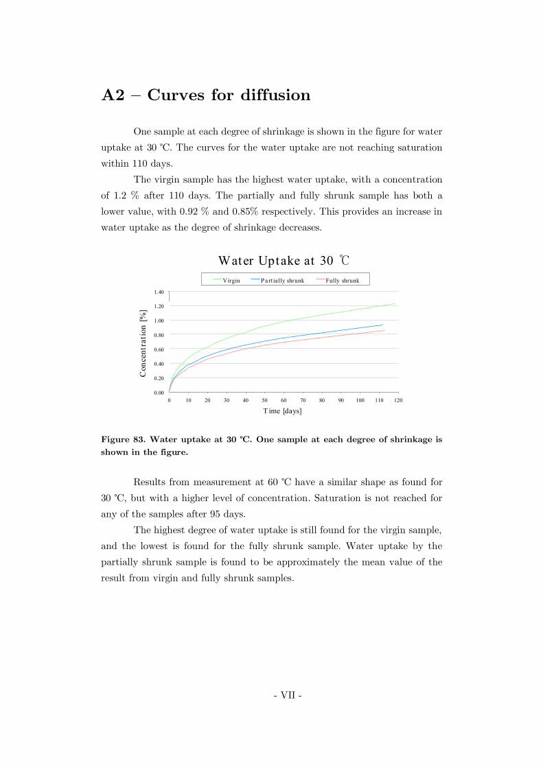
- VII -

A2 – Curves for diffusion

One sample at each degree of shrinkage is shown in the figure for wateruptake at 30 ℃. The curves for the water uptake are not reaching saturationwithin 110 days.

The virgin sample has the highest water uptake, with a concentrationof 1.2 % after 110 days. The partially and fully shrunk sample has both alower value, with 0.92 % and 0.85% respectively. This provides an increase inwater uptake as the degree of shrinkage decreases.

Figure 83. Water uptake at 30 ℃. One sample at each degree of shrinkage isshown in the figure.

Results from measurement at 60 ℃ have a similar shape as found for30 ℃, but with a higher level of concentration. Saturation is not reached forany of the samples after 95 days.

The highest degree of water uptake is still found for the virgin sample,and the lowest is found for the fully shrunk sample. Water uptake by thepartially shrunk sample is found to be approximately the mean value of theresult from virgin and fully shrunk samples.

0.00

0.20

0.40

0.60

0.80

1.00

1.20

1.40

0 10 20 30 40 50 60 70 80 90 100 110 120

Con

cent

rati

on[%

]

T ime [days]

Water Uptake at 30 ℃Virgin P a rt ially shrunk Fully shrunk

- VIII -


Measurement at 90 ℃ shows a linear increase after 10 days, andsaturation is not reached. As for 30 and 60 ℃, the water uptake increases witha decreasing degree of shrinkage.

For a virgin sample kept at 90 ℃, the water uptake after 105 days isfound to be 8 %. Both the partially and fully shrunk sample have lower wateruptake, but evince signs of increasing as seen for the virgin sample.

Water uptake for a stress control tube kept at rated temperature foran XLPE cable can be significant.


0.00

0.50

1.00

1.50

2.00

2.50

3.00

3.50

0 10 20 30 40 50 60 70 80 90 100

Con

cent

rati

on[%

]

Time [days]

Water Uptake at 60 ℃Virgin P artia lly shrunk Fully shrunk

0.00

1.00

2.00

3.00

4.00

5.00

6.00

7.00

8.00

9.00

0 10 20 30 40 50 60 70 80 90 100 110

Con

cent

rati

on[%

]

T ime [days]

Water Uptake at 90 ℃Virgin P a rt ially shrunk Fully shrunk

- IX -

When analysing the samples with the same degree of shrinkage, resultindicate that the water uptake will increase with temperature.

Figure 86 presents the water uptake by six virgin samples. Sampleskept at the same temperature have an approximated equal water uptake, andcan be seen by the overlap of the curves.

Figure 86. Water uptake by a virgin stress control tube. Two samples at eachtemperature are shown in the figure.

Analysis of the partially shrunk samples show curves with a greaterdispersion for samples kept at the same temperature. This is likely due to anuneven shrinkage of the samples.

Figure 87. Water uptake by a partially shrunk stress control tube. Two samplesat each temperature are shown in the figure.

0.00

1.00

2.00

3.00

4.00

5.00

6.00

7.00

8.00

9.00

0 10 20 30 40 50 60 70 80 90 100 110 120

Con

cent

ratio

n[%

]

T ime [days]

Water Uptake for Virgin SCT30℃ 60℃ 90℃

0.00

1.00

2.00

3.00

4.00

5.00

6.00

7.00

8.00

0 10 20 30 40 50 60 70 80

Con

cent

ratio

n[%

]

T ime [days]

Water Uptake for part ially shrunk SCT30℃ 60℃ 90℃

- X -

Result from fully shrunk samples is presented in Figure 88. The curvesfor the water uptake have a similar shape to the result found for virgin testsamples, but a lower value.

Samples kept at the same temperature have approximately equal wateruptake, given by the overlap of the curves.

Figure 88. Water uptake by a fully shrunk stress control tube. Two samples ateach temperature are shown in the figure.

0.00

1.00

2.00

3.00

4.00

5.00

6.00

0 10 20 30 40 50 60 70 80 90 100 110 120

Con

cent

rati

on[%

]

T ime [days]

Water uptake for fully shrunk SCT30℃ 60℃ 90℃

- XI -

Appendix B – Differential scanningcalorimetry

B1 – Test procedure DSC

The procedure for preparation of the DSC sample is performed in thefollowing steps.

1. The stress control tube is heated to the desired degree of shrinking forthe DSC measurement, and then cut into smaller pieces around onecm2.

2. These pieces are conditioned at 70 °C for a week in a vacuum dryingoven, and then held at 25 °C until removed. This procedure isperformed as for the diffusion experiment giving comparable results.

3. The tube is removed from the desiccator and immediately taken forpreparation for limitation of the influence from the surroundings.Gloves and a forceps should be used when preparing and to movingthe sample.

4. The crucible used for the DSC measurement has a volume of 40 µLand the samples of tube need to be cut into smaller pieces. The crucibleis used as a pan during measurement, and is heated from beneath. Thesample’s height should not be too large in order to avoid a temperaturegradient. Furthermore, the sample should be evenly distributed alongthe bottom of the crucible.

5. The DSC measurement program is set up for measurement. Atemperature interval is chosen and the measurement is named with theshrinking degree in addition to the number of sequence. Furthermore,the test specimen must be weighed and typed into the measurementprogram.

- XII -

6. The weight is found by placing the aluminium crucible on the scaleand reset to show zero weight. The specimen is placed in the crucibleand its weight is noted in the test program. A weight of 10mg is asuitable amount of sample for the analysis.

7. An aluminium lid should be placed on the top, sealing the crucible.Nitrogen is used during the DSC measurement and since it is desiredto have gas intrude into the crucible, three holes are made in the lidbefore sealing. A needle is used to make holes penetrating entirelythrough the lid.

8. Forceps is used to place the lid on top of the pan containing thespecimen. The crucible is then placed in an encapsulating press forsealing.

9. An empty crucible is made as above and used as a reference sample inthe measurement.

10. The test- and reference crucible are placed separately in the measuringdevice on each heating plate. Furthermore, both water-cooling and thenitrogen gas are checked to be in open position.

11. DSC-measurement is started from a computer, and is self-servicedduring the whole test period. Afterwards the measurement can beanalysed using the analysing program STARe Excellent.

- XIII -

B2 – DSC measurement results

Virgin stress control tube

Measurement 1

Results from the first DSCmeasurement on a virgin stresscontrol tube show that during thefirst run, the specific heat transferto the sample is quite unstable.

The curve show bothendothermic and exothermic peak.The maximum peak temperatureoccurs at approximately the sametemperature as the two othermeasurements.

The specific heat transfer isin the range of –0.2 to -0.46 W/g. Figure 89. Result from DSC measurement 1.

Measurement 2

The second measurementhas a more stable specific heat flowthan the first measurement.However, a local peak can also herebe found at 80 ℃.

During second run, thespecific heat flow is lower than thefirst run, and the local peak hasdisappeared.

The specific heat transfer isin the range of -0.23 to -0.47 W/g. Figure 90. Result from DSC measurement 2.

- XIV -

Measurement 3

The third measurement issimilar to the second measurementwith a local peak at 80 ℃.

The second run has a muchsmaller specific heat requirementthan the first run. This is also thelowest specific heat requirement byall samples. The local peak will alsohere disappear during the secondrun.

The specific heat transfer isin the range of -0.19 to -0.5 W/g. Figure 91. Result from DSC measurement 3.

Partially shrunk stress control tube

Measurement 1

The first measurement of apartially shrunk sample show thatthe first and second run is moresimilar than for a virgin sample.

A local peak is found duringthe first run. However, this peak issmaller than the one found in thevirgin samples. This peakdisappears during the second run.

The specific heat is in therange of -0.37 to -0.6 W/g.

Figure 92. Result from DSC measurement 1.

- XV -

Measurement 2

Results from the secondmeasurement are similar to thefirst.

The values in the first andsecond run are similar, but with alittle higher heat requirementduring the first run.

A local peak is found in thefirst run and disappears during thesecond run.

The specific heat is in therange of -0.32 to -0.55 W/g.


Measurement 3

The third measurement hasalmost identical specific heattransfer during the first and thirdmeasurement. A local peak duringthe first run is the difference thatdistinguishes them.

The specific heat is withinthe range of -0.38 to -0.61 W/g.This is the highest for threemeasurements, and the range withthe fully shrunken. The sample islikely a higher degree of shrinkagethan the two previous.


- XVI -

Fully shrunk stress control tube

Measurement 1

Results from the first DSCmeasurement of a fully shrunkstress control tube shows that thespecific heat during first and secondrun is approximately identical.

No local peak is presentduring this measurement.

The specific heat for themeasurement is within the range of-0.35 to -0.6 W/g.


Measurement 2

The second measurement issimilar the first.

The first and second run isalmost identical and no local peak isobserved.

The specific heat flowduring the measurement is withinthe range of -0.35 to -0.56 W/g.


- XVII -

Measurement 3

The third measurementdiffers out from the previous two.The first and second run is similar,however, a local peak can beobserved.

This measurement is similarto the third measurement of apartially shrunk sample. The localpeak is therefore likely caused by anincomplete shrinking.

The specific heat range iswithin -0.38 to -0.63 W/g.


- XVIII -

Appendix C – Results fromdielectric response measurements

Results from dielectric response measurements on Object S are hereprovided as figures. The figures presents the values of the dielectric losstangent, complex capacitances and the calculated conductivity for allmeasurements performed.

First, the results for measurements at 40, 90, 150 and 40 ℃ are givenfor Object L and Object S. Furthermore, the results from measurements atDSC temperatures are presented. At last, the measuring results fromexamination of an increased humidity are given. Results from the dry object,with and without plastic insulation, in addition to results from the wet objectmeasurements are presented.

- XIX -

C1 – Measurement result, Object L

Measurement at 40 ℃

Figure 98. Complex capacitance, , for ObjectL measured at 40 ℃.


Figure 100. Dielectric loss tangent for Object Lmeasured at 40 ℃.

Figure 101. Conductivity for Object Lcalculated from measurements at 40 ℃.

1.00E-13

1.00E-12

1.00E-11

0.01 0.1 1 10 100

Com

plex

capa

cita

nce,

C'[

F]

Frequency [Hz]

0.005 kV/ mm

0.010 kV/ mm

0.025 kV/ mm

0.050 kV/ mm

0.100 kV/ mm

0.010 kV/ mm

1.00E-14

1.00E-13

1.00E-12

1.00E-11

1.00E-10

0.001 0.01 0.1 1 10 100

Com

plex

capa

cita

nce,

C''

[F]

Frequency [Hz]

0.005 kV/ mm

0.010 kV/ mm

0.025 kV/ mm

0.050 kV/ mm

0.100 kV/ mm

0.010 kV/ mm

1.00E-12

1.00E-11

1.00E-10

1.00E-09

0.01 0.1 1 10 100

Com

plex

capa

cita

nce,

C'[

F]

Frequency [Hz]

0.025 kV/ mm

0.050 kV/ mm

0.125 kV/ mm

0.250 kV/ mm

0.500 kV/ mm

0.625 kV/ mm

0.750 kV/ mm

1.000 kV/ mm

0.050 kV/ mm

1.00E-12

1.00E-11

1.00E-10

1.00E-09

1.00E-08

1.00E-07

0.01 0.1 1 10 100

Com

plex

capa

cita

nce,

C''

[F]

Frequency [Hz]

0.025 kV/ mm

0.050 kV/ mm

0.125 kV/ mm

0.250 kV/ mm

0.500 kV/ mm

0.625 kV/ mm

0.750 kV/ mm

1.000 kV/ mm

0.050 kV/ mm

- XX -



Figure 103. Complex capacitance, , forObject L measured at 90 ℃.

Figure 104. Dielectric loss tangent for ObjectL measured at 90 ℃.

Figure 105. Conductivity for Object Lcalculated for measurements at 90 ℃.

1.00E-13

1.00E-12

1.00E-11

1.00E-10

0.01 0.1 1 10 100

Com

plex

capa

cita

nce,

C'[

F]

Frequency [Hz]

0.005 kV/ mm

0.010 kV/ mm

0.025 kV/ mm

0.050 kV/ mm

0.100 kV/ mm

0.010 kV/ mm

1.00E-14

1.00E-13

1.00E-12

1.00E-11

1.00E-10

1.00E-09

1.00E-08

0.001 0.01 0.1 1 10 100

Com

plec

capa

cita

nce,

C''

[F]

Frequency [Hz]

0.005 kV/ mm

0.010 kV/ mm

0.025 kV/ mm

0.050 kV/ mm

0.100 kV/ mm

0.010 kV/ mm

0.01

0.1

1

10

100

0.01 0.1 1 10 100

Die

lect

ric

loss

tang

ent,

tand

Frequency [Hz]

0.005 kV/ mm

0.010 kV/ mm

0.025 kV/ mm

0.050 kV/ mm

0.100 kV/ mm

0.010 kV/ mm

1.0E-10

1.0E-09

1.0E-08

1.0E-07

1.0E-06

0.01 0.1 1 10 100

Con

duct

ivity

,s[S

/m]

Frequency [Hz]

0.005 kV/ mm

0.010 kV/ mm

0.025 kV/ mm

0.050 kV/ mm

0.100 kV/ mm

0.010 kV/ mm

- XXI -




Figure 108. Dielectric loss tangent for ObjectL measured at 150 ℃.


1.00E-13

1.00E-12

1.00E-11

1.00E-10

0.01 0.1 1 10 100

Com

plex

capa

cita

nce,

C'[

F]

Frequency [Hz]

0.005 kV/ mm

0.010 kV/ mm

0.025 kV/ mm

0.050 kV/ mm

0.100 kV/ mm

0.010 kV/ mm

1.00E-13

1.00E-12

1.00E-11

1.00E-10

1.00E-09

1.00E-08

1.00E-07

1.00E-06

1.00E-05

0.001 0.01 0.1 1 10 100

Com

plex

capa

cita

nce,

C''

[F]

Frequency [Hz]

0.005 kV/ mm

0.010 kV/ mm

0.025 kV/ mm

0.050 kV/ mm

0.100 kV/ mm

0.010 kV/ mm

0

1

10

100

1000

0.01 0.1 1 10 100

Die

lect

ric

loss

tang

ent,

tand

Frequency [Hz]

0.005 kV/ mm

0.010 kV/ mm

0.025 kV/ mm

0.050 kV/ mm

0.100 kV/ mm

0.010 kV/ mm

1.0E-08

1.0E-07

1.0E-06

1.0E-05

0.01 0.1 1 10 100

Con

duct

ivity

,s[S

/m]

Frequency [Hz]

0.005 kV/ mm

0.010 kV/ mm

0.025 kV/ mm

0.050 kV/ mm

0.100 kV/ mm

0.010 kV/ mm

- XXII -

Measurement at 40 ℃, second run



Figure 112. Dielectric loss tangent for Object Lmeasured at 40 ℃, second run.

Figure 113. Conductivity for Object Lcalculated from measurements at 40 ℃, secondrun.

1.00E-13

1.00E-12

1.00E-11

1.00E-10

0.01 0.1 1 10 100

Com

plex

capa

cita

nce,

C'[

F]

Frequency [Hz]

0.005 kV/ mm

0.010 kV/ mm

0.025 kV/ mm

0.050 kV/ mm

0.100 kV/ mm

0.010 kV/ mm

1.00E-14

1.00E-13

1.00E-12

1.00E-11

1.00E-10

1.00E-09

0.001 0.01 0.1 1 10 100

Com

plex

capa

cita

nce,

C''

[F]

Frequency [Hz]

0.005 kV/ mm

0.010 kV/ mm

0.025 kV/ mm

0.050 kV/ mm

0.100 kV/ mm

0.010 kV/ mm

0.01

0.1

1

10

0.01 0.1 1 10 100

Die

lect

ric

loss

tang

ent,

tand

Frequency [Hz]

0.005 kV/ mm

0.010 kV/ mm

0.025 kV/ mm

0.050 kV/ mm

0.100 kV/ mm

0.010 kV/ mm

1.0E-10

1.0E-09

1.0E-08

1.0E-07

1.0E-06

0.01 0.1 1 10 100

Con

duct

ivity

,s[S

/m]

Frequency [Hz]

0.005 kV/ mm

0.010 kV/ mm

0.025 kV/ mm

0.050 kV/ mm

0.100 kV/ mm

0.010 kV/ mm

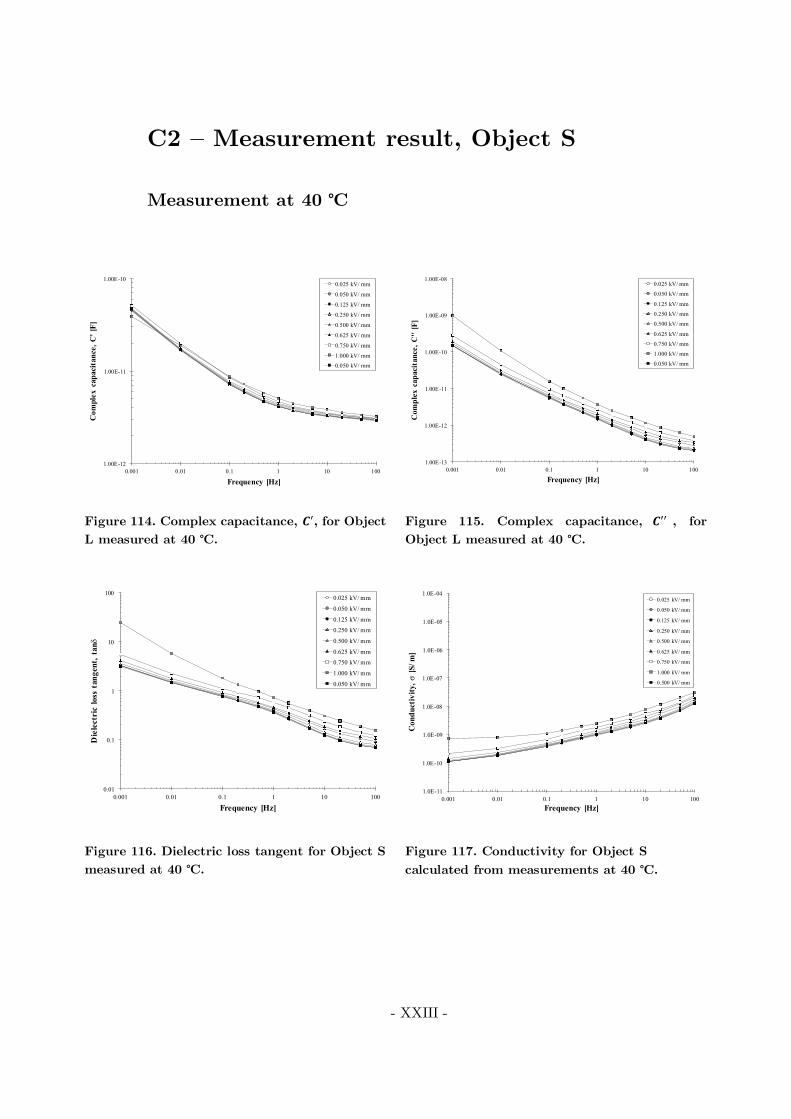
- XXIII -

C2 – Measurement result, Object S




Figure 116. Dielectric loss tangent for Object Smeasured at 40 ℃.

Figure 117. Conductivity for Object Scalculated from measurements at 40 ℃.

1.00E-12

1.00E-11

1.00E-10

0.001 0.01 0.1 1 10 100

Com

plex

capa

cita

nce,

C'[

F]

Frequency [Hz]

0.025 kV/ mm

0.050 kV/ mm

0.125 kV/ mm

0.250 kV/ mm

0.500 kV/ mm

0.625 kV/ mm

0.750 kV/ mm

1.000 kV/ mm

0.050 kV/ mm

1.00E-13

1.00E-12

1.00E-11

1.00E-10

1.00E-09

1.00E-08

0.001 0.01 0.1 1 10 100

Com

plex

capa

cita

nce,

C''

[F]

Frequency [Hz]

0.025 kV/ mm

0.050 kV/ mm

0.125 kV/ mm

0.250 kV/ mm

0.500 kV/ mm

0.625 kV/ mm

0.750 kV/ mm

1.000 kV/ mm

0.050 kV/ mm

0.01

0.1

1

10

100

0.001 0.01 0.1 1 10 100

Die

lect

ric

loss

tang

ent,

tand

Frequency [Hz]

0.025 kV/ mm

0.050 kV/ mm

0.125 kV/ mm

0.250 kV/ mm

0.500 kV/ mm

0.625 kV/ mm

0.750 kV/ mm

1.000 kV/ mm

0.050 kV/ mm

1.0E-11

1.0E-10

1.0E-09

1.0E-08

1.0E-07

1.0E-06

1.0E-05

1.0E-04

0.001 0.01 0.1 1 10 100

Con

duct

ivity

,s[S

/m]

Frequency [Hz]

0.025 kV/ mm

0.050 kV/ mm

0.125 kV/ mm

0.250 kV/ mm

0.500 kV/ mm

0.625 kV/ mm

0.750 kV/ mm

1.000 kV/ mm

0.500 kV/ mm

- XXIV -


Figure 118. Complex capacitance, , for ObjectS measured at 90 ℃.

Figure 119. Complex capacitance, , forObject S measured at 90 ℃.



1.00E-12

1.00E-11

1.00E-10

1.00E-09

1.00E-08

0.001 0.01 0.1 1 10 100

Com

plex

capa

cita

nce,

C'[

F]

Frequency [Hz]

0.025 kV/ mm

0.050 kV/ mm

0.125 kV/ mm

0.250 kV/ mm

0.500 kV/ mm

0.625 kV/ mm

0.750 kV/ mm

1.000 kV/ mm

0.050 kV/ mm

1.00E-13

1.00E-12

1.00E-11

1.00E-10

1.00E-09

1.00E-08

1.00E-07

0.001 0.01 0.1 1 10 100

Com

plex

capa

cita

nce,

C''

[F]

Frequency [Hz]

0.025 kV/ mm

0.050 kV/ mm

0.125 kV/ mm

0.250 kV/ mm

0.500 kV/ mm

0.625 kV/ mm

0.750 kV/ mm

1.000 kV/ mm

0.050 kV/ mm

0.1

1

10

100

1000

0.001 0.01 0.1 1 10 100

Die

lect

ric

loss

tang

ent,

tand

Frequency [Hz]

0.025 kV/ mm

0.050 kV/ mm

0.125 kV/ mm

0.250 kV/ mm

0.500 kV/ mm

0.625 kV/ mm

0.750 kV/ mm

1.000 kV/ mm

0.050 kV/ mm

1.0E-09

1.0E-08

1.0E-07

1.0E-06

1.0E-05

0.001 0.01 0.1 1 10 100

Con

duct

ivity

,s[S

/m]

Frequency [Hz]

0.025 kV/ mm

0.050 kV/ mm

0.125 kV/ mm

0.250 kV/ mm

0.500 kV/ mm

0.625 kV/ mm

0.750 kV/ mm

1.000 kV/ mm

0.500 kV/ mm

- XXV -


Figure 122. Complex capacitance, , for ObjectS measured at 150 ℃. Limited to 10 mHz as thelosses becomes too large.


Figure 124. Dielectric loss tangent for Object Smeasured at 150 ℃. Large dispersion in valuesas accuracy range is exceeded.


1.00E-12

1.00E-11

1.00E-10

1.00E-09

0.01 0.1 1 10 100

Com

plex

capa

cita

nce,

C'[

F]

Frequency [Hz]

0.025 kV/ mm

0.050 kV/ mm

0.125 kV/ mm

0.250 kV/ mm

0.500 kV/ mm

0.625 kV/ mm

0.750 kV/ mm

1.000 kV/ mm

0.050 kV/ mm

1.00E-12

1.00E-11

1.00E-10

1.00E-09

1.00E-08

1.00E-07

1.00E-06

0.001 0.01 0.1 1 10 100

Com

plex

capa

cita

nce,

C''

[F]

Frequency [Hz]

0.025 kV/ mm

0.050 kV/ mm

0.125 kV/ mm

0.250 kV/ mm

0.500 kV/ mm

0.625 kV/ mm

0.750 kV/ mm

1.000 kV/ mm

0.050 kV/ mm

0.1

1

10

100

1000

10000

0.01 0.1 1 10 100

Die

lect

ric

loss

tang

ent,

tand

Frequency [Hz]

0.025 kV/ mm

0.050 kV/ mm

0.125 kV/ mm

0.250 kV/ mm

0.500 kV/ mm

0.625 kV/ mm

0.750 kV/ mm

1.000 kV/ mm

0.050 kV/ mm

1.0E-08

1.0E-07

1.0E-06

1.0E-05

1.0E-04

0.001 0.01 0.1 1 10 100

Con

duct

ivity

,s[S

/m]

Frequency [Hz]

0.025 kV/ mm

0.050 kV/ mm

0.125 kV/ mm

0.250 kV/ mm

0.500 kV/ mm

0.625 kV/ mm

0.750 kV/ mm

1.000 kV/ mm

0.500 kV/ mm

- XXVI -

Measurement at 40 ℃, second run



Figure 128. Dielectric loss tangent for Object Smeasured at 150 ℃. Large dispersion in valuesas accuracy range is exceeded.


1.00E-12

1.00E-11

1.00E-10

1.00E-09

0.001 0.01 0.1 1 10 100

Com

plex

capa

cita

nce,

C'[

F]

Frequency [Hz]

0.025 kV/ mm

0.050 kV/ mm

0.125 kV/ mm

0.250 kV/ mm

0.500 kV/ mm

0.625 kV/ mm

0.750 kV/ mm

1.000 kV/ mm

0.050 kV/ mm

1.00E-13

1.00E-12

1.00E-11

1.00E-10

1.00E-09

1.00E-08

0.001 0.01 0.1 1 10 100

Com

plex

capa

cita

nce,

C''

[F]

Frequency [Hz]

0.025 kV/ mm

0.050 kV/ mm

0.125 kV/ mm

0.250 kV/ mm

0.500 kV/ mm

0.625 kV/ mm

0.750 kV/ mm

1.000 kV/ mm

0.050 kV/ mm

0.01

0.1

1

10

100

0.001 0.01 0.1 1 10 100

Die

lect

ric

loss

tang

ent,

tand

Frequency [Hz]

0.025 kV/ mm

0.050 kV/ mm

0.125 kV/ mm

0.250 kV/ mm

0.500 kV/ mm

0.625 kV/ mm

0.750 kV/ mm

1.000 kV/ mm

0.050 kV/ mm

1.0E-11

1.0E-10

1.0E-09

1.0E-08

1.0E-07

1.0E-06

1.0E-05

1.0E-04

1.0E-03

0.001 0.01 0.1 1 10 100

Con

duct

ivity

,s[S

/m]

Frequency [Hz]

0.025 kV/ mm

0.050 kV/ mm

0.125 kV/ mm

0.250 kV/ mm

0.500 kV/ mm

0.625 kV/ mm

0.750 kV/ mm

1.000 kV/ mm

0.500 kV/ mm

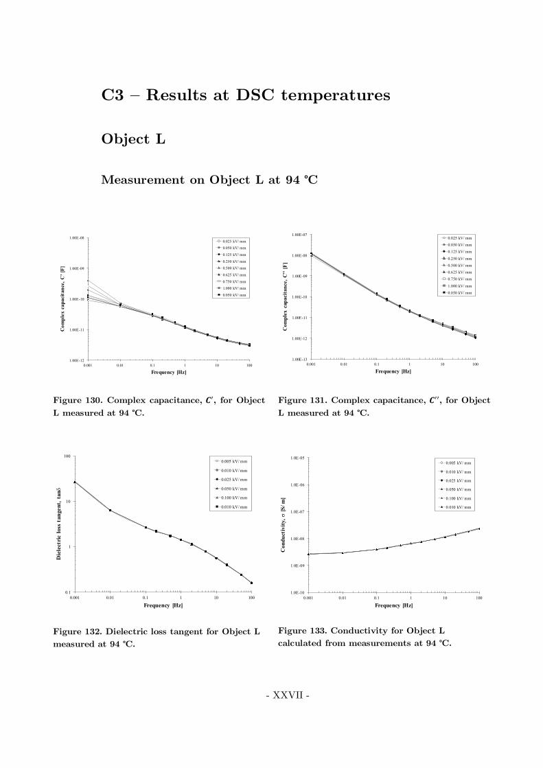
- XXVII -

C3 – Results at DSC temperatures

Object L

Measurement on Object L at 94 ℃



Figure 132. Dielectric loss tangent for Object Lmeasured at 94 ℃.


1.00E-12

1.00E-11

1.00E-10

1.00E-09

1.00E-08

0.001 0.01 0.1 1 10 100

Com

plex

capa

cita

nce,

C'[

F]

Frequency [Hz]

0.025 kV/ mm

0.050 kV/ mm

0.125 kV/ mm

0.250 kV/ mm

0.500 kV/ mm

0.625 kV/ mm

0.750 kV/ mm

1.000 kV/ mm

0.050 kV/ mm

1.00E-13

1.00E-12

1.00E-11

1.00E-10

1.00E-09

1.00E-08

1.00E-07

0.001 0.01 0.1 1 10 100

Com

plex

capa

cita

nce,

C''

[F]

Frequency [Hz]

0.025 kV/ mm

0.050 kV/ mm

0.125 kV/ mm

0.250 kV/ mm

0.500 kV/ mm

0.625 kV/ mm

0.750 kV/ mm

1.000 kV/ mm

0.050 kV/ mm

0.1

1

10

100

0.001 0.01 0.1 1 10 100

Die

lect

ric

loss

tang

ent,

tand

Frequency [Hz]

0.005 kV/ mm

0.010 kV/ mm

0.025 kV/ mm

0.050 kV/ mm

0.100 kV/ mm

0.010 kV/ mm

1.0E-10

1.0E-09

1.0E-08

1.0E-07

1.0E-06

1.0E-05

0.001 0.01 0.1 1 10 100

Con

duct

ivity

,s[S

/m]

Frequency [Hz]

0.005 kV/ mm

0.010 kV/ mm

0.025 kV/ mm

0.050 kV/ mm

0.100 kV/ mm

0.010 kV/ mm

- XXVIII -






1.00E-12

1.00E-11

1.00E-10

1.00E-09

1.00E-08

0.001 0.01 0.1 1 10 100

Com

plex

capa

cita

nce,

C'[

F]

Frequency [Hz]

0.025 kV/ mm

0.050 kV/ mm

0.125 kV/ mm

0.250 kV/ mm

0.500 kV/ mm

0.625 kV/ mm

0.750 kV/ mm

1.000 kV/ mm

0.050 kV/ mm

1.00E-13

1.00E-12

1.00E-11

1.00E-10

1.00E-09

1.00E-08

1.00E-07

0.001 0.01 0.1 1 10 100

Com

plex

capa

cita

nce,

C''

[F]

Frequency [Hz]

0.025 kV/ mm

0.050 kV/ mm

0.125 kV/ mm

0.250 kV/ mm

0.500 kV/ mm

0.625 kV/ mm

0.750 kV/ mm

1.000 kV/ mm

0.050 kV/ mm

0.1

1

10

100

0.001 0.01 0.1 1 10 100

Die

lect

ric

loss

tang

ent,

tand

Frequency [Hz]

0.005 kV/ mm

0.010 kV/ mm

0.025 kV/ mm

0.050 kV/ mm

0.100 kV/ mm

0.010 kV/ mm

1.0E-10

1.0E-09

1.0E-08

1.0E-07

1.0E-06

1.0E-05

0.001 0.01 0.1 1 10 100

Con

duct

ivity

,s[S

/m]

Frequency [Hz]

0.005 kV/ mm

0.010 kV/ mm

0.025 kV/ mm

0.050 kV/ mm

0.100 kV/ mm

0.010 kV/ mm

- XXIX -






1.00E-12

1.00E-11

1.00E-10

1.00E-09

1.00E-08

0.001 0.01 0.1 1 10 100

Com

plex

capa

cita

nce,

C'[

F]

Frequency [Hz]

0.025 kV/ mm

0.050 kV/ mm

0.125 kV/ mm

0.250 kV/ mm

0.500 kV/ mm

0.625 kV/ mm

0.750 kV/ mm

1.000 kV/ mm

0.050 kV/ mm

1.00E-13

1.00E-12

1.00E-11

1.00E-10

1.00E-09

1.00E-08

1.00E-07

0.001 0.01 0.1 1 10 100

Com

plex

capa

cita

nce,

C''

[F]

Frequency [Hz]

0.025 kV/ mm

0.050 kV/ mm

0.125 kV/ mm

0.250 kV/ mm

0.500 kV/ mm

0.625 kV/ mm

0.750 kV/ mm

1.000 kV/ mm

0.050 kV/ mm

0.1

1

10

100

1000

0.001 0.01 0.1 1 10 100

Die

lect

ric

loss

tang

ent,

tand

Frequency [Hz]

0.005 kV/ mm

0.010 kV/ mm

0.025 kV/ mm

0.050 kV/ mm

0.100 kV/ mm

0.010 kV/ mm

1.0E-09

1.0E-08

1.0E-07

1.0E-06

1.0E-05

0.001 0.01 0.1 1 10 100

Con

duct

ivity

,s[S

/m]

Frequency [Hz]

0.005 kV/ mm

0.010 kV/ mm

0.025 kV/ mm

0.050 kV/ mm

0.100 kV/ mm

0.010 kV/ mm

- XXX -

Object S

Measurement on Object S at 94 ℃





1.00E-12

1.00E-11

1.00E-10

1.00E-09

0.01 0.1 1 10 100

Com

plex

capa

cita

nce,

C'[

F]

Frequency [Hz]

0.025 kV/ mm

0.050 kV/ mm

0.125 kV/ mm

0.250 kV/ mm

0.500 kV/ mm

0.625 kV/ mm

0.750 kV/ mm

1.000 kV/ mm

0.050 kV/ mm

1.00E-12

1.00E-11

1.00E-10

1.00E-09

1.00E-08

1.00E-07

0.01 0.1 1 10 100

Com

plex

capa

cita

nce,

C''

[F]

Frequency [Hz]

0.025 kV/ mm

0.050 kV/ mm

0.125 kV/ mm

0.250 kV/ mm

0.500 kV/ mm

0.625 kV/ mm

0.750 kV/ mm

1.000 kV/ mm

0.050 kV/ mm

0.1

1

10

100

0.001 0.01 0.1 1 10 100

Die

lect

ric

loss

tang

ent,

tand

Frequency [Hz]

0.005 kV/ mm

0.010 kV/ mm

0.025 kV/ mm

0.050 kV/ mm

0.100 kV/ mm

0.010 kV/ mm

1.0E-10

1.0E-09

1.0E-08

1.0E-07

1.0E-06

1.0E-05

0.001 0.01 0.1 1 10 100

Con

duct

ivity

,s[S

/m]

Frequency [Hz]

0.005 kV/ mm

0.010 kV/ mm

0.025 kV/ mm

0.050 kV/ mm

0.100 kV/ mm

0.010 kV/ mm

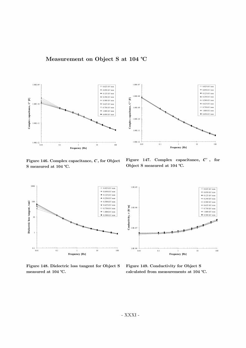
- XXXI -






1.00E-12

1.00E-11

1.00E-10

1.00E-09

0.01 0.1 1 10 100

Com

plex

capa

cita

nce,

C'[

F]

Frequency [Hz]

0.025 kV/ mm

0.050 kV/ mm

0.125 kV/ mm

0.250 kV/ mm

0.500 kV/ mm

0.625 kV/ mm

0.750 kV/ mm

1.000 kV/ mm

0.050 kV/ mm

1.00E-12

1.00E-11

1.00E-10

1.00E-09

1.00E-08

1.00E-07

0.01 0.1 1 10 100

Com

plex

capa

cita

nce,

C''

[F]

Frequency [Hz]

0.025 kV/ mm

0.050 kV/ mm

0.125 kV/ mm

0.250 kV/ mm

0.500 kV/ mm

0.625 kV/ mm

0.750 kV/ mm

1.000 kV/ mm

0.050 kV/ mm

0.1

1

10

100

1000

0.01 0.1 1 10 100

Die

lect

ric

loss

tang

ent,

tand

Frequency [Hz]

0.025 kV/ mm

0.050 kV/ mm

0.125 kV/ mm

0.250 kV/ mm

0.500 kV/ mm

0.625 kV/ mm

0.750 kV/ mm

1.000 kV/ mm

0.500 kV/ mm

1.0E-08

1.0E-07

1.0E-06

1.0E-05

0.01 0.1 1 10 100

Con

duct

ivity

,s[S

/m]

Frequency [Hz]

0.025 kV/ mm

0.050 kV/ mm0.125 kV/ mm

0.250 kV/ mm

0.500 kV/ mm

0.625 kV/ mm

0.750 kV/ mm1.000 kV/ mm

0.500 kV/ mm

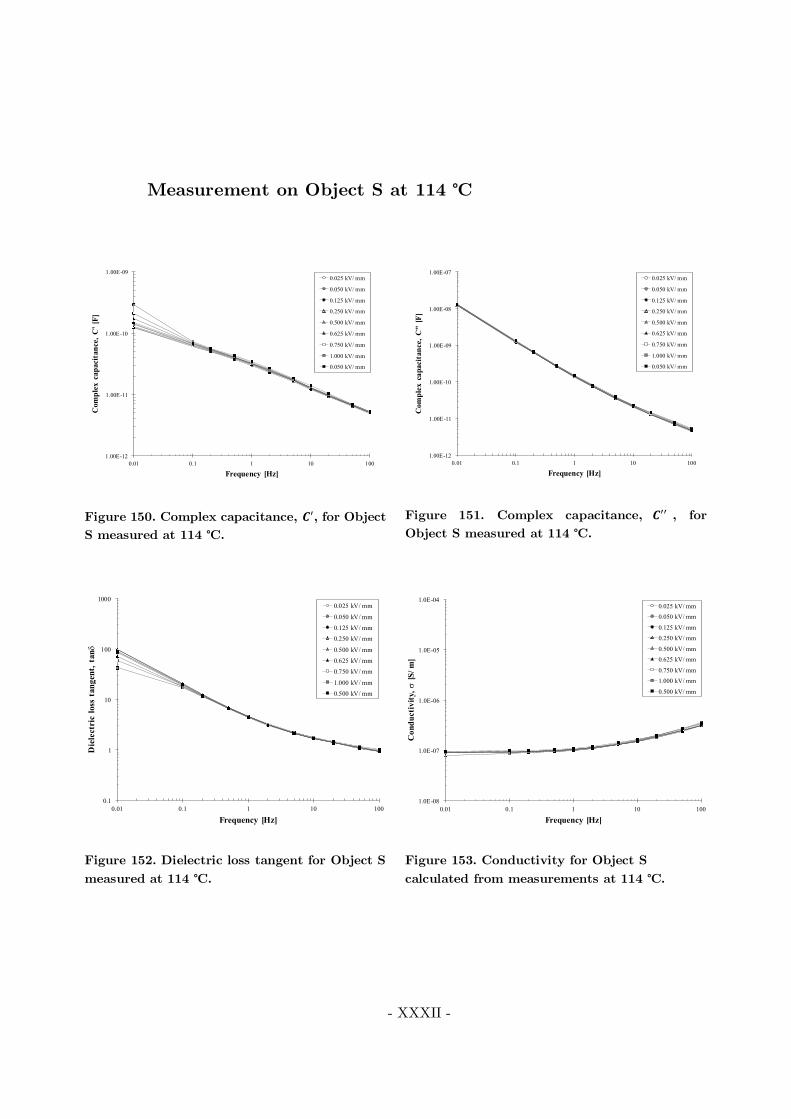
- XXXII -






1.00E-12

1.00E-11

1.00E-10

1.00E-09

0.01 0.1 1 10 100

Com

plex

capa

cita

nce,

C'[

F]

Frequency [Hz]

0.025 kV/ mm

0.050 kV/ mm

0.125 kV/ mm

0.250 kV/ mm

0.500 kV/ mm

0.625 kV/ mm

0.750 kV/ mm

1.000 kV/ mm

0.050 kV/ mm

1.00E-12

1.00E-11

1.00E-10

1.00E-09

1.00E-08

1.00E-07

0.01 0.1 1 10 100

Com

plex

capa

cita

nce,

C''

[F]

Frequency [Hz]

0.025 kV/ mm

0.050 kV/ mm

0.125 kV/ mm

0.250 kV/ mm

0.500 kV/ mm

0.625 kV/ mm

0.750 kV/ mm

1.000 kV/ mm

0.050 kV/ mm

0.1

1

10

100

1000

0.01 0.1 1 10 100

Die

lect

ric

loss

tang

ent,

tand

Frequency [Hz]

0.025 kV/ mm

0.050 kV/ mm

0.125 kV/ mm

0.250 kV/ mm

0.500 kV/ mm

0.625 kV/ mm

0.750 kV/ mm

1.000 kV/ mm

0.500 kV/ mm

1.0E-08

1.0E-07

1.0E-06

1.0E-05

1.0E-04

0.01 0.1 1 10 100

Con

duct

ivity

,s[S

/m]

Frequency [Hz]

0.025 kV/ mm

0.050 kV/ mm

0.125 kV/ mm

0.250 kV/ mm

0.500 kV/ mm

0.625 kV/ mm

0.750 kV/ mm

1.000 kV/ mm

0.500 kV/ mm

- XXXIII -

C4 – Measurements results examineeffect of increased humidity

Measurement on a dry test object

Figure 154. Complex capacitance, , for a drytest object measured at 20 ℃.

Figure 155. Complex capacitance, , for a drytest object measured at 20 ℃.

Figure 156. Dielectric loss tangent for a dry testobject measured at 20 ℃.

Figure 157. Conductivity for a dry test objectcalculated from measurements at 20 ℃.

1.00E-12

1.00E-11

1.00E-10

0.001 0.01 0.1 1 10 100

Com

plex

capa

cita

nce,

C'[

F]

Frequency [Hz]

0.025 kV/ mm 0.050 kV/ mm 0.125 kV/ mm0.250 kV/ mm 0.500 kV/ mm 0.625 kV/ mm0.750 kV/ mm 1.000 kV/ mm 0.050 kV/ mm

1.00E-13

1.00E-12

1.00E-11

1.00E-10

1.00E-09

1.00E-08

0.001 0.01 0.1 1 10 100

Com

plex

capa

cita

nce,

C''

[F]

Frequency [Hz]


0.01

0.1

1

10

100

1000

0.001 0.01 0.1 1 10 100

Die

lect

ric

loss

tang

ent,

tand

Frequency [Hz]


1.0E-12

1.0E-11

1.0E-10

1.0E-09

1.0E-08

1.0E-07

1.0E-06

0.001 0.01 0.1 1 10 100

Con

duct

ivity

,s[S

/m]

Frequency [Hz]


- XXXIV -

Measurement on test object wrapped in plastic foil andinsulation tape

Figure 158. Complex capacitance, , measuredat 20 ℃.


Figure 160. Dielectric loss tangent measured at20 ℃.


1.00E-12

1.00E-11

1.00E-10

0.001 0.01 0.1 1 10 100

Com

plex

capa

cita

nce,

C'[

F]

Frequency [Hz]


1.00E-13

1.00E-12

1.00E-11

1.00E-10

1.00E-09

1.00E-08

0.001 0.01 0.1 1 10 100

Com

plex

capa

cita

nce,

C''

[F]

Frequency [Hz]


0.01

0.1

1

10

0.001 0.01 0.1 1 10 100

Die

lect

ric

loss

tang

ent,

tand

Frequency [Hz]


1.0E-11

1.0E-10

1.0E-09

1.0E-08

1.0E-07

1.0E-06

0.001 0.01 0.1 1 10 100

Con

duct

ivity

,s[S

/m]

Frequency [Hz]


- XXXV -

Measurement on wet test object

Figure 162. Complex capacitance, , for a wettest object measured at 20 ℃.




1.00E-12

1.00E-11

1.00E-10

1.00E-09

1.00E-08

1.00E-07

1.00E-06

1.00E-05

1.00E-04

1.00E-03

0.001 0.01 0.1 1 10 100

Com

plex

capa

cita

nce,

C'[

F]

Frequency [Hz]


1.00E-12

1.00E-11

1.00E-10

1.00E-09

1.00E-08

1.00E-07

1.00E-06

1.00E-05

1.00E-04

1.00E-03

1.00E-02

0.001 0.01 0.1 1 10 100

Com

plex

capa

cita

nce,

C''

[F]

Frequency [Hz]


0

1

10

100

1000

10000

0.001 0.01 0.1 1 10 100

Die

lect

ric

loss

tang

ent,

tand

Frequency [Hz]


1.0E-08

1.0E-07

1.0E-06

1.0E-05

1.0E-04

1.0E-03

1.0E-02

1.0E-01

0.001 0.01 0.1 1 10 100

Con

duct

ivity

,s[S

/m]

Frequency [Hz]


- XXXVI -

Appendix D – Formulas used forcalculation of the conductivity

The conductivity of the test object can be calculated with theparameters found in dielectric spectroscopy measurements. The relationshipbetween dielectric loss tangent, permittivity and conductivity is seen in Eq.2.3, and can be rewritten as in Eq. D.1.

This equation is an approximation and will apply when the relation| | ≫ | | is fulfilled.

At low frequencies, the losses in the test object willbe dominated by the conductivity. Utilizing this relation,the conductivity of the stress control tube can becalculated using Eq. 4.1 with dielectric loss tangent foundat the lowest frequency.

As the capacitance measured by IDA 200 is theequivalent for both the PTFE rod and SCT, calculationsare necessary for determination of the complexpermittivity. The equivalent circuit is illustrated in Figure166, and is given as a parallel coupling.

Using the relation from Eq. D.2 for the parallelcoupling, complex permittivity for the stress control tubecan be determine as yield in Eq. D.3.

Figure 166. Equivalent circuitfor measurement of the totalcapacitance in the test object.

≈ tan ⋅ Eq. D.1

= ( − ) Eq. D.2

=′ − ( , ⋅ )

,Eq. D.3

A

↯High voltage supply

C PT FE C SC T

Currentm easurem en t

- XXXVII -

The complex permittivity of the PTFE rod is for this thesis used as2.1 [37]. The geometric capacitance, C0, is determined for each of the materials.Additionally, the value of C0 is required determined for both Object L andObject S as their distance between the electrodes is different.

After determined the relative permittivity, conductivity can becalculated with values found at the lowest frequency.

Object L

= ⋅ Eq. D.4

, = 8.85 ⋅ 10 ⋅⋅ 0.0125

0.1

= 4.344 ∙ 10 [ ]

Eq. D.5

, == 8.85 ⋅ 10 ⋅⋅ (0.0145 − 0.01252)

0.1

= 1.501 ∙ 10 [ ]

Eq. D.6

Object S

, = 8.85 ⋅ 10 ⋅⋅ 0.0125

0.02

= 2.172 ∙ 10 [ ]

Eq. D.7

, == 8.85 ⋅ 10 ⋅⋅ (0.0145 − 0.01252)

0.02

= 7.507 ∙ 10 [ ]

Eq. D.8

- XXXVIII -

Appendix E - Dissection of the wettest object

Dissection of the wet test object was performed after dielectric responsemeasurements. The stress control tube was closely examined for tracking onthe surface towards the electrodes.

Tracking is a formation of carbonaceous layers or lines on the surfaceof organic insulators [5]. As water is present in the test object, they can formconductive paths on the surface. If these conductive paths expand from oneelectrode to the other, they will short circuit the electrodes. Dielectric responsemeasurement results will thereby not be referred to the stress control tube.

Close examination of the stress control tube indicate that tracking havenot been present during measurements. A picture of the stress control tubecan be found in Figure 169. Observations made indicate that large heatgeneration have been formed at one electrode as illustrated in Figure 170.

As the electrodes also have been immersed in water, rust has beenformed at both electrodes. However, as tracking is not observed, the presenceof rust is assumed to not influence the measurement results.

Figure 167. Wet test object with plastic foil and PVC insulation tape.

Figure 168. Wet test object wrapped in plastic foil.

- XXXIX -

Figure 169. Dissection of the wet stress control tubeafter measurements.

Figure 170. Closer look at apoint where a heatgeneration have made amark on the stress controltube.

Figure 171. Metal electrodes and PTFE rod from the wet test object. Rust isobserved at each electrode.

- XL -

Appendix F – List of figures

Figure 1: Equipotential lines on a stripped cable. An enhancement occurs at the edge of thesemi-conductive layer. [9] ..................................................................................................... 9

Figure 2: Equipotential lines when a stress control tube is applied. Field grading gives a moreuniform distribution and a less enhancement at the edge. [9].......................................... 10

Figure 3: Schematic characteristic for a coating with field strength independent resistance. [4] ............................................................................................................................................. 11

Figure 4: Approximate circuit equivalent in order to illustrate field system along the end ofthe cable. [4] ........................................................................................................................ 11

Figure 5. Equivalent circuit of an impedance stress control material (dark blue layer) appliedto the cable. [10] ..................................................................................................................13

Figure 6: Parallel plate condenser. [16] a) with vacuum. b) with dielectric medium. c)Resulting net free charge on the surface of the plates when having a dielectric medium. ............................................................................................................................................. 16

Figure 7: Equivalent circuit of a dielectric medium with conduction, momentary polarisationand relaxation mechanism. ................................................................................................. 17

Figure 8. The current’s shape for both polarisation and depolarisation time period. [5] ......... 18

Figure 9: Real and imaginary part of the permittivity as a function of frequency....................20

Figure 10: Equivalent circuit for parallel circuit. ........................................................................22

Figure 11: Phasor diagram for parallel circuit. ............................................................................22

Figure 12: Equivalent circuit for time domain measurements. ...................................................23

Figure 13: Polarisation and depolarisation current as a function of time. [18] ..........................24

Figure 14: Principle for measuring dielectric response in frequency domain. Object is subjectedto a high voltage source. The current and voltage is measured with amplitude andangle. Parameters can be calculated with these values. ....................................................25

Figure 15: Different types of dielectric response function [26] ....................................................28

Figure 16: Typical curve received from the DSC measurement. [31] .........................................33

Figure 17: Geometry of test specimen. .........................................................................................37

- XLI -

Figure 18: Equipment used when performing Mass Uptake Measurement. A computerconnected to the measurement instrument Mettler Toledo UMX2. An electrostaticprecipitator removes the surface charge. ............................................................................37

Figure 19: Temperature program for DSC measurement. ...........................................................39

Figure 20: Illustration of the test samples used for DSC measurement. ....................................40

Figure 21: Cylinder consisting of metal electrodes assembled together with a PTFE rod. .......42

Figure 22. Cylinder consisting of PTFE rod, two metal electrodes and heat shrink stresscontrol tube. .........................................................................................................................43

Figure 23. Illustration of test object; (1) Corona rings, (2) PTFE ring insulating themeasuring electrode from the grounded corona ring, (3) stress control tube, (4) PTFErod, and (5) metallic clamps. [1] .........................................................................................43

Figure 24. Measurement inaccuracies for IDA 200 at different values of capacitance anddielectric loss tangent. [34] ..................................................................................................44

Figure 25. Measurement of electrical impedance. [33] .................................................................45

Figure 26. Connection diagram for Ungrounded Specimen Test (UST). ...................................45

Figure 27. Connection diagram for Grounded Specimen Test (GST). .......................................45

Figure 28. Measurement diagram for the experiment using UST without a guard. ..................46

Figure 29. Water content at 30 ℃, given as percentage of the total mass. One sample of eachdegree of shrinkage is shown in the figure. .........................................................................53



Figure 32. Graphically determination of the water increase per day. .......................................54

Figure 33. Water uptake for partially shrunk stress control tube at 30, 60 and 90 ℃. Resultsfrom two test samples at each temperature are shown. ....................................................55

Figure 34. Illustration of the temperatures found for the endothermic melting transition. ......57

Figure 35. DSC measurement on a sample of virgin stress control tube....................................59

Figure 36. DSC measurement for a partially shrunk stress control tube sample. .....................60

Figure 37. DSC measurement for a fully shrunk stress control tube sample. ........................... 61

- XLII -

Figure 38. Curves from DSC measurement of the three degrees of shrinkage, divided introfirst and second run. ............................................................................................................62

Figure 39. Equivalent circuit for measurement of the total capacitance in the test object. .....63

Figure 40. Dielectric loss tangent for a PTFE rod without a stress control tube. ....................64

Figure 41. Complex permittivity, ε', for a PTFE rod a stress control tube. .............................64

Figure 42. Real value of complex capacitance for Object L and PTFE rod. .............................65

Figure 43. Imaginary value of complex capacitance for Object L and PTFE rod. ....................65

Figure 44. Dielectric loss tangent for measurement at Object L. All fields are included with alower frequency limitation of 10 mHz.................................................................................67

Figure 45. Dielectric loss tangent as a function of the electric field for 150 ℃. ........................67

Figure 46. Real value of the complex capacitance, C', for Object L. .........................................68

Figure 47. Imaginary value of the complex capacitance, C'', for Object L. ...............................68

Figure 48. Dielectric loss tangent for Object S when including the entire frequency range from1 mHz to 100 Hz. .................................................................................................................69

Figure 49. Dielectric loss tangent at 40 ℃. Red curves illustrate the first measurement, whilethe blue presents the second measurement. .......................................................................70

Figure 50. Dielectric loss tangent as a function of electric field strength. .................................70

Figure 51. Complex capacitance C’ from measurement at Object S ......................................... 71

Figure 52. Complex capacitance C’’ from measurements on Object S. ..................................... 71

Figure 53. Real part of complex capacitance. ..............................................................................72

Figure 54. Imaginary part of the complex capacitance. ..............................................................72

Figure 55. Dielectric loss tangent, for first and second measurement at 40 ℃..........................73

Figure 56. Conductivity, σ, for first and second measurement on Object L at 40 ℃. ..............73

Figure 57. Real value of complex capacitance, C’, for Object S at 40 ℃. .................................74

Figure 58. Imaginary part of the complex capacitance, C’’, for Object S at 40 ℃. ..................74

Figure 59. Dielectric loss tangent for Object S at 40 ℃. ............................................................74

Figure 60. Conductivity, σ, for Object S at 40 ℃. ......................................................................74

- XLIII -

Figure 61. Real value of complex capacitance, C’, at DSC temperatures. .................................75

Figure 62. Imaginary part of the complex capacitance, C’’, at DSC temperatures. ..................75

Figure 63. Dielectric loss tangent for Object L at DSC temperatures. ......................................76

Figure 64. Calculated conductivity for Object L at DSC temperatures and all frequencies. ....76

Figure 65. Real value of complex capacitance, C’, at DSC temperatures. .................................77

Figure 66. Imaginary part of the complex capacitance, C’’, at DSC temperatures. ..................77

Figure 67. Dielectric loss tangent for Object L at DSC temperatures. ......................................78

Figure 68. Calculated conductivity for Object L at DSC temperatures and all frequencies. ....78

Figure 69. Conductivity obtained at an electric field strength of 0.1 kV/mm calculated atfrequency of 1 mHz. .............................................................................................................80

Figure 70. Conductivity calculated for Object L with values obtained at 1 mHz. ....................80

Figure 71. Conductivity obtained at an electric field strength of 0.1 kV/mm calculated atfrequency of 1 mHz. ............................................................................................................ 81

Figure 72. Conductivity calculated for Object S with values obtained at 10 mHz. ................. 81

Figure 73. Conductivity as a function of the electric field strength for both frequency- andtime domain analysis. ..........................................................................................................82

Figure 74. Complex permittivity, ’, for Object S......................................................................83

Figure 75. Complex permittivity, ’’, for Object S. ....................................................................83

Figure 76. Determination of water uptake for partially shrunk samples. After 39 days, theconcentration in the test samples will be approximately 4.6 % and 1.15 % for the testobject. ...................................................................................................................................84

Figure 77. Dielectric loss tangent for test object with and without application of plastic foiland insulation tape. .............................................................................................................85

Figure 78. Conductivity for test object with and without application of plastic foil andinsulation tape. ....................................................................................................................85

Figure 79. Conductivity for a wet and dry test object calculated for all frequencies. ...............86

Figure 80. Conductivity for wet and dry test object as a function of electric field strength at 1mHz. .....................................................................................................................................86

Figure 81. Dielectric loss tangent for a dry and wet test object.................................................87

- XLIV -

Figure 82: Geometry of test specimen. ........................................................................................ III

Figure 83. Water uptake at 30 ℃. One sample at each degree of shrinkage is shown in thefigure................................................................................................................................... VII

Figure 84. Water uptake at 60 ℃. One sample at each degree of shrinkage is shown in thefigure................................................................................................................................. VIII

Figure 85. Water uptake at 90 ℃. One sample at each degree of shrinkage is shown in thefigure................................................................................................................................. VIII

Figure 86. Water uptake by a virgin stress control tube. Two samples at each temperature areshown in the figure. ............................................................................................................ IX

Figure 87. Water uptake by a partially shrunk stress control tube. Two samples at eachtemperature are shown in the figure. ................................................................................. IX

Figure 88. Water uptake by a fully shrunk stress control tube. Two samples at eachtemperature are shown in the figure. .................................................................................. X

Figure 89. Result from DSC measurement 1. .......................................................................... XIII

Figure 90. Result from DSC measurement 2. .......................................................................... XIII

Figure 91. Result from DSC measurement 3. .......................................................................... XIV

Figure 92. Result from DSC measurement 1. .......................................................................... XIV

Figure 93. Result from DSC measurement 2. ............................................................................ XV

Figure 94. Result from DSC measurement 3. ............................................................................ XV

Figure 95. Result from DSC measurement 1. .......................................................................... XVI

Figure 96. Result from DSC measurement 2. .......................................................................... XVI

Figure 97. Result from DSC measurement 3. ......................................................................... XVII

Figure 98. Complex capacitance, C', for Object L measured at 40 ℃. ................................... XIX

Figure 99. Complex capacitance, C'', for Object L measured at 40 ℃. .................................. XIX

Figure 100. Dielectric loss tangent for Object L measured at 40 ℃. ..................................... XIX

Figure 101. Conductivity for Object L calculated from measurements at 40 ℃. .................. XIX

Figure 102. Complex capacitance, C', for Object L measured at 90 ℃. ................................... XX

Figure 103. Complex capacitance, C'', for Object L measured at 90 ℃. .................................. XX

- XLV -

Figure 104. Dielectric loss tangent for Object L measured at 90 ℃. ....................................... XX

Figure 105. Conductivity for Object L calculated for measurements at 90 ℃. ....................... XX

Figure 106. Complex capacitance, C', for Object L measured at 150 ℃. ............................... XXI

Figure 107. Complex capacitance, C'', for Object L measured at 150 ℃. .............................. XXI

Figure 108. Dielectric loss tangent for Object L measured at 150 ℃..................................... XXI

Figure 109. Conductivity for Object L calculated from measurements at 150 ℃. ................ XXI

Figure 110. Complex capacitance, C', for Object L measured at 40 ℃. ................................ XXII

Figure 111. Complex capacitance, C'', for Object L measured at 40 ℃. ............................... XXII

Figure 112. Dielectric loss tangent for Object L measured at 40 ℃, second run. ................ XXII

Figure 113. Conductivity for Object L calculated from measurements at 40 ℃, second run. ......................................................................................................................................... XXII

Figure 114. Complex capacitance, C', for Object L measured at 40 ℃. ...............................XXIII

Figure 115. Complex capacitance, C'', for Object L measured at 40 ℃. ..............................XXIII

Figure 116. Dielectric loss tangent for Object S measured at 40 ℃. ....................................XXIII

Figure 117. Conductivity for Object S calculated from measurements at 40 ℃. ................XXIII

Figure 118. Complex capacitance, C', for Object S measured at 90 ℃. .............................. XXIV

Figure 119. Complex capacitance, C'', for Object S measured at 90 ℃. ............................. XXIV

Figure 120. Dielectric loss tangent for Object S measured at 90 ℃. ................................... XXIV

Figure 121. Conductivity for Object S calculated from measurements at 90 ℃. ............... XXIV

Figure 122. Complex capacitance, C', for Object S measured at 150 ℃. Limited to 10 mHz asthe losses becomes too large. .......................................................................................... XXV

Figure 123. Complex capacitance, C'', for Object S measured at 150 ℃. ............................. XXV

Figure 124. Dielectric loss tangent for Object S measured at 150 ℃. Large dispersion in valuesas accuracy range is exceeded. ....................................................................................... XXV

Figure 125. Conductivity for Object S calculated from measurements at 150 ℃. ............... XXV

Figure 126. Complex capacitance, C', for Object L measured at 40 ℃. .............................. XXVI

- XLVI -

Figure 127. Complex capacitance, C'', for Object L measured at 40 ℃. ............................. XXVI

Figure 128. Dielectric loss tangent for Object S measured at 150 ℃. Large dispersion in valuesas accuracy range is exceeded. ..................................................................................... XXVI

Figure 129. Conductivity for Object S calculated from measurements at 150 ℃. ............. XXVI

Figure 130. Complex capacitance, C', for Object L measured at 94 ℃. ............................. XXVII

Figure 131. Complex capacitance, C'', for Object L measured at 94 ℃. ............................ XXVII

Figure 132. Dielectric loss tangent for Object L measured at 94 ℃. ................................. XXVII

Figure 133. Conductivity for Object L calculated from measurements at 94 ℃. .............. XXVII

Figure 134. Complex capacitance, C', for Object S measured at 104 ℃. .......................... XXVIII

Figure 135. Complex capacitance, C'', for Object S measured at 104 ℃. ......................... XXVIII

Figure 136. Dielectric loss tangent for Object S measured at 104 ℃. ............................... XXVIII

Figure 137. Conductivity for Object S calculated from measurements at 104 ℃. ........... XXVIII

Figure 138. Complex capacitance, C', for Object S measured at 114 ℃. ............................ XXIX

Figure 139. Complex capacitance, C'', for Object S measured at 114 ℃. ........................... XXIX

Figure 140. Dielectric loss tangent for Object S measured at 114 ℃. ................................. XXIX

Figure 141. Conductivity for Object S calculated from measurements at 114 ℃. ............. XXIX

Figure 142. Complex capacitance, C', for Object S measured at 94 ℃. ................................ XXX

Figure 143. Complex capacitance, C'', for Object S measured at 94 ℃. ............................... XXX

Figure 144. Dielectric loss tangent for Object S measured at 94 ℃. ..................................... XXX

Figure 145. Conductivity for Object S calculated from measurements at 94 ℃. ................. XXX

Figure 146. Complex capacitance, C', for Object S measured at 104 ℃. ............................ XXXI

Figure 147. Complex capacitance, C'', for Object S measured at 104 ℃. ........................... XXXI

Figure 148. Dielectric loss tangent for Object S measured at 104 ℃. ................................. XXXI

Figure 149. Conductivity for Object S calculated from measurements at 104 ℃. ............. XXXI

Figure 150. Complex capacitance, C', for Object S measured at 114 ℃. ........................... XXXII

- XLVII -

Figure 151. Complex capacitance, C'', for Object S measured at 114 ℃. .......................... XXXII

Figure 152. Dielectric loss tangent for Object S measured at 114 ℃. ................................ XXXII

Figure 153. Conductivity for Object S calculated from measurements at 114 ℃. ............ XXXII

Figure 154. Complex capacitance, C', for a dry test object measured at 20 ℃. ............... XXXIII

Figure 155. Complex capacitance, C'', for a dry test object measured at 20 ℃. .............. XXXIII

Figure 156. Dielectric loss tangent for a dry test object measured at 20 ℃. .................... XXXIII

Figure 157. Conductivity for a dry test object calculated from measurements at 20 ℃.. XXXIII

Figure 158. Complex capacitance, C', measured at 20 ℃. ................................................. XXXIV

Figure 159. Complex capacitance, C'', measured at 20 ℃.................................................. XXXIV

Figure 160. Dielectric loss tangent measured at 20 ℃. ...................................................... XXXIV

Figure 161. Complex capacitance, C'', measured at 20 ℃.................................................. XXXIV

Figure 162. Complex capacitance, C', for a wet test object measured at 20 ℃. ................ XXXV

Figure 163. Complex capacitance, C'', for a wet test object measured at 20 ℃. ............... XXXV

Figure 164. Complex capacitance, C', for a wet test object measured at 20 ℃. ................ XXXV

Figure 165. Complex capacitance, C'', for a wet test object measured at 20 ℃. ............... XXXV

Figure 166. Equivalent circuit for measurement of the total capacitance in the test object. ..................................................................................................................................... XXXVI

Figure 167. Wet test object with plastic foil and PVC insulation tape. ........................ XXXVIII

Figure 168. Wet test object wrapped in plastic foil. ....................................................... XXXVIII

Figure 169. Dissection of the wet stress control tube after measurements. ...................... XXXIX

Figure 170. Closer look at a point where a heat generation have made a mark on the stresscontrol tube. ................................................................................................................ XXXIX

Figure 171. Metal electrodes and PTFE rod from the wet test object. Rust is observed at eachelectrode. ..................................................................................................................... XXXIX

- XLVIII -

Appendix G – List of tables

Table 1: Diagnostic parameters ....................................................................................................26

Table 2: Temperature program used for the differential scanning calorimetry. ........................40

Table 3. Electric field strength in [kVpeak/mm] for the applied voltages. ..................................47

Table 4. Measurement program for Object S. .............................................................................48

Table 5. Measurement program for Object L. .............................................................................48

Table 6. Water content for six test samples of partially shrunk SCT after being immersed for80 days. ................................................................................................................................56

Table 7. DSC analysis of maximum endothermic phase transition for a virgin stress controltube.......................................................................................................................................58

Table 8: DSC analysis of maximum endothermic phase transition for partially shrunk stresscontrol tube. .........................................................................................................................59

Table 9. DSC analysis of maximum endothermic phase transition for fully shrunk stresscontrol tube. ........................................................................................................................ 61

Table 10. Percentage change in conductivity when increasing the complex permittivity from2.1 to 5.0 in the calculations of conductivity. ....................................................................79

condition assessment of medium voltage cable joints

Documents