0

ARTIFICIAL NEURAL NETWORK APPROACH FOR

CONDITION-BASED MAINTENANCE

Mostafa Sayyed

Master of Engineering Management

Universiti Putra Malaysia

1

Abstract

In this research, computerized maintenance management will be investigated. The rise of

maintenance cost forced the research community to look for more effective ways to schedule

maintenance operations. Using computerized models to come up with optimal maintenance

policy has led to better equipment utilization and lower costs. This research adopts Condition-

Based Maintenance model where the maintenance decision is generated based on equipment

conditions. Artificial Neural Network technique is proposed to capture and analyze equipment

condition signals which lead to higher level of knowledge gathering. This knowledge is used to

accurately estimate equipment failure time. Based on these estimations, an optimal maintenance

management policy can be achieved.

2

Abstrak

Dalam kajian ini, pengurusan penyenggaraan berkomputer akan disiasat. Kenaikan kos

penyelenggaraan terpaksa komuniti penyelidikan untuk mencari cara yang lebih berkesan untuk

menjadualkan operasi penyelenggaraan. Menggunakan model berkomputer untuk datang dengan

dasar penyelenggaraan optimum telah membawa kepada penggunaan peralatan yang lebih baik

dan kos yang lebih rendah. Penyelidikan ini menggunakan model Penyelenggaraan Berasaskan

Keadaan di mana keputusan penyelenggaraan dihasilkan berdasarkan keadaan peralatan. Teknik

Rangkaian Neural Buatan adalah dicadangkan untuk menangkap dan menganalisis isyarat

keadaan peralatan yang membawa kepada tahap yang lebih tinggi daripada pengumpulan

pengetahuan. Pengetahuan ini digunakan untuk menganggarkan dengan tepat masa kegagalan

peralatan. Berdasarkan anggaran ini, dasar pengurusan penyelenggaraan optimum dapat dicapai.

3

Acknowledgement

In the name of Allah, Most Gracious, Most Merciful Who had bestowed me knowledge, patience

and strength in completing this project report.

Alhamdulillah, I want to express my most heartfelt gratitude and appreciation to my supervisor,

Dr …… for his guidance and patience throughout the whole development of this work. His

advices were very encouraging and help me to rediscover my confidence to complete this

project. I am very grateful for everything that he shared to me and lead me to perform better.

Also, I would to give immense thanks to my examiner, Dr….. for his encourage comments and

ideas.

Next, I would like to express my highest gratitude to Abu Dhabi police who have been

supporting me in my studies as well as inspiring me till I am able to achieve to this level of

education.

Finally, I would like to thanks to all my colleagues who have helped to give me full support and

motivation and not to forget my brother and sister.

Thank you.

Mostafa Sayyed

4

Approval

This project report is submitted to the Department of Mechanical and Manufacturing

Engineering, Faculty of Engineering, Universiti Putra Malaysia and has been accepted as a

partial fulfillment of the requirement for the degree of Master of Engineering Management. The

members of the examination Committee are as follows:

Supervisor

Dr …….

Department of Mechanical and Manufacturing Engineering

Faculty of Engineering

Universiti Putra Malaysia

Examiner

Dr ………….

Department of Mechanical and Manufacturing Engineering

Faculty of Engineering

Universiti Putra Malaysia

5

Declaration

I hereby declare that the project report is my original work except for quotations and citations,

which have been duly acknowledged. I also declare that it has not been previously, and is not

concurrently, submitted for any other degree at Universiti Putra Malaysia or at any other

institution.

________________________________

Mostafa Sayyed

GS

Date:

6

Table of Contents

Abstract ........................................................................................................................................... 1

Abstrak ............................................................................................................................................ 2

Acknowledgement .......................................................................................................................... 3

Approval ......................................................................................................................................... 4

Declaration ...................................................................................................................................... 5

Table of Contents ............................................................................................................................ 6

List of figures .................................................................................................................................. 9

Chapter 1: Introduction ............................................................................................................. 10

1.1 Problem Statement ......................................................................................................... 12

1.2 Objectives of the Study .................................................................................................. 13

1.3 Scope of the Study.......................................................................................................... 13

Chapter 2: Literature Review.................................................................................................... 16

2.1 Computerization ............................................................................................................. 16

2.2 Maintenance Management ............................................................................................. 17

2.3 Computer Maintenance Management Systems .............................................................. 18

2.4 Selecting the Right CMMS ............................................................................................ 20

2.5 Installation and Implementation of CMMS ................................................................... 27

2.6 Evaluation and Design of CMMS .................................................................................. 29

7

2.7 Benefits of Using CMMS ............................................................................................... 31

2.8 Related Works ................................................................................................................ 34

Chapter 3: Methodology ........................................................................................................... 35

3.1 Introduction .................................................................................................................... 35

3.2 ANN Elements ............................................................................................................... 35

3.3 Sigmoid Neuron ............................................................................................................. 38

3.4 Hyperbolic Tangent Neuron ........................................................................................... 40

3.5 Neural Network Architecture ......................................................................................... 41

3.6 Neural Network Learning............................................................................................... 42

Error Function........................................................................................................................ 42

Gradient ................................................................................................................................. 43

Back-Propagation Learning ................................................................................................... 44

Chapter 4: Neural Condition-Based Maintenance (N-CBM) ................................................... 47

4.1 Component Stochastic Degradation ............................................................................... 47

4.2 Maintenance Cost ........................................................................................................... 48

4.3 Classical Condition-Based Maintenance ........................................................................ 49

4.4 Neural Condition-Based Maintenance ........................................................................... 52

Chapter 5: Results and Discussion ........................................................................................... 56

5.1 Experiment Implementation ........................................................................................... 56

Clearing Memory and Workspace ......................................................................................... 56

8

Setting Number of Simulation Experiment ........................................................................... 57

Setting Gamma Parameter ..................................................................................................... 57

Setting Simulation Parameters............................................................................................... 57

Collecting Neural Training Data ........................................................................................... 59

Train Neural Network ............................................................................................................ 59

Simulation Loop .................................................................................................................... 64

Generate Graphs .................................................................................................................... 65

5.2 Experiments Results ....................................................................................................... 65

Chapter 6: Conclusion .............................................................................................................. 71

Appendix ....................................................................................................................................... 73

References ................................................................................................................................... 101

9

List of figures

Figure ‎3.1: Diagram of one neuron. 36

Figure ‎3.2: Sigmoid function output. 39

Figure ‎3.3: Hyperbolic Tangent function output. 40

Figure ‎3.4: Multiple layers neural network. 41

Figure ‎3.5: Backpropogation learning for neural networks. 45

Figure ‎4.1: Degradation process over time (Hong et al, 2014). 48

Figure ‎4.2: Classical condition-based maintenance flow chart. 50

Figure ‎4.3: Neural condition-based maintenance flow chart. 53

Figure ‎5.1: Neural Network architecture and learning process. 60

Figure ‎5.2: Mean squared error during the learning process. 61

Figure ‎5.3: The gradient evolution as learning process progress. 62

Figure ‎5.4: Sample of actual values and the estimated values of the degradation process and the

difference between then (Error). 62

Figure ‎5.5: Correlation between the actual values and the estimated values. 63

Figure ‎5.6: Error distribution of the estimated values of the degradation process. 63

Figure ‎5.7: Cost rate with Gamma = 0. 66

Figure ‎5.8: Standard deviation of cost rate with Gamma = 0. 67

Figure ‎5.9: Cost rate with Gamma = 0.05. 68

Figure ‎5.10: Standard deviation of cost rate with Gamma = 0.05. 69

10

Introduction Chapter 1:

The emergence and growth of computers has brought technology that has eliminated the need to

have manual labor in certain roles and processes in organizations. The development of

computerized management software has made maintenance work easier for organizations

(Hernandez, 2001, 06). Over the years, these management systems have been developed to

include more functions and make them more efficient in the roles. This has led to the number of

operations in an organization that are under the management of a computerized system more,

making work easier and in the process reducing the number of employees in these organizations

(Idhammar, 1992).

The computerized management systems have resulted in many benefits to organizations

that have adopted them. Most organizations have reported a 28.3% increase in maintenance

productivity, 20.1% reduction in equipment’s downtime, 19.4% savings in lower material costs,

17.8% reduction in maintenance, repairs operation (MRO) inventory, and 14.5 months average

payback time (Morton, 2009). These benefits have made the computerized management systems

popular and in high demand. Competitiveness in the business world has forced organizations to

adopt measures that lead to the reduced costs of operations and increment in revenue. These

systems have proved reliable and managed to satisfy the needs of organizations that have

adopted them. Human labor has been replaced with the computerized systems that have proven

more reliable and efficient than human beings. These systems have a number of capabilities that

include: the ability to monitor operations that comprise processes, equipment’s state, scheduled

and unscheduled process, development of reports and their storage. They track employees’

performance and provide data that is important in the improvement of service delivery and

11

utilization of the available resources. These capabilities have made them a must have for large

organizations and medium sized ones, especially those involved in production and service

delivery (Norman, 1997).

The need to have more efficient management systems is high. This is a result of the need

to have systems that incorporate more functions, are more user-friendly and highly efficient. Just

like any other technology, there are changes that are taking place in the designs of the

computerized management systems. This is supposed to overcome some of the problems that

organizations that adopt these systems encounter. Some of the management systems in the

market are not user-friendly. This has created a problem when the staff takes more time to

understand how to operate and integrate the system into the organization (Patton, 2007). This has

resulted in hitches when organizations operating them fail to understand how to respond to the

system demands. Also, there is a need to design highly efficient systems that can handle more

tasks than the existing ones. This is to suit the demands of the market where organizations want

to replace human labor with the computerized systems to cut costs, increase efficiency, and

improve on other aspects of their operations that will result in reduction in costs (Raouf, Ali &

Duffuaa, 1993).

The existing designs have various capabilities that can be improved to make them more

efficient. They may include other functions that are lacking in the existing models (Autin, 1998).

This project will be concerned with the analysis of the existing designs and the design of a

system that has features lacking in the current models. This will result in a better system serving

more functions than the available ones do.

12

1.1 Problem Statement

The usual maintenance policy in practice is to wait for equipment failure before performing any

maintenance action. It turned out that this policy causes huge losses in term of Down-Time cost.

In the last two decades, Preventive Maintenance (PM) gain popularity due to its cost effective

approach. PM tries to perform maintenance before equipment failure so that no down-time is

experienced and full equipment’s utilization is achieved. However, performing maintenance on

equipment long before its failure time introduces unnecessary cost; especially, if maintenance is

being performed frequently on stable equipment.

Condition-Based Maintenance (CBM) has the ability to tackle this challenge by

estimating the remaining time until equipment failure based on equipment conditions. These

conditions can be any feature of equipment which indicates unstable behavior such as loud sound

or high temperature. Researchers have been developing CBM models to accurately estimate

failure time. All of their models are based on statistical approach to estimate failure time which

leads to low accuracy. This problem is due to the fact that statistical approach usually depends on

couple of numbers. For example, the average (mean) or standard deviation of equipment

temperature does not tell us anything about how fast the temperature is changing which is very

important information that may help to increase the accuracy of failure time estimation.

Therefore, adopting statistical approach leads to leaving so much of valuable information and

focusing on couple of numbers which problematic and not wise.

13

1.2 Objectives of the Study

The aim of this study is to develop Condition-Based Maintenance mechanism that has the ability

to capture all necessary information to accurately estimate equipment failure time. The following

are research objectives:

I. To design a policy for identifying any relevant information of equipment

conditions and behavior that can be used to enhance failure time estimation.

II. To develop neural network based mechanism that approximate equipment failure

time by extract the nonlinear hidden relationship among equipment’s and

components locally and globally.

III. To design maintenance management policy that takes advantage of neural failure

time estimator to achieve the lowest cost and highest utilization.

1.3 Scope of the Study

The need to have computer management systems that can do more than the current ones have led

to the desire to analyze the existing ones and identify the areas that can be improved to make

better systems. There are emerging issues that can be resolved by making some improvements in

the existing designs so as to make better systems that can store records of all existing assets of an

organization, as well as track and keep construction information of a building or product using

the Building Information Modeling (BIM). This information can be used to commission facilities

and validate performance (Modern Machine Shop, 2011). These two features that are on top of

the available ones would make these systems better than they are.

14

This project aims at understanding the way how CMMS systems work and how they may

be modified to include the above-named features that are important but lacking in the current

designs. Analysis of the existing systems will be done, and a new design will be formulated to

tackle the emerging issues.

Research on the computerized maintenance systems is of great benefit to the current and

future organizations. The need to improve efficiency and be able to utilize available resources

has to be done using technology that is improving rapidly. The government agencies that have

been in operation for many decades before information technology was adopted often encounter

problems when trying to use their available assets (Allen, 1999). This problem has often led to

underutilization of the available resources. The need to rate buildings and products based on their

quality on production is usually high to ensure that they are rated accordingly and where

necessary discarded. This information can be stored in the computerized maintenance systems

and used later when the building or system is in use (Elliott, 2000).

The improved efficiency and proper utilization of the available resources and assets to a

company would reduce wastage and cost of production, leading to lower costs of products they

sell and higher profits for the organizations (Modern Machine Shop, 2011). Higher quality is

another likely benefit of the high quality CMMS systems. This makes it of paramount

importance to engage in research to improve the existing designs and add features that will make

them better. Changes in technology support better systems, and the availability of information

will be an added advantage in the development and use of the systems.

Improvement in features of the computerized maintenance systems and their user-

friendliness will make it easy for people to adopt these systems and use them, especially those in

15

the developing countries where information technology is still at its infancy in terms of adoption

(Morton, 2009). These improvements will enable organizations that adopt these systems obtain

the full benefits of technology.

16

Literature Review Chapter 2:

This chapter analyses the information regarding the computer maintenance management systems

that are available. This information is derived from journals and books that contain the

researches that have been conducted in this field. The researches published provide details of the

research approach used, the methodology adopted, the results obtained, recommendations, and

conclusions. These journals are peer reviewed, making them acceptable in academics as sources

of information. These journals contain information that is relevant to this research study.

2.1 Computerization

Computers have led to the evolution of technology to such an extent that they have taken over

some of the duties that were undertaken by human beings. Computers have proven to be more

efficient than a human being (Raouf, Ali, & Duffuaa, 1993). This has led to the development of

software that enable computers play complex roles, thus eliminating lots of human labor and

errors that come with it. Their evolution from the simple office computers that can be used to

type and save documents and play a few media files has coincided with the need to reduce the

cost of production and improve the entire production system in the manufacturing industry. This

has been a result of the need to increase the efficiency and maintain the quality of good produced

(Sahoo & Liyanage, 2008). Human beings have been playing this role for centuries, but they

have always messed up due to human errors. High competition in the marketing world and the

need to reap maximum profits without having to increase the prices have necessitated the need to

cut the cost of production and improve quality to attract more customers (Raouf, Ali, & Duffuaa,

17

1993). Consequently, manufacturers and other business people have been forced to rely on

technology to achieve this target. The ability of computers to play myriad roles with a high

efficiency level and a low operation cost has led to their popularity. Computers have taken over

in most companies playing many roles that human beings used to undertake. In addition,

computers record the data as programmed and based on the security features of the system; thus,

the data is safe unlike when human beings used to record and file it (Sahoo & Liyanage, 2008).

Computers have solved issues that concern the efficiency. Also, they have created a reliable

system that can undertake many duties in a plant based on the program that it is running on is

able to do (Raouf, Ali, & Duffuaa, 1993). Technology is evolving at a fast rate developing

different software to perform different roles. All these programs are relying on the capabilities of

the computer to do complex and easy functions efficiently and easily. One of the systems that

have been developed to use a computer is the computer maintenance management system.

2.2 Maintenance Management

Maintenance plays a key role in organizations especially that deal with manufacturing of goods.

Machines need to be maintained after certain duration of time to ensure that they are functioning

well. The task of maintenance has been carried by human beings for many years. This has been

done by monitoring the productivity of machines and establishing the time within which the

machines are serviced to ensure they are capable of maintaining their productivity levels. This

has worked though not to the efficiency levels desired, thus creating the need to have systems

that can do that (Morton, 2009). The main reason is that it is cumbersome for human beings to

monitor the production of a machine and to track changes that may signify an imminent

18

breakdown. In most cases, human beings have noted problems with machines if they stall during

their work. This is solved by repairing the machine. The problem may also be noted if an

observation is made, showing a decline in production levels of the machine. This may be a result

of a problem that has been developing in the machine for a few days, but it has not been detected

because it had no effect on the production process. It is noted that it may have escalated to the

levels of slowing down and affecting the entire process based on how vital the machine is in the

factory (Idhammar, 1992). Conversely, the organization incurs huge losses that could have been

avoided if the problem had been identified in the very moment it occurred. The statistical data

pertaining to the machines and the whole production process is vital to determine which changes

are necessary (Patton, 2007). This has always posed a problem to human beings due to their

inability to memorize the whole data. A computer has proven it can handle data, thus making it

an ideal equipment to monitor the production process. The abilities of the computer and the

shortcomings of human beings have created the need for a computer system that can monitor the

production process and identify most of these problems that human beings could not detect

(Autonomous maintenance systems, 1993).

2.3 Computer Maintenance Management Systems

Computer maintenance management systems are computer systems that are developed to

undertake maintenance management in organizations. The roles a system can play are always

determined by the developer of the system (Idhammar, 1992). There are a lot of vendors of these

systems in the world. Most of these systems can perform many functions that are expected from

a computerized system. They have gained popularity since they were introduced into the market

19

with most companies adopting them. Their adoption has always led to unemployment with many

people getting displaced by these systems. Consequently, the cost of labor has reduced, thus

leading to a decrease in the production cost (Key impacts and benefits of computerized

maintenance management,, 1999). The systems have been developed to solve problems that

human beings failed to solve when managing the maintenance process. Management systems

have been developed with myriad abilities that enable them to multitask and efficiently solve a

number of key tasks in an organization (CMMS: What you need to know, 1994). These systems

are installed by organizations that try to undertake effective maintenance management by

evaluating and monitoring the ongoing production processes, facilities, stores and inventory

control, purchasing operation, accounting and information systems, and the entire maintenance

department in the organization. This requires setting up a system that can handle huge loads of

data and analyze (Eagle's ProTeus computerized maintenance management system supports

global solutions, 2002). This data helps the management determine when to undertake the

necessary maintenance of the facility and the processes that are undertaken there.

Traditional maintenance programs that rely on human beings identifying problems do so only

when an equipment breaks down. Further problems arise because the spare parts must be ordered

if none is available in the store (Idhammar, 1992). This is because the individuals responsible for

keeping a record of the available spare parts may have failed to order for a replenishment of the

spare parts after they run out of stock. A computerized maintenance system keeps a record of the

repair dates based on the recommendations of the manufacturers of the equipment or the

maintenance department (Brown & Paine, 1992). It keeps a record of the spare parts and

provides reminders to ensure that the spare parts are bought in advance. The system is also

repaired before it breaks down, which saves an organization lots of money (Wimsatt, 1998). This

20

is an aspect of computerized maintenance management that has provided huge benefits and

compelled many organizations to install these systems. There is a provision to include

information regarding the availability of the spare parts in the spare parts inventory. This comes

in handy to the maintenance department. It ensures that the spare parts are available in time and

that an equipment repair will not be delayed due to the lack of the spare parts that will most

certainly halt operations in the production line (H: Maintenance management, 2004). Planned

maintenance has the effect of controlling costs because the repairs that are done at the right time

can be budgeted and their cost can be controlled unlike those that are haphazard and dependent

on machines breaking down (Antonacci, 1994). It is impossible to determine how many times a

machine will break down; therefore, budgeting for repairs and maintenance cannot be made. This

is the aspect of computerized maintenance management systems that have enabled them to serve

the direst needs of the maintenance departments (Idhammar, 1992). Maintenance plays a key role

in any organization, especially those involved in manufacturing of goods. The properly

maintained machines and equipment are capable of working efficiently meeting their productions

targets and ensuring that an organization is able to meet its obligations to its buyers.

2.4 Selecting the Right CMMS

Organizations that install the computerized management systems must ensure that they have

made their objectives correctly to avoid installing a system that may not help them. This problem

arises when an organization is not ready for the changes that the system is going to introduce.

Organizations that have successfully installed these systems have initiated changes by beginning

with the individuals responsible for the installation (Silverberg, & Taylor, 1999). An

21

organization should undertake a thorough feasibility study and identify the tasks that the system

they intend to install should play. This should be followed by identifying the right system in the

market from a trusted vendor. This is a key role because the right vendor will provide a system

whose capabilities are tested and proven in the market and also offer orientation and maintenance

services (Carroll & Wilmot, 2003). The main motivation for the adoption of a computerized

system is a reduction of operation costs. This is achieved through the increase of the plant

efficiency, prevention of plant failures and unplanned downtime, and attainment of the high

safety standards. This process of identification of a proper system requires the individuals

responsible for the purchase and installation of the system to be proactive (Allen, 1999). This is

important because it helps them identify issues that will arise later and that will require being

addressed. This enables them to identify a system that has more features than they need. A

failure to do the following results in the purchase of a system that handles the existing functions

only to lose value once the organizations expands it functions (Maintenance of a computerized

management system and access control to the recycling center, 2013). This also demands a

change of approach from the top management to those dealing with operations. For the system to

be integrated into the organization successfully, everyone in the organization should approach

the whole maintenance management issues proactively and not reactively (Carroll & Wilmot,

2003). This avoids scenarios that arise when a problem that was imminent, but due to the

reactive nature of the management, it was not identified. This may lead to a complete halt of the

activities of an organization. The properly utilized maintenance programs perform preventive

and predictive maintenance (Silverberg, & Taylor, 1999). This enables the plant to run

uninterrupted, thus saving the organizations losses that could arise from the stall of operations.

22

This is achieved if the management is proactive and is able to use the potential of the

maintenance technology.

In addition, maintenance systems are installed in an organization with a specific goal in

mind. This varies from one organization to another due to various needs that may exist and that

are unique to each organization. The existing systems have capabilities to solve most of these

problems, but an organization must have the goal clearly spelt out to avoid purchasing an

expensive system and then end up failing to use it appropriately. The goals outlined help the

maintenance department determine what kind of information is expected from the system. It also

helps outline what type of costs and historical data the system will be expected to track

(Silverberg& Taylor, 1999). A clear goal also helps determine which equipment will be placed

on the preventive maintenance program and how to track and order spare parts for the

equipment. A goal also helps in the establishment of a benchmark that the system will use to rate

the performance of the equipment and determine which ones are in need of repair and

replacement (Birkland, 2006). The kind of information that the program requires in order to run

successfully is immense. This requires proper prioritization to ensure that all the information that

the system needs is put into the system (Silverberg & Taylor, 1999). This information includes

all assets owned by an organization, employees, drawings, and vendor and manufacturing

information, accounting data, preventive maintenance schedules, as well as other maintenance

data that must be coded and entered into the system. All this data is important if the system has

to play efficiently a role which it is designed for and was bought to play (Carroll & Wilmot,

2003).

Furthermore, due to the magnitude of this data, it is usually hard to enter all this data in

one step requiring the process to be subdivided into a number of tasks that will take a certain

23

period of time. Therefore, a priority must be set to ensure that the most important and basic

information is first entered into the system (Silverberg, & Taylor, 1999). It is information that the

system requires starting the operation and has an immediate impact in the organization. The

completion of this initial stage will make the system run while the rest of the data will be

included as time goes. Setting the right priorities in inputting data and following up the process

as listed will ensure that when the system starts operating it will be stable and able to ruin the

tasks it is programmed to play efficiently without failing because a failure may stop the whole

process and the program may have started with the most critical processes in the organization

(Carroll & Wilmot, 2003). These are the core operations of an organization whose collapse may

halt every other operation in the entire organization. In addition, the management needs to use a

think win-win approach (Silverberg, & Taylor, 1999). It is important due to conflicts that arise

during the implementation with certain departments reluctant to delegate all their functions to the

system. In such a scenario, a compromise is necessary to decide the best approach that will

gradually incorporate all the functions of the department to the system without creating

unnecessary rivalries within departments.

Consequently, the integration of the system receives the right support, and this makes it a

seamless process. This demands a real creativity from the management or application of common

sense to arrive at the right process that will gradually absorb all the functions of all departments

into the system (Silverberg & Taylor, 1999). The opposition the system might receive from

various people in the organization may require the management to apply listening skills so that

the fears of those opposing the system are put into consideration. There are those people who

perceive these systems as machines that cannot be trusted and whose main aim is to render

people working in the organization redundant. These people need to be listened to, especially if

24

explaining to them the benefits the system has does not work. Eventually, they slowly get to

understand the position of the organization and the need to use technology to improve the

efficiency (Allen, 1999). Most people resist change, and this poses one of the greatest problems

that organizations have to deal with when introducing the computerized management systems.

The management must listen to the source of the resistance that the subordinates have and then

deal with the problem proactively with that in mind. Organizations that successfully integrate the

system in their operations hold myriad open meetings within their workers and ensure that all

fears that people have are addressed in an amicable way (Silverberg, & Taylor, 1999).

Consequently, the workers cooperate and play their roles, thus ensuring that the integration

process is smooth and that all the necessary data from their different department has been

provided and properly entered into the system. Synergy has enabled many organizations to

implement the system with minimal resistance (Raouf, Ali, & Duffuaa, 1993). This is because all

the workers have felt part and parcel of the process because the organization has sought their

help both intellectual and manual during the implementation process. This has made employees

feel appreciated and view the system as one meant to make their work easier and increase their

efficiency.

Consequently, after following the right procedure of setting goals and preparing

employees for the imminent change, the management can identify the right management system

and continue with the purchase and installation of the later. There are problems that face

organizations that purchase a system that does not meet their needs (Molineaux, 1996). There are

systems that offer different functions. Most organizations seek systems that are able to deal with

the core functions of the organization. Core functions of most organizations are the integration

between equipment records and store items to provide an up-to-date value of materials present,

25

complete store room management functions for the single and multi-storage functions, and

purchasing system module covering all necessary function of the purchasing department. Work

order planning and scheduling functions including backlog, as well as preventive maintenance

module and history of every equipment, are the main core functions a management system can

be expected to play in an organization (Carroll & Wilmot, 2003). These are functions that prove

hard for the management to track because they require a number of individuals working in

different departments to compile their reports and hand them in to the management at certain

intervals or when demanded.

Systems existing in the market offer different packages. Some may have all the features

that cover the above features. Though, some may not integrate them properly if they are not used

accordingly and customized to suit the needs of the organization (Sahoo & Liyanage, 2008). This

arises from the inability of those responsible for entering data into the system and integrating it

into the organization to exploit all the available features adequately. The management must

decide on the best approach to use. Purchasing a system from an experienced and respected

vendor in the market is always better than purchasing a system with very few users. This occurs

because most of the companies that are in this business of making CMMS systems last less than

three years in the business. Statistics show that only 30% of the companies making CMMS

programs survive longer than that and only 10% produce systems with features that serve most

of the core functions of the organizations, especially those with huge operations (Carroll &

Wilmot, 2003).

Consequently, purchasing a system from a company that collapses soon is a huge loss to

the buyer because the maintenance services will not be offered. There is also a high likelihood

that the system will not be efficient, thus leading to a loss of funds and man hour spent entering

26

the data into the system. This makes it important to purchase a system with many users and one

that has been in operation for a couple of years. A huge base of users provides information about

the effectiveness of a system, making it easier for new users to decide whether the system will fit

their needs (Molineaux, 1996). The managements should draw a shortlist of systems from the

trusted vendors and then decide which one should be purchased. When identifying a system, the

priority should be given to such a system that can handle complex functions with those that can

easily be handled manually considered later. The vendor should also provide proper orientation

service to the employees. This implies that the management should also set aside money to be

spent on educating the entire staff that will handle the system. Expanding capabilities, both in the

hardware and software, implies that employees dealing with these systems should occasionally

upgrade their skills to ensure that they handle the system changes that may be introduced when

the vendor makes updates to the system (Autin, 1998).

The poorly trained workers may lead to a failure of the systems purchased and installed to

undertake the duties they were to fulfill to perform properly. This has caused failures of a

number of systems in many organizations because the workers do not have necessary skills to

handle the new system. Necessary skills are required to ensure that integrating of the system in

different departments is done properly and as dictated by the system. Due to the changes in the

staff that take place in the organizations, it is necessary to install a system that is easy to operate

and access (Singer, 1999). This helps to avoid problems that may arise if the employees that are

trained to use it were replaced by the new workers with minimal skills in handling such systems.

An ease to use system will pose few problems to the new staff and will take little time for them

to understand it.

27

2.5 Installation and Implementation of CMMS

The implementation of a computerized maintenance management system takes place in phases.

The first phase is the survey phase that consists of an interview between the management and a

computer analyst to determine the right system for the organization. This involves checking the

amount of work the new system is expected to handle (Singer, 1999). This stage exposes the

problems the organization is experiencing from its current system of managing operations in the

organization. Probable problems and constrains under which the new system to be installed is

likely to experience are identified and evaluated to identify how well to deal with them. A

proactive management also visits organizations that are already using the system that the

organization has decided to buy (Computerized maintenance management system increases

efficiency, 2011). This visit helps them identify the effectiveness of the system and its

limitations. The organization that is visited also helps solve questions, such as how many people

are required to handle the system, limitations of the system in terms of the reports it generates,

how the staff in the affected departments received the system, the length of the transition phase,

what can be changed in the system once bought, how the organization feels about the system,

and the quality of the sale service provided by the vendor of the system (Autin, 1998).The

purchase of the system provides the first stage towards implementing it.

The second stage involves evaluating the benefits of the system and its cost. The right

system should provide more benefits than the cost incurred to purchase and implement it (Singer,

2002). A budget containing the cost of software, the necessary hardware, and all other fees that

will be incurred during the entire process of purchase and implementation should be included in

the budget. A schedule showing the time frame should be drawn. The available hardware is

studied, and the program modules are designed. The modules are designed to produce the

28

required data. This is followed by testing the system to determine whether it works on the

hardware and produces the results expected (Norman, 1997). Then the system is purchased if it

passes the test it is subjected to.

The process of implementation provides the greatest challenge to any organization, due to

the large volumes of data that has to be entered into the system (Vavra, 2005). This data must be

compiled and then entered into the system. This process takes a long time, making it important to

set priorities that will determine which data to compile and integrate into the system first. Most

of the modules contained in the system require the data to be available in the system for them to

function. These modules include a database that keeps track of all plant equipment, inspection

and test data to add observations and measurement records to basic plant information, spare parts

data in the form of electronic inventory, a single line diagram generation capability with drop

down menus to facilitate elements and spare parts selection (Basta, 1996). A bar coding module

that generates the barcode labels that can be attached to all the equipment in the plant should be

included in the system (Applying bar code technology to today's maintenance systems, 1993).

These labels identify each device and provide easy access to equipment information. Bar coding

also eliminates entry of incorrect equipment information and identification (Eby & Bush, 1996).

The above procedure ensures that the right CMMS is bought and implemented. The compiled

data should be entered into the system accurately to avoid having the system produce the wrong

reports (Sahoo, 2008). This makes it very important to have all people in the implementation

department in support of the new system so that they do not deliberately enter the wrong data.

This has affected some organizations where the management has failed to acquire the support of

the employees. Employees have deliberately entered the wrong data so that the system fails. The

following act leads to the conclusion that the system is not effective as touted by the

29

management (Hernandez, 2001, 06). It is also recommended that the new system should be

learned in parallel to the old system that was in use, i.e. human maintenance, so that their

effectiveness is compared. This helps to convince the workers that a computer system is more

effective than human beings. The performance of the system should be evaluated after a given

period to determine whether it meets the expectations of the management (Cooper, 1998). This

allows the management to integrate more roles into the system once they are convinced that the

system has performed the few roles assigned perfectly. One of the major problems affecting most

organizations that implement a computerized management system is a failure to utilize all the

features of the system (Cleaveland, 2005). This is a loss to the organization because it paid for all

the features including the ones it does not use. The cause of this is workers who are not well

trained in utilizing the system (Eby & Bush, 1996).

2.6 Evaluation and Design of CMMS

The design of a computerized management system should be done with the end in mind. This

implies that before designing a system, a number of factors ought to be considered. The first

factor is the market needs (Raouf, Ali, &Duffuaa, 1993). This is based on the organizations that

are targeted as potential buyers of the system. If the system is designed for a certain organization

the needs of the organization must be considered before the system is designed. The prevailing

competition in the global market where the targeted organizations operate should be considered

(Tennessee inventors develop computerized maintenance management system, 2008). This is to

integrate the current and future needs of the organization so that the system can accommodate

the likely changes that occur when the organizations try to upgrade their operations so that they

30

remain ahead of their rivals (Polakoff & Laughlin, 1992). A failure to consider this aspect leads

to the development of a system that becomes obsolete within a short period of time. The ability

of the information system department to implement the system by supplying the necessary data is

also an important factor to consider. It is more important if a system is designed on the request of

a certain organization. The vendor must consider the readiness and the ability of the department

so that the developed design fits seamlessly (Klusman, 1995). The hardware and other

supporting infrastructure available must be considered. This should be done to avoid developing

a system that will require a complete overhaul of the available hardware that might be very

costly to an organization. Finally, the ability of organizations targeted to install, implement, and

utilize the CMMS should be considered (Autin, 1998). This is important because not all

industries developed them in the same way. Organizations that deal with information technology

are likely to install and utilize this system easily because their employees have the computer

knowhow while other industries might struggle due to little knowledge of computers that their

staff has, which makes the implementation and utilization process cumbersome (Elliott, 2000).

The management of the mainframe, management of the distributed environment or client

server, management of the desktop environment and management of the network are key areas of

a CMMS that must be well designed to ensure that organizations that use the system are able to

manage them properly (Carroll & Wilmot, 2003). These are the key areas that determine the

effectiveness of a CMMS in an organization. They are responsible for the collection of data, as

well as storage and processing of reports. The design of the system must ensure that those using

the system will be able to manage the network, the mainframe and the desktop environment

easily (Antonacci, 1994)). This is to avoid issues that arise due to inability of the staff handling

the system to obtain information from the system due to its complex nature. This poses a

31

challenge to a system developer to ensure that the system is advanced in its features and

functions, is compatible with the available hardware and is user friendly (Emmott, 1999). Some

vendors have developed very complex systems with many complex features that have flopped in

the market because they are not user friendly. Organizations desist from purchasing systems that

will pose challenges to their staff in terms of utilizing and maintaining (Autin, 1998).

2.7 Benefits of Using CMMS

The objective of maintenance is to reduce the costs incurred when operations slow down or stop

due to problems with the equipment used in the production process. To avoid this, all

organizations have people responsible for maintaining the equipment used by an organization.

This stretches further where an organization owns vehicles that it would want to monitor to avoid

incurring losses that arise from engine breakdowns and misuse of the vehicles by the drivers

(Leavitt, 2007). For many years, this has been done by human beings; though, the effectiveness

has been low. This has been solved by the use of the computerized systems that oversee the

entire operations of an organization (Mullin, 1992). Maintenance management is a continuous

process that runs parallel with the production process. This is because problems arise during the

production process that require maintenance to rectify and prevent them escalating to the extent

of halting the entire production process. These systems have the ability to produce reports

showing how the equipment has been performing at any given period (Koss, 1992).

The quality of the products produced must be tracked to avoid the production of low

quality goods that breach the set quality standards in the market. This implies that samples must

be collected occasionally and tested to determine their quality. Management systems can be

32

developed to undertake this role and release reports of the quality produced throughout the day

(Stoller, 2006). They have the ability to test the quality of all products released and where a

product of low quality is detected, it is ejected from the system or a warning is sent to the quality

department so that the defective product can be removed from the rest of the products (Hammer,

et al, 1992). This is more effective than what was done earlier when people had to collect

samples and test their quality. This is because defective products could still pass through without

the detection and land in the market, which would sometimes cost organizations huge losses if

consumers sued them due to the production of poor quality goods (Andel, 1996, 09).

Computerized maintenance management systems have saved organizations huge losses and kept

their quality standards high boosting their image in the market (Hammer, et al, 1992).

Asset management has often posed problems to management of huge organizations that

have many branches all over the world. This has led underutilization of the available assets

because some are not accounted for. Having records of all assets available to an organization has

proved important because it is possible to determine how to use all existing assets to achieve

growth objectives of the organization (Fulkerson, 2007, Dec). Systems also prevent theft of these

assets by employees who take advantage of the inability by the management to track all assets

available. This has increased productivity and reduced the loss of the valuable assets owned by

organizations (White, 2004).

Maintenance work has become easier and highly effective because computer systems

track performance of equipment and report drops in productivity. These drops indicate a need to

check the equipment for problems before its performance deteriorate (Duell & Beck, 2003). The

system also keeps records of the available spare parts and ensures that those that are running out

of stock are ordered in time. This eliminates instances where a machine breaks down but cannot

33

be repaired due to the lack of spare parts in the store. This has saved many organization losses

arising from equipment downtime (Slaichová & Marsíková, 2013). The system stores

information about maintenance routine of equipment as recommended by the manufacturer. The

system reminds the maintenance department about the dates to ensure that the equipment is

serviced in time to avoid breakdowns.

Computer systems produce reports of all operations that are integrated into it. These reports

provide the management with the valuable information that is used when they set targets for the

various departments. These reports are also used to determine which departments are

underperforming and which need to be changed to improve their productivity (Maintenance

management software computerized maintenance (cmms), 2013). The system also helps in

scheduling of duties. The tasks that it schedules include the allocation of manpower,

management of fluctuations in the workload, scheduling of work, management of the manpower

pool, control of backlogs, and monitoring flow of work orders (Maintenance system improves

manufacturing performance, 1996). Scheduling enables the management to achieve high

productivity from its employees. The increased productivity leads to high profits and high

efficiency in utilization of the available resources. The system is able to set the sequence of tasks

creating a program that ensures that all tasks are catered for (Westerkamp, 2006). This has

reduced wastage of manpower in the organization, which has enabled the management to reduce

unnecessary overheads by working with the right number of employees. This could not have

been possible if it were not used for the abilities of the management systems.

34

2.8 Related Works

Several works in literature are used the base for this research. One of the most related works is

published by Kevin Kaiser and Nagi Gebraeel (2009). The authors proposed Sensory Updated

Degradation-based Maintenance (SUDM) policy to perform predictive maintenance. SUDM

collects degradation signals from the equipment such as sound, vibration or temperature. Based

on these signals the Residual Life Distribution (RLD) is updated. RLD is a mathematical

function which describes probability of equipment life time. The remaining life time of the

equipment is estimated by calculating the expectation of RLD. In (Ming-Yi et al. 2010), the

authors tried to improve SUDM by proposing Statistically Planned and Individually Improved

Predictive Maintenance (SPII PdM). Their model is composed of two phases. In first phase, they

globally compute statistical parameters for all equipment’s. Afterward, every equipment will

have its statistical parameters updated individually. The most recent work (Hong et al. 2014)

focused on the local characteristics of maintenance. The author argued that statistical parameters

of equipment maintenance depend on degradation of each component in multi-components

equipment. Also, they distinguished between two types of equipment failure risk management.

For some equipment, maintenance should be delayed until failure time is very close which is

called Risk-Seeking management. The other is called Risk-Averse management where valuable

equipment should be maintained as soon as possible.

35

Methodology Chapter 3:

In this chapter, we describe the main methodology used in this research. The primary features of

the adopted methodology are highlighted with emphasis on its functionality and performance.

How the adopted methodology is implemented to solve the research problem is described in the

next chapter.

3.1 Introduction

Artificial Neural Networks (ANN) is one of the most powerful techniques in artificial

intelligence field. It is inspired by how human brain operates. This technique was created at the

end of forties of the last century. McCulloch and Pitts (1943) were first to show how this

technique can be very powerful to solve many difficult problems. ANN is a network of

interconnected small elements called neurons. Each one of these elements can perform specific

computation that lead to the targeted goal. The input data is provided to these elements and the

desired output should be expected. Nowadays, Artificial Neural Networks are used in many

fields such as medicine, engineering, business management and education.

3.2 ANN Elements

As mentioned above, artificial neural networks are composed of neurons. These neurons take a

list of input data and they used these data to produce an output. One of the first models of

neurons is called Perceptron. In this model, the input data is multiplied by a list of weights and

36

the result of this multiplication would be accumulated for output computation. If the sum of

weighted inputs is larger than some threshold, the neuron output would be equal to one.

Otherwise, it would be zero.

Figure ‎3.1: Diagram of one neuron.

{

∑

∑

The above figure describes the basic mathematical model for perceptron. In this model, the

neuron output can be modified by changing the threshold value or weight values assuming that

the input data is the same. This process of changing values is called Learning.

The following example is provided to show how the perceptron can be taught to produce

the desired output. Imagine, represents the equipment Age and it can take two values, New or

Old. The New value is denoted by zero; while the old value is denoted by one. Also, let

37

presents the equipment Sound which can take two values, Normal or Not Normal. The Normal

value is denoted by zero; while the Not Normal value is denoted by one. Likewise, represents

the equipment temperature which can take two values, Cold or Hot. The Cold value is denoted

by zero while the Hot value is denoted by one. Let the Output be the decision of performing the

maintenance. If perceptron output is equal to one, then the maintenance should be performed on

the equipment.

Now, imagine that we have equipment which is old ( ), with not normal sound

( ) and it is hot ( ). Clearly, in this situation we would like to perform the

maintenance (output = 1) before the equipment get damaged. In another situation, we have

equipment which is old ( ), with normal sound ( ) and it is cold ( ). In second

situation, we don’t need to perform maintenance (output = 0) since there is no indication of

equipment failure. Therefore, values of , , and threshold should be chosen in a way that

lead to output = 1 in the first situation and output = 0 in the second situation. A valid assignment

of values can be , , and threshold = 2.7. In first situation:

∑

( ) ( ) ( )

Which is larger than 2.7. As a result, output = 1. In the second situation:

∑

( ) ( ) ( )

Which is less than 2.7. Therefore, the perceptron output = 0. Values of weight should be

dependent on the equipment type. In previous the assignment, the most important input is

because it has the largest weight. For other type of equipment, maybe should be the most

38

important input. Therefore, any Learning process should take external parameters into

consideration to achieve the best weight and threshold values assignment.

3.3 Sigmoid Neuron

The mentioned perceptron model for neurons can be very useful in many applications. However,

it suffers from two important limitations. The first limitation is the type of input. Perceptron

assumes inputs to be binary (x has only two values which are 0 and 1). However, we may face a

situation where input has to have more than two values. For instance, in the previous example,

the Age input ( ) can be represented by the number of hours the equipment has been used. The

same can be applied to the other inputs.

The second limitation relates to how the output is calculated. Using perceptron

calculation leads to binary output as well. It will be very useful if the output can have multiple

values between 0 and one. One way to achieve this is by introducing more threshold values:

{

∑

∑

∑

∑

It is clear that such approach has limited application and introduces the challenge of learning the

best set of threshold.

39

Sigmoid neurons can solve these limitations by using the concept of Activation Function

(f(x)). The output of these neurons is calculated by applying the activation function to the sum of

weighted inputs and threshold:

(∑

)

where b stands for the bias (threshold). The activation function in these neurons is called the

Sigmoid function (hence the name):

( )

Which has the following shape:

Figure ‎3.2: Sigmoid function output.

It is obvious that the output of sigmoid neuron can have any value between zero and one

depending on the inputs, their weights and threshold assuming that ∑ .

40

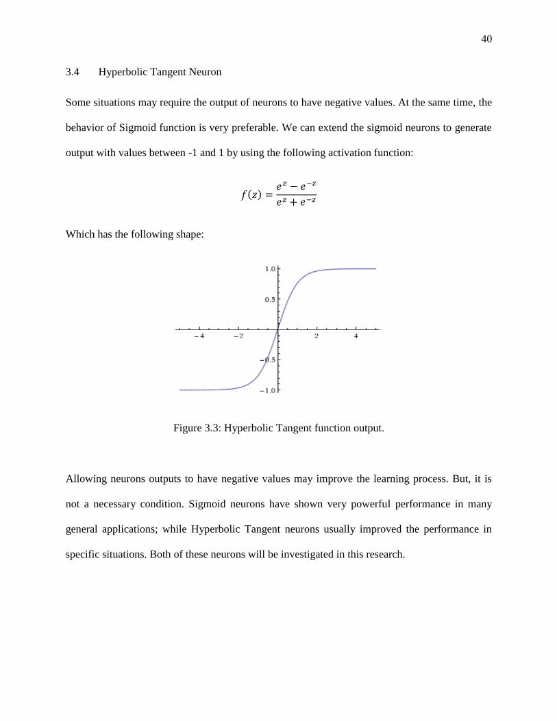
3.4 Hyperbolic Tangent Neuron

Some situations may require the output of neurons to have negative values. At the same time, the

behavior of Sigmoid function is very preferable. We can extend the sigmoid neurons to generate

output with values between -1 and 1 by using the following activation function:

( )

Which has the following shape:

Figure ‎3.3: Hyperbolic Tangent function output.

Allowing neurons outputs to have negative values may improve the learning process. But, it is

not a necessary condition. Sigmoid neurons have shown very powerful performance in many

general applications; while Hyperbolic Tangent neurons usually improved the performance in

specific situations. Both of these neurons will be investigated in this research.

41

3.5 Neural Network Architecture

As the name suggests, ANN is a network of connected neurons. Usually, Sigmoid neurons are

used. In this network, some neurons will have their input coming from external data source (i.e.

Condition-Based Monitoring system). Others will take the output of other neurons as their input.

Repeating this way of connecting neuron will lead to multiple layers neural networks. Neurons in

the first layer use external data as their input to calculate their output. Neurons in the second

layer use the outputs of first layer neurons as their input. This process keeps repeating until

neurons in the last layer calculate their outputs. The last layer outputs are the overall neural

network output.

Figure ‎3.4: Multiple layers neural network.

42

The first layer is called the input layer and the last layer is called output layer. Layers between

input layer and output layer are called hidden layers.

It is evident that neural network has much powerful capabilities in generating any type of

decision more than single perceptron. Mathematically speaking, neural networks are called

Universal Approximate. It means that neural network have the ability to approximate any

mathematical function in the whole universe. From philosophical point of view, we can assume

that neural networks can perform any mental or cognition computation which a human brain can

perform if the neural network is large enough and complex enough.

3.6 Neural Network Learning

In section 3.2, we saw an example of teaching a perceptron how to generate a binary

maintenance decision based on the binary input of equipment parameters. In the continuous form

of neurons (Sigmoid or Hyperbolic Tangent), we can use their continuous feature to have an

automatic learning mechanism. In the new learning model, neurons will start with random values

of weights and bias (threshold). Then, automatically they keep update these values based on their

run time experience.

Error Function

Every neuron in the neural networks updates their weights and bias based on estimation error.

For example, imagine a boy trying to throw a ball in a basket. The neural network inside this

boy’s brain keeps modifying its weight every time the boy misses the basket by values

43

depending on how much the boy missed the basket. This process keeps happening until the boy

scores. The same process is applied in artificial neural networks.

Having said that, an exact error function should be defined so that weights updates can be

calculated. By having the neural network output and the desired value, several error functions

can be formulated. One of the most used functions in literature is Squared Sum Error:

∑( )

Where is the neural network output at time t and is the desired output (what the neural

network should estimate) at time t. Any learning algorithm should try to minimize this error.

Gradient

Minimizing any continuous and differential function depends on a mathematical concept called

Gradient. Since Sigmoid (or Hyperbolic Tangent) neurons are used, the error function in

previous section is both continuous and differential. Therefore, Gradient can be employed to

minimize the error and calculate the best update for weight values. One way to describe the

gradient is to imagine it as a vector which point to the direction of the maximum value of the

function. The negative gradient points to the minimum value of the function. The gradient of

error function is calculated by taking the partial derivate of error function with respect to each

weight in the neural network:

44

[

]

The weights in this formula represent weights of all neuron in the whole network. It is

very difficult to calculate the gradient using the classical mathematical approach.

Back-Propagation Learning

Because of the complexity of error function in large neural network, computing the derivative

based on single weight is very tedious. Therefore, more practical method should be used. The

next flowchart (Figure 3.5) shows the general steps of back-propagation learning.

Each step in learning is called Epoch. The first step is to initialize the neural network

with required number of neurons and layers structure. Then, weights and bias values of each

neuron are chosen randomly. After that, the output of the neural network is calculated based on

the input data. First, the input is fed to the neuron in the input layer. Then, the output of input

layer neurons is fed to the second layer neurons. This process keeps repeating until neural

network output is calculated at the last layer neuron.

By having the neural network output, we can calculate the error value based of sum

squared error function. At this point, we need to check if the error is below sum threshold or if

the maximum allowed number of epoch is reached. If any of these conditions is correct, the

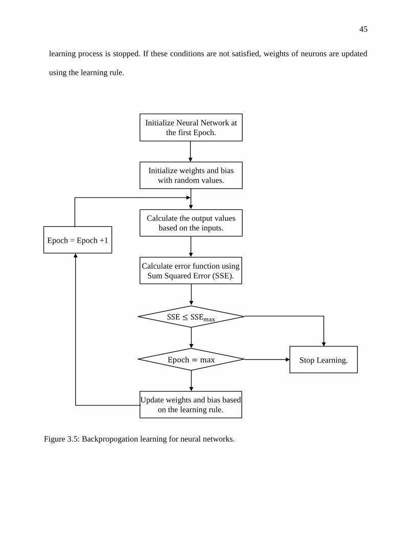
45

learning process is stopped. If these conditions are not satisfied, weights of neurons are updated

using the learning rule.

Epoch = Epoch +1

Update weights and bias based

on the learning rule.

E c max Stop Learning.

SSE ≤ SSEmax

Calculate error function using

Sum Squared Error (SSE).

Calculate the output values

based on the inputs.

Initialize weights and bias

with random values.

Initialize Neural Network at

the first Epoch.

Figure 3.5: Backpropogation learning for neural networks.

46

The learning rule depends on idea of propagating the error backwards from the neurons in

the output layer to the neurons of preceding layers. The new weights of each neuron are

calculated as follow:

( ) ( ) ( )

The weight at time t+1 is equal to the weight at time t in addition to the update value. The update

value is equal to the learning rate ( ) multiplied by ( ) where is the neuron output.

Lastly, the error coming from front layer neurons ( ) is multiplied by the update value.

47

Neural Condition-Based Maintenance (N-CBM) Chapter 4:

This chapter discusses how artificial neural networks technique is used to perform condition-

based maintenance. At the beginning, modeling of component degradation will be presented.

After that, maintenance cost calculations will be deliberated. Later, the classical approach of

estimating inspection interval will be discussed. Lastly, the adopted neural network

implementation will be delivered.

4.1 Component Stochastic Degradation

Most works in literature use stochastic approach to model component degradation. The amount

of degradation experienced by any component can be considered as a function of time ( ).

There are many uncertain factors which may affect the value of ( ). Therefore, stochastic

approach is used to calculate ( ). The most adopted stochastic process for this sort of modeling

is Gamma process where the probability density function is calculated as follow:

( ( )| ) ( ) ( )

( )

Here, a and b are gamma distribution parameters. Function () is gamma function. Also, the

mean of this process is ⁄ while the variance is ⁄ .

Having this degradation process in mind, we would like to define inspection time ( ) where the

inspection is performed at the end of this interval. Keep in mind that as time progress,

48

component degradation increases. Also, whenever a component replacement is performed, the

degradation process will restart from zero as seen in the following figure:

Figure ‎4.1: Degradation process over time (Hong et al, 2014).

Two types of maintenance can be defined. First type is Preventive Maintenance where the

component replacement is performed before its failure. Second type is Failure Maintenance

where the component is replaced only when it broke. Two values are associated with these types

of maintenance. These values represent the amount of degradation which requires the

maintenance. If the degradation is larger than or equal , the preventive maintenance can be

performed; while failure maintenance is performed when degradation reaches .

4.2 Maintenance Cost

There are three types of activities which generate cost. The first activity is inspection. Any

component should be inspected from time to time to check its degradation state. This activity

49

generates inspection cost ( ). The second activity is preventive replacement where the

component is replaced before it fails. This activity generates preventive cost ( ). The third

activity is failure replacement where the component is replaced after its failure. This activity

generates failure cost ( ).

In general, failure cost is most expensive with multiple orders of magnitude compared to other

types of cost. Preventive cost comes second with higher value than inspection cost. Keep in mind

that, inspection cost in generated whenever inspection is performed. And, the inspection is

performed every until an inspection leads to preventive replacement where preventive cost is

added as well. Therefore, the total cost over operation time ( ) can be calculated as follow:

( ) (∑ [

] ∑

∑ )

As seen in the previous equation, the total cost is combined of three mentioned types of costs.

The discount rate ( ) is introduced to add the effect cost reduction over time. The total number of

performed inspections is denoted by ; while represents the total number of preventative

replacement and represents the total number of failure replacement.

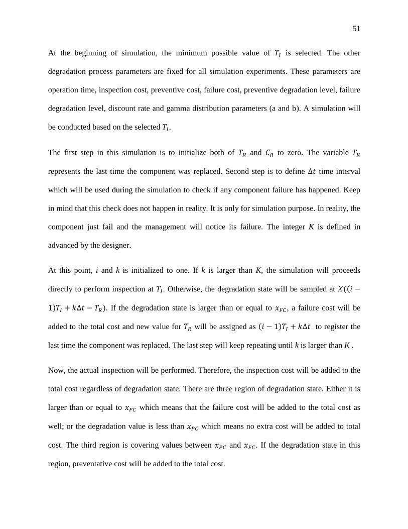
4.3 Classical Condition-Based Maintenance

The total cost formula emphasis that value of plays crucial role in minimizing the total cost.

Therefore, any good maintenance manager will try to find the optimal value of which results

in the minimum total cost on average. To find this optimal value, simulation approach is used in

literature. The main idea is to try every possible value of in simulation environment many

times and to adopt the best value on average. The following flow chart describes simulation.

50

Select 𝑇𝐼

Set 𝑇𝑅 and 𝐶𝑅

Set ∆𝑡 𝑇𝐼

𝐾, where 𝐾 is integer

Set 𝑘

If 𝑘 ≤ 𝐾 Sample 𝑥 𝑋((𝑖 )𝑇𝐼 𝑘∆𝑡 𝑇𝑅)

Set 𝑖

If 𝑥 ≥ 𝑥𝐹𝐶

𝐶𝑅 𝐶𝑅 𝐶𝐹𝑒 𝛾(𝑖 )𝑇𝐼+𝑘∆𝑡

𝑇𝑅 (𝑖 )𝑇𝐼 𝑘∆𝑡

𝑘 𝑘

Sample 𝑥 𝑋(𝑖𝑇𝐼 𝑇𝑅)

If 𝑥 ≥ 𝑥𝐹𝐶 𝐶𝑅 𝐶𝑅 𝐶𝐼𝑒 𝛾𝑖𝑇𝐼 𝐶𝐹𝑒

𝛾𝑖𝑇𝐼

If 𝑥 𝑥𝑃𝐶 𝐶𝑅 𝐶𝑅 𝐶𝐼𝑒 𝛾𝑖𝑇𝐼

𝐶𝑅 𝐶𝑅 𝐶𝐼𝑒 𝛾𝑖𝑇𝐼 𝐶𝑃𝑒

𝛾𝑖𝑇𝐼

𝑖 𝑖

No

Yes

Yes

No

No

No

Yes

Yes

Figure 4.2: 4.3 Classical condition-based maintenance flow chart.

51

At the beginning of simulation, the minimum possible value of is selected. The other

degradation process parameters are fixed for all simulation experiments. These parameters are

operation time, inspection cost, preventive cost, failure cost, preventive degradation level, failure

degradation level, discount rate and gamma distribution parameters (a and b). A simulation will

be conducted based on the selected .

The first step in this simulation is to initialize both of and to zero. The variable

represents the last time the component was replaced. Second step is to define ∆ time interval

which will be used during the simulation to check if any component failure has happened. Keep

in mind that this check does not happen in reality. It is only for simulation purpose. In reality, the

component just fail and the management will notice its failure. The integer K is defined in

advanced by the designer.

At this point, i and k is initialized to one. If k is larger than K, the simulation will proceeds

directly to perform inspection at . Otherwise, the degradation state will be sampled at ((

) ∆ ). If the degradation state is larger than or equal to , a failure cost will be

added to the total cost and new value for will be assigned as ( ) ∆ to register the

last time the component was replaced. The last step will keep repeating until k is larger than K .

Now, the actual inspection will be performed. Therefore, the inspection cost will be added to the

total cost regardless of degradation state. There are three region of degradation state. Either it is

larger than or equal to which means that the failure cost will be added to the total cost as

well; or the degradation value is less than which means no extra cost will be added to total

cost. The third region is covering values between and . If the degradation state in this

region, preventative cost will be added to the total cost.

52

4.4 Neural Condition-Based Maintenance

This research proposes to use machine learning technique which is very effective in many fields.

This technique is artificial neural networks which an attempt to imitate the ability of human brain

reasoning. Imagine that you have the ability to assign an employee to every machine for

maintenance purpose. This employee uses his advanced reasoning abilities to estimate the

degradation level of the machine. Based on his assessment, the employee will be able to assign

the best inspection interval. This approach is very costly and unrealistic.

Artificial neural networks provide us with human brain abilities without the extra cost. Also, it

can be tuned to be focused on one type of application and to be resized in any way necessary. In

this research, an inference engine based on artificial neural network is developed to estimate the

degradation level of the specific component. This engine takes the current degradation level as

an input to produce the maintenance decision. This decision is composed of two elements. The

first element is the expected degradation level in near future. The second element is the estimated

time to the failure point.

Similar to human brain, artificial neural networks requires training and learning before it can be

efficiently used. In the classical maintenance management approach, the simulation phase is used

to find the optimal inspection interval. Here, training phase is used to teach the neural network

how to accurately estimate the degradation level of the component under consideration. Also,

this phase provides us the best risk factor of our approach which is the estimation error during

the training. This risk measure can be used to generate the optimal maintenance decision which

results in much lower cost. Also, this risk measure can be used for any required analysis for the

overall risk management of maintenance operations.

53

Select 𝑇𝐼

Set 𝑇𝑅 and 𝐶𝑅

Set ∆𝑡 𝑇𝐼

𝐾, where 𝐾 is integer

Set 𝑘

If 𝑘 ≤ 𝐾 Simulate 𝑥𝑛 𝑁𝑒𝑢𝑟𝑜((𝑖 )𝑇𝐼 𝑘∆𝑡 𝑇𝑅)

Set 𝑖

If 𝑥𝑛 ≥ 𝑥𝐹𝐶

𝐶𝑅 𝐶𝑅 𝐶𝐹𝑒 𝛾(𝑖 )𝑇𝐼+𝑘∆𝑡

𝑇𝑅 (𝑖 )𝑇𝐼 𝑘∆𝑡

𝑘 𝑘

Sample 𝑥 𝑋(𝑖𝑇𝐼 𝑇𝑅)

If 𝑥 ≥ 𝑥𝐹𝐶 𝐶𝑅 𝐶𝑅 𝐶𝐼𝑒 𝛾𝑖𝑇𝐼 𝐶𝐹𝑒

𝛾𝑖𝑇𝐼

If 𝑥 𝑥𝑃𝐶 𝐶𝑅 𝐶𝑅 𝐶𝐼𝑒 𝛾𝑖𝑇𝐼

𝐶𝑅 𝐶𝑅 𝐶𝐼𝑒 𝛾𝑖𝑇𝐼 𝐶𝑃𝑒

𝛾𝑖𝑇𝐼

𝑖 𝑖

Simulate 𝑥𝑛 𝑁𝑒𝑢𝑟𝑜(𝑖𝑇𝐼 𝑇𝑅)

Train Neuro based on 𝑥 and 𝑥𝑛

𝑅𝑖𝑠𝑘 |𝑥 𝑥𝑛|

Figure 4.3: Neural condition-based maintenance flow chart.

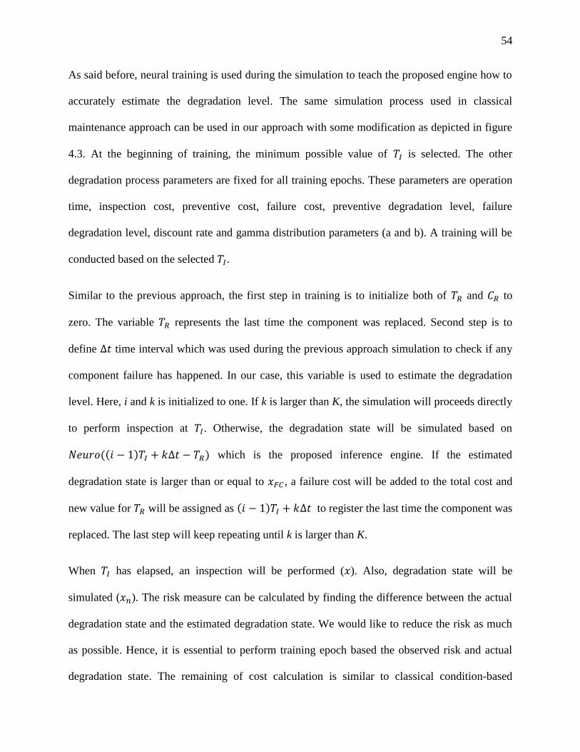
54

As said before, neural training is used during the simulation to teach the proposed engine how to

accurately estimate the degradation level. The same simulation process used in classical

maintenance approach can be used in our approach with some modification as depicted in figure

4.3. At the beginning of training, the minimum possible value of is selected. The other

degradation process parameters are fixed for all training epochs. These parameters are operation

time, inspection cost, preventive cost, failure cost, preventive degradation level, failure

degradation level, discount rate and gamma distribution parameters (a and b). A training will be

conducted based on the selected .

Similar to the previous approach, the first step in training is to initialize both of and to

zero. The variable represents the last time the component was replaced. Second step is to

define ∆ time interval which was used during the previous approach simulation to check if any

component failure has happened. In our case, this variable is used to estimate the degradation

level. Here, i and k is initialized to one. If k is larger than K, the simulation will proceeds directly

to perform inspection at . Otherwise, the degradation state will be simulated based on

(( ) ∆ ) which is the proposed inference engine. If the estimated

degradation state is larger than or equal to , a failure cost will be added to the total cost and

new value for will be assigned as ( ) ∆ to register the last time the component was

replaced. The last step will keep repeating until k is larger than K.

When has elapsed, an inspection will be performed ( ). Also, degradation state will be

simulated ( ). The risk measure can be calculated by finding the difference between the actual

degradation state and the estimated degradation state. We would like to reduce the risk as much

as possible. Hence, it is essential to perform training epoch based the observed risk and actual

degradation state. The remaining of cost calculation is similar to classical condition-based

55

maintenance. The inspection cost will be added to the total cost regardless of degradation state.

There are three region of degradation state. Either it is larger than or equal to which means

that the failure cost will be added to the total cost as well; or the degradation value is less than

which means no extra cost will be added to total cost. The third region is covering values

between and . If the degradation state in this region, preventative cost will be added to

the total cost.

56

Results and Discussion Chapter 5:

In this chapter, extensive evaluation of the proposed condition-based maintenance approach will

be presented. To highlight the strength of the proposed approach, direct comparison with one of

the most recent work (Hong et al, 2014) will conducted. Deep discussion for each experiment is

provided.

5.1 Experiment Implementation

For comparison reason, the same experiment settings used in (Hong et al, 2014) is adopted in this

thesis. To simplify the discussion of experiment implementation, an overall run from the main

simulation file is presented as step-by-step process. The source code for the remaining function

files is presented in the appendix. The main experiment steps are:

Clearing Memory and Workspace

This is the first step in any scientific simulation to prevent mixing data results from different

experiments.

clear all;

clc;

57

Setting Number of Simulation Experiment

As mentioned before, the simulation experiments have been conducted for several times. This is

done to show the strength of the proposed solution on average.

N = 5000;

Setting Gamma Parameter

This parameter controls the effect of inflation in cost calculation. If Gamma is zero, this means

that the cost at the end of the year is the same as the cost at the beginning of the year. However,

this is not the case in the reality. Inflation reduces the cost as time progress. Here, Gamma

represents the rate of cost reduction. Two set of simulation experiments were conducted. One set

is conducted where Gamma is zero and another is conducted where Gamma is 0.05.

gamma = 0;

Setting Simulation Parameters

These are the parameters used by Hong et al (2014). In their paper, the authors simulated piping

system in nuclear reactors. The degradation process is due corrosion resulted from heating which

affect the wall thickness of the pipes. At installation, pipe thickness is 6.5 mm. When thickness

reaches 4.5, preventive maintenance is performed. If the thickness is less than 3.41, failure

maintenance is performed. The first parameter is simulation time (T) which is in years.

58

T = 50;

All cost parameters are normalized. Inspection cost:

C_I = 0.1;

Preventive cost:

C_P = 1;

Failure cost:

C_F = 10;

Preventive maintenance threshold:

x_PC = 2;

Failure maintenance threshold:

x_FC = 3.09;

Gamma distribution parameters:

a = 10 / 9;

b = 100 / 9;

59

Collecting Neural Training Data

To train neural network, we need to generate training data. Here, training data is generated by

running stochastic simulation experiments and collecting all aspects of maintenance operations.

data = get_nn_train_data(T,x_PC,x_FC,a,b);

Train Neural Network

This is the most important step in our proposed condition-based maintenance. Here, the neural

engine is trained to be able to accurately estimate the degradation level of components.

[net, err, inputs, targets, outputs, errors, trainTargets, valTargets, testTargets, tr] =

create_nn(10, data);

Calculate and present Training, Validation and Test performance of the training process.

performance = perform(net,targets,outputs)

trainPerformance = perform(net,trainTargets,outputs)

valPerformance = perform(net,valTargets,outputs)

testPerformance = perform(net,testTargets,outputs)

View the Neural Network architecture.

view(net)

60

Figure ‎5.1: Neural Network architecture and learning process.

61

Next, we plot several Neural Network performance figures which show the several overall

performance aspects graphically.

figure, plotperform(tr)

figure, plottrainstate(tr)

figure, plotfit(net,inputs,targets)

figure, plotregression(targets,outputs)

figure, ploterrhist(errors)

Figure ‎5.2: Mean squared error during the learning process.

62

Figure ‎5.3: The gradient evolution as learning process progress.

Figure ‎5.4: Sample of actual values and the estimated values of the degradation process and the

difference between then (Error).

63

Figure ‎5.5: Correlation between the actual values and the estimated values.

Figure ‎5.6: Error distribution of the estimated values of the degradation process.

64

Simulation Loop

Here, every inspection interval will be investigated. This loop starts from 0.5 (half year) as

inspection interval and it keeps incrementing the inspection interval by 0.1 until it reach 50

years. For every inspect interval 5000 simulation experiments will be conducted which the

responsibility of the inner loop. After data of all simulation experiments were collected, the

average cost rate will be calculated in addition to the risk measurement which is the standard

deviation.

index = 0;

xaxis = 0;

yaxis = 0;

yaxis_ = 0;

for T_I = 0.5:0.1:T

C_R = 0;

C_R_ = 0;

K = 2;

for s = 1:N

Calculate the cost for Hong et al (2014) condition-based maintenance approach.

C_R(s) = simulateCost_Hong(T,T_I,gamma,C_I,C_P,C_F,x_PC,x_FC,a,b,K);

Calculate the cost for the proposed condition-based maintenance approach.

C_R_(s) = simulateCost_NN(T,T_I,gamma,C_I,C_P,C_F,x_PC,x_FC,a,b,K,net,err);

end

end

65

Generate Graphs

Comparison graphs are generated to show the difference and the outperformance of the proposed

condition-based maintenance approach compared to Hong et al (2014) condition-based

maintenance approach.

generatefigure_cost_rate(xaxis,[yaxis_ema; yaxis_ema_]);

generatefigure_cost_std(xaxis,[yaxis_ema_std; yaxis_ema_std_]);

5.2 Experiments Results

Two set of experiments were conducted. The first set does not take inflation into cost

calculations. In other words, Gamma parameter is set to zero. The second set of experiment

assumes an inflation rate of 5 % which means that Gamma parameter is set to 0.05. Two

important performances metric were used to evaluate the proposed approach. These metric are

Cost Rate and Standard Deviation. In all experiment, the average rate of degradation is 0.1. Keep

in mind that this degradation value is an average for stochastic process which means that the

actual degradation may be larger or smaller than the average value. However, if the process is

repeated so many times, the degradation process value will approach the average value. Saying

that the average degradation value is 0.1 under the adopted experiment settings from Hong et al

(2014) leads to two facts regarding maintenance. First, the degradation process will take around

20 years to reach the preventive maintenance degradation level (i.e. the pipe thickness is 5.5

mm). The same goes for failure maintenance. It will take the degradation process 30.09 years on

average to reach failure degradation level. In other words, the pipe thickness is reduced to value

less than or equal 3.41 mm.

66

Figure ‎5.7: Cost rate with Gamma = 0.

The first experiment calculates the cost rate where gamma is set to zero. Figure 5.7 shows the

cost rate for the proposed neural condition-based maintenance and Hong et al (2014) approach.

Both approaches achieve the minimum cost rate at interval inspection equal to 25 years. This due

to fact that at this inspection interval the maintenance cost is composed of only one inspection

cost and one preventive cost in Hong’s approach. In the proposed N-CBM, the cost is composed

of only one preventive cost from inspection interval 25 years until inspection interval 40 years.

This is the result of the proposed N-CBM capability of accurately estimating how much time is

67

left until the failure moment. In other words, the proposed approach is capable of performing

preventive maintenance directly before failure while Hong’s approach performs preventive

maintenance way before failure time (around 10 years ealier). On average, N-CBM reduced the

cost by 73.47 % compared to S-CBM.

Figure ‎5.8: Standard deviation of cost rate with Gamma = 0.

The second experiment calculates the standard deviation of cost rate where gamma is set to zero.

Figure 5.8 shows the standard deviation of cost rate for the proposed neural condition-based

maintenance and Hong et al (2014) approach. This metric measure how much cost rate fluctuate

68

during the simulation experiment. As this metric decreases, the stability of mechanism under

investigation increases. The proposed N-CBM maintenance system is more stable than S-CBM

system. On average, the stability of maintenance management is increased by 81.29 % after

using the proposed approach.

Figure ‎5.9: Cost rate with Gamma = 0.05.

The third experiment calculates the cost rate where gamma is set to 5 %. Figure 5.9 shows the

cost rate for the proposed neural condition-based maintenance and Hong et al (2014) approach.

As said before, Gamma parameter introduces the effect of inflation in cost calculation. This

69

means that the maintenance cost is shrinking as time progress by factor of 5 % every year.

Similarly to previous experiments, the proposed maintenance approach outperforms Hong’s

approach. The reduction in cost after using the proposed approach is 66.7 % on average.

Figure ‎5.10: Standard deviation of cost rate with Gamma = 0.05.

The last experiment calculates the standard deviation of cost rate where gamma is set to 5 %.

Figure 5.10 shows the standard deviation of cost rate for the proposed neural condition-based

70

maintenance and Hong et al (2014) approach. On average, the proposed maintenance

management approach is more stable then Hong’s approach by 73.02 %. Note that, between the

inspection interval value 17 years and the inspection interval value 30.9 years the proposed

maintenance management approach is extremely stable.

71

Conclusion Chapter 6:

In this thesis, new condition-based maintenance approach was proposed. First, the benefits of

using computerized maintenance were highlighted and emphasized. These benefits have made

the computerized management systems popular and in high demand. Competitiveness in the

business world has forced organizations to adopt measures that lead to the reduced costs of

operations and increment in revenue. These systems have proved reliable and managed to satisfy

the needs of organizations that have adopted them. Then, the reason behind using preventive

maintenance was introduced which is based on the fact that usual maintenance policy in practice

is to wait for equipment failure before performing any maintenance action. It turned out that this

policy causes huge losses in term of Down-Time cost. In the last two decades, preventive

maintenance gain popularity due to its cost effective approach. PM tries to perform maintenance

before equipment failure so that no down-time is experienced and full equipment’s utilization is

achieved. However, performing maintenance on equipment long before its failure time

introduces unnecessary cost; especially, if maintenance is being performed frequently on stable

equipment. The last statement establishes the motivation for using condition-based maintenance.

The main problem which this research tries to solve is that all of the existing condition-

based maintenance models are based on statistical approach to estimate failure time which leads

to low accuracy. This problem is due to the fact that statistical approach usually depends on

couple of numbers. Therefore, adopting statistical approach leads to leaving so much of valuable

information and focusing on couple of numbers which problematic and not wise. As a result, the

main objective of this study is to develop Condition-Based Maintenance mechanism that has the

ability to capture all necessary information to accurately estimate equipment failure time.

72

Neural Networks was chosen as the methodology for the proposed solution which is one

of the most powerful techniques in artificial intelligence field. It is inspired by how human brain

operates. This technique was created at the end of forties of the last century. It has been shown

that this technique can be very powerful to solve many difficult problems. Neural Networks is a

network of interconnected small elements called neurons. Each one of these elements can

perform specific computation that lead to the targeted goal. The input data is provided to these

elements and the desired output should be expected.

Condition-Based Maintenance mechanism based on neural network is developed to

estimate the degradation level of the specific component. This mechanism takes the current

degradation level as an input to produce the maintenance decision. This decision is composed of

two elements. The first element is the expected degradation level in near future. The second

element is the estimated time to the failure point. Experiments and evaluations showed the

outperformance of the proposed solution compared to the most recent cutting edge solution.

73

Appendix

This appendix presents the source code of the remaining functions used in our experimentation

and evaluation process. Each one of these function was written entirely in MATLAB.

Source code functions are:

function data = get_nn_train_data(T,x_PC,x_FC,a,b)

T_I = 0.1;

T_R = 0;

i = 1;

data = [];

while (i*T_I) < T

t_i = i * T_I;

x = gamrnd(a*(t_i-T_R),1/b);

data(size(data,1)+1,1) = t_i-T_R;

data(size(data,1),2) = x;

if x < x_PC

elseif x >= x_FC

T_R = t_i;

else

T_R = t_i;

end

i = i + 1;

end

end

74

function [net, err, inputs, targets, outputs, errors, trainTargets,

valTargets, testTargets, tr] = create_nn(num_neurons, data)

inputs = data(:,1)';

targets = data(:,2)';

% Create a Fitting Network

hiddenLayerSize = num_neurons;

net = fitnet(hiddenLayerSize);

% Choose Input and Output Pre/Post-Processing Functions

% For a list of all processing functions type: help nnprocess

net.inputs{1}.processFcns = {'removeconstantrows','mapminmax'};

net.outputs{2}.processFcns = {'removeconstantrows','mapminmax'};

% Setup Division of Data for Training, Validation, Testing

% For a list of all data division functions type: help nndivide

net.divideFcn = 'dividerand'; % Divide data randomly

net.divideMode = 'sample'; % Divide up every sample

net.divideParam.trainRatio = 70/100;

net.divideParam.valRatio = 15/100;

net.divideParam.testRatio = 15/100;

% For help on training function 'trainlm' type: help trainlm

% For a list of all training functions type: help nntrain

net.trainFcn = 'trainlm'; % Levenberg-Marquardt

% Choose a Performance Function

% For a list of all performance functions type: help nnperformance

net.performFcn = 'mse'; % Mean squared error

% Choose Plot Functions

% For a list of all plot functions type: help nnplot

net.plotFcns = {'plotperform','plottrainstate','ploterrhist', ...

'plotregression', 'plotfit'};

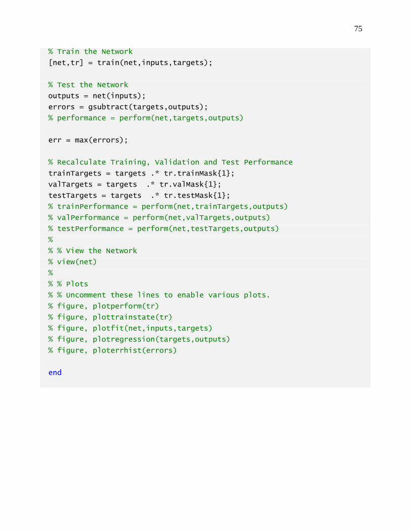
75

% Train the Network

[net,tr] = train(net,inputs,targets);

% Test the Network

outputs = net(inputs);

errors = gsubtract(targets,outputs);

% performance = perform(net,targets,outputs)

err = max(errors);

% Recalculate Training, Validation and Test Performance

trainTargets = targets .* tr.trainMask{1};

valTargets = targets .* tr.valMask{1};

testTargets = targets .* tr.testMask{1};

% trainPerformance = perform(net,trainTargets,outputs)

% valPerformance = perform(net,valTargets,outputs)

% testPerformance = perform(net,testTargets,outputs)

%

% % View the Network

% view(net)

%

% % Plots

% % Uncomment these lines to enable various plots.

% figure, plotperform(tr)

% figure, plottrainstate(tr)

% figure, plotfit(net,inputs,targets)

% figure, plotregression(targets,outputs)

% figure, ploterrhist(errors)

end

76

function C_R =

simulateCost_Hong(T,T_I,gamma,C_I,C_P,C_F,x_PC,x_FC,a,b,K)

C_R = 0;

T_R = 0;

dt = T_I / K;

i = 1;

while (i*T_I) < T

t_i = i * T_I;

for k = 1:K-1

tau_k = ((i-1)*T_I) + (k*dt) - T_R;

x = gamrnd(a*tau_k,1/b);

if x >= x_FC

C_R = C_R + (C_F * exp(-1*gamma*(((i-1)*T_I)+(k*dt))));

T_R = ((i-1)*T_I) + (k*dt);

end

if ((i-1)*T_I) + (k*dt) >= T

break;

end

end

if k == K-1

% x = (0.1 * (t_i-T_R));

x = gamrnd(a*(t_i-T_R),1/b);

if x < x_PC

C_R = C_R + (C_I * exp(-1*gamma*t_i));

elseif x >= x_FC

C_R = C_R + (C_I * exp(-1*gamma*t_i)) + (C_F * exp(-

1*gamma*t_i));

T_R = t_i;

else

C_R = C_R + (C_I * exp(-1*gamma*t_i)) + (C_P * exp(-

1*gamma*t_i));

T_R = t_i;

end

end

i = i + 1;

end

C_R = C_R / T;

end

77

function C_R =

simulateCost_NN(T,T_I,gamma,C_I,C_P,C_F,x_PC,x_FC,a,b,K,net,err)

C_R = 0;

T_R = 0;

dt = T_I / K;

i = 1;

while (i*T_I) < T

t_i = i * T_I;

for k = 1:K-1

tau_k = ((i-1)*T_I) + (k*dt) - T_R;

x = gamrnd(a*tau_k,1/b);

if x >= x_FC

C_R = C_R + (C_F * exp(-1*gamma*(((i-1)*T_I)+(k*dt))));

T_R = ((i-1)*T_I) + (k*dt);

end

if ((i-1)*T_I) + (k*dt) >= T

break;

end

end

if k == K-1

x_ = sim(net,(t_i-T_R));

if x_ + err >= x_FC

C_R = C_R + (C_I * exp(-1*gamma*t_i)) + (C_P * exp(-

1*gamma*t_i));

T_R = t_i;

end

end

i = i + 1;

end

C_R = C_R / T;

end

78

function generatefigure_cost_rate(X1, YMatrix1)

figure1 = figure('Name','Cost Rate');

% Create axes

axes1 = axes('Parent',figure1);

box(axes1,'on');

hold(axes1,'all');

% Create multiple lines using matrix input to plot

plot1 = plot(X1,YMatrix1);

set(plot1(1),'Marker','x','DisplayName','Hong');

set(plot1(2),'Marker','*','Color',[1 0 0],'DisplayName','Alzzaabi');

% Create xlabel

xlabel('Inspection interval (year)');

% Create ylabel

ylabel('Expectation of cost rate (per year)');

% Create title

title('Cost Rate');

% Create legend

legend(axes1,'show');

79

function generatefigure_cost_std(X1, YMatrix1)

figure1 = figure('Name','Standard Deviation of Cost Rate');

% Create axes

axes1 = axes('Parent',figure1);

box(axes1,'on');

hold(axes1,'all');

% Create multiple lines using matrix input to plot

plot1 = plot(X1,YMatrix1);

set(plot1(1),'Marker','x','DisplayName','Hong');

set(plot1(2),'Marker','*','Color',[1 0 0],'DisplayName','Alzzaabi');

% Create xlabel

xlabel('Inspection interval (year)');

% Create ylabel

ylabel('Standard Deviation of cost rate (per year)');

% Create title

title('Standard Deviation of Cost Rate');

% Create legend

legend(axes1,'show');

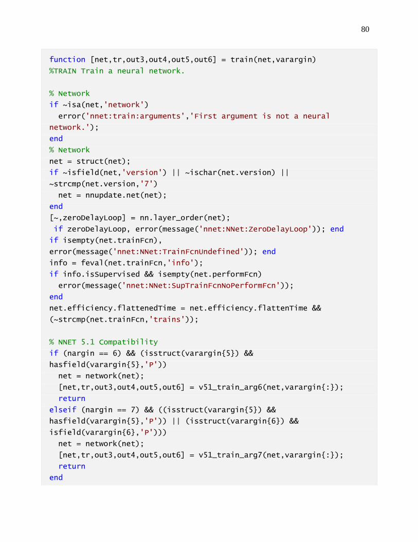
80

function [net,tr,out3,out4,out5,out6] = train(net,varargin)

%TRAIN Train a neural network.

% Network

if ~isa(net,'network')

error('nnet:train:arguments','First argument is not a neural

network.');

end

% Network

net = struct(net);

if ~isfield(net,'version') || ~ischar(net.version) ||

~strcmp(net.version,'7')

net = nnupdate.net(net);

end

[~,zeroDelayLoop] = nn.layer_order(net);

if zeroDelayLoop, error(message('nnet:NNet:ZeroDelayLoop')); end

if isempty(net.trainFcn),

error(message('nnet:NNet:TrainFcnUndefined')); end

info = feval(net.trainFcn,'info');

if info.isSupervised && isempty(net.performFcn)

error(message('nnet:NNet:SupTrainFcnNoPerformFcn'));

end

net.efficiency.flattenedTime = net.efficiency.flattenTime &&

(~strcmp(net.trainFcn,'trains'));

% NNET 5.1 Compatibility

if (nargin == 6) && (isstruct(varargin{5}) &&

hasfield(varargin{5},'P'))

net = network(net);

[net,tr,out3,out4,out5,out6] = v51_train_arg6(net,varargin{:});

return

elseif (nargin == 7) && ((isstruct(varargin{5}) &&

hasfield(varargin{5},'P')) || (isstruct(varargin{6}) &&

isfield(varargin{6},'P')))

net = network(net);

[net,tr,out3,out4,out5,out6] = v51_train_arg7(net,varargin{:});

return

end

81

% Calculation Mode

if ~isempty(varargin) && isstruct(varargin{end}) &&

isfield(varargin{end},'name')

calcMode = nncalc.defaultMode(net,varargin{end}); varargin(end) =

[];

else

if (net.efficiency.memoryReduction ~= 1)

varargin = [varargin {'reduction'

net.efficiency.memoryReduction}];

end

n = numel(varargin);

i = n + 1;

while (i-2 > 0) && ischar(varargin{i-2})

i = i - 2;

end

if (i < n)

nameValuePairs = varargin(i:n);

varargin(i:n) = [];

[calcMode,err] = nncalc.options2Mode(net,nameValuePairs);

if ~isempty(err), error('nnet:train:calcMode',err); end

else

calcMode = nncalc.defaultMode(net);

end

end

problem = calcMode.netCheck(net,calcMode.hints,false,false);

if ~isempty(problem), error(problem); end

% Check Composite Data for consistency

nargs = numel(varargin);

if nargs >= 1

isComposite = isa(varargin{1},'Composite');

else

isComposite = false;

end

for i=2:nargs

if isComposite ~= isa(varargin{i},'Composite')

error('nnet:sim:Composite','Data values must be all Composite or

82

not.');

end

end

% Check gpuArray data for consistency

if nargs >= 1

isGPUArray = isa(varargin{1},'gpuArray');

else

isGPUArray = false;

end

for i=2:nargs

vi = varargin{i};

if ~isempty(vi) && (isGPUArray ~= isa(vi,'gpuArray'))

error('nnet:sim:Composite','Data values must be all gpuArray or

not.');

end

end

% Fill in missing data consistent with type

if isComposite

emptyCell = Composite;

for i=1:numel(emptyCell)

emptyCell{i} = {};

end

else

emptyCell = {};

end

if (nargs < 1), X = emptyCell; else X = varargin{1}; end

if (nargs < 2), T = emptyCell; else T = varargin{2}; end

if (nargs < 3), Xi = emptyCell; else Xi = varargin{3}; end

if (nargs < 4), Ai = emptyCell; else Ai = varargin{4}; end

if (nargs < 5), EW = emptyCell; else EW=varargin{5}; end

if isComposite

for i=1:numel(X)

if ~exist(X,i), X{i} = {}; end

if ~exist(T,i), T{i} = {}; end

if ~exist(Xi,i), Xi{i} = {}; end

if ~exist(Ai,i), Ai{i} = {}; end

83

if ~exist(EW,i), EW{i} = {}; end

end

end

% Train

if ~feval(net.trainFcn,'supportsCalcModes');

% Train without advanced calculation modes

if isComposite

error('nnet:train:data',['Training function ' net.trainFcn ' does

not support Composite data.']);

end

if isGPUArray

error('nnet:train:data',['Training function ' net.trainFcn ' does

not support gpuArray data.']);

end

[net,data,tr,err] =

nntraining.setup(net,net.trainFcn,X,Xi,Ai,T,EW,true);

if ~isempty(err), nnerr.throw('Args',err), end

hints = nn7.netHints(net);

data.Pc = nn7.pc(net,data.X,data.Xi,data.Q,data.TS,hints);

data.Pd = nn7.pd(net,data.Pc,data.Q,data.TS,hints);

hints = nn7.dataHints(net,data,hints);

[net,tr] =

feval(net.trainFcn,'apply',net,tr,data,hints,net.trainParam);

else

% Check Data and Network

if isComposite

spmd

[~,rawData,trComp,err] =

nntraining.setup(net,net.trainFcn,X,Xi,Ai,T,EW,false);

if ~isempty(err), nnerr.throw('Args',err), end

QTSs = rawData.Q * rawData.TS;

end

QTSs = nnParallel.composite2Array(QTSs);

i = find(QTSs>0,1);

if isempty(i)

tr = [];

84

return;

end

tr = trComp{i};

else

[net,rawData,tr,err] =

nntraining.setup(net,net.trainFcn,X,Xi,Ai,T,EW,~isGPUArray);

if ~isempty(err), nnerr.throw('Args',err), end

if ((rawData.Q == 0) || (rawData.TS == 0));

tr = [];

return;

end

end

% Setup simulation/training calculation mode, network, data and

hints

[calcMode,calcNet,calcData,calcHints,net,resourceText] =

nncalc.setup1(calcMode,net,rawData);

if ~isempty(resourceText)

disp(' ')

disp('Computing Resources:')

nntext.disp(resourceText)

disp(' ')

end

trainFcn = str2func(net.trainFcn);

% Train in Parallel or Single mode

isParallel = isa(calcMode,'Composite');

if isParallel

spmd

[calcLib,calcNet] =

nncalc.setup2(calcMode,net,calcData,calcHints);

ws = warning('off','parallel:gpu:kernel:NullPointer');

[calcNet,tr] = trainFcn('apply',net,rawData,calcLib,calcNet,tr);

warning(ws);

if (calcMode.isMainWorker)

WB = calcMode.getwb(calcNet,calcHints);

end

if (labindex == 1), mainWorkerInd = calcLib.mainWorkerInd; end

85

end

mainWorkerInd = mainWorkerInd{1};

WB = WB{mainWorkerInd};

tr = tr{mainWorkerInd};

else

[calcLib,calcNet] =

nncalc.setup2(calcMode,calcNet,calcData,calcHints);

ws = warning('off','parallel:gpu:kernel:NullPointer');

[calcNet,tr] = trainFcn('apply',net,rawData,calcLib,calcNet,tr);

warning(ws);

WB = calcMode.getwb(calcNet,calcHints);

end

% Finalize Network and Training Record

net = setwb(net,WB);

end

net = network(net);

tr = nntraining.tr_clip(tr);

if isfield(tr,'perf')

tr.best_perf = tr.perf(tr.best_epoch+1);

end

if isfield(tr,'vperf')

tr.best_vperf = tr.vperf(tr.best_epoch+1);

end

if isfield(tr,'tperf')

tr.best_tperf = tr.tperf(tr.best_epoch+1);

end

% NNET 5.1 Compatibility

if nargout > 2

[out3,out5,out6] = sim(net,X,Xi,Ai,T);

out4 = gsubtract(T,out3);

end

86

function net = network(varargin)

%NETWORK Create a custom neural network.

if (nargin == 1)

in1 = varargin{1};

if isa(in1,'struct')

net = class(in1,'network');

elseif isa(in1,'network')

net = in1;

else

net = new_network(in1);

end

else

net = new_network(varargin{:});

end

function net =

new_network(numInputs,numLayers,biasConnect,inputConnect, ...

layerConnect,outputConnect,ignore) %#ok<INUSD>

% Defaults

if nargin < 1, numInputs = 0; end

if nargin < 2, numLayers = 0; end

if nargin < 3, biasConnect = false(numLayers,1); end

if nargin < 4, inputConnect = false(numLayers,numInputs); end

if nargin < 5, layerConnect = false(numLayers,numLayers); end

if nargin < 6, outputConnect = false(1,numLayers); end

% Checking

% TODO - Error checking

% NETWORK PROPERTIES

% Note: "Param" and "Config" properties in NETWORK and subobject

% (nnetInput, nnetOutput, nnetLayer, nnetWeight, nnetBias) properties

must

% always occur directly after their associated "Fcn" properties for

% NN_STRUCT2OBJECT conversions to work properly.

87

% Version

net.version = '8';

% Basics

net.name = 'Custom Neural Network';

net.efficiency.cacheDelayedInputs = true;

net.efficiency.flattenTime = true;

net.efficiency.memoryReduction = 1;

net.userdata.note = 'Put your custom network information here.';

% Sizes

net.numInputs = 0;

net.numLayers = 0;

net.numOutputs = 0;

net.numInputDelays = 0;

net.numLayerDelays = 0;

net.numFeedbackDelays = 0;

net.numWeightElements = 0;

net.sampleTime = 1;

% Connections

net.biasConnect = false(0,1);

net.inputConnect = false(0,0);

net.layerConnect = false(0,0);

net.outputConnect = false(1,0);

% Subobjects

net.inputs = cell(0,1);

net.layers = cell(0,1);

net.biases = cell(0,1);

net.outputs = cell(1,0);

net.inputWeights = cell(0,0);

net.layerWeights = cell(0,0);

% Functions and parameters

net.adaptFcn = '';

net.adaptParam = struct;

net.divideFcn = '';

88

net.divideParam = struct;

net.divideMode = 'sample';

net.initFcn = 'initlay';

net.performFcn = 'mse';

net.performParam = mse('defaultParam');

net.plotFcns = cell(1,0);

net.plotParams = cell(1,0);

net.derivFcn = 'defaultderiv';

net.trainFcn = '';

net.trainParam = nnetParam;

% Weight & bias values

net.IW = cell(0,0);

net.LW = cell(0,0);

net.b = cell(0,1);

% Hidden properties

net.revert.IW = {};

net.revert.LW = {};

net.revert.b = {};

% Obsolete properties

% NNET 6.0 Compatibility

net.gradientFcn = ''; % Obsolete

net.gradientParam = struct; % Obsolete

% CLASS

net = class(net,'network');

% ARCHITECTURE

net = setnet(net,'numInputs',numInputs);

net = setnet(net,'numLayers',numLayers);

net = setnet(net,'biasConnect',biasConnect);

net = setnet(net,'inputConnect',inputConnect);

net = setnet(net,'layerConnect',layerConnect);

net = setnet(net,'outputConnect',outputConnect);

function net = setnet(net,field,value)

89

subscripts.type = '.';

subscripts.subs = field;

net = subsasgn(net,subscripts,value);

90

function perf = perform(net,t,y,ew)

%PERFORM Calculate network performance.

if nargin < 3, error(message('nnet:Args:NotEnough')); end

[net,err] = nntype.network('format',net);

if ~isempty(err),nnerr.throw(nnerr.value(err,'NET')); end

if isempty(net.performFcn),

error(message('nnet:NNet:PerformFcnUndefined'));

end

if nargin < 4, ew = {1}; end

if ~iscell(t), t = {t}; end

if ~iscell(y), y = {y}; end

if ~iscell(ew), ew = {ew}; end

perf = nncalc.perform(net,t,y,ew,net.performParam);

91

function out1 = view(net)

%VIEW View a neural network diagram.

%

% <a href="matlab:doc view">view</a>(NET) generates a graphical view

of a neural network.

%

% Here a feedforward network is created, trained and viewed.

%

if nargin < 1,error(message('nnet:Args:NotEnough')); end

diagram = nn.view(net);

if nargout > 0, out1 = diagram; end

92

function [net,Y,E,Xf,Af,tr]=adapt(net,X,T,Xi,Ai)

%ADAPT Adapt a neural network.

if nargin < 1,error(message('nnet:Args:NotEnough')); end

if ~isa(net,'network'), error(message('nnet:adapt:NotANet')); end

if isempty(net.adaptFcn), error(message('nnet:adapt:Undef')); end

xMatrix = ~iscell(X);

if nargin < 3, T = {}; tMatrix = xMatrix; else tMatrix = ~iscell(T);

end

if nargin < 4, Xi = {}; xiMatrix = xMatrix; else xiMatrix =

~iscell(Xi); end

if nargin < 5, Ai = {}; aiMatrix = xMatrix; else aiMatrix =

~iscell(Ai); end

[X,err] = nntype.data('format',X);

if ~isempty(err),nnerr.throw(nnerr.value(err,'Inputs'));end

if ~isempty(T), [T,err] = nntype.data('format',T); end

if ~isempty(err),nnerr.throw(nnerr.value(err,'Targets'));end

if ~isempty(Xi), [Xi,err] = nntype.data('format',Xi); end

if ~isempty(err),nnerr.throw(nnerr.value(err,'Input delay

states'));end

if ~isempty(Ai), [Ai,err] = nntype.data('format',Ai); end

if ~isempty(err),nnerr.throw(nnerr.value(err,'Layer delay

states'));end

% Network

net = struct(net);

[~,zeroDelayLoop] = nn.layer_order(net);

if zeroDelayLoop, error(message('nnet:NNet:ZeroDelayLoop')); end

[net,X,Xi,Ai,T,~,Q,TS,err] = nntraining.config(net,X,Xi,Ai,T,{1});

if ~isempty(err), nnerr.throw(err), end

% ADAPT NETWORK

% -------------

tools = nn7;

hints = tools.netHints(net,tools.hints);

93

hints.outputInd = find(net.outputConnect);

% Processed inputs

Pc = tools.pc(net,X,Xi,Q,TS,hints);

% Delayed Inputs

Pd = tools.pd(net,Pc,Q,TS,hints);

% Adapt network

[net,Ac,tr] = feval(net.adaptFcn,net,Pd,T,Ai);

net = class(net,'network');

% Network outputs, errors, final inputs

Al = Ac(:,net.numLayerDelays+(1:TS));

Y = nnMATLAB.post_outputs(hints,Al(hints.outputInd,:));

E = gsubtract(T,Y);

Xf = Pc(:,TS+(1:net.numInputDelays));

Af = Ac(:,TS+(1:net.numLayerDelays));

% FORMAT OUTPUT ARGUMENTS

% -----------------------

if (xMatrix), Y = cell2mat(Y); end

if (tMatrix), E = cell2mat(E); end

if (xiMatrix), Xf = cell2mat(Xf); end

if (aiMatrix), Af = cell2mat(Af); end

94

function net = configure(net,in2,in3,in4)

%CONFIGURE Configure neural network inputs and outputs.

% Convert from Network to Struct

net = struct(net);

if nargin < 2

error(message('nnet:Args:NotEnough'));

elseif nargin == 2

% configure(net,x)

[x,err] = nntype.data('format',in2);

if ~isempty(err),nnerr.throw(nnerr.value(err,'Input data')); end

S = nnfast.numsignals(x);

if S ~= net.numInputs

error(message('nnet:NNet:InputNumMismatch'));

end

xi = 1:net.numInputs;

t = {};

ti = [];

elseif (nargin == 3) && ~ischar(in2)

% configure(net,x,t)

[x,err] = nntype.data('format',in2);

if ~isempty(err),nnerr.throw(nnerr.value(err,'Input data')); end

[t,err] = nntype.data('format',in3);

if ~isempty(err),nnerr.throw(nnerr.value(err,'Target data')); end

numInputs = nnfast.numsignals(x);

if numInputs ~= net.numInputs

error(message('nnet:NNet:InputNumMismatch'));

end

xi = 1:numInputs;

numOutputs = nnfast.numsignals(t);

if numOutputs ~= net.numOutputs

error(message('nnet:NNet:TargetNumMismatch'));

end

ti = 1:numOutputs;

95

elseif nnstring.first_match(lower(in2),{'input','inputs'})

% configure(net,'inputs',x) -or- (net,'inputs',x,xi)

[x,err] = nntype.data('format',in3);

if ~isempty(err),nnerr.throw(nnerr.value(err,'Input data')); end

numInputs = nnfast.numsignals(x);

if nargin < 4

if numInputs ~= net.numInputs

error(message('nnet:NNet:InputNumMismatch'));

end

xi = 1:numInputs;

else

xi = in4;

err = nntype.index_row_unique('check',in4);

if ~isempty(err), nnerr.throw(nnerr.value(err,'Indices')); end

if max(xi) > net.numInputs

error(message('nnet:NNet:InputIndexOutOfRange'));

end

if length(xi) ~= numInputs

error(message('nnet:NNData:NumIndicesSignalsMismatch'));

end

end

t = {};

ti = [];

elseif

nnstring.first_match(lower(in2),{'output','outputs','target','targets'

})

% configure(net,'outputs',t) or (net,'outputs',t,ti)

[t,err] = nntype.data('format',in3);

if ~isempty(err),nnerr.throw(nnerr.value(err,'Target data')); end

numOutputs = nnfast.numsignals(t);

if nargin < 4

if numOutputs ~= net.numOutputs

error(message('nnet:NNet:TargetNumMismatch'));

end

96

ti = 1:numOutputs;

else

ti = in4;

err = nntype.index_row_unique('check',ti);

if ~isempty(err), nnerr.throw(nnerr.value(err,'Indices')); end

if max(ti) > net.numOutputs

error(message('nnet:NNet:TargetIndexOutOfRange'));

end

if length(ti) ~= numOutputs

error(message('nnet:NNet:IndicesTargetsMismatch'));

end

end

x = {};

xi = [];

elseif ischar(in2)

error(message('nnet:Args:Unrec'));

else

error(message('nnet:Args:Unrec'));

end

net = struct(net);

% Ensure all values are double

for i=1:numel(x), x{i} = double(x{i}); end

for i=1:numel(t), t{i} = double(t{i}); end

% Expand Input, Target

X = cell(net.numInputs,1);

for z=1:length(xi)

i = xi(z);

X{i} = [x{z,:}];

end

T = cell(net.numOutputs,1);

for z=1:length(ti)

i = ti(z);

T{i} = [t{z,:}];

end

97

% Input/Output Feedback Consistency

layers2output = cumsum(net.outputConnect);

Xi = false(1,net.numInputs);

Xi(xi) = true;

Ti = false(1,net.numOutputs);

Ti(ti) = true;

for i = 1:net.numInputs

j = net.inputs{i}.feedbackOutput;

if ~isempty(j)

k = layers2output(j);

if Xi(i) || Ti(k)

X{i} = [X{i} T{k}];

T{k} = X{i};

Xi(i) = true;

Ti(k) = true;

end

end

end

xi = find(Xi);

ti = find(Ti);

% Configure

for i = xi

net = nn_configure_input(net,i,X{i});

end

outputs2layers = find(net.outputConnect);

for i=ti

ii = outputs2layers(i);

net = nn_configure_output(net,ii,T{i});

end

net = nnupdate.read_only_values(net);

net = network(net);

net = init(net);

98

function [net,delInputs,delLayers,delOutputs,change] = prune(net)

%PRUNE Delete neural inputs, layers and outputs with sizes of zero.

change = false;

% Remove Zero-Sized Input weights

for i=1:net.numLayers

for j=1:net.numInputs

if net.inputConnect(i,j)

if isempty(net.inputWeights{i,j}.delays)

net.inputConnect(i,j) = false;

net.inputWeights{i,j} = [];

net.IW{i,j} = [];

change = true;

end

end

end

end

% Remove Zero-Sized Layer weights

for i=1:net.numLayers

for j=1:net.numLayers

if net.layerConnect(i,j)

if isempty(net.layerWeights{i,j}.delays)

net.layerConnect(i,j) = false;

net.layerWeights{i,j} = [];

net.LW{i,j} = [];

change = true;

end

end

end

end

% Remove Zero-Sized Outputs

delOutputs = false(1,net.numOutputs);

output2layer = find(net.outputConnect);

for i = net.numOutputs:-1:1

ii = output2layer(i);

99

if (net.outputs{ii}.size == 0) || (net.outputs{ii}.processedSize ==

0)

net = nn_delete_output(net,ii);

delOutputs(i) = true;

change = true;

end

end

delOutputs = find(delOutputs);

% Remove Zero-Sized Layers

delLayers = false(1,net.numLayers);

for i=net.numLayers:-1:1

if (net.layers{i}.size == 0)

net = nn_delete_layer(net,i);

delLayers(i) = true;

change = true;

end

end

% Remove unused layers

keptLayers = find(~delLayers);

done = false;

while (~done)

done = true;

for i= net.numLayers:-1:1

if ~net.outputConnect(i) && all(net.layerConnect(:,i)==0)

net = nn_delete_layer(net,i);

delLayers(keptLayers(i)) = true;

keptLayers(i) = [];

done = false;

change = true;

end

end

end

delLayers = find(delLayers);

% Remove Zero-Sized Inputs

delInputs = false(1,net.numInputs);

100

for i=net.numInputs:-1:1

if (net.inputs{i}.size == 0) || (net.inputs{i}.processedSize == 0)

net = nn_delete_input(net,i);

delInputs(i) = true;

change = true;

end

end

% Remove unused inputs

keptInputs = find(~delInputs);

for i = net.numInputs:-1:1

if ~any(net.inputConnect(:,i))

net = nn_delete_input(net,i);

delInputs(keptInputs(i)) = true;

keptInputs(i) = [];

change = true;

end

end

delInputs = find(delInputs);

% Update dependent properties

if change

net = nn_update_read_only(net);

end

101

References

Allen, C. (1999). Computerized maintenance management is not just for large bottling

operations--a case study. Beverage World, 118(1678), 84-85.

Autin, E. A. (1998). Selection and design of computerized maintenance management systems.

IIE Solutions, 30(8), 32-35.

CMMS: What you need to know (computerized maintenance management systems). (1994).

Plant, 53(13), 17.

Computerized maintenance management system increases efficiency. (2011). Modern Machine

Shop, 83(10), 118-118,120.

Elliott, M. (2000). Computerized maintenance management systems. IIE Solutions, 32(8), 44.

Hernandez, V. M. (2001, 06). Computerized maintenance management systems: An overview.

Parks & Recreation, 36, 64-69.

Idhammar, C. (1992). Computerized maintenance management systems. Pulp & Paper, 66(11),

35.

Key impacts and benefits of computerized maintenance management. (1999). Modern Power

Systems, 19(6), 51.

Morton, R. (2009). Making computerized sense of maintenance. Material Handling

Management, 64(6), 44.

102

Norman, R. M. (1997). Fully exploit your computerized maintenance management. Modern

Casting, 87(5), 48.

Patton, J. (2007). Computerized plant maintenance. INTECH, 54(7), 46-48, 50, 52-53.

Raouf, A., Ali, Z., & Duffuaa, S. O. (1993). Evaluating a computerized maintenance

management system. International Journal of Operations & Production Management, 13(3), 38.

Silverberg, P. M., & Taylor, R. W. (1999). Steps to success for computerized maintenance.

Chemical Engineering, 106(1), 119.

Software for better management: How a CMMS (computerized maintenance management

systems) can act as a catalyst to improve your maintenance organization. (1993). Plant, 52(17),

13.

Allen, C. (1999). Computerized maintenance management is not just for large bottling

operations--a case study. Beverage World, 118(1678), 84-85.

Andel, T. (1996, 09). Maintenance management tools stop dollar drain. Transportation &

Distribution, 37, 63.

Antonacci, F. (1994). Computerized management keeps fleets in check. The American City &

County, 109(10), 64.

Applying bar code technology to today's maintenance systems.(1993). Plant, 52(10), 18.

Autin, E. A. (1998). Selection and design of computerized maintenance management systems.

IIE Solutions, 30(8), 32-35.

103

Autonomous maintenance systems: Tough talk and guidance to help you achieve TPM (total

productive maintenance) implementation. (1993). Plant, 52(17), 15-15,20.

Basta, N. (1996). Maintenance management tools get smart. Chemical Engineering, 103(3), 153.

Birkland, C. (2006). IT & maintenance management. Fleet Equipment, 32(4), 2.

Brown, L. C., & Paine, S. J. (1992). Computerized patient records - CPR and the law: Plan now.

Health Systems Review,25(6), 28.

Carroll, A., & Wilmot, K. (2003). Developing a maintenance management system requires

reliable data. Power Engineering, 107(11), 106-112.

Cleaveland, P. (2005). Asset management starts with maintenance management. Instrumentation

& Automation News : IAN, 53(3), 10-10,12.

CMMS: What you need to know (computerized maintenance management systems). (1994).

Plant, 53(13), 17.

Computerized maintenance management system increases efficiency. (2011). Modern Machine

Shop, 83(10), 118-118,120.

Cooper, C. (1998). An integrated system for mill maintenance. PPI, 40(12), 19-21.

Duell, M., & Beck, R. (2003, May 19). Enterprise asset performance management improves

plant maintenance. Oil & Gas Journal, 101, 52-54.

Eagle's ProTeus computerized maintenance management system supports global solutions.

(2002). Fleet Equipment, 28(10), 50.

104

Eby, M., & Bush, R. (1996).Maintenance management techniques for the future. Transmission &

Distribution World, 48(8), 94.

Elliott, M. (2000). Computerized maintenance management systems. IIE Solutions, 32(8), 44.

Emmott, L. C. (1999). Knowledge management systems: Maintenance on the front lines. Plant

Engineering, 53(9), 40-44.

Fulkerson, B. (2007, Dec). Product profile: Best practices in airline maintenance management.

Ground Support Worldwide,14, 32-33.

H: Maintenance management. (2004). Foundry Management & Technology, 132(1), 63.

Hammer, K., Egleston,Phillip C.,Jr, Steinert, M. P., & Goldstein, M. (1992). Computerized

maintenance boosts reliability, trims costs. Power Engineering, 96(1), 30.

Hernandez, V. M. (2001, 06). Computerized maintenance management systems: An overview.

Parks & Recreation, 36, 64-69.

Idhammar, C. (1992). Computerized maintenance management systems. Pulp & Paper, 66(11),

35.

Key impacts and benefits of computerized maintenance management. (1999). Modern Power

Systems, 19(6), 51.

Klusman, R. A. (1995). Establishing proactive maintenance management. Water Engineering &

Management, 142(1), 16.

Koss, J. P. (1992). Maintaining maintenance. Beverage World, 111(1523), 102.

105

Leavitt, W. (2007).The emerging world of fleet maintenance management. Fleet Owner,

102(12), 81-82,84,86.

Maintenance management software computerized maintenance (cmms). (2013). MENA Report,

Maintenance of a computerized management system and access control to the recycling center.

(2013). MENA Report

Maintenance system improves manufacturing performance. (1996). IIE Solutions, 28(2), 50.

Molineaux, R. (1996). Maintenance management: An area of data processing. Journal of

Housing and Community Development, 53(6), 9.

Morton, R. (2009). Making computerized sense of maintenance. Material Handling

Management, 64(6), 44.

Mullin, R. (1992). Maintenance software: The next generation. Chemical Week, 151(8), 33.

Norman, R. M. (1997). Fully exploit your computerized maintenance management. Modern

Casting, 87(5), 48.

Patton, J. (2007). Computerized plant maintenance. INTECH, 54(7), 46-48,50,52-53.

Polakoff, J. C., & Laughlin, S. K. (1992). How to tune up a computerized information system.

Journal of Accountancy, 174(3), 77.

Raouf, A., Ali, Z., & Duffuaa, S. O. (1993).Evaluating a computerized maintenance management

system. International Journal of Operations & Production Management, 13(3), 38.

106

Sahoo, T. (2008, May 19). CMMS improves refining maintenance management. Oil & Gas

Journal, 106, 50-54.

Sahoo, T., & Liyanage, J. P. (2008). Computerized maintenance management systems: For

effective plant performance. Chemical Engineering, 115(1), 38-41.

Silverberg, P. M., & Taylor, R. W. (1999). Steps to success for computerized maintenance.

Chemical Engineering, 106(1), 119.

Singer, T. (1999). Mobile computing enters maintenance mainstream. Plant Engineering, 53(11),

42-48.

Singer, T. (2002). ERP solutions: Are they right for maintenance management? Plant

Engineering, 56(11), 34-36.

Slaichová, E., & Marsíková, K. (2013). The effect of implementing a maintenance information

system on the efficiency of production facilities. Journal of Competitiveness, 5(3)

Software for better management: How a CMMS (computerized maintenance management

systems) can act as a catalyst to improve your maintenance organization. (1993). Plant, 52(17),

13.

Stoller, J. (2006). From maintenance to management. Plant, 65(5), 19.

Tennessee inventors develop computerized maintenance management system. (2008, Sep 10).

US Fed News Service, Including US State News.

Vavra, B. (2005). The long road to maintenance parts-management success. Plant Engineering,

59(8), 35-36.

107

Westerkamp, T. A. (2006). Maintaining maintenance. Industrial Engineer, 38(7), 37-42.

White, T. (2004). An exploratory study of the role of internet technologies in the field of

industrial maintenance: is knowledge management the way forward?/um estudoexploratório do

papel das tecnologias de internet no campo de manutenção industrial: gestão do conhecimento é

o futuro? Journal of Information Systems and Technology Management : JISTEM, 1(1), 94-110.

Wimsatt, A. (1998). Applications: A smart way to improve maintenance management. IIE

Solutions, 30(12), 72-73.