Conditional Random FieldsConditional Random Fields

B. Majoros

for eukaryotic gene predictionfor eukaryotic gene prediction

A hidden Markov model for discrete sequences is a generative model denoted by:

M = (Q, , Pt , Pe) where:

•Q={q0, q1, ... , qn} is a finite set of discrete states,

is a finite alphabet such as {A, C, G, T},

•Pt (qi | qj) is a set of transition probabilities between states,

•Pe (si | qj) is set of emission probabilities within states.

During operation of the machine, emissions are observable, but states are not.

The (0th-order) Markov assumption indicates that each state is dependent only on the immediately preceding state, and each emission is dependent only on the current state:

Decoding is the task of finding the most probable values for the unobservables.

Recall: Discrete-time Markov ChainsRecall: Discrete-time Markov Chains

states (labels):

emissions (DNA):

“unobservables”

“observables”

A A T C G

q17 q5 q23 q12 q6

Other topologies of the underlying Bayesian network can be used to model additional dependencies, such as higher-order emissions from individual states of a Markov chain:

More General Bayesian NetworksMore General Bayesian Networks

Incorporating evolutionary conservation from an alignment results in a PhyloHMM (also a Bayesian network), for which efficient decoding methods exist:

“unobservables”

“observables”

A A T C G

q17 q5 q23 q12 q6

=unobservable

=observable

states

target genome

“informant” genomes

A (discrete-valued) Markov random field (MRF) is a 4-tuple M=(, X, PM, G) where:

is a finite alphabet,

•X is a set of (observable or unobservable) variables taking values from ,

•PM is a probability distribution on variables in X,

•G=(X, E) is an undirected graph on X describing a set of dependence relations among variables,

such that PM(Xi|{Xk≠i}) = PM(Xi|NG(Xi)), for NG(Xi) the neighbors of Xi under G.

That is, the conditional probabilities as given by PM must obey the dependence relations (a generalized “Markov assumption”) given by the undirected graph G.

A problem arises when actually inducing such a model in practice—namely, that we can’t just set the conditional probabilities PM(Xi | NG(Xi)) arbitrarily and expect the joint probability PM(X) to be well-defined (Besag, 1974).

Thus, the problem of estimating parameters locally for each neighborhood is confounded by constraints at the global level...

Markov Random FieldsMarkov Random Fields

Suppose P(x)>0 for all (joint) value assignments x to the variables in X. Then by the Hammersley-Clifford theorem, the likelihood of x under model M is given by:

€

PM (x) =1Z

eQ(x)

€

Q(x0, x1,..., xn−1) = xiΦ i (xi )0≤i<n

∑ + xix jΦ i, j (xi , x j )+...0≤i< j<n

∑

...+ x0x1...xn−1Φ0,1,...,n−1(x0, x1,..., xn−1)

The Hammersley-Clifford TheoremThe Hammersley-Clifford Theorem

for normalization term Z:

and where any i term not corresponding to a clique must be zero. (Besag, 1974)

where Q(x) has a unique expansion given by:

€

Z= eQ( ′ x )

′ x

∑

The reason this is useful is that it provides a way to evaluate probabilities (whether joint or conditional) based on the “local” functions .

Thus, we can train an MRF by learning individual functions—one for each clique.

What is a clique?

A clique is any subgraph in which all vertices are neighbors.

A Conditional random field (CRF) is a Markov random field of unobservables which are globally conditioned on a set of observables (Lafferty et al., 2001):

Formally, a CRF is a 6-tuple M=(L,,Y,X,,G) where:

•L is a finite output alphabet of labels; e.g., {exon, intron},

is a finite input alphabet e.g., {A, C, G, T},

•Y is a set of unobserved variables taking values from L,

•X is a set of (fixed) observed variables taking values from ,

= {c : L|Y |×|X |→¡} is a set of potential functions, c(y,x),

•G=(V, E) is an undirected graph describing a set of dependence relations E among variables V = X Y, where E(X×X)=,

such that (, Y, e(c,x)/Z, G-X) is a Markov random field.

Conditional Random FieldsConditional Random Fields

Note that:

1. The observables X are not included in the MRF part of the CRF, which is only over the subgraph G-X. However, the X are deemed constants, and are globally visible to the functions.

2. We have not specified a probability function PM, but have instead given “local” clique-specific functions c which together define a coherent probability distribution via Hammersley-Clifford.

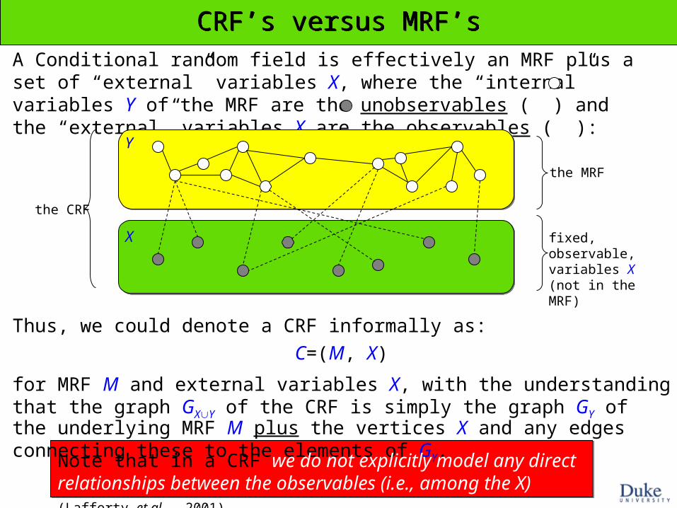
A Conditional random field is effectively an MRF plus a set of “external” variables X, where the “internal” variables Y of the MRF are the unobservables ( ) and the “external” variables X are the observables ( ):

CRF’s versus MRF’sCRF’s versus MRF’s

Thus, we could denote a CRF informally as:

C=(M, X)

for MRF M and external variables X, with the understanding that the graph GXY of the CRF is simply the graph GY of the underlying MRF M plus the vertices X and any edges connecting these to the elements of GY.

the MRF

fixed, observable, variables X (not in the MRF)

the CRF

Note that in a CRF we do not explicitly model any direct relationships between the observables (i.e., among the X) (Lafferty et al., 2001).

Y

X

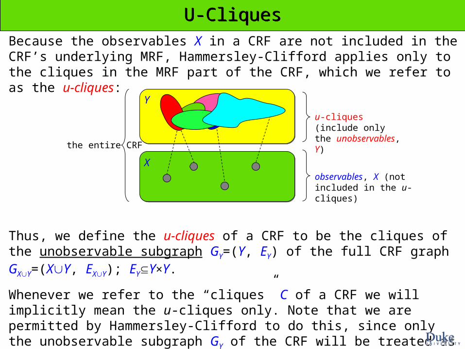
Because the observables X in a CRF are not included in the CRF’s underlying MRF, Hammersley-Clifford applies only to the cliques in the MRF part of the CRF, which we refer to as the u-cliques:

U-CliquesU-Cliques

Thus, we define the u-cliques of a CRF to be the cliques of the unobservable subgraph GY=(Y, EY) of the full CRF graph GXY=(XY, EXY); EYY×Y.

Whenever we refer to the “cliques” C of a CRF we will implicitly mean the u-cliques only. Note that we are permitted by Hammersley-Clifford to do this, since only the unobservable subgraph GY of the CRF will be treated as an MRF.

(NOTE: we will see later, however, that we may selectively include observables in the u-cliques)

u-cliques (include only the unobservables, Y)

observables, X (not included in the u-cliques)

the entire CRF

Y

X

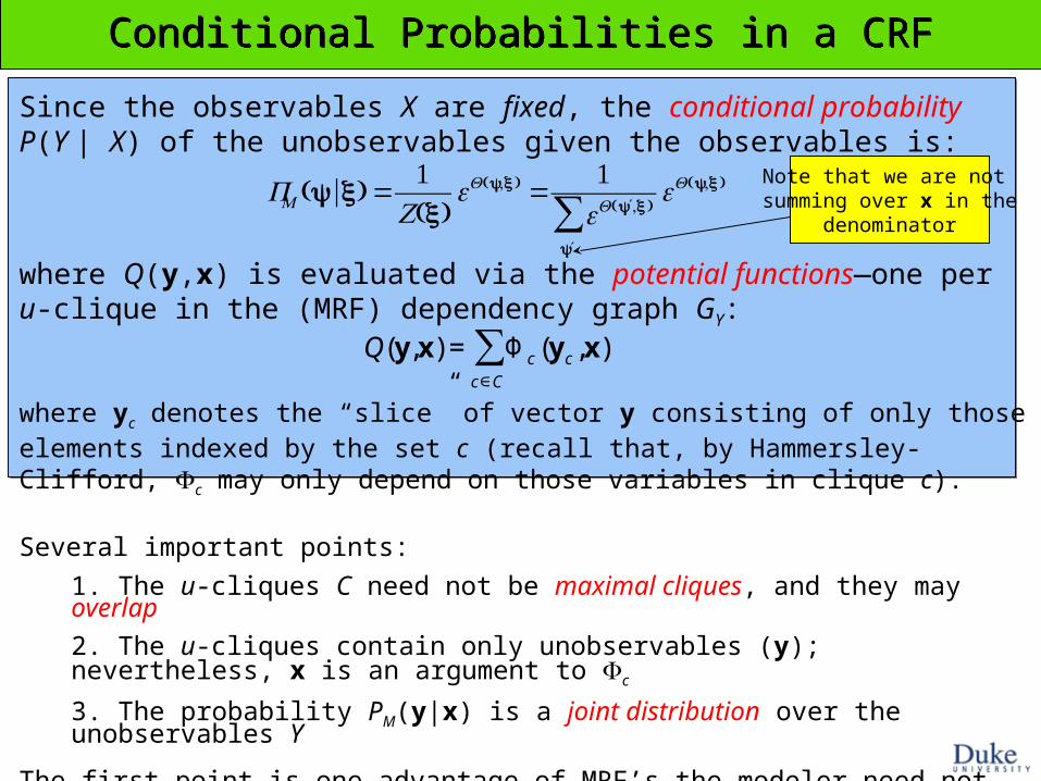
Since the observables X are fixed, the conditional probability P(Y | X) of the unobservables given the observables is:

Conditional Probabilities in a CRFConditional Probabilities in a CRF

€

PM (y|x) =1

Z(x)eQ(y,x) =

1eQ( ′ y ,x)

′ y

∑eQ(y,x)

where Q(y,x) is evaluated via the potential functions—one per u-clique in the (MRF) dependency graph GY:

€

Q(y,x) = Φc (y c,x)c∈C

∑

where yc denotes the “slice” of vector y consisting of only those elements indexed by the set c (recall that, by Hammersley-Clifford, c may only depend on those variables in clique c).

Several important points:

1. The u-cliques C need not be maximal cliques, and they may overlap

2. The u-cliques contain only unobservables (y); nevertheless, x is an argument to c

3. The probability PM(y|x) is a joint distribution over the unobservables Y

The first point is one advantage of MRF’s—the modeler need not worry about decomposing the computation of the probability into non-overlapping conditional terms. By contrast, in a Bayesian network this could result in “double-counting” of probabilities, and unwanted biases.

Note that we are not summing over x in the

denominator

A number of ad hoc modeling decisions are typically made with regard to the form of the potential functions:

1. The xixj...xk coefficients in the xixj..xkGi,j,...,k(xi,xj,..,xk) terms from Besag’s formula are typically ignored (they can in theory be absorbed by the potential functions).

2. c is typically decomposed into a weighted sum of feature sensors fi, producing:

3. Training of the model is typically performed in two steps (Vinson et al., 2007):

(i) train the individual feature sensors fi (independently) on known features of the appropriate type

(ii) learn the i’s using a gradient ascent procedure applied to the entire model all at once (not separately for each i).

€

P(y | x) =1

Ze

λ i f i (yc ,x )i∈F

∑c∈C

∑

Common AssumptionsCommon Assumptions

(Lafferty et al., 2001)

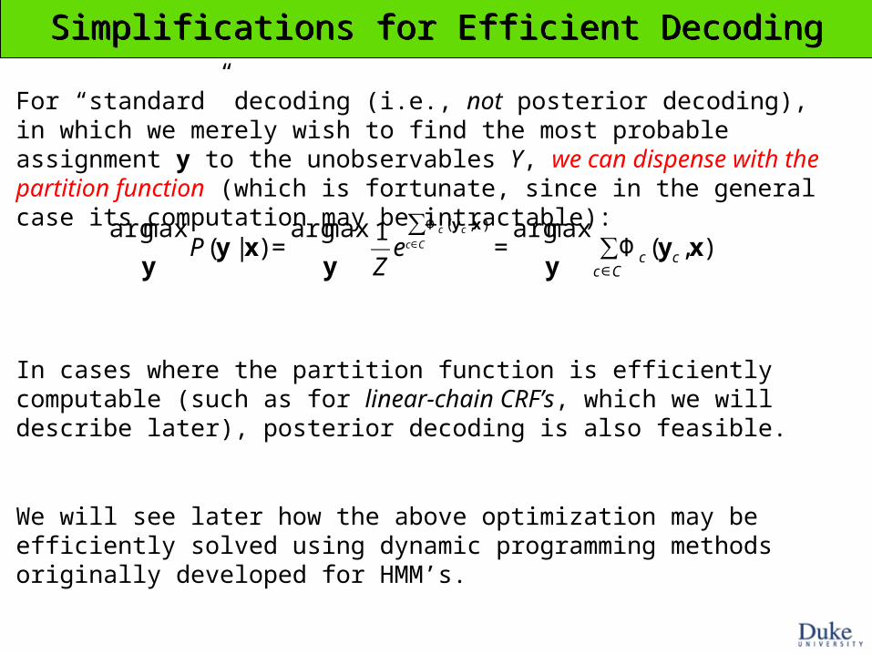
For “standard” decoding (i.e., not posterior decoding), in which we merely wish to find the most probable assignment y to the unobservables Y, we can dispense with the partition function (which is fortunate, since in the general case its computation may be intractable):

In cases where the partition function is efficiently computable (such as for linear-chain CRF’s, which we will describe later), posterior decoding is also feasible.

We will see later how the above optimization may be efficiently solved using dynamic programming methods originally developed for HMM’s.

Simplifications for Efficient DecodingSimplifications for Efficient Decoding

€

argmax

yP(y | x) =

argmax

y1

Ze

Φ c (y c ,x )c∈C

∑=

argmax

yΦc (y c,x)

c∈C∑

QuickTime™ and aTIFF (Uncompressed) decompressor

are needed to see this picture.

The Boltzmann AnalogyThe Boltzmann Analogy

€

Pboltzmann(x) =1Z

e−E(x) kT

The Boltzmann-Gibbs distribution from statistical thermodynamics is strikingly similar to the MRF formulation:

This gives the probability of a particular molecular configuration (or “microstate”) x occurring in an ideal gas at temperature T, where k=1.38×10-23 is the Boltzmann constant. The normalizing term Z is known as the partition function. The exponent E is the Gibbs free energy of the configuration.

The MRF probability function may be conceptualized somewhat analogously, in which the summed “potential functions” c (notice the difference in sign versus -E/kT) reflect the “interaction potentials” between variables, and measure the “compatibility,” “consistency,” or “co-occurrence patterns” of the variable assignments x:

The analogy is most striking in the case of crystal structures, in which the molecular configuration forms a lattice described by an undirected graph of atomic-level forces.

€

PMRF (x) =1

Ze

Φ c (x c )c∈C

∑

Although intuitively appealing, this analogy is not the justification for MRF’s—the Hammersley-Clifford result provides a mathematically justified means of evaluating an MRF (and thus a CRF), and is not directly based on a notion of state “dynamics”.

QuickTime™ and aTIFF (Uncompressed) decompressor

are needed to see this picture.

CRF’s for DNA SequenceCRF’s for DNA Sequence

A A T C G

q17 q5 q23 q12 q6

Recall the directed dependency model for a (0th-order) HMM:

For gene finding, the unobservables in a CRF would be the labels (exon, intron) for each position in the DNA. In theory, these may depend on any number of the observables (the DNA):

The u-cliques in such a graph can be easily identified as being either singleton labels or pairs of adjacent labels:

Such a model would need only two c functions—singleton for “singleton label” cliques (left figure) and pair for “pair label” cliques (right figure). We could evaluate these using the standard emission and transition distributions of an HMM (but we don’t have to).

Note that longer-range dependencies between labels are theoretically possible, but are not commonly used in gene finding (yet)

CRF’s versus HMM’sCRF’s versus HMM’s

€

argmaxφ

P(φ |S) =argmaxφ

P(φ)P(S|φ) =argmaxφ

log Ptrans(yi |yi−1)Pemit(si |yi )( )yi∈φ∑

€

argmax

φP(φ | S) =

argmax

φ1

Ze

λf (c,S )∑ =argmax

φλ i f i(c,S)

c,i

∑

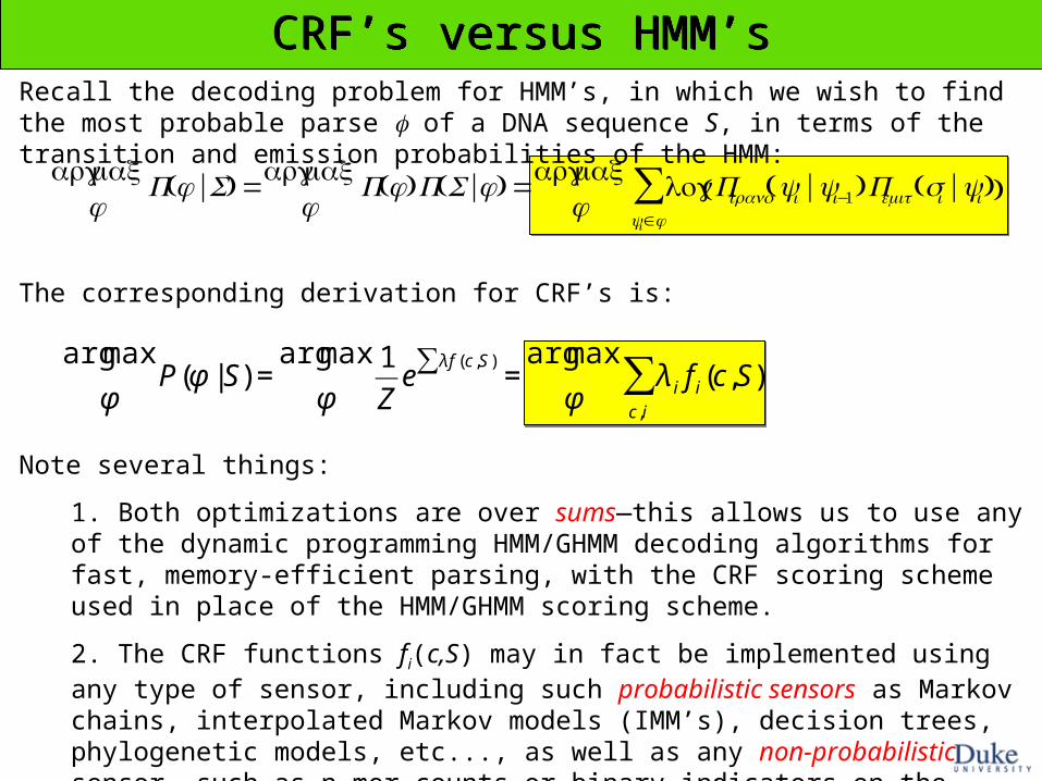
Recall the decoding problem for HMM’s, in which we wish to find the most probable parse of a DNA sequence S, in terms of the transition and emission probabilities of the HMM:

The corresponding derivation for CRF’s is:

Note several things:

1. Both optimizations are over sums—this allows us to use any of the dynamic programming HMM/GHMM decoding algorithms for fast, memory-efficient parsing, with the CRF scoring scheme used in place of the HMM/GHMM scoring scheme.

2. The CRF functions fi(c,S) may in fact be implemented using any type of sensor, including such probabilistic sensors as Markov chains, interpolated Markov models (IMM’s), decision trees, phylogenetic models, etc..., as well as any non-probabilistic sensor, such as n-mer counts or binary indicators on the existence of BLAST hits, etc...

How to Select Optimal Potential FunctionsHow to Select Optimal Potential Functions

?Aside from the Boltzmann analogy (i.e., “compatibility” of variable

assignments), little concrete advice is available at this time. Stay tuned.

sorry about that, man!

Training a CRF — Conditional Max LikelihoodTraining a CRF — Conditional Max Likelihood

€

θCML =argmax

θPθ (φ |S)

(S,φ)∈T

∏ ⎛

⎝ ⎜ ⎜

⎞

⎠ ⎟ ⎟

€

θMLE =argmax

θPθ (S,φ)

(S,φ)∈T

∏ ⎛

⎝ ⎜ ⎜

⎞

⎠ ⎟ ⎟

=argmaxθ

Pe(Si |yi ,di )Pt(yi |yi−1)Pd(di |yi )yi∈φ∏

(S,φ)∈T

∏ ⎛

⎝ ⎜ ⎜

⎞

⎠ ⎟ ⎟

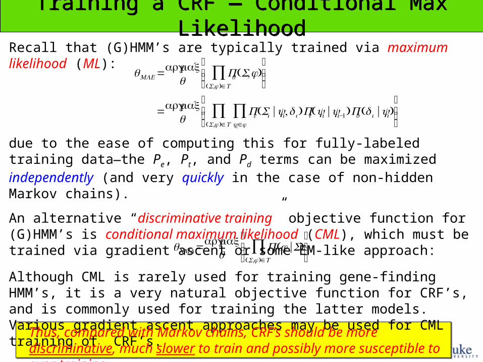
Recall that (G)HMM’s are typically trained via maximum likelihood (ML):

due to the ease of computing this for fully-labeled training data—the Pe, Pt, and Pd terms can be maximized independently (and very quickly in the case of non-hidden Markov chains).

An alternative “discriminative training” objective function for (G)HMM’s is conditional maximum likelihood (CML), which must be trained via gradient ascent or some EM-like approach:

Although CML is rarely used for training gene-finding HMM’s, it is a very natural objective function for CRF’s, and is commonly used for training the latter models. Various gradient ascent approaches may be used for CML training of CRF’s.

Thus, compared with Markov chains, CRF’s should be more discriminative, much slower to train and possibly more susceptible to over-training.

Avoiding Overfitting with RegularizationAvoiding Overfitting with Regularization

€

fobjective(θ) =Pθ (y|x)−||θ ||2

2σ 2

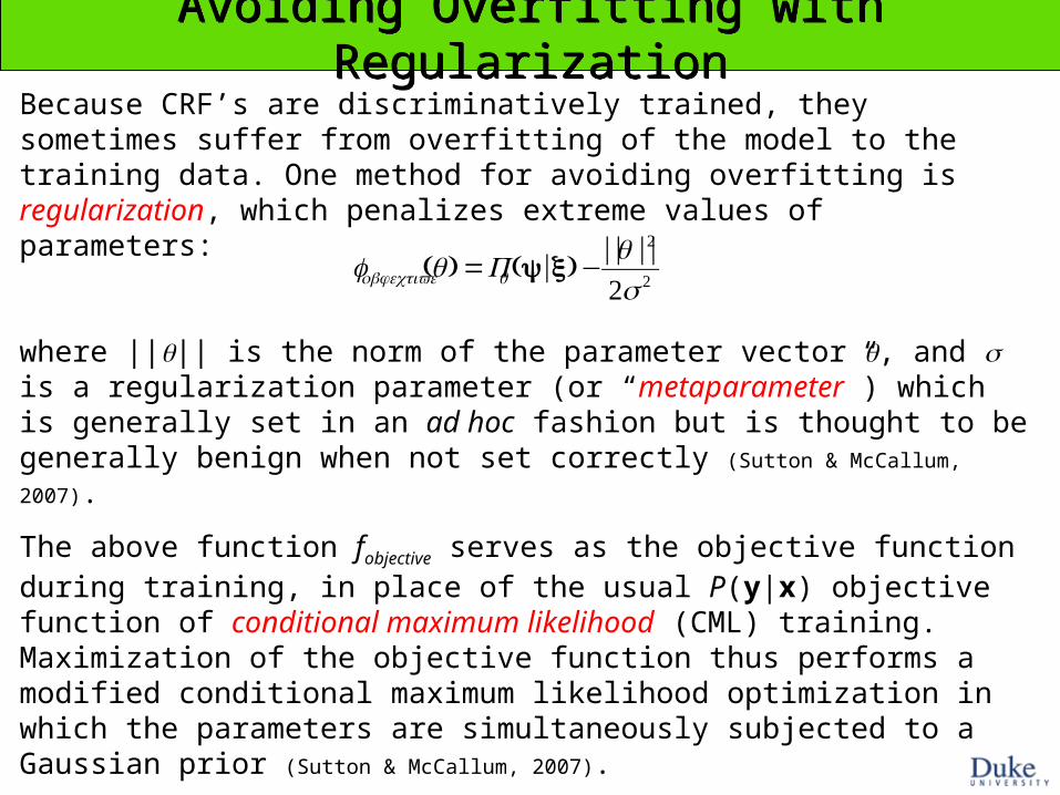
Because CRF’s are discriminatively trained, they sometimes suffer from overfitting of the model to the training data. One method for avoiding overfitting is regularization, which penalizes extreme values of parameters:

where ||θ|| is the norm of the parameter vector θ, and σ is a regularization parameter (or “metaparameter”) which is generally set in an ad hoc fashion but is thought to be generally benign when not set correctly (Sutton & McCallum, 2007).

The above function fobjective serves as the objective function during training, in place of the usual P(y|x) objective function of conditional maximum likelihood (CML) training. Maximization of the objective function thus performs a modified conditional maximum likelihood optimization in which the parameters are simultaneously subjected to a Gaussian prior (Sutton & McCallum, 2007).

Phylo-CRF’sPhylo-CRF’s

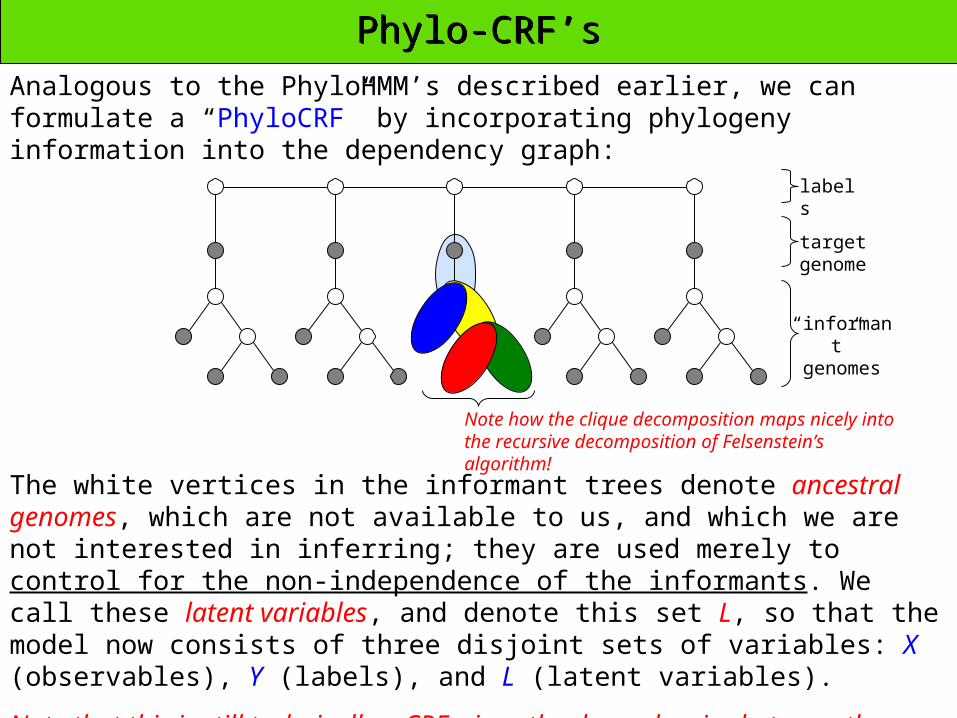
Analogous to the PhyloHMM’s described earlier, we can formulate a “PhyloCRF” by incorporating phylogeny information into the dependency graph:

labels

target genome

“informant” genomes

The white vertices in the informant trees denote ancestral genomes, which are not available to us, and which we are not interested in inferring; they are used merely to control for the non-independence of the informants. We call these latent variables, and denote this set L, so that the model now consists of three disjoint sets of variables: X (observables), Y (labels), and L (latent variables).

Note that this is still technically a CRF, since the dependencies between the observables are modeled only indirectly, through the latent variables (which are unobservable).

Note how the clique decomposition maps nicely into the recursive decomposition of Felsenstein’s algorithm!

U-cliques in a PhyloCRFU-cliques in a PhyloCRF

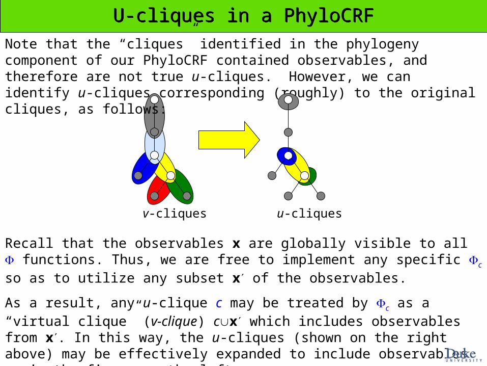
Note that the “cliques” identified in the phylogeny component of our PhyloCRF contained observables, and therefore are not true u-cliques. However, we can identify u-cliques corresponding (roughly) to the original cliques, as follows:

Recall that the observables x are globally visible to all functions. Thus, we are free to implement any specific c so as to utilize any subset x′ of the observables.

As a result, any u-clique c may be treated by c as a “virtual clique” (v-clique) cx′ which includes observables from x′. In this way, the u-cliques (shown on the right above) may be effectively expanded to include observables as in the figure on the left.

v-cliques u-cliques

Including Labels in the Potential FunctionsIncluding Labels in the Potential FunctionsIn order for the patterns of conservation among the informants to have any effect on decoding, the c functions evaluated over the branches of the tree need to take into consideration the putative label (e.g., coding, noncoding) at the current position in the alignment. This is analogous to the use of separate evolution models for the different states q in a PhyloHMM:

P(I(1),...,I(n) | S, q)

The same effect can be achieved in the PhyloCRF very simply by introducing edges connecting all informants and their ancestors directly to the label:

The only effect on the clique structure of the graph is to include the label in all (maximal) cliques in the phylogeny. The c functions can then evaluate the conservation patterns along the branches of the phylogeny in the specific context of a given label—i.e.,

mr(Xmouse=C, Xrodent=G, Y=exon) vs. mr(Xmouse=C, Xrodent=G, Y=intron)

label

target genome

“informant” genomes

The Problem of Latent VariablesThe Problem of Latent Variables

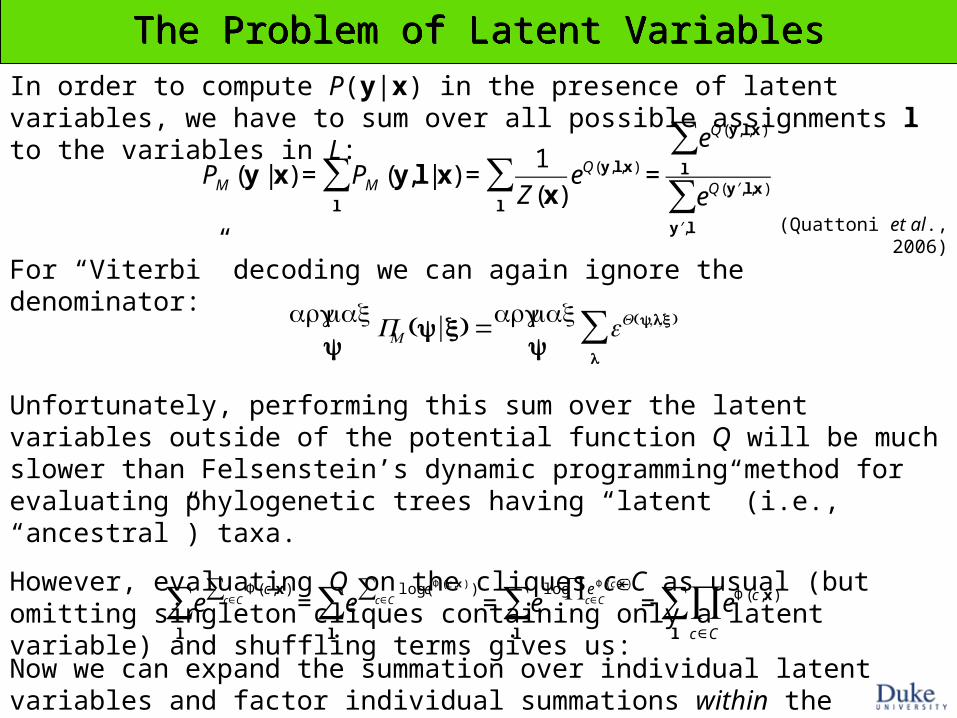
In order to compute P(y|x) in the presence of latent variables, we have to sum over all possible assignments l to the variables in L:

€

PM (y | x) = PM (y,l | x)l

∑ =1

Z(x)eQ(y,l ,x )

l

∑ =

eQ(y,l,x )

l

∑

eQ( ′ y ,l,x )

′ y ,l

∑(Quattoni et al., 2006)

For “Viterbi” decoding we can again ignore the denominator:

€

argmaxy

PM (y|x) =argmaxy

eQ(y,l,x)

l

∑

Unfortunately, performing this sum over the latent variables outside of the potential function Q will be much slower than Felsenstein’s dynamic programming method for evaluating phylogenetic trees having “latent” (i.e., “ancestral”) taxa.

However, evaluating Q on the cliques cC as usual (but omitting singleton cliques containing only a latent variable) and shuffling terms gives us:

€

eΦ(c,x )

c∈C∑

l

∑ = elog(e Φ ( c,x ) )

c∈C∑

l

∑ = elog e Φ ( c,x )

c∈C∏

l

∑ = eΦ(c,x )

c∈C

∏l

∑

Now we can expand the summation over individual latent variables and factor individual summations within the evaluation of Q...

Factoring Along a Tree StructureFactoring Along a Tree Structure

€

ξ(a) ξ(a,b) ξ(b,d)ξ(d)d

∑ ⎛

⎝ ⎜

⎞

⎠ ⎟ ξ(b,e)ξ(e)

e

∑ ⎛

⎝ ⎜

⎞

⎠ ⎟

b

∑ ⎡

⎣ ⎢

⎤

⎦ ⎥

a

∑ ξ(a,c) ξ(c, f )ξ( f )f

∑ ⎛

⎝ ⎜ ⎜

⎞

⎠ ⎟ ⎟ ξ(c,g)ξ(g)

g

∑ ⎛

⎝ ⎜ ⎜

⎞

⎠ ⎟ ⎟

c

∑ ⎡

⎣ ⎢ ⎢

⎤

⎦ ⎥ ⎥

a

c

f g

b

d e

€

PHMM (a) Pa→ b Pb→ dδ(d,xd)d

∑ ⎛

⎝ ⎜

⎞

⎠ ⎟ Pb→ eδ(e,xe)

e

∑ ⎛

⎝ ⎜

⎞

⎠ ⎟

b

∑ ⎡

⎣ ⎢

⎤

⎦ ⎥

a

∑ Pa→ c Pc→ fδ( f ,xf )f

∑ ⎛

⎝ ⎜ ⎜

⎞

⎠ ⎟ ⎟ Pc→ gδ(g,xg)

g

∑ ⎛

⎝ ⎜ ⎜

⎞

⎠ ⎟ ⎟

c

∑ ⎡

⎣ ⎢ ⎢

⎤

⎦ ⎥ ⎥

Consider the tree structure below. To simplify notation, let ξ() denote e(). Then the term from the previous slide expands along the cliques of the tree as follows:

€

ξ(a,b)ξ(a,c)ξ(b,d)ξ(b,e)ξ(c, f )ξ(c,g)g

∑f

∑e

∑d

∑c

∑b

∑a

∑ ξ(a)ξ(b)ξ(c)ξ(d)ξ(e)ξ( f )ξ(g)

€

ξ(a) a,bξ(a,b) b,dξ(b,d)ξ(d)d

∑ ⎛

⎝ ⎜

⎞

⎠ ⎟ b,eξ(b,e)ξ(e)

e

∑ ⎛

⎝ ⎜

⎞

⎠ ⎟

b

∑ ⎡

⎣ ⎢

⎤

⎦ ⎥

a

∑ a,cξ(a,c) c, fξ(c, f )ξ( f )f

∑ ⎛

⎝ ⎜ ⎜

⎞

⎠ ⎟ ⎟ c,gξ(c,g)ξ(g)

g

∑ ⎛

⎝ ⎜ ⎜

⎞

⎠ ⎟ ⎟

c

∑ ⎡

⎣ ⎢ ⎢

⎤

⎦ ⎥ ⎥

Any term inside a summation which does not contain the summation index variable can be factored out of that summation:

Now compare the CRF formulation (top) to the Bayesian network formulation under Felsenstein’s recursion (bottom), where Pa→b is the lineage-specific substitution probability, δ(d,xd)=1 iff d=xd (otherwise 0), and PHMM(a) is the probability of a under a standard HMM.

We can also introduce terms as in the common “linear combination” expansion of Q:

which may allow the CRF trainer to learn more discriminative “branch lengths”.

CRF:

Felsenstein:

€

eΦ(c,x )∏∑

Linear-Chain CRFs (LC-CRF’s)Linear-Chain CRFs (LC-CRF’s)

A common CRF topology for sequence parsing is the linear-chain CRF (LC-CRF) (Sutton & McCallum, 2007):

€

P(y|x) =1Z

ei fi (c)

i∈F∑

c∈C∑

=1Z

eπfemit(x,yt )+μftrans(x,yt−1,yt )

t=0

|S|−1

∑

For visual simplicity, all of the observables are denoted by a single shaded node. Because of the simplified structure, the u-cliques are now trivially identifiable as singleton labels (corresponding to “emission” functions femit) and pairs of labels (corresponding to “transition” functions ftrans):

where we have made the common modeling assumption that the functions expand as linear combinations of “feature functions” fi.

Abstracting External Information via Feature FunctionsAbstracting External Information via Feature Functions

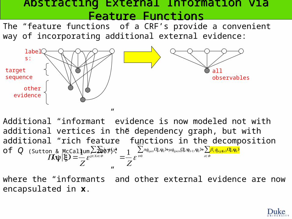
The “feature functions” of a CRF’s provide a convenient way of incorporating additional external evidence:

Additional “informant” evidence is now modeled not with additional vertices in the dependency graph, but with additional “rich feature” functions in the decomposition of Q (Sutton & McCallum, 2007):

€

P(y|x) =1Z

ei fi (c)

i∈F∑

c∈C∑

=1Z

eπfemit(x,yt )+μftrans(x,yt−1,yt )+ βi frich( i) (x,yt )

i∈F∑

t=0

|S|−1

∑

where the “informants” and other external evidence are now encapsulated in x.

other evidence

target sequence

labels:

all observables

Phylo-CRF’s RevisitedPhylo-CRF’s Revisited

Now a “PhyloCRF” can be formulated more simply as a CRF with a “rich feature” function that applies Felsenstein’s algorithm in each column (Vinson et al., 2007):

the CRF

“rich features” of the observables

Note that the resulting model is a hybrid between an undirected model (the CRF) and a directed model (the phylogeny).

Is this optimal? Maybe not—the CRF training procedure cannot modify any of the parameters inside of the phylogeny submodel so as to improve discrimination (i.e., labeling accuracy).

Then again, this separation may help to prevent overfitting.

Evaluated by Felsenstein’s pruning algorithm (outside of the CRF)

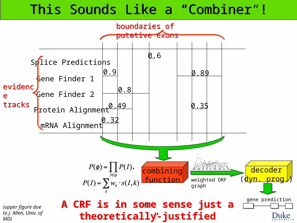
This Sounds Like a “Combiner”!This Sounds Like a “Combiner”!

Splice Predictions

Gene Finder 1

Gene Finder 2

Protein Alignment

mRNA Alignment

0.9 0.89

0.49

0.32

0.35

0.6

boundaries of putative exonsboundaries of putative exons

evidence tracksevidence tracks

0.8

combiningfunction

decoder(dyn. prog.)weighted ORF graph

gene prediction

(upper figure due to J. Allen, Univ. of MD)

A CRF is in some sense just a theoretically-justified “Combiner” program

A CRF is in some sense just a theoretically-justified “Combiner” program

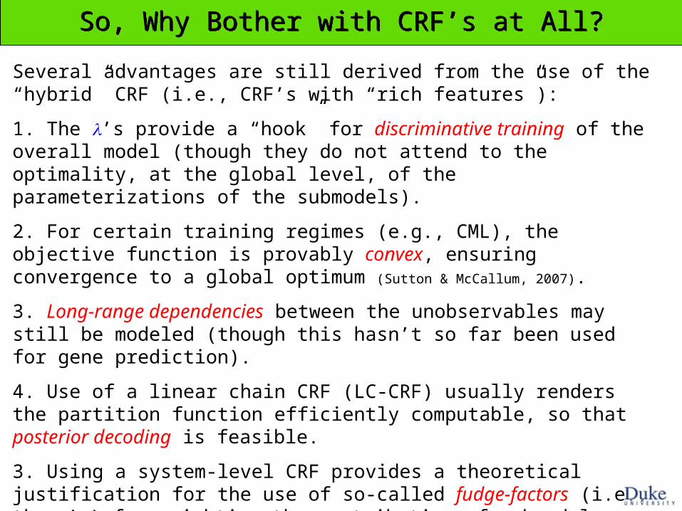
So, Why Bother with CRF’s at All?So, Why Bother with CRF’s at All?

Several advantages are still derived from the use of the “hybrid” CRF (i.e., CRF’s with “rich features”):

1. The ’s provide a “hook” for discriminative training of the overall model (though they do not attend to the optimality, at the global level, of the parameterizations of the submodels).

2. For certain training regimes (e.g., CML), the objective function is provably convex, ensuring convergence to a global optimum (Sutton & McCallum, 2007).

3. Long-range dependencies between the unobservables may still be modeled (though this hasn’t so far been used for gene prediction).

4. Use of a linear chain CRF (LC-CRF) usually renders the partition function efficiently computable, so that posterior decoding is feasible.

3. Using a system-level CRF provides a theoretical justification for the use of so-called fudge-factors (i.e., the ’s) for weighting the contribution of submodels...

Thus, these programs are all instances of (highly simplified) CRF’s!Thus, these programs are all instances of (highly simplified) CRF’s!

We should have been using CRF’s all along...We should have been using CRF’s all along...

The Ubiquity of Fudge FactorsThe Ubiquity of Fudge Factors

Many “probabilistic” gene finders utilize fudge factors in their source code, despite no obvious theoretical justification for their use:

• folklore about in the source code of a certain popular ab initio gene finder1

• fudge factor in: NSCAN (“conservation score coefficient”; Gross & Brent, 2005)

• fudge factor in: ExoniPhy (“tuning parameter”; Siepel & Haussler, 2004)

• fudge factor in TWAIN (“percent identity”; Majoros et al., 2005)

• fudge factor in GlimmerHMM (“optimism”; M. Pertea, pers. communication)

• fudge factor in TIGRscan (“optimism”; Majoros et al., 2004)

• lack of fudge factors in EvoGene (Pedersen & Hein, 2003)

€

7 / 3

1 folklore also states that this programs’s author made a “pact with the devil” in exchange for gene-finding accuracy; attempts to replicate this effect have so far been unsuccessful (unpub. data).

or, to put it another way:

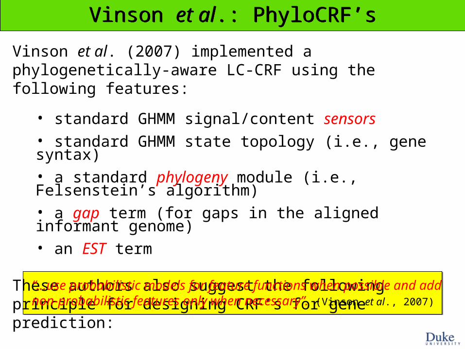
Vinson et al.: PhyloCRF’sVinson et al.: PhyloCRF’s

Vinson et al. (2007) implemented a phylogenetically-aware LC-CRF using the following features:

• standard GHMM signal/content sensors• standard GHMM state topology (i.e., gene syntax)• a standard phylogeny module (i.e., Felsenstein’s algorithm)• a gap term (for gaps in the aligned informant genome)• an EST term

These authors also suggest the following principle for designing CRF’s for gene prediction:

“...use probabilistic models for feature functions when possible and add non-probabilistic features only when necessary”. (Vinson et al., 2007)

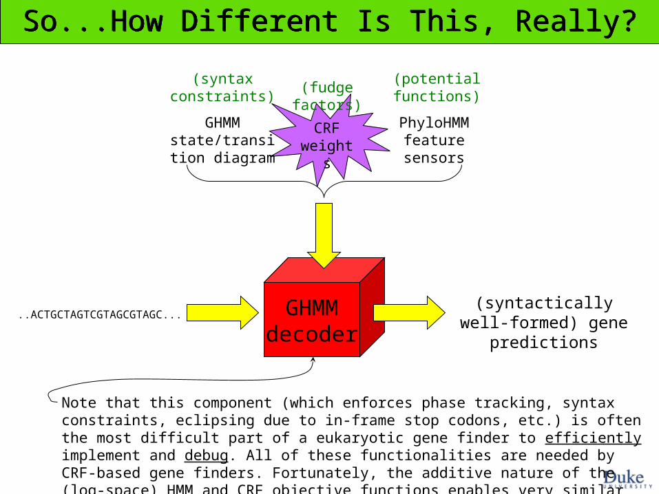
GHMMdecoder

..ACTGCTAGTCGTAGCGTAGC...(syntactically well-formed)

gene predictions

GHMM state/transition

diagram

CRF weights

PhyloHMM feature sensors

So...How Different Is This, Really?So...How Different Is This, Really?

(fudge factors)(syntax

constraints)(potential functions)

Note that this component (which enforces phase tracking, syntax constraints, eclipsing due to in-frame stop codons, etc.) is often the most difficult part of a eukaryotic gene finder to efficiently implement and debug. All of these functionalities are needed by CRF-based gene finders. Fortunately, the additive nature of the (log-space) HMM and CRF objective functions enables very similar code to be used in both cases.

GCTATCGATTCTCTAATCGTCTATCGATCGTGGTATCGTACGTTCATTACTGACT...

sensor 1

sensor 2

sensor n . . .ATG’s

GT’S

AG’s

. . .signal queues

sequence:

detect putative signals during left-to-right pass over squence

insert into type-specific signal queues

...ATG.........ATG......ATG..................GT

newly detected signal

elements of the

“ATG” queue

trellis links

Recall: Decoding via Sensors and Trellis LinksRecall: Decoding via Sensors and Trellis Links

ATGGATGCTACTTGACGTACTTAACTTACCGATCTCT0 1 2 0 1 2 0 1 2 0 1 2 0 1 2 0 1 2 0 1 2 0 1 2 0 1 2 0 1 2 0 1 2 0 1 2 0

in-frame stop codon!

Recall: Phase Constraints and “Eclipsing”Recall: Phase Constraints and “Eclipsing”

All of these syntactic constraints have to be tracked and enforced, just like in a “generative” gene finder!

In short: gene syntax hasn’t changed, even if our model has!

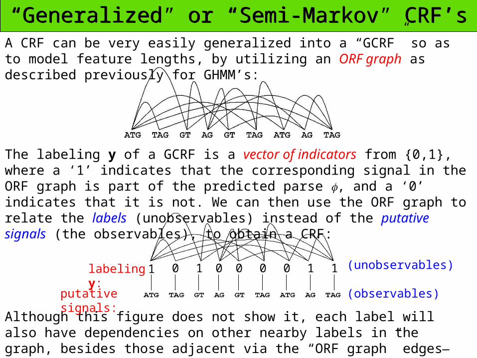
“Generalized” or “Semi-Markov” CRF’s“Generalized” or “Semi-Markov” CRF’s

The labeling y of a GCRF is a vector of indicators from {0,1}, where a ‘1’ indicates that the corresponding signal in the ORF graph is part of the predicted parse , and a ‘0’ indicates that it is not. We can then use the ORF graph to relate the labels (unobservables) instead of the putative signals (the observables), to obtain a CRF:

1 0 1 0 0 0 0 1 1labeling y:

Although this figure does not show it, each label will also have dependencies on other nearby labels in the graph, besides those adjacent via the “ORF graph” edges—i.e., there are implicit edges not shown in this representation. We will come back to this.

A CRF can be very easily generalized into a “GCRF” so as to model feature lengths, by utilizing an ORF graph as described previously for GHMM’s:

putative signals:

(unobservables)

(observables)

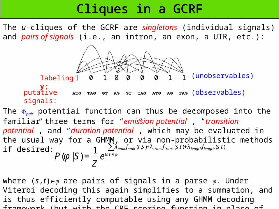
Cliques in a GCRFCliques in a GCRF

€

P(φ | S) =1

Ze

λ emit femit (t ,S)+λ trans f trans (s,t )+λ length f length (s ,t)( s ,t )∈φ

∑

The u-cliques of the GCRF are singletons (individual signals) and pairs of signals (i.e., an intron, an exon, a UTR, etc.):

where (s,t) are pairs of signals in a parse . Under Viterbi decoding this again simplifies to a summation, and is thus efficiently computable using any GHMM decoding framework (but with the CRF scoring function in place of the GHMM one).

The pair potential function can thus be decomposed into the familiar three terms for “emission potential”, “transition potential”, and “duration potential”, which may be evaluated in the usual way for a GHMM, or via non-probabilistic methods if desired:

1 0 1 0 0 0 0 1 1labeling y:

putative signals:

(unobservables)

(observables)

Enforcing Syntax ConstraintsEnforcing Syntax Constraints

...ATG...GT....ATG......ATG....TAG....GT.....GT

This can be handled by augmenting pair so as to evaluate to 0 unless the pair is well-formed: i.e., the paired signals must be labeled ‘1’ and all signals lying between them must be labeled ‘0’:

Finally, to enforce phase constraints we need to use three copies of the ORF graph, with links between the three graphs enforcing phase constraints based on lengths of putative features (not shown).

1 0 0 1

1 0 1 0 0 0 0 1 1labeling y:

Note that it is possible to construct a labeling y which is not syntactically valid, because the signals do not form a consistent path across the entire ORF graph. We are thus interested in constraining the functions so that only valid labelings have nonzero scores:

pair

0 00

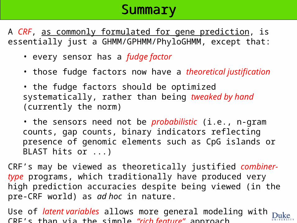
SummarySummary

A CRF, as commonly formulated for gene prediction, is essentially just a GHMM/GPHMM/PhyloGHMM, except that:

• every sensor has a fudge factor

• those fudge factors now have a theoretical justification

• the fudge factors should be optimized systematically, rather than being tweaked by hand (currently the norm)

• the sensors need not be probabilistic (i.e., n-gram counts, gap counts, binary indicators reflecting presence of genomic elements such as CpG islands or BLAST hits or ...)

CRF’s may be viewed as theoretically justified combiner-type programs, which traditionally have produced very high prediction accuracies despite being viewed (in the pre-CRF world) as ad hoc in nature.

Use of latent variables allows more general modeling with CRF’s than via the simple “rich feature” approach.

THE END

Besag J (1974) Spatial interaction and the statistical analysis of lattice systems. Journal of the Royal Statistical Society B 36, pp192-236.

Lafferty J, McCallum A, Pereira F (2001) Conditional random fields: Probabilistic models for segmenting and labeling sequence data. In: Proc. 18th International Conf. on Machine Learning.

Quattoni A, Wang S, Morency L-P, Collins M, Darrell T (2006) Hidden-state conditional random fields. MIT CSAIL Technical Report.

Sutton C, McCallum A (2006) An introduction to conditional random fields for relational learning. In: Getoor L & Taskar B (eds.) Introduction to statistical relational learning. MIT Press.

Vinson J, DeCaprio D, Pearson M, Luoma S, Galagan J (2007) Comparative Gene Prediction using Conditional Random Fields. In: B Scholkpf, J Platt, T Hoffman (eds.), Advances in Neural Information Processing Systems 19, MIT Press, Cambridge, MA.

References

AcknowledgementsSayan Mukherjee and Elizabeth Rach provided invaluable comments and suggestions for these slides.