conditional transformation models - arxiv · of conditional transformation models that allow the...
TRANSCRIPT

Conditional Transformation Models
Extended Version?
Torsten HothornLMU Munchen &Universitat Zurich
Thomas KneibUniversitat Gottingen
Peter BuhlmannETH Zurich
Abstract
The ultimate goal of regression analysis is to obtain information about the conditionaldistribution of a response given a set of explanatory variables. This goal is, however, sel-dom achieved because most established regression models only estimate the conditionalmean as a function of the explanatory variables and assume that higher moments are notaffected by the regressors. The underlying reason for such a restriction is the assumptionof additivity of signal and noise. We propose to relax this common assumption in theframework of transformation models. The novel class of semiparametric regression mod-els proposed herein allows transformation functions to depend on explanatory variables.These transformation functions are estimated by regularised optimisation of scoring rulesfor probabilistic forecasts, e.g. the continuous ranked probability score. The correspondingestimated conditional distribution functions are consistent. Conditional transformationmodels are potentially useful for describing possible heteroscedasticity, comparing spa-tially varying distributions, identifying extreme events, deriving prediction intervals andselecting variables beyond mean regression effects. An empirical investigation based ona heteroscedastic varying coefficient simulation model demonstrates that semiparametricestimation of conditional distribution functions can be more beneficial than kernel-basednon-parametric approaches or parametric generalised additive models for location, scaleand shape.
Keywords: boosting, conditional distribution function, conditional quantile function, contin-uous ranked probability score, prediction intervals, structured additive regression.
1. Introduction
One of the famous “Top ten reasons to become a statistician” is that statisticians are “meanlovers”(Friedman, Friedman, and Amoo 2002), referring of course to our obsession with means.Whenever a distribution is too complex to think or expound upon, we focus on the mean as asingle real number describing the centre of the distribution and block out other characteristicssuch as variance, skewness and kurtosis. Our willingness to simplify distributions this wayis most apparent when we deal with many distributions at a time, as in a regression settingwhere we describe the conditional distribution PY |X=x of a response Y ∈ R given different
?This is an extended version of Hothorn, Kneib, and Buhlmann (2013). Please cite this reference unlessyou’re referring to the additional applications presented in this document.ctm.pdf compiled November 29, 2012 from ctm.tex version 5081
arX
iv:1
201.
5786
v2 [
stat
.ME
] 2
8 N
ov 2
012

2 Conditional Transformation Models
configurations of explanatory variables X = x ∈ χ. Many regression models focus on theconditional mean E(Y |X = x) and treat higher moments of the conditional distributionPY |X=x as fixed or nuisance parameters that must not depend on the explanatory variables.As a consequence, model inference crucially relies on assumptions such as homoscedasticityand symmetry. Information on the scale of the response, for example prediction intervals,derived from such models also depends on these assumptions. Here, we propose a new classof conditional transformation models that allow the conditional distribution function P(Y ≤υ|X = x) to be estimated directly and semiparametrically under rather weak assumptions.Before we introduce this class of models in Section 2, we will attempt to set a scene ofcontemporary regression in the light of Gilchrist (2008) and place the major players onto thisstage.
Let Yx = (Y |X = x) ∼ PY |X=x denote the conditional distribution of response Y givenexplanatory variables X = x. We assume that PY |X=x is dominated by some measure µ andhas the conditional distribution function P(Y ≤ υ|X = x). A regression model describes thedistribution PY |X=x, or certain characteristics of it, as a function of the explanatory variablesx. We estimate such models based on samples of pairs of random variables (Y,X) fromthe joint distribution PY,X . It is convenient to assume that a regression model consists ofsignal and noise, i.e. a deterministic part and an error term. In the following, we denote theerror term by Q(U), where U ∼ U [0, 1] is a uniform random variable independent of X andQ : R→ R is the quantile function of an absolutely continuous distribution.
Apart from non-parametric kernel estimators of the conditional distribution function (Hall,Wolff, and Yao 1999, Hall and Muller 2003, Li and Racine 2008), there are two common waysto model the influence of the explanatory variables x on the response Yx:
Yx = r(Q(U)|x) “mean or quantile regression models” and (1)
h(Yx|x) = Q(U) “transformation models”. (2)
For each x ∈ χ, the regression function r(·|x) : R → R transforms the error term Q(U) in amonotone increasing way. The inverse regression function h(·|x) = r−1(·|x) : R → R is alsomonotone increasing. Because h transforms the response, it is known as a transformationfunction, and models in the form of (2) are called transformation models.
A major assumption underlying almost all regression models of class (1) is that the regressionfunction r is the sum of the deterministic part rx : χ→ R, which depends on the explanatoryvariables, and the error term:
r(Q(U)|x) = rx(x) +Q(U).
When E(Q(U)) = 0, we get rx(x) = E(Y |X = x), e.g. linear or additive models depending onthe functional form of rx. Model inference is commonly based on the normal error assumption,i.e. Q(U) = σΦ−1(U), where σ > 0 is a scale parameter and Φ−1(U) ∼ N (0, 1). Linearheteroscedastic regression models (Carroll and Ruppert 1982) allow describing the variance asa function of the explanatory variables Q(U) = σ(x)Q(U), where σ(x) is a (usually log-linear)function of x and Q is the quantile function of a symmetric distribution with E(Q(U)) = 0. Intime series analysis, GARCH models (Bollerslev 1986) share this idea. A novel semiparametricapproach is extended generalised additive models, where additive functions of the explanatoryvariables describe location, scale and shape (GAMLSS) of a certain parametric conditionaldistribution of the response given the explanatory variables (Rigby and Stasinopoulos 2005).
Torsten Hothorn, Thomas Kneib, and Peter Buhlmann 3
If the assumption of a certain parametric form of the conditional distribution is questionable,rx describes the τ quantile of Yx when the quantile function Q is such that Q(τ) = 0 for someτ ∈ (0, 1). This leads us to quantile regression (Koenker 2005), which is according to Stigler(2010) the “best approach to robust methods in higher dimensional linear model problems”.Estimating the complete conditional quantile function is less straightforward since we haveto fit separate models for a grid of probabilities τ , and the resulting regression quantiles maycross. Solutions to this problem can be obtained by combining all quantile fits in one jointmodel based on, for example, location-scale models (He 1997) or quantile sheets (Schnabeland Eilers 2012), or by monotonising the estimated quantile curves using non-decreasingrearrangements (Dette and Volgushev 2008).
For transformation models (2), additivity is assumed on the scale of the inverse regressionfunction h:
h(Yx|x) = hY (Yx) + hx(x).
When E(Q(U)) = 0, we get −hx(x) = E(hY (Yx)) = E(hY (Y )|X = x). The monotonetransformation function hY : R → R does not depend on x and might be known in advance(Box-Cox transformation models with fixed parameters, accelerated failure time models) oris commonly treated as a nuisance parameter (Cox model, proportional odds model). Oneis usually interested in estimating the function hx : χ → R, which describes the conditionalmean of the transformed response hY (Yx). The class of transformation models is rich andvery actively researched, most prominently in literature on the analysis of survival data.For example, the linear Weibull accelerated failure time model assumes a log transforma-tion hY (Yx) = log(Yx), a linear function for the conditional mean of the log-transformedresponse hx(x) = x>α, and a Weibull-distributed error term Q(U) = σQWeibull(U). Forthe Cox additive model, hY (Yx) = log(Λ(Yx)) is based on the unspecified integrated baselinehazard function Λ, hx(x) =
∑Jj=1 hx,j(x) is the sum of J smooth terms depending on the
explanatory variables and Q(U) = − log(− log(U)) is the quantile function of the extremevalue distribution. The proportional odds model has hY (Yx) = log(Γ(Yx)), with Γ being anunknown monotone increasing function, and Q(U) = log(U/(1− U)) is the quantile functionof the logistic distribution. Doksum and Gasko (1990) discussed the flexibility of this class ofmodels, and Cheng, Wei, and Ying (1995) introduced a generic algorithm for linear transfor-mation model estimation, that is, for models with hx(x) = x>α, treating the transformationfunction hY as a nuisance.
In recent years, transformation models have been extended in two directions. In the firstdirection, more flexible forms for the conditional mean function hx have been introduced,e.g. the partially linear transformation model hx(x) = x>(0,α)>+hsmooth(x1) (where hsmooth
is a smooth function of the first variable x1; Lu and Zhang 2010), the varying coefficientmodel hx(x) = x>(0, 0,α)> + hsmooth(x1)x2 (Chen and Tong 2010), random effects models(Zeng, Lin, and Yin 2005), and various approaches to additive transformation and acceleratedfailure time models, such as the boosting approaches by Lu and Li (2008) and Schmid andHothorn (2008). In the second direction, a number of authors have considered algorithms thatestimate hY and (partially) linear functions hx simultaneously, usually by a spline expansionof hY (e.g. Shen 1998, Cheng and Wang 2011), as an alternative to the common practise ofestimating hY post-hoc by some non-parametric procedure such as the Breslow estimator.
Although the transformation function hY is typically treated as an infinite dimensional nui-sance parameter, it is important to note that hY contains information about higher moments
4 Conditional Transformation Models
of Yx, most importantly variance and skewness. Simultaneous estimation of hY and hx istherefore extremely attractive because we can obtain information about the mean and highermoments of the transformed response at the same time. However, owing to the decompositionof the regression function r or the transformation function h into both a deterministic part de-pending on the explanatory variables (rx or hx) and a random part depending on the response(hY ) or error term (Q(U)), higher moments of the conditional distribution of Y given X = xmust not depend on the explanatory variables in mean regression and transformation models.As a consequence, the corresponding models cannot capture heteroscedasticity or skewnessthat is induced by certain configurations of the explanatory variables. Therefore, we cannotdetect these potentially interesting patterns, and our models will perform poorly when prob-ability forecasts, prediction intervals or other functionals of the conditional distribution areof special interest.
Recently, Wu, Tian, and Yu (2010) proposed a novel transformation model for longitudi-nal data that partially addresses this issue. For responses and explanatory variables X(t)observed at time t, the model assumes
h(Yx|t,x) = hY (Yx|t) + x(t)>α(t).
Here, the transformation hY is conditional on time, and higher moments may vary with time.However, since hY does not depend on the explanatory variables x, these higher moments maynot vary with one or more of the explanatory variables. In the context of longitudinal datawith functional explanatory variables, Chen and Muller (2012) consider a similar model, wherethe regression coefficients for functional principle components may depend on time t and theresponse Yx. Our contribution is a class of transformation models where the transformationfunction is conditional on the explanatory variables in the sense that the transformationfunction, and therefore higher moments of the conditional distribution of the response, maydepend on potentially all explanatory variables. As a consequence, the models suggested hereare able to deal with heteroscedasticity and skewness that can be regressed on the explanatoryvariables, and we will show that reliable estimates of the complete conditional distributionfunction and functionals thereof can be obtained.
We will introduce the conditional transformation models (Section 2), discuss the underly-ing model assumptions, and embed the estimation problem in the empirical risk minimisationframework (Section 3). For the sake of simplicity, we restrict ourselves to continuous responsesY that have been observed without censoring. Similar to other transformation models, condi-tional transformation models are flexible enough to deal with discrete responses and survivaltimes, as will be discussed in later sections. We present a computationally efficient algorithmfor fitting the models in Section 4. We study the asymptotic properties of the estimated con-ditional distribution functions in Section 5. The practical benefits of modelling the influenceof explanatory variables on the variance and higher moments of the response’ distributionare demonstrated in Section 6 with a special emphasis on distributional characteristics ofchildhood nutrition in India and on prediction intervals for birth weights of small foetus. Fi-nally, we use a heteroscedastic varying coefficient simulation model to evaluate the empiricalperformance of the proposed algorithm and compare the quality of conditional distributionfunctions estimated by a conditional transformation model and established parametric andnon-parametric procedures in Section 7.
Torsten Hothorn, Thomas Kneib, and Peter Buhlmann 5
2. Conditional Transformation Models
An attractive feature of transformation models is their close connection to the conditionaldistribution function. With the transformation function h(Yx|x) = Q(U), one can evaluatethe conditional distribution function of response Y given the explanatory variables x via
P(Y ≤ υ|X = x) = P(h(Y |x) ≤ h(υ|x)) = F (h(υ|x))
with absolute continuous distribution function F = Q−1. For additive transformation func-tions h = hY +hx, the conditional distribution function reads F (h(υ|x)) = F (hY (υ)+hx(x)),i.e. the distribution is evaluated for a transformed and shifted version of Y . Higher momentsonly depend on the transformation hY and thus cannot be influenced by the explanatoryvariables. Consequently, one has to avoid the additivity in the model h = hY + hx to al-low the explanatory variables to impact also higher moments. We therefore suggest a noveltransformation model based on an alternative additive decomposition of the transformationfunction h into J partial transformation functions for all x ∈ χ:
h(υ|x) =J∑j=1
hj(υ|x), (3)
where h(υ|x) is the monotone transformation function of υ. In this model, the transformationfunction h(Yx|x) and the partial transformation functions hj(·|x) : R→ R are conditional onx in the sense that not only the mean of Yx depends on the explanatory variables. For thisreason, we coin models of the form (3) Conditional Transformation Models (CTMs). Clearly,model (3) imposes an assumption, namely additivity of the conditional distribution functionon the scale of the quantile function Q:
Q(P(Y ≤ υ|X = x)) =J∑j=1
hj(υ|x).
It should be noted that here we assume additivity of the transformation function h and notadditivity on the scale of the regression function r as it is common for additive mean or quantileregression models (1). Furthermore, monotonicity of hj is sufficient but not necessary for hbeing monotone. Of course, we have to make further assumptions on hj to obtain reasonablemodels, but these assumptions are problem specific, and we will therefore postpone these issuesuntil Section 6. To ensure identifiability, we assume without loss of generality that the partialtransformation functions are centred around zero EY EXhj(Y |X) = 0 for all j = 1, . . . , J fornon-systematic error terms (E(Q(U)) = 0).
3. Estimating Conditional Transformation Models
The estimation of conditional distribution functions can be reformulated as a mean regressionproblem since P(Y ≤ υ|X = x) = E(I(Y ≤ υ)|X = x) for the binary event Y ≤ υ; thisconnection is widely used (e.g. by Hall and Muller 2003, Chen and Muller 2012). Similarto the approach of fitting multiple quantile regression models to obtain an estimate of theconditional quantile function, one could estimate the models E(I(Y ≤ υ)|X = x) for a gridof υ values separately. However, we instead suggest estimating conditional transformation

6 Conditional Transformation Models
models by the application of an integrated loss function that allows the whole conditionaldistribution function to be obtained in one step.
Let ρ denote a function of measuring the loss of the probability F (h(υ|X)) for the binaryevent Y ≤ υ. One candidate loss function is
ρbin((Y ≤ υ,X), h(υ|X)) := −[I(Y ≤ υ) log{F (h(υ|X))}+
{1− I(Y ≤ υ)} log{1− F (h(υ|X))}] ≥ 0,
the negative log-likelihood of the binomial model (Y ≤ υ|X = x) ∼ B(1, F (h(υ|x))) for thebinary event Y ≤ υ with link function Q = F−1. Alternatively, one may consider the squaredor absolute error losses
ρsqe((Y ≤ υ,X), h(υ|X)) :=1
2|I(Y ≤ υ)− F (h(υ|X))|2 ≥ 0
ρabe((Y ≤ υ,X), h(υ|X)) := |I(Y ≤ υ)− F (h(υ|X))| ≥ 0.
The squared error loss ρsqe is also known as the Brier score, and the absolute loss ρabe hasbeen applied for assessing survival probabilities in the Cox model by Schemper and Henderson(2000). We define the loss function ` for estimating conditional transformation models asintegrated loss ρ with respect to a measure µ dominating the conditional distribution P(Y ≤υ|X = x):
`((Y,X), h) :=
∫ρ((Y ≤ υ,X), h(υ|X)) dµ(υ) ≥ 0.
In the context of scoring rules, the loss ` based on ρsqe is known as the continuous rankedprobability score (CPRS) or integrated Brier score and is a proper scoring rule for assessingthe quality of probabilistic or distributional forecasts (see Gneiting and Raftery 2007, for anoverview). It seems natural to apply these scores as loss functions for model estimation, butwe are only aware of the work of Gneiting, Raftery, Westveld III, and Goldman (2005), whodirectly optimise the CPRS for estimating Gaussian predictive probability density functionsfor continuous weather variables. In the context of non-parametric or semiparametric esti-mation of conditional distribution functions, minimisation of the empirical analog of the riskfunction
EY,X`((Y,X), h) =
∫ ∫ρ((y ≤ υ,x), h(υ|x)) dµ(υ) dPY,X(y,x) ≥ 0
for estimating conditional distribution functions has not yet been considered.
Model estimation based on the risk EY,X`((Y,X), h) is reasonable because the correspondingoptimisation problem is convex and attains its minimum for the true conditional transforma-tion function h. We summarise these facts in the following lemma, whose proof in given inthe Appendix.
Lemma 1. The risk EY,X`((Y,X), h) is convex in h for convex losses ρ in h. The populationminimiser of EY,X`((Y,X), h) for ρ = ρbin and ρ = ρsqe is h(υ|x) = Q(P(Y ≤ υ|X = x)).For ρ = ρabe, the minimiser is
h(υ|x) =
{−∞ : P(Y ≤ υ|X = x) ≤ 0.5∞ : P(Y ≤ υ|X = x) > 0.5.

Torsten Hothorn, Thomas Kneib, and Peter Buhlmann 7
The corresponding empirical risk function defined by the data is
EY,X`((Y,X), f) =
∫ ∫ρ((y ≤ υ,x), h(υ|x)) dµ(υ) dPY,X(y,x) ≥ 0.
Based on an i.i.d. random sample (Yi,Xi) ∼ PY,X , i = 1, . . . , N of N observations from the
joint distribution of response and explanatory variables, we define PY,X as the distributionputting mass wi > 0 on observation i (wi ≡ N−1 for the empirical distribution). For com-putational convenience, we also approximate the measure µ by the discrete uniform measureµ, which puts mass n−1 on each element of the equi-distant grid υ1 < · · · < υn ∈ R over theresponse space. The number of grid points n has to be sufficiently large to closely approximatethe integral. The empirical risk is then
EY,X`((Y,X), h) =
N∑i=1
win−1
n∑ı=1
ρ((Yi ≤ υı,Xi), h(υı|Xi)) (4)
= n−1N∑i=1
n∑ı=1
wiρ((Yi ≤ υı,Xi), h(υı|Xi)).
This risk is the weighted empirical risk for loss function ρ evaluated at the observations (Yi ≤υı,Xi) for i = 1, . . . , N and ı = 1, . . . , n. Consequently, we can apply algorithms for fittinggeneralised additive models to the binary responses Yi ≤ υı under loss ρ for estimating model(3). Although this seems to be rather straightforward, there are two issues to consider. First,simply expanding the observations over the grid υ1 < · · · < υn increases the computationalcomplexity by n, which, even for moderately large sample sizes N , renders computing andstorage rather burdensome. Second, unconstrained minimisation of the empirical risk, i.e. nosmoothness of h in its first argument and h being independent of the conditioning x, leadsto estimates F (h(υ|x)) = P(Y ≤ υ) = N−1
∑Ni=1 I(Yi ≤ υ), i.e. the empirical cumulative
distribution function of Y for ρbin and ρsqe with wi = N−1. For ρabe, the empirical risk is
minimised by F (h(υ|x)) = 0 for all υ with P(Y ≤ υ) < 0.5 and otherwise by F (h(υ|x)) = 1.Therefore, careful regularisation is absolutely necessary to obtain reasonable models thatlead to smooth conditional distribution functions (i.e. smoothing in the Y -direction) and thatare similar for similar configurations of the explanatory variables (i.e. smoothing in the X-direction). Instead of adding a direct penalisation term to the empirical risk, we propose inthe next section a boosting algorithm for empirical risk minimisation that indirectly controlsthe functional form and complexity of the estimate h.
4. Boosting Conditional Transformation Models
We propose to fit conditional transformation models (3) by a variant of component-wiseboosting for minimising the empirical risk (4) with penalisation. In this class of algorithms,regularisation is achieved indirectly via the application of penalised base-learners and thecomplexity of the whole model is controlled by the number of boosting iterations. We referthe reader to Buhlmann and Hothorn (2007) for a detailed introduction to component-wiseboosting.
For conditional transformation models, we parameterise the partial transformation functionsfor all j = 1, . . . , J as
hj(υ|x) =(bj(x)> ⊗ b0(υ)>
)γj ∈ R, γj ∈ RKjK0 , (5)
8 Conditional Transformation Models
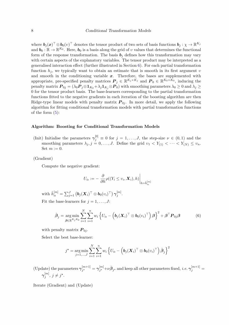
where bj(x)>⊗b0(υ)> denotes the tensor product of two sets of basis functions bj : χ→ RKjand b0 : R→ RK0 . Here, b0 is a basis along the grid of υ values that determines the functionalform of the response transformation. The basis bj defines how this transformation may varywith certain aspects of the explanatory variables. The tensor product may be interpreted as ageneralised interaction effect (further illustrated in Section 6). For each partial transformationfunction hj , we typically want to obtain an estimate that is smooth in its first argument υand smooth in the conditioning variable x. Therefore, the bases are supplemented withappropriate, pre-specified penalty matrices P j ∈ RKj×Kj and P 0 ∈ RK0×K0 , inducing thepenalty matrix P 0j = (λ0P j⊗1K0 +λj1Kj⊗P 0) with smoothing parameters λ0 ≥ 0 and λj ≥0 for the tensor product basis. The base-learners corresponding to the partial transformationfunctions fitted to the negative gradients in each iteration of the boosting algorithm are thenRidge-type linear models with penalty matrix P 0j . In more detail, we apply the followingalgorithm for fitting conditional transformation models with partial transformation functionsof the form (5):
Algorithm: Boosting for Conditional Transformation Models
(Init) Initialise the parameters γ[0]j ≡ 0 for j = 1, . . . , J , the step-size ν ∈ (0, 1) and the
smoothing parameters λj , j = 0, . . . , J . Define the grid υ1 < Y(1) < · · · < Y(N) ≤ υn.Set m := 0.
(Gradient)
Compute the negative gradient:
Uiı := − ∂
∂hρ((Yi ≤ υı,Xi), h)
∣∣∣∣h=h
[m]iı
with h[m]iı =
∑Jj=1
(bj(Xi)
> ⊗ b0(υı)>)γ[m]j .
Fit the base-learners for j = 1, . . . , J :
βj = arg minβ∈RKjK0
N∑i=1
n∑ı=1
wi
{Uiı −
(bj(Xi)
> ⊗ b0(υı)>)β}2
+ β>P 0jβ (6)
with penalty matrix P 0j .
Select the best base-learner:
j? = arg minj=1,...,J
N∑i=1
n∑ı=1
wi
{Uiı −
(bj(Xi)
> ⊗ b0(υı)>)βj
}2
(Update) the parameters γ[m+1]j? = γ
[m]j? +νβj? and keep all other parameters fixed, i.e. γ
[m+1]j =
γ[m]j , j 6= j?.
Iterate (Gradient) and (Update)
Torsten Hothorn, Thomas Kneib, and Peter Buhlmann 9
(Stop) if m = M . Output the final model
P(Y ≤ υ|X = x) = F(h[M ] (υ|x)
)= F
J∑j=1
(bj(x)> ⊗ b0(υ)>
)γ[M ]j
as a function of arbitrary υ ∈ R and x ∈ χ.
Before we investigate the asymptotic properties of the resulting estimates, we will discusssome details of this generic algorithm in the following.
Model Specification. The basis functions b0 and bj determine the form of the fittedmodel, and their choice is problem specific. In the simplest situation, in which the conditionaldistribution of Y given only one numeric explanatory variable x1 shall be estimated, one coulduse the basis functions b0(υ) = (1, υ)> and b1(x) = (1, x1)
>. The corresponding base-learneris then defined by the linear function
((1, x1)⊗ (1, υ))γ1 = (1, υ, x1, x1υ)γ1.
For each x1, the transformation is linear in υ with intercept γ1 + γ3x1 and slope γ2 + γ4x1,i.e. not only the mean may depend on x1 but also the variance. Restricting, for example,b0(υ) to be constant, i.e. b0(υ) ≡ 1, allows the effects of explanatory variables to be restrictedto the mean alone. Assuming b1(x) ≡ 1, on the other hand, yields a transformation functionthat is not affected by any explanatory variable. More flexible basis functions, e.g. B-splinebasis functions, allow also for higher moments to depend on the explanatory variables. Weillustrate appropriate choices of basis functions in Section 6.
Computational Complexity. For the estimation of base-learner parameters βj in (6),it is not necessary to evaluate the Kronecker product ⊗ in (5) and to compute the nN ×K0Kj design matrix for the jth base-learner. The base-learners used here are a special formof multidimensional smooth linear array models (Currie, Durban, and Eilers 2006), whereefficient algorithms for computing Ridge estimates (6) exist. The number of multiplicationsrequired for fitting the jth base-learner is approximately c6/(c2/N − 1), instead of N2c4 forthe simplest case with c = K0 = Kj and N = n (see Table 2 in Currie et al. 2006), andthe required memory for storing the design matrices is of the order NKj + NK0, insteadof NnKjK0. Note that only the gradient vector is of length Nn; all other objects can bestored in vectors or matrices growing with either N or n, and an explicit expansion of theobservations (Yi ≤ υı,Xi) for i = 1, . . . , N and ı = 1, . . . , n is not necessary.
Choice of Tuning Parameters. The number of boosting iterations M is the most impor-tant tuning parameter determined by resampling, e.g. by k-fold cross-validation or bootstrap-ping. For the latter resampling scheme, the weights wi in (4) are drawn from anN -dimensionalmultinomial distribution with constant probability parameters pi ≡ N−1, i = 1, . . . , N . Theout-of-bootstrap (OOB) empirical risk with weights wOOB
i = I(wi = 0) is then used as ameasure to assess the quality of the distributional forecasts for a varying number of boostingiterations M . It should be noted that the loss function used to fit the models is the samefunction that is used as a scoring rule to assess the quality of the probabilistic forecasts ofthe OOB observations.

10 Conditional Transformation Models
The smoothing parameters λj , j = 0, . . . , J in the penalty matrices are not tuned but ratherdefined such that the jth base-learner has low degrees of freedom. For our computations,we simplified the penalty term to P 0j = λj(P j ⊗ 1K0 + 1Kj ⊗ P 0), i.e. one parametercontrols the smoothness in both directions. Following Hofner, Hothorn, Kneib, and Schmid(2011a), the parameters λj were defined such that each base-learner has the same overall lowdegree of freedom. Note that the degree of freedom of the estimated partial transformationfunction adapts to the complexity inherent in the data via the number of boosting iterationsM (Buhlmann and Yu 2003). Different smoothness in the two directions can be imposed bychoosing different basis functions for b0 and bj , e.g. a linear basis function for bj and B-splinesfor b0.
Other parameters, such as knots or degrees of basis functions or the number n of grid pointsthe integrated loss function ` is approximated with are not considered as tuning parameters.The resulting estimates are rather insensitive to their different choices. Also, we do notconsider the distribution function F or the loss function ρ as tuning parameter but assumethat these are part of the model specification. Different versions of F and ρ lead to differentnegative gradients; these are given in the Appendix.
Monotonicity. The resulting estimate h[M ] (υ|x) is not automatically monotone in its firstargument. Monotonicity and smoothness in the Y -direction depend on each other, and too-complex estimates tend to suffer from non-monotonicity. Empirically, based on experimentsreported in Sections 6 and 7, non-monotonicity is a problem in poorly-fitting models, dueto either misspecification, overfitting, or a low signal-to-noise ratio. From our point of view,inspecting the model for non-monotonicity is helpful for model diagnostics and can be dealtwith by reducing model complexity. Alternatively, there are three possible modifications tothe algorithm that can be implemented to enforce monotonicity: (i) fit base-learners undermonotonicity constraints in (6), e.g. by using the iterative re-penalisation suggested by Eilers(2005) and applied to boosting by Hofner, Muller, and Hothorn (2011c), (ii) check mono-tonicity for each base-learner and select the best among the monotone candidates only, or(iii) select the base-learner such that it is the best one among all candidates that lead tomonotone updates in h[m]. None of these approaches had to be used for our empirical stud-ies, in which all resulting estimates were monotone for the appropriate number of boostingiterations M .
Model Diagnostics and Overfitting. Another convenient feature of transformation mod-els is that, with the correct model h for absolute continuous random variables Y , the errorsEi = h(Yi|Xi), i = 1, . . . , N are distributed according to F . Therefore, if the observed
residuals E[M ]i = h[M ](Yi|Xi) are unlikely to come from distribution F , e.g. assessed using
quantile-quantile plots or a Kolmogorov-Smirnov statistic, the model is likely to fit the data
poorly. However, a good agreement between E[M ]i and F does not necessarily mean that the
explanatory variables describe the response well. A high correlation between the ranking ofthe residuals and the ranking of the responses Y1, . . . , YN means that the estimated conditionaldistribution is very close to the unconditional empirical distribution of the responses. In thiscase, either the model may overfit or the response may be independent of the explanatoryvariables.
The fitted model may also be used to draw novel responses for given explanatory variables
Torsten Hothorn, Thomas Kneib, and Peter Buhlmann 11
using the model-based bootstrap via
Yi ={υ : Q(Ui) = h[M ](υ|Xi)
}, i = 1, . . . , N
where U1, . . . , UN are i.i.d. uniform random variables. The stability of the model can now beinvestigated by refitting the model with observations (Yi,Xi), i = 1, . . . , N .
5. Consistency of Boosted Conditional Transformation Models
The boosting algorithm presented here is a variant of L2WCBoost (Buhlmann and Yu 2003)applied to dependent observations with more general base-learners. In this section, we willdevelop a consistency result for the squared error loss ρsqe. For simplicity, we consider thecase in which the procedure is used with F (h) = h as the identity function, i.e. the error termis uniformly distributed. Thus, we consider conditional transformation models of the form
P(Y ≤ υ|X = x) = h(υ|x) =J∑j=1
hj(υ|xj),
where the partial transformation function hj is conditional on the jth explanatory variable
in x = (x1, . . . , xJ) ∈ χ and EY (N−1∑N
i=1 h(Y |Xi)) = 1/2. Our analysis is for the fixeddesign case with deterministic explanatory variables Xi or when conditioning on all Xis. Amodification for the random design case could be pursued along arguments similar to thosefor L2Boosting as in Buhlmann (2006).
As in Section 4, we use a basis expansion of h(υ|x):
hN,γ(υ|x) =J∑j=1
(bj(xj)
> ⊗ b0(υ)>)γj =
J∑j=1
K0,N∑k0=1
K1,N∑k1=1
γj,k0,k1b0,k0(v)bj,k1(xj),
where for the sake of simplicity the number of basis functions K1,N is equal for all xj .
Consider the (empirical) risk functions
Rn,N (h) = (nN)−1N∑i=1
n∑ı=1
(I(Yi ≤ υı)− h(υı|Xi))2
and
Rn,N,E(h) = (nN)−1N∑i=1
n∑ı=1
E[(I(Yi ≤ υı)− h(υı|Xi))2].
Denote the projected parameter by
γ0,N = arg minγ
Rn,N,E(hN,γ). (7)
We make the following assumptions:

12 Conditional Transformation Models
(A1) The coefficient vector γ0,N is sparse and satisfies
‖γ0,N‖1 = o
(√N
log(JNK0,NK1,N )
)(N →∞).
Thereby, the dimensionality J = JN can grow with N .
(A2) The basis functions satisfy: for some 0 < C <∞,
‖b0,k0‖∞ ≤ C, ‖bj,k1‖∞ ≤ C ∀j, k0, k1.
(A3)
(nN)−1N∑i=1
n∑ı=1
hγ0,N(υı|Xi)
2 ≤ D <∞ ∀n,N
.
Assumption (A1) is an `1-norm sparsity assumption, (A2) is a mild restriction since we aremodeling I(Y ≤ υ), and (A3) requires that the signal strength does not diverge as n,N →∞.
Theorem 1. Assume (A1)-(A3). Then, for fixed n or for n = nN →∞ (N →∞), and forM = MN →∞ (N →∞), MN = o(
√N/ log(JNK0,NK1,N )):
(nN)−1N∑i=1
n∑ı=1
(hγ[M ](υı|Xi)− hγ0,N(υı|Xi))
2 = oP (1) (N →∞).
A proof is given in the Appendix.
Convergence of hγ0,N(υ|x) to the true function h(υ|x) involves approximation theory to
achieve
(nN)−1N∑i=1
n∑ı=1
(hγ0,N(υı|Xi)− h(υı|Xi))
2 = o(1) (n,N →∞). (8)
We typically would want to estimate the function h(υ|x) well over the whole domain, e.g. [aυ, bυ]×χ. This may be too ambitious if J = dim(χ) = JN grows with N . Hence, we restrict ourselvesto the setting where the number of active variables Jact <∞ is fixed (from the active set S),i.e.
h(υ|x) =∑j∈S
hj(υ|xj), S ⊆ {1, . . . , J} with |S| = Jact.
For the approximation, we typically would need K0,N , K1,N → ∞ (N → ∞) for suitablebasis functions and n = nN → ∞ (N → ∞); furthermore, the grid υ1 < υ2 < . . . < υnshould become dense as n = nN → ∞, and also the values Xact
1 , . . . ,XactN should become
dense in χS ⊆ χ as N → ∞ (here, Xact = {Xj ; j ∈ S} ∈ χS). If J = JN grows, but thenumber of active variables in the model Jact <∞ is fixed, then some uniform approximationhγ0,N
(υ|x)→ h(υ|x) is possible under regularity conditions.
We provide a summary for a typical situation.

Torsten Hothorn, Thomas Kneib, and Peter Buhlmann 13
Corollary 1. Consider the setting as in Theorem 1, with J = JN potentially growing but fixeddimensionality of the active variables Jact < ∞, n = nN → ∞ (N → ∞), and the functionsare sufficiently regular such that (8) holds. Then, for M = MN as in Theorem 1:
(nN)−1N∑i=1
n∑ı=1
(hγ[M ](υı|Xi)− h(υı|Xi))2 = oP (1) (n,N →∞).
This result states that the estimated hγ[M ] are consistent for the true transformation func-tion h.
6. Applications
In this section, we present analyses with special emphasis on higher moments of the conditionaldistribution, which have received less attention in previous analyses of these problems. Weshow that semiparametric regression using conditional transformation models is a valuabletool for detecting interesting patterns beyond the conditional mean.
“Evolution Canyon” Bacteria
The Bacillus simplex populations from “Evolution Canyons” I and II in Israel have recentlydeveloped into a model study of bacterial adaptation and speciation under heterogeneousenvironmental conditions (Sikorski and Nevo 2005). These two canyons represent similarecological sites, 40 km apart, in which the orientation of the sun yields both a strongly sun-exposed, hot, ‘African’, south-facing slope and a cooler, mesic, lush, ‘European’, north-facingslope within a distance of only 50–400 m. Based on DNA sequences, the B. simplex populationphylogenetically splits into two major groups, GL1 and GL2. These main groups are furthersubdivided into phylogenetic groups, the so-called ‘putative ecotypes’ (PE), which show aclear preference for one of the two slope types (Sikorski and Nevo 2005, Sikorski, Pukall, andStackebrandt 2008b). GL2 is composed of only PE1 and PE2; GL1 consists of PE3–PE9.
Sikorski et al. (2008b) analysed the physiological properties of the bacteria that might ex-plain their characteristic slope-type preferences. For example, the physical integrity of the cellmembrane at different temperatures is crucial for cell survival, and particularly its fatty acidcomposition is of substantial importance. Sikorski, Brambilla, Kroppenstedt, and Tindall(2008a) compared the mean contents of the fatty acids that tolerate high and low tempera-tures of the B. simplex ecotypes. The data showed heteroscedastic variances across putativeecotypes, and Herberich, Sikorski, and Hothorn (2010) analysed the data using heteroscedas-ticity consistent covariance estimation techniques. Here, we aim at estimating the wholeconditional distribution of the fatty acid contents (FA) of each of the six putative ecotypesPE3–PE7 and PE9 from GL1.
The simplest conditional transformation model allowing for heteroscedasticity reads
P(FA ≤ υ|PE = PEk) = Φ(α0,k + αkυ), k ∈ {3, . . . , 7, 9}. (9)
The base-learner is defined by a linear basis b0(υ) = (1, υ)> for the grid variable and a dummy-encoding basis b1(PE) = (I(PE = PE3), . . . , I(PE = PE9))
> for the six putative ecotypes{3, . . . , 7, 9}. The resulting 12-dimensional parameter vector γ1 of the tensor product base-learner then consists of separate intercept and slope parameters for each of the putative
14 Conditional Transformation Models
Fatty acid content
Dis
trib
utio
n fu
nctio
n
0.0
0.1
0.2
0.3
0.4
0.5
0.7 0.8 0.9 1.0
PE3 PE4
0.7 0.8 0.9 1.0
PE5
PE6
0.7 0.8 0.9 1.0
PE7
0.0
0.1
0.2
0.3
0.4
0.5PE9
smoothlinear
linear M = ∞kernel
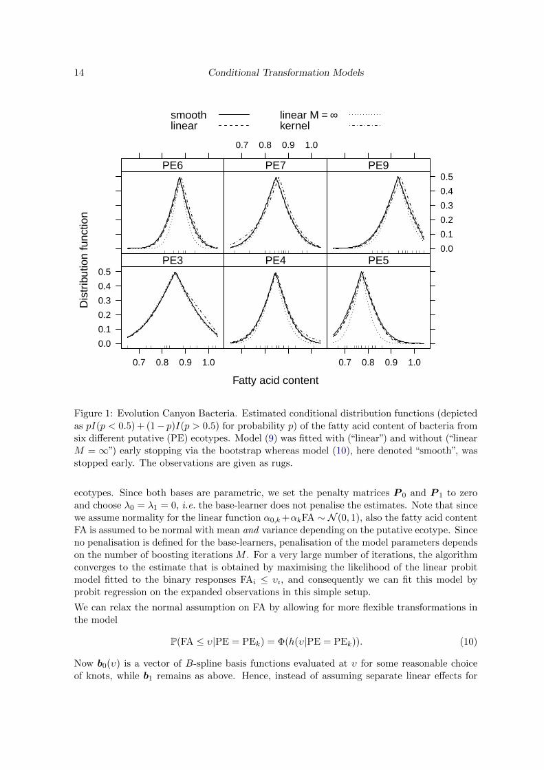
Figure 1: Evolution Canyon Bacteria. Estimated conditional distribution functions (depictedas pI(p < 0.5) + (1− p)I(p > 0.5) for probability p) of the fatty acid content of bacteria fromsix different putative (PE) ecotypes. Model (9) was fitted with (“linear”) and without (“linearM = ∞”) early stopping via the bootstrap whereas model (10), here denoted “smooth”, wasstopped early. The observations are given as rugs.
ecotypes. Since both bases are parametric, we set the penalty matrices P 0 and P 1 to zeroand choose λ0 = λ1 = 0, i.e. the base-learner does not penalise the estimates. Note that sincewe assume normality for the linear function α0,k+αkFA ∼ N (0, 1), also the fatty acid contentFA is assumed to be normal with mean and variance depending on the putative ecotype. Sinceno penalisation is defined for the base-learners, penalisation of the model parameters dependson the number of boosting iterations M . For a very large number of iterations, the algorithmconverges to the estimate that is obtained by maximising the likelihood of the linear probitmodel fitted to the binary responses FAi ≤ υı, and consequently we can fit this model byprobit regression on the expanded observations in this simple setup.
We can relax the normal assumption on FA by allowing for more flexible transformations inthe model
P(FA ≤ υ|PE = PEk) = Φ(h(υ|PE = PEk)). (10)
Now b0(υ) is a vector of B-spline basis functions evaluated at υ for some reasonable choiceof knots, while b1 remains as above. Hence, instead of assuming separate linear effects for

Torsten Hothorn, Thomas Kneib, and Peter Buhlmann 15
the putative ecotypes, we now assume separate non-parametric effects parameterised in termsof B-splines. To achieve smoothness of these non-parametric effects along the υ-grid, wespecify the penalty matrix P 0 as P 0 = D>D with second-order difference matrix D. Wedo not penalise differences between the estimated functions of different putative ecotypes,i.e. P 1 = 0, and therefore the penalty matrix of the tensor product is simply given byP 01 = λ0 diag(P 0, . . . ,P 0). Although we still assume h(FA|PE = PEk) ∼ N (0, 1), thefunction h may now be non-linear, and thus the conditional distribution of FA given PE maybe any distribution that can be generated by a monotone transformation of a standard normal.In this sense, the model (10) is non-parametric. The validity of the normal assumption onFA is plausible when the estimated functions h(υ|PE = PEk) are essentially linear in υ. Analternative non-parametric estimate can be obtained by kernel smoothing for mixed data types(Li and Racine 2008, Hayfield and Racine 2008), and we compare the two fits in Figure 1.
We fitted model (9) without (M =∞) and with early stopping (via 25-fold bootstrap strati-fied by PE) and model (10) with early stopping to the data and in addition report the resultof kernel smoothing, whose bandwidth was determined via cross-validation. The conditionaldistribution functions of fatty acid content given the putative ecotype are depicted in Figure 1.For probabilities larger than 0.5, the estimated conditional distribution functions were mir-rored at the 0.5 horizontal line to allow for easier graphical inspection of medians, variancesand potential skewness.
With respect to the conditional median, the four models lead to very similar results andsupport the conclusion from earlier investigations (Sikorski et al. 2008a, Herberich et al.2010) that the fatty acid content of B. simplex from putative ecotype PE5 is smaller thanthe others and that from PE9 is larger than the others, with the remaining ones showingno differences. The variability cannot be assumed to be constant across different putativeecotypes, but there is no indication of asymmetry. Early stopping and bandwidth choice viaresampling methods lead to almost the same estimated distribution functions. Minimisingthe empirical risk function without early stopping (“linear M = ∞”; this is equivalent tolinear probit regression on expanded observations) leads to slightly smaller variances in PE5
and PE6. The difficulty in discriminating between the linear model (9) and the more flexiblemodel (10) and the lack of asymmetry in the plots indicate that a normal assumption on fattyacid content is justifiable.
Childhood Nutrition in India
Childhood undernutrition is one of the most urgent problems in developing and transitioncountries. To provide information not only on the nutritional status but also on health andpopulation trends in general, Demographic and Health Surveys (DHS) conduct nationallyrepresentative surveys on fertility, family planning, maternal and child health, as well as childsurvival, HIV/AIDS, malaria, and nutrition. The resulting data – from more than 200 surveysin 75 countries so far – are available for research purposes at www.measuredhs.com.
Childhood nutrition is usually measured in terms of a Z score that compares the nutritionalstatus of children in the population of interest with the nutritional status in a reference pop-ulation. The nutritional status is expressed by anthropometric characteristics, i.e. height forage; in cases of chronic childhood undernutrition, the reduced growth rate in human develop-ment is termed stunted growth or stunting. The Z score, which compares an anthropometric
16 Conditional Transformation Models
10%
90%
−429 −373 −317
−1
2654
81
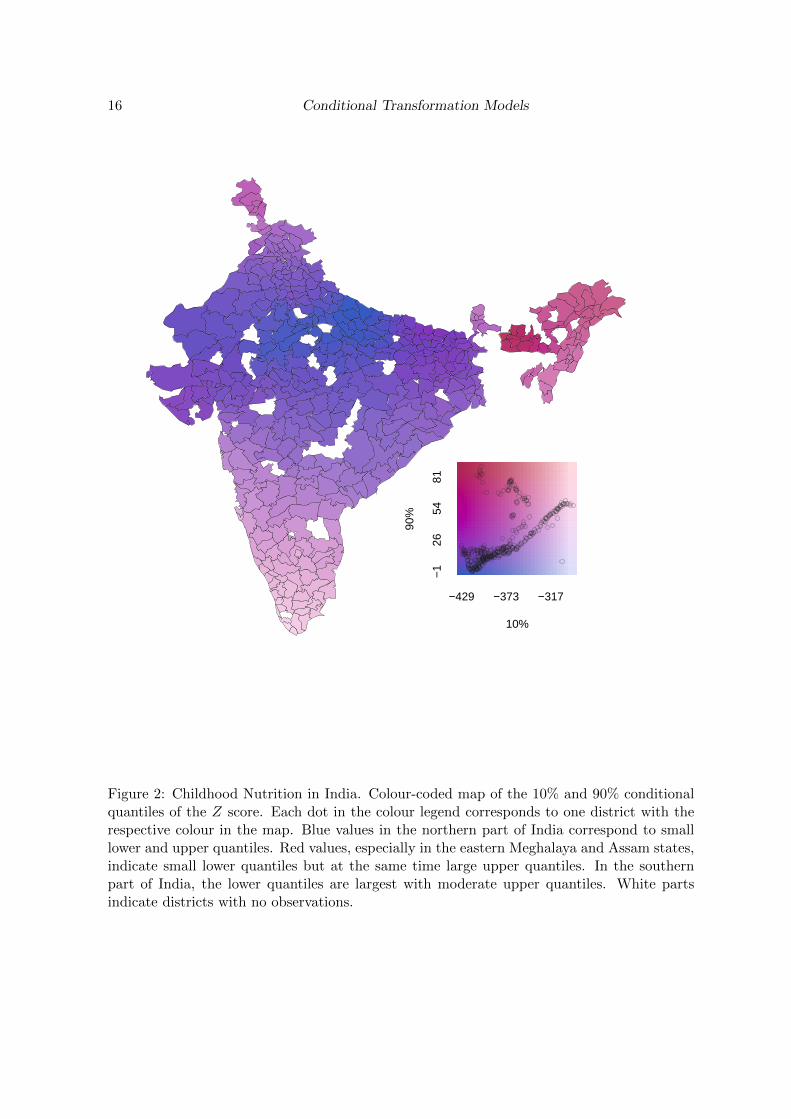
Figure 2: Childhood Nutrition in India. Colour-coded map of the 10% and 90% conditionalquantiles of the Z score. Each dot in the colour legend corresponds to one district with therespective colour in the map. Blue values in the northern part of India correspond to smalllower and upper quantiles. Red values, especially in the eastern Meghalaya and Assam states,indicate small lower quantiles but at the same time large upper quantiles. In the southernpart of India, the lower quantiles are largest with moderate upper quantiles. White partsindicate districts with no observations.

Torsten Hothorn, Thomas Kneib, and Peter Buhlmann 17
characteristic of child i to values from a reference population, is given as
Zi =ACi −m
s
where AC denotes the anthropometric characteristic of interest and m and s correspond tomedian and (a robust estimate for the) standard deviation in the reference population (strati-fied with respect to age, gender, and some other variables). While weight might be consideredas the most obvious indicator for undernutrition, we will focus on stunting, i.e. insufficientAC = height for age, in the following. Stunting provides a measure of chronic undernutrition,whereas insufficient weight for age might result from either acute or chronic undernutrition.Note that the Z score, despite its name, is not assumed to be normal.
Here we focus on estimating the whole distribution of the Z score measure for childhood nutri-tion in India, one of the fastest growing economies and the second-most populated country inthe world. Our investigation is based on India’s 1998–1999 Demographic and Health Survey(DHS, NFHS 2000) on 24, 166 children visited during the survey in 412 of the 640 districts ofIndia. The lower quantiles of this distribution can be used to assess the severity of childhoodundernutrition, whereas the upper quantiles give us information about the nutritional statusof children in families with above-average nutritional status.
The simplest conditional transformation model allowing for district-specific means and vari-ances reads
P(Z ≤ υ|district = k) = Φ(α0,k + αkυ), k = 1, . . . , 412.
The base-learner is defined by a linear basis b0(υ) = (1, υ)> for the grid variable and a dummy-encoding basis b1(district) = (I(district = 1), . . . , I(district = k))> for the 412 districts. Theresulting 824-dimensional parameter vector γ1 of the tensor product base-learner then consistsof separate intercept and slope parameters for each of the districts of India. Note that sincewe assume normality for the linear function α0,k+αkZ ∼ N (0, 1), also the Z score is assumedto be normal with mean and variance depending on the district.
We can relax the normal assumption on Z by allowing for more flexible transformations inthe model
P(Z ≤ υ|district = k) = Φ(h(υ|district = k)), k = 1, . . . , 412. (11)
Now b0(υ) is a vector of B-spline basis functions evaluated at υ for some reasonable choiceof knots, while b1 remains as above. Hence, instead of assuming separate linear effects forthe districts, we now assume separate non-parametric effects parameterised in terms of B-splines. To achieve smoothness of these non-parametric effects along the υ-grid, we specifythe penalty matrix P 0 as P 0 = D>D with second-order difference matrix D. It makessense to induce spatial smoothness on the conditional distribution functions of neighbouringdistricts since we do not expect the distribution of the Z score to change much from onedistrict to its neighbouring districts. In fact, spatial smoothing is absolutely necessary inthis example since otherwise we would estimate 412 separate distribution functions for thedistricts in India. To implement spatial smoothness of neighbouring districts, the penaltymatrix P 1 is chosen as an adjacency matrix, where the off-diagonal elements indicate whethertwo districts are neighbours (represented with a value of −1) or not (represented with a valueof 0). The diagonal of the adjacency matrix contains the number of neighbours for the

18 Conditional Transformation Models
corresponding district. The estimated conditional transformation function h(Z|district = k)can be interpreted as a transformation of the Z scores in district k to standard normality.Because the number of observations is large and the base-learner is fitted with penalisation,we stopped the boosting algorithm according to the in-sample empirical risk.
From the estimated conditional distribution functions, we compute the τ quantiles of the Zscore for each district via
Q(τ |district = k) = inf{υ : Φ(h(υ|district = k) ≥ τ}.
The conditional 10% and 90% quantiles are depicted in a colour-coded map in Figure 2.The spatially smooth estimated lower and upper conditional quantiles shown simultaneouslyallow differentiation between three groups of districts: (A) districts with small lower andupper conditional quantiles (blue, especially in the Uttar Pradesh state), where the Z scoreis stochastically smaller than that of the remaining parts of India and thus all children areless well fed; (B) districts with more severe inequality, i.e. small lower but at the sametime large upper quantiles (red, in the Meghalaya and Assam states); and (C) districts withrelatively large lower and upper quantiles, which indicates a relatively good nutrition statusof all children in the southern districts of India (violet, in Andhra Pradesh, Madhya Pradesh,Maharashtra, Tamil Nadu, and Kerala).
Head Circumference Growth
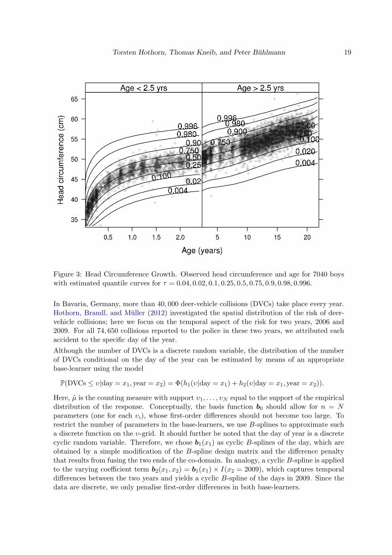
The Fourth Dutch Growth Study (Fredriks, van Buuren, Burgmeijer, Meulmeester, Beuker,Brugman, Roede, Verloove-Vanhorick, and Wit 2000) is a cross-sectional study that measuresgrowth and development of the Dutch population between the ages of 0 and 22 years. Thestudy measured, among other variables, head circumference (HC) and age of 7482 malesand 7018 females. Stasinopoulos and Rigby (2007) analysed the head circumference of 7040males with explanatory variable age using a GAMLSS model with a Box-Cox t distributiondescribing the first four moments of head circumference conditionally on age. The models showevidence of kurtosis, especially for older boys. We estimate the whole conditional distributionfunction via the conditional transformation model
P(HC ≤ υ|age = x) = Φ(h(υ|age = x)).
The base-learner is the tensor product of B-spline basis functions b0(υ) for head circumferenceand B-spline basis functions for age1/3. The root transformation just helps to cover thedata better with equidistant knots. The penalty matrices P 0 and P 1 penalise second-orderdifferences, and thus h will be a smooth bivariate tensor product spline of head circumferenceand age. It is important to note that smoothing takes place in both dimensions. Consequently,the conditional distribution functions will change only slowly with age, which is a reasonableassumption. Since the number of observations is also large, we stopped the algorithm basedon the in-sample empirical risk.
Figure 3 shows the data overlaid with quantile curves obtained via inversion of the estimatedconditional distributions. The figure can be directly compared with Figure 16 of Stasinopoulosand Rigby (2007) and also indicates a certain asymmetry towards older boys.
Deer-vehicle Collisions
Collisions of vehicles with roe deer are a serious threat to human health and animal welfare.
Torsten Hothorn, Thomas Kneib, and Peter Buhlmann 19
Figure 3: Head Circumference Growth. Observed head circumference and age for 7040 boyswith estimated quantile curves for τ = 0.04, 0.02, 0.1, 0.25, 0.5, 0.75, 0.9, 0.98, 0.996.
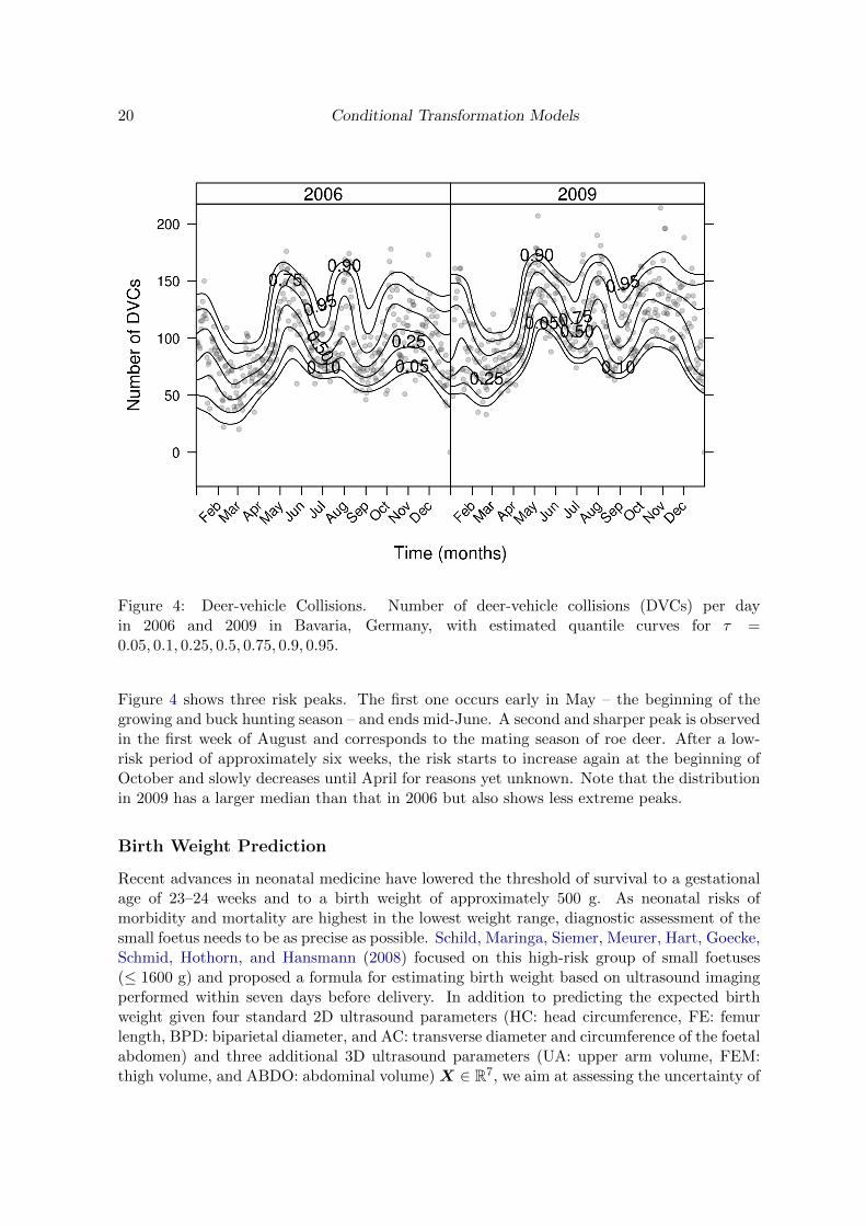
In Bavaria, Germany, more than 40, 000 deer-vehicle collisions (DVCs) take place every year.Hothorn, Brandl, and Muller (2012) investigated the spatial distribution of the risk of deer-vehicle collisions; here we focus on the temporal aspect of the risk for two years, 2006 and2009. For all 74, 650 collisions reported to the police in these two years, we attributed eachaccident to the specific day of the year.
Although the number of DVCs is a discrete random variable, the distribution of the numberof DVCs conditional on the day of the year can be estimated by means of an appropriatebase-learner using the model
P(DVCs ≤ υ|day = x1, year = x2) = Φ(h1(υ|day = x1) + h2(υ|day = x1, year = x2)).
Here, µ is the counting measure with support υ1, . . . , υN equal to the support of the empiricaldistribution of the response. Conceptually, the basis function b0 should allow for n = Nparameters (one for each υı), whose first-order differences should not become too large. Torestrict the number of parameters in the base-learners, we use B-splines to approximate sucha discrete function on the υ-grid. It should further be noted that the day of year is a discretecyclic random variable. Therefore, we chose b1(x1) as cyclic B-splines of the day, which areobtained by a simple modification of the B-spline design matrix and the difference penaltythat results from fusing the two ends of the co-domain. In analogy, a cyclic B-spline is appliedto the varying coefficient term b2(x1, x2) = b1(x1) × I(x2 = 2009), which captures temporaldifferences between the two years and yields a cyclic B-spline of the days in 2009. Since thedata are discrete, we only penalise first-order differences in both base-learners.
20 Conditional Transformation Models
Figure 4: Deer-vehicle Collisions. Number of deer-vehicle collisions (DVCs) per dayin 2006 and 2009 in Bavaria, Germany, with estimated quantile curves for τ =0.05, 0.1, 0.25, 0.5, 0.75, 0.9, 0.95.
Figure 4 shows three risk peaks. The first one occurs early in May – the beginning of thegrowing and buck hunting season – and ends mid-June. A second and sharper peak is observedin the first week of August and corresponds to the mating season of roe deer. After a low-risk period of approximately six weeks, the risk starts to increase again at the beginning ofOctober and slowly decreases until April for reasons yet unknown. Note that the distributionin 2009 has a larger median than that in 2006 but also shows less extreme peaks.
Birth Weight Prediction
Recent advances in neonatal medicine have lowered the threshold of survival to a gestationalage of 23–24 weeks and to a birth weight of approximately 500 g. As neonatal risks ofmorbidity and mortality are highest in the lowest weight range, diagnostic assessment of thesmall foetus needs to be as precise as possible. Schild, Maringa, Siemer, Meurer, Hart, Goecke,Schmid, Hothorn, and Hansmann (2008) focused on this high-risk group of small foetuses(≤ 1600 g) and proposed a formula for estimating birth weight based on ultrasound imagingperformed within seven days before delivery. In addition to predicting the expected birthweight given four standard 2D ultrasound parameters (HC: head circumference, FE: femurlength, BPD: biparietal diameter, and AC: transverse diameter and circumference of the foetalabdomen) and three additional 3D ultrasound parameters (UA: upper arm volume, FEM:thigh volume, and ABDO: abdominal volume) X ∈ R7, we aim at assessing the uncertainty of
Torsten Hothorn, Thomas Kneib, and Peter Buhlmann 21
this prediction. The data on 150 predominantly Caucasian women, collected in a prospectivecohort study at the universities in Bonn and Erlangen, Germany, analysed by Schild et al.(2008), were utilised to derive 80% prediction intervals for birth weight (BW).
We begin with the linear model estimated by Schild et al. (2008)
BWx = 656.41 + 1.832×ABDO + 31.198×HC + 5.779× FEM +
73.521× FL + 8.301×AC− 449.886× BPD + 32.534× BPD2 +
77.465× Φ−1(U),
and the classical prediction interval for a foetus with ultrasound parameters x is then thesymmetric interval around the estimated conditional mean E(BW|X = x), whose width is
given by 2× t150−8,0.9 × 77.465×√
1 + Var(E(BW|X = x)).
The normal assumption can be relaxed by deriving the upper and lower conditional quantilesfrom two quantile regression models. Linear quantile regression (Koenker and Bassett 1978)for the conditional 10%, 50% and 90% quantiles assumes that
BWx = α0,τ + x>ατ +Qτ (U), for τ = 0.1, τ = 0.5, and τ = 0.9
with Qτ (τ) = 0. The corresponding prediction interval for a foetus with ultrasound parame-ters x is now (α0,0.1 + x>α0.1, α0,0.9 + x>α0.9). A more flexible description of the functionalrelationship between ultrasound parameters and quantiles is given by the additive quantileregression model (Koenker, Ng, and Portnoy 1994)
BWx = α0,τ +7∑j=1
rj,τ (xj) +Qτ (U), for τ = 0.1, τ = 0.5, and τ = 0.9.
Here, rj,τ is a quantile-specific smooth function of the jth ultrasound parameter. Parametertuning is difficult for these models; we therefore applied a boosting approach to additive quan-tile regression (Fenske, Kneib, and Hothorn 2011, with early stopping via 25-fold bootstrap).Prediction intervals can now be derived by (α0,0.1 +
∑7j=1 rj,0.1(xj), α0,0.9 +
∑7j=1 rj,0.9(xj)).
Note that for either quantile regression model, the prediction interval is based on two separatemodels: one for τ = 0.1 and one for τ = 0.9.
Finally, we derive prediction intervals from the conditional transformation model
P(BW ≤ υ|X = x) = Φ
7∑j=1
hj(υ|xj)
where, under the assumption of additivity of the transformation function h, each ultrasoundparameter may influence the moments of the conditional birth weight distribution. The jthbase-learner is the tensor product of B-spline basis functions b0(υ) for birth weight and bj(xj)are B-spline basis functions for the jth ultrasound parameter. The penalty matrices P 0 andP j penalise second-order differences, and thus all estimates hj will be smooth bivariate tensorproduct splines of birth weight and the respective ultrasound parameter, with both dimensionsbeing subject to smoothing. The number of boosting iterations was determined by 25-foldbootstrap. From the estimated conditional distribution functions, we compute the τ quantiles
22 Conditional Transformation Models
of the birth weight via
Q(τ |X = x) = inf
υ : Φ
7∑j=1
hj(υ|xj)
≥ τ
and derive the prediction interval as (Q(0.1|X = x), Q(0.9|X = x)). Note that, unlike in thequantile regression approach, the prediction interval obtained from the conditional transfor-mation model is based on only one model that describes the whole conditional distribution ofbirth weight.
The observed birth weights ordered with respect to the predicted mean (linear model) ormedian (quantile regression and conditional transformation model) are depicted in Figure 5.In addition, the respective 80% prediction intervals are visualised by grey areas. It mustbe noted that, for all models, the prediction intervals are only interpretable for future ob-servations; however, poor coverage for the learning sample also indicates poor coverage forfuture cases. The prediction intervals obtained from linear quantile regression indicate thatthe model is confident about its predictions over the whole range of birth weights. This is alsothe case for the additive quantile regression models for birth weights of approximately 1000g, but the uncertainty increases for very small and larger foetuses. The intervals obtainedfrom the linear model and the conditional transformation model appear to be similar. Forbirth weights between 500 and 1400 g, the prediction intervals of the conditional transforma-tion model are symmetric around the median. This might be an indication that the normalassumption by the linear model is not completely unrealistic. The smaller interval widthsthat can be seen for the linear model are most likely due to the variance estimate in this caseignoring the model choice process that was performed prior to the final model fit by Schildet al. (2008). The conditional transformation model takes this variability into account. Theresults may also be an indication that the assumption of additivity of the transformationfunction rather than of the regression function (for quantile regression models) might be moreappropriate for modelling birth weights.
Beyond Mean Boston Housing Values
The Boston Housing data, first published by Harrison and Rubinfeld (1978) and later cor-rected and spatially aligned by Gilley and Pace (1996), have become a standard test-bed forvariable selection and model choice. Almost exclusively, the 13 explanatory variables havebeen selected with respect to their influence on the mean or median of the conditional medianhouse value in a certain tract. Assuming a conditional transformation model, we attempt todetect dependencies of higher moments of the conditional median house value from the ex-planatory variables. We focus on the 12 numeric explanatory variables and ignore the binaryvariable coding for Charles River boundary in the conditional transformation model
P(MEDV ≤ υ|X = x) = Φ
αtract + h0(υ|1) +12∑j=1
hj(1|xj) +12∑j=1
hj(υ|xj)
.
In this model, αtract is a tract-specific, spatial random effect, whose correlation structure isdetermined by a Markov random field defined by the neighbouring structure of the tracts cap-turing spatial autocorrelation and heterogeneity (similar as in the example on childhood nutri-tion in India). The term h0(υ|1) is an unconditional transformation of the median house value,

Torsten Hothorn, Thomas Kneib, and Peter Buhlmann 23
Observation
Bir
th w
eigh
t (in
g)
500
1000
1500
0 50 100 150
●
●●
●●
●●
●●
●●●
●●●
●
●●
●
●●
●●●
●●●●●
●●
●●●●
●
●●●●●
●
●●●●
●
●
●
●
●
●
●
●
●
●
●
●
●
●
●
●●
●
●
●
●
●
●
●
●
●
●
●
●●●●●●
●
●
●●
●
●
●
●●
●
●●●●
●
●●
●
●
●●
●●
●
●●
●
●●●●●●●●●●
●
●
●
●
●●●●
●
●●●
●
●●
●
●●
●●
●●
●●●
●●
●●●●●●
CTM
●●
●●●
●●
●
●
●●●●
●
●●●
●
●●
●●●●
●
●●●●●●●
●●●●
●
●
●
●
●●●●
●
●
●●
●
●●
●●
●
●
●●
●
●
●
●
●
●
●
●●●
●●
●
●
●
●
●
●●●●●
●
●
●
●●
●●
●
●
●
●●
●
●
●
●
●
●
●
●●
●
●
●
●
●
●●●●●●●●●●
●
●
●
●●
●
●
●●●●
●
●
●
●
●
●
●●
●●
●●
●●●
●
●
●
●●●●●●
LM
●
●●
●●
●●
●●
●
●
●●
●
●●
●
●
●
●
●●●●●
●●
●
●●●●●●
●
●●●●●●
●
●●
●●
●●
●
●
●
●●
●●
●●
●
●
●
●
●
●
●
●
●●●
●●●
●
●
●
●
●
●●●●
●●
●●●●
●
●
●●●●
●●
●
●●●●●
●●●●
●●
●
●●●●●
●●●
●
●●
●
●●
●
●●
●
●
●●●
●
●
●●●
●
●●●
●●●
●
●●
●
●
●
●●●
LQR
0 50 100 150
500
1000
1500
●●
●●●
●
●
●●
●
●
●
●
●
●●●
●
●
●
●
●●●●●●●
●●●●●
●
●●
●
●●
●●
●
●
●
●
●●●
●
●●
●
●
●
●
●
●
●●
●
●
●●
●●●
●●
●
●
●
●
●
●
●●●●●
●
●
●●
●●●
●
●
●●●●●
●●
●
●
●●●
●●●
●
●
●
●●●●●
●●●●●
●
●
●●
●
●●●
●●
●
●●
●
●
●
●●●
●●●●
●
●
●●●●●●
●●●
AQR
Figure 5: Birth Weight Prediction. Observed birth weights for 150 small foetuses (dots),ordered with respect to the estimated mean or median expected birth weight (central blackline). The shaded area represents foetus specific 80% prediction intervals for the linear model(LM), linear quantile regression model (LQR), additive quantile regression model (AQR) andconditional transformation model (CTM).
24 Conditional Transformation Models
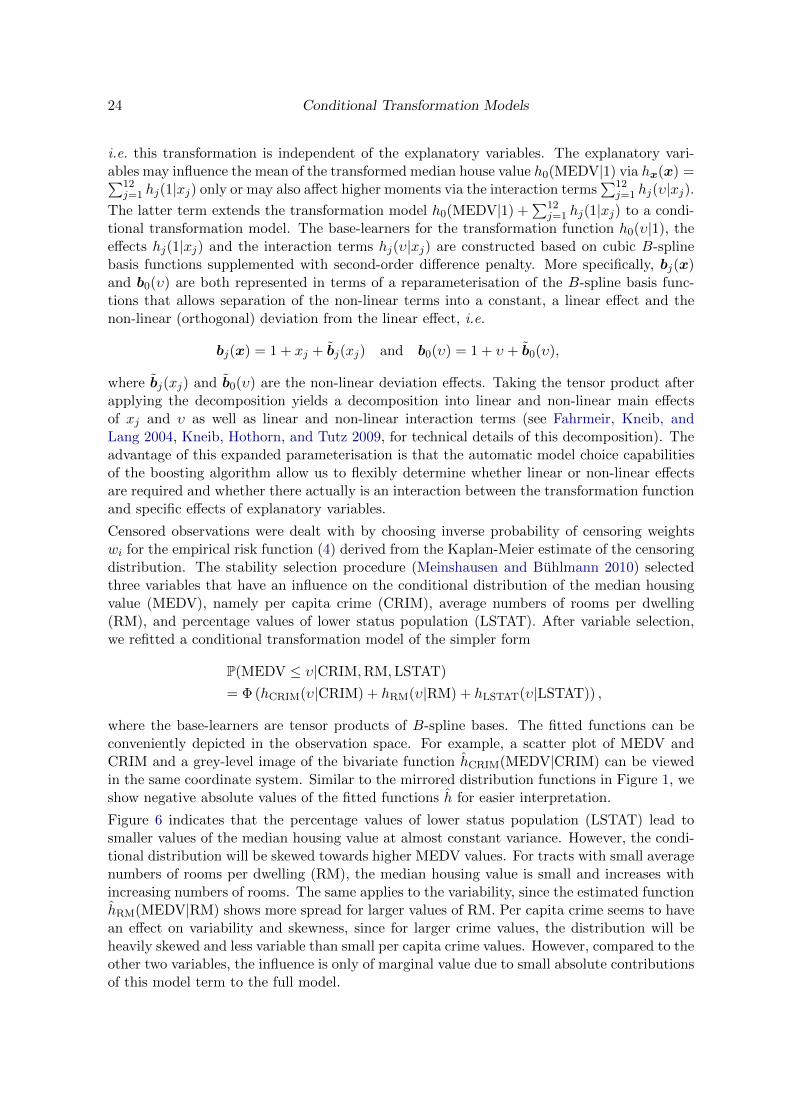
i.e. this transformation is independent of the explanatory variables. The explanatory vari-ables may influence the mean of the transformed median house value h0(MEDV|1) via hx(x) =∑12
j=1 hj(1|xj) only or may also affect higher moments via the interaction terms∑12
j=1 hj(υ|xj).The latter term extends the transformation model h0(MEDV|1) +
∑12j=1 hj(1|xj) to a condi-
tional transformation model. The base-learners for the transformation function h0(υ|1), theeffects hj(1|xj) and the interaction terms hj(υ|xj) are constructed based on cubic B-splinebasis functions supplemented with second-order difference penalty. More specifically, bj(x)and b0(υ) are both represented in terms of a reparameterisation of the B-spline basis func-tions that allows separation of the non-linear terms into a constant, a linear effect and thenon-linear (orthogonal) deviation from the linear effect, i.e.
bj(x) = 1 + xj + bj(xj) and b0(υ) = 1 + υ + b0(υ),
where bj(xj) and b0(υ) are the non-linear deviation effects. Taking the tensor product afterapplying the decomposition yields a decomposition into linear and non-linear main effectsof xj and υ as well as linear and non-linear interaction terms (see Fahrmeir, Kneib, andLang 2004, Kneib, Hothorn, and Tutz 2009, for technical details of this decomposition). Theadvantage of this expanded parameterisation is that the automatic model choice capabilitiesof the boosting algorithm allow us to flexibly determine whether linear or non-linear effectsare required and whether there actually is an interaction between the transformation functionand specific effects of explanatory variables.
Censored observations were dealt with by choosing inverse probability of censoring weightswi for the empirical risk function (4) derived from the Kaplan-Meier estimate of the censoringdistribution. The stability selection procedure (Meinshausen and Buhlmann 2010) selectedthree variables that have an influence on the conditional distribution of the median housingvalue (MEDV), namely per capita crime (CRIM), average numbers of rooms per dwelling(RM), and percentage values of lower status population (LSTAT). After variable selection,we refitted a conditional transformation model of the simpler form
P(MEDV ≤ υ|CRIM,RM,LSTAT)
= Φ (hCRIM(υ|CRIM) + hRM(υ|RM) + hLSTAT(υ|LSTAT)) ,
where the base-learners are tensor products of B-spline bases. The fitted functions can beconveniently depicted in the observation space. For example, a scatter plot of MEDV andCRIM and a grey-level image of the bivariate function hCRIM(MEDV|CRIM) can be viewedin the same coordinate system. Similar to the mirrored distribution functions in Figure 1, weshow negative absolute values of the fitted functions h for easier interpretation.
Figure 6 indicates that the percentage values of lower status population (LSTAT) lead tosmaller values of the median housing value at almost constant variance. However, the condi-tional distribution will be skewed towards higher MEDV values. For tracts with small averagenumbers of rooms per dwelling (RM), the median housing value is small and increases withincreasing numbers of rooms. The same applies to the variability, since the estimated functionhRM(MEDV|RM) shows more spread for larger values of RM. Per capita crime seems to havean effect on variability and skewness, since for larger crime values, the distribution will beheavily skewed and less variable than small per capita crime values. However, compared to theother two variables, the influence is only of marginal value due to small absolute contributionsof this model term to the full model.

Torsten Hothorn, Thomas Kneib, and Peter Buhlmann 25
x
Med
ian
hous
ing
valu
e
10
20
30
40
−1 0 1 2 3
●
●
●
●
●
●
●●
●
●
●
●
●
●
●
●
●
●
●
●
●
●
●●
●
●
●
●
●
●
●
●
●● ●
●●
●
●
●
●
●
●●
●
●●
●
●
●●●
●
●
●
●
●
●
●
●●
●
●
●
●
●
●
●
●
●
●
●●
●●
●
●● ●
●
●
●●
●●
●
●●
●
●
●●●
●
●
●
●
●
●
●
●●
●●
●● ●
●● ●
●●
● ●● ●
●
●
●●
●
● ●
●
●
●
●●
●
●
●●
●
●
●
●●●
●
●
● ●●
●
●
●
●●
●
●
●
●
●
●
●
●
●
●
●●
●
●● ●
●
●
●
●●
●
●
●
●●
●
●
●
●
●
●
●
●
●
●
●
●
●
●
●
●
●
●
●
●
●
●
●
●
●●
●
●
●
●
●
●
●
●
●
●
●
●
●
●
●
●
●
●
●
●
●
●
●
●
●
●
●
●
●
●
●
●
●
●
●
●●
●
● ●
●
●
●
●
●●
●
●
●
●
●●
●
●
●●
●
●
●
●
●
●
●
●
●
●
●
●
●
●●
●●
●
●●
●●
●
●
●
●
●
●
●
●
●
●●
●
●
●
●
●
●
●
●
●
●
●
●
●
●
●
●
●
●
●
●
●
●
●
●
●
●
●
●
●
●
●
●●
●
●
●●
●●
●
●
●
●
●
●
● ●
●●
●
●●
●
●
●
●
● ●
●
●
●
●
●
●
●
●
●
●
●● ●
●
●●
●
●
●
●
●
●●● ●●
● ●
●●
● ●
●●● ●
●
●
●
●
●
●
●
●
●
●
●● ●
●
●
●
●●
●
●
● ●
●
●
●
●
●
●
●●
●
●●●
●
● ●
●
●
●
●
●
●
●● ●
●
● ●
●
●
●
●
●
● ●
●
●
●
●●
●●
●
●
●●●
●●
●
●●
●●
●
●
●
●
●●
●
●● ●●
● ●●
●
●
●●
●
●
●
●
●●
●
●
●●
●
●
●
●●
●
●
●
●
●
●
●
●
●●
●
●
●
●
●
LSTAT
0 2 4 6 8
●
●
●
●
●
●
●●
●
●
●
●
●
●
●
●
●
●
●
●
●
●
●●●
●
●
●
●
●
●
●
●●●
●●●
●
●
●
●
●●
●
●●
●
●
●●●
●
●
●
●
●
●
●
●●
●
●
●
●
●
●
●
●
●
●
●●●●
●
●●●●
●
●●
●●
●
●●
●
●
●●●
●
●
●
●
●
●
●
●●
●●●●●●●●
●●
●●●●
●
●
●●
●
●●
●
●
●
●●
●
●
●●
●
●
●
●●●
●
●
●●●
●
●
●
●●
●
●
●
●
●
●
●
●
●
●
●●
●
●●●
●
●
●
●●
●
●
●
●●●
●
●
●
●
●
●
●
●
●
●
●
●
●
●
●
●
●
●
●
●
●
●
●
●●
●
●
●
●
●
●
●
●
●
●
●
●
●
●
●
●
●
●
●
●
●
●
●
●
●
●
●
●
●
●
●
●
●
●
●
●●
●
●●
●
●
●
●
●●
●
●
●
●
●●
●
●
●●
●
●
●
●
●
●
●
●
●
●
●
●
●
●●
●●
●
●●
●●
●
●
●
●
●
●
●
●
●
●●
●
●
●
●
●
●
●
●
●
●
●
●
●
●
●
●
●
●
●
●
●
●
●
●
●
●
●
●
●
●
●
●●
●
●
●●
●●
●
●
●
●
●
●
●●
●●
●
●●
●
●
●
●
●●
●
●
●
●
●
●
●
●
●
●
●●●
●
●●
●
●
●
●
●
●●● ●●
● ●
●●
● ●
● ●●●
●
●
●
●
●
●
●
●
●
●
●●●
●
●
●
●●
●
●
● ●
●
●
●
●
●
●
●●
●
●●●
●
●●
●
●
●
●
●
●
●●●
●
●●
●
●
●
●
●
●●
●
●
●
●●
●●
●
●
●●●
●●
●
●●
●●
●
●
●
●
●●
●
●●● ●
●●●
●
●
●●
●
●
●
●
●●
●
●
●●
●
●
●
●●
●
●
●
●
●
●
●
●
●●
●
●
●
●
●
CRIM−2 0 2
10
20
30
40
●
●
●
●
●
●
●●
●
●
●
●
●
●
●
●
●
●
●
●
●
●
●●
●
●
●
●
●
●
●
●
●● ●
●●●
●
●
●
●
●●
●
●●
●
●
● ●●
●
●
●
●
●
●
●
●●
●
●
●
●
●
●
●
●
●
●
●●
●●
●
●●●
●
●
●●
●●
●
● ●
●
●
●●●
●
●
●
●
●
●
●
●●
●●●
●●●
●●
●●
● ● ●●
●
●
●●
●
●●
●
●
●
●●
●
●
●●
●
●
●
●● ●
●
●
●●●
●
●
●
●●
●
●
●
●
●
●
●
●
●
●
●●
●
● ● ●
●
●
●
● ●
●
●
●
●●
●
●
●
●
●
●
●
●
●
●
●
●
●
●
●
●
●
●
●
●
●
●
●
●
●●
●
●
●
●
●
●
●
●
●
●
●
●
●
●
●
●
●
●
●
●
●
●
●
●
●
●
●
●
●
●
●
●
●
●
●
●●
●
● ●
●
●
●
●
●●
●
●
●
●
●●
●
●
●●
●
●
●
●
●
●
●
●
●
●
●
●
●
●●
●●
●
●●
●●
●
●
●
●
●
●
●
●
●
●●
●
●
●
●
●
●
●
●
●
●
●
●
●
●
●
●
●
●
●
●
●
●
●
●
●
●
●
●
●
●
●
●●
●
●
●●
●●
●
●
●
●
●
●
●●
●●
●
●●
●
●
●
●
●●
●
●
●
●
●
●
●
●
●
●
●●●
●
●●
●
●
●
●
●
● ● ●●●
●●
●●
●●
● ●●●
●
●
●
●
●
●
●
●
●
●
●● ●
●
●
●
●●
●
●
● ●
●
●
●
●
●
●
●●
●
● ● ●
●
● ●
●
●
●
●
●
●
●●●
●
● ●
●
●
●
●
●
●●
●
●
●
●●
●●
●
●
●● ●
●●
●
●●
●●
●
●
●
●
●●
●
●●●●
● ●●
●
●
●●
●
●
●
●
●●
●
●
●●
●
●
●
●●
●
●
●
●
●
●
●
●
●●
●
●
●
●
●
RM
−6
−5
−4
−3
−2
−1
0
Figure 6: Beyond Mean Boston Housing Values. Conditional transformation model for thethree selected variables per capita crime (CRIM), average numbers of rooms per dwelling(RM) and percentage values of lower status population (LSTAT). Each panel depicts thedata as scatter plots along with the corresponding negative absolute values of the estimatedtransformation function at the probit scale. The explanatory variables were standardisedprior to analysis.

26 Conditional Transformation Models
7. Empirical Evaluation
We shall compare the empirical performance of conditional transformation models fitted bymeans of the proposed boosting algorithm to two competitors. Conditional transformationmodels are semiparametric models in the sense that we assume a certain distribution for thetransformed responses and additivity of the model terms on the scale of the correspondingquantile function. Therefore, it is natural to compare the goodness of the estimated condi-tional distribution functions to a fully parametric approach and a non-parametric estimationtechnique.
For the sake of simplicity, we study a model in which two explanatory variables influence boththe conditional expectation and the conditional variance of a normal distributed response Y .The error term Φ−1(U) is standard normal, and, to obtain normal responses, we restrict thepossible transformations to linear functions:
Φ−1(U) = h(Yx|x) =∑j
hj(Yx|x) =∑j
bj(x)Yx − aj(x)
= Yx∑j
bj(x)−∑j
aj(x)
⇐⇒ Yx =Φ−1(U) +
∑j aj(x)∑
j bj(x)∼ N
∑j aj(x)∑j bj(x)
,
∑j
bj(x)
−2 .
Although the partial transformation functions are linear in Yx, the expectation and variancedepend on the explanatory variables in a non-linear way. The choices X1 ∼ U [0, 1], X2 ∼U [−2, 2], a1(x) = 0, a2(x) = x2, and b1(x) = x1, b2(x) = 0.5 lead to the heteroscedasticvarying coefficient model
Yx =1
x1 + 0.5x2 +
1
x1 + 0.5Φ−1(U), (12)
where the variance of Yx ranges between 0.44 and 4 depending on X1. This model can befitted in the GAMLSS framework under the assumptions that the expectation of the normalresponse depends on a smoothly varying regression coefficient (X1 + 0.5)−1 for X2 and thatthe variance is a smooth function of X1. This model is therefore fully parametric. As a non-parametric counterpart, we use a kernel estimator for estimating the conditional distributionfunction of Yx as a function of the two explanatory variables.
The conditional transformation model
P(Y ≤ υ|X1 = x1, X2 = x2) = Φ(h(υ|x1, x2)) = Φ(h1(υ|x1) + h2(υ|x2))
is a semiparametric compromise between these two extremes. The error distribution is as-sumed to be standard normal and additivity of the transformation function h is also partof the model specification. The base-learners are tensor products of B-spline basis functionsb0(υ) for Y and B-spline basis functions for X1 and X2, respectively. The penalty matricesP 0, P 1 and P 2 penalise second-order differences, and thus hj will be smooth bivariate tensorproduct splines of the response and explanatory variables X1 and X2. Smoothing takes placein both dimensions.
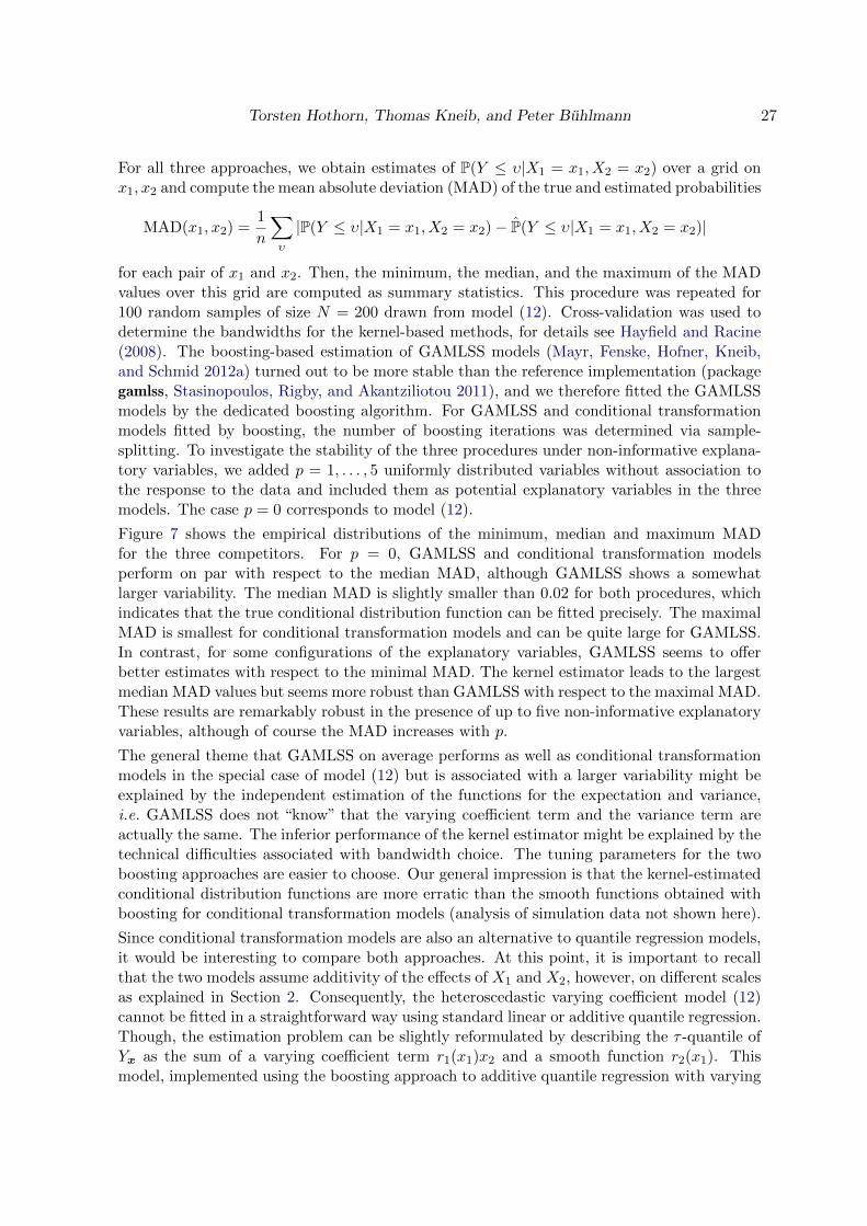
Torsten Hothorn, Thomas Kneib, and Peter Buhlmann 27
For all three approaches, we obtain estimates of P(Y ≤ υ|X1 = x1, X2 = x2) over a grid onx1, x2 and compute the mean absolute deviation (MAD) of the true and estimated probabilities
MAD(x1, x2) =1
n
∑υ
|P(Y ≤ υ|X1 = x1, X2 = x2)− P(Y ≤ υ|X1 = x1, X2 = x2)|
for each pair of x1 and x2. Then, the minimum, the median, and the maximum of the MADvalues over this grid are computed as summary statistics. This procedure was repeated for100 random samples of size N = 200 drawn from model (12). Cross-validation was used todetermine the bandwidths for the kernel-based methods, for details see Hayfield and Racine(2008). The boosting-based estimation of GAMLSS models (Mayr, Fenske, Hofner, Kneib,and Schmid 2012a) turned out to be more stable than the reference implementation (packagegamlss, Stasinopoulos, Rigby, and Akantziliotou 2011), and we therefore fitted the GAMLSSmodels by the dedicated boosting algorithm. For GAMLSS and conditional transformationmodels fitted by boosting, the number of boosting iterations was determined via sample-splitting. To investigate the stability of the three procedures under non-informative explana-tory variables, we added p = 1, . . . , 5 uniformly distributed variables without association tothe response to the data and included them as potential explanatory variables in the threemodels. The case p = 0 corresponds to model (12).
Figure 7 shows the empirical distributions of the minimum, median and maximum MADfor the three competitors. For p = 0, GAMLSS and conditional transformation modelsperform on par with respect to the median MAD, although GAMLSS shows a somewhatlarger variability. The median MAD is slightly smaller than 0.02 for both procedures, whichindicates that the true conditional distribution function can be fitted precisely. The maximalMAD is smallest for conditional transformation models and can be quite large for GAMLSS.In contrast, for some configurations of the explanatory variables, GAMLSS seems to offerbetter estimates with respect to the minimal MAD. The kernel estimator leads to the largestmedian MAD values but seems more robust than GAMLSS with respect to the maximal MAD.These results are remarkably robust in the presence of up to five non-informative explanatoryvariables, although of course the MAD increases with p.
The general theme that GAMLSS on average performs as well as conditional transformationmodels in the special case of model (12) but is associated with a larger variability might beexplained by the independent estimation of the functions for the expectation and variance,i.e. GAMLSS does not “know” that the varying coefficient term and the variance term areactually the same. The inferior performance of the kernel estimator might be explained by thetechnical difficulties associated with bandwidth choice. The tuning parameters for the twoboosting approaches are easier to choose. Our general impression is that the kernel-estimatedconditional distribution functions are more erratic than the smooth functions obtained withboosting for conditional transformation models (analysis of simulation data not shown here).
Since conditional transformation models are also an alternative to quantile regression models,it would be interesting to compare both approaches. At this point, it is important to recallthat the two models assume additivity of the effects of X1 and X2, however, on different scalesas explained in Section 2. Consequently, the heteroscedastic varying coefficient model (12)cannot be fitted in a straightforward way using standard linear or additive quantile regression.Though, the estimation problem can be slightly reformulated by describing the τ -quantile ofYx as the sum of a varying coefficient term r1(x1)x2 and a smooth function r2(x1). Thismodel, implemented using the boosting approach to additive quantile regression with varying

28 Conditional Transformation Models
MAD
0.000 0.015CTM
KernelGAMLSS
●●
●
●● ●● ●● ●● ●●
●● ●● ●● ● ●
p = 0
Min. M
AD
0.000 0.015CTM
KernelGAMLSS
●●
●
●
● ●●●
● ● ●●● ●
p = 1
Min. M
AD
0.000 0.015CTM
KernelGAMLSS
●●
●
●● ●● ●● ●● ●● ●●
●● ● ●● ●● ●●● ● ● ●
p = 2
Min. M
AD
0.000 0.015CTM
KernelGAMLSS
●●
●
● ●●
● ●
●● ●● ● ●● ●
p = 3
Min. M
AD
0.000 0.015CTM
KernelGAMLSS
●●
●
●● ●● ●●
● ●● ●●●●● ● ● ● ●●●
p = 4
Min. M
AD
0.000 0.015CTM
KernelGAMLSS
●●
●
● ● ● ●●●● ●●● ●
●●●● ●●●● ● ● ●
p = 5
Min. M
AD
0.010.030.05
●●
●
● ●●●
●●● ● ●●●● ●
p = 0
Med. M
AD
0.010.030.05●
●●
● ●
● ●●● ● ● ●
p = 1
Med. M
AD
0.010.030.05
●●
●
●● ●● ●●
●●●
p = 2
Med. M
AD
0.010.030.05
●●
●
●●
●●● ●● ●●
p = 3
Med. M
AD
0.010.030.05
●●
●
●● ●●
●
●
p = 4
Med. M
AD
0.010.030.05
●●
●
●●
●
p = 5
Med. M
AD
0.05 0.20●
●●
● ● ●●
●
p = 0
Max. M
AD
0.05 0.20
●●
●● ●●
●● ●
p = 1
Max. M
AD
0.05 0.20
●●
●●● ●
p = 2
Max. M
AD
0.05 0.20
●●
●●
● ●
p = 3
Max. M
AD
0.05 0.20
●●
●●
●
p = 4
Max. M
AD
0.05 0.20
●●
●●
● ●
p = 5
Max. M
AD
Figu
re7:
Em
pirical
Eva
luatio
n.
Min
imum
,m
edian
,an
dm
axim
um
ofth
em
eanab
solute
dev
iation(M
AD
)b
etween
true
and
estimated
prob
abilities
for
conditio
nal
tran
sform
ation
models
(CT
M),
non
-param
etrickern
eld
istribu
tionfu
nction
estimation
(Kern
el),an
dgen
eralisedad
ditiv
em
odels
for
locatio
n,
scale,an
dsh
ape
(GA
ML
SS)
for100
random
samples.
Valu
eson
the
ordin
atecan
be
interp
retedas
ab
solute
diff
erences
ofprob
abilities.
The
greyhorizon
tallin
escorresp
ond
toth
em
edian
ofC
TM
.

Torsten Hothorn, Thomas Kneib, and Peter Buhlmann 29
True quantile
Est
imat
ed q
uant
ile
−2
0
2
4
−2 0 2 4
0.5 quantileCTM
0.75 quantileCTM
−2 0 2 4
0.9 quantileCTM
0.5 quantileAQR
−2 0 2 4
0.75 quantileAQR
−2
0
2
4
0.9 quantileAQR
Figure 8: Comparison of conditional transformation models and additive quantile regression.Scatterplot of true versus estimated quantiles obtained from one conditional transformationmodel (CTM) and from three additive quantile regression (AQR) models fitted to 200 obser-vations drawn from the heteroscedastic varying coefficient model (12).
coefficients introduced by Fenske et al. (2011), allows the estimation of conditional τ -quantiles.We fitted three such quantile regression models (for τ = 0.5, 0.75, 0.9) to a sample of sizeN = 200 from model (12) and determined the optimal number of boosting iterations by theout-of-bootstrap empirical risk of the check function. To give an impression, we compare theseestimated τ -quantiles with the corresponding conditional quantiles obtained by inverting theestimated conditional distribution function from a conditional transformation model. Figure 8displays scatterplots of the true conditional quantiles over a grid of x1 and x2 values with thecorresponding estimated quantiles derived from one conditional transformation model andthe three additive quantile regression models for τ = 0.5, 0.75, 0.9, the latter models includingthe varying coefficient term. It seems that, in this example, both approaches recover the truequantiles equally good.
8. Discussion
In his book Quantile Regression, Koenker (2005) puts transformation models in the “twilight

30 Conditional Transformation Models
zone of quantile regression” and suggests that estimating conditional distribution functions bymeans of transformation models might be an alternative to the direct estimation of conditionalquantile functions. We undertook the “worthwhile exercise” (Koenker 2005, Section 8.1.1.)and developed a semiparametric framework for the estimation of conditional distributionfunctions by conditional transformation models that allows higher moments of the conditionaldistribution to depend on the explanatory variables.
Because the empirical risk function (4) is equivalent to well-established risk functions for bi-nary data, there are many potentially interesting algorithms that can be used to fit conditionaltransformation models, although dependent observations have to be dealt with. We chose acomponent-wise boosting approach mainly because of its divide-and-conquer strategy, whichallows a very efficient fitting of base-learners that depend on the response and on one or moreexplanatory variables at the same time via linear array models. In addition, the algorithmis general, and different base-learners appropriate for the model at hand can be easily imple-mented as illustrated in Section 6. Also very attractive are the model choice properties, asfor example illustrated by means of the Boston Housing data in Section 6. The theoreticaland empirical properties investigated in Sections 5 and 7 indicated that the method is ap-plicable to more high-dimensional situations as well. While boosting became popular owingto its success in fitting simple models under challenging circumstances – especially linear oradditive models for high-dimensional explanatory variables – the attractiveness of this class ofalgorithms for fitting challenging models in simple circumstances has been only rarely recog-nised. Exceptions are Ridgeway (2002) and Sexton and Laake (2012), who study boostingalgorithms for fitting density functions. Lu and Li (2008), Schmid and Hothorn (2008) andSchmid, Hothorn, Maloney, Weller, and Potapov (2011) proposed boosting algorithms fortransformation models that treat the transformation function hY as a nuisance parameter.In the same model framework, Tutz and Groll (2013) propose a likelihood-boosting approachfor fitting cumulative and sequential models for ordinal responses.
Boosting algorithms for estimating conditional quantiles by minimising the check functionhave been introduced by Kriegler and Berk (2010), Fenske et al. (2011), and Zheng (2012).The computation of prediction intervals based on pairs of such models is rather straightforward(Mayr, Hothorn, and Fenske 2012b). Our approach to the estimation of the conditionaldistribution function has the advantage that one model fits the whole distribution, whichcan then be used to derive arbitrary functionals from. The quantile score representation ofthe continuous ranked probability score (see Gneiting and Ranjan 2011) might be a basis todevelop a boosting technique similar to the one described in this paper for the estimation offull conditional quantile functions. The main difference between transformation and quantileregression models that we have to keep in mind is that additivity is assumed on two differentscales. From a practical point of view, diagnostic tools to assess on which of these scales it ismore appropriate to assume an additive model would be very important.
The applications presented in Section 6 showed that conditional transformation models aregeneric, and one can, by choosing appropriate base-learners, fit models that are specific to theproblem at hand. An empirical evaluation showed that the estimated conditional distribu-tion functions are on average as good as the estimates obtained from a parametric approach(GAMLSS) that relies on more assumptions. In comparison to non-parametric kernel dis-tribution estimators, conditional transformation models are more adaptable, for example tospatial or temporal data. The performance of the semiparametric models compared to that ofthe non-parametric competitor was considerably better at the small price of the assumption

Torsten Hothorn, Thomas Kneib, and Peter Buhlmann 31
of additivity of the transformation function.
It will be interesting to further study conditional transformation models with respect to thefollowing extensions. Instead of making assumptions about the quantile function Q represent-ing the error distribution, it would be possible to fit the corresponding distribution functionby techniques introduced for single index models (Tutz and Petry 2012). To reduce the com-plexity, one could restrict the partial transformation functions hj to linear functions, i.e. onlythe first two moments are allowed to be influenced by the explanatory variables. Furthermore,when the response Y = (Y1, Y2) is bivariate, the bivariate conditional distribution functionP(Y1 ≤ υ1, Y2 ≤ υ2|X = x) can be estimated by minimising the risk function∫ ∫
ρ{((y1 ≤ υ1 ∧ y2 ≤ υ2),x), h(υ1, υ2|x)} dµ(υ1) dµ(υ2) dPY,X(y1, y2,x)
in h. It might also be interesting to allow only certain moments to depend on certain ex-planatory variables. For example, a partially conditional transformation model of the form
h(υ|x) =
J1∑j=1
hj(υ|x) +J∑
j=J1+1
hj(1|x)
describes the conditional expectation∑J
j=J1+1 hj(1|x) of a transformation∑J1
j=1 hj(Yx|x).
Researchers pay most attention to the conditional distribution function in applications wherethe response is a survival time or has been censored owing to other reasons. In survival anal-ysis, it is common to deal with the conditional survivor function S(Yx|x) = 1− F (Yx|x) forsurvival time Y . In the seemingly simpler situation of an uncensored continuous response,many data analysts focus on the conditional mean and do not bother with the conditionaldistribution function at all. Most of the literature on transformation models therefore dealswith the censored case. The easiest way to deal with right-censoring is to minimise therisk function weighted by inverse probability of censoring weights, as in the generalised es-timating equations approach by Cheng et al. (1995), where parameters of a linear trans-formation model are estimated by the root of a V-statistic defined by all binary indicatorsI(Yi ≥ Yı), i, ı = 1, . . . , N . Accelerated failure time models fitted by boosting of an inverseprobability of censoring weighted risk function have been described by Hothorn, Buhlmann,Dudoit, Molinaro, and van der Laan (2006), and future research awaits the investigation ofthe performance of conditional transformation models under censoring.
Computational Details
Conditional transformation models were fitted using an implementation of component-wiseboosting in package mboost (version 2.1-2, Hothorn, Buhlmann, Kneib, Schmid, and Hofner2011). Package gamboostLSS (version 1.0-3, Hofner, Mayr, Fenske, and Schmid 2011b) wasused to fit GAMLSS models and kernel distribution estimation was performed using packagenp (version 0.40-13, Hayfield and Racine 2011). Linear quantile regression was computed usingpackage quantreg (version 4.79, Koenker 2011). All computations were performed using Rversion 2.13.2 (R Development Core Team 2011).
Throughout Section 6, we used the loss function defined by ρbin and modelled non-linearfunctions by cubic B-spline bases with 20 equi-distant knots. For further computational
32 Conditional Transformation Models
details we refer the reader to the R code that implements the analyses presented in Sections 6and 7, which is available in an experimental R package ctm at http://R-forge.R-project.org/projects/ctm. The results presented in this paper can be reproduced using this package,except for the birth weight data, which are not publically available.
Acknowledgements
We would like to thank Gareth O. Roberts, an anonymous associate editor and referee for theircareful review of an initial version of this paper. Andreas Mayr implemented the Normal()
family for gamboostLSS on our request, Achim Zeileis helped finding the right colors forFigure 2 and Ronald Schild provided us with the birth weight data. We are indepted to PaulEilers, Tilman Gneiting and Roger Koenker for their comments on a draft version and thankKaren A. Brune for improving the language. Financial support by Deutsche Forschungsge-meinschaft (grant HO 3242/4-1) is gratefully acknowledged.
References
Bollerslev T (1986). “Generalized Autoregressive Conditional Heteroskedasticity.” Journal ofEconometrics, 31(3), 307–327.
Buhlmann P (2006). “Boosting for High-dimensional Linear Models.” The Annals of Statistics,34(2), 559–583.
Buhlmann P, Hothorn T (2007). “Boosting Algorithms: Regularization, Prediction and ModelFitting.” Statistical Science, 22(4), 477–505. With discussion.
Buhlmann P, van de Geer S (2011). Statistics for High-Dimensional Data: Methods, Theoryand Applications. Springer Verlag, Berlin, Heidelberg, Germany.
Buhlmann P, Yu B (2003). “Boosting with the L2 Loss: Regression and Classification.”Journal of the American Statistical Association, 98, 324–339.
Carroll RJ, Ruppert D (1982). “Robust Estimation in Heterscedastic Linear Models.” TheAnnals of Statistics, 10(2), 429–441.
Chen K, Muller HG (2012). “Conditional Quantile Analysis When Covariates Are Functions,With Application to Growth Data.” Journal of the Royal Statistical Society: Series B(Statistical Methodology), 74(1), 67–89.
Chen K, Tong X (2010). “Varying Coefficient Transformation Models With Censored Data.”Biometrika, 97(4), 969–976.
Cheng G, Wang X (2011). “Semiparametric Additive Transformation Model Under CurrentStatus Data.” Electronic Journal of Statistics, 5, 1735–1764.
Cheng SC, Wei LJ, Ying Z (1995). “Analysis of Transformation Models With Censored Data.”Biometrika, 82(4), 835–845.

Torsten Hothorn, Thomas Kneib, and Peter Buhlmann 33
Currie ID, Durban M, Eilers PHC (2006). “Generalized Linear Array Models With Applica-tions to Multidimensional Smoothing.” Journal of the Royal Statistical Society: Series B(Statistical Methodology), 68(2), 259–280.
Dette H, Volgushev S (2008). “Non-crossing Non-parametric Estimates of Quantile Curves.”Journal of the Royal Statistical Society: Series B (Statistical Methodology), 70(3), 609–627.
Doksum KA, Gasko M (1990). “On a Correspondence Between Models in Binary RegressionAnalysis and in Survival Analysis.” International Statistical Review, 58(3), 243–252.
Eilers PHC (2005). “Unimodal Smoothing.” Journal of Chemometrics, 19(5-7), 317–328.
Fahrmeir L, Kneib T, Lang S (2004). “Penalized Structured Additive Regression for Space-Time Data: A Bayesian Perspective.” Statistica Sinica, 14(3), 731–761.
Fenske N, Kneib T, Hothorn T (2011). “Identifying Risk Factors for Severe Childhood Mal-nutrition by Boosting Additive Quantile Regression.” Journal of the American StatisticalAssociation, 106(494), 494–510.
Fredriks AM, van Buuren S, Burgmeijer RJF, Meulmeester JF, Beuker RJ, Brugman E, RoedeMJ, Verloove-Vanhorick SP, Wit J (2000). “Continuing Positive Secular Growth Change inThe Netherlands 1955–1997.” Pediatric Research, 47(3), 316–323.
Friedman HH, Friedman LW, Amoo T (2002). “Using Humor in the Introductory Statis-tics Course.” Journal of Statistics Education, 10(3). URL http://www.amstat.org/
publications/jse/v10n3/friedman.html.
Gilchrist W (2008). “Regression Revisited.” International Statistical Review, 76(3), 401–418.
Gilley OW, Pace RK (1996). “On the Harrison and Rubinfeld Data.” Journal of EnvironmentalEconomics and Management, 31, 403–405.
Gneiting T, Raftery AE (2007). “Strictly Proper Scoring Rules, Prediction, and Estimation.”Journal of the American Statistical Association, 102(477), 359–378.
Gneiting T, Raftery AE, Westveld III AH, Goldman T (2005). “Calibrated ProbabilisticForecasting Using Ensemble Model Output Statistics and Minimum CRPS Estimation.”Monthly Weather Review, 133(5), 1098–1118.
Gneiting T, Ranjan R (2011). “Comparing Density Forecasts Using Threshold- and Quantile-Weighted Scoring Rules.” Journal of Business & Economic Statistics, 29(3), 411–422.
Hall P, Muller HG (2003). “Order-preserving Nonparametric Regression, With Applicationsto Conditional Distribution and Quantile Function Estimation.” Journal of the AmericanStatistical Association, 98(463), 598–608.
Hall P, Wolff RCL, Yao Q (1999). “Methods for Estimating a Conditional Distribution Func-tion.” Journal of the American Statistical Association, 94(445), 154–163.
Harrison D, Rubinfeld DL (1978). “Hedonic Prices and the Demand for Clean Air.” Journalof Environmental Economics and Management, 5, 81–102.
34 Conditional Transformation Models
Hayfield T, Racine JS (2008). “Nonparametric Econometrics: The np Package.” Journal ofStatistical Software, 27(5), 1–32. URL http://www.jstatsoft.org/v27/i05.
Hayfield T, Racine JS (2011). np: Nonparametric Kernel Smoothing Methods for Mixed DataTypes. R package version 0.40-12, URL http://CRAN.R-project.org/package=np.
He X (1997). “Quantile Curves Without Crossing.” The American Statistician, 51(2), 186–192.
Herberich E, Sikorski J, Hothorn T (2010). “A Robust Procedure for Comparing MultipleMeans Under Heteroscedasticity in Unbalanced Designs.” PLoS ONE, 5(4), e9788.
Hofner B, Hothorn T, Kneib T, Schmid M (2011a). “A Framework for Unbiased ModelSelection Based on Boosting.” Journal of Computational and Graphical Statistics, 20(4),956–971.
Hofner B, Mayr A, Fenske N, Schmid M (2011b). gamboostLSS: Boosting Methods forGAMLSS Models. R package version 1.0-3/r39, URL http://R-Forge.R-project.org/
projects/gamboostlss/.
Hofner B, Muller J, Hothorn T (2011c). “Monotonicity-Constrained Species DistributionModels.” Ecology, 92(10), 1895–1901.
Hothorn T, Brandl R, Muller J (2012). “Large-scale Model-based Assessment of Deer-vehicleCollision Risk.” PLoS ONE, 7(2), e29510.
Hothorn T, Buhlmann P, Dudoit S, Molinaro A, van der Laan MJ (2006). “Survival Ensem-bles.” Biostatistics, 7(3), 355–373.
Hothorn T, Buhlmann P, Kneib T, Schmid M, Hofner B (2011). mboost: Model-BasedBoosting. R package version 2.1-1, URL http://CRAN.R-project.org/package=mboost.
Hothorn T, Kneib T, Buhlmann P (2013). “Conditional Transformation Models.” Journal ofthe Royal Statistical Society: Series B (Statistical Methodology). Accepted 2012-11-27.
Kneib T, Hothorn T, Tutz G (2009). “Variable Selection and Model Choice in GeoadditiveRegression Models.” Biometrics, 65(2), 626–634.
Koenker R (2005). Quantile Regression. Economic Society Monographs. Cambridge UniversityPress, New York.
Koenker R (2011). quantreg: Quantile Regression. R package version 4.76, URL http:
//CRAN.R-project.org/package=quantreg.
Koenker R, Bassett G (1978). “Regression Quantiles.” Econometrica, 46(1), 33–50.
Koenker R, Ng P, Portnoy S (1994). “Quantile Smoothing Splines.” Biometrika, 81(4), 673–680.
Kriegler B, Berk R (2010). “Small Area Estimation of the Homeless in Los Angeles: An Ap-plication of Cost-sensitive Stochastic Gradient Boosting.” The Annals of Applied Statistics,4(3), 1234–1255.

Torsten Hothorn, Thomas Kneib, and Peter Buhlmann 35
Li Q, Racine JS (2008). “Nonparametric Estimation of Conditional CDF and Quantile Func-tions With Mixed Categorical and Continuous Data.” Journal of Business and EconomicStatistics, 26(4), 423–434.
Lu W, Li L (2008). “Boosting Method for Nonlinear Transformation Models With CensoredSurvival Data.” Biostatistics, 9(4), 658–667.
Lu W, Zhang HH (2010). “On Estimation of Partially Linear Transformation Models.” Journalof the American Statistical Association, 105(490), 683–691.
Mayr A, Fenske N, Hofner B, Kneib T, Schmid M (2012a). “GAMLSS for High-dimensionalData–A Flexible Approach Based on Boosting.” Journal of the Royal Statistical Society:Series C (Applied Statistics), 61(3), 403–427.
Mayr A, Hothorn T, Fenske N (2012b). “Prediction Intervals for Future BMI Values ofIndividual Children–A Non-parametric Approach by Quantile Boosting.” BMC MedicalResearch Methodology, 12, 6.
Meinshausen N, Buhlmann P (2010). “Stability Selection.” Journal of the Royal StatisticalSociety: Series B (Statistical Methodology), 72(4), 417–473.
NFHS (2000). “National Family Health Survey (NFHS-2), 1998–1999: India.” InternationalInstitute for Population Sciences (IIPS) and ORC Macro. URL http://www.measuredhs.
com/pubs.
R Development Core Team (2011). R: A Language and Environment for Statistical Comput-ing. R Foundation for Statistical Computing, Vienna, Austria. ISBN 3-900051-07-0, URLhttp://www.R-project.org/.
Ridgeway G (2002). “Looking for Lumps: Boosting and Bagging for Density Estimation.”Computational Statistics & Data Analysis, 38(4), 379–392.
Rigby RA, Stasinopoulos DM (2005). “Generalized Additive Models for Location, Scale andShape.” Journal of the Royal Statistical Society: Series C (Applied Statistics), 54(3), 507–554.
Schemper M, Henderson R (2000). “Predictive Accuracy and Explained Variation in CoxRegression.” Biometrics, 56(1), 249–255.
Schild RL, Maringa M, Siemer J, Meurer B, Hart N, Goecke TW, Schmid M, Hothorn T,Hansmann ME (2008). “Weight Estimation By Three-dimensional Ultrasound Imaging inthe Small Fetus.” Ultrasound in Obstetrics and Gynecology, 32(2), 168–175.
Schmid M, Hothorn T (2008). “Flexible Boosting of Accelerated Failure Time Models.” BMCBioinformatics, 9, 269.
Schmid M, Hothorn T, Maloney KO, Weller DE, Potapov S (2011). “Geoadditive RegressionModeling of Stream Biological Condition.” Environmental and Ecological Statistics, 18(4),709–733.
Schnabel SK, Eilers PHC (2012). “Simultaneous Estimation of Quantile Curves Using Quan-tile Sheets.” AStA Advances in Statistical Analysis. doi:10.1007/s10182-012-0198-1.Accepted 2012-06-21.

36 Conditional Transformation Models
Sexton J, Laake P (2012). “Boosted Coefficient Models.” Statistics and Computing, 22(4),867–876.
Shen X (1998). “Proportional Odds Regression and Sieve Maximum Likelihood Estimation.”Biometrika, 85(1), 165–177.
Sikorski J, Brambilla E, Kroppenstedt RM, Tindall BJ (2008a). “The Temperature AdaptiveFatty Acid Content in Bacillus simplex Strains from “Evolution Canyon”, Israel.” Microbi-ology, 154(8), 2416–2426.
Sikorski J, Nevo E (2005). “Adaptation and Incipient Sympatric Speciation of Bacillus simplexunder Microclimatic Contrast at “Evolution Canyons” I and II, Israel.” Proceedings of theNational Academy of Sciences, U.S.A., 102(44), 15924–15929.
Sikorski J, Pukall R, Stackebrandt E (2008b). “Carbon Source Utilization Patterns of Bacillussimplex Ecotypes Do Not Reflect Their Adaptation to Ecologically Divergent Slopes in“Evolution Canyon”, Israel.” FEMS Microbiology Ecolocy, 66(1), 38–44.
Stasinopoulos DM, Rigby RA (2007). “Generalized Additive Models for Location Scale andShape (GAMLSS) in R.” Journal of Statistical Software, 23(7), 1–46. URL http://www.
jstatsoft.org/v23/i07.
Stasinopoulos M, Rigby B, Akantziliotou C (2011). gamlss: Generalized Additive Models forLocation Scale and Shape. R package version 4.1-1, URL http://CRAN.R-project.org/
package=gamlss.
Stigler SM (2010). “The Changing History of Robustness.” The American Statistician, 64(4),277–281.
Tutz G, Groll A (2013). “Likelihood-based Boosting in Binary and OrdinalRandom Effects Models.” Journal of Computational and Graphical Statistics.doi:10.1080/10618600.2012.694769. In press.
Tutz G, Petry S (2012). “Nonparametric Estimation of the Link Function Including VariableSelection.” Statistics and Computing, 22(2), 545–561.
van de Geer S (2000). Empirical Processes in M-Estimation. Cambridge University Press,Cambridge, UK.
Wu C, Tian X, Yu J (2010). “Nonparametric Estimation for Time-varying TransformationModels With Longitudinal Data.” Journal of Nonparametric Statistics, 22(2), 133–147.
Zeng D, Lin DY, Yin G (2005). “Maximum Likelihood Estimation for the Proportional OddsModel With Random Effects.” Journal of the American Statistical Association, 100(470),470–483.
Zheng S (2012). “QBoost: Predicting Quantiles with Boosting for Regression and BinaryClassification.” Expert Systems with Applications, 39(2), 1687–1697.
Torsten Hothorn, Thomas Kneib, and Peter Buhlmann 37
Appendix
Proofs
Proof. Proof of Lemma 1
Convexity: If the loss function ρ is convex in its second argument, so is the loss function `
`((Y,X), αh+ (1− α)g) ≤ α`((Y,X), h) + (1− α)`((Y,X), g),
with g(·|x) : R → R being a monotone increasing transformation function and α ∈ [0, 1],because of the convexity of ρ and the monotonicity and linearity of the Lebesgue integral.
Population Minimisers: Let f denote the density of F . With iterated expectation we have
EY,X`((Y,X), h) =
∫ ∫ ∫ρ((y ≤ υ,x), h(υ|x)) dµ(υ) dPY |X=x(y) dPX(x)
=
∫ ∫ ∫ρ((y ≤ υ,x), h(υ|x)) dPY |X=x(y)︸ ︷︷ ︸
=:Aυ,x(h(υ|x))
dµ(υ) dPX(x)
and the risk is minimal when Aυ,x(h(υ|x)) is minimal for the scalar h(υ|x) for all υ and x,i.e. when
0!
=∂Aυ,x(h(υ|x))
∂h(υ|x)
=
∫∂
∂h(υ|x)ρ((y ≤ υ,x), h(υ|x)) dPY |X=x(y)
ρ=ρsqe=
∫(I(y ≤ υ)− F (h(υ|x))f(h(υ|x)) dPY |X=x(y)
= f(h(υ|x))
{∫I(y ≤ υ) dPY |X=x(y)− F (h(υ|x))
}= f(h(υ|x)) {P(Y ≤ υ|X = x)− F (h(υ|x))}
which for f(h(υ|x)) > 0 is zero for h(υ|x) = F−1(P(Y ≤ υ|X = x)). Similar, for ρ = ρbinthe term
0!
=∂Aυ,x(h(υ|x))
∂h(υ|x)
=
∫−{I(y ≤ υ)
F (h(υ|x))f(h(υ|x))− 1− I(y ≤ υ)
1− F (h(υ|x))f(h(υ|x))
}dPY |X=x(y)
= f(h(υ|x))
{∫1− I(y ≤ υ) dPY |X=x(y)
1− F (h(υ|x))−∫I(y ≤ υ) dPY |X=x(y)
F (h(υ|x))
}= f(h(υ|x))
{1− P(Y ≤ υ|X = x)
1− F (h(υ|x))− P(Y ≤ υ|X = x)
F (h(υ|x))
}is zero for h(υ|x) = F−1(P(Y ≤ υ|X = x)) when f(h(υ|x)) > 0.
For the absolute error, note that
ρabe((Y ≤ υ,X), h(υ|X)) = I(Y ≤ υ){1− F (h(υ|X))}+ {1− I(Y ≤ υ)}F (h(υ|X))
38 Conditional Transformation Models
and thus
Aυ,x(h(υ|x)) =
∫ρabe((y ≤ υ,x), h(υ|x)) dPY |X=x(y)
=
∫I(Y ≤ υ){1− F (h(υ|X))}+ {1− I(Y ≤ υ)}F (h(υ|X)) dPY |X=x(y)
= {1− F (h(υ|X))}P(Y ≤ υ|X = x) + F (h(υ|X)){1− P(Y ≤ υ|X = x)}
This expression attains its minimal value of P(Y ≤ υ|X = x) for P(Y ≤ υ|X = x) ≤ 0.5when F (h(υ|X)) = 0. For P(Y ≤ υ|X = x) > 0.5, the minimum 1 − P(Y ≤ υ|X = x) isattained when F (h(υ|X)) = 1. Thus, absolute error will lead to too extreme estimated valuesof h and corresponding conditional distribution functions.
Proof. Proof of Theorem 1
We use a modified argument of a proof presented in Section 12.8.2. in Buhlmann and van deGeer (2011). Formally, we can write
I(Yi ≤ υı) = hγ0,N(υı|Xi) + εiı,
εiı = I(Yi ≤ υı)− hγ0,N(υı|Xi) (i = 1, . . . , N, ı = 1, . . . , n).
The errors εiı have reasonable properties, as discussed in (13) below.
There are two issues that need to be addressed. First, we define the inner products of functionsh and g
(h, g)n,N,E = n−1n∑ı=1
E[h(υı|X)g(υı|X)]
and
(h, g)n,N = n−1N−1N∑i=1
n∑ı=1
h(υı|Xi)g(υı|Xi).
The proof in Buhlmann and van de Geer (2011) can then be used with the scalar product(h, g)n,N .
Secondly, for controlling the probabilistic part of the proof, we need to show that the analogueof formula (12.26) in Buhlmann and van de Geer (2011) holds. This translates to deriving abound for
maxj,k0,k1
(b0,k0bj,k1 , ε)n,N = maxj,k0,k1
(nN)−1N∑i=1
n∑ı=1
b0,k0(υı)bj,k1(Xj)εiı.
Because hγ0,Nis the projection of I(Y ≤ υı) (ı = 1, . . . , n) onto the basis functions
b0,k0(υı)bj,k1(Xj)ı = 1, . . . , n) with respect to the ‖ · ‖n,N,E-norm (see (7)), and owing to thedefinition of εiı, we have
n−1n∑ı=1
E[εiıb0,k0(υı)bj,k1(Xj)] = 0 ∀j, k0, k1. (13)
Therefore,
(nN)−1N∑i=1
n∑ı=1
b0,k0(υı)bj,k1(Xj)εiı = N−1N∑i=1
Zi(j, k0, k1),
E[Zi(j, k0, k1)] = 0.

Torsten Hothorn, Thomas Kneib, and Peter Buhlmann 39
Furthermore, owing to the boundedness assumption in (A1), ‖Zi(j, k0, k1)‖∞ ≤ C1 for someconstant C1 < ∞ ∀i, j, k0, k1. Applying Hoeffding’s inequality, for independent (but notnecessarily identically distributed) random variables (van de Geer 2000, Lem. 3.5) and usingthe union bound, we obtain
maxj,k0,k1
(b0,k0bj,k1 , ε)n,N = OP
(√log(JNK0,NK1,N )/N
).
This, together with the proof from Section 12.8.2 in Buhlmann and van de Geer (2011)completes the proof of Theorem 1.
Gradients
Gradients for different loss functions ρ and arbitrary absolute continuous distribution func-tions F with density function f :
Uiıρ=ρbin=
I(Yi ≤ υı)
F(h[m]iı
) − 1− I(Yi ≤ υı)
1 + F(h[m]iı
) f
(h[m]iı
)Uiı
ρ=ρsqe=
{I(Yi ≤ υı)− F
(h[m]iı
)}f(h[m]iı
)Uiı
ρ=ρabe= {I(Yi ≤ υı)− (1− I(Yi ≤ υı))} f(h[m]iı
)
Affiliation:
Torsten HothornInstitut fur Statistik ISPM, Abteilung BiostatistikLudwig-Maximilians-Universitat Munchen Universitat ZurichLudwigstraße 33 Hirschengraben 84DE-80539 Munchen, Germany CH-8001 Zurich, SwitzerlandE-mail: [email protected]: http://www.stat.uni-muenchen.de/~hothorn/
Thomas KneibWirtschaftswissenschaftliche FakultatGeorg-August-Universitat GottingenPlatz der Gottinger Sieben 5DE-37073 Gottingen, Germany
Peter BuhlmannSeminar fur StatistikETH ZurichCH-8092 Zurich, Switzerland