Journal of Mathematical Sciences, VoI. 98, No. 1, 2000

CONDITIONALLY DEFINITE MATRICES Kh. D. Ikramov and N. V. SaveFeva UDC 512.643.8

1. Introduct ion

It is well known how important positivity is in various branches of mathematics . For objects that are positive, one can usually obtain much more complete results than in the general case. For example, in linear algebra, positive and positive-definite matrices are among the most thoroughly studied matrix classes. It is equally important that the results of this study have been well docmnented: one can learn the properties of the matr ix classes above from dozens of textbooks and monographs on matr ix theory.

Things are quite different when from the global property of (positive or negative) definiteness one turns to

the same property that holds only conditionally, i.e., as long as the argument does not leave a given subspace, orthant, polyhedron, or cone. We combine all these options under the term "conditionally definite" matrices. Matrices of this kind are understood to a lesser extent than the classical positive-definite matrices. Moreover, to the best of our knowledge, no book exposition yet exists of the problem of conditional definiteness. At most, there are some survey papers devoted to the particular types of conditional-definite matrices.

This fact, i.e., that a readily accessible exposition of the field is not available, and the importance of conditional definiteness in a number of applications served as a stimulus for writing this survey. The selection of material for the paper was to a considerable extent guided by what explains our interest in this subject, namely, our wish to develop a collection of computer procedures for checking whether a given matrix possesses a particular type of conditional definiteness. Typically, the matrix has scalar entries, which are then assmned to be integers or rational nmnbers. It is also admissible, however, that some or even all entries of the matrix contain parameters. In this case, the dependence on parameters must also be expressed by rational functions. Under these assumptions, the procedures must give exact answers, not answers that hold up to "round-off error analysis," which are typical of floating-point computations. This predetermines that the procedures to be included in the collection must be finite rational algorithms and their computer impleinentation must be based on a kind of error-free computation. For matrices with parameters, symbolic computation is used rather than an error-fi'ee one.

Let us clarify what was said above by using the ordinary positive definiteness as an example. According to one of the many equivalent definitions of this property, a Hernfitian matr ix A is positive definite if and only if all its eigenvalues are positive. This s tatement seems to give a constructive criterion for positive definiteness if one takes into account that well-polished routines are available for computing the eigenvalues of a matrix. These routines are especially efficient and accurate in the case where the matrices are Hermitian. The absolute errors of approximate eigenvalues tha t are computed by such a routine can be bounded a priori. Hence, when the routine stops, one has a set of "uncertainty intervals" that enclose the spectrum of the matr ix under investigation. If none of the intervals contains zero, then authent ic inferences are possible concerning the inertia of the matrix. In particular, one can give a certain answer whether the matr ix is positive definite. However, if zero belongs to the left-most interval, a precise inference about the definiteness becomes impossible. The transition fl'om the real (or complex) arithmetic to error-free computations does not

help here. Indeed, even for an integer matrix, the eigenvalues cannot, in general, be found by a finite (much

less by a rational) procedure. Fortunately, there exist criteria for positive definiteness, say, the classical deterininantal Sylvester crite-

rion, that can be implemented by means of error-free or symbolic coinputations. It turns out that criteria of this kind also exist for conditional definiteness. Our main aim in this survey is to describe them.

Translated from Itogi Nauki i Tekhniki, Seriya Sovremennaya Matematika i Ee Prilozheniya, Tematicheskie Obzory. Vol. 52, Algebra-9, 1998.

1072-3374/00/9801-0001 $25.00 �9 2000 Kluwer Academic/Plenum Publishers 1

The paper is organized as follows. In Sec. 2, we recall the basic criteria for global definiteness. Some facts from linear algebra are also given, which we shall need in the sequel. Matrices that are definite with respect to a linear subspace are treated in Sec. 3. Copositive matrices are considered in Sec. 4, and/C-copositive ones in Sec. 5. Our concluding remarks are given in Sec. 6.

Along with the strong definiteness, we discuss the same property in a weak form (in the classical case, these

two species are illustrated by the notions of positive definiteness and positive semidefiniteness, respectively). Most often, one encounters various kinds of conditional definiteness in mathematical programming where

all data typically are real numbers. For this reason, our discussion is limited to real matrices. As was already mentioned, our computer procedures even presuppose that the entries of matrices are integers or rational nmnbers. At the same time, the procedures can be easily generalized to the case of complex matrices with Gaussian entries.

2. P r e l i m i n a r i e s

In this survey, the symbols M,~ and 3:,~ stand for tim linear space of real n • n matrices and its subspace consisting of symmetric matrices, respectively.

Def ini t ion. A matrix A r S,~ is called positive semidefinite if (Ax, x) >_ 0 for any vector x r R '~. If (Ax, x) > 0 for any nonzero x, then A is a positive-definite matrix.

We denote by A ( i l , . . . , i~) the principal submatrix of A lying in rows and colmnns with indices ix , . . . , ik.

T h e o r e m 2.1 (the Sylvester criterion), A matrix A E S~ is positive definite if and only if all its leading principal minors are positive, i.e.,

d e t A ( 1 , . . . , k ) > 0, h = 1 , . . . , n . (2.1)

Tile property of positive definiteness is invariant under symmetric permutations of rows and columns of a matrix. Therefore, a more general formulation can be given for the Sylvester criterion I6, Theorem 7.2.5].

T h e o r e m 2.2. All principal minors of a positive-definite matrix are positive. A matrix A E Sn is positive definite if there exists a nested sequence of n principal minors of A (not just the leading principal minors) that are positive.

Tile nonnegativity of all principal minors is a necessary and sufficient condition for A to be positive semidefinite, which is implied by the following assertion.

T h e o r e m 2.3. A matrix A E Sn is positive semidefinite if and only if the matrix A + tin is positive definite for any c > O.

Here, one cannot check the signs of only leading principal minors, as was the case with the Sylvester criterion. For example [6, p. 404], both leading principal minors of the matrix

B = 0 - 1

are zero, i.e., nonnegative. However, the matrix B is not positive senfidefinite; rather it is negative semidefinite. The matrix

( 0 0 0 ) 0 0 1 , 0 1 0

for which all the leading principal minors are again zero, is indefinite.

2

We denote the number of positive eigenvalues and that of negative eigenvalues of the symmetric matr ix A by 7r(A) and u(A), respectively, and call them the positive inertia and the negative inertia of this matrix.

The symbol 6(A) s tands for the defect, or rank deficiency, of A (which is defined as the difference n - rankA) . The ordered triple

I n A = (r (2.3)

is called the inertia of A. The Sylvester criterion is known to be just a particular case of the following signature rule, which is due

to Jacobi. Let Ao = 1,

A ~ : d e t A ( 1 , . . . , k ) , k = l , . . . , n . (2.4)

T h e o r e m 2.4. Assume that all the leading principal minors of a matrix A E S,~ are nonzero. Then the positive inertia of A is equal to the number of sign coincidences in the sequence

A0, A1, . . . , An (2.5)

and the negative inertia to the number of sign variations in this sequence.

Below, we prove the Jacobi rule. This gives us a good reason to remind the reader of an important ex- t remal characterization of the eigenvalues of a symmetric matrix, which is called the Courant Fisher theorem.

T h e o r e m 2.5. Let A1 > A2 >_ . . . > A~ be eigenvalues of a matrix A E S~. Then

A k = max rain (Ax, x) (x ,x ) ' (2.6)

x r Lk x E L~

5~ = rain max (Ax, z) (x, x) " (2.7)

:r r 0 Ln-k+l x E Ln-k+l

In formula (2.6), the max imum is taken over all k-dimensional subspaces L~ of the space R '~. Similarly, in

(2.7), L~-k+l is an arbitrary subspace of dimension n - k + 1.

Theorem 2.5 implies the so-called interlacing inequalities

(2.8)

between the eigenvalues of the symmetric matr ix A and the eigenvalues #1 _> #2 _> "'" _> #~- i of its (arbitrary)

principal ( n - 1) • ( n - 1) sublnatrix. We prove the Jacobi signature rule by induction on the order n of A. For n = 1, the assertion is trivial.

Suppose it holds for all k < n (n > 1). The truncated sequence

Ao, A t , . . . , A,_j_ (2.9)

can be regmded as the Jacobi sequence for tile leading principal ( n - 1 ) • ( n - 1 ) submatr ix An-1. Suppose tha t

there are m coincidences and 1 variations in sign in sequence (2.9), m + l = n - 1. If #1 _> p2 _> "'" >_ #,.-1 are eigenvalues of the submat r ix A~_I, then, by the inductive assumption, m largest numbers out of the imlnbers pj must be positive, and l smallest nulnbers r~mst be negative. The interlacing inequalities (2.8) imply tha t A has at least m positive eigenvalues and l negative ones. Only the sign of the eigenvalue .~,~+~ has not yet been determined. Dividing the relation

Av. = A I - . . A mArn+l Arnq-2" "" An

by

A,~-I = #1 �9 �9 "#~n #m+l " �9 " #~-l ,

we conclude that the sign of A,~+~ coincides with that of the ratio A~/An_~. This proves tha t the Jacobi rule

is valid for the matr ix A. As an illustration, we find the inertia of a quasidefinite matr ix [39]. This is the term for a symmetric

partitioned matr ix

( A , ~ A 1 2 ) (2.10) A = A T A22 '

where the square n~ x nl submatrix A u is positive definite, and the n2 • n2 subinatrix A22, n2 = n - hi, is negative definite.

Since matr ix (2.10) contains the positive-definite submatrix AI~, it must have at least nl positive eigen-

values. Similarly, the presence of the negative-definite submatrix A22 implies that at least n2 eigenvalues of A must be negative. Since ni + n2 -- n, the matr ix A is nonsingular, and its inertia is

In A = (hi, n2, 0).

The Jacobi rule and its modifications are very helpful in various root separation problems, i.e., in the class of problems that deal with the location of roots of a (real) polynomial with respect to a given subset of

the complex plane. We give two examples of these applications. Assume tha t the real polynomial

f ( x ) = ao zn + a l z ~ - i + . . . + a.. (2.11)

has no multiple roots (this can be easily achieved if one divides f (x ) by tile greatest common divisor of f ( z )

and its derivative i f (z)) . We denote by a l , . . . , a~ the roots of f ( z ) . The sums

k = 0, 1, 2, Sk = O~kl 4:- . . . + Ozn~ . . . ,

are known as the Newton sums of the polynomial f ( z ) . Being symmetric functions of the roots c q , . . . , a~,

the Newton sums can be rationally expressed in terms of the coefficients a0, a~ , . . . , a~ of f ( x ) .

T h e o r e m 2.6 (the Borchardt-Jaeobi theorem). Th, e quadratic form

n--[

J = E Sl+rn Xl Z m l, r~z=O

is nondegenerate. I f 7c and lJ are the positive and the negative inertia, respectively, of the f o rm J, then the polynomial f ( x ) has ~ pairs of complez-conjugate roots and 7c - ~ real roots.

Our second example is the Routh-Hurwitz-Fuj iwara criterion. We set

=

for polynomial (2.11) and fornl the Bezout matr ix of the polynonfials f and g. Recall that the Bezout matrix

B(.f, g) is tile matr ix associated with tile quadratic form

B(w, z) = f ( w ) g ( z ) - f ( z )g(w) W - - Z

n

= Z bkt w k - i z l -1 . k,/=l

Finally, we transform the matrix B ( f , 9) = (b~j) into a new inatrix F according to the rule

fij = (-1)i+1 bij, i , j = 1 , . . . , n .

4

T h e o r e m 2.7 (Routh-Hurwi tz-Fnj iwara criterion), f f the matrix F is nonsingular, then its positive (negative)

inertia gives the number of roots of the polynomial f (x ) that have negative (positive) real parts.

The application of the Jacobi rule in the si tuations defined by Theorems 2.6 and 2.7 presupposes tha t all the leading principal minors of the corresponding matr ices are nonzero. If this assumption is not valid, it may still be possible to determine the inertia using the extensions of the Jacobi rule by Gundeffinger and Frobenius (see [4, Sec. 8]).

T h e o r e m 2.8. Assume that in sequence (2.4), the determinant A,~ # O, but a minor A~, k < n, may be

zero. In each such occasion (i.e., when A~ = 0), assume that A~_IA~+I # 0. Assign arbit'rnry signs to the

zero minors Ak. Then the Jacobi rule holds for the modified sequence (2.4).

T h e o r e m 2.9. Assume that in sequence (2.4), the determinant A~ ~ O, but it may be possible that Ak =

A~+I = 0 when k < n - 1 . In each such occasion, assume that Ak-IA~+2 # 0. Assign the same (arbitrary) sign

to Ak and A~+ 1 if A~_IA~+2 < 0 and different signs (in any one of the two possible ways) if Ak-IA~+2 > 0. Then the Jacobi rule holds for the modified sequence (2.4).

We reproduce an example from [4], which shows tha t the fllrther extension of the Jacobi signature rule

for the case where (2.4) contains subsequences of three or more successive zeros is impossible if one speaks about, general symmetric matrices. Assume that the coefficients a, ~, and 7 in the matr ix

0 0 0 a 0 00

A - 0 0 7 0 ~ 0 0 0

are nonzero. Then sequence (2.4) for this matr ix is

1, O, O, O , - a 2 3 7 .

) The sign of the determinant A4 is determined by tha t of the product .3 7. It is not difficult to see tha t the inertia of the matr ix A is (3, 1, 0) if/3 > 0, 7 > 0, and (1, 3, 0) if/3 < 0, 7 < 0, a l though in both cases A4 is negative.

We re turn to the discussion of the criteria for definiteness.

T h e o r e m 2.10. A matrix A E S,, is positive semidefinite 4[ and only if

A = S S T (2.12)

.for an n x m matrix S (m may be arbitrary), fl matri.~: A is positive definite if and only if the rank of the matrix S in (2.12) is equal to n.

A positive (semi)definite mat r ix A can be represented in the form (2.12) in many different ways. The most useful ones are the following.

(1) S = S T. In this case, (2.12) turns into

S 2 = A

and the matr ix S is a square root of A. There exists a mfique positive (semi)definite square root of A. It is

denoted by AV2. (2) S is a lower triangular matr ix with positive diagonal entries. Usually, this matr ix is denoted by L

and called the Cholesky factor of the matr ix A. The corresponding decomposi t ion of A is the product

A = L L T (2.13)

of the two tr iangular matrices, the lower matr ix L and the upper one L T. It is called the Cholesky decompo- sition of A.

Using relation (2.13) for the entries in position (1,1) yields

I . =

Thus, the calculation of the Cholesky factor requires square roots, i.e., the type of operation that we would like to avoid. Meanwhile, there exists another decomposition of a positive-definite matrix that is similar to the Cholesky decomposition but that can be found by employing only arithmetical operations. It is called

the L D L v decomposition:

A = L D L T. (2.14)

As opposed to the Cholesky factor, the matrix L in (2.14) has the unit main diagonal. The matrix D is diagonal:

D = diag (dn, �9 �9 �9 dn~).

It is not difficult to see that d t l = all = /kl,

dk~ = , k = 2, 3 , . . . , n .

As above, A~ is the leading principal k x k minor of the matrix A.

Note that the LDL T decomposition exists (and is unique) not only for positive-definite matrices but also for any symmetric matrix A in which all the leading principal minors are nonzero. Moreover, the last of these minors, i.e., det A, may be zero. If A is not positive semidefinite, then D contains diagonal entries of different signs.

The matrix transformation of the form

A -+ B = P A P T, (2.16)

where P is a nonsingular matrix, is called a congruence , and the matrices A and B in (2.16) are referred to as congrv, ent matrices. These matrices can be considered to be associated with the same quadratic form but in different bases of the space R '~. As a consequence, congruent matrices have the same inertia. In particular,

the diagonal matrix D in the L D L T decomposition of A indicates the inertia of the latter matrix. Assume that the nl x nl submatrix All in the partitioned matrix (2.10) is nonsingular. Applying to A

congruence (2.16) with the matrix

( I ~ 0 ) (2.17) P = --ATe A~-~ I,~ 2

yields the block-diagonal inatrix

The submatrix

B = ( All0 B2')0 ) . (2.18)

B22 = A22 - AT AS! A12

is usually denoted by A/Axl and is called tile Schur complement of the submatrix All in A. One important implication of formula (2.18) is the equality

InA = InAl l + In (A/An).

The inertias here are added entrywise. Suppose that the inverse matrix C = A -z is partitioned sinfilar to (2.10):

( Cu C12 ) C = Czl C22 "

Then

(2.19)

C22 = (A/Al i ) -~.

Hence, the submatrix C22 in the inverse matrix C has the same inertia as the Schur complement A/Al l in the original matrix A.

3. Pos i t ive Def in i teness on a Subspace

Suppose that we consider a subspace 12 C R ~ described by the system of linear equations

B x = O.

Here B is a p x n matrix. Without loss of generality, one can assume that

rank B = p.

This amounts to removing linearly dependent equations from system (3.1).

Def in i t ion . A matrix A E S~ is called 12-semidefinite if

If

then A is called an 12-definite matrix.

(3.1)

(3.2)

Not to complicate terminology, we did not mention positivity in the definitions above. The negative definiteness with respect to a subspace could have been considered with equal reason. However, only positive- definite matrices are generally discussed in this survey.

We mention that the discussion in this section is, to a large extent, based on the review article [91. The most straightforward approach to checking the/:-definiteness of a matrix is to reduce the test to

that for ordinary positive definiteness. Let P be a nonsingular n • n matrix such that

B P = (0 zp . (3.5)

We replace x in (3.1), (3.3)-(3.4) by a new variable:

= (3.6)

Let y = ( y ~ , . . . , y n ) T . Then condition (3.1) turns into the set of equalities

Yn-p+l =O,... ,Yn =0.

Now, instead of (3.3) and (3.4), we arrive at the requirement that the leading principal (n - p ) • (n - p ) submatrix of the matrix

J = P A P T (3.7)

be positive definite or positive semidefinite, respectively. The criterion obtained will be restated in an algorithmic form.

Algor i thm 1 for checking the 12-definiteness o f the matr ix A

1. Calculate a matrix P satisfying condition (3.5).

2. Form matrix (3.7). Ill fact, only the leading principal ( n - p ) • ( n - p ) submatrix J,~_p of matrix (3.7) can be calculated.

3. Apply to A,_p a criterion for the ordinary positive (semi)definiteness.

To justify our second algorithm, we shall need the following lemma.

L e m m a 3.1. Let n = 2m be an even integer. As sume that a matr ix A E S,. has the block form

An A12 ) A = AT. 0 '

(Ax, x ) > 0 VxE12, x ~ 0 , (3.4)

(Ax, x ) > 0 VxE12. (3.3)

wh, ere all the blocks are of order m, and the subrnatriz A12 is nonsingular. Then the inertia of A is (m., m, 0).

Proof . Obviously, the matrix A is nonsingular, and, hence, d(A) = 0. Note that A contains a zero principal submatrix of order rn. According to the Courant Fisher theorem, at least m of the eigenvalues of A are nonnegative. Actually, these eigenvalues are positive in view of the nonsingularity of A. In just the same way, A must have no less than rn negative eigenvalues. Since n = 2m, the assertion of the lemma follows.

Now we form an auxiliary (n + p) • (n + p) nmtrix:

Let the congruence

A B r ) A = B 0 " (3.8)

= g ) A O r

Q(P0 with the transforming matrix

be applied to A, P being a nonsingular matrix fl'om (3.5). The matrix A thus obtained can be partitioned as follows:

. o g o

By Lemina 3.1, the inertia of the submatrix

is

M=( Z')0 (3.9)

In M = (p, p, 0).

Suppose that the matrix M -1 is given a partitioned forln similar to (3.9). Then it is not difficult to see

that block (1,1) in M -1 is zero. This implies that

Applying (2.19) to A, one obtains

I n A = I n C i = I n M + I n A ~ _ p = (p, p, 0) + InAn_p. (3.10)

When deducing Algorithm l, we have found out that the L;-definiteness of the matrix A amounts to

positive definiteness of the submatrix A~_p. Therefore, the following theorem is valid.

T h e o r e m 3.1. A matrix A E S,~ is E-definite i f and only if, for the corresponding matrix (3.8), the positive inertia is eq~tal to n.

This assertion is immediate from relations (3.10). In the same way, relations (3.10) imply

T h e o r e m 3.2. A matrix A E S,~ is E-sem, idefinite if and only if, for the corresponding matriz (3.8), the negative inertia is equal to p.

Thus, Theorems 3.1 and 3.2 indicate a very simple criterion for E-definiteness.

Algorithm 2 for checking the s of the matrix A

1. Form matrix (3.8). 2. Find the inertia of A. If the positive inertia is equal to n, the matrix A is s If this condition

is not fulfilled but the negative inertia of matrix (3.8) is equal to p, then the matrix A is s

We embed matrix (3.8) into tile family of matrices of tile form

If re(A) = n, for A = A0, then

A B r ) B t _ r p "

= n

for any negative value of t that is sufficiently small in modulus. For such a t, the relation

In (A~) = In (t I,) + In (d - ~ B ~B)

= (0, p, 0 ) + I n ( A - S S)

in conjunction with (3.11) implies

(3.11)

I n ( A - _ 1 BrB) = (n, O, 0). t

In this way, an assertion is obtained, which is called the Finsler theorein ([16]; see also [1]).

Theorem 3.3. A matrix A E S, is s if and only if the matrix

A(k) = A + k B r B (3.12)

is positive definite for all sufficiently large positive values of h.

By a similar reasoning one can prove

Theorem 3.4. A matrix A E S,, is s if and only if, for matrix (3.12), the negative inertia is equal to p for all negative values of k that are sufficiently larye in modulus.

Now we shall discuss how the criteria for the s contained in Theorems 3.3 and 3.4 can be implemented with the use of computer algebra systems. Assmne that the Sylvester criterion is employed to check the positive definiteness of the matrix A (k). Any leading principal minor A~ (k) of A (k) can be regarded as a polynomial in k. The sign of its values, as k --+ +ec, is determined by the sign of the leading coefficient. For modest n, one can obtain explicit expansions for the minors Ai (k), using a computer algebra system; in fact, only the leading coefficients of these expansions are needed. As a result, we arrive at the following algorithm.

Algorithm 3 for checking the/: -def initeness of the matrix A

1. Form matrix (3.12). 2. Determine the signs of the leading coefficients of the polynomials Ai (k), which are the leading principal

minors of the matrix A (k). The matrix A is E-definite if and only if all these signs are positive.

The leading coefficients of the polynomials Ai (k) also determine tile signs of tile values of these polyno- mials as k --+ -eo . Thus, for verifying the s of a matrix, one must apply the Jacobi signature rule to the modified sequence of the leading coefficients (i.e., for the polynomial Ai, its leading coefficient is

multiplied by (-1)~). By virtue of Theorem 3.4, the matrix A is s if the sequence above contains exactly p sign alternations.

The criterion tbr the g-definiteness given by Theorem 3.1 can be converted into a set of determinantal inequalities similar to the Sylvester criterion. Assume that a nonzero minor of the maximal order is contained in the first p colunms of B. This can always be achieved by a proper permutat ion of the columns of B and a (symmetrical) permutat ion of the rows and cohmms of A. Along with matrix (3.8), consider its principal submatrices of the form

A~.= B~. 0 ' r = p + l , . . . , n .

Here A~ is the leading principal r x r submatrix of A, and the p x r matrix/~.~, has been obtained by deleting the last n - r columns of/9. Obviously, rank B,. = p. Thus, the arguments used in the proof of Theorem 3.1 are applicable to the matrix A~ as well. As a consequence, one has

In A~ = (p, p, 0) + In A,._p.

If A is g-definite, the submatrices fi~,._p, r = p + 1 , . . . , n, must be positive definite (see Algorithm 1).

Hence, for all matrices (3.13), the determinants have the same sign, namely, ( -1) p. In other words,

( - 1 ) " det Ar > 0, r = p + 1 , . . . , n. (3.14)

Conversely, assume that inequalities (3.14) hold. We define the matr ix .A; by analogy with (3.13). Note

that Bp corresponds to a nonzero minor of i3 and, hence, is nonsingular. Applying Lemma 3.1, we have

sign det Ap = ( -1) p.

According to (3.14), for all matrices A,., r = p + 1 , . . . , n, the determinants have the same sign, which coincides with the sign of det Ap.

Observe that the matrices Mp, .Ap+I, �9 . . , A,-1 become the leading principal submatrices of A = A~ when

the rows and columns of the latter are properly (and symmetrically) reordered. By the Jacobi signature rule the coincidence of signs of their deternfinants means that the positive inertia of A is at least

~(A~) + (,, - p) = n,

and the negative inertia of A is at least u(Ap) = p. However, the order of A is n +p, and, hence its inertia is

equal to (n, p, 0). By Theorem 3.1, this ainounts to the g-definiteness of A.

The determinantal inequalities (3.14) were found in [13, 35]. They lead to one more criterion for g- definiteness.

A l g o r i t h m 4 for c h e c k i n g the g -de f in i t eness o f t h e matr ix A

1. Find a nonzero minor of the maximal order in t9. By permuting the columns of/3, place this ininor into the first p colmnns. Perform the corresponding permutation of the rows and cohunns of A.

2. For the sequence of matrices (3.13), che& whether all inequalities (3.14) hold. If they do, then the matrix A is C-definite.

Suppose that the Jacobi rule is employed for computing the inertia of A in Algorithm 2. Then its stage 2 actually differs from stage 2 of Algorithm 4 only by the choice of a different sequence of principal nfinors. However, the principal minors in Algorithm 4 are known to be nonzero, which cannot be guaranteed for Algorithm 2. The price of this guarantee is that one has to carry out additional calculations at stage 1.

The determinantal conditions for the g-semidefiniteness can be established in a sinfilar way, but they are more intricate. Let R be a subset of the index set { 1, 2 , . . . , n}. We denote by An the t)rincipal snbmatrix of A which is defined by the choice of R. The symbol Bn stands for the matr ix that. is obtained by deleting the columns of B whose indices do not belong to R. By analogy with (3.13), let

An B~ ) An = Bn 0 '

10

Tile precondition according to which the leftlnost p x p submatrix of B is nonsingular remains valid. Then tile following assertion holds.

T h e o r e m 3.5. A matrix A E S~ is s if and only if

( -1 ) p det AR _> 0 (3.15)

for any index subset R such that R {1 ,2 , . . . ,p} .

One can compare inequalities (3.15) with the determinantal criterion for the ordinary positive selnidefi-

niteness. This criterion requires that all principal minors (and not only the leading ones) be nonnegative.

In [9], three other assertions are given that indicate constructive techniques for checking tile E-definiteness. Although obviously impractical, these techniques are described below just for the sake of completeness.

Let

0 " (3.16)

We will be interested ill the roots of the equation

det 34t = 0. (3.17)

This is an algebraic equation in t of degree less than n. Another option is to consider (3.17) as a generalized eigenvatue problem with t being the spectral parameter:

det (A + t C) = 0. (3.18)

Here A is matrix (3.8) and 0) 0 0 "

Both matrices are symmetric; in addition, C is senfidefinite. Therefore, all the roots of Eq. (3.17) are real.

T h e o r e m 3.6. A matrix A E S,, is s if and only if all the roots of Eq. (3.17) are negative.

Proof . If A is /;-definite, then the matr ix A is nonsingular. Note that the way in which the matrix Adt is obtained from the pair of matrices (A + t I,,, B) is similar to that in which A is generated fi'om the pair

(A, B). Also note that, along with A, tile matrix A + t I~ is s for any positive value of t. Hence, if It is nonsingular on the whole half-line t >_ 0. This proves the necessity part of tile theorem.

Conversely, assume that, for given matrices A and B, all tile roots of Eq. (3.17) are negative. Consider the eigenvalues A1, . . . , ;~+~ of tile matrix Adt as fllnctions of tile parameter t. Then none of these functions

can vanish on the half-line t _> 0. Thus, all the inatrices .s (t > 0) have the salne inertia. Since they contain

a zero p x p submatrix, the matrices must have at least p negative eigenvalues (none can be zero since 3dr is nonsingular). When t is positive and sufficiently large, the submatrix A + t I~ is positive definite, which implies that at least n eigenvalues of 3//t are positive. Therefore, one must have

(Mt) = (Mt) p

for any t _> 0. In particular, 7r(A) = n. By Theorem 3.1, this ensures the s of the matrix A. The corresponding criterion for s is stated as follows.

T h e o r e m 3.7. A matrix A E S~ is s ~f and only if all roots of Eq. (3.17) are nonpositive.

Let f (x) = 0 be a given algebraic equation. It was mentioned in Sec. 2 that, by counting tile inertia of the symmetric matrices appropriately generated from tile coefficients of f , one can solve such problems as determining the number of real roots of the equation or the number of roots ill the left half-plane of the

11

complex plane. In principle, the criterion contained in Theorem 3.6 amounts to checking that all the roots of

the algebraic equation (3.17) are real and, also, belong to the left ha l f plane. In the case under consideration, the additional difficulty encountered in these standard tests is that we do not have an explicit expansion of the polynomial p(t) = det A4t. One can argue that we encountered a similar difficulty in Algorithm 3. Here,

however, the situation is more complicated. When and if the coefficients of p(t) have been found, one still has to generate from them two new matrices and then compute the inertia of these new matrices.

Our next criterion is given by

T h e o r e m 3.8. A matrix A E S.~ is E-definite if and only i f the matrix M in (3.8) is nonsingular and the

leading principal n • n submatrix in the inverse matrix A -1 is positive semidefinite.

Proof . For this assertion, it is the sufficiency part that is easier to prove. Being nonsigular and having a zero p • p block, the inatrix A must have at least p negative eigenvalues. The positive semidefiniteness of the

n • n submatrix implies that 7c(A -~) > n. Hence, 7c(A) = 7c(A -~) = n, and the matrix A is E-definite by Theorem 3.1.

Conversely, let A be E-definite. partitioned:

According to Theorem 3.1, the matrix A is nonsingular. Let A -~ be

= L T M '

where K is an n • n subinatrix. We show that any nonzero eigenvalue # of K must be positive. We denote by x the corresponding eigenveetor, K x = p x, and let

Then the vector

satisfies the equation

or, which is the same, the equation

u = 1--LTx. #

w=(x) 0)

w = --# L T 0 w

. / ~ • = O.

Theorem 3.6, the number i must be negative. This proves the necessity part of the theorem. By $

If the test for the E-definiteness is to be based on Theorem 3.8, then it should provide for inverting the matrix .4 and then count.ing the inertia of the block K in the inverse matrix A -1 (for which, say, the Jacobi

rule can be employed). It is clear that such an approach is necessarily less efficient than Algorithm 2. Ore" last assertion modifies Theorems 3.1 and 3.2 for the case where the matrix A is nonsingular. In this

case, the Schur complement M / A is well defined, and the following equality holds:

I n A = I n A + In ( .A /A) = +

T h e o r e m 3.9. A nonsingular matrix A C S,~ i,v E-definite i f and only 'if

~(A) + ,~(BA-1B r) = n.

For" the E-semidefiniteness, the necessary and sufficient condition is the equality

~(A) + 7r(BA-1B T) = p.

12

Tile advantage of this formulation is that it involves only matrices of orders n and p and does not involve matrices of order n + p as in Algorithms 2 and 4. On the other hand, the nonsingularity of A is required as

a precondition, and one must compute the inverse matr ix A -1 (or the product B A - ~ B r without explicitly

forming A-l) .

In conclusion, we shall show some applications of the notion of s The extremal problem

min f ( x ) x E R ~

under the linear constraint (3.1) gives the most obvious example of a situation where the property of a matrix

to be E-definite is crucial. The matrix A that is important here is the matr ix of the second differential of f at a stationary point x0 E E. For f to have a local minimmn at x0, it is necessary that A be E-semidefinite. The point x0 does supply a local minimum to f if A is E-definite.

Euclidean distance matrices give one more example of tim conditional definiteness.

D e f i n i t i o n . A matrix A E Sn with zero diagonal entries and nonnegative off-diagonal ones is called a distance

matrix. The matrix A is called a Euclidean distance matrix if there exist points xl, . . . x~ E R ~ (r _< n) such

tha t aij = Ilxi - xjll~ (1 _< i , j <_ n). (3.19)

If relations (3.19) hold for a set of points in R ~ but not in R ~-1, then A is said to be irreducibly embeddable

in R ~. As early as in the thirties, various characterizations were proposed that distinguish the Euclidean distance

matrices in the class of the general distance matrices. The following assertion due to Schoenberg [17, 36] is

of the most interest to us.

T h e o r e m 3.10. Let e = ( 1 , 1 , . . . , 1 ) r . (3.20)

Then the distance n x n matrix A is a Euclidean distance matrix i f and only i f it is negative E-semi&fin i te

with respect to the subspace

eTx = 0. (3.21)

If

is the orthoprojector on the subspace E, and

1 P = I,~ - - e e r

n

r = rank ( P A P ) ,

then A is irreducibly embeddable in R".

Applying Theorem 3.2 to this particular situation, we can restate criterion 3.10 as follows.

T h e o r e m 3.11. The distance n • n matrix A is a Euclidean distance matrix i f and only if the bordered matrix

A = e r 0

has negative inertia 1. Furth, ermore, A is irreducibly embeddable in the space R" , where

r = n - 1 - a(A).

Tile criterion is given in this form in [20]. We mention that Euclidean distance matrices are used in conformation calculations to represent the squares of distances between the atoms in a molecular structure [19].

13

4. Coposi t ive Matrices

The nonnegative or thant of the n-dimensional space R ~ will be denoted by R+:

R ; = { x l x_>0}.

Inequalities like x _> y, where x and y are vectors in R '~, are to be interpreted elementwise.

D e f i n i t i o n . A matrix A E S,, is called copositive if

(Ax, x) _> 0

and strictly copositive if

V x c R : , (4.1)

(Ax, x ) > 0 V x E R ~ , x # 0 . (4.2)

R e m a r k . Sometimes an intermediate class of copositive-plus matrices is also considered (for example, see

[37]). These matrices are defined as copositive matrices with the additional property that

(Ax, x)=O, x E R ~ _ ', A x = 0 .

However, in this survey the discussion is limited to matr ix classes (4.1) and (4.2).

Obviously, if A is (strictly) copositive, the same is true of any one of its principal submatrices. In

particular, we have

L e m m a 4.1. All the diagonal entries of the copositive matrix A are nonnegative. If A is strictly copositive, then all its diagonal entries are positive.

Let P be a nonsingular nonnegative matrix.

L e m m a 4.2. If a matrix A E S,, is (strictly) copositive, then B = p T A p is also (strictly) copositive.

C o r o l l a r y 4.1. Suppose that B is obtained from a (strictly) copositive matrix A by a symmetrical perrn'atation of rows and columns. Then B is also (strictly) copositive.

We denote by Cn the set of n • n copositive matrices. Obviously, C,, is a cone in the space Mn (or S~).

(Here and in what follows, a "cone" always means a "convex cone.") The two subsets of the cone C,~ are well known.

L e m m a 4.3. Any nonnegative matrix A E S,~ is copositive. If all the diagonal elements aii in the nonnegative matrix A are positive, then A is strictly eopositive.

P r o o f . The first assertion of the l emmais obvious. Indeed, for x > 0, the inner product (A:r, x) is the stun of

n 2 nonnegative terms. If the main diagonal of A is positive and the component xi of the nonnegative vector :r is positive, then

(Az, x) _> > O.

Thus, the cone A/'~ of symmetric nonnegative n x n matrices is a part of the cone C,,. Positive semidefinite n x n matrices constitute one more subset of this cone, which we denote by 7)$D,. Obviously, 7)SD,~ is also a cone .

It turns out that, for n = 2, the following relation holds:

C~ = dV~.2 hJ 7&SD> (4.3)

Indeed, let the 2 x 2 matr ix A be copositive. Then

a:tl ~ O, a22 _> O.

14

If we also have at2 _> 0, then A E A&. In the case a~2 < 0, we consider the iimer p roduc t (Ax, x) for the

vectors x = (xt, x2) r with a nonzero first component xl. Sett ing t = x2/xl yields

2 2 (Ax, x) = a11x 1 q- 2a12xtx2 + a22x 2

= x ~ ( a l l - - 2a12t + a22t2).

For the polynomial

f ( t ) =a l l + 2a12t + a22t 2

to be nonnegative for any t _> 0, it is necessary, first of all, tha t the inequality a22 > 0 hold. Also, the value

f(to) that the polynomial assumes at the point of minimum to - a12 must be nonnegative, i.e. a22

a22 aH - - - > 0. (4.4)

a22

The inequality a22 > 0 combined with (4.4) ensures the positive semidefiniteness of the mat r ix A.

C o r o l l a r y 4.2. The conditions that are necessary and sufficient for the symmetric 2 • 2 matrix A to be copositive can be described by the set of inequalities

aH >_0, a22>0,

a12 + x/alia22 >_ O. (4.5)

Formally, condit ions (4.5) involve radicals. However, using relation (4.3), one can easily avoid comput ing radicals when verifying the copositivity of a matrix.

C o r o l l a r y 4 . 3 . Since any principal 2 x 2 submatrix of the matrix A E C~ is also copositive, one must have

a i j + ~ > > _ O V i , j , i # j . (4.6)

Among other things, this implies that if aii = 0 for the copositive matrix A, then aiy = ay~ > 0 for any j.

R e m a r k . In the same way as equality (4.3) was justified, one can prove the following assertion. Any strictly copositive 2 x 2 mat r ix is either a nonnegative matrix with positive diagonal entries or a positive-definite matrix.

Familiarity wi th the conjugate cone C~ allows one to better unders tand how the cone C,, itself is organized.

Recall that , for the cone ]C in the Euclidean space E, the conjugate (or dual) cone/C* is defined by the formula

= {y I (x,y)_>0 v x

If/C* =/C, then /C is a self-conjugate cone. For the matr ix spaces MR and S~, the most natural inner product is

(A, 13) tr (AB T) ~ aijbij. (4.7) i , j = l

Obviously, tr (AB r) _> 0 for any A, B E N2. Hence,

A& C As (4.8)

\Ve denote by E~j the n • n matr ix whose only nonzero entry is equal to 1 and placed in the t)osition

(i, j ) . It is easily s e e n tha t (A, ~ij) : tr (A~ji) = a i j .

For the t ime being, we assume M,, to be an underlying Euclidean space. Therefore, A& will be regarded as the cone of all nonnegat ive matrices (i.e., including nonsylnmetric ones). Note that the condit ion (A, B) _> 0 V B E A/~ implies, in particular, that

(A,E~j) >_O V i , j .

15

Hence, any matrix A E 3/s must be nonnegative. Comparing this fact to (4.8) shows that . ~ is a self-conjugate c o n e .

This result (i.e., that the cone A/,, is self-conjugate) also holds in the case where A& is interpreted as a subset of &; one must only replace the matrix Eij in the argument above by the symmetric matrix Eij + Eji.

Using the spectral decomposition of a symmetric matrix, it is easy to prove the following proposition: the cone 7)3:D~ of positive-semidefinite n x n matrices is self-conjugate as a subset of the space Sn.

Let us now find out what the cone C,* is, which is conjugate to the cone of copositive matrices with respect to the inner product (4.7). The definition below will be helpful.

Defini t ion. A quadratic form Q = (Bz , z) is called completely positive if Q can be expressed in the form

N

e -- E L~ (4.9) i=1

Here Li, i = 1 , . . . , N, are linear forms with nonnegative coefficients.

The matrix of a completely positive quadratic form is also called completely positive. If B is such a matrix, then it can be expressed in the form

N

B = ~ l i l T i , l,:ffR+,~ i = l , . . . , N , , (4.10) i=1

which corresponds to representation (4.9).

Remark . One can show that the classical definition of a completely positive matrix [2, Chap. XIII, Sec. 8] restricted to the case of square symmetric matrices is equivalent to the definition given above.

T h e o r e m 4.1. For the cone On of copositive n x n matrices, the conjugate cone (with respect to the inner product (4.7)) coincides with the cone 13~ of completely positive n x n matrices:

13,~ =d~. (4.11)

Proofi The fact that B~ is really a cone is quite obvious fl'om (4.10). Suppose that A E 13,*. Then

t r (AB)>_0 V B E B ~ .

In t)articular, setting here

one has

B = :cx T, x E RY;,

(4.12)

tr ( A z , z r ) = z r A z = ( A x , z ) > O.

Since this inequality holds for any z E R~_, the matrix A is copositive. Thus. the inclusion

/3* C Cn (4.13)

is established. Assmne now that A E Cn and that B is a completely positive matrix. Using representation (4.10) tbr/~,

one finds N N

tr (AS) : ~ tr(Al~,Z~) : ~ (A l~ , l , ) > O. i=1 i = i

Hence, A E 13", and G c G

13; = G ,

Combining this with (4.13) yields the equality

16

which is equivalent to (4.11).

It is shown in [14] tha t tile relation

d~ = PS~D~ + N'~ (4.14)

holds for n = 3, 4. Recall that , for subsets X and Y of the vector space V, the suln X ~- Y is defined to be the set

{ x + y l x E X , y e Y } .

M. Hall proved in [5, Chap. 16, Sec. 2] tha t equality (4.14) is false already for n = 5. Below we reproduce his arguments.

By conjugating bo th sides of (4.14), the equivalent relation is obtained, namely,

U,~ = C~ = P S i ; n i l ; = P S ~ nN.. (4.1.5)

Thus, in order to disprove (4.14), it suffices to produce a matr ix tha t would be nonnegative and positive semidefinite but, at the same time, not completely positive. For n = 5, all these requirements are satisfied by the matr ix B of the quadrat ic form

2 2 2 q 2 3 Q ( x l , . . . , xs) = x 1 + x 2 g- x 3 4- x/l + x 5 § x lx2 -- x lx5 + x2x3 + 2x3x4 + X4X5

1 1 1 , = (.T,2 -~- EXl - - X3) 2 -~- (X5 -}- EXl -~- X4) 2 @ ~ ( X l - - ~ X 3 - - -~- ~(x3 + x4) 2. ( 4 . 1 6 )

It is obvious from the first representation of the form Q that B is nonnegative, and from the second, t h a t / 3 is positive semidefinite. Suppose tha t B is completely positive. Then Q, being completely positive, admits the representation

Q = L~ + - . . + L~ + L~2,+1 + . . . + L~v.

All linear forms Li, i - 1 , . . . , N, have nonnegative coefficients and are nmnbered so that. L t , . . . , L~. are those in which x3 and x4 have positive coefficients. Since the form Q has no terms with the products xlx3, x2x4,

and x3xs, the forms L 1 , . . . , LT must have zero coefficients for Xl, x2, and xs, or

Hence,

L i = l~i) x3 + t 4 x4, > O. > O, i = 1 , . . . , r.

3 L ~ g - . . . g - L 2 = a x ~ + ~ x 3 x 4 + b x 2 4 , a > 0 , b > 0 . (4.17)

Let us set Q1 Q l ( x l , . . xs) 2 L 2 = -, = L,,+I + " " + N"

Then 3

Q ax.~ + ~'~J'4 + bx~ + @ ( x l , . . . ,xs). (4.18)

Consider both sides of (4.18) when the unknowns x3 and x4 assmne arbitrary values and the other nnknowns are expressed in terms of x3 and x4 by the formulas

X3 ~- X4 3x3 + x4 x3 + 3x4 :r I - - - - X 2 - - - - X 5 - -

2 4 4

In this case (see (4.16)),

and (4.18) assumes the form

5 Q = ~(: / :3 ,4-X4) 2,

~(x3 3 + x4) 2 = + x:3 4 + + Q, .

17

Since the quadrat ic form Q1 is positive senfidefinite, the inequalities

5 5 0 < a < g , 0 < b < -

must hold. Now we set x3 = 1, x4 -- - 1 ill (4.17) and have

3 < 5 /'([131) __ /41))2(, @ . . . ~_ [ (rt/3) __ /4))2('r ,, : a @ b - E - 8 --

5 3 1

8 2 4'

which is impossible. The source of the contradict ion is the assumption that the form Q is completely positive. Therefore, Q and its matr ix B cannot be completely positive.

Note now a remarkable spectral p roper ty of copositive matrices tha t makes them similar, to some extent, to nonnegative and positive-semidefinite matrices.

De f in i t i on . A square matr ix A is said to have the Perron property if its spectral radius p(A) is an eigenvalue of A.

Evidently, the Perron property is inherent in any positive-semidefinite matrix. The fact tha t all non- negative matrices (including nonsymmetr ic ones) have the Perron proper ty is the substance of the famous Perron-Frobenius theorem.

It turns out that the Perron proper ty is also valid for copositive matrices [21].

T h e o r e m 4.2. The spectral radius p(A) of the matrix A E d,~ is an eigenvalue of A.

P r o o f . Suppose that p = p(A) is not an eigenvalue of A. Then A must have - p as an eigenvalue. Let :r be a corresponding unit eigenvector:

Ax : - p x , [[ x 112= L

z = y - z , y>O, z>_O, ( y , z ) = 0 ,

We represent X as

and set u = y + z .

Obviously, u _> 0, [[ u II2= 1. Furthermore,

Hence,

(Ax, x) + (Au, u) : - # + (Au, u ) = 2 [(Ay, y )+ (Az, z)] > 0.

(Au, u) >_ p. (4.19)

However, the values that the quadratic form (Av, v) assumes on unit vectors v cannot exceed the maximal

eigenvalue A1 of the matr ix A (see (2.6)). Thus, (4.19) implies

(Au, u) = & = ~,

which contradicts the originM assumption.

R e m a r k . In fact, a more general result t han Theorem 4.2 is proved in [21]. Let ]C be an arbi trary cone in R n. A matr ix A E S~ is said to be copositive with respect to h2 if (Ax, x) > 0 for any x E ]C.

T h e o r e m 4.3 [21]. A matrix A ~ S,, has the Perron property 'if and only '~if A is copositive with respect to a self-conjugate cone ]C C R".

It was pointed out at the begimfing of this section that any principal submatr ix of the copositive matrix A is also copositive. This explains why most criteria for copositivity are based on a sequential analysis of principal submatrices, arranged in increasing order fl'om 1 to n. Thus, if the inspection of the main diagonal shows that some of its elements are negative, then A cannot be copositive. If all the diagonal entries are nonnegative, then A is still not copositive if at least one of inequalities (4.6) is violated, and so on.

18

If we use tile inductive apI)I'oach indicated above, then it is of inajor impor tance to examine the s i tuat ion where, for a certain k, all principal k x k submatrices have already been tested and proved to be copositive, and one has to pass to the analysis of (k + 1) x (k + 1) submatrices, hi this analysis, the terminology given below will be useful.

D e f i n i t i o n . Let m be a positive integer, 1 < m < n. A mat r ix A E S~ is called (strictly) copositive of order

m if any principal m x m submatr ix of A is (strictly) copositive. If A is a (strictly) copositive matr ix of order

m, but not of order m + 1, then m is said to be the exact order or index of (strict) copositivity of A.

In these terms, we have to verify whether the matr ix A E Sn is (strictly) copositive if it is already known

that A is (strictly) copositive of order n - 1. Following [18], we introduce one more auxiliary definition.

D e f i n i t i o n . Let A, B E S~, and B be strictly copositive. The pair (A, B) is called eodefinite if

Ax = ABx, x > 0, (4.20)

implies tha t A >_ 0. If (4.20) implies that A > 0, then the pair (A, B) is said to be strictly codefinite.

Let us consider the reasoning that is used in the proofs of several subsequent assertions. Suppose tha t A E Sn is a copositive matr ix of order n - 1; at the same time, A is not eopositive. Then, for some vectors in the nonnegat ive or thant R~, the values of the Rayleigh ratio

(Ax, x) p ( x ) - - (x ,x) (4.21)

are negative. Since all the principal ( n - 1) • ( n - 1) submatr ices are copositive, functional (4.21) is nonnegat ive on the bounda ry of R~_. Therefore, for the Rayleigh ratio, the min imum in R~: is furnished by an interior vector x0 > 0.

It is well known that the gradient of functional (4.21) at the point x0 is expressed by the formula

grad~(x0) - - - II x0 II 2

(Axo - ~(Xo)Xo).

If x0 delivers a local minimuln to the Rayleigh functional, then x0 is an eigenvector of the matr ix A, and ~(x0) is the corresponding eigenvalue. In the case under consideration, the mat r ix A must have a positive eigenvector associated with a negative eigenvalue.

Ins tead of the eigenvalues and eigenvectors of the mat r ix A, one can examine those of the problem Ax = ABx, where B E Sn is a strictly copositive matrix. Assume that A, not being copositive, has the index of coposit ivity n - 1. Repeat ing the argument above wi th obvious alterations, one arrives at the following conclusion: there exists a positive eigenvector x0 for the pair (A, B) that corresponds to the negative eigenvalue A0. In particular, taking as B the rank-1 matr ix

B = bb T,

where b is a positive vector, we find that

Axo = A0b bT xo = # b, (4.22)

the scalar factor # = (x0, b)A0 being negative.

T h e o r e m 4 .4 [18]. Let A E S~ be a (strictly) copositive matrix of order n - 1. Then the following statements are equivalent.

(1) A is (strictly) eopositive. (2) There exists a strictly copositive matrix t? E Sn such that the pair (A, B) is (strictly) codefinite. (3) For any strictly copositive matrix B E S,~ the pair (A, B) is strictly copositive.

19

P r o o f . Assume (1), and let B E S~ be a strictly copositive matrix. Suppose that the vector x in

Ax = A B x

is positive. Then the number

A - (Ax, x) (Bx, x)

is nonnegative (positive, respectively) since A is copositive (strictly copositive). Thus, the pair (A, 13) is codefinite (strictly codefinite).

The implication (3) ~ (2) is obvious. It reinains to show that (2) ) (1). Suppose that the matr ix A is

not copositive. Then the pair (A, B) admits a positive eigenvector x0 associated with the negative eigenvalue A0. This contradicts the fact that (A, B) is a eodefinite pair. The case where the pair (A, B) is strictly codefinite can be analyzed in a similar way.

T h e o r e m 4.5 [18]. Let A E S,~ be a copositive matrix of order n - 1. Then the following statements are

equivalent.

(1) A is not copositive.

(2) For any positive vector b, there exists a vector x > 0 such that A x = #b, # < O.

(3) The matrix A -1 exists and is nonpositive.

(4) det A < 0, and the adjoint matrix A = adj A is nonnegative.

P r o o f . The implication (1) ~ (2) is essentially established above (see (4.22)). Conversely, it follows from

(2) that the pair (A, bb r) is not codefinite; hence, A is not copositive. Thus, statements (1) and (2) are equivalent.

Now assume (2) and suppose that Ay = 0. For any b > 0, the equation A x = b admits a solution x which implies

yfb = y r A x = O.

Since b is an arbitrary positive vector, the vector y must be zero. Therefore, A is nonsingular. Moreover, it �9 follows from (2) that A - l b < 0 when b > 0. Regarding the coordinate vectors ei as the limits of sequences

of positive vectors, we infer that the vectors A-lei , i.e., the columns of the inverse matrix A - i , must be nonpositive. As for the reverse implication (3) > (2), it is obvious.

The iInplication (4) ~ (3) is equally obvious. Thus, the theorem will be proved completely if we prove the implication (1) ~ (4).

According to the reasoning that precedes Theorem 4.4, the matrix A has a negative eigenvahle A with an associated positive eigenvector x. Suppose that another eigenvalue # of A is also negative and that y is the corresponding eigenvector. One can assume that (x, y) = 0. Clearly, the vector y has positive as well as negative entries. Hence, we can construct a linear combination

z = x + ay (4.23)

which satisfies the following conditions: (a) the vector z is nonnegative, and (b) at least one of its entries is zero.

Vector (4.23) belongs to the boundary of the orthant R~_. Since A is a copositive matrix of order n - 1, the inequality

(Az, z) > 0

holds. On the other hand,

(A (x + ay) , x + c~y) = A(x, x) + #a2(y, y) < 0.

This contradiction proves that the matrix A has only one negative eigenvalue; thus, det A < 0. Since (1) and (3) are equivalent, the nonnegativity-of the adjoint matrix follows immediately.

The "strictly copositive version" of Theorem 4.5 can be proved in a similar way.

20

T h e o r e m 4.6 [18]. Let A E S,~ be a strictly copositive matrix of order n - 1. Then the following ,statements

are equivalent:

(1) A is not strictly copositive.

(2) For any positive vector b, there exists a vector x > 0 such that A x = pb, p <_ O.

(3) det A <_ O, and the adjoint matrix adj A is positive.

R e m a r k . We use Theorems 4.5 and 4.6 to give a different proof of the criteria for copositivity and strict copositivity in the case of 2 • 2 matrices. For n = 2, the copositivity of order n - 1 is equivalent to the relations

a l l > 0 , a22>0-

According to s ta tement (4) of Theorem 4.5, A is not copositive if and only if

and

2 det A = aua22 - a12 < 0

-al = (adj A) l > 0.

On the other hand, inequalities (4.5) are equivalent to A being copositive. In the same way, one can deduce the criterion of strict copositivity,

a l l > 0 , a22>0, a ~ 2 + ~ > 0

from s ta tement (3) of Theorem 4.6.

R e m a r k . In [18], Theorems 4.5 and 4.6 are used to produce criteria for copositivity and strict coposit ivi ty in the case of 3 • 3 matrices. The copositivity of order n - 1 means here that , first, the main diagonal of A mus t be nonnegative and, second, the inequalities

al2 + a~x/-577~ >_ 0, ata + ~ _> 0, a2a + ~ >_ 0 (4.24)

must be satisfied (see (4.6)). If these requirelnents are met, A will be copositive if and only if at least one of the conditions below holds:

det A _> 0 (4.25)

and + a,3v + a23v + /aHa22a3 > 0. (4.26)

To obtain a criterion of strict copositivity, one must require that , first, the main diagonal of A be positive, second, inequalities (4.24} be satisfied, with the sign > replaced by >, and, third, one of tile condit ions (4.25)

and (4.26) hold; in the third case, tile sign k in (4.25} must also be replaced by >. The bad feature of these criteria is tha t they involve radicals. Later in this section, rational criteria

for copositivity will be described that are applicable to low-order matrices. For the time being, we continue discussing the case of an arbitrary n.

In [37], Theorems 4.5 and 4.6 are supplemented by the following assertion.

T h e o r e m 4.7. Let A E S,,~ be a matrix with the index of eopositivity n - 1. Then

(1) I n A = ( n - 1, 1,0).

(2) A is positive semidefinite of order n - 1.

(3) I f A is strictly copositive of order n - 1, then it is positive definite of order n - 1, and the inverse

matr ix A -1 is negative.

[We ment ion that the notions of positive definiteness and positive semidefiniteness of order m are intro- duced by a complete analogy with the above definitions for the copositivity and strict copositivity of order HL]

P r o o f . Tile first s ta tement of tt~is theorem was already proved when tile implication (1) > (4) was justified in Theorein 4.5. Let A~_I be an arbitrary principal ( n - 1) • ( n - 1) submat r ix of the matr ix A. Then (1) and

21

interlacing inequalities (2.8) imply that all the eigenvalues #i of A,,_I, except, perhaps, for tile sinallest one, are positive. However, observe that (let A,.-1 is nonnegative since its value is a diagonal entry of the adjoint matr ix adj A. Hence, for the smallest eigenvalue #,~-1 one obtains

#n-z _> 0. (4.27)

This proves s ta tement (2) of the theorem. By Theorem 4.6, if A is strictly copositive of order n - 1, then the

adjoint matrix is positive; therefore we have #,.-1 > 0 instead of (4.27). Since det A < 0, the inverse matrix

A -~ must be negative. In [37], one can also find the following extension of Theorem 4.7.

T h e o r e m 4.8. Let A E S,~ be a matrix with the index of copositivity n - 1. Then

(1) A is positive definite of order n - 2.

(2) In the inverse matrix A -1, all the principal minors, with the possible exception of diagonal entries, are negative.

(3) A -1 is nonpositive, and its off-diagonal entries are negative.

P r o o f . Assume tha t A contains a singular principal submatr ix A~-2. No generality will be lost in considering A,_2 as the leading principal submatrix. We denote by r the rank of A,,-2. By p e m m t i n g symmetrical ly the first n - 2 rows and columns in A, one can always achieve that the leading principal r • r submat r ix A~ will be nonsingular. In the Schur complement C = A/A~, the diagonal entry ctl is zero; however, some off-diagonal entries of the first column mus t be nonzero. Otherwise, det A = det A,. det C = 0, which contradicts s tatement (4) of Theorem 4.5.

Suppose tha t the entry c~ , k > 1, is nonzero. Consider the principal (r + 2) x (r + 2) submatr ix

A ( 1 , . . . , r , r + l ; r + k).

Note that its order r + 2 does not exceed n - 1. This submatr ix is congruent to the direct sum

At@( Oc]~l CkkC]~l)" (4.28)

Since the second term in (4.28) has inertia (1, 1, 0), the submatr ix under consideration is not positive semidef- inite, contrary to the second s ta tement of Theorem 4.7.

Statement (2) is immedia te from (1) if we bear in mind the classical relationship between the minors of

the matrix A and those of its inverse B = A -1 [2, Chap. I, Sec. 4]. Being applied to the principal minors, this relation has the form

(let B(Zl" ' , . . . , z,,-k)" - det A(il,...,det A i~)

Here zl ' , . . . , z~_~~ is a subset of the index set 1,, 2.,.. . , n, complementing the subset i~, . . . , i~.

Assume tha t the off-diagonal entry b~j in B = A -1 is zero. Then, for the corresponding principal 2 x 2

minor, one has

bii b~j > O, b.~j bjj -

in contradiction to s ta tement (2). Using the results above, one can give a complete description of matrices with the index of copositivity

n - 1 .

T h e o r e m 4.9. Any of the two sets of conditions below i," necessaw and sufficient for a matrix A E S,. to have the index of copositivity n - 1:

(1) In A = (n - 1, 1, 0) and A -~ is nonpositive;

(2) det A < O, A -1 is nonpositive, and all the principal minors of A up to the order n - 2 are positive.

22

P r o o f . We shall first show that. bo th sets of conditions are equivalent. In the implication (1) > (2), the only nontrivial assertion is that of the posit ivity of the principal minors. Assume that tile leading principal minor A~, k < n - 2, is nonpositive. Consider first the case where A~ < 0. Then at least one of tile eigenvalues of the leading principal k • k submatr ix A~ is negative. A similar assertion is true for the principal submatr ix

A,_~. The conditions det A < 0, A -~ < 0 imply specifically that all the principal minors of order n - 1 in A are nonnegative; hence, An_~ _> 0. In such an event, aside from the smallest eigenvalue #=_~, which is negative, the submatr ix A,,-1 must have another nonposit ive eigenvalue. As a consequence, at least two eigenvalues of A are negative, which contradicts (1).

Now assume tha t Ak = 0. Let r be the rank of the principal submatr ix A~; obviously, r < n - 2. Applying the same reasoning as in the proof of the first s ta tement of Theorem 4.8, we can show tha t a principal submat r ix of order < n - 1 exists that has a negative eigenvalue. Then the leading principal submatr ix A,,-1 must also have a negative eigenvalue. The rest of the proof is similar to the analysis of the case Ak < 0.

Next we prove the reverse implication (2) > (1). Denot ing by An_l the de te rminant of the leading principal submatr ix A~_I, we again use the inequality A~_~ _> 0, which follows from the conditions det A <

0, A 1 _< 0. In conjunction with the posit ivity of tile leading principal minors of smaller orders, this inequality shows tha t the submatr ix A~_I is positive semidefinite. Therefore, the eigenvalue A~-i of the matrix A must be nonnegative. Since det A < 0, we have, in fact, A~_I > 0, A,~ < 0, and

In A = (n - 1, 1, 0).

The fact tha t both sets of conditions (1) and (2) are necessary is established by Theorems 4.7 and 4.8.

Now we shall prove tha t they are sufficient. Since set (1) is invariant under symmetric reorderings of rows and

columns in A, the same must be true for set (2). In tile preceding paragraph, the positive semidefiniteness

of the leading principal submatr ix A,,_l was derived from set (2). Tile invariance pointed out above implies

that in reality all the principal (n - 1) • (n - 1) submatrices are positive semidefinite and, hence, copositive. Thus, the matr ix A is copositive of order n - 1.

To prove tha t A is not copositive, one can use the ::anti-Perron" property of the inverse matr ix B = A -~. By the hypothesis, B < 0; hence, the negative number - p ( B ) is an eigenvalue of B. It is associated with the "Perron" eigenvector x all of whose nonzero components are positive. Recall tha t B and A have identical eigenvectors. Thus, A has a nonnegative eigenveetor x with tile associated negative eigenvalue

1 (Ax, x) p(B) (x,x)

However, the inequalities x >_ O, (Ax, x) < 0 are incompatible with copositivity. We infer that A has the index of copositivity n - 1, which completes the proof of the theorem.

The next two assertions describe a special subset of copositive matrices. They are proved in the same way as the theorems above [37].

T h e o r e m 4.10. Let A E S,, be a copositive matrix with index of strict copositivity n - 1. Then

(1) In A = (n - 1, 0, 1), and the zero eigenvalue of A is associated with a positive eigenvecto~

(2) A is positive semidefinite of ranh n - 1;

(3) A is positive definite of order n - 1.

T h e o r e m 4.11. The set of conditions below is necessary and s'a.~cient for the matrix A E S,, to be copositive

with index of strict copositivity n - 1: (a) det A = 0, (b) the leading principal minors of A up to the order

n - 1 are positive, and (c) A has a positive cigenvector associated with the zero eigenvalue.

Now tha t the special cases of copositivity have been described, one can obtain a complete characterization of it. The two auxiliary assertions below will be helpful.

L e m m a 4.4. Let A E S~ be a copositive matrix. Then the relations Xo >_ 0 and XTo A Xo = 0 imply the

inequality Axo > O.

23

P r o o f .

nonnegative o r than t to the quadrat ic form One can deduce fl'om the hypothesis of the lemina tha t the vector x0 supplies a Ininimum in the

,;,(x) = (Ax, (4.29)

Therefore, for any coordinate vector ei, we have

O~ ~o = li~n ~(x0 + ~e,:) -'~'(Xo) 0 X i c~---++0 O~

= l i m (A(xo + c~e~), Xo + c~e~) >_ O. c~---++0 OZ

Thus,

= , . . . , _>0.

Now the assertion of the lemma is immediate fl'om the well-known formula

grad ~p = 2A x.

L e m m a 4.5. Let A E S~ be a nonsingular copositive matrix. Then no column of the inverse matrix B = A -1 can be nonpositive.

P r o o f . Assume the contrary, i.e., tha t the i th column bi of B is nonpositive. Let x = -b~. Then x > 0, and

y = A x = - A bi - - e i <_ O. (4.30)

This yields bi~ = (e~,bi) = (y,x) = (Ax, x) < O.

Since A is copositive, we must, in fact, have the equality (Ax, x) = 0. This equality, combined with (4.30) and tile assmnpt ion x _> 0, contradicts the previous lemma.

Now we can s tate a criterion for copositivity. To be more exact, this is a criterion for the opposite property, i .e , the lack of copositivity.

T h e o r e m 4 .12 [37]. A matrix A E S,, is not copositive if and only if it contains a nonsinguIar principal

submatrix D such that a certain column of the inverse matrix D -1 is nonpositive.

P r o o f . The sumeiency part of tile theorem is ahnost obvious. According to Lemma 4.5, the submatr ix D cannot be copositive, but ~hen the whole matr ix A is not copositive either.

To prove the necessity part, assume tha t the index of copositivity of A is k, k _~ n - 1 (including tile case

k = 0). Then A contains a principal (k + 1) • (k + 1) submatrix, say: D which is not eopositive. By Theorem

4.5, tire inverse mat r ix D -1 exists and is nonpositive. Theorem 4.12 essentially coincides with the determinantal criterion of copositivity due do E. Keller.

T h e o r e m 4 .13 [23]. A matrix A E S~ is not copositive if and only if it contains a principal submatrix D

with det D < 0 for which all the cofactors of the last column are nonnegative.

P r o o f . If we replace the word "last" in this formulation by the word "certain/ ' then the identity of bo th statements, the present one and tha t of Theorem 4.12, will be obvious. However, the mention of the last cohmm does not have any real significance. Indeed, it was found in the proof of necessity that the whole matr ix D -1 is nonpositive, i.e., any column of the adjoint matr ix is nonnegative.

The criteria of strict copositivity below are justified in a sinfilar way.

T h e o r e m 4 .14 [37]. A matrix A E S~ is not strictly copositive if and only if at least one of the following conditions is satisfied:

(a) A contains a nonsinguIar principal submatrix D such that a certain column of D -~ is nonpositive;

(b) A contains a singular positive semidefinite principal submatrix with a nonnegative eigenvector attached to the zero eigenvalue.

24

T h e o r e m 4.15. A matrix A C S~ is not strictly copositive if and only 'if it contains a principal submatrix D with (let D <_ 0 for which all the cofaetors of the last column are positive.

This de terminanta l criterion for strict copositivity was found by Motzkin in 1967 [31]. It is expedient

to clarify the relat ionship between condit ion (b) of Theorem 4.14 and the Motzkin condit ion for tile case where det D = 0. Suppose that. A has the index of strict copositivity k. Then D is a singular principal (k + 1) x (k + 1) submatr ix that is not strictly copositive. According to s ta tement (3) of Theorem 4.6, the

adjoint mat r ix D = adj D is positive. If, fox" a singular D, the matr ix D is not zero, then rank D = k. In this

case, r a n k D = 1, and any column of D is a solution to the homogeneous linear sys tem Dx = 0. In other words, any column of the adjoint matr ix is a positive eigenvector of D associated with the zero eigenvalue.

Recall t ha t the use of criteria of this kind presupposes a sequential analysis of the principal submatrices arranged in increasing order. The procedure terminates as soon as a noncopositive submat r ix is found. Indeed, in this case the matr ix A itself cannot be copositive. The positive answer for copositivity can only be obtained when all the principal submatrices are inspected. Therefore, in general, tile amount of computat ional work in these criteria grows exponentially with the order n of a matrix.

This rapid growth is, to a certain extent, unavoidable. It was proved in [32] tha t the problem of verifying whether a given square integer matr ix is copositive or not is NP-complete. This explains why the situations that make it possible to significantly reduce the inspection of principal submatrices are so important . Two situations of this kind are discussed in [37].

T h e o r e m 4.16. Suppose that a matriz A E S~ has p positive eigenvalues, p < n. Then A is (strictly) copositive if and only if it is (strictly) copositive of order p + 1.

P r o o f . For definiteness, we shall consider only the s ta tement relating to copositive matrices. The strictly copositive case can be proved similarly.

The necessity part of the theorem is obvious. To prove the sufficiency part , assume that A is not

copositive and has index of copositivity 1. Then A contains a principal (l + 1) x (1 + 1) subinatrix A that is

not copositive. According to Theorem 4.7, the submatr ix _A must have 1 positive eigenvalues. Then A has at least 1 positive eigenvalues, which implies tha t l < p. However, this means tha t A contains a noncopositive principal submat r ix of order < p + 1, contrary to the hypothesis of the theorem.

T h e o r e m 4.17. Suppose that a matrix A E Sn is singular of rank r. Then A is copositive if and only if it is copositive of order r.

P r o o f . Only the sufficiency part needs proving. If r = ~r(A), then A is positive semidefinite and, hence,

copositive. For r > 7r(A), the preceding theorem can be applied. Indeed, the coposit ivity of A follows fl'om

the fact tha t it is copositive of order ~r(A) + 1 < r. The strictly copositive version of Theorem 4.17 is s ta ted as follows.

T h e o r e m 4.18. Suppose that a matrix A E Sn is singular of rank r. Then A is strictly copositive if and only if it is strictly copositive of order r + 1.

Thus, if the rank or the positive inertia of a matr ix A E Sn is considerably smaller than n, then, in order to get a positive answer to the question concerning its copositivity or strict copositivity, one can terminate the inspection of the principal subinatrices much earlier than in the general case.

Criteria of the Motzkin or Keller type are called inner criteria in [37], because when analyzing a principal submatr ix D, they do not use information concerning the part. of the matrix A tha t is exterior to D. There exist criteria of a different type, which are called outer criteria; the first of them were constructed in [37]. We give one of these criteria without proof. However, some preliminary nomenclature mus t be introduced simI)ly for formulat ing it.

Assmne tha t a leading principal submat ix A n in a matr ix A E S~ is nonsingular. We part i t ion A as in (2.10) and form the n x n matrix

( Cn C12 ) (4.31) C = C21 C22 '

25

where Cn = A-in, Cr2 = -A{llA12, C21 = A12A -~, (4.32)

and C22 = A / A n is the Schur complement of the submatr ix A n in A. In contrast to A, the matr ix C is

generally not symmetr ic since C21 = - C ~ . The transit ion from A to C is called the principal block pivotal operation with pivot An .

The principal block pivoting motivates a remarkable representat ion of the quadrat ic form (4.29). Let

y = Ax (4.33)

and part i t ion the vectors x and y in accordance with the par t i t ioning of A:

x = , y = . xe y2

Since the block A n is nonsingular, the subvector Xl can be expressed in terms of Yl and xe (see (4.33)),

- 1 xl = An Yl - A~Axexe . (4.34)

Substi tut ing this relation into the second block equality (4.33) yields

T - 1 ye = d12An + (A22- d~2A~lX gx2)X2. (4.35)

Hence, the mat r ix of Eqs. (4.34)-(4.35)is precisely matr ix the (4.31)-(4.32).

If, in tile quadrat ic form ~b(x) = (Ax, x), the original vector of tile unknowns x is replaced by tt~e new vector

217 2 '

then one gets

'r = (Cnyl, Yl) + (C22x2, x2).

Thus, the block elimination in the matr ix A is associated with the block decomposit ion of the corresponding quadratic form.

In outer criteria for copositivity, the inspection of a current principal submatr ix D is connected with an analysis of the corresponding block pivotal operation. By a symmetr ic permuta t ion of rows and colmnns of A, one can place D in the position of the block An in (2.10). Then the principal block pivotal operat ion is

described by mat r ix (4.31). If the submatr ix An is of order k, then let I = n - k be the order of the block C22.

De f in i t i on . Let A u be a given principal submatrix. We say tha t situation I occurs if, for a certain i, i = 1 , . . . , l, the diagonal entry cii of the block C22 and row i of the block C21 are nonpositive. If, for the index i above, there exists a negative entry in row i of the block Cm, then we say that s i tuat ion II occurs.

T h e o r e m 4 .19 [37]. A matrix A ~ S~ is not (strictly) copositive if and only if situation II (situation I) occurs for a positive-definite principal submatrix D of A.

R e m a r k . A case is possible where the submatrix D in Theorem 4.19 is vacuous. The vacuous square matr ix is considered to be positive definite, and, in t.his case, the mat r ix A itself must be interpreted as the Schur complement C22.

It is claimed in [37] that, from the computational s tandpoint , the outer criteria are much more efficient than the inner ones because the former require only the inspect ion of positive-definite principal submatrices. However, no numerical experiments are reported tllat would suppor t this claim. As for the argument pre- sented above, one must say that , being purely speculative, it is ra ther weak since something akin to it can be said of criteria of the Motzkin-Keller type, namely, they involve only principal submatrices with nonpositive determinants. It is not clear a priori what principal submatr ices are larger in number in tile given matr ix

26

A: those that are important for an outer criterion or those that are accounted for by an iimer criterion. For example, a positive-definite matr ix A does not contain any principal submatrices with nonpositive determi- nants; on the contrary, all the principal submatrices are positive definite. It should be added that a step of the outer criterion that amounts to a principal block pivotal operation is considerably more labor-consuming than one of the inner criterion.

Both inner and outer criteria organize the inspection of principal submatrices in the "bottom-up" direc- tion, i.e., from the smallest order to the largest one. However, the opposite direction should not be neglected. In some situations, the testing of an n x n matr ix A for copositivity can easily be reduced to a similar test

for one or several matrices of a smaller order. This approach was recently pursued in [7, 24]. The simt)lest situation of this kind is described by the lemma below�9

L e m m a 4.6. Let the matrix A E S,. be partitioned:

All

A: A T

A12 ... Aim A2e . . . A2~

J A~.~ .. . A,,~,~

where all off-diagonal submatrices Aij, i # j, are nonnegative. Then the (strict) copositivity of A amounts to the (strict) copositivity of all its principal submatrices A n , . . . , Atom.

C o r o l l a r y 4.4. Assume that the matrix A E S~ is partitioned:

A=( a'' a An-1 ' (4.36)

where the entry an and the vector a are nonnegative. Then the copositivity of A amounts to the copositivity of the principal submatrix A~_l.

R e m a r k . For convenience, here and in later formulations we consider only part i t ioning (4.36) of A, with the first row and the first column singled out. However, similar assertions clearly hold for other rows and columns of A.

The situation where the vector a in (4.36) is nonpositive is the next in order of complexity. To analyze

it, we need two assertions from [24].

L e m m a 4.7. Assume that in the partitioned matrix (2.10) the block An is of order 2. For a real parameter t, we define the (n - 1) x (n - 1) matrix

B ( t ) = ( bH(t)b~2(t) bm(t) (4.37)

by the formulas

where

bn(t) - ( A x x u , u ) , b~2(t) = uTAh2,

u = ( t , l - - t ) T.

Then the matrix A is (strictly) copositive if and only if the matrix B(t) is (strictly) copositive for any t E [0, 1].

P r o o f . Ally vector x E R~i with the first or second entry nonzero can be wri t ten as

( t ) R'~-2 tE[0, l] - (4.38) x = a l-t , c~>0 , y E ~ + ,

Y

It follows that the (strict) copositivity of the matrix A is equivalent to the following two requirements: first,

the submatrix A22 must be (strictly) copositive, and, second, the inner product (Ax, x) must be nonnegadve

27

(positive) for any vector x of type (4.38). The last requirement amounts to that the scalar product (By , v),

where

v = E R+ ~ Y

be nonnegative or positive respectively. Combining this with the (strict) copositivity of the submatrix A22, we conclude that B(t ) must be (strictly) copositive for any t E [0, 1].

L e m m a 4.8. Assume that a matrix A E S,~ is parti t ioned as in (4.36). Then A is (strictly) copositive i f and

only i f the three conditions below are met:

(1) a11_>0 ( a n > 0 ) ; (2) the submatrix A22 is (strictly) copositive;

(3) for any vector y such that n - - 1 y ~ R + , (a ,y)_<0,

the inequality

( ( a l i A 2 2 - a J ) y , y ) >_ 0 (> O, respectively) (4.39)

holds.

P r o o f . For definiteness, we shall prove the assertion relating to copositive matrices. The original definition of copositivity

(Ax, x) > 0 Vx E R~_ (4.40)

can be recast as the requirement that tile 2 x 2 submatr ix

(a,y) (A22y, y)

n - - I be copositive for any vector y E R+ . This becomes clear if one writes the vector x in (4.40) as

x = sy 0 y s '

with (t, s) ~ E R~.

If (a, y) _> 0, then the copositivity of matrix (4.41) is immediate from conditions (1) and (2). For the

case where (a~ y) < 0, all three conditions (4.5) are needed to ensure copositivity. The last of them assumes tile form of inequality (4.39).

T h e o r e m 4.20. Assume that the vector a in matr ix (4.36) is nonpositive. Then A is (strictly) copositive if

and only i f the two conditions below are fulfilled:

(1) all ~ 0 (> 0); (2) the (n - 1) • (n - 1) matrices A22 and aliA22 - aa T are (strictly) copositive.

P r o o f . Here we also restrict ourselves to considering only the copositive case. Since a _ 0, the vector y

in condition (3) of Lemma 4.8 is an arbitrary vector fl'om R"~-~ But then inequality (4.39) turns into the

requirement that the matrix a~A22 - aa ~ be copositive.

C o r o l l a r y 4.5. Assume that the vector a in matr ix (4.36) is nonpositive and a~ > O. Then A is (strictly)

copositive ~f and only ~f th, e (only) (n - 1) • (n - 1) matr#: al~A.,2 - a J is (strictly) copositive.

P r o o f . If the matrix B = aliA22 - aa T is (strictly) copositive~ the same lnust be true for the matrix

B + aa T = aliA.22. Since all > 0~ the submatrix A22 is also (strictly) copositive. Thus, the hypothesis of Theorem 4.20 relating to A2e is fulfilled automatically.

R e m a r k . Under the hypothesis of the corollary above, the matrix B differs fl'om the Schur complement A / a l l only by a positive scalar factor a11.

28

Another remarkable consequence of Theorem 4.20 is

T h e o r e m 4.21. Assume that all the @diagonal entries of a matrix A E Sn are nonpositive. Then A is (strictly) copositive i f and only if it is positive semidefinite (definite).

P r o o f . The sufficiency par t of the theorem is obvious. To prove the necessity, we use induction. Suppose tha t the assertion of the theorem is valid for any (n - 1) • (n - 1) matrix. If a n = 0, then the vector a inust

be zero (see the remark after inequalities (4.6)). By the inductive hypothesis, the copositive subinatr ix A:: is positive semidefinite. Hence, the whole matr ix A is positive semidefinite.

Now assume tha t al l > 0. According to Theorem 4.20, the matr ix B = ariA.z2 - aa T is copositive and, hence, positive semidefinite. Writing a vector x E R" as

x = , c t E R , y E R ~-t , Y

one deduces the positive semidefiniteness of A from the identity

a n ( d x , x) = (By, y) + [ano~ + (a, y)] 2.

The strictly copositive case can be proved similarly. In [24], Theorem 4.20 is used for construct ing a rational criterion for copositivity of the 3 • 3 matr ix

A = a12 a22 a23 . (4.42) at3 a23 a33

T h e o r e m 4.22. Assume that all the diagonal entries in matrix (4.42) are nonnegative (positive). Then (1) I f all the off-diagonal entries are nonnegative, then A is (strictly) copositive. (2) If exactly one off-diagonal entry, say, aij, is negative, then A is (strictly) copositive if and only if the

submatrix

(ai~aiJ)ai j ajj (4.43)

is (strictly) copositive.

(3) I f the entries aij and ai~ are negative, then A is (strictly) copositive if and only if the 2 • 2 matrices

a j ~ a k k ' a i ia f lc - - a i j a i k a i i a k k - - a2k (4.44)

are (strictly) copositive.

P r o o f . The first assertion of the theorem follows from Lemma 4.6, the second follows from Corollary 4.5, and the third from Theorem 4.20.

R e m a r k . For 2 x 2 matr ices (4.43) and (4.44), the copositivity is tested by means of inequality (4.5). It was already noted tha t this inequality can be given a rational form.

The main result of [24] is a rational criterion for copositivity of the 4 • 4 matr ix

A =

a l t a12 el3 a14 '~

J el2 a22 a23 a24

a13 a23 a33 a34

el4 a24 a34 a44

(4.45)

Suppose that the main diagonal of matr ix (4.45) has already been inspected and all the diagonal entries aii proved to be nonnegative (positive). In the criterion below, eight cases are distinguished tha t correspond to

29

distinct sign distributions for the off-diagonal entries aid. In each case, we either state that A is (strictly)

copositive or claim that the (strict) copositivity problem for A is equivalent to the same problem for matrices of a smaller order, their number being one, two, or three. Note that, in the descriptions of the cases, the nmnbers i, j , k, and 1 are indices of distinct rows (or columns) of the matrix A.

Case 1. All the off-diagonal entries a~y are nonnegative.

hi this case, A is (strictly) copositive by Letnlna 4.6. Case 2. There is only one negative off-diagonal entry, say, aij.

The matrix A is (strictly) copositive if and only if

aiiajj -a~j > 0 (> 0). (4.46)

Indeed, inequality (4.46) ensures the (strict) copositivity of submatrix (4.43). Consider the transition from this submatrix to A as a twofold augmentat ion by nonnegative rows and columns. Then it is clear that A must preserve the (strict) copositivity property.

Case 3. There are exactly two negative off-diagonal entries aij and akl belonging to distinct rows and columns of A.

The matrix A is (strictly) copositive if and only if the following inequalities hold:

> 0 (> 0). (4.47) 2 > 0 (>0) , a~kall--akl,_ a i i a j j - - a i j _

Assume, for simplicity, that i = 1, j = 2, k = 3, and l = 4. Then inequalities (4.47) ensure the (strict) copositivity of the block diagonal matrix

a12 a22 a34 a44

One can obtain A from this matrix by adjoining nonnegative elements in the off-diagonal blocks. By Lamina 4.6, A preserves the (strict) copositivity property.

Case ~. There are exactly two negative off-diagonal entries aij and a~:~ belonging to the same row i of A.

The matrix A is (strictly) copositive if and only if its principal submatrix corresponding to the indices

i, j , and k is (strictly) copositive. If we again set i = 1, j = 2, and k = 3, then, to obtain A, the leading principal 3 x 3 submatrix must be

augmented by the fourth row and column, which are nonnegative. This auglnentation preserves the (strict) copositivity property.

Case 5. There are exactly three negative off-diagonal entries agj, a~k, and a~ belonging to the same principal 3 x 3 submatrix of A.

The matrix A is (strictly) copositive if and only if the matrix

aij ayj aj~ (4.48) a i k a j k a k k

is positive semidefiifite (definite). By Theorein 4.21, matrix (4.48) is (strictly) copositive if and only if it is positive semidefinite (definite).

The transition flom (4.48) to A Call again be carried out by adjoining nonnegative numbers to the former matrix.

Case 6. There are exactly three negative off-diagonal entries aij, ai~, and a~z belonging to the same row i of A.

The lnatrix A is (strictly) copositive if and only if the 3 x 3 lnatrix below is (strictly) copositive:

a i i a j k - - a i j a i k a i i a k k - - a i k a i i a k l - - a i k a i l �9

a i i a j l - - a i j a i l a i i a k l - - a l k a l i a i i a u - - a21

30

This clainl is based on Corollary 4.5. Note that since the off-diagonal entries of the row i are negative,

one must have a~, > O (otherwise, A eanuot be eot)ositive; see inequality (4.6)).

For the two remaining eases, the analysis is much more complicated. Therefore, the claims below are not

supported by explanations. We only point out, that their justification in [24] uses Lemma 4.7.

C a s e 7. There are exactly three negative off-diagonal entries a~j, aj~, and akl ( they are not contained in

the same row or in the same principal submatrix of A).

The mat r ix A is (strictly) copositive if and only if inequality (4.46) holds and the 3 x 3 matrix B below

is (strictly) copositive. The entries of the matr ix B are given by the tbrmulas

2 b n = a ~ ( a j y a i ~ - 2ai~aj~ai j + a i ia jz ) ,

b22 - - a j j a k k - - a~k,

b33 a k k a l l - - a~r l, (4.49) b~2 = akk(a j ja~k -- a~jay~), b13 = a~k(ai~aj l -- ajka~z),

b2a = akka3z - aykakz.

We give an illustration of Case 7 taken from [24]. For the matrix

2 - 2 - 1 2

-2 3 2 -3 ) (4.50) A = - 1 2 1 1

2 - 3 1 4

the conditions above are met with i = 3, j = 1, k = 2. Calculating matrix (4.49), one finds

B = 6 2 0 . 18 0 3

Being a nonnegative matrix with a positive main diagonal, B is strictly copositive. Since

2 = 1 , a 3 3 a l l - - a 1 3

the matr ix A is strictly copositive as well. C a s e 8. There are exactly four negative off-diagonal entries aij , aye, akl, and a~l.

The matr ix A is (strictly) eopositive if and only if inequality (4.46) holds and the two 3 • 3 matrices are

(strictly) copositive, namely, matr ix (4.49) and the matrix C with the entries

This case is also illustrated by

C l l = a l l ( a i i a 2 1 - 2 a j z a i l a i j + ajjai~ ), 2

C22 ~ a i ia l l - - ail~ 2

c 3 3 ---- a k k a l l - - ak l ,

C12 = a l l ( a i i a j ! - a i j a i l ) ,

c 1 3 = al l (a ikaj l -- a i la jk ) , C23 z allaik -- ailakl.

[24]. For the matrix an example in

(4.51)

3 2 - 2 - 2 / 2 8 - 3 - 3

A = - 2 - 3 2 2.5 ' - 2 - 3 2.5 2

the conditions defining tile case hold with i = 1, j = 3, h - 2, l = 4. Inequality (4.46) is valid and matrices

(4.49) and (4.51) are as follows:

B = - 1 6 7 11 , C = 7 2 - 2 . - 8 11 7 - 2 - 2 7

31

We use Theorem 4.22 to show tha t bo th matrices are strictly copositive. In the mat r ix B, the off-diagonal entries of the first row are negative. The matr ix

has positive entries and, hence, is strictly copositive. It follows that the submat r ix

is also strictly copositive. This proves tha t B is strictly copositive. For the matr ix C, the strict coposit ivity can be verified in much the same way. One only has to consider

the third row instead of the first one. As a consequence, the whole matrix A is strictly eopositive. Rational algorithms for testing copositivity, similar in the approach to the criteria above, are given in

[7]. They are also meant for matr ices of low orders (up to order five inclusive). These algorithms take into account the sign distribution in a single fixed row rather than in the whole matrix; therefore, the number of distinct cases here is smaller than in [24]. No generality will be lost if one fixes the first row for the analysis below.

To describe the algorithms, the following notat ion will be needed:

mat (b l , . . . , b~) ei, i = 1 , . . . ,

is a row vector of length n - 1, with the entries al,d+l, l = i ,

= Z = j ,

0, otherwise is a square matr ix with the rows b~ , . . . , b~ E R ~ are coordinate row vectors in the ar i thmet ic space under consideration.

Assume tha t A is part i t ioned as

A = ( al~ a T ) a A 2 2 "

Let B = altA2e - aaT. Suppose tha t a n > 0 (otherwise, A is obviously not copositive). The values of tile

indices i, j , k (i, j, h, t) in the descriptions below const i tute a permutat ion of {1, 2, 3} ({1, 2, 3, 4}). For the 4 x 4 matr ix A, the following distinct cases are possible. Case 1. All the off-diagonal entries of the first row are nonnegative. The matr ix A is copositive if and only if its snblnatr ix A22 is copositive. Case 2. All the off-diagonal entries of the first row are nonpositive. The mat r ix A is eopositive if and only if the two 3 x 3 matrices A22 and B are copositive. Case 3. There is exactly one negative off-diagonal entry al,i+~ in the first row.

The mat r ix A is copositive if and only if the two 3 • 3 matrices A22 and W(i)BW(i) T are copositve. Here

= m a t f / ' : ' b -

Case d. There are exactly two negative off-diagonal entries at,i+1 and al,y+~ in the first row.

The matr ix A is copositive if and only if the three 3 • 3 matrices A~_.z, I/VtBWf, and 14~BW.e r are copositive. Here

Wt = m a t (e/., ej, ~ ik) , rclz2 : Ina t (ej, ~i,k, ~/.j,k). We illustrate this algori thm by an example borrowed from [7]. Suppose tha t we again check whether

matr ix (4.50) is copositive. For this matrix, the first row and the second satisfy the conditions of case 4 and the two remaining rows satisfy those of case 3. Technically, case 3 is simpler (one must form and analyze two

32

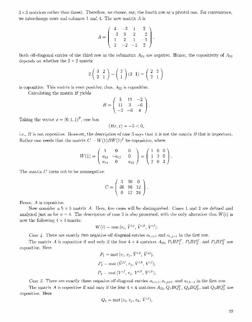
3 • 3 matrices rather than three). Therefore, we choose, say, the fourth row as a pivotal one. For convenience,

we interchange rows and columns 1 and 4. The new matrix A is

A =

4 - 3 1 2 '~

) - 3 3 2 - 2 1 2 1 - 1 "

2 - 2 - 1 2

Both off-diagonal entries of the third row in the submatrix A22 are negative. Hence, the copositivity of A22 depends on whether the 2 • 2 matr ix

2(3212)_(2),211,=(22,2) is copositive. This matrix is even positive; thus, A22 is copositive.

Calculating the matrix t3 yields

B = 11 3 - 6 . - 2 - 6 4

Taking the vector x = (0, 1, 1) T, one has

(Bz , z) = - 5 < O,

i.e., B is not copositive. However, the description of case 3 says that it is not the matr ix B that is important.

Rather one needs that the matrix C = W(1)BW(1) T be copositive, where

W(1) - -

(100)(100) a13 --al2 0 = 1 3 0 . a14 0 --a~2 2 0 3

The matr ix C turns out to be nonnegative:

C = 3 36 0 )

36 96 12 . 0 12 24

Hence, A is copositive. Now consider a 5 x 5 matr ix A. Here, five cases will be distinguished. Cases t and 2 are defined and

analyzed just as for n = 4. The description of case 3 is also preserved, with the only alteration that W(i) is

now the following 4 x 4 matrix:

w(i) = mat (e,:, r ?~'~, ~'~).

Case 4. There are exactly two negative off-diagonal entries al,i+t and al,j+t in the first row.

The matr ix A is copositive if and only if the four 4 • 4 matrices A22, P~BP T, P2BP T, and P3BP T are

copositive. Here

P1 = mat (ei, ej, ~fi,k, t~i,1),

P2 = mat, ( ? j , l ej, ?~ ,k Fi,l),

/?.3 = ma t (IF j'l, e~, f~g'~, vJ'~).

Case 5. There are exactly three negative off-diagonal entries at,i+t, al,j+l, and aLk+t in the first row.

The matrix A is copositive if and only if the four 4 x 4 matrices A22, Q~BQ T, Q2BQ T, and Q3BQ T are

copositive. Here

Q1 = mat (el, ej, ek, ~.i,l),

33

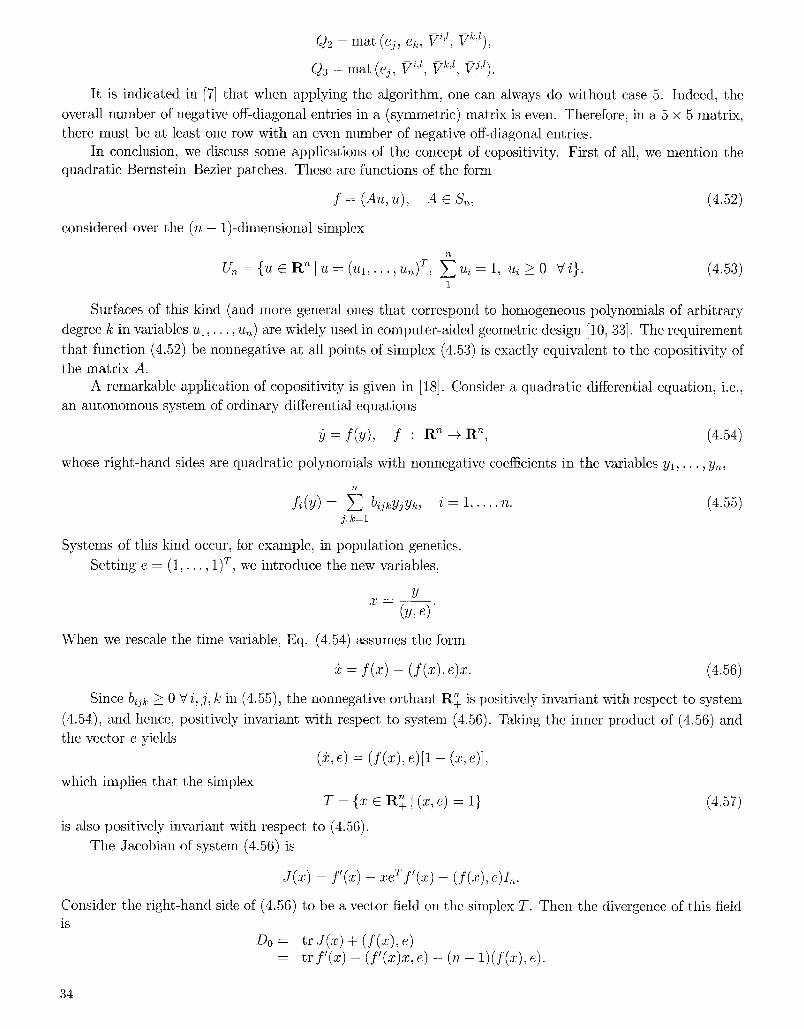
Q2 = mat (ej, e~, f7 i'l, f/~,l),

q3 = mat (ej, 17 ~'l, 17 k/, ~75/).

It is indicated in [7] that when applying the algorithm, one can always do without case 5. Indeed, the

overall number of negative off-diagonal entries in a (symmetric) matrix is even. Therefore, in a 5 x 5 matrix, there nmst be at least one row with an even number of negative off-diagonal entries.

In conclusion, we discuss some applications of the concept of copositivity. First of all, we mention the quadratic Bernstein Bezier patches. These are functions of the form

f = (A'< u), A ~ & , (4.52)

considered over the (n - 1)-dimensional simplex

U ~ = { u e R ~ l u = ( u ~ , . . . , u ~ ) r , f l u e = l , u~_>0 Vi}. (4.53)

Surfaces of this kind (and more general ones that correspond to homogeneous polynomials of arbitrary degree k in variables Ux, . . . , u,,) are widely used in computer-aided geometric design [10, aa] The requirement,

that function (4.52) be nonnegative at all points of simplex (4.53) is exactly equivalent to the copositivity of the matr ix A.

A remarkable application of eopositivity is given in [18]. Consider a quadratic differential equation, i.e., an autonolnous system of ordinary differential equations

[I = f ( y ) , f : R ~ ~ R ~, (4.54)

whose right-hand sides are quadratic polynolnials with nonnegative coefficients in the variables Y l , . . . , Y~,

f i (Y ) = f i bij~yyy~, i = 1 , . . . , n . (4.55) j, k = l

Systems of this kind occur, for example, in population genetics. Setting e = (1 , . . . , 1) r, we introduce the new variables,

Y X - -

When we rescale the time variable, gq. (4.54) assumes the form

:i: = f ( x ) - ( f ( : r ) , e )x . (4.56)

Since b~jk > 0 Y i , j , k in (4.55), the nonnegative orthant R~ is positively invariant with respect to system

(4.54), and hence, positively invariant with respect to systeln (4.56). Taking the inner product of (4.56) and the vector e yields

(5:,e) = ( f ( x ) , e)[1 - (x, e)],

which inlplies that the simplex

is also positively invariant with respect to (4.56). The Jacobian of system (4.56) is

J ( z ) = .f '(x) - x eT f ' ( x ) - (f(:r), e) I , .

Consider the right-hand side of (4.56) to be a vector field on the simt)lex T. Then the divergence of this field is

Do = tr J(:/~) ~- ( f ( x ) , e) = tr i f ( z ) - ( f ' ( x ) x , e) - (n - 1)(f(z), e).

34

On the set T, the divergence D0(x) coincides with the quadratic flmction

D(x) = tr f ' ( x ) ( x , e ) - ( f ' ( x ) x , e ) - ( n - 1)(f(x), e).

In coordinate notation,

D(x) = biji + buk - (n + 1) bi~k .z'jxk. (4.58) j,k=l i= l

For n = 3, simplex (4.57) is just a triangle in the plane

xl + x2 + x3 = 1.

By the criterion of Dulac, an autonomous system of ODE in the plane does not have periodic solutions (except

for constants) in a given simply connected domain if the divergence does not change sign in this domain. Since

Do(z) = D(x ) , x E T,

the inequality D(x) > 0 on T (or D(x) < 0 on T) excludes the existence of periodic orbits for system (4.56).

Such an inequality amounts to the requirement that the matrix of the quadratic form (4.58) be strictly

copositive (or strictly copositive up to a negative scalar factor). There are vector fields to which this criterion applies, for example, bij~ = 1 V i , j , k, because then D ( x ) = - 6 Vx E T.

5. ]~-Copositive Matrices

Let K; be a nonempty polyhedral cone in R":

= { lBx _> 0},

B being an m • n matrix.

De f in i t i on . A matrix A ~ Sn is called K-copositive if

(Ax, x) > 0 V z ~ ~5,

and strictly K-copositive if

(Ax, z ) > O V x E I ~ , z r

(5.1)

(5.2)

(5.3)

In particular, when /~ = R~_ (i.e., when t3 in (5.1) is the identity matrix Ix) (5.2) and (5.3) make us

return to the definitions of copositive and strictly copositive matrices. Moreover, system (5.1), defining the cone/~, may contain hyperplanes in an explicit or implicit way. By an explicit way we mean the situation where the system B z > 0 contains a pair of inequalities which, up to positive scalar factors, have the form

b~Xl + b2x2 + " �9 + b,~xn >_ 0

a n d

- b l x l - b2x2 . . . . . b,x,. >_ O.

Theoretically, the system B x >_ 0 can be equivalent to a systeln of linear equations. Hence, the case of matrices that are definite or semidefinite with respect to a linear subspace is also covered by definitions (5.2), (5.3).

Thus, polyhedral cones may be highly different. Accordingly, the characterizations of the corresponding copositive matrices (lifter substantially in complexity. We already had a chance to see this in the previous two sections of this survey. In the subsequent discussion, we shall also distinguish between different kinds of cones. In this respect, the definitions below will be helpful.

35

Def in i t i on . The dimension of a cone ~ is the dimension of its atone hull, i.e., of the linear space of smallest dimension containing K. A cone/~ C R ~ is te rmed solid if dim K = n.

De f in i t i on . A cone/C is pointed if tC n (-~C) = {0}. (5.4)

L e m m a 5.1. C o n e (5.1) is pointed if and only i f

rank B = n. (5.5)

P r o o f . Definition (5.4) is equivalent to the requirement that no line

y = ~ x 0 , - o c < t < 0%

belong to the cone/~. In o ther words, the system of linear homogeneous equations B x = 0 should not admit a nontrivial solution x0. This yields (5.5).

Another important special case of the general definition is where the rows of the matr ix B in (5.1) are linearly independent:

rank B = m. (.5.6)

It is easy to see that the cone K satisfying (5.6) must be solid.

In [22], it was pointed out that a simple sufficient condition for the matr ix A to be /Gcopos i t ive is that A be decomposable in the form

A = B r C B + S, (5.7)

where

and

the m • m matrix C is copositive (5.8)

the n • n matrix S is positive semidefinite. (5.9)

Clearly, this assertion holds for any polyhedral cone ]C. A matr ix A with decomposit ion (5.7) is strictly

K-copositive if (5.8) is valid and the matr ix S in (5.7) is positive definite.

In [27], the question is addressed whether decomposi t ion (5.7)-(5.9) is necessary for the mat r ix A E S~ to be ]C-copositive. A similar question related to strict hs is also treated. Many results of this paper are quite constructive, and therefore we discuss its contents in greater detail.

The case of a cone satisfying (5.6) is the simplest one. Let B be par t i t ioned as

S = (/71 B2). (5.10)

Without loss of generality, one can assume tha t the square m x m submatr ix /?~ is nonsingular. We make the following change of variables in (5.1)-(5.3):

x = Qg, (5.11)

where

Q__(B; ) 0 L,,-,~ "

Since BQ = (L,~ 0), the cone/C is now described by the inequality

u _> 0,

where u E R"" is a subvector in the part i t ion of y:

y z V

(5.12)

(5.13)

(5.14)

36

In the new variables,

(~,1 7~ = O r A Q = 7~r

where the block fi*n is of order m. Vectors y of the form

Y = v

the quadratic form y)(x) = (Ax, x) has the matrix

A~2 ) A22

obviously belong to K; (see (5.13)). Using the/C-copositivity of A for these vectors, we infer that

(5.15)

the submatriz ft22 in (5.15) must be positive semidefinite. (5.16)

Let us now consider vectors (5.14), where a subvector u is nonzero (and nonnegative). For these vectors Y~

~) = (Ay, y) = (.All u, '/s ~- 2(u, .ffM2 y) -}- (2~22v , v).

Suppose that v E ker A22. Then

'~ = ~(u) = ( A , ~ , u) + 2(u, A12v) >_ 0

for all u _> 0, and, hence A12v = 0. Thus, the inclusion

ker A22 C ker A12

holds. This implies, in particular, that the rank of the matrix

= &2&2A12 A[2 A22

coincides with the rank of the submatrix A22. Therefore (see (5.16)),

the matrix S is positive semidefinite.

Next, for the fixed vector u E R "~, the minimum in v of function (5.17) is attained on the vector

v = -A22A12u

(5.17)

and is equal to

where

(5.18)

(5.19)

(5.20)

(Cu,'a), (5.21)

C All + -T = - A12A22A12.

For any 'u > 0, the quadratic form (5.21) must be nonnegative, and, hence

matrix (5.22) is copositive.

The equality

(5.22)

(5.23)

0) 00 +s is obvious from (5.19) and (5.22). Returning to the original variable z, one obtains a decomposition of A:

A = Q - T f t Q - ~ = Q - r ( CO 00) Q-~+S" (5.24)

37

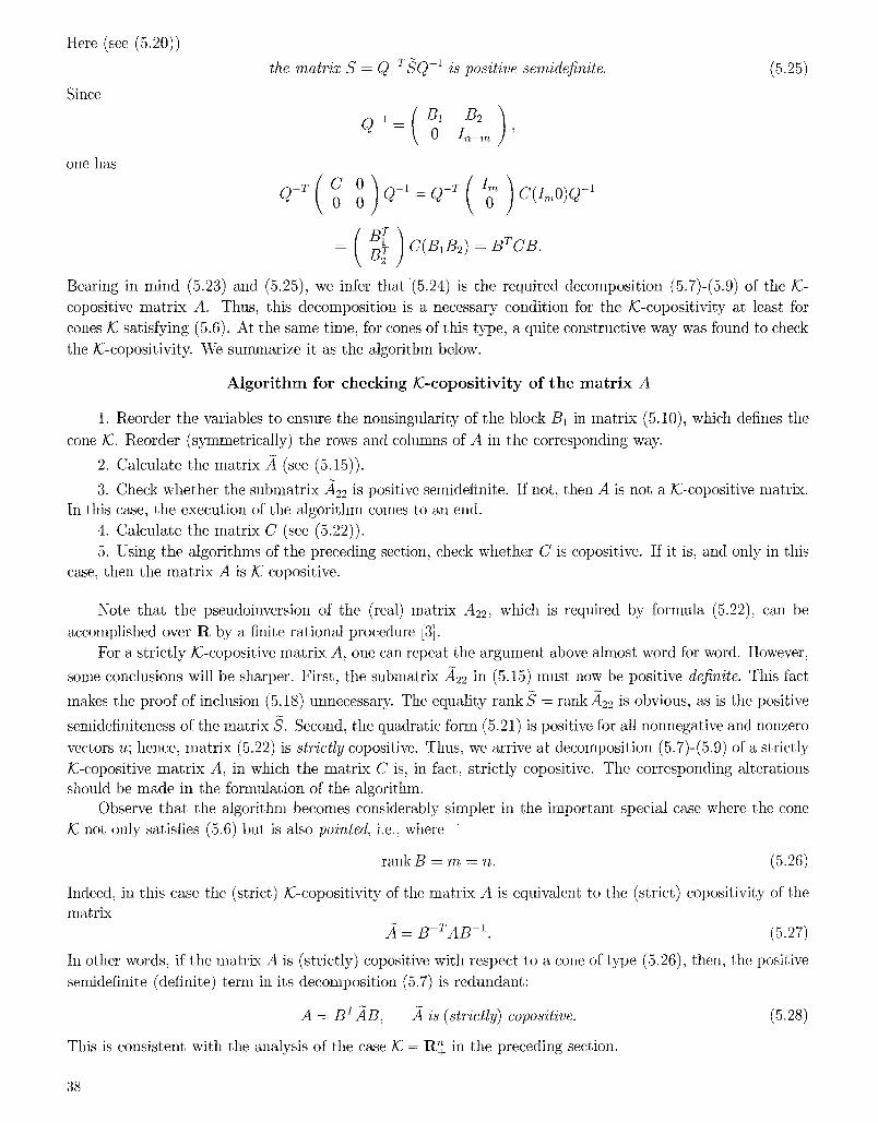
Here (see (5.20))

Since

one has

the matrix S = Q-r~;Q-1 is positive semidefinite.

Q_ I = ( B1 B2 ) 0 f~_,~ '

(.5.e5)

Bearing in mind (5.23) and (5.25), we infer that (5.24) is the required decomposition (5.7)-(5.9) of the/C- copositive matrix A. Thus, this decomposition is a necessary condition for the /C-copositivity at least for cones K satisfying (5.6). At the same time, for cones of this type, a quite constructive way was found to check the/C-copositivity. We summarize it as the algorithm below.

Algorithm for checking ~-coposit ivity of the matrix A

1. Reorder the variables to ensure the nonsingularity of the block B1 in matrix (5.10), which defines the

cone/C. Reorder (symmetrically) the rows and columns of A in the corresponding way.

2. Calculate the matrix A (see (5.15)).

3. Check whether the submatrix -~22 is positive semidefinite. If not, then A is not a K;-copositive matrix. In this case, the execution of the algorithm comes to an end.

4. Calculate the matrix C (see (5.22)). 5. Using the algorithms of the preceding section, check whether C is copositive. If it is, and only in this

case, then the matrix A is K-copositive.

Note that the pseudoinversion of the (real) matrix A22, which is required by formula (5.22), can be accomplished over R by a finite rational procedure [3].

For a strictly/C-copositive matrix A, one can repeat the argument above almost word for word. However,

some conclusions will be sharper. First, the submatrix A22 in (5.15) must now be positive definite. This fact

makes the proof of inclusion (5.18) unnecessary. The equality rank S = rank Aa2 is obvious, as is the positive

semidefiniteness of the matrix 5. Second, the quadratic form (5.21) is positive tor all nonnegative and nonzero vectors u; hence, matrix (5.22) is strictly copositive. Thus, we arrive at decomposition (5.7)-(5.9) of a strictly /C-copositive matrix A, in which the matrix C is, in fact, strictly copositive. The corresponding alterations should be made in the formulation of tile algorithm.

Observe that the algorithm becomes considerably simpler in the important special case where the cone /C not only satisfies (5.6) but is also pointed, i.e., where

rankB = m = n. (5.26)

Indeed, in this case tile (strict) /C-copositivity of the matrix A is equivalent to the (strict) copositivity of the matrix

= D- AB (5.27)

In other words, if the matrix A is (strictly) copositive with respect to a cone of type (5.26), then, the positive semidefinite (definite) term in its decomposition (5.7) is redundant:

A - Brf B, 2 is (strict@ opositive. (5.28)

This is consistent with the analysis of tile case/C = R~ in the preceding section.

38

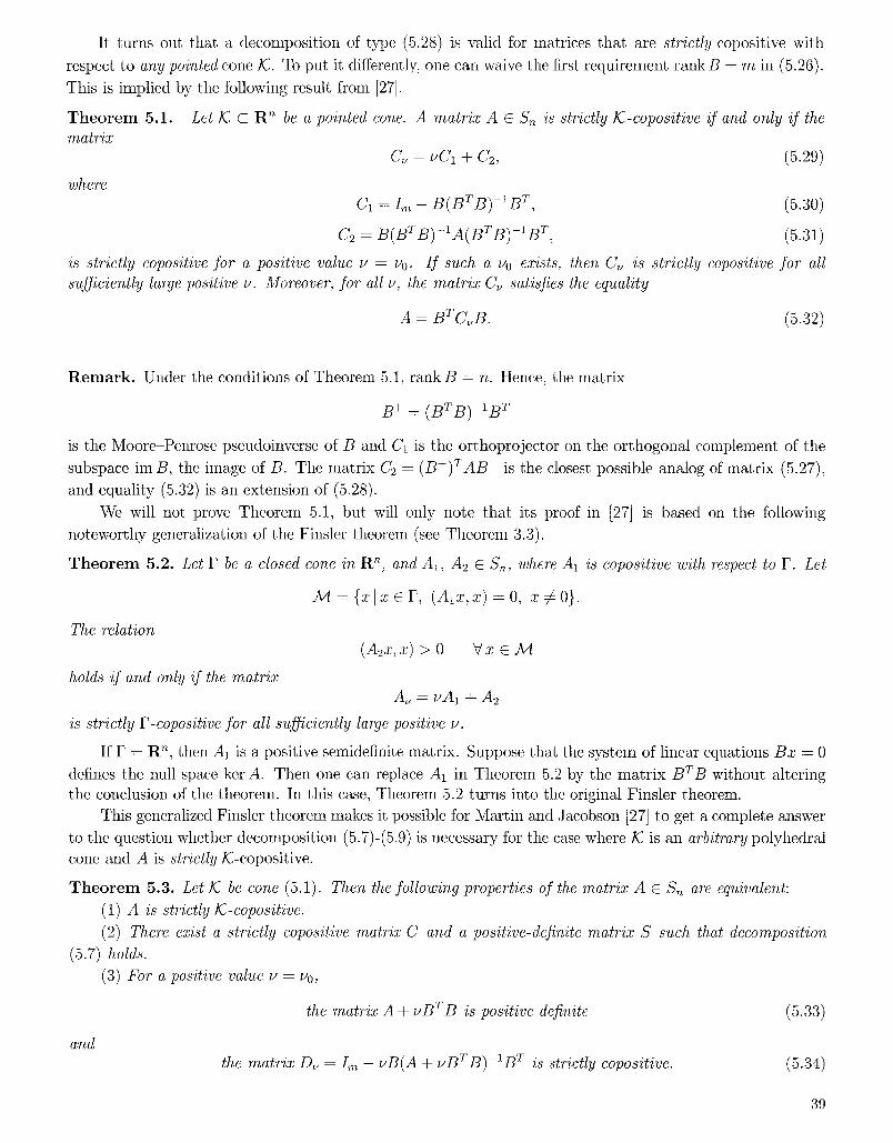
It turns out that a decomposi t ion of type (5.28) is valid for matrices tha t are strictly copositive with

respect to any pointed cone/C. To put it differently, one can waive the first requirement rank B = m in (5.26).

This is implied by the following result from [27].

Let/C C R " be a pointed cone. A matr ix A E S~ is strictly IC-copositive if and only i f the T h e o r e m 5.1. matrix

where

C. = + C2, (5.29)

C1 : / r n -- -B(-~TB) -I~T, (5.30)

C2 = B ( B r B) -~A(BT"B)-XB r, (5.31)

is strictly copositive for a positive value ~ = ~o. I f such a ~o exists, then C , is strictly copositive for all sufficiently large positive ~. Moreover, for all ~, the matrix C, satisfies the equality

A = B C B. (5.32)

R e m a r k . Under the conditions of Theorem 5.1, rank B = n. Hence, the matri•

B + = ( B T B ) - I B T

is the Moore-Penrose pseudoinverse of B and Ct is the or thoprojector on the or thogonal compleinent of the

subspaee im B, the image of B. The matr ix C2 = ( B + ) T A B + is the closest possible analog of matr ix (5.27),

and equality (5.32) is an extension of (5.28).

We will not prove Theorem 5.1, but will only note tha t its proof in [27] is based on the following

noteworthy generalization of the Finsler theorem (see Theorem 3.3).

T h e o r e m 5.2. Let F be a closed cone in R "~, and A1, A2 E Sn, where A~ is copositive with respect to F. Let

The relation

holds i f and only if the matrix

M={xlxEr, x 0}

(A2x, x) > 0 V x E M

A,, = r, A1 + A2

is strictly F-copositive for all sufficiently large positive z~.

If F = R ~, then A1 is a positive semidefinite matrix. Suppose that the system of linear equations B x = 0

defines the null space ker A. Then one can replace A1 in Theorem 5.2 by the ma t r ix B T B without altering the conclusion of the theorem. In this case~ Tlleorem 5.2 turns into the original Finsler theorem.

This generalized Finsler theorem makes it possible for Mart in and Jacobson [27] to get a complete answer

to the question whether decomposi t ion (5.7)-(5.9) is necessary for the case where/(7 is an arbitrary polyhedral cone and A is strictly ~-coposit ive.

T h e o r e m 5.3. Let 1C be cone (5.1). Th, en the following properties of the matrix A C Sn are equivalent:

(1) A is strictly ~-copositive.

(2) There exist a strictly copositive rnatr'i.~: C and a positive-definite matrix S such that decomposition

(5.7) holds.

(3) For a positive value ~ = Yo,

and

th, e matrix A + zJBT B is positive definite

the matrix D , = Im -- z~B(A + L, BY B ) - I B y is strictly copositive.

(5.33)

(5.34)

39

I f such a Uo exists, then conditions (5.33) and (5.34) are fulfilled for' all sufficiently large positive u.

R e m a r k . We can see that Theorem 5.3 ensures decomposition (5.7)-(5.9) with an excess: one can choose C to be even .strictly copositive.

For small m and n, conditions (5.33) and (5.34) call be verified with the use of symbolic computations (or even on paper). Hence, they can be considered to be a criterion for strict/C-copositivity. As all illustration, we reproduce below two examples from [27].

Suppose that a cone/C C R a is defined by the inequalities

3x + y - 8z > O,

- x - 3 y + 8 z > O.

One must determine whether tile quadratic form

tb = x 2 + y2 _ z 2

is strictly K:-copositive. For this exalnple,

The matrix in (5.33) is

A = d i a g ( 1 , 1 , - 1 ) , B = ( 3 1 - 8 / - 1 - 3 8 / " \

lOu+ 1 6u -32u ) 6u lOu + 1 -32u .

- 32u - 3 2 u 1 2 8 u - 1

The leading principal minors of E . are the polynomials

l O u + l , 64u 2 + 2 0 u + 1

and d(u) -= det E~ = 448/] 2 + 108/., - 1.

The leading coefficients of these three polynomials are positive. Thus, the matrix E , is positive definite for all sufficiently large positive u, and condition (5.33) is fulfilled.

If d(u) > 0, then one can examine the matrix

F,, = d(u)D(u) = d(r,)I.~ - u B adj (A + uBT B ) B T

instead of D , when checking condition (5.34). For our example, F,, is

( 5 4 u - 1 58u ) 58u 5 4 u - 1 "

positive and, hence, strictly copositive for u > 5!44" Applying Theorem 5.3, we This nlatrix is infer that the

form ga is strictly/(Lcopositive. Now we preserve the form ~b, but change sign in the second inequality defining K. Tile new cone ]C is

given by 3:r + y - 8z > 0,

x + 3y - 8z > O.

Neither the matrix B T B nor the matrix in (5.33) will change. Thus, condition (5.33) is again satisfied for all sufficiently large positive u. As for F, , this matrix assmnes the form

( 5 4 u - 1 - 5 8 u ) F, = - 5 8 u 5 4 u - 1 "

40

It will not be positive as ~ -+ oo; therefore, we check inequality (4.5). It is obvious that

{r~}~2 = (58~/) 2 > {Fv}n{F,,}22 = ( 5 4 ~ - 1) 2

for all sufficiently large ~, i.e., for these ~ the matrix F~ is not copositive. Hence, the form '~ is not copositive with respect to the new cone/~.

It has already been observed that the system of linear inequalities that defines the cone/C may contain, explicitly or implicitly, linear equations. Suppose that one can single out these equations in an explicit way. Then the original definition (5.1) of/C is replaced by

~: = {x I B lz _> 0, S~z = 0}. (5.35)

In this case, it is possible to obtain a decomposition of A that is more economical than that of (5.7)-(5.9). Here we cite one more result from [27].

T h e o r e m 5.4. Let IC be cone (5.35). decomposed as

Then a matrix A E S~ is strictly 1C-copositive if and only if A can be

A = .BTcI~I + S1, (5.36)

where C1 is a strictly copositive matrix and $1 is positive definite with respect to the linear subspace B2x = O.

The economy of decomposition (5.36) consists in the order of the copositive matr ix C1 being equal to the

number of "genuine" inequalities in system (5.1), and not to the overall number of inequalities in this system. As we will shortly see, the question whether decomposition (5.7)-(5.9) is necessary for tC-copositive

matrices proves to be much more delicate. However, for this case as well, one can get a number of useful implications from the results already stated above. One need only make use of the following simple observation: a matr ix A is/C-copositive if and only if the matrix A5 = A+e~In is strictly/C-coposit.ive for any ~ > 0. Applying Theorem 5.3 to A5, we obtain

T h e o r e m 5.5. Let 1C be cone (5.1). Then the following properties of a matrix A C S,~ are equivalent.

(1) A is copositive with respect to the cone 1C.

(2) For each 6 > O, there exist a strictly copositive matrix C5 and a positive-definite matrix S5 such that

and

A5 = A + ~I , = BTC~B + Ss. (5.37)

(3) For each ~ > O, there exists a positive value ~, = L'o (which may depend upon 6) such that

the matrix A5 + r'BT B is positive definite (5.38)

the matrix D,,~ = I,~ - r, B(A5 + r'BT B ) - I B T is strictly copositive. (5.39)

As was the case with Theorems 5.1 and 5.3, statements (2) and (3) become considerably simpler when

the cone /C is pointed. Indeed, for such a cone, already the matrix B T B is positive definite, and (5.38) is fulfilled automatically.

T h e o r e m 5.6. Let IC in (5.1) be a pointed cone. equivalent.

(1) A is copositive with respect to the cone 1C.

(2) For each 6 > O, there exists a strictly copositive matrix C5 such, that

A5 = A + 6I~ = BTCsB.

(3) For each ~ > O, the matrix

C,,,~ = ,C1 + C2~,

Then the .following pTvperties of a matrix A E S,, are

(5.40)

(5.41)

41

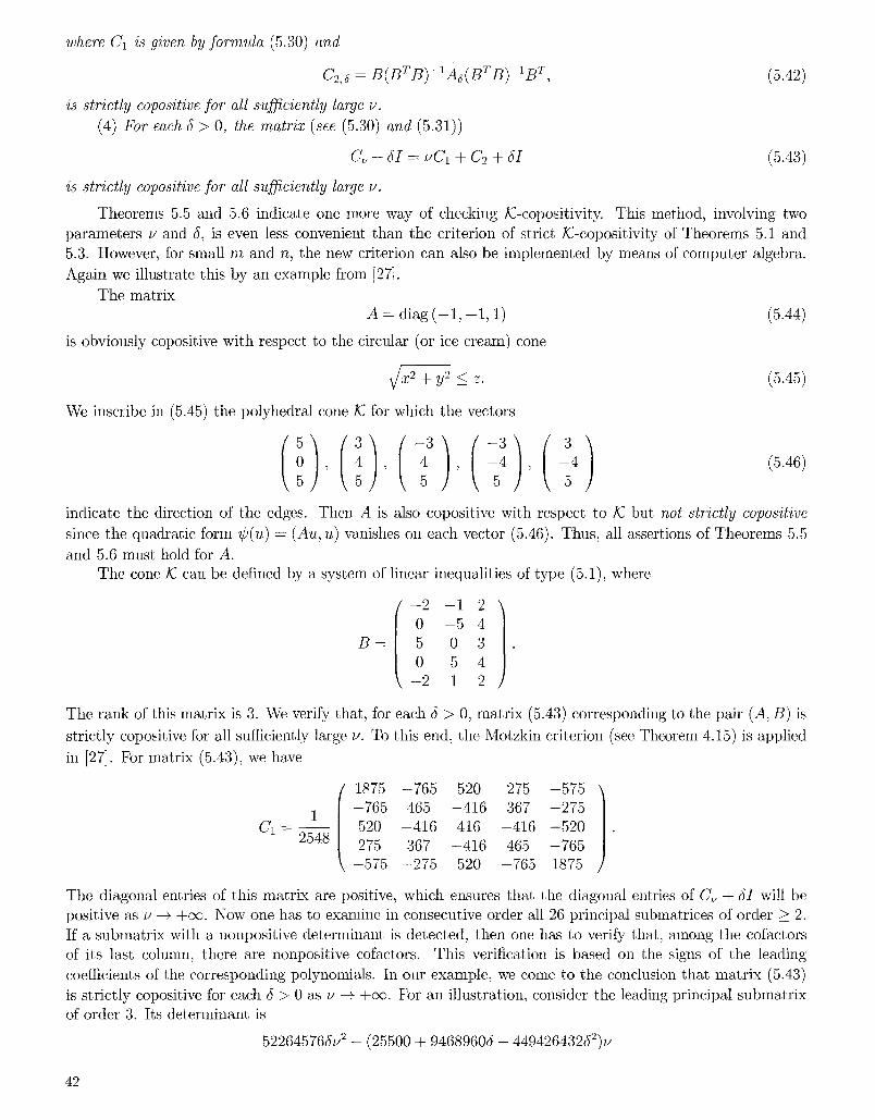
where C1 is given by formula (5.30) and

C2,5 = ]~(BT J~)-IAs([~T B) - I B T, (5.42)

is strictly copositive for all sufficiently large ~. (4) For each 5 > O, the matrix (see (5.30) and (5.31))

C, + 5I = 12C 1 -~ C2 ~- 5I (5.43)

is .strictly copositive for all sufficiently large ~.

Theorems 5.5 and 5.6 indicate one more way of checking tC-copositivity. This method, involving two parameters u and 5, is even less convenient than the criterion of strict /C-copositivity of Theorems 5.1 and 5.3. However, for small m and n, the new criterion can also be implemented by means of computer algebra.

Again we illustrate this by an example from [27].

The matrix A = diag ( - 1 , - 1 , 1) (5.44)

is obviously copositive with respect to the circular (or ice cream) cone

i x 2 + y2 < z. (5.45)

We inscribe in (5.45) the polyhedral cone K for which the vectors

0 , 4 , , , - ( 5 . 4 6 )

5 5 5 �9 5

indicate the direction of the edges. Then A is also copositive with respect to K7 but not strictly copositive since the quadratic form ~b(u) = (An, u) vanishes on each vector (5.46). Thus, all assertions of Theorems 5.5

and 5.6 must hold for A. The cone/(7 can be defined by a system of linear inequalities of type (5.1), where

B =

- 2 - 1 2 0 - 5 4 5 0 3 0 5 4

- 2 1 2

The rank of this matr ix is 3. We verify that, for each (5 > 0, matr ix (5.43) corresponding to the pair (A, B) is

strictly copositive for all sufficiently large z~. To this end, the Motzkin criterion (see Theorem 4.15) is applied

in [27]. For matrix (5.43), we have

1875 -765 520 275 -575 1 -765 465 -416 367 -275

= - - 520 -416 416 -416 -520 C1 2548 275 367 -416 465 -765

-575 -275 520 -765 1875

Tile diagonal entries of this matrix are positive, which ensures that tile diagonal entries of C,, + 5I will be positive as ~ --+ +co. Now one has to examine in consecutive order all 26 principal submatrices of order _> 2. If a submatrix with a nonpositive determinant is detected, then one has to verify that, among the cofactors of its last cohmm, there are nonpositive cofactors. This verification is based on the signs of the leading coeificients of the corresponding polynomials. In our example, we come to the conclusion that matr ix (5.43) is strictly copositive for each 5 > 0 as u --+ +oo. For an illustration, consider the leading principal subinatrix of order 3. Its determinant is

522645765u 2 - (25500 + 94689605 - 44942643252)u

42

+(225 - 336006 - 1000896062 + 41550745663)

and is positive for all sufficiently large p if 6 > 0 is fixed. No further analysis of this submatrix is required, and we can begin examining the next one.

Now we return to the discussion of decomposition (5.7)-(5.9) for the K-copositive matrix A. Recall that

for the cone K satisfying (5.6) the necessity of this decomposition was proved at the beginning of this section. Also recall that for strictly K;-copositive inatrices we managed to remove eventually all limitations on the type of cone (see Theorem 5.3). The following simple exatnple fl'om [27] shows that the situation is different for the/C-copositive case.

In R 2 we take

:(01 01) and let the cone/(2 be defined by system (5.1) with the matrix

( 1 0 ) (5.48) B = - 1 0 "

This system defines, in reality, the line z = 0. The quadratic form

'~/: = (Au, ~t) = 2xy

vanishes identically along this line. Thus, matrix (5.47) is K-copositive. We shall prove that this matrix does not admit decomposition (5.7)-(5.9). Indeed, for any symmetric matrix

the matrix

C = 9 7 '

~ : A - B T c ~ ~ ( -0~ + 2/~- 01 )

cannot be positive seinidefinite because det S = - 1 < 0. Consider the set of matrices C5 in decompositions (5.37) of matrix (5.47). The example above shows

that this set does not have a limit point as ~ --+ 0. Indeed, if such a limit point Co existed, then it would necessarily be a copositive matrix. The matrix

S0 = lira Sa = lim(A5 - B T c s B ) = A - B T C o B 5-+0 5--+0 is obviously positive semidefinite, which yields a decomposition of type (5.7) (5.9) of A:

A = B T C o B + So.

However, it has been proved that this decomposition is impossible. The cone defined by matrix (5.48) is not solid, and one could at tr ibute the counterexample above to this

fact. However, a more detailed analysis of matrix (5.44) and the solid cone K; given by the system of edges (5.46) shows that this/C-copositive matrix does not admit decoInposition (5.7)-(5.9) either.

In [28], a complete description is given of polyhedral cones/C such that any/Gcoposit ive inatrix can be represented in the form (5.7)-(5.9). Let us consider a cone in the matr ix space S~,, generated by cone (5.1) with the use of the formula

CB = { B T C B I C copositive}. (5.49)

Def in i t i on . Cone (5.1) is said to have the closure property if the matrix cone (5.49) is closed.

43

T h e o r e m 5.7. Let IG be cone (5.1). Any l~-copositive matrix A admits decomposition (5.7)-(5.9) if and only

i f the cone tG has the closure property and is either solid or pointed.

Unfortunately, it is not clear how the presence or absence of the closure property for a part icular cone/G

can be constructively verified. Thus, equality (5.6) is still the most general sufficient condition ensuring that

the ~-copositive matr ix A can be decomposed as in (5.7)-(5.9). However, two more partial results of this

kind can be found in [27].

T h e o r e m 5.8. Let 1~ in (5.1) be a solid cone. Suppose that the matrix B in (5.1) has no more than four

rows. Then any ~-copositive matrix A can be decomposed as in (5.7)-(5.9). Moreover, the copositive matrix

C can be chosen to be nonnegative.

This assertion differs from condition (5.6) in that the rows of the matrix B need not be linearly indepen-

dent.

T h e o r e m 5.9. Suppose that n = 2 and cone (5.1) is solid. Then any 1G-copositive 'matrix A either is positive

semidefinite or can be represented as

A = BTNB, where N is a nonnegative matrix.

Now we shall describe another type of criteria for ]Gcopositivity, which can be called enumerative type. One can think of criteria based on a sequential analysis of principal submatrices as their prototype in the

case where/(; = R~. For cone (5.1), the enumerat ion is governed by the set of submatrices tha t are formed

from the full rows of B. Such a submatrix will be called a row submatrix of B (this includes the vacuous row

submatrix of size 0 x n).

Suppose tha t ct C {1, 2 , . . . , m} is an index set defining the row sublnatrix B~. Then ~ will denote the

colnplementary index set and B~ will denote the complementary row submatrix. In the procedures under consideration, each step consists of certain tests for a matrix of the form

A D ~ = B~

c~ being an index set chosen for the current step.

0 ' (5 .50)

Tile description of tests will be given after some preliminary observations. If a matr ix A is strictly copositive with respect to cone (5.1), then it must also be s s being the null space of the matrix B.

In other words, (Ax, x) > 0 if Bx = 0 and x :fi 0. (5.51)

Thus, property (5.51) is a necessary condition for the matrix A to be strictly ~-eopositive. As such, it will

be called tile strong kernel condition. By the weak kernel condition we shall mean the property

(Ax, x) > 0 if Bx = 0 and A x r O. (5.52)

It is shown in [26] tha t for a solid cone K;, property (5.52) holds for any ]Gcopositive matr ix A.

As ill the preceding sections, the symbol e stands for the vector (1, 1 , . . . , 1) r , its dimension being defined

by the context. For a chosen nonvacuous row submatrix B~, consider the system

which consists of n + m - t(~1 linear equations. We say that B~ fails Test 1 if system (5.53) defines x in a unique way and this unique vector x satisfies the inequality

B~x > 0. (5.54)

44

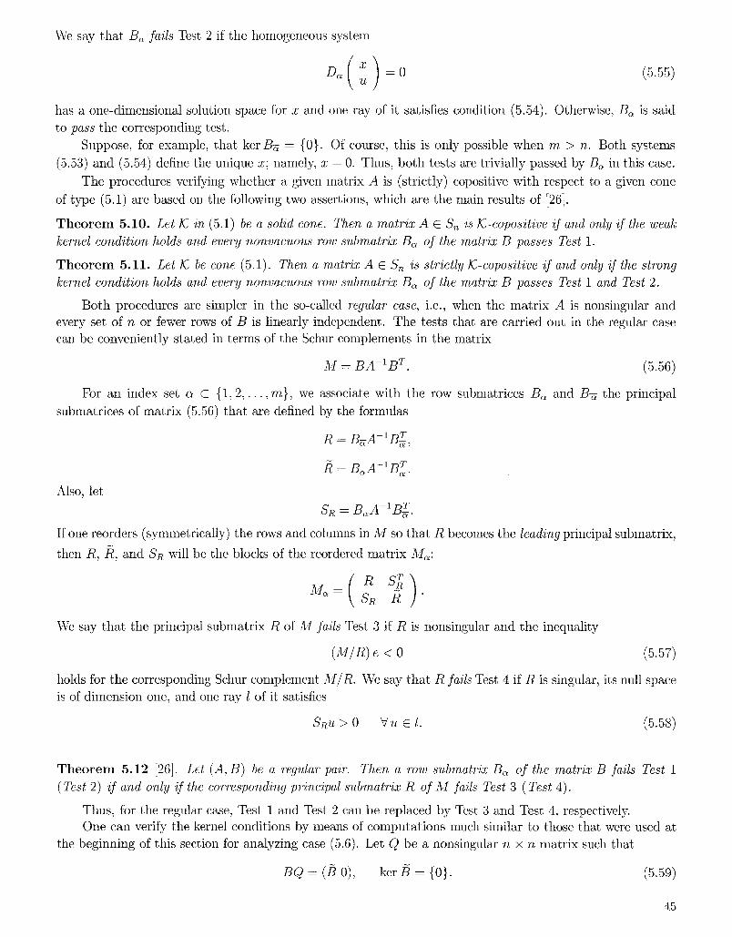
We say tha t B~ fails Test 2 if the homogeneous system

has a one-dimensional solution space for x and one ray of it satisfies condition (5.54). Otherwise, B~ is said to pass the corresponding test.

Suppose, for example, tha t ker B~ = {0}. Of course, this is only possible when m > n. Both systems

(.5.53) and (5.54) define the unique x; namely, x = 0. Thus, bo th tests are trivially passed by B~ in this case.

The procedures verifying whether a given matrix A is (strictly) copositive wi th respect to a given cone

of type (5.1) are based on the following two assertions, which are the main results of [26].

T h e o r e m 5.10. Let IC in (5.1) be a solid cone. Then a matrix A E S,~ is ]C-copositive if and only if the weak kernel condition holds and every nonvacuous row submatrix B~ of the matrix B passes Test 1.

T h e o r e m 5.11. Let lC be cone (5.1). Then a matrix A E S~ is strictly tC-copositive i f and only if the strong kernel condition holds and every nonvacuous row submatrix B~ of the matrix B passes Test 1 and Test 2.

Both procedures are simpler in the so-called regular case, i.e., when the mat r ix A is nonsingular and every set of n or fewer rows of B is linearly independent. The tests that are carried out in the regular case can be conveniently stated in terms of the Schur complements in the matrix

M = B A - 1 B r. (5.56)

For an index set c~ C {1, 2 , . . . , m}, we associate with the row submatrices B~ and B-~ the principal

submatrices of matr ix (5.56) tha t are defined by the formulas

Also, let

.~ -1 T z .Bo~ A Bo~.

SR = B~,A-1B$.

If one reorders (symmetrically) the rows and cohlnnls in M so tha t R becomes the leading principal sublnatrix,

then R, /~ , and SR will be the blocks of the reordered mat r ix M~:

We say tha t the principal subinatr ix R of M fails Test 3 if R is nonsingular and the inequality

(~f /R) e < 0 (5.57)

holds for the corresponding Schur complement M / R . We say t h a t / ~ fails Test 4 if R is singular, its null space is of dimension one, and one ray l of it satisfies

S~'a > 0 V'a E 1. (5.58)

T h e o r e m 5.12 [26]. Let (A, B) be a regular pair. Then a row submatrix B~ of the matrix B fails Test 1

( Test 2) if and only if the corresponding principal submatrix R of A.f .fails Test 3 ( Test 4).

Thus, for the regular case, Test 1 and Test 2 can be replaced by Test 3 and Test 4, respectively. One can verify the kernel condit ions by means of computa t ions much similar to those that were used at

the beginning of this section for analyzing case (5.6). Let Q be a nonsingular n • n matr ix such that

BQ = (B 0), ker B = {0}. (5.59)

45

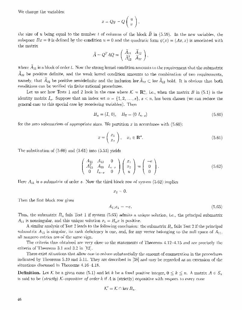
We change the variables:

x = Q y = Q v '

the size of u being equal to the number t of columns of the block /~ in (5.59). In the new variables, the

subspace Bx = 0 is defined by the condit ion u = 0 and the quadratic form r = (Ax, z) is associated with the matr ix

where -Art is a block of order t. Now the strong kernel condit ion alnounts to the requirement that the submatr ix

A22 be positive definite, and the weak kernel condition amounts to the combinat ion of two requirements,

namely, tha t -422 be positive semidefinite and the inclusion ker.422 C ker A~ hold. It is obvious tha t both conditions can be verified via finite rat ional procedures.

Let us see how Tests 1 and 2 look in the case where K = R~, i.e., when the matr ix B in (5.1) is the

identi ty matr ix In. Suppose tha t an index set a = {1, 2 , . . . , s}, s < n, has been chosen (we can reduce the

general case to this special case by reordering variables). Then

= (I, 0), = (0 In_ ) (5.60)

for the zero submatrices of appropria te sizes. We par t i t ion x in accordance with (5.60)

x t ) R.~. x = , x t E ( 5 . 6 1 ) 2C 2

k ]

The subst i tut ion of (5.60) and (5.61) into (5.53) yields

A~.~ ~ x2 = 0 . I,_~ u 0

(5.62)

Here AH is a submatr ix of order s. Now the third block row of system (5.62) implies

X 2 ~ - 0 .

Then the first block row gives

AlIxl = - e . (5.63)

Thus, the submatr ix B~ fails Test 1 if system (5.63) admits a unique solution, i.e., the principal submat r ix A u is nonsingular, and this unique solution xl = B~x is positive.

A similar analysis of Test 2 leads to the following conclusion: the submatr ix B~ fails Test 2 if the principal submatr ix AI1 is singular, its rank deficiency is one, and, for any vector belonging to the null space of AH, all nonzero entries are of the same sign.

The criteria thus obtained are very close so the s ta tements of Theoreins 4.12 4.15 and are precisely the criteria of Theorems 3.1 and 3.2 in [12].

There exist situations that allow one to reduce substantial ly the amount of enumerat ion in the procedures indicated by Theorems 5.10 and 5.11. They are described in [38] and may be regarded as an extension of the situations discussed in Theorems 4.16-4.18.

D e f i n i t i o n . Let ~ be a given cone (5.1) and let k be a fixed positive integer, 0 _< h _< n. A matr ix A E S,, is said to be (strictly) ]C-copositive of order h if A is (strictly) copositive with respect to every cone

]C = ~ N ker B~.

46

Here B~ is any row subinatr ix of tile matr ix B such tha t the null space ker B~ is of dimension k. If A is a

(strictly) K~-copositive mat r ix of order k, but not of order k + 1, then k is said to be its exact order or index

of (strict) /Gcopositivity.

T h e o r e m 5.13. Let tC in (5.1) be a pointed cone. Suppose that a matrix A E Sn has p positive eigenvalues,

p < n. Then A is (strictly) tC-copositive if and only if it is (strictly) 1C-copositive of order p + 1.

T h e o r e m 5.14. Let I~ in (5.1) be a pointed cone. Suppose that a matrix A E S~ is singular of rank r. Then A is lC-copositive if and only if it is lC-copositive of order r.

T h e o r e m 5.15. Let lC in (5.1) be a pointed cone. Suppose that a matrix A E S~ is singular of rank r. Then A is strictly lC-copositive if and only if it is strictly 1C-copositive of order r + 1.

One more result of this kind can be found in [38]. For obvious reasons, it has no correspondence in the case K: = Rn_.

T h e o r e m 5.16. Suppose that cone (5.1) is of dimension k < n. Then a matrix A E S~ is (strictly) IC-

copositive if and only if it is (strictly) ]C-copositive of order k.

The criteria of Theorems 5.10 and 5.11 can be thought of as extensions of the inner criteria from Sec. 4. The extensions of the outer criteria are discussed in [38]. Since tile descriptions of these extended criteria are ra ther bulky, they are not given here. We only want to point out tha t the principal pivoting scheme for quadrat ic programming is used as the main tool in outer criteria, by analogy with the case K; = R~.

We conclude this section by indicating two applications related to the not ion of tC-copositivity. Let

= F( t )x + G(t)u, x e R ~, ,a e R " ,

z ( t o ) = xo

be a linear system with the control function ~t(t). The problem is to mininfize the quadratic cost functional

tl J(Xo,U) =/[uT( t )R( t ) 'u ( t ) + xT(t)Q(t)x(t)]dt + :rT(t~)Hx(tl)

to

subject to controller constraints of the form

~ ( t ) n( t ) ~ 0 a.e. Oil [to, tl] ,

where B(t ) is a given l • m, matr ix function.

An analysis of this problem with the use of the analog of the classical condi t ion of Legendre ill the calculus of variations leads to the following inference: a necessary condition for J to be bounded below is tha t for almost all t E [to, t~] the matr ix R(t) be copositive with respect to the cone defined by the matr ix B(t) via formula (5.1). Note tha t this example is taken from [28].

An interesting application of Theorem 5.3 is given in [27]. Consider, along with the lnatrix A E S,, and cone (5.1), the hyperellipsoid

(Px, x) = 1, P E S,,, P is positive definite. (5.64)

One needs to evaluate the nf inimum rn of tile quadrat ic form '~(x) = (A:r, x) on hyperellipsoid (5.64) subject to constraints B x >_ O.

The following approach to this problem call be proposed. The number rn is the suprenmtn of positive d such tha t the matrix A - d P is copositive with respect to cone (5.1). Applying Theorem 5.3, we infer tha t

the supre lnum should be found of those 5 > 0 for which the matr ix A - ~P + p B T B is positive definite and the mat r ix I m - ~B(A - ~P + z~BTB)-IBT is strictly copositive for all sufficiently large ~.

47

We ilhlstrate this approach by an example from [27]. Assunte that n = 3, P = I3 (thus, hyperellipsoid

(5.64) is, in this case. a two-dimensional sphere), A = diag (1, 1, -1 ) , and

t3 = - 1 - 3 8 '

The leading principal minors of the symmetric matr ix A - dIa + r 'BYB are

10~ + 1 - d,

6 4 . 2 + (20 - 20 (~)z~ + (1 - ~)2

and d (zJ, ~) = (448 - 576 d)z9 + (108 - 256 d + 148 52)zJ - 1 + 6 + 52 - ~3.

Tile first, and second minors are clearly positive as ~, --+ +oo. The determinant d will only be positive for

sufficiently large z~ if (~ < 448/576 = 7/9.

For the symmetric 2 • 2 matrix

the entries are

and

F,,6 = d(L,, 5)Io - ~,B adj (A - 6L3 + ~'BT B ) B r

{F,,,a}t,, = {F,,,a}2,2 = (54 - 1286 + 94 (~2)~ - 1 + ($ + ~2 _ d3

{F,,a},,2 = (58 - 1280-+ 7052)t,.

If (~ = 7/9, the leading coefficients of both polynomials are positive. Thus, the matr ix F,, r/9 is positive (hence,

strictly copositive) as z, --+ + ~ . This analysis shows tha t the required supremum is equal to

(~ = 7/9.

In other words,

7(x,x) (Ax, x) >_

if B x >_ O, and the minimum of the form 'r on the intersection of the unit sphere and the cone Bx > 0 is

7/9.

6. C o n c l u d i n g R e m a r k s

In [15, 34], finite procedures are described for deciding whether or not a given inhomogeneous quadratic

function 'O(x) is bounded below on a polyhedron M defined by a system of linear inhomogeneous inequalities.

In the homogeneous case, the boundedness of a quadratic form below is equivalent to its nonnegativity on M. Indeed, assuming that "g'(Xo) < 0 for some point x0 E M, one finds that

' * ( t*0 ) = t 2 (x0) - o o

as t -+ +co (recall that the I)olyhedron M is a cone for tile llomogeneous case). Hence, tile procedures in

[15, 34] can also be used for checking/C-copositivity. However, their descriptions were not included in Sec. 5, tile reason being that, since these procedures are meant for a more general situation, they will be less efficient for the homogeneous problem than algorithms specially constructed for this case.

In the main body of this survey, the matr ix property of copositivity was discussed with respect to the three types of subsets of the n-dimensional space R ~, namely, linear subspaces, the nonnegative orthant R~c,

48

and, finally, arbitrary convex polyhedral cones. However, the copositivity can be defined and may be of interest for other types of subsets as well. By way of example, consider the ice cream cone

,).2 ~1/2 (6.1)

D e f i n i t i o n . A matrix A E S~ is called h'n-eopositive if (Ax, x) >_ 0 Vx E K~.

Using the inatrix g~ = diag ( - 1 , - 1 , . . . , - 1 , 1), one can rewrite (6.1) as

K , , = { x e R " [ ( J n x , x) >_0 A xn > 0}.

T h e o r e m 6.1 [25]. A matrix A E S~ is K,~-copositive if and only if the matrix A - p J ~ is positive semidefinite for some p >_ O.

Unfortunately, the criterion of K~-copositivity indicated in Theorem 6.1 cannot be regarded as a con-

structive one because it does not show how to find the required scalar p (or show its absence). Unlike the

criteria of the type of Theorem 3.3, here one cannot reduce the analysis to the investigation of the behavior of

the principal minors as # --+ oo. Indeed, the matr ix A - #J~ has a negative diagonal entry (n, n) as # -+ +c~

and, hence, it cannot be positive senfidefinite. As p -+ - o c , all diagonal entries, excluding the last one, are negative.

The first author was supported by the Russian Foundation for Basic Research, project No. 97-01-00927.

R e f e r e n c e s

1. R. E. Bellman, Introduction to Matrix Analysis, Mc Graw-Hill, New York (1970).

2. F. R. Gantmacher, The Theory of Matrices, Chelsea, New York (1959).

3. Kh. D. Ikramov, "Finite spectral procedures in linear algebra," Programmirovanie, 1, 56 69 (1994).

4. I. S. Iokhvidov, Hankel and Toeplitz Matrices and Forms. Algebraic Theory, Birkhauser, Boston (1982).

5. M. Hall, Jr., Combinatorial Theory; Blaisdell, Waltham (1967).

6. R. A. Horn and C. R. Johnson, Matrix Analysis, Cambridge University Press (1985).

7. L.-E. Andersson, G. Chang, and T. Elfving, "Criteria for copositive matrices using simplices and barycentric coordinates," Linear Algebra Appl., 220, 9 30 (1995).

8. L. M. Blumenthal, Theory and Applications of Distance Geometry, Oxford University Press, London (1953).

9. Y. Chabrillac and J.- P. Crouzeix, "Definiteness and semidefiniteness of quadratic forms revisited," Linear Algebra Appl., 63, 283 292 (1984).

10. G. Chang and T. W. Sederberg, "Nonnegative quadratic Bezier triangular patches," Comput. Aided Geom. Design., 11, 113-116 (1994).

11. B. W. Char, K. O. Geddes, G. H. Gonnet, M. B. Monagan, and S. M. Watt, MAPLE. Reference Manual. Fifth edition, WATCOM Publications, Ltd. (1988).

12. R. W. Cottle, G. J. Habetler; and C. E. Lemke, "On classes of copositive matrices," Linear Algebra Appl., 3, 295 310 (1970).

13. G. Debreu, "Definite and semidefinite quadratic forms," Economet~ica, 20, 295 300 (1952).

14. P. H. Diananda, "On nonnegative forms in real variables some or all of which are non-negative," Proc. Cambridge Philos. Soc., 58, 17-25 (1962).

15. B. C. Eaves, :'A finite procedure for determining if a quadratic form is bounded below on a closed polyhedral convex set," Math. Programming, 14, 122-124 (1978).

16. P. Finsler, "Uber das Vorkommen definiter und semidefiniter Formen und SchSren qnadratischer Formen," Com- ment. Math. Helv., 9, 188-192 (1937).

17. J. C. Gower, "Properties of Euclidean and non-Euclidean distance matrices," Linear Algebra Appl., 67, 81-97 (1985).

49

18. K. P. Hadeler, "On copositive matrices," Linear Algebra Appl., 49, 79-89 (1983).

19. T. Havel, I. Kuntz, and G. Crippen, "The theory and practice of distance geometry," Bull. Math. Biol., 45, 665-720 (1983).

20. T. L. Hayden and J. Wells, "Approximation by matrices positive semidefinite on a subspace," Linear Algebra Appl., 109, 115-130 (1988).

21. E. Haynsworth and A. J. Hoffman, "Two remarks on copositive matrices," Linear Algebra Appl., 2, 387-392 (1969).

22. D. H. Jaeobson, Extensions of Linear Quadratic Control, Optimization and Matrix Theory, Academic Press, New York (1977).

23. E. L. Keller, Quadratic Optimization and Linear Complementarity, Ph.D. Thesis, Univ. of Michigan, Ann Arbor (1969).

24. P. Li and Y. Y. Feng, "Criteria for eopositive matrices of order four," Linear Algebra Appl., 194, 109-124 (1993).

25. R. Loewy and H. Schneider, "Positive operators on the n-dimensional ice cream cone," J. Math.. Anal. AppL, 49, 375-392 (1975).

26. D. H. Martin, "Finite criteria for conditional definiteness of quadratic forms," Linear Algebra Appl., 39, 9-21 (1981).

27. D. H. Martin and D. H. Jacobson, "Copositive matrices and definiteness of quadratic forms subject to homoge- neons linear inequality constraints," Linear Algebra AppI., 35, 227-258 (1981).

28. D. H. Martin, M. J. D. Powell, and D. H. Jacobson, "On a decomposition of conditionally positive-semidefinite matrices," Linear Algebra Appl., 39, 51-59 (1981).

29. K. Menger, "Bericht fiber metrische Geometrie," dahresber. Deutsch. Math.-Verein., 40, 201-219 (1931).

30. K. Menger, "New foundations of Euclidean geometry," Amer. J. Math., 53, 721-745 (1931).

31. T. S. Motzkin, "Sign of Minors," O. Shisha, ed., Inequalities, Academic Press, New York (1967), pp. 225-240.

32. K. G. Murty and S. N. Kabadi, "Some NP-complete problems in quadratic and nonlinear programming," Math. Programming, 39, 117-129 (1987).

33. E. Nadler, "Nonnegativity of bivariate functions on a triangle," Comput. Aided Geom. Design., 9, 195 205 (1992).

34. A. F. Perold, "An alternative method for a global analysis of quadratic programs in a finite number of steps," Math. Programming, 15, 105 109 (1978).

35. P. A. Samuelson, Foundations of Economic Analysis, Harvard University Press, Cambridge (1947).

36. I. J. Schoenberg, "Remarks to M. Frdchet's article 'Sur la definition axiomatique d'une classe d'espaces vectoriels distanci~s applicables vectoriellement sur l'espace de Hilbert'," Ann. Math., 36, 724-732 (1935).

37. H. Vgliaho, "Criteria for copositive matrices," Linear Algebra Appl., 81, 19-34 (1986).

38. H. VSliaho, "Testing the definiteness of matrices on polyhedral cones," Linear Algebra Appl., 101, 135-165 (1988).

39. R. J. Vanderbei, "Symmetric quasi-definite marrices," SIAM J. Optim., 5, 100-113 (1995).

50