Conductivity (EM) Survey: A Survival Manual

R. Berle Clay Cultural Resource Analysts, Inc.

151 Walton Avenue Lexington, Ky, 40508

auvergne@earthlink.net; rbclay@CRAI-KY.com

A Conductivity Survey in Progress. The EM38 is carried in the right hand, ca 15 cm off the ground. It is contained in a sheath of foam insulation held together with Duct

Tape (!). The data logger is carried in the left hand and manipulated with the left thumb. Not so obvious is the marked rope below the EM38, the object of the author’s rapt

attention.

Introduction Conductivity survey, also known as electromagnetic survey (EM), measures the ability of the soil to conduct an electric current. The value, measured in siemens, is the reciprocal of resistivity (to convert to resistivity in ohm meters, divide the conductivity, in millisiemens per meter, into one thousand (Bevan 1983:51)). This said, there is considerable difference in the way earth conductivity and earth resistivity are measured. Although the theory behind EM survey is considerably more complex than the theory behind resistivity, fortunately there are a number of lucid published explanations aimed specifically at archaeologists (cf Bevan 1983, 1998:29-43, Frohlich and Lancaster 1986) as well as more technical discussions (McNeil 1980) which should be helpful to both the user and the manager. The following discussion builds on these and focuses on the personal experiences of the author from almost 20 years of use with one particular EM survey instrument. This brief introduction is designed to get the first user, or discouraged user (I find there are many of these) into (or back into) the field collecting useful EM data on archaeological sites. In the United States, one of the problems with doing EM survey is that the technology is used extensively by non-archaeologists for a variety of applications. Because of different field techniques and goals, there tends to be little communication between archaeological and non-archaeological users (with the exception of communication between the geophysicists themselves, who may or may not have archaeological interests). Again, EM technology has not been built specifically for archaeology but has remained generalized, hence applicable to a wide range of geophysical interests. However, these problems should not stand in the way of the widespread use of EM survey in archaeology, although they do.

Finally, I always think in terms of using EM survey in concert with magnetic survey, exploiting the specific advantages of the different survey methodologies (Clay 2001). Therefore I am less concerned with the strengths or weaknesses of EM survey in contrast to another form of survey technology in archaeology, but rather with how the specific qualities of EM survey data may be incorporated in a larger strategy for collecting geophysical data on archaeological sites.

Summary Comments To begin, it is useful to outline what I see as the strong and “weak” (from an archaeologist’s standpoint) points of EM survey technology and the specific survey problems I wish to discuss here. Most of these points I specifically mention; all are implicit throughout my discussion. Strong Points of EM survey: 1) Fast

2) Can be used in a variety of ground conditions (grass/brush/tree cover, ridged ground etc.) where other techniques may be more difficult to use. 3) Works well in team with magnetic gradient survey. 4) Can be used in dry periods as well as wet (an edge here on resistivity). 5) Can measure magnetic susceptibility (ppt) as well as earth conductivity (mS/m), a mixed blessing. 6) Can do a certain degree of vertical separation of geophysical phenomena.

Cautions (which must be managed with field technique) 1) Temperature drift 2) Digital lag 3) Appropriate visual output and data processing 4) Metal on the operator Weak Points 1) Sensitive to a wide range of metals (from flip tops to water mains!) 2) Much greater sensitivity of near-surface targets (can be seen as + or -) 3) Difficulty in making depth discrimination between targets 4) Directions of technological development making the meter less and less satisfactory for archaeology (a multi-pronged problem) 5) Subject to electrical interference of certain electromagnetic frequency (overhead power lines)

Historical Background EM techniques in archaeology seem to have been developed in Europe in the late 1960s and early 1970s (c.f. Tite and Mullins 1970). Their use in North American archaeology largely grew out of the commercial development in the 1970s of earth induction meters by Geonics, Ltd., a Canadian firm specializing in geophysical equipment. There work made available off the shelf instruments that could be used for a variety of applications including archaeology (also geology, soil science, and environmental monitoring).

One of the earlier published archaeological applications for the United States was by Bruce Bevan (1983), a geophysicist who received his training in geophysics and electrical engineering and his contacts with archaeology at the University of Pennsylvania. In the article he discussed the use of an EM31 earth induction meter at Fort de Chartres, an 18th Century French fort in Illinois, the Deer Creek historic Wichita site in Oklahoma, and La Ciudad, a Hohokam settlement near Phoenix, Arizona, against a more general background of the field methods he used to collect and analyze the data. In the three field trials Bevan produced plausible EM evidence for the existence of a buried fortification trench at Fort de Chartres, plowed down mounds at Deer Creek, and a feature at La Ciudad that may have been a prehistoric sedimentation basin.

Dr. Bevan has continued to be the principal geophysicist in the United States using EM techniques in archaeological prospection, by now on a world-wide selection of sites and emphasizing the use of multiple, complementary techniques. However, the techniques have been adopted by a number of archaeologists. A parallel interest in EM survey techniques has continued in continental Europe, particularly in France. Interestingly, although the first EM earth induction meter made specifically for archaeological applications seems to have been built in England (Howell 1966), a device known vernacularly as “the banjo” and a product of a fertile tradition of English geoprospection, English field methods since then have generally not consistently involved EM techniques (David 1995:20). This may reflect the fact that the technology has commercially developed in Canada, and not Great Britain where the widely used field

instruments have been developed locally in close cooperation with the Ancient Monuments Laboratory of English Heritage.

Theoretical Basis EM surveys use an instrument called an electromagnetic induction meter that induces an electromagnetic signal into the ground and measures how well it is conducted by the soil. The frequency of the signal may vary (the instrument I use generates an audio frequency signal of 14.6kHz) but critical to the design of the induction meter is the feature that there is no electrical connection between the survey instrument and the ground, unlike instruments measuring soil resistivity which use a variable array of metal probes inserted in the ground and wired to the resistivty meter, probes which must all or in part shifted to a new location to take a new reading. The induction meter uses a coil near ground surface to “broadcast” its high frequency signal that is received by another coil, also near ground surface. The transmitted signal causes the conductive material below the meter to generate its own faint signal that is detected by the receiver coil. Both coils are built into the meter and the spacing between them governs the effective depth to which the meter can measure earth conductivity. The instrument is not designed to be a metal detector but highly conductivity metals also generate a strong signal in response to the meter and their response tends to overload the circuitry. Rather, it is designed to measure the much smaller signals generated by the conductivity properties of soils. The electronics of the meter converts the signal into the measure of conductivity (because of its small size, millisiemens per meter or mS/m). In general, soil conductivity meters measure differences in the conductivity of soils that are a product of their composition and formation. A typical “spread” of soil types produces the following ranges of mS/m (Bevan 1998:8) (resistivity measurements are also listed):

Soil Resistivity ohm-m Conductivity mS/m

Sand, gravel 1000 – 10,000 0.1 – 1 Silty sand 200 – 1000 1 – 5 Loam 80 – 200 5 – 25 Silt 40 – 80 12.5 – 25 Clay 10 – 40 25 – 100 Saline soil 5 – 10 100 – 200

When soils have been moved around in an archaeological site by its occupants, conductivity contrasts can be created which a conductivity meter might record. In most cases this will be true if there is variation in soil composition in the local soil column. In addition, the composition and texture of the soil may be changed by cultural activity (and natural forces as well). An EM earth induction meter may record all of these events. But is quite important before doing a conductivity survey to have some idea of the local soil column, most directly but on a theoretical level, by consulting the local soil map and the description of the soil type. Often systematic shovel tests (which may have been used to initially locate an archaeological site) may have also collected valuable information on the local soil column, perhaps also its variation across a site.

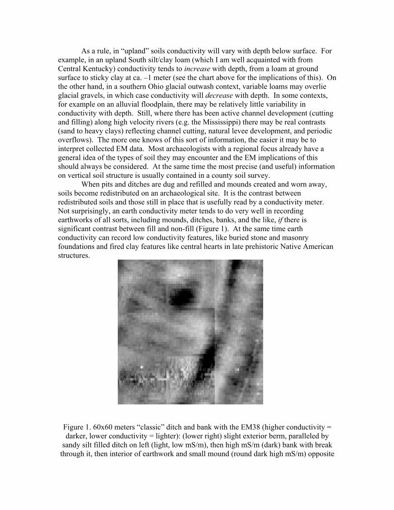
As a rule, in “upland” soils conductivity will vary with depth below surface. For example, in an upland South silt/clay loam (which I am well acquainted with from Central Kentucky) conductivity tends to increase with depth, from a loam at ground surface to sticky clay at ca. –1 meter (see the chart above for the implications of this). On the other hand, in a southern Ohio glacial outwash context, variable loams may overlie glacial gravels, in which case conductivity will decrease with depth. In some contexts, for example on an alluvial floodplain, there may be relatively little variability in conductivity with depth. Still, where there has been active channel development (cutting and filling) along high velocity rivers (e.g. the Mississippi) there may be real contrasts (sand to heavy clays) reflecting channel cutting, natural levee development, and periodic overflows). The more one knows of this sort of information, the easier it may be to interpret collected EM data. Most archaeologists with a regional focus already have a general idea of the types of soil they may encounter and the EM implications of this should always be considered. At the same time the most precise (and useful) information on vertical soil structure is usually contained in a county soil survey. When pits and ditches are dug and refilled and mounds created and worn away, soils become redistributed on an archaeological site. It is the contrast between redistributed soils and those still in place that is usefully read by a conductivity meter. Not surprisingly, an earth conductivity meter tends to do very well in recording earthworks of all sorts, including mounds, ditches, banks, and the like, if there is significant contrast between fill and non-fill (Figure 1). At the same time earth conductivity can record low conductivity features, like buried stone and masonry foundations and fired clay features like central hearts in late prehistoric Native American structures.

Figure 1. 60x60 meters “classic” ditch and bank with the EM38 (higher conductivity = darker, lower conductivity = lighter): (lower right) slight exterior berm, paralleled by

sandy silt filled ditch on left (light, low mS/m), then high mS/m (dark) bank with break through it, then interior of earthwork and small mound (round dark high mS/m) opposite

entrance through bank (diagonal sub soiling marks and possible external feature paralleling the berm)(Little Spanish Fort, Mississippi).

Because the earth induction technology uses “open” signal collectors, it can also

pick up other environmental noises that can seriously degrade the measurement. Depending upon their transmission frequency, overhead power lines can cause fluctuation in recorded mS/m. Importantly, earth spherics, notably lightning discharges, can cause unwanted noise that often persists for a time after the discharges. Finally, induction meters register the presence of various forms of metal (not simply ferrous material) both incorporated in the soil (pipes and other utilities) and above ground (for example wire fences and metal structures) that tend to overload the recording instrument (depending upon the size of, and characteristics of, the metal). They are similar to metal detectors, however in the latter the coils are “co-axial” (as opposed to laterally separated) providing a much more precise location of small metal objects. Because of these factors, it is my experience that the technology does not work particularly well for me as an archaeologist in urban or densely built up modern environments although it may be used with good effect in archaeological historic environments, particularly those which became archaeological in the 19th Century, or at least before ca 1940 (after which the amount of metal junk and modernizing utilities seems create a quantum jump in the environmental noises which can affect EM surveys).

Technological Choices While new suppliers of EM technology have recently entered the market, it is still dominated by Geonics, Ltd., a Canadian firm which also has had a long standing interest in archaeological applications (McNeil 1980, Geonics, Ltd. n.d.). Geonics produces a variety of instruments, all operating on the same principle, but varying in their intended application. The principal variation between machines is the spacing between transmitting and receiving coils, hence depth of sensitivity, reflecting the fact that a wide variety of users besides archaeologists (geologists, soil scientists, environmental monitors, etc.) use their technology. Two of their instruments, the EM31 and the EM38, have been used in archaeology. With an inter coil spacing of 3.66 meters, the EM31 effectively measures earth conductivity to ca 6 meters, while the EM38 with an inter coil spacing of 1 meter measures effective conductivity to ca 1.5 meters.

The “cost” in ease of use for the depth sensitivity of the EM31 is high. Physically it is a boom 4 meters along attached to an electronics unit. Both weigh 12.4kg (a data logger adds an additional 1.5kg). It is tedious instrument to carry through a long day and often difficult to thread through natural obstacles (trees etc.) without changing its orientation (which can affect the measurements it takes). By way of contrast, the EM38 is one meter long and weighs only 2.5kg (with 1.5kg for a data logger). As result it is principally the EM38 that has been used for more recent archaeological applications.

Depth Discrimination - Both instruments may be rotated 90 degrees to take measurements in the “horizontal” mode (effectively laying each instrument over on its side) at approximately one-half the depth sensitivity of the “vertical” mode and thus to explore vertical change in soils (an internal mercury switch signals the data logger of the change in orientation). However, it is not very handy to do this and it considerably slows down area survey so that both machines are effectively used in the “vertical” mode.

Nevertheless, this ability of earth induction meters does permit the surveyor to get a “feel” for vertical changes in soils, for example at the beginning of the survey as a check against published soil descriptions, without the necessity of collecting extensive data sets in the horizontal orientation and this can be important.

In EM meters the measure of conductivity is “generalized” over the depth of sensitivity. This means that any archaeological stratigraphy is also generalized and neither instrument effectively discriminates complex stratigraphic differences. This can be a problem given the depth sensitivity of the EM31, less so with the EM38 which, with its 1.5-meter depth sensitivity, is admirably suited to a wide range of minimally stratified, near-surface archaeological sites. Recently GSSI (GSSI n.d.) has offered an earth induction meter called the Gem 300 that purports to discriminate depth in conductivity by varying the frequency of the transmitter (Won et. al. 1996) under the general theory that lower frequencies penetrate to a greater depth than do higher ones. It is the opinion of Geonics Ltd. (McNeil 1996) that the Gem 300 does not perform as advertised and there have, to my knowledge, been no attempt to test depth discrimination with archaeological applications using it.

The following discussion is built around the EM38 that I have used extensively in archaeological survey. It is important to recognize that the technology is most sensitive to objects near ground surface (Bevan 1993:52-53, Fig. 7) in fact, the EM38 conductivity signal primarily reflects mS/m within the top 50 cm of the soil below the meter. This is dramatically illustrated in Figure 2, a conductivity survey of 2400 square meters of an archaeological site in Central Kentucky on an eroded hilltop in an area of eroded silt clay loam. The EM38 has done a fairly good job of picking out the plow scars in the clay subsoil which have created fairly subtle conductivity differences (see also Figure 1 above). It has done this because this hilltop has been heavily eroded by sheet erosion with the result that the clay is closer to the surface than otherwise, increasing the contrast between the plow zone and the subsoil. With the published soil column in one hand, and EM survey results in the other, it is possible to estimate the percentage of the column which has been lost to sheet erosion and this is important in the evaluation of archaeological site integrity.

The particular sensitivity of the EM38 also means that it reacts strongly to metal objects that are near or at ground surface such that historic “trash” tends to overwhelm the machine making the machine difficult to use in a recently quitted, metal laden historic contexts. These “nearer surface” targets can often be somewhat muted by carrying the EM38 15-30 cm above ground surface (a good technique to use where there is unimportant historic trash).

Figure 2. 40x60 meters of an archaeological site showing plow scars; higher conductivity

is darker, lower is lighter (although a surface collection was made from this area and items were recovered from shovel tests, no other features were identified in further

testing, probably because they had been destroyed by sheet erosion).

Temperature Drift - As Bevan has point out in detail (1998:42-43), the earth conductivity meter is affected by changes in temperature and this can be severe as the temperature of the instrument changes during the day (recorded conductivity in mS/m rises as the meter warms up). Some attempt should be made to control these changes during the course of measurement or they should be corrected afterwards with appropriate software because the resultant gradients in mS/m can obscure archaeological features. While the EM38 may be re-zeroed during the course of survey in response to this drift, this does not really solve the problem. The best approach is to turn the meter on at the beginning of the day (well before the beginning of the survey, 9 volt batteries don’t cost very much), allowing it to adjust to air temperature (for winter surveys I leave my EM38 in the garage over night). It is most affected by the contrast between sunlight and shade and left lying in full sunlight the changes can be dramatic. As a rule, if a day is overcast, the temperature remains fairly constant, and the EM38 has been “warmed up” before hand, drift is minimized. The effects of the sun particularly, but temperature in general, can be minimized as Bevan has indicated by carrying the EM38 in an envelope constructed of sheet foam one/half inches thick (cover photo) and it is probably good advice to always insulate it and, during data dumping and field breaks, keep the instrument shielded from the sun. Needless to say, none of these suggestions come from a Geonics manual; rather have been developed by Bevan (1998) building on extensive work with earth conductivity meters.

Moisture - Unlike resistivity, conductivity meters seem to function well over a wide range of soil moistures and this is one of their strong points. The meters may not function adequately over ice although they may be used over frozen ground (for example permafrost) with good results (Bevan, personal communication 2003). Even in the summer when quite dry, I have been able to get measurable variation, though slight, with the EM38 in conditions that a resistivity meter might find overwhelming (such high

resistance that it obscures any variation). In addition, because the EM38 requires no electrical connection to the ground, resistances created by poor probe/ground contact (exacerbated by low moisture, high resistance soil conditions) do not occur. This said, increased moisture causes conductivity to rise and a high water table, for example, should obscure the measurement of significant variation in mS/m. At the same time, if the general level of soil moisture changes during a survey (after a rainfall for example) the values of mS/m will also change and, if the rain has been excessive, the ability to discriminate low level variation in mS/m. In other words, a rain in the middle of a survey causes a problem (besides any lightning that might occur).

Data Logger - In operation the EM38 is most efficiently connected to an external data logger (it is tedious to record data manually, later enter it into a computer). This is carried in one hand (for example the left) while the EM38 is carried either suspended from a strap or on the end of their patented non-magnetic handle in the other hand. The operator should be careful to wear non-metallic shoes and no metal from approximately the waist down. In addition, the data logger and the cable connecting the two, because they are metal, should be carried as much as possible in a constant orientation relative to the EM38 sensors. Readings may be taken with the instrument resting on the ground, carried above it, or pulled behind on a non-magnetic sled. The handle supplied by Geonics results in a carrying height for me of ca 15 cm which, while it does reduce the depth sensitivity, tends to reduce somewhat the powerful effect of near conductivity (see above). I usually set the logger to take readings automatically every .5 second, moving forward over a marked rope at approximately one meter per second giving a reading every 50 cm. In these cases I carry the meter about 10-15 cm above the ground.

Digital/Analogue Output - The EM38 produces a continuous variable voltage output measuring mS/m. Earlier versions have an analogue output (they have a analogue meter with a needle read against a scale). It is difficult to interpolate a value and manually and rapidly record mS/m from such a meter although a common digital multimeter may be wired up to the output port to produce a readable signal (which is not mS/m although it can be converted to mS/m). Later versions produce digital output (they have a digital LCD readout). This is very easy to read if one is recording mS/m manually.

It is important to remember that, while the analogue output responds directly and rapidly to the measurement of conductivity below the meter, the digital output performs a running average of measurements of mS/m over approximately the last .5 second. It is common practice to survey in a zigzag pattern (out on one transect and back on the next) reducing the walking time by 50%, flipping the EM38 end-to-end at the end of each line (by simply reversing the direction the operator is facing, the EM38 is fully bi-directional in this sense). If the ground is traversed at approximately one-meter per second using an EM38 with digital output, there is a 50cm lag in the direction traveled between the point being measured on the ground and the value being recorded in the data logger with specific x/y coordinates. This does not occur in the EM38 with analogue output. If the operator returns on the adjacent transect going in the opposite direction, the lag of 50cm occurs again, but in the opposite direction, producing a one-meter offset between measurements for side-by-side transects. If there are significant linear features an offset of this magnitude will effectively obscure them and the lag must be corrected either as the data are collected, or by post-processing. (It was only when I was able to fully

correct this problem in zigzag data sets that I realized that in some soil types the EM38 does an excellent job of recording the low amplitude conductivity variation indicating cultivation scars).

The most direct way to avoid the problem altogether is to survey only on unidirectional traverses when using a digital EM38 and traveling at one meter per second (also true for the EM31, however it is difficult to carry that machine at a rate of one meter per second because of its size). Remember, however, that there will be a 50cm offset between features on the ground and as recorded. Alternatively, the speed of ground coverage can be reduced, however this increases the cost of survey time. I have found one software package (Geoplot 3.0) that can be used to easily correct the offset from using zigzag traverses (Figure 3) but it also imposes strictures on file size (see below).

Figure 3a. Conductivity (higher conductivity =- darker, lower = lighter) data collected on

zigzag traverses but uncorrected for digital lag Pinson Mounds, Tennessee.

Figure 3b. Same data with digital lag corrected by processing in Geoplot 3.0.

Despite the complications it produces, the signal averaging of digital meters reduces the noise in the output (here random variation in signal caused either by the electronics or by nearby conductivity effects) therefore it is a welcome feature. However, if you have a chance to purchase or use an analogue EM38 do not avoid it simply because it is not the latest model (with a LCD display) and by no means, if you have an analogue EM38, allow Geonics to modify the meter to digital output simply to keep up with things! Be prepared, however, to invest in a data logger for ease of data recording. With it you can zigzag to your heart’s content, ignoring the whole problem of digital lag, and producing excellent data sets. However, if there is metal around, for example in the case of historic archaeological sites, it will cause somewhat more variation in output as the meter manfully tries to keep up with the complex conductivity signals it encounters.

Magnetic Susceptibility - Like other earth conductivity meters, the EM38 can measure magnetic susceptibility in the in-phase mode (this term refers to the part of its self-generated signal which the EM38 is expressing). Magnetic susceptibility, measured in parts per thousand (ppt), in this sense is not a clear-cut phenomenon but, in the case of the EM38, it seems to record the effects of burning.

Although I have used this mode, I tend not to for three reasons. First, the EM38 measures ppt only to an effective depth of about 50cm (Geonics TN-21:15). When it is carried slightly above the ground this means that it is essentially plow zone that is being measured. In one case I was privileged to survey an archaeological site that had never been farmed (Millstone Bluff, Illinois, courtesy of Southern Illinois University). Using the in-phase measurement I was able to delineate late prehistoric structures with some success I believe because the near surface of the soil had not been extensively disturbed (Figure 3).

Figure 3. Magnetic susceptibility survey, Millstone Bluff, Illinois (darker = lower susceptibility, lighter=higher susceptibility). In the lower left hand a house is clearly

outlined, higher susceptibility floor (burned) surrounded by walls. In general, the areas of higher susceptibility seem to reflect the rebuilding and burning of houses around the

open plaza located on top of the bluff (courtesy of Southern Illinois University.

Secondly, it becomes apparent from balancing the EM38 in the in-phase that the height that it is carried above the ground is critical and that variation in height is translated into variation in recorded ppt (which can produce some strange output, Figure 4). Translated into action, this means that the EM38 should probably be placed on the ground for each measurement of ppt, if not, then carefully carried at a constant elevation. This slows down survey speed. Thirdly, because I generally combine conductivity survey with magnetic gradient survey (using a Geoscan Research FM36), I tend not to use the EM38 to survey magnetic susceptibility because the two survey techniques appear to produce somewhat redundant results.

Figure 4. 20x20 meter square centered over a brick kiln (dark ppt high) showing effects

of walking pace on measurement of ppt with EM38 carried at about 15cm above the ground surface (Auvergne Farm, Kentucky).

Data Collecting/Processing - At this point begin what may be the more important questions involved in the routine use of earth conductivity meters. I use a Polycorder 720 data logger generally supplied with the EM38 (and other models) by Geonics until quite recently (perhaps still?). This is loaded with a simple data recording program (DL720/38 Data Logging System Version 1.00) developed by Geonics (Geonics 1992). This requires that the operator set up a file typically for each square being surveyed (for example a 20 meter square) and, at the beginning of each transect, specify the number of the transect, the starting point, the direction of travel, and the automatic recording interval. This generates a data set (Figure 5) with x and y coordinates for each value of mS/m (the z value). At the beginning of the transect the operator starts the recorder, proceeds forward timing pace to marked intervals on a rope, then turns off the recorder at the end of the transect. A new transect (either zigzag or parallel) must be initiated with the logger (which can either increment or decrement the location, meaning you can go “either way”) before it is begun. Alternatively, the logger may be set so that it is triggered by pushing a button on the handle rather than automatically.

x y z

mS/m 40 23.5 4.516 40 24 4.76 40 24.5 4.76 40 25 4.576 40 25.5 4.64 40 26 4.944 40 26.5 5.064

Figure 5. Typical data set produced from data logger for processing.

This produces an x,y,z ascii file which can be downloaded using a companion

program in a laptop called DAT 38 (version 3.22a) (Geonics 1994) and converted into a file which can be read by a graphics program such as SURFER 8 (Golden Software). DAT 38 runs only in a pure DOS environment (not under Microsoft Windows) so I must keep Windows 98 loaded in my laptop (in addition to later versions) because only Windows 98, and not later versions, gives one the opportunity to run a program in a “real” DOS environment (thanks to Microsoft).

Data Processing – Traditionally, EM data have been presented as contoured maps (Figure 6). These are easily produced with a graphic program like SURFER 8 (Golden Software). However, unless contoured with a very close interval (at which point

Figure 6a. 40x60 meter conductivity data in contour map form (Boone’s Station, Ky.)

Figure 6b. 40x 60-meter conductivity data in gray scale form (note square house foundation with somewhat less distinct foundations to either side) (Boone’s Station,

Kentucky). Small low/high/low anomalies represent metal targets registered as the EM38 has passed over them. Note the pipeline that strays across the lower right hand corner, not

as obvious in the contoured presentation.

Graphically quite cluttered), contour maps may not be the best way to display very small variations in conductivity that may indicate archaeological features. I have tended to go for raster images generally in gray scale (most mapping programs can add color to both contour and raster graphics to enhance the output, sometimes making it easier to interpret). In addition, because I also routinely use a Geoscan Research FM36 fluxgate gradiometer, I generally process EM38 graphics in Geoscan Research’s Geoplot 3.0, a full service graphics package specifically designed for use with Geoscan instruments (magnetometers and resistivity meters). For example, Figure 7 shows a raster image produced with SURFER 8 using their “image” option, and one produced directly from Geoplot.

Figure 7a. Gray scale image of conductivity data produced in Geoplot 3.0. (Brick kiln, Auvergne Farm, infra Figure 4 for ppt of same feature.

Figure 7b. Gray scale image of conductivity data produced in Surfer 8.

Equipment Selection – Geonics has continually upgraded their line of earth

conductivity meters. The EM31 and EM38 have become of interest importantly in soil science (Davis et. al. n.d., Doerge et. al. n.d.) and have been updated to meet this demand. Two important changes have been made to the EM38 producing the EM38B and the EM38DD. The first measures mS/s and ppt concurrently. The second measures concurrently in both the vertical and horizontal modes, effectively recording two depth sensitivities simultaneously. These modifications seem to reflect the soil scientists’

interests in essentially the topsoil. (near, near surface). The company has been very conservative in their developments and accomplished these changes merely by doubling the electronic components. Both instruments are considerably less handy to carry, both heavier and off balance and are not recommended to archaeologists for this reason. As mentioned above, the measurement of ppt is of questionable importance, certainly if use of the EM38 is combined with magnetometer survey. Again, the advantages of having two depth sensitivities with the EM38 is also questionable and hardly worth the cost of doubling the cost of the meter and doubling its weight. Fortunately the straight EM38 is still being made and for the interested archaeologist, all may be rented from the company and a number of independent suppliers prior to purchase for trial or normal use (strongly recommended).

These changes reflect the fact that electromagnetic earth conductivity meters (and other forms of near-surface geophysical instrumentation) are increasingly being seen as passive data collecting sensors. Mounted on a sled or cart, singly or in arrays, and pulled across a site with a tug (for example an ATV), they may be used to cover large areas rapidly and at low cost. However, it should be understood that there is a considerable difference in measurement density between accepted soil science practice and archaeology. A recent soil science technical brief (Doerge et. al. n.d.: 3) suggests that 50 measurements of mS/m per acre is an acceptable density of readings for soil analysis. A normal density of mS/m readings in archaeology is 8,000 per acre and, using some types of magnetometers, 16,000 or more readings per acre.

This said, there is also a marked and increasing divergence in software theory and development between archaeologists and soil scientists (and others who use geophysical survey instrumentation). Most software packages used with the EM38 were not made specifically with archaeological applications in mind, but rather to serve, more generally, non-archaeological users. The problem comes not in the data processing software, rather in the data collecting software. For example, the latest version of the popular SURFER (SURFER 8) remains a highly flexible and useful package for the processing of geophysical data collected either by soil scientists or by archaeologists.

First, for hand-carried applications, non-archaeological use has moved away from the sort of simple data collecting procedure I have described above which requires a careful attention to the operator’s pace. Many data collecting programs, including that currently distributed by Geonics with the EM38, get around pace accuracy by substituting a different approach in which a “fiducial marker” is inserted by the operator in the data stream when a marked interval is crossed (say every 10 meters). When the data are downloaded and prepared for processing, the program will then “average out” the relative locations of the measurements on the y-axis between recorded fiducial markers (or between transect beginnings and ends). However this means that in the same data set (from a given square you are surveying) adjacent transects may have different numbers of readings reflecting variable traverse pace, yet the data sets remain acceptable to the processing program. Still, the problem of variable pace remains and this can reduce the accuracy of the data despite the averaging, which can make it less suitable for recognizing relatively subtle features. In addition, for towed data collecting, the EM38 is now being linked to GPS technology to provide real-time x and y coordinates. While these are touted as sub-meter in accuracy, they still introduce problems in the accuracy of the data that can effect interpretation.

A processing program I use represents a divergent theory. I use an English program, Geoplot 3.0 (Geoscan Research), to process conductivity data sets. This is one of the few software packages produced explicitly for archeogeophysics. Geoplot 3.0 is a well-designed program that has a series of processing features that allow it to handle resistivity and conductivity data (which, understandably, are processed in much the same manner) as well as magnetometer data. There is method to this, because I generally use the EM38 with an FM36 fluxgate gradiometer manufactured by Geoscan Research in the same survey and I can therefore use the same program to process my geophysical data.

This package, however, is very precise about the nature of the files it processes. A file is set up so that each traverse has the same number of data values. The Geoscan data collectors also are instrumented so that they collect a precise and constant number of values per transect. This is because they place a high premium on precise pacing (the more precise the better). Furthermore, this particular approach is moving towards denser data sets (more readings per meter) in an attempt to improve resolution of small archaeological features. Precise pacing remains an essential aspect of this search for finer resolution. If, and only if, earth conductivity files meet these data criteria, they may be easily imported into the Geoplot environment for processing (some processing packages permit the user to resample a data set to get around variable numbers of values per transect, but these may introduce additional complications). It is small wonder, however, that there is little understanding between these two divergent trends in data collecting, in short the data needs of archaeologists as opposed to the rest of the geophysical survey world seem to be quite different.

Geoplot 3.0 is not, however, nearly as well developed as SURFER 8 in producing graphic output for published images (for example putting in all forms of labels, marginal scales, colors, etc.) and most workers export processed data from Geoplot to SURFER to produce these graphics. I go one step further because I like the output of the Geoplot gridding algorithm better than the output of the SURFER gridding algorithm. I export the gray scale image from Geoplot as a *.bmp file from Geoplot into Didger 3 (Golden Software, in one sense a mini-GIS program), preserving its contrast, then move it into SURFER 8 to add the nice graphic details. All of this suggests that the processing of EM data for archaeology is more complex than the processing of other types of geophysical data. Really this is not the case; rather the user needs to be fully aware of what is being done.

Data Collecting Strategy I use both an earth conductivity meter and a form of magnetometer (fluxgate

gradiometer) in my work and both are well adapted to the fast paced and variable, unexpected conditions of cultural resource management as well as the more leisurely and “planned” fieldwork of non-CRM “research.” Furthermore I view them as an integrated pair of survey tools, not alternative choices (Clay 2001). As a rule I do not expect much from the pair in built over and busy urban contexts (with lots of metal in the form of utilities, construction debris, and just plain junk). Perhaps the most useful instrument here would be resistivity. Also, after having surveyed many of them, I tend to stay away from historic cemeteries. While I am able to locate graves at times, I have been in far too many situations where I am unable to sufficiently define the limits of, complexity of, and population of historic cemeteries with any accuracy. Because of this I tend to waste

clients’ time and money in the process. If a cemetery must be moved, the only positive way to define the graves is to strip the topsoil and outline the grave shafts. Discussing this with an archaeologist friend during the course of a survey, we both concluded that a historic act of burial tends to be a rather brief geophysical event: dig the grave, place the coffin, and fill it in (often in the space of an hour or two). This may not even produce major soil contrasts and perhaps the main contrast produced by the event is the difference in compactness between the grave filling and the surrounding undisturbed ground (remember also, any metal in the coffin may be 6 feet down, pretty deep for a fluxgate gradiometer to detect). It is of course this geophysical aspect that GPR can detect best, but even here, the technique is not fool proof.

As a rule, if there is any suggestion of large-scale earthworks at a site (mounds, banks, ditches, earthwork alignments, etc.), present, plowed-down, or potential, my first choice is an earth conductivity survey. This will generally indicate the nature of the earth moving that has been involved in the site, for example revealing plowed down mounds where they may not be visible today. Unless these structures also contain features that have a magnetic signature, they will not be detected by the magnetometer. I always, in these cases, follow the conductivity survey with magnetometer coverage.

On many sites, perhaps most, my first choice as a survey instrument is the fluxgate gradiometer simply because the instrument I use (Geoscan Research FM36) has the proven ability to reveal a wide range of possible archaeological features, is fast, and is well “integrated” with a software package specifically designed for it and for archaeological applications (Geoplot 3.0). This makes it easy to use although it takes some skill, training, and experience to effectively use a fluxgate magnetometer in gradiometer configuration. I then follow with the EM38 using the conductivity meter to further “inform” areas of the magnetometer survey that appear archaeologically interesting. This generally means that I do not completely resurvey the same area with the EM38, only parts of it. The two instruments effectively complement each other (Clay 2001).

In one sense the two complement each other quite nicely. Burned clay features (like prehistoric hearths and burned house floors) can look quite similar to the magnetometer to anomalies created by ferrous (iron) targets. On the other hand the EM38 conductivity meter will not respond to the burned clay feature per se. If it is sufficiently burned, like a brick mass, to reduce earth conductivity, that will be reflected in a lower value of mS/m. Thus a conductivity resurvey of a site in which several possible burned clay anomalies have been identified with a magnetometer will quickly establish if the anomalies are, in fact metal targets.

I down load data from the data logger in the field and generally check during the day on data quality, perhaps with a quick SURFER map (strongly recommended especially when you are covering a lot of ground). It is possible to make mistakes in setup (metal on one’s person, bad connections between the data logger and the EM38, or bad connections between the logger and the computer) that could potentially blight one’s daily efforts if not detected. In addition, a new field situation is always somewhat of a leap of faith. That is, there may be environmental conditions (e.g. an overhead power line) that create unacceptable noise. Again, it is nice to know early on if the conductivity results you are getting seem to have any archaeological implications at all.

As I have mentioned in passing, the processing of conductivity data can get somewhat involved and I have not gone into it in detail here. Needless to say processing may be 50% of the effort involved. I happen to use a combination of Geoplot 3.0 (Geoscan Research), Didger 3 (Golden Software), and SURFER 8 (Golden Software). There are many other possibilities, in fact the processing and presenting of geophysical data on archaeological sites is a creative endeavor and I rely increasingly on cad and GIS software packages.

In my CRM firm geophysical data collecting is generally tightly tied to a research design that integrates my data collecting with other forms of more traditional data collecting (metal detection, shovel tests, coring, strip plowing or scraping, test units, etc.). The geophysical survey generally precedes other forms of data collecting, most often at a phase 2, “site evaluation” point in site treatment under Sec. 106 of the National Historic Preservation Act. Importantly, the results of the geophysical data collecting do not dictate the traditional forms of data collecting with may be used, rather they inform the techniques which have been scheduled, generally in response to state wide guidelines for conducting site evaluation.

Many managers rightly fear that geophysical data that have not been adequately identified will drive the evaluation of archaeological resources without adequate checks. Rather, the geophysical survey techniques should be used as yet another archaeological field research “stage” in larger multi-stage research designs. For example, phase 2 evaluations may call for shovel testing (ST) at a systematic interval. If the ST has been informed by a prior earth conductivity survey, then the systematic ST design may be supplemented if necessary with additional ST to adequately sample anomalies identified by the EM38. In a stroke the systematic ST becomes also “smart” ST and certainly the mapped conductivity anomalies will aid in the interpretation of any and all shovel tests. While it may seem that geophysical survey merely adds to the cost of doing fieldwork, we have found that it reduces the cost mainly by helping to provide more adequate evaluations of archaeological contexts: for every field context where the geophysical data may indicate much more than might have been detected by conventional means (increasing the overall cost of fieldwork), many more sites are revealed as less than might have been supposed (reducing the overall cost).

One of the nice side effects of working in the CRM context is that, given such a field strategy, I rapidly find out what the conductivity data mean in archaeological terms. This is a continuing problem, communication back from the archaeologist who digs to the geophysical archaeologist who did a survey at some earlier point in time. All too often a geophysical survey of an archaeological site is performed by an itinerant specialist who never finds out what he/she was surveying or, worse yet, is not on hand to adequately explain the implications of the findings to the archaeologists doing the excavation.

This said, it also cannot be stressed too strongly that, to effectively use geophysical survey techniques in archaeology (EM survey and others), they must be “used.” This is a cryptic way of saying that it takes a lot of field experience to gain confidence in one’s results so that they can become a really effective adjunct of the archaeologist’s took kit. They are not techniques to be taken out of the box once a year merely to demonstrate for students or to apply to one’s pet project. All to often this sort of approach to their use has generated less that informative results (and the discouragement which I mentioned in beginning).

Postscript to Workshop Attendees One of the things I got out of the NPS workshop a number of years ago was contacts. Please feel free to send me your questions and I will try to answer them. Best yet, send me your graphics and I will be glad to comment on them so I can help you out. I can always be reached at the two following e-mail addresses: Home auvergne@earthlink.net Work rbclay@crai-ky.com Phone: Work (859) 252-4737 Fax: Work (859) 254-3747

Some Examples of Conductivity Survey

Example 1. Hollywood Site, Tunica County, Mississippi. This survey, covering

quite a large area, shows a series of plowed down house platforms and house floors. The Plowed down house platforms are the roughly circular anomalies. In one of them, at roughly 250 meters S, the square high conductivity shape of the fill of the platform is

quite visible. The houses are circular, low conductivity anomalies north of this feature. (graphics in Surfer 8).

Example 2. Hopeton Earthworks, Ohio. This is a conductivity survey of a small portion of a very large earthwork. Elements which are visible here are an earthwork bank in the lower left hand corner (a conductivity low) and in the west 60 meters the faint outline of

a circular earthwork which has been completely plowed down. There are cultivation scars over most of the area of this survey. This graphic processed in Surfer 8.

Example 3. Hopeton Earthworks, Ohio. Further processing of conductivity data. In this example further processing has been used to enhance the conductivity data. Here, a high

pass filer is used (central image) following by interpolation of values (bottom image). The circular earthwork on the left becomes somewhat more visible and a somewhat

rectangular conductivity low in the middle of it suggests a feature (in fact a shovel test at

this point produced fcr) (data courtesy of the National Park Service and Jennifer Pederson).

Carty, Near Columbus, OhioPossible Circle Fragment

Earth Conductivity (EM38)

Fluxgate Gradiometer (FM36)

Circle ?

Fence Row ?

Thermal feature ?+

The possible circle fragment shows upas magnetically “high” and “low” inconductivity and could be burned.

Because intense “dipole” signals showup in both magnetics and conductivity inthe area of the “fencerow,” it issuggested that they are iron fencingfragments.

Example 4. Showing the complementary nature of earth conductivity and magnetometry.

In this case both survey techniques indicate the portion of the earthwork and the magnetometry suggests that there is a burned structure below or in it, not indicated in the

conductivity data set (data courtesy of the Ohio Historical Society).

References Bevan, Bruce

1983 Electromagnetics for Mapping Buried Earth Features. Journal of Field Archaeology 10:47-54. 1998 Geophysical Exploration for Archaeology: An Introduction to Geophysical Exploration. Midwest Archaeological Center Special Report 1.

Clay, R. Berle Clay 2001 Why Two Ways Are Always Better Than One. Southeastern Archaeology 20:1:31-34.

David, Andrew

1995 Geophysical Survey in Archaeological Evaluation. Research and Professional Services Guideline No. 1,English Heritage Society.

Davis, J. Glenn, Newell R. Kitchen, Kenneth A. Sudduth, and Scott T. Drummond 1997 Using Electromagnetic Induction to Characterize Soils. Better Crops and Plant Food, No. 4, Potash and Phosphate Institute (PPI).

Doerge, T., N.R.Kitchen, and E.D.Lund n.d. Soil Electrical Conductivity Mapping. Site Specific Management Guidelines, SSMG-30, Potash and Phosphate Institute (PPI).

Frohlich, Bruno, and Warwick J. Lancaster 1985 Electromagnetic Surveying in Current Middle Eastern Archaeology: Application and Evaluation. Geophysics 51:7:1414-1425.

Geonics, Ltd. n.d. Selected Papers on the Application of Geophysical Instruments for Archaeology. Geonics, Ltd., Canada 1992 DL720/38 Data Logging System Operating Instructions for EM38 Ground Conductivity Meter With Polycorder Series 720 (Version 1.00). Geonics, Ltd., Canada. 1994 Computer Program Manual (Survey Data Reduction Manual) DAT 38, Version 3.22a. Geonics, Ltd. Canada.

Howell, M 1966 A Coil Conductivity Meter. Archaeometry 9:20:20-23. McNeill, J.D.

1980 Electrical Conductivity of Soils and Rocks. Technical Note TN-5, Geonics, Ltd. 1996 Why Dosen’t Geonics Limited Build a Multi-Frequency EM31 or EM38? Technical Note TN-30, Geonics, Ltd.

Tite, M.S., and C. Mullins 1970 Electromagnetic Prospecting on Archaeological Sites Using a Soil Conductivity Meter. Archaeometry 12:1:97-104.

Won. I.J., Dean A. Keiswetter, George R.A. Fields, and Lynn C. Sutton 1996 Gem-2: A New Multifrequency Electromagnetic Sensor. Journal of Environmental & Engineering Geophysics1:2: August, 129-138.