cone-pixels camera models using conformal geometric algebra for

Cone-pixels camera models using conformalgeometric algebra for linear and variant scalesensors

Thibaud Debaecker, Ryad Benosman, Sio Ieng

Abstract Camera calibration is a necessary step in 3D computer vision in order toextract metric information from 2D images. Calibration has been defined as the nonparametric association of a projection ray in 3D to every pixel in an image. It isnormally neglected that pixels have a finite surface that can be approximated by acone of view that has the usual ray of view of the pixel as a directrix axis. If thispixels’ physical topology can be easily neglected in the case of perspective cameras,it is an absolute necessity to consider it in the case of variant scale cameras such asfoveolar or catadioptric omnidirectional sensors which are nowadays widely usedin robotics. This paper presents a general model to geometrically describe cam-eras whether they have a constant or variant scale resolution by introducing thenew idea of using pixel-cones to model the field of view of cameras rather than theusual line-rays. The paper presents the general formulation using twists of confor-mal geometric algebra to express cones and their intersections in an easy and elegantmanner, and without which the use of cones would be too binding. The paper willalso introduce an experimental method to determine pixels-cones for any geometrictype of camera. Experimental results will be shown in the case of perspective andomnidirectional catadioptric cameras.

1 Introduction

A large amount of work has been carried out on perspective cameras introducing thepinhole model and the use of projective geometry. This model turns out to be veryefficient in most cases and it is still widely used within the computer vision com-munity. Several computation improvements have been introduced [7], neverthelessthis model has limitations. It can only be applied to projective sensors. Slight fluc-tuations in the calibration process lead to the fact that two rays of view of pixelsrepresenting the same point in the scene, rarely exactly intersect across the same 3D

ISIR, Institut des Systemes Intelligents et de Robotique, 4 place Jussieu, e-mail: {debaecker –benosman – ieng}@isir.fr

1

2 Thibaud Debaecker, Ryad Benosman, Sio Ieng

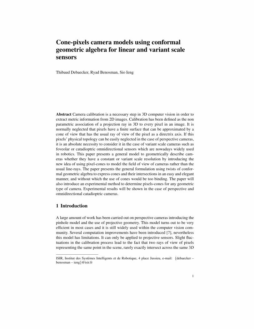
pixels

camera viewpoint

(a) Pixel-cones of a perspective camera.

Pixels

camera viewpoint

mirror viewpoint

Central Mirror

(b) Catadioptric pixel-cones after reflec-tion on a central mirror

Fig. 1 Pixel-cones in the case of perspective cameras and variant scale sensors (here a centralcatadioptric sensor). All cones are almost the same in (a), whereas in (b) the pixel-cones varydrastically according to the position of the pixel within the perspective camera observing the mirror.

point they should represent. Finally this model fails to introduce the reality of thesensor, as the approximation of the field of view of the pixel is restricted to a raythat can not match the real topology of the pixel that corresponds to a surface on theimage plane and not only a point. The limitations pointed out become drasticallyproblematic with the appearance of new kinds of non linear visual sensors like fove-olar retinas [4], or panoramic sensors (see [2] for an overview). As show in Fig. 1(a)in the case of a perpective cameras, the real field of view of pixels is a cone, in theperspective case all pixels produce similar cones of view. Cones being barely thesame, it is easily understandable why cones can be approximated using lines in thiscase. As shown in Fig. 1(b), for a catadioptric sensor (combination of a perspectivecamera and a hyperboloid mirror) it becomes obvious that the approximation usingrays will lead to large imprecisions specially in the computation of intersections,cones become then an absolute necessity. Different methods have been developedto cope with the issue of non perfect intersection of rays in the case of perspectivecameras. Bundle adjustment is one of the major techniques (a complete overview ofexisting methods can be found in [15]), it consists in refining a visual reconstructionto produce jointly optimal 3D structure and more accurate viewing parameters esti-mates. Optimal means that these methods are based on cost function minimizations.This processing can be seen as a consequence of the use of rays rather than cones,as we will show later intersections may happen even if the central rays of pixels donot intersect. Non intersections do not necessarily reflect an imprecise calibrationresult.

As shown in Fig. 2(a), most of the times, two rays do not have an exact inter-section in 3D space. In most cases, they are separated by a distance d which can becomputed easily if the pose information are known. The intersection is consideredacceptable if it is under a certain threshold. The cones defined by the surface of the

Title Suppressed Due to Excessive Length 3

pixel encompass the rays of view of the pixels (Fig. 2(b)), each ray of view corre-sponds to the directrix of each cone. The rays still do not intersect, but as shown inFig. 2(b) the cones do fully meet as the corresponding volume of intersection shownin Fig. 2(c) is not zero. Applying a bundle adjustment in this case will not lead tothe best solution as the perfect intersection of the ray because it does not necessarilycorrespond to the optimal intersection.The aim of the paper is not to compare the bundle adjustment versus projectivepixel-cone of view, but just to show that introducing cones gives the opportunityto be closer to the real physics of the intersection of pixels and thus generate moreaccurate situations. The topic of comparing the bundle adjustment versus volumeoptimization will surely be the topic of following paper. After explaining the im-portance of cones, determining experimentally the cones of a sensor introduces thenecessity of developing a calibration procedure that will be presented in section 3.Among the existing calibration methods, there has been recently an effort to devel-opp new methods that can handle the most general sensors non necessarily central orrelying on caustics ([14, 9]) but in its most most general form as a set of viewpointsand rays of view. The raxel approach [6] gave an interesting model for sensors dif-ferent from the classic pinholes cameras. The association of a pixel and a directionenables a wider range of camera calibration, but does not consider the non linearresolution aspect of the sensors, and the variation of the solid angle of each pixelfield of view. [10] provides also a general geometric model of a camera, but againthe field of view of pixels is not taken into account.

d

Pixel of camera 1Pixel of camera 2

Center ray 2Center ray 1

(a) Two rays of light in a 3Dspace.

d

Pixel of camera 1Pixel of camera 2

(c) Cones intersection

(b) Cones of light.

Fig. 2 Difference between ray of light and cone of light approach.

This paper is structured as follows. After describing in section 2 the mathematicalformulation of the general pixel-cones model using twists [13], an experimentalprotocol to find the pixel cones of light is presented in section 3. Section 4 showsthe results got from this protocol applied on a pinhole camera and a catadioptricsensor. Conclusions and future works are included in section 5.


2 General model of a cone-pixels camera

e2

e1e3

O

A1

A3A4A5

A7

A6

A8

A0

l0

pi,jpi-1,j

pi-1,j+1

t1

t2

A7 A1

A2

A3A4

A5

A6

A8 Ainit

A0

I

A

Fig. 3 Cones Geometric settings.

This section will present the general model of a camera using cone-pixels. Thereare several possible ways to write the equation of a cone. A single-sided conewith vertex V , axis ray with origin at V , unit-length direction A and cone angleθ ∈ (0,π/2) is defined by the set of points X such that vector X −V forms an angleθ with A. The algebraic condition is A · (X −V ) = |X −V |cos(θ). The solid coneis the cone plus the region it bounds, specified as A · (X −V ) ≥ |X −V |cos(θ). Itis quite painfull to compute the intersection of two cones, and this tends to becomeeven more complicated integrating rigid motions parameters between the two cones.Conformal geometric algebra through the use of twists allows to construct a widevariety of kinematics shapes. There exist many ways to define algebraic curves [3],among them twists can be used to generate various curves and shapes [13]. A kine-matic shape is a shape that results from the orbit effect of a point under the action ofa set of coupled operators. The nice idea is that the operators are what describes thecurve (or shape), as introduced in [13] these operators are the motors which are therepresentation of SE(3) in R4,1. The use of twists gives a compact representation ofcones and brings the heavy computation of the intersection of two general cones toa simple intersection of lines. The reader unfamiliar with geometric algebra, shouldrefer to [8, 5] for an overview of geometric algebra, examples of its use in computervision can be found in [11, 12].


2.1 Geometric settings

As shown in Fig. 3 in the case of a perspective camera, the image plane here repre-sented by I contains several rectangular pixels p(i, j), where i, j corresponds to theposition of the pixel. Considering p(i, j), its surface is represented by a rectangledefined by points A0...A8, with A0 corresponding to the center of the rectangle.

Given a line l (with unit direction) in space, the corresponding motor describinga general rotation around this line is given by : M (θ , l) = exp(− θ

2 l). The generalrotation of a point xθ around any arbitrary line l is :

x′θ = M (θ , l)xθ M (θ , l) (1)

The general form of 2twist generated curve is the set of points defined xθ such as :

xθ = M 2(λ2θ , l2)M 1(λ1θ , l1)x0M1(λ1θ , l1)M 2(λ2θ , l2) (2)

In what follows we are interested in generating ellipses that correspond to the valuesλ1 =−2 and λ2 = 1. l1 and l2 are the two rotation axis needed to define the ellipses[13].

Considering a single pixel pi, j (see Fig. 3), its surface can be approximated by theellipse generated by a point A that rotates around point A0 with a rotation axis cor-responding to e3 normal to the plane I. The ellipse E i, j(θ) generated correspondingto the pixel pi, j is the set of all the positions of A :

∀θ ∈ [0, ..,2π], E i, j(θ)= {Aθ =M 2(θ , l2)M 1(−2θ , l1)A0M1(−2θ , l1)M 2(θ , l2) | }

The initial position of A is to Ainit. The elliptic curve is generated by setting thetwo connected twists so that to obtain an ellipse with principal axis (A8A0,A6A0)in order to fit the rectangular surface of the projection of the pixel as shown in Fig.3. It is now possible to generate the cone corresponding to the field of view of thepixel. We set the line l∗0i, j

, cone axis corresponding to pi, j as :

l∗0i, j= e∧O∧A0.

Let the line lOAi, j be the generatrix of the cone. The pixel-cone of view of pi, j is the

cone C i, j defined by :

C i, j(θ) = M (θ , l0i, j)lOAi, jM (θ , l0i, j

) (3)

with M (θ , l0i, j) = exp(− θ

2 l0i, j).The same process is to be applied again after translating the pixel pi, j using

t1 and t2, that corresponds to the translation to switch from one pixel to the other.The projection pi, j of a pixel is moved to a next pixel :

pi+1, j+1 = T 2(t2)T 1(t1)pi, jT1(t1)T 2(t2)


where T (t) correspond to a translation operator in CGA.

2.2 The general model of a central cone-pixel camera

The general form of a central sensor whether it is linear scale (cones vary slightly)or variant scale is the expression of a bundle of cones. All cones C i, j will be lo-cated using spherical coordinates and located according to an origin set as the coneC 0,0(θ), that has e3 as a principal axis. The general form of a central linear scale

(a) A bundle of pixel-conesof a central linear sensor.

(b) A bundle of pixel-cones ofa central variant linear sensor

Fig. 4 Different configurations of pixel-cones, in the case of linear and variant scale sensors. Inred the principal cone according which every other is located.

camera (Fig. 4(a)) is then simply given by :

C i, jφ ,ψ(θ) = M 2(ψ,e23)M 1(φ ,e13)C

0,00,0 (θ)M 1(φ ,e13)M 2(ψ,e23) (4)

with θ , φ denote the spherical coordinates of the cone.The general form of a central variant scale sensor is slightly different. Each conehaving a different size, cones need to be defined according to their position. A coneC i, j

φ ,ψ is then defined by the angle between its vertex and generatrix. Due to the

central constraint, all cones have the same apex. The rotation axis l0i, j of C i, jψ,φ giving

its location is computed from l00,0 of C 0,00,0 is then :

l0i, j = M 2(ψ,e23)M 1(φ ,e13)l00,0M 1(φ ,e13)M 2(ψ,e23) (5)

Its generatrix li, j is defined as:

li, j = M (θ ,e12)l0i, jM (θ ,e12) (6)

The expression of C i, jφ ,ψ can then be computed using equation(3).


2.3 Intersection of cones

The intersection of two cones C im, jmφm,ψm

and C in, jnφn,ψn

can simply be computed using themeet product that results in a set of points of intersection Pm,n between the generatrixlines of the cones :

Pm,n = {C im, jmφm,ψm

∨C in, jnφn,ψn

} (7)

If the intersection exists Pm,n is not empty, the set of points then form a convex hullwhich volume can be computed using [1].

3 Experimental protocol

Cones being at the heart of the model, we will now give the experimental set up ofthe calibration procedure to provide an estimation of the cone of view of each pixelof a camera. The method is not restricted to a specific camera geometry, it relies onthe use of multiple planes calibration ([6, 16] ). As shown in Fig. 5, the camera to becalibrated is observing a calibration plane (in our case a computer screen), the aimis to estimate the cone of view of a pixel pi, j, by computing for each position of thescreen its projection surface SPk(i, j), k being the index of the calibration plane. The

R2,T2 R1,T1R3,T3R4,T4

Reference Camera

Unknownsensor

O

SP (i,j)4 SP (i,j)3 SP (i,j)2 SP (i,j)1

?

Fig. 5 Experimental protocol : Cone construction and determination of the center of projection ofthe sensor. The Ri, Ti represent the rigid motion between the reference camera and the calibrationplanes coordinates system.

metric is provided using a reference high resolution calibrated camera (RC)1 thatobserves the calibration planes. The reference camera uses the calibration planesto determine its parameters, the position of each plane is then known in the RCreference coordinates, and implicitly the metric on each calibration plane too. Theimpact surfaces SPki, j) once determined on each screen lead normally as shown inFig. 5 to the determination of all pixel-cones parameters.

Fig. 6 shows the experimental set up carried out for the experiments. The key-point of the calibration protocol relies then on the determination of pixels’ impactSPk(i, j). The idea is then to track the activity of each pixel p(i, j) while they are(see Fig. 8) observing the screens calibration planes. At each position the screen is

1 6 Megapixel digital single-lens Nikon D70 reflex camera fitted with 18-70-mm Nikkor microlens. The micro lens and the focus are fixed during the whole experiment.


UIS: Pinhole camera640*480Screen calibration plane

in position K

Reference Camera3002*2000

(a) Case of a pinhole camera asUIS.

UIS: Catadioptroc sensor

Reference Camera3002*2000

Mirror

Lens

SensorScreen calibration plane in position K

(b) Case of a catadioptric sensoras UIS.

Fig. 6 Experimental protocol for two kinds of UIS (Unknown Image Sensor) .

showing a scrolling white bar translating on a uniform black background (see Fig.6). The bar will cause a change in the grey level values of pixels when it is in theircone of vision. The pixels’ gray-level increases from zero (when the bar is outsideSPk(i, j)) to a maximum value (when the bar is completely inside SPk(i, j)), anddecreases down to zero when the bar is again outside SPk(i, j). Fig. 8 gives a visualexplanation of the process.

A sensitivity threshold can be chosen to decide pixels’ activation. Using the ref-erence camera calibration results, it is then possible once SPk(i, j) is determined tocompute its edges as the positions of yin and yout , in the RC coordinate system. Thebar is scrolled in two orthogonal directions providing two other edges xin and xout(Fig. 7), the envelope of SPk(i, j) is then completely known. The location and sizeof pixel-cones can then in a second stage be estimated once all SPk(i, j) are known.Cones are computed using the center of SPk(i, j) that give the rotation axis, the en-velope is given by computing rays that pass through all the intersection points of thevertex of each SPk(i, j) corresponding to each pixel (Fig. 5).

p(i,j)

O

xyz

youtyin

xin

xout

Bar scrolling

Screen pose k

SP (i,j)k

Fig. 7 Intersection surface SPk(i, j) between the calibration plane k and the cone C (i, j)

4 Experimental results

The following experiments were carried out using PointGrey DragonFly R©2, with a640×480 resolution and a parabolic catadioptric sensor with a telecentric lens, bothare central sensors. (Fig. 6(a)). Fig. 9 shows cones reconstruction on SP1(i, j) and


y<yin yin<y<youty~yin y~yout y>yout

Bar

p(i,j) value:(Gray-level)

Relative position of the scrolling bar and SP (i,j)

Position of the scrolling bar

(x or y)

Sensitivity threshold

p(i,j) is considered as active.

SP (i,j)kk

Fig. 8 Pixel response according to the scroll bar position: pixel activity.

SP2(i, j) in the case of a pinhole camera. Only few cones were drawn, it is then aexpected result to see repetitive pattern corresponding fields of squares of estimatedpixels impact.

Pose 1

Pose 2

ji

Fig. 9 Cones of view in the case of a pinhole camera.

In the case of the catadioptric camera, it is a geometric truth that the apertureangle of each cone will increase as pixels are far from the optical axis of the camera.This phenomenon is experimentally shown in Fig. 10 where the evolution of thesolid angle of pixel-cones are presented. In principle the solid angle should notdepend on the position of the calibration plane that was used to compute it, thecurves are then very close even if a small bias appears for very large cone-pixelsat the periphery of the mirror where the uncertainties of the measure on the surfacedue to the non linearity of the mirror are the highest.

The method allows the estimation of the position of the central point of the cali-brated sensor. in the case of the pinhole camera the calibration screens were locatedbetween 800− 1050 cm from the reference camera, while the camera to be cali-brated was set few cm far (see Fig. 6). In order to obtain a ground truth data thepinhole camera was calibrated using classic ray method. Three position of the op-tic center are then computed for comparison. the first one is given by the classiccalibration, the second by the intersection of the rotation axis of estimated conesand the last one by the intersection of all rays representing estimated cones. Theresults are shown in Table.1) We notice that a single viewpoint has been found foreach one, the classic ray method and the use of the rotation axis produce very sim-ilar results. There are slight variations in the position of the center using the third


Cone

of vi

ew: S

olid A

ngle

(in sr

)

0.02

10 20 30 40 50 60 70Mirror radius (in mm)

0

0.01

0.03

0.05

0.04

0.06

Fig. 10 Solid angle of view according to the mirror radius.

Table 1 Central projection point estimation coordinates: case of a pinhole camera

Ground Truth Axis estimation Error Apex estimation Error

x -78,33 -78,97 0,65 -78,97 0,65y 45,36 44,07 1,28 44,07 1,29z 45,74 57,89 12,16 57,90 12,16

approach that can be explained by the fact that the calibrated portion of the sen-sor used to estimate cones was limited (55× 60 pixels located around the centerof the image). Concerning the catadioptric sensor, the results show that the conesintersect at a single point. The a combination of a parabola and a telecentric lenscan only produce a central sensor, so far the method proved to be efficient. The es-timation of the position of the viewpoint using the principal axis of the estimatedcones and all the rays that form the estimated cones produce similar results (in mm:x = −23.38,y = 147.55,z = 384.79 and x = −23.32,y = 147.33,z = 385.57). Themean distance between the rotation axis and their estimated single point is 3.71 mm.The mean distance between the apex and their estimated single point is 2.97 mm.

5 Conclusion

This paper presented a general method to modelize cameras introducing the useof cones to give a better approximation of the pixels’ field of view (rather thanthe usual use of lines). We also introduced an experimental protocol to estimatecones that is not restricted to any geometry of cameras. The presented model usedconformal geometric algebra that allowed to handle cones in a simple manner usingtwists. Geometric algebra allows natural and simplified representations of geometricentities without which the formulation of the problem would have been much moredifficult. We are extending the use of cones to non central cameras that are variantscale and for which the use of lines is inadequate. Non central sensors introducemajor improvements in the field of view of robots as they allow a better and a moreadapted distribution of rays that eases the tasks to be performed.


References

1. C. B. Barber, D. P. Dobkin, and H. Huhdanpaa. The quickhull algorithm for convex hulls.ACM Transactions on Mathematical Software, 22(4):469–483, 1996.

2. R. Benosman and S. Kang. Panoramic Vision: Sensors, Theory, Applications. Springer, 2001.3. R. Campbell and P. Flynn. A survey of free-form object representation and recognition tech-

niques. 81(2):166–210, February 2001.4. T. Debaecker and R. Benosman. Bio-inspired model of visual information codification for

localization: from retina to the lateral geniculate nucleus. Journal of Integrative Neuroscience,6(3):1–33, 2007.

5. D.Hestenes and G. Sobczyk. Clifford Algebra to Geometric Calculus. D. Reidel Publ. Comp.,1984.

6. M. D. Grossberg and S. K. Nayar. A general imaging model and a method for finding itsparameters. ICCV, pages 108–115, 2001.

7. R. Hartley and A. Zisserman. Multiple view geometry in computer vision. Cambridge Univer-sity Press, 2003.

8. D. Hestenes. The design of linear algebra and geometry. Acta Applicandae Mathematicae:An International Survey Journal on Applying Mathematics and Mathematical Applications,23:65–93, 1991.

9. S. Ieng and R. Benosman. Geometric Construction of the Caustic Curves for CatadioptricSensors. Kluwer Academic Publisher, Dec. 2006.

10. S. Ramalingam, P. Sturm, and S. Lodha. Towards complete generic camera calibration. pagesI: 1093–1098, 2005.

11. B. Rosenhahn. Pose estimation revisited. PhD thesis, Christian-Albrechts-Universitat zu Kiel,Institut fur Informatik und Praktische Mathematik, 2003.

12. B. Rosenhahn, C. Perwass, and G. Sommer. Free-form pose estimation by using twist repre-sentations. Algorithmica, 38(1):91–113, 2003.

13. G. Sommer, B. Rosenhahn, and C. Perwass. Twists - an operational representation of shape.In IWMM GIAE, pages 278–297, 2004.

14. R. Swaminathan, M. Grossberg, and S. Nayar. Caustics of catadioptric cameras. ICCV01,pages II: 2–9, 2001.

15. B. Triggs, P. McLauchlan, R. Hartley, and A. Fitzgibbon. Bundle adjustment – A modernsynthesis. pages 298–375, 2000.

16. Z. Zhang. A flexible new technique for camera calibration. IEEE Transactions on PatternAnalysis and Machine Intelligence, 22(11):1330–1334, 2000.

cone-pixels camera models using conformal geometric algebra for

Documents