confessions of a team that did interdisciplinary research€¦ · confessions of a team that did...
TRANSCRIPT

Confessions of a Team that did Interdisciplinary Research
Warren Sanderson, Erich Striessnig Wolfgang Schöpp, Markus Amann

Why Confessions?
• Interdisciplinary research is something that many people say they want to do, but few actually admit doing it.

Interdisciplinary Research


The GrandPrograms Involved
• Mitigation of Air Pollution (MAG)
• World Population (POP)

Our offspring
Effects on Well-Being of Investing
in Cleaner Air in India

Take Home Messages
• Interdisciplinary Research can be done.
• It can be fun.
• It can be productive.
What’s in a name?
• Effects on Well-Being of Investing in Cleaner Air in India
• Well-Being
• Cleaner Air

The Model Parents
• GAINS MODEL • Greenhouse Gas and Air Pollution Interactions
and Synergies Model
• SEDIM • Simple Economic and Demographic
Interaction Model

Disciplines
• Energy Systems • Atmospheric Chemistry • Epidemiology • Economics • Demography
The Offspring’s Accomplishments
• “In India, air pollution abatement investments clearly improve well-being.”

Organization
• 1. This Introduction • 2. The GAINS Model – Markus Amann • 3. The SEDIM Model – Warren Sanderson • 4. Putting it all together in a coherent and
publishable package – Erich Striessnig • 5. YSSP research – Haochen Wang • 6. Panel Discussion of Future Interdisciplinary
Research

Economic Growth in a World of Environmental Constraints
The SEDIM Model

Constraints
• The 20th century was the century of growth. • The 21st century is going to be the century of
constraints.
• How can we think about integrating these constraints into an economic model?

Environmental Constraints
• Challenges posed by global climate change • economic costs of necessary abatement
policies modeling the impact of environmental degradation on human health and productivity
• Challenges posed by energy and natural resource scarcity
• substitution technologies transition to renewable energies

Demographic Constraints
• Challenges posed by unprecedented societal aging in • some parts of the world • include realistic demography • think about how aging societies are different from
“stable populations” • Opportunities generated by favorable age-structure
dynamics in others • How to make the most out of a potential
“demographic dividend”? • How to model the ongoing educational transitions?

Challenges for the Economic Growth Modeler
• Any realistic model of economic growth has to
take environmental challenges into account. – The constraints will be different in different parts
of the world – There is enormous uncertainty
Are We Really in Equilibrium
• Many economic growth models assume that we are:
• 1. in equilibrium • 2. have perfect foresight (or rational
expectations) • 3 and therefore there are no surprises. • (we know all our environmental problems
with certainty today)

Do We Believe This?
• In a world of unanticipated environmental
change and unanticipated costs, the assumption of perfect foresight makes no sense.

Out of Equilibrium
• We need a model capable of studying out-of-equilibrium dynamics.

Enter SEDIM
• SEDIM does not assume perfect foresight • agents are characterized by adaptive, forward
looking behavior • they make use of limited common
information on how the economy evolved in the past. . .
• . . . using this information they “plan ahead” and react to surprises.


𝐿𝑡 = � 𝑃𝑃𝑃𝑎,𝑡𝐸𝐸𝑎,𝑡
𝑎𝑎𝑎𝑎(𝑡)
𝑎=𝑎𝑎𝑎𝑎(𝑡)

Capital
• There are two types of capital holders – Consumers – Corporations and wealthy individuals

Capital
• Consumers have income from labor and from capital assets. They save for life-cycle purposes
• Their goal is to smooth consumption over their lifetime.
• BUT consumers have imperfect foresight.

Corporations
• Corporations and wealthy individuals receive income from capital investments.
• Their income depends on the rate of return to capital.
• They do not save for life-cycle consumption smoothing.
Total Factor Productivity

Measuring Well-Being
• In our paper in ES&T, we measured well-being using a version of the UN’s Human Development Index.
• Erich Striessnig will say more about this in a moment.
Challenge
• Reproducing India’s pattern of economic growth as it happened in the past and as it is expected to happen in the future.
• We did this by altering the rate of total factor productivity in a way that was consistent with the policy changes actually observed in India.

Interdisciplinarity
• SEDIM initially contained ideas from two disciplines: – Economics – Demography
• To do the research on India, we added a third discipline: – Epidemiology


The GAINS (Greenhouse Gases - Air Pollutants Interactions and Strategies) model
- Applications in Europe and Asia
Markus Amann Program Director
Mitigation of Air Pollution and Greenhouse Gases

0%
50%
100%
150%
200%
250%
300%
350%
400%
1945 1950 1955 1960 1965 1970 1975 1980 1985 1990 1995 2000 2005 2010
SO2
and
GDP
rela
tive
to 1
970
energy efficiencyimprovements
changes in fuelstructure
(end-of-pipe)emission controls
Actual SO2
Hypothetical GDP(3% growth/yr)
Actual GDP(constant 2000 Euro)
SO2 avoided through
How has pollution been reduced in Europe?
SO2 emissions in Western Europe: A 1970’s perspective

How has pollution been reduced in Europe?
Source: IIASA http://gains.iiasa.ac.at
SO2 emissions in Western Europe: 1945-2010
0%
50%
100%
150%
200%
250%
300%
350%
400%
1945 1950 1955 1960 1965 1970 1975 1980 1985 1990 1995 2000 2005 2010
SO2
and
GDP
rela
tive
to 1
970
Actual SO2
Hypothetical GDP(3% growth/yr)
SO2 avoided through

Source: IIASA http://gains.iiasa.ac.at
Decoupling between GDP and SO2 emissions in Western Europe
0%
50%
100%
150%
200%
250%
300%
350%
400%
1945 1950 1955 1960 1965 1970 1975 1980 1985 1990 1995 2000 2005 2010
SO2
and
GD
P re
lativ
e to
197
0
energy efficiencyimprovements
changes in fuelstructure
(end-of-pipe)emission controls
Actual SO2
Hypothetical GDP(3% growth/yr)
SO2 avoided through
0%
50%
100%
150%
200%
250%
300%
350%
400%
1945 1950 1955 1960 1965 1970 1975 1980 1985 1990 1995 2000 2005 2010
SO2
and
GD
P re
lativ
e to
197
0
energy efficiencyimprovements
changes in fuelstructure
(end-of-pipe)emission controls
Actual SO2
Hypothetical GDP(3% growth/yr)
SO2 avoided through
0%
50%
100%
150%
200%
250%
300%
350%
400%
1945 1950 1955 1960 1965 1970 1975 1980 1985 1990 1995 2000 2005 2010
SO2
and
GD
P re
lativ
e to
197
0
energy efficiencyimprovements
changes in fuelstructure
(end-of-pipe)emission controls
Actual SO2
Hypothetical GDP(3% growth/yr)
SO2 avoided through
0%
50%
100%
150%
200%
250%
300%
350%
400%
1945 1950 1955 1960 1965 1970 1975 1980 1985 1990 1995 2000 2005 2010
SO2
and
GD
P re
lativ
e to
197
0
energy efficiencyimprovements
changes in fuelstructure
(end-of-pipe)emission controls
Actual SO2
Hypothetical GDP(3% growth/yr)
SO2 avoided through
How has pollution been reduced in Europe?

GAINS: A multi-pollutant/multi-effect systems perspective
PM (BC, OC)
SO2 NOx VOC NH3 CO CO2 CH4 N2OHFCsPFCsSF6
Health impacts:PM (Loss in life expectancy) √ √ √ √ √
O3 (Premature mortality) √ √ √ √
Vegetation damage:O3 (AOT40/fluxes) √ √ √ √
Acidification(Excess of critical loads) √ √ √
Eutrophication(Excess of critical loads)
√ √
Climate impacts:Long-term (GWP100)
(√) (√)(√)
(√) (√) (√) √ √ √ √
Near-term forcing √ √ √ √ √ √ (√) √ (√) (√)
Carbon depositionto the Arctic and glaciers √

0
2
4
6
8
10
12
14
16
18
μg/m
3PM
2.5
Origin
Origin of PM2.5 - 2009
Source: IIASA GAINS
0
5
10
15
20
25
μg/m
3PM
2.5
Origin
Lyon, Centre Ville
WHO guideline
Netherlands average of the urban AIRBASE stations

0
5
10
15
20
25
μg/m
3PM
2.5
Origin
Origin of PM2.5 - 2009
Source: IIASA GAINS
Households
Primary PM: Traffic
Sec. PM: Traffic + agri.
Sec. PM: Industry + agri
Primary PM: Industry
Natural
Netherlands average of the urban AIRBASE stations Lyon, Centre Ville

IIASA’s GAINS systems approach for cost-effective emission reduction strategies
There are large international differences in • emission densities, • potentials and costs of further measures, • sensitivities of ecosystems, • meteorological and climatic conditions, etc.
Energy/agricultural projections
Emissions
Emission control options (~2000 measures)
Atmospheric dispersion
Costs
Environmental targets
Optimization
Air pollution impacts,Basket of GHG emissions

Policy applications of GAINS
GAINS has been the key scientific tool for • international environmental
agreements, e.g. • UN-ECE LRTAP • EU air quality and climate
policies
• international assessments • UNEP • IPCC • AMAP

0
50
100
150
200
250
0% 10% 20% 30% 40% 50% 60% 70% 80% 90% 100%
billi
on E
uro/
yr
Gap closure (% between CLE and MTFR)
Emission control costs
Emission control costs
The target of the Thematic Strategy on Air Pollution for 2030
Loss in statistical life expectancy
Current legislation 2030: 5 months life shortening
Maximum additional controls: 3.6 months life shortening
0
50
100
150
200
250
0% 10% 20% 30% 40% 50% 60% 70% 80% 90% 100%
billi
on E
uro/
yr
Gap closure (% between CLE and MTFR)
Benefits range
Emission control costs
Total health benefits vs. total emission control costs
0
1
2
3
4
5
0 10 20 30 40 50 60 70 80 90 100
Mar
gina
l cos
t/be
nefit
s (b
illio
n Eu
ro/%
gap
clo
sure
)
Gap closure (% between CLE and MTFR)
Marginal benefits (range)/%
Marginal costs/%
Optimal range for gap closure
Marginal health benefits vs. marg. emission control costs
Commission proposal: 67% ‘gap closure’ in 2030:
-50% health impacts compared to 2005

Range of future global emissions HTAP/GAINS policy scenarios vs RCP
0
20
40
60
80
100
120
140
160
1990 2000 2010 2020 2030 2040 2050
Mill
ion
tons
RCP
GAINS CLE
GAINS NFC
GAINS MTFR
SO2
0
20
40
60
80
100
120
140
160
180
1990 2000 2010 2020 2030 2040 2050
Mill
ion
tons
RCP
GAINS CLE
GAINS NFC
GAINS MTFR
NOx
0
1
2
3
4
5
6
7
8
1990 2000 2010 2020 2030 2040 2050M
illio
n to
ns
RCP
GAINS CLE
GAINS NFC
GAINS MTFR
BC
Source: GAINS model; ECLIPSE V5 scenario

0.00%
0.05%
0.10%
0.15%
0.20%
Using only airpollution control
measures
Using air pollutioncontrol measures
and GHG measuressimultaneously
Emis
sion
con
trol
cos
ts (
% o
f G
DP
(PPP
) in
203
0)
PM controls,households
PM end-of-pipe measures
NOx end-of-pipe measures
SO2 end-of-pipe measures
Co-generation
Energy efficiency, industry
Energy efficiency, households
Electricity savings
Costs for reducing PM2.5 population exposure in China by 50%
-8% CO2
Cost-effective portfolios to improve air quality include measures that also reduce long-lived GHGs
Co-benefits from an air quality perspective
Source: GAINS-Asia

Conclusions
• GAINS provides an integrated management approach for air pollution and greenhouse gases: multi-pollutant/multi-effect, multiple scale, cost-effectiveness
• GAINS shapes air quality and climate policies in Europe and Asia, provides focus on co-benefits
• GAINS has a long history of policy applications in Europe


Introduction The SEDIM Model Case Study of India Conclusion
Well-being and the Macro-economic Effects ofInvesting in Cleaner Air in India
Warren Sanderson1,2, Erich Striessnig1,3, Wolfgang Schöpp1,Markus Amann1
1International Institute for Applied Systems Analysis (IIASA)
2Stony Brook University (SUNY)
3Vienna University of Economics and Business (WU)
Population Association of America 2013 Annual MeetingNew Orleans, April 12

Introduction The SEDIM Model Case Study of India Conclusion
Outline
1 Introduction
2 The SEDIM Model
3 Case Study of India
4 Conclusion

Introduction The SEDIM Model Case Study of India Conclusion
The Future of Economic Growth Modeling
1 Environmental Constraints2 Demographic Constraints

Introduction The SEDIM Model Case Study of India Conclusion
Environmental Constraints
Challenges posed by global climate changeeconomic costs of necessary abatement policiesmodeling the impact of environmental degradation on humanhealth and productivity
Challenges posed by energy and natural resource scarcitysubstitution technologiestransition to renewable energies

Introduction The SEDIM Model Case Study of India Conclusion
Demographic Constraints
Challenges posed by unprecedented societal agingThink about how aging societies are different from “stablepopulations”
Opportunities generated by favorable age-structure dynamicsHow to make the most out of a potential “demographicdividend”?
Include realistic demography!
How to model the ongoing educational transitions?

Introduction The SEDIM Model Case Study of India Conclusion
The SEDIM Model
SEDIMSimple Economic Demographic Interaction Model
Agents’ are characterized by adaptive, forward looking behavior.
They make use of limited common information on how theeconomy evolved in the past. . .
. . . using this information, they “plan ahead”
They are able to react to “surprises”!
SEDIM does not assume perfect foresight

Introduction The SEDIM Model Case Study of India Conclusion
Case Study
Well-being and the Macro-economic Effects of Investing inCleaner Air in India

Introduction The SEDIM Model Case Study of India Conclusion
PM2.5 in India
Main Research Question:What effect do environmental regulations have on well-being?
Economic growth in India accompanied by tremendous increasesin emission concentration levels.
Policies aimed at implementing stringent emission standardslikely to result in huge health benefits.
We need a model which can balance the health benefits on theone hand and the economic costs on the other.
Introduction The SEDIM Model Case Study of India Conclusion
What is PM2.5?
DefinitionPM2.5 is particulate matter with a diameter of 2.5 microns or less
This stuff kills people!Well documented
Pope et. al. (New England Journal of Medicine, 2009)“[a] decrease of 10 µg per cubic meter in the concentration of fineparticulate matter was associated with an estimated increase in mean(±SE) life expectancy of 0.61 ± 0.20 year (P = 0.004).”Brook et. al. (Journal of the American Heart Association, 2010)“overall evidence is consistent with a causal relationship between PM2.5
exposure and cardiovascular morbidity and mortality.”

Introduction The SEDIM Model Case Study of India Conclusion
What is PM2.5?
DefinitionPM2.5 is particulate matter with a diameter of 2.5 microns or less
This stuff kills people!
Well documentedPope et. al. (New England Journal of Medicine, 2009)“[a] decrease of 10 µg per cubic meter in the concentration of fineparticulate matter was associated with an estimated increase in mean(±SE) life expectancy of 0.61 ± 0.20 year (P = 0.004).”Brook et. al. (Journal of the American Heart Association, 2010)“overall evidence is consistent with a causal relationship between PM2.5
exposure and cardiovascular morbidity and mortality.”
Introduction The SEDIM Model Case Study of India Conclusion
What is PM2.5?
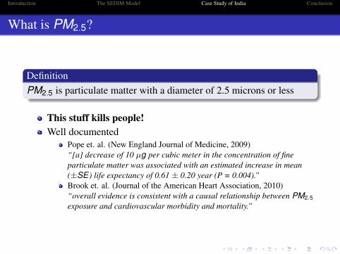
DefinitionPM2.5 is particulate matter with a diameter of 2.5 microns or less
This stuff kills people!Well documented
Pope et. al. (New England Journal of Medicine, 2009)“[a] decrease of 10 µg per cubic meter in the concentration of fineparticulate matter was associated with an estimated increase in mean(±SE) life expectancy of 0.61 ± 0.20 year (P = 0.004).”Brook et. al. (Journal of the American Heart Association, 2010)“overall evidence is consistent with a causal relationship between PM2.5
exposure and cardiovascular morbidity and mortality.”

Introduction The SEDIM Model Case Study of India Conclusion
Why India?
Delhi Mumbai KolkataPM2.5 99 52 73
Table 1 : Ambient concentrations of PM2.5 for various cities in 2005 in µg/m3. Source:GAINS
The WHO-standard for PM2.5 is 10µg/m3!

Introduction The SEDIM Model Case Study of India Conclusion
Why India?
Delhi Mumbai KolkataPM2.5 99 52 73
Table 1 : Ambient concentrations of PM2.5 for various cities in 2005 in µg/m3. Source:GAINS
The WHO-standard for PM2.5 is 10µg/m3!

Introduction The SEDIM Model Case Study of India Conclusion
PM2.5 abatement strategies
Indian Current Legislation (ICL)Controls on dust emissions from the power sector andindustry accounting for national emissions limit values
Low sulfur liquid fuels for the residential, commercialand transport sectors
Slow penetration of improved cooking stoves usingbiomass
CNG for buses and three wheelers in urban areas
Emission limit values for road transport sources up toEuro 4/IV
Emissions of sulfur from the power sector and industryremain uncontrolled
European Current Legislation (ECL)
EU-legislation
stationary sources in the power sector andindustry (Proposal for the Industrial EmissionsDirective)transport sources: phasing-in EU legislation upto EURO 6/IV for road transport and up tostage IV for non-road sources
National legislation on industrial and small combustionsources (if stricter than the EU-wide legislation)
These two policy interventions will be compared to a noadditional-control (NOC) scenario.

Introduction The SEDIM Model Case Study of India Conclusion
Reform Schedule
1 Phasing-in (2010-2019)gradual implementation of the emission regulations set by thereformmodeled as the building up of the total necessary abatementcapital stock
2 Maintenance Phase (2020-2030)abatement capital in place has to be maintained and operatedadditional costs from new facilities that also have to comply withthe new standard
Note: We do not maintain a certain level of PM2.5 concentration,but a certain standard of emissions

Introduction The SEDIM Model Case Study of India Conclusion
Costs and Benefits
Cost as fraction of GDP PM2.5 concentrationYear NOC ICL ECL NOC ICL ECL2010 0.00% 0.15% 0.54% 46 46 462015 0.00% 0.15% 0.55% 60 52 382020 0.00% 0.15% 0.43% 74 57 302030 0.00% 0.12% 0.29% 116 72 31
Table 2 : Cost as a fraction of GDP and PM2.5 concentrations (in µg/m3) in three scenarios,India, 2010, 2015, 2020, 2030. Source: GAINS
In 2005 India spent around 3.8% of GDP on health and 3.23% oneducation (Source: WDI)

Introduction The SEDIM Model Case Study of India Conclusion
Effects of PM2.5 in SEDIM
1 Effect of mortality2 Effect of morbidity

Introduction The SEDIM Model Case Study of India Conclusion
Effects of PM2.5 in SEDIM
1 Effect of mortalityEach additional 10µg/m3 of PM2.5 increases the relative risk ofdying at adult ages (>30) by 4%.
changes the age- and education structure of the populationpeople adapt their savings behaviorchanges in the rate of capital formation as well as changes in thepopulation age- and education structure affect the rate oftechnological change
2 Effect of morbidity

Introduction The SEDIM Model Case Study of India Conclusion
Effects of PM2.5 in SEDIM
1 Effect of mortality2 Effect of morbidity
Each additional 10µg/m3 of PM2.5 increases the number ofwork-loss days by 0.046 (Source: Hurley et. al. 2005)
affects the effective labor force

Introduction The SEDIM Model Case Study of India Conclusion
Results: GDP
YEAR NOC ICL ECL
Total GDP(in Billions)
2010 4.96 1.000 1.0002015 7.16 1.000 1.0012020 9.90 1.000 1.0032030 16.79 1.001 1.007
GDP perCapita
2010 4073 1.000 1.0002015 5514 1.000 1.0012020 7200 0.999 1.0002030 11135 0.996 0.995
GDP perWorker
2010 6713 1.000 1.0002015 8849 1.000 1.0012020 11392 0.999 1.0012030 17308 0.999 1.002
Table 3 : Total GDP, GDP per capita, and GDP per worker in three scenarios, India, 2010,2015, 2020, 2030. Notes: NOC in 2000 international US$. Numbers in ICL and ECL relative toNOC.

Introduction The SEDIM Model Case Study of India Conclusion
Results: Consumption
YEAR NOC ICL ECL
Consumptionper Capita
2010 3065 1.000 1.0002015 4291 0.998 0.9932020 5702 0.997 0.9932030 9213 0.995 0.992
PM2.5
2010 46 46 462015 60 52 382020 74 57 302030 116 72 31
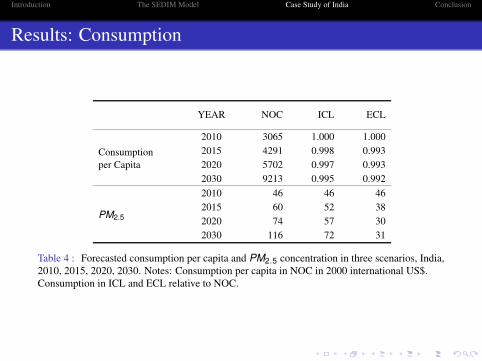
Table 4 : Forecasted consumption per capita and PM2.5 concentration in three scenarios, India,2010, 2015, 2020, 2030. Notes: Consumption per capita in NOC in 2000 international US$.Consumption in ICL and ECL relative to NOC.
Introduction The SEDIM Model Case Study of India Conclusion
Results: Consumption
YEAR NOC ICL ECL
Consumptionper Capita
2010 3065 1.000 1.0002015 4291 0.998 0.9932020 5702 0.997 0.9932030 9213 0.995 0.992
PM2.5
2010 46 46 462015 60 52 382020 74 57 302030 116 72 31
Table 4 : Forecasted consumption per capita and PM2.5 concentration in three scenarios, India,2010, 2015, 2020, 2030. Notes: Consumption per capita in NOC in 2000 international US$.Consumption in ICL and ECL relative to NOC.

Introduction The SEDIM Model Case Study of India Conclusion
Results: Longevity
YEAR NOC ICL ECL
Life Expectancy atBirth
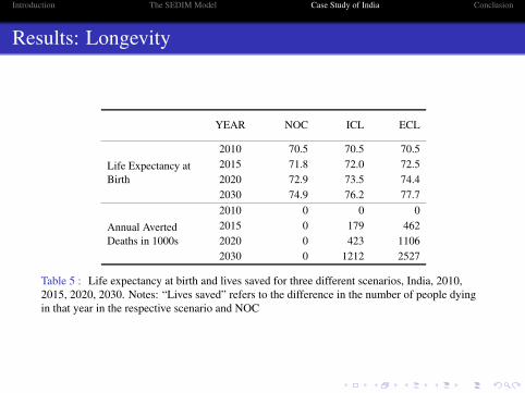
2010 70.5 70.5 70.52015 71.8 72.0 72.52020 72.9 73.5 74.42030 74.9 76.2 77.7
Annual AvertedDeaths in 1000s
2010 0 0 02015 0 179 4622020 0 423 11062030 0 1212 2527
Table 5 : Life expectancy at birth and lives saved for three different scenarios, India, 2010,2015, 2020, 2030. Notes: “Lives saved” refers to the difference in the number of people dyingin that year in the respective scenario and NOC
Introduction The SEDIM Model Case Study of India Conclusion
Results: Longevity
YEAR NOC ICL ECL
Life Expectancy atBirth
2010 70.5 70.5 70.52015 71.8 72.0 72.52020 72.9 73.5 74.42030 74.9 76.2 77.7
Annual AvertedDeaths in 1000s
2010 0 0 02015 0 179 4622020 0 423 11062030 0 1212 2527
Table 5 : Life expectancy at birth and lives saved for three different scenarios, India, 2010,2015, 2020, 2030. Notes: “Lives saved” refers to the difference in the number of people dyingin that year in the respective scenario and NOC
Introduction The SEDIM Model Case Study of India Conclusion
Political implications
In India investments in reducing PM2.5 will have no discernibleeffect on GDP growth
The large increase in longevity outweighs the small decreases inthe mean level of educational attainment and GDP per capita
Well-being is higher than in the NOC in both the ICL and theECL scenario
Policies aiming at reducing PM2.5 in India increasewell-being and almost pay for themselves

Introduction The SEDIM Model Case Study of India Conclusion
THANK YOU!

Introduction The SEDIM Model Case Study of India Conclusion
How does economic growth take place in SEDIM?
One type of output, Yt , is generated, using a Cobb-Douglasproduction function
Yt = At ∗ Lαt ∗ K 1−αt (1)
⇒ Anything that causes economic growth, has to do so by affectingone of these sources:
Lt . . . Effective Labor
Kt . . . Capital Stock
At . . . Total Factor Productivity
(α. . . Output Elasticity of Labor)

Introduction The SEDIM Model Case Study of India Conclusion
Effective Labor, Lt
The workforce in SEDIM includes the full information on thepopulation’s age- and educational attainment structure
Lt =
alfx(t)∑a=alfe(t)
POPa,t ∗ EUa,t (2)
alfe(t) . . . age of labor market entry in year talfx(t) . . . age of labor market exit in year tPOPa,t . . . population at age a in year tEUa,t . . . number of efficiency units embodied by worker
of age a in year t

Introduction The SEDIM Model Case Study of India Conclusion
Capital, Kt
Two types of capital holders
1 Consumers2 Corporations or “wealthy individuals”

Introduction The SEDIM Model Case Study of India Conclusion
Capital, Kt
Two types of capital holders
1 ConsumersIncome from labor and from capital assetsSave for life-cycle purposes
goal is to smooth consumption over their entire lifetimeBUT: suffer from imperfect foresight
2 Corporations or “wealthy individuals”
Introduction The SEDIM Model Case Study of India Conclusion
Capital, Kt
Two types of capital holders
1 Consumers2 Corporations or “wealthy individuals”

Introduction The SEDIM Model Case Study of India Conclusion
Capital, Kt
Two types of capital holders
1 Consumers2 Corporations or “wealthy individuals”
Receive income from capital investmentsNon-life-cycle savers
investment rate depends on rate of return to capital

Introduction The SEDIM Model Case Study of India Conclusion
Capital, Kt
Two types of capital holders
1 Consumers2 Corporations or “wealthy individuals”
The savings/investments of consumers and corporations interact to“buffer” the effect of aging.

Introduction The SEDIM Model Case Study of India Conclusion
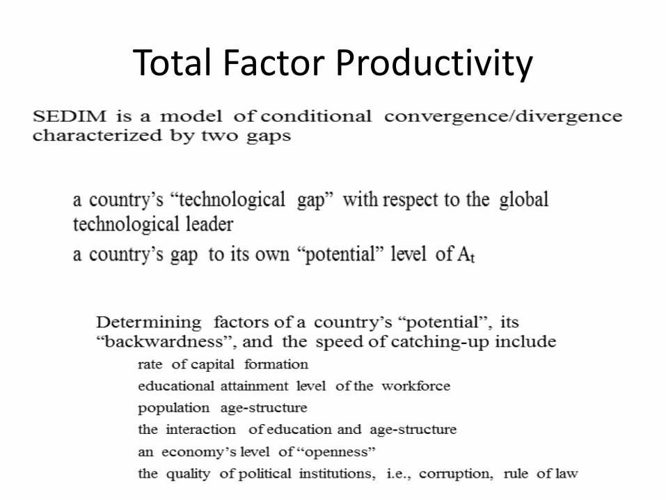
Total Factor Productivity, At
SEDIM is a model of conditional convergence/divergencecharacterized by two gaps
1 a country’s “technological gap” with respect to the global technologicalleader
2 a country’s gap to its own “potential” level of At
Determining factors of a country’s “potential”, its “backwardness”,and the speed of catching-up include
rate of capital formation
educational attainment level of the workforce
population age-structure
the interaction of education and age-structure
an economy’s level of “openness”
the quality of political institutions, i.e., corruption, rule of law

Introduction The SEDIM Model Case Study of India Conclusion
Results: HDI
ICL GCL
GDPLEXEDUTotal
HDI by component relative to NOC, India, 2030
0.00
00.
005
0.01
00.
015