configuration management in manufacturing and …
TRANSCRIPT

Clemson UniversityTigerPrints
All Dissertations Dissertations
12-2015
CONFIGURATION MANAGEMENT INMANUFACTURING AND ASSEMBLY: CASESTUDY AND ENABLER DEVELOPMENTKeith PhelanClemson University, [email protected]
Follow this and additional works at: https://tigerprints.clemson.edu/all_dissertations
Part of the Mechanical Engineering Commons
This Dissertation is brought to you for free and open access by the Dissertations at TigerPrints. It has been accepted for inclusion in All Dissertations byan authorized administrator of TigerPrints. For more information, please contact [email protected].
Recommended CitationPhelan, Keith, "CONFIGURATION MANAGEMENT IN MANUFACTURING AND ASSEMBLY: CASE STUDY ANDENABLER DEVELOPMENT" (2015). All Dissertations. 1591.https://tigerprints.clemson.edu/all_dissertations/1591

CONFIGURATION MANAGEMENT IN MANUFACTURING AND
ASSEMBLY: CASE STUDY AND ENABLER DEVELOPMENT
A Dissertation
Presented to
the Graduate School of
Clemson University
In Partial Fulfillment
of the Requirements for the Degree
Doctor of Philosophy
Mechanical Engineering
by
Keith Thomas Ashman Phelan
December 2015
Accepted by:
Dr. Joshua D. Summers, Committee Chair
Dr. Georges Fadel
Dr. Mary E. Kurz
Dr. Joshua A. Levine
Dr. Gregory M. Mocko

ii
ABSTRACT
The overall goal of this research is to improve the product configuration change
management process. The increase in the demand for highly customizable products has
led to many manufacturers using mass customization to meet the constantly changing
demands of a wide consumer base. However, effectively managing the configurations can
be difficult, especially in large manufacturers or for complex products with a large number
of possible configurations. This is largely due to a combination of the scope of the
configuration management system and the difficulty in understanding how changes to one
element of a configuration can propagate through the configuration system. To increase
the engineer’s ability to understand the configuration management system and how
changes can affect it, an improved method is required.
Based on the results of a case study at a major automotive OEM, a configuration
change management method is developed to address the aforementioned gap. In addition,
a set of design enablers is deployed as part of the method. The major contribution of this
work is the improved method for configuration change management and the use of graph
visualization in exploring configuration changes. The use of graph visualizations for
configuration management is validated through a user study, four implementation studies
using ongoing configuration changes at the OEM, and user feedback and evaluation. The
method is validated through application in three historical cases and user feedback. The
results show that the method increases the capabilities of the engineer in exploring a
proposed configuration change and identifying any potential errors.

iii
DEDICATION
Dedicated to my wife because without her support, I would not have made it this far and
to my parents for always encouraging me to strive for more.

iv
ACKNOWLEDGEMENTS
I sincerely thank my advisor Dr. Joshua Summers. I cannot overstate how much
his guidance has shaped me and my research during my time as a student. He has gone
above and beyond in mentoring me as an engineer, a researcher, and as a person.
I would also like to thank Dr. Fadel, Dr. Kurz, Dr. Levine, and Dr. Mocko for their
assistance as members of my committee. Specifically, I would like to thank Dr. Mocko for
continuing to challenge me to defend my research. This strengthened my belief in the
research and in my ability to present the research.
As most of my research was funded through projects with BMW Spartanburg, I
would like to them for their support and for providing the opportunity to work with them
for the past two and a half years. I would also like to thank the personnel in the Launch
and Change Control group for providing their time and expertise, without which the
research would not have been as successful. I would especially like to thank Matt
Wasatonic at BMW for countless hours of working with me and providing assistance in
whatever capacity was required.
Last, but not least, I thank all of my CEDAR team members, both present and past,
for supporting my research and assisting when called upon. The countless discussions of
research, current events, and, most importantly, college football always provided an outlet
when needed.

v
TABLE OF CONTENTS
Page
Abstract ................................................................................................................... ii
Dedication .............................................................................................................. iii
Acknowledgements ................................................................................................ iv
List of Tables ....................................................................................................... viii
List of Figures ..........................................................................................................x
Chapter One : Introduction ......................................................................................1
1.1 What is Configuration Management? ............................................................1
1.2 Why Configuration and Change Management? .............................................2
1.3 Dissertation Outline .......................................................................................4
Chapter Two : Preliminary Effort – Understanding Change Management .............7
2.1 Current Change Management Practice ..........................................................7
2.2 Study on Product Component Interaction ....................................................31
2.3 Conclusions ..................................................................................................46
2.4 Dissertation Roadmap ..................................................................................48
Chapter Three : Research Approach ......................................................................50
3.1 Research Questions and Tasks .....................................................................52
3.2 Dissertation Roadmap ..................................................................................60
Chapter Four : Configuration Change Management – A Case Study ....................62
4.1 Current Configuration Management Practice ..............................................62
4.2 Research Methods ........................................................................................71
4.3 Selection of the Case ....................................................................................73
4.4 Data Collection ............................................................................................74
4.5 Results ..........................................................................................................77
4.6 Conclusions ..................................................................................................85
4.7 Dissertation Roadmap ..................................................................................87

vi
Table of Contents (Continued)
Page
Chapter Five : Improved Method for Configuration Change Management ..........89
5.1 Proposed Process .........................................................................................89
5.2 Interaction Identification ..............................................................................91
5.3 Visualization and Interaction (V&I) ............................................................93
5.4 Complexity Analysis (CCA) ........................................................................95
5.5 Algorithmic Validation (AV) .....................................................................102
5.6 Conclusions ................................................................................................107
5.7 Dissertation Roadmap ................................................................................108
Chapter Six : Visualization Support Tool ............................................................110
6.1 Data Visualization: Review of Literature ..................................................110
6.2 Graph Layout User Study (Development Study) .......................................114
6.3 Development of the Visualization Tool .....................................................135
6.4 Implementation of the Visualization Tool .................................................139
6.5 Software Development ..............................................................................147
6.6 Conclusions ................................................................................................157
6.7 Dissertation Roadmap ................................................................................159
Chapter Seven : Visualization Tool Validation ...................................................160
7.1 Implementation Cases ................................................................................160
7.2 Rule Authoring User Study (Validation Study) .........................................167
7.3 User Feedback ............................................................................................179
7.4 Conclusions ................................................................................................181
7.5 Dissertation Roadmap ................................................................................182
Chapter Eight : Method Implementation and Recommendations ........................184
8.1 Implementation Cases ................................................................................184
8.2 User Feedback ............................................................................................192
8.3 System Architecture to Support the Configuration Management Method 193
8.4 Conclusions ................................................................................................197

vii
Table of Contents (Continued)
Page
8.5 Dissertation Roadmap ................................................................................198
Chapter Nine : Conclusions and Future Work .....................................................200
9.1 Concluding Remarks ..................................................................................200
9.2 Future Work ...............................................................................................205
REFERENCES ....................................................................................................208
Appendices ...........................................................................................................220
Appendix A: Complete DSM for Historical Example .....................................221
Appendix B: Trendline Graphs for Component Interaction Study ..................222
Appendix C: Example of a Configuration Rule Database ...............................227
Appendix D: Example Configuration Change Request Form .........................228
Appendix E: User Study Response Form ........................................................231
Appendix F: Visualization Tool Development User Study Graphs ................233
Appendix G: Visualization Tool Validation User Study Packets ....................245

viii
LIST OF TABLES
Table Page
Table 2.1: Example requirements table .................................................................18
Table 2.2: Section of an example design structure matrix (DSM) (a) initial and (b)
extended .............................................................................................................................20
Table 2.3: List of affected components for brake drum .........................................21
Table 2.4: E-S-V combination identification .........................................................22
Table 2.5: Combination vectors .............................................................................22
Table 2.6: Filtering of assembly combinations interface .......................................23
Table 2.7: Example DVP matrix ............................................................................24
Table 2.8: Requirements to tests relationships matrix ...........................................25
Table 2.9: Requirements to components relationship matrix ................................26
Table 2.10: Baseline test strategy ..........................................................................27
Table 2.11: Example of a test-analysis matrix .......................................................28
Table 2.12: Component interaction saturation for product architecture ................39
Table 2.13: Component interaction saturation for product configuration .............42
Table 2.14: Product architecture component interaction .......................................44
Table 2.15: Product configuration component interaction ....................................44
Table 3.1: Research Questions and Tasks..............................................................52
Table 4.1: Configuration management to change management mapping table .....69
Table 4.2: Examples of other case-based research in configuration management 70
Table 4.3: Justification for case study research method ........................................72
Table 4.4: Case study interviews conducted ..........................................................75
Table 4.5: Example rules in the rule database .......................................................77
Table 4.6: Visualization requirements and related issues to address .....................86
Table 6.1: Survey question triangulation .............................................................122
Table 6.2: Packet set-variable assignment ...........................................................124
Table 6.3: Number of correct responses for each question by group ..................128
Table 6.4: Percent of correct responses by variable ............................................129
Table 6.5: Average confidence for each question by group ................................129

ix
List of Tables (Continued)
Table Page
Table 6.6: Software platform selection overview ................................................138
Table 7.1: Number and percent of correct responses by group for Change 1 .....175
Table 7.2: Number and percent of correct responses by group for Change 2 .....175
Table 7.3: Number and percent of correct responses by group for Change 3 .....175
Table A.1: Full DSM for Brake Drum Example..................................................221
Table A.2: Example of a configuration rule database ..........................................227

x
LIST OF FIGURES
Figure Page
Figure 1.1: Configuration management entity relationships....................................2
Figure 1.2: Model depicting possible configuration variants (adapted from [4]) ....3
Figure 1.3: Dissertation overview ............................................................................5
Figure 2.1: Change Propagation Model (CPM) [19] .............................................12
Figure 2.2: 3-D CAD model for a pen (a) and the resulting connectivity graph
(b) .......................................................................................................................................35
Figure 2.3: Initial (a) and full populated (b) product design structure matrices for a
pen ......................................................................................................................................36
Figure 2.4: Graph of population densities for a pen ..............................................36
Figure 2.5: Initial (a) and fully populated (b) product configuration DSMs for a
product change ...................................................................................................................37
Figure 2.6: Product group 1 saturation graph ........................................................41
Figure 2.7: Product group 2 saturation graph ........................................................41
Figure 2.8: Product group 3 saturation graph ........................................................41
Figure 2.9: Product group 4 saturation graph ........................................................41
Figure 2.10: Product configuration saturation graph .............................................42
Figure 2.11: Group 1 saturation graph ...................................................................43
Figure 2.12: Group 2 saturation graph ...................................................................43
Figure 2.13: Group 3 saturation graph ...................................................................43
Figure 2.14: Dissertation roadmap .........................................................................49
Figure 3.1: Research plan overview.......................................................................50
Figure 3.2: Dissertation roadmap ...........................................................................61
Figure 4.1: Configuration change management process for OEM ........................81
Figure 4.2: Dissertation roadmap ...........................................................................88
Figure 5.1: Simplified process model with proposed tools....................................90
Figure 5.2: ER diagram for integrated database ....................................................93
Figure 5.3: Example graph for a proposed change ................................................94
Figure 5.4: Example graph edge input file.............................................................98
Figure 5.5: Example data representation for the complexity analysis tool ..........101

xi
List of Figures (Continued)
Figure Page
Figure 5.6: Simpler data representation for complexity analysis ........................102
Figure 5.7: Simplest data representation for complexity analysis .......................102
Figure 5.8: Dissertation roadmap .........................................................................109
Figure 6.1: Node-link diagram of a diesel engine for predicting change propagation
[71] ...................................................................................................................................112
Figure 6.2: Straight-edged graph [119] ................................................................113
Figure 6.3: Curved-edge graph[119] ....................................................................113
Figure 6.4: Functionally arranged graph (a) and circular graph layout (b) .........116
Figure 6.5: Graph colored based on part data (a) or based on interaction type
(b) .....................................................................................................................................117
Figure 6.6: Graph will all information (a) and option information only (b) ........117
Figure 6.7: Classroom layout ...............................................................................119
Figure 6.8: Example of a visualization graph (provided to Groups 1, 7) ............125
Figure 6.9: Modified 100mm confidence scale ...................................................127
Figure 6.10: Graph of the correctness for each question based on availability of
information .......................................................................................................................131
Figure 6.11: Graph of the correctness for each question based on color-coding .132
Figure 6.12: Graph for the correctness of each question based on layout ...........133
Figure 6.13: Graph of the correctness for each question based on order .............134
Figure 6.14: Example graph node input file ........................................................140
Figure 6.15: Example graph edge input file.........................................................141
Figure 6.16: Rule and corresponding graph for an inclusive, binary
relationship .......................................................................................................................142
Figure 6.17: Rule and corresponding graph for an exclusive, binary
relationship .......................................................................................................................142
Figure 6.18: Rule and corresponding graph for a relationship requiring an “OR”
node ..................................................................................................................................143
Figure 6.19: Rule and corresponding graph for a relationship with an “AND” node
..........................................................................................................................................143
Figure 6.20: Additional rule and graph for a relationship with an “AND” node .144
Figure 6.21: Graph visualization for a specific change .......................................144

xii
List of Figures (Continued)
Figure Page
Figure 6.22: Dissertation roadmap .......................................................................159
Figure 7.1: Visualization graph for windshield option change (Case 1) .............162
Figure 7.2: Visualization graph for existing model .............................................163
Figure 7.3: Visualization graph for replacement model ......................................164
Figure 7.4: Existing model graph with the Australian country option already
available ...........................................................................................................................166
Figure 7.5: Graph of the model to which the country option will be added ........167
Figure 7.6: Rule system graph provided to the experimental groups ..................173
Figure 7.7: Percent correct responses for Change 1 ............................................176
Figure 7.8: Percent correct responses for Change 2 ............................................177
Figure 7.9: Percent correct responses for Change 3 ............................................177
Figure 7.10: Dissertation Roadmap .....................................................................183
Figure 8.1: Method for evaluating the existing system........................................185
Figure 8.2: Implemented method for Problem 2 ..................................................188
Figure 8.3: Implemented method for Problem 3 ..................................................190
Figure 8.4: Configuration management support tool system architecture ...........196
Figure 8.5: Dissertation roadmap .........................................................................199
Figure A.1: Trendline for all product architectures .............................................222
Figure A.2: Trendline for Group 1 product architectures ....................................222
Figure A.3: Trendline for Group 2 product architectures ....................................223
Figure A.4: Trendline for Group 3 product architectures ....................................223
Figure A.5: Trendline for Group 4 product architectures ....................................224
Figure A.6: Trendline for all product changes .....................................................224
Figure A.7: Trendline for Group 1 with 1 added product change .......................225
Figure A.8: Trendline for Group 3 with 1 added product change .......................225
Figure A.9: Trendline for Group 4 with 1 added product change .......................226
Figure A.10: Graph for European models with functional grouping and coloring
based on interactions ........................................................................................................233
Figure A.11: Graph for US models with functional grouping and coloring based on
interactions .......................................................................................................................234

xiii
List of Figures (Continued)
Figure Page
Figure A.12: Graph for European models with functional grouping and coloring
based on interactions (options only) ................................................................................235
Figure A.13: Graph for US models with functional grouping and coloring based on
interactions (options only) ...............................................................................................236
Figure A.14: Graph for European models with functional grouping and coloring
based on parts ...................................................................................................................237
Figure A.15: Graph for US models with functional grouping and coloring based on
parts ..................................................................................................................................238
Figure A.16: Graph for European models with circular layout and coloring based
on interactions ..................................................................................................................239
Figure A.17: Graph for US models with circular layout and coloring based on
interactions .......................................................................................................................240
Figure A.18: Graph for European models with circular layout and coloring based
on parts .............................................................................................................................241
Figure A.19: Graph for US models with circular layout and coloring based on parts
..........................................................................................................................................242
Figure A.20: Graph for European models with circular layout and coloring based
on interactions (options only) ..........................................................................................243
Figure A.21: Graph for US models with circular layout and coloring based on
interactions (options only) ...............................................................................................244

1
CHAPTER ONE: INTRODUCTION
1.1 What is Configuration Management?
Configuration management is a method for capturing, verifying, and maintaining
the information regarding how product variants can feasibly achieve customer
requirements. The first aspect of this process is to understand the capabilities and
interrelationships of the components within the product family. Product families, or
“configurable products,” are defined according to the following criteria [1,2]:
Are adapted according to customer requirements [1]
Consist of (almost) only pre-designed components [1,2]
Have a pre-designed product structure [1]
Are adapted by systematic product configuration [1,2]
It is important to note that a key element of these criteria is that the components
that contribute to the product family are well specified, including the relationships between
the components. In this way, the configuration management process is different from
traditional design in that no new component types are created, nor are the interfaces
between components modified in any way [3]. Therefore, a difficulty in configuration
management is in accurately modeling this knowledge.
The second aspect of the configuration management process is to understand the
individual needs of the customer and how the needs can be met through the selection and
integration of specific components. As in the case of the product family domain
knowledge, the customer requirements should all be well-specified when conducting
configuration management. That is, before a new customer requirement should be added

2
as an option within a product family, a coordinating component for achieving that need
must first be identified. This relationship is shown in Figure 1.1.
Figure 1.1: Configuration management entity relationships
While this may seem counterintuitive, the goal of configuration management is not
to develop novel concepts, but rather to produce a new configuration of existing
components that is adapted to the needs of the customer [1].
1.2 Why Configuration and Change Management?
Configuration management is essential to mass customization because without it
the difficulty in managing the potential configurations can hinder the efficient manufacture
of product [3–5]. When viewed from the perspective of assembly lines, the many different
configurations can quickly lead to increases in the possibility of errors [3]. The high
number of configurations available, specifically in the automotive industry, is shown in the
model in Figure 1.2. These errors, depending on where they are identified in the product
life-cycle, can be extremely costly. As a result, configuration management is necessary for
successful manufacture of product families.

3
Figure 1.2: Model depicting possible configuration variants (adapted from [4])
An additional benefit of configuration management is the ability to effectively
conduct change management and product improvement [5]. While a central facet of
configuration management is an understanding of how the components interrelate, when a
change is required on a single component, one may identify how the specified change will
affect the other components within any of the variants in that product family. This includes
manufacturers that rely heavily on modifying existing products in the development of new
designs, as is the case with the intra-organizational benefits of product configuration
identified in a study of an aeronautics manufacturer [5]. As a current product is adapted to
fit new customer requirements, it is easy to identify how the modifications will affect the
other variants in a product family.
The implementation of configuration management also increases the amount of
product control and organizational support of a manufacturer [4,5]. Others describe
configuration management as a basic process within systems engineering that serves as the
“backbone” of many of the core processes that enable efficient manufacture of a

4
configurable product [4]. Similar findings on the benefits of configuration management
were identified in a case study based on interviews with employees in management
positions within an aeronautics OEM [5]. The interviewees all stated that the use of
configuration management practices increased the amount of control of the company over
the product and the product variant development process.
1.3 Dissertation Outline
This section presents an overview of the dissertation, visually depicted in Figure
1.3. Chapter One provides an introduction to the research. This includes the motivation
for the research and some background information on configuration management. Chapter
Two presents the foundation for the research: a review of current change management
practices (including a literature review and the development of a support tool for an
existing change management support method) and a study on product component
interaction. This preliminary research introduced the author to the principles of change
management and developed the interest in change management, specifically with regard to
change management in configurable products or products with multiple variants. Chapter
Three presents the overall research plan for the dissertation. This includes the research
objectives, their corresponding research sub-questions and the tasks that were executed to
achieve the objectives.

5
Figure 1.3: Dissertation overview
Chapter Four begins the process of answering the research questions through the
presentation of an industrial case study on configuration management. The case study and
accompanying literature review are intended to answer the question of how companies
conduct configuration management (RO 1). Based on the findings of the case study, an
improved method for configuration management, including design enabler support, is

6
presented in Chapter Five. The proposed method provides an integrated method that
incorporates support tools from multiple domains (data visualization, algorithmic
validation, and complexity analysis) to assist in the configuration management process.
Chapter Six focuses on the development and implementation of a graph
visualization support tool. The visualization support tool uses relationship information
from the product rule databases to assist in understanding how proposed changes can
propagate in unexpected ways. The validation of the graph visualization tool is presented
in Chapter Seven. This consists of four implementation cases of ongoing configuration
changes at the OEM and a user study to test the effectiveness of the proposed tool for
configuration rule implementation. Chapter Eight consists of a validation of the entire
configuration management support method through additional implementation cases and a
user feedback interview with a change manager at the OEM. Finally, Chapter Nine
concludes the dissertation and provides potential avenues for future research.

7
CHAPTER TWO: PRELIMINARY EFFORT – UNDERSTANDING CHANGE
MANAGEMENT
The purpose of the research presented in this chapter is to understand current
change management practice. This objective is achieved through the execution of three
related tasks: a literature review of change management practices, the development of a
change management support tool based on a verification, validation, and testing planning
method, and a study on component interaction for change propagation. These three tasks
will be discussed in the following sections, with the findings being summarized in 2.3.
2.1 Current Change Management Practice
In order to develop a better understanding of current configuration change
management, a literature review is conducted and a computational support tool is
developed to increase the usability and adoptability of an existing change management
method. These are discussed in Sections 2.1.1 and 2.1.2, respectively.
2.1.1 Literature Review of Change Management Practice
There has been a large amount of research conducted on ways to mitigate the effects
and/or occurrences of engineering change [6–9]. The research can be categorized
according to the following types of mitigation: tools for documentation, tools for decision-
making, and engineering change coping strategies [7].
2.1.1.1 Documentation Tools
The first type of tool involves those used for assistance in documentation and
managing the work flow of the engineering change process. Such tools are recognized as

8
necessary to effectively and efficiently execute engineering changes [6,10]. Engineering
change management systems that are primarily paper-based are typically inefficient in that
the information is largely centralized. As the number of engineering changes of a product
increases, the situation is compounded [6]. The high degree of centralization limits the
ability for all personnel within a company to have access to the changes and understand
how they can affect different operations within the company [11]. Therefore, having the
ability to document and manage change can greatly improve the efficiency of the change
management process by ensuring that all parties are kept current on a change’s status.
As a result, there has been a focus on computer-based systems for documenting the
instances of engineering change over the life of an engineering change. Huang and Mak
[12] use the following classification method for computer-based tools:
Dedicated engineering change management systems: They include databases of
engineering change activities and can generate engineering change forms.
Computer aided configuration management systems: These systems are software-
based engineering change management systems and allow the user to address
product structuring and versioning.
Product data management (PDM) or product life-cycle management (PLM)
systems: These systems incorporate all of the above functionalities and also are
able to encompass all stages of the product life-cycle, such as product planning.
Often, the scope of these systems requires that they be developed externally by
software design companies.
The increase in the use of computer networking in company infrastructures has led
to an increase in academic research into computer-based change management systems
[12,13]. One example, a stand-alone, web-based system for managing the engineering

9
change process, has been developed at the University of Hong Kong’s Department of
Industrial and Manufacturing Systems Engineering [13]. The proposed engineering
change management (ECM) system seeks to remove the limitations due to time and
geography typically found in paper-based systems by using a distributed web-based
system. The major limitation of the system is that it only supports basic ECM functions
and activities. Additionally, no case study regarding implementation or validation of the
tool is provided. Reddi [11,14] presents a framework for engineering change management
based on Service Oriented Architecture that allows for an agile engineering change
management process to be used in a collaborative environment. The primary limitation of
this work is that the tool was not validated with industry data, but rather with previous
research. Additionally, the tool requires an extensive amount of user expertise in order to
estimate the values for parameters used in the process.
Despite the prevalence of commercially available engineering change management
software packages, it has been found that few companies have moved to integrate these
systems [15]. Some possible reasons behind this are [12]:
Companies do not realize the systems are available
Available systems do not meet the needs of the user
Available systems are not worth the difficulty to implement
The systems require too much data input to be time-effective
The technology does not fulfil its functions as promised
In a study of three Swedish engineering companies [16], it was found that none of
the companies used the benefits of computer-based support of change management to their
full potential. However, it is understood that at the time of the report that all of the

10
companies were investing in these computer-based systems. The biggest determining
factor was whether it was more efficient to develop their own software or to revise
commercially available software for use within the company. In a similar review of two
British companies [6], the companies felt that adapting a commercially available system
would be more expensive and time-consuming than developing their own. Thus, cost of
adoption and development appear to be major hurdles in adoption.
The following conclusions are made regarding the current research on
documentation tools for configuration management:
Many of the tools discussed have not been implemented in an industry setting to
validate their usefulness
Difficulty in adopting an existing ECM system leads companies to develop their
own support tools instead
Many of the tools require a large amount of user input in order to fulfill the
required functions
2.1.1.2 Decision-Making Tools
A major emphasis of research on engineering change has been on tools to aid in the
decision-making of the engineering change process. While solid modelling, Failure Mode
and Effects Analysis (FMEA), and Value Analysis are examples of enablers that can be
used in engineering change mitigation, the focus of this section is on methods and research
prototype systems.
Ollinger and Stahovich [17] propose a tool called “RedesignIT,” a computer
program that employs model-based reasoning to create and evaluate proposals for redesign
plans. The program uses the relevant physical parameter of the design and the relationships

11
between the parameters to build the model. The benefit to this tool is that it proposes
modifications to the proposals to mitigate negative effects of the proposed change.
However, it only provides the parameters that should be modified and does not propose
how the quantities should be altered.
Laurenti and Rozenfeld [18] present a modified version of FMEA that specifically
covers the analysis of modifications to a system. The method, Failure Mode and Effect
Analysis of Modifications (FMEAM), was developed based on an integration of FMEA
and Design Review Based on Failure Mode (DRBFM). It incorporates a multi-disciplinary
work group to review engineering changes and the possible failure rates that may be
associated with them. At this point, there has been no validation of the feasibility or utility
of the proposed method.
The Change Prediction Model [19] is a tool for predicting how change will
propagate through a design. This method uses Design Structure Matrices (DSMs) to build
a product model. The product model consists of the relationships between components that
increase either the likelihood or impact of engineering change propagation. By
determining the possible propagation pathways, it is then possible to use the product model
to create DSMs representing the predicted likelihood and risk of a change. From these
DSMs it is possible to predict the possible impact of a change. This model is shown in
Figure 2.1.

12
Figure 2.1: Change Propagation Model (CPM) [19]
This method has also been used in additional research and has been applied in
several case studies [20–22]. A similar method has been proposed that uses DSMs to
determine the second-order relationships between requirements [23]. From these
secondary relationships, they were able to successfully predict how product requirements
would change as a result of an initial requirement change. By modelling the predicted
change early in the design process, during requirements development, it is possible to
minimize the associated costs resulting from an engineering change. The method was
shown to be successful in predicting the resulting changes in two industrial case studies,
but more validation is needed to explore its effectiveness. Another potential negative of
this method is that it requires an initial change in order to be effective.
Change Favorable Representation (C-FAR) [24] is a method that uses product
information to assist in the representation, propagation and evaluation of changes. C-FAR

13
decomposes a product into its basic entities and then represents these entities as vectors,
with the attributes of the entity as components of the vector. The approach then uses
matrices to create relationships between entity vectors, with the individual components of
the matrix being referred to as linkage values. The linkage values represent the relationship
between two attributes (one from each entity) and can be used to determine how change in
one attribute or entity can affect other entities/attributes. The method has been used with
numerous industrial case studies, but because of the high processing power required, it is
only feasible when used with fairly simple products.
The following conclusions are made regarding the current research on decision
tools for configuration management:
Many of the tools discussed have not been implemented in an industry setting to
validate their usefulness
Difficulty in adopting an existing ECM system leads companies to develop their
own support tools instead
Many of the tools require a large amount of user input in order to fulfill the
required functions
2.1.1.3 Engineering Change Mitigation Strategies
While other researchers [25,26] have also proposed strategies for mitigating the effects
of engineering change, Fricke, et al. [15] provides a comprehensive list of strategies:
1. Prevention: Reduce the number of emergent changes of a product. This is often the
majority of changes that occur for a given design [9,27]. It is understood that this can
be extremely difficult to execute effectively.
2. Front-loading: Early detection of engineering changes within the product- life-cycle.
This is in line with the “Rule of Ten” discussed earlier in the paper. The use of

14
concurrent engineering encourages early identification of changes that must be made
to a product. However, due to the ever-changing nature of the market, implementing
this to its fullest extent may prevent the company from changing to meet the latest
needs of the customer, possibly leading to an eventual loss of market share and
profitability.
3. Effectiveness: Conducting analysis on the benefit of executing an engineering change
against the cost of implementation. As previously mentioned, not all engineering
changes are meaningful and/or mandatory. Therefore, it is necessary that design
engineers understand the difference between meaningful and meaningless changes.
4. Efficiency: Implementing engineering changes as efficiently as possible by optimally
using available resources (time, costs, etc.). To facilitate this effort, engineering
changes must be communicated to all contributing parties as quickly as possible. In
some instances, this may be assisted by being flexible with the engineering change
process. Loch and Terweisch promoted this idea by proposing methods to remove
some of the bottlenecks in the process [28].
5. Learning and reviewing: Conducting a review of the engineering change process for
each implemented change. Despite the fact that every change is a chance to improve
upon a company’s engineering change management process, few companies regularly
execute reviews following a change. The United States Army has recognized the
importance of after-action reviews to continuously improve upon previous operations,
mandating that reviews be conducted at all levels.
Additional research has been done that supplements the above strategies. Tavcar and
Duhovnik [26] have developed a questionnaire to assist in the review process that assess
the quality of a company’s engineering change management process. The questionnaire
assesses the process based on a variety of information, including: resources expended in
implementation, duration of the engineering change, change tracking, frequency of

15
decision points, and the accuracy and precision of implementing the change in both
production and documentation. In their review of current engineering change practices,
Jarratt, et al. [8] believe that a fundamental shift away from “ab initio” design advocated
by many systematic design methods, such as the approach proposed by Pahl and Beitz [29],
would lead to increased effort in change research.
2.1.2 Development of a Change Management Support Tool
A recurring theme in review of existing change management practices is that
despite the prevalence of available methods for managing change, the difficulty in adopting
the proposed methods has resulted in many companies not implementing them. To better
understand how existing methods can be adapted to better increase adoptability, a
computational support tool was developed from an existing validation, verification and
testing (VV&T) planning method [30]. The VV&T method was selected due to its
inclusion of variant propagation pathways, which is an aspect that is unique to the method
and is of interest to the researcher. The purpose of this task is to determine how the
methods proposed in academia can be supported to increase their usability by industry and
therefore increase the level of adoption
2.1.2.1 Overview of Method
The purpose of the change management support tool is to assist a change engineer
in executing the validation, verification, and testing (VV&T) planning method discussed
in [30]. The support tool follows the steps outlined in the 7-Step VV&T planning [31]:

16
- Step 1: Identify requirements – identify the requirements for the system at one
level above the sub-system that contains the changed component
- Step 2: Conduct system analysis – determine the other components that are
likely to be affected by the changed component
- Step 3: Identify assembly configurations – identify the potential assembly
configurations for the affected components, including different variants and
suppliers for each component
- Step 4: Filter assembly configurations – determine whether any assembly
configurations can be removed from the VV&T method
- Step 5: Develop design validation plan (DVP) matrix – create the matrix for the
VV&T plan, including administrative data, such as responsibilities and
timelines for the validation of each requirement
- Step 6: Develop test strategy – determine the baseline for each test to be run
- Step 7: Conduct trade-off analysis – identify areas where tests can be combined
and prioritize the validation of specific requirements
2.1.2.2 Tool Requirements
Case studies of applying the method at International Truck and Reliable Sprinkler
led to requirements for the support tool. In addition to the primary requirement (the tool
should easily guide the engineer through the process) other requirements were identified
to mitigate some of the other issues that have been identified when using the 7-step
planning method. One major issue is the large amount of data that must be carried between
the steps, leading to the possibility for human input errors. Additionally, the tool should

17
assist in the documentation of the change management process. The resulting design
problem is as follows: Develop a computational support tool to guide a change engineer
through the 7-step VV&T process while minimizing the opportunity for error and assisting
in documenting the change process without the requirement for additional input.
As previously mentioned, one requirement of the tool was its adoptability. One
reason that support tools developed in academia are not used heavily in industry is the
resistance to new software or interfaces [1]. In order to ensure easy distribution and use of
the computational support tool, it was developed in Microsoft Excel using the Visual Basic
for Applications programming language. This allowed for simplified implementation
while maximizing the functionality of the tool for prototyping purposes.
To determine the appropriate level of automation, each step was analysed to
determine what information and reasoning needed to be supported and what would be
conducted manually. For example, in the first step (Identify Requirements), it is possible
to have the tool import a requirements list from an external source, such as a requirements
document generated and used by the company. However, because the source document
was of unknown origin, the information for this step is manually entered. On the other
hand, the creation of the Design Validation Plan (DVP) matrix is almost completely
automated. The only manual input required for this document is the administrative data,
such as team members and testing responsibility (Table 2.7). Another factor that prevented
automation of a step was the need for experiential knowledge in understanding the specifics
of the engineering change in question. This is shown in the filtering of assembly
configurations (Step 5). Determining which assembly configurations can be neglected is

18
dependent on the system in question. As such, it would be difficult to automate the
identification of which configurations could be eliminated.
Following the best practices for software engineering approaches, the module for
each step was created on an individual basis and then these modules were linked together
[32–34]. The tool consists of a series of spreadsheets that are able to be edited by the user.
Once pertinent data for a given step has been entered, an associated macro may be run to
facilitate the completion of that step in the process. The steps below follow the VV&T
plan development for an example change to the brake drum in an automotive braking
system.
2.1.2.3 Step 1 – Identify Requirements
The first step in the VV&T planning method is the identification of requirements
at the level of the component of interest and one system level above the component being
changed. An example of the requirement data table is shown in Table 2.1. It should be
noted that sections highlighted in yellow are those intended for data entry. This step also
stores the requirements for future use in the process. Note that these are not requirements
on the brake drum, but rather on the encapsulating braking system.
Table 2.1: Example requirements table

19
2.1.2.4 Step 2 – Conduct System Analysis
The next step in the process is a system analysis to identify any components that
may be affected by the component being changed. This interaction can include geometric,
behavioural, variant, and organization propagation pathways. In this step, the engineer
manually enters the design structure matrix (DSM) for the system containing the change
component. Additionally, the external components that interact with the system of interest
are included. The DSM is developed by identifying the relationships between components
in the system. In this example, only physical, geometric relationships are considered.
However, as discussed in the VV&T planning method [31], other possibilities exist for
relationships, such as organizational pathways. It is important to note that building the
DSM is a possible source of human error. A section of an example DSM entered by the
engineer is shown in Table 2.2 (a). The intersections with “1” represent interactions
between the specified components. The same section of the DSM is shown in Table 2.2(b)
and includes higher order interactions. The complete DSMs are found in 9.2Appendix A:.
Any cells containing “2” or higher represent higher order interactions and will be discussed
below. For instance, the brake drum directly interfaces with the brake lining. Because the
brake lining also directly interfaces with the foundation brake, a second order interaction
occurs between the foundation brake and the brake drum.

20
Table 2.2: Section of an example design structure matrix (DSM) (a) initial and (b)
extended
The support tool also requires the entry of the number of components, the change
component, and the desired order of interaction. The desired order of interaction is required
because research has shown that interactions at the second order are often useful in
identifying/predicting change propagation [27]. Once all relevant data has been entered,
the support tool populates the rest of the DSM with any higher order interactions (the
second order of interaction was desired in the example in Table 2.2) and a list of all of the
components affected by the change component is created. Based on the DSM from the
example in Table 2.2, the following list was created, as shown in Table 2.3. Thes
components will then be used in the next step.

21
Table 2.3: List of affected components for brake drum
2.1.2.5 Step 3 – Identify Assembly Configurations
The third step in the process is the identification of possible assembly
configurations. Each component affected by the engineering change (from list in Table
2.3) may have multiple variants and multiple suppliers. Therefore, when considering a
VV&T plan, it is necessary to determine all of the combinations that may need to be tested.
Testing all of the possible component combinations would be equivalent to a full-factorial
design of experiments, and while thorough, this may or may not be feasible. To support
this, the tool populates a list of components, while the engineer enters information
regarding the suppliers and variants possible for each component. Once the data is entered,
each element-supplier-variant (E-S-V) combination is given a unique identifier and the
total number of E-S-Vs for each component is tallied. This is shown in Table 2.4. For
example, the hub has two different variants from two different suppliers, while the brake
lining has the same variants from different suppliers.

22
Table 2.4: E-S-V combination identification
The tool also allows the engineer to remove any combinations from being evaluated
and provides an area for comments regarding the reasoning behind the removal. For the
example in Table 2.4, E-S-V 3.S5.V6 is not used because that specific variant of the tire
and wheel trim is not used in the platform being tested. It is important to note that the
removal of specific E-S-V combinations from the list of possible configurations is
manually executed by the engineer. The support tool also provides a list of all of the
combination vectors (possible combinations of different E-S-V combinations) for further
evaluation. The results from this are shown in Table 2.5. The list of combinations then
undergoes additional filtering in the following step.
Table 2.5: Combination vectors
Affected ElementsSupplier
(S#)
Variants
(V#)
E-S-V
Identifier
Combination
selection?
(Y or N)
Selection
reasoning
Number of
E-S-V
combinations
S1 V1 1.S1.V1 Y
S2 V1 1.S2.V1 Y
S3 V3 2.S3.V3 Y
S4 V4 2.S4.V4 Y
S5 V5 3.S5.V5 Y
S5 V6 3.S5.V6 N
Brake Lining 2
Hub
1
2
Variant 6 is not
used in this
platform
Tire and Wheel Trim
23
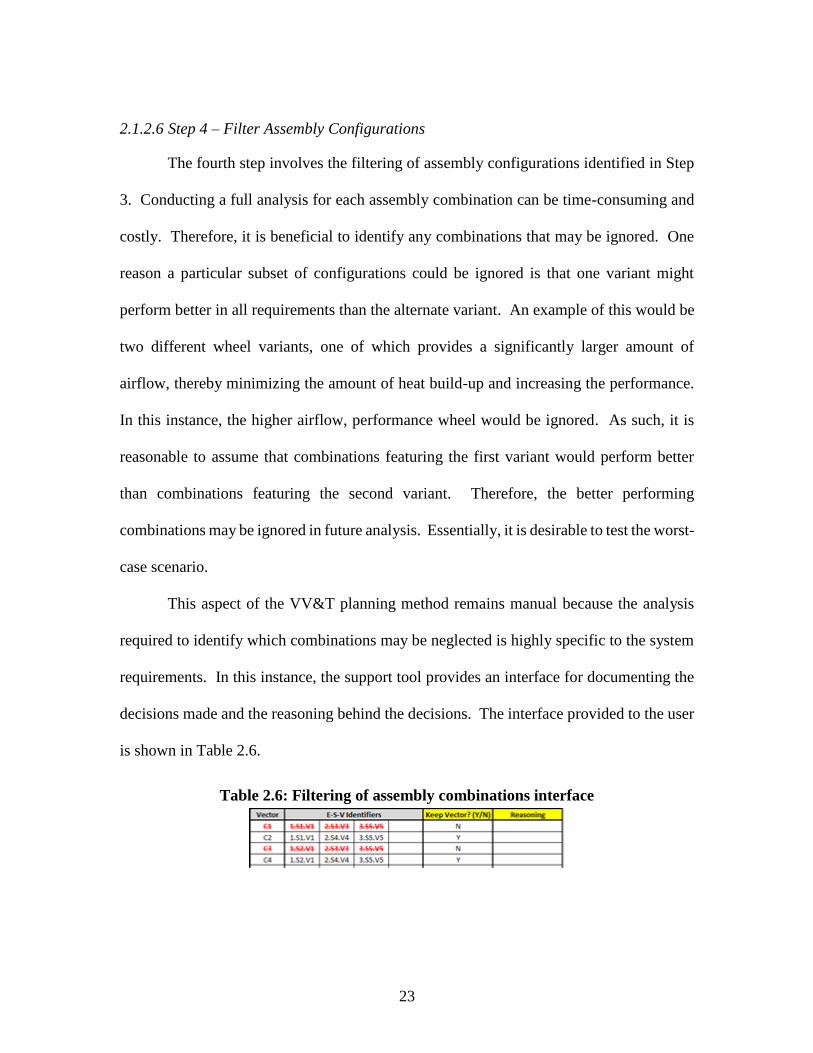
2.1.2.6 Step 4 – Filter Assembly Configurations
The fourth step involves the filtering of assembly configurations identified in Step
3. Conducting a full analysis for each assembly combination can be time-consuming and
costly. Therefore, it is beneficial to identify any combinations that may be ignored. One
reason a particular subset of configurations could be ignored is that one variant might
perform better in all requirements than the alternate variant. An example of this would be
two different wheel variants, one of which provides a significantly larger amount of
airflow, thereby minimizing the amount of heat build-up and increasing the performance.
In this instance, the higher airflow, performance wheel would be ignored. As such, it is
reasonable to assume that combinations featuring the first variant would perform better
than combinations featuring the second variant. Therefore, the better performing
combinations may be ignored in future analysis. Essentially, it is desirable to test the worst-
case scenario.
This aspect of the VV&T planning method remains manual because the analysis
required to identify which combinations may be neglected is highly specific to the system
requirements. In this instance, the support tool provides an interface for documenting the
decisions made and the reasoning behind the decisions. The interface provided to the user
is shown in Table 2.6.
Table 2.6: Filtering of assembly combinations interface

24
As shown in the example in Table 2.6, two of the combinations were neglected. As
a result, the associated cells were highlighted and marked through for ease of visualization.
The remaining combinations are stored for use in future analysis.
2.1.2.7 Step 5 – Develop Design Validation Plan (DVP) Matrix
The next step in the VV&T planning method is to construct the Design Validation
Plan (DVP) matrix. The DVP matrix consists of all of the administrative data as well as
all of the requirements, associated tests, and any additional information regarding how the
testing will be executed. An example DVP matrix is shown in Table 2.7. At present, much
of the administrative data must be entered manually, while 70% of the testing data is
populated by the tool. In Table 2.7, R1 is the requirement for a stopping distance of less
than 60 feet. The method to validate is a vehicle test as per FMVSS 121, with stopping
distance being the test measurable. The combinations vectors to be tested are C2 and C4.
Table 2.7: Example DVP matrix
Date
System
Req.
IndexRequirement Test
Combination
vectors
V & V
method
Test
measureable
Acceptance
criteria
Need for legal
certificationResponsibility Start date End date Remarks
R1Stopping
distance <60ft
As per
FMVSS 121C4, C2,
Vehicle
test
Distance in
ft.
As per
FMVSS 121Y A 07/10 08/10
R2
Stopping dist
<75ft after down
hill test
As per
FMVSS 121C4, C2,
Vehicle
test
Distance in
ft.
As per
FMVSS 121Y A 07/10 08/10
R3Brake lining life
>40000 miles
Fit lining
in field
vehicle
C4, C2,
Field
Demonst
ration
Lining wear
in in.
Average
life >40000
miles
N B 07/10 10/10
Manufacturing
Service
Supplier
Program #
DVP Ver #
DVP #
Development engineer
Team
Virtual test engineer
Physical test engineer
Requirements doc #
Marketing

25
In order to assist in the creation of the DVP matrix, additional data must be entered
elsewhere. The support tool uses a test database to store all information regarding the tests
that must be executed to evaluate the system.
Additionally, two separate matrices are required to aid the creation of the DVP
matrix. The matrices identify the relationships between the requirements and the system
components and between the requirements and the tests. Examples of these matrices are
shown in Table 2.8 and Table 2.9. The purpose of the two matrices is to relate the system
components and possible tests to the design requirements. Having this information allows
the engineer to focus on the aspects of the VV&T plan that are most relevant. Entering the
relationship information into the matrices is another potential source for human error as the
requirements to component information is likely to be determined based on experiential
knowledge. In the example, the brake lining life requirement relates only to the field
vehicle test as the other test only considers the performance during a single braking event.
Table 2.8: Requirements to tests relationships matrix
As
per
FM
VSS
12
1
Fit
linin
g in
fie
ld v
ehic
le
0
T1 T2 0
Stopping distance <60ft R1 Y
Stopping dist <75ft after down hill test R2 Y
Brake lining life >40000 miles R3 Y
0 0
Requirements x Tests
Re
qu
ire
me
nts
Tests

26
When relating the requirements to the components, the example shows that the
brake lining life requirement only relates to the brake lining and is not affected by the hub
or the tire and wheel trim.
Table 2.9: Requirements to components relationship matrix
All of the components, tests and requirements are automatically retrieved from
elsewhere in the support tool in order to reduce user data entry. Only the relationship data
is required to be manually entered during this stage of the process.
2.1.2.8 Step 6 – Develop Test Strategy
The sixth step in the VV&T planning method is to develop a baseline test strategy
to evaluate the requirements. The purpose of this step is to identify the acceptance criteria
for any tests that must be conducted, oftentimes based on the performance values for the
existing design. Once again, this step is highly specific to the system being evaluated and
requires the data to be entered manually. The support tool assists in this step by providing
Bra
ke C
ham
ber
Bra
ke L
inin
g
Axl
e
Hu
b
Tie
and
Wh
eel T
rim
Engi
ne
Inst
rum
ent
Pan
el
Fram
e
C4 C5 C12 C13 C14 C15 C16 C17
Stopping distance <60ft R1 Y Y
Stopping dist <75ft after down hill test R2 Y Y
Brake lining life >40000 miles R3 Y
0 0
Requirements x Components
Components
Re
qu
ire
me
nts

27
a table consisting of all of the tests identified in the DVP matrix with cells for each of the
information requirements. An example of the interface is shown in Table 2.10.
Table 2.10: Baseline test strategy
2.1.2.9 Step 7 – Conduct Trade-Off Analysis
The final step in the process is to conduct a trade-off analysis for the tests and
requirements to be conducted based on the DVP matrix. It is not always feasible to conduct
every test or to test every requirement due to cost or lead time restrictions. Therefore, it is
essential to prioritize which tests to conduct given certain parameters. The VV&T planning
method used in the development of this tool focuses on the requirements to be tested, as
opposed to the tests available to be run. The method uses the Verification Complexity
Index (VCI) to determine the complexity of verifying an individual requirement [1]. While
other methods for developing a testing plan exist, the VCI is chosen in the VV&T planning
method because it focuses on the requirements as opposed to the tests. The VCI is
calculated using the following equation:
(1) * ( * )severity testsVCI req num PI
In order to facilitate this, the support tool provides the requirements and tests from
the DVP matrix. The user enters the severity of each requirement, the cost and lead times
for each test, and the number of tests to verify each requirement as described in the VV&T
# TestBaseline
CombinationBaseline Test Description
Acceptance Criteria for the
modified design
T1As per FMVSS
121C3
With existing vehicle, identify
stopping distance
New system should be on par with
existing vehicle
T2Fit lining in
field vehicle

28
method. The tool calculates the VCI for each requirement and ranks them. An example of
the trade-off analysis matrix is shown in Table 2.11.
Table 2.11: Example of a test-analysis matrix
In the example shown in Table 2.11, a severity is entered for each requirement. The
severity is based on how necessary each requirement is. For instance, 9 would be a legal
requirement, whereas 1 would be less important. The tests are then populated on the table,
with the number of iterations of the test that are required to verify each requirement being
below the test identifier. Also in the same column are the cost and lead time per test, where
a high number indicates a relatively high cost or lead time. This indicates the relative
cost/time to the company for the tests. The scale can be adjusted to conform to company-
specific definitions. The performance indicator for each test is the cost multiplied by the
lead time. At this point, the VCI can be calculated according to Equation 1 and the
requirements are ranked accordingly.
Requirement 1 (R1) has the highest VCI in Table 2.11, which implies that the
change engineers should focus on that requirement to consider for trade-off and
T1 T2 0 0 0 0 0 0 0 0
R1 9 1 3 2268 1
R2 9 3 2187 2
R3 3 1 27 3
0
0
0
0
0
3 9
3 9
9 81 0 0 0 0 0 0
RequirementSeverity
(1/3/9)
Tests (# iterations req'd) Verification
complexity
index
Ranking
Performance indicator
Lead time/Test (1/3/9)
Cost/Test (1/3/9)

29
prioritization. The tool also allows the user to visualize how specific tests can possibly
verify multiple requirements.
2.1.2.10 Conclusions
The VV&T planning method the research in this section is based on [31] has been
shown to effectively mitigate change propagation resulting from an in-production
engineering change. However, the large amount of data entry involved and the planning
method’s reliance on an engineer’s experience can hinder the application of the method in
complex engineering systems.
The computational support tool described in this section successfully addresses
these issues. The support tool was shown to correctly guide an engineer through the
implementation of the VV&T planning method for a historic example of an engineering
change in an automotive brake assembly. The support tool also minimized the
opportunities for human error by carrying data over between the process steps. When
manually conducting the planning method for the described example, the user would have
to enter and keep track of 193 data points. With the implementation of the tool, the user
was required to manually input data in 129 locations. Therefore there was a 33% reduction
in the number of opportunities for human error. It should be noted that this is a fairly
simple system and the results would increase as the system becomes more complex.
Additionally, the support tool conducts all calculations and any analysis required for
evaluating change propagation beyond just the first order of interaction.
Without any additional input required from the user, the support tool provided
documentation to show how the prescribed VV&T planning method was implemented.

30
The documentation includes the requirements list, a list of the affected components, the
DVP matrix, the baseline test strategy, and the trade-off analysis. Additionally, the support
tool provides space to specify why individual decisions were made regarding the design of
the VV&T plan
Additional research needs to be conducted in order to improve the trade-off analysis
functionality of the computational support tool. Currently, the trade-off analysis is
conducted based solely on the Verification Complexity Index (VCI), which focuses on the
importance of verifying individual requirements, combined with the costs and lead times
for the associated tests. However, depending on the scope and characteristics of the
engineering change being made, different companies will have different goals in executing
the trade-off analysis. For instance, in certain situations, a requirement associated with an
engineering change may have legal ramifications and needs to be implemented
immediately. As a result, the company would likely focus on tests that focus on the legal
requirement and can be conducted with minimal lead time. Therefore additional trade-off
metrics need to be determined that can allow companies to determine which criteria are
most important and guide the testing plan in that direction.
Another area of future research is to consider the level of change propagation when
managing the effects of engineering change. As previously discussed, the support tool
allows for the consideration of change propagation beyond the first order. However, it is
not clear to what level the change propagation should be considered. Further research into
this area is discussed in the following section.

31
2.2 Study on Product Component Interaction
During the development of the change management support tool, the question was
asked about how deep one must traverse the relation graph to ensure complete exploration.
In order to answer this question, a study was conducted on product component and option
interaction using design structure matrices.
2.2.1 Background
Before executing the study, a review of design structure matrices, their use in
change management and understanding change propagation, and the use of complexity
metrics for understand product architecture was conducted.
2.2.1.1 Design structure matrices
Design structure matrices (DSM) are commonly used to better understand and
analyse product architectures [35]. DSMs can be used to model product architecture,
organizational structure, information flow, and design parameter relationships [35]. Others
extend the research by providing a review of the benefits of applying DSMs in
understanding product architecture, while acknowledging that a major limitation of DSMs
is that they are only applicable in a single domain [36]. The domain mapping matrix
(DMM) maps the interactions between DSMs from different domains [37]. Similarly,
DSMs are used to characterize complex systems by decomposing them down into clusters
or "building blocks" [38]. DSMs have also been used to explore how software architectures
can be managed [39], introducing architectural metrics, derived from the software
architecture DSMs, that can be used in development.

32
As DSMs become more prominent in engineering design, the number of proposed
applications in which DSMs can be implemented has increased [40]. An early example of
using DSMs to predict some aspect of product development resulted in a proposed method
to predict the time required for product development [41]. This time prediction model uses
the amount of dependencies between product development tasks to determine how required
changes to specific tasks will affect the other tasks. Other applications include product
configuration [42], modelling engineering design activities [43], and product modularity
[32].
2.2.1.2 Change propagation
As DSMs provide an effective method for both viewing and analysing the
interactions between components [21], they are commonly used to better understand
change propagation within a product or system. Based on a study on engineering changes
and how the interactions between product components could be used to better understand
change propagation through the product, a DSM-based engineering change management
tool was created to assist in product development [44]. DSMs have been used to understand
change propagation in a complex system by decomposing the system into interacting
subsystems [20]. The change requests over the system’s life-cycle was related to one
another by considering the decomposed subsystems from which they originated.
DSMs have also been used to predict change propagation. Based on the use of
DSMs in understanding change propagation, the Change Prediction Method (CPM)
software tool was developed to assist in visualizing the possible change propagation
pathways from a single component prior to the execution of an engineering change [19].

33
Since its development, the CPM tool has been implemented in case studies, demonstrating
the effectiveness of using DSMs to predict change propagation in a system [45,46]. While
the CPM tool focuses on change propagation in the product development process, the
DSMs primarily consist of product components with the change indices being subjectively
assigned.
Additional research on predicting requirements change has been conducted using
DSMs linking product requirements [23]. A historical based approach was used with many
different relationship sets to determine which combinations yielded the best predictors. A
significant conclusion from this research is the fact that using higher order DSMs,
specifically at the second order of interaction, is necessary to best predict future changes
to requirements. Thus, the question at hand is whether second or higher order interactions
are critical in other DSM applications for understanding and, eventually, predicting change.
To better answer this question, one may consider how product complexity could play a role
in increasing change propagation within a system or product.
2.2.1.3 Product complexity
When considering product structural or connectivity complexity, 29 different graph
theory metrics have been used for evaluating a product or system to predict assembly time
from component assemblies [47]. However, when focusing on how complexity can
influence change propagation within a product, the researchers focused on the complexity
metrics that primarily looked at the interactions between the components. This mirrors the
concept of complexity as coupling that is proposed in [48], with an initial algorithm based
on decomposability proposed to determine connectivity complexity. Using this algorithm,

34
a simple experiment was conducted using the proposed metric to evaluate multiple existing
products represented in different model types [49]. The experiment showed the importance
of coupling when considering complexity in a product's architecture. Similarly, the
connective complexity in a system was used to model and understand design tasks [50].
Using connectivity metrics, the researchers were able to identify patterns and infer
additional relationships within the system.
2.2.2 Approach
The approach used in this portion of the research consists of two phases. The first
phase is the development of the DSMs from models of existing products. The second phase
consists of the analysis of the products based on how the individual components or
elements interact beyond the first order of interaction. The analysis is done based on both
assembly models and also on product configuration (option) graphs.
2.2.2.1 Product architecture
In the development of the product assembly-based DSMs for this study, previous
models are used to address issues of research objectivity and bias. The DSMs allow one
to draw comparisons between the physical attributes of the product and the data on how
the product’s components interacted. This was especially beneficial in looking for patterns
between different products that exhibit similar interaction behaviours. Previous work was
done to create connectivity graphs of all of the physical interactions between components
within a product based on the analysis of a 3-D CAD model [47]. Figure 2.2 shows an
example of a 3-D CAD model and the corresponding connectivity graph. In the work

35
presented here, the types of relationships between components (elements) are not studied,
rather only the adjacency topology of the system architecture is investigated. Specifically,
the relationships in Figure 2.2(b) are capturing when parts are touching.
Figure 2.2: 3-D CAD model for a pen (a) and the resulting connectivity graph (b)
Using the connectivity graphs, it was possible to construct a DSM for each of the
products being analysed. It is important to note that these DSMs created from the
connectivity graphs only include physical interactions identified in the associated 3-D CAD
models. An example of the resulting DSM is shown in Figure 2.3(a). The second phase
begins with the identification of component interactions beyond the first order. The DSMs
are then populated with the higher order interactions. A higher order interaction is an
interaction between two components through other components. For example, in Figure
2.2(b), a second order interaction exists between the body and the grip body through the
rubber grip. An example of a completed DSM with higher order interactions is shown in
Figure 2.3(b). The cells in the DSM indicate the shortest path length between the
components, or the minimum order of interaction between components.

36
Figure 2.3: Initial (a) and full populated (b) product design structure matrices for a
pen
The final step is to calculate the population density of the DSMs at each order of
interaction. The population density refers to the percentage of existing interactions
compared to the total number of possible interactions. The population density includes any
interactions that take place up to and including a given order. In the example of the pen
(Figure 2.3(b)), the population density for the 1st order would be 33.33% (14 interactions
out of a possible 42). Then, for the 2nd order, the population density is 57.14% (24
interactions out of 42 possible interactions). The complete graph for the population
densities for all orders of interaction is shown in Figure 2.4.
Figure 2.4: Graph of population densities for a pen
Component Name A B C D E F G
Grip Body A 1 1 1
Rubber Grip B 1 1
Press Button C 1 1
Spring D 1 1
Ink Body E 1 1
Body F 1 1
Indexer G 1
Component Name A B C D E F G
Grip Body A 1 3 1 1 2 4
Rubber Grip B 1 2 2 2 1 3
Press Button C 3 2 4 4 1 1
Spring D 1 2 4 1 3 5
Ink Body E 1 2 4 1 3 5
Body F 2 1 1 3 3 2
Indexer G 4 3 1 5 5 2

37
Another statistic used to analyse the data is the average shortest path length applied
against the entire graph. The shortest path length for a given component is the minimum
number of steps required to reach every other component in the system. Therefore, the
average shortest path length for the DSM is the average for all of the relations in the system.
In the example shown in Figure 2.2, the maximum shortest path length for "press button"
to reach each of the other components is 4. By averaging the path lengths in the example,
the average maximum shortest path length is 4.143 (average of all values in its row).
2.2.2.2 Product configuration
In addition to considering propagation in products, product configuration data was
also evaluated. The purpose of this aspect of the research is to determine how DSMs for
product configuration are similar to DSMs for product architecture. This is of interest in
that it is important to understand change propagation in configuration management,
especially when using rule-based configuration management [51]. An example DSM for
product configuration is shown in Figure 2.5(a) considering 14 options. These are related
through option rules. This DSM represents the options found in a single change request.
Figure 2.5: Initial (a) and fully populated (b) product configuration DSMs for a
product change
Option Name A B C D E F G H I J K L M N
161 A
167 B 1
169 C 1 1
1CB D 1
2VB E 1
6UF F 1
823 G 1
842 H 1 1
843 I 1 1 1
858 J 1
8EB K 1
8S9 L 1
991 M 1 1 1 1 1 1
9AE N 1
Option Name A B C D E F G H I J K L M N
161 A
167 B 2 2 2 2 1 2
169 C 2 2 1 1 2
1CB D 2 4 1 3 4
2VB E 2 2 2 2 1 2
6UF F 2 2 2 2 1 2
823 G 2 4 3 1 2
842 H 1 1 3 2 3
843 I 1 3 1 2 1
858 J 2 4 2 3 1
8EB K 2 2 2 2 1 2
8S9 L 2 2 2 2 1 2
991 M 1 1 1 1 1 1
9AE N 2 2 2 2 2 1

38
In Figure 2.5(a), the elements of the DSM are product options that might be selected
independently or within packages by a customer. They relate to other options by a series
of rules that might be either engineering based or marketing focused. In the DSM, the
connections, through the rules, are shown by 1st order interactions in the DSM. For
example, in Figure 2.5(a), Option 167 is directly related to Option 991 through a
configuration rule. Using the same method discussed previously, a higher order DSM is
created. Figure 2.5(b) shows the resulting higher order DSM based on the DSM in Figure
2.5(a). When analysing product configurations, two levels of DSMs are used: a full
configuration ruleset, consisting of approximately 600 components connected by 1400
rules; and a series of configuration DSMs created by considering the affected components
from historical changes implemented at an automotive OEM. The DSMs are created by
starting with the options affected by the change. The rest of the DSM is populated using
the 1st and 2nd order interactions stemming from the initial change components. In the
example shown in Figure 2.5, the graph is not fully populated due to clustering in the
ruleset. For example, option 161 is not connected to any other options, while options 169,
1CB, 823, 842, 843, and 858 for a cluster and do not interact with any options outside of
the cluster. Once the higher order DSM is created, the same analysis is conducted as with
the product architecture DSMs. The purpose behind this is to use the conclusions drawn
from analysing product architecture and apply it to product configuration.
2.2.3 Results
The results were compiled for component saturation rates and higher order
component interaction levels.
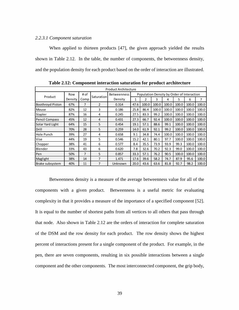
39
2.2.3.1 Component saturation
When applied to thirteen products [47], the given approach yielded the results
shown in Table 2.12. In the table, the number of components, the betweenness density,
and the population density for each product based on the order of interaction are illustrated.
Table 2.12: Component interaction saturation for product architecture
Betweenness density is a measure of the average betweenness value for all of the
components with a given product. Betweenness is a useful metric for evaluating
complexity in that it provides a measure of the importance of a specified component [52].
It is equal to the number of shortest paths from all vertices to all others that pass through
that node. Also shown in Table 2.12 are the orders of interaction for complete saturation
of the DSM and the row density for each product. The row density shows the highest
percent of interactions present for a single component of the product. For example, in the
pen, there are seven components, resulting in six possible interactions between a single
component and the other components. The most interconnected component, the grip body,
1 2 3 4 5 6 7
Boothroyd Piston 67% 7 2 0.314 47.6 100.0 100.0 100.0 100.0 100.0 100.0
Mouse 82% 12 3 0.186 25.8 86.4 100.0 100.0 100.0 100.0 100.0
Stapler 87% 16 4 0.245 27.5 83.3 99.2 100.0 100.0 100.0 100.0
Pencil Compass 45% 12 4 0.431 27.3 66.7 92.4 100.0 100.0 100.0 100.0
Solar Yard Light 64% 15 5 0.454 19.1 57.1 88.6 99.1 100.0 100.0 100.0
Drill 70% 28 5 0.259 14.0 61.9 92.1 99.2 100.0 100.0 100.0
Hole Punch 39% 27 4 0.658 9.1 34.8 74.4 100.0 100.0 100.0 100.0
Vise 44% 19 5 0.546 15.2 42.1 80.1 97.7 100.0 100.0 100.0
Chopper 38% 41 6 0.577 8.4 35.5 73.9 93.9 99.3 100.0 100.0
Blender 33% 43 6 0.620 7.8 32.6 70.2 92.3 99.0 100.0 100.0
Pen 50% 7 5 0.857 33.3 57.1 76.2 90.5 100.0 100.0 100.0
Maglight 38% 14 7 1.471 17.6 39.6 58.2 74.7 87.9 95.6 100.0
Brake subsystem 40% 11 7 Unknown 20.0 43.6 63.6 81.8 92.7 98.2 100.0
Row
Density
Population Density by Order of Interaction
Product Architecture
Product# of
CompSaturation
Betweenness
Density

40
interacts with three components out of the possible six. Therefore, the pen has a 50% row
density. The row density was considered as it may help to explain why some of the
saturation rates behave as they do.
Using visual inspection, one can separate the resulting graphs into groupings of
products that exhibit similar curves. Figure 2.6 shows the first grouping, consisting of the
stapler and the computer mouse. These curves exhibit quick saturations (3rd order) with a
steep initial slope. The second grouping is depicted in Figure 2.7 and consists of the pencil
compass, solar yard light, and the electric drill. The curves of this group exhibit slightly
slower saturations (4th order) and resemble a parabola. Figure 2.8 contains the third
grouping, consisting of the 3-hole punch, an electric food chopper/processor, a pony vise,
and an electric blender. These curves exhibit medium saturation order (4th/5th orders) and
have a slight “s-curve” as the order of interaction is increased. The final grouping is shown
in Figure 2.9 and consists of the pen, a Maglite flashlight, and the brake subsystem
modelled in the motivating project. The curves of this group exhibit slow saturations (5th-
7th orders) and are parabolic in shape. Trendlines that represented all of the points for each
product within the grouping were created using cubic polynomials. The resulting R2 values
are as follows: Group 1 – 0.9797; Group 2 – 0.9895; Group 3 – 0.9791; Group 4 – 0.9559.
The R2 value for the trendline from all of the product curves together is 0.8663. The
complete graphs showing the trendlines can be found in 9.2Appendix B:. It should be
noted that all of the trendlines were created using third order polynomials. The noticeable
increase in R2 values when the product curves are combined indicates that the groupings
are correct.

41
Figure 2.6: Product group 1 saturation
graph
Figure 2.7: Product group 2 saturation graph
Figure 2.8: Product group 3 saturation
graph
Figure 2.9: Product group 4 saturation graph
Similar results were created for four product configuration change DSMs from the
automotive OEM. The results are shown in Table 2.13. The resulting graphs for the
product configuration changes are shown in Figure 2.10. When a trendline is created for
the product configuration change curves, the R2 value is 0.2175. Much of this is due to
two of the curves not reaching 100% saturation.

42
Table 2.13: Component interaction saturation for product configuration
Figure 2.10: Product configuration saturation graph
When the product configuration subsets are considered alongside the products,
three of the changes (1, 2, 4) fit within three of the product groups. The resulting graphs
are shown in Figure 2.11, Figure 2.12, and Figure 2.13. It should be noted that Change 3
and the complete ruleset were not able to be matched to a specific group due to the low
maximum population density. When considering product configurations, it is common that
there will be clusters of product options that do not interact in any way with other clusters.
It the case of the complete ruleset, this was much more severe, with only 16.17% of the
possible interactions existing at maximum saturation (reached in the 10th order). When
trendlines for the three groups are created, the following R2 values are achieved: Group 1
1 2 3 4 5 6 7 8 9 10 11
Change 1 35% 38 7 8.3 32.6 50.9 61.5 73.7 92.9 100.0 100.0 100.0 100.0 100.0
Change 2 80% 26 N/A 21.5 71.1 78.8 78.8 78.8 78.8 78.8 78.8 78.8 78.8 78.8
Change 3 46% 14 N/A 12.1 34.1 37.4 39.6 39.6 39.6 39.6 39.6 39.6 39.6 39.6
Change 4 50% 17 5 19.9 52.9 86.8 98.5 100.0 100.0 100.0 100 100 100 100
Complete Ruleset 6% 395 N/A 0.63 2.24 4.63 7.26 10.35 13.29 15.12 15.92 16.14 16.17 16.17
Saturation# of
Comp
Population Density by Order of Interaction
Product Configuration
Row
DensityProduct

43
– 0.8533; Group 3 – 0.9197; Group 4 – 0.9408. The complete graphs can be found in
9.2Appendix B:.
2.2.3.2 Higher order component interaction
The average shortest path length is also considered as a method for better
understanding component interaction within a system. By applying the outlined approach
to the product DSMs, the following results table was created and is shown in Table 2.14.
Figure 2.11: Group 1 saturation graph
Figure 2.12: Group 2 saturation graph
Figure 2.13: Group 3 saturation graph

44
Table 2.14: Product architecture component interaction
In addition, the same approach was used to analyse the product configuration
DSMs. The resulting data is shown in Table 2.15.
Table 2.15: Product configuration component interaction
Visual inspection of both the product architecture and product configuration
datasets show that the average shortest path length and the order for complete saturation
are closely related. A larger sample population would be required for a more robust
correlation analysis. However, it is clear from the results that the relationships between
average shortest path length and complete saturation of the DSM are similar for both
Product Row Dens. Saturation Avg Path Comp
Boothroyd Piston 67% 2 2.00 7
Mouse 82% 3 2.58 12
Stapler 87% 4 3.50 12
Pencil Compass 45% 4 2.94 16
Solar Yard Light 64% 4 3.64 27
Drill 70% 5 4.14 7
Hole Punch 39% 5 4.00 15
Vise 44% 5 3.89 28
Chopper 38% 5 4.05 19
Blender 33% 6 4.71 41
Pen 50% 6 4.98 43
Maglight 38% 7 5.86 14
Brake subsystem 40% 7 5.45 11
Product Architecture
Product Row Dens. Saturation Avg Path Comp
Change 1 35% 7 (100%) 6.16 38
Change 2 80% 3 (78.8%) 2.42 26
Change 3 46% 4 (39.6%) 2.36 14
Change 4 50% 5 (100%) 4.00 17
Complete Ruleset 6% 11 (16.17%) 3.26 395
Product Configuration

45
product architecture and product configuration. Therefore, one can be used as a substitute
for the other.
2.2.4 Analysis
When the betweenness values are compared to the saturation curves for the four
product groupings, a correlation is suggested; as the betweenness density decreases, the
slope of the saturation curve increases, or the individual components more quickly interact
with all of the other components through higher order interactions. It can also be noted
that the betweenness density values for those products within a group are similar when
compared to the values for the other products (for example, all of the products in group 3
have values between 0.54 and 0.66). This shows that as the slope of the saturation curve
increases, the interconnectivity (betweenness) of the product increases.
Because of the familiarity with the products involved, it was possible to identify
additional relationships regarding the product groupings with respect to the product
architecture. It was noted that the products in group 4 exhibited a stacked-linear assembly
structure [53], which likely corresponds to a decreased saturation rate as components only
directly interact with neighbouring components along the body of the product. On the
opposite end of the spectrum, those products in group 1 all exhibit chassis product
architectures similar to the spokes of a wheel [53], where a single body or frame component
interacts with a large percentage of the other components in the product. This would
correspond with a rapid saturation rate as any given component would quickly interact with
the other components through higher order interactions as soon as it interacts with the

46
central frame/body component. Additionally, the high amount of interactions for a single
component is also shown in the row density statistic provided.
Average shortest path length is another metric often used when considering the
complexity of a system as it correlates to the level of interconnectedness of the components
in the system [47,50,54]. In the analysis of component interaction a clear relationship is
identified between the average shortest path length and the order of interaction at which
the DSM is fully saturated. This shows that as the level of interconnectivity of the system
increases, the DSM saturation rate also increases.
When comparing the metrics for product architecture and product configuration, it
is clear that the metrics for analysing product complexity can also be applied to evaluating
the complexity of a product configuration subset or even the entire product configuration
ruleset. This analysis is based on the similarities that were identified between the different
types of DSMs and the fact that the saturation graphs for the product configuration subsets
were able to be matched closely with the graphs depicting product architecture.
2.3 Conclusions
The research objective that is covered in this chapter is to increase understanding
of existing industry practices for conducting change management. This objective was
accomplished through three related sub-questions, discussed below.
The first sub-question is: What is the state-of-the-art for engineering change
management? In order to answer this question, a literature review of change management
practice was conducted. The literature review consisted of an analysis of engineering
change and change propagation, followed by a discussion of existing change management

47
tools and methods, including their usefulness and shortcomings. In the literature review,
it was identified that numerous tools and methods exist for engineering change
management. However, it was also noted that much of the research conducted in academia
is not put into practice in industry. The primary reasons for this include costs and difficulty
of adopting the methods or tools proposed by researchers.
The answers to the first sub-question directly tie into the second question: How can
the existing change management practices be improved to further enhance usability and
efficiency? To answer this question, a computational support tool was developed and
evaluated based on an existing change management planning method. The planning
method selected for adoption into a tool was chosen due to its focus on variant change
propagation, something that was not seen in the other change management support
methods. The resulting support tool was developed with an emphasis on increasing
adoptability and minimizing costs, while also increasing change management capabilities.
The support tool was evaluated using a case example and showed a significant decrease in
the potential for human entry error, as well as an ability to automatically document the
steps and decisions taken in the change management process.
During the development of the change management support tool, the question was
asked regarding the depth required to sufficiently evaluate the effects of change
propagation. The led to the final sub-question for this research objective: When
considering change propagation, what order of interaction is required to verify affected
components? In order to answer this question, a study was conducted on component
interaction. In the study, design structure matrices (DSMs) were created based on product

48
assembly models and option configuration rulesets. The DSMs were then evaluated based
on how quickly the components interacted with all of the other components through higher
order interactions. Through the study, it was found that the second or third order is
recommended when considering change propagation, though this is dependent on the
system and the change in question. Additionally, it was identified that interaction
saturation rates could be a useful metric when evaluating or describing the complexity in a
system.
2.4 Dissertation Roadmap
The motivation for this dissertation was an interest in product configuration, with
an emphasis on configuration change and configuration management practices. Chapter
Two presented the research in current change management practice that led to the author’s
interest in dynamic configuration management. Since this chapter has provided the
foundation for the remainder of the research, the next chapter (Chapter Three) builds on
this by presenting the research objectives of the dissertation. The progress of this
dissertation is shown in Figure 2.14 in which the completed portion is highlighted in green.

49
Figure 2.14: Dissertation roadmap

50
CHAPTER THREE: RESEARCH APPROACH
Once again, the goal of this research is to understand how configuration change
management is conducted in industry in order to increase the capabilities of the
configuration change management process through method development. An overview of
the research path followed is shown in Figure 3.1.
Figure 3.1: Research plan overview
In order to address this goal, the research is divided into three separate, but related,
objectives. The first objective consists of the preliminary work that led to the proposed
research: understanding existing industry practice for change management (Chapter Two).
This includes a review of current literature regarding engineering change management

51
methods and strategies. An existing method for identifying possible change propagation
pathways is selected and used to develop an engineering change management support tool
[55]. This method was selected in part because of its focus on understanding change
propagation through variant pathways. During the development of the support tool, a
question asked was about how far into a change propagation pathway is necessary to
identify affected components for verification. This led to a study into how design structure
matrices (DSMs) can be used to understand component and configuration option
interaction and interconnectedness [56]. As shown in Figure 3.1, the lessons learned from
the preliminary research were applied to product configuration to assist in understanding
and improving configuration change management.
The second research objective is to understand how a major automotive OEM
conducts configuration management (Chapter Four). The purpose of the second objective
is to develop a better understanding of product configuration management. The approach
taken to develop this understanding was through case study analysis at a major automotive
OEM to identify how the company conducts configuration management. A review of the
literature on configuration management in other industries and in academia provides
insight to determine if the processes identified in the case study are in line with the state-
of-the-art and relevant best practices [51]. As shown in Figure 3.1, the knowledge gained
from this objective is used to develop an improved configuration change management
method.
The third objective includes the development of an improved method for
conducting product configuration change management (Chapter Five). To accomplish this,

52
a visualization support tool was developed to assist in understanding the potential
implications of configuration changes and to increase the user’s ability to explore a
proposed change (Chapter Six). Additionally, the use of complexity metrics and a
satisfiability engine are explored in support of the method. During the development of the
visualization support tool, a user study was conducted to investigate the relationship
between specific graph parameters and the user’s ability to read and interpret the graph
[57]. To validate the effectiveness of the visualization method, a second user study was
employed (Chapter Seven). Further, the visualization tool was used in four ongoing
configuration changes at the automotive OEM. Additional validation is presented for the
overall configuration change management method through three select cases where the
benefit of the method was evaluated (Chapter Eight).
3.1 Research Questions and Tasks
Nine specific tasks were defined to answer these research questions. Table 3.1
illustrates the research objectives and their related tasks. These tasks are detailed further
in the following sections.
Table 3.1: Research Questions and Tasks
Research
Objectives Research Sub-questions Tasks
RO 1-
Understanding
existing industry
practice for change
management
RQ 1.1 What is the state-of-the-art for
engineering change management?
Task 1A: Review of
change management
practice
Task 1B: Support tool
development
Task 1C: Component
interaction study
RQ 1.2 How can the existing change management
practices be improved to further enhance usability
and efficiency?
RQ 1.3 When considering change propagation,
what order of interaction is required to verify
affected components?

53
RO 2- Understand
how an OEM
conducts
configuration
change
management
RQ 2.1 What is the state-of-the-art for
configuration management?
Task 2A: Review of
current configuration
management practices
Task 2B: Case study
with automotive OEM
RQ 2.2 How does a major automotive OEM
conduct configuration change management?
RO 3 –
Development of an
improved method
for configuration
change
management
RQ 3.1 How can data visualization be used to
increase the ability to understand component
relationships in a system?
Task 3A: Review of
visualization
techniques
Task 3B: Graph
layout user study
Task 3C: Rule
implementation user
study
Task 3D:
Implementation
RQ 3.2 Does the implementation of a graph
visualization design enabler assist in identifying
errors and understanding the relationships in a
proposed configuration change?
RQ 3.3 Does the proposed method assist in
identifying errors and understanding the
relationships in the possible product
configurations?
3.1.1 RO 1: Understanding existing industry practice for change management
The preliminary portion of this research began with a review of existing change
management practice. This is shown in the first research sub-question for the objective:
RQ 1.1: What is the state-of-the-art for change management practice?
The question is answered through a literature review of engineering change and
change propagation and the existing change management support tools to manage the
changes (Task 1A). The purpose of this task is to gain a better understanding for change
management in industry and identify areas where the existing practices can be
supplemented to increase their effectiveness and/or usability. During the review of existing
support tools it is identified that a significant gap exists between change management
methods proposed by academia and the methods in use by industry [15].

54
This led to the development of the second sub-question:
RQ 1.2: How can the existing change management practices be improved to further
enhance usability and efficiency?
To answer this research question, an existing change management support method
was selected and developed into a computational support tool to assist in its implementation
(Task 1B). The VV&T method was selected due to its inclusion of variant propagation
pathways, which is an aspect that is unique to the method and is of interest to the researcher
[30]. The purpose of this task is to determine how the methods proposed in academia can
be supported to increase their usability by industry and therefore increase the level of
adoption. During the development of the change management support tool, the question
was asked about how deep one must traverse the relation graph to ensure complete
exploration.
This led to the creation of the third sub-question:
RQ 1.3: When considering change propagation, what order of interaction is
required to verify affected components?
To answer this research question, a study is conducted on component interactions
using design structure matrices (Task 1C). In the study, component interactions (option
rules and touching parts) were used to identify how a change could potentially propagate
through a system at higher orders of interaction. The purpose of this task is to gain a better
understanding of component interaction in product architecture and configuration rulesets
and determine whether similar patterns exist between them.

55
3.1.2 RO 2: Understand how an OEM conducts configuration change management
In addition to regularly changing their products to remain current, many companies
also use multiple possible configurations to reach the needs of individual customers [58].
In the last decade, there has been a widespread shift in manufacturing from mass production
to mass customization, such as making multiple configurations from a single product
platform, which enables companies to maintain the efficient production practices
associated with mass production, while targeting specific customers [58,59]. Due to the
increased use of product configuration as a means towards mass customization, a large
amount of research has been conducted to develop tools for possible use in configuration
management [3,60–68]. However, research has shown that there is a significant gap
between the latest methods and tools developed in academia and what is being used in
industry [1]. If companies are not using the proposed methods, then it is necessary to
understand why the companies are not using those methods and what practices they are
using instead.
The first step in achieving this objective is to build a knowledge base regarding
configuration management practices in industry. This led to the research sub-question:
RQ 2.1: What is the state-of-the-art for configuration management?
This question is answered through a literature review of configuration management
and the existing configuration change management methods (Task 2A). The purpose of
this task is to gain a better understanding of configuration management in industry and aid
in identifying the specific practices in use at the OEM during the case study. While the
literature review provides a broad spectrum of knowledge regarding configuration

56
management practice, it does not provide the required level of detail regarding an
individual company’s practices.
This led to the development of the second sub-question:
RQ 2.2: How does a major automotive OEM conduct configuration change
management?
This question is answered through a case study on the configuration management
practices at a major automotive OEM in Spartanburg, SC (Task 2B). The manufacturer
was chosen as the preferred case because the company uses a large, but unknown, number
of configurations for each of the vehicle models and, therefore, must be able to identify
how configuration changes will impact the system. For example, in the current
configuration management method, the OEM uses over 600 rules to manage over 400
options that relate to approximately 1500 parts for a single vehicle model, resulting in
greater than 108 interactions between the elements. As a result of the large number of
elements affecting the possible configurations, proper configuration management is
essential.
The case study in Task 2B consists of data gathering through interviews, document
analysis, and direct observations of employees executing configuration change
management over a one year period. The purpose of the case study is to identify how the
manufacturer conducts configuration and configuration change management. Finally,
opportunities to improve the existing configuration management practices at the OEM are
recommended.

57
3.1.3 RO 3: Development of an improved method for configuration change management
In order for configuration management to be an effective process, the large amount
of data that is available to the engineer must be readily accessible and easy to understand.
It was shown in [51] that rule-based configuration management is used in the automotive
OEM being studied, as well as in numerous other manufacturers [69,70]. A major issue
that was identified with respect to rule-based configuration management is the difficulty in
making changes to the system and in determining the accuracy of the system. This is
primarily due to the scale of the ruleset that is required to completely specify the system
[3]. Previous research has shown that different visualization techniques can simplify the
process of analyzing large or complicated data sets. As previously stated, the scale of the
problem identified in the case study (greater than 108 possible interactions) results in the
problem being an ideal opportunity for the implementation of alternate data visualization
techniques. Therefore, it is necessary to develop additional resources to support the
visualization of the data found in the ruleset when using rule-based configuration
management.
The level of complexity involved in rule-based configuration management makes
it difficult to understand how changes can have unintended consequences throughout the
configuration system. Previous research has shown that data visualization can be useful
when considering complex systems [71–73]. This leads to the first sub-question for this
research objective:
RQ 3.1: How can data visualization be used to increase the ability to understand
component relationships in a system?
58
This question is answered through a review of data visualization techniques,
specifically focusing on graph visualization and their usefulness for identifying
relationships in complex systems (Task 3A). The purpose of this task is to determine how
data visualization has been used previously and then to determine whether the use of
visualizations would be beneficial in configuration change management. It was found that
using graph visualizations, based on past studies, could increase the capabilities for
understanding and managing changes to the configuration system.
Once it was determined that graph visualizations could be used in the new method,
it was necessary to identify which factors would affect the usefulness of the graph
visualization. This question is answered through a user study (Task 3B). The user study
was conducted with the specific purpose of determining which factors (layout, amount of
information, and color scheme) had the greatest effect on the usability of the graph
visualizations. The participants were provided with different variations of a portion of the
configuration system and were asked questions about different aspects of the rules or how
specific rule changes could affect the entire system. From the results, it was found that the
amount of information presented had the greatest influence on the participants’ ability to
answer questions about the rule system. After the completed development of the
visualization support tool, the next step was to evaluate its usefulness.
This led to the second sub-question:
RQ 3.2: Does the implementation of a graph visualization design enabler assist in
identifying errors and understanding the relationships in a proposed configuration change?

59
This question was partially answered through a second user study (Task 3C) to
determine whether the implementation of a graph visualization tool would increase the
accuracy and consistency of rule implementation into the configuration system. Further,
training was tested to determine its impact on usability. It was found that with limited
training, the graph was comparable to the existing method used by the personnel at the
OEM. Additionally, the visualization group showed the greatest improvement in
answering questions requiring a greater level of analysis.
The research question was also answered through using the visualization tool in
four ongoing configuration changes at the (Task 3D). In these changes, implementing the
visualization method allowed the users to better explore the effects of the proposed change
and identify potential conflicts. Additionally, a time study showed that the visualization
would allow the user to conduct the same analysis in approximately one fourth of the time
required in the current process.
While graph visualization is useful for understanding relationships between
components, certain aspects of configuration management require different reasoning
solutions, such as the ability to validate the system and identify conflicts. Thus, two
additional design enablers for conflict detection and complexity analysis are implemented
alongside graph visualization in the proposed method. The next step was to evaluate the
usefulness of the overall method.
The led to the third sub-question:
RQ 3.3: Does the proposed method assist in identifying errors and understanding
the relationships in the possible product configurations?

60
The research question was answered through implementing the proposed method
on three configuration changes (Task 3D). When applying the proposed method to the
three configuration changes, it was shown that the proposed method increases the user’s
capabilities when validating proposed configuration changes. Feedback obtained from a
formal interview with a primary user of the method, personnel from the Launch and
Change Control group at the OEM, showed that implementing the proposed method when
evaluating configurations would increase the group’s capability to correctly identify errors
and prevent future issues resulting from a proposed change. Additional informal feedback
received throughout the development of the proposed process supports also this conclusion.
3.2 Dissertation Roadmap
Chapter Three presented the discussed the research objectives and provided an
overview of the dissertation. With the structure of the dissertation established, the next
chapter (Chapter Four) begins the exploratory portion of the dissertation. In the following
chapter, a case study of an automotive OEM is presented to illustrate how companies
conduct configuration management. The progress of this dissertation is shown in Figure
3.2 in which the completed portion is highlighted in green.

61
Figure 3.2: Dissertation roadmap

62
CHAPTER FOUR: CONFIGURATION CHANGE MANAGEMENT – A CASE
STUDY
The purpose of the research in this chapter is to identify how a company conducts
configuration change management. Specifically, the research aims to better understand
how an individual manufacturer that heavily employs mass customization principles in its
manufacturing process implements configuration and change management to adapt to the
varied and changing needs of production. Based on the findings identified in the research,
recommendations are made to increase the effectiveness of configuration and change
management practices in industry.
4.1 Current Configuration Management Practice
A variety of techniques have been developed to assist in the implementation of
configuration management [5,42,66,74–77]. For the purposes of this research, the
classification scheme proposed in [3] is used to facilitate discussion of the different existing
methods. To examine the different methods, the type of reasoning is used as the central
comparison characteristic, specifically rule-based, model-based, and case-based reasoning
[78]. Viewing configuration management as an instance of engineering change
management is an additional facet of configuration change management that is discussed
in this chapter.
4.1.1 Rule-based reasoning
Rule-based reasoning is one of the earlier forms of implemented configuration
management and relies on a series of rules to manage the possible configurations of
components within a system. The rules can best be described as a set of conditions and

63
consequences (if “A” then “B”). Therefore, the condition relates to an existing component
or state of the product which, if met, results in an execution of the consequence action or
part inclusion. An example of this would be as follows: “If Part A is found in the
configuration, then Part B cannot be used in this configuration”. As a result, the execution
of this type of reasoning is deductive; each condition leads to consequences, which act as
conditions for subsequent rules. This allows the configurator to analyze each rule to
determine if the condition has been met, and if it has, to assign a consequence based on the
rule. The only complication occurs when consequences conflict and the configurator must
conduct additional reasoning to find a feasible solution. Examples of rule-based
configurators are [60–62].
A significant limitation to rule-based approaches involves the large number of rules
required to accurately represent the possible configurations. For instance, a single entity
or component within the possible thousands of components is likely to be governed by
multiple rules. Complexity is composed of three aspects: size, coupling and solvability
[49]. Here, coupling is of critical interest. Therefore, as the complexity of the product
increases, both with the increase in the number of possible components and in the degree
of coupling, the size of the rule database would increase drastically. This leads to two
known challenges: the ability to maintain the rule database and the difficulty in ensuring
the completeness of the rule database [3].
The first major challenge with rule-based reasoning is the ability of a rule database
to accurately represent all of the possible configurations. This is due to the sheer volume
of the database. The rule set for a complex system could have tens of thousands of rules

64
[3]; ensuring that each of these rules is accurate and that the rule set is complete is nearly
impossible.
For the second challenge, any change to a single component within the rule
database is likely to result in propagated change to multiple other components due to the
interaction of the rules, which in turn could result in additional changes. Therefore,
tracking the changes as they propagate through the system is necessary. This will be
discussed further in the discussion of product configuration as change management in
Section 4.2.4.
4.1.2 Case-based reasoning
Case-based reasoning uses preexisting product variants to assist in the development
of future configurations. As such, the configuration knowledge database consists of the
previous variants of a specific product and the information regarding each variant, such as
requirements met or component configuration [3]. Researchers have proposed a number
of steps for the case-based reasoning process [3,63,79,80], with the general approach as
follows:
Classify the cases already existing in the database
Input the customer requirements for the new design problem
Attempt to match the requirements to existing cases
Adapt the identified cases to the stated customer requirements
Evaluate the new cases for feasibility
Store the newly created configurations in the database with the information
regarding feasibility

65
Case-based reasoning is useful in situations where there are a limited number of
possible configurations [81]. As adapting the existing cases to meet the customer
requirements is necessary for case-based reasoning, the case set must span the possible
space. Another advantage of this process is the prevention of the loss of historical
knowledge, whether employee knowledge of existing products or information concerning
previous failed attempts [81]. The retention of engineering knowledge is one of the major
issues identified in a case study regarding the presence, or lack, of configuration
management in the aerospace industry [64]. One method has been proposed for applying
case-based reasoning to mass customization using a tree-structured bill of materials
diagram [63]. Others look at the reuse of manufacturing information to assist in developing
product platforms, a process similar to that of case-based reasoning, but focusing on the
development of the initial cases as opposed to creating variants to meet new requirements
[65,67]. By focusing on the creation of a complete initial case, one aims to make the
adaption to new product variants a simpler process.
The reliance of case-based reasoning on existing feasible configurations is the
primary disadvantage of the method. In order for case-based reasoning to be effective, the
customer requirements must be able to be matched with a reasonably close approximation.
If no such configuration exists, then either the new configuration must be completely
adapted from nothing or a significant portion must be adapted, negating the benefits of
using case-based reasoning. On the other hand, if the number of possible and existing
configurations is too large, the opposite can occur, where the subset of returned matches is

66
too large to be easily managed or the amount of adaption is too great, due to the number of
total components to be changed.
4.1.3 Model-based reasoning
Model-based reasoning relies on the assumption that each product can be
effectively modeled as a system [3,82]. Within the system model are entities that can be
decomposed into components and the interactions between the components. Numerous
types of approaches have been developed from model-based reasoning [3]; however, only
four types will be discussed here.
The first model-based approach is the use of description logics in configuration
management. Description logics are a form of knowledge management that allows for the
structured storage and reasoning of engineering information [83]. The three elements of
description logics are individuals (objects in the domain), concepts (sets of individuals)
and roles (relationships between individuals) [84]. Through the use of these elements, it is
possible to create complex descriptions of product configurations and use reasoning tools
to evaluate the feasibility and functionality of configurations. This aligns with one of the
major advantages of description logics for configuration management: the ability to
maintain consistency as the model is updated and new components are added to the system
[83]. However, a potential limitation of description logics is in the level of specificity of
the model. If the description logic system remains fairly general, then it is easy to maintain
consistency, but the model may become too simplistic. On the other hand, a specific model
may limit the ability of the system to work with complex products.

67
Another common model-based approach is resource-based configuration
management. In the resource-based approach, the primary consideration is the interaction
between the technical systems and their environments. Therefore, a specific configuration
is only considered feasible if the resources, both concrete and abstract, that the components
or environment require are equal to the resources supplied by either the environment or the
system [75]. A major advantage of this method is the simplicity of configuring systems
using this approach. The required resources of the environment are analyzed; a resource
that is not currently balanced is selected and a component is added to the system that can
remove the imbalance for the resource. This process continues until all of the resources in
the system are balanced. This method works well where only functional characteristics
must be considered, which is why it is used extensively in software configuration
management, such as the Koala Component Model [85]. However, because of the inability
of this approach to effectively consider component geometries, any configurations where
there are structural or physical constraints are not ideal for use with this method.
Constraint-based reasoning is another example of an approach derived from model-
based configuration management. In constraint-based reasoning, a component is defined
by its properties and the interfaces for interacting with other components [77]. The
constraints restrict the ways in which the components can be combined to form a
configuration. Therefore the goal of constraint-based configuration management is to build
a configuration of components that meet the constraint requirements based on a given set
of requirements. When solving a constraint problem, there are two basic assumptions: the
user knows the functional roles to be fulfilled and the user can identify at least one

68
component to fulfill each role [76]. Based on these assumptions, the user can use the set
of functional roles to determine the required components and use the constraining
relationships to identify feasible configurations for the design problem. A major
disadvantage for this method is that many of the available configurators using constraint-
based requires all possible constraint and functional relationships to be entered into the
system prior to use, whether they or not will be used [3].
A final approach is the treatment of configuration management as a multi-objective
optimization problem [86]. The basis for this approach is in resource-based reasoning in
that the optimization technique uses product and component information that is similar to
the resources used in that approach. However, in this method, equations are developed to
model the requirements, while connection matrices are used to model the interactions
between the available components. Then, through multi-objective optimization, the
configuration(s) with the highest overall satisfaction for the objective function (a weighted
equation of all of the requirements) is (are) selected for further review. Based on the
similarity to resource-based reasoning, the advantages and disadvantages are comparable.
An additional disadvantage is the large amount of data required to be input to run the
optimization. However, the use of optimization techniques makes the method more
adaptable to changes in the requirements and can factor in weighting functions for more
important requirements.
4.1.4 Product configuration system maintenance
Little research has been done that focuses on managing the dynamic product
information used in the configuration management process [87]. One of the challenges

69
identified with many of the previous configuration management methods is the difficulty
in maintaining the product information as the number and variety of possible components
changes over time due to changing customer requirements. A process-oriented approach
was proposed to assist in solving this problem [87]:
1. Identify new product configuration knowledge
2. Create a configuration model change request
3. Evaluate the configuration model change request
4. Update the product configuration model (or cancel the request if not approved)
The proposed process was intended for the systematic implementation of new
components into the set of possible configurations. It should be noted that the process is
similar to the general engineering change process which consists of the following steps [8]:
1. Request for an engineering change
2. Development of possible solutions
3. Evaluate impacts of the change
4. Engineering change approval
5. Implementation
6. Review
Table 4.1 shows how the steps of these two processes coincide.
Table 4.1: Configuration management to change management mapping table
Configuration Management Step # Change Management Step #
1 2
2 1
3 3
4 4, 5
Therefore, it is possible to consider the process of updating a product configuration
as a variation of engineering change management. As such, some of the tools used to

70
manage engineering changes and their propagation can be similarly applied to assist in
managing product configurations [12,31].
4.1.5 Configuration Management Case Studies in the Literature
As a result of the need for effective configuration management in industry,
numerous researchers are conducting industry case studies to determine how companies
are doing configuration management and how newly developed tools can be used to
increase their capabilities. Table 4.2 provides a sampling of industry case studies on
configuration management practices.
Table 4.2: Examples of other case-based research in configuration management
Ref
eren
ce
Indust
ry
Tool
Pro
pose
d
Rea
sonin
g
Purp
ose
Res
earc
h
Met
hod
[63] Machining equipment Yes C V II
[88] Playground
equipment
No M V
[89] Manufacturing
equipment
No C E IF, D
[90] Cement factory Yes M V
[70] Automotive Yes R V
[91] Power transformer No C E IF, S
[92] Electric bicycle Yes C V
[69] Custom bicycle
assembly
Yes R V
Reasoning Types:
C: Case Based Reasoning; M: Model Based Reasoning; R: Rule Based Reasoning
Purpose:
E: Exploratory; V: Tool Validation; C: Case Based Reasoning; M: Model Based
Reasoning; R: Rule Based Reasoning
Research Method:
IF: Interview (formal); II: Interview (informal); S: Software Analysis; D:
Document Analysis

71
From Table 4.2 it is clear that configuration management research is being
conducted across a variety of manufacturing domains, ranging from custom bicycle
assembly to automotive manufacturing to the design and assembly of modular playground
equipment. In the table, the third column (Tool Proposed) asks whether or not the purpose
of the case study is to assist in proposing a new tool for configuration management. The
Reasoning column specifies the type of reasoning identified through the case study. The
fifth column (Purpose) asks the purpose of the case study, whether it is purely exploratory
or if it is intended to validate a configuration management method. The final column
describes the investigative methods used in the case study, if available. The blank cells in
the table indicate a lack of available information regarding that column header.
4.2 Research Methods
When determining the type of research instrument or method to use to explore this
objective, the following questions may be asked, as discussed in [93]:
1. Form of the research problem – is it exploratory or explanatory?
2. Does the researcher require control over the events?
3. Is the phenomenon under study a contemporary or a historical event?
Using these questions, Table 4.3 is constructed to determine whether the case study
research method is a fit for this research objective.

72
Table 4.3: Justification for case study research method
Research
Question Question Answer Justification
RQ 2.1
Form of the research –
explanatory of exploratory? Explanatory
The research questions
seeks to explain the
configuration
management process at
the OEM
Does the researcher require
control over the events? No
The goal is to learn the
existing process.
Therefore, no control is
required.
Is the phenomenon under
study a contemporary or
historical event?
Contemporary
The research is conducted
regarding the active
configuration
management process.
When evaluating the type of research strategy to be used, the first question is the
form of the research. Because the research question seeks to understand “how” the OEM
conducted configuration management, the research is explanatory. Secondly, the goal of
the research is to understand the current processes at the OEM, which means that the
process should be studied in its present form, without any external controls in place by the
researcher. Lastly, while it is possible to study the configuration management process
using document analysis and interviews for a previous configuration change, better
conclusions and a more in-depth analysis is able to be conducted by evaluating the
configuration management process as a proposed configuration change is validated and
implemented.
Based on the answers provided in Table 4.3, a case study research method is chosen
to answer RQ 2.1. Additionally, case studies are often used when conducting design

73
research to understand the current process or how a design enabler can benefit the current
process [94–100]. The following sections detail the specifics of the case study research.
4.3 Selection of the Case
The subject of the case study was chosen because of the extensive amount of
configuration management conducted at this automotive OEM. Over the course of one
year, the manufacturing facility typically will conduct up to three launches per vehicle,
where four separate vehicles are manufactured at the plant, with one major launch
occurring every year for each vehicle. A launch consists of the addition of new
components, options or upgrades to the existing model line. A specific launch can
introduce new paint colors, a software upgrade, or an entirely new feature for the vehicle.
This means that the OEM has monthly launches with new options and/or packages.
Configuration management is especially important at this OEM in that the 600
possible options lead to more than 108 possible configurations for any given model, each
of which must, ideally, be validated for feasibility. The OEM asserts that, essentially, each
vehicle built in the plant is unique, resulting in over 300,000 unique vehicle configurations
built. Therefore, in order to ensure that each vehicle is a feasible configuration, an effective
configuration management system must be used.
A brief analysis of manufacturing and configuration management documents at the
facility illustrated the large number of possible factors that affect each possible
configuration. The total numbers of parts, options, and rules that comprise the current
configuration management system at the facility are approximately 1500 parts and 600

74
available options per vehicle, requiring approximately 800 configuration rules. This results
in over 108 possible interactions.
4.4 Data Collection
When conducting the case study, the primary means of data collection was through
targeted interviews with employees primarily from the Launch and Change Control
division of the manufacturing facility. At the OEM, Launch and Change Control is
responsible for planning and verifying all of the scheduled launches at the facility. This
includes determining which new components and options are ultimately included in a
launch and evaluating potential configurations for functional and assembly feasibility.
When conducting the interviews, targeted questions were asked that focused on the process
and the systems/tools used in implementing configuration management, with follow-up
interviews conducted to ensure accuracy of the information. The majority of the interviews
were conducted in person; however, a few interviews were primarily conducted over
teleconference due to unavailability of the required personnel as they were housed in the
Germany design facility. A summary of the interviews conducted is shown in Table 4.4.
The interviews were conducted by pairs from the research team to help increase objectivity
through interviewer triangulation. A total of 24 hours of interviews were conducted, with
summaries and transcripts generated to support the case study. These interviews were
conducted over the course of three months (Spring 2014) and included on site interviews
with associates at the US facility and video conference interviews with associates at the
European design headquarters. Additional interviews were conducted as needed
throughout the development of the configuration management.

75
Table 4.4: Case study interviews conducted
# Position Section Time
(hours) Topics of Discussion
1 Section
manager
Launch and Change
Control
6 Configuration
management and
change processes
2 Launch and
change
coordinator
Launch and Change
Control
15 Configuration
management and
change processes
3 Launch
planning
coordinator
Launch and Change
Control
5 Launch planning and
configuration change
process
4 Release
quality
assurance
specialist
Launch and Change
Control
3 Vehicle ordering and
configuration
management systems
5 Launch and
change
coordinator
Launch and Change
Control
3 Launch planning and
parts release
6 Electronics
specialist
Electrical/Electronics
Validation
1 Configuration
verification process
7 Product data
manager
Product Data 2 Rule database and
configuration change
process
8 Product data
manager
Special vehicle
projects
1 Configuration change
process
In addition to conducting interviews, a review of historical documents pertaining
to the execution of configuration management was done. Document analysis is a case
study tool for better understanding the specific systems in place at the case being studied
[93]. The primary documents analyzed were the master rules document used to list all of
the configuration rules for a specific vehicle (9.2Appendix C:) and the project change
request form (9.2Appendix D:) used for updating the rule system.

76
The purpose behind this was to evaluate the systems used at the manufacturer. The
classification system discussed in Section 4.1 assisted in classifying the configuration
management method and identifying the associated challenges.
As a goal of the research was to identify the process used for managing
configuration changes, ethnographic research was also conducted at the facility in
Spartanburg, SC. Ethnographic research is the study of a culture or environment through
close, direct observation [101]. The purpose of the ethnographic research was to obtain a
first-hand view of how configuration management is conducted and how configuration
changes are validated prior to approval and implementation. During this portion of the
case study, meetings with the change control personnel were observed to better understand
the following: the process by which changes are proposed, the status of ongoing changes
is discussed, and the exact method for improving changes at the plant level. Additionally,
the individual methods used by the change control personnel were observed as they
attempted to understand and validate ongoing configuration changes.
In conducting the case study, the researcher expected to find a robust configuration
management process in place that conformed to at least one of the existing approaches
identified in Section 4.2. Specific evidence is sought to confirm this pattern and the
associated counter patterns, according to best practices from case study research [102].
The findings of the case study are described in the following sections.

77
4.5 Results
4.5.1 Configuration management method
The foundation for the manufacturer’s configuration management system is a rule
database that contains the rules governing the possible options and packages for a specific
vehicle or “project” in the parlance of the OEM. For each vehicle, the rule database also
specifies which rules apply to which model codes. This is shown in the table below (Table
4.5):
Table 4.5: Example rules in the rule database
Model codes (in the right-most columns) can represent the country destination for
the vehicle specified or the engine type of the vehicle. The format for the rules in the
database includes a condition and a resulting consequence. In the above example, the
condition is designated by the “If-Part of the rule” (column 2) and the resulting
consequence is designated by the “Then-Part of the rule” (column 3). Additional options
are shown in the “Standard” column, which implies that a certain option is standard for the
prescribed model codes. The far left column describes whether the rule involves an
inclusion, Z, or exclusion, A. The values under the model codes dictates if the rule is active
for the specified model code, where “blank” is not active and “R” is required. For example,
the first rule states that for model KR01, if option L8AAA is present, then option S230A
is required. For the last rule, if option L8AAA is present, then option S536A is unavailable

78
for model KR01. The number in the “Description” column is a unique identifier for each
rule to enable quick referencing.
In this way, the process used at the OEM closely resembles the rule-based reasoning
approach described in Section 4.1.1. As such, the system is subject to many of the
limitations shared by other rule-based reasoning methods. The scope of the rule database
(approximately 800 rules per vehicle) makes it difficult to ensure the accuracy of all of the
rules and to ensure that the rule database covers the complete set of feasible configurations
for each vehicle. This was corroborated in the interviews with the personnel at the OEM,
who repeatedly mentioned that the size of the rule document made it extremely difficult to
identify individual issues. Additionally, maintaining the rule database, with either updates
or changes, is equally challenging due to the amount of possible change propagation and
ensuring that all necessary changes have been made. This issue was documented in three
of the interviews (#’s 1, 2, and 5) that were conducted with the personnel at the OEM.
Current rule database maintenance practices will be discussed in the following section.
The configuration management process also includes the ordering, or specifying,
of vehicles. Unlike many automotive OEMs, all vehicles produced at this manufacturer
are specified by an external customer. When the customer specifies a vehicle, they have
the ability to select all of the possible components or options that are available or feasible
based on location and other specified options. The tool used for specifying the vehicles
relies on the above rule database and ensures that a customer is not ordering a set of options
that is not feasible. Once the vehicle has been ordered, a third system uses the specified
options to identify the parts that are required for the vehicle. As all of the systems rely on

79
the rule database, it is imperative that all of the rules are accurate and complete. While not
the focus of this research, an additional issue that was identified is the difficulty of ensuring
that all of the varied systems communicate properly.
Throughout the interview process, an important theme that was discussed is the
necessity of the correctness of the rule database and how the rules are verified. Much of
the verification process is conducted purely based on the individual experience levels of
the employees that are familiar with specific aspects of the vehicle. For example, a
specialist from the electronics and electrical validation section said that much of the
verification was based on his experience with different vehicle systems and he knows to
look more closely at certain areas because they had been troublesome in the past. For
instance, windshields are often difficult to configure due to the large number of available
parts and their reliance on the presence or lack of over 10 different options. As a result,
one of the interviewees (# 2) stated that he would give special consideration to changes
involving windshields because of the high number of past issues. This view was similarly
expressed by all those involved with verifying the rules in the database.
Further, it is not uncommon for an error in the rule database to be identified only
when a vehicle is being assembled and either parts are missing or there are complications
that prevent two different options from being assembled on the same vehicle. For example,
one interviewee (# 2) described to the research team an instance where a vehicle had been
ordered in such a way that no windshield part number was ordered for installation on the
vehicle. Thus, the current approach based solely on experience in identifying possible
conflicts is not sufficient.

80
The primary limitation identified is that the manufacturer does not have a coherent
method for ensuring the accuracy and completeness of the entire rule set outside of
manually verifying every rule in the database. However, manual verification is not feasible
due to the scope of the rule set. There are approximately 1,500 parts in a typical bill of
materials for the vehicle, with nearly 10 variants per component. Additionally, there are a
half dozen models with dozens of variants and scores of options in configuring these
components. Ultimately, there are appromxiamtely 108 possible configurations that must
be checked for feasibility every three months.
4.5.2 Configuration change management process
Because managing changes to the rule database is the most difficult aspect of this
approach to configuration management according to the interviewees, as well as the
research discussed in Section 4.2.1, much of this research has been focused on how the
automotive OEM maintains the rule set. As stated previously, the manufacturer in question
conducts up to three launches per year per vehicle. Each of these launches contains
numerous changes to the possible vehicle configurations. In the launch process, the first
step is to determine the intent of the new launch content. The content for each launch is
determined by a series of workgroups that consist of personnel from Launch and Change
Control and representatives from the other sections. This can include personnel from
marketing, product data management, and the technical sections (electrical, body, power
train, and systems). Once the changes for a given launch is set, the information for updated
options and components are entered into a variant planning tool to assist the launch planner
in configuring the test cars that will be assembled prior to execution of the launch. The

81
variant planning tool also identifies the number of test cars that need to be built in order to
effectively generate a sample that is representative of the entire set of new possible
configurations resulting from the changes in the launch.
Concurrent to the launch process is the maintenance of the rule database to reflect
the changes to the possible configurations as a result of the launch. The configuration
change management process is shown in Figure 4.1.
Figure 4.1: Configuration change management process for OEM
This process consists of the following basic steps:

82
1. The configuration change is proposed, typically by a member of the technical sections
(electrical, body, power train, and systems)
2. After an initial review period, the change is distributed for further review by any
groups that may be affected by the change. This can include Product Data
Management, Launch and Change Control, and any additional affected technical
sections. Any issues identified during this step are brought back to the working group
for further action and review.
3. Once the review process is complete, the configuration change is discussed at a
weekly change approval meeting. If approved, the change is sent out for distribution
to any affected parties. If disapproved, the change goes back for additional review.
4. The product data management team receives the configuration change and manually
inputs any new rules and options/packages into the rule database.
This process can take anywhere from a couple days to three weeks, though the
typical situation is between two and three weeks, according to interviewee # 7. Multiple
situations were identified where a product change was rushed at the last minute and the
reviewers were not given sufficient time to conduct a full review of the change, which
normally takes about a week, but can take up to or greater than a month depending on the
complexity of the change. It should again be noted that the verification process is often
based primarily on the individual experience of the personnel reviewing the changes. For
instance, during one interview, the interviewee (# 2) mentioned that, due to his extensive
experience with vehicle windshields, he will often review any changes that include options
or rules concerning windshields. The primary issue with a high dependency on experiential
knowledge is maintaining that knowledge despite personnel turnover.
The primary disadvantage with the current configuration change approach is the
inability to see how new rules will affect existing rules. This includes ensuring that the

83
proper changes are implemented as a result of the new rules being implemented. One
example of a change not propagating properly through the rule database that was identified
during the case study involved a change made based on an error during assembly. It was
identified on the assembly line that an exhaust system used with the diesel versions of a
particular model was not compatible with a sports package due to a geometric constraint
with the included fog lights. The change was made as necessary based on the issue.
However, months later, it was decided that the fog lights should be added as a separate
option. The same problem was again identified during production between the exhaust
system and the fog lights because the rule regarding the geometric constraint was not
carried over from the sports package to the fog lights.
4.5.3 Historical problems
Numerous problems that stemmed from the use of the current configuration
management system are identified from the case study. Two primary problems are the
absence of an essential component during assembly (in the given example, a windshield
was not assigned to the vehicle) and rule constraints not being correctly translated during
the creation of a new ruleset (the fog light issue discussed above). In the first problem, a
vehicle was being assembled for which there was no windshield. This can occur because
parts are ordered based on the combination of options present for a given vehicle. If the
selected options result in a configuration that is not feasible (or for which there is no
applicable windshield), then there is an error in the system; the configuration management
rule database should prevent the combination of options that are not possible.

84
In another situation, also involving windshields, a new rule was created (and
approved) which artificially limited the possible windshield options for a given model. The
added rule disallowed the selection of the option for an anti-glare strip on the windshield
for certain models. However, due to limitations with the parts, this meant that the only
allowable configuration for customers desiring the anti-glare strip would also be required
to purchase the heads-up display option. There is no technical reason for the two options
to require the presence of the other option; therefore this is another example of a failure in
the current configuration management system to properly configure products.
In a third situation, the OEM is considering a change in the warning advisory labels
that are found on the passenger sun visors regarding child restraint. The issue is that some
of the visors come from the supplier with the labels already attached, whereas other labels
are affixed during assembly. Because the current configuration management system does
not include part interactions directly with the other components (rules, options, and
packages), the OEM has encountered a series of problems in making the change to the new
advisory labels. One issue is that certain options include sun visors come with the label
from the supplier, while others have the label affixed during assembly. The difficulty lies
in ensuring that any changes to the label are made to both types of options.
Based on the findings of the case study, an improved process with design enabler
support is recommended to assist in configuration management at the OEM. A discussion
of the conclusions made by the researcher are discussed in the following section.

85
4.6 Conclusions
The research objective for this chapter is to understand how an OEM conducts
configuration change management. This research objective is supported through two sub-
questions, which are discussed below.
The first sub-question is: What is the state-of-the-art for configuration
management? Answering this question helps to provide a knowledge base when evaluating
the configuration management practices at an OEM and can be used to help categorize the
OEM’s methods. The sub-question was answered through a literature review of current
configuration management practice. The literature review consists of a review of
configuration management and its importance in modern manufacturing, followed by a
review of existing tools and methods used in configuration management. Through the
literature review, a classification scheme for configuration management methods was
identified, with the capabilities and shortcomings or each category being discussed.
With a more complete understanding of configuration management practice in
mind, the following question can now be asked: How does a major automotive OEM
conduct configuration change management? To answer this question, a case study was
conducted at an automotive OEM facility in Spartanburg, SC. The case study primarily
consisted of both exploratory and targeted interviews with personnel from the Launch and
Change Control group at the OEM. In addition, document analysis and ethnographic
research was conducted to help understand how the company conducts configuration
management. It was identified that the company uses a rule-based configuration
management method. In addition, many of the shortcomings of the existing method at the

86
OEM matched the shortcomings for rule-based methods identified during the literature
review.
Through the course of the case study, a need was identified for a support tool to
assist in the configuration management process, to include managing the effects of
proposed configuration changes. In order to address the identified issues, the following
requirements are proposed:
- Able to easily visualize the interactions between configuration components
(including parts) to make it easier for personnel to understand possible
propagation pathways
- Able to highlight specific areas of interest to assist in simplifying the rule
database
- Able to check for errors in the existing rule database to ensure the validity of the
ruleset
- Able to preview how proposed configuration changes would affect the existing
rule database to prevent against the creation of impossible configurations
Table 4.6: Visualization requirements and related issues to address
Requirement Issue
Visualize interactions Errors resulting from unexpected change
propagation between options
Highlight specific areas Ruleset is too complex to understand in its
entirety
Check for errors in database Errors in configuration result are not
found until assembly is attempted
Preview changes Management of rule database is difficult
due to scope of assessing every possible
consequence of a change
These requirements were identified through the interviews to address specific
issues experienced by the automotive OEM in their current configuration management

87
process (shown in Table 4.6). Most of the requirements focus on the visualization aspect
of configuration management. The proposed development of a visualization method for
configuration management will be further discussed as next steps in Chapter Five.
4.7 Dissertation Roadmap
Chapter Four presented the methods and results of the case study on configuration
management at a major automotive OEM, concluding with a series of recommendations
regarding improvements to the current configuration management process. The next
chapter (Chapter Five) builds on the conclusions from the previous chapter by proposing
an improved method for configuration management with designer enabler support. The
progress of this dissertation is shown in Figure 4.2 in which the completed portion is
highlighted in green.

88
Figure 4.2: Dissertation roadmap

89
CHAPTER FIVE: IMPROVED METHOD FOR CONFIGURATION CHANGE
MANAGEMENT
The purpose of the research presented in this chapter is to develop an improved
method for configuration management with design enabler support. The developed
approach enables engineers in validating the configuration management system when
implementing configuration changes. This is done through (1) identifying possible change
propagation pathways when evaluating configuration changes, (2) aiding in identification
of errors in the current configuration management ruleset, and (3) determining whether a
proposed change will result in conflicts with existing rules. The requirements of the
configuration management support tool are established in the case study and described in
Table 4.6.
5.1 Proposed Process
In order to address the specified requirements, a series of support tools are
developed to enable the configuration and configuration change management processes.
The four tools are as follows and are described in more detail below: (1) interaction
identification, (2) visualization and interaction (V&I), (3) change complexity analysis
(CCA), and (4) algorithmic validation (AV). Figure 5.1 shows how the proposed tools
would fit into the current configuration change management process. For the purposes of
implementing the tools, a simplified model is used.

90
Figure 5.1: Simplified process model with proposed tools
As shown above, after a change is proposed, an initial review period would occur,
during which a complexity analysis can be conducted. The purpose of the complexity
analysis is to determine an estimate for the difficulty in validating the proposed change.
By determining the difficulty to validate the change, it is possible to cancel a proposed
change that would be overly difficult to validate but is not necessary. For a complicated
change that must be implemented, it allows the change personnel to properly plan for the
amount of time/effort required to validate the change. The complexity analysis support
tool is described in greater detail in Section 5.4.
If a proposed change is moved forward to the detailed review period, much of the
current validation is done through experiential knowledge, guessing how the specified
options will affect other options and other parts. The use of a visualization tool can greatly
increase the user’s ability to understand and explore the interactions between the affected
options and parts. Using the visualization within the proposed method is discussed further
in Section 5.3. As the use of data visualization for configuration management is a major

91
contribution by the author, an in-depth discussion on data visualization and the
development and implementation of the graph visualization tool will be discussed in
Chapter Six.
Before the change is approved, an algorithmic validation should be done to ensure
that there are no conflicts that would occur as a result of implementing the change. The
algorithmic validation uses satisfiability criteria to ensure that configurations can be built
based on the current rule set and that there are no situations where two rules could be in
conflict with each other. After final approval and distribution, the algorithmic validation
should be conducted a final time prior to implementation to ensure that the change is being
implemented correctly and that no changes are made to the rule database that would cause
any conflicts. The use of algorithmic validation will be discussed in greater detail in
Section 5.5.
5.2 Interaction Identification
To facilitate the implementation of the other tools, it is necessary to have a method
for mapping the interactions between the options/parts/packages and to filter the results to
only provide the interactions of interest for the specified change. The tool must provide all
interactions between the different types of change components (options/parts/packages),
including rules as specified in the part and option rule databases, and any options included
in functional groups. In order to facilitate this, the tool should be able to access the option
and part databases that govern how vehicles are configured and specified for parts. If the
database is not available, then the tool must be able to convert the available report

92
documents to obtain the relationships between the possible change components. An
example database model for the relationships discussed above is shown in Figure 5.2.
The primary elements of the database include Models, Options, Parts, and Rules.
These are the elements that form the foundation of the configuration management system
at the OEM. Release lines are similar to rules in that they govern whether a part is needed
for a specific configuration, but apply only to parts instead of options. In order to show
how all of these elements interact, the following tables are created: ReleaselineModels,
OptionModels, and RulesModels. FClasses are functional groupings of options that carry
an exclusive relationship. If the FClass is present in a configuration, one and only one
option from that FClass must be present in the configuration.

93
Figure 5.2: ER diagram for integrated database
Once the required rules are input into the tool, the tool should parse the rules into
interactions, where any change components in a single rule are considered to have a first
order interaction. In addition, the tool should provide the user with the option of selecting
a maximum order of interaction for the outputs, as previous research has shown the
importance of higher order interactions, and thus the tool should be able to support this.
In order to use the tool, the user inputs the vehicle model and the options or parts
of interest from dropdown menus and enters the desired order of interaction for
consideration. The output from the interaction identification tool should be a list of all
specified and affected options up to the desired order of interaction and lists the other
options with which each interacts, and how the options are related. Additional data that
may be added is the order of interaction at which the interaction takes place.
5.3 Visualization and Interaction (V&I)
Previous research has shown the benefits of visualizing data to assist in
understanding and exploring it. When evaluating a proposed change, therefore, it can be
useful to use a visualization support tool to graphically depict the affected options and
rules. The proposed visualization tool would use the outputs from the interaction
identification tool to produce a node-link graph to show the options/parts as nodes with the
rules or interactions as edges. An example of a node-link graph for a specific change is
shown below in Figure 5.3.

94
Figure 5.3: Example graph for a proposed change
Another essential component for the visualization tool is the ability to interact with
the graph. Therefore, the tool must be implemented in such a way as to be dynamic, rather
than simply a static graph viewer. The graph interaction increases the user’s ability to
explore the data and to better understand the interactions between the components. It is
recommended that the visualization tool should facilitate the following interactions:
Addition/subtraction of nodes to/from the graph
Relocating nodes to better cluster option/part groups
Addition/subtraction of rules/interactions between nodes

95
Highlighting specific nodes to view the potential propagation pathways
A method for algorithmically arranging the graph (i.e. force-directed layout)
In addition, the visualization tool should provide the capabilities of outputting a
static graph image for reference at a later time and the resulting rule set and/or interaction
list that would result from any changes made to the graph by the user. This can aid in
automated rule creation based on any knowledge gained from exploring the graph. The
development and implementation of the visualization tool will be further discussed in
Chapter Six.
5.4 Complexity Analysis (CCA)
The use of complexity metrics has been shown to be useful in evaluating change
propagation within a system. As such, a complexity analysis tool is recommended to
determine the difficulty of a proposed change through identifying the potential change
propagation that could result from the change.
5.4.1 Use of Complexity Metrics
Previous research has shown that complexity metrics can be used in prediction.
One such example is the use of 29 different graph theory metrics to predict product
assembly time [47,54,103]. In the research, the authors used the physical interactions
between product parts as the network. By using the resulting complexity metrics to train a
neural network, the authors were able to accurately predict additional product assembly
times. In a related study, the same complexity metrics were also used to successfully aid
in predicting a product’s market price [104]. Research in software design has shown that

96
complexity metrics can also be used to successfully predict errors or bugs in software
[105,106]. These examples show that complexity metrics have successfully been used in
multiple instances for prediction purposes and should be further explored for this research.
5.4.2 Data Organization and Source
In order to conduct the complexity analysis, one set of inputs is required: the
potential change components (vehicle options/packages/parts) and the relationships
between them. Because the relationship information required for the complexity analysis
includes the distinct components, a single input file can be used that has a list of binary
relationships between components. This input is created through a data parsing tool which
translates the option and part rules into conjunctive normal form (CNF). The following
subsections describe the inputs in more depth.
5.4.2.1 Components
The components, or graph nodes, consist of the vehicle options, parts, and packages
that the user is interested in changing or that can be affected by change propagation from
the changed components. However, the complexity analysis is only concerned with the
nodes and the connections between them, not any of the information regarding the nodes,
as was seen in the graph visualization tool. Therefore, the information provided by the
edge graph input file, which contains unique numerical identifiers for each distinct node,
is sufficient input for this data type.

97
5.4.2.2 Component Relationships
The relationships, or edges, between the components consist of the rules that govern
how the different components interact. These relationships include all of the rules as
specified in the option and part rule databases, as well as option functional group
information. It is also possible to use new rules as created in the conflict detection tool as
relationships. Because the complexity analysis is only concerned with the connections
between components and not the types of relationships, only the source and target of the
relationship is needed to conduct the analysis. As a result, it is possible to use the same
edge input files as for the graph visualization tool.
The source node of the edge refers to the “If” portion of the rule in a binary rule,
while the target node refers to the “Then” portion of the rule. In more complex rules (non-
binary), a more comprehensive grammar must be used and is discussed in 6.4.2.1. The
edge type represents the type of relationship between the nodes. Three different types of
relationships are currently used: inclusive, exclusive, and multiple-inclusive relationships.
An inclusive relationship means that the source requires the target to also be present.
Similarly, exclusive requires that the target must not be present. The multiple-inclusive
relationship is used in conjunction with “OR” and “AND” nodes to help delineate that the
relationship is not binary. Multiple-exclusive could also be represented separately, but has
not been used in the current implementation. An example of an edge input file is shown in
Figure 5.4.

98
Figure 5.4: Example graph edge input file
5.4.3 Methods
The following subsections describe the complexity metrics used in the complexity
analysis.
5.4.3.1 Size and Order Calculation
When analyzing a system or graph, the most basic complexity metrics are size and
order. The size of the graph is the number of nodes in the graph. The order is the number
of interactions between them. While these complexity metrics may seem overly simplified,
an analysis of 29 separate complexity metrics showed that an approximation for the
complete set of metrics could be found by using the size and order metrics, which are
simpler to calculate and easier to understand. The following subsection will discuss the
other available complexity metrics.

99
Using the example input file shown in Figure 5.4 the size of the system is the
number of distinct node ID numbers, which would be 17. The order of the system is found
by identifying the number of relationships in the edge list, which would be 18.
5.4.3.2 Other Potential Complexity Metrics
In some instances, it may be beneficial to use a broader group of complexity metrics
for analysis. While the size and order metrics can assist in identifying a general level of
difficulty to validate a change, using the full suite of metrics, in conjunction with a trained
neural net, could predict the level of difficulty or resources required for validation more
accurately. An example of using complexity metrics for prediction can be found in [47].
However, the focus of this technical report is on a tool used to provide the complexity
metrics for user analysis and while the other complexity metrics can be useful in the
analysis, the prediction methods are outside the scope of this report. A discussion of
additional metrics that have been successfully used by the research group can be found in
[107].
5.4.4 Implementation
This section describes the methods used to transform source data into a
representation that is easy to understand. Because this tool considers the potential level of
change propagation as a result of a configuration change, it is necessary to calculate the
complexity metrics at the first order of interaction (the change components and those they
directly interact with) and the second order of interaction (this includes any components
that interact with the affected components at the first order of interaction). Previous

100
research has shown that beyond the second order of interaction, the number of components
increases to near saturation and is not likely to provide additional utility [56]. Additionally,
the complexity metrics will vary significantly between different vehicle models. As such,
it is necessary to calculate the metrics for all applicable models that are affected by the
change. Once the metrics have been calculated, the tool need only to output the data in a
representation that is easy for the user to understand. Recommendations for how the
resulting data can best be represented can be found in 6.5.1.
5.4.4.1 Data Representation
The purpose of the data representation is to assist the user in predicting the
difficulty in validating a proposed configuration change. In this tool, the measure used to
determine the difficulty is the amount of potential change propagation as a result of a
change. This is represented by the increase in complexity from the first order of interaction
to the second order of interaction. Therefore, the goal of the data representation should be
to increase the user’s ability to quickly see how the complexity increases for each vehicle
model. In order to accomplish this, the researcher recommends a color-coded “flag” that
corresponds to the amount of complexity increase for each model. The amount of change
is based on the second order complexity metrics divided by the first order complexity
metric. Therefore, if the size increased from 13 to 29, the increase would be a factor of
2.2. In the proposed color scheme, a green “flag” represents little or no change propagation
(a factor of < 1.1). Yellow represents a small amount of propagation (factor of > 1.1 and
< 2.5). Orange is a moderate amount of propagation (factor of > 2.5 and < 5.5). Red is a
significant amount of change propagation (factor of > 5.5). These factors are for the size

101
and order metrics and were identified based on empirical data. It may be useful to modify
these values based on company practice for specific complexity metrics. An example
output for a larger set of complexity metrics is shown in Figure 5.5
Figure 5.5: Example data representation for the complexity analysis tool
In the figure, the vehicle models are shown in the left-hand column, with the
complexity metrics along the top. For each vehicle model, the first and second order
metrics are provided, along with the resulting flag for each metric. In the above example,
KR62 shows a significant amount of potential change propagation due to the proposed
change and is likely to require more resources for validation, whereas the US models
(KR03, KR23, KR63) show no propagation and are likely to be easier to validate. The
example representation provides maximum information for analysis. A less complicated,
Metric Size Order DOF Conn SP Sum SP Max SP mean FR Sum FR Max
1 13 18 18 36 374 4 2.3974 326 5
2 29 40 40 80 2666 6 3.3 1298 10
Flag Yellow Yellow Yellow Yellow Yellow Yellow Yellow Yellow Yellow
1 13 19 19 38 370 4 2.3718 342 5
2 54 76 76 152 7554 6 2.6 3966 42
Flag Orange Orange Orange Orange Orange Yellow Green Orange Red
1 12 16 16 32 334 4 2.5303 240 5
2 12 16 16 32 334 4 2.5303 240 5
Flag Green Green Green Green Green Green Green Green Green
1 12 16 16 32 334 4 2.5303 240 5
2 12 16 16 32 334 4 2.5303 240 5
Flag Green Green Green Green Green Green Green Green Green
1 13 18 18 36 374 4 2.3974 326 5
2 53 86 86 172 8874 6 3.2 4676 27
Flag Orange Orange Orange Orange Orange Yellow Yellow Orange Orange
1 17 25 25 50 690 4 2.5368 516 7
2 260 400 400 800 265270 10 0 89570 40
Flag Red Red Red Red Red Orange Green Red Red
1 12 16 16 32 334 4 2.5303 240 5
2 12 16 16 32 334 4 2.5303 240 5
Flag Green Green Green Green Green Green Green Green Green
KR62
KR01
KR02
KR03
KR23
KR61
KR63

102
and potentially easier to read representation could be used, such as Figure 5.6 or Figure
5.7.
Figure 5.6: Simpler data representation for complexity analysis
Figure 5.7: Simplest data representation for complexity analysis
Each of the above representations has potential advantages and disadvantages due
to the simplicity to read and amount of information provided.
5.5 Algorithmic Validation (AV)
In addition to exploration and complexity analysis, it may be necessary to determine
whether there are any conflicts or impossible configurations that may result from the
implementation of a proposed change. In other applications, a satisfiability solver has been
used to use a set of constraints to determine whether any conflicts exist. It is recommended
that a satisfiability tool be used with the existing rule database to determine whether or not
any conflicts exist. A discussion of algorithmic validation is included for completeness as
part of the developed method. While the design and use of this tool was done by the
Size Order
KR01 Yellow Yellow
KR02 Orange Orange
KR03 Green Green
KR23 Green Green
KR61 Orange Orange
KR62 Red Red
KR63 Green Green
KR01 KR02 KR03 KR23 KR61 KR62 KR63

103
researcher, its implementation was developed by a research project partner. A complete
discussion of the algorithmic validation methods can be found in [108].
5.5.1 Satisfiability
First-order Boolean logic provides techniques for reasoning about logical
expressions. These expressions are constructed as a series of operators and literals,
assembled according to a formal grammar. Literals are Boolean objects, which may take
values of either TRUE or FALSE. Within the case of configuration management, objects
like options, parts, etc. are literals, as they are either present on a vehicle instance (TRUE)
or not (FALSE). Operators are functions like OR, AND, and NOT, used to conjoin literals
into expressions that represent system constraints.
If all literals are assigned a truth value, then a Boolean expression containing them
may be resolved to either true or false. If, on the other hand, some or all of the literals are
unassigned, then the truth of the expression may be unresolved. Indeed, within
configuration management literals do not typically take explicit values, as it is the
discretion of the customer to choose which options, etc. are chosen for the vehicle. The
task for configuration management is to manage the set of system constraints, such that all
valid, user-selectable configurations result in correctly specified, buildable vehicles. When
working with Boolean expressions that contain unspecified literals, a pertinent question
may be “Is there any set of true/false values for literals that results in the expression
resolving to true?” This question is known as the Boolean satisfiability problem (SAT).
SAT approaches have been successfully applied in non-automotive sectors, for problems

104
ranging from software configuration validation, electronic circuit design validation, and
mathematical proof-checking.
5.5.2 Applications
The algorithmic validation tool will use the six question types discussed previously
(rule conflict, object activation, part family allocation, part family matching, antecedent
relationships, and implicit relationships) to validate each proposed change. When applying
the support tool, the user specifies the type of analysis to conduct from the above question
types. Based on the information identified in the case study, the following types of
questions should be supported:
1. “Rule conflict.” Is there a subset of two or more VRM rules such that no possible
configuration may satisfy them?
2. “Object activation.” Can all options/parts/etc. that are declared as being available for
selection actually be selected?
3. “Antecedent satisfiability.” Are there any rules for which the antecedent (IF-part) of
the rule cannot be satisfied? If so, then the effects of the rule are inconsequential, as
the rule is never active.
4. “Implicit relationships.” Are there any binary inclusion/exclusion object relationships
that are implicitly enforced, through the collected effects of explicit constraints?
5. “Part family allocation.” For a given family of alternative parts (e.g. all windshields),
will one (and only one) of the parts be allocated for every configuration?
6. “Part family matching.” Consider a suite of several part families, some of which are
intended to match to others for geometry or color reasons. Are the rules correctly
implemented, or is there a configuration that mismatches parts?
Based on the question type selected, the user is required to input additional data
into the rule set. For example, for part family questions, the user would be required to enter

105
the part family of interest and the members of the part family. Based on the additional
input, the satisfiability engine is able to determine whether multiple parts from the family
can exist in a single, valid configuration. It is also possible for the engine to evaluate the
existing rule set for conflicts without any additional inputs or changes to the rule database.
This can be useful not only in evaluating changes, but also in validating the current system.
The specifics and applications of each use case listed above are described in the following
sections.
5.5.2.1 Rule conflict
Rule conflict is the most basic level of conflict that should be considered. A rule
conflict implies that two rules in the database cannot be satisfied concurrently. An example
of this would be where option A requires the presence of option B; option B requires the
presence of option C; option C requires the absence of option A. While it is clear that the
three rules cannot coincide, the satisfiability solver may not return that the ruleset is invalid.
This is due to the fact that the absence of all three options is a viable configuration with the
above ruleset. The major downfall of this method is that any viable configuration will
result in a valid ruleset. One method for minimizing the impact of this issue is to implement
the rule conflict check alongside the object activation check discussed in the following
section. This check supports question 1 from the list above.
5.5.2.2 Object activation
Object activation tests to ensure a specific option, package or part is able to be
included in a valid configuration. This test is conducted iteratively for all of the objects in

106
the ruleset to check for disabled objects. An object is considered disabled if it is not valid
for any configuration. This can occur as a result of legacy options or packages that are no
longer in use, but were mistakenly left in the rule database. It is also possible that a
configuration change may result in disabling an object. This check supports question 2
from the list above.
Another aspect of the object activation test is to determine if any rules are disabled.
In this instance, the solver is checking to see whether the “if” portion of the rule, or
antecedent, is capable of being activated (is part of a valid configuration). This determines
whether or not any of the rules are disabled. This version of the test can be combined with
the rule conflict test to ensure that each rule is considered when determining whether there
is a conflict. This check supports question 3 from the list above.
5.5.2.3 Implicit relationships
In any complex system, implicit relationships between two entities will exist. An
implicit relationship is a relationship between two entities that is not stated, but still exists.
For instance, given the following situation: option A requires option B and option B
requires option C; an implicit relationship exists: option A requires option C. While it is
possible to manually identify these relationships by tracing the interactions between objects
throughout the ruleset, the use of the satisfiability solver simplifies the process. Given two
objects, the solver is able to quickly determine whether an implicit relationship exists
between them. This check supports question 4 from the list above.

107
5.5.2.4 Part families
While the object activation test checks to ensure that all parts are active, it is useful
to ensure that two different variants of the same part are not able to be in the same
configuration. For example, a car can be assembled with many different wheel options.
However, the configuration rules should result in only a single wheel variant being called.
These groupings of part variants are referred to as part families. Within a part family, a “1
and only 1” relationship exists, where only a single variant should be called from the part
family for a given configuration. Therefore, the solver checks that a part from the family
is valid and that only one part from the family is valid. This check supports question 5
from the list above.
Another application of part families is that certain parts or types of parts are
designed to fit with other parts. For instance, wheels of a certain diameter and width are
designed to fit with a tire with a matching diameter and width. An example that was
discussed during the case study was the fitting of exhaust tips and bumpers. At the OEM,
exhaust tips can either be round or square and must fit through a similarly shaped hole in
the bumper. When using the satisfiability solver, part families can be created for round
tips and the square tips, as well as for the round-hole bumpers and square-hole bumpers.
The solver can then check to ensure that only parts are called where the correct fit is
achieved. This check supports question 6 from the list above.
5.6 Conclusions
The third research objective is the development of an improved method for
configuration change management. Based on the findings of the case study, a configuration

108
change management method is proposed, along with design enabler support. The design
enablers that are integrated into the overall method include interaction evaluation to help
identify the relationships between potential change components, complexity analysis to
predict the difficulty of a proposed change and assist in determining the vehicle models
that will require the most effort, graph visualization to understand how the proposed change
can propagate through the system, and algorithmic validation to check for conflicts or other
user-defined queries about the changed system. While this chapter was focused on the over
research objective, the sub-questions that help to achieve this objective are presented in the
following chapters. The use of graph visualization to assist in configuration management
is discussed in greater detail in Chapter Six. Chapter Seven focuses on the validation of
the graph visualization design enabler, while the validation of the entire method is
presented in Chapter Eight.
5.7 Dissertation Roadmap
Chapter Five presented proposed a method for configuration management and
provided the foundation for four design enablers to support the proposed method. As three
of the design enablers (interaction identification, algorithmic validation, and complexity
analysis) are not the primary contribution of this research, only the visualization support
tool will be discussed in detail in the following chapter (Chapter Six). The progress of this
dissertation is shown in Figure 5.8 in which the completed portion is highlighted in green.

109
Figure 5.8: Dissertation roadmap

110
CHAPTER SIX: VISUALIZATION SUPPORT TOOL
The purpose of the research presented in this chapter is to develop a visualization
support tool for use in the configuration management method discussed in Chapter Five.
First, a review of data visualization and its applications is presented to show why graph
visualizations was selected for the support tool. Then a user study is presented to explain
why specific design decisions were made regarding the visualization tool. Based on the
findings from the literature review and the development user study, a graph visualization
support tool is developed to assist in exploring proposed changes as part of the
configuration management method.
6.1 Data Visualization: Review of Literature
It is necessary to be able to understand and interact with the data and communicate
it to others in a meaningful way [109]. This becomes even more important with increased
amounts of data. Previous research has shown that implementing a data visualization
method can be useful in increasing the ability to understand complex data systems [110–
112]. An example discussed in the literature is a set of computer files. If the files are listed
out with their locations, finding a specific file or understanding how the files are stored
would be nearly impossible. Using a tree graph, the file hierarchy can be broken down into
folders and subfolders to more easily illustrate the structure of the system.
Graph visualization, a subset of data visualization that uses a series of nodes and
edges to describe relationships, is applicable and in certain instances, ideal, for any dataset
where relationships between entities are a key focus of the data [113]. Graph visualizations

111
have been shown to be useful when identifying both direct and indirect relationships
between entities in a system [71–73,114]. This is a key application of the developed
visualization method for use in configuration management. Node-link graphs are
particularly useful when considering path finding, which is essential to understanding
possible propagation pathways [115]. It was identified that DSMs were useful in
identifying change propagation pathways up to a point, but once the data set become too
large, the DSMs were too difficult to interpret to be useful.
Graph visualizations have been used to understand change propagation where
network relationships are essential. However, in reviewing the literature, it does not appear
that graph visualizations have been used for configuration management. Therefore graph
visualization in change management is reviewed here. In the most similar instance to the
application derived from the case study, design structure matrices (DSMs) and node-link
graphs were used to understand change propagation pathways in physical product
components [46]. An example graph from this research is shown in Figure 6.1. Other
examples of using graph visualizations to understand and interact with data networks are
shown in [116–119].

112
Figure 6.1: Node-link diagram of a diesel engine for predicting change propagation
[71]
Though graph visualizations are useful in portraying network relationships and
information, many factors can affect the readability of the graph itself. One study into
these factors is how the use of straight (Figure 6.2) verses curved (Figure 6.3) edges to
connect components in the graph affected the overall readability of the graph [120]. The
researchers found that the use of edge curved edges had a detrimental impact on the
readability of the graphs.
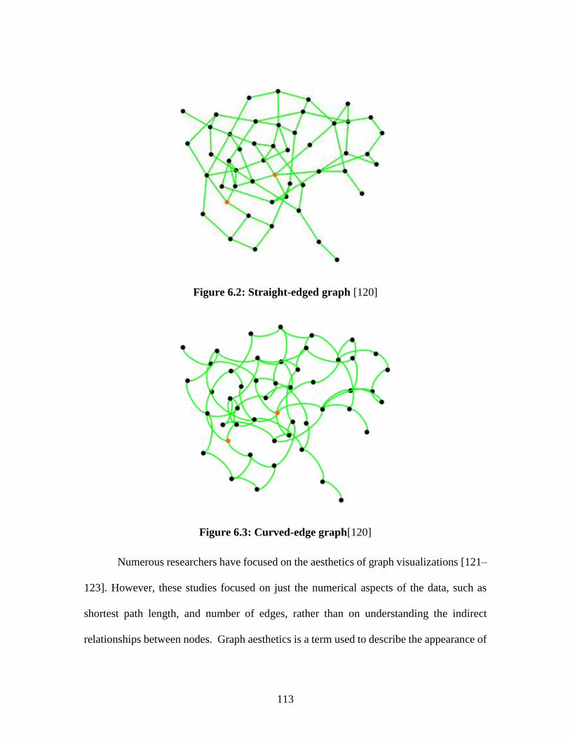
113
Figure 6.2: Straight-edged graph [120]
Figure 6.3: Curved-edge graph[120]
Numerous researchers have focused on the aesthetics of graph visualizations [121–
123]. However, these studies focused on just the numerical aspects of the data, such as
shortest path length, and number of edges, rather than on understanding the indirect
relationships between nodes. Graph aesthetics is a term used to describe the appearance of

114
a graph and includes readability. Archambault used a series of graph visualizations over
time to understand whether the “difference maps” were useful in understanding change to
a network over time [124]. The researchers found that users generally preferred the
difference maps for identifying changes over time. It was also found that use of the
difference maps was effective in answering questions about large scale changes over time.
Lastly, Holten considered how varying the drawing of edges in a directed graph affected
the readability of the graph [125].
Additionally, multiple researchers have provided guidelines on the use of color on
the effectiveness of visualizations as a whole and the potential effects of poor or ineffective
implementation [126–128]. Purchase et al. conducted a series of studies on the effects of
using different graph layout algorithms [123,129]. The researchers found that it was
difficult to show that any one algorithm provided the “best” result; however, it was shown
that the use of an algorithm, particularly one that minimizes crossing paths, is more
effective for improving graph readability. This sentiment is echoed in the review of graph
visualization layout techniques by Gibson, et al [130].
6.2 Graph Layout User Study (Development Study)
The first step in developing a visualization method for configuration management
is to understand the information requirements for the user interface. Specifically, what is
it that the user needs to see when applying the method. In this way, it is possible to
backtrack from the required information to the available information provided in the
current organizational systems to determine the additional requirements of the visualization
method. In order to better understand what information best assists the user in identifying

115
relationships between configuration components, such as options, parts, and configuration
rules, a user study was conducted using different variations on the layout and available
information provided to the user. The user study was designed in accordance with the
benchmark task method proposed in [131]. The remainder of the section provides
additional details regarding the design and execution of the development user study.
6.2.1 Research Questions for Development Study
Research has shown that different types of data representation may be more
accommodating for answering different types of questions about the system being
represented [121,125,129]. This led to the following research questions:
1. How does the layout of the data representation graph affect the ability of the user
to successfully answer questions about the system being represented?
2. How does the coloring of the data representation graph affect the ability of the
user to successfully answer questions about the system being represented?
3. Does a change in the amount of information represented affect the user’s ability to
answer questions about the system?
It is hypothesized that the layout will not have a significant impact, while increasing
the color-coding will increase the ability to correctly answer questions. This hypothesis is
made because the color-coding should increase the user’s ability to easily identify different
types of interactions. Additionally, the it is hypothesized that limiting the amount of
information will increase the accuracy of responses for those questions that are still
answerable, while making it impossible to answer the questions regarding the missing
information. This hypothesis is made because limiting the amount of information should
remove clutter from the graph, more easily highlighting where the interactions take place.

116
6.2.2 Variables for Development Study
In order to answer the above research question, a user study was developed and
executed. The user study consisted of three experimental variables:
geometry of the graph used for data visualization
coloring of the interactions between the nodes in the graph
amount of information available to the user
The first variable consisted of two levels: the graph is arranged with the vehicle
option nodes on the outside in a circle (Figure 6.4 (b)), or the vehicle option nodes arranged
based on the functionality of the option (Figure 6.4 (a)). The purpose of this variable was
to see if the layout of the graph allowed for easier identification of interactions or if the
shape did not matter and any shape would result in the same accuracy of the responses
(research question 1).
Figure 6.4: Functionally arranged graph (a) and circular graph layout (b)
The second variable included two levels: interactions regarding parts were red with
all other interactions grey (Figure 6.5 (a)), or interactions were color-coded based on
whether they were inclusions, exclusions, or either/or relationships (Figure 6.5 (b)). The

117
purpose of this variable was to determine whether the coloring allowed for easier
identification of different types of interactions (research question 2).
Figure 6.5: Graph colored based on part data (a) or based on interaction type (b)
The third variable included two levels: all information (Figure 6.6 (a)) or reduced
information (Figure 6.6 (b)). The purpose of this variable was to determine if removing
some of the information increased the user’s ability to answer the remaining questions with
greater clarity (research question 3).
Figure 6.6: Graph will all information (a) and option information only (b)

118
A final variable consisted of two different orders in which the questions were asked
and was simply used to determine whether the question order affected which questions
were answered correctly. This variable is not used to answer a research question, but to
ensure robustness of the experiment. Limited analysis was needed as the results were
comparable.
6.2.3 Participants for Development Study
The participants for this user study consisted of industrial engineering students
enrolled in the junior level industrial engineering operational research course (IE 3810 at
Clemson University). During the case study (discussed in Chapter Four), it was identified
that many of the engineers conducting configuration management at the OEM did not have
a mechanical engineering background, but they did have some form of engineering
background. Therefore, using junior-level industrial engineering students was applicable
for the purposes of this study. The students were selected for this study as they provided a
large sampling (78 students) with homogenous educational backgrounds and experience.
As such, it was unlikely that any variation in the results of the experiment would be due to
differences in educational preparation. The students had varying levels of work
experience, but due to the low likelihood of working with a visualization tool similar to the
one being used in the study, it was assumed that prior work experience was outside the
scope of the study. The students were not rewarded based on the quality of their results.
However, participation in the user study was counted as a “quiz grade” in order to ensure
participation for the experiment.

119
6.2.4 Environment for Development Study
The user study was conducted in a single one-hour session during a normally
scheduled class period of the junior operational research course. The students were told a
week in advance that they would be conducting an in-class exercise. By conducting the
experiment in a single session during the normal class period, the researcher was able to
ensure that the time of day for the experiment did not affect the outcome of the study while
maximizing the availability of the participants. The setting for the experiment was the
room in which the course usually met. The classroom layout was a typical, auditorium-
style classroom with a presentation stage in the front of the room and tables for the students
to sit at, all facing the front of the classroom (as depicted in Figure 6.7). The experience
of the students due to environmental conditions was uniform. The experiment was
conducted during the twelfth week of the Spring semester of the students’ junior year.
Figure 6.7: Classroom layout
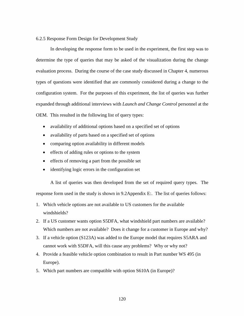
120
6.2.5 Response Form Design for Development Study
In developing the response form to be used in the experiment, the first step was to
determine the type of queries that may be asked of the visualization during the change
evaluation process. During the course of the case study discussed in Chapter 4, numerous
types of questions were identified that are commonly considered during a change to the
configuration system. For the purposes of this experiment, the list of queries was further
expanded through additional interviews with Launch and Change Control personnel at the
OEM. This resulted in the following list of query types:
availability of additional options based on a specified set of options
availability of parts based on a specified set of options
comparing option availability in different models
effects of adding rules or options to the system
effects of removing a part from the possible set
identifying logic errors in the configuration set
A list of queries was then developed from the set of required query types. The
response form used in the study is shown in 9.2Appendix E:. The list of queries follows:
1. Which vehicle options are not available to US customers for the available
windshields?
2. If a US customer wants option S5DFA, what windshield part numbers are available?
Which numbers are not available? Does it change for a customer in Europe and why?
3. If a vehicle option (S123A) was added to the Europe model that requires S5ARA and
cannot work with S5DFA, will this cause any problems? Why or why not?
4. Provide a feasible vehicle option combination to result in Part number WS 495 (in
Europe).
5. Which part numbers are compatible with option S610A (in Europe)?

121
6. Are there any option contradiction errors in the connectivity graph? If so, what are
they?
7. If a European customer wants S5ATA, how does this affect availability of other
vehicle options?
8. If a customer in Europe wants option S358A, what other vehicle options are affected,
and how?
9. Which windshields are not offered in the US?
10. Provide a feasible vehicle option combination to result in Part number WS 401 (for
Europe).
11. Is there any scenario where a combination of vehicle options will result in two
different windshields being required (in Europe)?
12. Are there any valid vehicle option combinations where no windshields are specified?
13. If windshield WS 399 was removed from the European model, would this cause any
issues? Why or why not?
Before conducting the experiment, it was necessary to ensure that each type of
query was being asked in multiple ways. Triangulating the queries to ensure each type is
covered in multiple ways is important when attempting to understand the relationship
between the independent and dependent variables within a study [102,132]. The
triangulation of questions for the user study is shown in Table 6.1.

122
Table 6.1: Survey question triangulation
The above table provides an expanded list of possible query types with the question
number from the survey that corresponds to that subject. The interaction between options
and parts has the highest level of querying as it is the most complex relationship within the
configuration model. Also, as the identification of errors in the configuration model is the
primary purpose of the data visualization, finding errors in the available parts and options
was important. While three of the query types were only given a single question in the
form, this was done purposefully as these subjects are not as central to the purpose of the
visualization and the number of total questions in the survey was purposefully limited to
keep the time requirement within a single class period.
Triangulation
Question type 1 2 3 4 5 6 7 8 9 10 11 12 13
Option availability X X
Option - part
interactionX X X X X X
US vs Europe
availabilityX
Effect of adding
rule/optionX
Using options to
choose a partX X
Finding option
errorsX X X
Option - option
interactionX X
Finding part errors X X X
Effect of removing
a partX
Question

123
6.2.6 Experimental Procedure for Development Study
The students arrived for the normally scheduled class and sat at tables of their
choice. Once all of the students had arrived and were seated, the user study packets were
distributed to the students. Each packet contained a form and two visualization graphs.
The assignment of groups and the contents of each packet will be discussed in the following
section. 12 different packet sets were randomly distributed throughout the class. All work
was conducted individually. Once the packets were distributed, the instructions were
provided to the participants. Additionally, a brief (approximately 5 minutes) tutorial on
the data visualization techniques was provided. This was done because none of the
participants had prior experience with the data visualization method being used to represent
the system discussed in the form. Following the tutorial, the students were allowed to ask
any questions regarding the form or the data visualization technique. The participants were
then given 40 minutes to complete the experiment. However, upon completion of the
questionnaire, individual students were allowed to submit their packets early and leave the
classroom.
6.2.7 Packet Set-Variable Assignment for Development Study
The sets (1-12) were assigned such that each packet set would test a different set of
variables. All relevant combinations were provided. It should be noted that the part-base
level for coloring variable requires the full level for the information availability level. The
assignment of the variables to the packet sets is shown in Table 6.2.
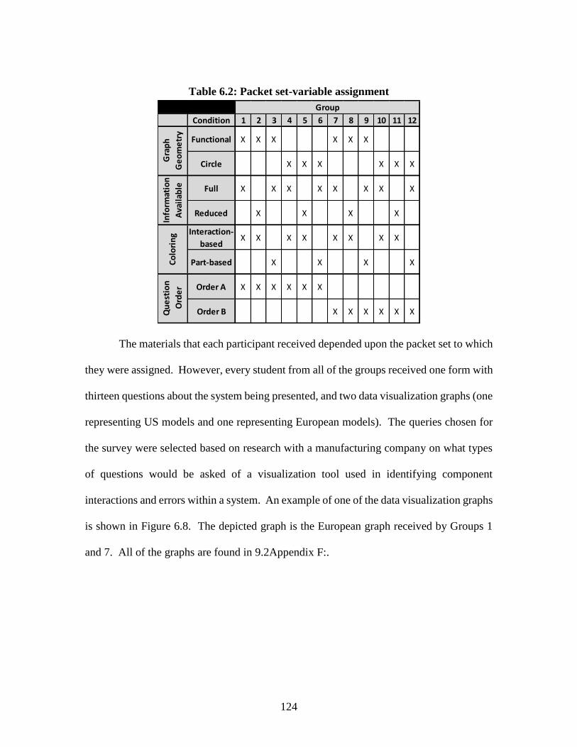
124
Table 6.2: Packet set-variable assignment
The materials that each participant received depended upon the packet set to which
they were assigned. However, every student from all of the groups received one form with
thirteen questions about the system being presented, and two data visualization graphs (one
representing US models and one representing European models). The queries chosen for
the survey were selected based on research with a manufacturing company on what types
of questions would be asked of a visualization tool used in identifying component
interactions and errors within a system. An example of one of the data visualization graphs
is shown in Figure 6.8. The depicted graph is the European graph received by Groups 1
and 7. All of the graphs are found in 9.2Appendix F:.
Condition 1 2 3 4 5 6 7 8 9 10 11 12
Functional X X X X X X
Circle X X X X X X
Full X X X X X X X X
Reduced X X X X
Interaction-
basedX X X X X X X X
Part-based X X X X
Order A X X X X X X
Order B X X X X X X
Group
Qu
est
ion
Ord
er
Co
lori
ng
Gra
ph
Ge
om
etr
y
Info
rmat
ion
Ava
ilab
le

125
Figure 6.8: Example of a visualization graph (provided to Groups 1, 7)
6.2.8 Pilot Study for Development Study
Prior to the execution of the user study, a pilot study was conducted. The purpose
of the pilot study was to determine the time requirements for the user study execution and
to validate the queries and procedures for the user study. The time required to conduct the
user study was a topic of consideration in that the user study needed to be conducted during
a single class period in order to minimize the impact on the students and to ensure that the
training and experiment could be conducted concurrently. The queries needed to be
validated to ensure that the participants were not confused by the wording and that the
novice students were capable of answering the queries.

126
To execute the pilot study, the procedure described earlier was used. Following the
presentation, the participants were given a block of time to finish. In this instance,
however, the time was not limited to allow for maximum time to finish. The participants
were nine beginning graduate level engineering students with no experience in using graph
visualizations for configuration management. The difference in experience level between
the participants in the pilot study and in the full study was not expected to be a factor due
to the similar level of inexperience with graph visualizations. Additionally, no conclusions
were drawn from the pilot study other than time to finish and question answerability.
After evaluating the responses, it was determined that only a few of the queries
needed rework in order to ensure that they were clearly understood and could be answered
by a novice user. Additionally, the average time requirement was determined to be
approximately 22 minutes, with a maximum time required of 28 minutes. The results of
the pilot study ensured that the user study could be executed in its present form, with
minimal modifications, during a single class period.
6.2.9 Evaluation Protocol for Development Study
The forms were evaluated according to the number of queries answered correctly.
In many of the queries, multiple correct answers were possible and varying levels of detail
were acceptable. As a result, the possibility existed for subjectivity in the grading process.
However, because a single evaluator was used to examine all of the responses, this
minimized the amount of variability in the grading process. As such, no inter-rater
reliability assessment was conducted.

127
6.2.10 Evaluation Metrics for Development Study
The metrics that were used for evaluation are correctness and confidence. These
metrics were chosen because it was not only important to determine which set of variables
produced the most accurate or correct responses, but also to determine the confidence of
the users in selecting those answers. As such, it was necessary to include a method for
measuring the participants’ confidence levels for each individual question.
Determining the correctness for each response was simple. The total number of
correct responses was determined, along with the number of possible correct answers (in
the packet sets with limited information available, not all questions were capable of being
answered). The confidence for each response was collected using a modified 100 mm
scale. In the traditional 100 mm scale, the user makes a tick mark along a blank 100 mm
line and the distance from the left side to the mark is measured and recorded for the
confidence [133,134]. A similar rating method was used in previous studies on confidence
in design review decision-making [135]. To simplify the process, the line used in this study
was graduated at 10% intervals, from 0 to 100. An example of the scale with a tick mark
is shown in Figure 6.9.
Figure 6.9: Modified 100mm confidence scale

128
6.2.11 Results for Development Study
A total of 78 forms were collected from the participants and evaluated by a single
grader, as previously discussed. The data was tabulated into spreadsheets for ease of
analysis.
For correctness, the results were consolidated according to the different variable
levels. For instance, all of the groups of individual participants that received the full
information in the graph (1, 3, 4, 6, 7, 9, 10, 12) were in one consolidation, while the groups
receiving reduced information (2, 5, 8, 11) were treated separately. This was done for each
variable in order to see how the different variables affected the accuracy of the responses.
The results for each group and the consolidated results are shown in Table 6.3 and Table
6.4 respectively. Blank spaces in Table 6.3 represent queries that were unanswerable due
to a lack of available information.
Table 6.3: Number of correct responses for each question by group
# responses 1 2 3 4 5 6 7 8 9 10 11 12 13
1A 7 2 5 6 3 7 1 5 3 6 7 7 1 2
2A 7 7 6 6 6
3A 7 1 5 5 2 5 0 4 2 4 6 5 1 4
4A 7 4 3 4 1 6 0 6 6 5 7 6 4 1
5A 7 3 5 3 1 3 1 5 6 6 3 4 3 2
6A 7 6 5 6 4
1B 6 3 3 5 2 5 0 3 2 3 6 4 1 1
2B 7 7 6 7 7
3B 5 3 3 3 0 5 0 4 3 5 3 2 3 1
4B 6 2 3 6 2 3 0 5 0 6 6 4 1 0
5B 6 3 4 3 2 4 0 4 3 5 5 3 0 2
6B 6 4 5 5 4
Pac
ket
Set
Query
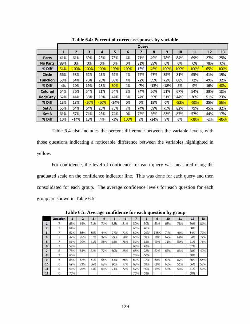
129
Table 6.4: Percent of correct responses by variable
Table 6.4 also includes the percent difference between the variable levels, with
those questions indicating a noticeable difference between the variables highlighted in
yellow.
For confidence, the level of confidence for each query was measured using the
graduated scale on the confidence indicator line. This was done for each query and then
consolidated for each group. The average confidence levels for each question for each
group are shown in Table 6.5.
Table 6.5: Average confidence for each question by group
1 2 3 4 5 6 7 8 9 10 11 12 13
Parts 41% 61% 69% 25% 75% 4% 71% 49% 78% 84% 69% 27% 25%
No Parts 89% 0% 0% 0% 0% 0% 81% 89% 0% 0% 0% 78% 0%
% Diff 54% 100% 100% 100% 100% 100% 13% 45% 100% 100% 100% 65% 100%
Circle 56% 58% 62% 23% 62% 4% 77% 67% 85% 81% 65% 41% 19%
Function 59% 64% 76% 28% 88% 4% 72% 59% 72% 88% 72% 49% 32%
% Diff 4% 10% 19% 18% 30% 4% -7% -13% -18% 8% 9% 16% 40%
Colored 54% 36% 54% 21% 54% 3% 74% 56% 51% 67% 54% 38% 10%
Red/Grey 62% 44% 36% 13% 44% 3% 74% 69% 51% 44% 36% 51% 23%
% Diff 13% 18% -50% -60% -24% 0% 0% 19% 0% -53% -50% 25% 56%
Set A 55% 64% 64% 25% 75% 7% 74% 69% 75% 82% 79% 45% 32%
Set B 61% 57% 74% 26% 74% 0% 75% 56% 83% 87% 57% 44% 17%
% Diff 10% -14% 13% 4% -1% 100% 2% -24% 9% 6% -39% -2% -85%
Query

130
6.2.12 Discussion for Development Study
It should first be noted that there are limitations in the analysis due to the responses
of the participants. From evaluating the responses, it was identified that some of the
participants did not take the experiment seriously or were confused by the instructions.
This conclusion was made due to a number of responses being unsuitable based on the
question being asked and/or instructions provided to the participants. For example, in
multiple instances, the participants would respond to a question asking for vehicle options
with a series of part numbers. This is clearly an example of the participants being confused
by what was being asked in the question. In such an instance, the response was simply
scored as incorrect, even if the thought process might have been correct. Additionally, a
number of students turned in their completed questionnaires after only 15 minutes of work.
During the pilot study discussed in Section 3, the fastest completion times were 20 minutes
or higher, so it is unlikely that multiple participants were able to finish that quickly. It is
more likely that the students rushed through the questions in order to be released early.
Fortunately, the above situations were in the small minority and should not significantly
affect the outcomes.
6.2.12.1 Availability of information
When considering the availability of part information, a definite trend existed
where the accuracy of the answerable questions greatly increased when the part
information was removed from the data visualization graph. Figure 6.10 illustrates the
percentage of correct responses for each question for both the full information and reduced
information (part vs. no parts) groups.

131
Figure 6.10: Graph of the correctness for each question based on availability of
information
In the questionnaires, the only questions that remained answerable after the removal
of the part information were Questions 1, 7, 8, and 12. In the above graph, all other
questions are shown as having 0% correct responses for the “No Parts” group. However,
for the answerable questions, the percentages of correct responses were significantly higher
in almost all situations. The percentages for the answerable questions ranged from 78% to
89%, whereas the range for the same questions for the “Parts” group was 27% to 71%.
This corresponds with the hypothesis that decreasing the amount of information presented
will increase the ability to answer correctly for those questions that are still answerable.
However, it should also be noted that for 9 of the 13 questions (the unanswerable
questions for the “No Parts” group), the one group was not even able to attempt the question
due to the lack of information. Therefore, there are clearly situations where the full amount
of information will be required in order to answer the questions. In such situations, it may

132
be advantageous, based on these results, to find other methods for limiting the total amount
of information presented to the user through the visualization graph.
6.2.12.2 Color-coding of interactions
There appears to be little correlation between the method for color-coding the
interactions between the components and the user’s ability to accurately answer the
questions. Figure 6.11 depicts the percentage of correct responses for each question for
the groups based on the type of color-coding used to identify interactions.
Figure 6.11: Graph of the correctness for each question based on color-coding
As seen in the above graph, the percentage of correct responses for each question
do not differ significantly based on the type of color-coding used to identify the
interactions. Only 5 of the 13 questions (3, 4, 10, 11, 13) show a marked difference
between the percentages of correct answers. Additionally, one of the questions (13) shows
a difference in the opposite direction (color-coding based on the node type being superior),
and the majority of the non-significant differences also show the node type color coding

133
being slightly superior. As such, it is impossible to show that there is a direct relationship
between the color-coding scheme used and the accuracy of the responses.
6.2.12.3 Confidence
An ANOVA was conducted for the confidence ratings for the different groups. The
analysis showed no statistically significant difference in the confidence of the users based
on which type of graph they were given. Due to differences in the way the confidence was
understood by the participants and a lack of variation in the results for confidence, no
conclusions were able to be made regarding the resulting confidence levels of the
participants for individual questions.
6.2.12.4 Graph geometry
No correlation was found between the geometry of the data visualization graph and
the accuracy of the responses. Figure 6.12 illustrates the percentage of correct responses
for each question for the groups based on the graph geometry.
Figure 6.12: Graph for the correctness of each question based on layout

134
As seen in the above graph, the percentages of correct responses for each question
are almost the same, regardless of the geometry of the graph. Only 2 of the 13 questions
show a marked difference between the percentages of correct answers. As such, it is
suspected that there is no relationship between the shape of the graph and the accuracy of
the responses
6.2.12.5 Question order
To ensure that question order did not play a factor in the accuracy of the responses,
two different orderings of the questions were used. Figure 6.13 illustrates the percentage
of correct responses for each question for the groups based on the order of the questions.
Figure 6.13: Graph of the correctness for each question based on order
As seen in the above graph, there is no trend for response accuracy based on the
order of the questions. Therefore, it can be concluded that the ordering of the questions
did not impact the results.

135
6.2.13 Findings of the Development Study
The results generally showed an increase in the percentage of correct answers for
those questions that could still be answered when the amount of information presented was
reduced. On the other hand, the color-coding scheme did not seem to have any identifiable
effect on the results. The most significant limitation in this study was the possibility for
variations in the amount of effort put forth by the participants. It was clear, based on the
results, that some of the students did not put forth their best effort or follow the instructions
of the experiment.
6.3 Development of the Visualization Tool
The purpose of the graph visualization creation tool is to automatically import the
output from the previous tool and display a node-link graph visualization. Additionally,
the tool will provide a degree of interaction for the user to be able to manipulate the graph.
As discussed in the literature review, the ability to interact with the visualization greatly
enhances the user’s ability to understand the representations being displayed in the graph.
A graph visualization software package was developed in order to fulfill the requirements
for the design enabler to support the proposed configuration management method. The
following section discusses the process for selecting the platform to be used for the graph
visualization tool.
6.3.1 Platform Selection
Three platforms are being considered for the development of the graph visualization
that will provide the foundation for the visualization method. These platforms are Gephi
[136], Data-Driven Documents (D3) [137], and Processing [138].

136
6.3.1.1 Gephi
Gephi is a visualization tool used for exploring networks, systems, and graphs
[136]. Unlike the other platforms being considered, Gephi is a fully functional software
package for importing node and edge data and displaying interactive network graphs. The
researcher also has some familiarity with Gephi as the early visualization graphs used in
the user study (discussed in 6.2) were created using this software. The major benefits of
Gephi are that it already exists, is open-sourced, and can be modified through the use of
plugins. The major drawbacks of Gephi are that many of its functions are unrelated to the
goals of this research, the development of new plugins would require learning a new
programming language, and does not provide, even with additional plugins, some
capabilities for data encoding that may be necessary for this research.
6.3.1.2 Data-Driven Documents (D3)
D3 is a JavaScript library that is used to visualize data in meaningful ways [137].
Because D3 is a JavaScript library, much of the desired functionality for the visualization
support tool is already available, but would require the supporting programming code for
interacting with the data and displaying the results properly. This leads to the major
benefit, and also drawback, of using D3. On the one hand, the required functionality
already exists and D3 is capable of a wide range of possibilities with respect to visualizing
graph-based data. The drawback is that D3 is run in HTML, which would require a better
understanding of data recovery and programming in HTML.

137
6.3.1.3 Processing
Processing is an open-source programming language that was designed specifically
to assist in adding a visual context to data [138]. Processing is a widely used language
within data visualization and has over 100 libraries to extend the capabilities of the original
software. The main positive of using processing as the platform is that the software is
completely build-to-suit, meaning that the resulting tool can be programmed to be exactly
what is required. Other benefits are that the large number of libraries can assist in
developing the necessary functions and the researcher is already familiar with the
programming language. The largest drawback is that the graph visualization software
would have to be built from scratch.
6.3.1.4 Summary
The level of familiarity, availability, and functionality for each of the possible
platforms is shown in Table 6.6: Software platform selection overview. Due to the low
level of familiarity with programming with D3, as a result of it being HTML-based, D3 is
rejected from the possible platforms. Additionally, Gephi is excluded because it is not
capable of some of the required functionality for the visualization support method. As a
result, Processing is chosen as the platform for the development of the visualization support
method.

138
Table 6.6: Software platform selection overview
6.3.2 Visualization Tool Requirements Identification
Through the course of the case study, a need was identified for support tools to
assist in the configuration management process, to include managing the effects of
proposed configuration changes. In order to address the identified issues, the following
requirements are proposed:
Able to easily visualize the interactions between configuration components
(including parts)
Able to highlight specific problem areas to assist in simplifying the rule database
Able to check for errors in the existing rule database
Able to preview how proposed configuration changes would affect the existing
rule database
These requirements were identified through the interviews to address specific
issues experienced by the automotive OEM in their current configuration management
process.

139
6.4 Implementation of the Visualization Tool
6.4.1 Data Organization and Source
In order to create each graph visualization, two sets of inputs are required: the nodes
(items of interest) and the edges (relationships) of the graph. Both of these inputs are
created through the additional software tools used to support the configuration management
process at the OEM (discussed in 5.2). The following subsections describe the inputs in
more depth.
6.4.1.1 Graph Nodes
The graph nodes, or items of interest, consist of the vehicle options, parts and
packages that exist in the configuration rule database. Also, the researcher created “AND”
and “OR” nodes to assist in representing rules that are not strictly binary. In addition to
the node label, the following information is recommended for capture in the input file: a
unique ID number for easy recall and data storage, the type of node, the lowest level of
interaction from the specified nodes, and the X/Y coordinates for the nodes position in the
graph.
Specifying the type of node increases the amount of information that can be visually
stored in the graph and allows for easier understanding of what a specific node entails. The
lowest level of interaction from the specific nodes identifies the number of interactions
required to move from the original nodes to a specific node (for example: in A->B->C,
where “A” is a node specified in the change document, the level of interaction for “C”
would be 2). This information is useful in that it can assist the user in determining the
likelihood of a change propagating to other components. Lastly, the X/Y coordinates are

140
useful if any prepositioning of the nodes is used for an initial layout of the graph. An
example node input file is shown in Figure 6.14.
Figure 6.14: Example graph node input file
6.4.1.2 Graph Edges
The graph edges, or relationships between the nodes, consist of the rules that govern
how the different components interact. These relationships include all of the rules as
specified in the option and part rule databases, as well as function class information. It is
also possible to use new rules as created in the conflict detection tool as relationships.
While it may be useful to label the edges on the graph, a label is not currently included in
the information provided in the edge input file. The information provided for each edge is
a unique ID number of easy data storage and recall, the source node of the edge, the target
node of the edge, and the type of edge.
The source node of the edge refers to the “If” portion of the rule in a binary rule,
while the target node refers to the “Then” portion of the rule. In more complex rules (non-

141
binary), a more comprehensive grammar must be used and is discussed in 6.4.2.1. The
edge type represents the type of relationship between the nodes. Three different types of
relationships are currently used: inclusive, exclusive, and multiple-inclusive relationships.
An inclusive relationship means that the source requires the target to also be present.
Similarly, exclusive requires that the target must not be present. The multiple-inclusive
relationship is used in conjunction with “OR” and “AND” nodes to help delineate that the
relationship is not binary. Multiple-exclusive could also be represented separately, but has
not been used in the current implementation. An example of an edge input file is shown in
Figure 6.15.
Figure 6.15: Example graph edge input file
6.4.2 Methods
The following subsections describe the two major functions of the visualization
tool: graph creation and graph manipulation.

142
6.4.2.1 Graph Creation
In graph creation, the data from the input files are read and displayed on the screen
in a node-link diagram. In order to accurately depict the different types of
rules/relationships between nodes, a visualization grammar was required. For binary rules,
the grammar consists of an arrow pointing from one node to another. An example of an
inclusive, binary rule is shown in Figure 6.16. In the figure, P5A3A is the source node,
and S5ACA is the target node, meaning that if P5A3A is present, S5ACA must also be
active. The green arrow is being used to represent the inclusivity of the relationship.
Figure 6.16: Rule and corresponding graph for an inclusive, binary relationship
On the other hand, an exclusive, binary relationship is shown in Figure 6.17. In
this instance, the presence of S5A1A requires that P5A3A not be present for the
configuration to work.
Figure 6.17: Rule and corresponding graph for an exclusive, binary relationship
When considering relationships that are not binary, “OR” and “AND” nodes are
used to assist in representing the rules. An example of a rule with an “OR” node is shown
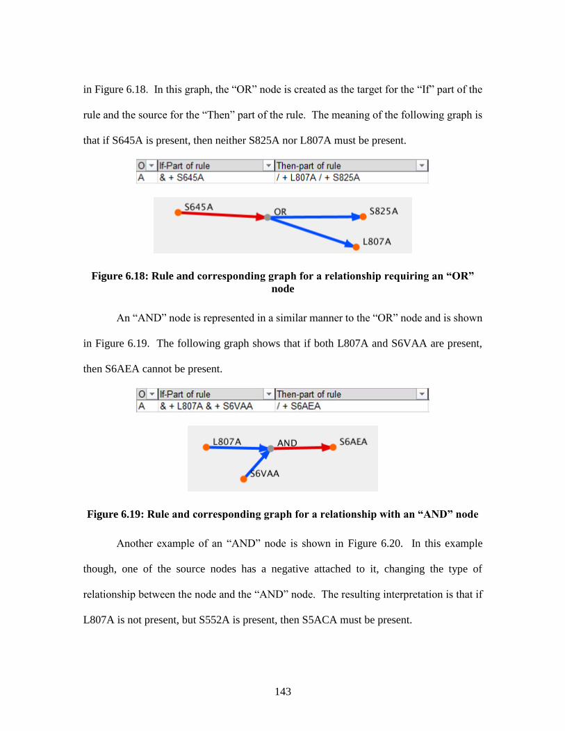
143
in Figure 6.18. In this graph, the “OR” node is created as the target for the “If” part of the
rule and the source for the “Then” part of the rule. The meaning of the following graph is
that if S645A is present, then neither S825A nor L807A must be present.
Figure 6.18: Rule and corresponding graph for a relationship requiring an “OR”
node
An “AND” node is represented in a similar manner to the “OR” node and is shown
in Figure 6.19. The following graph shows that if both L807A and S6VAA are present,
then S6AEA cannot be present.
Figure 6.19: Rule and corresponding graph for a relationship with an “AND” node
Another example of an “AND” node is shown in Figure 6.20. In this example
though, one of the source nodes has a negative attached to it, changing the type of
relationship between the node and the “AND” node. The resulting interpretation is that if
L807A is not present, but S552A is present, then S5ACA must be present.

144
Figure 6.20: Additional rule and graph for a relationship with an “AND” node
Colors were chosen to represent the types of relationships instead of either size or
dash-lines because in a more complex graph, it is more difficult to distinguish between or
trace different line thicknesses or different types of dashed lines. While red, green, and
blue were chosen for the colors in this mapping, a different set of colors could be used in
their place. An example of a completed graph is shown in Figure 6.21.
Figure 6.21: Graph visualization for a specific change

145
6.4.2.2 Graph Manipulation
While it is possible to explore a static graph visualization, the ability to interact
with the data greatly increases the user’s understanding of the system. As such, the
software tool supports graph manipulation. The current level of interaction includes the
ability to move nodes on the existing graph, to create new nodes and edges, to remove
nodes, to highlight a specific node and all of its interactions, and to rearrange the layout of
the graph to increase readability. Additional options are for the user to save the existing
visualization or to reset the visualization to its original state.
At the most basic level of interaction is the ability of the user to move the existing
nodes. This is necessary as it allows the user to manually position items of interest or to
cluster specific nodes based on some criteria. As the edges are directly linked to the nodes,
as the nodes are moved, the edges change to accommodate the placement of the nodes.
As one of the required tasks of the visualization is to assist in the evaluation of
potential changes to the system, it is necessary for the user to be able to add and remove
nodes and edges. At present, the current system allows the addition of both nodes and
edges, but only the manual removal of nodes. When a specific node is removed, however,
all of the associated edges are removed as well. When adding a node or edge, the user
must also have the ability to specify which type of node or edge is being created, along
with entering in any information that is to be stored in the associated data file.
When evaluating the potential propagation pathways from one node to another, it
is useful to be able to select a specific node for highlighting. When a node is selected, all
of its interactions are highlighted, while any relationships not directly related to the node

146
are dimmed slightly. These represent the first-order interactions for the node. It may also
be possible to allow the user to change the order of interaction for this highlighting for
increased user specificity. To show the full relationship, the path between nodes should be
between two components (options/parts/packages) and not “AND” or “OR” nodes, but
should pass through the intermediate nodes. An additional extension of this is that when
two nodes are selected, the shortest path between them (or all unique paths) is highlighted
to show the level of interaction between the two nodes.
Research has shown that while using a specific layout algorithm is not essential, it
is important to use some algorithm for arranging the nodes. This helps to alleviate clutter
and greatly increases the readability of the graph. For this visualization, a force-directed
algorithm is used and will be discussed further in the following section.
In addition to the ability to save the current visualization (which captures the current
image of the graph), it is also useful to be able to output the current data files that go with
the graph. The data files could be outputted in the data file format as described in 6.4.1 or
in the form of rules that could then be merged with the existing rule database.
6.4.2.3 Force-Directed Graph Layout
The force-directed algorithm is a basic graph layout algorithm that uses a repulsive
force between all nodes and an attractive force along all edges. To apply the algorithm, a
repulsive force is determined between the nodes and a movement value is created for each
node. Then the attractive force is determined for each edge and each nodes movement
value is adjusted accordingly. After both forces have been applied, the nodes are moved
according to their final movement values. This process is repeated until the user is satisfied

147
with the dispersion of the nodes. It is also important that outer boundaries are set for the
nodes to ensure that the graph does not grow continually, but rather reaches a steady-state.
6.5 Software Development
This section describes the programming methods used to transform source data into
a graph visualization and then allow the user to interact with the graph. All of the code
found in this section is from Processing (www.processing.org), a common visualization
programming language. The first task is to import the data from the graph and edge files
and store them locally for editing, as discussed in 6.5.1. A discussion of the data classes
that are used for data storage can be found in 6.5.2. From the graph data, the software then
creates the graph visualization, as discussed in 6.5.3. Lastly, the tool provides the ability
to interact with the graph, as discussed in 6.5.4.
6.5.1 Data Management
For each input file (node and edge), a data table is created. For the data tables, a
specific object class is used. The data is stored in a dataTable, along with some meta-data
about the table to increase the ability to search through the data. The purpose of this is to
store the data in a way that is more manageable both for retrieval and editing.
1 class dataTable {
2 int rowCount;
3 String[][] data;
4 String[] columnNames;
5
6 dataTable(String filename) {
7 String[] rows = loadStrings(filename);
8 data = new String[rows.length-1][];
9
10 // skip row 0 (column headers)
11 for (int i = 1; i < rows.length; i++) {
12 // skip empty rows
13 if (trim(rows[i]).length() == 0) { continue; }
14
15 // split the row on the tabs

148
16 String[] pieces = split(rows[i], TAB);
17
18 // copy Data into the table starting at pieces[1]
19 data[rowCount] = (subset(pieces, 0));
20
21 // increase row count
22 rowCount++;
23 }
24 // resize the array as necessary
25 data = (String[][]) subset(data, 0, rowCount);
26 }
27
28 int getRowCount() {
29 return rowCount;
30 }
31
32 String getString(int rowIndex, int col) {
33 return data[rowIndex][col];
34 }
35 }
6.5.2 Data Classes
To assist in creating the graph and storing information that is specific to the nodes
or edges, two additional data classes are used: Node and Edge. For the nodes, the Node
class stores the information from graph input file as well as contains a function for how the
nodes should be drawn on the graph. Additionally, another variable “selected” is either
turned on (1) or off (0) depending on whether or not the node has been highlighted. The
coloring of the node is defined according to the type of node.
1 class Node
2 {
3 String label;
4 int ID;
5 int selected = 0;
6 int nodeType;
7 float x;
8 float y;
9
10 Node(int _ID, String _label, int _nodeType, float _x, float _y) {
11 ID=_ID; label=_label; nodeType=_nodeType; x=_x; y=_y;
12 }
13
14 void draw(int selection) {
15 int opacity = 255;
16 if (selection == 1) {
17 opacity = 100;
18 }
19 strokeWeight(10);
20 if (selected == 1) {
21 strokeWeight(12);
22 opacity = 255;
23 }
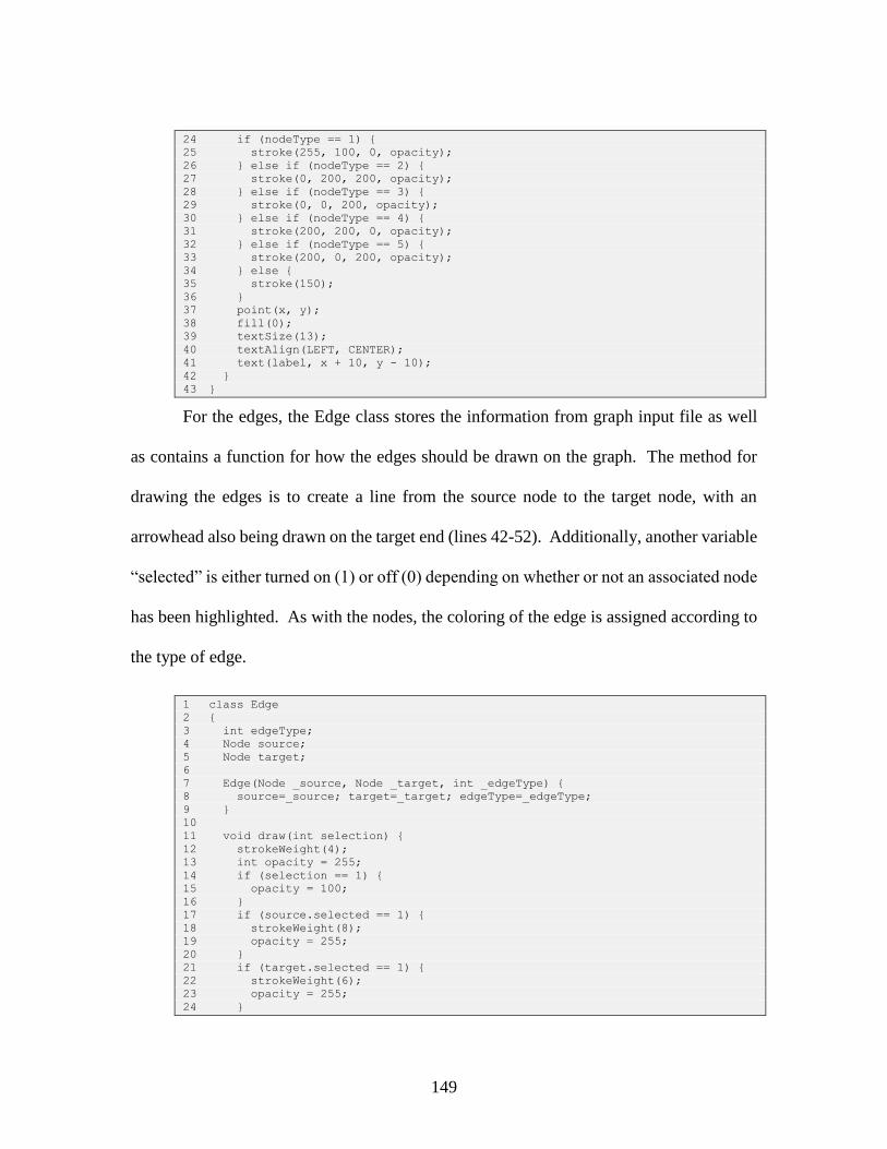
149
24 if (nodeType == 1) {
25 stroke(255, 100, 0, opacity);
26 } else if (nodeType == 2) {
27 stroke(0, 200, 200, opacity);
28 } else if (nodeType == 3) {
29 stroke(0, 0, 200, opacity);
30 } else if (nodeType == 4) {
31 stroke(200, 200, 0, opacity);
32 } else if (nodeType == 5) {
33 stroke(200, 0, 200, opacity);
34 } else {
35 stroke(150);
36 }
37 point(x, y);
38 fill(0);
39 textSize(13);
40 textAlign(LEFT, CENTER);
41 text(label, x + 10, y - 10);
42 }
43 }
For the edges, the Edge class stores the information from graph input file as well
as contains a function for how the edges should be drawn on the graph. The method for
drawing the edges is to create a line from the source node to the target node, with an
arrowhead also being drawn on the target end (lines 42-52). Additionally, another variable
“selected” is either turned on (1) or off (0) depending on whether or not an associated node
has been highlighted. As with the nodes, the coloring of the edge is assigned according to
the type of edge.
1 class Edge
2 {
3 int edgeType;
4 Node source;
5 Node target;
6
7 Edge(Node _source, Node _target, int _edgeType) {
8 source=_source; target=_target; edgeType=_edgeType;
9 }
10
11 void draw(int selection) {
12 strokeWeight(4);
13 int opacity = 255;
14 if (selection == 1) {
15 opacity = 100;
16 }
17 if (source.selected == 1) {
18 strokeWeight(8);
19 opacity = 255;
20 }
21 if (target.selected == 1) {
22 strokeWeight(6);
23 opacity = 255;
24 }

150
25 if (edgeType == 1) {
26 stroke(225,0,0, opacity);
27 fill(225,0,0, opacity);
28 }
29 if (edgeType == 2) {
30 stroke(0,75,255, opacity);
31 fill(0,75,255, opacity);
32 }
33 if (edgeType == 3) {
34 stroke(0,200,0, opacity);
35 fill(0,200,0, opacity);
36 }
37 float xSource = source.x;
38 float ySource = source.y;
39 float xTarget = target.x;
40 float yTarget = target.y;
41 line(xSource, ySource, xTarget, yTarget);
42 pushMatrix();
43 translate(xTarget, yTarget);
44 float a = atan2(xSource-xTarget, yTarget-ySource);
45 rotate(a);
46 strokeWeight(2);
47 beginShape();
48 vertex(0, 0);
49 vertex(-5, -15);
50 vertex(5, -15);
51 endShape();
52 popMatrix();
53 }
54 }
6.5.3 Graph Creation
In Processing, a base setup function is run initially, after which, a draw function is
run continuously. In the setup function, the data is transferred from the input files into the
dataTable classes and additional meta-data is collected about the graph. At the end of the
setup, the initial set of nodes and edges are stored through the storeNodes and storeEdge
functions.
1 void setup() {
2 nodeData = new dataTable("Nodes.tsv");
3 edgeData = new dataTable("Edges.tsv");
4 nodeCount = nodeData.getRowCount();
5 edgeCount = edgeData.getRowCount();
6 size(visHeight + 3 * border, visHeight);
7 day = day();
8 month = month();
9 year = year();
10
11 storeNodes();
12 storeEdges();
13 }

151
The storeNodes function retrieves the data from the nodes dataTable (nodeData)
and creates an entity of the Node class (line 11), which is then added to an ArrayList of all
nodes in the graph through the addNode function (line 12).
1 void storeNodes() {
2
3 for (int row = 0; row < nodeCount; row++) {
4 int nodeID = parseInt(nodeData.getString(row, 0));
5 String nodeName = nodeData.getString(row, 1);
6 int nodeType = parseInt(nodeData.getString(row, 2));
7 float x = parseFloat(nodeData.getString(row, 4));
8 x = centerX + (x * visHeight)/2;
9 float y = parseFloat(nodeData.getString(row, 5));
10 y = centerY + (y * visHeight)/2;
11 Node ni = new Node(nodeID, nodeName, nodeType, x, y);
12 addNode(ni);
13 }
14 }
The storeEdges function retrieves the data from the edges dataTable (edgeData)
and creates an entity of the Edge class (line 14), which is then added to an ArrayList of all
edges in the graph through the addEdge function (line 15). The edge uses the ID numbers
of the nodes to identify the source and target. Lines 10-13 show the method for matching
the current nodes to the edge.
1 void storeEdges() {
2 Node nSource = null;
3 Node nTarget = null;
4
5 int edgeSource, edgeTarget, nodeID;
6 for (int row = 0; row < edgeCount; row++) {
7 edgeSource = parseInt(edgeData.getString(row, 1));
8 edgeTarget = parseInt(edgeData.getString(row, 2));
9 int edgeType = parseInt(edgeData.getString(row, 3));
10 for(Node n: nodes) {
11 if(n.ID == edgeSource) { nSource = n; }
12 if(n.ID == edgeTarget) { nTarget = n; }
13 }
14 Edge e1 = new Edge(nSource, nTarget, edgeType);
15 addEdge(e1);
16 }
17 }
Once all of the data has been stored properly, the draw function is run continuously
to create the graph. The program draw function executes the Node and Edge class draw
functions, populating the items on the visualization (lines 12-13). Additionally, the legend,

152
instructions for interaction, the date of graph creation, and two interface buttons (reset and
save) are drawn (lines 6-10). The checkSelection function checks if any of the nodes have
been highlighted. This is used to determine whether the non-highlighted portions of the
graph should be dimmed. Lastly, the forceCheck variable is used to determine whether the
user has chosen to implement the force-directed algorithm. While the check is active, the
force directed algorithm will run continuously, until the user is satisfied with the graph
dispersion and turns off the algorithm.
1 void draw() {
2 selection = 0;
3 background(240);
4 scale(zoom);
5
6 drawReset();
7 drawSave();
8 drawDates();
9 drawLegend();
10 drawInstructions();
11 checkSelection();
12 for(Edge e: edges) { e.draw(selection); }
13 for(Node n: nodes) { n.draw(selection); }
14 if (forceCheck == 1) {
15 forceDirect();
16 }
17 }
The force-directed algorithm starts by looping through all of the nodes (line 10).
For each node, an initial movement vector is created. Then the repulsive forces from all
other nodes are calculated (lines 25-54). The algorithm first checks to make sure the nodes
are within a certain distance of each other (lines 28-33) and uses the magnitude and
direction between the nodes to create a movement value in the opposite direction (lines 34-
44). Then the node is adjusted accordingly.
After the repulsive forces have been evaluated, the attractive forces provided by the
edges are considered (lines 56-84). Again, the distance and direction between the nodes

153
are determined (lines 63-72) and used to create a move value towards the other node that
increases as the distance increases (lines 74-80). The nodes are then moved accordingly.
1 void forceDirect() {
2 float k = sqrt((visHeight * visHeight)/nodeCount);
3 float distX, distY, dist;
4 float centerDist, centerDistX, centerDistY;
5 float moveX, moveY, move;
6 float pushX, pushY, push;
7 float direction;
8 float pushFactor = 10000;
9 float pullFactor = 1000000000;
10 for (Node n1: nodes) {
11 distX = 0;
12 distY = 0;
13 dist = 0;
14 direction = 0;
15 pushX = 0;
16 pushY = 0;
17 push = 0;
18 moveX = 0;
19 moveY = 0;
20 move = 0;
21 centerDistX = n1.x - centerX;
22 centerDistY = n1.y - centerY;
23 centerDist = sqrt((centerDistX * centerDistX)+(centerDistY * centerDistY));
24
25 for (Node n2: nodes) {
26 if (n1 == n2) {}
27 else {
28 distX = n1.x - n2.x;
29 distY = n1.y - n2.y;
30 dist = sqrt((distX * distX) + (distY * distY));
31 direction = getDirection(distX, distY);
32 push = (1 / ((dist * dist) + 1)) * pushFactor;
33 if (dist < k && dist > -k) {
34 pushX = cos(direction) * push;
35 pushY = sin(direction) * push;
36 if (pushX > 15) {pushX = 15;}
37 if (pushX < -15) {pushX = -15;}
38 if (pushY > 15) {pushY = 15;}
39 if (pushY < -15) {pushY = -15;}
40 float newX = n1.x + pushX;
41 float newY = n1.y + pushY;
42 float newDistX = newX - centerX;
43 float newDistY = newY - centerY;
44 float newDist = sqrt((newDistX * newDistX) + (newDistY * newDistY));
45 if (newDist > 1.2 * radius) {
46 pushX = 0;
47 pushY = 0;
48 }
49 else {
50 n1.x += pushX;
51 n1.y += pushY;
52 }
53 }
54 }
55
56 for (Edge e: edges) {
57 distX = 0;
58 distY = 0;
59 dist = 0;
60 moveX = 0;

154
61 moveY = 0;
62 move = 0;
63 if (e.source == n1) {
64 distX = e.target.x - n1.x;
65 distY = e.target.y - n1.y;
66 }
67 else if (e.target == n1) {
68 distX = e.source.x - n1.x;
69 distY = e.source.y - n1.y;
70 }
71 dist = sqrt(distX * distX + distY * distY);
72 if (dist > k || dist < -k) {
73 direction = getDirection(distX, distY);
74 move = dist * dist * pullFactor;
75 moveX += cos(direction) * move;
76 moveY += sin(direction) * move;
77 if (moveX > 15) {moveX = 15;}
78 if (moveX < -15) {moveX = -15;}
79 if (moveY > 15) {moveY = 15;}
80 if (moveY < -15) {moveY = -15;}
81 }
82 n1.x = n1.x + moveX;
83 n1.y = n1.y + moveY;
84 }
85 }
86 }
87 }
6.5.4 Graph Interaction
Processing allows interaction with the visualization through the use of the computer
mouse and the keyboard. As such, all graph interactions use a combination of these input
devices. When the mouse is clicked, a left click will enable either the creation of a new
node (when the keys “o,” “p,” “f,” “t,” or “l” are pressed, depending on the type of node to
add) or the selection of a node (if the control key is pressed and the cursor is on an existing
node). Additionally, if the mouse is in a specific area (the reset and save “buttons” on the
screen) either the visualization is reset or a screenshot of the visualization is taken and
saved to the specified location (lines 11-14). A right click of the mouse, with the control
key down, will delete the node on which the cursor is placed (lines 16-20).
1 void mouseClicked() {
2 if (mouseButton == LEFT) {
3 if (keyPressed == true) {
4 if (key == 'o') { createNode(1); }
5 if (key == 'p') { createNode(2); }
6 if (key == 'f') { createNode(3); }
7 if (key == 'l') { createNode(4); }

155
8 if (key == 't') { createNode(5); }
9 if (keyCode == CONTROL) { selectNode(); }
10 }
11 if (mouseX <= 120 && mouseY <= 30) { resetAll(); }
12 if (mouseY >= 35 && mouseY <= 65) {
13 if (mouseX <= 120) { save("output_graph.jpeg"); }
14 }
15 }
16 if (mouseButton == RIGHT) {
17 if (keyPressed == true) {
18 if (keyCode == CONTROL) { deleteNode(); }
19 }
20 }
21 }
The selectNode function is used to highlight a specific node the interacting nodes
and edges. First, the selected variable is set to “1” indicating it is turned on. If the node is
already selected, then it is set to “0” to turn it off (lines 3-10). Then, all of the edges are
check to determine if they include the selected node. In the case of “OR” and “AND”
nodes, those nodes are also turned on to ensure than the full relationship is highlighted, not
just part of it.
1 void selectNode() {
2 for(Node n: nodes) {
3 if (dist(mouseX, mouseY, n.x, n.y) < 10) {
4 if (n.selected == 0) {
5 n.selected = 1;
6 }
7 else if (n.selected == 1) {
8 n.selected = 0;
9 }
10 }
11 }
12 for (Edge e:edges) {
13 if (e.source.selected == 1 || e.target.selected == 1) {
14 if (e.target.label.contains("OR") || e.target.label.contains("AND")) {
15 e.target.selected = 1;
16 }
17 else if (e.source.label.contains("OR") || e.source.label.contains("AND"))
{
18 e.source.selected = 1;
19 }
20 }
21 }
22 }
If a node is to be deleted, the deleteNode function is run. This function first
identifies which node is under the cursor. Then any edges attached to the node are removed
prior to the node itself being removed.

156
1 void deleteNode() {
2 for(int i = nodes.size(); i-- !=0;) {
3 Node n = nodes.get(i);
4 if (dist(mouseX, mouseY, n.x, n.y) < 10) {
5 for (int j = edges.size(); j-- !=0;) {
6 Edge e = edges.get(j);
7 if (e.source == n) {
8 edges.remove(j);
9 }
10 if (e.target == n) {
11 edges.remove(j);
12 }
13 }
14 nodes.remove(i);
15 }
16 }
17 }
In order to move a node, the mouse is left-clicked while on a node and dragged to
the desired location. To ensure that only a single node is selected, the draggedNode
variable is used. As the cursor moves with the node still selected, the position of the node
continually updates. Upon release of the mouse button, the draggedNode value returns to
-1 and the node is “dropped.”
1 void mouseDragged() {
2 if (mouseButton == LEFT) {
3 if (draggedNode == -1) {
4 for(Node n: nodes) {
5 if (dist(mouseX, mouseY, n.x, n.y) < 10) {
6 nSelect = n;
7 draggedNode = 1;
8 }
9 }
10 } else {
11 nSelect.x = mouseX;
12 nSelect.y = mouseY;
13 }
14 }
15 }
16
17
18 void mouseReleased() { draggedNode = -1; }
Lastly, the user has the ability to create a new edge between two nodes. When the
left mouse button is pressed and either the “a” or “z” keys are pressed, depending on the
type of interaction desired, the source node is selected. This is determined by a proximity
of the cursor to the node (lines 6-10). The newEdgeSource variable is used to ensure that
a single source and target are selected. After the source has been selected, the user (while
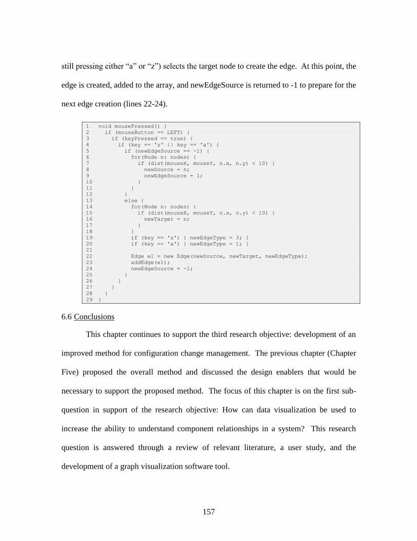
157
still pressing either “a” or “z”) selects the target node to create the edge. At this point, the
edge is created, added to the array, and newEdgeSource is returned to -1 to prepare for the
next edge creation (lines 22-24).
1 void mousePressed() {
2 if (mouseButton == LEFT) {
3 if (keyPressed == true) {
4 if (key == 'z' || key == 'a') {
5 if (newEdgeSource == -1) {
6 for(Node n: nodes) {
7 if (dist(mouseX, mouseY, n.x, n.y) < 10) {
8 newSource = n;
9 newEdgeSource = 1;
10 }
11 }
12 }
13 else {
14 for(Node n: nodes) {
15 if (dist(mouseX, mouseY, n.x, n.y) < 10) {
16 newTarget = n;
17 }
18 }
19 if (key == 'z') { newEdgeType = 3; }
20 if (key == 'a') { newEdgeType = 1; }
21
22 Edge e1 = new Edge(newSource, newTarget, newEdgeType);
23 addEdge(e1);
24 newEdgeSource = -1;
25 }
26 }
27 }
28 }
29 }
6.6 Conclusions
This chapter continues to support the third research objective: development of an
improved method for configuration change management. The previous chapter (Chapter
Five) proposed the overall method and discussed the design enablers that would be
necessary to support the proposed method. The focus of this chapter is on the first sub-
question in support of the research objective: How can data visualization be used to
increase the ability to understand component relationships in a system? This research
question is answered through a review of relevant literature, a user study, and the
development of a graph visualization software tool.
158
The literature review was conducted in order to understand how graph visualization
can be implemented for configuration change management. The literature review focused
on how data visualization is used to understand and manage large amounts of data. More
specifically, graph visualization was identified for its usefulness in understanding the
relationships between entities within a system. During the literature review, it was also
identified that numerous factors can affect the usefulness of graph visualizations. This led
to the second task to answer the above research question.
The user study was conducted in order to understand what aspects of the
visualization graph (color, layout, and availability of information) affect the user’s ability
to understand and identify relationships between vehicle options and parts in a
configuration system. The participants were given different graphs and tasked with
answering questions regarding the configuration system portrayed in the graph. The results
showed that color and layout did not have a significant impact while availability of
information (the removal of unnecessary information) greatly increased the users’ ability
to answer questions about the configuration system. This information was then used in the
development of the visualization software tool.
The graph visualization tool was developed using the Processing visualization
programming language. Based on a set of inputs from one of the other supporting design
enablers (interaction identification), the visualization tool creates a graph visualization of
the configuration system. The software tool also allows for a wide range of interactions
with the graph, including reshaping, adding and removing nodes and edges, and outputting
the resulting graph for future use or evaluation.

159
6.7 Dissertation Roadmap
Chapter Six focused on the development and implementation of the graph
visualization support tool. The next chapter (Chapter Seven) builds on this by presenting
the methods and results of three validation techniques: a user study, implementation cases,
and user feedback. The progress of this dissertation is shown in Figure 6.22 in which the
completed portion is highlighted in green.
Figure 6.22: Dissertation roadmap

160
CHAPTER SEVEN: VISUALIZATION TOOL VALIDATION
The purpose of the research presented in this chapter is to validate the graph
visualization support tool discussed in Chapter Six. Previous research has shown the need
for rigorous validation of design research [139]. As such, the Validation Square [140] is
used as a guideline for the validation of the visualization tool. The literature review
conducted during the development of the visualization tool in Section 6.1 answers first
aspect of validation – accepting the construct’s validity. The visualization tool was
evaluated through four implementation studies of ongoing configuration changes at the
OEM, a validation user study on the tool’s usefulness in rule implementation, and user
feedback.
7.1 Implementation Cases
In order to test the visualization tool throughout its development, the researcher
used the software to assist in validating in-progress configuration changes at the OEM.
These problems were identified by both the researcher and the OEM users as exemplars
appropriate for testing. This ties into the fourth aspect (accepting usefulness of method for
some example problems) of the Validation Square in that the problems being used for
evaluation are representative [140]. Additionally, because the tool was implemented by
the researcher alongside the personnel at the OEM conducting their own validation, the
fifth part (accepting the usefulness is linked to applying the method) is also fulfilled. The
following sections discuss how the visualization tool was used to assist in the analysis of
four ongoing changes at the OEM.

161
7.1.1 Case 1: Windshield Option Change
The first change for which the visualization tool was implemented involved
changing the rules that governed the relationships between two vehicle options.
Previously, the presence of option 358 required that option 3AP also be present. However,
this led to an issue in assigning parts for the vehicle, so a change was made that made the
presence of option 358 require the absence of option 3AP. This configuration change
affected all models for the X5 and X6 vehicle lines in the European markets and was
proposed in June 2014. The proposed change affected eight different options and explicitly
required the change or addition of ten rules.
One question that was asked regarding the change was whether it would result in
any windshields that were no longer valid. Essentially, were there any windshields that
required a configuration that no longer worked due to the change? To assist in answering
the question, a visualization graph for the windshields and all options affecting the ordering
of windshields was created (Figure 7.1). In the graph, the available windshields are found
on the left with labels of WS###, while the options are on the right and a represented by
S###A. The links between them represent the rules according the grammar discussed in
6.4.2.1. A brief review of the graph shows that no windshield requires the both 3AP and
358 to be present. To conduct this review, the options of concern (3AP and 358) are
identified in the graph. Then the windshield parts are identified in the graph (along the left
hand side). The rules for each windshield part is checked for whether it requires (has a
green arrow) to the options of concern. For example, WS905 requires option 358, but not
3AP. On the other hand, WS 401 requires 3AP, but not option 358.

162
Figure 7.1: Visualization graph for windshield option change (Case 1)
This is the same conclusion that the change control personnel at the OEM came to
while working concurrently on the configuration change. However, in the traditional
approach, the OEM engineers spent approximately 2 hours analyzing the change. With the
graph, the question was answered in minutes. In addition, the use of the visualization
assisted the researcher in understanding and explaining to the change control personnel as
to why the change was written as is and to validate that there were no other configuration
conflicts resulting from the implementation of the change.

163
7.1.2 Case 2: Indian Country Model Change
Another change in which the visualization tool proved helpful involved changing
the standard Indian country model for the one of the diesel SUVs from one model to
another. The intent of the configuration change validation in this instance was to determine
whether any additional rules needed to be added, other than changing the availability of the
option code between the two models.
In order to support the validation of this change, two separate graphs were created,
one for each model code that was effected. The graph for the model code that currently
existed as the model for use in India is shown in Figure 7.2. It should be noted that this is
an earlier instance of the graph visualization tool and the readability of the graphs has since
been improved to increase usability.
Figure 7.2: Visualization graph for existing model

164
The graph for the model that would replace the previous model is shown in Figure
7.3 below.
Figure 7.3: Visualization graph for replacement model
By comparing the two graphs, it was possible to determine if there were any
differences between the options and rules for the two models.
A brief inspection of the graphs above shows that a series of rules/options are
missing from the middle of the left side of the graph. Essentially, this meant that change
the engine size (the only significant change between the two model codes) resulted in no
longer disallowing a certain emissions standard in the ruleset. When asked if this was
intentional, the change control personnel at the OEM were not aware of the inconsistency.
To determine whether it would have been faster to create a list of the options and
rules present for each model, an additional study was conducted. In this study, the time
was determined to create the visualization and then inspect to determine where any

165
differences may lie. This time was compared to the amount of time it would take to identify
the difference using the methods in place at the OEM. It was determined that the use of
the visualization graph reduced the required time by 75%.
7.1.3 Case 3: Emissions Standards Option Change
Because the configuration changes are not written by personnel in the change
control group at the OEM, understanding the reasoning and implications behind the change
can be difficult when attempting to validate a specific change, even if the validation itself
is simple. This was the case with the third configuration change. This change focused on
the emissions standard levels (S161A, S167A, and S169A) for four vehicle models (KS01,
KS02, LS01, LS02) of the X5 vehicle line. The change was proposed and evaluated in
July 2014. After the analysis, it was determined that models LS01 and LS02 were being
created to allow a specific emission standard (S167A), which was not available for the
other two models.
7.1.4 Case 4: Australian Country Option Addition
The final change for which the visualization tool was implemented was the addition
of the Australian country option to a current model. Essentially, the OEM wanted to
expand its vehicle offerings in Australia.
In order to validate this change, a model was selected that most closely matched
the model being changed, but that already included the Australian country option. This
mirrored the method used by the change control personnel at the OEM. Two visualization
graphs were then created for the models. The first graph showed the model that already

166
had the option, shown in Figure 7.4. The second graph showed the model to which the
option was being added, shown in Figure 7.5. In addition, a blank node (“New Node 2”)
was added to the graph to mimic the option being added to the model. Also, the
corresponding rules between the new option and other related options were added to the
graph to create a close duplicate to the existing model.
Figure 7.4: Existing model graph with the Australian country option already
available

167
Figure 7.5: Graph of the model to which the country option will be added
Based on an inspection of the above graphs, no issues were identified to result from
adding the Australian country option to the new model. The only changes were that two
other options (S2AMA and L8LAA) were not available for the new model and those would
not be of concern. An additional application of this tool is that the new options and ruleset
that were created using the visualization tool could be exported to provide the written
rules/options that needed to be modified in the ruleset to implement the change.
7.2 Rule Authoring User Study (Validation Study)
One of the potential applications of the graph visualization support tool is to allow
the user to export any rules or options created through the graphical user interface. These
new rules or options could then be implemented directly into the OEM’s rule database to
avoid having to convert the rules to the correct format and enter them manually. As such,

168
a user study was conducted to evaluate the usefulness of the graph visualization support
tool for assisting in rule implementation. In addition, the user study evaluated the ability
of an untrained user (the participants) to understand and implement the visualization
support tool in conjunction with proposed configuration changes. The details of the
validation user study are discussed in the following sections.
7.2.1 Research Questions for Validation Study
Research has shown that different types of data representation may be more
accommodating for answering different types of questions about the system being
represented. Additionally, the use of a graphical user interface (GUI) for making changes
to a system or for implementing changes is a common method for simplifying data
maintenance. This led to the following research questions:
How does the use of a graphical method for rule implementation affect the user’s
ability to accurately author rule changes in a system?
How does the use of a graphical method for rule implementation affect multiple
users’ abilities to consistently author rule changes in a system?
It is hypothesized that the use of a graphical representation for rule implementation
will increase both the accuracy and consistency for making changes to the rule database.
This hypothesis is made because the graphical representation has been shown previously
to increase the user’s ability to understand the system better, and a better understanding
should lead to increased accuracy when implementing the changes.
Based on the initial results, which showed a marked decrease in the effectiveness
using the visualization method, the following research question was added:

169
How does the amount of training and familiarity with the visualization method
affect the user’s ability to implement rules in the system?
It is hypothesized that implementing a small training period will greatly increase
the familiarity of the participants with the method and will result in increased effectiveness
at implementing the rules.
7.2.2 Experimental Procedure for Validation Study
7.2.2.1 Variables for Validation Study
In order to answer the above research question, a user study was developed and
executed. The user study consisted of two variables: the method for implementing the rule
changes and the amount of training on the new visualization method. The first variable
consisted of two levels: implementation of changes through a graphical representation or
implementation using a text-based representation. The purpose of this variable was to see
if using a different method increased the user’s ability to accurately and consistently
implement the changes. The second variable had two levels, and only applied to the group
assigned the visualization method: a minimal amount of training on what the new method
is and a slightly increased training period (approximately five minutes) showing how the
new method can be used to show changes to the system. This variable was developed
based on concerns during the initial results that a lack of familiarity with the new method
was resulting in decreased scores, as opposed to the actual effectiveness of the new method.
7.2.2.2 Participants for Validation Study
The participants of the user study were senior, undergraduate, mechanical
engineering students at Clemson University. All of the students ranged in age between

170
approximately 19-24 years of age and had less than one year of coursework remaining prior
to graduation. The students were chosen for the experiment because, as seniors, they have
a similar level of experience to new employees at a company. Additionally, selecting the
participants from this course ensured that the students would have a similar educational
background. At the time of the experiment, all of the students were enrolled in the senior
mechanical engineering design course at Clemson University.
7.2.2.3 Environment for Validation Study
The user study was conducted in two sessions during a normally scheduled class
period of the senior mechanical engineering design course, with each group only attending
a single session. The control group and the experimental group with minimal training
attended the first session and the experimental group with additional training attended the
second session. The students were told in advance that they would be conducting an in-
class exercise while the instructor was unavailable. The setting for the experiment was the
classroom in which the course usually met (for two groups) or in a nearby classroom with
a slightly different setup (for the third group). While the classroom layouts were different
for the groups, the researcher did not believe this would be a factor in the results as all
environments were standard classroom types, with which the participants were familiar.
The classroom layouts were typical, auditorium-style classrooms with a projector in the
front of the room and tables for the students to sit at, either circular or in rows.
Additionally, minimal distractions were present during the experiment. In general, the
experience of the students due to environmental conditions was as uniform as possible.
171
7.2.2.4 Experimental Procedure for Validation Study
For the first session, the students arrived for the normally scheduled class and sat
at tables of their choice. Once all of the students had arrived and were seated, the user
study packets were randomly distributed to the students. Each packet contained a set of
documents according to whichever group the participant was assigned. The contents of the
packets will be discussed in the following section. Once the packets were handed out, the
participants were separated based on the packet that they had received. Once in separate
classrooms, each group was given a brief class instructing the students on the background
of the research and the specific instructions for their part of the research. The presentations
were developed to provide similar levels of detail regarding the study and to take a similar
amount of time to complete. This was necessary to ensure that all participants had a similar
level of familiarity with the processes being used; none of the students had experience with
the methods begin studied prior to the research being conducted. Following the
instructional period, the students were allowed to ask any questions regarding the survey
or the data visualization technique. The participants were then given 40 minutes to conduct
the experiment; however, upon completion of the study and a brief survey for additional
data collection, the students were allowed to turn their packets in early and leave the
classroom. While the participants were assigned to groups, the grouping was only
conducted to control variables; all work during the study was conducted individually.
The second session mirrored the first session, except only one group was present,
so the participants did not have to be divided. Additionally, the second session included
the increased training period during the presentation. The increased training period

172
consisted of providing an example (from a different rule database and product) of how a
change could be implemented to the system. The increased training period took less than
five minutes to conduct.
7.2.2.5 Packet Contents for Validation Study
The materials that each participant received with their packet depended upon which
group they were in, which was assigned randomly during distribution of the packets. The
control group, which implemented the changes using a text-based representation, received
an instruction sheet that contained the instructions, as well as a brief overview of the rule
grammar; three different configuration change documents, which contained information
regarding the background, solutions and implementation for the change; and the rule
system documents, which would be modified by the participant according to the
corresponding configuration change document. Both experimental groups, which
implemented the changes using a graphical representation, received an instruction sheet
that contained the instructions, as well as a brief overview of the rule visualization
techniques; three different configuration change documents, which contained information
regarding the background, solutions and implementation for the change (the same
documents provided to the control group); a single copy of the rule database, for reference
only; and three rule system graphs (Figure 7.6), which would be modified by the participant
according to the corresponding configuration change document. The configuration
changes chosen for the study were developed based on the types of changes that occur at a
local automotive manufacturing facility. Additionally, the documents were created to

173
mirror the change documents used at the OEM. The full packets received by all groups
(Groups A and C received the same packets) are found in 9.2Appendix G:.
Figure 7.6: Rule system graph provided to the experimental groups
7.2.3 Evaluation Protocol for Validation Study
The protocol analysis of the user study is relatively straight-forward. The resulting
rule systems were evaluated as to whether or not the resulting system accurately portrayed
the changes specified in the configuration change documents. In many instances, multiple
different results could be considered as correct, as long as the allowable configurations that
would result from the rule system would be the same. To account for the possibility of
multiple, different correct answers, the resulting configuration rule sets were evaluated to
determine if the set of allowable configurations would be the same for both the expected
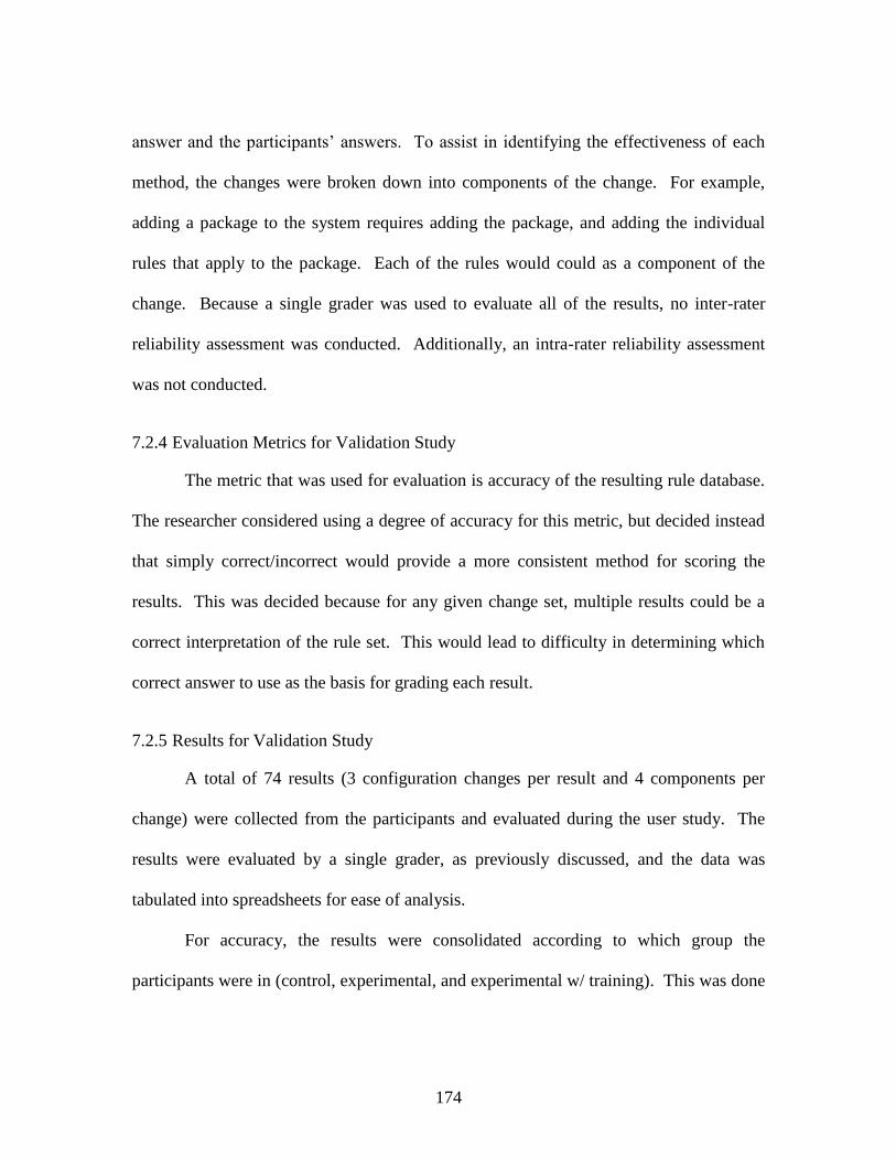
174
answer and the participants’ answers. To assist in identifying the effectiveness of each
method, the changes were broken down into components of the change. For example,
adding a package to the system requires adding the package, and adding the individual
rules that apply to the package. Each of the rules would could as a component of the
change. Because a single grader was used to evaluate all of the results, no inter-rater
reliability assessment was conducted. Additionally, an intra-rater reliability assessment
was not conducted.
7.2.4 Evaluation Metrics for Validation Study
The metric that was used for evaluation is accuracy of the resulting rule database.
The researcher considered using a degree of accuracy for this metric, but decided instead
that simply correct/incorrect would provide a more consistent method for scoring the
results. This was decided because for any given change set, multiple results could be a
correct interpretation of the rule set. This would lead to difficulty in determining which
correct answer to use as the basis for grading each result.
7.2.5 Results for Validation Study
A total of 74 results (3 configuration changes per result and 4 components per
change) were collected from the participants and evaluated during the user study. The
results were evaluated by a single grader, as previously discussed, and the data was
tabulated into spreadsheets for ease of analysis.
For accuracy, the results were consolidated according to which group the
participants were in (control, experimental, and experimental w/ training). This was done

175
in order to see how the rule implementation method affected the accuracy of the resulting
rule sets. The results for each group for changes 1, 2, and 3 are shown in Table 7.1, Table
7.2, and Table 7.3, respectively.
Table 7.1: Number and percent of correct responses by group for Change 1
Table 7.2: Number and percent of correct responses by group for Change 2
Table 7.3: Number and percent of correct responses by group for Change 3
7.2.6 Discussion for Validation Study
It should first be noted that there are limitations in the analysis. While the
participants had no previous experience with either method for rule implementation, the
use of spreadsheets and the basic logical grammar used in if-then statements is
Change 1
Group # % # % # % # %
1.1 1.2 1.3 1.4
Experimental 26 100% 15 58% 26 100% 25 96%
Control 25 100% 21 84% 24 96% 25 100%
Training 23 100% 20 87% 22 96% 23 100%
Change 2
Group # % # % # % # %
2.1 2.2 2.3 2.4
18 69% 17 89%
Control 25 100% 25 100% 25
Experimental 25 96% 15 58%
100% 19 79%
Training 23 100% 22 96% 22 96% 17 85%
3
Group # % # % # % # %
3.1 3.2 3.3 3.4
35% 9 35%
Control 23 92% 23 92% 25 100%
Experimental 26 100% 23 88% 9
52%
25 100%
Training 23 100% 19 83% 12 52% 12

176
commonplace. However, the use of node-link graphs to visually represent configuration
rules, and the grammar that is associated with it, is something the participants were unlikely
to have any experience with at any level. While a similar amount of training was provided
to the control and experimental groups, the experimental group that was given the graphs
was less likely to fully understand and become familiar with the process during the brief
training period. This likely caused the decrease in the capabilities of the graph visualization
method for rule implementation and was the reasoning for the second session with an
increased training period for the training group.
When considering the accuracy of the results based on the method of rule
implementation, a definite trend existed where the accuracy of the answerable questions
greatly increased with the use of the text-based (control) method. However, a brief training
session with the second experimental group significantly decreased the gap. Figure 7.7,
Figure 7.8, and Figure 7.9 illustrate the percentage of correct responses for each question
for all of the groups.
Figure 7.7: Percent correct responses for Change 1
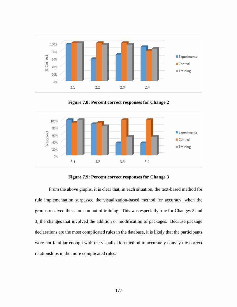
177
Figure 7.8: Percent correct responses for Change 2
Figure 7.9: Percent correct responses for Change 3
From the above graphs, it is clear that, in each situation, the text-based method for
rule implementation surpassed the visualization-based method for accuracy, when the
groups received the same amount of training. This was especially true for Changes 2 and
3, the changes that involved the addition or modification of packages. Because package
declarations are the most complicated rules in the database, it is likely that the participants
were not familiar enough with the visualization method to accurately convey the correct
relationships in the more complicated rules.

178
With the additional training period, the accuracy of the responses for the second
experimental group increases significantly and only lags behind the control group for the
third change. After reviewing the third change, the authors realized that an issue with the
wording in the question resulted in confusion as to how directionality in the visualization
was applied. This is likely the cause of the significant drop in accuracy for both of the
visualization groups for parts 3.3 and 3.4.
7.2.7 Findings for Validation Study
The purpose of this paper was to describe a user study that was conducted in order
to determine whether the use of a visualization-based method for configuration rule
implementation would increase the accuracy of the rule sets generated as a result of the
proposed changes. The researcher hypothesized that using the visualization-based method
would increase the accuracy of the results. The results proved the hypothesis to be false,
in that the average accuracy level for the text-based method was higher for all of the
changes, and significantly higher for the more complicated changes, or those requiring
package rule modification. The most significant limitation in this study was the difference
in the difficulty of learning the methods; the text-based method, using a spreadsheet and
standard if-then logic, was likely much easier for the participants to understand in the short
training period prior to the study. This could have led to a decrease in the familiarity of
the participants with the visualization-based method, resulting in decreased scores for that
group.
As a result of this limitation, a second study was conducted in which a group of
participants was given the same materials as the visualization group, but was also provided

179
with an additional amount of training (approximately five minutes) on the graph
visualization method. It was hypothesized that the increased training would lessen the delta
between the experimental and control groups. This hypothesis was proven to be mostly
true in that, for the majority of the changes, the experimental group with training performed
as well as the control group.
Possible future work includes conducting an additional user study where the
participants are not provided with the rules that are to be implemented; instead, the
participants would have to use the rule database to figure out what rules had to be
implemented in order to correctly implement the required solution. This would require a
greater amount of critical thinking about and understanding of the change, which is likely
to be better suited for the visualization-based, rather than text-based, method for
configuration management. The additional experiment would be structured similarly to
this study, with the primary difference being the amount of information provided to the
participants
7.3 User Feedback
In order to fully validate the usefulness of graph visualization for configuration
management, user feedback was gathered in the form of a targeted interview with a Launch
and Change Controller at the OEM. The interview was conducted with interviewee #2 at
the end of the development of the configuration management method. The interview lasted
approximately one hour. During the interview, the researcher reviewed the visualization
design enabler, including its usefulness, potential applications, and potential additional
functionality. The interviewee stated that using graph visualizations would be most helpful

180
when evaluating highly complicated changes to the configuration rule system, as is the case
in the example in Section 7.1.1. In these changes, the ability to quickly conduct path tracing
through the graph would greatly assist in understanding what other options would be
affected by the proposed change. Additionally, visually inspecting for patterns in the
graphs would increase the likelihood of identifying rule conflicts or redundancies.
However, the interviewee also stated that the addition of a conflict detection algorithm
within the graph visualization tool would greatly increase its usefulness. This would
remove the need for the user to conduct as many inspections of the graph, allowing the user
to focus on the potential propagation pathways.
In addition, the interview also revealed that other common uses of the graph
visualization tool would include the implementation of new packages and the introduction
of new model codes to the configuration rule database, as is the case in the examples
discussed in Sections 7.1.2 and 7.1.4. This is due to the level of interaction that is provided
by the graph visualization tool. When adding a new package, the user is able to add the
package and any associated rules and see how this can affect the system in unintended
ways. When adding or changing model codes, the user is able to create multiple graphs to
allow a comparison between an existing (proven) model code and the new (unproven)
model code. While discussing the comparison of graphs for different model codes, the
interview mentioned that automating the graph comparison and highlighting the difference
between two graphs would increase the effectiveness of the tools by not having to rely on
visual inspection alone. It was agreed, though, that having the visualization of the systems,
with the differences highlighted, would be preferable to a just a list of differences between

181
the models because of the ability to see how those differences could affect other aspects of
the rule database.
In conclusion, the interviewee stated that the graph visualization was a useful tool
for configuration management that had already assisted in identifying potential issues in
the limited implemented cases (as described in Section 7.1). As a result, the interviewee
felt that the graph visualization would be used on a weekly basis in the future, at least once
for each proposed change, and more for more complicated changes, to review potential
unintended consequences.
7.4 Conclusions
This chapter continues to support the third research objective: development of an
improved method for configuration change management. Previous chapters proposed the
overall method (Chapter Five) and presented the development and implementation of the
graph visualization design enabler (Chapter Six). The focus of this chapter is on the second
sub-question in support of the research objective: Does the implementation of a graph
visualization design enabler assist in identifying errors and understanding the relationships
in a proposed configuration change? This research question is answered through a user
study, a limited implementation case study, and user feedback.
The rule implementation user study tasked participants with using the graph
visualization method to implement proposed configuration changes into the rule system.
During the initial run, the participants using the graph visualization did not perform as well
as those using the spreadsheet-based method (the control group) due to a lack of familiarity
with the visualization method. With a small amount of additional training, a second group

182
of participants were able to perform at the same level as the control group. Additionally,
the graph visualization method showed promise when evaluating the reasoning behind the
rules.
To further test the usefulness of the graph visualizations for configuration
management, the method was implemented in four ongoing configuration changes at the
OEM. In all four instances, using graph visualization allowed the user to more easily
understand the implications of the proposed change and identify any errors resulting from
the changes. Additionally, a time study was conducted on evaluating one of the changes
with the visualization method versus using the existing method and a 75% time reduction
when using the graph visualizations was identified.
Finally, an additional interview conducted with the proposed users of the graph
visualization design enabler resulted in user feedback regarding its usefulness. The
feedback showed that implementing the graph visualization design enabler would greatly
increase the users’ ability to understand the implications of proposed changes.
7.5 Dissertation Roadmap
Chapter Seven presented the validation of the graph visualization support tool
through three evaluation techniques: a user study, four implementation cases, and user
feedback. The following chapter (Chapter Eight) expands the validation to the entire
configuration management method, including the other three design enablers (interaction
identification, algorithmic validation, and complexity analysis). The progress of this
dissertation is shown in Figure 7.10 in which the completed portion is highlighted in green.

183
Figure 7.10: Dissertation Roadmap

184
CHAPTER EIGHT: METHOD IMPLEMENTATION AND RECOMMENDATIONS
The purpose of the research presented in this chapter is to validate configuration
change management method discussed in Chapter Five. The configuration management
method was evaluated through three implementation studies at the OEM and user feedback.
Based on the findings of the implementation cases and the user feedback, a system
architecture for to support the configuration management method is presented.
8.1 Implementation Cases
In order to validate the proposed process, a series of implementation cases were
presented based on ongoing configuration changes or validation problems. The intent was
to show how the proposed method could be used to assist in each of the implementation
cases. These cases were presented by the OEM as challenge problems that were
representative of the types of problems normally experienced at the OEM. The cases are
discussed in the following sections.
8.1.1 Problem 1: Exhaust Tips
When building vehicles at the OEM, two different types of exhaust tips exist. The
exhaust tips can either be round or square depending on the options that affect the exhaust
system. For this OEM, the exhaust tips pass through the bumper. Therefore, the bumper
needs to have a hole that corresponds to the shape and size of the exhaust tip that will pass
through it. While there may be additional constraints between the bumper types and
exhaust tip types, this is the primary concern due to the large number of tips and bumpers
available. The goal of this is to determine whether the proposed method can prove that the

185
current configuration ruleset is free of any configurations where a round exhaust tip is
placed with a square bumper or vice versa.
8.1.1.1 Solution
Because this is a validation of the existing system, as opposed to validating a
proposed change, a modified validation flowchart is used (FIGURE). Essentially, only the
review loop is being used in this instance.
Figure 8.1: Method for evaluating the existing system
In order to validate the current configuration rule set the user would first be
required to enter some additional data into the ruleset through the conflict detection tool.
This additional information consists of the “part families” for the exhaust tips and the
bumpers. For each type of part, two families would be created, one with all parts (bumper
or exhaust tip) with a square interface and one with those with a round interface. Once the
four part families have been created, the user would define a set of rules that attempt to
force a round exhaust tip with a square bumper or a square exhaust tip with a round bumper.
At this point, the user would run the satisfiability solver (Step 1 in Figure 8.1). If the
satisfiability check is successful, then a configuration exists where the exhaust tip and

186
bumper are mismatched (round and square in same configuration). If the modified ruleset
is not satisfiable, then no configuration exists where there is the possibility for mismatched
exhaust tips and bumpers.
While the satisfiability solver will determine whether there is an incorrect
configuration, it does not state where the problem lies. One method for narrowing down
the configuration is to increase the number of specified rules in the modified ruleset. This
can be done by forcing specific model/option/part codes in the ruleset and rerunning the
satisfiability solver until the specific pair of parts is identified. From this point, the graph
visualization tool can be used to assist in determining why this error exists in the
configuration ruleset (Step 2 in Figure 8.1).
8.1.1.2 Conclusion
Based on using the above solution to validate the pairing of exhausting tips and
bumpers, the researchers are confident that the proposed method would correctly identify
any issues if they exist or validate the configuration set as correct if no errors are present.
This implementation case required the use of the algorithmic validation tool to check for
errors in the ruleset using user-modified rules and part families. Then the graph
visualization tool would assist in identifying why the issue (if one exists) is present in the
system. The complexity analysis tool was not used in the above solution as this
implementation case does not concern a proposed configuration change, but rather a
validation of the existing setup. Therefore, the complexity analysis tool would not help in
determining the difficulty of validating the change or for which models the validation
would be most difficult.

187
8.1.2 Problem 2: Passenger Visor Safety Labels
Due to the number of countries and languages for which the vehicles are assembled
at the facility, many of the warning labels are required to be available in multiple languages.
This results in a large number of part number variations with complicated rules to govern
which label part number is used for a given vehicle configuration. In order to streamline
the part management for this feature on the vehicle, it was decided that using graphical
cues, rather than verbal cues to display the warning would meet the intent behind the safety
regulations and would limit the number of different part numbers available. A
complicating issue with this proposed change is that some of the visors come with the label
already affixed, while others are attached on the vehicle assembly line. The goal of this is
to determine whether the proposed method can assist in validating the updated rules and
part numbers for the new labels prior to implementing the change.
8.1.2.1 Solution
In order to validate the proposed change discussed above, the configuration
management method is implemented as shown in Figure 8.2.

188
Figure 8.2: Implemented method for Problem 2
As this is a proposed configuration change that is not mandated, the first step would
be to determine the difficulty in validating the change (Step 1 in Figure 8.2). This would
be conducted using the complexity analysis tool. The user would enter the affected options
and parts into the complexity analysis tool and the tool would provide the expected level
of difficulty for validating each model that is affected by the proposed change. Based on
the software output, the change managers would be able to make a recommendation on
whether to move forward with the proposed change.
Assuming that the level of difficulty is not too severe for the assumed gain from
implementing the change, the next step would be to conduct an exploration of the proposed
change using the graph visualization tool (Step 2 in Figure 8.2). By entering the affected
options and parts, the user would be shown a localized graph of the configuration system.
From this, the user would be able to identify what options are likely to be affected by the
change and which options should be considered when determining the validity of different
configurations.

189
Additionally, the user could also use the algorithmic validation tool to ensure that
a single label is being affixed during assembly (Step 3 in Figure 8.2). In order to
accomplish this, the user would implement a part family, similar to the families discussed
in Section 8.1.1.1. By then forcing this rule, the satisfiability solver would check to ensure
that a single part from the family is being called based on the configuration specified. This
could also be used to ensure that either a label or a part with the label is called, but not
both.
8.1.2.2 Conclusion
Based on using the above solution to validate the proposed configuration change,
the researchers are confident that the proposed method would correctly identify any issues
in how the new part numbers are called. The graph visualization tool would assist in
identifying which options, and potentially parts, would be affected by the change and
should be considered when validating the potential configurations. This implementation
case also required the use of the algorithmic validation tool to check for errors in the ruleset
using user-modified rules and part families. The complexity analysis tool was used at the
beginning of the solution to determine the expected difficulty to validate the change for
each of the affected models.
8.1.3 Problem 3: Dark Carpet Validation
In United States markets, many customers did not like the fact that the light coloring
of the beige carpets would easily show dirt over time. As a result, a change was proposed
that would make a darker color the standard coloring for the lower half of the interior on

190
all configurations with the beige interior. Additionally, this change would only affect US
vehicle models, as it was not an issue with foreign markets.
8.1.3.1 Solution
In order to validate the proposed change discussed above, the configuration
management method is implemented as shown in Figure 8.3.
Figure 8.3: Implemented method for Problem 3
This is another example of a proposed configuration change that reflects customer
desires as opposed to legal mandates or regulations. Therefore, the first step is to consider
the potential difficulty in validating and implementing the change prior to moving forward.
This would be conducted using the complexity analysis tool (Step 1 in Figure 8.3). The
user would input the parts and options that are affected by the proposed change and the
software tool would provide a list of the affected models and the expected difficulty in
validating the changes for each. Based on the results, the change planners would determine
whether or not to move forward with the change.

191
The next step would be to use the graph visualization tool to explore the proposed
change to identify how the change would affect other options and parts (Step 2 in Figure
8.3). This would provide a subset of options and parts that should be considered when
validating the new option and part configurations. Similarly to the previous problem, the
change engineer could also use the algorithmic validation tool to ensure that the correct
parts were being called and that duplicate parts were not being called (Step 3 in Figure 8.3).
To accomplish this, the user would once again input part families, consisting of the darker
colored interior parts and specify rules forcing the inclusion of a part from this part family.
In the event of any inconsistencies, the graph visualization tool would be used to explore
the identified issue to understand why the error occurred.
8.1.3.2 Conclusion
Based on using the above solution to validate the proposed configuration change,
the researchers are confident that the proposed method would correctly identify any issues
in how the new part numbers are called. The graph visualization tool would assist in
identifying which options, and potentially parts, would be affected by the change and
should be considered when validating the potential configurations. This implementation
case also required the use of the algorithmic validation tool to check for errors in the ruleset
using user-modified rules and part families. The complexity analysis tool was used at the
beginning of the solution to determine the expected difficulty to validate the change for
each of the affected models.

192
8.2 User Feedback
In order to fully validate the usefulness of the configuration change management,
user feedback was gathered in the form of a targeted interview with a Launch and Change
Controller at the OEM and from informal feedback received throughout the development
of the configuration management method. During the interview, the researcher reviewed
the configuration change management method with the interviewee, including its
usefulness in the different validation tasks and in potential additional applications. In
addition to the applications of the visualization tool (discussed in Section 7.3), the
interviewee felt that the conflict detection algorithms would greatly increase the
capabilities of the change managers at the OEM. As was identified in the case study, a
major challenge with the existing method is the inability to verify the accuracy of the rule
database. Using the conflict detection algorithms would enable the engineers to validate
the rule database both before and after a proposed change to prevent any issues from
arising. The interviewee also felt that the use of part families in the algorithmic validation
design enabler would enhance their capabilities. This is due to the ability to do part
matching between multiple part families (as in the case of matching the bumpers and
exhaust tips) or ensuring a specific number of parts are present, despite multiple variants
(as in the case of ensuring a single windshield per vehicle).
The interviewee also stated that the complexity analysis would be a useful tool in
predicting which models would be most difficult to validate. The models that are most
difficult to validate present a worst-case scenario for a given change and the change
engineers could then focus on the identified models when validating the proposed change.

193
Focusing on the worst-case scenario assists in maximizing the usefulness of the engineer’s
time. The interviewee stated that this would be conducted early in the validation process
to maximize the time focused on the worst-case scenario. However, the interviewee also
requested additional functionality from the complexity analysis tool. The two additional
functions are the ability to predict the amount of time required to validate a change and the
ability to predict the number of test cars required to validate a proposed change. While the
complexity analysis tool does not predict the number of test vehicles for a change, it does
highlight which models are best suited for test car evaluation. This has the potential for
minimizing the number of test vehicles used for validation.
Overall, the interviewee felt that implementing the developed configuration change
management method will greatly increase their capabilities when validating a proposed
change. Using the existing methods, the validation process is limited to experiential
knowledge verification of the potential propagation pathways. Using the developed
method provides the change engineers with concrete evidence as to the presence of issues
in the database, both present and after a proposed change, and a method for exploring
unintended consequences from a proposed change.
8.3 System Architecture to Support the Configuration Management Method
Based on the requirements identified in the study and the feedback received through
user interviews and implementation cases, a suite of prototype software tools has been
developed, offering decision support and problem investigation functionality. Each tool is
specialized to support specific tasks within configuration management. The first three tools
(model refinement, visualization and interaction, and conflict detection) orient towards

194
validation tasks. The final tool (complexity analysis) is oriented toward planning in
advance of beginning a change.
The suite of software tools created share the same data sources and over-arching
support goals. These tools may be integrated into a single, cohesive software suite, from
which a user may choose to apply any one of the tools individually, depending on the user’s
needs. Figure 8.4 presents a schematic for the integration of these tools under a single
interface. From the central interface, a user may launch each of the specific tools in its
own module.
Note that data inputs are delivered from configuration rule databases (VRM and
TAIS) prior to execution of any tool. This constraint information provides the basis from
which each of the tools performs its function. To explore a future configuration change, it
may be necessary to experiment upon an altered version of this constraint information. For
this reason there are several data models available within the main interface. The current
state of the configuration ruleset is represented in only a single data model. Distinct,
separate changes may be managed by placing each change in a separate data model, within
the array of sandbox models available. Before launching any of the tools it is necessary to
carefully control which data model will be investigated.
The model refinement module is not directly called by the user for a specific task,
but rather supports the other modules. The purpose of this module is to input the data from
the user and from the current data model through the interface in order to output an
interaction model that can be used by the other analysis modules. As a result, there is no
direct output from this module to the interface.

195
If the user chooses a task related to complexity analysis, the model refinement
module is launched first. This module receives the user inputs regarding the vehicle models
in question, as well as the options or parts that are affected by the change. The model
refinement module then outputs an interaction model to the complexity module for
analysis. Based on the user inputs, a response of the complexity metrics and any flags (as
discussed in 5.4) are returned to the user. The user is then able to conduct further analysis
as needed.
If the user chooses a task related to visualization, the model refinement module is
launched first. This module receives the user inputs regarding the vehicle models in
question, as well as the options or parts that are affected by the change. The model
refinement module then outputs an interaction model to the visualization module for graph
creation an interaction. While in the visualization module, the user has the ability to
interact with the graph in order to facilitate increased understanding of the change and its
potential impact on the system. The user then has the option to save the modified graph to
a separate data model for future evaluation.
When a task requiring conflict detection analysis is selected, the conflict detection
module is launched. The user inputs and current data model are sent to the Problem
Manager for additional input by the user regarding the specific type of conflict and any
additional parameters (as discussed in 5.5). From this point, the query is converted into a
satisfiability problem and is solved using the SAT solver. The result is returned to the
Problem Manager for any additional queries and is also returned to the interface with the

196
results of the query. The user is then able to continue to make queries regarding any
potential conflicts.
Figure 8.4: Configuration management support tool system architecture

197
8.4 Conclusions
This chapter continues to support the third research objective: development of an
improved method for configuration change management. A previous chapter (Chapter
Five) proposed the overall method. While the following chapters presented the
development and validation of the graph visualization design enabler (Chapter Six and
Chapter Seven), the focus of this chapter returns to the overall configuration management
method: Does the proposed method assist in identifying errors and understanding the
relationships in the possible product configurations? This research question is answered
through user feedback and a limited implementation case study.
An interview conducted with the proposed users of the configuration management
method and the supporting design enablers resulted in user feedback regarding their
usefulness. The feedback showed that implementing the design enablers in the proposed
manner would greatly increase the users’ ability to understand the implications of proposed
changes. Additionally, the user feedback provided additional functionality
recommendations that should be incorporated.
To further test the usefulness of the graph visualizations for configuration
management, the method was implemented for three historical configuration changes. In
all three instances, the use of the proposed method and associated design enablers would
have increased the users’ ability to identify errors or prevent conflicts that were not seen
when the changes were first evaluated at the OEM.
Based on the evaluation of the configuration management method, a system
architecture is proposed for the suite of design enablers that is intended to assist in the

198
method’s implementation. The proposed suite consists of an integrated software tool that
combines the functionality of the four modules discussed previously: interaction
identification, complexity analysis, graph visualization, and algorithmic validation. By
integrating the four tools into a single piece of software, the usability and adoptability of
the design enablers is increased.
8.5 Dissertation Roadmap
Chapter Eight presented the validation of the proposed configuration management
method with design enabler support and provides final recommendations for the supporting
design enablers. The final chapter (Chapter Nine) concludes the dissertation and presents
opportunities for future work. The progress of this dissertation is shown in Figure 8.5 in
which the completed portion is highlighted in green.

199
Figure 8.5: Dissertation roadmap

200
CHAPTER NINE: CONCLUSIONS AND FUTURE WORK
This chapter presents the concluding remarks on this research in Section 9.1 and
the future work in Section 9.2.
9.1 Concluding Remarks
This dissertation presented a configuration change management method to explore
proposed configuration changes and mitigate the potential negative effects of the proposed
change. To achieve this, three research objectives were identified and addressed.
Research objective RO 1 (understanding the current practices for change
management) is foundational research that is discussed in Chapter Two. The research
objective consists of three research sub-questions that are useful in exploring existing
change management practice. Research question RQ 1.1 is answered through a review of
literature on current engineering change management practice. During the review, it was
identified that while many change management design enablers exist, companies are often
hesitant to use them due to a high degree of difficulty and costs in adopting the available
methods and/or tools. This led to research question RQ 1.2, which is answered through the
development and evaluation of a change management support tool based on an existing
change management method (a verification, validation and testing planning method). This
method was selected primarily because of its focus on variant change propagation, but also
because of its reliance on data entry and engineering experience. The purpose of
developing the support tool was to show how existing change management methods could
be improved to increase adoptability and usability. By implementing the VV&T planning

201
method into a support tool, the possibility of human error due to repeated data entry by
reducing the number of data points to be entered by 33%.
During the development of the change management support tool, the question was
asked as to what depth should be considered when determining the effects of change
propagation, leading to research question RQ 1.3. To answer this research question, a study
on component interaction was conducted using design structure matrices. In the study, the
way in which higher order interactions occurred was examined to determine if patterns
could be identified. Based on the results of the study, it was determined that the beyond
the second or third order of interaction, the number of component interactions present
would likely prevent any meaningful analysis from taking place, though this is dependent
on the system in question. Additionally, it was found that both product components and
configuration rules in a ruleset exhibited similar patterns when interacting at higher orders
of interaction.
The second research objective, RO 2, is to understand how an OEM conducts
configuration and configuration change management, and is discussed in Chapter Four.
This research objective is achieved through two research questions. The first research
question, RQ 2.1, seeks to understand the state-of-the-art for configuration management
practices. As such, the question is answered through a literature review of configuration
management research. Through the literature review, a classification scheme is identified
to assist in evaluating the configuration management practices in place at the automotive
OEM. Additionally, challenges with the existing methods are identified that will be of use
when evaluating the current methods at the OEM. Research question RQ 2.1 asks the

202
question of how a major automotive OEM conducts configuration management and is
answered through case study research. The case study consists of interviews with
personnel in the Launch and Change Control group at the OEM, document analysis, and
ethnographic research. Based on the results of the case study and the classification scheme
identified in the literature review, it was evident that the OEM employs a rule-based
configuration management system. In the current system, rule database explicitly states
how options can interact within a possible configuration. As such, many of the problems
commonly associated with rule-based reasoning in configuration management hold true.
The large size of the rule database make it difficult to verify either for completeness or
accuracy. Additionally, when making a change to the rule database, it is nearly impossible,
using the current methods, to determine the unintended consequences of a potential change.
Therefore, it was recommended that an improved process be implemented that incorporates
design enablers to assist in validating the existing rule database and exploring proposed
configuration changes to better understand unintended consequences.
The third research objective, RO 3, is discussed in Chapter Five through Chapter
Eight and includes the development of an improved method for configuration change
management. The first research question, RQ 3.1, to support this objective, discussed in
Chapter Six, asks how data visualization techniques can be used to assist in exploring a
proposed change. This question is answered in part through a literature review of data
visualization techniques and their uses. From the literature review, it was identified that
graph visualization is a useful method for visualizing data where the relationships between
components is important. To assist in developing a graph visualization design enabler for

203
use in configuration management, a user study was conducted to determine what factors
(color, layout, data availability) affect a user’s ability to read and interpret a graph
visualization of a configuration rule database. Based on the results, it was identified that
the amount of information presented to the user had the greatest effect on how well the user
could interpret the data; removal of clutter greatly increased the user’s ability to correctly
answer questions regarding the system.
Research question RQ 3.2 then asks whether the implementation of the proposed
graph visualization design enabler assists in configuration management (discussed in
Chapter Seven). This research question is answered through a second user study, a series
of implementation cases, and user feedback. In the second user study, the usefulness of
graph visualizations is compared to the existing method with respect to implementing rules
in the configuration rule database. The user study found that, with limited training, the
graph visualization method was as effective as the existing method when just implementing
rules and showed promise when evaluating the reasoning behind why the rules were
implemented. The series of implementation cases consisted of using the graph
visualization design enabler to assist in the validation of four ongoing, proposed
configuration changes at the OEM. In each case, using the graph visualization resulted in
identifying issues in the proposed changes that either were not identified using the existing
method or took longer to identify. Additionally, a time study was conducted and it was
determined that using graph visualizations resulted in a three-fourths reduction in the time
required to identify an issue. Lastly, the user feedback showed that implementing the graph

204
visualization would increase the capabilities of the configuration change validation
personnel at the OEM.
The third research question, RQ 3.3, addresses the effectiveness of the overall
configuration management method and is discussed in Chapter Eight. This research
question is answered through three additional implementation cases and user feedback. In
the implementation cases, the usability of the method is evaluated as to whether it is capable
of preventing issues from a proposed change or evaluating the current configuration system
for a specific set of criteria. From the implementation cases, it was found that the proposed
method would successfully validate the configuration ruleset in each of the three situations
more effectively and rapidly than when using the existing method. The user feedback
consisted of a targeted interview with a potential user of the proposed method and informal
feedback received throughout the development of the configuration management method.
Based on the feedback, it was identified that implementing the proposed configuration
management method with the associated design enablers would increase the group’s
capabilities when exploring and validating proposed changes.
While many of the applications of the proposed method have been focused on the
automotive OEM from the case study, it is expected that the method would also be
applicable in other domains. As stated in the case study, the configuration management
system at the OEM is representative of any system that employs rule-based reasoning for
configuration management. Therefore, the methods and design enablers proposed in this
research can also be implemented in any company that uses rule-based reasoning.

205
To conclude, the overarching goal of this research to develop a configuration
management method for exploring proposed configuration changes and mitigating the
negative effects of the change has been successfully developed and tested. In this process,
three research objectives are addressed that contribute directly to the body of knowledge
in the configuration management field. However, there are areas where the proposed
configuration management method can be improved by further research, which is discussed
next.
9.2 Future Work
The limitations in the proposed configuration management method are identified
for future research work. The first limitation of the research is that while the configuration
management method was evaluated for whether it would prevent issues in three historical
cases, the proposed method was not validated alongside the existing method for any
ongoing configuration changes. Evaluating the method alongside the existing method for
an ongoing change would aid in validating the research. This was not done during the
current research due to restrictions on the availability of data by the OEM in question. To
increase the effectiveness of the method, the system should be capable of tying in directly
to an OEM’s PDM system. This would be a Master’s level research project.
Second, the use of complexity analysis early in the proposed method is a means of
predicting the difficulty in validating a proposed change. While complexity metrics have
been shown to be useful in predicting other factors (market price, assembly times), no
research has been done to prove that they can be used for predicting change validation
requirements. Data for historical configuration change requests was collected during the

206
research, but a suitable metric for change validation difficulty was not available for the
previous changes. Thus, prior to conducting research on the predictive capabilities of
complexity metrics for change validation difficulty, a numerical value for the level of
difficulty must be determined. This is another Master‘s level research project.
Third, in evaluating the depth of interaction required when projecting potential
change propagation, the population density was evaluated at each level of interaction until
interaction saturation was met. When compared, patterns were identified that allowed for
the grouping of products and configuration rulesets based on the curve formed by the
population densities. Based on this, it is proposed that an additional complexity metric
could be identified that is based on the population density at each order of interaction.
While this was initially identified in this research, more substantial testing of the proposed
metric is required in order to prove its usefulness. This would also be a Master’s level
research project.
Lastly, the graph visualization software is limited to the ability to create the
visualizations and allow interaction with the resulting graph. The current degree of
interaction is limited to rearranging the layout of the graph to increase readability (either
using the force-directed algorithm of manually) and addition and subtraction of
nodes/edges. In order to maximize the potential of the graph visualization, increased
interaction and analytical capabilities may be necessary. Some examples of additional
functionality include the ability to do automated comparisons between multiple graphs,
highlighting logical conflicts within a single graph, and automated filtering of different

207
types of nodes or edges (parts, options, packages, trim types, etc.). This would be a
Master’s level research project.

208
REFERENCES
[1] Tiihonen, J., and Soininen, T., 1996, “State of the practice in product configuration–
a survey of 10 cases in the finnish industry,” Knowledge Intensive CAD, Chapman
& Hall, pp. 95–114.
[2] Simpson, T. W., 2005, “Product platform design and customization: Status and
promise,” AI Edam, 18(01), pp. 3–20.
[3] Sabin, D., and Weigel, R., 1998, “Product configuration frameworks-a survey,”
IEEE Intell. Syst. their Appl., 13(4), pp. 42–49.
[4] Knippel, E., and Schulz, A., 2004, “Lessons learned from implementing
configuration management within electrical/electronic development of an
automotive OEM,” 4th Annual Symposium of INCOSE 2004, Toulouse, France.
[5] Persson Slumpi, T., Ahlin, K., and Oberg, M., 2012, “Intraorganizational Benefits
from Product Configuration Information – A Complementary Model,” International
Design Conference 2012, Dubrovnik, Croatia, pp. 83–92.
[6] Kidd, M., and Thompson, G., 2000, “Engineering design change management,”
Integr. Manuf. Syst., (2000).
[7] Jarratt, T. A., Eckert, C. M., Caldwell, N., and Clarkson, P. J., 2011, “Engineering
change: an overview and perspective on the literature,” Res. Eng. Des., 22(2), pp.
103–124.
[8] Jarratt, T. A., Eckert, C. M., and Clarkson, P. J., 2004, “Engineering Change,”
Design Process Improvement, Springer, New York, NY.
[9] Shankar, P., Morkos, B., and Summers, J. D., 2012, “Reasons for change
propagation: a case study in an automotive OEM,” Res. Eng. Des., 23(4), pp. 291–
303.
[10] Huang, G. Q., Yee, W. Y., and Mak, K. L., 2003, “Current practice of engineering
change management in Hong Kong manufacturing industries,” J. Mater. Process.
Technol., 139(1-3), pp. 481–487.
[11] Reddi, K. R., and Moon, Y. B., 2011, “System dynamics modeling of engineering
change management in a collaborative environment,” Int. J. Adv. Manuf. Technol.,
55(9-12), pp. 1225–1239.
[12] Huang, G. Q., and Mak, K. L., 1998, “Computer aids for engineering change
control,” J. Mater. Process. Technol., 76(1), pp. 187–191.
209
[13] Huang, G. Q., Yee, W. Y., and Mak, K. L., 2001, “Development of a web-based
system for engineering change management,” Robot. Comput. Integr. Manuf.,
17(3), pp. 255–267.
[14] Reddi, K. R., and Moon, Y. B., 2011, “A framework for engineering change
management in enterprise resource planning using service-oriented architecture,”
Int. J. Bus. Inf. Syst., 8(1), pp. 46–65.
[15] Fricke, E., Gebhard, B., Negele, H., and Igenbergs, E., 2000, “Coping with changes:
Causes, findings, and strategies,” Syst. Eng., 3(4), pp. 169–179.
[16] Pikosz, P., and Malmqvist, J., 1998, “A comparative study of engineering change
management in three Swedish engineering companies,” 1998 ASME Design
Engineering Technical Conference, Atlanta, GA.
[17] Ollinger, G., and Stahovich, T., 2001, “Redesignit-a constraint-based tool for
managing design changes,” 2001 ASME Design Engineering Technical Conference,
pp. 1–11.
[18] Laurenti, R., and Rozenfeld, H., 2009, “An Improved Method of Failure Mode
Analysis for Design Changes,” 19th CIRP Design Conference, pp. 436–442.
[19] Clarkson, P. J., Simons, C., and Eckert, C. M., 2004, “Predicting Change
Propagation in Complex Design,” J. Mech. Des., 126(5), p. 788.
[20] Giffin, M. L., de Weck, O., Bounova, G., Keller, R., Eckert, C. M., and Clarkson,
P. J., 2009, “Change Propagation Analysis in Complex Technical Systems,” J.
Mech. Des., 131(8), p. 081001.
[21] Giffin, M. L., 2007, “Change propagation in large technical systems,”
Massachusetts Institute of Technology.
[22] Keller, R., Alink, T., and Pfeifer, C., 2007, “Product models in design: a combined
use of two models to assess change risks,” International Conference on Engineering
Design, Paris, France, pp. 1–12.
[23] Morkos, B., Shankar, P., and Summers, J. D., 2012, “Predicting requirement change
propagation, using higher order design structure matrices: an industry case study,”
J. Eng. Des., (November 2012), pp. 37–41.
[24] Cohen, T., Navathe, S. B., and Fulton, R. E., 2000, “C-FAR, change favorable
representation,” Comput. Des., 32(5-6), pp. 321–338.

210
[25] Terwiesch, C., and Loch, C., 1999, “Managing the process of engineering change
orders: the case of the climate control system in automobile development,” J. Prod.
Innov. Manag., 6782(98).
[26] Tavcar, J., and Duhovnik, J., 2005, “Engineering change management in individual
and mass production,” Robot. Comput. Integr. Manuf., 21(3), pp. 205–215.
[27] Saeed, B. I., Bowen, D. M., and Sohoni, V. S., 1993, “Avoiding engineering changes
through focused manufacturing knowledge,” IEEE Trans. Eng. Manag., 40(1), pp.
54–59.
[28] Loch, C., and Terwiesch, C., 1999, “Accelerating the process of engineering change
orders: capacity and congestion effects,” J. Prod. Innov. Manag., 6782(98).
[29] Pahl, G., Beitz, W., Feldhusen, J., and Grote, K.-H., 2007, Engineering Design: A
Systematic Approach, Springer-Verlag, London.
[30] Shankar, P., 2012, “Development of a design method to reduce change propagation
effects,” Clemson University.
[31] Shankar, P., Summers, J. D., and Phelan, K. T., 2014, “A verification and validation
planning method to address propagation effects in engineering design,” International
Symposium on Tools and Methods of Competitive Engineering, Istanbul, Turkey.
[32] Sullivan, K. J., Griswold, W. G., Cai, Y., and Hallen, B., 2001, “The structure and
value of modularity in software design,” ACM SIGSOFT Softw. Eng. Notes, 26(5),
p. 99.
[33] Sonnentag, S., 1998, “Expertise in professional software design: a process study.,”
J. Appl. Psychol., 83(1998), pp. 703–715.
[34] Parnas, D. L., and Clements, P. C., 1986, “A rational design process: How and why
to fake it,” IEEE Trans. Softw. Eng., SE-12(2), pp. 251–257.
[35] Browning, T. R., 2001, “Applying the design structure matrix to system
decomposition and integration problems: a review and new directions,” IEEE Trans.
Eng. Manag., 48(3), pp. 292–306.
[36] Danilovic, M., and Browning, T. R., 2007, “Managing complex product
development projects with design structure matrices and domain mapping matrices,”
Int. J. Proj. Manag., 25(3), pp. 300–314.
[37] Ezhilan, T., 2007, “Modeling requirements propagation to generate solutions for
minimizing mass.”

211
[38] Sharman, D. M., and Yassine, A. A., 2004, “Characterizing complex product
architectures,” Syst. Eng., 7(1), pp. 35–60.
[39] Sosa, M. E., Browning, T. R., and Mihm, J., 2007, “Dynamic, DSM-based analysis
of software product architectures,” 9th International Design Structure Matrix
Conference, Munich, Germany, pp. 349–361.
[40] Xiao, R., and Chen, T., 2010, “Research on design structure matrix and its
applications in product development and innovation: an overview,” Int. J. Comput.
Appl. Technol., 37(3/4), p. 218.
[41] Carrascosa, M., Eppinger, S. D., and Whitney, D. E., 1998, “Using the design
structure matrix to estimate product development time,” 1998 ASME Design
Engineering Technical Conference, Atlanta, GA, pp. 1–10.
[42] Helo, P. T., 2006, “Product configuration analysis with design structure matrix,”
Ind. Manag. Data Syst., 106(7), pp. 997–1011.
[43] Kumar, P., and Mocko, G. M., 2007, “Modeling and Analysis of an Ontology of
Engineering Design Activities Using the Design Structure Matrix,” 2007 ASME
International Design Engineering Technical Conference, Las Vegas, NV, pp. 1–13.
[44] He, R., Tang, D., and Xue, J., 2008, “Engineering change propagation based on
design structure matrix,” Comput. Integr. Manuf. Syst., 4(4), pp. 656–660.
[45] Jarratt, T. A., Eckert, C. M., and Clarkson, P. J., 2004, “The benefits of predicting
change in complex products: application areas of a DSM-based prediction tool,”
International Design Conference 2004, Dubrovnik, Croatia, pp. 1–7.
[46] Keller, R., Eger, T., Eckert, C. M., and Clarkson, P. J., 2005, “Visualising change
propagation,” International Conference on Engineering Design 2005, Melbourne,
Austrailia, pp. 1–12.
[47] Namouz, E. Z., and Summers, J. D., 2014, “Comparison of Graph Generation
Methods for Structural Complexity Based Assembly Time Estimation,” J. Comput.
Inf. Sci. Eng., 14(2).
[48] Summers, J. D., and Shah, J. J., 2010, “Mechanical Engineering Design Complexity
Metrics: Size, Coupling, and Solvability,” J. Mech. Des., 132(2), p. 021004.
[49] Ameri, F., Summers, J. D., Mocko, G. M., and Porter, M., 2008, “Engineering
design complexity: an investigation of methods and measures,” Res. Eng. Des.,
19(2-3), pp. 161–179.

212
[50] Mathieson, J. L., Miller, M., and Summers, J. D., 2011, “A Protocol for Connective
Complexity Tracking in the Engineering Design Process,” International Conference
on Engineering Design 2011, Copenhagen, Denmark.
[51] Phelan, K. T., Wilson, C., Summers, J. D., and Kurz, M. B., 2014, “A case study of
configuration management methods in a major automotive OEM,” 2014 ASME
International Design Engineering Technical Conference, Buffalo, NY.
[52] Freeman, L., 1977, “A set of measures of centrality based on betweenness,”
Sociometry, 40(1), pp. 35–41.
[53] Whitney, D. E., 2004, Mechanical Assemblies: The Design Manufacture, and Role
in Product Development, Oxford University Press, New York, NY.
[54] Summers, J. D., Miller, M. G., Mathieson, J. L., Mocko, G. M., Summers, J. D.,
Mathieson, J. L., and Mocko, G. M., 2014, “Manufacturing Assembly Time
Estimation Using Structural Complexity Metric Trained Artificial Neural
Networks,” J. Comput. Inf. Sci. Eng., 14(1), p. 11005.
[55] Shankar, P., Phelan, K. T., and Summers, J. D., 2016, “A Verification and Validation
Planning Method to Address Change Propagation Effects in Engineering Design and
Manufacturing,” Concurr. Eng. Res. Appl.
[56] Phelan, K. T., Summers, J. D., Pearce, B., and Kurz, M. E., 2015, “Higher order
interactions: Product and configuration study on DSM saturation,” International
Conference on Engineering Design, Milan, Italy, pp. 1–10.
[57] Phelan, K. T., Summers, J. D., Wilson, C., and Kurz, M. E., 2015, “Graph
visualization styles for use in configuration management: a user study,” 2015 ASME
Design Engineering Technical Conferences, Boston, MA, pp. 1–9.
[58] Scavarda, L. F., Reichhart, A., Hamacher, S., and Holweg, M., 2010, “Managing
product variety in emerging markets,” Int. J. Oper. Prod. Manag., 30(2), pp. 205–
224.
[59] Da Silveira, G., Borenstein, D., and Fogliatto, F. S., 2001, “Mass customization :
Literature review and research directions,” Int. J. Prod. Econ., 72, pp. 1–13.
[60] Choi, I., and Bae, S., 2001, “An Architecture for Active Product Configuration
Management in Industrial Virtual Enterprises,” Int. J. Adv. Manuf. Technol., 18(2),
pp. 133–139.
[61] Andersson, H., Steinkellner, S., and Erlandsson, H., 2010, “Configuration
Management of Models for Aircraft Simulation,” 27th International Congress of the
Aeronautical Sciences, pp. 1–10.

213
[62] Raffaeli, R., Mengoni, M., Germani, M., and Mandorli, F., 2009, “An Approach to
Support the Implementation of Product Configuration Tools,” 2009 ASME
International Design Engineering Technical Conference, San Diego, CA, pp. 1–12.
[63] Tseng, H.-E., Chang, C.-C., and Chang, S.-H., 2005, “Applying case-based
reasoning for product configuration in mass customization environments,” Expert
Syst. Appl., 29(4), pp. 913–925.
[64] Burgess, T. F., McKee, D., and Kidd, C., 2005, “Configuration management in the
aerospace industry: a review of industry practice,” Int. J. Oper. Prod. Manag., 25(3),
pp. 290–301.
[65] Alizon, F., Shooter, S. B., and Simpson, T. W., 2006, “Reuse of Manufacturing
Knowledge to Facilitate Platform-Based Product Realization,” J. Comput. Inf. Sci.
Eng., 6(2), p. 170.
[66] Byron, B., and Shooter, S. B., 2006, “Case Study: User Adoption of a Product
Configuration Management System at a Modular Playground Equipment Producer,”
2006 ASME International Design Engineering Technical Conferences,
Philadelphia, PA, pp. 1–9.
[67] Alizon, F., Shooter, S. B., and Simpson, T. W., 2005, “Introduction of the REUSE
Method: Retrieving Knowledge From Existing Product Designs,” Des. Eng. Parts A
B, 2005, pp. 335–343.
[68] Ramos, A. L., Ferreira, J. V., and Barceló, J., 2012, “Model-based systems
engineering: An emerging approach for modern systems,” Syst. Man, Cybern. Part
C Appl. Rev. IEEE Trans., 42(1), pp. 101–111.
[69] Chen, Z., and Wang, L., 2010, “Personalized product configuration rules with dual
formulations: A method to proactively leverage mass confusion,” Expert Syst.
Appl., 37(1), pp. 383–392.
[70] Sinz, C., Kaiser, A., and Küchlin, W., 2003, “Formal methods for the validation of
automotive product configuration data,” Ai Edam, 17(01), pp. 1–37.
[71] Keller, R., Eckert, C. M., and Clarkson, P. J., 2006, “Matrices or node-link diagrams:
which visual representation is better for visualising connectivity models?,” Inf. Vis.,
5(1), pp. 62–76.
[72] Becker, R. A., Eick, S. G., and Wilks, A. R., 1995, “Visualizing network data,” IEEE
Trans. Vis. Comput. Graph., 1(1), pp. 16–28.
[73] Lee, B., Plaisant, C., Parr, C. S., Fekete, J.-D., and Henry, N., 2006, “Task taxonomy
for graph visualization,” BELIV, Venice, Italy.

214
[74] Nummela, J., 2006, “Integrated Configuration Knowledge Management by
Configuration Matrices–A Framework for Representing Configuration
Knowledge,” Tampereen Tek. Yliop.
[75] Ommering, R. Van, 2003, “Configuration management in component based product
populations,” Softw. Config. Manag.
[76] Mittal, S., and Frayman, F., 1989, “Towards a Generic Model of Configuraton
Tasks.,” IJCAI, pp. 1395–1401.
[77] Siddique, Z., and Rosen, D., 2000, “Product family configuration reasoning using
discrete design spaces,” 2000 ASME Design Engineering Technical Conference, pp.
1–12.
[78] Summers, J. D., 2005, “Reasoning in Engineering Design.”
[79] Summers, J. D., McLaren, B., and Aha, D. W., 2004, “Towards Applying Case-
Based Reasoning to Composable Behavior Modeling,” Behavior Representation in
Modeling and Simulation, Arlington, VA.
[80] Summers, J. D., Lacroix, Z., and Shah, J. J., 2002, “Case-based design facilitated by
the design exemplar,” 7th Int. Conf. Artif. Intell. Des., pp. 453–476.
[81] Kolodner, J. L., 1992, “An introduction to case-based reasoning,” Artif. Intell. Rev.,
6, pp. 3–34.
[82] Ramos, A., Ferreira, J., and Barceló, J., 2012, “Model-based systems engineering:
An emerging approach for modern systems,” Syst. Man, …, 42(1), pp. 101–111.
[83] Borgida, A., 1995, “Description logics in data management,” IEEE Trans. Knowl.
Data Eng., 7(5).
[84] McGuinness, D., and Wright, J., 1998, “Conceptual modelling for configuration: A
description logic-based approach,” AI EDAM, (September 2000), pp. 333–344.
[85] Ommering, R. Van, and Linden, F. Van Der, 2000, “The Koala component model
for consumer electronics software,” IEEE Comput., pp. 78–85.
[86] Liu, Y., and Liu, Z., 2010, “Multi-objective product configuration involving new
components under uncertainty,” J. Eng. Des., 21(4), pp. 473–494.
[87] Mesihovic, S., and Malmqvist, J., 2004, “A Process-Oriented Approach for
Management of Product Configuration Models,” 2004 ASME International Design
Engineering Technical Conferences, Salt Lake, UT, pp. 1–11.

215
[88] Hart, K. M., Shooter, S. B., and Simpson, T. W., 2007, “Application of a Product
Platform Knowledge Management Methodology Using the Semantic Web Paradigm
to a Playground System,” Comput. Inf. Eng. Conf. Parts A B, 2, pp. 747–758.
[89] Forza, C., and Salvador, F., 2002, “Product configuration and inter-firm co-
ordination: An innovative solution from a small manufacturing enterprise,” Comput.
Ind., 49(1), pp. 37–46.
[90] Hvam, L., Pape, S., and Nielsen, M. K., 2006, “Improving the quotation process
with product configuration,” Comput. Ind., 57(7), pp. 607–621.
[91] Forza, C., and Salvador, F., 2002, “Managing for variety in the order acquisition and
fulfilment process: The contribution of product configuration systems,” Int. J. Prod.
Econ., 76(1), pp. 87–98.
[92] Shao, X.-Y., Wang, Z.-H., Li, P.-G., and Feng, C.-X. J., 2006, “Integrating data
mining and rough set for customer group-based discovery of product configuration
rules,” Int. J. Prod. Res., 44(14), pp. 2789–2811.
[93] Yin, R. K., 2014, Case Study Research: Design and Methods, Sage, Thousand Oaks,
CA.
[94] Frost, R., 1999, “Why does industry ignore design science?,” J. Eng. Des., 10(4),
pp. 301–304.
[95] Roth, S., 1999, “The state of design research: design issues,” Des. Res., 15(2), pp.
18–26.
[96] George, A. L., and Bennett, A., 2005, Case Studies and Theory Development in the
Social Sciences, MIT Press, Cambridge, MA.
[97] Flyvbjerg, B., 2006, “Five misunderstandings about case study research,” Qual. Inq.,
12(2), pp. 219–245.
[98] Sheldon, D. F., 2006, “Design review 2005/2006 - The ever increasing maturity of
design research papers and case studies,” J. Eng. Des., 17(6), pp. 481–486.
[99] Stowe, D. T., 2008, “The role of prototyping in mechanical design using case study
validation,” Clemson University.
[100] Teegavarapu, S., and Summers, J. D., 2008, “Case study method for design
research,” 2008 ASME Int. Des. Eng. Tech. Conf., pp. 1–9.
[101] LeCompte, M. D., and Schensul, J. J., 2010, Designing and Conducting
Ethnographic Research, AltaMira Press, Plymouth, UK.
216
[102] Noor, K. B. M., 2008, “Case study: a strategic research methodology,” Am. J. Appl.
Sci., 5(11), pp. 1602–1604.
[103] Owensby, J. E., and Summers, J. D., 2014, “Assembly Time Estimation: Assembly
Mate Based Structural Complexity Metric Predictive Modeling,” J. Comput. Inf.
Sci. Eng., 14(1), p. 011004.
[104] Mohinder, C. V. S., Sridhar, S., and Summers, J. D., 2014, “A comparative study:
structural complexity metrics applied against function and assembly product graphs
in predicting market price and assembly times,” Des. Comput. Cogn. 2014, p. 51.
[105] Khoshgoftaar, T. M., and Munson, J. C., 1990, “Predicting software development
errors using software complexity metrics,” Sel. Areas Commun. IEEE J., 8(2), pp.
253–261.
[106] Bhattacharya, P., Iliofotou, M., Neamtiu, I., and Faloutsos, M., 2012, “Graph-based
Analysis and Prediction for Software Evolution,” Proc. 34th Int. Conf. Softw. Eng.
(ICSE 2012), pp. 419–429.
[107] Mathieson, J. L., and Summers, J. D., 2010, “Complexity Metrics for Directional
Node-Link System Representations: Theory and Applications,” ASME International
Design Engineering Technical Conferences and Computers and Information in
Engineering Conference, pp. DETC2010–28561.
[108] Pearce, B., Phelan, K. T., Kurz, M. E., and Summers, J. D., 2016, “Configuration
Management through Constraint Programming,” CIRP Conference on Assembly
Technologies and Systems, Gothenburg, Sweden.
[109] Heer, J., Bostock, M., and Ogievetsky, V., 2010, “A tour through the visualization
zoo,” Commun. ACM, 53(6), pp. 59–67.
[110] Van Wijk, J. J., 2005, “The Value of Visualization,” VIS 05. IEEE Visualization,
2005., IEEE, Minneapolis, MN, pp. 79–86.
[111] Chen, C., and Yu, Y., 2000, “Empirical studies of information visualization: a meta-
analysis,” Int. J. Hum. Comput. Stud., 53(5), pp. 851–866.
[112] Gonzalez, V., and Kobsa, A., 2003, “Benefits of information visualization systems
for administrative data analysts,” International Conference on Information
Visualization, IEEE Comput. Soc, London, UK, pp. 331–336.
[113] Herman, I., Melancon, G., and Marshall, M. S., 2000, “Graph visualization and
navigation in information visualization: A survey,” IEEE Trans. Vis. Comput.
Graph., 6(1), pp. 24–43.

217
[114] Keller, R., Eckert, C. M., and Clarkson, P. J., 2005, “Multiple views to support
engineering change management for complex products,” Coord. Mult. Views
Explor. Vis. 2005. (CMV 2005). Proceedings. Third Int. Conf., pp. 33–41.
[115] Ghoniem, M., Fekete, J.-D., and Castagliola, P., 2004, “A comparison of the
readability of graphs using node-link and matrix-based representations,” IEEE
Symposium on Information Visualization, Austin, TX, pp. 17–24.
[116] Schaub, M., Matthes, F., and Roth, S., 2012, “Towards a Conceptual Framework for
Interactive Enterprise Architecture Management Visualizations,” Modellierung, pp.
75–90.
[117] Kurtoglu, T., and Tumer, I. Y., 2008, “A Graph-Based Fault Identification and
Propagation Framework for Functional Design of Complex Systems,” J. Mech.
Des., 130(5), p. 051401.
[118] Teacher, A. G. F., and Griffiths, D. J., 2011, “HapStar: automated haplotype
network layout and visualization,” Mol. Ecol. Resour., 11(1), pp. 151–3.
[119] Sorger, J., Buhler, K., Schulze, F., Liu, T., and Dickson, B., 2013, “neuroMAP—
Interactive graph-visualization of the fruit fly’s neural circuit,” IEEE Symposium
on Bioloical Data Visualization, Atlanta, GA.
[120] Xu, K., Rooney, C., Passmore, P., Ham, D.-H., and Nguyen, P. H., 2012, “A User
Study on Curved Edges in Graph Visualization,” IEEE Trans. Vis. Comput. Graph.,
18(12), pp. 2449–2456.
[121] Ware, C., Purchase, H. C., Colpoys, L., and McGill, M., 2002, “Cognitive
measurements of graph aesthetics,” Inf. Vis., 1(2), pp. 103–110.
[122] Purchase, H. C., 2014, “A healthy critical attitude: Revisiting the results of a graph
drawing study,” J. Graph Algorithms Appl., 18(2), pp. 281–311.
[123] Purchase, H. C., Carrington, D., and Allder, J.-A., 2002, “Empirical evaluation of
aesthetics-based graph layout,” Empir. Softw. Eng., 7(3).
[124] Archambault, D., Purchase, H. C., and Pinaud, B., 2011, “Difference map
readability for dynamic graphs,” Graph Drawing, pp. 50–61.
[125] Holten, D., Isenberg, P., van Wijk, J. J., and Fekete, J.-D., 2011, “An extended
evaluation of the readability of tapered, animated, and textured directed-edge
representations in node-link graphs,” IEEE Pacific Visualization Symposium, Hong
Kong, China, pp. 195–202.

218
[126] Brewer, C. A., 1999, “Color use guidelines for data representation,” Proceedings of
the Section on Statistical Graphics, Aerican Statistical Association, Alexandria, VA,
pp. 55–60.
[127] Wong, B., 2010, “Color coding,” Nat. Methods, 7(8), p. 573.
[128] Lee, S., Sips, M., and Seidel, H.-P., 2013, “Perceptually driven visibility
optimization for categorical data visualization.,” IEEE Trans. Vis. Comput. Graph.,
19(10), pp. 1746–1757.
[129] Purchase, H. C., 1998, “The effects of graph layout,” Australasian Computer Human
Interaction Conference, IEEE Comput. Soc, pp. 80–86.
[130] Gibson, H., Faith, J., and Vickers, P., 2012, “A survey of two-dimensional graph
layout techniques for information visualisation,” Inf. Vis., 12(3-4), pp. 324–357.
[131] North, C., Saraiya, P., and Duca, K., 2011, “A comparison of benchmark task and
insight evaluation methods for information visualization,” Inf. Vis., 10(3), pp. 162–
181.
[132] Griffee, D., 2005, “Research Tips: Interview Data Collection.,” J. Dev. Educ.
[133] Schraw, G., 1993, “Constraints on the calibration of performance,” Contemp. Educ.
Psychol., 18(4), pp. 455–463.
[134] Dinsmore, D. L., and Parkinson, M. M., 2013, “What are confidence judgments
made of? Students’ explanations for their confidence ratings and what that means
for calibration,” Learn. Instr., 24, pp. 4–14.
[135] Thimmaiah, S., Phelan, K. T., and Summers, J. D., 2013, “Predicting design
performance with and without controls,” 2013 ASME International Design
Engineering Technical Conference, Portland, OR.
[136] Bastian, M., Heymann, S., and Jacomy, M., 2009, “Gephi: An open source software
for exploring and manipulating networks,” Third International Conference on
Weblogs and Social Media, San Jose, CA, pp. 361–362.
[137] Bostock, M., Ogievetsky, V., and Heer, J., 2011, “D3 Data-Driven Documents,”
IEEE Trans. Vis. Comput. Graph., 17(12), pp. 2301–2309.
[138] Reas, C., and Fry, B., 2006, “Processing: Programming for the media arts,” AI Soc.,
20, pp. 526–538.
[139] Le Dain, M.-A., Blanco, E., and Summers, J. D., 2013, “Assessing design research
quality: investigating verification and validation criteria,” International Conference
on Engineering Design, Seoul, South Korea.

219
[140] Seepersad, C., Pedersen, K., Emblemsvåg, J., Bailey, R., Allen, J., and Mistree, F.,
2006, “The Validation Square: How Does One Verify and Validate a Design
Method?,” Decision Making in Engineering Design, ASME, Three Park Avenue
New York, NY 10016-5990, pp. 303–313.

220
APPENDICES

221
Appendix A:Complete DSM for Historical Example
The below table shows the completed design structure matrix (DSM) for the
historical example for the brake drum discussed in Section 2.1.2.
Table A.1: Full DSM for Brake Drum Example
Component Name
Internal External
A B C D E F G H I J K L M N O P Q
Inte
rnal
Foundation Brake A 1 1 1 1
Brake Drum B 1 1 1
Slack Adjuster C 1 1
Brake Chamber D 1 1 1 1
Brake Lining E 1 1
Air Tanks F 1 1 1 1
E Valve G 1 1 1 1
Brake Pedal H 1 1
Relay Valve I 1 1 1
Quick Release Valve J 1 1
Governor K 1 1
Exte
rnal
Axle L 1
Hub M 1
Tie and Wheel Trim N 1
Engine O 1 1
Instrument Panel P 1
Frame Q 1 1 1 1 1 1

222
Appendix B: Trendline Graphs for Component Interaction Study
The following graphs show the trendlines for the component interaction study
conducted in Section 2.2.
Figure A.1: Trendline for all product architectures
Figure A.2: Trendline for Group 1 product architectures

223
Figure A.3: Trendline for Group 2 product architectures
Figure A.4: Trendline for Group 3 product architectures

224
Figure A.5: Trendline for Group 4 product architectures
Figure A.6: Trendline for all product changes

225
Figure A.7: Trendline for Group 1 with 1 added product change
Figure A.8: Trendline for Group 3 with 1 added product change

226
Figure A.9: Trendline for Group 4 with 1 added product change

227
Appendix C: Example of a Configuration Rule Database
An example of the configuration rule database discussed in the case study in
Chapter Four. As the full document is over 1500x40, an abbreviated example is used.
Table A.2: Example of a configuration rule database

228
Appendix D: Example Configuration Change Request Form

229
230

231
Appendix E: User Study Response Form
Answer each question and provide your confidence in the answer you have provided.
“vehicle option” signifies a node marked S___A.
“windshield” or “part” signifies a node marked WS ___.
1. Which vehicle options are not available to US customers for the available
windshields?
2. If a US customer wants option S5DFA, what windshield part numbers are
available? Which numbers are not available? Does it change for a customer in
Europe and why?
3. If a vehicle option (S123A) was added to the Europe model that requires S5ARA
and cannot work with S5DFA, will this cause any problems? Why or why not?
4. Provide a feasible vehicle option combination to result in Part number WS 495 (in
Europe).
5. Which part numbers are compatible with option S610A (in Europe)?
6. Are there any option contradiction errors in the connectivity graph? If so, what are
they?

232
7. If a European customer wants S5ATA, how does this affect availability of other
vehicle options?
8. If a customer in Europe wants option S358A, what other vehicle options are
affected, and how?
9. Which windshields are not offered in the US?
10. Provide a feasible vehicle option combination to result in Part number WS 401 (for
Europe).
11. Is there any scenario where a combination of vehicle options will result in two
different windshields being required (in Europe)?
12. Are there any valid vehicle option combinations where no windshields are
specified?
13. If windshield WS 399 was removed from the European model, would this cause
any issues? Why or why not?

233
Appendix F: Visualization Tool Development User Study Graphs
The following graphs were used for the visualization tool development user study
discussed in Section 6.2.
Figure A.10: Graph for European models with functional grouping and coloring
based on interactions
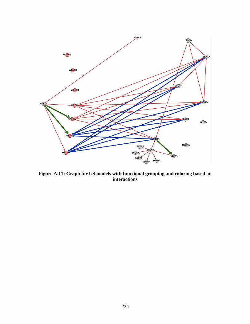
234
Figure A.11: Graph for US models with functional grouping and coloring based on
interactions
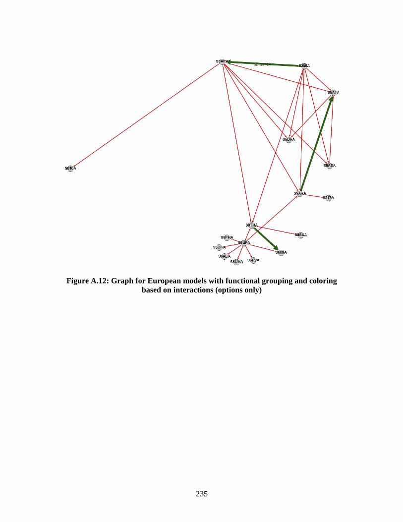
235
Figure A.12: Graph for European models with functional grouping and coloring
based on interactions (options only)

236
Figure A.13: Graph for US models with functional grouping and coloring based on
interactions (options only)

237
Figure A.14: Graph for European models with functional grouping and coloring
based on parts

238
Figure A.15: Graph for US models with functional grouping and coloring based on
parts

239
Figure A.16: Graph for European models with circular layout and coloring based
on interactions

240
Figure A.17: Graph for US models with circular layout and coloring based on
interactions
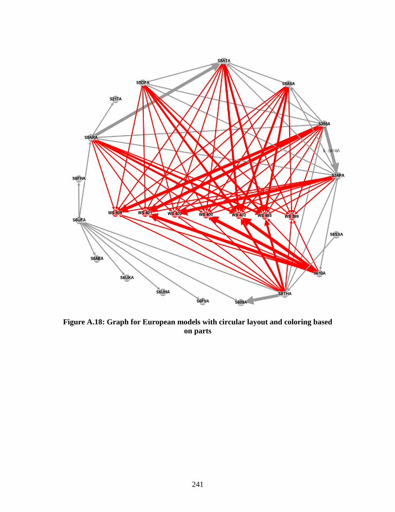
241
Figure A.18: Graph for European models with circular layout and coloring based
on parts

242
Figure A.19: Graph for US models with circular layout and coloring based on parts

243
Figure A.20: Graph for European models with circular layout and coloring based
on interactions (options only)

244
Figure A.21: Graph for US models with circular layout and coloring based on
interactions (options only)

245
Appendix G: Visualization Tool Validation User Study Packets

246
A

247
Provided
1x rule database
3x rule graphs
3x example configuration changes
Instructions
Based on the information provided in each configuration change, make edits to
the provided rule graph.
Configuration changes are independent – Configuration Change 1 should not be
considered when evaluating Configuration Change 2.
Use a fresh rule graph for each Configuration Change.
No changes need to be made to the rule database, it is for reference only.
If removing a rule is required, make sure it is clear which rule is to be removed
and how the removal is shown. Rule Grammar

248
Rule Database
Option type Name Description
Option MB1 VALUE MOTHERBOARD
Option MB2 HIGH-END MOTHERBOARD
Option CPU1 VALUE PROCESSOR UNIT
Option CPU2 MID-RANGE PROCESSOR UNIT
Option CPU3 HIGH-END PROCESSOR UNIT
Option VID1 VALUE VIDEO CARD
Option VID2 MID-RANGE VIDEO CARD
Option VID3 HIGH-END VIDEO CARD
Option HDD HARD DISK DRIVE
Option SSD SOLID STATE DRIVE
Option CD1 CD-ROM DISK DRIVE
Option BD1 BLURAY DISK DRIVE
Package VALU VALUE PACKAGE
Package BASE MID-RANGE PACKAGE
Rule type If-Part of rule Then-part of rule
- MB1 MB2
- CPU2 MB1
- CPU2 MB2
- CPU1 CPU2
- CPU1 CPU3
- CPU2 CPU3
- CD1 BD1
+ VID3 CPU3
+ VID2 CPU2 / CPU3
+ BD1 VID2 / VID3
PK VALU VID1 & CPU1 & MB1 & HDD
PK BASE VID2 & MB2 & SSD & CD1

249
Configuration change 1
Problem:
A previous change in the CPU (CPU2) from Supplier Y resulted in an incompatibility with all of the existing motherboards that are available for all laptops.
Solution:
A new motherboard (MB3) has been identified from Supplier X that meets the performance criteria for all of the CPUs currently being manufactured. Make the motherboard available for all laptops and ensure the correct CPUs are associated with the newly added motherboard.
Rule changes:
-Add new motherboard (MB3 – “High-end motherboard”) to the rule database
-Add inclusion between CPU2 and MB3
-Add exclusion between MB3 and MB1
-Add exclusion between MB3 and MB2

250
Change 1

251
Configuration change 2
Problem:
The supplier that manufacturers the parts for CPU1 has gone out of business, resulting in the potential loss of that option.
Solution:
A new supplier has been found that can produce a similar processor unit to the previous one used in CPU1. As a result, CPU1 remains a viable option. Video card rules must be changed due to new part compatibilities.
Rule changes:
-Add exclusion between CPU1 and VID1
-Remove inclusion between VID2 and CPU2 / CPU3
-Change package declaration for VALU from VID1 & CPU1 & MB1 & HDD to VID1 & MB1 & HDD
Bonus:
Why is the third rule change necessary?

252
Change 2

253
Configuration change 3
Problem:
Order history has shown that the customers are ordering the high-end video card (VID3) with the high-end CPU (CPU3), but have been settling for the less expensive motherboard (MB1). As MB1 is compatible with both options and has not been shown to hinder the performance of either higher-end option, many customers have ordered these together, resulting in a decrease in sales for laptops with the more expensive motherboard (MB2).
Solution:
Implement a new package (XPNS) that includes the high-end eversion of the motherboard (MB2), CPU (CPU3), and video card (VID3). In order for the customers to order either the high-end CPU or video card, they must include the XPNS package.
Rule changes:
-Add new package (XPNS – “High-end package”) to the ruleset
-Add package declaration for XPNS of SSD & BD1 & VID3 & MB2 & CPU3
-Add inclusion between VID3 and XPNS
-Add inclusion between CPU3 and XPNS

254
Change 3

255
B

256
Provided
3x rule database
3x example configuration changes
Instructions
Based on the information provided in each configuration change, make edits to
the provided rule database.
Configuration changes are independent – Configuration Change 1 should not be
considered when evaluating Configuration Change 2.
Use a fresh rule database for each Configuration Change.
If removing a rule is required, make sure it is clear which rule is to be removed
and how the removal is shown.
Rule Grammar
“-“ indicates mandatory exclusion (negative relationship)
“+” indicates mandatory inclusion (positive relationship)
“PK” indicates a package declaration rule (elements are included in the package)
“/” indicates “either/or” relationship (only one of them is required)
“&” indicates “and” relationships (both are required)

257
Configuration change 1
Problem:
A previous change in the CPU (CPU2) from Supplier Y resulted in an incompatibility with all of the existing motherboards that are available for all laptops.
Solution:
A new motherboard (MB3) has been identified from Supplier X that meets the performance criteria for all of the CPUs currently being manufactured. Make the motherboard available for all laptops and ensure the correct CPUs are associated with the newly added motherboard.
Rule changes:
-Add new motherboard (MB3 – “High-end motherboard”) to the rule database
-Add inclusion between CPU2 and MB3
-Add exclusion between MB3 and MB1
-Add exclusion between MB3 and MB2

258
Change 1
Option type Name Description
Option MB1 VALUE MOTHERBOARD
Option MB2 HIGH-END MOTHERBOARD
Option CPU1 VALUE PROCESSOR UNIT
Option CPU2 MID-RANGE PROCESSOR UNIT
Option CPU3 HIGH-END PROCESSOR UNIT
Option VID1 VALUE VIDEO CARD
Option VID2 MID-RANGE VIDEO CARD
Option VID3 HIGH-END VIDEO CARD
Option HDD HARD DISK DRIVE
Option SSD SOLID STATE DRIVE
Option CD1 CD-ROM DISK DRIVE
Option BD1 BLURAY DISK DRIVE
Package VALU VALUE PACKAGE
Package BASE MID-RANGE PACKAGE
Rule type If-Part of rule Then-part of rule
- MB1 MB2
- CPU2 MB1
- CPU2 MB2
- CPU1 CPU2
- CPU1 CPU3
- CPU2 CPU3
- CD1 BD1
+ VID3 CPU3
+ VID2 CPU2 / CPU3
+ BD1 VID2 / VID3
PK VALU VID1 & CPU1 & MB1 & HDD
PK BASE VID2 & MB2 & SSD & CD1
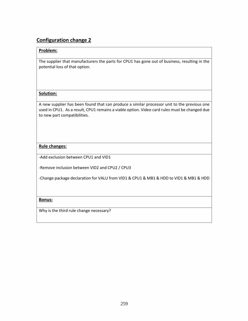
259
Configuration change 2
Problem:
The supplier that manufacturers the parts for CPU1 has gone out of business, resulting in the potential loss of that option.
Solution:
A new supplier has been found that can produce a similar processor unit to the previous one used in CPU1. As a result, CPU1 remains a viable option. Video card rules must be changed due to new part compatibilities.
Rule changes:
-Add exclusion between CPU1 and VID1
-Remove inclusion between VID2 and CPU2 / CPU3
-Change package declaration for VALU from VID1 & CPU1 & MB1 & HDD to VID1 & MB1 & HDD
Bonus:
Why is the third rule change necessary?

260
Change 2
Option type Name Description
Option MB1 VALUE MOTHERBOARD
Option MB2 HIGH-END MOTHERBOARD
Option CPU1 VALUE PROCESSOR UNIT
Option CPU2 MID-RANGE PROCESSOR UNIT
Option CPU3 HIGH-END PROCESSOR UNIT
Option VID1 VALUE VIDEO CARD
Option VID2 MID-RANGE VIDEO CARD
Option VID3 HIGH-END VIDEO CARD
Option HDD HARD DISK DRIVE
Option SSD SOLID STATE DRIVE
Option CD1 CD-ROM DISK DRIVE
Option BD1 BLURAY DISK DRIVE
Package VALU VALUE PACKAGE
Package BASE MID-RANGE PACKAGE
Rule type If-Part of rule Then-part of rule
- MB1 MB2
- CPU2 MB1
- CPU2 MB2
- CPU1 CPU2
- CPU1 CPU3
- CPU2 CPU3
- CD1 BD1
+ VID3 CPU3
+ VID2 CPU2 / CPU3
+ BD1 VID2 / VID3
PK VALU VID1 & CPU1 & MB1 & HDD
PK BASE VID2 & MB2 & SSD & CD1
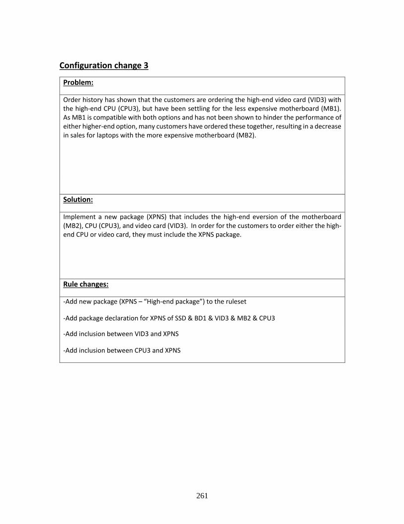
261
Configuration change 3
Problem:
Order history has shown that the customers are ordering the high-end video card (VID3) with the high-end CPU (CPU3), but have been settling for the less expensive motherboard (MB1). As MB1 is compatible with both options and has not been shown to hinder the performance of either higher-end option, many customers have ordered these together, resulting in a decrease in sales for laptops with the more expensive motherboard (MB2).
Solution:
Implement a new package (XPNS) that includes the high-end eversion of the motherboard (MB2), CPU (CPU3), and video card (VID3). In order for the customers to order either the high-end CPU or video card, they must include the XPNS package.
Rule changes:
-Add new package (XPNS – “High-end package”) to the ruleset
-Add package declaration for XPNS of SSD & BD1 & VID3 & MB2 & CPU3
-Add inclusion between VID3 and XPNS
-Add inclusion between CPU3 and XPNS

262
Change 3
Option type Name Description
Option MB1 VALUE MOTHERBOARD
Option MB2 HIGH-END MOTHERBOARD
Option CPU1 VALUE PROCESSOR UNIT
Option CPU2 MID-RANGE PROCESSOR UNIT
Option CPU3 HIGH-END PROCESSOR UNIT
Option VID1 VALUE VIDEO CARD
Option VID2 MID-RANGE VIDEO CARD
Option VID3 HIGH-END VIDEO CARD
Option HDD HARD DISK DRIVE
Option SSD SOLID STATE DRIVE
Option CD1 CD-ROM DISK DRIVE
Option BD1 BLURAY DISK DRIVE
Package VALU VALUE PACKAGE
Package BASE MID-RANGE PACKAGE
Rule type If-Part of rule Then-part of rule
- MB1 MB2
- CPU2 MB1
- CPU2 MB2
- CPU1 CPU2
- CPU1 CPU3
- CPU2 CPU3
- CD1 BD1
+ VID3 CPU3
+ VID2 CPU2 / CPU3
+ BD1 VID2 / VID3
PK VALU VID1 & CPU1 & MB1 & HDD
PK BASE VID2 & MB2 & SSD & CD1