conformal anomaly actions and dilaton interactionscoriano/tesi/mirko_serino.pdf · franco battiato....
TRANSCRIPT
arX
iv:1
407.
7113
v2 [
hep-
th]
1 A
ug 2
014
Universita Del Salento
Facolta di Scienze Matematiche, Fisiche e Naturali
Dipartimento di Matematica e Fisica “Ennio De Giorgi”
Conformal Anomaly Actions
and Dilaton Interactions
Supervisor
Prof. Claudio Coriano
Candidate
Mirko Serino
Tesi di Dottorato In Fisica - XXVI ciclo
Anno Accademico 2013 - 2014


i
piu diventa tutto inutile
e piu credi che sia vero
e il giorno della Fine
non ti servira l’inglese
Franco Battiato


iii
Aknowledgements
It is a pleasure to acknowledge all the people who made this work possible. First, I want to thank my advisor,
Claudio Coriano, for his teachings and his relentless encouragement through all these years, ever since I was an under-
graduate student. Obviously, next come my colleagues: Luigi Delle Rose, for his unceasing support and collaboration,
Carlo Marzo, for his friendship, his humour and all of his integrations by parts (!!!); Antonio Costantini, Perla Tedesco
and Annalisa De Lorenzis, for being part of our group; Roberta Armillis, Antonio Mariano and Antonio Quintavalle,
whom I always remember with pleasure; and all the people in our department with whom I have shared something
important, who are by far too many to be listed here.
I also want to thank professor Pietro Colangelo and professor Emil Mottola, for their support and the collaborations
we had.
Very special warm thanks and a huge hug are for all the members of my family, for being by my side at every step
along my path, especially in my most difficult moments.
Maurizio was the most important Presence in my life during the last year and a half and to him goes my deepest
gratitude for all his teachings and his purest friendship.
Last but not least, I want to dedicate this work to the most extraordinary woman I have ever met, loved and been
with: to Ilaria, wherever you are, from Here-And-Now to Eternity...

Contents
Contents v
List of publications ix
Introduction xi
1 Conformal symmetry and Weyl symmetry 1
1.1 Introduction . . . . . . . . . . . . . . . . . . . . . . . . . . . . . . . . . . . . . . . . . . . . . . . . . . . 1
1.2 The conformal group . . . . . . . . . . . . . . . . . . . . . . . . . . . . . . . . . . . . . . . . . . . . . . 1
1.3 Weyl symmetry and its connection to conformal invariance . . . . . . . . . . . . . . . . . . . . . . . . 3
2 The Three Graviton Vertex 9
2.1 Introduction . . . . . . . . . . . . . . . . . . . . . . . . . . . . . . . . . . . . . . . . . . . . . . . . . . . 9
2.2 Conventions and the trace anomaly equation . . . . . . . . . . . . . . . . . . . . . . . . . . . . . . . . 10
2.3 Definitions for the TTT Amplitude . . . . . . . . . . . . . . . . . . . . . . . . . . . . . . . . . . . . . . 12
2.3.1 General covariance Ward identities for the TTT . . . . . . . . . . . . . . . . . . . . . . . . . . 13
2.3.2 The anomalous Ward identities for the TTT . . . . . . . . . . . . . . . . . . . . . . . . . . . . 15
2.4 Three free field theory realizations of conformal symmetry . . . . . . . . . . . . . . . . . . . . . . . . . 15
2.5 Renormalization of the TTT . . . . . . . . . . . . . . . . . . . . . . . . . . . . . . . . . . . . . . . . . 17
2.6 The renormalized 3-graviton vertex with two lines on-shell . . . . . . . . . . . . . . . . . . . . . . . . . 20
2.7 Conclusions and perspectives: the integrated anomaly and the nonlocal action . . . . . . . . . . . . . . 23
3 Conformal correlators in position and momentum space 25
3.1 Introduction . . . . . . . . . . . . . . . . . . . . . . . . . . . . . . . . . . . . . . . . . . . . . . . . . . . 25
3.2 The correlators and the corresponding Ward identities . . . . . . . . . . . . . . . . . . . . . . . . . . . 27
3.3 Inverse mappings: correlators in position space from the momentum space Feynman expansion . . . . 29
3.3.1 The TOO case . . . . . . . . . . . . . . . . . . . . . . . . . . . . . . . . . . . . . . . . . . . . . 30
3.3.2 The V V V case . . . . . . . . . . . . . . . . . . . . . . . . . . . . . . . . . . . . . . . . . . . . . 31
3.3.3 The TV V case . . . . . . . . . . . . . . . . . . . . . . . . . . . . . . . . . . . . . . . . . . . . . 32
3.3.4 The TTT case . . . . . . . . . . . . . . . . . . . . . . . . . . . . . . . . . . . . . . . . . . . . . 35
3.4 Counterterms and their relation to the trace anomaly . . . . . . . . . . . . . . . . . . . . . . . . . . . 39
3.4.1 The counterterms for 2-point functions . . . . . . . . . . . . . . . . . . . . . . . . . . . . . . . . 39
3.4.2 Connection between counterterms and trace anomalies . . . . . . . . . . . . . . . . . . . . . . . 42
3.4.3 The counterterm for the TV V . . . . . . . . . . . . . . . . . . . . . . . . . . . . . . . . . . . . 44
3.4.4 The counterterms for the TTT . . . . . . . . . . . . . . . . . . . . . . . . . . . . . . . . . . . . 45
3.5 Handling massless correlators: a direct approach for general dimensions . . . . . . . . . . . . . . . . . 46
3.5.1 Pulling out derivatives . . . . . . . . . . . . . . . . . . . . . . . . . . . . . . . . . . . . . . . . . 47
3.5.2 Regularization of tensors . . . . . . . . . . . . . . . . . . . . . . . . . . . . . . . . . . . . . . . 51
3.5.3 Regularization of 3-point functions . . . . . . . . . . . . . . . . . . . . . . . . . . . . . . . . . . 52
v
vi CONTENTS
3.5.4 Application to the V V V case . . . . . . . . . . . . . . . . . . . . . . . . . . . . . . . . . . . . . 53
3.5.5 Application to the TOO case and double logs . . . . . . . . . . . . . . . . . . . . . . . . . . . . 55
3.6 Conclusions . . . . . . . . . . . . . . . . . . . . . . . . . . . . . . . . . . . . . . . . . . . . . . . . . . . 57
4 Dilaton interactions and the anomalous breaking of scale invariance in the Standard Model 59
4.1 Introduction . . . . . . . . . . . . . . . . . . . . . . . . . . . . . . . . . . . . . . . . . . . . . . . . . . . 59
4.1.1 The energy-momentum tensor . . . . . . . . . . . . . . . . . . . . . . . . . . . . . . . . . . . . . 60
4.2 One loop electroweak corrections to dilaton-gauge-gauge vertices . . . . . . . . . . . . . . . . . . . . . 62
4.2.1 The ργγ vertex . . . . . . . . . . . . . . . . . . . . . . . . . . . . . . . . . . . . . . . . . . . . . 63
4.2.2 The ργZ vertex . . . . . . . . . . . . . . . . . . . . . . . . . . . . . . . . . . . . . . . . . . . . . 64
4.2.3 The ρZZ vertex . . . . . . . . . . . . . . . . . . . . . . . . . . . . . . . . . . . . . . . . . . . . 65
4.2.4 Renormalization of dilaton interactions in the broken electroweak phase . . . . . . . . . . . . . 67
4.3 The off-shell dilaton-gluon-gluon vertex in QCD . . . . . . . . . . . . . . . . . . . . . . . . . . . . . . . 69
4.4 Non-gravitational dilatons from scale invariant extensions of the Standard Model . . . . . . . . . . . . 71
4.4.1 A classical scale invariant Lagrangian with a dilaton field . . . . . . . . . . . . . . . . . . . . . 72
4.4.2 The JDV V and TV V vertices . . . . . . . . . . . . . . . . . . . . . . . . . . . . . . . . . . . . . 73
4.4.3 The dilaton anomaly pole in the QED case . . . . . . . . . . . . . . . . . . . . . . . . . . . . . 74
4.4.4 The dilaton anomaly pole in the QCD case . . . . . . . . . . . . . . . . . . . . . . . . . . . . . 76
4.4.5 Mass corrections to the dilaton pole . . . . . . . . . . . . . . . . . . . . . . . . . . . . . . . . . 77
4.5 The infrared coupling of an anomaly pole and the anomaly enhancement . . . . . . . . . . . . . . . . . 78
4.6 Quantum conformal invariance and dilaton couplings at low energy . . . . . . . . . . . . . . . . . . . . 79
4.7 Conclusions . . . . . . . . . . . . . . . . . . . . . . . . . . . . . . . . . . . . . . . . . . . . . . . . . . . 80
5 Higher order dilaton interactions in the nearly conformal limit of the Standard Model 83
5.1 Introduction . . . . . . . . . . . . . . . . . . . . . . . . . . . . . . . . . . . . . . . . . . . . . . . . . . . 83
5.2 Anomalous interactions from the Ward identities . . . . . . . . . . . . . . . . . . . . . . . . . . . . . . 84
5.3 EMT’s and Correlators . . . . . . . . . . . . . . . . . . . . . . . . . . . . . . . . . . . . . . . . . . . . . 85
5.4 Ward identities . . . . . . . . . . . . . . . . . . . . . . . . . . . . . . . . . . . . . . . . . . . . . . . . . 87
5.5 Counterterms . . . . . . . . . . . . . . . . . . . . . . . . . . . . . . . . . . . . . . . . . . . . . . . . . . 89
5.6 Three and four dilaton interactions from the trace anomaly . . . . . . . . . . . . . . . . . . . . . . . . 91
5.7 Conclusions . . . . . . . . . . . . . . . . . . . . . . . . . . . . . . . . . . . . . . . . . . . . . . . . . . . 91
6 Conformal Trace Relations from the Dilaton Wess-Zumino Action 93
6.1 Introduction . . . . . . . . . . . . . . . . . . . . . . . . . . . . . . . . . . . . . . . . . . . . . . . . . . . 93
6.2 Conventions . . . . . . . . . . . . . . . . . . . . . . . . . . . . . . . . . . . . . . . . . . . . . . . . . . . 95
6.3 Overview of Weyl-gauging . . . . . . . . . . . . . . . . . . . . . . . . . . . . . . . . . . . . . . . . . . 98
6.3.1 Weyl-gauging for scale invariant theories . . . . . . . . . . . . . . . . . . . . . . . . . . . . . . . 98
6.3.2 Weyl-gauging for non scale invariant theories . . . . . . . . . . . . . . . . . . . . . . . . . . . . 100
6.3.3 The dynamical dilaton . . . . . . . . . . . . . . . . . . . . . . . . . . . . . . . . . . . . . . . . . 101
6.3.4 Weyl-gauging of the renormalized effective action . . . . . . . . . . . . . . . . . . . . . . . . . 103
6.4 The WZ effective action for d = 4 . . . . . . . . . . . . . . . . . . . . . . . . . . . . . . . . . . . . . . . 105
6.4.1 The counterterms in 4 dimensions . . . . . . . . . . . . . . . . . . . . . . . . . . . . . . . . . . 105
6.4.2 Weyl-gauging of the counterterms in 4 dimensions . . . . . . . . . . . . . . . . . . . . . . . . . 107
6.5 The WZ effective action for d = 6 . . . . . . . . . . . . . . . . . . . . . . . . . . . . . . . . . . . . . . . 108
6.5.1 The counterterms in 6 dimensions . . . . . . . . . . . . . . . . . . . . . . . . . . . . . . . . . . 109
6.5.2 General scheme-dependence of the trace anomaly in 6 dimensions . . . . . . . . . . . . . . . . . 109
6.5.3 Weyl-gauging of the counterterms in 6 dimensions . . . . . . . . . . . . . . . . . . . . . . . . . 110
6.5.4 The WZ action action for a free CFT: the (2, 0) tensor multiplet . . . . . . . . . . . . . . . . . 113

CONTENTS vii
6.6 Dilaton interactions and constraints from ΓWZ . . . . . . . . . . . . . . . . . . . . . . . . . . . . . . . 114
6.6.1 The recursive relation in 4 dimensions . . . . . . . . . . . . . . . . . . . . . . . . . . . . . . . . 118
6.6.2 The recursive relation in 6 dimensions . . . . . . . . . . . . . . . . . . . . . . . . . . . . . . . . 119
6.7 Conclusions . . . . . . . . . . . . . . . . . . . . . . . . . . . . . . . . . . . . . . . . . . . . . . . . . . . 120
A Appendix 123
A.1 Sign conventions . . . . . . . . . . . . . . . . . . . . . . . . . . . . . . . . . . . . . . . . . . . . . . . . 123
A.2 Results for Weyl-gauging . . . . . . . . . . . . . . . . . . . . . . . . . . . . . . . . . . . . . . . . . . . . 124
A.3 Weyl invariants and Euler densities in 2, 4 and 6 dimensions . . . . . . . . . . . . . . . . . . . . . . . . 124
A.4 Functional derivation of Riemann-quadratic integrals . . . . . . . . . . . . . . . . . . . . . . . . . . . . 126
A.5 Functional variations in 6 dimensions . . . . . . . . . . . . . . . . . . . . . . . . . . . . . . . . . . . . . 127
A.6 List of functional derivatives . . . . . . . . . . . . . . . . . . . . . . . . . . . . . . . . . . . . . . . . . 128
A.7 Graviton interaction vertices . . . . . . . . . . . . . . . . . . . . . . . . . . . . . . . . . . . . . . . . . 129
A.8 Comments on the inverse mapping . . . . . . . . . . . . . . . . . . . . . . . . . . . . . . . . . . . . . . 131
A.9 Regularizations and distributional identities . . . . . . . . . . . . . . . . . . . . . . . . . . . . . . . . 133
A.10 The Wess-Zumino action in 4 dimensions by the Noether method . . . . . . . . . . . . . . . . . . . . 135
A.11 The case d = 2 as a direct check of the recursive formulae . . . . . . . . . . . . . . . . . . . . . . . . . 136
B Appendix 139
B.1 Dilaton interaction vertices . . . . . . . . . . . . . . . . . . . . . . . . . . . . . . . . . . . . . . . . . . 139
B.2 The scalar integrals . . . . . . . . . . . . . . . . . . . . . . . . . . . . . . . . . . . . . . . . . . . . . . . 144
B.3 Contributions to VρZZ . . . . . . . . . . . . . . . . . . . . . . . . . . . . . . . . . . . . . . . . . . . . . 145
B.4 Standard Model self-energies . . . . . . . . . . . . . . . . . . . . . . . . . . . . . . . . . . . . . . . . . 149
Bibliography 151


List of publications
The chapters of this thesis are based on the following research papers:
• C. Coriano, L. Delle Rose, E. Mottola, and M. Serino
Graviton vertices and the mapping of anomalous correlators to momentum space for a general conformal field
theory
JHEP 1208 (2012) 147 [arXiv:1203.1339 [hep-th]]
• C. Coriano, L. Delle Rose, A. Quintavalle, M. Serino
Dilaton interactions and the anomalous breaking of scale invariance in the Standard Model
JHEP 1306 (2013) 077, [arXiv:1206.0590 [hep-ph]]
• C. Coriano, L. Delle Rose, C. Marzo, M. Serino
Higher order dilaton interactions in the nearly conformal limit of the Standard Model
Phys.Lett. B717 182-187 (2012), [ arXiv:1207.2930 [hep-ph]]
• C. Coriano, L. Delle Rose, C. Marzo, M. Serino
Conformal trace relations from the dilaton Wess-Zumino action
Phys.Lett. B726 (2013) 896-905, [ arXiv:1306.4248 [hep-th]]
• C. Coriano, C. Marzo, L. Delle Rose, M. Serino
The dilaton Wess-Zumino action in 6 dimensions from Weyl-gauging: local anomalies and trace relations
Class. Quantum Grav. 31 (2014) 105009, [arXiv:1311.1804 [hep-th]]
The following papers are related to the topics presented in this thesis but are not discussed in detail:
• C. Coriano, L. Delle Rose, A. Quintavalle and M. Serino
The conformal anomaly and the neutral currents sector of the Standard Model
Phys.Lett., B700 (2011) 29-38 [arXiv:1101.1624 [hep-ph]]
• C. Coriano, L. Delle Rose, and M. Serino
Gravity and the neutral currents: effective interactions from the trace anomaly
Phys.Rev., D83 (2011) 125028 [arXiv:1102.4558 [hep-ph]]
• C. Coriano, L. Delle Rose, M. Serino
Three and four point functions of stress energy tensors in D=3 for the analysis of cosmological non-gaussianities
JHEP 1212 (2012) 090 [ arXiv:1210.0136 [hep-th]]
• C. Coriano, L. Delle Rose, E. Mottola, M. Serino
Solving the conformal constraints for scalar operators in momentum space and the evaluation of Feynman’s
master integrals
JHEP 1307 (2013) 011 [arXiv:1304.6944 [hep-th]]
ix

x List of publications
• C. Coriano, A. Costantini, L. Delle Rose, M. Serino
Sum rules and the effective action of the composite Axion/Dilaton/Axino supermultiplet in N = 1 theories JHEP
1406 (2014) 136 [arXiv:1402.6369 [hep-ph]]
Proceedings
• L. Delle Rose, M. Serino Dilaton interactions in QCD and in the electroweak sector of the Standard Model
AIP Conf.Proc. 1492 (2012) 210-213 [arXiv:1208.6432]
• L. Delle Rose, M. Serino Massless scalar degrees of freedom in QCD and in the electroweak sector from the trace
anomaly
AIP Conf.Proc. 1492 (2012) 205-209 [arXiv:1208.6425]
Introduction
The first keystone of our present understanding of the fundamental interactions is the gauge symmetry. In fact, the
structure of the Standard Model of electroweak interactions is based on the symmetry group SU(2)L ×U(1)Y , where
L stands for the weak isospin, which characterizes left-handed fermions, and Y is the hypercharge quantum number.
Similarly, the theory of strong interactions, QCD, is entirely based on the non abelian group describing a gauged
colour symmetry, SU(3)C .
The symmetry of these groups dictates the structure of the fermion multiplets which couple to the corresponding
gauge currents and predicts the existence of four massless gauge bosons. By incorporating the spontaneous breaking
of the gauge symmetry via the Higgs mechanism, the Standard Model accounts for a gauge-invariant generation of the
masses both of the fermions and of the W±/Z bosons mediating weak interactions, while keeping the photon massless.
Beside the symmetry principles, the second fundamental pillar of a consistent quantum field theory is renormal-
izablity, which is invoked in order to remove the infinities plaguing the perturbative computations in order to obtain
predictive results. In the case of quantum electrodynamics or QED, the problem of renormalizability, for instance,
was solved in the late 40’s by Feynman [1, 2, 3, 4, 5, 6], Schwinger [7, 8, 9, 10, 11, 12, 13], Tomonaga [14] and Dyson
[15, 16]. A similar result in the case of non abelian gauge theories was presented only 20 years later, after that
Yang-Mills theories were recognized as a possible description of the fundamental interactions. In this case, the proof
of renormalizability was given by ’t Hooft in 1971 [17, 18].
Together, gauge symmetry and renormalizability allow to successfully account for three of the four fundamental
interactions observed in nature, i.e. electromagnetism, weak and strong interactions, at least up to the highest energy
which can be experimentally tested. Nonetheless, this picture is far from being complete. In fact, gravitation is still out
of this framework, and has so far defied any attempt to a proper quantization, consistent with perturbative unitarity
and renormalizability. Its formalism is obtained by gauging the 10-parameter Poincare group of rigid translations,
boosts and rotations acting in Minkowski space, which turns into the group of general coordinate transformations,
also called diffeomorphisms.
Despite the fact that General Relativity is a gauge theory which has successfully passed all the experimental tests
performed so far and that almost a century has passed since 1916, when it was formulated for the first time, a consistent
quantum description of gravitation is still lacking. This happens because no renormalization program is viable for the
quantized Einstein’s theory. In fact, due to well known power counting arguments, a necessary condition for a field
theory to be renormalizable is that the coupling constants in the Lagrangian must not have negative mass dimensions.
The Einstein-Hilbert action contains one such parameter, namely Newton’s constant G, whose dimension is [M ]−2
and
therefore the attempt to quantize General Relativity inevitably results in a non renormalizable theory. This implies
that the description of the dynamics of the gravitational field needs to be modified at very high energies, i.e. near the
Planck energy EP = (~ c5/G)12 ≈ 1.22 × 10¹⁹ GeV, where it is expected to play a decisive role in the dynamics of the
early universe.
At present, nobody has ever formulated a consistent quantum theory of gravitation, but there are two reasons why
one can draw really significant insights by coupling a relativistic field theory to a purely classical background metric.
First, the value of EP is bigger by fifteen orders of magnitude than the highest energy at which all the known
quantum field theories can be experimentally tested so far, i.e. 14 TeV’s at the Large Hadron Collider. This means
that the description of any scattering process will not be affected at all by the quantum fluctuations in the gravitational
xi
xii Introduction
field.
Second, and more importantly for the purposes of this work, beside the symmetry under general coordinate trans-
formations, which is enjoyed by any system embedded in curved space according to the formalism of General Relativity,
there is another one, which is typical of a subset of theories containing no dimensioful parameters, i.e. Weyl sym-
metry. A theory is said to be Weyl-symmetric if its action is invariant under the local rescaling of the metric tensor
gµν → e2σ(x)gµν , where σ(x) is a well-behaved function of the coordinates. It is trivial to see that the condition
expressing Weyl invariance is the tracelessness of the energy-momentum tensor, T µµ = 0.
On the other hand, it is known that the possibility to define a traceless energy-momentum tensor, for instance by
introducing proper terms of improvement, is the condition obeyed in Minkowski space by field theories which are in-
variant under the conformal group [19].We remark that the conformal constraints in Minkowski space are implemented
through rather nontrivial operators, whereas Weyl symmetry is much more straightforward to study. In particular,
the tracelessness condition on the stress-energy tensor, derived in curved space as a consequence of Weyl symmetry,
obviously remains valid in the flat limit as well.
Under some mild assumptions, it is possible to provide a simple algebraic criterion in curved space which allows to
establish whether a classical field theory is conformally invariant [20] or not. There is a great advantage in studying
field theories through their formal embedding in a curved space-time background. In fact many aspects of conformal
invariance can be studied much more easily than in Minkowski space, by analysing the constraints of the abelian Weyl
group. This issue is reviewed in chapter 1, to set the stage for all the subsequent work presented in this thesis. So far
for classical conformal field theories.
Conformal anomalies and the low-energy effective actions for gravity
It is known that, due to renormalization effects, the naive tracelessness condition of the energy-momentum tensor
that conformal field theories enjoy at the classical level is not inherited by the vacuum expectation value of the
corresponding quantum operator [21, 22, 23, 24, 25, 26]. Terms violating the classical Weyl symmetry due to quantum
effects are known as conformal or trace anomalies and are of two kinds. Terms of the first kind are proportional
to the beta functions of the theory and depend on the background gauge fields, so that they vanish only at the
renormalization group fixed points for theories containing interactions, whereas they do not appear at all in free field
theories. Terms of the second kind are c-number contributions depending on the background metric tensor and are
always present in the trace of the energy-momentum tensor of any field theory. It goes without saying that for theories
which are not conformally invariant at the classical level, these terms appear in the trace of vaccum expectation value
of the energy-momentum tensor together with the vacuum expectation value (vev) of the operators which classically
break conformal symmetry, e.g. the mass terms.
An outstanding feature of the conformal anomalies is that, whether they are seen as a consequence of renormaliza-
tion of UV singularities [24] or as an infrared effect [27], they affect the physics of the system at all energy scales. This
circumstance is generally true for chiral anomalies and has led ’t Hooft to formulate his famous anomaly matching
conditions [28], which are a powerful constraint for chiral theories describing the low-energy limit of QCD.
For conformal anomalies, as we have mentioned, there are contributions which depend on the beta-functions of the
theory, and hence on the energy scale, but there are also pure c-number contributions, built out of the metric tensor,
just as in the chiral case.
The existence of such scale-independent terms allows to look at the connection between conformal symmetry and
General Relativity also in other ways. In fact, since anomalies are a quantum effect that does not depend on the
energy scale and are built out of the metric background field, they affect the description of gravitation in the infrared
regime of the quantum theory, providing the first corrections to the classical Einstein-Hilbert action [29].
The dynamics of a quantum system in the infrared can be effectively described by a proper low-energy action
encoding the symmetries of the theory and describing the interactions of the degrees of freedom surviving in the
infrared regime [30], after integrating out the ultraviolet modes. If the theory is anomalous, the effective action is
modified and can always be thought as a sum of the anomalous and of the ordinary (non anomalous) one, which is
xiii
homogeneous under the action of the anomalous symmetry transformation.
Historically, the first example of this kind is the Wess-Zumino effective action for the SU(3)L × SU(3)R flavour
symmetry of low-energy QCD, describing the pion dynamics [31] and incorporating the effects of the chiral anomalies.
In this case, pions appear as (pseudo-) Goldstone bosons introduced specifically to solve the variational problem
defined by the anomalous Ward identities.
It is important to notice that anomalous effective actions solving the chiral constraints can also be defined without
introducing additional scalar fields, but in this case they are non-local (see e.g. [32] for an overview).
Of course, any variational solution of the anomaly equation cannot account for the non anomalous part part of the
effective action and is always defined modulo homogeneous terms. Determining such contributions requires a separate
effort. For example, in the case of the one-particle irreducible effective action, it is necessary to explicitly evaluate
the Feynman diagrams in the perturbative series, taking into account all the degrees of freedom in the fundamental
Lagrangian.
On the perturbative side, a signature of scalar degrees of freedom is present in computations of Feynman diagrams
as well. The chiral anomaly was discovered by Schwinger [33] and, later, by Adler, Bell and Jackiw [34, 35] in the
AV V diagram describing the decay of an axial-vector current (A) into two vector currents (V ). Soon after that,
it was pointed out by Dolgov and Zakharov that a salient feature of this diagram is the presence of a one-particle
massless pole [36]. Finally, this massless pole was interpreted as a signature of a scalar degree of freedom, identified
with the pion, interpolating between the axial and the vector currents. This interpretation is encoded in the modified
PCAC relation connecting the divergence of the axial current to the pion field plus the chiral anomaly term [34], which
successfully accounts for the experimental pion decay rate into two photons.
The situation for conformal anomalies has shown to be quite similar. A non-local effective action for the trace
anomaly in 4 dimensions was proposed for the first time in a paper by Deser, Duff and Isham [37], but this action has
a rather complicated form, as it contains logarithmic terms such as log(
(+R)/µ2)
, where µ is a renormalization
scale and R the Ricci scalar, which are hard to expand around the flat limit gµν = ηµν . Moreover, the possibility of the
existence of such logarithmic terms in the anomalous effective action was subsequently ruled out through cohomological
arguments in [38, 39, 40].
An action which provides the minimal variational solution of the anomaly equation in a general curved background
and can be easily expanded around flat space was found by Riegert in 1987 [41].
A salient feature of Riegert’s effective action is that, just like the non-local action for chiral anomalies, it predicts
the existence of massless scalar poles coupled to the anomaly, as shown in [27], so that, in order to complete the
correspondence between chiral and conformal anomalies, this pole should be found in perturbative computations.
Given the structure of the trace anomaly (see chapter 2), the easiest way to look for such an interpolating scalar state
in perturbation theory is to evaluate explicitly the TV V correlator in flat space, where T is the energy-momentum
tensor and V stands for a vector current. This Green function, at 1-loop, gives the next-to-leading order contribution
to the interaction between a graviton and two gauge bosons and is affected by the trace anomaly. In [27, 42] its
computation was performed in QED and the pole predicted by Riegert’s action was found. As Riegert’s action holds
for non abelian gauge theories as well, the computation was subsequently performed in QCD and in the Standard
Model [43, 44], confirming the presence of this contribution in all cases.
A similar analysis of anomaly poles in three point functions was performed in a supersymmetric context for N = 1
super Yang-Mills theory in [45]. In this work, it is shown that anomaly poles appear in the JVV correlator, with Jthe Ferrara-Zumino hypercurrent and V the vector supercurrent.
The next thing to accomplish, in order to complete this program, is to look for anomaly poles in the contributions
to the trace anomaly depending only on the metric tensor. This requires the study of correlation functions of the
energy-momentum tensor alone, as this is the quantum operator sourced by the metric tensor. Actually, a trace
anomaly already affects the 2-point function of the energy-momentum tensor, but it depends on the renormalization
scheme, so that the first correlator where scheme-independent contributions can be found is the TTT vertex.
Chapter 2 of this thesis presents a complete 1-loop computation of the three graviton vertex in 4 dimensions, in three
xiv Introduction
different free field theories which are conformally invariant, namely the scalar field with a proper term of improvement,
the Dirac fermion and the abelian gauge boson. The computation is performed in the off-shell kinematic configuration,
by evaluating all the diagrams in the perturbative expansion with the Passarino-Veltman tensor-reduction technique,
implemented in a symbolic manipulation program. The results are tested by checking the general covariance and the
trace Ward identities which descend from the well known master equations for the conservation and the anomalous
trace of the energy-momentum tensor. Renormalization is performed in the MS scheme.
The general result is given in terms of a set of 499 scalar coefficients multiplying a corresponding basis of rank-6
tensors. Due to the size of the general result, explicit coefficients are provided only in the limit in which two of the
three gravitons are on the mass-shell, for which we expand all the correlator on a basis of only 13 tensors.
In the end, Riegert’s effective action for the conformal anomaly is explicitly introduced and we briefly review one
of its two possible local formulations, i.e. in terms of two auxiliary scalar fields, which is discussed, for instance, in
[29]. In this paper the infrared effective action for gravity is studied, with special focus on the terms induced by
the anomaly, which are shown to be relevant in the infrared and, as such, provide the first quantum corrections to
General Relativity. The possible appearance of scalar poles interpolating between the gravitons and the anomalous
contributions to the TTT vertex is briefly discussed as a suggestion for further investigation.
Conformal symmetry in position and in momentum space
In chapter 3, we temporarily turn away from the discussion of the conformal anomaly effective actions and exploit
our computation of the TTT correlator to elaborate on the connection between conformal invariance in position and
momentum space.
The implications of the constraints of conformal invariance have been worked out mostly in position space, as for
instance in [46, 47], where the structure of various important 3-point correlators was established, modulo a small set
of constants.
On the other hand, explicit evaluations of correlators in specific conformally invariant field theories are performed
through the usual Feynman expansion, which is commonly and most easily implemented in momentum space. This
discrepancy is likely to hinder the comparison of results found in the two ways, especially when it comes to such
complicated correlators as the TTT , whose first explicit perturbative computation was performed for the first time in
[48] and is discussed here in chapter 2. Motivated by the search for a clear-cut way to map the results obtained with
these different approaches into each other, we develop two methods of comparison to which chapter 3 is devoted.
The first method is called the inverse mapping procedure. It starts from the integral expression in momentum
space of the 1-loop diagrams defining the correlators and proceeds with their (inverse) Fourier transform. This allows
to set a precise correspondence between Feynman diagrams with specific different topologies and the non-local terms
in the position space expressions for 3-point functions which are provided in [46]. Counterterms, which correspond to
local terms in position space, are considered separately, as they have to be added by hand in most cases.
Clearly, this method makes sense only with theories for which a specific Lagrangian formulation exists and that are
clearly defined in momentum space. Nevertheless, the implications of conformal constraints are much more general,
as they do not rely on a specific Lagrangian. In this sense, after using extensively the inverse-mapping procedure to
compare perturbative results with the constructions in [46], we turn to the development of a second method, which
works in the opposite direction. It is a general algorithm to Fourier-transform position space results, finding their
expressions in terms of integrals in momentum space. In order to deal with non Fourier-integrable expressions, the
use of an intermediate regulator is required, in the spirit of differential regularization [49]. An interesting result of this
analysis is a criterion to establish whether the conformal correlator which is studied can be realized in the framework
of a Lagrangian theory or not. In fact, the mapping procedure can end on momentum integrals containing logarith-
mic terms, which clearly cannot be generated from any Lagrangian theory. So, if the expressions of the transformed
correlators contain combinations of such terms which cannot be re-expressed as ordinary Feynman integrals, then it
is established that the underlying conformal field theory cannot be formulated in terms of a local Lagrangian.

xv
Dilatons and effective actions for conformal anomalies
Coming back to the discussion of the effective actions for conformal anomalies, we have already mentioned that
Riegert’s nonlocal action can be expressed in a local form at the cost of introducing two auxiliary scalar fields [29].
The presence of two such fields is the consequence of the existence of 2 independent cocycles for the Weyl group in 4
dimensions (see [38] and the discussion in chapter 6 of this work for details).
However, as the Weyl group is abelian, application of the general method of Wess and Zumino to the trace anomaly
[50] implies that a local effective action can be built in terms of one single (pseudo-)Goldstone boson, which is usually
called dilaton. The construction of this effective action is discussed extensively in chapter 6.
From chapter 4 onwards, this thesis deals with dilaton interactions.
Dilaton states may be either fundamental or composite scalars. In the first case, they result from the compactification
of extra dimensions (graviscalars) or, on the other hand, they may appear as effective degrees of freedom of a more
fundamental field theory, similar Nambu-Goldstone (NG) modes of a broken symmetry. While massless NG modes are
always present in the case of a spontaneously broken global symmetry, for radiative breakings their massless nature is
not necessarily guaranteed. In fact, non perturbative effects may contribute with a mass term and shift the position
of the massless poles encountered in the 1-particle irreducible (1PI) anomaly action.
If the dilaton is not a fundamental field, then, in close analogy with the pion case, it can be thought of as an
effective state mediating the coupling of matter to the trace anomaly, according to the interactions derived from the
Wess-Zumino action.
On the perturbative side, the pole identified in the TV V correlator in [27] suggests that there might be such effective
state interacting with matter via the trace anomaly. Moreover, as the pion is a composite state of fermions, it is quite
natural to elaborate on the idea that the dilaton is a composite state of particles belonging to a strongly interacting
sector which might be accessible in the near future at high energy colliders. This possibility was suggested, for instance,
in [51]. In this sense, the Wess-Zumino action for the conformal anomaly could describe the low-energy limit of a
theory whose more fundamental components might be revealed at energies higher than those probed so far at the
LHC. Then the dilaton could prove to be an effective degree of freedom surviving at energies lower than the scale Λ
at which conformal symmetry is broken.
Chapter 4, which is based on [52], discusses this scenario and presents complete 1-loop computations of the
interactions of a graviscalar particle, derived from the compactification of large extra dimensions, with the neutral
gauge currents of the Standard Model.
Then we turn, in the same chapter, to a discussion of scale invariant extensions of the Standard Model and to the
possibility that the anomaly poles found in the TV V in these theories [27, 42, 43, 44] might be describing the emergence
of an effective dilaton. We must mention that a very similar scenario shows up in the N = 1 super Yang-Mills theory,
where anomaly poles appearing the triangle correlator of the Ferrara hypercurrent and two vector supercurrents can
be interpreted as a signal of the exchange of a composite dilaton/axion/dilatino multiplet in the effective Lagrangian
[45].
Chapter 5, based on [53], extends the results of chapter 4 by working in the conformal limit of the Standard Model,
in which all the masses are set to zero. In this regime, we present the computation of 3- and 4-point traced correlators of
the energy-momentum tensor, which exactly match dilaton self-interactions in the on-shell limit. Techniques presented
in chapter 3, relying on the connection between the trace anomaly and the gravitational counterterms for conformal
field theories, are used to secure the correctness of the result.
Finally, chapter 6 deals with the Wess-Zumino action for the geometric sector of the conformal anomaly both in 4
and 6 dimensions, putting together the results presented in [54, 55]. The anomalous effective action is explicitly built
by using the most general renormalization scheme, exploiting a cohomological method presented for the first time
in [38]. Possible kinetic terms for the dilaton, which obviously cannot be derived by the analysis of the anomalous
constraints, are systematically reviewed. After the derivation of the most general anomalous effective action, an
xvi Introduction
interesting result is proven. First, the Wess-Zumino anomalous effective action is written in another way, i.e. as a
perturbative functional expansion with respect to the dilaton field, which is also a power series in the inverse conformal
breaking scale, 1/Λ. Each term of this power series, in turn, is a well defined and simple combination of traced Green
functions of the energy-momentum tensor. For consistency, then, one can require that each term in the perturbative
expansion must match the term proportional to the same power of 1/Λ in the explicit expression of the anomalous
effective action which is derived in the first part with cohomological methods. Imposing this consistency condition
results in an infinite set of recurrence relations, which allow to compute traced correlators of the energy-momentum
tensor to an arbitrarily high order.
Chapter 1
Conformal symmetry and Weyl
symmetry
1.1 Introduction
In this introductory chapter, we set the stage for all the results to be presented in the rest of the thesis. The
computations that we present are performed by embedding the quantum field theories that we are going to investigate
in a curved metric background gµν . Hereafter, the term matter fields will be used by us to refer to any fundamental
field except for the metric tensor. In particular we are going to present a short introduction on the concept of Weyl
symmetry and its various realization in a curved background. This will be useful for the analysis presented in the
later chapters. Weyl invariance in a curved background allows to address the issue of conformal invariance in any
free-falling frame. We recall that conformal invariance implies the possibility to define a traceless energy-momentum
tensor, as discussed, for instance, in [19]. The search for theories which exhibit scale invariance but not conformal
invariance has been at the center of several recent studies, as reviewed in [56]. The advantage of dealing with a Weyl
invariant theory in a curved background respect to a conformal symmetric theory in flat background is in the different
character of the two symmetry groups, as the first one is abelian. Therefore, one can derive specific implications for a
certain conformal invariant theory by starting from a simpler Weyl invariant theory on a curved background and the
specialising the result to a local free falling frame [20].
In the following sections, we first introduce the conformal group, then proceed to discuss Weyl invariance in curved
spacetime background. Finally, we review the argument presented in [20]. Our attention will be limited to the case of
any spacetime dimensions except for the case of d = 2 since in this case the conformal group is infinite dimensional.
1.2 The conformal group
We present a brief review, in d > 2 dimensions and euclidean space, of the transformations which identify the conformal
group SO(2, d). These may be defined as the transformations xµ → x′µ(x) that preserve the infinitesimal length up to
a local factor
dxµdxµ → dx′µdx
′µ = Ω(x)−2dxµdxµ . (1.1)
In the infinitesimal form, the conformal transformations are given by
x′µ(x) = xµ + aµ + ωµν xν + σ xµ + bµ x
2 − 2 b · xxµ , , (1.2)
with
Ω(x) = 1− λ(x) and λ(x) = σ − 2b · x . (1.3)
1

2 Conformal symmetry and Weyl symmetry
The transformation in eq. (1.2) is defined by translations (aµ), boosts and rotations (ωµν = −ωνµ), dilatations (σ)
and special conformal transformations (bµ). The first two define the Poincare subgroup which leaves invariant the
infinitesimal length and for which Ω(x) = 1. If we also consider the inversion
xµ → x′µ =xµx2
, Ω(x) = x2 , (1.4)
we can enlarge the conformal group to O(2, d). Special conformal transformations can be realized by a translation
preceded and followed by an inversion.
The Poincare subgroup containts the basic set of symmetries for any relativistic system. Its albegra is given by
i [Jµν , Jρσ] = δνρ Jµσ − δµρ Jνσ − δµσ Jρν + δνσ Jρµ ,
i [Pµ, Jρσ] = δµρ P σ − δµσ P ρ ,
[Pµ, P ν ] = 0 , (1.5)
where the J ’s are the generators of the Lorentz group and the four components of the momentum Pµ generate
rigid translations. For scale invariant theories, which contain no dimensionful paramters, the Poincare group can be
extended by including the dilatation generator D, corresponding to the fourth terms in the coordinate transformations
in (1.2), whose commutation relations with the other generators are
[Pµ, D] = i Pµ ,
[Jµν , D] = 0 . (1.6)
Finally, it is possible to further extend this group so as to include the four special conformal transformations, whose
generators we call Kµ, extending the algebra as
[Kµ, D] = −iKµ ,
[Pµ,Kν ] = 2 i δµν D + 2 i Jµν ,
[Kµ,Kν ] = 0 ,
[Jρσ,Kµ] = i δµρKσ − i δµσKρ . (1.7)
By the way, it is clear from (1.6) and (1.7) that scale invariance does not require conformal invariance, but conformal
invariance necessarily implies scale invariance.
Having specified the elements of the conformal group, we can define a quasi primary field Oi(x), where the index
i runs over the representation of the group to which the field belongs, through the transformation property under a
conformal transformation g
Oi(x)g→ O′i(x′) = Ω(x)ηDi
j(g)Oj(x) , (1.8)
where η is the scaling dimension of the field and Dij(g) denotes the representation of O(1, d− 1). In the infinitesimal
form we have
δgOi(x) = −(LgO)i(x) , with Lg = v · ∂ + η λ+1
2∂[µvν]Σ
µν , (1.9)
where the vector vµ is the infinitesimal coordinate variation vµ = δgxµ = x′µ(x)− xµ and (Σµν)ij are the generators of
O(1, d− 1) in the representation of the field Oi. The explicit form of the operator Lg can be obtained from eq. (1.2)
and eq. (1.3) and is given by
translations: Lg = aµ∂µ ,
rotations: Lg =ωµν
2[xν∂µ − xµ∂ν − Σµν ] ,
scale transformations : Lg = σ [x · ∂ + η] ,
special conformal transformations. : Lg = bµ[
x2∂µ − 2xµ x · ∂ − 2η xµ − 2xνΣµν]
. (1.10)
1.3 Weyl symmetry and its connection to conformal invariance 3
As already remarked, invariance of a matter system under the conformal group implies the possibility to define a
traceless energy-momentum tensor T µνI [19],
T µI µ = 0 , (1.11)
where the subscript I indicates that possible improvement terms have been added to the minimal energy-momentum
tensor which is obtained from the sole requirement of invariance under the Poincare group.
1.3 Weyl symmetry and its connection to conformal invariance
Now that conformal symmetry in flat space has been introduced, we can move on to curved space and discuss Weyl
symmetry. We assume that the reader is familiar with basic General Relativity, including the Vielbein formalism
which is necessary to embed fermions in a gravitational field, for which we refer to [26, 57]. In the following, we follow
the discussion in [20].
Let us suppose that our theory in flat space is described by an action functional
S =
∫
ddxL(Φ, ∂µΦ) , (1.12)
depending on the matter fields Φ and their first derivatives. This theory can be easily embedded in curved space,
replacing ordinary derivatives with diffeomorphism-invariant ones
S =
∫
ddx√gL(Φ,∇µΦ) , (1.13)
The energy-momentum tensor of the theory is defined as the source of the gravitational field appearing in Einstein’s
equations and it is given by
T µν =2√g
δSδgµν
. (1.14)
For a Lagrangian in flat space written in a diffeomorphic invariant form, scale invariance is equivalent to global Weyl
invariance. The equivalence can be shown quite straightforwardly by rewriting a scale transformation acting on the
coordinates of flat space and the matter fields Φ,
xµ → x′µ= eσxµ ,
Φ(x) → Φ′(x′) = e−dΦσΦ(x) , (1.15)
in terms of a rescaling of the metric tensor, the Vielbein and the matter fields
gµν(x) → e2σ gµν(x) ,
Va ρ(x) → eσ Va ρ(x) ,
Φ(x) → e−dΦσΦ(x) , (1.16)
leaving the coordinates x of the manifold invariant. We have denoted with dΦ the field scaling dimension, which is
deduced by an ordinary dimensional analysis of the Lagrangian density. The reason why (1.15) can be traded for (1.16)
is that metric tensors and the Vielbein always appear in order to contract derivative terms to obtain diffeomorphic
scalars.
Once we move to a curved metric background, it is natural to promote the global scaling parameter σ to a local
function, so that the transformation laws of the metric, Vielbein and matter fields are
g′µν(x) = e2σ(x) gµν(x) ,
V ′a ρ(x) = eσ(x) Va ρ(x) ,
Φ′(x) = e−dΦ σ(x) Φ(x) . (1.17)
4 Conformal symmetry and Weyl symmetry
The transformations of metric, Vielbein and matter fields shown in (1.17) define the abelian Weyl group. It is natural
to ask whether is possible to modify the theory in such a way that (1.17) leave the action functional invariant.
Historically, the scale symmetry was the first whose gauging was systematically studied, in an attempt, made by
Weyl, to connect electromagnetism with geometry. For this reason, this procedure was named Weyl-gauging. It can
be implemented in the same way as for QED, introducing an appropriate new field which takes a role similar to the
vector potential. This allows to define a new Lagrangian which is diffeomorphic and Weyl invariant at the same time.
For instance, for a free scalar theory described by the action
Sφ =1
2
∫
ddx√g gµν ∂µφ∂νφ, (1.18)
the derivative terms are modified according to
∂µ → ∂Wµ = ∂µ − dφWµ , (1.19)
where Wµ is a vector gauge field that shifts under a Weyl trasnformation as
Wµ →Wµ − ∂µσ . (1.20)
In the case of a covariant derivative acting on higher spin fields, such as a spin-1 field vµ, the Weyl-gauging has to
be supplemented with a prescription to render the generally covariant derivative Weyl invariant, which is to add to
(1.19) the modified Christoffel connection
Γλµν = Γλµν + δµλWν + δν
λWµ − gµνWλ . (1.21)
It is easy to check that this Christoffel symbol is Weyl invariant. So, pursuing closely the analogy with the gauging of
a typical abelian theory, we can define the Weyl covariant derivatives acting on vector fields as
∇Wµ vν = ∂µvν − dvWµvν − Γλµνvλ ,
∇Wµ vν → e−dvσ(x) ∇W
µ vν , (1.22)
with an obvious generalisation to tensors of arbitrary rank.
Of course, the extension of such a derivative to the fermion case requires the Vielbein formalism and is obtained by
the relation
∇µ → ∇Wµ = ∇µ − dψWµ + 2Σµ
νWν , Σµν ≡ V aµ V bνΣab , (1.23)
where we have denoted with dψ the scaling dimension of the spinor field (ψ) and with Σab the spinor generators of
the Lorentz group.
If we Weyl-gauge the scalar action (1.18) according to the prescriptions in (1.19) and (1.20), we obtain
Sφ,W =1
2
∫
ddx√g gµν ∂Wµ φ∂Wν φ =
1
2
∫
ddx√g gµν
(
∂µ − d− 2
2Wµ
)
φ
(
∂ν −d− 2
2Wν
)
φ
=1
2
∫
ddx√g gµν
∂µφ∂νφ− d− 2
2
(
φWµ ∂νφ+ φWν ∂µφ− d− 2
2WµWν φ
2
)
(1.24)
which, using φ∂µφ = 1/2 ∂µφ2 and integrating by parts, can be written in the form
Sφ,W =1
2
∫
ddx√g gµν
(
∂µφ∂νφ+ φ2d− 2
2Ωµν(W )
)
, (1.25)
where we have introduced the quantity
Ωµν(W ) = ∇µWν −WµWν +1
2gµνW
2 . (1.26)
The result of this procedure is a Weyl invariant Lagrangian in which the Weyl variation of the ordinary kinetic term
of φ is balanced by the variation of the Ω term.
1.3 Weyl symmetry and its connection to conformal invariance 5
This term plays a prominent role in the subsequent discussion, as we are going to ask whether it is possible to
enhance scale invariance to Weyl invariance without introducing the new degree of freedomWµ. To this aim, we notice
that there are two second rank tensors which can be built out of Wµ and its first covariant derivative, namely WµWν
and ∇µWν .
From (1.20), we can infer how they transform under a finite Weyl scaling,
∆(WµWν) = σµσν − (Wµσν +Wνσµ) , (1.27)
where we habve introduced σµ ≡ ∂µσ to keep the notation easy. To compute the finite Weyl-variation of ∆(∇µWν)
we recall the transformation rule for the Christoffel connection, Γλµν
∆Γλµν = gλσ(
gµσσν + gνσσµ − gµνσσ)
, (1.28)
which implies
∆(∇µWν) = −∇µσν − gµν σ · σ + 2 σµσν + gµνW · σ − (Wµ σν +Wν σµ) . (1.29)
If we notice that contracting (1.27) we obtain
∆(gµνW ·W ) = gµν (σ · σ − 2W · σ) , (1.30)
then we immediately conclude that the variation under a finite Weyl shift of Ωµν [W ] is independent of Wµ and
symmetric. More precisely, it is given by
∆Ωµν [W ] = −(
∇µσν − σµσν +1
2gµν σ ·σ
)
= −Ωµν [σ] . (1.31)
As Ωµν [σ] depends only on the scaling parameter σ, one can argue that it may be related to some purely geometrical
object. In fact, the variation of the Ricci tensor under a local scale trasnformation is given by
∆Rµν = Rµν [e2σgµν ]−Rµν [gµν ] = gµν∇2σ + (n− 2)
(
∇µσν − σµσν + gµν σ ·σ)
. (1.32)
From (1.32) we see that the tensor
Sµν = Rµν −gµν
2(n− 1)R (1.33)
transforms under Weyl-scalings in the same way as Ωµν , i.e.
∆Sµν = (n− 2)Ωµν [σ] . (1.34)
Now it is clear when Weyl-gauging can be replaced by a non-minimal coupling to the curvature. Since, according to
(1.33) and (1.34), the Weyl variation of Ωµν [W ] is proportional to the variation of Sµν , we see that whenever Wµ
appears in the action only in the combination Ωµν [W ], it can be replaced by Sµν . Replacing terms depending on Wµ
with a non minimal couplig to the Ricci tensor is a procedure referred to as Ricci gauging.
We still have to explore under what conditions, in an action which is Weyl-gauged, the terms depending on Wµ
appear only in the combination Ωµν . We are going to see that the sufficient condition for Ricci gauging to be possible
is preciely conformal invariance in flat space.
We can start our discussion by representing a conformal transformation of the metric in the form of a diffeomorphism
∂xµ
∂x′α∂xν
∂x′βgµν(x) = gαβ(x
′) and gαβ(x) = eσ(x)gαβ(x) . (1.35)
The functions σ in (1.35) form a subgroup of the group of local Weyl transformations that is induced by conformal
transformations, that we call the conformal Weyl group. Given (1.35), we can characterize the functions σ via the
condition∂xµ
∂x′α∂xν
∂x′βRµν(x) = Rαβ(y) = Rαβ [e
2σgµν ](x′) , (1.36)

6 Conformal symmetry and Weyl symmetry
which leads, in virtue of the transformation law of the tensor Sµν under Weyl shifts, given by (1.32) and (1.34), to the
differential equation
(n− 2)σαβ [σ] = Sµν − Sµν . (1.37)
The existence of global solutions of (1.37) is a non-trivial problem in general. Now, as in the flat-space limit Sαβ
vanishes, the condition (1.37) reduces to
∂ν σµ − σµσν +gµν2
σ ·σ = 0 . (1.38)
We find that the general solution of (1.38) identifying the subset of the σ functions defining the conformal group of
flat space is simply
σ(x) = log
(
1
1− 2 b · x+ b2 x2
)
, (1.39)
where b is any constant vector. We see that (1.39), for b infinitesimal, corresponds exactly to eq. (1.3). When expo-
nentiated as in (1.35), it gives a metric tensor producing the variation of the line interval defined in (1.1).
Now suppose that an action S admits Ricci gauging, so that the gauged action satisfies the condition
S(Φ, Sµν) = S(Φ′, Sµν + (n− 2)Ωµν [σ]) , (1.40)
where Φ′ denotes the Weyl-transformed fields. It follows in particular that, if Ωµν [σ] = 0, the action is invariant
even without gauging. But the condition Ωµν [σ] = 0 defines the conformal Weyl group in flat space, as shown in eqs.
(1.37)-(1.39); Ricci gauging is equivalent to the identity transformation, as the Riemann tensor always vanishes in flat
space [57]. This proves that, if an action admits Ricci gauging, it is conformally invariant in flat space.
All that remains to be proved is that conformal invariance in flat space is also sufficient for the action to admit Ricci
gauging. This result will be proved for actions which which contain only first derivatives of the conformally variant
fields. Suppose that an action S0 is conformally invariant in flat space. For infinitesimal conformal transformations
we then have the conservation law
δS0 =
∫
ddxσµjµ = cµ
∫
jµ = 0 , (1.41)
where jµ is the virial current [19, 58], defined as
jµ = πν (dΦδµν + 2Σµν)Φ , πµ =
δSδ(∂µΦ)
, (1.42)
where we remind that the Σ’s are the generators of the Lorentz group in the representation of the field Φ and σ = bν xν .
Eq. (1.41) holds for an arbitrary vector bµ, so it implies that jµ is the divergence of a second rank tensor,
jµ = ∂νJµν . (1.43)
As the actions we are considering contain only first derivatives of the conformally variant fields, the same must be
true for jµ. Therefore (1.43) is telling us that the tensor Jµν depends only on the conformally variant fields and not
on their derivatives, for otherwise jµ would contain higher derivatives of the same fields. This implies that jµ is at
most linear in the derivatives of the conformally variant fields. So, given the definition of the virial current (1.42), the
action S0 must be at most quadratic in the same derivatives.
We have got the intermediate result that as far as we consider actions containing only first derivatives of the confor-
mally variant fields, conformal invariance is allowed only for those which are at most quadratic in such derivatives.
In the case where the action is linear in the first derivatives the same argument implies that the virial current is
identically zero. This happens, for instance, for the Dirac fermion, which does vary under coformal transformations.
On the other hand, the argument does not impose any conditons on the conformally invariant fields.
1.3 Weyl symmetry and its connection to conformal invariance 7
Next we consider finite conformal transformations. As our actions are at most quadratic in the first derivatives of
the conformally variant fields and there are no higher derivatives of any field whatsoever, their variation under finite
conformal shifts is simply
∆S0 =
∫
ddx (σµjµ + σµσνK
µν) , (1.44)
where Kµν does not contain derivatives of the fields. Using the relation (1.43) , we can integrate by parts and write
(1.44) as
∆S0 =
∫
ddx (−Jµν∂µσν + σµσνKµν) . (1.45)
We can use (1.38) to recast (1.45) in the form
∆S0 =
∫
ddx σµσν
(
Kµν − Jµν +δµν
2Jλλ
)
. (1.46)
The function σ is given in (1.39): it has a specific form but otherwise depends on an arbitrary four-vector bµ. This is
sufficient to conclude that the integrand in (1.46) must vanish identically, so that
Kµν = Jµν − δµν
2J or Jµν = Kµν − δµν
n− 2K , (1.47)
where we have denoted with K and J the traces. Hence, invariance under finite conformal transformations implies
that the virial tensor Jµν is a specific linear function of the tensor Kµν which appears in the quadratic expansion.
This allows to construct the Ricci-gauged action, for which we return to curved space, where the results just derived
can be written as
jµ = ∇νJµν , with Jµν = Kµν − gµν
n− 2T . (1.48)
From the discussion in the preceding section, we learn that the Weyl gauge field is introduces only to compensate the
variation of the derivatives of the fields which change under Weyl transformations, according to eq. (1.23). As the
action is at most quadratic in the derivatives of the conformally variant fields, we can Weyl-gauge it by adding terms
that are at most quadratic in the Weyl field Wµ, namely
S = S0 +
∫
ddx√g (Wµj
µ +WµWνKµν) . (1.49)
The form of the first term follows from eqs. (1.23) and (1.42), while the tensor in the quadratic term is necessarily the
same as in (1.44), because derivative terms are the only ones that have non trivial properties under both Weyl and
conformal transformations. By the same integration by part as above, this time in curved space, we find that
S = S0 +
∫
ddx√g (−Jµν ∇µWν +WµWν K
µν) , (1.50)
which, using (1.47), can be written as
S = S0 −∫
ddx√g Jµν Ωµν [W ] . (1.51)
This shows that, for theories which are conformally invariant in the flat limit, the supplementary terms brought by
the Weyl-gauging appear only in the form Ωµν [W ], which is exactly the condition for Ricci gauging.
Therefore we have proved that a necessary and sufficient condition for a scale invariant action S to allow for Ricci
gauging is that the flat-space limit of the ungauged action S0 is conformally invariant. The Ricci-gauging is achieved
by (1.51).
All the discussion so far is purely classical. At the quantum level, Weyl symmetry is violated by the trace anomaly,
which will be introduced in chapter 2.

Chapter 2
The Three Graviton Vertex
2.1 Introduction
In several recent works [27, 42, 43] certain correlation functions describing the interaction between a gauge theory and
gravity with massless fields in the internal loop and related therefore to the trace anomalies in these theories have been
analysed. The interesting property that such anomalous amplitudes contain massless poles in 2-particle intermediate
states has been exposed in these investigations. In particular, this has been demonstrated in the TV V amplitude in
QED, characterized by the insertion of the energy-momentum tensor (T ) on 2-point functions of vector gauge currents
(V ). As long as the gravitational field is kept as a classical external source, which will always be the case in our
treatment, this amplitude gives the 1-loop contribution to the interaction between a gauge theory and gravity, a part
of which is mediated by the trace anomaly.
The complete evaluation of this amplitude in QCD and in the Standard Model [43, 44] confirms the conclusion of
[27], namely the presence of an effective massless scalar, “dilaton-like” degree of freedom in intermediate 2-particle
states, that is intimately connected with the trace anomaly, in the sense that the non-zero residue of the pole is
necessarily proportional to the coefficient of the anomaly. The perturbative results of [27, 42, 43] are also in agreement
with the anomaly-induced gravitational effective action in 4 dimensions whose non-local form was found in [59]. It
had been argued in [29, 60] that the local covariant form of this anomalous effective action necessarily implies effective
massless scalar degrees of freedom .
This is the 4-dimensional analogue of the anomaly-induced action in 2-dimensional CFT’s coupled to a background
metric generated by the 2-dimensional trace anomaly and related to the central term in the infinite dimensional
Virasoro algebra [61]. The anomaly-induced scalar in the 2-dimensional case is the Liouville mode of non-critical
string theory on the 2-dimensional world sheet of the string.
In even dimensions greater than 2 it is important to recognize that the anomaly-induced effective action discussed
in [29, 38, 59, 60] is determined only up to Weyl invariant terms. The full quantum effective action is not determined
by the trace anomaly alone, and hence only when certain anomalous contributions to the TV V or other amplitudes are
isolated from their non-anomalous parts should any comparison with the anomaly-induced effective action be made.
The non-anomalous components are dependent upon additional Weyl invariant terms in the quantum effective action,
corresponding to traceless parts of the Green functions of the theory.
While [27, 42, 43, 44] are focused on the search for signatures of massless scalar degrees of freedom in correlators
describing the interaction of gauge fields with the background gravitational field, exploiting the connection with
Riegert’s anomalous effective action, no such study has been attempted for the gravitational field self-interactions,
until recently. The simplest Green function accounting for such interaction, in the limit in which the gravitational
field is kept classical, is the 3-graviton correlator, whose explicit evaluation is technically quite demanding.
In this chapter we present the first explicit perturbative 1-loop computation of the three graviton vertex in 4 dimensions.
The computation was performed in momentum space in a completely off-shell configuration, but the remarkable
9

10 The Three Graviton Vertex
complexity of the general result allows us to present here, in a compact form, only the expression with two of three
gravitons on the external lines in an on-shell configuration.
We discuss the derivation of general covariance and anomalous trace Ward identities for the correlator, all of which
were explicitly checked in order to secure the correctness of the result. The computation of the necessary one loop
tensor integrals with three denominators and up to rank 6 that are necessary for the evaluation of the correlator was
performed with the Passarino-Veltman technique.
Though the original motivation for the explicit evaluation of the 〈TTT 〉 Green function was the search of anomaly
poles in the geometric sector of the trace anomaly, we did not not attempt in this work to address the issue of
their presence in the TTT correlator. Although this is an important motivation for initiating this study, the actual
demonstration of the existence of such poles requires a considerable additional effort, due to the extreme complexity of
the result. We expect to address this final point in a related work making use of the technical framework and building
upon the results of the present study.
2.2 Conventions and the trace anomaly equation
Before beginning the discussion of the TTT correlator investigated in our work, we introduce our definitions and
conventions.
We recall that the ordinary definition of the energy-momentum tensor (which we will address as EMT from now
on) in a classical theory described by an action S, which is embedded in curved space, is
T µν(z) = − 2√gz
δSδgµν(z)
= gµα(z) gνβ(z)2√gz
δSδgαβ(z)
, (2.1)
with det gµν(z) ≡ gz.
Now we introduce the generating functional of the theory in euclidean conventions, which we call W ,
W =1
N
∫
DΦ e−S−∫d4x
√g Aa
µ Vaµ
, (2.2)
where N is a normalization constant, Φ stands generally for all the quantum fields of the theory and we have explicitly
added the coupling of vector currents to background gauge fields Aaµ. Given (2.1), the vacuum expectation value (vev)
of the EMT is given, in terms of W , by
〈T µν(z)〉s =2√gz
δWδ gµν(z)
, (2.3)
with the subscript s meaning that the background fields are kept turned on. From now on the dependence on
coordinates will be dropped when not strictly necessary.
As for conformally invariant field theories, which will be the subject of most of this work, the trace of the EMT is
zero at the classical level, T µµ = 0, one would naively expect this to be true also for the vev of the EMT,
gµν 〈T µν〉s = 0 . (2.4)
But this is known not to be true, as the quantum theory shows non vanishing terms in this trace. In particular, when
the matter system which is classically conformal invariant at the classical level is embedded in a background of gauge
fields Aaµ and a gravitational field described by the metric tensor gµν , it is found, in 4 dimensions, that the traced vev
is given by [24, 25, 26]
gµν 〈T µν〉s ≡ A[g,A] =∑
I=f,s,V
nI
[
βa(I)F + βb(I)G+ βc(I)R+ βd(I)R2
]
− κ
4nV F
a µν F aµν , (2.5)
where g and Aa are short-hand notations respectively for the background metric and gauge field and the coefficients
βa, βb, βc and βd depend on the field content of the Lagrangian theory (e.g. fermions, scalars, vector bosons) and we

2.2 Conventions and the trace anomaly equation 11
I βa(I)× 2880 π2 βb(I)× 2880 π2 βc(I)× 2880 π2
S 32 − 1
2 −1
F 9 − 112 −6
V 18 −31 −12
Table 2.1: Anomaly coefficients for a conformally coupled scalar, a Dirac Fermion and a vector boson
have a multiplicity factor nI for each particle species1. Actually the coefficient of R2 must vanish identically
βd ≡ 0 (2.6)
since a non-zero R2 term does not satisfy the Wess-Zumino consistency condition for conformal anomalies [62, 63]. In
addition, the value of βc is regularization dependent, corresponding to the fact that it can be changed by the addition
of an arbitrary local term in the effective action proportional to the integral of R2. In particular, the values for βc
reported in table 2.1 hold in dimensional regularization, for which one finds the constraint [24, 26]
βc = −2
3βa . (2.7)
Thus only βa, βb and κ correspond to true anomalies in the trace of the stress tensor. For the purpose of this study,
the gauge field sector of the trace anomaly is not concerned, so that from now on we will assume that there is no
background gauge field, implying that the last term on the r.h.s in eq. (2.5), proportional to the squared field-strengths
F aµν , is absent, so that the trace anomaly functional depends only on the metric, A ≡ A[g]. In table 2.1 we list the
values of the coefficients for the three conformal free field theories with spin 0, 12 , 1, in which the computations described
in this work were performed.
A[g] contains the diffeomorphism-invariants built out of the Riemann tensor, Rαβγδ, as well as the Ricci tensor
Rαβ and the scalar curvature R. G and F in eq. (2.5) are the Euler density and the square of the Weyl tensor
respectively. All our conventions are listed in appendix A.3.
Eq. (2.5) plays the role of a generating functional for the anomalous Ward identities of any underlying field
theory. These conditions are not necessarily linked to any Lagrangian, since the solution of these and of the other
(non anomalous) Ward identities - which typically constrain a given correlator - are based on generic requirements of
conformal invariance. Nevertheless, for our purposes, all these identities can be extracted from an ordinary generating
functional, defined in terms of a generic Lagrangian L, which offers a convenient device to identify such relations.
Inserting these definitions in (2.5) and multiplying both sides by√g we obtain
2 gµνδWδ gµν
=√gA[g] . (2.8)
From (2.5) and (2.8) we can extract identities for the anomaly of correlators involving n insertions of energy-momentum
tensors, just by taking n functional derivatives of both sides with respect to the metric of (2.8) and setting gµν = δµν
at the end. For vertices with multiple insertions of gravitons, such as the TTT vertex, which are really involved,
a successful test of the anomalous Ward identities is crucial in order to secure the correctness of the result of the
perturbative computation.
1Equivalent and more popular notations are c ≡ 16π2βa and a ≡ −16π2βb

12 The Three Graviton Vertex
2.3 Definitions for the TTT Amplitude
For a multi-graviton vertex, it is convenient to define the corresponding correlation function as the n-th functional
variation with respect to the metric of the generating functional W evaluated in the flat-space limit
〈T µ1ν1(x1)...Tµnνn(xn)〉 =
[
2√gx1
...2√gxn
δnWδgµ1ν1(x1)...δgµnνn(xn)
]∣
∣
∣
∣
gµν=δµν
= 2nδnW
δgµ1ν1(x1)...δgµnνn(xn)
∣
∣
∣
∣
gµν=δµν
, (2.9)
so that it is explicitly symmetric with respect to the exchange of any couple of metric tensors. As we are going to deal
with correlation functions evaluated in the flat-space limit all through the work, we will omit to specify it from now
on, so as to keep our notation easy.
The 3-point function we are interested in studying is found by evaluating (2.9) for n = 3,
⟨
T µν(x1)Tρσ(x2)T
αβ(x3)⟩
= 8
[
−⟨
δSδgµν(x1)
δSδgρσ(x2)
δSδgαβ(x3)
⟩
+
⟨
δ2Sδgαβ(x3)δgµν(x1)
δSδgρσ(x2)
⟩
+
⟨
δ2Sδgρσ(x2)δgµν(x1)
δSδgαβ(x3)
⟩
+
⟨
δ2Sδgρσ(x2)δgαβ(x3)
δSδgµν(x1)
⟩
−⟨
δ3Sδgρσ(x2)δgαβ(x3)δgµν(x1)
⟩]
.
(2.10)
The last term is identically zero in dimensional regularization, being proportional to a massless tadpole. The Green
function⟨
δSδgµν(x1)
δSδgρσ(x2)
δSδgαβ(x3)
⟩
(2.11)
has the diagrammatic representation of a triangle topology, while the contributions
⟨
δ2Sδgρσ(x2)δgαβ(x3)
δSδgµν(x1)
⟩
,
⟨
δ2Sδgαβ(x3)δgµν(x1)
δSδgρσ(x2)
⟩
,
⟨
δ2Sδgρσ(x2)δgµν(x1)
δSδgαβ(x3)
⟩
(2.12)
have the topology of 2-point functions and are traditionally named, in perturbative analysis, as “bubbles”. We decide
to call them ”k”, ”q” and ”p” bubbles respectively, naming each one after the momentum flowing into or out of the
single graviton vertex. The diagrammatic representation of the four contributions is show in fig. 2.1.
We convey to choose a dependence on the momenta such that k is incoming at the point x1 and q and p are
outgoing at x2 and x3 respectively. These conventions are summarized by the Fourier transform
∫
d4x1 d4x2 d
4x3⟨
T µν(x1)Tρσ(x2)T
αβ(x3)⟩
e−i(k·x1−q·x2−p·x3) = (2π)4 δ(4)(k − p− q)⟨
T µνT ρσTαβ⟩
(q, p) . (2.13)
Of course, for a 2-point function we have
∫
d4x2 d4x3
⟨
T ρσ(x2)Tαβ(x3)
⟩
e−i(q·x2−p·x3) = (2π)4 δ(4)(p− q)⟨
T ρσTαβ⟩
(p) . (2.14)
It proves particularly useful to introduce a specific notation for the flat limit of functional derivatives with respect
to the metric,
[F ]µ1ν1µ2ν2...µnνn (x1, x2, . . . , xn) ≡
δn Fδgµ1ν1(x1) δgµ2ν2(x2) . . . δgµnνn(xn)
∣
∣
∣
∣
gµν=δµν
, (2.15)
for any functional (or function) F which depends on the background field gµν(x).

2.3 Definitions for the TTT Amplitude 13
q→
p→
k→
k→
q→
p→
k→
q→
p→
q→
p→
k→
Figure 2.1: One loop expansion of the 3-graviton vertex in terms of the triangle and the self-energy-type contributions.
Shown here are the diagrams for the scalar particle. The expansion for the other two CFT’s investigated can be obtained
by replacing the scalar by a fermion or a photon in the loops. In the former case one has to consider, for the triangle
case, two inequivalent contributions, distinguished by the direction of flow of the momentum flow of the fermion; for
the latter, ghost corrections follow the same topologies.
2.3.1 General covariance Ward identities for the TTT
The requirement of general covariance for the generating functional W immediately leads to the master Ward identity
for the conservation of the energy-momentum tensor. Assuming that the integration measure is invariant under
diffeomorphisms DΦ′ = DΦ′, standard manipulations lead to the master equation
∇ν 〈T µν(x1)〉 = ∇ν
(
2√gx1
δWδgµν(x1)
)
= 0 , (2.16)
which, expanding the covariant derivative, can be written as
2√gx1
(
∂νδW
δgµν(x1)− Γλλν(x1)
δWδgµν(x1)
+ Γµκν(x1)δW
δgκν(x1)+ Γνκν(x1)
δWδgµκ(x1)
)
= 0 , (2.17)
where the first of the three Christoffel symbols (for their definition see appendix A.1) is generated by differentiation
of 1/√gx1 in the definition of Tµν(x1) in (2.16) together with
Γααβ =1
2gαγ ∂β gαγ (2.18)
or, equivalently, as
2
(
∂νδW
δgµν(x1)+ Γµκν(x1)
δWδgκν(x1)
)
= 0 . (2.19)
By taking one and two functional derivatives of (2.19) with respect to gρσ(x2) and gρσ(x2) and gαβ(x3) respectively,
one gets, in curved spacetime,
4
[
∂νδ2W
δgρσ(x2)δgµν(x1)+δΓµκν(x1)
δgρσ(x2)
δWδgκν(x1)
+ Γµκν(x1)δ2W
δgµν(x1)δgρσ(x2)
]
= 0 , (2.20)
8
[
∂νδ3W
δgαβ(x3)δgρσ(x2)δgµν(x1)+δΓµκν(x1)
δgρσ(x2)
δ2Wδgαβ(x3)δgκν(x1)
+δΓµκν(x1)
δgαβ(x3)
δ2Wδgρσ(x2)δgκν(x3)
+δ2Γµκν(x1)
δgρσ(x2)δgαβ(x3)
δWδgµν(x1)
+ Γµκν(x1)δ3W
δgρσ(x2)δgαβ(x2)δgκν(x1)
]
= 0 . (2.21)
As we are interested in the flat spacetime limit, we must evaluate (2.20) and (2.21) by letting the Christoffel symbols
go to zero. Another simplification is obtained by noticing that the Green’s functions
⟨
δSδgµν(x1)
⟩
= − δWδgµν(x1)
(2.22)
and⟨
δ2Sδgµν(x1)δgαβ(x3)
⟩
(2.23)

14 The Three Graviton Vertex
are proportional to massless tadpoles, so that we can ignore them in the expression of the 2-point function,
δ2Wδgαβ(x3)δgµν(z)
=
⟨
δSδgµν(x1)
δSδgαβ(x3)
⟩
−⟨
δ2Sδgαβ(x3)δgµν(x1)
⟩
=
⟨
δSδgµν(x1)
δSδgαβ(x3)
⟩
. (2.24)
Thus the Ward identity for the 2-point function in flat coordinates is immediately seen to be
∂ν 〈T µν(x1)T ρσ(x2)〉 = 0 , (2.25)
where, due to the vanishing of (2.23), we have set
〈T µν(x1)T ρσ(x2)〉 ≡ 4
⟨
δSδgµν(x1)
δSδgρσ(x2)
⟩
. (2.26)
Obviously, its form in momentum space, exploiting the Fourier-transform (2.14), is
pµ 〈T µνT ρσ〉 (p) = 0 . (2.27)
The terms surviving in (2.21) are those in the first line. In order to make them explicit, we evaluate the functional
derivative of the Christoffel symbols using the rules in appendix A.1, namely (A.4), (A.6) and (A.7), finding
δΓµκν(x1)
δgρσ(x2)=
1
2δµα[
− sρσκν∂α + sρσαν∂κ + sρσακ∂ν
]
δ4(x12) , (2.28)
where we establish the convention δ4(x12) ≡ δ(x1 − x2) and so on for the other couples of points. Plugging this into
(2.21) and using (2.26), the second term becomes
8δΓµκν(x1)
δgρσ(x2)
δ2Wδgαβ(x3)δgκν(x1)
=
[
δµρ⟨
T νσ(x1)Tαβ(x3)
⟩
∂ν + δµσ⟨
T νρ(x1)Tαβ(x3)
⟩
∂ν
−⟨
T ρσ(x1)Tαβ(x3)
⟩
∂µ]
δ4(x12) . (2.29)
A completely analogous relation holds for the exchanged term(
gαβ(x3) ↔ gρσ(x2))
.
Finally, we can recast the Ward identity (2.21) in the form
∂ν⟨
T µν(x1)Tρσ(x2)T
αβ(x3)⟩
=
[
⟨
T ρσ(x1)Tαβ(x3)
⟩
∂µδ4(x12) +⟨
Tαβ(x1)Tρσ(x2)
⟩
∂µδ4(x13)
]
−[
δµρ⟨
T νσ(x1)Tαβ(x3)
⟩
+ δµσ⟨
T νρ(x1)Tαβ(x3)
⟩
]
∂νδ4(x12)
−[
δµα⟨
T νβ(x1)Tρσ(x2)
⟩
+ δµβ 〈T να(x1)T ρσ(x2)〉]
∂νδ4(x13) ,
(2.30)
having used the definitions (2.9) and (2.10).
Fourier-transforming according to (2.13) and (2.14), we get the Ward identity in momentum space that we need, i.e.
kν⟨
T µνT ρσTαβ⟩
(q, p) = pµ⟨
T ρσTαβ⟩
(q) + qµ⟨
T ρσTαβ⟩
(p)
−pν[
δµβ 〈T ναT ρσ〉 (q) + δµα⟨
T νβT ρσ⟩
(q)
]
− qν
[
δµσ⟨
T νρTαβ⟩
(p) + δµρ⟨
T νσTαβ⟩
(p)
]
. (2.31)
Similar Ward identities can be obtained when we contract with the momenta of the other lines. These are going to
be essential in order to test the correctness of the computation once we turn to perturbation theory.

2.4 Three free field theory realizations of conformal symmetry 15
2.3.2 The anomalous Ward identities for the TTT
The anomalous Ward identities for the 3-graviton vertex is obtained performing two functional variations of (2.8) and
taking the flat-space limit, thereby obtaining
δµν⟨
T µνT ρσTαβ⟩
(q, p) = 4 [A[g]]ρσαβ
(q, p)− 2⟨
T ρσTαβ⟩
(q)− 2⟨
T ρσTαβ⟩
(p)
= 4
[
βa([
F]ρσαβ
(q, p)− 2
3
[√gR
]ρσαβ(q, p)
)
+ βb[
G]ρσαβ
(q, p)
]
− 2⟨
T ρσTαβ⟩
(q)− 2⟨
T ρσTαβ⟩
(p) , (2.32)
where [. . . ]αβρσ (p, q) are contributions generated by functional derivatives of the anomaly, according to the notation
introduced in (2.15). We remark, if not obvious, that all the contractions with the metric tensor in the flat spacetime
limit (δµν) should be understood as being 4-dimensional. This is the case for all the anomaly equations. The various
contributions to the trace anomaly are given in terms of the functional derivatives of quadratic invariants in appendix
A.6. Analogous anomalous Ward identities can be obtained by tracing the other two pairs of indices.
2.4 Three free field theory realizations of conformal symmetry
At this point we illustrate our perturbative computation in momentum space. It was performed within the context of
three free field theories, namely a conformally coupled (improven) scalar, a Dirac fermion and the free Maxwell field.
The actions for the scalar and the fermion fields are respectively
Ss =1
2
∫
d4x√g
[
gµν ∇µφ∇νφ− χRφ2]
, (2.33)
Sf =1
2
∫
d4xV Vαρ
[
ψ γα (Dρ ψ)− (Dρ ψ) γα ψ]
. (2.34)
Here χ is the parameter corresponding to the “improvement term” one must add to the action of the free scalar field
so as to obtain a Weyl-invariant action; in particular, its value in 4 dimensions has to be χ = 1/6; the symbol Vαρ
is instead the Vielbein and V (=√g) its determinant, needed to embed fermions in the curved background, with its
covariant derivative Dµ as
Dµ = ∂µ + Γµ = ∂µ +1
2Σαβ Vα
σ∇µ Vβσ . (2.35)
The Σαβ are the generators of the Lorentz group in the case of a spin 1/2-field. For more details on embedding classical
fields into a curved background, we refer to [26, 57].
The action SV for the photon field is given by the sum of three terms
SV = SM + Sgf + Sgh , (2.36)
where the superscript V stands for vector boson and the three contributions are the Maxwell action, the gauge fixing
contribution and the ghost action, that must be taken into account as well, as gravity couples to any field with the
same strength,
SM =1
4
∫
d4x√g FαβFαβ , (2.37)
Sgf =1
2ξ
∫
d4x√g (∇αA
α)2 , (2.38)
Sgh = −∫
d4x√g ∂αc ∂αc . (2.39)
When performing formal manipulations with the Vielbein, one has to correspondingly modify the definition of the
functional derivative with respect to the background metric, so that the EMT defined in (2.1)becomes, in the fermion
case,
T µν = − 1
VV αµ
δSδV αν
. (2.40)

16 The Three Graviton Vertex
This tensor is not symmetric in general, but its antisymmetric part does not contribute to our calculations, so that,
for our purposes, we can adopt the symmetric definition
T µνdef≡ − 1
2V
(
V αµδ
δV αν+ V αν
δ
δV αµ
)
S . (2.41)
The EMT’s for the scalar and the fermion are then
T sµν = ∇µφ∇νφ− 1
2gµν gαβ∇αφ∇βφ+ χ
[
gµν−∇µ∇ν − 1
2gµν R+Rµν
]
φ2 (2.42)
T f µν =1
4
[
gµρ Vαν + gνρ Vα
µ − 2 gµν Vαρ
][
ψ γα (Dρ ψ)−(
Dρ ψ)
γα ψ
]
, (2.43)
while the EMT for the photon field is given by the sum of three terms
T µνV = T µνM + T µνgf + T µνgh , (2.44)
with
T µνM = FµαF να − 1
4gµνFαβFαβ , (2.45)
T µνgf =1
ξ
Aµ∇ν(∇ρAρ) +Aν∇µ(∇ρA
ρ)− gµν[
Aρ∇ρ(∇σAσ) +
1
2(∇ρA
ρ)2]
, (2.46)
T µνgh = − (∂µc ∂νc+ ∂ν c ∂µc− gµν∂ρc ∂ρc) . (2.47)
Now, to perform the explicit one loop computation, one must write down the integrals corresponding to the Feynman
diagrams drawn in fig. 2.1. Since the vev’s of the third order derivatives correspond to massless tadpoles, which can be
consistently set to zero in dimensional regularization, in order to write down the perturbative expansion vertices with
no more than to gravitons are needed; these require in turn to perform two variations of the action with respect to
the background metric. These results, together with the euclidean propagators, are listed in appendix A.7. Once one
has found them, tensor integrals must be evaluated. As mentioned in the introduction, they have been computed by
implementing in a symbolic manipulation program the Passarino-Veltman reduction technique. Given the complexity
of the result and to avoid any error, we have checked that all the expressions obtained satisfy the corresponding Ward
identities derived above.
Finally, we must remark that, as the 3-graviton correlator does not have any gauge field on the external lines, one
would expect it not to depend on the gauge-fixing procedure, which enters only in the virtualities running in the
loop. This is known to happen in the case of the gauge-field 2-point function and we explicitly checked that it is
the case also for our Green function, as expected. In other words, the computation of the correlator with the ver-
tices listed in appendix A.7 is completely equivalent to the same computation performed by sending 1/ξ → 0 and
omitting the diagrams with ghost loops. This is another non trivial check of our computation in the gauge boson sector.
We end this section by providing the expressions of the 2-point functions, which are necessary to test our compu-
tations. Their general structure before renormalization is
⟨
T µν Tαβ⟩
(p) = C1(p)
[
1
2
(
Θµα(p)Θνβ(p) + Θµβ(p)Θνα(p)
)
− 1
3Θµν(p)Θαβ(p)
]
+C2
3Θµν(p)Θαβ(p) ,
(2.48)
where the transverse tensor Θ is
Θαβ(p) = δαβ(p) p2 − pαpβ . (2.49)
The values of the form factors for the three free field theories at hand are respectively given by
Cs1(p) =16 + 15B0(p
2)
14400 π2, Cs2 = − 1
1440 π2, (2.50)
Cf1 (p) =2 + 5B0(p
2)
800 π2, Cf2 = − 1
240 π2, (2.51)
CV1 (p) =−11 + 10B0(p
2)
800 π2, CV2 = − 1
120 π2. (2.52)

2.5 Renormalization of the TTT 17
Here, B0(p2) is the 2-point scalar integral, the only one that can appear in a massless 2-point correlator in the flat
limit, as no scale is present and tadpoles can be consistently set to zero. Its expression is
B0(p2) =
1
π2
∫
ddl1
l2 (l + p)2=
2
ǫ− γ + log π + 2 + ln
(
µ2
p2
)
, (2.53)
with γ being the Euler constant.
The Ward identities discussed so far were tested before performing renormalization, but of course they hold even after
the subtraction of the ultraviolet singularities is performed. For diffeomorphism invariance Ward identities this is
easily understood, as the master equation from which these constraints descends, (2.16), can be very easily derived
requiring the bare generating functional to be invariant under general coordinate transformations. Every correlator in
such a Ward identity, for instance (2.31), can be split into a finite part and an infinite one, with the latter featuring a
1/ǫ pole, so that the coefficients of 1/ǫ and the finite (i.e. renormalized) contributions on both sides can be separately
equated.
The situation is rather different for trace Ward identities, because the master equation from which they descend,
(2.5), does not hold for the bare generating functional, but only for the renormalized one. A thorough, detailed
discussion of the last point, using the method of ζ-function regularization and holding also for the more general case of
non conformal field theories, can be found in [26]. A more direct approach for CFT’s, due to Duff [24] and enlightening
the relation between anomalies and counterterms, will be reviewed in chapter 3.
2.5 Renormalization of the TTT
In this section we address the problem of the renormalization of the 3-graviton vertex. In [64, 65] it was shown that
for scalar and gauge field theories, with and without spontaneous symmetry breaking, the counterterms for the theory
in flat space are sufficient to renormalize Green functions with one insertion of the EMT and an arbitrary number of
matter fields.
But for correlators including more than one insertion of the EMT, this is known not to be true. In fact, the theories
we are dealing with are not renormalizable, i.e. there are not enough constants in the Lagrangians which could be
split into a finite and an infinite part so as to produce the contributions needed to subtract infinities from correlators
involving multiple insertions of the EMT. Actually, power-counting arguments can immediately show that the number
of divergent correlators is infinite when gravitational interactions are present, as remarked in the Introduction.
It is then necessary to introduce counterterms by hand. For d = 4 with dimensional regularization and in the MS
renormalization scheme, it is known that the contribution that must be added to the generating functional in order
to remove 1-loop divergences is [24, 25]
Scounter = −µ−ǫ
ǫ
∑
I=f,s,V
nI
∫
ddx√g
(
βa(I)F + βb(I)G
)
,2
ǫ=
2
ǫ− γ − log π . (2.54)
Notice that one of the two objects that appear in the counterterm integral, G, is a total divergence in 4 but not in d
dimensions. In particular, G generates a counterterm which is effectively a projector on the extra (4− d)-dimensional
space and, as such, gives a contribution which needs to be included in order to perform a correct renormalization of
the vertex, in contrast with assertions that can be found in much of the literature on the subject. For instance, in
[66] the famous distinction between A and B-type anomalies for general (even) dimension was established, where the
B-type are defined as the anomalies to which conformal invariants built out of the Weyl tensor contribute, whereas
A-type ones are those proportional to the Euler density contribution. In [66] it was also claimed that the A-type
anomalies are not associated with poles in 1/ǫ. Such a result cannot be tested at the level of the 2-point function, as
the Euler anomaly does not contribute to it. To the extent of our knowledge, the fact tha this point is not true was first
pointed out in [46] and has been confirmed by our explicit computation in dimensional regularization in our approach.
Another way to show the presence of 1/ǫ poles associated to type-A anomalies relies on cohomological arguments,
which are used to build the Wess-Zumino effective action for conformal anomalies in dimensional regularization [38].
18 The Three Graviton Vertex
This approach is a starting point for the results presented in chapter 6, where it is briefly reviewed. The intimate
relation between anomalies and counterterms will be further explored in chapter 3.
We have used the 4-dimensional realization of F
F = RαβγδRαβγδ − 2RαβRαβ +1
3R2 . (2.55)
As remarked, G does not contribute to every correlator. For instance, in the case of the TT , the counterterm is
obtained by functional differentiation twice of Scounter, but one can easily check (see eq. (A.35)) that the second
variation of G vanishes in the flat limit. Hence, the only counterterm is given by
DαβρσF (x1, x2) = 4
δ2
δgαβ(x1)δgρσ(x2)
∫
ddw√g F
∣
∣
∣
∣
gµν=δµν
, (2.56)
whose form in momentum space is
DαβρσF (p) = 4
[
1
2
(
Θµα(p)Θνβ(p) + Θµβ(p)Θνα(p))
− 1
3Θµν(p)Θαβ(p)
]
, (2.57)
where Θ was defined in (2.49). We obtain the renormalized 2-point function by adding it according to (2.54), i.e.
⟨
Tαβ T ρσ⟩
ren(p) =
⟨
Tαβ T ρσ⟩
(p)− βaǫDαβρσF (p) . (2.58)
In the case of the 3-graviton vertex the counterterm action (2.54) generates the vertices
−µ−ǫ
ǫ
(
βaDµνρσαβF (x1, x2, x3) + βbD
µνρσαβG (x1, x2, x3)
)
, (2.59)
where
DµνρσαβF (x1, x2, x3) = 8
δ3
δgµν(x1)δgρσ(x2)δgαβ(x3)
∫
ddw√g F
∣
∣
∣
∣
gµν=δµν
, (2.60)
DµνρσαβG (z, x, y) = 8
δ3
δgµν(x1)δgρσ(x2)δgαβ(x3)
∫
ddw√g G
∣
∣
∣
∣
gµν=δµν
. (2.61)
The explicit form of (2.60) and (2.61) is derived by functionally deriving three times the general functional
I(a, b, c) ≡∫
d4x√g(
aRabcdRabcd + bRabRab + cR2)
, (2.62)
with respect to the metric for appropriate a, b and c, i.e.
a = 1 , b = −2 , c =1
3,
a = 1 , b = −4 , c = 1 .
For convenience, the computations leading to the general result are reproduced in appendix A.4. The renormalized
correlator is represented in fig. 2.2. It goes without saying that the counterterms for the 3-point function in momentum
space are given by the transform (2.13).
It is known that DµνρσαβG (q, p) is found to vanish identically in four dimensions. In fact, its explicit form is
DµνρσαβG (q, p) = −240
(
Eµσαγκ,νρβδλ + Eµραγκ,νσβδλ + α↔ β)
qγ qδ pκ pλ , (2.63)
where Eµσαγκ,νρβδλ is a projector onto completely antisymmetric tensors with five indices, so that it would yield zero in
four dimensions, reflecting the fact that the integral of the Euler density is a topological invariant in integer dimensions.
We have explicitly checked that, given the structure of the counterterm Lagrangian in (2.54), one necessarily needs
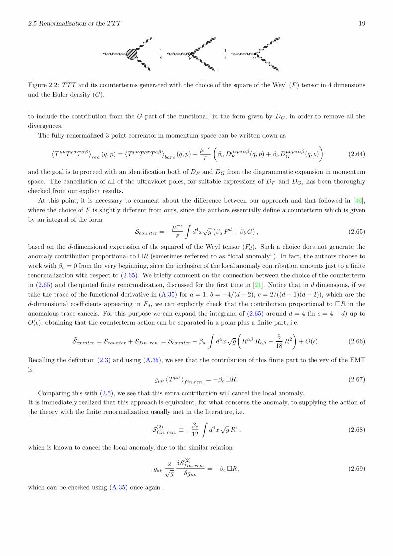
2.5 Renormalization of the TTT 19
−
1
ǫ F−
1
ǫ G
Figure 2.2: TTT and its counterterms generated with the choice of the square of the Weyl (F ) tensor in 4 dimensions
and the Euler density (G).
to include the contribution from the G part of the functional, in the form given by DG, in order to remove all the
divergences.
The fully renormalized 3-point correlator in momentum space can be written down as
⟨
T µνT ρσTαβ⟩
ren(q, p) =
⟨
T µνT ρσTαβ⟩
bare(q, p)− µ−ǫ
ǫ
(
βaDµνρσαβF (q, p) + βbD
µνρσαβG (q, p)
)
(2.64)
and the goal is to proceed with an identification both of DF and DG from the diagrammatic expansion in momentum
space. The cancellation of all of the ultraviolet poles, for suitable expressions of DF and DG, has been thoroughly
checked from our explicit results.
At this point, it is necessary to comment about the difference between our approach and that followed in [46],
where the choice of F is slightly different from ours, since the authors essentially define a counterterm which is given
by an integral of the form
Scounter = −µ−ǫ
ǫ
∫
d4x√g(
βa Fd + βbG
)
, (2.65)
based on the d-dimensional expression of the squared of the Weyl tensor (Fd). Such a choice does not generate the
anomaly contribution proportional to R (sometimes refferred to as “local anomaly”). In fact, the authors choose to
work with βc = 0 from the very beginning, since the inclusion of the local anomaly contribution amounts just to a finite
renormalization with respect to (2.65). We briefly comment on the connection between the choice of the counterterm
in (2.65) and the quoted finite renormalization, discussed for the first time in [21]. Notice that in d dimensions, if we
take the trace of the functional derivative in (A.35) for a = 1, b = −4/(d− 2), c = 2/((d− 1)(d − 2)), which are the
d-dimensional coefficients appearing in Fd, we can explicitly check that the contribution proportional to R in the
anomalous trace cancels. For this purpose we can expand the integrand of (2.65) around d = 4 (in ǫ = 4 − d) up to
O(ǫ), obtaining that the counterterm action can be separated in a polar plus a finite part, i.e.
Scounter = Scounter + Sfin. ren. = Scounter + βa
∫
d4x√g
(
Rαβ Rαβ − 5
18R2
)
+O(ǫ) . (2.66)
Recalling the definition (2.3) and using (A.35), we see that the contribution of this finite part to the vev of the EMT
is
gµν 〈T µν 〉fin.ren. = −βcR . (2.67)
Comparing this with (2.5), we see that this extra contribution will cancel the local anomaly.
It is immediately realized that this approach is equivalent, for what concerns the anomaly, to supplying the action of
the theory with the finite renormalization usually met in the literature, i.e.
S(2)fin. ren. ≡ −βc
12
∫
d4x√g R2 , (2.68)
which is known to cancel the local anomaly, due to the similar relation
gµν2√g
δS(2)fin. ren.
δgµν= −βcR , (2.69)
which can be checked using (A.35) once again .

20 The Three Graviton Vertex
−
1
ǫ Fd
−
1
ǫ G
Figure 2.3: The contributions to the renormalized TTT vertex from the square of the Weyl tensor in d-dimensions
(Fdd) and the Euler density (G).
−
1
ǫ Fd
= −
1
ǫ F−
Ffin
Figure 2.4: The relation between the counterterm generated by Fd and the same obtained from F . The difference is a
finite renormalization (Ffin) term in the counterterm Lagrangian, which generates the local contribution to the trace
anomaly.
2.6 The renormalized 3-graviton vertex with two lines on-shell
In general, a rank-6 tensor depending on 2 momenta can be expanded on a basis made up of 499 tensors built out
of the 2 momenta and the metric tensor δµν . The problem is that the scalar coefficients multiplying such tensors are
really complicated, in the most general kinematic configuration and it is no point reporting them explicitly.
Nevertheless, we have found that, in all of the three cases explicitly examined, if we go on-shell on the two outgoing
gravitons, the TTT vertex can be expanded on a basis made up of just thirteen tensors. This amounts to contracting
the amplitude with polarization tensors esλκ(p) which are transverse and traceless
pλ esλκ(p) = 0 , (es)λλ(p) = 0 , (2.70)
where the superscript denotes the helicity state of the graviton carrying the momentum p.
Given the assignment of the momenta established in (2.13), it is immediate to see that the contraction of the
amplitude with the polarization tensors with the properties (2.70) for the two outgoing gravitons is equivalent to the
replacements
p2 → 0 , q2 → 0 , pα → 0 , pβ → 0 , qρ → 0 , qσ → 0 , (2.71)
so that these conditions can be used to select the tensors that are non-vanishing after the on-shell limit is taken. We
are going to express our result for the amplitude in terms of such tensors.
The expansion of our Green’s function for a theory with nS scalars, nF fermions and nV vector bosons can be
generally written as
⟨
T µνT ρσTαβ⟩
(q, p)
∣
∣
∣
∣
On−Shell≡
∑
nI=nS ,nF ,nV
nI
13∑
i=1
ΩIi (s) tµνρσαβi (q, p) , s ≡ k2 = 2 p · q . (2.72)
The form factors for the three theories that we consider in this chapter are listed in table 2.2.
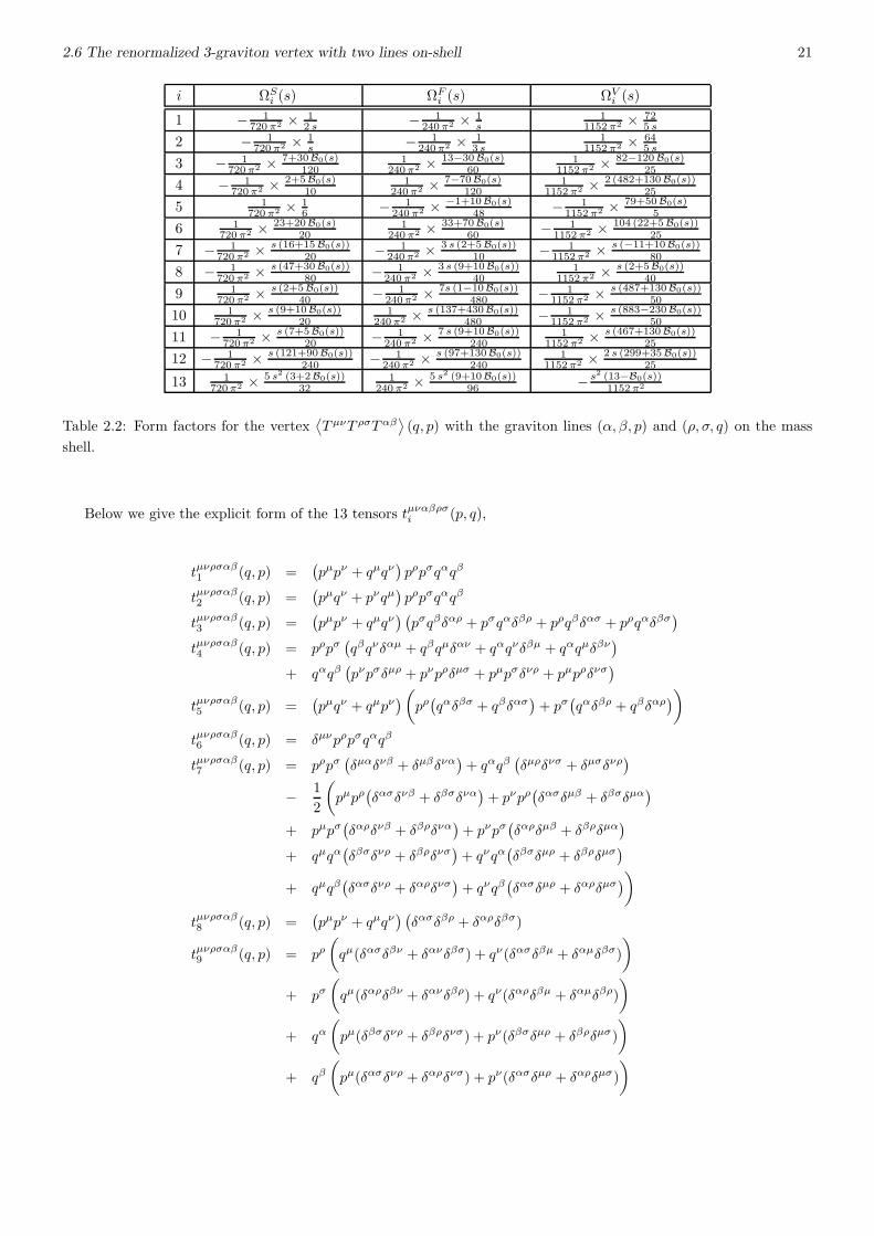
2.6 The renormalized 3-graviton vertex with two lines on-shell 21
i ΩSi (s) ΩFi (s) ΩVi (s)
1 − 1720 π2 × 1
2 s − 1240π2 × 1
s1
1152 π2 × 725 s
2 − 1720 π2 × 1
s − 1240π2 × 1
3 s1
1152 π2 × 645 s
3 − 1720 π2 × 7+30B0(s)
1201
240π2 × 13−30B0(s)60
11152π2 × 82−120B0(s)
25
4 − 1720π2 × 2+5B0(s)
101
240 π2 × 7−70B0(s)120
11152 π2 × 2 (482+130B0(s))
25
5 1720 π2 × 1
6 − 1240 π2 × −1+10B0(s)
48 − 11152 π2 × 79+50B0(s)
5
6 1720 π2 × 23+20B0(s)
201
240 π2 × 33+70B0(s)60 − 1
1152 π2 × 10⁴ (22+5B0(s))25
7 − 1720 π2 × s (16+15B0(s))
20 − 1240 π2 × 3 s (2+5B0(s))
10 − 11152π2 × s (−11+10B0(s))
80
8 − 1720 π2 × s (47+30B0(s))
80 − 1240 π2 × 3 s (9+10B0(s))
401
1152 π2 × s (2+5B0(s))40
9 1720 π2 × s (2+5B0(s))
40 − 1240π2 × 7s (1−10B0(s))
480 − 11152π2 × s (487+130B0(s))
50
10 1720π2 × s (9+10B0(s))
201
240π2 × s (137+430B0(s))480 − 1
1152 π2 × s (883−230B0(s))50
11 − 1720π2 × s (7+5B0(s))
20 − 1240 π2 × 7 s (9+10B0(s))
2401
1152 π2 × s (467+130B0(s))25
12 − 1720 π2 × s (121+90B0(s))
240 − 1240π2 × s (97+130B0(s))
2401
1152π2 × 2 s (299+35B0(s))25
13 1720π2 × 5 s2 (3+2B0(s))
321
240 π2 × 5 s2 (9+10B0(s))96 − s2 (13−B0(s))
1152π2
Table 2.2: Form factors for the vertex⟨
T µνT ρσTαβ⟩
(q, p) with the graviton lines (α, β, p) and (ρ, σ, q) on the mass
shell.
Below we give the explicit form of the 13 tensors tµναβρσi (p, q),
tµνρσαβ1 (q, p) =(
pµpν + qµqν)
pρpσqαqβ
tµνρσαβ2 (q, p) =(
pµqν + pνqµ)
pρpσqαqβ
tµνρσαβ3 (q, p) =(
pµpν + qµqν) (
pσqβδαρ + pσqαδβρ + pρqβδασ + pρqαδβσ)
tµνρσαβ4 (q, p) = pρpσ(
qβqνδαµ + qβqµδαν + qαqνδβµ + qαqµδβν)
+ qαqβ(
pνpσδµρ + pνpρδµσ + pµpσδνρ + pµpρδνσ)
tµνρσαβ5 (q, p) =(
pµqν + qµpν)
(
pρ(
qαδβσ + qβδασ)
+ pσ(
qαδβρ + qβδαρ)
)
tµνρσαβ6 (q, p) = δµνpρpσqαqβ
tµνρσαβ7 (q, p) = pρpσ(
δµαδνβ + δµβδνα)
+ qαqβ(
δµρδνσ + δµσδνρ)
− 1
2
(
pµpρ(
δασδνβ + δβσδνα)
+ pνpρ(
δασδµβ + δβσδµα)
+ pµpσ(
δαρδνβ + δβρδνα)
+ pνpσ(
δαρδµβ + δβρδµα)
+ qµqα(
δβσδνρ + δβρδνσ)
+ qνqα(
δβσδµρ + δβρδµσ)
+ qµqβ(
δασδνρ + δαρδνσ)
+ qνqβ(
δασδµρ + δαρδµσ)
)
tµνρσαβ8 (q, p) =(
pµpν + qµqν) (
δασδβρ + δαρδβσ)
tµνρσαβ9 (q, p) = pρ(
qµ(δασδβν + δανδβσ) + qν(δασδβµ + δαµδβσ)
)
+ pσ(
qµ(δαρδβν + δανδβρ) + qν(δαρδβµ + δαµδβρ)
)
+ qα(
pµ(δβσδνρ + δβρδνσ) + pν(δβσδµρ + δβρδµσ)
)
+ qβ(
pµ(δασδνρ + δαρδνσ) + pν(δασδµρ + δαρδµσ)
)
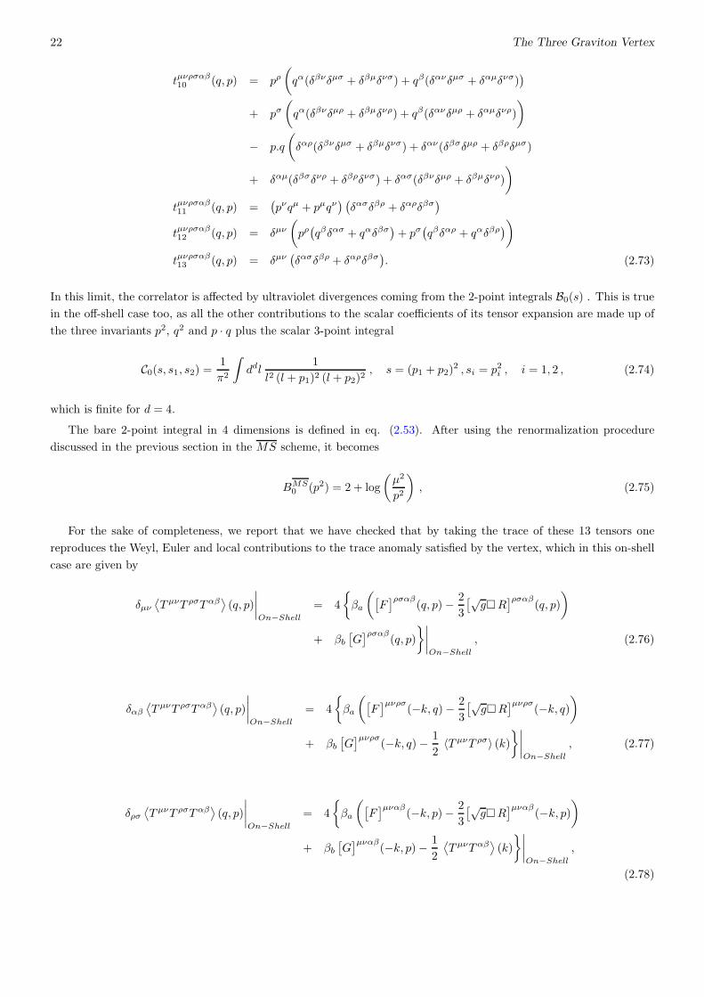
22 The Three Graviton Vertex
tµνρσαβ10 (q, p) = pρ(
qα(δβνδµσ + δβµδνσ) + qβ(δανδµσ + δαµδνσ))
+ pσ(
qα(δβνδµρ + δβµδνρ) + qβ(δανδµρ + δαµδνρ)
)
− p.q
(
δαρ(δβνδµσ + δβµδνσ) + δαν(δβσδµρ + δβρδµσ)
+ δαµ(δβσδνρ + δβρδνσ) + δασ(δβνδµρ + δβµδνρ)
)
tµνρσαβ11 (q, p) =(
pνqµ + pµqν) (
δασδβρ + δαρδβσ)
tµνρσαβ12 (q, p) = δµν(
pρ(
qβδασ + qαδβσ)
+ pσ(
qβδαρ + qαδβρ)
)
tµνρσαβ13 (q, p) = δµν(
δασδβρ + δαρδβσ)
. (2.73)
In this limit, the correlator is affected by ultraviolet divergences coming from the 2-point integrals B0(s) . This is true
in the off-shell case too, as all the other contributions to the scalar coefficients of its tensor expansion are made up of
the three invariants p2, q2 and p · q plus the scalar 3-point integral
C0(s, s1, s2) =1
π2
∫
ddl1
l2 (l + p1)2 (l + p2)2, s = (p1 + p2)
2 , si = p2i , i = 1, 2 , (2.74)
which is finite for d = 4.
The bare 2-point integral in 4 dimensions is defined in eq. (2.53). After using the renormalization procedure
discussed in the previous section in the MS scheme, it becomes
BMS0 (p2) = 2 + log
(
µ2
p2
)
, (2.75)
For the sake of completeness, we report that we have checked that by taking the trace of these 13 tensors one
reproduces the Weyl, Euler and local contributions to the trace anomaly satisfied by the vertex, which in this on-shell
case are given by
δµν⟨
T µνT ρσTαβ⟩
(q, p)
∣
∣
∣
∣
On−Shell= 4
βa
(
[
F]ρσαβ
(q, p)− 2
3
[√gR
]ρσαβ(q, p)
)
+ βb[
G]ρσαβ
(q, p)
∣
∣
∣
∣
On−Shell, (2.76)
δαβ⟨
T µνT ρσTαβ⟩
(q, p)
∣
∣
∣
∣
On−Shell= 4
βa
(
[
F]µνρσ
(−k, q)− 2
3
[√gR
]µνρσ(−k, q)
)
+ βb[
G]µνρσ
(−k, q)− 1
2〈T µνT ρσ〉 (k)
∣
∣
∣
∣
On−Shell, (2.77)
δρσ⟨
T µνT ρσTαβ⟩
(q, p)
∣
∣
∣
∣
On−Shell= 4
βa
(
[
F]µναβ
(−k, p)− 2
3
[√gR
]µναβ(−k, p)
)
+ βb[
G]µναβ
(−k, p)− 1
2
⟨
T µνTαβ⟩
(k)
∣
∣
∣
∣
On−Shell,
(2.78)

2.7 Conclusions and perspectives: the integrated anomaly and the nonlocal action 23
with
[F ]ρσαβ
(q, p)
∣
∣
∣
∣
On−Shell= 2 pρ pσqαqβ − p · q
(
pσqβδαρ − pρqβδασ − pσqαδβρ − pρqαδβσ)
+ (p · q)2(
δασδβρ + δαρδβσ)
, (2.79)
[G]ρσαβ
(q, p)
∣
∣
∣
∣
On−Shell= 2 pρpσqαqβ − p · q
(
pσqβδαρ − pρqβδασ − pσqαδβρ − pρqαδβσ)
+ (p · q)2(
δασδβρ + δαρδβσ)
, (2.80)
[√gR]
ρσαβ(q, p)
∣
∣
∣
∣
On−Shell=
1
2p · q
(
pσqβδαρ + pρqβδασ + pσqαδβρ + pρqαδβσ)
− 3
2(p · q)2
(
gασδβρ − δαρδβσ)
. (2.81)
2.7 Conclusions and perspectives: the integrated anomaly and the non-
local action
Before coming to our conclusions, we offer here a brief discussion of the possible extensions of our analysis in the
context of the emergence of massless degrees of freedom in the computation of correlators of the form TV V and TTT ,
as predicted by Riegert’s non local solution [59] of the anomaly equation.
We recall that an action that formally solves the anomaly equation (2.5) takes the form
Sanom[g,A] =1
8
∫
d4x√g
∫
d4x′√
−g′(
G+2
3R
)
x
G4(x, x′)
[
2 βa F + βb
(
G+2
3R
)
− 2κ
4FµνF
µν
]
x′
− βa + βb18
∫
d4x√g R2 (2.82)
where we keep the sum on all the contributions coming from different particle species implicit.
The notation G4(x, x′) denotes the Green’s function of the differential operator defined by
∆4 ≡ ∇µ
(
∇µ∇ν − 2Rµν +2
3gµν R
)
∇ν = 2 − 2Rµν∇µ∇ν −
1
3(∇µR)∇µ +
2
3R , (2.83)
which is the only order-4 differential operator enjoying the invariance property under Weyl transformations
√g G4(x, x
′) → √g G4(x, x
′) , for gµν → e2σ(x) gµν(x) , (2.84)
whereas the combination (G+ 2/3R) transforms as(
G+2
3R
)
→(
G+2
3R
)
+ 4∆4σ , for gµν → e2σ(x) gµν(x) , (2.85)
which immediately helps understanding how the trace of the EMT derived from (2.83) reproduces the trace anomaly
in (2.5).
As shown in [27, 29], performing repeated variations of the ”anomaly-induced” action (2.82) with respect to the
background metric gµν and to the Aα gauge field, one can reproduce the anomalous contribution of correlators with
multiple insertions of the EMT or of gauge currents. Of course, this action does not reproduce the homogeneous con-
tributions to the anomalous trace Ward identity (no variational solution could). Because these require an independent
computation in order to be identified, such as the perturbative 1-loop analysis undertaken in this work.
The action can be reformulated in such a way that its interactions become local [29], by introducing two auxiliary
scalar fields. After some manipulations, one can show that the apparently double pole in G4(x, x′) reduces to a single
pole and the anomaly-induced action near a flat background takes the simpler form
Sanom[g,A] → − κ
24
∫
d4x√g
∫
d4x′√
−g′Rx−1x,x′ [FαβF
αβ ]x′ . (2.86)
24 The Three Graviton Vertex
Notice that this action is valid to first order in metric variations around flat space. Its local expression is given by
Sanom[g,A;ϕ, ψ′] =
∫
d4x√g
[
−ψ′ϕ− R
3ψ′ +
c
2FαβF
αβϕ
]
. (2.87)
with ψ′ and ϕ defined as in [27]. Rx, in the equations above, is the linearised version of the Ricci scalar
Rx ≡ ∂xµ ∂xν h
µν − h, h = ηµν hµν . (2.88)
Eq. (2.87) shows the appearance of coupled massless degrees of freedom, whose interpretation was been offered in [27],
to which we refer for further details, using the approach of dispersion relations.
This analysis, so far, has been limited to the TV V correlator and could be extended, with a lot of additional effort,
to the case of the TTT vertex whose explicit computation has been discussed in this work. In particular, this analysis
could test directly if the pole structure present in the expression of the TTT vertex will match the prediction of the
same vertex once this is computed using (2.82) by functional differentiation with respect to the metric. This point
is technically very involved, since it requires a comparison between the off-shell result of a direct computation of the
TTT in perturbative field theory, as done in this work, with the anomalous part of the same correlator computed from
Riegert’ s variational solution. We hope to come back to discuss this point in a related work.

Chapter 3
Conformal correlators in position and
momentum space
3.1 Introduction
The analysis of correlation functions in d-dimensional quantum field theory possessing conformal invariance has found
widespread interest over the years (see [67] for an overview). Given the infinite dimensional character of the conformal
algebra in 2 dimensions, conformal field theories (CFT’s from now on) for d = 2 have received much more attention
than their 4-dimensional counterparts.
In d dimensional CFT’s the structure of generic conformal correlators is not entirely fixed just by conformal
symmetry, but for 2- and 3-point functions the situation is rather special and these can be significantly constrained,
up to a small number of constants. From the CFT side, some important information, mainly due to [46, 47], is
available. These results concern the TOO - with O denoting a generic scalar operator - TV V and TTT vertices, which
are determined by implementing the conformal constraints in position space. In the analysis of [46], in particular, it
was shown for the first time that some of these vertices are expressible in terms of few linearly independent tensor
structures: specifically, their numbers are 1 for the TOO vertex, 2 for the TV V and 3 for the TTT .
Imposing the conformal Ward identities and identifying these tensor structures directly in momentum space turns out
the be technically quite involved. The main goal of the present chapter is to present the result of a systematic study,
initiated in [48], enabling comparison of general results of d-dimensional CFT’s based on position space analyses, such
as those in [46, 47], with explicit realizations of anomalous 3-point vertices in free CFT’s, most commonly expressed
in momentum space. Recent results of studies of 3- and 4-point functions in d = 3 in the context of the ADS/CFT
correspondence are contained in [68, 69, 70].
Another significant difference between the position-space approach and the computations in momentum space is
that conformal anomalies necessarily arise quite differently in the two contexts. In the former case, in fact, anomalous
terms show up as ultra-local divergences proportional to delta functions or derivatives thereof at coincident spatial
points. Thus a very careful regularization procedure is required to determine these anomalous ultra-local contributions
which are absent for any finite point separation. The special strategy followed in determining these anomalous ultra-
local contributions in position space, developed in [46], deserves some comments. In this approach, the diffeomorphism
and trace Ward identities are solved in each case by combining a completely homogeneous solution, which is built on
the ground of the requirements of Lorentz and conformal invariance and is non local - i.e. obtained keeping the three
points separate - with inhomogeneous terms. The inhomogeneous terms are of two kinds: terms of the first kind are
semi-local (two coincident points out of three), are identified via the Operator Product Expansion of correlators and
account for ordinary contact terms in the Ward identities; the terms of the second kind are ultra-local (all three points
coincident). In particular, the latter contributions arise from the need to subtract ultraviolet singularities appearing
in the ultra-local limit and are responsible for the corresponding trace anomalies.
25
26 Conformal correlators in position and momentum space
It is clear that such a separation, based on the distinction of terms according to the separation/coincidence of
points at which operators are evaluated, does not make sense in momentum space. Here anomalies are thought either
as a remnant of the renormalization of ultraviolet divergences, that breaks conformal invariance via the introduction
of a mass scale µ (see for example [24, 25, 26]) or as an infrared effect, as can be seen in the dispersive approach of [27],
where the trace anomaly is shown originating from the imposition of all the non anomalous Ward identities and the
spectral representation of the amplitude. At first glance this appears to be quite different than the ultra-local delta
function terms obtained in the position space approach of [46, 47]. Thus, the relationship between this approaches
requires some clarification, and this is a principal motivation for the present work.
A necessary comment is that the eventual agreement of the two approaches may seem less surprising if it is re-
membered that coincident point singularities in euclidean position space become light cone singularities in Minkowski
spacetime, and these light cone singularities are associated with the propagation of massless fields, which generally
have long range infrared effects.
This chapter is composed of two main parts.
In the first part, building on the results of [46, 47], we analyse the structure of the 3-point correlators in configuration
and in momentum space for a general CFT. In particular we generalize previous studies of the TV V correlator,
perturbatively evaluated in 4 dimensions in [42, 43, 44] in QED, QCD and the Standard Model, to d dimensions. We
also study the TTT vertex, whose computation in 4 dimensions was presented in the previous chapter, and perform a
complete investigation of this correlator by the same approach. We give particular emphasis to the discussion of the
connection between the general approach of [46] and the perturbative picture. In particular, we give a diagrammatic
interpretation of the various contact terms introduced by Osborn and Petkou in order to solve the Ward identities for
generic positions of the points of the correlators. This allows to close a gap between their bootstrap method, previous
investigations of the TV V [27, 42, 43], and the recent computation of the TTT vertex. We show that the perturbative
analysis in momentum space in dimensional regularization is in complete agreement with their results.
It should be remarked that, in general, the momentum space formulation of the correlators of a CFT has remained
largely unexplored until the publication of [71, 72], where conformal constraints in momentum space for 3-point
functions are systematically explored, proving, as expected, much more difficult to implement with respect to the
corresponding position space constraints. The lack of this investigation for such a long time is mainly due to the fact
that momentum space is ideally suited for perturbative computations, which in turn always stem from a Lagrangian
formulation. This Lagrangian is often missing for CFT’s, which can be defined on the sole ground of symmetry
principles.
This brings us to the second part of the chapter, contained in section 3.5, where we discuss a general procedure to
map to momentum space any massless correlator given in position space and not necessarily related to a Lagrangian
description. The investigation of these correlators in momentum space reveals, in general, some specific facts, such
as the presence of single and multi-logarithmic integrands which, in general, cannot be re-expressed in terms of
ordinary master integrals, typical of the Feynman expansion. In particular, we conclude that, whenever the mentioned
logarithmic integrals do not cancel, the theory does not possess a Lagrangian formulation, because otherwise no such
integral would appear in the perturbative expansion.
To address these points, one has to formulate an alternative and general approach to perform the transforms, not
directly linked to the Lagrangian realization, since in this case such representation may not exist. The method
that is proposed relies on a d-dimensional version of differential regularization, similar to the approach suggested in
[47]. We use the standard technique of pulling out derivatives via partial integration in singular correlators in such
a way to make them Fourier-integrable, i.e. expressible as integrals in momentum space. This is combined with the
method of uniqueness [73], here generalized to tensor structures, in order to formulate a complete and self-consistent
procedure. As in [46, 47] we need an extra regulator (ω), unrelated to the dimensional regularization parameter ǫ. Our
approach is defined as a generic algorithm which can handle rather straightforwardly any massless correlator written
in configuration space. The algorithm has been implemented in a symbolic manipulation program and can handle, in

3.2 The correlators and the corresponding Ward identities 27
principle, correlators of any rank.
The aim of the method is to test the Fourier-integrability of a given correlator, by checking the cancellation of the
singularities in the extra regulator ω directly in momentum space, and to provide us with the direct expression of the
transform.
3.2 The correlators and the corresponding Ward identities
We provide the basic definitions of the correlators that we are going to investigate. We suppose that the theory admits
an euclidean generating functional W , in analogy with (2.2), which depends on the background metric gµν , acting as
source of the EMT T µν, on gauge fields Aaµ coupled to the gauge currents V aµ , and a source J for each scalar operator
O of the spectrum (for the sake of simplicity, we do not distinguish them ). Thus, if the classical theory is described
by an action S, we are embedding this into a curved space via the coupling to the metric g and supplying it with
additional source terms,
W [g,A, J ] =
∫
DΦ e−S−∫ddx
√g (Aa
µ Va µ+J O) . (3.1)
Then, the functional averages of O, V and T are obtained by differentiating the generating functional with respect to
the corresponding sources, i.e.
〈O(x)〉s = − 1√gx
δWδJ(x)
, 〈V aµ(x)〉s = − 1√gx
δWδAaµ(x)
, 〈T µν(x)〉s =2√gx
δWδ gµν(x)
. (3.2)
The construction of the correlators is straightforward. If the scalar operator O is coupled to the source J , the three
point function is defined via a triple functional derivative with respect to gµν once and to the scalar source J twice,
evaluated switching off the sources at the end, i.e.
〈T µν(x1)O(x2)O(x3)〉 =
δ2
δJ(x2)δJ(x3)
[
2√gx1
δWδgµν(x1)
]
g=δ
J=0
= 〈T µν(x1)O(x2)O(x3)〉J=0 +
⟨
δT µν[J ](x1)
δJ(x2)O(x3)
⟩
J=0
+
⟨
δT µν [J ](x1)
δJ(x3)O(x2)
⟩
J=0
, (3.3)
The second correlator that we will analyse will be the V V V vertex, which is defined by the third functional derivative
of the generating functional with respect to the source gauge field Aaµ(x)
⟨
V aµ(x1)Vb ν(x2)V
c ρ(x3)⟩
= − δ3W|g=δδAaµ(x1)δA
bν(x2)δA
cρ(x3)
∣
∣
∣
∣
A=0
. (3.4)
We remark that, due to Furry’s theorem, the gauge theory has to be non abelian in order to define a non vanishing
V V V correlator.
To derive the TV V correlator, we can first perform a functional derivative with respect to the metric and then
insert the vector currents by functionally differentiating with respect to the gauge field sources A, specifically
⟨
T µν(x1)Vaα(x2)V
b β(x3)⟩
=
δ2
δAaα(x2)δAbβ(x3)
[
2√gx1
δWδgµν(x1)
]
g=δ
A=0
=⟨
T µν(x1)Vaα(x2)V
b β(x3)⟩
A=0
+
⟨
δT µν(x1)
δAaα(x2)V b β(x3)
⟩
A=0
+
⟨
δT µν(x1)
δAbβ(x3)V aα(x2)
⟩
A=0
(3.5)
where Tµν is calculated in the presence of the background source Aaµ. The first term in the previous expression
represents the insertion of the three operators, while the last two are contact terms, with the topology of 2-point
functions, exploiting the linear dependence of the EMT from the source field A.
Finally, for the definition of the TTT Green function, which obviously does not change after including the additional
sources in the generating functional, we refer to section (2.3).
28 Conformal correlators in position and momentum space
Now we turn to the derivation of non-anomalous Ward identities, which hold for general dimensions, by which we
mean away from the (even) values of the space dimension for which the trace Ward identities become anomalous [26].
We assume that the generating functional W [g,A, J ] is invariant under diffeomorphisms,
W [g′, A′, J ′] = W [g,A, J ] , (3.6)
where g′ and A′ and J ′ are transformed metric, gauge field and scalar source under the general infinitesimal coordinate
transformation xµ → x′µ= xµ + ǫµ(x), under which they change according to
δgµν = ∇µǫν +∇νǫµ , δAaµ = −(
ǫλ∇λAaµ +Aa λ∇µǫλ
)
, δJ = −ǫλ∂λJ . (3.7)
Diffeomorphism invariance and gauge invariance of the generating functional respectively imply the relations
∇µ 〈T µν〉+∇νAaµ 〈V aµ〉+∇µ (Aa ν 〈V a µ〉) + ∂νJ 〈O〉 = 0 ,
∇µ 〈V aµ〉+ fabcAbµ 〈V cµ〉 = 0 , (3.8)
where fabc are the structure constants of the gauge group.
Naive conformal invariance gives the tracelessness condition
gµν 〈T µν〉s + (d− η) J 〈O〉s = 0 . (3.9)
This last Ward identity is naive, due to the appearance of an anomaly at quantum level, after renormalization of the
correlator, for even dimensions. However, it is the correct identity away from d = 2 k, for integer k. In this respect,
the functional differentiation of (3.8) and (3.9) allows to derive ordinary Ward identities for the various correlators.
If we want to include anomalies in 4-dimensional space, then remembering eq. (2.5) and the conditions on the β
coefficients discussed below it, we can write, in dimensional regularization,
gµν 〈T µν〉s =∑
I=f,s,V
nI
[
βa(I)
(
F − 2
3R
)
+ βb(I)G
]
− κ
4nV F
aµν F aµν + F [J ] , (3.10)
where by F [J ] we have denoted a possible functional of the background source for the scalar operators, whose form is
not unique, but depends on the dimensions of the corresponding operators. For example, in 4 dimensions and for the
operator O = φ2, where φ is the standard elementary scalar field, then F [J ] = p2 J
2, with p a c-number.
Now let us list the Ward identities implied by (3.8) for the various correlators. In the case of the TOO vertex one
has the equation
∂x1µ 〈T µν(x1)O(x2)O(x3)〉 = ∂x1
ν δ(d)(x12) 〈O(x1)O(x3)〉+ ∂x1ν δ(d)(x13) 〈O(x1)O(x2)〉 . (3.11)
For the V V V the conservation equation is
∂x1µ
⟨
V a µ(x1)Vb ν(x2)V
c ρ(x3)⟩
= fabd δ(d)(x12)⟨
V d ν(x1)Vc ρ(x3)
⟩
− facd δ(d)(x13)⟨
V d ρ(x1)Vc ν(x2)
⟩
, (3.12)
Finally, for the case of the TV V we obtain
∂x1µ
⟨
T µν(x1)Vaα(x2)V
b β(x3)⟩
= ∂νx1δd(x12)
⟨
V aα(x1)Vb β(x3)
⟩
+ ∂νx1δd(x31)
⟨
V aα(x2)Vb β(x1)
⟩
− δνα∂x1µ
(
δd(x12)⟨
V aµ(x1)Vb β(x3)
⟩)
− δνβ∂x1µ
(
δd(x31)⟨
V a α(x2)Vb µ(x1)
⟩)
,
(3.13)
together with the vector current Ward identities, following from gauge invariance,
∂x2α
⟨
T µν(x1)Vaα(x2)V
b β(x3)⟩
= 0 , ∂x3
β
⟨
T µν(x1)Vaα(x2)V
b β(x3)⟩
= 0 . (3.14)
The general covariance Ward identity for the TTT vertex was already given in section 2.3.1.
3.3 Inverse mappings: correlators in position space from the momentum space Feynman expansion 29
Now let us move to trace Ward identities for both general d and 4 dimensions. Discarding the V V V , the naive
identity (3.9) gives the non-anomalous conditions, for d dimensions
δµν 〈T µν(x1)O(x2)O(x2)〉 = (d− η)(
δ(d)(x12) 〈O(x1)O(x3)〉+ δ(d)(x13) 〈O(x1)O(x2)〉)
, (3.15)
δµν⟨
T µν(x1)Vaα(x2)V
b β(x3)⟩
= 0 , (3.16)
which become, when anomalies are properly included,
δµν 〈T µν(x1)O(x2)O(x2)〉 = (4− η)(
δ(d)(x12) 〈O(x1)O(x3)〉+ δ(d)(x13) 〈O(x1)O(x2)〉)
+δ2F [J ](x1)
δJ(x2)δJ(x3),
δµν⟨
T µν(x1)Va α(x2)V
b β(x3)⟩
= δab κ(
∂βδ(4)(x12)∂αδ(4)(x13)− δαβ ∂λδ(4)(x12)∂λδ
(4)(x13))
. (3.17)
The trace Ward identity for the TTT was given in section 2.3.2 in momentum space in 4 dimensions. Here we report
the coordinate-space versions of the non anomalous identity, holding for general d.
δµν⟨
T µν(x1)Tαβ(x2)T
ρσ(x3)⟩
= −2
(
δ(4)(x12) + δ(4)(x13)
)
⟨
Tαβ(x2)Tρσ(x3)
⟩
, (3.18)
and of the anomalous identity, valid only for d = 4
δµν⟨
T µν(x1)Tαβ(x2)T
ρσ(x3)⟩
= 4
(
βa
[
F (x1)−2
3R(x1)
]ρσαβ
(x2, x3) + βb [G(x1)]ρσαβ
(x2, x3)
)
− 2
(
δ(4)(x12) + δ(4)(x13)
)
⟨
Tαβ(x2)Tρσ(x3)
⟩
, (3.19)
with the compact notation for functional derivatives in the flat space limit introduced in (2.15).
3.3 Inverse mappings: correlators in position space from the momentum
space Feynman expansion
Having by now defined all the fundamental (anomalous and regular) Ward identities which allow to test the correctness
of the correlators we are interested in studying, we turn to compare the expressions of these correlators in position
space with their perturbative realizations in free field theories in momentum space.
We remind that an important result of [46] is the identification of the solution of the Ward identities in terms
of a set of constants and of certain linearly independent tensor structures in euclidean position space. Consistency
requires that the Fourier transforms of these tensor structures must occur in direct computations of the same vertex
functions in free field theories in momentum space, which are defined, in turn, via certain 1-loop integrals that can
be computed according to a well-defined set of Feynman rules, once the Lagrangian theory has been specified. This
implies that, after establishing the combination of these integrals defining the Green function in momentum space,
we can use them to infer what those tensor structures must be, and find the exact correspondence between CFT
amplitudes in position space and momentum space a posteriori. Obviously, this is only possible provided that we
have enough linearly independent vertex functions for different free theories to determine the linear combinations
uniquely. We call this procedure an inverse mapping, as it allows to re-express the correlators of [46] in such a form
that their Fourier-integrability is explicit. By integrable we mean, in this context, a function of coordinates whose
Fourier transform is not divergent and contains no additional regulator, in a sense made precise in section 3.5.1. This
result is obtained by pulling out derivatives of the corresponding diagrams, in the spirit of differential regularization
[49] in such a way that integrability becomes trivial.
More technical details on the inverse mapping method are explicitly provided in appendix A.8, where the TTT
correlator is used as an illustrative example.

30 Conformal correlators in position and momentum space
3.3.1 The TOO case
The first correlator that we are going to investigate is the TOO. In the perspective of comparing the coordinate space
results of [46] with momentum space perturbative expansions, it is also the most ambiguous, as such a perturbative
expansion requires establishing the scaling dimensions of the scalar operators once for all. For this reason, we are
going to perform such a test only in one specific case, i.e. for O = φ2.
The general structure of this Green function in coordinate space - for non coincident points - is
〈Tµν(x1)O(x2)O(x3)〉 =a
(x212)d/2 (x223)
η−d/2 (x231)d/2
h1µν(X23) , (3.20)
where a is a constant, η the scaling dimension of the scalar operator O and where
Xµ =Xµ√X2
, h1µν(X) = Xµ Xν −1
dδµν ,
where
xij ≡ xi − xj , Xij = −Xji ≡xikx2ik
− xjkx2jk
, i, j, k = 1, 2, 3 , k 6= i , k 6= j . (3.21)
In the short-distance limits of its external points, this vertex is singular for η → d/2 and needs regularization. In [46]
the Ward identities are solved through the analysis of the short distance limits of (3.20), by which we mean the limits
x1 → x2, x1 → x3. Some singular terms are found and thus the authors are forced to regularize them with the method
of differential regularization [49], which finally gives the modified expression
〈Tµν(x1)O(x2)O(x3)〉 =a
(x212)d/2 (x223)
η−d/2 (x231)d/2
h1µν(X23)
+[
Aµν(x12)−Aµν(x12) + Aµν(x31)−Aµν(x31)] N
(x223)η, (3.22)
where we have introduced the structures
Aµν(s) =a
N
1
sd
(
sµsνs2
− 1
dδµν
)
, Aµν(s) =a
N d
(
∂µ∂νd− 2
1
sd−2+η − d+ 1
ηSd δµν δ
d(s)
)
, (3.23)
and N is defined as the normalization constant of the 2-point function of the scalar operator
〈O(x1)O(x2)〉 =N
(x212)η. (3.24)
It is important to make some comments at this point, as the TOO is the simplest function, between those addressed
in this chapter, to require such a regularization procedure in order to account for the inhomogeneous terms in the
Ward identities. Notice that, in general, one can define a differentially regularized tensor A as
Aµν(s) =a
N d
(
1
d− 2∂µ∂ν
2
sd−2+ C δµν Sdδ
(d)(s)
)
, (3.25)
which exactly coincides with Aµν(s) for s 6= 0 and where the only difference between them is in the δ-function term,
whose coefficient is not fixed a priori, reflecting the arbitrariness typical of any regularization. It is precisely this kind
of term that discerns (3.22) from (3.20). The ambiguity in its coefficient is solved by requiring the Ward identities
to be satisfied by (3.22). In this way, the terms A − A are the contact contributions (sometimes called semi-local in
the literature) which consistently account for the r.h.s. of (3.11) and (3.15). Essentially the same argument holds
for the more complicated 3-point functions we are going to discuss in the next sections: only the formulas are more
complicated, due to the increasing number of tensor structures.
In the expression above Sd is the ”volume” of the sphere in d-dimensions,
Sd = 2 πd2 /Γ(d/2) . (3.26)

3.3 Inverse mappings: correlators in position space from the momentum space Feynman expansion 31
Figure 3.1: The fermion and the scalar sectors contributing to the conformal VVV vertex in any dimension.
Introducing (3.23) into (3.22), we find the explicit expression
〈Tµν(x1)O(x2)O(x3)〉 =a
(d− 2)2
(∂12µ ∂31ν + ∂12ν ∂
31µ ) +
d− 2
d(∂12µν + ∂31µν)
1
(x212)d/2−1(x223)
η−d/2+1(x231)d/2−1
+ ax212x
223 + x231x
223 − (x223)
2
(x212)d/2(x223)
η−d/2+1(x231)d/2
δµνd
+ aη − d+ 1
d ηSd δµν
δd(x12) + δd(x31)
(x223)η
, (3.27)
where, from now on, we set ∂12µ ≡ ∂∂x12µ
and ∂12µν ≡ ∂∂x12µ
∂∂x12 ν
. Notice that the first term of the second line
proportional to δµν is not manifestly integrable, but one can use identities such as x212+x213−x223 = 2x12 ·x13 in order
to rewrite it in the form
x212 x223 + x231 x
223 − (x223)
2
(x212)d/2 (x223)
d/2 (x231)d/2
=2
(d− 2)2∂12µ ∂
31µ 1
(x212)d/2−1(x231)
d/2−1(x223)η−d/2+1
(3.28)
which shows its integrability when η < d− 1.
Now, in order to test the consistency of the result (3.20) obtained from the application of the conformal Ward
identities for the TOO, we can consider a particular scalar free field theory. We suppose for instance that the scalar
operator O is given by O = φ2 with dimensions η = d− 2, whose EMT is
Tµν = ∂µφ∂νφ− 1
2δµν ∂αφ∂
αφ+1
4
d− 2
d− 1
[
δµν∂2 − ∂µ ∂ν
]
φ2 (3.29)
which is conserved and traceless in d dimensions.
Using the Feynman rules in momentum space together with the expression of a scalar propagator, after applying the
inverse mapping procedure detailed in appendix A.8, we obtain the Tφ2φ2 correlation function in d dimensions
⟨
Tµν(x1)φ2(x2)φ
2(x3)⟩
=2a(d− 1)
d(d − 2)2
[
∂12µ ∂31ν + ∂12ν ∂
31µ − δµν∂
12 · ∂31 − d− 2
2(d− 1)
(
− ∂12µν − ∂31µν + ∂12µ ∂31ν
+ ∂12ν ∂31µ + δµν
(
∂212 + ∂231 − 2∂12 · ∂31)
)]
1
(x212)d/2−1(x223)
d/2−1(x231)d/2−1
− ad− 1
d(d− 2)Sdδµν
δd(x12) + δd(x31)
(x223)d−2
. (3.30)
The equivalence of this expression with the solution given in (3.27) can be explicitly checked. We remark that (3.30)
is clearly integrable and does not require any intermediate regularization. The first term in the previous expression
comes from the triangle topology diagram while the last two, proportional to the delta functions, are contact terms
with 2-point topology (see eq. (3.3)).
3.3.2 The V V V case
The V V V vertex function is pretty easy to handle with the inverse mapping procedure. In [46] the general CFT
requirements fix the structure of the V V V to be
⟨
V aµ (x1)Vbν (x2)V
cρ (x3)
⟩
=fabc
(x212)d/2−1 (x223)
d/2−1 (x231)d/2−1
(a− 2b)X23µX31 ν X12 ρ
− b
[
1
x223X23µ Iνρ(x23) +
1
x231X31 ν Iµρ(x31) +
1
x212X12 ρ Iµν(x12)
]
, (3.31)

32 Conformal correlators in position and momentum space
where Iµν (x) is the inversion operator defined as
Iµν(x) = δµν − 2xµxν
x2. (3.32)
The correlator is Fourier-integrable, although this is not immediately evident from (3.31). The simplest way to prove
this point consists in showing that (3.31) can be reproduced in d-dimensions by the combination of the scalar and the
fermion sectors of a free field theory. For this purpose we use two realizations of the vector current V aµ , using scalar
and fermion fields
V aµ = φ∗ta (∂µφ)− (∂µφ∗) taφ , V aµ = ψ taγµψ . (3.33)
The diagrammatic expansion of this correlator consists of two triangle diagrams, the direct and the exchanged, both
in the scalar and fermion sectors. These two types of diagrams are shown in fig. 3.1 and it is well known how to write
down their expressions in momentum space, using the corresponding Feynman rules.
Performing the inverse mapping procedure, we find the result
⟨
V aµ (x1)Vbν (x2)V
cρ (x3)
⟩f= − cf f
abc
(d− 2)3∆µανβργ∂
α12∂
β23∂
γ31
1
(x212)d/2−1(x223)
d/2−1(x231)d/2−1
, (3.34)
⟨
V aµ (x1)Vbν (x2)V
cρ (x3)
⟩s=
cs fabc
(d− 2)2(
∂12µ + ∂31µ) (
∂23ν + ∂12ν) (
∂31ρ + ∂23ρ) 1
(x212)d/2−1(x223)
d/2−1(x231)d/2−1
(3.35)
for the fermion and the scalar sector respectively, where we have introduced the operator
∆µανβργ =1
4Tr [γµγαγνγβγργγ ] , (3.36)
and cf , cs are normalization constants whose numerical values are irrelevant here. Written in this form, with derivatives
pulled out, the two expressions are manifestly integrable.
Tracing over the γ matrices and applying the derivatives over all the denominators, we generate the result of [46]
by taking a linear combination of these two sectors
⟨
V aµ (x1)Vbν (x2)V
cρ (x3)
⟩
=
(
a taµνρ + b tbµνρ
)
fabc
(x212)d/2−1(x223)
d/2−1(x231)d/2−1
, (3.37)
where
taµνρ =1
d(d− 2)2(
∂12µ + ∂31µ) (
∂23ν + ∂12ν) (
∂31ρ + ∂23ρ)
− 1
dtbµνρ , (3.38)
tbµνρ = − 1
(d− 2)3∆µανβργ∂
α12∂
β23∂
γ31 . (3.39)
We have explicitly checked the equivalence between this expression and eq. (3.31). No additional term is required, in
position space, to account for the general covariance Ward identity (3.12).
3.3.3 The TV V case
The next correlator that we are going to discuss is the TV V , for which, together with the TTT vertex, the analysis re-
quired to confirm the correspondence between the position space solutions given in [46] and perturbative computations
in momentum space is much more involved, due to the growth of the number of tensors structures.
We begin with the expression of the TV V in position space at separate points, which is
⟨
Tµν(x1)Vaα (x2)V
bβ (x3)
⟩
=δab
(x212)d/2 (x231)
d/2 (x223)d/2−1
Iασ(x12) Iβρ(x31) tµνρσ(X23) , (3.40)
3.3 Inverse mappings: correlators in position space from the momentum space Feynman expansion 33
where the structure tµνρσ(X) is given by the following combination of 4-indices structures, which are traceless with
respect to (µ, ν),
tµνρσ(X) = a h1µν(X) δρσ + b h1µν(X)h1ρσ(X) + c h2µνρσ(X) + e h3µνρσ , (3.41)
with h1µν already introduced in (3.21), whereas
h2µνρσ(X) = Xµ Xρ δνσ + Xν Xσ δµσ + (ρ↔ σ)− 4
dXµ Xν δρσ − 4
dXρ Xσ δµν +
4
d2δµν δρσ ,
h3µνρσ = δµρδνσ + δµσδνρ −2
dδµνδρσ . (3.42)
On the other hand, if one considers the Ward identity (3.13) at separate points, i.e. with vanishing r.h.s. , the four
coefficients a,b,c and e are found to be constrained by
d a− 2 b+ 2 (d− 2) c = 0 , b = d (d− 2) e , (3.43)
so that there are two independent contributions to the TV V vertex for general dimensions.
As usual, the next step in the analysis of [46] is to study the 2-point coincidence limits x1 → x2, x1 → x3 in order
to identify the terms which are responsible for the r.h.s. of the Ward identity (3.13). Unlike the case of the V V V
and similarly to the case of the TOO, to which we refer for the details concerning the regularization procedure of
the short-distance singularities, some of the terms appearing in this limit on the r.h.s. of (3.13) are found to need
regularization. Then differential regularization is used to pull out derivatives and find some regularization-dependent
terms proportional to δ-functions. The solution obtained is connected to the normalization constant of the vector
current (unrenormalized) 2-point function, which is
⟨
V aµ (x1)Vbν (x2)
⟩
= CVIµν (x12)
(x212)d−1
. (3.44)
so that the complete, unrenormalized TV V correlator is given by
⟨
Tµν(x1)Vaα (x2)V
bβ (x3)
⟩
=δab
(x212)d/2 (x231)
d/2 (x223)d/2−1
Iασ(x12) Iβρ(x31) tµνρσ(X23)
+δab CV
[
Aµναρ(x12)−Aµναρ(x12)] Iρβ(x23)
(x223)d−1
+δab CV
[
Aµνσβ(x31)−Aµνσβ(x31)] Iσα(x23)
(x223)d−1
. (3.45)
Here, the structures A and A are respectively
CV Aµνρσ(s) =1
sdIρα(s) tµνασ(s) ,
CV Aµνρσ(s) =
[
2e
d(d− 2)δµν∂ρ∂σ − 2c
d(d − 2)δρσ∂µ∂ν −
c+ de
d(d− 2)(δνρ∂µ∂σ + δµρ∂ν∂σ)
+c− (d− 2)e
d(d− 2)(δνσ∂µ∂ρ + δµσ∂ν∂ρ)
]
1
sd−2− e
d(d− 4)∂µ∂ν∂ρ∂σ
1
sd−4
+1
d
[
2e δµνδρσ − (c+ de) (δµσδνρ + δµρδνσ)
]
Sd δ(d)(s) . (3.46)
Again, Aµνρσ(s) = Aµνρσ(s) for s 6= 0 and the coefficients in front of the δ-function terms in the last line of (3.46) are
determined only after imposing the Ward identities.
Now we are ready to check the correspondence between the complete expression of the unrenormalized TV V in
position space, (3.45), and the inverse-mapped momentum space 1-loop computations. We have drawn the diagram-
matic structure of the TV V in fig. 3.2. Using the information that the most general TV V is parametrized by just
two independent constants, we conclude that, in any dimension, it can be fully constructed as a linear combination of
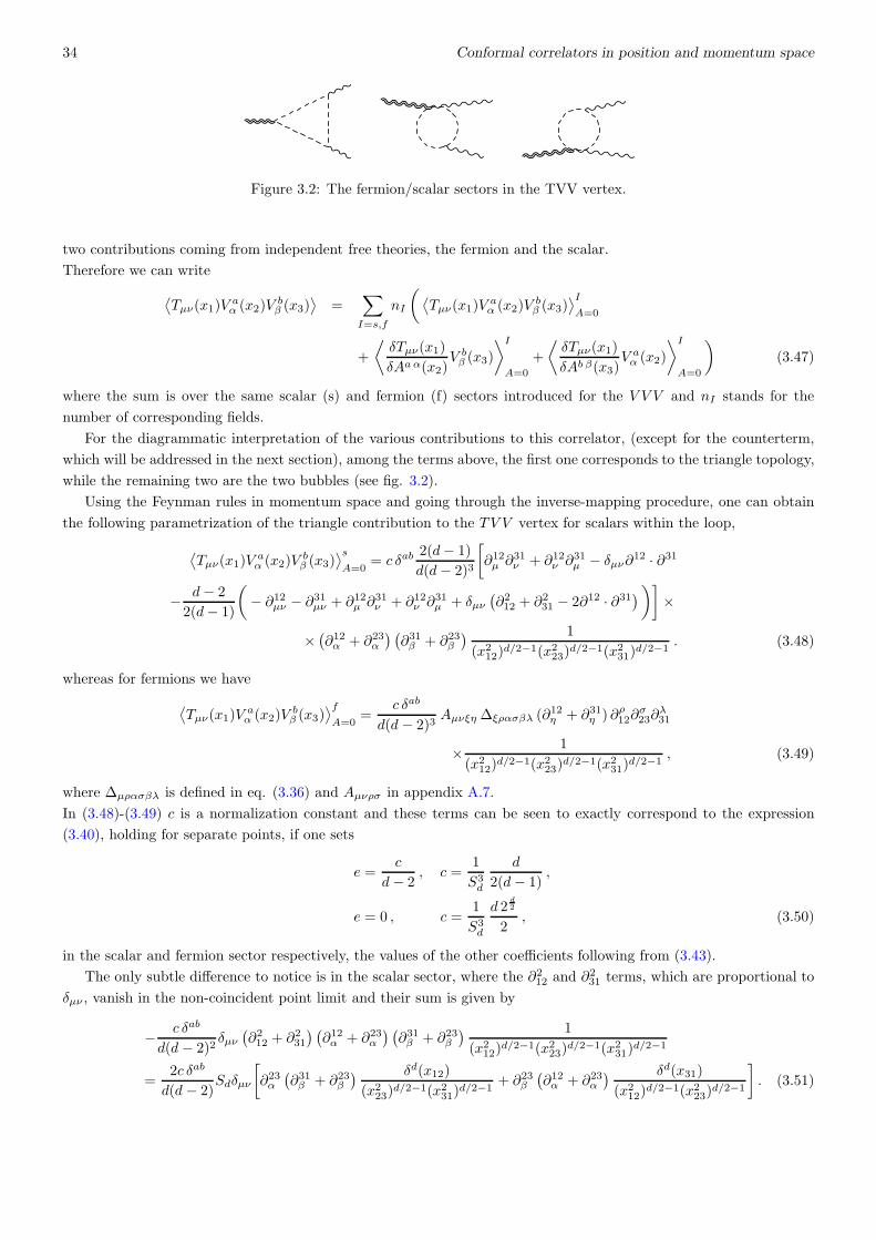
34 Conformal correlators in position and momentum space
Figure 3.2: The fermion/scalar sectors in the TVV vertex.
two contributions coming from independent free theories, the fermion and the scalar.
Therefore we can write
⟨
Tµν(x1)Vaα (x2)V
bβ (x3)
⟩
=∑
I=s,f
nI
(
⟨
Tµν(x1)Vaα (x2)V
bβ (x3)
⟩I
A=0
+
⟨
δTµν(x1)
δAa α(x2)V bβ (x3)
⟩I
A=0
+
⟨
δTµν(x1)
δAb β(x3)V aα (x2)
⟩I
A=0
)
(3.47)
where the sum is over the same scalar (s) and fermion (f) sectors introduced for the V V V and nI stands for the
number of corresponding fields.
For the diagrammatic interpretation of the various contributions to this correlator, (except for the counterterm,
which will be addressed in the next section), among the terms above, the first one corresponds to the triangle topology,
while the remaining two are the two bubbles (see fig. 3.2).
Using the Feynman rules in momentum space and going through the inverse-mapping procedure, one can obtain
the following parametrization of the triangle contribution to the TV V vertex for scalars within the loop,
⟨
Tµν(x1)Vaα (x2)V
bβ (x3)
⟩s
A=0= c δab
2(d− 1)
d(d− 2)3
[
∂12µ ∂31ν + ∂12ν ∂
31µ − δµν∂
12 · ∂31
− d− 2
2(d− 1)
(
− ∂12µν − ∂31µν + ∂12µ ∂31ν + ∂12ν ∂
31µ + δµν
(
∂212 + ∂231 − 2∂12 · ∂31)
)]
×
×(
∂12α + ∂23α) (
∂31β + ∂23β) 1
(x212)d/2−1(x223)
d/2−1(x231)d/2−1
. (3.48)
whereas for fermions we have
⟨
Tµν(x1)Vaα (x2)V
bβ (x3)
⟩f
A=0=
c δab
d(d − 2)3Aµνξη ∆ξρασβλ (∂
12η + ∂31η ) ∂ρ12∂
σ23∂
λ31
× 1
(x212)d/2−1(x223)
d/2−1(x231)d/2−1
, (3.49)
where ∆µρασβλ is defined in eq. (3.36) and Aµνρσ in appendix A.7.
In (3.48)-(3.49) c is a normalization constant and these terms can be seen to exactly correspond to the expression
(3.40), holding for separate points, if one sets
e =c
d− 2, c =
1
S3d
d
2(d− 1),
e = 0 , c =1
S3d
d 2d2
2, (3.50)
in the scalar and fermion sector respectively, the values of the other coefficients following from (3.43).
The only subtle difference to notice is in the scalar sector, where the ∂212 and ∂231 terms, which are proportional to
δµν , vanish in the non-coincident point limit and their sum is given by
− c δab
d(d − 2)2δµν
(
∂212 + ∂231) (
∂12α + ∂23α) (
∂31β + ∂23β) 1
(x212)d/2−1(x223)
d/2−1(x231)d/2−1
=2c δab
d(d − 2)Sdδµν
[
∂23α(
∂31β + ∂23β) δd(x12)
(x223)d/2−1(x231)
d/2−1+ ∂23β
(
∂12α + ∂23α) δd(x31)
(x212)d/2−1(x223)
d/2−1
]
. (3.51)

3.3 Inverse mappings: correlators in position space from the momentum space Feynman expansion 35
They have the topology of 2-point functions and must be carefully summed to those arising from the bubble diagrams
in order to reproduce exactly the contributions identified as A−A in (3.45). The bubble contributions are⟨
δTµν(x1)
δAa α(x2)V bβ (x3)
⟩s
A=0
=c δab(d− 1)
d(d− 2)2Sdδ
d(x12)(
(∂23µ + ∂31µ )δνα + (∂23ν + ∂31ν )δµα − δµν(∂23α + ∂31α )
)
×
×(∂23β + ∂31β )1
(x231)d/2−1(x223)
d/2−1, (3.52)
⟨
δTµν(x1)
δAb β(x3)V aα (x2)
⟩s
A=0
=c δab(d− 1)
d(d− 2)2Sdδ
d(x31)(
(∂23µ + ∂12µ )δνβ + (∂23ν + ∂12ν )δµβ − δµν(∂23α + ∂12β )
)
×
×(∂23α + ∂12α )1
(x212)d/2−1(x223)
d/2−1, (3.53)
and we thoroughly checked that the sum of (3.51), (3.52) and (3.53) corresponds to the solution of the Ward identities
(3.45) for e = c/(d− 2) and applying (3.43).
Similarly, the contact terms for the fermion sector in the diagrammatic expansion are found to be, after the inverse
mapping,⟨
δTµν(x1)
δAa α(x2)V bβ (x3)
⟩f
A=0
=c δab
d(d− 2)2Sdδ
d(x12)∆(2)µναβρσ∂
ρ31
1
(x231)d/2−1
∂σ311
(x231)d/2−1
, (3.54)
⟨
δTµν(x1)
δAb β(x3)V aα (x2)
⟩f
A=0
=c δab
d(d− 2)2Sdδ
d(x31)∆(2)µνβαρσ∂
ρ12
1
(x212)d/2−1
∂σ311
(x212)d/2−1
, (3.55)
with ∆(2) defined by
∆(2)µναβρσ = δανδβσδµρ + δαµδβσδνρ + δανδβρδµσ + δαµδβρδνσ − δανδβµδρσ − δαµδβνδρσ
− 2 δµν (δαρδβσ + δασδβρ − δαβδρσ) . (3.56)
These two contributions exactly match the A − A terms in (3.45) for e = 0 and applying (3.43), so that we can
conclude that our check for the agreement between the position space solution and the momentum space perturbative
computation is successful also for the TV V .
To conclude with the TV V , we notice that the Green functions discussed so far are unrenormalized. The issue of
renormalization will be addressed separately in section 3.4.
3.3.4 The TTT case
Now we are ready to turn to the analysis of the 3-graviton vertex, whose perturbative computation was presented in
chapter 2. The general structure of the TTT correlator in position space for separate points is [46]
⟨
T µν(x1)Tρσ(x2)T
αβ(x3)⟩
=1
(x212)d/2 (x223)
d/2 (x231)d/2
Iµν,µ′ν′ Iρσ,ρ′σ′
tµ′ν′ρ′σ′αβ(X12) , (3.57)
Iµν,αβ(s) = Iµρ(s)Iνσ(s)ǫρσ,αβT , s = x− y , (3.58)
where the tensor
ǫµν,αβT =1
2(δµαδνβ + δµβδνα
)
−1
dδµνδαβ (3.59)
is the projector onto the space of symmetric traceless tensors.
If we introduce
h4µνρσαβ(X) = h3µναρXσXβ + h3µνασXρXβ + (α ↔ β)
− 2
dδρσ h2µναβ(X)− 2
dδαβ h2µνρσ(X)− 8
d2δρσ δαβ h1µν(X) ,
h5µνρσαβ(X) =
[(
δµρδναδρβ + δνρδµαδρβ + (ρ↔ σ)
]
+
[
α ↔ β
]
− 4
dδµν h3 ρσαβ − 4
dδρσ h3µναβ − 4
dδαβ h3µνρσ − 8
d2δµνδρσδαβ , (3.60)

36 Conformal correlators in position and momentum space
then the rank-6 tensor tµνρσαβ(X) is written as
tµνρσαβ(X) = a h5µνρσαβ + b h4αβµνρσ(X) + b′(
h4µνρσαβ(X) + h4 ρσµναβ(X)
)
+ c h3µνρσh1αβ(X) + c′(
h3 ρσαβh1µν(X) + h3µναβh1 ρσ(X)
)
+ e h2µνρσ(X)h1αβ(X) + e′(
h2 ρσαβ(X)h1µν(X) + h2µναβ(X)h1 ρσ(X)
)
+ f h1µν(X)h1 ρσ(X)h1αβ(X) , (3.61)
with the constraints
b+ b′ = −2 a , c′ = c , e+ e′ = −4 b′ − 2 c
d2 a+ 2 (b+ b′)− (d− 2) b′ − d c+ e′ = 0 ,
d (d+ 2)(2 b′ + c) + 4 (e+ e′) + f = 0 , (3.62)
leaving only three unconstrained coefficients, say a, b and c.
The TTT needs regularization in the coincidence limits too, so we introduce the 2-point function for the energy-
momentum tensor,⟨
T µν(x1)Tαβ(x2)
⟩
= CTIµναβ(x12)(x212)
d/2. (3.63)
Following arguments similar to those for the TOO and TV V vertices, the authors in [46] arrive at the unrenormalized
expression
⟨
T µν(x1)Tρσ(x2)T
αβ(x3)⟩
=1
(x212)d/2 (x223)
d/2 (x231)d/2
Iµν,µ′ν′ Iρσ,ρ′σ′
tµ′ν′ρ′σ′αβ(X12)
+CT2
[
Aµνρσγδ(x12)−Aµνρσγδ(x12)
](Iγδαβ(x23)(x223)
d/2+
Iγδαβ(x13)(x213)
d/2
)
+CT2
[
Aµναβγδ(x13)−Aµναβγδ(x13)
](Iγδρσ(x32)(x232)
d/2+
Iγδρσ(x12)(x212)
d/2
)
+CT2
[
Aρσαβγδ(x23)−Aρσαβγδ(x23)
](Iγδµν(x31)(x231)
d/2+
Iγδµν(x21)(x221)
d/2
)
, (3.64)
where the A tensor is found to be, by computing the short distance limit of (3.57),
Aµνρσαβ(s) =1
(s2)d/2tµνρσαβ(s) , (3.65)
whereas its regularized counterpart is given by
Aµνρσαβ(s) = D.R.[
Aµνρσαβ(s)]
+
(
C h5µνρσαβ(s) +D(
δµν h3 ρσαβ + δρσ h3µναβ)
)
Sd δ(d)(s) , (3.66)
where the short-hand notation on the r.h.s. stands for the differentially regularized version of A, obtained, just as in
the case of the TOO and the TV V vertices, by re-expressing it as a (lengthy) combination of derivatives of powers of
s2 which are lower than d (compare with eq. (3.65)) which is no point reporting here explicitly and can be found in
eqs. (6.37)-(6.38) of [46].
Next comes the imposition of the Ward identities: by requiring the general covariance (2.30) and the non anomalous
trace (3.18) constraints to be satisfied, it is found that the values of the so far arbitrary coefficients C and D are
C =(d− 2)(2 a+ b)− d c
d (d+ 2), D =
CTd. (3.67)
As the general solution of the Ward identities, for any CFT, is parametrized by 3 independent constants, we conclude
that computing the correlator in the 3 independent free field theories considered in chapter 2 is enough to account
3.3 Inverse mappings: correlators in position space from the momentum space Feynman expansion 37
for the complete unrenormalized result in 4 dimensions, whereas for d 6= 4 the spin 1 sector is not conformally
invariant and we cannot build the general expression just by superposing the scalar and the fermion sectors. However,
the combination of the scalar and fermion sectors corresponds to a special solution for d = 3, where the TTT is
parametrized just by 2 independent constants, whereas in d = 2 there is just 1 such constant [46, 47].
As done before for the TOO, V V V and TV V correlators, here we check the result (3.57) building explicitly the
correlator in position space anti-transforming the diagrammatic expansion in free field theory. This allows to come
up with an expression for this vertex which is manifestly integrable. We will be using the Feynman rules obtained
from the Lagrangian descriptions for scalars, fermions and spin 1 in configuration space, given in section 2.4. We
start by testing the non-coincident case, for which we can omit the contact terms. This corresponds only to the
diagrams with triangle topology. We give the expressions in d dimensions for the scalar and the fermion cases, while -
as already remarked - we have to limit our analysis to d = 4 for the spin-1 vector boson. Moreover, in the vector case
the gauge-fixing and ghost parts of the amplitude have to cancel since the vertex is gauge invariant, as explained in
section 2.4, so that, performing our inverse mapping, we include in the interactions vertices for the vector field only
the Maxwell contributions.
We have⟨
δSδgµν(x1)
δSδgρσ(x2)
δSδgαβ(x3)
⟩s
= CsTTTVµνSφφ(i ∂
12,−i ∂31)V ρσSφφ(i ∂23,−i ∂12)V αβSφφ(i ∂
31,−i ∂23)
× 1
(x212)d/2−1 (x223)
d/2−1 (x231)d/2−1
, (3.68)
⟨
δSδgµν(x1)
δSδgρσ(x2)
δSδgαβ(x3)
⟩f
=
CfTTT (−1)
(
Tr[
V µνSψψ(i ∂12,−i ∂31) i γ · ∂12 V ρσSψψ(i ∂
23,−i ∂12) i γ · ∂23 V αβSψψ(i ∂31,−i ∂23) i γ · ∂31
]
+Tr[
V µνSψψ(i ∂31,−i ∂12) i γ · ∂31 V αβSψψ(i ∂
23,−i ∂31) i γ · ∂12 V ρσSψψ(i ∂12,−i ∂23) i γ · ∂12
]
)
× 1
(x212)d/2−1 (x223)
d/2−1 (x231)d/2−1
,
(3.69)
⟨
δSδgµν(x1)
δSδgρσ(x2)
δSδgαβ(x3)
⟩V
= CVTTT (−1)3 V µνγδSAA (i ∂12,−i ∂31)V ρσζξSAA (i ∂23,−i ∂12)V αβχωSAA (i ∂31,−i ∂23)
× δγξ δδχδζωx212 x
223 x
231
∣
∣
∣
∣
1ξ→0
. (3.70)
Due to the complexity of the expressions, we have chosen an implicit notation in which the dependences of the vertices
on the coordinates are obtained by replacing the momenta of the vertices in appendix A.7 with appropriate derivatives
with respect to the external position variables. For instance
V µνSφφ(p, q) → V µνSφφ(p, q) = V µνSφφ(i ∂12,−i ∂23) , (3.71)
with
p→ i ∂12 q → −i ∂23 . (3.72)
Explicitly
V µνSφφ(i ∂12,−i ∂23) = 1
2(i ∂12α) (−i ∂23β)Cµναβ + χ
(
δµν (i ∂12 − i ∂23)2 − (i ∂µ12 − i ∂µ23) (i ∂
ν12 − i ∂ν23)
)
. (3.73)
The replacements of p, q and l by the operator expressions p, q and l are specific for each vertex. In appendix A.8 we
provide some more details on this procedure. Notice that we have chosen the coupling parameter for the scalar field
in d dimensions at the corresponding conformal value χ = (d− 2)/4(d− 1).
38 Conformal correlators in position and momentum space
Expanding the derivatives contained in each vertex, the expression given in (3.57) is recovered by setting
CsTTT = − 8
S3d (d− 2)3
, CfTTT =2d/2+1
S3d (d− 2)3
, CVTTT =1
S34
. (3.74)
It was explicitly checked that the results in (3.68)-(3.70) with overall coefficients (3.74) match the result for separate
points presented in (3.57), with a, b and c assuming the values corresponding to the respective theories, as listed in
[46]:
a =1
8S3d
d3
(d− 1)3, b = − 1
8S3d
d4
(d− 1)3, c = − 1
8S3d
d2 (d− 2)2
(d− 1)3, for the scalar
a = 0 , b = − 1
16S3d
d2 2d2 , c = − 1
8S3d
d2 2d2 , for the fermion
a = − 16
S34
, b = 0 , c = − 64
S34
, for the photon . (3.75)
Next we compute the contributions with the topology of 2-point functions, which are needed to account for the
behaviour of the vertex in the short distance limits of two coincident points. In coordinate space we can write them
in a manifestly integrable form by pulling out derivatives in the same way as for the triangle diagram. We replace
the momenta with derivatives with respect to the corresponding coordinates acting on propagators, obtaining very
compact expressions for the vertex. As already mentioned, more details on this computation can be found in appendix
A.8, whereas here we just quote the results.
In the scalar case we have
⟨
δ2Sδgµν(x1)δgαβ(x3)
δSδgρσ(x2)
⟩s
=CsTTT2
V ρσSφφ(i ∂23,−i ∂12)V µναβSSφφ (i ∂
12,−i ∂23, i ∂23 − i ∂31)
× δ(d)(x31)
(x212)d/2−1(x223)
d/2−1,
⟨
δ2Sδgµν(x1)δgρσ(x2)
δSδgαβ(x3)
⟩s
=CsTTT2
V αβSφφ(i ∂31,−i ∂23)V µναβSSφφ (i ∂
23,−i ∂31,−i ∂23 + i ∂12)
× δ(d)(x12)
(x223)d/2−1(x231)
d/2−1,
⟨
δ2Sδgαβ(x3)δgρσ(x2)
δSδgµν(x1)
⟩s
=CsTTT2
V µνSφφ(i ∂12,−i ∂31)V αβρσSSφφ (i ∂
31,−i ∂12, i ∂12 − i ∂23)
× δ(d)(x23)
(x212)d/2−1(x231)
d/2−1. (3.76)
Notice that in the three contributions above, the p, q, and l dependence of the vertices correspond to mappings onto
p, q and l which are specific for each bubble. Similarly, in the fermion sector we obtain
⟨
δ2Sδgµν(x1)δgαβ(x3)
δSδgρσ(x2)
⟩f
= −CfTTT δ(d)(x31) tr[
V µναβSSψψ(i ∂12,−i ∂23) i γ · ∂12V ρσSψψ(i ∂
23,−i ∂12) i γ · ∂23]
× 1
(x223)d/2−1(x212)
d/2−1, (3.77)
and similar expressions for the k− and p-bubbles. Finally, for the spin-1 vector field we have
⟨
δ2Sδgµν(x1)δgαβ(x3)
δSδgρσ(x2)
⟩V
=CVTTT2
δ(d)(x31)VµνραβχSSAA (i ∂12,−i ∂23)V ρστωSAA (i ∂23,−i ∂12) δζτ δχω
x212 x223
∣
∣
∣
∣
1ξ→0
,
(3.78)
3.4 Counterterms and their relation to the trace anomaly 39
and similarly for the other bubble-type contributions. Again, we find that these results are in exact correspondence
with the contact terms A−A given in (3.64), which completes our check successfully.
The complete structure of the TTT vertex in 4 dimensions and in position space is thus obtained by combining
the triangle and the “k”,“p” and “q”-bubble topologies in the form
⟨
T µν(x1)Tρσ(x2)T
αβ(x3)⟩
=∑
I=s,f,V
8CITTT
[
−⟨
δSδgµν(x1)
δSδgσρ(x3)
δSδgαβ(x2)
⟩I
+
⟨
δ2Sδgµν(x1) δgαβ(x3)
δSδgρσ(x2)
⟩I
+
⟨
δ2Sδgµν(x1) δgρσ(x2)
δSδgαβ(x3)
⟩I
+
⟨
δ2Sδgαβ(x3) δgρσ(x2)
δSδgµν(x1)
⟩I ]
.
(3.79)
This expression is in agreement with the form of the unrenormalized energy-momentum tensor three point function
given in [46]. The integrability of this result is manifest, due to the (d/2− 1) exponent of each propagator in position
space, which corresponds, generically, to a 1/l2 behaviour in momentum space.
We are now ready to discuss the renormalization of the correlators discussed so far, elaborating on the meaning of
the counterterms and their relation to the trace anomaly.
3.4 Counterterms and their relation to the trace anomaly
So far, in comparing the position-space results of [46] with perturbative computations in momentum space, we discarded
the issue of renormalization of the divergent correlators, particularly of the TV V and TTT vertices (the V V V is
finite, whereas the ultraviolet behaviour of the TOO is of no particular interest and and will not be considered any
longer). The reason was simply that the inverse mapping procedure we used naturally allows to establish a direct
correspondence between 3- and 2-point function topologies and solutions of the conformal constraints at separate
points or in the coincidence limits in which 2 out of 3 points are pinched. On the other hand, divergent contributions,
corresponding to poles in 1/ǫ in the dimensional regularization scheme, are found, in position space, in the limit in
which all the three points coincide x1 ≈ x2 ≈ x3, which come from the high-momentum region in the loop integrals
defining our correlators in the perturbative picture (see, in particular, eq. (8.13) of [46]).
In this section we discuss the structure of counterterms for conformal 2- and 3-point functions and show how one
can derive them by imposing Ward identities on the renormalized vertices and telling the divergent contributions apart
from the finite ones we already treated in the previous section. We also comment on the relation between the traces
of the counterterms in the analytically continued dimension d and the trace anomaly of the corresponding correlators.
The results of this discussion are complementary with the ones of the previous section and, together, they complete
the study of the correspondence between position and momentum space results for conformal correlators, which was
the first goal of this chapter.
3.4.1 The counterterms for 2-point functions
As we are going to see, the interpretation of the anomaly and of its origin, in the process of renormalization, can be
different, depending on the way the correlator is represented. In fact, the anomaly can be attributed either to the
renormalized amplitude in 4 dimensions or, alternatively, to the specific structure of the counterterm in dimensional
regularization, which violates conformal invariance in d dimensions, while being traceless for d = 4. In the first case
the anomaly emerges as a feature of the d = 4 renormalized amplitude and, specifically, of its 4-dimensional trace (in
different even dimensions there will be a similar mechanism at work).
We start by illustrating the case of the TT , which allows to discuss both the renormalization of a 2-point function
and the connection of counterterms and trace anomalies. Together with the discussion of the counterterms for the
V V , which follows, this part is a warm-up exercise in view of the analysis of the counterterms for 3-point functions
that we will discuss afterwards.
40 Conformal correlators in position and momentum space
In the TT case conformal symmetry fixes this correlator up to constant.
Recalling eq. (3.63), the conformal EMT 2-point function is given by
⟨
T µν(x)Tαβ(0)⟩
=CTx2d
Iµν,αβ(x) , (3.80)
with Iµν,αβ(s) defined in (3.58) and (3.59).
In order to move in the framework of differential regularization, we pull out some derivatives and rewrite our correlator
as⟨
T µν(x)Tαβ(0)⟩
=CT
4 d (d− 2)2 (d+ 1)∆(d)µναβ 1
(x2)d−2, (3.81)
where the differential operator ∆d µναβ is defined as
∆(d)µναβ =1
2
(
ΘµαΘνβ + ΘµβΘνα)
− 1
d− 1ΘµνΘαβ , with Θµν = ∂µ∂ν − δµν ,
∂µ ∆(d)µναβ = 0 , δ(d)µν ∆(d)µναβ = 0 . (3.82)
This form of the TT correlator is Fourier-integrable (again, for the meaning of integrability see section 3.5, in particular
eq. (3.119)). It is also characterized by a UV divergence in the limit x → 0. To move to momentum space we can
split the 1/(x2)d−2 term into the product of two 1/(x2)d/2−1 factors and apply straightforwardly the fundamental
transform in eq. (3.119), obtaining
⟨
T µν Tαβ⟩
(p) ≡∫
ddx⟨
T µν(x)Tαβ(0)⟩
e−i p·x
=CT
4 d (d− 2)2 (d+ 1)
∫
ddx e−i p·x ∆(d)µναβ 1
(x2)d/2−1
1
(x2)d/2−1
=(2π)d C(d/2− 1)2 CT4 d (d− 2)2 (d+ 1)
∆(d)µναβ(p)
∫
ddl1
l2(l + p)2, (3.83)
where we use the momentum space counterparts of the operators introduced in (3.82),
Θµν(p) = δµν p2 − pµ pν ,
∆(d)µναβ(p) =1
2
(
Θµα(p)Θνβ(p) + Θµβ(p)Θνα(p)
)
− 1
d− 1Θµν(p)Θαβ(p) . (3.84)
Of course, due to conformal invariance, in d dimensions the TT correlator is anomaly-free, as apparent from (3.83),
δµν⟨
T µν Tαβ⟩
(p) = δαβ⟨
T µν Tαβ⟩
(p) = 0 . (3.85)
Now, as we move to d = 4 the correlator in momentum space has a UV singularity, coming from the 2-point integral,
shown in eqs. (2.53) and (2.75). Then one has to plug (2.53) into (3.83), expand all the result, including the 1/(d− 1)
factor in ∆(d)µναβ(p), around d = 4 and discard the terms that are O(ǫ), so as to end with the general expression of
the bare 2-point correlator, already met in eq. (2.53),
⟨
T µν Tαβ⟩
bare(p) = C1(p)
[
1
2
(
Θµα(p)Θνβ(p) + Θµβ(p)Θνα(p)
)
− 1
3Θµν(p)Θαβ(p)
]
+C2
3Θµν(p)Θαβ(p)
≡ C1(p)∆(4)µναβ(p) +
C2
3Θµν(p)Θαβ(p) . (3.86)
It must be pointed out that, whereas both the contributions to the unrenormalized correlator in the last line of (3.86)
separately respect the energy-momentum conservation Ward identity for the 2-point function (2.27), only the first one,
proportional to ∆(4)αβρσ(p) and carrying the divergence, is traceless in d = 4, while tracing the second, finite term
we obtain the anomalous relation
δ(4)µν⟨
T µνTαβ⟩
(p) =C2
3δ(4)µν Θµν(p)Θαβ(p) = C2 p
2 Θαβ(p) = 2 βc[
R]αβ
(p) . (3.87)
3.4 Counterterms and their relation to the trace anomaly 41
The last equality can be checked directly from eq. (2.5), by computing the first functional derivative of its r.h.s.
around flat space, which leaves R as the only contribution to the TT anomaly. The superscript 4 on the Kronecker
δ means that the metric is 4-dimensional, as usual.
The singular contribution in eq. (3.86) can be eliminated by the ordinary renormalization procedure in the MS
scheme, leaving a result that is finite and whose trace can be taken directly in 4 dimensions. The last two equations
allow to fix the final structure of the fully renormalized correlator in the form
⟨
T µν Tαβ⟩
ren(p) =
⟨
T µν Tαβ⟩
bare(p) + 6 βc
µ−ǫ
ǫ∆(4)µναβ(p) =
⟨
T µν Tαβ⟩
bare(p)− 4 βa
µ−ǫ
ǫ∆(4)µναβ(p) , (3.88)
where we have used eq. (2.7) in the last step.
So far, the anomaly can be unambiguously attributed to the regularization procedure, not to the counterterm, which
is traceless in the physical dimension where traces are taken.
Now we want to explore a second approach to the problem, which is the one exploited in [46] and that is particularly
suited to renormalization in position space.
To explain how to switch over to this point of view, let us write the renormalized correlator around the physical
dimension d = 4, but without doing any series expansion. Its form is
⟨
T µν Tαβ⟩
(p) =CT
4 d (d− 2)2 (d+ 1)∆(d)µναβ(p)B0(p
2)− 4 βaµ−ǫ
ǫ∆(4)µναβ(p) , (3.89)
where the counterterm is meant to remove the ultraviolet singularity as d → 4 and it is implicitly meant that the
values of CT and βa depend on the field content of the theory.
In other words, one keeps everything d-dimensional and subtracts from it the 4-dimensional ultraviolet divergence,
which does not exist away from d = 4.
As noticed above, the counterterm is traceless for d = 4 (i.e. contracting the indices with a 4-dimensional metric) but
not in general dimensions d. The key observation is that, as the correlator is written in d dimensions, it is natural to
compute its trace by contracting it with the d-dimensional metric.
We are free to split the δ(d)µν into a direct sum (⊕) of a 4-dimensional (δµν ≡ δ
(4)µν ) and of a (d− 4)-dimensional metrics
acting on the subspaces E4 and Ed−4 of d-dimensional euclidean space Ed
Ed = E4 +⊕Ed−4 ,
δ(d)µν = δ(4)µν + δ(d−4)µν . (3.90)
Then, by taking the trace we obtain
δ(d)µν ∆(4)µναβ(p) = δ(4)µν∆
(4)µναβ(p) + δ(d−4)µν ∆(4)µναβ(p) = δ(d−4)
µν ∆(4)µναβ(p) . (3.91)
To arrive at (3.91) we have used the tracelessness property
δ(4)µν∆(4)µναβ(p) = 0 . (3.92)
Thus, we find that the d-dimensional trace of ∆(4) is O(ǫ)
δ(d)µν ∆(4)µναβ =ǫ
3p2 Θαβ(p) . (3.93)
It is then apparent that the trace of the renormalized TT correlator around the physical dimension gives the correct
anomaly. In particular, the trace operation cancels the 1/ǫ pole of the counterterm
δ(d)µν
⟨
T µνTαβ⟩
(p) = −4βaǫδ(d−4)µν ∆(4)µναβ(p) = 2 βc p
2 Θαβ(p) +O(ǫ) , (3.94)
which is finite as ǫ→ 0 and reproduces the expected anomaly. From this point of view, the anomaly can be attributed
to the counterterm.
42 Conformal correlators in position and momentum space
Here the TT case is used only as an illustrative example. This procedure is very general and can be applied to any
correlator. In the following, we present simple relations that allow to extend this argument to arbitrary correlators
involving vector currents and/or EMT’s on their external lines. This will complete our discussion of the mapping be-
tween momentum and position space solutions of the conformal Ward identities and open the way to the computations
presented in chapters 5 and 6, for which the relation between counterterms of CFT’s and conformal anomalies is of
paramount importance.
Now we explain the reason why this approach is ideally suited for trace anomalies in position space CFT’s.
As already pointed out, in position space ultraviolet singularities appear, in 2 as in 3-point functions, in the form of
1/ǫ poles, only for completely coincident points (see, in particular, eq. (8.13) of [46]), i.e. 1-loop divergences are local.
This allows to write down the solution of the Ward identities as a sum of three pieces. The first piece is built on the
grounds of conformal invariance constraints for general d dimensions, keeping all the points separate. It respects naive
Ward identities.
The second term contains delta-functions forcing no more than two points to coincide and is obtained by regularizing the
terms appearing in the short-distance limits x1 → x2 and x1 → x3. These are needed to satisfy the (yet unrenormalized)
Ward identities. All this was reviewed in the previous section and, so far, neither ultraviolet singularities nor trace
anomalies appear, as everything is computed in general d dimensions.
In the limit in which all the three points coincide, one has to add a counterterm to remove ultraviolet singularities.
This term is thus proportional to 1/ǫ times δ-functions and derivatives thereof enforcing all the three points to coincide.
As all the rest of the correlator is kept d-dimensional, if the Green function contains EMT’s, the trace anomaly cannot
descend but from the trace of the counterterm, taken in d dimensions.
For example, let us write this down the renormalized TT in position space,
⟨
T µν(x)Tαβ(0)⟩
=CT
4 d (d− 2)2 (d+ 1)∆(d)µναβ 1
x2d−4− 4 βa
µ−ǫ
ǫ∆(4)µναβ δd(x− y) , (3.95)
from which the local structure of the counterterm is manifest.
To prepare for the discussion of the TV V counterterm, we end by briefly recalling the structure of the famous
vector 2-point function, given in (3.44) in position space for separate points and becoming, in momentum space
⟨
V aα Vbβ
⟩
(p) = δab CV Θαβ(p)B0(p2) , (3.96)
the coefficient CV depends on the nature of the vector current V . For the cases of the complex scalar and the fermion
field of eq. (3.33), this coefficient is
CsV = − 1
2d+1 πd−2 (d− 1), CfV = − d− 2
2d−1 πd−2 (d− 1). (3.97)
eq. (3.96) can be expanded around d = 4 to give
⟨
V aα Vbβ
⟩
bare(p) = δabΘαβ
(
c1 +c2ǫ
)
, (3.98)
where the values of c1 and c2 do not matter and which shows that both the bare part of the V V and the counterterms
that has to be added, being both proportional to Θαβ(p), separately satisfy the gauge invariance constraint,
pα⟨
V aα Vbβ
⟩
bare(p) = 0 . (3.99)
3.4.2 Connection between counterterms and trace anomalies
We review a method to derive the trace anomaly for CFT’s. The method is originally due to Duncan and Duff [24, 74]
and allows to generalize the discussion of the previous section to arbitrary correlators of EMT’s and vector currents
3.4 Counterterms and their relation to the trace anomaly 43
(we discard scalar operators).
As we have seen above, an argument in position space shows that the trace of the counterterms in d dimensions has
to yield the trace anomaly of the corresponding correlator.
Let us consider a general euclidean CFT described by a generating functional (3.1), depending on the background
gauge fields Aaµ and metric gµν . For some values of the space dimension, for instance d = 4, the generating func-
tional is affected by ultraviolet singularities. In the framework of dimensional regularization, 1-loop divergences are
parametrized by a pole in ǫ = 4 − d. For free field theories there are no higher order contributions and the generat-
ing functional is completely determined by the sum of the bare part (3.1) plus the 1-loop counterterms. These are
strongly constrained by the requirement of Weyl invariance for d = 4, which implies that the dimensionally continued
generating functional must consist of a combination of contributions, say C, enjoying the following properties:
• they must depend only on the background gauge fields Aaµ and metric gµν ;
• they must be invariant under gauge and general coordinate transformations ;
• as there are no dimensionful constants in the bare theory, their mass dimension must be 4 ;
• they must be Weyl invariant in 4 dimensions, i.e.
limd→4
2√ggµν
δCδgµν
= 0 . (3.100)
The set of these terms is well known in 4 dimensions, where the only one depending on the gauge fields is the squared
field-strength, F aµν F aµν , whereas the other two possible contributions were studied in chapter 2 and are the Weyl
tensor squared F and the Euler density in 4 dimensions, G.
We conclude that the renormalized generating functional for a CFT is written, in the MS scheme, in the form
Wren[g,A] ≡ W [g,A]− µ−ǫ
ǫWCt[g,A] = W [g,A]− µ−ǫ
ǫ
∫
ddx√g
(
cF F + cg G+ cA Faµν F aµν
)
. (3.101)
From this renormalized generating functional we can derive the vacuum expectation value of the EMT, using its
definition (2.3), and thus we can infer its trace. As (3.101) is written in dimensional regularization, it is clear that the
trace must be taken in d dimensions. Moreover, the bare action always enjoys conformal invariance in the limit d→ 4
(for scalars and fermions this is true already in d dimensions) as we have seen in the example of the EMT 2-point
function,
limd→4
[
2√ggµν
δW [g,A]
δgµν
]
= 0 , (3.102)
so it does not contribute to the trace anomaly.
We have to compute the contribution of the counterterm, taking the limit d→ 4 after tracing, i.e.
gµν 〈T µν〉s ≡ limd→4
gµν2√ggµν
δ
δgµν
[
− µ−ǫ
ǫ
∫
ddx√−g
(
cF F + cGG+ cA Faµν F aµν
)]
. (3.103)
It is easy to show, following the procedure illustrated in appendix A.4, that the following relations hold
2√ggµν
δ
δgµν
∫
ddx√g F = −ǫ
(
F − 2
3R
)
,
2√ggµν
δ
δgµν
∫
ddx√g G = −ǫG ,
2√ggµν
δ
δgµν
∫
ddx√g F a µν F aµν = −ǫ F aµν F aµν . (3.104)

44 Conformal correlators in position and momentum space
We see that, in this approach, the trace anomaly is intimately connected to the counterterms, as the O(ǫ) contributions
in (3.104) cancel the ǫ-pole in the 1-loop counterterm, yielding the finite result (2.5) if one sets the values of the
coefficients
cF = βa , cG = βb , cA = −κ4. (3.105)
Thus, we conclude that an equivalent form of (2.5) is
2√ggµν
δWCt[g,A]
δgµν= −ǫA[g,A] , (3.106)
where the trace is meant to be d-dimensional, due to the presence of the counterterm WCt, computed in dimensional
regularization. Of course we are neglecting O(ǫ2) terms due to the difference between ǫ and ǫ. This is the master
equation generating the trace Ward identities satisfied by the counterterms in d dimensions and extensively used in
[46]. We have checked that the counterterms for the TV V and TTT correlators studied in this chapter satisfy such
identities, as we are going do discuss below.
Finally, we still have to remark that, for interacting CFT’s, as Yang-Mills gauge bosons in d = 4, divergences that
are higher order than 1/ǫ may exist, in general, so that the renormalized generating functional might be of the form
Wren[g,A] = W [g,A]− µ−ǫ
ǫW(1)Ct [g,A]−
µ−ǫ
ǫ2W(2)Ct [g,A] + . . . , (3.107)
where the superscripts stand for the order of the divergence in 1/ǫ. Now, as the vev of the renormalized EMT is finite,
so has to be its trace, then the condition
gµνδW(n)
Ct [g,A]
δgµν= O(ǫn) , n = 1, 2, 3, . . . (3.108)
should hold. To our knowledge, there are no conformal invariants depending only on the metric whose Weyl variation
vanishes faster than linearly for d → 4 [38]. Moreover, concerning the gauge sector of the trace anomaly, the same
form as in (2.5) of the gauge field contribution to the trace anomaly was derived in [75] for QED, whereas in [76] it
was shown that it also holds for non abelian gauge theories after proper resummations are performed before taking
the limit d→ 4. These results imply that the trace anomaly is completely determined by the 1-loop contributions to
the counterterm and is thus given by (2.5).
3.4.3 The counterterm for the TV V
We now turn to the issue of the renormalization of the TV V in 4 dimensions, which will complete the test of the
correspondence between the position space solution of [46] and diagrammatic momentum space computations in
dimensional regularization.
The renormalized 3-point function has to satisfy the requirement of general covariance (3.13) as well as the anomalous
Ward identity (3.17). As explained at the end of section 2.4, the implications of general covariance for the counterterms
immediately descend from the Ward identities for the corresponding Green functions. Specifically, we write the
renormalized V V and TV V correlator as
〈V aα V bβ 〉ren(p) = 〈V aα V bβ 〉bare(p) +µ−ǫ
ǫ
κ
4Dαβ(p) ,
〈TµνV aα V bβ 〉ren(p, q) = 〈TµνV aα V bβ 〉bare(p, q) +µ−ǫ
ǫ
κ
4Dµναβ(p, q) , (3.109)
where the counterterms are derived according to the results of the previous section, applying the definitions of the
TV V and the V V vertices to the renormalized generating functional (3.101). Their expressions in position space are
found to be
Dαβ(x1, x2) =δ2F c γδF cγδ
δAa α(x2)δAb β(x3)
∣
∣
∣
∣
A=0
,
Dµναβ(x1, x2, x3) =δ2
δAa α(x2)δAb β(x3)
[
2√gx1
δF c γδF cγδδgµν(x1)
]
g=δ
∣
∣
∣
∣
A=0
, (3.110)
3.4 Counterterms and their relation to the trace anomaly 45
and we denote with Dαβ(p), Dµναβ(p, q) their Fourier transforms.
We find that (3.110) match the expressions presented in [46] and satisfy the constraints that are obtained by plugging
(3.109) into the general covariance and gauge invariance Ward identities, (3.13) and (3.14), then passing to momentum
space and isolating the divergent parts, i.e.
(p+ q)µDµναβ(p, q) = qν Dαβ(p)− δνβ qµDµα(p) + pν Dαβ(q)− δνα p
µDµβ(q) ,
pαDµναβ(p, q) = qβ Dµναβ(p, q) = 0 . (3.111)
We provide the explicit form of the counterterms in momentum space,
Dαβ(p) = Θαβ(p) ,
Dµναβ(p, q) = δαβ (pµ qν + qµ pν)− (δβν pµ + δβµ pν) qα − (δµα qν + δαν qµ) pβ
+ p · q (δµβ δνα + δµα δνβ)− δµν (p · q δαβ − qα pβ) . (3.112)
All that is left to check and is easily done is that the counterterm for the TV V satisfies the d-dimensional trace relation
discussed in 3.4.2 and encoded in eq. (3.106), which is
δ(d)µν Dµναβ(p, q) = −ǫ (qα pβ − p · q δαβ) , (3.113)
reproducing the correct anomaly.
We know that the identification of the divergent parts of the TV V correlator can be performed diagrammatically.
We just mention that the general form of the TV V amplitude can be expanded in a basis of 13 tensor structures
defined in [27]. A complete perturbative analysis shows that there is only 1 tensor structure which is affected by the
renormalization procedure, which coincides with the Dµναβ(p, q) counterterm introduced above. As found by direct
computations in [27, 42] for QED, in [43] for QCD and in [44] for the electroweak sector, renormalization of the TV V
vertex always affects only this tensor structure. Given the complexity of the computations and the wide difference
between the general CFT approach and the ordinary diagrammatic one, this agreement is obviously non trivial.
3.4.4 The counterterms for the TTT
For the case of the TTT , the discussion of the derivation of the counterterms was already done in chapter 2, so here
we do not report it. The definitions of the counterterms for the EMT 2- and 3-point functions (2.56), (2.60) and (2.61)
are identical, so that it is no point repeating the discussion.
Nevertheless, it is instructive to see how one can derive the analogue of the TTT counterterm (2.64) by using the
Ward identities to constrain the scalar coefficients and knowing the counterterm just for the 2-point function. In this
case we are bound to introduce the generic counterterms to the TTT vertex
⟨
T µνT ρσTαβ⟩
ren(p, q) =
⟨
T µνT ρσTαβ⟩
bare(p, q) +
1
ǫ
(
CF DµναβρσF (p, q) + CGD
µναβρσG (p, q)
)
, (3.114)
written in terms of arbitrary coefficients CF and CG that one cannot know a priori. With the addition of the
counterterms, it is clear that the renormalized vertex must satisfy (2.30) and two similar identities which follow by
exchanging indices and momenta properly. In fact, renormalization has to preserve general covariance. One can check
that DµναβρσG (p, q) is transverse, as (2.63) shows clearly,
kνDµναβρσG (p, q) = 0 , pαD
µναβρσG (p, q) = 0 qσD
µναβρσG (p, q) = 0 , (3.115)
so that, by inserting the expressions (2.58) and (3.114) into these Ward identities and taking (3.115) into account, one
obtains three conditions on the F-contribution to the counterterm, the first being
CF kνDµναβρσF (p, q) = −βa
qµDρσαβF (p) + pµDαβρσ
F (q)
−qν[
δµρDνσαβF (p) + δµσDνραβ
F (p)
]
− pν
[
δµαDνβρσF (q) + δµβDναρσ
F (q)
]
. (3.116)
46 Conformal correlators in position and momentum space
and the other two coming from a permutation of the indices and of the momenta. In (3.116) we have used the expression
(2.58) for the renormalized 2-point function. These three identities are easily seen to be satisfied if CF = −βa, as onecan check with a symbolic calculus program.
Once the first coefficient is fixed, the same argument can be applied to the three anomalous trace identities in d = 4−ǫdimensions, which can be exploited in order to fix CG. These identities descend from the double functional derivative
of (3.106) with respect to other 2 metric tensors and are
δµνDµναβρσF (p, q) = −4 ǫ
(
[
F]αβρσ
(p, q)− 2
3
[√gR
]αβρσ(p, q)
)
− 2 βa
(
DαβρσF (p) +Dαβρσ
F (q)
)
,
δµνDµναβρσG (p, q) = −4 ǫ
[
G]αβρσ
(p, q) . (3.117)
According to the previously established notation,[
F]αβρσ
(p, q) and[
G]αβρσ
(p, q) are the Fourier-transformed second
functional derivatives of the squared Weyl tensor and the Euler density respectively. Requiring (2.32) to be satisfied
by the renormalized 2 and 3-point correlators we get
δµν
(
− βa DµναβρσF (p, q) + CGD
µναβρσG (p, q)
)
= 4 ǫ
[
βa
(
[F ]αβρσ (p, q)− 2
3[√gR]αβρσ (p, q)
)
+ βb [G]αβρσ
(p, q)
]
− 2 βa
(
DαβρσF (p) +Dαβρσ
F (q)
)
,
(3.118)
and other two similar equations, obtained by shuffling indices and momenta as for the general covariance Ward
identities. Solving these conditions allows one to obtain the relation CG = −βb, as expected.
3.5 Handling massless correlators: a direct approach for general dimen-
sions
In the previous chapters we have tried to compare perturbative results in free field theory with general ones coming
from imposing conformal symmetry requirements on certain correlators. We have also seen that in this case one can
work backward from the explicit free field theory representation of these correlators in momentum space and match
them with the general solutions given by the conformal constraints in position space. This is the case of the TOO,
V V V and TV V correlators in general dimensions, while for the TTT the 4-dimensional solution of the Ward identities
is completely matched by a combination of scalar, vector and fermion sectors. As we consider the same 3-graviton
vertex in d dimensions, the vector contribution is not conformally invariant, and therefore the combination of the
scalar and the fermion sectors does not match the most general d-dimensional solution. This raises the issue if there
is, in general, a free field theory that can reproduce a given CFT correlator, and there is no simple answer. The goal
of CFT, in fact, is to bootstrap certain correlation functions bypassing, if necessary, a Lagrangian formulation.
In fact, one of the main features of the standard CFT approach in the identification of the correlators is to work in
position space with no reference to a Lagrangian. The finiteness of the Fourier transform is a necessary requirement in
order to proceed with the identification, if this turns out to exist, of the corresponding Lagrangian field theory, since
this could always be defined in momentum space.
Checking the finiteness (in momentum space) of a general solution given in position space is not an obvious step,
since a correlator in position space such as the TTT contains several hundreds of terms, most of them characterized
by a divergent Fourier expression in momentum space. For this reason here we are going to illustrate a very general
algorithm that allows to transform correlators of such a complexity using a direct approach. Our analysis will be
formulated in general but illustrated with few examples up to correlators of rank-4. For obvious reasons, we will be
choosing, as a test of our approach, some of the Green functions defined in the previous sections. These, in fact, as
we have seen, can be deduced from a Lagrangian formulation and therefore their expressions in momentum space are
well defined.
3.5 Handling massless correlators: a direct approach for general dimensions 47
Obviously, we need some intermediate regularization of the integrands (in position space) of these correlators in order
to proceed with the definition of the Fourier transform of each individual term. This is obtained by introducing a
power-like regulator (ω) which is the analogous of the ǫ regulator of ordinary dimensional regularization but otherwise
completely unrelated to it.
The algorithm implements a sequence of integration by parts before proceeding with the identification of the ω-
regulated transforms. As a consistency condition, the correlators that we investigate have finite Fourier expressions,
as expected, and we check the direct cancellation of all their Fourier singularities, which appear as poles (double and
single) in 1/ω.
The finite products of the procedure, which correspond to the Fourier space integrands, manifest specific logarithmic
terms. These, in general, are a new feature of the momentum space form of a given CFT correlator. They are expected
to appear once we rewrite any CFT correlation function from position to momentum space. In some cases, these log
terms can be rewritten as ordinary (non-logarithmic) integrals, while in other cases this may not be possible, and we
can think of the log-integrals, in all these second cases, as of new irreducible contributions.
In the correlators that we explicitly investigate, obviously, we know beforehand that they have to be matched by
free field theories. In this case, a brute force application of the algorithm would produce log-integrals which are, there-
fore, reducible to ordinary (non logarithmic) ones. When the ω singularities cancel, which indicates that it is possible
to recollect the terms in position space (and using integration by parts) in such a way that the Fourier expression is
manifestly finite, the logarithmic terms are absent. The use of the previous (Fourier-integrable) vertices allows to test
this approach and show its consistency.
Before proceeding with an explicit discussion of the method, we list here, for definiteness, the steps that have to
be followed in order to transform the expression of any given CFT correlator in position space to momentum space:
1. expansion of the correlator into its single tensor components;
2. rewriting of each component in terms of some “R-substitutions”, that we will define below;
3. application of the dimensional shift d → d − 2ω which can be performed generically in the expression resulting
from point 2 ;
4. implementation of the transform. The transform is implemented by eq. (3.119) for each single difference
xij = xi − xj .
As we are going to describe below, this method and the regularization imposed by the dimensional shift allows to test
quite straightforwardly the integrability of any correlator, a point already emphasized in [47] where this regularization
has been first introduced. The transform can be applied in several independent ways. These features share some
similarities with the so called “method of uniqueness” (see for instance [73]) used for massless integrals in momentum
or in configuration space.
3.5.1 Pulling out derivatives
One of the main steps that we will follow in the computation of the transform of the position space expression of
the correlators consists in rewriting a given position space tensor in terms of derivatives of other terms. We call
this rule a “derivative relation.” It allows one to reduce the degree of singularity of a given tensor structure, when
the variables are coincident, in the spirit of differential regularization. Differently from the standard approach of
differential regularization, which is 4-dimensional, we will be working in d dimensions. We will be using the term
48 Conformal correlators in position and momentum space
“integrable” to refer to expressions for which the Fourier transform exists and that are well defined in d dimensions,
although they may be singular for d = 4. Derivative relations, combined with the basic transform
1
(x2)α=
1
4απd/2Γ(d/2− α)
Γ(α)
∫
ddleil·x
(l2)d/2−α≡ C(α)
∫
ddleil·x
(l2)d/2−α
C(α) =1
4α πd/2Γ(d/2− α)
Γ(α)(3.119)
allow one to perform a direct mapping of these correlators to momentum space. We proceed with a few examples to
show how the lowering of the singularity takes place.
We start from tensors of rank 1. We use the relation
xµ
(x2)α= − 1
2(α− 1)∂µ
1
(x2)α−1= − i
22α−1πd/2Γ(d/2 + 1− α)
Γ(α)
∫
ddl eil·xlµ
(l2)d/2−α+1(3.120)
to extract the derivative, where in the last step we have used (3.119). Notice that by using (3.119) with α = d/2− 1
one can immediately obtain the equation
1
(x2)d/2−1= − 4 πd/2
Γ(d/2− 1)δ(d)(x) , (3.121)
which otherwise needs Gauss’ theorem to be derived.
Scalar 2-point functions describing loops in position space are next in difficulty. As an illustration, consider the
generalized 2-point function1
[(x − y)2]α[(x− y)2]β. (3.122)
Using (3.119) separately for the 1/[(x−y)2]α and the 1/[(x−y)2]β factors, the Fourier transform (FT ) of this expression
is found to be
FT[
1
[(x− y)2]α[(x− y)2]β
]
≡∫
ddx ddye−i(p·x+q·y)
[(x− y)2]α[(x− y)2]β
= (2π)2d C(α)C(β)
∫
ddl1
[l2]α[(l + p)2]β. (3.123)
The requirement of uniqueness for the transform allows to reformulate it by combining the powers of the propagators
into a single factor,
FT[
1
[(x − y)2]α+β
]
= (2π)2dC(α+ β)
(p2)d/2−α−β, (3.124)
giving, for consistency, a functional relation for the integral in (3.123)
∫
ddl1
[l2]α[(l + p)2]β=
C(α+ β)
C(α)C(β)
1
(p2)d/2−α−β= πd/2
Γ(d/2− α)Γ(d/2 − β)Γ(α + β − d/2)
Γ(α)Γ(β)Γ(d − α− β)
1
(p2)α+β−d/2.
(3.125)
In the TT and TV V cases, position space expressions such as xµ1 ...xµn/(x2)α up to rank 4 are common, and the use
of derivative relations - before proceeding with their final transform to momentum space - can be done in several ways.
Also in this case, as for the scalar functions, uniqueness shows that the result does not depend on the way we combine
the factors at the denominators with the corresponding numerators.
In order to deal with tensor expressions in position space, we introduce some notation. We denote by
Rnµ1...µn(x, α) ≡ xµ1 . . . xµn
(x2)α, (3.126)
the ratio between a generic tensor monomial in the vector x and a power of x2. This notation is meant to help us
denote in a compact way the tensor structures appearing in the expansion of any tensor correlator. We call these
3.5 Handling massless correlators: a direct approach for general dimensions 49
expressions “R-terms”.
After some differential and algebraic manipulation we can easily derive the first four R-terms,
R1µ(x, α) = − 1
2 (α− 1)∂µ
1
(x2)α−1,
R2µν(x, α) =
1
4 (α− 2) (α− 1)∂µ ∂ν
1
(x2)α−2+
δµν2 (α− 1)
1
(x2)α−1,
R3µνρ(x, α) = − 1
8(α− 3)(α− 2)(α− 1)∂µ ∂ν ∂ρ
1
(x2)α−3+
1
2(α− 1)
[
δµνR1ρ + δµρR
1ν + δνρR
1µ
]
(x, α− 1) ,
R4µνρσ(x, α) =
1
16(α− 4)(α− 3)(α− 2)(α− 1)∂µ ∂ν ∂ρ ∂σ
1
(x2)α−4
+1
2(α− 1)
[
δµνR2ρσ + δρσR
2µν + δµρR
2νσ + δνσR
2µρ + δµσR
2νρ + δνρR
2µσ
]
(x, α− 1)
− 1
4(α− 2)(α− 1)(δµνδρσ + δµρδνσ + δµσδνρ)
1
(x2)α−2. (3.127)
The use of R-terms allows to extract immediately the leading singularities of the correlators, as we show below. One
can use several different forms of R-substitutions for a given tensor component. For example, a rank 2 tensor can be
rewritten in R-form in several ways
(x− y)µ(x− y)ν[(x− y)2]d+1
= R2µν(x− y, d+ 1)
= R1µ(x− y, d/2 + 1)R1
ν(x− y, d/2)
=1
(x− y)2R1
µ(x− y, d/2)R1ν(x− y, d/2) . (3.128)
The derivative relations in the three cases shown above are obviously different, but the transform is unique. One can
also artificially rewrite the numerators at will by introducing trivial identities in position space, without affecting the
final expression of the mapping. We will be using this method in order to extract some of the logarithmic integrals
generated by this procedure. Obviously, this is possible only if we guarantee an intermediate regularization. We
implement it by a dimensional shift of the exponents of the propagators. The regulator will allow to smooth out the
singularity of the correlators around the value α = d/2, which is the critical value beyond which a function such as
1/[x2]α is not integrable, according to (3.119).
The structure of the singularities in position space of the corresponding scalars and tensor correlators can be
identified using the basic transform. For instance, using (3.119) for α = d/2 one encounters a pole in the expression of
the transform. For this reason we regulate dimensionally in position space such a singularity by shifting d→ d− 2ω.
At the same time we compensate with a regularization scale µ to preserve the dimension of the redefined correlator.
A similar approach has been discussed in [77], in an attempt to relate differential and dimensional regularization.
However, in our case as in [47] ω is an independent regulator which serves to test integrability in momentum space,
and for this reason is combined with a fundamental transform which is given by
µ2ω
[x2]d/2−ω=
µ2ω
4d/2−ωπd/2Γ(ω)
Γ(d/2− ω)
∫
ddleil·x
[l2]ω, (3.129)
that we can expand around ω ∼ 0 to obtain
µ2ω
[x2]d/2−ω=
πd/2
Γ(d/2)δ(d)(x)
[
1
ω− γ + log 4 + ψ(d/2)
]
− 1
(4π)d/2 Γ(d/2)
∫
ddl eil·x log
(
l2
µ2
)
+O(ω) . (3.130)
The subtraction of this pole in d dimensions is obviously related to the need of redefining correlators which are not
integrable, in analogy with the approach followed in differential regularization. The most popular example is 1/[x2]2,
which has no transform for d = 4, but is rewritten in the derivative form as [49]
1
x4= G(x2) , (3.131)

50 Conformal correlators in position and momentum space
where G(x2) is defined by
G(x2) =log x2M2
x2+ c , (3.132)
with c being a constant. This second approach can be easily generalized to d dimensions. One can use derivative
relations such as1
[x2]α=
1
2(α− 1)(2α− d)
1
[x2]α−1(3.133)
which is correct as far as α 6= d/2. For α = d/2 this relation misses the singularity at x = 0, which is apparent from
(3.121). For this reason, as far as α = d/2− ω eq. (3.133) remains valid and it can be used together with (3.121) and
an expansion in ω to give
µ2ω
[x2]d/2−ω= − 1
2ω
µ2ω
d− 2− 2ω
1
[x2]d/2−1−ω
=1
4− 2 d
(
1
ω+
2
d− 2
)
1
[x2]d/2−1− 1
2(d− 2)log(µ2x2)
[x2]d/2−1
=πd/2
Γ(d/2)
(
1
ω+
2
d− 2
)
δ(d)(x)− 1
2(d− 2)log(µ2x2)
(x2)d/2−1. (3.134)
The d-dimensional version of differential regularization can be obtained by requiring the subtraction of all the terms
in (3.134) which are proportional to δd(x), giving
1
[x2]d/2≡ − 1
2(d− 2)log(µ2x2)
(x2)d/2−1. (3.135)
This procedure clearly agrees with the traditional version of differential regularization in d = 4 [49],
1
x4≡ −1
4log(x2µ2)
x2. (3.136)
Notice that this analysis shows that, according to (3.134), the logarithmic integral in (3.130) is given by
∫
ddleil·x log
(
l2
µ2
)
= (2π)d[
−γ + log 4 + ψ(d/2)− 2
d− 2
]
δ(d)(x) +(4π)d/2
2(d− 2)Γ(d/2)
log(µ2x2)
[x2]d/2−1
=(4π)d/2
2(d− 2)Γ(d/2)
log(µ2x2)
[x2]d/2−1, (3.137)
having redefined the regularization scale properly
log µ2 = logµ2 + γ − log 4− ψ(d/2) +2
d− 2. (3.138)
Notice that also regulated (but singular) correlators can be mapped in several ways to momentum space, with identical
results, exactly as for no singular correlators. For instance, we can take 1/[x2]d/2 and use on it eq. (3.119) once
∫
ddx eik·x1
[x2]d/2→∫
ddx eik·xµ2ω
[x2]d/2−ω=
1
4d/2−ω πd/2Γ(ω)
Γ(d/2− ω)
∫
ddx ddl ei(k+l)·xµ2ω
[l2]ω
= 4ω πd/2Γ(ω)
Γ(d/2− ω)
µ2ω
[k2]ω, (3.139)
twice∫
ddxµ2ω
x2[x2]d/2−1−ω =1
4d/2−ωπdΓ(d/2− 1) Γ(1 + ω)
Γ(d/2− 1− ω)
∫
ddx ddl1 ddl2 e
i(k+l1+l2)·x µ2ω
[l21]d/2−1[l22]
1+ω
= 4ω πd/2Γ(ω)
Γ(d/2− ω)
µ2ω
[k2]ω, (3.140)
(where in the last step (3.125) was used) or any number of times, obtaining the same transform.
3.5 Handling massless correlators: a direct approach for general dimensions 51
As one can easily work out, the use of the dimensional regulator generates, after a Laurent expansion in ω, some
logarithmic integrals in momentum space. As we shall show, if the 1/ω poles cancel, then these integrals can be
avoided, in the sense that it will be possible to rewrite the correlator in such a way that they are absent. This means
that in this case one has to go back and try to rewrite the correlator in such a way that it takes an explicitly finite form
already in position space. In this case the mapping of the correlators onto momentum space is similar to the usual
Feynman expansion typical of perturbation theory. The condition of Fourier transformability is obviously necessary
in order to have, eventually, a Lagrangian description of the correlator. On the other hand, if the same poles do not
cancel, then the logarithms are a significant aspect of the correlator which, for sure, cannot be reproduced by a local
field theory Lagrangian anyhow, in particular not by a free field theory. We have left to appendix A.9 a few more
examples on the correct handling of these distributional identities.
3.5.2 Regularization of tensors
The regularization of other tensor contributions using this extension of differential regularization can be handled in a
similar and straightforward way. The use of the derivative relations on the R-terms, that map the tensor structures
into derivative of less singular terms, combined at the last stage with the basic transform, allows to get full control of
any correlator and guarantees its consistent mapping onto momentum space. We provide a few examples to illustrate
the procedure.
Consider, for instance, the tensor structure
tµ =(x− y)µ
[(x− y)2]d/2+1, (3.141)
whose R-form is, trivially,
tµ = R1µ
(
x− y,d
2+ 1
)
= −1
d∂µ
1
[(x− y)2]d/2, (3.142)
where the derivative is intended with respect to x− y. Now we send d→ d− 2ω in the exponent of the denominator,
introducing the proper mass scale, since d/2 is a critical value for integrability. This allows us to use the basic transform
(3.119), getting
tµ(ω) = − i µ2ω
(d− 2ω) 4d/2−ω πd/2Γ(ω)
Γ(d/2− ω)
∫
ddllµ
[l2]ωeil·(x−y) . (3.143)
We can expand in ω obtaining
tµ(ω) =i
d 2dπd/2 Γ(d/2)
[
−(
1
ω+
2
d− γ + log 4 + ψ(d/2)
)∫
ddl eil·(x−y) lµ
+
∫
ddl eil·(x−y) lµ log
(
l2
µ2
)]
+O(ω)
=πd/2
dΓ(d/2)∂µ
[
−(
1
ω+
4(d− 1)
d(d− 2)
)
δ(d)(x− y) +Γ(d/2)
2(d− 2)πd/2log(µ2(x− y)2)
[(x− y)2]d/2−1
]
, (3.144)
where in the last step we have used (3.137). Notice that the strength of the singularity has increased from δ(x)/ω to
∂µδ(x)/ω, due to the higher power (d/2) of the denominator in position space. It is clear that for finite correlators these
singular contributions must cancel. In general, the introduction of the regulator ω allows to perform algorithmically
the transform of any lengthy expression, leaving its implementation to a symbolic calculus program. Obviously, for
finite correlators this approach might look redundant, but it can be extremely useful in order to check the cancellation
of all the multiple and single pole singularities in a very efficient way. We will present more examples of this approach
in the next sections.
A more involved example is given by
tµν =(x− y)µ(x− y)ν[(x− y)2]d/2+1
, (3.145)
52 Conformal correlators in position and momentum space
to which corresponds the regulated expression
tµν(ω) =µ2ω(x− y)µ(x− y)ν[(x− y)2]d/2+1−ω (3.146)
and a minimal R-form given by
tµν(ω) = µ2ω R2µν
(
x− y,d
2+ 1− ω
)
. (3.147)
Using the list of replacements given in (3.127), the derivative form of tµν is given by
tµν(ω) =µ2ω
(d− 2− 2ω) (d− 2ω)∂µ ∂ν
1
[(x− y)2]d/2−ω−1+
δµνd+ 2− 2ω
µ2ω
[(x− y)2]d/2−ω, (3.148)
whose singularities are all contained in the second term, whose Fourier transform is given by
FT[
δµνd+ 2− 2ω
µ2ω
[(x− y)2]d/2−ω
]
=1
ω
δµν2d πd/2 (d+ 2)Γ(d/2)
+ O(ω0) , (3.149)
where we have omitted the regular terms. The procedure therefore allows to identify quite straightforwardly the
leading singularities of any tensor in position space, giving, in this specific case,
(x− y)µ(x− y)ν[(x− y)2]d/2+1−ω ∼ 1
ω
δµν2d πd/2 (d+ 2)Γ(d/2)
. (3.150)
We can repeat the procedure for correlators of higher rank. The singularities, after performing all the substitutions,
are proportional to the non-derivative terms isolated by the repeated replacement of eq. (3.127).
3.5.3 Regularization of 3-point functions
In the case of 3-point functions, the analysis of the corresponding singularities can be extracted quite simply.
Let us consider, for instance, the identity
FT[
1
[(x− y)2]α1 [(z − x)2]α2 [(y − z)2]α3
]
≡∫
ddx ddy ddze−i(k·z+p·x+q·y)
[(x− y)2]α1 [(z − x)2]α2 [(y − z)2]α3
= (2π)3d3∏
i=1
(
Γ(d/2− αi)
4αiπd/2Γ(αi)
)
δ(d)(k + p+ q)
∫
ddl
[l2]d/2−α1 [(l + p)2]d/2−α2 [(l − q)2]d/2−α3,
(3.151)
obtained using the fundamental transform (3.119), where all the physical momenta (k, p, q) are treated as incoming.
The convention for matching the momenta in (3.119) with the couples of coordinate is
l1 ↔ x− y , l2 ↔ z − x , l3 ↔ y − z , (3.152)
and the shift l → l− q (which is always possible in a regularized expression) has been performed at the end.
It is clear that the pre-factor on the r.h.s. of this relation has poles for αi = d/2 + n, with n ≥ 0. At the same time
the loop integral is asymptotically divergent if d =∑
i αi, where it develops a logarithmic singularity. In dimensional
regularization such a singularity corresponds to a single pole in ǫ = d−∑i αi. One can be more specific by discussing
further examples of typical 3-point functions.
For instance, consider the tensor structure
Q1αβµν =
(y − z)α (y − z)β (y − z)µ (y − z)ν[(x− y)2]d/2+1 [(z − x)2]d/2−1 [(y − z)2]d/2+1
, (3.153)
which appears in the TV V correlator and can be reduced to its R-form in several ways. We use a minimal substitution
and have
Q1αβµν =
1
[(x− y)2]d/2+1
1
[(z − x)2]d/2−1R4
αβµν
(
y − z,d
2+ 1
)
, (3.154)
3.5 Handling massless correlators: a direct approach for general dimensions 53
after which an application of the derivative reductions in (3.127) gives
Q1αβµν =
1
(d− 6) (d− 4) (d− 2) d
1
[(x − y)2]d/2+1
1
[(x− z)2]d/2−1
×
∂α ∂β ∂µ ∂ν1
[(y − z)2]d/2−3+ (d− 6) (d− 4)
δµν δαβ + δµα δνβ + δµβ δνα[(y − z)2]d/2−1
+ (d− 6) (δµν ∂α ∂β + δαβ ∂µ ∂ν + δµα ∂ν ∂β + δνβ ∂µ ∂α + δνα ∂µ ∂β + δµβ ∂ν ∂α)1
[(y − z)2]d/2−2
.
(3.155)
Before moving to momentum space, a quick glance at this equation shows that its transform does not exist. This
appears obvious from the presence of the overall factor 1/[(x−y)2]d/2+1 which needs regularization. The mapping can
be performed using the rules defined above, which give, for instance, for the coefficient of δµν δαβ + δµα δνβ + δµβ δνα,
FT[
1
d (d− 2)
µ2ω
[(x − y)2]d/2+1−ω [(z − x)2]d/2−1 [(y − z)2]d/2−1
]
=(2π)3d δ(d)(k + p+ q)
d (d− 2)
41+ω
(4π)3d/2Γ(ω − 1)
Γ(d/2− 1)2 Γ(d/2− 1− ω)
∫
ddlµ2ω
(l2)ω−1 (l + p)2 (l − q)2
=δ(d)(k + p+ q)
d(d− 2)
4 π3d/2
Γ(d/2− 1)3
[
− 1
ω
∫
ddll2
(l + p)2(l − q)2+
∫
ddll2 log
(
l2/µ2)
(l + p)2(l − q)2
]
+O(ω).
(3.156)
In a similar way, the Fourier transform of the first term is
FT[
1
(d− 6) (d− 4) (d− 2) d
µ2ω
[(x − y)2]d/2+1−ω1
[(z − x)2]d/2−1∂µ ∂ν ∂α ∂β
1
[(y − z)2]d/2−3
]
=(2π)3d δ(d)(k+p+q)
(d− 6) (d− 4) (d− 2) d
43+ω
(4π)3d/22 Γ(ω − 1)
Γ(d/2− 3) Γ(d/2− 1) Γ(d/2 + 1− ω)
×∫
ddl(l − q)α (l − q)β (l − q)µ (l − q)ν
(l2)ω−1 (l + p)2 [(l − q)]3
=δ(d)(k+p+q)
d (d− 2)
32 π3d/2
Γ(d/2− 1)3
[
− 1
ω
∫
ddll2 (l − q)α (l − q)β (l − q)µ (l − q)ν
(l + p)2[(l − q)2]3
]
+
∫
ddllog(
l2/µ2)
(l − q)α (l − q)β (l − q)µ (l − q)ν
(l + p)2[(l − q)2]3+O(ω) , (3.157)
illustrating quite clearly how the general procedure can be implemented.
Of course, the regularization can be performed by sending d→ d−2ω - with no distinction among the various terms
- or, alternatively, one can regulate only the non integrable terms. The two approaches, in a generic computation, will
differ only at O(ω) and as such they are equivalent.
Another important comment concerns the possibility of performing an explicit computation of the logarithmic
integrals. They are indeed calculable in terms of generalized hypergeometric functions (for general ω), but the small
ω expansion of these functions is rather difficult to re-express as a combination of ordinary functions and polylogs.
This is due to the need of performing a double expansion (in ǫ and in ω) if we move to d = 4 and insist, as we should,
on the use of dimensional regularization in the computation of the momentum integrals. This difficulty is attributed
to the absence of simple expansions of hypergeometric functions (ordinary and generalized) about non integer (real)
values of their indices. However, if the 1/ω terms for a combination of terms similar to those shown above cancel,
there are some steps which can be taken in order to simplify this final part of the computation.
3.5.4 Application to the V V V case
To illustrate the general procedure through a specific example, we reconsider the V V V case, that we know to be
integrable. We expand the position space correlator and perform the R-substitutions (3.127). The direct algorithm
54 Conformal correlators in position and momentum space
gives an expression which is not immediately recognized as being integrable and is
fabc
(a− 2 b)
(d − 2)3×
[
∂31µ1
(x231)d/2−1
∂12ν1
(x212)d/2−1
∂23ρ1
(x223)d/2−1
+ ∂12µ1
(x212)d/2−1
∂23ν1
(x223)d/2−1
∂31ρ1
(x231)d/2−1
]
+a
d (d− 2)2×
[
1
(x212)d/2−1
(
∂31µ1
(x231)d/2−1
∂23ν ∂23ρ1
(x223)d/2−1
+ ∂23ν1
(x223)d/2−1
∂31µ ∂31ρ1
(x231)d/2−1
)
+1
(x223)d/2−1
(
∂31ρ1
(x231)d/2−1
∂12µ ∂12ν1
(x212)d/2−1
+ ∂12ν1
(x212)d/2−1
∂31µ ∂31ρ1
(x231)d/2−1
)
+1
(x231)d/2−1
(
∂23ρ1
(x223)d/2−1
∂12µ ∂12ν1
(x212)d/2−1
+ ∂12µ1
(x212)d/2−1
∂23ν ∂23ρ1
(x223)d/2−1
)]
− 1
d− 2
(
b− a
d+ 2
)
×[
1
(x231)d/2−1
(
δµν(x212)
d/2∂23ρ
1
(x223)d/2−1
+δνρ
(x223)d/2
∂12µ1
(x212)d/2−1
)
+1
(x223)d/2−1
(
δµν(x212)
d/2∂31ρ
1
(x231)d/2−1
+δµρ
(x231)d/2
∂12ν1
(x212)d/2−1
)
+1
(x212)d/2−1
(
δµρ(x231)
d/2∂23ν
1
(x223)d/2−1
+δνρ
(x223)d/2
∂31µ1
(x231)d/2−1
)]
. (3.158)
The apparent non-integrability is due to terms of the form 1/(x2ij)d/2 in the last addend. For this reason, ignoring any
further information, to test the approach we proceed with a regularization of the non-integrable terms. The expression
in momentum space is obtained by sending d → d − 2ω in all the terms of the form 1/(x2ij)d/2. Expanding in ω the
result, one can show that, as expected, the 1/ω terms cancel, proving its integrability. We fill in few more details to
clarify this point. A typical not manifestly integrable term in V V V is
1
(x231)d/2−1
1
(x212)d/2
∂23ρ1
(x223)d/2−1
+1
(x223)d/2−1
1
(x212)d/2
∂31ρ1
(x231)d/2−1
, (3.159)
which in momentum space after ω regularization gives (omitting an irrelevant constant)
µ2ω Γ(ω)
∫
ddl2lρ − qρ
(l2)(l − q)2[(l + p)2]ω. (3.160)
Expanding in ω, the residue of the pole is given by the integral
∫
ddl2lρ − qρ
l2(l − q)2(3.161)
which vanishes in dimensional regularization. The finite term is logarithmic,
∫
ddllog(
(l + p)2/µ2)
(2lρ − qρ)
l2(l − q)2. (3.162)
The scale dependence also disappears, since the logµ2 term is also multiplied by the same vanishing integral. Obviously,
the non trivial part of the computation is in the appearance of a finite logarithmic integral which, due to the finiteness
of the correlator, has to be re-expressed in terms of other non-logarithmic contributions, i.e. of ordinary Feynman
integrals. There is no simple way to relate one single integral to an ordinary non-logarithmic contribution unless
one performs the entire computation and expresses the result in terms of special polylogarithmic functions, using
consistency. For correlators which are integrable, however, it is possible to relate two log integrals to regular Feynman
integrals. Single log integrals, at least in this case, can also be evaluated explicitly, as we illustrate in appendix A.9.

3.5 Handling massless correlators: a direct approach for general dimensions 55
By applying the algorithm we get
⟨
V aµ Vbν V
cρ
⟩
(p, q) = (2π)3d δ(d)(k + p+ q) i fabc
×
C(d/2− 1)3[
a (6− 4d) + 2 b d
d(d− 2)3
(
2 Jµνρ(p,−q) + (p+ q)µ Jνρ(p,−q) + pν Jµρ(p,−q)
− qρ Jµν(p,−q)− pν qµ Jρ(p,−q)− pµ qρ Jν(p,−q))]
+a
d(d− 2)2
(
− 2 (pµ + qµ)(
pν Jρ(p,−q) + qρ Jν(p,−q))
+ qρpν(
2 Jµ(p,−q) + (p− q)µ J(p,−q))
)
− C(d/2− 1)2
(4π)d/2 Γ(d/2) (d− 2)
(
a
d+ 2− b
)[
δµν
(
2 ILρ(p, 0,−q)− qρ IL(p, 0,−q))
+ δµρ
(
2 ILν(−q, 0, p) + pν IL(−q, 0, p))
+ δνρ
(
2 ILµ(q, 0, k) + kµ IL(q, 0, k)
)]
. (3.163)
The notations introduced for the momentum space integrals here and in the following point are explained in appendix
A.9. One can easily show the scale independence of the result, which is related to the finiteness of the expressions
and to the fact that the logarithmic contributions, in this case, are an artefact of the approach. For this reason, when
the scale independence of the regulated expressions has been proven, then one can go back and try to rewrite the
correlator in such a way that it is manifestly integrable. Obviously this may not be straightforward, especially if the
expression in position space is given by hundreds of terms. If, even after proving the finiteness of the expression, one
is unable to rewrite it in an integrable form, one can always apply the algorithm that we have presented, generating
the logarithmic integrals. Pairs of log integrals can be related to ordinary Feynman integrals by applying appropriate
tricks. We have illustrated in an appendix an example where we discuss the computation of the single log-integral
appearing in V V V . In the case of the TOO one encounters both single and double-log integrals.
3.5.5 Application to the TOO case and double logs
A similar analysis can be pursued in the TOO case. Also for this correlator we can apply a direct approach in order to
show the way to proceed in the test of its regularity. Using our basic transform (3.151) and introducing the regulator
ω to regulate the intermediate singularities, we can easily transform it to momentum space
FT[
〈Tµν(x1)O(x2)O(x3)〉]
≡ 〈Tµν OO〉 (p, q) = (2π)3d δ(d)(k + p+ q) a
×
C(d/2 − 1)3
d (d− 2)2
[
− 4 (d− 1)Jµν(p,−q)− 2 (d− 1)
(
(qν − pν)Jµ(p,−q) + (qµ − pµ)Jν(p,−q))
+
(
d (pµqν + pνqµ)− (d− 2) (pµpν + qµqν)
)
J(p,−q)]
+C(d/2− 1)2 C(d/2− ω)
dδµν
(∫
ddlµ2ω
l2[(l + p)2]ω(l − q)2+
∫
ddlµ2ω
l2(l + p)2[(l − q)2]ω
)
− C(d/2− 1)C(d/2− ω)2
dδµν
∫
ddl(µ2ω)2
[l2]2[(l + p)2]ω[(l − q)2]ω
. (3.164)
Once we perform an expansion in ω, the expression above is affected by double and single poles, which are expected
to vanish so as to guarantee a finite result.
The coefficient of the double pole is easily seen to take the form
−δµνa (2 π2)d dC(d/2− 1)
Γ(d/2)2I(0) , (3.165)
where the integral vanishes in dimensional regularization, being a massless tadpole.

56 Conformal correlators in position and momentum space
The coefficient of the simple pole is instead given by
δµν4d π5d/2 C(d/2− 1)2
dΓ(d/2)
1
Γ(d/2− 2) Γ(d/2)2
[
2
(
γ − log 4− ψ(d/2)
)
I(0)
+
(
IL(p, 0, 0) + IL(−q, 0, 0))]
+1
Γ(d/2− 1)2 Γ(d/2)
[
I(p) + I(q)
]
. (3.166)
The first term of (3.166) vanishes as in the case of the double pole, while for the remaining contributions we use the
relation
IL(p, 0, 0) =
∫
ddllog(
(l+p)2
µ2
)
[l2]2= − ∂
∂ω
∫
ddlµ2ω
[l2]2 [(l + p)2]ω
∣
∣
∣
∣
ω=0
. (3.167)
It is easy to see that the contributions in the last line in (3.166) cancel after inserting the explicit value for the 2-point
function in (3.125).
The finite part of the expression is found to be, after removing some additional tadpoles,
〈Tµν OO〉 (p, q) = (2π)3d δ(d)(k + p+ q) a
×
C(d/2 − 1)3
d (d− 2)2
[
− 4 (d− 1)Jµν(p,−q)− 2 (d− 1)
(
(qν − pν)Jµ(p,−q) + (qµ − pµ)Jν(p,−q))
+
(
d (pµqν + pνqµ)− (d− 2) (pµpν + qµqν)
)
J(p,−q)]
− δµν
[
C(d/2− 1)2
d πd/2 2d Γ(d/2)
(
(γ − log 4− ψ(d/2))(
I(p) + I(−q))
+(
IL(p, 0,−q) + IL(−q, 0, p))
)
+C(d/2− 1)
3 d 22d+1 πd Γ(d/2)2
(
12 (γ − log 4− ψ(d/2))(
IL(p, 0, 0) + IL(−q, 0, 0))
+3(
ILL(p, p, 0, 0) + 2 ILL(p,−q, 0) + ILL(−q,−q, 0, 0))
)]
, (3.168)
where now also double logarithmic integrals have appeared. Using the relations (3.125) and (3.167), the terms pro-
portional to (γ − log 4− ψ(d/2)), which are just a remain of the regularization procedure, cancel out, leaving us with
the simplified result
〈Tµν OO〉 (p, q) = (2π)3d δ(d)(k + p+ q) a
×
C(d/2 − 1)3
d (d− 2)2
[
− 4 (d− 1)Jµν(p,−q)− 2 (d− 1)
(
(qν − pν)Jµ(p,−q) + (qµ − pµ)Jν(p,−q))
+
(
d (pµqν + pνqµ)− (d− 2) (pµpν + qµqν)
)
J(p,−q)]
− δµνC(d/2− 1)
d (4π)d Γ(d/2)2
[
(4π)d/2 Γ(d/2)C(d/2− 1)
(
(
IL(p, 0,−q) + IL(−q, 0, p))
)
+(d− 4)(
ILL(p, p, 0) + 2 ILL(p,−q, 0, 0)+ ILL(−q,−q, 0, 0))
]
. (3.169)
It is slightly lengthy but quite straightforward to show that (3.169) can be re-expressed in terms of ordinary Feynman
integrals. This can be obtained by reducing all the tensor integrals (logarithmic and non-logarithmic) to scalar form.
After the reduction, one can check directly that specific combinations of logarithmic integrals can be expressed in terms
of ordinary master integrals. In this case these relations hold since the integrands of the logarithmic expansion (linear
combinations thereof) are equivalent to non-logarithmic ones, given the finiteness of the correlators. Obviously for a
correlator which is not integrable such a correspondence does not exist and the logarithmic integrals cannot be avoided.
This would be another signal, obviously, that the theory does not have a realization in terms of a local Lagrangian,
since a Lagrangian field theory has a diagrammatic description only in terms of ordinary Feynman integrals.
3.6 Conclusions 57
We conclude this section with few more remarks concerning the treatment of correlators with more general scaling
dimensions. For instance one could consider correlators of the generic form
〈Oi(xi)Oj(xj)Ok(xk)〉 =λijk
((xi − xj)2)∆i+∆j−∆k((xj − xk)2)∆j+∆k−∆i((xk − xi)2)∆k+∆i−∆j. (3.170)
In this case their expression in momentum space can be found by applying Mellin-Barnes methods. They can be
reconducted to integrals in momentum space of the form
J(ν1, ν2, ν3) =
∫
ddl
(l2)ν1((l − k)2)ν2((l + p)2)ν3, (3.171)
ν1 = d/2−∆i −∆j +∆k , ν2 = d/2−∆j −∆k +∆i , ν3 = d/2−∆k −∆i +∆j , (3.172)
which can be expressed [78] in terms of generalized hypergeometric functions F4[a, b, c, d;x, y] of two variables (x, y), the
two ratios of the 3 external momenta. The computation of these integrals with arbitrary exponents at the denominators
is by now standard lore in perturbation theory, with recursion relations which allow to relate shifts in the exponents
in a systematic way. The problem is more involved for correlators which require an intermediate regularization in
order to be transformed to momentum space. In this case one can show, in general, that the pole structure (in 1/ω)
of these can be worked out closely, but the finite O(1) contributions involve derivatives of generalized hypergeometric
functions respect to their indices a, b, c, d. Only in some cases the latter can be re-expressed in terms of polylogarithmic
functions, which are typical and common in ordinary perturbation theory. The possibility to achieve this is essentially
related to finding simple expansions of the hypergeometric functions around non integer (and not just rational) indicial
points. For integrable correlators, the analysis of Mellin-Barnes methods remains, however, a significant option, which
will probably deserve a closer look.
3.6 Conclusions
The work presented in this chapter has the main goal to close the gap between position space and momentum space
analysis of 3-point CFT’s correlators characterized by the presence of one and three EMT’s, and to provide a general
method to establish whether correlators built in position space CFT’s admit or not a Lagrangian formulation. We
have tried to map position space and momentum space approaches, showing their interrelation, using free field theory
realizations of the general solutions of these correlators in order to establish their expression in momentum space.
A parallel has been drawn between the approach to renormalization typical of standard perturbation theory and
the same approach based on the solution of the anomalous Ward identities, as discussed in [46, 47]. As a non trivial
test of the equivalence of both methods in 4 dimensions, we have verified that the counterterms predicted by the
general analysis in position space coincide with those obtained from momentum space in the Lagrangian predictions
derived from 1-loop free field theory calculations.
We have also discussed a, in the second part, a general algorithm that should prove useful to regulate and map
correlators from position space to momentum space, and we have illustrated how to perform such a mapping in a
systematic way with a number of examples. The method can be applied to the analysis of more complex correlators.
The power of the approach has been shown by re-analyisng conformal correlators investigated in the first part, offering
a complete test of its consistency.


Chapter 4
Dilaton interactions and the anomalous
breaking of scale invariance in the
Standard Model
4.1 Introduction
In this chapter we discuss the main features of dilaton interactions for fundamental and effective dilaton fields. In
particular, we elaborate on the various ways in which dilatons can couple to the Standard Model and on the role played
by the conformal anomaly as a way to characterize their interactions. In the case of a dilaton derived from a metric
compactification (graviscalar), we present the structure of the radiative corrections to its decay into two photons, a
photon and a Z, two Z gauge bosons and two gluons, together with their renormalization properties. We prove that,
in the electroweak sector, the renormalization of the theory is guaranteed only if the Higgs is conformally coupled. For
such a dilaton, its coupling to the trace anomaly is quite general, and determines, for instance, an enhancement of its
decay rates into two photons and two gluons. We then turn our attention to theories containing a non-gravitational
(effective) dilaton, which, in our perturbative analysis, manifests as a pseudo-Nambu Goldstone mode of the dilatation
current (JD). The infrared coupling of such a state to the 2-photons and to the 2-gluons sector, together with the
corresponding anomaly enhancements of its decay rates in these channels, is critically analysed.
Dilatons are part of the low energy effective action of several different types of theories, from string theory to
theories with compactified extra dimensions, but they may appear also in appropriate bottom-up constructions. For
instance, in scale invariant extensions of the Standard Model, the introduction of a dilaton field allows to recover scale
invariance, which is violated by the Higgs potential, by introducing a new, enlarged, Lagrangian. This is characterized
both by a spontaneous breaking of the conformal and of the electroweak symmetries.
In this case, one can formulate simple scale invariant extensions of the potential which can accommodate, via
spontaneous breaking, two separate scales: the electroweak scale (v), related to the vev of the Higgs field, and the
conformal symmetry breaking scale (Λ), related to the vev of a new field Σ = Λ + ρ, with ρ being the dilaton. The
second scale can be fine-tuned in order to proceed with a direct phenomenological analysis and is, therefore, of utmost
relevance in the search for new physics at the LHC.
In a bottom-up approach, and this will be one of the main points that we will address in our analysis, the dilaton
of the effective scale invariant Lagrangian can also be interpreted as a composite scalar, with the dilatation current
taking the role of an operator which interpolates between this state and the vacuum. We will relate this interpretation
to the appearance of an anomaly pole in the correlation function involving the dilatation current (JD) and two neutral
currents (V, V ′) of the Standard Model, providing evidence, in the ordinary perturbative picture, in favour of such a
59
60 Dilaton interactions and the anomalous breaking of scale invariance in the Standard Model
statement.
One of the main issues which sets a difference between the various types of dilatons is, indeed, the contribution
coming from the anomaly, which is expected to be quite large. Dilatons obtained from compactifications with large
extra dimensions and a low gravity scale, for instance, carry this coupling, which is phenomenologically relevant. The
same coupling is present in the case of an effective dilaton, appearing as a Goldstone mode of the dilatation current,
with some differences that we will specify in a second part of the chapter. The analysis will be carried out in analogy
to the pion case, which in a perturbative picture is associated with the appearance of an anomaly pole in the AV V
diagram (with A being the axial current).
This chapter is organized as follows. In a first part we will characterize the leading 1-loop interactions of a dilaton
derived from a Kaluza-Klein compactification of the gravitational metric. The set-up is analogous to that presented in
[79, 80] for a compactified theory with large extra dimensions and it involves all the neutral currents of the Standard
Model. We present also a discussion of the same interaction in the QCD case for off-shell gluons.
These interactions are obtained by tracing the TV V vertex, with T denoting the (symmetric and conserved)
energy-momentum tensor (EMT) of the Standard Model. This study is accompanied by an explicit proof of the
renormalizability of these interactions in the case of a conformally coupled Higgs scalar.
In a second part then we turn our discussion towards models in which dilatons are introduced from the ground
up, starting with simple examples which should clarify - at least up to operators of dimension 4 - how one can
proceed with the formulation of scale invariant extensions of the Standard Model. Some of the more technical material
concerning this point has been left to the appendices, where we illustrate the nature of the coupling of the dilaton to
the mass dependent terms of the corresponding Lagrangian. The goal of these technical additions is to clarify that
a fundamental (i.e. not a composite) dilaton, in a classical scale invariant extension of a given Lagrangian, does not
necessarily couple to the anomaly, but only to massive states, exactly as in the Higgs case. For an effective dilaton,
instead, the Lagrangian is derived at tree level on the basis of classical scale invariance, as for a fundamental dilaton,
but needs to be modified with the addition of an anomalous contribution, due to the composite nature of the scalar,
in close analogy to the pion case.
As we are going to show, if the dilaton is a composite state, identified with the anomaly pole of the JDV V
correlator, an infrared coupling of this pole (i.e. a non-zero residue) is necessary in order to claim the presence of
an anomaly enhancement in the V V decay channel, with the V V denoting on-shell physical asymptotic states, in a
typical S-matrix approach. Here our reasoning follows quite closely the chiral anomaly case, where the anomaly pole
of the AV V diagram, which describes the pion exchange between the axial vector (A) and the vector currents, is
infrared coupled only if V denote physical asymptotic states.
Clearly, our argument relies on a perturbative picture and is, in this respect, admittedly limited, forcing this issue
to be resolved at experimental level, as in the pion case. We recall that in the pion the enhancement is present in the
di-photon channel and not in the 2-gluon decay channel.
Perturbation theory, in any case, allows to link the enhancement of a certain dilaton production/decay channel, to
the virtuality of the gauge currents in the initial or the final state.
We conclude with a discussion of the possible phenomenological implications of our results at the level of anomaly-
enhanced dilaton decays, after pointing out the difference between the various ways in which the requirement of
scale invariance (classical or quantum) can be realized in a typical scale invariant extension of the Standard Model
Lagrangian.
4.1.1 The energy-momentum tensor
We start with a brief summary of the structure of the Standard Model interactions with a 4D gravitational background,
which is convenient in order to describe both the coupling of the graviscalar dilaton, emerging from the Kaluza-Klein
compactification, and of a graviton at tree level and at higher orders. In the background metric gµν the action takes
the form
S = SG + SSM + SI = − 1
κ2
∫
d4x√−g R+
∫
d4x√−gLSM + χ
∫
d4x√−g RH†H , (4.1)

4.1 Introduction 61
where κ2 = 16πGN , with GN being the four dimensional Newton’s constant and H is the Higgs doublet. We recall
that the EMT in our conventions is defined as
Tµν(x) =2
√
−g(x)δ[SSM + SI ]
δgµν(x), (4.2)
or, in terms of the SM Lagrangian, as
1
2
√−gTµν≡∂(√−gL)∂gµν
− ∂
∂xσ∂(√−gL)
∂(∂σgµν), (4.3)
which is classically covariantly conserved (gµρTµν;ρ = 0). In flat spacetime, the covariant derivative is replaced by the
ordinary derivative, giving the ordinary conservation equation (∂µTµν = 0).
We use the convention ηµν = (1,−1,−1,−1) for the metric in flat spacetime, parametrizing its deviations from the
flat case as
gµν(x) ≡ ηµν + κhµν(x) , (4.4)
with the symmetric rank-2 tensor hµν(x) accounting for its fluctuations.
In this limit, the coupling of the Lagrangian to gravity is given by the term
Lgrav(x) = −κ2T µν(x)hµν (x). (4.5)
In the case of theories with extra spacetime dimensions the structure of the corresponding Lagrangian can be found
in [79, 80]. For instance, in the case of a compactification over a S1 circle of a 5-dimensional theory to 4D, equation
(4.5) is modified in the form
Lgrav(x) = −κ2T µν(x) (hµν(x) + ρ(x) ηµν ) (4.6)
which is sufficient in order to describe dilaton (ρ) interactions with the fields of the Standard Model at leading order in
κ, as in our case. In this case the graviscalar field ρ is related to the g55 component of the 5D metric and describes its
massless Kaluza-Klein mode. The compactification generates an off-shell coupling of ρ to the trace of the symmetric
EMT. Notice that in this construction the fermions are assumed to live on the 4D brane and their interactions can be
described by the ordinary embedding of the fermion Lagrangian of the Standard Model to a curved 4D gravitational
background. We use the spin connection Ω induced by the curved metric gµν . This allows to define a spinor derivative
D which transforms covariantly under local Lorentz transformations. If we denote with a, b the Lorentz indices of a
local free-falling frame, and denote with σab the generators of the Lorentz group in the spinor representation, the spin
connection takes the form
Ωµ(x) =1
2σabV ν
a (x)Vbν;µ(x) , (4.7)
where we have introduced the Vielbein V µa (x). The covariant derivative of a spinor in a given representation (R) of
the gauge symmetry group, expressed in curved (Dµ) coordinates is then given by
Dµ =∂
∂xµ+Ωµ +Aµ, (4.8)
where Aµ ≡ Aaµ Ta(R) are the gauge fields and T a(R) the group generators, giving a Lagrangian of the form
L =√−g
i
2
[
ψγµ(Dµψ)− (Dµψ)γµψ]
−mψψ
. (4.9)
The derivation of the complete dilaton/gauge/gauge vertex in the Standard Model requires the computation of the
trace of the EMT T µµ (for the tree-level contributions), and of a large set of 1-loop 3-point functions. These are
diagrams characterized by the insertion of the trace into 2-point functions of gauge currents. The full EMT is given
by a minimal tensor T µνMin (without improvement) and by a term of improvement, T µνI , originating from SI , as
T µν = T µνMin + T µνI , (4.10)
62 Dilaton interactions and the anomalous breaking of scale invariance in the Standard Model
where the minimal tensor is decomposed into gauge, ghost, Higgs, Yukawa and gauge fixing (g.fix.) contributions
which can be found in [44]
T µνMin = T µνgauge + T µνferm. + T µνHiggs + T µνY ukawa + T µνg.fix. + T µνghost. (4.11)
Concerning the structure of the EMT of improvement, we introduce the ordinary parametrizations of the Higgs field
H =
(
−iφ+1√2(v + h+ iφ)
)
(4.12)
and of its conjugate H†, expressed in terms of h, φ and φ±, corresponding to the physical Higgs and the Goldstone
bosons of the Z and W± respectively. As usual, v denotes the Higgs vacuum expectation value. This expansion
generates a non-vanishing EMT, induced by SI , given by
T µνI = −2χ(∂µ∂ν − ηµν)H†H = −2χ(∂µ∂ν − ηµν)
(
h2
2+φ2
2+ φ+φ− + v h
)
. (4.13)
Notice that this term is generated by a Lagrangian which does not survive the flat spacetime limit. We are going to
show by an explicit computation that TI , if properly included with χ = 1/6, guarantees the renormalizability of the
model.
4.2 One loop electroweak corrections to dilaton-gauge-gauge vertices
In this section we will present results for the structure of the radiative corrections to the dilaton/gauge/gauge vertices
in the case of two photons, photon/Z and ZZ gauge currents. We have included in appendix B.1 the list of the
relevant tree level interactions extracted from the SM Lagrangian introduced above and which have been used in
the computation of these corrections. We identify three classes of contributions, denoted as A, Σ and ∆, with the
A-term coming from the conformal anomaly while the Σ and ∆ terms are related to the exchange of fermions, gauge
bosons and scalars (Higgs/Goldstones). The separation between the anomaly part and the remaining terms is typical
of the TV V interaction. In particular one can check that in a mass-independent renormalization scheme, such as
dimensional regularization with minimal subtraction, this separation can be verified at least at one loop level and
provides a realization of the (anomalous) conformal Ward identity
Γαβ(z, x, y) ≡ ηµν⟨
T µν(z)V α(x)V β(y)⟩
=δ2A(z)
δAα(x)δAβ(y)+⟨
T µµ(z)Vα(x)V β(y)
⟩
, (4.14)
where we have denoted by A(z) the anomaly and Aα the gauge sources coupled to the current V α. Notice that in
the expression above Γαβ denotes a generic dilaton/gauge/gauge vertex, which is obtained form the TV V vertex by
tracing the spacetime indices µν. A simple way to test the validity of (4.14) is to compute the renormalized vertex
〈T µνV αV ′β〉 (i.e. the graviton/gauge/gauge vertex) and perform afterwards its 4-dimensional trace. This allows to
identify the left-hand-side of this equation. On the other hand, the insertion of the trace of T µν (i.e. T µµ )into a
two point function V V ′, allows to identify the second term on the right-hand-side of (4.14), 〈T µµ (z)V α(x)V β(y)〉.The difference between the two terms so computed can be checked to correspond to the A-term, obtained by two
differentiations of the anomaly functional A. We recall that, in general, when scalars are conformally coupled, this
takes the form
A(z) =∑
i
βi2gi
Fαβi (z)F iαβ(z) + ... , (4.15)
where βi are clearly the mass-independent β functions of the gauge fields and gi the corresponding coupling constants,
while the ellipsis refer to curvature-dependent terms. We present explicit results starting for the ρV V ′ vertices
(V, V ′ = γ, Z), denoted as ΓαβV V ′ , which are decomposed in momentum space in the form
ΓαβV V ′(k, p, q) = (2 π)4 δ(k − p− q)i
Λ
(
Aαβ(p, q) + Σαβ(p, q) + ∆αβ(p, q))
, (4.16)
4.2 One loop electroweak corrections to dilaton-gauge-gauge vertices 63
where
Aαβ(p, q) =
∫
d4x d4y eip·x+iq·yδ2A(0)
δAα(x)δAβ(y)(4.17)
and
Σαβ(p, q) + ∆αβ(p, q) =
∫
d4x d4y eip·x+iq·y⟨
T µµ(0)Vα(x)V β(y)
⟩
. (4.18)
We have denoted with Σαβ the cut vertex contribution to ΓαβρV V ′ , while ∆αβ includes the dilaton-Higgs mixing on
the dilaton line, as shown in fig. 4.3. Notice that Σαβ and ∆αβ take contributions in two cases, specifically if the
theory has an explicit (mass dependent) breaking and/or if the scalar - which in this case is the Higgs field - is not
conformally coupled. The Aαβ(p, q) represents the conformal anomaly while Λ is dilaton interaction scale.
4.2.1 The ργγ vertex
The interaction between a dilaton and two photons is identified by the diagrams in figs. 4.1, 4.2, 4.3 and is summarized
by the expression
Γαβγγ (p, q) =i
Λ
[
Aαβ(p, q) + Σαβ(p, q) + ∆αβ(p, q)
]
, (4.19)
with the anomaly contribution given by
Aαβ =α
π
[
− 2
3
∑
f
Q2f +
5
2+ 6χ
]
uαβ(p, q)χ→ 1
6= −2βeeuαβ(p, q) , (4.20)
where
uαβ(p, q) = (p · q)ηαβ − qαpβ , (4.21)
and the explicit scale-breaking term Σαβ which splits into
Σαβ(p, q) = ΣαβF (p, q) + ΣαβB (p, q) + ΣαβI (p, q) . (4.22)
We obtain for the on-shell photon case (p2 = q2 = 0)
ΣαβF (p, q) =α
π
∑
f
Q2fm
2f
[
4
s+ 2
(
4m2f
s− 1
)
C0(
s, 0, 0,m2f ,m
2f ,m
2f
)
]
uαβ(p, q) ,
ΣαβB (p, q) =α
π
[
6M2W
(
1− 2M2W
s
)
C0(s, 0, 0,M2W ,M
2W ,M
2W )− 6
M2W
s− 1
]
uαβ(p, q) ,
ΣαβI (p, q) =α
π6χ
[
2M2WC0
(
s, 0, 0,M2W ,M
2W ,M
2W
)
uαβ(p, q)
− M2W
s
2C0(s, 0, 0,M2
W ,M2W ,M
2W ) ηαβ
]
, (4.23)
while the mixing contributions are given by
∆αβ(p, q) =α
π(s−M2H)
6χ
2∑
f
Q2fm
2f
[
2 + (4m2f − s)C0(s, 0, 0,m2
f ,m2f ,m
2f )
]
+ M2H + 6M2
W + 2M2W (M2
H + 6M2W − 4s)C0(s, 0, 0,M2
W ,M2W ,M
2W )
uαβ(p, q)
+α
π3χsM2
W C0(s, 0, 0,M2W ,M
2W ,M
2W )ηαβ , (4.24)
with α the fine structure constant. The scalar integrals are defined in appendix B.2. The Σ’s and ∆ terms are the
contributions obtained from the insertion on the photon 2-point function of the trace of the EMT, T µµ. Notice that
ΣI includes all the trace insertions which originate from the terms of improvement TI except for those which are

64 Dilaton interactions and the anomalous breaking of scale invariance in the Standard Model
bilinear in the Higgs-dilaton fields and which have been collected in ∆. The analysis of the Ward and Slavnov-Taylor
identities for the graviton-vector-vector correlators shows that these can be consistently solved only if we include the
graviton-Higgs mixing on the graviton line.
We have included contributions proportional both to fermions (F ) and boson (B) loops, beside the ΣI . A conformal
limit on these contributions can be performed by sending to zero all the mass terms, which is equivalent to sending
the vev v to zero and requiring a conformal coupling of the Higgs (χ = 1/6). In the v → 0 limit, but for a generic
parameter χ, we obtain
limv→0
(
Σαβ +∆αβ)
= limv→0
(
ΣαβB +ΣαβI
)
=α
π(6χ− 1)uαβ(p, q), (4.25)
which, in general, is non-vanishing. Notice that, among the various contributions, only the exchange of a boson or the
term of improvement contribute in this limit and their sum vanishes only if the Higgs is conformally coupled (χ = 16 ).
Finally, we give the decay rate of the dilaton into two on-shell photons in the simplified case in which we remove
the term of improvement by sending χ→ 0
Γ(ρ→ γγ) =α2m3
ρ
256Λ2 π3
∣
∣
∣
∣
β2 + βY − [2 + 3 xW + 3 xW (2− xW ) f(xW )] +8
3xt [1 + (1 − xt) f(xt)]
∣
∣
∣
∣
2
, (4.26)
where the contributions to the decay, beside the anomaly term, come from the W and the fermion (top) loops and
β2(= 19/6) and βY (= −41/6) are the SU(2) and U(1) β functions respectively. Here, as well as in the other decay
rates evaluated all through the paper, the xi are defined as
xi =4m2
i
m2ρ
, (4.27)
with the index ”i” labelling the corresponding massive particle, and xt denoting the contribution from the top quark,
which is the only massive fermion running in the loop. The function f(x) is given by
f(x) =
arcsin2( 1√x) , if x ≥ 1
− 14
[
ln 1+√1−x
1−√1−x − i π
]2
, if x < 1.(4.28)
which originates from the scalar 3-point master integral through the relation
C0(s, 0, 0,m2,m2,m2) = −2
sf(
4m2
s) . (4.29)
4.2.2 The ργZ vertex
The interaction between a dilaton, a photon and a Z boson is described by the ΓαβγZ correlation function (figs.. 4.1,
4.2, 4.3). In the on-shell case, with the kinematic defined by
p2 = 0 q2 =M2Z k2 = (p+ q)2 = s , (4.30)
the vertex ΓαβγZ is expanded as
ΓαβγZ =i
Λ
[
Aαβ(p, q) + Σαβ(p, q) + ∆αβ(p, q)
]
=i
Λ
[
1
2
(
s−M2Z
)
ηαβ − qα pβ]
(AγZ +ΦγZ(p, q)) + ηαβ ΞγZ(p, q)
. (4.31)
The anomaly contribution is
AγZ =α
π swcw
−1
3
∑
f
Cfv Qf +1
12(37− 30s2w) + 3χ (c2w − s2w)
, (4.32)
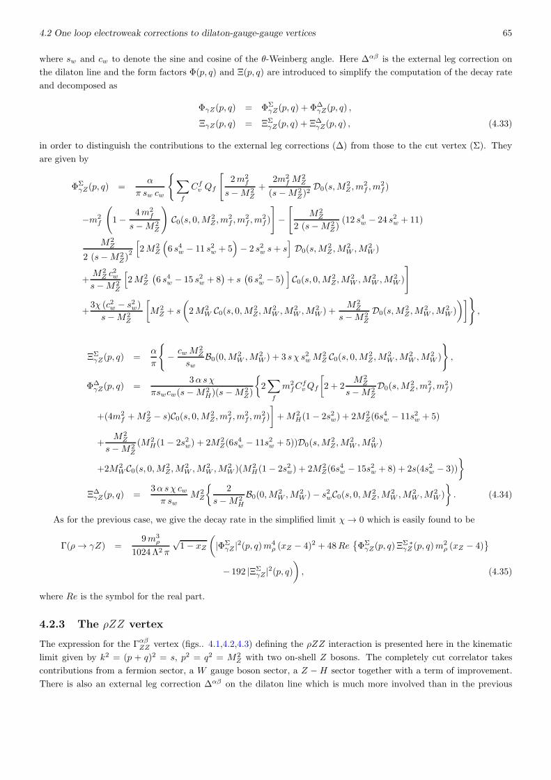
4.2 One loop electroweak corrections to dilaton-gauge-gauge vertices 65
where sw and cw to denote the sine and cosine of the θ-Weinberg angle. Here ∆αβ is the external leg correction on
the dilaton line and the form factors Φ(p, q) and Ξ(p, q) are introduced to simplify the computation of the decay rate
and decomposed as
ΦγZ(p, q) = ΦΣγZ(p, q) + Φ∆
γZ(p, q) ,
ΞγZ(p, q) = ΞΣγZ(p, q) + Ξ∆
γZ(p, q) , (4.33)
in order to distinguish the contributions to the external leg corrections (∆) from those to the cut vertex (Σ). They
are given by
ΦΣγZ(p, q) =
α
π sw cw
∑
f
Cfv Qf
[
2m2f
s−M2Z
+2m2
fM2Z
(s−M2Z)
2D0(s,M
2Z ,m
2f ,m
2f)
−m2f
(
1−4m2
f
s−M2Z
)
C0(s, 0,M2Z ,m
2f ,m
2f ,m
2f )
]
−[
M2Z
2 (s−M2Z)
(12 s4w − 24 s2w + 11)
M2Z
2 (s−M2Z)
2
[
2M2Z
(
6 s4w − 11 s2w + 5)
− 2 s2w s+ s]
D0(s,M2Z ,M
2W ,M
2W )
+M2Z c
2w
s−M2Z
[
2M2Z
(
6 s4w − 15 s2w + 8)
+ s(
6 s2w − 5)
]
C0(s, 0,M2Z,M
2W ,M
2W ,M
2W )
]
+3χ (c2w − s2w)
s−M2Z
[
M2Z + s
(
2M2W C0(s, 0,M2
Z,M2W ,M
2W ,M
2W ) +
M2Z
s−M2Z
D0(s,M2Z ,M
2W ,M
2W )
)]
,
ΞΣγZ(p, q) =
α
π
− cwM2Z
swB0(0,M
2W ,M
2W ) + 3 s χ s2wM
2Z C0(s, 0,M2
Z,M2W ,M
2W ,M
2W )
,
Φ∆γZ(p, q) =
3αsχ
πswcw(s−M2H)(s−M2
Z)
2∑
f
m2fC
fvQf
[
2 + 2M2Z
s−M2Z
D0(s,M2Z ,m
2f ,m
2f )
+(4m2f +M2
Z − s)C0(s, 0,M2Z ,m
2f ,m
2f ,m
2f )
]
+M2H(1 − 2s2w) + 2M2
Z(6s4w − 11s2w + 5)
+M2Z
s−M2Z
(M2H(1 − 2s2w) + 2M2
Z(6s4w − 11s2w + 5))D0(s,M
2Z ,M
2W ,M
2W )
+2M2WC0(s, 0,M2
Z,M2W ,M
2W ,M
2W )(M2
H(1 − 2s2w) + 2M2Z(6s
4w − 15s2w + 8) + 2s(4s2w − 3))
Ξ∆γZ(p, q) =
3α sχ cwπ sw
M2Z
2
s−M2H
B0(0,M2W ,M
2W )− s2wC0(s, 0,M2
Z,M2W ,M
2W ,M
2W )
. (4.34)
As for the previous case, we give the decay rate in the simplified limit χ→ 0 which is easily found to be
Γ(ρ→ γZ) =9m3
ρ
1024Λ2 π
√1− xZ
(
|ΦΣγZ |2(p, q)m4
ρ (xZ − 4)2 + 48Re
ΦΣγZ(p, q) Ξ
Σ ∗γZ (p, q)m
2ρ (xZ − 4)
− 192 |ΞΣγZ|2(p, q)
)
, (4.35)
where Re is the symbol for the real part.
4.2.3 The ρZZ vertex
The expression for the ΓαβZZ vertex (figs.. 4.1,4.2,4.3) defining the ρZZ interaction is presented here in the kinematic
limit given by k2 = (p + q)2 = s, p2 = q2 = M2Z with two on-shell Z bosons. The completely cut correlator takes
contributions from a fermion sector, a W gauge boson sector, a Z −H sector together with a term of improvement.
There is also an external leg correction ∆αβ on the dilaton line which is much more involved than in the previous
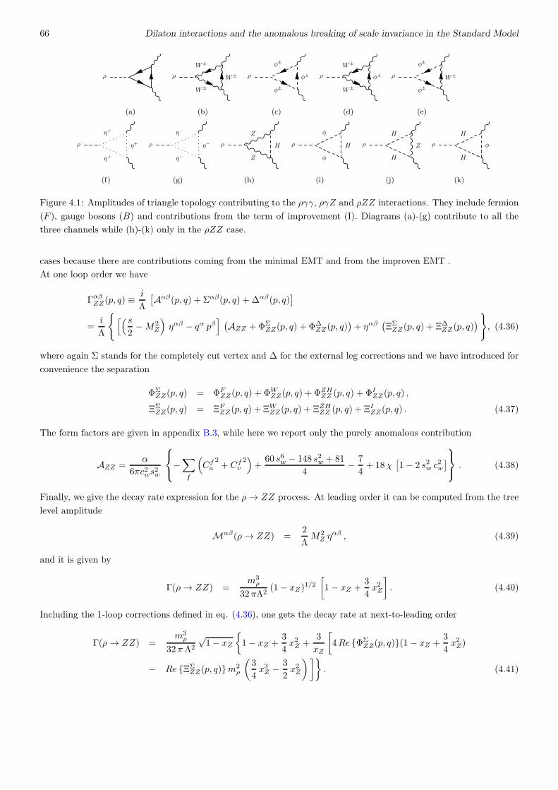
66 Dilaton interactions and the anomalous breaking of scale invariance in the Standard Model
ρ
(a)
W±
W±
W±
ρ
(b)
φ±
φ±
φ±
ρ
(c)
W±
φ±
W±
ρ
(d)
φ±
W±
φ±
ρ
(e)
η+
η+
η+
ρ
(f)
η−
η−
η−
ρ
(g)
Z
H
Z
ρ
(h)
φ
H
φ
ρ
(i)
H
Z
H
ρ
(j)
H
φ
H
ρ
(k)
Figure 4.1: Amplitudes of triangle topology contributing to the ργγ, ργZ and ρZZ interactions. They include fermion
(F ), gauge bosons (B) and contributions from the term of improvement (I). Diagrams (a)-(g) contribute to all the
three channels while (h)-(k) only in the ρZZ case.
cases because there are contributions coming from the minimal EMT and from the improven EMT .
At one loop order we have
ΓαβZZ(p, q) ≡i
Λ
[
Aαβ(p, q) + Σαβ(p, q) + ∆αβ(p, q)]
=i
Λ
[(s
2−M2
Z
)
ηαβ − qα pβ]
(
AZZ +ΦΣZZ(p, q) + Φ∆
ZZ(p, q))
+ ηαβ(
ΞΣZZ (p, q) + Ξ∆
ZZ(p, q))
, (4.36)
where again Σ stands for the completely cut vertex and ∆ for the external leg corrections and we have introduced for
convenience the separation
ΦΣZZ(p, q) = ΦFZZ(p, q) + ΦWZZ(p, q) + ΦZHZZ (p, q) + ΦIZZ(p, q) ,
ΞΣZZ(p, q) = ΞFZZ(p, q) + ΞWZZ(p, q) + ΞZHZZ (p, q) + ΞIZZ (p, q) . (4.37)
The form factors are given in appendix B.3, while here we report only the purely anomalous contribution
AZZ =α
6πc2ws2w
−∑
f
(
Cfa2+ Cfv
2)
+60 s6w − 148 s2w + 81
4− 7
4+ 18χ
[
1− 2 s2w c2w
]
. (4.38)
Finally, we give the decay rate expression for the ρ→ ZZ process. At leading order it can be computed from the tree
level amplitude
Mαβ(ρ→ ZZ) =2
ΛM2Z η
αβ , (4.39)
and it is given by
Γ(ρ→ ZZ) =m3ρ
32 πΛ2(1− xZ)
1/2
[
1− xZ +3
4x2Z
]
. (4.40)
Including the 1-loop corrections defined in eq. (4.36), one gets the decay rate at next-to-leading order
Γ(ρ→ ZZ) =m3ρ
32 πΛ2
√1− xZ
1− xZ +3
4x2Z +
3
xZ
[
4Re ΦΣZZ(p, q)(1− xZ +
3
4x2Z)
− Re ΞΣZZ(p, q)m2
ρ
(
3
4x3Z − 3
2x2Z
)]
. (4.41)
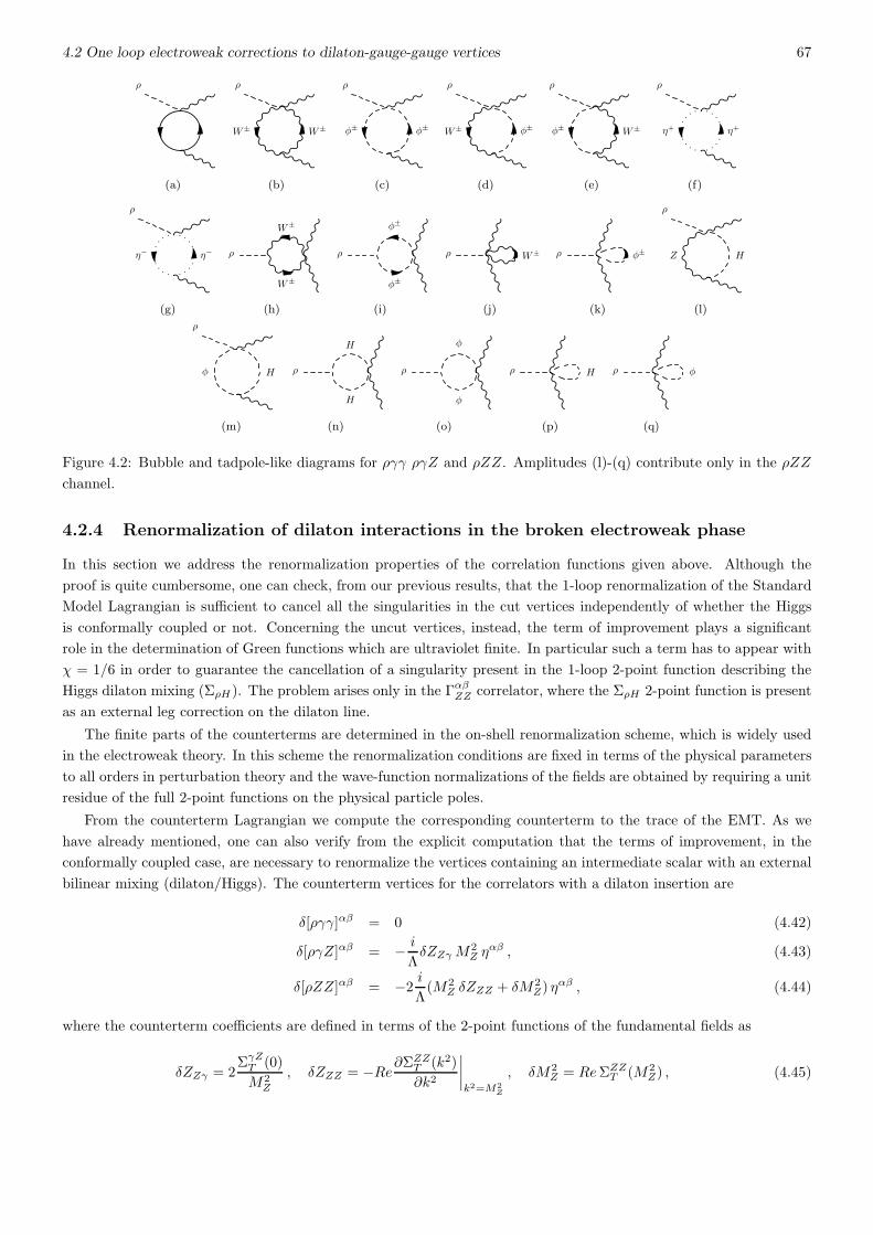
4.2 One loop electroweak corrections to dilaton-gauge-gauge vertices 67
ρ
(a)
W± W±
ρ
(b)
φ± φ±
ρ
(c)
W± φ±
ρ
(d)
φ± W±
ρ
(e)
η+ η+
ρ
(f)
η− η−
ρ
(g)
W±
W±
ρ
(h)
φ±
φ±
ρ
(i)
W±ρ
(j)
φ±ρ
(k)
Z H
ρ
(l)
φ H
ρ
(m)
H
H
ρ
(n)
φ
φ
ρ
(o)
Hρ
(p)
φρ
(q)
Figure 4.2: Bubble and tadpole-like diagrams for ργγ ργZ and ρZZ. Amplitudes (l)-(q) contribute only in the ρZZ
channel.
4.2.4 Renormalization of dilaton interactions in the broken electroweak phase
In this section we address the renormalization properties of the correlation functions given above. Although the
proof is quite cumbersome, one can check, from our previous results, that the 1-loop renormalization of the Standard
Model Lagrangian is sufficient to cancel all the singularities in the cut vertices independently of whether the Higgs
is conformally coupled or not. Concerning the uncut vertices, instead, the term of improvement plays a significant
role in the determination of Green functions which are ultraviolet finite. In particular such a term has to appear with
χ = 1/6 in order to guarantee the cancellation of a singularity present in the 1-loop 2-point function describing the
Higgs dilaton mixing (ΣρH). The problem arises only in the ΓαβZZ correlator, where the ΣρH 2-point function is present
as an external leg correction on the dilaton line.
The finite parts of the counterterms are determined in the on-shell renormalization scheme, which is widely used
in the electroweak theory. In this scheme the renormalization conditions are fixed in terms of the physical parameters
to all orders in perturbation theory and the wave-function normalizations of the fields are obtained by requiring a unit
residue of the full 2-point functions on the physical particle poles.
From the counterterm Lagrangian we compute the corresponding counterterm to the trace of the EMT. As we
have already mentioned, one can also verify from the explicit computation that the terms of improvement, in the
conformally coupled case, are necessary to renormalize the vertices containing an intermediate scalar with an external
bilinear mixing (dilaton/Higgs). The counterterm vertices for the correlators with a dilaton insertion are
δ[ργγ]αβ = 0 (4.42)
δ[ργZ]αβ = − i
ΛδZZγM
2Z η
αβ , (4.43)
δ[ρZZ]αβ = −2i
Λ(M2
Z δZZZ + δM2Z) η
αβ , (4.44)
where the counterterm coefficients are defined in terms of the 2-point functions of the fundamental fields as
δZZγ = 2ΣγZT (0)
M2Z
, δZZZ = −Re∂ΣZZT (k2)
∂k2
∣
∣
∣
∣
k2=M2Z
, δM2Z = ReΣZZT (M2
Z) , (4.45)

68 Dilaton interactions and the anomalous breaking of scale invariance in the Standard Model
ρH
(a)
ρH
(b)
ρH H
(c)
Figure 4.3: External leg corrections. Diagrams (b) and (c) appear only in the ρZZ sector.
and are defined in appendix B.4. It follows then that the ργγ interaction must be finite, as one can find by a direct
inspection of the Γαβγγ vertex, while the others require the subtraction of their divergences.
These counterterms are sufficient to remove the divergences of the completely cut graphs which do not contain
a bilinear mixing, once we set on-shell the external gauge lines. This occurs both for those diagrams which do not
involve the terms of improvement and for those involving TI . Regarding those contributions which involve the bilinear
mixing on the external dilaton line, we encounter two different situations.
In the ργZ vertex the insertion of the bilinear mixing ρH generates a reducible diagram of the form Higgs/photon/Z
whose renormalization is guaranteed, within the Standard Model, by the use of the Higgs/photon/Z counterterm
δ[HγZ]αβ =eMZ
2swcwδZZγ η
αβ . (4.46)
As a last case, we discuss the contribution to ρZZ coming from the bilinear mixing, already mentioned above. The
corrections on the dilaton line involve the dilaton/Higgs mixing ΣρH , the Higgs self-energy ΣHH and the term of
improvement ∆αβI ,HZZ , which introduces the Higgs/Z/Z vertex (or HZZ) of the Standard Model. The Higgs self-
energy and the HZZ vertex, in the Standard Model, are renormalized with the usual counterterms
δ[HH ](k2) = (δZH k2 −M2
HδZH − δM2H) , (4.47)
δ[HZZ]αβ =eMZ
sw cw
[
1 + δZe +2s2w − c2w
c2w
δswsw
+1
2
δM2W
M2W
+1
2δZH + δZZZ
]
ηαβ , (4.48)
where
δZH = −Re∂ΣHH(k2)
∂k2
∣
∣
∣
∣
k2=M2H
, δM2H = ReΣHH(M2
H) , δZe = −1
2δZγγ +
sw2cw
δZZγ ,
δsw = − c2w2sw
(
δM2W
M2W
− δM2Z
M2Z
)
, δM2W = ReΣWW
T (M2W ) , δZγγ = −∂Σ
γγT (k2)
∂k2
∣
∣
∣
∣
k2=0
. (4.49)
The self-energy ΣρH is defined by the minimal contribution generated by TMinµµ and by a second term derived from
TIµµ. This second term, with the conformal coupling χ = 1
6 , is necessary in order to ensure the renormalizability
of the dilaton/Higgs mixing. In fact, the use of the minimal EMT in the computation of this self-energy involves a
divergence of the form
δ[ρH ]Min = −4i
Λδt , (4.50)
with δt fixed by the condition of cancellation of the Higgs tadpole Tad (δt + Tad = 0). A simple analysis of the
divergences in ΣMin, ρH shows that the counterterm given in eq. (4.50) is not sufficient to remove all the singularities
of this correlator unless we also include the renormalization constant provided by the term of improvement which is
given by
δ[ρH ]I(k) = − i
Λ6χ v
[
δv +1
2δZH
]
k2 , with χ =1
6, (4.51)
and
δv = v
(
1
2
δM2W
M2W
+δswsw
− δZe
)
. (4.52)
One can show explicitly that this counterterm indeed ensures the finiteness of ΣρH .

4.3 The off-shell dilaton-gluon-gluon vertex in QCD 69
(a) (b) (c) (d) (e) (f)
(g) (h) (i) (j) (k)
Figure 4.4: QCD vertices at next-to-leading order. In the on-shell gluon case only diagram (a)contributes.
4.3 The off-shell dilaton-gluon-gluon vertex in QCD
After a discussion of the leading corrections to the vertices involving one dilaton and two electroweak currents we
investigate the interaction of a dilaton and two gluons beyond leading order, giving the expression of the full off-shell
vertex. The corresponding interaction with two on-shell gluons has been computed in [80] and is simply given by the
contributions of the anomaly and of the quark loop. We will come back to rediscuss the on-shell case in the second
part of this work, where we will stress some specific perturbative features of this interaction.
We show in fig. 4.4 a list of the NLO QCD contributions to dilaton interactions. As we have just mentioned, in
the 2-gluon on-shell case one can show by an explicit computation that each of these contributions vanishes, except
for diagram (a), which is non-zero when a massive fermion runs in the loop. For this specific reason, in the parton
model, the production of the dilaton in pp collisions at the LHC is mediated by the diagram of gluon fusion, which
involves a top quark in a loop.
We find convenient to express the result of the off-shell Γαβgg vertex in the form
Γαβgg (p, q) =i
Λ
A00(p, q)ηαβ +A11(p, q)pαpβ +A22(p, q)qαqβ +A12(p, q)pαqβ +A21(p, q)qαpβ
, (4.53)
where Aij(p, q) = Aijg (p, q) +Aijq (p, q) which are diagonal (∝ δab) in colour space.
After an explicit computation, we find
A00g (p, q) = −δab
g2NC16π2
2
(
p2 + q2 +11
3p · q
)
+ (p2 − q2)
[
B0(p2, 0, 0)− B0(q
2, 0, 0)
]
+(
p4 + q4 − 2(p2 + q2)p · q − 6p2q2)
C0((p+ q)2, p2, q2, 0, 0, 0)
,
A11g (p, q) = A22
g (q, p) = δabg2NC16 π2
2 +1
p · q2 − p2 q2
[
(p+ q)2 p · q B0((p+ q)2, 0, 0)
−p2 (q2 + p · q)B0(p2, 0, 0)− (2p · q2 − p2 q2 + p · q q2)B0(q
2, 0, 0)
+(
p2 q2(5q2 − p2) + 2p · q2(p2 + p · q − 2 q2))
C0((p+ q)2, p2, q2, 0, 0, 0)
]
,
A12g (p, q) = δab
g2NC4π2
p · q C0((p+ q)2, p2, q2, 0, 0, 0) ,
A21g (p, q) = δab
g2NC24 π2
11 +3
2
1
p · q2 − p2 q2(p2 + q2)
[
(p2 + p · q)B0(p2, 0, 0)
+(q2 + p · q)B0(q2, 0, 0)− (p+ q)2B0((p+ q)2, 0, 0)
−(
p · q(p2 + 4p · q + q2)− 2 p2 q2)
C0((p+ q)2, p2, q2, 0, 0, 0)
]
,

70 Dilaton interactions and the anomalous breaking of scale invariance in the Standard Model
A00q (p, q) = δab
g2
8π2
nf∑
i=1
2
3p · q − 2m2
i +m2i
p · q2 − p2q2
[
p2(
p · q + q2)
B0(p2,m2
i ,m2i )
+ q2(
p2 + p · q)
B0(q2,m2
i ,m2i )−
(
p2(
p · q + 2q2)
+ p · q q2)
B0((p+ q)2,m2i ,m
2i )
−(
p2q2(
p2 + q2 − 4m2i
)
+ 4m2i p · q2 + 4p2 q2 p · q − 2 p · q3
)
C0((p+ q)2, p2, q2,m2i ,m
2i ,m
2i )
]
,
A11q (p, q) = A22
q (q, p) = δabg2
8 π2
nf∑
i=1
2m2i q
2
p · q2 − p2q2
− 2 +1
p · q2 − p2q2
[
(
q2(
p2 + 3 p · q)
+ 2 p · q2)
B0(q2,m2
i ,m2i ) +
(
p2(
3 p · q + q2)
+ 2p · q2)
B0(p2,m2
i ,m2i )
−(
p2(
3 p · q + 2q2)
+ p · q(
4 p · q + 3q2))
B0((p+ q)2,m2i ,m
2i )
−(
2 p · q2(
2m2i + p2 + q2
)
+ p2q2(
p2 + q2 − 4m2i
)
)
+ 4p2q2 p · q + 2 p · q3)
C0((p+ q)2, p2, q2,m2i ,m
2i ,m
2i )
]
,
A12q (p, q) = δab
g2
8 π2
nf∑
i=1
2m2i p · q2
p · q2 − p2q2
2 +1
p · q2 − p2q2
[
−(
q2(
p2 + 3 p · q)
+ 2 p · q2)
B0(q2,m2
i ,m2i )
−(
p2(
3 p · q + q2)
+ 2 p · q2)
B0(p2,m2
i ,m2i ) +
(
p2(
3 p · q + 2q2)
+ p · q(
4 p · q + 3q2))
× B0((p+ q)2,m2i ,m
2i ) +
(
2 p · q2(
2m2i + p2 + q2
)
+ p2q2(
p2 + q2 − 4m2i
)
+ 4 p2 q2 p · q + 2 p · q3)
C0((p+ q)2, p2, q2,m2i ,m
2i ,m
2i )
]
,
A21q (p, q) = δab
g2
8 π2
nf∑
i=1
− 2
3+
2m2i p · q
p · q − p2q2+
m2i
(p · q − p2q2)2
[
− p2(
q2(
2p2 + 3 p · q)
+ p · q2)
× B0(p2,m2
i ,m2i )− q2
(
p2(
3 p · q + 2q2)
+ p · q2)
B0(q2,m2
i ,m2i ) +
(
2p4q2 + p2(
6 p · q q2
+ p · q2 + 2q4)
+ p · q2q2)
B0((p+ q)2,m2i ,m
2i ) + p · q
(
p2q2(
3p2 + 3q2 − 4m2i
)
+ 4m2i p · q2 + 8p2 q2 p · q − 2 p · q3
)
C0((p+ q)2, p2, q2,m2i ,m
2i ,m
2i )
]
, (4.54)
where NC is the number of colours, nf is the number of flavour and mi the mass of the quark. In the on-shell gluon
case, eq. (4.53) reproduces the same interaction responsible for Higgs production at LHC augmented by an anomaly
term. This is given by
Γαβgg (p, q) =i
ΛΦ(s)uαβ(p, q) , (4.55)
with uαβ(p, q) defined in eq. (4.21), and with the gluon/quark contributions included in the Φ(s) form factor (s =
k2 = (p+ q)2)
Φ(s) = −δab g2
24 π2
(11NC − 2nf) + 12
nf∑
i=1
m2i
[
1
s− 1
2C0(s, 0, 0,m2
i ,m2i ,m
2i )
(
1− 4m2i
s
)]
, (4.56)
where the first mass independent terms represent the contribution of the anomaly, while the others are the explicit
mass corrections.
The decay rate of a dilaton in two gluons can be evaluated from the on-shell limit in eq. (4.55) and it is given by
Γ(ρ → gg) =α2sm
3ρ
32 π3Λ2
∣
∣
∣
∣
βQCD + xt [1 + (1− xt) f(xt)]
∣
∣
∣
∣
2
, (4.57)
where we have taken the top quark as the only massive fermion and xi and f(xi) are defined in eq. (4.27) and eq.
(4.28) respectively. Moreover we have set βQCD = 11NC/3− 2nf/3 for the QCD β function.
4.4 Non-gravitational dilatons from scale invariant extensions of the Standard Model 71
4.4 Non-gravitational dilatons from scale invariant extensions of the
Standard Model
As we have pointed out in the introduction, a dilaton may appear in the spectrum of different extensions of the
Standard Model not only as a result of the compactification of extra spacetime dimensions, but also as an effective
state, related to the breaking of dilatation symmetry. In this respect, notice that in its actual formulation the Standard
Model is not scale invariant, but can be such, at classical level, if we slightly modify the scalar potential with the
introduction of a dynamical field Σ that allows to restore this symmetry and acquires a vacuum expectation value.
This task is accomplished by the replacement of every dimensionful parameter m according to m → mΣΛ , where Λ
is the classical conformal breaking scale. In the case of the Standard Model, classical scale invariance can be easily
accommodated with a simple change of the scalar potential.
This is defined, obviously, modulo a constant, therefore we may consider, for instance, two equivalent choices
V1(H,H†) = −µ2H†H + λ(H†H)2 = λ
(
H†H − µ2
2λ
)2
− µ4
4λ
V2(H,H†) = λ
(
H†H − µ2
2λ
)2
(4.58)
which give two different scale invariant extensions
V1(H,H†,Σ) = −µ
2Σ2
Λ2H†H + λ(H†H)2
V2(H,H†,Σ) = λ
(
H†H − µ2Σ2
2λΛ2
)2
, (4.59)
where H is the Higgs doublet, λ is its dimensionless coupling constant, while µ has the dimension of a mass and,
therefore, is the only term involved in the scale invariant extension. More details of this analysis can be found in the
next section.
The invariance of the potential under the addition of constant terms, typical of any Lagrangian, is lifted once we require
the presence of a dilatation symmetry. Only the second choice (V2) guarantees the existence of a stable ground state
characterized by a spontaneously broken phase. In V2 we parameterize the Higgs, as usual, around the electroweak
vev v as in eq. (4.12), and indicate with Λ the vev of the dilaton field Σ = Λ + ρ, and we have set φ+ = φ = 0 in the
unitary gauge.
The potential V2 has a massless mode due to the existence of a flat direction. Performing a diagonalization of the
mass matrix we define the two mass eigenstates ρ0 and h0, which are given by(
ρ0
h0
)
=
(
cosα sinα
− sinα cosα
)(
ρ
h
)
(4.60)
with
cosα =1
√
1 + v2/Λ2sinα =
1√
1 + Λ2/v2. (4.61)
We denote with ρ0 the massless dilaton generated by this potential, while h0 will describe a massive scalar, interpreted
as a new Higgs field, whose mass is given by
m2h0
= 2λv2(
1 +v2
Λ2
)
with v2 =µ2
λ, (4.62)
and with m2h = 2λv2 being the mass of the Standard Model Higgs. The Higgs mass, in this case, is corrected by the
new scale of the spontaneous breaking of the dilatation symmetry (Λ), which remains a free parameter.
The vacuum degeneracy of the scale invariant model can be lifted by the introduction of extra (explicit breaking)
terms which give a small mass to the dilaton field. To remove such degeneracy, one can introduce, for instance, the
term
Lbreak =1
2m2ρρ
2 +1
3!m2ρ
ρ3
Λ+ . . . , (4.63)

72 Dilaton interactions and the anomalous breaking of scale invariance in the Standard Model
where mρ represents the dilaton mass.
It is clear that in this approach the coupling of the dilaton to the anomaly has to be added by hand. The obvious
question to address, at this point, is if one can identify in the effective action of the Standard Model an effective state
which may interpolate between the dilatation current of the same model and the final state with two neutral currents,
for example with two photons. The role of the following sections will be to show rigorously that such a state can be
identified in ordinary perturbation theory in the form of an anomaly pole.
We will interpret this scalar exchange as a composite state whose interactions with the rest of the Standard
Model are defined by the conditions of scale and gauge invariance. In this respect, the Standard Model Lagrangian,
enlarged by the introduction of a potential of the form V2(H,H†,Σ), which is expected to capture the dynamics of this
pseudo-Goldstone mode, could take the role of a workable model useful for a phenomenological analysis. We will show
rigorously that this state couples to the conformal anomaly by a direct analysis of the JDV V correlator, in the form
of an anomaly pole, with JD and V being the dilatation and a vector current respectively. Usual polology arguments
support the fact that a pole in a correlation function is there to indicate that a specific state can be created by a field
operator in the Lagrangian of the theory, or, alternatively, as a composite particle of the same elementary fields.
Obviously, a perturbative hint of the existence of such intermediate state does not correspond to a complete
description of the state, in the same way as the discovery of an anomaly pole in the AV V correlator of QCD (with A
being the axial current) is not equivalent to a proof of the existence of the pion.
4.4.1 A classical scale invariant Lagrangian with a dilaton field
In this section we briefly describe the construction of a scale invariant theory to clarify some of the issues concerning
the coupling of a dilaton. In particular, the example has the goal to illustrate that in a classical scale invariant
extension of a given theory, the dilaton couples only to operators which are mass dependent, and thus scale breaking,
before the extension. We take the case of a fundamental dilaton field (not a composite) introduced in this type of
extensions.
A scale invariant extension of a given Lagrangian can be obtained if we promote all the dimensionful constants
to dynamical fields. We illustrate this point in the case of a simple interacting scalar field theory incorporating the
Higgs mechanism. At a second stage we will derive the structure of the dilaton interaction at order 1/Λ, where Λ is
the scale characterizing the spontaneous breaking of the dilatation symmetry.
Our toy model consists in a real singlet scalar with a potential of the kind of V2(φ) introduced in section 4.4,
L =1
2(∂φ)2 − V2(φ) =
1
2(∂φ)2 +
µ2
2φ2 − λ
φ4
4− µ4
4λ, (4.64)
obeying the classical equation of motion
φ = µ2 φ− λφ3 . (4.65)
Obviously this theory is not scale invariant due to the appearance of the mass term µ. This feature is reflected in the
trace of the EMT. Indeed the canonical EMT of such a theory and its trace are
T µνc (φ) = ∂µφ∂νφ− 1
2ηµν[
(∂φ)2 + µ2 φ2 − λφ4
2− µ4
2λ
]
,
T µc µ(φ) = −(∂φ)2 − 2µ2 φ2 + λφ4 +µ4
λ. (4.66)
Improving the EMT of the scalar field in such a way as to make its trace proportional only to the scale breaking
parameter, i.e. the mass µ, which is done by adding an extra contribution T µνI (φ, χ),
T µνI (φ, χ) = χ(
ηµνφ2 − ∂µ∂νφ2)
, (4.67)
where the parameter χ is left generic. The combination of the canonical plus the improvement EMT, T µν ≡ T µνc +T µνIhas the off-shell trace
T µµ(φ, χ) = (∂φ)2 (6χ− 1)− 2µ2 φ2 + λφ4 +µ4
λ+ 6χφφ . (4.68)

4.4 Non-gravitational dilatons from scale invariant extensions of the Standard Model 73
Using the equation of motion (4.65) and choosing χ = 1/6 the trace relation given above becomes proportional uniquely
to the scale breaking term µ
T µµ(φ, 1/6) = −µ2φ2 +µ4
λ. (4.69)
The scale invariant extension of the Lagrangian given in eq. (4.64) is achieved by promoting the mass terms to
dynamical fields by the replacement
µ→ µ
ΛΣ, (4.70)
obtaining
L =1
2(∂φ)2 +
1
2(∂Σ)2 +
µ2
2Λ2Σ2 φ2 − λ
φ4
4− µ4
4λΛ4Σ4 (4.71)
where we have used eq. (4.70) and introduced a kinetic term for the dilaton Σ. Obviously, the new Lagrangian is
dilatation invariant, as one can see from the trace of the improven EMT
T µµ(φ,Σ, χ, χ′) = (6χ− 1) (∂φ)2 + (6χ′ − 1) (∂Σ)2 + 6χφφ+ 6χ′ΣΣ− 2
µ2
Λ2Σ2 φ2 + λφ4 +
1
λ
µ4
Λ4Σ4 , (4.72)
which vanishes upon using the equations of motion for the Σ and φ fields,
φ =µ2
Λ2Σ2 φ− λφ3 ,
Σ =µ2
Λ2Σφ2 − 1
λ
µ4
Λ4Σ3 , (4.73)
and setting the χ, χ′ parameters at the special value χ = χ′ = 1/6.
As we have already discussed in section 4.4, the scalar potential V2 allows to perform the spontaneous breaking of
the scale symmetry around a stable minimum point, giving the dilaton and the scalar field the vacuum expectation
values Λ and v respectively
Σ = Λ + ρ , φ = v + h . (4.74)
For our present purposes, it is enough to expand the Lagrangian (4.71) around the vev for the dilaton field, as we are
interested in the structure of the couplings of its fluctuation ρ
L =1
2(∂φ)2 +
1
2(∂ρ)2 +
µ2
2φ2 − λ
φ4
4− µ4
4λ− ρ
Λ
(
−µ2 φ2 +µ4
λ
)
+ . . . , (4.75)
where the ellipsis refer to terms that are higher order in 1/Λ. It is clear, from (4.69) and (4.75), that one can write
an dilaton Lagrangian at order 1/Λ, as
Lρ = (∂ρ)2 − ρ
ΛT µµ(φ, 1/6) + . . . , (4.76)
where the equations of motion have been used in the trace of the energy-momentum tensor. Expanding the scalar
field around v would render the previous equation more complicated and we omit it for definiteness. We only have to
mention that a mixing term ∼ ρ h shows up and it has to be removed diagonalizing the mass matrix, switching from
interaction to mass eigenstates exactly in the way we discussed in section 4.4, to which we refer for the details.
It is clear, from this simple analysis, that a dilaton, in general, does not couple to the anomaly, but only to the
sources of explicit breaking of scale invariance, i.e. to the mass terms. The coupling of a dilaton to an anomaly is, on
the other hand, necessary, if the state is interpreted as a composite pseudo Nambu-Goldstone mode of the dilatation
symmetry. Thus, this coupling has to be introduced by hand, in strict analogy with the chiral case.
4.4.2 The JDV V and TV V vertices
This effective degree of freedom emerges both from the spectral analysis of the TV V [27, 42] and, as we are now going
to show, of the JDV V vertices, being the two vertices closely related. We recall that the dilatation current can be
defined as
JµD(z) = zνTµν(z) with ∂ · JD = T µµ. (4.77)
74 Dilaton interactions and the anomalous breaking of scale invariance in the Standard Model
The T µν has to be symmetric and on-shell traceless for a classical scale invariant theory, and includes, at quantum
level, the contribution from the trace anomaly together with the additional terms describing the explicit breaking
of the dilatation symmetry. The separation between the anomalous and the explicit contributions to the breaking
of dilatation symmetry is present in all the analysis that we have performed on the TV V vertex in dimensional
regularization. In this respect, the analogy between these types of correlators and the AV V diagram of the chiral
anomaly goes quite far, since in the AV V case such a separation has been shown to hold in the Longitudinal/Transverse
(L/T) solution of the anomalous Ward identities [81, 82, 83]. This has been verified in perturbation theory in the
same scheme.
We recall that the U(1)A current is characterized by an anomaly pole which describes the interaction between the
Nambu-Goldstone mode, generated by the breaking of the chiral symmetry, and the gauge currents. In momentum
space this corresponds to the nonlocal vertex
V λµνanom(k, p, q) =kλ
k2ǫµναβpαqβ + ... (4.78)
with k being the momentum of the axial-vector current and p and q the momenta of the two photons. In the equation
above, the ellipsis refer to terms which are suppressed at large energy. In this regime, this allows to distinguish
the operator accounting for the chiral anomaly (i.e. −1 in coordinate space) from the contributions due to mass
corrections. Polology arguments can be used to relate the appearance of such a pole to the pion state around the scale
of chiral symmetry breaking.
To identify the corresponding pole in the dilatation current of the JDV V correlator at zero momentum transfer,
one can follow the analysis of [84], where it is shown that the appearance of the trace anomaly is related to the presence
of a superconvergent sum rule in the spectral density of this correlator. At non-zero momentum transfer the derivation
of a similar behaviour can be obtained by an explicit computation of the spectral density of the TV V vertex [27] or
of the entire correlator, as done for QED and QCD [42, 43] and as we will show next.
Using the relation between JµD and the EMT T µν we introduce the JDV V correlator
ΓµαβD (k, p) ≡∫
d4z d4x e−ik·z+ip·x⟨
JµD(z)Vα(x)V β(0)
⟩
(4.79)
which can be related to the TV V correlator
Γµναβ(k, p) ≡∫
d4z d4x e−ik·z+ip·x⟨
T µν(z)V α(x)V β(0)⟩
(4.80)
according to
ΓµαβD (k, p) = i∂
∂kνΓµναβ(k, p) . (4.81)
As we have already mentioned, this equation allows us to identify a pole term in the JDV V diagram from the
corresponding pole structure in the TV V vertex. In the following we will show the emergence of the anomaly poles in
the QED and QCD cases.
4.4.3 The dilaton anomaly pole in the QED case
For definiteness, it is convenient to briefly review the characterization of the TV V vertex in the QED case with a
massive fermion (see [42] for more details). The full amplitude can be expanded in a specific basis of 13 tensors first
identified in [27]
Γµναβ(p, q) =
13∑
i=1
Fi(s; s1, s2,m2)φµναβi (p, q) , (4.82)
where the 13 invariant amplitudes Fi are functions of the kinematic invariants s = k2 = (p+q)2, s1 = p2, s2 = q2, with
p and q the momenta of the external photons, and of the internal fermion mass m. The list of the tensor structures
4.4 Non-gravitational dilatons from scale invariant extensions of the Standard Model 75
φi can be found in [27]. The number of these form factors reduces from 13 to 3 in the case of on-shell photons. For
our purposes, being interested in the appearance of the anomaly poles, we only need the contributions that generate
a non zero trace. These come from the tensors φµναβ1 and φµναβ2 which are
φµναβ1 =(
k2ηµν − kµkν)
uαβ(p, q),
φµναβ2 =(
k2ηµν − kµkν)
wαβ(p, q), (4.83)
where
uαβ(p, q) ≡ (p · q)ηαβ − qαpβ ,
wαβ(p, q) ≡ p2q2ηαβ + (p · q)pαqβ − q2pαpβ − p2qαqβ . (4.84)
For two on-shell final state photons (s1 = s2 = 0) and a massive fermion we obtain
F1(s; 0, 0, m2) = F1 pole +
e2m2
3 π2 s2− e2m2
3 π2 sC0(s, 0, 0,m2,m2,m2)
[
1
2− 2m2
s
]
, (4.85)
where
F1 pole = − e2
18 π2s(4.86)
and the scalar 3-point function C0(s, 0, 0,m2,m2,m2) is given by
C0(s, 0, 0,m2,m2,m2) =1
2slog2
a3 + 1
a3 − 1, with a3 =
√
1− 4m2/s . (4.87)
In the massless fermion case two properties of this expansion are noteworthy: 1) the trace anomaly takes contribution
only from a single tensor structure (φ1) and invariant amplitude (F1) which coincides with the pole term; 2) the residue
of this pole as s→ 0 is non-zero, showing that the pole is coupled in the infrared. Notice that the form factor F2, which
in general gives a non-zero contribution to the trace in the presence of mass terms, is multiplied by a tensor structure
(φ2) which vanishes when the two photons are on-shell. Therefore, similarly to the case of the chiral anomaly, also
in this case the anomaly is entirely given by the appearance of an anomaly pole. We stress that this result is found
to be exact in dimensional regularization, which is a mass independent scheme: at perturbative level, the anomalous
breaking of the dilatation symmetry, related to an anomaly pole in the spectrum of all the gauge-invariant correlators
studied in this work, is separated from the sources of explicit breaking. The latter are related to the mass parameters
and/or to the gauge bosons virtualities p2 and q2.
To analyse the implications of the pole behaviour discussed so far for the TV V vertex and its connection with the
JDV V correlator, we limit our attention on the anomalous contribution (F1 φµναβ1 ), which we rewrite in the form
Γµναβpole (k, p) ≡ − e2
18π2
1
k2(
ηµνk2 − kµkν)
uαβ(p, q) , q = k − p . (4.88)
This implies that the JDV V correlator acquires a pole as well
ΓµαβD pole = −i e2
18π2
∂
∂kν
[
1
k2(
ηµνk2 − kµkν)
uαβ(p, k − p)
]
(4.89)
and acting with the derivative on the right hand side we finally obtain
ΓµαβD pole(k, p) = ie2
6π2
kµ
k2uαβ(p, k − p)− i
e2
18π2
1
k2(
ηµνk2 − kµkν) ∂
∂kνuαβ(p, k − p). (4.90)
Notice that the first contribution on the right hand side of the previous equation corresponds to an anomaly pole,
shown pictorially in fig. 4.5. In fact, by taking a derivative of the dilatation current only this term will contribute to
the corresponding Ward identity
kµ ΓµαβD (k, p) = i
e2
6π2uαβ(p, k − p), (4.91)
which is the expression in momentum space of the usual relation ∂JD ∼ FF , while the second term trivially vanishes.
Notice that the pole in (4.91) has disappeared, and we are left just with its residue on the r.h.s., or, equivalently, the
pole is removed in eq. (4.88) if we trace the two indices (µ, ν).

76 Dilaton interactions and the anomalous breaking of scale invariance in the Standard Model
JµD
γ
γ
Figure 4.5: Exchange of a dilaton pole mediated by the JDV V correlator.
4.4.4 The dilaton anomaly pole in the QCD case
The analysis presented for the dilatation current of QED can be immediately generalized to the case of QCD. Following
a similar reasoning, we expand the on-shell TV V vertex, with V denoting now the gluon, as
Γµναβ(p, q) = δab3∑
i=1
Φi(s; 0, 0) tµναβi (p, q) with p2 = q2 = 0 , (4.92)
with the tensor basis given by
tµναβ1 (p, q) = (s ηµν − kµkν)uαβ(p, q),
tµναβ2 (p, q) = −2 uαβ(p, q) [s ηµν + 2(pµ pν + qµ qν)− 4 (pµ qν + qµ pν)] ,
tµναβ3 (p, q) =(
pµqν + pνqµ)
gαβ +s
2
(
ηανηβµ + ηαµηβν)
−ηµν(s
2ηαβ − qαpβ
)
−(
ηβνpµ + ηβµpν)
qα −(
ηανqµ + ηαµqν)
pβ , (4.93)
where δab is the diagonal matrix in colour space. Again we have s = k2 = (p + q)2, with the virtualities of the
two gluons being p2 = q2 = 0. Notice that in the massless fermion limit only the first (t1) of these 3 form factors
contributes to the anomaly. The corresponding on-shell form factors with massive quarks are
Φ1(s; 0, 0) = − g2
72π2 s(2nf − 11NC) +
g2
6π2
nf∑
i=1
m2i
1
s2− 1
2sC0(s, 0, 0,m2
i ,m2i ,m
2i )
[
1− 4m2i
s
]
,
Φ2(s; 0, 0) = − g2
288π2 s(nf −NC)
− g2
24π2
nf∑
i=1
m2i
1
s2+
3
s2D0(s, 0, 0,m
2i ,m
2i ) +
1
sC0(s, 0, 0,m2
i ,m2i ,m
2i )
[
1 +2m2
i
s
]
,
Φ3(s; 0, 0) =g2
288π2(11nf − 65NC)−
g2NC8π2
[
11
6B0(s, 0, 0)− B0(0, 0, 0) + s C0(s, 0, 0, 0, 0, 0)
]
+g2
8π2
nf∑
i=1
1
3B0(s,m
2i ,m
2i ) +m2
i
[
1
s+
5
3sD0(s, 0, 0,m
2i ) + C0(s, 0, 0,m2
i ,m2i ,m
2i )
[
1 +2m2
i
s
] ]
,
(4.94)
where mi denotes the quark mass, and we have summed over the fermion flavours (nf ), while NC denotes the number
of colours. Notice the appearance of the 1/s pole in Φ1, which saturates the contribution to the trace anomaly in the
massless limit which becomes
Φ1(s; 0, 0) = − g2
72π2 s(2nf − 11NC) . (4.95)
As for the QED case, this is the only invariant amplitude which contributes to the anomalous trace part of the
correlator. The pole completely accounts for the trace anomaly and is clearly inherited by the QCD dilatation current,
for the same reasonings discussed above.
4.4 Non-gravitational dilatons from scale invariant extensions of the Standard Model 77
4.4.5 Mass corrections to the dilaton pole
The discussion of the mass corrections to the massless dilaton can follow quite closely the strategy adopted in the pion
case using partially conserved axial currents (PCAC) techniques. Also in this case, as for PCAC in the past, one can
assume a partially conserved dilaton current (PCDC) in order to relate the decay amplitude of the dilaton fρ to its
mass mρ and to the vacuum energy.
For this goal we define the 1-particle transition amplitudes for the dilatation current and the EMT between the vacuum
and a dilaton state with momentum pµ
〈0|JµD(x)|ρ, p〉 = −i fρ pµ e−ip·x
〈0|T µν(x)|ρ, p〉 =fρ3
(
pµpν − ηµν p2)
e−ip·x, (4.96)
both of them giving
∂µ〈0|JµD(x)|ρ, p〉 = ηµν〈0|T µν(x)|ρ, p〉 = −fρm2ρ e
−ip·x. (4.97)
We introduce the dilaton interpolating field ρ(x) via a PCDC relation
∂µJµD(x) = −fρm2
ρ ρ(x) (4.98)
with
〈0|ρ(x)|ρ, p〉 = e−ip·x (4.99)
and the matrix element
Aµ(q) =
∫
d4x eiq·x 〈0|T JµD(x)Tαα(0)|0〉, (4.100)
where T . . . denotes the time ordered product.
Using dilaton pole dominance we can rewrite the contraction of qµ with this correlator as
limqµ→0
qµAµ(q) = fρ 〈ρ, q = 0|Tαα(0)|0〉 , (4.101)
where the soft limit qµ → 0 with q2 ≫ m2ρ ∼ 0 has been taken.
At the same time the dilatation Ward identity on the amplitude Aµ(q) in eq. (4.100) gives
qµAµ(q) = i
∫
d4x eiq·x∂
∂xµ〈0 |T JµD(x)Tαα(0)| 0〉
= i
∫
d4x eiq·x 〈0 |T ∂µJµD(x)Tαα(0)| 0〉+ i
∫
d4x eiq·x δ(x0)⟨
0∣
∣
[
J0D(x), T
αα(0)
]∣
∣ 0⟩
. (4.102)
The commutator of the time component of the dilatation charge density and the trace of the EMT can be rewritten
as[
J0D(0,x), T
αα(0)
]
= −iδ3(x) (dT + x · ∂)Tαα(0) (4.103)
where dT is the canonical dimension of the EMT (dT = 4). Inserting eq. (4.103) in the Ward identity (4.102) and
neglecting the first term due to the nearly conserved dilatation current (mρ ∼ 0), we are left with
qµAµ(q) = dT 〈0|Tαα(0)|0〉 . (4.104)
In the soft limit, with q2 ≫ m2ρ, comparing eq. (4.101) and eq. (4.104) we obtain
limqµ→0
qµAµ = fρ 〈ρ, q = 0|Tαα(0)|0〉 = dT 〈0|Tαα(0)|0〉 . (4.105)
Introducing the vacuum energy density ǫvac =⟨
0|T 00 |0⟩
= 14 〈0|Tαα (0)|0〉 and using the relation in eq. (4.97) we have
〈ρ, p = 0|T µµ|0〉 = −fρm2ρ =
dTfρǫvac (4.106)
78 Dilaton interactions and the anomalous breaking of scale invariance in the Standard Model
from which we finally obtain (dT = 4)
f2ρm
2ρ = −16 ǫvac. (4.107)
This equation fixes the decay amplitude of the dilaton in terms of its mass and the vacuum energy. Notice that ǫvac
can be related both to the anomaly and possibly to explicit contributions of the breaking of the dilatation symmetry
since
ǫvac =1
4
⟨
0
∣
∣
∣
∣
β(g)
2gFµνF
µν
∣
∣
∣
∣
0
⟩
+ ... (4.108)
where the ellipsis saturate the anomaly equation with extra mass-dependent contributions, which may be far larger
in size then the anomaly term. In (4.108) we have assumed, for simplicity, the coupling of the pole to a single gauge
field, with a beta function β(g), but obviously, it can be generalized to several gauge fields.
In the case of higher dimensional operators we would get
ǫvac =1
4
⟨
0
∣
∣
∣
∣
β(g)
2gFµν F
µν
∣
∣
∣
∣
0
⟩
+∑
i
gi (di − 4) 〈0|Oi|0〉 , (4.109)
valid around the scale at which the PCDC approximation holds. Therefore a massless pole can be corrected non-
perturbatively according to some completion theory, causing its mass to shift. Perturbation theory gives indications
about the interpolating fields which can couple to it, as we have seen by exploiting the chiral analogy, but not more
than that. The corrections are model-dependent and can be the subject of additional phenomenological searches, but
the dilatation current takes the role, with no doubt, of an interpolating field for the propagation of such a scalar
intermediate state.
4.5 The infrared coupling of an anomaly pole and the anomaly enhance-
ment
It is easy to figure out from the results of the previous sections that the coupling of a (graviscalar) dilaton to the
anomaly causes a large enhancement of its 2-photons and 2-gluons decays. One of the features of the graviscalar
interaction is that its coupling includes anomalous contributions which are part both of the 2-photons and of the
2-gluons cross sections. For this reason, if an enhancement with respect to the Standard Model rates is found only in
one of these two channels and it is associated to the exchange of a spin zero intermediate state, this result could be
used to rule out the exchange of a graviscalar.
On the other hand, for an effective dilaton, identified by an anomaly pole in the JDV V correlator of the Standard
Model, the case is more subtle, since the coupling of this effective state to the anomaly has to be introduced by hand.
This state should be identified, in the perturbative picture, with the corresponding anomaly pole. The situation,
here, is closely similar to the pion case: in fact, in perturbative QCD, the anomalous AV V diagram is characterized
by the presence of an anomaly pole in the variable k2, with k denoting the momentum of the axial-vector current,
which is explicitly shown in eq. (4.78). It is interesting to note that this structure has a non-vanishing residue for
on-shell photons and for massless quarks running in the loop. In this case the pole is said to be infrared coupled. This
feature, supplemented by usual polology arguments, leads to a π → γγ decay rate which is enhanced with respect to
the non-anomalous case. On the other hand, if the photons are virtual or the quarks are massive the anomaly pole
decouples, namely, its residue is zero. We refer to [83] for more details.
The same behaviour is shared by the conformally anomalous TV V diagram [42], so let us illustrate this important
point in the QED case by considering the off-shell correlator. We denote with s1 and s2 the virtualities of the two final
state photons and with m the mass of the fermion running in the loops. The case with on-shell photons and a massive
fermion has already been discussed in section 4.4.3. There we have shown that the anomaly pole has a non-vanishing
residue only in the conformal limit, when all masses are set to zero. Indeed, in the case of a massive fermion, besides
the fact that the anomaly pole anyway appears in the corresponding invariant amplitude F1(s; 0, 0, m2), as one can

4.6 Quantum conformal invariance and dilaton couplings at low energy 79
see from eq. (4.85), it will decouple, showing a zero residue
lims→0
sΓµναβ(s; 0, 0, m2) = 0 . (4.110)
As for the chiral anomaly case, the absence of the internal fermion masses is not sufficient to guarantee the infrared
coupling of the anomaly pole. Indeed, if m = 0 but the photons are taken off-shell, being characterized by non zero
virtualities s1 and s2, one can check that the entire correlator is completely free from anomaly poles as
lims→0
sΓµναβ(s; s1, s2, 0) = 0 . (4.111)
The computation of this limit needs the explicit results for all the invariant amplitudes Fi, which are not given here
due to their lengthy expressions but can be found in [42].
One should be aware of the fact that the same pole is present in the AV V diagram when V V are now the gluons.
If the two gluons are on-shell, as in the 2-photon case, the perturbative anomaly pole is again infrared coupled.
Obviously, such an an enhancement is not observable, since the gluons cannot be on-shell, because of confinement. In
the perturbative picture, a non-zero virtuality of the two gluons is then sufficient to exclude an infrared coupling of
the anomaly pole.
We feel, however, that a simple perturbative analysis may not be completely sufficient to decide whether or not
the coupling of such a state to the gluon anomaly takes place. On the other hand, there is no doubt, by the same
reason, that such a coupling should occur in the 2-photon case, being the photons massless asymptotic states. In this
case the corresponding anomaly pole of the JDγγ vertex is infrared coupled.
In general, in the case of an effective dilaton, one is allowed to write down a Lagrangian which is assumed to be
scale invariant and, at a second stage, introduce the direct coupling of this state to the trace anomaly. The possibility
of coupling such a state to the photon and to the gluons or just to the photons, for instance, is a delicate issue for
which a simple perturbative approach is unable to offer a definite answer.
4.6 Quantum conformal invariance and dilaton couplings at low energy
Similar enhancements are present in the case of quantum scale invariant extensions of the Standard Model [51], where
one assumes that the spectrum of the theory is extended with new massive states in order to set the β functions of the
gauge couplings to vanish. In a quantum scale invariant theory such as the one discussed in [51], the dilaton couples
only to massive states, but the heavy mass limit and the condition of the vanishing of the complete β functions, leave
at low energy a dilaton interaction proportional only to the β functions of the low energy states. The ”remnant”
low energy interaction is mass-independent and coincides with that due to a typical anomalous coupling, although its
origin is of different nature, since anomalous contributions are genuinely mass-independent.
For this reason, the decays of a dilaton produced by such extensions carries anomaly-like enhancements as in the
graviscalar case. Obviously, such enhancements to the low energy states of the Standard Model would also be typical
of the decay of a Higgs field, which couples proportionally to the mass of an intermediate state, if quantum scale
invariance is combined with the decoupling of a heavy sector. This, in general, causes an enhancement of the Higgs
decay rates into photons and gluons. A partial enhancement only of the di-photon channel could be accomplished, in
this approach, by limiting the above quantum scale invariant arguments only to the electroweak sector.
As a second example, we consider the situation in which all the SM fields are embedded in a (quantum) Conformal
Field Theory (CFT) extension [51] and we discuss the (loop-induced) couplings of the dilaton to the massless gauge
bosons. At tree level the dilaton of [51] couples to the SM fields only through their masses, as the fundamental
dilaton which we have discussed previously, and, in this respect, it behaves like the SM Higgs, without scale anomaly
contributions. For this reason the dilaton interaction with the massless gauge bosons is induced by quantum effects
mediated by heavy particles running in the loops (in this context heavier or lighter is referred to the dilaton mass),

80 Dilaton interactions and the anomalous breaking of scale invariance in the Standard Model
and not by anomalous terms. When the mass mi of the particle running in the loop is much greater than the dilaton
mass, the coupling to the massless gauge bosons becomes
Lρ =αs8π
∑
i
bigρ
Λ(F ag µν)
2 +αem8π
∑
i
biemρ
Λ(Fγ µν)
2 , (4.112)
where biem and big are the contributions of the heavy field i to the 1-loop β function (computed in the MS scheme) for
the electromagnetic and strong coupling constants respectively. The β functions are normalized as
βi =g3
16π2bi . (4.113)
Note that this result is independent from the heavy mass mi as one can prove by analysing the structure of the mass
corrections of the dilaton coupling, which reads as
ΓρV V ∼ g2
π2Λm2i
[
1
s− 1
2C0(s, 0, 0,m2
i ,m2i ,m
2i )
(
1− 4m2i
s
)]
∼ g2
π2Λ
1
6+O
(
s
m2i
)
(4.114)
where s = m2ρ is fixed at the dilaton mass and we have performed the large mass limit of the amplitude using
C0(s, 0, 0,m2i ,m
2i ,m
2i ) ∼ − 1
2m2i
(
1 +1
12
s
m2i
+O(s2
m4i
)
)
(4.115)
valid for m2i ≫ s = m2
ρ. This shows that in the case of heavy fermions, the dependence on the fermion mass cancels.
Obviously, this limit generates an effective coupling which is proportional to the β function related to the heavy
flavours. The same reasonings can be employed to the Higgs case as well. It clear that this coupling to the massless
gauge bosons is dependent from new heavy states and, therefore, from the UV completion of the SM. This is certainly
the case for the Standard Model Higgs whose double photon decay is one of the most important decay channel for
new physics discoveries.
For the dilaton case the situation is slightly different. Surely we do not understand the details of the CFT extension,
nor its particle spectrum, but nevertheless we know that the conformal symmetry is realized at the quantum level.
Therefore the complete β functions, including the contribution from all states, must vanish
β =g3
16π2
[
∑
i
bi +∑
j
bj]
= 0 , (4.116)
where i and j run over the heavy and light states respectively. Exploiting the consequence of the quantum conformal
symmetry, the dilaton couplings to the massless gauge bosons become
Lρ = −αs8π
∑
j
bjgρ
Λ(F ag µν)
2 − αem8π
∑
j
bjemρ
Λ(Fγ µν)
2 , (4.117)
in which the dependence from the β functions of the light states is now explicit. We emphasize that the appearance
of the light states contributions to the β functions is a consequence of the vanishing of the complete β, and, therefore,
of the CFT extension and not the result of a direct coupling of the dilaton to the anomaly.
4.7 Conclusions
We have presented a general discussion of dilaton interactions with the neutral currents sector of the Standard Model.
In the case of a fundamental graviscalar as a dilaton, we have presented the complete electroweak corrections to the
corresponding interactions and we have discussed the renormalization properties of the same vertices. In particular,
we have shown that the renormalizability of the dilaton vertices is inherited directly from that of the Standard Model
only if the Higgs sector is characterized by a conformal coupling (χ) fixed at the value 1/6.
Then we have moved to an analysis of the analytic structure of the JDV V correlator, showing that it supports an
anomaly pole as an interpolating state, which indicates that such a state can be interpreted as the Nambu-Goldstone
(effective dilaton) mode of the anomalous breaking of the dilatation symmetry.
4.7 Conclusions 81
In fact, the trace anomaly seems to bring in some important information concerning the dynamics of the Standard
Model, aspects that we have tried to elucidate. For this reason, we have extended a previous analysis of ours of the
TV V vertex, performed in the broken electroweak phase and in QCD, in order to characterize the dynamical behaviour
of the analogous JDV V correlator. The latter carries relevant information on the anomalous breaking of the dilatation
symmetry in the Standard Model. In fact, as we move to high energy, far above the electroweak scale, the Lagrangian
of the Standard Model becomes approximately scale invariant. This approximate dilatation symmetry is broken by a
quantum anomaly and its signature, as we have shown in our analysis, is in the appearance of an anomaly pole in the
JDV V correlator. The same pole might appear in correlators with multiple insertions of JD, but the proof of their
existence is far more involved and requires further investigations. This pole is clearly massless in the perturbative
picture, and accounts for the anomalous breaking of this approximate scale invariance.

Chapter 5
Higher order dilaton interactions in the
nearly conformal limit of the Standard
Model
5.1 Introduction
In the previous chater we have elaborated on dilaton interactions with neutral gauge currents in QCD and in the
Standard Model and we have seen that the two main features distinguishing dilaton vertices from those of the Higgs
field are respectively the appearance of the conformal symmetry breaking scale Λ and the anomalous enhancements,
which are present both for the fundamental graviscalar and the effective, composite dilaton field. The whole analysis
was carried out including all the mass terms in the 1-loop radiative corrections.
In this chapter we turn to the investigation of dilaton self-interactions in the nearly conformal limit of the Standard
Model, in which conformal symmetry is broken only by the dilatation anomaly, through a hierarchy of anomalous Ward
identities for the divergence of its dilatation current. In this approximation, the identities allow to extract the coupling
of the dilaton to the trace anomaly, which we compute up to the quartic order in the conformal breaking scale. Our
approach can be easily extended to discuss the anomaly contributions to the dilaton effective action to an arbitrarily
high order. They allow to make a distinction between the Higgs and the dilaton at a phenomenological level.
The possibility that the Standard Model is characterized at high energy by a nearly conformal dynamics has
motivated several investigations spanning considerable time [51, 85, 86, 87, 88]. If not for a quadratic term present
in the Higgs potential, the model would in fact enjoy a dilatation symmetry which is broken by the vev of the Higgs
field in the process of spontaneous symmetry breaking.
A dilaton couples to the trace of the energy-momentum tensor (EMT) T µµ, and the coupling is affected by a trace
anomaly. The trace anomaly equation plays a key role in characterizing the dynamics of the dilaton interactions, with
a breaking of the dilatation symmetry which is enforced by two different contributions.
They can be easily identified from the structure of the corresponding Ward identity satisfied by the dilaton (ρ)V V
vertex [52], with V denoting a neutral (or charged) vector current, but also of higher vertices, such as the cubic
(TTT ) and quartic (TTTT ) dilaton interactions, which are part of the dilaton effective action as well. One specific
contribution is the coupling of the dilaton to the anomaly, the second one being related to explicit mass terms generated
at the electroweak scale. In fact, the basic trace anomaly equation which takes the role of the generating functional
of all the Ward identities satisfied by the dilaton vertices is given by
gµν 〈T µν〉s = A[g] + 〈T µµ〉s , (5.1)
where the anomalous (A[g]) and the explicit (〈T µν〉) contributions are clearly separated. As usual, gravity plays simply
83

84 Higher order dilaton interactions in the nearly conformal limit of the Standard Model
ρ
ρ
ρ
ρ
ρ
ρ
ρ
Figure 5.1: Cubic and quartic dilaton interactions. In the nearly conformal limit the computation of the interactions
involves virtual scalars, spin 1 and fermion exchanges.
an auxiliary role, since one takes the flat limit in all the hierarchical Ward identities which are obtained from (5.1)
after the functional differentiations.
The goal of this chapter is to stress on some specific features of the dilaton effective action which follow up from
(5.1) and which are related to the structure of the anomalous contributions. In particular, in a nearly conformal phase
of the Standard Model, which can be approximated by an exact SU(3)C × SU(2)L × U(1)Y gauge theory, cubic and
quartic contributions to the dilaton dynamics are essentially fixed by the anomaly and can be extracted, with some
effort, from a diagrammatic analysis of (5.1) expanded up to the fourth order in the metric. This is the approach that
we will be following in our case and on which we are going to elaborate. In particular, we will present the expressions
of such contributions. These interactions set a key distinction between a Higgs and a dilaton at every order, being the
Higgs not affected by the scale anomaly, and can provide the basis for a direct phenomenological analysis of possible
dilaton interactions at the LHC.
Their derivation will bypass the direct diagrammatic computation, relying instead on the connection between
conformal anomalies and counterterms in dimensional regularization, which was thoroughly discussed in section 3.4.2.
5.2 Anomalous interactions from the Ward identities
To illustrate the role of the anomaly in a more direct way and its possible significance in setting a distinction between
the Higgs and the dilaton, we recall that the interaction of the dilaton ρ with the Standard Model fields is given to
first order by
Lint = − 1
Λρ T µµ , (5.2)
where Λ is the conformal breaking scale, which remains a free parameter of the effective action. For convenience, let
us recall the ordinary definition of the EMT of the Standard Model
T µν = − 2√g
δ Sδgµν
, (5.3)
in terms of the action S, so that its quantum average in terms of the euclidean generating functional of the theory,
W , depending from the background metric gµν(x),
W =1
N
∫
DΦ e−S . (5.4)
is given by
〈T µν〉s =2√g
δWδ gµν
, (5.5)
where the background fields are kept switched on, as the subscript s indicates.
The identification of the anomaly contributions to dilaton interactions, on general grounds, requires an analysis
of the anomalous Ward identities satisfied by the respective correlators. In this chapter we will concentrate on the
extraction of the anomalous contribution to the quartic dilaton interactions, using as a fundamental scenario the
Standard Model in the unbroken phase (i.e. with v → 0).
5.3 EMT’s and Correlators 85
In this approximation, explicit trace insertions vanish for on-shell massless final states (i.e. for gauge fields) and we
neglect all the contributions related both to the Higgs and to virtual corrections with a massive dilaton in the loops.
In the same limit all the mixing contributions related to a possible term of improvement are not present [52] and the
computation of the anomalous terms amounts to the extraction of some finite parts.
Explicit (i.e. non anomalous) corrections, also present in the fundamental Ward identity, are calculable, but they
are model-dependent. In fact, they require the introduction of some extra potential for the dilaton/Higgs system. Its
form necessarily has to rely on extra assumptions, such as the specific choice of breaking of the conformal symmetry,
as illustrated in chapter 4. They are obtained by inserting the trace (T µµ) operator on generic correlators involving
all the fields of the Standard Model (plus other dilaton lines). In the conformal limit such contributions, which have
been discussed in [52] in the case of a single dilaton, drop out and the computations simplify considerably.
In this approximation the breaking of the dilatation symmetry does not contain any explicit scale-dependent term,
and it is only due to the anomaly, which is induced by renormalization. We call this approximation ”nearly conformal”.
As we have pointed out before, the breaking of the dilatation symmetry shows up, at a perturbative level, with the
appearance of a massless pole in the JDV V correlator in the neutral and charged current sectors of the theory, with
a residue which is proportional to a specific beta-function of the theory, related to the final state. This takes the role
of a Nambu-Goldstone mode of the broken dilatation symmetry and it has been shown to affect each gauge invariant
sector of the dilaton-to-two gauge bosons matrix elements.
To extract the anomalous contributions of the higher order interactions shown in fig. 5.1 we start from the explicit
expression of the anomaly, which in d = 4 is given by [24, 25]
A[g] =∑
I=f,s,V
nI
[
βa(I)F + βb(I)G+ βc(I)R
]
. (5.6)
A[g] contains the diffeomorphism-invariants built out of the Riemann tensor, Rαβγδ, the Ricci tensor Rαβ and the
scalar curvature R. In particular, G and F in eq. (5.6) are the Euler density and the square of the Weyl tensor
respectively, given in appendix A.3, with coefficients βa and βb depending on the field content of the Lagrangian
(scalar, fermion,vector) and we have a multiplicity factor nI for each particle species. The form of the trace anomaly
in (5.6) already contains the constraint βd = 0 discussed in chapter 2 and we are discarding the gauge sector, which
is not concerned for the purposes of this chapter.
In addition, the value of βc is regularization-dependent, corresponding to the fact that it can be changed by the
addition of an arbitrary local R2 term in the effective action. The values given in table 2.1 are those obtained in
dimensional regularization, in which the relation βc = −2/3 βa is found to hold. The values of the coefficients for three
theories of spin 0, 12 , 1, that we are going to consider are listed in chapter 2, table 2.1.
Taking (5.5) into account, in terms of W the fundamental trace anomaly equation can be rewritten in the form
2 gµνδWδgµν
=√gA[g] (5.7)
and plays the role of a generating functional for the anomalous Ward identities of any underlying Lagrangian field
theory being, therefore, model independent. From (5.7) we can extract several identities satisfied by the anomaly
term, for correlators involving n insertions of energy-momentum tensors, by performing n − 1 functional derivatives
with respect to the metric of both sides of (5.7) and taking the trace of the result at the very end.
5.3 EMT’s and Correlators
In perturbation theory, imposing the conservation Ward identity for the EMT and the Ward identities for the vector
currents - whenever these are present - is sufficient to obtain the corresponding anomalous term from the complete
diagrammatic expansion. In particular, in dimensional regularization, the anomaly comes for free at the end of the
computations, but this is a demanding job.
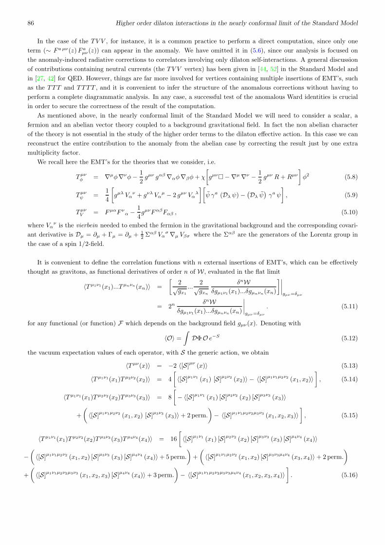
86 Higher order dilaton interactions in the nearly conformal limit of the Standard Model
In the case of the TV V , for instance, it is a common practice to perform a direct computation, since only one
term (∼ F aµν(z)F aµν(z)) can appear in the anomaly. We have omitted it in (5.6), since our analysis is focused on
the anomaly-induced radiative corrections to correlators involving only dilaton self-interactions. A general discussion
of contributions containing neutral currents (the TV V vertex) has been given in [44, 52] in the Standard Model and
in [27, 42] for QED. However, things are far more involved for vertices containing multiple insertions of EMT’s, such
as the TTT and TTTT , and it is convenient to infer the structure of the anomalous corrections without having to
perform a complete diagrammatic analysis. In any case, a successful test of the anomalous Ward identities is crucial
in order to secure the correctness of the result of the computation.
As mentioned above, in the nearly conformal limit of the Standard Model we will need to consider a scalar, a
fermion and an abelian vector theory coupled to a background gravitational field. In fact the non abelian character
of the theory is not essential in the study of the higher order terms to the dilaton effective action. In this case we can
reconstruct the entire contribution to the anomaly from the abelian case by correcting the result just by one extra
multiplicity factor.
We recall here the EMT’s for the theories that we consider, i.e.
T µνφ = ∇µφ∇νφ− 1
2gµν gαβ∇αφ∇βφ+ χ
[
gµν−∇µ∇ν − 1
2gµν R+Rµν
]
φ2 (5.8)
T µνψ =1
4
[
gµλ Vαν + gνλ Vα
µ − 2 gµν Vαλ
][
ψ γa (Dλ ψ)−(
Dλ ψ)
γa ψ
]
, (5.9)
T µνV = FµαF να − 1
4gµνFαβFαβ , (5.10)
where Vαν is the vierbein needed to embed the fermion in the gravitational background and the corresponding covari-
ant derivative is Dµ = ∂µ + Γµ = ∂µ + 12 Σ
αβ Vασ∇µ Vβσ where the Σαβ are the generators of the Lorentz group in
the case of a spin 1/2-field.
It is convenient to define the correlation functions with n external insertions of EMT’s, which can be effectively
thought as gravitons, as functional derivatives of order n of W , evaluated in the flat limit
〈T µ1ν1(x1)...Tµnνn(xn)〉 =
[
2√gx1
...2√gxn
δnWδgµ1ν1(x1)...δgµnνn(xn)
]∣
∣
∣
∣
gµν=δµν
= 2nδnW
δgµ1ν1(x1)...δgµnνn(xn)
∣
∣
∣
∣
gµν=δµν
. (5.11)
for any functional (or function) F which depends on the background field gµν(x). Denoting with
〈O〉 =∫
DΦO e−S (5.12)
the vacuum expectation values of each operator, with S the generic action, we obtain
〈T µν(x)〉 = −2 〈[S]µν (x)〉 (5.13)
〈T µ1ν1(x1)Tµ2ν2(x2)〉 = 4
[
〈[S]µ1ν1 (x1) [S]µ2ν2 (x2)〉 − 〈[S]µ1ν1µ2ν2 (x1, x2)〉]
, (5.14)
〈T µ1ν1(x1)Tµ2ν2(x2)T
µ3ν3(x3)〉 = 8
[
− 〈[S]µ1ν1 (x1) [S]µ2ν2 (x2) [S]µ3ν3 (x3)〉
+
(
〈[S]µ1ν1µ2ν2 (x1, x2) [S]µ3ν3 (x3)〉+ 2perm.
)
− 〈[S]µ1ν1µ2ν2µ3ν3 (x1, x2, x3)〉]
, (5.15)
〈T µ1ν1(x1)Tµ2ν2(x2)T
µ3ν3(x3)Tµ4ν4(x4)〉 = 16
[
〈[S]µ1ν1 (x1) [S]µ2ν2 (x2) [S]µ3ν3 (x3) [S]µ4ν4 (x4)〉
−(
〈[S]µ1ν1µ2ν2 (x1, x2) [S]µ3ν3 (x3) [S]µ4ν4 (x4)〉+ 5perm.
)
+
(
〈[S]µ1ν1µ2ν2 (x1, x2) [S]µ3ν3µ4ν4 (x3, x4)〉+ 2perm.
)
+
(
〈[S]µ1ν1µ2ν2µ3ν3 (x1, x2, x3) [S]µ4ν4 (x4)〉+ 3perm.
)
− 〈[S]µ1ν1µ2ν2µ3ν3µ4ν4 (x1, x2, x3, x4)〉]
. (5.16)
5.4 Ward identities 87
Notice that in dimensional regularization
〈[S]µν (x)〉 = 〈[S]µ1ν1µ2ν2 (x1, x2)〉 = 〈[S]µ1ν1µ2ν2µ3ν3 (x1, x2, x3)〉 = 〈[S]µ1ν1µ2ν2µ3ν3µ4ν4 (x1, x2, x3, x4)〉 = 0 (5.17)
being proportional to massless tadpoles. In particular, this implies that, to perform a perturbative computation of
a correlator of order n, one would be needing interaction vertices with at most n − 1 gravitons. Concerning the
diagrammatic structure of each contribution, the correlator
〈[S]µ1ν1 (x1) [S]µ2ν2 (x2) [S]µ3ν3 (x3) [S]µ4ν4 (x4)〉 (5.18)
has a box topology;
〈[S]µ1ν1 (x1) [S]µ2ν2 (x2) [S]µ3ν3 (x3)〉 (5.19)
which is the first contribution to the graviton 3-point function, and
〈[S]µ1ν1µ2ν2 (x1, x2) [S]µ3ν3 (x3) [S]µ4ν4 (x4)〉 , (5.20)
which corresponds to a contact term in 〈TTTT 〉, are represented by triangles.
The remaining contributions,
〈[S]µ1ν1 (x1) [S]µ2ν2 (x2)〉 , (5.21)
the contact terms 〈TTT 〉, which are
〈[S]µ1ν1µ2ν2 (x1, x2) [S]µ3ν3 (x3)〉 (5.22)
and the two remaining types of diagrams which enter into 〈TTTT 〉,
〈[S]µ1ν1µ2ν2 (x1, x2) [S]µ3ν3µ4ν4 (x3, x4)〉 (5.23)
and
〈[S]µ1ν1µ2ν2µ3ν3 (x1, x2, x3) [S]µ4ν4 (x4)〉 , (5.24)
have the topologies of 2-point functions. Our conventions for the choice of the external momenta, which are taken to
be all incoming, are defined via the Fourier transform
∫
d4x1 d4x2 d
4x3 d4x4 〈T µ1ν1(x1)T
µ2ν2(x2)Tµ3ν3(x3)T
µ4ν4(x4)〉 e−i(k1·x1+k2·x2+k3·x3+k4·x4) =
(2π)4 δ(4)(k1 + k2 + k3 + k4) 〈T µ1ν1T µ2ν2T µ3ν3T µ4ν4〉 (k2, k3, k4) , (5.25)
and similar for the 3- and 2-point functions.
5.4 Ward identities
We start from the analysis of the general covariance Ward identities, which partially overlaps with the discussion in
chapter 2, which is limited to the TTT vertex.
The identities we look for are obtained from the functional relation
∇ν1 〈T µ1ν1(x1)〉 = ∇ν1
(
2√gx1
δWδgµ1ν1(x1)
)
= 0 (5.26)
which, after an expansion, becomes
2√gx1
(
∂ν1δW
δgµ1ν1(x1)− Γλλν1(x1)
δWδgµ1ν1(x1)
+ Γµ1κν1(x1)
δWδgκν1(x1)
+ Γν1κν1(x1)δW
δgµ1κ(x1)
)
= 0.
(5.27)
88 Higher order dilaton interactions in the nearly conformal limit of the Standard Model
Cancelling the second and fourth terms in parentheses, (5.27) takes the simpler form
2
(
∂ν1δW
δgµ1ν1(x1)+ Γµ1
κν1(x1)δW
δgκν1(x1)
)
= 0 . (5.28)
The Ward identities we are interested in are obtained by functional differentiation of (5.28) and give
4
[
∂ν1δ2W
δgµ2ν2(x2)δgµ1ν1(x1)+δΓµ1
κν1(x1)
δgµ2ν2(x2)
δWδgκν1(x1)
+ Γµ1κν1(x1)
δ2Wδgµ2ν2(x2)δgκν1(x1)
]
= 0 , (5.29)
for single
8
[
∂ν1δ3W
δgµ3ν3(x3)δgµ2ν2(x2)δgµ1ν1(x1)+δΓµ1
κν1(x1)
δgµ2ν2(x2)
δ2Wδgµ3ν3(x3)δgκν1(x1)
+δΓµ1
κν1(x1)
δgµ3ν3(x3)
δ2Wδgµ2ν2(x2)δgκν1(x3)
+δ2Γµ1
κν1(x1)
δgµ2ν2(x2)δgµ3ν3(x3)
δWδgκν1(x1)
+ Γµ1κν1(x1)
δ3Wδgµ2ν2(x2)δgµ3ν3(x2)δgκν1(x1)
]
= 0 , (5.30)
double, and
16
[
∂ν1δ4W
δgµ4ν4(x4)δgµ3ν3(x3)δgµ2ν2(x2)δgµ1ν1(x1)+
(
δΓµ1κν1(x1)
δgµ2ν2(x2)
δ3Wδgµ4ν4(x4)δgµ3ν3(x3)δgκν1(x1)
+(
2 ↔ 4, 2 ↔ 3)
)
+
(
δ2Γµ1κν1(x1)
δgµ3ν3(x3)δgµ2ν2(x2)
δ2Wδgµ4ν4(x4)δgκν1(x1)
+(
2 ↔ 4, 3 ↔ 4)
)
+δ3Γµ1
κν1(x1)
δgµ4ν4(x4)δgµ3ν3(x3)δgµ2ν2(x2)
δWδgκν1(x1)
+ Γµ1κν1(x1)
δ4Wδgµ4ν4(x4)δgµ3ν3(x3)δgµ2ν2(x2)δgκν1(x1)
= 0 (5.31)
triple differentiations of the master equation (5.26). In the Ward identity satisfied by the 4-point function we have
left implicit the contributions obtained by permuting the action of the functional derivatives.
To move to the flat spacetime limit of (5.29) and (5.30), we use the notations in (2.15) and set to zero the
contributions from the massless tadpoles, obtaining
∂ν1 〈T µ1ν1(x1)Tµ2ν2(x2)〉 = 0 , (5.32)
∂ν1 〈T µ1ν1(x1)Tµ2ν2(x2)T
µ3ν3(x3)〉 = −2[
Γµ1κν1(x1)
]µ2ν2(x2) 〈T κν1(x1)T µ3ν3(x3)〉
−2[
Γµ1κν1(x1)
]µ3ν3(x3) 〈T κν1(x1)T µ3ν3(x3)〉 , (5.33)
∂ν1 〈T κν1(x1)T µ2ν2(x2)Tµ3ν3(x3)T
µ4ν4(x4)〉 = −2
(
[
Γµ1κν1(x1)
]µ2ν2(x2) 〈T κν1(x1)T µ3ν3(x3)T
µ4ν4(x4)〉
+(
2 ↔ 3, 2 ↔ 4)
)
− 4
(
[
Γµ1κν1(x1)
]µ2ν2µ3ν3(x2, x3) 〈T κν1(x1)T µ4ν4(x4)〉+
(
2 ↔ 4, 3 ↔ 4)
)
,
(5.34)
which after some manipulations give the transversality constraint for the 2-point functions and
k1 ν1 〈T µ1ν1T µ3ν3T µ2ν2〉 (k2, k3) = −kµ1
3 〈T µ3ν3T µ2ν2〉 (k2)− kµ1
2 〈T µ2ν2T µ3ν3〉 (k3)
+ k3 ν1
[
δµ1ν3 〈T ν1µ3T µ2ν2〉 (k2) + δµ1µ3 〈T ν1ν3T µ2ν2〉 (k2)]
+ k2 ν1
[
δµ1ν2 〈T ν1µ2T µ3ν3〉 (k3) + δµ1µ2 〈T ν1ν2T µ3ν3〉 (k3)]
.
(5.35)
5.5 Counterterms 89
Similarly, in the case of the 4-point function TTTT , using (5.25) we obtain
k1 ν1 〈T µ1ν1T µ3ν3T µ2ν2T µ4ν4〉 (k2, k3, k4) =[
− kµ1
2 〈T µ2ν2T µ3ν3T µ4ν4〉 (k3, k4)
+ k2 ν1
(
δµ1ν2 〈T ν1µ2T µ3ν3T µ4ν4〉 (k3, k4) + δµ1µ2 〈T ν1ν2T µ3ν3T µ4ν4〉 (k3, k4))
+(
2 ↔ 3, 2 ↔ 4)
]
+
[
2 k2 ν1
(
[gµ1µ2 ]µ3ν3 〈T ν1ν2T µ4ν4〉 (k4) + [gµ1ν2 ]µ3ν3 〈T ν1µ2T µ4ν4〉 (k4))
+ 2 k3 ν1
(
[gµ1µ3 ]µ2ν2 〈T ν1ν3T µ4ν4〉 (k4) + [gµ1ν3 ]
µ2ν2 〈T ν1µ3T µ4ν4〉 (k4))
+
(
kν32 δµ1µ3 + kµ3
2 δµ1ν3
)
〈T µ2ν2T µ3ν3〉 (k4) +(
kν23 δµ1µ2 + kµ2
3 δµ1ν2
)
〈T µ3ν3T µ2ν2〉 (k4) +(
2 ↔ 4, 3 ↔ 4)
]
.
(5.36)
Similar identities are obtained for the momenta of the other external gravitons.
5.5 Counterterms
Coming to a discussion of the counterterms to the 4-dilaton amplitude, these are obtained from the 1-loop Lagrangian
which accounts for the gravitational counterterms to pure graviton amplitudes in the MS scheme,
Scounter = −µ−ǫ
ǫ
∑
I=s,f,V
nI
∫
ddx√g
(
βa(I)F + βb(I)G
)
. (5.37)
Again, the dimensional parameter is ǫ = 4− d.
In the case of the 4-graviton vertex the counterterm action (5.37) generates the vertex
−µ−ǫ
ǫ
(
βaDµ1ν1µ2ν2µ3ν3µ4ν4F (x1, x2, x3, x4) + βbD
µ1ν1µ2ν2µ3ν3µ4ν4G (x1, x2, x3, x4)
)
, (5.38)
where
Dµ1ν1µ2ν2µ3ν3µ4ν4F (x1, x2, x3, x4) = 24
δ4
δgµ1ν1(x1)δgµ2ν2(x2)δgµ3ν3(x3)δgµ4ν4(x4)
∫
ddw√g F , (5.39)
Dµ1ν1µ2ν2µ3ν3µ4ν4G (x1, x2,3 , x4) = 24
δ4
δgµ1ν1(x1)δgµ2ν2(x2)δgµ3ν3(x3)δgµ4ν4(x4)
∫
ddw√g G , (5.40)
and similarly for the 2- and 3-point correlators.
Using these expressions, the fully renormalized 2-, 3- and 4-point correlators in momentum space can be written
down as
〈T µ1ν1T µ2ν2〉ren (k2) = 〈T µ1ν1T µ2ν2〉bare (k2)−µ−ǫ
ǫβaD
µ1ν1µ2ν2F (k2) ,
〈T µ1ν1T µ2ν2T µ3ν3〉ren (k2, k3) = 〈T µ1ν1T µ2ν2T µ3ν3〉bare (k2, k3)
− µ−ǫ
ǫ
(
βaDµ1ν1µ2ν2µ3ν3F (k2, k3) + βbD
µ1ν1µ2ν2µ3ν3G (k2, k3)
)
,
〈T µ1ν1T µ2ν2T µ3ν3T µ4ν4〉ren (k2, k3, k4) = 〈T µ1ν1T µ2ν2T µ3ν3T µ4ν4〉bare (k2, k3, k4)
− µ−ǫ
ǫ
(
βaDµ1ν1µ2ν2µ3ν3µ4ν4F (k2, k3, k4) + βbD
µ1ν1µ2ν2µ3ν3µ4ν4G (k2, k3, k4)
)
.
(5.41)
From these relations and from (5.35), (5.36) it is clear that counterterms must be related by the same general covari-
ance Ward identities which relate the bare correlators. One can also separately check these identites for F- and G-
counterterms just by writing them down and equating the coefficients of βa and βb. We omit the explicit forms of the

90 Higher order dilaton interactions in the nearly conformal limit of the Standard Model
counterterms, which are necessary in order to test all these constraints. We have checked all of them with a symbolic
calculus program.
A second, powerful constraint on the counterterms comes from the anomalous Ward identities for the Green
functions at hand, which are obtained through functional derivation of (5.7), passing to the flat space limit and using
the definition (5.11). A direct computation gives the equations
δµ1ν1 〈T µ1ν1T µ2ν2〉 (k2) = 2 [√gA]µ2ν2 (k2) = 2 [R]µ2ν2 (k2) , (5.42)
δµ1ν1 〈T µ1ν1T µ2ν2T µ3ν3〉 (k2, k3) = 4 [√gA]
µ2ν2µ3ν3 (k2, k3)− 2 〈T µ2ν2T µ3ν3〉 (k2)− 2 〈T µ2ν2T µ3ν3〉 (k3)
= 4
[
βa
(
[F ]µ3ν3µ2ν2 (k2, k3)−2
3[√gR]µ3ν3µ2ν2 (k2, k3)
)
+ βb [G]µ3ν3µ2ν2 (k2, k3)
]
− 2 〈T µ2ν2T µ3ν3〉 (k2)− 2 〈T µ2ν2T µ3ν3〉 (k3) , (5.43)
δµ1ν1 〈T µ1ν1T µ2ν2T µ3ν3T µ4ν4〉 (k2, k3, k4) = 8 [√gA]
µ2ν2µ3ν3µ4ν4 (k2, k3, k4)
− 2 〈T µ2ν2T µ3ν3T µ4ν4〉 (k2, k3)− 2 〈T µ2ν2T µ3ν3T µ4ν4〉 (k2, k4)− 2 〈T µ2ν2T µ3ν3T µ4ν4〉 (k3, k4)
= 8
[
βa
(
[√g F ]
µ2ν2µ3ν3µ4ν4 (k2, k3, k4)−2
3[√gR]
µ2ν2µ3ν3µ4ν4 (k2, k3, k4)
)
+ βb [√g G]
µ2ν2µ3ν3µ4ν4 (k2, k3, k4)
]
−2 〈T µ2ν2T µ3ν3T µ4ν4〉 (k2, k3)− 2 〈T µ2ν2T µ3ν3T µ4ν4〉 (k2, k4)− 2 〈T µ2ν2T µ3ν3T µ4ν4〉 (k3, k4) . (5.44)
The explicit expressions of the multiple functional derivatives of the various operators in square bracket ([ ]) are very
lengthy and we omit them.
At this stage, we can extract from (5.44) four trace identities (one for each graviton) for the counterterms of the
4-point functions (5.39) and (5.40), relating them to the corresponding 2- and 3-point ones. As these counterterms
have been independently tested through general covariance Ward identities, this provides a useful test of the anomaly
contributions to the 4-point function as well, which is used to deduce the form of the quartic dilaton interactions. The
identity, involving traces in d dimensions, is a direct consequence of eq. (3.106), which was extensively discussed, and
its form is
δdµ1ν1 Dµ1ν1µ2ν2µ3ν3µ4ν4F (k2, k3, k4) = − ǫ
2
(
[√g F ]
µ2ν2µ3ν3µ4ν4 (k2, k3, k4)−2
3[√gR]
µ2ν2µ3ν3µ4ν4 (k2, k3, k4)
)
− 2Dµ2ν2µ3ν3µ4ν4F (k3, k4)− 2Dµ2ν2µ3ν3µ4ν4
F (k2, k4)− 2Dµ2ν2µ3ν3µ4ν4F (k2, k3) ,
δdµ1ν1 Dµ1ν1µ2ν2µ3ν3µ4ν4G (k2, k3, k4) = − ǫ
2[√g G]
µ2ν2µ3ν3µ4ν4 (k2, k3, k4)
− 2Dµ2ν2µ3ν3µ4ν4G (k3, k4)− 2Dµ2ν2µ3ν3µ4ν4
G (k2, k4)− 2Dµ2ν2µ3ν3µ4ν4G (k2, k3) .
(5.45)
The superscript d in (5.45) indicates that the trace has to be taken in d = 4− ǫ dimensions and the 3-point function
counterterms were computed and tested in [48], as discussed in chapter 2. The correctness of the counterterms
computed for the 4-point function was already put to a test by the general covariance Ward identities. Now we can
understand why it was worth computing them. In fact, the identities (5.45) relate these counterterms to the functional
derivatives of the trace anomaly, whose computation is not less difficult. Nevertheless, with well checked expressions
for the counterterms, we can use eq. (5.45) to test our functional derivatives of the trace anomaly. The test is highly
non trivial, given the complexity of the expressions involved. We succesfully performed it.
From the discussion in section 3.4.2, it follows that the traced 3- and 4- point correlators of the EMT exactly
coincide with the traces of their counterterms in dimensional regularization. These correlators are expected to be the
constituents of the dilaton perturbative effective action, which we indicate as Γ[ρ] and can be tentatively written as
the functional series expansion
Γ[ρ] = · · ·+∫
d4x1d4x2d
4x3 〈T µ1µ1(x1)T
µ2µ2(x2)T
µ3µ3(x3)〉 ρ(x1)ρ(x2)ρ(x3)
+
∫
d4x1d4x2d
4x3d4x4 〈T µ1
µ1(x1)Tµ2µ2(x2)T
µ3µ3(x3)T
µ4µ4(x4)〉 ρ(x1)ρ(x2)ρ(x3)ρ(x4) + . . . (5.46)
5.6 Three and four dilaton interactions from the trace anomaly 91
We will see in the next chapter that the solution of the anomalous constraints generates an expression which is more
involved than (5.46). Nevertheless, the traced correlators of the EMT are the basic constituents of both actions and,
in the on-shell limit, they exactly coincide.
5.6 Three and four dilaton interactions from the trace anomaly
From (5.42)-(5.44) and from the knowledge of the trace anomalies therein, that we have explicitly computed, one can
get the form of the off-shell 3- and 4-dilaton (ρ) interactions, which are found to be
Vφρρρ = − 1
Λ3
3(
k42 + k43)
+ 6 k2 · k3(
k22 + k23)
+ 4 (k2 · k3)2 + 5 k22 k23
360 π2,
Vψρρρ = − 1
Λ3
18(
k42 + k43)
+ 36 k2 · k3(
k22 + k23)
+ 29 (k2 · k3)2 + 25 k22 k23
360 π2,
VVρρρ = − 1
Λ3
18(
k42 + k43)
+ 36 k2 · k3(
k22 + k23)
+ 49 (k2 · k3)2 + 5 k22 k23
180 π2, (5.47)
together with the new quartic dilaton interactions
Vφρρρρ = − 1
Λ4
1
60 π2
[
3(
(k22)2 + (k23)
2 + (k24)2)
+ 6(
k24 k4 · (k2 + k3) + k23 k3 · (k2 + k4) + k22 k2 · (k3 + k4))
+4(
(k2 · k4)2 + (k2 · k3)2 + (k3 · k4)2)
+ 6 (k2 · k3 k2 · k4 + k3 · k2 k3 · k4 + k4 · k2 k4 · k3)
+ 5(
k22 k23 + k23 k
24 + k22 k
24
)
+ 5(
k22 k3 · k4 + k23 k2 · k4 + k24 k2 · k3)
]
,
Vψρρρρ = − 1
Λ4
1
120 π2
[
36(
(k22)2 + (k23)
2 + (k24)2)
+ 72(
k24 k4 · (k2 + k3) + k23 k3 · (k2 + k4) + k22 k2 · (k3 + k4))
+58(
(k2 · k4)2 + (k2 · k3)2 + (k3 · k4)2)
+ 82 (k2 · k3 k2 · k4 + k3 · k2 k3 · k4 + k4 · k2 k4 · k3)
+ 50(
k22 k23 + k23 k
24 + k22 k
24
)
+ 55(
k22 k3 · k4 + k23 k2 · k4 + k24 k2 · k3)
]
,
VVρρρρ = − 1
Λ4
1
60 π2
[
36(
(k22)2 + (k23)
2 + (k24)2)
+ 72(
k24 k4 · (k2 + k3) + k23 k3 · (k2 + k4) + k22 k2 · (k3 + k4))
+98(
(k2 · k4)2 + (k2 · k3)2 + (k3 · k4)2)
+ 122 (k2 · k3 k2 · k4 + k3 · k2 k3 · k4 + k4 · k2 k4 · k3)
+ 10(
k22 k23 + k23 k
24 + k22 k
24
)
+ 35(
k22 k3 · k4 + k23 k2 · k4 + k24 k2 · k3)
]
. (5.48)
Both the cubic and the quartic terms can be easily modified to account for all the contributions generated in the
nearly conformal limit of the Standard Model, in the form
Vρρρ/ρρρρ =∑
i=s,f,V
Ni Viρρρ/ρρρρ (5.49)
where NV = 8 + 3 + 1 = 12 is the number of gauge fields, Nf = 3 × 6 + 3 + 3/2 = 45/2 is the number of Dirac
fermions, where the factor 1/2 is due to the fermion chirality, and Ns = 4 counts the real scalars of the Higgs doublet.
These corrections, as we have already remarked, are typical of the dilaton interactions and can be derived without any
explicit diagrammatic computation. They provide the starting ground for an analysis of the dilaton effective action,
and characterize the terms which allows to differentiate between the Higgs and the dilaton at the radiative level.
5.7 Conclusions
The analysis of dilaton interactions and of their role in the context of the electroweak symmetry breaking is particularly
interesting at phenomenological level.
92 Higher order dilaton interactions in the nearly conformal limit of the Standard Model
In fact, the Standard Model, in the limit in which we drop the Higgs vev, is conformally invariant at high energy,
with a breaking of scale invariance, in this limit, which is related only to the trace anomaly. The anomalous coupling
of the dilaton is responsible for setting a remarkable difference between this state and the Higgs, a property which
remains valid - with no distinction - even if the dilaton is assumed to be a fundamental or a composite scalar or
a graviscalar. We have shown that the anomalous corrections at any order to the dilaton effective action, in the
conformal limit, can be extracted from a general (and model independent) analysis of the Ward identities, with no
further input. We have illustrated the approach up to the quartic order.

Chapter 6
Conformal Trace Relations from the
Dilaton Wess-Zumino Action
6.1 Introduction
Anomaly-induced actions play a considerable role among effective field theories. Simple instances of these types of
actions are theories with chiral fermions in the presence of anomalous abelian symmetries [31, 89, 90, 91], other
examples involve conformal [24, 66, 92, 93] and superconformal anomalies [94].
Direct computations of these actions can be performed in ordinary perturbation theory by the usual Feynman
expansion at 1 loop, but alternative approaches are also possible. In fact, an action which reproduces the same
anomaly at low energy can be constructed quite directly, just as a variational solution of the anomaly condition,
without any reference to the diagrammatic expansion. In gravity, typical examples are anomaly actions such as the
Riegert action [41], or the Wess-Zumino (WZ from now on) dilaton action [95], which reproduce the anomaly either
with a non-local (Riegert) or with a local (WZ) effective operator, using a dilaton field in the latter case [96]. These
types of actions are not unique, since possible contributions which are conformally invariant are not identified by the
variational procedure. It should also be mentioned that a prolonged interest in these actions has been and is linked
to the study of the irreversibility of the Renormalization Group (RG) flow in various dimensions [97, 98, 99, 100, 101]
and of the trace anomaly matching [50], since Zamolodchikov’s proof of his c-theorem for d = 2 [102].
A salient feature of some of these anomaly actions, if formulated in a local form, as in the WZ case, is the inclusion
of extra degrees of freedom compared to the original tree-level action. In the case of the chiral anomaly this additional
degree of freedom is the axion (θ(x)), which is linearly coupled to the anomaly functional in the form of a (θ/M)FF
term - the anomaly coupling - with F and F denoting the field strength of the gauge field and its dual respectively.
The anomaly interaction is accompanied by a new scale (M). This is the scale at which the anomalous symmetry
starts to play a role in the effective theory. A large value of M , for instance, is then associated with a decoupling of
the anomaly in the low energy theory. In the 1-particle irreducible (1PI) effective action this is obtained - in the chiral
case - by allowing the mass of the fermions (∼M) that run in the anomaly loops to grow large. The underlying idea
of keeping the anomaly interaction in the form of a local operator at low energy - such as the (θ/M)FF term - while
removing part of the physical spectrum, is important in the study of the renormalization group (RG) flows of large
classes of theories, both for chiral and for conformal anomalies.
For conformal anomalies [24], which is the case of interest in this chapter, the pattern is similar to the chiral case,
with the introduction of a dilaton field in place of the axion in order to identify the structure of the corresponding
WZ action, and the inclusion of a conformal scale (Λ). As in the chiral case, one of the significant features of the
WZ conformal anomaly action is the presence of a linear coupling of the Goldstone mode of the broken symmetry
(the dilaton) to the anomaly functional, but with a significant variant. In this case, in fact, this linear term has to be
corrected by additional contributions, due to the non invariance of the anomaly functional under a Weyl transformation.
93

94 Conformal Trace Relations from the Dilaton Wess-Zumino Action
This procedure, which allows to identify the structure of WZ action, goes under the name of the Noether method
(see for instance [54, 103]) and has to be iterated several times, due to the structure of the anomaly functional, before
reaching an end. Given the fact that anomaly functional takes a different form in each spacetime dimension, the
anomaly action will involve interactions of the dilaton field of different orders in each dimension.
In [54] we have investigated an alternative approach, useful for the computation of this action, which exploits the
structure of the counterterms in dimensional regularization and their Weyl-gauging, bypassing altogether the Noether
procedure. This approach has been discussed in d = 4 by several authors [95, 104], and in a cohomological context in
[38]. This construction in dimensions higher than 2 or 4 is interesting for several reasons. The WZ action was been
used in [103] in the attempt to generalize the proof of the weak a-theorem provided in [100], although some additional
work is required, due to the complexity of dispersive analysis of scattering amplitudes of more than 4 particles. At
the same time it plays an equally important role in the study of the AdS/CFT correspondence. An example is the
investigation of the anomaly matching between conformal tensor multiplets on the six dimensional boundary and a
stack of M5 branes of AdS7 supergravity in the bulk [105, 106]. We will present, as an application of our formalism,
the expression of the WZ action for this specific CFT realization in d = 6.
In the two previous chapters, we have focused our attention on interactions concerning a dilaton field, featuring
a coupling to the trace anomaly, which we have interpreted as an effective, low-energy signature of a possible hidden
conformal sector that could be investigated in future data analysis at hadron colliders, maybe at the LHC.
In this final chapter, we turn to a different kind of analysis, switching from the phenomenological aspects to a more
formal application of dilaton interactions. We look at our dilaton as at a WZ Goldstone boson for CFT’s, which means
that its self-interactions stem only from the trace anomaly. These self-interactions are related, in turn, to definite
combinations of traced EMT correlation functions, which coincide with those analysed in chapter 5 in the on-shell
limit.
We will start our investigation by introducing our conventions for the anomalous equations and the structure of
correlation functions of traces of the EMT for a generic CFT. Then we give a brief account of the method of Weyl-
gauging, which was already extensively discussed, for scale invariant theories, in chapter 1. This gives us the chance
to introduce the quadratic kinetic term for the dilaton field. We also comment on the Weyl-gauging for theories
containing dimensionful constants, as the dilaton might actually be a massive state. This way, we can account for a
mass term preserving Weyl symmetry.
In the past, the gauging has been discussed in various ways both in the context of extensions of the Standard Model
[85, 86] and in cosmology, where it has been shown that the introduction of an extra scalar brings to a dynamical
adjustment of the cosmological constant [104]. Recent discussions of the role of the dilaton in quantum gravity can
be found in [107, 108]. This review gives us the chance to classify the possible kinetic terms for the dilaton, on the
ground of conformal symmetry requirements and limiting ourselves to terms that are at most marginal in a wilsonian
sense.
Then we turn to the original part of this chapter and apply the method of Weyl-gauging to the counterterms of
a CFT in order to determine the WZ conformal anomaly action and show that in any even (d = 2k) dimensions all
the hierarchy of correlation functions involving traces of the EMT of a CFT is determined in terms of those of lower
orders, up to 2k, which are, in turn, completely fixed by the conformal anomaly. For every even dimension d, it is
the highest order of dilaton anomalous self-interactions which corresponds to the maximum order of the independent
traced correlators that are necessary to fix the entire hierarchy. This order, in turn, equals the space dimension, as
discussed in [54, 55]. It turns out that all the correlators which are order 2k+1 or higher are recursively generated by
the first 2k, through a simple algorithm that is discussed in detail. The method also allows to compute the first 2k
traced correlation functions of the EMT just by knowing the structure of the WZ action, thus providing an alternative
way to the counterterm approach used in chapter 5.
We work out explicitly the cases d = 4 and d = 6, while the case in 2 dimensions is left to appendix A.11. Both in
the 4- and in the 6-dimensional case, we derive the dilaton effective action by taking into account the counterterms

6.2 Conventions 95
required within a minimal subtraction scheme, in a sense that will be made clearer below.
We mention that general results on the structure of the WZ action in any even dimensions have been presented in
[109], using the general form of the Euler density, which is sufficient to identify the nonlocal structure of the anomaly
in a specific scheme. However, the identification of the contributions related to the so called local anomalies requires
a separate effort, that we undertake here. This more general approach allows us to set a distinction between the
nonlocal and local contributions to the anomalous effective action.
As an application in 6 dimensions, we present the WZ action for the (2,0) tensor multiplet, which has been in-
vestigated in the past in the context of the AdS7/CFT6 holographic anomaly matching. Of the first 6 independent
correlators, we give the explicit expressions in the most general scheme of the first 4. We have computed the order 5
and 6 Green functions, but they are lengthy and add nothing essential to our discussion.
The gauging procedure, especially in 6 dimensions, in a general scheme, is quite demanding from the technical side.
We set a distinction between the operators in the anomaly that are responsible for the universal (scheme-independent)
contributions, i.e. the Euler density and the Weyl invariants, and the operators which are responsible for the scheme-
dependence, such as the R term in 4 dimensions, establishing clearly the relation between their contribution to the
WZ effective action and the counterterms in the minimal scheme. This clarifies the difference with the prescription
of [109]. We then move to the analysis of the structure of the traced correlators and of their hierarchy, showing how
to solve it in terms of the first d correlation functions. We have left to appendix A.3 a discussion of some of the
more technical steps. appendix A.11 includes the consistency checks of the recursion relations satisfied by the traced
correlators in 2 dimensions, presenting the expressions of the first traced Green functions up to rank 6 in this case.
6.2 Conventions
For practical reasons, we recollect here all the basic definitions necessary for the purpose of this chapter. In a generic
euclidean field theory, defining the generating functional of the theory W as
W [g] =
∫
DΦ e−S , (6.1)
where S is the generic euclidean action depending on the set of all the quantum fields (Φ) and on the background
metric (g), the vev of the EMT is given by
〈T µν(x)〉s =2√gx
δW [g]
δgµν(x)=
2√gx
δ
δgµν(x)
∫
DΦ e−S , (6.2)
and contains the response to the metric fluctuations keeping the background sources turned on, as the superscript s
indicates; for the purpose of this chapter, the only background field is the metric tensor gµν , whereas gx ≡ |gµν(x)| isits determinant.
For CFT’s in a even dimensional space which are coupled to a background metric and neither scalar fields nor
vector currents, the trace anomaly condition takes the general symbolic form
gµν〈T µν〉s = A[g] , (6.3)
An anomalous relation of the form (6.3) holds in any even dimension, where A[g] is a scalar functional depending only
on the metric tensor, which can be written, in complete generality, as [24, 25, 66]
A[g] =∑
i
ci (Ii +∇µJµi )− (−1)d/2 aEd , (6.4)
where√g Ii are the conformal invariants available in d dimensions, whose number rapidly increases with d, whereas
Ed is the Euler density in d dimensions. They are both defined in appendix A.3.
The contribution coming from the Euler density is usually denoted as the A part of the anomaly, while the rest is

96 Conformal Trace Relations from the Dilaton Wess-Zumino Action
called the B part. For every even value of the space dimension, say 2k, the Ii’s are 2k-dimensional combinations of the
Weyl tensor for 2k dimensions and covariant derivatives thereof. The total derivative terms ∇µJµi are known under
the name of local anomaly contributions and are sometimes omitted, as they are scheme-dependent. This scheme
dependence has already been discussed in section 2.5 for the case d = 4 and will be further explored in the following
in d = 4 and d = 6. The total derivatives can be removed by adding proper local counterterms to the action, as we
thoroughly show in sections 6.4 and 6.5.
Let us provide the explicit expressions of the trace anomaly in 4 and 6 dimensions. In the first case, in order to
stick to the notations of the previous chapters, we set −a = βb and c = βa and have the anomaly functional
A[g] = βa
(
F − 2
3R
)
+ βbG , (6.5)
where F is the squared 4-dimensional Weyl tensor and G is the Euler density, both defined appendix A.3 and we are
omitting the distinction between the various kinds of contributions that can go into the β coefficients.
The specific expression of (6.4) for d = 6 is instead
A[g] =3∑
i=1
ci (Ii +∇µJµi ) + aE6 , (6.6)
where√g Ii , (i = 1, 2, 3), are the three Weyl invariants available in 6 dimensions.
Our goal will be to determine the structure of the dilaton WZ action in the most general case for both d = 4
and d = 6, with the inclusion of the contributions related to the total derivative terms and to completely clarify the
relation of the latter to the various possible choices of the counterterms.
As already emphasized, multiple stress-energy tensor correlators can be defined in various ways, differing by contact
terms. These depend on the positions of the g−12 factors entering in the definition of the EMT respect to the functional
derivatives. We choose to define the Green function of n EMT’s in flat space in the completely symmetric fashion as
〈T µ1ν1(x1) . . . Tµnνn(xn)〉 ≡
2n√gx1 . . .
√gxn
δnW [g]
δgµ1ν1(x1) . . . . . . δgµnνn(xn)
∣
∣
∣
∣
gµν=δµν
. (6.7)
It is also useful to recall some notation to denote the functional derivatives with respect to the metric of generic
functionals in the limit of a flat background
[f(x)]µ1ν1...µnνn (x1, . . . , xn) ≡
δn f(x)
δgµnνn(xn) . . . δgµ1ν1(x1)
∣
∣
∣
∣
gµν=δµν
(6.8)
and the corresponding expression with traced indices
[f(x)]µ1...µn
µ1...νn(x1, x2, . . . , xn) ≡ δµ1ν1 . . . δµnνn [f(x)]
µ1ν1...µnνn (x1, . . . , xn) , (6.9)
where the curved euclidean metric gµν is replaced by δµν .
It is clear that, in any CFT in even dimensions, the only object which plays a role in the determination of the
traces of these correlators is the anomaly functional, as one can realize by a direct computation. Specifically, from (6.3)
one can derive trace identities for the n-point correlation functions. In fact, in momentum space the entire hierarchy,
which is generated by functional differentiation of (6.3), takes the form
〈T (k1) . . . T (kn+1)〉 = 2n [√gA]
µ1...µn
µ1...νn(k1, . . . , kn+1)
− 2
n∑
i=1
〈T (k1) . . . T (ki−1)T (ki+1) . . . T (kn+1 + ki)〉 . (6.10)
In the expression above we have introduced the notation T ≡ T µµ to denote the trace of the EMT. All the momenta
characterizing the vertex are taken as incoming.
6.2 Conventions 97
The identity (6.10) relates a n-point correlator to correlators of order n − 1, together with the completely traced
derivatives of the anomaly functionals. In 4 dimensions, these are√g F,
√g G and
√gR. For
√g F , which is a con-
formal invariant, the completely traced functional derivatives are identically zero. For√g G these are non vanishing
at any arbitrary order n ≥ 2, i.e. for the TTT and higher order functions, whereas√gR contributes also to the
trace of the 2-point function.
In order to characterize the expansion of the scalars appearing in the trace anomaly equation for d = 6 , we
introduce the basis of dimension 6 scalars obtained from the Riemann tensor, its contractions and derivatives, which
is given by the 15 terms in table 6.1, according to the conventions of [110]
K1 = R3 K2 = RRµν Rµν K3 = RRµνλκ Rµνλκ
K4 = Rµν Rν
αRαµ K5 = Rµν RλκRµλκν K6 = Rµν R
µαλκ Rναλκ
K7 = Rµνλκ Rµναβ Rλκαβ K8 = Rµνλκ R
µαβκRναβλ K9 = RR
K10 = RµνRµν K11 = RµνλκR
µνλκ K12 = ∂µR∂µR
K13 = ∇ρRµν ∇ρRµν K14 = ∇ρRµναβ ∇ρRµναβ K15 = ∇λRµκ∇κRµλ
Table 6.1: Basis of dimension-6 scalars on which the Euler density and the conformal invariants in 6 dimensions are
expanded.
In terms of such basis, the Euler density takes the form
E6 = K1 − 12K2 + 3K3 + 16K4 − 24K5 − 24K6 + 4K7 + 8K8 . (6.11)
Defining a Weyl transformation of the metric as
gµν(x) → e2σ(x) gµν(x), (6.12)
the three Weyl invariants (modulo a√g factor) in d = 6, restricted to operators of dimension 6, Ii , i = 1, 2, 3, are
given by the expressions (see appendix A.3 for their definitions in terms of the Weyl and Riemann tensors)
I1 =19
800K1 −
57
160K2 +
3
40K3 +
7
16K4 −
9
8K5 −
3
4K6 +K8 ,
I2 =9
200K1 −
27
40K2 +
3
10K3 +
5
4K4 −
3
2K5 − 3K6 +K7 ,
I3 =1
25K1 −
2
5K2 +
2
5K3 +
1
5K9 − 2K10 + 2K11 +K13 +K14 − 2K15 . (6.13)
It is easy to prove that for the three scalars defined above the products√g Ii are Weyl invariant in 6 dimensions, i.e.,
denoting with δW the operator implementing an infinitesimal Weyl transformation,
δW Ii = −6 σIi . (6.14)
The origin of the derivative terms ∇µJµi in eq. (6.6) is discussed in section 6.5. Their explicit expressions are
∇µJµ1 = − 3
800∇µ
[
− 5
(
44Rλκ∇µRλκ − 50Rλκ∇σRµρ − 3Rµν ∂νR− 4Rνλκα∇µRνλκα
+40Rµλνκ∇νRλκ
)
+ 19R∂µR
]
,
∇µJµ2 = − 3
200∇µ
[
− 5
(
4Rλκ∇µRλκ + 10Rλκ∇κRµλ + 7Rµν ∂νR− 4Rνλκα∇µRνλκα
− 40Rµλνκ∇νRλκ
)
+ 9R∂µR
]
,
∇µJµ3 =
1
25∇µ
[
10
(
2 ∂µR− 5∇νRµν +Rνρ∇µRνρ − 2Rµν ∂νR−Rνλκα∇µRνλκα
− 10Rµλνκ∇νRλκ
)
− 3R∂µR
]
. (6.15)
98 Conformal Trace Relations from the Dilaton Wess-Zumino Action
For about the completely traced derivatives of the anomaly functionals in d = 6,√g Ii,
√g E6 and
√g∇µJ
µi , those
of√g Ii, which are conformal invariants, are identically zero. Concerning
√g E6, which is cubic in the Riemann
tensor, these contributions are non vanishing at any arbitrary order n ≥ 3. Finally,√g∇µJ
µi contribute to lower
order functions as well. In particular, being ∇µJµ1 and ∇µJ
µ2 at least quadratic in the Riemann tensor, they give non-
vanishing contributions from order 3 onwards, whereas ∇µJµ3 contains a term which is linear in R and thus contributes
a non-vanishing trace to the 2-point function as well.
6.3 Overview of Weyl-gauging
The goal of this section is to extend the method of Weyl-gauging, already discussed in chapter 1, to non scale invariant
theories. We first give a quick overview of the method for classical theories and later discuss its application to the
renormalized quantum effective action of a CFT, so as to provide the basics for our derivation of the WZ action for
conformal anomalies. We also comment on possible kinetic terms for the dilaton, which obviously cannot be determined
by the anomaly equation. Their possible form is suggested on the sole requirement of conformal invariance.
6.3.1 Weyl-gauging for scale invariant theories
Scale invariance in flat space is equivalent, once the Lagrangian has been merged in a gravitational background, to
global Weyl invariance. The equivalence is shown by rewriting a scale transformation acting on the coordinates of flat
space and the fields Φ,
xµ → x′µ= eσxµ ,
Φ(x) → Φ′(x′) = e−dΦσΦ(x) , (6.16)
in terms of a rescaling of the metric tensor, the Vielbein and the matter fields
gµν(x) → e2σ gµν(x) ,
Va ρ(x) → eσ Va ρ(x) ,
Φ(x) → e−dΦσΦ(x) , (6.17)
leaving the coordinates x unchanged, where dΦ is the canonical scaling dimension of the field Φ. In a curved metric
background, we can promote σ to a local function, and thus turn the global scale transformations (6.17) into
g′µν(x) = e2σ(x) gµν(x) ,
V ′a ρ(x) = eσ(x) Va ρ(x) ,
Φ′(x) = e−dΦ σ(x) Φ(x) , (6.18)
leave the fundamental Lagrangian invariant.
Following closely the analogy with quantum electrodynamics, derivative terms are modified according to the prescrip-
tion
∂µ → ∂Wµ = ∂µ − dφWµ , (6.19)
where Wµ is the Weyl vector gauge field, that shifts under Weyl scaling as
Wµ →Wµ − ∂µσ , (6.20)
just as for a gauge transformation of the vector potential. In the case of higher spin fields, e.g. a vector field vµ, the
Weyl-gauging has to be supplemented with a prescription to render the general covariant derivative Weyl invariant,
which is to add to (6.19) the modified Christoffel connection
Γλµν = Γλµν + δµλWν + δν
λWµ − gµνWλ . (6.21)
6.3 Overview of Weyl-gauging 99
This hatted Christoffel symbol is Weyl invariant, so that we can define the Weyl covariant derivatives acting on vector
fields as
∇Wµ vν = ∂µvν − dvWµvν − Γλµνvλ ,
∇Wµ vν → e−dvσ(x) ∇W
µ vν , (6.22)
which is obviously generalized to tensors of arbitrary rank.
In order to include fermions, we can define the covariant derivative
∇µ → ∇Wµ = ∇µ − dψWµ + 2Σµ
νWν , Σµν ≡ Vaµ Vb
νΣab , (6.23)
where Σab are the spinor generators of the Lorentz group. More details on the Weyl-gauging for scale invariant theories
are given in chapter 1.
Here we want to discuss kinetic terms for the additional degree of freedom that is introduced when a theory is
Weyl-gauged. For instance, the Weyl vector field Wµ can be rendered dynamical by the inclusion of a kinetic term
built out of an appropriate field strength
FWµν ≡ ∂µWν − ∂νWµ , (6.24)
which is manifestly Weyl invariant.
A second possibility is to maintain the expression of Wµ identifying it with the gradient of a dilaton field,
Wµ(x) =∂µρ(x)
Λ. (6.25)
As we will shortly point out below, this second choice offers an interesting physical interpretation, in connection with
the breaking of the conformal symmetry, which is related to the conformal scale Λ. Notice that in this second case
the Ω term generates non trivial cubic and quartic interactions between the original scalar and the dilaton
Ωµν
(
∂ρ
Λ
)
=∇µ∂νρ
Λ− ∂µρ ∂νρ
Λ2+
1
2gµν
(∂ρ)2
Λ2, (6.26)
which bring the Weyl-gauged action for the scalar field (1.25) to the form
Sφ,∂ρ =1
2
∫
ddx√g gµν
(
∂µφ∂νφ+d− 2
2φ2
ρ
Λ+
(
d− 2
2
)2
φ2(∂ρ)
2
Λ2
)
. (6.27)
As the field strength FWµν in (6.24), on account of (6.25) is obviously zero, the standard way to give a kinetic term to
the dilaton is by introducing a conformally coupled scalar field χ and imposing the field redefinition
χ(ρ) ≡ Λd−22 e−
(d−2) ρ
2Λ . (6.28)
It is clear that, with the choice (6.25), we are no longer gauging the Weyl group, but we are just using a compensation
procedure to introduce an additional scalar field which we later render dynamical via the kinetic term for χ. As
we shall see in the next section, this is mandatory if one wants to achieve Weyl invariance for a theory containing
dimensional parameters. At this point, the dynamics of the combined scalar/dilaton/graviton system is described by
the Weyl invariant action
S = Sχ(ρ),imp + Sφ,∂ρ , (6.29)
having combined (1.25), where φ is replaced by χ, and (6.27). The kinetic action for χ, Sχ(ρ),imp, takes the form
Sχ(ρ),imp =Λd−2
2
∫
ddx√g e−
(d−2) ρ
Λ
(
(d− 2)2
4Λ2gµν ∂µρ ∂νρ−
1
4
d− 2
d− 1R
)
. (6.30)
The Weyl-gauging procedure, as we have described it so far, is possible only when we take as a starting point a scale
invariant Lagrangian, with dimensionless constants. Things are different when an action is not scale invariant in flat
space, and in that case the same gauging requires some extra steps. We illustrate this point below and discuss the
modification of the procedure outlined above, by considering again a scalar theory as an example. This approach
exemplifies a situation which is typical in theories with spontaneous breaking of the ordinary gauge symmetry, such
as the Standard Model.

100 Conformal Trace Relations from the Dilaton Wess-Zumino Action
6.3.2 Weyl-gauging for non scale invariant theories
We consider a free scalar theory with a mass term
S2 =1
2
∫
ddx√g(
gµν ∂µφ∂νφ+m2 φ2)
. (6.31)
Scale invariance is lost, but it can be recovered. There are two ways to promote this action to a scale invariant one.
The first is simply to render the mass term dynamical
m→ mΣ
Λ, (6.32)
using a second scalar field, Σ. The action (6.31), with the replacement (6.32), can be extended with the inclusion of
the kinetic term for Σ. The inclusion of Σ and the addition of two conformal couplings (i.e. of two Ricci gaugings)
both for φ and Σ brings to the new action
SΣ2 =
∫
ddx√g
[
1
2gµν
(
∂µφ∂νφ+ ∂µΣ ∂νΣ
)
+1
2m2 Σ2
Λ2φ2 +
1
4
d− 2
d− 1R
(
φ2 +Σ2
)]
, (6.33)
which is Weyl invariant in curved space. These types of actions play a role in the context of Higgs-dilaton mixing
in conformal invariant extension of the Standard Model, where φ is replaced by the Higgs doublet and Σ is assumed
to acquire a vacuum expectation value (vev) which coincides with the conformal breaking scale Λ (〈Σ〉 = Λ) (see for
instance [52]). The mixing is induced by a simple extension of (6.33), where the mass term is generated via the scale
invariant potential
Spot = λ
∫
d4x√g
(
φ2 − µ2
2λ
Σ2
Λ2
)2
(6.34)
(with m = µ). This choice provides a clear example of a Weyl invariant Lagrangian that allows a spontanous breaking
of the Z2 symmetry of the scalar sector φ, following the breaking of the conformal symmetry (〈Σ〉 = Λ,with〈ρ〉 = 0).
The theory is obviously Weyl invariant, but the contributions proportional to the Ricci scalar R do not survive in the
flat limit.
We have to mention that the approach to Weyl-gauging discussed so far for scale invariant and non scale invariant
theories is not unique. In fact, a second alternative in the construction of a Weyl invariant Lagrangian in curved space,
starting from (6.31), using the compensation procedure, which amounts to the replacements
m → me−ρ/Λ ,
gµν → gµν ≡ gµν e−2ρ/Λ
φ → φ ≡ φ eρ/Λ ,
∂µφ → ∂µφ = eρ/Λ ∂Wµ φ . (6.35)
It is immediately seen that, for instance, that the application of the replacements (6.35) to the scalar field action
(6.31) give
S2 ≡ S2(g, φ) =1
2
∫
d4x√g
[
gµν ∂µφ∂νφ+ gµν Ωµν
(
∂ρ
Λ
)
φ2 +m2 e−2 ρ/Λ φ2]
, (6.36)
where Ω(∂ρ/Λ) was defined in (6.26). Also in this case, the compensator ρ ca be promoted to a dynamical field by
adding to S2 the kinetic contribution of a conformally coupled scalar (6.30), thereby obtaining the total action
ST ≡ S2 + Sχ(ρ),imp . (6.37)
Notice that in this case we choose not to require the Ricci gauging of the Ω (∂ρ/Λ) term in S2, but we leave it as it is,
thereby generating additional interactions between the dilaton and the scalar φ in flat space. Obviously, also following
this second route, we can incorporate spontaneous breaking of the Z2 symmetry of the φ field after the breaking of
conformal invariance (with 〈Σ〉 = Λ). This is obtained, as before, by the inclusion of the potential (6.34).
In this second approach the Ω(∂ρ/Λ) terms are essential in order to differentiate between the two residual dilaton
interactions in flat space. In the context of Weyl invariant extensions of the Standard Model, such terms are naturally
present in the analysis of [86].
6.3 Overview of Weyl-gauging 101
6.3.3 The dynamical dilaton
So far, we have reviewed how to build standard kinetic terms for a dilaton field, essentially by requiring Weyl invariance
to be preserved. Nevertheless, a general Lagrangian describing the dilaton dynamics could contain, in principle, higher
derivative contributions.
It is trivial that any diffeomorphism-invariant functional of the field-enlarged metric gµν in (6.35) is Weyl invariant.
Thus, by applying the Weyl-gauging procedure to all the infinite set of diffeomorphism invariant functionals which
can be built out of the metric tensor and of increasing mass dimension, one can identify the homogeneous terms of
the anomaly action. Beside, there will be the anomalous contributions, which are accounted for by the WZ action.
The latter can be added in order to identify a consistent anomaly action. As we will see, these terms play no role in
the determination of the hierarchy (6.10), so that the ambiguity intrinsic to their choice is no harm for our results.
The Weyl invariant terms may take the form of any scalar contraction of Rµνρσ, Rµν , R and Weyl covariant
derivatives thereof and can be classified by their mass dimension. Typical examples are
Jn ∼ 1
Λ2(n−2)
∫
d4x√
gRn . (6.38)
In principle, all these terms can be included into Γ0[g] ≡ Γ0[g, ρ] which describes the non anomalous part of the
renormalized action
Γ0[g] ∼∑
n
Jn[g] . (6.39)
Here we recall the structure of the operators that are at most marginal from the Renormalization Group viewpoint.
The first term that can be included is trivial, corresponding to a cosmological constant contribution
S(0)ρ = Λd
∫
ddx√
g = Λd∫
ddx√g e−
d ρΛ . (6.40)
Here the superscript number in round brackets in S(2n) denotes the order of the contribution in the derivative expansion,
so to distinguish the scaling behaviour of the various terms under the variation of the length scale. These terms can
be included into the effective action of the theory, that we name Γ0[g] ≡ Γ0[g, ρ], which describes the non anomalous
part of the interactions,
Γ0[g] ∼∑
n
Jn[g] . (6.41)
The next contribution to Γ0 is the kinetic term for the dilaton, which can be obtained in two ways. The first method
is to consider the Weyl-gauged Einstein-Hilbert term
∫
ddx√
g R =
∫
ddx√g e
(2−d) ρ
Λ
[
R− 2 (d− 1)ρ
Λ+ (d− 1) (d− 2)
(∂ρ)2
Λ2
]
=
∫
ddx√g e
(2−d) ρ
Λ
[
R− (d− 1) (d− 2)(∂ρ)
2
Λ2
]
, (6.42)
with the inclusion of an appropriate normalization
S(2)ρ = −Λd−2 (d− 2)
8 (d− 1)
∫
ddx√
g R , (6.43)
which reverts the sign in front of the Einstein term. We recall that the extraction of a conformal factor (σ) from the
Einstein-Hilbert term from a fiducial metric gµν (gµν = gµνeσ) generates a kinetic term for (σ) which is ghost-like. In
this case the non-local anomaly action, which in perturbation theory takes Riegert’s form [59], can be rewritten in the
WZ form but at the cost of sacrificing covariance, due to the specific choice of the fiducial metric.
An alternative method consists in writing down the usual conformal invariant action for a scalar field χ in a curved
background
S(2)χ =
1
2
∫
ddx√g
(
gµν ∂µχ∂νχ− 1
4
d− 2
d− 1Rχ2
)
. (6.44)

102 Conformal Trace Relations from the Dilaton Wess-Zumino Action
By the field redefinition χ ≡ Λd−22 e−
(d−2) ρ
2Λ eq. (6.44) becomes
S(2)ρ =
Λd−2
2
∫
ddx√g e−
(d−2) ρ
Λ
(
(d− 2)2
4Λ2gµν ∂µρ ∂νρ−
1
4
d− 2
d− 1R
)
, (6.45)
which, for d = 4, reduces to the familiar form
S(2)ρ =
1
2
∫
d4x√g e−
2 ρΛ
(
gµν ∂µρ ∂νρ−Λ2
6R
)
(6.46)
and coincides with the previous expression (6.43), obtained from the formal Weyl invariant construction.
In four dimensions we can build the following possible subleading contributions (in 1/Λ) to the effective action
which, when gauged, can contribute to the fourth order dilaton action
S(4)ρ =
∫
d4x√g
(
αRµνρσ Rµνρσ + β Rµν Rµν + γ R2 + δR
)
. (6.47)
The fourth term (∼ R) is just a total divergence, whereas two of the remaining three terms can be traded for the
squared Weyl tensor F and the Euler density G. As√g F is Weyl invariant and G is a topological term, neither of
them contributes, when gauged according to (6.35), so that the only non vanishing 4-derivative term in the dilaton
effective action in four dimensions is
S(4)ρ = γ
∫
d4x√
g R2 = γ
∫
d4x√g
[
R− 6
(
ρ
Λ− (∂ρ)
2
Λ2
)]2
. (6.48)
with γ a dimensionless constant. Thus, we have got the final form of the dilaton effective action in d = 4 up to order
four in the derivatives of the metric tensor
Sρ = S(0)ρ + S(2)
ρ + S(4)ρ + · · · =
∫
d4x√
g
α− Λd−2 (d− 2)
8 (d− 1)R+ γ R2
+ . . . , (6.49)
where the ellipsis refer to additional operators which are suppressed in 1/Λ. In flat space (gµν → δµν), (6.48) becomes
Sρ =∫
d4x
[
e−4 ρΛ α+
1
2e−
2 ρΛ (∂ρ)
2+ 36 γ
(
ρ
Λ− (∂ρ)
2
Λ2
)]
+ . . . (6.50)
where the ellipsis refer to higher dimensional contributions. In general we can identify Γ0[g] with Sρ as given in (6.49),
thereby fixing the Weyl invariant contribution to Γren.
Now we consider the case of 6 dimensions, where operators are marginal up to dimension 6. From (6.45), the
kinetic term in 6 dimensions is just
Sχ(τ),imp =∫
d6x√g e−
4 τΛ
(
2Λ2 gµν ∂µτ ∂ντ −Λ4
10R
)
. (6.51)
The possible 4-derivative terms (n = 2) are∫
d6x√
g
(
α Rµνλκ Rµνλκ + β Rµν Rµν + γ R2 + δ R
)
. (6.52)
The R contribution in this expression can be obviously omitted, being a total derivative. We can also replace the
Riemann tensor with the Weyl tensor squared and remain with only two (as√g Cµνλκ Cµνλκ =
√g Cµνλκ Cµνλκ e
2ρΛ )
non trivial contributions, Rµν Rµν and R2. We present here the expression of (6.52) for a conformally flat metric,
while the result for a general gravitational background can be computed exploiting the Weyl-gauged tensors given in
appendix A.3,
S(4)ρ =
∫
d6x√
g
(
α Rµν Rµν + β R2
)
=
∫
d6x e−2 ρΛ
[
100α
(
ρ
Λ− 2
(∂ρ)2
Λ2
)2
+ 2 β
(
15(ρ)2
Λ2− 68
Λ3ρ (∂ρ)
2+ 72
(∂ρ)4
Λ4
)]
. (6.53)

6.3 Overview of Weyl-gauging 103
The last contributions that are significant down to the infrared regime are the marginal ones, i.e. the 6-derivative
operators. To derive them we follow the analysis in [103]. We use the basis of diffeomorphic invariants which are order
6 in the derivatives, on which the I ′is are expanded (see eq. (6.13)). It is made of 11 elements, 6 of which contain the
Riemann tensor, that can be traded for a combination of the Weyl tensor and the Ricci tensor and scalar, so that we
are left with only the 5 terms in (K1 −K11) (see table 6.1) that do not contain the Riemann tensor. As we are going
to write down the result only in the flat limit, we can exploit two additional constraints. Indeed in [111] it was shown
that, in this case, the integral of
R3 − 11RRµν Rµν + 30Rµν Rν
αRαµ − 6RR+ 20RµνRµν (6.54)
vanishes, so that we can use this result to eliminate RµνRµν .
Then, as the Euler density can be written in the form
E6 =21
100R3 − 27
20RRµν Rµν +
3
2Rµ
ν RναRα
µ + 4Cµνλκ Cµναβ C
λκαβ
− 8CµνλκCµαλβ Cνα
κβ − 6Rµν C
µαλκ Cναλκ +6
5RCµνλκ Cµνλκ − 3Rµν Rλκ Cµλκν , (6.55)
it is apparent that only the first three terms are non vanishing on a conformally flat metric. Now, as in the effec-
tive action these contributions are integrated and the Euler density is a total derivative, one can thereby replace
Rµν Rν
αRαµ for R3 and RRµν Rµν . In the end, Weyl-gauging R3, Rµν Rµν and RR is sufficient to account for all
the possible 6-derivative terms of the dilaton effective action which do not vanish in the flat space limit. After some
integrations by parts, one can write the overall contribution as
S(6)ρ =
∫
d6x√
g
[
γ R3 + δR Rµν Rµν + ζ RR
]
=
∫
d6x 20
[
1
Λ3
(
5 ζ2ρρ− (50 γ + 7 δ − 30 ζ) (ρ)3 − 8 (δ + 5 ζ)ρ (∂∂ρ)2)
+1
Λ4
(
50 (6 γ + δ − 2 ζ) (ρ)2 (∂ρ)2 − 16 (δ + 5 ζ)ρ ∂µ∂νρ ∂µρ ∂νρ
+8 (2 δ + 5 ζ) (∂ρ)2(∂∂ρ)2)
− 120
Λ5(5 γ + δ − ζ)ρ (∂ρ)4 +
80
Λ6(5 γ + δ − ζ) (∂ρ)6
]
. (6.56)
We have introduced the compact notation (∂ρ)n ≡
(
∂λρ ∂λρ)n/2
, (∂∂ρ)2 ≡ ∂µ∂νρ ∂
µ∂νρ to denote multiple derivatives
of the dilaton field. The Weyl invariant part of the dilaton effective action is then given by
Γ0[g, ρ] = S(0)ρ + S(2)
ρ + S(4)ρ + S(6)
ρ + . . . , (6.57)
where the ellipsis denote all the possible higher-order, irrelevant terms.
6.3.4 Weyl-gauging of the renormalized effective action
The starting relation of our argument is the cocycle condition satisfied by the WZ anomaly-induced action. We recall
that a WZ action is constructed by solving the constraints coming from the conformal anomaly and differs from the
effective action computed using perturbation theory and integrating out the matter fields.
For instance, direct computations of several correlators [27, 42] have shown that these are in agreement with the
expression predicted by the non-local anomaly action proposed by Riegert [59]. In this respect the WZ and the
Riegert’s action show significantly different features.
A WZ form of the non-local anomaly action is regained from Riegert’s expression only at the cost of sacrificing
covariance, by the choice of a fiducial metric [112]. However, the WZ action becomes generally covariant at the price
of introducing one extra field, the dilaton, which plays a key role in order to extract information on some significant
implications of the anomaly, as we are going to show.
104 Conformal Trace Relations from the Dilaton Wess-Zumino Action
We will derive this action from the Weyl-gauging of the counterterms for CFT’s in dimensional regularization [38].
We will be using the term renormalized action to denote the anomaly-induced action which is given by the sum of the
Weyl-invariant (non anomalous) terms, denoted by Γ0, and of the counterterms ΓCt which one extracts in ordinary
perturbation theory [24]. Explicitly
Γren[g, ρ] = Γ0[g, ρ] + ΓCt[g], (6.58)
where the dependence on the dilaton ρ in Γ0 is generated by the Weyl-gauging of diffeomorphism invariant functionals
of the metric, discussed in the previous section. This action correctly reproduces the anomaly, which is generated by
the Weyl variation of ΓCt.
The change in the notation with respect to (3.101) requires some comment. In (3.101) the generating functional
W was used, whereas here we are replacing it by the effective action Γ. This notation is more general and better
suits the conventions that are met in the literature. In fact, even though we are dealing only with exactly conformal
field theories, we know that CFT’s are believed to be both the ultraviolet and infrared limits of any RG flow; but
despite the fact that in the two phases the mathematics is the same, yet the physics is quite different, because down
in the infrared regime a lot of the microspcopic degrees of freedom showing up at high energies have been integrated
out. This is why we choose to switch from the rather generic generating functional W to the more common Γ, which
typically indicates effective actions. Of course, the different numbers of degrees of freedom in the two CFT’s show up
in the different values of the scalar coefficients c and a in the trace anomaly equation (6.4).
We have also hidden the 1/ǫ pole of the counterterm inside ΓCt, just for convenience, so that the following relation
holds (see eq. (3.101))
ΓCt[g] = −µ−ǫ
ǫWCt[g] . (6.59)
The cocycle condition summarizes the response of the functional Γ under a Weyl-gauging of the metric, which is given
by (see also eq. (6.35))
gµν → gµν = gµν e−2 ρ/Λ . (6.60)
In particular, we can define the Weyl-gauged renormalized effective action,
Γren[g, ρ] ≡ Γ0[g, ρ] + ΓCt[g] , (6.61)
and the WZ action, ΓWZ , is identified from the relation
Γren[g, ρ] = Γren[g, ρ]− ΓWZ[g, ρ] . (6.62)
We recall that the Weyl transformation of the field-enlarged system is realised by
g′µν = gµν e2σ ,
ρ′ = ρ+ σ . (6.63)
The defining condition of the WZ action is that its variation equals the trace anomaly, i.e.
δWΓWZ [g, ρ] =
∫
ddx√g σA[g] . (6.64)
We will exploit explicitly the relation (6.62) in 4 and 6 dimensions in the main text and for d = 2 in appendix A.11.
It is possible to prove it in complete generality for arbitrary even dimensions, under very general hypotheses. The
proof combines cohomological arguments and dimensional regularization, explicitly deriving the algorithm to be used
below, showing that it automatically generates effective actions satifying the WZ consistency condition for the Weyl
group. The proof lies beyond the goal of this chapter, so that we refer to the original paper by Mazur and Mottola
for the details [38].

6.4 The WZ effective action for d = 4 105
Here we limit to a sketchy derivation of the result. First, we observe that the Weyl-gauged the effective action
(6.61) is naturally expected to consist of the non gauged action plus a function of the dilaton and the metric, say
Γ1[g, ρ]
Γren[g] = Γren[g] + Γ1[g, ρ] . (6.65)
Recalling the discussion of section 3.4.2, where it was shown that the Weyl variation of the renormalized generating
functional in dimensional regularization is the trace anomaly, we can write this condition, with the generating functional
replaced by the effective action Γ, in the equivalent integral form
δWΓren[g] =
∫
ddx√gA[g] , (6.66)
which is the same constraint satisfied by the WZ action, (6.64). Observing that any functional of the hatted metric
gµν is Weyl invariant by construction1, it follows that the Weyl variation of the hatted renormalized effective action
(6.61) is expected to vanish, which, taking (6.66) into account, is explicitly written as
∫
ddx√gA[g] + δWΓ1[g, ρ] = 0 . (6.67)
Considering (6.67) together with (6.64), it is natural to identify Γ1 with the WZ effective action,
Γ1[g, ρ] ≡ −ΓWZ [g, ρ] , (6.68)
thus obtaining (6.62). Of course, our argument is of variational nature, so we are allowed to write (6.68) modulo Weyl
invariant terms. Nevertheless, these can always be absorbed into the part of the effective action giving the kinetic
terms for the dilaton, which were reviewed above.
6.4 The WZ effective action for d = 4
Having reviewed the structure of the Weyl invariant operators in the dilaton effective action Γren and the cocycle
condition, we move on to the hard core of this chapter and construct the WZ effective actions, which are the mean
we will exploit to derive the recursive algorithm for the computation of traced EMT correlation functions of arbitrary
order.
6.4.1 The counterterms in 4 dimensions
One standard approach followed in the derivation of the WZ anomaly action is the Noether method, in which ρ
is linearly coupled to the anomaly. Further terms are then introduced in order to correct for the non invariance
under Weyl transformations of the anomaly functional itself. This approach, reviewed in appendix A.10, does not
make transparent the functional dependence of the WZ action on the Weyl invariant metric gµν , which motivates our
analysis. Here, instead, we proceed with a construction of the same effective action by applying the Weyl-gauging
procedure to the renormalized effective action. For definiteness, in the following we briefly review the discussion of
the connection of the counterterms in to the trace anomaly and the scheme dependence of the latter.
Following the discussion in [24], we start by introducing the counterterm action
ΓCt[g] = −µ−ǫ
ǫ
∫
ddx√g
(
βaF + βbG
)
, ǫ = 4− d , (6.69)
where µ is a regularization scale. It is this form of ΓCt, which is part of Γren to induce the anomaly condition
2√ggµν
δΓren[g]
δgµν
∣
∣
∣
∣
d→4
=2√ggµν
δΓCt[g]
δgµν
∣
∣
∣
∣
d→4
= A[g]. (6.70)
1This observation is definitely true for functionals that are defined in the physical dimensions. For the counterterms in dimensional
regularization some care is needed. For details, see [38]
106 Conformal Trace Relations from the Dilaton Wess-Zumino Action
In (6.70) we have exploited the Weyl invariance of the non anomalous action Γ0[g]
gµνδΓ0[g]
δgµν
∣
∣
∣
∣
d→4
= 0 , (6.71)
with the anomaly generated entirely by the counterterm action ΓCt[g]. This follows from the well known relations
2√ggµν
δ
δgµν
∫
ddx√g F = −ǫ
(
F − 2
3R
)
, (6.72)
2√ggµν
δ
δgµν
∫
ddx√g G = −ǫG , (6.73)
which give
〈T 〉 = 2√ggµν
δΓCt[g]
δgµν
∣
∣
∣
∣
d→4
= βa
(
F − 2
3R
)
+ βbG . (6.74)
The R term in eq. (6.72) is prescription dependent and can be avoided if the F -counterterm is chosen to be
conformal invariant in d dimensions, i.e. using the square Fd of the Weyl tensor in d dimensions (see appendix (A.3)),
ΓdCt[g] = −µ−ǫ
ǫ
∫
ddx√g
(
βaFd + βbG
)
. (6.75)
In fact, expanding (6.75) around d = 4 and computing the O(ǫ) contribution to the vev of the traced EMT we find
∫
ddx√g Fd =
∫
ddx√g
[
F − ǫ
(
RαβRαβ − 5
18R2
)
+O(
ǫ2)
]
, (6.76)
2
3R =
2√ggµν
δ
δgµν
∫
d4x√g
(
RαβRαβ − 5
18R2
)
. (6.77)
These formulae, combined with (6.72), give
2√ggµν
δ
δgµν
∫
ddx√g Fd = −ǫ F +O
(
ǫ2)
, (6.78)
in which the R term is now absent.
In general, one may want to vary arbitrarily the coefficient in front of the R anomaly in (6.3). This can be
obtained by the inclusion of the counterterm
βfin
∫
d4x√g R2 , (6.79)
where βfin is an arbitrary parameter, and the subscript fin stands for ”finite”, given that (6.79) is just a finite,
prescription-dependent contribution. In fact, the relation
2√ggµν
δ
δgµν
∫
d4x√g R2 = 12R (6.80)
allows to modify at will the coefficient in front of R in the anomaly functional. This is obtained by adding the finite
contribution (6.79) to the action of the theory and by tuning appropriately the coefficient βfin. When (6.79) is present,
the overall counterterm is
ΓCt[g] + βfin
∫
d4x√g R2 (6.81)
and the modified trace anomaly equation becomes
〈T 〉 = βa F + βbG− 2
3
(
βa − 18 βfin
)
R . (6.82)
Nevertheless, the contribution (6.79) breaks the conformal symmetry of the theory. This implies that the only mod-
ification of the effective action which modifies the coefficient of R in the trace anomaly and is, at the same time,
consistent with conformal symmetry is the replacement of F with Fd, removing the R anomaly altogether.
6.4 The WZ effective action for d = 4 107
6.4.2 Weyl-gauging of the counterterms in 4 dimensions
At this point we illustrate the practical implementation of the gauging procedure on the renormalized effective action.
It is natural to expand the gauged counterterms in a double power series with respect to ǫ = 4− d and κΛ ≡ 1/Λ
around (ǫ, κΛ) = (0, 0). Their formal expansions are
− 1
ǫ
∫
ddx√
g F = −1
ǫ
∫
ddx∞∑
i,j=0
1
i!j!ǫi (κΛ)
j∂i+j
(√g F
)
∂ǫi ∂κjΛ,
−1
ǫ
∫
ddx√
g G = −1
ǫ
∫
ddx
∞∑
i,j=0
1
i!j!ǫi (κΛ)
j∂i+j
(√g G)
∂ǫi ∂κjΛ. (6.83)
It is clear that only the O(ǫ) contributions are significant, as every higher order term would still be O(ǫ) at least after
the division by ǫ, therefore vanishing for d→ 4.
On the other hand, we observe that in the gauged Riemann tensor there are no more than two dilaton fields (see
appendix A.3). But κΛ can appear in the gauged counterterms only through the dilaton, so that the conditions
∂n(√
g F)
∂κnΛ= O(ǫ2) ,
∂n(√
g G)
∂κnΛ= O(ǫ2) , n ≥ 5 (6.84)
are found to hold.
Finally, in (6.83) there are terms which are O(1/ǫ) and deserve special attention. Taking, for example, the first
of (6.83), they are F/ǫ plus something more. But everything differing from F/ǫ is found to vanish after proper
integrations by parts and the same holds for the other gauged counterterm.
Thus we have obtained the intermediate results
− µ−ǫ
ǫ
∫
ddx√
g F = −µ−ǫ
ǫ
∫
ddx√g F +
∫
d4x√g
1
Λ
(
− ρF − 4
3Rρ+ 4Rαβ∇α∂βρ
)
+2
Λ2
(
2Rαβ ∂αρ ∂βρ−R
3(∂ρ)
2+ (ρ)
2 − 2∇β∂αρ∇β∂αρ
)
− 8
Λ3∂αρ ∂βρ∇β∂αρ−
2
Λ4
(
(∂ρ)2)2
, (6.85)
− µ−ǫ
ǫ
∫
ddx√
g G = −µ−ǫ
ǫ
∫
ddx√g G+
∫
d4x√g
1
Λ
(
− ρG− 4Rρ+ 8Rαβ∇β∂αρ
)
+2
Λ2
[
2Rρρ+R (∂ρ)2 + 4Rαβ(
∂αρ ∂βρ− ρ∇β∂αρ
)
+ 6 (ρ)2 − 6∇β∂αρ∇β∂αρ
]
− 4
Λ3
(
2Rαβ ρ ∂αρ ∂βρ+ 2 ρ (ρ)2+ 5 (∂ρ)
2ρ+ 6 ∂αρ ∂βρ∇β∂αρ− 2 ρ∇β∂αρ∇β∂αρ
)
+2
Λ4
(
4 ρ (∂ρ)2 ρ+ 3(
(∂ρ)2)2
+ 8 ρ ∂αρ ∂βρ∇β∂αρ
)
. (6.86)
The expressions above can be simplified using integrations by parts and the identity for the commutator of covariant
derivatives of a vector,
[∇µ,∇ν ] vρ = Rλρµν vλ . (6.87)

108 Conformal Trace Relations from the Dilaton Wess-Zumino Action
After these manipulations we find that the Weyl-gauging of the counterterms gives
− µ−ǫ
ǫ
∫
ddx√
g F = −µ−ǫ
ǫ
∫
ddx√g F +
∫
d4x√g
[
− ρ
Λ
(
F − 2
3R
)
− 2
Λ2
(
R
3(∂ρ)
2+ (ρ)
2
)
+4
Λ3(∂ρ)
2ρ − 2
Λ4
(
(∂ρ)2)2]
, (6.88)
−µ−ǫ
ǫ
∫
ddx√
g G = −µ−ǫ
ǫ
∫
ddx√g G+
∫
d4x√g
[
− ρ
ΛG+
4
Λ2
(
Rαβ − R
2gαβ)
∂αρ ∂βρ
+4
Λ3(∂ρ)
2ρ− 2
Λ4
(
(∂ρ)2)2]
. (6.89)
As a consistency check, one can apply a Weyl transformation to (6.88) and (6.89), and see that it gives zero, which is
the basic requirement for a WZ action. Recalling the defining relation for the WZ action, (6.62), we can finally write
ΓWZ [g, ρ] =
∫
d4x√g
βa
[
ρ
Λ
(
F − 2
3R
)
+2
Λ2
(
R
3(∂ρ)
2+ (ρ)
2
)
− 4
Λ3(∂ρ)
2ρ+
2
Λ4(∂ρ)
4
]
+ βb
[
ρ
ΛG− 4
Λ2
(
Rαβ − R
2gαβ)
∂αρ ∂βρ−4
Λ3(∂ρ)
2ρ+
2
Λ4
(
(∂ρ)2)2]
. (6.90)
Notice that the ambiguity in the choice of the Weyl tensor discussed above - i.e. between F and Fd - implies that
no dilaton vertex is expected to emerge from the gauging of the Fd-counterterm, as it is conformal invariant. This is
indeed the case and we find the relation
−µ−ǫ
ǫ
∫
ddx√
g Fd = −µ−ǫ
ǫ
∫
ddx√g Fd −
∫
d4x√gρ
ΛF , (6.91)
that modifies the structure of the WZ action eliminating from (6.90) all the terms multiplying βa but (ρ/Λ) F .
Finally we remark that, in the case in which a finite counterterm of the kind (6.79) is present, the formulae of this
section are modified according to the simple prescription (see eq. (6.82)),
βa → βa − 18 βfin , (6.92)
as it is possibile to render all the quantum effective action Weyl invariant. This is obtained, as discussed above, by
the Weyl-gauging of the complete counterterm
ΓCt[g] = −µ−ǫ
ǫ
∫
ddx√g
(
βa F + βbG
)
+ βfin
∫
d4x√g R2 . (6.93)
In this case the compensating WZ action for∫
d4x√g R2 can be generated by the relation
∫
d4x√
g R2 =
∫
d4x√g R2 + 18
∫
d4x√g
[
− 2
3
ρ
ΛR+
2
Λ2
(
R
3(∂ρ)
2+ (ρ)
2
)
− 4
Λ3(∂ρ)2 ρ +
2
Λ4
(
(∂ρ)2)2]
. (6.94)
Comparing the result given above with (6.88), eq. (6.92) follows immediately.
6.5 The WZ effective action for d = 6
We repeat step by step the procedure outlined for the 4-dimensional case, discussing the possible choices of the
counterterms in 6 dimensions in full generality, highlighting the details of the difference between the choice of the
Weyl invariants√g Ii and their d-dimensional counterparts,
√g Idi , in particular deriving the finite renormalization
distinguishing them. These results are then used in the study of the various possible WZ actions.
6.5 The WZ effective action for d = 6 109
6.5.1 The counterterms in 6 dimensions
As we have discussed above, we construct the effective action by applying the Weyl-gauging procedure to the renormal-
ized effective action, which breaks scale invariance via the anomaly. First we must introduce the 1-loop counterterm
action, which is given by the integrals of all the possible Weyl invariants and of the Euler density, each continued to
d dimensions,
ΓCt[g] = −µ−ǫ
ǫ
∫
ddx√g
( 3∑
i=1
ci Ii + aE6
)
, ǫ = 6− d , (6.95)
where µ is a regularization scale. This form of ΓCt induces the anomaly relation
2√ggµν
δΓren[g]
δgµν
∣
∣
∣
∣
d→6
=2√ggµν
δΓCt[g]
δgµν
∣
∣
∣
∣
d→6
= A[g] . (6.96)
where we have exploited once again the Weyl invariance of the non anomalous action Γ0[g] in 6 dimensions
gµνδΓ0[g]
δgµν
∣
∣
∣
∣
d→6
= 0, (6.97)
with the anomaly generated entirely by the counterterm action ΓCt[g], due to the relations
2√ggµν
δ
δgµν
∫
ddx√g Ii = −ǫ
(
Ii +∇µJµi
)
, (6.98)
2√ggµν
δ
δgµν
∫
ddx√g E6 = −ǫ E6 , (6.99)
so that from (6.96) we find
〈T 〉 = 2√ggµν
δΓCt[g]
δgµν
∣
∣
∣
∣
d→4
=
3∑
i=1
ci (Ii +∇µJµi ) + aE6 . (6.100)
The explicit expressions of the derivative terms was given in section 6.2 and can be obtained through the functional
variations listed in appendix A.5. These terms above are renormalization prescription dependent and are not present if,
instead of the counterterms√g Ii, one chooses scalars that are conformal invariant in d dimensions, i.e. the Idi ’s defined
in appendix A.3. Notice that the inclusion of d-dimensional counterterms simplifies considerably the computation of
the dilaton WZ action, as shown in [109]. In fact, in this scheme, the contribution of the Idi ’s to the same action is
just linear in the dilaton field and can be derived from the counterterm
ΓdCt[g] = −µ−ǫ
ǫ
∫
ddx√g
( 3∑
i=1
ci Idi + aE6
)
. (6.101)
It can be explicitly checked that by expanding (6.101) around d = 6 and computing the order O(ǫ) contribution to
the vev of the traced EMT one obtains the relation
2√ggµν
δ
δgµν
∫
ddx√g Idi = −ǫ Ii +O
(
ǫ2)
. (6.102)
In this simplified scheme, it is possible to give the structure of the WZ action in any even dimension [109], just by
adding to the contribution of such invariants the one coming from the Euler density Ed, being the total derivative
terms ∇µJµi absent.
6.5.2 General scheme-dependence of the trace anomaly in 6 dimensions
In this section we establish a connection between the two renormalization schemes used to derive the dilaton WZ
action, with the inclusion of invariant counterterms of B type which are either d or 6-dimensional, in close analogy
110 Conformal Trace Relations from the Dilaton Wess-Zumino Action
with the 4-dimensional case. For d = 6 we proceed in a similar way. We expand the d-dimensional counterterms
around d = 6 to identify the finite contributions as
Idi = Ii + (d− 6)∂Idi∂d
∣
∣
∣
∣
d=6
= Ii − ǫ∂Idi∂d
∣
∣
∣
∣
d=6
. (6.103)
Using (6.103) in the d-dimensional counterterms, we have
−1
ǫ
∫
ddx√g Idi = −1
ǫ
∫
ddx√g Ii +
∫
ddx√g∂Idi∂d
∣
∣
∣
∣
d=6
. (6.104)
This implies, due to (6.98) and (6.102), that
− 1
ǫ
2√ggµν
δ
δgµν
∫
ddx√g Ii = Ii −
2√ggµν
δ
δgµν
∫
ddx√g∂Idi∂d
∣
∣
∣
∣
d=6
(6.105)
and hence we conclude that a finite counterterms which can account for the i-th total derivative term in the trace
anomaly
2√ggµν
δ
δgµν
∫
ddx√g∂Idi∂d
∣
∣
∣
∣
d=6
= −∇µJµi . (6.106)
This clearly identifies the terms that we can add to (6.95) in order to arbitrarily vary the coefficients ci in (6.100).
They are given by the derivatives of the d-dimensional terms Idi evaluated at d = 6, linearly combined with arbitrary
coefficients c′i
Γ′Ct[g] = −µ
−ǫ
ǫ
∫
ddx√g
( 3∑
i=1
ci Ii + aE6
)
+
∫
d6x√g
3∑
i=1
c′i∂Idi∂d
∣
∣
∣
∣
d=6
(6.107)
which gives the modified trace anomaly relation
〈T ′〉 ≡ 2√ggµν
δΓ′Ct[g]
δgµν
∣
∣
∣
∣
d→4
=3∑
i=1
ci Ii + aE6 +3∑
i=1
(ci − c′i) ∇µJµi . (6.108)
Then, the choice c′i = ci in (6.107) allows to move back to the scheme in which the local anomaly contribution is not
present.
We list the three local counterterms of (6.107),
∂Id1∂d
∣
∣
∣
∣
d=6
=1
16000
(
− 307K1 + 3465K2 − 540K3 − 3750K4 + 6000K5 + 3000K6
)
,
∂Id2∂d
∣
∣
∣
∣
d=6
=1
4000
(
− 167K1 + 1965K2 − 540K3 − 2750K4 + 3000K5 + 3000K6
)
,
∂Id3∂d
∣
∣
∣
∣
d=6
=1
500
(
− 18K1 + 140K2 − 90K3 − 70K9 + 500K10 − 250K11 + 25K12
− 625K13 + 750K15
)
.
(6.109)
Finally, in general one might also be interested to generate an anomaly functional in which the derivative terms appear
in combinations that are different from those in eq. (6.6). For this goal, one should use proper linear combinations of
the Ki according to the relations listed in (A.5).
6.5.3 Weyl-gauging of the counterterms in 6 dimensions
At this point we have to Weyl-gauge the renormalized effective action.
6.5 The WZ effective action for d = 6 111
Again, we expand the gauged counterterms in a double power series with respect to ǫ = 6−d and κΛ ≡ 1/Λ around
(ǫ, κΛ) = (0, 0). Denoting generically with A either the Euler density E6 or the three invariants Ii’ s, the expansion
takes the form
−1
ǫ
∫
ddx√
g A = −1
ǫ
∫
ddx∞∑
i,j=0
1
i!j!ǫi (κΛ)
j∂i+j
(√g A
)
∂ǫi ∂κjΛ, (6.110)
only the O(ǫ) contributions are significant, due to the 1/ǫ factor in front of the counterterms. On the other hand,
similarly to the case in 4 dimensions, the condition
∂n(√
g A)
∂κnΛ= O(ǫ2) , n ≥ 7 (6.111)
holds, as the Euler density and the three conformal invariants are at most cubic in the Riemann tensor and in its
double covariant derivatives and, besides, there are no terms with more than two dilatons in the gauged Riemann
tensor. All the terms which are of O(1/ǫ) in (6.110) and are different from Ii’ s or, respectively, E6 are found to vanish
after some integrations by parts. Therefore, after gauging the counterterms we end up with the general result
−µ−ǫ
ǫ
∫
ddx√
g A = −µ−ǫ
ǫ
∫
ddx√g A+ΣA +O(ǫ) . (6.112)
where each ΣA term is related to the corresponding specific invariant A. For instance, if A = I1, then the corresponding
Σ term is Σ1, and so on for each of the Ii’s, whereas for the contribution of the Euler density we have A = E6 and
ΣA = Σa.
Their explicit expressions are
Σ1 =
∫
d6x√g
− ρ
Λ
(
I1 +∇µJµ1
)
+1
Λ2
[
3
4RµλκαRνλκα ∂µρ ∂νρ−
3
40RµνλκRµνλκ (∂ρ)
2 − 3
10R (∇∂ρ)2
+9
4Rµλκν Rλκ ∂µρ ∂νρ− 3Rµνλκ∇ν∂λρ∇µ∂κρ−
57
800R2 (∂ρ)
2
− 21
16RµλRλ
ν ∂µρ ∂νρ−9
4Rµν ρ∇µ∂νρ+
57
160Rµν Rµν (∂ρ)
2
+3
2Rµν∇λ∂µρ∇λ∂νρ+
57
80RRµν∂µρ ∂νρ+
57
160R (ρ)
2
]
+1
Λ3
[
− 7
16(ρ)
3+
3
2(∇∂ρ)2 ρ− 6Rµνλκ ∂ρρ ∂νρ∇µ∂σρ
+3Rµν ∇λ∂νρ ∂µρ ∂λρ− 9
4Rµν ∂µρ ∂νρρ−
3
5R∂µρ ∂νρ∇µ∂νρ
]
+1
Λ4
[
− 3
2(∂ρ)
2(∇∂ρ)2 − 3
8(∂ρ)
2(ρ)
2+
3
4∂µ (∂ρ)
2∂µ (∂ρ)
2 − 3
20R (∂ρ)
4
]
+1
Λ5
3
2(∂ρ)
4ρ− (∂ρ)
6
Λ6
, (6.113)
for I1,
Σ2 =
∫
d6x√g
− ρ
Λ
(
I2 +∇µJµ2
)
+1
Λ2
[
3RµλκαRνλκα ∂µρ ∂νρ+27
40R (ρ)2 − 6
5R (∇∂ρ)2 − 27
200R2 (∂ρ)2
− 3
10RµνλκRµνλκ (∂ρ)
2+ 3Rµλκν Rλκ ∂µρ ∂νρ−
15
4RµλRλ
ν ∂µρ ∂νρ
− 3Rµν ∇ν∂µρρ+27
40Rµν Rµν (∂ρ)
2+ 6Rµν ∇λ∂µρ∇λ∂νρ+
27
20RRµν ∂µρ ∂νρ
]
112 Conformal Trace Relations from the Dilaton Wess-Zumino Action
+1
Λ3
[
11
4(ρ)
3 − 6 (∇∂ρ)2 ρ− 8Rµν ∇λ∂νρ ∂µρ ∂λρ− 6Rµν ∇µ∂νρ (∂ρ)
2
+8Rµνλκ ∂νρ ∂λρ∇µ∂κρ+ 5Rµν ∂µρ ∂νρρ+18
5R∂µρ ∂νρ∇µ∂νρ+ 3R (∂ρ)2 ρ
]
+1
Λ4
[
6 (∂ρ)2(∇∂ρ)2 − 9
2(∂ρ)
2(ρ)
2 − 3 ∂µ (∂ρ)2∂µ (∂ρ)
2 − 3
5R (∂ρ)
4
]
+6
Λ5(∂ρ)4 ρ− 4
Λ6(∂ρ)6
, (6.114)
for the second invariant I2 and
Σ3 =
∫
d6x√g
− ρ
Λ
(
I3 +∇µJµ3
)
+1
Λ2
[
− 3
25R2 (∂ρ)
2+
13
10RµνR∂µρ ∂νρ−
2
5Rµνλκ Rµνλκ (∂ρ)
2
+9
10R (ρ)
2 − 3
10R∂µρ∂µρ−
12
5R (∇∂ρ)2 − 5RµλRλ
ν ∂µρ ∂νρ
+7Rµν ∇µ∂νρρ− 9Rµν ∂µρ∂νρ −ρ2ρ+2
5Rµν Rµν (∂ρ)2
+8Rµν ∇λ∇ν∂µρ ∂λρ+ 16Rµνλκ∇ν∂λρ∇µ∂κρ
]
+1
Λ3
[
2 (ρ)3 − 8 (∇∂ρ)2 ρ− 16
5R∂µρ ∂νρ∇µ∂νρ+ 8Rµν ∂µρ ∂νρρ
+32Rµνλκ ∂νρ ∂ρρ∇µ∂σρ
]
+1
Λ4
[
− 4 (∂ρ)2 (ρ)2 − 4 ∂µ (∂ρ)2 ∂µ (∂ρ)2 + 16 (∂ρ)2 (∇∂ρ)2 − 4
5R (∂ρ)4
]
(6.115)
for the third invariant I3, while the contribution from the integrated Euler density is
Σa =
∫
d6x√g
− ρ
ΛE6 +
1
Λ2
[
12RµλκαRνλκα ∂µρ ∂νρ− 3RµνλκRµνλκ (∂ρ)2
+24Rµλκν Rλκ ∂µρ ∂νρ+ 12Rµν Rµν (∂ρ)2 − 24RµλRνλ ∂µρ ∂νρ+ 12RRµν ∂µρ ∂νρ− 3R2 (∂ρ)2]
+1
Λ3
[
16Rµνλκ ∂νρ ∂λρ∇µ∂κρ− 16Rµν ∇µ∂νρ (∂ρ)2+ 32Rµν ∇µ∂λρ∇λ∂νρ
− 8R∂µρ ∂νρ∇µ∂νρ+ 8R (∂ρ)2 ρ− 16Rµν ∂µρ ∂νρ
]
+1
Λ4
[
24 (∂ρ)2(∇∂ρ)2 − 24 (∂ρ)
2(ρ)
2 − 6R (∂ρ)4
]
+36
Λ5ρ (∂ρ)
4 − 24
Λ6(∂ρ)
6
. (6.116)
The derivation of (6.113)-(6.116) is very involved and we have used several integration by parts to get to the previous
expressions. The WZ effective action is then obtained from (6.62) and, in a general gravitational background, it is
just given by the combination of (6.113)-(6.116) with the proper coefficients, up to a minus sign, i.e.
ΓWZ [g, ρ] = −( 3∑
i=1
ciΣi + aΣa
)
. (6.117)
Before presenting the expression of the dilaton WZ action, we pause for a comment. It is clear from our analysis
that the form of this action is not unique, due to the renormalization scheme dependence of the counterterms which
are chosen before performing the Weyl-gauging. As we have seen in section 6.5.2, this ambiguity manifests in the
coefficients c′i which parametrizes the local terms of the anomaly, proportional to the derivatives of the currents Jµi .
Obviously, it is preferable to be able to characterize this ambiguity in a more complete way, and the analysis of

6.5 The WZ effective action for d = 6 113
the relation between counterterms in 6 and in d dimensions serves this purpose. In fact, this allows to identify the
functionals whose variation generates the local anomaly terms. By proceeding in this way one is able to identify
a 3-parameter class of renormalization schemes, related to the coefficients c′i, which become free parameters in the
anomaly action. For this purpose we exploit the relations
− µ−ǫ
ǫ
∫
ddx√g Idi = −µ
−ǫ
ǫ
∫
ddx√g Ii +
∫
d6x√g∂Idi∂d
∣
∣
∣
∣
d=6
= −µ−ǫ
ǫ
∫
ddx√g Idi +
∫
d6x√gρ
ΛIi , (6.118)
where the last line follows from the transformations properties of Idi in d dimensions under Weyl scaling. From (6.112)
and (6.118) we infer that
∫
d6x√g∂Ii∂d
∣
∣
∣
∣
d=6
= −Σi +
∫
d6x√gρ
ΛIi . (6.119)
Then can immediately use (6.119) to infer that the WZ action corresponding to the modified effective action (6.107)
is given by
ΓWZ [g, ρ] = −( 3∑
i=1
(ci − c′i)Σi + aΣa +3∑
i=1
c′i
∫
d6x√gρ
ΛIi
)
. (6.120)
In particular, it is clear that, choosing the counterterms with Ii → Idi , as in eq. (6.101), we get just the so-called
universal terms, as done in [109] for general even dimensions.
ΓWZ [g, ρ] = −( 3∑
i=1
ci
∫
d6x√gρ
ΛIi + aΣa
)
. (6.121)
In the flat space limit (gµν → δµν) there are obvious simplifications and (6.117)takes the form
ΓWZ [δ, ρ] = −∫
d6x√g
− c3Λ2
ρ2ρ+1
Λ3
[(
− 7
16c1 +
11
4c2 + 2 c3
)
(ρ)3
+
(
3
2c1 − 6 c2 − 8 c3
)
(∂∂ρ)2 ρ
]
+1
Λ4
[(
− 3
2c1 + 6 c2 + 16 c3 + 24 a
)
(∂ρ)2 (∂∂ρ)2
−(
3
8c1 +
9
2c2 + 4 c3 + 24 a
)
(∂ρ)2(ρ)
2+
(
3
4c1 − 3 c2 − 4 c3
)
∂µ (∂ρ)2∂µ (∂ρ)
2
]
1
Λ5
(
3
2c1 + 6 c2 + 36 a
)
(∂ρ)4 ρ− 1
Λ6
(
c1 + 4 c2 + 24 a
)
(∂ρ)6
. (6.122)
The structures of the flat space limits of (6.120) and (6.121) follow trivially. Having obtained the most general form
for the WZ action for conformal anomalies in 6 dimensions, we now turn to discuss one specific example in d = 6,
previously studied within the AdS/CFT correspondence. This provides an application of the results of the previous
sections.
6.5.4 The WZ action action for a free CFT: the (2, 0) tensor multiplet
In this section we are going to determine the coefficients of the WZ action for the (2,0) tensor multiplet in d = 6,
which has been investigated in the past in the context of the AdS7/CFT6 holographic anomaly matching.
Free field realizations of CFT’s are particularly useful in the analysis of the anomalies and their matching between
theories in regimes of strong and weak coupling, allowing to relate free and interacting theories of these types. In
this respect, the analysis of correlation functions which can be uniquely fixed by the symmetry is crucial in order to
compute the anomaly for theories characterized by different field contents in general spacetime dimensions. This is the
preliminary step in order to investigate the matching with other realizations which share the same anomaly content.
These are correlation functions which contain up to 3 EMT’s and that can be determined uniquely, in any dimensions,
114 Conformal Trace Relations from the Dilaton Wess-Zumino Action
modulo a set of coefficients, such as the number of fermions, scalars and/or spin 1, which can be fixed within a specific
field theory realization [46, 47]
While in d = 4 these correlation functions can be completely identified by considering a generic theory which
combines free scalar, fermions and gauge fields [46, 47, 48], in d dimensions scalars and fermions need to be accompanied
not by a spin 1 (a 1-form) but by a κ -form (d = 2κ+ 2). In d = 6 this is a 2-form, Bµν [106].
Coming to specific realizations and use of CFT’s in d = 6, we mention that, for instance, the dynamics of a single
M5 brane is described by a free N = (2, 0) tensor multiplet which contains 5 scalars, 2 Weyl fermions and a 2-form
whose strength is anti-selfdual. For N coincident M5 branes, at large N values, the anomaly matching between the
free field theories realizations and the interacting (2, 0) CFT’s, investigated in the AdS7×S4 supergravity description,
has served as an interesting test of the correspondence between the A and B parts of the anomalies in both theories
[105, 106].
We have summarized in table 6.2 the coefficients of the WZ anomaly action in the case of a scalar, a fermion and
a non-chiral Bµν form, which are the fields appearing in the (2,2)CFT. Anomalies in the (2,0) and the (2,2) theories
are related just by a factor 1/2, after neglecting the gravitational anomalies related to the imaginary parts of the (2,0)
multiplet [106].
We have extracted the anomaly coefficients in table 6.2 from [106], having performed a redefinition of the third
invariant I3 in the structure of the anomaly functional (6.6). We choose to denote with Ii, Ji and ci the anomaly
operators and coefficients in [106]
I1 = I1 , I2 = I2 , I3 = 3 I3 + 8 I1 − 2 I2 . (6.123)
Actually in [106] the third conformal invariant, whose implicit expression can be found in [113], is given by
I3 ≡ Cαγλκ(
δαβ − 4Rα
β +6
5δαβ R
)
Cβγλκ +
(
8 δακ δβ
λ − 1
2gαβ g
κλ
)
∇κ∇λCαγλκ Cβγλκ , (6.124)
which differs from our choice, reported in appendix A.3. The relation in (6.123) between the third invariant I3 and
I3 can be derived expanding (6.124) on the basis of the K-scalars given in table 6.1 and comparing it to the third of
(6.13).
In light of (6.123), as the conformal anomalies depend only on the field content of the theory, i.e.
A[g] =
3∑
i=1
ci (Ii +∇µJµi ) =
3∑
i=1
ci
(
Ii +∇µJµi
)
, (6.125)
by replacing (6.123) on the r.h.s. of (6.125), we conclude that the relations between the anomaly coefficients ci and ci
are
c1 = c1 + 8 c3 , c2 = c2 − 2 c3 , c3 = 3 c3 . (6.126)
The WZ action can be derived from eq. (6.117) by inserting the expressions of the ci’s and a extracted from table 6.2.
These can be specialized to the scalar (S), fermion (F) and to the 2-form (B) cases, thereby generating via (6.125) the
corresponding anomaly functionals. For the (2, 0) tensor multiplet this is obtained from the relation
AT [g] =1
2
(
10AS[g] + 2AF [g] +AB[g]
)
. (6.127)
6.6 Dilaton interactions and constraints from ΓWZ
So far, we have extracted the structure of the WZ action and thus of the anomaly-related dilaton interactions via the
Weyl-gauging of the effective action, adding to the results which can be found in the literature all the scheme-dependent
terms. We now turn to analysing the Weyl-gauged effective action of the CTF’s with a perturbative approach. This
analysis will generate a new expression of the WZ effective action, in terms of traced correlators of the EMT. We

6.6 Dilaton interactions and constraints from ΓWZ 115
I c1 × 7! (4 π)3 c2 × 7! (4 π)3 c3 × 7! (4 π)3 a× 7! (4 π)3
S 203 − 7
3 6 − 572
F 643 −112 120 − 191
72
B − 36883 − 3458
3 540 − 2214
T −560 −700 420 − 2458
Table 6.2: Anomaly coefficients for a conformally coupled scalar (S), a Dirac Fermion (F), a 2-form field (B) and the
chiral (2, 0) tensor multiplet (T), to be normalized by an overall 1/(7! (4π)3)
wiil then require this expression to match the form obtained in the previous sections, for consistency. From this the
recursive algorithm will follow.
We proceed with a Taylor expansion in κΛ of the gauged metric which is given by
gµν = gµν e−2κΛρ =
(
δµν + κhµν
)
e−2κΛρ =
(
δµν + κhµν
) ∞∑
n=0
(−2)n
n!(κΛ ρ)
n , (6.128)
where κ =√16 πGN , with GN the Newton constant in 4 (6) dimensions. As we are considering only the dilaton
contributions, we focus on the functional expansion of the renormalized and Weyl-gauged effective action Γren[g, ρ]
with respect to κΛ. This is easily done using the rule for the derivation of composite functionals,
∂Γren[g, ρ]
∂κΛ=
∫
ddyδΓren[g, ρ]
δgµν(x)
∂gµν(x)
∂κΛ. (6.129)
Applying (6.129) repeatedly and taking (6.128) into account, the perturbative series takes the form
Γren[g, ρ] = Γren[g, ρ] +1
2! Λ2
∫
ddx1ddx2
δ2Γren[g, ρ]
δgµ1ν1(x1)δgµ2ν2(x2)
∂gµ1ν1(x1)
∂κΛ
∂gµ2ν2(x2)
∂κΛ
+1
3! Λ3
(∫
ddx1ddx2d
dx3δ3Γren[g, ρ]
δgµ1ν1(x1)δgµ2ν2(x2)δgµ3ν3(x3)
∂gµ1ν1(x1)
∂κΛ
∂gµ2ν2(x2)
∂κΛ
∂gµ3ν3(x3)
∂κΛ
+3
∫
ddx1ddx2
δ2Γren[g, ρ]
δgµ1ν1(x1)δgµ2ν2(x2)
∂2gµ1ν1(x1)
∂κ2Λ
∂gµ2ν2(x2)
∂κΛ
)
+ . . . (6.130)
Until now we have always defined the Green functions of the EMT in terms of the ordinary generating functional
W , accorging to (6.7). It goes without saying that, either at UV or IR fixed points of the RG flow, this definition is
generalized through the simple replacement W → Γ. As we are interested in the flat space limit of the dilaton action,
we can write (6.130) by taking the limit of a conformally flat background metric (gµν → δµν ≡ δµν e−2κΛρ) obtaining
Γren[δ, ρ] = Γren[δ, ρ] +1
2! Λ2
∫
ddx1ddx2 〈T (x1)T (x2)〉 ρ(x1)ρ(x2)
− 1
3! Λ3
[∫
ddx1ddx2d
dx3 〈T (x1)T (x2)T (x3)〉 ρ(x1)ρ(x2)ρ(x3)
+ 6
∫
ddx1ddx2 〈T (x1)T (x2)〉 (ρ(x1))2ρ(x2)
]
+ . . . , (6.131)
where we have used eq. (6.7) in the definition of the EMT’ s correlators and the obvious relation
∂ngµν(x)
∂κnΛ
∣
∣
∣
∣
gµν=δµν ,κΛ=0
= (−2)n(ρ(x))
nδµν . (6.132)
From (6.131) one may identify the expression of ΓWZ = Γren[δ, ρ] − Γren[δ, ρ] written in terms of the traced n-point
correlators of stress-energy tensors. This has to coincide with eq. (6.90) evaluated in the conformally flat limit and
given by
−ΓWZ [δ, ρ] = −∫
d4x
[
2 βaΛ2
(ρ)2+ (βa + βb)
(
− 4
Λ3(∂ρ)
2ρ+
2
Λ4(∂ρ)
4
)]
. (6.133)
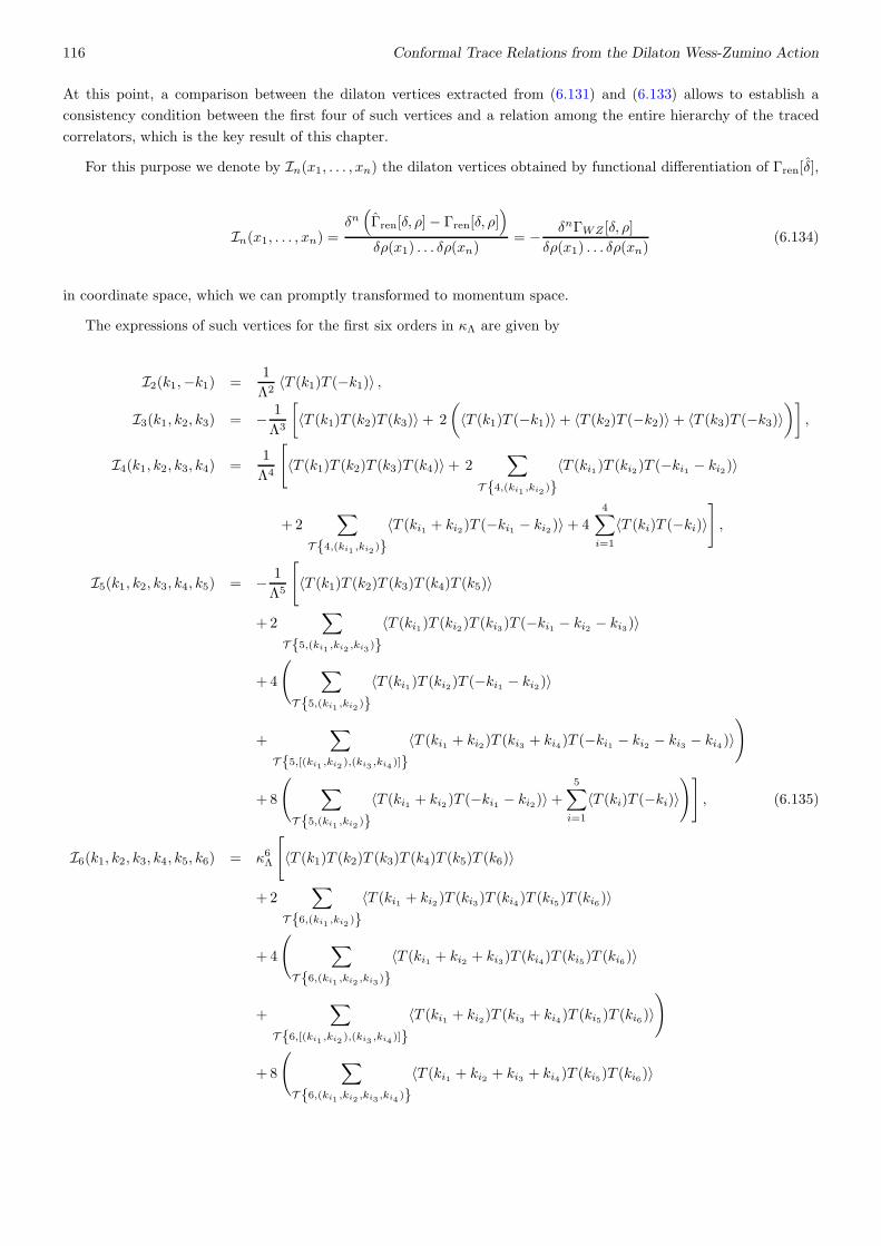
116 Conformal Trace Relations from the Dilaton Wess-Zumino Action
At this point, a comparison between the dilaton vertices extracted from (6.131) and (6.133) allows to establish a
consistency condition between the first four of such vertices and a relation among the entire hierarchy of the traced
correlators, which is the key result of this chapter.
For this purpose we denote by In(x1, . . . , xn) the dilaton vertices obtained by functional differentiation of Γren[δ],
In(x1, . . . , xn) =δn(
Γren[δ, ρ]− Γren[δ, ρ])
δρ(x1) . . . δρ(xn)= − δnΓWZ [δ, ρ]
δρ(x1) . . . δρ(xn)(6.134)
in coordinate space, which we can promptly transformed to momentum space.
The expressions of such vertices for the first six orders in κΛ are given by
I2(k1,−k1) =1
Λ2〈T (k1)T (−k1)〉 ,
I3(k1, k2, k3) = − 1
Λ3
[
〈T (k1)T (k2)T (k3)〉 + 2
(
〈T (k1)T (−k1)〉+ 〈T (k2)T (−k2)〉+ 〈T (k3)T (−k3)〉)]
,
I4(k1, k2, k3, k4) =1
Λ4
[
〈T (k1)T (k2)T (k3)T (k4)〉+ 2∑
T 4,(ki1 ,ki2 )〈T (ki1)T (ki2)T (−ki1 − ki2)〉
+2∑
T 4,(ki1 ,ki2)〈T (ki1 + ki2)T (−ki1 − ki2 )〉+ 4
4∑
i=1
〈T (ki)T (−ki)〉]
,
I5(k1, k2, k3, k4, k5) = − 1
Λ5
[
〈T (k1)T (k2)T (k3)T (k4)T (k5)〉
+2∑
T 5,(ki1 ,ki2 ,ki3)〈T (ki1)T (ki2)T (ki3)T (−ki1 − ki2 − ki3)〉
+4
(
∑
T 5,(ki1 ,ki2 )〈T (ki1)T (ki2)T (−ki1 − ki2)〉
+∑
T 5,[(ki1 ,ki2 ),(ki3 ,ki4)]〈T (ki1 + ki2)T (ki3 + ki4)T (−ki1 − ki2 − ki3 − ki4 )〉
)
+8
(
∑
T 5,(ki1 ,ki2 )〈T (ki1 + ki2 )T (−ki1 − ki2)〉+
5∑
i=1
〈T (ki)T (−ki)〉)]
, (6.135)
I6(k1, k2, k3, k4, k5, k6) = κ6Λ
[
〈T (k1)T (k2)T (k3)T (k4)T (k5)T (k6)〉
+2∑
T 6,(ki1 ,ki2 )〈T (ki1 + ki2 )T (ki3)T (ki4)T (ki5)T (ki6)〉
+4
(
∑
T 6,(ki1 ,ki2 ,ki3)〈T (ki1 + ki2 + ki3)T (ki4)T (ki5)T (ki6)〉
+∑
T 6,[(ki1 ,ki2 ),(ki3 ,ki4)]〈T (ki1 + ki2)T (ki3 + ki4)T (ki5)T (ki6)〉
)
+8
(
∑
T 6,(ki1 ,ki2 ,ki3 ,ki4 )〈T (ki1 + ki2 + ki3 + ki4 )T (ki5)T (ki6)〉

6.6 Dilaton interactions and constraints from ΓWZ 117
+∑
T 6,[(ki1 ,ki2 ,ki3),(ki4 ,ki5 )]〈T (ki1 + ki2 + ki3)T (ki4 + ki5)T (ki6)〉
+∑
T 6,[(ki1 ,ki2 ),(ki3 ,ki4 )]〈T (ki1 + ki2 )T (ki3 + ki4)T ((ki5 + ki6))〉
)
+16
(
1
2
∑
T 6,(ki1 ,ki2 ,ki3)〈T (ki1 + ki2 + ki3)T (−ki1 − ki2 − ki3)〉
+∑
T 6,(ki1 ,ki2 )〈T (ki1 + ki2 )T (−ki1 − ki2)〉+
6∑
i=1
〈T (ki)T (−ki)〉)]
. (6.136)
These results can be easily extended to any higher order. The recipe, in this respect, is really simple:
in order to construct the vertex at order n one has to sum to the n-point function all the lower order functions in the
hierarchy, down to n = 2, partitioning the momenta in all the possible ways and symmetrising each single contribution.
The normalization factor in front of the correlator of order-k is always 2n−k, while the factor in front of the vertex
of order n is (−κΛ)n. Notice that, for n even, we have an additional 1/2 factor in front of the contributions from the
2-point functions in which each EMT carries n/2 momenta, to avoid double counting.
Notice that the expressions of the dilaton interactions in (6.136) have been derived withour any reference to the
dimensions of space, so that they hold for any even dimension. As such, they can be thoroughly tested in the simplest
case, i.e. d = 2. We did check them in 2 dimensions, as illustrated in appendix A.11.
We pause for a moment to clarify the notation used in (6.135) for the organization of the momenta and the meaning
of the symbol T .
For example T 4, (ki1 , ki2) denotes the six pairs of distinct momenta in the case of the four point functions
T 4, (ki1 , ki2 ) = (k1, k2), (k1, k3), (k1, k4), (k2, k3), (k2, k4), (k3, k4) , (6.137)
where we are combining the 4 momenta k1, ...k4 into all the possible pairs, for a total of(
42
)
terms. With five momenta
(k1, k2, k3, k4, k5) the available pairs are
T 5, (ki1 , ki2 ) = (k1, k2), (k1, k3), (k1, k4), (k1, k5), (k2, k3), (k2, k4), (k2, k5), (k3, k4), (k3, k5), (k4, k5)(6.138)
while the possible triples are
T 5, (ki1 , ki2 , ki3) = (k1, k2, k3), (k1, k2, k4), (k1, k2, k5), (k1, k3, k4), (k1, k3, k5),(k1, k4, k5), (k2, k3, k4), (k2, k3, k5), (k2, k4, k5), (k3, k4, k5) . (6.139)
As we move to higher orders, the description of the momentum dependence gets slightly more involved and we need to
distribute the external momenta into two pairs. The notation T 5, [(ki1 , ki2), (ki3 , ki4)] denotes the set of independent
paired couples which can be generated out of 5 momenta. Their number is 15 and they are given by
T 5, [(ki1 , ki2), (ki3 , ki4)] = [(k1, k2), (k3, k4)], [(k1, k2), (k3, k5)], [(k1, k2), (k4, k5)][(k1, k3), (k2, k4)], [(k1, k3), (k2, k5)], [(k1, k3), (k4, k5)], [(k1, k4), (k2, k3)], [(k1, k4), (k2, k5)], [(k1, k4), (k3, k5)],
[(k1, k5), (k2, k3)], [(k1, k5), (k2, k4)], [(k1, k5), (k3, k4)], [(k2, k3), (k4, k5)], [(k2, k4), (k3, k5)], [(k2, k5), (k3, k4)] .(6.140)
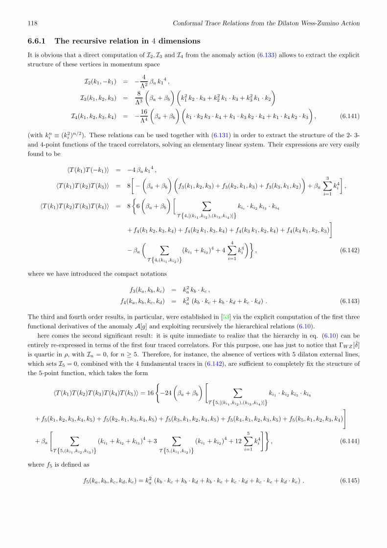
118 Conformal Trace Relations from the Dilaton Wess-Zumino Action
6.6.1 The recursive relation in 4 dimensions
It is obvious that a direct computation of I2, I3 and I4 from the anomaly action (6.133) allows to extract the explicit
structure of these vertices in momentum space
I2(k1,−k1) = − 4
Λ2βa k1
4 ,
I3(k1, k2, k3) =8
Λ3
(
βa + βb
)(
k21 k2 · k3 + k22 k1 · k3 + k23 k1 · k2)
I4(k1, k2, k3, k4) = − 16
Λ4
(
βa + βb
)(
k1 · k2 k3 · k4 + k1 · k3 k2 · k4 + k1 · k4 k2 · k3)
, (6.141)
(with kni ≡ (k2i )n/2). These relations can be used together with (6.131) in order to extract the structure of the 2- 3-
and 4-point functions of the traced correlators, solving an elementary linear system. Their expressions are very easily
found to be
〈T (k1)T (−k1)〉 = −4 βa k14 ,
〈T (k1)T (k2)T (k3)〉 = 8
[
−(
βa + βb
)(
f3(k1, k2, k3) + f3(k2, k1, k3) + f3(k3, k1, k2)
)
+ βa
3∑
i=1
k4i
]
,
〈T (k1)T (k2)T (k3)T (k4)〉 = 8
6
(
βa + βb
)[
∑
T 4,[(ki1 ,ki2 ),(ki3 ,ki4 )]kii · ki2 ki3 · ki4
+ f4(k1 k2, k3, k4) + f4(k2 k1, k3, k4) + f4(k3 k1, k2, k4) + f4(k4 k1, k2, k3)
]
− βa
(
∑
T 4,(ki1 ,ki2 )(ki1 + ki2)
4 + 44∑
i=1
k4i
)
, (6.142)
where we have introduced the compact notations
f3(ka, kb, kc) = k2a kb · kc ,f4(ka, kb, kc, kd) = k2a (kb · kc + kb · kd + kc · kd) . (6.143)
The third and fourth order results, in particular, were established in [53] via the explicit computation of the first three
functional derivatives of the anomaly A[g] and exploiting recursively the hierarchical relations (6.10).
here comes the second significant result: it is quite immediate to realize that the hierarchy in eq. (6.10) can be
entirely re-expressed in terms of the first four traced correlators. For this purpose, one has just to notice that ΓWZ [δ]
is quartic in ρ, with In = 0, for n ≥ 5. Therefore, for instance, the absence of vertices with 5 dilaton external lines,
which sets I5 = 0, combined with the 4 fundamental traces in (6.142), are sufficient to completely fix the structure of
the 5-point function, which takes the form
〈T (k1)T (k2)T (k3)T (k4)T (k5)〉 = 16
−24
(
βa + βb
)
[
∑
T 5,[(ki1 ,ki2 ),(ki3 ,ki4)]ki1 · ki2 ki3 · ki4
+ f5(k1, k2, k3, k4, k5) + f5(k2, k1, k3, k4, k5) + f5(k3, k1, k2, k4, k5) + f5(k4, k1, k2, k3, k5) + f5(k5, k1, k2, k3, k4)
]
+ βa
[
∑
T 5,(ki1 ,ki2 ,ki3)(ki1 + ki2 + ki3 )
4+ 3
∑
T 5,(ki1 ,ki2 )(ki1 + ki2)
4+ 12
5∑
i=1
k4i
]
, (6.144)
where f5 is defined as
f5(ka, kb, kc, kd, ke) = k2a (kb · kc + kb · kd + kb · ke + kc · kd + kc · ke + kd · ke) . (6.145)
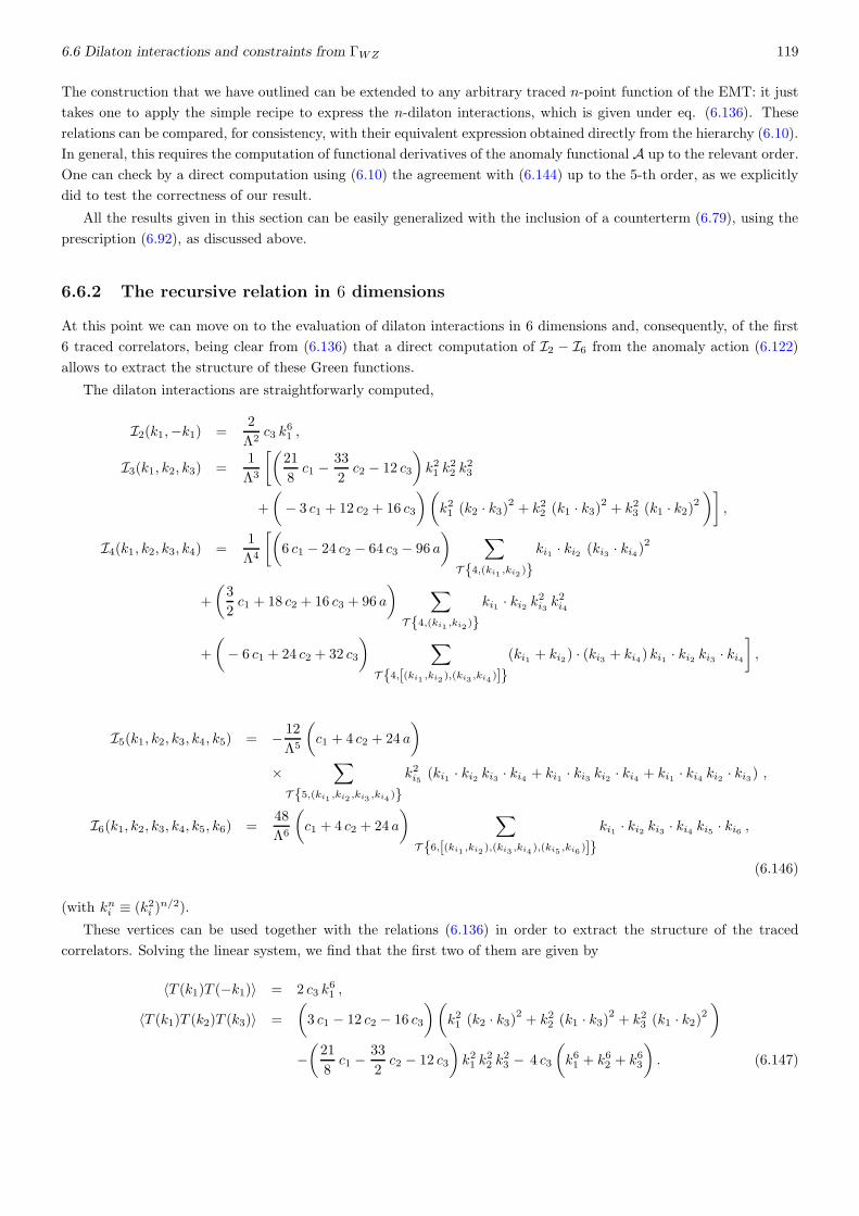
6.6 Dilaton interactions and constraints from ΓWZ 119
The construction that we have outlined can be extended to any arbitrary traced n-point function of the EMT: it just
takes one to apply the simple recipe to express the n-dilaton interactions, which is given under eq. (6.136). These
relations can be compared, for consistency, with their equivalent expression obtained directly from the hierarchy (6.10).
In general, this requires the computation of functional derivatives of the anomaly functional A up to the relevant order.
One can check by a direct computation using (6.10) the agreement with (6.144) up to the 5-th order, as we explicitly
did to test the correctness of our result.
All the results given in this section can be easily generalized with the inclusion of a counterterm (6.79), using the
prescription (6.92), as discussed above.
6.6.2 The recursive relation in 6 dimensions
At this point we can move on to the evaluation of dilaton interactions in 6 dimensions and, consequently, of the first
6 traced correlators, being clear from (6.136) that a direct computation of I2 − I6 from the anomaly action (6.122)
allows to extract the structure of these Green functions.
The dilaton interactions are straightforwarly computed,
I2(k1,−k1) =2
Λ2c3 k
61 ,
I3(k1, k2, k3) =1
Λ3
[(
21
8c1 −
33
2c2 − 12 c3
)
k21 k22 k
23
+
(
− 3 c1 + 12 c2 + 16 c3
)(
k21 (k2 · k3)2 + k22 (k1 · k3)2 + k23 (k1 · k2)2)]
,
I4(k1, k2, k3, k4) =1
Λ4
[(
6 c1 − 24 c2 − 64 c3 − 96 a
)
∑
T 4,(ki1 ,ki2 )ki1 · ki2 (ki3 · ki4)2
+
(
3
2c1 + 18 c2 + 16 c3 + 96 a
)
∑
T 4,(ki1 ,ki2)ki1 · ki2 k2i3 k2i4
+
(
− 6 c1 + 24 c2 + 32 c3
)
∑
T 4,[(ki1 ,ki2 ),(ki3 ,ki4 )](ki1 + ki2) · (ki3 + ki4) ki1 · ki2 ki3 · ki4
]
,
I5(k1, k2, k3, k4, k5) = − 12
Λ5
(
c1 + 4 c2 + 24 a
)
×∑
T 5,(ki1 ,ki2 ,ki3 ,ki4 )k2i5 (ki1 · ki2 ki3 · ki4 + ki1 · ki3 ki2 · ki4 + ki1 · ki4 ki2 · ki3 ) ,
I6(k1, k2, k3, k4, k5, k6) =48
Λ6
(
c1 + 4 c2 + 24 a
)
∑
T 6,[(ki1 ,ki2 ),(ki3 ,ki4),(ki5 ,ki6 )]ki1 · ki2 ki3 · ki4 ki5 · ki6 ,
(6.146)
(with kni ≡ (k2i )n/2).
These vertices can be used together with the relations (6.136) in order to extract the structure of the traced
correlators. Solving the linear system, we find that the first two of them are given by
〈T (k1)T (−k1)〉 = 2 c3 k61 ,
〈T (k1)T (k2)T (k3)〉 =
(
3 c1 − 12 c2 − 16 c3
)(
k21 (k2 · k3)2 + k22 (k1 · k3)2 + k23 (k1 · k2)2)
−(
21
8c1 −
33
2c2 − 12 c3
)
k21 k22 k
23 − 4 c3
(
k61 + k62 + k63
)
. (6.147)

120 Conformal Trace Relations from the Dilaton Wess-Zumino Action
The structure of the 4-point Green function is much more complicated and can be expressed in a compact notation
through the expression
〈T (k1)T (k2)T (k3)T (k4)〉 =
[
4 c3
(
7 f2i,2i,2i + 6 f2i,2i,ij + 3 f2i,2i,2j + 12 f2i,ij,ij + 12 f2i,2j,ij + 8 f ij,ij,ij)
+
(
− 18 c1 + 72 c2 + 96 c3
)
f2i,jk,jk + 4
(
24 a+ 3 c1 − 12 c2 − 8 c3
)
f2i,2j,kl
− 6
(
16 a+ c1 − 4 c2
)
f ij,kl,kl +
(
63
4c1 − 99 c2 − 72 c3
)
f2i,2j,2k
+
(
− 6 c1 + 24 c2 + 32 c3
)(
2 f2i,jk,jl + f ij,ik,jl)]
. (6.148)
Here we have introduced a compact notation for the basis of the 12 scalar functions f ...(k1, k2, k3, k4) on which
the correlator is expanded, leaving their dependence on the momenta implicit not to make the formula clumsy. As
dimensional analysis forces every term in the Green function to be the product of three scalar products of momenta,
the role of the tree superscripts on each of the f ’s is to specify the way in which the momenta are distributed. We
present below the expressions of the first four scalar f ’s, from which it should be clear how to derive the explicit forms
of all the others. We obtain
f2i,2i,2i(k1, k2, k3, k4) =
4∑
i=1
(ki)6 ,
f2i,2i,ij(k1, k2, k3, k4) =
4∑
i=1
(ki)4∑
j 6=iki · kj ,
f2i,2i,2j(k1, k2, k3, k4) =
4∑
i=1
(ki)4∑
j 6=ik2j ,
f2i,ij,ij(k1, k2, k3, k4) =4∑
i=1
(ki)2∑
j 6=i(ki · kj)2 . (6.149)
Notice that each one of the f ’s is completely symmetric with respect to any permutation of the momenta, as for the
whole correlator. The structure of the 5- and 6-point functions is essentially similar to (6.147), although they require
much broader bases of scalar functions to account for all their terms and we do not report them explicitly.
Again, it is clear that the hierarchy in eq. (6.10) can be entirely re-expressed in terms of the first 6 traced
correlators. In fact, one notices that ΓWZ [δ] is at most of order 6 in ρ, which implies
In(x1, . . . , xn) = 0 , n ≥ 7 . (6.150)
Therefore, for instance, the absence of vertices with 7 dilaton external lines, which sets I7 = 0 and the knowledge of
the first 6 fundamental Green functions are sufficient to completely fix the structure of the 7-point function, and so
for the vertices of higher orders. In this way one can determine all the others recursively, up to the desired order. The
consistency of these relations could be checked, in principle, by a direct comparison with their expression obtained
directly from the hierarchy (6.10). This requires the explicit computation of functional derivatives of the anomaly
functional A up to the relevant order, which is a much more time-consuming task.
6.7 Conclusions
Our analysis has had the goal of showing that the infinite hierarchy of fully traced correlation functions generated
by the anomaly constraint in a generic CFT in even dimensions has as fundamental building blocks, in d dimensions,
only the first d correlators. For instance, in d = 4 only correlators with 2, 3 and 4 traces are necessary to identify the
entire hierarchy. This result can be simply derived from the structure of the WZ action, which only contains dilaton
6.7 Conclusions 121
interactions up to the quartic order. Non anomalous terms, which are homogeneous under Weyl transformations
and can be of arbitrarily higher orders in ρ, do not play any role in this construction. The WZ action can also be
determined, in general, by the Noether method, where the dilaton is coupled directly to the anomaly and corrections
are included in order to take care of the Weyl non-invariance of the functional. Alternatively, the same action is
fixed by the cocycle condition, which shows that its functional dependence on the dilaton field takes place via the
Weyl-gauging of the metric tensor. In our analysis we have introduced an expression of the anomaly-induced action
in which the anomaly contribution is generated directly by the counterterms, evaluated in dimensional regularization.
The WZ conformal anomaly actions that we have derived include all the contributions related to the local part
of the anomaly. This result adds full generality to the analysis of dilaton effective actions, which carry an intrinsic
regularization scheme dependence, due to the appearance in the anomaly functional of terms that are different from
the Euler density and the d-dimensional Weyl invariants in the specific space dimension. In general, the extraction of
these extra contributions, as one can figure out from our study, is very involved, with a level of difficulty that grows
with the dimensionality of the space in which the underlying CFT is formulated. Our main results for WZ dilaton
actions, especially in d = 6, are remarkably simplified in flat space. Comparing our results with those of the previous
literature [105], we have given the form of the WZ action in the case of the CFT of the (2, 0) tensor multiplet, which,
in the past, has found application in the AdS7/CFT6 correspondence.

Appendix A
Appendix
A.1 Sign conventions
The definition of the Fourier transform of a n-EMT’s correlation functions, which holds for any other n-point function
as well, is given by
∫
ddx1 . . . ddxn 〈T µ1ν1(x1) . . . T
µnνn(xn)〉 e−i(k1·x1+···+kn·xn) = (2π)d δ(d)
(
n∑
i=1
ki
)
〈T µ1ν1(k1) . . . Tµnνn(kn)〉 ,
(A.1)
where all the momenta are conventionally taken to be incoming.
The covariant derivatives of a contravariant vector Aµ and of a covariant one Bµ are respectively
∇νAµ ≡ ∂νA
µ + ΓµνρAρ , (A.2)
∇νBµ ≡ ∂νBµ − ΓρνµBρ , (A.3)
with the Christoffel symbols defined as
Γαβγ =1
2gακ [−∂κgβγ + ∂βgκγ + ∂γgκβ ] . (A.4)
Our definition of the Riemann tensor is
Rλµκν = ∂νΓλµκ − ∂κΓ
λµν + ΓλνηΓ
ηµκ − ΓλκηΓ
ηµν . (A.5)
The Ricci tensor is defined by the contraction Rµν = Rλµλν and the scalar curvature by R = gµνRµν .
The functional variations with respect to the metric tensor are computed using the relations
δ√g = −1
2
√g gαβ δg
αβ δ√g =
1
2
√g gαβ δgαβ
δgµν = −gµαgνβ δgαβ δgµν = −gµαgνβ δgαβ (A.6)
The structure sαβγδ has been repeatedly used throughout the calculations: it comes from
− δgαβ(z)
δgγδ(x)
∣
∣
∣
∣
gµν=δµν
=1
2
[
δαγδβδ + δαδδβγ]
δ(4)(z − x) = sµναβ δ(4)(z − x) . (A.7)
The variations of the Christoffel symbols are tensors themselves and their expression is
δΓαβγ =1
2gαλ[
−∇λ(δgβγ) +∇γ(δgβλ) +∇β(δgγλ)]
,
∇ρδΓαβγ =
1
2gαλ[
−∇ρ∇λ(δgβγ) +∇ρ∇γ(δgβλ) +∇ρ∇β(δgγλ)]
. (A.8)
123

124 Appendix
A.2 Results for Weyl-gauging
In the Weyl-gauging of the counterterms, we use the following relations
Γαβγ = Γαβγ +1
Λ
(
δβα∇γρ+ δγ
α∇βρ− gβγ∇αρ
)
,
Rµνλσ = Rµνλσ + gνλ
(∇σ∂µρ
Λ+∂µρ ∂σρ
Λ2
)
− gνσ
(∇λ∂µρ
Λ+∂µρ ∂λρ
Λ2
)
+ δµσ
(∇λ∂νρ
Λ+∂νρ ∂λρ
Λ2
)
− δµλ
(∇σ∂νρ
Λ+∂νρ ∂σρ
Λ2
)
+
(
δµλ gνσ − δµσ gνλ
)
(∂ρ)2
Λ2,
Rµν = Rµν − gµν
(
ρ
Λ− (d− 2)
(∂ρ)2
Λ2
)
− (d− 2)
(∇µ∂νρ
Λ+∂µρ ∂νρ
Λ2
)
,
R ≡ gµν Rµν = e2 ρΛ
[
R− 2 (d− 1)ρ
Λ+ (d− 1) (d− 2)
(∂ρ)2
Λ2
]
. (A.9)
When specialized to the case of Weyl transformations, for which δW gµν = 2σgµν , the variations of the Christoffel
symbols and their covariant derivatives (A.8) are
δWΓαβγ = −gβγ ∂ασ + δβα ∂γσ + δγ
α ∂βσ ⇒ δWΓααγ = d ∂γσ ,
∇λδWΓαβγ = −gβγ∇λ∂ασ + δβ
α∇λ∂γσ + δγα∇λ∂βσ ⇒ δW∇λΓ
ααγ = d∇λ∂γσ . (A.10)
Using the Palatini identity
δRαβγλ = ∇λ(δΓαβγ)−∇γ(δΓ
αβλ) ⇒ δRαβ = ∇α(δΓ
λβλ)−∇λ(δΓ
λαβ) (A.11)
we obtain the expressions for the Weyl variations of the Riemann and Ricci tensors
δWRαβγδ = gβδ∇γ∂
ασ − gβγ ∇δ∂ασ + δγ
α∇delta∂βσ − δdeltaα∇γ∂βσ ,
δWRαβ = gαβ σ + (d− 2)∇α∂βσ . (A.12)
It is also customary to introduce the Cotton tensor,
Cαβγ = ∇γKαβ −∇βKαγ , where Kαβ =1
d− 2
(
Rαβ − gαβ2 (d− 1)
R
)
. (A.13)
Using (A.10)-(A.12) one can easily show that the variation of the Cotton tensor is simply given by
δW Cαβγ = −∂λσ Cλαβγ , (A.14)
which is expressed in terms of the Weyl tensor.
A.3 Weyl invariants and Euler densities in 2, 4 and 6 dimensions
It is well known that the object one has to deal with in order to construct Weyl-invariant objects for general dimensions
d is the traceless part of the Riemann tensor, called the Weyl tensor, defined by
Cαβγδ = Rαβγδ −1
d− 2(gαγ Rδβ + gαδ Rγβ − gβγ Rδα − gβδRγα) +
1
(d− 1)(d− 2)(gαγ gδβ + gαδ gγβ)R . (A.15)
This object enjoys the same symmetry properties of the Riemann tensor, i.e.
Cαβγδ = −Cβαγδ = Cβαδγ = Cδγβα , (A.16)
and, moreover, is traceless with respect to any couple of its indices. It is invariant under Weyl scalings of the metric
δWCαβγδ = 0 . (A.17)

A.3 Weyl invariants and Euler densities in 2, 4 and 6 dimensions 125
It is apparent from (A.15), it is not defined for d = 2,so that no Weyl-invariant object depending only on the metric
can be built out of it.
In 4 dimensions, the only quantity which is Weyl invariant, when multiplied by√−g, is the Weyl tensor squared,
which is given by
F ≡ CαβγδCαβγδ = RαβγδRαβγδ − 2RαβRαβ +1
3R2 . (A.18)
Its d-dimensional version, which we call Fd, is instead
Fd ≡ CαβγδCαβγδ = RαβγδRαβγδ −4
d− 2RαβRαβ +
2
(d− 2)(d− 1)R2 (A.19)
There are three dimension-6 scalars that are Weyl invariant when multiplied by√g. Their choice is not unique
at all, as one can always take linear combinations of them. In particular, the literature is full of different choices
for the third one, which involves differential operators. In this work we adopt the definition of I3 given, for general
dimensions, in [114]
Id1 ≡ Cµναβ Cµρσβ Cνρσ
α =d2 + d− 4
(d− 1)2 (d− 2)3K1 −
3 (d2 + d− 4)
(d− 1) (d− 2)3K2 +
3
2 d2 − 6 d+ 4K3
+6 d− 8
(d− 2)3K4 −
3 d
(d− 2)2K5 −
3
d− 2K6 +K8
Id2 ≡ Cµναβ Cαβρσ Cµνρσ =
8 (2 d− 3)
(d− 1)2 (d− 2)3K1 +
72− 48 d
(d− 1) (d− 2)3K2 +
6
d2 − 3 d+ 2K3
+16 (d− 1)
(d− 2)2K4 −
24
(d− 2)2K5 −
12
d− 2K6 +K7
Id3 ≡ d− 10
d− 2
(
∇αCβγρσ∇αCβγρσ − 4 (d− 2) Cγρσ Cγρσ
)
+4
d− 2
(
+2
(d− 1)R
)
Cαβρσ Cαβρσ
=16
(d2 − 3d+ 2)2K1 −
32
(d− 1) (d− 2)2K2 +
8
d2 − 3 d+ 2K3 +
16
(d− 1) (d− 2)2K9
− 32
(d− 2)2K10 +
8
d− 2K11 +
4 (d− 6)
(d− 1) (d− 2)2K12 +
88− 12 d
(d− 2)2K13 +K14 +
8 (d− 10)
(d− 2)2K15 .
(A.20)
We mention that the general problem of constructing all the possible Weyl-invariant coordinate scalars depending on
the metric tensor was solved in full generality in [115].
The other quantity with which one can construct an integral which is Weyl invariant (in fact, a constant) for
general dimensions is the Euler density, defined, for a general even number of dimensions d = 2k, as
E2k =1
2kδµ1a1ν1b1...µkakνkbk R
µ1ν1λ1κ1 . . . Rµkνkakbk . (A.21)
The antisymmetric Kronecker symbol is defined by
δν1a1ν2a2...νnan = n!∑
P(a1,...,an)
(−1)TP gν1P(a1) . . . gνnP(an) , (A.22)
where TP e is the number of inversions the permutation P of the n numbers a1, . . . an is made of.
By applying the general definition A.21, we find that in 2, 4 and 6 dimensions respectively, it is given by the
expressions
E2 = R ,
E4 ≡ G = RαβγδRαβγδ − 4RαβRαβ + R2 ,
E6 =21
100R3 − 27
20RRµν Rµν +
3
2Rµ
ν RναRα
µ + 4Cµνρσ Cµναβ C
ρσαβ
− 8Cµνρσ Cµαρβ Cνα
σβ − 6Rµν C
µαρσ Cναρσ +6
5RCµνρσ Cµνρσ − 3Rµν Rρσ Cµρσν . (A.23)
Of course, in the last expression C is the Weyl tensor in 6 dimensions.
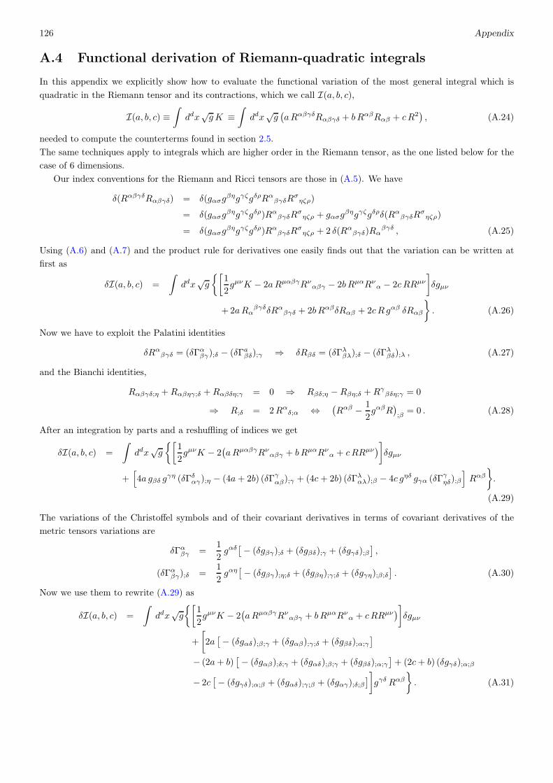
126 Appendix
A.4 Functional derivation of Riemann-quadratic integrals
In this appendix we explicitly show how to evaluate the functional variation of the most general integral which is
quadratic in the Riemann tensor and its contractions, which we call I(a, b, c),
I(a, b, c) ≡∫
ddx√gK ≡
∫
ddx√g(
aRαβγδRαβγδ + bRαβRαβ + cR2)
, (A.24)
needed to compute the counterterms found in section 2.5.
The same techniques apply to integrals which are higher order in the Riemann tensor, as the one listed below for the
case of 6 dimensions.
Our index conventions for the Riemann and Ricci tensors are those in (A.5). We have
δ(RαβγδRαβγδ) = δ(gασgβηgγζgδρRαβγδR
σηζρ)
= δ(gασgβηgγζgδρ)RαβγδR
σηζρ + gασg
βηgγζgδρδ(RαβγδRσηζρ)
= δ(gασgβηgγζgδρ)RαβγδR
σηζρ + 2 δ(Rαβγδ)Rα
βγδ , (A.25)
Using (A.6) and (A.7) and the product rule for derivatives one easily finds out that the variation can be written at
first as
δI(a, b, c) =
∫
ddx√g
[
1
2gµνK − 2aRµαβγRναβγ − 2bRµαRνα − 2cRRµν
]
δgµν
+2aRαβγδδRαβγδ + 2bRαβδRαβ + 2cRgαβ δRαβ
. (A.26)
Now we have to exploit the Palatini identities
δRαβγδ = (δΓαβγ);δ − (δΓaβδ);γ ⇒ δRβδ = (δΓλβλ);δ − (δΓλβδ);λ , (A.27)
and the Bianchi identities,
Rαβγδ;η +Rαβηγ;δ +Rαβδη;γ = 0 ⇒ Rβδ;η −Rβη;δ +Rγβδη;γ = 0
⇒ R;δ = 2Rαδ;α ⇔(
Rαβ − 1
2gαβR
)
;β= 0 . (A.28)
After an integration by parts and a reshuffling of indices we get
δI(a, b, c) =
∫
ddx√g
[
1
2gµνK − 2
(
aRµαβγRναβγ + bRµαRνα + cRRµν)
]
δgµν
+[
4a gβδ gγη (δΓδαγ);η − (4a+ 2b) (δΓγαβ);γ + (4c+ 2b) (δΓλαλ);β − 4c gηδ gγα (δΓ
γηδ);β
]
Rαβ
.
(A.29)
The variations of the Christoffel symbols and of their covariant derivatives in terms of covariant derivatives of the
metric tensors variations are
δΓαβγ =1
2gαδ[
− (δgβγ);δ + (δgβδ);γ + (δgγδ);β]
,
(δΓαβγ);δ =1
2gαη[
− (δgβγ);η;δ + (δgβη);γ;δ + (δgγη);β;δ]
. (A.30)
Now we use them to rewrite (A.29) as
δI(a, b, c) =
∫
ddx√g
[
1
2gµνK − 2
(
aRµαβγRναβγ + bRµαRνα + cRRµν)
]
δgµν
+
[
2a[
− (δgαδ);β;γ + (δgαβ);γ;δ + (δgβδ);α;γ]
− (2a+ b)[
− (δgαβ);δ;γ + (δgαδ);β;γ + (δgβδ);α;γ]
+ (2c+ b) (δgγδ);α;β
− 2c[
− (δgγδ);α;β + (δgαδ);γ;β + (δgαγ);δ;β]
]
gγδRαβ
. (A.31)

A.5 Functional variations in 6 dimensions 127
The presence of the factor gcdRab imposes two symmetry constraints on the terms in the last contribution in square
brackets. By adding and subtracting −(4a+ 2b) (δgac);d;b we obtain the expression
δI(a, b, c) =
∫
ddx√g
[
1
2gµνK − 2
(
aRµαβγRναβγ + bRµαRνα + cRRµν)
]
δgµν
+
[
(4a+ 2b)[
(δgαγ);β;δ − (δgαγ);δ;β]
+ (4a+ b)(δgαβ);γ;δ + (4c+ b) (δgγδ);α;β
− (4a+ 2b+ 4c) (δgαγ);δ;β
]
gγδRαβ
. (A.32)
The commutation of covariant derivatives allows us to write
gγδ[
(δgαγ);β;δ − (δgαγ);δ;β]
Rαβ = gγδ[
− δgασRσγδβ − δgγσR
σαβδ
]
Rαβ
= gγδ[
− sµνασRσγβδ − sµνcσR
σαβδ
]
Rαβ δgµν
= (−RµαRνα +RµανβRαβ)δgµν . (A.33)
Inserting this back into (A.32) we get
δI(a, b, c) =∫
ddx√g
[
1
2gµνK − 2aRµαβγRναβγ + 4aRµαRνα − (4a+ 2b)RµανβRαβ − 2cRRµν
]
δgµν
+
[
(4a+ b)(δgαβ);γ;δ + (4c+ b) (δgγδ);α;β − (4a+ 2b+ 4c) (δgαγ);δ;β
]
gγδ Rαβ
.
(A.34)
If the coefficients are a = c = 1 and b = −4, i.e. if the integrand is the Euler density, the last three terms are zero.
All that is left to do is a double integration by parts for each one of the last three terms, to factor out δgµν . This is
easily performed and the final result can be written as
δ
δgµνI(a, b, c) =
δ
δgµν
∫
ddx√g(
aRαβγδRαβγδ + bRαβRαβ + cR2)
=√g
1
2gµνK − 2aRµαβγRναβγ + 4aRµαRνα − (4a+ 2b)RµανβRαβ − 2cRRµν
+(4a+ b)Rµν + (4c+ b) gµνRαβ ;α;β − (4a+ 2b+ 4c)Rνβ ;β;µ
. (A.35)
A.5 Functional variations in 6 dimensions
The results for the trace anomaly in 6 dimensions, presented in section 6.5.1, are obtained by computing the functional
variations of the integrals of the Ki in dimensional regularization, which can be obtained with the same techniques
employed in appendix A.4.
A simple counting of the metric tensors needed to contract all the indices for any Ki shows that
δW
∫
ddx√g Ki =
∫
ddx√g [−ǫKi +D(Ki)] σ , ǫ = 6− d , (A.36)
where the second term on the right hand side, D(Ki), is a total derivative contribution. We give the complete list of
128 Appendix
these terms below. We obtain
D(K1) = 12 (d− 1)∇µ (R∂µR)
D(K2) = ∇µ
[
4 (d− 1)Rνλ∇µRνλ + 2 (d− 2) Rµν ∂νR+ (d+ 2) R∂µR
]
D(K3) = 4∇µ
[
R∂µR+ 2Rµν ∂νR+ (d− 1) Rνλκα∇µRνλκα]
D(K4) = 3∇µ
[
d− 2
2Rµν ∂νR + (d− 2)Rνλ∇λRµν + 2Rνρ∇µRνρ
]
D(K5) = ∇µ
[
−R∂µR−Rµν ∂νR + 2 (d− 1) Rνλ∇λRµν − 2 dRνλ∇µRνλ + 2 (d− 2) Rµλνκ∇κRνλ
]
D(K6) = ∇µ
[
2Rµν ∂νR + 4Rνλ∇µRνλ +d+ 2
2Rνλκα∇µRνλκα − 2 dRµλνκ∇κRνλ
]
D(K7) = 6∇µ
[
Rνλκα∇µRνλκα + 4Rνλκµ∇λRνκ
]
D(K8) = 3∇µ
[
1
2Rνλκα∇µRνλκα + 2Rνλ (∇λRµν −∇µRνλ)
]
D(K9) = ∇µ
[
4 (d− 1) ∂µR− (d− 2) R∂µR
]
D(K10) = ∇µ
[
2 ∂µR+ 2 (d− 2) ∇νRµν + 2Rµν ∂νR− 4Rνλ∇λRµν − (d− 2) Rνλ∇µRνλ
]
D(K11) = ∇µ
[
8∇νRµν − (d+ 2) Rνλκα∇µRνλκα − 16Rµλνκ∇κRνλ
]
D(K12) = 4∇µ
[
R∂µR− (d− 1) ∂µR
]
D(K13) = 2 ∇µ
[
− ∂µR− (d− 2) ∇νRµν −Rµν ∂νR+ 2Rνλ∇λRµν + 2Rνλ∇µRνλ
]
D(K14) = 8∇µ
[
−∇νRµν +Rνλκα∇µRνλκα + 2Rµλνκ∇κRνλ
]
D(K15) = ∇µ
[
− ∂µR− 2 (d− 2) ∇νRµν − 3Rµν ∂νR + 6Rνλ∇λRµν
+2Rνλ∇µRνλ − 2 (d− 2) Rµλνκ∇κRνλ
]
. (A.37)
A.6 List of functional derivatives
We list here the contributions to the trace anomalies for three point function coming from the elementary quadratic
objects. They are given by
[
RλµκνRλµκν
]αβρσ(p, q) = p · q
[
p · q(
δαρδβσ + δασδβρ)
−(
δαρpσqβ + δασpρqβ
+ δβρpσqα + δβσpρqα)]
+ 2 pρpσqαqβ ,
[
RµνRµν]αβρσ
(p, q) =1
4p · q
(
δαρpβqσ + δασpβqρ + δβρpαqσ + δβσpαqρ)
+1
2(p · q)2δαβδρσ +
1
4p2q2
(
δαρδβσ + δασδβρ)
−[
1
4p2(
qαqρδβσ + qαqσδβρ + qβqρδασ + qβqσδαρ)
+1
2δαβ(
p · q (pρqσ + pσqρ)− q2pρpσ)
+ (α, β, p) ↔ (ρ, σ, q)
]
,
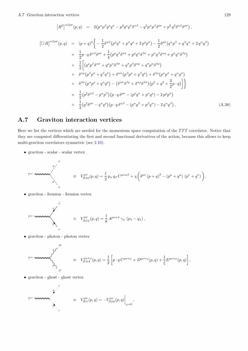
A.7 Graviton interaction vertices 129
[
R2]αβρσ
(p, q) = 2(
pαpβqρqσ − p2qρqσδαβ − q2pαpβδρσ + p2 q2δαβδρσ)
,
[
R]αβρσ
(p, q) = (p+ q)2
− 1
2δαβ(
pρqσ + pσqρ + 2 pρpσ)
− 1
2δρσ(
qαpβ + qβqα + 2 qαqβ)
+1
2p · q δαβδρσ +
1
4
(
pρqβδασ + pρqαδβσ + pσqβδαρ + pσqαδβρ)
+1
2
[
(
qρpβδασ + qρpαδβσ + qσpβδαρ + qσpαδβρ)
+ δαρ(
pβpσ + qβqσ)
+ δασ(
pβpρ + qβqρ)
+ δβρ(
pαpσ + qαqσ)
+ δβσ(
pαpρ + qαqρ)
−(
δασδβρ + δαρδβσ)(
p2 + q2 +3
2p · q
)
]
+1
2
(
p2δαβ − pαpβ)(
p · q δρσ − (pρqσ + pσqρ)− 2 pρpσ)
+1
2
(
q2δρσ − qσqρ)(
p · q δαβ − (pαqβ + pβqα)− 2 qαqβ)
, (A.38)
A.7 Graviton interaction vertices
Here we list the vertices which are needed for the momentum space computation of the TTT correlator. Notice that
they are computed differentiating the first and second functional derivatives of the action, because this allows to keep
multi-graviton correlators symmetric (see 2.10).
• graviton - scalar - scalar vertex
T µν
φ
φ
p
q
≡ V µνSφφ(p, q) =1
2pα qβ C
µναβ + χ
(
δµν (p+ q)2 − (pµ + qµ) (pν + qν)
)
,
• graviton - fermion - fermion vertex
T µν
ψ
ψ
p
q
≡ V µνSψψ(p, q) =1
8Aµναλ γα (pλ − qλ) ,
• graviton - photon - photon vertex
T µν
Aτ
Aω
p
q
≡ V µντωSAA (p, q) =1
2
[
p · q Cµντω +Dµντω(p, q) +1
ξEµντω(p, q)
]
,
• graviton - ghost - ghost vertex
T µν
c
c
p
q
≡ V µνScc(p, q) = −V µνSφφ(p, q)
∣
∣
∣
∣
χ=0
,

130 Appendix
• graviton - graviton - scalar - scalar vertex
T µν
T ρσ
φ
φ
k
l
p
q
≡ V µνρσSSφφ(p, q, l) =1
2p · q sµνρσ − 1
4Gµνρσ(p, q) +
1
4δρσ pα qβ C
µναβ
+χ
[(
δµλ δακ δνβ + δµα δνκ δβλ − δµκ δνλ δαβ − δµν δαλ δβκ)
sρσλκ
+1
2δρσ
(
δµα δνβ − δµν δαβ)]
(pα qβ + pβ qα + pα pβ + qα qβ)
+
[(
δµν δαβ − δµα δνβ)
[
Γλαβ]ρσ
(l) i ( pλ + qλ)
+
(
δµα δνβ − 1
2δµν δαβ
)
[
Rαβ]ρσ
(l)
]
,
• graviton - graviton - fermion - fermion vertex
T µν
T ρσ
ψ
ψ
k
l
p
q
≡ V µνρσSSψψ(p, q) =1
16
[
− 4 sµνρσ − 2 δµν sαλρσ + 2 δαµ sνλρσ + 2 δαν sµλρσ
+ δµλ sανρσ + δνλ sαµρσ + δρσ Aµναλ]
γα (pλ − qλ) ,
• graviton - graviton - photon - photon vertex
T µν
T ρσ
Aτ
Aω
k
l
p
q ≡ V µνρστωSSAA (p, q, l) =1
2
[
Bαµρσβλγν +1
4Bµνρσαλγβ
]
Fαβγλτω(p, q)
+1
ξ
(
Hµνρστω(p, q, l) + Iµνρστω(p, q, l)
)
+1
4δρσ
[
p · q Cµντω +Dµντω(p, q) +1
ξEµντω(p, q)
]
,
• graviton - graviton - ghost - ghost vertex
T µν
T ρσ
c
c
k
l
p
q
≡ V µνρσSScc (p, q, l) = −V µνρσSSφφ(p, q, l)
∣
∣
∣
∣
χ=0
.
We have simplified the notation by introducing, for convenience, the tensor structures
Aµναλ = 2 δµν δαλ − δαµ δλν − δαν δλµ
Bαµρσβλγν = sαµρσ δβλ δγν + sβλρσ δαµ δγν + sγνρσ δαµ δβλ
Cµναβ = δµαδνβ + δµβδνα − δµνδαβ ,
Dµνρσ(p, q) = δµνpσqρ + δρσ(
pµqν + pνqµ)
− δµσpνqρ − δµρpσqν − δνσpµqρ − δνρpσqµ
Eµνρσ(p, q) = δµν[
pρpσ + qρqσ + pρqσ]
−[
δνσpµpρ + δνρqµqσ + δµσpνpρ + δµρqνqσ]
,

A.8 Comments on the inverse mapping 131
Fµνρστω(p, q) = −δτρδωµpσqν + δτρδωνpσqµ + δτσδωµpρqν − δτσδωνpρqµ + (τ, p) ↔ (ω, q)
Gµνρσ(p, q) = δµσ[
pρqν + qρpν]
+ δνσ[
pρqµ + qρpµ]
+ δµρ[
pσqν + qσpν]
+ δνρ[
pσqµ + qσpµ]
− δµν[
pρqσ + qρpσ]
Hµνρστω(p, q, l) =
[(
sµωρσ δνλ + sνλρσ δµω)
pλ pτ + δµω
(
sλτρσ lν + sλτρσ pν)
pλ
+1
2δµω (p+ l)
ν
(
− lτ δρσ + 2 lλ sτλρσ
)
+ (µ↔ ν)
]
+ (τ, p) ↔ (ω, q)
Iµνρστω(p, q, l) = δµν
1
2δρσ lτ (p+ q + l)ω − sλτρσ
[
qω pλ + lλ (p+ q + l)ω]
− sλωρσ[
pτ pλ + qλ (q + l)τ]
− sµνρσ(
pω pτ + qω pτ)
+ (τ, p) ↔ (ω, q).
We have performed all our computations in the Feynman gauge (ξ = 1) The euclidean propagators of the fields in this
case are
〈φφ〉 (p) =1
p2⟨
ψ ψ⟩
(p) =p · γp2
.
〈AµAν〉 (p) =δµν
p2,
〈c c〉 (p) = − 1
p2. (A.39)
A.8 Comments on the inverse mapping
In this appendix we offer some calculational details in the derivation of the expression of the TTT correlator in position
space via the inverse mapping procedure. The remarks apply as well to any other correlator.
For example, eq. (3.68) refers to the contribution coming from the triangle diagram shown in fig. 2.1. We assign
the loop momentum l to flow from the upper external point (x3) to the lower one (x2) on the right, the other two
flows being determined by momentum conservation. We denote the third external point as x1. For the scalar case, for
instance, the complete 1-loop triangle diagram is
8
∫
ddl
(2π)dV µνSφφ(l − q,−l− p)V ρσSφφ(l,−l+ q)V αβSφφ(l + p,−l)
l2 (l − q)2 (l + p)2(A.40)
The vertices are defined in appendix A.7. The first argument in each vertex denotes the momentum of the incoming
particle, the second argument is the momentum of the outgoing one. A typical term appearing in the loop integral is
then
I ≡∫
ddl
(2π)dlµ lν (l + p)ρ (l + p)σ(l − q)α (l − q)β
l2 (l − q)2 (l + p)2. (A.41)
From (3.119) the propagators in configuration space are
1
l2 (l − q)2 (l + p)2= C(1)3
∫
ddx12 ddx23 d
dx31ei [l·x23+(l−q)·x12+(l+p)·x31]
(x212)d/2−1 (x223)
d/2−1 (x231)d/2−1
, (A.42)
where Cα) has been defined in (3.119). It is straightforward to see that (A.41) is given by∫
ddl
(2π)dlµ lν (l + p)ρ (l + p)σ(l − q)α (l − q)β
l2 (l − q)2 (l + p)2=
C(1)3∫
ddl
(2π)dddx12 d
dx23 ddx31
(−i)6 ∂µ23 ∂ν23 ∂ρ31 ∂σ31 ∂α12 ∂β12 ei [l·x23+(l−q)·x12+(l+p)·x31]
(x212)d/2−1 (x223)
d/2−1 (x231)d/2−1
. (A.43)
132 Appendix
We can now integrate by parts moving the derivatives onto the propagators, getting
I = C(1)3∫
ddl
(2π)dddx12 d
dx23 ddx31 e
i [l·x23+(l−q)·x12+(l+p)·x31]
× i6 ∂µ23 ∂ν23 ∂
ρ31 ∂
σ31 ∂
α12 ∂
β12
1
(x212)d/2−1 (x223)
d/2−1 (x231)d/2−1
. (A.44)
The second line is immediately identified with the coordinate space Green’s function.
This can be done for each term of (A.40), justifying the rule quoted in section 3.3.4, that we have used for all the
inverse mappings of the work. According to this the correlators in coordinate space can be obtained replacing the
momenta in the vertices with “i” times the respective derivative which then act directly on the propagators after a
partial integration.
The same arguments could be applied to the bubbles. Nevertheless, we have seen in 3.3.4 that derivatives of delta
functions appear in the scalar case. These are generated by the dependence of the V µνρσSSφφ(p, q, l) from the momentum
l of the graviton bringing the pair of indices ρσ (see appendix A.7). They are due to coupling of the scalar with
derivatives of the metric through the Ricci scalar R in the improvement term (see eq. (2.33)) and state that the
graviton feels the metric gradient. We discuss this below, showing how to inverse-map the third bubble in fig. (2.1),
getting (3.76).
This bubble can be seen as the (x2 → x3) limit of the triangle and its diagrammatic momentum-space expression at
1-loop is∫
ddl
(2π)dV µνSφφ(l − q,−l − p)V αβρσSSφφ (l + p,−l+ q,−q)
(l − q)2 (l + p)2. (A.45)
As the two propagators are expressed by
1
(l + q)2 (l + p)2= C(1)2
∫
ddx12 ddx31
ei [(l−q)·x12+(l+p)·x31]
(x212)d/2−1 (x231)
d/2−1, (A.46)
the dependence of the second vertex on p cannot be ascribed to neither of them.
Two typical terms encountered in (A.45) are
∫
ddl
(2π)d(l + p)ρ (l + p)σ(l − q)α (l − q)β
(l − q)2 (l + p)2,
∫
ddl
(2π)d(l + p)ρ (l + p)σ(l − q)α pβ
(l − q)2 (l + p)2. (A.47)
The first one is treated at once restricting the procedure used for the three point function to the case of two propagators.
For the second one, the following relation is immediately checked:
∫
ddl
(2π)d(l + p)ρ (l + p)σ(l − q)α pβ
(l − q)2 (l + p)2=
C(1)2∫
ddl
(2π)dddx12 d
dx23 ddx31 δ
(d)(x23)(−i)4 ∂ρ31 ∂σ31 ∂α12 (∂31 − ∂23)
β ei [l·x23+(l−q)·x12+(l+p)·x31]
(x212)d/2−1 (x231)
d/2−1.
(A.48)
Notice that an integration by parts brings in a derivative on the delta functions giving
C(1)2∫
ddl
(2π)dddx12 d
dx23 ddx31 e
i [l·x23+(l−q)·x12+(l+p)·x31] (i)4 ∂ρ31 ∂σ31 ∂
α12 (∂31 − ∂23)
β δd(x23)
(x212)d/2−1 (x231)
d/2−1.
(A.49)
This approach has been followed in all the derivations of the expressions given in (3.3.4).
The integration on l brings about a δ(d)(x12 + x23 + x31), so that it is natural to chose the parameterization
x12 = x1 − x2 , x23 = x2 − x3 , x31 = x3 − x1 . (A.50)
A.9 Regularizations and distributional identities 133
A more inviolved example is the 4-particle vertex. For instance the VSSφφ(i ∂31,−i ∂12, i (∂12 − ∂23)) is obtained from
VSSφφ(p, q, l) with the functional replacements
p→ p = i ∂31, q → q = −i ∂12 l → l = i (∂12 − ∂23) (A.51)
giving
V µνρσSSφφ(i ∂31,−i ∂12, i (∂12 − ∂23)) =
1
2i ∂31 · (−i) ∂12sµνρσ − 1
4Gµνρσ(i ∂31,−i ∂12) +
1
4δρσ i ∂31α (−i) ∂12β Cµναβ
+χ
[(
δµλ δακ δνβ + δµα δνκ δβλ − δµκ δνλ δαβ − δµν δαλ δβκ)
sρσλκ
+1
2δρσ
(
δµα δνβ − δµν δαβ)]
(i ∂31α (−i)∂12 β + i ∂31β (−i)∂12α + i ∂31α i ∂31β + (−i)∂12α (−i)∂12β)
−[(
δµα δνβ − δµν δαβ)(
[
Γλαβ]ρσ
(i (∂12 − ∂23))
)
(−i) (i ∂31λ + (−i) ∂12λ)
+1
2
(
δµα δνβ − 1
2δµν δαβ
)(
[
Rαβ]ρσ
(i (∂12 − ∂23))
)]
. (A.52)
A.9 Regularizations and distributional identities
We add few more comments and examples which illustrate the regularization that we have applied in the computation
of the various correlators.
The computation of the logarithmic integrals requires some care due to the distributional nature of some of these
formulas. As an example we consider the integrals
H1 =
∫
ddl eil·xµ2ω
[l2]1+ωH2 =
∫
ddl eil·xµ2ω
[l2]ωH3 =
∫
ddl eil·x log
(
l2
µ2
)
(A.53)
We can relate them in the form
H3 = − ∂
∂ωH2
∣
∣
∣
∣
ω=0
=
(
∂
∂ωH1
∣
∣
∣
∣
ω=0
)
(A.54)
In the two cases we get, using (3.119)
− ∂
∂ωH2
∣
∣
∣
∣
ω=0
= − (4 π)d/2 Γ(d/2)
(x2)d/2(A.55)
and∂
∂ωH1
∣
∣
∣
∣
ω=0
=2d−2πd/2Γ(d/2− 1)
[x2]d/2−1
(
log(x2µ2) + γ − log 4− ψ
(
d− 2
2
))
(A.56)
By redefining the regularization scale µ with eq. (3.138) we clearly obtain from (A.56)
∫
ddllog(l2/µ2)eil·x
l2= 2d−2πd/2Γ(d/2− 1)
log x2µ2
[x2]d/2−1(A.57)
and
H3 =
(
∂
∂ωH1
∣
∣
∣
∣
ω=0
)
= 2d−2πd/2Γ(d/2− 1)
(
log x2µ2
[x2]d/2−1
)
(A.58)
The use of H2 instead gives
H3 = − ∂
∂ωH2
∣
∣
∣
∣
ω=0
= −2dπd/2Γ(d/2)
[x2]d/2(A.59)
Notice that this second relation coincides with (A.58) away from the point x = 0, but differs from it right on the
singularity, since
log x2µ2
[x2]d/2−1= −2 (d− 2)
(
πd/2
Γ(d/2)log(x2µ2) δd(x) +
1
[x2]d/2
)
(A.60)
134 Appendix
For this reason we take (A.58) as the regularized expression of H3, in agreement with the standard approach of dif-
ferential regularization.
The direct method discussed in the second part of the work, though very general and applicable to any correlator,
introduces in momentum space some logarithmic integrals which are more difficult to handle. They take the role
of the ordinary master integrals of perturbation theory. The scalar integrals needed for the tensor reduction of the
logarithmic contributions in the text are defined in (A.69). After a shift of the momentum in the argument of the
logarithm, a standard tensor reduction gives
ILµ(0, p1, p2) = CL1(p1, p2) p1µ + CL2(p1, p2) p2µ ,
CL1(p1, p2) =(p1
2 − p1 · p2)p22 IL(0, p1, p2) + (p22 − p1 · p2) ILµµ(0, p1, p2)
2 (p1 · p2)2 − p12 p22,
CL2(p1, p2) =(p2
2 − p1 · p2)p12 IL(0, p1, p2) + (p12 − p1 · p2) ILµµ(0, p1, p2)
2 (p1 · p2)2 − p12 p22. (A.61)
To complete the computation of the V V V correlator we need the explicit form of the logarithmic integrals in terms
of ordinary logarithmic and polylogarithmic functions. We define
I ≡∫
ddllog(
l2/µ2)
(l+ p1)2(l − p2)2= − ∂
∂λ
∫
ddlµ2λ
(l2)λ (l + p1)2 (l − p2)2 λ=0
. (A.62)
The logarithmic integral is identified from the term of O(λ) in the series expansion of the previous expression. Because
the coefficient in front of the parametric integral starts at this order, we just need to know the zeroth order expansion
of the integrand, which we separate into two terms. The first one is integrable
I1 =
∫ 1
0
dtt−ǫ(yt)1−ǫ−λ
A(t)1−ǫ=
∫ 1
0
dtt−ǫ(yt)1−ǫ
A(t)1−ǫ+O(λ) ≡ I
(0)1 +O(λ) , (A.63)
while the last term has a singularity in t = 0 which must be factored out and re-expressed in terms of a pole in λ
I2 = −∫ 1
0
dtt−ǫ(x/t)1−ǫ−λ
A(t)1−ǫ= −x
1−ǫ−λ
λ
∫ 1
0
dt1
A(t)1−ǫd
dttλ
= −x1−ǫ−λ
λ
[
1− (ǫ− 1)
∫ 1
0
dttλ
A(t)1−ǫ
(
1
t− t1+
1
t− t2
)]
=x1−ǫ
λ
− 1 + (ǫ− 1)
∫ 1
0
dt1
A(t)1−ǫ
(
1
t− t1+
1
t− t2
)]
+ x1−ǫ[
log x+ (ǫ− 1)
∫ 1
0
dtlog (t/x)
A(t)1−ǫ
(
1
t− t1+
1
t− t2
)]
+O(λ) ≡ 1
λI(−1)2 + I
(0)2 +O(λ) ,
(A.64)
where t1 and t2 are the two roots of A(t) = yt2+(1−x− y)t+x. We are now able to write down the full λ-expansion
of J(1, 1, λ) and to extract the logarithmic integral I
I = −π2−ǫi1+2ǫ
(p23)ǫ
Γ(1− ǫ)Γ(2− ǫ)Γ(ǫ)
Γ(2− 2ǫ)
1
ǫ− 1
I(0)1 + I
(0)2
. (A.65)
The previous expression can be expanded in d = 4−2ǫ dimensions in which it manifests a 1/ǫ pole of ultraviolet origin
I =π2−ǫi1+2ǫ
(p23)ǫ
(
−1
ǫ+ γ
)[
A(x, y) + ǫB(x, y)
]
+O(ǫ) , (A.66)
where A(x, y) and B(x, y) are defined from the ǫ-expansion of the two integrals I(0)1 and I
(0)2 as
A(x, y) = x log x+
∫ 1
0
dt
A(t)
[
yt− x log (t/x)
(
1
t− t1+
1
t− t2
)]
, (A.67)
B(x, y) = −x log2 x+
∫ 1
0
dt
A(t)
[
yt (log (t− t1) + log (t− t2)− 2 log t)
− x log (t/x)
(
1
t− t1+
1
t− t2
)
(log (t− t1) + log (t− t2)− log (x/y)− 1)
]
. (A.68)
A.10 The Wess-Zumino action in 4 dimensions by the Noether method 135
We introduce here a systematic short-hand notation to denote the momentum-space integrals. We define
Iµ1,...,µn(p) =
∫
ddllµ1 . . . lµn
l2 (l + p)2,
Jµ1,...,µn(p1, p2) =
∫
ddllµ1 . . . lµn
l2 (l + p1)2(l + p2)2,
ILµ1...µn(p1, p2, p3) =
∫
ddllµ1 . . . lµn
log(
(l + p1)2/µ2
)
(l + p2)2(l + p3)2,
ILLµ1...µn(p1, p2, p3, p4) =
∫
ddllµ1 . . . lµn
log(
(l + p1)2/µ2
)
log(
(l + p2)2/µ2
)
(l + p3)2(l + p4)2. (A.69)
For correlators which are finite, the double logarithmic contributions will appear in combinations that can be re-
expressed in terms of ordinary Feynman integrals.
A.10 The Wess-Zumino action in 4 dimensions by the Noether method
The dilaton effective action that we have obtained by the Weyl-gauging of the counterterms in chapter 6 can be
recovered also through an iterative technique, that we briefly review.
In this second approach one begins by requiring that the variation of the dilaton effective action under the Weyl
transformations be equal to the anomaly
δWΓWZ [g, τ ] =
∫
d4x√g σ
[
βa
(
F − 2
3R
)
+ βbG
]
. (A.70)
It is natural to start with the ansatz
Γ(1)WZ [g, τ ] =
∫
d4x√gτ
Λ
[
βa
(
F − 2
3R
)
+ βbG
]
. (A.71)
As√g F is Weyl invariant, the variation of τ saturates the F -contribution in (A.70). But
√g G and
√gR are
not conformally invariant. Their variations under Weyl scalings introduce additional terms that must be taken into
account. The general strategy is to compute the infinitesimal variation of these terms and to add terms which are
quadratic in the derivatives of the dilaton and that cancel this extra contributions. But these, when Weyl-transformed,
will generate additional terms which must be compensated in turn. The iteration stops at the fourth order in the
dilaton field. We go through all the computation of the WZ action in some detail. The piece of (A.71) whose first
Weyl variation is most easily worked out is the contribution√g τ R. We integrate it by parts twice and find that
δW
∫
d4x√gτ
ΛR = δW
∫
d4x√g gµν gρσ Rµν
1
Λ∇σ∂ρτ ,
=
∫
d4x√g
(
σ R− 1
Λgρσ δWΓλρσ ∂λτ R+
1
Λτ gµν δWRµν
)
. (A.72)
Using (A.10) and (A.12) this turns into
δW
∫
d4x√gτ
ΛR =
∫
d4x√g
(
σR+2
ΛR∂λτ ∂
λσ +6
Λτσ
)
. (A.73)
Now we perform an infinitesimal Weyl variation of the contribution√g τ G and we find
δW
∫
d4x√gτ
ΛG =
∫
d4x√g
σG+2
Λτ
[
RαβγδδWR
αβγδ −
(
4Rαβ − gαβR)
δWRαβ
]
. (A.74)
After using the algebraic symmetries of the Riemann and Ricci tensors and relabeling the indices we obtain
δW
∫
d4x√gτ
ΛG =
∫
d4x√g
σG+τ
Λ
[
4Rλγβα − 4
(
gαγRβλ + gβλRαγ − 2 gλγ Rαβ)
+2
(
gαγgβλ − gαβgγλ)
R
]
∇λ∇β(δW gαγ)
.
(A.75)

136 Appendix
Now we set δW gαγ = 2 σgαγ and after a double integration by parts we obtain
δW
∫
d4x√gτ
ΛG =
∫
d4x√g
σG+8
Λ
[(
Rαβ − 1
2gαβ R
)
∂ασ ∂βτ
]
. (A.76)
Combined together, eqs. (A.73) and (A.76) give the Weyl variation of the first ansatz (A.71)
δWΓ(1)WZ [g, τ ] =
∫
d4x√g
σ
[
βa
(
F − 2
3R
)
+ βbG
]
+1
Λ
[
βa
(
4
3R∂λτ ∂λσ + 4τ σ
)
+ 8 βb ∂ασ ∂βτ
(
Rαβ − gαβ
2R
)]
. (A.77)
In order to cancel second line in the integrand in (A.77) we correct with the second ansatz
Γ(2)WZ [g, τ ] = Γ
(1)WZ [g, τ ] +
1
Λ2
∫
d4x√g
βa
(
2
3R (∂τ)
2+ 2 (τ)
2
)
− 4 βb
(
Rαβ − gαβ
2R
)
∂ατ ∂βτ
.
(A.78)
We then find that the variation of this second ansatz is given by
δWΓ(2)WZ [g, τ ] =
∫
d4x√g
σ
[
βa
(
F − 2
3R
)
+ βbG
]
+1
Λ2
[
βa
(
8τ ∂λτ ∂λσ + 4 (∂τ)2 σ)
+8 βb
(
(∂τ)2σ − ∂ατ ∂βτ ∇β∂ασ
)
]
. (A.79)
It is then necessary to compensate for terms which are cubic in the dilaton. The structure of the spurious contributions
in (A.79) suggests the third ansatz
Γ(3)WZ [g, τ ] = Γ
(2)WZ [g, τ ]−
4
Λ3
∫
d4x√g (βa + βb) (∂τ)
2τ . (A.80)
The variation of (A.80) is
δWΓ(3)WZ [g, τ ] =
∫
d4x√g
σ
[
βa
(
F − 2
3R
)
+ βbG
]
+4
Λ2βb
(
2∇β∂ατ ∂βτ ∂ασ + (∂τ)
2σ)
− 8
Λ3(βa + βb) ∂
ατ ∂ατ ∂βτ ∂βσ
=
∫
d4x√g
σ
[
βa
(
F − 2
3R
)
+ βbG
]
− 8
Λ3(βa + βb) ∂
ατ ∂ατ ∂βτ ∂βσ
, (A.81)
which finally allows to infer the structure of the complete WZ action
ΓWZ [g, τ ] = Γ(3)WZ [g, τ ] +
2
Λ4
∫
d4x√g (βa + βb)
(
(∂τ)2)2
. (A.82)
eq. (A.82) coincides with (6.90) and it is easy to check that no more terms are needed to ensure that (A.70) holds.
A.11 The case d = 2 as a direct check of the recursive formulae
Here we discuss how to cross-check the relations (6.136), elaborating on the 2-dimensional case, which is the easiest
one of course.
It is clear that the expressions of the dilaton vertices In given in (6.136) do not depend on the working dimensions.
Therefore we take d = 2 and check the agreement between the correlators that result from (6.136) and those found
by a direct functional differentiation of the anomaly via the hierarchy (6.10). This provides a strong check of the
correctness of (6.136). In fact, the equation of the trace anomaly in 2 dimensions takes the form
〈T 〉 = − c
24 πR , (A.83)
A.11 The case d = 2 as a direct check of the recursive formulae 137
where c = ns + nf , with ns and nf being the numbers of free scalar and fermion fields respectively. It is derived from
the counterterm
ΓCt[g] = −µǫ
ǫ
c
24 π
∫
ddx√g R , ǫ = d− 2 . (A.84)
The Weyl-gauging procedure for the integral of the scalar curvature gives
−µǫ
ǫ
∫
ddx√
g R = −µǫ
ǫ
∫
ddx√g R+
∫
d2x√g
[
τ
ΛR+
1
Λ2(∂τ)
2
]
. (A.85)
The second term in (A.85) is, modulo a constant, the Wess-Zumino action in 2 dimensions,
ΓWZ [g, τ ] = − c
24 π
∫
d2x√g
[
τ
ΛR+
1
Λ2(∂τ)
2
]
, (A.86)
from which we can extract the 2-dilaton amplitude according to (6.134)
I2(k1 − k1) =1
Λ2〈T (k1)T (−k1)〉 =
c
12 πk21 . (A.87)
Starting from the 2-dilaton vertex, which is the only non-vanishing one, exploiting (6.150) and inverting the remaining
relations, we get the Green functions
〈T (k1)T (k2)T (k3)〉 = − c
6 π
(
k21 + k22 + k23)
,
〈T (k1)T (k2)T (k3)T (k4)〉 =c
π
(
k21 + k22 + k23 + k24)
,
〈T (k1)T (k2)T (k3)T (k4)T (k5)〉 = −8 c
π
(
k21 + k22 + k23 + k24 + k25)
,
〈T (k1)T (k2)T (k3)T (k4)T (k5)T (k6)〉 =80 c
π
(
k21 + k22 + k23 + k24 + k25 + k26)
. (A.88)
These results exactly agree with the combinations of completely traced multiple functional derivatives of the anomaly
(A.83) that one derives from (6.10), providing a consistency check of our recursive formulas (6.136).
We also report the expression we obtain of the order-six correlator in d = 4.
〈T (k1)T (k2)T (k3)T (k4)T (k5)T (k6)〉 = 32
120
(
βa + βb
)
[
∑
T 6,[(ki1 ,ki2 ),(ki3 ,ki4 )]ki1 · ki2 ki3 · ki4
+ f6(k1, k2, k3, k4, k5, k6) + f6(k2, k1, k3, k4, k5, k6) + f6(k3, k1, k2, k4, k5, k6)
+ f6(k4, k1, k2, k3, k5, k6) + f6(k5, k1, k2, k3, k4, k6) + f6(k6, k1, k2, k3, k4, k5)
]
− βa
[
∑
T 6,(ki1 ,ki2 ,ki3 ,ki4 )(ki1 + ki2 + ki3 + ki4 )
4+ 4
∑
T 6,(ki1 ,ki2 ,ki3 )(ki1 + ki2 + ki3)
4
+11∑
T 6,(ki1 ,ki2 )(ki1 + ki2)
4+ 48
5∑
i=1
k4i
]
, (A.89)
where we have introduced the compact notation
f6(ka, kb, kc, kd, ke, kf ) = k2a (kb · kc + kb · kd + kb · ke + kb · kf + kc · kd + kc · ke+ kc · kf + kd · ke + kd · kf + ke · kf ) . (A.90)


Appendix B
Appendix
B.1 Dilaton interaction vertices
The Feynman rules used throughout the paper are collected here. We have
• dilaton - gauge boson - gauge boson vertex
ρ
V β
V α
k1
k2
= V αβρV V (k1, k2) = −2 i
Λ
M2V η
αβ − 1
ξ
(
kα1 kβ1 + kα2 k
β2 + 2 kα1 k
β2
)
(B.1)
where V stands for the gluons or for the vector gauge bosons A,Z and W± and, if the gauge bosons are gluons,
a color-conserving δab matrix must be included.
• dilaton - fermion - fermion vertex
ρ
ψ
ψ
k1
k2
= Vρψψ(k1, k2) = − i
2Λ
3 (k/1 − k/2) + 8mf
(B.2)
If the fermions are quarks, the vertex must be multiplied by the identity color matrix δab.
• dilaton - ghost - ghost vertex
139
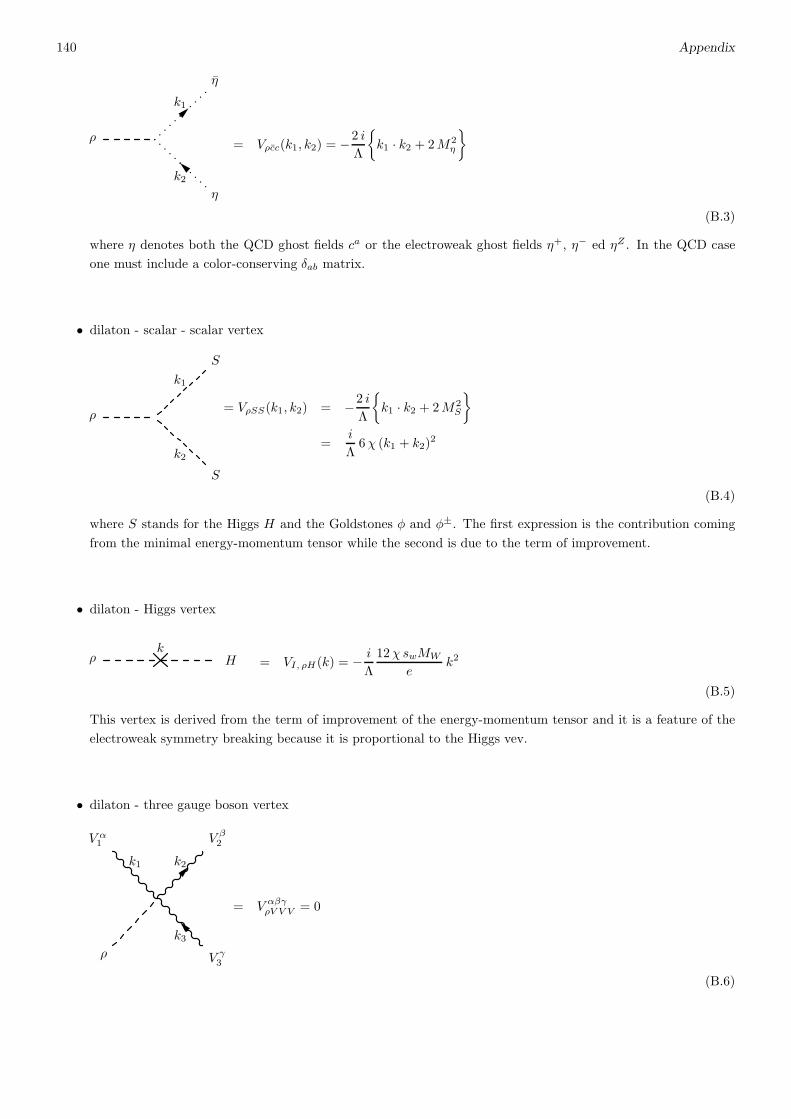
140 Appendix
ρ
η
η
k1
k2
= Vρcc(k1, k2) = −2 i
Λ
k1 · k2 + 2M2η
(B.3)
where η denotes both the QCD ghost fields ca or the electroweak ghost fields η+, η− ed ηZ . In the QCD case
one must include a color-conserving δab matrix.
• dilaton - scalar - scalar vertex
ρ
S
S
k1
k2
= VρSS(k1, k2) = −2 i
Λ
k1 · k2 + 2M2S
=i
Λ6χ (k1 + k2)
2
(B.4)
where S stands for the Higgs H and the Goldstones φ and φ±. The first expression is the contribution coming
from the minimal energy-momentum tensor while the second is due to the term of improvement.
• dilaton - Higgs vertex
ρ Hk
= VI, ρH(k) = − i
Λ
12χ swMW
ek2
(B.5)
This vertex is derived from the term of improvement of the energy-momentum tensor and it is a feature of the
electroweak symmetry breaking because it is proportional to the Higgs vev.
• dilaton - three gauge boson vertex
ρ
V α1
Vγ3
Vβ2
k1
k3
k2
= V αβγρV V V = 0
(B.6)
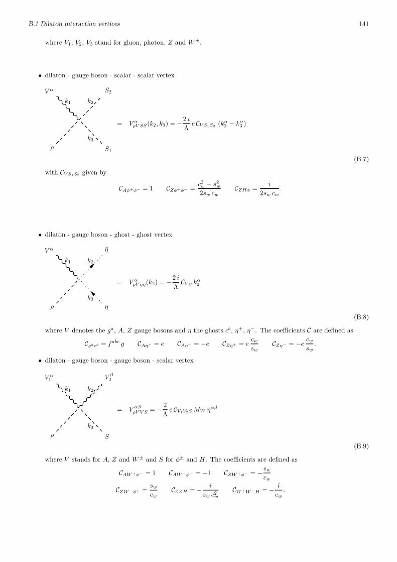
B.1 Dilaton interaction vertices 141
where V1, V2, V3 stand for gluon, photon, Z and W±.
• dilaton - gauge boson - scalar - scalar vertex
ρ
V α
S1
S2
k1
k3
k2
= V αρV SS(k2, k3) = −2 i
Λe CV S1S2 (kα2 − kα3 )
(B.7)
with CV S1S2 given by
CAφ+φ− = 1 CZφ+φ− =c2w − s2w2sw cw
CZHφ =i
2sw cw.
• dilaton - gauge boson - ghost - ghost vertex
ρ
V α
η
η
k1
k3
k2
= V αρV ηη(k2) = −2 i
ΛCV η kα2
(B.8)
where V denotes the ga, A, Z gauge bosons and η the ghosts cb, η+, η−. The coefficients C are defined as
Cgacb = fabc g CAη+ = e CAη− = −e CZη+ = ecwsw
CZη− = −e cwsw.
• dilaton - gauge boson - gauge boson - scalar vertex
ρ
V α1
S
Vβ2
k1
k3
k2
= V αβρV V S = − 2
Λe CV1V2SMW ηαβ
(B.9)
where V stands for A, Z and W± and S for φ± and H . The coefficients are defined as
CAW+φ− = 1 CAW−φ+ = −1 CZW+φ− = −swcw
CZW−φ+ =swcw
CZZH = − i
sw c2wCW+W−H = − i
cw.

142 Appendix
• dilaton - scalar - ghost - ghost vertex
ρ
S
η
η
k1
k3
k2
= V ρSηη = −4 i
Λe CSηMW
(B.10)
where S = H and η denotes η+, η− and ηz. The vertex is defined with the coefficients
CHη+ = CHη− =1
2swCHηz =
1
2sw cw.
• dilaton - three scalar vertex
ρ
S1
S3
S2
k1
k3
k2
= VρSSS = −4 i
Λe CS1S2S3
(B.11)
with S denoting H , φ and φ±. We have defined the coefficients
CHφφ = CHφ+φ− =1
2sw cw
M2H
MZCHHH =
3
2sw cw
M2H
MZ.
• dilaton - scalar - fermion - fermion vertex
ρ
S
ψ
ψ
k1
k3
k2
= VρSψψ = −2 i
Λ
e
sw cw
mf
MZ
(B.12)
where S is only the Higgs scalar H .

B.1 Dilaton interaction vertices 143
• dilaton - gluon - fermion - fermion vertex
ρ
g
ψ
ψ
k3
k2
= V aαρgψψ =3 i
Λg T a γα .
(B.13)
• dilaton - photon - fermion - fermion vertex
ρ
Aα
ψ
ψ
k1
k3
k2
= V αργψψ = Qf e3 i
Λγα
(B.14)
where Qf is the fermion charge expressed in units of e.
• dilaton - Z - fermion - fermion vertex
ρ
Zα
ψ
ψ
k1
k3
k2
= V αρZψψ =3 i
2Λsw cwe (Cfv − Cfa γ
5) γα
(B.15)
where Cfv and Cfa are the vector and axial-vector couplings of the Z gauge boson to the fermion (f). Their
expressions are
Cfv = If3 − 2s2wQf Cfa = If3 .
If3 denotes the 3rd component of the isospin.
144 Appendix
• dilaton - four gauge bosons vertex
Vγ3
Vβ2
V α1
ρ
V δ4
= V αβγδρV V V V = 0
(B.16)
where V1, V2, V3 and V4 denote g, A, Z or W±.
• dilaton - gauge boson - gauge boson - scalar - scalar vertex
S1
Vβ2
V α1
ρ
S2
= V αβρV V SS =2 i
Λe2 CV1V2S1S2 η
αβ
(B.17)
where V1 and V2 denote the neutral gauge bosons A and Z, while the possible scalars are φ, φ± and H . The
coefficients are
CAAφ+φ− = 2 CAZφ+φ− =c2w − s2wsw cw
CZZφ+φ− =
(
c2w − s2w)2
2s2w c2w
CZZφφ = CZZHH =1
2s2w c2w
.
B.2 The scalar integrals
We collect in this appendix the definition of the scalar integrals appearing in the computation of the correlators. 1-,
2- and 3-point functions are denoted, respectively as A0, B0 and C0, with
A0(m20) =
1
iπ2
∫
dnl1
l2 −m20
,
B0(k2,m2
0,m21) =
1
iπ2
∫
dnl1
(l2 −m20) ((l + k)2 −m2
1),
C0((p+ q)2, p2, q2,m20,m
21,m
22) =
1
iπ2
∫
dnl1
(l2 −m20) ((l + p)2 −m2
1) ((l − q)2 −m22). (B.18)
We have also used the finite combination of 2-point scalar integrals
D0(p2, q2,m2
0,m21) = B0(p
2,m20,m
21)− B0(q
2,m20,m
21) . (B.19)
The explicit expressions of A0, B0 and C0 can be found in [116].
B.3 Contributions to VρZZ 145
B.3 Contributions to VρZZ• The fermion sector
ΦFZZ(p, q) =∑
f
αm2f
π sc2ws2w (s− 4M2
Z)
(
s− 2M2Z
) (
Cf 2a + Cf 2
v
)
+2αm2
f
π sc2w (s− 4M2Z)
2s2w
[(
2M4Z − 3sM2
Z + s2)
Cf 2a + Cf 2
v M2Z
(
2M2Z + s
)]
D0(s,M2Z ,m
2f ,m
2f)
+αm2
f
2 π sc2w (s− 4M2Z)
2s2w
(
s− 2M2Z
) [
4M4Z − 2
(
8m2f + s
)
M2Z + s
(
4m2f + s
)]
Cf 2a
+Cf 2v
[
4M4Z + 2
(
3s− 8m2f
)
M2Z − s
(
s− 4m2f
)]
C0(s,M2Z ,M
2Z ,m
2f ,m
2f ,m
2f )
ΞFZZ (p, q) =∑
f
−αm2
f
π sc2w (s− 4M2Z) s
2w
[(
2M4Z − 4sM2
Z + s2)
Cf 2a + 2Cf 2
v M4Z
]
−αm2
f
π c2ws2w
Cf 2a B0(s,m
2f ,m
2f )−
2αm2f M
2Z
π sc2w (s− 4M2Z)
2s2w
[
s2Cf 2a − 2
(
Cf 2a + Cf 2
v
)
M4Z
+2s(
Cf 2v − Cf 2
a
)
M2Z
]
D0(s,M2Z ,m
2f ,m
2f )−
αm2f
π sc2w (s− 4M2Z)
2s2w
[
[
4M8Z
−2(
8m2f + 5s
)
M6Z + 3s
(
12m2f + s
)
M4Z − 16s2m2
fM2Z + 2s3m2
f
]
Cf 2a
+Cf 2v M4
Z
[
4M4Z − 2
(
8m2f + s
)
M2Z + s
(
4m2f + s
)]
]
C0(s,M2Z ,M
2Z ,m
2f ,m
2f ,m
2f )
• The W boson sector
ΦWZZ(p, q) =α
s2w c2w π
[
M2Z
2 s (s− 4M2Z)
[
2M2Z
(
−12s6w + 32s4w − 29s2w + 9)
+ s(
12s6w − 36s4w + 33s2w − 10) ]
]
+αM2
Z
2 s2w c2w π s (s− 4MZ)2
[4M4Z(12s
6w − 32s4w + 29s2w − 9)
+2M2Zs(s
2w − 2)(12s4w − 12s2w + 1) + s2(−4s4w + 8s2w − 5)]D0(s,M
2Z ,M
2W ,M
2W )
+αM2
Z
2 π s2w c2w s (s− 4MZ)2
[
− 4M6Z(s
2w − 1)(4s2w − 3)(12s4w − 20s2w + 9)
+2M4Zs(18s
4w − 34s2w + 15)(4(s2w − 3)s2w + 7)− 2M2
Zs2(12s8w − 96s6w + 201s4w − 157s2w + 41) +
s3(−12s6w + 32s4w − 27s2w + 7)
]
C0(s,M2Z ,M
2Z ,M
2W ,M
2W ,M
2W )
ΞWZZ(p, q) =αM2
Z
2 π s2w c2w s(s− 4M2
Z)
[
2M4Z
(
−12s6w + 32s4w − 29s2w + 9)
+sM2Z
[
4(
s4w + s2w)
− 7]
− 2s2(
s2w − 1)
]
+αM2
Z
π s2wc2w
(−2s4w + 3s2w − 1)B0(s,M2W ,M
2W )
+αM2
Z
π s2w c2w s(s−M2
Z)2
[
2M6Z
(
12s6w − 32s4w + 29s2w − 9)
+ sM4Z
(
−24s6w + 92s4w − 110s2w + 41)
+s2M2Z
(
−12s4w + 26s2w − 13)
+ 2s3(
s2w − 1)2 ]D0(s,M
2Z ,M
2W ,M
2W )
+αM2
Z
4 π s2w c2w s(s−M2
Z)2
[
− 8M8Z
(
s2w − 1) (
4s2w − 3) (
12s4w − 20s2w + 9)
+4sM6Z
(
24s8w − 60s6w + 30s4w + 25s2w − 18)
+ 2s2M4Z(−20s6w + 76s4w − 103s2w + 46)
+s3M2Z
(
−4s4w + 24s2w − 19)
− 2s4(
s2w − 1) ]
C0(s,M2Z ,M
2Z ,M
2W ,M
2W ,M
2W )
146 Appendix
• The (Z,H) sector
ΦZHZZ (p, q) =−α
4 π s c2ws2w (s− 4M2
Z)
[
M2H
(
s− 2M2Z
)
+ 3sM2Z − 2M4
Z
]
+2(
M2Z −M2
H
) (
A0(M2Z)−A0(M
2H))
+1
(s− 4M2Z)
[
2M2H
(
sM2Z − 2M4
Z + s2)
+ 3s2M2Z − 14sM4
Z + 8M6Z
]
B0(s,M2Z ,M
2Z)
− 1
(s− 4M2Z)
(
2M2H + s
) [
2M2H
(
s−M2Z
)
− 3sM2Z
]
B0(s,M2H ,M
2H)
+2
(s− 4M2Z)
[
sM4H + 6
(
s−M2H
)
M4Z +
(
2M4H − 3sM2
H − 3s2)
M2Z
]
B0(M2Z ,M
2Z ,M
2H)
+
(
2M2H + s
)
(s− 4M2Z)
[
M2Z
(
−8sM2H − 2M4
H + s2)
+ 2M4Z
(
4M2H + s
)
+ 2sM4H
]
C0(s,M2Z ,M
2Z ,M
2Z ,M
2H ,M
2H)
+M2H
(s− 4M2Z)
[
2M2H
(
sM2Z − 2M4
Z + s2)
− 20sM4Z + 16M6
Z + s3]
C0(s,M2Z ,M
2Z ,M
2H ,M
2Z ,M
2Z)
ΞZHZZ (p, q) = − α
8 π s c2ws2w (s− 4M2
Z)
− 4M2Z
(
M4Z +M2
HM2Z − 3sM2
Z + s2)
+2(
M2H −M2
Z
) (
s− 2M2Z
) (
A0(M2Z)−A0(M
2H))
− 1
(s− 4M2Z)
[(
8M6Z + s3
)
M2H +M2
Z
(
s− 4M2Z
) (
s− 2M2Z
) (
3s− 2M2Z
)]
B0(s,M2Z ,M
2Z)
+1
(s− 4M2Z)
[
2(
4M4H − s2
)
M4Z − s
(
2M2H + s
)
2M2Z + s2M2
H
(
2M2H + s
)]
B0(s,M2H ,M
2H)
+8M2
Z
(s− 4M2Z)
[
−sM4H −
(
3M2H + 5s
)
M4Z +
(
M2H + s
) (
M2H + 2s
)
M2Z
]
B0(M2Z ,M
2Z ,M
2H)
−(
2M2H + s
)
(s− 4M2Z)
[
4(
7s− 4M2H
)
M6Z + 4
(
M2H − s
) (
M2H + 3s
)
M4Z
+2s(
−M4H − 2sM2
H + s2)
M2Z + s2M4
H
]
C0(s,M2Z ,M
2Z ,M
2Z ,M
2H ,M
2H)
− 1
(s− 4M2Z)
[(
8M6Z + s3
)
M4H + 4M2
Z
(
s− 4M2Z
) (
2M4Z − sM2
Z + s2)
M2H
+4sM4Z
(
s− 4M2Z
)
2]
C0(s,M2Z ,M
2Z ,M
2H ,M
2Z ,M
2Z)
• Term of improvement
ΦIZZ(p, q) =3χα
2 π s2w c2w (s− 4M2
Z)2
(c2w − s2w)2
[
2M2Zs− 8M4
Z
+2M2Z(s+ 2M2
Z)D0
(
s,M2Z,M
2W ,M
2W
)
+ 2(
c2wM2Z(8M
4Z − 6M2
Zs+ s2)− 2M6Z + 2M4
Zs)
×C0(
s,M2Z ,M
2Z ,M
2W ,M
2W ,M
2W
)
]
+ 2M2Zs− 8M4
Z + 2M2Z(s+ 2M2
Z)[
B0
(
s,M2Z ,M
2Z
)
−B0
(
M2Z ,M
2Z ,M
2H
) ]
+(
3M2Zs− 2M2
H(s−M2Z)) [
B0
(
s,M2H ,M
2H
)
− B0
(
s,M2Z ,M
2Z
) ]
+M2H
(
2M2H(s−M2
Z) + 8M4Z − 6M2
Zs+ s2)
C0(
s,M2Z ,M
2Z ,M
2H ,M
2Z ,M
2Z
)
+(
2M2H(M
2H − 4M2
Z)(s−M2Z) + sM2
Z(s+ 2M2Z))
C0(
s,M2Z ,M
2Z ,M
2Z ,M
2H ,M
2H
)
B.3 Contributions to VρZZ 147
ΞIZZ(p, q) = − 3χαs
8 π s2w c2w(s− 4M2
Z)2
(c2w − s2w)2
[
4M4Z(s− 4M2
Z) + 8M4Z(s−M2
Z)D0
(
s,M2Z,M
2W ,M
2W
)
+2M4Z
[
s2 − 2M2Zs+ 4M4
Z + 4c2wM2Z(s− 4M2
Z)]
C0(
s,M2Z ,M
2Z ,M
2W ,M
2W ,M
2W
)
]
+4M2Zs
4wc
2ws(s− 4M2
Z)2C0
(
s,M2Z ,M
2Z ,M
2W ,M
2W ,M
2W
)
+ 4M2Z(s− 4M2
Z)
+[
M2Zs(s+ 2M2
Z)−M2H(s
2 − 2M2Zs+ 4M4
Z)] [
B0
(
s,M2H ,M
2H
)
− B0
(
s,M2Z,M
2Z
) ]
+8M4Z(s−M2
Z)[
B0
(
s,M2Z ,M
2Z
)
− B0
(
M2Z ,M
2Z ,M
2H
) ]
+M2H
[
4M4Z(s− 4M2
Z)
+M2H(s
2 − 2MZ2s+ 4M4Z)]
C0(
s,M2Z ,M
2Z ,M
2H ,M
2Z,M
2Z
)
+[
M2H(M
2H − 4M2
Z)(s2 − 2M2
Zs+ 4M4Z)
+2M2Zs(s
2 − 6M2Zs+ 14M4
Z)]
C0(
s,M2Z ,M
2Z ,M
2Z ,M
2H ,M
2H
)
.
• External leg corrections
The ∆αβ(p, q) correlator is decomposed as
∆αβ(p, q) =
[
ΣMin, ρH(k2) + ΣI, ρH(k2)
]
1
s−M2H
V αβHZZ +
(
Λ
i
)
VI, ρH(k)1
s−M2H
ΣHH(k2)1
s−M2H
V αβHZZ
+ ∆αβI,HZZ(p, q)
where ΣHH(k2) is the Higgs self-energy, V αβHZZ and VI, ρH are tree level vertices defined in appendix (B.1) and
∆αβI, HZZ(p, q) is expanded into the three contributions of improvement as
∆αβI,HZZ = ∆αβ
(F ), HZZ (p, q) + ∆αβ(W ), HZZ (p, q) + ∆αβ
(Z,H), HZZ (p, q)
=[(s
2−M2
Z
)
ηαβ − qαpβ]
Φ∆ZZ(p, q) + ηαβ Ξ∆
ZZ(p, q)
=[(s
2−M2
Z
)
ηαβ − qαpβ]
(
Φ∆FZZ (p, q) + Φ∆W
ZZ (p, q) + Φ∆WZZ (p, q)
)
+ ηαβ(
Ξ∆FZZ (p, q) + Ξ∆W
ZZ (p, q) + Ξ∆WZZ (p, q)
)
.
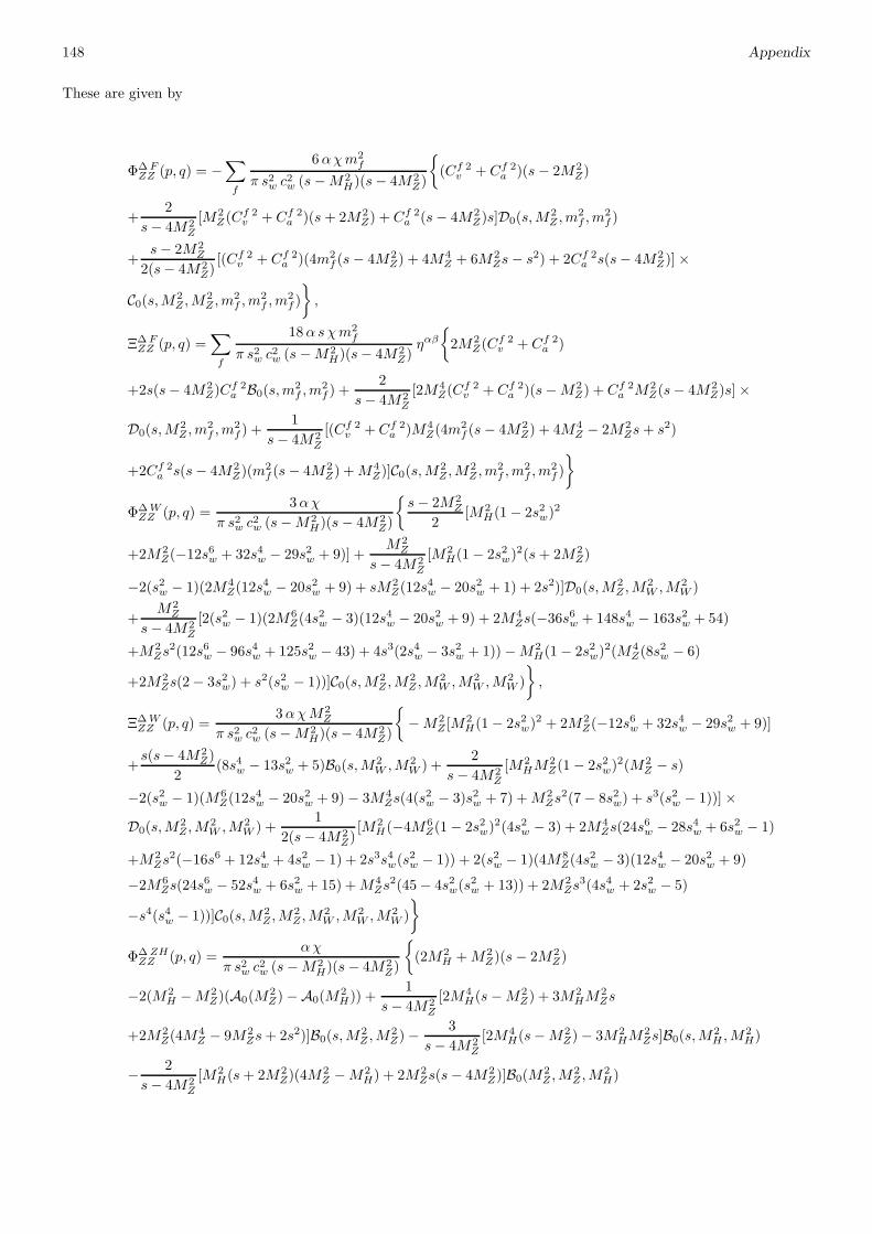
148 Appendix
These are given by
Φ∆FZZ (p, q) = −
∑
f
6αχm2f
π s2w c2w (s−M2
H)(s− 4M2Z)
(Cf 2v + Cf 2
a )(s− 2M2Z)
+2
s− 4M2Z
[M2Z(C
f 2v + Cf 2
a )(s+ 2M2Z) + Cf 2
a (s− 4M2Z)s]D0(s,M
2Z ,m
2f ,m
2f )
+s− 2M2
Z
2(s− 4M2Z)
[(Cf 2v + Cf 2
a )(4m2f (s− 4M2
Z) + 4M4Z + 6M2
Zs− s2) + 2Cf 2a s(s− 4M2
Z)]×
C0(s,M2Z ,M
2Z ,m
2f ,m
2f ,m
2f )
,
Ξ∆FZZ (p, q) =
∑
f
18α sχm2f
π s2w c2w (s−M2
H)(s− 4M2Z)
ηαβ
2M2Z(C
f 2v + Cf 2
a )
+2s(s− 4M2Z)C
f 2a B0(s,m
2f ,m
2f ) +
2
s− 4M2Z
[2M4Z(C
f 2v + Cf 2
a )(s−M2Z) + Cf 2
a M2Z(s− 4M2
Z)s]×
D0(s,M2Z ,m
2f ,m
2f ) +
1
s− 4M2Z
[(Cf 2v + Cf 2
a )M4Z(4m
2f (s− 4M2
Z) + 4M4Z − 2M2
Zs+ s2)
+2Cf 2a s(s− 4M2
Z)(m2f (s− 4M2
Z) +M4Z)]C0(s,M2
Z ,M2Z ,m
2f ,m
2f ,m
2f )
Φ∆WZZ (p, q) =
3αχ
π s2w c2w (s−M2
H)(s− 4M2Z)
s− 2M2Z
2[M2
H(1− 2s2w)2
+2M2Z(−12s6w + 32s4w − 29s2w + 9)] +
M2Z
s− 4M2Z
[M2H(1− 2s2w)
2(s+ 2M2Z)
−2(s2w − 1)(2M4Z(12s
4w − 20s2w + 9) + sM2
Z(12s4w − 20s2w + 1) + 2s2)]D0(s,M
2Z ,M
2W ,M
2W )
+M2Z
s− 4M2Z
[2(s2w − 1)(2M6Z(4s
2w − 3)(12s4w − 20s2w + 9) + 2M4
Zs(−36s6w + 148s4w − 163s2w + 54)
+M2Zs
2(12s6w − 96s4w + 125s2w − 43) + 4s3(2s4w − 3s2w + 1))−M2H(1− 2s2w)
2(M4Z(8s
2w − 6)
+2M2Zs(2− 3s2w) + s2(s2w − 1))]C0(s,M2
Z ,M2Z ,M
2W ,M
2W ,M
2W )
,
Ξ∆WZZ (p, q) =
3αχM2Z
π s2w c2w (s−M2
H)(s− 4M2Z)
−M2Z [M
2H(1− 2s2w)
2 + 2M2Z(−12s6w + 32s4w − 29s2w + 9)]
+s(s− 4M2
Z)
2(8s4w − 13s2w + 5)B0(s,M
2W ,M
2W ) +
2
s− 4M2Z
[M2HM
2Z(1− 2s2w)
2(M2Z − s)
−2(s2w − 1)(M6Z(12s
4w − 20s2w + 9)− 3M4
Zs(4(s2w − 3)s2w + 7) +M2
Zs2(7− 8s2w) + s3(s2w − 1))]×
D0(s,M2Z ,M
2W ,M
2W ) +
1
2(s− 4M2Z)
[M2H(−4M6
Z(1− 2s2w)2(4s2w − 3) + 2M4
Zs(24s6w − 28s4w + 6s2w − 1)
+M2Zs
2(−16s6 + 12s4w + 4s2w − 1) + 2s3s4w(s2w − 1)) + 2(s2w − 1)(4M8
Z(4s2w − 3)(12s4w − 20s2w + 9)
−2M6Zs(24s
6w − 52s4w + 6s2w + 15) +M4
Zs2(45− 4s2w(s
2w + 13)) + 2M2
Zs3(4s4w + 2s2w − 5)
−s4(s4w − 1))]C0(s,M2Z ,M
2Z ,M
2W ,M
2W ,M
2W )
Φ∆ZHZZ (p, q) =
αχ
π s2w c2w (s−M2
H)(s− 4M2Z)
(2M2H +M2
Z)(s− 2M2Z)
−2(M2H −M2
Z)(A0(M2Z)−A0(M
2H)) +
1
s− 4M2Z
[2M4H(s−M2
Z) + 3M2HM
2Zs
+2M2Z(4M
4Z − 9M2
Zs+ 2s2)]B0(s,M2Z ,M
2Z)−
3
s− 4M2Z
[2M4H(s−M2
Z)− 3M2HM
2Zs]B0(s,M
2H ,M
2H)
− 2
s− 4M2Z
[M2H(s+ 2M2
Z)(4M2Z −M2
H) + 2M2Zs(s− 4M2
Z)]B0(M2Z ,M
2Z ,M
2H)

B.4 Standard Model self-energies 149
− 3M2H
s− 4M2Z
[2M2H(s−M2
Z)(4M2Z −M2
H)−M2Zs(s+ 2M2
Z)]C0(s,M2Z ,M
2Z ,M
2Z ,M
2H ,M
2H) +
M2H
s− 4M2Z
×
[2M4H(s−M2
Z) +M2H(4M4
Z − 2M2Zs+ s2) + 2M2
Z(8M4Z − 14M2
Zs+ 3s2)]C0(s,M2Z ,M
2Z ,M
2H ,M
2Z,M
2Z)
Ξ∆ZHZZ (p, q) = − 3αχ
π s2w c2w (s−M2
H)(s− 4M2Z)
M4Z(2M
2H +M2
Z)
+1
2(M2
Z −M2H)(s− 2M2
Z)(A0(M2Z)−A0(M
2H)) +
1
4(s− 4M2Z)
[M4H(4M
4Z − 2M2
Zs+ s2)
+M2HM
2Zs(s+ 2M2
Z)−M2Z(16M
6Z − 28M4
Zs+ 18M2Zs
2 − 3s3)]B0(s,M2Z ,M
2Z)
− 3M2H
4(s− 4M2Z)
[M2H(4M4
Z − 2M2Zs+ s2)−M2
Zs(s+ 2M2Z)]B0(s,M
2H ,M
2H)
+2
s− 4M2Z
[M2Zs(M
2H − 2M2
Z)2 −M2
HM4Z(M
2H − 4M2
Z)−M4Zs
2]B0(M2Z ,M
2Z ,M
2H)
+3M2
H
4(s− 4M2Z)
× [M2H(4M
4Z − 2M2
Zs+ s2)(M2H − 4M2
Z) + 2M2Zs(16M
4Z − 6M2
Zs+ s2)] ×
C0(s,M2Z ,M
2Z ,M
2Z ,M
2H ,M
2H) +
1
4(s− 4M2Z)
[M6H(4M4
Z − 2M2Zs+ s2) + 2M4
HM2Z(s
2 − 4M4Z)
−4M2HM
2Z(8M
6Z − 10M4
Zs+ 6M2Zs
2 − s3) + 4M4Zs(s− 4M2
Z)2]C0(s,M2
Z ,M2Z ,M
2H ,M
2Z ,M
2Z)
ΣMin, ρH(k2) =e
48π2 sw cwMZ
∑
f
m2f
[
3(4m2f − k2)B0(k
2,m2f ,m
2f ) + 12A0(m
2f )− 2k2 + 12m2
f
]
− 1
2
[
3(
k2(M2H − 6M2
W ) + 2M2W (M2
H + 6M2W ))
B0(k2,M2
W ,M2W ) + 6(M2
H + 6M2W )A0(M
2W )
−k2(M2H + 18M2
W ) + 6M2W (M2
H − 2M2W )
]
− 1
4
[
3(
M2H(2M2
Z + s) + 12M4Z − 6M2
Zs)
× B0(s,M2Z ,M
2Z) + 9M2
H(2M2H + s)B0(s,M
2H ,M
2H) + 6(M2
H + 6M2Z)A0(M
2Z) + 18M2
HA0(M2H)
+2(9M4H +M2
H(3M2Z − 2s)− 6M4
Z − 9M2Zs)
]
ΣI, ρH(k2) =3e
16π2 sw cw
k2M2H
M2Z
χ
[
B0(k2,M2
W ,M2W ) +
3
2B0(k
2,M2H ,M
2H) +
1
2B0(k
2,M2Z ,M
2Z)
]
B.4 Standard Model self-energies
We report here the expressions of the self-energies appearing in Section 4.2.4 which define the renormalization condi-
tions. They are given by
ΣγγT (p2) = − α
4π
2
3
∑
f
NfC2Q
2f
[
− (p2 + 2m2f )B0(p
2,m2f ,m
2f ) + 2m2
fB0(0,m2f ,m
2f ) +
1
3p2]
+
[
(3p2 + 4M2W )B0(p
2,M2W ,M
2W )− 4M2
WB0(0,M2W ,M
2W )
]
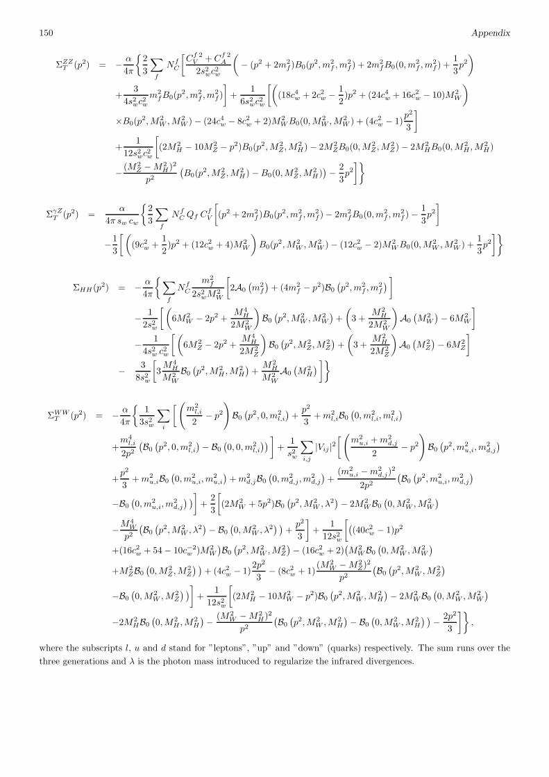
150 Appendix
ΣZZT (p2) = − α
4π
2
3
∑
f
NfC
[
Cf 2V + Cf 2
A
2s2wc2w
(
− (p2 + 2m2f)B0(p
2,m2f ,m
2f ) + 2m2
fB0(0,m2f ,m
2f ) +
1
3p2)
+3
4s2wc2w
m2fB0(p
2,m2f ,m
2f )
]
+1
6s2wc2w
[(
(18c4w + 2c2w − 1
2)p2 + (24c4w + 16c2w − 10)M2
W
)
×B0(p2,M2
W ,M2W )− (24c4w − 8c2w + 2)M2
WB0(0,M2W ,M
2W ) + (4c2w − 1)
p2
3
]
+1
12s2wc2w
[
(2M2H − 10M2
Z − p2)B0(p2,M2
Z,M2H)− 2M2
ZB0(0,M2Z ,M
2Z)− 2M2
HB0(0,M2H ,M
2H)
− (M2Z −M2
H)2
p2(
B0(p2,M2
Z ,M2H)−B0(0,M
2Z,M
2H))
− 2
3p2]
ΣγZT (p2) =α
4π sw cw
2
3
∑
f
NfC Qf C
fV
[
(p2 + 2m2f )B0(p
2,m2f ,m
2f )− 2m2
fB0(0,m2f ,m
2f )−
1
3p2]
−1
3
[(
(9c2w +1
2)p2 + (12c2w + 4)M2
W
)
B0(p2,M2
W ,M2W )− (12c2w − 2)M2
WB0(0,M2W ,M
2W ) +
1
3p2]
ΣHH(p2) = − α
4π
∑
f
NfC
m2f
2s2wM2W
[
2A0
(
m2f
)
+ (4m2f − p2)B0
(
p2,m2f ,m
2f
)
]
− 1
2s2w
[(
6M2W − 2p2 +
M4H
2M2W
)
B0
(
p2,M2W ,M
2W
)
+
(
3 +M2H
2M2W
)
A0
(
M2W
)
− 6M2W
]
− 1
4s2w c2w
[(
6M2Z − 2p2 +
M4H
2M2Z
)
B0
(
p2,M2Z ,M
2Z
)
+
(
3 +M2H
2M2Z
)
A0
(
M2Z
)
− 6M2Z
]
− 3
8s2w
[
3M4H
M2W
B0
(
p2,M2H ,M
2H
)
+M2H
M2W
A0
(
M2H
)
]
ΣWWT (p2) = − α
4π
1
3s2w
∑
i
[
(
m2l,i
2− p2
)
B0
(
p2, 0,m2l,i
)
+p2
3+m2
l,iB0
(
0,m2l,i,m
2l,i
)
+m4l,i
2p2(
B0
(
p2, 0,m2l,i
)
− B0
(
0, 0,m2l,i
))
]
+1
s2w
∑
i,j
|Vij |2[
(
m2u,i +m2
d,j
2− p2
)
B0
(
p2,m2u,i,m
2d,j
)
+p2
3+m2
u,iB0
(
0,m2u,i,m
2u,i
)
+m2d,jB0
(
0,m2d,j,m
2d,j
)
+(m2
u,i −m2d,j)
2
2p2(
B0
(
p2,m2u,i,m
2d,j
)
−B0
(
0,m2u,i,m
2d,j
) )
]
+2
3
[
(2M2W + 5p2)B0
(
p2,M2W , λ
2)
− 2M2WB0
(
0,M2W ,M
2W
)
−M4W
p2(
B0
(
p2,M2W , λ
2)
− B0
(
0,M2W , λ
2) )
+p2
3
]
+1
12s2w
[
(
(40c2w − 1)p2
+(16c2w + 54− 10c−2w )M2
W
)
B0
(
p2,M2W ,M
2Z
)
− (16c2w + 2)(
M2WB0
(
0,M2W ,M
2W
)
+M2ZB0
(
0,M2Z ,M
2Z
) )
+ (4c2w − 1)2p2
3− (8c2w + 1)
(M2W −M2
Z)2
p2(
B0
(
p2,M2W ,M
2Z
)
−B0
(
0,M2W ,M
2Z
) )
]
+1
12s2w
[
(2M2H − 10M2
W − p2)B0
(
p2,M2W ,M
2H
)
− 2M2WB0
(
0,M2W ,M
2W
)
−2M2HB0
(
0,M2H ,M
2H
)
− (M2W −M2
H)2
p2(
B0
(
p2,M2W ,M
2H
)
− B0
(
0,M2W ,M
2H
) )
− 2p2
3
]
,
where the subscripts l, u and d stand for ”leptons”, ”up” and ”down” (quarks) respectively. The sum runs over the
three generations and λ is the photon mass introduced to regularize the infrared divergences.
Bibliography
[1] R. Feynman, Phys.Rev. 76, 749 (1949).
[2] R. Feynman, Phys.Rev. 74, 1430 (1948).
[3] R. Feynman, Phys.Rev. 76, 769 (1949).
[4] R. Feynman, Phys.Rev. 80, 440 (1950).
[5] R. Feynman, Phys.Rev. 74, 939 (1948).
[6] R. P. Feynman, Phys.Rev. 84, 108 (1951).
[7] J. S. Schwinger, Phys.Rev. 73, 416 (1948).
[8] J. S. Schwinger, Phys.Rev. 74, 1439 (1948).
[9] J. S. Schwinger, Phys.Rev. 75, 651 (1948).
[10] J. S. Schwinger, Phys.Rev. 76, 790 (1949).
[11] J. Schwinger, Phys.Rev. 75, 898 (1949).
[12] J. S. Schwinger, Phys.Rev. 82, 914 (1951).
[13] J. S. Schwinger, Phys.Rev. 91, 713 (1953).
[14] S. Tomonaga, Prog.Theor.Phys. 1, 27 (1946).
[15] F. Dyson, Phys.Rev. 75, 486 (1949).
[16] F. Dyson, Phys.Rev. 75, 1736 (1949).
[17] G. ’t Hooft, Nucl.Phys. B33, 173 (1971).
[18] G. ’t Hooft, Nucl.Phys. B35, 167 (1971).
[19] J. Polchinski, Nucl.Phys. B303, 226 (1988).
[20] A. Iorio, L. O’Raifeartaigh, I. Sachs, and C. Wiesendanger, Nucl.Phys.B495, 433 (1997), arXiv:hep-th/9607110.
[21] D. Capper and M. Duff, Nuovo Cim. A23, 173 (1974).
[22] D. Capper and M. Duff, Nucl.Phys. B82, 147 (1974).
[23] D. Capper, M. Duff, and L. Halpern, Phys.Rev. D10, 461 (1974).
[24] M. J. Duff, Nucl. Phys. B125, 334 (1977).
[25] M. J. Duff, Class. Quant. Grav. 11, 1387 (1994), arXiv:hep-th/9308075.
151

152 BIBLIOGRAPHY
[26] N. Birrell and P. Davies, Cambridge Monogr.Math.Phys. (1982).
[27] M. Giannotti and E. Mottola, Phys. Rev. D79, 045014 (2009), arXiv:0812.0351.
[28] G. ’t Hooft, NATO Adv.Study Inst.Ser.B Phys. 59, 135 (1980).
[29] E. Mottola and R. Vaulin, Phys. Rev. D74, 064004 (2006), arXiv:gr-qc/0604051.
[30] K. Wilson and J. B. Kogut, Phys.Rept. 12, 75 (1974).
[31] J. Wess and B. Zumino, Phys.Lett. B37, 95 (1971).
[32] C. Coriano, M. Guzzi, and S. Morelli, Eur. Phys. J. C55, 629 (2008), arXiv:0801.2949.
[33] J. S. Schwinger, Phys.Rev. 82, 664 (1951).
[34] S. L. Adler, Phys.Rev. 177, 2426 (1969).
[35] J. Bell and R. Jackiw, Nuovo Cim. A60, 47 (1969).
[36] A. D. Dolgov and V. I. Zakharov, Nucl. Phys. B27, 525 (1971).
[37] S. Deser, M. J. Duff, and C. J. Isham, Nucl. Phys. B111, 45 (1976).
[38] P. O. Mazur and E. Mottola, Phys.Rev. D64, 104022 (2001), arXiv:hep-th/0106151.
[39] N. Boulanger, Phys.Rev.Lett. 98, 261302 (2007).
[40] N. Boulanger, JHEP 0707, 069 (2007).
[41] R. J. Riegert, Phys.Lett. B134, 56 (1984).
[42] R. Armillis, C. Coriano, and L. Delle Rose, Phys.Rev. D81, 085001 (2010), arXiv:0910.3381.
[43] R. Armillis, C. Coriano, and L. Delle Rose, (2010), arXiv:1005.4173.
[44] C. Coriano, L. Delle Rose, and M. Serino, Phys.Rev. D83, 125028 (2011), arXiv:1102.4558.
[45] C. Coriano, A. Costantini, L. Delle Rose, and M. Serino, (2014), arXiv:1402.6369.
[46] H. Osborn and A. C. Petkou, Ann. Phys. 231, 311 (1994), arXiv:hep-th/9307010.
[47] J. Erdmenger and H. Osborn, Nucl.Phys. B483, 431 (1997), arXiv:hep-th/0103237.
[48] C. Coriano, L. Delle Rose, E. Mottola, and M. Serino, JHEP 1208, 147 (2012), arXiv:1203.1339.
[49] D. Z. Freedman, K. Johnson, and J. I. Latorre, Nucl.Phys. B371, 353 (1992).
[50] A. Schwimmer and S. Theisen, Nucl.Phys. B847, 590 (2011), arXiv:1011.0696.
[51] W. D. Goldberger, B. Grinstein, and W. Skiba, Phys.Rev.Lett. 100, 111802 (2008), arXiv:0708.1463.
[52] C. Coriano, L. Delle Rose, A. Quintavalle, and M. Serino, JHEP 1306, 077 (2013), arXiv:1206.0590.
[53] C. Coriano, L. Delle Rose, C. Marzo, and M. Serino, Phys.Lett. B717, 182 (2012), arXiv:1207.2930.
[54] C. Coriano, L. Delle Rose, C. Marzo, and M. Serino, Phys.Lett. B726, 896 (2013), arXiv:1306.4248.
[55] C. Coriano, L. Delle Rose, C. Marzo, and M. Serino, Class. Quantum Grav. 31, 105009 (2014), arXiv:1311.1804.
[56] Y. Nakayama, (2013), arXiv:1302.0884.
BIBLIOGRAPHY 153
[57] S. Weinberg, Gravitation and cosmology (John Wiley and sons, New York, 1972).
[58] J. Callan, Curtis G., S. R. Coleman, and R. Jackiw, Annals Phys. 59, 42 (1970).
[59] R. J. Riegert, Phys. Lett. B134, 56 (1984).
[60] E. Mottola, Acta Physica Polonica B41, 2031 (2010), arXiv:1008.5006.
[61] A. M. Polyakov, Phys. Lett. B103, 207 (1981).
[62] L. Bonora, P. Cotta-Ramusino, and C. Reina, Phys.Lett. B126, 305 (1983).
[63] I. Antoniadis, P. O. Mazur, and E. Mottola, Nucl. Phys. B388, 627 (1992), hep-th/9205015.
[64] D. Z. Freedman, I. J. Muzinich, and E. J. Weinberg, Ann. Phys. 87, 95 (1974).
[65] D. Z. Freedman and E. J. Weinberg, Annals Phys. 87, 354 (1974).
[66] S. Deser and A. Schwimmer, Phys. Lett. B309, 279 (1993), arXiv:hep-th/9302047.
[67] E. Fradkin and M. Palchik, Phys.Rept. 300, 1 (1998).
[68] A. Bzowski, P. McFadden, and K. Skenderis, JHEP 1203, 091 (2012), arXiv:1112.1967.
[69] J. M. Maldacena and G. L. Pimentel, JHEP 1109, 045 (2011), arXiv:1104.2846.
[70] S. Raju, Phys.Rev. D85, 126008 (2012), arXiv:1201.6452.
[71] C. Coriano, L. Delle Rose, E. Mottola, and M. Serino, JHEP 1307, 011 (2013), arXiv:1304.6944.
[72] A. Bzowski, P. McFadden, and K. Skenderis, (2013), arXiv:1304.7760.
[73] D. Kazakov and A. Kotikov, Theor.Math.Phys. 73, 1264 (1988).
[74] A. Duncan, Phys.Lett. B66, 170 (1977).
[75] S. L. Adler, J. C. Collins, and A. Duncan, Phys. Rev. D15, 1712 (1977).
[76] J. C. Collins, A. Duncan, and S. D. Joglekar, Phys. Rev. D16, 438 (1977).
[77] G. V. Dunne and N. Rius, Phys. Lett. B293, 367 (1992), arXiv:hep-th/9206038.
[78] A. I. Davydychev, J.Phys.A A25, 5587 (1992).
[79] T. Han, J. D. Lykken, and R.-J. Zhang, Phys.Rev. D59, 105006 (1999), arXiv:hep-ph/9811350.
[80] G. F. Giudice, R. Rattazzi, and J. D. Wells, Nucl.Phys. B595, 250 (2001), arXiv:hep-ph/0002178.
[81] M. Knecht, S. Peris, M. Perrottet, and E. de Rafael, JHEP 03, 035 (2004), arXiv:hep-ph/0311100.
[82] F. Jegerlehner and O. V. Tarasov, Phys. Lett. B639, 299 (2006), arXiv:hep-ph/0510308.
[83] R. Armillis, C. Coriano, L. Delle Rose, and M. Guzzi, JHEP 12, 029 (2009), arXiv:0905.0865.
[84] J. Horejsi and M. Schnabl, Z. Phys. C76, 561 (1997), arXiv:hep-ph/9701397.
[85] W. Buchmuller and N. Dragon, Phys.Lett. B195, 417 (1987).
[86] W. Buchmuller and N. Dragon, Nucl.Phys. B321, 207 (1989).
[87] M. Shaposhnikov and D. Zenhausern, Phys.Lett. B671, 162 (2009), arXiv:0809.3406.
154 BIBLIOGRAPHY
[88] K. A. Meissner and H. Nicolai, Phys.Lett. B648, 312 (2007), arXiv:hep-th/0612165.
[89] S. Treiman, E. Witten, R. Jackiw, and B. Zumino, (1986).
[90] L. Faddeev, Phys.Lett. B145, 81 (1984).
[91] O. Babelon, F. Schaposnik, and C. Viallet, Phys.Lett. B177, 385 (1986).
[92] S. Deser, Phys. Lett. B479, 315 (2000), arXiv:hep-th/9911129.
[93] A. M. Polyakov, Phys.Lett. B103, 211 (1981).
[94] M. Chaichian, W. Chen, and C. Montonen, Phys.Rept. 346, 89 (2001), arXiv:hep-th/0007240.
[95] I. Antoniadis, P. O. Mazur, and E. Mottola, Nucl.Phys. B388, 627 (1992), arXiv:hep-th/9205015.
[96] A. Codello, G. D’Odorico, C. Pagani, and R. Percacci, Class.Quant.Grav. 30, 115015 (2013), arXiv:1210.3284.
[97] I. Jack and H. Osborn, Nucl.Phys. B343, 647 (1990).
[98] A. Cappelli, D. Friedan, and J. I. Latorre, Nucl.Phys. B352, 616 (1991).
[99] D. Anselmi, J. Erlich, D. Freedman, and A. Johansen, Phys.Rev. D57, 7570 (1998), arXiv:hep-th/9711035.
[100] Z. Komargodski and A. Schwimmer, JHEP 1112, 099 (2011), arXiv:1107.3987.
[101] K. Yonekura, JHEP 1304, 011 (2013), arXiv:1212.3028.
[102] A. Zamolodchikov, JETP Lett. 43, 730 (1986).
[103] H. Elvang et al., JHEP 1210, 011 (2012), arXiv:1205.3994.
[104] E. Tomboulis, Nucl.Phys. B329, 410 (1990).
[105] F. Bastianelli, S. Frolov, and A. A. Tseytlin, Nucl.Phys. B578, 139 (2000), arXiv:hep-th/9911135.
[106] F. Bastianelli, S. Frolov, and A. A. Tseytlin, JHEP 0002, 013 (2000), arXiv:hep-th/0001041.
[107] T. Henz, J. M. Pawlowski, A. Rodigast, and C. Wetterich, Phys.Lett. B727, 298 (2013), arXiv:1304.7743.
[108] R. Percacci, New J.Phys. 13, 125013 (2011), arXiv:1110.6758.
[109] F. Baume and B. Keren-Zur, (2013), arXiv:1307.0484.
[110] M. Henningson and K. Skenderis, JHEP 9807, 023 (1998), arXiv:hep-th/9806087.
[111] D. Anselmi, Nucl.Phys. B567, 331 (2000), arXiv:hep-th/9905005.
[112] I. Antoniadis and E. Mottola, Phys.Rev. D45, 2013 (1992).
[113] T. Arakelian, D. Karakhanian, R. Manvelyan, and R. Mkrtchian, Phys.Lett. B353, 52 (1995).
[114] T. Parker and S. Rosenberg, J. Differential Geom. 25, 157 (1987).
[115] C. Fefferman and C. R. Graham, (2007), arXiv:0710.0919.
[116] A. Denner, Fortschr. Phys. 41, 307 (1993), arXiv:0709.1075.