YITP-SB-15-??

Conformal Field Theory (for string theorists)

Christopher P. Herzog

C. N. Yang Institute for Theoretical Physics, Department of Physics and Astronomy

Stony Brook University, Stony Brook, NY 11794

Abstract

A write up of about ten lectures on conformal field theory given as part of a first semester course

on string theory.

Contents

1 Opening Remarks 1

2 Conformal Transformations in One and Two Dimensions are Special 3

3 Correlation Functions are Highly Constrained by Conformal Symmetry 4

4 Noether’s Theorem 6

5 Conformal Anomaly 8

6 Path Integral Approach 15

7 BRST meets CFT 19

8 From Operators to States: The Vacuum 23

8.1 Bosonization . . . . . . . . . . . . . . . . . . . . . . . . . . . . . . . . . . . . . . . . 27

8.2 R Sector Fermions . . . . . . . . . . . . . . . . . . . . . . . . . . . . . . . . . . . . . 28

8.3 The βγ System . . . . . . . . . . . . . . . . . . . . . . . . . . . . . . . . . . . . . . . 30

9 From Operators to States: Virasoro and Super Virasoro 32

10 Thermal Partition Function 35

A Bosonization and Cocycles 36

1 Opening Remarks

To date in this class, string theory boils down to the study four free (quadratic) quantum field

theories: one for the X fields, one for the ψ fields, one for the bc ghost system, and one for the βγ

ghost system. We saw a BRST action that coupled the X and ψ fields to world-sheet supergravity,

and hence required the presence of the bc and βγ ghosts in addition to some auxiliary fields d and

∆ and also ghosts for the Weyl and super-Weyl symmetry. After some elementary path-integral

manipulations, these extra fields dropped out, and we were left with simple, quadratic actions for

the remaining X, ψ, bc and βγ fields on a flat world sheet hab = ηab.

The full quantum world-sheet supergravity action had a number of symmetries which are no

longer evident in the gauge fixed action for X, ψ, bc and βγ. Among other symmetries, the full

quantum action had world-sheet diffeomorphism invariance, σ → σ′(σ). Under diffeomorphisms, the

metric changes in the usual way

h′cd(σ′) =

∂σa

∂σ′c∂σb

∂σ′dhab(σ) . (1)

1

Another symmetry was world-sheet Weyl invariance, hab → Λ(x)hab. There were then corresponding

rules for how the fields X, ψ, bc, and βγ transform under diffeomorphisms and Weyl scaling. We

gauge fixed by choosing a flat world-sheet metric hab = ηab. However, this gauge fixing is not

complete. There are residual gauge transformations that are a combination of a diffeomorphism and

a Weyl scaling that leave the metric ηab invariant. These residual gauge transformations are called

conformal transformations:

Definition. A conformal transformation is a map on coordinates σ → σ′ that preserves the metric

up to a scale factor

h′ab(σ) = Λ(σ)hab(σ) .

Example. In the case when hab = ηab, two conformal transformations are

• Elements of the Poincare group (Lorentz group and translations) for which Λ = 1.

• Dilations x→ λx, λ ∈ R, for which Λ = λ2.

Note in the Euclidean case, hab = δab, the Lorentz group is replaced by rotations. Both rota-

tions and dilations manifestly preserve the angles between vectors, motivating the choice of word

“conformal”, which means preserving angles.

Remark. The set of conformal transformations C forms a group when the transformation σ → σ′

is invertible.

Definition. A conformal field theory is a quantum field theory which has C as a classical symmetry

of the action.

Almost all the quantum field theories we study, when coupled to gravity, will be diffeomorphism

invariant. The litmus test for figuring out when a quantum field theory in a fixed background space-

time is a conformal field theory is then the presence of local Weyl invariance. Perhaps as a result, in

the literature there is a certain carelessness and interchanging in the use of the words Weyl scaling

and conformal transformation. We will try to be careful here.

Having fixed hab = ηab, the field theories for X, ψ, bc, and βγ become examples of conformal field

theories. In fact, we will eventually see they are essentially all the same conformal field theory, just

expressed in different variables. We can therefore use the extensive and highly developed machinery

of conformal field theory to systematize our understanding of these four systems. The goal of these

lectures will be four-fold:

1. To replace the cumbersome oscillator algebra manipulations with (in our view) more elegant

operator product expansions.

2. To streamline calculations involving the BRST symmetry.

3. To understand how a quantum anomaly in the classical conformal symmetry restricts the types

of consistent string theories.

4. To set up machinery for string scattering calculations.

2

References

These lecture notes draw largely from chapters 2, 3, 6, 8, and 10 of Polchinski’s classic string theory

text book [1]. I have also drawn on early chapters in Di Francesco, Senechal, and Mathieu’s classic

work on conformal field theory [2] and P. van Nieuwenhuizen’s unpublished string theory lecture

notes [3]. Another nice publicly available reference I found are unpublished notes by M. Kreuzer [4].

2 Conformal Transformations in One and Two Dimensions

are Special

In one dimension, any diffeomorphism y(x) is conformal with g′yy = ∂x∂y

∂x∂y gxx.

In two dimensions, for convenience, consider the Euclidean case hab = δab.1 We take advantage

of complex numbers:

z = σ1 + iσ2 , z = σ1 − iσ2 , (2)

∂ ≡ ∂z =1

2(∂1 − i∂2) , ∂ ≡ ∂z =

1

2(∂1 + i∂2) . (3)

The world sheet metric then has components

hzz = hzz =1

2, hzz = hzz = 0 . (4)

In complex coordinates, any holomorphic transformation z → w(z) along with its anti-holomorphic

counterpart z → w(z) is conformal:

h′ww(w, w) =∂z

∂w

∂z

∂whzz(z, z) where Λ =

∂z

∂w

∂z

∂w. (5)

In more than two dimensions, the set of conformal transformations is far smaller. It is generated

by

• translations: xµ → xµ + aµ.

• dilations: xµ → axµ.

• rigid rotations: xµ →Mµνx

ν .

• special conformal transformations:

xµ → xµ − bµx2

1− 2b · x− b2x2.

In d Euclidean dimensions, these transformations generate a connected part of the Lorentz group

SO+(1, d+ 1). This group forms an important subgroup of the conformal transformations in d = 2,

where it is isomorphic to the set of Moebius transformations on the complex plane, SO+(1, 3) =

1To return to the Lorentzian case, one can make the Wick rotation σ0 = −iσ2.

3

PSL(2,C). In particular, translations, dilations, rotations, and special conformal transformations

on the plane combine to give the transformation rule

z → az + b

cz + d, (6)

where a, b, c, and d ∈ C. Without further conditions on a, b, c, and d, this map would be in

GL(2,C). However, as multiplying a, b, c, and d by an overall scale factor does not change the

transformation rule, we are free to set ad− bc = 1 and restrict to SL(2,C). Furthermore, the map is

invariant under the sign flip (a, b, c, d)→ (−a,−b,−c,−d), which restricts the group to PSL(2,C).

We can also consider the corresponding Lie algebra sl(2,C) for PSL(2,C). This Lie algebra has

the generators conventionally labeled

L−1 = ∂z , L0 = z∂z , L1 = z2∂z . (7)

(There is another copy of sl(2,C) generated by complex conjugates of L0, L−1, and L1.) The

operator L−1 generates a translation, L0 a combination of dilation and rotation, and L1 a special

conformal transformation. These generators satisfy the standard sl(2,C) Lie algebra

[L0, L−1] = −L−1 , [L0, L1] = L1 , [L−1, L1] = 2L0 . (8)

(In quantum mechanics, we might make the replacements L0 → Jz, L−1 → J−, and L1 → J+.)

An infinite dimensional representation of this algebra is furnished by the monomials zn where

L0zn = nzn , L±1z

n = nzn±1 . (9)

At first sight there is something a bit odd about this representation; under what inner product do the

eigenvectors zn have finite norm and is there a notion of Hermiticity? To obtain an inner product,

we make the transformation z = e−it. Under this transformation, we find the new generators

L−1 = −ie−it∂t , L0 = −i∂t , L1 = −ieit∂t . (10)

There is then an obvious inner product based on the orthogonality of Fourier modes on the circle,∫ 2π

0

(eint)†(eimt)dt = 2πδn,m , (11)

and under which L0 is now clearly Hermitian. Back in the z coordinate, interestingly, this inner

product corresponds to a contour integral along the curve |z| = 1. This so-called plane to cylinder

map z = eit along with corresponding contour integrals will play a key role as we go forward.

3 Correlation Functions are Highly Constrained by Confor-

mal Symmetry

The transformation properties of fields fix two and also three point functions up to some undeter-

mined constants. Previously in the class, we saw examples of how X and ψ transform infinitesimally

4

under such conformal transformations. The finite versions of those rules are as follows:

∂zX′(z, z) =

(∂w

∂z

)∂wX(w, w) , (12)

ψ′(z) =

(∂w

∂z

)1/2

ψ(w) . (13)

The fields ∂X and ψ are examples of primary fields. More generally we have the definition:

Definition. For any meromorphic map z → w(z), a primary field satisfies the transformation rule

φ′(w, w) =

(∂w

∂z

)−h(∂w

∂z

)−hφ(z, z) . (14)

The quantity h is called the holomorphic conformal dimension, h the anti-holomorphic conformal

dimension. The quantities h + h = ∆ are the conformal (or scaling) dimension and h − h = s the

spin.

Applying this definition to our two examples, we find that h = 1 and h = 0 for ∂X while h = 1/2

and h = 0 for ψ. Reassuringly, the fermion has spin one half and an object with a world-sheet

vector index has spin one. Moreover, the conformal dimension ∆ is equal to the naive engineering

dimension in both cases, as it should be for free fields.

The notion of quasi-primary will also be important for us. A quasi-primary satisfies this trans-

formation rule (14) but only for the Moebius transformation PSL(2,C). We will see later that the

stress-tensor is an important example of a quasi-primary field that is not also primary.

The conformal symmetry fixes the form of the two-point correlation function of quasi-primary

fields. To keep the formulae simple, we will focus on a case where h = 0. The transformation rule

(14) on the fields imply that for the correlation function(∂w1

∂z1

)−h1(∂w2

∂z2

)−h2

〈φ1(z1)φ2(z2)〉 = 〈φ1(w1)φ2(w2)〉 . (15)

I have removed the primes on the right hand side because I have assumed that the vacuum state in

which I evaluate the correlation function is invariant under the map w(z). Thus the quantities in

brackets on the left and right hand side should have the same functional form.

First consider translations w = z + b. Translation invariance2 of the vacuum and locality imply

that 〈φ1(z1)φ2(z2)〉 = f(z1 − z2). Next consider dilations/rotation, w = az. We find from the

constraint (15) that a−h1−h2f(z1− z2) = f(az1− az2), which implies that f(z) = c12z−h1−h2 where

c12 is independent of z1 and z2. Finally, consider an inversion w = 1/z, which implies(− 1

z21

)−h1(− 1

z22

)−h2 c12

(z1 − z2)h1+h2=

c12

(1/z1 − 1/z2)h1+h2.

This constraint can only be satisfied if the two-point correlation function vanishes c12 = 0 or if

h1 = h2. We find the result

〈φ1(z1, z1)φ2(z2, z2)〉 =c12δh1,h2δh1,h2

(z1 − z2)2h1(z1 − z2)2h1, (16)

2Note that certain vacua we consider later, in particular the vacua for the bc-system, are not translation invariant.

They have operators inserted at z = 0 and z →∞.

5

where we now give the general case h 6= 0 as well. Applying this result to the X and ψ fields, we

obtain

〈∂X(z, z)∂X(z′, z′)〉 ∼ 1

(z − z′)2, (17)

〈ψ(z)ψ(z′)〉 ∼ 1

z − z′. (18)

Integrating the first relation twice and inserting a conventional normalization we have that

〈Xµ(z, z)Xν(z′, z′)〉 = −α′

2ηµν log |z − z′|2 . (19)

4 Noether’s Theorem

Combining complex analysis with Noether’s theorem and corresponding Ward identities will let

us replace commutator and oscillator algebras with (in our view) more elegant operator product

expansions. To that end, consider the following transformation rule on a quantum field:

φ′(σ) = φ(σ) + ρ(σ)δφ(σ) , (20)

where ρ(σ)� 1 is a small parameter. When ρ(σ) is constant, the transformation is assumed to be a

symmetry of the action. Through Ward identities, this symmetry constrains the form of correlation

functions. Consider first the one point function of an operator O:

〈O〉 =

∫[dφ]e−S[φ]O(σ′) . (21)

Invariance under change of variables means

0 =

∫[dφ′]e−S[φ′]O(σ′)−

∫[dφ]e−S[φ]O(σ′) .

Assuming that the field φ′ is related to φ via the transformation rule and applying Noether’s theorem,

one then finds

0 =1

2πi

∫d2σ ρ(σ)〈(∇aja(σ))O(σ′)〉+ 〈δO(σ′)〉 ,

where ja(σ) is the conserved current associated with the global symmetry. The factor of 1/(2πi)

out front is simply a convenient normalization for ja(σ). We now take a very particular form for

ρ(σ), that it’s a constant ε � 1 in a region R that includes σ′ and zero elsewhere. Using Stoke’s

Theorem, we find an alternate expression for 〈δO(σ′)〉:

0 = − ε

2π

∮∂R

〈(jzdz − jzdz)O(z′, z′)〉+ 〈δO(z′, z′)〉 . (22)

In complex coordinates, current conservation is the condition ∂zjz + ∂zjz = 0. However, in many

cases of interest jz is holomorphic and each term in the current conservation condition vanishes

6

independently.3 Then we can use the residue theorem:

Resz→z′j(z)O(z′, z′) + Resz→z′ (z)O(z′, z′) =1

iεδO(z′, z′) , (23)

where we have defined j(z) ≡ jz(z, z) and (z) ≡ jz(z, z). In other words, singularities of coincident

operators are telling us about transformation rules for O. There is also now the intriguing possibility

of starting with a holomorphically conserved current instead of with a transformation rule. Given

such a current, we can now use this result to deduce a transformation rule on the field.

We have removed the expectation values in the relation (23). The reason is that, revisiting the

arguments above, we are free to include any number of additional operator insertions in the path

integral, so long as they are not in the region R. The relation (23) will continue to hold with these

additional insertions. Thus equality holds as an operator equality inside a correlation function, as

long as the other operators do not become coincident with O(z′, z′) or j(z).

We can push this formalism further and reformulate equal time commutators of conserved

charges [Q1, Q2] in terms of singularities that appear as conserved currents approach each other,

Resz1→z2j1(z1)j2(z2). To make this reformulation, we first have to introduce the notion of radial

quantization, where time runs radially outward from z = 0. A constant time slice is then a circle

with a constant value of |z|. (After a plane to cylinder map z = ew, time propagation looks more

familiar. On the cylinder, one considers a CFT on a spatial circle, and time propagation is along

the cylinder.) In this picture of radial quantization, the relation between the conserved charge Q

and the current j(z) is

Q(C) =

∮C

dz

2πij(z) . (24)

Consider three concentric circles, C1, C2, and C3 about the origin with increasing radii (equiva-

lently larger times). We claim the operator

Q1(C3)Q2(C2)−Q1(C1)Q2(C2) (25)

is the equal time commutator of the two Qj . When inserted in the path integral, the contour integrals

can be written in a simpler form due to time ordering, which in this context is radial ordering:

Q1Q2 −Q2Q1 = [Q1, Q2] . (26)

But given the expression as a contour integral, we can deform the contour

[Q1, Q2] =

∮C2

dz2

2πiResz1→z2j1(z1)j2(z2) . (27)

3There is a subtlety here. Holomorphicity in this business is something that occurs after one has applied the

classical equations of motion. Here however, we are attempting to say something about quantum field theory and

path integrals. By holomorphic, we don’t mean jz as an off-shell operator is holomorphic. We mean when jz(z, z)

appears inside a correlation function and is not coincident with other operator insertions, the correlation function will

depend only on z, not on z.

7

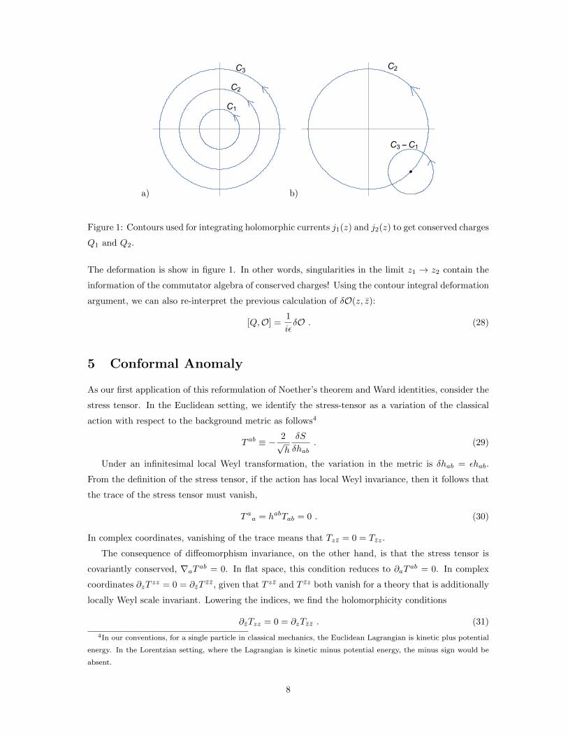
a)

C1

C2

C3

b)

C2

C3 -C1

Figure 1: Contours used for integrating holomorphic currents j1(z) and j2(z) to get conserved charges

Q1 and Q2.

The deformation is show in figure 1. In other words, singularities in the limit z1 → z2 contain the

information of the commutator algebra of conserved charges! Using the contour integral deformation

argument, we can also re-interpret the previous calculation of δO(z, z):

[Q,O] =1

iεδO . (28)

5 Conformal Anomaly

As our first application of this reformulation of Noether’s theorem and Ward identities, consider the

stress tensor. In the Euclidean setting, we identify the stress-tensor as a variation of the classical

action with respect to the background metric as follows4

T ab ≡ − 2√h

δS

δhab. (29)

Under an infinitesimal local Weyl transformation, the variation in the metric is δhab = εhab.

From the definition of the stress tensor, if the action has local Weyl invariance, then it follows that

the trace of the stress tensor must vanish,

T aa = habTab = 0 . (30)

In complex coordinates, vanishing of the trace means that Tzz = 0 = Tzz.

The consequence of diffeomorphism invariance, on the other hand, is that the stress tensor is

covariantly conserved, ∇aT ab = 0. In flat space, this condition reduces to ∂aTab = 0. In complex

coordinates ∂zTzz = 0 = ∂zT

zz, given that T zz and T zz both vanish for a theory that is additionally

locally Weyl scale invariant. Lowering the indices, we find the holomorphicity conditions

∂zTzz = 0 = ∂zTzz . (31)

4In our conventions, for a single particle in classical mechanics, the Euclidean Lagrangian is kinetic plus potential

energy. In the Lorentzian setting, where the Lagrangian is kinetic minus potential energy, the minus sign would be

absent.

8

We will follow convention here and introduce a rescaled version of the stress tensor:

T (z) ≡ −2πTzz , (32)

T (z) ≡ −2πTzz . (33)

(The 2π will cancel a corresponding 2π in the Cauchy residue formula.) Given such a holomorphic

operator, we can build a large set of holomorphically conserved currents

j(z) = iv(z)T (z) , (z) = iv(z)∗T (z) , (34)

where v(z) is any meromorphic function. Using the relation (23), we can then study the associated

symmetry transformations of the fields.

Consider first our X CFT. The Euclidean action is

S =1

4πα′

∫d2σ√hhab∂aX · ∂bX . (35)

From the definition of the stress tensor, we find

T ab =1

2πα′

[∂aX · ∂bX − 1

2habhcd∂cX · ∂dX

], (36)

or in components

T (z) = − 1

α′∂X · ∂X , (37)

T (z) = − 1

α′∂X · ∂X . (38)

Now we saw previously that

〈∂Xµ(z)∂Xµ(z′)〉 = − Dα′/2

(z − z′)2, (39)

where D is the number of space time dimensions. Thus, in the stress tensor, we need to regulate

the divergence as z → z′. One common prescription is normal ordering. Our stress tensor is really

T (z) = − 1

α′:∂Xµ(z)∂Xµ(z): (40)

≡ − 1

α′limz→z′

[∂Xµ(z)∂Xµ(z′) +

Dα′/2

(z − z′)2

]. (41)

Given this normal ordering prescription, we can then study how X transforms in response to

symmetries associated with j(z) = iv(z)T (z). The first step is to use Wick’s theorem to consider

the singular terms in T (z)Xµ(z′) as z → z′:

T (z)Xµ(0) ∼ − 2

α′:∂Xν(z)∂Xν(z):Xµ(0) + . . .

∼ − 2

α′∂z

[−α′

2ηµν log |z|2

]∂Xν(z) + . . .

∼ 1

z∂Xµ(0) + . . . (42)

9

The ellipsis indicates terms which are not singular in the limit z → 0. This expression is frequently

referred to as an operator product expansion (OPE). We will shortly give a more formal definition

below. From the residue relation (23), we then obtain

1

iεδXµ = iv(z)∂Xµ + iv(z)∗∂Xµ . (43)

This rule is recognizable as an infinitesimal coordinate transformation with

z′ = z + εv(z) , (44)

the finite version of which is z′ = w(z) for a meromorphic function w. But such coordinate trans-

formations are precisely the conformal transformations we discussed earlier, which leave the metric

invariant up to a local scale factor. We may then tentatively conclude that v(z)T (z) generates

conformal transformations.

As OPEs will be of central importance, it is useful to get some additional practice with simple

examples. Let us consider then the operator ∂Xµ(z) instead of Xµ(z). In this case, we obtain

T (z)∂Xµ(0) = − 2

α′∂z∂w

[−α′

2ηµν log |z − w|2

]∂Xν(z) + . . .

=1

(z − w)2∂Xµ(z) + . . .

=1

(z − w)2∂Xµ(w) +

1

z − w∂2Xµ(w) + . . . (45)

From this OPE, we can deduce the transformation rule for ∂Xµ, namely

δ∂Xµ = −εv(z)∂2Xµ − ε(∂v)(∂Xµ) . (46)

Let us compare this transformation rule with what we would expect for a primary operator (for

simplicity with h = 0):

O′(z′) =

(∂z′

∂z

)−hO(z) , (47)

where the infinitesimal version is given by z′ = z + εv(z). Then

δO = O′(z)−O(z)

= O′(z′ − εv(z))−O(z)

= O′(z′)− εv(z)∂z′O′(z′)−O(z)

= (1 + ε∂zv)−hO(z)− εv(z)∂zO(z)−O(z)

= −hε(∂v)O − εv∂O (48)

The relation of this transformation rule to the OPE suggests the following alternate definition of a

primary field. It is a field which has the following OPE with the stress tensor:

T (z)O(0) ∼ h

z2O(0) +

1

z∂O(0) + . . . (49)

10

I do not want to delve too deeply into when a product of two nearby operators can be expressed

as an (infinite) sum of local operators. In the Lorentzian case, there are obvious subtleties involved

with what exactly is meant by “near”. Even in the Euclidean case, such sums can have various

pathologies. However, in the CFT case, for the operators we study, it is almost always the case that

the OPE will take the (schematic) form

O(z)O′(w) =

∞∑k=−N

(z − w)kOk(w) . (50)

Exercise 1. Verify that h = h = α′

4 k2 for the operator O = :eik·X :.

Using the OPE machinery and the residue relation (23), we can check if T (z) itself is a primary

field, at least for the X system:

T (z)T (w) ∼ 1

α′2:∂Xµ∂Xµ(z): :∂Xν∂Xν(w):

∼ 2

α′2(−∂z∂wηµν

α′

2log |z − w|2)(−∂z∂wηνµ

α′

2log |z − w|2)

+4

α′2(−∂z∂wηµν

α′

2log |z − w|2):∂Xν(z)∂Xµ(w):

∼ηµµ2

1

(z − w)4− 2

α′1

(z − w)2:∂Xµ(z)∂Xµ(w): + . . .

∼ D

2

1

(z − w)4+

2

(z − w)2T (w) +

1

(z − w)∂T (w) + . . . (51)

While here D is the number of X fields, more generally for a two dimensional CFT, the coefficient

of the leading 1/(z−w)4 term in the OPE of two stress tensors is identified with the central charge

c of the theory. (In this case c = D.) The central charge is an obstruction to the stress-tensor

transforming as a primary field:

δT (z) = −ε c12

(∂3v)− 2ε(∂v)T − εv∂T (52)

However, since ∂3v vanishes for v(z) = 1, z, or z2, i.e. the generators of sl(2,R), the stress tensor does

have a simple transformation rule under elements of PSL(2,C) and is an example of a quasi-primary

field.

The finite form of the transformation rule for the stress tensor is(∂z′

∂z

)2

T ′(z′) = T (z)− c

12{z′, z} (53)

where the quantity on the right is the Schwarzian derivative

{f, z} ≡ 2(∂3zf)(∂zf)− 3(∂2

zf)2

2(∂zf)2, (54)

Exercise 2. Verify that the finite form of the transformation rule above has the correct infinitesimal

form. Also verify that the finite form of the transformation composes correctly.

11

A Famous Calculation: The Equation of State of a CFT

Consider a cylinder parametrized by w = σ1 + iσ2 where σ2 is periodic with period β: σ2 + β ∼ σ2.

Eventually, we will be able to interpret σ2 a Euclidean time coordinate and β = 1/T as the inverse

temperature, but for now we can treat β as just some length scale characterizing the cylinder. There

is a plane to cylinder transformation given by the exponential map z = e2πw/β . Let us see how the

stress tensor behaves with respect to this transformation:(∂z

∂w

)2

T (z)pl = T (w)cyl −c

12{z, w} . (55)

Plugging in the exponential map yields(2π

β

)2

z2T (z)pl = T (w)cyl −c

12

2(∂3wz)(∂wz)− 3(∂2

wz)2

2(∂wz)2

= T (w)cyl −c

12

(2π

β

)22− 3

2. (56)

Given the symmetries of the plane, it seems reasonable to assume that in the vacuum state 〈T (z)〉pl =

0. It follows from the Schwarzian derivative then that

〈T (w)〉cyl = − c

24

(2π

β

)2

. (57)

Translating back to a rectilinear coordinate system, we obtain

T 22 = −T 11 =1

2π(T (z) + T (z)) = − c

24π

(2π

β

)2

. (58)

We can interpret this result in one of two ways. If we think of σ1 as the Euclidean time coordinate

and the CFT as living on a circle of circumference β, then Wick rotating to Minkowski signature,

we obtain a negative Casimir energy

T tt = −T 11 = − πc

6β2. (59)

Alternatively, we can treat σ2 as a Euclidean time direction, in which case β = 1/T is interpreted as

an inverse temperature. In this case, Wick rotating back, we get a positive thermal energy density

T tt = −T 22 =πcT 2

6. (60)

The Trace Anomaly

The presence of a nonzero central charge c in a conformal field theory is intimately related to the

presence of a trace anomaly: the trace of the stress tensor will not vanish on a curved manifold but

instead is given by

〈Tµµ〉 =c

24πR . (61)

Classically, the right hand side should be zero, but the measure in the path integral may not respect

the Weyl scaling symmetry and there can be an anomaly. The form of the right hand side is fixed

12

by symmetry. It must be a scalar quantity under the action of diffeomorphisms that has scaling

weight two – the same as the stress tensor in two dimensions. For CFT, the only candidate is the

Ricci scalar.

There are two points of view regarding this trace anomaly. From the point of view of conformal

field theory, gravity on the world sheet is not dynamical and the anomaly is global. The quantity

c tells us interesting things about the properties of the CFT, for example as we saw above, the

equation of state. From the point of view of string theory, where world sheet gravity is dynamial

(in a sense), the anomaly is a gauged anomaly and indicates a pathology in the theory. It indicates

that the string theory will depend in a nontrivial way on the world sheet metric hab even though

the choice of world sheet metric should have been a gauge choice. In the context of string theory, it

had better be that at the end of the day the total central charge c should vanish.

In this section, we will demonstrate that the trace anomaly in the stress tensor implies the

Schwarzian derivative transformation rule. The proof begins with the statement that mixed partial

derivatives commute:

〈T ab(x)T cc(x′)〉√h(x)

√h(x′) = 2

δ

δhab(x)〈T cc(x′)〉

√h(x′)

= hcd(x′)2

δ

δhcd(x′)〈T ab(x)〉

√h(x) . (62)

I am renaming the world-sheet coordinates x in this section because I want to reserve the letter σ for

Weyl transformations. In the second equality, we can replace the variation with respect to hcd(x′)

with an equivalent variation with respect to a Weyl scaling parameter σ. Under an infinitesimal

Weyl scaling, δhcd = 2hcdδσ, and thus

2δ

δhab(x)〈T cc(x′)〉

√h(x′) =

δ

δσ(x′)〈T ab(x)〉

√h(x) . (63)

Plugging the result for the trace anomaly into the left hand side, we will solve this functional

differential equation for 〈T ab(x)〉 and thereby establish the Schwarzian derivative transformation

rule. To solve the differential equation, we use dimensional regularization and work in n = 2 + ε

dimensions. The first observation is that R transforms nicely with respect to Weyl variations in

2 + ε dimensions. The variation of the Ricci scalar with respect to the metric is familiar from the

derivation of Einstein’s equations:

δ

δhab

∫dnx√hR = (−Rab +

1

2habR)

√h . (64)

Restricting to Weyl variations, we then obtain

δ

δσ

∫dnx√hR = (n− 2)R

√h . (65)

In other words, R behaves like an eigenvector with eigenvalue (n− 2) under Weyl transformations.

We can therefore replace the trace of the stress tensor in the differential equation (63) with a Weyl

variation of the trace anomaly:

c

24π(n− 2)2

δ

δhab(x)

(δ

δσ(x′)

∫dnx√hR

)=

δ

δσ(x′)〈T ab(x)〉

√h(x) . (66)

13

We can now functionally integrate with respect to σ′ on both sides to obtain

〈T ab(x)〉√h(x) =

c

12π(n− 2)

δ

δhab(x)

∫dnx′

√h(x′)R(x′)

=c

12π(n− 2)

[−Rab +

1

2gabR

]√h(x) , (67)

where in the last line we are again deriving Einstein’s equations from the Einstein-Hilbert action. I’ve

dropped a constant of integration on both sides. More precisely, we should think about integrating

σ from some reference metric h0ab to the metric of interest hab. We are really computing the change

in the stress tensor as we scale from one metric to another. However, things are simple in two

dimensions because every metric is Weyl equivalent to the flat metric hab = e2σδab. Moreover, if we

are computing the one point function of the stress tensor in the vacuum, it is reasonable to assume

that 〈T ab〉δab= 0, as we did in the previous section. Then we can take the constant of integration

in the solution (67) to vanish.

We have to be careful in evaluating the solution (67) because Einstein’s equations vanish iden-

tically in d = 2 dimensions. Continuing to work in n = 2 + ε dimensions, we have that for a metric

of the form hab = e2σδab the relevant curvatures are

Rab = (2− n)[∂a∂bσ − (∂aσ)(∂bσ)]− δab(∂2σ + (n− 2)(∂σ)2) , (68)

R = −e−2σ[2(n− 1)∂2σ + (n− 1)(n− 2)(∂σ)2] . (69)

We are implicitly contracting indices in the quantities (∂2σ) and (∂σ)2 with the flat metric δab. The

Einstein tensor reduces to

Rab −1

2habR = (n− 2)

([−∂a∂bσ + (∂aσ)(∂bσ)] + δab

[∂2σ +

1

2(n− 3)(∂σ)2

]). (70)

Carefully taking the limit n→ 2, we obtain our result for the stress tensor

〈Tab(x)〉 =c

12π

[∂a∂bσ − (∂aσ)(∂bσ)− δab

(∂2σ − 1

2(∂σ)2

)]. (71)

In our complex coordinates, we can write instead

〈T (z)〉 = − c6

[∂2zσ − (∂zσ)2

]. (72)

As we discussed, after gauge fixing to δab, the residual symmetry of the CFT is a combination

of a Weyl scaling and diffeomorphism that leaves the metric invariant:

hzz =∂z

∂w

∂z

∂we2σ(z)hzz , (73)

or equivalently

σ =1

2log

∂w

∂z+

1

2log

∂w

∂z. (74)

14

Under the Weyl rescaling, we find that the new stress tensor becomes

〈T (z)〉hab= − c

6

[1

2∂z∂2zw

∂zw− 1

4

(∂2zw

∂zw

)2]

= − c6

[1

2

∂3zw

∂zw+

(−1

2− 1

4

)(∂2zw)2

(∂zw)2

]= − c

12

[2(∂3

zw)(∂zw)− 3(∂2zw)2

(∂zw)2

]. (75)

Finally, we need to perform a diffeomorphism associated with the map z → w(z):

〈T (w)〉δab=

(∂z

∂w

)2

〈T (z)〉hab. (76)

At the end of the day, we recover the Schwarzian derivative formula for the transformation of the

stress tensor, starting from a background where 〈T (z)〉δab= 0:(

∂w

∂z

)2

〈T (w)〉 = − c

12{w, z} . (77)

6 Path Integral Approach

We return to a study of the four CFTs relevant for string theory: the X, ψ, bc and βγ systems.

Our plan in this section is four-fold. From the action, we will derive the OPEs of these fundamental

fields. Next we will derive/recall the form of the stress tensor. Using the stress tensor and building

block OPEs, we will verify that the fields have the correct scaling dimensions h and h. Finally,

by considering the OPE of the stress tensor with itself, we will derive expressions for the central

charges. As output, we will see that both the bosonic string and the spinning string have vanishing

total central charge c and thus have no Weyl anomaly.

The X System

We begin with the X system. We already argued for the singularity in the OPE of two Xµ fields

based on conformal symmetry alone. However, there is a small hole in the logic that we need to fill:

that the normalization of the OPE is consistent with our conventional normalization of the action

of the Xµ system. That action, in complex coordinates, is

S =1

2πα′

∫d2z ∂X · ∂X , (78)

where the measure d2z = 2d2σ.

Consider the expectation value of the following composite operator O[X]:

〈O[X]〉 =

∫[dX]e−SO[X] , (79)

15

The integral of a total derivative must vanish, even in the path integral context, and so

0 =

∫[dX]

δ

δXµ(z, z)

(e−SO[X]

)=

∫[dX]

(− δS

δXµ(z, z)O[X] +

δO[X]

δXµ(z, z)

)e−S

= −⟨

δS

δXµ(z, z)O[X]

⟩+

⟨δO[X]

δXµ(z, z)

⟩=

1

πα′⟨O[X]∂∂Xµ(z, z)

⟩+

⟨δO[X]

δXµ(z, z)

⟩. (80)

If Xµ(z, z) does not appear in O[X], then

⟨O∂∂X(z, z)

⟩= 0 . (81)

In this sense, then, we claim that the equation of motion ∂∂X(zz) = 0 holds as an operator equation

at the quantum level. Of course, if O[X] does depend on Xµ(z, z), then things are different. One

may consider the special case where O[X] = Xν(z′, z′), in which case we find

1

πα′∂z∂zX

µ(z, z)Xν(z′, z′) + δµνδ2(z − z′, z − z′) = 0 , (82)

which will also hold as an operator equation inside expectation values 〈· · · 〉 provided no other

operators get too close. To determine the OPE of two Xµ fields, we now integrate this expression.

Recall from electricity and magnetism that a point charge ρ = δ(σ1, σ2) in two dimensions has a

logarithmic potential function φ = − log r where r2 = (σ1)2 + (σ2)2. Another way of expressing this

relation is Poisson’s equation, which in d spatial dimensions takes the form

∇2φ = −Vol(Sd−1)ρ . (83)

In complex coordinates, ∇2 = 4∂∂ and δ2(σ1, σ2) = 2δ2(z, z), and we find then that

∂∂ log |z|2 = 2πδ2(z, z) . (84)

We conclude that the normalization we asserted before is indeed correct,

Xµ(z, z)Xν(z′, z′) ∼ −α′

2ηµν log |z − z′|2 . (85)

For the X system, we already wrote down the stress tensor and (assuming the above normaliza-

tion) used the OPEs to verify that Xµ has conformal weights h = h = 0 and that each Xµ field

contributes one unit to the central charge. We can thus move on.

The bc System

Consider the one derivative action

S =1

2πg

∫d2z b∂c , (86)

16

where b and c are anti-commuting. By dimensional analysis, it must be that for this free field theory,

hb + hc = 1. Let us then parametrize our ignorance by setting hb = λ and hc = 1− λ.

I claim this action actually encodes both the bc ghost system and the ψ system. That it encodes

the ghost system is clear from (2.155) and (2.171) in PvN’s notes, provided we set g = 1. In this

case, since b naturally has two lower world-sheet indices and c one upper index, it is natural to take

hc = −1 and hb = 2. To see that the general bc system encodes (two copies) of the ψ system, we

need to do a little more work. We split the fermionic fields into pieces

b =1√2

(ψ1 + iψ2) , c =1√2

(ψ1 − iψ2) . (87)

The action is then

S =1

4πg

∫d2z(ψ1∂ψ1 + ψ2∂ψ2) . (88)

Up to a factor of i, this expression is precisely two copies of (3.37) in PvN’s notes with the iden-

tification g = l2 = 2α′. (In contrast, to recover the fermions with Polchinski’s normalization, we

should instead set g = 1.) In this case, hc = hb = 12 .

To obtain the OPE of the b(z) and c(z) fields, we follow precisely the same steps that we did

with the X system. The equations of motion are ∂c(z) = 0 = ∂b(z). It then follows from the path

integral that

∂c(z)b(0) = 2πg δ2(z, z) . (89)

From differentiating the OPE of the two X fields, it is straightforward to deduce that ∂z−1 =

2πδ2(z, z) or

c(z1)b(z2) ∼ g

z12. (90)

Because the b and c fields anti-commute, we also have the relation

b(z1)c(z2) = −c(z2)b(z1) ∼ g

z12. (91)

In the fermionic case that hb = hc = 12 , this OPE also implies the two-point function

〈c(z1)b(z2)〉 =g

z12. (92)

For more general λ, the nature of the vacuum state introduces some subtleties that we will return

to later.

For the stress-tensor, comparing with (2.185) in PvN’s notes (where g is set equal to one) we see

that for the ghost system, we can write

T (z) = :(∂b)c:− 2∂(:bc:) . (93)

For the fermions, from (3.67) in PvN’s notes, we have instead that

T (z) = − 1

2g(:ψ1∂ψ1: + :ψ2∂ψ2:) , (94)

17

or in terms of the bc fields

T (z) =1

g

[:(∂b)c:− 1

2∂(:bc:)

]. (95)

The natural generalization seems to be (and indeed is as we will verify by taking the appropriate

OPEs)

T (z) =1

g[:(∂b)c:− λ∂(:bc:)] . (96)

We consider three OPEs, T (z) with b(w), c(w), and T (w). From the OPE with b(w),

T (z)b(w) ∼ (∂zb(z))1

z − w− λ∂z

(b(z)

1

z − w

)∼ λ

(z − w)2b(z) +

(1− λ)

z − w∂zb(z)

∼ λ

(z − w)2b(w) +

1

z − w∂b(w) , (97)

we verify that b(w) is a primary field with conformal dimension hb = λ. From the OPE with c(w),

T (z)c(w) ∼ −(∂z

1

z − w

)c(z) + λ∂z

(c(z)

z − w

)∼ 1− λ

(z − w)2c(z) +

λ

z − w∂c(z)

∼ 1− λ(z − w)2

c(w) +∂c(w)

z − w, (98)

we verify that c(w) is a primary field with conformal dimension hc = 1 − λ. To obtain the central

charge, we look at the leading singularity in the T (z)T (w) OPE:

T (z)T (w) ∼ 1

g2[:(∂b)c:− λ∂(:bc:)] (z) [:(∂b)c:− λ∂(:bc:)] (w)

∼(∂z

1

z − w

)(∂w

1

z − w

)− λ∂w

(1

z − w∂z

1

z − w

)−λ∂z

(1

z − w∂w

1

z − w

)+ λ2∂z∂w

(1

z − w

)2

+ . . .

∼ 1

(z − w)4

(−1 + 3λ+ 3λ− 6λ2

)+ . . . (99)

where we have left the subleading yet still singular terms as an exercise for the reader to compute.

From the leading (z − w)−4 term, however, we can read off the central charge of the bc system

cbc = −12λ2 + 12λ− 2 = −3(2λ− 1)2 + 1 . (100)

For the bc ghost system with λ = 2, we obtain cbc = −26. Meanwhile for two copies of the ψ system,

with λ = 12 , we obtain cbc = 1, or cψ = 1/2 for each copy.

The βγ System

We consider the analog of the bc system above for commuting fields β and γ. At the penalty of

introducing a parameter ε = ±1 whose sign depends on whether bc commute or anti-commute, one

18

can treat both cases simultaneously. For clarity, I find it simpler to separate the two cases. We shall

nevertheless be brief here, and leave most of the relevant checks as an exercise for the reader. The

action is

S =1

2πg

∫d2z β∂γ , (101)

where again we parametrize our ignorance by setting hβ = λ and hγ = 1 − λ. The Ward identity

following from the equations of motion is

∂zγ(z)β(0) = 2πgδ2(z, z) . (102)

As before, this relation can be integrated to give the singularity in the OPE:

γ(z)β(0) ∼ g

z. (103)

Now however because β and γ commute, we get instead

β(z)γ(0) ∼ −gz. (104)

The stress tensor has exactly the same form as before

T (z) = :(∂β)γ:− λ∂(:βγ:) . (105)

The central charge is then minus what it was before

cβγ = 3(2λ− 1)2 − 1 . (106)

(The computation is essentially identical to the bc system. The minus sign is the difference in sign

between the OPE for b(z)c(0) and the OPE for β(z)γ(0).) Through their index structure, for the

ghost system hβ = 3/2 while hγ = −1/2. In this case, the central charge works out to be cβγ = 11.

Exercise 3. Calculate the singular terms in the T (z)T (0) operator product expansion both for the

bc system and for the βγ system. Assume hb = hβ = λ and hc = hγ = 1− λ.

Canceling the Trace Anomaly

We considered two types of string theory, the bosonic string and the spinning string. We can see now

that in each case, the total central charge vanishes. Thus in each case, there is no Weyl anomaly.

X ψ bc βγ ctot

bosonic 26 · 1 0 1 · (−26) 0 0

spinning 10 · 1 10 · 12 1 · (−26) 1 · 11 0

7 BRST meets CFT

We argued in the earlier part of the course that the BRST charge QB should be nilpotent: Q2B = 0.

We would like in this section to use OPE techniques to verify nilpotency. As a bonus, we will see

19

again that the bosonic string and spinning string are consistent only in D = 26 and D = 10 space

time dimensions, respectively.

The BRST current in the bosonic string case is

jB(z) = cTm(z) +1

2cT g(z) + αB∂

2c . (107)

In the spinning string case, we have instead

jB(z) = cTm(z) +1

2cT g(z) + αS∂

2c+ γJm(z) +1

2γJg(z) . (108)

Here the superscript m stands for matter fields – X and ψ – while g stands for ghosts – bc and βγ.

We will write the full stress tensor T (z) and supercurrent J(z) in the spinning string case only. The

way to divide it up into matter and ghost pieces should be obvious at this point, as should the way

to restrict it to the purely bosonic case:

T (z) = − 1

α′∂X · ∂X − 1

2ψ · ∂ψ + (∂b)c− 2∂(bc) + (∂β)γ − 3

2∂(βγ) , (109)

J(z) = i

(2

α′

)1/2

ψ · ∂X − 1

2(∂β)c+

3

2∂(βc)− 2bγ . (110)

(We are using Polchinski’s normalization of the ψ fields here.) Note that the ∂2c term we added

to the current jB reflects a certain choice. As a total derivative, it will not contribute to the total

charge QB . The form of such a derivative correction is highly constrained by dimensional analysis –

it must contain one derivative, one c field, and something else that will make the total dimension of

the term equal to one. One can think of this term as arising from ordering ambiguity in composite

operators making up the first few terms in jB(z). It turns out that this ∂2c term is necessary in

order that jB(z) transform as a primary operator in CFT language, as we will see.

As QB is an anti-commuting operator, we can check nilpotency by looking at

{QB , QB} =

∮dw

2πiResz→wjB(z)jB(w) .

We will check the bosonic case and leave the spinning string as a (rather long) exercise. Since we

are only interested in the residue, we will focus on the 1/(z − w) term in the OPE only. We will

divide the computation up into four pieces:

jB(z)jB(w) =

[c(Tm +

1

2T g) + αB∂

2c

](z)

[c(Tm +

1

2T g) + αB∂

2c

](w)

∼ c(z)c(w)Tm(z)Tm(w) +

(Tm(w)

1

2c(z)T g(z)c(w)− (z ↔ w)

)+αB2

[c(z)T g(z)∂2c(w)− (z ↔ w)

]+

1

4c(z)T g(z)c(w)T g(w) . (111)

The first piece expands to give

c(z)c(w)Tm(z)Tm(w) ∼ c(z)c(w)

[cm

2(z − w)4+

2

(z − w)2Tm(w) +

1

z − w∂Tm(w)

]∼ . . .+

1

z − w

[∂Tmc2 + 2Tm(∂c)c+

cm12

(∂3c)c]

(w) . (112)

20

The first term above cancels on its own because c(w)2 = 0. We will see momentarily how the

remaining two terms combine with the rest of the OPE.

For the second piece, consider first the composite operator

cT g = c[(∂b)c− 2∂(bc)] = 2c(∂c)b . (113)

The second piece thus expands to give

Tm(w)1

2c(z)T g(z)c(w)− (z ↔ w) ∼ Tm(w)c(z)(∂c(z))b(z)c(w)− (z ↔ w)

∼ 1

z − w(Tm(w)c(∂c)(z) + Tm(z)c(∂c)(w))

∼ 2Tm(w)c(w)(∂c(w))

z − w, (114)

which cancels agains the second term in the expression (112).

Next consider the third piece. Using again the expression (113), the third term can be written

αB2

[cT g(z)∂2c(w)− (z ↔ w)

]∼ αB

2

[2c(∂c)b(z)∂2c(w)− (z ↔ w)

]∼ αB

[c(∂c)(z)

(∂2w

1

z − w

)− (z ↔ w)

]. (115)

The second term, with z and w swapped, will not give rise to a simple pole proportional to 1/(z−w).

The first term will however:

αB2

[cT g(z)∂2c(w)− (z ↔ w)

]∼ . . .+

αBz − w

∂2(c(∂c)(w))

∼ . . .+αBz − w

∂(c(∂2c)(w)) . (116)

As it’s proportional to αB , reassuringly it’s a total derivative and will not affect the nilpotency of

Q2B .

Last but not least, we consider the fourth piece, the OPE involving the two ghost stress tensors:

:c(∂c)b(z)::c(∂c)b(w): ∼(

1

z − w

)2

∂c(z)∂c(w)−(∂z

1

z − w

)(1

z − w

)c(z)∂c(w)

−(

1

z − w

)(∂w

1

z − w

)∂c(z)c(w) +

(∂z

1

z − w

)(∂w

1

z − w

)c(z)c(w)

+1

z − w(∂c)b(z)c(∂c)(w)−

(∂z

1

z − w

)cb(z)c(∂c)(w)

−(∂w

1

z − w

)c(∂c)(z)cb(w) +

1

z − wc(∂c)(z)(∂c)b(w) . (117)

The second set of four terms all come from single contractions and vanish trivially by the anti-

commutativity of the b and c fields. The first set of four terms come from double contractions and

simplify to give the 1/(z − w) term

:c(∂c)b(z)::c(∂c)b(w): ∼ . . .+1

z − w

[(1 +

1

2

)(∂2c)(∂c)(w)−

(1

2+

1

6

)(∂3c)c(w)

]. (118)

21

We can rewrite the first term using the total derivative ∂(c(∂2c)) that we found in evaluating the

contraction of the matter stress tensor portion with the ghost stress tensor (114):

:c(∂c)b(z)::c(∂c)b(w): ∼ . . .+1

z − w

[−3

2∂(c(∂2c))(w)−

(3

2+

2

3

)(∂3c)c(w)

]. (119)

Assembling the four pieces (112), (114), (116), and (119), we obtain

jB(z)jB(w) ∼ . . .+ 1

z − w

[cm − 26

12(∂3c)c+

(αB −

3

2

)∂(c(∂2c))

](w) (120)

Thus we find that the BRST charge is nilpotent if the matter sector has total central charge cm = 26,

or equivalently if bosonic string theory lives in 26 space time dimensions. There is also a total

derivative term which we do not need to vanish for nilpotency. However, if we can choose αB = 3/2,

in which case the residue vanishes completely. This choice has the advantage that it makes jB(z) a

primary operator, as we now check:

T (z)jB(w) ∼ Tm(z)c(w)Tm(w) + T g(z)c(w)

(Tm(w) +

1

2T g(w)

)+ T g(z)αB∂

2c(w)

∼ c(w)

(cm

2(z − w)4+

2Tm(w)

(z − w)2+∂Tm(w)

z − w

)+Tm(w)

(− c(w)

(z − w)2+

∂c(w)

(z − w)

)+

1

2T g(z)c(w)T g(w)

+αB∂2w

(− c(w)

(z − w)2+∂c(w)

z − w

). (121)

The one nontrivial term here is

1

2T g(z)c(w)T g(w) ∼ [(∂b)c− 2∂(bc)] (z) c(∂c)b(w)

∼(∂z

1

z − w

)1

z − w∂c(w)−

(∂z

1

z − w

)(∂w

1

z − w

)c(w)

−2∂z

(1

(z − w)2

)∂c(w) + 2∂z

(1

z − w∂w

1

z − w

)c(w)

+1

2

(cT g(w)

(z − w)2+∂(cT g)(w)

z − w+

). (122)

where the last line comes just from the single contractions. Assembling the pieces produces

T (z)jB(w) ∼ c(w)

(z − w)4

(cm2− 5− 6αB

)+

∂c(w)

(z − w)3(3− 2αB)

+jB(w)

(z − w)2+∂jB(w)

z − w. (123)

Indeed, jB(z) is a primary operator with conformal scaling dimension h = 1 provided αB = 3/2 and

cm = 26.

With a little more work, one can also recover the BRST transformation rules. We will leave that

as an exercise for the interested reader:

jB(z)b(0) ∼ 3

z3+

1

z2jg(0) +

1

zT (0) (124)

jB(z)c(0) ∼ 1

zc∂c(0) (125)

jB(z)O(0) ∼ h

z2cO(0) +

1

z(h(∂c)O(0)) + c∂O(0)) , (126)

22

where we have introduced the ghost current jg(z) = −:bc: and an arbitrary primary field O(z). The

simple poles reflect the BRST transformation rules.

Exercise 4. In the bosonic string, compute the singular terms in the OPE of the BRST current

jB(z) with b(w), c(w), and with a primary field O(w) of weight h.

A similar exercise for the spinning string demonstrates that cm = 15 and hence that the spinning

string exists in 10 target space-time dimensions. Really, this check on the space-time dimensions is

redundant having already ensured that the Weyl anomaly vanishes. Remember that in constructing

the BRST symmetry, we built in a Weyl scaling symmetry.

Exercise 5. (Lengthy) In the spinning string, verify that jB(z)jB(w) has no residue at the simple

pole z = w when cm = 15. Compute also the OPE of T (z) with jB(w). What value of αS is required

for j(z) to be a primary field?

8 From Operators to States: The Vacuum

There are a number of subtleties associated with how to define states (and in particular the vacuum

state) in CFT that we have thus far largely been able to sweep under the rug.5 To understand

these subtleties, we make a mode decomposition of the fields and think instead about creation and

annihilation operators. From the point of view of the closed string theory (and also the doubled

version of the open string), it makes perhaps more sense to work on a cylinder. The natural string

vacuum will be the one associated to the cylinder. From the point of view of CFT, the plane is a

more symmetric starting point. We saw already some nontrivial things happen when we map back

and forth, z = ew, w = σ2 − iσ1. Here z parametrized the plane while w parametrizes the cylinder.

(We have taken a somewhat strange complex structure on the cylinder in order to eliminate some

troublesome factors of√−1.)

Recall that for a holomorphic primary field, we have the transformation rule

O(z) =

(∂z

∂w

)−hO′(w) = z−hO′(w) . (127)

On the string worldsheet, given translation invariance in time and space, it makes sense to consider

a Fourier decomposition

O′(w) =

∞∑n=−∞

en(iσ1−σ2)On , (128)

where we have the Fourier modes

On =1

2π

∫ 2π

0

dσ1e−inσ1

O′(σ1, 0) . (129)

5One place where these subtleties threatened to derail the lectures was an apparent conflict between the OPE of

the bc fields and the claim that two point correlation functions in CFT are only nonzero when the scaling dimensions

of the operators involved are the same. Purposefully, I did not put brackets around the bc OPE, and after this part

of the lecture series, we will hopefully see why.

23

Employing the transformation rule, we find that in the z plane, we can write

O(z) =

∞∑n=−∞

Onzn+h

, On =

∮|z|=1

dz

2πizzn+hO(z) . (130)

(There is a minus sign in changing from the σ1 variable to the z variable that cancels against the

fact that the dσ1 integral goes clockwise in the z plane while the contour integral is usually taken

to go counter-clockwise.)

There is a tension emerging here. On the cylinder, it makes sense to think of On as raising

operators for n < 0 and as lowering operators for n > 0. However, on the plane, there have appeared

some non-homogenous factors of zh that seem to make it more natural to split the operators around

n = −h rather than around n = 0. To define the path integral, we need boundary conditions as

σ2 → −∞ on the cylinder or correspondingly r → 0 on the plane (in radial quantization). These

boundary conditions conventionally define an initial state. We can imagine changing that state by

inserting an operator at r = 0. The vacuum |1〉 in the z-plane naively should correspond to inserting

the identity operator at r = 0. More generally, we can imagine inserting any local operator at the

origin and producing a corresponding state. For a primary operator, we have O(0)|1〉 = |O〉. But

now in order for this expression to be well defined and nonsingular, from the sum (130) it had better

be true that

On|1〉 = 0 , n > −h . (131)

Unlike the cylinder vacuum where On is an annihilation operator for any n > 0, on the plane there is

(depending on the sign of h) a set of lowering operators which fail to annihilate the z-plane vacuum

or a set of raising operators which do annihilate it.

Interestingly, using the Cauchy residue theorem, we can replace ∂nO(0)|1〉, for n = 0, 1, 2, . . .,

up to a combinatorial factor, with a corresponding mode operator

∂nO(0)|1〉 = n!

∮dz

2πizn+1O(z)|1〉

= n!O−h−n|1〉 . (132)

This contour integral gives an alternate way of understanding the condition (131). By construction,

O(z)|1〉 is assumed to be a well defined state in the limit z → 0 with no singular behavior. The

contour integral for n < 1 must then vanish because it no longer has a simple pole. With the

definition of the On, the vanishing in turn implies the condition (131).

Let’s consider two examples to start – the X system and the bc system – both of which are of

key importance for the bosonic string. We will then move on to states in the ψ and βγ system in

the context of the spinning string.

For the X field, the raising and lowering operators are conventionally denoted αm and are given

a normalization such that

∂X(z) = −i(α′

2

)1/2∑m

αmzm+1

, (133)

24

where [αm, αn] = mδm+n,0. As ∂X(z) is a primary field of conformal scaling dimension h = 1, we

find that

αm|1〉 = 0 for m > −1 . (134)

In this case, things remain in our comfort zone, and |1〉 is the usual vacuum for a scalar field.

The bc system is the first case where things are strange. The conformal scaling dimensions are

hb = 2 and hc = −1. Thus according to our rules

bm|1〉 = 0 if m ≥ −1 , (135)

while

cm|1〉 = 0 if m ≥ 2 . (136)

As the anti-commutation relations are {bm, cn} = δm+n,0, we would expect the usual vacuum in

this system (i.e. the vacuum on the cylinder) to be annihilated instead by all bn and cn with n > 0.

We then need to specify how b0 and c0 act. As they satisfy the same anti-commutation relations

{b0, c0} = 1 as a pair of fermionic creation and annihilation operators, the vacuum on the cylinder is

two-fold degenerate: |↑〉 and |↓〉. Thinking of b0 as a lowering operator and c0 as a raising operator,

we then choose

c0|↑〉 = 0 , c0|↓〉 = |↑〉 , (137)

b0|↓〉 = 0 , b0|↑〉 = |↓〉 . (138)

Given that c0 and c1 do not annihilate |1〉, the relation between these degenerate vacua and the

z-plane vacuum is then

|1〉 = b−1|↓〉 , (139)

or equivalently c1|1〉 = |↓〉.There is a small fly in the ointment. Recall that the Hermitian conjugate of these mode operators

is given by replacing the mode number with minus the mode number: b†n = b−n and c†n = c−n. If

we were then to insert 1 = {b0, c0} into the naive inner product

〈↓|↓〉 = 〈↓|b0c0 + c0b0|↓〉 , (140)

we would find that 〈↓|↓〉 = 0. The way to remedy the situation is to modify the inner product such

that the conjugate state to |↓〉 is

〈↓|c = 〈↑| = 〈↓|c0 . (141)

Bizarrely and also truly, the inner product on the z-plane then needs to be modified by the intro-

duction of three c fields!

〈1|c = 〈1|c−1c0c1 . (142)

25

At this point, we can try to resolve the apparent contradiction between the fact that the OPE

of a b and c field has a 1/z singularity with the fact that their correlation function in vacuum

〈b(z)c(0)〉 should vanish by the PSL(2,C) subgroup of the conformal symmetry group. The key

point is that we assumed the |1〉 vacuum in discussing the relation between conformal symmetry

and the two-point functions. Using the relation (132), we can make the replacement

c−1c0c1|1〉 =1

2(∂2c(0))(∂c(0))c(0)|1〉 . (143)

We can then compare the right hand side with the Taylor expansion

c(z2)c(z1)c(0) = (c0 + z2∂c(0) +1

2z2

2∂2c(0) + . . .)(c0 + z1∂c(0) +

1

2z2

1∂2c(0) + . . .)c(0)

=1

2z1z2(z2 − z1)(∂2c(0))(∂c(0))c(0) + . . . . (144)

The simplest correlation function in which we would need to use the OPE of a b and c field is thus

secretly a five point correlation function,

〈1|b(w)c(z)c(z2)c(z1)c(0)|1〉 , (145)

not a two point function.

Exercise 6. Compute 〈1|b(w)c(z)c−1c0c1|1〉. What happens to this two-point function under in-

version w → 1/w and z → 1/z.

The mode expansion for the ψ and βγ systems depend on whether we are in the R or NS sector.

Recall the three cases:

ψ(z) =∑r∈Z+ν

ψrzr+1/2

, (146)

β(z) =∑r∈Z+ν

βrzr+3/2

, (147)

γ(z) =∑r∈Z+ν

γrzr−1/2

. (148)

In the R sector ν = 0 and the field is periodic, while in the NS sector ν = 1/2 and the field

is anti-periodic. After the transformation from the cylinder to the plane, the NS sector (perhaps

surprisingly) becomes nicer than the R sector. A factor of√z in the conformal transformation

removes the branch cut from the anti-periodic boundary conditions whereas in the R sector, the√z

leads to a branch cut.

The vacuum on the cylinder in the NS and R sector is defined via the usual conditions

ψr|0〉NS = βr|0〉NS = γR|0〉NS = 0 if r =1

2,

3

2, . . . (149)

ψr|0〉R = γr|0〉R = βr|0〉R = 0 if r = 1, 2, . . . (150)

Like b0 and c0, the modes ψ0, β0, and γ0 need special consideration. We will take γ0 to be a creation

operator and so assume β0|0〉R = 0.

26

In contrast, on the z-plane, the vacuum is naturally defined through (131). In the NS sector, we

find the conditions

ψr|1〉 = 0 , r =1

2,

3

2, . . . (151)

βr|1〉 = 0 , r = −1

2,

1

2,

3

2, . . . (152)

γr|1〉 = 0 , r =3

2,

5

2, . . . (153)

Thus |1〉 and |0〉NS agree for the ψ system, while they do not agree for the the βγ system. Unfortu-

nately, it’s less clear at this point how to relate |1〉 and |0〉NS for the βγ system than it was for the

bc system.

In the R sector, the |1〉 state is defined by regularity to be

ψr|1〉 = 0 , r = 0, 1, . . . , (154)

βr|1〉 = 0 , r = −1, 0, 1, . . . , (155)

γr|1〉 = 0 , r = 1, 2, . . . . (156)

At this point, it is not clear how the operator-state correspondence should function. The relation

(132) would seem to relate raising and lowering operators to fractional derivatives involving ∂1/2.

As we will see, the resolution involves a new concept, bosonization.

8.1 Bosonization

In 1+1 dimensions, fermions and bosons are not so different. Let H(z) be the holomorphic part of

a scalar field (with α′ = 2). The OPE of two such fields is then

H(z)H(0) ∼ − log z , (157)

i.e. the holomorphic part of the OPE of X(z, z)X(0) with α′ = 2. It turns out then that the normal

ordered operator :eiH(z): is very similar to a fermionic field ψ(z). We find the OPE’s:

eiH(z)e−iH(0) ∼ 1

z, (158)

eiH(z)eiH(0) ∼ O(z) , (159)

e−iH(z)e−iH(0) ∼ O(z) . (160)

We recognize the OPE of the bc systems with b(z) = eiH(z) and c(z) = e−iH(z). Moreover, with the

usual stress tensor for H(z), the operators e±iH(z) should have conformal weight h = 1/2. Thus, we

recognize e±iH(z) = 1√2(ψ1±iψ2) as linear combinations of the usual fermionic fields on the spinning

string. We should check though that eiH(z) and e−iH(z′) anti-commute at equal times |z| = |z′|.First consider the anti-commutator

[H(z), H(z′)] = − log(z − z′) + log(z′ − z) , (161)

= log(−1)

= πi .

27

Next we use the Campbell-Baker-Hausdorff formula in the special case where the relevant double

commutators vanish, [, [, ]] = 0:

et(X+Y ) = etXetY e−t2

2 [X,Y ] , (162)

From this relation, it follows that

etXetY = et(X+Y )et2

2 [X,Y ]

= etY etXet2[X,Y ] . (163)

In our case, X = H(z), Y = ±H(z) and t = i. As a result et2[X,Y ] = −1, and the operators e±iH(z)

do indeed satisfy the relevant anti-commutation relation.

We will perform one more computation which will let us relate the momentum current associ-

ated with H(z) to the fermion number current associated with ψ(z) (or equivalently ghost current

associated with b and c). We would like to match the OPE of eiH((z) and e−iH(−z) to that of b(z)

with c(−z). Unlike in previous computations, we will expand here around the midpoint z = 0:

:eiH(z)::e−iH(−z): ∼ 1

2z:eiH(z)e−iH(−z):

∼ 1

2z:eiH(0)+iz∂H(0)+i z

2

2 ∂2H(0)e−iH(0)+iz∂H(0)−i z22 ∂

2H(0):

∼ 1

2z:e2iz∂H(0) +O(z3):

∼ 1

2z+ i∂H(0) + 2zTH(0) +O(z2) . (164)

Exercise 7. Demonstrate the first relation in the computation above.

We can then compare that expression with

b(z)c(−z) ∼ 1

2z+ :b(z)c(−z):

∼ 1

2z+ :b(0)c(0): + : [(∂b)c(0)− b(∂c)(0)] :z . (165)

where the linear term in z is twice the stress-tensor Tbc for the bc system when λ = 1/2. We can

thus make the identifications between stress tensors TH = Tbc and conserved currents i∂H = :bc:.

Exercise 8. The general bc system with arbitrary weights hb = λ and hc = 1 − λ can also be

bosonized. Show that the bosonized system is the linear dilaton CFT with stress tensor

TH = −1

2(∂H)2 + α∂2H .

Show that ekH is a conformal primary with respect to TH and determine its conformal scaling

dimension h. What is the relation between α and λ?

8.2 R Sector Fermions

Our first application of the bosonization technology will be to the R sector fermions ψ(z). Let us

first reorganize the fermionic modes

b(z) =1√2

(ψ1 + iψ2) =∑n∈Z

ψnzn+1/2

, c(z) =1√2

(ψ1 − iψ2) =∑n∈Z

ψnzn+1/2

. (166)

28

On the cylinder, the R sector ground state is thus defined by the conditions

ψn|0〉R = ψn|0〉R = 0 , n = 1, 2, 3, . . . . (167)

The definition is incomplete as we still must decide what to do with the ψ0 and ψ0 modes. In ten

dimensions, we would have five pairs of such modes, which anti-commute among themselves. For

simplicity, let us focus on just one such pair. The situation is completely analogous to the bc system

we studied earlier. We have that {ψ0, ψ0} = 1 and the ground state |0〉R becomes degenerate:

ψ0|↓〉 = 0 , ψ0|↑〉 = |↓〉 (168)

ψ0|↓〉 = |↑〉 , ψ0|↑〉 = 0 . (169)

We can then use bozonization to figure out the relation between |↓〉 and |1〉. Let us assume there

is an operator A↓ which does the job, |↓〉 = A↓|1〉. From the definition of the |↓〉 vacuum, we must

find the following leading singular behavior as the operators ψ(z) and ψ(z) get close to A↓(0):

ψ(z)A↓(0)|1〉 =

−1∑n=−∞

ψnzn+1/2

A↓(0)|1〉 = O(z1/2) , (170)

ψ(z)A↓(0)|1〉 =

0∑n=−∞

ψnzn+1/2

A↓(0)|1〉 = O(z−1/2) . (171)

These OPEs suggest that A↓(z) = eiH(z)/2. Correspondingly, we could define |↑〉 = A↑(0)|1〉 and

A↑(z) = e−iH(z)/2.

In ten dimensions, we really have five pairs of fermionic operators. To map from the cylinder

vacuum to the z-plane vacuum, we could define a product of such exponentials of holomorphic scalar

fields

Θs = exp

(i

5∑a=1

saHa

), (172)

where sa = ±1/2 depending on which of the degenerate R-vacua one is interested in. The holomor-

phic scalar fields are then given by the following linear combinations of fermionic fields

e±iH0

=1√2

(±ψ0 + ψ1) , (173)

e±iHa

=1√2

(ψ2a ± iψ2a+1) , a = 1, 2, 3, 4 . (174)

Note that to be compatible with Lorentzian signature in space-time, the defintition of H0 involves

some extra signs and i’s.

The observant reader will at this point complain that an operator e±iHa

has no reason to anti-

commute with an operator e±iHb

when a 6= b, and yet they should if these operators really define

fermions. Cocycles can be constructed to fix this problem, but time is short, and we will not develop

cocycles further.

29

8.3 The βγ System

The last order of business is to understand the vacuum in the βγ system, both in the R and NS

sectors. The solution involves a further wrinkle. As β and γ already commute, a bosonization

procedure replacing them with a single holomorphic scalar would lead to a CFT with the wrong

statistics.6 The solution involves introducing a holomorphic scalar and an anti-commuting bc system.

To avoid confusion, we will relabel b→ η and c→ ξ. The holomorphic scalar we call φ. The following

composites of η, ξ and φ have the correct OPEs to replace β and γ:

β(z) = :e−φ(z)∂ξ(z): , γ(z) = :eφ(z)η(z): . (175)

β(z)β(0) = :e−φ(z)∂ξ(z)::e−φ(0)∂ξ(0): ∼ 1

zO(z) = O(1) ,

β(z)γ(0) = :e−φ(z)∂ξ(z)::eφ(0)η(0): ∼ z

(− 1

z2

)= −1

z,

γ(z)γ(0) = :eφ(z)η(z)::eφ(0)η(0): ∼ 1

zO(z) = O(1) . (176)

We can also try to check that the conformal weights work out correctly. To that end, we should

first try to identify the matching between the stress tensors:

γ(z)β(−z) =1

2z+ :γ(z)β(−z):

=1

2z+ : (γ(0) + z∂γ(0) + . . .) (β(0)− z∂β(0) + . . .) :

=1

2z+ :γ(0)β(0): + z: (−γ∂β(0) + (∂γ)β(0)) : + . . . ,

=1

2z+ jβγ(0)− 2z(Tβγ(0) + ∂jβγ(0)) + . . . (177)

We have identified jβγ = :βγ: and Tβγ = :(∂β)γ: − 32∂(:βγ:). We now compare this OPE with the

corresponding OPE after the “bosonization” procedure

:eφ(z)η(z): :e−φ(−z)∂ξ(−z): = (2z):eφ(z)e−φ(−z):

(1

(2z)2+ :η(z)∂ξ(−z):

)= 2z:e2z∂φ(0):

(1

(2z)2+ :η(0)∂ξ(0): +O(z)

)= 2z

(1 + 2z∂φ(0) + 2z2(∂φ(0))2

)( 1

(2z)2+ :η∂ξ(0):

)+O(z2)

=1

2z+ ∂φ(0) + z

[∂φ(0)2 + 2:η∂ξ(0):

]+O(z2) . (178)

Thus we can make the identification of currents :βγ: = ∂φ. But we can also make an identification

of stress tensors:

Tβγ = −1

2:(∂φ)2:− :η∂ξ:− ∂2φ = Tφ + Tηξ , (179)

where the total derivative ∂2φ term comes from jβγ . The piece −:η∂ξ: we recognize as a stress

tensor for the bc system with λ = 1 implying hη = 1 and hξ = 0. The stress tensor for the φ(z) field,

6If we use exponential operators e2nωH , where ω2 = ±1 and n is integer, then the operators commute, but β and

γ will have the wrong OPE.

30

however, has been modified from the form we discussed previously. It is now the “linear dilaton”

CFT, and we can determine the weight of ekφ using our by now standard procedure computing

the singular terms in Tφ(z)ekφ(0). The answer is that hk = −k(1 + k/2). For k = ±1, we obtain

h+ = −3/2 and h− = 1/2. We can then verify that the scaling dimensions before and after the

“bosonization” procedure are compatible,

hβ = h− + 1 + hξ , hγ = h+ + hη . (180)

We now apply this modified “bosonization” procedure to look at the R and NS ground state of

the βγ system. First consider the NS ground state. On the cylinder, we have

βr|0〉NS = γr|0〉NS = 0 , r =1

2,

3

2, . . . (181)

We assume an operator such that the cylinder vacuum can be related to the z-plane vaccum via

|0〉NS = ANSβγ (0)|1〉 . (182)

By definition of the cylinder vacuum, we must find the following singularities in the OPEs

γ(z)ANSβγ (0)|1〉 =

∑n≤− 1

2

γnzn−1/2

ANSβγ (0)|1〉 = O(z) , (183)

β(z)ANSβγ (0)|1〉 =

∑n≤− 1

2

βnzn+3/2

ANSβγ (0)|1〉 = O(z−1) . (184)

These OPEs then suggest that

ANSβγ = e−φ(z) . (185)

Indeed,

:eφ(z)η(z)::e−φ(0): ∼ O(z) , (186)

:e−φ(z)∂ξ(z)::e−φ(0): ∼ 1

z∂ξ(0) . (187)

The R sector works analogously. On the cylinder, the vacuum is defined by

βr|0〉R = 0 , r = 0, 1, 2, . . . (188)

γr|0〉R = 0 , r = 1, 2, 3, . . . . (189)

We let |0〉R = ARβγ(0)|1〉. The fields then satisfy the OPEs

γ(z)ARβγ(0)|1〉 =

0∑n=−∞

γnzn−1/2

ARβγ(0)|1〉 = O(z1/2) , (190)

β(z)ARβγ(0)|1〉 =

−1∑n=−∞

βnzn+3/2

ARβγ(0)|1〉 = O(z−1/2) . (191)

These OPEs then suggest the identification

ARβγ = e−φ/2 , (192)

31

as we may check

:eφ(z)η(z)::e−φ(0)/2: = O(z1/2) , (193)

:e−φ(z)∂ξ(z)::e−φ(0)/2: = O(z−1/2) . (194)

9 From Operators to States: Virasoro and Super Virasoro

In the previous section, we mapped out the relation between the vacuum state on the cylinder –

a natural starting point for the quantization of the string – and the vacuum state on the plane

– perhaps a more natural starting point in the context of conformal field theory. Here, we would

like to consider excited states. In the context of conformal field theory, these excited states can be

grouped together into representations of the Virasoro algebra, as we will now see.

For the stress-tensor, the transformation rule from the cylinder to the plane involves a Schwarzian

derivative, as we saw previously

z2T (z) = T (w) +c

24. (195)

There is thus a choice of where it is most natural to define the modes. Conventionally, the modes

are defined in the z-plane:

Ln =

∮dz

2πizzn+2T (z) . (196)

Relative to modes Tn on the cylinder, there is then a shift:

Ln = Tn +c

24δn,0 . (197)

The modes Ln are conventionally called Virasoro generators.

Let us consider the action of the Virasoro generators Ln on the z-plane vacuum |1〉. By the

relation (132), we have that

Lm|1〉 = 0 if m ≥ −1 . (198)

In particular L±1 and L0 annihilate the z-plane vacuum. As L±1 and L0 generate (half) of the

PSL(2,C) subgroup of the conformal group, the vacuum |1〉 is sometimes called the PSL(2,C) (or

sl(2,C)) invariant vacuum.

To check this claim about the invariance of |1〉, let us use our OPE technology to investigate the

commutator algebra of the Virasoro generators. Their commutator algebra we can deduce from our

OPE rules

Resz1→z2 zm+11 T (z1)zn+1

2 T (z2) = Resz1→z2 zm+11 zn+1

2

(c

2z412

+2

z212

T (z2) +1

z12∂T (z2)

)=

c

12(∂3zm+1

2 )zn+12 + 2(∂zm+1

2 )zn+12 T (z2) + zm+n+2

2 ∂T (z2)

=c

12(m3 −m)zm+n−1

2 − (∂zm+12 )(zn+1

2 )T (z2)

−zm+12 (∂zn+1

2 )T (z2) + ∂(zm+n+22 T (z2))

=c

12(m3 −m)zm+n−1

2 + (m− n)zm+n+12 T (z2) + ∂(· · · ) (199)

32

From this residue calculation, we can read off the commutator of two Virasoro generators

[Lm, Ln] =c

12(m3 −m)δm+n + (m− n)Lm+n . (200)

Indeed, when m = −1, 0, and 1, the central term vanishes, and the generators satisfy the usual

sl(2,C) Lie algebra.

We can also consider the commutator of a Virasoro generator with a mode of a primary field

Resz1→z2 zm+11 T (z1)zn+h−1

2 O(z2) ∼ Resz1→z2 zm+11 zn+h−1

2

(h

z212

O(z2) +1

z12∂O(z2)

)(201)

= h(∂zm+12 )zn+h−1

2 O(z2) + zm+n+h2 ∂O(z2)

= h(m+ 1)zm+n+h−12 O(z2)− (∂zm+n+h

2 )O(z2) + ∂(zm+n+h2 O(z2))

= h(m+ 1)zm+n+h−12 O(z2)− (m+ n+ h)zm+n+h−1

2 O(z2) + ∂(· · · ) ,

from which we can read off

[Lm, On] = [(h− 1)m− n]Om+n . (202)

One special case is the dilation operator L0 for which the action on a conformal primary state is

L0|O〉 = [L0, O−h]|1〉 = hO−h|1〉 . (203)

Thus the eigenvalues of L0 are the conformal weights of the states. Another special case is L−1,

which acts like a derivative operator

L−1∂nO(0)|1〉 = n![L−1, O−h−n]|1〉 = (n+ 1)!O−h−n−1|1〉 = ∂n+1O(0)|1〉 . (204)

More generally, if we act on a conformal primary state, we obtain

Lm|O〉 = [Lm, O−h]|1〉 = [(h− 1)m+ h]Om−h|1〉 . (205)

This relation has an interesting consequence from (131): the relation implies that Lm annihilates

a conformal primary state if m > 0. Under the action of Lm then |O〉 has an interpretation as a

highest weight state. The descendants are obtained by acting with L−m operators, m ≥ 1, in all

possible ways subject to the commutation relations (200). A descendant has the form

|d〉 = L−m1L−m2

· · ·L−mk|O〉 . (206)

The conformal weight of a descendant is obtained by acting with L0

L0|d〉 = (h+m1 +m2 + · · ·+mk)|O〉 , (207)

because [L0, L−m] = mL−m. The integer N = m1+m2+. . .+mk is called the level of the descendant.

Such a representation of the Virasoro algebra is called a Verma module.

Assuming an inner product such that L†m = L−m, which should hold true for unitary CFTs, we

can find some interesting constraints. One such constraint is the positivity of the inner product

〈O|LmL−m|O〉 ≥ 0 . (208)

33

Using the commutation relations (200), this inner product is equivalent to

〈O|2mL0 +c

12(m3 −m)|O〉 =

[2mh+

c

12(m3 −m)

]. (209)

Restricting to m = 1, it follows that h ≥ 0. According to this restriction, our ghost systems bc and

βγ are non-unitary since hc = −1 and hγ = −1/2. For m sufficiently large, it follows also that c ≥ 0.

There are additional constraints one may obtain by looking at inner products involving more than

two Lm. This line of reasoning leads to some very interesting physics, including the development of

minimal models in CFT. But this line of development takes us too far afield from the subject of the

course – string theory.

Instead, we should also mention the supersymmetric extension of the Virasoro algebra – the

super Virasoro algebra. Given the supercurrent J(z) (110), we can form a generalized holomorphic

current jη(z) = η(z)J(z) by multiplying by an arbitrary holomorphic Grassman valued function

η(z). This process is similar to the v(z)T (z) current we considered before. Such currents generate

the local superconformal transformations, as we can verify using our OPE technology:

1

iεδX(0) = Resz→0 η(z)J(z)X(0) ∼ ηψ(0) , (210)

1

iεδψ(0) ∼ η∂X(0) , (211)

1

iεδb(0) ∼ η∂β(0) ,

1

iεδc(0) ∼ ηγ(0) , (212)

1

iεδβ(0) ∼ ηb(0) ,

1

iεδγ(0) ∼ η∂c(0) . (213)

To figure out the supersymmetric analog of the Virasoro algebra, starting with the formulae

(109) and (110), consider the OPEs of the stress tensor T (z) and supercurrent J(z):

T (z)T (0) ∼ c

2z4+

2

z2T (0) +

1

z∂T (0) , (214)

T (z)J(0) ∼ 3

2z3J(0) +

1

z∂J(0) , (215)

J(z)J(0) ∼ 2c

3z3+

2

zT (0) . (216)

Decomposing J(z) into modes

J(z) =∑r∈Z+ν

Grzr+3/2

, (217)

we obtain the following commutation relations, additional to (200) which remains unchanged,

{Gr, Gs} = 2Lr+s +c

12(4r2 − 1)δr+s,0 , (218)

[Lm, Gr] =m− 2r

2Gm+r . (219)

As before ν = 0 in the R sector and ν = 1/2 in the NS sector. A highest weight state of a super-

Virasoro primary would then be annihilated by Gr for all r > 0. A Verma module is created by

acting with all possible combinations of Gr, r < 0, subject to the commutation relations.

34

10 Thermal Partition Function

We wish to calculate the partition function of the bosonic string at a temperature T = 1/β:

Z(β) = tr e−βH . (220)

The open string has mass spectrum M2 = (N−1)/α′. The degeneracy comes from two contributions.

One part of the degeneracy is the number of different ways of getting N with raising operators αµ−n,

n > 0. In light cone gauge, we can further restrict aµ−n such that µ = 1, . . . , 24. The second

contribution is from momentum vectors k such that k2 +M2 = 0. The partition function then takes

the schematic form

Z(β) =

∞∑N=0

∫d26k

(2π)26δ

(k2 +

N − 1

α′

)p(N)e−β

√(N−1)/α′

, (221)

where p(N) is a degeneracy factor coming from the raising operators αµ−n.

We can write a generating function for p(N) in the following way:

∞∑N=0

p(N)qN =

( ∞∏n=0

1

1− qn

)24

. (222)

If we focus on creation operators for a fixed µ, a general word will have Nµn αµ−n raising operators.

The degeneracy p(Nµ) is then the number of ways of writing Nµ as a sum of positive integers while

the degeneracy p(N) is further the number of ways of expressing N as a sum over the Nµ.

Defining q = e2πiτ , the quantity on the right hand side of (222) is closely related to the Dedekind

eta function

η(τ) = eπiτ/12∞∏n=1

(1− qn) . (223)

The Dedekind eta function η(τ) has simple transformation properties under the discrete group

SL(2,Z). This group can be generated by the elements T : τ → τ + 1 and S : τ → −1/τ :

η(τ + 1) = eπi/12η(τ) , (224)

η(−1/τ) =√−iτ η(τ) . (225)

The T transformation rule is straightforward to understand. The S rule requires a fair amount of

work to derive. The quantity η(τ)24 is sometimes called the modular discriminant ∆(τ).

We would like to study the asymptotic behavior of Z(β) at high temperatures. The answer to

this question requires an understanding of the behavior of p(N) at large N , a question that Hardy

and Ramanujan first answered almost a hundred years ago. We have the following contour integral

35

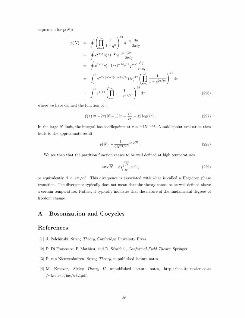
expression for p(N):

p(N) =

∮ ( ∞∏n=1

1

1− qn

)24

q−Ndq

2πiq

=

∮e2πiτη(τ)−24q−N

dq

2πiq

=

∮e2πiτη(−1/τ)−24τ12q−N

dq

2πiq

=

∫ 1

0

e−2π(N−1)iτ−2π/iτ (iτ)12

( ∞∏n=1

1

1− e2π/iτ

)24

dτ

=

∫ 1

0

ef(τ)

( ∞∏n=1

1

1− e2π/iτ

)24

dτ. (226)

where we have defined the function of τ :

f(τ) ≡ −2π(N − 1)iτ − 2π

iτ+ 12 log(iτ) . (227)

In the large N limit, the integral has saddlepoints at τ = ±iN−1/2. A saddlepoint evaluation then

leads to the approximate result

p(N) ∼ 1

2N27/4e4π√N . (228)

We see then that the partition function ceases to be well defined at high temperatures

4π√N − β

√N

α′> 0 , (229)

or equivalently β < 4π√α′. This divergence is associated with what is called a Hagedorn phase

transition. The divergence typically does not mean that the theory ceases to be well defined above

a certain temperature. Rather, it typically indicates that the nature of the fundamental degrees of

freedom change.

A Bosonization and Cocycles

References

[1] J. Polchinski, String Theory, Cambridge University Press.

[2] P. Di Francesco, P. Mathieu, and D. Senechal, Conformal Field Theory, Springer.

[3] P. van Nieuwenhuizen, String Theory, unpublished lecture notes.

[4] M. Kreuzer, String Theory II, unpublished lecture notes, http://hep.itp.tuwien.ac.at

/∼kreuzer/inc/sst2.pdf.

36