confrontation of traditional and computer … sandanusova.pdf · acta didactica universitatis...

Acta Didactica Universitatis Comenianae Mathematics, Issue 6, 2006

CONFRONTATION OF TRADITIONAL AND COMPUTER SUBSIDIZE LEARNING OF FUNCTION1

MARTINA SANDANUSOVÁ

Abstract. I used program Equation Grapher at the teaching of theme Function. The results of these experiment I described in following article. The basic hypothesis that I verified was: The using of computers during teaching of mathematics could make education more effec-tive and enhance motivation of pupils on mathematics lessons. Résumé. Jái utilisé le logiciel Equation Grapher dans lénseignement du thème Fonctions. Les résultats de cette expérience jái décrit dans lárticle présenté. L´hypothèse principale, que jái vérifié, était: Les ordinateurs dans lénseignement des mathématiques peuvent améliorer le processus de lénseignement et augmenter la motivation des élèves aux cours des mathématiques. Zusammenfassung. Das Programm Equation Grapher habe ich zum Unterricht der Funktion-en benutzt. Das Ergebnis von diesem Experiment habe ich in folgendem Artikel beschrieben. Die Basis-Hypothese, die ich verifizieren wollte, lautet: Die Computer während der Mathe-unterricht koenen der Unterrrichtprocess effektiver zu machen und die Schuele-rmotiva-tion zu erhoehen. Riassunto. Ho usato il programma Equation Grapher per l’insegnamento dell’argomento Fun-zioni. Il risultato di questo esperimento è descritto nel seguente articolo. Le ipotesi di base da me verificate sono state: l’uso dei computers durante l’insegnamento della matematica pot-rebbe permettere un’educazione più efficace e accrescere le motivazioni degli studenti durante le lezioni di matematica. Abstrakt. Program Equation Grapher som použila pri vyučovaní tematického celku Fun-kcie. Výsledky tohto experimentu som popísala v nasledujúcom článku. Základná hypoté-za, ktorú som overovala znela: Počítače vo vyučovaní matematiky môžu zefektívniť vyu-čovací proces a pomôžu zvýšiť motiváciu žiakov na hodine matematiky.

1 This article was partly supported by European Social Funds JPD 3 BA-2005/1-063 and SOPLZ-

2005/1-225

M. SANDANUSOVÁ 64

Key words: Confrontation, traditional, computer subsidize learning, function, Equation Grapher, motivation of pupils, effective learning

1 INTRODUCTION The goal of the experiment was to show that using the computer could be

solve the plenty of issues more effectively. From three classes of the first grade on secondary technical school were

chosen two classes – one with worse results (1.B. experimental group) and one class with better results (1.D. control group) from math.

Lessons’ themes were functions and their properties. Division of themes: Total number of lessons: 10 What is a function? Definition 2 Decreasing and increasing function 2 Bounded function 2 Even and odd function 1 Periodic and inverse function 1 Revision and written exam 2 Initial conditions in the classes:

1.D − control group 1.B − experimental group Number of students in the class 26 33

Semi – annual aver-age in math 1,88 2,54

Total Semi – annual average 2,03 2,4

Teaching aids

color chalk, blackboard newspapers, textbooks

(Matematika pre študijné odbory SOŠ a SOU − 2. časť;

Matematika pre 1. ročník gymnázií a SOŠ – zošit 2 –

Rovnice a nerovnice; Zbierka úloh z matematiky pre SOŠ

a SOU – 1. časť

shareware Equation Grapher at 11 computers,

felt-tips and textbook as in control group television

CONFRONTATION OF TRADITIONAL AND COMPUTER LEARNING 65

The students were taught 4/1 lessons in a week (3 lessons had a theory of functions and 1+1had a training).

There were students divided to three groups in the experimental group, so that each of them had a computer. The students had been taught traditional les-sons before. The reason was that they would not be allowed to use the com-puters at the further examinations in the future. Division of the themes in the experimental group: Theory: What is function?

Definition. 2 Decreasing and increasing function 2 Bounded function 2 Even and odd function 1 Periodic and inverse function 1

Experiment:

Groundwork with Regression Analyzer and Equation Grapher 1 Calculate problems from theory with computer 2 Goniometric function 1 Written exam with PC 1

The students sat in two lines, in front of the room was a blackboard, and

teacher’s work at table with PC and television, where the students can see what teacher is doing on PC.

2 TRADITIONAL LEARNING IN THE CONTROL GROUP (1.D)

Structure of lessons and time interval:

1. LESSON

Theme: Function – the domain of a function D(f) and the range of the function H(f). Goal: Definition of the function, D(f) and H(f). 1. For motivation of the students was used an example of trajectory from phys-

ics where they already could see the function and its graph. They wrote the relationship and draw a diagram. 10 min

2. Definition of new ideas of functions. What is a function and how it is entered?

M. SANDANUSOVÁ 66

Ex.1. What is the domain of the function f: 3y x= , g: 1y x= (the teacher

solved the problems)? Ex.2. What is the domain of the function (students solved the problems on

the blackboard)? 10 min

u: 3 2y x= − ; 3, 2x ∈ −

a) D(u), H(u) b) u(1), u(−5) c) Decide if the points [0; 2], [0; −2] and [2; 6] belong to the function u.

Ex.3. Calculate D(f) of the function 2: 3f y x x= − (students solved the problems in the exercise book). 5 min

3. Homework from the textbook. 5 min

2. LESSON Theme: Graph of the function. Goal: Introduce a definition of graph of the function, specify domain of definition from the graphs. 1. Revision of homework (three students from class). 10 min 2. Revision from last lesson, new examples. 15 min

Ex. Specify D(f), D(g), f(3), g(3) and solve the problem whether 5∈H(f), H(g):

21 2 5: ; :3 2 ( 3).(2 )

xf y g yx x x x

+= =

− + − +

3. Define the graph of a function; what is the graph of a function and give an example. 15 min Ex. Draw a graph of given functions:

] ] ]{ ] ]{ ]}}{ 2

: 2;3 ; 4; 1 ; 3;5 ; : 0;0 ; 2,5;7 ; 4;0 ;

: 2 1, 3; 2; 1; 0;1; 2; 3 ; :

g y h y

z y x x u y x

= − − = −

= − + ∈ − − − =

Ex. Calculate the co-ordinates of intersection point of function h with x, y axis 5 min

1:1

xh yx

−=

+

4. Homework from the textbook. 5 min


3. LESSON Theme: Decreasing and increasing function. Goal: Define decreasing and increasing function; determine them from the graph or by the aid of calculation. 1. Homework control. 10 min 2. Revision and new problems from last lesson. 15 min

Ex.1. Draw a graph of function f and calculate its D(f) and H(f) : 2f y x= −

Ex.2. Draw a graph of function u: 2y x b= + , { }2; 3; 0; 5b ∈ − and describe the difference.

Ex.3. Draw a graph of function u: 1y ax= − , { }1; 0; 1a ∈ − and describe the difference.

3. Definition of decreasing and increasing functions, its graph. The teacher solved the problems on the blackboard. 15 min

2: 2 1; : 3f y x g y x= − − =

The third graph is not function.

4. Homework, draw a graph and properties of the function. 5 min

1 2 3

: 2 1

( ) 2 1 ; ( ) 2 1; ( ) 2 1

f y x

y f x x y f x x y f x x

= −

= = − = = − = = −

4. LESSON Theme: Properties of functions – increasing, decreasing, one – to − one function. Goal: Acquisition idea, when functions are increasing or decreasing and launch new properties, when a function is one − to − one. 1. Inspection and analyse homework responsibilities, because they had the prob-

lems with drawn of the functions. We repeated problems together with the students on the lesson. 10 min

M. SANDANUSOVÁ 68

2. Theoretical application of the new properties of functions – one – to − one, how this property relates with another properties of function − increasing and decreasing. Explanation on the examples. 15 min

The fourth, sixth and seventh graph are not functions.

3. Application of the typical problems from praxis (service textbook Matema-tika pre 1. ročník gymnázií a SOŠ – zošit 2 – Rovnice a nerovnice p. 58–61). 15 min

4. Acquisition of survey about the graphs – bring the biggest quantity of vari-ous graphs especially from the newspapers or magazines. 5 min

5. LESSON Theme: Properties of functions – bounded and unbounded function. Goal: Application of the new properties of functions following own know-how and brought material. 1. Selected students presented articles with graphs from the newspapers –

development crowns towards euro, demographic development, change in temperature etc. 25 min

2. Definition of the function bounded from the bottom and bounded from the above. Example: 15 min Ex. Write everything what do you know about displayed function.

2: 0,5 4; : 2,5; :f y x g y x h y x= + = − − =

3. Homework: Draw the graph of given function and specify all its properties.

22

2

2:111

xf yxx

= −

− +

10 min


6. LESSON Theme: Properties of function – bounded and unbounded function – its maximum and minimum. Goal: Examination of student’s knowledge and application of the concept of maxi-mum and minimum of functions. 1. Inspection and analyse of homework, identification of problems with func-

tion displaying. Finding of the solution. 10 min 2. Set an exam to students, which implies theoretical and practical tasks. Stu-

dents created definitions, described increasing and decreasing functions and drew graph of the function, which was one – to − one and which was not one – to − one. This exam has served only for feedback of teacher and it was not marked. 15 min

3. Application of new definition for maximum and minimum of functions. Dem-onstration on graphs and materials used at previous lessons. 15 min

4. Set homework from the book (Zbierka úloh z matematiky pre SOŠ a SOU, 1. časť). 5 min

7. LESSON Theme: Properties of functions – even and odd functions. Goal: Application of the new properties – reading from the graph and verifica-tion using the calculations. 1. Revision of homework, students had no problems with it. 5 min 2. Summarise of achieved knowledge, explanation of limitations found in exam.

10 min 3. You draw these functions (use the graphs of functions that are drawn on the

board) 15 min 2 33;3 : ; : 2 ; : ; :x f y x g y x i y x j y x∈ − = = = =

4. Calculate if the function is even or odd. 10 min 5. Students independently solved tasks. Unsolved tasks remain on homework.

10 min 3

41: 2 ; : ; : ;u y x v x x z yx

= − + =

2 1: 3 ( 2 1); :1

w y x x t yx

= ⋅ − + =−

M. SANDANUSOVÁ 70

8. LESSON Theme: Properties of function – periodic and inverse function. Goal: Definition and dispersing of periodic function. Determination of inverse function by graphical and calculative ways. 1. Revision of homework on the lesson. 5 min 2. Summarise and solve some exercises before complex exam. 5 min 3. On the graph of goniometric functions f: siny x= , g: tgy x= in the near

future was illustrated the concept of periodic functions and the inverse func-tion – complex solution was demonstrated on function g: 20 min

2 3: 5

4x

g y+

= −

4. Set of other examples. ( )2: 1p y x x x= + − 10 min

9. LESSON Theme: Repetition. Goal: Review of achieved knowledge on examples. Ex.1. Define the graph and properties of given functions and define its point

of intersection with axis. 2 26 9 2( ): , : , : 2 , :

1 3x x x x xt y h y v y x k y

x x x+ + −

= = = =− +

Ex.2. Determine if given prescriptions are functions, if they are find D(f) and decide if they are even or odd functions:

2

1

4y

x=

− 2 12 0x x− + − ≥ 2

21

xy

x=

+

( ) ( )1

2 3y

x x=

− ⋅ + 3 4y x= − ( ) ( )4 5y x x= − ⋅ −

Ex.3. Find inverse functions to the functions: 7 12 3

xy

x−

=+

3 2

3x

y−

= 22x

yx

=

Ex.4. Define all linear functions, which pass points [ ]A -6;0 , [ ]B 3;3 . Ex.5. Construct graphs of the functions:

1 1y x x= + − − 22( )x xyx−

= 2y x=


10. LESSON Theme: Repetition – written exam. Goal: Attestation of achieved results on written exam. The exam tasks were the same for all students. Maximum number of achieved points was 15 and took time 35 min. Ex.1. Define D(f) of given functions: 5 points

2

1:5 6

g yx x

=− +

2 points

3:k y x= 1 point 1:h y

x x=

− 2 points

Ex.2. Have the function 2 3:1

xg yx

+=

−. 3 points

Calculate g(5), g(1). 1 point Calculate x if g(x)=0 1 point Calculate if is true that ( )2 H g∈ 1 point

Ex.3. Determine D(f) and properties of given functions. 6 points

)( 22 1:

2

x xj y

x

+= and draw the function j 4 points

2

1:4

p yx

=−

3 points

Ex.4. Calculate the co-ordinates of intersection points of function h with x, y axis and inverse function to given function. 1 point

: 2 1o y x= − 1 point

Specification of evaluation of solution: Ex.1. Function g

− determine correct conditions: 2 25 6 0 5 6 0x x x x− + ≠ ∧ − + > 1 point

− determine correct D(g): ( ) ( )( ) , 2 3,D g = −∞ ∪ ∞ 1 point

Function k − determine correct D(k): ( )D k R= 1 point

M. SANDANUSOVÁ 72

Function h − determine correct conditions: 0, 0x x x x x− > > ⇔ < 1 point − determine correct D(h): ( )( ) , 0D h = −∞ 1 point

Ex.2. Calculate 13(5) 3,254

g = = 0,5 point

g(1) – isn't definite at point 1 0,5 point

as g(x)=0 so 3 1,52

x = − = − 1 point

2 ( )H g∉ 1 point Ex.3. Drawing the graph of function j: 1 point

determine correct D(j): 1 point )( )(2 2( ) ;0 1 ( ) 0; 1D j y x D j y x= −∞ ⇒ = − − ∧ = ∞ ⇒ = +

properties – increasing on full D(f) 0,5 point is odd 0,5 point

isn't bounded 0,5 point isn't periodic 0,5 point

calculate 2( ) 4 0 2x D p x x∈ ⇔ − > ⇔ >

) )((( ) ; 2 2;D p = −∞ − ∪ ∞ 1 point

properties – increasing on the ( ), 2−∞ − and decreasing on the ( )2, ∞ 0,5 point

even 0,5 point

bounded below2

1 04x

>−

0,5 point

isn't periodic 0,5 point

Ex.4. Calculate intersection with axis x − ]0,5; 0 and y − ]0; 1 − 0,5 point

calculation of inverse function 1 1:2

xo y− += 0,5 point


Valuation:

Percentage of completion method

Mark Pointing valuation

100 % − 85,1 % 1 15,00 – 12,76 85 % − 70,1 % 2 12,75 – 10,51 70 % − 55,1 % 3 10,50 – 8,26 55 % − 40,1 % 4 8,25 – 6,10

40 % − 0 % 5 6,00 – 0,00

3 LEARNING PROCESS WITH THE SUPPORT OF EQUATION

GRAPHER

1. LESSON Theme and Goal: Introduction to the Equation Grapher. 1. Acquaintance with software Regression Analyzer – software for processing

of statistical data. 15 min 2. Introduction to the Equation Grapher. I had translated the Main Menu of

the application. We're passed together individual offers. Practically we had tried to put some functions f: y = 2x − 1, which we entered in the command line. Students worked easily with window Function Pad. Problems appeared with the length of axis. We set the right axis in windows Range. I left students work without my help while they did not familiarise with the icons of the main menu. Students had several problems: − Malfunction of icon maxim and minimum − Malfunction of icon intersection − Problem solution: − Function hadn't got maximum either minimum, we could it verify in

the window Log where was displayed the answer. − We set function g: y = −2x − 1 and using the icon for intersection, in the

Log window we found the value of intersection point 30 min

2. LESSON Theme: Solution of specific examples. Goal: Solution of examples from theoretical lesson with using the computer.

M. SANDANUSOVÁ 74

Students solved examples with using of EG.

Ex.1. What is D(f) of the functions f: y = 3x, g: y = 1/x ? u: y = x3 – 2; )3;2x ∈ − a) D(u), H(u) b) u(1), u(−0,5) c) Decide if the points [0; 2], [0; −2] and [2; 6] belong to the function u. Students wrote out a command of the individual functions in the com-mand line and from the graph they very simply verify the answer. Prob-lems were with function “u”, because they didn’t know how to set x^3. They were not familiar with Function Pad yet.

Ex.3. Calculate D(f) of the function 2: 3f y x x= − .

Students set improper command of fun-ction e.g. y = sqrt x^2−3x. Graphs looked like in the picture. Without using the brac-kets the computer calculate the second root only from x^2 instead of whole ex-pression x^2−3x.

Ex.4. Determine D(f), f(3) and solve problem 5∈ H(f)

a) 21: ;3 2

f yx x

=− +

b) 2 5:( 3).(2 )

xf yx x

+=

− +

Repeated error with brackets at setting the function y = 1/x^2 − − 3x+2. Correct notation is y = 1/(x^2 − 3x+2). These two func-tions have different properties, which can we see on their graphs.

Inscription of next function had to look like this y = (2x − 5)/ /(sqrt((x − 3).(2 + x)). It was im-portant to explain to students, that expression (2x + 5) has to be in parenthesis, because we divide it with sqrt. There had to be paren-thesis around the whole square


root, because we are making it from the product of both brackets. After solving problems with brackets, students simply solved the tasks us-

ing proper icons from the Log window, they read fast and accurate answer: y-Cacl: Could not be evaluated

Ex.5. Draw graphs:

] ]{ ]}] ]{ ]}

}{2

: 2;3 ; 4; 1 ; 3;5 ;

: 0;0 ; 2,5;7 ; 4;0

: 2 1; 3; 2; 1;0;1;2;3

:

g y

h y

z y x x

u y x

= − −

= −

= − + ∈ − − −

=

Ex.6. Calculate co-ordinates intersection points of 1:1

xh yx

−=

+ with x, y-axis.

Calculation in exercise book was replaced with automatic calcula-tion in EG, using necessary icons. Examples of incorrect notation of the function in the command line are e.g.: • x − 1/ x + 1 • (x − 1)/x + 1 • x − 1/(x + 1) Correct inscription had looked now y = (x − 1)/(x + 1). The diffe-rence you can see on the graph.

3. LESSON Theme: Solution of the specific exam-ples. Goal: Solution of examples from theo-retical lesson with using the computer. Ex.1. Draw the graph of function u:

y = 2x + b, }{ 2;3;0;5b∈ − , and describe the difference between these functions.

M. SANDANUSOVÁ 76

It was very simple to draw these functions for the students. They exactly saw how the function is changed when the parameter b is changed.

Ex.2. Draw the graph of function u: y = ax – 1, }{ 1; 0; 1a ∈ − and describe the differences.

Ex.3. Draw graphs of these functions and describe the properties of these func-tions:

1: 2 1; ( ) 2 1 ;f y x y f x x= − = = −

2 3( ) 2 1; ( ) 2 1y f x x y f x x= = − = = −

Problems are appeared at the notation of this function, and the correct notation should be:

1 2 3(2 1); 2 ( ) 1; (2( ( ) 1)y abs x y abs x y abs abs x= − = − = − and then students could describe the properties of function.

Ex.4. Designate the properties of the following functions: 3

41: 2 ; : ; : ;u y x v x x z yx

= − + =

2 1: 3 ( 2 1); :1

w y x x t yx

= ⋅ − + =−

Concerning the problems with the notation of the brackets, they home-

work was to note down this function: 22

2

2:111

xf yxx

= −

− +

.

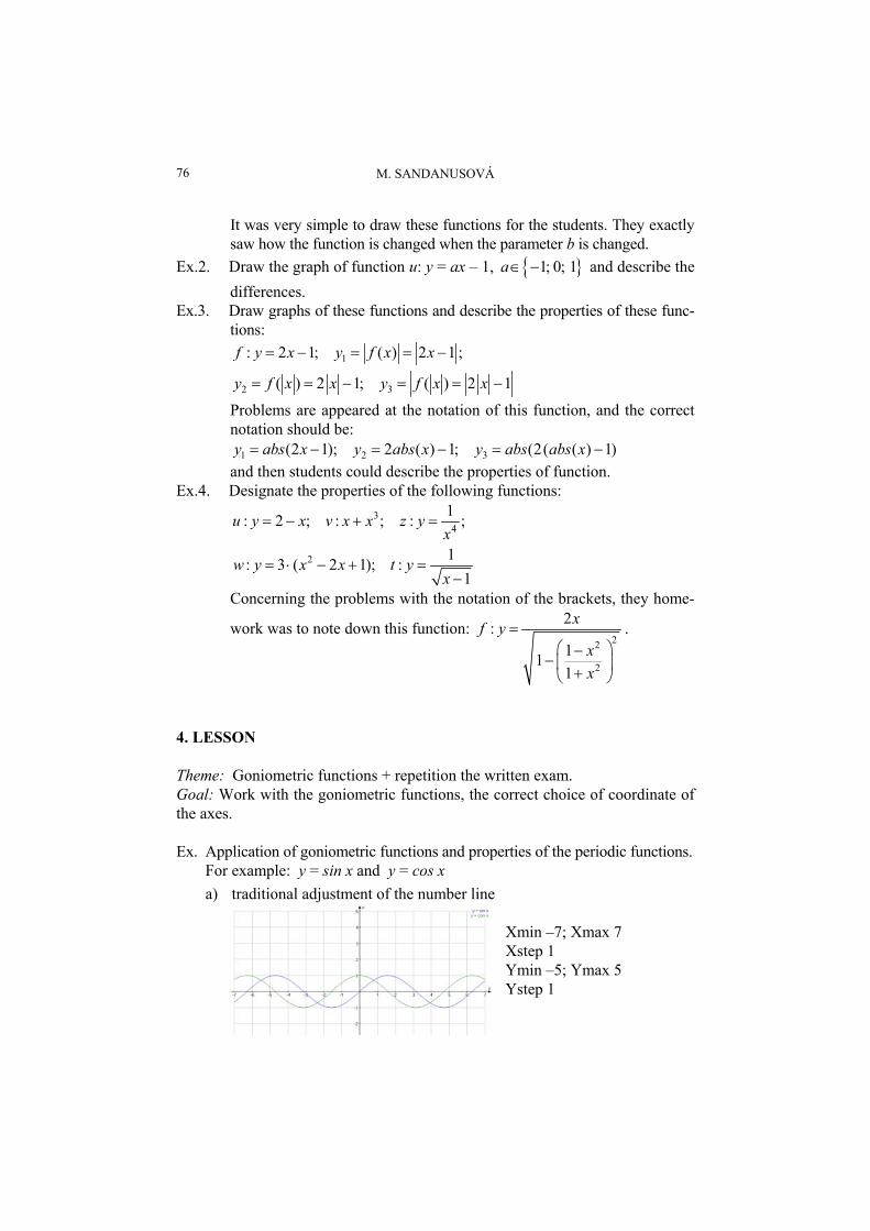
4. LESSON Theme: Goniometric functions + repetition the written exam. Goal: Work with the goniometric functions, the correct choice of coordinate of the axes. Ex. Application of goniometric functions and properties of the periodic functions.

For example: y = sin x and y = cos x a) traditional adjustment of the number line

Xmin –7; Xmax 7

Xstep 1 Ymin –5; Ymax 5 Ystep 1


1 2 3 4 5 6 7-1-2-3-4-5-6-7

1

2

3

4

5

-1

-2

-3

-4

-5

x

yy = x^3

y = 1/ (sqrt (abs (x)-x))y = 1/ (sqrt (x^2-5x+6))

b) changing the interval on the multiplying π/2 with Options – Angles –Radians, in the window Range − Re

Xmin −7,796 Xmax 9,42; Xstep 1,57 Ymin −3,14; Ymax 3,14 Ystep 1

c) changing the axis x to grades with Options – Angles – Degrees in the win-dow Range with icon sin and Re

Xmin –540; Xmax 540 Xstep 90 Ymin −3,14; Ymax 3,14 Ystep 1

5. LESSON Theme: Written exam. Goal: The verification of the student’s knowledge – same as in the 1.D. All groups of students wrote this exam at the same time. To avoid the facilitation, the teachers are not mathematicians. Students could use the computers, but the calculation should be also recalculated without using the computer. Students had 30 minutes for this exam. Solve with EGUATION GRAPHER Ex.1. g: y = 1/(sgrt (x^2−5x + 6)) k: y = x^3 h: y = 1/(sqrt (abs(x) − x))

M. SANDANUSOVÁ 78

0.5 1 1.5 2 2.5 3 3.5 4 4.5 5 5.5 6 6.5 7-0.5-1-1.5-2-2.5-3-3.5-4-4.5-5-5.5-6-6.5-7

0.51

1.52

2.53

3.54

4.55

5.56

6.57

-0.5-1

-1.5-2

-2.5-3

-3.5-4

-4.5-5

-5.5-6

-6.5-7

x

yy = (2x+3)/ (x-1)

1 2 3 4 5 6 7-1-2-3-4-5-6-7

1

2

3

4

5

-1

-2

-3

-4

-5

x

yy = 1/ (sqrt (x^2-4))

y = (2x(1+x^2))/ (2abs (x))

Ex.2. g: y = (2x+3)/(x−1) Y-Calc: y = 3.25 for x = 5 X -Calc: y = 0 for x = −1.5 X-Calc: y-value could not be found

Ex.3. j: y = (2x(1+x^2))/(2abs x) p: y = 1/(sqrt(x^2−4)) Ex.4. o: y = 2x−1 X-Intersection x = 0.5 Y-Intersection: y = −1 o-1: y = (x+1)/2 Intersection: y = 1 for x = 1

4 ANALYSIS OF THE ACHIEVEMENT RESULTS For the relative comparison is processing their achieved results listed together. 1.B. – experimental group (33 students) 1.D. – control group (26 students) In the Table 1 are listed the results from the written exam. The results of the

class 1.B. (using the computers) seem to be better like in the class 1.D. In the first line are listed the maximum points, which they could obtain for

the each example, also their total number (CP) of the mark (ZN), which student


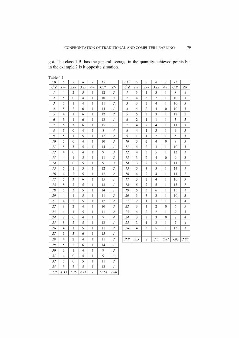
got. The class 1.B. has the general average in the quantity-achieved points but in the example 2 is it opposite situation.

Table 4.1

1.B. 5 3 6 1 15 1.D. 5 3 6 1 15 Č.Ž 1.ex 2.ex 3.ex 4.ex C.P. ZN Č.Ž 1.ex 2.ex 3.ex 4.ex C.P. ZN 1 4 2 5 1 12 2 1 3 1 3 1 8 4 2 5 0 4 1 10 3 2 4 3 2 1 10 3 3 5 1 4 1 11 2 3 3 2 4 1 10 3 4 5 2 6 1 14 1 4 4 2 4 0 10 3 5 4 1 6 1 12 2 5 5 3 3 1 12 2 6 5 1 6 1 13 1 6 2 1 1 1 5 5 7 5 3 6 1 15 1 7 4 2 4 1 11 3 8 3 0 4 1 8 4 8 4 1 3 1 9 3 9 5 1 5 1 12 2 9 1 1 2 1 5 5

10 5 0 4 1 10 3 10 3 2 4 0 9 3 11 5 3 5 1 14 1 11 4 2 3 1 10 3 12 4 0 4 1 9 3 12 4 3 5 1 13 1 13 4 1 5 1 11 2 13 3 2 4 0 9 3 14 3 0 5 1 9 3 14 3 2 5 1 11 2 15 5 1 5 1 12 2 15 5 3 5 1 14 1 16 4 2 5 1 12 2 16 4 2 4 1 11 2 17 5 3 6 1 15 1 17 3 2 4 1 10 3 18 5 2 5 1 13 1 18 5 2 5 1 13 1 19 5 3 5 1 14 1 19 5 3 6 1 15 1 20 4 1 5 1 11 2 20 3 3 3 1 10 3 21 4 2 5 1 12 2 21 2 1 3 1 7 4 22 3 2 4 1 10 3 22 3 1 2 0 6 5 23 4 1 5 1 11 2 23 4 2 2 1 9 3 24 2 0 4 1 7 4 24 3 2 3 0 8 4 25 5 2 5 1 13 1 25 3 1 2 1 7 4 26 4 1 5 1 11 2 26 4 3 5 1 13 1 27 5 3 6 1 15 1 28 4 2 4 1 11 2 P.P 3.5 2 3.5 0.81 9.81 2.88 29 5 2 6 1 14 1 30 3 1 4 1 9 3 31 4 0 4 1 9 3 32 5 0 5 1 11 2 33 5 2 5 1 13 1 P.P 4.33 1.36 4.91 1 11.61 2.00

M. SANDANUSOVÁ 80

In the Table 4.2 you can see the mark from math at the end of the first half-year (MAT1/2) and the mark from the written exam.

Table 4.2

1.B. 1.D. Č. Ž. MAT1/2 Exam Č. Ž. MAT 1/2 Exam

1 4 2 1 3 4 2 4 3 2 2 3 3 3 2 3 2 3 4 2 1 4 2 3 5 1 2 5 1 2 6 2 1 6 3 5 7 2 1 7 1 3 8 2 4 8 2 3 9 3 2 9 3 5 10 3 3 10 2 3 11 1 1 11 2 3 12 3 3 12 2 1 13 4 2 13 3 3 14 3 3 14 1 2 15 2 2 15 1 1 16 4 2 16 1 2 17 3 1 17 2 3 18 1 1 18 1 1 19 3 1 19 1 1 20 2 2 20 2 3 21 3 2 21 3 4 22 3 3 22 3 5 23 3 2 23 2 3 24 5 4 24 1 4 25 2 1 25 2 4 26 3 2 26 1 1 27 1 1

28 3 2 P.P 1.88 2.88

29 1 1 30 3 3 31 3 3 32 3 2 33 2 1

P.P. 2.64 2.00


Students from the class 1.B had worse average from math than class 1.D, but they were in opposite situation at the beginning of this experiment.

Exam – 1.B

Table 4.3 Moments

N 33 Sum Weights 33

Mean 2 Sum Observations 66

Std Deviation 0.90138782 Variance 0.8125

Skewness 0.54506521 Kurtosis −0.447719

Uncorrected SS 158 Corrected SS 26

Coeff Variation 45.0693909 Std Error Mean 0.15691148

Table 4.4

Basic Statistical Measures

Location Variability

Mean 2.000000 Std Deviation 0.90139

Median 2.000000 Variance 0.81250

Mode 2.000000 Range 3.00000

Interquartile Range 2.00000

In the Table 4.4 you can see the average mark of exam, median and modus,

and its value is two. This value of the mark you can find in the Table 4.5, where 95 % of the total number of students has mark between the interval 1,68038 – 2,31962.

Table 4.5

Basic Confidence Limits Assuming Normality

Parameter Estimate 95 % Confidence Limits

Mean 2.00000 1.68038 2.31962

Std Deviation 0.90139 0.72489 1.19226

Variance 0.81250 0.52546 1.42148

M. SANDANUSOVÁ 82

Figure 4.1. Graphical distribution of student’s marks in the class

Exam – 1.D Table 4.6

Moments N 26 Sum Weights 26 Mean 2.88461538 Sum Observations 75 Std Deviation 1.24344435 Variance 1.54615385 Skewness −0.0356096 Kurtosis −0.6053832 Uncorrected SS 255 Corrected SS 38.6538462 Coeff Variation 43.1060707 Std Error Mean 0.2438595

The average value of the exam mark is 2.88 and it is worse than in the class

1.B.

Table 4.7

Basic Statistical Measures Location Variability

Mean 2.884615 Std Deviation 1.24344 Median 3.000000 Variance 1.54615 Mode 3.000000 Range 4.00000 Interquartile Range 2.00000


Table 4.8

Basic Confidence Limits Assuming Normality

Parameter Estimate 95 % Confidence Limits Mean 2.88462 2.38238 3.38685 Std Deviation 1.24344 0.97518 1.71646 Variance 1.54615 0.95098 2.94624

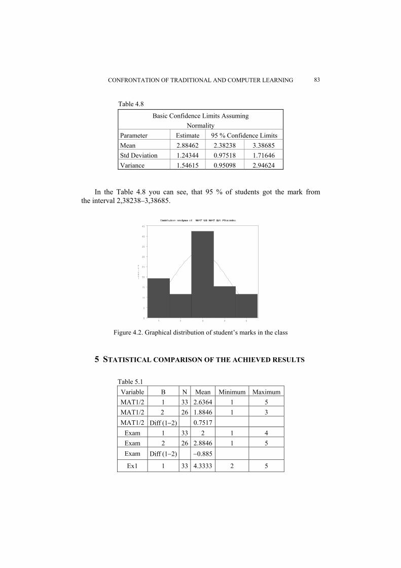
In the Table 4.8 you can see, that 95 % of students got the mark from the interval 2,38238–3,38685.

Figure 4.2. Graphical distribution of student’s marks in the class 5 STATISTICAL COMPARISON OF THE ACHIEVED RESULTS

Table 5.1 Variable B N Mean Minimum Maximum MAT1/2 1 33 2.6364 1 5 MAT1/2 2 26 1.8846 1 3 MAT1/2 Diff (1−2) 0.7517

Exam 1 33 2 1 4 Exam 2 26 2.8846 1 5 Exam Diff (1−2) −0.885

Ex1 1 33 4.3333 2 5

M. SANDANUSOVÁ 84

Variable B N Mean Minimum Maximum Ex1 2 26 3.5 1 5

Ex1 Diff (1−2) 0.8333

Ex2 1 33 1.3636 0 3

Ex2 2 26 2 1 3

Ex2 Diff (1−2) −0.636

Ex3 1 33 4.9091 4 6

Ex3 2 26 3.5 1 6

Ex3 Diff (1−2) 1.4091

Ex4 1 33 1 1 1

Ex4 2 26 0.8077 0 1

Ex4 Diff (1−2) 0.1923

Points 1 33 11.606 7 15

Points 2 26 9.8077 5 15

Points Diff (1−2) 1.7984

The Table 5.1 shows the comparison between both classes. Column B desig-

nated by number 1 is the class 1.B, by number 2 is designated the class 1.D and Diff (1−2) means the difference between these two classes. Column N shows the number of students in each class. The fifth, the sixth and the seventh column are average min and max mark or number of points.

In the Table 5.1 you can also see that class 1.B have about 0.7517 worse to-tal average marks from mathematics than 1.D.

But the class 1.B reached about 0.885 better average marks from the writ-ten exam than class 1.D. Simple examples:

Ex.1 − minimal number of achieved points in the experimental sample is 2 from the total of number of 5,

− errors, which occurred here, were caused by the wrong notation of function h in the command line,

Ex.2 − class 1.D was more successful by calculation of this example, because students in class 1.B did not correct understand the computer report,

Ex.3, Ex.4 − better experimental sample. Points − better experimental group about 1.7984.

The main hypothesis that I verified was the effect of using of computers in the teaching process.


Advantages by using of computers: − high motivation of students, − individuality, − high objectivity, − time savings, − better results from the written exam.

Disadvantages, which I remarked in use of computers:

− lack of lessons using the computers − different level of computer skills of each student,

− in the further education useless (without agreement of the subject commis-sion, students can not use computers in the higher school years or gradua-tion).

REFERENCES

Hecht, T.: Matematika pre 1. ročník gymnázií a SOŠ, Bratislava, Orbis Pictus Istropolitana Jirásek, F.: Zbierka úloh z matematiky pre SOŠ a študijné odbory SOU 1. časť, Bratislava, SPN 1986 Kudláček, L.: Matematika pre 1. a 2. ročník štúdia na stredných priemyselných školách pre pracu-

júcich, Bratislava, SPN 1976 Kutzler, B.: Úvod do Derive 6, Linc, Gutenberg Druck 2003 Odvárko, O.: Matematika pre študijné odbory SOŠ a SOU 2. časť, Bratislava, SPN 1993 Sandanusová M.: Počítače v procese vyučovania matematiky, rigorózna práca, FMFI UK, 2003

MARTINA SANDANUSOVÁ, Department of Algebra, Geometry and Didactics of Mathematics, Faculty of Mathematics, Physics and Informatics, Comenius University, 842 48 Bratislava, Slovakia E-mail: [email protected]

confrontation of traditional and computer … sandanusova.pdf · acta didactica universitatis...

Documents