confronting weathering models with real world data
TRANSCRIPT

I
Confronting weathering models with real world data collected in the Sierra
Morena, Spain.
MSc Thesis report
Denys van den Berg January 2015

II
Confronting weathering models with real world data collected in the Sierra Morena, Spain.
MSc Thesis report
Denys van den Berg BSc (reg.nr. 900822052130) Wageningen University May 2015 – January 2016
Supervisor: Arnaud Temme (Wageningen University) 2nd supervisor: Tom Vanwalleghem (University of Cordoba)
Course code: SGL-80436

III
Abstract Rock weathering is the first step in soil formation. It supplies the raw materials necessary to produce soils. However, our understanding of the processes and mechanisms behind rock weathering is limited and weathering is often simplistically represented as the repeated splitting of rock fragments into two equal parts. The research that has been done on weathering has produced a number of different weathering models. These models were compared to laboratory weathering experiments for a single rock type and judged to accurately represent the weathering process. This study takes the next step and confronts two types of weathering models with real world data from several different rock types. Samples were collected from roadcut profiles in the Sierra Morena, Spain. The samples were collected from different depths in a profile to simulate a weathering chrono-sequence. The samples were sieved and represented as Particle Size Distributions (PSD’s). Per profile, the sample PSD’s were compared with PSD’s produced by the weathering models. No significant difference was found between the different rock types, but between the model types a noteworthy difference was found. Both models succeeded in modelling close matches of the sample PSD’s. A symmetric weathering model (splitting into equal parts) outperforms asymmetric models by a small margin, both in modelling the PSD’s of entire profiles and in modelling the PSD’s of single samples. Another important result is that models with weathering resulting in two equal fragments never produced the best results. Especially this last part will have to be taken into account when modelling weathering. Keywords: gneiss, quartzite, schist, slate, saprolite, particle size distribution, weathering models, weathering, rock weathering, Sierra Morena, Spain.

IV
Acknowledgements I want to thank several people for lending me their invaluable assistance over the course of this study: Minke Wuis, a fellow Msc-student, assisted me during the fieldwork and part of the laboratory work. Andrea Román for also assisting during parts of the fieldwork and her help in developing the sieving method. Garry Willgoose for taking the time to adjust his newest weathering model and making it available to me. Arnaud Temme and Tom Vanwalleghem, my supervisors, were always ready to look at my results and methods and provide advice on how to proceed. Jeroen Schoorl, Benny Guralnik, Tony Reimann and Tom Veldkamp for humoring me and playing the “Determine the rock type of this rock from Spain”-game.

V
Table of Contents Introduction ............................................................................................................................................. 1
Study area ................................................................................................................................................ 4
Topography ......................................................................................................................................... 4
Geology ................................................................................................................................................ 6
Climate................................................................................................................................................. 6
Vegetation ........................................................................................................................................... 6
Background .............................................................................................................................................. 8
Clarification of terms ........................................................................................................................... 8
Surface Armouring............................................................................................................................... 9
Modelling weathering ......................................................................................................................... 9
Methods ................................................................................................................................................ 10
Data collection ................................................................................................................................... 10
Site selection ................................................................................................................................. 10
Fieldwork ....................................................................................................................................... 10
Laboratory work ............................................................................................................................ 11
Modelling ........................................................................................................................................... 13
Initial data ...................................................................................................................................... 13
Error correction ............................................................................................................................. 14
Weathering models ....................................................................................................................... 14
Results ................................................................................................................................................... 15
Fieldwork ........................................................................................................................................... 15
Saprolite analysis ............................................................................................................................... 15
Grain size distributions. ..................................................................................................................... 16
Modelling ........................................................................................................................................... 20
Symmetrical weathering ............................................................................................................... 21
Asymmetrical weathering ............................................................................................................. 22
Comparing models per location .................................................................................................... 22
Comparing models per layer ......................................................................................................... 23
Discussion .............................................................................................................................................. 25
Can weathering explain the data collected during the fieldwork? ................................................... 25
Surface armouring ......................................................................................................................... 25
Cracks and intrusions .................................................................................................................... 25
Parent material .............................................................................................................................. 26
Future research ............................................................................................................................. 26
Do the known weathering pathways match the data collected during the fieldwork?.................... 26
Symmetrical weathering ............................................................................................................... 26
Asymmetrical weathering ............................................................................................................. 27

VI
Changing weathering geometries ................................................................................................. 27
Future research ............................................................................................................................. 28
Does a difference in lithology explain observed differences in weathering behaviour? .................. 28
Weathering models ....................................................................................................................... 28
Saprolite analysis ........................................................................................................................... 29
Causes of differing signals ............................................................................................................. 29
Future research ............................................................................................................................. 30
Conclusion ............................................................................................................................................. 31
References ............................................................................................................................................. 32
Appendix ................................................................................................................................................ 35

1
Introduction The weathering of rock is a much researched topic in soil science, geology and other related fields. The reason for this is that rock weathering is the source of soil, which we require to grow food and for many other purposes (FAO, 2015). The importance of soils is especially recognized in the concept known as the Critical Zone. As noted by the U.S. Research Council Committee:
The Critical Zone includes the land surface and its canopy of vegetation, rivers, lakes and shallow seas and it extends through the pedosphere, unsaturated vadose zone and saturated groundwater zone. Interactions at this interface between the solid Earth and its fluid envelopes determine the availability of nearly every life-sustaining resource (U.S. Nat. Res. Cou. Com. Basic Res. Opp. Earth Sci., 2001, p.36).
Knowing how rocks become soil is therefore an important part in improving our understanding of how landscapes evolve and how we can continue to use them to generate resources (Brantley and Lebedeva, 2011). Many different approaches to investigate rock weathering and its influence on landscape evolution exist. The key elements remain the same. Rock weathering has two aspects: physical and chemical weathering. Physical weathering, which breaks down and disintegrates material into smaller fragments, is driven by mechanical forces such as gradual or sudden temperature differences (Wakasa et al. 2012), ice or salt expansion (Dixon et al. 2001, Wells et al. 2007) and abrasion by wind or water. Chemical weathering reduces, oxidizes and dissolves material into other substances (Chigira, 1990). Although the effects of these two weathering types are easy to separate in theory, what is seen in the field is always the result of an interplay between them (Anderson et al. 2007, Pope, 2013). For instance physically weakened rocks develop cracks, which increases the surface area for chemical weathering, which speeds up the process of the rocks breaking down further (Royne et al., 2008). In addition to this, some researchers also recognize biological weathering, a combination of physical and chemical weathering caused by the presence of organisms. An example of this would be that mechanical pressure is exerted by growing and expanding roots while at the same time the root exudates chemically interact with the rocks. In some specific cases it is possible to separate the different types of weathering and identify which is the dominant one(Matsukura and Hirose, 1999, Yokoyama, 2006). In general, the interplay between physical and chemical weathering makes it impossible to determine the dominant weathering process. It is possible however to identify where combined weathering is the most active. Vertically down a profile, the interplay between the different types of weathering results in transition zones (or weathering fronts) between solid bedrock and soil (Chigira, 1990), see Figure 1. These transition zones are where weathering is the most active. A good example of these transition zones can be found in a paper by Brantley et al. (2013) which they use to explain a pattern they found in the absence and presence of pyrite in the bedrock and above-lying layers. The material in transition zones is known as saprolite, saprock or “rotten rock” because it appears to be solid rock but can easily be broken even with one’s bare hands (Graham et al. 2010). In practice, matters are even less clear cut than presented up to now. Not only do the different weathering types intermingle, but, as identified by Wells et al. (2007, 2008), both physical and chemical weathering can also follow different weathering pathways. A weathering pathway describes the series of weathering events that occur when rock starts weathering (Weathered rock in Figure 1) until it becomes soil (Soil in Figure 1). These weathering events cause a change in the particle size distribution of the material. Different weathering pathways mean that the resulting particles of the weathering events have different sizes, the amount of resulting particles will be different or both the sizes and the amounts differ. The Saprolite section in Figure 1 gives an indication of these differences. Wells et al. only investigated one rock type in their study, but they suspected that

2
different rock types, while weathering under the same circumstances, would also follow different weathering pathways.
Figure 1. Clarification of terms used compared to weathering grades established by Little (1969).
This is corroborated by Gracheva (2011), who showed that different rock types indeed follow different weathering pathways. Wells et al. were able to show that one of their physical weathering pathways closely matched the results of their salt-weathering experiment of quartz-chlorite schist. However, to date, there has not been a follow-up comparison between their weathering pathways and field observations. Also, no further lab experiments have been carried out to compare the weathering pathways of different rock types under the same climate. Because of this lack of follow-up research, soil development and soil evolution models only include weathering processes and transition zones to a limited degree. While the level of detail for the saprolite itself can differ from a single input function to multiple layers or weathering fronts (Vanwalleghem et al. 2013), the weathering itself is often reduced to a weathering fraction. In addition, the weathering event always results in two equally sized particles. Due to the complexity of the interrelated processes this is understandable and for an evolution model of a homogenous soil column it may be enough. However, in a situation with multiple parent materials, such as a model (LORICA) that integrates soil evolution and landscape evolution (Temme and Vanwalleghem, in press) a weathering fraction alone will not be enough to accurately represent what happens in reality. Instead, weathering should be a function of the rock type that is weathering. This includes not only the weathering fraction, but also the number of resulting particles and their respective sizes. My main objective is to confront physical weathering pathways from literature (Wells et al., 2007, 2008) to real world data collected from different lithologies. To meet this objective I have formulated several research questions:

3
- Can physical weathering explain the data collected during the fieldwork? - Which weathering pathway best matches the data collected during the fieldwork? - Does a difference in lithology lead to differences in weathering behaviour?
It is hoped that this research will provide new opportunities and directions for future research.

4
Study area
Topography The study area is part of the Sierra Morena mountain range in Spain. All samples were taken from the part of the mountain range closest to Cordoba, shown in Figure 2. The letters indicate the parent material found at the sampling locations. Numbers are added if a parent material was encountered multiple times.
Figure 2. Satellite view of Spain and sampling locations (Google Earth, 2013 a, 2013 b, 2015 a). Legend: Q: Quartzite, Sch: Schist, G: Gneiss, Sl: Slate.
The drainage (Figure 3) follows a dendritic pattern in the northern part of the study area, indicating that the rock types present there are approximately equally resistant to erosion in all directions. The southern part of the study area shows a more parallel drainage pattern, but no pronounced slope was observed in the field. This hints at outcrops of weathering resistant rock being present in the southern part, likely remnants or intrusions related to the bands of weathering resistant rock bisecting the study area. The slopes in the study area vary between 0° and 37°, with an average slope of 17°. No pattern can be recognised in the locations of the steep and flat areas. The only noteworthy features are the steep slopes on the bands of weathering resistant rocks dissecting the study area (Figure 4).

5
Figure 3. Drainage pattern of the study area (Instituto Geográfico Nacional de España,2015).
Figure 4. Slope map of the study area including sample locations (Instituto Geográfico Nacional de España, 2015).

6
Geology The Sierra Morena is part of the Iberian Massif. The Iberian Massif is an exposure of the European Variscan orogeny, created when the landmasses of Laurasia and Gondwana collided in the late Paleozoic. During the Mesozoic the dominating process was erosion, resulting in large areas ending up as planation surfaces, including the region now known as the Sierra Morena. Over time, gentle uplift of the whole area and differential erosion of the folded and metamorphosed rock created the Sierra Morena as it is today with its Appalachian (or Ardennes) topography. This geological history of the region can be recognized in the rock types. Slate, schist, limestones, dolomites, gneiss, granodiorite, quartzite and many other (partially) metamorphosed rocks are present (Gutiérrez et al. 2014, Núñez and Recio, 2007). This wide range of rock types was what made this area ideal for this study, since one of the goals was to compare the effects of differing rock types. See Figure 5 for a geological map of the Sierra Morena, including the sample locations.
Figure 5. Geological map of the Sierra Morena (Isasa et al. 1982, Google Earth,2015 b) including sampling locations. Legend: Q1, Arkose (conglomerates); Q2, Slate or Quartzite; Sch1, Slate or Quartzite; Sch2, Phyllites; Sch3, Shale or Greywacke; G1, Granodiorite or Mica or Quartz or Greywacke; G2, Gneiss with quartz or Gabbro; Sl, Slate or Greywacke.
Climate The climate of the region is a typical Mediterranean climate with average annual temperatures between 14 and 17 °C and annual rainfall between 600 and 1000 mm (Núñez and Recio, 2007). In an average year only 40 days with temperatures below 0 °C are expected. As such, in the current climate, frost weathering does not play a large role. During cooler periods in history, such as ice ages, frost weathering would have had a larger impact than it does today. This means that at least some of the weathering profiles found during fieldwork are (partially) the result of frost weathering. The maximum temperature can, as experienced during the fieldwork in May 2015, reach at least 30 °C during the day. While this does not directly result in an increase of weathering, these daily temperatures provide a favourable climate for plant growth.
Vegetation The main vegetation for the study area consists of olive tree plantations, dehesa’s and (semi)natural vegetation or matorrales (Joffre et al. 1988).

7
The olive tree plantations consist mainly of olive trees with low grasses and weeds covering the ground in between. These plantations occupy most of the upper slopes. The lower slopes and valleys are used for dehesa’s, the typical Mediterranean oak forests with natural vegetation in between. The areas not suitable to either of these two landuses are covered by the natural vegetation of the region, which is dense evergreen shrublands. Overall the vegetation is capable of dealing with a yearly moisture deficit and the shallow soils. These two factors result in active but limited biological weathering. Due to the shallow soils, the roots of most plants will reach saprolite or bedrock and influence the weathering process. However, the lack of moisture inhibits this plant growth. During cooler or wetter periods in history this limitation might have been less severe and biological weathering may have played a larger role.
8
Background
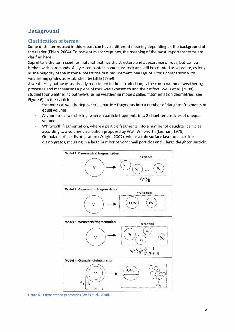
Clarification of terms Some of the terms used in this report can have a different meaning depending on the background of the reader (Ehlen, 2004). To prevent misconceptions, the meaning of the most important terms are clarified here. Saprolite is the term used for material that has the structure and appearance of rock, but can be broken with bare hands. A layer can contain some hard rock and still be counted as saprolite, as long as the majority of the material meets the first requirement. See Figure 1 for a comparison with weathering grades as established by Little (1969). A weathering pathway, as already mentioned in the introduction, is the combination of weathering processes and mechanisms a piece of rock was exposed to and their effect. Wells et al. (2008) studied four weathering pathways, using weathering models called fragmentation geometries (see Figure 6), in their article:
- Symmetrical weathering, where a particle fragments into a number of daughter fragments of equal volume.
- Asymmetrical weathering, where a particle fragments into 2 daughter particles of unequal volume.
- Whitworth fragmentation, where a particle fragments into a number of daughter particles according to a volume distribution proposed by W.A. Whitworth (Lerman, 1979).
- Granular surface disintegration (Wright, 2007), where a thin surface layer of a particle disintegrates, resulting in a large number of very small particles and 1 large daughter particle.
Figure 6. Fragmentation geometries (Wells et al., 2008).

9
A weathering model is an attempt to simplify a weathering process/mechanism to a series of equations. The goal is to be able to predict how a weathering profile will develop. In this study the goal is to explain how a weathering profile developed. The coarse fraction of a (soil) sample consists of all particles larger than 2 mm in diameter. The fine fraction of a (soil) sample consists of all particles as small or smaller than 2 mm in diameter. The fine fraction is further subdivided into coarse sand, fine sand and the combined silt and clay fraction. All particles between 2 mm and 0,6 mm in diameter are classified as coarse sand. All particles between 0,6 mm and 0,063 mm are classified as fine sand. All particles smaller than 0,063 mm are classified as silt and clay.
Surface Armouring Surface armouring (or soil armouring) is the process of the coarsening of the particle size distribution of the surface layer, due to selective removal of fine material from the soil surface (Sharmeen and Willgoose, 2006). The fine, easily transportable fraction of the soil surface is removed by wind or water, leaving the coarser and less mobile fraction behind. If this process is not disrupted, eventually all fine material is transported away and the coarse fraction remains as a kind of armour. An example of an armour layer (created in aeolian conditions) is the desert pavement that is present in deserts all over the world. Such an armour layer prevents or slows erosion of the materials below it. Over time the armour layer will weather, or the transport capacity of the eroding forces will increase, with erosion increasing again as a result. Surface armouring explains why some surface horizons are coarser than the underlying horizons.
Modelling weathering In the model of Wells et al. (2007, 2008) all aspects of weathering are a function of volume. Any weathering event that occurs results in a redistribution of the volume of the parent particle over a number of smaller size classes. The resulting fragments are assumed to be roughly spherical. As such their diameter can be calculated using the equation for the volume of a sphere, Equation 1:
𝑉𝑜𝑙𝑢𝑚𝑒 = 4
3𝜋𝑟3
Equation 1. Volume of a sphere
Wells et al. include the relationship derived by McDowell and Bolton (1998) that states that weathering rate (or fracture probability) decreases with particle volume. This relationship is grounded purely in physical weathering, as it was developed based on pressure experiments on particle grains. Chemical weathering was not taken into account, although a decreasing particle volume would lead to an increase in the total reactive surface. This means that the weathering rate is reduced to merely an indication of the speed by which the Particle Size Distribution (PSD) changes. Wells et al. used this as an argument to compare only their most aggressive salt-weathering experiment with their model results. They observed a linear relationship between the salt loading and the speed with which their samples fractured, while there was no difference in the evolution of their PSD’s. Based on these assumptions, the evolution of the PSD is only dependant on how particles fracture and into how many daughter particles they fracture.

10
Methods In this study a part of the necessary follow-ups mentioned in the introduction is carried out. Samples and observations were collected from eight sites in the Sierra Morena (Spain). The sites had differing parent lithologies to take the effect of different parent materials into account. The resulting size distributions are compared with model runs of two of the four physical weathering pathways of Wells et al. to identify the best fits. The models selected for the comparison are the symmetrical and asymmetrical weathering models.
Data collection All samples used in this study were obtained from roadcuts. Samples were cleaned and sieved to determine their PSD (Wells et al. 2007). During the sieving a separate dry and wet sieving cycle was used. The results of both cycles were different since only the wet sieving broke up all aggregates and saprock.
Site selection Two days were spent driving around the study area to locate sample locations. The locations had to be accessible, differing in parent lithology, be in stable positions and be continuous from the soil surface down to bedrock or slightly weathered rock (see Figure 7). The goal of the data collection was to sample locations with intact and continuous weathering sequences to find a weathering chrono-sequence. This goal required sampling only stable positions with continuous profiles. The geological map was used for inspiration. Ultimately, 8 locations were selected. See Figure 2 or Figure 4 for the locations in the study area.
Fieldwork Each location has been sampled in the same way. First, for each profile, a vertical strip of roughly 50 cm wide was cleared of plants and the outer 5-10 cm of material was removed. This was to ensure that the sample only included saprolite and soil and that any influence of the outer layer’s exposure to the elements was absent. An example of a cleaned profile is shown in Figure 7. Characteristics documented per location were the length from the top down to the bedrock, aspect, slope and coordinates. Subsequently, the profile was studied and divided into different layers based on differences in colour, texture, hardness and reaction to hydrochloric acid (HCl). Although the division was based on characteristics which can also be used to distinguish soil horizons, in this study a layer is not a soil horizon. This is because the division into layers was based on differences in weathering stage instead of soil formation. Maximum layer thickness was 1 m. Within a layer the PSD was assumed constant. Layers were numbered from the surface down to bedrock. Samples were collected from the centre of each layer. Before each sample was taken, the material surrounding the sample was removed to allow for easier determination of the final volume sampled. During the collection, the direct application of force to the material was minimized in order to prevent the loss of material. For each sample, about three kilograms of material was collected. To determine bulk density of the sample, the volume of the collected material was calculated by measuring the dimensions of the gap left by the removed material with a sliding ruler. Each entire profile was also intensively photographed, with special attention for the sample locations. Pictures were taken both before and after sampling. Additional characteristics of each sample were also documented, such as the Munsell colour code, the presence of soil biota and other features of import. I also attempted to construct 3D models of the sample sites to more accurately determine the volumes of the collected samples. This involved combining many (between 15 and 30 per sample) pictures through the free programs Photosynth (2010) and Meshlab (2014) according to the method by Mark Willis (2010) into Digital Elevation Models. However, the resulting point clouds were too sparse to accurately determine the volumes. Therefore I decided not to include them in this study.

11
In addition to my field observations, four experts were asked to determine the rock type based on bedrock samples. By combining all the observations the most likely Rock type was assigned to each sample.
Figure 7. An example of a cleaned profile.
Laboratory work The laboratory work was split into two parts: a coarse fraction analysis and a fine fraction analysis. The coarse fraction analysis focussed on the PSD of all fragments as large as 2 mm or larger. The fine fraction analysis focussed on the PSD of the fragments smaller than 2 mm.
Coarse fraction analysis Each sample was processed the same, regardless of the location from which it was collected or the depth from which it was collected. First, the entire sample was weighed on a Baxtran TQ60M digital scale, to a precision of 5 grams. Then, a 200-300 g subsample was weighed and set aside for the fine fraction analysis. The remaining amount was then manually sieved with a 2 mm sieve. During sieving, roots and other non-soil components of the sample were removed. The result was two subsamples, one containing all material initially smaller than 2 mm in diameter and one containing all material initially 2 mm or larger in diameter. Both subsamples were then weighed again, after which the coarse subsample was further subdivided by mechanical sieving. The mechanical sieving was carried out by running each sample through a stack of different sieves that were stacked on top of a vibrating plate. The stack consisted of sieves with 12,6 mm, 11,2 mm, 10 mm, 8 mm, 6,3 mm, 5 mm and 4 mm openings, with a collection tray at the bottom. The contents of the seven sieves and the collection tray were then weighed. This resulted in eight size classes. A size class contains all fragments with an intermediate axis or B-axis equal to or greater than its size class and smaller than the following size class (Leopold, 1970). For example, the size class 11,2 mm
12
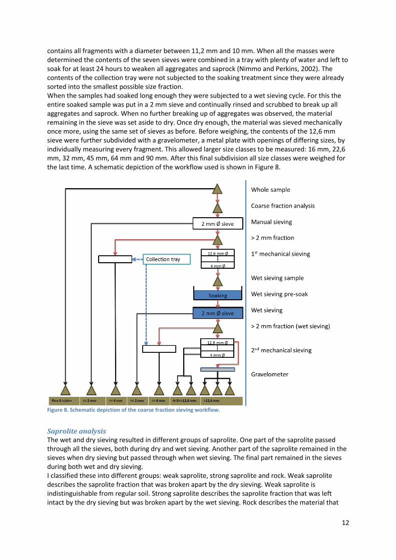
contains all fragments with a diameter between 11,2 mm and 10 mm. When all the masses were determined the contents of the seven sieves were combined in a tray with plenty of water and left to soak for at least 24 hours to weaken all aggregates and saprock (Nimmo and Perkins, 2002). The contents of the collection tray were not subjected to the soaking treatment since they were already sorted into the smallest possible size fraction. When the samples had soaked long enough they were subjected to a wet sieving cycle. For this the entire soaked sample was put in a 2 mm sieve and continually rinsed and scrubbed to break up all aggregates and saprock. When no further breaking up of aggregates was observed, the material remaining in the sieve was set aside to dry. Once dry enough, the material was sieved mechanically once more, using the same set of sieves as before. Before weighing, the contents of the 12,6 mm sieve were further subdivided with a gravelometer, a metal plate with openings of differing sizes, by individually measuring every fragment. This allowed larger size classes to be measured: 16 mm, 22,6 mm, 32 mm, 45 mm, 64 mm and 90 mm. After this final subdivision all size classes were weighed for the last time. A schematic depiction of the workflow used is shown in Figure 8.
Figure 8. Schematic depiction of the coarse fraction sieving workflow.
Saprolite analysis The wet and dry sieving resulted in different groups of saprolite. One part of the saprolite passed through all the sieves, both during dry and wet sieving. Another part of the saprolite remained in the sieves when dry sieving but passed through when wet sieving. The final part remained in the sieves during both wet and dry sieving. I classified these into different groups: weak saprolite, strong saprolite and rock. Weak saprolite describes the saprolite fraction that was broken apart by the dry sieving. Weak saprolite is indistinguishable from regular soil. Strong saprolite describes the saprolite fraction that was left intact by the dry sieving but was broken apart by the wet sieving. Rock describes the material that

13
was left intact by both the dry and wet sieving. Strong saprolite and rock are indistinguishable without wet sieving and were weighed as one group after dry sieving. The amount of strong saprolite in this group might be an indication of differences in weathering behaviour. To investigate this the relative amount of strong saprolite in the combined strong saprolite and hard rock fraction was determined for each sample, Equation 2.
𝑅𝑒𝑙𝑎𝑡𝑖𝑣𝑒 𝑎𝑚𝑜𝑢𝑛𝑡 𝑜𝑓 𝑠𝑡𝑟𝑜𝑛𝑔 𝑠𝑎𝑝𝑟𝑜𝑐𝑘 (%) = 𝑠𝑡𝑟𝑜𝑛𝑔 𝑠𝑎𝑝𝑟𝑜𝑐𝑘
(𝑠𝑡𝑟𝑜𝑛𝑔 𝑠𝑎𝑝𝑟𝑜𝑐𝑘 + ℎ𝑎𝑟𝑑 𝑟𝑜𝑐𝑘)
Equation 2. Relative amount of strong saprolite
Each sample was regarded as an independent sample for this analysis. The results were sorted by parent material and subjected to Analysis of Variance and two tailed t-tests to determine whether the means were different.
Fine fraction analysis The fine fraction subsamples, taken from the main samples above, were sieved via a different method. Before sieving, each sample was oven dried at 105 °C for 24 hours to remove all moisture. After drying, each sample was weighed to determine the total mass. Then the sample was sieved mechanically using stacked sieves with 2 mm, 0,6 mm and 0,063 mm openings, with a collection tray at the bottom, on top of a vibrating plate. Using a rubber bottle-cap, any material remaining in each sieve was gently ground to break up remaining aggregates. The size classes were then weighed. The contents of these sieves represented how much of the coarse classes (2 mm and larger), the coarse sand class (between 2 and 0,6 mm), the fine sand class (between 0,6 and 0,063 mm) and the silt and clay class (smaller than 0,063 mm) made up the total sample. Between each sieving session the sieves were cleaned using paper towels and after the final weighing and cleaning the sieves were weighed themselves.
Modelling The modelling was split into three parts: The initial data analysis, an error correction and the weathering model setup. The initial data was used to calculate a number of additional values necessary to run the weathering models. An error correction was necessary to correct the error that had been introduced into the dataset during the laboratory work. The weathering model setup details how the collected and corrected data was used to run the models and the assumptions underlying each model.
Initial data Additional values, besides the actual measurements, were calculated. These were: the mass of the sample sieved in Spain (entire sample minus fine fraction sample), the total mass of a sample before the wet sieving treatment (the sum of all dry sieving classes 4 mm or more in diameter) and the total mass of a sample after the wet sieving treatment (the sum of all wet sieving classes). The latter two masses were used to calculate how much fine fraction material was washed away during the wet sieving. Another set of calculations was applied to the fine fraction. The masses after sieving were summed and compared with the total mass before sieving. The mass after sieving was always less than it was before, so some material was lost in between. This difference was redistributed over the three classes, according to how much percent each class contributes to the total mass, to calculate the final mass. The final masses of each fine fraction class were used to calculate how much of each class was present in the material that was removed by the wet and dry sieving. Not every sample collected had the same mass, with some of the heavier samples weighing twice as much as the lighter samples. That is why, after all fractions were calculated, all masses were converted to mass percentages. As part of this conversion, the contents of several of the coarser size classes were merged. The 12,6 and 16 mm class were merged into one 12,6 mm class, the 22,6 and 32 mm class were merged into one 22,6 mm class and the 45, 64 and 90 mm class were merged into

14
one 45 mm class. This was done to bring the size classes more in line with the size classes defined by Wentworth (1922). The mass percentages were used to create a number of different graphs, which can be found in the Results section. These graphs were used to explore the data before the modelling phase.
Error correction An error was discovered halfway through the analysis. The 2 mm fraction was often much larger than would be expected. When re-examining the sieving method the error was found to originate from the assumption that it was not necessary to include the contents of the collection tray in the wet sieving. This caused both an overestimation of the mass of the 2 mm class and an underestimation of the mass of the entire fine fraction. To solve this, half of the mass of the 2 mm class was redistributed across the three fine fraction classes based on the results of the fine fraction analysis. The redistributed amount is an arbitrary fraction based on my estimate of the size of the error.
Weathering models
General setup Four different weathering models were used by Wells et al., but only the symmetrical and asymmetrical models were used for this study because they provided the best results according to the original paper. Because physical and chemical weathering are inversely related when only considering particle size, for this study I assumed that the weathering rate remains constant regardless of particle size. The models were used, with varying input parameters, to weather 10.000 fragments with a starting diameter of 128 mm. The models were run for 600 weathering cycles. The resulting 600 PSD’s were compared to the PSD’s obtained from the collected samples. This was done on a per layer basis. The absolute difference between each size class in a modelled PSD and each corresponding size class in a sampled PSD was calculated. The sum of the differences per PSD was divided by the number of size classes to obtain the averaged difference between that modelled PSD and the current sampled PSD. The modelled PSD with the lowest averaged difference for a layer was selected as the one best simulating reality for that layer. To evaluate correspondence at the profile scale the optimal matches for each layer were used. Their remaining differences were summed and divided by the number of layers in a profile. The result was an overall indication of how well a profile was modelled by the weathering model. Note that a chronological order, in the selection of PSD’s, is not enforced. As such, a layer could have an optimal match at a later weathering cycle than the layer above it. This is intentional, since weathering rate is not solely a function of depth below the surface (Borelli et al. 2013). The formation of cracks can cause deep layers to be more exposed to weathering than shallower layers.
Symmetrical weathering The symmetrical model was based on the assumption that particles fracture into a number of particles that have the same volume. This symmetrical weathering model was run with the number of resulting particles ranging from 2 to 8 This model uses a fracture probability of 5% for each particle per weathering cycle.
Asymmetrical weathering The asymmetrical model was based on the assumption that particles fracture into 2 daughter particles (of differing volume) according to a ratio. This ratio was kept constant for each model run. The ratios used were 6/4, 7/3, 8/2 and 9/1. The ratio 5/5 was already represented by the symmetrical model with 2 resulting particles. For this report the asymmetrical model was only run for 2 particles. This model uses a fracture chance of 10% for each particle per weathering cycle.

15
Results
Fieldwork The results of the observations done during the fieldwork are shown in Table 1. Table 1. Location characteristics.
Table 1 includes the observed total depth of each profile, its aspect, its slope and the number of layers identified. Only the final rock type is shown in Table 1, for all the different rock types resulting from the expert assessment, see the Appendix.
Saprolite analysis The results of the calculation of the relative amount of strong saprolite per parent material, including error bars, are shown in Figure 9.
Figure 9. Relative amount of strong saprolite per parent material
The Analysis of Variance for the four parent materials resulted in a P-value of 0.006, indicating that the parent materials differ in the relative amount of strong saprolite. Two-tailed t-tests between the different parent materials resulted in quartzite being identified as different from slate and gneiss for a P-value of 0,05. The tow-tailed t-test between quartzite and schist resulted in a p-value of 0,06. Between gneiss, schist and slate no difference was observed.
Location Depth (cm) Aspect (°) Slope (°) Layers Rock type
Q1 85 135 5 4 quartzite
Q2 85 160 15 3 quartzite
G1 570 70 46 7 gneiss
G2 210 / 0 4 gneiss
Sch1 230 / 0 5 schist
Sch2 270 340 20 5 schist
Sch3 410 300 20 5 schist
Sl 180 0 25 3 slate/shale
0%
10%
20%
30%
40%
50%
60%
70%
80%
90%
100%
Quartzite Gneiss Schist Slate
Relative amount of strong saprolite per parent material
Quartzite
Gneiss
Schist
Slate

16
Grain size distributions. The results of the laboratory work are shown in Figure 10, Figure 11 and Figure 12. A gradual bar graph was created by summing up each size class in order for each layer (Figure 10). By then putting a profile’s layers in sequential order I could detect deviations from the expected evolution of a PSD. A series of regular bar graphs was created to compare the differences in PSD’s between layers (Figure 11 and Figure 12). A layer is compared with the layer closest to bedrock. The differences are expressed as the percentage by which each size class’s contribution to the PSD changed. These graphs made it possible to more precisely identify where profiles differed and what caused the differences. The results of additional analyses are shown in the Appendix. Several aspects of the profiles in Figure 10 stand out:
- Profiles G2, Sch3 and Sl show a PSD evolution that would be expected, with the fine fraction decreasing and the coarse fraction increasing with distance from the surface.
- Profile Q1’s PSD’s show an opposite evolution, with the fine fraction decreasing and the coarse fraction increasing the closer a layer is to the surface.
- Profile Sch2’s PSD’s show almost no differences between the layers. - Profiles Sch1, Q2 and G1 all have layers in the upper parts of their profile that closely match
their near bedrock layers. These are layer 3 for profile Sch1, Layer 1 for profile Q2 and layers 4 and 2 for profile G1.
The bar graphs in Figure 11 and Figure 12 provide more detail:
- Profile Q1’s PSD’s opposite evolution is mostly due to an increase in the coarsest size class (45 mm and larger). At the same time the smallest size classes are showing an increase relative to bedrock, but this increase is small compared to that of the coarsest size class.
- Profile Q2’s top layer has less fine fraction material than its lowest layer. - Profile G1’s layers 4 and 2 are almost identical to its lowest layer. If these are left out of the
picture, the remaining layers show an expected PSD evolution. - Profile G2’s top layer has less fine fraction material than the layer below it. - Profile Sch2’s material primarily weathers to a size between 2 and 4 mm in diameter. - Profile Sch3’s material primarily weathers to the size of fine sand. - Profile Sch1 and Sl reveal no new information in Figure 11 or Figure 12 compared to Figure
10.

17
Figure 10. Gradual bar graphs of laboratory sieving results. The numbers at the bottom indicate the depth of the layer with higher numbers indicating deeper layers.

18
Figure 11. PSD evolution bar graphs relative to bedrock of locations Q1, Q2, G1 and G2.

19
Figure 12. PSD evolution bar graphs relative to bedrock for locations Sch1, Sch2, Sch3 and Sl.

20
Modelling As an introduction to the modelling results, examples of how the model PSD’s were compared to the sample PSD’s are shown in Figure 13 and Figure 14.
Figure 13. Example graph of model matchups at sample level.
Figure 14. Example graph of model matchups at profile level.
Figure 13 shows the cumulative weights of the particle size classes of a sample’s PSD compared to one of the PSD’s generated by a model. The model underestimates the smaller particles sizes and overestimates the larger particle sizes, but is a close match for the sample as a whole. As mentioned in the Methods section, the absolute differences between the model and the sample were averaged to obtain the weighted difference between the sample and this model output. Figure 14 shows the result of combining the model results with the lowest differences into a profile averaged difference. In this graph the differences between the sample and symmetrical weathering models with differing numbers of resulting particles are shown. The model resulting in 3 daughter particles differs the least from the Slate profile while the model resulting in 8 daughter particles differs the most from the profile as a whole. The other models all result in differences between 3 and 4 percent. No preference for an even or uneven number of daughter particles can be seen.
0%
20%
40%
60%
80%
100%
0 1/256 1/64 1/16 1/4 1 4 16 64Cu
mu
lati
ve w
eig
ht
of
mat
eri
al
Particle size
Model matchup at sample level
Sample
Model
0%
1%
2%
3%
4%
5%
6%
7%
8%
9%
2 3 4 5 6 7 8
Dif
fere
nce
Number of daughter particles
Model comparison at profile level
Sl

21
Symmetrical weathering Figure 15 shows the results of the profile level comparison for the symmetrical model. The symmetrical model has the lowest difference with 4 or 6 daughter particles for the samples Q2, G1, Sch1, Sch2 and Sch3. The model results in the largest differences with 5 daughter particles for these five profiles. Other daughter particle distributions also result in large differences, but no overall pattern can be detected in these maxima. A pattern that does stand out is that models with 2 or 8 daughter particles are never the best model. Especially the model runs with 8 daughter particles result in large differences, except for profile G2. However, profile G2 only shows marginal differences between different numbers of daughter particles. Profiles Q1 and Sl show the lowest differences for 2 to 5 daughter particles, but model runs with profile Q2 result in the lowest differences for 6 or 7 daughter particles. Overall, different rock types show preferences for different symmetrical weathering geometries, but even between profiles with the same parent material there are large differences.
Figure 15. Profile averaged differences between symmetrical weathering and samples.
0%
1%
2%
3%
4%
5%
6%
7%
8%
9%
2 3 4 5 6 7 8
Dif
fere
nce
Number of daughter particles
Quartzite and Gneiss
Q1
Q2
G1
G2
0%
1%
2%
3%
4%
5%
6%
7%
8%
9%
2 3 4 5 6 7 8
Dif
fere
nce
Number of daughter particles
Schist and Slate
Sch1
Sch2
Sch3
Sl

22
Asymmetrical weathering Figure 16 shows the results of the profile level comparison for the asymmetrical model. Two different groups of profiles can be recognized. The group consisting of the profiles Q2 and Sch1 shows a clear decrease in the difference between the model and the sample with an increasing skewness of the ratios of daughter particles. The group consisting of the other profiles shows little to no difference between the different ratios of daughter particles. Overall, no clear pattern can be discerned based on rock type.
Figure 16. Profile averaged differences between asymmetrical weathering and samples.
Comparing models per location To better compare the models and to determine how closely the models simulate reality, the best fitting model results per location are combined in Table 2. Included in Table 2 are also the model parameters that produced the best fitting PSD. Per layer the model that produced the best fit is made bold. The symmetrical model runs produce the best fits overall. In the case of Q1 and G2, the asymmetrical model produces better results, but only by a small margin. Both models produce PSD’s that closely match the sampled profiles. However, the best performing number of resulting fragments and the
0%
1%
2%
3%
4%
5%
6%
7%
8%
9%
5/5 6/4 7/3 8/2 9/1
Dif
fere
nce
Ratio of daughter particles
Quartzite and Gneiss
Q1
Q2
G1
G2
0%
1%
2%
3%
4%
5%
6%
7%
8%
9%
5/5 6/4 7/3 8/2 9/1
Dif
fere
nce
Ratio of daughter particles
Schist and Slate
Sch1
Sch2
Sch3
Sl

23
best performing ratio of resulting fragments deviate from what is expected. As mentioned in the introduction, most models that incorporate weathering do so by repeatedly splitting rock fragments into two particles of equal size. Only for the asymmetrical models is this option ever the best result, for profile Sch2, and for that one profile the symmetrical models still performed better. The single slate location deviates from the quartzite, gneiss and schist locations with its optimal result for 3 fragments or a 7/3 ratio. No other difference based on rock type can be distinguished. Table 2. Comparison of optimal matches for the symmetrical and asymmetrical weathering model per location. Optimal matches include the model parameters that produced the match. For each location the best match is made bold.
Comparing models per layer To better compare the models and to determine how closely the models simulate reality, the best fitting model results per layer are combined in Table 3. Included in Table 3 are also the model parameters that produced the best fitting PSD. Per layer the model that produced the best fit is made bold. The symmetrical models produce the best fit for most of the samples. Some of these results are only better by a few tenths of a percent. However, most of the symmetrical optimal matches are better than the asymmetrical results by a margin of 1% or more, Sch2’s layer 2 being the largest with a difference of 2,7% between the two models. When the asymmetrical models produce a better fit for a sample the difference between the two types of models is at most 0,5%. Some profiles show a radical shift in the optimal number of daughter particles over the depth of the profile. The profiles Q1, G1 and G2 are good examples of this shift, although the nature of their shifts is opposite. Q1’s number of daughter particles increases with decreasing depth, shifting from 2 daughter particles to 8 daughter particles. G1 and G2’s number of daughter particles decreases with decreasing depth, shifting from an average of 7 daughter particles to 2 daughter particles. Other profiles, such as Q2, Sch2, Sch3 and Sl, show little to no change over the depth of their profile. Some profiles show a radical shift in the optimal ratios of their daughter particles over the depth of the profile. The profiles Q1, G1, Sch2 and Sch3 are good examples of this shift, although the nature of their shifts differs. The ratios of the daughter particles of profiles Q1 and Sch2 become more skewed with decreasing depth, shifting from a 7/3 ratio to a 9/1 ratio. The ratios of the daughter particles of profiles G1 and Sch3 become less skewed with decreasing depth, shifting from a 9/1 ratio to a 5/5 ratio. Other profiles, such as Q2, G2 and Sch1, show little to no change in their daughter particle ratios over the depth of their profile. Both models did not produce a good match for profiles G1 and Sch2. Where all other profiles had at least 2 samples where the models matched to within 2%, G1 has only one sample that is matched to within 2% and Sch2 has none. Overall, no pattern can be discerned based on rock type.
Location Symmetrical (%) Fragments Asymmetrical (%) Ratio
Q1 2,9% 5 2,8% 8/2
Q2 3,0% 6 3,6% 9/1
G1 5,5% 6 6,2% 8/2
G2 4,4% 7 4,1% 8/2
Sch1 2,5% 4 2,5% 9/1
Sch2 4,3% 6 5,4% 5/5
Sch3 3,1% 6 5,0% 9/1
Sl 2,3% 3 3,0% 7/3

24
Table 3. Comparison of optimal matches for the symmetrical and asymmetrical weathering model per layer. Optimal matches include the model parameters that produced the match. For each layer the best match is made bold.
Location Layer Symmetrical (%) Fragments Asymmetrical (%) Ratio Location Layer Symmetrical (%) Fragments Asymmetrical (%) Ratio
Q1 1 2,5% 8 3,1% 9/1 Sch1 1 1,1% 3 0,6% 8/2
2 1,3% 5 2,2% 8/2 2 0,9% 4 1,9% 9/1
3 2,2% 2 2,1% 7/3 3 2,0% 7 2,1% 9/1
4 1,7% 2 1,7% 5/5 4 1,8% 4 2,4% 9/1
5 2,2% 6 3,3% 9/1
Q2 1 4,0% 8 4,3% 9/1
2 1,8% 6 3,7% 9/1 Sch2 1 3,3% 6 5,7% 9/1
3 2,3% 7 2,9% 9/1 2 3,3% 6 6,0% 6/4
3 4,1% 6 4,4% 8/2
G1 1 1,9% 2 1,8% 6/4 4 3,1% 6 3,1% 7/3
2 6,7% 7 6,9% 9/1 5 5,4% 5 6,5% 7/3
3 4,1% 6 5,3% 6/4
4 6,9% 4 7,0% 9/1 Sch3 1 4,5% 6 6,1% 6/4
5 4,6% 6 6,7% 6/4 2 2,5% 6 4,6% 5/5
6 3,8% 6 5,4% 9/1 3 2,0% 6 4,1% 8/2
7 5,6% 4 6,1% 8/2 4 1,7% 6 3,8% 8/2
5 4,1% 8 5,0% 9/1
G2 1 1,5% 2 1,5% 8/2
2 1,8% 2 1,4% 8/2 Sl 1 1,9% 3 1,7% 7/3
3 5,3% 8 6,4% 9/1 2 2,2% 3 2,0% 7/3
4 5,3% 7 5,8% 9/1 3 2,8% 3 3,9% 9/1
5 2,3% 6 3,3% 9/1

25
Discussion The discussion covers the various aspects of the research questions. Each research question is followed by suggestions for future research.
Can weathering explain the data collected during the fieldwork? Weathering alone, and by extension the models, is not enough to explain all of the profiles. Other natural processes need to be included to explain the observed profiles. Profiles such as Q1, Q2, G1, G2, Sch1 and Sch2 do not conform to a pattern of a continually decreasing coarse fraction and steadily increasing fine fraction from bedrock to the surface. The additional processes necessary to explain these profiles are surface armouring, crack formation and intrusions and the nature of the parent material.
Surface armouring Surface armouring (Sharmeen and Willgoose, 2006) explains why the top layers of Q2 and G2 contain less fine fraction material than the layers below them. Erosion processes removed the finer material while leaving the heavier coarse material behind. The effects of this process on the two profiles are very clear when taking both Figure 10 and Figure 11 into account. The effect of the surface armouring did not influence the current results since a chronological order was not enforced during the model comparison. In the original paper by Sharmeen and Willgoose they noted that surface armouring resulted in a change in weathering behaviour during their simulations:
It was possible for the combined erosion and weathering process to generate a particle size distribution that was coarser than the pre-existing armour, but because there were more fines in the armour layer available for transport (i.e. exposed at the surface) the transport rate increase.(Sharmeen and Willgoose, 2006,p. 1209).
Profile Q1 might also be the result of surface armouring, but surface armouring only works on the upper parts of a profile. Q1’s largest size class’s relative mass increases with decreasing distance to the surface over the entire profile. What could explain this inverted profile is a complex combination of erosion and deposition. Normally, the profile weathers and erodes, resulting in an armour layer. Then a landslide occurs and buries the armour layer. Weathering and erosion continue and a new armour layer is formed, while the older armour layer is still present in some part lower in the profile. If such a succession of events would happen multiple times, that could explain the profile of Q1. Note that this is purely speculation on my part, as I could not find any mention of a similar profile in literature. During the fieldwork no evidence was found that either proves or disproves this theory, but weathering alone cannot explain profile Q1.
Cracks and intrusions The presence of cracks or intrusions explains why some samples were at a different stage in the weathering process, as could be seen in Figure 10, Figure 11 and Figure 12. A similar situation was encountered in the Mucone river basin by Borelli et al. (2013) where the presence of faults and cracks caused differences in weathering grades horizontally across profiles. The material close to faults and cracks is more exposed to water and organisms, resulting in faster weathering. Another process that can explain differences in weathering stages is the formation of intrusions. An intrusion of magma into existing rock introduces fresh material and metamorphoses the existing material. Both the existing and new material are then at the beginning of their weathering process. Material that is not affected by the intrusion is then at a more advanced stage in the weathering process, resulting in a disturbed chronosequence. Both of these processes could explain the discontinuities observed in the profiles G1 and Sch1. Most likely cracks and faults are the cause of these discontinuities, since intrusions would have metamorphosed more of the surrounding material as well.

26
Parent material Surface armouring and the formation of cracks or intrusions cannot explain why the profile of Sch2 is as constant as was observed. Likely, the parent material is the reason why the material of Sch2 primarily weathers to a size between 2 and 4 mm. Borelli et al. (2013) also found a relation between the amount of sand in residual soils and the underlying parent material. They found this relation for granite and gneiss, but it should be just as true for a schist. Schist is the result of the metamorphosis of clays and muds and a typical weathering result would be silt and clay particles, but quartz schists exist as well and these would weather into more sandy materials. This would also explain why little to no difference can be observed between the different layers as quartz is slow in weathering. Weathering is taking place in the profile, as can be seen in Figure 12, as there is an increase in the 4 to 10 mm size classes in the deeper layers which is followed by a decrease of those size classes in the upper layers.
Future research New weathering models should include the various aspects addressed here, as weathering alone could not adequately explain all the profiles. Erosion or surface armouring can be accounted for by including an erosion module, a good example of such a module was presented in the paper by Sharmeen and Willgoose (2006). Including the formation of cracks, intrusions and faults as part of a model will be challenging, due to the randomness inherent in their formation. One option that could account for both would be to allow layers to have different weathering stages or weathering speeds at the start of a model run. Such an option could then also allow for the distinction of different parent materials and their weathering behaviour.
Do the known weathering pathways match the data collected during the fieldwork? Most of the profiles had at least one very good matchup among the models used for this report. The traditional weathering geometry with 2 identical daughter particles produced acceptable results, but models with different parameters always performed better. This part of the discussion will compare the traditional weathering geometry with the alternate weathering geometries used in this study. This will also involve a closer look at the most notable aspects of the modelling results, such as the modelling parameters that produced the best and worst matchups and possible explanations for why they did so.
Symmetrical weathering The models resulting in 2 daughter particles never result in the lowest difference, as can be seen in Table 2. This directly contradicts the results obtained by Wells et al. (2008) during their laboratory weathering experiments. In their experiments, the 2 daughter particle model best represented their results, but they themselves also stated that the scope of the experiment was very limited. Only one rock type was tested (quartz-chlorite schist) and the material was only exposed to salt weathering. They hypothesized that weathering under field conditions might follow a different weathering pathway, which is indeed what the results of this study indicate. The models with either 4 or 6 daughter particles result in the lowest differences for most of the profiles, Q2, G1 and Sch3 being the best examples of this. These same profiles have the worst matchups for models resulting in an uneven amount of daughter particles. This might be related to the crystal structure of the respective parent materials, which could favour fracturing along predetermined and equally distributed lines. This suggests a similar relation between weathering geometry and parent material as is suggested between by the PSD’s of profile Sch2 and its parent material. However, the parent material alone is not a perfect explanation. Comparing Q1 directly with Q2 reveals that the two profiles strongly differ in the optimal number of daughter particles. The lines shown in Figure 15 almost mirror each other, with Q1 having the best matches for smaller, uneven

27
amounts of daughter particles and Q2 having the best matches for larger, even amounts of daughter particles. The two locations seem to be the result of very different weathering regimes, despite having the same parent material. The only documented difference between the two quartzite locations is their slope and although research (Yokoyama et al. 2006, Borelli et al., 2013) shows that location characteristics can influence weathering, this is not the only possible reason for the differences. A differing chemical composition might also be the cause, but a chemical analysis was not a part of this research due to the assumption that the differences within parent materials would be negligible.
Asymmetrical weathering The models resulting in 2 identical daughter particles only result in the lowest difference for profile Sch2, as can be seen in Table 2. This again contradicts the results obtained by Wells et al. (2008) during their laboratory weathering experiments. The traditional weathering model of 2 identical daughter particles is shown to also be one of the worst options if asymmetrical weathering is possible. The profiles Q2 and Sch1 show a clear increase in the quality of the matchups as the skewness of the ratio between the daughter particles increases. This might be related to the crystal structure of the parent material as some parent materials might favour the breaking off of small pieces, also known as spalling (Sharmeen and Willgoose, 2006), over fracturing into larger daughter particles. This report only covers this weathering behaviour with the 8/2 and 9/1 geometries but even better matchups might be achieved by further skewing the ratios. More likely is that one of the other models from the Background section, such as the granular disintegration model, will be beter able to model this kind of weathering behaviour. The other profiles show little difference between the asymmetrical models.
Changing weathering geometries Wells et al. (2008) mention in their discussion that the weathering models they used (Sharmeen and Willgoose, 2006) no longer applied to particles as small or smaller than 0,063 mm. Given the sizes and processes involved with those particle sizes it is highly likely that chemical weathering would play a much larger role and that the physical weathering models no longer apply. They did not consider that such a shift might also occur for larger particle sizes in the weathering process, yet that is what is suggested by the contents of Table 3. Comparison of optimal matches for the symmetrical and asymmetrical weathering model per layer. Optimal matches include the model parameters that produced the match. For each layer the best match is made bold. A shift in the most optimal weathering geometry can be recognized when looking at these results for the profiles Q1, G1 and G2 for symmetrical weathering and the profiles Q1, G1, Sch2 and Sch3 for asymmetrical weathering. Both symmetrical G1 and G2 have optimal matches for models that result in a large number of daughter particles for their lower layers, but the upper layers have optimal matches for models with a small number of daughter particles. Q1‘s symmetrical profile shows a shift in the opposite direction, with the number of daughter particles increasing with decreasing depth. The asymmetrical profiles of Q1 and Sch2 become more skewed with decreasing depth, while G1 and Sch3 become less skewed with decreasing depth. All of these shifts indicate a possibility for the weathering geometry of a rock to change as part of its weathering pathway (Wright, 2007). Physical weathering is typically the dominant weathering type for large fragments and becomes less active as particle sizes decrease. Chemical weathering starts playing a larger and larger role as the size of particles decreases and the surface area increases. This shift from physical to chemical weathering or from chemical to physical weathering could be the cause of a shift in weathering geometry. Although the expected development would be a shift from physical to chemical weathering, due to the decreasing size of the particles, the paper by Hall et al. (2002), about the nature of weathering in cold regions, reveals that the opposite can also be true. They discovered that the activity of chemical weathering is not that reliant on temperature as is generally thought, but that it is instead tied to the presence of moisture. This might explain why

28
different optimal weathering geometries are found for different depths of these profiles as the amount of moisture available probably differs with depth. An alternative explanation could be that instead of these profiles being a weathering chrono-sequence they are a weathering climo-sequence. Under different climates different types of weathering are active. Frost weathering for instance will play a more prominent role during cooler periods. Salt weathering will be most active during periods that frequently alternate between wet and dry conditions. While both are types of physical weathering the resulting weathering pathways (and weathering models that accurately model it) are probably very different. Different climates are also likely to have different amounts of moisture present in the profiles and in that way chemical weathering also differs between climates. The difference between the current results and those of Wells et al. (2008) can also be attributed to the difference between the types of weathering that affected the samples. However, if the difference in the current results is due to the effect of climate then those differences should also be visible in other profiles.
Future research Many possibilities for new research are possible based on these results. The current results show that the typical weathering geometry, with 2 symmetrical daughter particles, never resulted in the best matchup with the field data. Therefore, new research will have to asses which weathering geometry performs the best with respect to the area of interest. It can no longer be blindly assumed that the typical weathering geometry will suffice for each location. It is highly recommended to also include a model that accounts for spalling behaviour in such an assessment, considering the results in Table 3. New models might also attempt to include the possibility of a change in the preferred weathering geometry. This will be challenging to model, since the transition from one weathering geometry to another is likely to be gradual, just like a transition between physical and chemical weathering. This paper does provide a method to such a change in observed profiles: By running each model separately for all depths of a profile and comparing which model produces the best matchup for each depth. Overall no clear pattern emerges based on rock type. It is likely that rock type is a determining factor in the weathering of rocks, but the impact of other factors, such as the location and specific chemical composition, is higher, based on the current results. This does not mean that the rock type is not a deciding factor. It is even highly likely that only a limited number of weathering pathways are feasible for some rock types. Which of those becomes the most active type is then a function of the location characteristics. The current sample size is too small to verify if this true.
Does a difference in lithology explain observed differences in weathering behaviour? Differences in lithology do not explain the observed differences. The different models and analyses revealed no pattern based on the parent materials. Locations with the same parent material displayed opposite behaviour in reaction to the same models. The only differing factor that did display correspondence based on the parent material was the relative amount of strong saprolite.
Weathering models The profiles Q1 and Q2 are the prime example for the differences between locations with the same parent material. For the symmetrical weathering, Figure 15, Q1 displays the lowest differences for models resulting in few daughter particles while Q2 displays the lowest differences for models resulting in many daughter particles. The difference is further emphasized by the asymmetrical weathering, Figure 16. The results for Q1 show no difference between the differently skewed models, but Q2’s results differ up to 2% between the 5/5 and 9/1 skewed model.

29
Looking at the site characteristics, Table 1, both quartzite locations appear to be very similar. The schist and gneiss location characteristics differ to a much greater amount, but the differences in their weathering behaviour, although still present, are not as pronounced or as extreme. The symmetrical weathering behaviour of Q2 is even more similar to that of Sch3 than it is to Q1 and Q1 is more similar to the behaviour of Sl than it is to Q2. This difference might be partly ascribed to subtle differences in the individual locations crystal structure makeup, but it is far more likely there is a different underlying cause. The differences between lithologies are of the same order of magnitude as the differences within lithologies. Therefore it is reasonable to assume that the location characteristics such as the slope, the aspect, the climate and the vegetation have a higher impact on the weathering pathway than the rock type. The reason that these characteristics are so influential is because they affect the amount of available moisture (Yokoyama and Matsukura, 2006, Elliot, 2008), which is required for chemical weathering to become active. This does not mean that the rock type is not a deciding factor. It is even highly likely that only a limited number of weathering pathways are feasible for some rock types (Nicholson and Nicholson, 2000). The current amount of samples is not large enough to indicate if such a limitation in the number of possible weathering pathways exists.
Saprolite analysis The analysis of the relative amount of strong saprolite was the only analysis that indicated a difference between the parent materials. The two-tailed t-tests identified the quartzite samples as being different from the slate and gneiss samples for a P-value of 0,05 and the comparison with the schist samples resulted in a p-value of 0,06. The schist p-value is small enough that I also consider this an indication that the schist samples and the quartzite samples were collected from different populations. The cause of this difference might be related to the amount of quartz in the parent material. Quartzite is the only rock type among the four to be rich in quartz, in the other parent materials quartz is a lesser component. Research by Merriam et al. (1970) found an inverse relation between the tensile strength of a rock sample and the amount of quartz in the sample. A similar relation was found by Elliot (2008) for another set of samples. They relate this inverse relation to the crystal structure of quartz rich rock types:
Quartz-rich rocks tend to be composed of more or less equidimensional grains arranged in an aplitic (or sugary) texture characterized by little intergrowth or interlocking of grains. In contrast the texture of low-quartz rocks is composed of interlocking laths and prisms (Merriam et al. 1970, p. 158).
This would indicate that the dry pre-treatment and subsequent sieving did not break up the sugary texture of the quartzite strong saprolite. The subsequent wet pre-treatment did break up this structure, much like a sugar cube is slow to come apart by regular sieving but quick to break apart when water is added, although part of that process is the sugar dissolving instead of breaking apart. Assuming that the collected samples consisted mostly, if not completely, of saprolite and rock fragments, this suggests that the more interlocking structure of the gneiss, schist and slate is more easily shaken apart than the sugary texture of the quartzite. Future research could use this differing result of the pre-treatments to quickly and cheaply get an estimation of which samples contain more quartz.
Causes of differing signals There are two possible causes for differences in the signals that can be ascribed to human error. These are the way the parent materials were determined and the way the samples were sieved. During the fieldwork no rock determination was carried out, instead samples were collected and later presented to four experts. The samples were not subjected to a chemical analysis. The experts did not always reach the same conclusion for a sample and in that case the rock type that was chosen the most was used as the final result. Give the wide range of the results and the differing behaviour

30
for some of the locations (such as G1 and G2 or Q1 and Q2), it is likely that one or more of these final rock types was incorrect. The pre-sieving treatment methods used for the study might have been unsuitable or might have produced incomplete results. The paper by Häfele and Weichmann (1997) revealed that the different methods they used to prepare saprolitic material for sieving resulted in significantly different PSD’s. Instead of using a wetting and washing pre-treatment they subjected their samples to a sonic washing, with similar results. The largest differences they found were in the total amount in the coarse fraction and in the amount of clay particles. The results of the saprolite analysis also indicate that different sieving pre-treatments can result in different classifications for parts of a sample. The current treatment used was based on the methods of Nimmo and Perkins (2002) and I am confident that all material was sorted correctly.
Future research The differences in the amounts of strong saprolite could provide a cheap and quick assessment of the relative amount of quartz in samples. However, more research into this relationship is needed before it can be used. Studies of this relationship should try to include rock types not encountered in this study to ensure the relationship is not limited to this set of samples. It is also advisable to compare the results of a sonic washing treatment and a wetting and washing treatment to identify which of the two results in a more complete breakdown of saprolite. More research is also needed into the influence of rock types on weathering behaviour, as the current results are inconclusive on that account due to the small number of profiles sampled. Such research should try to sample locations that are from the same region and possess similar location characteristics such as slope and aspect. This is to minimize the differences caused by these factors. In all cases where the rock type is used to differentiate between groups it is advisable to include a chemical analysis of the samples. Especially when only a small number of samples is collected.

31
Conclusion
Can weathering explain the data collected during the fieldwork? Although weathering alone, and by extension the models, are not enough to explain all of the profiles, by accounting for other natural processes the profiles can be explained. For future models the effect of including profile rejuvenation or crack formation could be accounted for by adjusting either the weathering speed or adjusting the age of a profile’s layers.
Do the known weathering pathways match the data collected during the fieldwork? Most of the profiles had at least one very good matchup among the models used for this report. The models were able to produce results accurate to within a few percent of the real world profiles. The symmetrical weathering model with two daughter particles produced acceptable results, but models with different parameters always performed better. This means that existing models with a weathering module should be re-evaluated or adjusted to incorporate alternative weathering geometries.
Does a difference in lithology explain observed differences in weathering behaviour? The relative amount of strong saprolite was the only aspect of weathering behaviour that could be related to lithology. The weathering behaviour did not show a relation based on rock type. The quartzite samples even displayed almost opposite weathering behaviour. The number of samples per rock type was very limited and future studies should consist of a larger number of sampled profiles. The overall conclusion of confronting weathering models with field data is that the current weathering geometry models are adequate at representing reality. Existing models should be adapted to include processes such as surface armouring and differing weathering speeds and weathering stages. Future models should include multiple weathering geometries since the symmetrical two daughter particle model was always outperformed. Currently, no distinction can be made based on rock type, but the results of the saprolite analysis suggest that weathering does differ between rock types.

32
References Anderson, S.P., Blanckenburg, F., White, A.F. (2007). Physical and chemical controls on the critical zone, Elements 3, 315-319. Arnaud, R.J.St., Whiteside, E.P. (1963). Physical breakdown in relation to soil development, Journal of soil science 14 (2). Borelli, L., Perri, F., Critelli, S., Gullà, G. (2013). Characterization of granitoid and gneissic weathering profiles of the Mucone River basin (Calabria, southern Italy), Catena 113, 325-340. Brantley, S.L., Lebedeva, M. (2011). Learning to read the chemistry of regolith to understand the critical zone, Annual review of earth and planetary science 39, 387-416. Brantley, S.L., Holleran, M.E., Jin, L., Bazilevskaya, E. (2013). Probing deep weathering in the Shale Hills Critical Zone Observatory, Pennsylvania (USA): the hypothesis of nested chemical reaction fronts in the subsurface, Earth surface processes and landforms 38, 1280-1298. Chigira, M. (1990). A mechanism of chemical weathering of mudstone in a mountainous area, Engineering Geology 29, 119-138. Dixon, J.C., Thorn, C.E., Darmody, R.G., Schlyter, P. (2001). Weathering rates of fine pebbles at the soil surface in Karkevagge, Swedish Lapland, Catena 45, 273-286. Ehlen, J. (2004). Above the weathering front: contrasting approaches to the study and classification of weathered mantle, Geomorphology 67, 7-21. Elliot, C. (2008). Influence of temperature and moisture availability on physical rock weathering along the Victoria Land coast, Antarctica, Antarctic science 20, 61-67. FAO (2015). Key messages of the international year of soils, http://www.fao.org/soils-2015/about/key-messages/en/, accessed on 13/02/2015. Google earth V. 7.1.5.1557 (04/10/2013) a. Spain. Latitude 40.027537° Longitude -3.141593°, Eye altitude 1219.70 km. SIO, NOAA, U.S. Navy, NGA, GEBCO. Landsat. http://www.earth.google.com, accessed on 29/10/2015. Google earth V. 7.1.5.1557 (04/10/2013) b. Southern Spain. Latitude 37.471793° Longitude -4.426435°, Eye altitude 475.25 km. SIO, NOAA, U.S. Navy, NGA, GEBCO. Landsat. http://www.earth.google.com, accessed on 29/10/2015. Google earth V. 7.1.5.1557 (14/05/2015) a. Cordoba and Sierra Morena, Spain. Latitude 38.040101° Longitude -4.735842°, Eye altitude 58.15 km. DigitalGlobe. http://www.earth.google.com, accessed on 09/12/2015. Google earth V. 7.1.5.1557 (14/05/2015) b. Sierra Morena, Spain. Latitude 38.095208° Longitude -4.762027°, Eye altitude 28.12 km. IGME. DigitalGlobe. Google. http://www.earth.google.com, accessed on 09/12/2015. Gracheva, R. (2011). Formation of soil diversity in the mountainous tropics and subtropics: rocks, time and erosion, Geomorphology 135, 224-231.

33
Graham, R.C., Rossi, A.M., Hubbert, K.R. (2010). Rock to regolith conversion: producing hospitable substrates for terrestrial ecosystems, GSA today 20 (2), 4-9. Gutiérrez, F., Gutiérrez, M., Martín-Serrano, A. (2014). The geology and gemorphology of Spain: a concise introduction, Landscapes and landforms of Spain, 1-24. Häfele, S., Wiechmann, H. (1997). Körnung von saproliten als methodenabhängige grösse, Zeitschrift für Pflanzenernährung Bodenkunde 160, 349-355. Hall, K., Thorn, C.E., Matsuoka, N., Prick, A. (2002). Weathering in cold regions: some thoughts and perspectives, Progress in physical geography 26, 577-603. Instituto Geográfico Nacional de España. LiDAR-PNOA map of Hoja nr. 902 of the MTN50. Accessed at http://centrodedescargas.cnig.es/CentroDescargas/buscadorCatalogo.do?codFamilia=MDT05 on 21/10/2015. Isasa, O.A., Domínguez, J.B., Sánchez, M.C., Blancha, J.C.P., García, F.J.R., González, J.S., Ruiz, A.G., Higueras, P.H., Ochoa, C.Q., Pascual, L.A.C. (1982). Mapa geologico de España 1:50.000 [Adamuz], Instituto Geologico y Minero España. Joffre, R., Vacher, J., De los Llanos, C., Long, G. (1988). The dehesa: an agrosilvopastoral system of the Mediterranean region with special reference to the Sierra Morena area of Spain, Agroforestry systems 6, 71-96. Leopold, L.B. (1970). An improved method for size distribution of stream bed gravel, Water resources research 6 (5), 1357-1366. Lerman, A. (1979). Geochemical processes: water and sediment environments, John Wiley and Sons, New York. Little, A.L. (1969). The engineering classification of residual tropical soils, Proceedings of the International Conference on Soil Mechanics and Foundation Engineering 7th edition, Mexico, 1, 1-10. Matsukura, Y., Hirose, T. (1999). Five year measurements of rock tablet weathering on a forested hillslope in a humid temperate region, Engineering geology 55, 69-76. Merriam, R., Rieke III, H.H., Kim, Y.C. (1970). Tensile strength related to mineralogy and texture of some granitic rocks, Engineering geology 4, 155-160. Meshlab (2014). 3D-Coform project, www.meshlab.sourceforge.net (accessed on 21/09/2015). Microsoft Photosynth (2010). Microsoft corporation, www.photosynth.net (accessed on 24/08/2015). Nicholson, D.T., Nicholson, F.H. (2000). Physical deterioration of sedimentary rocks subjected to experimental freeze-thaw weathering, Earth surface processes and landforms 25, 1295-1307. Nimmo J.R. and Perkins K.S. (2002). Aggregate stability and size distribution, in Dane, J.H. and Topp, G.C., eds., Methods of soil analysis, Part 4 – Physical methods: Madison, Wisconsin, Soil Science Society of America, 317-328.

34
Núñez, M.A., Recio, J.M. (2007). Kaolinitic paleosols in the south west of the Iberian Peninsula (Sierra Morena region, Spain). Paleoenvironmental implications, Catena 70, 388-395. Pope, G.A. (2013). Weathering and sediment genesis. In : Shroder, J. (editor in chief), Pope, G.A. (ed.), Treatise on geomorphology, Academic Press, San Diego, CA 4, Weathering and soils geomorphology , 284-293. Royne, A., Jamtveit, B., Mathiesen, J., Malthe-Sorensson, A. (2008). Controls on rock weathering rates by reaction-induced hierarchical fracturing, Earth and planetary science letters 275, 364-369. Sharmeen, S., Willgoose, G.R. (2006). The interaction between armouring and particle weathering for eroding landscapes, Earth surface processes and landforms 31, 1195-1210. Temme, A.J.A.M., Vanwalleghem, T. (in press), LORICA, a new model for linking landscape and soil profile evolution: Development and sensitivity analysis. U.S. National Research Council Committee on Basic Research Opportunities in the Earth Sciences (2001). Basic research opportunities in Earth Science, National Academy Press, Washington D.C., 35-44. Vanwalleghem, T., Stockmann, U., Minasny, B., McBratney, A.B. (2013). A quantitative model for integrating landscape evolution and soil formation, Journal of geophysical research: earth surface 118, 331-347. Wakasa, S.A., Nishimura, S., Shimizu, H., Matsukura, Y. (2012). Does lightning destroy rocks?: results form a laboratory lightning experiment using an impulse high-current generator, Geomorphology 161-162, 110-114. Wells, T., Willgoose, G., Binning, P. (2007). Laboratory simulation of the salt weathering of schist: 2. Fragmentation of the fine schist particles, earth surface processes and landforms 32, 687-697. Wells, T., Willgoose, G.R., Hancock, G.R. (2008). Modelling weathering pathways and processes of the fragmentation of salt weathered quartz-chlorite schist, Journal of geophysical research 113. Wentworth, C.K. (1922). A scale of grade and class terms for clastic sediments, The journal of geology 30 (5), 377-392. Willis, M. (2010). How to create a digital elevation model from Photosynth point clouds, http://palentier.blogspot.nl/2010/12/how-to-create-digital-elevation-model.html (accessed on 21/09/2015). Wright, J.S. (2007). An overview of the role of weathering in the production of quartz silt, Sedimentary geology 202, 337-351. Yokoyama, T., Matsukura, Y. (2006). Field and laboratory experiments on weathering rates of granodiorite: separation of chemical and physical processes, Geology 34 (10), 809-812.

35
Appendix Full location characteristics table, including specifics per layer.
Location Layer Start depth (cm) End depth (cm) Volume (cm³) Weight (kg) Munsell colour HCl D10 D50 D90
L01 1 0 15 2400 2,69 5YR 4/2 0 0,063 0,063 12,5
2 15 30 2349 3,89 7,5YR 6/6 0 >0,063 0,063 5
3 30 50 1680 3,625 5YR 5/8 0 0,063 0,6 2
4 50 85 3249 4,52 5YR 5/8 0 0,063 0,6 2
L02 1 0 30 1848 2,545 10YR 3/6 0 0,063 2 22,6
2 30 90 2376 3,53 7,5YR 5/8 0 0,063 2 45
3 90 150 1296 3,06 5YR 5/8 0 0,063 0,6 22,6
4 150 210 1089 2,05 5YR 5/8 0 0,063 0,6 12,5
5 210 270 1890 2,945 5YR 5/8 0 0,063 0,6 45
L03 1 0 10 1800 0,94 7,5YR 3/4 0 0,063 0,6 2
2 10 25 900 0,89 7,5YR 4/6 0 0,063 0,6 6,3
3 25 80 1584 2,735 7,5YR 5/8 0 0,6 6,3 22,6
4 80 150 1785 2,715 7,5YR 5/8 0 0,063 2 12,5
5 150 230 1400 2,765 10YR 3/4 0 0,6 10 22,6
L04 1 0 10 770 1,315 7,5YR 3/4 0 0,063 2 22,6
2 10 55 2560 2,265 7,5YR 3/4 0 0,063 2 12,5
3 55 85 1815 1,77 7,5YR 7/8 0 0,063 2 22,6
L05 1 0 20 2700 2,26 7,5YR 3/4 0 0,063 0,6 4
2 20 70 2340 1,87 7,5YR 5/6 0 0,063 0,063 2
3 70 115 2880 3,06 10YR 5/6 0 0,063 10 22,6
4 115 210 2700 4,01 7,5YR 4/4 0 0,6 12,5 22,6
L06 1 0 40 2352 1,735 7,5YR 3/4 0 0,063 0,6 2
2 40 140 2816 2,2 7,5YR 4/6 0 0,6 12,5 22,6
3 140 240 1938 2,52 7,5YR 4/6 0 0,6 2 22,6
4 240 340 1320 3,135 7,5YR 4/6 0 0,6 22,6 45
5 340 440 1380 4,46 7,5YR 5/6 0 0,6 2 22,6
6 440 540 1425 3,225 7,5YR 5/6 0 0,6 5 22,6
7 540 570 1620 3,5 7,5YR 5/6 0 0,6 22,6 45
L07 1 0 25 2760 4,155 10YR 4/4 4 0,063 0,6 2
2 25 110 2898 3,14 10YR 5/4 4 0,063 0,6 2
3 110 205 3276 3,15 10YR 6/4 4 0,063 2 8
4 205 300 2250 2,815 10YR 6/4 4 0,063 2 8
5 300 400 5400 3,54 10YR 6/6 4 0,063 10 22,6
L08 1 0 30 1632 3,565 7,5YR 3/4 0 0,063 0,6 8
2 30 90 2208 3,09 5YR 4/6 0 0,6 2 10
3 90 180 3108 4,465 5YR 4/6 0 2 45 45
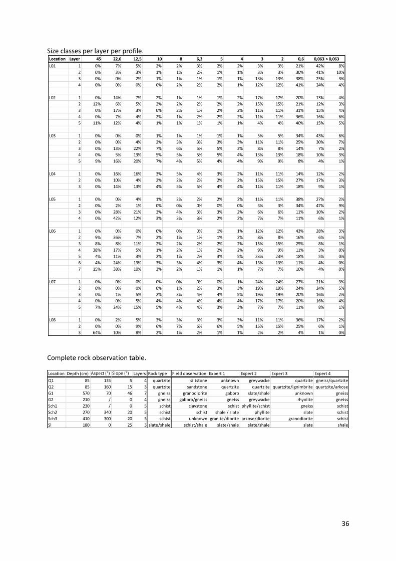
36
Size classes per layer per profile.
Complete rock observation table.
Location Layer 45 22,6 12,5 10 8 6,3 5 4 3 2 0,6 0,063 > 0,063
L01 1 0% 7% 5% 2% 2% 3% 2% 2% 3% 3% 21% 42% 8%
2 0% 3% 3% 1% 1% 2% 1% 1% 3% 3% 30% 41% 10%
3 0% 0% 2% 1% 1% 1% 1% 1% 13% 13% 38% 25% 3%
4 0% 0% 0% 0% 2% 2% 2% 1% 12% 12% 41% 24% 4%
L02 1 0% 14% 7% 2% 1% 1% 1% 2% 17% 17% 20% 13% 4%
2 12% 6% 5% 2% 2% 2% 2% 2% 15% 15% 21% 12% 3%
3 0% 17% 3% 0% 2% 1% 2% 2% 11% 11% 31% 15% 4%
4 0% 7% 4% 2% 1% 2% 2% 2% 11% 11% 36% 16% 6%
5 11% 12% 4% 1% 1% 1% 1% 1% 4% 4% 40% 15% 5%
L03 1 0% 0% 0% 1% 1% 1% 1% 1% 5% 5% 34% 43% 6%
2 0% 0% 4% 2% 3% 3% 3% 3% 11% 11% 25% 30% 7%
3 0% 13% 22% 7% 6% 5% 5% 3% 8% 8% 14% 7% 2%
4 0% 5% 13% 5% 5% 5% 5% 4% 13% 13% 18% 10% 3%
5 9% 16% 20% 7% 4% 5% 4% 4% 9% 9% 8% 4% 1%
L04 1 0% 16% 16% 3% 5% 4% 3% 2% 11% 11% 14% 12% 2%
2 0% 10% 4% 2% 2% 2% 2% 2% 15% 15% 27% 17% 3%
3 0% 14% 13% 4% 5% 5% 4% 4% 11% 11% 18% 9% 1%
L05 1 0% 0% 4% 1% 2% 2% 2% 2% 11% 11% 38% 27% 2%
2 0% 2% 1% 0% 0% 0% 0% 0% 3% 3% 34% 47% 9%
3 0% 28% 21% 3% 4% 3% 3% 2% 6% 6% 11% 10% 2%
4 0% 42% 12% 3% 3% 3% 2% 2% 7% 7% 11% 6% 1%
L06 1 0% 0% 0% 0% 0% 0% 1% 1% 12% 12% 43% 28% 3%
2 9% 36% 7% 2% 1% 1% 1% 2% 8% 8% 16% 6% 1%
3 8% 8% 11% 2% 2% 2% 2% 2% 15% 15% 25% 8% 1%
4 38% 17% 5% 1% 2% 1% 2% 2% 9% 9% 11% 3% 0%
5 4% 11% 3% 2% 1% 2% 3% 5% 23% 23% 18% 5% 0%
6 4% 24% 13% 3% 3% 4% 3% 4% 13% 13% 11% 4% 0%
7 15% 38% 10% 3% 2% 1% 1% 1% 7% 7% 10% 4% 0%
L07 1 0% 0% 0% 0% 0% 0% 0% 1% 24% 24% 27% 21% 3%
2 0% 0% 0% 0% 1% 2% 3% 3% 19% 19% 24% 24% 5%
3 0% 1% 5% 2% 3% 4% 4% 5% 19% 19% 20% 16% 2%
4 0% 0% 5% 4% 4% 4% 4% 4% 17% 17% 20% 16% 4%
5 7% 24% 15% 5% 4% 4% 3% 3% 7% 7% 11% 8% 1%
L08 1 0% 2% 5% 3% 3% 3% 3% 3% 11% 11% 36% 17% 2%
2 0% 0% 9% 6% 7% 6% 6% 5% 15% 15% 25% 6% 1%
3 64% 10% 8% 2% 1% 2% 1% 1% 2% 2% 4% 1% 0%
Location Depth (cm) Aspect (°) Slope (°) Layers Rock type Field observation Expert 1 Expert 2 Expert 3 Expert 4
Q1 85 135 5 4 quartzite siltstone unknown greywacke quartzite gneiss/quartzite
Q2 85 160 15 3 quartzite sandstone quartzite quartzite quartzite/ignimbrite quartzite/arkose
G1 570 70 46 7 gneiss granodiorite gabbro slate/shale unknown gneiss
G2 210 / 0 4 gneiss gabbro/gneiss gneiss greywacke rhyolite gneiss
Sch1 230 / 0 5 schist claystone schist phyllite/schist gneiss schist
Sch2 270 340 20 5 schist schist shale / slate phyllite slate schist
Sch3 410 300 20 5 schist unknown granite/diorite arkose/diorite granodiorite schist
Sl 180 0 25 3 slate/shale schist/shale slate/shale slate/shale slate shale

37
Detailed PSD change graphs.
-150
-100
-50
0
50
100
150
200
2 to 13 to 24 to 3
Change in size fractions between layers from bottom to top Q1
45 mm (gr)
22,6 mm (gr)
12,5 mm (gr)
10 mm (gr)
8 mm (gr)
-150
-100
-50
0
50
100
150
2 to 13 to 2
Change in size fractions between layers from bottom to top Q2
45 mm (gr)
22,6 mm (gr)
12,5 mm (gr)
10 mm (gr)
8 mm (gr)
6,3 mm (gr)
-400
-300
-200
-100
0
100
200
300
400
2 to 13 to 24 to 35 to 46 to 57 to 6
Change in size fractions between layers from bottom to top G1
45 mm (gr)
22,6 mm (gr)
12,5 mm (gr)
10 mm (gr)
8 mm (gr)
6,3 mm (gr)
-300
-200
-100
0
100
200
300
400
2 to 13 to 24 to 3
Change in size fractions between layers from bottom to top G2
45 mm (gr)
22,6 mm (gr)
12,5 mm (gr)
10 mm (gr)
8 mm (gr)
6,3 mm (gr)
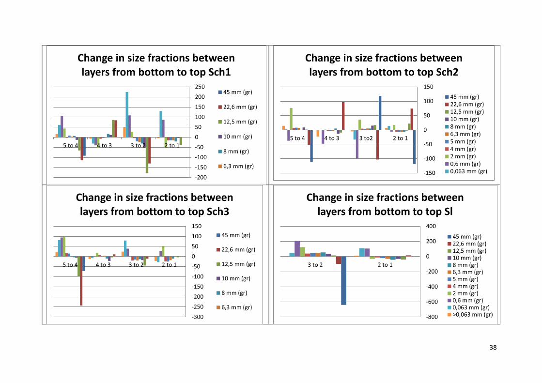
38
-200
-150
-100
-50
0
50
100
150
200
250
2 to 13 to 24 to 35 to 4
Change in size fractions between layers from bottom to top Sch1
45 mm (gr)
22,6 mm (gr)
12,5 mm (gr)
10 mm (gr)
8 mm (gr)
6,3 mm (gr)-150
-100
-50
0
50
100
150
2 to 13 to24 to 35 to 4
Change in size fractions between layers from bottom to top Sch2
45 mm (gr)22,6 mm (gr)12,5 mm (gr)10 mm (gr)8 mm (gr)6,3 mm (gr)5 mm (gr)4 mm (gr)2 mm (gr)0,6 mm (gr)0,063 mm (gr)
-300
-250
-200
-150
-100
-50
0
50
100
150
2 to 13 to 24 to 35 to 4
Change in size fractions between layers from bottom to top Sch3
45 mm (gr)
22,6 mm (gr)
12,5 mm (gr)
10 mm (gr)
8 mm (gr)
6,3 mm (gr)
-800
-600
-400
-200
0
200
400
2 to 13 to 2
Change in size fractions between layers from bottom to top Sl
45 mm (gr)22,6 mm (gr)12,5 mm (gr)10 mm (gr)8 mm (gr)6,3 mm (gr)5 mm (gr)4 mm (gr)2 mm (gr)0,6 mm (gr)0,063 mm (gr)>0,063 mm (gr)

39
-100%
0%
100%
200%
300%
400%
2 to 13 to 24 to 3
Percentage change in size fractions between layers from bottom to top
Q1 45 mm (%)
22,6 mm (%)
12,5 mm (%)
10 mm (%)
8 mm (%)
6,3 mm (%)
-100%
0%
100%
200%
300%
400%
2 to 13 to 2
Percentage change in size fractions between layers from bottom to top
Q2 45 mm (%)
22,6 mm (%)
12,5 mm (%)
10 mm (%)
8 mm (%)
6,3 mm (%)
-200%
0%
200%
400%
600%
800%
1000%
2 to 13 to 24 to 35 to 46 to 57 to 6
Percentage change in size fractions between layers from bottom to top
G1 45 mm (%)22,6 mm (%)12,5 mm (%)10 mm (%)8 mm (%)6,3 mm (%)5 mm4 mm (%)2 mm (%)0,6 mm (%)0,063 mm (%)>0,063 mm (%) -200%
0%
200%
400%
600%
800%
2 to 13 to 24 to 3
Percentage change in size fractions between layers from
bottom to top G2 45 mm (%)
22,6 mm (%)
12,5 mm (%)
10 mm (%)
8 mm (%)
6,3 mm (%)

40
-200%
-100%
0%
100%
200%
300%
400%
2 to 13 to 24 to 35 to 4
Percentage change in size fractions between layers from bottom to top
Sch1 45 mm (%)22,6 mm (%)12,5 mm (%)10 mm (%)8 mm (%)6,3 mm (%)5 mm4 mm (%)2 mm (%)0,6 mm (%)0,063 mm (%)>0,063 mm (%) -200%
-100%
0%
100%
200%
300%
400%
500%
2 to 13 to24 to 35 to 4
Percentage change in size fractions between layers from bottom to top
Sch2 45 mm (%)
22,6 mm (%)
12,5 mm (%)
10 mm (%)
8 mm (%)
-150%
-100%
-50%
0%
50%
100%
150%
200%
2 to 13 to 24 to 35 to 4
Percentage change in size fractions between layers from bottom to top
Sch3 45 mm (%)
22,6 mm (%)
12,5 mm (%)
10 mm (%)
8 mm (%)
6,3 mm (%)
-200%
0%
200%
400%
600%
800%
2 to 13 to 2
Percentage change in size fractions between layers from bottom to top
Sl 45 mm (%)22,6 mm (%)12,5 mm (%)10 mm (%)8 mm (%)6,3 mm (%)5 mm4 mm (%)2 mm (%)0,6 mm (%)0,063 mm (%)

41
-250
-200
-150
-100
-50
0
50
100
150
200
250
4 to 14 to 24 to 3
Change in size fractions relative to bedrock Q1
45 mm (gr)
22,6 mm (gr)
12,5 mm (gr)
10 mm (gr)
8 mm (gr)
6,3 mm (gr)
-150
-100
-50
0
50
100
150
3 to 13 to 2
Change in size fractions relative to bedrock Q2
45 mm (gr)
22,6 mm (gr)
12,5 mm (gr)
10 mm (gr)
8 mm (gr)
6,3 mm (gr)
-500
-400
-300
-200
-100
0
100
200
300
400
7 to 17 to 27 to 37 to 47 to 57 to 6
Change in size fractions relative to bedrock G1
45 mm (gr)22,6 mm (gr)12,5 mm (gr)10 mm (gr)8 mm (gr)6,3 mm (gr)5 mm (gr)4 mm (gr)2 mm (gr)0,6 mm (gr)0,063 mm (gr)>0,063 mm (gr) -600
-400
-200
0
200
400
600
4 to 14 to 24 to 3
Change in size fractions relative to bedrock G2
45 mm (gr)
22,6 mm (gr)
12,5 mm (gr)
10 mm (gr)
8 mm (gr)
6,3 mm (gr)

42
-300
-200
-100
0
100
200
300
400
500
5 to 15 to 25 to 35 to 4
Change in size fractions relative to bedrock Sch1
45 mm (gr)
22,6 mm (gr)
12,5 mm (gr)
10 mm (gr)
8 mm (gr)
6,3 mm (gr)
-250
-200
-150
-100
-50
0
50
100
150
5 to 15 to 25 to 35 to 4
Change in size fractions relative to bedrock Sch2
45 mm (gr)
22,6 mm (gr)
12,5 mm (gr)
10 mm (gr)
8 mm (gr)
6,3 mm (gr)
-300
-250
-200
-150
-100
-50
0
50
100
150
200
5 to 15 to 25 to 35 to 4
Change in size fractions relative to bedrock Sch3
45 mm (gr)
22,6 mm (gr)
12,5 mm (gr)
10 mm (gr)
8 mm (gr)
6,3 mm (gr)-800
-600
-400
-200
0
200
400
3 to 13 to 2
Change in size fractions relative to bedrock Sl
45 mm (gr)22,6 mm (gr)12,5 mm (gr)10 mm (gr)8 mm (gr)6,3 mm (gr)5 mm (gr)4 mm (gr)2 mm (gr)0,6 mm (gr)0,063 mm (gr)

43