1

Congestion control with multi-packet feedbackIhsan Ayyub Qazi, Lachlan L. H. Andrew, and Taieb Znati

Abstract— Many congestion control protocols use explicit feed-back from the network to achieve high performance. Most ofthese either require more bits for feedback than are availablein the IP header or incur performance limitations due toinaccurate congestion feedback. There has been recent interestin protocols which obtain high resolution estimates of congestionby combining the ECN marks of multiple packets, and using thisto guide MI-AI-MD window adaptation. This paper studies thepotential of such approaches, both analytically and by simulation.The evaluation focuses on a new protocol called Binary MarkingCongestion Control (BMCC). It is shown that these schemes canquickly acquire unused capacity, quickly approach a fair ratedistribution, and have relatively smooth sending rates, even onhigh bandwidth-delay product networks. This is achieved whilemaintaining low average queue length and negligible packet loss.Using extensive simulations, we show that BMCC outperformsXCP, VCP MLCP, CUBIC, CTCP, SACK, and in some casesRCP, in terms of average flow completion times. Suggestions arealso given for the incremental deployment of BMCC.

Index Terms— Congestion Control, TCP, AQM, ECN

I. INTRODUCTION

The Transmission Control Protocol (TCP) has been in-strumental to the successful development and growth of theInternet and its applications. However, recent advances inwired and wireless communications technology have lead toa tremendous growth in the range of path bandwidth-delayproducts (BDP) in the Internet [1]. There has simultaneouslybeen an increase in the diversity of applications carried overthe Internet (e.g., voice over IP, video conferencing, and socialnetworking). These advances have stressed the congestioncontrol algorithm in TCP and the need for more efficient,fair, robust, and easy to deploy congestion control protocolsis increasingly important.

While considerable research has gone into addressing thelimitations of TCP, prior research has focused on two extremepoints in the design space of congestion control protocols.

At one end are end-to-end schemes that rely on implicitcongestion signals such as packet loss [2], delay [3], jitter [4]or combinations of these [5]. Since loss and delay only occur

Ihsan Ayyub Qazi (corresponding author) is with the Department ofComputer Science at the LUMS School of Science and Engineering, Lahore,Pakistan. (Email: ihsan.qazi@lums.edu.pk). While performing a subsetof this work, Ihsan Ayyub Qazi was with the Department of ComputerScience, University of Pittsburgh, Pittsburgh, PA, 15260 USA and the Centrefor Advanced Internet Architectures, Swinburne University of Technology,Hawthorn, VIC 3122, Australia.

Lachlan Andrew is with the Centre for Advanced Internet Architectures,Swinburne University of Technology, Hawthorn, VIC 3122, Australia (Email:landrew@swin.edu.au).

Taieb Znati is with the Department of Computer Science, University ofPittsburgh, Pittsburgh, PA, 15260 USA (Email: znati@cs.pitt.edu)

This work was supported by NSF grants 010536 and 010684, AustralianResearch Council (ARC) grants DP0985322 and FT0991594, and the LUMSFaculty Startup Grant.

once a link is overloaded, these schemes must introduceunnecessary packet losses or queuing at the bottleneck.

On the other end are “network-based” schemes in whichrouters explicitly specify a rate (used by RCP [6] and ATM’sAvailable Bit Rate (ABR) [7]) or change in window size (usedby XCP [1]) for each individual flow. These schemes facetwo big deployment challenges on today’s Internet: (1) Theyrequire more bits for feedback than are available in the IPheader (128 for XCP [8] and 96 for RCP [9]) which requireseither changing the IP header1, use of IP options, or theaddition of a “shim” layer. This makes universal deployment ofsuch protocols challenging. (2) It is difficult for such protocolsto co-exist with TCP traffic, often requiring complex router-level mechanisms for fair bandwidth sharing [8], [9].

Between these extremes are “limited feedback” schemes,such as TCP with random early discard (RED) and explicitcongestion notification (ECN) [11], [12], and VCP [13], whichrequire changes at the end-hosts with incremental supportfrom the routers. In these schemes, each packet signals thecongestion level with up to 2-bit resolution. VCP uses a 2-bit estimate of the load factor (ratio of input traffic plusqueue length to capacity) to trigger a fixed multiplicativeincrease (MI), additive increase (AI) or multiplicative decrease(MD) window update, at low load, high load and overload.However, convergence speed improves significantly when theload is estimated to 4-bit resolution [14], for which there isinsufficient space in the IP header of a single packet.

There are several methods for obtaining high resolutioncongestion estimates using the existing ECN bits of streamsof packets. Random marking of packets based on the levelof congestion was proposed in [15], and used by the REMprotocol [16]. Higher resolution estimates can be obtainedusing side-information in packet headers to indicate how tointerpret the ECN mark of a given packet [17], [18], [19]. Mostof these schemes require a pre-specified resolution, which istraded against the number of packets needed to carry the ECNmarks. Adaptive deterministic packet marking (ADPM [20])implicitly adapts its effective quantization resolution based onthe dynamics of the value and obtains a resolution of 1/n afterreceiving n packets, for n up to 216 or beyond. ADPM pro-vides a MSE that is several orders of magnitude smaller [20],[21] than the estimators based on random marking of packets[15], [16] or deterministic marking with static quantization[19], [22].

This paper investigates the ability of MI-AI-MD schemes(such as VCP [13]) to use high-resolution estimates of loadfactor based on ECN marks spread over multiple packets. Tothis end, we design the Binary Marking Congestion Control

1Modifying IP is slow: work on IPv6 started around 1992, but it accountedfor less than 1% of Internet traffic as of December 2008 [10].

(BMCC) protocol that uses ADPM to obtain congestion es-timates with up to 16-bit resolution using ECN, in a waycompatible with existing RED/ECN. We present analyticalmodels that provide insights into the convergence properties ofMI-AI-MD algorithms, and study the incremental deploymentof these protocols when they co-exist with TCP traffic andtraverse different kinds of bottleneck routers.

With BMCC, each router periodically computes the loadfactor on each of its links. End-hosts obtain a high resolutionestimate of the bottleneck load factor using ADPM. WithADPM, each packet signals a bound on the bottleneck loadfactor. The receiver’s estimate of the load factor is updatedwhenever a new packet provides a tighter bound. This estimateis echoed back to the sources via acknowledgement packetsusing TCP options. Based on this value, sources apply load-dependent MI-AI-MD algorithm. BMCC achieves efficientand fairness bandwidth allocations on high BDP paths whilemaintaining low bottleneck queue and loss rate. In terms ofaverage flow completion times (AFCT) for typical Internetflow sizes, BMCC outperforms XCP, VCP, MLCP, CUBIC,CTCP, SACK [23] using RED/ECN, and sometimes even RCP,which was optimized for AFCT.

The main contribution of this paper is the design andanalysis of a congestion control protocol that achieves per-formance comparable to that of feedback-rich protocols, suchas RCP, using only incrementally deployable signaling. Thepresentation and analysis of the proposed protocol involvesthree different components.

The first component, presented in Section II, focuses on thespecification of the BMCC protocol, which uses the existingtwo ECN bits to obtain high resolution congestion estimates.The major issues related to the design of BMCC are discussedin Section III. BMCC achieves faster convergence by usingADPM to increase the feedback resolution, allowing faster rateincrease during low load and more precise decreases duringcongestion.

The second component, presented in Section IV, focuses onthe analysis of BMCC. It is worth noting that the analysis isapplicable, not only to BMCC, but also to the class of MI-AI-MD algorithms with multi-bit resolution, including UNO [24]and MPCP [25].

The analysis shows that reducing the MI factor when loadincreases results in a concave window growth, which quicklyacquires spare capacity with minimal overshoot. The ns-2 sim-ulation results in Section V show that BMCC achieves betterthroughput, fairness and short AFCT than many benchmarkprotocols in a wide range of scenarios.

The final component, discussed in Section VI, studies thefeasibility of BMCC’s incremental deployment in the Internet.The study focuses on the co-existence of BMCC with differentversions of TCP, such as CUBIC [2], CTCP [5], and TCPSACK, and on how to deal with situations where traffic maytraverse network bottlenecks that do not all support BMCCmarking. To prevent starvation of BMCC flows, a modificationof the original BMCC protocol is proposed, whereby thedecision of when to respond to congestion is decoupled fromthe decision of how to respond to congestion. This allowsTCP and BMCC sources to back off based on a common

signal while allowing BMCC sources to retain the benefit ofbasing the backoff factor on the estimated congestion level.This solution has applicability beyond BMCC.

II. ALGORITHM AND PROTOCOL

A congestion control protocol must specify how congestionis estimated, how that information is communicated to thesender, and how the sender should respond. BMCC estimatescongestion in terms of the load factor at each link, whichis a weighted sum of the link utilization and the queueingdelay [13]. The maximum load factor along a flow’s path iscommunicated using ADPM, to the sender which responds us-ing load-dependent MI-AI-MD. The components of a BMCCsystem are as follows.

A. BMCC Router

A BMCC router divides time into intervals of length tp, andcomputes the load factor in each interval as [7], [13], [16]

f =λ+ κ1qavγlCltp

(1)

where λ is the amount of bytes received during tp, Cl is thelink capacity in bytes/sec, γl ≤ 1 is the target utilization2 [26],qav is an estimate of the average queue length in bytes3, andκ1 ≤ 1 controls how fast to drain the queue [11], [16].

The router conveys its load factor to the sender by applyingADPM [20] to packets’ ECN bits as follows: Recall thatthe ECN bits on an unmarked packet are initially (10)2, androuters set these bits to (11)2 to indicate congestion. Chooseu to be a “severely congested” load factor. BMCC marks thepacket with (11)2 if f ≥ u or the packet already contains amark (11)2. Otherwise, ADPM computes a deterministic hashh of the packet contents, such as the 16-bit IPid field in theIPv4 header or the checksum of the payload in case of IPv6.This hash is compared to f , and the packet is marked with(01)2 if f > h, or left unchanged otherwise. At the receiver,the ECN bits will reflect the state of the most congested routeron the path.

Router Implementation Complexity: For each packet, aBMCC router calculates a hash of the packet (simply reversingthe bits of the IPid field [20]), performs a comparison, and setsup to two header bits. At the larger timescale of tp, it requiresmultiplication by two constants and an addition to calculate f .(Note that the denominator of (1) is a constant.) It also uses acount of the total bytes sent, which routers already record, andthe average queue size, which can be measured at a frequencythat does not scale up with bit-rate.

B. BMCC Receiver

As part of ADPM, the receiver maintains the current esti-mate, f̂ of the load factor at the bottleneck on the forward

2Note that this corresponds to a virtual queue with capacity γlCl.3We calculate the average as qav(t+ tq) = a.qav(t)+ (1− a).q(t+ tq),

where q(t) is the instantaneous queue length, and tq ≪ tp. We set tq =10ms, a = 0.875, and κ1 = 0.5 similar to [13].

path. When a packet is received, this estimate is updated as:

f̂ ←

u if becn = (11)2h if (becn = (10)2 and h < f̂ )

or (becn = (01)2 and h > f̂ )f̂ otherwise

where becn refers to the two ECN bits in the IP header of thereceived packet. The estimate f̂ is sent to the sender using TCPoptions, as described in Section II-E. Note that the receiver’sestimate will lag behind the true value [21], except that valuesover u are signaled immediately to indicate severe overload.

The resolution depends on the fraction of packets that hashto a particular range. For BMCC, values of f below a thresholdη0 are rounded up to η0, and the hash is such that 1/4 ofpackets hash to values in (η0, η) for some design parameterη, 1/4 of packets hash to (η, 1) and 1/2 hash to (1, u).

Remark 1: The systemic effect of ADPM is to indicate themaximum load factor to the receiver. On leaving a router,a packet will be marked if the load factor of that router orany upstream router exceeds the packet’s hash value. When amarked packet is received, if h > f̂ the receiver updates itsestimate to h since it is a tighter lower bound on the maximumf . Conversely, the hash of an unmarked packet provides anupper bound on the maximum f on the path.

C. BMCC Sender

To achieve both high bottleneck utilization and fair band-width allocation with low fluctuation in rates, BMCC usesthree modes of operation, based on whether the load is low(f < η), medium (f ∈ [η, 1)) or overload (f > 1).

1) Low Load (η0 ≤ f̂ < η): To increase bottleneckutilization when the load is low, sources apply MI with factorsproportional to (1− f̂)/f̂ . In particular, flows with RTT equalto tp apply

w(t+ T ) = w(t)

(1 + κ2

1− f̂f̂

), (2)

where T is the RTT of the flow and κ2 is the step size. BMCCuses κ2 = 0.35, which is in the range κ2 ∈ (0, 1/2) suggestedby Theorem 1 of [13]. VCP [13] approximates this using afixed MI parameter independent of f̂ .

BMCC aims to give equal rate to flows with different RTTs.Since flows with large RTTs update less often, the rule

w(t+ T ) = w(t)

(1 + κ2

1− f̂f̂

)T/tp

(3)

is used so that windows grow at a rate independent of T . Tomirror the benefits of traditional slow start, new flows remainin MI until f̂ first reaches 1,

2) Medium Load (η ≤ f̂ < 1): When utilization is high,BMCC uses AIMD to achieve fairness. In medium load,sources apply AI:

w(t+ T ) = w(t) + α, (4)

with α = (T/tp)2 chosen to cause the equilibrium window to

be proportional to the flow’s RTT, giving RTT fairness.

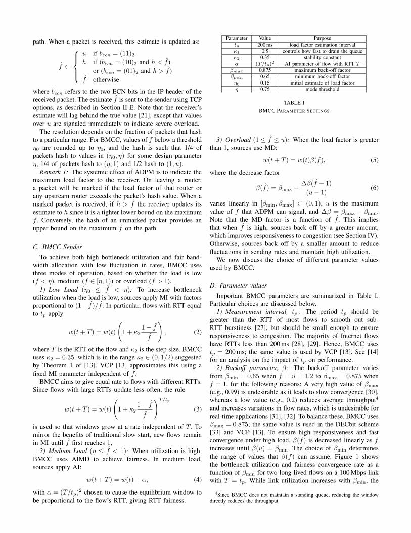
Parameter Value Purposetp 200 ms load factor estimation intervalκ1 0.5 controls how fast to drain the queueκ2 0.35 stability constantα (T/tp)2 AI parameter of flow with RTT T

βmax 0.875 maximum back-off factorβmin 0.65 minimum back-off factorη0 0.15 initial estimate of load factorη 0.75 mode threshold

TABLE IBMCC PARAMETER SETTINGS

3) Overload (1 ≤ f̂ ≤ u): When the load factor is greaterthan 1, sources use MD:

w(t+ T ) = w(t)β(f̂), (5)

where the decrease factor

β(f̂) = βmax −∆β(f̂ − 1)

(u− 1)(6)

varies linearly in [βmin, βmax] ⊂ (0, 1), u is the maximumvalue of f that ADPM can signal, and ∆β = βmax − βmin.Note that the MD factor is a function of f̂ . This impliesthat when f̂ is high, sources back off by a greater amount,which improves responsiveness to congestion (see Section IV).Otherwise, sources back off by a smaller amount to reducefluctuations in sending rates and maintain high utilization.

We now discuss the choice of different parameter valuesused by BMCC.

D. Parameter values

Important BMCC parameters are summarized in Table I.Particular choices are discussed below.

1) Measurement interval, tp : The period tp should begreater than the RTT of most flows to smooth out sub-RTT burstiness [27], but should be small enough to ensureresponsiveness to congestion. The majority of Internet flowshave RTTs less than 200 ms [28], [29]. Hence, BMCC usestp = 200 ms; the same value is used by VCP [13]. See [14]for an analysis on the impact of tp on performance.

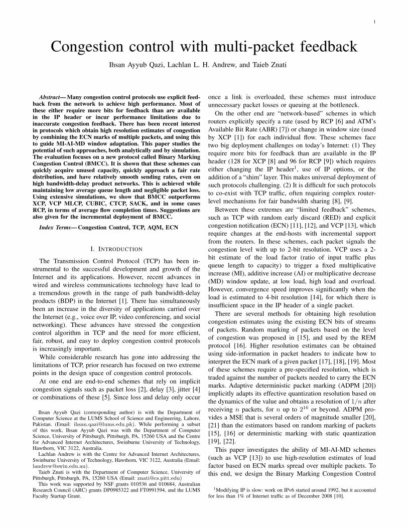
2) Backoff parameter, β: The backoff parameter variesfrom βmin = 0.65 when f = u = 1.2 to βmax = 0.875 whenf = 1, for the following reasons: A very high value of βmax

(e.g., 0.99) is undesirable as it leads to slow convergence [30],whereas a low value (e.g., 0.2) reduces average throughput4

and increases variations in flow rates, which is undesirable forreal-time applications [31], [32]. To balance these, BMCC usesβmax = 0.875; the same value is used in the DECbit scheme[33] and VCP [13]. To ensure high responsiveness and fastconvergence under high load, β(f) is decreased linearly as fincreases until β(u) = βmin. The choice of βmin determinesthe range of values that β(f) can assume. Figure 1 showsthe bottleneck utilization and fairness convergence rate as afunction of βmin for two long-lived flows on a 100 Mbps linkwith T = tp. While link utilization increases with βmin, the

4Since BMCC does not maintain a standing queue, reducing the windowdirectly reduces the throughput.

0

20

40

60

80

100

0 0.25 0.5 0.75 1

Util

izat

ion

(%)

β

(a)

1

1.2

1.4

1.6

1.8

2

0 0.25 0.5 0.75 1

Con

verg

ence

Rat

e

β

(b)

Fig. 1. Bottleneck utilization and fairness convergence rate as a function ofβ(f) = βmin for two flows on a 100 Mbps with T = tp.

convergence rate decreases. To balance these, BMCC usesβmin = 0.65.

3) Mode threshold, η: The minimum value of β(f) de-termines the parameter η, which defines the transition pointbetween applying MI and AIMD. To encourage high utiliza-tion, η should be large, but small enough to prevent flowsfrom entering MI after overload detection, which can lead tohigh packet loss rate. It suffices that η < minf≥1(fβ(f)).The minimum of fβ(f) = 0.723 occurs for f = u (sinceβ(f) = βmin for f ≥ u, the quadratic fβ(f) for f < u isconcave, and β(1) > uβ(u)). BMCC uses η = 0.75.

E. Reverse Signalling Overhead

The BMCC receiver communicates the estimated loadfactor, f̂ , to the sender using TCP options. Unlike on theforward path, TCP options are acceptable for this becausethey need not be processed by the routers. However, theycan introduce overhead. The number of bytes needed in TCPoptions depends on the desired feedback resolution. If 16-bitfeedback resolution is used, as in our implementation, thenthe feedback fits in a minimum sized (4 byte) TCP option.Rather than piggybacking f̂ on every ACK, it is only necessaryto send f̂ if it changes. This approach (which we call “non-redundant”) increases the sensitivity to lost ACKs.

The alternative used by BMCC is to send the estimateimmediately after it changes, and then to send redundantcopies with decreasing frequency. Each receiver maintains acounter i. The ith option is sent i packets after the previousone, so that options are sent on ACKs 1, 3, 6, 10,... The counteris reset to 1 each time f̂ changes and incremented by 1 eachtime f̂ is sent. This scheme is robust against losing a smallnumber of ACKs, but if f̂ changes once per n packets, theoverhead is only O(1/

√n) times that of naı̈vely echoing on

every ACK.The reduction in overhead was evaluated by ns2 simulations

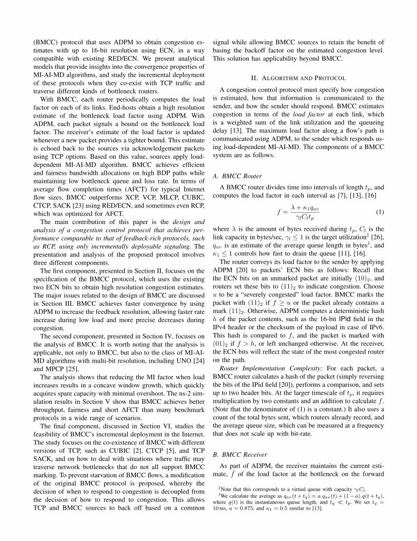
of a dumbbell topology with a bottleneck link of capacity100 Mbps, carrying ten long-lived flows in each direction withT=80ms. Table II shows statistics that correspond to theaverage of the ten flows in the forward path. Of 552942 ACKsgenerated by the receivers, the price estimate changed for 6914(1.3%), which carried f̂ under both schemes, whereas 12.9%carried f̂ under BMCC’s robust scheme.

ACKs sent ACKs with f̂ Reduction(%)non-redundant 552942 6914 98.7

BMCC 552942 71476 87.1

TABLE IIOVERHEAD OF SIGNALLING FROM RECEIVER TO SENDER.

III. DESIGN ISSUES

The design of BMCC gives rise to several questions whoseanswers requires careful consideration of network load andoperating conditions. The objective of this section is to addressthese questions and describe the approaches BMCC uses tomanage traffic efficiently and achieve high network perfor-mance.

a) What is the congestion level assumed by new flows?:ADPM needs an initial estimate of the congestion level. Newflows initially estimate f̂ = η0 = 0.15, and thus increase theirwindows by a factor of 1+ κ2(1− η0)/η0 ≈ 3 per tp. This isa faster increase than existing TCP slow start when T = tp.

b) Can new flows cause overload before ADPM has beenable to signal congestion?: The estimates of f signalled byADPM lag behind the true value. Hence, a flow may notdetect overload and apply MD in a given tp interval [20].In the presence of a large number of flows, congestion willbe avoided if most reduce their windows, even if some missthe congestion signal. However, if f > u = 1.2, each flowdecreases its window deterministically (using the standardECN “Congestion Experienced” codepoint) which preventspersistent congestion. Note that ADPM provides feedback wellbefore the buffer overflows, and so new flows need not causelarge bursts of loss and timeouts, even if there is some delayin detecting congestion.

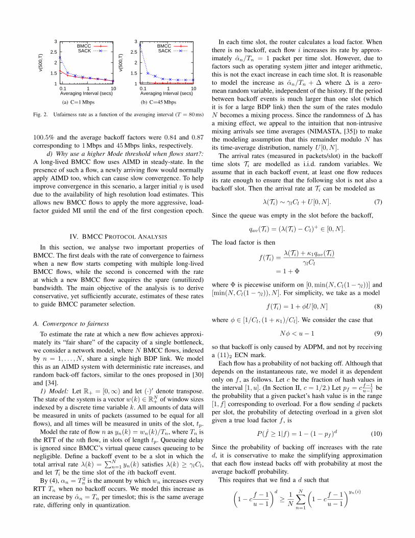
c) Sources may apply different backoff factors at the sametime; does this lead to unfairness?: The backoff factor appliedby a BMCC source depends on its estimate of the load factor.This estimate can be different across sources due to ADPM.This may lead to short-term unfairness (on the scale of a fewRTTs). To quantify this, we compare the level of unfairnesscaused by TCP SACK and BMCC for a range of time scales.

Consider an averaging interval s. For two SACK flows, letXi(t, s) be the average rate of flow i over the interval (t, t+s),and let the “unfairness rate” be

v(τ, s) =1

τ

∫ τ

0

maxi(Xi(t, s))

minj(Xj(t, s))dt,

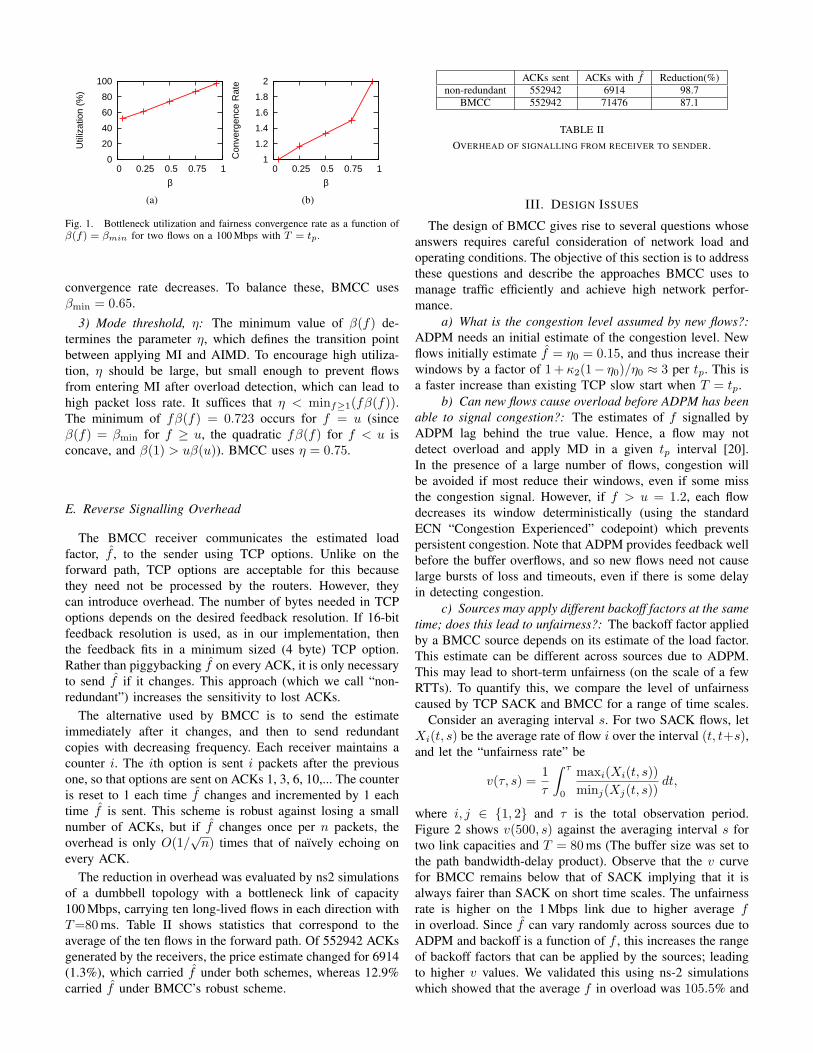
where i, j ∈ {1, 2} and τ is the total observation period.Figure 2 shows v(500, s) against the averaging interval s fortwo link capacities and T = 80ms (The buffer size was set tothe path bandwidth-delay product). Observe that the v curvefor BMCC remains below that of SACK implying that it isalways fairer than SACK on short time scales. The unfairnessrate is higher on the 1 Mbps link due to higher average fin overload. Since f̂ can vary randomly across sources due toADPM and backoff is a function of f , this increases the rangeof backoff factors that can be applied by the sources; leadingto higher v values. We validated this using ns-2 simulationswhich showed that the average f in overload was 105.5% and

1

1.5

2

2.5

3

0.1 1 10

v(50

0,T

)

Averaging Interval (secs)

BMCCSACK

(a) C=1 Mbps

1

1.5

2

2.5

3

0.1 1 10

v(50

0,T

)

Averaging Interval (secs)

BMCCSACK

(b) C=45 Mbps

Fig. 2. Unfairness rate as a function of the averaging interval (T = 80ms)

100.5% and the average backoff factors were 0.84 and 0.87corresponding to 1Mbps and 45Mbps links, respectively.

d) Why use a higher Mode threshold when flows start?:A long-lived BMCC flow uses AIMD in steady-state. In thepresence of such a flow, a newly arriving flow would normallyapply AIMD too, which can cause slow convergence. To helpimprove convergence in this scenario, a larger initial η is useddue to the availability of high resolution load estimates. Thisallows new BMCC flows to apply the more aggressive, load-factor guided MI until the end of the first congestion epoch.

IV. BMCC PROTOCOL ANALYSIS

In this section, we analyse two important properties ofBMCC. The first deals with the rate of convergence to fairnesswhen a new flow starts competing with multiple long-livedBMCC flows, while the second is concerned with the rateat which a new BMCC flow acquires the spare (unutilized)bandwidth. The main objective of the analysis is to deriveconservative, yet sufficiently accurate, estimates of these ratesto guide BMCC parameter selection.

A. Convergence to fairness

To estimate the rate at which a new flow achieves approxi-mately its “fair share” of the capacity of a single bottleneck,we consider a network model, where N BMCC flows, indexedby n = 1, . . . , N , share a single high BDP link. We modelthis as an AIMD system with deterministic rate increases, andrandom back-off factors, similar to the ones proposed in [30]and [34].

1) Model: Let R+ = [0,∞) and let (·)′ denote transpose.The state of the system is a vector w(k) ∈ RN

+ of window sizesindexed by a discrete time variable k. All amounts of data willbe measured in units of packets (assumed to be equal for allflows), and all times will be measured in units of the slot, tp.

Model the rate of flow n as yn(k) = wn(k)/Tn, where Tn isthe RTT of the nth flow, in slots of length tp. Queueing delayis ignored since BMCC’s virtual queue causes queueing to benegligible. Define a backoff event to be a slot in which thetotal arrival rate λ(k) =

∑Nn=1 yn(k) satisfies λ(k) ≥ γlCl,

and let Ti be the time slot of the ith backoff event.By (4), αn = T 2

n is the amount by which wn increases everyRTT Tn when no backoff occurs. We model this increase asan increase by α̂n = Tn per timeslot; this is the same averagerate, differing only in quantization.

In each time slot, the router calculates a load factor. Whenthere is no backoff, each flow i increases its rate by approx-imately α̂n/Tn = 1 packet per time slot. However, due tofactors such as operating system jitter and integer arithmetic,this is not the exact increase in each time slot. It is reasonableto model the increase as α̂n/Tn + ∆ where ∆ is a zero-mean random variable, independent of the history. If the periodbetween backoff events is much larger than one slot (whichit is for a large BDP link) then the sum of the rates moduloN becomes a mixing process. Since the randomness of ∆ hasa mixing effect, we appeal to the intuition that non-intrusivemixing arrivals see time averages (NIMASTA, [35]) to makethe modeling assumption that this remainder modulo N hasits time-average distribution, namely U [0, N ].

The arrival rates (measured in packets/slot) in the backofftime slots Ti are modelled as i.i.d. random variables. Weassume that in each backoff event, at least one flow reducesits rate enough to ensure that the following slot is not also abackoff slot. Then the arrival rate at Ti can be modeled as

λ(Ti) ∼ γlCl + U [0, N ]. (7)

Since the queue was empty in the slot before the backoff,

qav(Ti) = (λ(Ti)− Cl)+ ∈ [0, N ].

The load factor is then

f(Ti) =λ(Ti) + κ1qav(Ti)

γlCl

= 1 + Φ

where Φ is piecewise uniform on [0,min(N,Cl(1− γl))] and[min(N,Cl(1− γl)), N ]. For simplicity, we take as a model

f(Ti) = 1 + ϕU [0, N ] (8)

where ϕ ∈ [1/Cl, (1 + κ1)/Cl]. We consider the case that

Nϕ < u− 1 (9)

so that backoff is only caused by ADPM, and not by receivinga (11)2 ECN mark.

Each flow has a probability of not backing off. Although thatdepends on the instantaneous rate, we model it as dependentonly on f , as follows. Let c be the fraction of hash values inthe interval [1, u]. (In Section II, c = 1/2.) Let pf = c f−1

u−1 bethe probability that a given packet’s hash value is in the range[1, f ] corresponding to overload. For a flow sending d packetsper slot, the probability of detecting overload in a given slotgiven a true load factor f , is

P (f̂ ≥ 1|f) = 1− (1− pf )d (10)

Since the probability of backing off increases with the rated, it is conservative to make the simplifying approximationthat each flow instead backs off with probability at most theaverage backoff probability.

This requires that we find a d such that(1− cf − 1

u− 1

)d

≥ 1

N

N∑n=1

(1− cf − 1

u− 1

)yn(i)

for all i. By Lemma 1 in the appendix, it is sufficient that dsatisfy this for the largest f , namely f = 1+N/ϕ. Since theright hand side is larger when yn are more spread out, and weexpect yn to converge, it seems conservative to set d to satisfythis for yn(0). Thus we take

d =

log

(1N

∑Nn=1

(1− c Nϕ

u−1

)yn(0))

log(1− c Nϕ

u−1

) . (11)

A simpler and more insightful, though less conservative, modelwould simply use

d =γlCl

N.

We model flows’ f̂ at each stage as having identicalmarginal distribution satisfying (10), and a joint distributionsuch that f̂ > 1 for at least one flow, independent of previousbackoffs. By (6), this implies that flow n backs off by afactor βn, where the vectors β(Ti) = (β1(Ti), . . . , βN (Ti))′at different back-off instants are i.i.d. random variables. Flowsn for which f̂ < 1 have βn = 1. Then the dynamics of theentire network of sources are described by [30]

Y (i+ 1) = A(i)Y (i) (12)

where

A(i) = diag(β(Ti)) +1

Ne(e′ − β′(Ti)), (13)

Y (i) = [y1(i), y2(i), ..., yN (i)]′ and e = (1, . . . , 1)′ ∈ RN×1.2) Rate of Convergence: We will now use the model (6)–

(13) to determine the rate of convergence to fairness.The main result of this section isTheorem 1: Under the model given by the numbered equa-

tions (6)–(13), the expected values of the rates converge as

E[Y (i)]− γlCl

Ne = µi−1

(E[Y (0)]−

(γlCl

N+

1

2

)e

)(14)

where

µ = βmax(1− Z(d+ 1)) + (1 +MϕN)Z(d+ 1)+

M

(Z(d+ 2)− 1

ζ(d+ 1)− ϕN

2

), ζ =

c

u− 1,M =

∆β

2(u− 1),

and

Z(x) =1− (1− ζϕN)x

ζxϕN.

Proof: Since β, and hence A, are i.i.d.,

E[Y (i)] =i−1∏j=0

A(j)Y (0) = (E[A(0)])i−1E[Y (0)]. (15)

The convergence is thus determined by the eigenvalues ofE[A(0)]. The dominant eigenvalue of E[A(0)] is 1, witheigenvector e. This implies that the component of Y (i) in thedirection of e is constant, and by (7) is equal to (γlCl/N +1/2)e. All other eigenvalues are E[β(f̂)]. It remains to showthat E[β(f̂)] = µ.

Recall that f̂ is the estimate of f at a given backoff time.The expected backoff factor in overload conditioned on f is

E[β(f̂)|f ] = P (f̂ < 1|f)E[β(f̂)|f̂ < 1, f ]+

P (f̂ ≥ 1|f)E[β(f̂)|f̂ ≥ 1, f ]. (16)

Now E[β(f̂)|f̂ < 1, f ] = 1 since sources do not backoff whenf̂ < 1, and by (10), P (f̂ < 1|f) = (1− pf )d.

Finally, by (6) and (8),

E[β(f̂)|f̂ ≥ 1, f ] =1

f − 1

∫ f−1

0

(βmax −∆βψ

u− 1)dψ

= βmax −∆β(f − 1)

2(u− 1). (17)

Let ζ = cu−1 . Then E[β(f̂)|f ] can be averaged over f−1 ∼

ϕU(0, N) to give

E[β(f̂)] =1

ϕN

∫ ϕN

0

[(1− (1− ζψ)d)× (18)(βmax −

∆βψ

2(u− 1)

)+ (1− ζψ)d]dψ

=βmax (1− Z(d+ 1)) + (1 +MϕN)Z(d+ 1)

+M

(Z(d+ 2)− 1

ζ(d+ 1)− ϕN

2

)

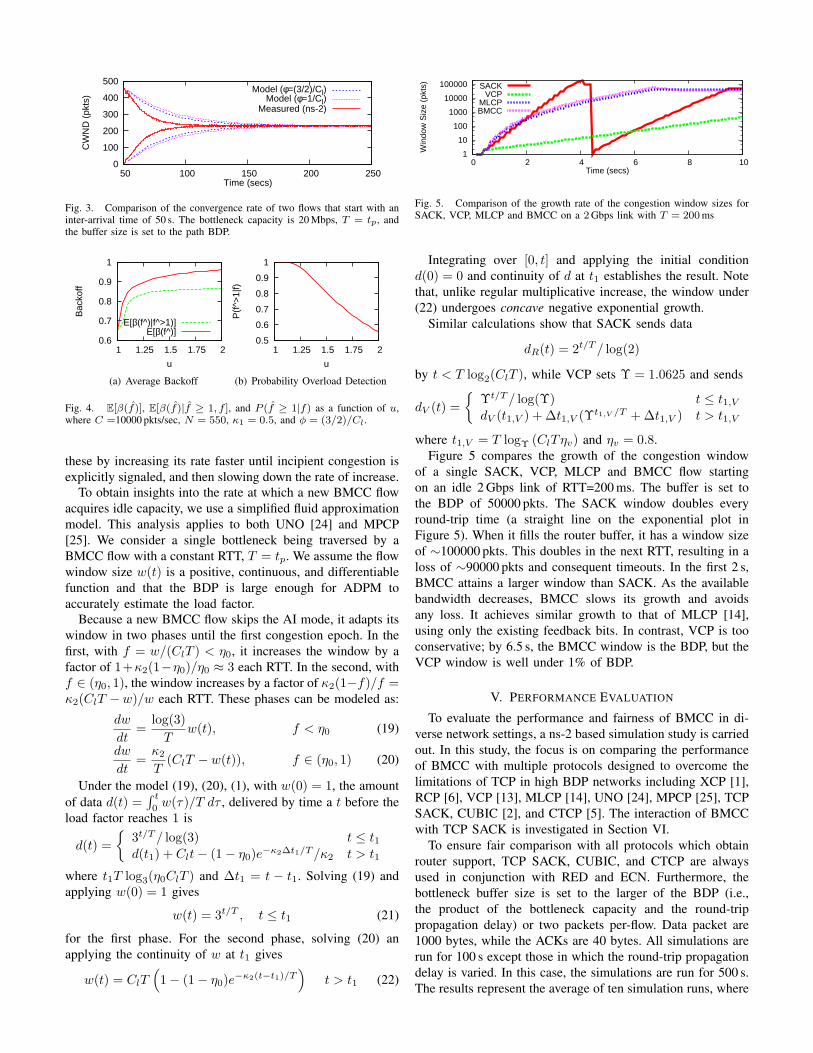
Figure 3 shows the average window size of two BMCC flowsthat have an inter-arrival time of 50 s. The bottleneck capacityis 20 Mbps and T = tp. The data points corresponding tothe ‘Model’ curves are determined as follows: The rates inthe model evolve in terms of congestion epochs. To plotthe window versus time in Figure 3, we assume that eachepoch has the mean duration. To calculate the latter we dividethe reduction in the sum of window sizes every backoffslot (assuming independence) by the increase in the sum ofwindow sizes per slot. Each data point corresponding to the‘Measured’ curve represents the average of 200 simulationruns with random flow starting times t1 ∼ U [0, tp] andt2 ∼ 50U [1, 1 + tp], where t1 and t2 are the starting timesof Flow 1 and Flow 2, respectively. For the model, each flowuses d = Cl/N . Observe that the expected window size of theflows converge to the same value and the model conservativelyestimates the rate of convergence.

Impact of u on backoff: The value of u determines themaximum value of f that can be signalled by ADPM. Figure4(a) shows that the expected backoff factor E[β(f̂)] increaseswith u. This happens because pf , which is the probabilitythat a packet detects overload, decreases with u (see Figure4(b)). Observe that when u = 1.2, flows detect overload withprobability close to 1.

B. How Fast does BMCC Acquire Spare Bandwidth?

A well known problem of TCP SACK is that a flow sendingon a path with large BDP and spare bandwidth takes too longto start up [6], and then causes many packet losses whenthe window finally reaches the BDP [36]. BMCC addresses

0

100

200

300

400

500

50 100 150 200 250

CW

ND

(pk

ts)

Time (secs)

Model (φ=(3/2)/Cl)Model (φ=1/Cl)

Measured (ns-2)

Fig. 3. Comparison of the convergence rate of two flows that start with aninter-arrival time of 50 s. The bottleneck capacity is 20 Mbps, T = tp, andthe buffer size is set to the path BDP.

0.6

0.7

0.8

0.9

1

1 1.25 1.5 1.75 2

Bac

koff

u

E[β(f^)|f^>1)]E[β(f^)]

(a) Average Backoff

0.5

0.6

0.7

0.8

0.9

1

1 1.25 1.5 1.75 2

P(f

^>1|

f)

u

(b) Probability Overload Detection

Fig. 4. E[β(f̂)], E[β(f̂)|f̂ ≥ 1, f ], and P (f̂ ≥ 1|f) as a function of u,where C =10000 pkts/sec, N = 550, κ1 = 0.5, and ϕ = (3/2)/Cl.

these by increasing its rate faster until incipient congestion isexplicitly signaled, and then slowing down the rate of increase.

To obtain insights into the rate at which a new BMCC flowacquires idle capacity, we use a simplified fluid approximationmodel. This analysis applies to both UNO [24] and MPCP[25]. We consider a single bottleneck being traversed by aBMCC flow with a constant RTT, T = tp. We assume the flowwindow size w(t) is a positive, continuous, and differentiablefunction and that the BDP is large enough for ADPM toaccurately estimate the load factor.

Because a new BMCC flow skips the AI mode, it adapts itswindow in two phases until the first congestion epoch. In thefirst, with f = w/(ClT ) < η0, it increases the window by afactor of 1+κ2(1−η0)/η0 ≈ 3 each RTT. In the second, withf ∈ (η0, 1), the window increases by a factor of κ2(1−f)/f =κ2(ClT −w)/w each RTT. These phases can be modeled as:

dw

dt=

log(3)

Tw(t), f < η0 (19)

dw

dt=κ2T(ClT − w(t)), f ∈ (η0, 1) (20)

Under the model (19), (20), (1), with w(0) = 1, the amountof data d(t) =

∫ t

0w(τ)/T dτ , delivered by time a t before the

load factor reaches 1 is

d(t) =

{3t/T / log(3) t ≤ t1d(t1) + Clt− (1− η0)e−κ2∆t1/T /κ2 t > t1

where t1T log3(η0ClT ) and ∆t1 = t − t1. Solving (19) andapplying w(0) = 1 gives

w(t) = 3t/T , t ≤ t1 (21)

for the first phase. For the second phase, solving (20) anapplying the continuity of w at t1 gives

w(t) = ClT(1− (1− η0)e−κ2(t−t1)/T

)t > t1 (22)

1

10

100

1000

10000

100000

0 2 4 6 8 10

Win

dow

Siz

e (p

kts)

Time (secs)

SACKVCP

MLCPBMCC

Fig. 5. Comparison of the growth rate of the congestion window sizes forSACK, VCP, MLCP and BMCC on a 2Gbps link with T = 200ms

Integrating over [0, t] and applying the initial conditiond(0) = 0 and continuity of d at t1 establishes the result. Notethat, unlike regular multiplicative increase, the window under(22) undergoes concave negative exponential growth.

Similar calculations show that SACK sends data

dR(t) = 2t/T / log(2)

by t < T log2(ClT ), while VCP sets Υ = 1.0625 and sends

dV (t) =

{Υt/T / log(Υ) t ≤ t1,VdV (t1,V ) + ∆t1,V (Υ

t1,V /T +∆t1,V ) t > t1,V

where t1,V = T logΥ (ClTηv) and ηv = 0.8.Figure 5 compares the growth of the congestion window

of a single SACK, VCP, MLCP and BMCC flow startingon an idle 2 Gbps link of RTT=200 ms. The buffer is set tothe BDP of 50000 pkts. The SACK window doubles everyround-trip time (a straight line on the exponential plot inFigure 5). When it fills the router buffer, it has a window sizeof ∼100000 pkts. This doubles in the next RTT, resulting in aloss of ∼90000 pkts and consequent timeouts. In the first 2 s,BMCC attains a larger window than SACK. As the availablebandwidth decreases, BMCC slows its growth and avoidsany loss. It achieves similar growth to that of MLCP [14],using only the existing feedback bits. In contrast, VCP is tooconservative; by 6.5 s, the BMCC window is the BDP, but theVCP window is well under 1% of BDP.

V. PERFORMANCE EVALUATION

To evaluate the performance and fairness of BMCC in di-verse network settings, a ns-2 based simulation study is carriedout. In this study, the focus is on comparing the performanceof BMCC with multiple protocols designed to overcome thelimitations of TCP in high BDP networks including XCP [1],RCP [6], VCP [13], MLCP [14], UNO [24], MPCP [25], TCPSACK, CUBIC [2], and CTCP [5]. The interaction of BMCCwith TCP SACK is investigated in Section VI.

To ensure fair comparison with all protocols which obtainrouter support, TCP SACK, CUBIC, and CTCP are alwaysused in conjunction with RED and ECN. Furthermore, thebottleneck buffer size is set to the larger of the BDP (i.e.,the product of the bottleneck capacity and the round-trippropagation delay) or two packets per-flow. Data packet are1000 bytes, while the ACKs are 40 bytes. All simulations arerun for 100 s except those in which the round-trip propagationdelay is varied. In this case, the simulations are run for 500 s.The results represent the average of ten simulation runs, where

0

20

40

60

80

100

1000010001001010.1

Util

izat

ion

(%)

Bottleneck Capacity (Mbps)

BMCCXCPRCP

MLCPVCP

SACK+REDCUBIC+REDCTCP+RED

(a)

0

20

40

60

80

100

100001000100101

Util

izat

ion

(%)

Round-trip Propagation Delay (ms)

BMCCXCPRCP

MLCPVCP

SACK+REDCUBIC+REDCTCP+RED

(b)

0

20

40

60

80

100

1000100101

Util

izat

ion

(%)

Number of Long-lived Flows

BMCCXCPRCP

MLCPVCP

SACK+REDCUBIC+REDCTCP+RED

(c)

0

20

40

60

80

100

100806040200

Util

izat

ion

(%)

Buffer Size (% of BDP)

BMCCXCPRCP

MLCPVCP

SACKCUBICCTCP

(d)

0

20

40

60

80

100

2 4 6 8 10 12 14 16 18

Util

izat

ion

(%)

Link ID

BMCCXCPRCP

MLCPVCP

SACK+REDCUBIC+REDCTCP+RED

(e)

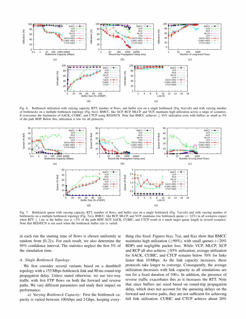
Fig. 6. Bottleneck utilization with varying capacity, RTT, number of flows, and buffer size on a single bottleneck (Fig. 6(a)-(d)) and with varying numberof bottlenecks on a multiple bottleneck topology (Fig. 6(e)). BMCC, like XCP, RCP, MLCP, and VCP, maintains high utilization across a range of scenarios.It overcomes the limitations of SACK, CUBIC, and CTCP using RED/ECN. Note that BMCC achieves ≥ 95% utilization even with buffers as small as 5%of the path BDP. Below this, utilization is low for all protocols.

0

10

20

30

40

50

1000010001001010.1

Que

ue (

% B

uf)

Bottleneck Capacity (Mbps)

BMCCXCPRCP

MLCPVCP

SACK+REDCUBIC+REDCTCP+RED

(a)

0

10

20

30

40

50

100001000100101

Que

ue (

% B

uf)

Round-trip Propagation Delay (ms)

BMCCXCPRCP

MLCPVCP

SACK+REDCUBIC+REDCTCP+RED

(b)

0

10

20

30

40

50

1000100101Q

ueue

(%

Buf

)Number of Long-lived Flows

BMCCXCPRCP

MLCPVCP

SACK+REDCUBIC+REDCTCP+RED

(c)

0

10

20

30

40

50

100806040200

Que

ue (

% B

uf)

Buffer Size (% of BDP)

BMCCXCPRCP

MLCPVCP

SACKCUBICCTCP

(d)

0

0.5

1

1.5

2

2.5

3

2 4 6 8 10 12 14 16 18

Que

ue (

% B

uf)

Link ID

BMCCXCPRCP

MLCPVCP

SACK+REDCUBIC+REDCTCP+RED

(e)

Fig. 7. Bottleneck queue with varying capacity, RTT, number of flows, and buffer size on a single bottleneck (Fig. 7(a)-(d)) and with varying number ofbottlenecks on a multiple bottleneck topology (Fig. 7(e)). BMCC, like RCP, MLCP, and VCP, maintains low bottleneck queue (< 10%) in all scenarios expectwhen RTT ≤ 1ms or the buffer size is <5% of the path BDP. XCP, SACK, CUBIC, and CTCP result in a much larger queue length in several scenarios.Note that RED/ECN is not used when the bottleneck buffer size is varied.

in each run the starting time of flows is chosen uniformly atrandom from [0, 2] s. For each result, we also determine the95% confidence interval. The statistics neglect the first 5% ofthe simulation time.

A. Single Bottleneck TopologyWe first consider several variants based on a dumbbell

topology with a 155 Mbps bottleneck link and 80 ms round-trippropagation delay. Unless stated otherwise, we use two-waytraffic with five FTP flows on both the forward and reversepaths. We vary different parameters and study their impact onperformance.

a) Varying Bottleneck Capacity: First the bottleneck ca-pacity is varied between 100 kbps and 2 Gbps, keeping every-

thing else fixed. Figures 6(a), 7(a), and 8(a) show that BMCCmaintains high utilization (≥90%), with small queues (<20%BDP) and negligible packet loss. While VCP, MLCP, XCPand RCP all also achieve ≥85% utilization, average utilizationfor SACK, CUBIC, and CTCP remains below 70% for linksfaster than 10 Mbps. As the link capacity increases, theseprotocols take longer to converge. Consequently, the averageutilization decreases with link capacity as all simulations arerun for a fixed duration of 100 s. In addition, the presence ofreverse traffic exacerbates this as it increases the RTT. Notethat since buffers are sized based on round-trip propagationdelay, which does not account for the queueing delays on theforward and reverse paths, they are not sufficient for achievingfull link utilization. CUBIC and CTCP achieve about 20%

0.0001

0.001

0.01

0.1

1

10

100

1000010001001010.1

Loss

Rat

e (%

)

Bottleneck Capacity (Mbps)

BMCCXCPRCP

MLCPVCP

SACK+REDCUBIC+REDCTCP+RED

(a)

0.0001

0.001

0.01

0.1

1

10

100

100001000100101

Loss

Rat

e (%

)

Round-trip Propagation Delay (ms)

BMCCXCPRCP

MLCPVCP

SACK+REDCUBIC+REDCTCP+RED

(b)

0.0001

0.001

0.01

0.1

1

10

100

1000100101

Loss

Rat

e (%

)

Number of Long-lived Flows

BMCCXCPRCP

MLCPVCP

SACK+REDCUBIC+REDCTCP+RED

(c)

0.0001

0.001

0.01

0.1

1

10

100

100806040200

Loss

Rat

e (%

)

Buffer Size (% of BDP)

BMCCXCPRCP

MLCPVCP

SACKCUBICCTCP

(d)

0.0001

0.001

0.01

0.1

1

10

100

2 4 6 8 10 12 14 16 18

Loss

Rat

e (%

)

Link ID

BMCCXCPRCP

MLCPVCP

SACK+REDCUBIC+REDCTCP+RED

(e)

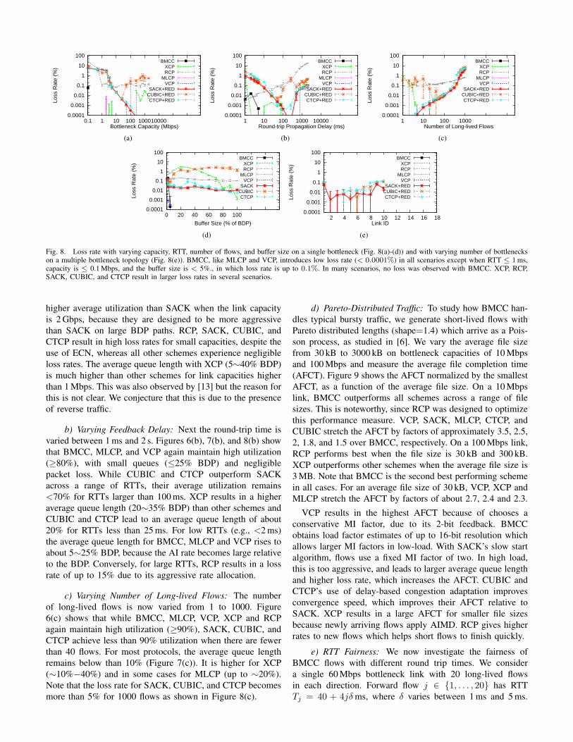
Fig. 8. Loss rate with varying capacity, RTT, number of flows, and buffer size on a single bottleneck (Fig. 8(a)-(d)) and with varying number of bottleneckson a multiple bottleneck topology (Fig. 8(e)). BMCC, like MLCP and VCP, introduces low loss rate (< 0.0001%) in all scenarios except when RTT ≤ 1ms,capacity is ≤ 0.1 Mbps, and the buffer size is < 5%., in which loss rate is up to 0.1%. In many scenarios, no loss was observed with BMCC. XCP, RCP,SACK, CUBIC, and CTCP result in larger loss rates in several scenarios.

higher average utilization than SACK when the link capacityis 2 Gbps, because they are designed to be more aggressivethan SACK on large BDP paths. RCP, SACK, CUBIC, andCTCP result in high loss rates for small capacities, despite theuse of ECN, whereas all other schemes experience negligibleloss rates. The average queue length with XCP (5∼40% BDP)is much higher than other schemes for link capacities higherthan 1 Mbps. This was also observed by [13] but the reason forthis is not clear. We conjecture that this is due to the presenceof reverse traffic.

b) Varying Feedback Delay: Next the round-trip time isvaried between 1 ms and 2 s. Figures 6(b), 7(b), and 8(b) showthat BMCC, MLCP, and VCP again maintain high utilization(≥80%), with small queues (≤25% BDP) and negligiblepacket loss. While CUBIC and CTCP outperform SACKacross a range of RTTs, their average utilization remains<70% for RTTs larger than 100 ms. XCP results in a higheraverage queue length (20∼35% BDP) than other schemes andCUBIC and CTCP lead to an average queue length of about20% for RTTs less than 25 ms. For low RTTs (e.g., <2 ms)the average queue length for BMCC, MLCP and VCP rises toabout 5∼25% BDP, because the AI rate becomes large relativeto the BDP. Conversely, for large RTTs, RCP results in a lossrate of up to 15% due to its aggressive rate allocation.

c) Varying Number of Long-lived Flows: The numberof long-lived flows is now varied from 1 to 1000. Figure6(c) shows that while BMCC, MLCP, VCP, XCP and RCPagain maintain high utilization (≥90%), SACK, CUBIC, andCTCP achieve less than 90% utilization when there are fewerthan 40 flows. For most protocols, the average queue lengthremains below than 10% (Figure 7(c)). It is higher for XCP(∼10%−40%) and in some cases for MLCP (up to ∼20%).Note that the loss rate for SACK, CUBIC, and CTCP becomesmore than 5% for 1000 flows as shown in Figure 8(c).

d) Pareto-Distributed Traffic: To study how BMCC han-dles typical bursty traffic, we generate short-lived flows withPareto distributed lengths (shape=1.4) which arrive as a Pois-son process, as studied in [6]. We vary the average file sizefrom 30 kB to 3000 kB on bottleneck capacities of 10 Mbpsand 100 Mbps and measure the average file completion time(AFCT). Figure 9 shows the AFCT normalized by the smallestAFCT, as a function of the average file size. On a 10 Mbpslink, BMCC outperforms all schemes across a range of filesizes. This is noteworthy, since RCP was designed to optimizethis performance measure. VCP, SACK, MLCP, CTCP, andCUBIC stretch the AFCT by factors of approximately 3.5, 2.5,2, 1.8, and 1.5 over BMCC, respectively. On a 100 Mbps link,RCP performs best when the file size is 30 kB and 300 kB.XCP outperforms other schemes when the average file size is3 MB. Note that BMCC is the second best performing schemein all cases. For an average file size of 30 kB, VCP, XCP andMLCP stretch the AFCT by factors of about 2.7, 2.4 and 2.3.

VCP results in the highest AFCT because of chooses aconservative MI factor, due to its 2-bit feedback. BMCCobtains load factor estimates of up to 16-bit resolution whichallows larger MI factors in low-load. With SACK’s slow startalgorithm, flows use a fixed MI factor of two. In high load,this is too aggressive, and leads to larger average queue lengthand higher loss rate, which increases the AFCT. CUBIC andCTCP’s use of delay-based congestion adaptation improvesconvergence speed, which improves their AFCT relative toSACK. XCP results in a large AFCT for smaller file sizesbecause newly arriving flows apply AIMD. RCP gives higherrates to new flows which helps short flows to finish quickly.

e) RTT Fairness: We now investigate the fairness ofBMCC flows with different round trip times. We considera single 60 Mbps bottleneck link with 20 long-lived flowsin each direction. Forward flow j ∈ {1, . . . , 20} has RTTTj = 40 + 4jδms, where δ varies between 1 ms and 5 ms.

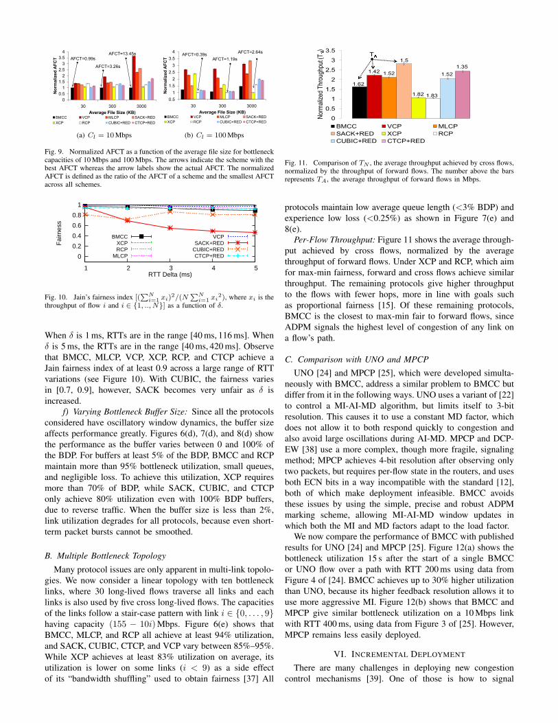
(a) Cl = 10Mbps (b) Cl = 100Mbps

Fig. 9. Normalized AFCT as a function of the average file size for bottleneckcapacities of 10 Mbps and 100 Mbps. The arrows indicate the scheme with thebest AFCT whereas the arrow labels show the actual AFCT. The normalizedAFCT is defined as the ratio of the AFCT of a scheme and the smallest AFCTacross all schemes.

0

0.2

0.4

0.6

0.8

1

1 2 3 4 5

Fai

rnes

s

RTT Delta (ms)

BMCCXCPRCP

MLCP

VCPSACK+RED

CUBIC+REDCTCP+RED

Fig. 10. Jain’s fairness index [(∑N

i=1 xi)2/(N

∑Ni=1 xi

2), where xi is thethroughput of flow i and i ∈ {1, .., N}] as a function of δ.

When δ is 1 ms, RTTs are in the range [40 ms, 116 ms]. Whenδ is 5 ms, the RTTs are in the range [40 ms, 420 ms]. Observethat BMCC, MLCP, VCP, XCP, RCP, and CTCP achieve aJain fairness index of at least 0.9 across a large range of RTTvariations (see Figure 10). With CUBIC, the fairness variesin [0.7, 0.9], however, SACK becomes very unfair as δ isincreased.

f) Varying Bottleneck Buffer Size: Since all the protocolsconsidered have oscillatory window dynamics, the buffer sizeaffects performance greatly. Figures 6(d), 7(d), and 8(d) showthe performance as the buffer varies between 0 and 100% ofthe BDP. For buffers at least 5% of the BDP, BMCC and RCPmaintain more than 95% bottleneck utilization, small queues,and negligible loss. To achieve this utilization, XCP requiresmore than 70% of BDP, while SACK, CUBIC, and CTCPonly achieve 80% utilization even with 100% BDP buffers,due to reverse traffic. When the buffer size is less than 2%,link utilization degrades for all protocols, because even short-term packet bursts cannot be smoothed.

B. Multiple Bottleneck Topology

Many protocol issues are only apparent in multi-link topolo-gies. We now consider a linear topology with ten bottlenecklinks, where 30 long-lived flows traverse all links and eachlinks is also used by five cross long-lived flows. The capacitiesof the links follow a stair-case pattern with link i ∈ {0, . . . , 9}having capacity (155 − 10i)Mbps. Figure 6(e) shows thatBMCC, MLCP, and RCP all achieve at least 94% utilization,and SACK, CUBIC, CTCP, and VCP vary between 85%–95%.While XCP achieves at least 83% utilization on average, itsutilization is lower on some links (i < 9) as a side effectof its “bandwidth shuffling” used to obtain fairness [37] All

Fig. 11. Comparison of TN , the average throughput achieved by cross flows,normalized by the throughput of forward flows. The number above the barsrepresents TA, the average throughput of forward flows in Mbps.

protocols maintain low average queue length (<3% BDP) andexperience low loss (<0.25%) as shown in Figure 7(e) and8(e).

Per-Flow Throughput: Figure 11 shows the average through-put achieved by cross flows, normalized by the averagethroughput of forward flows. Under XCP and RCP, which aimfor max-min fairness, forward and cross flows achieve similarthroughput. The remaining protocols give higher throughputto the flows with fewer hops, more in line with goals suchas proportional fairness [15]. Of these remaining protocols,BMCC is the closest to max-min fair to forward flows, sinceADPM signals the highest level of congestion of any link ona flow’s path.

C. Comparison with UNO and MPCPUNO [24] and MPCP [25], which were developed simulta-

neously with BMCC, address a similar problem to BMCC butdiffer from it in the following ways. UNO uses a variant of [22]to control a MI-AI-MD algorithm, but limits itself to 3-bitresolution. This causes it to use a constant MD factor, whichdoes not allow it to both respond quickly to congestion andalso avoid large oscillations during AI-MD. MPCP and DCP-EW [38] use a more complex, though more fragile, signalingmethod; MPCP achieves 4-bit resolution after observing onlytwo packets, but requires per-flow state in the routers, and usesboth ECN bits in a way incompatible with the standard [12],both of which make deployment infeasible. BMCC avoidsthese issues by using the simple, precise and robust ADPMmarking scheme, allowing MI-AI-MD window updates inwhich both the MI and MD factors adapt to the load factor.

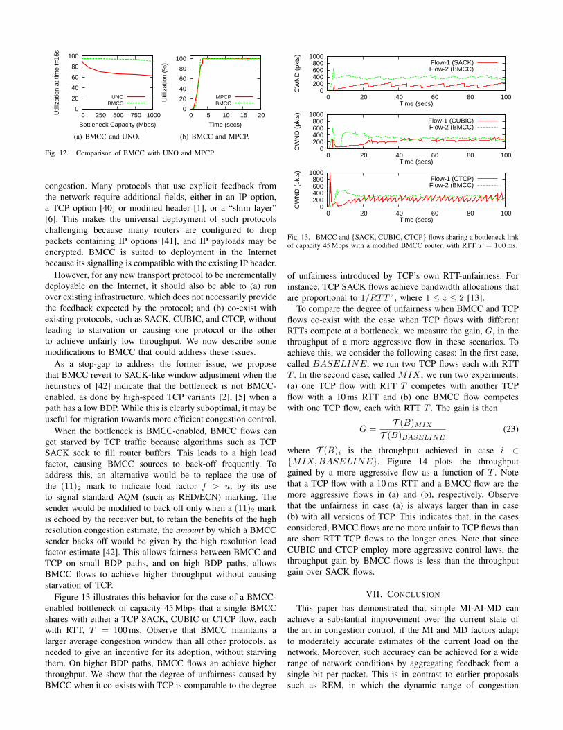
We now compare the performance of BMCC with publishedresults for UNO [24] and MPCP [25]. Figure 12(a) shows thebottleneck utilization 15 s after the start of a single BMCCor UNO flow over a path with RTT 200 ms using data fromFigure 4 of [24]. BMCC achieves up to 30% higher utilizationthan UNO, because its higher feedback resolution allows it touse more aggressive MI. Figure 12(b) shows that BMCC andMPCP give similar bottleneck utilization on a 10 Mbps linkwith RTT 400 ms, using data from Figure 3 of [25]. However,MPCP remains less easily deployed.

VI. INCREMENTAL DEPLOYMENT

There are many challenges in deploying new congestioncontrol mechanisms [39]. One of those is how to signal

0

20

40

60

80

100

0 250 500 750 1000Util

izat

ion

at ti

me

t=15

s

Bottleneck Capacity (Mbps)

UNOBMCC

(a) BMCC and UNO.

0

20

40

60

80

100

0 5 10 15 20

Util

izat

ion

(%)

Time (secs)

MPCPBMCC

(b) BMCC and MPCP.

Fig. 12. Comparison of BMCC with UNO and MPCP.

congestion. Many protocols that use explicit feedback fromthe network require additional fields, either in an IP option,a TCP option [40] or modified header [1], or a “shim layer”[6]. This makes the universal deployment of such protocolschallenging because many routers are configured to droppackets containing IP options [41], and IP payloads may beencrypted. BMCC is suited to deployment in the Internetbecause its signalling is compatible with the existing IP header.

However, for any new transport protocol to be incrementallydeployable on the Internet, it should also be able to (a) runover existing infrastructure, which does not necessarily providethe feedback expected by the protocol; and (b) co-exist withexisting protocols, such as SACK, CUBIC, and CTCP, withoutleading to starvation or causing one protocol or the otherto achieve unfairly low throughput. We now describe somemodifications to BMCC that could address these issues.

As a stop-gap to address the former issue, we proposethat BMCC revert to SACK-like window adjustment when theheuristics of [42] indicate that the bottleneck is not BMCC-enabled, as done by high-speed TCP variants [2], [5] when apath has a low BDP. While this is clearly suboptimal, it may beuseful for migration towards more efficient congestion control.

When the bottleneck is BMCC-enabled, BMCC flows canget starved by TCP traffic because algorithms such as TCPSACK seek to fill router buffers. This leads to a high loadfactor, causing BMCC sources to back-off frequently. Toaddress this, an alternative would be to replace the use ofthe (11)2 mark to indicate load factor f > u, by its useto signal standard AQM (such as RED/ECN) marking. Thesender would be modified to back off only when a (11)2 markis echoed by the receiver but, to retain the benefits of the highresolution congestion estimate, the amount by which a BMCCsender backs off would be given by the high resolution loadfactor estimate [42]. This allows fairness between BMCC andTCP on small BDP paths, and on high BDP paths, allowsBMCC flows to achieve higher throughput without causingstarvation of TCP.

Figure 13 illustrates this behavior for the case of a BMCC-enabled bottleneck of capacity 45 Mbps that a single BMCCshares with either a TCP SACK, CUBIC or CTCP flow, eachwith RTT, T = 100 ms. Observe that BMCC maintains alarger average congestion window than all other protocols, asneeded to give an incentive for its adoption, without starvingthem. On higher BDP paths, BMCC flows an achieve higherthroughput. We show that the degree of unfairness caused byBMCC when it co-exists with TCP is comparable to the degree

0 200 400 600 800

1000

0 20 40 60 80 100

CW

ND

(pk

ts)

Time (secs)

Flow-1 (SACK)Flow-2 (BMCC)

0 200 400 600 800

1000

0 20 40 60 80 100

CW

ND

(pk

ts)

Time (secs)

Flow-1 (CUBIC)Flow-2 (BMCC)

0 200 400 600 800

1000

0 20 40 60 80 100

CW

ND

(pk

ts)

Time (secs)

Flow-1 (CTCP)Flow-2 (BMCC)

Fig. 13. BMCC and {SACK, CUBIC, CTCP} flows sharing a bottleneck linkof capacity 45 Mbps with a modified BMCC router, with RTT T = 100ms.

of unfairness introduced by TCP’s own RTT-unfairness. Forinstance, TCP SACK flows achieve bandwidth allocations thatare proportional to 1/RTT z , where 1 ≤ z ≤ 2 [13].

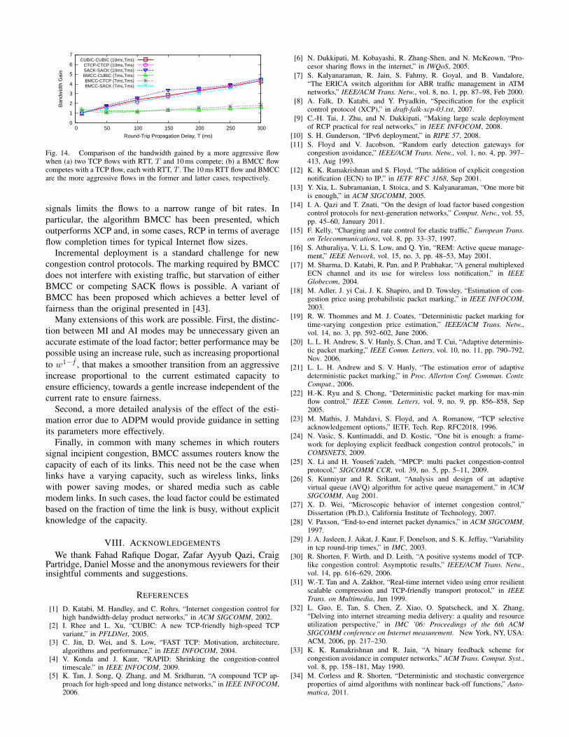
To compare the degree of unfairness when BMCC and TCPflows co-exist with the case when TCP flows with differentRTTs compete at a bottleneck, we measure the gain, G, in thethroughput of a more aggressive flow in these scenarios. Toachieve this, we consider the following cases: In the first case,called BASELINE, we run two TCP flows each with RTTT . In the second case, called MIX , we run two experiments:(a) one TCP flow with RTT T competes with another TCPflow with a 10 ms RTT and (b) one BMCC flow competeswith one TCP flow, each with RTT T . The gain is then

G =T (B)MIX

T (B)BASELINE(23)

where T (B)i is the throughput achieved in case i ∈{MIX,BASELINE}. Figure 14 plots the throughputgained by a more aggressive flow as a function of T . Notethat a TCP flow with a 10 ms RTT and a BMCC flow are themore aggressive flows in (a) and (b), respectively. Observethat the unfairness in case (a) is always larger than in case(b) with all versions of TCP. This indicates that, in the casesconsidered, BMCC flows are no more unfair to TCP flows thanare short RTT TCP flows to the longer ones. Note that sinceCUBIC and CTCP employ more aggressive control laws, thethroughput gain by BMCC flows is less than the throughputgain over SACK flows.

VII. CONCLUSION

This paper has demonstrated that simple MI-AI-MD canachieve a substantial improvement over the current state ofthe art in congestion control, if the MI and MD factors adaptto moderately accurate estimates of the current load on thenetwork. Moreover, such accuracy can be achieved for a widerange of network conditions by aggregating feedback from asingle bit per packet. This is in contrast to earlier proposalssuch as REM, in which the dynamic range of congestion

0

1

2

3

4

5

6

7

0 50 100 150 200 250 300

Ban

dwid

th G

ain

Round-Trip Propagation Delay, T (ms)

CUBIC-CUBIC (10ms,Tms)CTCP-CTCP (10ms,Tms)SACK-SACK (10ms,Tms)BMCC-CUBIC (Tms,Tms)BMCC-CTCP (Tms,Tms)BMCC-SACK (Tms,Tms)

Fig. 14. Comparison of the bandwidth gained by a more aggressive flowwhen (a) two TCP flows with RTT, T and 10 ms compete; (b) a BMCC flowcompetes with a TCP flow, each with RTT, T . The 10 ms RTT flow and BMCCare the more aggressive flows in the former and latter cases, respectively.

signals limits the flows to a narrow range of bit rates. Inparticular, the algorithm BMCC has been presented, whichoutperforms XCP and, in some cases, RCP in terms of averageflow completion times for typical Internet flow sizes.

Incremental deployment is a standard challenge for newcongestion control protocols. The marking required by BMCCdoes not interfere with existing traffic, but starvation of eitherBMCC or competing SACK flows is possible. A variant ofBMCC has been proposed which achieves a better level offairness than the original presented in [43].

Many extensions of this work are possible. First, the distinc-tion between MI and AI modes may be unnecessary given anaccurate estimate of the load factor; better performance may bepossible using an increase rule, such as increasing proportionalto w1−f̂ , that makes a smoother transition from an aggressiveincrease proportional to the current estimated capacity toensure efficiency, towards a gentle increase independent of thecurrent rate to ensure fairness.

Second, a more detailed analysis of the effect of the esti-mation error due to ADPM would provide guidance in settingits parameters more effectively.

Finally, in common with many schemes in which routerssignal incipient congestion, BMCC assumes routers know thecapacity of each of its links. This need not be the case whenlinks have a varying capacity, such as wireless links, linkswith power saving modes, or shared media such as cablemodem links. In such cases, the load factor could be estimatedbased on the fraction of time the link is busy, without explicitknowledge of the capacity.

VIII. ACKNOWLEDGEMENTS

We thank Fahad Rafique Dogar, Zafar Ayyub Qazi, CraigPartridge, Daniel Mosse and the anonymous reviewers for theirinsightful comments and suggestions.

REFERENCES

[1] D. Katabi, M. Handley, and C. Rohrs, “Internet congestion control forhigh bandwidth-delay product networks,” in ACM SIGCOMM, 2002.

[2] I. Rhee and L. Xu, “CUBIC: A new TCP-friendly high-speed TCPvariant,” in PFLDNet, 2005.

[3] C. Jin, D. Wei, and S. Low, “FAST TCP: Motivation, architecture,algorithms and performance,” in IEEE INFOCOM, 2004.

[4] V. Konda and J. Kaur, “RAPID: Shrinking the congestion-controltimescale.” in IEEE INFOCOM, 2009.

[5] K. Tan, J. Song, Q. Zhang, and M. Sridharan, “A compound TCP ap-proach for high-speed and long distance networks,” in IEEE INFOCOM,2006.

[6] N. Dukkipati, M. Kobayashi, R. Zhang-Shen, and N. McKeown, “Pro-cesor sharing flows in the internet,” in IWQoS, 2005.

[7] S. Kalyanaraman, R. Jain, S. Fahmy, R. Goyal, and B. Vandalore,“The ERICA switch algorithm for ABR traffic management in ATMnetworks,” IEEE/ACM Trans. Netw., vol. 8, no. 1, pp. 87–98, Feb 2000.

[8] A. Falk, D. Katabi, and Y. Pryadkin, “Specification for the explicitcontrol protocol (XCP),” in draft-falk-xcp-03.txt, 2007.

[9] C.-H. Tai, J. Zhu, and N. Dukkipati, “Making large scale deploymentof RCP practical for real networks,” in IEEE INFOCOM, 2008.

[10] S. H. Gunderson, “IPv6 deployment,” in RIPE 57, 2008.[11] S. Floyd and V. Jacobson, “Random early detection gateways for

congestion avoidance,” IEEE/ACM Trans. Netw., vol. 1, no. 4, pp. 397–413, Aug 1993.

[12] K. K. Ramakrishnan and S. Floyd, “The addition of explicit congestionnotification (ECN) to IP,” in IETF RFC 3168, Sep 2001.

[13] Y. Xia, L. Subramanian, I. Stoica, and S. Kalyanaraman, “One more bitis enough,” in ACM SIGCOMM, 2005.

[14] I. A. Qazi and T. Znati, “On the design of load factor based congestioncontrol protocols for next-generation networks,” Comput. Netw., vol. 55,pp. 45–60, January 2011.

[15] F. Kelly, “Charging and rate control for elastic traffic,” European Trans.on Telecommunications, vol. 8, pp. 33–37, 1997.

[16] S. Athuraliya, V. Li, S. Low, and Q. Yin, “REM: Active queue manage-ment,” IEEE Network, vol. 15, no. 3, pp. 48–53, May 2001.

[17] M. Sharma, D. Katabi, R. Pan, and P. Prabhakar, “A general multiplexedECN channel and its use for wireless loss notification,” in IEEEGlobecom, 2004.

[18] M. Adler, J. yi Cai, J. K. Shapiro, and D. Towsley, “Estimation of con-gestion price using probabilistic packet marking,” in IEEE INFOCOM,2003.

[19] R. W. Thommes and M. J. Coates, “Deterministic packet marking fortime-varying congestion price estimation,” IEEE/ACM Trans. Netw.,vol. 14, no. 3, pp. 592–602, June 2006.

[20] L. L. H. Andrew, S. V. Hanly, S. Chan, and T. Cui, “Adaptive determinis-tic packet marking,” IEEE Comm. Letters, vol. 10, no. 11, pp. 790–792,Nov. 2006.

[21] L. L. H. Andrew and S. V. Hanly, “The estimation error of adaptivedeterministic packet marking,” in Proc. Allerton Conf. Commun. Contr.Comput., 2006.

[22] H.-K. Ryu and S. Chong, “Deterministic packet marking for max-minflow control,” IEEE Comm. Letters, vol. 9, no. 9, pp. 856–858, Sep2005.

[23] M. Mathis, J. Mahdavi, S. Floyd, and A. Romanow, “TCP selectiveacknowledgement options,” IETF, Tech. Rep. RFC2018, 1996.

[24] N. Vasic, S. Kuntimaddi, and D. Kostic, “One bit is enough: a frame-work for deploying explicit feedback congestion control protocols,” inCOMSNETS, 2009.

[25] X. Li and H. Yousefi’zadeh, “MPCP: multi packet congestion-controlprotocol,” SIGCOMM CCR, vol. 39, no. 5, pp. 5–11, 2009.

[26] S. Kunniyur and R. Srikant, “Analysis and design of an adaptivevirtual queue (AVQ) algorithm for active queue management,” in ACMSIGCOMM, Aug 2001.

[27] X. D. Wei, “Microscopic behavior of internet congestion control,”Dissertation (Ph.D.), California Institute of Technology, 2007.

[28] V. Paxson, “End-to-end internet packet dynamics,” in ACM SIGCOMM,1997.

[29] J. A. Jasleen, J. Aikat, J. Kaur, F. Donelson, and S. K. Jeffay, “Variabilityin tcp round-trip times,” in IMC, 2003.

[30] R. Shorten, F. Wirth, and D. Leith, “A positive systems model of TCP-like congestion control: Asymptotic results,” IEEE/ACM Trans. Netw.,vol. 14, pp. 616–629, 2006.

[31] W.-T. Tan and A. Zakhor, “Real-time internet video using error resilientscalable compression and TCP-friendly transport protocol,” in IEEETrans. on Multimedia, Jun 1999.

[32] L. Guo, E. Tan, S. Chen, Z. Xiao, O. Spatscheck, and X. Zhang,“Delving into internet streaming media delivery: a quality and resourceutilization perspective,” in IMC ’06: Proceedings of the 6th ACMSIGCOMM conference on Internet measurement. New York, NY, USA:ACM, 2006, pp. 217–230.

[33] K. K. Ramakrishnan and R. Jain, “A binary feedback scheme forcongestion avoidance in computer networks,” ACM Trans. Comput. Syst.,vol. 8, pp. 158–181, May 1990.

[34] M. Corless and R. Shorten, “Deterministic and stochastic convergenceproperties of aimd algorithms with nonlinear back-off functions,” Auto-matica, 2011.

[35] F. Baccelli, S. Machiraju, D. Veitch, and J. Bolot, “The role of pastain network measurement,” IEEE/ACM Trans. Netw., vol. 17, no. 4, pp.1340–1353, Aug. 2009.

[36] S. Ha and I. Rhee, “Hybrid slow start for high-bandwidth and long-distance networks,” in PFLDnet, 2008.

[37] S. H. Low, L. L. H. Andrew, and B. P. Wydrowski, “UnderstandingXCP: Equilibrium and fairness,” in IEEE INFOCOM, 2005.

[38] X. Li and H. Yousefi’zadeh, “DCP-EW: Distributed congestion-controlprotocol for encrypted wireless networks,” in IEEE WCNC, 2010.

[39] D. Papadimitriou, M. Welzl, M. Scharf, and B. Briscoe, “Open researchissues in internet congestion control,” in RFC 6077, Feb 2011.

[40] M. Suchara, L. L. H. Andrew, R. Witt, K. Jacobsson, B. P. Wydrowski,and S. H. Low, “Implementation of provably stable maxnet,” in Proc.Broadnets, 2008.

[41] R. Fonseca, G. M. Porter, R. H. Katz, S. Shenker, and I. Stoica, “IPoptions are not an option,” UC Berkeley, Tech. Rep., December 2005.

[42] I. A. Qazi, L. L. H. Andrew, and T. Znati, “Incremental deployment ofnew ECN-compatible congestion control,” in PFLDNeT, 2009.

[43] ——, “Congestion control using efficient explicit feedback,” in IEEEINFOCOM, 2009.

APPENDIX

Lemma 1: For any 0 ≤ a ≤ b ≤ 1, any integer N , realnumber d and collection of real numbers yn,

ad ≥ 1

N

N∑n=1

ayn implies bd ≥ 1

N

N∑n=1

byn .

Proof: Since ax is convex in x, for all k ≥ 1 and all x,we have ax/k + a0(k − 1)/k ≥ ax/k, whence

1

k

N∑n=1

(ayn(i)−d − 1) ≥N∑

n=1

(a(yn(i)−d)/k − 1).

Substituting k = log(a)/ log(b) ≥ 1 gives thatN∑

n=1

(ayn(i)−d−1) ≤ 0 impliesN∑

n=1

(byn(i)−d−1) ≤ 0

from which the result follows.

Ihsan Ayyub Qazi received the BSc. (Hons) degreein Computer Science and Mathematics from the La-hore University of Management Sciences (LUMS),Pakistan, in 2005 and the Ph.D. degree in ComputerScience from the University of Pittsburgh, PA, USAin August 2010.

He is an Assistant Professor in the Department ofComputer Science at the LUMS School of Scienceand Engineering, Lahore, Pakistan. From 2010 to2011, he was a Postdoctoral Research Fellow at theCentre for Advanced Internet Architectures, Swin-

burne University of Technology, Australia. He is the recipient of the AndrewMellon Fellowship and the Best Graduate Student Research Award fromthe University of Pittsburgh in 2009. His current research interests includefuture Internet design, green networking, wireless networks, and performancemodeling of networked systems. He is a member of the ACM.

Lachlan L. H. Andrew (M’97-SM’05) received theB.Sc., B.E. and Ph.D. degrees in 1992, 1993, and1997, from the University of Melbourne, Australia.Since 2008, he has been an associate professor atSwinburne University of Technology, Australia, andsince 2010 he has been an ARC Future Fellow.From 2005 to 2008, he was a senior research en-gineer in the Department of Computer Science atCaltech. Prior to that, he was a senior researchfellow at the University of Melbourne and a lecturerat RMIT, Australia. His research interests include

energy-efficient networking and performance analysis of resource allocationalgorithms. He was co-recipient of the best paper award at IEEE INFOCOM2011 and IEEE MASS 2007. He is a member of the ACM.

Taieb Znati received the M.S degree from PurdueUniversity, West Lafayette, Indiana and the Ph.D.degree in Computer Science from Michigan StateUniversity, East Lansing in 1988.

He is a Professor in the Department of Com-puter Science at the University of Pittsburgh witha joint appointment in Telecommunications in theDepartment of Information Science. He has servedas general chair for several networking conferencesincluding INFOCOM 2005 and SECON 2004. He isa member of the steering committee of ACM SenSys

and has served on the editorial board of several journals including IEEETransactions of Parallel and Distributed Systems, Journal of Adhoc Networks,and Journal on Wireless Systems and Mobile Computing. His current researchinterests include routing and congestion in high speed networks, QoS in wiredand wireless networks, data dissemination in wireless sensor networks, andperformance analysis of network protocols.