conical indentation ehhhhhhhhhhii 26 oct smhhhhhhhhhhh ... · ~before report documentation page f...
TRANSCRIPT
D-A127 529 PRANALYSIS OF CONICAL INDENTATION OF AN 1/2ESTIC/PERFECTLY PLASTIC HALF-S..(U) UENNSYLYANIA
STATE UNIV UNIVERSITY PARK APPLIED RESEARCH LAB.
UNCLASSIFIED T KATO 26 OCT 82 ARL/PSU/TM-82-230 F/G 28/1 Li
EhhhhhhhhhhiIsmhhhhhhhhhhhsmhhhhhhhhhhhEhhhhhhhhhhhhIsmhhhhohhhhhhsmhhhhhhhohhh
N
L 13 '.i
1.0 ..
111 ii 11 6
111.25 141111A 1.
MICROCOPY RESOLUTION TEST CHARTNATIONAL BUREAU OF STANDARDS-1963-A
I
UV,4.
.
7'dp
AN ANALYSIS OF CONICAL INDENTATION OF AN ELASTIC!
PERFECTLY PLASTIC HALF-SPACE BY NONLINEAR FINITE
ELEMENT TECHNIQUES
Takehiko Kato
Technical Memorandum
File No. TM 82-230
October 26, 1982
Contract No. N00024-79-C-6043
Copy No.
The Pennsylvania State University
Intercollege Research Programs and Facilities
APPLIED RESEARCH LABORATORY
Post Office Box 30
State College, Pa. 16801
IL. APPV, . !C .TLEISECIDiSTFi UTiM U03IT8D3
NAVY DEPARTMENT
NAVAL SEA SYSTEMS CO%1A\ND ,
33 05 02 076

UNCLASSIFIEDSECURITY CLASSIFICATION OF THIS PAGE (When Data Entered)
REPORT DOCUMENTATION PAGE f READ INSTRUCTIONS~BEFORE COMPLETING FORM
I. REPORT NUMBER Iz. GOVT ACCESSION NO. 3. vCIPIENT'S CATALOG NUMBER
4. TITLE (and Subtitle) . T F. O REP PERIOD COVERED
AN ANALYSIS OF CONICAL INDENTATION OF AN O
ELASTIC/PERFECTLY PLASTIC HALF-SPACE BY M.S. Thesis, November 1982NONLINEAR FINITE ELEMENT TECHNIQUES 6. PERFORMING ORG. REPORT NUMBER
82-2307. AUTHOR(s) 8. CONTRACT OR GRANT NUMBER(s)
Takehiko Kato N00024-79-C-6043
9. PERFORMING ORGANIZATION NAME AND ADDRESS 10. PROGRAM ELEMENT. PROJECT. TASK
AREA & WORK UNIT NUMBERS
The Pennsylvania State UniversityApplied Research Laboratory, P.O. Box 30State College, PA 16801
11. CONTROLLING OFFICE NAME AND ADDRESS 12. REPORT DATE
Naval Sea Systems Command October 26, 1982Department of the Navy 13. NUMBER OF PAGES
Washington, DC 20362 119 pages14. MONITORING AGENCY NAME & ADDRESS(I1 different from Controlling Office) 15. SECURITY CLASS. (of this report)
UNCLASSIFIED, UNLIMITED
ISa. DECLASSIFICATIONDOWNGRADINGSCH EDULE
16. DISTRIBUTION STATEMENT (of this Report)
Approved for public release, dis :ibution unlimited,per NSSC (Naval Sea Systems Command), December 17, 1982
17. DISTRIBUTION STATEMENT (of the abstract entered In Block 20, if different from Report)
IS. SUPPLEMENTARY NOTES
19. KEY WORDS (Continue on reverse side if necessary and identify by block number)
indentation, elastic, finite, element
20. ABSTRACT (Continue on reverse side if necessary and identify by block number)
A detailed analysis of the deformation and stress fields produced in anelastic/perfectly plastic half-space by a rigid conical indenter was performedusing the elastic/plastic finite element code BOPACE-3D. The analysis considers:
O ,, the elastic deformation and stress fields with finite element results beingcompared to the closed-form solutions obtained by Sneddon, the elastic/plasticdeformation and stress fields, and the residual deformation and stress fieldswhich have not been analyzed to date. A special loading technique was devel-oped to find the residual solutions.
DD 'JAN R 1473 EDITION OF I NOV GS IS OBSOLETE UNCLASSIFIEDSECURITY CLASSIFICATION OF THIS PAGE (When Data Entererl

* .i -. . ** *
UNCLASSIFIED
SECURITY CLASSIFICATION OF THIS PAOE(Whn Data intefnd)
The included angle of the rigid conical indenter was set to c= 1360
to simulate a Vickers pyramidal indenter. Idealized soda-line glass waschosen as an elastic/perfectly plastic brittle material.
Stresses obtained during the loading-unloading cycle near the elastic/plastic boundary were transformed to the principal stresses and the residual
-" principal stresses to allow analysis of median, radial and lateral crackinitiation and propagation.
La
UNCLASSIFIED
SECURITY CLASSIFICATION OF THIS PAOE(W"hn Data Enlercd)

~iii
ABSTRACT
i.- A detailed analysis of the deformation and stress fields produced
in an elastic/perfectly plastic half-space by a rigid conical indenter
was performed using the elastic/plastic finite element code BOPACE-3D.
The analysis considers: the elastic deformation and stress fields
with finite element results being compared to the closed-form solutions
obtained by Sneddon, the elastic/plastic deformation and stress fields,
and the residual deformation and stress fields which have not been
analyzed to date. A special loading technique was developed to find
the residual solutions.
The included angle of the rigid conical indenter was set to
- 3641to simulate a Vickers pyramidal indenter. Idealized soda-
line glass was chosen as an elastic/perfectly plastic brittle material.
Stresses obtained during the loading-unloading cycle near the
elastic/plastic boundary were transformed to the principal stresses and
the residual principal stresses to allow analysis of median, radial
and lateral crack initiation and propagation.:/ Accesslon For
NTIS GRA&IDTIC TABUnannounced C]Justificatlon
ByDistribution/Availability Codes
4 •Avail and/orDist Special
;: . '.1..-m- - -"" " " " ' -' ' " ' m ii "m r -' i I i ~ A ' ' '
iv
TABLE OF CONTENTS
Page
ABSTRACT ........... .......................... iii
LIST OF TABLES ........ ....................... .... vi
LIST OF FIGURES ......... ...................... .. vii
LIST OF SYMBOLS .......... ...................... x
ACKNOWLEDGEMENTS ......... ...................... ... xv
Chapter
I. INTRODUCTION ..... ................. .i...11.1 General Introduction .. .. ............ 11.2 Purpose of the Investigation .............. 21.3 Scope of the Investigation .. .. ......... 2
II. ELASTIC/PLASTIC FINITE ELE21ENT METHOD ... ....... 42.1 General Concepts ....... ............... 4
2.1.1 Stress-Strain Equations .... ........ 42.1.2 Incremental Stiffness Method .. ..... 82.1.3 Other Stiffness Methods .......... ... 11
2.2 BOPACE - 3D ...... ................ ... 142.3 Verification of Nonlinear Finite Element
Code .......... ............... .... 152.3.1 Comparison to Yamada's Analysis. 152.3.2 Comparison to Marcal and King's
Analysis ............... 16
III. SOLUTION TECHNIQUES AND THE INDENTATION MODEL. . 283.1 Method of Approach ....... .............. 283.2 Finite Element Model and Grids .......... ... 293.3 Material Used in this Investigation .. ..... 34
IV. ELASTIC AND ELASTIC/PLASTIC CONICAL INDENTATION. 364.1 Introduction.................36
- 4.2 Method of Analysis .......... ...... 374.3 Results and Discussion ............... ... 39
4.3.1 Elastic Conical Indentation ......... 444.3.2 Elastic/Plastic Conical Indentation. 47
* V. RESIDUAL SOLUTIONS FOR ELASTIC/PLASTIC CONICALINDENTATION ....... .................... ... 525.1 Introduction ..... ................. .... 525.2 Method of Analysis ..... .............. ... 525.3 Results and Discussion ..... ............ ... 53
w "
~v
TABLE OF CONTENTS (Continued)
Page
VI. ANALYSIS OF FRACTURE MECHANISMS INDUCED BYINDENTATION ....... .................... . 626.1 Introduction ...... ................. ... 626.2 Failure Modes beneath the Indenter ... ...... 62
6.2.1 Crack Systems near the Surface ........ 646.2.2 Subsurface Crack Systems ........ 64
6.3 Fracture Initiation and Propagation ... ...... 656.3.1 Identification of the Tensile Peak
Stresses ................. 656.3.2 Critical Flaw Size .............. .... 666.3.3 Fracture Initiation and Propagation
Zones ...... ................. ... 69
VII. CONCLUSIONS AND RECOMMENDATIONS ... .......... ... 747.1 Conclusions ...... .................. ... 747.2 Recommendations ..... ................ ... 76
APPENDIX A: THE ELASTIC STRESS FIELDS FOR POINT, SPHERICAL ANDCONICAL INDENTATION ..... ............... ... 78
APPENDIX B: THE ANALYTICAL-EXPERIMENTAL EQUATIONS FOR ELASTIC/PLASTIC INDENTATION ..... ............... ... 97
BIBLIOGRAPHY ........................ 99
".
Io

LIST OF TABLES
Page
1. Tensile Peak Stresses and the Corresponding CrackSystem .......... ......................... ... 67
2. Threshold Flaw Sizes for the Initiation of Each CrackSystem ......... ......................... .... 70
3. Relationship between a, 6, and b.... .............. 95
an b9
4.
vii
LIST OF FIGURES
Page
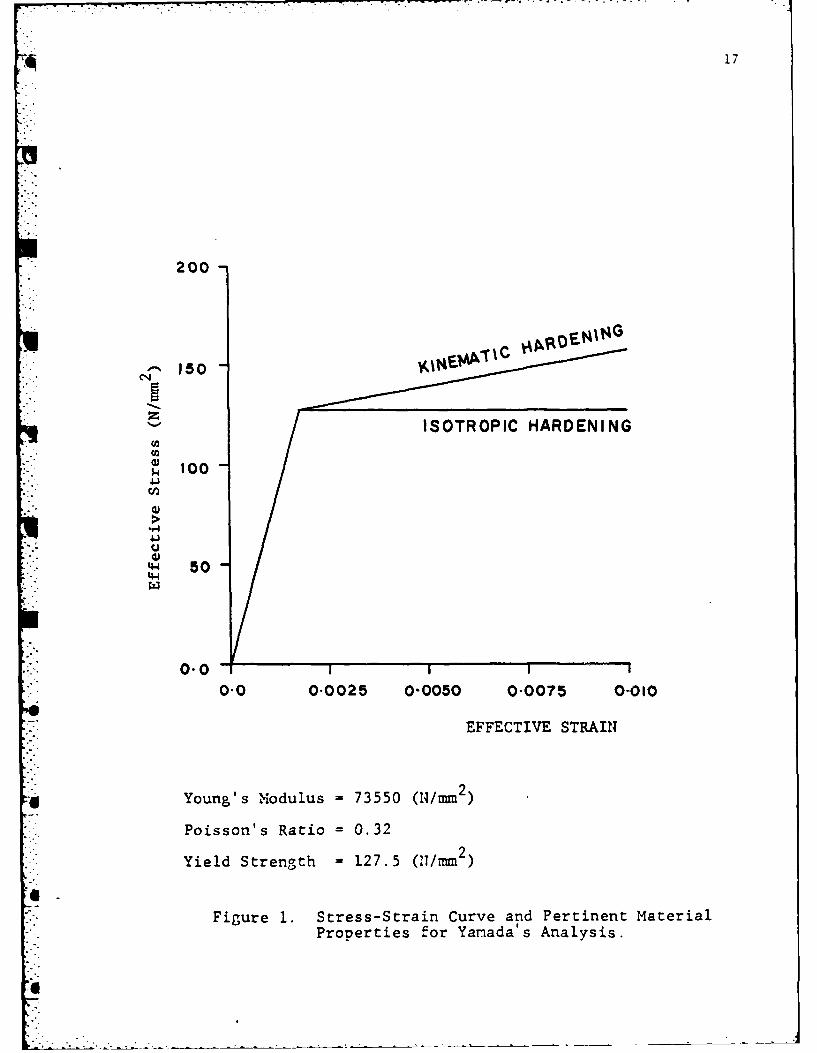
1. Stress-Strain Curve and Pertinent MaterialProperties for Yamada's Analysis .... ............. ... 17
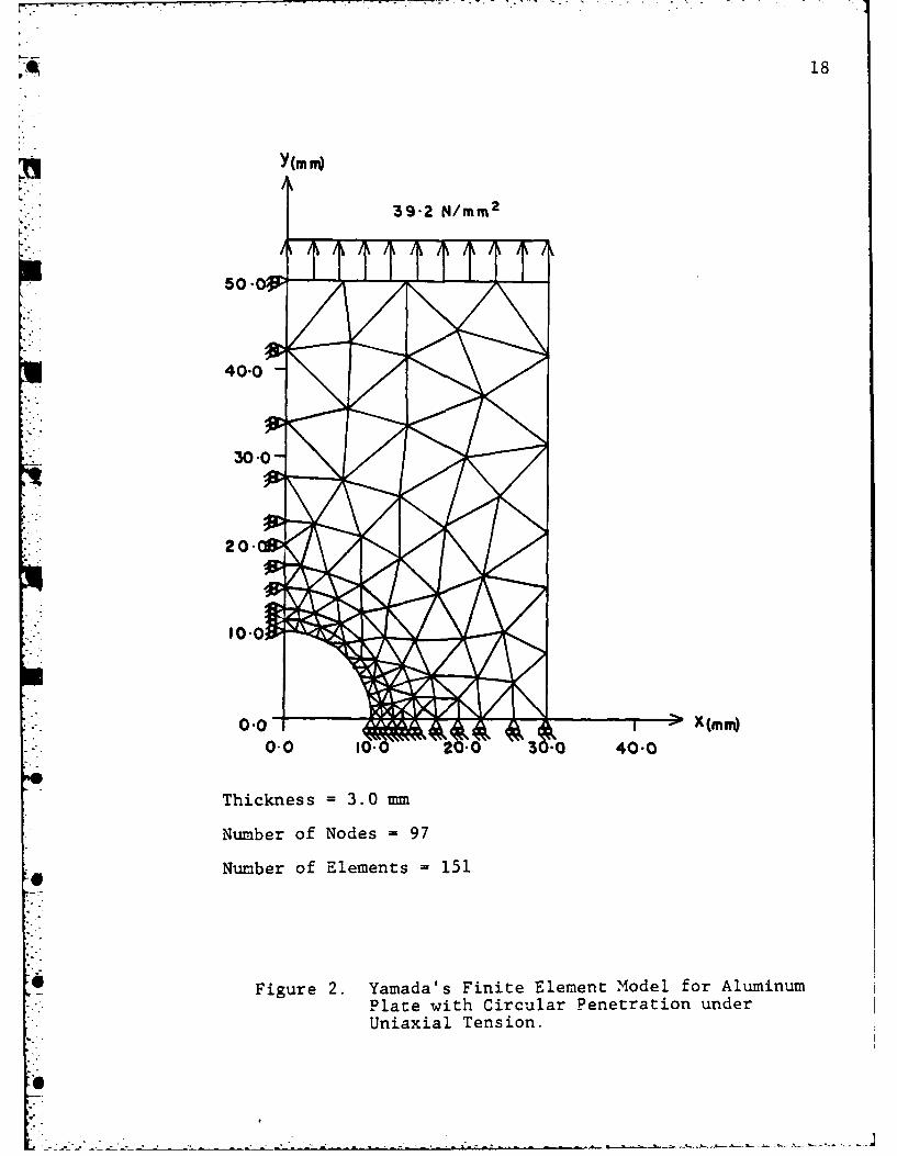
2. Yamada's Finite Element Model for Aluminum Plate
with Circular Penetration under Uniaxial Tension ........ 18
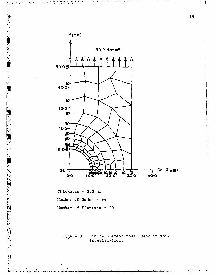
3. Finite Element Model Used in this Investigation ....... 19
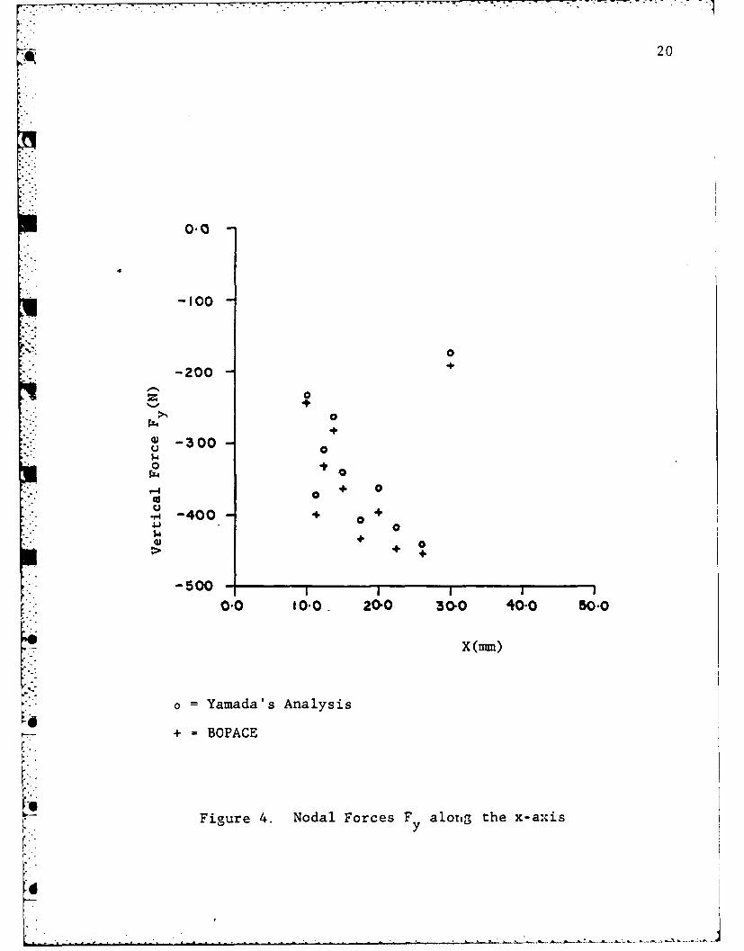
4. Nodal Forces F along the x-axis .... ............ ... 20y
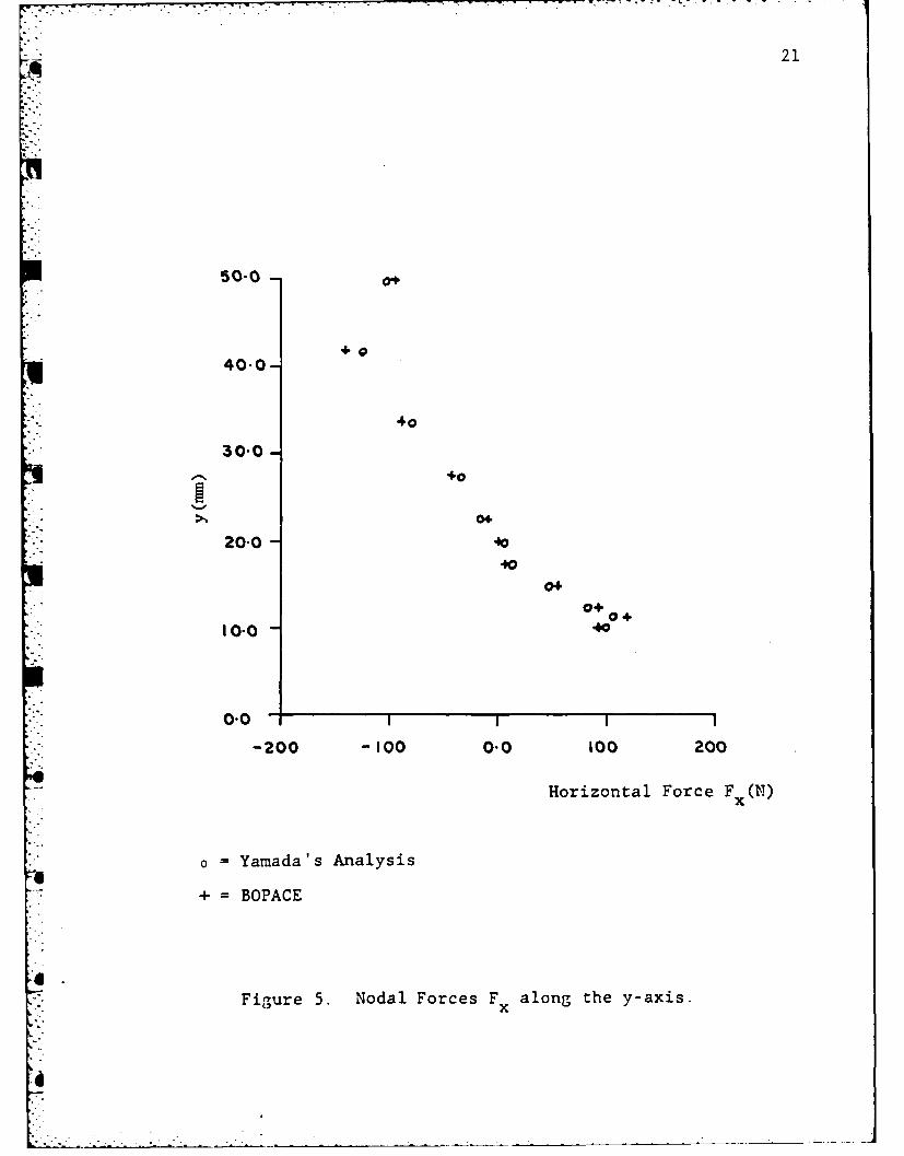
5. Nodal Forces F along the y-axis .... ............ ... 21x
6. Nodal Displacement Ux along the x-axis ............. .. 22
7. Nodal Displacement U along the y-axis ............. .. 23
y8. Improved Model Used in the Investigation of Plastic
Regions .......... ......................... ... 25
9. Character and Extent of Plastic Regions Obtained inthis Investigation for Selected Load Factors ... ....... 26
10. Character and Extent of Plastic Regions Obtained inMarcal and King's Analysis for Selected Load Factors. . . 27
11. Axisymmetric Finite Element Model for IndentationAnalysis ......... .......... ...... 30
12. Axisymmetric Finite Element Sub-Grids for IndentationAnalysis (Insert A of Figure 11) ........... .. 31
13. Axisymmetric Finite Element Sub-Grids for IndentationAnalysis (Insert B of Figure 12) ... ............. .... 32
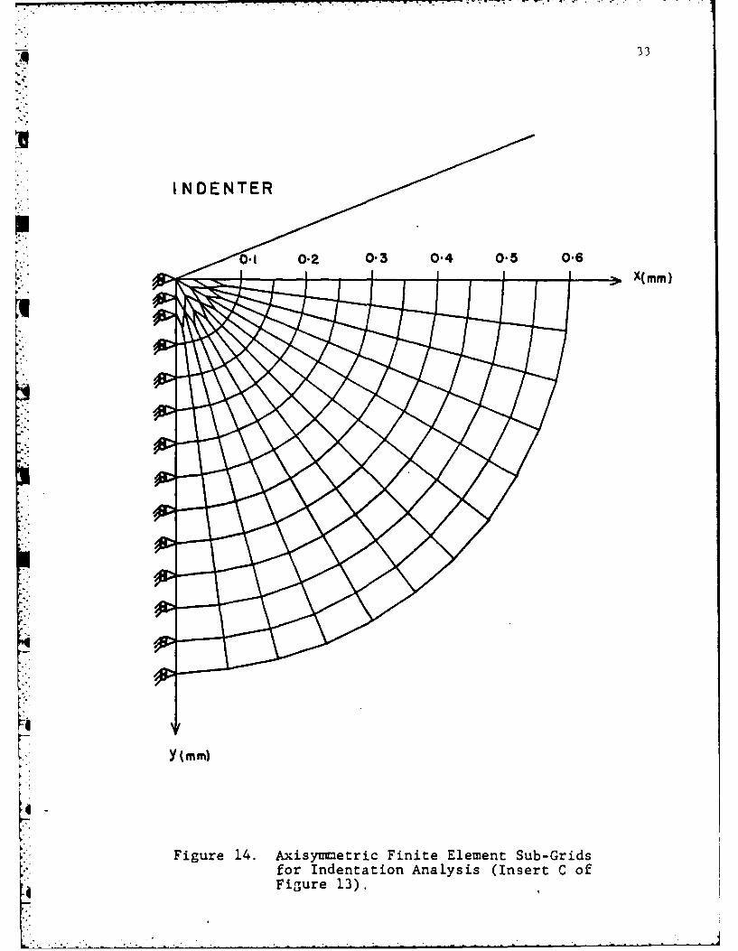
14. Axisymmetric Finite Element Sub-Grids for IndentationAnalysis (Insert C of Figure 13) ...... ............. 33
15. Stress-Strain Curve and Pertinent Material Properties ofIdealized Soda-Lime Glass for Indentation Analysis. . . . 35
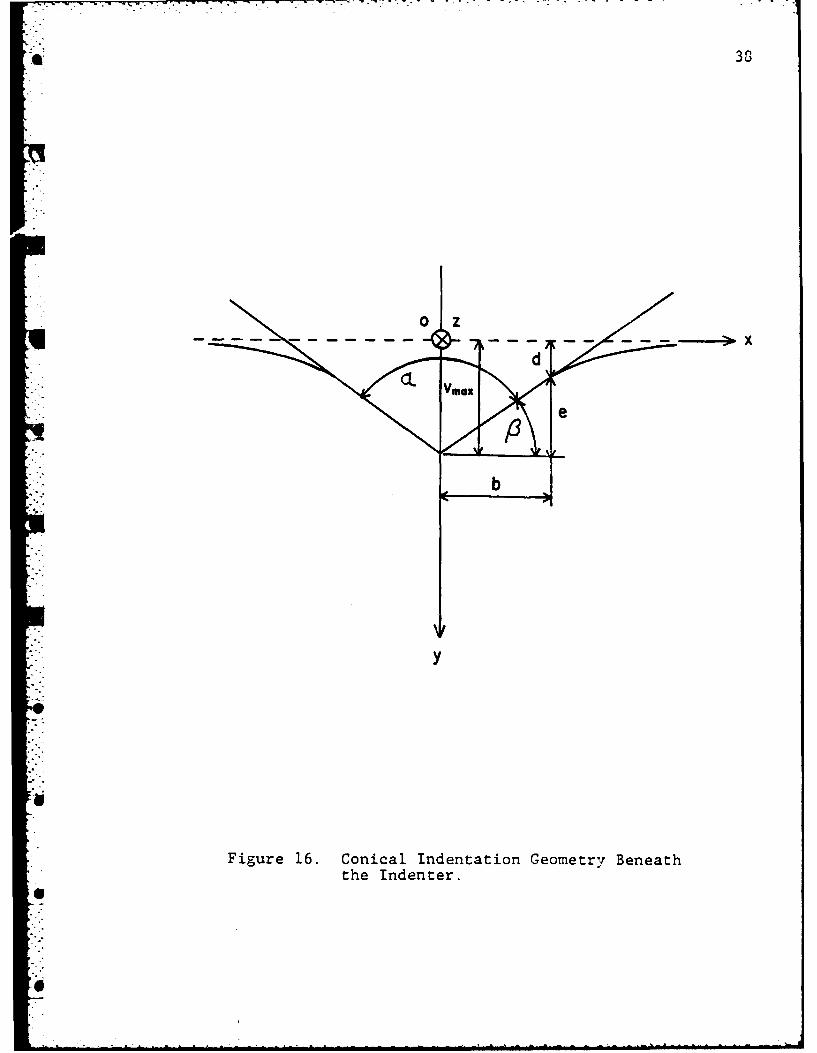
16. Conical Indentation Geometry Beneath the Indenter . . . . 36
4.
4°
b~7.
viii
LIST OF FIGURES (Continued)
Page
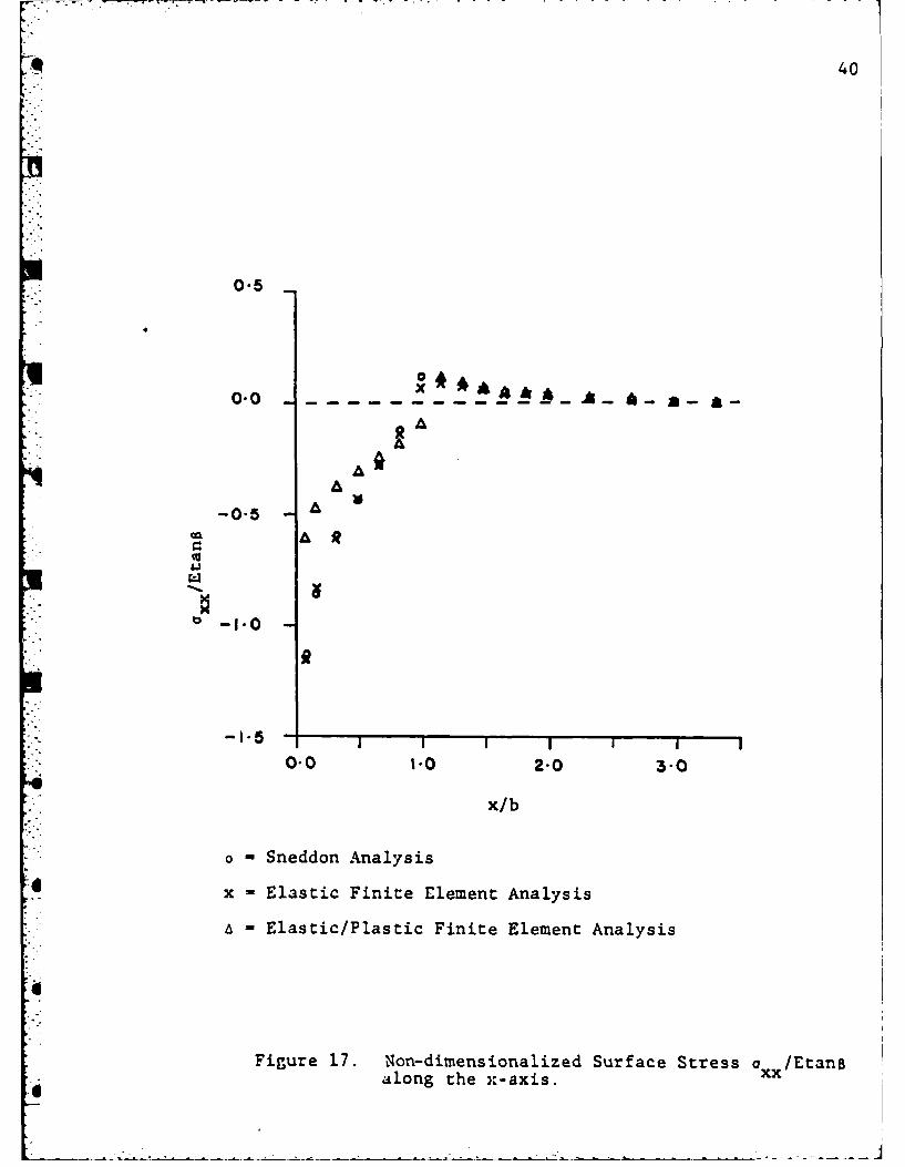
17. Non-dimensionalized Surface Stress a /Etanaalong the x-axis, ....... .................... .... 40
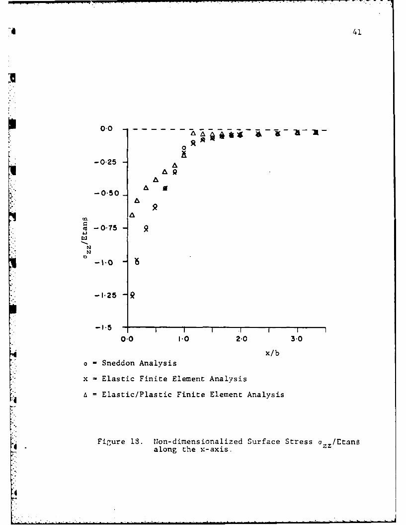
18. Non-dimensionalized Surface Stress a /EtanSzz
along the x-axis .................... ........ .. 41
19. Non-dimensionalized Subsurface Stress xx/Etandand a zz/Etan8 along the y-axis ... ............. .... 42
20. Non-dimensionalized Subsurface Stress a /Etanaalong the y-axis ........ .. .................... 43
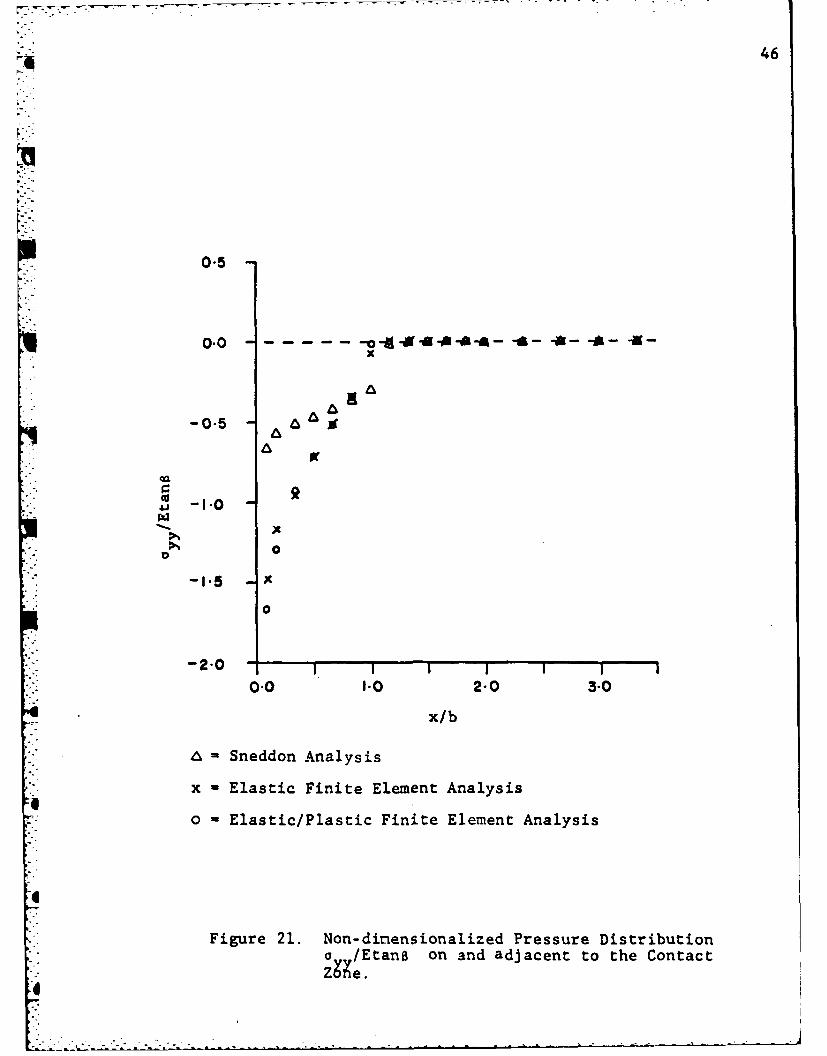
21. Non-dimensionalized Pressure Distribution a /Etan6 onyyand adjacent to the Contact Zone .... ............ ... 46
22. Elastic/Plastic Mesh Deformation .... ............ ... 48
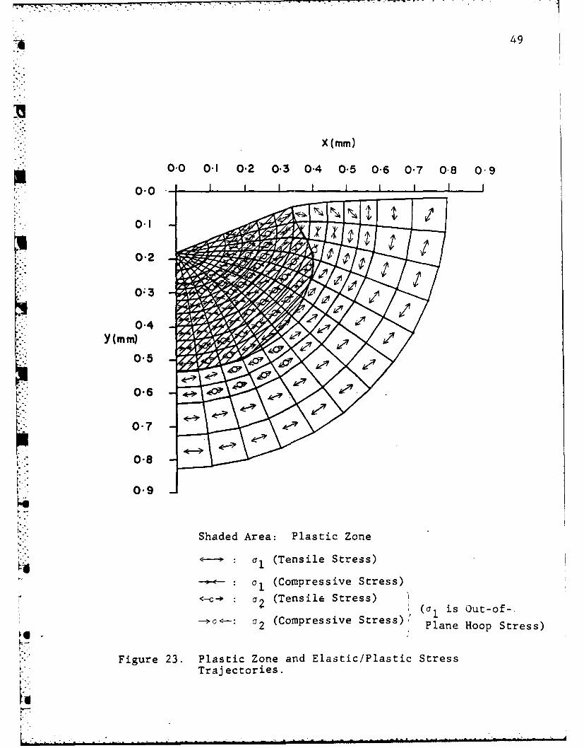
23. Plastic Zone and Elastic/Plastic Stress Trajectories . 49
24. Comparison of Nodal Forces Resulting from Indentationand Equivalent Nodal Loads .... ............... .... 54
25. Geometrical Comparison of Indentation Profile and
Residual Crater ....... ..................... .... 55
26. Elastic/Plastic Residual Mesh Deformation ........ 57
27. Non-dimensionalized Residual Surface Stresses along thex-axis ......... ......................... .... 58
28. Non-dimensionalized Residual Subsurface Stressesalong the y-axis ....... .................... .. 59
29. Plastic Zone and Residual Stress Trajectories ... ...... 61
30. Schematic Diagram of Indentation Cracks ........... .... 63
31. Crack Initiation and Propagation Zones in the LoadingPhase ....... ..... .......................... 72
32. Crack Initiation and Propagation Zones during theUnloading Phase ........ .................... .... 73
33. Point Indentation Geometry .... ............... .... 79
34. Spherical Indentation Geometry beneath the Indenter. . . 81
................ . *
ixI:I
LIST OF FIGURES (Continued)
Pase
35. Conical Indentation Geometry beneath the Indenter . . . 83
36. Comparison of Elastic Point, Spherical and ConicalStress Fields (I): Non-dimensionalized Stress G .. 87
xx
37. Comparison of Elastic Point, Spherical and ConicalIndentation Stress Fields (II): Non-dimensionalizedStress, a ........... ...................... 88
YY
38. Comparison of Elastic Point, Spherical and ConicalIndentation Stress Fields (III): Non-dimensionalizedStress, a ....... ..................... ... 89
zz
39. Comparison of Elastic Point, Spherical and ConicalIndentation Stress Fields (IV): Non-dimensionalizedStress, a ................... 90
40. Included Angle Effect of Conical Indentation (I):Non-dimensionalized Stress, a ...... ............ 91xx
41. Included Angle Effect of Conical Indentation (II):Non-dimensionalized Stress, a ................... ... 92yy
42. Included Angle Effect of Conical Indentation (III):Non-dimensionalized Stress, a .. ........... ..... 93
43. Included Angle Effect of Conical Indentation (IV):Non-dimensionalized Stress, a ............ 94
xy
x
LIST OF SYIBOLS
D diameter of spherical indenter
E Young's Modulus
F applied load
F x, F nodal forces
F Sneddon's elastic applied load for conicalindentation
F ,Fp load resultants generated from summation offthe vertical nodal forces on the contact surface
for the case of elastic and elastic/plastic finiteelement analysis
G shear modulus
H indentation hardness
H' strain hardening rate
Ko Sneddon's stress parameters for elastic conicaln indentation
Q Sneddon's geometric parameter for elastic conical
indentation
R Hertzian geometric parameter (= )2+z2
S plastic hardening parameter
U,Uy nodal displacementsx y
Y yield strength
a contact-surface radius for spherical indentation
4 b contact-surface radius for conical indentation
c plastic zone size
c critical flaw size
d,e Sneddon's geometric parameters for elastic conicalindentation
rq Xi
LIST OF SYMBOLS (Continued)
f maximum depth of Hertzian spherical indentation
h Hertzian geometrical parameter for elastic spherical
indentation
P(P) surface pressure distribution fo- elastic conicalindentation
P mean pressure for spherical indentation
P mean pressure for conical indentationm
P' mean pressure for point indentation
r radial distance from origin (-(x 2+y 2+z ))
t Sneddon's geometric parameter for elastic conical
indentation
u,v horizontal and vertical displacements
v residual vertical displacement
w Hertzian geometric parameter for elastic spherical
indentation
x,y,z Cartesian coordinates
a' included angle of rigid conical indenter
excluded angle of rigid conical indenter (= 1
Ye elastic geometric parameter for conical indentation
Y H geometric parameter of plastic hysterisis for conicalindentation
r crack surface energy
Eeffective (equivalent) strain
dEi. strain incrementsV 1.dE!. deviatoric strain increments
xii
LIST OF SYMBOLS (Continued)
dE j plastic strain increments
d p equivalent plastic strain increments
6 ij Kronecker's delta function
Sneddon's geometric parameters
angles in spherical coordinate system
Lame's constants
- dX Prandtl-Reuss scalar factor of proportionality
v Poisson's ratio
l, 29,ao3 principal stresses (a1>a a 3)
axa y,a Zx stresses for Cartesian coordinates
o rr' aee0 , T rO stresses for spherical coordinates
Ra residual stress
a equivalent stress
a 'deviatoric stress
do stress incrementsii
do equivalent stress increments
".do'
do' deviatoric stress increments
[B] displacement-strain matrix
[D] stress-strain matrix
[D e elastic stress-strain matrix
II
Ixiii
LIST OF SYMBOLS (Continued)
[Dp] plastic stress-strain matrix
[DT] material tangential modulus matrix
( l strain matrix
{eo} prestrain matrix
{E} nodal strain matrix
n
{de} incremental strain matrix
{dE p } incremental plastic strain matrix
[K] overall stiffness matrix
[k] stiffness matrix
[ke] elastic stiffness matrix[kp] plastic stiffness matrix
[ki] stiffness matrix after ith increment
[kT] tangential stiffness matrix
-I Q} force matrix after i th increment
{Q I initial load matrix0
{Q} e,n,X equivalent nodal load matrix correspondingto {Eo }
0
IQ} en, equivalent nodal load matrix correspondingto (a }
0
{Q}n nodal force matrix
"dQ.} incremental force matrix after ith increment
{dQ}n incremental nodal force matrix
r I thq} displacement matrix after i increment
4
xiv
LIST OF SYMBOLS (Continued)
{qo} initial displacement matrix
{q}n nodal displacement matrix
{dqi} incremental displacement matrix after ith- • increment
{dq}n incremental nodal displacement matrix
(a} stress matrix
{ao} initial stress matrix0
{da} incremental stress matrix
I
a
6l

.. "
ACKNOWLEDGMENTS
The author is indebted to Dr. Joseph C. Conway, Professor
of Engineering Mechanics, and Dr. Robert N. Pangborn, Assistant
Professor of Engineering Mechanics, for their assistance and
encouragement in the research and preparation of this thesis.
Appreciation is also extended toward Dr. R. G. Vos, Boeing Aero-
space Company Missiles and Space Group, and Dr. Richard A. Queeney,
Professor of Engineering Mechanics, for their helpful advice.
The author would also like to thank the people in the Applied
Research Laboratory for their support of the research along with those
who have critiqued this thesis under the contract with the Office of
Naval Research, Research Initiation, Fund No. 7074.
.
CHAPTER I
INTRODUCTION
1.1 Generai Introduction
Elastic contact problems and elastic indentation problems
involving the normal application of a load against an elastic half-
space by a rigid body have been of considerable interest in various
fields of applied mechanics. The point indentation problem was
solved in closed-form by Boussinesq [1] and Michell [2]. The closed-
form solution for spherical indentation was developed by Hertz [3]
and Huber [4]. The conical indentation problem was solved in closed-
form by Sneddon [5,6].
As the theory of plasticity has advanced, elastic/plastic
contact-indentation problems have been approached analytically [7,8,9],
experimentally [10,11] and numerically [12,13,14,15]. To the author's
knowledge, the problem of normal loading of an elastic/perfectly
plastic half-space by a rigid conical indenter has not been analyzed,
despite the fact that aspects of this problem are of great interest
in many fields, including indentation fracture mechanics. An analytical
solution to this problem would be extremely difficult to develop but
the use of the high-speed computer combined with the proper finite
element code have made its solution possible. In this investigation a
finite element code which incorporates the pure tangential stiffness
incremental method was applied to obtain a solution to the problem of
elastic/plastic conical indentation.
6.
.................................
2
1.2 Purpose of the Investigation
The purpose of this investigation was to perform fundamental
research on elastic/plastic conical indentation problems associated
with the machining of brittle materials. It is anticipated that the
design, fabrication .and maintenance capabilities for brittle structures
can be improved when the basic understanding of fundamental failure
mechanisms associated with resultant generated elastic/plastic stress
fields and residual stress fields is increased. The resultant
axisynmetric elastic/plastic stress fields associated with both
loading and unloading can then be related to median, radial and
lateral cracking. In order to obtain this solution, it was necessary
to apply axisymmetric elastic/plastic analysis and cyclic loading
in the finite element program.
1.3 Scope of the Investigation
This investigation consists of four primary sections. The first
section considers the development of a finite element model for the
conical indentation problem and the verification of the model by
comparing numerically generated results with the closed-form results
for an elastic half-space derived by the well-known Sneddon solution.
Secondly, an elastic/plastic conical indentation analysis is performed
using the finite element model with plastic analysis capability to
generate the elastic/plastic stress and strain fields and to determine
the extent of plastic deformation near the indentation site. Thirdly,
a loading-unloading cycle is simulated in order to obtain the residual
S

stress fields associated with elastic/plastic indentation. Finally,
the results in terms of generated stress fields are related to the
initiation and propagation of median, radial and lateral cracks
beneath the indenter.
,. o4
0-
a
a

CHAPTER II
ELASTIC/PLASTIC FINITE ELE4ENT METHOD
2.1 General Concepts
This section discusses the general concepts utilized in the
solution of elastic/plastic problems by finite element techniques.
This approach is based on a plastic stress-strain matrix derived
from the Prandtl-Reuss equations, and on incremental or iterative
stiffness methods.
2.1.1 Stress-Strain Equations
It has been well established that the plastic constitutive
equation can be expressed in incremental form. In this investigation,
the selected incremental plasticity relations conform to the Prandtl-
Reuss flow rule, which is the usual flow rule associated with the
well-known Huber-Mises yield surface criterion [7,16,17]. The
Prandtl-Reuss flow rule uses the strain increment deij, which is
related to the stress increment doi4. The incremental stress-
strain relations with the differential form of the Iluber-Mises
yield surface criterion can be represented in matrix form as:
{do} - [DP]{dc} , (I)
where {do} and {de} are defined as the -:olumn matrices of
do and delj, respectively; and (Dp ] is the plastic stress-strain
matrix. Equation (1) can be expressed as:

a5
6 ao.do Z - dc. (i = 1,2,3,4,5,6), (2)
"-" j=l ae J
where the coefficients 3o./D. are the partial stiffness components:1 J
[28]. Hooke's law for isotropic elastic materials can be expressed in
matrix form as:
{o} = [De]{,} , (3)
where the elastic stress-strain matrix [De ] is given as:
i-V V V 0 0 01-2 l-2v l-2v
v 1-v V1-2v 1-2v 1-2v 0 0 0
v v 1-vl-2v 1-2v 1-2v 0 0 0
[De , 2Go o A ~(4)1
0 0 0 0 0
o o o2
o o 0 0 0 2
For the elastic/plastic finite element method, the plastic stress-
strain matrix [Dp] for yielded elements takes the place of the elastic
stress-strain matrix [Del.
The Prandtl-Reuss stress-strain relations for the deviatoric
strain increment de' during continued loading are:ij
S.dc' a' dX + (5)ij ij 2G
6-.
A 6
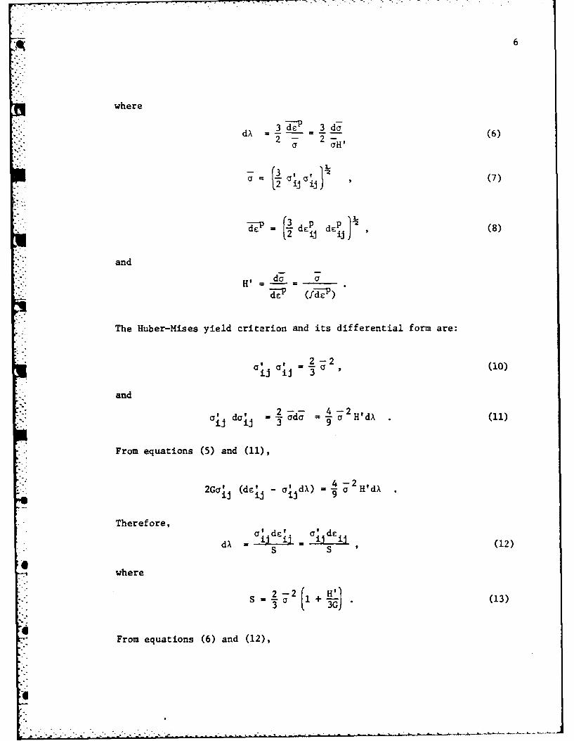
where
dX 3d(TE 3 da(62- 2-
a aH'
a 2 j ~j~3 (7)
=j. dep. dJY.J (8)
and
H' dTE P (fd )
The Huber-Mises yield criterion and its differential form are:
aj 2j .;2, (10)
and
ajj daj .a 4-2 H'dA (1
From equations (5) and (11),
2G~ d' ajdI a H'dX
Therefore,a' dF-'j cy' d
ciA j ~ 1 i(12)S S
0 where
S CY(1 +(13)
From equations (6) and (12),

7
de dc..k, kd k: (4doi S 2GdE = 2Gdci - ij.- .(1 4 ")
The total stress increment do is:
Sdo do' + E dEii
= 2G de i + 1-2v 6iideii ij (15)
Equation (15) can be represented in matrix form as:
(d l = [DPI (dcl , (16)
where
[DP ] 2G-
i-v -__ _-Z1-2v S 1-2v S
SYM.,-'O a' a't a'SmV xx yy V yy zz
1-2v S 1-2v S
V a- at - a Ti a 2x zz _ _zz 1- zz
12--2v S S l-2v S
a t at at T1 T2_ _ - zz X 1
.. xy S yz S S
a t''; a t O1
T T T 2" ''a'rr2xx __Y T zz _ j yz Y- -yz S zx ST yz S 2 s
a' a' y' T T 2T - T zz xv zx vz zx 1 zx
S zx S zx S zx S S 2 S
(17):4It is obvious that equation (16) is similar in form to equation (3) and
that the necessary modifcation from elastic to elastic/plastic behavior
a
8
would be to replace [De] by [Dp] for yielded elements as successive
yielding takes place. This procedure was developed by Marcal and
King [18] and Yamada, Yoshimara and Sakurai [19,201.
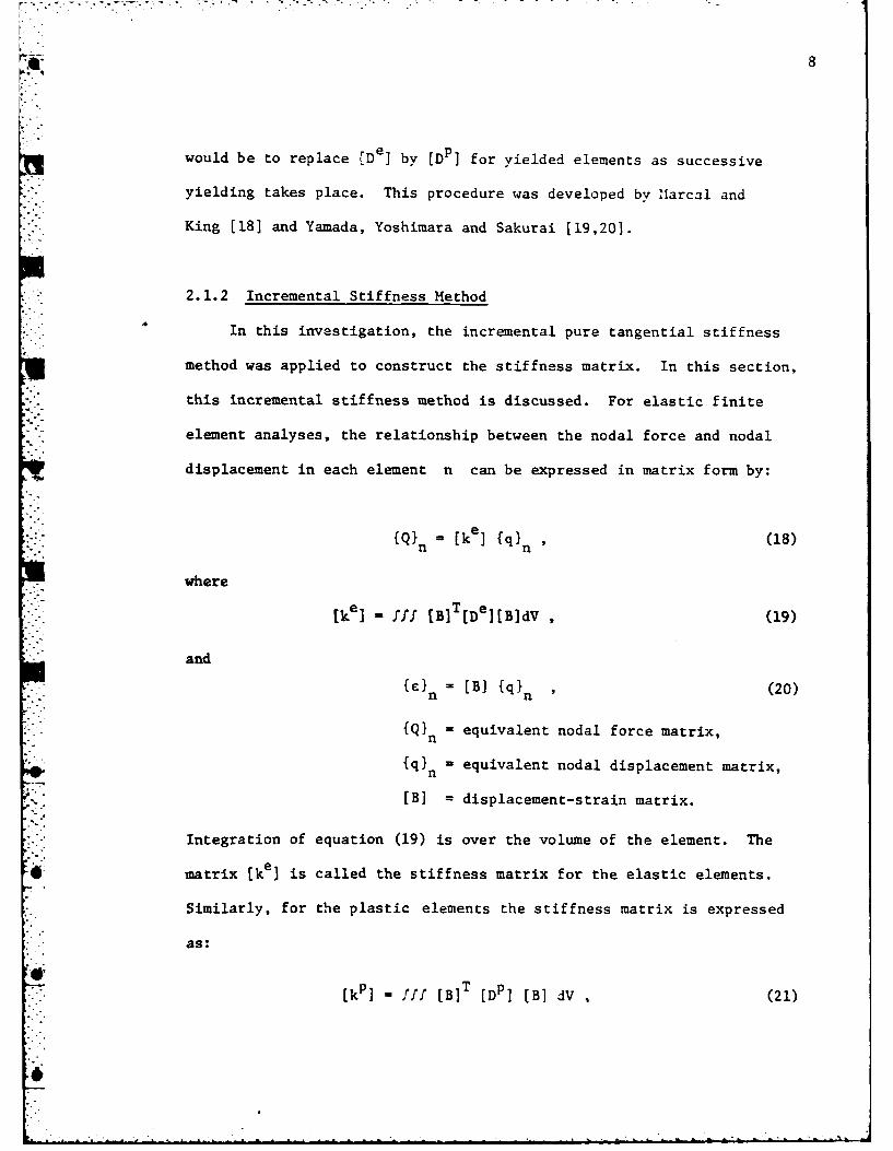
2.1.2 Incremental Stiffness Method
In this investigation, the incremental pure tangential stiffness
method was applied to construct the stiffness matrix. In this section,
this incremental stiffness method is discussed. For elastic finite
element analyses, the relationship between the nodal force and nodal
displacement in each element n can be expressed in matrix form by:
( = [ke] {q} ' (18)
where
[ke = ff [B]T[De [B]dV (19)
and
.E} = [B] {q}n ' (20)n .n
{Q}n = equivalent nodal force matrix,n
{q} = equivalent nodal displacement matrix,
[B] = displacement-strain matrix.
Integration of equation (19) is over the volume of the element. The
* matrix [ke] is called the stiffness matrix for the elastic elements.
Similarly, for the plastic elements the stiffness matrix is expressed
as:
T[kp] = Al [B] [DP] [B] dV , (21)
i,

9
and
{dQ}n [kP]{dq} " (22)n L n
The overall stiffness matrix [ki, which is an assemblage of the stiffness
U matrices [keI and [k], relates the nodal load increment (dQ} to the
nodal displacement increment {dq} as:
{dQ} = [k] {dq} . (23)
In order to solve the incremental equation (22) for an elastic-
plastic problem, the load-deflection relation is first expressed by:
{Q}n [k]{qnnn
=IV (B]T [D] (B] dV {qn
T(B] {cT}dV (24)
*i Using variational techniques,
T{dQ} = f [B] (da} dV
n V
V= (V [B T [DT] {de}dV
= V [B]T [DT] [B] dV {dq}
= [kT ] {dq} , (25)
where [DT] and [T] are called the material tangential modulus matrix,
"- and the structural tangent stiffness matrix, respectively. It is

10
obvious that
[De] = [DT
[ke, [k]
for the elastic element and
[Dp] [DT],
[kp] - [kT]
for the plastic element.
The matrix [Dp] is updated for each increment of load with
computation of the plastic strain increment {dc p} at the yielded
elements. The tangent stiffness matrix [k] is computed at the end
of each increment and used for each succeeding increment according
to the following equations:
{Q} = {QoI + E (dQ.I , (26)10 j=l
i
{q {q} + E {dq.} , (27)j =l
and
[ki_] (dqi} = {dQi} , (28)
after the ith increment where {Qo} and (qo} are the initial loads
and displacements, usually null vectors. The above procedure is
called the "incremental tangent stiffness method."
L' .

2.1.3 Other Stiffness Methods
For elastic/plastic finite element analyses, there are three
major stiffness methods in addition to the incremental stiffness
method, the iterative method, the initial strain method and the initial
stress method. The iterative method [21,22] is used for elastic/plastic
behavior when the deformation theory of plasticity is employed. Suppose
the nonlinear nodal force and nodal displacement relation is expressed
as:
{Q~n [k(qQ)]{q} n (29)
where the force {Q} is entirely known and the displacement {qJn isnn
entirely unknown. Such an iterative procedure involves an initial guess
for the displacement {q} (). An increasingly accurate series t
vectors
q(i) {q}(2) {q}(N) (30)[q} n ' q n . . . . {}n(0
is then generated with the objective being convergence to the exact
vector {q} The first iteration is obtained from:
[k({q1 (o) {Q {q}(l) = {Q} , (31)nn n n
which has a formal solution:
(i) (k()i (Q}n (32){qn n
The general procedure is to solve the equation:
6. [k({q}(i-l), {Qn {q}(i) = {Q} (33)
n

12
In 6rder to find the current step, the displacements from the pre-
ceding step are used.
The major problems arising from the use of this method are:
1) there is no guarantee of convergence,
2) a new secant stiffness must be generated at each step, and
3) a new stiffness matrix must be inverted at each szep.
The preceding two methods, incremental method and iterative method,
are variable stiffness methods with stiffness matrices generated for
each step. In addition to these variable stiffness methods, there are
constant stiffness methods: the initial strain method and the initial
stress method. These have been developed to reduce the computation
time by utilizing the same stiffness throughout.
In the case of the initial strain method [22), use is made in the
first iteration of the elastic stress-strain [De] given by equation (4)
to define [ke ] of equation (19) and solve the equation:
[ke] {q}(1) {Q} , (34)
where fql defines the displacement vector for the first iteration
and [Q) is the total prescribed load vector. This yields an approxi-
mate displacement vector {q}(l). A corresponding approximate strain
is found from:
{ = [B] (q}(1) (35)
Hence the exact stress corresponding to the approximate strain is:
1) (Del p (1() -[ 1(')} (36)
4=.

13
where E: is an artificiallv imposed prestrain. An artificial0
equivalent nodal load corresponding to {c 1(I) is:0
{Q- (1) = V [B]T [De] I(11 dV (37)e,n,Z V o
0
The second iteration becomes:
e, (2)[ke ] {q}(2) = {Q} + {QIe, (38)
e, n,.E0
in which the second displacement vector {q} (2) is sought. The
recurrent equation then becomes:
[kel {q}(i)= {q} + {((il) 39)e,n,2.
0
For the initial stress method [22,23,24], equation (36) can
be described as:
D(1) +() (40)a. =[(De] {} +c} ,(0
00where {ao }0 I ) is an artificially introduced prestress. Corresponding
to {ao } we have
{QI(i) -V [B]T {a } dV (41)il i {q e,nZ - 0
The second iteration involves solution {q(2) as:
Q} e (42)
[ke ] {q}( 2) = {Q} + {Q} ,n,Z (42)
a0
--- -'-' -- -" -.."-.*i
14
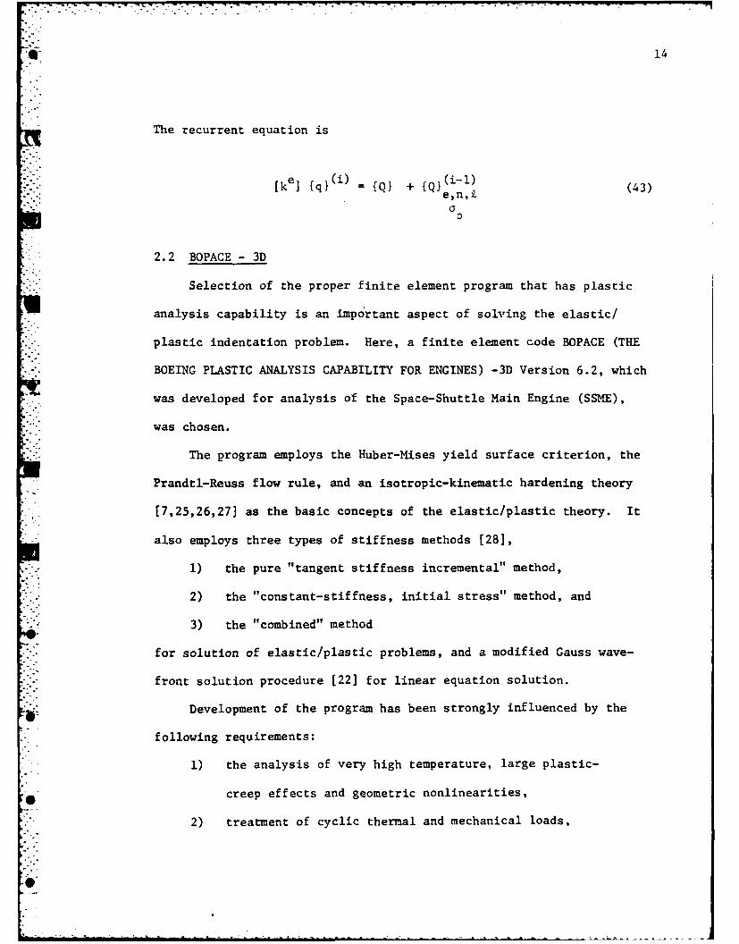
The recurrent equation is
'.e, ( i )
[ke] q}(i) - {Q} + {Q} (43)e,n,Z
0
2.2 BOPACE- 3D
Selection of the proper finite element program that has plastic
analysis capability is an important aspect of solving the elastic/
plastic indentation problem. Here, a finite element code BOPACE (THE
BOEING PLASTIC ANALYSIS CAPABILITY FOR ENGINES) -3D Version 6.2, which
was developed for analysis of the Space-Shuttle Main Engine (SSME),
was chosen.
The program employs the Huber-Mises yield surface criterion, the
Prandtl-Reuss flow rule, and an isotropic-kinematic hardening theory
[7,25,26,27] as the basic concepts of the elastic/plastic theory. It
*also employs three types of stiffness methods [28],
1) the pure "tangent stiffness incremental" method,
2) the "constant-stiffness, initial stress" method, and
3) the "combined" method
for solution of elastic/plastic problems, and a modified Gauss wave-
front solution procedure [22] for linear equation solution.
Development of the program has been strongly influenced by the
following requirements:
1) the analysis of very high temperature, large plastic-
*i creep effects and geometric nonlinearities,
2) treatment of cyclic thermal and mechanical loads,
15
3) improved material constitutive theory which closely follows
actual behavior under variable temperature conditions, and
" 4) a stable numerical solution approach which avoids cumulative
* errors.
The above characteristics make it one of the most sophisticated finite
element codes currently available for many types of general nonlinear
problems.
2.3 Verification of Nonlinear Finite Element Code
Before applying the solution technique adopted in this investiga-
tion to the indentation problem, the technique was first verified
by comparing generated elastic/plastic results for two variations of
a selected plane-stress problem with those independently obtained from
the literature. The plane-stress problem selected was a plate with a
circular penetration subjected to uniaxial tension.
2.3.1 Comparison to Yamada's Analysis
Here, the results obtained from the elastic/plastic finite element
code used in this investigation are compared to those obtained by
Yamada [Personal Note] for an aluminum plate with a circular penetration
subjected to uniaxial tension. The comparison is made in terms of
*e forces and displacements along the vertical and horizontal symmetry
axes of the plate for the same nodal coordinates. The Yamada solution
employs an incremental theory upon which many current nonlinear finite
* element codes are based [NASTRAN, NONSAP, etc.]
16
* "The stress-strain curve and pertinent material properties for
the aluminum plate material are shown in Figure I for both isotropic
and kinematic hardening. Figures 2 and 3 show the finite element
meshes adopted by Yamada and in this investigation,respectively. Both
meshes employ the same nodal point coordinates for easy comparison of
4 solutions but different element shapes since Yamada's program considers
only triangular elements and the finite element code adopted in this
investigation utilizes quadrilateral elements. This resulted in an
* apparent distortion of quadrilateral elements (Figure 3). Due to
symmetry, only the first quadrant of the plate was discretized. A
uniform tensile stress of 39.2 N/mm2 , which was selected in the
Yamada solution, was applied in the y-direction along the upper edge
of the plate.
Comparisons of the nodal forces and displacements along the
horizontal and vertical axes of symmetry are shown in Figures 4 through
7. Results obtained from the two finite element codes are within 10
percent, with the differences caused primarily by the dissimilarity
of element shapes. Theoretically, the accuracy could be improved for
a given number of nodes by using quadrilateral elements, since the
increased degrees-of-freedom would permit a closer approximation to
the displacements within an element [22,23].
2.3.2 Comparison to Marcal and King's Analysis
In the previous section, a coarse grid model was used to compare
e two different solution techniques. In order to determine the extent
and character of the plastic region as a function of applied tensile
14 17
200
-'150 1
ISOTROPIC HARDENING
tOO
0.0
0. -05 0050 007 -1
EFETVESRI
Yon' ouu 750w4m
Possn' Rai003
wPoete Youg' Yaodulus An7350ysis.
18
Y(mrO
392 N/mm 2
400
~30,0 -
"" " 20.CO
-- i0.0 L -Xlmm)
.0.0 0 -0 40-0
Thickness f 3.0 mm
Number of Nodes = 97
Number of Elements = 151
0_ Figure 2. Yamada's Finite Element Model for AluminumPlate with Circular Penetration underUniaxial Tension.
..
19
39.2mm)m
400-
0.0 1 X(M M)
Thickness =3.0 tmm
- Humber of Hodes - 94
flumber of Elements = 70
F Figure 3. Finite El1ement Model Used in This
r Investigation.
20
0.0
-100
0
-200 4
0+
00rZ4 -300
0 +
-v-400 +
0 o>" +- 0
> o
-500iIi
0.0 I0"0. 200 30-0 40"0 50-0
X (mm)
o = Yamada's Analysis
+ BOPACE
K- Figure 4. Nodal Forces F along the x-axis
------------------------------------------
21
50-0 0
40-0-
4040
3000
20.0- .040
0+
0+ 0
10.0 40
-200 -100 0.0 100 200
Horizontal Force F (N)x
o=Yamada's Analysis
+ =BOPACE
Figfure 5. Nodal Forces F along the y-axis.x
4

A 22
-0.006
-0007 0
+0
4J 0* -* -0.008 -
-00+ 8
+
U 0+ 9
r-4
r . 00N$14
; -0011
-0-012-0.0 I0-0 20.0 30.0 40.0 50.0
x(Mi)
o = Yamada's Analysis
+ BOPACE
* Figure 6. Nodal Displacement U along the x-axis.x
a'".

', 23
50.0 0+
o+440.0
0+
0+t . 30'0-
200
0+0+
0+
t00+.10.0 - 0+
0.0•I I ii
0.0 001 0.02 0.03 0-04' Vertical Displacements U (mm)
y
o = Yamada's Analysis
+ = BOPACE
Figure 7. Nodal Displacements U along the y-axis.y
24
stress, the model was reconstructed so that nodal density near
the stress concentration would be increased. Through this remesh-
ing, the number of nodes and elements and the maximum wavefronts were
m increased to 399, 350 and 33 from 94, 70 and 15, respectively. This
improved model is shown in Figure 8. The material used for this
investigation was linear strain-hardening aluminum, with the following
mechanical properties; Young's modulus 7000 kg/mm 2 , Poisson's ratio
2 20.2, Yield stress 24.3 kg/mm , strain hardening rate 225 kg/mm
These values were obtained from Zienkievicz's [211 and Marcal and King's
[18] finite element analysis of a linear strain-hardening aluminum
perforated strip, whose diameter-width-height ratio was 1:2:3.6
instead of 1:3:5 of this investigation.
The plastic regions for load factors of 1.5, 2.0 and 2.5 are
shown in Figure 9. A load factor of 1.0 represents the load required
to cause incipience of yielding in the plate. Load factors of 1.5,
2.0 and 2.5 resulted in progressive yielding of the plate near the
circular penetration. Figure 10 shows the plastic regions obtained
by Marcal and King. Comparison of Figure 9 and 10 indicates that the
character and extent of the plastic regions are nearly identical
for both analyses in spite of the shape difference of the specimens.
6
iS

q 25
50.'0
40-0
30.0
20-0
10.0
0.0 X (MM)
00 10.0 20-0 30.0 40-0
Number of 11odes =399
Number of Elements =350
Figure 8. Improved Model used in the Investigationof Plastic Regions.

* 26
2-55
25-
1-5 2-0 235
Diameter:Width:Height =1:3:5
Figure 9. Character and Extent of Plastic RegionsObtained in this Investigation forSelected Load Factors.

27
2-3
2-3
1-4 16 2-0 2-3
Diatneter:Widrth:Hieight 1:2:3.6
Figure 10. Character and Extent of Plastic RegionsObtained in 'Marcal and King's Analysisfor Selected Load Factors.

CHAPTER III
SOLUTION TECHNIQUES AND THE INDENTATION MODEL
3.1 Method of Approach
Since an analytical solution to the elastic/plastic problem
is not available at this time, the investigation of elastic/plastic
conical indentation was accomplished entirely by finite element
techniques. The objective was to develop and demonstrate numerical
techniques which can be applied to elastic/plastic problems
involving flow, fracture and residual stress effects beneath a
conical indenter. These techniques will be explained in greater
detail in subsequent chapters.
In the loading procedure, three separate stages were required
to simulate elastic/plastic loading and unloading of a half-space
by a rigid conical indenter. In the first stage, initial loading
was applied through nodal displacements selected to simulate
*conical indentation at the contact-surface. Displacement loading
was used since there is no analytical method currently available
for predicting the load distribution for elastic/plastic conical
indentation. The second stage was designed to obtain the equivalent
surface nodal loads which would result in the same stress and displace-
ment fields as those obtained by the displacement loading of the first
stage. This was accomplished by using the numerical results obtained
0- following the displacement loading of the first stage. In the third
stage, the equivalent surface nodal loads were reduced to zero in order
0

29
to simulate unloading of the specimen. During this stage, the re-
sidual displacement beneath the indenter and the residual stress
fields were generated.
The error norm for each stage in the analysis was limited to
within 5 percent.
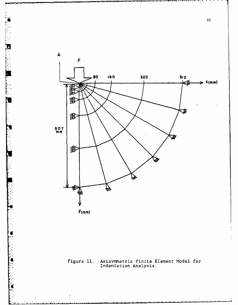
3.2 Finite Element Model and Grids
The axisymmetric finite element idealization for the indentation
analysis of the half-space is shown in Figures 11 through 14. Figure
11 shows the overall outline of the model and Figures 12, 13, and 14
are sub-grids which must be inserted into the appropriate central
sectors of Figures 11, 12, and 13, respectively, to construct the
entire model. There are 470 nodes and 427 elements, and the maximum
wavefront that governs CPU-time (22] is 15. Loading is applied in
the vertical direction along the y-axis, as shown in the figures. The
finite element mesh was designed to meet the following objectives:
1) to reduce the maximum wavefront in order to minimize
CPU-time and core storage requirements,
2) to reduce the occurrence of singularities for elements
in regions of primary interest by considering the shapes
of elements,
3) to reduce the number of elements in regions that are of
less interest by using curved boundary elements which
include intermediate nodes at the edge of the elements,
4) to limit the maximum output to 30,000 printed lines, which
is the maximum number of printed lines for JOB-category 5
D" .
30
AF
64
* Figure 11. Axisynunetric Finite Element Model forIndentation Analysis.
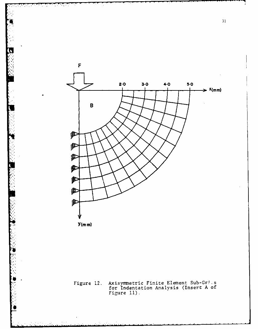
31
Y(MM)
Figure 12. Axisynmetric Finite Element Sub-Gr .. sfor Indentation Analysis (Insert A ofFigure 11).

-. 32
051.0 1-5 0
t X(MM)
0-6
* Figure 13. Ajzisymetric Finite Element Sub-Gridsfor Indentation Analysis (Insert B ofFigure 12).
33
IN ENE
4-
Figure 14. Axisyinmetric Finite Element Sub-Gridsfor Indentation Analysis (Insert C of
a Figure 13).

* 34
r of PSU-IBM 370, by controlling the total number of
elements,
5) to generate or preprocess the input data easily.
* 3.3 Material Used in this Investigation
*. The material selected for this analysis was idealized soda-
lime glass. Soda-lime glass is a brittle material used in many
" . fracture mechanics experiments and its behavior is well established
for Vickers pyramidal indentation and spherical indentation. It is
known that soda-lime glass exhibits elastic/perfectly plastic behavior
when subjected to indentation loading. It was thus an appropriate
material for the nonlinear finite elem nt model. The stress-strain
curve for this elastic/perfectly plastic soda-lime glass is shown
in Figure 15 together with its pertinent material properties.
°"--------kLA

-a - 35
S •ELASTIC
5-0
4-0
ELASTIC/PERFECTLY PLASTIC
U) 3.0
4-i
>2.0-W
ci
14444
1.0
0
0 0.1 0-2 0-3 0.4 0.5
Effective Strain (mm/mm)
Young's Modulus - 49.0 (GPa)
Poisson's Ratio - 0.22
Yield Strength - 3.92 (GPa)
Figure 15. Stress-Strain Curve and Pertinent MaterialProperties of Idealized Soda-Lime Class forIndentation Analysis.
CHAPTER IV
ELASTIC AND ELASTIC/PLASTIC CONICAL INDENTATION
4.1 Introduction
The finite element model for conical indentation of a half-
space was formulated so that it could be applied to both elastic and
elastic/plastic indentations. This required the method of loading to
be carefully considered. For the case of elastic indentation, the
pressure distribution, resultant forces and displacements directly
beneath the indenter can be obtained from a closed-form solution by
Sneddon, as shown in Appendix A. Each of these parameters can be
used as load input to the finite element program at appropriate
nodes beneath the indenter to model elastic conical indentation.
As the material begins to yield, the pressure distribution, and
resultant forces beneath the indenter are completely unknown, while
the displacement field is partially specified. In the case of the
displacement field, nodal points on the contact surface must conform
to the profile of the indenter. For regions adjacent to the contact
*i surface, the displacement of surface nodes would be automatically
generated as output of the finite element code.
In order to generate a model which can apply to both elastic
and elastic/plastic conical indentations, it was decided to input
load through the displacements of surface nodes along the contact
surface. This would allow direct comparison of the finite element
results with those obtained from the closed-form solution for
a~
37
elastic indentation, and also afford partial specification of the
displacement field beneath the indenter for elastic/plastic indenta-
tion.
4.2 Method of Analysis
The coordinate system adopted in the analysis, the geometrical
characteristics associated with the indenter geometry, and the dis-
placement loading are shown in Figure 16. In order to simulate
Vickers indentation, the included angle of the indenter was set to
a =136 degrees.
An elastic finite element analysis was performed initially to
* -. "verify the finite element model. Here, the contact surface radius
was selected as b = 0.30 mm, resulting in a depth of indentation
v = (d+e) = 0.19 mm that was computed from the Sneddon solution.,-..'max
The Sneddon solution also allowed specification of both vertical and
horizontal displacements of surface nodes within and adjacent to
the contact surface. In the finite element analysis, however, only
the vertical displacement of the nodes on the contact surface was
specified. Horizontal displacement was computed as output in order
to allow a greater degree of freedom on and adjacent to the contact
surface.
Following the elastic finite element analysis, the elastic/plastic
finite element analysis w.. conducted. As described earlier, the dis-
placement field beneath the indenter is only partially described in
this case. A trial elastic/plastic run was made, in which the
initial vertical displacements of nodes within the contact surface
-- - - - - - - - - -
*~ 3d
Figure 16. Conical Indentation Geometry Beneaththe Indenter.

39
-were obtained from the Sneddon solution for assumed elastic/perfectly
plastic behavior of soda-lime glass. Following this step, nodal
force resultants were checked for the nodes adjacent to the contact
surface to determine whether any vertical tensile tractions existed.
This condition, when encountered, indicated a divergence of elastic/
plastic surface deformations from the elastic Sneddon displacements,
resulting in "overlap" of vertical surface displacements with the
indenter profile. This was alleviated through trial reductions of
the indentation depth that were repeated until the vertical tensile
tractions were reduced to zero or assumed small compressive values.
For soda-lime glass, it was found that closed-form computation of
vertical displacements on the contact surface resulted in no
tensile tractions for the selected contact surface radius and there-
fore applied for elastic/plastic indentation.
4.3 Results and Discussions
The elastic and elastic/plastic results expressed in terms of
surface stresses and stresses directly beneath the conical indenter
0@ are shown in Figures 17 to 20. In these figures, elastic results
obtained from the closed-form Sneddon solution and the elastic
finite element analysis are compared to those obtained in the
elastic/plastic finite element analysis. In each case stresses
are non-dimensionalized with respect to the factor Etana = (eE/b),
while distances along the free surface of the half-space and beneath
the indenter are nondimensionalized with respect to the contact sur-
face radius, b.
0j
0-5
44
0.0 ---
-0-5
-. 0 -I*0I
-l-5 _-
1-
0.0 1.O 2.0 3.0
x/b
o - Sneddon Analysis
al x = Elastic Finite Element Analysis
- Elastic/Plastic Finite Element Analysis
Figure 17. Non-dimensionalized Surface Stress oxx /EtanBalong the x-axis.
41
-025 A
-050 A
a -0.75
N-- I.0
-125 -
-1.50.0 10 2"0 3-0
x/bo = Sneddon Analysis
x = Elastic Finite Element Analysis
A = Elastic/Plastic Finite Element Analysis
Figure 13. Non-dimensionalized Surface Stress j /EtanBalong the n-axis. zz
,4

42
o /Etan = z,/EtanS
xx Zz
-1.0 -0"5 0.0 0"5
II I0 x OA I°"x
A a
A gi .A 0-01 0-02 0-03
1.0 oI I I
ik CS
" * A
2.0 2.o-0 U /
y/b k AhIII
3-0 3.0
Ia
o = Sneddon Analysis
x = Elastic Finite Element Analysis
A Elastic/Plastic Finite Element Analysis
4
Figure 19. Non-dimensionalized Subsurface Stress 'xx/EtanB
and z/Etan8 along the y-axis. XXan zza
Ue

43
aY /EtanByy
-20-1-5 -1.0 -0-5 0.0
xO 0C
2-0 1O
3-0 ]&
o =Sneddon Analysis
x =Elastic Finite Element Analysis
A =Elastic/Plastic Finite Element Analysis
Figure 20. Non-dimensionalized Subsurface Stressa/Etan3 along the y-axis.yy

44
4.3.1 Elastic Conical Indentation
Considering initially the elastic conical indentation, it is
-obvious that excellent agreement is obtained between elastic stresses
generated by the closed-form Sneddon solution and the elastic finite
*element analysis both on the surface of the half-space and directly
beneath the conical indenter. Minor differences are found at the
edge of contact (x/b = 1.00). These differences are caused by the
inability of the finite element grid to actually express the high
stress gradient in this region. Alon' the surface at the edge of
contact, both the Sneddon solution and the elastic finite element
analysis show a tensile peak in what will be cermed the horizontal
stress component, a n, Figure 17. This peak, also found in spherical
indentation, is usually associated with ring cracking and subsequent
Hertzian cone cracking. This will be discussed further in a sub-
sequent section. Within the contact zone, this stress becomes
compressive, reaching a compressive maximum directly beneath the
indenter. Outside the contact area, this stress decreases from the
tensile peak to zero as distance increases from the contact surface.
The out-of-plane hoop stress, a , along the surface is everywhere". '.ZZ'
compressive, with the peak compressive value being found directly
* beneath the indenter, Figure 18. This stress also gradually decreases
to zero as distance from the origin increases.
Directly beneath the indenter, the horizontal stress, axx ,
W Figure 19, changes from high compressive values at the surface to
small tensile values at approximately one contact radius from the

4 43
surface. The highest tensile value is found at the point of y/b 1.60.
Beyond this point, this stress gradually decreases to zero. Tensile
values of this stress result in median cracking, found beneath
pyramidal and conical indenters. The subject of median cracking will
be discussed in a subsequent section. The out-of-plane hoop stress,
a , is of course equal to the horizontal stress, a., along this axisZZ
of symmetry. The subsurface vertical stress component, a yy, shown in
Figure 20, is everywhere compressive; reaching a peak magnitude directly
beneath the indenter and rapidly decreasing to zero at increased
distance from the origin.
Figure 21 shows the pressure distribution, ayy, within and ad-
jacent to the contact zone. Within the contact zone (x/b < 1.00) the
classical pressure distribution expected beneath a conical indenter is
obtained from the elastic finite element analysis for the prescribed
displacement loading. As can be seen from the figure, this corresponds
very well to that obtained from the closed-form Sneddon solution for
elastic conical indentation. This verifies the displacement loading
condition assumed in this investigation, where only vertical dis-
placements of surface nodal points are specified. In addition, the
load resultant predicted from the Sneddon solution (Appendix A),
F = 3004N, compares well with that determined independently by
4 summation of the vertical nodal forces on the contact surface of
0 < x/b < 1.00, F= 2943N. This factor further substantiates the
displacement method of load application.4- .
1
46
0.5
0.0 ... -. - .. ..4 - -'- -i- --
x
-0.5 aAiAca41 1-0
0-I.5 "
0
0.0 1.0 2-0 3-0
x/b
" Sneddon Analysis
x - Elastic Finite Element Analysis
* 0 - Elastic/Plastic Finite Element Analysis
Figure 21. Non-dimensionalized Pressure Distributiona /Etans on and adjacent to the ContactZ°e.

____________________ .______._____,__. .._ -. - ,- -7--r------;
47
4.3.2 Elastic/Plastic Conical Indentation
In generating elastic/plastic stress states beneath the conical
indenter, the model was allowed to yield according to the Huber-
Mises yield criterion at nodal points beneath the indenter with sub-
sequent flow being governed by the Prandtl-Reuss flow rule. The
elastic/perfectly plastic stress-strain curve was assumed for soda-
lime glass. During each iteration loop, both the elastic and elastic/
plastic portions of the stiffness matrix were updated. As stated
earlier, the vertical nodal point displacement along the contact sur-
face was used as load input for an assumed contact radius of 0.30 mm.
The elastic Sneddon solution was used to predict vertical displacements,
thus raising an obvious question regarding the use of an elastic
solution for the prediction of elastic/plastic displacements beneath
the conical indenter.
The applicability of the elastic Sneddon solution for the pre-
diction of vertical displacements on the contact surface was judged
by observation of mesh deformation for the elastic/plastic case, and
the extent and character of the plastic region. The mesh deformation
for the elastic/plastic conical indentation is shown in Figure 22.
The corresponding extent and character of the plastically deformed
* region and the stress trajectories beneath the indenter can be seen in
Figure 23. These figures indicate a continuity of surface deformation
. both within and adjacent to the contact surface, and also plastic
* -region characteristics similar to those measured experimentally and
predicted analytically. The shape of the plastic zone obtained by
a ,- a~an, ~ m mnmuma~ =n Ul~ me

X (mm)
0-0 0-1 0-2 0-3 0-4 0-5 0-6 0-7 0-8 0-9
01
0-2
0-3
0-4Y(mm)
0.5
0-6
0-7
0.8
0-9
Figure 22. Elastic/Plastic Mesh Deformation.
49
=X*om)
: i. X (M)
00 01 02 03 0.4 05 0-6 07 08 0- 9
• 0.1 -.0*I
0-2
0O'3
0r4
0°5
0-7
" 0"8
0.9
Shaded Area: Plastic Zone
a, (Tensile Stress)
~i(Compressive Stress)
a?(Tensile Stress)(1is Out-of-
" 2 (Compressive Stress) Plane Hoop Stress)
Figure 23. Plastic Zone and Elastic/Plastic StressTrajectories.

450
the elastic/plastic finite element analysis is nearly hemispheiical
and is centered directly beneath the indenter. Its radius c is
approximately 0.35 mm, resulting in a ratio of c/b equal to 1.16.
This c/b ratio compares favorably with a value of 1.159 explicitly
obtained by Johnson [11] (APPENDIX B) as a function of material
properties, with the center of the plastic region at the undeformed
origin. These factors were therefore considered as substantiation
of the assumed displacement loading as obtained from the Sneddon
solution. Observation of Figure 23 illustrates the difference in the
principal stress trajectories of the elastic and plastic regions. In
the elastic region, the in-plane hoop stress is the maximum principal
stress, a1, whereas in the plastic region, the out-of-plane hoop stress
is mainly the maximum principal stress, aI.
In figures 17 to 20, the elastic/plastic stress fields along
the surface of the half-space are compared with the elastic solutions
obtained from the finite element analysis and the Sneddon solution.
The horizontal stress, axx, along the surface shows the characteristic
tensile peak at the elastic/plastic boundary as indicated in Figure 17.
Within the contact zone, this stress is again compressive, reaching a
compressive peak directly beneath the indenter. Outside the region
of contact, this stress rapidly approaches the value obtained in the
elastic analysis at the elastic/plastic boundary. This tensile
peak is usually associated with ring cracking, as suggested in the
previous section. The out-of-plane hoop stress, azz, along the sur-
face again is everywhere compressive, with the peak compression being
found directly beneath the indenter, as indicated in Figure 18.
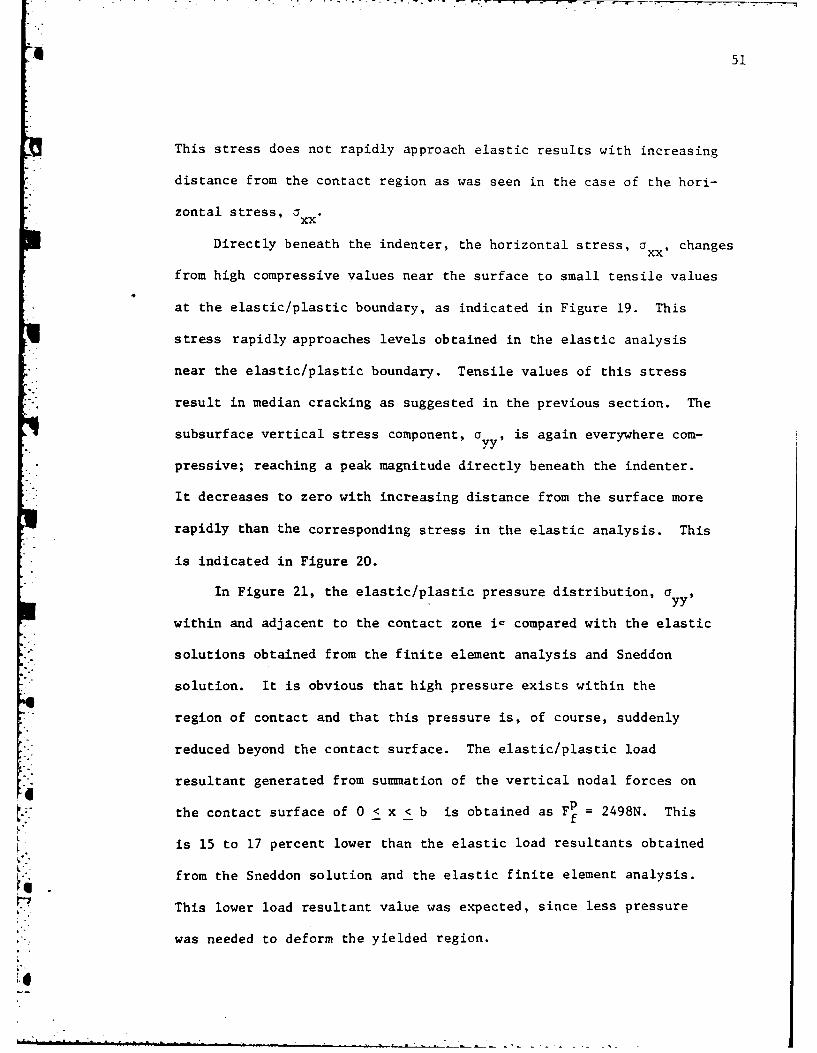
"4 51
This stress does not rapidly approach elastic results with increasing
distance from the contact region as was seen in the case of the hori-
zontal stress, ax.xx
Directly beneath the indenter, the horizontal stress, axx, changes
from high compressive values near the surface to small tensile values
at the elastic/plastic boundary, as indicated in Figure 19. This
stress rapidly approaches levels obtained in the elastic analysis
near the elastic/plastic boundary. Tensile values of this stress
result in median cracking as suggested in the previous section. The
subsurface vertical stress component, a , is again everywhere com-
pressive; reaching a peak magnitude directly beneath the indenter.
It decreases to zero with increasing distance from the surface more
rapidly than the corresponding stress in the elastic analysis. This
is indicated in Figure 20.
In Figure 21, the elastic/plastic pressure distribution, yy'
within and adjacent to the contact zone i- compared with the elastic
solutions obtained from the finite element analysis and Sneddon
solution. It is obvious that high pressure exists within the
region of contact and that this pressure is, of course, suddenly
reduced beyond the contact surface. The elastic/plastic load
resultant generated from summation of the vertical nodal forces ongeneratedT on
the contact surface of 0 < x < b is obtained as F= 2498N. Thisf
. is 15 to 17 percent lower than the elastic load resultants obtained
from the Sneddon solution and the elastic finite element analysis.
This lower load resultant value was expected, since less pressure
was needed to deform the yielded region.
-. -Crr
CHAPTER V
" RESIDUAL SOLUTIONS FOR ELASTIC/PLASTIC CONICAL INDENTATION
5.1 Introduction
* "In this chapter, residual stress, displacement and strain fields
resulting from the elastic/plastic conical indentation are generated.
Development of the residual solution required that a load-unload cycle
consisting of two separate loading stages (stage II and III) be formu-
lated. During the loading stage of the cycle (stage II), equivalent
nodal forces were applied as load input to surface nodes within the
contact area. These equivalent nodal loads were obtained from the nodal
force output obtained in stage I displacement loading and produce the
* surface deformation and resultant stress, displacement and strain
distribution beneath the indenter. A procedure developed to convert the
nodal force output obtained in stage I to the equivalent nodal load is
discussed in greater detail in the following sections of this chapter.
In the unloading stage of the cycle (stage III), the equivalent nodal
loads were reduced to zero, resulting in the required residual solutions.
5.2 Method of Analysis
The procedure used to obtain the equivaleit nodal loads in the
contact area from the nodal force output obtained in stage I is dis-
cussed in this section. These equivalent nodi! loads are, as mentioned
previously, used during the loading stage of the cycle (stage II).
F
- o__ -_ _-
53
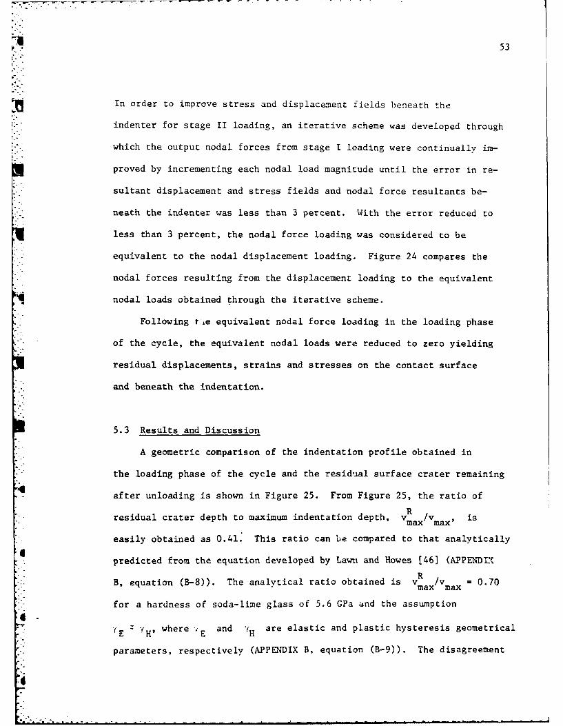
In order to improve stress and displacement fields beneath the
indenter for stage II loading, an iterative scheme was developed through
which the output nodal forces from stage I loading were continually im-
proved by incrementing each nodal load magnitude until the error in re-
, sultant displacement and stress fields and nodal force resultants be-
neath the indenter was less than 3 percent. With the error reduced to
less than 3 percent, the nodal force loading was considered to be
equivalent to the nodal displacement loading. Figure 24 compares the
nodal forces resulting from the displacement loading to the equivalent
nodal loads obtained through the iterative scheme.
Following tie equivalent nodal force loading in the loading phase
of the cycle, the equivalent nodal loads were reduced to zero yielding
residual displacements, strains and stresses on the contact surface
and beneath the indentation.
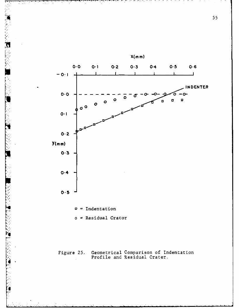
5.3 Results and Discussion
A geometric comparison of the indentation profile obtained in
the loading phase of the cycle and the residual surface crater remaining
6- after unloading is shown in Figure 25. From Figure 25, the ratio of
Rresidual crater depth to maximum indentation depth, Vmax /V max' is
easily obtained as 0.41. This ratio can be compared to that analytically:I
predicted from the equation developed by Lawu and Howes [46] (APPENDLX
RB, equation (B-8)). The analytical ratio obtained is v /v = 0.70
for a hardness of soda-lime glass of 5.6 GPa and the assumption
"(E =H9 where E and H are elastic and plastic hysteresis geometrical
parameters, respectively (APPENDIX B, equation (B-9)). The disagreement
i° •

* 54
-'600-
M 500-
400-
0
.~300-
Cd
o 200-
Cd
0
0
0.0 0-5 1.0
=Nodal Forces resulted by Indentation (Output ofw Stages I)
a=Equivalent Nodal Loads (Input for Stage II)
Figure 24. Comparison of Nodal Forces Resulting, fromIndentation and Equivalent Nodal Loads.
55
X(M M)
0-0 0.1 0.2 0.3 0-4 0-5 0.6
4 INDENTER
o 00 103
0 0
0.2
Y(MM)
0.3
0-4
0-5
o = Indentation
o =Residual Crator
Figure 25. Geometrical Comparison of IndentationProfile and Residual Crater.
56
between the finite element and analytical results may be caused by the' R
"assumption E H" By using the value of /V = 0.41 predicted""f
max max
by the finite element solution and equation (B-8), a geometrical para-
meter ratio yE/YH of 1.26 is obtained resulting in a geometrical para-
meter for plastic hysteresis yH of 1.25. This result is based on an
assumed elastic geometrical parameter y = 7/2 defined by Sneddon [5,6].
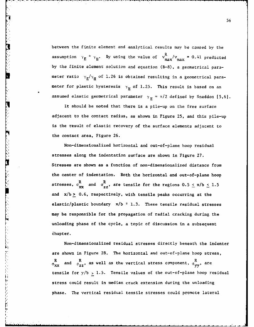
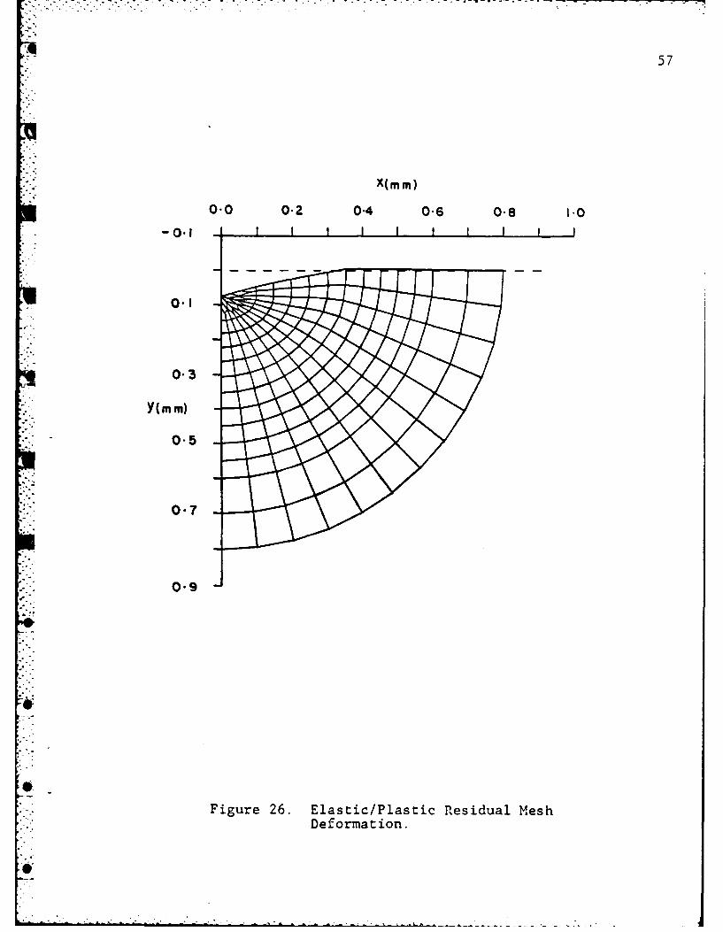
It should be noted that there is a pile-up on the free surface
adjacent to the contact radius, as shown in Figure 25, and this pile-up
is the result of elastic recovery of the surface elements adjacent to
the contact area, Figure 26.
Non-dimensionalized horizontal and out-of-plane hoop residual
stresses along the indentation surface are shown in Figure 27.
Stresses are shown as a function of non-dimensionalized distance from
the center of indentation. Both the horizontal and out-of-plane hoop•R R
stresses, a2 and a , are tensile for the regions 0.5 < x/b < 1.5
and x/b> 0.6, respectively, with tensile peaks occurring at the
elastic/plastic boundary x/b = 1.3. These tensile residual stresses
may be responsible for the propagation of radial cracking during the
unloading phase of the cycle, a topic of discussion in a subsequent
chapter.
Non-dimensionalized residual stresses directly beneath the indenter
are shown in Figure 28. The horizontal and out-of-plane hoop stress,
R R Rai xand czz, as well as the vertical stress component, ayy are
tensile for y/b > 1.5. Tensile values of the out-of-plane hoop residual
stress could result in median crack extension during the unloading
phase. The vertical residual tensile stresses could promote lateral
57
X(mm)
0.0 0.2 0.4 0.6 0.8 1.0
-0.1
[i 0.1-
0.3
Y(mm)
0-5
0-7
0. 9
Figure 26. Elastic/Plastic Residual MeshDeformation.

l.A. 58
I0.
0*1 0
A
AA0
00A_0 - A0 0 0
0
0
00
-0-0
0.0 1-0 2-0 3-0x/b
a ,/Etano
d all /EtanB
*Figure 27. Non-dimensionalized Residual SurfaceStresses along the x-axis.

q 59
Ra /EtanS
-0-15 -0.1 -0-05 0.0 0.05
0-0 - II0 0 A
A 100
0 &
ylb 0
200
106
AO
3.0o
a = R /Etan B aR/Ea
4 yy
Figure 28. Non-dimensionalized Residual Subsurface Stressesalong the y-ax:is.
" 60
crack propagation upon unloading. Both of these possibilities
will be explored in the following chapter.
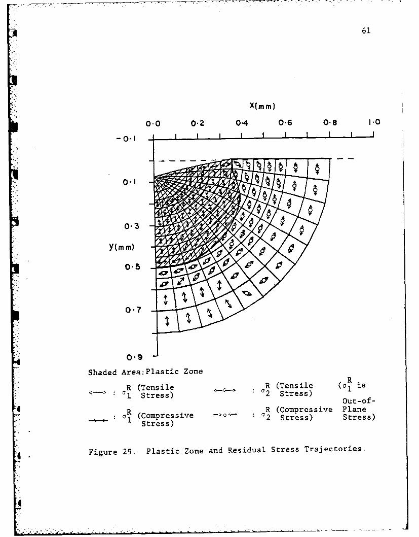
The residual plastic zone and stress trajectories are shown in
Figure 29. Comparison with Figure 23 reveals that the size of the
plastic zone has increased approximately 20 percent during the un-
loading phase due to elastic recovery in the plastic region. Of
major interest are the stress trajectories in the elastic region
where fracture can be extended during the unloading phase. In
this region the stress trajectories indicate the possible propagation
of the lateral cracking driven by the in-plane hoop stress, a R
from points near the elastic/plastic boundary. Near the surface,
the trajectories indicate that the out-of-plane hoop residual
R Rstress, a = al' would result in the radial crack extension. Forzz
subsurface regions, the trajectories indicate the possibility of
the median crack propagation by the out-of-plane hoop residual stress,
R;-." ZZP.a
* .- zz
a.'
0.'
4 61
X(M M)
0.0 0-2 0-4 0-6 0.8 1.0
-0I
0.3
Y(M M)
0-7
0.9
Shaded Area:Plastic Zone
RR (Tensile R (Tensile (a1 is
*a Iates :C1A 2 Stress)
Out -of -
OR (opesv ><OR (Compressive Plane01 (opesv -o- 2 Stress) Stress)
Stress)
* Figure 29. Plastic Zone and Residual Stress Trajectories.

CHAPTER VI
ANALYSIS OF FRACTURE MECHANISMS INDUCED BY INDENTATION
6.1 Introduction
Analytical and experimental investigations considering the
mechanics of crack initiation and propagation beneath spherical,
conical, Vickers pyramidal, and point indentations in a variety of
materials have been the topic of many recent investigations [29-48].
In this chapter, fracture mechanisms beneath conical indentation in
soda-lime glass are further described by applying the numerical results
obtained in the preceding chapters to approximate fracture mechanics
theories. Conical indentation was chosen for analysis as it closely
simulates loading conditions found in a large variety of machining
processes.
6.2 Failure Modes beneath the Indenter
There are four major crack systers introduced as indentation
fracture mechanisms. These crack systems can be classified by the
cracks initiated and propagated near the surface and at subsurface
locations. It has also been experimentally and analytically shown that
these crack systems are initiated on or near the elastic/plastic boundary
with subsequent extension into the elastic region. The schematic
diagram of these crack systems is shoun in Figure 30.
0 o

63
RADIAL MEDIAN
SURFACERINGCRACK
MEDIANCRACKCS
ELASTIC/PLASTICLAELBOUNDARY CAK
Figure 30. Schematic Diagram of Indenta-tion Cracks.
-64
6.2.1 Crack Systems near the Surface
Near the surface, two major crack systems are usually found in
axisymmetric indentation. They are surface ring crack system which is
minitiated in the loading phase of the cycle [35,361, and radial crack
system which is usually initiated and propagated during the unloading
phase of the cycle [33,35,36]. It is known that surface ring crack
system is often propagated as a Hertzian cone crack [31,35,37,40] in
the case of spherical indentation. In the case of Vickers pyramidal
indentation, radial crack system is often initiated in the loading phase
and propagated during the unloading phase of the cycle, since the edges
of pyramidal indenter create highly singular regions in the specimen
[33,36,41,42].
6.2.2 Subsurface Crack System
Two major subsurface crack systems are also found. They are me-
dian crack system, which is initiated and propagated during the load-
ing phase and further propagated during the unloading phase of the
cycle [33,35,36,38], and lateral crack system, which is usually ini-
tiated and propagated during the unloading phase of the cycle. It
is known that the shape of the median cracking is penny-like or half-
penny-like [33,34,36,38,39,43] beneath the indentation. Lateral crack
system is often initiated with the surface ring crack and propagated
as a Hertzian cone crack in the case of spherical indentation [31,35,
37,40] as described in the last section. In the case of Vickers pyra-
midal indentation, lateral crack system is initiated on the elastic/
plastic boundary and propagated to the surface [33,35,37,38.41].
.4
65
6.3 Fracture Initiation and Propagation
In the discussion of fracture initiation and propagation during
elastic/plastic conical indentation, only the opening mode (K -mode)
was considered. To correlate the stresses numerically obtained by
. the finite element method with opening mode fracture, the tensile
peak stresses at the surface and at subsurface locations must be
considered, especially near the elastic/plastic boundary.
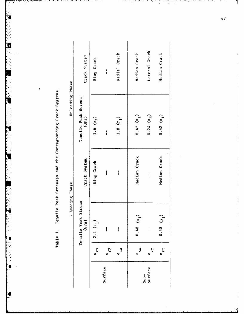
6.3.1 Identification of the Tensile Peak Stresses
The necessary tensile stress fields and tensile stress trajectories
for loading and unloading of a conical indenter were numerically
determined in the preceding chapters. By observation of Figures 17
and 27, the maximum surface tensile stresses are found at the elastic!
plastic boundary. In the loading phase, the maximum value of the
horizontal surface stress, a xx corresponding to surface ring
cracking, is obtained as 2.2 GPa. During the unloading phase, the
Rmaximum values of the horizontal surface residual stress, a
corresponding to the surface ring cracking, and the surface out-of-
plane residual hoop stress, a corresponding to radial cracking,
are obtained as 1.6 GPa and 1.8 GPa, respectively. By observation of
Figures 19 and 28, the maximum subsurface tensile stresses along
the y-axis are also found at the elastic/plastic boundary. In the
loading phase, the maximum value of the subsurface horizontal stress,
xx , which is equal to the subsurface out-of-plane hoop stress, qzzI
a corresponding zo the median cracking, is obcained as 0.48 GPa. During
the unloading phase of the cycle, the maximum values of the subsurface
6-
* 66
horizontal residual stress, a = a R correspouding to the medianc ZZ9
" cracking, and the subsurface vertical residual stress, a R corres-yy
-- ponding to the laterial cracking, are obtained as 0.42 GPa and 0.24 GPa,
respectively. Those tensile peak stresses are shown in Table 1 with
the corresponding crack systems which they initiate.
6.3.2 Critical Flaw Size
*The peak tensile stresses obtained in the previous section can
be combined with an appropriate fracture mechanics theory to predict
fracture initiation and propagation beneath the indenter. Crack
initiation is here predicted by the Griffith flaw hypothesis [29,301:
a >(2Er/rcf) (6.1)
where a is the critical stress causing stable fracture, E is Young's
modulus, r is the crack surface energy and cf is the flaw size. By
solving equation (6.1) for cf9 the following expression is obtained
for the critical flaw size corresponding to the tensile peak stress:
2cf > (2Er/Try). (6.2)
On the surface, the critical flaw sizes corresponding to the
horizontal tensile peak stress, 2.2 GPa, and the horizontal residual
*O peak stress, 1.6 GPa, are obtained from equation (6.2) as 0.025 um
and 0.048 um, respectively. These critical flaw sizes will result in
initiation and propagation of the surface ring cracking. Also on the
surface, the critical flaw size corresponding to the out-of-plane hoop
residual tensile peak stress, 1.8 GPa, can be calculated as 0.039 um
which will result in initiation and propagation of the median cracking.
67
W -4cl
4-i ~c U c Si CJ S.
4 to -H -4 w ) ,
Uo .1i- i cu
02
0 4
4.) a) m C4
C14 -T 02.1 0
0m CO 5.
0 Ji
A.4 "0 ,- -cn4 e
0 -4 . t (4 -
-4 -4I
00 c
m2 E-4E.4
'.44
0nrl
68
At subsurface locations along the y-axis, the critical flaw sizes
, . corresponding to the horizontal or out-of-plane hoop tensile peak stress,
* 0.48 GPa, and the horizontal or out-of-plane hoop residual tensile peak
stress, 0.42 GPa, are obtained from equation (6.2) as 0.54 wm and 0.7 im,
respectively. These critical flaw sizes will result in initiation and
propagation of median crack system. Also at subsurface locations along
the y-axis, the critical flaw size corresponding to the vertical residual
tensile peak stress, 0.24 GPa, can be obtained as 2.17 pm, which will
result in initiation and propagation of lateral crack system.
The c'itical flaw sizes have been discussed in recent papers.
Lawn and Evans [36] have given the critical condition for the initiation
of subsurface flaws as:
cf = 44.2 (KIC/H) . (6.3)
Hagan [43,441 has developed a similar expression for the largest flaw
size which could be nucleated by the intersecting flow lines beneath
the indenter:
cf 2.95 (K Ic/H)2 (6.4)
In these equations, KC and H are the critical stress intensity factor
and hardness, respectively. For values of KIC = 0.7 11m -3 /2 and
H = 5.6 GPa for soda-lime glass, equations (6.3) and (6.4) predicteda
critical flaw sizes of 0.7 Pm and 0.46 um, respectively. The void size
for soda-lime glass has been experimentally measured by Hagan [441
as 0.6 jim. These flaw sizes were correlated to the median cracking.SSwain and Hagan [35] and Chiang, Marshall and Evans [47] correlated
4'
- "p .-.-- . - . - . . .-. ..
69
the crack systems and the threshold flaw sizes, The threshold flaw
sizes for median and radial crack systems were estimated as 1.0 m
and that for lateral crack system was estimated as 3.0 urm. All of those
U critical flaw sizes are compared in Table 2. The critical flaw size
obtained by the finite element analysis with the Griffith energy
hypothesis agrees very well with experimental and analytical values
for median crack system. However the critical flaw sizes obtained by
Swain et al. and Chiang et al. are clearly overestimated as compared
with other analytical, experimental and numerical values for crack
initiation.
6.3.3 Fracture Initiation and Propagation Zones
As described previously, the critical flaw sizes required for
the initiation and propagation of the various crack systems are
obtained from the Griffith energy hypothesis with the stresses generated
by the finite element method. It was, then, found that the critical
flaw sizes predicted by Swain et al. and Chian et al. were overesti-
mated when compared with the critical flaw sizes obtained in this
investigation.
However, by use of these overestimated flaw sizes, the critical
stresses can be generated by equation (6.1) to predict probable
crack initiation and propagation zones. The values of the critical
stress corresponding to initiation and propagation of the median and
radial crack systems is obtained as 0.35 GPa from equation (6.1) with
the value of cf = 1.0 im. Also the value of the critical stress
corresponding to lateral crack system can be obtained as 0.2 GPa from"I
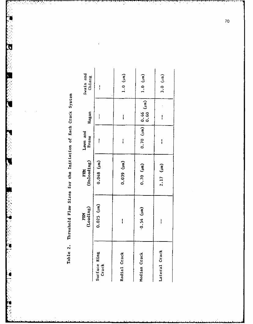
70
m 00 01
cL ca
ca w*-2
(.3 0 NI en0
0 00
Cu r.
coc
4-i4
mCC

*Q 71
equation (6.1) with the value of cf = 3.0 Pm. These two critical
- stress values can be compared with the stresses generated by the
finite element analysis. In Figure 31, the assumed crack initiation
and propagation zones corresponding to a > 0.35 GPa in the loading
phase are plotted. Those can be thought of as the assumed surface
'.ring crack zone and the assumed median crack zone. In Figure 32,
the assumed crack initiation and propagation zones corresponding
to o >0.35 GPa and a1 > 0.2 GPa during the unloading phase of the cycle
. are plotted. Those can be thought of as the potential median crack,
radial crack and lateral crack zones.
hi
r
a-2
a"
.....,,
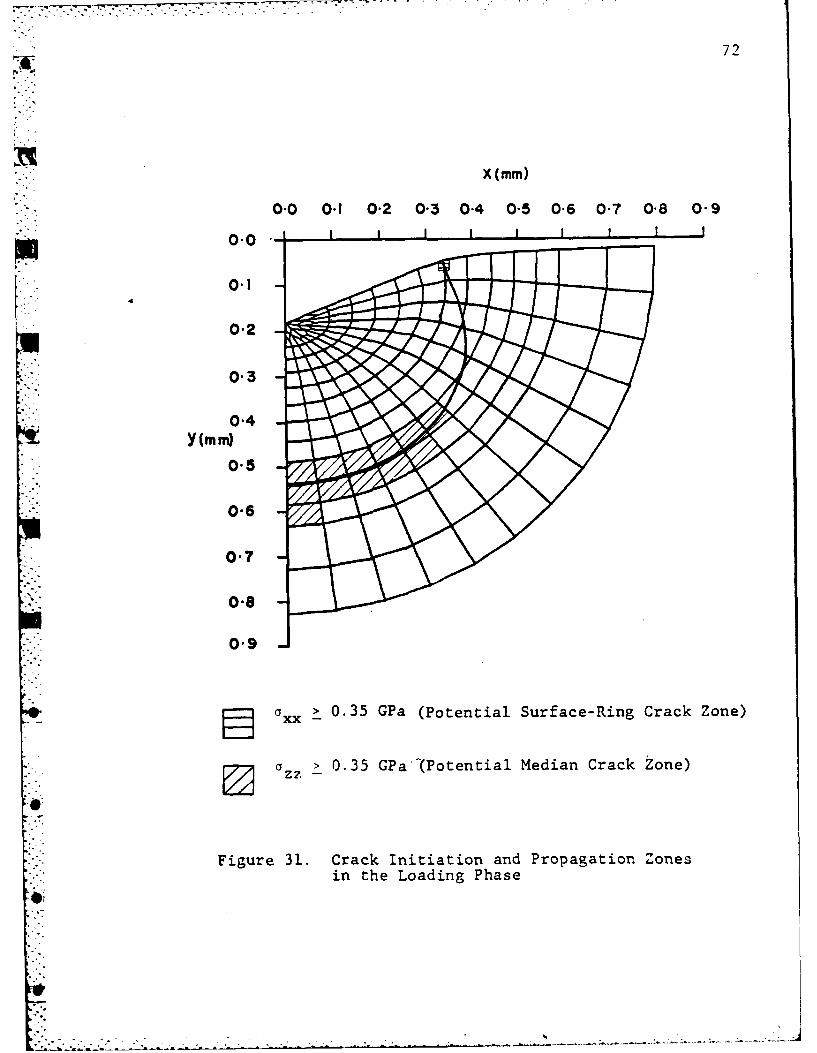
79
X (mm)
0.0 0-1 0-2 0-3 0-4 0-5 0-6 0-7 0-8 0-9
0.0
0-2
0.3
0-4Y (mmff
0-5
0-6
0-7
0.8
0.9
low CF xx 0.35 GPa (Potential Surface-Ring Crack Zone)
I7 7.~~ 0.35 GPa"(Potential Median Crack Zone)
Figure 31. Crack Initiation and Propagation Zonesin the Loading Phase

a 73
X(mm o)
0.0 0.2 0.4 0.6 0.8 1.0
-0.1
0.3
Y(mm)
0.5
0-7
"- 0.9 _"
or a > 0.35 GPa (Potential MedianSo zz -Crack Zone)
Szz> 0.35 GPa (Potential Radial CrackZone)
•___ R- 1 > 0.2 GPa (Potential Lateral Crack
Zone)
4Figure 32. Crack Initiation and Propagation Zones during
the Unloading Phase.
o-
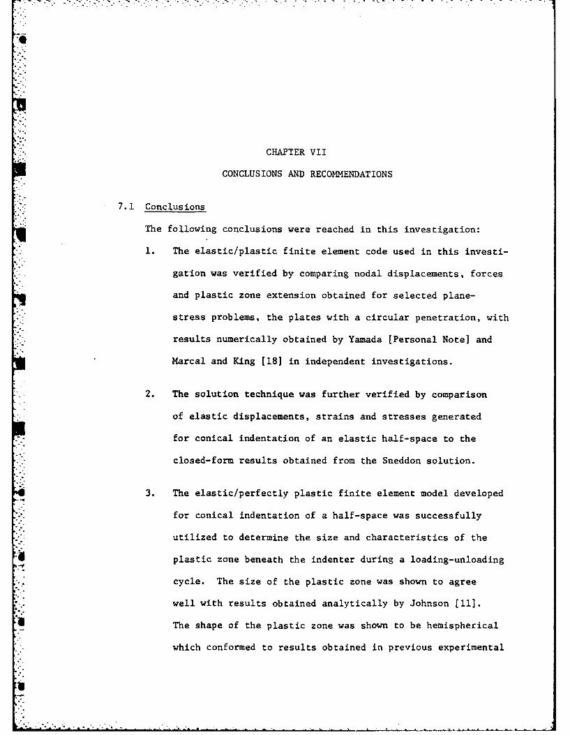
CHAPTER VII
CONCLUSIONS AND RECOMMENDATIONS
7.1 Conclusions
The following conclusions were reached in this investigation:
1. The elastic/plastic finite element code used in this investi-
gation was verified by comparing nodal displacements, forces
and plastic zone extension obtained for selected plane-
stress problems, the plates with a circular penetration, with
results numerically obtained by Yamada [Personal Note] and
Marcal and King (18] in independent investigations.
2. The solution technique was further verified by comparison
of elastic displacements, strains and stresses generated
for conical indentation of an elastic half-space to the
closed-form results obtained from the Sneddon solution.
3. The elastic/perfectly plastic finite element model developed
for conical indentation of a half-space was successfully
utilized to determine the size and characteristics of the
plastic zone beneath the indenter during a loading-unloading
cycle. The size of the plastic zone was shown to agree
well with results obtained analytically by Johnson [11].
The shape of the plastic zone was shown to be hemispherical
which conformed to results obtained in previous experimental

jq 75
and analytical investigations. The origin of the hemis-
pherical plastic zone was found to be on the deformed
surface directly beneath the indenter, not on the undeformed
surface.
4. The displacement, strain and stress fields were successfully
generated by the elastic/plastic finite element model for a
loading-unloading cycle. Resulting loading and residual
stress fields were examined to determine the location and
magnitude of tensile peak stresses which would result in
the initiation and subsequent propagation of the ring, radial,
median and lateral crack systems. Tensile peak stresses
were characteristically found on the elastic/plastic boundary
near the surface and at subsurface locations directly
beneath the indentation. The out-ofLplane hoop stress, which
controlled both radial and median cracking, was found to
change sign near the surface from compression during the
loading phase to tension during the unloading phase of the
cycle. This indicates that radial crack propagation
and the additional median crack propagation takes place
during the unloading phase, a fact experimentally verified.
5. By use of the Griffith energy hypothesis with the generated
tensile peak stresses, the critical flaw sizes, resulting in
initiation of the crack systems, were obtained. The critical
flaw sizes obtained in this investigation agreed well with

76
critical flaw sizes predicted analytically and experimentally
by Lawn et al. [361, Hagan [43,44], Swain et al. [351 and
Chiang et al. [47] for each crack system.
6. Fracture initiation and propagation zones for the loading
phase and unloading phase of the cycle were generated through
comparison of the tensile peak stresses obtained in this
investigation to critical stresses obtained from the Griffith
energy hypothesis and maximum allowable flaw sizes. These
fracture initiation and propagation zones agreed well with
actual initiation and propagation zones experimentally
observed.
7.2 Recomendations
The following subjects are recommended as topics for further
research:
1. The elastic/plastic finite element model should be expanded
to consider elastic/plastic strain hardening in order to
analyze more realistic indentation models.
2. Investigation should be expanded to consider more brittle,
lower yield strength/Young's modulus ratio models such as
MgO and ZnS in order to determine the effect of these para-
meters on the extent and character of the plastic zone and
resultant crack systems.
3. Shear peaks as well as tensile peaks should be investigated
as they affect fracture initiation through dislocation
activity and crack propagation by Mode II loading.
44 : -' hnau ' d - , " -- - m" ""

77
4. The elastic/plastic finite element model should be expanded
to consider non-axisymmetric indentation such as Vickers
pyramidal indentation and obtain characteristics of the
singularities created by the edges of the indenter.
5. The elastic/plastic finite element technique should be
combined with statistical analysis, such -s "The Monte
Carlo method' in order to closely model elastic/plastic
indentation fracture.
aL'
-a
6. .

* 78
APPENDIX A
THE ELASTIC STREAS FIELDS FOR POINT, SPHERICAL AND CONICAL INDENTATION
1. Point Indentation (Boussinesque and Michell Solution)
The well known non-dimensionalized stress field equations for
the point indentation problem 1121 are given for the coordinate
system shown in Figure 33 as:
ar~~~~o - se.. ics +11
p 4(X+i)
C2 206 (A-1)-4-(cosO-sin e) secp 4Ck-s-i'
Tr sine cose sec 0
where
=E
(l+v)(1-2v)
E= 2 (1-4v)
' F
F applied load
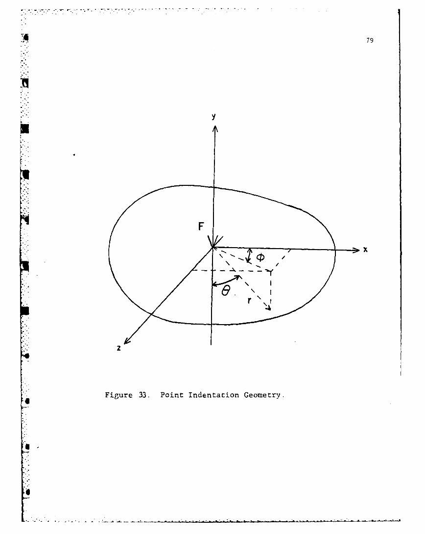
79
La
Figure 33. Point Indentation Geometry.
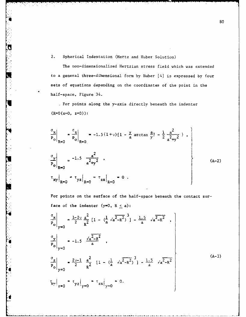
6 80
2. Spherical Indentation (Hertz and Huber Solution)
The non-dimensionalized Hertzian stress field which was extended
to a general three-ditiensional form by Huber [4] is expressed by four
sets of equations depending on the coordinates of the point in the
half-space, Figure 34.
For points along the y-axis directly beneath the indenter
(R=0(xffO, z=0)):
..a . -1.5{1+v)[1 - arctan 2
pPO a y 2 a2+yR=O R=0
2a-1.5 aP1. 2 2y'2(A-2)
0R=0 O
yzYf= = tzxI =0.";: XYR=O yRfi zxR=0
For points on the surface of the half-space beneath the contact sur-
face of the indenter (y=0, R < a):
Cx _ 1-2v a 1 2 15 2 2p 2 2 a a1: o~~ y-/a 22 /2R ) ._]a /2R
i ay =-1.5 Va2-R2Po aP y=O
z I = a 1 2 2 1.5 /a2_)
O 2 Ry=0 2 -(a /a-R) a
T TYZI y zxl = 0.S! z=O y
4i

RD-A127 529 AN ANALYSIS OF CONICAL INDENTATION OF AN 2/2ELASTIC/PERFECTLY PLASTIC HALF-S..CU) UENNSYLYANIRSTATE UNIV UNIVERSITY PARK APPLIED RESEARCH LAB.
UNCLASSIFIED T KATO 26 OCT 82 ARL/PSU/TM-82-230 F/G 28/11 N
EEmhomhohmoiE
kimE I M2
liiii ~ us. All
MICROCOPY RESOLUTION TEST CHARTNATIONAL BUREAU OF STANDARDS- 19 3 -A
)6

81
°f
Figure 34. Spherical Indentation Geometry
beneath the Indenter.
,i-°
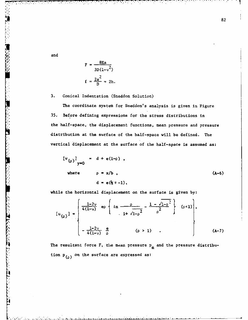
7W77. , o
-- * . .7". 7- 7." .7 7 7 4 -" "
82
R. and
8Ea• F =
3D(l-v 2)
f = 2a-2 2h.D
3. Conical Indentation (Sneddon Solution)
The coordinate system for Sneddon's analysis is given in Figure
35. Before defining expressions for the stress distributions in
the half-space, the displacement functions, mean pressure and pressure
distribution at the surface of the half-space will be defined. The
vertical displacement at the surface of the half-space is assumed as:
. [V~o) ] d + e(1-Q)
where p - x/b , (A-6)
d - e(kTr-),
while the horizontal displacement on the surface is given by:
1-2v I -
4 (i-v) 2[uo ] =1+ ,/1-P 2 P
:.1-2,u'-" ( i - ) 0( P > i) .( A -7 )
The resultant force F, the mean pressure pm and the pressure distribu-
tion P(P) on the surface are expressed as:
1 b
• I " - . . ' " - " ' . . .i : " .* i
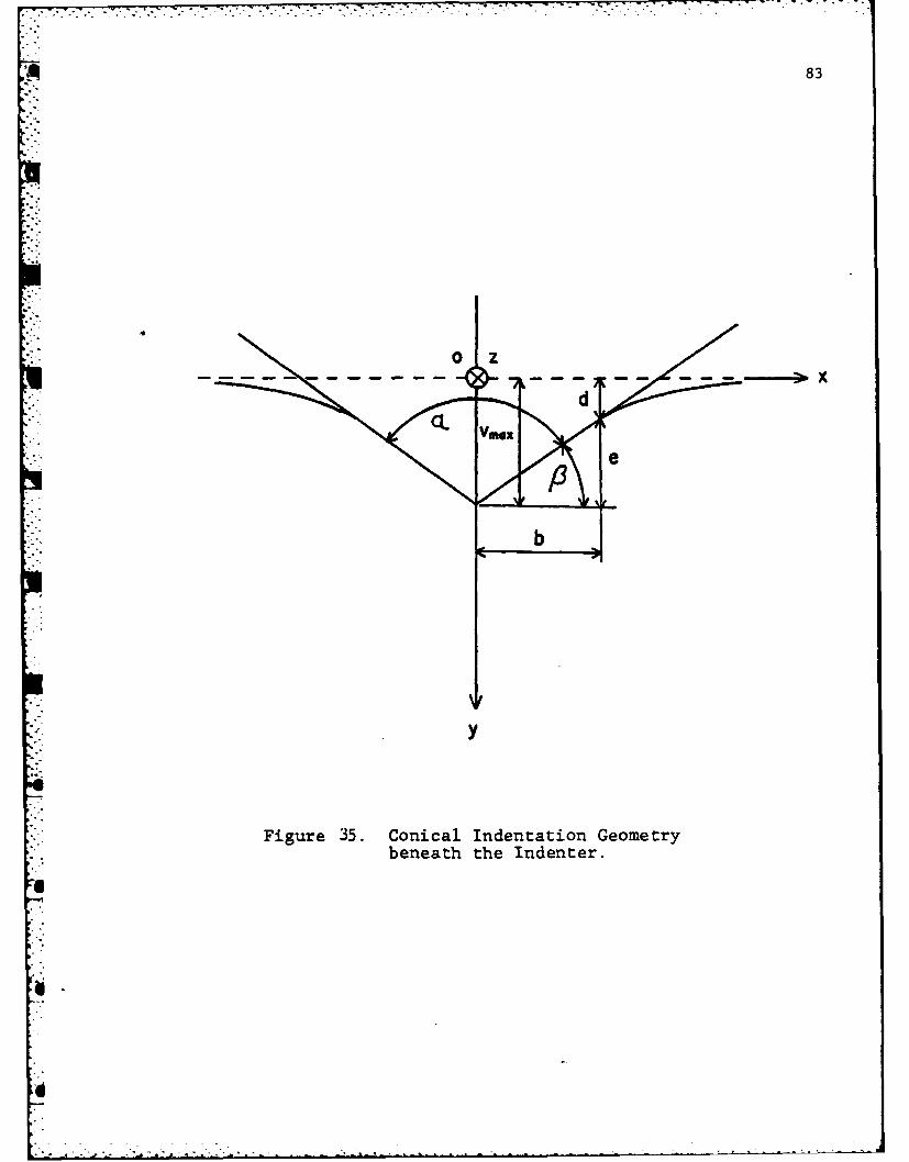
4 83
0
Figure 35. Conical Indentation Geometrybeneath the Indenter.
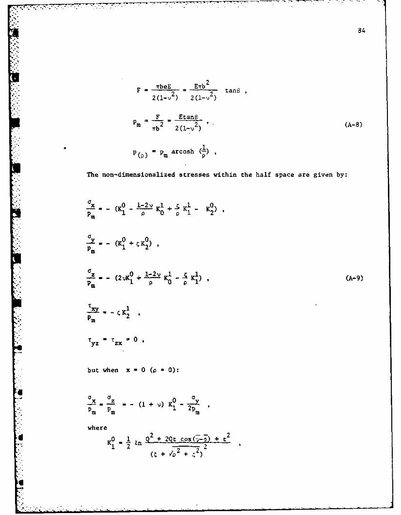
84
F- i"rbeE Erb2F = tanS"-" 12 i- 2
2(1-v ) 2(-\ )
F EtanBPm 2 2 ' (A-8)
7rb2 2(1-v 2)
P(p) = Pm arcosh )p
The non-dimensionalized stresses within the half space are given by:
ax 0(K 0 -2\..K.... 1 K 0
P -(K 1 P P 1 K2 )
a0 00K ,(K + ; K 2 '
az 0 1-2bt w- x - K- K) (A-9)
aMI 0 a
-.-
m'"
ut whereaa o a oz 0 aq Yo(7.
1 2 ~ 2... I - " t2 2 2
+ .-
U.

85
0 1 cos bK =
--2 Q2 ~
K1.- I V2 + 2 Q Cos1 it 2__2_
K"--co[( / p-+ )- Coso €12Vp 2 + ~2
1 0 1 1K 0 [pKl -KI - (l-Q sin)],
and
S= e =b tana,b
2 2 4 2 2 2
11__*=arctan *= arctan 2
4. Comparison of the three elastic indentation stress fields.
To compare the three elastic stress fields" which are given in the
preceding sections of APPENDIX A for the same condition, Young's
modulus E, Poisson's ratio v, and the resultant force F must be fixed.
For the finite element analysis of conical indentation, the following
four values were defined:
E = 49000 N/mm2 v = 0.22
Contact radius b = 0.3 mm cone angle a 1360 (a = 220)
From these four values the resultant force F can be obtained from
equation (A-8):
I -° .- ..
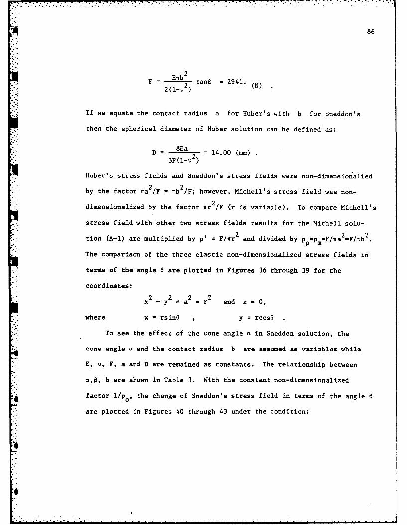
86
1° -b
F = 2 tanB = 2941. (N)2 (1-v)
If we equate the contact radius a for Huber's with b for Sneddon's
then the spherical diameter of Huber solution can be defined as:
;:' 8Ea
D =14.00 ( )2
3F(l-v2)
Huber's stress fields and Sneddon's stress fields were non-dimensionalied
by the factor ra 2/F = rb 2/F; however, Michell's stress field was non-
dimensionalized by the factor 7rr 2/F (r is variable). To compare Michell's
stress field with other two stress fields results for the Michell solu-
2 2 2:-" tion (A-l) are multiplied by p' f F/irr and divided by pp=Pm=fiF/Ta =F/rb
The comparison of the three elastic non-dimensionalized stress fields in
terms of the angle e are plotted in Figures 36 through 39 for the
coordinates:
x 2 + y 2 a2 r2 and z =0,
where x - rsin6 y =rcosO
To see the effect of the cone angle a in Sneddon solution, the
cone angle a and the contact radius b are assumed as variables while
E, v, F, a and D are remained as constants. The relationship between
a,$, b are shown in Table 3. With the constant non-dimensionalized
factor i/po, the change of Sneddon's stress field in terms of the angle e
are plotted in Figures 40 through 43 under the condition:
4
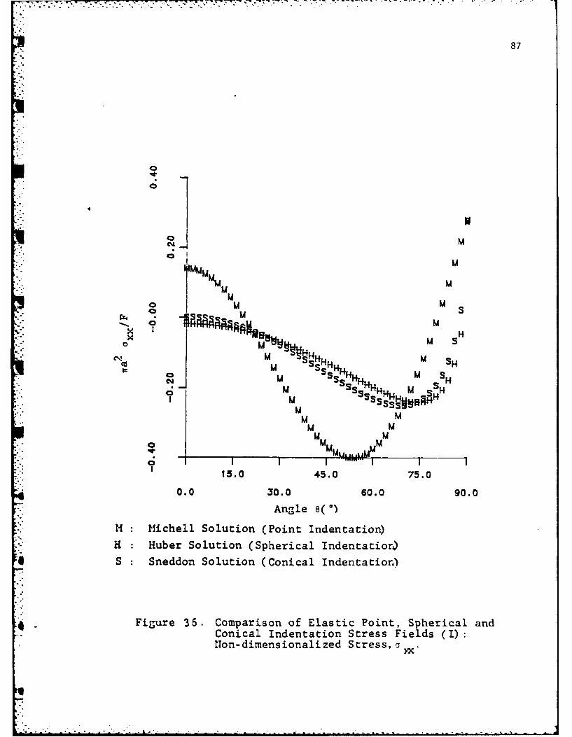
87
CM4-4
M
MUMU
C'
M' S
UM Ss
o MUM
o
:<" 4
M ~ Mihl Soltio (P44 InenatonH~~~ Huber Souin(peiaHnetto 1
4~~0 J Sndo Souin(oial4dnair
-S H
Ho-iesinlzdStes
* *,. * *. .,. - -
M
, UM, MI
15.0 45.0 75.00.0 30.0 60.0 90.0
[:.-.Angle 6( °
. "'.M :Michell Solution (Point Indentation)
i-H :Huber Solution (Spherical Indentatior)
|S :Sneddon Solution (Conical Indentation)
i Figure 35. Comparison of Elastic Point, Spherical and
~Conical Indentation Stress Fields (1):,li on-dimensionalized Stress,, X.
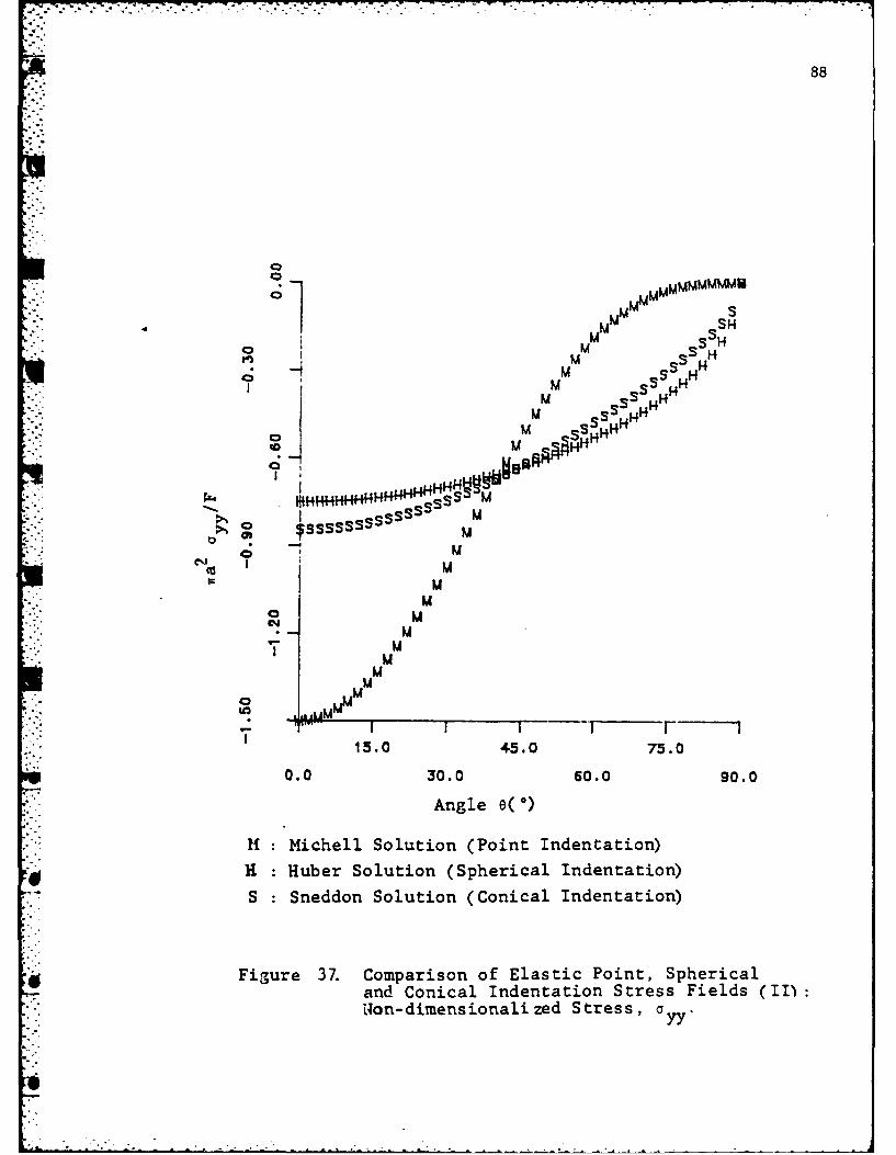
88
C ~~MMMMMESMM
M SH
M _s SIHSM sS H
M SS HH
M -' HH
;T .I4HHHHHHHHHH S$S M
I 5 ~~sSSS 5
SSSSSS MU
o , M==: M
I MM
Mo M MM
15.0 45.0 75.0
0.0 30.0 60.0 90.0
Angle e(o)
11 :Michell Solution (Point Indentation)
I : Huber Solution (Spherical Indentation)
S : Sneddon Solution (Conical Indentation)
* Figure 37. Comparison of Elastic Point, Sphericaland Conical Indentation Stress Fields (ID:Non-dimensionalized Stress, a
m.. •
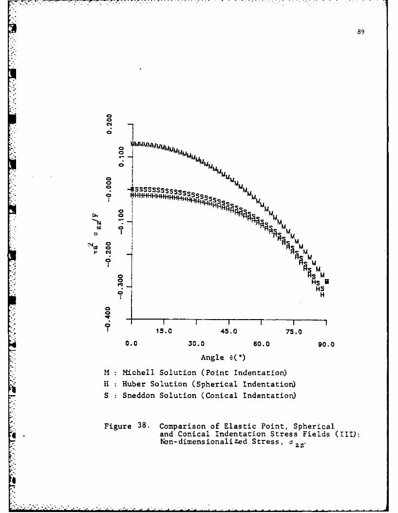
--------------- : - - -.
89
LJUMM'M M
-SSSSSSS0*SS - _ M'IHHHHHIH HH S S HS M
C i**[1~rTHH JSS S
N n~Mo rTu
-' " o 1 'A
i '
-,C I I IFIIF"-I 15 .0 4 5 .0 75 .0
0.0 30.0 60.0 90.0: i
A n g l e e ( )".: H :Michell Solution (Point Indentation)i 'I 11 :Ruber Solution (Spherical Indentation)
S :Sneddon Solution (Conical Indentation)
* Figure 38. Comparison of Elastic Point, Sphericaland Conical Indentation Stress Fields (III):"il Non-dimensionalized Stress, z
.-
i• "
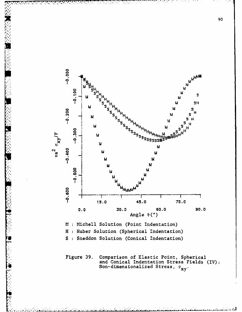
90
M MMN
o i S14S S°
'I SH Uo M H
S
• .. •4
o 14 H04 M S M SH14 S H'I S HS-. ld SH4HHH M S H H
I Sss 144 U SN4- s HH M SS H
:! 1 S ~S HH , S
.M,M M• ,-o U l U
MMSM M,_., - U
:-,,I15.0 45.0 75.0
0.0 o 0.0 o0.0o 90.0oo7 Angle 9()
i,:: 11 Michell Solution (Point Indentation)
,...4
."".H : Huber Solution (Spherical Indentation)IIS : Sneddon Solution (Conical Indentation)
• .. Figure 39. Comparison of Elastic Point, Sphericaland Conical Indentation Stress Fields (IV):
-,-IINon-dimensionalized Stress, a xy"
b" ,IA"U

91
CB
Io
I c _ 9 HH
_ IMDC B H
M.:au .. H* , HME) 0 CH HH
IA A AA4AA A A A WAAAAAAAAA
' 1.HH0 HHHHHHHHUH
CO IHHHHHHHHHHHHHHH1 5
9 8 95 ~B9 S
04 D
PODDDD DMM m
15.0 45.0 75.0
0.0 30.0 60.0 90.0
Angle e(0)
A: Sneddon Solution (Conical Indentation): "160B: Sneddon Solution (Conical Indentation): c = 1200C: Sneddon Solution (Conical Indentation): = 800D: Sneddon Solution (Conical Indentation): 4 = 00H: Huber Solution (Spherical IndentationM: Michell Solution (Point Indentation)
4 - Figure 40. Included Angle Effect of Conical Indentation(I): Non-dimensionalized Stress, a
IX
- .'. .af ~ .c 'xx*

92
0A
R ~ HAAACa HAA2 CBHH"AA Ma
c H~ AADC 9 HH. AAAA B H
MDC _ HH AAAAAAAAAAAA ADC Hi" ~ ~ C _13,,0" H DB
oD C H 4 UD Hr ? |/ " c ". HH c ".,MD c a M14 uc H
a HHH 9 H0 C B H D- DC U a H
CO C B aA UDC13U D C Ba HH HH
MD c 1.. BU °0 C n,4-. D C
0 ? M D CCili oU D a¢o MM D
U DDDD0UI
15.0 45.0 75.0
0.0 30.0 60.0 90.0
Angle e(*)
L A: Sneddon Solution (Conical Indentation): a = 1600B: Sneddon Solution (Conical Indentation): a = 1200C: Sneddon Solution (Conical Indentation): a = 800D: Sneddon Solution (Conical Indentation): a = 400H: Huber Solution (Spherical Indentation)M: Michell Solution (Point Indentation)
Figure 41. Included Angle Effect of Conical Indentation(II): Non-dimensionalized Stress, ai.'.
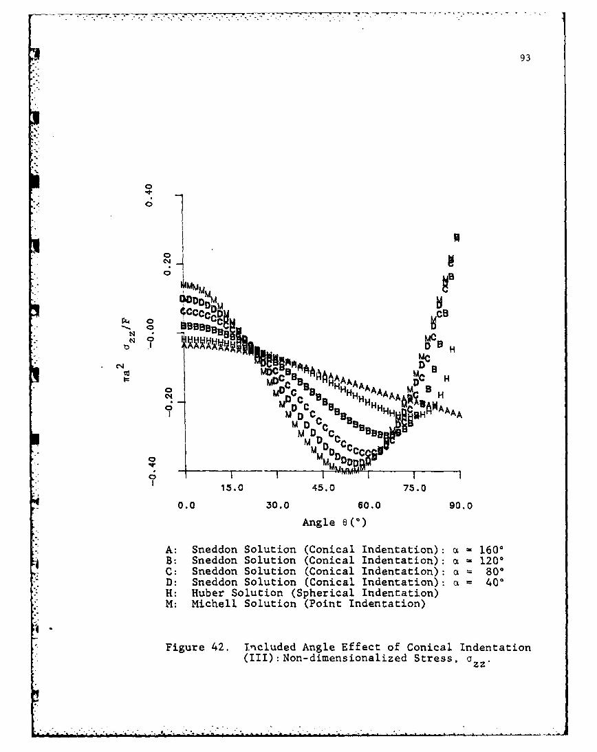
• ., -.-.-- w '-rw- r -w -- - -..... : - -.--- .. - . .. -
93
rz4D 0a
D H
C' M
AAAAOOIAAAAA Hw0 MCCO Ba HHHAAAAA HC 11 C a~ HHUAA
D C a, HH CBNAAM MDDC C 113 HHR INC1H~.Am DC C B13 -
%U DDD~
15.0 45.0 75.0
0.0 30.0 60.0 90.0
Angle 8(0)
A: Sneddon Solution (Conical Indentation): a=1600B: Sneddon Solution (Conical Indentation): ac- 1200C: Sneddon Solution (Conical Indentation): ac= 800D: Sneddon Solution (Conical Indentation): a 40*H: Huber Solution (Spherical Indentation)M: Michell Solution (Point Indentation)
Figure 42. included Angle Effect of Conical Indentation(III):Non-dimensionalized Stress, a ZZ
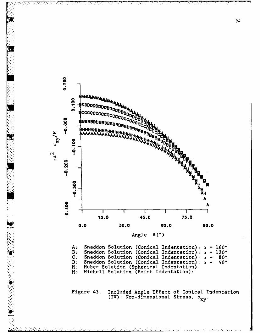
94
C!
I- uDeelflnuODD Mu..o CC~oco ccD0DDMuDO%
0 BBBB.B999BB9 CcCCgH
44 HH HHHH4tH 91I AAAAAAAAA HAHHH B~
A4%N
Cd
AHA
A
15.0 45.0 75.0
0.0 30.0 60.0 90.0
Angle e 0
A: Sneddon Solution (Conical Indentation): a 1600*B: Sneddon Solution (Conical Indentation): a = 1200-C: Sneddon Solution (Conical Indentation): a - 800
D: Sneddon Solution (Conical Indentation): a 400H: Huber Solution (Spherical Indentation)11: Michell Solution (Point Indentation):
Figure 43. Included Angle Effect of Conical Indentation(IV): Non-dimensional Stress,a
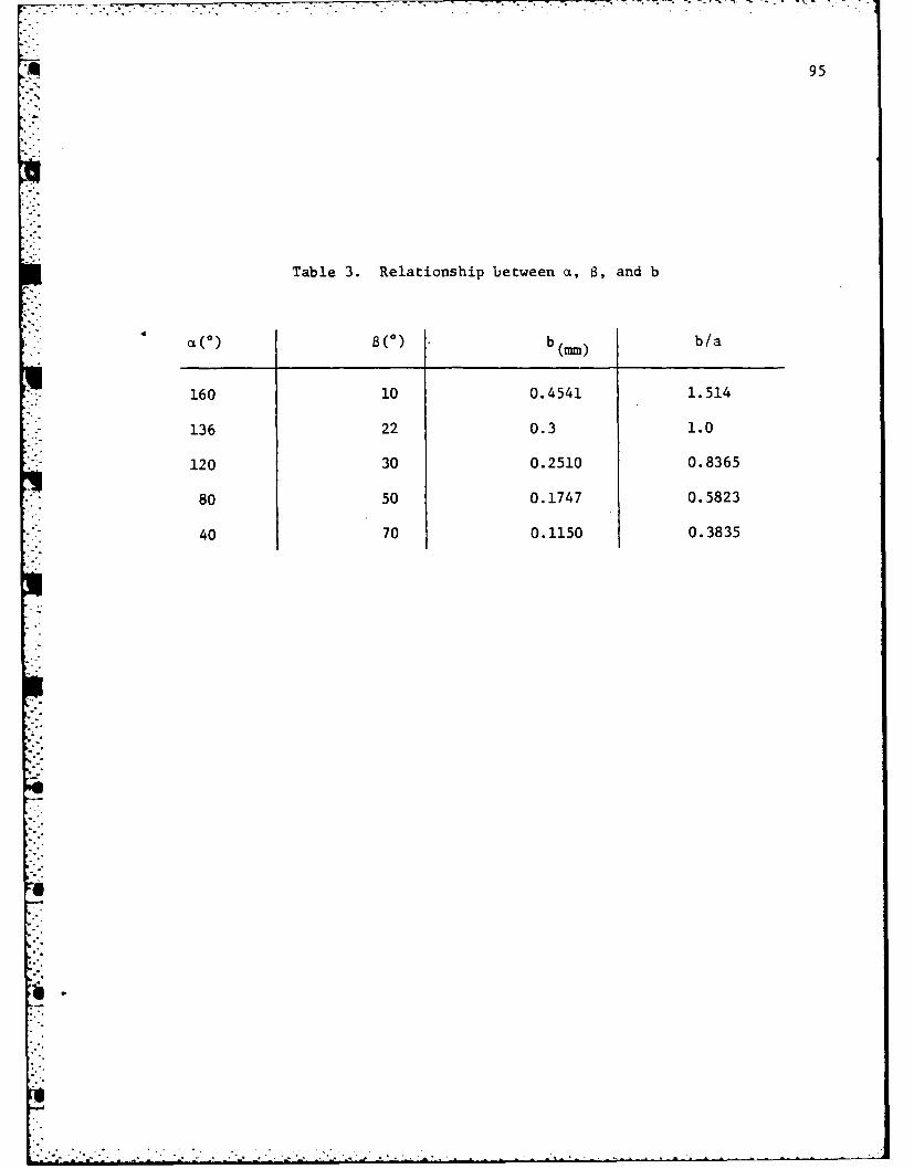
95
Table 3. Relationship between a, B, and b
a0 b () b/a
160 10 0.4541 1.514
136 22 0.3 1.0
120 30 0.2510 0.8365
80 50 0.1747 0.5823
40 70 0.1150 0.3835
96
2 2 2x + y a O0.09
By comparing these figures with Figures 36 to 39, it is obvious
P that Sneddon's stress field behaves like Hertzian stress field under
the same contact radius and also Sneddon's stress field behaves like- - 4
Michell's stress field under the sharp included angle and small
contact radius as be expected.
........................... . . . . .

,. . ,_. . . , . . .. _ > . _.5.. ._.... .: .,2 . . . . -- I ' ' - . " -': . . "
97
APPENDIX B
THE ANALYTICAL-EXPERINENTAL EQUATIONS FOR ELASTIC/PLASTIC INDENTATION
Various formulas to define the indentation hardness, H, in terms
of Young's modulus, E, Poisson's ratio, v, and yield strength, Y,
have been developed by Johnson [11], Perrott [37,39], and Izumitani [121.
These formulas were derived by utilizing Hill's elastic-plastic
solution of the expansion of a spherical or cylindrical cavity [7,8]
along with experimental observations.
Johnson's formula for a conical indentation is:
H 25 + 2 in c) ,(B-l)
with
E 3tana - 6(l-v)(--) - 4(1-2v) , (B-2)
Y
and for a wedge indentation is:
.°"-" H 2 1 c (3H F3 [t + in (B-3)
with
4E 2f'y tanB - (5-4v) ) - 3(1-2v) (B-4)
where c is the radius of the plastic zone and the center is the
*undeformed origin.
Perrott's formula for conical and pyramidal indentation is:
"- H [Etan" = 0.494 + 0.577 Zn y(l 2 1 (B-5)
" "
98
Izumitani's formula for knoop indentation is:
H 2.. . " = " + 2 n )c
B- 6
with(-)
3 . E(3 E
b - 3(l-v)Y=
(B-7)
which are the same as Hill's equations for the expansion of a spherical
cavity in an infinite medium.
The relationship between indentation depth vmax and residual crater
-'aRdepth v in terms of material properties and geometrical properties
for the conical indentation problem is expressed by Lawn and Howes
[461 as:( R Y2 2max I (l-V 2 ) ) co H (B-8)V m a x F H
('-E
where H is the indentation hardness, and JE is the elastic
geometrical parameter which is expressed as:
.YE btans 2 7 for Sneddons solution) (B-9)
and JH is actually an unknown geometrical parameter of plastic
hysteresis; however, it is usually defined as Y' YE
F .
a-.
I99
BIBLIOGRAPHY
1. Boussinesq, J., "Application des Potentials a l'Etude de'lEquilibre et du Mouvement des Solides Elastiques,"
Gauthier-Villars, Paris, (1885).
* 2. Michell, J.H., "Elementary Distributions of Plane Stress,"Proceedings of the London Mathematical Society, Vol. 32,. (1900),pp. 35-61.
3. Hertz, H., Hertz's Miscellaneous Papers, translated by D.E. Jonesand G.A. Schott, Macmillan, New York, (1896), pp. 146-162, 163-183.
4. Huber, H.T., "Zur Theorie der Beriihrun fester elastischerKfrper," Annalen Der Physik, Ser 4, 14, (1904), pp. 153-163.
5. Sneddon, I.N., "Boussinesq Problem for a Rigid Cone,"Cambridge Philosophical Society, proceeding, Vol. 44, (1948),pp. 492-507.
6. Sneddon, I.N., Fourier Transforms, McGraw-Hill, (1951),pp. 462-468.
7. Hill, R., The Mathematical Theory of Plasticity, ClarendonPress, Oxford, (1950), Chapter 5.
8. Hill, R., "General Feature of Plastic-Elastic Problems asExemplified by Some Particular Solutions," Journal of AppliedMechanics, Vol. 16, (1949), pp. 295-300.
9. Hamilton, G.M. and Goodman, L.E., "The Stress Field Created bya Circular Sliding Contact," Journal of Applied Mechanics,Vol. 33, (1966), pp. 371-376.
10. Johnson, K.L., "An Experimental Determination of the ContactStresses between Plastically Deformed Cylinders and Spheres,"Engineering Plasticity, University Press, Cambridge, (1968),pp. 341-361.
* 11. Johnson, K.L., "The Correlation of Indentation Experiments,"Journal of the Mechanics and Physics of Solids, Vol. 18, (1970),pp. 115-126.
12. Izumitani, T. and Suzuki, I., "Indentation Hardness and LappingHardness of Optical Glass," Glass Technology, Vol. 14, No. 2,(April 1973), pp. 35-41.
13. Parrons, B. and Wilson, E.A., "A Method of Determining theSurface Contact Stress Resulting from Interference Fits,"Journal of Engineering for Industry, Transaction, ASME,(February 1970), pp. 208-218.
1-2 ., -. . . . . .

K. 100
14. Hardy, C., Baronet, C.N. and Tordion, G.W., "The Elastic-' Plastic Indentation of a Half-Space by a Rigid Sphere,". International Journal for Numerical Method in Engineering,- Vol. 3 (1977), pp. 451-462.
15. Imaoka, M. and Yasui, I., "Finite Element Analysis of Indenta-tion on Glass," Journal of Non-Crystalline Solids, Vol. 22,
* "-(1976), pp. 315-729.
- 16. Mises, R. Von, "Mechanik der festen Krper im plastischen* deformablem Zustand," Goettinger Nachrichten. Mathematische-
Physikalisch Klasse, (1913), pp. 582-592.
17. Johnson W. and Mellor, P.B., "Engineering Plasticity," VanNostrand Reinhold, (1978).
18. Marcal, P.V. and King, I.P., "Elastic-Plastic Analysis of Two-dimensional Stress System by the Finite Element Method,"International Journal of Mechanical Science, Vol. 9, (1967),pp. 143-155.
19. Yamada, Y., Yoshimura, N. and Sakurai, T., "Plastic Stress-Strain Matrix and Its Application for the Solution of Elastic-Plastic Problems by the Finite Element Method," Report of the
- Institute of Industrial Science, Aug. 1967, University of Tokyo,Tokyo, Japan.
20. Yamada, Y., Kawai, T., Yoshimura, N. and Sakurai, T., "Analysis*of the Elastic-Plastic Problems by the Matrix Displacement
Method," Proceeding of 2nd Conference on Matrix Methods ofStructural Mechanics, Wright-Patterson Air Force Base, Ohio,(1968), pp. 1271-1299.
21. Zienkievicz, O.C., The Finite Element Method, Third EditionMcGraw-Hill, (1977).
22. Desai, C.S. and Abel, J.F., Introduction to the Finite ElementMethod. A Numerical Method for Engineering Analysis, VanNostrand Reinhold Company, (1972).
23. Vos, LG., "Note on Residual Force Method," Comment on a paperby G.C. Nayak and O.C. Zienkievicz, International Journal forNumerical Methods in Engineering, Vol. 6, No. 3.
24. Vos, R.G., "Finite Element Solution !f Nonlinear Structure byPerturbation Technique," First Internitional Conference onNumerical Methods in Nonlinear Mechanics, University of Texasat Austin, Texas, September 1974.

101
25. Prayer, W., "The Theory of Plasticity: A Survey of RecentAchievements," Proceeding of the Institution for MechanicalEngineering, Vol. 169, (1955), pp. 41-57.
26. Hodge, P.G., "Piecewise Linear Plasticity," Proceeding of the9th International Congress of Applied Mechanics, Vol. 8,University de Bruxelles, (1956), pp. 65-72.
27. Vos, R.G. and Armstrong, W.H., "Improved Hardening Theoryfor Cyclic Plasticity," Technical Note in AIAA Journal,March 1973.
28. Vos, R.G., "Development of Solution Technique for NonlinearStructural Analysis," Boeing Report to NASA MSFC, ContractNAS 8-29625, Document D 180-18325, September 1974.
29. Knott, J.F., Fundamentals of Fracture Mechanics, Butterworthand Co., London, (1977).
30. Lawn, B.R. and Wilshaw, T.R., Fracture of Brittle Solids,Cambridge University Press, (1975).
31. Lawn, B.R., Wilshaw, T.R. and Hatley, N.E.W., "A ComputerSimulation Study of Hertzian Cone Crack Growth," InternationalJournal of Fracture, Vol. 10, No. 1, (1974), pp. 1-16.
32. Lawn, B.R. and Swain, M.V., "Microfracture Beneath PointIndentations in Brittle Solids," Journal of Material Science,Vol. 10, (1975), pp. 113-122.
33. Lawn, B.R. and Wilshaw, T.R., "Review Indentation Fracture:Principles and Applications," Journal of Material Science,Vol. 10, (1975), pp. 1049-1081.
34. Lawn, B.R. and Fuller, E.R., "Equilibrium Penny-like Cracks inIndentation Fracture," Journal of Material Science, Vol. 10,(1975), pp. 2016-2024.
35. Swain, M.V. and Hagan, J.T., "Indentation Plasticity and theEnsuing Fracture of Glass," Journal of Physics D. AppliedPhysics, Vol. 9, (1976), pp. 2201-2214.
36. Lawn, B.R. and Evans, A.G., "A Model of Crack Initiation inElastic/Plastic Indentation Fields," Journal of MaterialScience, Vol. 12 (1977), pp. 2195-2199.
37. Perrott, C.M., "Elastic-Plastic Indentation: Hardness andIFracture," Wear, Vol. 45, (1977), pp. 293-309.

102
38. Hagan, J.T. and Swain, M.V., "The Origin of Median and LateralCracks around Plastic Indents in Brittle Materials," Journalof Physics D. Applied Physics, Vol. 11, (1978), pp. 7091-2102.
39. Perrott, C.M., "On the Indentation Fracture of Cemented CarbideII - The Nature of Surface Fracture Toughness," Wear, Vol. 47,(1978), pp. 81-91.
40. Conrad, H., Keshavan, M.K. and Sargent, G.A., "Hartzian Fractureof Pyrex Glass under Quasi-Static Loading Conditions," Journalof Material Science, Vol. 14, (1979), pp. 1473-1494.
41. Marshall, D.B. and Lawn, B.R., "Residual Stress Effects inSharp Contact Cracking, Part 1 Indentation Fracture Mechanics,"Journal of Material Science, Vol. 14, (1979),pp. 2001-2012.
42. Marshall, D.B., Lawn, B.R. and Chantikul, P., "Residual StressEffects in Sharp Contact Cracking, Part 2 Strength Degradation,"Journal of Material Science, Vol. 14, (1979), pp. 2225-2235.
43. Hagan, J.T., "Micromechanics of Crack Nucleation during Indenta-tions," Journal of Material Science Vol. 14, (1979), pp. 2975-2980.
44. Hagan, J.T., "Shear Deformation ninder Pyramidal Indentation inSoda-Lime Glass," Journal of Material Science, Vol. 15, (1980),pp. 1417-1424.
45. Conway, J.C. and Kirchner, H.P., "The Mechanics of Crack Initia-tion and Propagation beneath a Moving Sharp Indenter," Journalof Material Science, Vol. 15, (1980), pp. 2879-2883.
46. Lawn, B.R. and Howes, V.R., "Elastic Recovery at HardnessIndentations," Journal of Material Science, Vol. 16 (1981),pp. 2745-2752.
47. Chiang, S.S., Marshall, D.B. and Evans, A.G., "The Responseof Solids to Elastic/Plastic Indentation. I. Stresses andResidual Stresses, II. Fracture Initiation," Journal ofApplied Physics, 53 (1), January 1982, pp. 298-317.

DISTRIBUTION LIST FOR TM 82-230
Commander (NSEA 0342)Naval Sea Systems CommandDepartment of the NavyWashington, DC 20362 Copies 1 and 2
Commander (NSEA 9961)Naval Sea Systems CommandDepartment of the NavyWashington, DC 20362 Copies 3 and 4
Defense Technical Information Center5010 Duke StreetCameron StationAlexandria, VA 22314 Copies 5 through 10
1:- , J,7
*; .,*
44
U ".44.1
Ilk -
ivy