07.07.10

Conjoint Analysis 7.7.2010 Gp 1

Conjoint AnalysisBasic Principle

Klaus Goepel 7.7.2010

Conjoint analysis or Stated preferenceanalysis is a statistical techniquethat originated inmathematical psychology.

Conjoint AnalysisBasic Principle

The presentation explains the principle, using a simple example. It shows, how to calculate the part-worth utilities and how to derive the relative preferences from individual attributes from there. A full factorial and a fractional factorial design is used. An Excel template for this example is available from the author.

07.07.10

Conjoint Analysis 7.7.2010 Gp 2

Today it is used in manyof the social sciencesand applied sciencesincluding

- Marketing, - Product management,- Operations research.

Conjoint AnalysisBasic Principle

Keywords

conjoint analysis, stated preference analysis, linear regression, product management, marketing, part-worth, utilities, relative preference, statistics, analytic hierarchy process, AHP

Conjoint AnalysisBasic Principle

Buying a smart phone, MP3 player…

a

Attribute 2: Delivery

Your Preference

Attribute 1:

b

Memory

The preference for a combination of(conjoint) attributes will reveal the “part-worth” of individual attributes.

Attribute 1: MemoryAttribute 2: Delivery

07.07.10

Conjoint Analysis 7.7.2010 Gp 3

a b

Higher emphasis on short delivery time.

Higher emphasis onlarge memory size

Buying a smart phone, MP3 player…

Conjoint AnalysisBasic Principle

The preference for a combination of(conjoint) attributes will reveal the “part-worth” of individual attributes.

Buying a smart phone, MP3 player…

Conjoint AnalysisBasic Principle

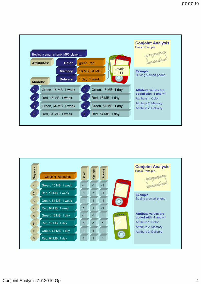
Part-worth utilities of individual attributes are calculated based on the ranking of a defined set of combinations of attribute values.

07.07.10

Conjoint Analysis 7.7.2010 Gp 4

Attributes: Color

Memory

Delivery

green, red

16 MB, 64 MB

1 day, 1 week

Green, 16 MB, 1 week1

Red, 16 MB, 1 week 2

Green, 64 MB, 1 week3

Red, 64 MB, 1 week4

Models:

5 Green, 16 MB, 1 day

6 Red, 16 MB, 1 day

7 Green, 64 MB, 1 day

8 Red, 64 MB, 1 day

Buying a smart phone, MP3 player…

Levels:-1; +1

Conjoint AnalysisBasic Principle

Attribute 1: ColorAttribute 2: MemoryAttribute 2: Delivery

Attribute values are coded with -1 and +1

ExampleBuying a smart phone

Red, 64 MB, 1 day8

Green, 64 MB, 1 day7

Red, 16 MB, 1 day6

Green, 16 MB, 1 day5

Red, 64 MB, 1 week4

Green, 64 MB, 1 week3

Red, 16 MB, 1 week 2

Green, 16 MB, 1 week1

-1 -1 1

1 -1 1

-1 1 1

1 1 1

-1 -1 -1

1 -1 -1

-1 1 -1

1 1 -1

Col

or

Mem

ory

Del

iver

y

“Conjoint” AttributesSeq

uenc

e Conjoint AnalysisBasic Principle

Attribute 1: ColorAttribute 2: MemoryAttribute 2: Delivery

Attribute values are coded with -1 and +1

ExampleBuying a smart phone

07.07.10

Conjoint Analysis 7.7.2010 Gp 5

-1 -1 1

1 -1 1

-1 1 1

1 1 1

-1 -1 -1

1 -1 -1

-1 1 -1

1 1 -1k attributes: 2k combinations

Design MatrixFull factorial design

Conjoint AnalysisBasic Principle

k attributes: 2k possible combinations

Full factorial Design

Design Matrix

8

7

6

5

4

3

2

1

-1 -1 1

1 -1 1

-1 1 1

1 1 1

-1 -1 -1

1 -1 -1

-1 1 -1

1 1 -1

X1 X2 X3

8

4

7

3

5 6

21colorX1

memory

X2

deliv

ery

X3

Conjoint AnalysisBasic Principle

Full factorial Design

X1: Color = (+1,-1)X2: Memory = (+1,-1)X3: Delivery = (+1,-1)

Graphical Representation ofCombinations

07.07.10

Conjoint Analysis 7.7.2010 Gp 6

Red, 64 MB, 1 day8

Green, 64 MB, 1 day7

Red, 16 MB, 1 day6

Green, 16 MB, 1 day5

Red, 64 MB, 1 week4

Green, 64 MB, 1 week3

Red, 16 MB, 1 week 2

Green, 16 MB, 1 week1

-1 -1 1

1 -1 1

-1 1 1

1 1 1R

ank

-1 -1 -1

1 -1 -1

-1 1 -1

1 1 -1

“Conjoint” AttributesSeq

uenc

e

6

5

2

1

8

7

4

3

X1 X2 X3

Conjoint AnalysisBasic Principle

Ranking of combinations

X1: Color = (+1,-1)X2: Memory = (+1,-1)X3: Delivery = (+1,-1)

Linear model function with part-worth utilities

Ranking = part-worth of attribute 1 * attribute 1 levelRanking = part-worth of attribute 1 * attribute 1 level+ part-worth of attribute 2 * attribute 2 level

Ranking = part-worth of attribute 1 * attribute 1 level+ part-worth of attribute 2 * attribute 2 level+ part-worth of attribute 3 * attribute 3 level

Ranking = part-worth of attribute 1 * attribute 1 level+ part-worth of attribute 2 * attribute 2 level+ part-worth of attribute 3 * attribute 3 level+ baseline preference

Y = βcolor*X1 + βmemory*X2 + βdelivery*X3 + µ

Conjoint AnalysisBasic Principle

Linear Model Function

X1: Color = (+1,-1)X2: Memory = (+1,-1)X3: Delivery = (+1,-1)

The system of linear equations can be solvedwith linear regression

07.07.10

Conjoint Analysis 7.7.2010 Gp 7

Ran

k

Part-worth utilities

-1 -1= * βColor + βMemory -1+* βDelivery* + µ8

1 -1 -1

… … …

7

-1 -1 1

1 -1 1

-1 1 1

1 1 1

-1 1 -1

1 1 -1

… … …6

5

2

1

4

3

Conjoint AnalysisBasic Principle

Linear Model Function

The system of linear equations can be solvedwith linear regression

8

4

7

3

5 6

21

8

7

6

5

4

3

2

1

-1 -1 1

1 -1 1

-1 1 1

1 1 1

-1 -1 -1

1 -1 -1

-1 1 -1

1 1 -1

X1 X2 X3

6

5

2

1

8

7

4

3

Ran

k

Conjoint AnalysisBasic Principle

Graphical Representation ofCombinations

07.07.10

Conjoint Analysis 7.7.2010 Gp 8

Main effect X1

8

7

6

5

4

3

2

1

-1 -1 1

1 -1 1

-1 1 1

1 1 1

-1 -1 -1

1 -1 -1

-1 1 -1

1 1 -1

X1 X2 X3

6

5

2

1

8

7

4

3

Ran

k

βCol=

7

1

3

5

8

4

2

6

X1

1616 - 20¼ [16 - 20]¼ [16 - 20] ÷2 = -0.5

Conjoint AnalysisBasic Principle

Calculating Part-worth Utilities

βColor = - 0.5

Graphical Representation ofCombinations

βMem= 1010 - 26¼ [10 - 26] ÷2 =

Main effect X2

8

7

6

5

4

3

2

1

-1 -1 1

1 -1 1

-1 1 1

1 1 1

-1 -1 -1

1 -1 -1

-1 1 -1

1 1 -1

X1 X2 X3

6

5

2

1

8

7

4

3

Ran

k

-2

8

4

7

3

5 6

21X2

Conjoint AnalysisBasic Principle

βMemory = - 2βColor = - 0.5

Calculating Part-worth Utilities

Graphical Representation ofCombinations

07.07.10

Conjoint Analysis 7.7.2010 Gp 9

Main effect X3

8

7

6

5

4

3

2

1

-1 -1 1

1 -1 1

-1 1 1

1 1 1

-1 -1 -1

1 -1 -1

-1 1 -1

1 1 -1

X1 X2 X3

6

5

2

1

8

7

4

3

Ran

k

βDel=

X3

87

5 6

43

21

1414 - 22¼ [14 - 22] ÷2 = -1

Conjoint AnalysisBasic Principle

βDelivery = - 1βMemory = - 2βColor = - 0.5

Calculating Part-worth Utilities

Graphical Representation ofCombinations

-1βDel=

8

4

7

3

5 6

21

Part-worth utilities

βMem= -2

-0.5βColor=

Conjoint AnalysisBasic Principle

βDelivery = - 1βMemory = - 2βColor = - 0.5

Calculating Part-worth Utilities

Graphical Representation ofCombinations

07.07.10

Conjoint Analysis 7.7.2010 Gp 10

0

1

2

3

4

5

6

7

8

9

1 week 1 week 1 week 1 week 1 day 1 day 1 day 1 day

16 MB 16 MB 64 MB 64 MB 16 MB 16 MB 64 MB 64 MB

green red green red green red green red

RankModel

Actual ranking and description with linear model function

Conjoint AnalysisBasic Principle

Ranking and Model Function

βDelivery = - 1βMemory = - 2βColor = - 0.5

0

1

2

3

4

5

6

7

8

9

1 week 1 week 1 week 1 week 1 day 1 day 1 day 1 day

16 MB 16 MB 64 MB 64 MB 16 MB 16 MB 64 MB 64 MB

green red green red green red green red

RankModel

Y = 4.5 -0.5 Xcolor -2 XMemory -1 XDelivery

Actual ranking and description with linear model function

Conjoint AnalysisBasic Principle

βDelivery = - 1βMemory = - 2βColor = - 0.5

Ranking and Model Function

07.07.10

Conjoint Analysis 7.7.2010 Gp 11

8

4

7

3

5 6

21

Variations for Xi=±1

±1·βMem= ±2 = 4

±0.5 = 1±1 ·βCol =

±1 = 2±1·βDel=

7

Delivery 29%2÷7 =

Memory 57%4÷7 =

Color 14%1÷7 =

Conjoint AnalysisBasic Principle

Calculating relative preferences

Attributes Criteria, Sub-criteria - comparison

Levels

Part-worth Utilities

Ranking

Weights: Principal Eigenvector

Ratio Scale, relative Scale

Evaluation of Alternatives

Conjoint Analysis AHP

Comparisonsk2 – k2

Combinations2k

k=4: 16 possible combinations k=4: 6 pair-wise comparisons

Conjoint AnalysisBasic Principle

Conjoint Analysis &Analytic Hierarchy Process AHP

07.07.10

Conjoint Analysis 7.7.2010 Gp 12

8

7

6

5

4

3

2

18

4

2

6

7

5

1

3

-1 -1 1

1 -1 1

-1 1 1

1 1 1

-1 -1 -1

1 -1 -1

-1 1 -1

1 1 -1

6

5

2

1

8

7

4

3

Ran

k

X1 X2 X3

Conjoint AnalysisBasic Principle

Fractional Design

8

7

6

5

4

3

2

18

4

2

6

7

5

1

3

-1 -1 1

1 -1 1

-1 1 1

1 1 1

-1 -1 -1

1 -1 -1

-1 1 -1

1 1 -1

6

5

2

1

8

7

4

3

Ran

k

X1 X2 X3

Conjoint AnalysisBasic Principle

Fractional Design

Graphical Representation

07.07.10

Conjoint Analysis 7.7.2010 Gp 13

8

5

3

2

8

4

2

6

7

5

1

3

-1 -1 1

1 1 1

1 -1 -1

-1 1 -1

Fractional design23-1

6

1

7

4

Ran

k

X1 X2 X3

Conjoint AnalysisBasic Principle

Fractional Design

Graphical Representation

23-13

4 III

±3 = 12

4

1

3

2 4

3

2

1

-1 -1 1

1 1 1

1 -1 -1

-1 1 -1

Fractional design23-1

6

1

7

4

Ran

k

X1 X2 X3

Conjoint AnalysisBasic Principle

Fractional Design

Graphical Representation

07.07.10

Conjoint Analysis 7.7.2010 Gp 14

4

3

2

1

-1 -1 1

1 1 1

1 -1 -1

-1 1 -1

2

3

4

1

Main effect X1

6

1

7

4

Ran

k

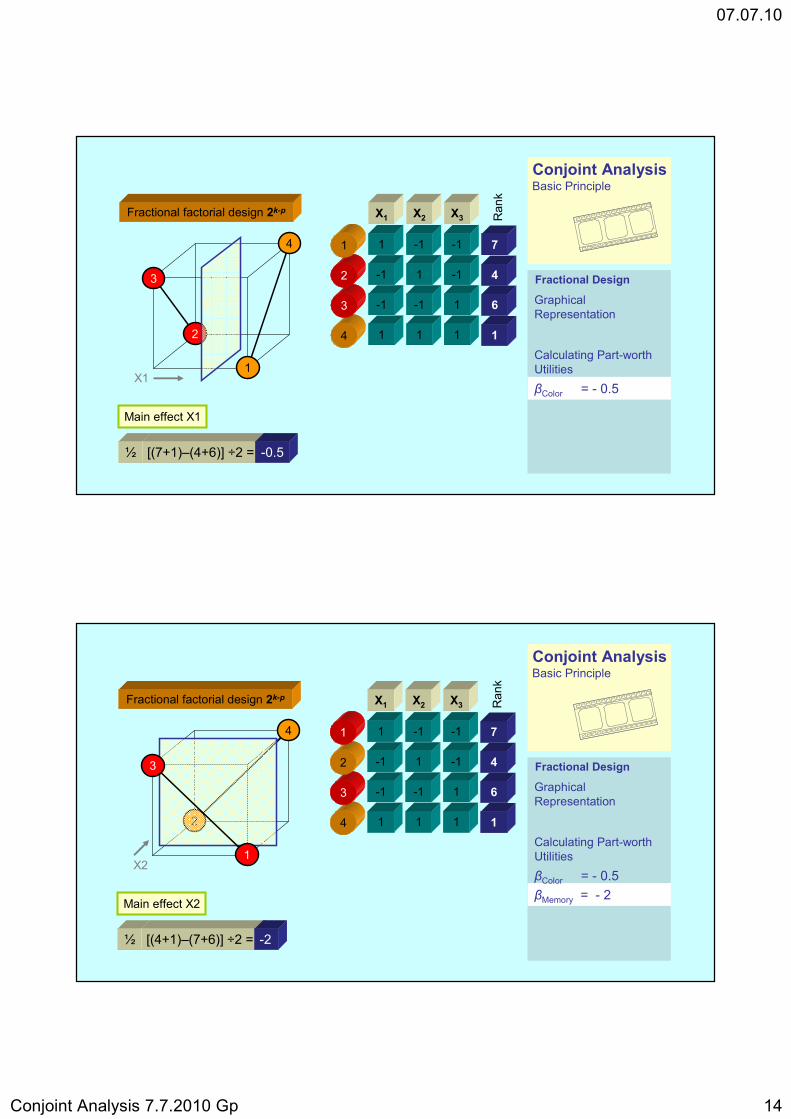
½ [(7+1)–(4+6)] ÷2 = -0.5

Fractional factorial design 2k-p

X1

X1 X2 X3

Conjoint AnalysisBasic Principle

Fractional Design

βColor = - 0.5

Graphical Representation

Calculating Part-worth Utilities

4

3

2

1

-1 -1 1

1 1 1

1 -1 -1

-1 1 -1

2

4

3

1

Main effect X2

6

1

7

4

Ran

k

½ [(4+1)–(7+6)] ÷2 = -2

Fractional factorial design 2k-p

X2

X1 X2 X3

Conjoint AnalysisBasic Principle

Fractional Design

βMemory = - 2βColor = - 0.5

Calculating Part-worth Utilities

Graphical Representation

07.07.10

Conjoint Analysis 7.7.2010 Gp 15

4

3

2

1

-1 -1 1

1 1 1

1 -1 -1

-1 1 -1

Main effect X3

2

1

4

3

6

1

7

4

Ran

k

½ [(6+1)–(7+4)] ÷2 = -1

Fractional factorial design 2k-p

X3

X1 X2 X3

Conjoint AnalysisBasic Principle

Fractional Design

βDelivery = - 1βMemory = - 2βColor = - 0.5

Graphical Representation

Calculating Part-worth Utilities

Conjoint AnalysisBasic Principle

Fractional Design

Using a fractional factorial design the number of attribute combinations can be reduced.

07.07.10

Conjoint Analysis 7.7.2010 Gp 16

Conjoint AnalysisBasic Principle

Simple conjoint analysiscan be done with linearregression, but more sophisticated statisticalmodels and solutionsare available.