connectflow technical summary - foster wheeler technical summary release 11 ... steady-state and...

$: ConnectFlow Technical Summary - Foster Wheeler Technical Summary Release 11 ... steady-state and time-dependent behaviour; ... Simulation of fluid flow and transport in fractured rock$
AMEC Public

ConnectFlow Technical Summary Release 11.0

Date: June 2013

From: AMEC

Our Reference: AMEC/ENV/CONNECTFLOW/15

AMEC/ENV/CONNECTFLOW/15 Page 2

AMEC Public

Title ConnectFlow Technical Summary Our Reference

AMEC/ENV/CONNECTFLOW/15

Confidentiality, copyright & reproduction

Copyright Energy, Safety and Risk Consultants (UK) Limited, part of AMEC plc. All rights reserved. This computer program is protected by copyright law and international treaties. Save as permitted under the Copyright Designs and Patents Act 1988, or the terms of any licence granted by the copyright owner, no part of this program may be used, reproduced, distributed or modified in any way. Warning: Any unauthorised act, including reproduction or distribution of this program or any portion of it, may result in both a civil claim for damages and criminal prosecution.. To minimise our impact on the environment, AMEC uses paper from sustainable sources

Contact Details AMEC Building 150 Harwell Oxford Didcot Oxfordshire OX11 0QB United Kingdom Tel +44 (0) 1635 280300 Fax +44 (0) 1635 280301 amec.com


AMEC Public

Contents

1 Introduction 10

1.1 User Interface 10 1.2 Availability 12 1.3 The iCONNECT Club 12 1.4 Documentation 12

2 Concepts within the Model 13

2.1 Nesting of sub-models 13 2.2 Representation of fractures 15 2.3 Current physics 19

2.3.1 CPM physics 19 2.3.2 DFN physics 20 2.3.3 ConnectFlow (Nested DFN/CPM) physics 20

2.4 Boundary conditions 22 2.4.1 NAPSAC equations 22 2.4.2 NAMMU Equations 22

2.5 Interface Conditions 22 2.5.1 Approach 1 (`Mass-Lumping') 22 2.5.2 Interface conditions -- approach 2 (`Distributed Flux') 23

2.6 Transport 24


AMEC Public

Preface ConnectFlow is the suite of AMEC’s groundwater modelling software that includes the NAMMU continuum porous medium (CPM) module and the NAPSAC discrete fracture network (DFN) module. ConnectFlow is also the name given to the concept of nesting NAMMU and NAPSAC sub-models into a combined CPM/DFN model. Hence, ConnectFlow is very flexible tool for modelling groundwater flow and transport in both fractured and porous media on a variety of scales. This document provides a general overview of ConnectFlow, including a description of the equations solved and the numerical methods used. This document describes technical aspects of building and solving nested CPM/DFN models. The technical features of the current release of NAMMU and NAPSAC are described in separate documents. Additional more detailed information about the capabilities and potential applications of ConnectFlow is available from AMEC on request. The following documentation is available for ConnectFlow:

ConnectFlow Technical Summary Document;

ConnectFlow Command Reference Manual;

ConnectFlow Installation and Running Guide. The following documentation is available for NAMMU:

NAMMU Technical Summary Document;

NAMMU Command Reference Manual;

NAMMU Verification Document;

NAMMU Installation and Running Guide. The following documentation is available for NAPSAC:

NAPSAC Technical Summary Document;

NAPSAC Command Reference Manual;

NAPSAC Verification Document;

NAPSAC Installation and Running Guide.

Combined Capabilities ConnectFlow is the module that allows nested models containing regions of continuum porous medium (CPM) models and discrete feature network (DFN) models to be constructed. It is also the name of the suite of software that includes the CPM only model NAMMU and the DFN only module NAPSAC.

Combined (CPM/DFN) Capabilities ConnectFlow is the module that is based on a nested CPM/DFN concept. ConnectFlow has been developed over a period of more than 10 years. It is developed under a rigorous quality system that conforms to the international standards ISO 9001 and TickIT. ConnectFlow can be used to model the following physics and geometries:

3D models only;

single or multiple DFN sub-regions nested within CPM regions;

single CPM sub-regions nested within DFN region;


AMEC Public

stratigraphic layers with DFN representation can be interfaced to layers with a CPM representation;

models are built up of grids with different patches being assigned to either a CPM or DFN subdomain;

nesting of detailed DFN models within nested CPM models using embedded (‘constraint’) grids to represent site-scale and region-scales;

stochastic DFN and CPM models;

steady-state and transient constant-density groundwater flow;

advective transport through a combined DFN/CPM based on a particle tracking approach. ConnectFlow can be used to model the following features:

local DFN models to represent the detailed flow in fractures around tunnels, shafts, canisters or boreholes nested within a CPM model that extends the model to appropriate boundaries;

detailed CPM models of tunnels, shafts and canisters within a DFN model to represent the interaction between flow in a fractured media and backfilled tunnels;

continuous representation of deterministic faults/fracture zones through the DFN and CPM sub-models using consistent data formats and a combination of explicit fracture planes in DFN regions and an implicit fracture zone (IFZ) method in the CPM region.

quantifying conceptual uncertainties between DFN and CPM models.

Continuum Porous Medium (CPM) Capabilities NAMMU is the module that is based on a CPM representation. NAMMU has been developed over a period of more than 20 years and has been verified extensively in international comparison exercises. It is developed under a rigorous quality system that conforms to the international standards ISO 9001 and TickIT. NAMMU can be used to model the following physics and geometries:

groundwater flow in saturated and unsaturated conditions;

saline groundwater flow with density dependent on concentration;

coupled groundwater flow and heat transport with density dependent on temperature;

saline groundwater flow and heat transport with density dependent on concentration and temperature;

groundwater in a dual porosity system based on the Warren and Root model;

contaminant transport, including the effects of advection, dispersion, sorption and with solubility limitations;

radioactive decay chains, including interacting chains linked by solubility limitation of a common radionuclide;

flow and transport in 3D, 2D vertical sections, 2D areal and 2D radial geometries;

steady-state and time-dependent behaviour;

deterministic and stochastic continuum modelling;

sensitivity to model parameters, using the adjoint sensitivity method. NAMMU can be used to model the following features:

complex lithology distributions;

conductive and semi-impermeable fracture zones;


AMEC Public

stochastic models of permeability and porosity;

3D volumes of enhanced or reduced permeability;

boreholes, tunnels and shafts both in terms of geometry and as boundary conditions;

specified value (Dirichlet) and specified flux (Neumann) type boundary conditions;

non-linear infiltration model of surface recharge/discharge areas and magnitude;

hydrostatic boundary condition and outflow conditions for vertical boundaries;

time-varying boundary conditions to model land uplift, or time-dependent contaminant discharge;

sources of heat, salinity or contaminant at points or in volume. NAMMU models and results can be displayed by:

3D visualisation system (GeoVisage for NAMMU) allows 3D rendering of finite-elements, rock types, permeability, variables, fracture zones, flow arrows, pathlines;

2D plot output and numerical output includes:

views of finite-element meshes and boundaries;

2D slices through to show the mesh or contours of variables (head, salinity, etc.);

plots of the mesh and variables on surfaces;

velocity arrows showing direction of flow and magnitude;

line graphs and data graphs;

calculation of integrals (e.g. flux across a plane);

pathlines in steady-state and transient flows;

backward pathlines to the show region of influence for a borehole;

time evolution of a variable at a point. NAMMU models have been used in the following applications:

safety assessment calculation in support of radioactive waste disposal programmes;

modelling in support of groundwater protection schemes;

modelling of landfills;

regional groundwater flow;

aquifer contamination;

site investigation;

pump test simulation;

tracer tests;

saline intrusion;

design and evaluation of remediation strategies. NAMMU is used in support of the radioactive waste disposal programmes of many countries throughout the world, by both the nuclear regulators and by national disposal organisations and consultants working for these organisations. NAMMU has a wide range of facilities for specifying the model domain, the properties of the rocks, fluids and solutes within the domain, the equations to be solved and the output options required. The advanced 3D visualisation package, GeoVisage, is available for NAMMU. In addition to these standard facilities, many options are available that allow the user to customise the functionality of


AMEC Public

NAMMU for a particular project. For example, it is possible for the user to specify a site-specific relationship between fluid density, solute concentration, fluid temperature and pressure.

Discrete FRACTURE Network (DFN) Capabilities NAPSAC is the module that is based on a DFN representation.

NAPSAC has been developed over a period of more than 15 years and has been verified extensively in international comparison exercises (e.g. STRIPA and TRUE block). It is developed under a rigorous quality system that conforms to the international standards ISO 9001 and TickIT. Simulation of fluid flow and transport in fractured rock is an essential tool for the study of water resources, oil and gas reservoir management, assessment of underground waste disposal facilities, evaluation of hot dry rock reservoirs, and for the characterisation and remediation of contaminated land management. It can be used to interpret field and laboratory data, to validate conceptual models, to make quantitative predictions, and to develop practical solutions for a range of environmental, reservoir engineering, and civil engineering problems. NAPSAC is a finite-element software package for modelling fluid flow and transport in fractured rock. A discrete fracture network (DFN) approach is used to model fluid flow and transport of tracers and contaminants through the fractured rock. NAPSAC incorporates fracture generation, flow simulation, upscaling, transport and 3D graphics capabilities using GeoVisage. The Graphical User Interface to NAPSAC allows models to be generated and analysed quickly. A job submission (‘batch’) facility is included in the GUI that allows additional options not yet implemented in the GUI to accessed - these features are indicated below

†.

NAPSAC has been developed over a 15-year period and has developed a number of sophisticated capabilities including: Geological modelling:

NAPSAC has the flexibility to model a variety of scales varying from well/borehole scale to the regional/reservoir scales. Detail can be included to model heterogeneity of a single heterogeneous fracture as well as models with many tens to millions of fractures at a regional or reservoir scale.

the DFN approach allows users to compare aspects of their conceptual geologic models and field observations with simulated models. This comparison includes, fracture orientation, size, transmissivity and flow distribution. An examination of the simulated network can be performed using hypothetical cores, stereonets, fracture maps and connectivity analysis.

generation of regular and irregular meshes and structural grids (e.g. ZMap, VIP, FEMGEN and a CAD format);

inclusion of deterministic fractures by specification within the NAPSAC data or by importing a fracture file (e.g. GOCAD Vset, GOCAD Tsurf, Seisworks pointsets and other international formats). Deterministic Faults (or structures) can be used to control populations of stochastic fractures (i.e. proximity or ‘Damage Zone' models). For example, NAPSAC allows the clustering of fractures around parent fractures, random points or surfaces. NAPSAC allows spatially varying fracture densities based on 3D maps of fracture drivers;

variable distribution laws for stochastic fracture parameters. NAPSAC can generate stochastic fractures from a wide variety of probability distribution functions. Not just Fractal!

coupling of distributions/parameters to same features i.e. length-aperture relationships.

areal / volumetric distribution of stochastic fractures can be imported from external map or grid data- e.g. bed thickness, curvature (‘strain’), lithological (mechanical) variation.

dynamic behaviour of ‘production fractures’ and present-day stress can be incorporated.


AMEC Public

all scale ranges, from core observation to seismic scale, can be simulated and integrated into the final model.

high permeability ‘matrix streaks’ may be incorporated into models as extra flow conduits.

flow in the matrix can be represented by additional flow channels. NAPSAC is able to:

simulate steady-state or transient flow in a fracture-network;

enable steady-state calculations to be perform on very large networks, because it uses an efficient finite-element scheme;

calculate the full equivalent continuum permeability tensor including off-diagonals, principal values and directions. This is automated to sample flows in several different directions. This can be used for upscaling, analysis of scale dependencies and determination of the representative elementary volume (REV);

calculate porosity and inter-fracture matrix block size;

identify connected fracture clusters around wells;

predict transient pressures and drawdowns at well bores for various types of pump tests;

calculate steady-state and transient inflows to tunnels and shafts;

calculate the effects of hydro-mechanical coupling. The hydraulic aperture is coupled to a stress distribution based on an analytical description of the stress field due to either rock overburden or a radial stress around a tunnel;

simulate tracer transport through the network using a stochastic particle tracking method. Output

† includes plots of breakthrough curves for many thousands of particles, particle

tracks, swarms of particles at specified times or the points of arrival on the surfaces of the model. This can be used to calculate dispersion of a solute transported by the groundwater;

simulate mass transport for a variable density fluid. This can be used to model coupled groundwater flow and salt transport

†;

simulate unsaturated flow in fractured rocks;

†analysis of percolation between surfaces;

NAPSAC can be used for the following applications:

simulation of a range of hydrogeological tests (hydraulic borehole/well tests, including constant, head, pressure and flow tests);

site and regional scale modelling to determine the effects of various forms of fracture flow to determine, pressure distributions, flows and travel times to discharge points under natural conditions;

to understand and simulate the behaviour of fracture-influenced sites/reservoirs by being able to parameterise and justify heterogeneous continuum models. For example, the estimation of equivalent parameters for input to conventional dual-porosity simulators;

simulation of solute transport (tracer) experiments;

simulation of hydraulic impact of a tunnel or shaft construction;

simulation of various simple hydromechanical models for the purpose of estimating the impact of rock overburden and insitu stress.

NAPSAC has been used in the following industries:

water resources for the purpose of hydraulic test and tracer simulation, fractured reservoir estimation and parameterisation, and remediation studies (such as the estimation of fracture flow in dual porosity systems). In addition, it can be used to model saline ingression and unsaturated flow;


AMEC Public

deep radioactive waste disposal, as both a tool useful for site-characterisation and safety assessments (simulation of hydrogeological tests and estimation of flow distributions and travel times to the biosphere);

oil and gas industry to aid well planning, simulation of various well tests (PBU etc), and the parameterisation of oil simulation software by calculation of up-scaled equivalent continuum parameters (permeability, porosity and matrix block-size and distribution);

hot-dry rock studies to estimate connectivity and parameters (permeabilities), to help analyse the effectiveness of the fractured reservoir;

civil engineering projects concerned with construction or remediation in fractured rock. This includes the estimation of water ingress due to excavation of tunnels, studies of underground oil caverns, dam construction in fractured rocks, remediation or containment of contaminated fractured sites.


AMEC Public

1 Introduction ConnectFlow is the suite of AMEC’s groundwater modelling software that includes the NAMMU continuum porous medium (CPM) module and the NAPSAC discrete fracture network (DFN) module. ConnectFlow is also the name given to the concept of nesting NAMMU and NAPSAC sub-models into a combined CPM/DFN model. Hence, ConnectFlow is very flexible tool for modelling groundwater flow and transport in both fractured and porous media on a variety of scales. This document provides a general overview of ConnectFlow, including a description of the equations solved and the numerical methods used. Additional more detailed information about the capabilities and potential applications of ConnectFlow is available from AMEC on request.

1.1 User Interface Input to ConnectFlow is specified using a structured free-format input language, which has been designed to be readily comprehensible to the user. The commands in ConnectFlow are the super-set of commands in NAMMU and NAPSAC. A modification is necessary to the top-level NAPSAC commands though to distinguish them from the NAMMU commands as follows:

>> SET LIMITS >> SET NAPSAC LIMITS

>> DATA INPUT >> NAPSAC DATA INPUT

>> MODIFY MODEL >> NAPSAC MODIFY MODEL

>> CALCULATION >> NAPSAC CALCULATION

>> OUTPUT DATA >> NAPSAC OUTPUT DATA

The full set of ConnectFlow commands and their syntax is recorded in the Command Reference Manual that is available as an on-line HTML document. Hypertext links are used in such a way as to show the hierarchy of commands. The ConnectFlow executable can be used to run pure NAMMU (>> NAMMU), pure NAPSAC (>> NAPSAC) or combine ConnectFlow (>> CONNECTFLOW) input datasets using the top-level commands as indicated. Jobs can be run in batch using a command line executable on either Unix or Windows. Alternatively, the Graphical User Interface (GUI) is available for both creating input data and submitting jobs to a specified processor.

Figure 1-1: ConnectFlow GUI console window

The intention of the GUI is to make it easier for the new user to define a model without having learn the input language structure and syntax. The GUI is organised in object based approach where objects represent the base building blocks of a model such as grids, fracture sets, deterministic fracture zones, lithological units etc. The GUI provides a framework for defining the properties of each object side using windows, and storing the data within a project. A particular model is then a collection of objects. The input commands to define the model are created automatically when a job is run as a pre-processing step.


AMEC Public

Figure 1-2: The ConnectFlow window for defining rock properties. This makes it simple to

define whether a rock is to represented by CPM or DFN concepts.

The GUI has been designed so that is very simple to create alternative concepts within the same domain, such that it is fast to switch between CPM, DFN and combined DFN/CPM models. The steps in setting up a ConnectFlow model typically are as follows:

1. Set up a model domain made up of cells or patches with each cell/patch assigned to a rock type.

2. For each rock, select which type of representation, CPM or DFN, is to be used. Define the hydrogeological parameters e.g. permeability, porosity. There may be several instances of a rock type with either different concepts or properties to quantify conceptual and parametric uncertainties.

3. Define deterministic fracture geometries and parameters.

4. Define stochastic fracture sets.

5. Create a model by selecting a domain, the instances of each rock, fracture objects and boundary conditions.

6. Solve for flow and transport for the model. There are other facilities available in ConnectFlow, such as exporting fracture geometries and upscaling DFN models to obtain equivalent CPM permeabilities. The output from ConnectFlow currently takes four forms:


AMEC Public

text files containing information about the model, the performance of the solver and any output options requested;

ASCII files used to export results such as transport statistics, fracture geometries, upscaled equivalent permeabilities from DFN models;

postscript graphics files.

1.2 Availability ConnectFlow is written in standard FORTRAN 95 and is therefore portable across a wide range of computers. ConnectFlow is supported on a range of computer platforms, from desktop PCs running windows to Unix mainframes. The software is available from AMEC by contacting the support team [email protected] or from a download at www.connectflow.com. ConnectFlow is primarily available through the international collaboration within the iCONNECT Club.

1.3 The iCONNECT Club The iCONNECT club (integrated CONtinuum and NEtwork approach to groundwater flow and Contaminant Transport) is AMEC’s response to the desire expressed by those involved in radioactive waste management to address a range of generic and site-specific issues related to the evaluation of the geosphere as part of a safety assessment. The purpose of the iCONNECT club is to draw like-minded organisations together into a club in order to dilute the costs of addressing modelling issues, in particular those generic issues faced by organisations wanting to evaluate the performance of the geosphere as part of a repository safety assessment. The iCONNECT club will act as a forum for the focused application and enhancement of the ConnectFlow methodology, resulting in wide-ranging benefits to all participants.

1.4 Documentation A comprehensive set of documentation has been produced for ConnectFlow. The following manuals are available:

1. ConnectFlow Technical Summary Document (this document). This document provides a general technical overview of the software, including a description of the equations solved and the numerical methods used.

2. ConnectFlow Installation and Running Guide. This document describes how to install and run ConnectFlow on the various computer platforms supported.

3. ConnectFlow Verification Document. This document describes the testing of ConnectFlow’s capabilities.

4. ConnectFlow Reference Manual. This document describes in detail the commands and keywords available in the ConnectFlow input language used to specify the model, the finite-element equations to be solved, and the post-processing required. This document is available in an electronic on-line form, which has the advantage of cross-referencing using hypertext links.


AMEC Public

2 Concepts within the Model

2.1 Nesting of sub-models

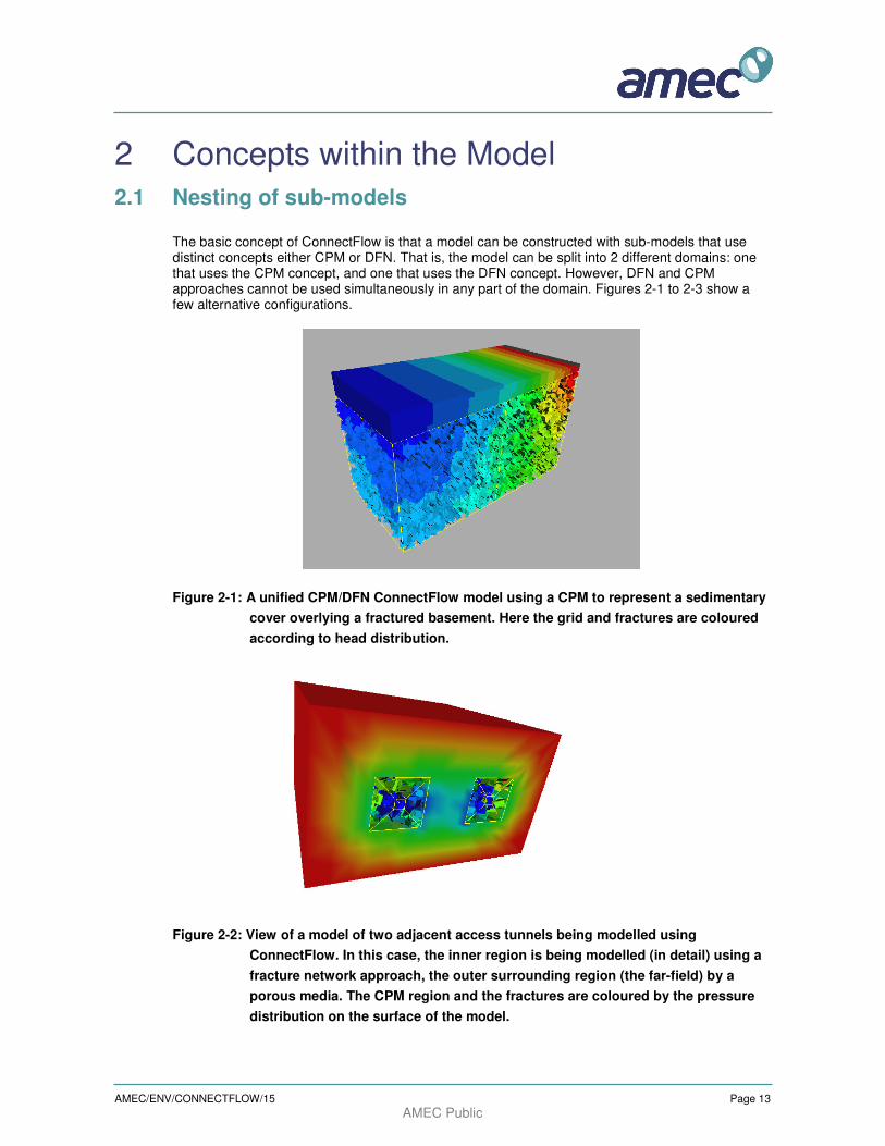
The basic concept of ConnectFlow is that a model can be constructed with sub-models that use distinct concepts either CPM or DFN. That is, the model can be split into 2 different domains: one that uses the CPM concept, and one that uses the DFN concept. However, DFN and CPM approaches cannot be used simultaneously in any part of the domain. Figures 2-1 to 2-3 show a few alternative configurations.

Figure 2-1: A unified CPM/DFN ConnectFlow model using a CPM to represent a sedimentary

cover overlying a fractured basement. Here the grid and fractures are coloured

according to head distribution.

Figure 2-2: View of a model of two adjacent access tunnels being modelled using

ConnectFlow. In this case, the inner region is being modelled (in detail) using a

fracture network approach, the outer surrounding region (the far-field) by a

porous media. The CPM region and the fractures are coloured by the pressure

distribution on the surface of the model.


AMEC Public

Figure 2-3: A CPM representation of a modelled tunnel (shown in the centre of the figure),

embedded within a DFN model. The different colours in the CPM model relate to

different properties for tunnel excavated damage zone, skin and actual tunnel.

Many fractures have been removed to more clearly illustrate the tunnel.

These figures illustrate the flexibility of ConnectFlow. The benefits of this flexibility include:

being able to use the most appropriate concept for different lithological units for sedimentary settings, e.g. a fracture basement covered by a sedimentary cover;

the ability to switch easily between concepts to quantify conceptual uncertainties in using a CPM versus DFN model to calculate performance measures;

in using a single software to implement DFN and CPM models it is easier to compare consistency between equivalent representations;

the flexibility to nest detailed models of important areas e.g. a fractured near-field within a much larger CPM domain to capture realistic boundary conditions and guarantee rigorous coupling between the sub-models;

the ability to nest an appropriate CPM representation of engineered structures, such as repositories within a detailed DFN model.

Again the ConnectFlow concept is that different regions can be represented in different ways and then formally nested together. This is different from the case where discrete fracture objects co-exist with a porous medium model of the rock matrix. Representations of the interaction between fractures and the rock matrix within the same domain can be represented in ConnectFlow, but it should be recognised that this is a quite different issue. Fracture/matrix interactions are dealt with in NAMMU and NAPSAC in different ways as described in the Technical Summary Documents for these modules. In a combined DFN/CPM model, flow in the DFN and CPM models is nested formally by internal boundary conditions at the interface between the two sub-regions. These boundary conditions are implemented as equations that ensure continuity of pressure and conservation of mass at the interface between the two sub-regions. On the DFN side of the interface, these boundary conditions are defined at nodes that lie along the lines (traces) that make up the intersections between fractures and the interface surface. On the CPM side, the boundary conditions are applied


AMEC Public

to nodes in finite-elements that abut the interface surface. Thus, extra equations are added to the discrete system matrix to link nodes in the DFN model to nodes in the finite-element CPM model. By using equations to ensure both continuity of pressure and continuity of mass, then a more rigorous approach to nesting is obtained than by simply interpolating pressures, say, between separate DFN and CPM models. The equations used in the nesting are described in Section 2.3.

2.2 Representation of fractures

In NAPSAC fractures are represented as explicit planar objects with either a rectangular or triangular shape. Each fracture plane is described by the following attributes:

1. Geometry: defined by centre position, strike, dip, orientation (a rotation within the plane of the fracture), strike length, dip length and shape. Alternatively, a fracture can be defined by the positions of its corners.

2. Flow properties: defined by either hydraulic aperture or transmissivity based on a parallel plate concept. Addition parameters include storativity and transport aperture, which are defined in terms of one of a choice of models and the associated parameters.

3. Additional: the fracture set is stored for each fracture. Also, fractures can be subdivided into subfractures to represent fracture roughness or channelling. In this case, a reference to the original unsubdivided fracture is stored.

Fractures can be generated in several ways either as deterministic fractures defined individually or as stochastic sets of fractures with their attributes defined in terms of probability distribution functions (PDFs) for each fracture attribute. Deterministic fractures can be input in terms defining the attributes of each fracture individually or by reading a formatted file.

The DFN concept is that fluid flow passes through a rock volume primarily via the interconnected network of fracture objects, there is no flow through the interfracture volumes. Hence, the DFN model has to include all fractures that contribute significantly to flow on the scale of interest. An example of a DFN model is shown in Figure 2-4. Fracture generation is described in the NAPSAC Technical Summary Document.


AMEC Public

Figure 2-4: An example of a simple DFN model within a cube. Here, two stochastic sets of

fractures are generated both sub-vertical but with different mean strikes.

Fractures are coloured by set.

In NAMMU fractures can be represented explicitly by including thin elements in the finite-element mesh. However, this is generally impractical in large regional-scale models for example, and so an alternative implicit fracture zone (IFZ) representation is implemented. In this method fractures, or fracture zones, are defined as discrete objects, but they are incorporated into the finite-element model by modifying the hydraulic properties (directional permeability and porosity) of finite-elements crossed by the fractures to represent the equivalent properties for the combined fracture/matrix system within each individual element.


AMEC Public

Figure 2-5: Application of CPM IFZ method for representing equivalent permeability of

regional-scale fracture zones in a deterministic model. Top: Finite-element grid

with fracture zones structures superimposed. Fracture zones that are coloured

red have a higher transmissivity than those coloured blue. Bottom: equivalent

permeability in each finite-element with fracture zones superimposed. Elements

are coloured according to the logarithm of permeability from red (high) to low

(blue).


AMEC Public

An example of the IFZ approach is shown in Figure 2-5. The implementation of the IFZ method is described in the NAMMU Technical Summary Document.

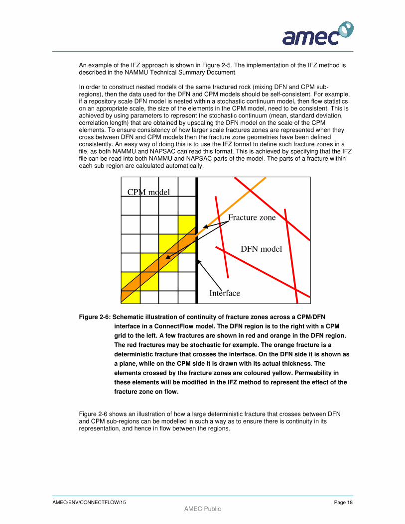
In order to construct nested models of the same fractured rock (mixing DFN and CPM sub-regions), then the data used for the DFN and CPM models should be self-consistent. For example, if a repository scale DFN model is nested within a stochastic continuum model, then flow statistics on an appropriate scale, the size of the elements in the CPM model, need to be consistent. This is achieved by using parameters to represent the stochastic continuum (mean, standard deviation, correlation length) that are obtained by upscaling the DFN model on the scale of the CPM elements. To ensure consistency of how larger scale fractures zones are represented when they cross between DFN and CPM models then the fracture zone geometries have been defined consistently. An easy way of doing this is to use the IFZ format to define such fracture zones in a file, as both NAMMU and NAPSAC can read this format. This is achieved by specifying that the IFZ file can be read into both NAMMU and NAPSAC parts of the model. The parts of a fracture within each sub-region are calculated automatically.

DFN model

Interface

CPM model

Fracture zone

Figure 2-6: Schematic illustration of continuity of fracture zones across a CPM/DFN

interface in a ConnectFlow model. The DFN region is to the right with a CPM

grid to the left. A few fractures are shown in red and orange in the DFN region.

The red fractures may be stochastic for example. The orange fracture is a

deterministic fracture that crosses the interface. On the DFN side it is shown as

a plane, while on the CPM side it is drawn with its actual thickness. The

elements crossed by the fracture zones are coloured yellow. Permeability in

these elements will be modified in the IFZ method to represent the effect of the

fracture zone on flow.

Figure 2-6 shows an illustration of how a large deterministic fracture that crosses between DFN and CPM sub-regions can be modelled in such a way as to ensure there is continuity in its representation, and hence in flow between the regions.


AMEC Public

2.3 Current physics

2.3.1 CPM physics

In CPM-only (NAMMU) models a wide range of physics is implemented including:

Saturated groundwater flow;

Unsaturated groundwater flow;

Dual porosity flow;

Coupled groundwater flow and salt transport (variable density flow);

Coupled groundwater flow and heat transport;

Radionuclide transport with chains, decay, sorption and solubility limitations;

Saturated groundwater flow in a porous medium is modelled in terms of Darcy’s law,

q = - . RkP

µ∇ Equation 2-1

and the equation of continuity,

∂

∂φρ ρ

t + .( ) = 0( )l l∇ q . Equation 2-2

where q is the Darcy velocity,

k is the permeability,

µ is the fluid viscosity,

P R is the residual pressure (see below),

φ is the porosity, and

ρ l is the fluid density.

These are combined to form a single second-order equation for the residual pressure,

∂

∂φρ ρ

µt - .( ) = 0R( ) .l l

kP∇ ∇ , Equation 2-3

and the flux for this pressure equation is

FP l= ρ q n. , Equation 2-4

where n is the outward normal to the boundary across which the flux is specified.

The residual pressure, PR is related to the total pressure P

T by the expression

P P g z zR T= + −ρ 0 0( ) ,


AMEC Public

where ρ 0 is a reference density, g is gravitational acceleration, z is height, and z0 is a reference

elevation.

The hydraulic head, h, is related to the residual pressure by

hP

g

R

=ρ 0

.

These are the basic equations that are solved by NAMMU. It is straightforward to formulate the pressure equation in terms of total pressure, residual pressure, or pressure head, and all three formulations are supported by NAMMU.

2.3.2 DFN physics

A more restricted range of physics is currently available in NAPSAC:

Saturated groundwater flow;

Unsaturated groundwater flow; The equation describing transient flow through a fracture-network is

Pg

T

t

P

g

S 2∇=∂

∂

ρρ , Equation 2-5 where T is the transmissivity of the fracture plane that according to the parallel plate law is related to the hydraulic aperture e by

µ

ρ

12

3ge

T −=, Equation 2-6

and S is the fracture storativity which is dependent both on fluid and rock compressibility. The choice of a suitable model for fracture storativity is important for an accurate transient flow model. Three models for fracture storativity are available in NAPSAC:

;gAeS ρ= Equation 2-7

];/1[ feCRKNgS += ρ Equation 2-8

.bTS α= Equation 2-9

Here A, RKN, Cf, α and β are constants that can be specified by the user.

2.3.3 ConnectFlow (Nested DFN/CPM) physics

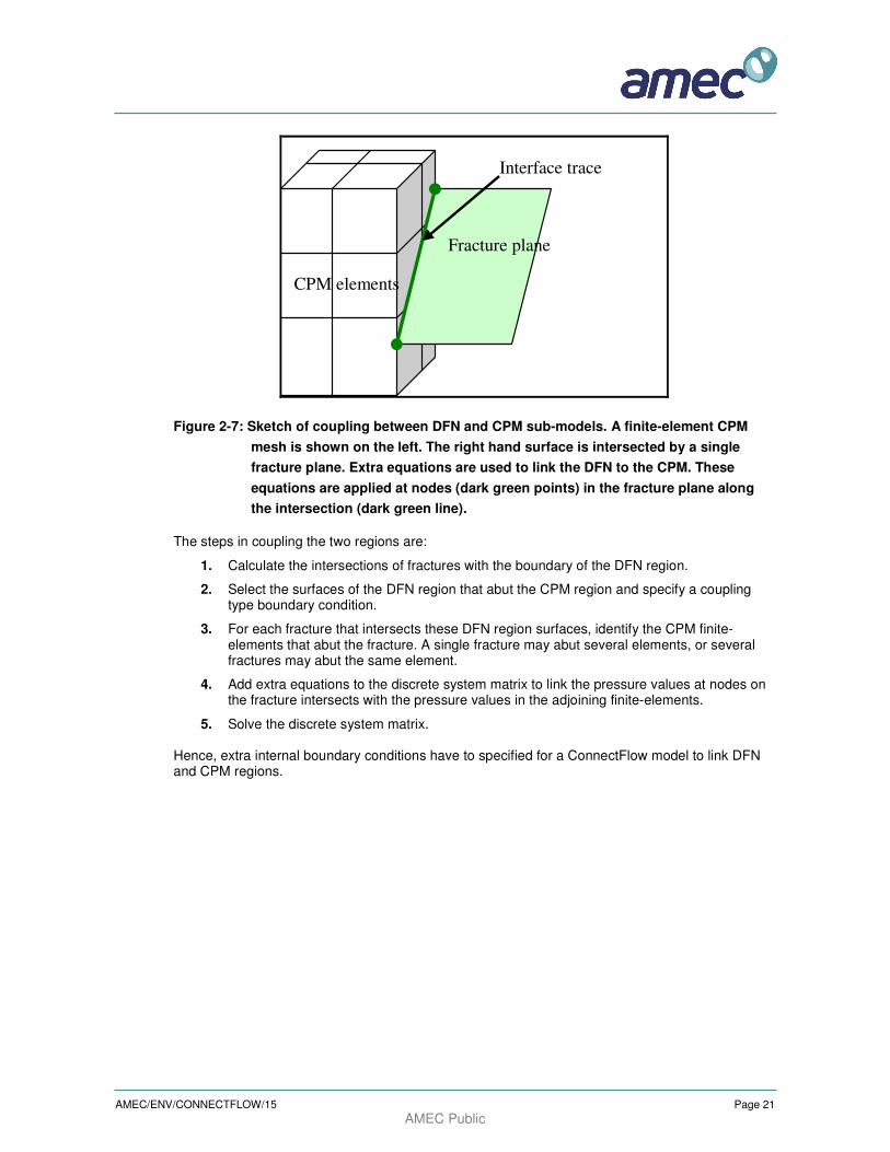
ConnectFlow only supports saturated groundwater flow with linear boundary conditions. The coupling between DFN and CPM regions at their common interface is implemented as additional equations that link residual pressure values at nodes in the fracture planes to pressure values in the CPM finite-element mesh. These equations ensure continuity in pressure and conservation of groundwater flux (i.e. mass flux) across the interface. Figure 2-7 shows this configuration.


AMEC Public

CPM elements

Fracture plane

Interface trace

Figure 2-7: Sketch of coupling between DFN and CPM sub-models. A finite-element CPM

mesh is shown on the left. The right hand surface is intersected by a single

fracture plane. Extra equations are used to link the DFN to the CPM. These

equations are applied at nodes (dark green points) in the fracture plane along

the intersection (dark green line).

The steps in coupling the two regions are:

1. Calculate the intersections of fractures with the boundary of the DFN region.

2. Select the surfaces of the DFN region that abut the CPM region and specify a coupling type boundary condition.

3. For each fracture that intersects these DFN region surfaces, identify the CPM finite-elements that abut the fracture. A single fracture may abut several elements, or several fractures may abut the same element.

4. Add extra equations to the discrete system matrix to link the pressure values at nodes on the fracture intersects with the pressure values in the adjoining finite-elements.

5. Solve the discrete system matrix. Hence, extra internal boundary conditions have to specified for a ConnectFlow model to link DFN and CPM regions.


AMEC Public

2.4 Boundary conditions

2.4.1 NAPSAC equations

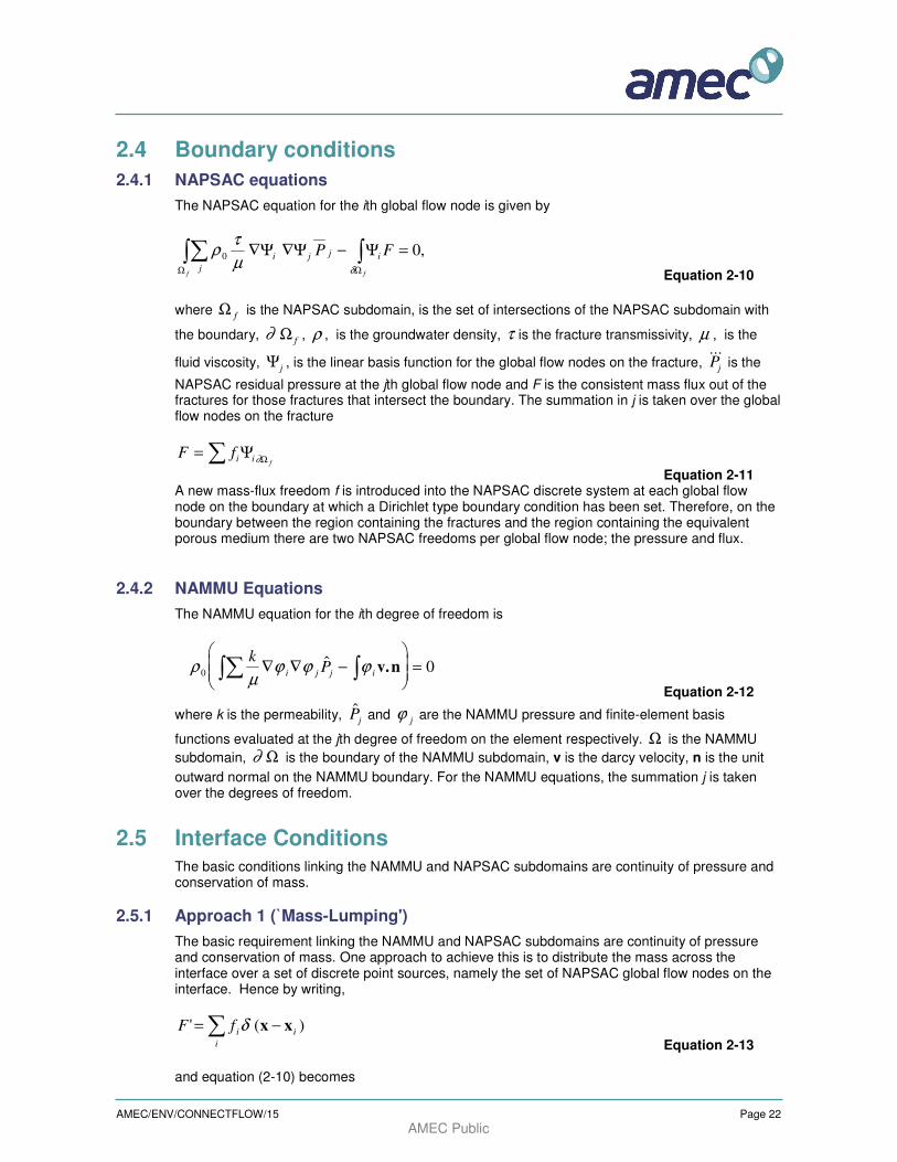
The NAPSAC equation for the ith global flow node is given by

ρτ

µδ

0 0j

i j j i

f f

P F∑∫ ∫∇Ψ ∇Ψ − =Ω Ω

Ψ ,

Equation 2-10

where Ω f is the NAPSAC subdomain, is the set of intersections of the NAPSAC subdomain with

the boundary, ∂ Ω f , ρ , is the groundwater density, τ is the fracture transmissivity, µ , is the

fluid viscosity, Ψj , is the linear basis function for the global flow nodes on the fracture, &&&Pj is the

NAPSAC residual pressure at the jth global flow node and F is the consistent mass flux out of the fractures for those fractures that intersect the boundary. The summation in j is taken over the global flow nodes on the fracture

F fi if

= ∑ ΨΩ∂

Equation 2-11 A new mass-flux freedom f is introduced into the NAPSAC discrete system at each global flow node on the boundary at which a Dirichlet type boundary condition has been set. Therefore, on the boundary between the region containing the fractures and the region containing the equivalent porous medium there are two NAPSAC freedoms per global flow node; the pressure and flux.

2.4.2 NAMMU Equations

The NAMMU equation for the ith degree of freedom is

ρµ

ϕ ϕ ϕ0 0k

Pi j j i∇ ∇ −

=∫∑∫ $ v.n

Equation 2-12

where k is the permeability, $Pj and ϕ j are the NAMMU pressure and finite-element basis

functions evaluated at the jth degree of freedom on the element respectively. Ω is the NAMMU

subdomain, ∂ Ω is the boundary of the NAMMU subdomain, v is the darcy velocity, n is the unit

outward normal on the NAMMU boundary. For the NAMMU equations, the summation j is taken over the degrees of freedom.

2.5 Interface Conditions The basic conditions linking the NAMMU and NAPSAC subdomains are continuity of pressure and conservation of mass.

2.5.1 Approach 1 (`Mass-Lumping')

The basic requirement linking the NAMMU and NAPSAC subdomains are continuity of pressure and conservation of mass. One approach to achieve this is to distribute the mass across the interface over a set of discrete point sources, namely the set of NAPSAC global flow nodes on the interface. Hence by writing,

F f i

i

i' ( )= −∑ δ x x

Equation 2-13 and equation (2-10) becomes


AMEC Public

∇Ψ ∇Ψ − =∑∫ i j j i

f

P f∂ Ω

0

. Equation 2-14 Conservation of mass across the interface requires

ρµ

ϕ ϕ ϕ0 0k

P x fi j j i j j

j

∇ ∇

− =∑∫ ∑ ( )

. Equation 2-15 Continuity of pressure at the interface requires

P x Pi j

j

i j=∑Ψ ( ) $

Equation 2-16 Hence the solution to equation (2-14) and (2-15) are the constrains for the discrete interface problem. This approach amounts to interpolating the pressures from the NAMMU model at the NAPSAC global flow nodes on the interface with ‘mass-lumping’ the flux between the two regions into point sources at the global flow nodes.

2.5.2 Interface conditions -- approach 2 (`Distributed Flux')

Alternatively, it is more precise to insert F from equation (2-11) into equation (2-12) to get

kP Fi j j i

µϕ ϕ ϕ

∂

∑∫ ∫∇ ∇ − =$

Ω

0

. Equation 2-17 In this case F is a line source of mass into the NAMMU element in which the ith freedom lies distributed along the lines of intersections with the fracture planes. Thus the second term in equation (2-17) may be written as

ϕ i

f

j jf dlracture

∫ Ψ

Equation 2-18 where the integral is along the trace of the fracture on the finite-element boundary, and the summation is over the fractures that abut the current finite-element. The following condition is consistent with the above treatment of conservation of mass. If we take a weighted residual approach to the continuity of pressure

Ψ i P P dl∫ − =( $ ) 0

Equation 2-19 where I ranges over all the global flow node on the edge of the fracture, the integral is along the

trace of the fracture on the finite-element boundary, $P is the NAMMU pressure and P is the NAPSAC pressure. Since

$ $P P P Pi i

i

i

i

i= =∑ ∑ϕ and Ψ, Equation 2-20


AMEC Public

equations (2-18) and (2-19) imply

Ψ Ψ Ψi

j

j j i

j

j jP dl P dl∑∫ ∑∫− =fracture frracture

ϕ $ 0 . Equation 2-21

Note that the cross terms in the interface problem are transposes of each other. The second approach to distributing the flux along the fracture is more robust than the first since it distributes the flux from the NAPSAC fractures along the trace of the fracture on the NAMMU elements that it abuts. Thus, if a long fracture abuts many NAMMU elements then this approach ensures an appropriate amount of flux enters or exits each element.

2.6 Transport Particle tracking algorithms for advective transport of a solute are implemented for both the CPM and DFN concepts. In CPM models, particles can be tracked in 3 different ways.

A deterministic method by moving along a discretised path with local finite-element velocity field. At each discrete section of the path, the local velocity vector is calculated, and then the particle is moved with that velocity for an appropriate time-step.

A mass conserving deterministic method by moving along a discretised path using velocities calculated using the mass conserving Cordes-Kinselbach algorithm. These velocities are constant across tetrahedral sub-elements.

A mass conserving stochastic method again using the Cordes-Kinselbach algorithm to calculate the particle velocities. The difference with this implementation is that particles are constrained to travel between transport nodes defined on the surface of each element. The stochastic nature of this method arises when a particle is tracked from a transport node. Each particle is given four different start points that are slightly perturbed from the original location of the transport node. Consequently the particle can sometimes have more than one destination node. For a given realisation the destination picked is determined using weightings for each destination (determined by the number of start points that send the particle there) and a calculated pseudo-random number.

In DFN models, a stochastic ‘pipe’ network type algorithm is used. Particles are moved between pairs of fracture intersections stepping from one intersection to another. At any intersection there may be several possible destinations that the particle may potentially moved to next as flow follows different channels through a fracture. A random process weighted by the mass flux between pairs of intersections (connected by a ‘pipe’) is used to select which path is followed for this particular particle. Hence, there is explicit hydrodynamic dispersion process built into the transport algorithm used in NAPSAC. The time taken to travel between any two intersections, the distance travelled and flow-wetted surface are calculated for each pipe based and flow rates and geometries. In a nested ConnectFlow model particles can be traced through both DFN and CPM regions continuously using the appropriate algorithm according to the region the particle is currently in. Note particles starting at a given coordinate in the DFN region are very unlikely to be located in a fracture, so that they have to be started in a nearby fracture to ensure they are in a flow channel. This process can be controlled by the user by specifying a ‘search radius’ around the start point for a list of potential fractures to start the particle in. Particles can then be started in from fractures in this list by selecting them according to a flux weighting.