cons training the high redshift quas ar … training the high-redshift quas ar luminos ity function...
TRANSCRIPT

C O N S T R A I N I N G
T H E
H I G H - R E D S H I F T
Q U A S A R L U M I N O S I T Y F U N C T I O N
J A S M I N E L I L I A N E B A R N A R D F I N E R
S U P E R V I S O R : D R . D A N I E L M O R T L O C K
Submitted in partial fulfilment of the requirementsfor the degree of
M A S T E R O F P H I L O S O P H Y
Astrophysics GroupDepartment of Physics
Imperial College London
1
JASMINE FINER — IMPERIAL COLLEGE LONDON January 30, 2017
C O P Y R I G H T D E C L A R AT I O N
The copyright of this thesis rests with the author and is made available under a Creative CommonsAttribution Non-Commercial No Derivatives licence. Researchers are free to copy, distribute ortransmit the thesis on the condition that they attribute it, that they do not use it for commercialpurposes and that they do not alter, transform or build upon it. For any reuse or redistribution,researchers must make clear to others the licence terms of this work.
D E C L A R AT I O N O F O R I G I N A L I T Y
I declare that the work contained in this thesis is my own original work, and any sources used inthe writing of this thesis are appropriately referenced.
A C K N O W L E D G E M E N T S
I would like to thank my supervisor, Dr. Daniel Mortlock, Imperial College London, for hiscontinued support throughout my studies. I would also like to thank my internal examinerProf. Steve Warren, Imperial College London, and my external examiner Dr. Elizabeth Stanway,University of Warwick for their efforts.
I extend my sincere gratitude to the members of the Imperial College Astrophysics Group, theacademic staff and the administrative staff without whom I would not have been able to submitthis thesis.
I would also like to thank the Science and Technology Facilities Council for providing me with thefunding without which I could not have completed this research.
Finally, I would like to thank Thomas Kershaw for his endless encouragement and support.
2
JASMINE FINER — IMPERIAL COLLEGE LONDON January 30, 2017
A B S T R A C T
Accretion onto supermassive black holes powers quasars so luminous that they can be observed athigh redshifts. However, mass estimates of these quasars are in conflict with current theories of blackhole growth during these early epochs. The root of this inconsistency lies within our theoreticalunderstanding of black hole formation and evolution at high redshift, methods of estimating highredshift black hole masses, and the statistical approach to constraining the high redshift black holepopulation. This thesis focuses on the latter. We propose a correction to the completeness of thez ∼ 6 Stripe 82 survey (Jiang et al., 2009) in the form of a shift in magnitude limit of ∆M1450 = −0.47.We present an updated formalism of parameter inference for the quasar luminosity function, usinga 6 parameter double power law model
Φ(M1450, z) =10k(z−zref)Φ∗
100.4(α+1)(M1450−M∗1450−j(z−zref)) + 100.4(β+1)(M1450−M∗
1450−j(z−zref)), (1)
and find maximum a posteriori estimates β = −3.76, M∗1450 = −26.5, j = 0.0849, Φ∗ = 3.25 ×10⁻⁹ Mpc−3, α = −1.73, k = −0.165. In comparison to previous work on the redshift 6 quasarluminosity function (Willott et al., 2010a), our modelling prefers a steeper fall off at the QLF’s brightend, a brighter break magnitude which evolves slowly with redshift and a more gradual decreasein number density with redshift.
3

C O N T E N T S
1 Introduction 9
1.1 Characteristics of active galactic nuclei . . . . . . . . . . . . . . . . . . . . . . . . . . . 9
1.2 Supermassive black holes at high redshift . . . . . . . . . . . . . . . . . . . . . . . . . 11
2 The Quasar Luminosity Function 17
2.1 Double power law QLF . . . . . . . . . . . . . . . . . . . . . . . . . . . . . . . . . . . . 18
2.2 The black hole mass function . . . . . . . . . . . . . . . . . . . . . . . . . . . . . . . . 20
3 Quasar Surveys 22
3.1 The Sloan Digital Sky Survey . . . . . . . . . . . . . . . . . . . . . . . . . . . . . . . . 22
3.2 z ∼ 5 quasar surveys . . . . . . . . . . . . . . . . . . . . . . . . . . . . . . . . . . . . . 23
3.3 z ∼ 6 quasar surveys . . . . . . . . . . . . . . . . . . . . . . . . . . . . . . . . . . . . . 25
4 QLF parameter estimation methodology 29
4.1 The QLF likelihood . . . . . . . . . . . . . . . . . . . . . . . . . . . . . . . . . . . . . . 29
4.2 Simulating quasar surveys . . . . . . . . . . . . . . . . . . . . . . . . . . . . . . . . . . 32
4.3 Maximum likelihood estimation . . . . . . . . . . . . . . . . . . . . . . . . . . . . . . 32
4.3.1 The ∆S Statistic . . . . . . . . . . . . . . . . . . . . . . . . . . . . . . . . . . . . 34
4.4 Bayesian Parameter Inference . . . . . . . . . . . . . . . . . . . . . . . . . . . . . . . . 35
4.4.1 Highest posterior density regions . . . . . . . . . . . . . . . . . . . . . . . . . 36
4.4.2 Markov-Chain Monte Carlo . . . . . . . . . . . . . . . . . . . . . . . . . . . . . 36
4.5 Grid method for low numbers of parameters . . . . . . . . . . . . . . . . . . . . . . . 41
4
JASMINE FINER — IMPERIAL COLLEGE LONDON January 30, 2017
5 Parameter estimation of the QLF 43
5.1 Results from maximum likelihood estimation . . . . . . . . . . . . . . . . . . . . . . . 43
5.2 Stripe 82 Completeness . . . . . . . . . . . . . . . . . . . . . . . . . . . . . . . . . . . . 45
5.3 Treatment of overlapping surveys . . . . . . . . . . . . . . . . . . . . . . . . . . . . . 46
5.4 Maximum likelihood estimates for corrected selection function . . . . . . . . . . . . . 47
5.5 Prior Distribution on QLF parameters . . . . . . . . . . . . . . . . . . . . . . . . . . . 48
5.6 MCMC analysis of QLF parameters . . . . . . . . . . . . . . . . . . . . . . . . . . . . . 48
6 Discussion 58
5

L I S T O F F I G U R E S
1.1 The spectrum of the first quasar, 3C 273. . . . . . . . . . . . . . . . . . . . . . . . . . . 10
1.2 The geometry of reverberation mapping. . . . . . . . . . . . . . . . . . . . . . . . . . 14
2.1 The evolution of the comoving spatial density of quasars with M1450 < −26.8. . . . . 18
2.2 The Eddington ratio distribution at z ∼ 6. . . . . . . . . . . . . . . . . . . . . . . . . . 21
3.1 Spectra of 9 high redshift quasars. . . . . . . . . . . . . . . . . . . . . . . . . . . . . . 23
3.2 The photometric bands of the Sloan Digital Sky Survey. . . . . . . . . . . . . . . . . . 24
3.3 Selection functions of the z ∼ 5 quasar surveys. . . . . . . . . . . . . . . . . . . . . . . 25
3.4 Selection functions of z ∼ 6 quasar surveys. . . . . . . . . . . . . . . . . . . . . . . . . 28
4.1 Results from simulating high redshift quasar surveys. . . . . . . . . . . . . . . . . . . 33
4.2 Highest posterior density regions. . . . . . . . . . . . . . . . . . . . . . . . . . . . . . 37
4.3 MCMC trace plots. . . . . . . . . . . . . . . . . . . . . . . . . . . . . . . . . . . . . . . 38
4.4 Log-likelihood of the MCMC chain. . . . . . . . . . . . . . . . . . . . . . . . . . . . . 39
4.5 Autocorrelation function calculated using the emcee algorithm. . . . . . . . . . . . . 40
4.6 The autocorrelation function of an MCMC chain. . . . . . . . . . . . . . . . . . . . . . 41
5.1 Results of maximum likelihood analysis of the 3 parameter QLF model. . . . . . . . 43
5.2 Results of maximum likelihood analysis of the 4 parameter QLF model. . . . . . . . 44
5.3 The effective completeness of the deep Stripe 82 survey. . . . . . . . . . . . . . . . . . 45
5.4 The corrected effective completeness of the deep Stripe 82 survey. . . . . . . . . . . . 46
5.5 Positions of quasars discovered in the two Stripe 82 surveys. . . . . . . . . . . . . . . 47
6

JASMINE FINER — IMPERIAL COLLEGE LONDON January 30, 2017
5.6 Corrected selection functions after accounting for overlapping area and shift inmagnitude limit of the deep Stripe 82 survey. . . . . . . . . . . . . . . . . . . . . . . . 47
5.7 Marginalised posterior distributions of the 3 parameter QLF at z ∼ 6. . . . . . . . . . 49
5.8 Marginalised posterior distributions of the 3 parameter QLF at z ∼ 6 parameterisingthe normalisation with Φ26 = Φ(−26, 6) rather than Φ∗ = Φ(M∗1450, 6). Contoursare (99.7%, 95.4%, 90%, 68.3% highest posterior density regions. Blue points are themaximum likelihood values of M∗1450 = −25.13, β = −2.81, Φ26 = 0.1980.1 Gpc−3
with α fixed at α = −1.5. . . . . . . . . . . . . . . . . . . . . . . . . . . . . . . . . . . . 50
5.9 Results from MCMC analysis of 3 parameter QLF at z ∼ 6. . . . . . . . . . . . . . . . 51
5.10 Marginalised posterior distributions of the 4 parameter QLF at z ∼ 5. . . . . . . . . . 52
5.11 Results from MCMC analysis of 4 parameter QLF at z ∼ 5. . . . . . . . . . . . . . . . 53
5.12 Corrected selection functions and simulated quasar samples. . . . . . . . . . . . . . . 54
5.13 Corner plot showing results from MCMC analysis of double power law QLF with 6free parameters, and simulated quasar samples. . . . . . . . . . . . . . . . . . . . . . 55
5.14 Corner plot showing results from MCMC analysis of double power law QLF with 6free parameters. . . . . . . . . . . . . . . . . . . . . . . . . . . . . . . . . . . . . . . . . 56
5.15 Plots of the QLF for different sets of parameters sampled from the posterior distribution. 57
7
L I S T O F TA B L E S
3.1 z ∼ 6 SDSS main sample. . . . . . . . . . . . . . . . . . . . . . . . . . . . . . . . . . . . 26
3.2 Complete sample of z ∼ 6 quasars discovered in the SDSS Stripe 82. . . . . . . . . . . 26
3.3 z ∼ 6 quasars from the CHFQS Survey. . . . . . . . . . . . . . . . . . . . . . . . . . . . 27
8
1 | I N T R O D U C T I O N
This thesis is concerned with an outstanding question of quasar formation. Quasars are some of themost energetic objects in our universe. They are so luminous that they can be seen in the very earlyuniverse, where other astrophysical sources are typically too faint to be observed, leaving largeuncertainty about astrophysical processes during this epoch. It is thought that quasars form byaccretion onto supermassive black holes, as such, the luminosity of a quasar is closely related to themass of the central black hole and observing quasar luminosities and emission lines allows us toplace estimates on their respective black hole masses. At the same time, theoretical models of blackhole evolution and quasar formation have been formulated and in general are unable to explaintheir respective black hole masses. This thesis investigates possible origins of this inconsistency.
1 . 1 C H A R A C T E R I S T I C S O F A C T I V E G A L A C T I C N U C L E I
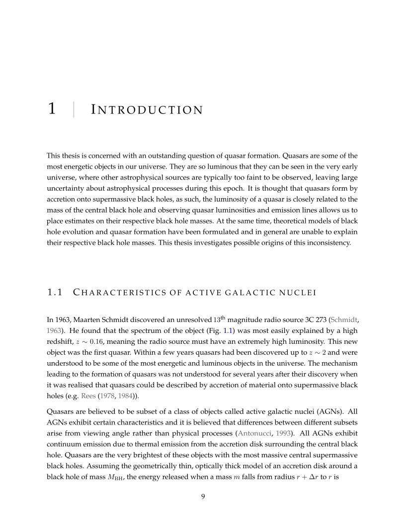
In 1963, Maarten Schmidt discovered an unresolved 13th magnitude radio source 3C 273 (Schmidt,1963). He found that the spectrum of the object (Fig. 1.1) was most easily explained by a highredshift, z ∼ 0.16, meaning the radio source must have an extremely high luminosity. This newobject was the first quasar. Within a few years quasars had been discovered up to z ∼ 2 and wereunderstood to be some of the most energetic and luminous objects in the universe. The mechanismleading to the formation of quasars was not understood for several years after their discovery whenit was realised that quasars could be described by accretion of material onto supermassive blackholes (e.g. Rees (1978, 1984)).
Quasars are believed to be subset of a class of objects called active galactic nuclei (AGNs). AllAGNs exhibit certain characteristics and it is believed that differences between different subsetsarise from viewing angle rather than physical processes (Antonucci, 1993). All AGNs exhibitcontinuum emission due to thermal emission from the accretion disk surrounding the central blackhole. Quasars are the very brightest of these objects with the most massive central supermassiveblack holes. Assuming the geometrically thin, optically thick model of an accretion disk around ablack hole of mass MBH, the energy released when a mass m falls from radius r + ∆r to r is
9
JASMINE FINER — IMPERIAL COLLEGE LONDON January 30, 2017
Figure 1.1: The spectrum of quasar 3C 273 discovered by Schmidt (1963). This figure is reproducedfrom Schmidt (1963)
∆E ≈ GMBHm
r
∆r
r.
From the virial theorem, half of this energy is converted to heat with corresponding lumionsity
∆L =GMBHm
2r2∆r, (1.1)
where m denotes the accretion rate. If the disk is optically thick, we can assume black body emissionand a differential ring between radius r and r + ∆r has a luminosity
∆L = 2× 2π r ∆r σSBT4(r), (1.2)
where σSB = 5.67 × 10⁻⁸ W m−2 K−4 is the Stefan-Boltzmann constant and T (r) is the radialtemperature profile of the disk. The factor of2 comes from the fact that the disc radiates from bothsides.
Combining eq. (1.1) and eq. (1.2) we can obtain the radial temperature profile of the accretion disk,
T (r) =
(3GMBHm
8πσSBr3
) 14
=
(3GMBHm
8πσSBr3S
) 14(r
rS
)− 34
, (1.3)
where in the last step we have replaced r with the Schwarzchild radius of a black hole rs =
2GMBH/c2 ≈ 3× 10³MBH/M� m, and the extra factor of 3 comes from considering dissipation by
10

JASMINE FINER — IMPERIAL COLLEGE LONDON January 30, 2017
friction in the disk.
The thermal emission of a geometrically thin, optically thick accretion disk produces a very broadspectrum of continuum emission with large flux at infrared, optical and ultraviolet wavelengths,peaking in the UV. This continuum emission is variable on timescales, tvar as short as one week.This provides empirical evidence for size of the nuclear region of the quasar to be less thanr = c tvar ' 1000 AU, where the last equality holds for tvar = 1 week. These sizes are much smallerthan that of the host galaxy, and are extremely difficult to resolve, thus these objects are seen aspoint sources.
Another important characteristic of all AGNs (except for one subset, BL Lacs whose spectrum showsalmost no emission lines) is the presence of strong emission lines, which are extremely broad inquasars and arise from regions close to the central engine, the broad line region (BLR). These linestypically have ∆λ/λ & 0.03 corresponding to ∆v . 10, 000 km s−1. This value of ∆v is inconsistent
with thermal line broadening requiring temperaturesT ∼ 1010K at which all atoms would be fullyionised and no emission lines would be produced. Instead, these lines are thought to be Dopplerbroadened as a result of rotational velocities from Keplerian motion,
vrot ∼√GMBH
r=
c√2
(r
rS
)− 12
,
and hence must arise from regions close to the black hole where orbital speeds are the greatest. Toobtain the required broadening vrot = 10, 000 km s−1, the radial distance must be r ∼ 500 rS .
By examining ratios of allowed and forbidden transitions that occur in the BLR (described in detailin Peterson (1997), but beyond the scope of this thesis), it is possible to determine the particledensity, ne ∼ 1× 1010 cm−3, of the BLR as well as the proportion of the volume that contains gasthat produces emission lines, the filling factor, ε≪ 1. The general picture of the BLR is then that it isa small region close to the central engine, made up of dense clouds of gas. These clouds absorb andre-emit continuum radiation from the source, and Doppler broadened emission lines are observedin the spectrum of the AGN.
Most AGNs (again with the exception of BL Lacs) also exhibit narrow emission lines with typical∆v ∼ 400 km s−1. This suggests that the narrow line region (NLR) is much larger than the BLR.Similar arguments lead to the belief that the NLR is also made up of clouds of gas that are lessdense than those in the BLR , with typical values of ne ∼ 104 cm−3.
1 . 2 S U P E R M A S S I V E B L A C K H O L E S AT H I G H R E D S H I F T
Currently, over 200, 000 quasars have been catalogued, with most discovered in the Sloan DigitalSky Survey (York et al., 2000). Most of these quasars have been discovered with redshifts z < 4,
11
JASMINE FINER — IMPERIAL COLLEGE LONDON January 30, 2017
however there are now ∼ 200 quasars with z & 5 including the most distant known quasar atz ∼ 7.1 (Mortlock et al., 2011).
If mass estimates of the z > 6 supermassive black holes powering these objects (Willott et al., 2010;Wu et al., 2015) are correct, then they suggest that the black holes have been able to accrete up to∼ 1010 M� between hydrogen recombination at z ∼ 1100 and z ∼ 7, less than 109 years. This wouldrequire either a very large seed black hole of M & 105 M� (Begelman et al., 2006) or a very highaccretion rate (Abramowicz, 2005).
B L A C K H O L E S E E D S
Black hole seeds are currently thought to be the remnants of the first generation stars (Pop III stars),which formed out of the primordial hydrogen and helium gas and therefore have zero metallicity.A second possibility would be that black hole seeds form as a result of direct gravitational collapseof gas and dust in high density regions of the universe (Begelman et al., 2006) without ever havingundergone stellar burning. The former of these is thought to produce seeds of . 100 M� (Zhanget al., 2008). The latter model would provide a sufficiently massive seed (MBH ∼ 105 M�), howeverthese objects are predicted to be rarer and unlikely to make up the entire population of high redshiftsupermassive black holes.
T H E E D D I N G T O N L I M I T
The Eddington limit defines a maximum luminosity for a spherically symmetric system of accretionof matter onto a central dense source. This limit is the result of radiation pressure due to photonsreleased as potential energy of the in-falling material is converted to heat and light, which thenstreams outwards, away from the black hole. The radiation pressure for a spherically symmetricsystem is given by,
Prad =L
c
1
4πR2,
where L is the luminosity of the source. This pressure exerts a force Frad = Pradκm, where κ isthe opacity of the surrounding medium and m is the mass of in-falling material. If we make theassumption that the accreted material is mostly ionised hydrogen, i.e. protons coupled to electrons,then the opacity is provided by Thomson scattering, with cross section σT , by electrons. The forcethen has the largest effect on protons, with mass mp � me. The opacity is then given by κ = σT /mp.The Eddington limit becomes important when this force is comparable to the gravitational forceexerted on the in-falling material,
Fgrav =GMm
R2.
12

JASMINE FINER — IMPERIAL COLLEGE LONDON January 30, 2017
The Eddington Luminosity is defined as the value of L = Ledd for which these forces are equal.When L ≥ LEdd the force due to radiation pressure from photons is equal to or larger than thegravitational force and matter is unable to reach the surface of the black hole. Ledd is given by
Ledd =4πGMmpc
σT.
We can relate the mass accretion rate to the luminosity of the quasar via
L = εMaccc2 =
ε
1− εMBHc2,
where Macc is the rate at which matter is accreted onto the black hole and ε is the fraction of rest-mass energy that is radiated away. The fraction of mass that is therefore gained by the black hole isgiven by: MBH = Macc/(1− ε).
We can obtain an upper bound on the mass of the SMBH as a function of time powering a quasar byassuming Eddington limited accretion for the lifetime of the quasar. The mass of the black hole as afunction of time is given by (Volonteri, 2010),
MBH(t) = MBH(t0) exp
{1− εε
t− t0TEdd
},
where Tedd ∼ 0.45 Gyr. For a radiative efficiency, ε = 0.1 for a spherically symmetric non-rotatingblack hole, and an initial seed mass of MBH(t0) = 105 M� (Begelman et al., 2006), it will take∼ 500 Myr for the black hole to reach 109 M�. We know of the existence of supermassive black holesat redshift 7, which corresponds to ∼ 780 Myr after the Big Bang. As such, it would, theoretically,
be possible for these objects to form in time via accretion if they accrete at the Eddington limit fortheir entire life and if a large enough seed can be produced sufficiently early (i.e. within the first280 Myr of the Big Bang).
S U P E R E D D I N G T O N A C C R E T I O N
In principle, this is not a hard limit and theories of super Eddington accretion have been developed(Paczynski, 1998; Abramowicz, 2005) in which rather than a friction dominated thin accretion disk,advection dominated accretion flows (ADAFs) are present in which the radiation pressure fromphotons is suppressed and super Eddington accretion rates can be achieved, even when luminositiesremain sub-Eddington.
13
JASMINE FINER — IMPERIAL COLLEGE LONDON January 30, 2017
M A S S E S T I M AT E S O F S U P E R M A S S I V E B L A C K H O L E S
As discussed in section 1.1, the continuum emission of quasars is variable even on short timescales.Thus, it is possible to exploit the response of the BLR to this continuum variability to determine itssize using reverberation mapping (Vestergaard & Peterson, 2006; Peterson, 2010). Using a simplisticmodel of the BLR as a shell of gas clouds surrounding the central engine, it becomes clear thata time lag, τ , will be measured between the response of clouds closer to the observer and thosefurther away.
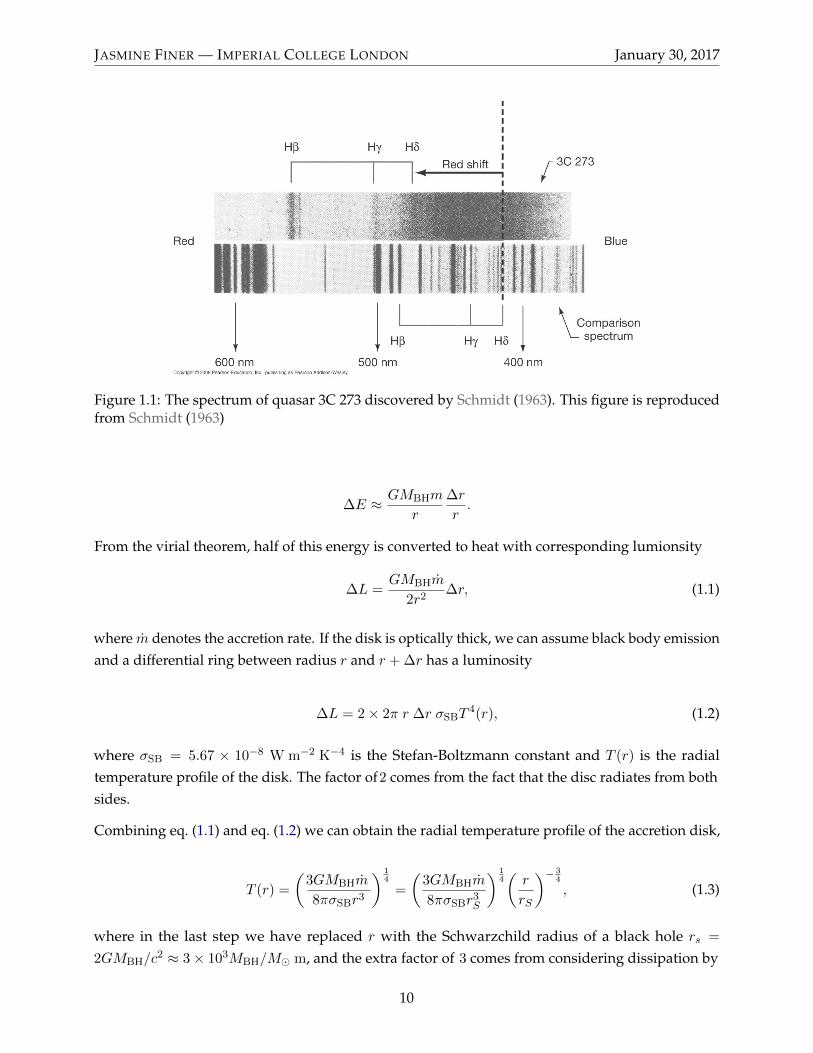
Consider a cloud a distance R away from the central black hole at position (0, 0), Fig. 1.2.
R
(0, 0)θ
To observer
Figure 1.2: Graphic depicting a shell of gas clouds surrounding the central black hole, at posi-tion (0, 0) and the response of gas clouds at position (R, θ) to a continuum burst, (after Peterson(1997)).Sent
This cloud will reemit a continuum burst at a time lag, τ , corresponding to the path difference, δbetween the light from the central engine and the emission lines from the BLR cloud, i.e.
δ = R+R cos θ
The time lag will therefore be given by
τ =R
c(1 + cos θ).
By measuring these time delays it is possible to produce maps of the BLR and estimate its size,allowing us to make virial mass estimates of the central black hole, defined as
MBH = fR∆V 2
G, (1.4)
where R is the size of the BLR, ∆V is the emission line width and f is a scale factor that depends onthe geometry of the BLR and is of order unity (Vestergaard & Peterson, 2006).
Reverberation mapping has been used to estimate the masses of many black holes at low redshift
14

JASMINE FINER — IMPERIAL COLLEGE LONDON January 30, 2017
(Vestergaard & Peterson, 2006; Vestergaard & Osmer, 2009; Peterson, 2010), and various scalingrelations have been determined allowing mass estimates to be made without having to use reverber-ation mapping, a very resource expensive process. These scaling relations rely on observation thatthere is a relation between the characteristic size, R of a region producing certain broad emissionlines and the continuum luminosity that excites the gas in this region, for example,R(Hβ) ∝ L0.53
1450
(Kaspi et al., 2005). This R− L relation allows for the quasar luminosity to be used as a proxy for Rin equation eq. (1.4). The line width of theMgII line can then be related to black hole mass, e.g., bythe following empirical relation (Vestergaard & Osmer, 2009),
logMBH = 6.68 + 2 logFWHM(MgII)
1000 km s−1+ 0.5 log
L3000
1037 W.
This relation was used by Willott et al. (2010) to estimate black hole masses of z ∼ 6 quasars.Note other empirical scaling relations exist for different broad lines and continuum luminosities(Vestergaard & Peterson, 2006). However, the assumption that these relations can be extrapolated tohigh redshift may not hold and it is a complicated process to treat the uncertainties that arise in allvariables.
We now have an overview of the assumed physical mechanism driving observed quasar luminosities.As the observed luminosities lead to inconsistencies with theoretically predicted mass ranges, itis clear that somewhere an assumption has to be violated. These might be one or more of thefollowing:
• BLACK HOLE SEEDS The mechanisms by which black hole seeds are produced are not well un-derstood. If it is possible to produce very massive black hole seeds (i.e. by direct gravitationalcollapse) less time is needed for accretion.
• EVOLUTIONARY MODELS The development of accretion models that allow for radiativelyinefficient accretion onto black holes or super-Eddington accretion would allow black holesto reach 109 M� in the time between the Big Bang and z ∼ 6. These models would need toreproduce exactly the population of accreting black holes observed in the early universe.
• MASS ESTIMATES If scaling relations relating black hole masses to emission line equivalentwidths are, in fact, overestimates of black hole mass, this could result in a partial resolution toinconsistencies between black hole masses and evolutionary models.
The physical processes and mechanisms outlined above determine the observed number density ofquasars in the sky at a given redshift with a given magnitude. Therefore, any models determining theevolution and growth of supermassive black holes must in turn recreate this distribution, the quasarluminosity function (QLF). An accurate model for this distribution based on observations will allowus to pinpoint where our assumptions in the Black Hole evolutionary models have broken down.Previous efforts (detailed in section 4.3) to constrain the high redshift quasar luminosity function
15

JASMINE FINER — IMPERIAL COLLEGE LONDON January 30, 2017
have used maximum likelihood estimates and have not treated surveys covering overlapping areasconsistently and an improved statistical analysis will also aid in the understanding of this problem.As such, the remainder of this thesis is concerned with statistical analysis of the high redshift quasarpopulation. In the following we introduce a self consistent approach to determining the distributionof quasars at high redshift, which must then be reproduced by any model of active supermassiveblack hole evolution at high redshift.
16

2 | T H E Q U A S A R L U M I N O S I T Y F U N C T I O N
The quasar luminosity function (QLF) describes the expected number, N , of quasars in a givencomoving volume, V , with magnitudes in the range [Mλ,Mλ + ∆Mλ] and redshifts in the range[z, z + ∆z],
dN = Φ(Mλ, z)dV dMλ,
where Mλ denotes the magnitude of a quasar at a given wavelength λ.
The QLF has been measured at a range of different redshifts so it is possible to see the evolution ofthe spatial density of quasars, ρ(Mλ < Mref) =
∫Mref
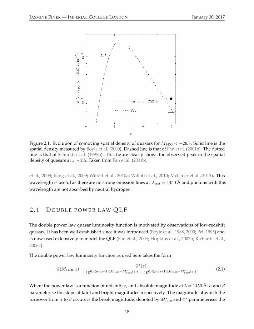
−∞ Φ(Mλ, z) dM as a function of redshift. Thisnumber density is observed to increase with redshift up until z ∼ 2.5 (Schmidt, 1968) after whicha steep decrease with redshift is observed (Osmer, 1982; Warren et al., 1994; Schmidt et al., 1995b;Fan et al., 2001c; Richards et al., 2006a). Fig. 2.1 shows a plot of the cumulative spatial densityρ(M1450 < −26.8) from Fan et al. (2001b) with the best fit values of Fan et al. (2001b); Boyle et al.(2000); Schmidt et al. (1995a) as shown in Fan et al. (2001c). It can be seen from this figure thatthe number density of bright quasars is low for z ∼ 0 today and increases rapidly up to a peak atz = 2.5. For greater redshifts the number density of bright quasars decreases rapidly with redshift.
At high redshift, there is an upper limit on the mass of a supermassive black hole due to the limitedtime available for accretion. Observationally, this manifests itself as an upper limit on the absolutemagnitude of a supermassive black hole. As a result we expect a break magnitude such that thenumber density of quasars with magnitudes brighter than this break decreases extremely rapidly.This break magnitude will move towards the faint end with increasing redshift as there is even lesstime for the black hole to accrete matter. Quasars with magnitudes fainter than this break have nothad to experience such rapid accretion but will there will still be decrease in number density withmagnitude due to the limited time available for accretion, but this rate will be slower.
Hopkins et al. (2007b) combines estimations of the QLF across different wavelength bands (X-ray,(Steffen et al., 2003; Ueda et al., 2003); radio, (Willott et al., 2001); optical, (Fan et al., 2001b; Croomet al., 2004; Willott et al., 2009)) to estimate the bolometric QLF and its evolution. The remainderof this report will be concerned with the QLF at 1450 A measured by (Fan et al., 2001b,c,a; Jiang
17
JASMINE FINER — IMPERIAL COLLEGE LONDON January 30, 2017
Figure 2.1: Evolution of comoving spatial density of quasars for M1450 < −26.8. Solid line is thespatial density measured by Boyle et al. (2000). Dashed line is that of Fan et al. (2001b). The dottedline is that of Schmidt et al. (1995b). This figure clearly shows the observed peak in the spatialdensity of quasars at z ∼ 2.5. Taken from Fan et al. (2001b).
et al., 2008; Jiang et al., 2009; Willott et al., 2010a; Willott et al., 2010; McGreer et al., 2013). Thiswavelength is useful as there are no strong emission lines at λrest = 1450 A and photons with thiswavelength are not absorbed by neutral hydrogen.
2 . 1 D O U B L E P O W E R L AW Q L F
The double power law quasar luminosity function is motivated by observations of low-redshiftquasars. It has been well established since it was introduced (Boyle et al., 1988, 2000; Pei, 1995) andis now used extensively to model the QLF (Fan et al., 2004; Hopkins et al., 2007b; Richards et al.,2006a).
The double power law luminosity function as used here takes the form
Φ(M1450, z) =Φ∗(z)
100.4(α(z)+1)(M1450−M∗1450(z)) + 100.4(β(z)+1)(M1450−M∗
1450(z)). (2.1)
Where the power law is a function of redshift, z, and absolute magnitude at λ = 1450 A. α and βparameterise the slope at faint and bright magnitudes respectively. The magnitude at which theturnover from α to β occurs is the break magnitude, denoted by M∗1450 and Φ∗ parameterises the
18

JASMINE FINER — IMPERIAL COLLEGE LONDON January 30, 2017
normalisation of the QLF and is the number density of quasars at the break magnitude. In principleall parameters of the QLF can evolve with redshift and additional parameters can then be includedto characterise this evolution.
Two canonical evolutionary models are pure density evolution (PDE) and pure luminosity evolution(PLE) (Boyle et al., 2000; Croom et al., 2004; Ueda et al., 2003; Richards et al., 2005). These onlyconsider evolution with redshift of the normalisation parameter, Φ∗, and the break magnitude,M∗1450, respectively. It is also common (Hopkins et al., 2007b) to combine these models to obtainluminosity dependent density evolution (LDDE), as well as to add evolution for the faint end slope,α and bright end slope β (Hopkins et al., 2007b).
At high redshift, the number density of luminous quasars is limited by the lack of time available foraccretion. Therefore, as redshift increases we would expect the number density to decrease. In asimilar vein, we would also expect the break magnitude to shift towards the faint end of the QLF.As such, the parameterisation that I will be implementing for the z ∼ 6 quasar luminosity is
Φ∗(z) = 10k(z−zref)Φ∗ (2.2)
M∗1450(z) = M1450 + j(z − zref) (2.3)
with j and k left as parameters to be fit to the data and zref = 6. The parameterisation of Φ∗(z) isadopted from Fan et al. (2001b). The parameterisation ofM∗1450 is a linear expansion ofM∗1450(z) tofirst order and is similar to that used in Croom et al. (2004); Richards et al. (2005) to model the lowredshift QLF.
We chose not to include evolution of α and β with redshift, as from results at z ∼ 5 and z ∼ 6 M∗1450
and Φ∗ have the clearest evolution. Both Willott et al. (2010a), using data at z ∼ 6 and McGreeret al. (2013), using quasars at z ∼ 5 fix α = −1.5 and find that β is consistent within the range oftheir uncertainty. However this is not the case for M∗1450 or Φ∗, hence we chose to evolve theseparameters as they are the ones for which there is evidence of strong evolution.
We therefore have up to 6 parameters, β, α,Φ∗, k,M∗1450, j, which we need to estimate, and a fullQLF with the form
Φ(M1450, z) =10k(z−zref)Φ∗
100.4(α+1)(M1450−M∗1450−j(z−zref)) + 100.4(β+1)(M1450−M∗
1450−j(z−zref)). (2.4)
19
JASMINE FINER — IMPERIAL COLLEGE LONDON January 30, 2017
2 . 2 T H E B L A C K H O L E M A S S F U N C T I O N
The population of black holes in the universe is described by the black hole mass function (BHMF).This gives the number of black holes per comoving volume element with masses in the range[M,M + dM ]. The characteristic shape of the BHMF has a sharp cut off at high mass (Shankar et al.,2009; Vestergaard et al., 2008) due to AGN feed back and in the case of high redshift, the lack oftime for black hole growth (Volonteri & Rees, 2005). (Willott et al., 2010) adopts a Schechter function(Schechter, 1976) form of the BHMF:
Φ(MBH) = Φ∗(MBH
M∗BH
)αexp
(− MBH
M∗BH
)(2.5)
This has the same power law form as the QLF at the faint end, but a sharper cut off at the brightend as is theoretically favoured by e.g. Shankar et al. (2009); Willott et al. (2010).
T H E E D D I N G T O N R AT I O D I S T R I B U T I O N
The Eddington ratio is defined as the ratio of a quasar’s bolometric luminosity to the Eddingtonluminosity determined by the mass of the SMBH at the centre of the quasar.
λ =Lbol
LEdd(2.6)
By measuring this quantity for observed quasars it is possible to determine the distribution in λ.This distribution tells us how active the population of quasars we observe are and by measuringthis over a range of redshifts can tell us how the behaviour of the population evolves. Willott et al.(2010) have made the first determination of the Eddington ratio distribution P (λ) at z = 6. Theyfound that the distribution can be approximated by a lognormal distribution with a peak at λ = 0.6
and a narrow dispersion of 0.3 dex (Fig. 2.2).
This observation implies that there are very few black holes at z = 6 with λ < 0.1, suggesting thatthere are extremely few inactive black holes at z = 6 and that most of them are accreting close totheir Eddington rates. Large hydrodynamical simulations by Sijacki et al. (2009) have also reachedsimilar conclusions.
The BHMF is directly related to the QLF. If one is only interested in the mass function of SMBH thatpower quasars, then it is possible to transform the BHMF to the QLF by convolution of the BHMFwith the Eddington ratio distribution
dn
dLbol=
∫ ∫dn
dMP (λ) δD[M −M(λ, Lbol)] dλdM, (2.7)
20

JASMINE FINER — IMPERIAL COLLEGE LONDON January 30, 2017
Figure 2.2: The Eddington ratio distribution. Red histogram shows the Eddington ratio for z = 6while blue histogram shows that of z = 2. The intrinsic distribution (black curve) is a lognormaldistribution with and intrinsic peak at λ = 0.6 and dispersion 0.3 dex. Figure taken from Willottet al. (2010)
whereM(λ, Lbol) =
Lbol
βλ, β =
4πGmpc
σT.
This relationship has the following implication. If we can provide a self consistent formalism withwhich to estimate the parameters of the QLF, then we can use mass estimates to understand howthe population of active black holes behaves at high redshift. Any theoretical model or observationof black hole mass must reproduce the QLF, thus it will provide us a bench mark with which tocompare future models to data.
21
3 | Q U A S A R S U R V E Y S
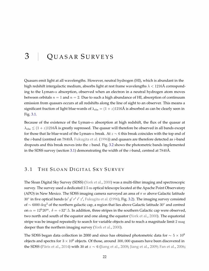
Quasars emit light at all wavelengths. However, neutral hydrogen (HI), which is abundant in thehigh redshift intergalactic medium, absorbs light at rest frame wavelengths λ < 1216A correspond-ing to the Lyman-α absorption, observed when an electron in a neutral hydrogen atom movesbetween orbitals n = 1 and n = 2. Due to such a high abundance of HI, absorption of continuumemission from quasars occurs at all redshifts along the line of sight to an observer. This means asignificant fraction of light blue-wards ofλobs = (1 + z)1216A is absorbed as can be clearly seen inFig. 3.1.
Because of the existence of the Lyman-α absorption at high redshift, the flux of the quasar atλobs ≤ (1 + z)1216A is greatly supressed. The quasar will therefore be observed in all bands exceptfor those that lie blue-ward of the Lyman-α break. At z ∼ 6 this break coincides with the top end ofthe i-band (centred on 7840A Fukugita et al. (1996)) and quasars are therefore detected as i-banddropouts and this break moves into the z band. Fig. 3.2 shows the photometric bands implementedin the SDSS survey (section 3.1) demonstrating the width of the i-band, centred at 7840A.
3 . 1 T H E S L O A N D I G I TA L S K Y S U R V E Y
The Sloan Digital Sky Survey (SDSS) (York et al., 2000) was a multi-filter imaging and spectroscopicsurvey. The survey used a dedicated 2.5 m optical telescope located at the Apache Point Observatory(APO) in New Mexico. The SDSS imaging camera surveyed an area of π sr above Galactic latitude30◦ in five optical bands (u′ g′ r′ i′ z′, Fukugita et al. (1996), Fig. 3.2). The imaging survey consistedof ∼ 6000 deg2 of the northern galactic cap, a region that lies above Galactic latitude 30◦ and centredon α = 12h20m, δ = +32◦.5. In addition, three stripes in the southern Galactic cap were observed,two north and south of the equator and one along the equator (York et al., 2000). The equatorialstripe was be imaged repeatedly to search for variable objects and to reach a magnitude limit 2 mag
deeper than the northern imaging survey (York et al., 2000).
The SDSS began data collection in 2000 and since has obtained photometric data for ∼ 5 × 10⁸
objects and spectra for 3× 10⁶ objects. Of those, around 300, 000 quasars have been discovered inthe SDSS (Paris et al., 2014) with 30 at z ∼ 6 (Jiang et al., 2008; Jiang et al., 2009; Fan et al., 2006;
22
JASMINE FINER — IMPERIAL COLLEGE LONDON January 30, 2017
Figure 3.1: Spectra of 9 high redshift quasars found in the CFHQS survey (Willott et al., 2009).Wavelengths are λobs. Figure taken from Willott et al. (2010a).
Jiang et al., 2015). The SDSS pioneered the search for redshift 6 quasars and was followed by theCanada France High-z Quasar survey (CHFHQS, Willott et al. (2009)) and the UKIRT Infrared DeepSky Survey (UKIDSS, Lawrence et al. (2007)).
3 . 2 z ∼ 5 Q U A S A R S U R V E Y S
z ∼ 5 S D S S M A I N S A M P L E
The bright end of the z ∼ 5 luminosity function is best sampled by the seventh data release (DR7)of the SDSS main survey (DR7QSO) (Abazajian et al., 2009; McGreer et al., 2013). The selectionalgorithm (Richards et al., 2002) for this survey was not complete before the survey was already inprogress (McGreer et al., 2013). Using the method prescribed in Richards et al. (2006b) DR7 quasarswere identified from regions with uniform target selection. Colour cuts were also applied (McGreeret al., 2013) resulting in 146 quasars with 4 .7 < z < 5 .1 in an effective area of 6222 deg2 . These
23

JASMINE FINER — IMPERIAL COLLEGE LONDON January 30, 2017
Figure 3.2: The 5 photometric bands implemented in the SDSS survey. Figure taken from Fukugitaet al. (1996).
quasars are shown in the left hand panel of Fig. 3.3.
z ∼ 5 S T R I P E 8 2 S A M P L E
11 new quasars were found in SDSS DR7 (Abazajian et al., 2009), which selects quasars with4 .7 < z < 5 .1 to a magnitude limit of i . 20 .2. A total of 14 new quasars with z > 4 .6 werefound in BOSS DR9 (Ross et al., 2012). This survey was primarily designed to find quasars with2 .2 < z < 3 .5 (McGreer et al., 2013) however the survey covered a large section of Stripe 82and the search was extended to find z > 4 .6 quasars in Stripe 82. Four quasar candidates wereobserved on the Magellan Spectrograph, of which one was a star and one had previously beendiscovered in BOSS, leaving a total of 2 new high redshift quasars. The bulk of the spectroscopicobservations were made at the MMT 6 .5 m telescope. Over the course of several observing runs atotal of 57 spectroscopically confirmed quasars were observed at MMT with 4 .3 < z < 5 .46.
Of the 84 observed quasars, 73 are spectroscopically confirmed with 52 within the redshift range4 .7 < z < 5 .1. The final area of Stripe 82 used for quasar selection was 235 deg2 (McGreer et al.,2013).
24

JASMINE FINER — IMPERIAL COLLEGE LONDON January 30, 2017
Figure 3.3: The selection functions and quasar samples from the SDSS main sample (left) and Stripe82 redshift 5 quasar sample (right) (McGreer et al., 2013). Contours show 20%, 40%, 60% and 80%completeness. Red points are the quasars selected from the surveys after a redshift cut of 4.7 < z <5.1 has been applied.
3 . 3 z ∼ 6 Q U A S A R S U R V E Y S
S D S S M A I N S A M P L E
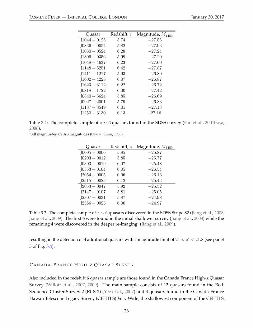
The most up to date description of the SDSS main high-z sample (Fan et al., 2001b,c,a, 2006) is givenin Fan et al. (2006) and contains 14 quasars with 5.74 < z < 6.42. The survey has a magnitude limitof z′ < 20.2 and as a result the bright end of the quasar luminosity function is well sampled by the
quasars in this survey. Quasars are selected from a effective area of ∼ 6600 deg2 and the selectionfunction shown in the first panel of Fig. 3.4. The selection function for this survey was first describedin Fan (2003), and adjusted to the cosmology used in this thesis by Willott et al. (2010a). Noticeablythe quasars found in this survey are clustered close to the cut off in the selection function.
S D S S S T R I P E 8 2
A small patch of the SDSS survey, Stripe 82, was imaged by Jiang et al. (2008) to search for fainterquasars.
6 new quasars were found in this new∼ 260 deg2 area spanning 30◦ < α < 310◦, −1.5◦ < δ < 1.5◦
with a magnitude limit of 20 < z′ < 21 (see panel 2 of Fig. 3.4), greater than that of the SDSS mainsample due to repeated imaging of the same area of sky. This search was extended further in Jianget al. (2009) on a slightly smaller patch ranging 60◦ < α < 310◦ and an effective area of 195 deg2
25
JASMINE FINER — IMPERIAL COLLEGE LONDON January 30, 2017
Quasar Redshift, z Magnitude, M11450
J1044− 0125 5.74 −27.55J0836 + 0054 5.82 −27.93J1030 + 0524 6.28 −27.24J1306 + 0356 5.99 −27.20J1048 + 4637 6.23 −27.60J1148 + 5251 6.42 −27.87J1411 + 1217 5.93 −26.80J1602 + 4228 6.07 −26.87J1623 + 3112 6.22 −26.72J0818 + 1722 6.00 −27.42J0840 + 5624 5.85 −26.69J0927 + 2001 5.79 −26.83J1137 + 3549 6.01 −27.13J1250 + 3130 6.13 −27.16
Table 3.1: The complete sample of z ∼ 6 quasars found in the SDSS survey (Fan et al., 2001b,c,a,2006).1All magnitudes are AB magnitudes (Oke & Gunn, 1983).
Quasar Redshift, z Magnitude, M1450
J0005− 0006 5.85 −25.87J0203 + 0012 5.85 −25.77J0303− 0019 6.07 −25.48J0353 + 0104 6.05 −26.54J2054 + 0005 6.06 −26.16J2315− 0023 6.12 −25.43
J2053 + 0047 5.92 −25.52J2147 + 0107 5.81 −25.05J2307 + 0031 5.87 −24.98J2356 + 0023 6.00 −24.97
Table 3.2: The complete sample of z ∼ 6 quasars discovered in the SDSS Stripe 82 (Jiang et al., 2008;Jiang et al., 2009). The first 6 were found in the initial shallower survey (Jiang et al., 2008) while theremaining 4 were discovered in the deeper re-imaging. (Jiang et al., 2009).
resulting in the detection of 4 additional quasars with a magnitude limit of 21 < z′ < 21.8 (see panel3 of Fig. 3.4).
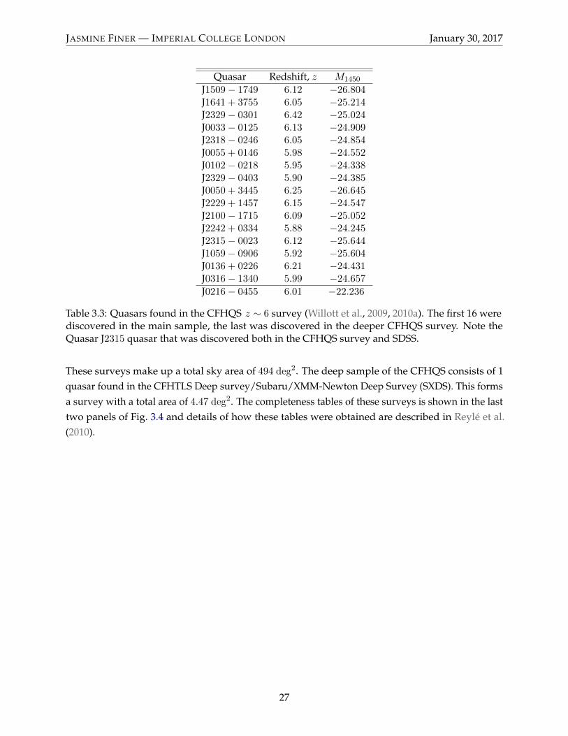
C A N A D A - F R A N C E H I G H - Z Q U A S A R S U R V E Y
Also included in the redshift 6 quasar sample are those found in the Canada France High-z QuasarSurvey (Willott et al., 2007, 2009). The main sample consists of 12 quasars found in the Red-Sequence Cluster Survey 2 (RCS-2) (Yee et al., 2007) and 4 quasars found in the Canada-FranceHawaii Telescope Legacy Survey (CFHTLS) Very Wide, the shallowest component of the CFHTLS.
26
JASMINE FINER — IMPERIAL COLLEGE LONDON January 30, 2017
Quasar Redshift, z M1450
J1509− 1749 6.12 −26.804J1641 + 3755 6.05 −25.214J2329− 0301 6.42 −25.024J0033− 0125 6.13 −24.909J2318− 0246 6.05 −24.854J0055 + 0146 5.98 −24.552J0102− 0218 5.95 −24.338J2329− 0403 5.90 −24.385J0050 + 3445 6.25 −26.645J2229 + 1457 6.15 −24.547J2100− 1715 6.09 −25.052J2242 + 0334 5.88 −24.245J2315− 0023 6.12 −25.644J1059− 0906 5.92 −25.604J0136 + 0226 6.21 −24.431J0316− 1340 5.99 −24.657
J0216− 0455 6.01 −22.236
Table 3.3: Quasars found in the CFHQS z ∼ 6 survey (Willott et al., 2009, 2010a). The first 16 werediscovered in the main sample, the last was discovered in the deeper CFHQS survey. Note theQuasar J2315 quasar that was discovered both in the CFHQS survey and SDSS.
These surveys make up a total sky area of 494 deg2. The deep sample of the CFHQS consists of 1quasar found in the CFHTLS Deep survey/Subaru/XMM-Newton Deep Survey (SXDS). This formsa survey with a total area of 4.47 deg2. The completeness tables of these surveys is shown in the lasttwo panels of Fig. 3.4 and details of how these tables were obtained are described in Reyle et al.(2010).
27

JASMINE FINER — IMPERIAL COLLEGE LONDON January 30, 2017
Figure 3.4: Selection functions and quasar samples of z ∼ 6 surveys used by Willott et al. (2010a) tocalculate the quasar luminosity function at z ∼ 6. Contours are placed at 20%, 40%, 60% and 80%completeness. Red points show the complete quasar samples from each survey.
28
4 | Q L F PA R A M E T E R E S T I M AT I O N M E T H O D -
O L O G Y
Parameter estimation is a statistical problem and as a result many statistical and algorithmic tech-niques must be used in order to treat the problem correctly. I start by constructing the likelihood ofthe quasar luminosity function, section 4.1, before moving on to discuss two methods of performingparameter inference, maximum likelihood estimation, with χ2 confidence intervals to quantifyuncertainties, section 4.3, and Bayesian parameter inference, section 4.4. I also outline a methodfor simulating quasar surveys for the purposes of comparing results from simulations to resultswith actual data, section 4.2. Finally, I describe the algorithms for producing results and caluclat-ing the likelihood and posterior distributions for the quasar luminosity function. For the case oflow dimensionality, Np ≤ 3, this can be done by evaluating the likelihood or posterior over a Np
dimensional array, section 4.5. However, for Np > 3 we must utilize a Markov Chain Monte Carloalgorithm, section 4.4.2.
4 . 1 T H E Q L F L I K E L I H O O D
Whether for use in a Bayesian or maximum likelihood approach to parameter inference, it isnecessary to construct the likelihood of observing data given a model for the QLF. We want toconstruct the probability, Pr(d|θ,M) of observing a set of N data points d = {d1, d2, ..., dN} givena model, M with P parameters θ = {θ1, θ2, ..., θP }. For the case of the QLF our data are themagnitudes and redshifts, {M1450,i, zi} of each quasar and the total number Nq of quasars found inthe survey, and the parameters are those of the QLF outlined in chapter 2 . This likelihood can beconstructed via two different methods, outlined below.
The expected number of quasars to be detected with magnitudes and redshifts in the range[M1450,M1450 + ∆M1450], [z, z + ∆z] in a survey is given by:
29

JASMINE FINER — IMPERIAL COLLEGE LONDON January 30, 2017
dN =A
4πΦ(M1450, z) p(M1450, z)
dV
dzdM1450 dz (4.1)
= f(M1450, z) dM1450 dz, (4.2)
where Φ(M1450, z) is defined in eq. (2.1), p(M1450, z) is the selection function of the specific surveyand A is the area of the survey. The expected number N is then given by the integral of equation 4.1over all M1450 and z. Equation 4.2 defines f(M1450, z).
Constructing the likelihood
Marshall et al. (1983) and Fan et al. (2001a) describe a method for calculating the likelihood of acomplete sample of quasars using Poisson probabilities. The survey coverage is split into cells ofsize ∆M1450∆z. As long as the cells are infinitesimally small, onlync = {0, 1} quasars are detectedin each cell. The likelihood for a given survey is a product over these probabilities for each cell. Therate in the Poisson probability is given by the expected number of quasars in the cth cell, Nc:
Nc = f(M1450,c, zc) ∆M1450 ∆z (4.3)
The likelihood, L, of the full sample is then given by
L =
Nc∏c=1
Nncc exp−Nc
nc!(4.4)
=
Nc∏c=1
exp−Nc
Nq∏i = 1︸ ︷︷ ︸
cells with nc=1
Ni (4.5)
= exp∑c
−Nc︸ ︷︷ ︸=−N
Nq∏i=1
Ni. (4.6)
Combining 4.6 with 4.1 and 4.3, and noting that∑cNc = N , we arrive at
L =
Nq∏i=1
Φ(M1450,i, zi) p(M1450,i, zi)dV
dz
∣∣∣∣z=zi
∆M1450,i ∆zi×∫ ∫
Φ(M1450, z) p(M1450, z)dV
dzdM1450 dz
30
JASMINE FINER — IMPERIAL COLLEGE LONDON January 30, 2017
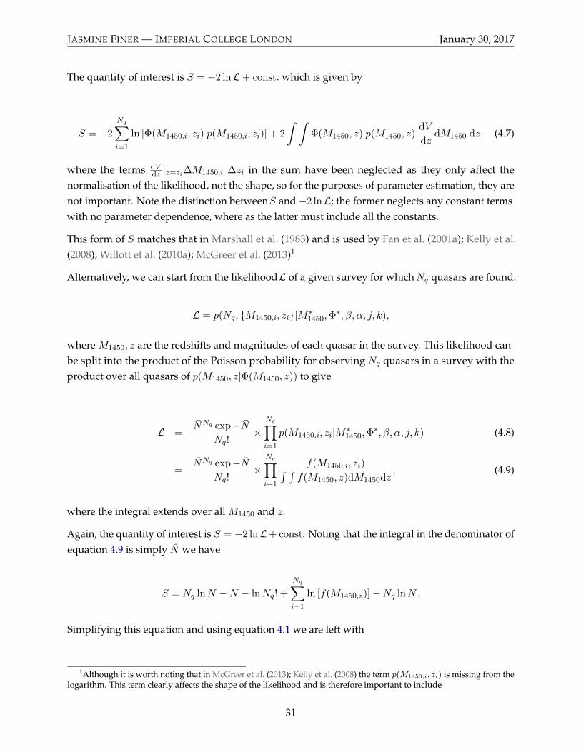
The quantity of interest is S = −2 lnL+ const. which is given by
S = −2
Nq∑i=1
ln [Φ(M1450,i, zi) p(M1450,i, zi)] + 2
∫ ∫Φ(M1450, z) p(M1450, z)
dV
dzdM1450 dz, (4.7)
where the terms dVdz |z=zi∆M1450,i ∆zi in the sum have been neglected as they only affect the
normalisation of the likelihood, not the shape, so for the purposes of parameter estimation, they arenot important. Note the distinction betweenS and −2 lnL; the former neglects any constant termswith no parameter dependence, where as the latter must include all the constants.
This form of S matches that in Marshall et al. (1983) and is used by Fan et al. (2001a); Kelly et al.(2008); Willott et al. (2010a); McGreer et al. (2013)1
Alternatively, we can start from the likelihoodL of a given survey for whichNq quasars are found:
L = p(Nq, {M1450,i, zi}|M∗1450,Φ∗, β, α, j, k),
where M1450, z are the redshifts and magnitudes of each quasar in the survey. This likelihood canbe split into the product of the Poisson probability for observing Nq quasars in a survey with theproduct over all quasars of p(M1450, z|Φ(M1450, z)) to give
L =NNq exp−N
Nq!×
Nq∏i=1
p(M1450,i, zi|M∗1450,Φ∗, β, α, j, k) (4.8)
=NNq exp−N
Nq!×
Nq∏i=1
f(M1450,i, zi)∫ ∫f(M1450, z)dM1450dz
, (4.9)
where the integral extends over all M1450 and z.
Again, the quantity of interest is S = −2 lnL+ const. Noting that the integral in the denominator ofequation 4.9 is simply N we have
S = Nq ln N − N − lnNq! +
Nq∑i=1
ln [f(M1450,z)]−Nq ln N .
Simplifying this equation and using equation 4.1 we are left with
1Although it is worth noting that in McGreer et al. (2013); Kelly et al. (2008) the term p(M1450,i, zi) is missing from thelogarithm. This term clearly affects the shape of the likelihood and is therefore important to include
31

JASMINE FINER — IMPERIAL COLLEGE LONDON January 30, 2017
S = −2
Nq∑i=1
ln [Φ(M1450,i, zi) p(M1450,i, zi)] + 2
∫ ∫Φ(M1450, z) p(M1450, z)
dV
dzdM1450 dz, (4.10)
which is identical to 4.7 and again we have neglected terms for which there is no parametricdependence.
4 . 2 S I M U L AT I N G Q U A S A R S U R V E Y S
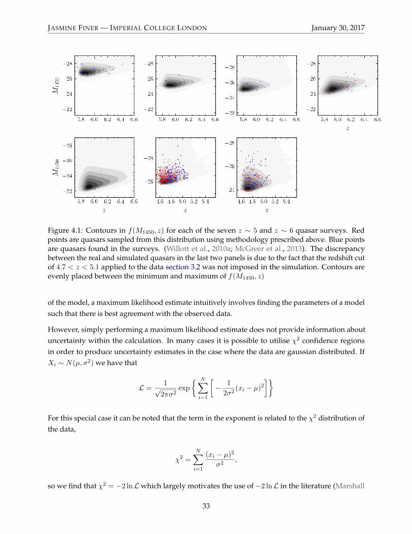
In order to simulate a quasar survey for the purposes of testing our analysis, it is necessary tosample from f(M1450, z). Plots of f(M1450, z) for the seven z ∼ 5 & z ∼ 6 surveys are shown ascontours in Fig. 4.1. As this is not an analytic function and as the completeness is in the form ofa 2-D array, we cannot use methods such as inverse transform sampling or rejection sampling togenerate draws from this distribution.
To draw a sample, {M1450, z}, from a distribution evaluated on an array, A, we perform the followingsteps.
1. Generate Nq, the number of samples to be drawn from the expected number of quasars in thesurvey: Nq ∼ Po(Nexp)
2. For k = 0...N
• sample Yk ∼ U [0, sum(A)]
• Perform a sorted search of the cumulative sum of A to find index [i, j] where Yk wouldbe found in A
• This index gives an interval in [M1450,i,M1450,i + ∆M1450] and [zj , zj + ∆z].
• Draw sample M1450,k ∼ U [M1450,i ≤M1450,k] ≤M1450,i + ∆M1450
• Draw sample zk ∼ U [zj ≤ zk ≤ zj + ∆z]
These simulations are shown as red points in Fig. 4.1. The real quasars are shown for reference asblue points, and contours show the distribution f(M1450, z).
4 . 3 M A X I M U M L I K E L I H O O D E S T I M AT I O N
Maximum likelihood estimation is a method of obtaining point estimates for the parameters of amodel. As the likelihood is defined as the probability of observing a data set given the parameters
32
JASMINE FINER — IMPERIAL COLLEGE LONDON January 30, 2017
Figure 4.1: Contours in f(M1450, z) for each of the seven z ∼ 5 and z ∼ 6 quasar surveys. Redpoints are quasars sampled from this distribution using methodology prescribed above. Blue pointsare quasars found in the surveys. (Willott et al., 2010a; McGreer et al., 2013). The discrepancybetween the real and simulated quasars in the last two panels is due to the fact that the redshift cutof 4.7 < z < 5.1 applied to the data section 3.2 was not imposed in the simulation. Contours areevenly placed between the minimum and maximum of f(M1450, z)
of the model, a maximum likelihood estimate intuitively involves finding the parameters of a modelsuch that there is best agreement with the observed data.
However, simply performing a maximum likelihood estimate does not provide information aboutuncertainty within the calculation. In many cases it is possible to utilise χ2 confidence regionsin order to produce uncertainty estimates in the case where the data are gaussian distributed. IfXi ∼ N(µ, σ2) we have that
L =1√
2πσ2exp
{ N∑i=1
[− 1
2σ2(xi − µ)2
]}
For this special case it can be noted that the term in the exponent is related to the χ2 distribution ofthe data,
χ2 =
N∑i=1
(xi − µ)2
σ2,
so we find that χ2 = −2 lnLwhich largely motivates the use of −2 lnL in the literature (Marshall
33
JASMINE FINER — IMPERIAL COLLEGE LONDON January 30, 2017
et al., 1983; Fan et al., 2001b; Willott et al., 2010a; McGreer et al., 2013).
4.3.1 The ∆S Statistic
Lampton et al. (1976) provides a method for producing confidence intervals once the likelihood hasbeen calculated, which I will summarise here. For a set of N data points whose deviations fromthe values expected by a given model are Gaussian, S will be distributed as χ2 with N degrees offreedom. If we then minimise S with respect to p model parameters to obtain theSmin statistic, wecan say that this is χ2 distributed with N − p degrees of freedom. So for the purposes of plottingconfidence regions, it is sensible to talk about the statistic: ∆S = S − Smin which will once again beχ2 distributed with p degrees of freedom, i.e. ∆S ∼ χ2
p, so we can write that for any number, T ,
Pr(∆S > T ) = Pr(χ2p > T )
We can then define contours SL such that SL = Smin + T where we have
Pr(∆S > SL − Smin) = Pr(χ2p > SL − Smin)
It can be noted that the left hand side is simply the probability, α, of a contour failing to enclosethe true value, where α is defined via α = Pr[χ2
p > χ2p(α)]. This leaves the required contour for
confidence C = 1− α as,SL = Smin + χ2
p(α). (4.11)
In many cases, however, one is only interested in a subset of the parameters used in the minimisationof S. Cases can include those where there are nuisance parameters which are not of interest in theanalysis, or when for presentation purposes the confidence regions need to be in two dimensionalspace. In this case, one can project the initial p dimensional parameter space on to a subspace ofq interesting parameters. The method of creating this subspace is as follows: at each point in theq dimensional subspace, minimise S w.r.t. the remaining p− q parameters. Contours can then beplaced again at positions given by eq. (4.11). Furthermore, numerical simulations (Avni, 1976) showthat the level of confidence with which the p parameters are estimated can be accurately given by aχ2q function, reducing the size of the confidence regions to:
SL = Smin + χ2q(α). (4.12)
This method of reduced numbers of parameters has been employed numerous times in evaluatingconfidence regions for the 4 parameters of the QLF (Willott et al., 2010a; McGreer et al., 2013).Fig. 5.1 shows confidence regions for the z = 6 QLF parameters from (Willott et al., 2010a). It does,however, rely on the assumption that input data are gaussian distributed random variables, which
34

JASMINE FINER — IMPERIAL COLLEGE LONDON January 30, 2017
is not necessarily the case, and is therefore not a particularly robust method of producing reliablecontours.
4 . 4 B AY E S I A N PA R A M E T E R I N F E R E N C E
Bayes’ theorem (Bayes & Price, 1763) states that the probability P (A|B), is defined as
P (A|B) =P (A)P (B|A)
P (B),
where P(A|B) is the probability of an event A occurring given the event B has already occurred.
A common application of Bayes’ theorem is in data analysis, where some collected data is used toinfer constraints on parameters of a given model. The quantity of interest is then the posterior, i.e.the probability of our model being correct, given that we’ve observed the data. For a set ofN datapoints, d = {d1, d2, ..., dN} that is to be fit by a model, M , with P parameters θ = {θi = 1, θ2, ..., θP },Bayes’ theorem can be written as
Pr(θ|d,M) =Pr(θ|M) Pr(d|θ,M)
Pr(d|M), (4.13)
Once data has been included, Pr(θ|d,M) is the posterior distribution in θ.
Using the law of total probability, Pr(B) =N∑i=1
Pr(B|Ai)P (Ai) and generalising to the continuous
case, we can write Pr(d|M) =∫
Pr(θ′|M) Pr(d|θ′,M)dθ′ and so eq. (4.13) becomes
Pr(θ|d,M) =Pr(θ|M) Pr(d|θ,M)∫
Pr(θ′|M) Pr(d|θ′,M) dθ′. (4.14)
As introduced in 4.1, Pr(d|θ,M) is the likelihood - the conditional probability of obtaining the datagiven the parameters of a model. Pr(θ|M) is the prior distribution on the model parameters andincorporates any prior knowledge. The normalised product of these two terms gives the posteriordistribution Pr(θ|d,M) on the possible parameter values.
In many cases, for reasons of displaying results on two-dimensional paper or if there are nuisanceparameters in which we are not interested, it can be useful to reduce a multi-dimensional posteriordistribution to just 1 or 2 dimensions. This can be done by marginalising (i.e. integrating) over theparameters we are not interested in. For example, suppose we want the posterior on simply θ1 andθ2 we can write
35

JASMINE FINER — IMPERIAL COLLEGE LONDON January 30, 2017
Pr(θ1, θ2|d,M) =
∫ ∞−∞
...
∫ ∞−∞
Pr(θ1, θ2, θ3...θP |d,M)dθ3...dθP
.
4.4.1 Highest posterior density regions
Even with 1 or 2 dimensional marginal posteriors, a result can still be difficult to interpret. The aimof any parameter estimation question is to place constraints on possible values of the parameters.Extracting a single value in parameter space that maximises the posterior distribution (the maximuma posteriori point estimate), gives the most concrete result to a question of parameter estimation,but in the process discards much of the information obtained by evaluating the posterior in the firstplace, and ignores uncertainty. Instead, much more information is obtained by defining a credibleregion, C, that encloses a chosen fraction, f , of the posterior distribution. So that
∫C
Pr(θ′|d)dθ′ = f. (4.15)
It is important to note that C is not uniquely defined by eq. (4.15). Instead, we can impose thecondition that all values within the credible region must have P (θ|d) ≥ p such that f is redefined as
∫Pr(θ′|d)Θ(Pr(θ′|d)− p)dθ′ = f. (4.16)
In general these regions can be defined to enclose any fraction, f , but common choices are the usual1σ, 2σ, 3σ confidence intervals analogous to χ2 confidence intervals, or alternatively 30%, 60%, 90%
credible regions.
4.4.2 Markov-Chain Monte Carlo
For a model with NP & 4 parameters, the grid method outlined in section 4.5 becomes computa-tionally inefficient. Markov Chain Monte Carlo simulations draw samples θ from an approximatedistribution to the actual posterior. The approximate distribution is then adjusted and a new drawis made. Each step of an MCMC chain is dependent only on the previous step2 and so, in principle,the algorithm can uniformly and randomly sample the posterior.
In general the Markov chain simulation is initiated with a starting value θ0. Subsequent drawsθt are then sampled from the transition distribution Tt(θ
t|θt−1). This transition distribution isconditional only on the previous draw but must be chosen such that the Markov Chain converges
2This by definition forms the Markov Chain. A Markov chain is defined as a chain of values θ0, θ1, θ2...θN such thatfor any value of t, the distribution on θt is only conditional on the value of θt−1.
36

JASMINE FINER — IMPERIAL COLLEGE LONDON January 30, 2017
Figure 4.2: Figure illustrating a HPD region of a one dimensional distribution. Defining HPDregions via eq. (4.16) ensures contours of constant p are the smallest possible contours defined byeq. (4.15). In addition, values of θ on the boundary of C are all equally probable.
to the posterior distribution p(θ|d). As such, it is often useful to allow the transition distribution tobe updated at each step of the chain, speeding up the rate of convergence.
Many algorithms implementing MCMC can be used. The most common are the Metropolis andGibbs samplers. These algorithms differ most drastically in the choice of transition distribution andits dependence on step number. For reference, the algorithm for the Metropolis Hastings algorithm(Metropolis et al., 1953; Hastings, 1970) is presented here (Gelman et al., 2014).
1. Starting point θ0 is drawn from the starting distribution p0(θ) under the requirement thatp(θ0|d) > 0.
2. For t = 1, 2, ... :
i) Sample a proposal θ∗ from a proposal distribution at time t, Jt(θ∗|θt−1).
ii) Calculate the ratio of densities,
r =p(θ∗|d)/Jt(θ
∗|θt−1)
p(θt−1|d)/Jt(θt−1|θ∗) .
iii) Set
37

JASMINE FINER — IMPERIAL COLLEGE LONDON January 30, 2017
θt =
θ∗ with probability min(r, 1)
θt−1 otherwise.
The MCMC routine employed in the subsequent analysis is the emcee python package emcee.py
written by Foreman-Mackey et al. (2013). This algorithm is a python implementation of the AffineInvariant MCMC Ensemble Sampler by Goodman & Weare (2010) and has been used extensively incosmology and astrophysics . Trace plots of MCMC chains for parameters of the QLF are shown inFig. 4.3
Figure 4.3: Trace plots of MCMC chain sampling from the posterior distribution of QLF parametersfrom the 3 parameter model as used by Willott et al. (2010a).
B U R N - I N
During an MCMC sampling routine, the sampler can take time to find the peak of the posteriordistribution. This is the burn-in period. As such, the first few samples are not useful in representingthe posterior and can be discarded. In the following analysis initial draws are discarded until the
38

JASMINE FINER — IMPERIAL COLLEGE LONDON January 30, 2017
first draw x0 that satisfies L(x0|θ) = 0.9×max[L(x|θ)] which ensures that the first retained sampleis a plausible draw from the target distribution.
Figure 4.4: Plot of lnL for each draw from the posterior distribution of the three parameter modelof the QLF as used in Willott et al. (2010a)
A U T O - C O R R E L AT I O N F U N C T I O N
An important check for behaviour of an MCMC chain is to look at the auto-correlation function.For every element in a chain, the autocorrelation function evaluates the correlation between thestep and all the other points in the chain. It is therefore a function of time-lag, t, or distance in stepsbetween two points in the chain, where
ρt =E[(θi − µ)(θi+t − µ)]
E[(θi − µ)2]E[(θi+t − µ)2],
where ρt is the autocorrelation function at lag t, θi are steps in the Markov chain with mean µ and Edenotes the expected value operator.
The most computationally efficient way to evaluate the autocorrelation function for an MCMC chainis to use a Fast Fourier Transform (FFT) algorithm Foreman-Mackey et al. (2013). This howevercan underestimate the noise in ρt at large lags, due to the fact that FwaFTs use periodic boundaryconditions. Once the FFT reaches the end of the chain, the algorithm simply loops round andevaluates the correlation with the first step again. This can be clearly seen by comparing figuresFig. 4.5 and Fig. 4.6. In the former there is little noise at large lag due to improper treatment ofboundary conditions, whereas in the latter we see the level of noise increase at large time lag. Inboth the ACF at low lag is the same. This effect is not of great importance, however, because we aremost interested in the ACF at small time lag, which gives an indication of how many points in the
39

JASMINE FINER — IMPERIAL COLLEGE LONDON January 30, 2017
chain are correlated.
Figure 4.5: The autocorrelation function of MCMC chains for the 3 parameter QLF, constructedusing the emcee.py algorithm utilising fast Fourier transforms. It is clear in these plots that there isa lack of noise at large lag, caused by improper treatment of boundary conditions.
E F F E C T I V E S A M P L E S I Z E
One can naively be led to believe that, when sampling a posterior with m chains of n samples, thetotal sample size isN = n×m. However, correlations can arise between consecutive draws meaningthat this number can be substantially lower than n×m, and effectively one is only sampling neff < N
times. For example, for a MCMC run of 50 chains each sampling 10, 000 times (i.e. N = 500, 000), if,on inspection of the ACF, draws are still correlated up until n = 50, then roughly only every 50th
draw is truly random. This means that each chain samples ∼ 200 draws, resulting in an effectivesample size of neff ∼ 10, 000.
S T O P P I N G C R I T E R I A
There is no universally agreed stopping criteria for an MCMC sampling routine. As such, wechose to use 12 chains each sampling 10, 000 times from the posterior distribution. This waschosen because even with large correlations between samples, the effective sample size will still
40

JASMINE FINER — IMPERIAL COLLEGE LONDON January 30, 2017
Figure 4.6: The autocorrelation function of MCMC chains for the 3 parameter QLF, constructedwithout periodic boundary conditions. It is clear in these plots that there is more noise at large lagthan in Fig. 4.5.
be fairly large. Further we implement the Gelman-Rubin convergence diagnostic, Rc (Gelman& Rubin, 1992; Brooks & Gelman, 1998) to determine if our samples have converged to the trueposterior distribution. This statistic compares the within-chain and between chain variances foreach parameter of the model. A large value ofRc suggests large differences in these variances andindicates that the sampler has not converged on the true posterior distribution. We look for a valueof Rc < 1.2 for all model parameters, as suggested by Brooks & Gelman (1998).
4 . 5 G R I D M E T H O D F O R L O W N U M B E R S O F PA R A M E T E R S
If Np ≤ 3 the most computationally efficient way to estimate the maximum likelihood parameters isto evaluate an Np dimensional array of S = −2 logL over a range of values of the parameters. Thisis particularly efficient for the case of the QLF as it is possible to factorise out the value of Φ∗ suchthat S becomes
41

JASMINE FINER — IMPERIAL COLLEGE LONDON January 30, 2017
−2
Nq∑i=1
ln[Φ0(M1450,i, zi)p(M1450,i, zi)] − 2Nq ln[Φ∗] + Φ∗× 2
∫ ∫Φ0(M1450, z)p(M1450, z)
dV
dzdM1450 dz .
Where Φ0(M1450, z) is defined as Φ(M1450, z)/Φ∗. The two underlined terms need to be only
evaluated for each of the Np − 1 parameters and then simply adjusted to calculate the likelihood foreach value of Φ∗ as well.
This means that S can be evaluated over Np − 1 dimensions and then linearly scaled to evaluate thelikelihood at different values of Φ∗. To find the maximum likelihood parameters, we then find thecoordinates of the minimum of the array of S.
To display confidence intervals, we can either use the ∆S prescription section 4.3.1 by minimising thearray over the dimensions we wish to ignore. Alternatively, we can perform numerical integrationover the same dimensions to display the marginal posterior distribution (section 4.4). In this casethe limits of integration pmin, pmax provide a uniform prior distribution Pr(θ) = U [pmin, pmax]. Wethen place contours corresponding to highest posterior density regions (section 4.4.1).
42

5 | PA R A M E T E R E S T I M AT I O N O F T H E Q L F
5 . 1 R E S U LT S F R O M M A X I M U M L I K E L I H O O D E S T I M AT I O N
Willott et al. (2010a) used quasars from the SDSS and CFHQS quasar surveys to estimate constraintson the z ∼ 6 quasar luminosity function. The 1/Va method prescribed in Avni & Bahcall (1980) wasused to determine the shape of the QLF. Due to a lack of faint quasars in the sample, the faint endslope was fixed at α = −1.5, a value quoted by Croom et al. (2004); Hunt et al. (2004); Richardset al. (2005); Croom et al. (2009) from lower redshift surveys where large numbers of faint quasarshave been observed. Nevertheless it is worth noting that the faint end has been found to steepentowards high redshift (Glikman et al., 2010; Masters et al., 2012). Using a maximum likelihood fitthe following parameters were obtained: Φ∗ = 1.14× 10⁻⁸ Mpc−3, M∗1450 = −25.13, β = −2.81.
(a)
−5−4−3−2−1
β
−28
−27
−26
−25
−24
−23
−22
M∗ 1450
(b)
−5−4−3−2−1
β
−28
−27
−26
−25
−24
−23
−22
M∗ 1450
(c)
Figure 5.1: Confidence regions for the bright end slope, β and break magnitude M∗1450 contoursshow (68.3%, 90%, 95.4%, 99%) confidence. In 5.1a and 5.1b, contours were obtained accordingto the prescription in Lampton et al. (1976). In 5.1c contours were obtained by marginalisingover Φ∗ and plotting highest posterior density regions corresponding to the same confidence.The star in 5.1a and blue dot in 5.1b and 5.1c corresponds to the maximum likelihood value ofM∗1450 = −25.13, β = −2.81 as found by Willott et al. (2010a)
Using the method prescribed by Lampton et al. (1976) (see subsection 4.3.1) contour regionscorresponding to a confidence of (68.3%, 90%, 95.4%, 99%) were obtained Figure 5.1a. Also shown
43

JASMINE FINER — IMPERIAL COLLEGE LONDON January 30, 2017
in Figure 5.1 is a recreation of the Willott results (Figure 5.1b) and the marginal posterior distributionin β and M∗1450 produced according to the description in section 4.5 (Figure 5.1c). Both methods ofproducing contour plots of credible regions give similar results, however marginalisation is a muchmore rigorous approach as we are not assuming Gaussian errors in our data.
McGreer et al. (2013) performed a similar analysis on the z ∼ 5 data, with β fixed at β = −4.0, andobtained maximum likelihood values of log Φ∗(z = 6) = −8.94, M∗1450 = −27.21, β = −4, α =
−2.03 (Figure 5.2a). An analogous plot to Figure 5.2a was produced using the same analysisas Willott et al. (2010a) and is shown in Figure 5.2b below. There is a noticeable discrepancybetween these two figures. As noted in Equation 4.1, the likelihood McGreer et al. (2013) use isslightly different from the one use here, as the term p(M1450,i, zi) is missing from the logarithm inEquation 4.9. Fixing β = −4.0, we obtain maximum likelihood values of M∗1450 = −27.01, Φ∗ =
0.1, α = −1.79. In Figure 5.2a all 4 model parameters are allowed to vary for calculation of thelikelihood. However, the maximum likelihood values that McGreer et al. (2013) take correspondto setting β = −4.0. Therefore contours in Figure 5.2a are plotted with respect to the maximumlikelihood at fixed β rather than the global maximum likelihood. In Figure 5.2b we have calculatedconfidence intervals with respect to the global maximum likelihood value ofM∗1450 = −27.39, β =
−5.71, Φ∗(z = 6) = 0.528 × 10⁻⁸Mpc−3, α = −1.94 . In both cases, the confidence intervals are(68.3%, 95.4%, 99%) Finally, we show the marginalised posterior distribution obtained using themethod in section 4.5 (Figure 5.2c) and position contours at highest posterior density regionscorresponding to the same confidence.
-2.5 -3.0 -3.5 -4.0 -4.5 -5.0 -5.5β
-23.0
-24.0
-25.0
-26.0
-27.0
-28.0
M∗ 1450
(a) (b) (c)
Figure 5.2: Confidence regions for the bright end slope, β and break magnitude M∗1450. Contoursshow (68.3%, 95.4%, 99%) confidence intervals. In 5.2a and 5.2b, contours were obtained accordingto the prescription in Lampton et al. (1976). In 5.2c, contours were obtained by marginalisingover Φ∗ and plotting highest posterior density regions corresponding to the same confidence. InFigure 5.2a the blue cross corresponds to the McGreer et al. (2013) maximum likelihood estimateswith β fixed at β = −4, while in Figure 5.2b and Figure 5.2c the blue points correspond to themaximum likelihood values calculated here.
44

JASMINE FINER — IMPERIAL COLLEGE LONDON January 30, 2017
5 . 2 S T R I P E 8 2 C O M P L E T E N E S S
As noted in section 3.3 the two Stripe 82 surveys cover overlapping areas. The deeper of the twosurveys a fraction of the area of the shallower with a fainter magnitude limit and discovered 4 newquasars. We can think of the 4 new quasars as being discovered in the area of sky where only thedifference in completeness between the two stripe 82 surveys is high. Taking the difference betweenpanels 2 & 3 of Fig. 3.4 we are left with the solid contours shown in the right hand panel of Fig. 5.3.
Figure 5.3: Right hand panel: Blue contours are the completeness of the inital Stripe 82 run (Jianget al., 2008). Grey contours are those of the second survey (Jiang et al., 2009) and solid contoursare those of the effective completeness, demonstrating that one quasar lies at a point with zerocompleteness. Left hand panel: The likelihood as a function of the parameter ∆M1450 which definethe shift in magnitude limit of the survey. The maximum likelihood of ∆M1450 = −0.497.
Upon inspection of this figure we can clearly notice a quasar in a position of zero completeness, i.e.with no probability of being found in this newly available region in M1450 and z space, suggesting amore conservative magnitude limit and that this quasar should have been found in the shallowersurvey. If we introduce a new parameter ∆M corresponding to a shift in magnitude limit of theStripe 82 deep survey and perform a maximum likelihood analysis we find that the likelihood ofthe ∆M = 0.0 (i.e. that the completeness is as quoted in Jiang et al. (2009)) is zero, see Fig. 5.3.
The maximum likelihood value for ∆M1450 = −0.497. We then need to apply this new magnitudelimit to the completeness table to and obtain the right hand panel of Fig. 5.4. Here we can clearlysee that all quasars found in the survey are at points of non-zero completeness.
45

JASMINE FINER — IMPERIAL COLLEGE LONDON January 30, 2017
Figure 5.4: Figures showing the effective completeness of the second Stripe 82 survey (Jiang et al.,2009). It is clear from the left hand panel that one of the quasars here lies at a point of zerocompleteness. This suggests that the survey’s magnitude limit was not as faint as originally thought.The right hand panel shows the new completeness after performing a maximum likelihood estimateof the value ∆M = −0.497.
5 . 3 T R E AT M E N T O F O V E R L A P P I N G S U R V E Y S
When the Stripe 82 survey was conducted, an initial survey (Jiang et al. 2008) was carried out over∼ 260 deg2 and 6 quasars were found. This survey covers a right ascension range of 30 < α < 310.Subsequently, a deeper survey (Jiang et al. 2009) surveyed 195 deg2 of the sky and found asubsequent 4 quasars at fainter magnitudes, with a right ascension range of 60◦ < α < 310◦. Thetwo surveys both span a declination range of −1.5◦ < δ < 1.5◦ (Fig. 5.5 summarises the coverageof the two surveys and the positions of the quasars that were discovered). The correspondingcompleteness of these two surveys are shown in panels 2 and 3 of Fig. 3.4.
The overlap between the two surveys (see Fig. 5.5) means that they cannot be treated independently.Instead one needs to treat the shallower of the two surveys as only surveying the range 4h < α < 2h
(the yellow shaded area in Fig. 5.5) where the surveys don’t overlap. Three quasars will thenbe part of this sample with an effective area of 65 deg2 while the remaining 7 discovered in therange 30◦ < α < 310◦ (blue shaded region in Fig. 5.5) will be part of the deep sample with an area195 deg2.
46
JASMINE FINER — IMPERIAL COLLEGE LONDON January 30, 2017
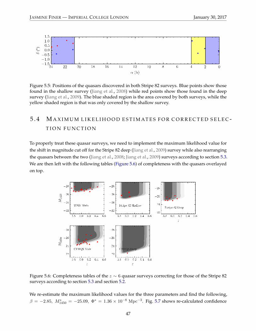
Figure 5.5: Positions of the quasars discovered in both Stripe 82 surveys. Blue points show thosefound in the shallow survey (Jiang et al., 2008) while red points show those found in the deepsurvey (Jiang et al., 2009). The blue shaded region is the area covered by both surveys, while theyellow shaded region is that was only covered by the shallow survey.
5 . 4 M A X I M U M L I K E L I H O O D E S T I M AT E S F O R C O R R E C T E D S E L E C -T I O N F U N C T I O N
To properly treat these quasar surveys, we need to implement the maximum likelihood value forthe shift in magnitude cut off for the Stripe 82 deep (Jiang et al., 2009) survey while also rearrangingthe quasars between the two (Jiang et al., 2008; Jiang et al., 2009) surveys according to section 5.3.We are then left with the following tables (Figure 5.6) of completeness with the quasars overlayedon top.
Figure 5.6: Completeness tables of the z ∼ 6 quasar surveys correcting for those of the Stripe 82surveys according to section 5.3 and section 5.2.
We re-estimate the maximum likelihood values for the three parameters and find the following,β = −2.85, M∗1450 = −25.09, Φ∗ = 1.36 × 10⁻⁸ Mpc−3. Fig. 5.7 shows re-calculated confidence
47

JASMINE FINER — IMPERIAL COLLEGE LONDON January 30, 2017
intervals in all parameters.
5 . 5 P R I O R D I S T R I B U T I O N O N Q L F PA R A M E T E R S
On inspection of Figure 5.1 it becomes clear that there is a degeneracy between the break magnitudeand bright end slope of the quasar luminosity function. This is a result of the small sample of faintquasars observed in the redshift 6 surveys. In principle they could all be fit by a double power lawwhere the break magnitude was fainter than the faintest quasar and therefore in principle the breakmagnitude could have any value lower than ∼ −27 as long as the bright end slope was shallowenough to pass through all the data points. With only the redshift 6 data, it is difficult to imposeconstraints that would break this degeneracy. However, there are a much larger number of quasarsobserved at z ∼ 5 (McGreer et al. (2013), section 3.2), and including these in our sample will providemore data at faint magnitudes will allow us to place tighter constraints on the shape of the quasarluminosity function.
In order to account for the evolution of the QLF parameters, we need to introduce extra parametersinto our analysis. Most importantly these include evolution of number density, parameterised by k,and evolution of the break magnitude, parameterised by j.
We can further constrain these parameters with the knowledge that there will be more quasars atz = 5 than z = 6 due to the extra time available for accretion to those at z = 5. Following withthe same reasoning, we expect the break magnitude to move to the bright end as we increase theredshift. We therefore expect k ≤ 0 and j ≥ 0. We also impose uniform priors on all parameters,with the condition Φ∗ ≥ 0, M∗1450 < 0, α < 0, β < α. With the redshift 5 data constraining theshape of the QLF and prior distributions on QLF parameters it is possible to implement an MCMCroutine to sample from the posterior distribution on QLF parameters.
5 . 6 M C M C A N A LY S I S O F Q L F PA R A M E T E R S
With prior distributions on QLF parameters and the inclusion of redshift 5 data, we are now in aposition to use an MCMC routine to sample from the posterior distribution on 6 QLF parameters.
We start by ensuring that the results detailed in section 4.3 are reproduced on the double power lawmodel with 3 parameters using only the redshift 6 data. Fig. 5.7 shows the posterior distribution ofQLF parameters obtained by evaluating the likelihood over a grid in β,M∗1450 and Φ∗.
Figure 5.7 shows that there are large degeneracies between all the parameters of the QLF with thisparameterisation. As a result of these large degeneracies the MCMC routine is unable to samplecorrectly from the posterior distribution. If we chose to fix the number density at a given value ofM1450, rather than at M∗1450, we can break the degeneracies between Φ∗ and β and Φ∗ and M∗1450.
48
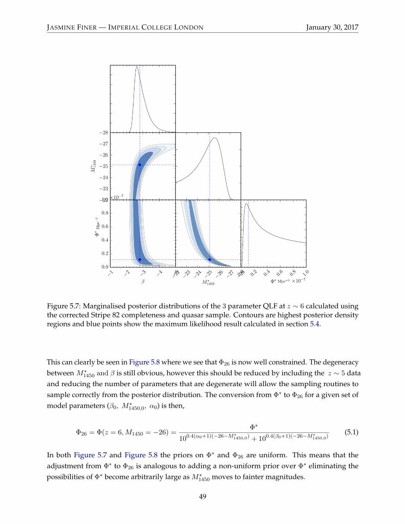
JASMINE FINER — IMPERIAL COLLEGE LONDON January 30, 2017
Figure 5.7: Marginalised posterior distributions of the 3 parameter QLF at z ∼ 6 calculated usingthe corrected Stripe 82 completeness and quasar sample. Contours are highest posterior densityregions and blue points show the maximum likelihood result calculated in section 5.4.
This can clearly be seen in Figure 5.8 where we see that Φ26 is now well constrained. The degeneracybetween M∗1450 and β is still obvious, however this should be reduced by including the z ∼ 5 dataand reducing the number of parameters that are degenerate will allow the sampling routines tosample correctly from the posterior distribution. The conversion from Φ∗ to Φ26 for a given set ofmodel parameters (β0, M
∗1450,0, α0) is then,
Φ26 = Φ(z = 6,M1450 = −26) =Φ∗
100.4(α0+1)(−26−M∗1450,0) + 100.4(β0+1)(−26−M∗
1450,0)(5.1)
In both Figure 5.7 and Figure 5.8 the priors on Φ∗ and Φ26 are uniform. This means that theadjustment from Φ∗ to Φ26 is analogous to adding a non-uniform prior over Φ∗ eliminating thepossibilities of Φ∗ become arbitrarily large as M∗1450 moves to fainter magnitudes.
49
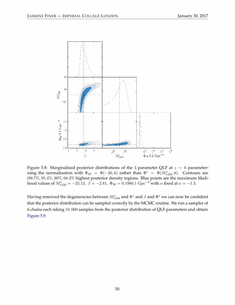
JASMINE FINER — IMPERIAL COLLEGE LONDON January 30, 2017
Figure 5.8: Marginalised posterior distributions of the 3 parameter QLF at z ∼ 6 parameter-ising the normalisation with Φ26 = Φ(−26, 6) rather than Φ∗ = Φ(M∗1450, 6). Contours are(99.7%, 95.4%, 90%, 68.3% highest posterior density regions. Blue points are the maximum likeli-hood values of M∗1450 = −25.13, β = −2.81, Φ26 = 0.1980.1 Gpc−3 with α fixed at α = −1.5.
Having removed the degeneracies between M∗1450 and Φ∗ and β and Φ∗ we can now be confidentthat the posterior distribution can be sampled correctly by the MCMC routine. We run a sampler of6 chains each taking 10, 000 samples from the posterior distribution of QLF parameters and obtainFigure 5.9.
50
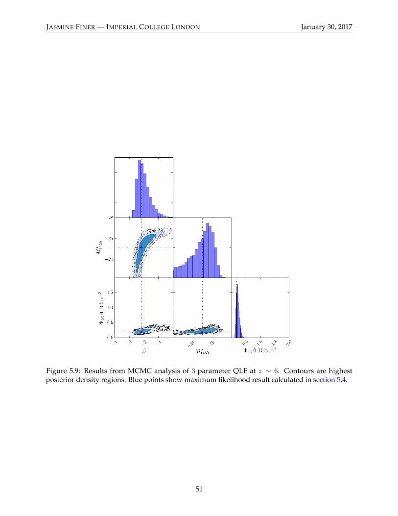
JASMINE FINER — IMPERIAL COLLEGE LONDON January 30, 2017
Figure 5.9: Results from MCMC analysis of 3 parameter QLF at z ∼ 6. Contours are highestposterior density regions. Blue points show maximum likelihood result calculated in section 5.4.
51

JASMINE FINER — IMPERIAL COLLEGE LONDON January 30, 2017
We see that the MCMC sampler converges to the correct posterior distribution of QLF parameters.In particular, the degeneracy betweenM∗1450 and β is clear. This allows us to extend the analysis tohigher dimensions where exactly calculating the posterior using the method prescribed in section 4.5is computationally slow and inefficient.
For completeness, we repeat this analysis for the 4 parameter QLF model at z ∼ 5. Figure 5.10 showsthe posterior distribution of QLF parameters for the 4 parameter model adopted by McGreer et al.(2013) calculated using the grid method (section 4.5). The blue points are the maximum likelihoodvalues of the parameters using the likelihood prescribed in section 4.1. Figure 5.11 shows resultsof MCMC analysis with 8 chains each sampling 10, 000 times from the 4 dimensional posteriordistribution. Again, as in the 3 parameter case, the grid method and MCMC analysis produceconsistent results.
Figure 5.10: Marginalised posterior distributions of the 4 parameter QLF at z ∼ 5. Contours arehighest posterior density regions and blue points show the maximum likelihood result as calculatedin McGreer et al. (2013).
52
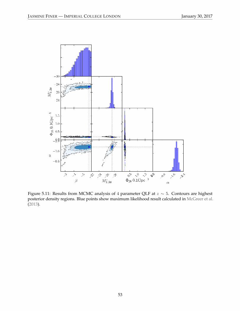
JASMINE FINER — IMPERIAL COLLEGE LONDON January 30, 2017
Figure 5.11: Results from MCMC analysis of 4 parameter QLF at z ∼ 5. Contours are highestposterior density regions. Blue points show maximum likelihood result calculated in McGreer et al.(2013).
53

JASMINE FINER — IMPERIAL COLLEGE LONDON January 30, 2017
We then included both redshift 5 and 6 data in our analysis and allowed for 6 free parameters:β,M∗1450,Φ
∗, α, k, j. Initially, we ran our analysis on quasars sampled from f(M1450, z) with thefollowing values for QLF parameters: α = −1.5, β = −2.81,M∗1450 = −25.13,Φ∗ = 11.4 Gpc−3, k =
−0.47, j = 0.0. Quasars were simulated from the same completeness tables but the survey areaswere increased by a factor of 10 to produce tighter constraints on the QLF parameters. The samplesare shown in Fig. 5.12 and results from this analysis are shown in Fig. 5.13. From these results wesee that the MAP estimates are consistent with the qlf model parameters from which the quasarsare sampled.
Figure 5.12: Figure showing contours of corrected completeness, as in Fig. 5.6 with simulated quasarsurveys shown as red points. The true quasars are shown as blue points, corrected for overlappingsurvey areas.
54

JASMINE FINER — IMPERIAL COLLEGE LONDON January 30, 2017
Figure 5.13: Corner plot showing results from MCMC analysis of double power law QLF with6 free parameters, with quasars simulated from a double power law QLF with parameters (β =−2.81, M∗1450 = −25.13, Φ∗ = 11.4 Gpc−3, α = −1.5, j = 0.1, k = −0.47).
Using the real data Fig. 5.14 is obtained. Maximum A Posteriori (MAP) estimates are β =
−5.45, M∗1450 = −27.36, j = 0.0198, Φ∗ = 3.0 Gpc−3, α = −1.95, k = −0.25. From this fig-ure, it seems that bright break magnitudes with steep bright end slopes are favoured by the data.This could suggest the possibility of adopting a QLF of the form Schechter (1976),
Φ(M1450, z) = 10k(z−zref)Φ∗ 100.4(α+1)(M1450−M∗1450−j(z−zref)) × exp−100.4(M1450−M∗
1450−j(z−zref))],
(5.2)
which is characterised by an exponential fall off of the bright slope. Note that this is the same formas the BHMF as described in section 2.2.
55
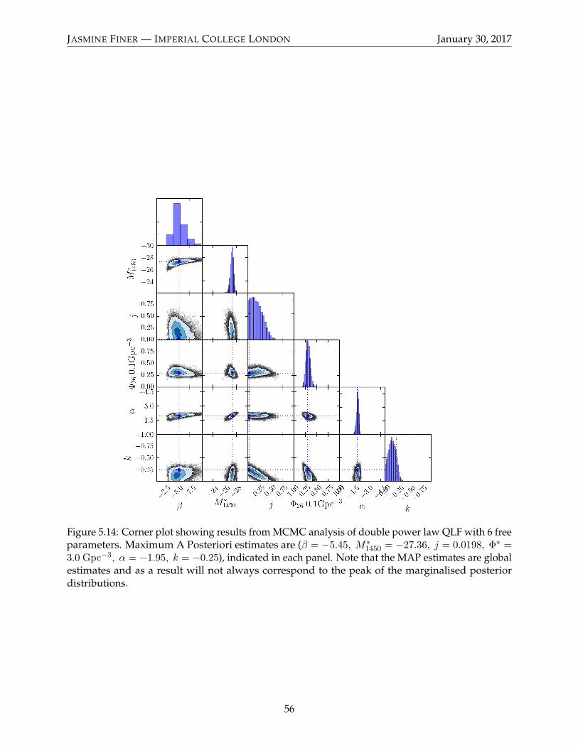
JASMINE FINER — IMPERIAL COLLEGE LONDON January 30, 2017
Figure 5.14: Corner plot showing results from MCMC analysis of double power law QLF with 6 freeparameters. Maximum A Posteriori estimates are (β = −5.45, M∗1450 = −27.36, j = 0.0198, Φ∗ =3.0 Gpc−3, α = −1.95, k = −0.25), indicated in each panel. Note that the MAP estimates are globalestimates and as a result will not always correspond to the peak of the marginalised posteriordistributions.
56

JASMINE FINER — IMPERIAL COLLEGE LONDON January 30, 2017
To better interpret the results of our MCMC analysis, it is useful to visualise the possibilities for theluminosity function. Taking 50 draws from the posterior, we can calculate the luminosity functionfor different combinations of QLF parameters we have sampled, as shown in Fig. 5.15. In in the twopanels, the line colours correspond to the same values of QLF parameters.
Figure 5.15: Figure showing plots of the QLF for different parameters sampled from the posterior inFig. 5.14. Left hand panel shows the QLF at z = 5, the right hand panel shows the QLF at z = 6.Note that colours in each panel correspond to the same QLF parameters. The thick black linescorrespond to the McGreer et al. (2013) best fit values and Willott et al. (2010a) best fit values forz ∼ 5 and z ∼ 6 respectively. The best fit QLF in the left hand panel is systematically above thesamples, which is due to the fact that the likelihood used in McGreer et al. (2013) is slightly differentto the one used in this thesis, as discussed in section 5.1
57
6 | D I S C U S S I O N
As we have seen, there is an outstanding issue with our understanding of quasar formation.Observations of quasars powered by black holes with masses up to 109M� at redshifts & 6 leaveunanswered the question of how black holes have evolved to reach such high masses within only1 billion years of the Big Bang. This inconsistency could arise from a misunderstanding of theblack hole seed formation, black hole growth or from uncertainties in the black hole mass estimatesthemselves. Observationally, these physical mechanisms all contribute to the observed QLF and itsevolution with redshift. The aim of this thesis, therefore, was to present a self-consistent approachto obtaining posterior distributions on QLF parameters at z ∼ 6. By improving the accuracyof statistical analysis we provide reliable constraints on the quasar luminosity function whichevolutionary models and mass estimates must reproduce.
We first presented a method for treating the case of overlapping surveys and apply a correctionto the completeness of the SDSS Stripe 82 shallow survey (Jiang et al., 2008). These adjustmentshave only a small effect on the maximum likelihood estimates of QLF parameters, in comparison tothose found in Willott et al. (2010a). This is because approximately 4 out of 50 quasars in the samplewere affected by the update. However, with larger high redshift quasar surveys in the future it willbecome all the more important to treat these problems carefully and correctly, using the correctformalism.
We then introduced the methodology (see section 4.4) for obtaining posterior distributions on thequasar luminosity function parameters by using MCMC. Due to the limited number of quasarsat z ∼ 6, we use quasars from z ∼ 5 (McGreer et al., 2013) to impose what are effectively priorconstraints on the z ∼ 6 QLF parameters.
The following 6 parameter model of the QLF was used, described in detail in chapter 2,
Φ(M1450, z) =10k(z−zref)Φ26
100.4(α+1)(M1450−M∗1450−j(z−zref)) + 100.4(β+1)(M1450−M∗
1450−j(z−zref)), (6.1)
where we have introduced a new parameterisation of the QLF normalisation, fixing it at a referencemagnitude M1450 = −26 rather than at M∗1450. This new parameterisation with uniform priorson Φ26 is equivalent to imposing non-uniform priors on the original normalisation parameter, Φ∗
58
JASMINE FINER — IMPERIAL COLLEGE LONDON January 30, 2017
and removes many of the degeneracies between the parameters of the model. This improves theperformance of MCMC routines when sampling from the posterior distribution.
Maximum A-Posteriori point estimates for these parameters are (β = −5.45, M∗1450 = −27.36, j =
0.0198, Φ∗ = 3 Gpc−3, α = −1.95, k = −0.25). As in Willott et al. (2010a), no uncertainties arequoted due to the existence of large degeneracies between parameters, however confidence regionscan be seen in the corner plots in section 5.6. The bright end is noticeably steeper than quoted byWillott et al. (2010a) and this could lead to the possibility of using a Schechter (1976) QLF of theform
Φ(M1450, z) = 10k(z−zref)Φ∗ 100.4(α+1)(M1450−M∗1450−j(z−zref)) × exp−100.4(M1450−M∗
1450−j(z−zref))].
characterised by an exponential fall-off at the bright end.
The value of k is smaller than calculated previously by Fan et al. (2001c) suggesting the fall off innumber density of quasars with redshift is slower than previously thought. The value ofj is small,as expected, and our results are consistent with a value j = 0. Further analysis could include modelcomparison to decide if the inclusion of this evolution is needed, and whether or not the data wouldbe better fit by also including evolution in β and/or α.
With a self-consistent approach to obtaining posterior distributions on QLF parameters in place,two avenues of future work should be pursued to understand the formation of supermassive blackholes at high redshift. Assuming current mass estimates of the black holes powering quasars inthe early universe are accurate, it is possible to obtain the black hole mass function (BHMF) byde-convolving the QLF with the Eddington ratio, λ = L/LEdd of high redshift black holes. TheBHMF is defined analogously to the quasar luminosity function and L and MBH are related viathe Eddington ratio distribution, λ. Thus the BHFM and the QLF are related via a convolutionwith the distribution of Eddington ratios. Large hydrodynamical simulations of black hole growthhave been performed (Di Matteo et al., 2012) and these can then be constrained by the necessity torecreate the BHMF at each given redshift.
It is also important to consider the possibility that the black hole mass estimates are inaccurate. Ifblack hole masses are, in fact, less massive than currently thought, then current models of blackhole growth may be able to explain their existence. As described in chapter 1, black hole massesat high redshift are estimated via scaling relations (Vestergaard & Peterson, 2006; Vestergaard &Osmer, 2009) observed at low-z. However, the assumption that these relations apply at high redshiftmay not be valid, and the complicated nature of the uncertainties means that classical regression isdifficult. Implementation of a Bayesian hierarchical model would allow updated mass estimates andincorporate correct treatment of the large number of uncertainties arising from these measurements.
In conclusion, we have developed a rigorous method of statistical analysis with which QLF parame-
59

JASMINE FINER — IMPERIAL COLLEGE LONDON January 30, 2017
ters can be estimated. We further discussed the appropriate adjustments that must be made whenselecting quasars from overlapping surveys. The results of this work are intended to provide areliable benchmark to which future evolutionary models should be compared, thereby aiding in theunderstanding of quasar formation.
60

B I B L I O G R A P H Y
Abazajian, K. N., Adelman-McCarthy, J. K., Agueros, M. A., et al. 2009, ApJS, 182, 543
Abramowicz, M. A. 2005, in Growing Black Holes: Accretion in a Cosmological Context, ed.A. Merloni, S. Nayakshin, & R. A. Sunyaev, 257
Abramowicz, M. A., Czerny, B., Lasota, J. P., & Szuszkiewicz, E. 1988, ApJ, 332, 646
Alvarez, M. A., Wise, J., & Abel, T. 2009, ApJL, 701, L133
Antonucci, R. 1993, ARAA, 31, 473
Avni, Y. 1976, ApJ, 210, 642
Avni, Y., & Bahcall, J. N. 1980, ApJ, 235, 694
Bayes, M., & Price, M. 1763, Philosophical Transactions of the Royal Society of London Series I, 53,370
Begelman, M. C., Volonteri, M., & Rees, M. J. 2006, MNRAS, 370, 289
Bondi, H., & Hoyle, F. 1944, MNRAS, 104, 273
Boyle, B. J., Shanks, T., Croom, S. M., et al. 2000, MNRAS, 317, 1014
Boyle, B. J., Shanks, T., & Peterson, B. A. 1988, MNRAS, 235, 935
Brooks, S. P., & Gelman, A. 1998, Journal of computational and graphical statistics, 7, 434
Burbidge, G. R., Burbidge, E. M., & Sandage, A. R. 1963, Reviews of Modern Physics, 35, 947
Croom, S. M., Smith, R. J., Boyle, B. J., et al. 2004, MNRAS, 349, 1397
Croom, S. M., Richards, G. T., Shanks, T., et al. 2009, MNRAS, 399, 1755
Di Matteo, T., Colberg, J., Springel, V., Hernquist, L., & Sijacki, D. 2008, ApJ, 676, 33
Di Matteo, T., Khandai, N., DeGraf, C., et al. 2012, ApJ, 745, L29
Fan, X. 2003, in Bulletin of the American Astronomical Society, Vol. 35, American AstronomicalSociety Meeting Abstracts, 1415
Fan, X., Narayanan, V. K., Lupton, R. H., et al. 2001a, AJ
Fan, X., Strauss, M. A., Richards, G. T., et al. 2001b, AJ
Fan, X., Strauss, M. A., Schneider, D. P., et al. 2001c, AJ
Fan, X., Hennawi, J. F., Richards, G. T., et al. 2004, AJ, 128, 515
Fan, X., Strauss, M. A., Richards, G. T., et al. 2006, AJ, 131, 1203
Foreman-Mackey, D., Hogg, D. W., Lang, D., & Goodman, J. 2013, PASP, 125, 306
Fukugita, M., Ichikawa, T., Gunn, J. E., et al. 1996, AJ, 111, 1748
Gelman, A., Carlin, J. B., Stern, H. S., & Rubin, D. B. 2014, Bayesian Data Analysis
61

JASMINE FINER — IMPERIAL COLLEGE LONDON January 30, 2017
Gelman, A., & Rubin, D. B. 1992, Statistical science, 457
Glikman, E., Bogosavljevic, M., Djorgovski, S. G., et al. 2010, ApJ, 710, 1498
Goodman, J., & Weare, J. 2010, CAMCOS, 5, 65
Hao, L., Strauss, M. A., Fan, X., et al. 2005, AJ, 129, 1795
Hastings, W. K. 1970, Biometrika, 57, 97
Hopkins, P. F., Lidz, A., Hernquist, L., et al. 2007a, ApJ, 662, 110
Hopkins, P. F., Richards, G. T., & Hernquist, L. 2007b, ApJ, 654, 731
Hunt, M. P., Steidel, C. C., Adelberger, K. L., & Shapley, A. E. 2004, ApJ, 605, 625
Ikeda, H., Nagao, T., Matsuoka, K., et al. 2011, ApJL, 728, L25
Jiang, L., McGreer, I. D., Fan, X., et al. 2015, AJ, 149, 188
Jiang, L., Fan, X., Annis, J., et al. 2008, AJ, 135, 1057
Jiang, L., Fan, X., Bian, F., et al. 2009, AJ, 138, 305
Kaspi, S., Maoz, D., Netzer, H., et al. 2005, ApJ, 629, 61
Kellermann, K. I. 2013, Bulletin of the Astronomical Society of India, 41, 1
Kelly, B. C., Fan, X., & Vestergaard, M. 2008, ApJ, 682, 874
Kelly, B. C., & Merloni, A. 2012, Advances in Astronomy, 2012, 970858
Kelly, B. C., & Shen, Y. 2013, ApJ, 764, 45
Kelly, B. C., Vestergaard, M., Fan, X., et al. 2010, ApJ, 719, 1315
Komatsu, E., Dunkley, J., Nolta, M. R., et al. 2009, ApJS, 180, 330
Lampton, M., Margon, B., & Bowyer, S. 1976, ApJ, 208, 177
Lawrence, A., Warren, S. J., Almaini, O., et al. 2007, MNRAS, 379, 1599
Marshall, H. L., Tananbaum, H., Avni, Y., & Zamorani, G. 1983, ApJ, 269, 35
Marshall, J. L., Burles, S., Thompson, I. B., et al. 2008, in SPIE, Vol. 7014, Ground-based and AirborneInstrumentation for Astronomy II, 701454
Masters, D., Capak, P., Salvato, M., et al. 2012, ApJ, 755, 169
McGreer, I. D., Jiang, L., Fan, X., et al. 2013, ApJ, 768, 105
Metropolis, N., Rosenbluth, A. W., Rosenbluth, M. N., Teller, A. H., & Teller, E. 1953, Journal ofChemical Physics, 21, 1087
Mortlock, D. J., Warren, S. J., Venemans, B. P., et al. 2011, Nature, 474, 616
Netzer, H. 2015, ARAA, 53, 365
Oke, J. B., & Gunn, J. E. 1983, ApJ, 266, 713
Osmer, P. S. 1982, ApJ, 253, 28
Pacucci, F., Volonteri, M., & Ferrara, A. 2015, MNRAS, 452, 1922
Paczynski, B. 1998, AcA, 48, 667
Paris, I., Petitjean, P., Aubourg, E., et al. 2014, A&A, 563, A54
Pei, Y. C. 1995, ApJ, 438, 623
Peterson, B. M. 1997, An Introduction to Active Galactic Nuclei
Peterson, B. M. 2010, in Bulletin of the American Astronomical Society, Vol. 42, American Astro-nomical Society Meeting Abstracts #215, 581
62

JASMINE FINER — IMPERIAL COLLEGE LONDON January 30, 2017
Press, W. H., Teukolsky, S. A., Vetterling, W. T., & Flannery, B. P. 2002, Numerical recipes in C++ :the art of scientific computing
Rees, M. J. 1978, The Observatory, 98, 210
—. 1984, ARA&A, 22, 471
Reyle, C., Delorme, P., Willott, C. J., et al. 2010, a, 522, A112
Richards, G. T., Fan, X., Newberg, H. J., et al. 2002, AJ, 123, 2945
Richards, G. T., Croom, S. M., Anderson, S. F., et al. 2005, MNRAS, 360, 839
Richards, G. T., Lacy, M., Storrie-Lombardi, L. J., et al. 2006a, ApJS, 166, 470
Richards, G. T., Strauss, M. A., Fan, X., et al. 2006b, AJ, 131, 2766
Ross, N. P., Myers, A. D., Sheldon, E. S., et al. 2012, ApJS, 199, 3
Schechter, P. 1976, ApJ, 203, 297
Schmidt, M. 1963, Nature, 197, 1040
—. 1968, ApJ, 151, 393
Schmidt, M., Schneider, D. P., & Gunn, J. E. 1995a, AJ, 110, 68
—. 1995b, AJ, 110, 68
Schneider, D. P., Schmidt, M., & Gunn, J. E. 1994, AJ, 107, 1245
—. 1999, AJ, 117, 40
Shankar, F., & Mathur, S. 2007, ApJ, 660, 1051
Shankar, F., Weinberg, D. H., & Miralda-Escude, J. 2009, ApJ, 690, 20
—. 2013, MNRAS, 428, 421
Shen, Y., & Kelly, B. C. 2012, ApJ, 746, 169
Siana, B., Polletta, M. d. C., Smith, H. E., et al. 2008, ApJ, 675, 49
Sijacki, D., Springel, V., & Haehnelt, M. G. 2009, MNRAS, 400, 100
Steffen, A. T., Barger, A. J., Cowie, L. L., Mushotzky, R. F., & Yang, Y. 2003, ApJL, 596, L23
Tanaka, T., & Haiman, Z. 2009, ApJ, 696, 1798
Ueda, Y., Akiyama, M., Ohta, K., & Miyaji, T. 2003, ApJ, 598, 886
Urry, C. M., & Padovani, P. 1995a, PASP, 107, 803
—. 1995b, PASP, 107, 803
Vestergaard, M., Fan, X., Tremonti, C. A., Osmer, P. S., & Richards, G. T. 2008, ApJL, 674, L1
Vestergaard, M., & Osmer, P. S. 2009, ApJ, 699, 800
Vestergaard, M., & Peterson, B. M. 2006, ApJ, 641, 689
Volonteri, M. 2010, AR&A, 18, 279
Volonteri, M., Habouzit, M., Pacucci, F., & Tremmel, M. 2015a, ArXiv e-prints, arXiv:1511.02588Volonteri, M., Lodato, G., & Natarajan, P. 2008, MNRAS, 383, 1079
Volonteri, M., & Rees, M. J. 2005, ApJ, 633, 624
Volonteri, M., Silk, J., & Dubus, G. 2015b, ApJ, 804, 148
Warren, S. J., Hewett, P. C., & Osmer, P. S. 1994, ApJ, 421, 412
Willott, C. J., Rawlings, S., Blundell, K. M., Lacy, M., & Eales, S. A. 2001, MNRAS, 322, 536
Willott, C. J., Delorme, P., Omont, A., et al. 2007, AJ, 134, 2435
63
JASMINE FINER — IMPERIAL COLLEGE LONDON January 30, 2017
Willott, C. J., Delorme, P., Reyle, C., et al. 2009, AJ, 137, 3541Willott, C. J., Albert, L., Arzoumanian, D., et al. 2010, AJ, 140, 546Willott, C. J., Delorme, P., Reyle, C., et al. 2010a, AJ, 139, 906Wu, X.-B., Wang, F., Fan, X., et al. 2015, Nature, 518, 512Yee, H. K. C., Gladders, M. D., Gilbank, D. G., et al. 2007, in Astronomical Society of the Pacific
Conference Series, Vol. 379, Cosmic Frontiers, ed. N. Metcalfe & T. Shanks, 103York, D. G., Adelman, J., Anderson, Jr., J. E., et al. 2000, AJ, 120, 1579Yu, Q., & Tremaine, S. 2002, MNRAS, 335, 965Zhang, W., Woosley, S. E., & Heger, A. 2008, ApJ, 679, 639
64