-1-

Consequences of Political Instability, Governance and Bureaucratic Corruption on Inflation and Growth: The Case of Pakistan

Adnan Haider*

Research Analyst

Monetary Policy Department State Bank of Pakistan

Musleh ud Din

Joint Director Pakistan Institute of Development

Economics

Ejaz Ghani

Chief of Research

Pakistan Institute of Development Economics

ABSTRACT This paper presents a theoretical model withmicro-foundations that captures some important features ofPakistan's economy which have emergedin sixty-four years of its history.A comparison of Pakistan’s economic performance during different regimes shows that macroeconomic fundamentals tend to show an improvement during the autocratic regimes as compared with those prevailing during democratic regimes. In particular, periods of autocratic regimes are typically characterized by low inflation, robust growth and low level of bureaucratic corruption due to better governance. In contrast, the economic performance during the democratic regimes has been observed to worsen with weak governance and high levels of corruption, high inflation due partly to reliance on seigniorage to finance public spending, and lackluster growth. Using annual data from 1950 to 2011, computational modeling is carried outby applying Markov-Regime switching technique with maximum-likelihood procedures.The estimation results based on empirical modeling setup are supportiveof the above stylized-facts and also confirm theimplications of the theoretical model. JEL Classifications:D73, E31, E3, H6, O42 Key Words:Political Instability; Governance; Corruption; Inflation; Growth

*Corresponding Author- Email: adnan.haider@sbp.org.pk; Telephone: +92-21-32453895. The authors

aregrateful to Omar Farooq Saqib, Safdar Ullah Khan, Syed Kalim Hyder Bukhari and Sajawal Khan for sharing theirviewson structural characteristics of the political economy of Pakistan. They are also thankful to Asad Jan and Nasir Hameed Rao for providing excellent editorial assistance. The views expressed in the paper are those of the authors’ and not necessarily of the State Bank of Pakistan or Pakistan Institute of Development Economics. The usual disclaimer applies.

-2-

TABLE OF CONTENTS

S. No. Contents Page No.

1. Introduction ………………………………………. 3

2. How Corruption and Governance Lead to Inflation and Growth?

………………………………………. 6

3. Description of Theoretical Model ………………………………………. 11

3.1 Agent Preferences ………………………………………. 12

3.2 Firm’s Behavior ………………………………………. 14

3.3 Behavior of Bureaucratic Corruption

across political regimes ………………………………………. 15

3.4 Government ………………………………………. 16

3.5 Analytical Solution of Theoretical Model ………………………………………. 17

4. Description of Empirical Model ………………………………………. 20

4.1 Data ………………………………………. 20

4.2 Specification of Econometric Models ………………………………………. 21

4.3 Regime Switching Modeling Approach ………………………………………. 22

5. The Results ………………………………………. 25

5.1 Calibration Results of Theoretical Model ………………………………………. 25

5.2 Estimation Results of Regime-Switching

Model ………………………………………. 26

6. Concluding Remarks ………………………………………. 29

7. References ………………………………………. 30

8. Appendices ………………………………………. 33

-3-

“Countries that have pursued distortionary macroeconomic policies, including high inflation, large budget deficits and misaligned exchange rates, appear to have suffered more macroeconomic volatility and also grown more slowly during the postwar period. Does this reflect the causal effect of these macroeconomic policies on economic outcomes? One reason to suspect that the answer may be no is that countries pursuing poor macroeconomic policies also have weak „„institutions,‟‟ including political institutions that do not constrain politicians andpolitical elites, ineffective enforcement of property rights for investors, widespread corruption,and a high degree of political instability.”

Acemogluet al., (2003)

1 INTRODUCTION Political regimes in Pakistan have strongly influenced the economic outcomes. Whereas the

autocratic regimes have tended to exhibit good economic performance with low and stable

inflation, robust growth, and fiscal discipline helped by relatively high revenue generation and

checks on public expenditure, the democratic regimes have been marked by macroeconomic

instability and sluggish economic growth. In addition, autocratic regimes also witnessed

relatively stable external sector along with low trade deficit and high capital inflows in the form of

foreign direct investments and portfolio investments, which indicates high level of confidence of

foreign investors in the domestic economy. On the other hand, key economic indicators have

generally deteriorated during different episodes of democratic regimes.1Table 1 summarizesthe

relative performance of selected macroeconomic variables across different political regimes.

Table 1: Performance of Selected Macroeconomic Indicators across Political Regimes

Regime* RGDPgr TFPgr PINVgr BBR ER INF UR M2gr Corrp Gov

1 3.18 2.10 22.14 -5.41 3.41 3.54 0.15 8.30 1.83 6.88

2 2.74 0.09 2.73 -9.11 4.55 4.38 0.10 10.41 3.13 6.25

3 5.69 1.19 7.45 -11.04 4.76 2.71 0.84 10.80 3.50 3.95

4 5.35 1.28 6.19 -9.24 4.76 3.80 1.85 9.42 3.00 3.50

5 3.67 -0.98 -2.46 -6.88 7.81 6.70 1.94 10.04 1.67 3.47

6 4.87 0.62 8.49 -9.44 9.90 16.69 2.32 18.87 1.50 6.27

7 6.45 1.67 4.94 -8.59 13.67 7.27 3.70 15.62 2.05 6.17

8 5.12 0.40 4.81 -9.57 22.87 9.30 4.37 16.48 2.00 3.89

9 2.44 -2.81 3.84 -9.09 28.11 9.83 4.70 17.77 2.00 4.75

10 4.69 -0.20 1.27 -7.01 34.85 11.72 5.43 15.35 2.23 7.94

11 2.17 -1.78 -0.33 -7.64 43.08 9.81 6.00 13.37 2.96 9.96

12 3.48 -0.02 0.84 -6.29 52.53 5.39 6.85 9.75 2.35 9.96

13 5.45 1.71 7.05 -4.52 60.02 6.57 7.06 16.35 2.67 5.60

14 3.68 1.90 7.28 -7.83 62.63 12.00 5.20 15.35 2.00 6.50

15 2.62 -0.77 -8.92 -5.47 82.68 15.43 5.78 12.63 1.00 8.60

Variable List:RGDPgr = Average growth of real gross domestic product; TFPgr = Average growth of total factor productivity; PINVgr=Average growth of real private investment; BBR = Average of Budget Balance ratio to GDP (in percent); ER = Average Exchange rate; INF = Average inflation rate (in percent); UR = Average Unemployment rate; M2gr = Average growth in broad money (M2); Corrp = Aveage level of Corruption and Gov = Average Level of Governance.

* For political regime categorization, please refer to table A4 in appendix. Further, shaded rows represent autocratic regimes. Source: Author’s calculations. For data sources and description of variables, please refer section 3.

1For comprehensive comparison of both regimes, see Iqbal et al., (2008), and Zaidi (2006).

-4-

The economy grew more than 5 percent per annum on average during autocratic

regimes, which is 1.5 percentage points higher than the average growth rate observed during

democratic regimes. Similarly, in all autocratic regimes, average economic growth remained

above 5 percent with the exception of the second regime in which average economic growth

was 2.74 percent. However, in the case of all democratic regimes average annual growth

remainedin the range from 2 percent to 5 percent. Therefore, more than 5 percent average

annual growth across all autocratic regimes signifies the relatively strong macroeconomic

fundamentals during these regimes. Similarly, growth in total factor productivity (TFP) during

autocratic regimes outstripped the same in democratic eras: average annual growth of TFP

during autocratic regimes was 1.19 percent as compared with TFP growth of -0.15 percent

during the democratic regimes. A look at other macroeconomic indicators also shows that the

economic performance during the autocratic regimes has been much better than that observed

during the democratic regimes. For example, real private investment is a leading indicator of

confidence the general public has in the government and its policies. Growth performance of

real investment in autocratic eras has been far better than in the democratic regimes. Average

growth in real investment in autocratic regimes was 5.67 percent per annum as compared with

3.70 percent during the democratic regimes.

Autocratic regimes have also outperformedthe democratic regimes in terms of fiscal

discipline and price stability. Consider, for example, the budget balance ratio which is the ratio

of fiscal balance to GDP; the higher the ratio in absolute terms the worse is the fiscal position.

Barring short periods where democratic regimes have a slight edge over autocratic regimes, the

former have mostly outperformed the latter in terms of fiscal discipline: average budge balance

ratio in autocratic regimes is -8.1 percent whereas in democratic regimes the same is -7.9

percent. In terms of price stability, the democratic regimes have often been marked by high

levels of inflation: average inflation in autocratic regimes stood at 4.9 percent per annum as

compared with 10 percent for democratic regimes.

What factors could explain the differences in economic performance during autocratic

and democratic regimes? A growing and influential body of empirical research has sought to

identifythe causes of poor economic outcomes as reflected in high inflation and low economic

growth. There is a near consensus in the literature that poor economic outcomes are often

associated with lack of good governance and poor state institutions which promote rent seeking

and corruption thus impeding the process of economic growth.2

In the case of Pakistan, few studies have examined the role of governance and

2 See for instance, Baumol (1990), Murphy et al., (1991), Acemoglu (1995), Mauro (1995) and Baumol (2004).

-5-

institutions in macroeconomic outcomes. For example, Khawaja and Khan (2009), Hussain

(2008) and Qayyumet al., (2008)note that good governance and better institutional quality are

necessary conditions for batter economic outcomes.Siddique and Ahmed (2010a, 2010b)

investigate the long run positive relationship between institutional quality and economic growth.

They find unidirectional causality running from institutional quality to economic growth. Another

recent study byZakria and Fida (2011) finds indirect effects of democracy on economic growth.

Similarly, Qureshiet al., (2010) and Khan and Saqib (2011) find positive and significant impact of

political instability (where political instability is defined as frequent cabinet changes and

government in crises) on inflation in Pakistan.

The above studies are mostly empirical in nature and lack theoretical foundations

without which it is difficult to explain how governance, democracy, political instability, quality of

institutions and other deeper determinants impact inflation and growth. This study fills the gap in

the literature by developing a theoretical model with micro-foundations thatcaptures someof the

highlighted features of Pakistan's economy. Furthermore, using actual data, computational

modeling is doneby applying Markov-Regime switching technique with maximum-likelihood

procedures.Theestimationresults based on empirical modeling setup are in line with the stylized-

facts and also confirm the intuitive implications of the theoretical model.

The rest of the paper is organized as follows: section 2 reviews the literature that

explores the links between corruption, quality of governance, inflation and economic growth.

Section 3 presents theoretical model. Section 4 describes data and empirical methodology.

Main findings are discussed in section 5 and the concluding remarksare stated in section 6.

2. HOW CORRUPTION AND GOVERNANCE LEAD TO INFLATION AND ECONOMIC

GROWTH?

Cross country studies provide many plausible explanations of persistence of high inflation with

low economic growth. In general, high inflation might be associated with market imperfections,

exchange rates fluctuations, cost-push factors such as food supply shortages, energy inflation in

the case of oil importing countries and conventional demand pull factors including private

consumption and government expenditures. But research brings a common synthesis that in the

long run inflation can persist only when there is excessive money supply growth [see for

instance,McCandless and Weber (1995), David and Kanago (1998) andFischer et al, (2002)].

Several empirical studies on inflation-growth nexus have found that high and persistent inflation

is harmful to economic growth whereas low and stable inflation is considered as conducive for

-6-

the process of economic growth. For example, Khan and Senhadji (2001) estimatethe threshold

levels of inflation both for advance and emerging economies. They find that up to these

threshold levels growth is positively related with inflation and beyond these levels, inflation

exerts a negative effect on economic growth.In particular, the threshold estimates are 1-3

percent and 7-11 percent for industrial and developing countries, respectively. Figure 1 shows

the relationship between CPI inflation and real GDP growth and between CPI inflation and M2

growth for OECD3(organization for economic corporation and development) and developing

countries4 for the sample 1984 to 2010.

Figure 1: Relationships of CPI Inflation with Economic Growth and Broad Money Growth

Source: Author‟s calculations based on International Financial Statistics of IMF Database.

This figure shows positive relationship between CPI inflation and M2 growth for both

panels of countries. For developing countries this relationship is much stronger as

3 List of OECD countries: Australia, Austria , Belgium , Canada , Denmark, Finland, France, Greece , Hungary,

Iceland, Ireland, Italy, Japan, Korea, Luxembourg, Netherland, New Zealand, Norway, Poland, Portugal, Spain, Sweden, Switzerland, Turkey, United Kingdom and United States. 4 List of Developing Countries: Bangladesh, Chile, Colombia, Costa Rica, Egypt, Ghana, India, Indonesia, Israel,

Jamaica, Jordan, Malawi, Malaysia, Morocco, Myanmar, Nigeria, Pakistan, Romania, South Africa, Sri Lanka, Thailand, Tunisia, Uganda, Venezuela and Zimbabwe.

0

2

4

6

8

10

12

14

16

2 3 4 5 6 7

Ave

rag

e In

fla

tio

n R

ate

(in

%)

Average Output Growth (in %)

Economic Growth and Inflation Rate in OECD Countries

0

5

10

15

20

25

30

35

40

2 3 4 5 6 7

Ave

rag

e In

fla

tio

n R

ate

(in

%)

Average Output Growth (in %)

Economic Growth and Inflation Rate in Developing Countries

2

4

6

8

10

12

14

16

4 6 8 10 12 14 16 18 20

Ave

rag

e In

fla

tio

n R

ate

(in

%)

Average Money Growth (in %)

Inflation Rate and Money Growth in OECD Countries

3

8

13

18

23

28

33

38

43

48

10 20 30 40 50 60

Ave

rag

e In

fla

tio

n R

ate

(in

%)

Average Money Growth (in %)

Inflation Rate and Money Growth in Developing Countries

-7-

comparedwith OECD case. Similarly, it shows negative relationship between CPI inflation and

Real GDP growth for both the panels. In developing countries inflation normally persists at high

levels so the negative relationship in this case is much stronger as compared with OECD

countries where inflation remains below its threshold level. These observations confirm that high

inflation is harmful for economic growth especially for emerging countries and it is mainly

determined by high growthin money supply.

Apart from monetarist interpretations of high inflation coupled with low economic

growth,recent research provides better explanations of the causes of high money growth and

hence inflation. Rahmani and Yousefi (2009) classifythese explanationsinto three broad

categories: a) political business cycle theories of inflation determination; b) time inconsistency

theory of optimal planning; and c) seigniorage explanations of high rate of money growth and

inflation.

The literature on political business cycle (PBC) theories provides two main explanations

for sustained inflation: political instability with deficit bias hypothesis and war of attrition

philosophy. The seminal attempts by Nordhaus (1975) and Alesina and Tabellini (1990)relate

political instability to deficit bias as a possible determinant of inflationboth in the long and short

run spans. Nordhaus (1975)argues that with expectations augmented Phillips curve (EAPC)

where expectations are assumed to be adaptive, there could be a likelihood of higher than

social optimal inflation rate in the long-run. Alesina(1987),Alesina(1989),Rogoff and

Sibert(1988) consider rational expectationsapproach as opposed to adaptive expectation

schemes and come up with similar results. Alesina and Tabellini (1990) invoke deficit bias

hypothesis and explain that alternating governments are either uncertain of each others’

preferences or they disagree over the composition of public spending that gives rise to

excessively high budget deficits. This deficit bias thus yields suboptimal outcomes which put

pressure on inflation in both short and long run. Thus in this case inflation is a result of

opportunistic behavior by alternative governments that are in office and try to influence myopic

voters for reelection.

Alesina and Drazen (1991) expound the war of attrition philosophy which is the

extension of Hibbs’ (1977) findings.These studiesfocus on the cyclical behavior of the economy

and consider inflation as the result of ideological differences of political parties that come to

power alternately within a setting of asymmetric information among key political parties. The

higher the number of political parties in a legislative council, the higher the likelihood of conflict,

the harder it is to reach agreements and the higher the increase in fiscal which ultimately leads

to high inflation.

-8-

The second line of research attemptsto explain the reasons of high inflation rates within

an optimal planning framework with time inconsistency problems.These problems occur as a

result of the game between policy making authorities and the private sector agents. The seminal

attempts in this direction are Kydland and Prescott (1977), Barro and Gordon (1983a), Barro

and Gordon (1983b), Backus and Driffill (1985) andRogoff(1985). These studies explain the

high money supply growth and inflation rates by using game theoretic approaches. The main

argument is that the policy makers in certain cases take advantage of discretionary powers with

the assumption of asymmetric information while preparing policies to reduce unemployment or

to increase economic growth at the cost of higher inflation. Private agents on the other hand are

rational and aware of thesehidden incentives.They do not trust policy rules unless some kind of

strict commitments exist. Therefore, credibility plays a major role in such cases. This body of

research also proposes reputation and delegation as possible solutions to lower money growth

and inflation rates.

The third line of research for explaining high inflation rate is seigniorage.Khan and Saqib

(2011) andCarlstom and Fuerst (2000) consider a weak form of fiscal theory of price level

(weak-form FTPL) determination. According to the theory of optimal taxation5, the government

tries to equate the marginal cost of inflation tax with the marginal cost of output taxes in order to

minimize the distortions of taxation. Therefore, the government may choose to use seigniorage

as a way to finance public expenditures and budget deficit. Recent studies including Telartaret

al., (2010), Aisen and Veiga (2008), Aisen and Veiga (2006),Cukeirmanet al. (1992) and

Paldem (1987)also provide similar arguments that economies with political instability and weak

institutions lack an efficient tax system, which results in reliance on seigniorage. To meet the

demand for public expenditures governments print more money which eventually leads to higher

inflation.

It is generally accepted that these three explanations for high money growth and high

inflation can help in understanding the situation in developing countries. However, there could

be some other plausiblereasons due to the existence of bad governance, poor quality of

institutions and high level of corruption activitiesin developing countries which can cause high

inflation rates along with low economic growth. Figure 2 shows the relationship between

governance and corruption with CPI inflation and real GDP growth for sixty OECD and

developing countries.

5 See, for instance, Phelps (1973), Vegh (1989), and Aizenman (1992).

-9-

-10-

Figure 2: Relationships of CPI Inflation and Economic Growth with Corruption and Governance

Source: Author‟s calculations based on International Financial Statistics of IMF Database and International Country Risk Guide (ICRG) database.

This figure shows that less corruption and good governance is negatively related with

average CPI inflation and positively related with real GDP growth. There are a number of

reasons that can explain these stylized facts:a) corruption may cause a misallocation of talent

and skills away from productive (entrepreneurial) activities [Acemoglu(1995) and Murphy et al.,

(1991)];b) corruption may undermine the protection of the property rights, create obstacles to

doing business and impede innovation and technological transfer [Hall and Jones (1999)and

North (1990)];d) corruption may cause firms to expand less rapidly, to adopt inefficient

technologies and to shift their operations to the informal sector [Svensson, (2005)];e) corruption

may limit the extent of a country’s trade openness and reduce inflows of foreign investment

[Pellegrini and Gerlagh(2004) and Wei (2000)]; f) corruption may lead to costly concealment and

detection of illegal income, resulting in a deadweight loss of resources [Blackburn et al.(2006)

and Blackburn and Forgues-Puccio(2007)]; g) corruption may compromise human development

0

5

10

15

20

25

30

35

40

6.0 7.0 8.0 9.0 10.0

Ave

rag

e In

fla

tio

n R

ate

(in

%)

Average Governance Index

Inflation Rate and Governance in all Selected Countries

0

5

10

15

20

25

30

35

40

0.5 1.5 2.5 3.5 4.5 5.5

Ave

rage

Infl

atio

n R

ate

(in

%)

Average Corruption Index

Inflation Rate and Corruption in all Selected Countries

0

1

2

3

4

5

6

6.0 7.0 8.0 9.0 10.0

Ave

rage

Out

put

Gro

wth

(in

%)

Average Governance Index

Economic Growth and Governance in all Selected Countries

0

1

2

3

4

5

6

1.0 2.0 3.0 4.0 5.0 6.0

Ave

rage

Ou

tpu

t G

row

th (

in %

)

Average Corruption Index

Economic Growth and Corruption in all Selected Countries

-11-

through a deterioration in the scale and quality of public health and education programs

[Blackburn and Sarmah(2008), Gupta et al.(2000) andReinikka and Svensson(2005)]; and h)

corruption may cause a general misallocation of public expenditures as certain areas of

spending are targeted more for their capacity to generate bribes than their potential to improve

living standards [Gupta et al. (2001), Mauro (1995) andTanzi and Davoodi(1997)].

In terms of public finances, corruption and poor governance may independently impact

both the expenditure and revenue sides of the government′s budget: for any given state of the

latter, corruption can distort the composition of expenditures in ways described above; for any

given state of the former, corruption can alter the manner by which revenues must be

generated, as suggested by other empirical evidence. Thus Ghura (1998), Imam and Jacobs

(2007) and Tanzi and Davoodi (1997, 2000) conclude that corruption reduces total tax revenues

by reducing the revenues from almost all taxable sources.The implication is that, ceteris

paribus, other means of raising income must be sought, and one of the most tempting of these

is seigniorage. Significantly, it has been found that inflation is positively related to the incidence

of corruption, see for instance, Al-Marhubi(2000) and Rahmani and Yousefi (2009). These

studies also noted that corruption causes inflation to increase directly by increasing government

expenditures and therefore budget deficit that is financed by seigniorage. However, there is an

indirect channel through which corruption increase the inflation rate. Since the growth rate of

GDP is lower when corruption is higher and since the inflationary effect of the growth in the

money supply is higher when the growth rate of GDP is lower, the higher the inflation rate the

higher is corruption.

3DESCRIPTION OF THE THEORETICAL MODEL

This section provides a detailed description of the theoretical model explicitly outlining its micro-

foundations.6The model economy consists of private households, public officials, firms and

government as representative agents. Every agent tries to optimize its objective function subject

to its constraints. The model links corruption motives of public officials and governance behavior

of government with different political regimes. These links have implications for the role of

corruption and governance on inflation and growth which are discussed in the results section of

the paper.

6This model is an extension of Blackburn and Powell (2011) and Del Monte and Papagni (2001).

-12-

3.1 Agent’s Preferences

The theoretical modelconsiders an economy inhabited by acontinuum of infinite-lived agents,

who derive their lifetimeutility based on consumption of private goods, tC , consumption ofpublic

goods and services, tS , and leisure, )1( tL . Theagents-population is normalized to one and

divided into a fraction, )1,0( of private agents (or assumed to be standardhouseholds), who

provide labor to firms and the remaining fraction, )1,0()1( as bureaucrats, who work for the

government aspublic officials. Labor supply decision of each agent followsstandard Walrasian

features.

At time t, the intertemporal utility function of the representative agent is specified as:

0

)1(,,t

tttt

t

t LSCUU (3.1)

Where, )1,0( is a discount factor. It is assumed that utility function is separable in each of its

argument and its specification is given as:

1

)1()log()log()1(,,

1

ttttttt

LSCLSCU (3.2)

Where, is elasticity of labor supply and 1 is weight associated with consumption of public

good in the agents welfare function. Utility function (3.2) also follows standard assumption about

increasing with diminishing return in each of its argument, i.e., 0)( tU and

0)(22 tU .

Each agent maximizes his/her lifetime utility function (3.1) subject to the following intertemporal

(flow) budget constraint:

tt

t

t

ttt

t

t

tt ARP

MLWA

P

MSC )1(1

1

(3.3)

-13-

and a sequence of cash-in-advance (CIA) constraint:

tttt

t

t AASCP

M

1

1 (3.4)

Where, tM denotes nominal money holdings at time t, tA denotes real asset holdings at time t,

tP denotes the general price level and tR is the real returns on assets. The optimization

process solves the following problem as:

0

1

1

2

1

1

1

1

)1(1

)1()log()log(

t

tttt

t

t

t

t

t

t

tttt

t

t

ttt

t

tt

t

AASCP

M

AP

MSCAR

P

MLW

LSC

(3.5)

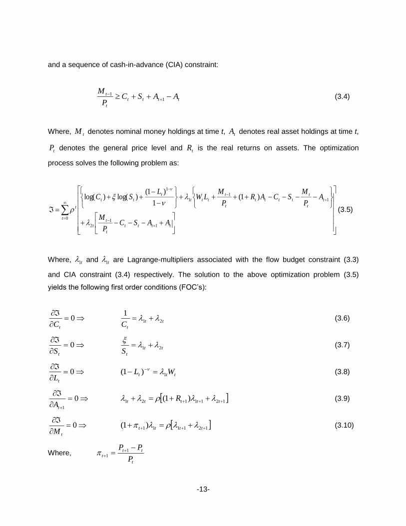
Where, t1 and t1 are Lagrange-multipliers associated with the flow budget constraint (3.3)

and CIA constraint (3.4) respectively. The solution to the above optimization problem (3.5)

yields the following first order conditions (FOC’s):

0

tC tt

tC21

1 (3.6)

0

tS tt

tS21

(3.7)

0

tL ttt WL 1)1(

(3.8)

01tA

1211121 )1( ttttt R (3.9)

0

tM 121111)1( tttt (3.10)

Where, t

tt

tP

PP

1

1

-14-

3.2 Firm’s Behavior

Each firm hires labor from private households, tL andproduces output, tY with capital, tK

index of technological innovation,7 tZ andgovernance, tG . The production function specification

is Cobb-Douglas which is in line with the endogenousgrowth literature.8

1)( ttttt KLGZY )1,0( , 1 (3.11)

Where, 0 .Following,Barro (1990), Huangand Wie (2006) and Choudharyet. al(2010),

governance, tG can be defined as:

ttG 10 (3.12)

Where, t is a lump-sum taxpaid to government on behalf of the governance and denotes the

parameter of governance efficiency scale. If it is less then unity then it implies thatgovernment is

unable to translate tax revenue into effective governance.9

Due to long-run considerations, prices areassumed to be completely flexible and there is no

fixed cost. Thetotal variable cost of each firm consists of wages, tt LW , lump-sum tax cost , t

and rate of return on capital, tt KR .Firm’s profit maximization problem implies:

ttttttttt KRLWKLGZ 1)( (3.13)

From (3.12), we have,

tttttttttGKL

GKRLWKLGZttt

1)(max 1

,,

FOC’s are:

7 It captures positive externality effect associated with learning-by-doing process as similar with endogenous growth

literature. See for example: Jones (1995) and Romer (1986). 8For seminal work, please refer: Barro(1990) and Barro and Sala-i-Martin (1992).

9Following, Choudharyet. al, (2010), Hall and Jones (1999) and North (1990), good governance is defined in terms of

institutional credibility, effective laws/regulations and infrastructure stability which favors production process.

-15-

0

tL t

t

t WL

Y (3.14)

0

tK t

t

t RK

Y )1( (3.15)

0

tG

1

t

t

G

Y (3.16)

These FOC’s simply state that on optimum marginal products are equal to their respective

prices. Further due to the consideration of Walrasian features, there is no markup associated

with any price.

3.3 Behavior of Bureaucratic Corruption across Political Regimes

In order to model bureaucratic corruption, it is assumed that afraction, )1,0( , of public

officials is involved incorruption by embezzling public funds. This creates a leakage in

thegovernment revenues which puts pressures on government to make lessexpenditure on

public infrastructure. This can be observed by simply linking corruption with governance

efficiency scale. Following, Svensson (1995) we assume that is inversely linked with .

Therefore, (3.16) can be written as:

1

t

t

G

Y

(3.17)

This implies that an increase in the level of bureaucratic corruption leads toward less-effective

governance. So in this way government can directlyaffect a firm’s net-worth, an assumption

consistent with Choudharyet. al (2010). However, outcome of this type of bureaucratic

corruption isuncertain because of the changing nature of political regimes. An autocratic regime,

where government aims at good governance, bears amonitoring cost in order to reduce the

level of corruption.Following, Del Monte and Papagni (2001), it is assumed that onoptimal

government imposes a penalty of getting caught, which isexactly equal to the monetary value of

monitoring cost. While maintaining the assumption of risk neutrality, the bureaucrat maximizes

expected profits as:

-16-

tttBE )1()( (3.18)

Where, is the probability of getting caught which is defined as: 2)2/1( . This implies

that as corruption rises, probability of getting caught also rises with the penalty rate . The

Optimization problem yields the following solution:

0)2/1()( 2

tt

BE

01 t

1 (3.19)

Hence, as penalty rate rises bureaucratic corruption reduces. Using (3.19) it is easy to define

political regimes as politically stable and politically instable as:

(a) 0lim

1 : Politically Sable Regime

(b) 0

lim

0 : Politically Instable Regime

In politically stable regime, as penalty rate rises, bureaucratic corruption reduces. This reduction

causes increase in governance efficiency scale. It promotes favorable conditions for firms to

produce more and on aggregate, the economy wide output increases.

3.4 Government

In our model economy, the government performs the following tasks. It receives tax revenues

from firms in exchange of the governance it provides. Among these tax revenues, it makes

expenditures on public infrastructure at the rate, )1,0( and also pays salaries to public

officials, tt LW)1( . Since a fraction of public officials is involved in corruption there is a

possible leakage of the available tax revenue which otherwisecan be available for expenditures.

Hence, corruption causes deficit in the government fiscal balance. This deficit is finance

-17-

bymonetary seigniorage, )( 1 tt HH which ultimately causes inflation in the economy. Thus, the

government budget constraint is the following:

tttt

t

t LWP

H

m

m )1()1(

1

(3.20)

Where, t)1( is the remaining amount of public fundsafter corruption and m is the rate of

growth in monetary base defined as:1

1

t

tt

H

HHm . Therefore, in this way on aggregate both

weak governance and corruption are positively associated with high inflationarydue to high

dependency on monetary seigniorage and,reduce output by effecting firms's net-worth via (3.17)

and (3.19) channels.

Hence, as(3.17), (3.19) and (3.20) confirm that as stable political regime comes into power,

governance increases and bureaucratic corruption reduces thus increasingoutput and slowing

down the inflationary process. Unstable political regime reverses the whole scenario. Therefore,

both governance and corruption have different implications on inflation and growth in different

political regimes.

3.5 Solution ofthe theoretical Model

Due to long run considerations, we will restrict our model solution to the balance growth

equilibrium of the model. For simplicity, it is assumed that the steady state growth rate of all real

variablesis .For solution, we need to collect all equilibrium conditions of the model with the

assumptions that capital and money markets are clear in the long run, i.e. tt KA and

tt HM . The equilibrium conditions, therefore, are:

(a) tt

tC21

1

(b) tt

tS21

(c) ttt WL 1)1(

-18-

(e) 1211121 )1( ttttt R

(f) 121111)1( tttt t

t

tP

P 1

11

(g) tttt

t

t AASCP

M

1

1

(h) tt

t

tttt

t

ttt AR

P

MLWA

P

MSC )1(1

1

(i) ttG

1

(j) t

t

t WL

Y

(k) t

t

t RK

Y )1(

(l) t

t

G

Y

(m) tttt

t

t LWP

H

m

m )1()1(

1

In the balanced-growth path tC grows at a constant rate )1( . So )( 21 tt growsat

1)1( . Thus condition (e) implies: 111211 ))(1( ttt r . Substituting it in (f)

implies:

)()1)(1( 11211111 ttt

By virtue of the binding CIA constraint (g), inflation is constant and inversely related to growth

according to:

1

1

1 m (3.21)

(f) and (g) also yield the following result:

-19-

1)1)(1(

2R (3.22)

In aggregate tx comprises the income of all agents as:

t

tttttttt

LWLWLWLx

)1()1()1)(1(

After simplification and substituting equilibrium conditions we have:

ttt

t YYY

x

(3.23)

CIA and agents budget constraint simultaneously simplifies with equilibrium conditions as:

tt

t

t RKxP

H

Therefore,

ttt

t

t YYYP

H

1)1(

Substituting it in (m) we get:

ttttt LWYm

m

)1()1(1

1

After simplification we get:

)1()1(

)1()1()1()1(

1

m

m

)1()1(

)1()1(

1

m

m

-20-

)1(

)1()1(

m

Hence,

)1(

)1()1(

m (3.24)

Hence, (3.19), (3.21) and (3.24) show that in the presence of corruption, an increase in

governance inefficiency leads to inflationary pressure along with low economic growth.

4DESCRIPTION OF EMPIRICAL MODELS This section briefly outlines the empirical setup by illustrating data, specification of econometric

models and regime switching estimation methodology used in this paper.

4.1 Data To estimate the model parameters, data over the annual frequencies from 1950 to 2011on

fourteen macroeconomic/political variables are used:the inflation rate based on consumer price

index (CPI); real gross domestic product (Real GDP); per capita output; trade shares in terms of

GDP as a proxy of openness; agriculture output shares in terms of GDP; nominal exchange rate

of Pak-Rupees in terms of US dollars; government borrowing; fiscal balance ratio as percent of

GDP; private sector credit; international oil prices; avg. year of schooling as proxy of human

capital; central bank governor turnover; index of corruption and index of governance. Details on

the construction and the sources of the data set are provided in table A1 of appendix-A.

Descriptive statistics and pair-wise correlation matrix of above mentioned variables are also

reported in table A2 and table A3 of appendix-A. These correlations are consistent with the

standard theory. The results based on descriptive statistics show that average levels of

corruption and governance for the complete sample are 2.24 and 6.21 respectively.The low

values of corruption and governance indices indicate high levels of corruption along with poor

governance. The average inflation and economic growth for the complete sample are 7.5 and

5.0 respectively. The correlation coefficients of corruption with inflation and growth are -0.48 and

0.11. These negative values show positive relationship of corruption with inflation and positive

correlation values of corruption with growth shows negative relationship. Similarly, pair-wise

-21-

correlation values show negative relationship of governance with inflation and positive

relationship of governance with growth.

4.2 Specification of the Econometric Models Following standard practices, we specify two econometric models, one for the explanation of

inflation and second for economic growth. The approach followed here is to add corruption and

governance in both the models as explanatory variables along with the standard determinants of

inflation and economic growth. In order to examine the interactions of governance and

corruption with inflation and growth across different political regimes, we find it useful to

estimate econometric models with Markov-Regime switching approach. This approach enables

us to examine the varying nature of deeper determinants across different regimes. The

specification of growth modelis consistent with Barro (1991), Hall and Jones (1999), Ahmed and

Danish (2010a, 2010b) and Zakaria and Fida (2011); whereas the specification of the

econometric model for inflation is consistent with Al-Marhubi(2000), Rahmani and Yousefi

(2009), Khan and Saqib (2011). These specifications are given as:

ttsttstttt

ttttttt

govcorrupTurnoverCBGovernerOilpPvtCredit

FBRingGovtBorrowExRateAgriOutputopennpcy

inf,,2,1987

6543210inf

and

tytsttsttt

ttttttt

govcorrupHCOilp

PvtCreditFBRingGovtBorrowAgriOutputopenny

,,2,187

6543210 inf

Where; inf := CPI inflation rate; y :=real GDP growth; pcy :=per capita output growth;

openn := trade shares as percent of GDP; ExRate :=nominal exchange rate; GovtBorrowing :=

net budgetary borrowing as percent of GDP; FBR := fiscal balance ratio as percent of GDP;

PvtCredit := growth in private sector credit; Oilp := international oil prices;CBGovernerTurnover

:= Central Bank Governer Turnover; HC :=Human capital; corrupt := index of corruption;gov :=

index of governanceand’s := residual terms.

Here, s' and s' are fixed coefficients and s' and s' are regime switching

coefficients. St represents the state at time t with switching to take place between autocratic and

-22-

democratic regimes. We also allow the variance of the error terms to switch simultaneously

between the states.

4.3Markov Regime Switching Approach

The Markov Regime Switching (hence after, MRS) modeling approach was originally introduced

byGoldfeld and Quandt (1973) in the field of econometrics. Cosslett and Lee (1985) have

extended this approach by providing iterative algorithms to compute likelihood functions. This

seminal attempt was similar in spirit of the state-space modeling using Kalman filter approach.

Later, this approach hasbeen used extensively in various economic applications, including

Hamilton (1989), in the case of business cycle modeling and Engel and Hamilton (1990) for

exchange rate analysis. To validate the outcomes of this approach various statistical tests have

been developed. Some of the tests based on moment conditions and stationarity diagnostics

can be found in Tjøstheim (1986), Yang (2000)and Francq and Zakoïan (2001). A

comprehensive textbook treatment of this approach can be found in Hamilton (1994).

In our case, this approach allows us to estimate how much bureaucratic corruption and

governance quantitatively impacts inflation and economic growth across different political

regimes. Some of the technical details are given below.

Let us assume a time series, t , (let it denotes inflation rate) with its conditional density

function: );|( 1 ttf where; 1t is the information set which contains past values and other

explanatory variables and is the vector of parameters to be estimated. The simplest two-

state case in which the structural changes occur at the particular time, 1tt , its density function

changes to );,1|( 1 ttf for 1t observations and );,2|( 1 ttf for other 1ttn

observations. The corresponding likelihood functionsare:

1

0

1 );,1|(t

t

ttf and

1

0

1 );,2|(tt

t

tt

n

f . For example, the time series ,tit uu where ).,0(...~ 2

it diiu For i = 1,

2, the density function is:

2

2

21

)(

2

1exp

)1416.3(2

1);,|(

i

it

i

tt

uif

. In order to

model multiple regime shifts, we can replace the index i in the density function );,|( 1 tt if

by a discrete variable St, whose possible values are 1, 2, . . . , k and the density function

-23-

generalizes to );,|( 1 ttt Sf .Thus St, can be considered as a regime indicator which is

serially dependent upon St-1, St-2, …, St-k, in which case the regime switching process is referred

to as akth order Markov switching process. It is important to note that St,has its own distribution

which cannot be observed, which means that we cannot construct the likelihood function by

using );,|( 1 ttt Sf . Consequently, we must have the density function );|( 1 ttf by

eliminating the unobserved term St. If the past information 1t does not help in evaluating the

distribution of St, we can use an approach here: we consider a conditional likelihood,

)|( 1ttSP , and multiply it to the conditional density );,|( 1 ttt Sf :

J

s

ttttttt

t

SPSff1

111 )|();,|();|( (4.1)

The unobserved term Stcan be eliminated by summing up all the possible values of it. The

corresponding likelihood is:

T

t

T

t

k

s

ttttttt

t

SPSff1 1 1

111 )|();,|();|( (4.2)

This log-likelihood function from (4.2) can be written as:

T

t

T

t

k

s

ttttttt

t

SPSffL1 1 1

111 )|();,|(ln);|(lnln (4.3)

This function is a weighted average of the density functions for multiple regimes, with

weights being the probability of each regime. Finally this MRS representation is used to

estimate the model with explanatory variables with endogenous regime switching.

For solution algorithms, Hamilton (1994) simplifies the analysis to the cases where the

density function of t depends only on finitely many past values of St:

);,,...,,|();,,|( 1111 tmtttttttt SSSfSSf (4.4)

-24-

for some finite integer m, and the corresponding conditional likelihood is

)|,...,,( 11 tmttt SSSP , with the assumption that Stfollows a first-order Markov chain:

ststttttt pSSPSSP 1111 )|(),|( , wherethe transition probability, tt ssp 1 , is specified as a

constant coefficient that is independent of time t (time-invariant). The conditional likelihood

)|,...,,( 11 tmttt SSSP can then be calculated iteratively through two equations as follows:

k

s

tmttss

k

s

tmtttmttttmtt

mt

tt

mt

SSPp

SSPSSSPSSP

1

111

1

1111111

1

1

1

)|,...,(

)|,...,(),,...,|()|,...,(

k

s

ttss

tmttss

t

tt

tt

mSPp

mSSPp

1

11

11

0),|(

,0),|,...,(

1

1

(4.5)

fort = 2, 3. . . . , T. Note that the left-hand side term )|,...,,( 11 tmttt SSSP differs from the

second term on the right-hand side )|,...,,( 11 tmttt SSSP in that all of the Stterms are one

period ahead. The term, )|,...,,( 11 tmttt SSSP , in which the first St-1 term and 1t are both

subscripted by the same period of time, is then computed as follows:

)|(

)|,...,(),,...,|(

)|,...,(),,...,|(

)|,...,(),,...,|()|,...,(

1

11

1 1

11

11

tt

tmtttmttt

K

s

k

s

tmtttmttt

tmtttmttttmtt

f

SSPSSf

SSPSSf

SSPSSfSSP

t mt

(4.6)

fort = 1, 2, . . . , T . Given initial values, )|,...,,( 01 mttt SSSP , we can calculate

)|,...,,( 11 tmttt SSSP by using (4.5) and (4.6) iteratively, as discussed in Kim and Nelson

(1999). Now to determine the initial values, )|,...,,( 01 mttt SSSP , we first note that if we further

assume that ,)|(),...,,|( 11021 jj ssjjjjj PSSPSSSP for j = 0, 1, 2, . . ., then we

have: )|()|,...,,,( 0)1(0)1(11 )2()1(11 mssssssm SPpppSSSSP mm .

Given the m terms of transition probabilities )2()1(11 mm ssssss ppp , we have to

determine kvalues for the )|( )1( YsP m term for the kpossible states of s-(m-1). The easiest

-25-

approach is to assume they are some given constants such as the same number k−1 for each

of them. Hamilton (1994) also provides an alternative way to find these initial values, i.e. to

consider these as fixed parameters just like the way the transition probabilities ststp 1 are

assumed to be fixed parameters. Therefore, this approach starts the filter at time t=1, and the

initial values are obtained from ordinary least square regression. Once the coefficients of the

model are estimated using an iterative maximum likelihood procedure and the transition

probabilities are generated, it can provide an easy way to use the algorithm in Kim and Nelson

(1999) to derive the filtered probabilities for St using all the information up to time t.

5 THE RESULTS

This section provides a discussion ofthe main results based on calibration of the theoretical

model and estimation of regime switching models of inflation and economic growth. Calibration

results are presented in Appendix B,whereas estimation results are reported in Appendix C.

5.1 Calibration Results of the Theoretical Model

The deep parameter values for model calibrations are given in Table B1 of section B. Most of

these parameter values are based on authors’ calculations except that the share of governance

in the production function is taken from Choudharyet al., (2010). The parameter value of

discount factor() is set in order to obtain historical mean of the nominal interest rate in the

steady state which turns out to be 0.987 for Pakistan’s case. The value of steady state growth

() is 6.0, which is calculated by taking long-run average of real GDP of the whole sample.

Share of governance () in production function is set to be 0.25. The share of expenditure on

public infrastructure () is calculated by taking the ratio of total expenditure on public

infrastructure to GDP which turns out to be 0.45. The share of public officials (bureaucrats) in

the economy(1-) is calculated by taking the ratio of employed labor in public sector to total

labor force and the obtained value is 0.25. The parameter of corruption () and governance ()

are calculated from indices of bureaucratic corruption and governance. Using these parameter

values, the theoretical model is calibrated recursively. The process of iteration is performed up

to forty years,where the initial period is taken as 1970. It covers the full post- partition episode of

Pakistan’s economy.10 Model simulation results for CPI inflation and real GDP growth are given

10

East, West Pakistan separation.

-26-

in Table B2 and Figures B1, B2 and B3 of Appendix B.These results show that simulated series

of the theoretical model closely mimic the actual series. The subsample results across different

political regimes are also robust. It confirms the implications of the theoretical model that when

any autocratic regime comes into power macroeconomic fundamentals tend to improve with

slowdown in inflation, robust growth, and lower bureaucratic corruption due to good governance.

But in the case of democratic regimes, these results are reversed: governance becomes weak

with increase in the level of corruption. Also, the elected governments tend to rely more on

seigniorage to finance their expenditures with adverse consequences for inflation and growth.

The model calibration results also indicate that the model is quite suitable for analyzing the

inflation dynamics in Pakistan: within sample inflation predictions outperform growth predictions

which implies that inflation in Pakistan is more sensitive to political instability, corruption and

poor governance.

5.2Estimation Results of Regime Switching Models

The estimation results11 of regime switching models (RSM) are reported in Table C1. Both

econometric models of inflation and economic growth are subdivided into two forms: one with

corruption and second with governance. This is due to computational simplicity as parameters

associated with these variables are varying (not fixed) subject to regime change. It reduces

computational complexity in terms of state selection and also provides independent smoothed

probabilities at high and low frequencies across sub political regimes. The parameters

associated with all other explanatory variables are treated as fixed and their estimated values

can be interpreted in the usual way.

The first term in all RSMs is intercept which is insignificant in all the cases.It indicates

the fitness of these RSMs showing that there are minimum risks of omitted variable bias. The

per capita output growth is negatively related with CPI. The estimates of agriculture output

shares in inflation regressions also provide similar results. In case of growth models, these

results are robust. The estimation results of growth model show that Inflation contributes

negatively to output growth. It implies that to have sustained output growth, inflation should be

curtailed at non-harmful levels.

11

MATLAB package MS-Regress (developed by Marcelo Perlin (2009)) is used to estimate Multivariate Markov-

Regime Switching models with Maximum likelihood procedures. This toolkit is freely available on internet on the following link: www.mathworks.com [Reference: Parlin, M. (2009). MS-Regress: A package for Markov-Regime Switching Models in MATLAB. Matlab central: File Exchange]

-27-

Trade openness estimates in the case of inflation models appear are positive and

significant. One possible interpretation may be the higher propensity of imports which may put

pressure on balance of payment position through the trade account. Worsening of balance of

payment position means depreciation of local currency and hence ends up with high inflation.

Similarly, estimation results of growth models show trade openness as a positive and significant

determinant of output growth, because it is associated with productivity improvements resulting

from enhanced competitiveness.

The results of RSM1 and RSM2 show that Inflation is positively related to nominal

exchange rate and negatively to output growth. Again being a net importer, any depreciation of

local currency will have an adverse impact on inflation and economic growth. The government

borrowing ratio is positively associated with inflation and negatively with output growth.The

higher is the government borrowing from the domestic financial sector the higher will be the

crowding out of the private sector resulting in low economic activity and low level of output

growth.

The fiscal balance ratio is negatively related to inflation which basically shows that

higher deficit is accompanied with higher inflation. As with the majority of developing countries,

due to lower credit rating in international market, the main source of financing the fiscal deficit is

borrowing from internal sources. Higher fiscal deficit affects the rate of inflation in two ways;

firstby directly increasing inflation and, second by increasing the government borrowing which in

turn impacts the rate of inflation. But surprisingly, it has a negative association with output

growth which means that higher fiscal deficit will bring a higher level of output growth. The fiscal

balance ratio is statistically significant in the model but its contribution in explaining output

growth is marginal.

The private sector credit is negatively associated with inflation, which shows that private

sector credit stimulates output which helps in curtailing inflation. This result is in contrast with

earlier findings. Although private sector credit is statistically significant but its contribution in the

explanation of inflation in the model is marginal. The private sector credit is positively related to

output growth showing that access to the financial resourcesstimulates economic activity and

hence output growth.

As Pakistan is a net oil importer, inflation is positively related to international oil

prices.The estimation results of inflation models confirm this scenario. Due to scarce financial

resources, any hike in international oil prices is passed on to domestic consumers leading to

higher cost of transportation and increase in prices of consumer items. Similar to the estimates

-28-

of the inflation model, the growth model estimates show that international oil prices are

negatively associated with economic growth.

Inflation is positively associated with central bank governor turnover, which means that

frequent changes in the top leadership of the central bank could be inflationary. One possible

interpretation of this positive relationship may be the validity of fiscal dominance hypothesis that

potentially undermines central bank policy decisions on price stability. Output growth is

positively related to human capital which is in line with the predictions of the endogenous growth

models. A well-educated and skilled human capital can be instrumental in research and

development, adoption of new technology and productivity improvements resulting in higher

output growth.

The regime switching estimates of corruption in the case of inflation model showpositive

linkageswith inflation both in autocratic and democratic regimes. However, in autocratic regime,

its magnitude is negligible,whereas in democratic regimes corruption significantly contributes

towards high inflation. Similar results are found in the case of governance, which is negatively

related to inflation in both the regimes. In autocratic regimes, high magnitude of governance

implies a significant slowdown of inflation in such regimes. These dynamics can also be

observed from Figure C1 and Figure C2 of Appendix-C, where Markov-regime switching

probabilities of corruption and governance are plotted along with inflation. These figures show

that democratic regimes are more vulnerable with high level of corruption and bad governance.

The resultsof growth model show a negative association of corruptionwith economic

growth both in autocratic and democratic regimes. Corruption significantly declineseconomic

growth in democratic regimes but autocratic regimes show insignificant results. Governance

appears is positively related to economic growth in both the regimes. In autocratic regimes, high

magnitude of governance implies a significant surge in growth process. These results are robust

in the case of Markov-Regime switching plots which are shown in Figure C3 and Figure C4 of

Appendix-C, where smoothing probabilities of corruption and governance are plotted with real

GDP growth. These figures show that autocratic regimes tend to show better economic

performance with robust economic growth, low level of corruption, and good governance.

Along with regime switching estimates, autoregressive coefficients (of order 1)of the

inflation models show high persistence.Such high persistence means inflation takes a fair

amount of time in changing its curvature. Once the economy enters in high inflationary period,

sustained effortsare required to get the economy back to a low level of inflation. The level of

corruption and poor quality of governance are the main determinants of high persistence rate in

inflation indicating that both corruption and poor governance cause continuous distortions in

-29-

market mechanisms and price structures making inflation stubborn. However, in the case of

economic growth, low level of persistence in output is observed indicating that output is more

vulnerable to different types of political regimes. Sustained output growth requires corruption

free implementation of development activities which could only be achieved with good

governance.These findings are consistent with the implications of the theoretical models.

6 CONCLUDING REMARKS

This study mainly focuses on analyzing the consequences of political instability, governance

and bureaucratic corruption on inflation and growth in the case of Pakistan. A representative

agent model with micro-foundations and two Markov-Regime switching models of inflation and

growth have been used. The analyses based on both these approaches show that high

corruption along with weak governance cause high inflation and low growth. In an environment

with weak governance, agents enhance their level of corruption resulting in leakages in public

revenues and forcing the government to rely on seigniorage to finance public expenditures with

adverse consequences for inflation and economic growth. Based on stylized facts, the paper

shows that both corruption and poor governance typically coincide with political instability during

the democratic regimes signifying the critical need to achieve political stability and to enhance

the quality of governance for better economic outcomes.

-30-

References

[1]. Acemoglu, D. (1995). Reward Structures and the Allocation of Talent. European Economic Review, 39: 17 – 33.

[2]. Acemoglu, D., Johnson, S., Robinson, J. and Thaicharoen, Y. (2003). Institutional causes, macroeconomic symptoms: volatility, crises and growth. Journal of Monetary Economics, 50: 49 – 123.

[3]. Acemoglu, D., Johnson, S., and Robinson, J. A. (2005). Institutions as the fundamental causes of long-run growth. In (Eds), Handbook of Economic Growth. Ed. Aghion, P. and Durlauf, P., Amsterdam: Elsevier, 385 – 472.

[4]. Aisen, A., and Veiga, F. J. (2006). Does Political Instability Lead to Higher Inflation? A Panel Data Analysis. Journal of Money, Credit and Banking, 38: 1379 – 1389.

[5]. Aisen, A., and Veiga, F. J. (2008). Political Instability and Inflation Variability. Public Choice, 135: 207 – 223.

[6]. Aizenman, J. (1992). Competitive Externalitties and Optimal Seigniorage. Journal of Money, Credit, and Banking, 24: 71 – 71.

[7]. Al-Marhubi, F. A. (2000). Corruption and Inflation. Economic Letters, 66: 199 – 202. [8]. Alesina, A. (1987). Macroeconomic Policy in a Two-Party System as a repeated Game. The Quarterly

Journal of Economics, 102: 651-678. [9]. Alesina, A. (1989). Politics and Business Cycles in Industrial Democracies. Economic Policy, 4: 57-

98. [10]. Alesina, A., and Drazen, A. (1991). Why are stabilization delayed? American Economic Review, 81:

1170 – 1188. [11]. Alesina, A., andTabellini, G. (1990). Voting on the budget deficit. American Economic Review, 80: 37

– 49. [12]. Backus, D., and Driffill, J. (1985). Inflation and Reputation. American Economic Review, 75: 530 –

538. [13]. Barro, R. J. (1990). Government spending in a simple model of endogenous growth. Journal of

Political Economy, 98: 103 – 125. [14]. Barro, R. J. (1991). Economic Growth in a Cross Section of Countries. The Quarterly Journal of

Economics, 106: 407 – 443. [15]. Barro, R. J., and Gordon, D. B. (1983a). A Positive Theory of Monetary Policy in a Natural Rate

Model. Journal of Political Economy, 91: 589 – 610. [16]. Barro, R. J., and Gordon, D. B. (1983b). Rules, Discretion and Reputation in a Model of Monetary

Policy. Journal of Monetary Economics, 12: 101 – 121. [17]. Barro, R. J., and Lee, J. W. (2010). A New Data Set of Education Attainment in the World, 1950 –

2010. NBER working paper: 15902. [18]. Barro, R., and Sala-i-Martin, X. (1992). Public Finance in Models of Economic Growth. The Review of

Economic Studies, 59: 645 – 661. [19]. Baumol, W.J. (1990). Entrepreneurship: Productive, Unproductive, and Destructive. Journal of

Political Economy, 98: 893 – 921. [20]. Baumol, W.J. (2004). On Entrepreneurship, Growth and Rent-seeking: Henry George Updated. The

American Economist, 48: 9 – 16. [21]. Blackburn, K., Bose, N. and Haque. E.M. (2006). The Incidence and Persistence of Corruption in

Economic Development. Journal of Economic Dynamics and Control, 30: 2447-2467. [22]. Blackburn, K., and Forgues-Puccio. G. F. (2007). Distribution and Development in a Model of

Misgovernance. European Economic Review, 51, 1534-1563.

-31-

[23]. Blackburn, K., and Powell, J. (2011). Corruption, Inflation and Growth. Economic Letters, 113: 225 – 227.

[24]. Blackburn, K., and Sarmah, R. (2008). Corruption, Development and Demography. Economics of Governance, 9: 341-362.

[25]. Carlstrom, C., and Fuerst, T. (2000). The fiscal theory of price level. FRBC Economic Review, 36, 22 – 32.

[26]. Choudhary, M. A., Hanif, M. N., Khan, S., and Rehman, M. (2010), Procyclical Monetary Policy and Governance. Working Paper No. 37, State Bank of Pakistan.

[27]. Cosslett, S. R., and Lee, L. F. (1985). Serial Correlation in Discrete Variable Models. Journal of Econometrics, 27: 79 – 97.

[28]. Cukierman, A., Edwards, S., and Tabellini, G. (1992). Seigniorage and Political Instability. American Economic Review, 82, 537 – 555.

[29]. Davis, G., and Kanago, B. (1998). High and Uncertain Inflation: Results from a new dataset. Journal of Money, Credit, and Banking, 30: 218 – 230.

[30]. Del Monte, A., and Papagni, E. (2001). Public expenditure, corruption, and economic growth: the case of Italy.European Journal of Political Economy, 17: 1 – 16.

[31]. Edwards, S., and Tabellini, G. (1991). Explaining Fiscal Policy and Inflation in Developing Countries. Journal of International Money and Finance, 10: 16 – 48.

[32]. Engel, c. and Hamilton, J. D. (1990). Long Swings in the dollar. Are they in the data and do markets know it? American Economic Review, 80: 689 – 713.

[33]. Fischer, S., Sahay, R., and Vegh, C. (2002). Modern Hyper- and High Inflations. Journal of Economic Literature, 40: 837 – 880.

[34]. Francq, C., and Zakoïan, J. M. (2001). Stationarity of Multivariate Markov-Switching ARMA Models, Journal of Econometrics, 102: 339 – 364.

[35]. Ghura, D. (1998). Tax Revenue in Sub-Saharan Africa: Effect of Economic Policies and Corruption. Working Paper No.135, International Monetary Fund.

[36]. Goldfeld, S. M., and Quandt, R. E. (1973). A Markov Model for Switching Regressions. Journal of Econometrics, 1: 3 – 16.

[37]. Gupta, S., de Mello, L., and Sharan, R. (2001). Corruption and Military Spending. European Journal of Political Economy, 17: 749-777.

[38]. Gupta S., Davoodi, H. and Tiongson E. (2000). Corruption and the Provision of Health Care and Education Services. IMF Working Paper, 00/116.

[39]. Hall, R. E., and Jones, C. I. (1999). Why do some countries produce so much more output per worker than others? The Quarterly Journal of Economics, 114: 93 – 116.

[40]. Hamilton, J. D. (1989). A New Approach to the Economic Analysis of Nonstationary Time Series and the Business Cycle. Econometrica, 57: 357 – 384.

[41]. Hamilton, J. D. (1994). Time Series Analysis. Princeton, NJ: Princeton University Press. [42]. Hibbs, D. A. (1977). Political Parties and Macroeconomic Policy. The American Political Science

Review, 71: 1467 – 1487. [43]. Huang, H., and Wie, Shang-Jin. (2006).Monetary policies for developing countries: The role of

institutional quality. Journal of International Economics, 70: 239 – 252. [44]. Hussain, A. (2008). Power Dynamics, Institutional Instability and Economic Growth: The Case of

Pakistan. Manuscript, The Asian Foundation. [45]. Imam, P. A. and Jacobs, D. F. (2007). Effect of Corruption on Tax Revenues in the Middle East.

Working Paper No. 270, International Monetary Fund [46]. Iqbal, N., Khan, S. J. I., and Irfan, M. (2008). Democracy, Autocracy and Macroeconomic

Performance in Pakistan. Kashmir Economic Review, XVII: 61 – 88. [47]. Jones, C.I. (1995). R & D Based Models of Economic Growth. Journal of Political Economy, 103: 759

– 84. [48]. Khan, M. S., and Senhadji, A. S. (2001). Threshold Effects in the Relationship between Inflation and

Growth. IMF Staff Papers, 48: 1–21. [49]. Khan, S. U., and Saqib, O. F. (2011), Political Instability and Inflation in Pakistan. Journal of Asian

Economics, in forthcoming issue, doi: 10.1016/j.asieco.2011.08.006. [50]. Khawaja, M. I., and Khan, S. (2009). Reforming institutions: Where to Begin? Pakistan Development

Review, 48: 241 – 267.

-32-

[51]. Kim, C. J., and Nelson, C. R. (1999). State-Space Models with Regime Switching. Cambridge, Massachusetts: MIT Press.

[52]. Kydland, F. E., and Prescott, E. C. (1977). Rules Rather Than Discretion: The Inconsistency of Optimal Plans. Journal of Political Economy, 85: 473 – 493.

[53]. Mauro, P. (1995). Corruption and Growth. The Quarterly Journal of Economics, 110: 681 – 710. [54]. McCandless, J. T., and Weber, W. E. (1995). Some Monetary Facts. Federal Reserve Bank of

Minneapolis Quarterly Review, 19: 2 – 11. [55]. Murphy, K. M., Shleifer, A., and Vishny, R.W. (1991). The Allocation of Talent: Implications for

Growth. The Quarterly Journal of Economics, 106: 503 – 530. [56]. Murphy, K. M., Shleifer, A., and Vishny, R.W. (1993). Why is Rent-Seeking so Costly to Growth?

American Economic Review, 83: 409 – 414. [57]. Nordhaus, W. D. (1975). Political Business Cycle. The Review of Economic Studies, 42: 169 – 190. [58]. North, D. C. (1990). Institutions, institutional change and economic performance. Cambridge:

CambridgeUniversity Press. [59]. Paldem, M. (1987). Inflation and Political Instability in Eight Latin American Countries. Public Choice,

52: 143 – 168. [60]. Pellegrini, L., and Gerlagh, R. (2004). Corruption’s Effect on Growth and its Transmission Channels.

Kyklos, 57: 429 – 456. [61]. Phelps, E. (1973). Inflation in the Theory of Public Finance. Swedish Journal of Economics, 75: 67 –

82. [62]. Qayyum, A., Khawaja, M. I., and Hyder, A. (2008). Growth Diagnostic in Pakistan,European Journal

of Scientific Research, 24: 433 – 450. [63]. Qureshi, M. N., Ali, K., and Khan, I. R. (2010). Political Instability and Economic Development:

Pakistan Time-Series Analysis. International Research Journal of Finance and Economics, 56: 179 – 192.

[64]. Rahmani, T., and Yousefi, H. (2009). Corruption, Monetary Policy and Inflation: A Cross Country Examination. Unpublished manuscript.

[65]. Reinikka, R., and Svensson, J. (2005). Fighting Corruption to Improve Schooling: Evidence from a Newspaper Campaign in Uganda. Journal of European Economic Association, 3: 259-267.

[66]. Rogoff, K. (1985). The optimal Degree of Commitment to an Intermediate Monetary Target. Quarterly Journal of Economics, 100: 1169 – 1190.

[67]. Rogoff, K., and Sibert, A. (1988). Elections and Macroeconomic Policy Cycles. The Review of Economic Studies, 55: 1 – 16.

[68]. Romer, P. (1986). Increasing Returns and Long-Run Growth. Journal of. Political Economy, 94: 1002 – 1037.

[69]. Siddiqui, D. A. and Ahmed, Q. M. (2010a). Does Institutions effect growth in Pakistan? An empirical investigation. Unpublished memo, Department of Economics, University of Karachi, Pakistan.

[70]. Siddiqui, D. A. and Ahmed, Q. M. (2010b). The causal relationship between Institutions and Economic Grwoth: An empirical investigation for Pakistan Economy. Unpublished memo, Department of Economics, University of Karachi, Pakistan.

[71]. Svensson, J. (2005). Eight Questions about Corruption. Journal of Economic Perspectives, 19: 19 – 42.

[72]. Tanzi, V., and Davoodi. H. R. (1997). Corruption, Public Investment, and Growth. Working Paper No. 139, International Monetary Fund.

[73]. Tanzi, V., and Davoodi. H. R. (2000). Corruption, Growth, and Public Finances. Working Paper No. 182, International Monetary Fund.

[74]. Telartar, E., Telartar, F., Cavuoglu, T., and Tosun, U. (2010). Political Instability, Political Freedom and Inflation. Applied Economics, 42: 3839 – 3847.

[75]. Tjøstheim, D. (1986). Some Doubly Stochastic Time Series Models. Journal of Time Series Analysis, 7: 51 – 72.

[76]. Vegh, C. (1989). Government Spending and Inflationary Finance: A Public Finance Approach. IMF Staff Papers, 36: 657 – 677.

[77]. Wei, S. (2000). How Taxing is Corruption on International Investors?.Review of Economics and Statistics, 82: 1 – 11.

[78]. Yang, M. X. (2000). Some Properties of Vector Autoregressive Processes with Markov-Switching Coefficients. Econometric Theory, 16: 23 – 43.

-33-

[79]. Zaidi, S. A. (2005). Issues in Pakistan Economy. Second Ed., Oxford University Press, Karachi, Pakistan.

[80]. Zakaria, M. and Fida, B. A. (2010). Democratic Institutions and Variability of Economic Growth in Pakistan: Some Evidence from the Time-series Analysis. Pakistan Development Review, 48: 269 – 289.

-34-

Appendix-A

Table A1: Description and Sources of Selected Variables

S. No Variable Description / Source

VAR1 CPI Inflation Rate Overall domestic inflation. This series is the annual growth rates of consumer price index (CPI: base 2000=100) for Pakistan. Data source of this variable is FBS, Islamabad, Pakistan.

VAR2 Real GDP Growth Real Gross Domestic Product (Real GDP). This series is the annual growth rates of Real GDP with base 2000-01. Data source of this variable is Pakistan Economic Survey, MOF, Islamabad, Pakistan.

VAR3 Per Capital Output Growth

Per capita output is calculated by taking ratio of Real GDP to total population. Then series is constructed by taking annual growth rates of per capita output. Data on total population is taken from Pakistan Economic Survey, Various issues, MOF, Islamabad, Pakistan.

VAR4 Trade Share Trade Shares are computed by taking ratio of total trade (total exports + total imports) to nominal GDP. This series is taken as proxy of trade openness. Data on total exports and total imports are taken from FBS, Islamabad, Pakistan.

VAR5 Agriculture Output Share

Agriculture output shares are calculated by taking ratio of total agriculture output to real GDP. Data on agriculture output is taken from Pakistan Economic Survey, MOF, Islamabad, Pakistan.

VAR6 Exchange Rate Bilateral nominal Exchange rate of Pakistan Rupees in terms of US Dollars. The data of this series is taken from the Statistics Department of the State Bank of Pakistan, Karachi, Pakistan.

VAR7 Government Borrowing Ratio

Government Borrowing ratio is computed by taking ratio of net budgetary borrowing to GDP. The data on net budgetary borrowing is taken from Statistics Department of the State Bank of Pakistan, Karachi, Pakistan.

VAR8 Fiscal Balance Ratio Fiscal Balance Ratio is computed by taking ratio of total budget balance (total revenue - total expenditure) to nominal GDP. The data on fiscal balance is taken from Pakistan Economic Survey, various issues, MOF, Islamabad, Pakistan.

VAR9 Growth in Private Credit

The series is the annual growth rates of total private sector credit. Data of this series is taken from Statistics Department of the State Bank of Pakistan, Karachi, Pakistan.

VAR10 International Oil Prices

Data on international oil prices is taken from International Financial Statistics (IFS) of International Monetary Fund database.

VAR11 Human Capital Data on Human capital formation is proxy by average year of schooling. Data source of this variable is Barro and Lee (2010).

VAR12 Central Bank Governor Turnover

This variable is proxy by a dummy variable. In this series, value 1 being assigned to all those years where governor turnover (State Bank of Pakistan) is taking place.

VAR13 Index of Corruption Index of Corruption is taken from Barro (1991) and International Country Risk Guide (ICRG) database. This index is ranked from 0 to 10. Low index value of corruption shows high level of corruption.

VAR14 Index of Governance Index of Governance is also taken from Barro (1991) and International Country Risk Guide (ICRG) database. This index is ranked from 0 to 10. Low index value of governance shows poor level of governance.

Notes- MOF: Ministry of Finance; FBS: Federal Bureau of Statistics

-35-

Table A2: Descriptive Statistics of Selected Variables Included in Regime Switching Regressions

S. No. Variables Mean Median Maximum Minimum Variance Std. Dev.

Kurtosis No. of Obs.

1. CPI Inflation Rate 7.45 6.04 27.98 -3.23 31.96 5.65 5.08 61

2. Real GDP Growth 4.94 5.03 9.83 -1.33 5.53 2.35 -0.44 61

3. Per Capital Output Growth 2.25 2.18 7.78 -3.70 5.30 2.30 -0.12 61

4. Trade Share 29.45 30.14 39.30 16.56 32.25 5.68 -0.58 62

5. Agriculture Output 0.33 0.30 0.53 0.21 0.01 0.10 -1.04 62

6. Exchange Rate 23.50 9.99 85.55 3.31 565.19 23.77 0.11 62

7. Government Borrowing Ratio 7.97 3.10 25.32 -2.75 75.01 8.66 -1.12 62

8. Fiscal Balance Ratio -8.04 -8.25 -2.48 -15.80 7.41 2.72 0.02 62

9. Growth in Private Credit 15.48 15.01 46.23 -13.82 109.33 10.46 1.01 61

10. International Oil Prices 20.28 14.77 97.04 1.62 533.12 23.09 3.16 62

11. Human Capital 2.18 1.83 4.90 0.85 1.59 1.26 -0.34 62

12. Central Bank Governor Turnover

0.25 0.00 1.00 0.00 0.19 0.43 -0.55 62

13. Index of Corruption 2.24 2.00 3.50 1.00 0.63 0.79 -1.02 62

14. Index of Governance 6.21 6.00 10.83 2.17 4.96 2.23 -0.95 62

Table A3: Pairwise Correlation Matrix

Var1 Var2 Var3 Var4 Var5 Var6 Var7 Var8 Var9 Var10 Var11 Var12 Var13 Var14

Var1 1.00 - - - - - - - - - - - - -

Var2 -0.05 1.00 - - - - - - - - - - - -

Var3 -0.05 -0.21 1.00 - - - - - - - - - - -

Var4 0.43 0.02 0.09 1.00 - - - - - - - - - -

Var5 -0.42 -0.13 -0.19 -0.72 1.00 - - - - - - - - -

Var6 0.27 -0.12 0.01 0.54 -0.76 1.00 - - - - - - - -

Var7 -0.47 -0.04 -0.07 -0.66 0.72 -0.57 1.00 - - - - - - -

Var8 0.09 -0.11 -0.04 0.26 -0.32 0.57 -0.53 1.00 - - - - - -

Var9 -0.16 0.42 0.37 0.00 -0.01 -0.13 0.09 -0.13 1.00 - - - - -

Var10 0.36 0.01 0.10 0.56 -0.71 0.82 -0.53 0.45 -0.04 1.00 - - - -

Var11 0.32 -0.01 0.10 0.62 -0.85 0.97 -0.63 0.55 -0.05 0.87 1.00 - - -

Var12 0.23 -0.21 -0.19 0.05 -0.18 0.20 -0.11 -0.06 -0.16 0.18 0.19 1.00 - -

Var13 -0.48 0.11 0.08 -0.38 0.53 -0.50 -0.76 -0.62 0.17 -0.53 -0.55 -0.25 1.00 -

Var14 -0.04 0.13 0.03 -0.29 0.42 -0.67 0.58 -0.58 0.07 -0.44 -0.61 -0.03 0.44 1.00

-34-

Table A4:List of Pakistan’s Political Regimes

Regime* Duration Type** President / Governor Prime Minister(s)

1 Oct 19, 1951 to Aug 07, 1955 Democratic Malik Ghulam Mohammed KhawajaNazimuddin / Mohammad Ali Bogra

2 Aug 07, 1955 to Oct 27, 1958 Autocratic Major General IskandarMirza Chaudhry Mohammad Ali / HussainShaheedSuharwardy / I.I. Chundrigar / Malik Feroze khan Noon

3 Oct 27, 1958 to Mar 25, 1969 Autocratic Field Marshal Mohammad Ayub Khan Post Abolished

4 Mar 25, 1969 to Dec 20, 1971 Autocratic General Agha Mohammad Yahya khan Nurul Amin

5 Dec 20, 1971 to Aug 14, 1973 Democratic Zulfikar Ali Bhutto Post Abolished

6 Aug 14, 1973 to Sep 16, 1978 Democratic ChaudhryFazalIllahi Zulfikar Ali Bhutto

7 Sep 16, 1978 to Aug 17, 1988 Autocratic General Mohammad Zia-ul-Haq Muhammad Khan Junejo

8 Aug 17, 1988 to Jul 18, 1993 Democratic GhulamIshaq Khan

Benazir Bhutto /Ghulam Mustafa Khan Jatoi /Mian Mohammad Nawaz Sharif/BalakhSherMazari/Mian Mohammad Nawaz Sharif

9 Jul 18, 1993 to Nov 14, 1993 Democratic WasimSajjad MoinQureshi

10 Nov 14, 1993 to Dec 2, 1997 Democratic SardarFarooq Ahmad Khan Leghari Benazir Bhutto / Malik Miraj Khalid/Mian Mohammad Nawaz Sharif

11 Dec 2, 1997 to Jan 1, 1998 Democratic WasimSajjad Mian Mohammad Nawaz Sharif

12 Jan 1, 1998 to Jun 20, 2001 Democratic Justice (Ret.) RafiqueTarrar Mian Mohammad Nawaz Sharif

13 Jun 20, 2001 to Aug 18, 2008 Autocratic General Parvez Musharraf Mir Zafarullah Khan Jamali / ChuadharyShujaatHussain / Shaukat Aziz

14 Aug 18, 2008 to Sep 9, 2008 Democratic Muhammad MianSoomro

Muhammad MianSoomro / Syed YousafRazaGillani

15 Sep 9, 2008 to Dated Democratic Asif Ali Zardari Syed YousafRazaGillani

Notes-Source: Khan and Saqib (2011).Shaded rowsrepresentautocratic regimes.

*Our data sample starts from 1950. Therefore, we have excluded initial two regimes, [Aug 14, 1947 to Sep 11, 1948, Governor: Quaid-e-Azam Mohammed Ali Jinnah] and [Sep 14, 1948 to Oct 19, 1951, Governor: KhawajaNazimuddin]. **Type of political regimes is specified on the basis of the selection of presidents where autocratic type indicates military regime.

-35-

Appendix – B:Calibration Results of Theoretical Model

Table B1: Parameter Values for Calibration

Parameter Description Value Source

Discount Factor 0.987 Author’s Calculations

Steady State Growth Rate 6.000 Author’s Calculations

Share of ‘G’ in production function 0.250 Choudharyet al., (2010)

Share of expenditure on public infrastructure 0.450 Author’s Calculations

)1( Share of Public Officials in the economy 0.250 Author’s Calculations based on Labor Survey Data

Parameter of Corruption [0,10] Recursive calculation based on Index of Corruption

Parameter of Governance [0,10] Recursive calculation based on Index of Governance

Table B2: Model Calibration Results

Regime* RGDP Growth

(Actual) RGDP Growth

(Simulated) CPI Inflation

(Actual) CPI Inflation (Simulated)

4 5.35 8.61 3.80 3.76

5 3.67 8.66 6.70 5.97

6 4.87 5.80 16.69 9.25

7 6.45 7.48 7.27 7.08

8 5.12 5.63 9.30 9.36

9 2.44 5.38 9.83 9.61

10 4.69 4.54 11.72 11.56

11 2.17 5.94 9.81 9.27

12 3.48 5.37 5.39 4.88

13 5.45 6.11 6.57 6.19

14 3.68 6.20 12.00 8.23

15 2.62 4.48 15.43 12.03 Note: For list of regimes, please refer table A4.

Figure B1:

3

4

5

6

7

8

9

10

3

4

4

5

5

6

6

7

0 2 4 6 8 10 12 14 16 18 20 22 24 26 28 30 32 34 36 38 40

HP Filtered Long-run trended growth (Actual) HP Filtered Long-run trended growth (Simulated)

Recursive Calibrations of Theoretical Model for Real GDP Growth: Long Run Trend Analysis

-36-

Figure B2:

Notes- Shaded area in these figures represent democratic regimes. Horizontal axis shows annual periods (starts from 1970).

0.0

5.0

10.0

15.0

20.0

25.0

30.0

35.0

0 2 4 6 8 10 12 14 16 18 20 22 24 26 28 30 32 34 36 38 40

Actual Inflation Simulated Inflation (Model)

0.0

2.0

4.0

6.0

8.0

10.0

12.0

0 2 4 6 8 10 12 14 16 18 20 22 24 26 28 30 32 34 36 38 40

Actual Annual Growth (in %) Simulated Growth (Model)

Recursive Calibrations of Theoretical Model for CPI Inflation

Recursive Calibrations of Theoretical Model for Real GDP Growth

-37-

Appendix – C: Regime Switching Modeling Results

Table C1: Estimation Results Based on Regime Switching Modeling Approach

RSM1 RSM2 RSM3 RSM4

Dependent Variables

Regressors with Fixed coefficients CPI Inflation Rate CPI Inflation Rate Real GDP Growth Real GDP Growth

Intercept 0.061 0.064 0.051 0.053

(0.184) (0.196) (0.152) (0.183)

CPI Inflation Rate --- --- -0.049 -0.057

--- --- (0.047) (0.034)

Real GDP Growth --- --- --- ---

--- --- --- ---

Per Capital Output Growth -0.124 -0.119 --- ---

(0.031) (0.027) --- ---

Trade Share 0.314 0.268 0.081 0.072

(0.117) (0.023) (0.053) (0.061)

Agriculture Output Share -0.247 -0.133 --- ---

(0.098) (0.071) --- ---

Exchange Rate 0.063 0.052 -0.012 -0.014

(0.030) (0.028) (0.009) (0.011)

Government Borrowing Ratio 0.307 0.249 -0.032 -0.028

(0.075) (0.064) (0.015) (0.014)

Fiscal Balance Ratio -0.192 -0.271 -0.097 -0.084

(0.026) (0.037) (0.051) (0.044)

Growth in Private Credit -0.087 -0.081 0.094 0.089

(0.069) (0.064) (0.030) (0.026)

International Oil Prices 0.081 0.076 -0.014 -0.017

(0.029) (0.021) (0.008) (0.010)

Human Capital --- --- 0.0314 0.028

--- --- (0.012) (0.011)

Central Bank Governor Turnover 0.027 0.025 --- ---

(0.016) (0.014) --- ---

AR(1) 0.586 0.421 0.042 0.038

(0.049) (0.043) (0.014) (0.013)

Regressors with Regime Switching coefficients

Avg. regime switching estimates of Corruption on autocratic regimes -0.012 --- 0.034 ---

(0.097) --- (0.019) ---

Avg. regime switching estimates of Corruption on democratic regimes -0.109 --- 0.019 ---

(0.039) --- (0.011) ---

Avg. regime switching estimates of governance on autocratic regimes --- -0.063 --- 0.064

--- (0.016) --- (0.021)

Avg. regime switching estimates of governance on democratic regimes --- -0.021 --- 0.020

--- (0.041) --- (0.008)

Avg. Probability of autocratic Regime Switching States

0.92 0.91 0.93 0.92

Avg. Probability of democratic Regime Switching States

0.95 0.94 0.94 0.92

Avg. Duration of Autocratic Regimes 35 35 35 35

Avg. Duration of Democratic Regimes 29 29 29 29

Final Log Likelihood Ratios -169.24 -168.48 -126.76 -127.23

Note: Standard Errors are given in parentheses.

-38-

Figure – C1

0

5

10

15

20

25

30

0.0

0.1

0.2

0.3

0.4

0.5

0.6

0.7

0.8

0.9

1.0

FY

51

FY

53

FY

55

FY

57

FY

59

FY

61

FY

63

FY

65

FY

67

FY

69

FY

71

FY

73

FY

75

FY

77

FY

79

FY

81

FY

83

FY

85

FY

87

FY

89

FY

91

FY

93

FY

95

FY

97

FY

99

FY

01

FY

03

FY0

5

FY

07

FY

09

FY

11

Probabilites of Low Corruption Regimes Inflation Rate

Markov Regime Smoothed Probabilites: Inflation Rate and Corruption Case

0

5

10

15

20

25

30

0.0

0.1

0.2

0.3

0.4

0.5

0.6

0.7

0.8

0.9

1.0

FY

51

FY

53

FY

55

FY

57

FY

59

FY

61

FY

63

FY

65

FY

67

FY

69

FY

71

FY

73

FY

75

FY

77

FY

79

FY

81

FY

83

FY

85

FY

87

FY

89

FY

91

FY

93

FY

95

FY

97

FY

99

FY

01

FY

03

FY0

5

FY

07

FY

09

FY

11

Probabilites of High Corruption Regimes Inflation Rate

-39-

Figure –C2

0

5

10

15

20

25

30

0.0

0.1

0.2

0.3

0.4

0.5

0.6

0.7

0.8

0.9

1.0

FY5

1

FY5

3

FY5

5

FY5

7

FY5

9

FY6

1

FY6

3

FY6

5

FY6

7

FY6

9

FY7

1

FY7

3

FY7

5

FY7

7

FY7

9

FY8

1

FY8

3

FY

85

FY

87

FY

89

FY

91

FY

93

FY

95

FY

97

FY

99

FY

01

FY

03

FY05

FY

07

FY

09

FY

11

Probabilites of Low Governance Regimes Inflation Rate

Markov Regime Smoothed Probabilites: Inflation Rate and Governance Case

0

5

10

15

20

25

30

0.0

0.1

0.2

0.3

0.4

0.5

0.6

0.7

0.8

0.9

1.0

FY5

1

FY5

3

FY5

5

FY5

7

FY5

9

FY6

1

FY6

3

FY6

5

FY6

7

FY6

9

FY7

1

FY7

3

FY7

5

FY7

7

FY7

9

FY8

1

FY

83

FY

85

FY

87

FY

89

FY

91

FY

93

FY

95

FY

97

FY

99

FY

01

FY

03

FY05

FY

07

FY

09

FY1

1

Probabilites of High Governance Regimes Inflation Rate

-40-

Figure – C3

2

3

4

5

6

7

8

9

10

0.0

0.1

0.2

0.3

0.4

0.5

0.6

0.7

0.8

0.9

1.0

FY

51

FY

53

FY

55

FY

57

FY

59

FY

61

FY

63

FY

65

FY

67

FY

69

FY

71

FY

73

FY

75

FY

77

FY

79

FY

81

FY

83

FY

85

FY

87

FY

89

FY

91

FY

93

FY

95

FY

97

FY

99

FY

01

FY

03

FY05

FY

07

FY

09

FY

11

Probabilites of Low Corruption Regimes Output Growth

Markov Regime Smoothed Probabilites: Ouput Growth and Corruption Case

2

3

4

5

6

7

8

9

10

0.0

0.1

0.2

0.3

0.4

0.5

0.6

0.7

0.8

0.9

1.0

FY

51

FY

53

FY

55

FY

57

FY

59

FY

61

FY

63

FY

65

FY

67

FY

69

FY

71

FY

73

FY

75

FY

77

FY

79

FY

81

FY

83

FY

85

FY

87

FY

89

FY

91

FY

93

FY

95

FY

97

FY

99

FY

01

FY

03

FY05

FY

07

FY

09

FY

11

Probabilites of High Corruption Regimes Output Growth

-41-

Figure – C4

2

3

4

5

6

7

8

9

10

0.0

0.1

0.2

0.3

0.4

0.5

0.6

0.7

0.8

0.9

1.0

FY

51

FY

53

FY

55

FY

57

FY

59

FY

61

FY

63

FY

65

FY

67

FY

69

FY

71

FY

73

FY

75

FY

77

FY

79

FY

81

FY

83

FY

85

FY

87

FY

89

FY

91

FY

93

FY

95

FY

97

FY

99

FY

01

FY

03

FY0

5

FY

07

FY

09

FY

11

Probabilites of Low Governance Regimes Output Growth

Markov Regime Smoothed Probabilites: Ouput Growth and Governance Case

2

3

4

5

6

7

8

9

10

0.0

0.1

0.2

0.3

0.4

0.5

0.6

0.7

0.8

0.9

1.0

FY

51

FY

53

FY

55

FY

57

FY

59

FY

61

FY

63

FY

65

FY

67

FY

69

FY

71

FY

73

FY

75

FY

77

FY

79

FY

81

FY

83

FY

85

FY

87

FY

89

FY

91

FY

93

FY

95

FY

97

FY

99

FY

01

FY

03

FY0

5

FY

07

FY

09

FY

11

Probabilites of High Governance Regimes Output Growth