conservation applications of lidar - water … applications of lidar terrain analysis workshop...

Conservation Applications of LiDAR

Terrain Analysis Workshop Exercises

2012

These exercises are part of the “Conservation Applications of LiDAR” project – a series of hands‐on workshops designed to help Minnesota GIS specialists effectively use LiDAR‐derived data to address natural resource issues. The project is funded by a grant from the Environment and Natural Resources Trust Fund, and is presented by the University of Minnesota Water Resources Center with expertise provided from the University of Minnesota, MN

Department of Natural Resources, MN Board of Water and Soil Resources, and USDA Natural Resources Conservation Service. More information is at http://tsp.umn.edu/lidar.

2 “Terrain Analysis” Workshop Exercises

Digital Terrain Analysis Workshop Exercises

Exercise 1: LiDAR DEM Data and Terrain Attributes .............................................................................. 3

A. Basic Properties ‐ Examining Source Data ............................................................................................ 3

B. DEM Pre‐processing .............................................................................................................................. 3

Activate Spatial Analyst Extension ........................................................................................................ 3

Pit Filling ................................................................................................................................................ 4

Filter ...................................................................................................................................................... 5

C. Calculate Primary Attributes ................................................................................................................. 6

Slope...................................................................................................................................................... 6

Aspect ................................................................................................................................................... 7

Plan and Profile Curvature .................................................................................................................... 8

Hillshade ................................................................................................................................................ 9

Flow Direction ..................................................................................................................................... 10

D. Calculate Secondary Attributes .......................................................................................................... 11

Flow Accumulation (Requires output from Flow Direction) ............................................................... 11

Stream Power Index (SPI).................................................................................................................... 12

Compound Topographic Index (CTI) ................................................................................................... 13

Exercise 2: Interpretation ................................................................................................................... 14

A. Visualization / Comparative Techniques ............................................................................................ 14

Terrain Attribute Comparison ............................................................................................................. 14

Orthophoto/Terrain Attribute Comparison ........................................................................................ 14

Swipe ................................................................................................................................................... 15

Specific Colormaps for each Terrain Attribute ................................................................................... 15

B. Determining Thresholds...................................................................................................................... 16

Threshold Value Display ...................................................................................................................... 16

Percentile Analysis .............................................................................................................................. 16

Visualizing the Results ......................................................................................................................... 18


Exercise 1: LiDAR DEM Data and Terrain Attributes

A.BasicProperties‐ExaminingSourceData

1. Start ArcMap.

2. Add to your map the raster of our area of interest as a new layer.

3. Click the name of the layer in the map Table of Contents and rename it: DEM.

4. Select this DEM Layer again, right‐click > Properties.

Click the Source tab in the properties for the layer to get a full description of the layer

including cell size, format, extent and spatial reference.

Now click the Symbology tab. Here you can change the color ramp.

o Workshop demonstration ‐ colormap and stretch‐type adjustments

Check‐on the Hillshade option to emphasize the terrain features. This does not affect the

analysis or change the data, but aids in visualization.

Once you have examined all layer properties, click OK to close the layer properties.

B.DEMPre‐processing

ActivateSpatialAnalystExtension

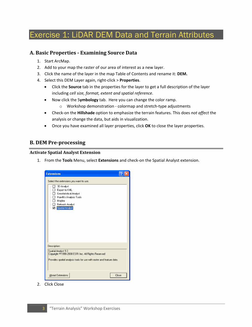
1. From the Tools Menu, select Extensions and check‐on the Spatial Analyst extension.

2. Click Close


SinkFilling

1. Launch ArcToolbox by clicking the toolbar icon.

2. Expand the Spatial Analyst Tools, then expand the Hydrology Toolset. Double‐click the Fill tool

to start it.

There are several additional ways to find this (or any) tool in ArcToolBox:

select the Index tab at the bottom of ArcToolbox and scroll through the list to find Fill (sa).

select the Search tab at the bottom and type in fill to find any tools with 'fill' in their titles.

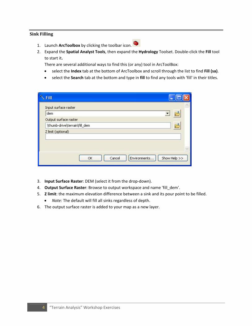
3. Input Surface Raster: DEM (select it from the drop‐down).

4. Output Surface Raster: Browse to output workspace and name 'fill_dem'.

5. Z limit: the maximum elevation difference between a sink and its pour point to be filled.

Note: The default will fill all sinks regardless of depth.

6. The output surface raster is added to your map as a new layer.


Filter

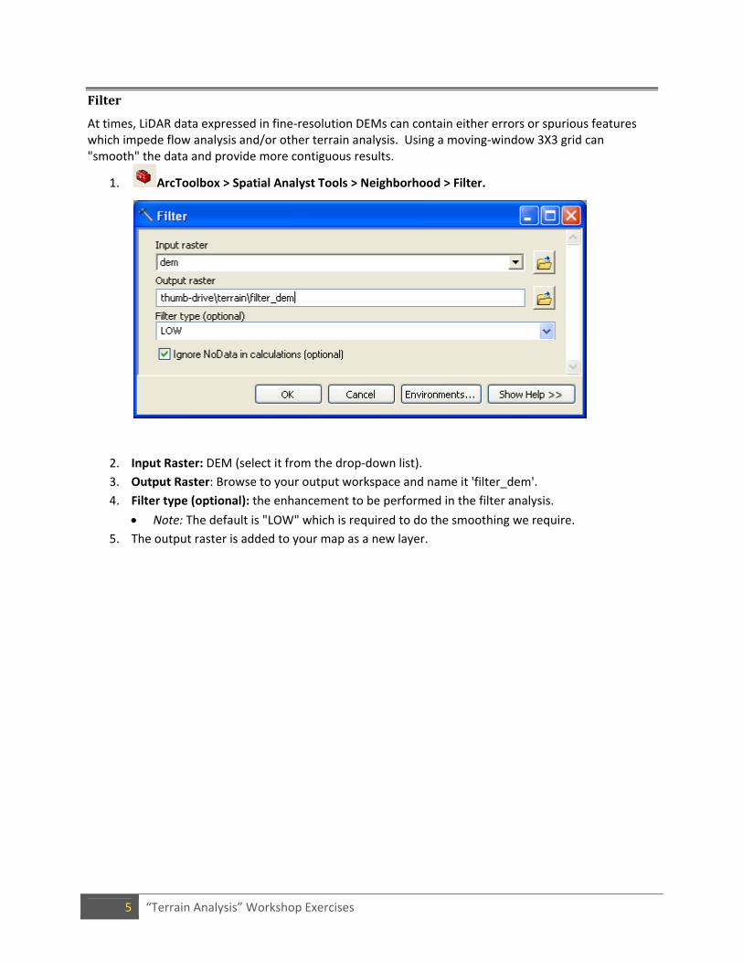
At times, LiDAR data expressed in fine‐resolution DEMs can contain either errors or spurious features which impede flow analysis and/or other terrain analysis. Using a moving‐window 3X3 grid can "smooth" the data and provide more contiguous results.

1. ArcToolbox > Spatial Analyst Tools > Neighborhood > Filter.

2. Input Raster: DEM (select it from the drop‐down list).

3. Output Raster: Browse to your output workspace and name it 'filter_dem'.

4. Filter type (optional): the enhancement to be performed in the filter analysis.

Note: The default is "LOW" which is required to do the smoothing we require.

5. The output raster is added to your map as a new layer.


C.CalculatePrimaryAttributes

Slope

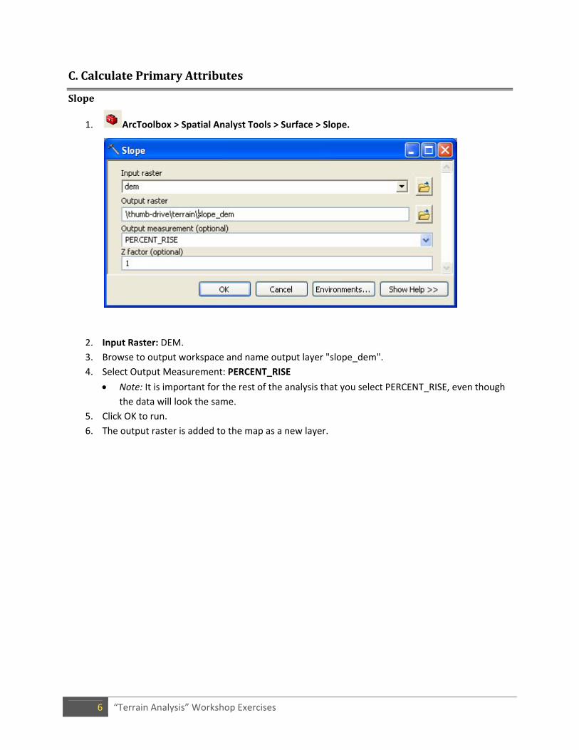
1. ArcToolbox > Spatial Analyst Tools > Surface > Slope.

2. Input Raster: DEM.

3. Browse to output workspace and name output layer "slope_dem".

4. Select Output Measurement: PERCENT_RISE

Note: It is important for the rest of the analysis that you select PERCENT_RISE, even though

the data will look the same.

5. Click OK to run.

6. The output raster is added to the map as a new layer.


Aspect

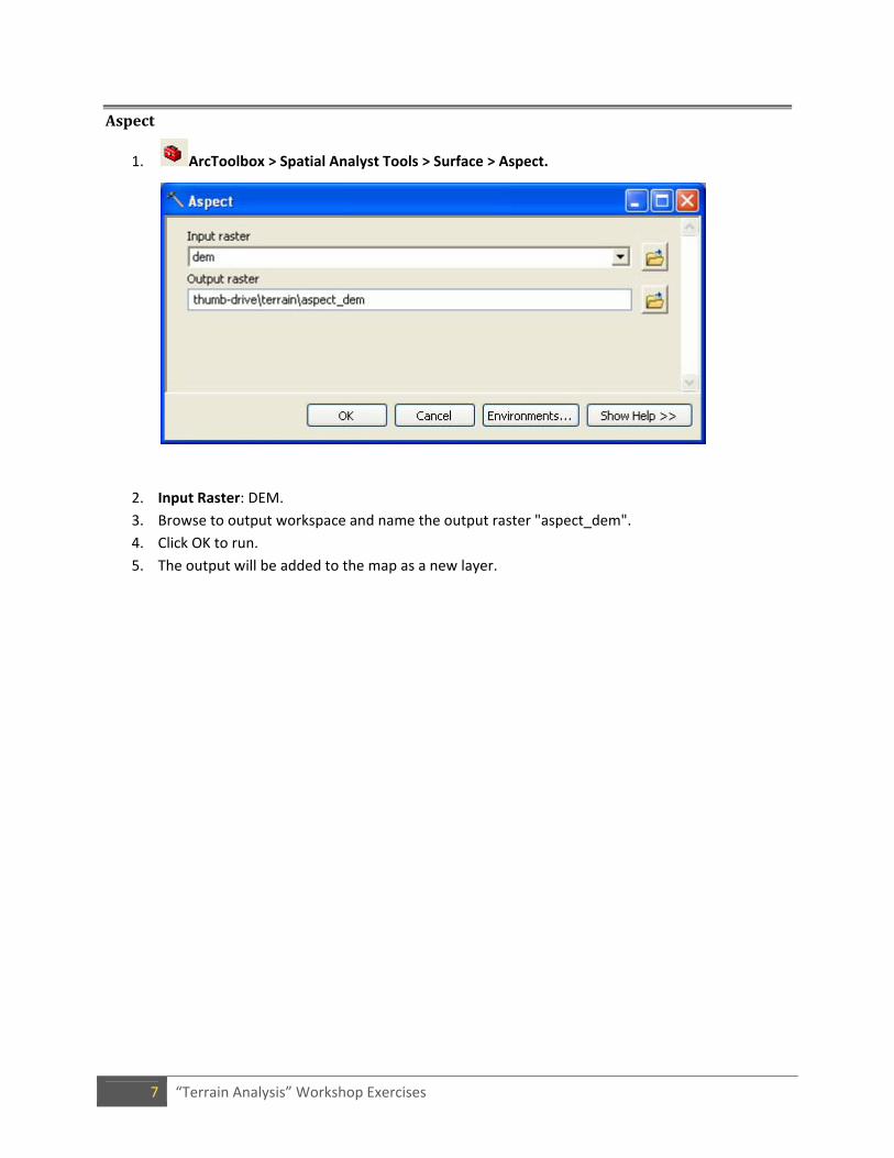
1. ArcToolbox > Spatial Analyst Tools > Surface > Aspect.


3. Browse to output workspace and name the output raster "aspect_dem".

4. Click OK to run.

5. The output will be added to the map as a new layer.


PlanandProfileCurvature

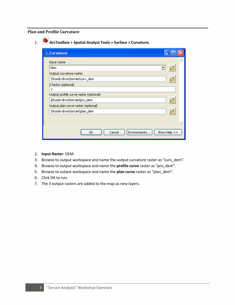
1. ArcToolbox > Spatial Analyst Tools > Surface > Curvature.


3. Browse to output workspace and name the output curvature raster as "curv_dem".

4. Browse to output workspace and name the profile curve raster as "pro_dem".

5. Browse to output workspace and name the plan curve raster as "plan_dem".

6. Click OK to run.

7. The 3 output rasters are added to the map as new layers.


Hillshade

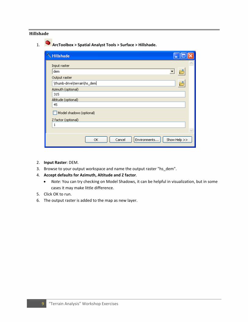
1. ArcToolbox > Spatial Analyst Tools > Surface > Hillshade.


3. Browse to your output workspace and name the output raster "hs_dem".

4. Accept defaults for Azimuth, Altitude and Z factor.

Note: You can try checking on Model Shadows, it can be helpful in visualization, but in some

cases it may make little difference.

5. Click OK to run.

6. The output raster is added to the map as new layer.


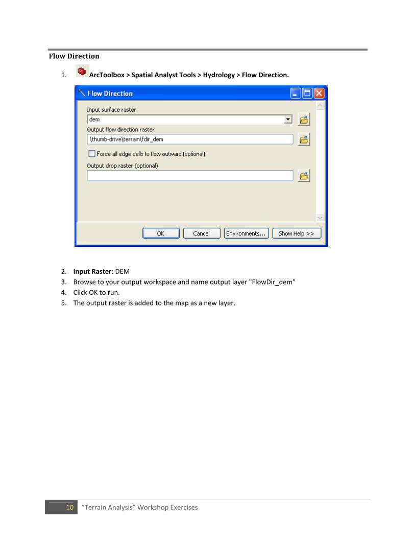
FlowDirection

1. ArcToolbox > Spatial Analyst Tools > Hydrology > Flow Direction.

2. Input Raster: DEM

3. Browse to your output workspace and name output layer "FlowDir_dem"

4. Click OK to run.



D.CalculateSecondaryAttributes

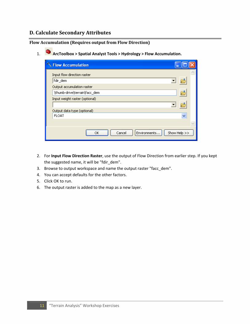
FlowAccumulation(RequiresoutputfromFlowDirection)

1. ArcToolbox > Spatial Analyst Tools > Hydrology > Flow Accumulation.

2. For Input Flow Direction Raster, use the output of Flow Direction from earlier step. If you kept

the suggested name, it will be "fdir_dem".

3. Browse to output workspace and name the output raster "facc_dem".

4. You can accept defaults for the other factors.

5. Click OK to run.



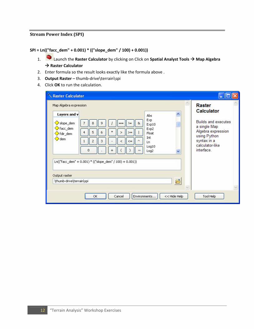
StreamPowerIndex(SPI)

SPI = Ln(("facc_dem" + 0.001) * (("slope_dem" / 100) + 0.001))

1. Launch the Raster Calculator by clicking on Click on Spatial Analyst Tools Map Algebra

Raster Calculator

2. Enter formula so the result looks exactly like the formula above .

3. Output Raster – thumb‐drive\terrain\spi

4. Click OK to run the calculation.


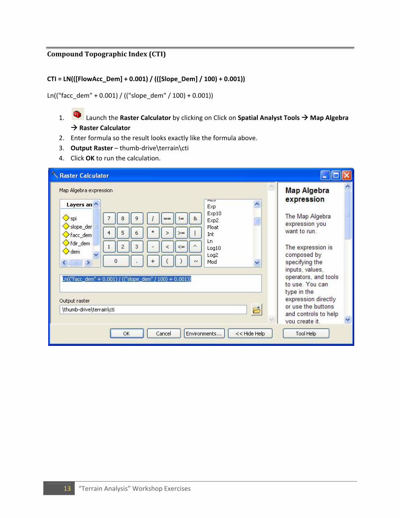
CompoundTopographicIndex(CTI)

CTI = LN(([FlowAcc_Dem] + 0.001) / (([Slope_Dem] / 100) + 0.001))

Ln(("facc_dem" + 0.001) / (("slope_dem" / 100) + 0.001))

1. Launch the Raster Calculator by clicking on Click on Spatial Analyst Tools Map Algebra

Raster Calculator

2. Enter formula so the result looks exactly like the formula above.

3. Output Raster – thumb‐drive\terrain\cti

4. Click OK to run the calculation.


Exercise 2: Interpretation

A.Visualization/ComparativeTechniques

TerrainAttributeComparison

Often, the best way to understand differences in terrain attribute calculations is to view each layer in conjunction with one another. By paying careful attention to a specific portion of the landscape, one can overlay each of the terrain attributes to gain a better understanding of why each attribute's value is what it is.

Orthophoto/TerrainAttributeComparison

Using air photos to do a rough validation is acceptable for the largest features only, but more importantly, utilizing orthophotography is a great way to better understand your landscape. While ground‐truthing is the most effective and accurate way to determine how your terrain attributes are describing the landscape, this is not always possible, especially on privately‐owned land. Furthermore, orthophotos when used with flow accumulation and its associated secondary terrain attributes, often help in assessing whether or not hydrologic conditioning is required for the task at hand

Add MNGEO WMS Service –

1. Open ArcMap and click on 'Add Data'

2. Look in the Catalog, and click on 'GIS Servers'

3. Highlight 'Add WMS Server' so that it appears in the Name window, and hit 'Add'. An 'Add WMS

Server' window will pop up.

4. To bring up the Imagery server, type http://geoint.lmic.state.mn.us/cgi‐bin/wms? in the URL

window. You can click on the 'Layers' button to see a list of the layers available under the wms.

Click 'OK'.

5. To bring up the Scanned DRG server, type http://geoint.lmic.state.mn.us/cgi‐bin/wmsz? in the

URL window. You can hit the 'Get Layers' button to see a list of the layers available under the

wms. Click 'OK'.

6. Now when you look under 'GIS Servers' you have two new entries: 'LMIC WMS server (aerial

photography) on geoint.lmic.state.mn.us' and 'LMIC WMS server (quad sheet drgs) on

geoint.lmic.state.mn.us'

7. Still in the 'Add Data' window under 'GIS Servers', highlight one of the services listed under #6 to

bring it into the 'Name' window, then click on 'Add'. The service, with all of its layers, has now

been added to your ArcMap project.

8. Click on the '+' to open the map service


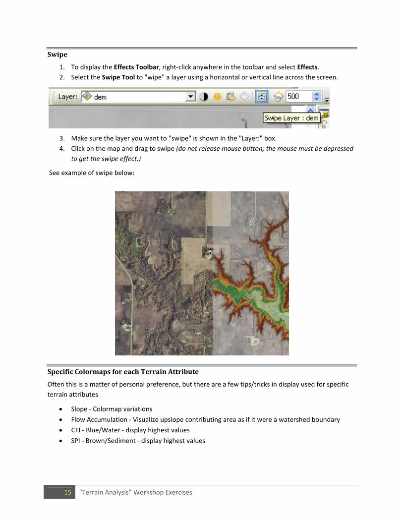
Swipe

1. To display the Effects Toolbar, right‐click anywhere in the toolbar and select Effects.

2. Select the Swipe Tool to "wipe" a layer using a horizontal or vertical line across the screen.

3. Make sure the layer you want to "swipe" is shown in the "Layer:" box.

4. Click on the map and drag to swipe (do not release mouse button; the mouse must be depressed

to get the swipe effect.)

See example of swipe below:

SpecificColormapsforeachTerrainAttribute

Often this is a matter of personal preference, but there are a few tips/tricks in display used for specific

terrain attributes

Slope ‐ Colormap variations

Flow Accumulation ‐ Visualize upslope contributing area as if it were a watershed boundary

CTI ‐ Blue/Water ‐ display highest values

SPI ‐ Brown/Sediment ‐ display highest values


B.DeterminingThresholds

ThresholdValueDisplay

1. Add to your map the raster of our area of interest as a new layer.

2. Click the name of the layer in the map Table of Contents and rename it: DEM.

3. Select this DEM Layer again, right‐click > Properties.

a. Now click the Symbology tab. Here you can change the color ramp.

b. Workshop demonstration ‐ colormap and stretch‐type adjustments

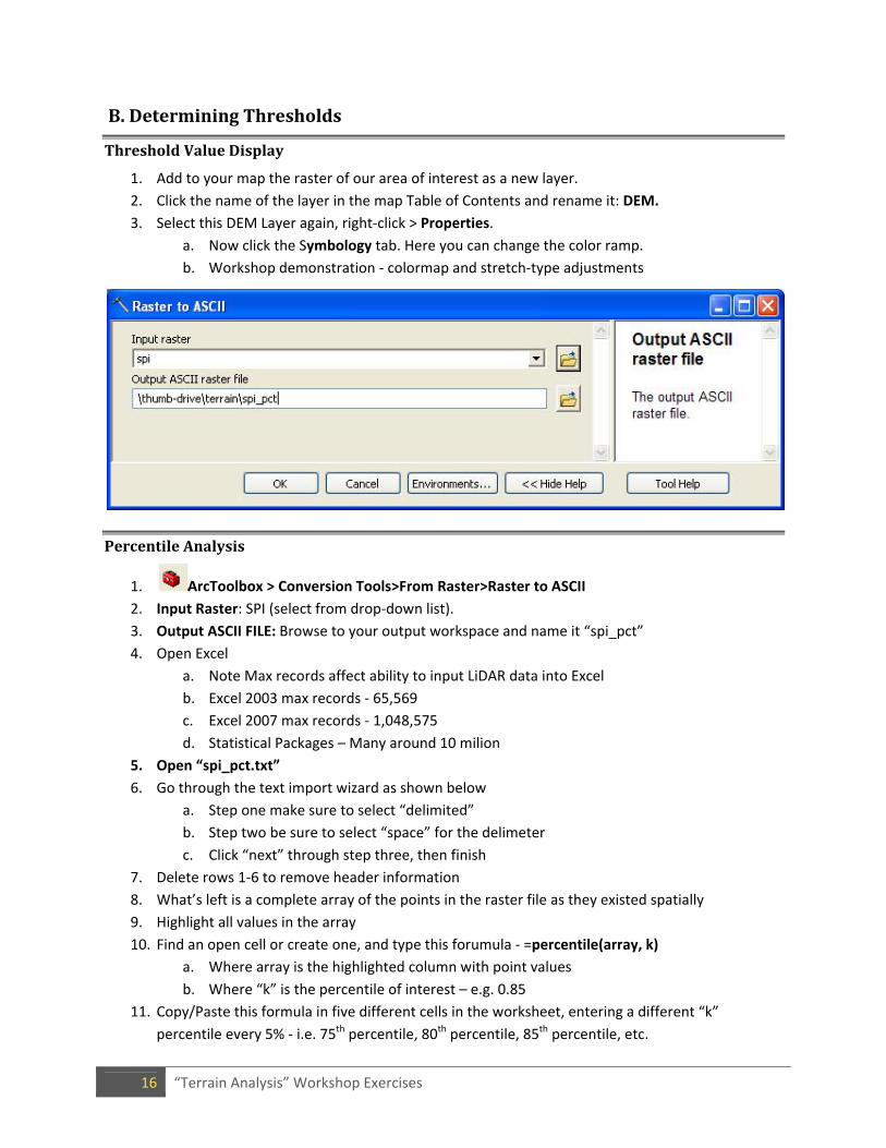
PercentileAnalysis

1. ArcToolbox > Conversion Tools>From Raster>Raster to ASCII

2. Input Raster: SPI (select from drop‐down list).

3. Output ASCII FILE: Browse to your output workspace and name it “spi_pct”

4. Open Excel

a. Note Max records affect ability to input LiDAR data into Excel

b. Excel 2003 max records ‐ 65,569

c. Excel 2007 max records ‐ 1,048,575

d. Statistical Packages – Many around 10 milion

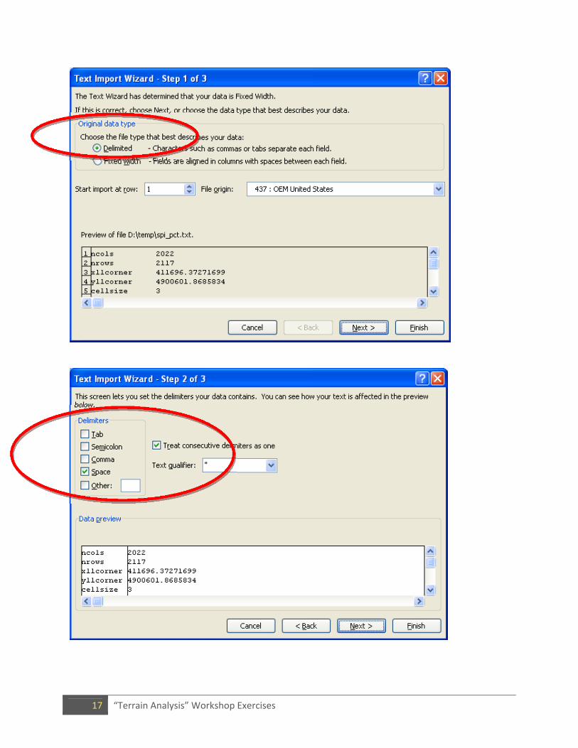
5. Open “spi_pct.txt”

6. Go through the text import wizard as shown below

a. Step one make sure to select “delimited”

b. Step two be sure to select “space” for the delimeter

c. Click “next” through step three, then finish

7. Delete rows 1‐6 to remove header information

8. What’s left is a complete array of the points in the raster file as they existed spatially

9. Highlight all values in the array

10. Find an open cell or create one, and type this forumula ‐ =percentile(array, k)

a. Where array is the highlighted column with point values

b. Where “k” is the percentile of interest – e.g. 0.85

11. Copy/Paste this formula in five different cells in the worksheet, entering a different “k”

percentile every 5% ‐ i.e. 75th percentile, 80th percentile, 85th percentile, etc.


VisualizingtheResults

1. Select the SPI Layer again, right‐click > Properties.

a. Now click the Symbology tab. Here you can change the color ramp.

b. Workshop demonstration ‐ colormap and stretch‐type adjustments for five classified

threshold values

2. Select “add‐data” , navigate to \thumb‐drive\terrain and add erosion

3. Compare these known sites of observed gullies to classified values

4. Are there areas with high SPI values and no erosion features detected, or vice versa?

5. Prioritize sites for conservation targeting based on severity and even spatial distribution across

the pilot area.

conservation applications of lidar - water … applications of lidar terrain analysis workshop...

Documents