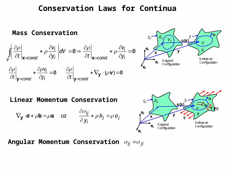
Conservation Laws for Continua

e3

e1

e2

OriginalConfiguration

DeformedConfiguration

S

R

R0S0b

t

n

V T(n)

yx

u(x)

or ij

j ji

b ay

y σ b a

e3

e1

e2

OriginalConfiguration

DeformedConfiguration

S

R

R0S0

n

V

yx

u(x)V0

Mass Conservation

Linear Momentum Conservation

0 0i i

i iconst constV

v vdV

t y t y

x x

0 ( ) 0i

iconst const

v

t y t

yy y

v

Angular Momentum Conservation ij ji

( ) 1

2i i i ij ij i iiA V V V

dr T v dA b v dV D dV v v dV

dt

n

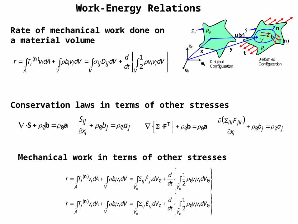
Rate of mechanical work done ona material volume

e3

e1

e2

OriginalConfiguration

DeformedConfiguration

S

R

R0S0b

t

n

V T(n)

yx

u(x)

Conservation laws in terms of other stresses

0 0 0 0ij

j ji

Sb a

x

S b a

0 0 0 0ik jk

j ji

Fb a

x

TF b a

Mechanical work in terms of other stresses

0 0

( )0 0 0

1

2i i i ij ji i iiA V V V

dr T v dA b v dV S F dV v v dV

dt

n

0 0

( )0 0 0

1

2i i i ij ij i iiA V V V

dr T v dA b v dV E dV v v dV

dt

n

Work-Energy Relations

2

0iij ij i i i i i

V

dvD dV dA

dtV V S

dV v b v dV t v

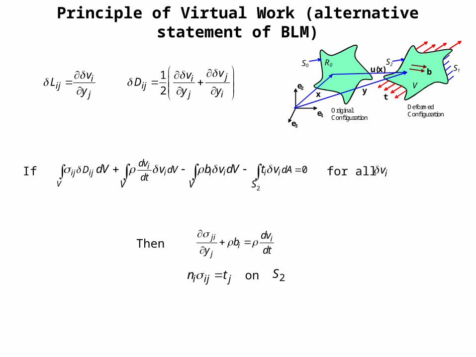
Principle of Virtual Work (alternative statement of BLM)

1

2ji i

ij ijj j i

vv vL D

y y y

e3

e1

e2

OriginalConfiguration

DeformedConfiguration

S2R0S0

b

t

Vyx

u(x) S1

ji ii

j

dvb

y dt

If for all iv

Then

i ij jn t 2Son

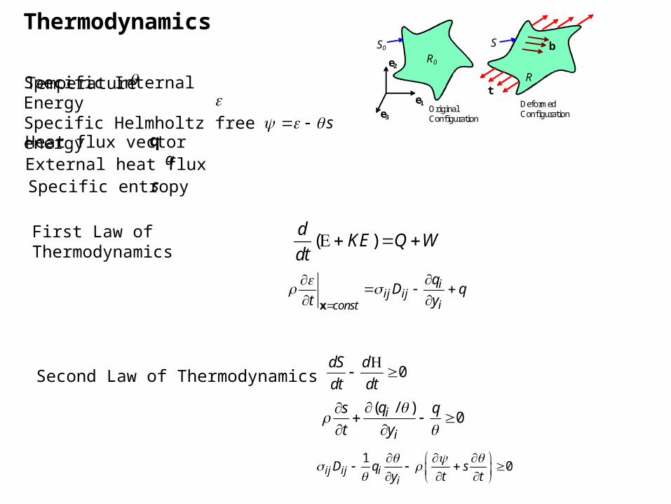
Thermodynamics

e3

e1

e2

OriginalConfiguration

DeformedConfiguration

S

R

R0

S0 b

t

Specific Internal EnergySpecific Helmholtz free energy s

Temperature

Heat flux vector q

External heat flux q

First Law of Thermodynamics ( )d

KE Q Wdt

iij ij

iconst

qD q

t y

x

Second Law of Thermodynamics 0dS d

dt dt

Specific entropy s

( / )0i

i

qs q

t y

10ij ij i

iD q s

y t t

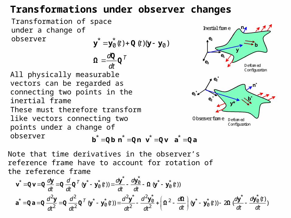
Transformations under observer changes

Transformation of space under a change of observer

e3

e1

e2

DeformedConfiguration

b

n

y

DeformedConfiguration

b*

n*

y*

e2*

e3*

e2*

Inertial frame

Observer frame

* *0 0( ) ( )( )t t y y Q y y

All physically measurable vectors can be regarded as connecting two points in the inertial frame

These must therefore transform like vectors connecting two points under a change of observer

* * * * b Qb n Qn v Qv a Qa

Note that time derivatives in the observer’s reference frame have to account for rotation of the reference frame

*** * * * *0

0 0

2 * *2 2 2 * ** * * 2 * *0 0

0 02 2 2 2

( ( )) ( ( ))

( )( ( )) ( ( )) 2 ( )

T

T

dd d dt t

dt dt dt dt

d d td d d d dt t

dt dt dtdt dt dt dt

yy yv Qv Q Q Q y y Ω y y

y yy y Ω ya Qa Q Q Q y y Ω y y Ω

Td

dt

QΩ Q

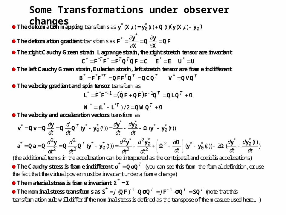
The deformation mapping transforms as * *0 0( , ) ( ) ( ) ( , )t t t t y X y Q y X y

The deformation gradient transforms as *

*

y y

F Q QFX X

The right Cauchy Green strain Lagrange strain, the right stretch tensor are invariant * * * * *T T T C F F F Q QF C E E U U

The left Cauchy Green strain, Eulerian strain, left stretch tensor are frame indifferent * * * *T T T T T B F F QFF Q QCQ V QVQ

The velocity gradient and spin tensor transform as

* * * 1 1

* * *( ) / 2

T T

T T

L F F QF QF F Q QLQ Ω

W L L QWQ Ω

The velocity and acceleration vectors transform as **

* * * * *00 0

2 * *2 2 2 * ** * * 2 * *0 0

0 02 2 2 2

( ( )) ( ( ))

( )( ( )) ( ( )) 2 ( )

T

T

dd d dt t

dt dt dt dt

d d td d d d dt t

dt dt dtdt dt dt dt

yy yv Qv Q Q Q y y Ω y y

y yy y Ω ya Qa Q Q Q y y Ω y y Ω

(the additional terms in the acceleration can be interpreted as the centripetal and coriolis accelerations)

The Cauchy stress is frame indifferent * Tσ QσQ (you can see this from the formal definition, or use the fact that the virtual power must be invariant under a frame change)

The material stress is frame invariant * Σ Σ

The nominal stress transforms as * 1 1( ) T T TJ J S QF Q Q F Q SQσ σ (note that this transformation rule will differ if the nominal stress is defined as the transpose of the measure used here…)

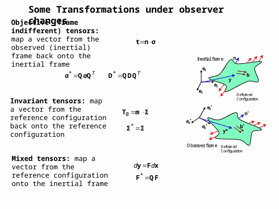
Some Transformations under observer changes

e3

e1

e2

DeformedConfiguration

b

n

y

DeformedConfiguration

b*

n*

y*

e2*

e3*

e2*

Inertial frame

Observer frame

Objective (frame indifferent) tensors: map a vector from the observed (inertial) frame back onto the inertial frame

t n σ

* *T T σ QσQ D QDQ

Invariant tensors: map a vector from the reference configuration back onto the reference configuration

0 T m Σ

* Σ Σ

Mixed tensors: map a vector from the reference configuration onto the inertial frame

d dy F x

* F QF

Some Transformations under observer changes

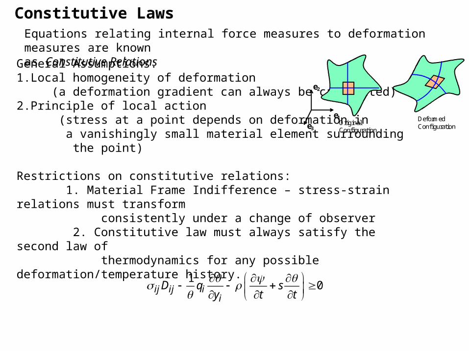
Constitutive Laws

General Assumptions:1.Local homogeneity of deformation (a deformation gradient can always be calculated)2.Principle of local action (stress at a point depends on deformation in a vanishingly small material element surrounding the point)

Restrictions on constitutive relations: 1. Material Frame Indifference – stress-strain relations must transform consistently under a change of observer 2. Constitutive law must always satisfy the second law of thermodynamics for any possible deformation/temperature history.

Equations relating internal force measures to deformation measures are knownas Constitutive Relations

e3

e1

e2

OriginalConfiguration

DeformedConfiguration

10ij ij i

iD q s

y t t

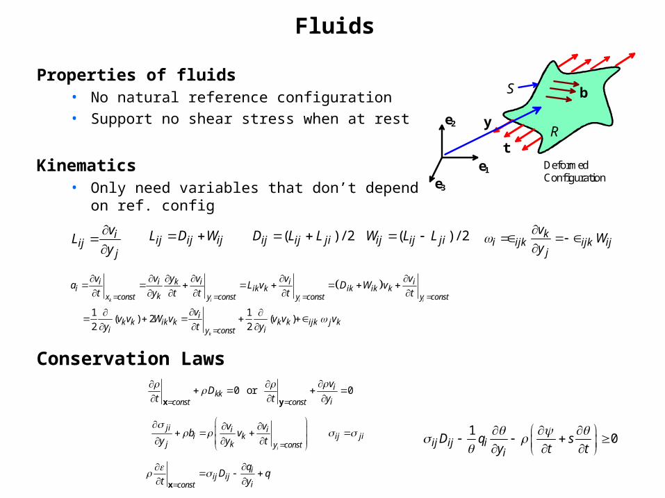
Fluids

Properties of fluids• No natural reference configuration• Support no shear stress when at rest

Kinematics• Only need variables that don’t depend

on ref. config

Conservation Laws

e3

e1

e2

DeformedConfiguration

S

R

b

t

y

iij

j

vL

y

( ) / 2 ( ) / 2ij ij ij ij ij ji ij ij jiL D W D L L W L L k

i ijk ijk ijj

vW

y

1 1( ) 2 ( )

2 2

k i i i

k

i i k i i ii ik k ik ik k

kx const y const y const y const

ik k ik k k k ijk j k

i iy const

v v y v v va L v D W v

t y t t t t

vv v W v v v v

y t y

0 or 0ikk

iconst const

vD

t t y

x y

i

ji i ii k ij ji

j k y const

v vb v

y y t

iij ij

iconst

qD q

t y

x

10ij ij i

iD q s

y t t

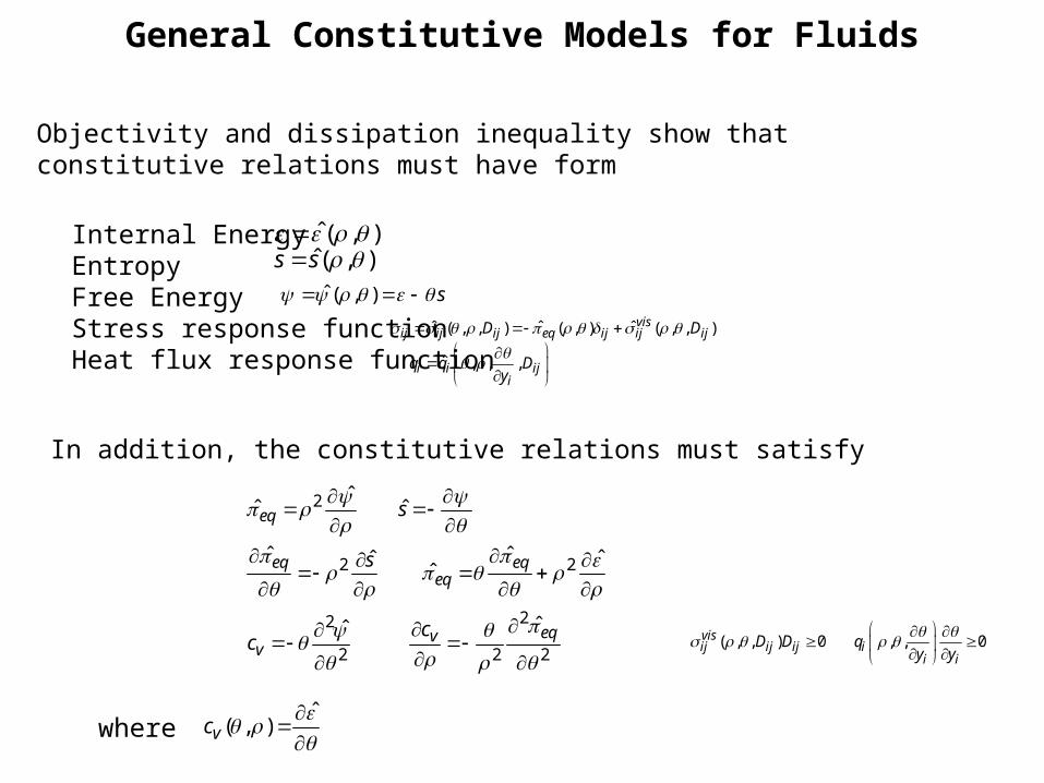
General Constitutive Models for Fluids

Objectivity and dissipation inequality show that constitutive relations must have form

Internal EnergyEntropyFree EnergyStress response functionHeat flux response function

ˆ( , ) ˆ( , )s s

ˆ ( , ) s

ˆ ˆ ˆ( , , ) ( , ) ( , , )visij ij ij eq ij ij ijD D

ˆ , , ,i i iji

q q Dy

In addition, the constitutive relations must satisfy

2

2 2

22

2 2 2

ˆˆ ˆ

ˆ ˆ ˆˆˆ

ˆˆ

eq

eq eqeq

eqvv

s

s

cc

( , , ) 0 , , 0vis

ij ij ij ii i

D D qy y

ˆ( , )vc

where

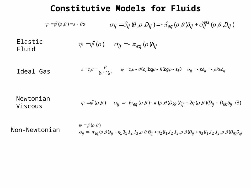
Constitutive Models for Fluids

ˆ ( ) ( )ij eq ij Elastic Fluid

0log log( 1)v v v ij ij ij

pc c c R s p R

Ideal Gas

ˆ ( , ) ( ( , ) ( , ) ) 2 ( , )( / 3)ij eq kk ij ij kk ijD D D Newtonian Viscous

1 1 2 3 2 1 2 3 3 1 2 3

ˆ ( , )

( , ) ( , , , , ) ( , , , , ) ( , , , , )ij eq ij ij ij ik kjI I I I I I D I I I D D

Non-Newtonian

ˆ ˆ ˆ( , , ) ( , ) ( , , )visij ij ij eq ij ij ijD D ˆ ( , ) s

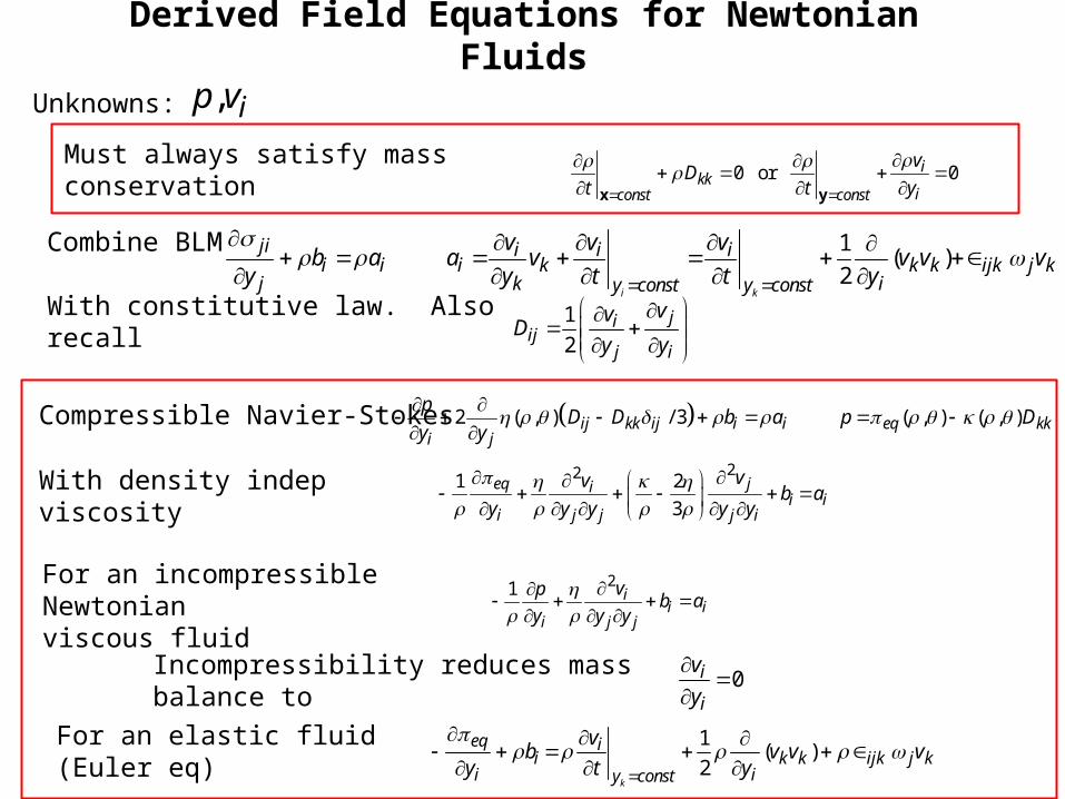
Derived Field Equations for Newtonian Fluids

1( )

2i k

ji i i ii i i k k k ijk j k

j k iy const y const

v v vb a a v v v v

y y t t y

Combine BLM

With constitutive law. Also recall

Compressible Navier-Stokes 2 ( , ) / 3 ( , ) ( , )ij kk ij i i eq kki j

pD D b a p D

y y

221 2

3eq ji

i ii j j j i

vvb a

y y y y y

With density indep viscosity

1( )

2k

eq ii k k ijk j k

i iy const

vb v v v

y t y

For an elastic fluid (Euler eq)

21 ii i

i j j

vpb a

y y y

For an incompressible Newtonianviscous fluid

1

2ji

ijj i

vvD

y y

0i

i

v

y

Incompressibility reduces mass balance to

0 or 0ikk

iconst const

vD

t t y

x yMust always satisfy mass conservation

Unknowns: , ip v

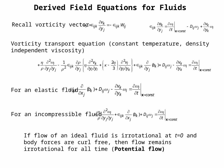
Derived Field Equations for Fluids

2 2 2

2

1 2( )

3i k l k i

ijk ijk k ij j ij j j l l l k j k const

v v vb D

y y y y y y y y y t

x

Vorticity transport equation (constant temperature, density independent viscosity)

For an elastic fluid

ki ijk ijk ij

j

vW

y

Recall vorticity vector

( ) k iijk k ij j i

j k const

vb D

x y t

x

2( )i i

ijk k ij jj j j const

b Dy y x t

xFor an incompressible fluid

k i kijk ij j i

j kconst

a vD

y t y

x

If flow of an ideal fluid is irrotational at t=0 and body forces are curl free, then flow remains irrotational for all time (Potential flow)

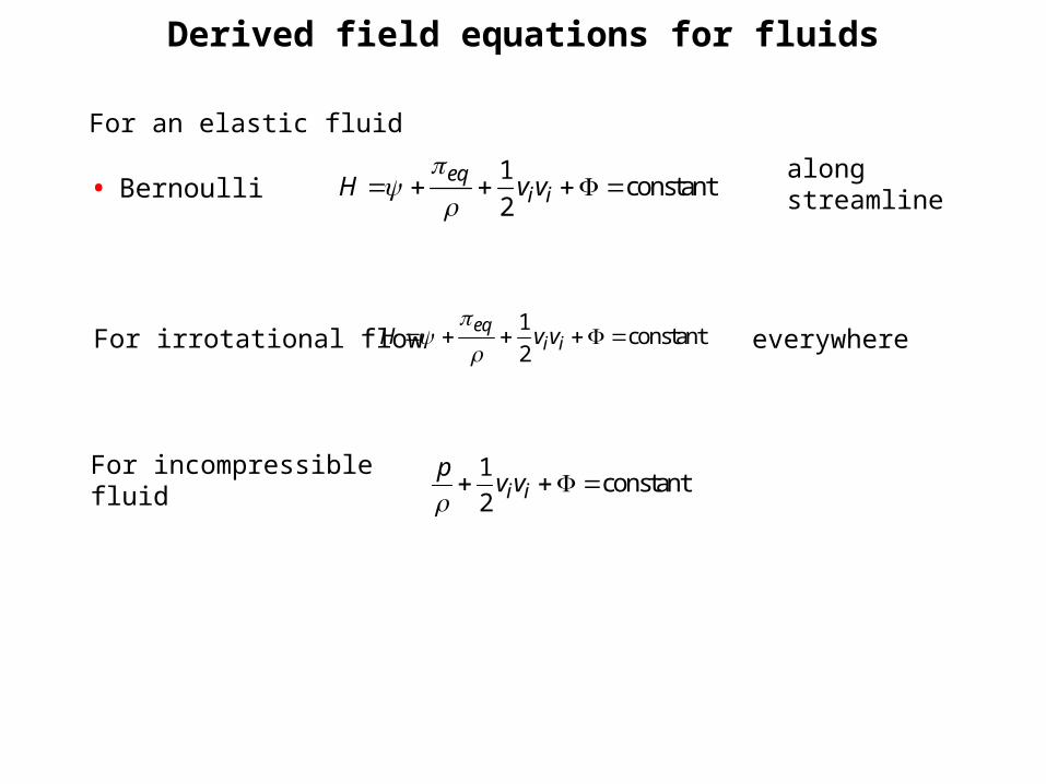
Derived field equations for fluids

• Bernoulli1

constant2

eqi iH v v

along streamline

For an elastic fluid

For irrotational flow1

constant2

eqi iH v v

everywhere

For incompressible fluid 1constant

2 i ip

v v

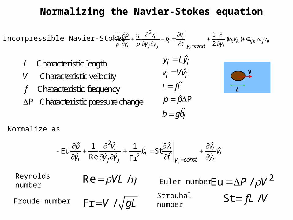
Normalizing the Navier-Stokes equation

21 1( )

2k

i ii k k ijk j k

i j j iy const

v vpb v v v

y y y t y

Characteristic length

Characteristic velocity

Characteristic frequency

P Characteristic pressure change

L

V

f

Normalize as

2

2

ˆ ˆ ˆˆ 1 1 ˆ ˆEu Stˆˆ ˆ ˆ ˆRe Fr

k

i i ii i

i j j iy const

v v vpb v

y y y t y

Re /VL Reynolds number

Incompressible Navier-Stokes

ˆ

ˆ

ˆ

ˆ P

ˆ

i i

i i

i

y Ly

v Vv

t ft

p p

b gb

Euler number 2Eu /P V

Froude number Fr /V gL Strouhal number St /fL V

V

L

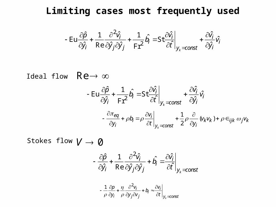
Limiting cases most frequently used

2

ˆ ˆˆ 1 ˆ ˆEu Stˆˆ ˆFr

k

i ii i

i iy const

v vpb v

y t y

Ideal flow Re

Stokes flow

2 ˆ ˆˆ 1 ˆˆˆ ˆ ˆRe

k

i ii

i j j y const

v vpb

y y y t

2

2

ˆ ˆ ˆˆ 1 1 ˆ ˆEu Stˆˆ ˆ ˆ ˆRe Fr

k

i i ii i

i j j iy const

v v vpb v

y y y t y

0V

1( )

2k

eq ii k k ijk j k

i iy const

vb v v v

y t y

21

k

i ii

i j j y const

v vpb

y y v t

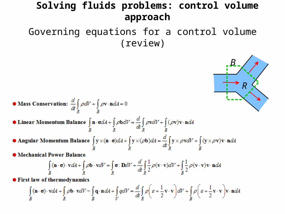
Governing equations for a control volume (review)

B

R

Solving fluids problems: control volume approach

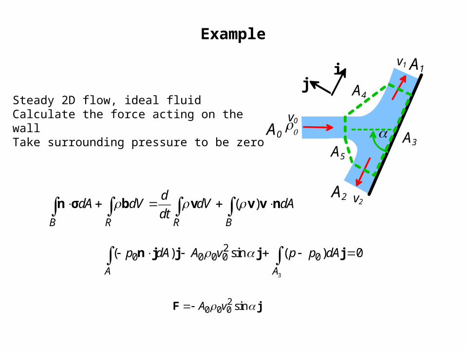
Example

v0

v1

v2

A0

A2

A1

A3

A4

A5

ji

Steady 2D flow, ideal fluidCalculate the force acting on the wallTake surrounding pressure to be zero

( )B R R B

ddA dV dV dA

dt n σ b v v v n

3

20 0 0 0 0( ) sin ( ) 0

A A

p dA A v p p dA n j j j j

20 0 0 sinA v F j

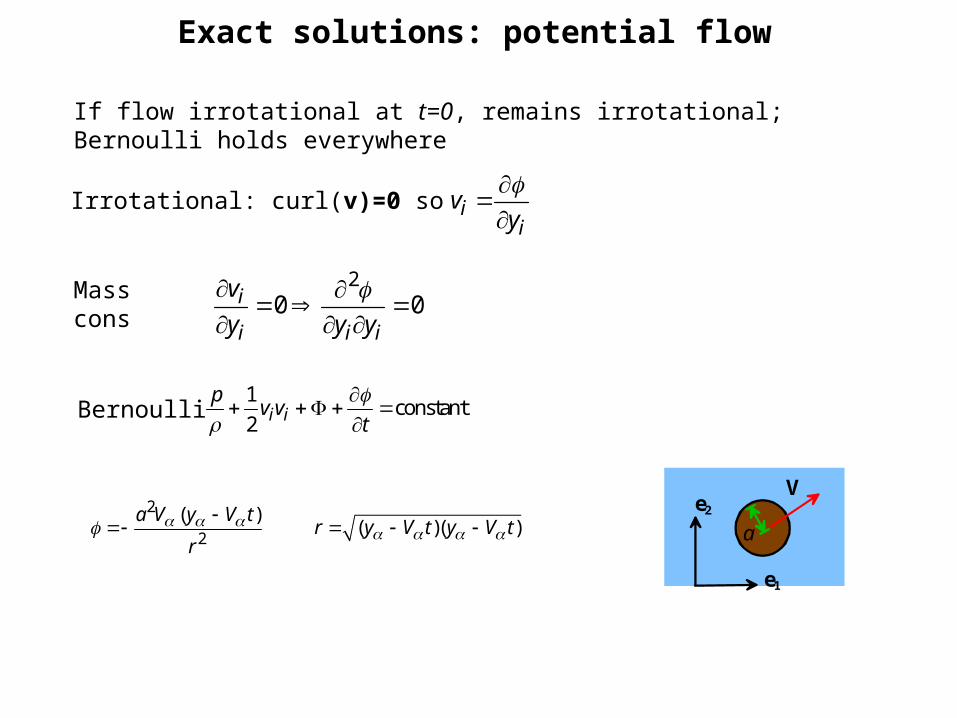
Exact solutions: potential flow

20 0i

i i i

v

y y y

Mass cons

Bernoulli1

constant2 i i

pv v

t

If flow irrotational at t=0, remains irrotational; Bernoulli holds everywhere

Irrotational: curl(v)=0 so ii

vy

V

e1

e2

a2

2

( )( )( )

a V y V tr y V t y V t

r

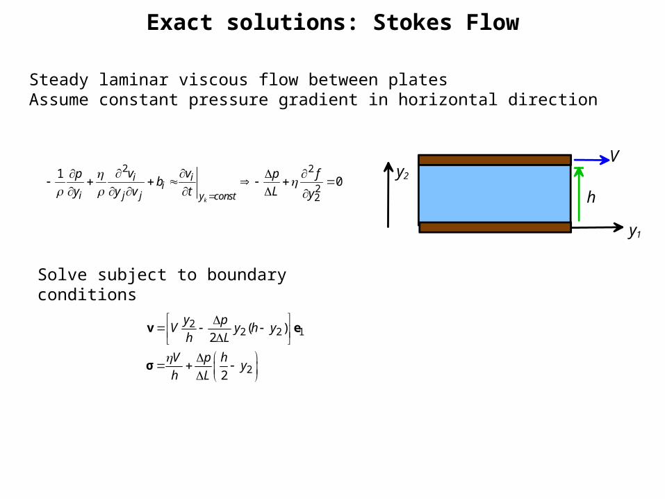
Exact solutions: Stokes Flow

Vy2

y1

h

Steady laminar viscous flow between platesAssume constant pressure gradient in horizontal direction

22 2 1

2

( )2

2

y pV y h y

h L

V p hy

h L

v e

σ

2 2

22

10

k

i ii

i j j y const

v vp p fb

y y v t L y

Solve subject to boundary conditions

Exact Solutions: AcousticsAssumptions:

Small amplitude pressure and density fluctuationsIrrotational flowNegligible heat flow

Mass conservation:

ss const

pc

For small perturbations: 2

sp

ct t

k

ii

i y const

vpb

y t

Approximate N-S as:22

2k

i

i y const

vp

y t t

0i

iconst

v

t y

x

22

k

ii

i i i y const

vpb

y y y t

22 22 2

2 20 0

jis s

i j i i

vvc c

y y y yt t

Combine:

(Wave equation)

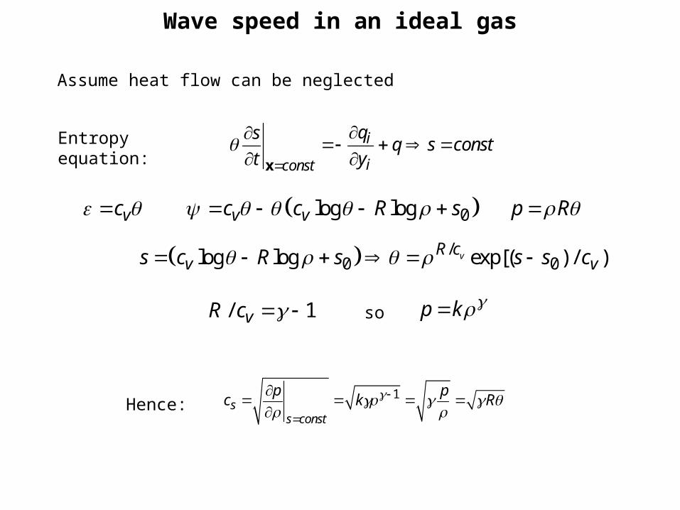
Wave speed in an ideal gas

i

iconst

qsq s const

t y

xEntropy equation:

0log logv v vc c c R s p R

/0 0log log exp[( ) / )vR c

v vs c R s s s c

Hence:

Assume heat flow can be neglected

1s

s const

p pc k R

/ 1vR c p k so

Application of continuum mechanics to elasticity

e3

e1

e2

OriginalConfiguration

DeformedConfiguration

S

RR0

S0 b

t

u

x

y

Material characterized by

Modulus G' (N/m2)

(frequency)-1

109

105

GlassyViscoelastic

Rubbery

MeltGlass Transitiontemperature Tg

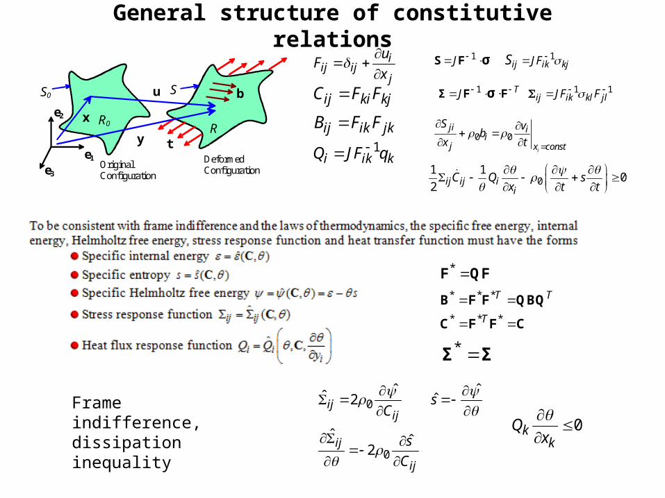
General structure of constitutive relations

e3

e1

e2

OriginalConfiguration

DeformedConfiguration

S

RR0

S0 b

t

u

x

y

0

0

ˆ ˆˆ ˆ2

ˆ ˆ2

ijij

ij

ij

sC

s

C

0kk

Qx

iij ij

j

uF

x

ij ki kj

ij ik jk

C F F

B F F

1

i ik kQ JF q

1 1ij ik kjJ JFS S F σ

1 1 1Tij ik kl jlJ JF F Σ F Fσ

0 0i

ji ii

j x const

S vb

x t

01 1

02 ij ij i

iC Q s

x t t

* F QF

* Σ Σ

* * *

* * *

T T

T

B F F QBQ

C F F C

Frame indifference, dissipation inequality

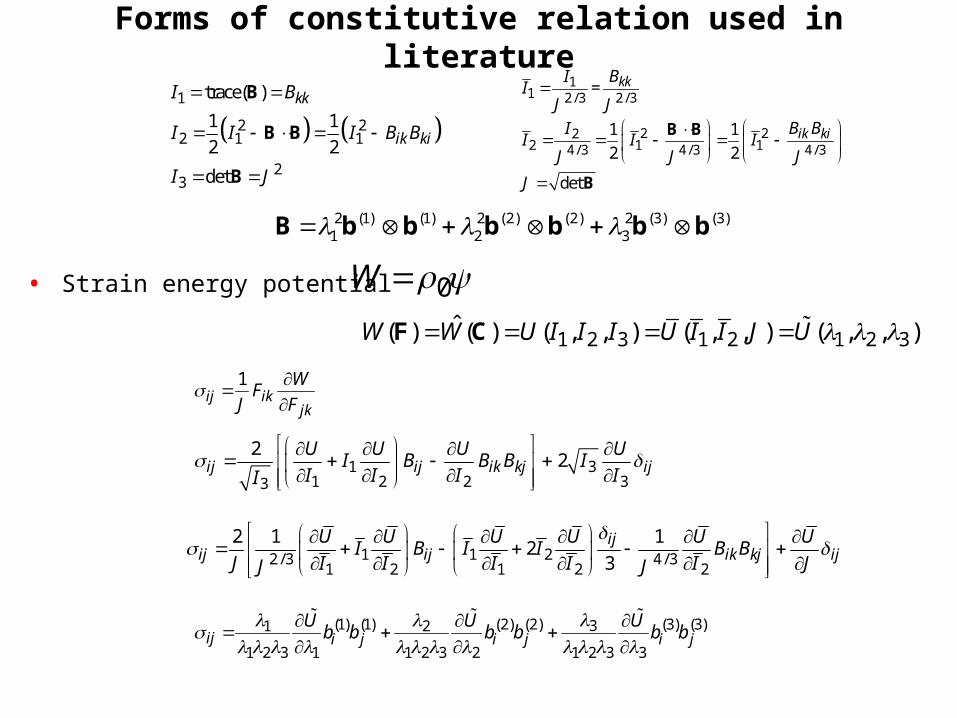
Forms of constitutive relation used in literature

1

2 22 1 1

23

trace( )

1 1

2 2

det

kk

ik ki

I B

I I I B B

I J

B

B B

B

11 2 / 3 2 / 3

2 222 1 14 / 3 4 / 3 4 / 3

=

1 1

2 2

det

kk

ik ki

BII

J J

B BII I I

J J J

J

B B

B

1 2 3 1 2 1 2 3ˆ( ) ( ) ( , , ) ( , , ) ( , , )W W U I I I U I I J U F C

• Strain energy potential 0W

1ij ik

jk

WF

J F

1 31 2 2 33

22ij ij ik kj ij

U U U UI B B B I

I I I II

1 1 22 /3 4 /31 2 1 2 2

2 1 12

3ij

ij ij ik kj ijU U U U U U

I B I I B BJ I I I I I JJ J

(1) (1) (2) (2) (3) (3)31 2

1 2 3 1 1 2 3 2 1 2 3 3ij i j i j i j

U U Ub b b b b b

2 (1) (1) 2 (2) (2) 2 (3) (3)1 2 3 B b b b b b b

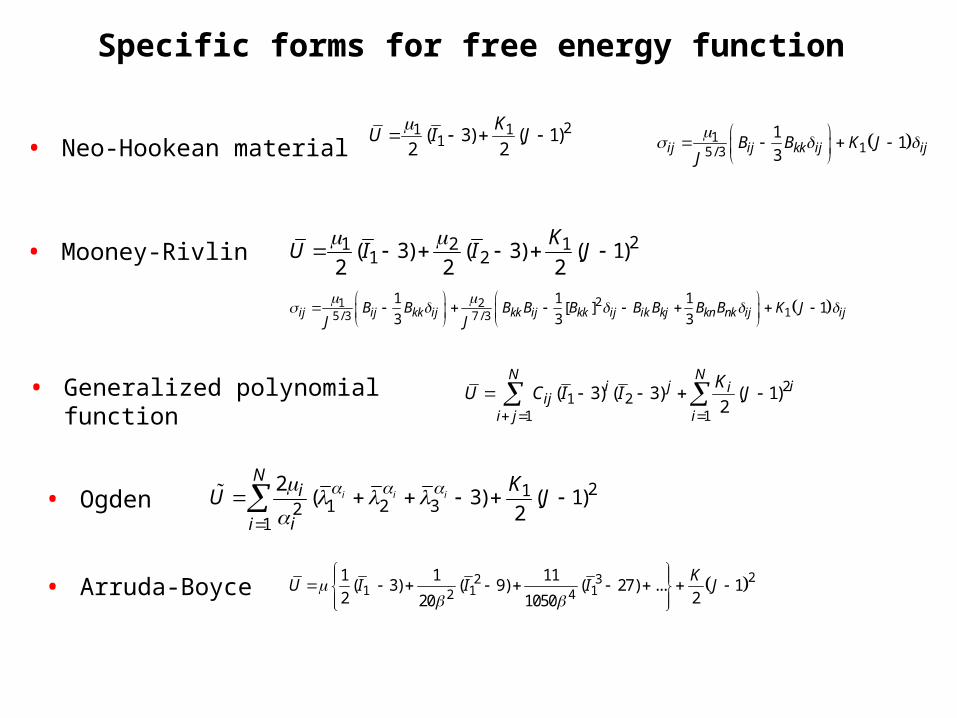
Specific forms for free energy function

• Neo-Hookean material21 1

1( 3) ( 1)2 2

KU I J

• Mooney-Rivlin 21 2 11 2( 3) ( 3) ( 1)

2 2 2

KU I I J

115/ 3

11

3ij ij kk ij ijB B K JJ

21 215/3 7 /3

1 1 1[ ] 1

3 3 3ij ij kk ij kk ij kk ij ik kj kn nk ij ijB B B B B B B B B K JJ J

• Generalized polynomial function 21 2

1 1

( 3) ( 3) ( 1)2

N Ni j ii

iji j i

KU C I I J

211 2 32

1

2( 3) ( 1)

2i i i

Ni

ii

KU J

• Ogden

22 31 1 12 4

1 1 11( 3) ( 9) ( 27) ... 1

2 220 1050

KU I I I J

• Arruda-Boyce

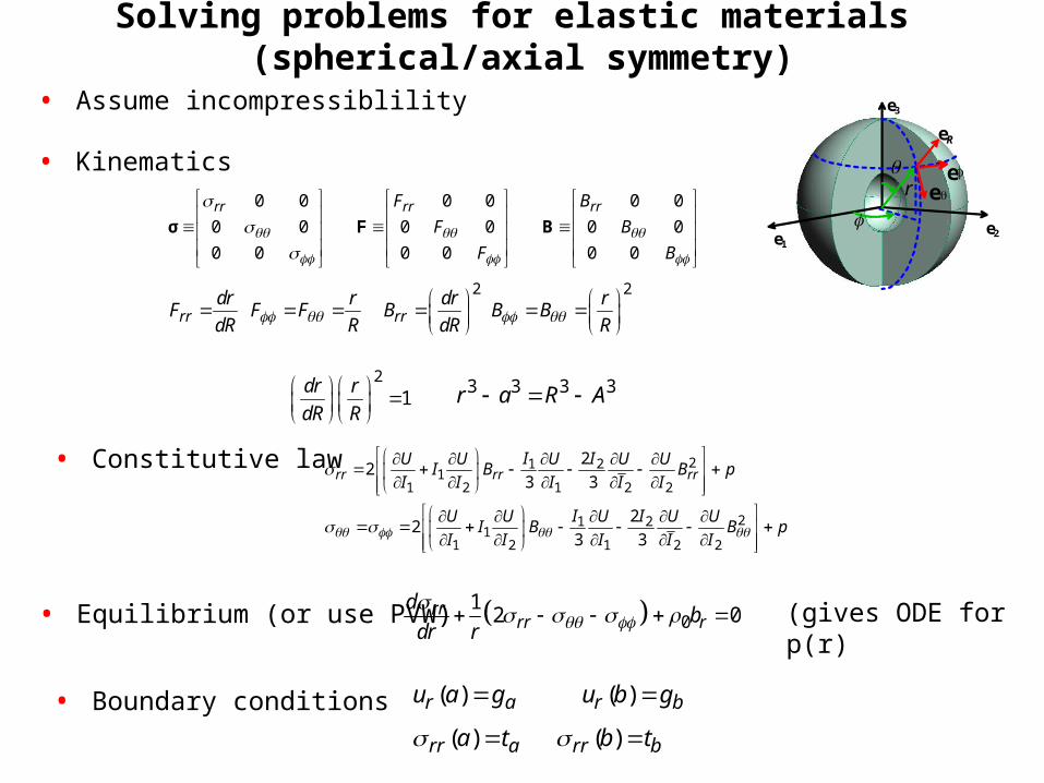
Solving problems for elastic materials (spherical/axial symmetry)

r

eR

ee

e1

e2

e3

0 0 0 0 0 0

0 0 0 0 0 0

0 0 0 0 0 0

rr rr rrF B

F B

F B

σ F B

2 2

rr rrdr r dr r

F F F B B BdR R dR R

• Assume incompressiblility

• Kinematics

2

1dr r

dR R

3 3 3 3r a R A

21 21

1 2 1 2 2

21 21

1 2 1 2 2

22

3 3

22

3 3

rr rr rrI IU U U U U

I B B pI I I I I

I IU U U U UI B B p

I I I I I

• Constitutive law

01

2 0rrrr r

db

dr r • Equilibrium (or use PVW)

( ) ( )r a r bu a g u b g

(gives ODE for p(r)

( ) ( )rr a rr ba t b t • Boundary conditions

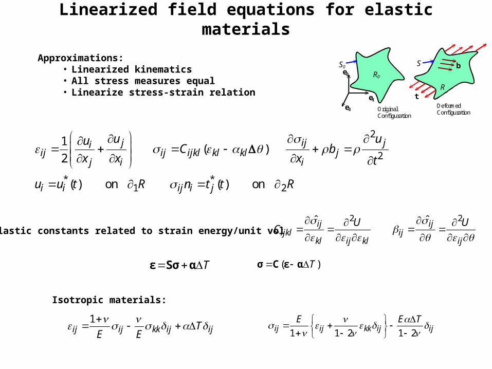
Linearized field equations for elastic materials

2

2

* *1 2

1( )

2

( ) on ( ) on

j ij jiij ij ijkl kl kl j

j i i

i i ij i j

u uuC b

x x x t

u u t R n t t R

e3

e1

e2

OriginalConfiguration

DeformedConfiguration

S

R

R0

S0 b

t

2 2ˆ ˆij ijijkl ij

kl ij kl ij

U UC

Elastic constants related to strain energy/unit vol

Approximations:• Linearized kinematics• All stress measures equal• Linearize stress-strain relation

1ij ij kk ij ijT

E E

1 1 2 1 2ij ij kk ij ijE E T

Isotropic materials:

( )T σ C ε αT ε Sσ α

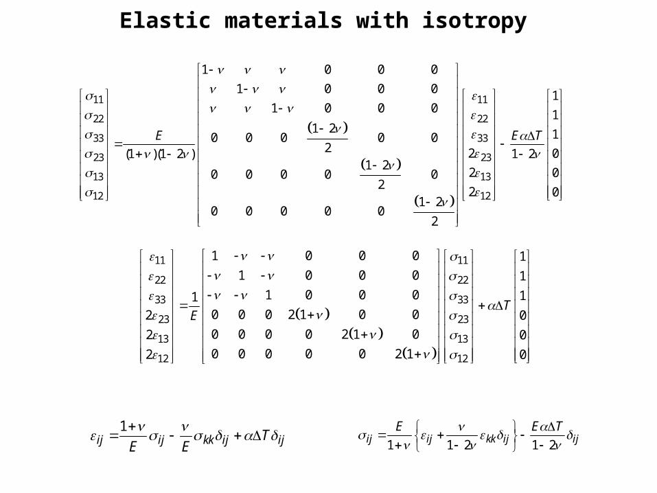
Elastic materials with isotropy

11 11

22 22

33 33

23 23

13 13

12 12

1 0 0 0

1 0 0 0 11 0 0 0 1

1 2 10 0 0 0 02 2 0(1 )(1 2 ) 1 2

1 22 00 0 0 0 0

22 0

1 20 0 0 0 0

2

E E T

11 11

22 22

33 33

23 23

13 13

12 12

1 0 0 0 1

1 0 0 0 1

1 0 0 0 110 0 0 2 1 0 02 0

0 0 0 0 2 1 02 0

0 0 0 0 0 2 12 0

TE

1ij ij kk ij ijT

E E

1 1 2 1 2ij ij kk ij ijE E T

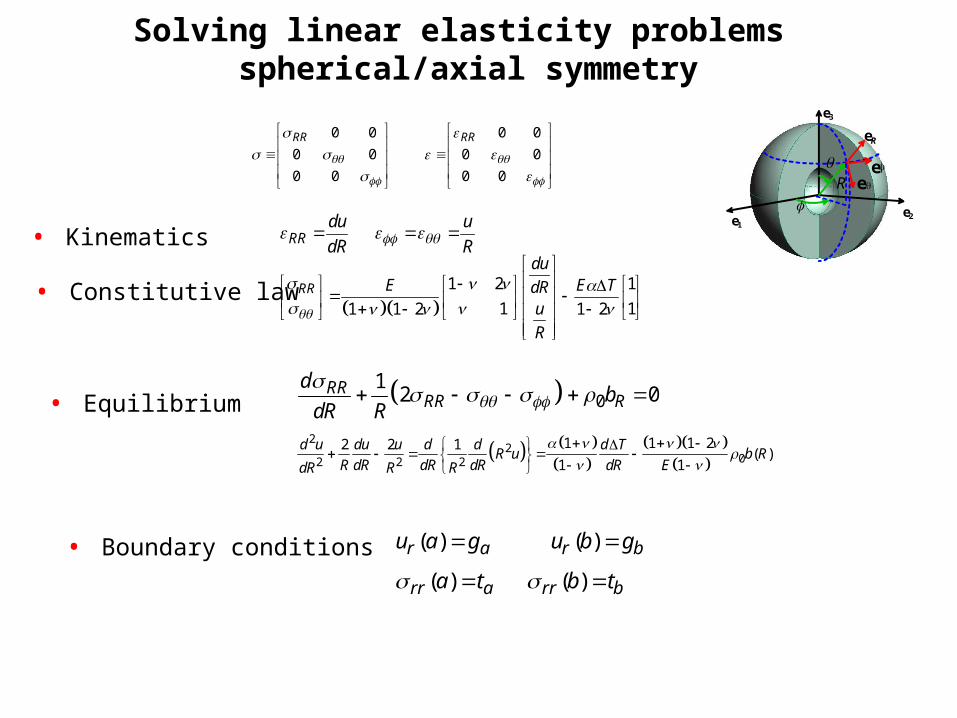
Solving linear elasticity problems spherical/axial symmetry

R

eR

ee

e1

e2

e3

0 0 0 0

0 0 0 0

0 0 0 0

RR RR

1 2 1

1 11 1 2 1 2RR

duE E TdR

u

R

01

2 0RRRR R

db

dR R

• Constitutive law

22

02 2 2

1 1 1 22 2 1( )

1 1

d u du u d d d TR u b R

R dR dR dR dR EdR R R

• Equilibrium

RRdu u

dR R • Kinematics

( ) ( )r a r bu a g u b g

( ) ( )rr a rr ba t b t • Boundary conditions

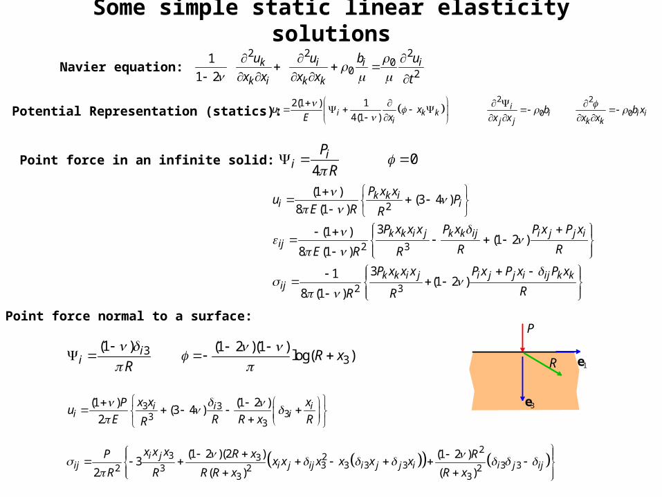
Some simple static linear elasticity solutions

2

2 3

2 3

(1 )(3 4 )

8 (1 )

3(1 )(1 2 )

8 (1 )

31(1 2 )

8 (1 )

k k ii i

k k i j k k ij i j j iij

k k i j i j j i ij k kij

P x xu P

E R R

P x x x P x P x P x

R RE R R

P x x x P x P x P x

RR R

04

ii

P

R

Point force in an infinite solid:

Point force normal to a surface:

e1

P

e3

R3

3(1 ) (1 2 )(1 )

log( )ii R x

R

3 333

3

(1 ) (1 2 )(3 4 )

2i i i

i ix x xP

uE R R x RR

2

3 233 3 3 3 3 32 3 2 2

3 3

(1 2 )(2 ) (1 2 )3

2 ( ) ( )

i jij i j ij i j j i i j ij

x x x R xP Rx x x x x x

R R R R x R x

2 2 20

0 2

1

1 2k i i i

k i k k

u u b u

x x x x t

Navier equation:

2(1 ) 1

4(1 )i i k ki

u xE x

Potential Representation (statics): 2 2

0 0i

i i ij j k k

b b xx x x x

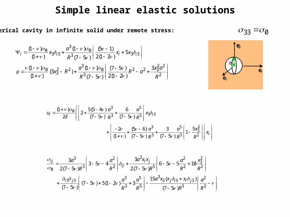
Simple linear elastic solutions

a

e2

e1

e3

30 0

3 3 3 33

3 2 22 2 2 20 0 33 3 2

(1 ) (1 ) (5 1)5

(1 ) 2(1 2 )(7 5 )

(1 ) (1 ) 3(7 5 )(3 )

(1 ) 2(1 2 )(7 5 )

i i i ia

x x xR

a x ax R R a

R R

3 50

3 33 5

23 53

3 5 2

(1 ) 5(5 4 ) 62

2 (7 5 ) (7 5 )

52 (5 6) 31

(1 ) (7 5 ) (7 5 )

i i

i

a au x

E R R

xa ax

R R R

3 23 2 23

3 2 5 2 20

33 5 23 3 3 3 3

3 5 5 2

333 5 4 6 5 5 10

2(7 5 ) 2(7 5 )

15 ( )(7 5 ) 5(1 2 ) 3

(7 5 ) (7 5 )

ij i jij

i j j i i j

a x x xa a a

R R R R R

a x x xa a a

R R R R

33 0 Spherical cavity in infinite solid under remote stress:

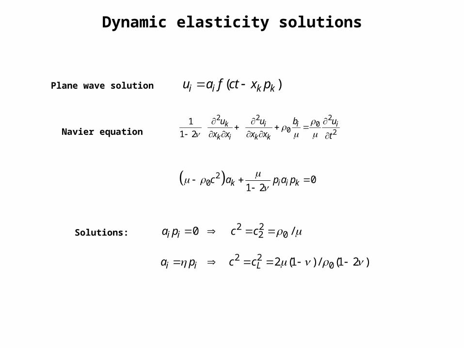
Dynamic elasticity solutions

( )i i k ku a f ct x p Plane wave solution

2 2 20

0 2

1

1 2k i i i

k i k k

u u b u

x x x x t

Navier equation

20 0

1 2k i i kc a p a p

2 22 00 /i ia p c c Solutions:

2 202 (1 ) / (1 2 )i i La p c c