conservation laws for some systems of nonlinear … · journal of applied mathematics volume 2012,...
TRANSCRIPT
Hindawi Publishing CorporationJournal of Applied MathematicsVolume 2012, Article ID 871253, 13 pagesdoi:10.1155/2012/871253
Research ArticleConservation Laws for Some Systems ofNonlinear Partial Differential Equations viaMultiplier Approach
Rehana Naz
Centre for Mathematics and Statistical Sciences, Lahore School of Economics, Lahore 53200, Pakistan
Correspondence should be addressed to Rehana Naz, rehananaz [email protected]
Received 26 July 2012; Accepted 20 September 2012
Academic Editor: Fazal M. Mahomed
Copyright q 2012 Rehana Naz. This is an open access article distributed under the CreativeCommons Attribution License, which permits unrestricted use, distribution, and reproduction inany medium, provided the original work is properly cited.
The conservation laws for the integrable coupled KDV type system, complexly coupled kdvsystem, coupled system arising from complex-valued KDV in magnetized plasma, Ito integrablesystem, and Navier stokes equations of gas dynamics are computed by multipliers approach. Firstof all, we calculate the multipliers depending on dependent variables, independent variables,and derivatives of dependent variables up to some fixed order. The conservation laws fluxesare computed corresponding to each conserved vector. For all understudying systems, the localconservation laws are established by utilizing the multiplier approach.
1. Introduction
The partial differential equations, which arise in the sciences, dynamics, fluid mechanics,electromagnetism, economics and so forth, express conservation of mass, momentum, energy,electric charge, or value of firm. All the conservation laws of partial differential equationsmay not have physical interpretation but are essential in studying the integrability of thePDE. The high number of conservation laws for a partial differential equation grantees thatthe partial differential equation is strongly integrable and can be linearized or explicitlysolved [1]. Moreover, the conservation laws are used for analysis, particularly, developmentof numerical schemes, soliton solutions, study of properties such as bi-Hamiltonian structuresand recursion operators, and reduction of partial differential equations.
There are different methods for the construction of conservation laws as describedby Naz [2], Naz et al. [3], Bluman et al. [4], Hereman et al. [5], and references therein.Rocha Filho and Figueiredo [6] developed computer packages based on Noether’s methodfor the variational problems. Wolf [7] and Wolf et al. [8] introduced computer programmesin REDUCE to calculate conservation laws.
2 Journal of Applied Mathematics
In this work, the multiplier approach is used to derive the conservation laws for somesystems of partial differential equations important due to physical point of view. Stuedel [9]introduced the multiplier approach and the conserved vectors were written in a characteristicform as DiT
i = ΛαEα. The determining equations for the multipliers (characteristics) wereobtained by taking the variational derivative of DiT
i = QαEα for the arbitrary functionsnot only for solutions of system of partial differential equations [10]. A conserved vectoris associated with each multiplier. The conservation laws for the integrable coupled kdv-typesystem, complexly coupled KDA system, coupled system arising from complex-valued KDVin magnetized plasma, Ito integrable system, and Navier stokes equations of gas dynamicsare computed by utilizing the multiplier approach. The conserved vectors derived here canbe used in constructing the solutions of underlying systems in the following different ways.The corresponding potential system can be written for the conservation laws, and symmetryreductions [11] can be carried out. Another approach to deduce exact solutions is via thedouble reduction theory [12–14]. The exact solution can be derived if the conservation lawsgive physical conserved quantities like Naz et al. [15]. The exact solutions of systems underconsideration are subject of future work.
The outline of paper is as follows. In Section 2, some definitions related withmultiplierapproach are presented. The conservation laws for integrable coupled kdv-type system,complexly coupled kdv system, coupled system arising from complex-valued KDV inmagnetized plasma, Ito integrable system, and Navier stokes equations of gas dynamics areconstructed in Section 3. Conclusions are summarized in Section 4.
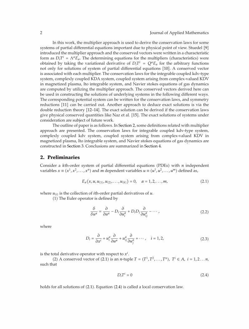
2. Preliminaries
Consider a kth-order system of partial differential equations (PDEs) with n independentvariables x ≡ (x1, x2, . . . , xn) and m dependent variables u ≡ (u1, u2, . . . , um) defined as,
Eα
(x, u, u(1), u(2), . . . , u(k)
)= 0, α = 1, 2, . . . , m, (2.1)
where u(i) is the collection of ith-order partial derivatives of u.(1) The Euler operator is defined by
δ
δuα=
∂
∂uα−Di
∂
∂uαi
+DiDj∂
∂uαij
− · · · , (2.2)
where
Di =∂
∂xi+ uα
i
∂
∂uα+ uα
ij
∂
∂uαj
+ · · · , i = 1, 2, (2.3)
is the total derivative operator with respect to xi.(2) A conserved vector of (2.1) is an n-tuple T = (T1, T2, . . . , Tn), T i ∈ A, i = 1, 2 . . . n,
such that
DiTi = 0 (2.4)
holds for all solutions of (2.1). Equation (2.4) is called a local conservation law.

Journal of Applied Mathematics 3
(3) The multipliers Λα of system (2.1) has the property
DiTi = ΛαEα, (2.5)
for the arbitrary function uα [9, 10].(4) The determining equations for the multipliers are obtained by taking variational
derivative of (2.5) (see [10]):
δ
δuα[ΛαEα] = 0. (2.6)
Equation (2.6) holds for the arbitrary functions uα not only for the solutions of system (2.1).Equation (2.6) yields multipliers for all local conservation laws. Then conserved
vectors can be derived systematically using (2.5) as the determining equation. But in someproblems it is not difficult to construct the conserved vectors by elementary manipulationsonce the multiplier has been determined.
3. Conservation Laws for Nonlinear Systems of PartialDifferential Equations
3.1. Integrable Coupled System
Consider the integrable coupled system [16, 17]
E1 = ut +[uxx − (k + 3)(k + 6)u2 − k2v2
]
x+ 2k[(k + 6)vux + (k + 3)uvx = 0,
E2 = vt +[vxx − k(k − 3)v2 − (k + 3)2u2
]
x+ 2(k + 3)[kvux + (k − 3)uvx = 0.
(3.1)
The group invariant solution of (3.1)was derived in [17]. Here wewill construct conservationlaws for coupled system (3.1). Consider simple multipliers of the form Λ1(t, x, u, v) andΛ2(t, x, u, v). Multipliers Λ1 and Λ2 for the system (3.1) have the property that
Λ1E1 + Λ2E2 = DtT1 +DxT
2, (3.2)
for all functions u(t, x) and v(t, x) where the total derivative operators Dt and Dx from (2.3)are
Dt =∂
∂t+ ut
∂
∂u+ vt
∂
∂v+ utt
∂
∂ut+ vtt
∂
∂vt+ utx
∂
∂ux+ vtx
∂
∂vx+ · · · ,
Dx =∂
∂x+ ux
∂
∂u+ vx
∂
∂v+ uxx
∂
∂ux+ vxx
∂
∂vx+ uxt
∂
∂ut+ vxt
∂
∂vt+ · · · .
(3.3)
The right-hand side of (3.2) is a divergence expression and T1 and T2 are the componentsof the conserved vector T = (T1, T2). The determining equations for the multipliers
4 Journal of Applied Mathematics
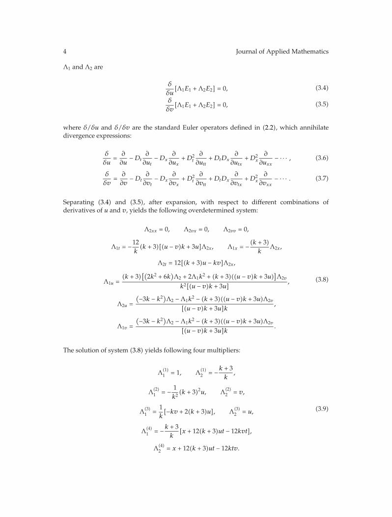
Λ1 and Λ2 are
δ
δu[Λ1E1 + Λ2E2] = 0, (3.4)
δ
δv[Λ1E1 + Λ2E2] = 0, (3.5)
where δ/δu and δ/δv are the standard Euler operators defined in (2.2), which annihilatedivergence expressions:
δ
δu=
∂
∂u−Dt
∂
∂ut−Dx
∂
∂ux+D2
t
∂
∂utt+DtDx
∂
∂utx+D2
x
∂
∂uxx− · · · , (3.6)
δ
δv=
∂
∂v−Dt
∂
∂vt−Dx
∂
∂vx+D2
t
∂
∂vtt+DtDx
∂
∂vtx+D2
x
∂
∂vxx− · · · . (3.7)
Separating (3.4) and (3.5), after expansion, with respect to different combinations ofderivatives of u and v, yields the following overdetermined system:
Λ2xx = 0, Λ2vx = 0, Λ2vv = 0,
Λ1t = −12k(k + 3)[(u − v)k + 3u]Λ2x, Λ1x = − (k + 3)
kΛ2x,
Λ2t = 12[(k + 3)u − kv]Λ2x,
Λ1u =(k + 3)
[(2k2 + 6k
)Λ2 + 2Λ1k
2 + (k + 3)((u − v)k + 3u)]Λ2v
k2[(u − v)k + 3u],
Λ2u =
(−3k − k2)Λ2 −Λ1k2 − (k + 3)((u − v)k + 3u)Λ2v
[(u − v)k + 3u]k,
Λ1v =
(−3k − k2)Λ2 −Λ1k2 − (k + 3)((u − v)k + 3u)Λ2v
[(u − v)k + 3u]k.
(3.8)
The solution of system (3.8) yields following four multipliers:
Λ(1)1 = 1, Λ(1)
2 = −k + 3k
,
Λ(2)1 = − 1
k2 (k + 3)2u, Λ(2)2 = v,
Λ(3)1 =
1k[−kv + 2(k + 3)u], Λ(3)
2 = u,
Λ(4)1 = −k + 3
k[x + 12(k + 3)ut − 12kvt],
Λ(4)2 = x + 12(k + 3)ut − 12ktv.
(3.9)

Journal of Applied Mathematics 5
From (3.2) and (3.9), we obtained following four conserved vectors:
T(1)1 = − 1
k[(k + 3)u − kv],
T(1)2 =
1k
[6(k + 3)2u2 − 12k(k + 3)uv + kvxx − kuxx − 3uxx
],
T(2)1 = − 1
2k2
[u2(k + 3)2 − k2v2
],
T(2)2 =
16k2
[3(k + 3)2u2
x − 3k2v2x + 4(k + 6)(k + 3)3u3 − 4k3(k − 3)v3
−12k(k + 3)3u2v + 12k3(k + 3)uv2 − 6(k + 3)2uuxx + 6k2vvxx
],
T(3)1 = − 1
k
[(k + 3)u2 − kuv
],
T(3)2 =
13k
[3(k + 3)u2
x + 2(k + 3)2(k + 12)u3
− 2k3v3 − 6k(k + 3)(k + 9)u2v + 6k2(k + 6)uv2
−6(k + 3)uuxx + 3kuxxv + 3kuvxx − 3kuxvx
],
T(4)1 = − 1
k
[6(k + 3)2tu2 + 6k2tv2
−12k(k + 3)tuv + (k + 3)ux − kvx
],
T(4)2 =
1k
[− (k + 3)(x + 12(k + 3)tu − 12ktv)uxx
+ (x + 12(k + 3)ut − 12ktv)kvxx + 6(k + 3)2tu2x + 6tk2v2
x
− 12k(k + 3)tuxvx + (k + 3)ux − kvx + 48(k + 3)3tu3
− 48k3tv3 − 144k(k + 3)2tu2v + 144k2(k + 3)tuv2
+6(k + 3)2xu2 + 6k2xv2 − 12k(k + 3)xuv].
(3.10)
3.2. Higher-Order Conservation Laws forComplexly Coupled KDV System
The conservation laws of complexly coupled KDV were discussed in Naz [18]
ut − 6uux − 6vvx − uxxx = 0,
vt − 6uvx − 6vux − vxxx = 0,(3.11)

6 Journal of Applied Mathematics
and six conserved vectors were derived by multipliers approach with multipliers of formΛ1(t, x, u, v) and Λ2(t, x, u, v). Now we will consider higher-order multipliers and derive theassociated conservation laws fluxes. The determining equations for multipliers of the formΛ1(t, x, u, v, ux, vx, uxx, vxx) and Λ2(t, x, u, v, ux, vx, uxx, vxx) from (2.6) are
δ
δu[Λ1(ut − 6uux − 6vvx − uxxx) + Λ2(vt − 6uvx − 6vux − vxxx)] = 0, (3.12)
δ
δv[Λ1(ut − 6uux − 6vvx − uxxx) + Λ2(vt − 6uvx − 6vux − vxxx)] = 0, (3.13)
where the standard Euler operators δ/δu and δ/δv are given by (3.6) and (3.7). Equations(3.12) and (3.13) are separated, after expansion, according to different combinations ofderivatives of u and v and after some simplification the following system of equations forΛ1,Λ2 is obtained:
Λ1xx = 0, Λ1vx = 0, Λ1xvxx = 0, Λ1vvxx = 0, Λ1ux = 0, Λ1vx = 0,
Λ2xx = 0, Λ2vx = 0, Λ2xvxx = 0, Λ2vvxx = 0, Λ2ux = 0, Λ2vx = 0,
Λ1vxxvxx = 0, Λ2vxxvxx = 0, Λ2vv = 6Λ1vxx , Λ1vv = 6Λ2vxx ,
Λ1t = 6Λ2xv + 6Λ1xu, Λ2t = 6Λ1xv + 6Λ2xu,
Λ1u = Λ2v, Λ2u = Λ1v, Λ1uxx = Λ2vxx , Λ2uxx = Λ1vxx .
(3.14)
The solution of system (3.14) yields
Λ1 = c1 + u(c3 + c4t) + v(c5 + c6t) +x
6c4 +
(3u2 + 3v2 + uxx
)c7 + (6uv + vxx)c8,
Λ2 = c2 + v(c3 + c4t) + u(c5 + c6t) +x
6c6 + (6uv + vxx)c7 +
(3u2 + 3v2 + uxx
)c8,
(3.15)
where c1, c2, . . . , c8 are arbitrary constants. The first six multipliers are same as derived in [18].The two new multipliers are actually the higher-order multipliers associated with constantsc7 and c8
Λ(7)1 = 3u2 + 3v2 + uxx, Λ(7)
2 = 6uv + vxx,
Λ(8)1 = 6uv + vxx, Λ(8)
2 = 3u2 + 3v2 + uxx.
(3.16)

Journal of Applied Mathematics 7
Equation (2.5)with multipliers given in (3.16) gives two new conservation laws
T(7)1 = 3uv2 + u3 +
12uuxx +
12vvxx,
T(7)2 = −6uvvxx − 27u2v2 − 1
2vvtx − 9
2u4 − 1
2u2xx
− 3uxxv2 − 3u2uxx − 9
2v4 − 1
2v2xx −
12uutx +
12vxvt +
12uxut,
T(8)1 = 3u2v + v3 +
12uvxx +
12uxxv,
T(8)2 = −1
2uvtx − 18u3v − uxxvxx − 18uv3 − 3v2vxx
− 3u2vxx − 12vutx − 6uvuxx +
12uxvt +
12vxut.
(3.17)
The two new higher-order conservation laws (3.17) are obtained for the system (3.11).
3.3. Conservation Laws for Complex-Valued KDV in Magnetized Plasma
The complexly coupled KDV
wt −(|w|2w
)
x−wxxx = 0 (3.18)
arises in the study of the asymptotic investigation of electrostatic waves of a magnetizedplasma [19]. The variable w is the complex field amplitude w = u + iv. The representation of(3.18) in real field variables u and v is
ut − 3u2ux − 2uvvx − v2ux − uxxx = 0,
vt − 3v2vx − 2uvux − u2vx − vxxx = 0.(3.19)
The conservation laws for system (3.19) are derived here by using multiplier approach.The determining equations for multipliers of the form Λ1(t, x, u, v, ux, vx, uxx, vxx) andΛ2(t, x, u, v, ux, vx, uxx, vxx) from (2.6) are
δ
δu
[Λ1
(ut − 3u2ux − 2uvvx − v2ux − uxxx
)+ Λ2
(vt − 3v2vx − 2uvux − u2vx − vxxx
)]= 0,
δ
δv
[Λ1
(ut − 3u2ux − 2uvvx − v2ux − uxxx
)+ Λ2
(vt − 3v2vx − 2uvux − u2vx − vxxx
)]= 0.
(3.20)

8 Journal of Applied Mathematics
Equation (3.20) finally results in the following overdetermined system:
Λ2xx = 0, Λ1ux = 0, Λ2ux = 0, Λ1vx = 0, Λ2vx = 0,
Λ1uxx = Λ2vxx , Λ2uxx = 0, Λ1vxx = 0,
Λ1uxx = Λ2vxx , Λ2uxx = 0, Λ1vxx = 0,
Λ2vx =Λ2x
v, Λ2xvxx = 0, Λ2vv = 6vΛ2vxx ,
Λ2vvxx = 0, Λ2vxxvxx = 0,
Λ1t =3v
(uxx + u3 + v2u
)Λ2x,
Λ2t =3v
(Λ2xvxx + Λ2xu
2v + Λ2xv3),
Λ1x =Λ2xu
v,
Λ1u = 2Λ2vxxu2 − 2Λ2vxxv
2 + Λ2v,
Λ2u = 2Λ2vxxuv,
Λ1v = 2Λ2vxxuv.
(3.21)
The solution of system (3.21) yields following five multipliers:
Λ(1)1 = 0, Λ(1)
2 = 1,
Λ(2)1 = 1, Λ(2)
2 = 0,
Λ(3)1 = u, Λ(3)
2 = v,
Λ(4)1 = u3 + uv2 + uxx,
Λ(4)2 = u2v + v3 + vxx,
Λ(5)1 = 3t
(u3 + uv2 + uxx
)+ xu,
Λ(5)2 = 3t
(v3 + u2v + vxx
)+ xv.
(3.22)
Journal of Applied Mathematics 9
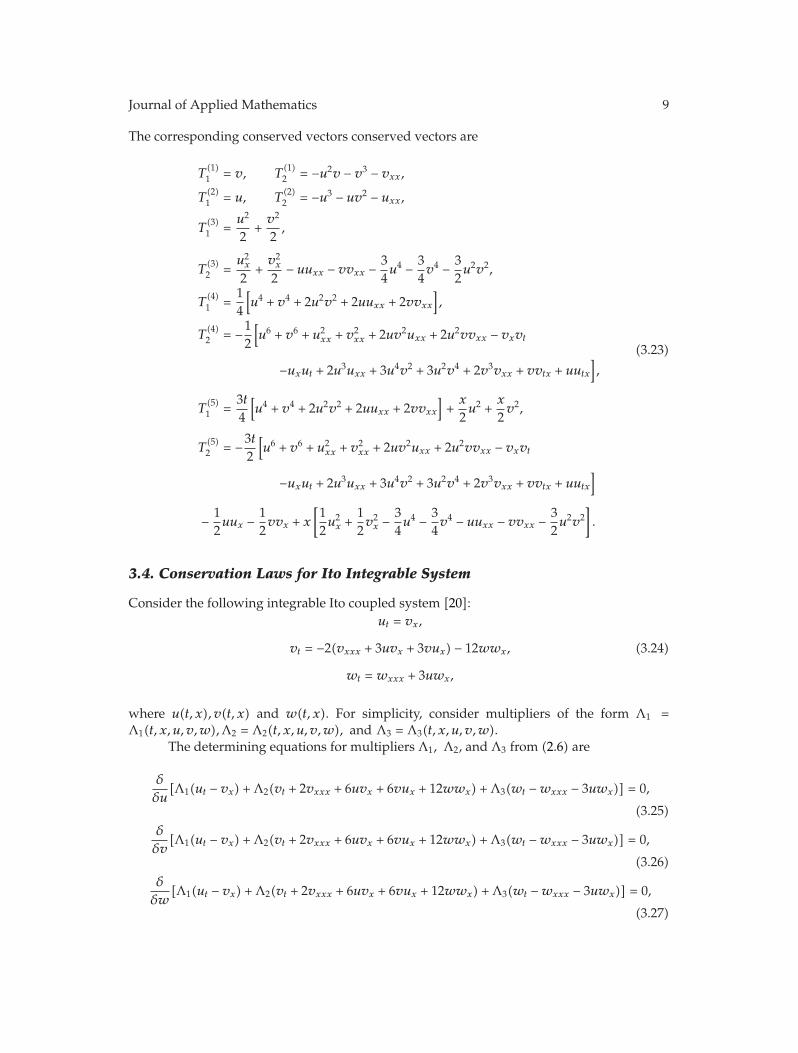
The corresponding conserved vectors conserved vectors are
T(1)1 = v, T
(1)2 = −u2v − v3 − vxx,
T(2)1 = u, T
(2)2 = −u3 − uv2 − uxx,
T(3)1 =
u2
2+v2
2,
T(3)2 =
u2x
2+v2x
2− uuxx − vvxx − 3
4u4 − 3
4v4 − 3
2u2v2,
T(4)1 =
14
[u4 + v4 + 2u2v2 + 2uuxx + 2vvxx
],
T(4)2 = −1
2
[u6 + v6 + u2
xx + v2xx + 2uv2uxx + 2u2vvxx − vxvt
−uxut + 2u3uxx + 3u4v2 + 3u2v4 + 2v3vxx + vvtx + uutx
],
T(5)1 =
3t4
[u4 + v4 + 2u2v2 + 2uuxx + 2vvxx
]+x
2u2 +
x
2v2,
T(5)2 = −3t
2
[u6 + v6 + u2
xx + v2xx + 2uv2uxx + 2u2vvxx − vxvt
−uxut + 2u3uxx + 3u4v2 + 3u2v4 + 2v3vxx + vvtx + uutx
]
− 12uux − 1
2vvx + x
[12u2x +
12v2x −
34u4 − 3
4v4 − uuxx − vvxx − 3
2u2v2
].
(3.23)
3.4. Conservation Laws for Ito Integrable System
Consider the following integrable Ito coupled system [20]:ut = vx,
vt = −2(vxxx + 3uvx + 3vux) − 12wwx,
wt = wxxx + 3uwx,
(3.24)
where u(t, x), v(t, x) and w(t, x). For simplicity, consider multipliers of the form Λ1 =Λ1(t, x, u, v,w),Λ2 = Λ2(t, x, u, v,w), and Λ3 = Λ3(t, x, u, v,w).
The determining equations for multipliers Λ1, Λ2, and Λ3 from (2.6) are
δ
δu[Λ1(ut − vx) + Λ2(vt + 2vxxx + 6uvx + 6vux + 12wwx) + Λ3(wt −wxxx − 3uwx)] = 0,
(3.25)δ
δv[Λ1(ut − vx) + Λ2(vt + 2vxxx + 6uvx + 6vux + 12wwx) + Λ3(wt −wxxx − 3uwx)] = 0,
(3.26)δ
δw[Λ1(ut − vx) + Λ2(vt + 2vxxx + 6uvx + 6vux + 12wwx) + Λ3(wt −wxxx − 3uwx)] = 0,
(3.27)
10 Journal of Applied Mathematics
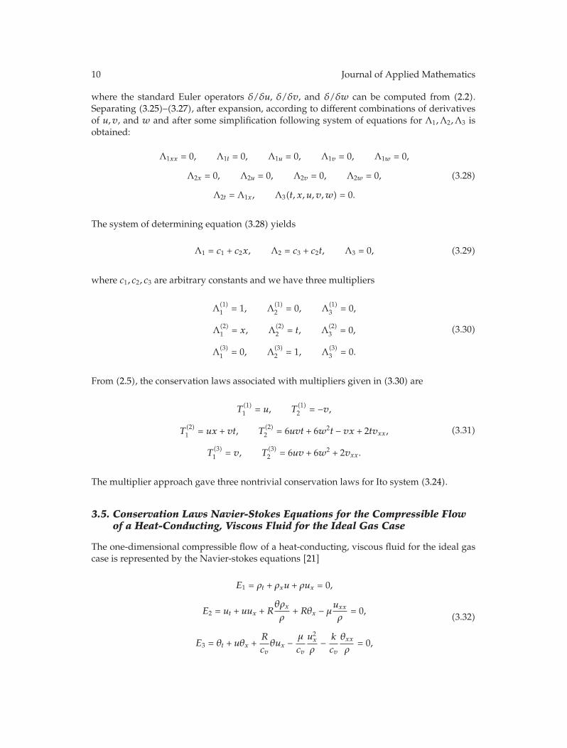
where the standard Euler operators δ/δu, δ/δv, and δ/δw can be computed from (2.2).Separating (3.25)–(3.27), after expansion, according to different combinations of derivativesof u, v, and w and after some simplification following system of equations for Λ1,Λ2,Λ3 isobtained:
Λ1xx = 0, Λ1t = 0, Λ1u = 0, Λ1v = 0, Λ1w = 0,
Λ2x = 0, Λ2u = 0, Λ2v = 0, Λ2w = 0,
Λ2t = Λ1x, Λ3(t, x, u, v,w) = 0.
(3.28)
The system of determining equation (3.28) yields
Λ1 = c1 + c2x, Λ2 = c3 + c2t, Λ3 = 0, (3.29)
where c1, c2, c3 are arbitrary constants and we have three multipliers
Λ(1)1 = 1, Λ(1)
2 = 0, Λ(1)3 = 0,
Λ(2)1 = x, Λ(2)
2 = t, Λ(2)3 = 0,
Λ(3)1 = 0, Λ(3)
2 = 1, Λ(3)3 = 0.
(3.30)
From (2.5), the conservation laws associated with multipliers given in (3.30) are
T(1)1 = u, T
(1)2 = −v,
T(2)1 = ux + vt, T
(2)2 = 6uvt + 6w2t − vx + 2tvxx,
T(3)1 = v, T
(3)2 = 6uv + 6w2 + 2vxx.
(3.31)
The multiplier approach gave three nontrivial conservation laws for Ito system (3.24).
3.5. Conservation Laws Navier-Stokes Equations for the Compressible Flowof a Heat-Conducting, Viscous Fluid for the Ideal Gas Case
The one-dimensional compressible flow of a heat-conducting, viscous fluid for the ideal gascase is represented by the Navier-stokes equations [21]
E1 = ρt + ρxu + ρux = 0,
E2 = ut + uux + Rθρxρ
+ Rθx − μuxx
ρ= 0,
E3 = θt + uθx +R
cvθux −
μ
cv
u2x
ρ− k
cv
θxxρ
= 0,
(3.32)
Journal of Applied Mathematics 11
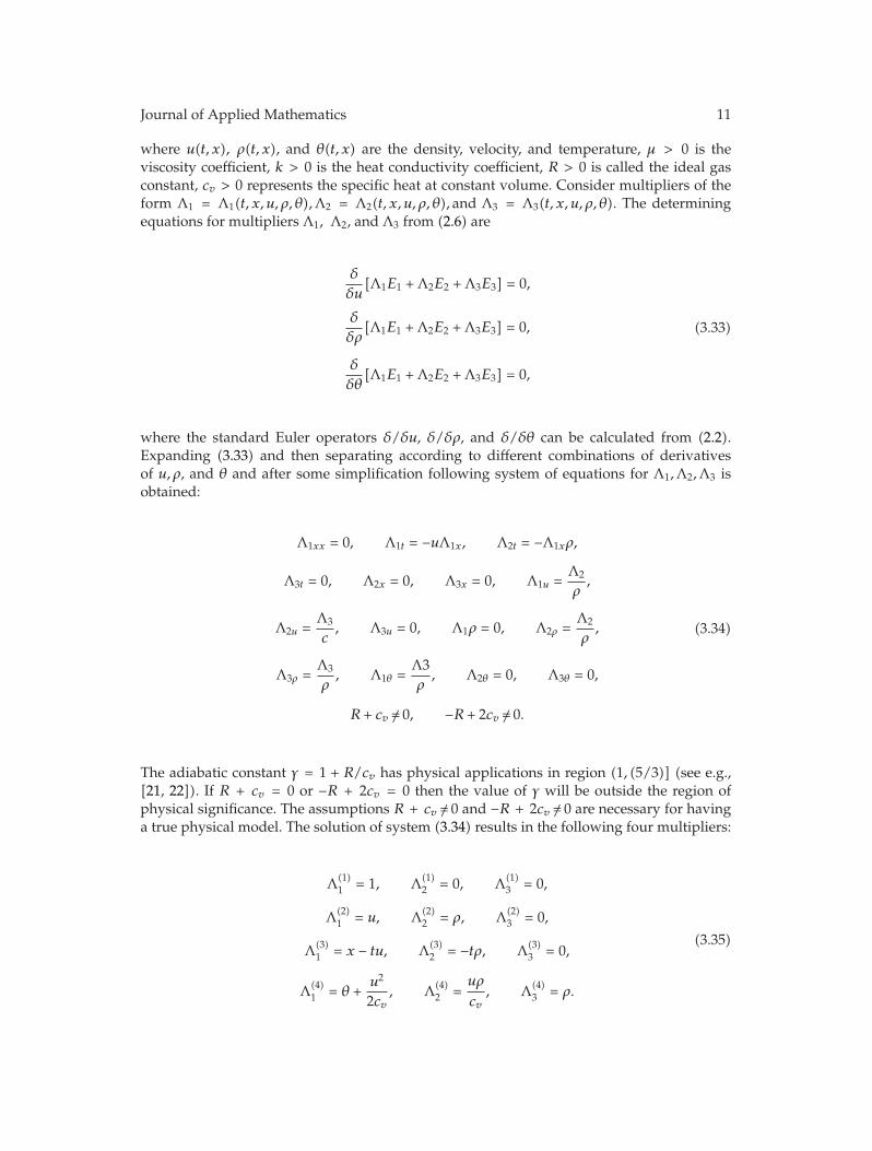
where u(t, x), ρ(t, x), and θ(t, x) are the density, velocity, and temperature, μ > 0 is theviscosity coefficient, k > 0 is the heat conductivity coefficient, R > 0 is called the ideal gasconstant, cv > 0 represents the specific heat at constant volume. Consider multipliers of theform Λ1 = Λ1(t, x, u, ρ, θ),Λ2 = Λ2(t, x, u, ρ, θ), and Λ3 = Λ3(t, x, u, ρ, θ). The determiningequations for multipliers Λ1, Λ2, and Λ3 from (2.6) are
δ
δu[Λ1E1 + Λ2E2 + Λ3E3] = 0,
δ
δρ[Λ1E1 + Λ2E2 + Λ3E3] = 0,
δ
δθ[Λ1E1 + Λ2E2 + Λ3E3] = 0,
(3.33)
where the standard Euler operators δ/δu, δ/δρ, and δ/δθ can be calculated from (2.2).Expanding (3.33) and then separating according to different combinations of derivativesof u, ρ, and θ and after some simplification following system of equations for Λ1,Λ2,Λ3 isobtained:
Λ1xx = 0, Λ1t = −uΛ1x, Λ2t = −Λ1xρ,
Λ3t = 0, Λ2x = 0, Λ3x = 0, Λ1u =Λ2
ρ,
Λ2u =Λ3
c, Λ3u = 0, Λ1ρ = 0, Λ2ρ =
Λ2
ρ,
Λ3ρ =Λ3
ρ, Λ1θ =
Λ3ρ
, Λ2θ = 0, Λ3θ = 0,
R + cv /= 0, −R + 2cv /= 0.
(3.34)
The adiabatic constant γ = 1 + R/cv has physical applications in region (1, (5/3)] (see e.g.,[21, 22]). If R + cv = 0 or −R + 2cv = 0 then the value of γ will be outside the region ofphysical significance. The assumptions R + cv /= 0 and −R + 2cv /= 0 are necessary for havinga true physical model. The solution of system (3.34) results in the following four multipliers:
Λ(1)1 = 1, Λ(1)
2 = 0, Λ(1)3 = 0,
Λ(2)1 = u, Λ(2)
2 = ρ, Λ(2)3 = 0,
Λ(3)1 = x − tu, Λ(3)
2 = −tρ, Λ(3)3 = 0,
Λ(4)1 = θ +
u2
2cv, Λ(4)
2 =uρ
cv, Λ(4)
3 = ρ.
(3.35)
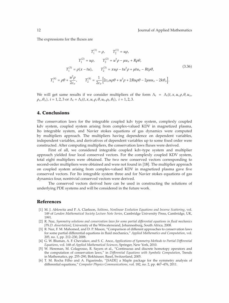
12 Journal of Applied Mathematics
The expressions for the fluxes are
T(1)1 = ρ, T
(1)2 = uρ,
T(2)1 = uρ, T
(2)2 = u2ρ − μux + Rρθ,
T(3)1 = ρ(x − tu), T
(3)2 = xuρ − tu2ρ + μtux − Rtρθ,
T(4)1 = ρθ +
u2ρ
2cv, T
(4)2 =
12cv
[2cvuρθ + u3ρ + 2Ruρθ − 2μuux − 2kθx
].
(3.36)
We will get same results if we consider multipliers of the form Λi = Λi(t, x, u, ρ, θ, ux,ρx, θx), i = 1, 2, 3 or Λi = Λi(t, x, u, ρ, θ, ut, ρt, θt), i = 1, 2, 3.
4. Conclusions
The conservation laws for the integrable coupled kdv type system, complexly coupledkdv system, coupled system arising from complex-valued KDV in magnetized plasma,Ito integrable system, and Navier stokes equations of gas dynamics were computedby multipliers approach. The multipliers having dependence on dependent variables,independent variables, and derivatives of dependent variables up to some fixed order wereconstructed. After computing multipliers, the conservation laws fluxes were derived.
First of all, we considered integrable coupled kdv-type system and multiplierapproach yielded four local conserved vectors. For the complexly coupled KDV system,total eight multipliers were obtained. The two new conserved vectors corresponding tosecond-order multipliers were obtained and were not found in [18]. The multiplier approachon coupled system arising from complex-valued KDV in magnetized plasma gave fiveconserved vectors. For Ito integrable system three and for Navier stokes equations of gasdynamics four, nontrivial conserved vectors were derived.
The conserved vectors derived here can be used in constructing the solutions ofunderlying PDE systems and will be considered in the future work.
References
[1] M. J. Ablowitz and P. A. Clarkson, Solitons, Nonlinear Evolution Equations and Inverse Scattering, vol.149 of London Mathematical Society Lecture Note Series, Cambridge University Press, Cambridge, UK,1991.
[2] R. Naz, Symmetry solutions and conservation laws for some partial differential equations in fluid mechanics[Ph.D. dissertation], University of the Witwatersrand, Johannesburg, South Africa, 2008.
[3] R. Naz, F. M. Mahomed, and D. P. Mason, “Comparison of different approaches to conservation lawsfor some partial differential equations in fluid mechanics,” Applied Mathematics and Computation, vol.205, no. 1, pp. 212–230, 2008.
[4] G. W. Bluman, A. F. Cheviakov, and S. C. Anco, Applications of Symmetry Methods to Partial DifferentialEquations, vol. 168 of Applied Mathematical Sciences, Springer, New York, 2010.
[5] W. Hereman, M. Colagrosso, R. Sayers et al., “Continuous and discrete homotopy operators andthe computation of conservation laws,” in Differential Equations with Symbolic Computation, Trendsin Mathematics, pp. 255–290, Birkhauser, Basel, Switzerland, 2005.
[6] T. M. Rocha Filho and A. Figueiredo, “[SADE] a Maple package for the symmetry analysis ofdifferential equations,” Computer Physics Communications, vol. 182, no. 2, pp. 467–476, 2011.

Journal of Applied Mathematics 13
[7] T. Wolf, “A comparison of four approaches to the calculation of conservation laws,” European Journalof Applied Mathematics, vol. 13, no. 2, pp. 129–152, 2002.
[8] T. Wolf, A. Brand, and M. Mohammadzadeh, “Computer algebra algorithms and routines for thecomputation of conservation laws and fixing of gauge in differential expressions,” Journal of SymbolicComputation, vol. 27, no. 2, pp. 221–238, 1999.
[9] H. Steudel, “Uber die Zuordnung zwischen Invarianzeigenschaften und Erhaltungssatzen,”Zeitschrift fur Naturforschung, vol. 17, pp. 129–132, 1962.
[10] P. J. Olver, Applications of Lie Groups to Differential Equations, vol. 107 of Graduate Texts in Mathematics,Springer, New York, NY,USA, 2nd edition, 1993.
[11] G. Bluman, “Potential symmetries and equivalent conservation laws,” in Modern Group Analysis:Advanced Analytical and Computational Methods in Mathematical Physics, pp. 71–84, Kluwer Academic,Dodrecht, The Netherlands, 1993.
[12] A. Sjoberg, “Double reduction of PDEs from the association of symmetries with conservation lawswith applications,” Applied Mathematics and Computation, vol. 184, no. 2, pp. 608–616, 2007.
[13] A. Sjoberg, “On double reductions from symmetries and conservation laws,” Nonlinear Analysis: RealWorld Applications, vol. 10, no. 6, pp. 3472–3477, 2009.
[14] A. H. Bokhari, A. Y. Al-Dweik, F. D. Zaman, A. H. Kara, and F. M. Mahomed, “Generalization of thedouble reduction theory,” Nonlinear Analysis: Real World Applications, vol. 11, no. 5, pp. 3763–3769,2010.
[15] R. Naz, F. M. Mahomed, and D. P. Mason, “Conservation laws via the partial Lagrangian andgroup invariant solutions for radial and two-dimensional free jets,” Nonlinear Analysis: Real WorldApplications, vol. 10, no. 6, pp. 3457–3465, 2009.
[16] S. Y. Lou, B. Tong, H.-c. Hu, and X.-y. Tang, “Coupled KdV equations derived from two-layer fluids,”Journal of Physics A, vol. 39, no. 3, pp. 513–527, 2006.
[17] S. Qian and L. Tian, “Group-invariant solutions of a integrable coupled system,” Nonlinear Analysis:Real World Applications, vol. 9, no. 4, pp. 1756–1767, 2008.
[18] R. Naz, “Conservation laws for a complexly coupled KdV system, coupled Burgers’ system andDrinfeld-Sokolov-Wilson system via multiplier approach,” Communications in Nonlinear Science andNumerical Simulation, vol. 15, no. 5, pp. 1177–1182, 2010.
[19] A. A. Mohammad and M. Can, “Exact solutions of the complex modified Korteweg-de Vriesequation,” Journal of Physics A, vol. 28, no. 11, pp. 3223–3233, 1995.
[20] H. A. Zedan, “Symmetry analysis of an integrable Ito coupled system,” Computers &Mathematics withApplications, vol. 60, no. 12, pp. 3088–3097, 2010.
[21] J. Wang, “Boundary layers for compressible Navier-Stokes equations with outflow boundarycondition,” Journal of Differential Equations, vol. 248, no. 5, pp. 1143–1174, 2010.
[22] A. N. W. Hone, “Painleve tests, singularity structure and integrability,” Nonlinear Science, pp. 1–34,2005.

Submit your manuscripts athttp://www.hindawi.com
Hindawi Publishing Corporationhttp://www.hindawi.com Volume 2014
MathematicsJournal of
Hindawi Publishing Corporationhttp://www.hindawi.com Volume 2014
Mathematical Problems in Engineering
Hindawi Publishing Corporationhttp://www.hindawi.com
Differential EquationsInternational Journal of
Volume 2014
Applied MathematicsJournal of
Hindawi Publishing Corporationhttp://www.hindawi.com Volume 2014
Probability and StatisticsHindawi Publishing Corporationhttp://www.hindawi.com Volume 2014
Journal of
Hindawi Publishing Corporationhttp://www.hindawi.com Volume 2014
Mathematical PhysicsAdvances in
Complex AnalysisJournal of
Hindawi Publishing Corporationhttp://www.hindawi.com Volume 2014
OptimizationJournal of
Hindawi Publishing Corporationhttp://www.hindawi.com Volume 2014
CombinatoricsHindawi Publishing Corporationhttp://www.hindawi.com Volume 2014
International Journal of
Hindawi Publishing Corporationhttp://www.hindawi.com Volume 2014
Operations ResearchAdvances in
Journal of
Hindawi Publishing Corporationhttp://www.hindawi.com Volume 2014
Function Spaces
Abstract and Applied AnalysisHindawi Publishing Corporationhttp://www.hindawi.com Volume 2014
International Journal of Mathematics and Mathematical Sciences
Hindawi Publishing Corporationhttp://www.hindawi.com Volume 2014
The Scientific World JournalHindawi Publishing Corporation http://www.hindawi.com Volume 2014
Hindawi Publishing Corporationhttp://www.hindawi.com Volume 2014
Algebra
Discrete Dynamics in Nature and Society
Hindawi Publishing Corporationhttp://www.hindawi.com Volume 2014
Hindawi Publishing Corporationhttp://www.hindawi.com Volume 2014
Decision SciencesAdvances in
Discrete MathematicsJournal of
Hindawi Publishing Corporationhttp://www.hindawi.com
Volume 2014 Hindawi Publishing Corporationhttp://www.hindawi.com Volume 2014
Stochastic AnalysisInternational Journal of