Consistent Approach for Calculating Protein pKa’s

using Poisson-Boltzmann Model

A THESIS

SUBMITTED TO THE FACULTY OF THE GRADUATE SCHOOL

OF THE UNIVERSITY OF MINNESOTA

BY

Han Wool Yoon

IN PARTIAL FULFILLMENT OF THE REQUIREMENTS

FOR THE DEGREE OF

MASTER OF SCIENCE

Adviser: Yuk Sham

June 2013

© Han Wool Yoon 2013

ALL RIGHTS RESERVED

i

Acknowledgements

First, I would like to thank Prof. Yuk Sham, my research advisor, for his guidance and

support over the years. He has been an inspiration for me and I look forward to continue

my journey in the field of computational biology at USC. I also would like to thank all the

past and current members in the Prof. Sham’s lab who have been helpful in giving me

valuable feedbacks in my research. I also wish to express my gratitude to my committee

members, Dr. Elizabeth Amin and Dr. Carlos Sosa. I want to give special thanks to

Melody Lee for editorial critiques of my thesis and her encouragement. Lastly, but not

least, I want to thank my parents, Yong Chul Yoon and Eun Ja Park, and my fiancé,

Michelle Sham, who have always supported me by all means throughout my academic

career. My research could not have been completed without their support and patience.

ii

Abstract

Accurate prediction of protein pKa‘s is important to understand protein

electrostatics and functions. Improving the accuracy of pKa prediction using the Poisson-

Boltzmann electrostatic model remains an active area of research. The major challenge

is to determine the appropriate dielectric constant (P) that best describes the

heterogeneous protein environment. The common use of a single large P often fails to

reproduce large experimental pKa shifts of biological important residues. In this study, I

implemented a two steps approach, as described in earlier PDLD/S model, that uses a

single low dielectric constant for calculating the intrinsic protein pKa‘s when all other

ionizable group are neutralized and a single large dielectric constant for evaluating the

pKa‘s shifts as a result of charge-charge coupling between ionizable groups. This

approach is less sensitive to the dielectric constants used and can reliably reproduce the

commonly observed protein pKa‘s and others with abnormal large pKa shifts.

iii

Table of Contents

List of Tables ....................................................................................................................... iv

List of Figures ...................................................................................................................... v

Introductions

1.1 Ionizable residues in Proteins ...................................................................................... 1

1.2 Calculating pKa in Proteins ........................................................................................... 2

1.3 Poisson Boltzmann Electrostatic Model ....................................................................... 5

1.4 Dielectric constant in protein ...................................................................................... 7

1.5 Evaluating protein pKa with PDLD/S model : Intrinsic and apparent pKa .................... 9

1.6 Evaluating titration curve for monoprotic acid ......................................................... 11

1.7 Coulombic interaction energies between ionizable groups ...................................... 12

1.8 Project Objectives ...................................................................................................... 14

Method

2.1 Implementation of intrinsic pKa calculation

2.1.1 Protein Preparation ..................................................................................... 16

2.1.2 Electrostatic free energy calculation .......................................................... 16

2.1.3 Molecular Dynamics simulation .................................................................. 17

2.2 Calculation of pKa shifts by charge-charge interaction

2.2.1 Preparation ................................................................................................. 19

2.2.2 Calculation of charge-charge interaction energies ..................................... 20

2.2.3 Titration of average charges ....................................................................... 21

2.2.4 Simple case tests ......................................................................................... 22

2.3 Project Objectives ...................................................................................................... 24

Results and Discussions

3.1 Classic PB method tests ............................................................................................. 24

3.2 Results of decoupling charge-charge interactions with PB method .......................... 28

3.3 Statistical sampling of conformations ........................................................................ 37

3.4 Comparison to other benchmarks ............................................................................. 46

Conclusions ............................................................................................................. 50

Reference ................................................................................................................ 51

Reference ................................................................................................................ 54

iv

List of Tables

Table 1 Model pKa of side chains of ionizable amino acids in water ................................ 5

Table 2 Atom types that used for charge-charge interaction calculation ...................... 20

Table 3 Protein structures and experimental pKa data sets ........................................... 24

Table 4 Classic PB method in function of single dielectric constant .............................. 26

Table 5 Large pKa shifts predictions with classic PB method ........................................ 28

Table 6 Prediction for general cases with our method ................................................... 33

Table 7 Intrinsic and Wij calculation for general cases at P= 4 .................................... 34

Table 8 Our method for large pKa shifts cases .............................................................. 34

Table 9 Intrinsic pKa shifts and Wij for large pKa shifts cases ........................................ 35

Table 10 All individual calculations for 87 residues with MD conformational sampling .. 37

Table 11 Summary of pKa calculation with MD conformational sampling(MDCS) ......... 39

Table 12 pKa calculation comparison between 1HEL and 2LZT .................................... 43

Table 13 Our method with MDCS for large pKa shifts ................................................... 44

Table 14 Comparison of calculations with MDCS at P= 4 and 10 for general cases ..... 45

Table 15 Comparison of calculations with MDCS at P= 4 and 10 for large pKa shifts ... 45

Table 16 Comparison of Wij to benchmarks from Sham et al. ....................................... 47

Table 17 Comparison of our method to other benchmarks ........................................... 47

v

List of Figures

Figure 1 Protein folding processes that determine pKa of ionizable groups in protein ..... 2

Figure 2 Thermodynamic cycle for predicting pKa of an ionizable group in protein .......... 3

Figure 3 Finite-difference Poisson-Boltzmann electrostatic solvent model ...................... 7

Figure 4 Flow chart of intrinsic pKa calculation .............................................................. 15

Figure 5 Flow chart of Wij calculation ............................................................................ 19

Figure 6 Finding apparent pKa on titration curve ........................................................... 22

Figure 7 Simple test cases for <q> titration ................................................................... 23

Figure 8 Experimental vs calculated pKa for 87 sites .................................................... 35

Figure 9 Experimental vs calculated pKa shifts from model pKa for 87 sites .................. 36

Figure 10 Scattered plots of calculated pKa of 2LZT vs 1HEL ....................................... 44

Figure A Free energy graphs for Linear Response Approximation ................................. 44

1

Introductions

1.1 Ionizable residues in proteins

Protein electrostatics is an important factor governing the structural

stabilities and functions of proteins.[1-4] A consistent model for predicting

accurately the protein pKa’s can further provide the theoretical model for drug

discovery and protein design applications. Proteins consist of amino acids with

ionizable side chains that undergo proton association and dissociation reactions

in aqueous solution. The pKa’s of these ionizable groups can be greatly

influenced by their local environments such as the composition of the solvent

mixture, pH and ionic concentration. In the unfolded state, the pKa of these

ionizable sidechains are presumed to be solvent exposed and their pKa‘s are

typically similar to that of the individual amino acids in aqueous solution. During

the protein folding process, however, these ionizable groups become localized

onto the surface or into the interior regions of the protein that engages in an

intricate network of electrostatic and non-electrostatic interactions involving

hydrogen bonding, charge-charge, charge-dipole, and hydrophobic interactions

(Figure 1). These local heterogeneous environment greatly influences the overall

energetics and stability of each ionizable residues and their corresponding

apparent pKa‘s in proteins. Ability to quantify the compensatory electrostatic and

non-electrostatic effects provides a rigorous benchmark for examining protein

electrostatics.

2

Figure 1-1 Amino acids(a) form peptide chains(b) followed by secondary and tertiary

structures (c). Ionizable sites are localized into heterogeneous electrostatic

environments (d).

1.2 Calculating pKa in proteins

Understanding the role of electrostatic interactions in proteins is crucial for

the study of biological functions. There are many essential biological processes

that are modulated by the specific ionizable state of these ionizable groups. It

governs the overall protein stability, folding pathway, ion transport, molecular

association and catalysis. [1-3] Consistently and accurately quantifying the pKa of

ionizable groups and its specific ionization state in proteins is not a trivial task.

Before the availability of 3 dimensional protein structures, early Tanford and

Kirkwood (TK) model introduced for protein pKa calculation assumes proteins as

an impenetrable macroscopic spheres consisting of a low dielectric hydrophobic

protein core surrounded by ionizable group located on the surfaces of the

protein.[5] In the era of X-ray protein crystallography that reveals many of these

ionizable residues are buried, rigorous methods such as protein dipoles Langevin

dipoles (PDLD) [6] , Poisson-Boltzmann (PB) [7-9] , and generalized Born (GB)

[10, 11] type models have emerged that take into account the full atomistic detail

3

of the protein structure, as well as the explicit and implicit representation of

solvent environment. With increase in computational power, algorithm design and

the number of high resolution crystallized protein structures available for

examining protein pKa’s, the accuracy in many of these computational models

have significantly enhance over the past decades.

Figure 2. Thermodynamic cycle for predicting pKa of an ionizable group in a protein. w

and p designate water and protein, respectively. ∆𝐺𝑠𝑜𝑙𝑣𝑤→𝑝

designates a change in

solvation free energy of moving the titratable group from water to its protein.

The most widely used method for evaluating protein pKa is based on the

thermodynamic cycle shown in Figure 2. Instead of directly calculating the

4

change in free energy of deprotonation of the indicated ionizable group inside the

protein, the method utilizes the deprotonation of the ionizable group in the

aqueous phase as our reference reaction. This allows us to take the advantage

of using the reference pKa values of ionizable amino acids which can be

measured experimentally (Table 1). ∆𝐺𝑠𝑜𝑙𝑣𝑤→𝑝

designates the change in solvation

free energy of moving the titratable group from water (w) to its protein (p)

environment. Both the ∆𝐺bond and the ∆𝐺solv(H+) terms are canceled from this

cycle and the free energy difference of deprotonation of the side chain of the

ionizable group can be given by

∆𝐺𝑝(𝐴𝐻 → 𝐴− + 𝐻+) = ∆𝐺𝑤(𝐴𝐻 → 𝐴− + 𝐻+)

+ ∆𝐺𝑠𝑜𝑙𝑣𝑤→𝑝(𝐴−) − ∆𝐺𝑠𝑜𝑙𝑣

𝑤→𝑝(𝐴𝐻) (1.1)

which can be expressed in terms of pKa units as

pKap(AH) = pKa

w(AH) + 1

2.303RT∆∆𝐆𝐬𝐨𝐥𝐯

𝐰→𝐩(𝐀𝐇 → 𝐀−) (1.2)

Since we have the reference values for pKaw(AH), the only problem is to evaluate

the change in the solvation energies of moving the protonated group from the

protein to water and the deprotonated group from water to protein or vice versa

depending on whether it is an acid or base. Both the PDLD and PB model which

have been parameterized to reproduce the solvation free energy of small

molecules and ions are described below.

5

Protein ionizable groups 𝒑𝑲𝒂𝒘, 𝒎𝒐𝒅

N-terminal NH3 7.5 – 8.0

C-terminal COO− 3.6 – 3.8

Arginine 12.0 – 12.5

Aspartic Acid 3.9 – 4.0

Cysteine 8.3

Glutamic Acid 4.3 – 4.4

Histidine 6.3 – 6.5

Lysine 10.4 – 10.5

Tyrosine 9.6

Table 1 Model pKa of side chains of ionizable amino acids in water.

1.3 Poisson Boltzmann Electrostatic Model

Poisson-Boltzmann (PB) electrostatic continuum type models are one of

the most popular methods for examining protein electrostatics. There are several

implementations of PB model within popular software including Delphi [9, 12,

13], CHARMM [14], APBS[15], and Amber [16, 17] and web servers such as

H++[18-20] and CHARMM-gui. [21] The Poisson-Boltzmann equation is given by

∇ ∙ 𝜀(𝒓)∇𝜙(𝒓) − 𝜅2𝜀(𝒓)sinh[𝜙(𝒓)] = −𝟒𝜋𝜌0(𝒓) (1.3)

where 𝜙(𝒓) is the electrostatic potential that we need to calculate at distance r,

𝜌0(𝒓) is the permanent charge density, 𝜀(𝒓) is the distance dependent dielectric

constant, and 𝜅 is the inverse Debye-Huckel salt screening length defined as

6

𝜅2(𝒓)𝜀(𝒓) =8𝜋𝑁𝑎𝑒2𝐼

𝑘𝛽𝑇 (1.4)

where Na is the Avogadro’s number, e is the electronic charge, and I is the ionic

concentration. Using the Taylor series expansion, we can approximate

sinh[𝜙(𝒓)] as 𝜙(𝒓) giving the linearized Poisson Boltzmann (LPB) equation as

∇ ∙ 𝜀(𝒓)∇𝜙(𝒓) − 𝜅2𝜀(𝒓)𝜙(𝒓) = −4𝜋𝜌0(𝒓) (1.5)

which can be calculated more rapidly. Since proteins are irregularly shaped, the

PB equation can also be solved numerically with several discretization methods

commonly referred as finite-difference Poisson-Boltzmann (FDPB) method. The

implementation of Poisson-Boltzmann models is described in Figure 3. The

space grid is built around the protein with each grid point represents by a

polarizable implicit solvent molecule with a water dielectric constant 80 while

each of the protein atoms is given a partial charge with a specific protein

dielectric constant. From each grid, the electrostatic potential of the system is

calculated iteratively based on equation 1.5 until converged and the electrostatic

energy can then by evaluated by the effective potential acting the charges of

each of the titratable group.

7

Figure 3. Poisson-Boltzmann electrostatic solvent models. The protein is implicitly

treated as a dielectric medium. The dielectric constant of water, (), is 80. The space is

gridded up and each grid point represents a polarizable water molecule

1.4 Dielectric constant in protein

The major challenge in PB method is to determine the appropriate

dielectric constant that best describes the heterogeneous protein environment.

The meaning of the protein dielectric constant, ε𝑝, has been discussed

repeatedly. [22-24] While early studies have assumed the protein dielectric

8

constant as the experimentally determined protein dielectric constant, it is only

recently realized that it is a simply scaling factor that accounts for missing

electrostatic effects such as solvent reorientation and reorganization, protein

flexibility, polarization effect, and other medium’s responsiveness to charges

within the electrostatic models. Thus, if an electrostatic model captures all the

physically details of the described system in atomistic detail, the dielectric

constant required for calculating all Coulombic interactions should be equivalent

to 1. If an electrostatic model is described largely in a macroscopic way, such as

neglecting the effect of protein relaxation and solvent reorganizations, the

effective protein dielectric required to reproduce to experimental electrostatic

behavior can be set as high as 10~20 to capture the missing dielectric screening

effect due to the electrostatically induced solvent and protein reorganization.

Therefore, the dielectric constant of protein depends on how the model describes

the physical properties rather than directly being related to the experimental

observations. In the recent meeting among the pKa-cooperative members, a

focus group working on current advances in pKa calculation, it has been

concluded that the best results generally could be produced with ε𝑝= 8~20 within

the Poisson-Boltzmann model.[25-27] Unfortunately, while many

implementations based on PB method reproduce the experimental pKa quite well,

they often fail to predict the pKa of biological interesting and relevant ionizable

groups that exhibit large pKa shifts within buried sites. This has been pointed out

earlier by Warshel and coworkers that the use of high dielectric constant leads

the prediction to a null model where ∆pKa = 0 and even this null model would

9

seem to predict pKa quite well because most of the protein pKa shifts are

small.[23, 28] As a result, research focus on what protein dielectric constant

should be used for accurate pKa prediction using the PB model remains an active

area of research.

1.5 Evaluating protein pKa with PDLD/S Model: Intrinsic pKa and apparent

pKa

The semi-Microscopic Protein Dipole Langevin Dipole (PDLD/S)

evaluates the electrostatic solvation free energy based on the LRA method.[23,

29] (See Appendix A for more details of LRA method) The approach adopted for

protein pKa calculation involved a two steps approach that uses a single low

dielectric constant for calculating the intrinsic protein pKa‘s when all other

ionizable group are neutralized and a single large dielectric constant for

evaluating the pKa‘s shifts as a result of charge-charge coupling between

ionizable groups. The detail of the PDLD type model is described elsewhere. The

two steps approach for evaluating the protein pKa is described as follows. To

evaluate the intrinsic pKa, the self-energy of ionizing this group when all other

ionizable groups are neutralized are decoupled from the charge-charge

interaction within the protein, ∆𝐺𝑞𝑄p

, and ∆∆𝐺solvw→p

can be expressed as

(∆∆𝐺solvw→p

)𝑖

= ∆𝐺𝑞𝜇p

+ ∆𝐺𝑞𝛼p

+ ∆𝐺𝑞𝑤p

+ ∆𝐺𝑞𝑄p

− ∆𝐺selfw

= (∆𝐺selfp

− ∆𝐺selfw )

𝑖 + ∆𝐺𝑞𝑄

p (1.6)

10

.

Within this formalism, the charge-charge interactions are decoupled and are

evaluated independently. The term, ‘self-energy’, is defined as the free energy

associated with changing the charge of an ionizable group from zero to their

average charge in its specific environment. It does not require the evaluation of

the gas phase free energy as it is cancelled within the ∆∆𝐺𝑠𝑜𝑙𝑣𝑤→𝑝

. The self-energy

term consists of the opposing energetic influences involving ∆𝐺𝑞𝜇p

, ∆𝐺𝑞𝛼p

, and

∆𝐺𝑞𝑤p

which are the free energy of the electrostatic interactions between the

charge of an ionizable group and the surrounding permanent dipoles, polarizable

dipoles, and water, respectively. Finally, equation 1.6 can be expressed in terms

of pKa as

p𝐾a,𝑖app

= p𝐾a,𝑖int + ∆p𝐾a,𝑖

charges (1.7)

where p𝐾a,𝑖app

is the “expected” or the apparent pKa of residue i in protein, p𝐾a,𝑖int

is the pKa of i-th residue when all surrounding ionizable groups are neutralized

and ∆p𝐾a,𝑖charges

is the pKa shift due to the charge-charge coupling between

residue I and all surrounding ionizable residues.

The presence of ionized groups polarizes the local environment that can

lead to large dielectric screening between charges. By evaluating the intrinsic

pKa when all other ionizable groups are neutralized, the approach focuses on

evaluating the desolvation free energy associated with moving the ionizable

group of interest from water to protein and circumvents the need to use of a large

11

dielectric constant to properly describe the induce screening between the

charged ionized groups. Implementation of this strategy into the existing PB

model will be the main subject of my thesis. The work will focus on identifying the

optimal protein dielectric constant for accurate protein pKa prediction.

1.6 Evaluating titration curve for monoprotic acid

Evaluation of charge-charge interactions have been introduced elsewhere.

[23, 28, 29] To begin, one must first examine the ionization of the single amino

acid side chain which is described by the proton dissociation reaction of a

monoprotic acid.

Its Gibbs free energy of reaction is described by

∆𝐺 = −𝑅𝑇ln𝐾𝑎 (1.8)

where R is the gas constant, T is the temperature, and Ka is the equilibrium acid

dissociation constant defined as

𝐾a = [A−][H+]

[AH] (1.9)

Such expression can be re-written in pKa units, −log(𝐾a) , as the well-known

Henderson-Hasselbalch equation

pH = p𝐾a + log[A−]

[AH] (1.10)

12

Denoting [A−]

[AH]0 as 𝑓acid which is the fractional concentration of deprotonated

acdis from its initial protonated state, Eq. 1.10 can be rewritten as

𝑓acid = [A−]

[AH]0 =

1

1+ 10(p𝐾a−pH ) (1.11)

Now by multiplying the integer charge, q0, of the acid(-1) or base(+1), the

average charge of a given acid can be expressed

⟨𝑞⟩ = 𝑞0

1+ 10𝛾( pH −p𝐾a) (1.12)

whereis +1 for base and -1 for acid. Note that at the point where pH is equal to

pKa, the average charge <q> becomes 0.5. Therefore, by calculating Eq. 1.12 at

each pH point whose interval is small enough to interpolate, we can find the

apparent pKa on its titration curve.

1.7 Evaluating interactions between titratable groups

The reaction free energy of deprotonation, ∆𝐺0, for a monoprotic acid at

a specific pH is given by

∆𝐺 0 = −2.3𝑅𝑇𝛾[𝑝𝐾𝑎 − 𝑝𝐻] (1.13)

If pH around an acid is higher than its pKa, ∆𝐺 0 is negative and the

deprotonation reaction is spontaneous, and vice versa. Now, we need to

consider the charge-charge interactions between i-th titratable residue with all

13

other titratable groups. The charge-charge interaction can be evaluated within

the macroscopic formalism using the Coulombic expression

∑ ∆𝐺𝑖𝑗p𝑁

𝑗≠𝑖 = ∑⟨𝑞𝑖⟩⟨𝑞𝑗⟩

𝑟𝑖𝑗ε𝑖𝑗= ∑ ⟨𝑞𝑖⟩⟨𝑞𝑗⟩𝑊𝑖𝑗

𝑁𝑗≠𝑖

𝑁𝑗≠𝑖 (1.14)

where rij is the distance and εij is the effective dielectric constant (normally

denoted as εeff is a single uniform dielectric is used) between i-th and j-th ionized

residues. Because ε𝑖𝑗 involved interaction between charges and is described with

in a macroscopic way, the ε𝑒𝑓𝑓 of 40 and higher can be used.

<q> is the effective average charges at the given pH evaluated based on

eq. 1.12 . The total free energy of the i-th residue is given by combining equation

1.13 and 1.14 as

∆Gi = ∆G

0 + ∆Gijp

= −2.3𝑅𝑇𝛾[𝑝𝐾𝑎 − 𝑝𝐻] + ∑ ⟨𝑞𝑖⟩⟨𝑞𝑗⟩𝑊𝑖𝑗𝑁𝑗≠𝑖 (1.15)

while the average charge of i-th residue, <qi>, can also be defined as [23]

⟨𝑞𝑖⟩ =𝑞𝑖

0 exp−𝛽∆𝐺𝑖

(1+exp−𝛽∆𝐺𝑖) (1.16)

where 𝛽 is the inverse of the thermodynamic temperature and qi0 is the initial

charge of the titratable group, thus, +1 and -1 for base and acid respectively.

Note that equation 1.15 and 1.16 are solved self-consistently through iteration

14

until converged. By titrating the average charge, the apparent pKa is found where

<q> is equal to ±0.5 based on Eq. 1.16.

1.8 Project Objectives

Although Warshel’s group has repeatedly pointed out the advantages of

this decoupling charge-charge interactions strategy, this still has been

overlooked and misunderstood in PB models. In the meanwhile, the reliability of

pKa calculations has not been improved as much as the development of new and

complicated methods with the increase of computational power over the past

decades. [25] Interestingly, to the best of our knowledge, there is no Poisson-

Boltzmann based method that has been described to–date that has adopted this

two steps method by first evaluating the intrinsic pKa and then the pKa shift from

charge-charge interactions using two different dielectric constants

In this thesis, the previously described PDLD/S approach is incorporated

into Poisson-Boltzmann model to verify the hypothesis that both general and

large pKa shifts can be more reliably predicted by decoupling charge-charge

interactions and applying more consistent small dielectric constant for intrinsic

pKa calculation. Our results are compared to the classic PB method and other

benchmarks to identify the optimal dielectric constants required by the model.

Finally, we will demonstrate that incorporating protein relaxation within this new

approach can further improve its predictive pKa accuracy.

Methods

15

2.1 Implementation of intrinsic pKa calculation

A general process flow chart is given in Figure 4. The details of the

implementation is described below.

16

Figure 4 The flow chart of intrinsic pKa calculation

2.1.1 Protein preparation

X-ray protein crystal structures are obtained from Protein Data Bank.

CHARMM (Chemistry at Harvard Molecular Mechanics), a program for

macromolecular simulations, [14] is used for structure preparation. CHARMM27

protein force field is used for atomic description of the protein structure. [30]

Since original X-ray structures do not include hydrogen and disulfide bonds, they

are assigned systematically based on the CHARMM27 force field.

2.1.2 Electrostatic free energy calculations

pKa calculations based on original X-ray crystallographic structure are

taken directly after protein preparation in 2.1.1. PKa calculation that account for

protein relaxation is evaluated using the trajectory obtained from MD simulation.

The snapshots of each protein structure coordinates taken at every 1

nanosecond as independent structural conformation sample were used with

water and counter ions surrounding the proteins removed. The intrinsic pKa

calculation was implemented with CHARMM script language. For each protein

structure conformation (X-ray or simulated MD snapshot), all ionizable residues

(ASP, GLU, TYR, SER, LYS, ARG, and HIS) as well as the N-terminal and C-

terminal regions are neutralized by reassigning partial atomic charges that can

reproduce the experimental solvation energy of that chemical entity. The pKa

calculation is carried out iteratively for each ionizable residues based on the PB

model implemented within CHARMM.

17

For each PB calculation, the dielectric constants for the protein interior

and water are set to 4 and 80, respectively. 0.15M of salt concentration is used.

The grids are generated around the protein with 1.5 Å spacing. For better

accuracy, smaller spacing with 1 Å is applied around the indicated ionizable

group. The electrostatic free energy of the indicated group in deprotonated states

from water to protein is calculated by Poisson-Boltzmann equation module in

CHARMM. Now the side chain of the indicated group is protonated and all

hydrogen positions within 4 Å of the group are energy minimized to ensure that

the added hydrogen does not sterically clash with others atoms. The electrostatic

free energy of the group in protonated states in water and in protein site

calculated in the same way with the same parameters. The intrinsic pKa shifts are

calculated based on Eq. 1.9. For pKa calculation with MD simulation, these steps

are “embarrassingly” parallelized with scripting by distributing over large number

of serial processes and repeated for all sampled conformations. The intrinsic pKa

values for each ionizable residue along the trajectory are averaged based on

Linear Response Approximation (LRA) method.

2.1.3 Molecular Dynamics simulation

Each protein structure is solvated in a box with TIP3P explicit water

model[31] with 15 Å buffer region from the surface of the protein structure. Na+ or

Cl- ion is added at 2 Å from the box boundary to electroneutralize the total charge

of the system. MD simulation is performed using NAMD version 2.6. [32] with

periodic boundary condition using Particle Mesh Ewald (PME) [33]. Each system

18

is energy minimized with conjugate gradient algorithm for 5000 steps with

50kcal/(mol•Å2) restrain on each heavy atom. SHAKE method [34] was employed

allowing only hydrogen atoms to move at fixed bond length. During initialization

the restraint system is gradually heated from 25 K to 300 K increasing 25 K at

every 10 picoseconds for 100 picoseconds at 2 femtosecond time step. For the

next 100 ps, the heavy atom restraints are gradually decreased and removed

under NVT condition. The final unrestrained equilibration is carried out for 100 ps

followed by 10~50 nanoseconds of MD simulation at 1atm and 300K under NPT

condition. Snapshots of the protein-water system coordinates are saved at every

1 picosecond. If the simulation is successfully finished, the configurations along

the trajectory is superimposed to the initial structure and the divergence and the

stability of the protein structure is evaluated with Cα atoms roots mean square

deviations (RMSD) plot generated from the RMSD trajectory tool in VMD. [35] If

RMSD shows large structural fluctuations a small constrain is employed during

the simulation. All MD simulation were carried out using Itasaca high

performance computer at the University of Minnesota Supercomputing Institute.

2.2 Calculation of pKa shifts by Charge-Charge interaction

An overall procedure is given in Figure 5. The detail of the implementation

is described as follows.

19

Figure 5 The flow chart of apparent pKa calculation

2.2.1 Preparation

Once the intrinsic pKa is calculated, the values are used as the starting

points to evaluate the apparent pKa based on equation 1.15 and 1.16. The

module was developed in Perl. For the macroscopic treatment of the charge-

charge interaction, the protein is treated as a macroscopic medium of large

dielectric constant with only the ionizable side chains are considered. Each

ionizable side chain is assigned either a single or double ionized centers based

on the chemical nature of the ionizable group as shown in Table 2. For Ser, Tyr

and Lys, a +/- 1 charge is assigned to the single electronegative atom as the

20

ionizable center. For Arg, Lys, His, Asp and Glu, double ionizable centers are

assigned with an initial value of +/- 0.5 charge to reflect on the multiple

tautomeric protonation states of the side chain.

Residue Atom Type Initial charge

Arginine NH1&NH2 0.5 for each

Lysine NZ 1

Histidine ND1&NE2 -0.5 for each

Aspartate acid OD1&OD2 -0.5 for each

Glutamic acid OE1&OE2 -0.5 for each

Tyrosine OH -1

Serine OG -1

Table 2 Atom types that used to calculate the charge-charge interactions energy and the

initial charges assigned

As shown in Eq. 1.11, the distance between two charges is one of the factors

used to evaluate charge-charge interactions. The computational complexity of

calculating all the distances in the system is O(n!) where n is the number of the

ionizable site. Therefore, the computation cost would be dramatically increased

as the number of ionizable sites increases. Moreover, the charge-charge

coupling calculation is an iterative procedure over the incremental range of pH.

Therefore, the total computational cost becomes O(n! x n!). To improve on the

overall efficiency, the interatomic distance, rij is calculated only once for each

protein structure conformation in the beginning and stored as a lookup two

dimensional matrix table for the iterative Coulombic interaction energies

calculation.

2.2.2 Calculation of Charge-Charge interaction energies

21

The charge-charge interaction energies are calculated based on Eq. 1.16

and 1.17 at 0.2 pH intervals. Uncoupled free energy, Wi0 for each titratable group

is calculated at incremental pH based on the calculated intrinsic pKa. The Eq.

1.18 and 1.19 are solved iteratively until convergence is achieved. The

Coulombic energy between residue i and j, 𝑞𝑖 𝑞𝑗

𝑟𝑖𝑗ε𝑒𝑓𝑓 , is stored in an n x n matrix

where n is the total number of the sites. For those residues whose side chains

have two protonation sites, the interaction energy is calculated for both atoms

and summated as one. For example, when the charge-charge interaction energy

between a lysine and a glutamic acid group is calculated, two interactions are

considered between NZ and OE1, and between NZ and OE2. By assigning a half

of the charge to each atom, we can reflect the resonance form more consistently.

2.2.3 Titration curve and apparent pKa

Once the average charges, <qi>, for the titrated for each residue is

evaluated, the pH point where <qi> becomes a half of its initial charge (+1 for

base. -1 for acid) is identified as apparent pKa. (Figure 6). Because it is titrated at

0.2 pH unit intervals, there is no guarantee that one of the titration point will

exactly hit <qi>=0.5. Because calculating with smaller intervals increases the

computational cost, it is better to approximate the apparent pKa point assuming

that the titration curve around <qi>=0.5 is almost linear. The titration curve is

traced from the both sides until the closest upper bound and the lower bound

from 0.5 are found. The apparent pKa is calculated using the linear properties

with the proportions as described in Figure 6.

22

Figure 6 A description showing how to find apparent pKa which is at <qi>=0.5. The

curve is traced from both sides and the upper and lower bounds closest to 0.5 are

selected. Assuming that the curve is close to linear, the midpoint calculated using

(b−0.5)

(x2−x1) ×(x2-x1) + x1

2.2.4 Simple case tests

Two simple cases were tested to see if this program captures the correct

pKa shift trends. (Figure 7). Two ionizable groups were put together within 4 Å . In

principle, the interaction between opposite charges are energetically favorable.

As seen in Figure 7-(a), the base and acid stabilize each other shifting pKa down

for the acid and shifting pKa up for the base to stay in charged states. In contrast,

two bases nearby destabilize each other and tend not to have a charge-charge

interaction by shifting down the pKa.(Figure 7-(b)) Note that there is no shift in the

23

titration curve for the lysine group. This can be explained by the fact that once

the charge of the histidine is zero, there shouldn’t be any coupling.

(a)

(b)

Figure 7 Simple test cases. Two ionizable groups were located 4 Å away from each

other and the average charges were titrated.

24

2.3 Protein pKa Benchmark

To evaluate our model, 7 protein structures were used with their well-

established experimental pKa data. (Table 3)

Proteins

Number

of

residue

PDB Experiment set ref

Lysozmye 26 1HEL [36]

RNaseA 28 7RAA [37]

Ovomucoid 11 1OMU [38, 39]

Barnase 28 1A2P [40, 41]

Thioredocxin-Oxidized 30 1TRS [42]

Thioredoxin-Reduced 30 1TRW [42]

BPTI 14 5PTI [43]

Table 3 Protein structures tested and their experimental pKa data references. MD

simulations were performed for each protein for 20ns.

3. Results and Discussion

3.1 PB method with single dielectric constants

First, we tested the dependence of the dielectric constants in the classic

PB method that uses charged states with single dielectric constants and single

structures. The comparisons between calculated and experimental pKa values

are listed in Table 4. We tested a set of dielectric constants, 4, 6, 10, and 20. At

this point, our focus was on the effect of the dielectric constants in classical PB

25

model. Thus, single structures are used for predictions. The numbers listed in

Table 4 are root mean square deviations from the experimental pKa.

It is clear from the results that when a higher dielectric constant is used, the

numbers show better correlations with the experimental values in overall.

However, the good correlations observed at high dielectric constants such as P=

20 or 40 do not necessarily mean that the model is consistent. As pointed out

earlier, when compared to the null model, where ΔpKa = 0, the PB model

reproduces similar results at P = 10 and 20. This result gives rise to the

uncertainty of whether the best correlation at P = 20 and 40 is due to the lack of

sensitivity of the electrostatic model itself. The use of a high dielectric constant

screens significantly the electrostatic interaction with its surrounding environment

which can inadvertently leads to the null model outcome. As most of the pKa

shifts are experimentally observed to range below 1 pKa unit, it become important

to question the consistency of the given model even when the RMSD appears

“seemingly” more accurate. The prediction for ovomucoid is the only exceptional

case from this trend. Unlike other proteins whose most of the experimental pKa

shift from water pKa are less than 1.0 pKa unit, half of the residues in ovomucoid

showed more than 1.2 unit of experimental pKa shift from water pKa. Therefore,

merely decreasing overall pKa shifts with high dielectric constant in ovomucoid

results in an opposite trend which predicts pKa further from the experimental pKa.

26

Proteins

Number

of

Residue

= 4 = 6 = 10 = 20 = 40

Null

Model

Lysozmye 10 2.6 1.9 1.4 1.1 1.1 1.5

RNaseA 14 2.3 1.6 1.1 0.7 0.5 0.7

Ovomucoid 6 0.6 0.6 0.7 0.8 0.9 1.1

Barnase 10 3.8 2.6 1.7 1.0 0.8 1

Thioredocxin-Ox 17 1.5 1.1 1.0 1.0 1.1 1.2

Thioredoxin-red 17 2.4 1.4 0.9 1.1 1.4 1.6

BPTI 13 1.0 0.9 0.8 0.8 0.7 0.7

Total 87 2.3 1.6 1.3 1.0 1.0 1.2

Table 4 Classic PB method in function of single dielectric constant. Listed numbers root mean

square deviations (RMSD from experimental pKa values. The null model represents when there is

no pKa shift which is pKamod – pKa

exp.

One may argue that using high dielectric constants by decreasing the

overall pKa shift still predicts pKa values close to experimental data well. Indeed,

Antosiewicz et al. [27] and Teixeira et al. [26] concluded that using single

dielectric constant at 20 generate reliable results in PB method. One way to

evaluate the possible false positive is to test special cases whose experimental

pKa shifts are large. Warshel and his coworkers tested their PDLD/S model to

predict such discriminative pKa shifts in their previous work by decoupling

charge-charge interactions. [29]. Here, we performed the similar experiment but

with PB model. The classic PB method with single dielectric constants was used

to calculate pKa of the residues that are well known for their experimentally

observed huge pKa shifts. (Table 5)

27

As expected, the use of high single dielectric constant of 20 and 40

severely underestimated the pKa shifts for these residues. The average pKa shift

from the model pKa at P= 20 is 1.4 which is much smaller than that of the null

model (4.3 pK unit). In contrast, the use of P= 4 overestimates the large pKa

shifts observed in experiment. This can be especially observed in the calculated

results of the the pKa of HIS6 of erabutoxin b which was estimated even below

zero.

Optimal results were observed when P= 10 was used to predict the pKa.

This predicts general cases quite well while also predicting large pKa shifts with

smaller errors. These results coincide with the general agreement from the

meeting among the pKa cooperative members, a focus group of researchers

working on pKa predictions. They observed that a majority of PB based methods

usually generate the best results at P= 8 to 10 although they still saw significant

errors occasionally.[25] Starting from this classic method, we introduce our

method that decouples charge-charge interaction in the next section.

28

Table 5 Reported large experimental pKa shifts and the deviations of calculated pKa from

experimental pKa using classic PB model that uses charged states. The experimental

pKa were determined in [44], [45], and [46] for staphylococcal nuclease, erabutoxin b,

and horse heart cytochrome c, respectively. The PDB structures used here are 2SNM

for Staphylococcal nuclease, 3EBX for erabutoxin b, and 1HRC for horse heart

cytochrome c.

3.2 Results of decoupling charge-charge interaction with PB method

The previous section addressed the challenge of the classic PB method.

The model, while valid in a number of situations, is inadequate in addressing

large pKa shifts which are biologically important and relevant. As such, the

challenge of this study is to see if we can develop a method in which we can

avoid the dependence on the dielectric constant.

Sham et al. pointed out that it is possible to examine self-energy and

charge-charge interaction independently by decoupling these two terms.[29] By

doing so, one can use a more consistent dielectric constant for the intrinsic pKa

29

while the use of high dielectric constant for charge-charge interaction (Wij) is

allowed. However, their work was implemented on PDLD/S which is a semi-

microscopic model. Here, we tested this approach using PB model. We

separated the charge-charge interaction terms with eff = 40 within 15Å from the

site and 80Å for other residues outside this range. The intrinsic pKa were

calculated when all ionizable residues are neutralized based on Eq. 1.19. The

same set of dielectric constants were used for the same proteins. The calculated

apparent pKa are listed in Table 6. Compared to the classic PB method, slight

improvements are shown in most of the cases. Unlike the results from the classic

PB method that show the best correlation with experimental pKa at P= 10, a

better correlation was always observed at higher dielectric constants, thus, the

best results were obtained at P= 20.

Although the overall accuracy did not change much, there are significant

improvements in the predictions for lysozyme and RNaseA. In lysozyme, half of

the calculated pKa showed large errors ranging 1.5~5.9 units at P= 4 in the

classic PB method. As a result, with our method, large improvements were

observed in a majority of the ionizable residues.

However, there were several residues for which both the classic PB

method and our method could not account for. For example, GLU7 still showed a

large error of 2.4 unit at low dielectric constants with our method. Additionally, in

barnase, the predictions at P= 4 with both classic PB method and our method

were still very different from the experimental pKa although most of the numbers

30

were improved after treating intrinsic pKa and charge-charge couplings

separately. Especially, extremely large errors were observed for GLU73 and

GLU75. When the intrinsic pKa and charge-charge interactions are inspected

separately, it can be observed that the intrinsic pKa shifts mostly accounted for

the large pKa shifts obtained. Therefore, these large perturbations must not be

from charge-charge interactions, but rather caused by unconsidered protein

relaxation effects or inappropriate dielectric boundary conditions since they are

located on the surface.

For a better overview, all predicted pKa values were plotted against the

experimental data in Figure 8. Overall, the plots show that most of these

ionizable groups benefits from higher dielectric constants. While significantly

large errors such as ASP26 in thioredoxin are observed, the model is shown to

be accurate in a majority of residues observed. However, as seen in calculations

with the classic PB method, this does not necessarily mean that the prediction is

consistent because it may fall into a null model. To see if our model still shows

the null model trend as the classic PB method, plots of the null model versus our

calculated pKa shifts are shown in Figure 9. Note that most of the plots for the

null model are ranged between -1 and 1. These plots clearly show that most of

the predicted pKa shifts became smaller when the dielectric constant was

increased and as a result, the plots become flatter which reflects a lower

consistency approaching the null model. Again, this makes the results look highly

correlated with the experimental pKa by forcing most of the predictions to be in

the similar range as pKa shifts in the null model. The problem is that the model

31

that uses a high dielectric constant also scales down all other large shifts within

this range. To use high dielectric constant for good overall prediction, it is

inevitable to give up the accuracy for biologically important or relevant residues

that have large pKa shifts.

For a better insight on the effect of the charge-charge couplings, the

intrinsic pKa and Wij at P= 4 and 10 are listed in Table 7. Our predictions for most

of the proteins were improved by adding Wij to the intrinsic pKa. However, the

apparent pKa’s were not perturbed much by Wij which shows around 0.8 shifts

from the intrinsic pKa in average. Our results correspond to a mutagenesis study

in which small effects on pKa by charge charge interactions were observed by

testing how much pKa is changed by mutating target ionizable residues to

nonpolar residues. Their results found that there were only about 1 pKa unit

changes.[47] This is because there should be large dielectric screenings

between charge-charge interactions. Indeed, our results show that when a eff=

40~80 is used, the observed Wij remains within a reasonably small range.

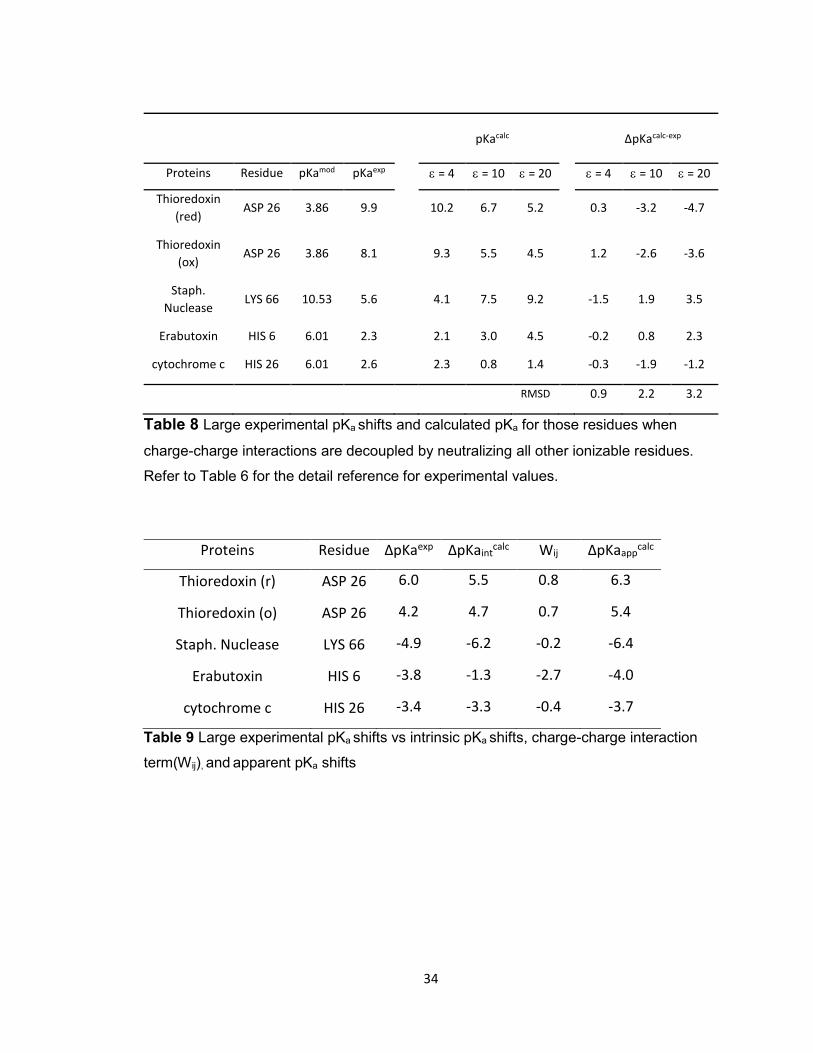
Our method so far has shown that a similar or even better predictions can

be achieved with the strategy of decoupling charge-charge interactions. Now, as

our main focus in this study, the calculations for the large experimental pKa with

our method were conducted and the results are listed in Table 8. The intrinsic

pKa shifts at P= 4 and the Wij with eff= 40,80 are listed in Table 9 for better

insight of the effect of decoupling charge-charge interactions. In contrast to the

classic PB method where P= 10 generated the optimal results, the accuracy of

32

our predictions is always seen better at lower dielectric constants. This trend is

exactly opposite to the results from general cases seen in Table 6 with our

methods. This reflects the dilemma more clearly that even though we get better

results in general with higher dielectric constants approaching the null model, we

really need to use low constants to accurately predict such large pKa shifts.

However, using single dielectric constants means that dielectric screening from

both charge-charge interaction and other induced dipole or non-polar interactions

are adjusted at the same extent. Therefore, this leads to overestimation of

charge-charge interactions at low dielectric constants and underestimation at

high dielectric constants as observed in Table 6. Even though the best prediction

from the classic PB method in Table 5 could be obtained at P= 10 for the large

pKa shifts, errors larger than 1.2 unit were observed in all of the calculations. In

our model, we could solve this dilemma by decoupling the charge-charge

couplings and predict these large pKa shifts using P= 4 as accurate as the

classic PB model that used P= 10. This strongly supports our motivation in this

study.

33

Proteins PDB = 4 = 6 = 10 = 20

Lysozmye 1HEL 1.3 1.0 1.0 0.9

RNaseA 7RAA 1.5 1.2 0.9 0.8

Ovomucoid 1OMU 0.8 0.7 0.6 0.6

Barnase 1A2P 3.6 2.5 1.6 1.1

Thioredoxin-ox 1TRS 1.2 1.1 1.2 1.2

Thioredoxin-red 1TRW 2.4 2.0 1.7 1.8

BPTI 5PTI 0.9 0.5 0.3 0.3

Total 1.9 1.5 1.2 1.1

Table 6. RMSD of calculated apparent pKa with our method a dielectric constants of

4,6,10, and 20 for intrinsic pKa calculation when all ionizable residues are neutralized.

Proteins Intrinsic Apparent

Lysozmye 2.0 1.7

RNaseA 1.7 2.1

Ovomucoid 1.3 0.8

Barnase 3.5 3.6

Thioredocxin-Ox 1.3 1.5

Thioredoxin-red 2.1 2.5

BPTI 1.5 0.9

Total 2.0 1.9

Table 7 RMSD of calculated intrinsic and apparent pKa before and after Wij.

34

pKacalc ΔpKacalc-exp

Proteins Residue pKamod pKaexp = 4 = 10 = 20 = 4 = 10 = 20

Thioredoxin

(red) ASP 26 3.86 9.9 10.2 6.7 5.2 0.3 -3.2 -4.7

Thioredoxin

(ox) ASP 26 3.86 8.1 9.3 5.5 4.5 1.2 -2.6 -3.6

Staph.

Nuclease LYS 66 10.53 5.6 4.1 7.5 9.2 -1.5 1.9 3.5

Erabutoxin HIS 6 6.01 2.3 2.1 3.0 4.5 -0.2 0.8 2.3

cytochrome c HIS 26 6.01 2.6 2.3 0.8 1.4 -0.3 -1.9 -1.2

RMSD 0.9 2.2 3.2

Table 8 Large experimental pKa shifts and calculated pKa for those residues when

charge-charge interactions are decoupled by neutralizing all other ionizable residues.

Refer to Table 6 for the detail reference for experimental values.

Proteins Residue ΔpKaexp ΔpKaintcalc Wij ΔpKaapp

calc

Thioredoxin (r) ASP 26 6.0 5.5 0.8 6.3

Thioredoxin (o) ASP 26 4.2 4.7 0.7 5.4

Staph. Nuclease LYS 66 -4.9 -6.2 -0.2 -6.4

Erabutoxin HIS 6 -3.8 -1.3 -2.7 -4.0

cytochrome c HIS 26 -3.4 -3.3 -0.4 -3.7

Table 9 Large experimental pKa shifts vs intrinsic pKa shifts, charge-charge interaction

term(Wij), and apparent pKa shifts

35

Figure 8 Experimental vs calculated pKa for all 87 sites from the 7 proteins using four

different dielectric constant, 4,6,10, and 20.

36

Figure 9 Experimental vs calculated pKa shifts from model pKa for all 87 residues from 7

proteins using different

3.3 Statistical sampling of conformations

Even though the results so far show that we can effectively predict the

discriminative large pKa shifts at a low dielectric constant by decoupling charge-

37

charge interactions, the overall accuracy is not satisfying with P= 4 for intrinsic

pKa calculation. One important factor that has not been addressed so far is the

effect of protein relaxation. We performed a MD simulation for each protein and

took conformations every 1 ns to get statistically independent samples. All

individual calculations are listed in Table 10 after averaging the pKa calculations

at P= 4 and the overall summaries are listed in Table 11.

Residue pKa

int Wij pKaapp pKa

exp ΔpKa

calc-

axp

Residue pKa

int Wij pKaapp pKa

exp ΔpKacalc-axp

Lysozyme BPTI

ASP18 3.4 -1.4 2.0 2.7 -0.7 Asp3 4.2 -0.7 3.5 3.4 0.1

ASP48 1.7 -1.3 0.5 2.5 -2.0 Glu7 7.0 -1.1 5.9 3.8 2.1

ASP52 4.2 -0.7 3.5 3.7 -0.2 Lys15 10.6 -0.2 10.4 10.6 -0.2

ASP66 1.9 -1.2 0.7 2.0 -1.3 Arg17 11.6 0.1 11.7 12.7 -1.0

ASP87 3.1 -1.1 2.1 2.1 0.0 Arg20 12.2 0.3 12.5 13.9 -1.4

ASP101 4.0 -1.0 3.0 4.1 -1.1 Lys26 10.2 -0.1 10.1 10.6 -0.5

ASP119 3.3 -1.0 2.3 3.2 -0.9 Arg39 11.7 0.4 12.1 13 -0.9

GLU7 4.1 -1.3 2.8 2.9 -0.1 Lys41 8.2 0.4 8.6 10.8 -2.2

GLU35 4.9 -0.7 4.2 6.2 -2.0 Arg42 11.2 0.5 11.7 13.4 -1.7

HSP15 5.6 -0.7 4.9 5.7 -0.8 Lys46 10.6 -0.1 10.5 10.6 -0.1

RMSD 0.7 Glu49 4.3 -0.8 3.5 3.6 -0.1

Asp50 4.6 -1.1 3.5 3.0 0.5

Barnase Arg53 11.3 1.1 12.4 13.9 -1.5

Asp8 2.3 -1.3 1.0 2.9 -1.9 RMSD 1.2

Asp12 4.5 -1.0 3.5 3.8 -0.3

His18 8.1 -0.2 7.9 7.9 0.0

Asp22 4.3 -0.7 3.6 3.3 0.3 RNaseA

Glu29 1.6 -1.1 0.6 3.8 -3.2 Glu2 4.6 -1.3 3.2 2.8 0.4

Asp44 4.1 -0.6 3.5 3.4 0.1 Glu9 4.6 -0.5 4.0 4 0.0

Asp54 2.3 -1.4 0.9 3.31 -2.4 His12 8.0 -0.6 7.4 6.2 1.2

Glu60 4.8 -1.1 3.6 3.4 0.2 Asp14 3.6 -1.1 2.5 2 0.5

Glu73 3.4 -1.3 2.1 2.1 0.0 Asp38 4.2 -1.4 2.7 3.5 -0.8

Asp75 5.4 -1.3 4.1 3.1 1.0 His48 8.2 0.4 8.7 6 2.7

Asp86 2.5 -1.0 1.5 4.2 -2.7 Glu49 4.0 -0.5 3.5 4.7 -1.2

RMSD 1.6 Asp53 3.6 -0.7 2.9 3.9 -1.0

Asp83 4.6 -1.1 3.5 3.5 0.0

Ovomucoid Glu86 5.0 -0.9 4.1 4.1 0.0

38

Asp7 5.0 -0.4 4.6 2.7 1.9 His105 6.4 -0.3 6.1 6.7 -0.6

Glu10 5.4 -0.8 4.6 4.1 0.5 Glu111 3.7 -0.9 2.8 3.5 -0.7

Glu19 5.7 -1.1 4.7 3.2 1.5 His119 5.8 -0.7 5.2 6.1 -0.9

Asp27 4.9 -1.2 3.7 2.3 1.4 Asp121 3.2 -1.2 2.0 3.1 -1.1

Glu43 5.2 -0.3 5.0 4.8 0.2 RMSD 1.0

His52 5.9 -0.2 5.8 7.5 -1.7

1.3

TRX-red TRX-ox

Glu6 4.1 -0.1 4.0 4.8 -0.8 Glu6 3.6 -0.3 3.3 4.9 -1.6

Glu13 4.2 -0.5 3.7 4.4 -0.7 Glu13 4.7 -0.7 3.9 4.4 -0.5

Asp16 4.9 -0.2 4.7 4 0.7 Asp16 4.1 -0.5 3.6 4.2 -0.7

Asp20 6.2 -1.2 5.0 3.8 1.2 Asp20 4.9 -1.3 3.6 3.8 -0.2

Asp26 9.3 0.6 9.9 9.9 0.0 Asp26 8.3 0.9 9.1 8.1 1.0

Glu47 4.3 -0.5 3.8 4.1 -0.3 Glu47 4.3 -0.9 3.5 4.3 -0.8

Glu56 5.1 -1.1 4.0 3.3 0.7 Glu56 5.2 -1.1 4.1 3.3 0.8

Asp58 2.4 -1.0 1.4 5.3 -3.9 Asp58 5.0 1.3 6.3 5.2 1.1

Asp60 5.2 0.7 5.9 2.8 3.1 Asp60 2.8 -0.9 1.9 2.7 -0.8

Asp61 3.7 0.0 3.7 4.2 -0.5 Asp61 3.2 -0.3 2.9 3.9 -1.0

Asp64 3.5 -0.9 2.6 3.2 -0.6 Asp64 4.5 -0.1 4.4 3.2 1.2

Glu68 5.6 -0.8 4.8 4.9 -0.1 Glu68 5.2 -1.1 4.1 5.1 -1.0

Glu70 4.4 -0.9 3.5 4.6 -1.1 Glu70 4.4 -1.1 3.3 4.8 -1.5

Glu88 5.6 -1.1 4.5 3.7 0.8 Glu88 6.5 -1.1 5.4 3.6 1.8

Glu95 4.4 -1.4 3.0 4.1 -1.1 Glu95 4.2 -0.9 3.3 4.1 -0.8

Glu98 5.3 -0.6 4.8 3.9 0.9 Glu98 5.5 -0.8 4.7 3.9 0.8

Glu103 4.7 -0.5 4.3 4.4 -0.1 Glu103 4.3 -0.6 3.7 4.5 -0.8

RMSD 1.4 RMSD 1.0

Table 10 All individual calculations for 87 residues of 7 proteins after 20 ns of MD

simulations. 20 conformations for every 1 ns were used and the average pKa were

calculated.

39

Proteins <ΔpKa,int> <ΔpKa,app> ΔpKa,appX-ray,P= 4

Lysozyme 0.7 1.1 1.7

RNaseA 1.1 1.0 1.5

Ovomucoid 1.8 1.2 0.8

Barnase 2.0 1.3 3.6

Thioredoxin-Ox 1.1 1.0 1.2

Thioredoxin-red 1.4 1.4 2.4

BPTI 1.3 0.9 0.9

Total 1.3 1.2 2.0

Table 11 Summary of RMSD of ΔpKa between experimental pKa and calculated intrinsic and

apparent pKa at , P= 4 by averaging them over trajectories from 10 ns of MD simulations.

Wij is the averages of absolute values of the shifts by charge-charge couplings. For comparison,

the result without MD simulation sampling is also listed

After sampling multiple conformations, the overall accuracy of the

prediction was significantly improved from the results with only single structures.

The majority improvements were achieved in intrinsic pKa calculation while the

shifts by Wij were in the similar range as the calculations with single structures.

Many other groups have incorporated Monte-Carlo simulation into PB model to

take account for protein flexibilities.[25, 26, 48] Here, we also see the

improvement by incorporating MD simulation into the PB method. Since we

decouple charge-charge interactions and do conformational sampling, we should

be able to use a small P which will compensate for only missing induced dipole

interaction, quantum entities, or other small electrostatic effects that this model

does not capture.

In detail, lysozyme, barnase, and reduced thioredoxin especially show

40

much smaller deviations from the experimental data when we use MD

conformational sampling. For example, in case of lysozyme without

conformational sampling, even though there was a big improvement in pKa

prediction for ASP66 compared to the classic PB method, big deviations of 2.7

pKa unit from the experimental pKa was observed. This large errors was corrected

to -1.3 unit error after the samplings. This residue is buried and surrounded by

many hydroxyl group and a better desolvation effect could have been captured

by MD simulations. Glu73 and ASP75 of barnase, which affected the overall

accuracy significantly, also showed much improvement after the sampling. With

the single X-ray structure, the deviations from experimental the pKa were 8.8 for

GLU73 and 6.6 for ASP75 which is a very undesirable result. GLU73 which is

exposed to solvent was corrected and this may be explained by correct dielectric

boundaries obtained by MD samplings . ASP75 is a buried residue and very

close to the side chain of ARG83 within 2 Å . In X-ray structure calculation, the

intrinsic pKa showed extremely high shifts which suggests overestimation of the

desolvation effect despite the presence of the arginine group nearby. The

standard deviation of the intrinsic pKa of this residue over the trajectories was

1.27 unit which is a larger fluctuation than most cases. Therefore, statistical

sampling can resolve such errors that can appear in a static protein structure.

These results indicate that the pKa of ionizable groups both on the surface and in

the buried sites can be more reliably evaluated by considering protein relaxation

effect.

Another way to evaluate the validity of MD conformational sampling is by

41

comparing pKa calculations between two different X-ray structures for the same

protein to see if the results converge to each other. We used 2 PDB structures

for hen egg lysozyme, 1HEL and 2LZT. The comparison of deviations from the

experimental pKa is listed in Table 12. For both structure, better correlations with

experimental data were obtained after MD sampling. Although the overall

accuracy is similar to each other for single structures, opposite predictions for

ASP66 were observed. The pKa’s of this group for both structures were predicted

in the same direction after MD simulation. To see if the calculations converge

regardless of the accuracy, the calculated pKa for 27 ionizable residues, including

arginine, lysine, and histidines whose experimental pKa is not available, are

plotted in Figure 10. It is clearly shown that the numbers were predicted in a

more narrow range from each other with higher R2 value than when calculated

with single structures. Therefore, MD conformational sampling also gets rid of the

variability of single original structures and enables one to get more robust

predictions.

Now, the question remains if large pKa shifts can be more accurately

predicted with consideration of the protein relaxation effect. The predictions and

comparisons with the results from single structure are listed in Table 13.

Although the predictions for ASP 26 of both thioredoxin and LYS 66 of

staphylococcal nuclease were improved, the predictions for two other histidine

cases got worse. During the MD simulation, these two cases have been

stabilized and the large pKa shifts were underestimated with the averaged

structures. The difficulty of predicting pKa of histidines with MD conformational

42

sampling is discussed in detail later. Despite the worsen predictions for these

histidines, the similar total RMSD was obtained and it was still shown to be better

than the results at P= 10 with the classic PB method. As a result, our data show

that our method is accurate in predicting both the large pKa shifts and other

normal cases using low dielectric constants.

To verify that a low dielectric constant is more consistent when it takes

account into the protein relaxation effect, in contrast to the classic PB model, we

tested our model at P= 10 as well. (Table 14, 16) As seen in Table 14, the

values obtained at P= 10 were accurate and similar to those obtained at P= 4

which shows that our method can use a small dielectric constant and still

reproduce experimental pKa. Another important point is that there was much

more improvement when looking at a comparison between single structures to

averaged structures at P= 4 than at P= 10. This leads us to the question of null

model again. Since we are already dealing with the protein relaxation effect, high

dielectric constants would underestimate other missing electrostatic effects even

more. This explanation is supported in the observed worsening for the

predictions of large pKa shifts at P= 10 with the MD conformational sampling as

seen in Table 15. Not only did the lower P predict these cases much more

accurately, but the RMSD value observed at P= 10 was significantly worse than

the results obtained with single structures which has been shown in Table 8.

43

Therefore, we conclude that our method with MD conformational sampling

can effectively and consistently predict pKa at P= 4 for both normal cases and

large pKa shifts without having to worry about which dielectric constants we

would need to use.

With conformation sampling With single X-ray structure

ID RES ΔpKa2lzt ΔpKa1hel ΔpKa2lzt ΔpKa1hel

18 ASP 0.7 -0.7 -1.0 -0.8

48 ASP -1.5 -2.0 2.2 1.0

52 ASP 1.0 -0.2 -1.0 0.2

66 ASP -2.3 -1.3 -2.1 2.7

87 ASP 0.4 0.0 0.4 0.6

101 ASP 0.2 -1.1 0.0 -0.2

119 ASP -1.0 -0.9 -0.9 -0.5

7 GLU 0.4 -0.1 0.6 2.4

35 GLU -1.1 -2.0 -1.4 -1.1

15 HSE -0.1 -0.8 0.9 1.0

RMSD 1.1 1.1 1.2 1.3

Table 12 pKa calculation comparisons between 1HEL and 2LZT which are the same

protein, hen egg lysozyme. Both single structure and MD simulation sampling were

tested. Listed numbers are the deviations from experimental pKa.

44

Figure 10 Scattered plots of the calculated pKa of 2LZT vs 1HEL. Both single structure

and MD simulation sampling were tested

pKacalc ΔpKacalc-exp

Proteins Residue pKamod pKaexp pKaint Wij pKaapp ΔpKa,app ΔpKa,appXray

Thioredoxin

(red) ASP 26 3.86 9.9 9.3 0.6 9.9 0.0 0.3

Thioredoxin

(ox) ASP 26 3.86 8.1 8.3 0.4 8.7 0.6 1.2

Staph.

Nuclease LYS 66 10.53 5.6 6.5 -0.4 6.1 0.5 -1.5

Erabutoxin HIS 6 6.01 2.3 6.1 -2.0 4.2 2.0 -0.2

cytochrome c HIS 26 6.01 2.6 4.4 -0.2 4.2 1.5 -0.3

RMSD 1.1 0.9

Table 13 Our methods with MD conformational sampling for large pKa shift cases

45

Proteins <Apparen>

= 4 <Apparent>

= 10 Apparent, X-ray, = 4

Apparent, X-ray, = 10

Lysozyme 1.1 1.0 1.3 1.2

RNaseA 1.0 1.0 2.1 0.9

Ovomucoid 1.2 0.8 0.8 0.6

Barnase 1.3 1.0 1.5 1.6

Thioredoxin-Ox 1.0 1.0 2.5 1.2

Thioredoxin-red 1.4 1.4 0.9 1.7

BPTI 1.2 0.4 3.6 0.3

Total 1.2 1.0 1.9 1.2

Table 14 RMSD between experimental pKa and the predicted pKa with our method at

two different dielectric constants

pKacalc ΔpKacalc-exp

Proteins Residue pKamod pKaexp = 4 = 10 = 4 = 10

Thioredoxin

(red)

ASP 26 3.86 9.9 9.9 5.4 0.0 -2.7

Thioredoxin

(ox)

ASP 26 3.86 8.1 8.7 6.3 0.6 -3.6

Staph.

Nuclease

LYS 66 10.53 5.6 6.1 8.5 0.5 2.9

Erabutoxin HIS 6 6.01 2.3 4.2 4.8 2.0 2.5

cytochrome c HIS 26 6.01 2.6 4.2 0.5 1.5 -2.1

RMSD 1.1 3.3

Table 15 RMSD between experimental pKa and the predicted pKa with our method at

two different dielectric constants

46

3.4 Comparison to other benchmarks

After we verified the validity of our method, we compared our

results to other benchmarks. First, since our method was motivated by Sham et

al. [23] which decoupled charge-charge interactions in PDLD/S model and

showed a very good agreement with experimental data, we evaluate our Wij

comparing to the results in the previous work for lysozyme. (Table 15) No large

perturbation by charge-charge interaction is observed in both predictions which

are the desirable results as addressed in section 3.3. Our implementation has

larger shifts for ASP52, ASP66, and ASP87. But for these cases, larger shifts

help predict the experimental pKa better.

Now, we compare our model to two other PB based benchmarks

The first is H++ which is a webserver where one can quickly calculate the pKa of

a submitted protein. [18-20] As recommended by them as an optimal value, we

used a single dielectric constant of P= 10. Another benchmark has been

reported in Nielsen at al.[48] This work incorporated Monte-Carlo simulation

sampling for protein relaxation effects using DelPhi II. They used dielectric

constant of 8 for most of the calculations and 16 for special criteria. The

comparisons are listed in Table 15. We could reproduce the similar accuracy to

theirs using lower dielectric constant. However, to our tests with the classic PB

model, H++ failed to reproduce the large pKa shifts.

47

residue Our Wij Sham et al.

GLU7 -1.3 -1.4

ASP18 -1.4 -0.9

GLU35 -0.7 -0.5

ASP48 -1.3 -1.0

ASP52 -0.7 -0.1

ASP66 -1.2 -0.6

ASP87 -1.1 -0.5

ASP101 -1.0 -1.3

ASP119 -1.0 -1.0

avg 1.1 0.8 Table 16 Comparison of calculated Wij between ours and the results from Sham at al

[23]

Proteins Our method H++ Nielsen et al.

Lysozyme 1.1(2.0) 1.0(1.6) 1.2(2.6)

RNaseA 1.0(2.7) 1.1(2.5) 1.0(2.4)

Ovomucoid 1.3(1.9) 0.7(1.0) 1.2(2.6)

Barnase 1.6(3.2) 1.4(3.1) -

Thioredoxin-Ox

0.9(1.8) 1.0(4.2) -

Thioredoxin-red

1.0(3.9) 1.0(4.6) -

BPTI 0.9(2.2) 0.8(2.2) 0.7(2.0)

Total 1.2 1.4 1

Table 17 Comparison of out method to other benchmarks. Listed numbers are RMSD

from experimental data and the largest errors are listed in bracket

3.5 Limitations and other challenges

While not the main focus of this study, we found several important

discrepancies depending on the parameters set in the calculation. One is the

dielectric boundary conditions. There are several ways to define the boundary

48

between proteins and solvents. It can be defined by either the van der Waals

surface or molecular surface. Theoretically, even though using the molecular

surface which takes account for accessibility of solvents is more physically

sound, we often observed better accuracy when using the van der Waals

surface. This has been previously addressed elsewhere.[25, 49] We

occasionally observed significantly large differences between two results with

different boundary settings. In this study, we chose the conditions which

generated the smaller perturbation for each protein.

Another difficulty we faced was the convergence problem in the

calculation of Wij which resulted in unacceptable huge pKa shifts. It is likely that

this was due to systemic errors caused by the sequential calculation for each

residue. The Coulombic interaction energies were calculated in the order of the

residue number as defined in the PDB file. As a result, the calculation can be

trapped in a fluctuation between two numbers. This can be solved either by

giving a different number of iterative steps to choose the smaller perturbation

around 1 pKa unit shift or by calculating the energies in different order of the

residues. However, more consistent method needs to be devised to effectively

remove this problem.

We wanted to stress the pKa calculation of histidine. Many times, histidine

should be treated in a special way since its side chain has two possible

protonation sites(HSD and HSE) and it can have a flipped configuration.

Especially, the calculated numbers can be very different between before and

after MD conformational sampling. We usually calculate the pKa with single X-ray

49

structure first to start with the initial protonated states that have smaller pKa shifts

which are suggested to be more stable. Then, MD simulation is performed with

these states. However, it sometimes turns out that it actually becomes

destabilized during the MD simulation and we have to perform the simulation with

the other protonated states. This can be very crucial in the studies of proteins

where histidine plays a very important role in protein stability and conformational

change such as Dengue virus envelope protein.[50, 51] Similarly, glutamic acid

and aspartate acid have two possible protonation sites in the carboxyl groups.

Even though the alternative protonation does not matter during MD simulation in

this case since they are simulated in charged states, significantly different pKa

values are often observed in the calculation depending on which site is

protonated. Thus, proper protonation site needs to be selected carefully.

Lastly, our implementation actually includes the calculations for

serine and tyrosine but the results were not satisfying. One possible scenario is

that CHARMM27 parameter defines the radius of protonated and deprotonated

oxygen in their side chain in the same sizes. After trying different radius and

partial charges, we found that the result is very sensitive to these parameter

values. Also, more experimental data sets are required to evaluate the

calculations for these two residues more reliably.

Conclusions

This study presents a more reliable and robust calculation with

PB methods by decoupling charge-charge interactions and incorporating explicit

50

MD conformational sampling. Our method takes away the problem of adjusting

dielectric constants which inevitably causes a loss of accuracy either in normal

cases or large pKa shifts cases. We tested our method that incorporated the

PDLD/S approach against the classic PB model which has been initially

suggested by Warshel and coworkers. There have been a lot of efforts to

improve the pKa prediction with PB model for decades by many other

considerations such as optimizing hydrogen bond, other parameters, and, most

importantly, trying to find an ‘optimal’ dielectric constant. Our work contributes to

narrowing down these considerations by eliminating this dependence of dielectric

constants in PB model.

51

Reference

1. Warshel, A. and R.M. Weiss, Energetics of Heme-Protein Interactions in Hemoglobin. Journal of the American Chemical Society, 1981. 103(2): p. 446-451.

2. Warshel, A. and S.T. Russell, Calculations of Electrostatic Interactions in Biological-Systems and in Solutions. Quarterly Reviews of Biophysics, 1984. 17(3): p. 283-422.

3. Matthew, J.B., Electrostatic Effects in Proteins. Biophysical Journal, 1985. 47(2): p. A20-A20.

4. Nakamura, H., Roles of electrostatic interaction in proteins. Q Rev Biophys, 1996. 29(1): p. 1-90.

5. Tanford, C. and J.G. Kirkwood, Theory of Protein Titration Curves. I. General Equations for Impenetrable Spheres. Journal of the American Chemical Society, 1957. 79(20): p. 5333-5339.

6. Lee, F.S., Z.T. Chu, and A. Warshel, Microscopic and semimicroscopic calculations of electrostatic energies in proteins by the POLARIS and ENZYMIX programs. Journal of Computational Chemistry, 1993. 14(2): p. 161-185.

7. Gilson, M.K. and B. Honig, Calculation of the Total Electrostatic Energy of a Macromolecular System - Solvation Energies, Binding-Energies, and Conformational-Analysis. Proteins-Structure Function and Genetics, 1988. 4(1): p. 7-18.

8. Gilson, M.K., K.A. Sharp, and B.H. Honig, Calculating the Electrostatic Potential of Molecules in Solution - Method and Error Assessment. Journal of Computational Chemistry, 1988. 9(4): p. 327-335.

9. Nicholls, A. and B. Honig, A Rapid Finite-Difference Algorithm, Utilizing Successive over-Relaxation to Solve the Poisson-Boltzmann Equation. Journal of Computational Chemistry, 1991. 12(4): p. 435-445.

10. Bashford, D. and D.A. Case, Generalized born models of macromolecular solvation effects. Annual Review of Physical Chemistry, 2000. 51: p. 129-152.

11. Onufriev, A., D. Bashford, and D.A. Case, Modification of the generalized Born model suitable for macromolecules. Journal of Physical Chemistry B, 2000. 104(15): p. 3712-3720.

12. Rocchia, W., E. Alexov, and B. Honig, Extending the applicability of the nonlinear Poisson-Boltzmann equation: Multiple dielectric constants and multivalent ions. Journal of Physical Chemistry B, 2001. 105(28): p. 6507-6514.

13. Rocchia, W., et al., Rapid grid-based construction of the molecular surface and the use of induced surface charge to calculate reaction field energies: Applications to the molecular systems and geometric objects. Journal of Computational Chemistry, 2002. 23(1): p. 128-137.

14. Brooks, B.R., et al., CHARMM: The Biomolecular Simulation Program. Journal of Computational Chemistry, 2009. 30(10): p. 1545-1614.

15. Baker, N.A., et al., Electrostatics of nanosystems: Application to microtubules and the ribosome. Proceedings of the National Academy of Sciences of the United States of America, 2001. 98(18): p. 10037-10041.

16. Ponder, J.W. and D.A. Case, Force fields for protein simulations. Adv Protein Chem, 2003. 66: p. 27-85.

17. Salomon-Ferrer, R., D.A. Case, and R.C. Walker, An overview of the Amber biomolecular simulation package. Wiley Interdisciplinary Reviews: Computational Molecular Science, 2013. 3(2): p. 198-210.

52

18. Gordon, J.C., et al., H++: a server for estimating pKas and adding missing hydrogens to macromolecules. Nucleic Acids Res, 2005. 33(Web Server issue): p. W368-71.

19. Myers, J., et al., A simple clustering algorithm can be accurate enough for use in calculations of pKs in macromolecules. Proteins-Structure Function and Bioinformatics, 2006. 63(4): p. 928-938.

20. Anandakrishnan, R., B. Aguilar, and A.V. Onufriev, H++ 3.0: automating pK prediction and the preparation of biomolecular structures for atomistic molecular modeling and simulations. Nucleic Acids Res, 2012. 40(Web Server issue): p. W537-41.

21. Jo, S., et al., CHARMM-GUI: a web-based graphical user interface for CHARMM. J Comput Chem, 2008. 29(11): p. 1859-65.

22. Simonson, T. and C.L. Brooks, Charge Screening and the Dielectric Constant of Proteins:  Insights from Molecular Dynamics. Journal of the American Chemical Society, 1996. 118(35): p. 8452-8458.

23. Sham, Y.Y., Z.T. Chu, and A. Warshel, Consistent Calculations of pKa's of Ionizable Residues in Proteins:  Semi-microscopic and Microscopic Approaches. The Journal of Physical Chemistry B, 1997. 101(22): p. 4458-4472.

24. Warshel, A. and A. Papazyan, Electrostatic effects in macromolecules: fundamental concepts and practical modeling. Current Opinion in Structural Biology, 1998. 8(2): p. 211-217.

25. Alexov, E., et al., Progress in the prediction of pKa values in proteins. Proteins, 2011. 79(12): p. 3260-75.

26. Teixeira, V.H., et al., On the use of different dielectric constants for computing individual and pairwise terms in poisson-boltzmann studies of protein ionization equilibrium. J Phys Chem B, 2005. 109(30): p. 14691-706.

27. Antosiewicz, J., J.A. McCammon, and M.K. Gilson, Prediction of pH-dependent properties of proteins. J Mol Biol, 1994. 238(3): p. 415-36.

28. Schutz, C.N. and A. Warshel, What are the dielectric "constants" of proteins and how to validate electrostatic models? Proteins, 2001. 44(4): p. 400-17.

29. Sham, Y.Y. and A. Warshel, The surface constraint all atom model provides size independent results in calculations of hydration free energies. Journal of Chemical Physics, 1998. 109(18): p. 7940-7944.

30. Bashford, D. and M. Karplus, pKa's of ionizable groups in proteins: atomic detail from a continuum electrostatic model. Biochemistry, 1990. 29(44): p. 10219-10225.

31. Jorgensen, W.L., et al., Comparison of simple potential functions for simulating liquid water. The Journal of Chemical Physics, 1983. 79(2): p. 926-935.

32. Bashford, D., An object-oriented programming suite for electrostatic effects in biological molecules An experience report on the MEAD project, in Scientific Computing in Object-Oriented Parallel Environments, Y. Ishikawa, et al., Editors. 1997, Springer Berlin Heidelberg. p. 233-240.

33. Cerutti, D.S., et al., Staggered Mesh Ewald: An Extension of the Smooth Particle-Mesh Ewald Method Adding Great Versatility. Journal of Chemical Theory and Computation, 2009. 5(9): p. 2322-2338.

34. Ryckaert, J.-P., G. Ciccotti, and H. Berendsen, Numerical integration of the cartesian equations of motion of a system with constraints: molecular dynamics of n-alkanes. Journal of Computational Physics, 1977. 23(3): p. 327-341.

35. Humphrey, W., A. Dalke, and K. Schulten, VMD: visual molecular dynamics. J Mol Graph, 1996. 14(1): p. 33-8, 27-8.

53

36. Webb, H., et al., Remeasuring HEWL pK(a) values by NMR spectroscopy: methods, analysis, accuracy, and implications for theoretical pK(a) calculations. Proteins, 2011. 79(3): p. 685-702.

37. Baker, W.R. and A. Kintanar, Characterization of the pH titration shifts of ribonuclease a by one- and two-dimensional nuclear magnetic resonance spectroscopy. Archives of Biochemistry and Biophysics, 1996. 327(1): p. 189-199.

38. Schaller, W. and A.D. Robertson, pH, ionic strength, and temperature dependences of ionization equilibria for the carboxyl groups in turkey ovomucoid third domain. Biochemistry, 1995. 34(14): p. 4714-23.

39. Forsyth, W.R., et al., Theoretical and experimental analysis of ionization equilibria in ovomucoid third domain. Biochemistry, 1998. 37(24): p. 8643-52.

40. Sali, D., M. Bycroft, and A.R. Fersht, Stabilization of protein structure by interaction of alpha-helix dipole with a charged side chain. Nature, 1988. 335(6192): p. 740-3.

41. Oliveberg, M., V.L. Arcus, and A.R. Fersht, pKA values of carboxyl groups in the native and denatured states of barnase: the pKA values of the denatured state are on average 0.4 units lower than those of model compounds. Biochemistry, 1995. 34(29): p. 9424-33.

42. Qin, J., G.M. Clore, and A.M. Gronenborn, Ionization equilibria for side-chain carboxyl groups in oxidized and reduced human thioredoxin and in the complex with its target peptide from the transcription factor NF kappa B. Biochemistry, 1996. 35(1): p. 7-13.

43. Brown, L.R., et al., The influence of a single salt bridge on static and dynamic features of the globular solution conformation of the basic pancreatic trypsin inhibitor. 1H and 13C nuclear-magnetic-resonance studies of the native and the transaminated inhibitor. Eur J Biochem, 1978. 88(1): p. 87-95.

44. Garcia-Moreno, B., et al., Experimental measurement of the effective dielectric in the hydrophobic core of a protein. Biophys Chem, 1997. 64(1-3): p. 211-24.

45. Inagaki, F., et al., Conformation of erabutoxins a and b in aqueous solution as studied by nuclear magnetic resonance and circular dichroism. Eur J Biochem, 1978. 89(2): p. 433-42.

46. Cohen, J.S., W.R. Fisher, and A.N. Schechter, Spectroscopic studies on the conformation of cytochrome c and apocytochrome c. J Biol Chem, 1974. 249(4): p. 1113-8.

47. Russell, A.J., P.G. Thomas, and A.R. Fersht, Electrostatic effects on modification of charged groups in the active site cleft of subtilisin by protein engineering. J Mol Biol, 1987. 193(4): p. 803-13.

48. Nielsen, J.E. and G. Vriend, Optimizing the hydrogen-bond network in Poisson-Boltzmann equation-based pK(a) calculations. Proteins, 2001. 43(4): p. 403-12.

49. Tjong, H. and H.X. Zhou, On the dielectric boundary in Poisson-Boltzmann calculations. Journal of Chemical Theory and Computation, 2008. 4(3): p. 507-514.

50. Mukhopadhyay, S., R.J. Kuhn, and M.G. Rossmann, A structural perspective of the flavivirus life cycle. Nat Rev Microbiol, 2005. 3(1): p. 13-22.

51. Fritz, R., K. Stiasny, and F.X. Heinz, Identification of specific histidines as pH sensors in flavivirus membrane fusion. J Cell Biol, 2008. 183(2): p. 353-61.

52. Lee, F.S., et al., Calculations of antibody-antigen interactions: microscopic and semi-microscopic evaluation of the free energies of binding of phosphorylcholine analogs to McPC603. Protein Eng, 1992. 5(3): p. 215-28.

54

Appendix A

Linear Response Approximation

It is necessary to consider protein reorganization and relaxation during the

charge process. Linear Response Approximation(LRA) has been introduced and

adopted by many electrostatic computation approaches to achieve it efficiently.

[6, 23, 52] In LRA, it is assumed that the curvatures of the free energy graphs of

two different charged states (Figure 4) are identical. Because λa = λb by this

assumption, the following equation can be derived

Δ𝐺a→b =1

2[⟨𝑉a − 𝑉b⟩a + ⟨𝑉a − 𝑉b⟩b] (1.6)

where ‘a’ and ‘b’ designates non-charged and charged sates, respectively and <

> represensts average values from a set of conformations using statistical

mechanics with Monte Carlo or Molecular Dynamic simulations. However, the

free energy associated with the non-charged state is neglectible compared to the

charged state. Therefore, Eq 1.6 is further simplified as

Δ𝐺a→b ≅1

2⟨∆𝑉⟩b (1.7)

55

Figure A. Two parabolas describe the function of the free energy of the non-

charged state(a) and the charged state(b). By the assumption of LRA, the

curvatures of two free energy graphs are same. This leads to the linear

relationship of <Vb - Va>a + Δ𝐺a→b =<Va - Vb>b - Δ𝐺a→b where 𝐺a→b is the free

energy associated with the adiabatic charging process